Nuclear Spins in Quantum Dots - Reykjavík University · Nuclear Spins in Quantum Dots Proefschrift...
93
Nuclear Spins in Quantum Dots
-
Upload
nguyendieu -
Category
Documents
-
view
219 -
download
0
Transcript of Nuclear Spins in Quantum Dots - Reykjavík University · Nuclear Spins in Quantum Dots Proefschrift...
Nuclear Spins in Quantum Dots

Nuclear Spins in Quantum Dots
Proefschrift
ter verkrijging van de graad van doctor
aan de Technische Universiteit Delft,
op gezag van de Rector Magnificus prof.dr.ir. J.T. Fokkema,
voorzitter van het College voor Promoties,
in het openbaar te verdedigen op dinsdag 16 september 2003 om 10.30 uur
door
Sigurdur Ingi ERLINGSSON
Meistaraprof ı edlisfraedi
Haskoli Islands
geboren te Reykjavık, IJsland.
Dit proefschrift is goedgekeurd door de promotor:
Prof. dr. Yu. V. Nazarov
Samenstelling van de promotiecommissie:
Rector Magnificus, voorzitter
Prof.dr. Yu. V. Nazarov Technische Universiteit Delft, promotor
Prof.dr.ir. G. E. W. Bauer, Technische Universiteit Delft
Prof.dr.ir. L. P. Kouwenhoven, Technische Universiteit Delft
Prof.dr. D. Pfannkuche, Universiteit Hamburg, Duitsland
Prof.dr. D. Loss, Universiteit Basel, Zwitserland
Prof.dr. V. Gudmundsson, Universiteit IJsland, IJsland
dr.ir. L. Vandersypen Technische Universiteit Delft
Published and distributed by: DUP Science
DUP Science is an imprint of
Delft University Press
P.O. Box 98 Telephone: +31 15 27 85678
2600 MG Delft Telefax: +31 15 27 85706
The Netherlands E-mail: [email protected]
ISBN 90-407-2431-8
Keywords: quantum dots, electron spin, hyperfine interaction
Copyright c© 2003 by Sigurdur I. Erlingsson
All rights reserved. No part of the material protected by this copyright notice
may be reproduced or utilized in any form or by any means, electronic or me-
chanical, including photocopying, recording or by any information storage and
retrieval system, without permission from the publisher: Delft University Press.
Printed in the Netherlands
Preface
The work presented in this thesis is the result of four years of PhD research
in the theoretical physics group in Delft. In the beginning of my PhD I knew
that I wanted to work on electron spins and quantum dots but I only had vague
ideas about what that entailed. With time these ideas became more clear,
largely with the help of my supervisors, and I found myself working on the
problem of quantum dots containing electron spins and how they interact with
the surrounding nuclei. As it turned out this field was, and still is, a very active
field of research. I feel privileged to have been able to do my research in Delft
since it has allowed me to meet and interact with many great scientists, in Delft
and elsewhere. It is a difficult task to adequately thank all the people who in
one way or another contributed to my work, but in any case I will try.
Let me first thank my supervisors. During my first year in Delft I was super-
vised by Daniela Pfannkuche. Daniela taught me many things, especially the
importance of many-body wave functions and being careful in using the single-
particle picture. I would also like to thank her for helping me and Ragnhildur
when we were settling in the Netherlands, and for her hospitality during my
visit to Hamburg.
My main supervisor for the last three years, after Daniela moved to Hamburg
for a professorship, was Yuli Nazarov. I have to admit that after my initial
‘encounters’ with Yuli I was rather intimidated by him. Well, as it turned out
those fears were completely unfounded. I would like to thank Yuli for teaching
me how to keep things simple, showing me the value of being honest in science,
giving me invaluable ‘pep-talks’ when I felt stuck and simply exceeding his duties
as a supervisor.
Although not being directly involved in my daily supervision, I learned a lot
from Gerrit Bauer, especially concerning practical and political matters in the
science business which, I was surprised to learn, are very important indeed. We
also share a ‘passion’ for fantasy novels and Gerrit gave me quite a few hints
concerning good books.
I have had the pleasure of working, and discussing, with very good people
in our group, whether they are the ‘permanent’ staff, guests or postdocs. I
would like to thank Yaroslav Blanter, Milena Grifoni, Joos Thijssen, Arkadi
v

vi
Odintsov, Alexander Khaetskii, Mikeo Eto and Yasuhiro Tokura. The postdocs
in our group have also taught me a great deal and we had some nice time over
a few beers: thanks to Wolfgang Belzig, Mauro Ferreira, Takeshi Nakanishi,
Dmitri Bagrets, Michael Thorwarts, Miriam Blaauboer, Wataru Izumida and
Antonio DiLorenzo. I would especially like to thank our group secretary, Yvonne
Zwang. She has always been very helpful, even though I failed her unofficial
Dutch course.
When I began my studies, I joined the three PhD students who were already
in the theory group: Maarten Wegewijs, Daniel Huertas-Hernandes and Freek
Langeveld. I would like to thank them for our many interactions concerning
physics related matters and all kinds of other stuff. Our reading group “The
Physical Review” helped me understand many things, especially how difficult
it is to keep a reading group going! I would also like to thank Malek Zareyan
and Marcus Kinderman for many fruitful discussions. I have enjoyed many
fun activities and discussions with the ‘younger generation’ of PhD students.
Thank you guys: Joel Peguiron, Oleg Jouravlev, Jens Tobiska, Alexey Kovalev,
Gabriele Campagnano, Sijmen Gerritsen, Omar Usmani and Wouter Wetzels.
Special thanks go to Leo Kouwenhoven for giving me the opportunity to
participate in the qdot-group meetings and teaching me the difference between a
theorist proposal and ‘reality’. I would also like to thank Silvano DeFrancenschi
and Lieven Vandersypen for many enlightening discussions. Many thanks go
to the PhD’s in Leo’s group, past and present: Wilfred van der Wiel, Jeroen
Elzerman, Ronald Hanson and Laurens Willems van Beveren. They helped me
understand “all I wanted to know about quantum dots, but was afraid to ask”.
I would also like to thank a few people which I have had the privilege of
discussing with, listening to their talks or just playing football with (in some
cases all of the above): Hannes Majer, Pablo Jarillo-Herrero, Sami Sapmaz, Al-
berto Morpurgo, Irinel Chiorescu, Eugen Onac, Kees Harmans, Vladimir Fal’ko,
Daniel Loss, Hans-Andreas Engel, Michael Tews and Alexander Chudnovksii.
I want to thank my family for always supporting me and being there when I
needed. Takk fyrir mamma, pabbi, Ella og Steindor. My early interest in science
was sparked by all the books on physics, chemistry, electronics and engineering
in my parents’ library. My current science ‘carrier’ can be traced directly to
those humble beginnings, at least if a few year period where I wanted to be a
film director is disregarded. Even though my brother Steindor and I disagree
on many things, especially concerning science, he has helped me recognize that
science, just like any other human endeavor, is no more infallible than the people
who practice it. Finally I want to thank my fiancee Ragnhildur. She really
helped me cope with my thesis and the accompanying stress. Elsku Ragnhildur,
takk fyrir hjalpina.
Contents
1 Introduction 1
1.1 Quantum dots . . . . . . . . . . . . . . . . . . . . . . . . . . . . 1
1.2 Spin admixture . . . . . . . . . . . . . . . . . . . . . . . . . . . . 2
1.2.1 Spin-orbit interaction . . . . . . . . . . . . . . . . . . . . 3
1.2.2 The hyperfine interaction . . . . . . . . . . . . . . . . . . 4
1.3 Quantum dynamics and the reduced density matrix formalism . . 6
1.4 Spin-flip rates . . . . . . . . . . . . . . . . . . . . . . . . . . . . . 7
1.5 Dynamics of electron spins . . . . . . . . . . . . . . . . . . . . . . 8
1.6 This thesis . . . . . . . . . . . . . . . . . . . . . . . . . . . . . . . 9
References . . . . . . . . . . . . . . . . . . . . . . . . . . . . . . . 10
2 Nucleus-mediated spin-flip transitions in GaAs quantum dots 13
2.1 Introduction . . . . . . . . . . . . . . . . . . . . . . . . . . . . . . 14
2.2 Model and assumptions . . . . . . . . . . . . . . . . . . . . . . . 15
2.3 Comparison and estimates . . . . . . . . . . . . . . . . . . . . . . 19
References . . . . . . . . . . . . . . . . . . . . . . . . . . . . . . . 22
3 Hyperfine-mediated transitions between a Zeeman split doublet
in GaAs quantum dots: The role of the internal field 23
3.1 Introduction . . . . . . . . . . . . . . . . . . . . . . . . . . . . . . 24
3.2 Model and assumptions . . . . . . . . . . . . . . . . . . . . . . . 25
3.3 Internal magnetic field . . . . . . . . . . . . . . . . . . . . . . . . 27
3.4 Transition rate . . . . . . . . . . . . . . . . . . . . . . . . . . . . 29
3.5 Discussion . . . . . . . . . . . . . . . . . . . . . . . . . . . . . . . 34
References . . . . . . . . . . . . . . . . . . . . . . . . . . . . . . . 35
4 Nuclear spin induced coherent oscillations of transport current
through a double quantum dot 37
4.1 Introduction . . . . . . . . . . . . . . . . . . . . . . . . . . . . . . 38
4.2 Model . . . . . . . . . . . . . . . . . . . . . . . . . . . . . . . . . 39
4.3 Density matrix and average electron spin . . . . . . . . . . . . . 43
4.4 Nuclear system dynamics . . . . . . . . . . . . . . . . . . . . . . 45
vii
viii Contents
4.4.1 Integrals of motion . . . . . . . . . . . . . . . . . . . . . . 45
4.4.2 Numerical integration . . . . . . . . . . . . . . . . . . . . 54
4.5 Conclusions . . . . . . . . . . . . . . . . . . . . . . . . . . . . . . 55
References . . . . . . . . . . . . . . . . . . . . . . . . . . . . . . . 55
5 Time-evolution of the effective nuclear magnetic field due to a
localized electron spin 57
5.1 Introduction . . . . . . . . . . . . . . . . . . . . . . . . . . . . . . 58
5.2 Hyperfine interaction in quantum dots . . . . . . . . . . . . . . . 59
5.3 Semiclassical dynamics . . . . . . . . . . . . . . . . . . . . . . . . 60
5.4 Adiabatic approximation for the electron spin . . . . . . . . . . . 64
5.5 Correlation functions . . . . . . . . . . . . . . . . . . . . . . . . . 66
5.6 Nuclear subsystem dynamics . . . . . . . . . . . . . . . . . . . . 67
5.7 Conclusion . . . . . . . . . . . . . . . . . . . . . . . . . . . . . . 71
References . . . . . . . . . . . . . . . . . . . . . . . . . . . . . . . 71
A Thermal average over nuclear spin pairs 73
B Matrix elements for a parabolic quantum dot 75
Summary 77
Samenvatting 79
Curriculum Vitae 83
List of Publications 85
Chapter 1
Introduction
The continuing miniaturization of components used in integrated circuits are
pushing devices ever closer to a regime where the expected classical behavior
becomes strongly influenced by quantum effects [1]. From the point of view of
those who would like to squeeze more and more ‘classical’ devices onto a chip
this prospect is quite discouraging. The opposite viewpoint would be to come up
with new devices which take advantage of these quantum effects. The operation
of such devices would require coherent control of the quantum systems with
precision which is quite difficult to achieve. There are both fundamental and
practical obstacles that need to be overcome, if that is at all possible. The most
ambitious of these proposed devices is the quantum bit, or qubit, which would
form the building blocks of quantum computers [2–5].
There are many competing ideas on how to build qubits. The most mature
systems are based on NMR techniques and manipulating trapped ions, but there
are serious problems regarding scalability in those systems. On the contrary,
solid state systems are more promising with respects to scalability but the prob-
lem of decoherence is much greater [6–8]. One proposed realization is based on
localized electron spins in semiconductor quantum dots [9, 10]. The electron spin
is a natural two level system and the electron spin should be less susceptible to
environmental effects, e.g. relaxation and decoherence , than orbital degrees of
freedom. It is also important that the technology to manufacture well controlled
microstructures is well established and great technological advances have been
made in the direction of controlling single spins in quantum dots. The question
still remains what the detailed effects of the environment on the spin are.
1.1 Quantum dots
Quantum dots are micron-size, or smaller, structures which are manufactured
using lithographic techniques or various so-called self-assembly methods. Irre-
1
2 Introduction
spective of the method used to fabricate them, quantum dots are characterized
by their localized wavefunctions and discrete energy spectrum [11]. Here the
focus is on quantum dots in GaAs/AlGaAs heterostructures. This material is
both technologically important and has peculiar material features which are im-
portant. GaAs is a polar semiconductor which is crucial in determining both
the electron-phonon, and the spin-orbit interaction. Both Ga and As nuclei
have nonzero nuclear spin which give rise to properties which are not present,
or quite reduced, in other semiconductors, e.g. silicon.
Usually GaAs quantum dots are fabricated starting from a 2DEG at an
AlGaAs/GaAs interface, or quantum well. The quantum dots are defined by
etching through the 2DEG or by depositing gates on top of the heterostructure.
Applying a negative voltage on these gates will deplete the 2DEG below them.
Assuming a parabolic confinement in the 2DEG plane is in most cases a good
approximation. The quantum dot Hamiltonian for a generic confining potential
V (z) in the z direction is
H0 =(p + eA(r))2
2m∗+
1
2m∗Ω2
0(x2 + y2) + V (z) + gµBS · B, (1.1)
where A is the gauge dependent vector potential which determines the magnetic
field B = ∇×A. Knowing the potential V (r) of the dot and the applied mag-
netic field B the eigenstates are obtained by solving the stationary Schrodinger
equation
H0〈r|n, s〉 = ~ωn,s〈r|n, s〉. (1.2)
Here the eigenstates are labeled with the orbital index n which represents the
relevant orbital quantum numbers and s indicates the spin state.
GaAs quantum dots come mainly in two flavors, socalled lateral and vertical
quantum dots. Differences in fabrication of the dots is reflected in different
choices of the confining potential V (z). Initially, only the vertical dots allowed
precise control of the number of electrons in the quantum dot, which could be
tuned from 0 to few tens [12]. Recent experiments have also demonstrated this
control in lateral quantum dots [13], and more importantly, the lateral dots
allow greater control over the electron confinement potential in the dot. The
results presented in this thesis apply equally well to vertical and lateral dots,
the only difference being different numerical values due to the slightly different
orbital wave functions.
1.2 Spin admixture
The Hamiltonian in Eq. (1.1) only takes into account the confining potential,
the minimum coupling to the vector field A. As a first approximation this
1.2 Spin admixture 3
is a good starting point but more terms in the Hamiltonian are required for
realistic modeling of the quantum dot. Let us assume for the moment that the
coordinate system is chosen such that [Sz, H0] = 0, thus the eigenstates of H0
are also eigenstates of Sz,
Sz|s〉 = ~s|s〉, s = ±1
2. (1.3)
Here the orbital indices are suppressed for the moment. When a small perturb-
ing term H ′, which contains spin operators such that [Sz, H ′] 6= 0, is added to
H0 the eigenfunctions become
|′′+′′〉 ≈ |+〉 + α|−〉 (1.4)
|′′−′′〉 ≈ |−〉 − α∗|+〉, (1.5)
where α is the strength of the perturbation. The admixture refers to the small
component of the opposite spin, but the states still retain most of their spin
‘up’ and ‘down’ characteristics as long as α 1. The admixture terms in Eq.
(1.5) include contributions from different orbitals, so any inter-orbital scattering
mechanism will lead to scattering between spin states. The magnitude of the
spin scattering is determined by α and the orbital scattering mechanism.
There are a number of possible admixture mechanisms in GaAs. The most
important ones are due to hyperfine interaction and spin-orbit interaction. Al-
though one could also include inelastic cotunneling in this list it is not an in-
trinsic mechanism of the dot since the cotunneling can be turned down to an
arbitrarily small value by pinching of the quantum dot. No such ’turning-off’
exists for the hyperfine or spin-orbit interaction although polarizing the nu-
clear system has been proposed as a means for reducing the effectiveness of the
hyperfine scattering [14].
1.2.1 Spin-orbit interaction
The spin-orbit interaction is a relativistic correction to the Hamiltonian in Eq.
(1.2). The textbook method of introducing the SO interaction is by considering
the problem of an electron moving in a frame with a given stationary electric
field E = −∇V (r) but zero magnetic field. In the reference frame moving
with the electron the magnetic field is not zero since the Lorentz transformation
of the electric field results in a small magnetic field [15]. This magnetic field
couples to the electron spin giving rise to a Zeeman-like term. The Hamiltonian
for the spin-orbit (SO) interaction (including the factor 1/2 due to the Thomas
precession) is
HSO =~
2m2c2(∇V × p) · S, (1.6)
4 Introduction
where p and S are operators for momentum and spin, respectively. For any time
reversal symmetric (no applied magnetic field) single particle Hamiltonian Hsp,
Kramers theorem tells that all eigenstates of the total Hamiltonian H = Hsp +
HSO are doubly degenerate [16, 17]. Non-zero transition amplitude between
such doublet components is only possible in the presence of a magnetic field.
In bulk matter this Hamiltonian becomes modified due to details of the
structure of the underlying material. Here symmetry of the crystal lattice plays
an important role [18, 19]. The SO interaction Hamiltonian can be written quite
generally as
HSO = ~Ω · S, (1.7)
where Ω is some generalized precession frequency whose detailed form is deter-
mined by the structure of the crystal lattice. In GaAs, which has a zinc blende
structure, the dominant SO coupling in the conduction band is due to the lack
of inversion center in the crystal lattice. The resulting SO coupling, the socalled
Dresselhaus term, may be written as
HD = ~ΩD · S, (1.8)
where the SO precession frequency is defined as [20]
ΩD,x =η
~m∗√
2Egm∗px(p2
y − p2z), (1.9)
where η is a material dependent parameter (0.07 in GaAs), Eg is the gap energy
and m∗ is the effective electron mass. The other components of ΩD are obtained
by cyclic permutation of the indices.
In addition to the intrinsic lack of an inversion center in GaAs, it is also pos-
sible to break the lattice symmetry at hetero-interfaces, e.g. at AlGaAs/GaAs
interfaces. The spin orbit coupling arising from this effect is usually called the
Rashba term
HR = 2α~−1(p × nhet) · S, (1.10)
where α ∼ 10−11 eVm in GaAs determines the strength of the coupling and nhet
is a unit vector normal to the interface [21, 22]. In a recent paper the in situ
control of the different SO couplings in a GaAs 2DEG was demonstrated [23].
1.2.2 The hyperfine interaction
Both Ga and As have a nuclear spin I = 3/2. This gives rise to the hyperfine
interaction, i.e. conduction electrons interact with the magnetic moments of the
1.2 Spin admixture 5
nuclei. The Hamiltonian of the hyperfine coupling of an electron spin to a single
nucleus at position R can be written as
HHF = 2µBγn~
(
3(I · n)(S · n) − I · S|r − R|3 +
8π
3I · Sδ(r − R)
)
(1.11)
where n = (r − R)/|r − R|, γn is the nucleus magnetic moment. The former
term in Eq. (1.11) is the usual coupling between magnetic dipoles of the electron
and nuclei but the latter term, socalled contact term, is a correction due to the
non-zero electron density at the nucleus [24].
In GaAs, and other materials with s-orbital conduction band, the dipole-
dipole term is strongly suppressed, leaving the contact term as the dominant
contribution. The contact term Hamiltonian become
HHF = A∑
k
S · Ikδ(r − Rk), (1.12)
where A is the (band renormalized) hyperfine constant and Ik is the spin oper-
ator of nuclei at Rk. The sum runs over all nuclei in the sample. Although Ga
and As have different hyperfine coupling constants, or A’s in Eq. (1.12), we will
consider only a single effective nuclear species characterized by a single A which
is the weighted sum of the contributions from different isotopes of the Ga and
As nuclei. The energy scales associated with this Hamiltonian can be extracted
from A and the concentration of nuclear spins Cn. Assuming a completely po-
larized (in the z direction) nuclear state one can extract the Zeeman splitting
of the spin doublet
En = AICn, (1.13)
where I is the nuclear spin of the Ga and As nuclei. Note that this result does
not depend on the form of the wavefunction. This spin splitting is a quantity
that has been measured: En = 0.135 meV in GaAs samples [25, 26].
The form of the Hamiltonian is quite suggestive since it can be written on
the form [27]
HHF = S · K (1.14)
which is formally equivalent to the Zeeman term in Eq. (1.1) but the difference
is that the field is now an operator
K = A∑
k
Ikδ(r − Rk). (1.15)
By introducing two identity operators I =∑
n |n〉〈n| in the orbital Hilbert space
the K operator can be written as
K =∑
n
|n〉〈n|K∑
m
|m〉〈m|
=∑
n
|n〉〈n|Kn,n +∑
n6=m
|n〉〈m|Kn,m, (1.16)
6 Introduction
where we have defined
Kn,m = A∑
k
Ikψ∗n(Rk)ψm(Rk). (1.17)
The former term acts as an effective magnetic field within a given orbital but the
latter term gives rise to admixture of the opposite spin component in different
orbital. The size of the admixture is determined by K/~(ωn − ωm) 1. The
admixture has the same form as for spin-orbit coupling but there is an important
difference that the transition amplitude due to the hyperfine interaction does
not vanish at zero magnetic field, since Kramers theorem no longer applies.
In the same way as the electron spin is affected by the nuclei so are the nuclei
influenced by the electron spin. The hyperfine coupling causes each nuclear spin
to precess around the average electron spin. As long as the number of nuclei
in the dot is much greater than one, this precession frequency is much smaller
than for the electron. In addition to the hyperfine field due to the electron spin
(and external magnetic field) each nuclei precesses in the dipolar field due to
its nearest neighbor spins. Since the dipole-dipole interaction energy between
different nuclei is Edip ≈ 10−9 meV (corresponding to a local magnetic field
Bdip ≈ 10−5T ) disregarding direct nuclear spin interaction is a good approxi-
mation, at least up to times determined by Edip. The complete dynamics of the
electron plus nuclear spin system is quite complicated and not solvable except
for simple cases. However, the very different timescales involved, i.e. electron
spin motion is much faster than for the nuclear spin, help to solve the problem.
1.3 Quantum dynamics and the reduced density
matrix formalism
Solving the dynamics of the isolated quantum dot is a trivial exercise once the
eigenfunctions and eigenvalues of Eq. (1.1) are known. In order to describe
a realistic system the environment of the system has to be taken into account.
The term environment usually means all other degrees of freedom, e.g. phonons,
magnetic and non-magnetic impurities and nuclear spins, to name a few [28–30].
For a bosonic environment (phonons) there exists a powerful method to extract
the equation of motion of the reduced density matrix of the electron [28, 31–33].
The effects of the environment is included into an integral kernel K and the
resulting equations of motion can be written as
d
dtρnn′ = −i(ωn −ωn′)ρnn′ +
∫ t−t0
0
dτ∑
mm′
Knn′,mm′(τ)ρmm′(t− τ) (1.18)
The integral kernel is related to the self-energy of the reduced density matrix
propagator and it is thus quite convenient to include higher order contributions.
1.4 Spin-flip rates 7
In many cases the Markov approximation is valid and the integral term reduces
to∑
mm′
Γnn′;mm′ρmm′(t) (1.19)
where the transition rate is
Γnn′;mm′ = limt0→−∞
∫ t−t0
0
dτKnn′,mm′(τ) (1.20)
The transition rate in Eq. (1.20), using the lowest order self-energy term, are
equal to the Fermi Golden Rule result. Once these transition rates are known
the equations of motion, including all non-diagonal density matrix terms has to
be solved to describe coherent dynamics. Only including the diagonal elements
gives the usual master-equation approach. The timescale of the decay of the
diagonal elements is usually called T1 and of the off-diagonal T2, these term
being borrowed from the NMR community [34].
In most cases the dominant bosonic environment in semiconductors is the
phonon bath, which can be thought of as quantized lattice vibrations. Besides
the usual deformation potential electron phonon coupling the piezoelectric cou-
pling in GaAs needs to be considered. In piezoelectric materials electric fields
are induced if the lattice is distorted. The piezoelectric coupling to acoustic
phonons can be written as [35]
He−p =∑
ν,q
(
~
2ρV cνq
)
eir·q(bν,q + b†ν,−q), (1.21)
where q is the wavevector, ρ is the mass density, cν is the sound velocity of
branch ν and V is the normalization volume. Due to the different dependence
on q in the coupling constants for the deformation and piezoelectric phonons, the
latter mechanism dominates at low energy. In GaAs it turns out that the piezo-
electric interactions wins over the deformation potential coupling for phonon
energies below ≈0.1 meV. This means that for electron spin dynamics, for which
the natural energy scale is the Zeeman splitting, the piezoelectric phonon cou-
pling should be used.
1.4 Spin-flip rates
In the previous section the general formalism for calculating transition rates was
introduced. Applying it to transitions between states with different spin requires
some mechanism that couples the spin components. Calculating transition rates
between quantum dot states with different spin, socalled spin-flip rates, has
been the subject of quite a few papers recently. The system of choice is GaAs
quantum dots since they are technologically most relevant.
8 Introduction
A very important feature of quantum dots, and other confined systems,
is their discrete energy spectrum. In fact, the same applies to 2DEGs in mag-
netic fields where the spectrum is discrete which strongly suppresses the electron
spin-flip rates. This feature has been studied, both in connection with hyperfine
interaction [36] and spin-orbit interaction [37]. By comparing various spin-orbit
related mechanisms in GaAs quantum dots it was shown that the most impor-
tant mechanism is caused by the lack of inversion symmetry, as reflected in the
Hamiltonian in Eq. (1.8) [38]. These calculations were done for a dot containing
two electrons and the spin-flip transition was from a triplet to singlet so that
the energy of the emitted phonon was in the meV range. Similar calculation
were also done for transitions between doublet components [39]. Besides the
difference in energy scales, i.e. phonon energies corresponding to the Zeeman
splitting as opposed to much larger singlet-triplet splitting, the consequences
of Kramers theorem show up in a vanishing transition amplitude at zero mag-
netic field, which strongly reduces the spin-flip rate. Other spin-orbit related
spin-flip rates have also been proposed, e.g. based on motion of the interface of
AlGaAs/GaAs heterostructures [40].
In the last few years quite ingenious ways of actually measuring singlet-
triplet transition rates in GaAs quantum dot have been devised [41–43]. These
measurement give a transition rate of T1 ≈200µs. The resolving power of these
experiments are limited by cotunneling so the intrinsic spin-flip rates could still
be lower, giving rise to longer relaxation times [43]. Similar measurements for
transitions between Zeeman split doublet levels of a single electron in a dot in
high magnetic fields give a lower bound on the relaxation time T1 & 50µs, the
resolution again being limited by technical issues [44].
1.5 Dynamics of electron spins
The spin-flip rates in quantum dots are usually very small. At timescales much
smaller than the inverse spin-flip rate the phonons should be frozen out. This
has motivated researchers to calculate dynamics without the phonons. The en-
vironment which most strongly interacts with the electron spin in GaAs quan-
tum dots are the nuclear spins, which couple to the electron via the hyperfine
interaction. Calculating the dynamics of the electron spin in the presence of hy-
perfine coupling to many nuclei is quite a challenging task. Before attacking the
whole problem of solving the exact electron spin dynamics some basic features
of the dynamics can be identified. For short timescales the nuclear system is
static and the electron spin experiences a fixed nuclear magnetic field. At times
longer than ∼ 1µs the nuclear system “starts” precessing around the average
electron spin and finally at times & 1 ms the dipole-dipole interaction starts
effecting the nuclear spin dynamics.
1.6 This thesis 9
Quite a few papers have been written on the dynamics of the electron spin
in the presence of hyperfine interaction [45–50]. Not all of these papers treat
the nuclear system in the same way and the different approximations used can
give quite different results.
The role of the position dependent hyperfine coupling was stressed in Ref.
[46] where the authors calculated a certain electron spin correlation function
which showed non-exponential decay. The same coupling was considered in
Ref. [45] but there an ensemble of quantum dots was considered, resulting in
very different behavior. An important point made in these two papers, and
others, is the large difference of timescales of the electron and nuclear system,
which can be utilized in solving the dynamic of the electron spin coupled to the
nuclear spin system.
1.6 This thesis
In the second chapter of the thesis the spin-flip rate in a two electron quantum
dot, mediated by hyperfine interaction with the nuclei, is estimated. The tran-
sition involves virtual transitions to higher energy states and the rate shows a
divergence at magnetic field values at which special level crossings occur.
In chapter three a similar spin-flip rate is calculated for a single electron in
a quantum dot. A semiclassical picture of the nuclear system is developed.
The subject of the fourth chapter is an application of the semiclassical de-
scription of the hyperfine interaction to explain intriguing current oscillations
observed in transport through a double dot system [51]. We present a model
for the transport cycle where the interplay of the electron spin and the nuclear
system leads to an oscillating hyperfine coupling, and thus curret.
The last chapter deals with the dynamics of a single electron spin in a quan-
tum dot in the presence of the hyperfine interaction. We extend the semiclassi-
cal description to include non-homogeneous hyperfine coupling which results in
complicated, but not chaotic motion of the electron spin.
10 Introduction
References
[1] Mesoscopic Physics and Electronics, edited by T. Ando et al. (Springer-
Verlag, Berlin, 1998).
[2] I. L. Chuang, R. Laflamme, P. W. Shor, and W. H. Zurek, Science 270,
1633 (1995).
[3] C. H. Bennet, Physics Today 24 (1995).
[4] S. Lloyd, Scientific American 140 (1995).
[5] D. P. DiVincenzo, Science 270, 255 (1995).
[6] Y. Nakamura, Y. A. Pashkin, and J. S. Tsai, Nature 398, 786 (1999).
[7] J. E. Mooij et al., Science 285, 1036 (1999).
[8] B. E. Kane, Nature 393, 133 (1998).
[9] D. Loss and D. P. DiVincenzo, Phys. Rev. A 57, 120 (1998).
[10] L. M. K. Vandersypen et al., quant-ph/0207059.
[11] L. P. Kouwenhoven, D. G. Austing, and S. Tarucha, Rep. Prog. Phys. 64,
701 (2001).
[12] S. Tarucha et al., Phys. Rev. Lett. 77, 3613 (1996).
[13] J. M. Elzerman et al., Phys. Rev. B 67, 161308 (2003).
[14] G. Burkard, D. Loss, and D. P. DiVincenzo, Phys. Rev. B 59, 2070 (1999).
[15] J. D. Jackson, Classical Electrodynamics, 2nd ed. (John Wiley & Sons, New
York, 1975).
[16] J. J. Sakurai, Modern Quantum Mechanics (Addison-Wesley, New York,
1985).
[17] Y. Yafet, in Solid State Physics, edited by F. Seitza and F. Turnbull (Aca-
demic Press, New York, 1963).
[18] G. Dresselhaus, Phys. Rev. 100, 580 (1955).
[19] C. Kittel, Quantum Theory of Solids (John Wiley & Sons, Inc., New York,
1963).
[20] M. I. D’yakonov and V. Y. Kachorovksii, Sov. Phys. Semicond. 20, 110
(1986).
[21] Y. A. Bychkov and E. I. Rashba, JETP Lett. 79, 78 (1984).
[22] L. W. Molenkamp, G. Schmidt, and G. E. W. Bauer, Phys. Rev. B 64,
121202(R) (2001).
[23] J. B. Miller et al., Phys. Rev. Lett. 90, 076807 (2003).
References 11
[24] C. Cohen-Tannoudji, B. Diu, and F. Laloe, Quantum Mechanics (Wiley,
New York, 1977).
[25] D. Paget, G. Lampel, B. Sapoval, and V. I. Safarov, Phys. Rev. B 15, 5780
(1977).
[26] M. Dobers et al., Phys. Rev. Lett. 61, 1650 (1988).
[27] M. I. D’yakonov and V. I. Perel, Sov. Phys. JETP 38, 177 (1974).
[28] R. P. Feynman and F. L. Vernon, Ann. Phys. 24, 118 (1963).
[29] A. J. Legget et al., Rev. Mod. Phys. 59, 1 (1987).
[30] N. V. Prokof’ev and P. C. E. Stamp, Rep. Prog. Phys. 63, 669 (2000).
[31] J. Rammer, Rev. Mod. Phys. 63, 781 (1991).
[32] H. Schoeller and G. Schoen, Phys. Rev. B 50, 18436 (1994).
[33] J. Konig, J. Schmid, H. Schoeller, and G. Schon, Phys. Rev. B 54, 16820
(1996).
[34] C. P. Slichter, Principles of Magnetic Resonance, 3rd ed. (Springer-Verlag,
Berlin, 1990).
[35] P. J. Price, Ann. Phys. 133, 217 (1981).
[36] J. H. Kim, I. D. Vagner, and L. Xing, Phys. Rev. B 49, 16777 (1994).
[37] D. M. Frenkel, Phys. Rev. B 43, 14228 (1991).
[38] A. V. Khaetskii and Y. V. Nazarov, Phys. Rev. B 61, 12639 (2000).
[39] A. V. Khaetskii and Y. V. Nazarov, Phys. Rev. B 64, 125316 (2001).
[40] L. M. Woods, T. L. Reinecke, and Y. Lyanda-Geller, Phys. Rev. B 66,
161318(R) (2002).
[41] T. Fujisawa, Y. Tokura, and Y. Hirayama, Phys. Rev. B 63, R81304 (2001).
[42] T. Fujisawa, Y. Tokura, and Y. Hirayama, Physica B 298, 573 (2001).
[43] T. Fujisawa et al., Nature 419, 278 (2002).
[44] R. Hanson et al., cond-mat/0303139 (unpublished).
[45] I. A. Merkulov, A. L. Efros, and M. Rosen, Phys. Rev. B 65, 205309 (2002).
[46] A. V. Khaetskii, D. Loss, and L. Glazman, Phys. Rev. Lett. 88, 186802
(2002).
[47] J. Schliemann, A. V. Khaetskii, and D. Loss, Phys. Rev. B 66, 245303
(2002).
[48] S. Saykin and V. Privman, Nano Lett. 2, 651 (2002).
[49] R. de Sousa and S. Das Sarma, Phys. Rev. B 67, 033301 (2003).
[50] Y. G. Seminov and K. W. Kim, Phys. Rev. B 67, 73301 (2003).
[51] K. Ono and S. Tarucha, (unpublished).
12 Introduction
Chapter 2
Nucleus-mediated spin-flip transitions in
GaAs quantum dots
Sigurdur I. Erlingsson, Yuli V. Nazarov, and Vladimir I. Fal’ko
Spin-flip rates in GaAs quantum dots can be quite slow, thus opening up the
possibilities to manipulate spin states in the dots. We present here estimations of
inelastic spin-flip rates, between triplet and singlet states, mediated by hyperfine
interaction with nuclei. Under general assumptions the nucleus-mediated rate
is proportional to the phonon relaxation rate for the corresponding non-spin-
flip transitions. The rate can be accelerated in the vicinity of a singlet-triplet
excited state crossing. The small proportionality coefficient depends inversely
on the number of nuclei in the quantum dot. We compare our results with
known mechanisms of spin-flip in GaAs quantum dot.
13
14 Nucleus-mediated spin-flip transitions in GaAs quantum dots
2.1 Introduction
The electron spin states in bulk semiconductor and heterostructures have at-
tracted much attention in recent years. Experiments indicate very long spin de-
coherence times and small transition rates between states of different spin [1–3].
These promising results have motivated proposals for information processing
based on electron spins in quantum dots, which might lead to a realization of a
quantum computer [4, 5].
A quantum dot is a region where electrons are confined. The energy spec-
trum is discrete, due to the small size, and can display atomic-like proper-
ties [6, 7]. Here we will consider quantum dots in GaAs-AlGaAs heterostruc-
tures. The main reasons for studying them are that relevant quantum dots are
fabricated in such structures and GaAs has peculiar electron and phonon prop-
erties which are of interest. There are two main types of gate controlled dots in
these systems, so-called vertical and lateral dots [8]. They are characterized by
different transverse confinement, which is approximately a triangular well and
a square well for the lateral and vertical dots, respectively.
Manipulation of the electron spin in a coherent way requires that it should be
relatively well isolated from the surrounding environment. Coupling a quantum
dot, or any closed quantum system, to its environment can cause decoherence
and dissipation. One measure of the strength of the coupling to the environment
is the transition rates, or inverse lifetimes, of the quantum dot states. Calcu-
lations of transition rates between different spin states due to phonon-assisted
spin-flip process mediated by spin-orbit coupling, which is one possibility for
spin relaxation, have given surprisingly low rates in quantum dots [9–11]. For
these calculations it is very important that the electron states are discrete, and
the result differs strongly from that obtained in application to two dimensional
(2D) extended electron states in GaAs. The same argument applies to the
phonon-scattering mechanisms, since certain phonon processes possible in 2D
and 3D electron systems are not effective in scattering the electron in 0D. An
alternative mechanism of spin relaxation in quantum dots is caused by hyperfine
coupling of nuclear spins to those of electrons. Although the hyperfine inter-
action mediated spin relaxation in donors was considered a long time ago [12],
no analysis has been made yet, to our knowledge, of the hyperfine interaction
mediated spin flip processes in quantum dots.
The present paper offers an estimation of the scale of hyperfine interaction
induced spin relaxation rates in GaAs quantum dots and its magnetic field
dependence. The transition is from a triplet state to a ground state singlet. The
main result is presented by the expression in Eq. (2.12). Since the parameters of
hyperfine interaction between conduction band electrons and underlying nuclei
in GaAs have been extensively investigated [13, 14], including the Overhauser
effect and spin-relaxation in GaAs/AlGaAs heterostructures [15–19], we are able
2.2 Model and assumptions 15
now to predict the typical time scale for this process in particular quantum dot
geometries. The rate that we find depends inversely on the number of nuclei
in the dot (which can be manipulated by changing the gate voltage) and is
proportional to the inverse squared exchange splitting in the dot (which can be
varied by application of an external magnetic field with orientation within the
2D plane). The following text is organized in two sections: section 2.2, where
the transition rates in systems with discrete spectra are analyzed and section
2.3 where the obtained result is compared to transition rates provided by the
spin-orbit coupling mechanism.
2.2 Model and assumptions
The ground state of the quantum dot is a many electron singlet |Sg〉, for suf-
ficiently low magnetic fields. This can change at higher magnetic fields. We
assume that the system is in a regime of magnetic field so that the lowest lying
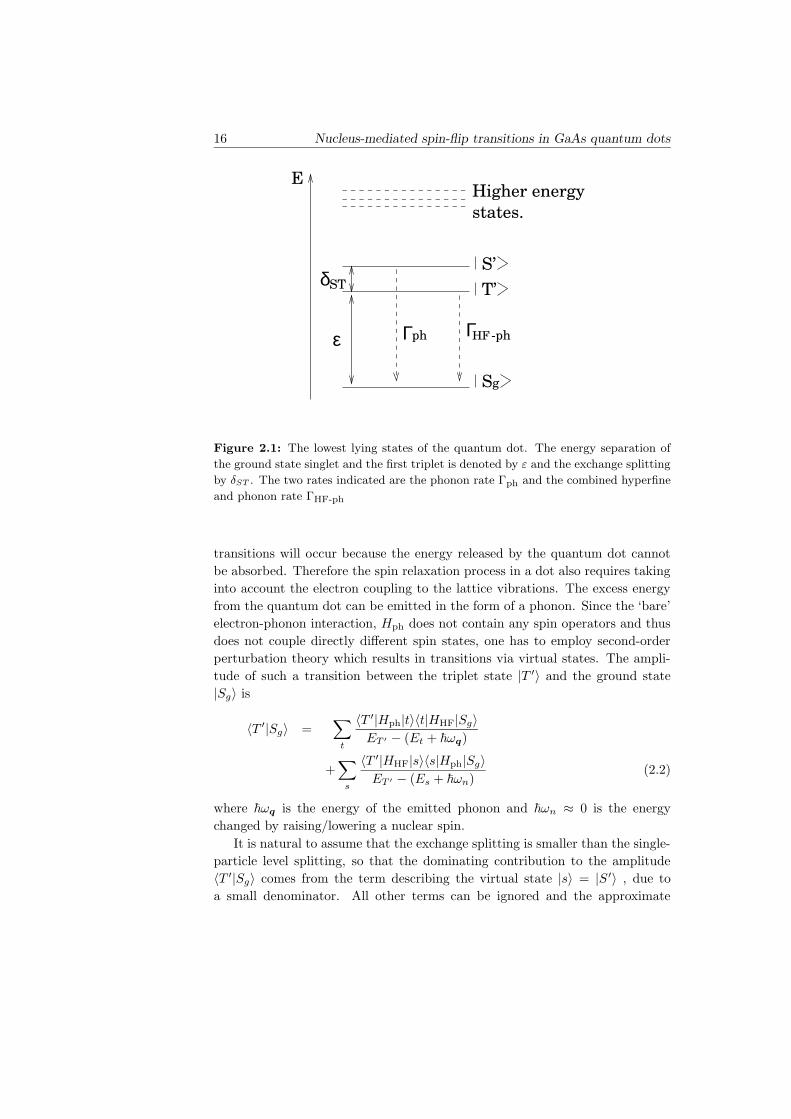
states are ordered as shown in Fig. 2.1. The relevant energy scales used in the
following analysis are given by the energy difference between the triplet state
(we assume small Zeeman splitting) and the ground state ε = ET ′ − Eg, and
exchange splitting δST = ES′ − ET ′ between the first excited singlet and the
triplet. It is possible to inject an electron into an excited state of the dot. If
this excited state is a triplet, the system may get stuck there since a spin-flip is
required to cause transitions to the ground state.
The Γ-point of the conduction band in GaAs is mainly composed of s orbitals,
so that the hyperfine interaction can be described by the contact interaction
Hamiltonian [20]
HHF = A∑
i,k
Si · Ik δ(ri − Rk) (2.1)
where Si (Ik) and ri (Rk) denote the spin and position the ith electron (kth
nuclei). This coupling flips the electron spin and simultaneously lowers/raises
the z -component of a nuclear spin, which mixes spin states and provides the
possibility for relaxation.
But the hyperfine interaction alone does not guarantee that transitions be-
tween the above-described states occur, since the nuclear spin flip cannot relax
the excessive initial-state energy. (The energy associated with a nuclear spin
is the nuclear Zeeman, ~ωn, energy which is three orders of magnitude smaller
than the electron Zeeman energy and the energies related to the orbital degree
of freedom.) For free electrons, the change in energy accompanying a spin flip
caused by the hyperfine scattering is compensated by an appropriate change in
its kinetic energy. In the case of a quantum dot, or any system with discrete
a energy spectrum, this mechanism is not available and no hyperfine induced
16 Nucleus-mediated spin-flip transitions in GaAs quantum dots
S’T’
Sg
Higher energy states.
δST
Γph HF -phΓε
E
Figure 2.1: The lowest lying states of the quantum dot. The energy separation of
the ground state singlet and the first triplet is denoted by ε and the exchange splitting
by δST . The two rates indicated are the phonon rate Γph and the combined hyperfine
and phonon rate ΓHF-ph
transitions will occur because the energy released by the quantum dot cannot
be absorbed. Therefore the spin relaxation process in a dot also requires taking
into account the electron coupling to the lattice vibrations. The excess energy
from the quantum dot can be emitted in the form of a phonon. Since the ‘bare’
electron-phonon interaction, Hph does not contain any spin operators and thus
does not couple directly different spin states, one has to employ second-order
perturbation theory which results in transitions via virtual states. The ampli-
tude of such a transition between the triplet state |T ′〉 and the ground state
|Sg〉 is
〈T ′|Sg〉 =∑
t
〈T ′|Hph|t〉〈t|HHF|Sg〉ET ′ − (Et + ~ωq)
+∑
s
〈T ′|HHF|s〉〈s|Hph|Sg〉ET ′ − (Es + ~ωn)
(2.2)
where ~ωq is the energy of the emitted phonon and ~ωn ≈ 0 is the energy
changed by raising/lowering a nuclear spin.
It is natural to assume that the exchange splitting is smaller than the single-
particle level splitting, so that the dominating contribution to the amplitude
〈T ′|Sg〉 comes from the term describing the virtual state |s〉 = |S ′〉 , due to
a small denominator. All other terms can be ignored and the approximate
2.2 Model and assumptions 17
amplitude takes the form
〈T ′|Sg〉 ≈〈T ′|HHF|S′〉〈S′|Hph|Sg〉
ET ′ − ES′
. (2.3)
The justification for this assumption is that we aim at obtaining estimates of
the rates, and including higher states would not affect the order of magnitude,
even if the exchange splitting is substantial. Note that the phonon and nuclear
state are not explicitly written in Eq. (2.3).
The transition rate from |T ′〉 to |Sg〉 is given by Fermi’s golden rule,
ΓHF-ph =2π
~
∑
N ′
q,µ′
|〈T ′|Sg〉|2δ(Ei − Ef), (2.4)
where N ′q and µ′ are the final phonon and nuclear states respectively and Ei
and Ef stand for the initial and final energies. Inserting Eq. (2.3) into Eq. (2.4)
and averaging over initial nuclear states with probability P (µ), we obtain an
approximate equation for the nucleus mediated transition rate
ΓHF-ph =2π
~
∑
N ′
q
|〈S′;N ′q|Hph|Sg;Nq〉|2δ(Ei −Ef)
×∑
µ′,µ
P (µ)|〈T ′;µ′|HHF|S′;µ〉|2(ET ′ − ES′)2
(2.5)
= Γph(ε)∑
µ′,µ
P (µ)|〈T ′;µ′|HHF|S′;µ〉|2(ET ′ − ES′)2
, (2.6)
where Γph is the non-spin-flip phonon rate as a function of the relaxed energy
ε = ET ′ − ESg.
We will approximate the many-body orbital wave functions by symmetric,
|ΨS〉, and antisymmetric, |ΨT 〉, Slater determinants corresponding to the sin-
glet and triplet states respectively. It is not obvious a priori why this approx-
imation is applicable, since the Coulomb interaction in few electron quantum
dots can be quite strong [21]. The exact energy levels are very different from
those obtained by simply adding the single particle energies. However the wave
function will not drastically change and especially the matrix elements calcu-
lated using Slater determinants are comparable to the ones obtained by using
exact ones. The singlet and triplet wave functions can be decomposed into
orbital and spin parts: |T ′〉 = |ΨT 〉|T 〉 and |S〉 = |ΨS〉|S〉, where
|T 〉 = −νx − iνy√2
|1,+1〉 +νx + iνy√
2|1,−1〉 + νz|1, 0〉, (2.7)
18 Nucleus-mediated spin-flip transitions in GaAs quantum dots
Using the above discussed wave functions in Eq. (2.6) we obtain the following∑
µ′µ
P (µ)|〈T ′;µ|HHF|S′;µ′〉|2 =
A2
4Gcorr
∑
k
(
|Ψ1(Rk)|2 − |Ψ2(Rk)|2)2, (2.8)
where Ψ1,2 are the wave functions of the lowest energy states. The factor Gcorr
contains the nuclear correlation functions
Gcorr =∑
η,γ=x,y,z
νην∗γ
(
Gηγ +1
2i∑
κ
εγηκ〈Iκ〉)
. (2.9)
Here we have introduced symmetric part of the nuclear correlation tensor Gηγ =
〈δIηδIγ + δIγδIη〉/2, where δIη = Iη − 〈Iη〉. The νη’s are the coefficients in the
triplet state expansion in Eq. (2.7) and εγηκ is the totally anti-symmetric tensor.
We assume that nuclei are identical and non-interacting (thus we can drop the
k subscript), which gives for an isotropic system Gcorr = I(I+1)/3 = 1.25 since
Ga and As both have nuclear spin I = 3/2.
Let us now introduce the length scales ` and z0 which are the spatial extent
of the electron wave function in the lateral direction and the dot thickness
respectively. Let Cn denote concentration of nuclei with non-zero spin. The
effective number of nuclei contained within the quantum dot is
Neff = Cn`2z0. (2.10)
In GaAs Neff 1 and the sum over the nuclei in Eq. (2.8) can be replaced by
Cn
∫
d3Rk and we define the dimensionless quantity
γint = `2z0
∫
d3Rk
(
|Ψ1(Rk)|2 − |Ψ2(Rk)|2)2. (2.11)
To relate the hyperfine constant A (which has dimension energy× volume) to a
more convenient parameter we note that the splitting of spin up and spin down
states at maximum nuclear polarization is En = ACnI, where I = 3/2 is the
nuclear spin. Thus, the hyperfine mediated transition rate is
ΓHF-ph = Γph(ε)
(
En
δST
)2Gcorrγint
(2I)2Neff(2.12)
Note that the rate is inversely proportional to the number of nuclei Neff in
the quantum dot and depends on the inverse square of δST , which are both
possible to vary in experiments [22, 23]. In particular, the singlet-triplet splitting
of excited states of a dot can be brought down to zero value using magnetic
field parallel to the 2D plane of the heterostructure, which would accelerate
the relaxation process. The nuclear correlation functions in Gcorr may also be
manipulated by optical orientation of the nuclear system [13, 14].
2.3 Comparison and estimates 19
2.3 Comparison and estimates
We now consider Eq. (2.12) for a specific quantum dot structure. It is assumed
that the lateral confinement is parabolic and that the total potential can be split
into a lateral and transverse part. For vertical dots the approximate transverse
wave function is
χver(z) =
(
2
z0
)1/2
sin
(
πz
z0
)
, (2.13)
where z0 is the thickness of the quantum well, i.e. the dot thickness. The wave
functions in the lateral direction are the Darwin-Fock solutions φn,l(x, y) with
radial quantum number n and angular momentum l. The single particle states
corresponding to (n, l) = (0, 0) and (0,±1) are used to construct the Slater
determinant for a two-electron quantum dot. In the case of these states the
factor γint in Eq. (2.11) is then γint = 0.12 for a vertical dot and γint = 0.045
for a lateral one.
One property of the Darwin-Fock solution is the relation `−2 = ~ωm∗/~2
where ω =√
Ω20 + ω2
c/4 is the effective confining frequency and ωc = eB/m∗
the cyclotron frequency. Inserting this and Eq. (2.10) into Eq. (2.12) the rate
for parabolic quantum dots becomes
ΓHF-ph = Γph(ε)~ω
(
En
δST
)2Gcorrγint
(2I)2
(
m∗
~2Cnz0
)
. (2.14)
Spin relaxation due to spin orbit related mechanisms in GaAs quantum
dots were investigated by Khaetskii and Nazarov in Refs. [10] and [9]. We
will summarize their results here for comparison with our hyperfine-phonon
mechanism. In Ref. [10], it has been found that the dominating scattering
mechanism is due to the absence of inversion symmetry. There are three rates
related to this mechanism,
Γ1 = Γph(ε)8
3
(
m∗β2
~ω
)3
, (2.15)
Γ2 = Γph(ε)7
24
(m∗β2)(~ω)
E2z
, (2.16)
Γ5 = Γph(ε) 6(m∗β2)(g∗µBB)2~ω
(~Ω0)4. (2.17)
The Hamiltonian representing the absence of inversion symmetry has two dis-
tinct contribution which behave differently under a certain unitary transforma-
tion [10]. This behavior results in the two different rates in Eqs. (2.15) and
(2.16). The inclusion of Zeeman splitting gives the rate in Eq. (2.17). Here,
m∗β2 is determined by the transverse confinement and band structure param-
eters and Ez = 〈p2z〉/(2m∗). For vertical dots of thickness z0 = 15 nm, then
20 Nucleus-mediated spin-flip transitions in GaAs quantum dots
m∗β2 ≈ 4× 10⁻³ meV, but one should be cautious when considering a different
thickness, since m∗β2 ∝ z−40 , so the rates are sensitive to variations in z0 .
The transition rates in Eqs. (2.12), (2.15) and (2.16) are all proportional to the
phonon rate Γph evaluated for the same energy difference ε. It is thus sufficient
to compare the only the proportionality coefficients.
Let us now consider for which confining energies the different rates are com-
parable. At zero magnetic field Γ1 = Γ2 at ~Ω0 ≈ 0.8 meV. The estimated
confining energies of vertical quantum dots used in experiment are in the range
2 − 5.5 meV [7, 23, 24]. For those dots Γ2 Γ1 due to the very different de-
pendence on the confinement, Γ1 ∝ (~Ω0)−3 and Γ2 ∝ ~Ω0. Doing the same
for Γ1 and ΓHF-ph we obtain that those rates are equal at ~Ω0 ≈ 4.4 meV.
The numerical values used for the hyperfine rate in Eq. (2.12) are the follow-
ing: En = 0.13 meV [15], δST = 2.3 meV [25] and a z0 = 15 nm. Thus, for
B = 0 T and the previously cited experimental values for the confining energy
the dominant transition rate is Eq. (2.16).
For clarity we will give the values of the rates. The non-spin-flip rate Γph(ε)
is given in Ref. [10] and using the values ~Ω0 = 5.5 meV and B = 0 T we get
Γph ≈ 3.6 × 10⁷ s−1, (2.18)
ΓHF-ph ≈ 2 × 10⁻² s−1, (2.19)
Γ2 ≈ 1 × 10² s−1. (2.20)
The values of level separations ε = 2.7 meV and δST = 2.84 meV are taken from
Ref. [23].
An application of a magnetic field to the dot may result in two effects.
The rate Γ5 becomes larger than Γ2 for magnetic fields around B = 1 T (~Ω0 =
3 meV) to B ≈ 5.4 T (~Ω0 = 5.5 meV). More importantly, the exchange splitting
δST can vanish in some cases and the hyperfine rate in Eq. (2.12) will dominate.
It is also worth noting that in this limit the approximation used in obtaining
Eq. (2.3) becomes very good. Since the rates considered here are all linear in
the phonon rate the divergence of Γph at the singlet-triplet transition does not
affect the ratio of the rates. The above estimates were focused on vertical dots.
To obtain the corresponding results for lateral dots the value of γint in Eq. (2.14)
should be used.
In summary, we have calculated the nucleus mediated spin-flip transition
rate in GaAs quantum dots. The comparison of our results to those previously
obtained for the spin-orbit scattering mechanism indicates that the rates we
obtained here are relatively low, due to the discrete spectrum, so we believe
that hyperfine interaction would not cause problems for spin-coherent manip-
ulation with GaAs quantum dots. Nevertheless, the hyperfine rate, which was
found to be lower than the spin-orbit rates at small magnetic field, may diverge
and become dominant at certain values of magnetic field corresponding to the
2.3 Comparison and estimates 21
resonance between triplet and singlet excited states in the dot.
This work is a part of the research program of the “Stichting vor Funde-
menteel Onderzoek der Materie (FOM)”, EPSRC and INTAS. One of authors
(VF) acknowledges support from NATO CLG and thanks R. Haug and I. Aleiner
for discussions.
22 Nucleus-mediated spin-flip transitions in GaAs quantum dots
References
[1] J. M. Kikkawa and D. D. Awschalom, Phys. Rev. Lett. 80, 4313 (1997).
[2] Y. Ohno et al., Physica E 6, 817 (2000).
[3] T. Fujisawa, Y. Tokura, and Y. Hirayama, Phys. Rev. B 63, R81304 (2001).
[4] D. Loss and D. P. DiVincenzo, Phys. Rev. A 57, 120 (1998).
[5] G. Burkard, D. Loss, and D. P. DiVincenzo, Phys. Rev. B 59, 2070 (1999).
[6] R. C. Ashoori, Nature 379, 413 (1996).
[7] S. Tarucha et al., Phys. Rev. Lett. 77, 3613 (1996).
[8] L. P. Kouwenhoven et al., in Mesoscopic Electron Transport, NATO Se-
ries, edited by L. L. Sohn, L. P. Kouwenhoven, and G. Schoen (Kluwer,
Dordrecht, 1997), Chap. Electron transport in quantum dots, p. 105.
[9] A. V. Khaetskii and Y. V. Nazarov, Physica E 6, 470 (2000).
[10] A. V. Khaetskii and Y. V. Nazarov, Phys. Rev. B 61, 12639 (2000).
[11] D. M. Frenkel, Phys. Rev. B 43, 14228 (1991).
[12] D. Pines, J. Bardeen, and C. P. Slichter, Phys. Rev. 106, 489 (1957).
[13] D. Paget, G. Lampel, B. Sapoval, and V. I. Safarov, Phys. Rev. B 15, 5780
(1977).
[14] D. Paget and V. L. Berkovits, in Optical Orientation, edited by F. Meier
and B. P. Zakharchenya (North-Holland, Amsterdam, 1984).
[15] M. Dobers et al., Phys. Rev. Lett. 61, 1650 (1988).
[16] A. Berg, M. Dobers, R. R. Gerhardts, and K. v. Klitzing, Phys. Rev. Lett.
64, 2563 (1990).
[17] I. D. Vagner, T. Maniv, and E. Ehrenfreund, Solid State Comm. 44, 635
(1982).
[18] S. E. Barrett et al., Phys. Rev. Lett. 74, 5112 (1995).
[19] R. Tycko et al., Science 268, 1460 (1995).
[20] S. W. Brown, T. A. Kennedy, and D. Gammon, Solid State Nucl. Magn.
Reson. 11, 49 (1998).
[21] D. Pfannkuche, Ph.D. thesis, Universitat Karlshuhe, 1998.
[22] W. G. van der Wiel et al., Physica B 256-258, 173 (1998).
[23] S. Tarucha et al., Physica E 3, 112 (1998).
[24] L. P. Kouwenhoven et al., Science 278, 1788 (1997).
[25] F. Bolton, Phys. Rev. B 54, 4780 (1996).
Chapter 3
Hyperfine-mediated transitions between
a Zeeman split doublet in GaAs
quantum dots: The role of the internal
field
Sigurdur I. Erlingsson, Yuli V. Nazarov
We consider the hyperfine-mediated transition rate between Zeeman split
states of the lowest orbital level in a GaAs quantum dot. We separate the
hyperfine Hamiltonian into a part which is diagonal in the orbital states and
another one which mixes different orbitals. The diagonal part gives rise to an
effective (internal) magnetic field which, in addition to an external magnetic
field, determines the Zeeman splitting. Spin-flip transitions in the dots are
induced by the orbital mixing part accompanied by an emission of a phonon. We
evaluate the rate for different regimes of applied magnetic field and temperature.
The rates we find are bigger than the spin-orbit related rates provided the
external magnetic field is sufficiently low.
23
24Hyperfine-mediated transitions between a Zeeman split doublet in GaAs
quantum dots: The role of the internal field
3.1 Introduction
Manipulation of an individual quantum state in a solid state system is currently
the focus of an intense research effort. There are various schemes which have
been proposed and they are in various stages of development. [1–4] Many pro-
posals concentrate on the spin degree of freedom of an electron in a quantum
dot. Recent experiments indicate very long spin decoherence times and small
transition rates between states of different spin [5–7] in some semiconductor
heterostructures.
A characteristic feature of a quantum dot is its discrete energy spectrum.
Depending on the strength of the confinement, both potential and magnetic, an
orbital level energy separation of a few meV is possible. [8] This large energy
separation strongly affects inelastic transition rates in the dot. The nuclei in
GaAs have a substantial hyperfine interactions with the conduction electrons.
This makes it relevant to investigate hyperfine related effects in quantum dots
in GaAs-AlGaAs heterostructures.
Manipulating the electron spin while maintaining phase coherence requires
that it should be relatively well isolated from the environment. Coupling a
quantum dot, or any closed quantum system, to its environment can cause
decoherence and dissipation. One of the measures of the strength of the coupling
to the environment are the transition rates, or inverse lifetimes, between the
quantum dot states. In GaAs there are two main mechanisms that can cause
finite lifetimes of the spin states. These are the spin-orbit interaction and the
hyperfine interaction with the surrounding nuclei. If a magnetic field is applied
the change in Zeeman energy due to a spin-flip has to be accompanied by phonon
emission. For two electron quantum dots, where the transitions are between
triplet and singlet spin states, both spin-orbit [9, 10] and hyperfine [11] mediated
transitions have been studied. In both cases the transition rates are much
smaller than the usual phonon rates, the spin-orbit rate being the higher except
when the excited singlet and triplet states cross. [11] For low magnetic fields,
i.e. away from the singlet-triplet transition, the energy of the emitted phonon
can be quite large and the transitions involve deformation phonons rather than
piezoelectric ones.
If there are an odd number of electrons in the dot the ground state is usually
a spin doublet so that energy change associated with the spin-flip is the electron
Zeeman energy. Owing to the small g-factor in GaAs this energy is rather small
compared to the orbital level spacing and the dominating phonon mechanism is
due to piezoelectric phonons. Recently spin-orbit mediated spin-flip transitions
between Zeeman levels were investigated [12]. Due to Kramer’s degeneracy the
transition amplitude for the spin-flip is proportional to the Zeeman splitting.
This results in a spin-orbit spin-flip rate proportional to the fifth power of the
Zeeman splitting.
3.2 Model and assumptions 25
In this paper we consider hyperfine mediated transitions between Zeeman
split levels in a quantum dot. The transition amplitude remains finite at zero
external magnetic field, resulting in a spin-flip rate [Eq. (3.27)] that is propor-
tional to the cube of the Zeeman splitting. The cause of this is an internal
magnetic field due to the hyperfine interaction. We consider the important con-
cept of internal magnetic field in some detail. Since the parameters of hyperfine
interaction between conduction band electrons and underlying nuclei in GaAs
have been extensively investigated [13, 14], including the Overhauser effect and
spin-relaxation in GaAs/AlGaAs heterostructures [15–19] , we are able to cal-
culate the hyperfine-mediated spin-flip transition rate for quantum dots in such
structures.
Upon completion of this work we learned about recent results of Khaetskii,
Loss and Glazman [20]. They consider essentially the same situation and model
and obtain electron spin decoherence without considering any mechanism of
dissipation. This is in clear distinction from the present result for the spin-flip
rate that requires a mechanism of dissipation, i.e. phonons.
The rest of the paper is organized as follows: in section 3.2 the model used
is introduced in addition to the basic assumptions and approximations used,
section 3.3 deals with the internal magnetic field due to the hyperfine interaction
and section 3.4 contains the derivation of the transition rates. Finally, in section
3.5 the results are discussed.
3.2 Model and assumptions
We consider a quantum dot embedded in a AlGaAs/GaAs heterostructure.
Since the details of the quantum dot eigenstates are not important for now,
it suffices to say that the energy spectrum is discrete and the wave functions
are localized in space. The spatial extension of the wave function in the lateral
and transverse direction (growth direction) are denoted with ` and z0, respec-
tively. Quantum dots in these heterostructures are formed at a GaAs/AlGaAs
interface, where the confining potential is very strong so that ` z0. We define
the volume occupied by an electron as VQD = π`2z0. The Hamiltonian of the
quantum dot can be written in the form
H0 =∑
l
(
εl + gµBB · S)
|l〉〈l|, (3.1)
where εl are the eigenenergies which depend on the structure of the confining
potential and the applied magnetic field B. The magnetic field also couples to
the electron spin via the Zeeman term, where g is the conduction band g-factor
and µB is the Bohr magneton.
Since the Γ point of the conduction band in GaAs is mainly composed of s
26Hyperfine-mediated transitions between a Zeeman split doublet in GaAs
quantum dots: The role of the internal field
orbitals the dipole interaction with the nuclei vanishes and the hyperfine inter-
action can be described by the usual contact term
HHF = AS ·∑
k
Ikδ(r − Rk), (3.2)
where S (Ik) and r (Rk) denote, respectively, the spin and position of the
electron (kth nuclei). The delta function indicates that the point-like nature
of the contact interaction will result in a position dependent coupling. The
coupling constant A has the dimension volume×energy. To get a notion of the
related energy scale, it is straightforward to relate A to the energy splitting of
the doublet for a fully polarized nuclear system,
En = ACnI, (3.3)
Cn being density of nuclei and I the spin of a nucleus. In GaAs this energy is
En ≈ 0.135 meV, which corresponds to a magnetic field of about 5 T. [15] For a
given quantum dot geometry the number of nuclei occupying the dot is defined
as NQD = CnVQD. Since the Ga and As nuclei have the same spin and their
coupling constants are comparable, we will assume that all the nuclear sites are
characterized by the same hyperfine coupling A, and Cn ≈ a−30 where a0 is the
lattice spacing. For realistic quantum dots NQD ≈ 104 − 106, and it is therefore
an important big parameter in the problem.
The coupling between the electron and the phonon bath is represented with
Hph =∑
q,ν
αν(q)(bq,νeiq·r + b†q,νe
−iq·r), (3.4)
where b†qν and bqν are creation and annihilation operators for the phonon mode
with wave-vector q on brach ν. In GaAs there are two different coupling mecha-
nisms, deformation ones and piezoelectric ones. For transitions between Zeeman
split levels in GaAs, i.e. low energy emission, the most effective phonon mecha-
nism is due to piezoelectric phonons. We will assume that the heterostructure is
grown in the [100] direction. This is the case for almost all dots and it imposes
important symmetry relations on the coupling coefficient. The square of the
coupling coefficient for the piezoelectric phonons is then given by (see Ref. [21])
α2ν(q) =
(eh14)2~
2ρcνV qAν(θ) (3.5)
where (eh14) is the piezoelectric coefficient, ρ is the mass density, cν is the
speed of sound of branch ν, V is normalization volume, we have defined q =
q(cosφ sin θ, sinφ sin θ, cos θ) and the Aν ’s are the so-called anisotropy functions,
see Appendix B.
3.3 Internal magnetic field 27
3.3 Internal magnetic field
In this section we will introduce the concept of the effective magnetic field,
the internal field, acting on the electron due to the hyperfine interaction. This
internal field is a semiclassical approximation to the nuclear system, this ap-
proximation being valid in the limit of a large number of nuclei, NQD 1.
If the nuclei are noticeably polarized, this field coincides with the Overhauser
field that represents the average nuclear polarization. It is important that the
internal field persists even at zero polarization giving rise to Zeeman splitting
of the order EnN−1/2QD .
First we write the Hamiltonian in Eq. (3.2) in the basis of the electron orbital
states and present it as a sum of two terms
HHF = H0HF + VHF, (3.6)
where the terms are defined as
H0HF = A
∑
l
|l〉〈l|S ·∑
k
|〈Rk|l〉|2Ik (3.7)
VHF = A∑
l 6=l′
|l〉〈l′|S ·∑
k
〈l|Rk〉〈Rk|l′〉Ik. (3.8)
By definition H0HF does not couple different orbital levels. By combining Eqs.
(3.1) and (3.7) one obtains the following Hamiltonian
H0 =∑
l
(
εl + gµBBl · S)
|l〉〈l|. (3.9)
We will regard the mixing term VHF as a perturbation to H0. The justification
for this is that the typical fluctuations of the electron energy due to the hyperfine
interaction are much smaller than the orbital energy separation.
We now concentrate on H0 and formulate a semiclassical description of it.
For this we consider the operator of the orbitally dependent effective magnetic
field,
Bl = B +1
gµBKl, (3.10)
where
Kl =En
ICn
∑
k
|〈Rk|l〉|2Ik. (3.11)
Our goal is to replace the operator Kl with a classical field. To prove the
replacement is reasonable we calculate the average of the square for a given
unpolarized nuclear state |µ〉
K2l = 〈µ|K2
l |µ〉 ≈E2
n
NQD. (3.12)
28Hyperfine-mediated transitions between a Zeeman split doublet in GaAs
quantum dots: The role of the internal field
We cannot simply replace Kl by its eigenvalues: as in the case of the usual spin
algebra, different components of Kl do not commute. In addition its square
does not commute with individual components, [K2l , K
αl ] 6= 0. To estimate
fluctuations of Kl we calculate the uncertainty relations between its components
∆Kαl ∆Kβ
l ≥ αlE2n
N3/2QD
≈ K2l
1
N1/2QD
, (3.13)
where αl is a numerical constant o(1) which depends on the details of the orbital
wave functions. Since N−1/2QD 1 we have proved that the quantum fluctuations
in Kl are much smaller than its typical amplitude. The semiclassical picture
introduced above is only valid for high temperatures, kT EnN−1QD, where there
are many states available to the nuclear system and the typical amplitude of Kl
is proportional to EnN−1/2QD . For temperatures below EnN
−1QD the nuclear system
will predominantly be in the ground state and the classical picture breaks down.
This is similar to the quantum mechanical description of a particle moving in a
potential. At zero temperature it will be localized in some potential minimum
and quantum mechanics will dominate. At sufficiently high temperatures the
particle occupies higher energy states and its motion is well described by classical
mechanics. Having established this we can replace the average over the density
matrix of the nuclei by the average over a classical field Kl, and note that it
has no ‘hat’, whose values are Gaussian distributed
P (Kl) =
(
1
2πσ2l
)3/2
exp
(
− (Kl − K(0)l )2
2σ2l
)
, (3.14)
where σ2l = 1
3 (〈K2l 〉 − 〈Kl〉2) is the variance and K
(0)l is the average, or Over-
hauser, field. In the case of a polarized nuclear system the variance decreases
and the distribution becomes sharper around the Overhauser field, eventually
becoming P (Kl) = δ(Kl −K(0)l ) as σ2
l → 0. The effective magnetic field acting
on the electron is Bl = Bln where n is the unit vector along the total field for a
given Kl, see Fig. 3.1. For this configuration the spin eigenfunctions are |n±〉,corresponding to eigenvalues
n · S|n±〉 = ±1
2|n±〉. (3.15)
The effective Zeeman Hamiltonian is then
HZ = gµBBl · S (3.16)
in this given internal field configuration. The spectrum of H0 thus consists of
many doublets distinguished by the value of Bl. The magnitude of the effective
field Bl determines the Zeeman splitting of each doublet,
∆l = gµBBl
= (E2B +K2
l + 2EBKl cos θ)1/2 (3.17)
3.4 Transition rate 29
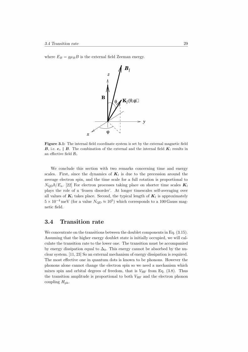
where EB = gµBB is the external field Zeeman energy.
θ
φ
(θ,φ)l
lB
KB
x
y
z
Figure 3.1: The internal field coordinate system is set by the external magnetic field
B, i.e. ez ‖ B. The combination of the external and the internal field Kl results in
an effective field Bl.
We conclude this section with two remarks concerning time and energy
scales. First, since the dynamics of Kl is due to the precession around the
average electron spin, and the time scale for a full rotation is proportional to
NQD~/En. [22] For electron processes taking place on shorter time scales Kl
plays the role of a ‘frozen disorder’. At longer timescales self-averaging over
all values of Kl takes place. Second, the typical length of Kl is approximately
5 × 10⁻⁴ meV (for a value NQD ≈ 105) which corresponds to a 100 Gauss mag-
netic field.
3.4 Transition rate
We concentrate on the transitions between the doublet components in Eq. (3.15).
Assuming that the higher energy doublet state is initially occupied, we will cal-
culate the transition rate to the lower one. The transition must be accompanied
by energy dissipation equal to ∆0. This energy cannot be absorbed by the nu-
clear system. [11, 23] So an external mechanism of energy dissipation is required.
The most effective one in quantum dots is known to be phonons. However the
phonons alone cannot change the electron spin so we need a mechanism which
mixes spin and orbital degrees of freedom, that is VHF from Eq. (3.8). Thus
the transition amplitude is proportional to both VHF and the electron phonon
coupling Hph.
30Hyperfine-mediated transitions between a Zeeman split doublet in GaAs
quantum dots: The role of the internal field
Here we assume that the electron is in the lowest orbital state |0〉 since
the phonon mechanism will bring the electron to this state from any higher
orbital on timescales much smaller than those related to transitions between
the doublet components. Thus we consider an initial state of the entire system
|i〉 = |0,n−;µ;N〉 which is a product state of the electron, nuclear |µ〉 and
phonon |N〉 systems and the final state |f〉 = |0,n+;µ′;N ′〉. Note that to a
given state of the nuclear system |µ〉, which is a product state of all individual
nuclei, there is an associated value of the classical field Kl. The transition
amplitude between |i〉 and |f〉, in second order perturbation theory, reads
T =∑
l 6=0
( 〈0,n+;µ′|VHF|l,n−;µ〉〈l;N ′|Hph|0;N〉(ε0 − εl) + EB
+〈0;N ′|Hph|l;N〉〈l,n+;µ′|VHF|0,n−;µ〉
(ε0 − εl) − EB
)
. (3.18)
The summation is over virtual states involving higher orbitals and the denom-
inators in Eq. (3.18) contains the energy differences between different orbital
states. The internal field depends on the orbital state, resulting in a rather
complicated expression. Albeit the energy related to the internal field is much
smaller than the orbital separation so we can safely replace the Zeeman splitting
with EB . The reason for that is that only at high external fields where ∆0 ≈ EB
will the effects of the Zeeman splitting be appreciable in the denominator. The
internal field also appears in the phonon rate since it determines the electron
energy difference between the initial and final states. Since Hph does not con-
nect different nuclear states and conversely VHF does not mix different phonon
states the sums over intermediate phonon and nuclear states reduce to a single
term. From this transition amplitude the transition rate is obtained via Fermis
golden rule
Γsf =2π
~
∑
N ′
∑
µ′
|T |2δ(Ei − Ef), (3.19)
where Ei −Ef is the energy difference between the initial and final states of the
combined systems. Substituting Eq. (3.18) into Eq. (3.19) we get the following
3.4 Transition rate 31
relation for the spin-flip rate
Γsf =∑
l,l′ 6=0
( 〈l,n−;µ|VHF|0,n+〉〈0,n+|VHF|l′,n−;µ〉((ε0 − εl) + EB)((ε0 − εl′) + EB)
× 2π
~
∑
N ′
〈0;N |Hph|l;N ′〉〈l′;N ′|Hph|0;N〉δ(Ei − Ef)
+〈l,n−;µ|VHF|0,n+〉〈l′,n+|VHF|0,n−;µ〉
((ε0 − εl) + EB)((ε0 − εl′) − EB)
×2π
~
∑
N ′
〈0;N |Hph|l;N ′〉〈0;N ′|Hph|l′;N〉δ(Ei − Ef)
+〈0,n−;µ|VHF|l,n+〉〈0,n+|VHF|l′,n−;µ〉
((ε0 − εl) − EB)((ε0 − εl′) + EB)
×2π
~
∑
N ′
〈l;N |Hph|0;N ′〉〈l′;N ′|Hph|0;N〉δ(Ei − Ef)
+〈0,n−;µ|VHF|l,n+〉〈l′,n+|VHF|0,n−;µ〉
((ε0 − εl) − EB)((ε0 − εl′) − EB)
× 2π
~
∑
N ′
〈l;N |Hph|0;N ′〉〈0;N ′|Hph|l′;N〉δ(Ei − Ef)
)
.
(3.20)
The spin-flip rate depends on the initial state of the nuclear system |µ〉. This
poses the problem of how to deal with the nuclear state |µ〉, since we already
demoted all the spin operators to a collective classical variable. A conceptually
simple solution lies in the fact that when Eqs. (3.20) and (3.8) are considered
together one sees that the rate is a sum over all pairs of nuclei in the system.
Focusing on a given pair of nuclei k and k′, all the other nuclei are unchanged
when the electron spin is ‘scattered’ on by this pair. By simply redefining
the classical field such that it is composed of all nuclei except this given pair
we can circumvent the problem. This procedure will not change our previous
result regarding the properties of Kl and by defining |µ〉 = |µk〉|µk′〉 makes it
straightforward to work with the nuclear states in Eq. (3.20).
Although the transition rate can be very slow, the typical duration of a
transition event is set by energy uncertainty, ~/∆0. This is much shorter than
the typical time for nuclear system dynamics so that the nuclear system is frozen
in a given value of K0 during the transition. In this case taking an average over
K0, using the probability distribution in Eq. (3.14), is not well motivated. For
now we will postpone the averaging over the classical field. Expanding the
energy denominators to second order in the Zeeman splitting and performing
the thermal average over nuclei spin pairs (see Appendix A) we obtain the
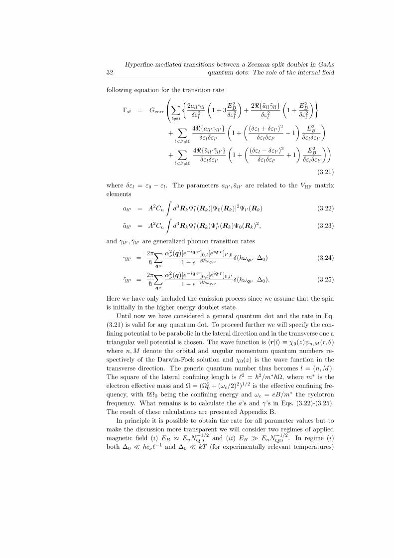
32Hyperfine-mediated transitions between a Zeeman split doublet in GaAs
quantum dots: The role of the internal field
following equation for the transition rate
Γsf = Gcorr
∑
l 6=0
2allγll
δε2l
(
1 + 3E2
B
δε2l
)
+2<allγll
δε2l
(
1 +E2
B
δε2l
)
+∑
l<l′ 6=0
4<all′γll′δεlδεl′
(
1 +
(
(δεl + δεl′)2
δεlδεl′− 1
)
E2B
δεlδεl′
)
+∑
l<l′ 6=0
4<all′ γll′δεlδεl′
(
1 +
(
(δεl − δεl′)2
δεlδεl′+ 1
)
E2B
δεlδεl′
))
(3.21)
where δεl = ε0 − εl. The parameters all′ , all′ are related to the VHF matrix
elements
all′ = A2Cn
∫
d3RkΨ∗l (Rk)|Ψ0(Rk)|2Ψl′(Rk) (3.22)
all′ = A2Cn
∫
d3RkΨ∗l (Rk)Ψ∗
l′(Rk)Ψ0(Rk)2, (3.23)
and γll′ , γll′ are generalized phonon transition rates
γll′ =2π
~
∑
qν
α2ν(q)[e−iq·r]0,l[e
iq·r]l′,01 − e−β~ωq,ν
δ(~ωqν−∆0) (3.24)
γll′ =2π
~
∑
qν
α2ν(q)[e−iq·r]0,l[e
iq·r]0,l′
1 − e−β~ωq,νδ(~ωqν−∆0). (3.25)
Here we have only included the emission process since we assume that the spin
is initially in the higher energy doublet state.
Until now we have considered a general quantum dot and the rate in Eq.
(3.21) is valid for any quantum dot. To proceed further we will specify the con-
fining potential to be parabolic in the lateral direction and in the transverse one a
triangular well potential is chosen. The wave function is 〈r|l〉 ≡ χ0(z)ψn,M (r, θ)
where n,M denote the orbital and angular momentum quantum numbers re-
spectively of the Darwin-Fock solution and χ0(z) is the wave function in the
transverse direction. The generic quantum number thus becomes l = (n,M).
The square of the lateral confining length is `2 = ~2/m∗
~Ω, where m∗ is the
electron effective mass and Ω = (Ω20 + (ωc/2)
2)1/2 is the effective confining fre-
quency, with ~Ω0 being the confining energy and ωc = eB/m∗ the cyclotron
frequency. What remains is to calculate the a’s and γ’s in Eqs. (3.22)-(3.25).
The result of these calculations are presented Appendix B.
In principle it is possible to obtain the rate for all parameter values but to
make the discussion more transparent we will consider two regimes of applied
magnetic field (i) EB ≈ EnN−1/2QD and (ii) EB EnN
−1/2QD . In regime (i)
both ∆0 ~cν`−1 and ∆0 kT (for experimentally relevant temperatures)
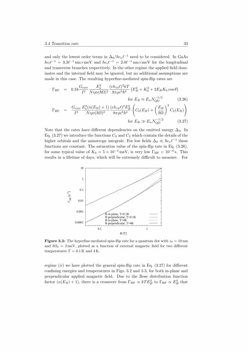
3.4 Transition rate 33
and only the lowest order terms in ∆0/~cν`−1 need to be considered. In GaAs
~cl`−1 = 3.3`−1 nm×meV and ~ct`
−1 = 2.0`−1 nm×meV for the longitudinal
and transverse branches respectively. In the other regime the applied field dom-
inates and the internal field may be ignored, but no additional assumptions are
made in this case. The resulting hyperfine-mediated spin-flip rates are
ΓHF = 0.34Gcorr
I2
E2n
NQD(~Ω)2(eh14`)
2kT
8πρc5~4
(
E2B +K2
0 + 2EBK0 cos θ)
for EB ≈ EnN−1/2QD (3.26)
ΓHF =Gcorr
I2
E2n(n(EB) + 1)
NQD(~Ω)2(eh14`)
2E3B
8πρc5~4
(
C0(EB) +
(
EB
~Ω
)2
C2(EB)
)
for EB EnN−1/2QD (3.27)
Note that the rates have different dependencies on the emitted energy ∆0. In
Eq. (3.27) we introduce the functions C0 and C2 which contain the details of the
higher orbitals and the anisotropy integrals. For low fields ∆0 ~cν`−1 these
functions are constant. The saturation value of the spin-flip rate in Eq. (3.26),
for some typical value of K0 = 5 × 10⁻⁴ meV, is very low ΓHF < 10−6 s. This
results in a lifetime of days, which will be extremely difficult to measure. For
0.0001
0.001
0.01
0.1
1
10
0.1 1
Γ HF
[s-1
]
B [T]
B in-plane, T=0.1KB perpendicular, T=0.1KB in-plane, T=4KB perpendicular, T=4K
Figure 3.2: The hyperfine-mediated spin-flip rate for a quantum dot with z0 = 10nm
and ~Ω0 = 2meV, plotted as a function of external magnetic field for two different
temperatures T = 0.1 K and 4 K.
regime (ii) we have plotted the general spin-flip rate in Eq. (3.27) for different
confining energies and temperatures in Figs. 3.2 and 3.3, for both in-plane and
perpendicular applied magnetic field. Due to the Bose distribution function
factor (n(EB) + 1), there is a crossover from ΓHF ∝ kTE2B to ΓHF ∝ E3
B that
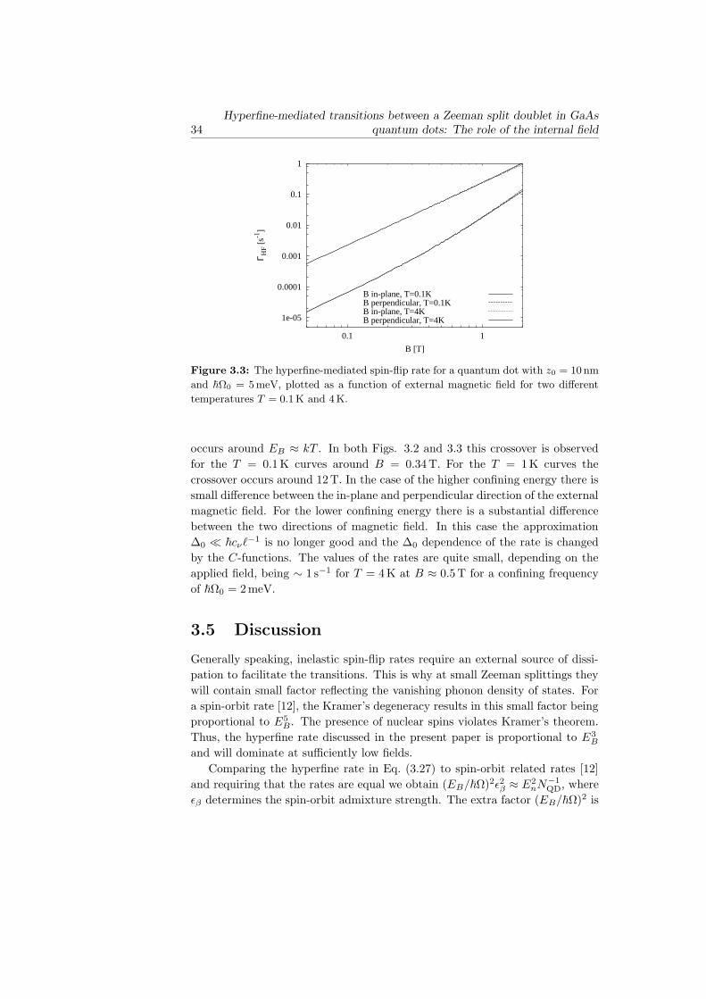
34Hyperfine-mediated transitions between a Zeeman split doublet in GaAs
quantum dots: The role of the internal field
1e-05
0.0001
0.001
0.01
0.1
1
0.1 1
Γ HF
[s-1
]
B [T]
B in-plane, T=0.1KB perpendicular, T=0.1KB in-plane, T=4KB perpendicular, T=4K
Figure 3.3: The hyperfine-mediated spin-flip rate for a quantum dot with z0 = 10 nm
and ~Ω0 = 5 meV, plotted as a function of external magnetic field for two different
temperatures T = 0.1 K and 4K.
occurs around EB ≈ kT . In both Figs. 3.2 and 3.3 this crossover is observed
for the T = 0.1 K curves around B = 0.34 T. For the T = 1 K curves the
crossover occurs around 12T. In the case of the higher confining energy there is
small difference between the in-plane and perpendicular direction of the external
magnetic field. For the lower confining energy there is a substantial difference
between the two directions of magnetic field. In this case the approximation
∆0 ~cν`−1 is no longer good and the ∆0 dependence of the rate is changed
by the C-functions. The values of the rates are quite small, depending on the
applied field, being ∼ 1 s−1 for T = 4 K at B ≈ 0.5 T for a confining frequency
of ~Ω0 = 2 meV.
3.5 Discussion
Generally speaking, inelastic spin-flip rates require an external source of dissi-
pation to facilitate the transitions. This is why at small Zeeman splittings they
will contain small factor reflecting the vanishing phonon density of states. For
a spin-orbit rate [12], the Kramer’s degeneracy results in this small factor being
proportional to E5B . The presence of nuclear spins violates Kramer’s theorem.
Thus, the hyperfine rate discussed in the present paper is proportional to E3B
and will dominate at sufficiently low fields.
Comparing the hyperfine rate in Eq. (3.27) to spin-orbit related rates [12]
and requiring that the rates are equal we obtain (EB/~Ω)2ε2β ≈ E2nN
−1QD, where
εβ determines the spin-orbit admixture strength. The extra factor (EB/~Ω)2 is
References 35
due to Kramers degeneracy which suppresses the spin-orbit rate compared to
hyperfine one at low fields. The crossover occurs at EB ≈ ~Ω(EnN−1/2QD /εβ),
which correspond to magnetic field B ≈ 0.3 T, assuming typical quantum dot
parameters z0 = 10 nm and ~Ω0 = 4 meV.
The role of the internal field produced by the nuclei is that the spin-flip rate
does not vanish even for in the absence of external magnetic field. We show
that the minimum rate is rather small, corresponding to a relaxation time of the
order of days. We believe that the internal field will play an important role when
the full dynamics of the electron spin in the presence of the nuclear system is
considered. Our model should also be applicable to other polar semiconductors
which have non-zero nuclear spin, e.g. InAs where the g-factor is much larger.
One author (SIE) would like to thank Daniela Pfannkuche, Alexander Chud-
novskii for fruitful discussions. We also acknowledge discussions with Daniel
Loss and Alexander V. Khaetskii. This work is a part of the research program
of the “Stichting voor Fundementeel Onderzoek der Materie (FOM)”
References
[1] Y. Nakamura, Y. A. Pashkin, and J. S. Tsai, Nature 398, 786 (1999).
[2] J. E. Mooij et al., Science 285, 1036 (1999).
[3] B. E. Kane, Nature 393, 133 (1998).
[4] D. Loss and D. P. DiVincenzo, Phys. Rev. A 57, 120 (1998).
[5] J. M. Kikkawa and D. D. Awschalom, Phys. Rev. Lett. 80, 4313 (1997).
[6] Y. Ohno et al., Physica E 6, 817 (2000).
[7] T. Fujisawa, Y. Tokura, and Y. Hirayama, Phys. Rev. B 63, R81304 (2001).
[8] L. P. Kouwenhoven et al., in Mesoscopic Electron Transport, NATO Se-
ries, edited by L. L. Sohn, L. P. Kouwenhoven, and G. Schoen (Kluwer,
Dordrecht, 1997), Chap. Electron transport in quantum dots, p. 105.
[9] A. V. Khaetskii and Y. V. Nazarov, Phys. Rev. B 61, 12639 (2000).
[10] A. V. Khaetskii and Y. V. Nazarov, Physica E 6, 470 (2000).
[11] S. I. Erlingsson, Y. V. Nazarov, and V. I. Fal’ko, Phys. Rev. B 64, 195306
(2001).
[12] A. V. Khaetskii and Y. V. Nazarov, Phys. Rev. B 64, 125316 (2001).
[13] D. Paget, G. Lampel, B. Sapoval, and V. I. Safarov, Phys. Rev. B 15, 5780
(1977).
Using the notation in Ref. [12] the spin-orbit admixture constant is εβ = β~/a, where a
is the lateral quantum dot size, corresponding to ` in the present paper.

36Hyperfine-mediated transitions between a Zeeman split doublet in GaAs
quantum dots: The role of the internal field
[14] D. Paget and V. L. Berkovits, in Optical Orientation, edited by F. Meier
and B. P. Zakharchenya (North-Holland, Amsterdam, 1984).
[15] M. Dobers et al., Phys. Rev. Lett. 61, 1650 (1988).
[16] A. Berg, M. Dobers, R. R. Gerhardts, and K. v. Klitzing, Phys. Rev. Lett.
64, 2563 (1990).
[17] I. D. Vagner, T. Maniv, and E. Ehrenfreund, Solid State Comm. 44, 635
(1982).
[18] S. E. Barrett et al., Phys. Rev. Lett. 74, 5112 (1995).
[19] R. Tycko et al., Science 268, 1460 (1995).
[20] A. V. Khaetskii, D. Loss, and L. Glazman, Phys. Rev. Lett. 88, 186802
(2002).
[21] P. J. Price, Ann. Phys. 133, 217 (1981).
[22] I. A. Merkulov, A. L. Efros, and M. Rosen, Phys. Rev. B 65, 205309 (2002).
[23] J. H. Kim, I. D. Vagner, and L. Xing, Phys. Rev. B 49, 16777 (1994).
Chapter 4
Nuclear spin induced coherent
oscillations of transport current through
a double quantum dot
Sigurdur I. Erlingsson, Oleg N. Jouravlev and Yuli V. Nazarov
We propose a mechanism for coherent oscillations of transport current through
a double quantum dot. It is based on coupling of the states of different spin due
to hyperfine interaction with nuclei. We study the dependence of the current
oscillations on various system parameters and external magnetic field. Our
results may qualitatively explain recent experimental observations.
37
38Nuclear spin induced coherent oscillations of transport current through a
double quantum dot
4.1 Introduction
Motivated by possible device applications which utilize both the spin and charge
of electrons there has been a great effort to come up with means of manipulat-
ing the electron spin and even the nuclear spin of the host material. In GaAs
the dominant coupling mechanism between electron and nuclear spins is the
hyperfine interaction. Furthermore, the nuclear spin relaxation times are much
longer than other timescales related to electron dynamics [1]. This difference of
timescales has facilitated many experiments where a quasi-stationary polariza-
tion of the nuclear system is achieved and its effect on the electronic behavior
can be observed [2–5]. Many recent experiments have involved novel ways of
controlling the coupling of the electron and nuclear spin [6, 7], and even co-
herent oscillations between ’up’ and ’down’ polarized nuclear system have been
reported [8].
Transport experiments have proven to be a very good tool to probe nanos-
tructures. This is especially true in quantum dots where the control of the dot
energetics allows for a detailed study of the quantum dot spectrum, both in the
linear regime and in excitation spectroscopy [9, 10]. In between the conduction
peaks, i.e. in the Coulomb blockade regime, there still flows a small current due
to cotunneling [11]. This cotunneling current, sometimes referred to as leakage
current, has been discussed in connection with limitations of operating SET
devices [12].
Unexpected oscillations of the leakage current through a double quantum dot
in a spin blockade regime have been observed in transport experiments [13]. The
system is the same as used in a recent experiment where current rectification was
observed in the transport characteristics [14]. The origin of this rectification was
explained in terms of spin blockade, i.e. interdot transitions between states with
different spins are blocked. The inclusion of a spin-flip mechanism lifts the spin
blockade, giving rise to a small leakage current in a similar way cotunneling lifts
the Coulomb blockade. Related ideas of spin blockade based on certain selection
rules have previously were proposed in [15]. More recently, spin blockade was
observed in transport through quantum dot systems that was attributed to spin
polarized leads [16]. The timescale of the leakage current oscillations, which is
much larger than the usual timescale related to electronic transport, and the fact
that the oscillation period and amplitude were modified by resonant excitation
of the nuclei indicates that the origin of the oscillations may be traced to the
hyperfine interaction [13].
Here we propose a novel transport mechanism based on the hyperfine inter-
action which leads to an oscillating leakage current in the spin blockade regime.
This mechanism may, in a qualitative way, shed light on some of the experi-
mental results observed in Ref. [13]. The key steps in formulating a solution
of the problem are (i) calculating the stationary solution of the density matrix
4.2 Model 39
for the double dot system assuming a fixed nuclear system and (ii) using that
stationary solution to determine the average electrons spins in the dots which
are then used to calculate the dynamics of the nuclear system. This approach
is only valid if the transport timescales are much shorter than the dynamical
timescales associated with the nuclear system. We assume that this is the case in
the system studied here. The relevant transport processes may be characterized
by 4 rates, the left (right) barrier tunnel rate ΓL (ΓR), the inelastic interdot tun-
nel rate Γi and the transport rate in the spin blockade regime ∝ (KA/∆ST )2Γi,
where KA and ∆ST respectively characterize the coupling and energy separa-
tion of the blocked and non-blocked spin states. The factor (KA/∆ST ) 1 is
responsible for suppressing the current in the spin blockade regime in compar-
ison with non-blocked current ∝ Γi. The fastest nuclear spin process which
enters the density matrix is the precession frequency γ of the nuclear system in
the hyperfine field of the average electron spins [17]. This results in the condi-
tion Γi (∆ST /KA)2γ for the validity of our approach. The timescale of the
oscillation is determined by the factor γ−1(∆ST /KA), which can be quite long
approaching tenths of seconds.
4.2 Model
For details of the setup we refer the reader to Ref. [14]. Each charge configura-
tion of the double dot system can be characterized by (NL,NR) where NL(NR)
is the number of charges of the left (right) dot, see Fig. 4.1. The multiplicity
of the (0,1) configuration is 2 since it is a spin doublet, denoted by |±〉. The
(1,1) configuration has a multiplicity of 4, one singlet |S0〉 and 3 triplets |Ti〉,i = 1, 2, 3. At low magnetic fields the total spin of the configuration (0,2) is a
singlet [14], the state being denoted by |Sg〉.It is instructive to look more closely at the eigenstates of the double dot
system since they are instrumental in determining the transport characteristics.
Also, the spin structure of the eigenstates becomes clear after diagonalizing the
Hamiltonian of the double dot system. The Hamiltonian for the isolated double
dot system is
HDD = H0 +HT +HC (4.1)
where H0 is the Hamiltonian of each dot
H0 =∑
η
(εLηd†LηdLη + (εRη + e∆V )d†RηdRη) (4.2)
where d†αη creates a particle in state α = L,R with spin η =↑, ↓ and e∆V
is determined by the voltage drop over the central barrier. Using the above
assumptions about the possible charge configurations, only one orbital level on
40Nuclear spin induced coherent oscillations of transport current through a
double quantum dot
each is dot is relevant. The quantization axis of the electron spin is along the
external magnetic field that is applied parallel to the 2DEG plane. The orbitals
are not affected by the field and thus the sole effect of magnetic field is through
the Zeeman energy
εαη = ~Ωα ± ∆/2, (4.3)
where ~Ωα is the ground state orbital energy of the α = L,R dot and ∆ = gµBB
is the Zeeman splitting. The second term in Eq. (4.1) is the tunneling Hamilto-
nian describing interdot tunneling between the L and R orbital, assuming spin
conservation,
Ht =∑
η
(Vτd†LηdRη + V ∗
τ d†RηdLη), (4.4)
where Vτ is the tunneling amplitude. The Coulomb interaction is approximated
by the following expression
HC = ULnL↑nL↓ + URnR↑nR↓ +∑
ηη′
ULRnLηnRη′ . (4.5)
where nαη = d†αηdαη, UL and UR are the charging energies for the on-site
charging and ULR is the interdot charging energy.
Once a suitable basis has been chosen, the double dot Hamiltonian can be
diagonalized. It is convenient to introduce the following basis states
|0; η〉 = d†Rη|〉|η; η′〉 = d†Lηd
†Rη|〉
|0; ↑↓〉 = d†R↑d†R↓|〉.
These states are eigenstates of H0 and HC but not HT . It is easy to establish
that only three (of seven possible ) states are coupled by HT . By diagonalizing
the submatrix of these three states, the resulting eigenstates and eigenenergies
are
|T2〉 =1√2(| ↑; ↓〉 + | ↓; ↑〉), ET2
= ~ΩL + ~ΩR + ULR (4.6)
|S0〉 ≈ 1√2(| ↑; ↓〉 − | ↓; ↑〉), ES0
≈ ET2+
|Vτ |2e∆V − δU
(4.7)
|Sg〉 ≈ |0; ↑↓〉, ESg≈ ET2
− eδV + δU − |Vτ |2eδV − δU
, (4.8)
where δU = UR −ULR. These equations were obtained assuming Vτ (e∆V −δU), which is a good approximation for the system in question. The other four
4.2 Model 41
eigenstates are simply
|T1〉 = | ↑; ↑〉, ET1= ET2
− ∆ (4.9)
|T3〉 = | ↓; ↓〉, ET3= ET2
+ ∆ (4.10)
|±〉 = |0; ↑/↓〉, E± = ~ΩR ± ∆/2. (4.11)
The triplet states are degenerate at B = 0 and otherwise they are separated by
the Zeeman splitting ∆. The (1, 1) singlet has a higher energy at zero field than
the triplet states. The |S0〉 and |T3〉 states cross at a magnetic field
B∗ =1
gµB
|Vτ |2e∆V − δU
. (4.12)
The hyperfine interaction induces mixing of the singlet and triplets in the
(1, 1) configuration which lift the spin blockade. Since we are interested in
the leakage current oscillations, other spin-flip mechanisms that only give rise
to a dc current will not be considered. Our starting point is to introduce a
semiclassical picture of the hyperfine interaction. This approximation [17–19]
is valid when the number of nuclei in the quantum dot NQD 1. The part of
the total Hamiltonian which explicitly contains the electron spin operators SL
and SR is
Hs = KL · SL + KR · SR + gµBBext · (SL + SR)
=1
2(KL + KR) ·
(
SL + SR
)
+1
2(KL − KR) ·
(
SL − SR
)
+gµBBext · (SL + SR)
= gµBBSz +1
2KA · (SL − SR) (4.13)
where g is the g-factor, µB is the Bohr magneton and KL (KR) it the semiclas-
sical effective nuclear magnetic field acting on the electron spin localized in the
left (right) dot. In Eq. (4.13) the quantization axis has been set along the total
magnetic field
B = Bext +1
2gµB(KL + KR) (4.14)
and Sz is the z-component of the total spin operator. The latter term in Eq.
(4.14) does not couple the singlet and triplets, it only changes the Zeeman
splitting of the triplet states. The second term in Eq. (4.13) mixes the (1,1)
singlet and triplet states, i.e. the mixing is proportional to the asymmetry in
the two effective nuclear magnetic fields
KA = KL − KR. (4.15)
The spin operator is Sα =∑
η,γ σηγd†αηdαη where σ = (σx, σy , σz) are the Pauli matrices
and d†Lη
creates an electron with spin η in dot α.
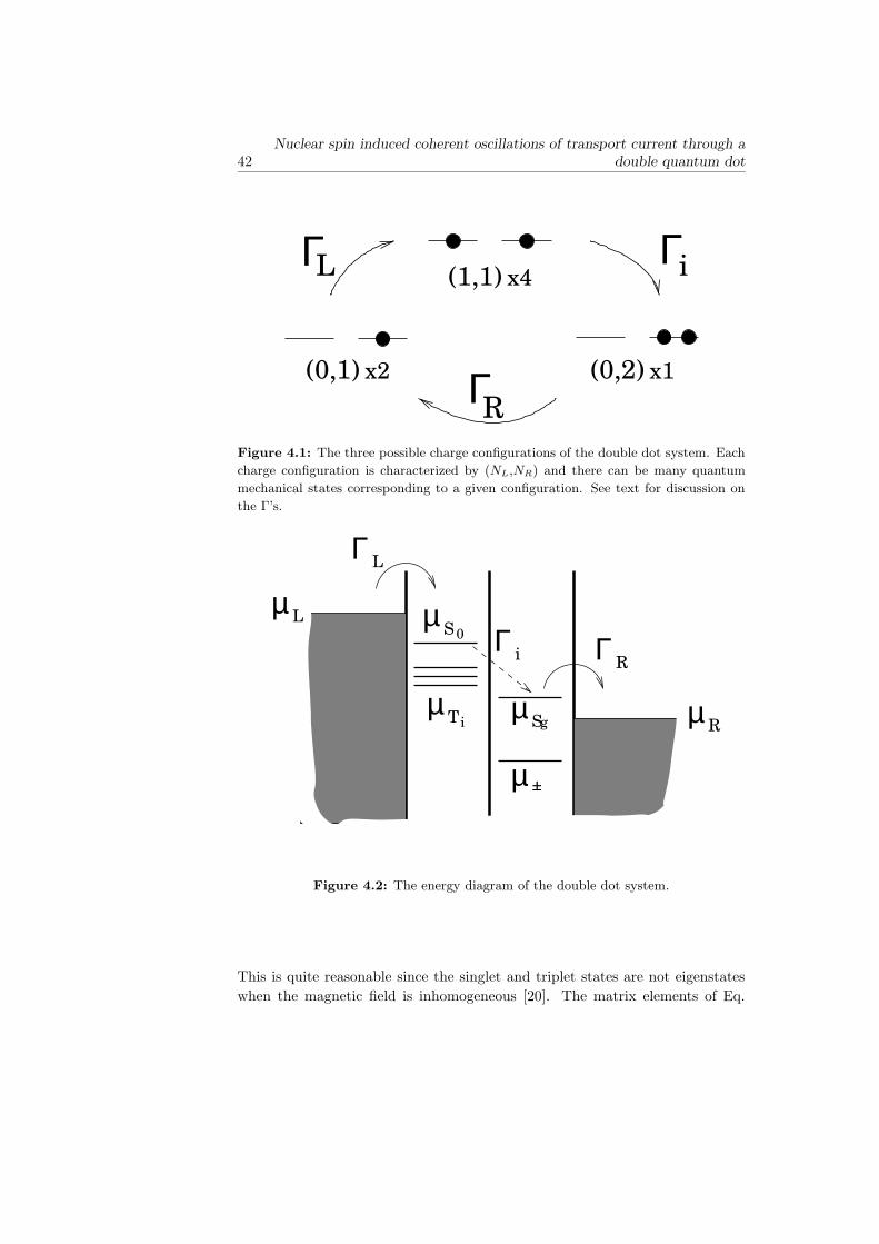
42Nuclear spin induced coherent oscillations of transport current through a
double quantum dot
ΓR
ΓL i
x2(0,1) (0,2) x1
(1,1) x4Γ
Figure 4.1: The three possible charge configurations of the double dot system. Each
charge configuration is characterized by (NL,NR) and there can be many quantum
mechanical states corresponding to a given configuration. See text for discussion on
the Γ’s.
S0µ
µ +
T iµ
Sgµ µ R
µ L
Γ i RΓ
LΓ
Figure 4.2: The energy diagram of the double dot system.
This is quite reasonable since the singlet and triplet states are not eigenstates
when the magnetic field is inhomogeneous [20]. The matrix elements of Eq.
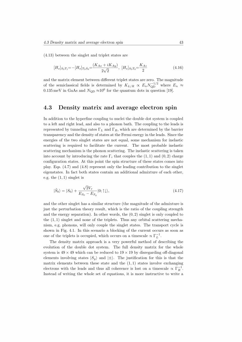
4.3 Density matrix and average electron spin 43
(4.13) between the singlet and triplet states are
[Hs]S0T1=−[Hs]T3S0
=(KAx + iKAy)
2√
2, [Hs]S0T0
=KAz
2(4.16)
and the matrix element between different triplet states are zero. The magnitude
of the semiclassical fields is determined by KL/R ∝ EnN−1/2QD where En ≈
0.135 meV in GaAs and NQD ≈106 for the quantum dots in question [19].
4.3 Density matrix and average electron spin
In addition to the hyperfine coupling to nuclei the double dot system is coupled
to a left and right lead, and also to a phonon bath. The coupling to the leads is
represented by tunneling rates ΓL and ΓR, which are determined by the barrier
transparency and the density of states at the Fermi energy in the leads. Since the
energies of the two singlet states are not equal, some mechanism for inelastic
scattering is required to facilitate the current. The most probable inelastic
scattering mechanism is the phonon scattering. The inelastic scattering is taken
into account by introducing the rate Γi that couples the (1, 1) and (0, 2) charge
configuration states. At this point the spin structure of these states comes into
play. Eqs. (4.7) and (4.8) represent only the leading contribution to the singlet
eigenstates. In fact both states contain an additional admixture of each other,
e.g. the (1, 1) singlet is
|S0〉 = |S0〉 +
√2Vτ
ES0− ESg
|0; ↑↓〉, (4.17)
and the other singlet has a similar structure (the magnitude of the admixture is
just the perturbation theory result, which is the ratio of the coupling strength
and the energy separation). In other words, the (0, 2) singlet is only coupled to
the (1, 1) singlet and none of the triplets. Thus any orbital scattering mecha-
nism, e.g. phonons, will only couple the singlet states. The transport cycle is
shown in Fig. 4.1. In this scenario a blocking of the current occurs as soon as
one of the triplets is occupied, which occurs on a timescale ∝ Γ−1L .
The density matrix approach is a very powerful method of describing the
evolution of the double dot system. The full density matrix for the whole
system is 49 × 49 which can be reduced to 19 × 19 by disregarding off-diagonal
elements involving states |Sg〉 and |±〉. The justification for this is that the
matrix elements between these state and the (1, 1) states involve exchanging
electrons with the leads and thus all coherence is lost on a timescale ∝ Γ−1R .
Instead of writing the whole set of equations, it is more instructive to write a
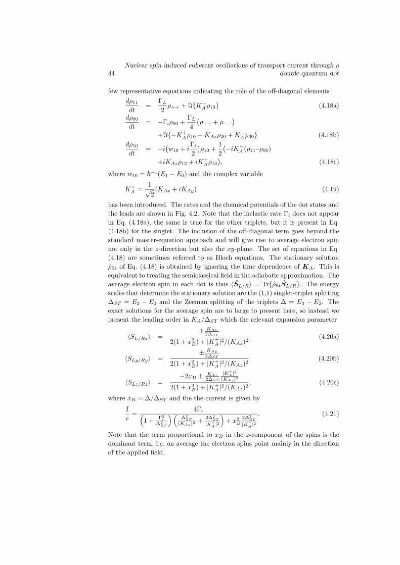
44Nuclear spin induced coherent oscillations of transport current through a
double quantum dot
few representative equations indicating the role of the off-diagonal elements
dρ11
dt=
ΓL
2ρ++ + =K+
Aρ10 (4.18a)
dρ00
dt= −Γiρ00 +
ΓL
4
(
ρ++ + ρ−−
)
+=−K+Aρ10 +KAzρ20 +K−
Aρ30 (4.18b)
dρ10
dt= −i
(
w10 + iΓi
2
)
ρ10 +1
2
(
−iK−A (ρ11−ρ00)
+iKAzρ12 + iK+Aρ13
)
, (4.18c)
where w10 = ~−1(E1 − E0) and the complex variable
K+A =
1√2(KAx + iKAy) (4.19)
has been introduced. The rates and the chemical potentials of the dot states and
the leads are shown in Fig. 4.2. Note that the inelastic rate Γi does not appear
in Eq. (4.18a), the same is true for the other triplets, but it is present in Eq.
(4.18b) for the singlet. The inclusion of the off-diagonal term goes beyond the
standard master-equation approach and will give rise to average electron spin
not only in the z-direction but also the xy-plane. The set of equations in Eq.
(4.18) are sometimes referred to as Bloch equations. The stationary solution
ρSt of Eq. (4.18) is obtained by ignoring the time dependence of KA. This is
equivalent to treating the semiclassical field in the adiabatic approximation. The
average electron spin in each dot is thus 〈SL/R〉 = TrρStSL/R. The energy
scales that determine the stationary solution are the (1,1) singlet-triplet splitting
∆ST = E2 − E0 and the Zeeman splitting of the triplets ∆ = E3 − E2. The
exact solutions for the average spin are to large to present here, so instead we
present the leading order in KA/∆ST which the relevant expansion parameter
〈SL/Rx〉 =± KAx
2∆ST
2(1 + x2B) + |K+
A |2/(KAz)2(4.20a)
〈SLy/Ry〉 =± KAy
2∆ST
2(1 + x2B) + |K+
A |2/(KAz)2(4.20b)
〈SLz/Rz〉 =−2xB ± KAz
2∆ST
|K+
A|2
(KAz)2
2(1 + x2B) + |K+
A |2/(KAz)2, (4.20c)
where xB = ∆/∆ST and the the current is given by
I
e=
4Γi(
1 +Γ2
i
∆2ST
)(
∆2ST
(KAz)2 +2∆2
ST
|K+
A|2
)
+ x2B
2∆2ST
|K+
A|2
. (4.21)
Note that the term proportional to xB in the z-component of the spins is the
dominant term, i.e. on average the electron spins point mainly in the direction
of the applied field.
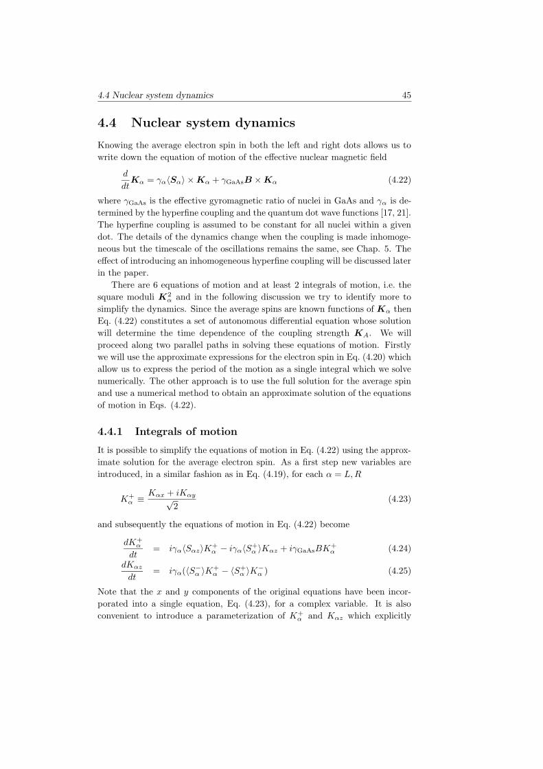
4.4 Nuclear system dynamics 45
4.4 Nuclear system dynamics
Knowing the average electron spin in both the left and right dots allows us to
write down the equation of motion of the effective nuclear magnetic field
d
dtKα = γα〈Sα〉 × Kα + γGaAsB × Kα (4.22)
where γGaAs is the effective gyromagnetic ratio of nuclei in GaAs and γα is de-
termined by the hyperfine coupling and the quantum dot wave functions [17, 21].
The hyperfine coupling is assumed to be constant for all nuclei within a given
dot. The details of the dynamics change when the coupling is made inhomoge-
neous but the timescale of the oscillations remains the same, see Chap. 5. The
effect of introducing an inhomogeneous hyperfine coupling will be discussed later
in the paper.
There are 6 equations of motion and at least 2 integrals of motion, i.e. the
square moduli K2α and in the following discussion we try to identify more to
simplify the dynamics. Since the average spins are known functions of Kα then
Eq. (4.22) constitutes a set of autonomous differential equation whose solution
will determine the time dependence of the coupling strength KA. We will
proceed along two parallel paths in solving these equations of motion. Firstly
we will use the approximate expressions for the electron spin in Eq. (4.20) which
allow us to express the period of the motion as a single integral which we solve
numerically. The other approach is to use the full solution for the average spin
and use a numerical method to obtain an approximate solution of the equations
of motion in Eqs. (4.22).
4.4.1 Integrals of motion
It is possible to simplify the equations of motion in Eq. (4.22) using the approx-
imate solution for the average electron spin. As a first step new variables are
introduced, in a similar fashion as in Eq. (4.19), for each α = L,R
K+α ≡ Kαx + iKαy√
2(4.23)
and subsequently the equations of motion in Eq. (4.22) become
dK+α
dt= iγα〈Sαz〉K+
α − iγα〈S+α 〉Kαz + iγGaAsBK
+α (4.24)
dKαz
dt= iγα(〈S−
α 〉K+α − 〈S+
α 〉K−α ) (4.25)
Note that the x and y components of the original equations have been incor-
porated into a single equation, Eq. (4.23), for a complex variable. It is also
convenient to introduce a parameterization of K+α and Kαz which explicitly
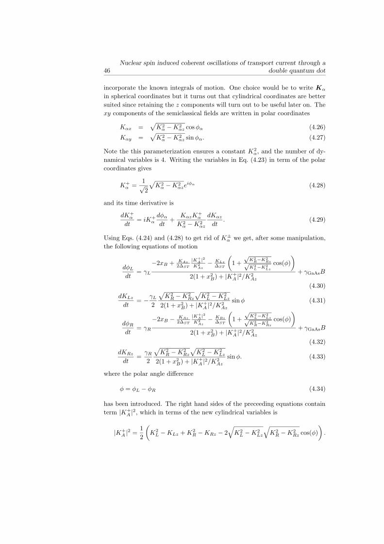
46Nuclear spin induced coherent oscillations of transport current through a
double quantum dot
incorporate the known integrals of motion. One choice would be to write Kα
in spherical coordinates but it turns out that cylindrical coordinates are better
suited since retaining the z components will turn out to be useful later on. The
xy components of the semiclassical fields are written in polar coordinates
Kαx =√
K2α −K2
αz cosφα (4.26)
Kαy =√
K2α −K2
αz sinφα. (4.27)
Note the this parameterization ensures a constant K2α, and the number of dy-
namical variables is 4. Writing the variables in Eq. (4.23) in term of the polar
coordinates gives
K+α =
1√2
√
K2α −K2
αzeiφα (4.28)
and its time derivative is
dK+α
dt= iK+
α
dφα
dt+
KαzK+α
K2α −K2
αz
dKαz
dt. (4.29)
Using Eqs. (4.24) and (4.28) to get rid of K±α we get, after some manipulation,
the following equations of motion
dφL
dt= γL
−2xB + KAz
2∆ST
|K+
A|2
K2Az
− KLz
∆ST
(
1 +
√K2
R−K2
Rz√K2
L−K2
Lz
cos(φ)
)
2(1 + x2B) + |K+
A |2/K2Az
+ γGaAsB
(4.30)
dKLz
dt= −γL
2
√
K2R −K2
Rz
√
K2L −K2
Lz
2(1 + x2B) + |K+
A |2/K2Az
sinφ (4.31)
dφR
dt= γR
−2xB − KAz
2∆ST
|K+
A|2
K2Az
− KRz
∆ST
(
1 +
√K2
L−K2
Lz√K2
R−K2
Rz
cos(φ)
)
2(1 + x2B) + |K+
A |2/K2Az
+ γGaAsB
(4.32)
dKRz
dt=γR
2
√
K2R −K2
Rz
√
K2L −K2
Lz
2(1 + x2B) + |K+
A |2/K2Az
sinφ. (4.33)
where the polar angle difference
φ = φL − φR (4.34)
has been introduced. The right hand sides of the preceeding equations contain
term |K+A |2, which in terms of the new cylindrical variables is
|K+A |2 =
1
2
(
K2L −KLz +K2
R −KRz − 2√
K2L −K2
Lz
√
K2R −K2
Rz cos(φ)
)
.
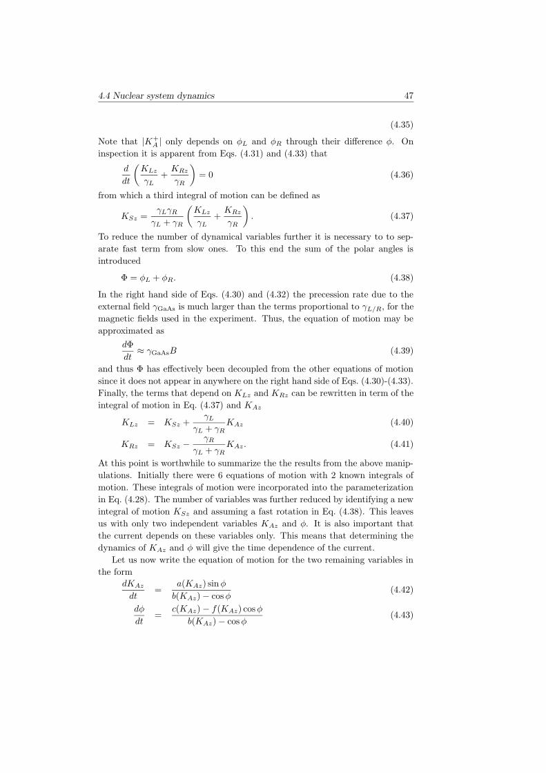
4.4 Nuclear system dynamics 47
(4.35)
Note that |K+A | only depends on φL and φR through their difference φ. On
inspection it is apparent from Eqs. (4.31) and (4.33) that
d
dt
(
KLz
γL+KRz
γR
)
= 0 (4.36)
from which a third integral of motion can be defined as
KSz =γLγR
γL + γR
(
KLz
γL+KRz
γR
)
. (4.37)
To reduce the number of dynamical variables further it is necessary to to sep-
arate fast term from slow ones. To this end the sum of the polar angles is
introduced
Φ = φL + φR. (4.38)
In the right hand side of Eqs. (4.30) and (4.32) the precession rate due to the
external field γGaAs is much larger than the terms proportional to γL/R, for the
magnetic fields used in the experiment. Thus, the equation of motion may be
approximated as
dΦ
dt≈ γGaAsB (4.39)
and thus Φ has effectively been decoupled from the other equations of motion
since it does not appear in anywhere on the right hand side of Eqs. (4.30)-(4.33).
Finally, the terms that depend on KLz and KRz can be rewritten in term of the
integral of motion in Eq. (4.37) and KAz
KLz = KSz +γL
γL + γRKAz (4.40)
KRz = KSz −γR
γL + γRKAz. (4.41)
At this point is worthwhile to summarize the the results from the above manip-
ulations. Initially there were 6 equations of motion with 2 known integrals of
motion. These integrals of motion were incorporated into the parameterization
in Eq. (4.28). The number of variables was further reduced by identifying a new
integral of motion KSz and assuming a fast rotation in Eq. (4.38). This leaves
us with only two independent variables KAz and φ. It is also important that
the current depends on these variables only. This means that determining the
dynamics of KAz and φ will give the time dependence of the current.
Let us now write the equation of motion for the two remaining variables in
the form
dKAz
dt=
a(KAz) sinφ
b(KAz) − cosφ(4.42)
dφ
dt=
c(KAz) − f(KAz) cosφ
b(KAz) − cosφ(4.43)
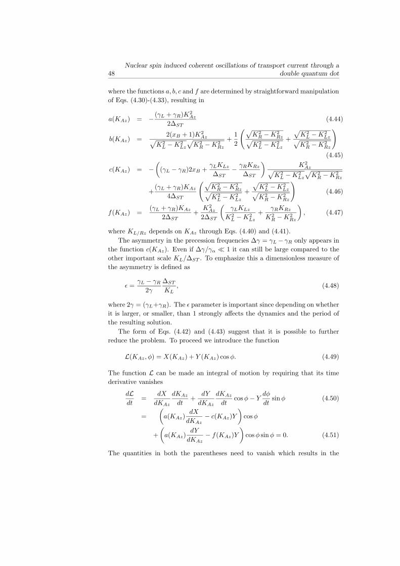
48Nuclear spin induced coherent oscillations of transport current through a
double quantum dot
where the functions a, b, c and f are determined by straightforward manipulation
of Eqs. (4.30)-(4.33), resulting in
a(KAz) = − (γL + γR)K2Az
2∆ST(4.44)
b(KAz) =2(xB + 1)K2
Az√
K2L −K2
Lz
√
K2R −K2
Rz
+1
2
(
√
K2R −K2
Rz√
K2L −K2
Lz
+
√
K2L −K2
Lz√
K2R −K2
Rz
)
(4.45)
c(KAz) = −(
(γL − γR)2xB +γLKLz
∆ST− γRKRz
∆ST
)
K2Az
√
K2L −K2
Lz
√
K2R −K2
Rz
+(γL + γR)KAz
4∆ST
(
√
K2R −K2
Rz√
K2L −K2
Lz
+
√
K2L −K2
Lz√
K2R −K2
Rz
)
(4.46)
f(KAz) =(γL + γR)KAz
2∆ST+
K2Az
2∆ST
(
γLKLz
K2L −K2
Lz
+γRKRz
K2R −K2
Rz
)
, (4.47)
where KL/Rz depends on KAz through Eqs. (4.40) and (4.41).
The asymmetry in the precession frequencies ∆γ = γL − γR only appears in
the function c(KAz). Even if ∆γ/γα 1 it can still be large compared to the
other important scale KL/∆ST . To emphasize this a dimensionless measure of
the asymmetry is defined as
ε =γL − γR
2γ
∆ST
KL, (4.48)
where 2γ = (γL+γR). The ε parameter is important since depending on whether
it is larger, or smaller, than 1 strongly affects the dynamics and the period of
the resulting solution.
The form of Eqs. (4.42) and (4.43) suggest that it is possible to further
reduce the problem. To proceed we introduce the function
L(KAz, φ) = X(KAz) + Y (KAz) cosφ. (4.49)
The function L can be made an integral of motion by requiring that its time
derivative vanishes
dLdt
=dX
dKAz
dKAz
dt+
dY
dKAz
dKAz
dtcosφ− Y
dφ
dtsinφ (4.50)
=
(
a(KAz)dX
dKAz− c(KAz)Y
)
cosφ
+
(
a(KAz)dY
dKAz− f(KAz)Y
)
cosφ sinφ = 0. (4.51)
The quantities in both the parentheses need to vanish which results in the
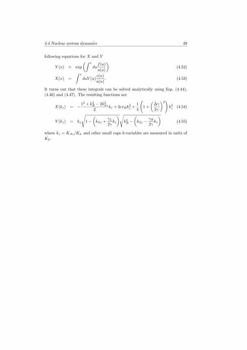
4.4 Nuclear system dynamics 49
following equations for X and Y
Y (x) = exp
(∫ x
duf(u)
a(u)
)
(4.52)
X(x) =
∫ x
duY (u)c(u)
a(u). (4.53)
It turns out that these integrals can be solved analytically using Eqs. (4.44),
(4.46) and (4.47). The resulting functions are
X(kz) = −12 + k2R − 2k2
Sz
2kz + 2εxBk
2z +
1
4
(
1 +
(
∆γ
2γ
)2)
k3z (4.54)
Y (kz) = kz
√
1 −(
kSz +γL
2γkz
)
√
k2R −
(
kSz −γR
2γkz
)
(4.55)
where kz = KAz/KL and other small caps k-variables are measured in units of
KL.
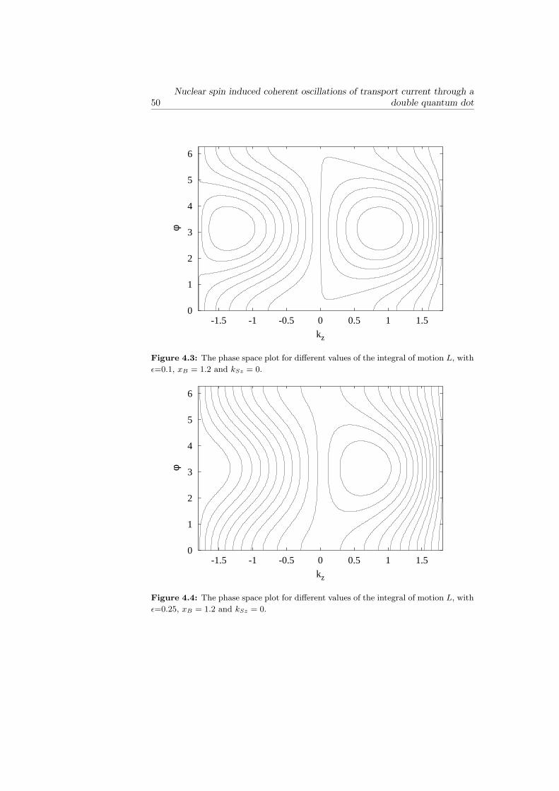
50Nuclear spin induced coherent oscillations of transport current through a
double quantum dot
0
1
2
3
4
5
6
-1.5 -1 -0.5 0 0.5 1 1.5
φ
kz
Figure 4.3: The phase space plot for different values of the integral of motion L, with
ε=0.1, xB = 1.2 and kSz = 0.
0
1
2
3
4
5
6
-1.5 -1 -0.5 0 0.5 1 1.5
φ
kz
Figure 4.4: The phase space plot for different values of the integral of motion L, with
ε=0.25, xB = 1.2 and kSz = 0.
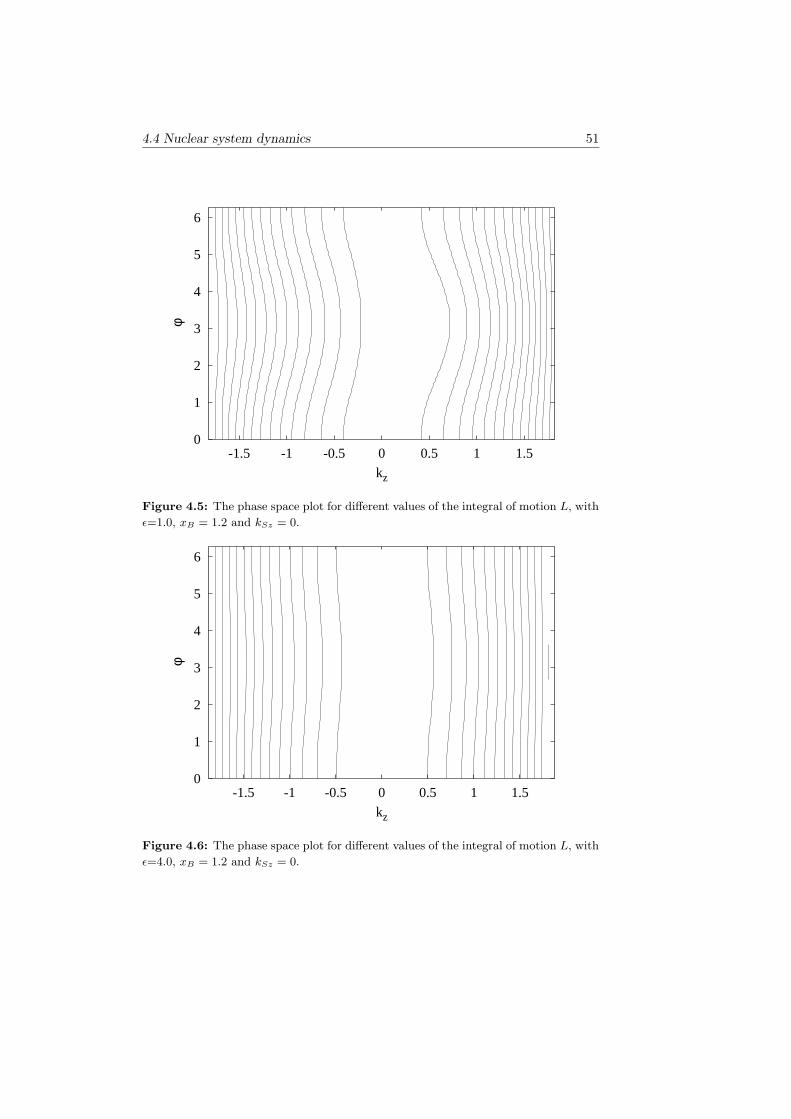
4.4 Nuclear system dynamics 51
0
1
2
3
4
5
6
-1.5 -1 -0.5 0 0.5 1 1.5
φ
kz
Figure 4.5: The phase space plot for different values of the integral of motion L, with
ε=1.0, xB = 1.2 and kSz = 0.
0
1
2
3
4
5
6
-1.5 -1 -0.5 0 0.5 1 1.5
φ
kz
Figure 4.6: The phase space plot for different values of the integral of motion L, with
ε=4.0, xB = 1.2 and kSz = 0.
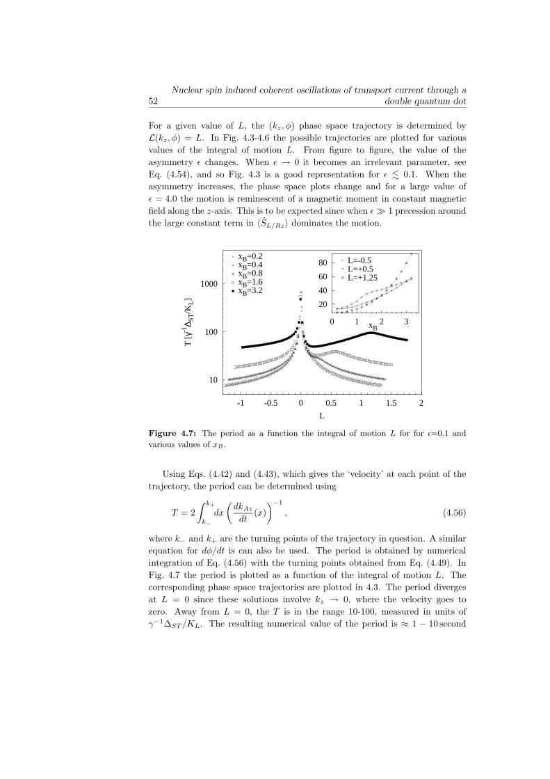
52Nuclear spin induced coherent oscillations of transport current through a
double quantum dot
For a given value of L, the (kz, φ) phase space trajectory is determined by
L(kz, φ) = L. In Fig. 4.3-4.6 the possible trajectories are plotted for various
values of the integral of motion L. From figure to figure, the value of the
asymmetry ε changes. When ε → 0 it becomes an irrelevant parameter, see
Eq. (4.54), and so Fig. 4.3 is a good representation for ε . 0.1. When the
asymmetry increases, the phase space plots change and for a large value of
ε = 4.0 the motion is reminescent of a magnetic moment in constant magnetic
field along the z-axis. This is to be expected since when ε 1 precession around
the large constant term in 〈SL/Rz〉 dominates the motion.
10
100
1000
-1 -0.5 0 0.5 1 1.5 2
T [
γ-1∆ S
T/K
L]
L
xB=0.2xB=0.4xB=0.8xB=1.6xB=3.2
20
40
60
80
0 1 2 3xB
L=-0.5L=+0.5L=+1.25
Figure 4.7: The period as a function the integral of motion L for for ε=0.1 and
various values of xB .
Using Eqs. (4.42) and (4.43), which gives the ‘velocity’ at each point of the
trajectory, the period can be determined using
T = 2
∫ k+
k−
dx
(
dkAz
dt(x)
)−1
, (4.56)
where k− and k+ are the turning points of the trajectory in question. A similar
equation for dφ/dt is can also be used. The period is obtained by numerical
integration of Eq. (4.56) with the turning points obtained from Eq. (4.49). In
Fig. 4.7 the period is plotted as a function of the integral of motion L. The
corresponding phase space trajectories are plotted in 4.3. The period diverges
at L = 0 since these solutions involve kz → 0, where the velocity goes to
zero. Away from L = 0, the T is in the range 10-100, measured in units of
γ−1∆ST /KL. The resulting numerical value of the period is ≈ 1 − 10 second

4.4 Nuclear system dynamics 53
10
100
-1 -0.5 0 0.5 1 1.5 2 2.5 3
T [
γ-1∆ S
T/K
L]
L
xB=0.2xB=0.4xB=0.8xB=1.6xB=3.2
10
20
30
0 1 2 3xB
L=-0.5L=+0.5L=+1.0
Figure 4.8: The period as a function the integral of motion L for for ε=1.0 and
various values of xB .
for γ−1∆ST /KL ≈ 0.01 − 0.1 sec. Thus the period is quite long, approaching
seconds and even above that.
Similar data for the period when ε = 1.0 is shown in Fig. 4.8. Note that
the period is decreased in comparison to the ε = 0.1 case. We cannot a priori
determine the value of the asymmetry since it is determined by sample quality
and fabrication errors. The value of ε is extracted from experimental data
through the magnetic field, or xB , behavior of the period. The insets of Figs.
4.7 and 4.8 show the xB dependence for some fixed values of L. For ε = 0.1
there is a monotonic increase of T with xB but for the the larger asymmetry
ε = 1.0 the behavior is non-monotonic with a minimum around xB . 1. This
reflects that the period for large asymmetry is
T (ε 1) ∝ (x2B + 1) + const
xBε. (4.57)
Note the 1/ε dependence which reduces the period. For low asymmetry the
period behaves as
T (ε 1) ∝ (x2B + 1) + const. (4.58)
The different xB dependence of the period observed in the experiment should
indicate whether the asymmetry is large or small.
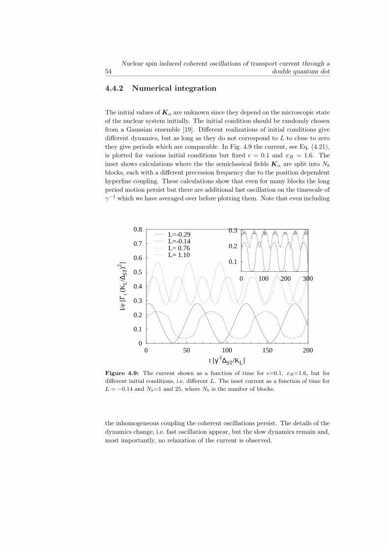
54Nuclear spin induced coherent oscillations of transport current through a
double quantum dot
4.4.2 Numerical integration
The initial values of Kα are unknown since they depend on the microscopic state
of the nuclear system initially. The initial condition should be randomly chosen
from a Gaussian ensemble [19]. Different realizations of initial conditions give
different dynamics, but as long as they do not correspond to L to close to zero
they give periods which are comparable. In Fig. 4.9 the current, see Eq. (4.21),
is plotted for various initial conditions but fixed ε = 0.1 and xB = 1.6. The
inset shows calculations where the the semiclassical fields Kα are split into Nb
blocks, each with a different precession frequency due to the position dependent
hyperfine coupling. These calculations show that even for many blocks the long
period motion persist but there are additional fast oscillation on the timescale of
γ−1 which we have averaged over before plotting them. Note that even including
0
0.1
0.2
0.3
0.4
0.5
0.6
0.7
0.8
0 50 100 150 200
I/e
[Γi (
KL/∆
ST)2 ]
t [γ-1∆ST/KL]
L=-0.29L=-0.14L= 0.76L= 1.10
0.1
0.2
0.3
0 100 200 300
Figure 4.9: The current shown as a function of time for ε=0.1, xB=1.6, but for
different initial conditions, i.e. different L. The inset current as a function of time for
L = −0.14 and Nb=1 and 25, where Nb is the number of blocks.
the inhomogeneous coupling the coherent oscillations persist. The details of the
dynamics change, i.e. fast oscillation appear, but the slow dynamics remain and,
most importantly, no relaxation of the current is observed.
4.5 Conclusions 55
4.5 Conclusions
In conclusion, we have proposed a novel transport mechanism which leads to an
oscillating current, whose period is proportional to γ−1∆ST /KL. For low asym-
metry and high magnetic fields xB the period can become quite large. Some of
our model parameters are not well known so the numerical value of the period is
not quite certain, although it should lie in the range 0.1-10 sec. The asymmetry
plays an important role in determining the dynamics of the system. Due to
the different magnetic field dependence of the period depending on whether the
asymmetry is large or small, it should be possible to determine from experimen-
tal data in which regime ε lies. For small ε the period increased monotonically
with magnetic field. This seems to be the consistent with the experimental data,
which indicates that the asymmetry is not so large in the sample used. Indeed,
this might expected since the two dots are nominally identical [13]. Taking into
account inhomogeneous hyperfine coupling does not destroy the long period
oscillations although it introduces additional short period motion.
References
[1] D. Paget and V. L. Berkovits, in Optical Orientation, edited by F. Meier
and B. P. Zakharchenya (North-Holland, Amsterdam, 1984).
[2] D. Paget, G. Lampel, B. Sapoval, and V. I. Safarov, Phys. Rev. B 15, 5780
(1977).
[3] G. Salis et al., Phys. Rev. Lett. 86, 2677 (2001).
[4] G. Salis, D. D. Awschalom, Y. Ohno, and H. Ohno, Phys. Rev. B 64,
195304 (2001).
[5] K. R. Wald et al., Phys. Rev. Lett. 73, 1011 (1994).
[6] J. H. Smet et al., Nature 415, 281 (2002).
[7] R. K. Kawakami et al., Science 294, 131 (2001).
[8] T. Machida, T. Yamazaki, K. Ikushima, and S. Komiyama, App. Phys.
Lett. 82, 409 (2003).
[9] L. P. Kouwenhoven et al., in Mesoscopic Electron Transport, NATO Se-
ries, edited by L. L. Sohn, L. P. Kouwenhoven, and G. Schoen (Kluwer,
Dordrecht, 1997), Chap. Electron transport in quantum dots, p. 105.
[10] L. P. Kouwenhoven, D. G. Austing, and S. Tarucha, Rep. Prog. Phys. 64,
701 (2001).
[11] S. DeFranceschi et al., Phys. Rev. Lett. 86, 878 (2001).
[12] H. Matsuoka and S. Kimura, Jpn. J. Appl. Phys. 34, 1326 (1995).
56Nuclear spin induced coherent oscillations of transport current through a
double quantum dot
[13] K. Ono and S. Tarucha, (unpublished).
[14] K. Ono, D. G. Austing, Y. Tokura, and S. Tarucha, Science 297, 1313
(2002).
[15] D. Weinman, W. Haussler, and B. Kramer, Phys. Rev. Lett. 74, 984 (1995).
[16] M. Ciorga et al., App. Phys. Lett. 80, 2177 (2002).
[17] I. A. Merkulov, A. L. Efros, and M. Rosen, Phys. Rev. B 65, 205309 (2002).
[18] M. I. D’yakonov and V. Y. Kachorovksii, Sov. Phys. Semicond. 20, 110
(1986).
[19] S. I. Erlingsson and Y. V. Nazarov, Phys. Rev. B 66, 155327 (2002).
[20] R. Sousa, X. Hu, and S. D. Sarma, Phys. Rev. A 64, 43207 (2001).
[21] S. I. Erlingsson and Y. V. Nazarov, (in preparation).
Chapter 5
Time-evolution of the effective nuclear
magnetic field due to a localized
electron spin
Sigurdur I. Erlingsson, Yuli V. Nazarov
An effective spin Hamiltonian is considered where the spatial dependence of
the electron wavefunction results in an inhomogeneous hyperfine coupling of the
electron spin to different nuclear spins. A semiclassical description of the nuclear
spin system is introduced which also takes into account the inhomogeneous
coupling. Using that the electron spin dynamics are much faster than for the
nuclear spins, an approximate solution for dynamics of the nuclear system is
obtained. From this solution certain electron spin correlation functions are
calculated. Contrary to what one may guess, the dynamics are not chaotic and
the correlation functions show no decay in time, only complicated oscillations.
This may be attributed to the fact that the system has many integrals of motion
and that it is close to exactly solvable.
57
58Time-evolution of the effective nuclear magnetic field due to a localized
electron spin
5.1 Introduction
The coherent manipulation of localized spins in solid state systems is currently
a very active field research. Studying such systems may lead to new insight
regarding fundamental questions, e.g. the measurement problem in quantum
mechanics and limitations on control of such systems due to environmental
effects. There are also possible applications in which conventional electronics is
used in combination with spin manipulation. This field of research is commonly
referred to as spintronics. One of the most ambitious goals in this field of
research is developing a quantum bit, or qubit. Such qubits would form the
basic building blocks of the quantum computer. Building a qubit in solid state
systems is advantageous since fabrication techniques are very advanced and
scaling the number of qubits is straightforward, at least in theory. However,
environmental effects are much stronger in comparison with systems based on
NMR or trapped ions (which lack scalability). The qubit should be any (quasi)
two level system in which the strength of the coupling to the environment can
be sufficiently well controlled so that the residual environmental interactions are
below a threshold set by the operating speed of the device [1–3]. The benefit
of working with individual spins is that they are natural two level systems and
the spin is less susceptible to environmental effects. There are two timescales,
socalled T1 and T2, which are used to characterize the quality of the qubit.
These terms are borrowed from the NMR community which have been using
them long before anyone thought of the qubit [4, 5]. The lifetime of a certain
state of the qubit, or energy relaxation time, is determined by T1 while T2 gives
the decoherence time.
Since the first proposal [6], the qubit candidate based on localized electron
spins in quantum dots has been the subject of many theoretical and experimental
studies. This system, and any other, has to fulfill some strict criteria to be a
viable qubit, the most difficult to realize being long relaxation and decoherence
times. There already have been quite a few studies of the relaxation time of
electron spins in GaAs (which seems to be the most relevant material) quantum
dots [7–11] for various different spin-flip mechanisms and they all give very long
relaxation times. The operation of a qubit requires making a superposition of
states that persists during the decoherence time. A few papers have addressed
the question of the decoherence time of electron spin in GaAs quantum dots
[12–17]. It was suggested in the literature that the most important source for
decoherence of electron spins in GaAs quantum dots would be hyperfine coupling
to the surrounding nuclei. In Ref. [12] the characteristic timescale for the decay
of a specific correlation function was associated with the decoherence time of
the electron spin. The decohence in this case was due to the spatially dependent
hyperfine coupling constant which caused small frequency changes through flip-
flop processes involving spatially separated nuclei. A different approach was
5.2 Hyperfine interaction in quantum dots 59
used in Ref. [13] which focused on developing an effective magnetic field acting
on the electron spin due to the total nuclear spin system. The authors were
interested in ensemble averaged quantities and so they averaged over all possible
initial configurations of the effective nuclear field.
In this work we will try to bridge between these two approaches, i.e. we will
further develop the idea of the effective magnetic field due to the nuclear system
acting on the electron spin in the quantum dot [10] including the effects of the
spatially varying hyperfine coupling constant. The dynamics of the system will
be represented by a set of equations of motion for the electron spin and the
various subsystem of nuclei which are defined in such a way that the coupling
to the electron spin is the same for all the nuclei within a subsystem. Due to
the large difference of timescales for the electron and nuclear spin systems we
are able to solve the problem in two steps. In the first step we establish that the
nuclear system can be treated as an adiabatic effective nuclear magnetic field
acting on the electron. The latter step involves the backaction of the electron
spin which will determine the evolution of the nuclear spins.
5.2 Hyperfine interaction in quantum dots
The Hamiltonian describing the hyperfine coupling between conduction band
electrons and the lattice nuclei in GaAs is of the well known form of the contact
potential
HHF = AS ·∑
k
Ikδ(r − Rk). (5.1)
In the GaAs conduction band (which is mainly composed of s-orbitals), the
dipole-dipole part of the hyperfine interaction vanishes [18]. The quantum dots
considered here are quite general, but we introduce some restrictions to simplify
the model. First of all it is assumed that the number of electrons is fixed,
preferably to one. From the experimental point of view this assumptions is
quite reasonable since having only a single electron in the dot has already been
demonstrated [19, 20]. Also, by pinching off the connection to the leads the
electron number should remain fixed over very long timescales. It can also be
argued that our treatment applies for odd number of electron since the ground
state should be a doublet. The second assumption is that the orbital level
splitting is the largest energy scale of the system. In this case the hyperfine
Hamiltonian can be projected to the lowest orbital level since contributions from
higher orbitals are strongly suppressed due the large orbital energy separation.
If the ground state orbital ψ(r) of the the quantum dot is known, then an
effective spin Hamiltonian can be written as
Hs = gµBB · S + γGaAs
∑
k
B · Ik +∑
k
A|ψ(Rk)|2S · Ik (5.2)
60Time-evolution of the effective nuclear magnetic field due to a localized
electron spin
where B is the external applied field and the hyperfine interaction has been
projected onto the lowest orbital.
5.3 Semiclassical dynamics
The fact that the single electron spin is coupled to a large number of nuclei but
each nucleus is only coupled to the single electron spin hints at an asymmetry
in the behavior of the electron and nuclear spins. Indeed the electron precesses
in an effective nuclear magnetic field which is due to the whole nuclear spin
system. This field is ∝√
NQD times larger than the corresponding hyperfine
field caused by the single electron spin in which the nuclear spins precess. Thus
the dynamics of the electron are much faster than the dynamics of the nuclei.
Also, the large number of nuclei involved makes it possible to treat the nuclear
system in a semiclassical way [10, 13, 21]. In the following section we discuss
the origin of the different dynamical timescales involved in the problem and we
introduce a semiclassical approximation to the dynamics of the system.
The Hamiltonian in Eq. (5.1) describes the coupling of a single electron spin
to many nuclear spins. The actual number is determined by the confinement of
the electron, i.e. the number of nuclei the electron is coupled to is proportional
to the volume that the electron occupies. In a typical quantum dot a single
electron spin may be coupled to 106 nuclear spins. When the electrons interacts
with so many (independent) nuclei it is possible to interpret the combined effect
of the nuclei as an effective magnetic field .
The last term in Eq. (5.2) represents the coupling of the electron spin and the
nuclear system through the hyperfine interaction. By introducing the operator
of the nuclear magnetic field
K =∑
k
A|ψ0(Rk)|2Ik, (5.3)
the hyperfine coupling can be written as
HHF = S · K. (5.4)
Before proceeding further it is convenient to introduce a different way of writing
Eq. (5.3). The wavefunction of the ground state orbital has some characteristic
spatial extent which is determined by the confining potential. Without loss of
generality it may be assumed that the lateral and transverse confining lengths
are ` and z0 respectively. The volume of the quantum dot is the defined as
VQD = πz0`2. (5.5)
Let us define a dimensionless function
f(Rk) = VQD|ψ(Rk)|2. (5.6)
5.3 Semiclassical dynamics 61
Furthermore, denoting the maximum value of f with fMax we introduce a di-
mensionless coupling constant
gk = g(Rk) =f(Rk)
fMax. (5.7)
The hyperfine coupling constant expressed in terms of the concentration, Cn, of
nuclei with spin I and a characteristic energy En is
A =En
CnI. (5.8)
The energy En is the maximum Zeeman splitting possible due to a fully polarized
nuclear system, its value being En ≈ 0.135 meV in GaAs [22, 23]. The nuclear
system operator can then be written as
K = A∑
k
f(Rk)
VQDIk (5.9)
=AfMax
VQD
∑
k
gkIk (5.10)
=EnfMax
NQDI
∑
k
gkIk (5.11)
where NQD = CnVQD is the effective number of nuclei in the dot. The operator
defined in Eq. (5.11) represents combined contributions from many independent
spins. For a typical unpolarized nuclear system the average squared modulus
can be estimated as
〈K2〉 =(EnfMax)
2
(NQDI)2
∑
kk′
gkgk′〈Ik · Ik′〉
=(EnfMax)
2
NQDI2
1
NQD
∑
k
g2kI(I + 1)
=E2
n
NQD
I(I + 1)f2Maxg
2
I2. (5.12)
where the average squared coupling strength is
g2 =1
NQD
∑
k
g2(Rk). (5.13)
It is important to note that
√
〈K2〉 ∝ EnN−1/2QD and that this field acts on the
electron spin even in the absence of polarization in the nuclear system. As was
shown in Ref. [10] the typical fluctuations in the components of K are
∆Kα∆Kβ & 〈K2〉 1
N1/2QD
. (5.14)
62Time-evolution of the effective nuclear magnetic field due to a localized
electron spin
This means that as long as NQD 1 the operator in Eq. (5.11) can be replaced
by a classical vector whose length is determined by Eq. (5.12). The actual
value of K is completely random since it determined by unknown details of the
nuclear system. The value of the effective nuclear field should be chosen from a
Gaussian distribution [10, 13]
P (K) =
(
1
2πσ2
)3/2
exp
(
−K2
2σ2
)
, (5.15)
where σ2 = 13 〈K2〉 is the variance of the distribution.
Let us now turn to the dynamics of the combined electron and nuclear spins.
The dynamics of both are determined by the Heisenberg equation of motion
d
dtS = K × S + gµBB × S (5.16)
d
dtIk =
EnfMax
NQDgkS × Ik + γGaAsB × Ik. (5.17)
Multiplying Eq. (5.17) with gk and summing over k gives the equation of motion
for K
d
dtK =
EnfMax
NQDS ×
(
∑
k
g2kIk
)
+ γGaAsBnB × K (5.18)
In contrast to the simple dynamics of the electron spin, the equation of motion
for K is quite complicated. The reason for the asymmetry in the form of Eqs.
(5.16) and (5.18) is the position dependent coupling gk. The quantity in the
brackets on the rhs of Eq. (5.18) can not be expressed in terms of K. Only in
the simple case of constant gk it is possible to write a closed equation of motion
for K and S [14].
Even though Eqs. (5.16) and (5.18) cannot in general be solved it possible
to extract general features of the dynamics. Assuming B = 0, the electron
spin will precess with frequency ∝ EnN−1/2QD (since this is the magnitude of the
effective nuclear magnetic field) and the nuclear system precesses with frequency
∝ EnN−1QD. The ratio of these two precession frequencies is N
1/2QD 1, which
means that the electron spin effectively feels a quasi stationary nuclear system
and in turn the nuclear system feels a time averaged electron spin.
To incorporate the (i) separation of timescales, (ii) the inhomogeneous cou-
pling we introduce a scheme that separates the nuclear system into Nb subsys-
tems, each being characterized by a fixed coupling gb. The effective nuclear field
of a given subsystem is
Kb =EnfMax
NQDIgb
∑
k∈b
Ik (5.19)
5.3 Semiclassical dynamics 63
where the notation k ∈ b is shorthand for all nuclei whose coupling is gk ∈[gb − δg/2, gb + δg/2]. As long as Nb NQD each subsystem can be replaced
by a classical variable. The initial condition for each block is chosen from a
Gaussian distribution whose variance is
〈K2b 〉 = 〈K2〉 g2
bVb
VQDg2, (5.20)
where Vb is the volume of the region which fulfills gk ∈ [gb − δg/2, gb + δg/2].
The volume of the subsystem Vb is related to gb via
Vb ≡∣
∣
∣
∣
dV
dg
∣
∣
∣
∣
g=gb
δg, (5.21)
where V is the volume of the region where g ≥ gb. The functional form of g(r) is
determined by the density |ψ(r)|2. For example, using a parabolic confinement
in the lateral direction and assuming a steplike density of the 2DEG in the
transverse direction gives a coupling g(r) = exp(−r‖/`)2 . The volume V is
then given by
V (g) = z0π`2 ln(1/g), (5.22)
which results in the following subsystem volume
Vb = VQDδg
gb. (5.23)
Note that the value of the total effective field which the electron experiences
does not depend on Nb.
Taking all this together we arrive at the following set of equations which
determine the approximate dynamics of the nuclear system.
dKb
dt=EnfMax
INQDgb〈S〉 × Kb + γGaAsB × Kb, (5.24)
where the average electron spin 〈S〉 is determined by the total effective nuclear
field
K =∑
b
Kb. (5.25)
Obviously separating the nuclear system into subsystem with a constant gb is
an approximation to the continuous coupling gk. As the number of subsystems
increases gb will more closely represent gk. However, for the the semiclassical ap-
proximation to be valid each subsystem must contain many nuclear spins. Thus,
increasing Nb should better reproduce the actual system, as long as Nb NQD.
The Nb differential equations, with the associated random initial conditions
constitute a set of autonomous differential equations. Its solutions, for a given
functional form 〈S〉 = S(K) completely determines the dynamics of the nu-
clear system. The solution of the average spin will be the discussed in the next
section.

64Time-evolution of the effective nuclear magnetic field due to a localized
electron spin
5.4 Adiabatic approximation for the electron spin
As we have shown in the previous section, the nuclear spin system may be
treated as a slowly varying effective nuclear magnetic field acting on the elec-
tron spin. Assuming a constant external magnetic field along the z-axis, the
Hamiltonian for the electron spin reads
He(t) = ∆Sz + S · K(t), (5.26)
∆ = gµBB being the Zeeman splitting due to the external field. Let us now
introduce a general magnetic field
H(t) = ∆ez + K(t), (5.27)
to represent any slowly varying magnetic field. It is convenient to introduce the
instantaneous eigenfunctions of the Hamiltonian, which are solutions of
He(t)|n(t);±〉 = E±(t)|n(t);±〉. (5.28)
The eigenstates are labeled by n(t) to indicate that these eigenstates are either
pointing ‘up’ (+) or ‘down’ (-) along the total magnetic field, whose direction
is determined by the normal vector
n(t) =H(t)
|H(t)| . (5.29)
For spin 1/2 in an external field, the eigenenergies can be written as E±(t) =
±E(t), where
E(t) =1
2
√
H2x(t) +H2
y (t) +Hz(t)2 (5.30)
and the corresponding eigenstates are written in the basis of the Sz eigenvectors
|n(t);+〉 =1
√
1 + |a(t)|2(| ↑〉 + a(t)| ↓〉) (5.31)
|n(t);−〉 =1
√
1 + |a(t)|2(−a∗(t)| ↑〉 + | ↓〉). (5.32)
The time dependent mixing of spin components is ∆ and K is given by
a(t) =H+(t)√
2
(√
H2x(t) +H2
y (t) +Hz(t)2 −Hz(t))
|H+(t)|2 (5.33)
where
H+(t) =Hx(t) + iHy(t)√
2(5.34)
5.4 Adiabatic approximation for the electron spin 65
The wavefunction may be expanded in basis of instantaneous eigenstates
|ψ(t)〉 =∑
σ=±
cσ(t)|n(t);σ〉 (5.35)
where the expansion coefficients are
c±(t) = c±(t0) exp
(
γ±(t) − i
~
∫ t
t0
dτE±(τ).
)
(5.36)
The additional phase factor appearing in the previous equation is the usual
adiabatic phase [24]
γ±(t) =
∫ t
t0
dτ〈n(τ);±|d/dτ |n(τ);±〉. (5.37)
Integrating by parts the rhs of the last equation and using the orthogonality of
the instantaneous eigenstates, it can be shown that the phase γ± is an imaginary
number. Also, for a doublet γ± = ±γ.Using the wave function in Eq. (5.35), the average electron spin is
〈S(t)〉 ≡ 〈ψ(t)|S|ψ(t)〉 (5.38)
=∑
σ=±
|cσ(t0)|2〈n(t);σ|S|n(t);σ〉
+2<
c∗+(t0)c−(t0) exp
(
2γ(t) − i
~
∫ t
t0
dτ2E(τ)
)
.
(5.39)
The latter term in Eq. (5.39) oscillates with frequency E(t)/h EnN−1QD/h, so
its average is zero on the timescales of the nuclear system. The average value
of the electron spin entering Eq. (5.24) is
〈S〉 =∑
σ=±
|cσ(t0)|2〈n(t);σ|S|n(t);σ〉 (5.40)
=1
2cos(θ0)
H
|H| , (5.41)
where θ0 is the angle between the initial electron spin and n, see Fig. 5.1 Dis-
sipation will direct the spin opposite to instantaneous magnetic field. This is
why we expect that at a timescale longer than that of dissipation the spin will
be anti-parallel to instantaneous field and will follow this direction when this
field slowly changes. To account for this we assume in further calculations that
the spin is indeed antiparallel to instantaneous magnetic field.
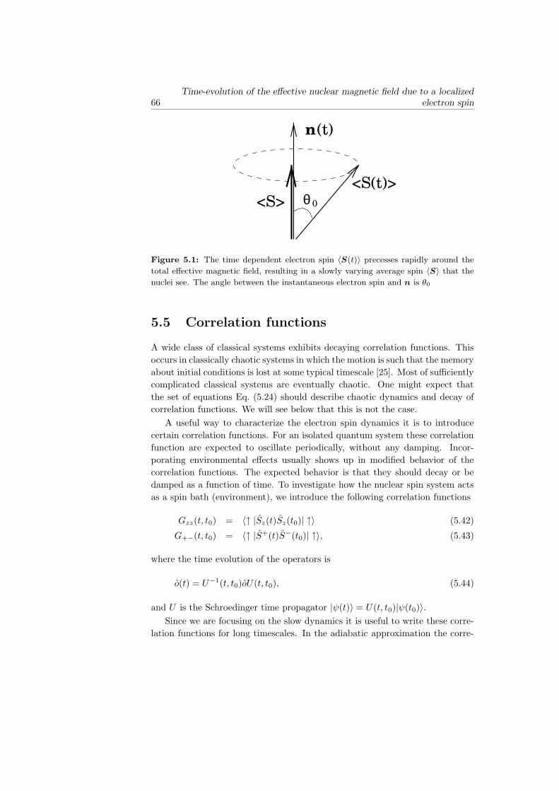
66Time-evolution of the effective nuclear magnetic field due to a localized
electron spin
<S(t)><S> θ 0
n(t)
Figure 5.1: The time dependent electron spin 〈S(t)〉 precesses rapidly around the
total effective magnetic field, resulting in a slowly varying average spin 〈S〉 that the
nuclei see. The angle between the instantaneous electron spin and n is θ0
5.5 Correlation functions
A wide class of classical systems exhibits decaying correlation functions. This
occurs in classically chaotic systems in which the motion is such that the memory
about initial conditions is lost at some typical timescale [25]. Most of sufficiently
complicated classical systems are eventually chaotic. One might expect that
the set of equations Eq. (5.24) should describe chaotic dynamics and decay of
correlation functions. We will see below that this is not the case.
A useful way to characterize the electron spin dynamics it is to introduce
certain correlation functions. For an isolated quantum system these correlation
function are expected to oscillate periodically, without any damping. Incor-
porating environmental effects usually shows up in modified behavior of the
correlation functions. The expected behavior is that they should decay or be
damped as a function of time. To investigate how the nuclear spin system acts
as a spin bath (environment), we introduce the following correlation functions
Gzz(t, t0) = 〈↑ |Sz(t)Sz(t0)| ↑〉 (5.42)
G+−(t, t0) = 〈↑ |S+(t)S−(t0)| ↑〉, (5.43)
where the time evolution of the operators is
o(t) = U−1(t, t0)oU(t, t0), (5.44)
and U is the Schroedinger time propagator |ψ(t)〉 = U(t, t0)|ψ(t0)〉.Since we are focusing on the slow dynamics it is useful to write these corre-
lation functions for long timescales. In the adiabatic approximation the corre-
5.6 Nuclear subsystem dynamics 67
lation functions may be written as
Gzz(t, t0) =1
4
(
1 − |a(t)|21 + |a(t)|2
)(
1 − |a(t0)|21 + |a(t0)|2
)
(5.45)
G+−(t, t0) = 2
(
a(t)
1 + |a(t)|2)(
a∗(t0)
1 + |a(t0)|2)
. (5.46)
Furthermore, it is possible to define a new correlation function
G(t, t0) = Gzz(t, t0) +1
2(G+−(t, t0) +G−+(t, t0)) (5.47)
= 〈↓ |S(t) · S(t0)| ↑〉 (5.48)
The most interesting regime corresponds to weak external magnetic fields.
In this case there is no preferred direction and the dynamics show the richest
behavior. In that limit the correlation functions take the simplified form
Gzz(t, t0) =Kz(t)Kz(t0)
4K(t)K(t0)(5.49)
G+−(t, t0) =K+(t)K−(t0)
4K(t)K(t0)(5.50)
G(t, t0) =K(t) · K(t0)
4K(t)K(t0)(5.51)
From these equations it is evident that the electron spin correlation function is
determined by the nuclear system variables.
For completeness we also give the results for the opposite limit. For large
external magnetic fields the correlation functions reflect that the dynamics is
mainly a precession around the external field. The correlation function are
Gzz(t, t0) =1
4
(
1 − Kx(t)2 +Ky(t)2 +Kx(t0)2 +Ky(t0)
2
2∆2
)
(5.52)
G+−(t, t0) =1
4
(
K+(t)K−(t0)
∆2
)
. (5.53)
5.6 Nuclear subsystem dynamics
The dynamics of the combined electron and nuclear system is given by Eqs.
(5.24) and (5.39). The large separation of timescales allows the electron spin
to be calculated separately, resulting in an average spin that depends on K. In
the absence of an external magnetic field the average electron takes the simple
form given in Eq. (5.39) and the equations of motion for the Kb’s become
d
dtKb = γgb
∑
b Kb
|∑
b Kb|× Kb. (5.54)
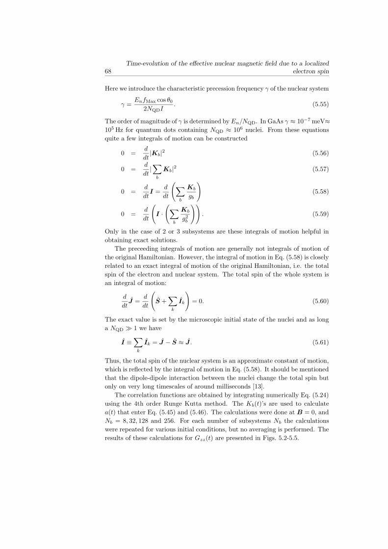
68Time-evolution of the effective nuclear magnetic field due to a localized
electron spin
Here we introduce the characteristic precession frequency γ of the nuclear system
γ =EnfMax cos θ0
2NQDI. (5.55)
The order of magnitude of γ is determined by En/NQD. In GaAs γ ≈ 10−7 meV≈105 Hz for quantum dots containing NQD ≈ 106 nuclei. From these equations
quite a few integrals of motion can be constructed
0 =d
dt|Kb|2 (5.56)
0 =d
dt|∑
b
Kb|2 (5.57)
0 =d
dtI =
d
dt
(
∑
b
Kb
gb
)
(5.58)
0 =d
dt
(
I ·(
∑
b
Kb
g2b
))
. (5.59)
Only in the case of 2 or 3 subsystems are these integrals of motion helpful in
obtaining exact solutions.
The preceeding integrals of motion are generally not integrals of motion of
the original Hamiltonian. However, the integral of motion in Eq. (5.58) is closely
related to an exact integral of motion of the original Hamiltonian, i.e. the total
spin of the electron and nuclear system. The total spin of the whole system is
an integral of motion:
d
dtJ =
d
dt
(
S +∑
k
Ik
)
= 0. (5.60)
The exact value is set by the microscopic initial state of the nuclei and as long
a NQD 1 we have
I ≡∑
k
Ik = J − S ≈ J . (5.61)
Thus, the total spin of the nuclear system is an approximate constant of motion,
which is reflected by the integral of motion in Eq. (5.58). It should be mentioned
that the dipole-dipole interaction between the nuclei change the total spin but
only on very long timescales of around milliseconds [13].
The correlation functions are obtained by integrating numerically Eq. (5.24)
using the 4th order Runge Kutta method. The Kb(t)’s are used to calculate
a(t) that enter Eq. (5.45) and (5.46). The calculations were done at B = 0, and
Nb = 8, 32, 128 and 256. For each number of subsystems Nb the calculations
were repeated for various initial conditions, but no averaging is performed. The
results of these calculations for Gzz(t) are presented in Figs. 5.2-5.5.

5.6 Nuclear subsystem dynamics 69
-0.25
0
0.25
0 100 200 300 400 500 600 700 800 900 1000
Gzz
t [γ-1]
Figure 5.2: Numerical calculations of the correlation function Gzz(t) for Nb = 8 and
various randomly chose initial conditions. The curves are offset for clarity and the
vertical range is the same for all curves, i.e. −0.25 to 0.25
-0.25
0
0.25
0 100 200 300 400 500 600 700 800 900 1000
Gzz
t [γ-1]
Figure 5.3: Numerical calculations of the correlation function Gzz(t) for Nb = 32
and various randomly chose initial conditions. The curves are offset for clarity and
the vertical range is the same for all curves, i.e. −0.25 to 0.25
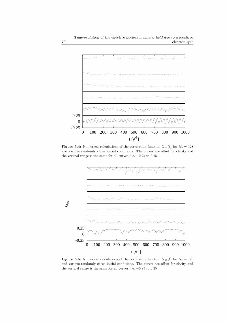
70Time-evolution of the effective nuclear magnetic field due to a localized
electron spin
-0.25
0
0.25
0 100 200 300 400 500 600 700 800 900 1000
t [γ-1]
Figure 5.4: Numerical calculations of the correlation function Gzz(t) for Nb = 128
and various randomly chose initial conditions. The curves are offset for clarity and
the vertical range is the same for all curves, i.e. −0.25 to 0.25
-0.25
0
0.25
0 100 200 300 400 500 600 700 800 900 1000
Gzz
t [γ-1]
Figure 5.5: Numerical calculations of the correlation function Gzz(t) for Nb = 128
and various randomly chose initial conditions. The curves are offset for clarity and
the vertical range is the same for all curves, i.e. −0.25 to 0.25
5.7 Conclusion 71
The common feature of all curves, for all values of Nb, is that they do not decay
with time. This behaviour persists to even higher times, not shown here. Even
though more complicated behaviour is observed for large Nb, the characteristic
frequencies of the correlation function oscillations do not show any obvious
dependence on the number of subsystems use, as long as Nb 1.
5.7 Conclusion
Although a more detailed study of the dynamics is needed, it is evident from
the numerical calculations that the correlation functions of the electron spins
do not show any decay in time. In the limit of low external magnetic field, the
dynamics of the system can be quite complicated depending on the initial state
of the subsystems and their number Nb. The timescale of the slow electron
evolution is determined by γ−1 even though the details depend on the initial
conditions and the number of subsystems. At high applied magnetic fields the
behaviour of the correlation functions is constrained by the external field, see
Eqs. (5.52) and (5.53)
Since the system has many integrals of motion, it may be close to exactly
solvable and thus one expects periodic oscillations and no decay [26]. The ob-
served behaviour of the system may be explained in this way, i.e. the oscillations
of the correlation function reflect that the system lies somewhere on the bound-
ary on being exactly solvable. These features will probaly vanish if further terms
into the Hamiltonian in Eq. (5.2) are included. The most natural term would
be the dipole-dipole interaction between the nuclei which would kill most of the
integrals of motion. It is important to recognize that the timescale related to
the dipole-dipole interaction is very long, of the order 10−3 s, and the relaxation
time would reflect that.
In connection to coherently controlling the spin, the motion of the electron
spin in the effective nuclear magnetic field will cause ‘errors’. Even though
in this model nuclear spins do not decohere the electron spin, they leads to
a complicated (unknown) evolution that is difficult to predict. Consequently,
an electron spin initially in | ↑〉 can be found in the opposite spin state on a
timescale ∝ γ−1. Thus, the hyperfine coupling to the nuclear system does not
lead to decoherence in this model but it can strongly affect the dynamics of the
electron spin.
References
[1] Y. Nakamura, Y. A. Pashkin, and J. S. Tsai, Nature 398, 786 (1999).
[2] J. E. Mooij et al., Science 285, 1036 (1999).
72Time-evolution of the effective nuclear magnetic field due to a localized
electron spin
[3] B. E. Kane, Nature 393, 133 (1998).
[4] C. P. Slichter, Principles of Magnetic Resonance, 3rd ed. (Springer-Verlag,
Berlin, 1990).
[5] A. Abragam, Principles of Nuclear Magnetism (Oxford University Press,
New York, 1961).
[6] D. Loss and D. P. DiVincenzo, Phys. Rev. A 57, 120 (1998).
[7] A. V. Khaetskii and Y. V. Nazarov, Phys. Rev. B 61, 12639 (2000).
[8] A. V. Khaetskii and Y. V. Nazarov, Phys. Rev. B 64, 125316 (2001).
[9] S. I. Erlingsson, Y. V. Nazarov, and V. I. Fal’ko, Phys. Rev. B 64, 195306
(2001).
[10] S. I. Erlingsson and Y. V. Nazarov, Phys. Rev. B 66, 155327 (2002).
[11] L. M. Woods, T. L. Reinecke, and Y. Lyanda-Geller, Phys. Rev. B 66,
161318(R) (2002).
[12] A. V. Khaetskii, D. Loss, and L. Glazman, Phys. Rev. Lett. 88, 186802
(2002).
[13] I. A. Merkulov, A. L. Efros, and M. Rosen, Phys. Rev. B 65, 205309 (2002).
[14] Y. G. Seminov and K. W. Kim, Phys. Rev. B 67, 73301 (2003).
[15] R. de Sousa and S. Das Sarma, Phys. Rev. B 67, 033301 (2003).
[16] S. Saykin and V. Privman, Nano Lett. 2, 651 (2002).
[17] J. Schliemann, A. V. Khaetskii, and D. Loss, Phys. Rev. B 66, 245303
(2002).
[18] S. W. Brown, T. A. Kennedy, and D. Gammon, Solid State Nucl. Magn.
Reson. 11, 49 (1998).
[19] S. Tarucha et al., Phys. Rev. Lett. 77, 3613 (1996).
[20] J. M. Elzerman et al., Phys. Rev. B 67, 161308 (2003).
[21] M. I. D’yakonov and V. Y. Kachorovksii, Sov. Phys. Semicond. 20, 110
(1986).
[22] D. Paget, G. Lampel, B. Sapoval, and V. I. Safarov, Phys. Rev. B 15, 5780
(1977).
[23] M. Dobers et al., Phys. Rev. Lett. 61, 1650 (1988).
[24] A. Messiah, Quantum Mechanics (Norht-Holland Publishing Co., Amster-
dam, 1962), Vol. 2.
[25] A. M. O. deAlmeida, Hamiltonian systems: chaos and quantization (Cam-
bridge University Press, Cambridge, 1988).
[26] J. Schliemann, private communication.

Appendix A
Thermal average over nuclear spin pairs
Even though we do not average over the classical field Kl, which is fixed, there
are still fluctuations in the nuclear system. Each pair of nuclei can fluctuate,
without affecting the classical field. One should think of these fluctuations as
small deviations around a given value of Kl, i.e. we (thermally) average over the
pairs for a fixed value of the classical field. When the thermal average over a pair
of free nuclei is performed the following nuclear correlation function appears in
Eq. (3.21)
Gcorr = (Sα+−)∗Sβ
+−〈δIαk δI
βk′〉T
= (Sα+−)∗Sβ
+−〈δIαδIβ〉T δk,k′ , (A.1)
where δIα = Iα − 〈Iα〉T and the electron spin matrix elements are Sα+− =
〈n+|Sα|n−〉. The Kronekker delta reflects that there are no correlations be-
tween two different nuclei and we have dropped the k subscript in 〈δIαδIβ〉Tsince the nuclei is assumed to be identical. By defining the symmetric correlator
gαβ =1
2〈δIαδIβ + δIβδIα〉T (A.2)
we get the following
Gcorr = (Sα+−)∗Sβ
+−(gαβ + i/2εαβγ〈Iγ〉T ). (A.3)
In an isotropic system, 〈I〉T = 0, the value of the correlation function is Gcorr =12
13I(I + 1).
73
74 Thermal average over nuclear spin pairs
Appendix B
Matrix elements for a parabolic
quantum dot
Using the Darwin-Fock solutions and the Fang-Howard variational solution for
the triangular quantum well we obtain the following equation for Eqs. (3.22)-
(3.25)
all′γll′ = δM,M ′
A2Cn
VQDζ
(eh14`)2∆3
8πρc5~4
Γ(n+ n′ + |M | + 1)2−3(n+n′+|M |)
n!n′!(n+ |M |)!(n′ + |M |)!
×(n(∆) + 1)∑
ν
c5
c5ν
(
∆
~cν`−1
)2(n+n′+|M |−1)
×∫ π
0
d(cos θ)Aν(θ)
(sin θ)2(n+n′+|M |) exp
(
− 12
(
∆ sin θ~cν`−1
)2)
(
1 +(
∆ cos θ3~cνz−1
0
)2)3
(B.1)
where ζ−1 = z0∫
dz|χ(z)|4 and c−5 = c−5l + c−5
t is the effective sound velocity
of the phonons. The anisotropy functions are
At(θ) =sin2 θ(8 cos4 θ + sin4 θ)
4(B.2)
Al(θ) =9 cos2 θ sin4 θ
2. (B.3)
The equation for all′ γll′ is identical except for a different Kronekker delta func-
tion δM,−M ′ . The integral needs in general to be evaluated numerically but
when ∆ ~cν`−1 the exponential term and the denominator become unity
and the resulting integral is simple to calculate.
75
76 Matrix elements for a parabolic quantum dot
Summary
Nuclear Spins in Quantum Dots
The main theme of this thesis is the hyperfine interaction between the many
lattice nuclear spins and electron spins localized in GaAs quantum dots. This
interaction is an intrinsic property of the material. Despite the fact that this
interaction is rather weak, it can, as shown in this thesis, strongly influence the
dynamics of electron spins in quantum dots. In chapter 1 some basic features
of quantum dots are described and the most important sources for the mixing
of spin components in GaAs, i.e. the hyperfine and spin-orbit interaction, are
introduced and discussed.
The hyperfine mediated transition rate from a triplet state to the ground
state singlet is considered in chapter 2. The transition involves changing both
the orbital and spin degree of freedom so the phonon scattering alone cannot
facilitate the transition. Also, the hyperfine interaction alone can not cause the
transition because the nuclear spin system cannot absorb the energy released by
the singlet-to-triplet transition. Thus, both a source of inelastic scattering and
the hyperfine interaction are required for the transition. The resulting transition
involves virtual excited states. Assuming a small exchange splitting a simple
expression for the transition rate is obtained that involves only the first excited
singlet state.
The subject of chapter 3 is the hyperfine mediated transitions between Zee-
man split doublet components of the ground state orbital of a single-electron
quantum dot. The spin-flip mechanism is the same as for the singlet-triplet
case, i.e. the transition goes via higher orbital virtual states and involves both
the hyperfine interaction and phonon scattering. A closer look is taken at the
relevant electron-phonon coupling mechanism: The piezoelectric phonons. In
addition, a semiclassical picture of the nuclear system is formulated. The great
number of nuclei in the quantum dot makes it possible to consider them as
an effective nuclear magnetic field acting on the electron spin. The transition
amplitude between the doublet components due to the hyperfine interaction re-
mains finite even if the external magnetic field goes to zero. This is in contrast
to spin-orbit interaction where the transition amplitude vanishes at zero field.
77
78 Summary
Thus, at sufficiently low magnetic field the hyperfine related spin-flip rate will
dominate the spin-orbit one. The rates obtained in chapters 2 and 3 are usually
much smaller than non-spin-flip transition rates in quantum dots.
Transport through a GaAs double quantum dot in the socalled spin-blockade
regime is the subject of chapter 4. The current is blocked due to the absence
of transitions between singlet and triplet states within the quantum dots. Mo-
tivated by a recent experiment, we consider the influence of the hyperfine in-
teraction on transport in the spin-blockade regime. A small transport current
will flow if the singlet and triplet states are mixed. In our model the mixing
is induced by the different effective nuclear magnetic fields acting the electron
spins in the two dots. Not only does the nuclear system affect the electron spins
and lift the spin-blockade, there is also a back-action on the nuclear system
that is determined by the average electron spin in the two dots. The nuclear
system precesses around the average electron spin, leading to a time dependent
transport current whose characteristics are in qualitative agreement with the
experimental observations.
In the last chapter the dynamics induced by the hyperfine coupling of the
electron and nuclear spins in a quantum dot are studied. An effective spin
Hamiltonian is considered where the spatial dependence of the electron wave-
function results in an inhomogenoues hyperfine coupling of the electron spin to
different nuclear spins. Generally, it is not possible to solve this Hamiltonian
except in the special case of homogeneous coupling. To obtain an approximate
solution, we split the nuclear system into Nb subsystems where all nuclei within
a given subsystem have equal coupling to the electron spin. An important fea-
ture of the original Hamiltonian is the separation of the timescales, i.e. the
electron spin dynamics are much faster than that of the nuclear spins. This
allows us to use the adiabatic approximation when calculating the average elec-
tron spin which each nuclear spin sees. In this way the electron spin is removed
from the problem leaving 3Nb coupled differential equations. These are solved
numerically and the results used to calculate certain electron spin correlation
functions. Contrary to what one may guess, the dynamics are not chaotic and
the correlation functions show no decay in time, only complicated oscillations.
This may be be attributed to the fact that the system has many integrals of
motion and that it is close to exactly solvable. This behavior persists even for
Nb 1, which is the limit in which our approximation becomes more accurate.
Sigurdur I. Erlingsson, Delft 2003
Samenvatting
Nucleaire Spins in Quantum Dots
Het hoofdthema van dit proefschrift is de hyperfijninteractie tussen de spins
van de vele nucleı in het kristalrooster en de spins van gelokaliseerde elektro-
nen in GaAs quantum dots. Deze interactie is een intrinsieke eigenschap van
het materiaal. Ondanks het feit dat deze interactie vrij zwak is, kan ze, zoals
aangetoond in dit proefschrift, de dynamica van elektronspins in quantum dots
sterk beınvloeden. In hoofdstuk 1 worden enkele basiseigenschappen van quan-
tum dots beschreven en worden de belangrijkste bronnen voor de vermenging
van de spin componenten in GaAs, dwz. de hyperfijninteractie en de spin-baan
interactie, geıntroduceerd en besproken.
De door de hyperfijninteractie gemedieerde overgang van een triplet toestand
naar de singlet grondtoestand wordt beschouwd in hoofdstuk 2. De overgang
gaat gepaard met een verandering van zowel de baan- als de spinvrijheidsgraad
waardoor met fononen verstrooiıng alleen de overgang niet bewerkstelligd kan
worden. Ook de hyperfijninteractie kan de overgang niet alleen veroorzaken om-
dat het nucleaire spinsysteem de energie die vrijkomt bij de triplet-naar-singlet
overgang niet kan opnemen. Dus, zowel een bron van inelastische verstrooiıng
als de hyperfijninteractie zijn nodig voor de overgang. De resulterende overgang
gaat gepaard met virtuele aangeslagen toestanden. Onder de aanname van een
kleine zgn. ’exchange’ splitsing is een simpele uitdrukking verkregen voor de
snelheid van de overgang, waarbij alleen de eerste aangeslagen singlet toestand
betrokken is.
Het onderwerp van hoofdstuk 3 is de door hyperfijninteractie gemedieerde
overgang tussen Zeeman-gesplitste doubletcomponenten van de laagste orbitaal
van een een-elektron quantum dot. Het spin-flip mechanisme is hetzelfde als in
het geval van de singlet-tripletcomponenten, dwz. de overgang gaat via hogere
virtuele orbitaaltoestanden and gaat samen met zowel de hyperfijninteractie als
fononen verstrooiing. De relevante elektron-fonon koppeling is nader bekeken:
de piezo-elektrische fononen. Bovendien is een semi-klassiek beeld van het nu-
cleaire systeem geformuleerd. Het grote aantal nuclei in de quantum dot maakt
het mogelijk om deze te beschouwen als een effectief nucleair magnetisch veld
79
80 Samenvatting
dat op de elektronspin werkt. De overgangsamplitude tussen de doubletcompo-
nenten ten gevolge van de hyperfijninteractie blijft eindig, zelfs als het externe
mangeetveld naar nul gaat. Dit is in tegenstelling tot de overgang ten gevolge
van spin-baan interactie, waarvan de overgangsamplitude verdwijnt bij nul veld.
Bij magnetische velden die laag genoeg zijn zal de hyperfijn-gerelateerde spin-flip
snelheid dus domineren over de spin-baangerelateerde. De snelheden verkregen
in hoofdstuk 2 en 3 zijn gewoonlijk veel lager dan de snelheden in quantum dots
voor overgangen zonder spin-flip.
Transport door een GaAs dubbele quantum dot in het zogenaamde spin-
blokkade regime is het onderwerp van hoofdstuk 4. De stroom is geblokkeerd
door de afwezigheid van overgangen tussen singlet en triplettoestanden in de
quantum dots. Gemotiveerd door een recent experiment beschouwen we de in-
vloed van de hyperfijninteractie op het transport in het spinblokkade regime.
Een kleine stroom zal lopen als de singlet en triplet toestanden vermengd wor-
den. In ons model wordt de vermenging veroorzaakt door de verschillende effec-
tieve nucleaire magneetvelden die op de spins in de twee dots werken. Niet alleen
beınvloedt het nucleaire systeem de elektronspins en heft het de spinblokkade
op, er is ook een terugwerking op het nucleaire systeem dat wordt bepaald door
de gemiddelde elektronspin in de twee dots. Het nucleaire systeem precedeert
om de elektronspin, wat leidt tot een tijdsafhankelijke stroom waarvan de karak-
teristieken kwalitatief overeenkomen met de experimentele waarnemingen
In het laatste hoofdstuk wordt de dynamica bestudeerd die wordt geınduceerd
door de hyperfijnkoppeling van de elektronspins en de nucleaire spins. Een ef-
fectieve spin Hamiltoniaan wordt beschouwd waar de plaatsafhankelijkheid van
de golffunctie van het elektron resulteert in een inhomogene hyperfijnkoppel-
ing van de elektronspin naar de verschillende nuclei. Het is niet mogelijk om
deze Hamiltoniaan op te lossen, behalve in het speciale geval van een homogene
koppeling. Om een benadering van de oplossing te verkrijgen splitsen we het
nucleaire systeem in Nb subsystemen, waarbij alle nuclei in een gegeven sub-
systeem gelijke koppeling hebben naar de elektronspin. Een belangrijke eigen-
schap van de originele Hamiltoniaan is de scheiding van de tijdsschalen, i.e.
de dynamica van de elektronspin is veel sneller dan die van de nucleaire spins.
Hierdoor mogen we de adiabatische benadering toepassen bij het berekenen van
de gemiddelde elektronspin die door elke nucleaire spin wordt gezien. Op deze
manier wordt de elektronspin uit het probleem verwijderd en blijven er 3Nb
gekoppelde differentiaalvergelijkingen over. Deze zijn numeriek opgelost en de
resultaten zijn gebruikt om bepaalde elektron correlatiefuncties te berekenen.
In tegenstelling tot wat men zou denken is de dynamica niet chaotisch en laten
de correlatiefuncties geen verval zien in de tijd, enkel ingewikkelde oscillaties.
Dit zou kunnen worden toegeschreven aan het feit dat het systeem vele beweg-
ingsintegralen heeft en dat het bijna exact oplosbaar is. Dit gedrag houdt aan
81
voor Nb 1, de limiet waarin onze benadering nauwkeuriger wordt.
Sigurdur I. Erlingsson, Delft 2003
82 Samenvatting
Curriculum Vitae
Sigurdur I. Erlingsson
25 August 1972 Born in Reykjavik, Iceland
1988-1993: High School/Gymnasium education
Hafnarfirdi, Iceland
1990-1991: Exchange student in Charleston, South Carolina, USA.
1993-1999: M.Sc. physics from the University of Iceland under
the supervision of Prof. Vidar Gudmundsson
Title: Finite size effects in the far-infrared absorption of a confined 2DEG
1999-2003: PhD physics from the Delft University of Technology under
the supervision of Prof. Yuli V. Nazarov
Title: Nuclear Spins in Quantum Dots
83
84
List of publications
1. Nucleus-mediated spin-flip transitions in GaAs quantum dots
S.I. Erlingsson,Yu. V. Nazarov and V. I. Fal’ko, PRB 64, 195306 (2001)
2. Hyperfine-mediated spin-flip transitions in GaAs quantum dots
S.I. Erlingsson,Yu. V. Nazarov and V. I. Fal’ko, Physica E 12, 823 (2002)
3. Hyperfine-mediated transitions between a Zeeman split doublet in GaAs
quantum dots: the role of the internal field
S.I. Erlingsson and Yu. V. Nazarov, PRB 66, 155327 (2002)
4. Hyperfine-mediated transitions between a Zeeman split doublet in GaAs
quantum dots: the role of the internal field
S.I. Erlingsson and Yu. V. Nazarov, J. Supercond., 16, 293 (2003)
5. Coherent oscillations of current due to nuclear spins
S.I. Erlingsson and Yu. V. Nazarov, submitted to PRL
6. Time-evolution of the effective nuclear magnetic field due to a localized
electron spin
S.I. Erlingsson and Yu. V. Nazarov, in preparation
85
![Coulomb-Blockade Oscillations in Quantum Dots and Wires · a sawtooth like oscillation of the charge imbalance results [Fig. 1.5(b)]. Tunneling is blocked at low temperatures, except](https://static.fdocuments.nl/doc/165x107/5ed9313e6714ca7f476950d6/coulomb-blockade-oscillations-in-quantum-dots-and-wires-a-sawtooth-like-oscillation.jpg)