
Morphodynamic modelling of estuarine channel-shoal systems ... · Morphodynamic modelling of...
143
Morphodynamic modelling of estuarine channel-shoal systems Morfodynamisch modelleren van estuarine plaat-geul systemen
Transcript of Morphodynamic modelling of estuarine channel-shoal systems ... · Morphodynamic modelling of...
Morphodynamic modelling ofestuarine channel-shoal systems
Morfodynamisch modelleren vanestuarine plaat-geul systemen

Morphodynamic modelling ofestuarine channel-shoal systems
Proefschrift
ter verkrijging van de graad van doctor
aan de Technische Universiteit Delft,
op gezag van de Rector Magnificus prof.dr.ir. J.T. Fokkema,
voorzitter van het College voor Promoties,
in het openbaar te verdedigen op maandag 28 juni 2004 om 13.00 uur
door
Anneke HIBMA
civiel ingenieur
geboren te Amsterdam
Dit proefschrift is goedgekeurd door de promotoren:
Prof.dr.ir. H.J. de Vriend
Prof.dr.ir. M.J.F. Stive
Toegevoegd promotor:
Dr.ir. Z.B. Wang
Samenstelling promotiecommissie:
Rector Magnificus voorzitter
Prof.dr.ir. H.J. de Vriend Technische Universiteit Delft, promotor
Prof.dr.ir. M.J.F. Stive Technische Universiteit Delft, promotor
Dr.ir. Z.B. Wang Technische Universiteit Delft, toegevoegd promotor
Prof.dr.ir. J. van de Kreeke University of Miami, FL, United States
Prof.dr. G. Di Silvio University of Padua, Italy
Dr. H.E. de Swart Universiteit Utrecht
Prof.dr.ir. G.S. Stelling Technische Universiteit Delft
Dr. H.M. Schuttelaars heeft als begeleider in belangrijke mate aan de totstandkoming van het
proefschrift bijgedragen.
Cover design: Ada Beuling
The figures on the cover show different stages of estuarine channel–shoal pattern formation
(also see Fig. 5.3).
Copyright c© 2004 by Anneke Hibma
Printed by PrintPartners Ipskamp BV, the Netherlands
ISBN 90-9017987-9
This thesis is also published in the series of ‘Communications on Hydraulic and Geotechnical
Engineering’, Faculty of Civil Engineering and Geosciences, Delft University of Technology,
Report No. 04-3, ISSN 0169-6548.
Summary
Estuaries and tidal lagoons occur in many coastal areas world-wide. They attract a variety of
human activities, such as navigation, recreation, fishing and aquaculture, economic activity in
the border zone, sand mining, land reclamation and in some cases hydrocarbon mining. On
the other hand, many estuaries and lagoons form the basis of highly valuable and sometimes
unique ecosystems. For the proper management of these systems, it is important to be able to
predict the impacts of human activities and natural forces. Understanding and predicting the
morphodynamic evolution of estuaries is still limited, because of its complexity and because it
involves a wide range of time and space scales.
In this research we focus on meso- and macro-scale morphodynamics of estuaries where tidal
motion forms the principal forcing. On these scales channels and shoals form highly dynamic
elements. The general objectives are to improve our knowledge and prediction capabilities of
the morphodynamic behaviour of channels and shoals in estuaries and coastal lagoons, at time
scales from decades to centuries.
A literature survey (Hibma et al., 2000) has revealed that various forcings influence the to-
pography of estuaries on different time- and space-scales. Main actors determining meso- and
macro-scale morphological characteristics of estuaries are tidal currents and wind waves. Due
to the non-linear interaction and associated feedback between forcings and topography, mor-
phodynamic response is often not only directly related to the energetic forcing frequencies
(forced behaviour), but exhibits also free behaviour. The morphodynamic response scales of
sedimentary features display such variability that seldom all features can attain an equilibrium
state (even in a dynamic sense) in response to the forcing conditions. As a result, the overall
morphological system may remain in a continuous transient state. From observations, empirical
relations between flow and size of channels are derived, as well as between flow and number of
channels, in which the width to depth ratio, total size of the estuary and type of sediment also
play a role.
Different types of model approaches are developed and used to investigate and simulate the
evolution of estuarine morphology on meso- and macro-scales. On macro scale, we discern two
types of models, (semi-) empirical models (also referred to as behaviour-oriented, aggregated or
hierarchical models) and macro-scale process-based models, which are both aggregated model
v
vi Summary
approaches.
Process-based models derived for meso-scale modelling are mathematical representations of
physical laws per cross-section for one-dimensional models or on a local, discrete grid for two-
and three-dimensional models. Within this model type two principal approaches can be dis-
cerned. For simplicity, we will speak of complex models in contrast to idealised models. Idealised
models make use of simplified geometries, forcings and physical formulations, compared to com-
plex models. Against the loss of simulating situations for realistic geometries and forcings stands
more fundamental insight into the physics and the ability to make long-term morphodynamic
computations, involving a formal aggregation to macro-scale evolution.
Each model type has its own area of applicability due to the applied assumptions and model
formulations. Jointly, these models cover a wide span of time and space scales. Consequently,
different model types are difficult to compare, which complicates verification of model results
and insight into the implication of model formulations and assumptions.
At present, due to improved physical insight and increased computational power, the ability to
use complex process-based models is enhanced. This research shows that this model type can
bridge different scales, by extending the meso-scale model into the macro-scale domain, and
different model approaches, by making a link with idealised models.
Firstly, this link is made for a one-dimensional model, by comparing the cross-sectionally aver-
aged results of the (complex) process–based morphodynamic model Delft3D and the idealised
model of Schuttelaars and De Swart (2000). The differences between the two models in their
mathematical–physical formulation as well as the boundary conditions are identified. The source
code of the complex model is modified to resemble the formulations in the idealised model. This
so-named intermediate model bridges between the two approaches and enables a comparison
of model results. The effects of each of the differences on producing cross-sectionally averaged
morphological equilibria of tidal inlets with arbitrary length and forced at the seaward bound-
ary by a prescribed M2 and M4 sea surface elevation is studied.
The results of the idealised and intermediate model show good agreement with respect to the
water levels and velocities in a schematised estuary. The development of the cross–sectionally
averaged profiles in the process–based model resemble qualitatively the unique and multiple
equilibrium profiles of the idealised model, although an equilibrium is not achieved in the strict
sense of zero bed level change everywhere. The model adaptations in water motion and sediment
transport have no qualitative influence on the morphodynamic results. Hence, the simplifica-
tions in these formulations as used in the idealised model are justified. Only the adaptations of
the boundary condition of the bed at the entrance has qualitative influence on the morphody-
namic equilibria. It can be inferred that this morphological boundary condition is an essential
element in controlling the behaviour of morphodynamic models for tidal inlets and estuaries.
The results and conclusions drawn from this intermediate model are used in the set-up of a
two-dimensional complex model. In order to compare the results with idealised two-dimensional
Summary vii
models, the geometry of the estuary is schematised to a long rectangular basin. Sinusoidal
perturbations of various wavelengths in longitudinal as well as transversal direction and small
amplitude are imposed on the equilibrium bed of the basin. Short-term as well as long-term
simulations are made, for a narrow and wide basin.
The growth of the perturbations and their dependency on width and depth of the basin and
the local maximum velocity is investigated. Prevalent wavelengths increase with increasing
width and flow velocity. Initial model results from the short-term simulations are compared
with linear stability analyses of idealised two-dimensional models for validation and in order
to gain insight into the processes responsible for the growth. The dominant wavelengths are
of the same order of magnitude as those found in the idealised model of Schramkowski et al.
(2002) and their dependency on width and velocity agrees qualitatively. (Exponential) growth
of the perturbations during long-term simulations provides information on the validity limits
of the idealised models. Subsequent pattern formation and changes of dominant along-channel
and cross-channel wavelengths are attributed to non-linear interactions. The morphological
developments during long-term simulations suggest that channel–shoal patterns evolve into a
unique morphodynamic equilibrium state, independent of the initial perturbation.
The ability of this complex process-based model to reproduce the formation of channel–shoal
patterns far into the non-linear domain is further investigated. Starting from a linear sloping
bed, on which random perturbations are imposed, the model results show how a simple and
regular pattern of initially grown undulations merges to complex larger scale channel–shoal
patterns. The emerging patterns are compared with field observations. The overall pattern
agrees qualitatively with patterns observed in the Western Scheldt estuary, The Netherlands,
and in the Patuxent River estuary, Virginia. Quantitative comparison of the number of channels
and meander length scales with observations gives reasonable accordance.
The final series of simulations is made for a funnel-shape basin. The residual flow and sediment
transport circulations for the resulting channel–shoal pattern are analysed and compared to
the Western Scheldt estuary. Subsequently, the model is applied to investigate the impact of
dredging and dumping in the channel system. The starting point is a conceptual model in which
ebb- and flood channels and enclosed shoals form morphodynamic units (cells) with their own
sediment circulation. Model results show that dumping sediment in a channel not only reduces
the channel depth, but also induces erosion in the opposite channel, which eventually can lead
to the degeneration of a multiple channel system into a single channel.
In conclusion, the present research has resulted in increased insight into morphodynamic mod-
elling of estuarine channel–shoal systems and increased understanding of the morphological
behaviour of these systems. The complex process-based model used in this research is applied
to analyse apparent contrasts between different types of models and is shown to diminish these
contrasts. This modelling approach is an innovative step towards an integrated modelling ap-
proach in which different model types and field data are combined in order to make optimal use
viii Summary
of each research method. The results show that this meso-scale process-based model provides a
tool, complementary to fieldwork, theoretical behaviour analyses and laboratory experiments,
for the analysis of the large-scale morphological behaviour of tide-dominated estuaries. Rec-
ommendations for improvement of model formulations include the morphological boundary
condition and the drying and flooding procedure. Recommendations for further research in-
clude the extension of the analysis of simplified situations by investigating other forces and
geometries, application of the model to human interventions and including intertidal areas,
which will involve mathematical, numerical as well as physical difficulties.
Samenvatting
Estuaria en getijdebekkens komen in veel kustgebieden, verspreid over de hele wereld voor.
Deze inlandse wateren, in open contact met de zee, trekken diverse menselijke activiteiten aan,
zoals scheepvaart, recreatie, visserij en aquacultuur, economische activiteiten in de grenszone,
zand- en landwinning en soms olie- en gaswinning. Daarnaast vormen veel estuaria en getijde-
bekkens de basis voor zeer waardevolle en soms unieke ecosystemen. Om deze systemen goed te
kunnen beheren is het belangrijk de gevolgen van menselijke activiteiten en natuurlijke forcerin-
gen te kunnen voorspellen. Het begrijpen en voorspellen van de voortdurende evolutie van de
bodemvormen, de morfodynamische evolutie, van estuaria is gelimiteerd door de complexiteit
ervan en door de wijde range aan tijd- en ruimteschalen.
In dit onderzoek richten we ons op de morfodynamiek van estuaria op meso- en macroschaal
(jaren tot decennia), waarbij de getijbeweging de voornaamste forcering vormt. Op deze schalen
vormen platen en geulen hoogdynamische elementen. De algemene doelstellingen zijn het ver-
beteren van de kennis en de voorspellingsmogelijkheden van het morfodynamisch gedrag van
platen en geulen in estuaria en getijdebekkens op tijdschalen van decaden tot eeuwen.
Uit literatuuronderzoek (Hibma e.a., 2000) blijkt dat verscheidene forceringen de topografie
van estuaria beınvloeden op verschillende tijd- en ruimteschalen. De voornaamste actoren die
de meso- en macroschaal morfologische kenmerken van estuaria bepalen zijn de getijdestromin-
gen en (wind)golven. Door de niet-lineaire interactie en de daarbij behorende feedback tussen
forcering en topografie is de morfodynamische respons vaak niet direct gerelateerd aan de fre-
quenties van de energetische forceringen (geforceerd gedrag), maar vertoont ook vrij gedrag. De
reikwijdte van de morfodynamische respons van sedimentologische elementen vertoont zo’n vari-
abiliteit dat zelden alle elementen een evenwichtstoestand kunnen bereiken (zelfs in dynamische
zin) in respons op de geforceerde condities. Als resultaat kan het morfologische systeem als
geheel in een continue overgangsstaat blijven. Uit observaties zijn empirische relaties herleid
tussen zowel stroming en geulafmetingen, als tussen stroming en het aantal geulen, waarbij de
verhouding breedte–diepte, de totale grootte van het estuarium en het type sediment ook een
rol spelen.
Verschillende typen modelbenaderingen zijn ontwikkeld en gebruikt om de evolutie van estuar-
iene morfologie te onderzoeken en te simuleren op meso- en macroschaal. Op macroschaal onder-
ix
x Samenvatting
scheiden we twee typen modellen: (semi-) empirische modellen (ook wel gedragsgeorienteerde,
geaggregeerde of hierarchische modellen genoemd) en macroschaal procesgebaseerde modellen.
Beide zijn geaggregeerde modelbenaderingen.
Procesgebaseerde modellen, afgeleid voor modellering op mesoschaal, zijn mathematische re-
presentaties van fysische wetten voor een doorsnede bij eendimensionale modellen of op een
lokaal, diskreet grid bij twee- en driedimensionale modellen. Binnen dit model type kunnen
twee principe benaderingen worden onderscheiden. Om het eenvoudig te houden spreken we
van complexe modellen tegenover geıdealiseerde modellen. Deze laatste maken vergeleken met
complexe modellen, gebruik van vereenvoudigde geometrieen, forceringen en fysische formu-
leringen. Tegenover het verlies van het simuleren van realistische geometrien en forceringen
staat meer fundamenteel inzicht in de fysica en de mogelijkheid om lange-termijn morfody-
namische berekeningen te maken, door een formele aggregatie naar evolutie op macroschaal.
Elk modeltype heeft een eigen toepassingsgebied door de toegepaste aannamen en modelformu-
leringen. Samen hebben deze modellen een breed bereik over tijd- en ruimteschalen. Als gevolg
hiervan zijn de verschillende modellen moeilijk met elkaar te vergelijken, wat de verificatie van
de modelresultaten bemoeilijkt, evenals het inzicht in de implicaties van modelformuleringen en
aannamen. Tegenwoordig is de mogelijkheid om complexe modellen te gebruiken toegenomen
door verbeterd inzicht in de fysica en de toegenomen kracht van de computer. Dit onderzoek
laat zien dat dit complexe modeltype zowel verschillende schalen overbrugt, door het mesoschaal
model te rekken naar het macroschaal domein, als ook verschillende modelbenaderingen over-
brugt, door een link te leggen met geıdealiseerde modellen.
Deze verbinding is eerst gemaakt voor een eendimensionaal model, door de breedte-gemiddelde
resultaten van het (complexe) procesgebaseerde morfodynamisch model Delft3D te vergelijken
met het geıdealiseerde model van Schuttelaars en de Swart (2000). De verschillen tussen de
twee modellen in zowel de mathematisch–fysische formuleringen als de randvoorwaarden zijn
geıdentificeerd. De broncode van het complexe model is aangepast om de formuleringen van
het geıdealiseerde model weer te geven. Dit zogenoemde intermediate model overbrugt de twee
modelbenaderingen en maakt een vergelijking van modelresultaten mogelijk. De effecten van
ieder verschil op de productie van breedte-gemiddelde morfologische evenwichten van getijde-
bekkens met arbitraire lengte en geforceerd aan de zeezijde met een voorgeschreven M2 en M4
waterstandsvariatie zijn bestudeerd.
De resultaten van het gıdealiseerde en het intermediate model tonen goede overeenkomsten
met betrekking tot de waterstanden en snelheden in een geschematiseerd estuarium. De ont-
wikkeling van het breedte-gemiddelde profiel in het procesgebaseerde model geeft kwalitatief
zowel de unieke als de meervoudige evenwichtsprofielen van het geıdealiseerde model weer,
hoewel een evenwicht niet bereikt wordt in de strikte betekenis dat nergens het niveau van
de bodem verandert. De modelaanpassingen in de waterbeweging en het sedimenttransport
hebben geen kwalitatieve invloed op de morfodynamische resultaten. Dus de vereenvoudigin-
gen in deze formuleringen zoals gebruikt in het geıdealiseerde model zijn gerechtvaardigd. Alleen
Samenvatting xi
de aanpassing van de bodemrandvoorwaarde aan de monding heeft kwalitatieve invloed op het
morfodynamisch evenwicht. Hieruit kan geconcludeerd worden dat deze morfologische rand-
voorwaarde een essentieel element vormt in de aansturing van het gedrag van morfodynamische
modellen voor getijdebekkens en estuaria.
De resultaten en conclusies getrokken uit dit intermediate model zijn gebruikt in het opzetten
van een tweedimensionaal complex model. Om de resultaten te kunnen vergelijken met geıdea-
liseerde tweedimensionale modellen, is de geometrie van het model geschematiseerd tot een lang
rechthoekig bekken. Sinusvormige verstoringen met verschillende golflengten in zowel longitudi-
nale als transversale richting en met kleine amplitude zijn opgelegd op de evenwichtsbodem van
het bekken. Simulaties op zowel korte-termijn als lange-termijn zijn gemaakt, voor een smal en
een breed bekken.
De groei van de verstoringen en hun afhankelijkheid van de breedte en diepte van het bekken en
de lokale maximale snelheid is onderzocht. Preferente golflengten nemen toe wanneer breedte en
stroomsnelheid toenemen. Initiele modelresultaten van de korte-termijn simulaties zijn vergele-
ken met de lineaire stabiliteitsanalyses van geıdealiseerde twee-dimensionale modellen om te
valideren en om inzicht te krijgen in de processen die verantwoordelijk zijn voor de groei. De
dominante golflengten zijn van dezelfde orde van grootte als die gevonden in het geıdealiseerde
model van Schramkowski e.a. (2002) en hun afhankelijkheid van breedte en snelheid komt
kwalitatief overeen. (Exponentiele) groei van de verstoringen gedurende lange-termijn simu-
laties geeft informatie over de grenzen aan de geldigheid van de geıdealiseerde modellen. De
daaropvolgende patroon ontwikkeling en veranderingen in dominante golflengten in langs- en
dwarsrichting zijn toegeschreven aan niet-lineaire interacties. De morfologische ontwikkeling
gedurende de lange-termijn simulaties suggereren dat het plaat–geulpatroon evolueert naar een
unieke morfodynamische evenwichts toestand, onafhankelijk van de initiele verstoring.
De mogelijkheid van dit complexe procesgebaseerde model om de vorming van plaat–geul-
patronen te reproduceren tot ver in het niet-lineaire domein is verder onderzocht. Modelre-
sultaten laten zien hoe, beginnend met een lineair hellende bodem waarop random verstorin-
gen zijn aangebracht, een eenvoudig en regelmatig patroon van initieel groeiende bodemvor-
men samensmelten tot complexe grootschalige plaat–geulpatronen. De ontstane patronen zijn
vergeleken met veld-observaties. Het grootschalige patroon komt kwalitatief overeen met patro-
nen die geobserveerd zijn in het Westerschelde-estuarium in Nederland en het Patuxent River
estuarium in Virginia, USA. Kwantitatieve vergelijking van het aantal geulen en de lengte-
schalen van de meander met observaties geven redelijke overeenkomsten.
De laatste serie simulaties is gemaakt voor een trechtervormig bekken. De reststroming en
circulaties van sedimenttransport voor het resulterende plaat–geulpatroon zijn geanalyseerd en
vergeleken met die in de Westerschelde. Vervolgens is het model toegepast om de impact van
baggeren en storten in het geulsysteem te onderzoeken. Daarbij is uitgegaan van een conceptueel
model waarin eb- en vloedgeulen en de omsloten platen morfodynamische eenheden (cellen)
xii Samenvatting
vormen met hun eigen sediment circulatie. Modelresultaten laten zien dat het storten van
sediment in een geul niet alleen de geuldiepte doet afnemen, maar ook erosie veroorzaakt in
de ertegenover liggende geul, wat uiteindelijk kan leiden tot degeneratie van een meergeulen
systeem tot een enkele geul.
Conclusies: dit onderzoek heeft geresulteerd in een verbeterd inzicht in de morfodynamische
modellering van estuariene plaat–geulsystemen en in een beter begrip van het morfologisch
gedrag van deze systemen. Het complexe procesgebaseerde model, dat in dit onderzoek is
gebruikt, is toegepast om ogenschijnlijke tegenstellingen tussen verschillende typen modellen
te analyseren en heeft laten zien dat deze tegenstellingen te verkleinen. Deze aanpak is een
innovatieve stap richting een geıntegreerde modelleer benadering waarin verschillende typen
modellen en veld data gecombineerd worden om optimaal gebruik te maken van iedere onder-
zoeksmethode. De resultaten laten zien dat dit mesoschaal procesgebaseerde model een middel
vormt, aanvullend op veldwerk, theoretische analyses en laboratorium experimenten, voor de
analyse van het grootschalig morfologisch gedrag van estuaria die door getijde gedomineerde
zijn. Aanbevelingen voor verbeteringen van model formuleringen bevatten de morfologische
randvoorwaarde en de droogval procedure. Aanbevelingen voor verder onderzoek bevatten de
uitbreiding van de analysen voor vereenvoudigde situaties met onderzoek naar andere forcerin-
gen en geometrieen, de toepassingen van het model voor menselijke ingrepen in het plaat–
geulsysteem en het modelleren van de intergetijde gebieden, wat mathematische, numerieke en
fysische vragen met zich mee zal brengen.
Contents
Summary v
Samenvatting ix
1 Introduction 1
1.1 Estuarine morphodynamics . . . . . . . . . . . . . . . . . . . . . . . . . . . . . 1
1.2 Objectives and research questions . . . . . . . . . . . . . . . . . . . . . . . . . . 4
1.3 Mathematical modelling . . . . . . . . . . . . . . . . . . . . . . . . . . . . . . . 4
1.4 Research approach and outline . . . . . . . . . . . . . . . . . . . . . . . . . . . . 5
2 Modelling estuarine morphodynamics 9
2.1 Introduction . . . . . . . . . . . . . . . . . . . . . . . . . . . . . . . . . . . . . . 9
2.2 Meso- and macro-scale observations and macro-scale models . . . . . . . . . . . 11
2.2.1 Macro-scale features . . . . . . . . . . . . . . . . . . . . . . . . . . . . . 11
2.2.2 Meso-scale features . . . . . . . . . . . . . . . . . . . . . . . . . . . . . . 12
2.2.3 Channel-shoal patterns . . . . . . . . . . . . . . . . . . . . . . . . . . . . 12
2.2.4 Macro-scale behaviour-oriented modelling . . . . . . . . . . . . . . . . . . 16
2.3 Meso-scale models for macro-scale features . . . . . . . . . . . . . . . . . . . . . 17
2.3.1 Complex and idealised models: one-dimensional models . . . . . . . . . . 18
2.3.2 Complex and idealised models: two- and three-dimensional models . . . . 19
2.3.3 Sand and mud models . . . . . . . . . . . . . . . . . . . . . . . . . . . . 24
2.4 Discussion . . . . . . . . . . . . . . . . . . . . . . . . . . . . . . . . . . . . . . . 25
2.5 Conclusions . . . . . . . . . . . . . . . . . . . . . . . . . . . . . . . . . . . . . . 26
3 Comparison of equilibrium profiles of estuaries in idealised and process-based
models 29
3.1 Introduction . . . . . . . . . . . . . . . . . . . . . . . . . . . . . . . . . . . . . . 29
3.2 Description of the models . . . . . . . . . . . . . . . . . . . . . . . . . . . . . . 31
3.3 Model results . . . . . . . . . . . . . . . . . . . . . . . . . . . . . . . . . . . . . 34
3.3.1 Hydrodynamic results . . . . . . . . . . . . . . . . . . . . . . . . . . . . 35
3.3.2 Morphodynamic results . . . . . . . . . . . . . . . . . . . . . . . . . . . . 40
xiii
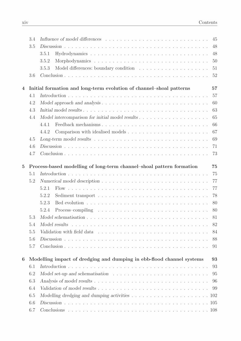
xiv Contents
3.4 Influence of model differences . . . . . . . . . . . . . . . . . . . . . . . . . . . . 45
3.5 Discussion . . . . . . . . . . . . . . . . . . . . . . . . . . . . . . . . . . . . . . . 48
3.5.1 Hydrodynamics . . . . . . . . . . . . . . . . . . . . . . . . . . . . . . . . 48
3.5.2 Morphodynamics . . . . . . . . . . . . . . . . . . . . . . . . . . . . . . . 50
3.5.3 Model differences: boundary condition . . . . . . . . . . . . . . . . . . . 51
3.6 Conclusion . . . . . . . . . . . . . . . . . . . . . . . . . . . . . . . . . . . . . . . 52
4 Initial formation and long-term evolution of channel–shoal patterns 57
4.1 Introduction . . . . . . . . . . . . . . . . . . . . . . . . . . . . . . . . . . . . . . 57
4.2 Model approach and analysis . . . . . . . . . . . . . . . . . . . . . . . . . . . . . 60
4.3 Initial model results . . . . . . . . . . . . . . . . . . . . . . . . . . . . . . . . . . 63
4.4 Model intercomparison for initial model results . . . . . . . . . . . . . . . . . . . 65
4.4.1 Feedback mechanisms . . . . . . . . . . . . . . . . . . . . . . . . . . . . . 66
4.4.2 Comparison with idealised models . . . . . . . . . . . . . . . . . . . . . . 67
4.5 Long-term model results . . . . . . . . . . . . . . . . . . . . . . . . . . . . . . . 69
4.6 Discussion . . . . . . . . . . . . . . . . . . . . . . . . . . . . . . . . . . . . . . . 71
4.7 Conclusion . . . . . . . . . . . . . . . . . . . . . . . . . . . . . . . . . . . . . . . 73
5 Process-based modelling of long-term channel–shoal pattern formation 75
5.1 Introduction . . . . . . . . . . . . . . . . . . . . . . . . . . . . . . . . . . . . . . 75
5.2 Numerical model description . . . . . . . . . . . . . . . . . . . . . . . . . . . . . 77
5.2.1 Flow . . . . . . . . . . . . . . . . . . . . . . . . . . . . . . . . . . . . . . 77
5.2.2 Sediment transport . . . . . . . . . . . . . . . . . . . . . . . . . . . . . . 78
5.2.3 Bed evolution . . . . . . . . . . . . . . . . . . . . . . . . . . . . . . . . . 80
5.2.4 Process–compiling . . . . . . . . . . . . . . . . . . . . . . . . . . . . . . 80
5.3 Model schematisation . . . . . . . . . . . . . . . . . . . . . . . . . . . . . . . . . 81
5.4 Model results . . . . . . . . . . . . . . . . . . . . . . . . . . . . . . . . . . . . . 82
5.5 Validation with field data . . . . . . . . . . . . . . . . . . . . . . . . . . . . . . 84
5.6 Discussion . . . . . . . . . . . . . . . . . . . . . . . . . . . . . . . . . . . . . . . 88
5.7 Conclusion . . . . . . . . . . . . . . . . . . . . . . . . . . . . . . . . . . . . . . . 91
6 Modelling impact of dredging and dumping in ebb-flood channel systems 93
6.1 Introduction . . . . . . . . . . . . . . . . . . . . . . . . . . . . . . . . . . . . . . 93
6.2 Model set-up and schematisation . . . . . . . . . . . . . . . . . . . . . . . . . . 95
6.3 Analysis of model results . . . . . . . . . . . . . . . . . . . . . . . . . . . . . . . 96
6.4 Validation of model results . . . . . . . . . . . . . . . . . . . . . . . . . . . . . . 99
6.5 Modelling dredging and dumping activities . . . . . . . . . . . . . . . . . . . . . 102
6.6 Discussion . . . . . . . . . . . . . . . . . . . . . . . . . . . . . . . . . . . . . . . 105
6.7 Conclusions . . . . . . . . . . . . . . . . . . . . . . . . . . . . . . . . . . . . . . 108

Contents xv
7 Conclusions and recommendations 111
7.1 Conclusions . . . . . . . . . . . . . . . . . . . . . . . . . . . . . . . . . . . . . . 111
7.2 Recommendations . . . . . . . . . . . . . . . . . . . . . . . . . . . . . . . . . . . 114
Acknowledgements 123
About the author 125
Publications 126

xvi Contents
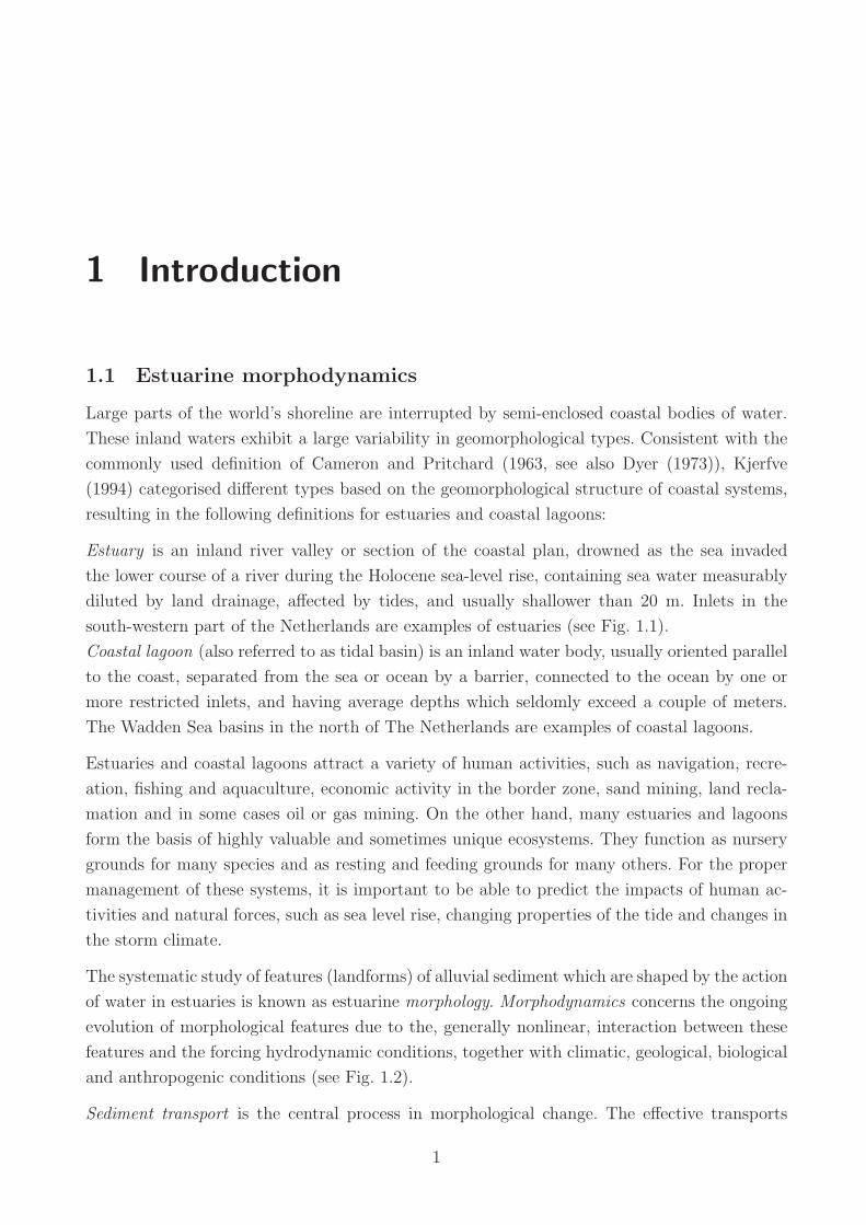
1 Introduction
1.1 Estuarine morphodynamics
Large parts of the world’s shoreline are interrupted by semi-enclosed coastal bodies of water.
These inland waters exhibit a large variability in geomorphological types. Consistent with the
commonly used definition of Cameron and Pritchard (1963, see also Dyer (1973)), Kjerfve
(1994) categorised different types based on the geomorphological structure of coastal systems,
resulting in the following definitions for estuaries and coastal lagoons:
Estuary is an inland river valley or section of the coastal plan, drowned as the sea invaded
the lower course of a river during the Holocene sea-level rise, containing sea water measurably
diluted by land drainage, affected by tides, and usually shallower than 20 m. Inlets in the
south-western part of the Netherlands are examples of estuaries (see Fig. 1.1).
Coastal lagoon (also referred to as tidal basin) is an inland water body, usually oriented parallel
to the coast, separated from the sea or ocean by a barrier, connected to the ocean by one or
more restricted inlets, and having average depths which seldomly exceed a couple of meters.
The Wadden Sea basins in the north of The Netherlands are examples of coastal lagoons.
Estuaries and coastal lagoons attract a variety of human activities, such as navigation, recre-
ation, fishing and aquaculture, economic activity in the border zone, sand mining, land recla-
mation and in some cases oil or gas mining. On the other hand, many estuaries and lagoons
form the basis of highly valuable and sometimes unique ecosystems. They function as nursery
grounds for many species and as resting and feeding grounds for many others. For the proper
management of these systems, it is important to be able to predict the impacts of human ac-
tivities and natural forces, such as sea level rise, changing properties of the tide and changes in
the storm climate.
The systematic study of features (landforms) of alluvial sediment which are shaped by the action
of water in estuaries is known as estuarine morphology. Morphodynamics concerns the ongoing
evolution of morphological features due to the, generally nonlinear, interaction between these
features and the forcing hydrodynamic conditions, together with climatic, geological, biological
and anthropogenic conditions (see Fig. 1.2).
Sediment transport is the central process in morphological change. The effective transports
1
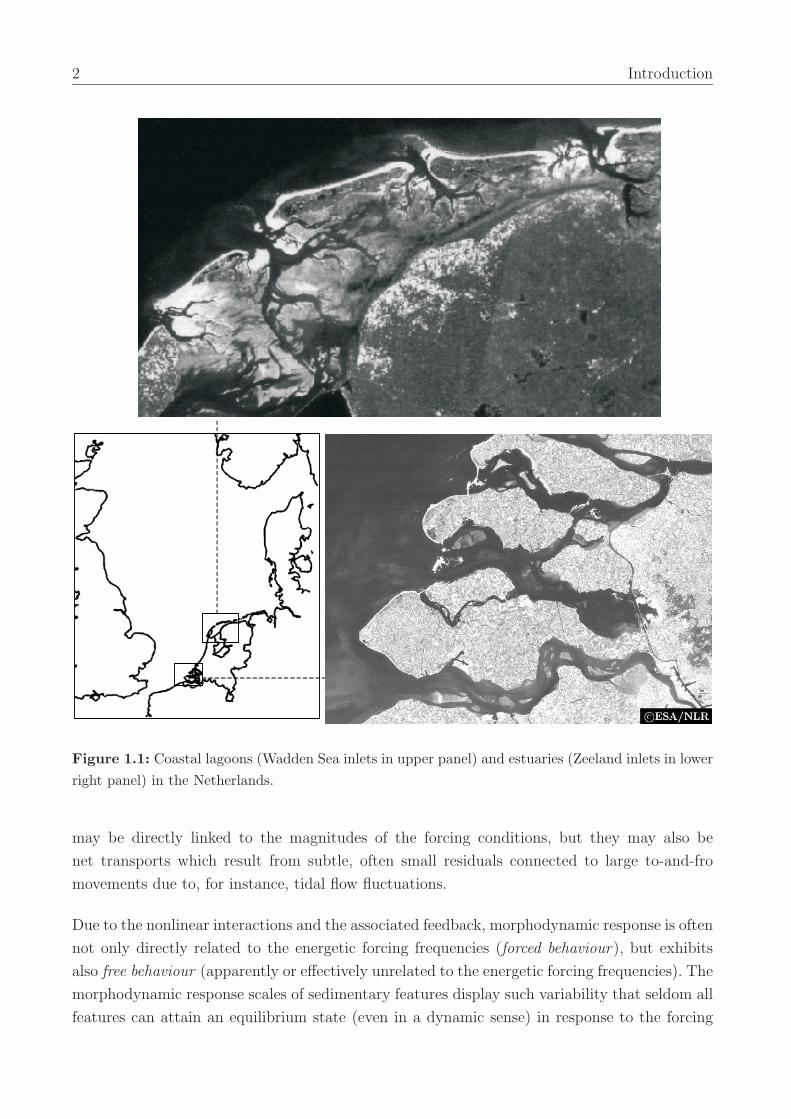
2 Introduction
Figure 1.1: Coastal lagoons (Wadden Sea inlets in upper panel) and estuaries (Zeeland inlets in lowerright panel) in the Netherlands.
may be directly linked to the magnitudes of the forcing conditions, but they may also be
net transports which result from subtle, often small residuals connected to large to-and-fro
movements due to, for instance, tidal flow fluctuations.
Due to the nonlinear interactions and the associated feedback, morphodynamic response is often
not only directly related to the energetic forcing frequencies (forced behaviour), but exhibits
also free behaviour (apparently or effectively unrelated to the energetic forcing frequencies). The
morphodynamic response scales of sedimentary features display such variability that seldom all
features can attain an equilibrium state (even in a dynamic sense) in response to the forcing
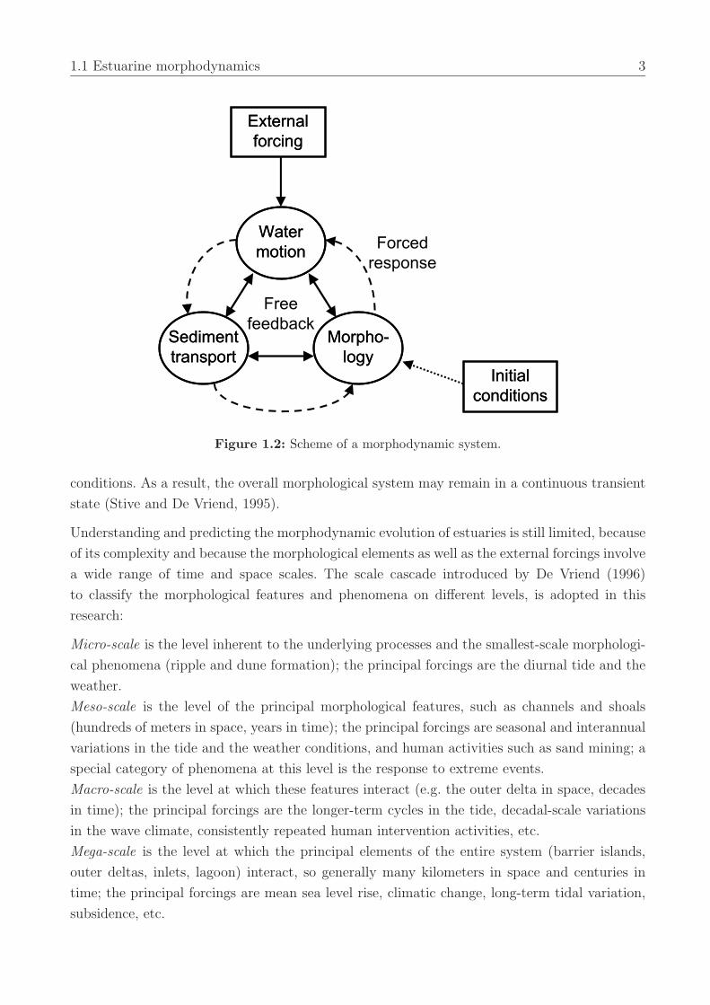
1.1 Estuarine morphodynamics 3
Figure 1.2: Scheme of a morphodynamic system.
conditions. As a result, the overall morphological system may remain in a continuous transient
state (Stive and De Vriend, 1995).
Understanding and predicting the morphodynamic evolution of estuaries is still limited, because
of its complexity and because the morphological elements as well as the external forcings involve
a wide range of time and space scales. The scale cascade introduced by De Vriend (1996)
to classify the morphological features and phenomena on different levels, is adopted in this
research:
Micro-scale is the level inherent to the underlying processes and the smallest-scale morphologi-
cal phenomena (ripple and dune formation); the principal forcings are the diurnal tide and the
weather.
Meso-scale is the level of the principal morphological features, such as channels and shoals
(hundreds of meters in space, years in time); the principal forcings are seasonal and interannual
variations in the tide and the weather conditions, and human activities such as sand mining; a
special category of phenomena at this level is the response to extreme events.
Macro-scale is the level at which these features interact (e.g. the outer delta in space, decades
in time); the principal forcings are the longer-term cycles in the tide, decadal-scale variations
in the wave climate, consistently repeated human intervention activities, etc.
Mega-scale is the level at which the principal elements of the entire system (barrier islands,
outer deltas, inlets, lagoon) interact, so generally many kilometers in space and centuries in
time; the principal forcings are mean sea level rise, climatic change, long-term tidal variation,
subsidence, etc.
4 Introduction
In this research we focus on the meso- and macro-scale morphodynamics of estuaries where tidal
motion forms the principal forcing. On these scales channels and shoals form highly dynamic
elements. At this moment the morphological changes of channels and shoals are insufficiently
predictable.
1.2 Objectives and research questions
The general objectives of this research are:
(1) Gathering better knowledge of mechanisms behind morphodynamic behaviour of channels
and shoals in estuaries and coastal lagoons.
(2) Improving morphological prediction capabilities, using numerical models, at time scales from
decades to centuries.
These objectives are articulated in the following research questions:
• To what extent can present numerical models be used to model and investigate morpho-
dynamic behaviour of channels and shoals on meso- to macro-scales?
• What are the mechanisms responsible for morphodynamic behaviour of channels and
shoals in estuaries?
• To what extent can we predict the morphodynamic response of estuarine systems to
human interventions?
1.3 Mathematical modelling
Different types of model approaches have been developed and used to investigate and simu-
late the morphological evolution on meso- and macro-scales. Each model has its own area of
applicability, due to the applied assumptions and model formulations. Jointly, these models
cover the wide span of time and space scales. Consequently, results from different models are
difficult to compare, which complicates verification of model results and hampers insight into
the implications of model formulations and assumptions.
We discern two types of macro-scale models, which are both aggregated model approaches. The
first type assimilates empirical data with an aggregated process description. These models are
based on elementary physics, but include the empirical knowledge on the equilibrium state of
estuaries. In these (semi-) empirical models the geometry is simplified by aggregation into a
number of morphological elements and processes are aggregated by including empirical relations
between geometry and long-term hydrodynamic conditions. In literature, this type of models
is referred to as behaviour-oriented or aggregated models. The other type of models aggregates
1.4 Research approach and outline 5
the physical system on which the process knowledge is applied. E.g. the basin hypsometry,
i.e. the distribution of horizontal surface area per elevation range, is aggregated to a single
representative hypsometry on which the incoming and reflected tidal wave propagates. We will
refer to this type as macro-scale process-based models. Process-based models derived for meso-
scale modelling are mathematical representations of physical laws per cross-section for one-
dimensional models or on a local, discrete grid for two- and three-dimensional models. Within
the meso-scale process-based model approach two principal approaches can be discerned. For
simplicity, we will speak of complex models in contrast to idealised models. Idealised models
make use of simplified geometries, forcings and physical formulations, compared to complex
models. Against the loss of the possibility to simulate realistic geometries and forcings stands
a more fundamental insight into the physics and the ability to cover large time spans.
At present, due to improved physical insight and increased computational power, the ability
to use complex process-based models is enhanced, specifically the capability to aggregate the
meso-scale processes towards macro-scale morphological behaviour. These simulation models
consist of a number of modules that describe waves, currents and sediment transport. The
process-based model used this research takes into account the dynamic interaction of these
processes with bed-topography changes. The feedback of morphological changes of water and
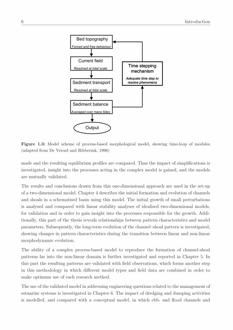
sediment motion is established by using the modules in a time-loop (see Fig. 1.3). Although the
processes determining the water motion and sediment transport are simulated on a time-scale
of typically one tidal period, larger time-scales are reached by continuing the computations
over a longer time-span, and applying larger time-steps for the bed level changes than for the
hydrodynamic and sediment transport processes (De Vriend and Ribberink, 1996).
1.4 Research approach and outline
Preceding this thesis, a literature survey of the morphodynamic processes in estuaries and
tidal basins at different time and space scales was carried out and reported in Morphological
development of inter-tidal areas and modelling with estmorf. Part II: literature survey (in
Dutch) by Hibma et al. (2000). The issues relevant to this thesis are incorporated in Chapter
2. This Chapter describes the state-of-the-art of modelling estuarine morphodynamics at the
meso- and macro-scale levels. Parts of the research presented in this thesis are included, showing
that a complex process-based model type can cover different scale levels, by extending the meso-
scale model into the macro-scale domain, and different model approaches, by making a link with
idealised models.
Chapter 3 describes this link between complex process-based and idealised models. An inter-
mediate model is set up to simulate the development of one-dimensional equilibrium profiles of
estuaries. This intermediate model is a modified version of the complex model, in which the sim-
plifications of the idealised model are adopted. A thorough comparison of model formulations is
6 Introduction
Figure 1.3: Model scheme of process-based morphological model, showing time-loop of modules(adapted from De Vriend and Ribberink, 1996)
made and the resulting equilibrium profiles are compared. Thus the impact of simplifications is
investigated, insight into the processes acting in the complex model is gained, and the models
are mutually validated.
The results and conclusions drawn from this one-dimensional approach are used in the set-up
of a two-dimensional model. Chapter 4 describes the initial formation and evolution of channels
and shoals in a schematised basin using this model. The initial growth of small perturbations
is analysed and compared with linear stability analyses of idealised two-dimensional models,
for validation and in order to gain insight into the processes responsible for the growth. Addi-
tionally, this part of the thesis reveals relationships between pattern characteristics and model
parameters. Subsequently, the long-term evolution of the channel–shoal pattern is investigated,
showing changes in pattern characteristics during the transition between linear and non-linear
morphodynamic evolution.
The ability of a complex process-based model to reproduce the formation of channel-shoal
patterns far into the non-linear domain is further investigated and reported in Chapter 5. In
this part the resulting patterns are validated with field observations, which forms another step
in this methodology in which different model types and field data are combined in order to
make optimum use of each research method.
The use of the validated model in addressing engineering questions related to the management of
estuarine systems is investigated in Chapter 6. The impact of dredging and dumping activities
is modelled, and compared with a conceptual model, in which ebb- and flood channels and
1.4 Research approach and outline 7
enclosed shoals form morphodynamic units (cells) with their own sediment circulation.
In Chapter 7 the conclusions of this thesis are summarized and the aforementioned research
questions are answered. Additionally, recommendations for further research are given.
The core of this thesis, formed by Chapters 2 to 6, has been published or submitted for pub-
lication in the open literature. This explains why these chapters are written in the format of
separate papers.

8 Introduction
2 Modelling estuarine morphodynamics 1
Abstract
Estuaries and tidal lagoons display a complex morphological character both on the meso- and
macro-scale. Single and multiple channel-shoal patterns and branching or braided patterns can
be encountered on the meso-scale. On the macro-scale the hypsometry of tidal basins may
differ widely. Our insight into and understanding of morphodynamic processes leading to these
patterns is limited. While observations and empirical relations have been established over many
decades, it is only the last two decades that macro-scale models have been introduced to explain
macro-scale features. The emergence of meso-scale features in the long-term, however, was
limited to empirical and qualitative findings. Recently, meso-scale process-based models have
been introduced that show ability to reproduce meso-scale patterns in a macro-scale evolution.
This chapter attempts to highlight this recent capacity by bridging meso-scale and macro-scale
observations and process knowledge to increase our understanding of estuarine and tidal basin
morphological evolution. It is shown that positive feedback processes leading to self-organization
may be derived from first physical principles on smaller scales. In fact, this may be seen as a
first successful step in the issue of aggregation of smaller estuarine process scales to larger ones.
2.1 Introduction
Estuaries and tidal lagoons occur in many coastal areas world-wide. These tidally forced systems
are important from ecological, economical and recreational viewpoint. Besides, they have a
considerable impact on adjacent shorelines that they interrupt by influencing the sediment
budget (Stive and Wang, 2003).
The morphology of estuaries is a result of non-linear interaction between water and sediment
motion and bed topography. Understanding and predicting the morphodynamic evolution of
estuaries is still limited, because of its complexity and because it involves a wide range of time
and space scales. A distinction between morphological features on different levels as introduced
1. This chapter is in press for publication as: A. Hibma, M.J.F. Stive and Z.B. Wang, 2004. Estuarine mor-phodynamics. In: Coastal Morphodynamic Modeling. Special Issue Coastal Engineering, C. Lackan (Ed.)
9
10 Modelling estuarine morphodynamics
by De Vriend (1996) is adopted in this paper. The smallest morphological phenomena, ripples
and dunes formed on the bed, are categorized as micro-scale features. Meso-scale features are
alternating and interacting ebb- and flood-channels and shoals. On an aggregated scale they
belong to macro-scale elements like the inlet gorge and the ebb-tidal delta. On mega-scale
we discern the entire estuary and its adjacent coast including the shore face. On each level
the morphological phenomena result from interaction between the features and the forcing at
that level, which can be aggregated smaller scale forcing, particularly when it concerns self-
organization.
In this contribution we focus on meso- and macro-scales features in estuaries where tidal motion
forms the principal forcing. Different types of model approaches are developed and used to
investigate and simulate the morphological evolution on these scales. Each model has its own
area of applicability due to the applied assumptions and model formulations. Jointly, these
models cover the wide span of time and space scales. Consequently, results from different models
are difficult to compare, which complicates verification of model results and insight into the
implication of model formulations and assumptions.
We discern two types of macro-scale models, which are both aggregated model approaches. The
first type assimilates empirical data with an aggregated process description. In literature, this
type of models is referred to as behaviour-oriented, aggregated or hierarchical models. Examples
of this type are the box model of Di Silvio (1989) and the ASMITA model (Stive et al., 1998).
The other type of models aggregates the physical system on which the process knowledge is
applied. We will refer to this type as macro-scale process-based models (e.g. Friedrichs and
Aubrey, 1996 and Dronkers, 1998). Process-based models derived for meso-scale modelling are
mathematical representations of physical laws per cross-section for one-dimensional models or
on a local, discrete grid for two- and three-dimensional models. Within the meso-scale process-
based model approach two principal approaches can be discerned. For simplicity, we will speak
of complex models in contrast to idealised models. Idealised models make use of simplified
geometries, forcings and physical formulations, compared to complex models. Against the loss
of simulating situations for realistic geometries and forcings stands more fundamental insight
into the physics and the ability to make long-term morphodynamic computations.
At present, due to improved physical insight and increased computational power, the abil-
ity to use complex process-based models is enhanced. These simulation models consist of a
number of modules that describe waves, current and sediment transport. The process-based
models discussed in this paper take into account the dynamic interaction of these processes
with bed-topography changes. The feedback of morphological changes of water and sediment
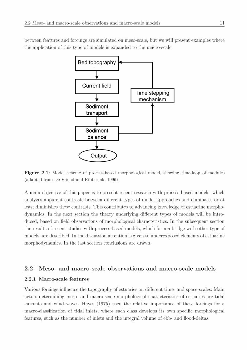
motion is established by using the modules in a time-loop (see Fig. 2.1). Though the processes
are simulated on a time-scale of typically one tidal period, larger time-scales are reached by
continuing the computations over a longer time-span, and applying larger time-steps for the
bed level changes than the processes (De Vriend and Ribberink, 1996). In general, interaction
2.2 Meso- and macro-scale observations and macro-scale models 11
between features and forcings are simulated on meso-scale, but we will present examples where
the application of this type of models is expanded to the macro-scale.
Figure 2.1: Model scheme of process-based morphological model, showing time-loop of modules(adapted from De Vriend and Ribberink, 1996)
A main objective of this paper is to present recent research with process-based models, which
analyzes apparent contrasts between different types of model approaches and eliminates or at
least diminishes these contrasts. This contributes to advancing knowledge of estuarine morpho-
dynamics. In the next section the theory underlying different types of models will be intro-
duced, based on field observations of morphological characteristics. In the subsequent section
the results of recent studies with process-based models, which form a bridge with other type of
models, are described. In the discussion attention is given to underexposed elements of estuarine
morphodynamics. In the last section conclusions are drawn.
2.2 Meso- and macro-scale observations and macro-scale models
2.2.1 Macro-scale features
Various forcings influence the topography of estuaries on different time- and space-scales. Main
actors determining meso- and macro-scale morphological characteristics of estuaries are tidal
currents and wind waves. Hayes (1975) used the relative importance of these forcings for a
macro-classification of tidal inlets, where each class develops its own specific morphological
features, such as the number of inlets and the integral volume of ebb- and flood-deltas.
12 Modelling estuarine morphodynamics
Also the macro-scale shape of estuaries is associated with the influence of waves and tide. Based
on observations, Friedrichs and Aubrey (1996) developed a model for short tidal basins that
correlates these forcings with the hypsometry of basins, i.e. the distribution of horizontal surface
area with respect to elevation. Convex profiles (from a bottom point-of-view) are associated
with tide dominance, thus large tidal amplitudes and minor wave activity, and concave profiles
are correlated with wave-dominated basins. The physical background forms the assumption
that tidal flats are in equilibrium if the maximum bottom shear stress, resulting from tidal
currents and wind waves, is spatially uniform.
2.2.2 Meso-scale features
De Vriend et al. (1989) also observes this interaction between currents, waves and topography
for a meso-scale feature as shoals. The growth of tidal flats is associated with the tide, while
the waves have a destructive character, which enhances when the water depth above the shoal
decreases. On the long run, this results in an average height of shoals.
In channels the influence of waves is smaller due to larger depths. Flow alone can be used
in relation to the cross-channel area of channels. A threshold flow velocity or bottom shear
stress (well above the threshold for initiation of sediment motion) is needed for a stable inlet
channel (Escoffier, 1940; Van de Kreeke, 1990, 1992). Empirically, cross-sections of channels are
found to correlate linearly with the tidal prism, which is a measure of flow capacity (Bruun
and Gerritsen, 1960; O’Brien, 1969; Eysink, 1990). This relation seems to have upper and
lower limits. Observations suggest that there is a maximum size of the channels, above that
the channels will bifurcate into more channels (Allersma, 1992, 1994, also see Stive and Wang
(2003)). This maximum size seems to depend on the width to depth ratio as well as the total
size of the estuary, and type of sediment. For decreasing channel dimensions, the flow capacity
decreases. A minimum size of the channel is needed to exert a certain bottom shear stress,
below which a channel is not able to remain open.
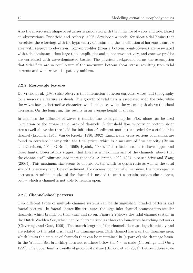
2.2.3 Channel-shoal patterns
Two different types of multiple channel systems can be distinguished, braided patterns and
fractal patterns. In fractal or tree-like structures the large inlet channel branches into smaller
channels, which branch on their turn and so on. Figure 2.2 shows the tidal-channel system in
the Dutch Wadden Sea, which can be characterized as three- to four-times branching networks
(Cleveringa and Oost, 1999). The branch lengths of the channels decrease logarithmically and
are related to the tidal prism and the drainage area. Each channel has a certain drainage area,
which limits the amount of channels that can be maintained in (a part of) the drainage basin.
In the Wadden Sea branching does not continue below the 500-m scale (Cleveringa and Oost,
1999). The upper limit is usually of geological nature (Rinaldo et al., 2001). Between these scale
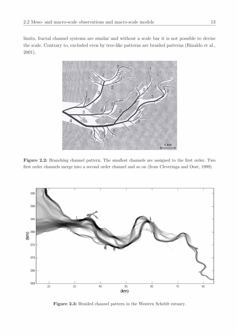
2.2 Meso- and macro-scale observations and macro-scale models 13
limits, fractal channel systems are similar and without a scale bar it is not possible to devise
the scale. Contrary to, excluded even by tree-like patterns are braided patterns (Rinaldo et al.,
2001).
Figure 2.2: Branching channel pattern. The smallest channels are assigned to the first order. Twofirst order channels merge into a second order channel and so on (from Cleveringa and Oost, 1999).
Figure 2.3: Braided channel pattern in the Western Scheldt estuary.
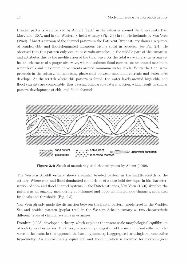
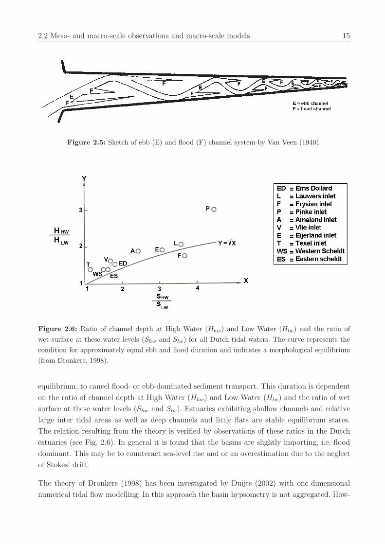
14 Modelling estuarine morphodynamics
Braided patterns are observed by Ahnert (1960) in the estuaries around the Chesapeake Bay,
Maryland, USA, and in the Western Scheldt estuary (Fig. 2.3) in the Netherlands by Van Veen
(1950). Ahnert’s cartoon of the channel pattern in the Patuxent River estuary shows a sequence
of braided ebb- and flood-dominated meanders with a shoal in between (see Fig. 2.4). He
observed that this pattern only occurs at certain stretches in the middle part of the estuaries,
and attributes this to the modification of the tidal wave. As the tidal wave enters the estuary it
has the character of a progressive wave, where maximum flood currents occur around maximum
water levels and maximum ebb-currents around minimum water levels. When the tidal wave
proceeds in the estuary, an increasing phase shift between maximum currents and water level
develops. At the stretch where this pattern is found, the water levels around high ebb- and
flood currents are comparable, thus causing comparable lateral erosion, which result in similar
pattern development of ebb- and flood channels.
Figure 2.4: Sketch of meandering tidal channel system by Ahnert (1960).
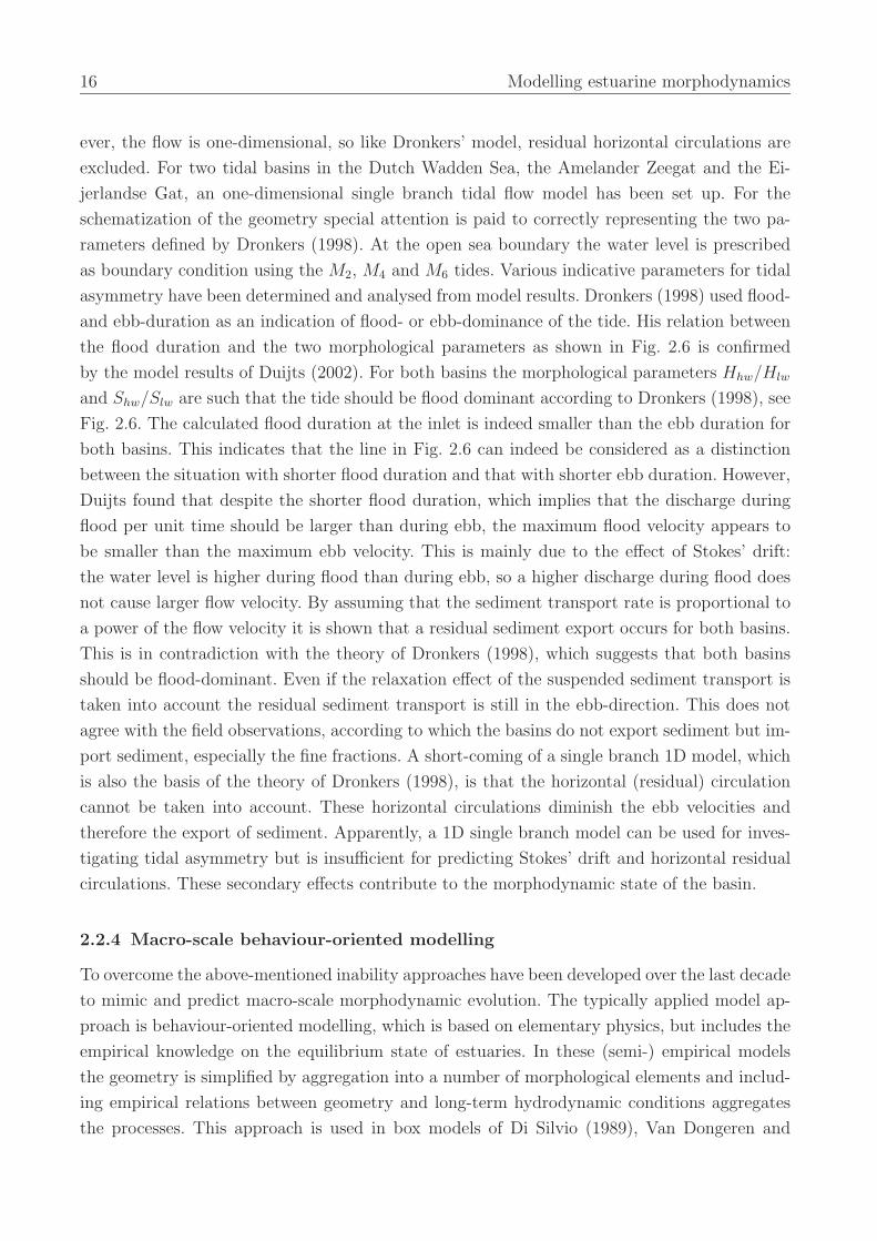
The Western Scheldt estuary shows a similar braided pattern in the middle stretch of the
estuary. Where ebb- and flood-dominated channels meet a threshold develops. In his character-
ization of ebb- and flood channel systems in the Dutch estuaries, Van Veen (1950) sketches the
pattern as an ongoing meandering ebb-channel and flood-dominated side channels, separated
by shoals and thresholds (Fig. 2.5).
Van Veen already made the distinction between the fractal pattern (apple tree) in the Wadden
Sea and braided pattern (poplar tree) in the Western Scheldt estuary as two characteristic
different types of channel systems in estuaries.
Dronkers (1998) developed a theory, which explains the macro-scale morphological equilibrium
of both types of estuaries. The theory is based on propagation of the incoming and reflected tidal
wave in the basin. In this approach the basin hypsometry is aggregated to a single representative
hypsometry. An approximately equal ebb and flood duration is required for morphological
2.2 Meso- and macro-scale observations and macro-scale models 15
Figure 2.5: Sketch of ebb (E) and flood (F) channel system by Van Veen (1940).
Figure 2.6: Ratio of channel depth at High Water (Hhw) and Low Water (Hlw) and the ratio ofwet surface at these water levels (Shw and Slw) for all Dutch tidal waters. The curve represents thecondition for approximately equal ebb and flood duration and indicates a morphological equilibrium(from Dronkers, 1998).
equilibrium, to cancel flood- or ebb-dominated sediment transport. This duration is dependent
on the ratio of channel depth at High Water (Hhw) and Low Water (Hlw) and the ratio of wet
surface at these water levels (Shw and Slw). Estuaries exhibiting shallow channels and relative
large inter tidal areas as well as deep channels and little flats are stable equilibrium states.
The relation resulting from the theory is verified by observations of these ratios in the Dutch
estuaries (see Fig. 2.6). In general it is found that the basins are slightly importing, i.e. flood
dominant. This may be to counteract sea-level rise and or an overestimation due to the neglect
of Stokes’ drift.
The theory of Dronkers (1998) has been investigated by Duijts (2002) with one-dimensional
numerical tidal flow modelling. In this approach the basin hypsometry is not aggregated. How-
16 Modelling estuarine morphodynamics
ever, the flow is one-dimensional, so like Dronkers’ model, residual horizontal circulations are
excluded. For two tidal basins in the Dutch Wadden Sea, the Amelander Zeegat and the Ei-
jerlandse Gat, an one-dimensional single branch tidal flow model has been set up. For the
schematization of the geometry special attention is paid to correctly representing the two pa-
rameters defined by Dronkers (1998). At the open sea boundary the water level is prescribed
as boundary condition using the M2, M4 and M6 tides. Various indicative parameters for tidal
asymmetry have been determined and analysed from model results. Dronkers (1998) used flood-
and ebb-duration as an indication of flood- or ebb-dominance of the tide. His relation between
the flood duration and the two morphological parameters as shown in Fig. 2.6 is confirmed
by the model results of Duijts (2002). For both basins the morphological parameters Hhw/Hlw
and Shw/Slw are such that the tide should be flood dominant according to Dronkers (1998), see
Fig. 2.6. The calculated flood duration at the inlet is indeed smaller than the ebb duration for
both basins. This indicates that the line in Fig. 2.6 can indeed be considered as a distinction
between the situation with shorter flood duration and that with shorter ebb duration. However,
Duijts found that despite the shorter flood duration, which implies that the discharge during
flood per unit time should be larger than during ebb, the maximum flood velocity appears to
be smaller than the maximum ebb velocity. This is mainly due to the effect of Stokes’ drift:
the water level is higher during flood than during ebb, so a higher discharge during flood does
not cause larger flow velocity. By assuming that the sediment transport rate is proportional to
a power of the flow velocity it is shown that a residual sediment export occurs for both basins.
This is in contradiction with the theory of Dronkers (1998), which suggests that both basins
should be flood-dominant. Even if the relaxation effect of the suspended sediment transport is
taken into account the residual sediment transport is still in the ebb-direction. This does not
agree with the field observations, according to which the basins do not export sediment but im-
port sediment, especially the fine fractions. A short-coming of a single branch 1D model, which
is also the basis of the theory of Dronkers (1998), is that the horizontal (residual) circulation
cannot be taken into account. These horizontal circulations diminish the ebb velocities and
therefore the export of sediment. Apparently, a 1D single branch model can be used for inves-
tigating tidal asymmetry but is insufficient for predicting Stokes’ drift and horizontal residual
circulations. These secondary effects contribute to the morphodynamic state of the basin.
2.2.4 Macro-scale behaviour-oriented modelling
To overcome the above-mentioned inability approaches have been developed over the last decade
to mimic and predict macro-scale morphodynamic evolution. The typically applied model ap-
proach is behaviour-oriented modelling, which is based on elementary physics, but includes the
empirical knowledge on the equilibrium state of estuaries. In these (semi-) empirical models
the geometry is simplified by aggregation into a number of morphological elements and includ-
ing empirical relations between geometry and long-term hydrodynamic conditions aggregates
the processes. This approach is used in box models of Di Silvio (1989), Van Dongeren and
2.3 Meso-scale models for macro-scale features 17
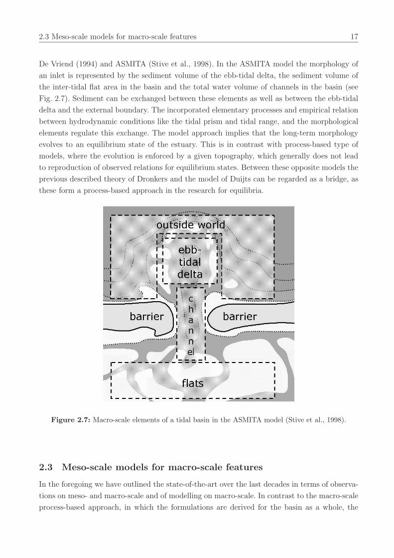
De Vriend (1994) and ASMITA (Stive et al., 1998). In the ASMITA model the morphology of
an inlet is represented by the sediment volume of the ebb-tidal delta, the sediment volume of
the inter-tidal flat area in the basin and the total water volume of channels in the basin (see
Fig. 2.7). Sediment can be exchanged between these elements as well as between the ebb-tidal
delta and the external boundary. The incorporated elementary processes and empirical relation
between hydrodynamic conditions like the tidal prism and tidal range, and the morphological
elements regulate this exchange. The model approach implies that the long-term morphology
evolves to an equilibrium state of the estuary. This is in contrast with process-based type of
models, where the evolution is enforced by a given topography, which generally does not lead
to reproduction of observed relations for equilibrium states. Between these opposite models the
previous described theory of Dronkers and the model of Duijts can be regarded as a bridge, as
these form a process-based approach in the research for equilibria.
Figure 2.7: Macro-scale elements of a tidal basin in the ASMITA model (Stive et al., 1998).
2.3 Meso-scale models for macro-scale features
In the foregoing we have outlined the state-of-the-art over the last decades in terms of observa-
tions on meso- and macro-scale and of modelling on macro-scale. In contrast to the macro-scale
process-based approach, in which the formulations are derived for the basin as a whole, the
18 Modelling estuarine morphodynamics
meso-scale process-based models describe the bathymetry and physical conditions on a local
grid or per cross-section. Recently, increased insights into processes on meso-scales have pro-
moted the application of meso-scale models on temporal macro-scales. The lead in this has been
taken by the so-named idealised models, using simplified geometries, forcings and physical for-
mulations. The results achieved have led to the observation that these approaches can reveal
realistic spatial macro-scale features. Using this insight it is first shown that complex, process-
based models are now able to reproduce results of idealised models and, more importantly, that
these models are able to tackle more complex geometrical and more variable forcing conditions.
This should be considered as an important step towards realistic hindcasting and forecasting
of macro-scale evolution.
2.3.1 Complex and idealised models: one-dimensional models
One-dimensional idealised models are used to study width-averaged equilibrium profiles of
estuaries (Schuttelaars and De Swart, 1996, 2000; Lanzoni and Seminara, 2002; Pritchard et al.,
2002). Lanzoni and Seminara investigate equilibria in frictionally dominated funnel-shaped
estuaries. Pritchard et al. also incorporates the region above MSL, to investigate the profiles
of intertidal mudflats. The velocities for the equilibrium profiles in these models are found to
be uniformly distributed across the flat, in accordance with field observations of Friedrichs and
Aubrey (1996).
A link between these one-dimensional idealised and complex process-based models is made by
Hibma et al. (2003b) and described in Chapter 3. They modified the complex process-based
model Delft3D (Roelvink and van Banning, 1994; Wang et al., 1992, 1995b) in order to make a
comparison with the idealised model of Schuttelaars and de Swart (1996, 2000). Their idealised
model is based on first physical principles, but focuses on selected morphodynamic phenomena
by simplifying the equations in an appropriate way. These simplifications are adopted in mod-
ified versions of the complex model. This so-named intermediate model forms a link between
the two approaches and enables a comparison of model results. By comparing, the impact of
simplifications in the idealised model is investigated and the insight into the processes acting in
the complex model is improved. The simplifications in model formulations appeared to have no
qualitative influence on the morphodynamic equilibria. Only the different boundary condition
of the bed at the entrance of the estuary has essential influence on the model results. In the
idealised model the bed level is fixed at this point. In the complex process-based model this
point is not fixed by definition, which prevents the formal existence of equilibrium where no
tidally averaged sediment transport occurs. The importance of the boundary condition is also
discussed by Lanzoni and Seminara (2002). In their model the net sediment flux is set to zero
over the boundary, which implies an internal re-distribution of sediment in order to come to an
equilibrium profile. However, none of the model formulations is considered to adequately de-
scribe the natural behaviour at this point (Hibma et al., 2003b). Therefore, it is recommended
2.3 Meso-scale models for macro-scale features 19
to extend the model region to include the ebb-tidal delta when studying the evolution of tidal
basins (e.g. Wang et al., 1995b; Cayocca, 2001; Van Leeuwen and De Swart, 2002; Van Leeuwen
et al., 2003).
The agreement found between idealised and complex model results reveals that the morpho-
logical development in both type of models is controlled by the same physical processes. In
agreement with observations, the character of a M2 tidal wave depends on the basin length. In
basins, which are short relative to the tidal wavelength, a standing tidal wave occurs. Maximum
velocities are observed in a basin, which has approximately the resonance length (which is about
a quarter of the tidal wave length). A propagating wave occurs in much longer embayments.
The morphologically developed longitudinal profile for a short basin is linear if no external
overtides are imposed. If overtides are imposed, the profile is convex or concave depending on
the phase difference between the semi-diurnal tide and overtides. The equilibrium depth near
the entrance increases as the length of the basin increases. For long embayments the profile
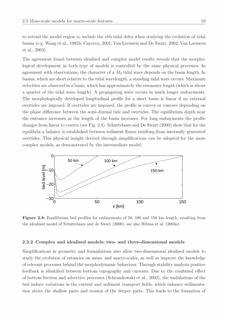
changes from linear to convex (see Fig. 2.8). Schuttelaars and De Swart (2000) show that for the
equilibria a balance is established between sediment fluxes resulting from internally generated
overtides. This physical insight derived through simplifications can be adopted for the more
complex models, as demonstrated by the intermediate model.
0 50 100 150−30
−20
−10
0
x [km]
bed
leve
l [m
]
150 km
100 km 50 km
Figure 2.8: Equilibrium bed profiles for embayments of 50, 100 and 150 km length, resulting fromthe idealised model of Schuttelaars and de Swart (2000), see also Hibma et al. (2003a).
2.3.2 Complex and idealised models: two- and three-dimensional models
Simplifications in geometry and formulations also allow two-dimensional idealised models to
study the evolution of estuaries on meso- and macro-scales, as well as improve the knowledge
of relevant processes behind the morphodynamic behaviour. Through stability analysis positive
feedback is identified between bottom topography and currents. Due to the combined effect
of bottom friction and advective processes (Schramkowski et al., 2002), the undulations of the
bed induce variations in the current and sediment transport fields, which enhance sedimenta-
tion above the shallow parts and erosion of the deeper parts. This leads to the formation of
20 Modelling estuarine morphodynamics
channels and shoals in estuaries. Seminara and Tubino (1998, 2001), Schuttelaars and De Swart
(1999) and Schramkowski et al. (2002) use this method to determine the growth rate of small-
amplitude undulations as a function of the wave number. They find optimum growth rates,
indicating preferable wavelengths of channel-shoal patterns. Such analyses are either linear and
therefore restricted to initial exponential growth, or weakly non-linear and therefore restricted
to patterns close to the linearly most unstable mode. Moreover, they are practically restricted
to idealised situations. The physical processes that are included in these idealised models and
held responsible for the formation of channels and shoals, are also captured in complex process-
based numerical models, where computations can be carried further into the domain of strongly
non-linear interaction and more complex situations. However, it is difficult to identify the rel-
evant processes in a complex model. The two-dimensional complex model approach by Hibma
et al. (2003a) diminishes the gap between the idealised and complex model approach. In this
approach, described in detail in Chapter 5, the geometry of an estuary is schematized to a
rectangular basin, comparable to the idealised situations of the stability analyses, and morpho-
dynamic simulations are made with the complex process-based modelling system Delft3D. The
computations are continued far into the non-linear domain.
The two-dimensional, depth-averaged complex model results show how a simple and regular
pattern of initially grown undulations arises from small random perturbations in the bed. Due to
non-linear interactions these undulations merge to larger scale channel-shoal patterns (Fig. 2.9).
The model is validated with field observations (see Fig. 2.10 for the hypsometric curves). In the
middle stretch of the estuary the braided pattern of ebb- and flood meanders has developed,
showing good correspondence with the sketch of Ahnert (see Fig. 2.4). At the seaward part
the pattern resembles the pattern described by Van Veen, where a continuing ebb-dominated
channel has formed with flood-dominated side channels (see Fig. 2.5). For increasing width-
to-depth ratios, the number of channels in the cross-section of the modelled estuary increases
(Fig. 2.11), as observed by Allersma (1992, 1994).
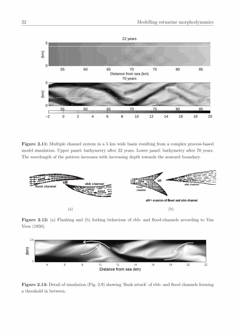
Also the topography of smaller scale features, such as the thresholds at the intersection of
an ebb- and flood channel, show good resemblance to field observations. Van Veen (1950)
described two typical compositions of a bar in crossing channels (see Fig. 2.12). He observed
that the flood- and ebb-channel seem to evade one another. In some cases two opposing channels
approach each other in a sort of flank attack, where the bar is formed between the point of one
channel and along the flank of the other. Examples of this feature are highlighted in Fig. 2.13,
which is a detail of the model simulation shown in Fig. 2.9. In the other case, the ebb- or
flood-channel splits into two branches, forming a forked tongue that embraces the oncoming
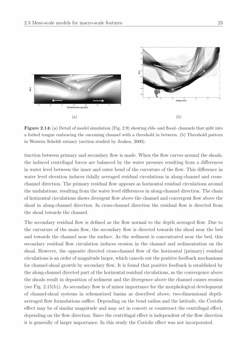
channel. Fig. 2.14(a) gives another detail of the model simulation that shows this feature. It
shows a striking resemblance to the pattern shown in Fig. 2.14(b), which is the Baarland-
Terneuzen threshold area in the Western Scheldt estuary (Jeuken, 2000). Both patterns show a
forked bar area where ebb and flood channels meet. The similarity is confirmed by the tidally
2.3 Meso-scale models for macro-scale features 21
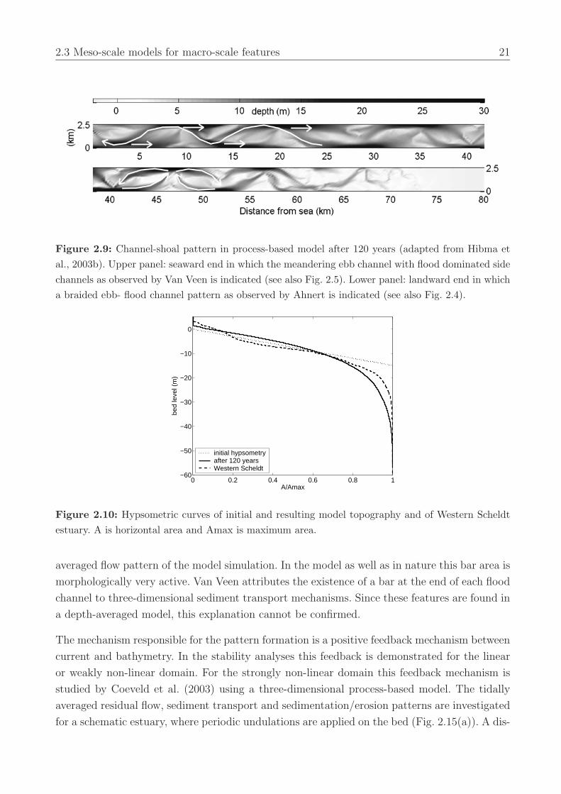
Figure 2.9: Channel-shoal pattern in process-based model after 120 years (adapted from Hibma etal., 2003b). Upper panel: seaward end in which the meandering ebb channel with flood dominated sidechannels as observed by Van Veen is indicated (see also Fig. 2.5). Lower panel: landward end in whicha braided ebb- flood channel pattern as observed by Ahnert is indicated (see also Fig. 2.4).
0 0.2 0.4 0.6 0.8 1−60
−50
−40
−30
−20
−10
0
A/Amax
bed
leve
l (m
)
initial hypsometryafter 120 yearsWestern Scheldt
Figure 2.10: Hypsometric curves of initial and resulting model topography and of Western Scheldtestuary. A is horizontal area and Amax is maximum area.
averaged flow pattern of the model simulation. In the model as well as in nature this bar area is
morphologically very active. Van Veen attributes the existence of a bar at the end of each flood
channel to three-dimensional sediment transport mechanisms. Since these features are found in
a depth-averaged model, this explanation cannot be confirmed.
The mechanism responsible for the pattern formation is a positive feedback mechanism between
current and bathymetry. In the stability analyses this feedback is demonstrated for the linear
or weakly non-linear domain. For the strongly non-linear domain this feedback mechanism is
studied by Coeveld et al. (2003) using a three-dimensional process-based model. The tidally
averaged residual flow, sediment transport and sedimentation/erosion patterns are investigated
for a schematic estuary, where periodic undulations are applied on the bed (Fig. 2.15(a)). A dis-
22 Modelling estuarine morphodynamics
55 60 65 70 75 80 850
5
Distance from sea (km)
(km
)22 years
−2 0 2 4 6 8 10 12 14 16 18 20
55 60 65 70 75 80 850
5
(km
)
70 years
Figure 2.11: Multiple channel system in a 5 km wide basin resulting from a complex process-basedmodel simulation. Upper panel: bathymetry after 22 years. Lower panel: bathymetry after 70 years.The wavelength of the pattern increases with increasing depth towards the seaward boundary.
(a) (b)
Figure 2.12: (a) Flanking and (b) forking behaviour of ebb- and flood-channels according to VanVeen (1950).
Figure 2.13: Detail of simulation (Fig. 2.9) showing ’flank attack’ of ebb- and flood channels forminga threshold in between.
2.3 Meso-scale models for macro-scale features 23
(a) (b)
Figure 2.14: (a) Detail of model simulation (Fig. 2.9) showing ebb- and flood- channels that split intoa forked tongue embracing the oncoming channel with a threshold in between. (b) Threshold patternin Western Scheldt estuary (section studied by Jeuken, 2000).
tinction between primary and secondary flow is made. When the flow curves around the shoals,
the induced centrifugal forces are balanced by the water pressure resulting from a differences
in water level between the inner and outer bend of the curvature of the flow. This difference in
water level elevation induces tidally averaged residual circulations in along-channel and cross-
channel direction. The primary residual flow appears as horizontal residual circulations around
the undulations, resulting from the water level differences in along-channel direction. The chain
of horizontal circulations shows divergent flow above the channel and convergent flow above the
shoal in along-channel direction. In cross-channel direction the residual flow is directed from
the shoal towards the channel.
The secondary residual flow is defined as the flow normal to the depth averaged flow. Due to
the curvature of the main flow, the secondary flow is directed towards the shoal near the bed
and towards the channel near the surface. As the sediment is concentrated near the bed, this
secondary residual flow circulation induces erosion in the channel and sedimentation on the
shoal. However, the opposite directed cross-channel flow of the horizontal (primary) residual
circulations is an order of magnitude larger, which cancels out the positive feedback mechanisms
for channel-shoal growth by secondary flow. It is found that positive feedback is established by
the along-channel directed part of the horizontal residual circulations, as the convergence above
the shoals result in deposition of sediment and the divergence above the channel causes erosion
(see Fig. 2.15(b)). As secondary flow is of minor importance for the morphological development
of channel-shoal systems in schematized basins as described above, two-dimensional depth-
averaged flow formulations suffice. Depending on the bend radius and the latitude, the Coriolis
effect may be of similar magnitude and may act in concert or counteract the centrifugal effect,
depending on the flow direction. Since the centrifugal effect is independent of the flow direction
it is generally of larger importance. In this study the Coriolis effect was not incorporated.
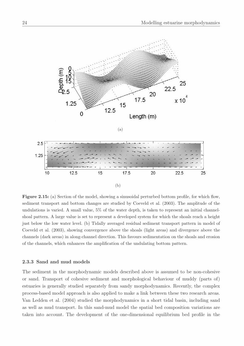
24 Modelling estuarine morphodynamics
(a)
(b)
Figure 2.15: (a) Section of the model, showing a sinusoidal perturbed bottom profile, for which flow,sediment transport and bottom changes are studied by Coeveld et al. (2003). The amplitude of theundulations is varied. A small value, 5% of the water depth, is taken to represent an initial channel-shoal pattern. A large value is set to represent a developed system for which the shoals reach a heightjust below the low water level. (b) Tidally averaged residual sediment transport pattern in model ofCoeveld et al. (2003), showing convergence above the shoals (light areas) and divergence above thechannels (dark areas) in along-channel direction. This favours sedimentation on the shoals and erosionof the channels, which enhances the amplification of the undulating bottom pattern.
2.3.3 Sand and mud models
The sediment in the morphodynamic models described above is assumed to be non-cohesive
or sand. Transport of cohesive sediment and morphological behaviour of muddy (parts of)
estuaries is generally studied separately from sandy morphodynamics. Recently, the complex
process-based model approach is also applied to make a link between these two research areas.
Van Ledden et al. (2004) studied the morphodynamics in a short tidal basin, including sand
as well as mud transport. In this sand-mud model the spatial bed composition variations are
taken into account. The development of the one-dimensional equilibrium bed profile in the
2.4 Discussion 25
short basin appeared to be approximately equal to the model results for sand only. However,
the morphological time scales are considerably decreased due to the availability of the fine
sediment. The final bed composition is validated with field data from the Dutch Wadden Sea,
showing a realistic distribution of the two types of sediment, where the major part of the estuary
has a sand-dominated surface and a muddy area is found at the landward end.
2.4 Discussion
Throughout the last decades observations as well as model investigations have contributed
to the insight into physical processes determining morphological evolution of estuaries. The
increased understanding of the physics also contributes to the ability to use mathematical
models for investigation and prediction of the morphological development of complex systems
as estuaries. Various model approaches are developed each with their own advantages in a
certain area of interest. Between different models or theories apparent contrasts occur, which
complicate the understanding of model results and knowledge of the acting processes. In the
previous section recently developed models are described which resolve or at least diminish these
contrasts. These models, in this paper so-named intermediate models, belong to the process-
based type of models. On the process-scale a link between the morphodynamic sand and mud
models is made. On a larger scale level the physical insight into complex process-based models is
improved by applying simplified geometries or formulations, thus eliminating apparent contrasts
with idealised models. Explaining the physics behind the empirical relationships makes a link
between (semi-) empirical models and process-based models. Where apparent contrasts between
different model approaches can be eliminated, possibilities to use the advantages of each model
increase, which improves knowledge on estuarine morphodynamics.
Though the intermediate models described in this paper span a wide range of the estuarine
morphodynamics, they do not cover the entire scope. A notable limitation is the restriction to
the tidal motion as external force of the system. In all models wind waves are considered of
minor importance compared to the tidal motion and therefore neglected.
The increasing application area of the complex process-based models has not reached all charac-
teristic morphological features yet. An underexposed field of research seems to be the simulation
of fractal channel patterns. Very recently, Marciano (2003, see also Marciano et al. (accepted
for publication)) was able to reproduce fractal-like channel patterns in an idealised basin, using
a similar approach as in Hibma et al. (2003a, see Chapter 5). Though much validation has to be
done, the first results, as shown in Fig. 2.16, are promising. The model of Wang (1992a, see also
Stive and Wang (2003)) which is based on stability analyses gains some physical knowledge. A
relation for the most stable mode of channels for tidal lagoons, where fractal patterns occur, is
found. The relation suggests that channels become smaller and closer spaced when the slope of
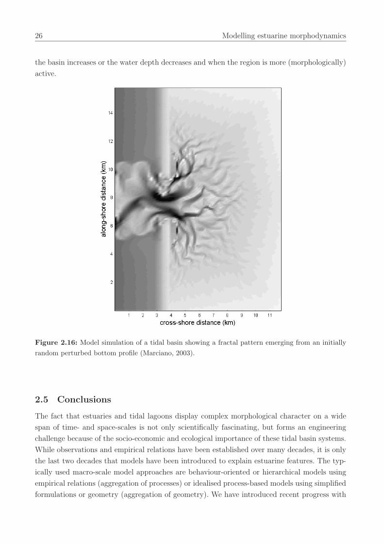
26 Modelling estuarine morphodynamics
the basin increases or the water depth decreases and when the region is more (morphologically)
active.
Figure 2.16: Model simulation of a tidal basin showing a fractal pattern emerging from an initiallyrandom perturbed bottom profile (Marciano, 2003).
2.5 Conclusions
The fact that estuaries and tidal lagoons display complex morphological character on a wide
span of time- and space-scales is not only scientifically fascinating, but forms an engineering
challenge because of the socio-economic and ecological importance of these tidal basin systems.
While observations and empirical relations have been established over many decades, it is only
the last two decades that models have been introduced to explain estuarine features. The typ-
ically used macro-scale model approaches are behaviour-oriented or hierarchical models using
empirical relations (aggregation of processes) or idealised process-based models using simplified
formulations or geometry (aggregation of geometry). We have introduced recent progress with
2.5 Conclusions 27
complex meso-scale, process-based models that show the ability to reproduce the macro-scale
hypsometry of tidal basins as well as meso-scale channel-shoal patterns in a long-term, macro-
scale evolution. These models neither aggregate geometry or processes and therefore form a
bridge between the contrasting model approaches. The results reconciliate observations and
process knowledge both on meso- and macro-scale. The positive feedback processes leading to
self-organization can be derived from first physical principles on smaller scales. In fact, this
may be seen as a first successful step in the issue of aggregation of smaller estuarine process
scales to larger ones.

28 Modelling estuarine morphodynamics
3 Comparison of longitudinal equilibrium
profiles of estuaries in idealised and
process-based models 1
Abstract
The process–based morphodynamic model Delft3D–MOR and the idealised model of Schut-
telaars and De Swart (2000) are compared with each other. The differences between the two
models in their mathematical–physical formulation as well as the boundary conditions are
identified. Their effect on producing cross-sectionally averaged morphological equilibria of tidal
inlets with arbitrary length and forced at the seaward boundary by a prescribed M2 and M4 sea
surface elevation is studied and an inventory is made of all relevant differences. The physical
formulations in the source code of Delft3D–MOR are modified in various steps to resemble the
formulations in the idealised model. The effect of each of the differences between the idealised
and process–based model are studied by comparing the results of the idealised model to those
of the adapted process–based model. The results of the idealised model can be qualitatively
reproduced by the process-based model as long as the same morphological boundary condition
is applied at the open sea end. This means that the simplifications concerning the mathematical
formulation of the physical processes in the idealised model can be justified. Furthermore, it
can be inferred that the morphological boundary condition at the open sea end is an essential
element in controlling the behaviour of morphodynamic models for tidal inlets and estuaries.
3.1 Introduction
Tidal inlets are observed in many coastal areas all over the world. The length of these inlets
varies from ten to a few hundred kilometres, the width from a few up to a hundred kilometer,
1. This chapter has been published as: A. Hibma, H.M. Schuttelaars and Z.B. Wang, 2003. Comparison oflongitudinal equilibrium profiles of estuaries in idealised and process-based models. Ocean Dynamics Vol. 53(3), p. 252-269
29

30 Comparison of equilibrium profiles of estuaries in idealised and process-based models
whereas the depth generally varies from a few to tens of meters. These geometric characteris-
tics are strongly influenced by the tidal climate, possible river inflow and the type of sediment
available at that specific site (see Officer (1976)). Complex morphodynamic patterns on all
length and time scales, such as channel–shoal systems, migrating bedforms (ripples, dunes and
sandwaves) and channels, are observed in these tidal embayments. Apart from being morpho-
dynamically active areas in themselves, tidal inlets strongly influence the sediment budget of
the coastal system. Furthermore, from an ecological, economical and recreational point of view,
these areas usually are very important. Due to this great variety and complexity of tidal inlets
and processes observed in them, together with the many different fields of interest that can
be addressed, various approaches have been used to study tidal inlets (De Vriend, 1996). To
model and predict the morphological development of tidal inlets, process–based models, i.e.,
mathematical models based on physical laws, have been developed. These models contain the
state–of–the–art physical descriptions and parameterisations. Morphodynamic predictions at
time scales shorter than 10 years can be performed. On longer time scales field observations
suggest that there should be certain (empirical) relations between the hydrodynamic forcing
and morphodynamic equilibria of tidal inlets. However, such relations cannot be formally de-
rived analysing the results obtained with process–based models. It is not even known if a
morphodynamic equilibrium exists in the context of a process–based model. This is one of the
reasons, may be even the most important one, why process–based models like Delft3D–MOR
cannot be used for long–term morphodynamic simulations in tidal inlets. Another drawback
of these models is that they are too complicated to get more physical insight into which pro-
cesses are responsible for the observed phenomena. To gain this insight, formally integrated
long–term models or idealised models have been developed. These models are also based on
first physical principles, but focus on specific morphodynamic phenomena by simplifying the
equations in an appropriate way. Due to these simplifications, the results can be analysed us-
ing standard mathematical tools, providing physical insight. Idealised models have proven to
be well–suited to study morphodynamic equilibria in tidal inlets (Schuttelaars and De Swart,
1996, 2000; Van Leeuwen et al., 2000; Pritchard et al., 2002; Lanzoni and Seminara, 2002).
However, the influence of the simplifications on the resulting morphodynamic equilibria has
never been investigated. Another drawback of these models is that they can only deal with
simplified geometries.
In this Chapter, the idealised model discussed in Schuttelaars and De Swart (2000) and the
process–based model Delft3D–MOR described in Roelvink and van Banning (1994) will be used
to study the existence of cross-sectionally averaged morphodynamic equilibria for embayments
of arbitrary length, forced at the seaward boundary by both a prescribed M2 and M4 sea
surface elevation. The focus of this Chapter is on identifying the main differences between
these two models and investigating the influence of these differences on the morphological
development. This results on the one hand in a justification of the simplifications made in
the idealised models. On the other hand, it shows that within the modelling context of the
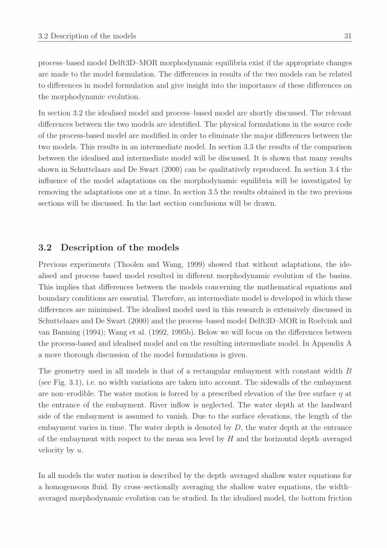
3.2 Description of the models 31
process–based model Delft3D–MOR morphodynamic equilibria exist if the appropriate changes
are made to the model formulation. The differences in results of the two models can be related
to differences in model formulation and give insight into the importance of these differences on
the morphodynamic evolution.
In section 3.2 the idealised model and process–based model are shortly discussed. The relevant
differences between the two models are identified. The physical formulations in the source code
of the process-based model are modified in order to eliminate the major differences between the
two models. This results in an intermediate model. In section 3.3 the results of the comparison
between the idealised and intermediate model will be discussed. It is shown that many results
shown in Schuttelaars and De Swart (2000) can be qualitatively reproduced. In section 3.4 the
influence of the model adaptations on the morphodynamic equilibria will be investigated by
removing the adaptations one at a time. In section 3.5 the results obtained in the two previous
sections will be discussed. In the last section conclusions will be drawn.
3.2 Description of the models
Previous experiments (Thoolen and Wang, 1999) showed that without adaptations, the ide-
alised and process–based model resulted in different morphodynamic evolution of the basins.
This implies that differences between the models concerning the mathematical equations and
boundary conditions are essential. Therefore, an intermediate model is developed in which these
differences are minimised. The idealised model used in this research is extensively discussed in
Schuttelaars and De Swart (2000) and the process–based model Delft3D–MOR in Roelvink and
van Banning (1994); Wang et al. (1992, 1995b). Below we will focus on the differences between
the process-based and idealised model and on the resulting intermediate model. In Appendix A
a more thorough discussion of the model formulations is given.
The geometry used in all models is that of a rectangular embayment with constant width B
(see Fig. 3.1), i.e. no width variations are taken into account. The sidewalls of the embayment
are non–erodible. The water motion is forced by a prescribed elevation of the free surface η at
the entrance of the embayment. River inflow is neglected. The water depth at the landward
side of the embayment is assumed to vanish. Due to the surface elevations, the length of the
embayment varies in time. The water depth is denoted by D, the water depth at the entrance
of the embayment with respect to the mean sea level by H and the horizontal depth–averaged
velocity by u.
In all models the water motion is described by the depth–averaged shallow water equations for
a homogeneous fluid. By cross–sectionally averaging the shallow water equations, the width–
averaged morphodynamic evolution can be studied. In the idealised model, the bottom friction
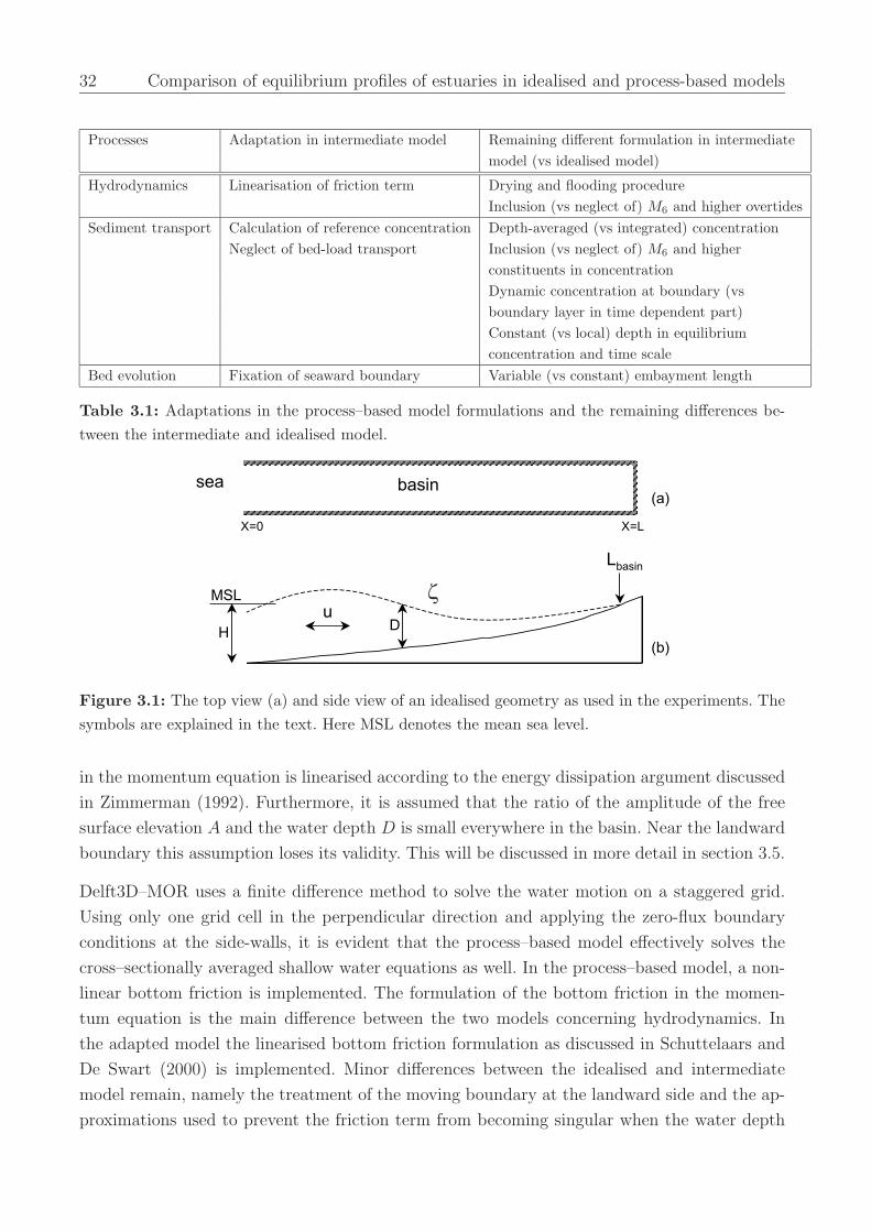
32 Comparison of equilibrium profiles of estuaries in idealised and process-based models
Processes Adaptation in intermediate model Remaining different formulation in intermediatemodel (vs idealised model)
Hydrodynamics Linearisation of friction term Drying and flooding procedureInclusion (vs neglect of) M6 and higher overtides
Sediment transport Calculation of reference concentration Depth-averaged (vs integrated) concentrationNeglect of bed-load transport Inclusion (vs neglect of) M6 and higher
constituents in concentrationDynamic concentration at boundary (vsboundary layer in time dependent part)Constant (vs local) depth in equilibriumconcentration and time scale
Bed evolution Fixation of seaward boundary Variable (vs constant) embayment length
Table 3.1: Adaptations in the process–based model formulations and the remaining differences be-tween the intermediate and idealised model.
Figure 3.1: The top view (a) and side view of an idealised geometry as used in the experiments. Thesymbols are explained in the text. Here MSL denotes the mean sea level.
in the momentum equation is linearised according to the energy dissipation argument discussed
in Zimmerman (1992). Furthermore, it is assumed that the ratio of the amplitude of the free
surface elevation A and the water depth D is small everywhere in the basin. Near the landward
boundary this assumption loses its validity. This will be discussed in more detail in section 3.5.
Delft3D–MOR uses a finite difference method to solve the water motion on a staggered grid.
Using only one grid cell in the perpendicular direction and applying the zero-flux boundary
conditions at the side-walls, it is evident that the process–based model effectively solves the
cross–sectionally averaged shallow water equations as well. In the process–based model, a non-
linear bottom friction is implemented. The formulation of the bottom friction in the momen-
tum equation is the main difference between the two models concerning hydrodynamics. In
the adapted model the linearised bottom friction formulation as discussed in Schuttelaars and
De Swart (2000) is implemented. Minor differences between the idealised and intermediate
model remain, namely the treatment of the moving boundary at the landward side and the ap-
proximations used to prevent the friction term from becoming singular when the water depth

3.2 Description of the models 33
vanishes. Furthermore, in the idealised model it is assumed that the tidal amplitude divided by
water depth is always small. Hence only residual velocities and the M2 and M4 tidal constituents
are determined, whereas in the process–based model all overtides are taken into account. An
overview of the model adaptations and differences is given in Table 3.1.
The sediment in the embayment is assumed to be uniform and non–cohesive. It is mainly
transported as suspended load. In the idealised model this transport is described by a depth–
integrated concentration equation. The large shear stresses caused by the tidal currents erode
the sediment which gets into suspension. This is parameterised by a sediment pickup func-
tion proportional to u2. Advective and diffusive processes result in a net transport of sediment
which is deposited under the influence of gravity. At the seaward boundary, it is required that
averaged over a tidal period no net erosion or deposition occurs (i.e., the depth at the en-
trance is fixed in the idealised model). At the landward boundary, no sediment flux is allowed.
In the process–based model the transport of sediment is described by a depth–averaged con-
centration equation. The pick-up function is determined by the suspended transport capacity
according to a sediment transport formula. Depending on the choice of the sediment transport
formula the effect of the critical velocity for erosion of sediment can be taken into account.
The seaward boundary condition distinguishes between inflow and outflow conditions: during
inflow the concentration at the entrance equals the equilibrium concentration, whereas during
outflow conditions the concentration is usually calculated dynamically. Contrary to the ide-
alised model, this allows for a change of water depth at the entrance of the embayment. At
the landward side, no sediment fluxes are allowed. Bed-load transport is also incorporated in
the model, which is neglected in the idealised model. The other main differences between the
idealised and process–based model are the parameterisation of the erosion of sediment and the
boundary condition at the entrance. In the adapted version of Delft3D–MOR, the bed-load
transport is set to zero and the sediment pickup function as proposed in the idealised model
has been implemented to calculate the equilibrium concentration. At the open sea boundary
the dynamic equilibrium sediment concentration is prescribed as a boundary condition. This
dynamic equilibrium concentration is determined by solving the local concentration equation
in which both the advective and diffusive contributions are neglected. Hence the variation of
the concentration in the water column is only determined by the pick-up term and the depo-
sition term. However, this condition does not result in a fixation of the bed at the entrance.
The implication of this distinction between the models will be discussed later in section 3.4
(exp. 7c, see Table 3.3). Small discrepancies in the formulation of sediment transport remain
between the depth–averaged and depth–integrated model, which are described in more detail
in Appendix A. Furthermore, in the idealised model only residual concentrations and the M2
and M4 constituents of the concentrations are determined, whereas in the process–based model
all constituents are obtained.
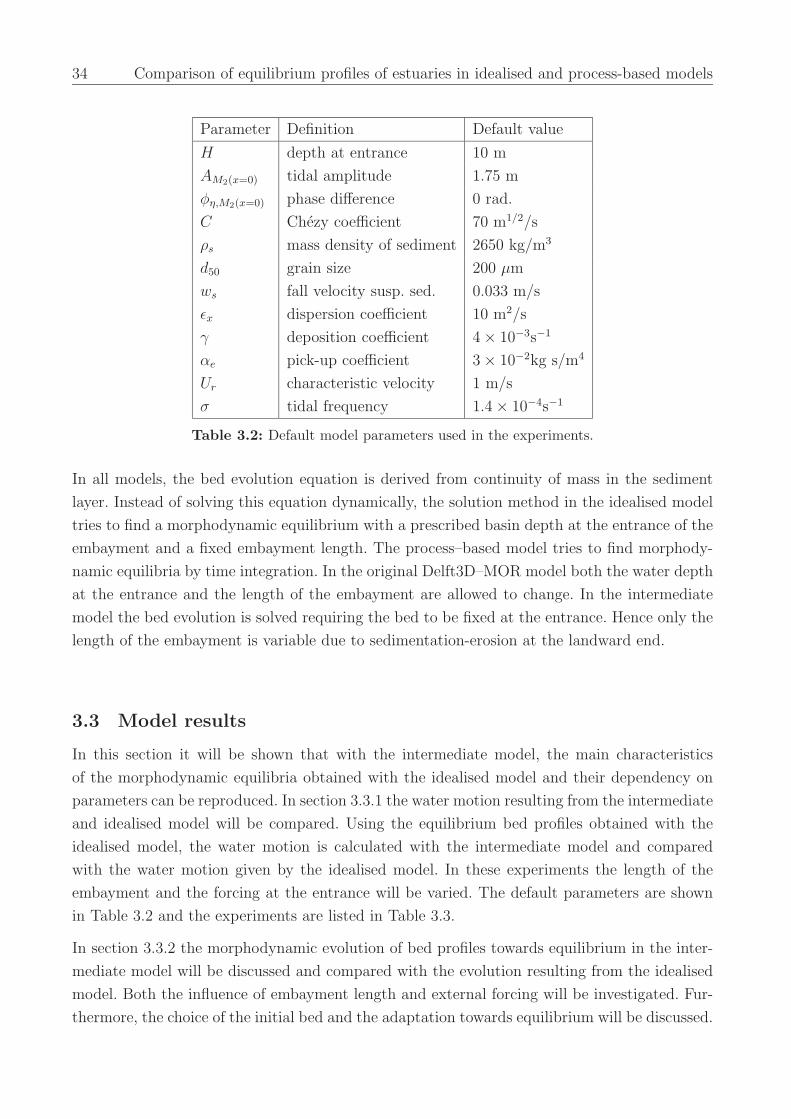
34 Comparison of equilibrium profiles of estuaries in idealised and process-based models
Parameter Definition Default value
H depth at entrance 10 m
AM2(x=0) tidal amplitude 1.75 m
φη,M2(x=0) phase difference 0 rad.
C Chezy coefficient 70 m1/2/s
ρs mass density of sediment 2650 kg/m3
d50 grain size 200 µm
ws fall velocity susp. sed. 0.033 m/s
εx dispersion coefficient 10 m2/s
γ deposition coefficient 4 × 10⁻³s−1
αe pick-up coefficient 3 × 10⁻²kg s/m4
Ur characteristic velocity 1 m/s
σ tidal frequency 1.4 × 10⁻⁴s−1
Table 3.2: Default model parameters used in the experiments.
In all models, the bed evolution equation is derived from continuity of mass in the sediment
layer. Instead of solving this equation dynamically, the solution method in the idealised model
tries to find a morphodynamic equilibrium with a prescribed basin depth at the entrance of the
embayment and a fixed embayment length. The process–based model tries to find morphody-
namic equilibria by time integration. In the original Delft3D–MOR model both the water depth
at the entrance and the length of the embayment are allowed to change. In the intermediate
model the bed evolution is solved requiring the bed to be fixed at the entrance. Hence only the
length of the embayment is variable due to sedimentation-erosion at the landward end.
3.3 Model results
In this section it will be shown that with the intermediate model, the main characteristics
of the morphodynamic equilibria obtained with the idealised model and their dependency on
parameters can be reproduced. In section 3.3.1 the water motion resulting from the intermediate
and idealised model will be compared. Using the equilibrium bed profiles obtained with the
idealised model, the water motion is calculated with the intermediate model and compared
with the water motion given by the idealised model. In these experiments the length of the
embayment and the forcing at the entrance will be varied. The default parameters are shown
in Table 3.2 and the experiments are listed in Table 3.3.
In section 3.3.2 the morphodynamic evolution of bed profiles towards equilibrium in the inter-
mediate model will be discussed and compared with the evolution resulting from the idealised
model. Both the influence of embayment length and external forcing will be investigated. Fur-
thermore, the choice of the initial bed and the adaptation towards equilibrium will be discussed.
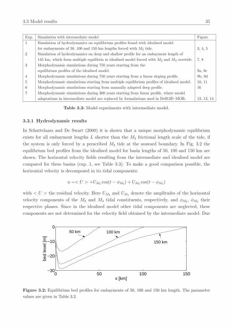
3.3 Model results 35
Exp. Simulation with intermediate model Figure1 Simulation of hydrodynamics on equilibrium profiles found with idealised model
for embayments of 50, 100 and 150 km lengths forced with M2 tide. 3, 4, 52 Simulation of hydrodynamics on deep and shallow profile for an embayment length of
145 km, which form multiple equilibria in idealised model forced with M2 and M4 overtide. 7, 83 Morphodynamic simulations during 750 years starting from the
equilibrium profiles of the idealised model. 9a, 9c4 Morphodynamic simulations during 750 years starting from a linear sloping profile. 9b, 9d5 Morphodynamic simulations starting from multiple equilibrium profiles of idealised model. 10, 116 Morphodynamic simulations starting from manually adapted deep profile. 167 Morphodynamic simulations during 300 years starting from linear profile, where model
adaptations in intermediate model are replaced by formulations used in Delft3D–MOR. 12, 13, 14
Table 3.3: Model experiments with intermediate model.
3.3.1 Hydrodynamic results
In Schuttelaars and De Swart (2000) it is shown that a unique morphodynamic equilibrium
exists for all embayment lengths L shorter than the M2 frictional length scale of the tide, if
the system is only forced by a prescribed M2 tide at the seaward boundary. In Fig. 3.2 the
equilibrium bed profiles from the idealised model for basin lengths of 50, 100 and 150 km are
shown. The horizontal velocity fields resulting from the intermediate and idealised model are
compared for these basins (exp. 1, see Table 3.3). To make a good comparison possible, the
horizontal velocity is decomposed in its tidal components:
u =< U > +UM2 cos(t − φM2) + UM4 cos(t − φM4)
with < U > the residual velocity. Here UM2 and UM4 denote the amplitudes of the horizontal
velocity components of the M2 and M4 tidal constituents, respectively, and φM2 , φM4 their
respective phases. Since in the idealised model other tidal components are neglected, these
components are not determined for the velocity field obtained by the intermediate model. Due
0 50 100 150−30
−20
−10
0
x [km]
bed
leve
l [m
]
150 km
100 km 50 km
Figure 3.2: Equilibrium bed profiles for embayments of 50, 100 and 150 km length. The parametervalues are given in Table 3.2.
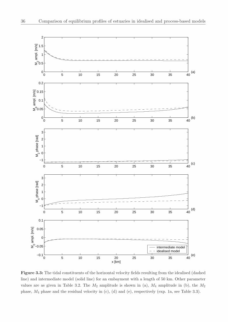
36 Comparison of equilibrium profiles of estuaries in idealised and process-based models
0 5 10 15 20 25 30 35 400
0.5
1
1.5
2
(a)
M2 a
mpl
. [m
/s]
0 5 10 15 20 25 30 35 400
0.05
0.1
0.15
0.2
M4 a
mpl
. [m
/s]
(b)
0 5 10 15 20 25 30 35 40
−1
0
1
2
3
M2 p
hase
[rad
]
(c)
0 5 10 15 20 25 30 35 40
−1
0
1
2
3
M4 p
hase
[rad
]
(d)
0 5 10 15 20 25 30 35 40−0.1
−0.05
0
0.05
0.1
M0 a
mpl
. [m
/s]
(e)
x [km]
intermediate modelidealised model
Figure 3.3: The tidal constituents of the horizontal velocity fields resulting from the idealised (dashedline) and intermediate model (solid line) for an embayment with a length of 50 km. Other parametervalues are as given in Table 3.2. The M2 amplitude is shown in (a), M4 amplitude in (b), the M2
phase, M4 phase and the residual velocity in (c), (d) and (e), respectively (exp. 1a, see Table 3.3).
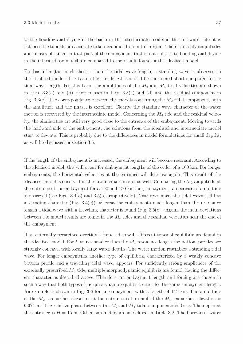
3.3 Model results 37
to the flooding and drying of the basin in the intermediate model at the landward side, it is
not possible to make an accurate tidal decomposition in this region. Therefore, only amplitudes
and phases obtained in that part of the embayment that is not subject to flooding and drying
in the intermediate model are compared to the results found in the idealised model.
For basin lengths much shorter than the tidal wave length, a standing wave is observed in
the idealised model. The basin of 50 km length can still be considered short compared to the
tidal wave length. For this basin the amplitudes of the M2 and M4 tidal velocities are shown
in Figs. 3.3(a) and (b), their phases in Figs. 3.3(c) and (d) and the residual component in
Fig. 3.3(e). The correspondence between the models concerning the M2 tidal component, both
the amplitude and the phase, is excellent. Clearly, the standing wave character of the water
motion is recovered by the intermediate model. Concerning the M4 tide and the residual veloc-
ity, the similarities are still very good close to the entrance of the embayment. Moving towards
the landward side of the embayment, the solutions from the idealised and intermediate model
start to deviate. This is probably due to the differences in model formulations for small depths,
as will be discussed in section 3.5.
If the length of the embayment is increased, the embayment will become resonant. According to
the idealised model, this will occur for embayment lengths of the order of a 100 km. For longer
embayments, the horizontal velocities at the entrance will decrease again. This result of the
idealised model is observed in the intermediate model as well. Comparing the M2 amplitude at
the entrance of the embayment for a 100 and 150 km long embayment, a decrease of amplitude
is observed (see Figs. 3.4(a) and 3.5(a), respectively). Near resonance, the tidal wave still has
a standing character (Fig. 3.4(c)), whereas for embayments much longer than the resonance
length a tidal wave with a travelling character is found (Fig. 3.5(c)). Again, the main deviations
between the model results are found in the M4 tides and the residual velocities near the end of
the embayment.
If an externally prescribed overtide is imposed as well, different types of equilibria are found in
the idealised model. For L values smaller than the M4 resonance length the bottom profiles are
strongly concave, with locally large water depths. The water motion resembles a standing tidal
wave. For longer embayments another type of equilibria, characterized by a weakly concave
bottom profile and a travelling tidal wave, appears. For sufficiently strong amplitudes of the
externally prescribed M4 tide, multiple morphodynamic equilibria are found, having the differ-
ent character as described above. Therefore, an embayment length and forcing are chosen in
such a way that both types of morphodynamic equilibria occur for the same embayment length.
An example is shown in Fig. 3.6 for an embayment with a length of 145 km. The amplitude
of the M2 sea surface elevation at the entrance is 1 m and of the M4 sea surface elevation is
0.074 m. The relative phase between the M2 and M4 tidal components is 0 deg. The depth at
the entrance is H = 15 m. Other parameters are as defined in Table 3.2. The horizontal water
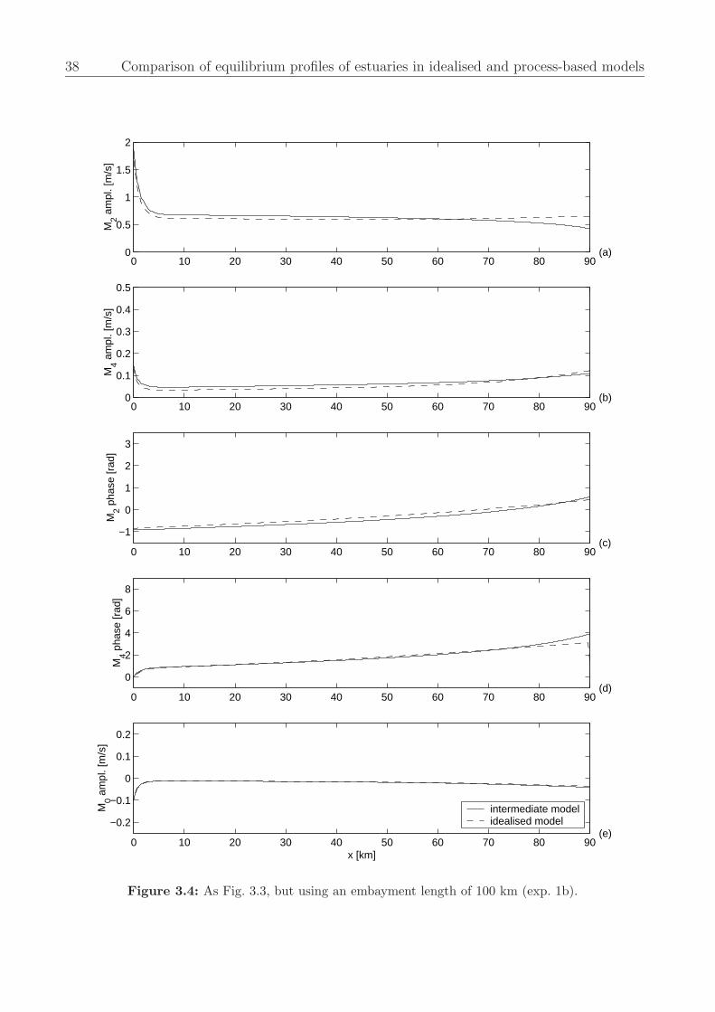
38 Comparison of equilibrium profiles of estuaries in idealised and process-based models
0 10 20 30 40 50 60 70 80 900
0.5
1
1.5
2
(a)
M2 a
mpl
. [m
/s]
0 10 20 30 40 50 60 70 80 900
0.1
0.2
0.3
0.4
0.5
(b)
M4 a
mpl
. [m
/s]
0 10 20 30 40 50 60 70 80 90
−1
0
1
2
3
(c)
M2 p
hase
[rad
]
0 10 20 30 40 50 60 70 80 90
0
2
4
6
8
(d)
M4 p
hase
[rad
]
0 10 20 30 40 50 60 70 80 90
−0.2
−0.1
0
0.1
0.2
(e)
M0 a
mpl
. [m
/s]
x [km]
intermediate modelidealised model
Figure 3.4: As Fig. 3.3, but using an embayment length of 100 km (exp. 1b).
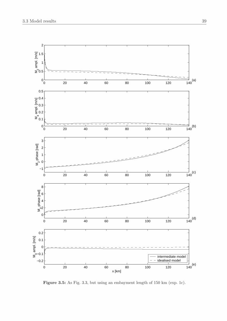
3.3 Model results 39
0 20 40 60 80 100 120 1400
0.5
1
1.5
2
(a)
M2 a
mpl
. [m
/s]
0 20 40 60 80 100 120 1400
0.1
0.2
0.3
0.4
0.5
(b)
M4 a
mpl
. [m
/s]
0 20 40 60 80 100 120 140
−1
0
1
2
3
(c)
M2 p
hase
[rad
]
0 20 40 60 80 100 120 140
0
2
4
6
8
(d)
M4 p
hase
[rad
]
0 20 40 60 80 100 120 140
−0.2
−0.1
0
0.1
0.2
(e)
M0 a
mpl
. [m
/s]
x [km]
intermediate modelidealised model
Figure 3.5: As Fig. 3.3, but using an embayment length of 150 km (exp. 1c).
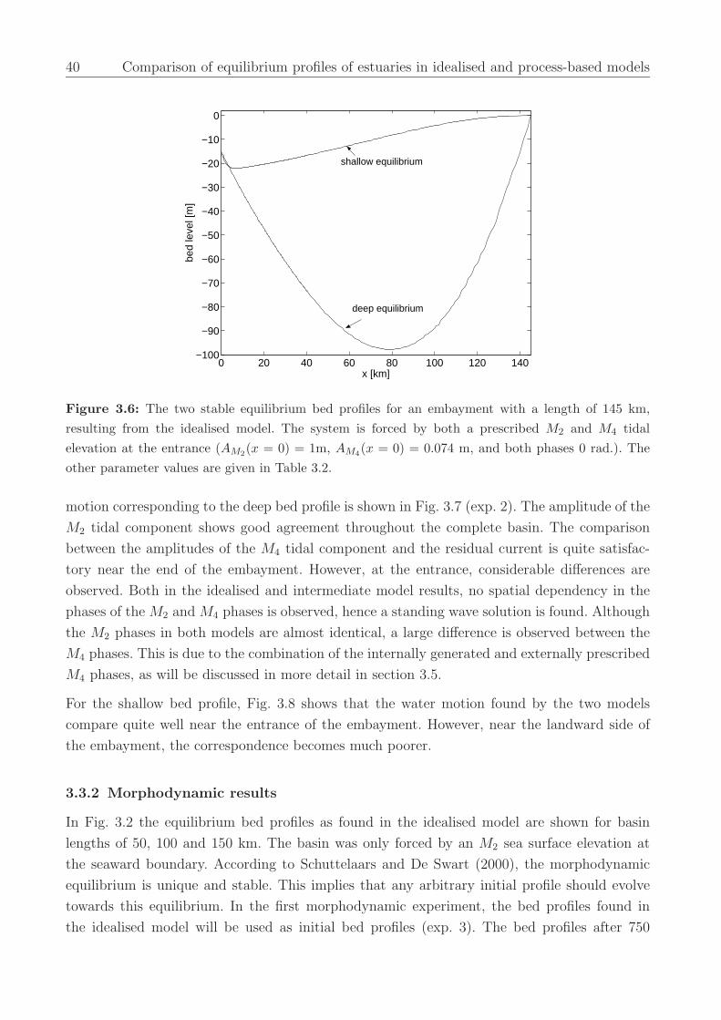
40 Comparison of equilibrium profiles of estuaries in idealised and process-based models
0 20 40 60 80 100 120 140−100
−90
−80
−70
−60
−50
−40
−30
−20
−10
0
x [km]
bed
leve
l [m
]
shallow equilibrium
deep equilibrium
Figure 3.6: The two stable equilibrium bed profiles for an embayment with a length of 145 km,resulting from the idealised model. The system is forced by both a prescribed M2 and M4 tidalelevation at the entrance (AM2(x = 0) = 1m, AM4(x = 0) = 0.074 m, and both phases 0 rad.). Theother parameter values are given in Table 3.2.
motion corresponding to the deep bed profile is shown in Fig. 3.7 (exp. 2). The amplitude of the
M2 tidal component shows good agreement throughout the complete basin. The comparison
between the amplitudes of the M4 tidal component and the residual current is quite satisfac-
tory near the end of the embayment. However, at the entrance, considerable differences are
observed. Both in the idealised and intermediate model results, no spatial dependency in the
phases of the M2 and M4 phases is observed, hence a standing wave solution is found. Although
the M2 phases in both models are almost identical, a large difference is observed between the
M4 phases. This is due to the combination of the internally generated and externally prescribed
M4 phases, as will be discussed in more detail in section 3.5.
For the shallow bed profile, Fig. 3.8 shows that the water motion found by the two models
compare quite well near the entrance of the embayment. However, near the landward side of
the embayment, the correspondence becomes much poorer.
3.3.2 Morphodynamic results
In Fig. 3.2 the equilibrium bed profiles as found in the idealised model are shown for basin
lengths of 50, 100 and 150 km. The basin was only forced by an M2 sea surface elevation at
the seaward boundary. According to Schuttelaars and De Swart (2000), the morphodynamic
equilibrium is unique and stable. This implies that any arbitrary initial profile should evolve
towards this equilibrium. In the first morphodynamic experiment, the bed profiles found in
the idealised model will be used as initial bed profiles (exp. 3). The bed profiles after 750
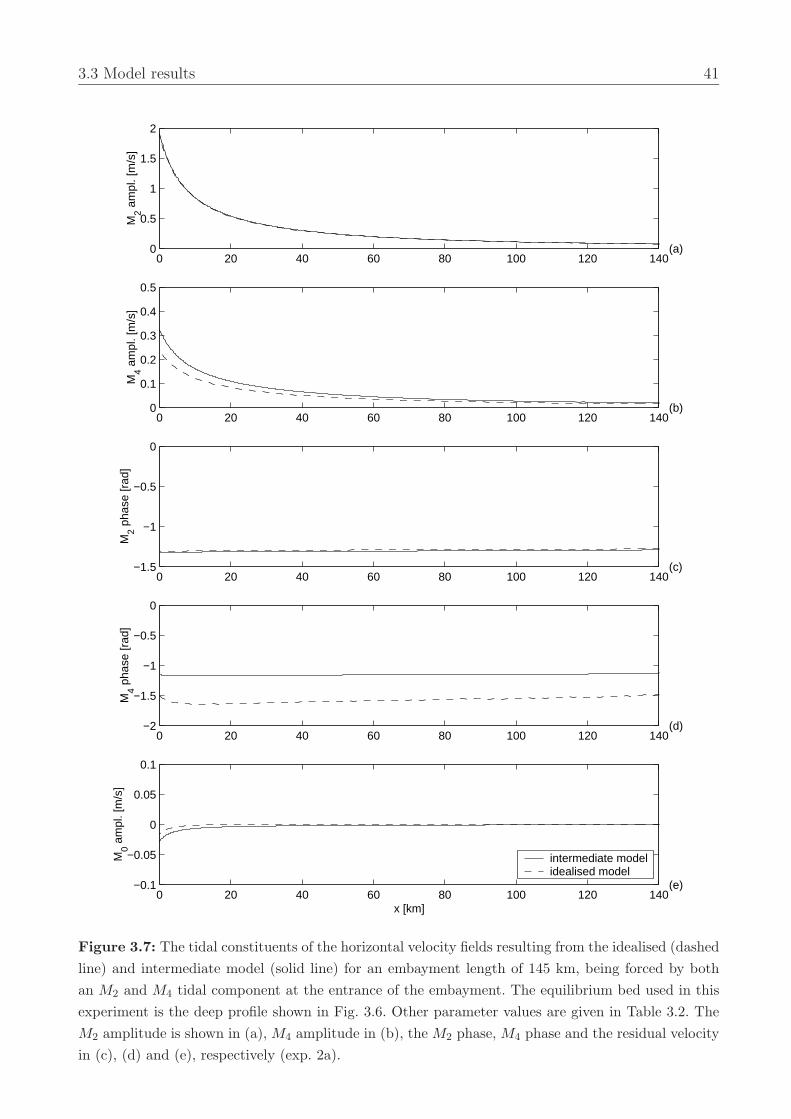
3.3 Model results 41
0 20 40 60 80 100 120 1400
0.5
1
1.5
2
(a)
M2 a
mpl
. [m
/s]
0 20 40 60 80 100 120 1400
0.1
0.2
0.3
0.4
0.5
(b)
M4 a
mpl
. [m
/s]
0 20 40 60 80 100 120 140−1.5
−1
−0.5
0
(c)
M2 p
hase
[rad
]
0 20 40 60 80 100 120 140−2
−1.5
−1
−0.5
0
(d)
M4 p
hase
[rad
]
0 20 40 60 80 100 120 140−0.1
−0.05
0
0.05
0.1
(e)
M0 a
mpl
. [m
/s]
x [km]
intermediate modelidealised model
Figure 3.7: The tidal constituents of the horizontal velocity fields resulting from the idealised (dashedline) and intermediate model (solid line) for an embayment length of 145 km, being forced by bothan M2 and M4 tidal component at the entrance of the embayment. The equilibrium bed used in thisexperiment is the deep profile shown in Fig. 3.6. Other parameter values are given in Table 3.2. TheM2 amplitude is shown in (a), M4 amplitude in (b), the M2 phase, M4 phase and the residual velocityin (c), (d) and (e), respectively (exp. 2a).
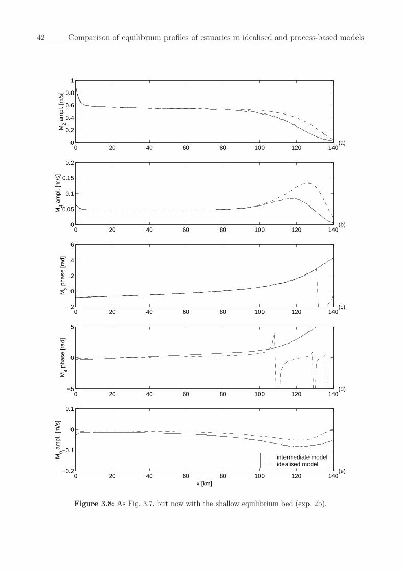
42 Comparison of equilibrium profiles of estuaries in idealised and process-based models
0 20 40 60 80 100 120 1400
0.2
0.4
0.6
0.8
1
(a)
M2 a
mpl
. [m
/s]
0 20 40 60 80 100 120 1400
0.05
0.1
0.15
0.2
(b)
M4 a
mpl
. [m
/s]
0 20 40 60 80 100 120 140−2
0
2
4
6
(c)
M2 p
hase
[rad
]
0 20 40 60 80 100 120 140−5
0
5
(d)
M4 p
hase
[rad
]
0 20 40 60 80 100 120 140−0.2
−0.1
0
0.1
M0 a
mpl
. [m
/s]
(e)
x [km]
intermediate modelidealised model
Figure 3.8: As Fig. 3.7, but now with the shallow equilibrium bed (exp. 2b).
3.3 Model results 43
years are shown in Fig. 3.9(a). These profiles qualitatively resemble the equilibrium profiles
from the idealised model: a deep pool is found near the entrance of the basin, whereas the
bed is more or less constantly sloping with a zero depth at the landward side. During the first
years of evolution, relatively large changes are observed near the entrance of the embayment.
The deep pool as observed in the results of the idealised model starts to fill up. The adjacent
profile also shallows in landward direction. For the basin lengths of 100 and 150 km this process
is not completed after 750 years, which causes the hump around x = 25 km in the profiles.
As can be inferred from Fig. 3.9(c), the time needed to evolve towards the new equilibrium
depends on the embayment length. In this figure, the yearly change in bed height averaged over
the complete basin length is shown as a function of time. For an inlet of 50 km, Fig. 3.9(c)
shows that after approximately 40 years the changes to the bed are negligible compared to the
initial changes. Continuing the time–integration leads to sedimentation at the landward side of
the embayment and hence a shortening of the embayment. For longer embayments, the same
evolution can be observed. However, the corresponding initial phase of relatively fast adaptation
is much longer. To make the uniqueness of the morphodynamic equilibrium plausible, another
initial bed profile is chosen for all embayment lengths. This bed is chosen to be constantly
sloping (exp. 4, see Fig. 3.9(b)). Again, the same observations concerning the evolution can
be made. The initial evolution is (relatively) fast, but in this case a pool is being formed near
the entrance. After some time (in this case approximately 200 years) the amplitude of the bed
changes integrated over the basin decreases exponentially. Again, the quasi–equilibrium profiles
found in the intermediate model show a good qualitative agreement to the equilibrium profiles
predicted by the idealised model. Although these bed changes do not go to zero, even after
integrating for a long time (here 750 years), these changes become very small and mainly affect
the length of the basin. This adaptation of the length also prevents a quantitative agreement
between the developed profiles starting from the different initial profiles, because the lengths
of the basins no longer coincide.
Previous results show that morphodynamic equilibria exist in the intermediate model. As al-
ready discussed before, the idealised model predicts the existence of multiple equilibria for a
basin length of 145 km and AM2(x = 0) = 1 m, AM4(x = 0) = 0.074m and φη,M2(x = 0) =
φη,M4(x = 0) = 0 rad (see Fig. 3.6). Using these equilibria as initial profiles, their morpho-
dynamic evolution can be studied (exp. 5). The equilibrium with the relatively shallow bed
has the same morphodynamic evolution as those only forced with an M2 tidal component (see
Figs. 3.10 and 3.11(a)): in the first few decades, a relatively fast bottom change takes place
near the entrance of the embayment and the pools become less pronounced. Next, the basin
slowly starts to fill up at the end. Due to this adaptation of the basin length, the profile starts
to deepen again near the entrance of the basin. The evolution of the basin, starting from the
other equilibrium, shows that a lot of deposition takes place in the embayment (see Figs. 3.10
and 3.11(b)). The embayment is filling up, starting near the entrance, just as in the case of a
shallow equilibrium bed. After approximately 10000 years, the erosion–deposition in the first
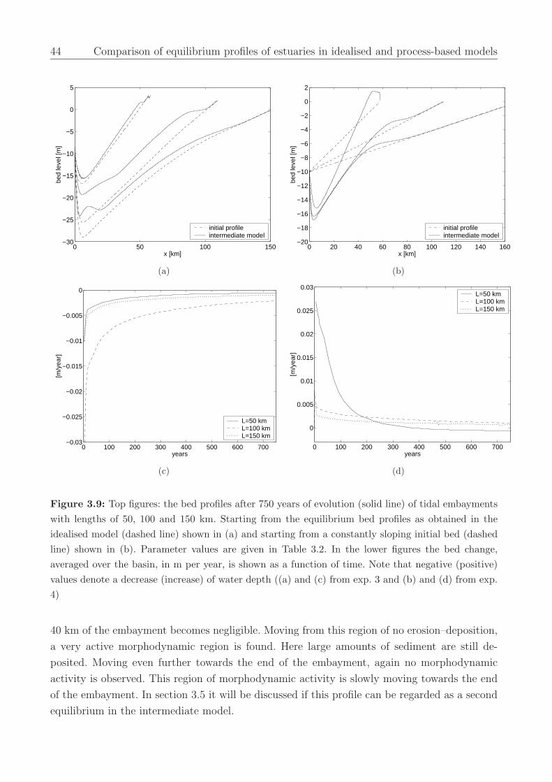
44 Comparison of equilibrium profiles of estuaries in idealised and process-based models
0 50 100 150−30
−25
−20
−15
−10
−5
0
5
x [km]
bed
leve
l [m
]
initial profileintermediate model
(a)
0 20 40 60 80 100 120 140 160−20
−18
−16
−14
−12
−10
−8
−6
−4
−2
0
2
x [km]
bed
leve
l [m
]
initial profileintermediate model
(b)
0 100 200 300 400 500 600 700−0.03
−0.025
−0.02
−0.015
−0.01
−0.005
0
years
[m/y
ear]
L=50 kmL=100 kmL=150 km
(c)
0 100 200 300 400 500 600 700
0
0.005
0.01
0.015
0.02
0.025
0.03
years
[m/y
ear]
L=50 kmL=100 kmL=150 km
(d)
Figure 3.9: Top figures: the bed profiles after 750 years of evolution (solid line) of tidal embaymentswith lengths of 50, 100 and 150 km. Starting from the equilibrium bed profiles as obtained in theidealised model (dashed line) shown in (a) and starting from a constantly sloping initial bed (dashedline) shown in (b). Parameter values are given in Table 3.2. In the lower figures the bed change,averaged over the basin, in m per year, is shown as a function of time. Note that negative (positive)values denote a decrease (increase) of water depth ((a) and (c) from exp. 3 and (b) and (d) from exp.4)
40 km of the embayment becomes negligible. Moving from this region of no erosion–deposition,
a very active morphodynamic region is found. Here large amounts of sediment are still de-
posited. Moving even further towards the end of the embayment, again no morphodynamic
activity is observed. This region of morphodynamic activity is slowly moving towards the end
of the embayment. In section 3.5 it will be discussed if this profile can be regarded as a second
equilibrium in the intermediate model.
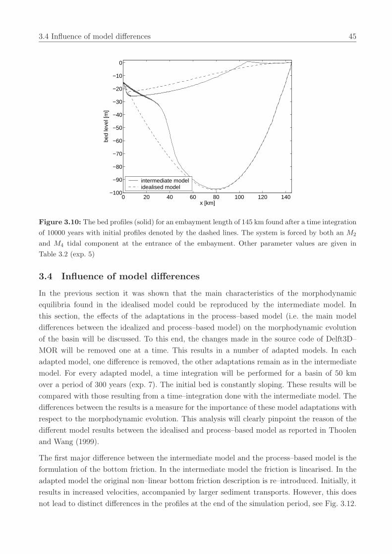
3.4 Influence of model differences 45
0 20 40 60 80 100 120 140−100
−90
−80
−70
−60
−50
−40
−30
−20
−10
0
x [km]
bed
leve
l [m
]
intermediate modelidealised model
Figure 3.10: The bed profiles (solid) for an embayment length of 145 km found after a time integrationof 10000 years with initial profiles denoted by the dashed lines. The system is forced by both an M2
and M4 tidal component at the entrance of the embayment. Other parameter values are given inTable 3.2 (exp. 5)
3.4 Influence of model differences
In the previous section it was shown that the main characteristics of the morphodynamic
equilibria found in the idealised model could be reproduced by the intermediate model. In
this section, the effects of the adaptations in the process–based model (i.e. the main model
differences between the idealized and process–based model) on the morphodynamic evolution
of the basin will be discussed. To this end, the changes made in the source code of Delft3D–
MOR will be removed one at a time. This results in a number of adapted models. In each
adapted model, one difference is removed, the other adaptations remain as in the intermediate
model. For every adapted model, a time integration will be performed for a basin of 50 km
over a period of 300 years (exp. 7). The initial bed is constantly sloping. These results will be
compared with those resulting from a time–integration done with the intermediate model. The
differences between the results is a measure for the importance of these model adaptations with
respect to the morphodynamic evolution. This analysis will clearly pinpoint the reason of the
different model results between the idealised and process–based model as reported in Thoolen
and Wang (1999).
The first major difference between the intermediate model and the process–based model is the
formulation of the bottom friction. In the intermediate model the friction is linearised. In the
adapted model the original non–linear bottom friction description is re–introduced. Initially, it
results in increased velocities, accompanied by larger sediment transports. However, this does
not lead to distinct differences in the profiles at the end of the simulation period, see Fig. 3.12.
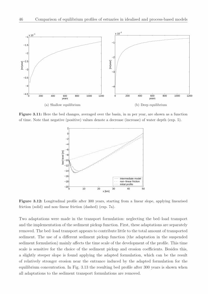
46 Comparison of equilibrium profiles of estuaries in idealised and process-based models
0 200 400 600 800 1000 1200−4.5
−4
−3.5
−3
−2.5
−2
−1.5
−1x 10
−4
years
[m/y
ear]
(a) Shallow equilibrium
0 200 400 600 800 1000 1200
−4
−3
−2
−1
x 10−3
years
[m/y
ear]
(b) Deep equilibrium
Figure 3.11: Here the bed changes, averaged over the basin, in m per year, are shown as a functionof time. Note that negative (positive) values denote a decrease (increase) of water depth (exp. 5).
0 10 20 30 40 50−20
−18
−16
−14
−12
−10
−8
−6
−4
−2
0
2
x [km]
bed
leve
l [m
]
intermediate modelnon−linear frictioninitial profile
Figure 3.12: Longitudinal profile after 300 years, starting from a linear slope, applying linearisedfriction (solid) and non–linear friction (dashed) (exp. 7a).
Two adaptations were made in the transport formulation: neglecting the bed–load transport
and the implementation of the sediment pickup function. First, these adaptations are separately
removed. The bed–load transport appears to contribute little to the total amount of transported
sediment. The use of a different sediment pickup function (the adaptation in the suspended
sediment formulation) mainly affects the time scale of the development of the profile. This time
scale is sensitive for the choice of the sediment pickup and erosion coefficients. Besides this,
a slightly steeper slope is found applying the adapted formulation, which can be the result
of relatively stronger erosion near the entrance induced by the adapted formulation for the
equilibrium concentration. In Fig. 3.13 the resulting bed profile after 300 years is shown when
all adaptations to the sediment transport formulations are removed.
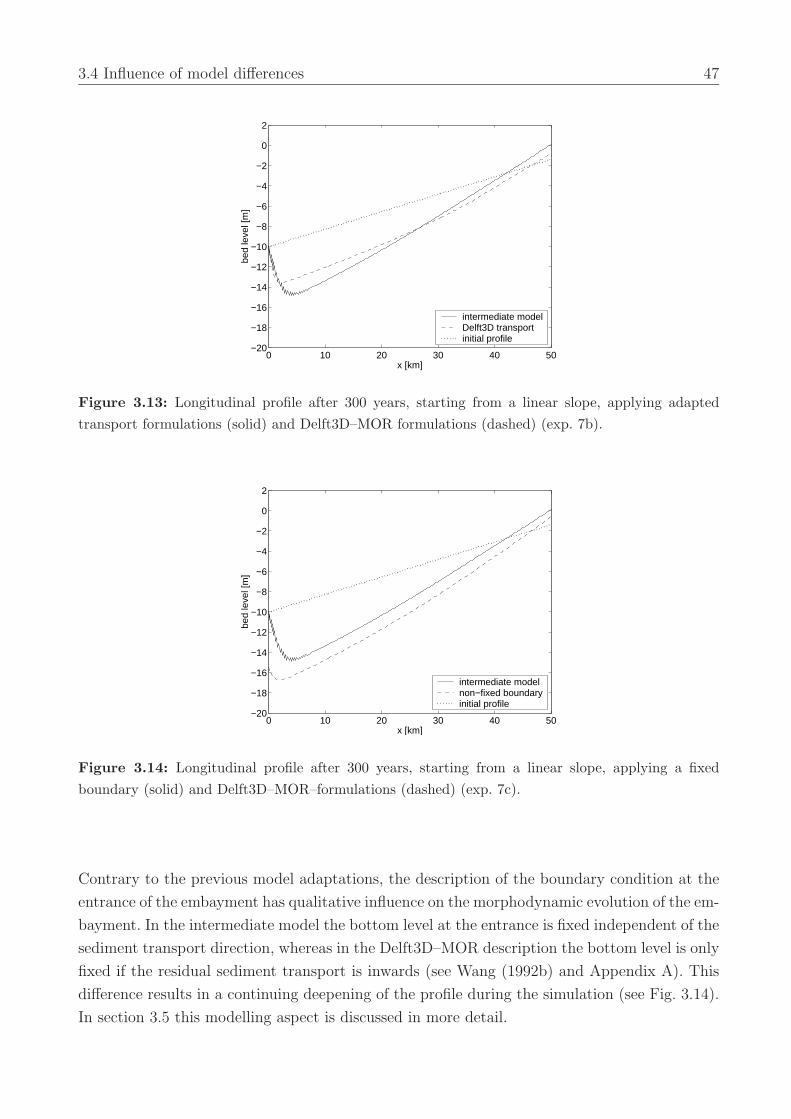
3.4 Influence of model differences 47
0 10 20 30 40 50−20
−18
−16
−14
−12
−10
−8
−6
−4
−2
0
2
x [km]
bed
leve
l [m
]
intermediate modelDelft3D transportinitial profile
Figure 3.13: Longitudinal profile after 300 years, starting from a linear slope, applying adaptedtransport formulations (solid) and Delft3D–MOR formulations (dashed) (exp. 7b).
0 10 20 30 40 50−20
−18
−16
−14
−12
−10
−8
−6
−4
−2
0
2
x [km]
bed
leve
l [m
]
intermediate modelnon−fixed boundaryinitial profile
Figure 3.14: Longitudinal profile after 300 years, starting from a linear slope, applying a fixedboundary (solid) and Delft3D–MOR–formulations (dashed) (exp. 7c).
Contrary to the previous model adaptations, the description of the boundary condition at the
entrance of the embayment has qualitative influence on the morphodynamic evolution of the em-
bayment. In the intermediate model the bottom level at the entrance is fixed independent of the
sediment transport direction, whereas in the Delft3D–MOR description the bottom level is only
fixed if the residual sediment transport is inwards (see Wang (1992b) and Appendix A). This
difference results in a continuing deepening of the profile during the simulation (see Fig. 3.14).
In section 3.5 this modelling aspect is discussed in more detail.
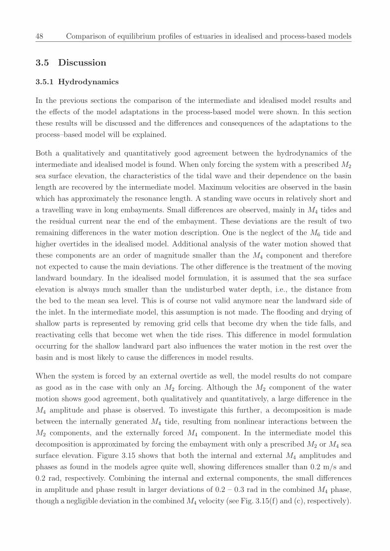
48 Comparison of equilibrium profiles of estuaries in idealised and process-based models
3.5 Discussion
3.5.1 Hydrodynamics
In the previous sections the comparison of the intermediate and idealised model results and
the effects of the model adaptations in the process-based model were shown. In this section
these results will be discussed and the differences and consequences of the adaptations to the
process–based model will be explained.
Both a qualitatively and quantitatively good agreement between the hydrodynamics of the
intermediate and idealised model is found. When only forcing the system with a prescribed M2
sea surface elevation, the characteristics of the tidal wave and their dependence on the basin
length are recovered by the intermediate model. Maximum velocities are observed in the basin
which has approximately the resonance length. A standing wave occurs in relatively short and
a travelling wave in long embayments. Small differences are observed, mainly in M4 tides and
the residual current near the end of the embayment. These deviations are the result of two
remaining differences in the water motion description. One is the neglect of the M6 tide and
higher overtides in the idealised model. Additional analysis of the water motion showed that
these components are an order of magnitude smaller than the M4 component and therefore
not expected to cause the main deviations. The other difference is the treatment of the moving
landward boundary. In the idealised model formulation, it is assumed that the sea surface
elevation is always much smaller than the undisturbed water depth, i.e., the distance from
the bed to the mean sea level. This is of course not valid anymore near the landward side of
the inlet. In the intermediate model, this assumption is not made. The flooding and drying of
shallow parts is represented by removing grid cells that become dry when the tide falls, and
reactivating cells that become wet when the tide rises. This difference in model formulation
occurring for the shallow landward part also influences the water motion in the rest over the
basin and is most likely to cause the differences in model results.
When the system is forced by an external overtide as well, the model results do not compare
as good as in the case with only an M2 forcing. Although the M2 component of the water
motion shows good agreement, both qualitatively and quantitatively, a large difference in the
M4 amplitude and phase is observed. To investigate this further, a decomposition is made
between the internally generated M4 tide, resulting from nonlinear interactions between the
M2 components, and the externally forced M4 component. In the intermediate model this
decomposition is approximated by forcing the embayment with only a prescribed M2 or M4 sea
surface elevation. Figure 3.15 shows that both the internal and external M4 amplitudes and
phases as found in the models agree quite well, showing differences smaller than 0.2 m/s and
0.2 rad, respectively. Combining the internal and external components, the small differences
in amplitude and phase result in larger deviations of 0.2 – 0.3 rad in the combined M4 phase,
though a negligible deviation in the combined M4 velocity (see Fig. 3.15(f) and (c), respectively).
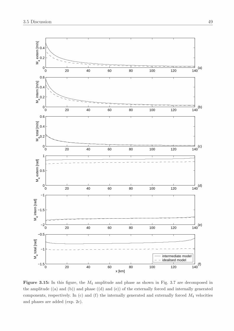
3.5 Discussion 49
0 20 40 60 80 100 120 1400
0.2
0.4
M4 e
xter
n [m
/s]
(a)
0 20 40 60 80 100 120 1400
0.5
1
M4 e
xter
n [r
ad]
(d)
0 20 40 60 80 100 120 1400
0.2
0.4
0.6
M4 in
tern
[m/s
]
(b)
0 20 40 60 80 100 120 140−2
−1.5
−1
M4 in
tern
[rad
]
(e)
0 20 40 60 80 100 120 140−1.5
−1
−0.5
M4 to
tal [
rad]
x [km]
(f)
intermediate modelidealised model
0 20 40 60 80 100 120 1400
0.2
0.4
0.6
M4 to
tal [
m/s
]
(c)
Figure 3.15: In this figure, the M4 amplitude and phase as shown in Fig. 3.7 are decomposed inthe amplitude ((a) and (b)) and phase ((d) and (e)) of the externally forced and internally generatedcomponents, respectively. In (c) and (f) the internally generated and externally forced M4 velocitiesand phases are added (exp. 2c).

50 Comparison of equilibrium profiles of estuaries in idealised and process-based models
3.5.2 Morphodynamics
Albeit small, differences in the velocity field imply that the sediment transport field and there-
fore the morphological equilibria deviate. The morphological development of the longitudinal
profiles forced by the M2 only show initially the largest changes near the entrance of the em-
bayment, after which the adjustments rapidly decrease. These initial changes are due to the
remaining difference in the sediment transport formulation. However, qualitatively the resulting
profiles resemble the equilibrium profiles of the idealised model. Therefore, the processes found
in this model can be adopted for the intermediate model, which is a balance between sediment
fluxes resulting from the interaction of the main M2 tide and internally generated overtides in
velocity and concentrations. An equilibrium is not achieved in the intermediate model in the
strict sense of zero net sediment transport throughout the basin. In Schuttelaars and De Swart
(1996, 2000) it was shown that to reach an equilibrium in the strict sense, it is essential that
a finite velocity is allowed at places where the depth vanishes (i.e., only the water flux has to
become zero at these points). This condition is not implemented in the intermediate model.
Therefore, an equilibrium in the strict sense will never be found. Due to the sedimentation
the length of the basin decreases. For this new basin length the profile is not an equilibrium
anymore. This again results in morphodynamic changes which are most pronounced at the
entrance of the basin. Theoretically, it can be expected that this process will eventually lead to
a trivial equilibrium, i.e. the complete filling up of the basin. A possible solution to avoid this
behaviour could be the implementation of a (small) river flow at the landward end, thereby
allowing a finite velocity at the landward side (De Jong, 1998).
Prescribing an overtide at the seaward boundary, multiple equilibria were found in the idealised
model for certain basin lengths. The morphodynamic evolution starting from the multiple equi-
librium is simulated for a long period in the intermediate model. In the idealised model the
shallow basin shows a similar type of evolution as those without an externally prescribed over-
tide. This can be understood by realising that for this equilibrium a balance is found between
sediment fluxes resulting from the interaction of the main M2 tide and internally generated
overtides only. The externally generated velocities are too weak to contribute substantially to
this balance. At first sight, the evolution of the deep basin looks completely different. How-
ever, the qualitative changes near the entrance are identical as those shown in, for example
Fig. 3.9(a) where the embayment is only forced by a prescribed M2 tide: the embayment starts
to become shallower due to the difference in the sediment transport formulation. The deposi-
tion term in the intermediate model is not dependent on the local depth as in the idealised
model, which result in much larger deposition for the large depths in this basin. This process
is slowly moving from the entrance of the embayment to the landward side. Due to the large
depth, the changes in this case are larger than in Fig. 3.9(a). However, the standing tidal wave
is maintained during this evolution and the presence of the externally forced overtide remains
important. The sediment fluxes resulting from the interaction between the main M2 tide and
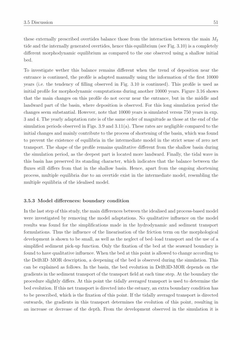
3.5 Discussion 51
these externally prescribed overtides balance those from the interaction between the main M2
tide and the internally generated overtides, hence this equilibrium (see Fig. 3.10) is a completely
different morphodynamic equilibrium as compared to the one observed using a shallow initial
bed.
To investigate wether this balance remains different when the trend of deposition near the
entrance is continued, the profile is adapted manually using the information of the first 10000
years (i.e. the tendency of filling observed in Fig. 3.10 is continued). This profile is used as
initial profile for morphodynamic computations during another 10000 years. Figure 3.16 shows
that the main changes on this profile do not occur near the entrance, but in the middle and
landward part of the basin, where deposition is observed. For this long simulation period the
changes seem substantial. However, note that 10000 years is simulated versus 750 years in exp.
3 and 4. The yearly adaptation rate is of the same order of magnitude as those at the end of the
simulation periods observed in Figs. 3.9 and 3.11(a). These rates are negligible compared to the
initial changes and mainly contribute to the process of shortening of the basin, which was found
to prevent the existence of equilibria in the intermediate model in the strict sense of zero net
transport. The shape of the profile remains qualitative different from the shallow basin during
the simulation period, as the deepest part is located more landward. Finally, the tidal wave in
this basin has preserved its standing character, which indicates that the balance between the
fluxes still differs from that in the shallow basin. Hence, apart from the ongoing shortening
process, multiple equilibria due to an overtide exist in the intermediate model, resembling the
multiple equilibria of the idealised model.
3.5.3 Model differences: boundary condition
In the last step of this study, the main differences between the idealised and process-based model
were investigated by removing the model adaptations. No qualitative influence on the model
results was found for the simplifications made in the hydrodynamic and sediment transport
formulations. Thus the influence of the linearisation of the friction term on the morphological
development is shown to be small, as well as the neglect of bed–load transport and the use of a
simplified sediment pick-up function. Only the fixation of the bed at the seaward boundary is
found to have qualitative influence. When the bed at this point is allowed to change according to
the Delft3D–MOR description, a deepening of the bed is observed during the simulation. This
can be explained as follows. In the basin, the bed evolution in Delft3D-MOR depends on the
gradients in the sediment transport of the transport field at each time step. At the boundary the
procedure slightly differs. At this point the tidally averaged transport is used to determine the
bed evolution. If this net transport is directed into the estuary, an extra boundary condition has
to be prescribed, which is the fixation of this point. If the tidally averaged transport is directed
outwards, the gradients in this transport determines the evolution of this point, resulting in
an increase or decrease of the depth. From the development observed in the simulation it is
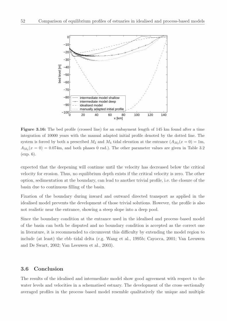
52 Comparison of equilibrium profiles of estuaries in idealised and process-based models
0 20 40 60 80 100 120 140−100
−90
−80
−70
−60
−50
−40
−30
−20
−10
0
x [km]
bed
leve
l [m
]
intermediate model shallowintermediate model deepidealised modelmanually adapted initial profile
Figure 3.16: The bed profile (crossed line) for an embayment length of 145 km found after a timeintegration of 10000 years with the manual adapted initial profile denoted by the dotted line. Thesystem is forced by both a prescribed M2 and M4 tidal elevation at the entrance (AM2(x = 0) = 1m,AM4(x = 0) = 0.074m, and both phases 0 rad.). The other parameter values are given in Table 3.2(exp. 6).
expected that the deepening will continue until the velocity has decreased below the critical
velocity for erosion. Thus, no equilibrium depth exists if the critical velocity is zero. The other
option, sedimentation at the boundary, can lead to another trivial profile, i.e. the closure of the
basin due to continuous filling of the basin.
Fixation of the boundary during inward and outward directed transport as applied in the
idealised model prevents the development of those trivial solutions. However, the profile is also
not realistic near the entrance, showing a steep slope into a deep pool.
Since the boundary condition at the entrance used in the idealised and process–based model
of the basin can both be disputed and no boundary condition is accepted as the correct one
in literature, it is recommended to circumvent this difficulty by extending the model region to
include (at least) the ebb–tidal delta (e.g. Wang et al., 1995b; Cayocca, 2001; Van Leeuwen
and De Swart, 2002; Van Leeuwen et al., 2003).
3.6 Conclusion
The results of the idealised and intermediate model show good agreement with respect to the
water levels and velocities in a schematised estuary. The development of the cross–sectionally
averaged profiles in the process–based model resemble qualitatively the unique and multiple
3.6 Conclusion 53
equilibrium profiles of the idealised model, although an equilibrium is not achieved in the strict
sense of zero net sediment transport.
Using the idealised model, the physical processes resulting in the equilibria are identified: when
no overtide is prescribed, the balance between sediment fluxes results from the interaction of the
main M2 tide and internally generated overtides. Prescribing a M4 overtide, a different type of
balance, due to interactions between the main M2 tide and the externally prescribed overtides,
can be found. Since the morphological development in the different models is qualitatively the
same and controlled by the same physical processes, it can be inferred that the same processes
determine the equilibrium and evolution in the process-based model.
The model adaptations in water motion and sediment transport have no qualitative influence
on the morphodynamic results. Hence, the simplifications in these formulations as used in the
idealised model are justified. Only the adaptations of the boundary condition of the bed at the
entrance has qualitative influence on the morphodynamic equilibria: the existence of equilibria
in the process–based model strongly depends on this boundary condition. However, none of the
model formulations is considered to adequately describe the natural behaviour at this point.
Therefore, it is recommended to extend the model region to include (at least) the ebb–tidal
delta when studying the evolution of tidal basins.
Appendix A: Model formulations
In this appendix, the main model formulations of the process-based model Delft3D–MOR, the
adaptations in the intermediate model and the remaining differences with the idealised model
are described.
In this study, the water motion is simulated in a one-dimensional model and the influence of
Coriolis, density differences and wind or waves are neglected. The equation for conservation of
momentum in the Delft3D-model can therefore be simplified to:
∂u
∂t+ u
∂u
∂x+ g
∂η
∂x+
gu|U |C2(d + η)
− ν∂2u
∂x2= 0 (3.1)
and the continuity equation is given by:
∂η
∂t+
∂u(d + η)
∂x= 0 (3.2)
54 Comparison of equilibrium profiles of estuaries in idealised and process-based models
in which:
C : Chezy coefficient (m1/2/s)
d : water depth w.r.t. MSL (m)
g : gravitational acceleration (m2/s)
u : depth-averaged velocity (m/s)
U : magnitude of total velocity (m/s)
ρ : mass density of water (kg/m3)
ν : diffusion coefficient (eddy viscosity) (m2/s)
η : water level (m)
In the idealised model these shallow water equations are also applied, but the last term in
Eq. 3.1 is neglected because it is very small (ν = 1(m2/s)). The friction term is linearised
according to the energy dissipation condition of Lorentz (1922, see also Zimmerman (1992)).
In the intermediate model the friction term in Eq. 3.1 is replaced by this linearised term:
ru
d + ηwith r =
8UrCD
3πand Ur =
AσL
H(3.3)
in which:
r : linearised friction coefficient (m/s)
Ur : characteristic velocity scale (m/s)
CD : drag coefficient, g/C2
A : tidal amplitude (m)
σ : tidal frequency (s−1)
L : length of estuary (m)
H : depth of estuary at the mouth (m)
For small depths this friction term is expanded in the idealised model as:
ru
1 − αh(1 − εη) (3.4)
in which ε = A/H is a small parameter, h is the local depth and α is a factor close to 1
which prevents the term to become infinite for small water depths. The expansion is valid if
1 − αh � εη.
In the intermediate model this expansion is not applied. Instead, a drying and flooding pro-
cedure is used when a minimum water depth is reached. The shallow part is represented by
removing grid cells that become dry when the tide falls, and reactivating cells that become wet
when the tide rises. This difference in model description can lead to deviations in the water
motion.
Additionally, deviations in the water motion can occur due to those non-linear interactions
3.6 Conclusion 55
which result in M6 and higher overtides. These are taken into account in the intermediate
model and neglected in the idealised model.
The sediment transport in Delft3D–MOR consists of a suspended part and a bed-load part. Sim-
ilar to the idealised model, the bed-load transport is set to zero in the intermediate model. The
depth-averaged advection-diffusion equation is used to calculate the suspended load transport.
For the one-dimensional version of the Delft3D-MOR model this equation is given by:
∂hcs
∂t+ u
∂hcs
∂x− ∂
∂x
(εxh
∂cs
∂x
)= wsΓ(ce − cs) (3.5)
in which:
εx : dispersion coefficient (m2/s)
cs : concentration of suspended sediment in volume
sediment per volume water (m3/m3)
ce : equilibrium concentration of suspended
sediment (m3/m3)
ws : fall velocity of suspended sediment (m/s)
Γ : coefficient depending on ws, u and bed shear
stress velocity (–)
In the idealised model, a parametrisation of the suspension processes is used in the right hand
term of the depth-integrated advection–diffusion equation, given by:
∂Cs
∂t+ u
∂Cs
∂x− ∂
∂x
(εx
∂Cs
∂x
)= αeu
2 − γCs (3.6)
in which αe is the pick-up function, related to sediment properties and γ is the deposition
coefficient related to settling velocity and vertical mixing. Whereas in the intermediate model
the depth–averaged concentration cs is used as variable, this model uses the depth–integrated
concentration Cs = cshρs as variable. Herein, ρs is the density of the sediment. This parameter
is included, because in the idealised model the mass of the sediment is used in the formulations
and in Delft3D-MOR its volume.
Delft3D-MOR uses a suspended sediment transport formula to calculate the equilibrium concen-
tration ce in Eq. 3.5. The parameterisation of the idealised model is adopted in the intermediate
model to calculate ce. For an equilibrium state of the basin, the deposition equals the erosion,
thus Cs = αe/(γu2). To allow for the differences in dimensions between the two models, ce in
the intermediate model is calculated by:
ce =αe
γρsHU2 (3.7)
56 Comparison of equilibrium profiles of estuaries in idealised and process-based models
in which the depth at the entrance, H, is used to represent the depth. Note that H is constant,
while in the idealised model the local depth is used. This gives a difference in model formulations.
When the basin is not in equilibrium, the formulations also differ on the factor in front of
the parameterised term. This factor contains the parameter Γ which is depth-dependent in the
intermediate model, while the factor γ is depth-independent in the idealised model. This results
in a time scale which still depends on the local depth in the intermediate model, while it is
constant in the idealised model.
At the seaward boundary, the intermediate model applies a dynamic evolving concentration:
∂hcs
∂t= wsΓ(ce − cs) (3.8)
The description of the suspended sediment concentration differs slightly from the idealised
model. In this model a distinction between the time–averaged and time–varying part of the
concentration is made. For the time-averaged part the erosion is equal to the deposition. For
the time–varying part Eq. 3.6 is solved without diffusion, thus εx = 0.
The bed level variations result from gradients in the sediment transport, based on the conser-
vation of sediment mass. In both models the bed evolution is given by:
(1 − εpor)∂za
∂t+
∂Sx
∂x= 0 (3.9)
in which:
za : bed level (m)
Sx : sediment transport in x-direction (m3/m/s)
εpor : bed porosity
For the term ∂Sx
∂xthe right-hand term of 3.5 or 3.6 is used to obtain a higher order accuracy in
the numerical computations.
The bed level at the open boundary point is fixed independent of the sediment transport direc-
tion in the idealised model, while in Delft3D-MOR the bottom level is only fixed if the residual
sediment transport is directed into the basin. In the intermediate model the condition of the
idealised model is adopted.
In summary, the friction term, the sediment transport formulation and the fixation of the
bed at the open boundary are adapted in the intermediate model. The remaining differences
in the flow computations concern the generation of higher order non-linear terms and the dry-
ing and flooding procedures at intertidal areas. In the sediment transport the models differ on
(1) the parameterisation of the erosion and deposition term, (2) the depth–integrated versus
depth–averaged concentration in the advection-diffusion equation and (3) the boundary layer
at the open boundary.
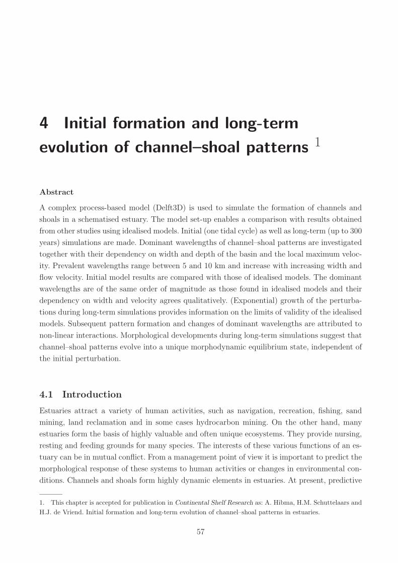
4 Initial formation and long-term
evolution of channel–shoal patterns 1
Abstract
A complex process-based model (Delft3D) is used to simulate the formation of channels and
shoals in a schematised estuary. The model set-up enables a comparison with results obtained
from other studies using idealised models. Initial (one tidal cycle) as well as long-term (up to 300
years) simulations are made. Dominant wavelengths of channel–shoal patterns are investigated
together with their dependency on width and depth of the basin and the local maximum veloc-
ity. Prevalent wavelengths range between 5 and 10 km and increase with increasing width and
flow velocity. Initial model results are compared with those of idealised models. The dominant
wavelengths are of the same order of magnitude as those found in idealised models and their
dependency on width and velocity agrees qualitatively. (Exponential) growth of the perturba-
tions during long-term simulations provides information on the limits of validity of the idealised
models. Subsequent pattern formation and changes of dominant wavelengths are attributed to
non-linear interactions. Morphological developments during long-term simulations suggest that
channel–shoal patterns evolve into a unique morphodynamic equilibrium state, independent of
the initial perturbation.
4.1 Introduction
Estuaries attract a variety of human activities, such as navigation, recreation, fishing, sand
mining, land reclamation and in some cases hydrocarbon mining. On the other hand, many
estuaries form the basis of highly valuable and often unique ecosystems. They provide nursing,
resting and feeding grounds for many species. The interests of these various functions of an es-
tuary can be in mutual conflict. From a management point of view it is important to predict the
morphological response of these systems to human activities or changes in environmental con-
ditions. Channels and shoals form highly dynamic elements in estuaries. At present, predictive
1. This chapter is accepted for publication in Continental Shelf Research as: A. Hibma, H.M. Schuttelaars andH.J. de Vriend. Initial formation and long-term evolution of channel–shoal patterns in estuaries.
57
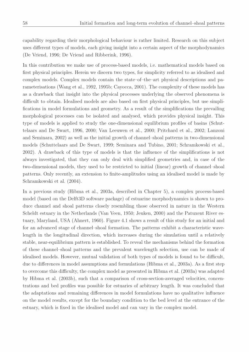
58 Initial formation and long-term evolution of channel–shoal patterns
capability regarding their morphological behaviour is rather limited. Research on this subject
uses different types of models, each giving insight into a certain aspect of the morphodynamics
(De Vriend, 1996; De Vriend and Ribberink, 1996).
In this contribution we make use of process-based models, i.e. mathematical models based on
first physical principles. Herein we discern two types, for simplicity referred to as idealised and
complex models. Complex models contain the state–of–the–art physical descriptions and pa-
rameterisations (Wang et al., 1992, 1995b; Cayocca, 2001). The complexity of these models has
as a drawback that insight into the physical processes underlying the observed phenomena is
difficult to obtain. Idealised models are also based on first physical principles, but use simpli-
fications in model formulations and geometry. As a result of the simplifications the prevailing
morphological processes can be isolated and analysed, which provides physical insight. This
type of models is applied to study the one-dimensional equilibrium profiles of basins (Schut-
telaars and De Swart, 1996, 2000; Van Leeuwen et al., 2000; Pritchard et al., 2002; Lanzoni
and Seminara, 2002) as well as the initial growth of channel–shoal patterns in two-dimensional
models (Schuttelaars and De Swart, 1999; Seminara and Tubino, 2001; Schramkowski et al.,
2002). A drawback of this type of models is that the influence of the simplifications is not
always investigated, that they can only deal with simplified geometries and, in case of the
two-dimensional models, they used to be restricted to initial (linear) growth of channel–shoal
patterns. Only recently, an extension to finite-amplitudes using an idealised model is made by
Schramkowski et al. (2004).
In a previous study (Hibma et al., 2003a, described in Chapter 5), a complex process-based
model (based on the Delft3D software package) of estuarine morphodynamics is shown to pro-
duce channel and shoal patterns closely resembling those observed in nature in the Western
Scheldt estuary in the Netherlands (Van Veen, 1950; Jeuken, 2000) and the Patuxent River es-
tuary, Maryland, USA (Ahnert, 1960). Figure 4.1 shows a result of this study for an initial and
for an advanced stage of channel–shoal formation. The patterns exhibit a characteristic wave-
length in the longitudinal direction, which increases during the simulation until a relatively
stable, near-equilibrium pattern is established. To reveal the mechanisms behind the formation
of these channel–shoal patterns and the prevalent wavelength selection, use can be made of
idealised models. However, mutual validation of both types of models is found to be difficult,
due to differences in model assumptions and formulations (Hibma et al., 2003a). As a first step
to overcome this difficulty, the complex model as presented in Hibma et al. (2003a) was adapted
by Hibma et al. (2003b), such that a comparison of cross-section-averaged velocities, concen-
trations and bed profiles was possible for estuaries of arbitrary length. It was concluded that
the adaptations and remaining differences in model formulations have no qualitative influence
on the model results, except for the boundary condition to the bed level at the entrance of the
estuary, which is fixed in the idealised model and can vary in the complex model.
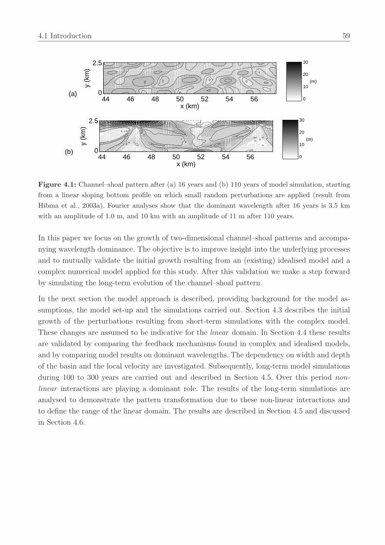
4.1 Introduction 59
44 46 48 50 52 54 560
2.5
x (km)
y (k
m)
(m)
(a)0
10
20
30
44 46 48 50 52 54 560
2.5
x (km)
y (k
m)
(m)
(b)0
10
20
30
Figure 4.1: Channel–shoal pattern after (a) 16 years and (b) 110 years of model simulation, startingfrom a linear sloping bottom profile on which small random perturbations are applied (result fromHibma et al., 2003a). Fourier analyses show that the dominant wavelength after 16 years is 3.5 kmwith an amplitude of 1.0 m, and 10 km with an amplitude of 11 m after 110 years.
In this paper we focus on the growth of two-dimensional channel–shoal patterns and accompa-
nying wavelength dominance. The objective is to improve insight into the underlying processes
and to mutually validate the initial growth resulting from an (existing) idealised model and a
complex numerical model applied for this study. After this validation we make a step forward
by simulating the long-term evolution of the channel–shoal pattern.
In the next section the model approach is described, providing background for the model as-
sumptions, the model set-up and the simulations carried out. Section 4.3 describes the initial
growth of the perturbations resulting from short-term simulations with the complex model.
These changes are assumed to be indicative for the linear domain. In Section 4.4 these results
are validated by comparing the feedback mechanisms found in complex and idealised models,
and by comparing model results on dominant wavelengths. The dependency on width and depth
of the basin and the local velocity are investigated. Subsequently, long-term model simulations
during 100 to 300 years are carried out and described in Section 4.5. Over this period non-
linear interactions are playing a dominant role. The results of the long-term simulations are
analysed to demonstrate the pattern transformation due to these non-linear interactions and
to define the range of the linear domain. The results are described in Section 4.5 and discussed
in Section 4.6.
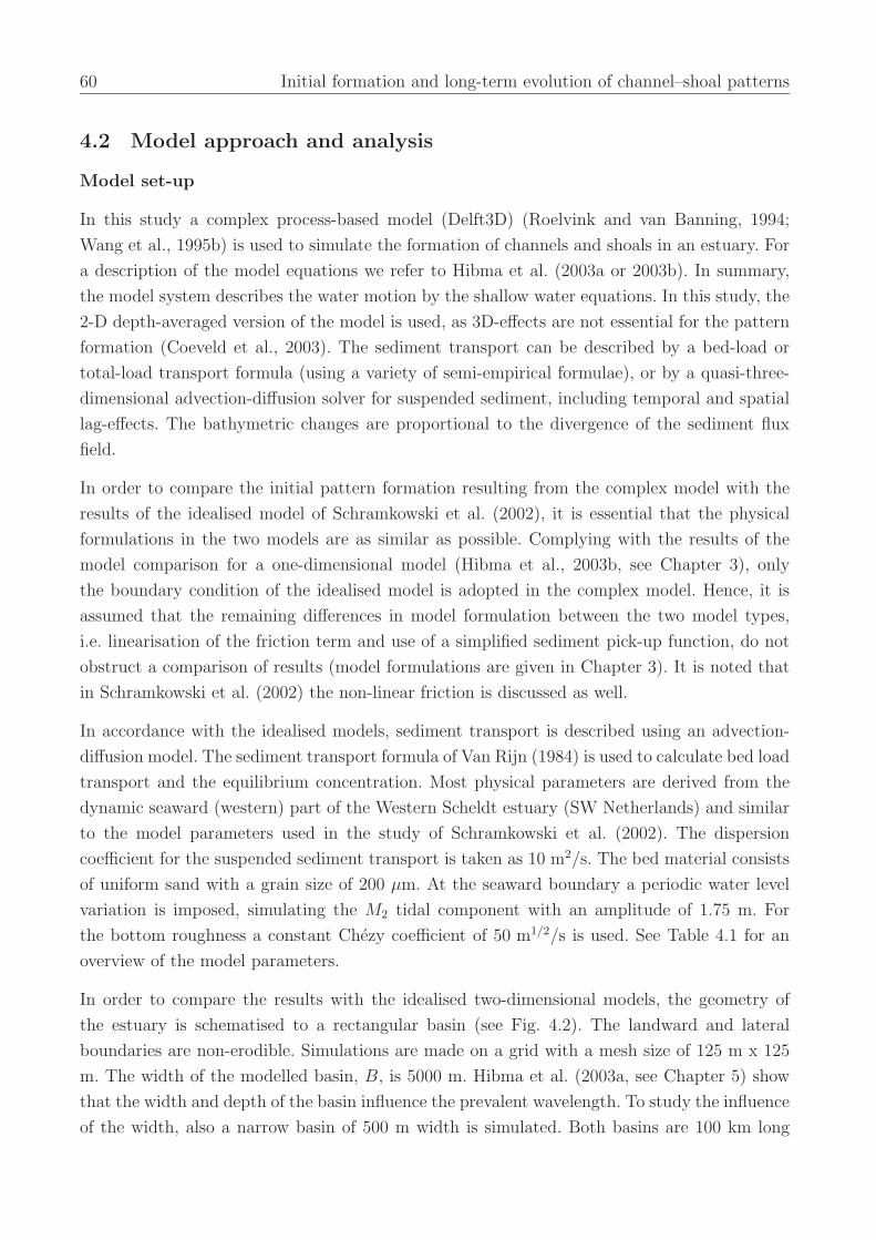
60 Initial formation and long-term evolution of channel–shoal patterns
4.2 Model approach and analysis
Model set-up
In this study a complex process-based model (Delft3D) (Roelvink and van Banning, 1994;
Wang et al., 1995b) is used to simulate the formation of channels and shoals in an estuary. For
a description of the model equations we refer to Hibma et al. (2003a or 2003b). In summary,
the model system describes the water motion by the shallow water equations. In this study, the
2-D depth-averaged version of the model is used, as 3D-effects are not essential for the pattern
formation (Coeveld et al., 2003). The sediment transport can be described by a bed-load or
total-load transport formula (using a variety of semi-empirical formulae), or by a quasi-three-
dimensional advection-diffusion solver for suspended sediment, including temporal and spatial
lag-effects. The bathymetric changes are proportional to the divergence of the sediment flux
field.
In order to compare the initial pattern formation resulting from the complex model with the
results of the idealised model of Schramkowski et al. (2002), it is essential that the physical
formulations in the two models are as similar as possible. Complying with the results of the
model comparison for a one-dimensional model (Hibma et al., 2003b, see Chapter 3), only
the boundary condition of the idealised model is adopted in the complex model. Hence, it is
assumed that the remaining differences in model formulation between the two model types,
i.e. linearisation of the friction term and use of a simplified sediment pick-up function, do not
obstruct a comparison of results (model formulations are given in Chapter 3). It is noted that
in Schramkowski et al. (2002) the non-linear friction is discussed as well.
In accordance with the idealised models, sediment transport is described using an advection-
diffusion model. The sediment transport formula of Van Rijn (1984) is used to calculate bed load
transport and the equilibrium concentration. Most physical parameters are derived from the
dynamic seaward (western) part of the Western Scheldt estuary (SW Netherlands) and similar
to the model parameters used in the study of Schramkowski et al. (2002). The dispersion
coefficient for the suspended sediment transport is taken as 10 m2/s. The bed material consists
of uniform sand with a grain size of 200 µm. At the seaward boundary a periodic water level
variation is imposed, simulating the M2 tidal component with an amplitude of 1.75 m. For
the bottom roughness a constant Chezy coefficient of 50 m1/2/s is used. See Table 4.1 for an
overview of the model parameters.
In order to compare the results with the idealised two-dimensional models, the geometry of
the estuary is schematised to a rectangular basin (see Fig. 4.2). The landward and lateral
boundaries are non-erodible. Simulations are made on a grid with a mesh size of 125 m x 125
m. The width of the modelled basin, B, is 5000 m. Hibma et al. (2003a, see Chapter 5) show
that the width and depth of the basin influence the prevalent wavelength. To study the influence
of the width, also a narrow basin of 500 m width is simulated. Both basins are 100 km long
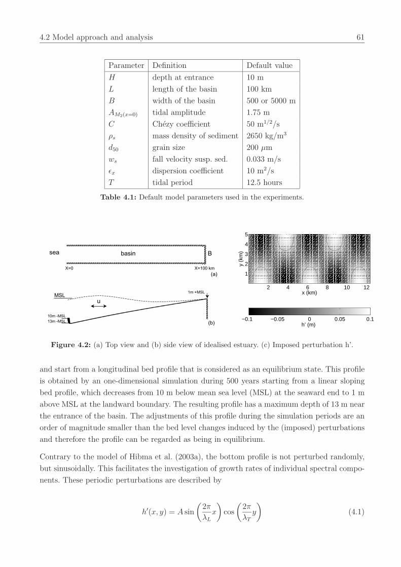
4.2 Model approach and analysis 61
Parameter Definition Default value
H depth at entrance 10 m
L length of the basin 100 km
B width of the basin 500 or 5000 m
AM2(x=0) tidal amplitude 1.75 m
C Chezy coefficient 50 m1/2/s
ρs mass density of sediment 2650 kg/m3
d50 grain size 200 µm
ws fall velocity susp. sed. 0.033 m/s
εx dispersion coefficient 10 m2/s
T tidal period 12.5 hours
Table 4.1: Default model parameters used in the experiments.
2 4 6 8 10 12
1
2
3
4
5
x (km)
y (k
m)
−0.1 −0.05 0 0.05 0.1h’ (m)
Figure 4.2: (a) Top view and (b) side view of idealised estuary. (c) Imposed perturbation h’.
and start from a longitudinal bed profile that is considered as an equilibrium state. This profile
is obtained by an one-dimensional simulation during 500 years starting from a linear sloping
bed profile, which decreases from 10 m below mean sea level (MSL) at the seaward end to 1 m
above MSL at the landward boundary. The resulting profile has a maximum depth of 13 m near
the entrance of the basin. The adjustments of this profile during the simulation periods are an
order of magnitude smaller than the bed level changes induced by the (imposed) perturbations
and therefore the profile can be regarded as being in equilibrium.
Contrary to the model of Hibma et al. (2003a), the bottom profile is not perturbed randomly,
but sinusoidally. This facilitates the investigation of growth rates of individual spectral compo-
nents. These periodic perturbations are described by
h′(x, y) = A sin
(2π
λL
x
)cos
(2π
λT
y
)(4.1)
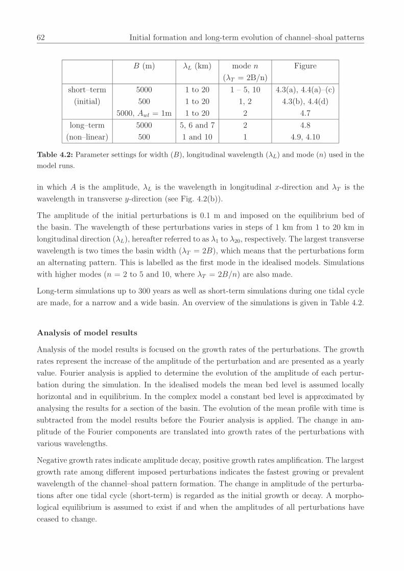
62 Initial formation and long-term evolution of channel–shoal patterns
B (m) λL (km) mode n Figure
(λT = 2B/n)
short–term 5000 1 to 20 1 – 5, 10 4.3(a), 4.4(a)–(c)
(initial) 500 1 to 20 1, 2 4.3(b), 4.4(d)
5000, Awl = 1m 1 to 20 2 4.7
long–term 5000 5, 6 and 7 2 4.8
(non–linear) 500 1 and 10 1 4.9, 4.10
Table 4.2: Parameter settings for width (B), longitudinal wavelength (λL) and mode (n) used in themodel runs.
in which A is the amplitude, λL is the wavelength in longitudinal x-direction and λT is the
wavelength in transverse y-direction (see Fig. 4.2(b)).
The amplitude of the initial perturbations is 0.1 m and imposed on the equilibrium bed of
the basin. The wavelength of these perturbations varies in steps of 1 km from 1 to 20 km in
longitudinal direction (λL), hereafter referred to as λ1 to λ20, respectively. The largest transverse
wavelength is two times the basin width (λT = 2B), which means that the perturbations form
an alternating pattern. This is labelled as the first mode in the idealised models. Simulations
with higher modes (n = 2 to 5 and 10, where λT = 2B/n) are also made.
Long-term simulations up to 300 years as well as short-term simulations during one tidal cycle
are made, for a narrow and a wide basin. An overview of the simulations is given in Table 4.2.
Analysis of model results
Analysis of the model results is focused on the growth rates of the perturbations. The growth
rates represent the increase of the amplitude of the perturbation and are presented as a yearly
value. Fourier analysis is applied to determine the evolution of the amplitude of each pertur-
bation during the simulation. In the idealised models the mean bed level is assumed locally
horizontal and in equilibrium. In the complex model a constant bed level is approximated by
analysing the results for a section of the basin. The evolution of the mean profile with time is
subtracted from the model results before the Fourier analysis is applied. The change in am-
plitude of the Fourier components are translated into growth rates of the perturbations with
various wavelengths.
Negative growth rates indicate amplitude decay, positive growth rates amplification. The largest
growth rate among different imposed perturbations indicates the fastest growing or prevalent
wavelength of the channel–shoal pattern formation. The change in amplitude of the perturba-
tions after one tidal cycle (short-term) is regarded as the initial growth or decay. A morpho-
logical equilibrium is assumed to exist if and when the amplitudes of all perturbations have
ceased to change.
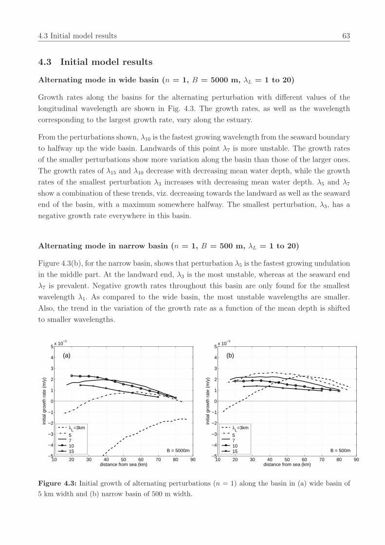
4.3 Initial model results 63
4.3 Initial model results
Alternating mode in wide basin (n = 1, B = 5000 m, λL = 1 to 20)
Growth rates along the basins for the alternating perturbation with different values of the
longitudinal wavelength are shown in Fig. 4.3. The growth rates, as well as the wavelength
corresponding to the largest growth rate, vary along the estuary.
From the perturbations shown, λ10 is the fastest growing wavelength from the seaward boundary
to halfway up the wide basin. Landwards of this point λ7 is more unstable. The growth rates
of the smaller perturbations show more variation along the basin than those of the larger ones.
The growth rates of λ15 and λ10 decrease with decreasing mean water depth, while the growth
rates of the smallest perturbation λ3 increases with decreasing mean water depth. λ5 and λ7
show a combination of these trends, viz. decreasing towards the landward as well as the seaward
end of the basin, with a maximum somewhere halfway. The smallest perturbation, λ3, has a
negative growth rate everywhere in this basin.
Alternating mode in narrow basin (n = 1, B = 500 m, λL = 1 to 20)
Figure 4.3(b), for the narrow basin, shows that perturbation λ5 is the fastest growing undulation
in the middle part. At the landward end, λ3 is the most unstable, whereas at the seaward end
λ7 is prevalent. Negative growth rates throughout this basin are only found for the smallest
wavelength λ1. As compared to the wide basin, the most unstable wavelengths are smaller.
Also, the trend in the variation of the growth rate as a function of the mean depth is shifted
to smaller wavelengths.
10 20 30 40 50 60 70 80 90−5
−4
−3
−2
−1
0
1
2
3
4
5x 10
−3
distance from sea (km)
initi
al g
row
th r
ate
(m/y
)
B = 5000m
(a)
λL=3km
571015
10 20 30 40 50 60 70 80 90−5
−4
−3
−2
−1
0
1
2
3
4
5x 10
−3
distance from sea (km)
initi
al g
row
th r
ate
(m/y
)
B = 500m
(b)
λL=3km
571015
Figure 4.3: Initial growth of alternating perturbations (n = 1) along the basin in (a) wide basin of5 km width and (b) narrow basin of 500 m width.
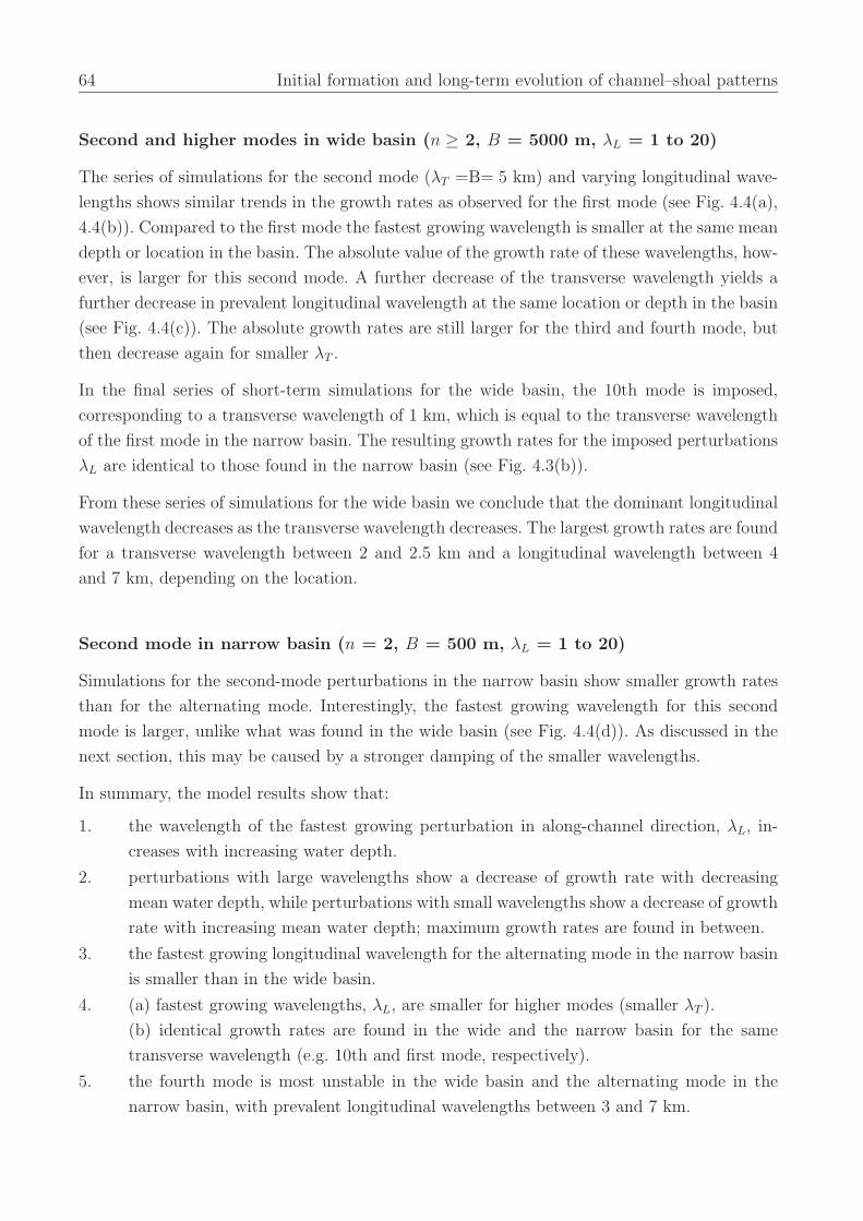
64 Initial formation and long-term evolution of channel–shoal patterns
Second and higher modes in wide basin (n ≥ 2, B = 5000 m, λL = 1 to 20)
The series of simulations for the second mode (λT =B= 5 km) and varying longitudinal wave-
lengths shows similar trends in the growth rates as observed for the first mode (see Fig. 4.4(a),
4.4(b)). Compared to the first mode the fastest growing wavelength is smaller at the same mean
depth or location in the basin. The absolute value of the growth rate of these wavelengths, how-
ever, is larger for this second mode. A further decrease of the transverse wavelength yields a
further decrease in prevalent longitudinal wavelength at the same location or depth in the basin
(see Fig. 4.4(c)). The absolute growth rates are still larger for the third and fourth mode, but
then decrease again for smaller λT .
In the final series of short-term simulations for the wide basin, the 10th mode is imposed,
corresponding to a transverse wavelength of 1 km, which is equal to the transverse wavelength
of the first mode in the narrow basin. The resulting growth rates for the imposed perturbations
λL are identical to those found in the narrow basin (see Fig. 4.3(b)).
From these series of simulations for the wide basin we conclude that the dominant longitudinal
wavelength decreases as the transverse wavelength decreases. The largest growth rates are found
for a transverse wavelength between 2 and 2.5 km and a longitudinal wavelength between 4
and 7 km, depending on the location.
Second mode in narrow basin (n = 2, B = 500 m, λL = 1 to 20)
Simulations for the second-mode perturbations in the narrow basin show smaller growth rates
than for the alternating mode. Interestingly, the fastest growing wavelength for this second
mode is larger, unlike what was found in the wide basin (see Fig. 4.4(d)). As discussed in the
next section, this may be caused by a stronger damping of the smaller wavelengths.
In summary, the model results show that:
1. the wavelength of the fastest growing perturbation in along-channel direction, λL, in-
creases with increasing water depth.
2. perturbations with large wavelengths show a decrease of growth rate with decreasing
mean water depth, while perturbations with small wavelengths show a decrease of growth
rate with increasing mean water depth; maximum growth rates are found in between.
3. the fastest growing longitudinal wavelength for the alternating mode in the narrow basin
is smaller than in the wide basin.
4. (a) fastest growing wavelengths, λL, are smaller for higher modes (smaller λT ).
(b) identical growth rates are found in the wide and the narrow basin for the same
transverse wavelength (e.g. 10th and first mode, respectively).
5. the fourth mode is most unstable in the wide basin and the alternating mode in the
narrow basin, with prevalent longitudinal wavelengths between 3 and 7 km.
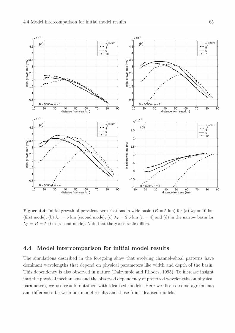
4.4 Model intercomparison for initial model results 65
10 20 30 40 50 60 70 80 900
0.5
1
1.5
2
2.5
3
3.5
4
4.5
5x 10
−3
distance from sea (km)
initi
al g
row
th r
ate
(m/y
)
B = 5000m, n = 1
(a) λL=7km
8910
10 20 30 40 50 60 70 80 900
0.5
1
1.5
2
2.5
3
3.5
4
4.5
5x 10
−3
distance from sea (km)
initi
al g
row
th r
ate
(m/y
)
B = 5000m, n = 2
(b) λL=4km
567
10 20 30 40 50 60 70 80 900
0.5
1
1.5
2
2.5
3
3.5
4
4.5
5x 10
−3
distance from sea (km)
initi
al g
row
th r
ate
(m/y
)
B = 5000m, n = 4
(c) λL=3km
456
10 20 30 40 50 60 70 80 90−1
−0.5
0
0.5
1
1.5
2
2.5
3x 10
−3
distance from sea (km)
initi
al g
row
th r
ate
(m/y
)
B = 500m, n = 2
(d)λ
L=3km
6912
Figure 4.4: Initial growth of prevalent perturbations in wide basin (B = 5 km) for (a) λT = 10 km(first mode), (b) λT = 5 km (second mode), (c) λT = 2.5 km (n = 4) and (d) in the narrow basin forλT = B = 500 m (second mode). Note that the y-axis scale differs.
4.4 Model intercomparison for initial model results
The simulations described in the foregoing show that evolving channel–shoal patterns have
dominant wavelengths that depend on physical parameters like width and depth of the basin.
This dependency is also observed in nature (Dalrymple and Rhodes, 1995). To increase insight
into the physical mechanisms and the observed dependency of preferred wavelengths on physical
parameters, we use results obtained with idealised models. Here we discuss some agreements
and differences between our model results and those from idealised models.
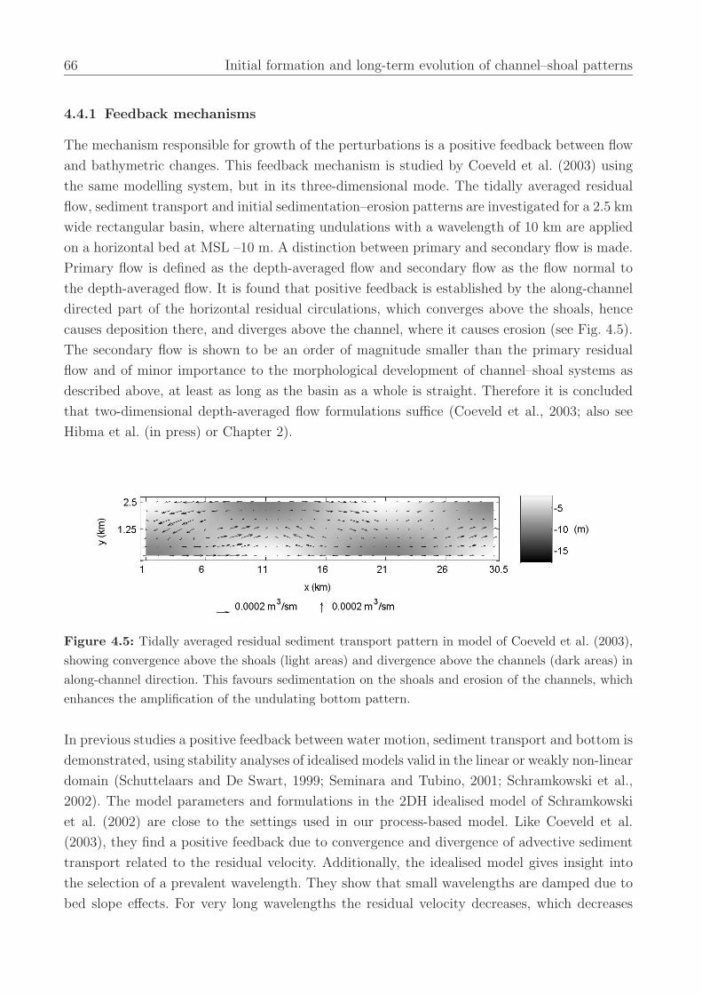
66 Initial formation and long-term evolution of channel–shoal patterns
4.4.1 Feedback mechanisms
The mechanism responsible for growth of the perturbations is a positive feedback between flow
and bathymetric changes. This feedback mechanism is studied by Coeveld et al. (2003) using
the same modelling system, but in its three-dimensional mode. The tidally averaged residual
flow, sediment transport and initial sedimentation–erosion patterns are investigated for a 2.5 km
wide rectangular basin, where alternating undulations with a wavelength of 10 km are applied
on a horizontal bed at MSL –10 m. A distinction between primary and secondary flow is made.
Primary flow is defined as the depth-averaged flow and secondary flow as the flow normal to
the depth-averaged flow. It is found that positive feedback is established by the along-channel
directed part of the horizontal residual circulations, which converges above the shoals, hence
causes deposition there, and diverges above the channel, where it causes erosion (see Fig. 4.5).
The secondary flow is shown to be an order of magnitude smaller than the primary residual
flow and of minor importance to the morphological development of channel–shoal systems as
described above, at least as long as the basin as a whole is straight. Therefore it is concluded
that two-dimensional depth-averaged flow formulations suffice (Coeveld et al., 2003; also see
Hibma et al. (in press) or Chapter 2).
Figure 4.5: Tidally averaged residual sediment transport pattern in model of Coeveld et al. (2003),showing convergence above the shoals (light areas) and divergence above the channels (dark areas) inalong-channel direction. This favours sedimentation on the shoals and erosion of the channels, whichenhances the amplification of the undulating bottom pattern.
In previous studies a positive feedback between water motion, sediment transport and bottom is
demonstrated, using stability analyses of idealised models valid in the linear or weakly non-linear
domain (Schuttelaars and De Swart, 1999; Seminara and Tubino, 2001; Schramkowski et al.,
2002). The model parameters and formulations in the 2DH idealised model of Schramkowski
et al. (2002) are close to the settings used in our process-based model. Like Coeveld et al.
(2003), they find a positive feedback due to convergence and divergence of advective sediment
transport related to the residual velocity. Additionally, the idealised model gives insight into
the selection of a prevalent wavelength. They show that small wavelengths are damped due to
bed slope effects. For very long wavelengths the residual velocity decreases, which decreases
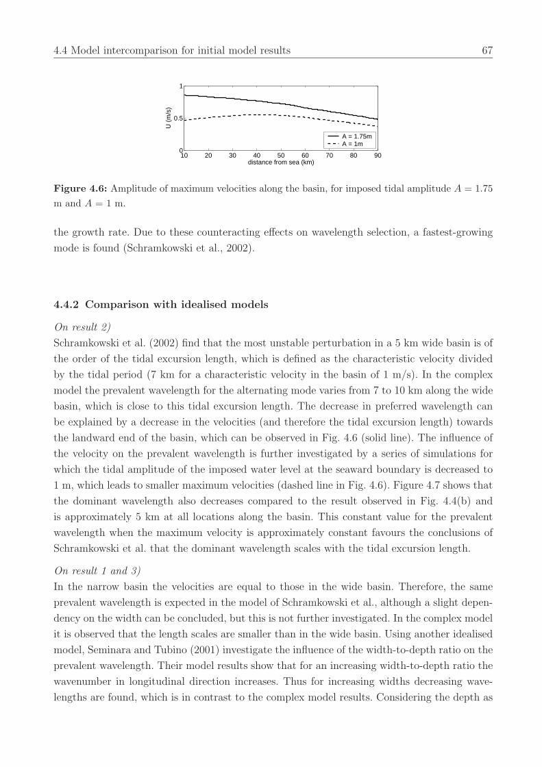
4.4 Model intercomparison for initial model results 67
10 20 30 40 50 60 70 80 900
0.5
1
distance from sea (km)U
(m
/s)
A = 1.75mA = 1m
Figure 4.6: Amplitude of maximum velocities along the basin, for imposed tidal amplitude A = 1.75m and A = 1 m.
the growth rate. Due to these counteracting effects on wavelength selection, a fastest-growing
mode is found (Schramkowski et al., 2002).
4.4.2 Comparison with idealised models
On result 2)
Schramkowski et al. (2002) find that the most unstable perturbation in a 5 km wide basin is of
the order of the tidal excursion length, which is defined as the characteristic velocity divided
by the tidal period (7 km for a characteristic velocity in the basin of 1 m/s). In the complex
model the prevalent wavelength for the alternating mode varies from 7 to 10 km along the wide
basin, which is close to this tidal excursion length. The decrease in preferred wavelength can
be explained by a decrease in the velocities (and therefore the tidal excursion length) towards
the landward end of the basin, which can be observed in Fig. 4.6 (solid line). The influence of
the velocity on the prevalent wavelength is further investigated by a series of simulations for
which the tidal amplitude of the imposed water level at the seaward boundary is decreased to
1 m, which leads to smaller maximum velocities (dashed line in Fig. 4.6). Figure 4.7 shows that
the dominant wavelength also decreases compared to the result observed in Fig. 4.4(b) and
is approximately 5 km at all locations along the basin. This constant value for the prevalent
wavelength when the maximum velocity is approximately constant favours the conclusions of
Schramkowski et al. that the dominant wavelength scales with the tidal excursion length.
On result 1 and 3)
In the narrow basin the velocities are equal to those in the wide basin. Therefore, the same
prevalent wavelength is expected in the model of Schramkowski et al., although a slight depen-
dency on the width can be concluded, but this is not further investigated. In the complex model
it is observed that the length scales are smaller than in the wide basin. Using another idealised
model, Seminara and Tubino (2001) investigate the influence of the width-to-depth ratio on the
prevalent wavelength. Their model results show that for an increasing width-to-depth ratio the
wavenumber in longitudinal direction increases. Thus for increasing widths decreasing wave-
lengths are found, which is in contrast to the complex model results. Considering the depth as
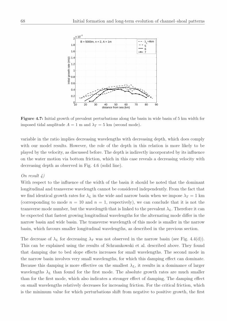
68 Initial formation and long-term evolution of channel–shoal patterns
10 20 30 40 50 60 70 80 900
0.2
0.4
0.6
0.8
1
1.2
1.4
1.6
1.8
2x 10
−3
distance from sea (km)
initi
al g
row
th r
ate
(m/y
)
B = 5000m, n = 2, A = 1m λL=4km
567
Figure 4.7: Initial growth of prevalent perturbations along the basin in wide basin of 5 km width forimposed tidal amplitude A = 1 m and λT = 5 km (second mode).
variable in the ratio implies decreasing wavelengths with decreasing depth, which does comply
with our model results. However, the role of the depth in this relation is more likely to be
played by the velocity, as discussed before. The depth is indirectly incorporated by its influence
on the water motion via bottom friction, which in this case reveals a decreasing velocity with
decreasing depth as observed in Fig. 4.6 (solid line).
On result 4)
With respect to the influence of the width of the basin it should be noted that the dominant
longitudinal and transverse wavelength cannot be considered independently. From the fact that
we find identical growth rates for λL in the wide and narrow basin when we impose λT = 1 km
(corresponding to mode n = 10 and n = 1, respectively), we can conclude that it is not the
transverse mode number, but the wavelength that is linked to the prevalent λL. Therefore it can
be expected that fastest growing longitudinal wavelengths for the alternating mode differ in the
narrow basin and wide basin. The transverse wavelength of this mode is smaller in the narrow
basin, which favours smaller longitudinal wavelengths, as described in the previous section.
The decrease of λL for decreasing λT was not observed in the narrow basin (see Fig. 4.4(d)).
This can be explained using the results of Schramkowski et al. described above. They found
that damping due to bed slope effects increases for small wavelengths. The second mode in
the narrow basin involves very small wavelengths, for which this damping effect can dominate.
Because this damping is more effective on the smallest λL, it results in a dominance of larger
wavelengths λL than found for the first mode. The absolute growth rates are much smaller
than for the first mode, which also indicates a stronger effect of damping. The damping effect
on small wavelengths relatively decreases for increasing friction. For the critical friction, which
is the minimum value for which perturbations shift from negative to positive growth, the first
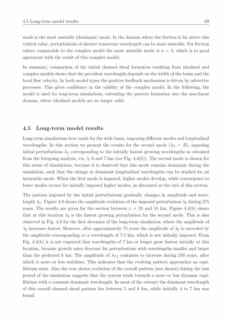
4.5 Long-term model results 69
mode is the most unstable (dominant) mode. In the domain where the friction is far above this
critical value, perturbations of shorter transverse wavelength can be more unstable. For friction
values comparable to the complex model the most unstable mode is n = 5, which is in good
agreement with the result of this complex model.
In summary, comparison of the initial channel–shoal formation resulting from idealised and
complex models shows that the prevalent wavelength depends on the width of the basin and the
local flow velocity. In both model types the positive feedback mechanism is driven by advective
processes. This gives confidence in the validity of the complex model. In the following, the
model is used for long-term simulations, extending the pattern formation into the non-linear
domain, where idealised models are no longer valid.
4.5 Long-term model results
Long-term simulations were made for the wide basin, imposing different modes and longitudinal
wavelengths. In this section we present the results for the second mode (λT = B), imposing
initial perturbations λL corresponding to the initially fastest growing wavelengths as obtained
from the foregoing analysis, viz. 5, 6 and 7 km (see Fig. 4.4(b)). The second mode is chosen for
this series of simulations, because it is observed that this mode remains dominant during the
simulation, such that the change in dominant longitudinal wavelengths can be studied for an
invariable mode. When the first mode is imposed, higher modes develop, while convergence to
lower modes occurs for initially imposed higher modes, as discussed at the end of this section.
The pattern imposed by the initial perturbations gradually changes in amplitude and wave-
length λL. Figure 4.8 shows the amplitude evolution of the imposed perturbation λ6 during 275
years. The results are given for the section between x = 25 and 55 km. Figure 4.4(b) shows
that at this location λ6 is the fastest growing perturbation for the second mode. This is also
observed in Fig. 4.8 for the first decennia of the long-term simulation, where the amplitude of
λ6 increases fastest. However, after approximately 75 years the amplitude of λ6 is exceeded by
the amplitude corresponding to a wavelength of 7.5 km, which is not initially imposed. From
Fig. 4.4(b) it is not expected that wavelengths of 7 km or longer grow fastest initially at this
location, because growth rates decrease for perturbations with wavelengths smaller and larger
than the preferred 6 km. The amplitude of λ7.5 continues to increase during 250 years, after
which it more or less stabilises. This indicates that the evolving pattern approaches an equi-
librium state. Also the ever slower evolution of the overall pattern (not shown) during the last
period of the simulation suggests that the system tends towards a more or less dynamic equi-
librium with a constant dominant wavelength. In most of the estuary the dominant wavelength
of this overall channel–shoal pattern lies between 5 and 8 km, while initially 4 to 7 km was
found.
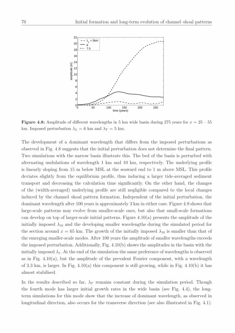
70 Initial formation and long-term evolution of channel–shoal patterns
0 50 100 150 200 2500
2
4
6
8
10
12
14
16
18
20
22
time (years)
ampl
itude
(m
)
λL = 5km
67.5
Figure 4.8: Amplitude of different wavelengths in 5 km wide basin during 275 years for x = 25 – 55km. Imposed perturbation λL = 6 km and λT = 5 km.
The development of a dominant wavelength that differs from the imposed perturbations as
observed in Fig. 4.8 suggests that the initial perturbation does not determine the final pattern.
Two simulations with the narrow basin illustrate this. The bed of the basin is perturbed with
alternating undulations of wavelength 1 km and 10 km, respectively. The underlying profile
is linearly sloping from 15 m below MSL at the seaward end to 1 m above MSL. This profile
deviates slightly from the equilibrium profile, thus inducing a larger tide-averaged sediment
transport and decreasing the calculation time significantly. On the other hand, the changes
of the (width-averaged) underlying profile are still negligible compared to the local changes
induced by the channel–shoal pattern formation. Independent of the initial perturbation, the
dominant wavelength after 100 years is approximately 3 km in either case. Figure 4.9 shows that
large-scale patterns may evolve from smaller-scale ones, but also that small-scale formations
can develop on top of larger-scale initial patterns. Figure 4.10(a) presents the amplitude of the
initially imposed λ10 and the developing smaller wavelengths during the simulated period for
the section around x = 65 km. The growth of the initially imposed λ10 is smaller than that of
the emerging smaller-scale modes. After 100 years the amplitude of smaller wavelengths exceeds
the imposed perturbation. Additionally, Fig. 4.10(b) shows the amplitudes in the basin with the
initially imposed λ1. At the end of the simulation the same preference of wavelengths is observed
as in Fig. 4.10(a), but the amplitude of the prevalent Fourier component, with a wavelength
of 3.3 km, is larger. In Fig. 4.10(a) this component is still growing, while in Fig. 4.10(b) it has
almost stabilised.
In the results described so far, λT remains constant during the simulation period. Though
the fourth mode has larger initial growth rates in the wide basin (see Fig. 4.4), the long-
term simulations for this mode show that the increase of dominant wavelength, as observed in
longitudinal direction, also occurs for the transverse direction (see also illustrated in Fig. 4.1).
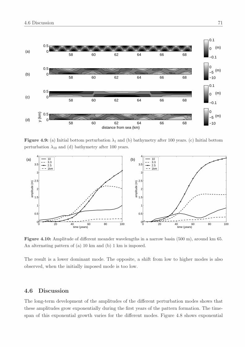
4.6 Discussion 71
58 60 62 64 66 680
0.5
(a)(m)
−0.1
0
0.1
58 60 62 64 66 680
0.5
(b)(m)
−10−50
58 60 62 64 66 680
0.5
(c)(m)
−0.1
0
0.1
58 60 62 64 66 680
0.5
distance from sea (km)
y (k
m)
(d)(m)
−10
−5
0
Figure 4.9: (a) Initial bottom perturbation λ1 and (b) bathymetry after 100 years. (c) Initial bottomperturbation λ10 and (d) bathymetry after 100 years.
0 20 40 60 80 1000
0.5
1
1.5
2
2.5
3
3.5
4
time (years)
ampl
itude
(m
)
(a) 103.32.51km
0 20 40 60 80 1000
0.5
1
1.5
2
2.5
3
3.5
4
time (years)
ampl
itude
(m
)
(b) 103.32.51km
Figure 4.10: Amplitude of different meander wavelengths in a narrow basin (500 m), around km 65.An alternating pattern of (a) 10 km and (b) 1 km is imposed.
The result is a lower dominant mode. The opposite, a shift from low to higher modes is also
observed, when the initially imposed mode is too low.
4.6 Discussion
The long-term development of the amplitudes of the different perturbation modes shows that
these amplitudes grow exponentially during the first years of the pattern formation. The time-
span of this exponential growth varies for the different modes. Figure 4.8 shows exponential
72 Initial formation and long-term evolution of channel–shoal patterns
growth of perturbation λ6 during 60 years and the growth of the emerged perturbation λ7.5
can be regarded as exponential during 120 years. Also the amplitudes of damped perturbations
decay exponentially. The exponential growth suggests that during this period the amplitudes are
so small that non-linear interaction of the perturbations can be neglected. Hence, the evolution
can be described using a linear set of equations.
This allows for the comparison between the initial results of the complex model and idealised
models. The prevalent wavelength is related to the local velocity and the width of the basin. In
the long-term simulations an increase of the dominant wavelength was observed for the second
and higher modes in the wide basin. This can be explained by a change in the local velocities
over the width of the basin as a channel–shoal pattern emerges. The velocities decrease over the
deposition areas and increase in the eroding channels due to the influence of bottom friction.
The increased velocity in the channels increases the inertial length scale and is likely to increase
the meander wavelength.
The opposite, the emergence of smaller dominant wavelengths, is observed for the first mode,
when the imposed perturbations are much longer than the initially preferred lengths. This can
be triggered by very small perturbations induced by computational round offs, which grow
faster than the large scale imposed perturbations. These observations, as well as the results
for the narrow basin, suggest that channel–shoal patterns evolve into a unique morphodynamic
equilibrium state, independent of the initial perturbation. For basins with initially small and
random perturbations, therefore including all wavelengths, it is expected and observed that
the evolving channel–shoal pattern shows similar characteristics and increasing length scales,
resulting in a unique morphodynamic equilibrium state.
As discussed in Hibma et al. (2003b), a static equilibrium with the tidally averaged sediment
transport identically equal to zero cannot be found using this model. Therefore, a dynamic
equilibrium state is considered to be reached when the change in amplitudes of all perturba-
tions is negligible. Starting from different initial perturbations, the achieved morphodynamic
equilibria are not identical, but have the same pattern characteristics, composed of the same
dominant wavelengths.
The increase of the dominant longitudinal wavelength is stronger in the case of a random initial
perturbation than in the model simulations described in the present paper. This is attributed
to the additional change in transverse wavelength, which was chosen constant here. When
starting from random perturbations, the initially emerging dominant transverse wavelength is
small (smaller than imposed in the present long-term simulations), and it is accompanied by
small dominant longitudinal wavelengths. Both tend to increase, and since the longitudinal
wavelength also depends on λT , the increase of the latter is enhanced.
During the long-term simulations the period of exponential growth of the perturbations indi-
cates the applicability range of the idealised models. At a certain point in time, the amplitude
ceases to grow or decay exponentially, after which the linearisation of the equations is no longer
4.7 Conclusion 73
valid. The subsequent evolution of the pattern, particularly the change in preferent wavelength,
is determined by non-linear interactions and can therefore not be described by linearised mod-
els. Model results for this stage of pattern development can be validated against field data.
Patterns resulting from the complex model and from field observations are shown to agree in
Hibma et al. (2003a, described in Chapter 5), despite simplifications in model parameters and
geometry. From sensitivity simulations is concluded that the applied sediment transport formu-
lation and grain size mainly influence the time scale, not the large scale pattern development.
For further study it is interesting to include the marches, introducing mud and vegetation,
which is of special interest for biological and ecological purposes. Then also waves should be
taken into account, as these are considered to play a role in the final shoal height by their
eroding effect (De Vriend et al., 1989).
4.7 Conclusion
A complex (process-based) model system was applied to simulate the formation of channels and
shoals in a schematised estuary. The results of the short-term model simulations show that the
wavelength of the fastest growing perturbation increases for increasing velocity and increasing
width of the rectangular basin. In a wide estuary (B = 5 km) the most unstable of the imposed
perturbations has a longitudinal wavelength, λL, of 3 to 6 km and a transverse wavelength, λT ,
of 2.5 km (fourth mode). For the alternating mode (λT = 10 km), the most unstable longitudinal
wavelength λL is 7 to 10 km. In a narrow estuary (B = 500 m) the preferred wavelengths are
smaller. For the alternating mode (λT = 1 km) the dominant wavelength λL varies from 7 km
at the deep seaward end to 3 km at the shallow landward end. Comparison with the idealised
model of Schramkowski et al. (2002) shows agreement concerning the preferred wavelength in
the wide basin. This suggests that this wavelength should be proportional to the tidal excursion
length, hence the characteristic flow velocity. This mutual validation of results from the idealised
and complex models is a step forward in the modelling of estuarine morphodynamics.
The growth curves during the long-term simulations over 100 to 300 years exhibit an exponen-
tial growth during the first decennia. During this period the linear approach of the idealised
models is valid. The subsequent development of the channel–shoal pattern in the complex model
can be attributed to non-linear processes. The long-term simulations show that modes with a
wavelength different from the one of the initially imposed perturbations develop.
The minor changes in amplitude of the channel–shoal patterns at the end of the long-term
simulations suggest that a morphodynamic equilibrium state is reached. The wavelength of this
equilibrium pattern is independent of the initial perturbation. Similar to the initial formation,
the dominant wavelengths seem to depend on the width of the basin and the local maximum
velocity, which influence the flow meandering via the lateral boundaries and inertia, respectively.
74 Initial formation and long-term evolution of channel–shoal patterns
The possibilities obtained for mutual validation initiated by a one-dimensional model (Hibma et
al., 2003b) has been further extended by this research. The model intercomparison provides bet-
ter understanding and improved insight into the modelling skills concerning morphodynamics
of estuarine channel–shoal systems. This gained knowledge can be used to apply an integrated
model approach in which different model types and field data are combined in order to make
optimal use of each research method.
5 Process-based modelling of long-term
channel–shoal pattern formation 1
Abstract
The formation of channel and shoal patterns in a schematic estuary is investigated using a
2-D depth-averaged numerical model based on a description of elementary flow and sediment
transport processes. The schematisations apply to elongated inland estuaries, sandy, well-mixed
and tide-dominated. The model results show how, due to non-linear interactions, a simple and
regular pattern of initially grown perturbations merges to complex larger scale channel–shoal
patterns. The emerging patterns are validated with field observations. The overall pattern agrees
qualitatively with patterns observed in the Western Scheldt estuary, The Netherlands, and
in the Patuxent River estuary, Virginia. Quantitative comparison of the number of channels
and meander length scales with observations and with an analytical model gives reasonable
accordance. Complementary to other research approaches, this model provides a tool to study
the morphodynamic behaviour of channels and shoals in estuaries.
5.1 Introduction
Channels and shoals are important features in estuaries and tidal inlets. The channels provide
access to harbours further inland, and the intertidal areas are important feeding and breeding
grounds for a variety of species and are thus of great ecological importance.
Comparable phenomenological descriptions of channel–shoal systems, based on observations,
are published by Van Veen (1950) for the Dutch tidal waters, Ahnert (1960) for estuaries
around Chesapeake Bay, USA and Robinson (1960) for estuaries in Great Britain. These authors
categorised the channels as ebb- and flood-dominated. An important characteristic of these ebb-
and flood-channels is that they seem to evade one another. Van Veen explained this from the
1. This chapter has been published as: A. Hibma, H.J. de Vriend and M.J.F. Stive, 2003. Numerical modellingof shoal pattern formation in well-mixed elongated estuaries. Estuarine, Coastal and Shelf Science Vol. 57, 5-6,p.981-991
75
76 Process-based modelling of long-term channel–shoal pattern formation
difference in meander action between ebb and flood, and from the opposite directions of the
sand streams in those channels, which leads to the formation of a bar or threshold where they
meet. His analyses are based on observations.
At present, despite the availability of modern computing techniques, estuaries are still difficult
to model, because the behaviour of channel–shoal systems is complex and involves a wide range
of space and time scales (De Vriend, 1996). The formation of channels and shoals in estuaries
cannot always be attributed to spatial and temporal variations of external forcing factors and
must therefore be a manifestation of free behaviour inherent to the system. The capability to
predict channel and shoal behaviour is of great practical interest, for economical as well as
environmental aspects of estuarine management. Therefore, a better insight into the physical
mechanisms behind this aspect of estuarine morphodynamics is worth pursuing.
The tidal motion is used as a driving mechanism in several studies to determine the one-
dimensional morphodynamic equilibrium profiles of estuaries (Boon and Byrne, 1981; Friedrichs
and Aubrey, 1996; Schuttelaars and De Swart, 1996; Lanzoni and Seminara, 2002). Studies of
the 2-dimensional long-term interaction between channels and shoals in estuaries are scarce and
the understanding of shoal genesis is still limited (Dalrymple and Rhodes, 1995). Beside field
observations and laboratory experiments (Bolla Pittaluga et al., 2001) various model approaches
can be used to investigate the mechanisms behind channel–shoal interactions (De Vriend, 1996;
De Vriend and Ribberink, 1996; Di Silvio and Padovan, 1998) uses a 2-dimensional model in
which the morphological evolution is driven by the action of waves and tidal currents via the
definition of an appropriate equilibrium concentration.
The approach of Seminara and Tubino (1998) and Schuttelaars and De Swart (1999) is based
on stability analysis and focuses on the initial formation of the channel–shoal pattern. These
authors determine the growth rate of small-amplitude undulations (modes) as a function of
the wave number vector. Their analyses demonstrate that growing free modes can occur. Such
analyses are linear and therefore restricted to initial exponential growth, or weakly non-linear
and therefore restricted to patterns close to the linearly most unstable mode. Moreover, they
are practically restricted to idealised situations.
The physical processes included in these idealised models and held responsible for the formation
of channels and shoals are also captured in the more complex process-based numerical modelling
system Delft3D (Wang et al., 1992, 1995b). This system is based on coupled descriptions of
small-scale hydrodynamic and sediment transport processes, and steps forward through time
by updating the bed topography using sediment mass balance. A model based on this system
should therefore be able to reproduce morphological features such as channels and shoals. Once
the model has been validated, it can be used to gain insight into the underlying mechanisms.
Moreover, computations with this validated model can be carried further into the domain of
strongly non-linear interaction and more complex geometries.
5.2 Numerical model description 77
The overall objective of the study described herein is to improve the knowledge of the mecha-
nisms responsible for the formation of channels and shoals in sandy estuaries. The main thrust
of the present paper is to assess to what extent a 2-D depth-averaged process-based model
reproduces this phenomenon. Like Seminara and Tubino (1998) and Schuttelaars and De Swart
(1999), an idealised sandy estuary of constant width is considered, in order to come to grips
with the physical processes. The initial model results are compared to those of the analytical
approach. The emerging channel–shoal pattern is validated with field data.
5.2 Numerical model description
The Delft3D modelling system is designed to simulate wave propagation, currents, sediment
transport, morphological developments and water quality in coastal, river and estuarine areas
(Roelvink and van Banning, 1994; Verbeek et al., 1999). Delft3D is a finite-difference system
in which the processes are simulated on a curvilinear grid allowing for an efficient and accurate
representation of complex domains. The computational grid is staggered, with the water level,
the water depth and the velocity components all defined at different locations within a grid cell
(Stelling, 1984). The principal constituents of an estuarine morphodynamic model are the flow,
sediment transport and bottom change modules. These will be described below.
5.2.1 Flow
The flow module computes unsteady flow resulting from tidal and meteorological forcings. It
is based on the shallow water equations. In this study, the 2DH (2–D depth-averaged) mode
is applied and density differences are neglected, thereby constraining the model to well-mixed
situations. The depth averaged equations for conservation of momentum in x- and y-direction
are given by:
∂u
∂t+ u
∂u
∂x+ v
∂u
∂y+ g
∂η
∂x− fv +
gu|U |C2(d + η)
− Fx
ρw(d + η)− ν
(∂2u
∂x2+
∂2u
∂y2
)= 0 (5.1)
and
∂v
∂t+ u
∂v
∂x+ v
∂v
∂y+ g
∂η
∂y+ fu +
gv|U |C2(d + η)
− Fy
ρw(d + η)− ν
(∂2v
∂x2+
∂2v
∂y2
)= 0 (5.2)
The depth averaged continuity equation is given by:
∂η
∂t+
∂u(d + η)
∂x+
∂v(d + η)
∂y= 0 (5.3)
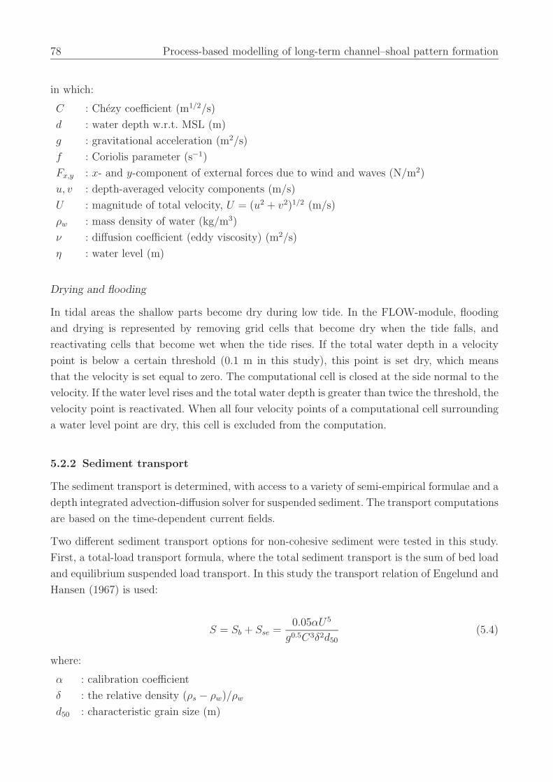
78 Process-based modelling of long-term channel–shoal pattern formation
in which:
C : Chezy coefficient (m1/2/s)
d : water depth w.r.t. MSL (m)
g : gravitational acceleration (m2/s)
f : Coriolis parameter (s−1)
Fx,y : x- and y-component of external forces due to wind and waves (N/m2)
u, v : depth-averaged velocity components (m/s)
U : magnitude of total velocity, U = (u2 + v2)1/2 (m/s)
ρw : mass density of water (kg/m3)
ν : diffusion coefficient (eddy viscosity) (m2/s)
η : water level (m)
Drying and flooding
In tidal areas the shallow parts become dry during low tide. In the FLOW-module, flooding
and drying is represented by removing grid cells that become dry when the tide falls, and
reactivating cells that become wet when the tide rises. If the total water depth in a velocity
point is below a certain threshold (0.1 m in this study), this point is set dry, which means
that the velocity is set equal to zero. The computational cell is closed at the side normal to the
velocity. If the water level rises and the total water depth is greater than twice the threshold, the
velocity point is reactivated. When all four velocity points of a computational cell surrounding
a water level point are dry, this cell is excluded from the computation.
5.2.2 Sediment transport
The sediment transport is determined, with access to a variety of semi-empirical formulae and a
depth integrated advection-diffusion solver for suspended sediment. The transport computations
are based on the time-dependent current fields.
Two different sediment transport options for non-cohesive sediment were tested in this study.
First, a total-load transport formula, where the total sediment transport is the sum of bed load
and equilibrium suspended load transport. In this study the transport relation of Engelund and
Hansen (1967) is used:
S = Sb + Sse =0.05αU5
g0.5C3δ2d50
(5.4)
where:
α : calibration coefficient
δ : the relative density (ρs − ρw)/ρw
d50 : characteristic grain size (m)
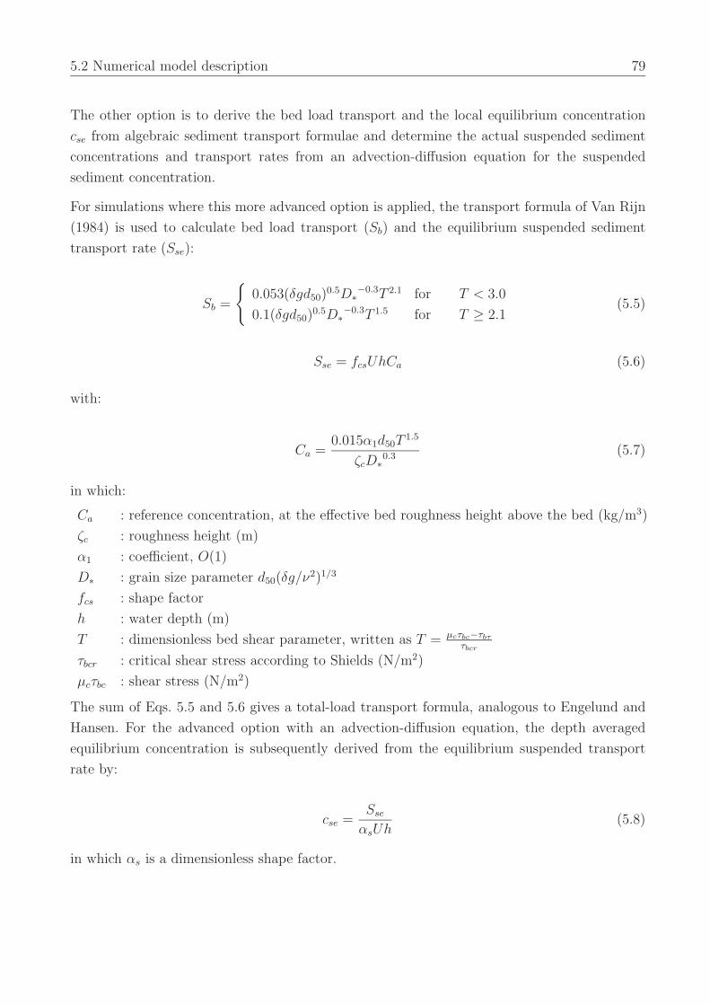
5.2 Numerical model description 79
The other option is to derive the bed load transport and the local equilibrium concentration
cse from algebraic sediment transport formulae and determine the actual suspended sediment
concentrations and transport rates from an advection-diffusion equation for the suspended
sediment concentration.
For simulations where this more advanced option is applied, the transport formula of Van Rijn
(1984) is used to calculate bed load transport (Sb) and the equilibrium suspended sediment
transport rate (Sse):
Sb =
{0.053(δgd50)
0.5D∗−0.3T 2.1 for T < 3.0
0.1(δgd50)0.5D∗−0.3T 1.5 for T ≥ 2.1
(5.5)
Sse = fcsUhCa (5.6)
with:
Ca =0.015α1d50T
1.5
ζcD∗0.3 (5.7)
in which:
Ca : reference concentration, at the effective bed roughness height above the bed (kg/m3)
ζc : roughness height (m)
α1 : coefficient, O(1)
D∗ : grain size parameter d50(δg/ν2)1/3
fcs : shape factor
h : water depth (m)
T : dimensionless bed shear parameter, written as T = µcτbc−τbτ
τbcr
τbcr : critical shear stress according to Shields (N/m2)
µcτbc : shear stress (N/m2)
The sum of Eqs. 5.5 and 5.6 gives a total-load transport formula, analogous to Engelund and
Hansen. For the advanced option with an advection-diffusion equation, the depth averaged
equilibrium concentration is subsequently derived from the equilibrium suspended transport
rate by:
cse =Sse
αsUh(5.8)
in which αs is a dimensionless shape factor.
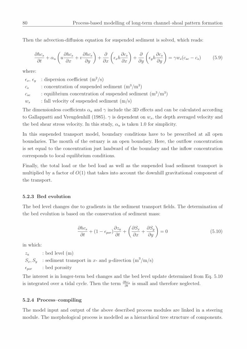
80 Process-based modelling of long-term channel–shoal pattern formation
Then the advection-diffusion equation for suspended sediment is solved, which reads:
∂hcs
∂t+ αu
(u∂hcs
∂x+ v
∂hcs
∂y
)+
∂
∂x
(εxh
∂cs
∂x
)+
∂
∂y
(εyh
∂cs
∂y
)= γws(cse − cs) (5.9)
where:
εx, εy : dispersion coefficient (m2/s)
cs : concentration of suspended sediment (m3/m3)
cse : equilibrium concentration of suspended sediment (m3/m3)
ws : fall velocity of suspended sediment (m/s)
The dimensionless coefficients αu and γ include the 3D effects and can be calculated according
to Gallappatti and Vreugdenhill (1985). γ is dependent on ws, the depth averaged velocity and
the bed shear stress velocity. In this study, αu is taken 1.0 for simplicity.
In this suspended transport model, boundary conditions have to be prescribed at all open
boundaries. The mouth of the estuary is an open boundary. Here, the outflow concentration
is set equal to the concentration just landward of the boundary and the inflow concentration
corresponds to local equilibrium conditions.
Finally, the total load or the bed load as well as the suspended load sediment transport is
multiplied by a factor of O(1) that takes into account the downhill gravitational component of
the transport.
5.2.3 Bed evolution
The bed level changes due to gradients in the sediment transport fields. The determination of
the bed evolution is based on the conservation of sediment mass:
∂hcs
∂t+ (1 − εpor)
∂za
∂t+
(∂Sx
∂x+
∂Sy
∂y
)= 0 (5.10)
in which:
za : bed level (m)
Sx, Sy : sediment transport in x- and y-direction (m3/m/s)
εpor : bed porosity
The interest is in longer-term bed changes and the bed level update determined from Eq. 5.10
is integrated over a tidal cycle. Then the term ∂hcs
∂tis small and therefore neglected.
5.2.4 Process–compiling
The model input and output of the above described process modules are linked in a steering
module. The morphological process is modelled as a hierarchical tree structure of components.
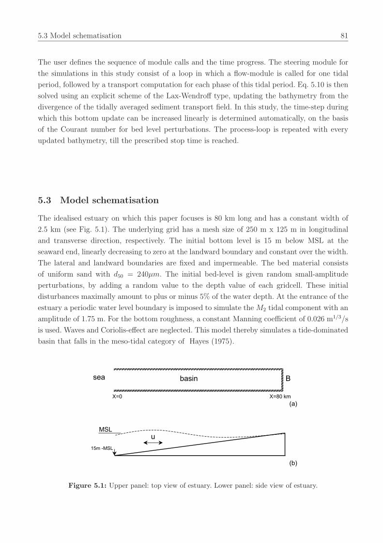
5.3 Model schematisation 81
The user defines the sequence of module calls and the time progress. The steering module for
the simulations in this study consist of a loop in which a flow-module is called for one tidal
period, followed by a transport computation for each phase of this tidal period. Eq. 5.10 is then
solved using an explicit scheme of the Lax-Wendroff type, updating the bathymetry from the
divergence of the tidally averaged sediment transport field. In this study, the time-step during
which this bottom update can be increased linearly is determined automatically, on the basis
of the Courant number for bed level perturbations. The process-loop is repeated with every
updated bathymetry, till the prescribed stop time is reached.
5.3 Model schematisation
The idealised estuary on which this paper focuses is 80 km long and has a constant width of
2.5 km (see Fig. 5.1). The underlying grid has a mesh size of 250 m x 125 m in longitudinal
and transverse direction, respectively. The initial bottom level is 15 m below MSL at the
seaward end, linearly decreasing to zero at the landward boundary and constant over the width.
The lateral and landward boundaries are fixed and impermeable. The bed material consists
of uniform sand with d50 = 240µm. The initial bed-level is given random small-amplitude
perturbations, by adding a random value to the depth value of each gridcell. These initial
disturbances maximally amount to plus or minus 5% of the water depth. At the entrance of the
estuary a periodic water level boundary is imposed to simulate the M2 tidal component with an
amplitude of 1.75 m. For the bottom roughness, a constant Manning coefficient of 0.026 m1/3/s
is used. Waves and Coriolis-effect are neglected. This model thereby simulates a tide-dominated
basin that falls in the meso-tidal category of Hayes (1975).
Figure 5.1: Upper panel: top view of estuary. Lower panel: side view of estuary.
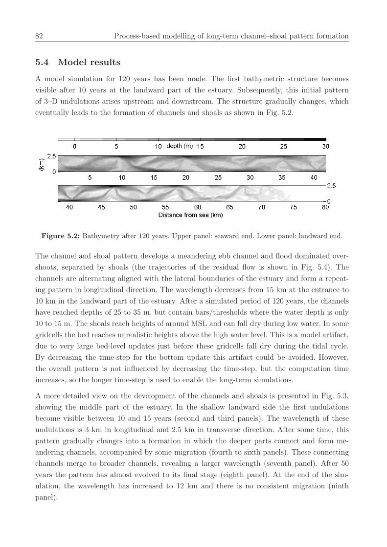
82 Process-based modelling of long-term channel–shoal pattern formation
5.4 Model results
A model simulation for 120 years has been made. The first bathymetric structure becomes
visible after 10 years at the landward part of the estuary. Subsequently, this initial pattern
of 3–D undulations arises upstream and downstream. The structure gradually changes, which
eventually leads to the formation of channels and shoals as shown in Fig. 5.2.
Figure 5.2: Bathymetry after 120 years. Upper panel: seaward end. Lower panel: landward end.
The channel and shoal pattern develops a meandering ebb channel and flood dominated over-
shoots, separated by shoals (the trajectories of the residual flow is shown in Fig. 5.4). The
channels are alternating aligned with the lateral boundaries of the estuary and form a repeat-
ing pattern in longitudinal direction. The wavelength decreases from 15 km at the entrance to
10 km in the landward part of the estuary. After a simulated period of 120 years, the channels
have reached depths of 25 to 35 m, but contain bars/thresholds where the water depth is only
10 to 15 m. The shoals reach heights of around MSL and can fall dry during low water. In some
gridcells the bed reaches unrealistic heights above the high water level. This is a model artifact,
due to very large bed-level updates just before these gridcells fall dry during the tidal cycle.
By decreasing the time-step for the bottom update this artifact could be avoided. However,
the overall pattern is not influenced by decreasing the time-step, but the computation time
increases, so the longer time-step is used to enable the long-term simulations.
A more detailed view on the development of the channels and shoals is presented in Fig. 5.3,
showing the middle part of the estuary. In the shallow landward side the first undulations
become visible between 10 and 15 years (second and third panels). The wavelength of these
undulations is 3 km in longitudinal and 2.5 km in transverse direction. After some time, this
pattern gradually changes into a formation in which the deeper parts connect and form me-
andering channels, accompanied by some migration (fourth to sixth panels). These connecting
channels merge to broader channels, revealing a larger wavelength (seventh panel). After 50
years the pattern has almost evolved to its final stage (eighth panel). At the end of the sim-
ulation, the wavelength has increased to 12 km and there is no consistent migration (ninth
panel).
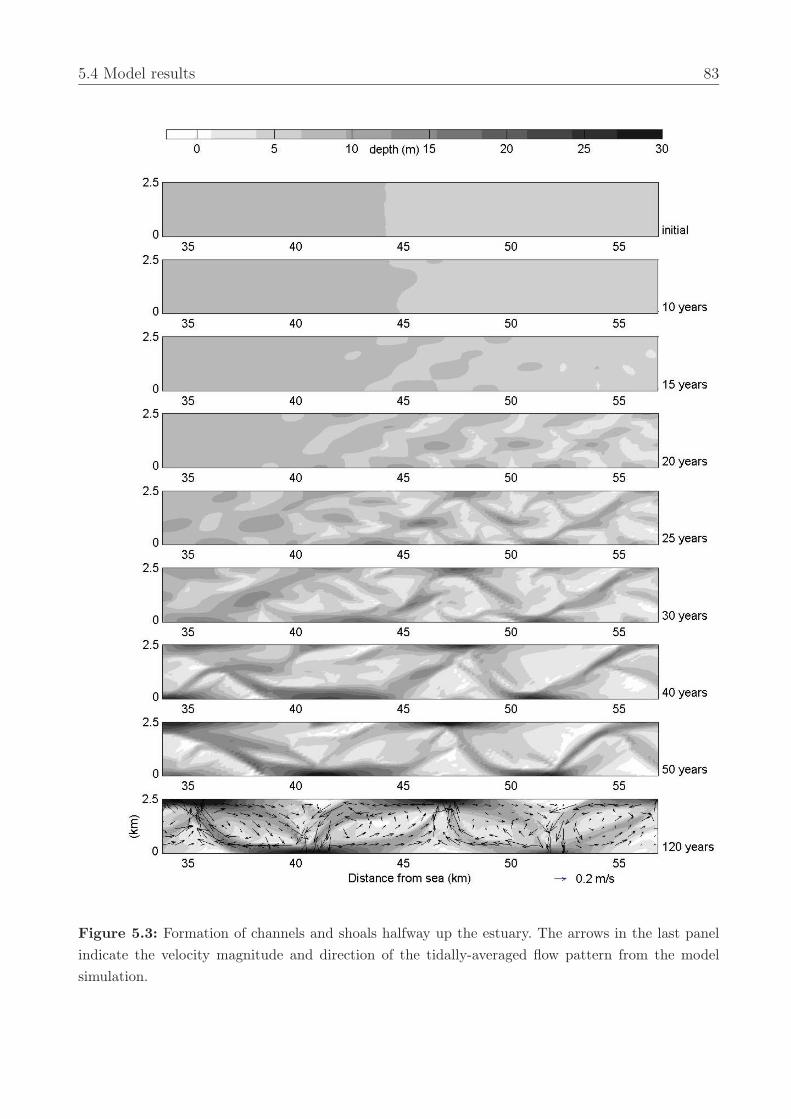
5.4 Model results 83
Figure 5.3: Formation of channels and shoals halfway up the estuary. The arrows in the last panelindicate the velocity magnitude and direction of the tidally-averaged flow pattern from the modelsimulation.
84 Process-based modelling of long-term channel–shoal pattern formation
The first scour holes and deposition areas form more slowly in the deeper seaward part. They
form an alternating pattern, with a wavelength in the longitudinal direction of 7 to 10 km (upper
panel Fig. 5.2, i.e. considerably larger than in the shallow parts of the estuary. The evolution
of the pattern is similar to that in the shallow part, showing migration and an increase of
wavelengths. This pattern evolution slows during the simulation and the global pattern is more
or less fixed after 100 years. Locally, at the crossings of the channels, the bathymetry remains
highly dynamic, as the channel ends move to and fro.
The above simulation uses the total load transport formula of Engelund and Hansen (1967).
When the Van Rijn formulations (1984) for total load transport are used, the initial results
are similar, though the time scales differ. Using Van Rijn’s formulations, the growth of the
erosional and depositional areas is initially slower in the landward area, while it is slightly
faster at the mouth of the model estuary. This is probably due to the smaller exponent in the
transport relationship, and by the inclusion of a threshold of motion. The development of the
channel–shoal pattern is largely analogous, but local differences exist.
Van Rijn’s relationships are also used for the equilibrium concentration and the bed-load trans-
port rate when the advection-diffusion solver for suspended sediment is applied. Using this
option, the dispersion coefficient is set at 10 m2/s (Fischer, 1979). The adaptation length of
the sediment concentration, defined by the water depth times the current velocity divided by
the fall velocity of the sediment is typically 500 m. Due to this modulation of suspended load
transport, the emerging initial pattern is somewhat smoother in this case. The location and
wavelength of the initial undulations remain similar to the previous cases. The time needed for
the initial pattern to become visible is longer than in the total-load transport case, probably
due to the smoothing effect of suspended transport, which forms the main transport mode.
The bed load transport accounts for less than 10% of the suspended load transport. During
the transition to the channel–shoal pattern, the shoals attain greater heights probably due to
lag-effects. In the shallow landward part of the estuary, the pattern deviates from those seen
before. Three to four meandering channels are formed in parallel, separated by shoals. This
pattern remains stable.
5.5 Validation with field data
The model is validated against field observations by Van Veen (1950) and Ahnert (1960). Ahn-
ert studied the estuaries around the Chesapeake Bay, Maryland, USA. The main interest of Van
Veen is the Western Scheldt estuary in The Netherlands. This 160 km long funnel-shaped estu-
ary, with an entrance width of 6 km, exhibits a well-developed system of channels and shoals. In
his characterisation of channel patterns in estuaries, Van Veen categorised channels as ebb- and
flood-dominated. His cartoon of an idealised channel system is presented in Fig. 5.4(b). It shows
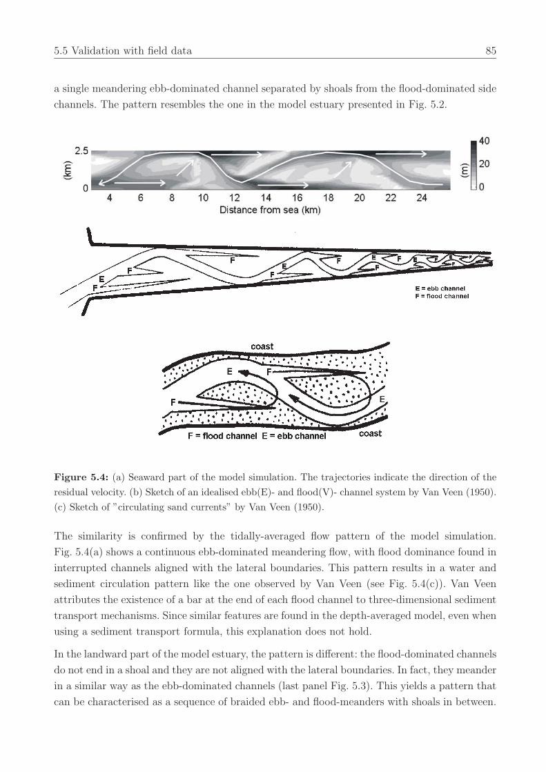
5.5 Validation with field data 85
a single meandering ebb-dominated channel separated by shoals from the flood-dominated side
channels. The pattern resembles the one in the model estuary presented in Fig. 5.2.
Figure 5.4: (a) Seaward part of the model simulation. The trajectories indicate the direction of theresidual velocity. (b) Sketch of an idealised ebb(E)- and flood(V)- channel system by Van Veen (1950).(c) Sketch of ”circulating sand currents” by Van Veen (1950).
The similarity is confirmed by the tidally-averaged flow pattern of the model simulation.
Fig. 5.4(a) shows a continuous ebb-dominated meandering flow, with flood dominance found in
interrupted channels aligned with the lateral boundaries. This pattern results in a water and
sediment circulation pattern like the one observed by Van Veen (see Fig. 5.4(c)). Van Veen
attributes the existence of a bar at the end of each flood channel to three-dimensional sediment
transport mechanisms. Since similar features are found in the depth-averaged model, even when
using a sediment transport formula, this explanation does not hold.
In the landward part of the model estuary, the pattern is different: the flood-dominated channels
do not end in a shoal and they are not aligned with the lateral boundaries. In fact, they meander
in a similar way as the ebb-dominated channels (last panel Fig. 5.3). This yields a pattern that
can be characterised as a sequence of braided ebb- and flood-meanders with shoals in between.
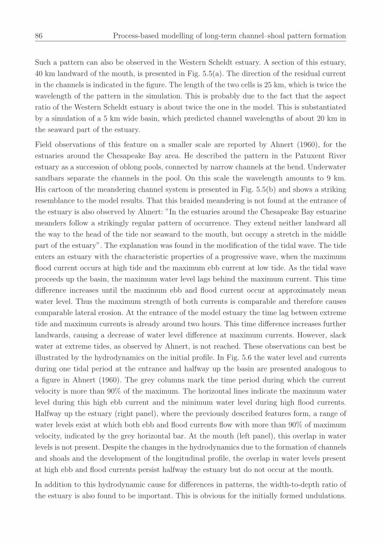
86 Process-based modelling of long-term channel–shoal pattern formation
Such a pattern can also be observed in the Western Scheldt estuary. A section of this estuary,
40 km landward of the mouth, is presented in Fig. 5.5(a). The direction of the residual current
in the channels is indicated in the figure. The length of the two cells is 25 km, which is twice the
wavelength of the pattern in the simulation. This is probably due to the fact that the aspect
ratio of the Western Scheldt estuary is about twice the one in the model. This is substantiated
by a simulation of a 5 km wide basin, which predicted channel wavelengths of about 20 km in
the seaward part of the estuary.
Field observations of this feature on a smaller scale are reported by Ahnert (1960), for the
estuaries around the Chesapeake Bay area. He described the pattern in the Patuxent River
estuary as a succession of oblong pools, connected by narrow channels at the bend. Underwater
sandbars separate the channels in the pool. On this scale the wavelength amounts to 9 km.
His cartoon of the meandering channel system is presented in Fig. 5.5(b) and shows a striking
resemblance to the model results. That this braided meandering is not found at the entrance of
the estuary is also observed by Ahnert: ”In the estuaries around the Chesapeake Bay estuarine
meanders follow a strikingly regular pattern of occurrence. They extend neither landward all
the way to the head of the tide nor seaward to the mouth, but occupy a stretch in the middle
part of the estuary”. The explanation was found in the modification of the tidal wave. The tide
enters an estuary with the characteristic properties of a progressive wave, when the maximum
flood current occurs at high tide and the maximum ebb current at low tide. As the tidal wave
proceeds up the basin, the maximum water level lags behind the maximum current. This time
difference increases until the maximum ebb and flood current occur at approximately mean
water level. Thus the maximum strength of both currents is comparable and therefore causes
comparable lateral erosion. At the entrance of the model estuary the time lag between extreme
tide and maximum currents is already around two hours. This time difference increases further
landwards, causing a decrease of water level difference at maximum currents. However, slack
water at extreme tides, as observed by Ahnert, is not reached. These observations can best be
illustrated by the hydrodynamics on the initial profile. In Fig. 5.6 the water level and currents
during one tidal period at the entrance and halfway up the basin are presented analogous to
a figure in Ahnert (1960). The grey columns mark the time period during which the current
velocity is more than 90% of the maximum. The horizontal lines indicate the maximum water
level during this high ebb current and the minimum water level during high flood currents.
Halfway up the estuary (right panel), where the previously described features form, a range of
water levels exist at which both ebb and flood currents flow with more than 90% of maximum
velocity, indicated by the grey horizontal bar. At the mouth (left panel), this overlap in water
levels is not present. Despite the changes in the hydrodynamics due to the formation of channels
and shoals and the development of the longitudinal profile, the overlap in water levels present
at high ebb and flood currents persist halfway the estuary but do not occur at the mouth.
In addition to this hydrodynamic cause for differences in patterns, the width-to-depth ratio of
the estuary is also found to be important. This is obvious for the initially formed undulations.
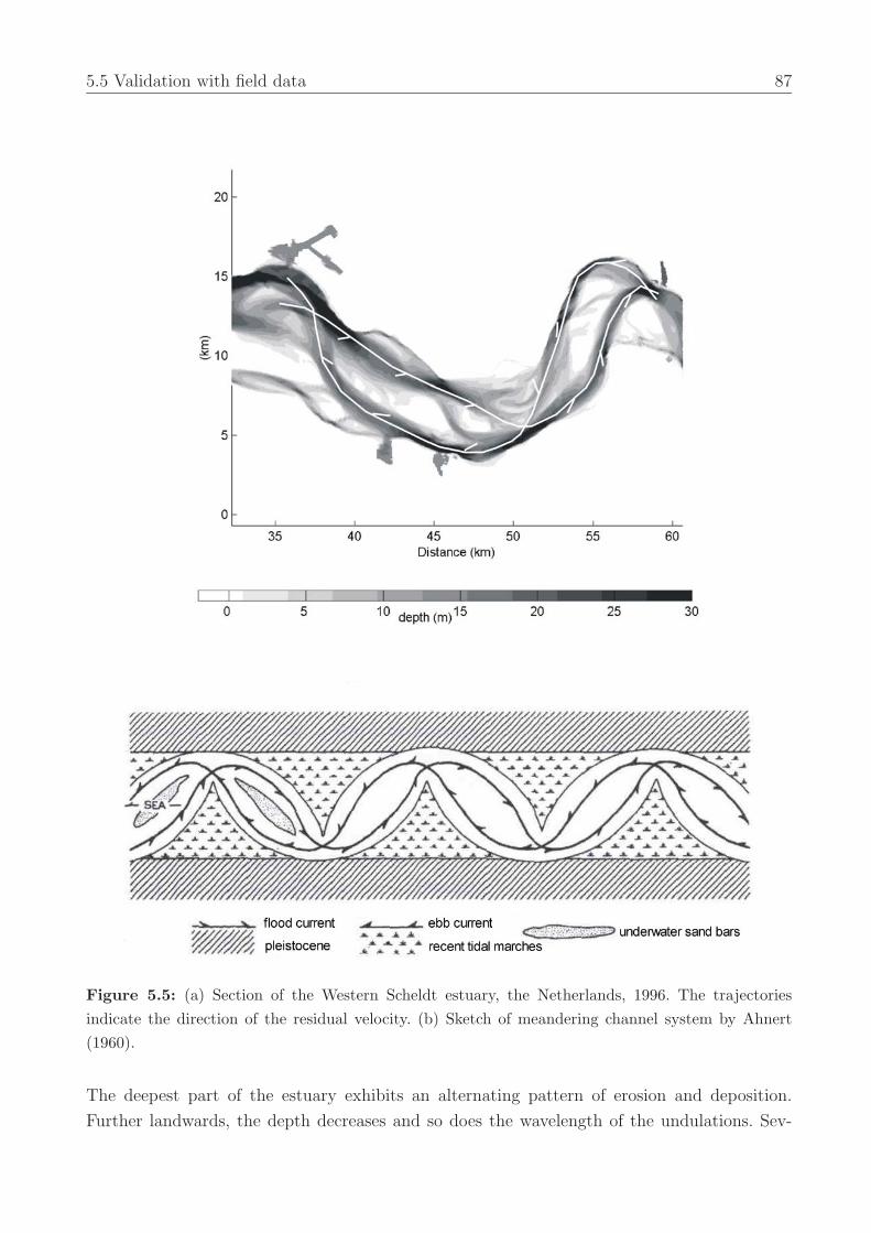
5.5 Validation with field data 87
Figure 5.5: (a) Section of the Western Scheldt estuary, the Netherlands, 1996. The trajectoriesindicate the direction of the residual velocity. (b) Sketch of meandering channel system by Ahnert(1960).
The deepest part of the estuary exhibits an alternating pattern of erosion and deposition.
Further landwards, the depth decreases and so does the wavelength of the undulations. Sev-
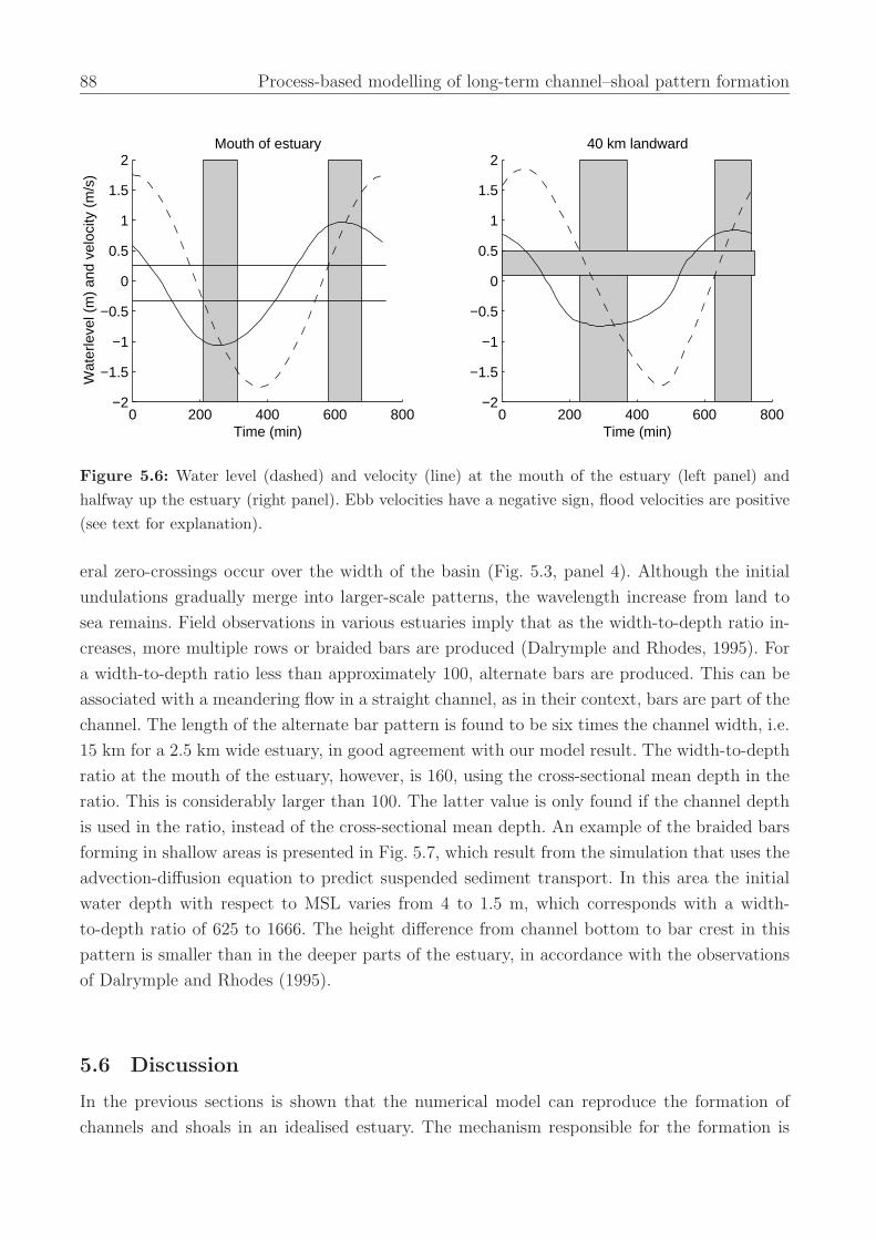
88 Process-based modelling of long-term channel–shoal pattern formation
0 200 400 600 800−2
−1.5
−1
−0.5
0
0.5
1
1.5
240 km landward
Time (min)0 200 400 600 800
−2
−1.5
−1
−0.5
0
0.5
1
1.5
2Mouth of estuary
Wat
erle
vel (
m)
and
velo
city
(m
/s)
Time (min)
Figure 5.6: Water level (dashed) and velocity (line) at the mouth of the estuary (left panel) andhalfway up the estuary (right panel). Ebb velocities have a negative sign, flood velocities are positive(see text for explanation).
eral zero-crossings occur over the width of the basin (Fig. 5.3, panel 4). Although the initial
undulations gradually merge into larger-scale patterns, the wavelength increase from land to
sea remains. Field observations in various estuaries imply that as the width-to-depth ratio in-
creases, more multiple rows or braided bars are produced (Dalrymple and Rhodes, 1995). For
a width-to-depth ratio less than approximately 100, alternate bars are produced. This can be
associated with a meandering flow in a straight channel, as in their context, bars are part of the
channel. The length of the alternate bar pattern is found to be six times the channel width, i.e.
15 km for a 2.5 km wide estuary, in good agreement with our model result. The width-to-depth
ratio at the mouth of the estuary, however, is 160, using the cross-sectional mean depth in the
ratio. This is considerably larger than 100. The latter value is only found if the channel depth
is used in the ratio, instead of the cross-sectional mean depth. An example of the braided bars
forming in shallow areas is presented in Fig. 5.7, which result from the simulation that uses the
advection-diffusion equation to predict suspended sediment transport. In this area the initial
water depth with respect to MSL varies from 4 to 1.5 m, which corresponds with a width-
to-depth ratio of 625 to 1666. The height difference from channel bottom to bar crest in this
pattern is smaller than in the deeper parts of the estuary, in accordance with the observations
of Dalrymple and Rhodes (1995).
5.6 Discussion
In the previous sections is shown that the numerical model can reproduce the formation of
channels and shoals in an idealised estuary. The mechanism responsible for the formation is
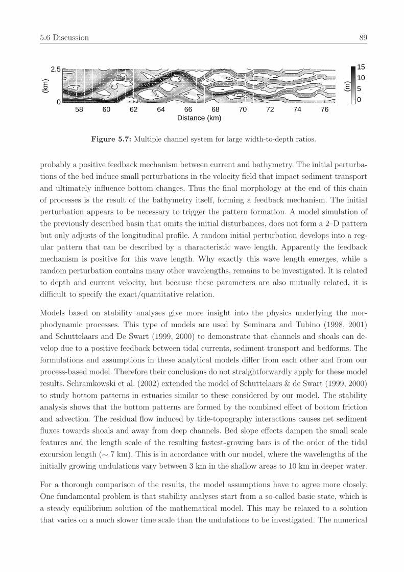
5.6 Discussion 89
0
5
10
15
58 60 62 64 66 68 70 72 74 760
2.5
Distance (km)
(km
)
(m)
Figure 5.7: Multiple channel system for large width-to-depth ratios.
probably a positive feedback mechanism between current and bathymetry. The initial perturba-
tions of the bed induce small perturbations in the velocity field that impact sediment transport
and ultimately influence bottom changes. Thus the final morphology at the end of this chain
of processes is the result of the bathymetry itself, forming a feedback mechanism. The initial
perturbation appears to be necessary to trigger the pattern formation. A model simulation of
the previously described basin that omits the initial disturbances, does not form a 2–D pattern
but only adjusts of the longitudinal profile. A random initial perturbation develops into a reg-
ular pattern that can be described by a characteristic wave length. Apparently the feedback
mechanism is positive for this wave length. Why exactly this wave length emerges, while a
random perturbation contains many other wavelengths, remains to be investigated. It is related
to depth and current velocity, but because these parameters are also mutually related, it is
difficult to specify the exact/quantitative relation.
Models based on stability analyses give more insight into the physics underlying the mor-
phodynamic processes. This type of models are used by Seminara and Tubino (1998, 2001)
and Schuttelaars and De Swart (1999, 2000) to demonstrate that channels and shoals can de-
velop due to a positive feedback between tidal currents, sediment transport and bedforms. The
formulations and assumptions in these analytical models differ from each other and from our
process-based model. Therefore their conclusions do not straightforwardly apply for these model
results. Schramkowski et al. (2002) extended the model of Schuttelaars & de Swart (1999, 2000)
to study bottom patterns in estuaries similar to these considered by our model. The stability
analysis shows that the bottom patterns are formed by the combined effect of bottom friction
and advection. The residual flow induced by tide-topography interactions causes net sediment
fluxes towards shoals and away from deep channels. Bed slope effects dampen the small scale
features and the length scale of the resulting fastest-growing bars is of the order of the tidal
excursion length (∼ 7 km). This is in accordance with our model, where the wavelengths of the
initially growing undulations vary between 3 km in the shallow areas to 10 km in deeper water.
For a thorough comparison of the results, the model assumptions have to agree more closely.
One fundamental problem is that stability analyses start from a so-called basic state, which is
a steady equilibrium solution of the mathematical model. This may be relaxed to a solution
that varies on a much slower time scale than the undulations to be investigated. The numerical
90 Process-based modelling of long-term channel–shoal pattern formation
model, however, starts from an arbitrary initial topography, and allows the mean profile and
the channel–shoal pattern to evolve concurrently. In analytical models, the basic state can be
computed a priori, but this is not possible in the numerical model. Using the analytical basic
state as an initial profile in the numerical simulation requires close agreement of the model
assumptions, otherwise the numerical model starts adjusting the profile while the undular
patterns emerge. At present our model only concludes that local changes to bed level due to the
initial pattern formation are up to an order of magnitude larger than the changes in the width-
averaged longitudinal profile. A preliminary comparison of the evolution of this longitudinal
profile with the equilibrium profiles of Schuttelaars and de Swart (2000) shows some agreement,
especially the deepening near the entrance of the basin and the steepening of the landward slope.
A full mutual comparison of the numerical and the analytical models is done by (Hibma et al.,
2003b), described in Chapter 3. This requires an adapted version of the present process-based
modelling system, where the model formulations resemble the descriptions in the analytical
model.
The subsequent development of the undulations into larger scale patterns falls out of the scope of
stability analyses, because the processes are highly non-linear. During this process the channels
deepen, the shoals grow and the wave lengths increase. The current velocities in the develop-
ing channels increase, which can explain the increase of length scale through the associated
increased inertia. At the end of the simulation the inter tidal shoals have reached an average
height of 1.0 m below the local mean water level. While locally the sills at the junction of
channels remain morphologically active, the overall large scale pattern is more or less stable.
The stability depends both on an equilibrium between morphology and currents, and on the
presence of non-erodible lateral boundaries. These prevent further lateral movement and associ-
ated dynamic behaviour in the channels. The boundaries will therefore also influence the length
scale of the pattern in the developed stage. During the initial formation the length scales of the
bed patterns are smaller than the width of the basin and the boundaries do not significantly
influence on the length scales or processes. The conclusions are substantiated by sensitivity
simulations for variable basin widths. The model formulation also neglected wind waves. Dur-
ing the simulation the shoals attain shallower depths, which would result in increased wave
influence. In the type of estuary studied for this paper – a long inland basin – waves are typ-
ically moderate. In the long run, they probably influence the average height of shoals, as this
decreases during storms and increases during calm weather periods (De Vriend et al., 1989).
The influence of this phenomenon on overall pattern formation is expected to be minor however,
and therefore neglected in the present analysis.
Despite inherent limitations, the simplified geometry and the basic parameter setting contribute
to the transparency and generalisation of the obtained results. Most model parameters only
influence the length scale of the patterns or the time scale of the formation, but the underlying
processes remain the same. However, the neglect of waves and large river runoff limit the validity
of the model to elongated inland estuaries, that are tidally dominated and well-mixed.
5.7 Conclusion 91
5.7 Conclusion
The channel–shoal patterns emerging from the numerical simulations agree with patterns that
are known from nature. The initially formed undulations seem to correspond at least qualita-
tively with the results of the linear stability analyses of Schramkowski et al. (2002), although
a full mutual comparison was not feasible, due to the differences in model assumptions and
formulations.
The relatively simple initial pattern of erosion and deposition, once it has reached a finite
amplitude and therefore has become subject to non-linear interaction processes, increases in
spatial scale and forms specific, quasi-regular patterns of channels and shoals. The global pattern
is stable after approximately a century. These realistic channel–shoal patterns are produced by
a 2–D depth-averaged numerical model. Within the parameter ranges considered, the results
seem to be insensitive to the specific sediment transport formulation applied. In a later phase,
the interaction with mudflats and marshes should be included, introducing cohesive sediment
and vegetation, in order to simulate the large-scale evolution of natural systems.
Appreciating the need for further validation and analysis, it can be concluded that this model
provides a tool, complementary to fieldwork, theoretical behaviour analyses and laboratory
experiments, for the analysis of the large-scale morphological behaviour of estuaries and tide-
dominated coastal lagoons.

92 Process-based modelling of long-term channel–shoal pattern formation
6 Modelling impact of dredging and
dumping in ebb-flood channel systems 1
Abstract
For a channel–shoal system in a funnel-shaped basin the impact of dredging and dumping
is investigated using a complex process-based model. First, the residual flow and sediment
transport circulations are analysed for the channel–shoal pattern, which has emerged after a
long-term model simulation. Results are compared to the Western Scheldt estuary, which formed
the inspiration for this study. Subsequently, different dredge and dump scenario’s are modelled,
according to a conceptual model, in which ebb- and flood channels and enclosed shoals form
morphodynamic units (cells) with their own sediment circulation. Model results show that
dumping sediment in a channel further reduces the channel depth and induces erosion in the
opposite channel, which enhances tilting of the cross-section of the cell and eventually can lead
to the degeneration of a multiple channel system onto a single channel. The impact of different
dredging and dumping cases agrees with results from a stability analysis. This means that this
type of model applied to a realistic geometry can potentially be used for better prediction of
the impact of human interventions.
6.1 Introduction
Previous chapters demonstrated that a (complex) process-based model is capable of modelling
estuarine channel–shoal systems on their lifetime scale. Model results have been validated
against idealised models, comparing initial growth and the processes underlying the positive
feedback mechanism (Chapter 4, also see Hibma et al. (2003c)), as well as against field observa-
tions (Chapter 5, also see Hibma et al. (2003a)), showing good correspondence with ebb-flood
channel patterns described by Van Veen (1950) and Ahnert (1960). Characteristic features of
ebb and flood channel systems are studied by Van Veen (1950); Van den Berg et al. (1996);
1. The contents of this chapter is accepted for publication in the conference proceedings of Physics of Estuariesand Coastal Seas, Yucatan, Mexico, 2004, under the same title by A. Hibma, Z.B. Wang, M.J.F. Stive and H.J.de Vriend.
93
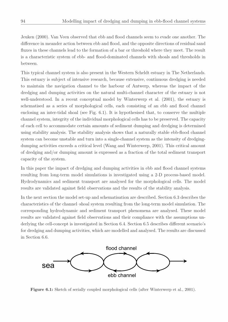
94 Modelling impact of dredging and dumping in ebb-flood channel systems
Jeuken (2000). Van Veen observed that ebb and flood channels seem to evade one another. The
difference in meander action between ebb and flood, and the opposite directions of residual sand
fluxes in these channels lead to the formation of a bar or threshold where they meet. The result
is a characteristic system of ebb- and flood-dominated channels with shoals and thresholds in
between.
This typical channel system is also present in the Western Scheldt estuary in The Netherlands.
This estuary is subject of intensive research, because extensive, continuous dredging is needed
to maintain the navigation channel to the harbour of Antwerp, whereas the impact of the
dredging and dumping activities on the natural multi-channel character of the estuary is not
well-understood. In a recent conceptual model by Winterwerp et al. (2001), the estuary is
schematised as a series of morphological cells, each consisting of an ebb and flood channel
enclosing an inter-tidal shoal (see Fig. 6.1). It is hypothesised that, to conserve the multiple
channel system, integrity of the individual morphological cells has to be preserved. The capacity
of each cell to accommodate certain amounts of sediment dumping and dredging is determined
using stability analysis. The stability analysis shows that a naturally stable ebb-flood channel
system can become unstable and turn into a single-channel system as the intensity of dredging-
dumping activities exceeds a critical level (Wang and Winterwerp, 2001). This critical amount
of dredging and/or dumping amount is expressed as a fraction of the total sediment transport
capacity of the system.
In this paper the impact of dredging and dumping activities in ebb and flood channel systems
resulting from long-term model simulations is investigated using a 2-D process-based model.
Hydrodynamics and sediment transport are analysed for the morphological cells. The model
results are validated against field observations and the results of the stability analysis.
In the next section the model set-up and schematisation are described. Section 6.3 describes the
characteristics of the channel–shoal system resulting from the long-term model simulation. The
corresponding hydrodynamic and sediment transport phenomena are analysed. These model
results are validated against field observations and their compliance with the assumptions un-
derlying the cell-concept is investigated in Section 6.4. Section 6.5 describes different scenario’s
for dredging and dumping activities, which are modelled and analysed. The results are discussed
in Section 6.6.
Figure 6.1: Sketch of serially coupled morphological cells (after Winterwerp et al., 2001).
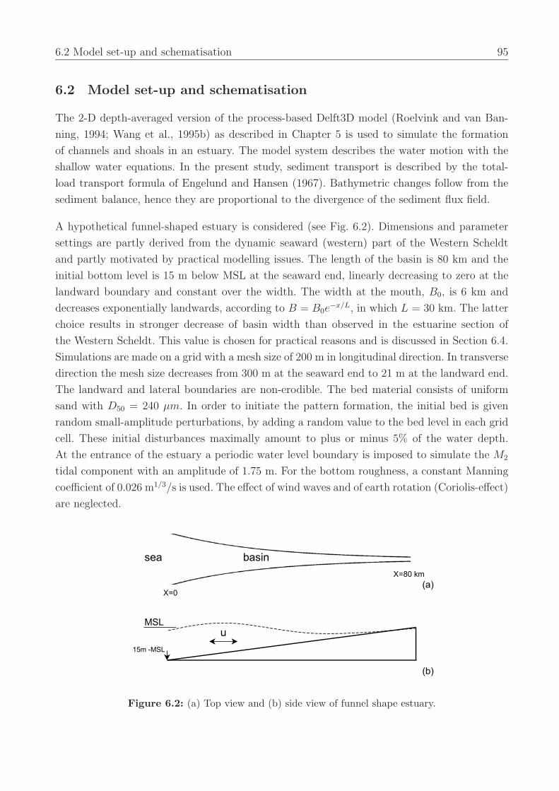
6.2 Model set-up and schematisation 95
6.2 Model set-up and schematisation
The 2-D depth-averaged version of the process-based Delft3D model (Roelvink and van Ban-
ning, 1994; Wang et al., 1995b) as described in Chapter 5 is used to simulate the formation
of channels and shoals in an estuary. The model system describes the water motion with the
shallow water equations. In the present study, sediment transport is described by the total-
load transport formula of Engelund and Hansen (1967). Bathymetric changes follow from the
sediment balance, hence they are proportional to the divergence of the sediment flux field.
A hypothetical funnel-shaped estuary is considered (see Fig. 6.2). Dimensions and parameter
settings are partly derived from the dynamic seaward (western) part of the Western Scheldt
and partly motivated by practical modelling issues. The length of the basin is 80 km and the
initial bottom level is 15 m below MSL at the seaward end, linearly decreasing to zero at the
landward boundary and constant over the width. The width at the mouth, B0, is 6 km and
decreases exponentially landwards, according to B = B0e−x/L, in which L = 30 km. The latter
choice results in stronger decrease of basin width than observed in the estuarine section of
the Western Scheldt. This value is chosen for practical reasons and is discussed in Section 6.4.
Simulations are made on a grid with a mesh size of 200 m in longitudinal direction. In transverse
direction the mesh size decreases from 300 m at the seaward end to 21 m at the landward end.
The landward and lateral boundaries are non-erodible. The bed material consists of uniform
sand with D50 = 240 µm. In order to initiate the pattern formation, the initial bed is given
random small-amplitude perturbations, by adding a random value to the bed level in each grid
cell. These initial disturbances maximally amount to plus or minus 5% of the water depth.
At the entrance of the estuary a periodic water level boundary is imposed to simulate the M2
tidal component with an amplitude of 1.75 m. For the bottom roughness, a constant Manning
coefficient of 0.026 m1/3/s is used. The effect of wind waves and of earth rotation (Coriolis-effect)
are neglected.
Figure 6.2: (a) Top view and (b) side view of funnel shape estuary.
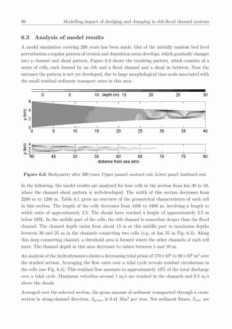
96 Modelling impact of dredging and dumping in ebb-flood channel systems
6.3 Analysis of model results
A model simulation covering 200 years has been made. Out of the initially random bed level
perturbation a regular pattern of erosion and deposition areas develops, which gradually changes
into a channel and shoal pattern. Figure 6.3 shows the resulting pattern, which consists of a
series of cells, each formed by an ebb and a flood channel and a shoal in between. Near the
entrance the pattern is not yet developed, due to large morphological time scale associated with
the small residual sediment transport rates in this area.
Figure 6.3: Bathymetry after 200 years. Upper pannel: seaward end. Lower panel: landward end.
In the following, the model results are analysed for four cells in the section from km 30 to 50,
where the channel–shoal pattern is well-developed. The width of this section decreases from
2200 m to 1200 m. Table 6.1 gives an overview of the geometrical characteristics of each cell
in this section. The length of the cells decreases from 4400 to 3400 m, involving a length to
width ratio of approximately 2.5. The shoals have reached a height of approximately 2.5 m
below MSL. In the middle part of the cells, the ebb channel is somewhat deeper than the flood
channel. The channel depth varies from about 15 m at this middle part to maximum depths
between 20 and 25 m in the channels connecting two cells (e.g. at km 35 in Fig. 6.3). Along
this deep connecting channel, a threshold area is formed where the other channels of each cell
meet. The channel depth in this area decreases to values between 5 and 10 m.
An analysis of the hydrodynamics shows a decreasing tidal prism of 170×106 to 90×106 m3 over
the studied section. Averaging the flow rates over a tidal cycle reveals residual circulations in
the cells (see Fig. 6.4). This residual flow amounts to approximately 10% of the total discharge
over a tidal cycle. Maximum velocities around 1 m/s are reached in the channels and 0.5 m/s
above the shoals.
Averaged over the selected section, the gross amount of sediment transported through a cross-
section in along-channel direction, Sgross, is 0.41 Mm3 per year. Net sediment fluxes, Snet, are
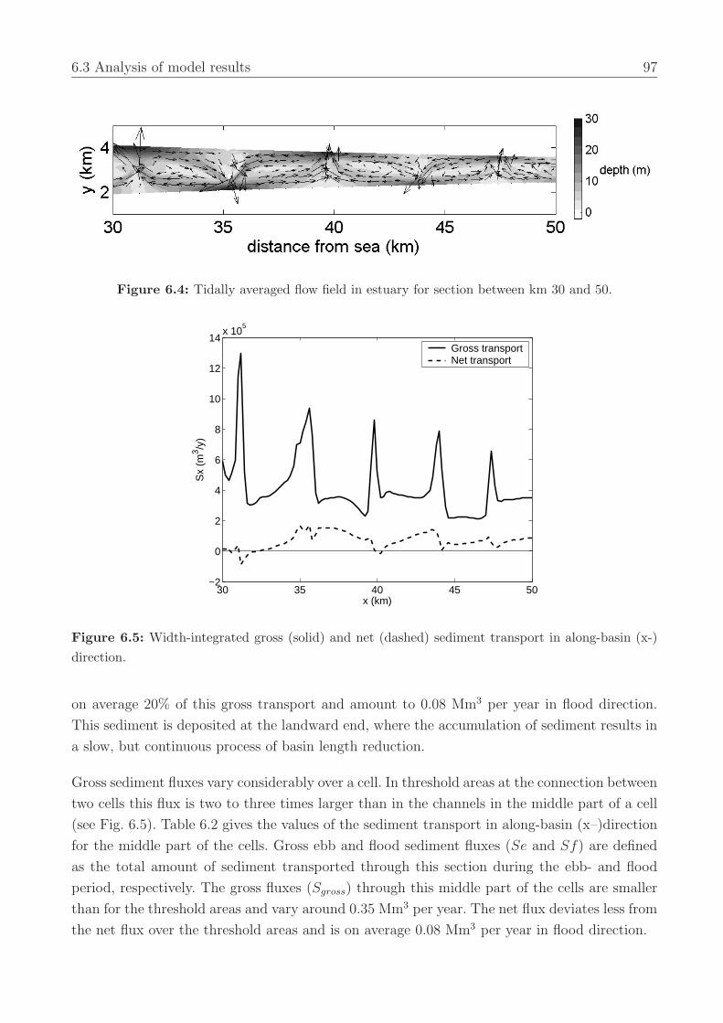
6.3 Analysis of model results 97
Figure 6.4: Tidally averaged flow field in estuary for section between km 30 and 50.
30 35 40 45 50−2
0
2
4
6
8
10
12
14x 10
5
x (km)
Sx
(m3 /y
)
Gross transportNet transport
Figure 6.5: Width-integrated gross (solid) and net (dashed) sediment transport in along-basin (x-)direction.
on average 20% of this gross transport and amount to 0.08 Mm3 per year in flood direction.
This sediment is deposited at the landward end, where the accumulation of sediment results in
a slow, but continuous process of basin length reduction.
Gross sediment fluxes vary considerably over a cell. In threshold areas at the connection between
two cells this flux is two to three times larger than in the channels in the middle part of a cell
(see Fig. 6.5). Table 6.2 gives the values of the sediment transport in along-basin (x–)direction
for the middle part of the cells. Gross ebb and flood sediment fluxes (Se and Sf) are defined
as the total amount of sediment transported through this section during the ebb- and flood
period, respectively. The gross fluxes (Sgross) through this middle part of the cells are smaller
than for the threshold areas and vary around 0.35 Mm3 per year. The net flux deviates less from
the net flux over the threshold areas and is on average 0.08 Mm3 per year in flood direction.
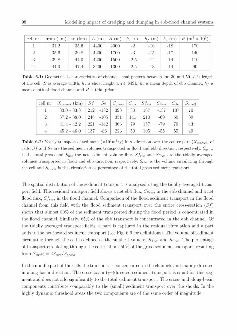
98 Modelling impact of dredging and dumping in ebb-flood channel systems
cell nr. from (km) to (km) L (m) B (m) hs (m) hf (m) he (m) P (m3 × 106)
1 31.2 35.6 4400 2000 -2 -16 -18 170
2 35.6 39.8 4200 1700 -3 -15 -17 140
3 39.8 44.0 4200 1500 -2.5 -14 -14 110
4 44.0 47.4 3400 1300 -2.5 -13 -14 90
Table 6.1: Geometrical characteristics of channel–shoal pattern between km 30 and 50. L is lengthof the cell, B is average width, hs is shoal height w.r.t. MSL, he is mean depth of ebb channel, hf ismean depth of flood channel and P is tidal prism.
cell nr. Xmidcel (km) Sf Se Sgross Snet Sfres Seres Scirc Scirc%
1 33.0 - 33.8 212 -182 393 30 167 -137 137 70
2 37.2 - 38.0 246 -105 351 141 210 -69 69 39
3 41.4 - 42.2 221 -142 363 79 157 -79 79 43
4 45.2 - 46.0 137 -86 223 50 105 -55 55 49
Table 6.2: Yearly transport of sediment (×103m3/y) in x–direction over the center part (Xmidcel) ofcells. Sf and Se are the sediment volumes transported in flood and ebb direction, respectively. Sgross
is the total gross and Snet the net sediment volume flux. Sfres and Seres are the tidally averagedvolumes transported in flood and ebb direction, respectively. Scirc is the volume circulating throughthe cell and Scirc% is this circulation as percentage of the total gross sediment transport.
The spatial distribution of the sediment transport is analysed using the tidally averaged trans-
port field. This residual transport field shows a net ebb flux, Seres, in the ebb channel and a net
flood flux, Sfres, in the flood channel. Comparison of the flood sediment transport in the flood
channel from this field with the flood sediment transport over the entire cross-section (Sf)
shows that almost 80% of the sediment transported during the flood period is concentrated in
the flood channel. Similarly, 65% of the ebb transport is concentrated in the ebb channel. Of
the tidally averaged transport fields, a part is captured in the residual circulation and a part
adds to the net inward sediment transport (see Fig. 6.6 for definitions). The volume of sediment
circulating through the cell is defined as the smallest value of Sfres and Seres. The percentage
of transport circulating through the cell is about 50% of the gross sediment transport, resulting
from Scirc% = 2Scirc/Sgross.
In the middle part of the cells the transport is concentrated in the channels and mainly directed
in along-basin direction. The cross-basin (y–)directed sediment transport is small for this seg-
ment and does not add significantly to the total sediment transport. The cross- and along-basin
components contribute comparably to the (small) sediment transport over the shoals. In the
highly dynamic threshold areas the two components are of the same order of magnitude.
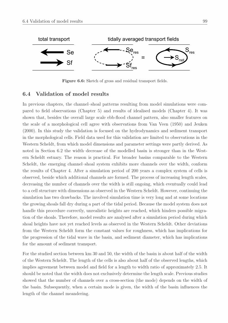
6.4 Validation of model results 99
Figure 6.6: Sketch of gross and residual transport fields.
6.4 Validation of model results
In previous chapters, the channel–shoal patterns resulting from model simulations were com-
pared to field observations (Chapter 5) and results of idealised models (Chapter 4). It was
shown that, besides the overall large scale ebb-flood channel pattern, also smaller features on
the scale of a morphological cell agree with observations from Van Veen (1950) and Jeuken
(2000). In this study the validation is focused on the hydrodynamics and sediment transport
in the morphological cells. Field data used for this validation are limited to observations in the
Western Scheldt, from which model dimensions and parameter settings were partly derived. As
noted in Section 6.2 the width–decrease of the modelled basin is stronger than in the West-
ern Scheldt estuary. The reason is practical. For broader basins comparable to the Western
Scheldt, the emerging channel–shoal system exhibits more channels over the width, conform
the results of Chapter 4. After a simulation period of 200 years a complex system of cells is
observed, beside which additional channels are formed. The process of increasing length scales,
decreasing the number of channels over the width is still ongoing, which eventually could lead
to a cell structure with dimensions as observed in the Western Scheldt. However, continuing the
simulation has two drawbacks. The involved simulation time is very long and at some locations
the growing shoals fall dry during a part of the tidal period. Because the model system does not
handle this procedure correctly, unrealistic heights are reached, which hinders possible migra-
tion of the shoals. Therefore, model results are analysed after a simulation period during which
shoal heights have not yet reached levels as observed in the Western Scheldt. Other deviations
from the Western Scheldt form the constant values for roughness, which has implications for
the progression of the tidal wave in the basin, and sediment diameter, which has implications
for the amount of sediment transport.
For the studied section between km 30 and 50, the width of the basin is about half of the width
of the Western Scheldt. The length of the cells is also about half of the observed lengths, which
implies agreement between model and field for a length to width ratio of approximately 2.5. It
should be noted that the width does not exclusively determine the length scale. Previous studies
showed that the number of channels over a cross-section (the mode) depends on the width of
the basin. Subsequently, when a certain mode is given, the width of the basin influences the
length of the channel meandering.
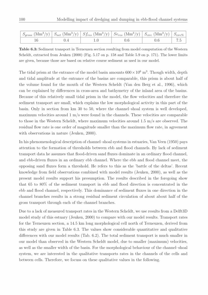
100 Modelling impact of dredging and dumping in ebb-flood channel systems
Sgross (Mm3/y) Snet (Mm3/y) Sfres (Mm3/y) Seres (Mm3/y) Scirc (Mm3/y) Scirc%
16 0.4 1.0 0.6 0.6 7.5
Table 6.3: Sediment transport in Terneuzen section resulting from model computation of the WesternScheldt, extracted from Jeuken (2000) (Fig. 5.17 on p. 158 and Table 5.9 on p. 171). The lower limitsare given, because those are based on relative course sediment as used in our model.
The tidal prism at the entrance of the model basin amounts 600×106 m3. Though width, depth
and tidal amplitude at the entrance of the basins are comparable, this prism is about half of
the volume found for the mouth of the Western Scheldt (Van den Berg et al., 1996), which
can be explained by differences in cross-area and bathymetry of the inland area of the basins.
Because of this relatively small tidal prism in the model, the flow velocities and therefore the
sediment transport are small, which explains the low morphological activity in this part of the
basin. Only in section from km 30 to 50, where the channel–shoal system is well developed,
maximum velocities around 1 m/s were found in the channels. These velocities are comparable
to those in the Western Scheldt, where maximum velocities around 1.5 m/s are observed. The
residual flow rate is one order of magnitude smaller than the maximum flow rate, in agreement
with observations in nature (Jeuken, 2000).
In his phenomenological description of channel–shoal systems in estuaries, Van Veen (1950) pays
attention to the formation of thresholds between ebb and flood channels. By lack of sediment
transport data he assumes that flood-driven sand fluxes dominate in an ordinary flood channel,
and ebb-driven fluxes in an ordinary ebb channel. Where the ebb and flood channel meet, the
opposing sand fluxes form a threshold. He refers to this as the ’battle of the deltas’. Recent
knowledge from field observations combined with model results (Jeuken, 2000), as well as the
present model results support his presumption. The results described in the foregoing show
that 65 to 80% of the sediment transport in ebb and flood direction is concentrated in the
ebb and flood channel, respectively. This dominance of sediment fluxes in one direction in the
channel branches results in a strong residual sediment circulation of about about half of the
gross transport through each of the channel branches.
Due to a lack of measured transport rates in the Western Scheldt, we use results from a Delft3D
model study of this estuary (Jeuken, 2000) to compare with our model results. Transport rates
for the Terneuzen section, a 14.5 km long morphological cell north of Terneuzen, derived from
this study are given in Table 6.3. The values show considerable quantitative and qualitative
differences with our model results (Tab. 6.2). The total sediment transport is much smaller in
our model than observed in the Western Scheldt model, due to smaller (maximum) velocities,
as well as the smaller width of the basin. For the morphological behaviour of the channel–shoal
system, we are interested in the qualitative transports rates in the channels of the cells and
between cells. Therefore, we focuss on these qualitative values in the following.
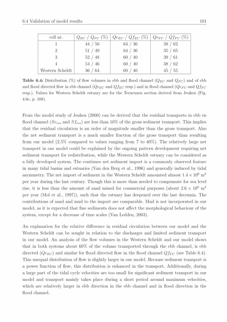
6.4 Validation of model results 101
cell nr. QEC / QFC (%) QeEC / QfEC (%) QeFC / QfFC (%)
1 44 / 56 64 / 36 38 / 62
2 51 / 49 64 / 36 35 / 65
3 52 / 48 60 / 40 39 / 61
4 54 / 46 60 / 40 38 / 62
Western Scheldt 36 / 64 60 / 40 45 / 55
Table 6.4: Distribution (%) of flow volumes in ebb and flood channel (QEC and QFC) and of ebband flood directed flow in ebb channel (QeEC and QfEC resp.) and in flood channel (QeFC and QfFC
resp.). Values for Western Scheldt estuary are for the Terneuzen section derived from Jeuken (Fig.4.6c, p. 108).
From the model study of Jeuken (2000) can be derived that the residual transports in ebb en
flood channel (Seres and Sfres) are less than 10% of the gross sediment transport. This implies
that the residual circulation is an order of magnitude smaller than the gross transport. Also
the net sediment transport is a much smaller fraction of the gross transport than resulting
from our model (2.5% compared to values ranging from 7 to 40%). The relatively large net
transport in our model could be explained by the ongoing pattern development requiring net
sediment transport for redistribution, while the Western Scheldt estuary can be considered as
a fully developed system. The continues net sediment import is a commonly observed feature
in many tidal basins and estuaries (Van den Berg et al., 1996) and generally induced by tidal
asymmetry. The net import of sediment in the Western Scheldt amounted almost 1.4× 10⁶ m3
per year during the last century. Though this is more than needed to compensate for sea level
rise, it is less than the amount of sand mined for commercial purposes (about 2.6 × 10⁶ m3
per year (Mol et al., 1997)), such that the estuary has deepened over the last decennia. The
contributions of sand and mud to the import are comparable. Mud is not incorporated in our
model, as it is expected that fine sediments does not affect the morphological behaviour of the
system, except for a decrease of time scales (Van Ledden, 2003).
An explanation for the relative difference in residual circulation between our model and the
Western Scheldt can be sought in relation to the discharges and limited sediment transport
in our model. An analysis of the flow volumes in the Western Scheldt and our model shows
that in both systems about 60% of the volume transported through the ebb channel, is ebb
directed (QeEC) and similar for flood directed flow in the flood channel QfFC (see Table 6.4).
This unequal distribution of flow is slightly larger in our model. Because sediment transport is
a power function of flow, this distribution is enhanced in the transport. Additionally, during
a large part of the tidal cycle velocities are too small for significant sediment transport in our
model and transport mainly takes place during a short period around maximum velocities,
which are relatively larger in ebb direction in the ebb channel and in flood direction in the
flood channel.
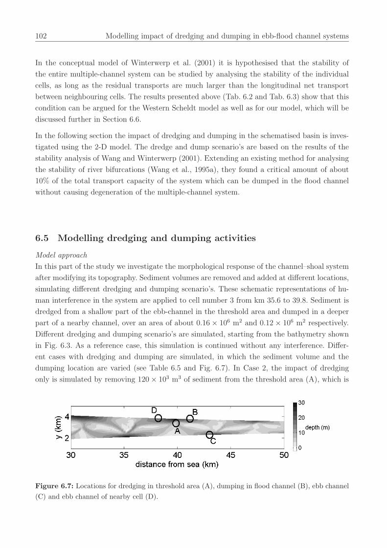
102 Modelling impact of dredging and dumping in ebb-flood channel systems
In the conceptual model of Winterwerp et al. (2001) it is hypothesised that the stability of
the entire multiple-channel system can be studied by analysing the stability of the individual
cells, as long as the residual transports are much larger than the longitudinal net transport
between neighbouring cells. The results presented above (Tab. 6.2 and Tab. 6.3) show that this
condition can be argued for the Western Scheldt model as well as for our model, which will be
discussed further in Section 6.6.
In the following section the impact of dredging and dumping in the schematised basin is inves-
tigated using the 2-D model. The dredge and dump scenario’s are based on the results of the
stability analysis of Wang and Winterwerp (2001). Extending an existing method for analysing
the stability of river bifurcations (Wang et al., 1995a), they found a critical amount of about
10% of the total transport capacity of the system which can be dumped in the flood channel
without causing degeneration of the multiple-channel system.
6.5 Modelling dredging and dumping activities
Model approach
In this part of the study we investigate the morphological response of the channel–shoal system
after modifying its topography. Sediment volumes are removed and added at different locations,
simulating different dredging and dumping scenario’s. These schematic representations of hu-
man interference in the system are applied to cell number 3 from km 35.6 to 39.8. Sediment is
dredged from a shallow part of the ebb-channel in the threshold area and dumped in a deeper
part of a nearby channel, over an area of about 0.16 × 10⁶ m2 and 0.12 × 10⁶ m2 respectively.
Different dredging and dumping scenario’s are simulated, starting from the bathymetry shown
in Fig. 6.3. As a reference case, this simulation is continued without any interference. Differ-
ent cases with dredging and dumping are simulated, in which the sediment volume and the
dumping location are varied (see Table 6.5 and Fig. 6.7). In Case 2, the impact of dredging
only is simulated by removing 120 × 103 m3 of sediment from the threshold area (A), which is
Figure 6.7: Locations for dredging in threshold area (A), dumping in flood channel (B), ebb channel(C) and ebb channel of nearby cell (D).
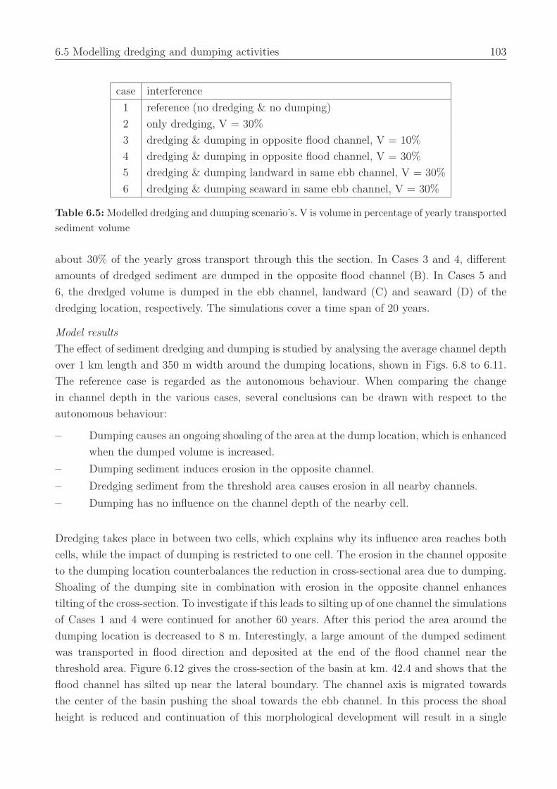
6.5 Modelling dredging and dumping activities 103
case interference
1 reference (no dredging & no dumping)
2 only dredging, V = 30%
3 dredging & dumping in opposite flood channel, V = 10%
4 dredging & dumping in opposite flood channel, V = 30%
5 dredging & dumping landward in same ebb channel, V = 30%
6 dredging & dumping seaward in same ebb channel, V = 30%
Table 6.5: Modelled dredging and dumping scenario’s. V is volume in percentage of yearly transportedsediment volume
about 30% of the yearly gross transport through this the section. In Cases 3 and 4, different
amounts of dredged sediment are dumped in the opposite flood channel (B). In Cases 5 and
6, the dredged volume is dumped in the ebb channel, landward (C) and seaward (D) of the
dredging location, respectively. The simulations cover a time span of 20 years.
Model results
The effect of sediment dredging and dumping is studied by analysing the average channel depth
over 1 km length and 350 m width around the dumping locations, shown in Figs. 6.8 to 6.11.
The reference case is regarded as the autonomous behaviour. When comparing the change
in channel depth in the various cases, several conclusions can be drawn with respect to the
autonomous behaviour:
– Dumping causes an ongoing shoaling of the area at the dump location, which is enhanced
when the dumped volume is increased.
– Dumping sediment induces erosion in the opposite channel.
– Dredging sediment from the threshold area causes erosion in all nearby channels.
– Dumping has no influence on the channel depth of the nearby cell.
Dredging takes place in between two cells, which explains why its influence area reaches both
cells, while the impact of dumping is restricted to one cell. The erosion in the channel opposite
to the dumping location counterbalances the reduction in cross-sectional area due to dumping.
Shoaling of the dumping site in combination with erosion in the opposite channel enhances
tilting of the cross-section. To investigate if this leads to silting up of one channel the simulations
of Cases 1 and 4 were continued for another 60 years. After this period the area around the
dumping location is decreased to 8 m. Interestingly, a large amount of the dumped sediment
was transported in flood direction and deposited at the end of the flood channel near the
threshold area. Figure 6.12 gives the cross-section of the basin at km. 42.4 and shows that the
flood channel has silted up near the lateral boundary. The channel axis is migrated towards
the center of the basin pushing the shoal towards the ebb channel. In this process the shoal
height is reduced and continuation of this morphological development will result in a single
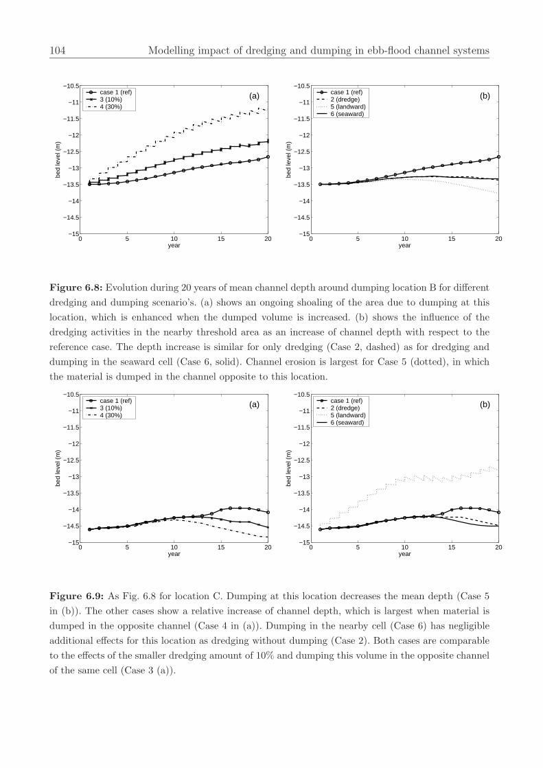
104 Modelling impact of dredging and dumping in ebb-flood channel systems
0 5 10 15 20−15
−14.5
−14
−13.5
−13
−12.5
−12
−11.5
−11
−10.5
year
bed
leve
l (m
)
(a)case 1 (ref)3 (10%)4 (30%)
0 5 10 15 20−15
−14.5
−14
−13.5
−13
−12.5
−12
−11.5
−11
−10.5
year
bed
leve
l (m
)
(b)case 1 (ref)2 (dredge)5 (landward)6 (seaward)
Figure 6.8: Evolution during 20 years of mean channel depth around dumping location B for differentdredging and dumping scenario’s. (a) shows an ongoing shoaling of the area due to dumping at thislocation, which is enhanced when the dumped volume is increased. (b) shows the influence of thedredging activities in the nearby threshold area as an increase of channel depth with respect to thereference case. The depth increase is similar for only dredging (Case 2, dashed) as for dredging anddumping in the seaward cell (Case 6, solid). Channel erosion is largest for Case 5 (dotted), in whichthe material is dumped in the channel opposite to this location.
0 5 10 15 20−15
−14.5
−14
−13.5
−13
−12.5
−12
−11.5
−11
−10.5
year
bed
leve
l (m
)
(a)case 1 (ref)3 (10%)4 (30%)
0 5 10 15 20−15
−14.5
−14
−13.5
−13
−12.5
−12
−11.5
−11
−10.5
year
bed
leve
l (m
)
(b)case 1 (ref)2 (dredge)5 (landward)6 (seaward)
Figure 6.9: As Fig. 6.8 for location C. Dumping at this location decreases the mean depth (Case 5in (b)). The other cases show a relative increase of channel depth, which is largest when material isdumped in the opposite channel (Case 4 in (a)). Dumping in the nearby cell (Case 6) has negligibleadditional effects for this location as dredging without dumping (Case 2). Both cases are comparableto the effects of the smaller dredging amount of 10% and dumping this volume in the opposite channelof the same cell (Case 3 (a)).
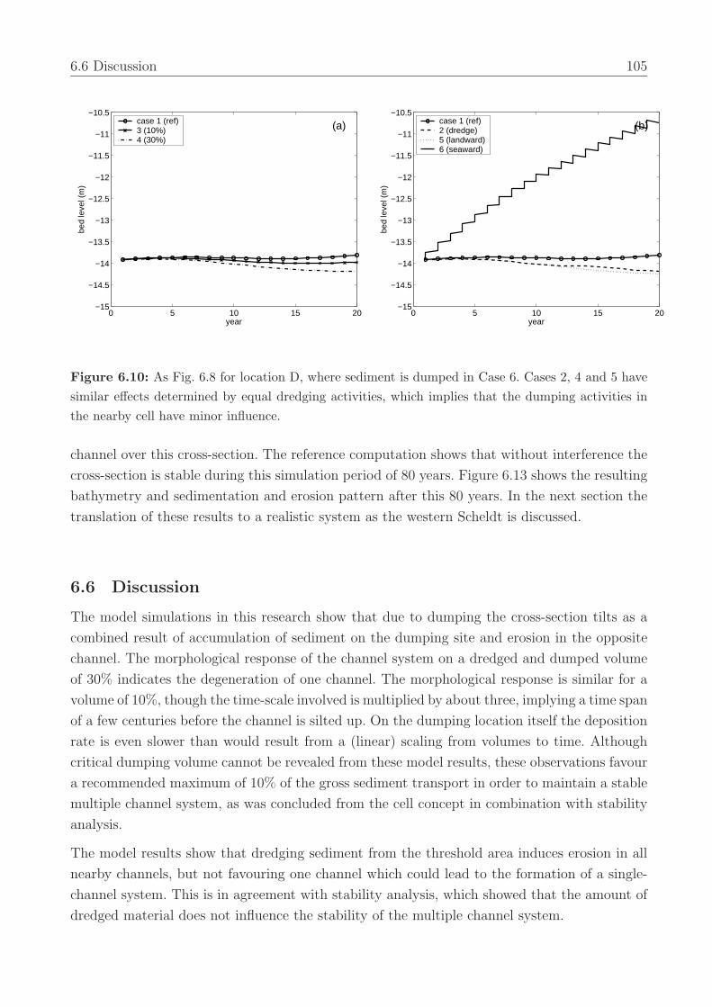
6.6 Discussion 105
0 5 10 15 20−15
−14.5
−14
−13.5
−13
−12.5
−12
−11.5
−11
−10.5
year
bed
leve
l (m
)
(a)case 1 (ref)3 (10%)4 (30%)
0 5 10 15 20−15
−14.5
−14
−13.5
−13
−12.5
−12
−11.5
−11
−10.5
year
bed
leve
l (m
)
(b)case 1 (ref)2 (dredge)5 (landward)6 (seaward)
Figure 6.10: As Fig. 6.8 for location D, where sediment is dumped in Case 6. Cases 2, 4 and 5 havesimilar effects determined by equal dredging activities, which implies that the dumping activities inthe nearby cell have minor influence.
channel over this cross-section. The reference computation shows that without interference the
cross-section is stable during this simulation period of 80 years. Figure 6.13 shows the resulting
bathymetry and sedimentation and erosion pattern after this 80 years. In the next section the
translation of these results to a realistic system as the western Scheldt is discussed.
6.6 Discussion
The model simulations in this research show that due to dumping the cross-section tilts as a
combined result of accumulation of sediment on the dumping site and erosion in the opposite
channel. The morphological response of the channel system on a dredged and dumped volume
of 30% indicates the degeneration of one channel. The morphological response is similar for a
volume of 10%, though the time-scale involved is multiplied by about three, implying a time span
of a few centuries before the channel is silted up. On the dumping location itself the deposition
rate is even slower than would result from a (linear) scaling from volumes to time. Although
critical dumping volume cannot be revealed from these model results, these observations favour
a recommended maximum of 10% of the gross sediment transport in order to maintain a stable
multiple channel system, as was concluded from the cell concept in combination with stability
analysis.
The model results show that dredging sediment from the threshold area induces erosion in all
nearby channels, but not favouring one channel which could lead to the formation of a single-
channel system. This is in agreement with stability analysis, which showed that the amount of
dredged material does not influence the stability of the multiple channel system.
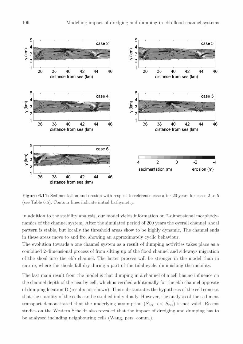
106 Modelling impact of dredging and dumping in ebb-flood channel systems
Figure 6.11: Sedimentation and erosion with respect to reference case after 20 years for cases 2 to 5(see Table 6.5). Contour lines indicate initial bathymetry.
In addition to the stability analysis, our model yields information on 2-dimensional morphody-
namics of the channel system. After the simulated period of 200 years the overall channel–shoal
pattern is stable, but locally the threshold areas show to be highly dynamic. The channel ends
in these areas move to and fro, showing an approximately cyclic behaviour.
The evolution towards a one channel system as a result of dumping activities takes place as a
combined 2-dimensional process of from silting up of the flood channel and sideways migration
of the shoal into the ebb channel. The latter process will be stronger in the model than in
nature, where the shoals fall dry during a part of the tidal cycle, diminishing the mobility.
The last main result from the model is that dumping in a channel of a cell has no influence on
the channel depth of the nearby cell, which is verified additionally for the ebb channel opposite
of dumping location D (results not shown). This substantiates the hypothesis of the cell concept
that the stability of the cells can be studied individually. However, the analysis of the sediment
transport demonstrated that the underlying assumption (Snet << Sres) is not valid. Recent
studies on the Western Scheldt also revealed that the impact of dredging and dumping has to
be analysed including neighbouring cells (Wang, pers. comm.).
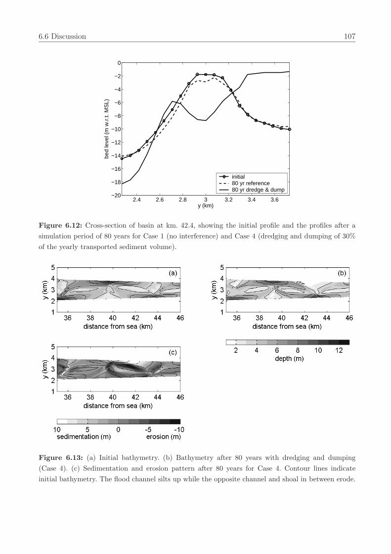
6.6 Discussion 107
2.4 2.6 2.8 3 3.2 3.4 3.6−20
−18
−16
−14
−12
−10
−8
−6
−4
−2
0
y (km)
bed
leve
l (m
w.r
.t. M
SL)
initial80 yr reference80 yr dredge & dump
Figure 6.12: Cross-section of basin at km. 42.4, showing the initial profile and the profiles after asimulation period of 80 years for Case 1 (no interference) and Case 4 (dredging and dumping of 30%of the yearly transported sediment volume).
Figure 6.13: (a) Initial bathymetry. (b) Bathymetry after 80 years with dredging and dumping(Case 4). (c) Sedimentation and erosion pattern after 80 years for Case 4. Contour lines indicateinitial bathymetry. The flood channel silts up while the opposite channel and shoal in between erode.
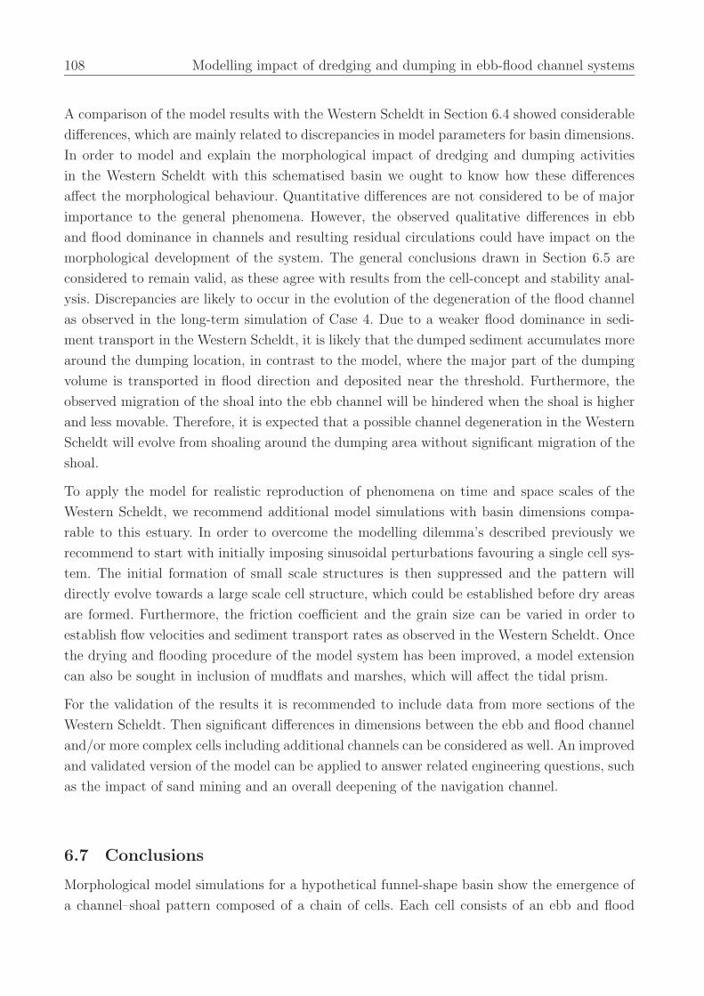
108 Modelling impact of dredging and dumping in ebb-flood channel systems
A comparison of the model results with the Western Scheldt in Section 6.4 showed considerable
differences, which are mainly related to discrepancies in model parameters for basin dimensions.
In order to model and explain the morphological impact of dredging and dumping activities
in the Western Scheldt with this schematised basin we ought to know how these differences
affect the morphological behaviour. Quantitative differences are not considered to be of major
importance to the general phenomena. However, the observed qualitative differences in ebb
and flood dominance in channels and resulting residual circulations could have impact on the
morphological development of the system. The general conclusions drawn in Section 6.5 are
considered to remain valid, as these agree with results from the cell-concept and stability anal-
ysis. Discrepancies are likely to occur in the evolution of the degeneration of the flood channel
as observed in the long-term simulation of Case 4. Due to a weaker flood dominance in sedi-
ment transport in the Western Scheldt, it is likely that the dumped sediment accumulates more
around the dumping location, in contrast to the model, where the major part of the dumping
volume is transported in flood direction and deposited near the threshold. Furthermore, the
observed migration of the shoal into the ebb channel will be hindered when the shoal is higher
and less movable. Therefore, it is expected that a possible channel degeneration in the Western
Scheldt will evolve from shoaling around the dumping area without significant migration of the
shoal.
To apply the model for realistic reproduction of phenomena on time and space scales of the
Western Scheldt, we recommend additional model simulations with basin dimensions compa-
rable to this estuary. In order to overcome the modelling dilemma’s described previously we
recommend to start with initially imposing sinusoidal perturbations favouring a single cell sys-
tem. The initial formation of small scale structures is then suppressed and the pattern will
directly evolve towards a large scale cell structure, which could be established before dry areas
are formed. Furthermore, the friction coefficient and the grain size can be varied in order to
establish flow velocities and sediment transport rates as observed in the Western Scheldt. Once
the drying and flooding procedure of the model system has been improved, a model extension
can also be sought in inclusion of mudflats and marshes, which will affect the tidal prism.
For the validation of the results it is recommended to include data from more sections of the
Western Scheldt. Then significant differences in dimensions between the ebb and flood channel
and/or more complex cells including additional channels can be considered as well. An improved
and validated version of the model can be applied to answer related engineering questions, such
as the impact of sand mining and an overall deepening of the navigation channel.
6.7 Conclusions
Morphological model simulations for a hypothetical funnel-shape basin show the emergence of
a channel–shoal pattern composed of a chain of cells. Each cell consists of an ebb and flood
6.7 Conclusions 109
channel enclosing a shoal and including threshold areas at the connections with adjacent cells.
This pattern agrees with field observations. Analysis of the model results shows that the major
part of the ebb and flood sediment fluxes are transported through the ebb and flood channel,
respectively. This quantifies the concept of estuarine channel systems of Van Veen (1950).
Where opposing sediment fluxes meet, a threshold is formed. In the present model the residual
sediment circulation through the cell is about half of the gross sediment transport. This is
well above the ratio computed with the Western Scheldt model (Jeuken, 2000), which can be
explained by enhanced effects of small (relative) differences in discharges and limited sediment
transport due to low velocities in the model.
Modelling various dredging and dumping scenarios shows that dumping sediment in a channel
not only reduces the channel depth, but also induces erosion in the opposite channel. The
influence on the channel depth of the nearby cell is negligible. Dredging sediment from the
threshold area causes erosion in all nearby channels. The recommendation based on the stability
analysis, viz. to restrict the dumping volume to maximally 10% of the gross sediment transport,
is supported by our model results.
The comparison with the data-based cell concepts of Van Veen (1950) and Winterwerp et al.
(2001), and the stability analysis of Wang and Winterwerp (2001) provides for mutual valida-
tion, in addition to the validations against field observations and other model approaches in
previous studies. It means another step forward in the application of this type of model to inves-
tigate and predict the morphodynamic response of estuarine systems to human interventions.
In order to reliably use the model results for explanation and prediction of the morphological
behaviour of the Western Scheldt it is recommended to setup a model in which the model
parameters are set such, that gross and net sediment transport rates are closer to reality.

110 Modelling impact of dredging and dumping in ebb-flood channel systems
7 Conclusions and recommendations
The objectives of this study are (1) to get a better insight into the mechanisms underlying the
morphodynamic behaviour of channels and shoals in estuaries and coastal lagoons and (2) to
improve the morphological prediction capabilities, using numerical models, at time scales from
decades to centuries. This has led to the conclusions and recommendations summarised below.
7.1 Conclusions
Applicability of numerical models to model and investigate morphodynamic be-
haviour of channels and shoals on meso- to macro-scales
While observations have been made and empirical relations have been established over many
decades, it is only the last two decades that models have been introduced to explain estuarine
features. Commonly used macro-scale model approaches are behaviour-oriented or hierarchical
models using empirical relations (aggregation of processes) or idealised process-based models us-
ing simplified formulations or geometry (aggregation of geometry). We have shown that complex
meso-scale, process-based models have the ability to reproduce the macro-scale hypsometry of
tidal basins as well as meso-scale channel–shoal patterns in a long-term, macro-scale evolution.
These models neither aggregate geometry or processes and therefore form a bridge between the
different model approaches. The results reconciliate observations and process knowledge both
on a meso- and a macro-scale. The positive feedback processes leading to pattern formation can
be derived from first physical principles on smaller scales. In fact, this may be seen as a first
successful step in the aggregation of smaller-scale estuarine process to larger-scale phenomena.
From the intermediate cross-sectionally averaged model results it is concluded that the simpli-
fied formulations used in the idealised model are justified. Only the adaptation of the morpho-
logical boundary condition at the entrance has a qualitative influence on the morphodynamic
equilibrium. This morphological boundary condition is an essential control for the behaviour of
morphodynamic models of tidal inlets and estuaries.
The ability of the complex 2-D depth-averaged model to reproduce realistic channel–shoal
systems is demonstrated by validating initial pattern formation with idealised model results
111
112 Conclusions and recommendations
and evolved patterns with field observations. Within the parameter ranges considered, the
model results seem to be insensitive to the specific sediment transport formulation applied.
Despite inherent limitations, the simplified geometry and the basic parameter setting contribute
to the transparency and the generalisation of the results obtained. Most model parameters only
influence the length scale of the patterns or the time scale of the formation, but the underlying
processes remain the same. However, neglecting wind waves and large river runoff limits the
validity of the model to elongated inland estuaries that are tidally dominated and well-mixed.
Mechanisms responsible for the morphodynamic behaviour of channels and shoals
in estuaries
The pattern of channel and shoals in estuaries is superimposed on a spatially uniform cross-
sectionally averaged profile of the basin. The profile development in the complex model is shown
to be qualitatively the same as in the idealised model of Schuttelaars and De Swart (2000) and
the equilibrium profile is controlled by the same physical processes. Using the idealised model,
the main physical process was identified as the interaction of the main M2-tide and its geometry-
induced overtides, leading to sediment fluxes that balance each other in the equilibrium state.
The fact that the complex 2-D depth-averaged numerical model produces realistic channel–
shoal patterns indicates that the modelling system includes the necessary processes responsible
for the evolution of estuarine channel–shoal systems. Further analysis of the model results, as
well as the linear stability analysis of idealised models, shows that there is a positive feedback
between the channel and shoal formation and the residual transport field, due to convergence
of advective transport above shoals and its divergence above channels. It is also demonstrated
that 3-D effects are not essential for the first order pattern formation.
The evolving pattern exhibits a dominant wavelength, which depends on the width of the basin
and the local maximum flow velocity. These parameters can be expressed in the dimensionless
the width–to–depth ratio, B/h, as a measure for the width, and tidal amplitude–to–depth ratio,
A/h, capturing the relation between velocity and depth. Additionally, the Shields parameter is
a commonly used dimensionless parameter, which includes velocity and grain size.
The width of the basin influences the meander length scale via the lateral boundaries and
the flow velocity has influence via inertia. During the formation of the channel–shoal system,
the velocities in the deepening channels increase, which leads to increase of the dominant
wavelength.
Along with the differences in water depth between channels and shoals, the differences in ve-
locities in channels and above shoals increase, which result into stronger (residual) circulation
of water and sediment and an enhanced growth rate of the channel–shoal system. Due to this
positive feedback, certain infinitesimal morphological perturbations tend to grow exponentially
and reach non-negligible amplitudes. Yet, long-term simulations suggest that a unique morpho-
7.1 Conclusions 113
dynamic equilibrium state develops, i.e. the exponential growth is reduced as the amplitude
increases.
Even after a stable overall pattern has established, the threshold areas remain highly dynamic.
Gross sediment transport capacities are maximal at these locations, where the flood-dominated
sand flux in the flood channel and ebb-dominated flux in the ebb channel meet. The dominance
of these fluxes adds to the tidally averaged residual circulation of sediment in the channel cell
enclosing a shoal.
Wind waves are considered to play a role in the (dynamic) equilibrium height of shoals, since
their eroding effect increases as the depth above the shoals decreases. Because this process is
not included in the model simulations, the eventual shoal height is not considered to be realistic.
However, in this research the shoal height is kept limited to avoid the influence of an inadequate
drying and flooding procedure, which plays a more important role in the modelled shoal height.
Predictability limits on the morphodynamic response of estuarine systems to hu-
man interventions
Limitations in applicability of numerical models as identified in the foregoing also limit the
capability to predict the impact of human interventions. At present, complex process-based
models are able to predict the morphological response of estuarine systems reasonably well at the
meso-scale. For macro-scale simulations, geometrical and/or processes descriptions have to be
simplified. This limits the use of these aggregated models for answering estuarine management
questions in specific situations. For example, the morphological time scale varies with grain
size. The model uses a constant value grain size throughout the basin, whereas varying grain
sizes are observed.
Due to increasing physical insight and computational power and ever improving numerical
techniques, the predictive capability of complex process-based models will keep on improving.
Yet, limitations in predictability will always remain, as a result of model uncertainties and
uncertainties inherent to the natural system (e.g. in the forcing, due to the deterministically
unpredictable occurrence of storm events).
Combining different model types and field and/or laboratory experiments improves the predic-
tive capabilities, since it provides for mutual validation and for the possibility to make use of
the strong points of each method (e.g. idealised models provide insight into the processes, while
complex models can simulate changes in complex geometries).
In summary, an intermediate cross-sectionally averaged process-based model is developed to
model equilibrium profiles of tidal basins and investigate differences in model formulations and
results between complex and idealised model. A good qualitative agreement has been found and

114 Conclusions and recommendations
insight into the effects of different model formulations is obtained. A complex two-dimensional
model is applied to investigate initial formation and long-term evolution of channel–shoal sys-
tems. Initial model results are compared to the results of linear stability analyses of idealised
models providing insight into the processes and validation of the model results. Long-term sim-
ulations show changes in pattern characteristics due to non-linear interactions and result in a
dynamic equilibrium state that agrees qualitatively with patterns observed in nature. Finally,
dredging and dumping in a multiple channel system is modelled and the resulting impact agrees
reasonably with results from stability analyses, though the translation to a realistic estuary is
subject to the validity of the applied model parameters. This research has brought together
different models and data. The possibilities obtained for mutual validation have resulted in a
better understanding and improved insight into the modelling skills concerning the morphody-
namics of estuarine channel–shoal systems. The complex process-based two-dimensional model
is shown to be a suitable tool for studying these systems on meso- as well as macro-scale. This
model type forms a sound basis for further development in modelling estuarine morphodynam-
ics.
7.2 Recommendations
With respect to model formulations the following recommendations are made:
– The seaward morphological boundary condition is shown to be an essential control to
the behaviour of morphodynamic models for tidal inlets and estuaries. However, none
of the model formulations discussed herein has been shown to adequately describe the
natural behaviour at this point. Therefore it is recommended to further investigate this
boundary condition and/or to extend the model region towards (at least) the edge of
the ebb–tidal delta when studying the evolution of tidal basins.
– Remaining differences in model formulations between the intermediate and idealised
one-dimensional model result in quantitative differences in the equilibrium profiles of the
tidal basins. Herein the parameterisation of the erosion and deposition term is considered
to be the most influential and is recommended for further research.
– Using the conclusions from the intermediate and one-dimensional model comparison, a
qualitative comparison of 2-D pattern formation in complex and idealised models could
be made. Selection of a dominant wavelength is influenced by the formulation of the
bed-slope effect, which differs between the two models. We advise to further investigate
the influence of this term in the sediment transport formulation and its contribution to
(quantitative) differences in model results.
– The model formulation for shallow areas (flooding and drying procedure) is not ad-
equate, as unrealistic heights of shoals above high water level can be reached. This
issue is addressed by Talstra (2003), introducing another computational scheme. So far,
7.2 Recommendations 115
this has not resulted in an overall improvement of the model behaviour. It is therefore
recommended to reconsider the drying- and wetting procedure.
Concerning further research following up this thesis, we recommend the following:
– The model comparison of the initial 2-D channel–shoal formation is based on the conclu-
sions from the intermediate model. For a thorough (quantitative) comparison of results
the model formulations should be further investigated and compared. It would be in-
teresting to extend this research by studying the long-term amplitude changes in more
detail, in order to get more insight into the regime of exponential growth and the non-
linearity of interactions. Furthermore, the model can be used to investigate to what
extent the amplitude of the initial perturbations determine the long-term evolution and
the final morphodynamic equilibrium pattern. The latter can also provide information
on the ability to return to an equilibrium state after (human) interference.
– The meander wavelength is shown to depend on the local velocity and the width of
the basin. Further research is needed to reveal quantitative relationships with proposed
dimensionless ratios B/h, A/h and the Shields parameter.
– Modelling simplified geometries and basic forcings is a successful approach to get in-
sight into the system response and the underlying processes. The model analysis can
be extended by investigating other geometries and forcings. For estuarine systems it
is recommended to investigate the long-term influence of sea level rise, storm events,
Coriolis force and wind waves. In order to simulate the large-scale evolution of natu-
ral systems the interaction with mudflats and marshes should be included, introducing
cohesive sediment and vegetation.
– Model results, applying an analogous model approach as used in this research, showed
that branching channel–shoal patterns can be reproduced in a short tidal basin (Mar-
ciano, 2003, also see Marciano et al. (accepted for publication)). Further research apply-
ing different geometries can reveal information on the selection of the number of channels
and braiding or branching behaviour of channels. Geometrical restrictions should be var-
ied in order to study the forced and free pattern formation as a result of (combined)
erodible and non-erodible boundaries and/or local constrictions.
– The impact of different dredge and dump scenario’s on the channel pattern in a schema-
tised funnel-shaped basin agrees with results from the cell-concept and the stability
analysis. However, qualitative differences in sediment transport patterns with a realistic
estuary such as the Western Scheldt hinders reliable translation of model results to real
consequences of human interference in this estuary. Therefore, we recommend to setup
a model which incorporates model parameters closer to this system, such that gross and
net sediment transport rates correspond better.
– In this research the height of the shoals is kept restricted to a limited elevation. For
further substantial progress in the research on estuarine systems, we recommend to
116 Conclusions and recommendations
find solutions for the mathematical, numerical as well as physical difficulties, which
are introduced by shallow intertidal areas (e.g. possible other processes dominating the
sediment exchange between channels and shoals).
Due to continuously improving physical insight, ever better numerical methods and increasing
computer power, the ability to use complex process-based models keeps on increasing. Thus the
processes incorporated, the complexity of geometry and the time-span of the simulations that
can be handled get closer to reality. We emphasize, however, the value of modelling simplified
situations for transparency and genericity of the results obtained.
References
Ahnert, F., 1960. Estuarine meanders in the Chesapeake Bay area. Geographical Review 50,
390–401.
Allersma, E., 1992. Management study of the eastern part of the Western Scheldt; Analysis of
the physical system. Report Z368, WL|Delft Hydraulics.
Allersma, E., 1994. Channels in estuaries; 1-D modelling of parallel channels. Report H1828,
WL|Delft Hydraulics.
Bolla Pittaluga, M., Tambroni, N., Zucca, C., Solari, L., Seminara, G., 2001. Long term mor-
phodynamic equilibrium of tidal channels: preliminary laboratory observations. In: Ikeda, S.
(Ed.), IAHR Proceedings of the River, Coastal and Estuarine Morphodynamics Conference.
Boon, J. D., Byrne, R. J., 1981. On basin hypsometry and the morphodynamic response of
coastal inlet systems. Marine Geology 40, 27–48.
Bruun, P., Gerritsen, F., 1960. Stability of coastal inlets. North-Holland Publishing Cy, Ams-
terdam.
Cameron, W. M., Pritchard, D. W., 1963. Estuaries. In: The Sea. Vol. 2. M. N. Hill (Ed.), John
Wiley & Sons, New York, pp. 306–324.
Cayocca, F., 2001. Long-term morphological modeling of a tidal inlet: the arcachon basin,
france. Coastal Engineering 42, 115–142.
Cleveringa, J., Oost, A. P., 1999. The fractal geometry of tidal-channel systems in the Dutch
Wadden Sea. Geologie en Mijnbouw 78, 21–30.
Coeveld, E. M., Hibma, A., Stive, M. J. F., 2003. Feedback mechanisms in channel-shoal for-
mation. In: Proceedings of Coastal Sediments Conference. Clearwater Beach, FL, USA, on
CD-ROM.
Dalrymple, R. W., Rhodes, R. M., 1995. Estuarine dunes and bars. In: Perillo, G. M. E. (Ed.),
Geomorphology and Sedimentology of Estuaries. Vol. 53 of Development in Sedimentology.
Elsevier, Amsterdam, pp. 359–422.
De Jong, K., 1998. Tidally averaged transport models. Ph.D. thesis, Delft University of Tech-
nology.
De Vriend, H. J., 1996. Mathematical modelling of meso–tidal barrier island coasts. Part I:
Empirical and semi–emperical models. In: Liu, P. L.-F. (Ed.), Advances in coastal and ocean
engineering. World Scientific, Singapore.
117
118 References
De Vriend, H. J., Louters, T., Berben, F., Steijn, R. C., 1989. Hybrid prediction of a sandy shoal
in a mesotidal estuary. In: Falconer, R. A. e. (Ed.), Hydraulic and environmental modelling
of coastal, estuarine and river waters. Gower Technical, Aldershot.
De Vriend, H. J., Ribberink, J. S., 1996. Mathematical modelling of meso–tidal barrier island
coasts. Part II: Process–based simulation models. In: Liu, P. L.-F. (Ed.), Advances in coastal
and ocean engineering. World Scientific, Singapore.
Di Silvio, G., 1989. Modelling the morphological evolution of tidal lagoons and their equilibrium
configurations. In: XXII Congress of the IAHR. Ottawa, Canada.
Di Silvio, G., Padovan, A., 1998. Interaction between marches, channels and shoals in a tidal
lagoon investigated by a 2-d morphological model. In: Hydro-Science and -Engineering, III.
Dronkers, J., 1998. Morphodynamics of the Dutch Delta. In: Dronkers, J., Scheffers, M. (Eds.),
Physics of estuaries and coastal seas. Balkema, Rotterdam.
Duijts, 2002. Tidal asymmetry in the Dutch Wadden Sea. A model study of morphodynamic
equilibrium of tidal basins. M.Sc.–thesis, Delft University of Technology, The Netherlands.
Dyer, K. R., 1973. Estuaries: A Physical introduction. John Wiley & Sons, London.
Engelund, F., Hansen, E., 1967. A monograph on sediment transport in alluvial streams. Teknisk
Forlag, Copenhagen.
Escoffier, F. F., 1940. The stability of tidal inlets. Shore and Beach 8 (4), 114–115.
Eysink, W. D., 1990. Morphological response of tidal basins to change. In: ASCE Proceedings
of Coastal Engineering Conference. Vol. 2. Delft.
Fischer, H. B., 1979. Mixing in inland and coastal waters. Academic Press, San Diego.
Friedrichs, C. T., Aubrey, D. G., 1996. Uniform bottom shear stress and equilibrium hypsometry
of intertidal flats. In: Pattiaratchi, C. (Ed.), Mixing in estuaries and coastal seas. Amer.
Geophys. Union, Washington D.C.
Gallappatti, R., Vreugdenhill, C. B., 1985. A depth–integrated model for suspended sediment
transport. Journal of Hydraulic Research 23, 359–377.
Hayes, M. O., 1975. Morphology of sand accumulation in estuaries: an introduction to the
symposium. In: Cronin, L. E. (Ed.), Estuarine research II. Academic press, New York, pp.
3–22.
Hibma, A., De Vriend, H. J., Stive, M. J. F., 2003a. Numerical modelling of shoal pattern
formation in well-mixed elongated estuaries. Estuarine, Coastal and Shelf Science 57 (5-6),
981–991.
Hibma, A., Jeuken, C., Wang, Z. B., 2000. Morfologische ontwikkeling van intergetijde-gebieden
en modellering met ESTMORF. Deel II: literatuurstudie (in Dutch). Report Z2776, WL|Delft
Hydraulics.
Hibma, A., Schuttelaars, H. M., De Vriend, H. J., 2003c. Initial formation and evolution of
channel-shoal patterns in estuaries. In: Sanchez-Arcilla, A., Bateman, A. (Eds.), IAHR Pro-
ceedings of the River, Coastal and Estuarine Morphodynamics Conference.
References 119
Hibma, A., Schuttelaars, H. M., Wang, Z. B., 2003b. Comparison of longitudinal equilibrium
profiles of estuaries in idealised and process-based models. Ocean Dynamics 53 (3), 252–269.
Hibma, A., Stive, M. J. F., Wang, Z. B., in press. Estuarine Morphodynamics. In: Coastal
Morphodynamic Modeling. Special issue Coastal Engineering. C.V. Lakhan (Ed.).
Jeuken, M. C. J. L., 2000. On the morphological behaviour of tidal channels in the Westerschelde
estuary. Ph.D. thesis, University of Utrecht, The Netherlands, Also published as Proc. Royal
Geographical Society nr. 279.
Kjerfve, B., 1994. Coastal lagoon processes. Elsevier, Amsterdam.
Lanzoni, S., Seminara, G., 2002. Long–term evolution and morphodynamic equilibrium of tidal
channels. Journal of Geophysical Research 107, C, 1–13.
Lorentz, 1922. Ein rechnungsansatz fur den widerstand bei flussigkeitsschwingungen (in Ger-
man). De Ingenieur 695 (37), 252–254.
Marciano, R., 2003. Morphodynamic modelling of fractal channel patterns in a tidal basin.
M.Sc.–thesis, Delft University of Technology, The Netherlands.
Marciano, R., Wang, Z. B., Hibma, A., De Vriend, H. J., Defina, A., accepted for publication.
Modelling of channel patterns in short tidal basins. Journal of Geophysical Research, Earth
Surface .
Mol, G., Van Berchum, A. M., Krijger, G. M., 1997. De toestand van de Westerschelde aan
het begin van de verdieping 48’/43’. Beschrijving van de trends in fysische, biologische en
chemische toestand (in Dutch). Tech. Rep. Report RIKZ-97.049, ISBN 90-369-3412-5, RIKZ,
Rijkswaterstaat.
O’Brien, M. P., 1969. Equilibrium flow areas of inlets on sandy coasts. Journal of the Waterways
and Harbour Division, ASCE 95 (WW1), 43–52.
Officer, C. B., 1976. Physical oceanography of estuaries (and associated coastal waters). John
Wiley & Sons, New York.
Pritchard, D., Hogg, A. J., Roberts, W., 2002. Morphological modelling of intertidal mudflats:
the role of cross-shore tidal currents. Continental Shelf Research 22, 1887–1895.
Rinaldo, A., Lanzoni, S., Marani, M., 2001. River and tidal networks. In: River, Coastal and
Estuarine Morphodynamics. G. Seminara and P. Blondeaux (Eds.), Springer-Verlag Berlin
Heidelberg., Ch. 9, pp. 191–211.
Robinson, A. H. W., 1960. Ebb–flood channel systems in sandy bays and estuaries. Geography
45, 183–199.
Roelvink, J. A., van Banning, C. K. F. M., 1994. Design and development of DELFT3D and
application to coastal morphodynamics. In: Verwey, A., Minns, A. W., Babovic, V., Maksi-
movic, C. (Eds.), Hydroinformatics ’94. Balkema, Rotterdam.
Schramkowski, G. P., Schuttelaars, H. M., De Swart, H. E., 2002. The effect of geometry and
bottom friction on local bed forms in a tidal embayment. Continental Shelf Research 22,
1821–1833.
120 References
Schramkowski, G. P., Schuttelaars, H. M., De Swart, H. E., 2004. Non-linear channel–shoal
dynamics in long tidal embayments. Ocean Dynamics , in press.
Schuttelaars, H. M., De Swart, H. E., 1996. An idealized long–term morphodynamic model of
a tidal embayment. European Journal of Mechanics, B/Fluids 15 (1), 55–80.
Schuttelaars, H. M., De Swart, H. E., 1999. Initial formation of channels and shoals in a short
tidal embayment. Journal of Fluid Mechanics 386, 15–42.
Schuttelaars, H. M., De Swart, H. E., 2000. Multiple morphodynamic equilibria in tidal em-
bayments. Journal of Geophysical Research C 105, 24105–24118.
Seminara, G., Tubino, M., 1998. On the formation of estuarine free bars. In: Dronkers, J.,
Scheffers, M. B. A. M. (Eds.), Physics of Estuaries and Coastal Seas. Balkema, Rotterdam.
Seminara, G., Tubino, M., 2001. Sand bars in tidal channels. Part 1. Free bars. J. Fluid Mech.
440, 49–74.
Stelling, G. S., 1984. On the construction of computational methods for shallow water flow
problems. Communications 35, Rijkswaterstaat, The Hague.
Stive, M. J. F., Capobianco, M., Wang, Z. B., Ruol, P., Buijsman, M. C., 1998. Morphodynamics
of a tidal lagoon and the adjacent coast. In: Dronkers, J., Scheffers, M. (Eds.), Physics of
estuaries and coastal seas. Balkema, Rotterdam.
Stive, M. J. F., De Vriend, H. J., 1995. Modelling shoreface profile evolution. Marine Geology
126, 235–248.
Stive, M. J. F., Wang, Z. B., 2003. Morphodynamic modelling of tidal basins and coastal inlets.
In: Advances in coastal modelling. C. Lakhan (Ed.), Ch. 13, pp. 367–392.
Talstra, H., 2003. Numerieke modellering van het lange-termijn morfologisch gedrag van estu-
aria. (in Dutch). M.Sc.–thesis, Delft University of Technology, The Netherlands.
Thoolen, P. M. C., Wang, Z. B., 1999. Sediment transport modelling for the Western Scheldt.
Report Z2649, WL|Delft Hydraulics, Delft.
Van de Kreeke, J., 1990. Can multiple inlets be stable? Estuarine Coastal Shelf Science 30,
261–273.
Van de Kreeke, J., 1992. Stability analysis of a two-inlet bay system. Coastal Engineering 14,
481–497.
Van den Berg, J. H., Jeuken, C. J. L., Van der Spek, A. J. F., 1996. Hydraulic processes affecting
the morphology and evolution of the Westerschelde estuary. In: Estuarine shores: Evolution,
environments and human alterations. K. F. Nordstrom and C. T. Roman (Eds.). John Wiley
& Sons Ltd., Ch. 7, pp. 157–184.
Van Dongeren, A. P., De Vriend, H. J., 1994. A model of morphological behavior of tidal basins.
Coastal Engineering 22 (3/4), 287–310.
Van Ledden, M., 2003. Sand–mud segregation in estuaries and tidal basins. Ph.D. thesis, Delft
University of Technology, The Netherlands.
Van Ledden, M., Wang, Z. B., Winterwerp, H., De Vriend, H. J., 2004. Sand-mud morphody-
namics in a short tidal basin. Ocean Dynamics , in press.
References 121
Van Leeuwen, S. M., De Swart, H. E., 2002. Intermediate modelling of tidal inlet systems:
spatial asymmetries in flow and mean sediment transport. Continental Shelf Research 22,
1795–1810.
Van Leeuwen, S. M., Schuttelaars, H. M., De Swart, H. E., 2000. Tidal and morphologic prop-
erties of embayments: Effects of sediment deposition processes and length variation. Phys.
Chem. Earth (B) 25, 365–368.
Van Leeuwen, S. M., Van der Vegt, M., De Swart, H. E., 2003. Morphodynamics of ebb-tidal
deltas: a model approach. Estuarine, Coastal and Shelf Science 57 (5-6), 899–907.
Van Rijn, L. C., 1984. Sediment transport. Part II: Suspended load transport. ASCE Journal
of Hydraulic Engineering 110, 1613–1641.
Van Veen, J., 1950. Ebb and flood channel systems in the Netherlands tidal waters (in
Dutch, English summary). Journal of the Royal Dutch Geographical Society (KNAG) 67,
303–325, Republished, translated and annotated by Delft University of Technology, 2001.
(http://www.waterbouw.tudelft.nl/research/specialPublications/Van Veen.pdf).
Verbeek, H., Wang, Z. B., Thoolen, P. M. C., 1999. Secondary currents in estuarine morpho-
dynamic modelling, a case study of the Western Scheldt. In: Seminara, G. (Ed.), IAHR
Proceedings of the River, Coastal and Estuarine Morphodynamics Conference.
Wang, Z. B., 1992a. Fundamental considerations on morphodynamic modelling in tidal regions,
Part I: Theoretical analysis and 1D test computations. Report Z331, WL|Delft Hydraulics,
The Netherlands.
Wang, Z. B., 1992b. Some considerations on the mathematical modelling of morphological
processes in tidal regions. In: Prandle, D. (Ed.), Dynamics and exchanges in estuaries and
the coastal zone. Physics of Estuaries and Coastal Seas 1990.
Wang, Z. B., Fokkink, R. J., De Vries, M., Langerak, A., 1995a. Stability of river bifurcations
in 1D morphological models. Journal of Hydraulic Research 33, No. 6, 739–750.
Wang, Z. B., Louters, T., De Vriend, H. J., 1992. A morphodynamic model for a tidal inlet. In:
Arcilla, A. S., Pastor, M., Zienkiewicz, O. (Eds.), Computing Modelling in Ocean Engineering′91. Balkema, Rotterdam.
Wang, Z. B., Louters, T., De Vriend, H. J., 1995b. Morphodynamic modelling of a tidal inlet
in the Wadden Sea. Marine Geology 126, 289–300.
Wang, Z. B., Winterwerp, J. C., 2001. Impact of dredging and dumping on the stability of
ebb–flood channel systems. In: Ikeda, S. (Ed.), IAHR Proceedings of the River, Coastal and
Estuarine Morphodynamics Conference.
Winterwerp, J. C., Wang, Z. B., Stive, M. J. F., Arends, A., Jeuken, C., Kuijper, C., Thoolen,
P. M. C., 2001. A new morphological schematization of the Western Scheldt estuary, the
Netherlands. In: Ikeda, S. (Ed.), IAHR Proceedings of the River, Coastal and Estuarine
Morphodynamics Conference.
Zimmerman, J. T. F., 1992. On the Lorentz linearization of a nonlinearly damped tidal

122 References
Helmholtz oscillator. Proc. Koninklijke Nederlandse Akademie van Wetenschappen 95, 127–
145.
Acknowledgements
The first phase of doing a PhD-research is often described as swimming. I can confirm and
extent this metaphor by my experience in the waters of Florida: first you are enjoying the
comfortable water and explore the field until far out of the coast, far more than necessary and
sensible. Then suddenly, you are brought back to reason, faced by a shark. You yell to your
supervisor: ”Henk, een haai!”, you turn around and start to swim back with a well defined
focus – the coast. In your effort to this goal you feel backed by your supervisor, though not
always taking care that he is able to follow your way. While it feels you are swimming fast,
the coast appears quite far away and it seems you are not making much progress. And then
suddenly, the coast appears to be near and almost relaxed the last meters are covered until the
solid ground under your feet is reached. On the beach you are glad it is over, but can look back
on this experience with very much pleasure!
This research was supported by the DIOC-programme ’Hydraulic Engineering and Geohydrol-
ogy’ of Delft University of Technology under Theme 1 ’Aggregated-scale prediction in morpho-
dynamics’, project 1.4. It is embedded as such in Project 03.01.03 of the Delft Cluster Strategic
Research Programme on the ’Sustainable development of low-lying deltaic areas’ under Theme
3 ’Coasts and rivers’. The Delft3D model was provided by WL|Delft Hydraulics.
I feel lucky to have been surrounded by so many people, who contributed to the progress as
well as the pleasure during my research. First of all I want to thank my supervisors. You
have given me the freedom to choose the research direction I wanted, the supervision I asked
and the support I needed for all initiatives I proposed. Huib de Vriend, it is unbelievable
that someone can do so much work in so little time and seems to enjoy it all. Thanks for
your enthusiasm, conscientious and constructive criticism and giving insight into the ’research-
politics’. Marcel Stive, your care about everyone’s well-being is unique. Thanks for being a
motivator by proposing ideas and research-hypotheses, as well as actively introducing people to
your network. Zheng-Bing Wang, your knowledge seems endless. Thanks for explaining many
things with much patience and for your enormous enthusiasm. Henk Schuttelaars, discussing
with you on a variety of subjects is educational and amusing. Thanks for your critical supervision
and enjoyable company.

Then I want to thank Co van de Kreeke. I enjoyed our cooperation on different occasions and
thanks for your and Hetty’s hospitality in Miami. Huib de Swart and Guus Stelling, thanks for
the discussions and giving me insight into different modelling aspects. I also want to thank the
MSc-students, Martijn van Rijsewijk, Alexandro Tittonel, Martijn Coeveld, Harmen Talstra
and Raffaele Marciano. I appreciated cooperating with you.
The three months I spend at the Virginia Institute of Marine Science have broadened my view
and been enjoyable. Carl Friedrichs, thank you and your family for the enormous hospitality
during my stay there. Grace Battisto and colleagues, thanks for your pleasant company and
helping me around. And of course: Alaydis Barbosa, David Fugate and Courtney Harris, without
you it wouldn’t have been so much fun. Thanks for the friendship, dinners and drives to the
gym ;-)
Then much thanks to my colleagues, who contributed essentially to the pleasure of working
at the university. I highly appreciated the sincere interest in each others work. I will miss
the serious as well as nonsense discussions during the morning coffee break in our tropical
paradise (thanks Chantal). It also has been much joy to attend conferences together in Sweden
(running with Edwin), Japan (endless bath-sessions with Saskia en Hanneke), Hamburg (ein
Doppelzimmer fur Einzelnutzung for Hans), Florida (bathing with Marije and the memorable
swim with Henk) and Barcelona (keeping the bus waiting because Mark, Francois and I cannot
get enough of the fantastic waves). Additionally, I want to thank Mathijs for useful discussions
and advices, Mark Voorendt for your always quick and accurate technical assistance and Stefan,
Mark van K., Marcel and Martin for an enjoyable evening defining the propositions.
My last word of thanks is for Mam and Klaas, paranimfen Pauline en Judith, cover designer
Ada, Azarja, family and friends. Ups and downs in live and research prevent boredom, but are
ambivalently appreciated. My full appreciation and thanks is for your continuous interest and
support to overcome the downs and enjoy the ups!
Anneke Hibma
Delft, June 2004
About the author
Anneke Hibma was born in Amsterdam, the Netherlands, on December 29th 1974. She gradu-
ated from secondary school, Willem Lodewijk Gymnasium in Groningen, in 1993. She moved to
Delft, where she started her academic education at Delft University of Technology. As a part of
her study Civil Engineering she gained work experience in Tanamalwila, Sri-Lanka, on a Wewa
(water reservoir) restoration project, with three other students. They surveyed land, designed
water works and made an irrigation scheme. She did her final MSc-project at WL|Delft Hy-
draulics, entitled ”Process-based modelling of tidal inlet dynamics. Evaluation of Frisian Inlet
data.” and graduated cum laude in 1999 at the Section of Hydraulic Engineering.
In April 2000 she started her PhD-research at Delft University of Technology on morphodynamic
modelling of estuarine channel-shoal systems, which resulted in the present dissertation. She
visited the Virginia Institute of Marine Science, USA, for three months to take part in field
measurements and data analysis of the Chesapeake Bay estuary. The research was supported
by the DIOC (1.4) and Delft Cluster (03.01.03) programmes.
Publications
Journal articles
Hibma, A., H.J. de Vriend and M.J.F. Stive (2003). Numerical modelling of shoal pattern
formation in well-mixed elongated estuaries. Estuarine, Coastal and Shelf Science. Vol. 57, 5-6,
p.981-991.
Hibma, A., H.M. Schuttelaars and Z.B. Wang (2003). Comparison of longitudinal equilibrium
profiles of estuaries in idealised and process-based models. Ocean Dynamics. Vol. 53 (3), p.
252-269.
Hibma, A., M.J.F. Stive and Z.B. Wang (2004). Estuarine morphodynamics. In: Coastal Mor-
phodynamic Modeling. Special Issue Coastal Engineering. Ed. C.V. Lakhan. (in press).
Hibma, A., H.M. Schuttelaars and H.J. de Vriend. Initial formation and long-term evolution of
channel-shoal patterns in estuaries. Accepted for publication in Continental Shelf Research.
Marciano, R., Z.B. Wang, A. Hibma, H.J. de Vriend and A. Defina. Modelling of channel
patterns in short tidal basins. Accepted for publication in Journal of Geophysical Research,
Earth Surface.
Van de Kreeke, J. and A. Hibma. Observations on silt and sand transport in the throat section
of the Frisian Inlet. Submitted to Coastal Engineering.
Conference proceedings
Hibma, A. and J. van de Kreeke (2001). Tidal variations in sand concentrations in the Frisian
Inlet. Coastal Dynamics Conference, Lund, Sweden. p.453-462.
Hibma, A., H.J. de Vriend and M.J.F. Stive (2001). Channel and shoal formation in estuaries.
River, Coastal and Estuarine Morphodynamics Conference (IAHR), Obihiro, Japan. p.463-472.
Hibma, A., H.M. Schuttelaars and Z.B. Wang (2002).Comparison of longitudinal equilibrium
profiles of estuaries in idealised and process-based models. Physics of Estuaries and Coastal
Seas, Hamburg, Germany. p.280-283.
Coeveld, E.M., A. Hibma and M.J.F. Stive (2003). Feedback mechanisms in channel-shoal
formation. Coastal Sediments Conference, St. Petersburg, FL, USA. (on CD-ROM)
Hibma, A., J. van de Kreeke and M. van Rijsewijk (2003). Tidal variations in suspended sed-
iment concentration and related sediment transport in the Frisian Inlet. Coastal Sediments
Conference, St. Petersburg, FL, USA. (on CD-ROM)
Hibma, A., H.M. Schuttelaars and H.J. de Vriend (2003). Initial formation and evolution of
channel-shoal patterns in estuaries. River, Coastal and Estuarine Morphodynamics Conference
(IAHR), Barcelona, Spain. p. 749-760.
Hibma, A. Z.B. Wang, M.J.F. Stive and H.J. de Vriend (2004). Modelling impact of dredging
and dumping in ebb-flood channel systems. Physics of Estuaries and Coastal Seas, Yucatan,
Mexico. Accepted for presentation and publication.
Miscellaneous
Hibma, A., C. Jeuken and Z.B. Wang (2000), Morphological development of inter-tidal areas
and modelling with estmorf. Part II: literature survey (in Dutch). WL|Delft Hydraulics,
report Z2776.