
Microbial production of antimicrobial compounds from … delen ervan te kopiëren voor persoonlijk...
136
Faculteit Bio-ingenieurswetenschappen Academiejaar 2015-2016 Microbial production of antimicrobial compounds from biorefinery sidestreams Kyrina Denis Promotors: Prof. Dr. ir. Korneel Rabaey & Prof. Dr. ir. Ingmar Nopens Tutors: ir. Pieter Candry & ir. Timothy Van Daele Masterproef voorgedragen tot het behalen van de graad van Master in de bio-ingenieurswetenschappen: Chemie en Bioprocestechnologie
Transcript of Microbial production of antimicrobial compounds from … delen ervan te kopiëren voor persoonlijk...
Faculteit Bio-ingenieurswetenschappen
Academiejaar 2015-2016
Microbial production of antimicrobial
compounds from biorefinery sidestreams
Kyrina Denis
Promotors: Prof. Dr. ir. Korneel Rabaey & Prof. Dr. ir. Ingmar Nopens
Tutors: ir. Pieter Candry & ir. Timothy Van Daele
Masterproef voorgedragen tot het behalen van de graad van
Master in de bio-ingenieurswetenschappen: Chemie en Bioprocestechnologie


De auteur en promotor gerren de toelating deze scriptie voor consultatie beschikbaar te stellen
en delen ervan te kopiëren voor persoonlijk gebruik. Elk ander gebruik valt onder de beperkin-
gen van het auteursrecht, in het bijzonder met betrekkíng tot de verplichting uitdrukkelijk de
bron te vermelden bij het aa,nhalen van resultaten uit deze scriptie.
The author and promoter give the permission to use this thesis for consultation and to copy
parts of it for personal use. Every other use is subject to the copyright laws, more specifi.cally
the source must be extensively specified when using results from this thesis.
Ghent, June 2016
The promoters,
Raba*y Prof- dr. ir. Ingmar Nopens
The author,The tutors.
q - - : .- : i . - ' . - . . . - - - , t '
ir. Pieter Candry ir. Timothy Van Daeie Kyrina Denis


Acknowledgment
Via this acknowledgment I would like to thank everyone who helped me through this journey.
I can not believe how these last few years studying bio-engineering have crept by, ending with
this literal master piece.
At first I would like to thank my promoters Prof. dr. ir. Korneel Rabaey and Prof. dr. ir. Ingmar
Nopens. The meetings were always very useful, as they were the penultimate strategy to move
the thesis in a consistent direction. The additional literature, knowledge and support were
extremely helpful and much appreciated.
Next, I would like to thank my tutors, ir. Pieter Candry and ir. Timothy Van Daele. I think
the help I received was above all expectations, ranging from revising my work, explaining
procedures, helping me determine the direction of the thesis, practical help and even doing
experiments when I was not able to. Therefore, I can not express how grateful I am for never
feeling I had to do it completely on my own.
Another important person, which had a major impact on the course of this thesis and deserves
a special place in this acknowledgment is dr. Jan Arends. Thank you, not only for teaching
me a lot of the practical things used in this thesis but also for your continuous presence
throughout.
Further, I would also like to thank the entire CMET team and my fellow students. More
specifically Tim Lacoere and Greet Van de Velde for analyzing a lot of my samples this year.
Lastly I would like to thank my close friends, family and in-laws, more specifically:
My boyfriend Yoram ♥, with whom I’ve been with for almost 6 years. Gradually I am
forgetting how life was before meeting you.
My parents, who have cared and supported me my whole life, and keep supporting me even
though I already moved out.
My older brother Yoshi and little brother Ymre. Since growing up, I now realize how lucky
I am to have the support system of two people who have been with me for as long as I can
remember.
i

ii
Abstract
Fossil fuel depletion has resulted in a search for more sustainable solutions. One possibility
is the usage of biomass obtained from industrial or agricultural waste streams. This can be
converted into so-called platform chemicals using bio-processes, from which they can be fur-
ther valorized into an array of chemicals used for fuels, solvents, etc. Short-chain fatty acids
(SCFAs) are one of those platform chemicals and are produced during anaerobic digestion.
When methanogenesis is suppressed and the right environmental conditions are maintained,
SCFAs can be coupled to other substrates present in or added to the fermentation broth
such as ethanol, producing medium chain fatty acids (MCFAs, e.g. caproate) in a process
called “chain elongation”. MCFAs are interesting compounds which can be used as fossil
fuels, antimicrobials, etc. However, MCFAs are toxic compounds for the chain elongating
microorganisms as well, thus continuous extraction might be necessary to produce economic
amounts. An electrochemical cell which can be used for extraction has proven to be a valuable
option for boosting MCFA production.
In order to gain fundamental knowledge about the process described above, i.e. fermentation,
chain elongation and extraction, modeling can be a powerful tool. A lot has been done in
literature on modeling the fermentation and extraction part, but nothing on chain elongation.
Therefore, in this thesis a mathematical model was built for chain elongation, based upon
stoichiometry derived by Spirito et al. (2014) and bacterial growth models.
The model consisted of several parameters which were not readily available from literature.
Consequently, experiments were designed and conducted that would allow parameter estima-
tion. As model simulations showed that initial conditions influence the subsequent growth
rate, producing growth curves in a 96-well plate appeared to be an attractive possibility. Af-
ter conducting the experiments however, it appeared that the acquired data deviated tremen-
dously from what would be expected. Part of the problem was thought to be that the
stoichiometry derived by Spirito et al. (2014) did not encompass thermodynamic limitations.
Next to that, side reactions seemed to occur as well, resulting in larger substrate consumption
than expected. This study thus demonstrates the need for a model which takes thermody-
namic limitations and side reactions into account, even during parameter estimation.
iii

iv
Samenvatting
De uitputting van fossiele brandstoffen hebben een zoektocht naar alternatieven in gang
gestoken. Een mogelijkheid is het gebruik van biomassa, vergaard als afvalstroom van de
landbouw of industriele processen. Biomassa kan omgezet worden met behulp van biopro-
cessen tot de zogenaamde platformchemicalien. Deze hebben de mogelijkheid om nog verder
omgevormd te worden tot een reeks van nieuwe moleculen, gebruikt als brandstoffen, solven-
ten, etc. Korte keten vetzuren (KKVZ) zijn een van de mogelijke platform chemicalien en
worden geproduceerd tijdens anaerobe vergisting. Onder de juiste omstandigheden en indien
methanogenese onderdrukt wordt, kunnen KKVZ gekoppeld worden aan andere gereduceerde
moleculen aanwezig in de vergister. Dit proces noemt men ketenverlenging en produceert
middellange keten vetzuren zoals caproaat, die gebruikt kunnen worden als brandstof, an-
tibiotica, etc. Echter zijn deze ook toxisch voor de ketenverlengende microorganismen, dus
continue extractie van deze moleculen kan noodzakelijk zijn om een voldoende hoge productie
te garanderen, onder andere mogelijk via een electrochemische cel.
Modelleren kan een waardevol hulpmiddel vormen om meer kennis te vergaren over het com-
plete proces. In de literatuur was reeds veel informatie te vinden omtrent het modelleren
van fermentatie en extractie, maar niets over ketenverlenging. Daarom werd in deze thesis
de focus gelegd op het bouwen van een mathematisch model voor ketenverlenging. Dit was
gebaseerd op massabalansen voor de stoichiometrie vergaard van Spirito et al. (2014) en bac-
teriele groei modellen.
Dit model bevatte verschillende parameters die momenteel niet in literatuur beschikbaar
bleken voor ketenverlenging. Daarom werden experimenten ontworpen en uitgevoerd om ook
hier meer informatie over te vergaren. Uit modelsimulaties bleek het gebruik van groeicurven
in 96-well platen een mogelijke manier om veel van deze parameters tegelijkertijd te kunnen
schatten. Indien echter de zo verworven data geanalyseerd werd bleek deze ver af te liggen van
wat verwacht werd. Verondersteld werd dat een deel van het probleem te wijten was aan de
stoichiometrie van Spirito et al. (2014) die geen rekening houdt met thermodynamische limi-
taties. Verder leken ook nevenreacties plaats te vinden. Deze thesis toont daarmee aan dat,
ook gedurende parameterschatting, rekening gehouden moet worden met thermodynamische
aspecten en nevenreacties.
v

vi
Contents
Acknowledgment i
Abstract iii
Nederlandse samenvatting v
Contents ix
Abbreviations xi
Symbols xiii
1 Literature Review 1
1.1 Biorefineries . . . . . . . . . . . . . . . . . . . . . . . . . . . . . . . . . . . . . 1
1.1.1 Carboxylate platform . . . . . . . . . . . . . . . . . . . . . . . . . . . 1
1.1.2 Fermentation and anaerobic digestion . . . . . . . . . . . . . . . . . . 3
1.1.3 Inhibition of methanogenesis . . . . . . . . . . . . . . . . . . . . . . . 4
1.1.4 Chain elongation . . . . . . . . . . . . . . . . . . . . . . . . . . . . . . 5
1.1.5 Fatty acid toxicity . . . . . . . . . . . . . . . . . . . . . . . . . . . . . 6
1.1.6 Extraction . . . . . . . . . . . . . . . . . . . . . . . . . . . . . . . . . . 9
1.2 Modeling . . . . . . . . . . . . . . . . . . . . . . . . . . . . . . . . . . . . . . 11
1.2.1 Introduction . . . . . . . . . . . . . . . . . . . . . . . . . . . . . . . . 11
1.2.2 Bacterial growth . . . . . . . . . . . . . . . . . . . . . . . . . . . . . . 11
1.2.2.1 Introduction . . . . . . . . . . . . . . . . . . . . . . . . . . . 11
1.2.2.2 Bacterial growth models . . . . . . . . . . . . . . . . . . . . . 12
1.2.2.3 Parameter estimation . . . . . . . . . . . . . . . . . . . . . . 15
1.2.3 ADM1 . . . . . . . . . . . . . . . . . . . . . . . . . . . . . . . . . . . . 17
1.3 Research objectives . . . . . . . . . . . . . . . . . . . . . . . . . . . . . . . . . 19
vii
2 Materials and Methods 21
2.1 Mixed Culture . . . . . . . . . . . . . . . . . . . . . . . . . . . . . . . . . . . 21
2.1.1 Mixed culture at HRT 7d . . . . . . . . . . . . . . . . . . . . . . . . . 21
2.1.2 Mixed culture at HRT 4d . . . . . . . . . . . . . . . . . . . . . . . . . 23
2.2 Pure Culture . . . . . . . . . . . . . . . . . . . . . . . . . . . . . . . . . . . . 23
2.3 Chain elongation model . . . . . . . . . . . . . . . . . . . . . . . . . . . . . . 24
2.4 Parameter Estimation of µmax, K S and K I . . . . . . . . . . . . . . . . . . . 26
2.4.1 Introduction . . . . . . . . . . . . . . . . . . . . . . . . . . . . . . . . 26
2.4.2 Initial experiments . . . . . . . . . . . . . . . . . . . . . . . . . . . . . 27
2.4.3 Control experiments . . . . . . . . . . . . . . . . . . . . . . . . . . . . 28
2.4.4 General experiments . . . . . . . . . . . . . . . . . . . . . . . . . . . . 28
2.5 Parameter estimation of growth yield . . . . . . . . . . . . . . . . . . . . . . . 29
2.6 pH change of medium in function of added protons . . . . . . . . . . . . . . . 29
2.7 Analysis . . . . . . . . . . . . . . . . . . . . . . . . . . . . . . . . . . . . . . . 29
2.7.1 FA Analysis . . . . . . . . . . . . . . . . . . . . . . . . . . . . . . . . . 29
2.7.2 EtOH Analysis . . . . . . . . . . . . . . . . . . . . . . . . . . . . . . . 30
2.7.3 Solids Analysis . . . . . . . . . . . . . . . . . . . . . . . . . . . . . . . 30
2.7.4 Headspace Gas Analysis . . . . . . . . . . . . . . . . . . . . . . . . . . 30
2.8 Software . . . . . . . . . . . . . . . . . . . . . . . . . . . . . . . . . . . . . . . 30
2.8.1 Growth rate determination . . . . . . . . . . . . . . . . . . . . . . . . 30
2.8.2 Model simulations . . . . . . . . . . . . . . . . . . . . . . . . . . . . . 30
3 Results 33
3.1 Reactor data . . . . . . . . . . . . . . . . . . . . . . . . . . . . . . . . . . . . 33
3.1.1 Mixed culture at HRT 7d . . . . . . . . . . . . . . . . . . . . . . . . . 33
3.1.2 Mixed culture at HRT 4d . . . . . . . . . . . . . . . . . . . . . . . . . 36
3.2 The effect of proton addition on pH change of medium . . . . . . . . . . . . . 39
3.3 Method development of growth curves . . . . . . . . . . . . . . . . . . . . . . 41
3.4 Data collection . . . . . . . . . . . . . . . . . . . . . . . . . . . . . . . . . . . 48
3.4.1 High SEtOH experiment . . . . . . . . . . . . . . . . . . . . . . . . . . 48
3.4.2 High SBut experiment . . . . . . . . . . . . . . . . . . . . . . . . . . . 50
3.4.3 Ratio-experiment . . . . . . . . . . . . . . . . . . . . . . . . . . . . . . 52
3.5 Growth yield . . . . . . . . . . . . . . . . . . . . . . . . . . . . . . . . . . . . 54
4 Discussion 55
4.1 Reactor performance and stability . . . . . . . . . . . . . . . . . . . . . . . . 55
4.2 Model simulations . . . . . . . . . . . . . . . . . . . . . . . . . . . . . . . . . 57
4.3 Quality control of pure culture kinetics . . . . . . . . . . . . . . . . . . . . . . 58
4.3.1 Comparison of final FA concentrations BTs and WP . . . . . . . . . . 58
viii
4.3.2 Comparison between actual and expected product formation . . . . . 58
4.3.3 Does substrate consumption lead to growth? . . . . . . . . . . . . . . 66
4.3.4 Yield . . . . . . . . . . . . . . . . . . . . . . . . . . . . . . . . . . . . . 66
4.4 Parameter estimation: a critical review . . . . . . . . . . . . . . . . . . . . . . 67
5 Conclusions and perspectives 69
Bibliography 71
A ADM1 77
B Stock solutions 81
B.1 Trace element solution SL-10 . . . . . . . . . . . . . . . . . . . . . . . . . . . 81
B.2 Selenite-tungstate . . . . . . . . . . . . . . . . . . . . . . . . . . . . . . . . . . 82
B.3 Seven vitamin solution . . . . . . . . . . . . . . . . . . . . . . . . . . . . . . . 82
C Additional figures 83
C.1 From literature . . . . . . . . . . . . . . . . . . . . . . . . . . . . . . . . . . . 84
C.2 Layout of WPs . . . . . . . . . . . . . . . . . . . . . . . . . . . . . . . . . . . 85
C.3 Initial experiments growth curves . . . . . . . . . . . . . . . . . . . . . . . . . 87
C.4 Control experiment growth curves . . . . . . . . . . . . . . . . . . . . . . . . 89
C.5 Model simulations . . . . . . . . . . . . . . . . . . . . . . . . . . . . . . . . . 94
C.6 Substrate consumption versus product formation . . . . . . . . . . . . . . . . 113
C.7 Substrate consumption versus growth . . . . . . . . . . . . . . . . . . . . . . 114
C.8 Parameter estimation . . . . . . . . . . . . . . . . . . . . . . . . . . . . . . . 116
ix

x
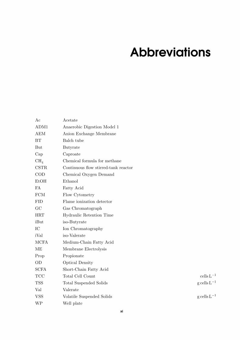
Abbreviations
Ac Acetate
ADM1 Anaerobic Digestion Model 1
AEM Anion Exchange Membrane
BT Balch tube
But Butyrate
Cap Caproate
CH4 Chemical formula for methane
CSTR Continuous flow stirred-tank reactor
COD Chemical Oxygen Demand
EtOH Ethanol
FA Fatty Acid
FCM Flow Cytometry
FID Flame ionization detector
GC Gas Chromatograph
HRT Hydraulic Retention Time
iBut iso-Butyrate
IC Ion Chromatography
iVal iso-Valerate
MCFA Medium-Chain Fatty Acid
ME Membrane Electrolysis
Prop Propionate
OD Optical Density
SCFA Short-Chain Fatty Acid
TCC Total Cell Count cells L−1
TSS Total Suspended Solids g cells L−1
Val Valerate
VSS Volatile Suspended Solids g cells L−1
WP Well plate
xi

xii
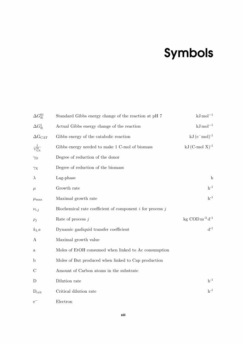
Symbols
∆G01R Standard Gibbs energy change of the reaction at pH 7 kJ mol−1
∆G1R Actual Gibbs energy change of the reaction kJ mol−1
∆GCAT Gibbs energy of the catabolic reaction kJ (e–mol)-1
1YM
GX
Gibbs energy needed to make 1 C-mol of biomass kJ (C-mol X)-1
γD Degree of reduction of the donor
γX Degree of reduction of the biomass
λ Lag-phase h
µ Growth rate h-1
µmax Maximal growth rate h-1
νi,j Biochemical rate coefficient of component i for process j
ρj Rate of process j kg COD m-3 d-1
kLa Dynamic gasliquid transfer coefficient d-1
A Maximal growth value
a Moles of EtOH consumed when linked to Ac consumption
b Moles of But produced when linked to Cap production
C Amount of Carbon atoms in the substrate
D Dilution rate h-1
Dcrit Critical dilution rate h-1
e− Electron
xiii
F Flow rate m3 h-1
KH Henry’s law equilibrium constant M bar-1
KI Inhibition constant g L-1
KS Substrate affinity parameter g L-1
m Maintenace coefficient h-1
PCO2,gas CO2 gas phase partial pressure bar
PH2,act Actual H2 partial pressure atm
PH2,eq H2 partial pressure in equilibrium for certain SEtOH and SAc atm
PH2 H2 partial pressure atm
pHLL Lower limit of the pH where either 50% or 0% of the microorganisms are inhibited
pHUL Upper limit of the pH where either 50% or 0% of the microorganisms are inhibited
QS Maximal substrate uptake rate h-1
qS Substrate uptake rate h-1
qin Incoming flow rate m3 d-1
qout Outgoing flow rate m3 d-1
R Gasconstant 8.3144598 J (mol K)-1
S Substrate concentration g L-1
S∗ Threshold substrate concentration g L-1
Sin Incoming substrate concentration g L-1
SCO2,liq Liquid CO2 concentration M
Sin,i Incoming concentration of component i kg COD m-3 or kmole Nm-3
Sliq,i Reactor concentration of a component i kg COD m-3 or kmole Nm-3
T Temperature K
V Volume tank m3
Vliq Liquid volume m3
X Biomass concentration g L-1
xiv

Y Growth yield g biomass (g substrate)-1
YM Maximal yield when only growth occurs g biomass (g substrate)-1
xv

xvi
CHAPTER 1Literature Review
1.1 Biorefineries
Fossil fuels are a non-renewable source, so the availability of these is decreasing over time.
Apart from that, their utilization is linked to environmental pollution and their price is not
stable. These concerns have resulted into a search for more sustainable solutions, for example
the use of biomass in the so-called “biorefineries”. These offer an alternative to fossil resources
with a lower environmental impact for production of energy carriers and chemicals (Cherubini
and Jungmeier, 2010). Similar to oil refineries, the value of each stream must be maximized
so as to create additional fuels or chemicals, while nutrients and water are recycled (Agler
et al., 2011).
1.1.1 Carboxylate platform
Biorefineries are divided into platforms, based on the targeted or central chemical or an im-
portant intermediate. Two very well known platforms exist for biorefineries. First, the sugar
platform consists of biomass being converted into five or six-carbon monosaccharides, which
can be further processed into fuels. Second, syngas platform processes convert biomass into
syngas, which can then be further processed e.g. by catalysis into fuels (Agler et al., 2011).
However, a third platform exists as well, which is called the “carboxylate platform”, with
carboxylates being the dissociated form of fatty acids (FAs). In this thesis however, the dis-
sociated name will be used to refer to both the dissociated and undissociated form of the acid.
In the carboxylate platform biomass, often derived as industrial and agricultural waste, is con-
verted into Short-Chain Fatty Acids (SCFAs, which are C2 to C5 carboxylic acids acetate
(Ac), propionate (Prop), iso-butyrate (iBut), butyrate (But), iso-valerate (iVal) and valerate
(Val)). The SCFAs are made by subsequently hydrolyzing and fermenting the feedstock using
2 1.1 BIOREFINERIES
undefined and anaerobic mixed cultures. The use of mixed cultures is preferable, since they
are able to handle the complexity and variability of these waste streams (Agler et al., 2011).
Apart from that, mixed cultures are more resilient, which means the need for sterilization
and antibiotic additions can be circumvented, facilitating the operation of the bioprocesses
in a (semi)-continuous mode for many years. Lastly, when working with an open mixed cul-
ture, it is also possible for the culture to be enriched with uncultured isolates which can have
advanced functions (Spirito et al., 2014). The SCFAs made from the primary fermentation
are oftentimes further modified via secondary fermentation steps, in separate bioprocesses
or using separate pure-culture biochemical, electrochemical or thermochemical steps (Agler
et al., 2011).
Since SCFAs are a key intermediate for the production of methane, anaerobic digestion is
included in the carboxylate platform (Agler et al., 2011). Anaerobic digestion is known
as an important technique to treat organic waste streams due to the production of biogas,
which has a high calorific value and can be used as a renewable energy source (Appels et al.,
2008). However, it is still considered as a low value product, resulting in economically un-
desirable production without government incentive. Therefore, it may be useful to suppress
the methane-producing bacteria in order to achieve products with a higher monetary value
(Spirito et al., 2014).
In what follows, the production of caproate (Cap), a high value product targeted by many
studies on carboxylate platform processes, will be described. Cap, also known as hexanoic
acid or caproic acid, can for instance be used as an antimicrobial compound (Vasudevan et al.,
2014). Since more and more bacteria are becoming resistant to known antibiotics, a search
for new antibiotics is of crucial importance for the future of mankind (Burow et al., 2014).
Secondly, Cap can be further processed into fuels. As mentioned earlier, there is a need for
renewable and sustainable alternatives to fossil fuels. Solar energy and wind energy can be
very useful, however there is still a need for liquid fuels as well. At the moment, the most
widely used biofuel is ethanol (EtOH) (Vasudevan et al., 2014). However, since the distilla-
tion of EtOH is energy-intensive (between 20 and 25% of the energetic value of the product is
used during distillation for corn and cellulosic EtOH) (Agler et al., 2012), alternatives which
are more easily separated can be very useful. Converting the EtOH into Cap can therefore
be beneficial, since Cap is more energy dense and can be turned into a fuel as well, as long
as it is more easily extracted (Vasudevan et al., 2014). Next to that, Cap can also be used as
an additive to animal feed, feedstock for esterification into food product (Vasudevan et al.,
2014) or corrosion inhibitor (Spirito et al., 2014).
CHAPTER 1 LITERATURE REVIEW 3
1.1.2 Fermentation and anaerobic digestion
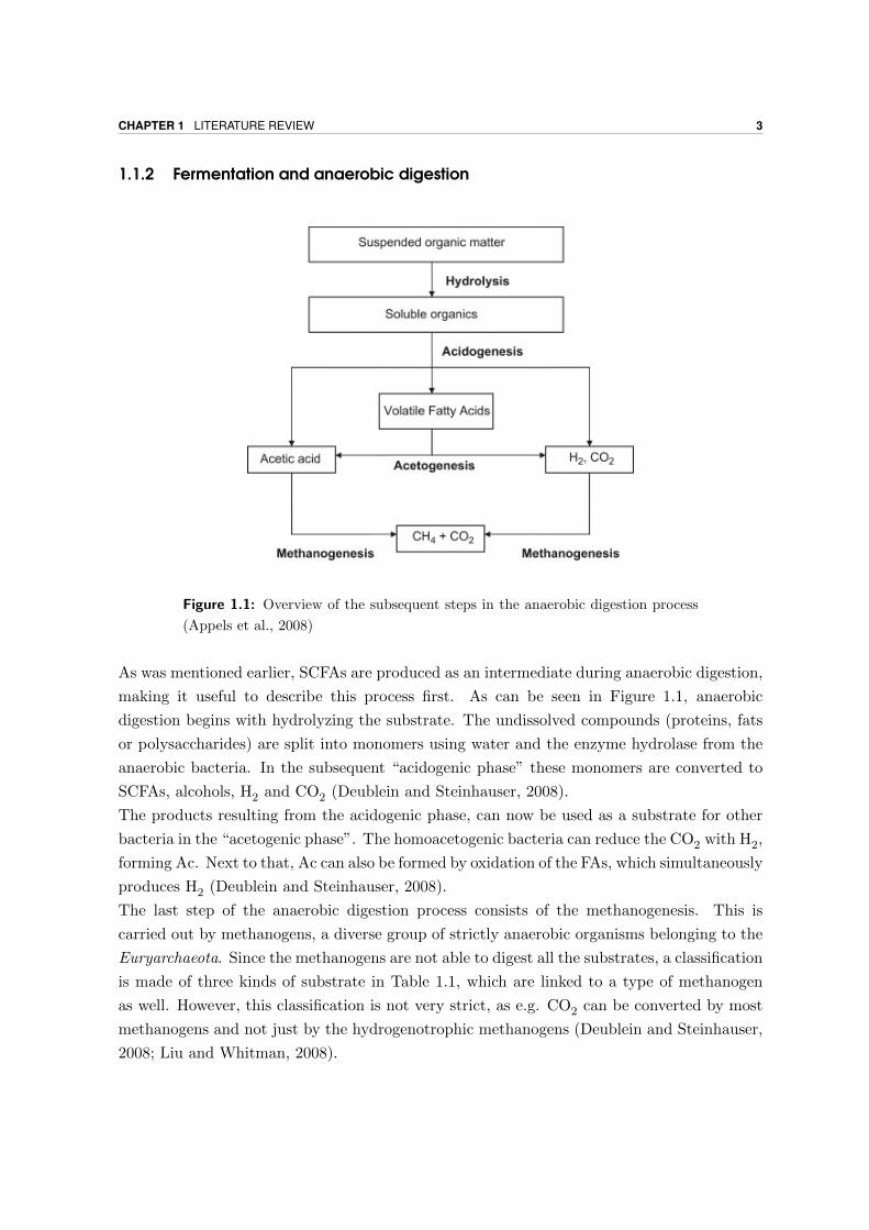
Figure 1.1: Overview of the subsequent steps in the anaerobic digestion process
(Appels et al., 2008)
As was mentioned earlier, SCFAs are produced as an intermediate during anaerobic digestion,
making it useful to describe this process first. As can be seen in Figure 1.1, anaerobic
digestion begins with hydrolyzing the substrate. The undissolved compounds (proteins, fats
or polysaccharides) are split into monomers using water and the enzyme hydrolase from the
anaerobic bacteria. In the subsequent “acidogenic phase” these monomers are converted to
SCFAs, alcohols, H2 and CO2 (Deublein and Steinhauser, 2008).
The products resulting from the acidogenic phase, can now be used as a substrate for other
bacteria in the “acetogenic phase”. The homoacetogenic bacteria can reduce the CO2 with H2,
forming Ac. Next to that, Ac can also be formed by oxidation of the FAs, which simultaneously
produces H2 (Deublein and Steinhauser, 2008).
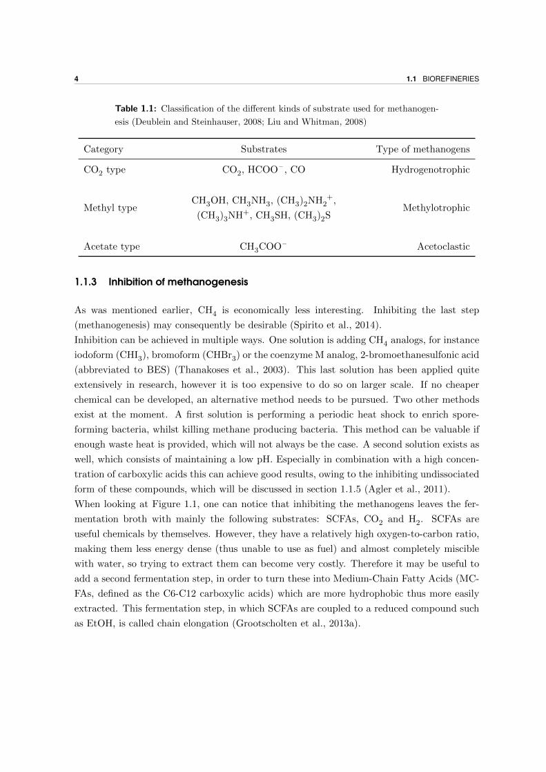
The last step of the anaerobic digestion process consists of the methanogenesis. This is
carried out by methanogens, a diverse group of strictly anaerobic organisms belonging to the
Euryarchaeota. Since the methanogens are not able to digest all the substrates, a classification
is made of three kinds of substrate in Table 1.1, which are linked to a type of methanogen
as well. However, this classification is not very strict, as e.g. CO2 can be converted by most
methanogens and not just by the hydrogenotrophic methanogens (Deublein and Steinhauser,
2008; Liu and Whitman, 2008).
4 1.1 BIOREFINERIES
Table 1.1: Classification of the different kinds of substrate used for methanogen-
esis (Deublein and Steinhauser, 2008; Liu and Whitman, 2008)
Category Substrates Type of methanogens
CO2 type CO2, HCOO– , CO Hydrogenotrophic
Methyl typeCH3OH, CH3NH3, (CH3)2NH +
2 ,
(CH3)3NH+, CH3SH, (CH3)2SMethylotrophic
Acetate type CH3COO– Acetoclastic
1.1.3 Inhibition of methanogenesis
As was mentioned earlier, CH4 is economically less interesting. Inhibiting the last step
(methanogenesis) may consequently be desirable (Spirito et al., 2014).
Inhibition can be achieved in multiple ways. One solution is adding CH4 analogs, for instance
iodoform (CHI3), bromoform (CHBr3) or the coenzyme M analog, 2-bromoethanesulfonic acid
(abbreviated to BES) (Thanakoses et al., 2003). This last solution has been applied quite
extensively in research, however it is too expensive to do so on larger scale. If no cheaper
chemical can be developed, an alternative method needs to be pursued. Two other methods
exist at the moment. A first solution is performing a periodic heat shock to enrich spore-
forming bacteria, whilst killing methane producing bacteria. This method can be valuable if
enough waste heat is provided, which will not always be the case. A second solution exists as
well, which consists of maintaining a low pH. Especially in combination with a high concen-
tration of carboxylic acids this can achieve good results, owing to the inhibiting undissociated
form of these compounds, which will be discussed in section 1.1.5 (Agler et al., 2011).
When looking at Figure 1.1, one can notice that inhibiting the methanogens leaves the fer-
mentation broth with mainly the following substrates: SCFAs, CO2 and H2. SCFAs are
useful chemicals by themselves. However, they have a relatively high oxygen-to-carbon ratio,
making them less energy dense (thus unable to use as fuel) and almost completely miscible
with water, so trying to extract them can become very costly. Therefore it may be useful to
add a second fermentation step, in order to turn these into Medium-Chain Fatty Acids (MC-
FAs, defined as the C6-C12 carboxylic acids) which are more hydrophobic thus more easily
extracted. This fermentation step, in which SCFAs are coupled to a reduced compound such
as EtOH, is called chain elongation (Grootscholten et al., 2013a).
CHAPTER 1 LITERATURE REVIEW 5
1.1.4 Chain elongation
Depending on the conditions of the fermentation broth, the β-oxidation pathway (which is
used as the main pathway to break down FAs in order to use it as a carbon and energy source)
can be reversed in order to undergo reduction reactions. It is this reverse β oxidation pathway
that is considered the route for chain elongation (Spirito et al., 2014; Chen et al., 2014). The
pathway is depicted in Figure 1.2.
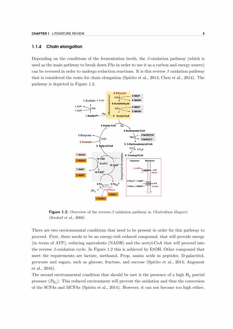
Figure 1.2: Overview of the reverse-β oxidation pathway in Clostridium kluyveri
(Seedorf et al., 2008)
There are two environmental conditions that need to be present in order for this pathway to
proceed. First, there needs to be an energy-rich reduced compound, that will provide energy
(in terms of ATP), reducing equivalents (NADH) and the acetyl-CoA that will proceed into
the reverse β-oxidation cycle. In Figure 1.2 this is achieved by EtOH. Other compound that
meet the requirements are lactate, methanol, Prop, amino acids in peptides, D-galactitol,
pyruvate and sugars, such as glucose, fructose, and sucrose (Spirito et al., 2014; Angenent
et al., 2016).
The second environmental condition that should be met is the presence of a high H2 partial
pressure (PH2). This reduced environment will prevent the oxidation and thus the conversion
of the SCFAs and MCFAs (Spirito et al., 2014). However, it can not become too high either,
6 1.1 BIOREFINERIES
because H2 is also produced during chain elongation, thus limiting the reaction thermody-
namically (Angenent et al., 2016).
The pathway depicted in Figure 1.2 can use other carboxylates than Ac as well, in which the
carbon chain from the carboxylate will be elongated with 2 C-atoms at a time. So Ac [C2]
will be elongated to But [C4], But [C4] can be elongated to Cap [C6], propionate [C3] can be
elongated to valerate [C5], etc (Spirito et al., 2014).
From Figure 1.2, one can see that from the six EtOH molecules that enter the pathway, one
EtOH molecule is transformed into Ac and the other five are coupled to five carboxylates.
The production of Ac from EtOH (∆G=10.5 kJ mol−1) produces one ATP via substrate-level
phosphorylation, which, when coupled to ADP phosphorylation, is a highly endergonic pro-
cess (∆G=32 kJ mol−1). To make the pathway thermodynamically feasible, this process must
thus be coupled to the exergonic reverse β-oxidation cycle (∆G = −38.6 kJ mol−1). This
results in a Gibbs energy change of about −37.0 kJ mol−1 for But and Cap formation at tem-
peratures ranging from 25 to 55 ◦C and a pH of 7. The Gibbs energy change of the chain
elongation which couples Ac and lactate has been calculated to be about −60 kJ mol−1 for
the same conditions. Another possibility is to use H2 as the electron donor. However, us-
ing H2 directly is thermodynamically unfeasible. It is only possible to do this indirectly by
converting the H2 into EtOH, using homoacetogenesis (producing Ac from H2 and CO2) and
then reducing this Ac into EtOH. This sequence however is very slow in microbiomes (i.e.
open microbial communities), but can be successful with some pure cultures (Seedorf et al.,
2008; Spirito et al., 2014).
1.1.5 Fatty acid toxicity
As was mentioned earlier, the MCFAs (for instance Cap) can be used as an antimicrobial
compound (Vasudevan et al., 2014). Organic acids have already a long history of being used
as preservative of perishable food. However, the mechanism in which they are able to inhibit
the microorganisms is not yet completely understood, although different theories exist (Ricke,
2003).
A first explanation is known as the uncoupling theory. This states that the undissociated
form of the organic acids can easily penetrate the lipid membrane of the bacteria. Once
inside, the organic acid will dissociate into the proton and anion due to the neutral pH of
the intracellular fluid (mostly ranging between 6.5 and 7.5). As protons are released, a drop
of the internal pH of the cells would be expected. However this is prevented by the use of
the plasma membrane ATPase. These are a group of enzymes able to pump the protons out
of the cell by hydrolyzing ATP molecules, which now cannot be used for bacterial growth.
If this is still not sufficient, new ATP needs to be formed, but at high concentrations it is
possible that the proton pumping capacity is exhausted. This will result in a depletion of
CHAPTER 1 LITERATURE REVIEW 7
ATP and consequently in a drop of the internal pH, ultimately resulting in a degradation of
acid-sensitive proteins and DNA. Since the dissociated form of the organic acid is lipophobic,
it is only the undissociated form that is able to penetrate the membrane. As the amount
of the undissociated form depends on the pH of the broth, it is only logical that toxicity is
mostly a problem at lower pH (Palmqvist and Hahn-Hagerdal, 2000; Roos and Boron, 1981;
Ricke, 2003).
A second explanation is called “anion accumulation”. Like before, it is possible for the undis-
sociated form of the organic acid to diffuse through the lipid membrane. Once inside the
organic acid dissociates and gets captured. This leads to a combined effect of intracellular pH
decrease and enzyme inhibition or interference by the anions (Palmqvist and Hahn-Hagerdal,
2000).
Next to the previously described theories, other less direct antimicrobial actions were found
for organic acids as well. These are for instance the interference with nutrient transport,
damaging the cytoplasmatic membrane and ultimately causing leaks, disrupting the outer
membrane permeability and affecting the synthesis of macromolecules. However, it appears
that some microorganisms are more resilient to the FAs, because they are themselves able to
decrease the internal pH (Ricke, 2003). Further, it should be mentioned that not all the FAs
have the same effect. It was found that for C2-C6 FAs inhibition only started at a certain
threshold concentration, and that at this threshold concentration the inhibition was the same
except for Ac, which was found to be lower. This could probably be explained by the fact
that Ac is a byproduct from the sugar and amino acid fermentation (Pratt et al., 2012).
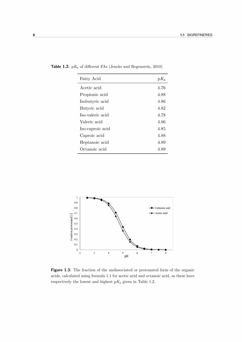
As is clear from the previous discussion, the pH from the fermentation broth plays an impor-
tant role in the inhibition of the microorganisms, as it determines the amount of undissoci-
ated organic acid. In Table 1.2 pKa values of different FAs from the carboxylate platform are
shown. Using formula 1.1, better known as the Henderson-Hasselbalch equation, the fraction
of undissociated organic acid can be calculated as shown in Figure 1.3. Here it is interesting
to see that at pH lower than 5.5 the fraction of protonated FAs starts to increase rapidly.
Because of this reason, it may be useful to work at higher pH’s. However, the pH should not
be too high either, as a lower pH will inhibit the methanogens (Agler et al., 2011).
pH = pKa + log
([A−]
[HA]
)(1.1)
8 1.1 BIOREFINERIES
Table 1.2: pKa of different FAs (Jencks and Regenstein, 2010)
Fatty Acid pKa
Acetic acid 4.76
Propionic acid 4.88
Isobutyric acid 4.86
Butyric acid 4.82
Iso-valeric acid 4.78
Valeric acid 4.86
Iso-caproic acid 4.85
Caproic acid 4.88
Heptanoic acid 4.89
Octanoic acid 4.89
Figure 1.3: The fraction of the undissociated or protonated form of the organic
acids, calculated using formula 1.1 for acetic acid and octanoic acid, as these have
respectively the lowest and highest pKa given in Table 1.2.
CHAPTER 1 LITERATURE REVIEW 9
1.1.6 Extraction
Next to applying a higher pH, toxicity of FAs can also be decreased by continuously extracting
these from the broth so toxicity levels will not be reached. Apart from that, extraction will
also be necessary to purify or perhaps further valorise the end product. However, separating
and purifying the fermentation broth has proven pricey in the past, accounting for the ma-
jority of production cost. To decrease the separation cost, a lot of attention went into this
matter, providing different techniques along the way (Singhania et al., 2013).
A first technique is liquid-liquid extraction. It is one of the oldest techniques, and consists
of extracting the desired product with a suitable solvent. The efficiency of this process will
largely depend on the characteristics of the compound targeted for extraction, its concentra-
tion and finally the solvent used. Some examples of possible solvents are alcohols, ketones,
ethers, aliphatic hydrocarbons and organophosphates. After a first extraction, the compound
can be resuspended in an aqueous solution by the use of a pH gradient. To further improve
separation it is possible to use membrane-based solvent extraction. Here the transfer of the
FAs between the immiscible liquids will occur at the pores of a membrane. Then the usually
volatile solvent can be recovered by the use of stripping or distillation. Pertraction is another
technique that is very similar to liquid-liquid extraction. Here, extraction and stripping will
be done by the use of a three-phase contacter with two liquid-liquid interfaces through a
liquid membrane. There are three types of membranes that can be used: supported liquid
membrane, emulsion liquid membrane and bulk liquid membrane. Drawback of the previously
described techniques is the use of solvents, which are usually hazardous and not 100% efficient
(Singhania et al., 2013; Spirito et al., 2014).
Some other techniques for separation that will not be discussed in further detail are crystal-
lization, ion exchange (which requires a lot of acid, base and water and leads to formation
of salts), adsorption (which has a very short lifetime), distillation, esterification and reactive
extraction (Spirito et al., 2014; Trad et al., 2015).
Lastly, solvent-free membrane processes are another approach and are able to be more effi-
cient, eco-friendly as well as more economic than previous techniques (Trad et al., 2015). For
membrane separation, a feed is needed containing at least two components from which one or
more components will cross a semi-permeable barrier (the membrane) faster than the other.
Here it is necessary to obtain a constant purity after extraction, without having an altered
driving force for separation. The membrane itself can be composed of inorganic, organic
or composite materials and separate the compounds via diffusion (in which a concentration
difference is the driving force) or sieving (for which the absolute pressure drop is the driving
force). Various membrane configurations are applied, e.g. hollow fibers, sheets or combined
into bundled hollow fiber, flat plate or spiral wound sheet membranes. Different membrane
processes exist, e.g. pervaporation, electrodialysis and membrane electrolysis (Spirito et al.,
2014). This last example will be discussed in further detail, as it is the most relevant for this
10 1.1 BIOREFINERIES
thesis.
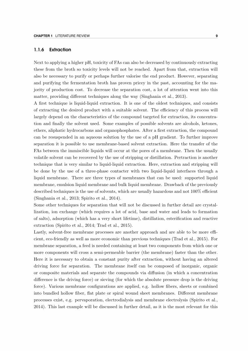
The experimental setup for membrane electrolysis is depicted in Figure 1.4. The cathode
compartment contains the catholyte which exists of circulated fermentation broth, and the
anode compartment contains the anolyte which consists of a clean and low pH solution (An-
dersen et al., 2014). The reactions that take place are summarized in Table 1.3.
Figure 1.4: Schematic overview of the Membrane electrolysis setup (Saxena et al.,
2007)
Table 1.3: Reactions at the membrane electrolysis (Saxena et al., 2007)
Location Type of reaction Reaction
Cathode Reduction 2H2O + 2e– −−→←−− 2OH– + H2 ↑Anode Oxidation H2O −−→←−− 2H+ + 0.5O2 ↑ + 2e–
Using an external power source, electrons are able to flow from the anode to the cathode.
However, to obey the charge conservation principle, this flow needs to be compensated by a
flow from either an anion from the catholyte to the anolyte or a cation from the anolyte to the
catholyte. By applying an anion exchange membrane (AEM), only an anion flow can close
the electrical circuit, while retaining solids, microorganisms and uncharged molecules larger
than the pore size of the membrane. If the pH of the catholyte is sufficiently high, then the
FAs will be present in their anion form, so they will be able to move through the AEM. In
the acidic anolyte, carboxylates will be protonated, inhibiting migration back to the cathode
compartment. The anodic oxidation of H2O - as seen in Table 1.3 - replenishes protons in
the anolyte (Andersen et al., 2014). In a study by Xu et al. (2015) it was possible to reach
concentrations of the FAs slightly above the maximum water solubility, thus creating a new
separated phase, which is the ultimate goal of this technique.
CHAPTER 1 LITERATURE REVIEW 11
1.2 Modeling
1.2.1 Introduction
There are different potential objectives to create a process model. One possible reason is to
gain fundamental knowledge. This can then be used to detect bottlenecks in the process or to
optimize the process parameters (Thour, 2014). This might also be possible for the process
described above (i.e. fermentation, chain elongation and extraction). It can be used to find
ideal pH, initial concentrations, HRT, extraction current, etc. in order to increase the Cap
production, which is the ultimate goal.
For the fermentation part, the Anaerobic Digestion Model No.1 (ADM1) will be described in
section 1.2.3. For chain elongation, no existing models were found in literature. Therefore, a
model was developed based on bacterial growth models, which are explained in section 1.2.2.2.
The model is described in section 2.3. For the modeling part, the extraction process is not
investigated, since it is currently more important to set up a reliable kinetic model. Moreover,
extraction models are well-developed and widely available in literature (Adler et al., 2011;
Gjelstad et al., 2007; Kolev et al., 2013; Lu et al., 2008)
1.2.2 Bacterial growth
1.2.2.1 Introduction
The growth of a microorganism is illustrated in a simplified way in Figure 1.5. An energy
carrier (ATP in this scheme) can be produced via the conversion of substrate S into pro-
duct P, also called the catabolic reaction. This energy carrier will then be consumed via an
anabolic reaction, in which a carbon source SX and a nitrogen source NX are transformed
into the numerous biomass components (X ). This scheme shows that substrate consumption
can be linked to biomass growth. This linkage can also be expressed using the biomass yield
(Y ). Uncoupled catabolic and anabolic processes exist as well, i.e. when the energy carrier is
consumed to provide energy for a non-growth-related maintenance process (m).
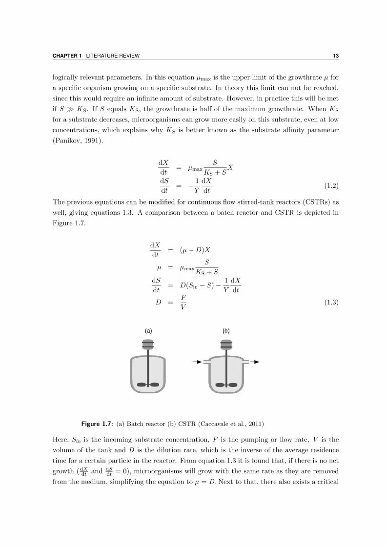
In the absence of light, the catabolic and anabolic reaction are redox reactions, schematically
shown in Figure 1.6. For the catabolism, where energy is produced, electrons will always flow
from a reduced e– -donor to an oxidized e– -acceptor. For the anabolism however, the flow of
electrons is dependent on the oxidation state of the biomass versus the oxidation state of the
nitrogen and carbon source. If electrons are produced when making biomass, an e– -acceptor
will be required which will usually be the same as for the catabolic reaction (as depicted
in Figure 1.6). Otherwise, if electrons are needed for this conversion, an e– -donor will be
required which is also usually the same as for the catabolic reaction. If the stoichiometry
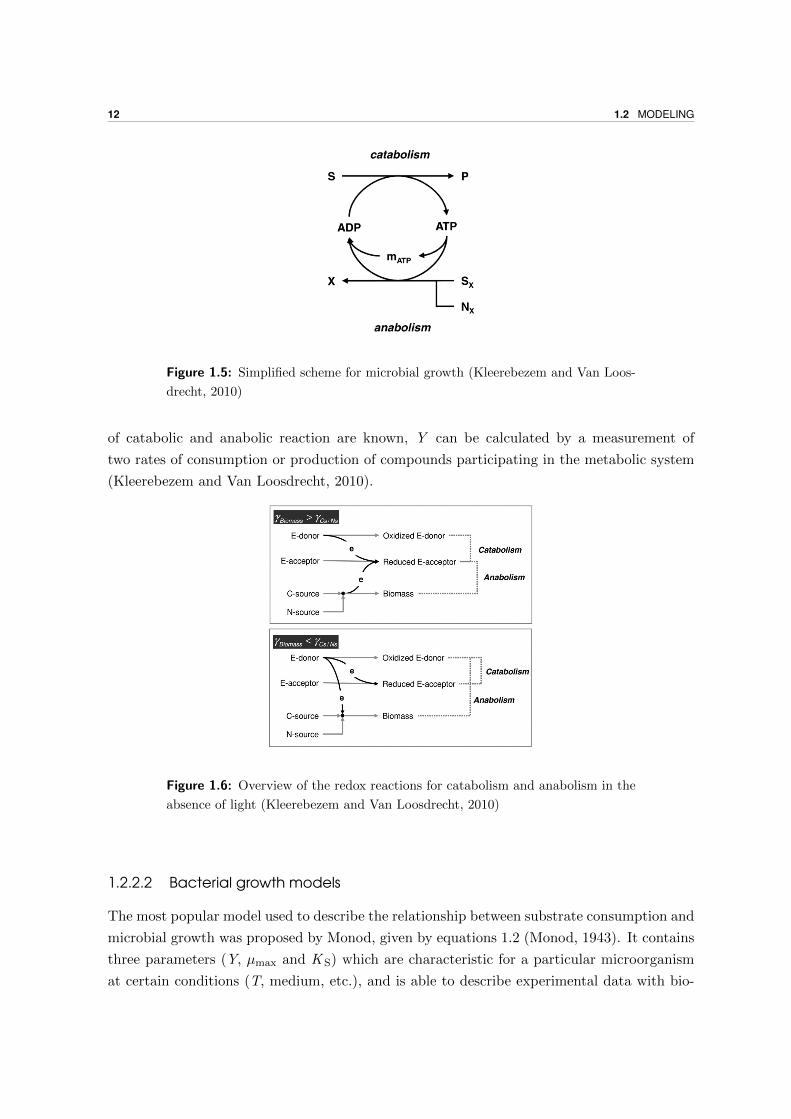
12 1.2 MODELING
Figure 1.5: Simplified scheme for microbial growth (Kleerebezem and Van Loos-
drecht, 2010)
of catabolic and anabolic reaction are known, Y can be calculated by a measurement of
two rates of consumption or production of compounds participating in the metabolic system
(Kleerebezem and Van Loosdrecht, 2010).
Figure 1.6: Overview of the redox reactions for catabolism and anabolism in the
absence of light (Kleerebezem and Van Loosdrecht, 2010)
1.2.2.2 Bacterial growth models
The most popular model used to describe the relationship between substrate consumption and
microbial growth was proposed by Monod, given by equations 1.2 (Monod, 1943). It contains
three parameters (Y, µmax and K S) which are characteristic for a particular microorganism
at certain conditions (T, medium, etc.), and is able to describe experimental data with bio-
CHAPTER 1 LITERATURE REVIEW 13
logically relevant parameters. In this equation µmax is the upper limit of the growthrate µ for
a specific organism growing on a specific substrate. In theory this limit can not be reached,
since this would require an infinite amount of substrate. However, in practice this will be met
if S � K S. If S equals K S, the growthrate is half of the maximum growthrate. When K S
for a substrate decreases, microorganisms can grow more easily on this substrate, even at low
concentrations, which explains why K S is better known as the substrate affinity parameter
(Panikov, 1991).
dX
dt= µmax
S
KS + SX
dS
dt= − 1
Y
dX
dt(1.2)
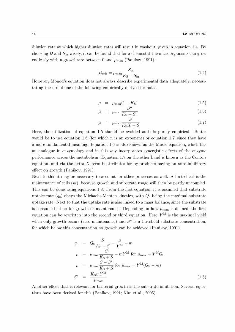
The previous equations can be modified for continuous flow stirred-tank reactors (CSTRs) as
well, giving equations 1.3. A comparison between a batch reactor and CSTR is depicted in
Figure 1.7.
dX
dt= (µ−D)X
µ = µmaxS
KS + SdS
dt= D(Sin − S)− 1
Y
dX
dt
D =F
V(1.3)
Figure 1.7: (a) Batch reactor (b) CSTR (Caccavale et al., 2011)
Here, Sin is the incoming substrate concentration, F is the pumping or flow rate, V is the
volume of the tank and D is the dilution rate, which is the inverse of the average residence
time for a certain particle in the reactor. From equation 1.3 it is found that, if there is no net
growth (dXdt and dSdt = 0), microorganisms will grow with the same rate as they are removed
from the medium, simplifying the equation to µ = D. Next to that, there also exists a critical
14 1.2 MODELING
dilution rate at which higher dilution rates will result in washout, given in equation 1.4. By
choosing D and S in wisely, it can be found that for a chemostat the microorganisms can grow
endlessly with a growthrate between 0 and µmax (Panikov, 1991).
Dcrit = µmaxSin
KS + Sin(1.4)
However, Monod’s equation does not always describe experimental data adequately, necessi-
tating the use of one of the following empirically derived formulas.
µ = µmax(1−KS) (1.5)
µ = µmaxSn
KS + Sn(1.6)
µ = µmaxS
KSX + S(1.7)
Here, the utilization of equation 1.5 should be avoided as it is purely empirical. Better
would be to use equation 1.6 (for which n is an exponent) or equation 1.7 since they have
a more fundamental meaning: Equation 1.6 is also known as the Moser equation, which has
an analogue in enzymology and in this way incorporates synergistic effects of the enzyme
performance across the metabolism. Equation 1.7 on the other hand is known as the Contois
equation, and via the extra X term it attributes for by-products having an auto-inhibitory
effect on growth (Panikov, 1991).
Next to this it may be necessary to account for other processes as well. A first effect is the
maintenance of cells (m), because growth and substrate usage will then be partly uncoupled.
This can be done using equations 1.8. From the first equation, it is assumed that substrate
uptake rate (qs) obeys the Michaelis-Menten kinetics, with Qs being the maximal substrate
uptake rate. Next to that the uptake rate is also linked to a mass balance, since the substrate
is consumed either for growth or maintenance. Depending on how µmax is defined, the first
equation can be rewritten into the second or third equation. Here YM is the maximal yield
when only growth occurs (zero maintenance) and S ∗ is a threshold substrate concentration,
for which below this concentration no growth can be achieved (Panikov, 1991).
qS = QSS
KS + S=
µ
Y M+m
µ = µmaxS
KS + S−mY M for µmax = Y MQS
µ = µmaxS − S∗
KS + Sfor µmax = Y M(QS −m)
S∗ =KSmY
M
µmax(1.8)
Another effect that is relevant for bacterial growth is the substrate inhibition. Several equa-
tions have been derived for this (Panikov, 1991; Kim et al., 2005).
CHAPTER 1 LITERATURE REVIEW 15
µ = µmaxS
KS + S
KI
KI + S(1.9)
µ = µmaxS
KS + S + S2
KI
(1.10)
µ = µmaxS
KS + Sexp
(−SKI
)(1.11)
Equations 1.9, 1.10 and 1.11 are respectively called the Monod-Ierusalimsky equation, the
Haldane-Andrews equation and the Aiba-Edwards equation. Here they are shown for sub-
strate inhibition, but the first equation can be used for product inhibition as well. KI is the
inhibition parameter. The smaller its value, the more easily a microorganism is inhibited, as
the effects are noticeable at smaller concentrations.(Panikov, 1991; Kim et al., 2005).
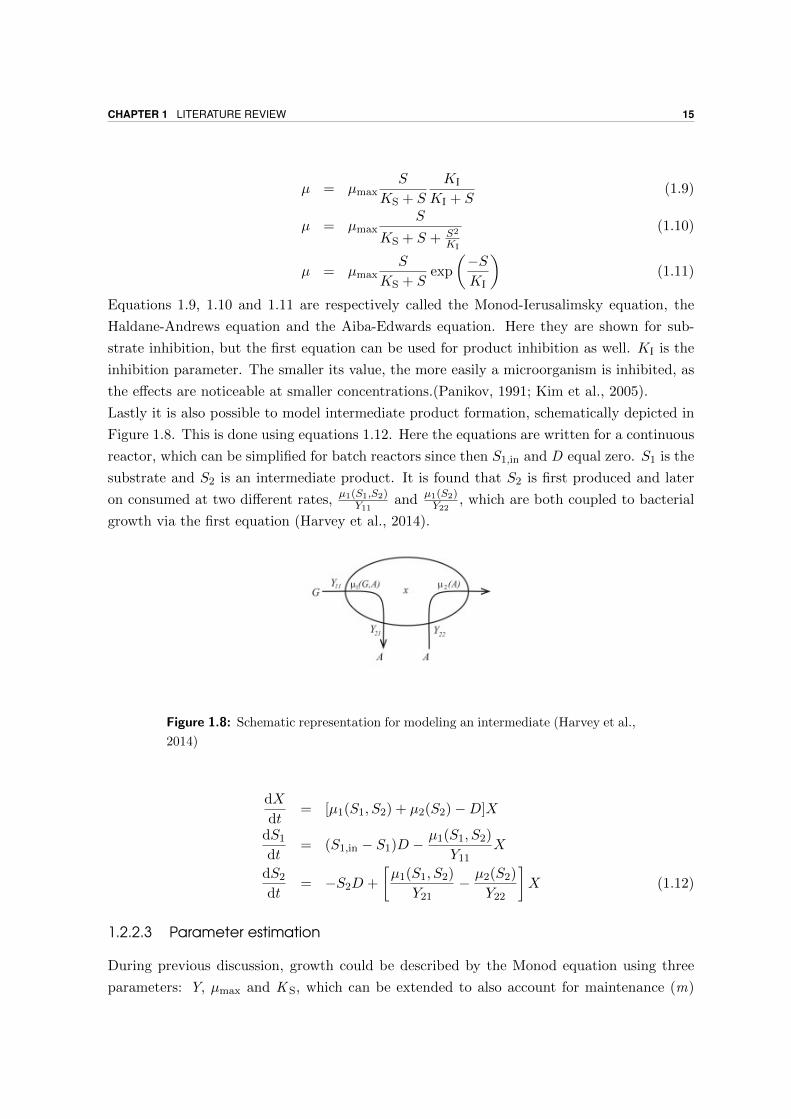
Lastly it is also possible to model intermediate product formation, schematically depicted in
Figure 1.8. This is done using equations 1.12. Here the equations are written for a continuous
reactor, which can be simplified for batch reactors since then S1,in and D equal zero. S1 is the
substrate and S2 is an intermediate product. It is found that S2 is first produced and later
on consumed at two different rates, µ1(S1,S2)Y11
and µ1(S2)Y22
, which are both coupled to bacterial
growth via the first equation (Harvey et al., 2014).
Figure 1.8: Schematic representation for modeling an intermediate (Harvey et al.,
2014)
dX
dt= [µ1(S1, S2) + µ2(S2)−D]X
dS1dt
= (S1,in − S1)D −µ1(S1, S2)
Y11X
dS2dt
= −S2D +
[µ1(S1, S2)
Y21− µ2(S2)
Y22
]X (1.12)
1.2.2.3 Parameter estimation
During previous discussion, growth could be described by the Monod equation using three
parameters: Y, µmax and K S, which can be extended to also account for maintenance (m)
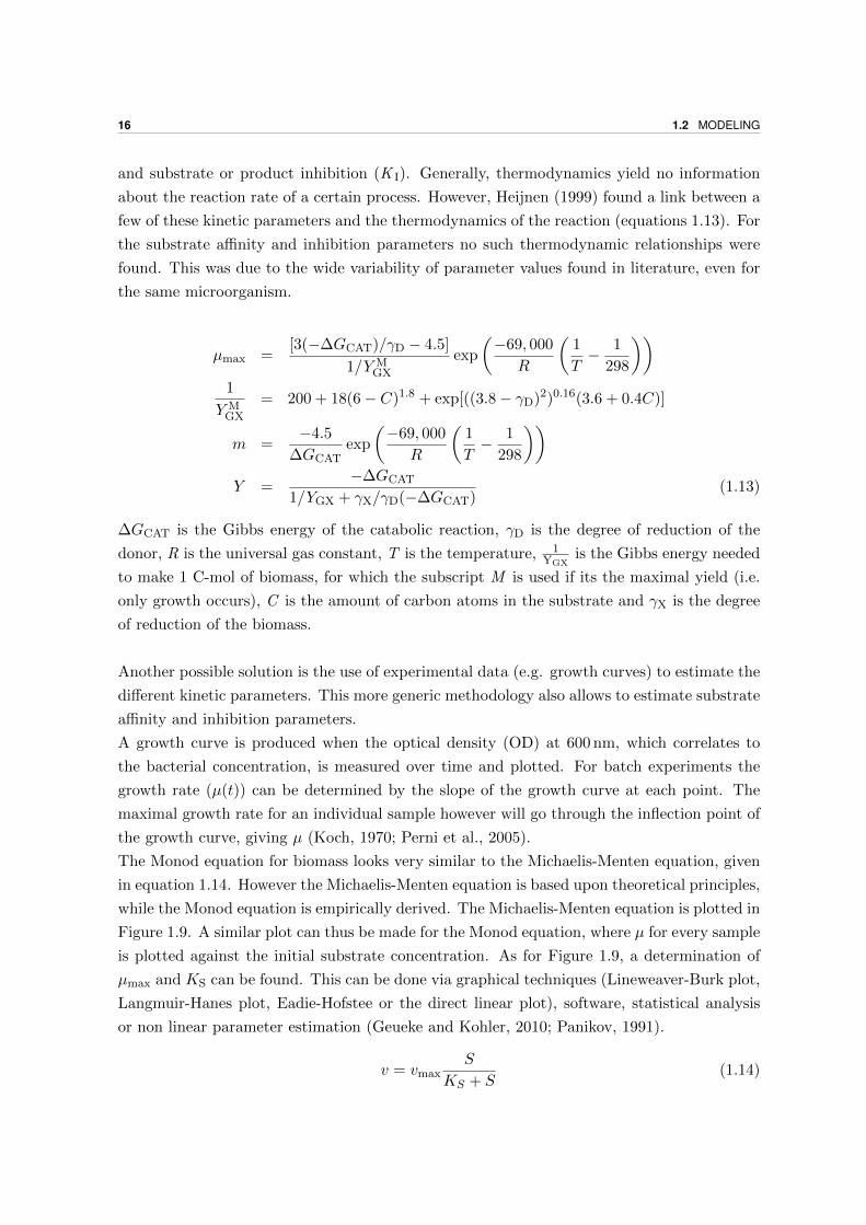
16 1.2 MODELING
and substrate or product inhibition (K I). Generally, thermodynamics yield no information
about the reaction rate of a certain process. However, Heijnen (1999) found a link between a
few of these kinetic parameters and the thermodynamics of the reaction (equations 1.13). For
the substrate affinity and inhibition parameters no such thermodynamic relationships were
found. This was due to the wide variability of parameter values found in literature, even for
the same microorganism.
µmax =[3(−∆GCAT)/γD − 4.5]
1/Y MGX
exp
(−69, 000
R
(1
T− 1
298
))1
Y MGX
= 200 + 18(6− C)1.8 + exp[((3.8− γD)2)0.16(3.6 + 0.4C)]
m =−4.5
∆GCATexp
(−69, 000
R
(1
T− 1
298
))Y =
−∆GCAT
1/YGX + γX/γD(−∆GCAT)(1.13)
∆GCAT is the Gibbs energy of the catabolic reaction, γD is the degree of reduction of the
donor, R is the universal gas constant, T is the temperature, 1YGX
is the Gibbs energy needed
to make 1 C-mol of biomass, for which the subscript M is used if its the maximal yield (i.e.
only growth occurs), C is the amount of carbon atoms in the substrate and γX is the degree
of reduction of the biomass.
Another possible solution is the use of experimental data (e.g. growth curves) to estimate the
different kinetic parameters. This more generic methodology also allows to estimate substrate
affinity and inhibition parameters.
A growth curve is produced when the optical density (OD) at 600 nm, which correlates to
the bacterial concentration, is measured over time and plotted. For batch experiments the
growth rate (µ(t)) can be determined by the slope of the growth curve at each point. The
maximal growth rate for an individual sample however will go through the inflection point of
the growth curve, giving µ (Koch, 1970; Perni et al., 2005).
The Monod equation for biomass looks very similar to the Michaelis-Menten equation, given
in equation 1.14. However the Michaelis-Menten equation is based upon theoretical principles,
while the Monod equation is empirically derived. The Michaelis-Menten equation is plotted in
Figure 1.9. A similar plot can thus be made for the Monod equation, where µ for every sample
is plotted against the initial substrate concentration. As for Figure 1.9, a determination of
µmax and KS can be found. This can be done via graphical techniques (Lineweaver-Burk plot,
Langmuir-Hanes plot, Eadie-Hofstee or the direct linear plot), software, statistical analysis
or non linear parameter estimation (Geueke and Kohler, 2010; Panikov, 1991).
v = vmaxS
KS + S(1.14)
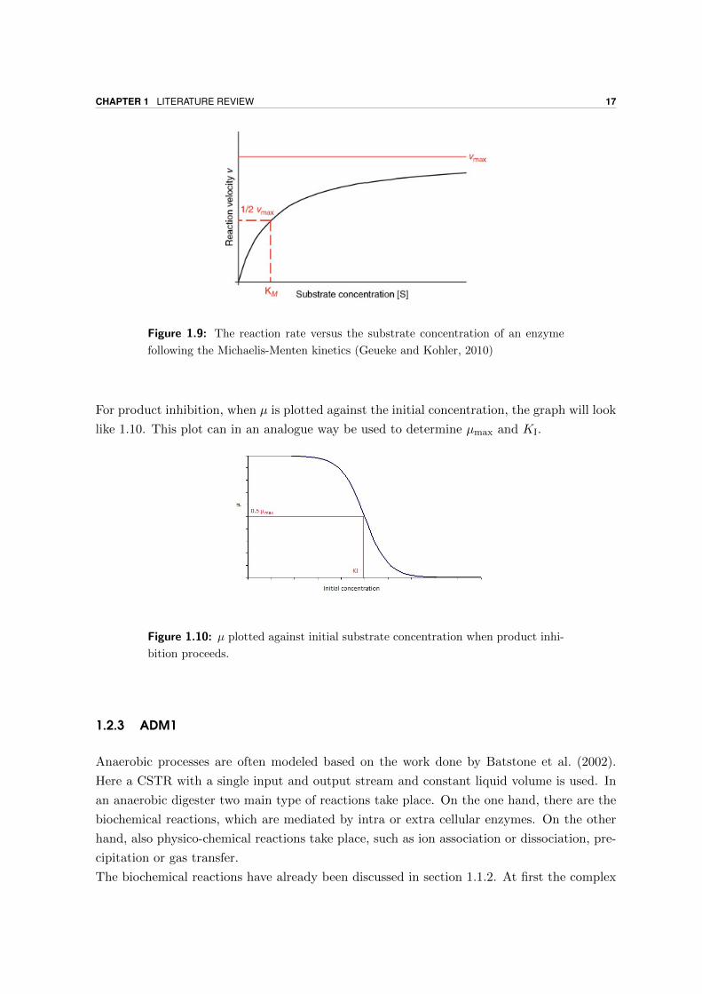
CHAPTER 1 LITERATURE REVIEW 17
Figure 1.9: The reaction rate versus the substrate concentration of an enzyme
following the Michaelis-Menten kinetics (Geueke and Kohler, 2010)
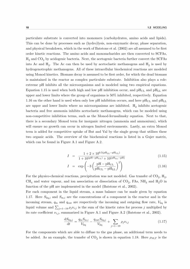
For product inhibition, when µ is plotted against the initial concentration, the graph will look
like 1.10. This plot can in an analogue way be used to determine µmax and KI.
Figure 1.10: µ plotted against initial substrate concentration when product inhi-
bition proceeds.
1.2.3 ADM1
Anaerobic processes are often modeled based on the work done by Batstone et al. (2002).
Here a CSTR with a single input and output stream and constant liquid volume is used. In
an anaerobic digester two main type of reactions take place. On the one hand, there are the
biochemical reactions, which are mediated by intra or extra cellular enzymes. On the other
hand, also physico-chemical reactions take place, such as ion association or dissociation, pre-
cipitation or gas transfer.
The biochemical reactions have already been discussed in section 1.1.2. At first the complex
18 1.2 MODELING
particulate substrate is converted into monomers (carbohydrates, amino acids and lipids).
This can be done by processes such as (hydro)lysis, non-enzymatic decay, phase separation,
and physical breakdown, which in the work of Batstone et al. (2002) are all assumed to be first
order kinetic reactions. The amino acids and monosacharides are then converted to SCFAs,
H2 and CO2 by acidogenic bacteria. Next, the acetogenic bacteria further convert the SCFAs
into Ac and H2. The Ac can then be used by acetoclastic methanogens and H2 is used by
hydrogenotrophic methanogens. All of these intracellular biochemical reactions are modeled
using Monod kinetics. Biomass decay is assumed to be first order, for which the dead biomass
is maintained in the reactor as complex particulate substrate. Inhibition also plays a role:
extreme pH inhibits all the microorganisms and is modeled using two empirical equations.
Equation 1.15 is used when both high and low pH inhibition occur, and pHUL and pHLL are
upper and lower limits where the group of organisms is 50% inhibited, respectively. Equation
1.16 on the other hand is used when only low pH inhibition occurs, and here pHUL and pHLL
are upper and lower limits where no microorganisms are inhibited. H2 inhibits acetogenic
bacteria and free ammonia inhibits acetoclastic methanogens, which can be modeled using
non-competitive inhibition terms, such as the Monod-Ierusalimsky equation. Next to that,
there is a secondary Monod term for inorganic nitrogen (ammonia and ammonium), which
will ensure no growth can occur in nitrogen limited environments. Lastly, an extra Monod
term is added for competitive uptake of But and Val by the single group that utilises these
two organic acids. The overview of the biochemical reactions is listed in a Gujer matrix,
which can be found in Figure A.1 and Figure A.2.
I =1 + 2× 100.5(pHLL−pHUL)
1 + 10(pH−pHUL) + 10(pHLL−pH)(1.15)
I = exp
(−3
(pH− pHUL
pHUL − pHLL
)2)
(1.16)
For the physico-chemical reactions, precipitation was not modeled. Gas transfer of CO2, H2,
CH4 and water vapour, and ion association or dissociation of CO2, FAs, NH3 and H2O in
function of the pH are implemented in the model (Batstone et al., 2002).
For each component in the liquid stream, a mass balance can be made given by equation
1.17. Here Sliq,i and Sin,i are the concentrations of a component in the reactor and in the
incoming stream, qin and qout are respectively the incoming and outgoing flow rate, Vliq is
liquid volume and∑
j=1−19 ρjνi,j is the sum of the kinetic rates for process j multiplied by
its rate coefficient νi,j , summarized in Figure A.1 and Figure A.2 (Batstone et al., 2002).
dSliq,idt
=qinSin,iVliq
− qoutSliq,iVliq
+∑
j=1−19
ρjνi,j (1.17)
For the components which are able to diffuse to the gas phase, an additional term needs to
be added. As an example, the transfer of CO2 is shown in equation 1.18. Here ρ10,T is the
CHAPTER 1 LITERATURE REVIEW 19
additional rate term dependent on the temperature, kLa is the dynamic gas-liquid transfer
coefficient, KH,CO2 is the Henry’s law equilibrium constant, PCO2,gas is the CO2 gas phase
partial pressure and SCO2,liq is the liquid CO2 concentration (Batstone et al., 2002).
ρ10,T = kLaCO2(SCO2,liq −KH,CO2PCO2,gas) (1.18)
To account for the ion association or dissociation, the acidic and basic form of the chemical
are put together in one formula (e.g. SCO2 and SHCO −3
become SIC which equals S10). An
additional charge balance will then complete the set of equations. To calculate the individual
concentrations, the acid-base equilibrium constant is used (Batstone et al., 2002).
For the gas phase similar equations such as equation 1.17 can be made. However, there is
only one production rate term, which is the gas transfer to the liquid phase. Next to that,
no input stream is provided and the output will be either equalized to the total transfer rate
or calculated from headspace pressure and restricted flow through an orifice, which need to
be adjusted for the water vapour pressure at the reactor temperature (Batstone et al., 2002).
1.3 Research objectives
The process described above consists of three subprocesses: fermentation, chain elongation
and extraction using an electrochemical cell. In literature, there is a lot of information about
modeling of fermentation and extraction (Adler et al., 2011; Gjelstad et al., 2007; Kolev et al.,
2013; Lu et al., 2008; Batstone et al., 2002), but nothing about modeling chain elongation.
In order to fully model the entire process, this part needs to be modeled as well. For this
reason, the objectives of this thesis are as followed:
� Maintain a mixed culture able in chain elongation in order to get more feeling with the
process (possible pH, retention time, etc.) and to create inoculum for experiments
� Create a mathematical model for chain elongation using literature
� Design and conduct experiments for parameter estimation
� Do a quality control on acquired data
� Estimate the parameters using acquired data

CHAPTER 2Materials and Methods
2.1 Mixed Culture
2.1.1 Mixed culture at HRT 7d
A semi-continuous batch reactor system was installed in a temperature controlled room of
34 ◦C in order to create inoculum for further kinetic tests and get more feeling with the pro-
cess. The reactor had a volume of 900 mL, was mixed by a magnetic stirrer and fed manually
by extracting 300 mL of effluent, of which about 15 mL was extracted before settling and
the rest after settling to retain biomass. The reactor was then replenished by 300 mL of M9
medium with additional Ac and EtOH, for which the composition is given in Table 2.1. This
feeding process was done three times per week, resulting in a hydraulic retention time (HRT)
of 7 days. The pH of the fermentation broth was kept above 6.95 using a Prominent pH
controller, a pH probe, and a pump for dosing a 2 M NaOH solution. Gas was collected in an
acid gas trap.
Table 2.1: Composition of M9 medium
Chemical Concentration
Na2HPO4 · 2 H2O 7.5 g L−1
KH2PO4 3 g L−1
NaCl 0.5 g L−1
NH4Cl 0.5 g L−1
MgSO4 · 7 H2O 0.1 g L−1
Acetate 5 g L−1
Ethanol 2 mL L−1
22 2.1 MIXED CULTURE
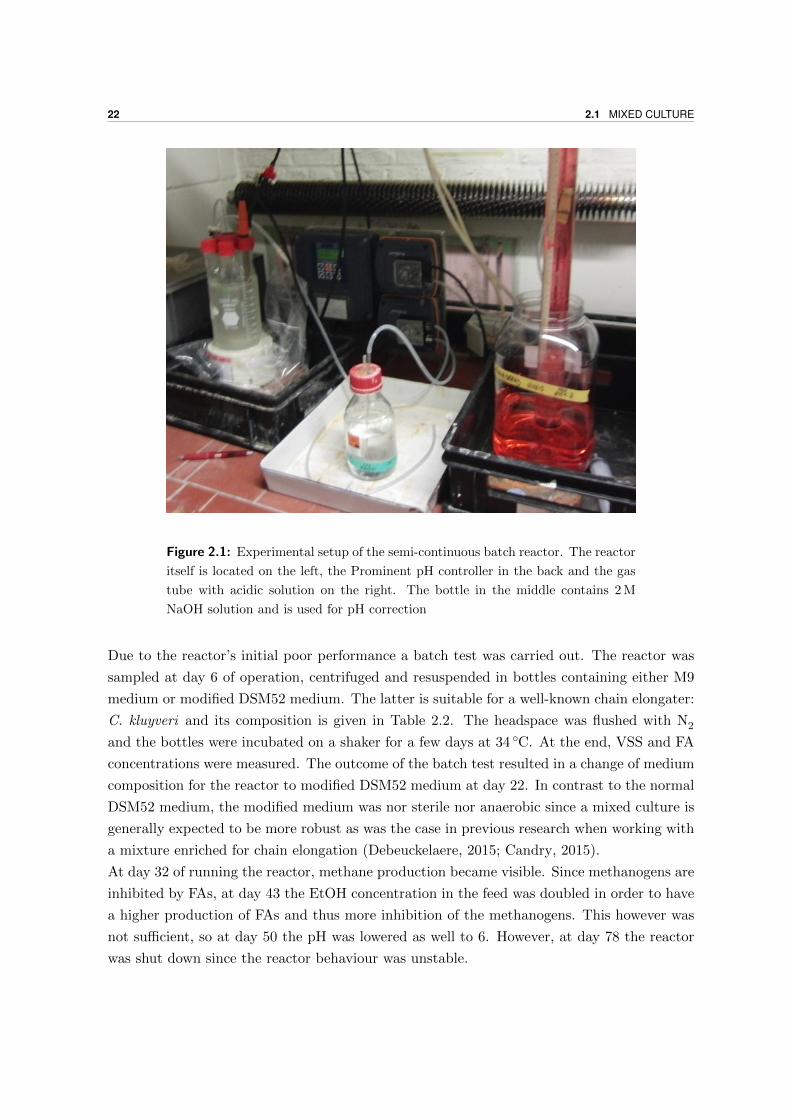
Figure 2.1: Experimental setup of the semi-continuous batch reactor. The reactor
itself is located on the left, the Prominent pH controller in the back and the gas
tube with acidic solution on the right. The bottle in the middle contains 2 M
NaOH solution and is used for pH correction
Due to the reactor’s initial poor performance a batch test was carried out. The reactor was
sampled at day 6 of operation, centrifuged and resuspended in bottles containing either M9
medium or modified DSM52 medium. The latter is suitable for a well-known chain elongater:
C. kluyveri and its composition is given in Table 2.2. The headspace was flushed with N2
and the bottles were incubated on a shaker for a few days at 34 ◦C. At the end, VSS and FA
concentrations were measured. The outcome of the batch test resulted in a change of medium
composition for the reactor to modified DSM52 medium at day 22. In contrast to the normal
DSM52 medium, the modified medium was nor sterile nor anaerobic since a mixed culture is
generally expected to be more robust as was the case in previous research when working with
a mixture enriched for chain elongation (Debeuckelaere, 2015; Candry, 2015).
At day 32 of running the reactor, methane production became visible. Since methanogens are
inhibited by FAs, at day 43 the EtOH concentration in the feed was doubled in order to have
a higher production of FAs and thus more inhibition of the methanogens. This however was
not sufficient, so at day 50 the pH was lowered as well to 6. However, at day 78 the reactor
was shut down since the reactor behaviour was unstable.
CHAPTER 2 MATERIALS AND METHODS 23
Table 2.2: Composition of modified DSM52 medium for mixed culture
Chemical Concentration
K2HPO4 0.31 g L−1
KH2PO4 0.23 g L−1
NH4Cl 0.25 g L−1
MgSO4 · 7 H2O 0.2 g L−1
Trace element solution SL-10 (see B.1) 1 mL L−1
Selenite-tungstate (see B.2) 1 mL L−1
Yeast extract 1 g L−1
NaHCO3 2.5 g L−1
Seven vitamin solution (see B.3) 1 mL L−1
K-acetate 8.172 g L−1
Ethanol 10 mL L−1
2.1.2 Mixed culture at HRT 4d
At a later time point, a new reactor set up was started. To tackle issues, which will be de-
scribed in section 3.1.1, another approach was taken for this reactor system. In the reactor,
pH was controlled at 6.5 and instead of manual feeding, the feeding process was more con-
tinuous with the use of pumps. A time-based controller was used to control the two pumps.
Influent and effluent were pumped simultaneously 5 times a day, resulting in an HRT of 4
days. Medium composition was similar to that in Table 2.2, but K-Ac was 4.28 g L−1 and
EtOH 10.3 mL L−1. The medium without vitamins, trace elements and NaHCO3 was first
autoclaved, followed by sterile addition of these components. The pH of the influent was
corrected between 6.5 and 7. The reactor underwent three phases. During phase 1, no BES
was added. However, as CH4 was being produced, at day 28 a new phase was initiated in
which 25 mM BES was added to the mixture to inhibit the methanogens. At day 100, phase
3 started in which BES addition was halted and MgSO4 was replaced by 0.3 g L−1 L-cysteine.
2.2 Pure Culture
Clostridium kluyveri (DSM 555) was grown in an anaerobic DSM52 medium. The composition
of this medium is given in Table 2.3. To make the medium sterile and anaerobic, the following
procedure was followed based on the considerations of Plugge (2005). First the salts, resazurin
and K-Ac were dissolved and boiled. The bottle was then cooled in ice under N2 atmosphere.
When the solution was cooled down, EtOH was added and the mixture was distributed over
Balch tubes (BTs) and/or penicillin flasks under N2 atmosphere. The tubes or flasks were
24 2.3 CHAIN ELONGATION MODEL
closed using rubber stoppers and aluminum crimp seals. The headspace was flushed with N2
using a gas exchange device and the mixture was autoclaved. A first filter-sterilized stock
solution under N2 atmosphere containing 30 mL 1 M NaHCO3, 1 mL trace elements SL-10 (see
Table B.1), 1 mL Se-WO4 (see Table B.2) and 1 mL 7 vitamin solution (see Table B.3) were
added to reach a final concentration of 2.5 g NaHCO3 L−1. A second filter-sterilized stock
solution of 5 g L−1 Cysteine-HCl.H2O and 5 g L−1 Na2S · 9 H2O in DSM52 salt solution under
N2 atmosphere was added to reach concentrations of 0.25 g L−1 of both compounds in the
medium.
Table 2.3: Composition of modified DSM52 medium for Clostridium kluyveri
Chemical Concentration
K2HPO4 0.31 g L−1
KH2PO4 0.23 g L−1
NH4Cl 0.25 g L−1
MgSO4 · 7 H2O 0.2 g L−1
Trace element solution SL-10 (see B.1) 1 mL L−1
Selenite-tungstate (see B.2) 1 mL L−1
Yeast extract 1 g L−1
Resazurin 0.5 mg L−1
NaHCO3 2.5 g L−1
Seven vitamin solution (see B.3) 1 mL L−1
L-Cysteine-HCl.H2O 0.25 g L−1
Na2S · 9 H2O 0.25 g L−1
K-acetate 10 g L−1
Ethanol 20 mL L−1
2.3 Chain elongation model
Figure 1.2 shows the overview of the chain elongation from Ac to But. An analogous scheme
can be followed, but instead of coupling to Ac, EtOH can now be coupled to But forming Cap.
When written into chemical formulas following equations were found for the chain elongating
reaction (Seedorf et al., 2008; Spirito et al., 2014):
6 EtOH + 4 Ac– r1−−→ 5 But– + H+ + 2 H2 + 4 H2O
6 EtOH + 5 But–r2−−→ 1 Ac– + 5 Cap– + H+ + 2 H2 + 4 H2O
Assuming that i) the first reaction would take place at rate r1 and the second reaction at
rate r2; ii) the reactions only take place in one direction and; iii) water concentration remain
CHAPTER 2 MATERIALS AND METHODS 25
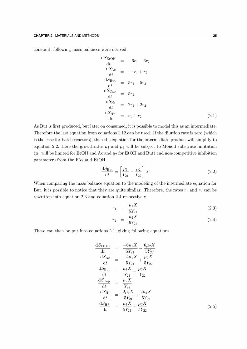
constant, following mass balances were derived:
dSEtOH
dt= −6r1 − 6r2
dSAc
dt= −4r1 + r2
dSBut
dt= 5r1 − 5r2
dSCap
dt= 5r2
dSH2
dt= 2r1 + 2r2
dSH+
dt= r1 + r2 (2.1)
As But is first produced, but later on consumed, it is possible to model this as an intermediate.
Therefore the last equation from equations 1.12 can be used. If the dilution rate is zero (which
is the case for batch reactors), then the equation for the intermediate product will simplify to
equation 2.2. Here the growthrates µ1 and µ2 will be subject to Monod substrate limitation
(µ1 will be limited for EtOH and Ac and µ2 for EtOH and But) and non-competitive inhibition
parameters from the FAs and EtOH.
dSBut
dt=
[µ1Y21− µ2Y22
]X (2.2)
When comparing the mass balance equation to the modeling of the intermediate equation for
But, it is possible to notice that they are quite similar. Therefore, the rates r1 and r2 can be
rewritten into equation 2.3 and equation 2.4 respectively.
r1 =µ1X
5Y21(2.3)
r2 =µ2X
5Y22(2.4)
These can then be put into equations 2.1, giving following equations.
dSEtOH
dt=−6µ1X
5Y21− 6µ2X
5Y22dSAc
dt=−4µ1X
5Y21+µ2X
5Y22dSBut
dt=
µ1X
Y21− µ2X
Y22dSCap
dt=
µ2X
Y22dSH2
dt=
2µ1X
5Y21+
2µ2X
5Y22dSH+
dt=
µ1X
5Y21+µ2X
5Y22(2.5)
26 2.4 PARAMETER ESTIMATION OF µMAX, K S AND K I
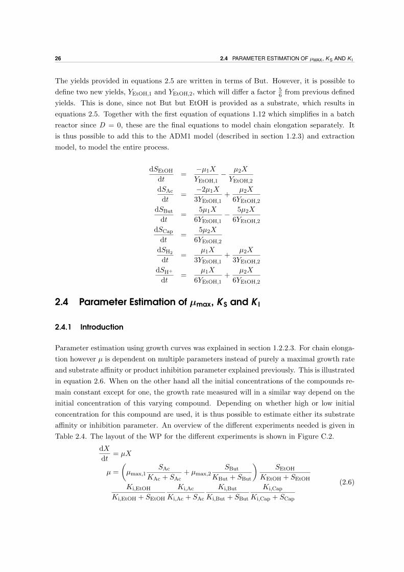
The yields provided in equations 2.5 are written in terms of But. However, it is possible to
define two new yields, YEtOH,1 and YEtOH,2, which will differ a factor 56 from previous defined
yields. This is done, since not But but EtOH is provided as a substrate, which results in
equations 2.5. Together with the first equation of equations 1.12 which simplifies in a batch
reactor since D = 0, these are the final equations to model chain elongation separately. It
is thus possible to add this to the ADM1 model (described in section 1.2.3) and extraction
model, to model the entire process.
dSEtOH
dt=
−µ1XYEtOH,1
− µ2X
YEtOH,2
dSAc
dt=
−2µ1X
3YEtOH,1+
µ2X
6YEtOH,2
dSBut
dt=
5µ1X
6YEtOH,1− 5µ2X
6YEtOH,2
dSCap
dt=
5µ2X
6YEtOH,2
dSH2
dt=
µ1X
3YEtOH,1+
µ2X
3YEtOH,2
dSH+
dt=
µ1X
6YEtOH,1+
µ2X
6YEtOH,2
2.4 Parameter Estimation of µmax, K S and K I
2.4.1 Introduction
Parameter estimation using growth curves was explained in section 1.2.2.3. For chain elonga-
tion however µ is dependent on multiple parameters instead of purely a maximal growth rate
and substrate affinity or product inhibition parameter explained previously. This is illustrated
in equation 2.6. When on the other hand all the initial concentrations of the compounds re-
main constant except for one, the growth rate measured will in a similar way depend on the
initial concentration of this varying compound. Depending on whether high or low initial
concentration for this compound are used, it is thus possible to estimate either its substrate
affinity or inhibition parameter. An overview of the different experiments needed is given in
Table 2.4. The layout of the WP for the different experiments is shown in Figure C.2.
dX
dt= µX
µ =
(µmax,1
SAc
KAc + SAc+ µmax,2
SBut
KBut + SBut
)SEtOH
KEtOH + SEtOH
Ki,EtOH
Ki,EtOH + SEtOH
Ki,Ac
Ki,Ac + SAc
Ki,But
Ki,But + SBut
Ki,Cap
Ki,Cap + SCap
(2.6)
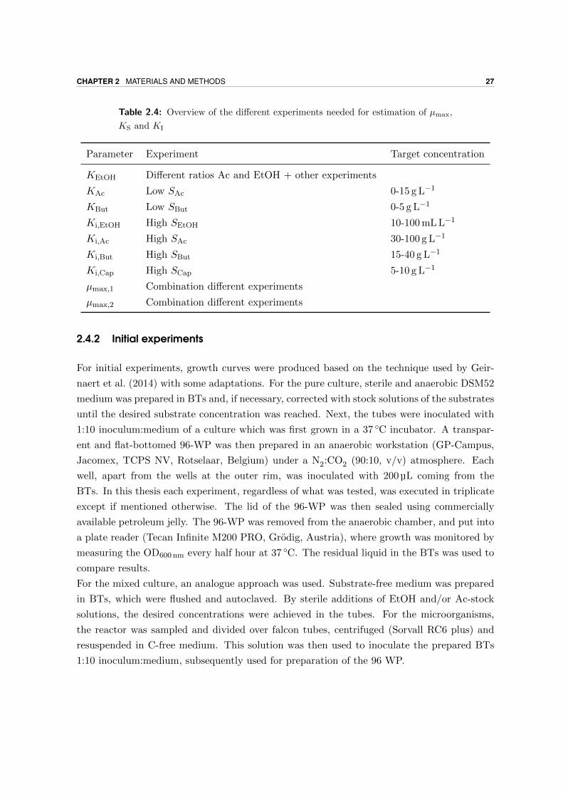
CHAPTER 2 MATERIALS AND METHODS 27
Table 2.4: Overview of the different experiments needed for estimation of µmax,
KS and KI
Parameter Experiment Target concentration
KEtOH Different ratios Ac and EtOH + other experiments
KAc Low SAc 0-15 g L−1
KBut Low SBut 0-5 g L−1
Ki,EtOH High SEtOH 10-100 mL L−1
Ki,Ac High SAc 30-100 g L−1
Ki,But High SBut 15-40 g L−1
Ki,Cap High SCap 5-10 g L−1
µmax,1 Combination different experiments
µmax,2 Combination different experiments
2.4.2 Initial experiments
For initial experiments, growth curves were produced based on the technique used by Geir-
naert et al. (2014) with some adaptations. For the pure culture, sterile and anaerobic DSM52
medium was prepared in BTs and, if necessary, corrected with stock solutions of the substrates
until the desired substrate concentration was reached. Next, the tubes were inoculated with
1:10 inoculum:medium of a culture which was first grown in a 37 ◦C incubator. A transpar-
ent and flat-bottomed 96-WP was then prepared in an anaerobic workstation (GP-Campus,
Jacomex, TCPS NV, Rotselaar, Belgium) under a N2:CO2 (90:10, v/v) atmosphere. Each
well, apart from the wells at the outer rim, was inoculated with 200 µL coming from the
BTs. In this thesis each experiment, regardless of what was tested, was executed in triplicate
except if mentioned otherwise. The lid of the 96-WP was then sealed using commercially
available petroleum jelly. The 96-WP was removed from the anaerobic chamber, and put into
a plate reader (Tecan Infinite M200 PRO, Grodig, Austria), where growth was monitored by
measuring the OD600 nm every half hour at 37 ◦C. The residual liquid in the BTs was used to
compare results.
For the mixed culture, an analogue approach was used. Substrate-free medium was prepared
in BTs, which were flushed and autoclaved. By sterile additions of EtOH and/or Ac-stock
solutions, the desired concentrations were achieved in the tubes. For the microorganisms,
the reactor was sampled and divided over falcon tubes, centrifuged (Sorvall RC6 plus) and
resuspended in C-free medium. This solution was then used to inoculate the prepared BTs
1:10 inoculum:medium, subsequently used for preparation of the 96 WP.
28 2.4 PARAMETER ESTIMATION OF µMAX, K S AND K I
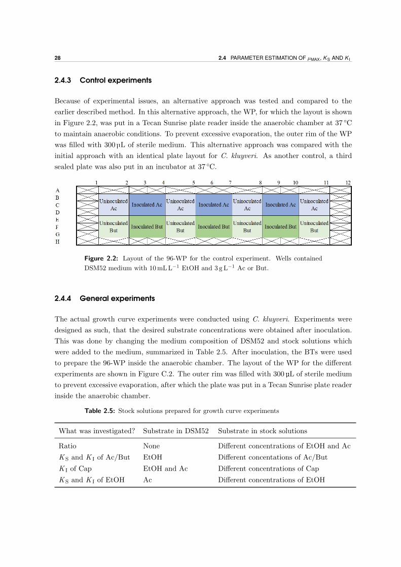
2.4.3 Control experiments
Because of experimental issues, an alternative approach was tested and compared to the
earlier described method. In this alternative approach, the WP, for which the layout is shown
in Figure 2.2, was put in a Tecan Sunrise plate reader inside the anaerobic chamber at 37 ◦C
to maintain anaerobic conditions. To prevent excessive evaporation, the outer rim of the WP
was filled with 300 µL of sterile medium. This alternative approach was compared with the
initial approach with an identical plate layout for C. kluyveri. As another control, a third
sealed plate was also put in an incubator at 37 ◦C.
Figure 2.2: Layout of the 96-WP for the control experiment. Wells contained
DSM52 medium with 10 mL L−1 EtOH and 3 g L−1 Ac or But.
2.4.4 General experiments
The actual growth curve experiments were conducted using C. kluyveri. Experiments were
designed as such, that the desired substrate concentrations were obtained after inoculation.
This was done by changing the medium composition of DSM52 and stock solutions which
were added to the medium, summarized in Table 2.5. After inoculation, the BTs were used
to prepare the 96-WP inside the anaerobic chamber. The layout of the WP for the different
experiments are shown in Figure C.2. The outer rim was filled with 300 µL of sterile medium
to prevent excessive evaporation, after which the plate was put in a Tecan Sunrise plate reader
inside the anaerobic chamber.
Table 2.5: Stock solutions prepared for growth curve experiments
What was investigated? Substrate in DSM52 Substrate in stock solutions
Ratio None Different concentrations of EtOH and Ac
K S and K I of Ac/But EtOH Different concentations of Ac/But
K I of Cap EtOH and Ac Different concentrations of Cap
K S and K I of EtOH Ac Different concentrations of EtOH
CHAPTER 2 MATERIALS AND METHODS 29
2.5 Parameter estimation of growth yield
Penicillin bottles were prepared, which contained 10 mL L−1 of EtOH and 3 g L−1 Ac or But.
These bottles were inoculated (1:10 inoculum:medium) and sampled. Samples were analyzed
on EtOH concentration and biomass concentration using VSS. The bottles were incubated at
37 ◦C and at a later time point analyzed again. YETOH,1 and YETOH,2 could be determined
using equation 2.7 for the Ac and But bottles respectively.
YEtOH =VSSend −VSSbegin
SEtOH,begin − SEtOH,end(2.7)
2.6 pH change of medium in function of added protons
As chain elongating reactions produce H+, it was checked how the pH of the medium changed
if protons were added. 1 L of Ac-free medium was divided over 3 equal volumes of 330 mL.
Here, either no K-Ac, 1.372 g of K-Ac or 2.734 g of K-Ac was added. Each Ac concentration
was further divided over three times 100 mL, in order to conduct the experiment in triplicate.
A stock solution of exactly 1 M HCl was made, and pH was checked after every addition of
0.1 mL HCl solution. At a later time point, 1 L of Ac-free medium was prepared, which was
divided over 3 times 100 mL and 3 times 200 mL. Again pH was checked after every addition
of either 0.1 mL HCl stock solution for 100 mL medium or 0.2 mL HCl stock solution for 200
mL medium.
2.7 Analysis
2.7.1 FA Analysis
FA Analysis was performed in accordance with Andersen et al. (2014). C2-C8 fatty acids
(including isoforms C4-C6) were measured by gas chromatography (GC-2014, Shimadzur,
The Netherlands) with DB-FFAP 123-3232 column (30 m x 0.32 mm x 0.25 µm; Agilent,
Belgium) and a flame ionization detector (FID). Liquid samples were conditioned with sulfuric
acid and sodium chloride and 2-methyl hexanoic acid as internal standard for quantification
of further extraction with diethyl ether. Prepared sample (1 µL) was injected at 200 ◦C with
a split ratio of 60 and a purge flow of 3 mL min−1. The oven temperature increased by
6 ◦C min−1 from 110 ◦C to 165 ◦C where it was kept for 2 minutes. FID had a temperature of
220 ◦C. The carrier gas was nitrogen at a flow rate of 2.49 mL min−1.
30 2.8 SOFTWARE
2.7.2 EtOH Analysis
The samples containing EtOH were diluted first to obtain EtOH concentrations below 1 g L−1
prior to the measurements. The analysis was performed using Ion Chromatography (IC)
(Dionex DX 500).
2.7.3 Solids Analysis
Total Suspended Solids (TSS) and Volatile Suspended Solids (VSS) Analysis were performed
following Standard Methods 2540D and E (APHA, 1992).
2.7.4 Headspace Gas Analysis
The gas phase composition was analyzed using a Compact Gas Chromatograph (GC) (Global
Analyser Solutions, Breda, The Netherlands), equipped with a Molsieve 5�A pre-column and
Porabond column (CH4, O2, H2 and N2) and a Rt-Q-bond pre-column and column (CO2,
N2O and H2S). Concentrations of gases were determined by means of a thermal conductivity
detector.
2.8 Software
2.8.1 Growth rate determination
The growth rates were determined using the gcFit function in the “grofit” package by Kahm
and Kschischo (2015). The package was called upon in RStudio (RStudio Team, 2015). The
calculated growth curves were produced with the parameters estimated with a spline fit,
whilst assuming logistic growth via equation 2.8. Here A is a the maximal growth value, µ
the maximal slope thus growth rate and λ the lag-phase. This was done, as the spline fit
always gave estimated parameters, whilst other fits only gave parameters if the fit was good
enough.
y(t) =A
1 + exp(4µA (λ− t) + 2)(2.8)
2.8.2 Model simulations
Model simulations were done using the “Model” instance in the biointense model environment
(Van Daele et al., 2015), which provides the ability to construct a model consisting of algebraic
equations, ordinary differential equations or a combination of both. The package was called
upon in IPython notebook (Perez and Granger, 2007). Literature values were used for the
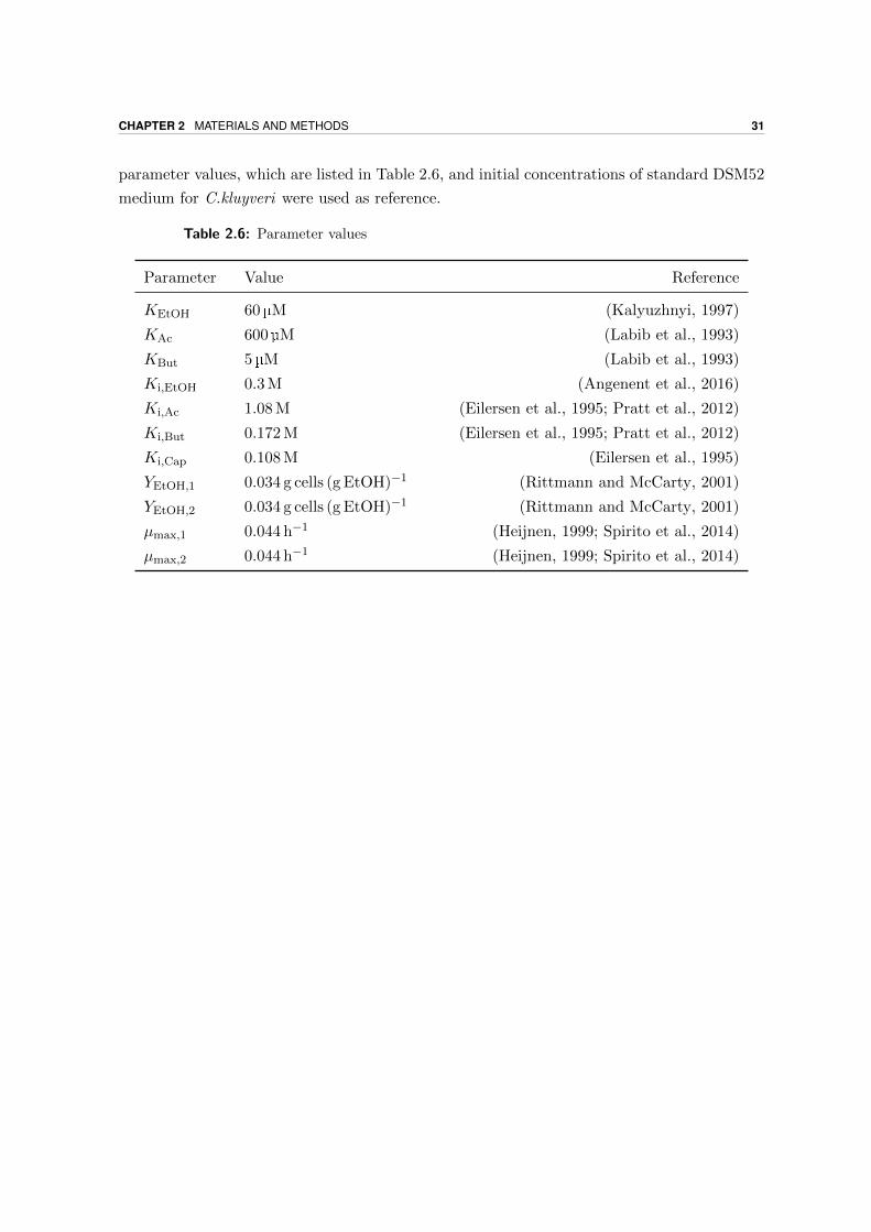
CHAPTER 2 MATERIALS AND METHODS 31
parameter values, which are listed in Table 2.6, and initial concentrations of standard DSM52
medium for C.kluyveri were used as reference.
Table 2.6: Parameter values
Parameter Value Reference
KEtOH 60 µM (Kalyuzhnyi, 1997)
KAc 600 µM (Labib et al., 1993)
KBut 5 µM (Labib et al., 1993)
Ki,EtOH 0.3 M (Angenent et al., 2016)
Ki,Ac 1.08 M (Eilersen et al., 1995; Pratt et al., 2012)
Ki,But 0.172 M (Eilersen et al., 1995; Pratt et al., 2012)
Ki,Cap 0.108 M (Eilersen et al., 1995)
YEtOH,1 0.034 g cells (g EtOH)−1 (Rittmann and McCarty, 2001)
YEtOH,2 0.034 g cells (g EtOH)−1 (Rittmann and McCarty, 2001)
µmax,1 0.044 h−1 (Heijnen, 1999; Spirito et al., 2014)
µmax,2 0.044 h−1 (Heijnen, 1999; Spirito et al., 2014)

CHAPTER 3Results
3.1 Reactor data
3.1.1 Mixed culture at HRT 7d
To determine the stability (required to do additional parameter estimation tests) and perfor-
mance of the reactor, the evolution of the FA concentrations, the VSS concentration, and the
gas production were monitored.
Figure 3.1 shows the concentrations of the FAs in the reactor. During a period of 78 days (11
times the HRT), no stable operation was achieved . Initially, But and Cap concentrations were
very low. A batch test (Figure 3.2) was performed to see if DSM52 medium would give better
results. Since the batch test showed higher VSS, But, and Cap concentrations, the DSM52
medium was used from day 22 onwards. This change resulted in a boost of the (MC)FA
production, as illustrated in Figure 3.1. The maximum total FA concentration following the
change in medium composition was 10.76 g L−1, with a Cap concentration of 6.02 g L−1.
To counteract methanogenesis, the EtOH concentration was increased in the influent at day
43, which appeared to boost the FA production. As methanogenesis still proceeded how-
ever, at day 50 the pH was lowered to 6 as well. However, this resulted in a lower reactor
productivity, since the FA concentrations were reduced (and Ac showed an increase).
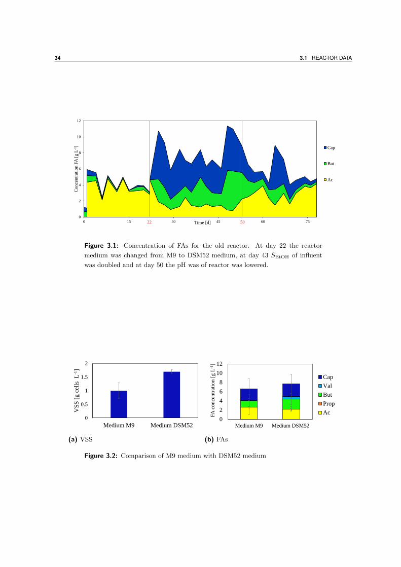
34 3.1 REACTOR DATA
0
2
4
6
8
10
12
0 15 30 45 60 75
Co
nce
ntr
atio
n F
A [
g L
-1]
Time [d]
Cap
But
Ac
22 50
Figure 3.1: Concentration of FAs for the old reactor. At day 22 the reactor
medium was changed from M9 to DSM52 medium, at day 43 SEtOH of influent
was doubled and at day 50 the pH was of reactor was lowered.
0
0.5
1
1.5
2
Medium M9 Medium DSM52
VS
S [
g c
ells
L
-1]
(a) VSS
0
2
4
6
8
10
12
Medium M9 Medium DSM52
FA
co
nce
ntr
atio
n [
g L
-1]
Cap
Val
But
Prop
Ac
(b) FAs
Figure 3.2: Comparison of M9 medium with DSM52 medium
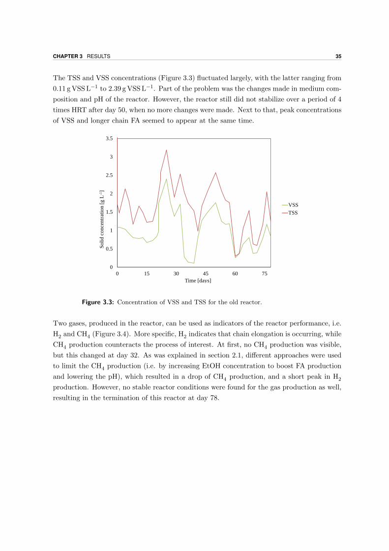
CHAPTER 3 RESULTS 35
The TSS and VSS concentrations (Figure 3.3) fluctuated largely, with the latter ranging from
0.11 g VSS L−1 to 2.39 g VSS L−1. Part of the problem was the changes made in medium com-
position and pH of the reactor. However, the reactor still did not stabilize over a period of 4
times HRT after day 50, when no more changes were made. Next to that, peak concentrations
of VSS and longer chain FA seemed to appear at the same time.
0
0.5
1
1.5
2
2.5
3
3.5
0 15 30 45 60 75
So
lid
co
nce
ntr
atio
n [
g L
-1]
Time [days]
VSS
TSS
Figure 3.3: Concentration of VSS and TSS for the old reactor.
Two gases, produced in the reactor, can be used as indicators of the reactor performance, i.e.
H2 and CH4 (Figure 3.4). More specific, H2 indicates that chain elongation is occurring, while
CH4 production counteracts the process of interest. At first, no CH4 production was visible,
but this changed at day 32. As was explained in section 2.1, different approaches were used
to limit the CH4 production (i.e. by increasing EtOH concentration to boost FA production
and lowering the pH), which resulted in a drop of CH4 production, and a short peak in H2
production. However, no stable reactor conditions were found for the gas production as well,
resulting in the termination of this reactor at day 78.
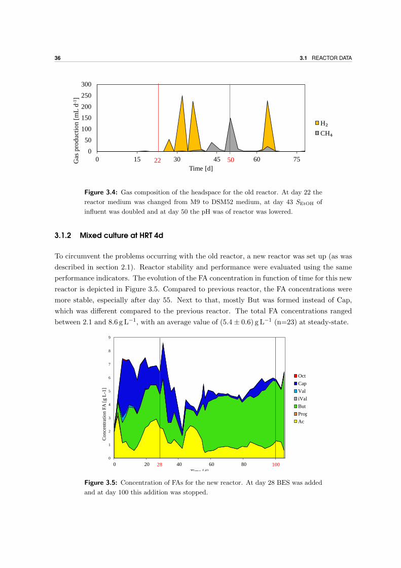
36 3.1 REACTOR DATA
0
50
100
150
200
250
300
0 15 30 45 60 75Gas
pro
du
ctio
n [
mL
d-1
]
Time [d]
H₂
CH₄
22 50
Figure 3.4: Gas composition of the headspace for the old reactor. At day 22 the
reactor medium was changed from M9 to DSM52 medium, at day 43 SEtOH of
influent was doubled and at day 50 the pH was of reactor was lowered.
3.1.2 Mixed culture at HRT 4d
To circumvent the problems occurring with the old reactor, a new reactor was set up (as was
described in section 2.1). Reactor stability and performance were evaluated using the same
performance indicators. The evolution of the FA concentration in function of time for this new
reactor is depicted in Figure 3.5. Compared to previous reactor, the FA concentrations were
more stable, especially after day 55. Next to that, mostly But was formed instead of Cap,
which was different compared to the previous reactor. The total FA concentrations ranged
between 2.1 and 8.6 g L−1, with an average value of (5.4± 0.6) g L−1 (n=23) at steady-state.
0
1
2
3
4
5
6
7
8
9
0 20 40 60 80 100
Co
nce
ntr
atio
n F
A [
g L
-1]
Time [d]
Oct
Cap
Val
iVal
But
Prop
Ac
28 100
Figure 3.5: Concentration of FAs for the new reactor. At day 28 BES was added
and at day 100 this addition was stopped.
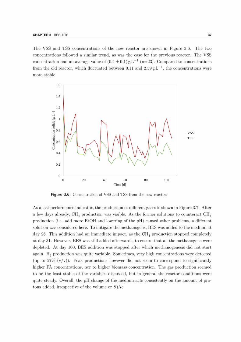
CHAPTER 3 RESULTS 37
The VSS and TSS concentrations of the new reactor are shown in Figure 3.6. The two
concentrations followed a similar trend, as was the case for the previous reactor. The VSS
concentration had an average value of (0.4± 0.1) g L−1 (n=23). Compared to concentrations
from the old reactor, which fluctuated between 0.11 and 2.39 g L−1, the concentrations were
more stable.
0
0.2
0.4
0.6
0.8
1
1.2
1.4
1.6
0 20 40 60 80 100
Co
nce
ntr
atio
n s
oli
ds
[g L
-1]
Time [d]
VSS
TSS
Figure 3.6: Concentration of VSS and TSS from the new reactor.
As a last performance indicator, the production of different gases is shown in Figure 3.7. After
a few days already, CH4 production was visible. As the former solutions to counteract CH4
production (i.e. add more EtOH and lowering of the pH) caused other problems, a different
solution was considered here. To mitigate the methanogens, BES was added to the medium at
day 28. This addition had an immediate impact, as the CH4 production stopped completely
at day 31. However, BES was still added afterwards, to ensure that all the methanogens were
depleted. At day 100, BES addition was stopped after which methanogenesis did not start
again. H2 production was quite variable. Sometimes, very high concentrations were detected
(up to 57% (v/v)). Peak productions however did not seem to correspond to significantly
higher FA concentrations, nor to higher biomass concentration. The gas production seemed
to be the least stable of the variables discussed, but in general the reactor conditions were
quite steady. Overall, the pH change of the medium acts consistently on the amount of pro-
tons added, irrespective of the volume or S)Ac.
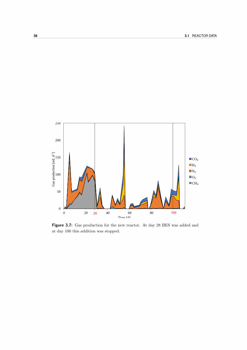
38 3.1 REACTOR DATA
0
50
100
150
200
250
0 20 40 60 80 100
Gas
pro
du
ctio
n [
mL
d-1
]
Time [d]
CO₂
H₂
N₂
O₂
CH₄
28 100
Figure 3.7: Gas production for the new reactor. At day 28 BES was added and
at day 100 this addition was stopped.
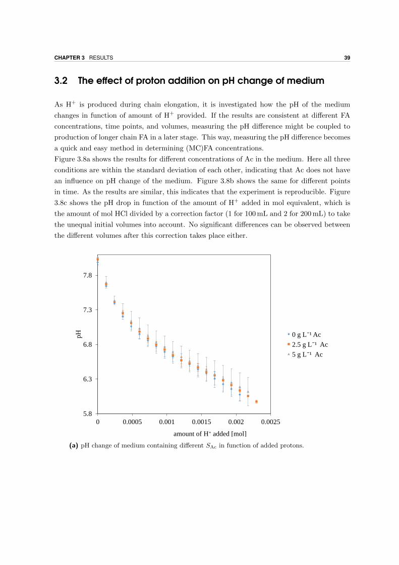
CHAPTER 3 RESULTS 39
3.2 The effect of proton addition on pH change of medium
As H+ is produced during chain elongation, it is investigated how the pH of the medium
changes in function of amount of H+ provided. If the results are consistent at different FA
concentrations, time points, and volumes, measuring the pH difference might be coupled to
production of longer chain FA in a later stage. This way, measuring the pH difference becomes
a quick and easy method in determining (MC)FA concentrations.
Figure 3.8a shows the results for different concentrations of Ac in the medium. Here all three
conditions are within the standard deviation of each other, indicating that Ac does not have
an influence on pH change of the medium. Figure 3.8b shows the same for different points
in time. As the results are similar, this indicates that the experiment is reproducible. Figure
3.8c shows the pH drop in function of the amount of H+ added in mol equivalent, which is
the amount of mol HCl divided by a correction factor (1 for 100 mL and 2 for 200 mL) to take
the unequal initial volumes into account. No significant differences can be observed between
the different volumes after this correction takes place either.
5.8
6.3
6.8
7.3
7.8
0 0.0005 0.001 0.0015 0.002 0.0025
pH
amount of H+ added [mol]
0 g L⁻¹ Ac
2.5 g L⁻¹ Ac
5 g L⁻¹ Ac
(a) pH change of medium containing different SAc in function of added protons.
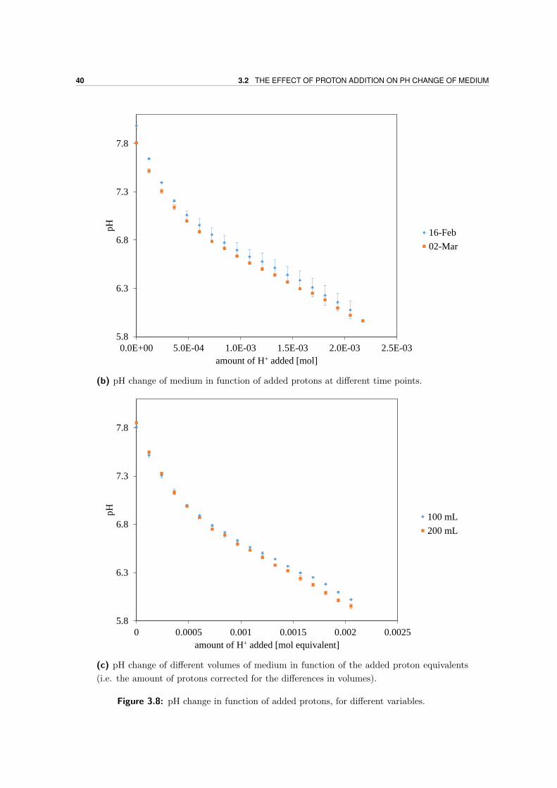
40 3.2 THE EFFECT OF PROTON ADDITION ON PH CHANGE OF MEDIUM
5.8
6.3
6.8
7.3
7.8
0.0E+00 5.0E-04 1.0E-03 1.5E-03 2.0E-03 2.5E-03
pH
amount of H+ added [mol]
16-Feb
02-Mar
(b) pH change of medium in function of added protons at different time points.
5.8
6.3
6.8
7.3
7.8
0 0.0005 0.001 0.0015 0.002 0.0025
pH
amount of H+ added [mol equivalent]
100 mL
200 mL
(c) pH change of different volumes of medium in function of the added proton equivalents
(i.e. the amount of protons corrected for the differences in volumes).
Figure 3.8: pH change in function of added protons, for different variables.
CHAPTER 3 RESULTS 41
3.3 Method development of growth curves
Parameter estimation was attempted using the growth curve technique. During the initial
experiments, the growth curves were evaluated on different aspects. It was verified whether
growth could be observed and be related to chain elongation. Next, deviations among tripli-
cates were investigated and outcomes of BTs and WP were compared.
Figure 3.9 shows data from the first growth experiment conducted for C. kluyveri as de-
scribed in section 2.4.2. The titles correspond to the calculated concentrations of EtOH and
Ac respectively. These differ from the real concentrations which were measured from the
BTs. The layout of the upper 4 rows of plots is as such, that identical proportions of EtOH
and Ac (1:0,2:1,4:1 and 8:1) are plotted horizontally next to each other, and identical EtOH
concentrations (0.075 M, 0.15 M, 0.3 M and 0.6 M) are plotted vertically next to each other.
In nearly all the plots from Figure 3.9, triplicates showed a similar pattern. Further, all the
growth curves showed an initial increase in OD at around 2 hours. This increase was possibly
not caused by growth, considering that the uninoculated wells experienced this increase as
well. As there was no second increase visible in all three replicates, microorganisms were
probably unable to grow under present conditions.
When the same experiment was performed with the mixed community from the old reactor
(Figure C.3), all the inoculated growth curves showed an increase in OD. As the uninocu-
lated growth curves remained nearly flat, this implied that growth could be observed in all the
wells. In Figure 3.10 the FA concentrations at the end of the experiment were compared. The
BTs had a higher SCap and SBut , and lower SAc. When linking this to the chain elongation
reaction, it was concluded that the microorganisms in the BT had a higher productivity. In
the WP little to no But and Cap were detected, indicating that growth taking place during
the experiment was not caused by chain elongating organisms.
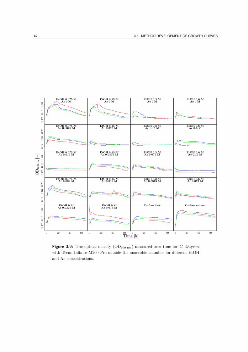
42 3.3 METHOD DEVELOPMENT OF GROWTH CURVES
EtOH 0.075 MAc 0 M
0.1
20.1
60.2
0
EtOH 0.15 MAc 0 M
EtOH 0.3 MAc 0 M
EtOH 0.6 MAc 0 M
EtOH 0.075 MAc 0.0375 M
0.12
0.16
0.20
EtOH 0.15 MAc 0.075 M
EtOH 0.3 MAc 0.15 M
EtOH 0.6 MAc 0.3 M
EtOH 0.075 MAc 0.019 M
0.12
0.16
0.2
0
EtOH 0.15 MAc 0.0375 M
EtOH 0.3 MAc 0.075 M
EtOH 0.6 MAc 0.15 M
EtOH 0.075 MAc 0.009 M
0.1
20.
16
0.20
EtOH 0.15 MAc 0.019 M
EtOH 0.3 MAc 0.0375 M
EtOH 0.6 MAc 0.075 M
EtOH 0 MAc 0.0375 M
0 20 40 60
0.12
0.16
0.20
EtOH 0 MAc 0.075 M
0 20 40 60
C−free inoc
0 20 40 60
C−free uninoc
0 20 40 60
Time [h]
OD
600
nm
[−
]
Figure 3.9: The optical density (OD600 nm) measured over time for C. kluyveri
with Tecan Infinite M200 Pro outside the anaerobic chamber for different EtOH
and Ac concentrations.
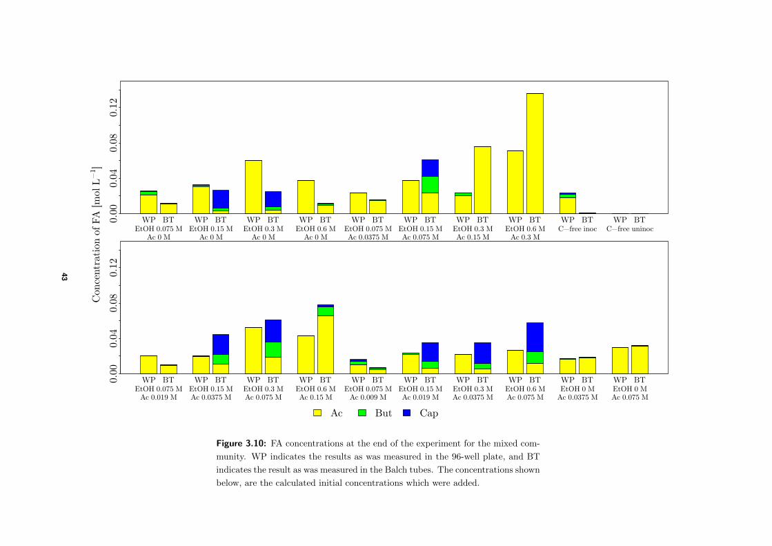
WP BT WP BT WP BT WP BT WP BT WP BT WP BT WP BT WP BT WP BT0.00
0.04
0.08
0.12
EtOH 0.075 M EtOH 0.15 M EtOH 0.3 M EtOH 0.6 M EtOH 0.075 M EtOH 0.15 M EtOH 0.3 M EtOH 0.6 M C−free inoc C−free uninocAc 0 M Ac 0 M Ac 0 M Ac 0 M Ac 0.0375 M Ac 0.075 M Ac 0.15 M Ac 0.3 M
WP BT WP BT WP BT WP BT WP BT WP BT WP BT WP BT WP BT WP BT0.00
0.04
0.08
0.12
EtOH 0.075 M EtOH 0.15 M EtOH 0.3 M EtOH 0.6 M EtOH 0.075 M EtOH 0.15 M EtOH 0.3 M EtOH 0.6 M EtOH 0 M EtOH 0 MAc 0.019 M Ac 0.0375 M Ac 0.075 M Ac 0.15 M Ac 0.009 M Ac 0.019 M Ac 0.0375 M Ac 0.075 M Ac 0.0375 M Ac 0.075 M
Ac But Cap
Con
centr
atio
n o
f FA
[m
ol L
−1 ]
Figure 3.10: FA concentrations at the end of the experiment for the mixed com-
munity. WP indicates the results as was measured in the 96-well plate, and BT
indicates the result as was measured in the Balch tubes. The concentrations shown
below, are the calculated initial concentrations which were added.
43
44 3.3 METHOD DEVELOPMENT OF GROWTH CURVES
The experiment was also repeated for a pure culture of only C. kluyveri, as previously no
growth could be observed. The results can be found in Figure C.4. Here, the variability
between the different triplicates was higher than in the previous experiment and apart from
a decrease in OD at the start, the OD of the uninoculated wells remained nearly constant in
time. Some other wells showed a rise in OD, which therefore implied that growth was taking
place in these wells. However, when final FA concentrations of the 96-WP were compared to
the FA concentrations in the BT (depicted in Figure 3.11) very different concentrations for
the two methods were found as well. In most cases the BTs contained more Cap, more But
and less Ac, as was the case for the mixed community. This then implied that microorganisms
were more active in the BT than in the WP. However, for the wells containing only Ac the
opposite was true, although there seemed to be even more problems occurring here in regards
to mass balances (i.e. 0.075 M Ac and 0 M EtOH should normally not result in 0.1 M Cao).
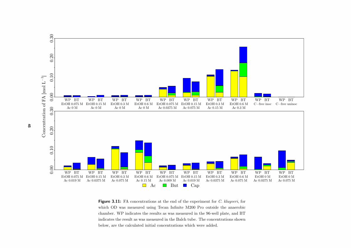
WP BT WP BT WP BT WP BT WP BT WP BT WP BT WP BT WP BT WP BT0.00
0.10
0.20
0.30
EtOH 0.075 M EtOH 0.15 M EtOH 0.3 M EtOH 0.6 M EtOH 0.075 M EtOH 0.15 M EtOH 0.3 M EtOH 0.6 M C−free inoc C−free uninocAc 0 M Ac 0 M Ac 0 M Ac 0 M Ac 0.0375 M Ac 0.075 M Ac 0.15 M Ac 0.3 M
WP BT WP BT WP BT WP BT WP BT WP BT WP BT WP BT WP BT WP BT0.00
0.10
0.20
0.30
EtOH 0.075 M EtOH 0.15 M EtOH 0.3 M EtOH 0.6 M EtOH 0.075 M EtOH 0.15 M EtOH 0.3 M EtOH 0.6 M EtOH 0 M EtOH 0 MAc 0.019 M Ac 0.0375 M Ac 0.075 M Ac 0.15 M Ac 0.009 M Ac 0.019 M Ac 0.0375 M Ac 0.075 M Ac 0.0375 M Ac 0.075 M
Ac But Cap
Con
centr
atio
n o
f FA
[m
ol L
−1 ]
Figure 3.11: FA concentrations at the end of the experiment for C. kluyveri, for
which OD was measured using Tecan Infinite M200 Pro outside the anaerobic
chamber. WP indicates the results as was measured in the 96-well plate, and BT
indicates the result as was measured in the Balch tube. The concentrations shown
below, are the calculated initial concentrations which were added.
45
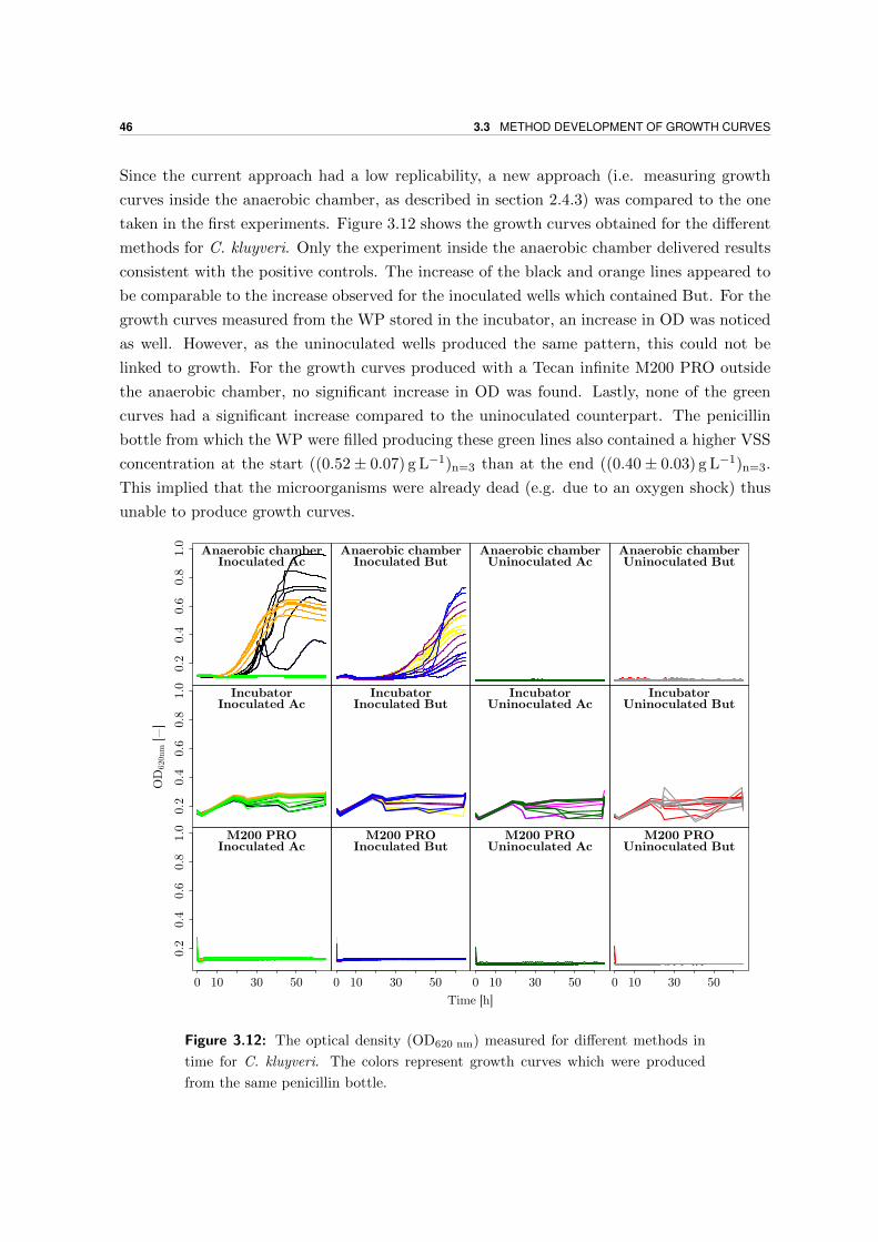
46 3.3 METHOD DEVELOPMENT OF GROWTH CURVES
Since the current approach had a low replicability, a new approach (i.e. measuring growth
curves inside the anaerobic chamber, as described in section 2.4.3) was compared to the one
taken in the first experiments. Figure 3.12 shows the growth curves obtained for the different
methods for C. kluyveri. Only the experiment inside the anaerobic chamber delivered results
consistent with the positive controls. The increase of the black and orange lines appeared to
be comparable to the increase observed for the inoculated wells which contained But. For the
growth curves measured from the WP stored in the incubator, an increase in OD was noticed
as well. However, as the uninoculated wells produced the same pattern, this could not be
linked to growth. For the growth curves produced with a Tecan infinite M200 PRO outside
the anaerobic chamber, no significant increase in OD was found. Lastly, none of the green
curves had a significant increase compared to the uninoculated counterpart. The penicillin
bottle from which the WP were filled producing these green lines also contained a higher VSS
concentration at the start ((0.52± 0.07) g L−1)n=3 than at the end ((0.40± 0.03) g L−1)n=3.
This implied that the microorganisms were already dead (e.g. due to an oxygen shock) thus
unable to produce growth curves.
Inoculated AcAnaerobic chamber
0.2
0.4
0.6
0.8
1.0
Anaerobic chamberInoculated But
Anaerobic chamberUninoculated Ac
Anaerobic chamberUninoculated But
IncubatorInoculated Ac
0.2
0.4
0.6
0.8
1.0
IncubatorInoculated But
IncubatorUninoculated Ac
IncubatorUninoculated But
M200 PROInoculated Ac
0.2
0.4
0.6
0.8
1.0
0 10 30 50
M200 PROInoculated But
0 10 30 50 0 10 30 50
M200 PROUninoculated Ac
M200 PROUninoculated But
0 10 30 50
Time [h]
OD
620
nm
[−
]
Figure 3.12: The optical density (OD620 nm) measured for different methods in
time for C. kluyveri. The colors represent growth curves which were produced
from the same penicillin bottle.
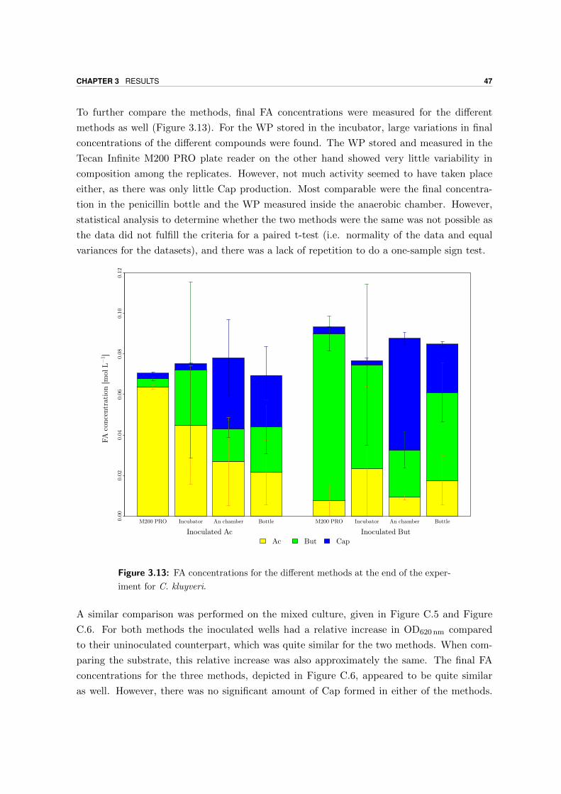
CHAPTER 3 RESULTS 47
To further compare the methods, final FA concentrations were measured for the different
methods as well (Figure 3.13). For the WP stored in the incubator, large variations in final
concentrations of the different compounds were found. The WP stored and measured in the
Tecan Infinite M200 PRO plate reader on the other hand showed very little variability in
composition among the replicates. However, not much activity seemed to have taken place
either, as there was only little Cap production. Most comparable were the final concentra-
tion in the penicillin bottle and the WP measured inside the anaerobic chamber. However,
statistical analysis to determine whether the two methods were the same was not possible as
the data did not fulfill the criteria for a paired t-test (i.e. normality of the data and equal
variances for the datasets), and there was a lack of repetition to do a one-sample sign test.
M200 PRO Incubator An chamber Bottle M200 PRO Incubator An chamber Bottle0.00
0.02
0.04
0.06
0.08
0.10
0.12
Inoculated Ac Inoculated ButAc But Cap
FA
con
centr
atio
n [
mol
L−
1 ]
Figure 3.13: FA concentrations for the different methods at the end of the exper-
iment for C. kluyveri.
A similar comparison was performed on the mixed culture, given in Figure C.5 and Figure
C.6. For both methods the inoculated wells had a relative increase in OD620 nm compared
to their uninoculated counterpart, which was quite similar for the two methods. When com-
paring the substrate, this relative increase was also approximately the same. The final FA
concentrations for the three methods, depicted in Figure C.6, appeared to be quite similar
as well. However, there was no significant amount of Cap formed in either of the methods.
48 3.4 DATA COLLECTION
This again seemed to contradict the statement that growth occurred. As it appeared that
growth and Cap formation were not linked, it was possible that growth occurred via different
reactions. This seems plausible, as in a mixed culture there are different species, making
the possible reactions less straightforward. Therefore, for the actual experiments used for
parameter estimation only the pure culture C. kluyveri was used.
3.4 Data collection
Table 2.4 provides an overview of the different experiments conducted for estimation of µmax,
KS and KI of the different compounds. However, only the high SEtOH, high SBut and ratio-
experiment will be discussed due to failure of the other experiments and a lack of time to
redo them. Data was reviewed on the same points as previously (i.e. comparable triplicates,
whether growth was observed through chain elongation, if BTs and WP had similar results).
Next to that, it was determined whether substrate consumption and product formation took
place following stoichiometry derived by Spirito et al. (2014).
3.4.1 High SEtOH experiment
Figure 3.14 shows the resulting growth curves, produced for the high SEtOH experiment.
Data was corrected with the uninoculated control containing no EtOH, which gave nearly flat
growth curves with an average OD620 nm of 0.100± 0.003 (n=358). The correction ensured an
OD close to zero to allow a better fit to the growth curves by the Grofit-package, improving
the accuracy of estimations for µ, λ and A. From Figure 3.14 it was seen that triplicates were
quite similar for lower SEtOH, but became more dissimilar when higher concentrations were
provided. Next to that, the growth curves had a characteristic shape: the OD rose until a
maximum was reached and then started to decline. This corresponded to lag-time, growth
and decay respectively. However, this downward slope could not be predicted by the model
as decay was not added to the model. This was because it was not of importance during
parameter estimation and would already be added to the fermentation part of an overall
model. Apart from that, the corrected growth curves and calculated growth curves using
Grofit were quite similar. When the final FA concentrations were determined for WP and
BT, depicted in Figure C.7, the WP had a higher SCap and SBut and lower SAc than the BTs,
which indicated higher activity of the microorganisms in the WP.
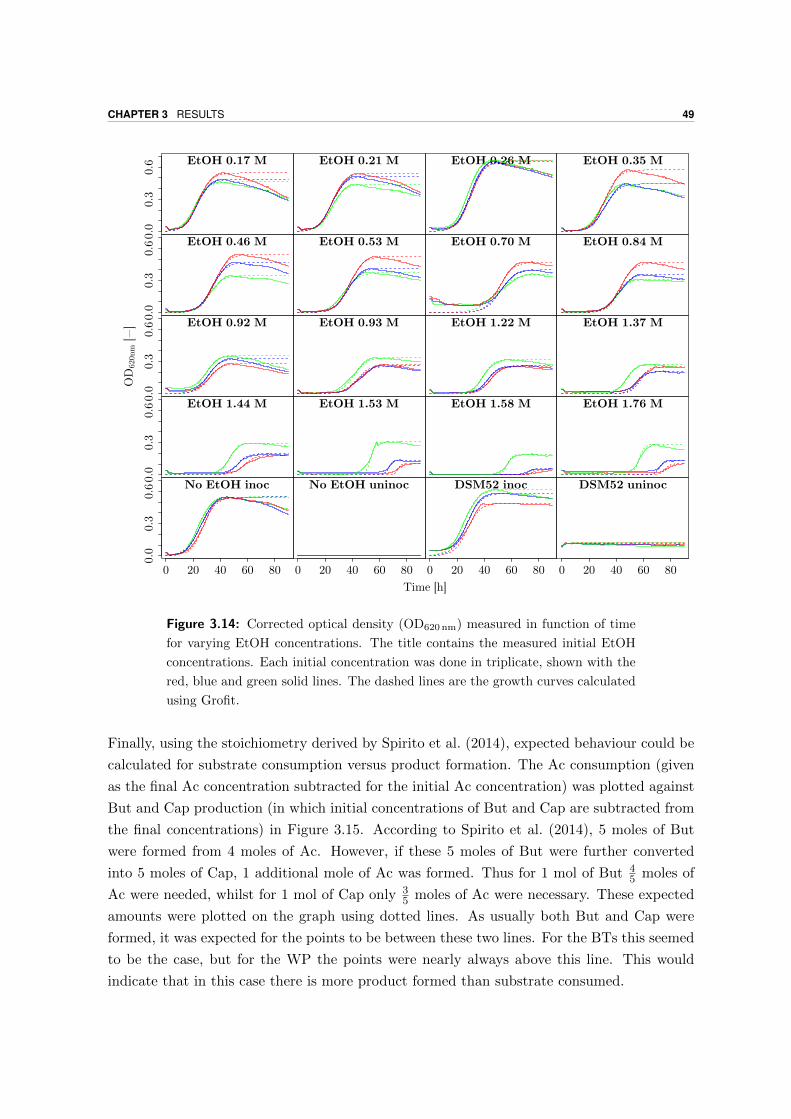
CHAPTER 3 RESULTS 49
EtOH 0.17 M
0.0
0.3
0.6 EtOH 0.21 M EtOH 0.26 M EtOH 0.35 M
EtOH 0.46 M
0.0
0.3
0.6 EtOH 0.53 M EtOH 0.70 M EtOH 0.84 M
EtOH 0.92 M
0.0
0.3
0.6 EtOH 0.93 M EtOH 1.22 M EtOH 1.37 M
EtOH 1.44 M
0.0
0.3
0.6 EtOH 1.53 M EtOH 1.58 M EtOH 1.76 M
No EtOH inoc
0.0
0.3
0.6
0 20 40 60 80
No EtOH uninoc
0 20 40 60 80
DSM52 inoc
0 20 40 60 80
DSM52 uninoc
0 20 40 60 80
Time [h]
OD
620n
m [−
]
Figure 3.14: Corrected optical density (OD620 nm) measured in function of time
for varying EtOH concentrations. The title contains the measured initial EtOH
concentrations. Each initial concentration was done in triplicate, shown with the
red, blue and green solid lines. The dashed lines are the growth curves calculated
using Grofit.
Finally, using the stoichiometry derived by Spirito et al. (2014), expected behaviour could be
calculated for substrate consumption versus product formation. The Ac consumption (given
as the final Ac concentration subtracted for the initial Ac concentration) was plotted against
But and Cap production (in which initial concentrations of But and Cap are subtracted from
the final concentrations) in Figure 3.15. According to Spirito et al. (2014), 5 moles of But
were formed from 4 moles of Ac. However, if these 5 moles of But were further converted
into 5 moles of Cap, 1 additional mole of Ac was formed. Thus for 1 mol of But 45 moles of
Ac were needed, whilst for 1 mol of Cap only 35 moles of Ac were necessary. These expected
amounts were plotted on the graph using dotted lines. As usually both But and Cap were
formed, it was expected for the points to be between these two lines. For the BTs this seemed
to be the case, but for the WP the points were nearly always above this line. This would
indicate that in this case there is more product formed than substrate consumed.
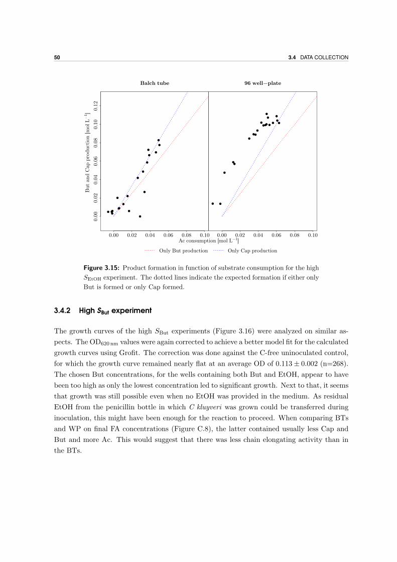
50 3.4 DATA COLLECTION
●
●
●
●
●
●
●
●
●
●
●
●
●
●●
●
●●
●
●
Balch tube
0.00 0.02 0.04 0.06 0.08 0.10
0.00
0.02
0.04
0.06
0.08
0.10
0.12
●
●
●●
●●
●●
●
●
●
●
●
●
●
●
●●
●
●
96 well−plate
0.00 0.02 0.04 0.06 0.08 0.10Ac consumption [mol L−1]
But
and C
ap p
roduct
ion [
mol
L−
1 ]
Only But production Only Cap production
Figure 3.15: Product formation in function of substrate consumption for the high
SEtOH experiment. The dotted lines indicate the expected formation if either only
But is formed or only Cap formed.
3.4.2 High SBut experiment
The growth curves of the high SBut experiments (Figure 3.16) were analyzed on similar as-
pects. The OD620 nm values were again corrected to achieve a better model fit for the calculated
growth curves using Grofit. The correction was done against the C-free uninoculated control,
for which the growth curve remained nearly flat at an average OD of 0.113± 0.002 (n=268).
The chosen But concentrations, for the wells containing both But and EtOH, appear to have
been too high as only the lowest concentration led to significant growth. Next to that, it seems
that growth was still possible even when no EtOH was provided in the medium. As residual
EtOH from the penicillin bottle in which C kluyveri was grown could be transferred during
inoculation, this might have been enough for the reaction to proceed. When comparing BTs
and WP on final FA concentrations (Figure C.8), the latter contained usually less Cap and
But and more Ac. This would suggest that there was less chain elongating activity than in
the BTs.
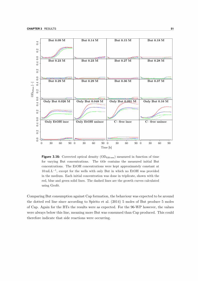
CHAPTER 3 RESULTS 51
But 0.09 M0.
00.2
0.4 But 0.14 M But 0.15 M But 0.18 M
But 0.23 M
0.0
0.2
0.4 But 0.23 M But 0.27 M But 0.28 M
But 0.29 M
0.0
0.2
0.4 But 0.29 M But 0.36 M But 0.37 M
Only But 0.026 M
0.0
0.2
0.4 Only But 0.048 M Only But 0.091 M Only But 0.16 M
Only EtOH inoc
0.0
0.2
0.4
0 30 60 90
Only EtOH uninoc
0 30 60 90
C−free inoc
0 30 60 90
C−free uninoc
0 30 60 90
Time [h]
OD
620n
m [−
]
Figure 3.16: Corrected optical density (OD620 nm) measured in function of time
for varying But concentrations. The title contains the measured initial But
concentrations. The EtOH concentrations were kept approximately constant at
10 mL L−1, except for the wells with only But in which no EtOH was provided
in the medium. Each initial concentration was done in triplicate, shown with the
red, blue and green solid lines. The dashed lines are the growth curves calculated
using Grofit.
Comparing But consumption against Cap formation, the behaviour was expected to be around
the dotted red line since according to Spirito et al. (2014) 5 moles of But produce 5 moles
of Cap. Again for the BTs the results were as expected. For the 96-WP however, the values
were always below this line, meaning more But was consumed than Cap produced. This could
therefore indicate that side reactions were occurring.
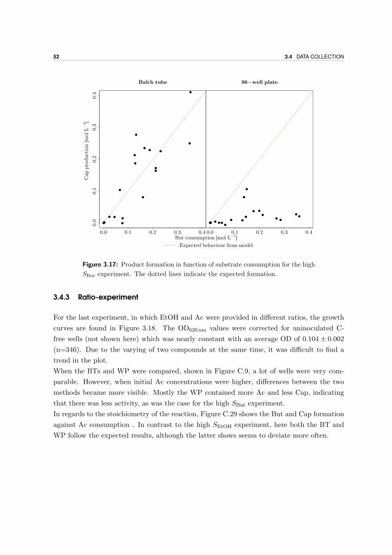
52 3.4 DATA COLLECTION
●
●
●
●
●
●
●
●
●●
●
●
●
●
● ●●
●●●
Balch tube
0.0 0.1 0.2 0.3 0.4
0.0
0.1
0.2
0.3
0.4
● ●
●
●
●
●
●
●
●●
●●
●●
●● ●
●●●
96−well plate
0.0 0.1 0.2 0.3 0.4But consumption [mol L−1]
Cap
pro
duct
ion [
mol
L−
1 ]
Expected behaviour from model
Figure 3.17: Product formation in function of substrate consumption for the high
SBut experiment. The dotted lines indicate the expected formation.
3.4.3 Ratio-experiment
For the last experiment, in which EtOH and Ac were provided in different ratios, the growth
curves are found in Figure 3.18. The OD620 nm values were corrected for uninoculated C-
free wells (not shown here) which was nearly constant with an average OD of 0.104± 0.002
(n=346). Due to the varying of two compounds at the same time, it was difficult to find a
trend in the plot.
When the BTs and WP were compared, shown in Figure C.9, a lot of wells were very com-
parable. However, when initial Ac concentrations were higher, differences between the two
methods became more visible. Mostly the WP contained more Ac and less Cap, indicating
that there was less activity, as was the case for the high SBut experiment.
In regards to the stoichiometry of the reaction, Figure C.29 shows the But and Cap formation
against Ac consumption . In contrast to the high SEtOH experiment, here both the BT and
WP follow the expected results, although the latter shows seems to deviate more often.
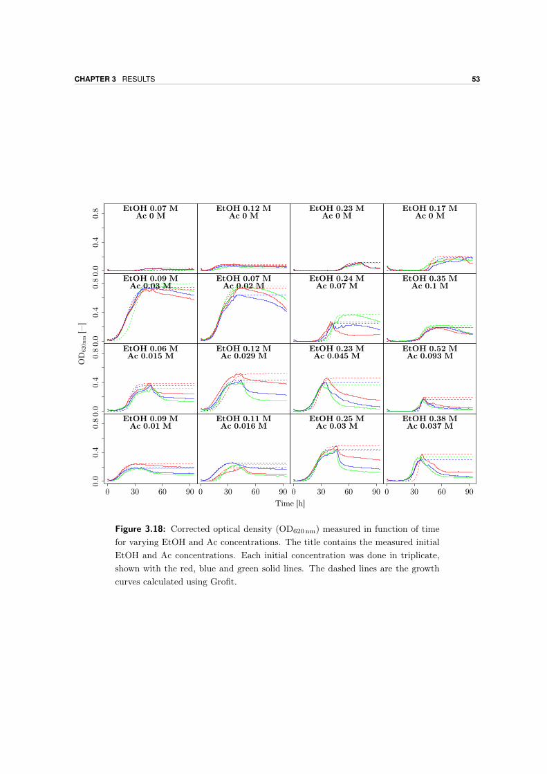
CHAPTER 3 RESULTS 53
EtOH 0.07 MAc 0 M
0.0
0.4
0.8 EtOH 0.12 M
Ac 0 MEtOH 0.23 M
Ac 0 MEtOH 0.17 M
Ac 0 M
EtOH 0.09 MAc 0.03 M
0.0
0.4
0.8 EtOH 0.07 M
Ac 0.02 MEtOH 0.24 M
Ac 0.07 MEtOH 0.35 M
Ac 0.1 M
EtOH 0.06 MAc 0.015 M
0.0
0.4
0.8 EtOH 0.12 M
Ac 0.029 MEtOH 0.23 MAc 0.045 M
EtOH 0.52 MAc 0.093 M
EtOH 0.09 MAc 0.01 M
0.0
0.4
0.8
0 30 60 90
EtOH 0.11 MAc 0.016 M
0 30 60 90
EtOH 0.25 MAc 0.03 M
0 30 60 90
EtOH 0.38 MAc 0.037 M
0 30 60 90
Time [h]
OD
620n
m [−
]
Figure 3.18: Corrected optical density (OD620 nm) measured in function of time
for varying EtOH and Ac concentrations. The title contains the measured initial
EtOH and Ac concentrations. Each initial concentration was done in triplicate,
shown with the red, blue and green solid lines. The dashed lines are the growth
curves calculated using Grofit.
54 3.5 GROWTH YIELD
3.5 Growth yield
To determine the growth yields YEtOH,1 and YEtOH,2, penicillin bottles were inoculated con-
taining EtOH and Ac or EtOH and But respectively. For the bottles containing EtOH and Ac,
one bottle (the green lines in Figure 3.12) appeared to have not grown. This was confirmed by
measuring the VSS concentration, which was higher at the start (0.52 g cells L−1) than at the
end (0.4 g cells L−1). As tests were done in triplicate, only two samples remained for which the
growth yield could be determined. This resulted in YEtOH,1 of (0.047± 0.008) g cells (g EtOH)−1,
which was determined as the average and standard deviation of the two values. No proper
error propagation was performed, as this value was rather used as an indicative value. When
the same was attempted for the YEtOH,2, the VSS concentration was always higher at the be-
ginning than at the end. Next to that, in two of the three bottles more EtOH was produced
than consumed. Because of these considerations, no YEtOH,2 could be determined.
CHAPTER 4Discussion
4.1 Reactor performance and stability
The reactor data was already discussed in section 3.1. The values gained here were used
to compare the reactors to each other and to literature values in regards to stability, final
concentrations of FAs and their ratios.
Stability was only reached for the reactor with an HRT of 4 days. In this reactor however
mostly But and only little Cap was produced. On average, after stability was reached, the
effluent contained (0.42± 0.37) g L−1 Cap (n=23). The reactor with an HRT of 7 days on the
other hand had a higher SCap but higher variability as well ((2.04± 2.01) g L−1)(n=37). The
maximal SCap here was 6.02 g L−1 and the total FA concentration never went above 11.4 g L−1.
Comparing this to literature values, the most similar setup was a (fed)-batch reactor by Stein-
busch et al. (2011). This reactor started with synthetic medium which contained 3 g L−1 of
Ac and 2.3 g L−1 of EtOH, less than applied in this thesis. Apart from addition of EtOH when
it became depleted, no additional substrate was added. This resulted in effluent containing
final Cap concentrations of 8.27 g L−1 at pH 7 and 0.12 g L−1 at pH 5.5. As SCap in this thesis
remained between these values as well, this was quite comparable but rather on the low side.
As it however was not in the objective to have a high SCap but rather stable conditions, lower
Cap concentrations were tolerated if stability was reached.
As this was not the case for the first reactor, an explanation was sought. The unstable nature
could for instance be caused by addition of high substrate concentrations. This resulted in
high activity which in turn entailed high (MC)FA-concentrations. It appeared that high FA-
concentrations (according to Figure 3.1 this seemed to be around the 8-10 g L−1 benchmark)
inhibited microorganisms. It then took several dilutions for the FA concentrations to become
low enough before inhibition was lifted and growth could re-start. This was checked, by plot-
ting the subsequent biomass production (in percentage of the biomass concentration) for the
respective Cap concentration in Figure 4.1. There seemed to be a somewhat downward trend
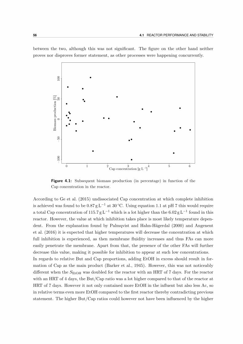
56 4.1 REACTOR PERFORMANCE AND STABILITY
between the two, although this was not significant. The figure on the other hand neither
proves nor disproves former statement, as other processes were happening concurrently.
●
●●
●
●
●
●
●●
●
●
●
●
●
●
●
●
●
●
●
●
●
●
●
●
●
●
●
●
●
●
●
0 1 2 3 4 5 6
−10
0−
500
5010
0
Cap concentration [g L−1]
Bio
mas
s pro
duct
ion [%
]
Figure 4.1: Subsequent biomass production (in percentage) in function of the
Cap concentration in the reactor.
According to Ge et al. (2015) undissociated Cap concentration at which complete inhibition
is achieved was found to be 0.87 g L−1 at 30 ◦C. Using equation 1.1 at pH 7 this would require
a total Cap concentration of 115.7 g L−1 which is a lot higher than the 6.02 g L−1 found in this
reactor. However, the value at which inhibition takes place is most likely temperature depen-
dent. From the explanation found by Palmqvist and Hahn-Hagerdal (2000) and Angenent
et al. (2016) it is expected that higher temperatures will decrease the concentration at which
full inhibition is experienced, as then membrane fluidity increases and thus FAs can more
easily penetrate the membrane. Apart from that, the presence of the other FAs will further
decrease this value, making it possible for inhibition to appear at such low concentrations.
In regards to relative But and Cap proportions, adding EtOH in excess should result in for-
mation of Cap as the main product (Barker et al., 1945). However, this was not noticeably
different when the SEtOH was doubled for the reactor with an HRT of 7 days. For the reactor
with an HRT of 4 days, the But/Cap ratio was a lot higher compared to that of the reactor at
HRT of 7 days. However it not only contained more EtOH in the influent but also less Ac, so
in relative terms even more EtOH compared to the first reactor thereby contradicting previous
statement. The higher But/Cap ratios could however not have been influenced by the higher
CHAPTER 4 DISCUSSION 57
EtOH/Ac concentration, but rather by the retention time. According to Grootscholten et al.
(2013b), lowering the HRT decreased Cap concentrations while the SBut remained approxi-
mately the same.
FA concentrations and ratios were further influenced by pH. This was noticed, as lowering
the pH resulted into higher SAc and lower SBut, SCap and total FA concentration. This was
comparable to what could be found in literature (Steinbusch et al., 2011) and could be ex-
plained by the higher fraction of undissociated FAs at lower pH. As it is the protonated form
resulting in inhibition, the activity decreases at higher pH, thus lowering the FA concentra-
tion (Palmqvist and Hahn-Hagerdal, 2000). Next to that, a lower pH in itself can reduce
activity, since part of the energy needs to be invested into maintaining a neutral internal pH
(Angenent et al., 2016).
4.2 Model simulations
Simulations on the chain elongation model were done for different parameters (listed in Table
2.6) and initial conditions. These simulations could then be used to determine if the model
behaviour acted normally and whether it was comparable to the obtained growth curves. The
parameters were literature values, as parameter estimation was not achieved due to lack of
data and issues that will be explained in section 4.3. The outcome of the simulations can be
found in the appendix (section C.5).
The model simulations acted as expected. Higher inhibition parameters (which indicate that
inhibition takes place only at higher concentrations) resulted in faster growth without altering
the final concentrations. Substrate affinity parameters influenced growth rates as well, but
depending on which compound was limiting, different steady-state outcomes were reached.
Different yields mostly influenced the steady-state concentrations of the biomass, but other
concentrations were also dependent on whether EtOH or Ac was the limiting substrate. The
same holds true for the maximal growth rates, however this mostly influenced how fast growth
proceeded.
When initial concentrations were varied, for instance SEtOH, higher concentrations resulted
in a higher biomass and Cap production, unless Ac was the limiting substrate. When SEtOH
became zero, But could no longer be transformed into Cap, resulting in steady-state But
concentrations larger than zero. Most interesting was that the model simulations did show
that higher concentrations led to slower growth due to the inhibition parameter. This effect
was most noticeable around the inhibition parameter as well (Figure C.11). The same holds
true for substrate affinity parameters, although not shown here. Consequently, this suggested
that growth curves, as described in section 1.2.2.3, was indeed a valid tool in determining
most model parameters.
Compared to actual obtained growth curves, steady-state conditions for biomass were reached
more quickly than modeled here, which would suggest µmax are higher than determined via
58 4.3 QUALITY CONTROL OF PURE CULTURE KINETICS
literature. Apart from that, final Cap concentrations were rather overestimated, with values
of more than 150 mM (17.4 g L−1). But on the other hand was underestimated, at concen-
trations lower than 0.5 mM (0.044 g L−1). This problem could be solved by having a lower
µmax,2 compared to µmax,1. In that case, But will quickly be formed but not as quickly fur-
ther elongated to Cap. When EtOH becomes depleted, this leaves higher But at steady-state.
However, this still would not explain why final SBut were also high during the high SEtOH ex-
periment, when EtOH was not the limiting substrate. Perhaps current inhibition phenomena
included in the model were not sufficient, and an extra factor should be added which would
allow complete inhibition, resolving into no growth instead of slower growth at very high FA
concentrations.
4.3 Quality control of pure culture kinetics
4.3.1 Comparison of final FA concentrations BTs and WP
As described in section 3.4, deviating results were found between the final FA concentrations
of the BTs and WP, which were experiment dependent. For instance in the high SEtOH exper-
iment, a higher activity was found for the WP, but for the high SBut and ratio-experiment the
opposite was true. In this section, possible explanations for this phenomenon are described.
There are various reasons why the activity of one method is different than the other. A clear
difference between the two methods is the volume. During growth in BTs, the microorgan-
isms flocculate and sink to the bottom. This could result in diffusion limitations, causing that
around the cells substrate is depleted and the products, which are toxic, are accumulating
and thereby hampering growth (Jeanson et al., 2015). As the volume is smaller for the WP,
this effect would take place to a lesser extent.
Another important difference between the methods was that the headspace of the WP was
not sealed. H2 produced during chain elongation could diffuse to the environment, preventing
its build-up in the headspace. Literature (Smith and Mccarty, 1989; Spirito et al., 2014; An-
genent et al., 2016) showed the need for a minimum PH2 in the headspace for chain elongation
to take place. Below this threshold, products can be degraded by the β-oxidation pathway.
This low PH2 in the headspace of the WP as opposed to the sealed BTs - where H2 could
build up - could potentially explain part of the discrepancy between the two experimental
conditions.
4.3.2 Comparison between actual and expected product formation
The stoichiometry derived by Spirito et al. (2014) was used to calculate the expected product
formation for the measured substrate consumption. When the actual product formation was
plotted on the same graph (described in section 3.4), this was as expected for the BTs but
CHAPTER 4 DISCUSSION 59
not always for the WP, indicating that a difference exists between these two methods. Hence,
a hypothesis for these events is provided in this section.
For the high SEtOH experiment for instance, there was always more product (But and Cap)
formed than substrate (Ac) consumed in the WP, whilst this was not a problem for the BTs.
According to the mass balance, additional Ac had to be formed. As there were high amounts
of EtOH present in this experiment, the oxidation of EtOH would therefore be the most logical
choice to explain the addition Ac formation, given by following equation (Spirito et al., 2014):
EtOH + H2O −−→ Ac + H+ + 2H2
The shift to EtOH oxidation could then be explained by the low PH2 in the WP as opposed
to the BTs, where build-up was possible.
To confirm this hypothesis, thermodynamic calculations were done based on Kleerebezem and
Van Loosdrecht (2010). The Gibbs energy change is determined by equation 4.1. Here ∆G01R
is the standard Gibbs energy change of the reaction at pH 7, which equals 2.7 kJ mol−1 at
37 ◦C (Junicke et al., 2016) and ∆G1R is the actual Gibbs energy change for the reaction. If the
Gibbs energy change equals zero, the reaction is in thermodynamic equilibrium (Kleerebezem
and Van Loosdrecht, 2010). Using the initial SAc and SEtOH, the H2 partial pressure where
the reaction is in equilibrium can be calculated giving PH2,eq. If the actual PH2 (PH2,act) is
smaller than the PH2,eq, ∆G1R is smaller than zero, making the reaction thermodynamically
feasible. The larger the difference between the PH2,eq and PH2,act, the more negative ∆G1R
becomes and the more the reaction is inclined to proceed from a thermodynamic point of view.
Therefore, the PH2,eq is a measure of the thermodynamic driving force of the reaction. This
is because a higher calculated PH2,eq results in a larger potential difference between PH2,act
and PH2,eq which in turn makes ∆G1R more negative.
∆G1R = ∆G01
R +RTp2H2
SAc
SEtOH(4.1)
From the But and Cap production (which were calculated as the final concentration of But
and Cap minus the initial concentrations), the expected amount of Ac consumption was cal-
culated. The concentration of “produced Ac”, for instance via EtOH oxidation, could then be
determined as this was the difference between the expected Ac consumption and the actual
consumption. Based on the reaction stoichiometry, the additional EtOH consumed for Ac
production was equal to the produced Ac concentration. By dividing this by the initial EtOH
concentration, the fraction of EtOH used for oxidation could thus be determined.
In Figure 4.2 the maximal PH2,eq is plotted against the fraction of EtOH which according to
the data was consumed for Ac production. The term maximal is added, because PH2,eq will
even be smaller as there is a thermodynamic limitation for ATP production during EtOH
oxidation as well (∆G0 = 32 kJ mol−1) (Seedorf et al., 2008). The calculated values seem
quite realistic. There is no need for abnormally high PH2 for the reaction to become ther-
modynamically limited and the EtOH consumed to make up the gap between expected and
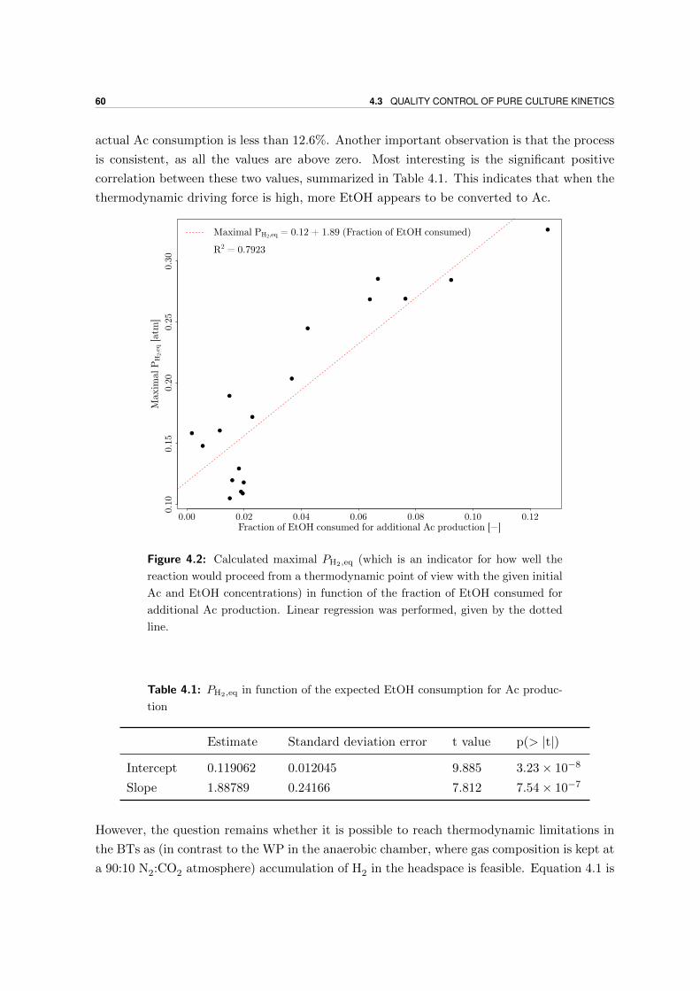
60 4.3 QUALITY CONTROL OF PURE CULTURE KINETICS
actual Ac consumption is less than 12.6%. Another important observation is that the process
is consistent, as all the values are above zero. Most interesting is the significant positive
correlation between these two values, summarized in Table 4.1. This indicates that when the
thermodynamic driving force is high, more EtOH appears to be converted to Ac.
●
●
●
●
●
●
●
●
●
●
●
●●
●●
●
●●
0.00 0.02 0.04 0.06 0.08 0.10 0.12
0.10
0.15
0.20
0.25
0.30
Fraction of EtOH consumed for additional Ac production [−]
Max
imal
PH
2,eq
[at
m]
Maximal PH2,eq = 0.12 + 1.89 (Fraction of EtOH consumed)
R2 = 0.7923
Figure 4.2: Calculated maximal PH2,eq (which is an indicator for how well the
reaction would proceed from a thermodynamic point of view with the given initial
Ac and EtOH concentrations) in function of the fraction of EtOH consumed for
additional Ac production. Linear regression was performed, given by the dotted
line.
Table 4.1: PH2,eq in function of the expected EtOH consumption for Ac produc-
tion
Estimate Standard deviation error t value p(> |t|)
Intercept 0.119062 0.012045 9.885 3.23× 10⁻⁸
Slope 1.88789 0.24166 7.812 7.54× 10⁻⁷
However, the question remains whether it is possible to reach thermodynamic limitations in
the BTs as (in contrast to the WP in the anaerobic chamber, where gas composition is kept at
a 90:10 N2:CO2 atmosphere) accumulation of H2 in the headspace is feasible. Equation 4.1 is
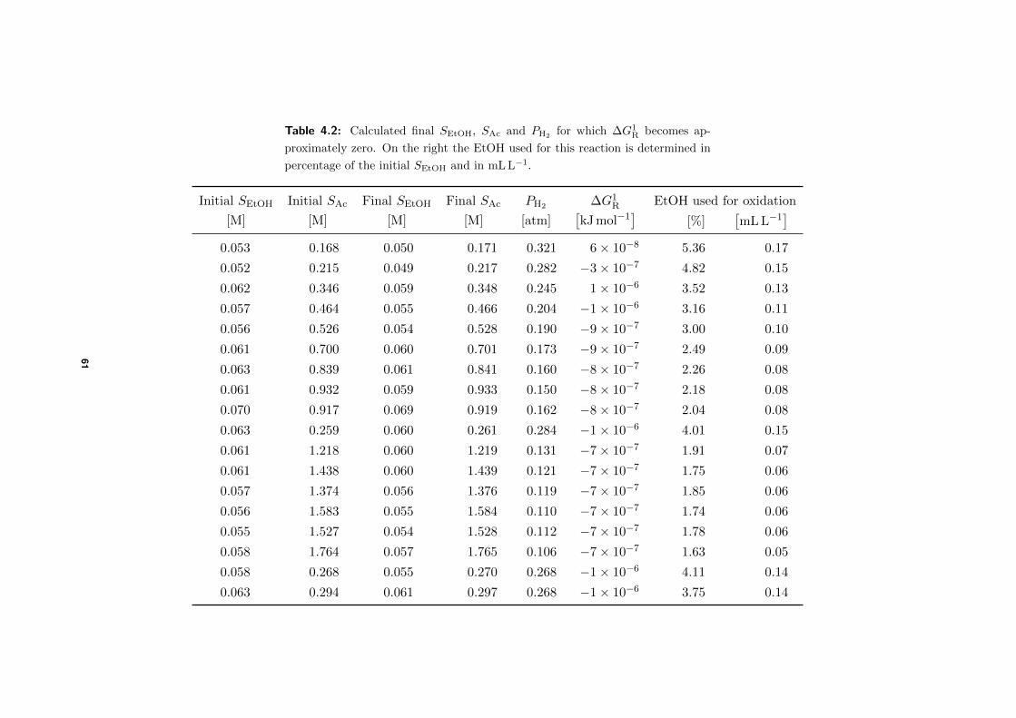
Table 4.2: Calculated final SEtOH, SAc and PH2for which ∆G1
R becomes ap-
proximately zero. On the right the EtOH used for this reaction is determined in
percentage of the initial SEtOH and in mL L−1.
Initial SEtOH Initial SAc Final SEtOH Final SAc PH2 ∆G1R EtOH used for oxidation
[M] [M] [M] [M] [atm][kJ mol−1
][%]
[mL L−1
]0.053 0.168 0.050 0.171 0.321 6× 10⁻⁸ 5.36 0.17
0.052 0.215 0.049 0.217 0.282 −3× 10⁻⁷ 4.82 0.15
0.062 0.346 0.059 0.348 0.245 1× 10⁻⁶ 3.52 0.13
0.057 0.464 0.055 0.466 0.204 −1× 10⁻⁶ 3.16 0.11
0.056 0.526 0.054 0.528 0.190 −9× 10⁻⁷ 3.00 0.10
0.061 0.700 0.060 0.701 0.173 −9× 10⁻⁷ 2.49 0.09
0.063 0.839 0.061 0.841 0.160 −8× 10⁻⁷ 2.26 0.08
0.061 0.932 0.059 0.933 0.150 −8× 10⁻⁷ 2.18 0.08
0.070 0.917 0.069 0.919 0.162 −8× 10⁻⁷ 2.04 0.08
0.063 0.259 0.060 0.261 0.284 −1× 10⁻⁶ 4.01 0.15
0.061 1.218 0.060 1.219 0.131 −7× 10⁻⁷ 1.91 0.07
0.061 1.438 0.060 1.439 0.121 −7× 10⁻⁷ 1.75 0.06
0.057 1.374 0.056 1.376 0.119 −7× 10⁻⁷ 1.85 0.06
0.056 1.583 0.055 1.584 0.110 −7× 10⁻⁷ 1.74 0.06
0.055 1.527 0.054 1.528 0.112 −7× 10⁻⁷ 1.78 0.06
0.058 1.764 0.057 1.765 0.106 −7× 10⁻⁷ 1.63 0.05
0.058 0.268 0.055 0.270 0.268 −1× 10⁻⁶ 4.11 0.14
0.063 0.294 0.061 0.297 0.268 −1× 10⁻⁶ 3.75 0.14
61
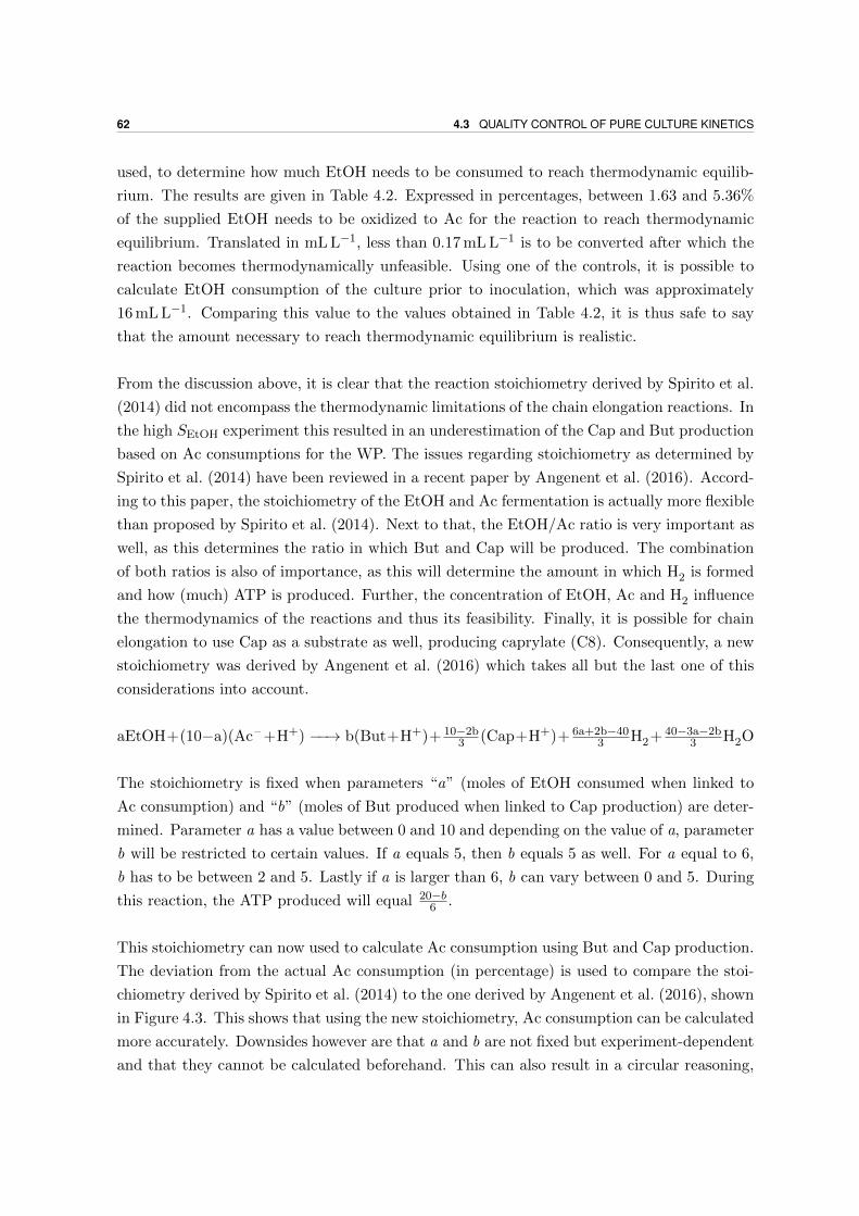
62 4.3 QUALITY CONTROL OF PURE CULTURE KINETICS
used, to determine how much EtOH needs to be consumed to reach thermodynamic equilib-
rium. The results are given in Table 4.2. Expressed in percentages, between 1.63 and 5.36%
of the supplied EtOH needs to be oxidized to Ac for the reaction to reach thermodynamic
equilibrium. Translated in mL L−1, less than 0.17 mL L−1 is to be converted after which the
reaction becomes thermodynamically unfeasible. Using one of the controls, it is possible to
calculate EtOH consumption of the culture prior to inoculation, which was approximately
16 mL L−1. Comparing this value to the values obtained in Table 4.2, it is thus safe to say
that the amount necessary to reach thermodynamic equilibrium is realistic.
From the discussion above, it is clear that the reaction stoichiometry derived by Spirito et al.
(2014) did not encompass the thermodynamic limitations of the chain elongation reactions. In
the high SEtOH experiment this resulted in an underestimation of the Cap and But production
based on Ac consumptions for the WP. The issues regarding stoichiometry as determined by
Spirito et al. (2014) have been reviewed in a recent paper by Angenent et al. (2016). Accord-
ing to this paper, the stoichiometry of the EtOH and Ac fermentation is actually more flexible
than proposed by Spirito et al. (2014). Next to that, the EtOH/Ac ratio is very important as
well, as this determines the ratio in which But and Cap will be produced. The combination
of both ratios is also of importance, as this will determine the amount in which H2 is formed
and how (much) ATP is produced. Further, the concentration of EtOH, Ac and H2 influence
the thermodynamics of the reactions and thus its feasibility. Finally, it is possible for chain
elongation to use Cap as a substrate as well, producing caprylate (C8). Consequently, a new
stoichiometry was derived by Angenent et al. (2016) which takes all but the last one of this
considerations into account.
aEtOH+(10−a)(Ac– +H+) −−→ b(But+H+)+ 10−2b3 (Cap+H+)+ 6a+2b−40
3 H2+ 40−3a−2b3 H2O
The stoichiometry is fixed when parameters “a” (moles of EtOH consumed when linked to
Ac consumption) and “b” (moles of But produced when linked to Cap production) are deter-
mined. Parameter a has a value between 0 and 10 and depending on the value of a, parameter
b will be restricted to certain values. If a equals 5, then b equals 5 as well. For a equal to 6,
b has to be between 2 and 5. Lastly if a is larger than 6, b can vary between 0 and 5. During
this reaction, the ATP produced will equal 20−b6 .
This stoichiometry can now used to calculate Ac consumption using But and Cap production.
The deviation from the actual Ac consumption (in percentage) is used to compare the stoi-
chiometry derived by Spirito et al. (2014) to the one derived by Angenent et al. (2016), shown
in Figure 4.3. This shows that using the new stoichiometry, Ac consumption can be calculated
more accurately. Downsides however are that a and b are not fixed but experiment-dependent
and that they cannot be calculated beforehand. This can also result in a circular reasoning,
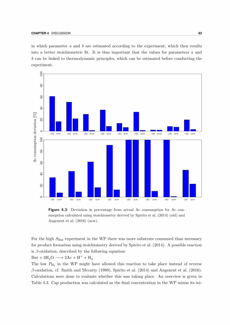
CHAPTER 4 DISCUSSION 63
in which parameter a and b are estimated according to the experiment, which then results
into a better stoichiometric fit. It is thus important that the values for parameters a and
b can be linked to thermodynamic principles, which can be estimated before conducting the
experiment.
old new old new old new old new old new old new old new old new old new
020
4060
8010
0
old new old new old new old new old new old new old new old new
020
4060
8010
0
Ac
consu
mpti
on d
evia
tion
[%
]
Figure 4.3: Deviation in percentage from actual Ac consumption for Ac con-
sumption calculated using stoichiometry derived by Spirito et al. (2014) (old) and
Angenent et al. (2016) (new).
For the high SBut experiment in the WP there was more substrate consumed than necessary
for product formation using stoichiometry derived by Spirito et al. (2014). A possible reaction
is β-oxidation, described by the following equation:
But + 2H2O −−→ 2Ac + H+ + H2
The low PH2 in the WP might have allowed this reaction to take place instead of reverse
β-oxidation, cf. Smith and Mccarty (1989), Spirito et al. (2014) and Angenent et al. (2016).
Calculations were done to evaluate whether this was taking place. An overview is given in
Table 4.3. Cap production was calculated as the final concentration in the WP minus its ini-
64 4.3 QUALITY CONTROL OF PURE CULTURE KINETICS
tial value. According to the stoichiometry provided by Spirito et al. (2014), it was expected
for this to equal the But consumption. The discrepancy between the actual consumption
and consumption used for Cap production would then equal the But consumed for oxidation.
With this value, the Ac that should be produced because of oxidation could be calculated.
However, this value still deviates a lot from the measured Ac production, thereby suggesting
that But was consumed for processes other than chain elongation and β-oxidation, which were
not measured.
In conclusion, it was thought that H2 played an important role in the thermodynamics of
the pathway. Data suggested that PH2 was kept too low in the WP, resulting in additional
EtOH oxidation. This was opposed to the BT, for which according to calculations only a
small amount of EtOH oxidation already resulted in thermodynamically limitations for the
reaction. The switch to a new stoichiometry derived by Angenent et al. (2016), which is more
flexible, could lower the gap between the actual substrate consumption and the consumption
based on product formation. However, this was not sufficient, as other reactions seemed to
occur as well.
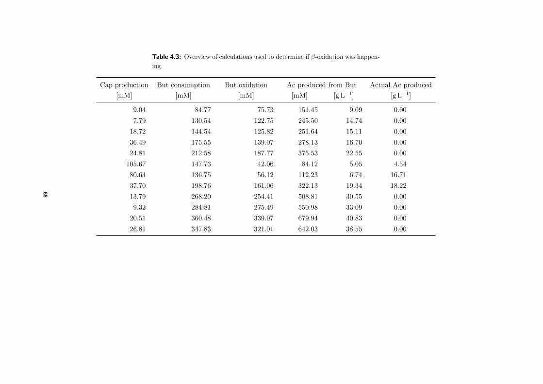
Table 4.3: Overview of calculations used to determine if β-oxidation was happen-
ing
Cap production But consumption But oxidation Ac produced from But Actual Ac produced
[mM] [mM] [mM] [mM] [g L−1] [g L−1]
9.04 84.77 75.73 151.45 9.09 0.00
7.79 130.54 122.75 245.50 14.74 0.00
18.72 144.54 125.82 251.64 15.11 0.00
36.49 175.55 139.07 278.13 16.70 0.00
24.81 212.58 187.77 375.53 22.55 0.00
105.67 147.73 42.06 84.12 5.05 4.54
80.64 136.75 56.12 112.23 6.74 16.71
37.70 198.76 161.06 322.13 19.34 18.22
13.79 268.20 254.41 508.81 30.55 0.00
9.32 284.81 275.49 550.98 33.09 0.00
20.51 360.48 339.97 679.94 40.83 0.00
26.81 347.83 321.01 642.03 38.55 0.00
65
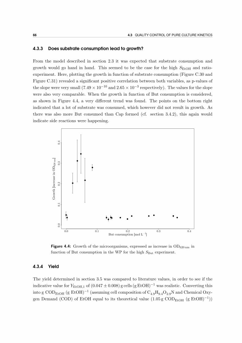
66 4.3 QUALITY CONTROL OF PURE CULTURE KINETICS
4.3.3 Does substrate consumption lead to growth?
From the model described in section 2.3 it was expected that substrate consumption and
growth would go hand in hand. This seemed to be the case for the high SEtOH and ratio-
experiment. Here, plotting the growth in function of substrate consumption (Figure C.30 and
Figure C.31) revealed a significant positive correlation between both variables, as p-values of
the slope were very small (7.49× 10⁻¹⁰ and 2.65× 10⁻³ respectively). The values for the slope
were also very comparable. When the growth in function of But consumption is considered,
as shown in Figure 4.4, a very different trend was found. The points on the bottom right
indicated that a lot of substrate was consumed, which however did not result in growth. As
there was also more But consumed than Cap formed (cf. section 3.4.2), this again would
indicate side reactions were happening.
●
● ● ●●
●● ●
●●
●
●●
●
●
●
●
●
0.0 0.1 0.2 0.3 0.4
0.0
0.1
0.2
0.3
0.4
But consumption [mol L−1]
Gro
wth
[in
crea
se i
n O
D62
0 nm
]
Figure 4.4: Growth of the microorganisms, expressed as increase in OD620 nm in
function of But consumption in the WP for the high SBut experiment.
4.3.4 Yield
The yield determined in section 3.5 was compared to literature values, in order to see if the
indicative value for YEtOH,1 of (0.047± 0.008) g cells (g EtOH)−1 was realistic. Converting this
into g CODEtOH (g EtOH)−1 (assuming cell composition of C4.9H9.4O2.9N and Chemical Oxy-
gen Demand (COD) of EtOH equal to its theoretical value (1.05 g CODEtOH (g EtOH)−1))
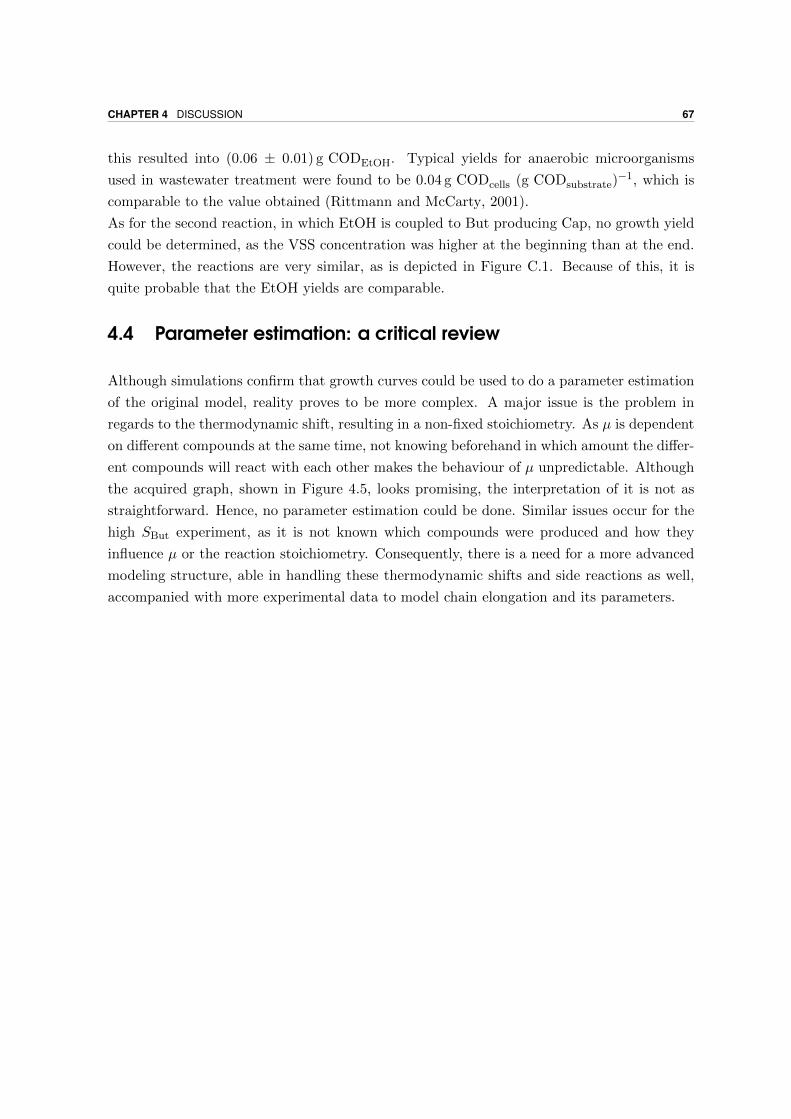
CHAPTER 4 DISCUSSION 67
this resulted into (0.06 ± 0.01) g CODEtOH. Typical yields for anaerobic microorganisms
used in wastewater treatment were found to be 0.04 g CODcells (g CODsubstrate)−1, which is
comparable to the value obtained (Rittmann and McCarty, 2001).
As for the second reaction, in which EtOH is coupled to But producing Cap, no growth yield
could be determined, as the VSS concentration was higher at the beginning than at the end.
However, the reactions are very similar, as is depicted in Figure C.1. Because of this, it is
quite probable that the EtOH yields are comparable.
4.4 Parameter estimation: a critical review
Although simulations confirm that growth curves could be used to do a parameter estimation
of the original model, reality proves to be more complex. A major issue is the problem in
regards to the thermodynamic shift, resulting in a non-fixed stoichiometry. As µ is dependent
on different compounds at the same time, not knowing beforehand in which amount the differ-
ent compounds will react with each other makes the behaviour of µ unpredictable. Although
the acquired graph, shown in Figure 4.5, looks promising, the interpretation of it is not as
straightforward. Hence, no parameter estimation could be done. Similar issues occur for the
high SBut experiment, as it is not known which compounds were produced and how they
influence µ or the reaction stoichiometry. Consequently, there is a need for a more advanced
modeling structure, able in handling these thermodynamic shifts and side reactions as well,
accompanied with more experimental data to model chain elongation and its parameters.
68 4.4 PARAMETER ESTIMATION: A CRITICAL REVIEW
●
●
●
●
●
●
●
●
●
●
●
●
●
●
●
●
0.0 0.5 1.0 1.5
0.0
100.0
150.0
200.
025
0.03
00.
035
0.040
Initial EtOH concentration [M]
µ [
h−
1 ]
Figure 4.5: The determined µ using the Grofit package in function of the initial
SEtOH.
CHAPTER 5Conclusions and perspectives
In this thesis, an attempt was made to model chain elongation, as this was not yet available in
literature. The chain elongation model was based upon the stoichiometry derived by Spirito
et al. (2014) and the bacterial growth models (Panikov, 1991; Harvey et al., 2014; Kim et al.,
2005). Model simulations seemed to acknowledge the growth curve methodology as a valid
tool for parameter estimation of the chain elongation model. However, the obtained data
showed deviating results, thus suggesting important flaws in the moment that need to be
tackled first.
One of these flaws was the deviation between the expected substrate consumption, determined
via stoichiometry and product formation data, and the actual substrate consumption. The
discrepancy was thought to be related to thermodynamic pathway shifts caused by the low
partial vapor pressure of H2. This resulted in additional acetate production through ethanol
oxidation which was not foreseen in the model. It was shown that using the stoichiometry
derived by Angenent et al. (2016), which takes more consideration upon these thermodynamic
principles, could lower the offset between expected and actual acetate consumption. The dis-
tinction however remained during another experiment, even when taking these considerations
into account. For this experiment, it was concluded that other side reactions could occur
as well. Because the growth curve methodology relied on a fixed stoichiometry in which the
influence of all the compounds is known, it was impossible to do a parameter estimation
with the acquired data. Hence, in future research more careful attention must go to the side
reactions and the corresponding thermodynamic considerations. In this respect, the stoichio-
metric model derived by Angenent et al. (2016) could help to minimize the offset between
measured and expected substrate consumption, but momentarily stoichiometry can only be
determined afterwards. Therefore, the influence of the initial conditions on the parameters
used in the stoichiometric model should be investigated in more detail using thermodynamical
principles.
70
Another aspect of this thesis was the reactor data obtained with a mixed community capable
in chain elongation, which proved to be quite unstable at first. Changing to lower Ac concen-
trations, HRT and a more continuous feeding regime however resolved the issues, although
then mostly But instead of Cap was produced. The more stable character seemed to be caused
by the lower fatty acid concentrations in general, though this needs further investigation.
In regards to the DSM52 medium, its pH change acted consistently if the same amount of
protons were added (provided a correction was made for the initial volume), irregardless on
the amount of Ac present. As H+ can also be an indication of chain elongating activity,
further research might be able to link pH change of the medium to the production of longer
chain fatty acids. This way, measuring the pH difference might become a quick and easy
method in determining chain elongating activity.
Bibliography
Adler, P., Hugen, T., Wiewiora, M., and Kunz, B. (2011). Modeling of an integrated
fermentation/membrane extraction process for the production of 2-phenylethanol and 2-
phenylethylacetate. Enzyme and Microbial Technology, 48(3):285–292.
Agler, M. T., Spirito, C. M., Usack, J. G., Werner, J. J., and Angenent, L. T. (2012).
Chain elongation with reactor microbiomes: upgrading dilute ethanol to medium-chain
carboxylates. Energy & Environmental Science, 5(8):8189–8192.
Agler, M. T., Wrenn, B. a., Zinder, S. H., and Angenent, L. T. (2011). Waste to bioproduct
conversion with undefined mixed cultures: The carboxylate platform. Trends in Biotech-
nology, 29(2):70–78.
Andersen, S. J., Hennebel, T., Gildemyn, S., Coma, M., Desloover, J., Berton, J., Tsukamoto,
J., Stevens, C., and Rabaey, K. (2014). Electrolytic Membrane Extraction Enables Produc-
tion of Fine Chemicals from Biorefinery Sidestreams. Environmental Science & Technology,
48:7135–7142.
Angenent, L. T., Richter, H., Buckel, W., Spirito, C. M., Steinbusch, K. J., Plugge, C.,
Strik, D. P., Grootscholten, T. I., Buisman, C. J., and Hamelers, H. V. (2016). Chain
elongation with reactor microbiomes: open-culture biotechnology to produce biochemicals.
Environmental Science & Technology, 50:2796–2810.
APHA (1992). Standard Methods for the Examination of Water and Wastewater. Amer-
ican Public Health Association/American Water Works Association/Water Environment
Federation, Washington DC, USA, 18th edition.
Appels, L., Baeyens, J., Degreve, J., and Dewil, R. (2008). Principles and potential of the
anaerobic digestion of waste-activated sludge. Progress in Energy and Combustion Science,
34(6):755–781.
Barker, H., Kamen, M., and Bornstein, B. (1945). The Synthesis of Butyric and Caproic
Acids from Ethanol and Acetic Acid by Clostridium Kluyveri. Proceedings of the National
Academy of Sciences of the United States of America, 31(12):373–381.
Batstone, D. J., Keller, J., Angelidaki, I., Kalyuzhnyi, S., Pavlostathis, S., Rozzi, A., Sanders,
W., Siegrist, H., and Vavilin, V. (2002). Anaerobic digestion model No 1 (ADM1). Water
Science and Technology, 45(10):65–73.
Burow, E., Simoneit, C., Tenhagen, B. a., and Kasbohrer, a. (2014). Oral antimicrobials
increase antimicrobial resistance in porcine E. coli - A systematic review. Preventive Vet-
erinary Medicine, 113(4):364–375.
Caccavale, F., Iamarino, M., Pierri, F., and Tufano, V. (2011). Control and Monitoring of
Chemical Batch Reactors. Springer-Verlag, London.
Candry, P. (2015). pH Hysteresis and electrolysis for zero-chemical input control of fermen-
tation processes. Master’s thesis, Universiteit Gent, Ghent.
Chen, L., Zhang, J., and Chen, W. N. (2014). Engineering the Saccharomyces cerevisiae β-
Oxidation Pathway to Increase Medium Chain Fatty Acid Production as Potential Biofuel.
PloS one, 9(1):1–10.
Cherubini, F. and Jungmeier, G. (2010). LCA of a biorefinery concept producing bioethanol,
bioenergy, and chemicals from switchgrass. International Journal of Life Cycle Assessment,
15(1):53–66.
Debeuckelaere, M. (2015). Enhancement of building blocks production : effect of operational
parameters on specific carboxylate production. Master’s thesis, Universiteit Gent, Ghent.
Deublein, D. and Steinhauser, A. (2008). Biogas from waste and renewable resources: an
introduction. Wiley-VCH, Weinheim.
Eilersen, a. M., Henze, M., and Kloft, L. (1995). Effect of volatile fatty acids and trimethy-
lamine on denitrification in activated sludge. Water Research, 29(5):1259–1266.
Ge, S., Usack, J. G., Spirito, C. M., and Angenent, L. T. (2015). Long-Term n-Caproic Acid
Production from Yeast-Fermentation Beer in an Anaerobic Bioreactor with Continuous
Product Extraction. Environmental Science & Technology, 49(13):8012–8021.
Geirnaert, A., Steyaert, A., Eeckhaut, V., Debruyne, B., Arends, J. B., Van Immerseel, F.,
Boon, N., and Van de Wiele, T. (2014). Butyricicoccus pullicaecorum, a butyrate producer
with probiotic potential, is intrinsically tolerant to stomach and small intestine conditions.
Anaerobe, 30:70–74.
Geueke, B. and Kohler, H.-P. E. (2010). Enzyme Assays, Substrate Specificities, Kinetic
Parameters: Measurement of Enzyme Activities. In Timmis, K. N., editor, Handbook
of Hydrocarbon and Lipid Microbiology, chapter Enzyme Ass, pages 4196–4202. Springer,
Berlin.
72
Gjelstad, A., Rasmussen, K. E., and Pedersen-Bjergaard, S. (2007). Simulation of flux during
electro-membrane extraction based on the Nernst-Planck equation. Journal of Chromatog-
raphy A, 1174:104–111.
Grootscholten, T. I. M., Steinbusch, K. J. J., Hamelers, H. V. M., and Buisman, C. J. N.
(2013a). Chain elongation of acetate and ethanol in an upflow anaerobic filter for high rate
MCFA production. Bioresource Technology, 135:440–445.
Grootscholten, T. I. M., Steinbusch, K. J. J., Hamelers, H. V. M., and Buisman, C. J. N.
(2013b). Improving medium chain fatty acid productivity using chain elongation by re-
ducing the hydraulic retention time in an upflow anaerobic filter. Bioresource Technology,
136:735–738.
Harvey, E., Heys, J., and Gedeon, T. (2014). Quantifying the effects of the division of labor
in metabolic pathways. Journal of theoretical biology, 360:222–242.
Heijnen, J. (1999). Bioenergetics of Microbial Growth. In Flickinger, M. C. and Drew,
S. W., editors, Encyclopedia of Bioprocess Technology: Fermentation, Biocatalysts and
Bioseparation, pages 267–291. John Wiley & Sons, Inc.
Jeanson, S., Floury, J., Gagnaire, V., Lortal, S., and Thierry, A. (2015). Bacterial Colonies
in Solid Media and Foods: A Review on Their Growth and Interactions with the Micro-
Environment. Frontiers in Microbiology, 6:1–20.
Jencks, W. and Regenstein, J. (2010). Ionization Constants of Acids and Bases. In Lundblad,
R. L. . and MacDonald, F. M. ., editors, Handbook of Biochemistry and Molecular Biology,
chapter Ionization, pages 305–351. CRC Press.
Junicke, H., Van Loosdrecht, M. C. M., and Kleerebezem, R. (2016). Kinetic and thermody-
namic control of butyrate conversion in non-defined methanogenic communities. Applied
Microbiology and Biotechnology, 100(2):915–25.
Kahm, M. and Kschischo, M. (2015). grofit package documentation.
Kalyuzhnyi, S. V. (1997). Batch anaerobic digestion of glucose and its mathematical modeling.
II. Description verification and application of model. Bioresource Technology, 59:249–258.
Kim, D.-J., Choi, J.-W., Choi, N.-C., Mahendran, B., and Lee, C.-E. (2005). Modeling of
growth kinetics for Pseudomonas spp. during benzene degradation. Applied Microbiology
and Biotechnology, 69(4):456–462.
Kleerebezem, R. and Van Loosdrecht, M. C. M. (2010). A Generalized Method for Thermo-
dynamic State Analysis of Environmental Systems. Environmental Science & Technology,
40(1):1–54.
73

Koch, a. L. (1970). Turbidity measurements of bacterial cultures in some available commercial
instruments. Analytical biochemistry, 38(1):252–259.
Kolev, S. D., St John, A. M., and Cattrall, R. W. (2013). Mathematical modeling of the
extraction of uranium(VI) into a polymer inclusion membrane composed of PVC and di-
(2-ethylhexyl) phosphoric acid. Journal of Membrane Science, 425-426:169–175.
Labib, F., Ferguson, J. F., Benjamin, M. M., Merigh, M., and Ricker, N. L. (1993). Mathemat-
ical Modeling of an Anaerobic Butyrate Degrading Consortia: Predicting Their Response
to Organic Overloads. Environmental Science & Technology, 27(13):2673–2684.
Liu, Y. and Whitman, W. B. (2008). Metabolic, Phylogenetic, and Ecological Diversity of the
Methanogenic Archaea. Annals of the New York Academy of Sciences, 1125(1):171–189.
Lu, Y. C., Yi, S. S., and Luo, G. S. (2008). Modeling of the mass transfer and conduction
behavior in electro-electrodialysis with oil/water emulsion as the catholyte. Journal of
Membrane Science, 322(1):265–274.
Monod, J. (1943). Recherches sur la croissance des cultures bacteriennes. Herman, Paris.
Palmqvist, E. and Hahn-Hagerdal, B. (2000). Fermentation of lignocellulosic hydrolysates.
II: Inhibitors and mechanisms of inhibition. Bioresource Technology, 74(1):25–33.
Panikov, N. S. (1991). Kinetics, Microbial Growth. In Flickinger, M. C. and Drew, S. W.,
editors, Encyclopedia of Bioprocess Technology: Fermentation, Biocatalysts and Biosepara-
tion, chapter Kinetics,, pages 1513–1543. John Wiley & Sons, Inc, New York.
Perez, F. and Granger, B. E. (2007). IPython: a system for interactive scientific computing.
Computing in Science and Engineering, 9(3):21–29.
Perni, S., Andrew, P. W., and Shama, G. (2005). Estimating the maximum growth rate from
microbial growth curves: definition is everything. Food Microbiology, 22(6):491–495.
Plugge, C. M. (2005). Anoxic media design, preparation, and considerations. Methods in
Enzymology, 397:3–16.
Pratt, S., Liew, D., Batstone, D., Werker, A., Morgan-Sagastume, F., and Lant, P. (2012).
Inhibition by fatty acids during fermentation of pre-treated waste activated sludge. Journal
of Biotechnology, 159:38–43.
Ricke, S. C. (2003). Perspectives on the use of organic acids and short chain fatty acids as
antimicrobials. Poultry science, 82(4):632–639.
Rittmann, B. E. and McCarty, P. L. (2001). Microbial Kinetics. In Environmental Biotech-
nology: Principles and Applications, pages 84–98. McGraw-Hill Book Co., New York.
74
Roos, a. and Boron, F. (1981). Intracellular pH. Physiological Reviews, 61(2):296–434.
RStudio Team (2015). RStudio: Integrated Development Environment for R. RStudio, Inc.,
Boston, MA.
Saxena, A., Gohil, G. S., and Shahi, V. K. (2007). Electrochemical membrane reactor: Single-
step separation and ion substitution for the recovery of lactic acid from lactate salts. In-
dustrial and Engineering Chemistry Research, 46(4):1270–1276.
Seedorf, H., Fricke, W. F., Veith, B., Bruggemann, H., Liesegang, H., Strittmatter, A.,
Miethke, M., Buckel, W., Hinderberger, J., Li, F., Hagemeier, C., Thauer, R. K., and
Gottschalk, G. (2008). The genome of Clostridium kluyveri, a strict anaerobe with unique
metabolic features. Proceedings of the National Academy of Sciences of the United States
of America, 105(6):2128–2133.
Singhania, R. R., Patel, A. K., Christophe, G., Fontanille, P., and Larroche, C. (2013).
Biological upgrading of volatile fatty acids, key intermediates for the valorization of biowaste
through dark anaerobic fermentation. Bioresource Technology, 145:166–174.
Smith, D. P. and Mccarty, P. L. (1989). Energetic and rate effects on methanogenesis of
ethanol and propionate in perturbed CSTRs Authors. Biotechnology and Bioengineering,
34(1):39–54.
Spirito, C. M., Richter, H., Rabaey, K., Stams, A. J., and Angenent, L. T. (2014). Chain
elongation in anaerobic reactor microbiomes to recover resources from waste. Current
Opinion in Biotechnology, 27:115–122.
Steinbusch, K. J. J., Hamelers, H. V. M., Plugge, C. M., and Buisman, C. J. N. (2011).
Biological formation of caproate and caprylate from acetate: fuel and chemical production
from low grade biomass. Energy & Environmental Science, 4(1):216–224.
Thanakoses, P., Black, A. S., and Holtzapple, M. T. (2003). Fermentation of corn stover to
carboxylic acids. Biotechnology and Bioengineering, 83(2):191–200.
Thour, M. (2014). Bottleneck analysis and throughput improvement through simulation-based
multi objective optimization. Bachelor’s thesis, University of Skovde.
Trad, Z., Akimbomi, J., Vial, C., Larroche, C., Taherzadeh, M. J., and Fontaine, J.-P. (2015).
Development of a submerged anaerobic membrane bioreactor for concurrent extraction of
volatile fatty acids and biohydrogen production. Bioresource Technology, 196:290–300.
Van Daele, T., Van Hoey, S., and Nopens, I. (2015). pyideas: an open source python package
for model analysis. In Krist V. Gernaey, J. K. H. and Gani, R., editors, 12th International
Symposium on Process Systems Engineering and 25th European Symposium on Computer
75

Aided Process Engineering, volume 37 of Computer Aided Chemical Engineering, pages 569
– 574. Elsevier.
Vasudevan, D., Richter, H., and Angenent, L. T. (2014). Upgrading dilute ethanol from syngas
fermentation to n-caproate with reactor microbiomes. Bioresource Technology, 151:378–382.
Xu, J., Guzman, J. J., Andersen, S. J., Rabaey, K., and Angenent, L. T. (2015). In-line and
selective phase separation of medium-chain carboxylic acids using membrane electrolysis.
Chemical Communications, 51:6847–6850.
76

APPENDIX AADM1
77
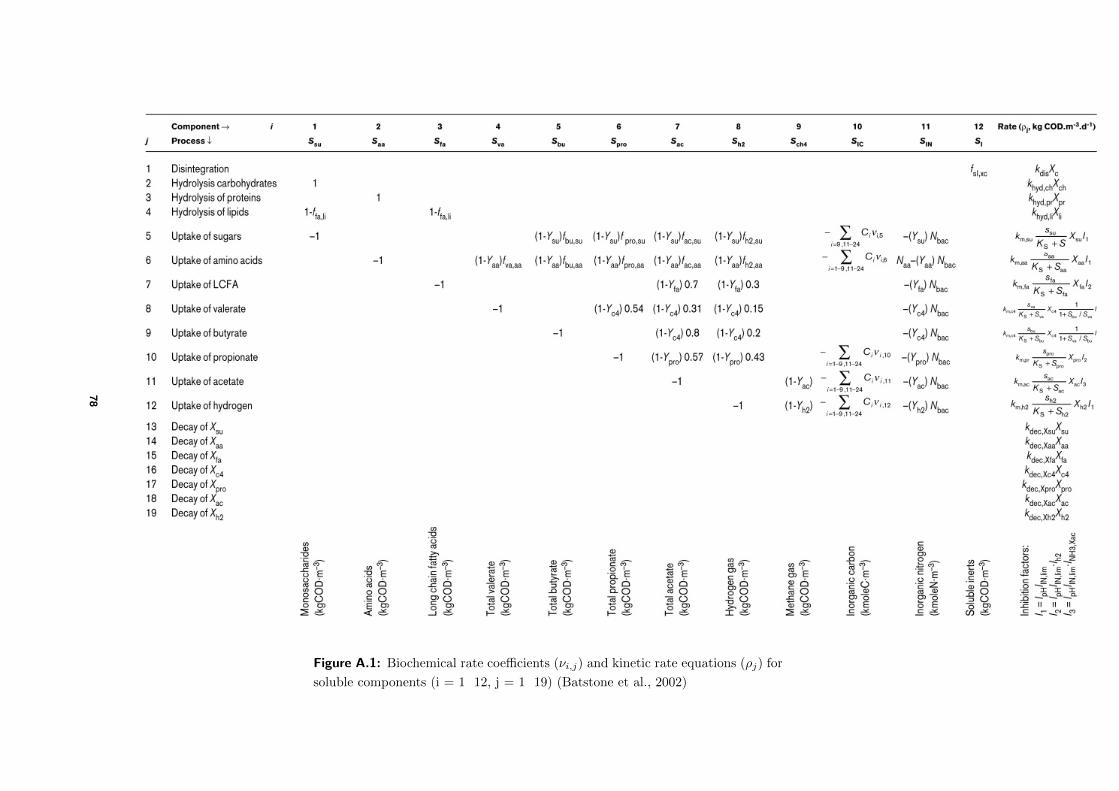
Figure A.1: Biochemical rate coefficients (νi,j) and kinetic rate equations (ρj) for
soluble components (i = 1 12, j = 1 19) (Batstone et al., 2002)
78
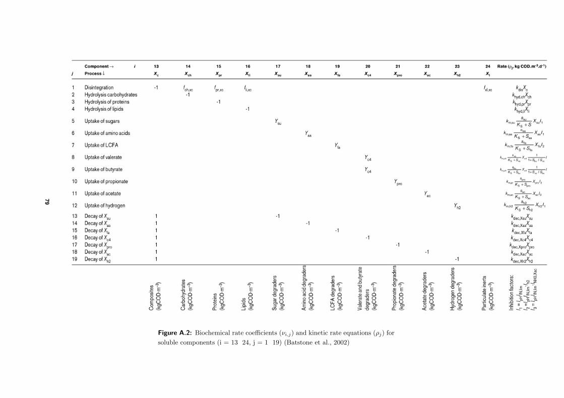
Figure A.2: Biochemical rate coefficients (νi,j) and kinetic rate equations (ρj) for
soluble components (i = 13 24, j = 1 19) (Batstone et al., 2002)
79

80
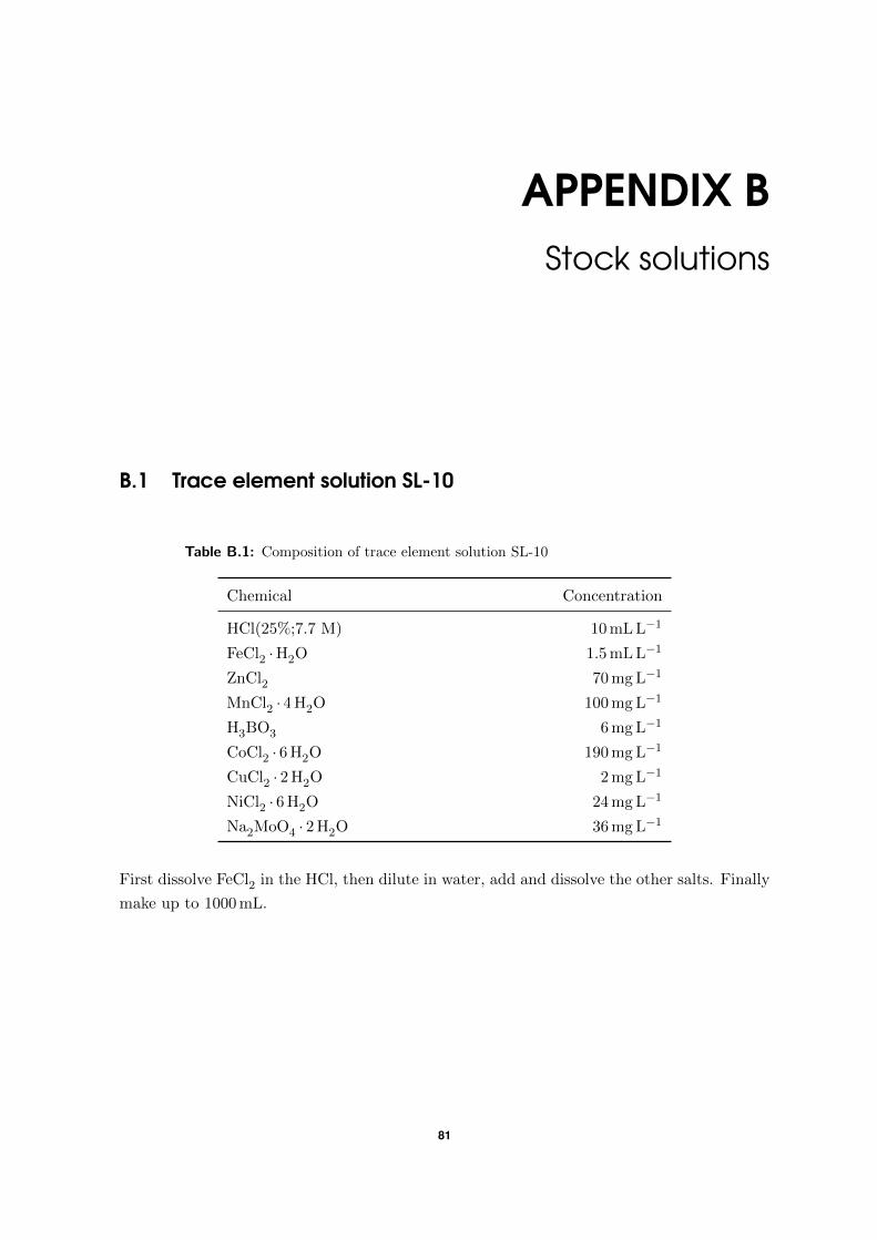
APPENDIX BStock solutions
B.1 Trace element solution SL-10
Table B.1: Composition of trace element solution SL-10
Chemical Concentration
HCl(25%;7.7 M) 10 mL L−1
FeCl2 ·H2O 1.5 mL L−1
ZnCl2 70 mg L−1
MnCl2 · 4 H2O 100 mg L−1
H3BO3 6 mg L−1
CoCl2 · 6 H2O 190 mg L−1
CuCl2 · 2 H2O 2 mg L−1
NiCl2 · 6 H2O 24 mg L−1
Na2MoO4 · 2 H2O 36 mg L−1
First dissolve FeCl2 in the HCl, then dilute in water, add and dissolve the other salts. Finally
make up to 1000 mL.
81
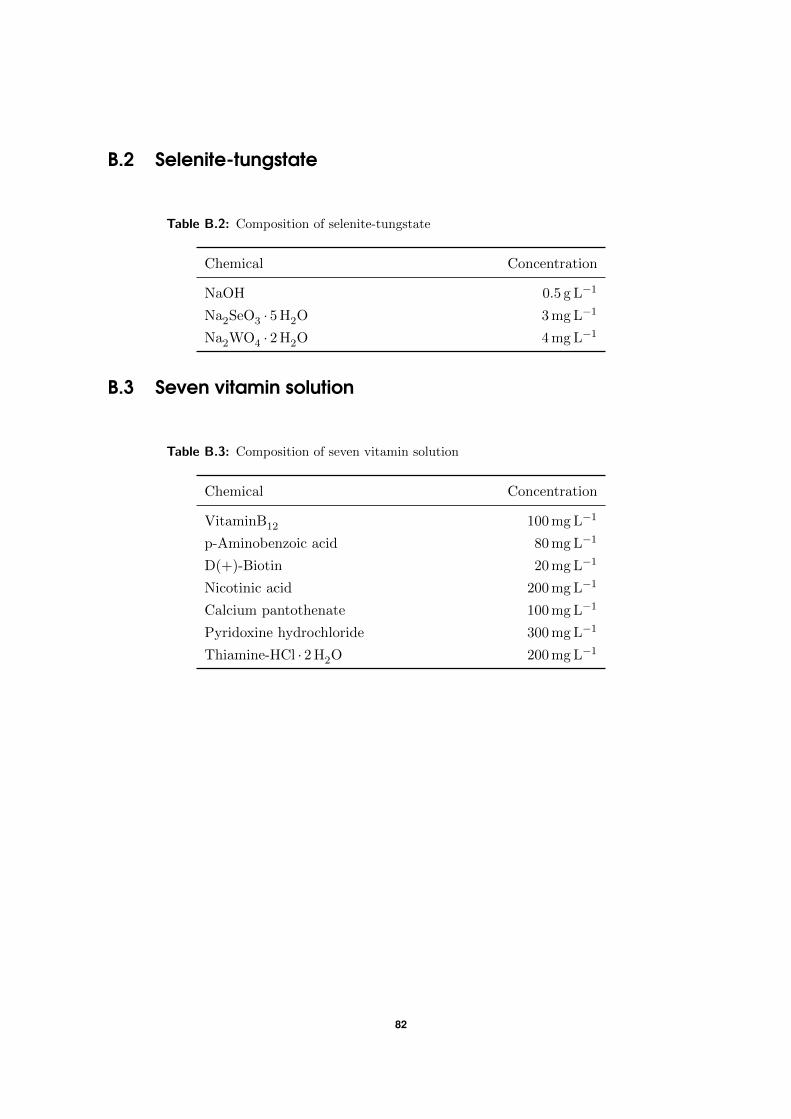
B.2 Selenite-tungstate
Table B.2: Composition of selenite-tungstate
Chemical Concentration
NaOH 0.5 g L−1
Na2SeO3 · 5 H2O 3 mg L−1
Na2WO4 · 2 H2O 4 mg L−1
B.3 Seven vitamin solution
Table B.3: Composition of seven vitamin solution
Chemical Concentration
VitaminB12 100 mg L−1
p-Aminobenzoic acid 80 mg L−1
D(+)-Biotin 20 mg L−1
Nicotinic acid 200 mg L−1
Calcium pantothenate 100 mg L−1
Pyridoxine hydrochloride 300 mg L−1
Thiamine-HCl · 2 H2O 200 mg L−1
82

83
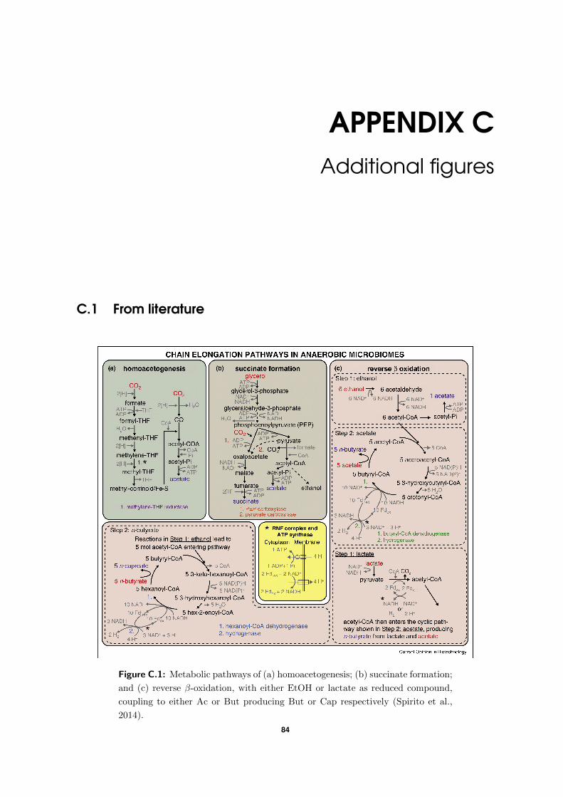
APPENDIX CAdditional figures
C.1 From literature
Figure C.1: Metabolic pathways of (a) homoacetogenesis; (b) succinate formation;
and (c) reverse β-oxidation, with either EtOH or lactate as reduced compound,
coupling to either Ac or But producing But or Cap respectively (Spirito et al.,
2014).
84
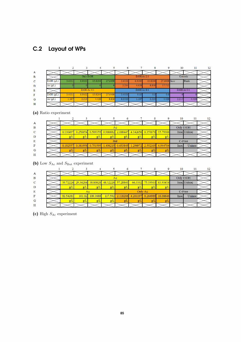
C.2 Layout of WPs
(a) Ratio experiment
(b) Low SAc and SBut experiment
(c) High SAc experiment
85
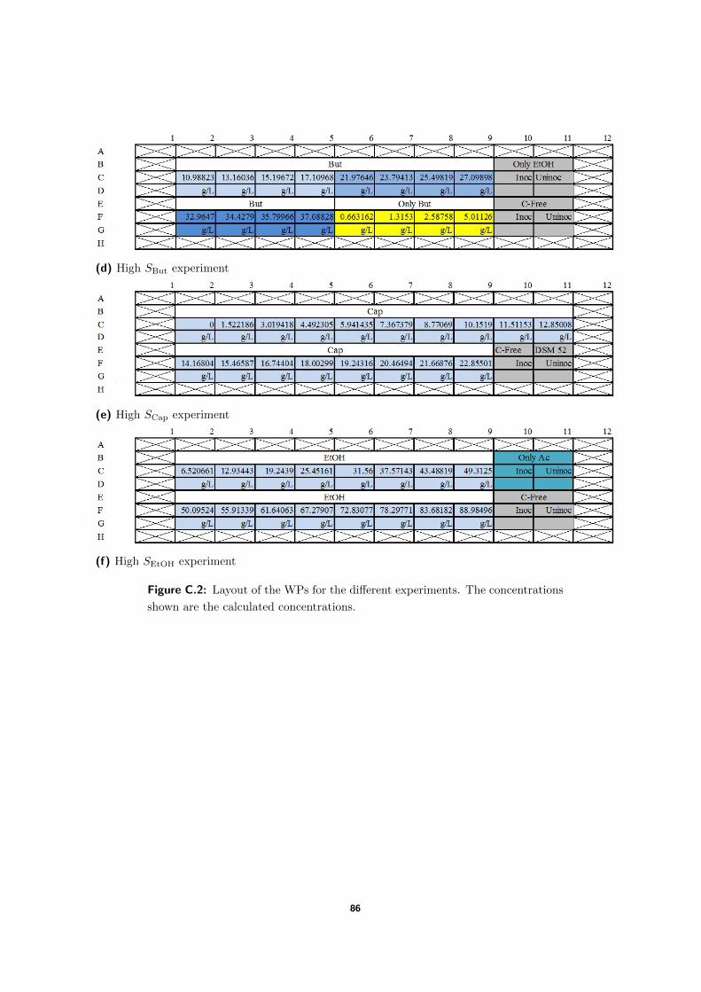
(d) High SBut experiment
(e) High SCap experiment
(f) High SEtOH experiment
Figure C.2: Layout of the WPs for the different experiments. The concentrations
shown are the calculated concentrations.
86
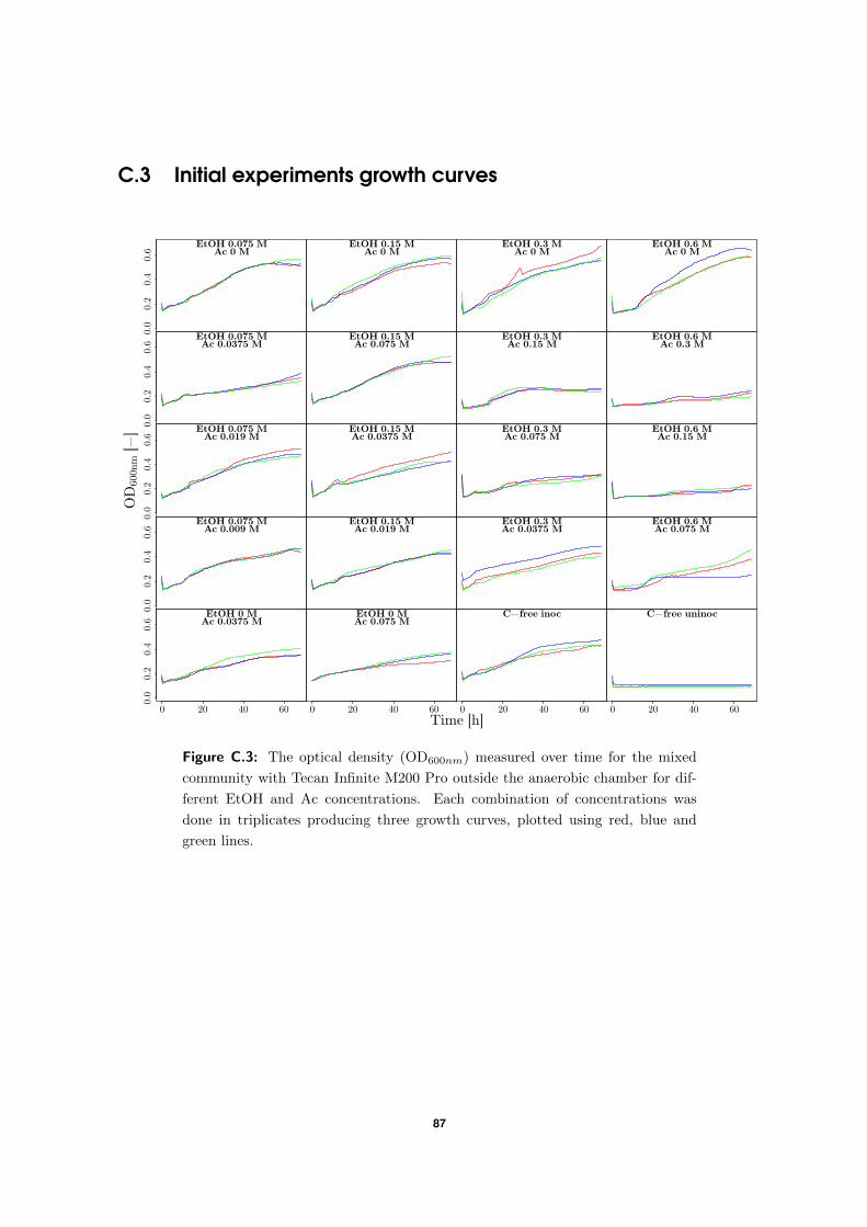
C.3 Initial experiments growth curves
EtOH 0.075 MAc 0 M
0.0
0.2
0.4
0.6
EtOH 0.15 MAc 0 M
EtOH 0.3 MAc 0 M
EtOH 0.6 MAc 0 M
EtOH 0.075 MAc 0.0375 M
0.0
0.2
0.4
0.6
EtOH 0.15 MAc 0.075 M
EtOH 0.3 MAc 0.15 M
EtOH 0.6 MAc 0.3 M
EtOH 0.075 MAc 0.019 M
0.0
0.2
0.4
0.6
EtOH 0.15 MAc 0.0375 M
EtOH 0.3 MAc 0.075 M
EtOH 0.6 MAc 0.15 M
EtOH 0.075 MAc 0.009 M
0.0
0.2
0.4
0.6
EtOH 0.15 MAc 0.019 M
EtOH 0.3 MAc 0.0375 M
EtOH 0.6 MAc 0.075 M
EtOH 0 MAc 0.0375 M
0 20 40 60
0.0
0.2
0.4
0.6
EtOH 0 MAc 0.075 M
0 20 40 60
C−free inoc
0 20 40 60
C−free uninoc
0 20 40 60
Time [h]
OD
600
nm
[−
]
Figure C.3: The optical density (OD600nm) measured over time for the mixed
community with Tecan Infinite M200 Pro outside the anaerobic chamber for dif-
ferent EtOH and Ac concentrations. Each combination of concentrations was
done in triplicates producing three growth curves, plotted using red, blue and
green lines.
87
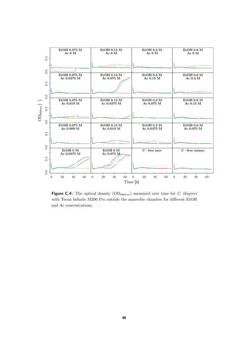
EtOH 0.075 M
Ac 0 M
0.0
0.4
EtOH 0.15 M
Ac 0 M
EtOH 0.3 M
Ac 0 M
EtOH 0.6 M
Ac 0 M
EtOH 0.075 M
Ac 0.0375 M
0.0
0.4
EtOH 0.15 M
Ac 0.075 M
EtOH 0.3 M
Ac 0.15 M
EtOH 0.6 M
Ac 0.3 M
EtOH 0.075 M
Ac 0.019 M
0.0
0.4
EtOH 0.15 M
Ac 0.0375 M
EtOH 0.3 M
Ac 0.075 M
EtOH 0.6 M
Ac 0.15 M
EtOH 0.075 M
Ac 0.009 M
0.0
0.4
EtOH 0.15 M
Ac 0.019 M
EtOH 0.3 M
Ac 0.0375 M
EtOH 0.6 M
Ac 0.075 M
EtOH 0 M
Ac 0.0375 M
0 20 40 60
0.0
0.4
EtOH 0 M
Ac 0.075 M
0 20 40 60
C−free inoc
0 20 40 60
C−free uninoc
0 20 40 60
Time [h]
OD
600nm
[−
]
Figure C.4: The optical density (OD600nm) measured over time for C. kluyveri
with Tecan Infinite M200 Pro outside the anaerobic chamber for different EtOH
and Ac concentrations.
88
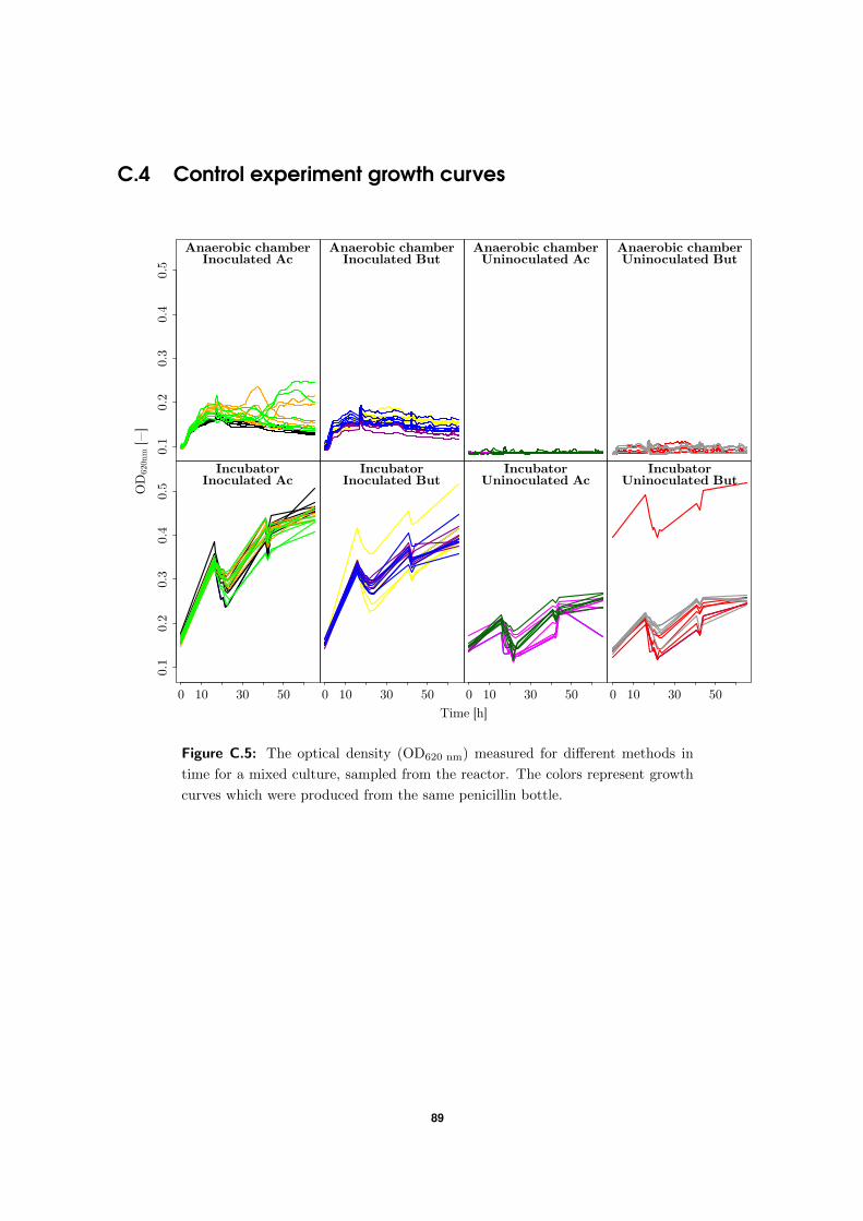
C.4 Control experiment growth curves
Inoculated AcAnaerobic chamber
0.1
0.2
0.3
0.4
0.5
Anaerobic chamberInoculated But
Anaerobic chamberUninoculated Ac
Anaerobic chamberUninoculated But
IncubatorInoculated Ac
0.1
0.2
0.3
0.4
0.5
0 10 30 50
IncubatorInoculated But
0 10 30 50
IncubatorUninoculated Ac
0 10 30 50
IncubatorUninoculated But
0 10 30 50
Time [h]
OD
620n
m [−
]
Figure C.5: The optical density (OD620 nm) measured for different methods in
time for a mixed culture, sampled from the reactor. The colors represent growth
curves which were produced from the same penicillin bottle.
89
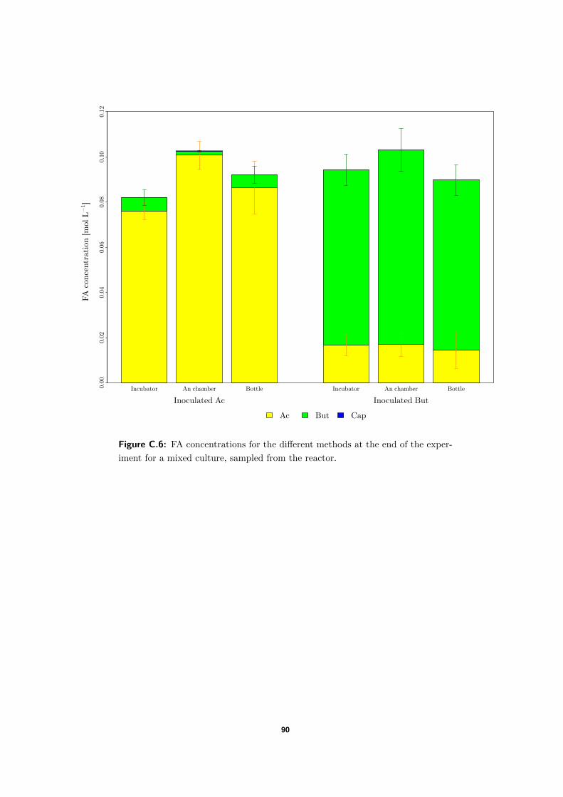
Incubator An chamber Bottle Incubator An chamber Bottle0.00
0.02
0.04
0.06
0.08
0.10
0.12
Inoculated Ac Inoculated But
Ac But Cap
FA
con
centr
atio
n [m
ol L
−1 ]
Figure C.6: FA concentrations for the different methods at the end of the exper-
iment for a mixed culture, sampled from the reactor.
90
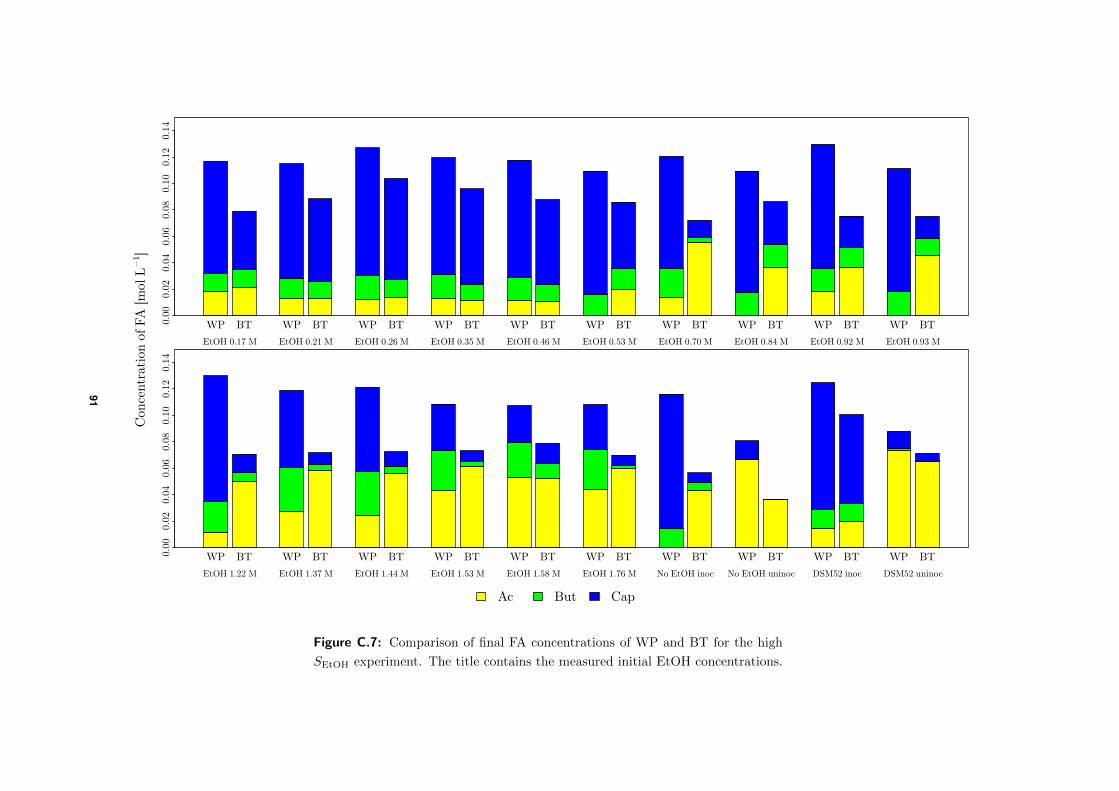
WP BT WP BT WP BT WP BT WP BT WP BT WP BT WP BT WP BT WP BT0.00
0.02
0.04
0.06
0.08
0.10
0.12
0.14
EtOH 0.17 M EtOH 0.21 M EtOH 0.26 M EtOH 0.35 M EtOH 0.46 M EtOH 0.53 M EtOH 0.70 M EtOH 0.84 M EtOH 0.92 M EtOH 0.93 M
WP BT WP BT WP BT WP BT WP BT WP BT WP BT WP BT WP BT WP BT0.00
0.02
0.04
0.06
0.08
0.10
0.12
0.14
EtOH 1.22 M EtOH 1.37 M EtOH 1.44 M EtOH 1.53 M EtOH 1.58 M EtOH 1.76 M No EtOH inoc No EtOH uninoc DSM52 inoc DSM52 uninoc
Ac But Cap
Con
centr
atio
n o
f FA
[m
ol L
−1 ]
Figure C.7: Comparison of final FA concentrations of WP and BT for the high
SEtOH experiment. The title contains the measured initial EtOH concentrations.
91
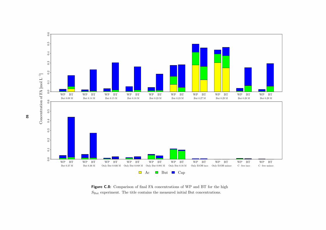
WP BT WP BT WP BT WP BT WP BT WP BT WP BT WP BT WP BT WP BT
0.0
0.1
0.2
0.3
0.4
0.5
0.6
But 0.09 M But 0.14 M But 0.15 M But 0.18 M But 0.23 M But 0.23 M But 0.27 M But 0.29 M But 0.28 M But 0.29 M
WP BT WP BT WP BT WP BT WP BT WP BT WP BT WP BT WP BT WP BT
0.0
0.1
0.2
0.3
0.4
0.5
0.6
But 0.37 M But 0.36 M Only But 0.026 M Only But 0.048 M Only But 0.091 M Only But 0.16 M Only EtOH inoc Only EtOH uninoc C−free inoc C−free uninoc
Ac But Cap
Con
centr
atio
n o
f FA
[m
ol L
−1 ]
Figure C.8: Comparison of final FA concentrations of WP and BT for the high
SBut experiment. The title contains the measured initial But concentrations.
92
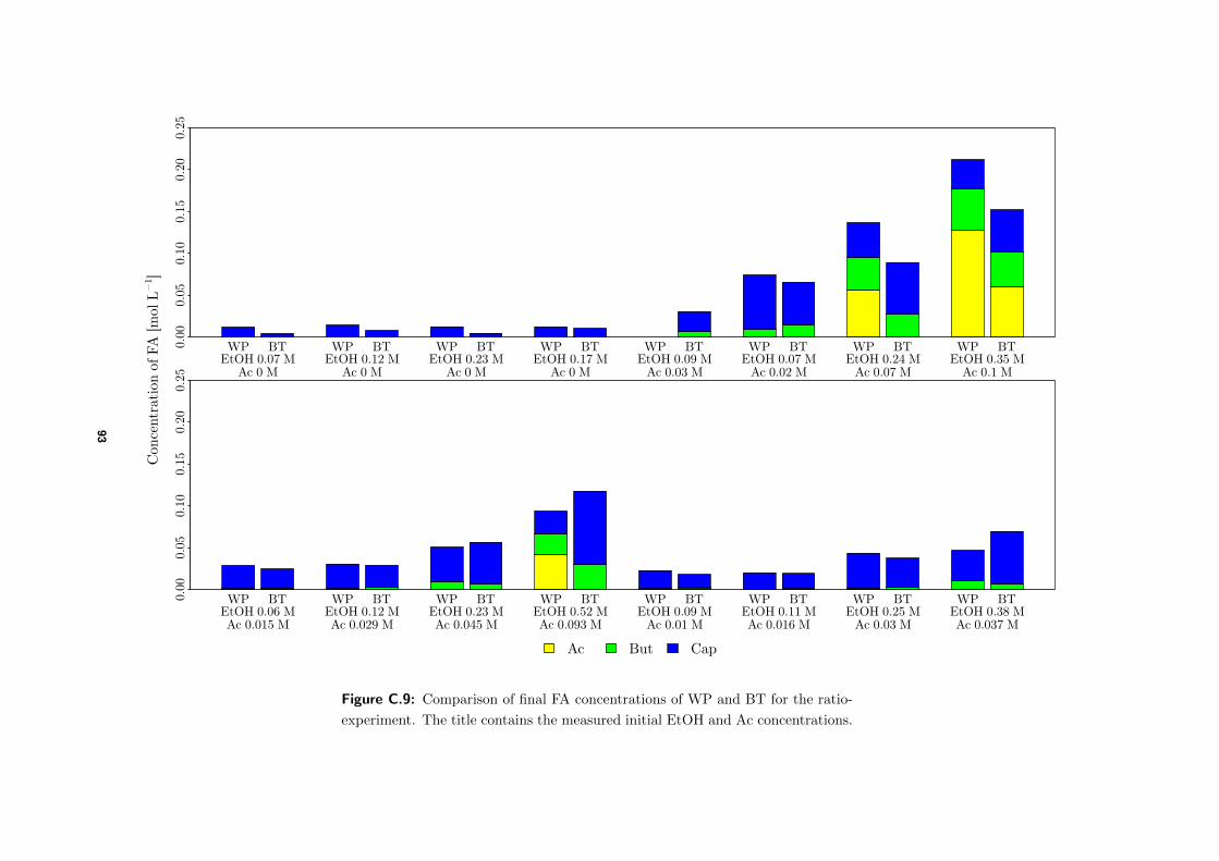
WP BT WP BT WP BT WP BT WP BT WP BT WP BT WP BT0.00
0.05
0.10
0.15
0.20
0.25
EtOH 0.07 M EtOH 0.12 M EtOH 0.23 M EtOH 0.17 M EtOH 0.09 M EtOH 0.07 M EtOH 0.24 M EtOH 0.35 MAc 0 M Ac 0 M Ac 0 M Ac 0 M Ac 0.03 M Ac 0.02 M Ac 0.07 M Ac 0.1 M
WP BT WP BT WP BT WP BT WP BT WP BT WP BT WP BT0.00
0.05
0.10
0.15
0.20
0.25
EtOH 0.06 M EtOH 0.12 M EtOH 0.23 M EtOH 0.52 M EtOH 0.09 M EtOH 0.11 M EtOH 0.25 M EtOH 0.38 MAc 0.015 M Ac 0.029 M Ac 0.045 M Ac 0.093 M Ac 0.01 M Ac 0.016 M Ac 0.03 M Ac 0.037 M
Ac But Cap
Con
centr
atio
n o
f FA
[m
ol L
−1 ]
Figure C.9: Comparison of final FA concentrations of WP and BT for the ratio-
experiment. The title contains the measured initial EtOH and Ac concentrations.
93
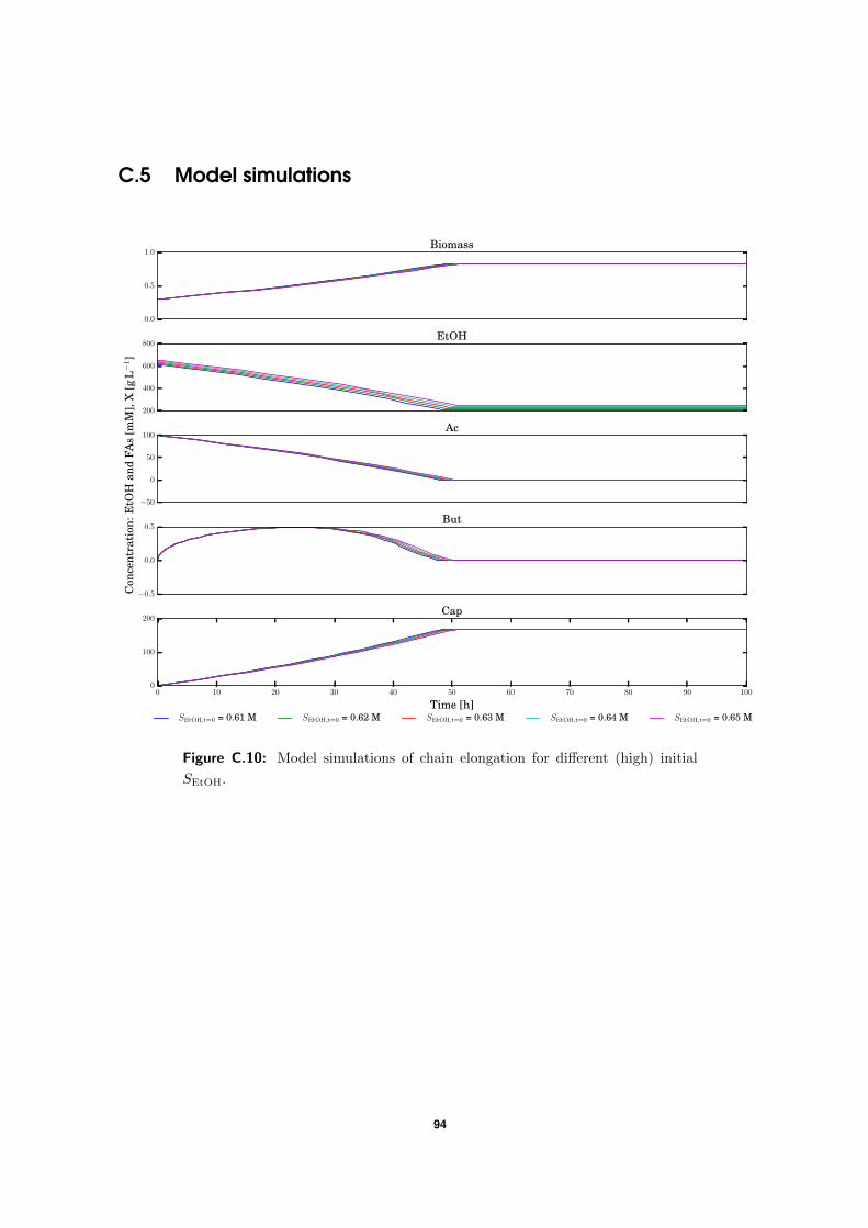
C.5 Model simulations
0.0
0.5
1.0Biomass
200
400
600
800EtOH
−50
0
50
100Ac
−0.5
0.0
0.5But
0 10 20 30 40 50 60 70 80 90 100
Time [h]
0
100
200Cap
SEtOH,t=0 = 0.61 M SEtOH,t=0 = 0.62 M SEtOH,t=0 = 0.63 M SEtOH,t=0 = 0.64 M SEtOH,t=0 = 0.65 M
Con
cent
rati
on:E
tOH
and
FAs
[mM
],X
[gL−
1]
Figure C.10: Model simulations of chain elongation for different (high) initial
SEtOH.
94
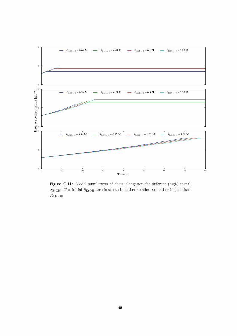
0.0
0.5
1.0
SEtOH,t=0 = 0.04 M SEtOH,t=0 = 0.07 M SEtOH,t=0 = 0.1 M SEtOH,t=0 = 0.13 M
0.0
0.5
1.0
SEtOH,t=0 = 0.24 M SEtOH,t=0 = 0.27 M SEtOH,t=0 = 0.3 M SEtOH,t=0 = 0.33 M
0 10 20 30 40 50 60 70 80
Time [h]
0.0
0.5
1.0
SEtOH,t=0 = 0.94 M SEtOH,t=0 = 0.97 M SEtOH,t=0 = 1.01 M SEtOH,t=0 = 1.05 M
Bio
mas
sco
ncen
trat
ion
[gL−
1]
Figure C.11: Model simulations of chain elongation for different (high) initial
SEtOH. The initial SEtOH are chosen to be either smaller, around or higher than
Ki,EtOH.
95
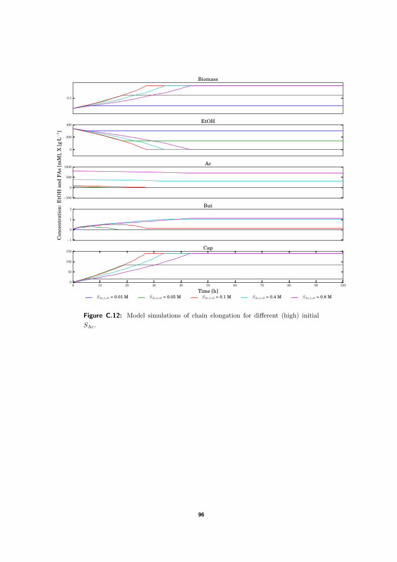
0.5
Biomass
0
200
400EtOH
−500
0
500
1000Ac
−1
0
1
2But
0 10 20 30 40 50 60 70 80 90 100
Time [h]
0
50
100
150Cap
SAc,t=0 = 0.01 M SAc,t=0 = 0.05 M SAc,t=0 = 0.1 M SAc,t=0 = 0.4 M SAc,t=0 = 0.8 M
Con
cent
rati
on:E
tOH
and
FAs
[mM
],X
[gL−
1]
Figure C.12: Model simulations of chain elongation for different (high) initial
SAc.
96
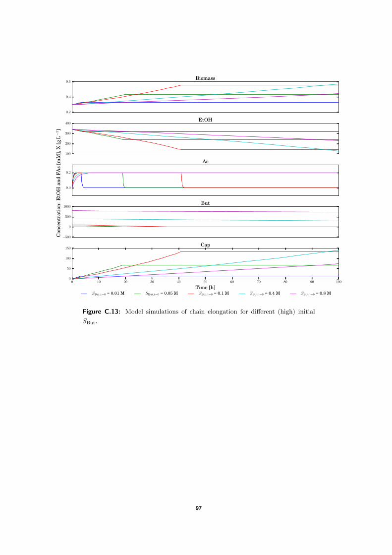
0.2
0.4
0.6Biomass
100
200
300
400EtOH
0.0
0.2
Ac
−500
0
500
1000But
0 10 20 30 40 50 60 70 80 90 100
Time [h]
0
50
100
150Cap
SBut,t=0 = 0.01 M SBut,t=0 = 0.05 M SBut,t=0 = 0.1 M SBut,t=0 = 0.4 M SBut,t=0 = 0.8 M
Con
cent
rati
on:E
tOH
and
FAs
[mM
],X
[gL−
1]
Figure C.13: Model simulations of chain elongation for different (high) initial
SBut.
97
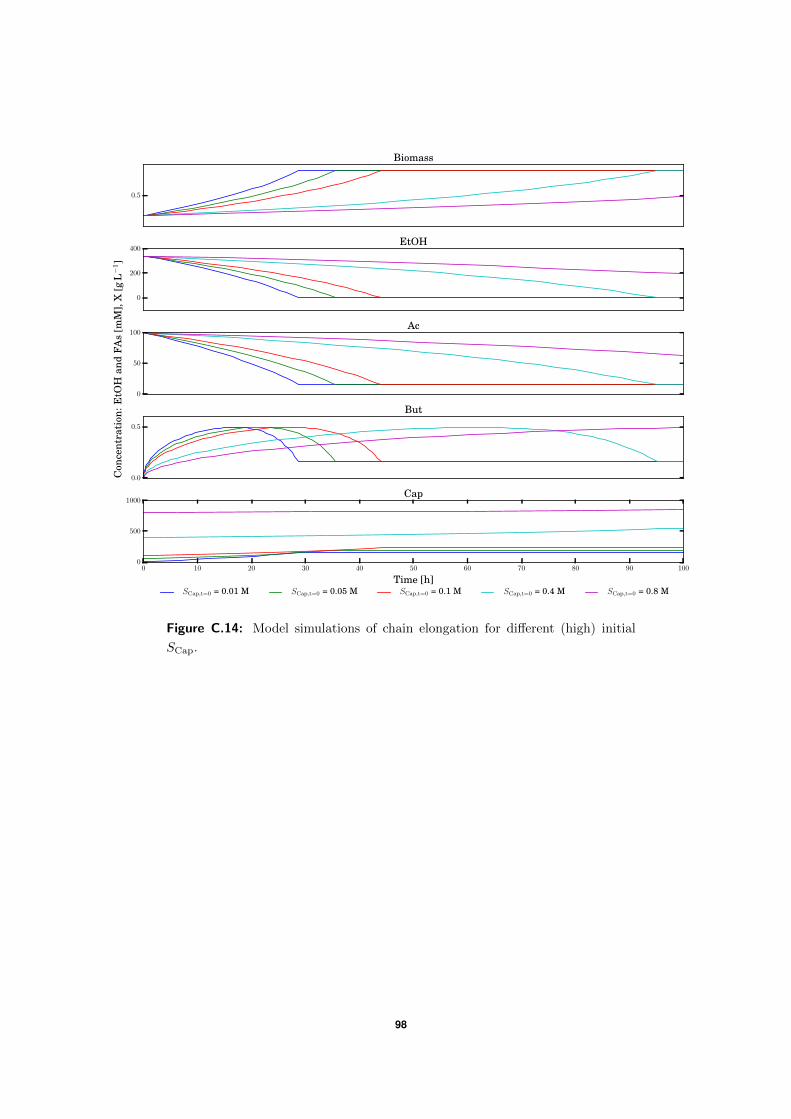
0.5
Biomass
0
200
400EtOH
0
50
100Ac
0.0
0.5
But
0 10 20 30 40 50 60 70 80 90 100
Time [h]
0
500
1000Cap
SCap,t=0 = 0.01 M SCap,t=0 = 0.05 M SCap,t=0 = 0.1 M SCap,t=0 = 0.4 M SCap,t=0 = 0.8 M
Con
cent
rati
on:E
tOH
and
FAs
[mM
],X
[gL−
1]
Figure C.14: Model simulations of chain elongation for different (high) initial
SCap.
98
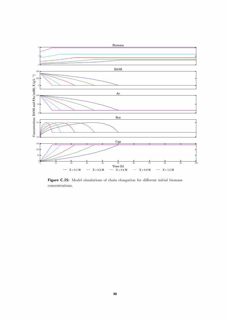
0
1
2Biomass
0
200
400EtOH
0
50
100Ac
0.0
0.5
But
0 10 20 30 40 50 60 70 80 90 100
Time [h]
0
50
100
150Cap
X = 0.1 M X = 0.2 M X = 0.4 M X = 0.8 M X = 1.5 M
Con
cent
rati
on:E
tOH
and
FAs
[mM
],X
[gL−
1]
Figure C.15: Model simulations of chain elongation for different initial biomass
concentrations.
99
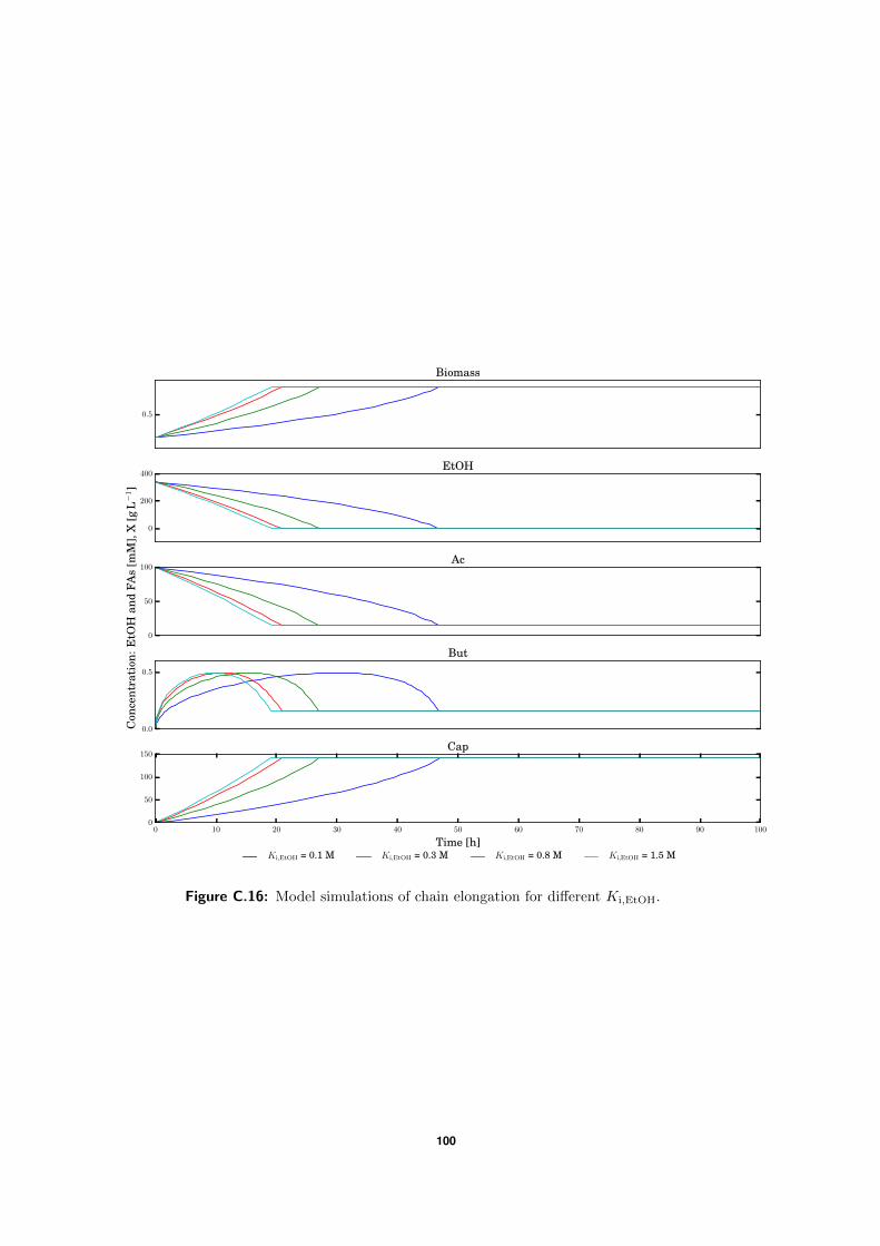
0.5
Biomass
0
200
400EtOH
0
50
100Ac
0.0
0.5
But
0 10 20 30 40 50 60 70 80 90 100
Time [h]
0
50
100
150Cap
Ki,EtOH = 0.1 M Ki,EtOH = 0.3 M Ki,EtOH = 0.8 M Ki,EtOH = 1.5 M
Con
cent
rati
on:E
tOH
and
FAs
[mM
],X
[gL−
1]
Figure C.16: Model simulations of chain elongation for different Ki,EtOH.
100
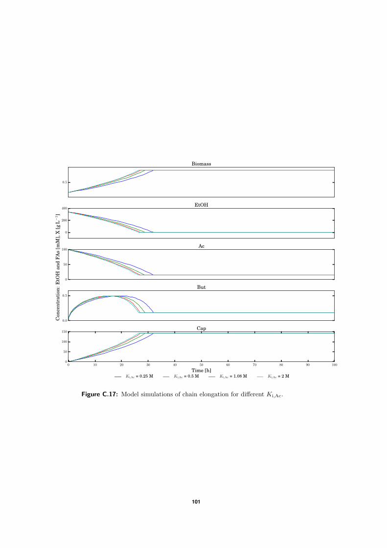
0.5
Biomass
0
200
400EtOH
0
50
100Ac
0.0
0.5
But
0 10 20 30 40 50 60 70 80 90 100
Time [h]
0
50
100
150Cap
Ki,Ac = 0.25 M Ki,Ac = 0.5 M Ki,Ac = 1.08 M Ki,Ac = 2 M
Con
cent
rati
on:E
tOH
and
FAs
[mM
],X
[gL−
1]
Figure C.17: Model simulations of chain elongation for different Ki,Ac.
101
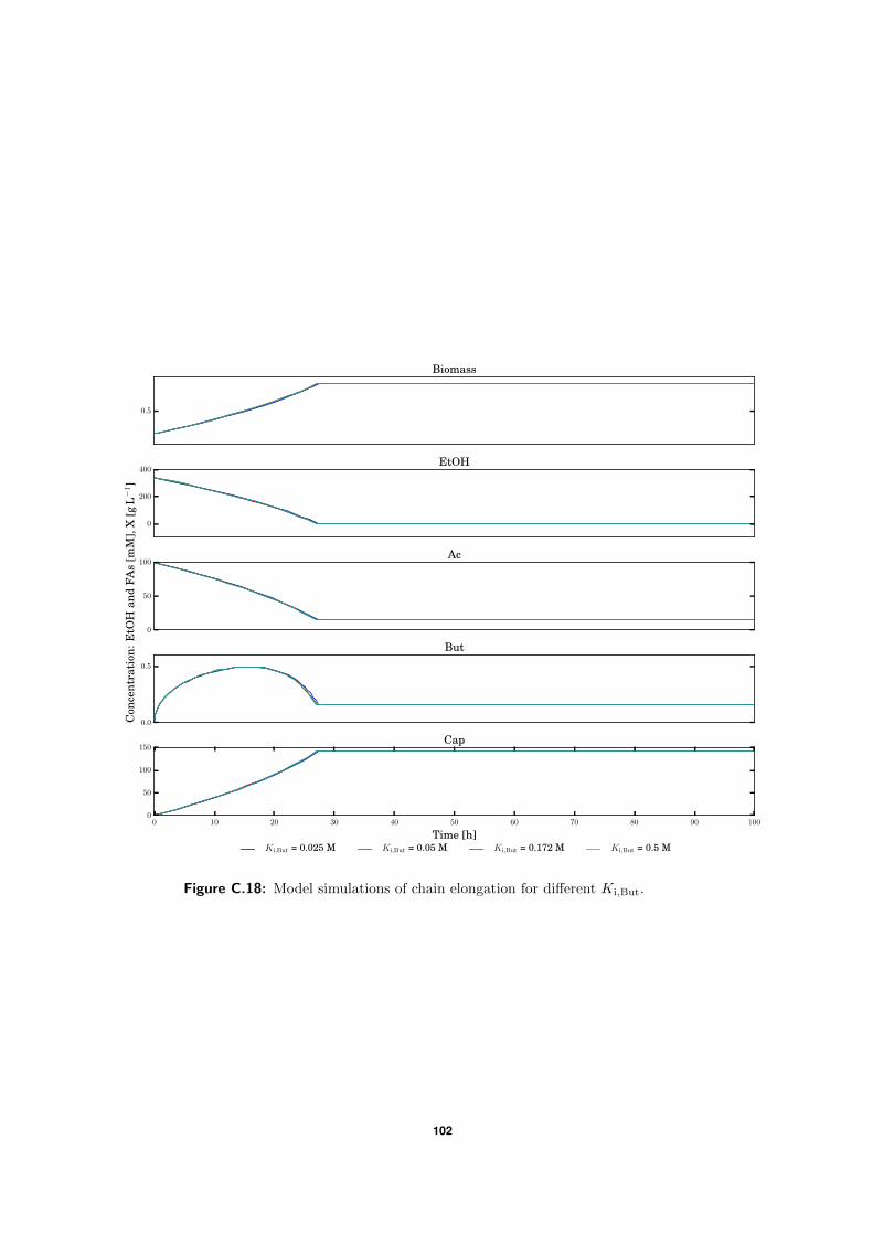
0.5
Biomass
0
200
400EtOH
0
50
100Ac
0.0
0.5
But
0 10 20 30 40 50 60 70 80 90 100
Time [h]
0
50
100
150Cap
Ki,But = 0.025 M Ki,But = 0.05 M Ki,But = 0.172 M Ki,But = 0.5 M
Con
cent
rati
on:E
tOH
and
FAs
[mM
],X
[gL−
1]
Figure C.18: Model simulations of chain elongation for different Ki,But.
102
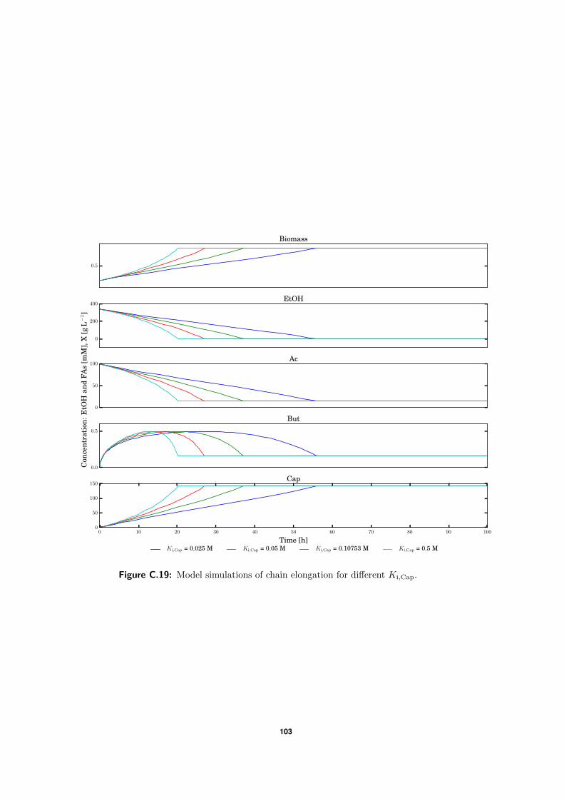
0.5
Biomass
0
200
400EtOH
0
50
100Ac
0.0
0.5
But
0 10 20 30 40 50 60 70 80 90 100
Time [h]
0
50
100
150Cap
Ki,Cap = 0.025 M Ki,Cap = 0.05 M Ki,Cap = 0.10753 M Ki,Cap = 0.5 M
Con
cent
rati
on:E
tOH
and
FAs
[mM
],X
[gL−
1]
Figure C.19: Model simulations of chain elongation for different Ki,Cap.
103
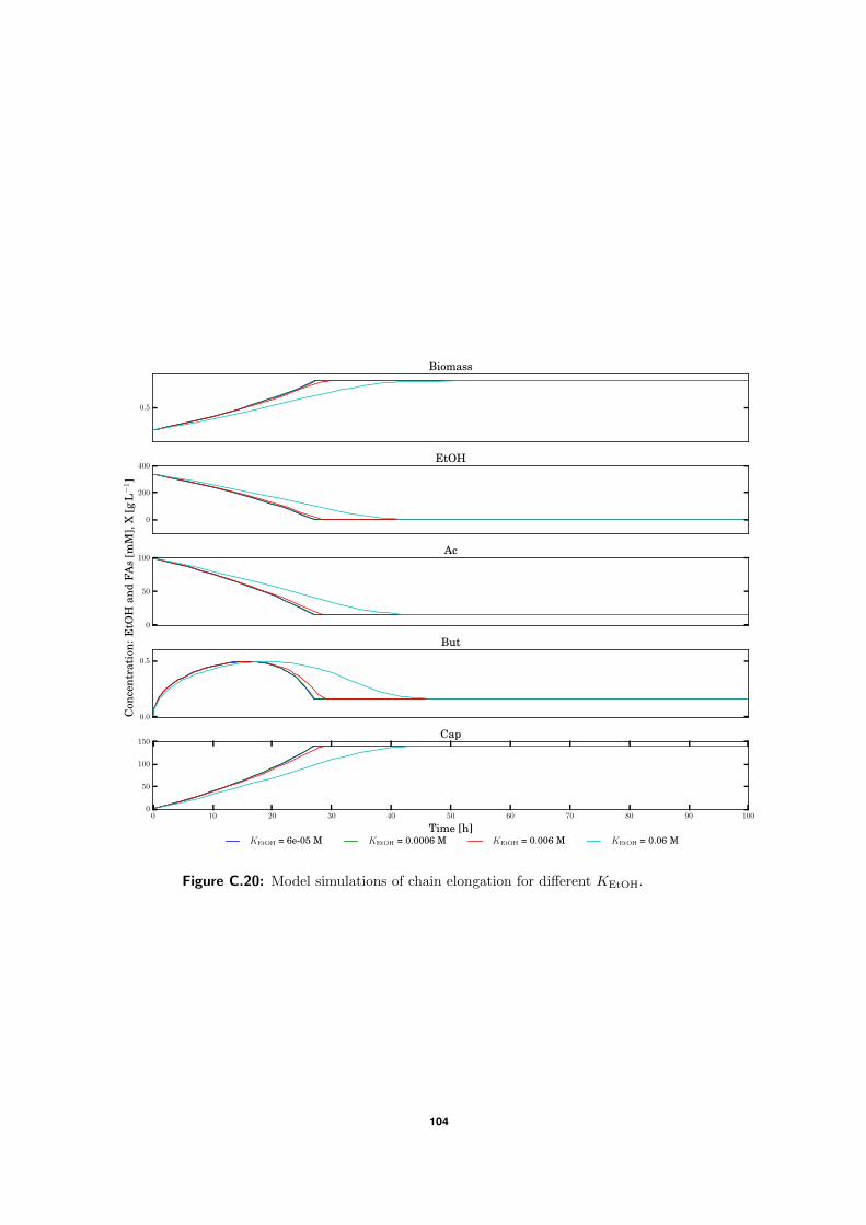
0.5
Biomass
0
200
400EtOH
0
50
100Ac
0.0
0.5
But
0 10 20 30 40 50 60 70 80 90 100
Time [h]
0
50
100
150Cap
KEtOH = 6e-05 M KEtOH = 0.0006 M KEtOH = 0.006 M KEtOH = 0.06 M
Con
cent
rati
on:E
tOH
and
FAs
[mM
],X
[gL−
1]
Figure C.20: Model simulations of chain elongation for different KEtOH.
104
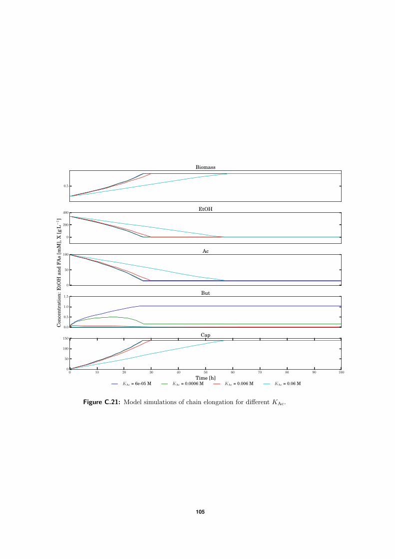
0.5
Biomass
0
200
400EtOH
0
50
100Ac
0.0
0.5
1.0
1.5But
0 10 20 30 40 50 60 70 80 90 100
Time [h]
0
50
100
150Cap
KAc = 6e-05 M KAc = 0.0006 M KAc = 0.006 M KAc = 0.06 M
Con
cent
rati
on:E
tOH
and
FAs
[mM
],X
[gL−
1]
Figure C.21: Model simulations of chain elongation for different KAc.
105
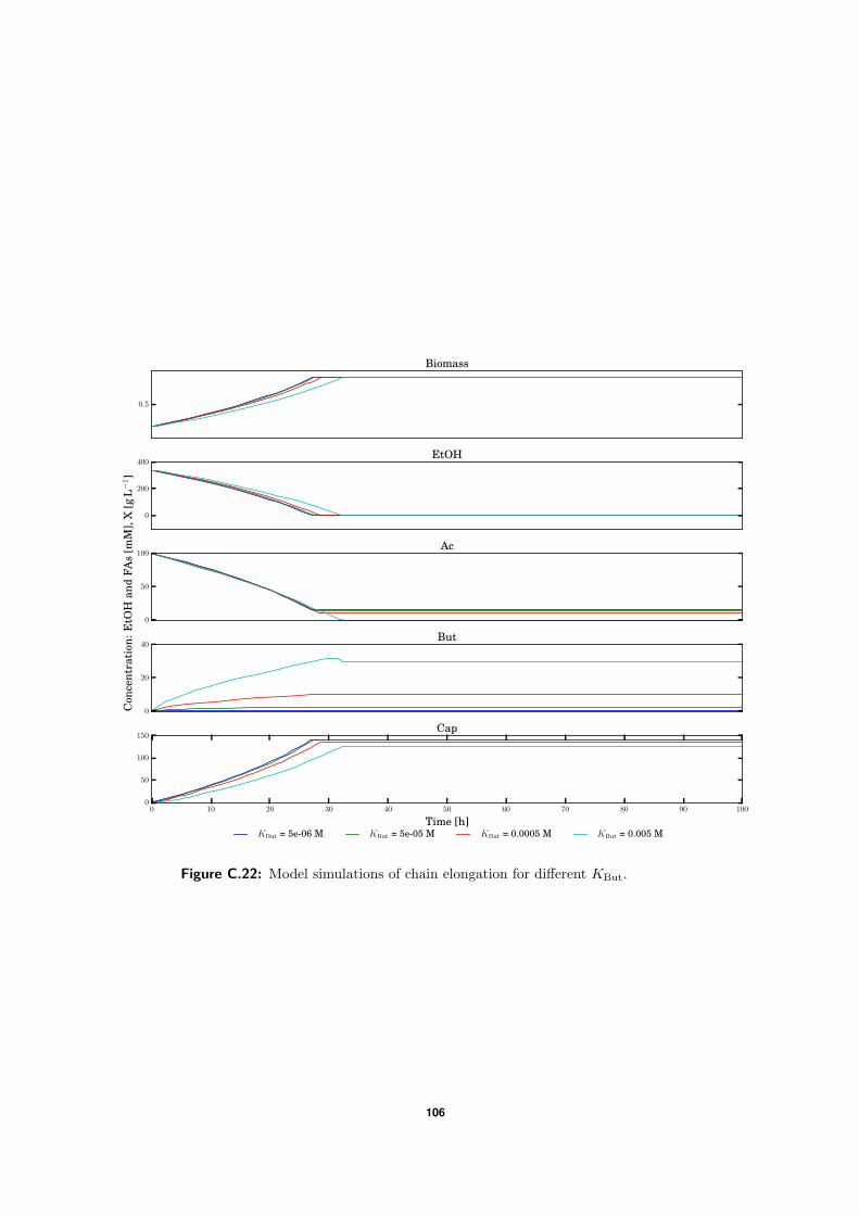
0.5
Biomass
0
200
400EtOH
0
50
100Ac
0
20
40But
0 10 20 30 40 50 60 70 80 90 100
Time [h]
0
50
100
150Cap
KBut = 5e-06 M KBut = 5e-05 M KBut = 0.0005 M KBut = 0.005 M
Con
cent
rati
on:E
tOH
and
FAs
[mM
],X
[gL−
1]
Figure C.22: Model simulations of chain elongation for different KBut.
106
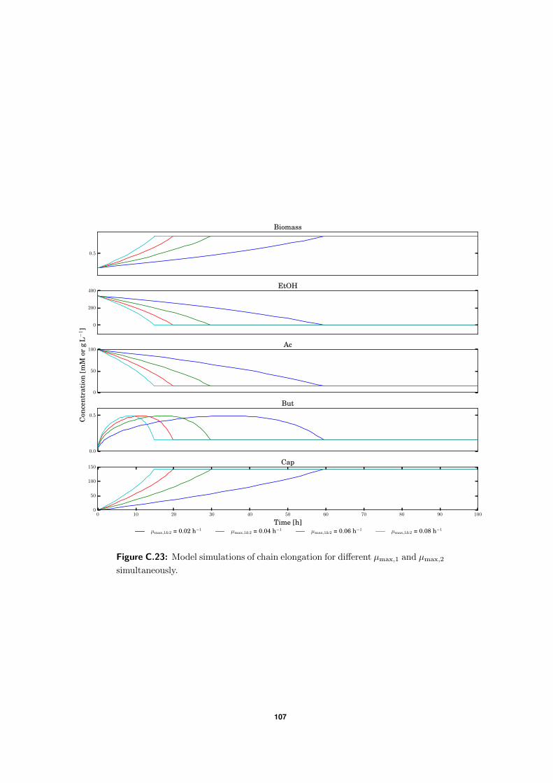
0.5
Biomass
0
200
400EtOH
0
50
100Ac
0.0
0.5
But
0 10 20 30 40 50 60 70 80 90 100
Time [h]
0
50
100
150Cap
µmax,1&2 = 0.02 h−1 µmax,1&2 = 0.04 h−1 µmax,1&2 = 0.06 h−1 µmax,1&2 = 0.08 h−1
Con
cent
rati
on[m
Mor
gL−
1]
Figure C.23: Model simulations of chain elongation for different µmax,1 and µmax,2
simultaneously.
107
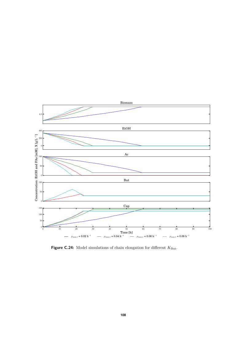
0.5
Biomass
0
200
400EtOH
0
50
100Ac
0
50
100But
0 10 20 30 40 50 60 70 80 90 100
Time [h]
0
50
100
150Cap
µmax,1 = 0.02 h−1 µmax,1 = 0.04 h−1 µmax,1 = 0.06 h−1 µmax,1 = 0.08 h−1
Con
cent
rati
on:E
tOH
and
FAs
[mM
],X
[gL−
1]
Figure C.24: Model simulations of chain elongation for different KBut.
108
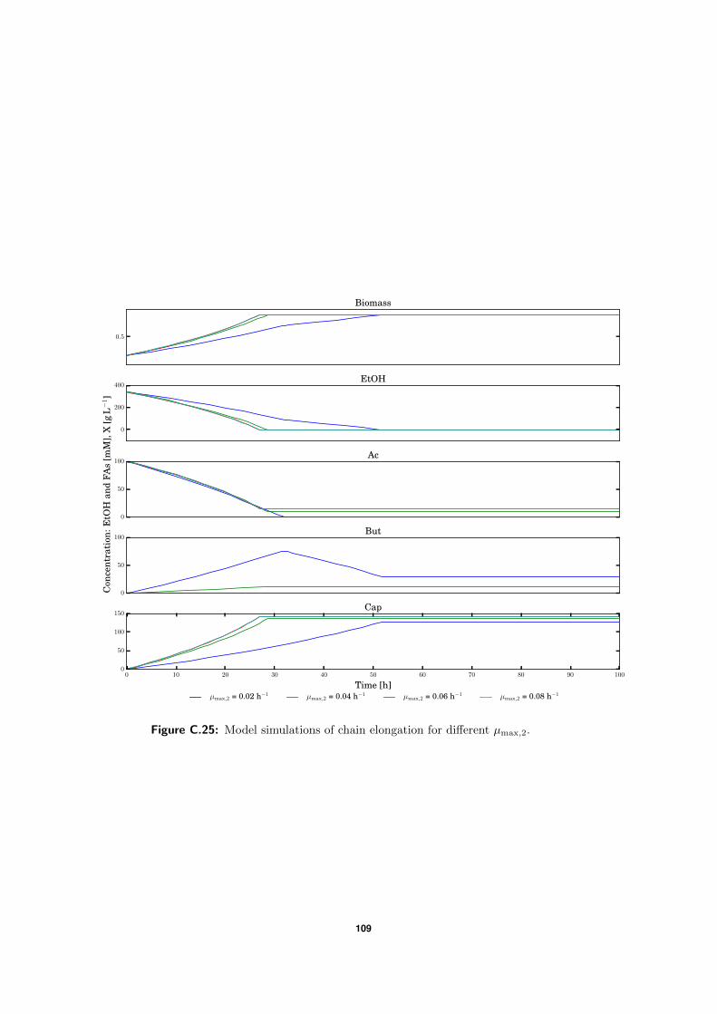
0.5
Biomass
0
200
400EtOH
0
50
100Ac
0
50
100But
0 10 20 30 40 50 60 70 80 90 100
Time [h]
0
50
100
150Cap
µmax,2 = 0.02 h−1 µmax,2 = 0.04 h−1 µmax,2 = 0.06 h−1 µmax,2 = 0.08 h−1
Con
cent
rati
on:E
tOH
and
FAs
[mM
],X
[gL−
1]
Figure C.25: Model simulations of chain elongation for different µmax,2.
109
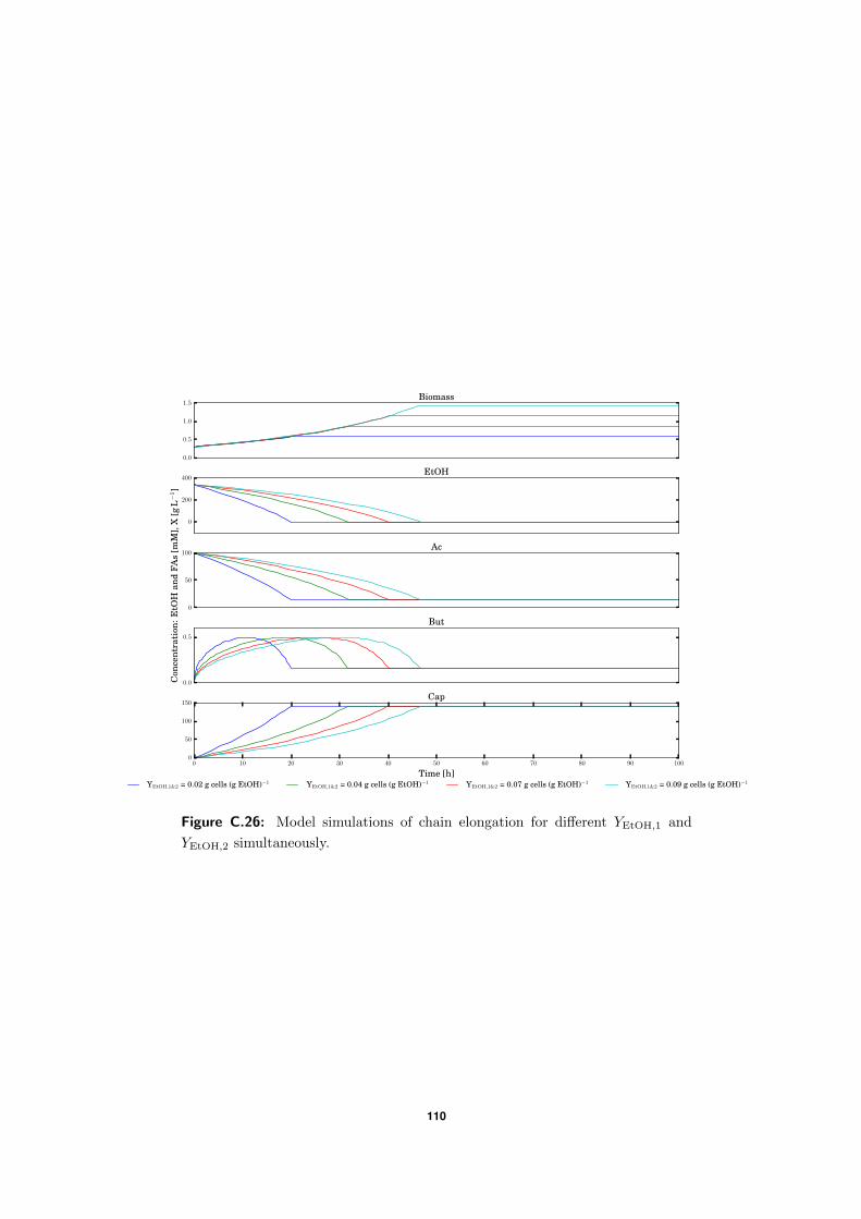
0.0
0.5
1.0
1.5Biomass
0
200
400EtOH
0
50
100Ac
0.0
0.5
But
0 10 20 30 40 50 60 70 80 90 100
Time [h]
0
50
100
150Cap
YEtOH,1&2 = 0.02 g cells (g EtOH)−1 YEtOH,1&2 = 0.04 g cells (g EtOH)−1 YEtOH,1&2 = 0.07 g cells (g EtOH)−1 YEtOH,1&2 = 0.09 g cells (g EtOH)−1
Con
cent
rati
on:E
tOH
and
FAs
[mM
],X
[gL−
1]
Figure C.26: Model simulations of chain elongation for different YEtOH,1 and
YEtOH,2 simultaneously.
110
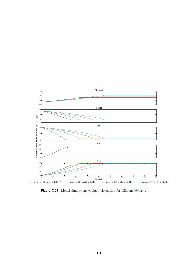
0.0
0.5
1.0
1.5Biomass
0
200
400EtOH
0
50
100Ac
0
20
40
60But
0 10 20 30 40 50 60 70 80 90 100
Time [h]
0
50
100
150Cap
YEtOH,1 = 0.02 g cells (g EtOH)−1 YEtOH,1 = 0.04 g cells (g EtOH)−1 YEtOH,1 = 0.07 g cells (g EtOH)−1 YEtOH,1 = 0.09 g cells (g EtOH)−1
Con
cent
rati
on:E
tOH
and
FAs
[mM
],X
[gL−
1]
Figure C.27: Model simulations of chain elongation for different YEtOH,1.
111
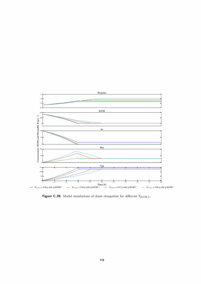
0.0
0.5
1.0
1.5Biomass
0
200
400EtOH
0
50
100Ac
0
50
100But
0 10 20 30 40 50 60 70 80 90 100
Time [h]
0
50
100
150Cap
YEtOH,2 = 0.02 g cells (g EtOH)−1 YEtOH,2 = 0.04 g cells (g EtOH)−1 YEtOH,2 = 0.07 g cells (g EtOH)−1 YEtOH,2 = 0.09 g cells (g EtOH)−1
Con
cent
rati
on:E
tOH
and
FAs
[mM
],X
[gL−
1]
Figure C.28: Model simulations of chain elongation for different YEtOH,2.
112
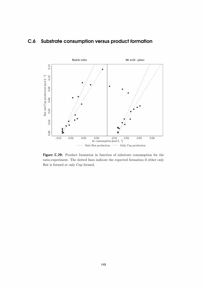
C.6 Substrate consumption versus product formation
●●●
●
●
●
●
●
●
●
●●
●
●
●●
●
●
Balch tube
−0.01 0.02 0.05 0.08
0.00
0.02
0.04
0.06
0.08
0.10
0.12
●●●
●
●
●
●
●●
● ●
●
●
●
●
●
●
96 well−plate
−0.01 0.02 0.05 0.08Ac consumption [mol L−1]
But
and C
ap p
roduct
ion [
mol
L−
1 ]
Only But production Only Cap production
Figure C.29: Product formation in function of substrate consumption for the
ratio-experiment. The dotted lines indicate the expected formation if either only
But is formed or only Cap formed.
113
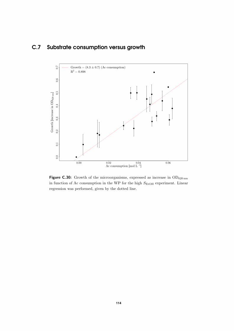
C.7 Substrate consumption versus growth
● ●●
●
●
●
●
●
●
●
●
●
●
●
●
●
●●
0.00 0.02 0.04 0.06
0.0
0.1
0.2
0.3
0.4
0.5
0.6
0.7
Ac consumption [mol L−1]
Gro
wth
[in
crea
se i
n O
D62
0 nm
]
Growth = (8.3 ± 0.7) (Ac consumption)
R2 = 0.898
Figure C.30: Growth of the microorganisms, expressed as increase in OD620 nm
in function of Ac consumption in the WP for the high SEtOH experiment. Linear
regression was performed, given by the dotted line.
114
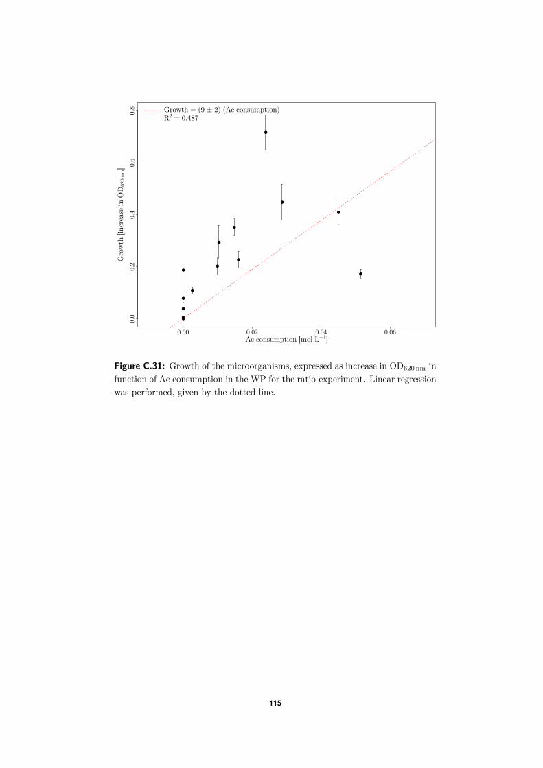
●
●
●
●
●
●
●●
●
●
●
●
●
●
0.00 0.02 0.04 0.06
0.0
0.2
0.4
0.6
0.8
Ac consumption [mol L−1]
Gro
wth
[in
crea
se i
n O
D62
0 nm
]
Growth = (9 ± 2) (Ac consumption)R2 = 0.487
Figure C.31: Growth of the microorganisms, expressed as increase in OD620 nm in
function of Ac consumption in the WP for the ratio-experiment. Linear regression
was performed, given by the dotted line.
115
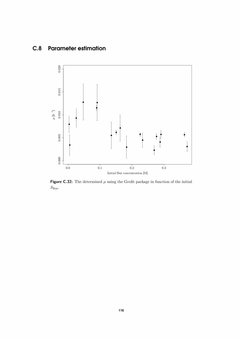
C.8 Parameter estimation
●
●
●
●
●
●
●
●
●
●
●
●
●
●
● ●
●
●
0.0 0.1 0.2 0.3
0.000
0.0
05
0.0
100.0
150.
020
Initial But concentration [M]
µ [
h−
1 ]
Figure C.32: The determined µ using the Grofit package in function of the initial
SBut.
116
![€¦ · Web view23Temudo MF, Muyzer G, Kleerebezem R, van Loosdrecht MCM. Diversity of microbial communities in open mixed culture fermentations: impact of the pH and carbon source[J].](https://static.fdocuments.nl/doc/165x107/5f0a638a7e708231d42b64fd/web-view-23temudo-mf-muyzer-g-kleerebezem-r-van-loosdrecht-mcm-diversity-of.jpg)