
Mathematical Modelling of the Mean Wave Drift Force in Current-PhD_Huijsmans
206
Stellingen 7t:< s Ret optreden van 'irregular frequencies' bij watergolfdiffraktie problemen kan ef- 1 fectief bestreden worden door gebruik te maken van een gemodificeerde rand- integraal vergelijking. Rierbij worden op het inwendige vrije vloeistof oppervlak frequentie onafhankelijke Neumann of Dirichlet randvoorwaarden voorgeschreven. Ret bepalen van de golfdriftkrachten door middel van een drukintegratie meth- 2 ode dient aangevuld te worden met een methode, die gebaseerd is op de wet van behoud van impuls. Bepallng van de golfdriftkracht door drukintegratie, met medeneming van de in- .3 vloed van voorwaartse snelheid, vereist een nauwkeurige behandeling van de dif- ferentiatie van de stationaire potentiaal op het vrij oppervlak en de oppervlakte van het drijvende object. De aanpak van Aranha ter bepaling van de golfdriftdemping leidt tot grote on- L, nauwkeurigheden bij toepassingen voor drie dimensionale problemen. 5 De invloed van stroom op de golfdriftkrachten mag niet verwaarloosd worden. Het opzetten door de overheid van nieuwe topinstituten naast de bestaande ken- nis infrastructuur in Nederland, leidt tot een grote mate van versnippering van beschikbare onderzoeksfondsen. Ret gebruik van 'symbolic computation' in het onderwijs kan ondersteunend b werken bij het ontwikkelen van een analytisch denkvermogen. Echter in de on- derzoekspraktijk dienen de resultaten van 'symbolic computation' door ditzelfde analytische denkvermogen met terughoudendheid beschouwd te worden. I I7 In het bridge speelt de psychologische benadering van het spel en de individu- 8 ele afspeelkwaliteiten een grotere rol dan het beheersen van een gekompliceerd biedsysteem. De wet op het primair onderwijs geeft de schoolbesturen een grote mate van zelf- standigheid. Het ware te wensen dat dit beleid van de overheid niet leidt tot het afschuiven van de verantwoordelijkheid van de overheid voor het primair onder- wijs. A 0 Met een relatief geringe efficiency winst bij het vervoer van goederen over water, lijkt een aanleg van een Betuwe spoorlijn overbodig. 11 Ret leren van het doen van onderzoek bij de universitaire onleidinzen is door de 4-jarige opleidingsstructuur in de knel geraakt. I C) Ret rokersvraagstuk tijdens het bridgen zou voor een groot deel opgelost zijn, s: indien de spelers aan tafel zich door een normaal fatsoensbesef lieten leiden.
-
Upload
carlos-garrido -
Category
Documents
-
view
17 -
download
4
description
Mathematical Modelling of the Mean Wave Drift Force in Current
Transcript of Mathematical Modelling of the Mean Wave Drift Force in Current-PhD_Huijsmans

Stellingen7t:< s
Ret optreden van 'irregular frequencies' bij watergolfdiffraktie problemen kan ef-1 fectief bestreden worden door gebruik te maken van een gemodificeerde rand
integraal vergelijking. Rierbij worden op het inwendige vrije vloeistof oppervlakfrequentie onafhankelijke Neumann of Dirichlet randvoorwaarden voorgeschreven.
Ret bepalen van de golfdriftkrachten door middel van een drukintegratie meth-2 ode dient aangevuld te worden met een methode, die gebaseerd is op de wet van
behoud van impuls.
Bepallng van de golfdriftkracht door drukintegratie, met medeneming van de in-.3 vloed van voorwaartse snelheid, vereist een nauwkeurige behandeling van de dif
ferentiatie van de stationaire potentiaal op het vrij oppervlak en de oppervlaktevan het drijvende object.
De aanpak van Aranha ter bepaling van de golfdriftdemping leidt tot grote onL, nauwkeurigheden bij toepassingen voor drie dimensionale problemen.
5 De invloed van stroom op de golfdriftkrachten mag niet verwaarloosd worden.
Het opzetten door de overheid van nieuwe topinstituten naast de bestaande kennis infrastructuur in Nederland, leidt tot een grote mate van versnippering vanbeschikbare onderzoeksfondsen.
Ret gebruik van 'symbolic computation' in het onderwijs kan ondersteunendb werken bij het ontwikkelen van een analytisch denkvermogen. Echter in de on
derzoekspraktijk dienen de resultaten van 'symbolic computation' door ditzelfdeanalytische denkvermogen met terughoudendheid beschouwd te worden.
I
I 7In het bridge speelt de psychologische benadering van het spel en de individu
8 ele afspeelkwaliteiten een grotere rol dan het beheersen van een gekompliceerdbiedsysteem.
De wet op het primair onderwijs geeft de schoolbesturen een grote mate van zelf~ standigheid. Het ware te wensen dat dit beleid van de overheid niet leidt tot het
afschuiven van de verantwoordelijkheid van de overheid voor het primair onderwijs.
A0 Met een relatief geringe efficiency winst bij het vervoer van goederen over water,lijkt een aanleg van een Betuwe spoorlijn overbodig.
11 Ret leren van het doen van onderzoek bij de universitaire onleidinzen is door de
4-jarige opleidingsstructuur in de knel geraakt.
I C) Ret rokersvraagstuk tijdens het bridgen zou voor een groot deel opgelost zijn,s: indien de spelers aan tafel zich door een normaal fatsoensbesef lieten leiden.
TRdiss2767
Mathematical Modelling of the Mean WaveDrift Force in Current
A Numerical and Experimental study
Rene H. M. Huijsmans

Printed by:Grafisch Bedrijf Ponsen & Looijen BY, Wageningen, Netherlands
Mathematical Modelling of the Mean WaveDrift Force in Current
A Numerical and Experimental study
Proefschrift
ter verkrijging van de graad van doctoraan de Technische Universiteit Delft,
op gezag van de Rector Magnificus Prof. Jr. K.F. Wakker,in het openbaar te verdedigen ten overstaan van een commissie,
door het College van Dekanen aangewezen,op maandag 17 juni 1996 te 10.30 uur
door
Rene Herman Maria HUIJSMANS
wiskundig ingenieurgeboren te Breda
Dit proefsehrift is goedgekeurd door de promotor:Prof. Dr. Ir. A.J. Hermans
Samenstelling promotiecommissie:Rector Magnifieus, voorzitterProf.dr.ir, A.J.Hermans, TU DELFT,promotorProf.dr.ir.J.A.Pinkster, fae WbMtProf.dr.ir.J.H.Vugts, fae CtProf.ir.M. van Holst, fae WbMtProf.dr.B.Molin, Ecole Superieur Marseille,FrProf G.E.Hearn, U-New Castle, Groot BritannieProf.dr.ir. G.Kuiper, fae WbMt
ISBN-nummer: 90-75757-02-6Copyright © R.H.M. Huijsmans, MARIN, 1996. All rights reserved.
Aan Gretha, Jeroen, Ingeen Ouders

Contents
1 Abstract 3
2 Introduction 5
3 Mathematical formulation 113.1 Problem formulation . . . . . . . . . . . . . . . . .. 11
3.1.1 Linearization of the free surface condition .. 143.1.2 Linearization of the body boundary condition 15
3.2 The potential function . . . . . . . . . . . . 163.3 The boundary condition on the free surface. 193.4 The body boundary conditions. 203.5 The steady potential . . . 21
4 Expansion of the potential 254.1 The integral equation. . . . . . . . . . . . . . 254.2 The amplitude distributions of the potentials . 30
5 The Green's function 335.1 The expansion of the Green's function 335.2 The zero order Green's function"po .. 375.3 The first-order Green's function v, .. 38
5.3.1 A transformation in the complex plane 385.3.2 An expression of derivatives of "po . . . 395.3.3 The agreement of both expressions .. 40
5.4 The uniform expansion of the Green's function. 405.4.1 Large distance R 415.4.2 The far field . . 44
1
11
5.5 Suppression of irregular frequencies .5.5.1 The Lid method: theory ...5.5.2 Implementation of lid method5.5.3 Discussion lid method
OONTENTS
47475165
6 The forces on the body 676.1 Added mass and damping . . . . . . 676.2 The exciting forces and the motions . 716.3 The mean wave drift forces. . . . . . 79
7 Model test experiments 857.1 Wave drift force measurements. 85
7.1.1 Passive mooring. . . . . 857.1.2 Active mooring . . . . . 87
7.2 Extinction tests in regular waves 897.3 Model test conditions . . . . . . . 93
8 Validation 998.1 200 kDWT Tanker 100% Loaded 99
8.1.1 First order responses . . . . . . . . . 1008.1.2 Wave drift forces in current TlOO % . 1068.1.3 Wave drift damping TlOO % 107
8.2 200 kDWT tanker 40% loaded . . . . . . . 1088.2.1 First order Responses. . . . . . . . 1108.2.2 Wave drift forces in current T40 % 1168.2.3 Wave drift damping T40 % 118
8.3 200 kDWT tanker 70% loaded . . . . . . . 1198.3.1 Wave drift damping T70 % .... 120
8.4 Time domain results 200 kDWT tanker 40% loaded 121
9 An engineering view of wave drift damping 123
10 Discussion 127
11 Conclusions 129
Bibliography 131
CONTENTS
A Derivation of integral equation
B Integral equation irregular frequenciesB.1 Integration of free surface panel
C Integration rankine source
D The fsc for the radiation potential
E The mj-terms
F The computations of '1/;1F.1 A transformation in the complex planeF.2 An expression of derivatives of '1/;0F.3 The derivatives of the '1/;1 • • • • •
G The far field expansionG.1 The residue of 'I/; ..••..•.G.2 The method of stationary phaseG.3 Asymptotic behaviour of ~o ..
H Error estimates from experiments
I Dynamic positioning at model scale1.1 Global set-up . . . . . . . . .1.2 Components in a DP system1.3 The control loop .
1.3.1 Mathematical model of the ship1.3.2 The extended Kalman filter1.3.3 The controller .
Curriculum Vitae
111
139
143. 145
149
153
157
159159161163
167167168171
175
177177178179179180182
187

IV CONTENTS
List of Figures
2.1 A typical mooring layout of turret-moored tanker 72.2 Undisturbed stationary flow 82.3 Disturbed stationary flow 9
3.1 System of co-ordinates. . . 173.2 The coordinate system and the six modes of ship mo-
tion. . . . . . . . . . 183.3 Steady wave system. . . . 22
4.1 Coordinates at waterline. . 264.2 Stationary potential in free surface around a 200 kDWT
tanker in cross-flow conditions. . 31
5.1 Contours of integration. .... 355.2 Wave pattern of oscillating translating source T < 1/4. 355.3 Contours of integration. 375.4 "po, R is variable, the source in (0,0, -1), w = 1.4. . .. 385.5 "pI, R is variable, the source in (0,0, -1), w = 1.4.. " 415.6 Large distance e-; R is variable, the source in (0,0, -1),
w = 1.4. . . . . . . . . . . . . . . . . . . . . . . . . .. 435.7 "p and "p(= LV"p), R is variable, the source in (0,0, -1),
w = 1.4. . . . . . . . . . . . . . . . . . . . . . . . . .. 445.8 "p and FF"p, R is variable, the source in (0,0, -1), w =
1.4. ..... 465.9 Ship........... 475.10 Ship section. . . . . . . 475.11 Panel distribution box 515.12 Surge added mass no lid. 53
v
VI LIST OF FIGURES
5.13 Surge damping no lid. ..... 535.14 Surge-pitch added mass no lid. . 535.15 Surge-pitch damping no lid. 535.16 Heave added mass no lid. . . . 545.17 Heave damping no lid. ... . 545.18 Roll-sway added mass no lid. . 545.19 Roll-sway damping no lid. 545.20 Roll added mass no lid. . 555.21 Roll damping no lid. .. 555.22 Yaw added mass no lid. . 555.23 Yaw damping no lid. . . 555.24 Surge added mass with lid. . 565.25 Surge damping with lid. .. 565.26 Surge-pitch added mass with lid. 565.27 Surge-pitch damping with lid. 565.28 Heave added mass with lid. .. 575.29 Heave damping with lid. . . . . 575.30 Roll-sway added mass with lid. 575.31 Roll-sway damping with lid. 575.32 Roll added mass with lid. 585.33 Roll damping with lid. . . 585.34 Yaw added mass with lid. 585.35 Yaw damping with lid. . . 585.36 Surge added mass effect free surface panels. 595.37 Surge damping effect free surface panels. . . 595.38 Surge-pitch added mass effect free surface panels. 595.39 Surge-pitch damping effect free surface panels. 595.40 Heave added mass effect free surface panels. . . 605.41 Heave damping effect free surface panels. . . . . 605.42 Roll-sway added mass effect free surface panels. 605.43 Roll-sway damping effect free surface panels. 605.44 Roll added mass effect free surface panels. 615.45 Roll damping effect free surface panels. . . 615.46 Yaw added mass effect free surface panels. 615.47 Yaw damping effect free surface panels. . . 615.48 Surge added mass comparison original-lid. 62
LIST OF FIGURES VII
5.49 Surge damping comparison original-lid. . . . . . 625.50 Surge-pitch added mass comparison original-lid. 635.51 Surge-pitch damping comparison original-lid. 635.52 Heave added mass comparison original-lid. . . 635.53 Heave damping comparison original-lid. 635.54 Roll-sway added mass comparison original-lid. 645.55 Roll-sway damping comparison original-lid. 645.56 Roll added mass comparison original-lid. 645.57 Roll damping comparison original-lid.. . 645.58 Yaw added mass comparison original-lid. 655.59 Yaw damping comparison original-lid. 65
6.1 Panel description Sphere . . . . . . . . 706.2 Panel description free surface around Sphere 706.3 Surge-heave added mass coefficients of a half-immersed
sphere of radius a and Fr = 0.04. . . . . . . . . . . .. 716.4 Surge-heave added mass coefficients of a half-immersed
sphere of radius a and Fr = 0.04. (No free surfacecontribution) 71
6.5 Surge-surge contribution to the added mass and thedamping coefficients of a half-immersed sphere of radiusa and Fr = 0.04. ... . . . . . . . . . . . . . . . .. 72
6.6 Added mass coupling coefficients Fn=O.O and Fn-0.05. 726.7 Damping coupling coefficients Fn=O.O and Fn-0.05 736.8 The surge exciting forces, without speed, computed by
Nossen, the Haskind relation and pressure integration. 756.9 The heave exciting forces, without speed, computed by
Nossen, the Haskind relation and pressure integration. 756.10 The surge exciting forces. . 766.11 The heave exciting forces. 776.12 The surge motion . . . . . 776.13 The heave motion. . . . . 786.14 Drift force on sphere for Fn=O.O and Fn=0.04. . 806.15 The drift forces on a restrained sphere. . . . . . 836.16 The drift forces on a free sphere, without the stationary
potential in the body boundary conditions. . . . . . .. 83
YIll LIST OF FIGURES
6.17 The drift forces on a free sphere, with the stationarypotential in the body boundary conditions. 84
6.18 The wave drift damping on a free sphere. . . . . . . .. 84
7.1 Set-up of wave drift force measurement passive mooring 867.2 Spring characteristics mooring system. .. 877.3 Dynamic positioning set-up top-view . . . 887.4 Dynamic positioning set-up cross-section . 887.5 Set-up extinction test. . . . . . . . . . . . 907.6 Decay curve surge in regular waves unfiltered. 917.7 Decay curve surge in regular waves filtered. . 917.8 Logarithmic decrement.. . . . . . . . 92
8.1 Body plan of the 200 kDWT tanker. 998.2 Panel description of 200 kDWT tanker fully loaded. 1018.3 Panel description of free surface 200 kDWT tanker fully
loaded. . . . . . . . . . . . . . . . . . . . . . . . 1018.4 Surge response in 180 degree waves, no current. 1028.5 Heave response in 180 degree waves, no current. 1028.6 Pitch response in 180 degree waves, no current. 1028.7 Surge response in 180 degree waves, 1.5 mls current. 1038.8 Heave response in 180 degree waves, 1.5 tsi]» current. 1038.9 Pitch response in 180 degree waves,1.5 su]« current.. 1038.10 Surge response in 135 degree waves, 1.5 mls current. 1048.11 Sway response in 135 degree waves, 1.5 ta]s current. . 1048.12 Heave response in 135 degree waves, 1.5 mls current. 1048.13 Yaw response in 135 degree waves, 1.5 mls current. 1048.14 Surge response in 135 degree waves, 135 degree current
at 1.5 m/s.. . . . . . . . . . . . . . . . . . . . . . . . . 1058.15 Sway response in 135 degree waves, 135 degree current
at 1.5m/s. . . . . . . . . . . . . . . . . . . . . . . . . . 1058.16 Heave response in 135 degree waves, 135 degree current
at 1.5 tu]s.. . . . . . . . . . . . . . . . . . . . . . . . . 1058.17 Yaw response in 135 degree waves, 135 degree current
at 1.5 m/s 1058.18 Wave drift force surge in 180 degree waves, 180 degree
current at 0.0 m/s. . 106
LIST OF FIGURES IX
8.19 Wave drift force surge in 180 degree waves, 180 degreecurrent at 1.5 ta]«. . . . . . . . . . . . . . . . . . . . . 106
8.20 Wave drift force surge in 135 degree waves, 180 degreecurrent at 1.5 tu] s. . . . . . . . . . . . . . . . . . . . . 106
8.21 Wave drift force sway in 135 degree waves, 180 degreecurrent at 1.5 txi]«. . 106
8.22 Wave drift force surge in 135 degree waves, 135 degreecurrent at 1.5 ta]«. . 107
8.23 Wave drift force sway in 135 degree waves, 135 degreecurrent at 1.5 tii]«. . . . . . . . . . . . . . . . . . . 107
8.24 Wave drift damping surge in 180 degree waves.. . .. 1088.25 Panel description of 200 kDWT tanker 40% loaded.. 1098.26 Surge response in 180 degree waves, 1.2 mls current. 1108.27 Heave response in 180 degree waves, 1.2 mls current. 1108.28 Pitch response in 180 degree waves, 1.2 mls current. 1118.29 Surge response in 150 degree waves, no current. 1118.30 Sway response in 150 degree waves, no current. 1118.31 Heave response in 150 degree waves, no current. 1128.32 Roll response in 150 degree waves, no current. . 1128.33 Pitch response in 150 degree waves, no current. 1128.34 Yaw response in 150 degree waves, no current. . 1128.35 Surge response in 150 degree waves, 1.2 mls current. 1138.36 Sway response in 150 degree waves, 1.2 tu]« current. . 1138.37 Heave response in 150 degree waves, 1.2 mls current. 1138.38 Roll response in 150 degree waves, 1.2 in]s current.. 1138.39 Pitch Response in 150 degree waves, 1.2 tn]« current. 1148.40 Yaw response in 150 degree waves, 1.2 tn]« current.. 1148.41 Surge response in 150 degree waves, 150 degree current
at 1.2 tii]« 1148.42 Sway response in 150 degree waves, 150 degree current
at 1.2 m/s 1148.43 Heave response in 150 degree waves, 150 degree current
at 1.2 m/s 1158.44 Roll response in 150 degree waves, 150 degree current
at 1.2 tu]« 115
x LIST OF FIGURES
8.45 Pitch response in 150 degree waves, 150 degree currentat 1.2m/s 115
8.46 Yaw response in 150 degree waves, 150 degree currentat 1.2 m/s.. . . . . . . . . . . . . . . . . . . . . . . . . 115
8.47 Wave drift force surge in 180 degree waves, 180 degreecurrent at 1.2 ta]», . . . . . . . . . . . . . . . . . . . . 116
8.48 Wave drift force surge in 150 degree waves, 180 degreecurrent at 0.0 tu]«, . 116
8.49 Wave drift force sway in 150 degree waves, 180 degreecurrent at 0.0 ta]», . 116
8.50 Wave drift force surge in 150 degree waves, 180 degreecurrent at 1.2 tu] s. . . . . . . . . . . . . . . . . . . . . 117
8.51 Wave drift force sway in 150 degree waves, 180 degreecurrent at 1.2 tu]«. . . . . . . . . . . . . . . . . . . . . 117
8.52 Wave drift force surge in 150 degree waves, 150 degreecurrent at 1.2 ta]«. . 117
8.53 Wave drift force sway in 150 degree waves, 150 degreecurrent at 1.2 tn]«. . . . . . . . . . . . . . . . . . . 117
8.54 Wave drift damping in surge in 180 degree waves.... 1188.55 Panel description of 200 kDWT tanker 70% loaded. . . 1198.56 Wave drift damping in surge in 180 degree waves, 180
degree current at 1.2 m/s. . 1218.57 Wave drift force surge in 150 degree waves; Fn=0.02
150 degree current, Fn=0.02. 1228.58 Wave drift force sway in 150 degree waves; 150 degree
current, Fn=0.02. 122
9.1 Approximation wave drift damping surge using Aranha'sexpression for a floating sphere. . . . . . . . . . . . . . 126
9.2 Approximation wave drift damping surge using Aranha'sexpression for a 200 kDWT in head waves and current. 126
10.1 Estimates of wave drift force using extinction tests. 128
A.l Computational domain integral equation.. 140
B.1 Integration over free surface panel. .... 146

LIST OF FIGURES
C.1 Integration over a Panel j.C.2 Projection onto Panel j.
F.1 Contours of integration .
Xl
150150
160

XlI LIST OF FIGURES
List of Tables
5.1 Location irregular frequencies for a square box. .... 52
7.1 Model test conditions for current speed 0.0 m/s T100%in 180 deg. waves. 93
7.2 Model test conditions for current speed 1.5 ui]« TlOO%in 180 deg, waves and 180 deg, current direction. . " 94
7.3 Model test conditions for current speed 1.5 ta]« TlOO%in 135 deg. waves and 180 deg, current direction. . .. 94
7.4 Model test conditions for current speed 1.5 m/s TlOO%in 135 deg, waves and 135 deg. current direction. . .. 95
7.5 Model test conditions for current speed 1.2 tu] s TlOO%in 180 deg. waves and 180 deg, current direction. . .. 95
7.6 Model test conditions for current speed 1.2 m/s T40%in 180 deg. waves and 180 deg, current direction. . .. 96
7.7 Model test conditions for current speed 1.2 m/s T40 %in 150 deg. waves. 96
7.8 Model test conditions T40I 977.9 Model test conditions T40% for current speed 0.0 m/s
in 150 deg. waves. 977.10 Extinction test conditions for current speed 0.0 m/s
T40% in 180 deg. waves. 987.11 Extinction test conditions for current speed 0.0 m/s
T70% in 180 deg. waves. 98
8.1 Particulars of the 200 k DWT tanker fully loaded. 1008.2 Particulars of the 200 k DWT Tanker 40% loaded 1098.3 Particulars of the 200 kDWT tanker 70% Loaded. 120
1

Chapter 1
Abstract
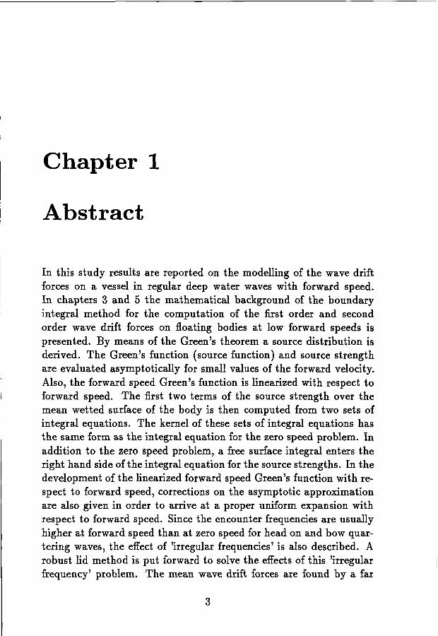
In this study results are reported on the modelling of the wave driftforces on a vessel in regular deep water waves with forward speed.In chapters 3 and 5 the mathematical background of the boundaryintegral method for the computation of the first order and secondorder wave drift forces on floating bodies at low forward speeds ispresented. By means of the Green's theorem a source distribution isderived. The Green's function (source function) and source strengthare evaluated asymptotically for small values of the forward velocity.Also, the forward speed Green's function is linearized with respect toforward speed. The first two terms of the source strength over themean wetted surface of the body is then computed from two sets ofintegral equations. The kernel of these sets of integral equations hasthe same form as the integral equation for the zero speed problem. Inaddition to the zero speed problem, a free surface integral enters theright hand side of the integral equation for the source strengths. In thedevelopment of the linearized forward speed Green's function with respect to forward speed, corrections on the asymptotic approximationare also given in order to arrive at a proper uniform expansion withrespect to forward speed. Since the encounter frequencies are usuallyhigher at forward speed than at zero speed for head on and bow quartering waves, the effect of 'irregular frequencies' is also described. Arobust lid method is put forward to solve the effects of this 'irregularfrequency' problem. The mean wave drift forces are found by a far
3
4 CHAPTER 1. ABSTRAOT
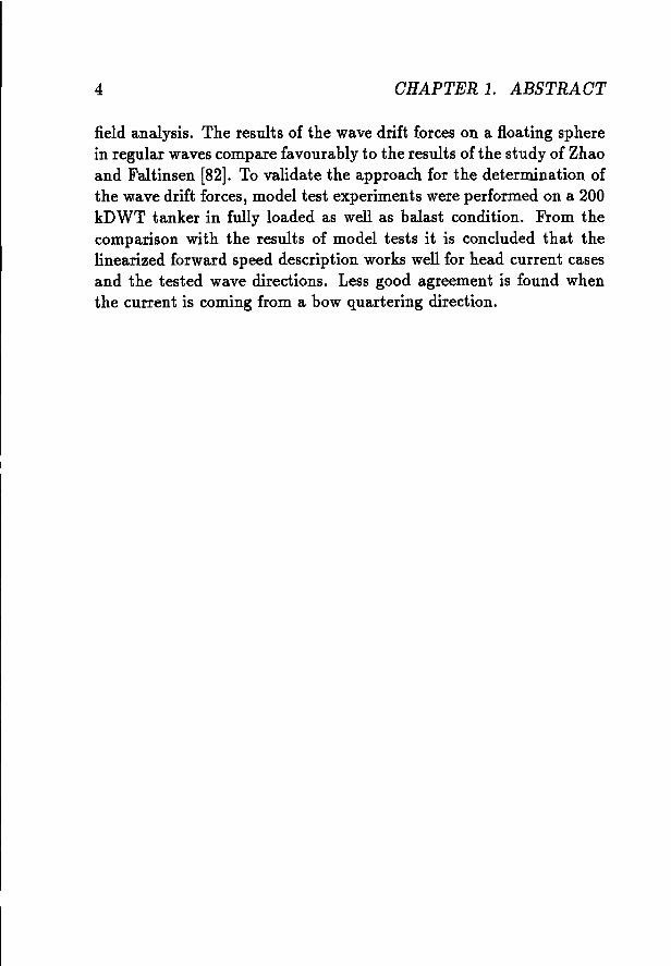
field analysis. The results of the wave drift forces on a floating spherein regular waves compare favourably to the results of the study of Zhaoand Faltinsen [82]. To validate the approach for the determination ofthe wave drift forces, model test experiments were performed on a 200kDWT tanker in fully loaded as well as balast condition. From thecomparison with the results of model tests it is concluded that thelinearized forward speed description works well for head current casesand the tested wave directions. Less good agreement is found whenthe current is coming from a bow quartering direction.
Chapter 2
Introduction
In the exploration and production of oil and gas in offshore locationsmore and more use is made of moored floating vessels. The introduction of the first floating vessels as production platforms was motivated,among other reasons, by an absence of a pipeline infrastructure in thevinicity of the oil wells. Nowadays, however, the increasing capitalcosts of a fixed platform for deep water oil production and the needfor environmentally safe removal of the platform once production hasstopped provide further incentive for the development of moored floating production systems. As the mooring system has to withstand theforces of wind, waves and current, a lot of emphasis has been placed inthe last twenty years on reliable assesment of the motions caused byenvironmental conditions. Given that the mooring system is likely toencounter severe environmental conditions in its service lifetime, thereal need is for the assesment of the motions of the floating vessel insuch conditions, which requires state-of-the-art numerical techniques.The full non-linear treatment of the flow around the vessel in thesesevere wave conditions, including eg viscous effects, is still very farfrom practical application. Therefore there is still a need for a linearapproach tothe fluid-body interaction, in which the essential detailsof the fluid-body flow is maintained. The applicability of such linearapproaches should however be validated against model test experiments, in which the environmental conditions can be controlled andmonitored more reliably than in real life. In the assesment of the loads
5
6 CHAPTER 2. INTRODUCTION
on the mooring system of the vessel essential work has been accomplished in the past by van Oortmerssen [69], who calculated to firstorder the reaction of the vessel due to motions and waves using a linearized frequency domain potential flow theory. He showed that it ispossible to compute in time domain, based on frequency domain results, the non-linear forces of the mooring system acting on the vessel.The hydrodynamic reactions of the vessel were described by means ofconvolution of the motion velocity with retardation functions. One ofthe properties of a catenary moored floating vessel is that the naturalperiod of the mooring system is very high (from 50 seconds up to several minutes). Using a linear model of the fluid-body interaction onedoes not arrive at the correct excitation at the natural period. Severalauthors [54, 14, 48] have pointed out in the past that the weak nonlinear fluid-body interaction is responsible for the excitation at thenatural period of the system. A pioneering effort was performed byPinkster [54] in which he carefully derived a pressure integration technique to arrive at the second order wave excitation (meaning quadraticwith respect to the incident wave height) in regular waves. He alsoderived approximate expressions for the second order wave excitationin bi-chromatic waves. The correctness of Pinkster's approximativeapproach for the low frequency excitation was demonstrated by Benschop et al, [5J and Yue [38]. As a consequence of the motions of thevessel in the vinicity of the natural period of the system, not only thewave excitation is of importance, but also the damping of the completemooring-vessel system. In the case of a first order process we see thatthe amplitude of the surge motion of the moored vessel at the naturalfrequency is given by :
where 1.£ is the natural frequency of the mooring system in surge (a::),Bxx(l.£) is the damping of the mooring-vessel system at the natural frequency and F:;(I.£) is the wave exciting force at the natural frequency1.£. Since by nature the moored vessel itself has very low damping inthe surge direction (minimum resistance) all other possible sources ofdamping will influence the surge motion of the vessel as well.
internal turret external turret
7
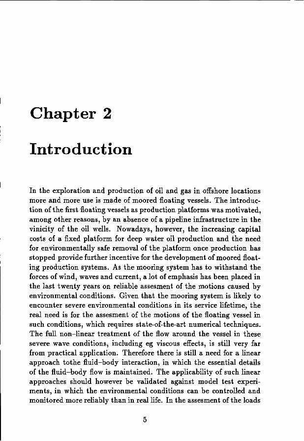
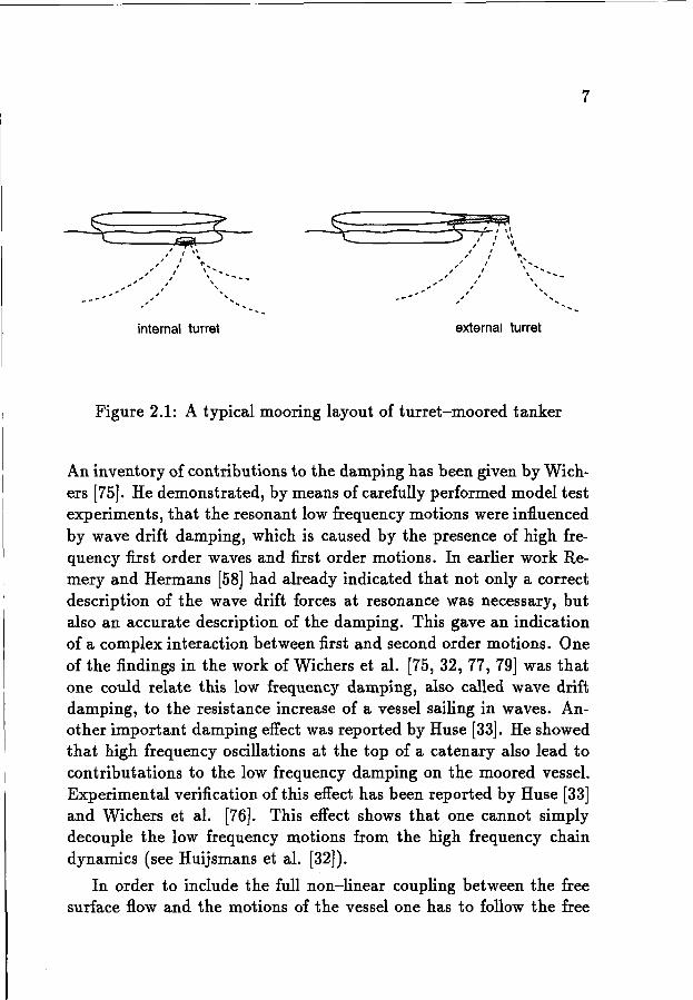
Figure 2.1: A typical mooring layout of turret-moored tanker
An inventory of contributions to the damping has been given by Wichers [75]. He demonstrated, by means of carefully performed model testexperiments, that the resonant low frequency motions were influencedby wave drift damping, which is caused by the presence of high frequency first order waves and first order motions. In earlier work Remery and Hermans [58] had already indicated that not only a correctdescription of the wave drift forces at resonance was necessary, butalso an accurate description of the damping. This gave an indicationof a complex interaction between first and second order motions. Oneof the findings in the work of Wichers et al. [75, 32, 77, 79] was thatone could relate this low frequency damping, also called wave driftdamping, to the resistance increase of a vessel sailing in waves. Another important damping effect was reported by Huse [33]. He showedthat high frequency oscillations at the top of a catenary also lead tocontributations to the low frequency damping on the moored vessel.Experimental verification of this effect has been reported by Huse [33]and Wichers et al. [76]. This effect shows that one cannot simplydecouple the low frequency motions from the high frequency chaindynamics (see Huijsmans et al. [32]).
In order to include the full non-linear coupling between the freesurface flow and the motions of the vessel one has to follow the free
8 CHAPTER 2. INTRODUCTION
surface and the body boundary at each time step. First attempts atmodelling the flow following a complete non-linear description of thefree surface flow have been performed amongst others by Romate [60]and extended to large body motion by van Daalen [70] and Broeze [9].Possible weak non-linear extensions from linearized potential flow descriptions of the three-dimensional motions of a vessel in waves werediscussed by Beck [4]. Experience in the use of such non-linear
----- ~----..- -Ux -
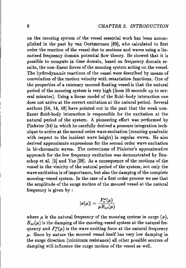
Figure 2.2: Undisturbed stationary flow
approaches as reported by Beck [4] has demonstrated that the computational effort required effort is still very large. In addition, problemswere reported by Romate [59], Broeze, and Van Daalen [9, 70] withrespect to the correct modelling of the evolution of the boundariesat intersection points. In this area a lot of progress is still requiredto bring such non-linear flow models within reach of engineering practice. Approximate forward speed linearized potential flow models havebeen put forward to model the wave drift force at low forward speed[29], [23],[55],[82]. Forward speed diffraction effects have been modelled using boundary element methods using the Green's function for atranslation oscillating source. The first effective results were reportedamongst others by Chang [10] , Bougis [6], Inglis [34]. The main drawbacks of their approach were that the Green's function was (and stillis) very cumbersome to compute and stationary potential flow effects
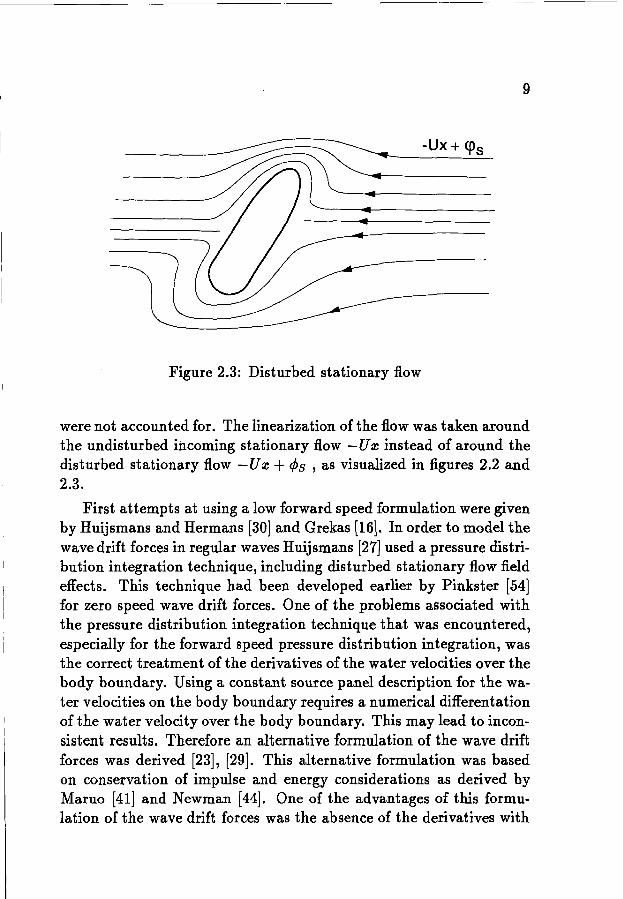
9
-Ux + <l's
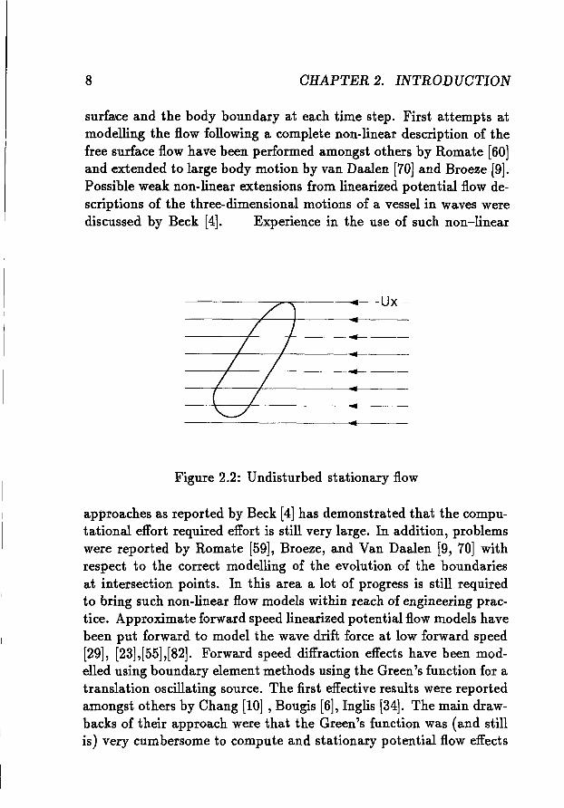
l~-Figure 2.3: Disturbed stationary flow
were not accounted for. The linearization of the flow was taken aroundthe undisturbed incoming stationary flow -U:c instead of around thedisturbed stationary flow -U:c + <Ps , as visualized in figures 2.2 and2.3.
First attempts at using a low forward speed formulation were givenby Huijsmans and Hermans [30] and Grekas [16]. In order to model thewave drift forces in regular waves Huijsmans [27] used a pressure distribution integration technique, including disturbed stationary flow fieldeffects. This technique had been developed earlier by Pinkster [54]for zero speed wave drift forces. One of the problems associated withthe pressure distribution integration technique that was encountered,especially for the forward speed pressure distribution integration, wasthe correct treatment of the derivatives of the water velocities over thebody boundary. Using a constant source panel description for the water velocities on the body boundary requires a numerical differentationof the water velocity over the body boundary. This may lead to inconsistent results. Therefore an alternative formulation of the wave driftforces was derived [23], [29]. This alternative formulation was basedon conservation of impulse and energy considerations as derived byMaruo [41] and Newman [44]. One of the advantages of this formulation of the wave drift forces was the absence of the derivatives with
10 OHAPTER 2. INTRODUOTION
respect to the water velocities. The formulation for low forward speedwas also independently derived by Nossen [52] and Grue et al. [17].Grue [20] also gave an expression of the mean yaw moment in regular waves. One drawback of using the alternative formulation of thewave drift forces is that it is then not possible to model the wave driftforces in bi-chromatic waves. If such results are needed, especiallyfor shallow water applications, one has to refer back to the pressureintegration techniques. Using time domain type of methods for thelinearized potential flow problem Prins [56] gave an accurate accountof how wave drift forces could be calculated using a pressure distribution technique including low forward speed effects. Sierevogel et al,[64] extended this linearized time domain approach to higher forwardspeeds. One disadvantage of the time domain algorithm is that itcreates a large computational burden, both on memory as well as onCPU. One way of overcoming this problem is to solve the ship motionproblem in the frequency domain. In linearized theory the time domain solution and the frequency domain solution are equivalent (seeCummins [12] and Ogilvie [53]). We shall therefore reformulate theship motion problem into the frequency domain.This study is confined to the low forward speed in regular water wavesin deep water.
Chapter 3
Mathematical formulation
In order to calculate the hydrodynamic forces on the vessel, we develop an expression for the pressures on the vessel. Assuming that theflow is irrotational and no viscous effects are present, we are able todescribe the ship motion problem in a potential flow formulation. Inthis chapter the velocity potential is written as the summation of asteady and a non-steady part. Also, the integral equation and the freesurface condition for the potential are derived.The formulation of the ship motion problem is presented in the firstsection. In the second section the velocity potential is presented andthe non-steady part of the velocity potential is described. The thirdsection deals with the boundary condition on the free surface, thefourth section presents the body boundary conditions. The last sectiongives the general equations for the steady potential and also explainshow the derivatives of the steady potential are obtained.
3.1 Problem formulation
The object of this study will be a floating vessel, sailing in deep waterin the presence of waves and current. We assume that the forwardspeed effects can be modelled analogously to the effects of current.This means that towing the vessel in waves or applying current andwaves onto the vessel can be interchanged with an appropriate notionof the wave frequencies involved.
11
12 CHAPTER 3. MATHEMATICAL FORMULATION
We shall use a coordinate system fixed to the vessel, such thatthe undisturbed free surface coincides with the z=Q plane. The vertical z--axis is positive in upward direction. We distinguish betweenfrequencies in the earth-fixed coordinate system denoted as Wo andfrequencies of encounter w in a ship-fixed system. One of the mainpurposes of this study is to model and compute the hydrodynamicinteraction of the vessel with waves and current.
In earlier work of ship motion studies of eg Bougis et al. [6] and Inglis[34], the basic linearization of the flow was around the ambient flowU, not taking into account the effect of the change of the stationary:flow field due to the presence of the body. Basically this means thatgeometrical restrictions limit the applicability of such a linearizationscheme. However, for ship type vessels with relatively large lengthover beam ratios ( larger than 3) sailing at zero drift angles, this approach became a widely used approximation. So-called strip theorytype of ship motion theories have been developed based on these assumptions. In the wave resistance type of ship problem as formulatedby Dawson [13] and discussed byeg Raven (57] and Jensen (35], thedouble body :flow became the linearization point of the formulation ofthe wave making potential. In cross :flow conditions, which are veryfrequently encountered by offshore moored vessels, the linearizationaround the double body :flow is required. For :floating bodies withsharp corners at the stern or bow of the ship, the basic flow aroundwhich the linearization is taken may also include viscous effects. Theway the vorticity is generated at these sharp edges must be taken intoaccount.
In the present approach no viscous effects are included, whichmeans that no vorticity will be present in the :fluid, nor will it begenerated due to boundaries in the :fluid.
From Newton's law we derive the motions of the vessel.
dMV -Fdt --t
Where F t is the force acting on the vessel due to the incoming wavesand the motions of the vessel. The force Ft is determined through the
3.1. PROBLEM FORMULATION
integration of the pressure on the wetted part of the vessel S.
13
Neglecting all viscous effects in the fluid-vessel interaction the pressure distribution can then be calculated using Bernoulli's equation.We assume the fluid to be irrotational, therefore we can introduce avelocity potential iJ?, describing the local velocity in the fluid by V'iJ?After integration of the Euler equations the Bernoulli equation reads:
1 I 12 1 2P = Po - piJ?t - -p V'iJ? - pgz +-U2 2
In order to calculate the forces on the body we need an expression forthe potential iJ? The potential iJ? satisfies the continuity equation inthe fluid leading to Laplace's equation.
..!liJ? = 0
The vessel is moving in a fluid bounded by the free surface and thesea floor. The free surface is an unknown quantity at first. At thefree surface the kinematic and dynamic conditions are satisfied, whichstate that once a fluid particle is in the free surface it will not leavethe free surface and the pressure at the free surface stays constant.The conditions at the free surface now read:
iJ? + 1 1V'iJ?1 2 + (lU2- 0 }
t 2 9 2 - At the free surface z = ((~, t)(t +V'iJ? . V'( - iJ? z = 0
(3.1)The boundary conditions at the wetted part ( S ) of the vessel statesthat no flux of water is entering the vessel.
(V' . n)iJ? = 0 at S (3.2)
where the velocity U is taken with respect to the coordinate systemfixed to the vessel in the average position. Since we confine ourselvesto the ship moving in deep water we shall not impose a sea bottomboundary condition. The problem defined so far, is still very unattackable, due to the non-linearities involved. In case of zero forward speed
14 CHAPTER 3. MATHEMATICAL FORMULATION
attempts have been made to include non-linear effects such as presented by Broeze [9] and Van Daalen [70] for three-dimensional waveproblems and two-dimensional ship motion problems. (For a reviewsee Beck [4].) Inclusion of forward speed effects in the mathematicalmodelling of the three- dimensional ship motions is still a major task.We shall therefore linearize the boundary conditions around small amplitude ship motions and small amplitude incoming waves. Prins [56]recently presented a time domain solution procedure for the linearthree-dimensional ship motion problem with forward speed. He usedrankine sources distributed over the free surface and the mean wettedpart of the floating vessel to describe the evolution of the free surfaceand the vessel motions with time.Artificial boundary conditions at infinity are required to close the computational domain. Sierevogel [63] derived time independent artificialradiation conditions. One disadvantage of the time domain algorithmis that it creates a large computational burden, both on memory aswell as on CPU. One way of overcoming this problem is to solve theship motion problem in the frequency domain. In linearized theory thetime domain solution and the frequency domain solution are equivalent(see Cummins [12] and Ogilvie [53]). We shall therefore reformulatethe ship motion problem into the frequency domain.
3.1.1 Linearization of the free surface condition
Combining the kinematic and dynamic boundary conditions (3.1) atthe free surface gives:
The non-linearities are eminent in this equation, ie the potential ~ isdefined at the unknown surface z = , and is non-linear in V~ itself.In order to linearize the boundary condition from the free surface tothe plane z = 0, we use Taylor series expansions of the potential andits derivatives.
3.1. PROBLEM FORMULATION
Using
15
(3.5)
~(z,y,(, t) = ~(z,y,O, t) +\ (~:to +~(' (~:~to +... (3.4)
For ( we write:
I' 1( 1 ) 1 2." = -- <.I.>t + - V<.I.> . V<.I.> +-u9 2 2g
Equation (3.3) becomes at z = 0:
<.I.>tt+ g<.l.>z+ (V<.I.> ·V<.I.» - ~ (<.I.>t + !V<.I.>. V<.I.> - !U2) •
t 9 2 2
. (<.I.>tt+ g<.l.>z)z + +V<.I.>· v(V<.I.> ~ V<.I.» =0 + CJ((3) (3.6)
For the purpose of linearization we decouple the potential <.I.> into asteady and a non-steady part.
(3.7)
The free surface condition now reads, after retaining only the termslinear in ¢ and quadratic in ¢ :
- - - 1- - - -¢tt + 2(V¢· V¢t) +"2V¢· V(V¢· V¢) + g¢z
- - - 1 - - 2 - 1-+V¢· V(V¢· V¢) - "2(V¢. V¢ - u )(¢zz + g¢ttz) +
-¢zz(V¢ . V¢+¢t) = 0 at z=O (3.8)
3.1.2 Linearization of the body boundary condition
The body boundary condition can be linearized as follows:Assuming small oscillatory motions of the vessel we apply the bodyboundary conditions to the mean wetted surface of the vessel ( S ).For the steady potential ¢ :
(V . '!!)¢ = 0 on the body S
16 CHAPTER 3. MATHEMATICAL FORMULATION
and for the non-steady part ~ :
a denotes the displacement of the vessel at some point ( ~ ) on S. Inthe remainder we denote the mean wetted surface still as S or it willbe clearly stated in the context.
In terms of translation and rotation with respect to the center ofgravity a is defined as :
where X and n are the translatory and rotational motions of the vesselin the center of gravity. These equations were first derived by Timmanand Newman in 1962 [68].
3.2 The potential function
In this section the velocity potential is described and the time dependent part is split into a diffracted and a radiated part.
The following restrictions apply for the flow around the vessel:
• The fluid is an ideal fluid, there is no viscosity.
• The fluid is incompressible and homogeneous.
• The fluid has an irrotational motion.
• There is a gravity force field g.
• The depth h is supposed to be infinite.
The fluid velocity ~ is expressed by the gradient of a velocity potential~.
~(~, t) = \7~(~, t) for x E the fluid domain and the boundary (3.9)
3.2. THE POTENTIAL FUNCTION 17
The fluid is incompressible and homogeneous which states V . 1! = O.Now the potential function q. satisfies Laplace's equation in the fluiddomain.
V2q.(~, t) = 0 for x E fluid domain (3.10)
The total velocity potential function will be split into a steady and anon-steady part.
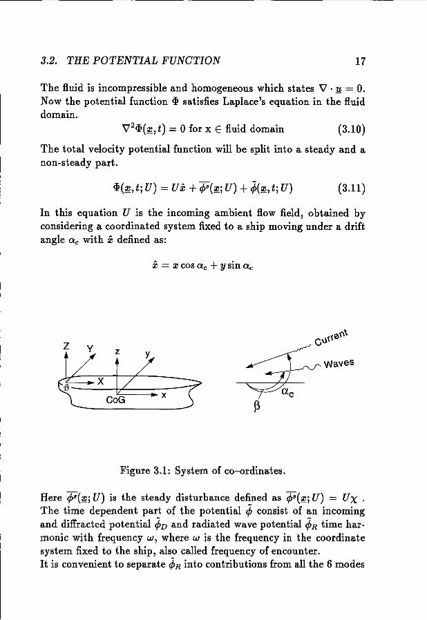
q.(.~, tj U) = u« +¢8(~j U) +~(~, tj U) (3.11)
In this equation U is the incoming ambient flow field, obtained byconsidering a coordinated system fixed to a ship moving under a driftangle Q c with :l: defined as:
:l: = :vcos Q c +Y sin Q c
z y z y
x
Figure 3.1: System of co-ordinates.
Waves
Here ¢8(~j U) is the steady disturbance defined as ¢8(~j U) = UXThe time dependent part of the potential ~ consist of an incomingand diffracted potential ~D and radiated wave potential ~R time harmonic with frequency w, where w is the frequency in the coordinatesystem fixed to the ship, also called frequency of encounter.It is convenient to separate ¢R into contributions from all the 6 modes
18 CHAPTER 3. MATHEMATICAL FORMULATION
z y
xu
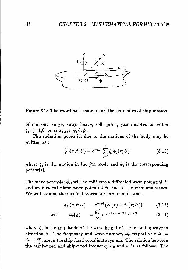
Figure 3.2: The coordinate system and the six modes of ship motion.
of motion: surge, sway, heave, roll, pitch, yaw denoted as eitherej, j=1,6 or as x,y,z,<p,O,,,p .
The radiation potential due to the motions of the body may bewritten as :
6
¢R(~' t;U) = e-iwt L ejcPJC~; U)j=1
(3.12)
where ej is the motion in the jth mode and cPj is the correspondingpotential.
The wave potential ¢D will be split into a diffracted wave potential cP7and an incident plane wave potential cPo due to the incoming waves.We will assume the incident waves are harmonic in time.
¢D(~,t; U)
with cPo(~)
= e-iwt (cPo(~) + cP7(~; U))
= gea eko[z+ixcos/Hivsin,13]
Wo
(3.13)
(3.14)
where ea is the amplitude of the wave height of the incoming wave indirection {3. The frequency and wave number, Wo respectively ko =
2
~ = 2;, are in the ship-fixed coordinate system. The relation betweenthe earth-fixed and ship-fixed frequency Wo and w is as follows: The
3.3. THE BOUNDARY CONDITION ON THE FREE SURFACE19
frequency in the earth-fixed coordinate system is:
W = Wo +koU cos({3 - ac ) (3.15)
3.3 The boundary condition on the freesurface
The vertical elevation of any point on the free surface may be definedby a function z = ((:v, y, t). Newman[47, chapter 6] shows that theeffects of the free surface must be expressed in terms of appropriateboundary conditions on this surface. In this section the free surfacecondition is derived in the frequency domain.The free surface condition for the non-steady part of the velocity potential can be computed by using equation (3.11) in (3.8). In appendixD the derivation is presented, applied for head current.The free surface condition now becomes formulated in the frequencydomain:
where D(X,¢) is a linear differential operator acting on ¢ as definedin the appendix (D).
We assume ¢(~, tj U) to be oscillatory (see section 3.2).
¢(~, tj U) = ¢D +¢R = (4)0 + 4>7 +i: 4>i(i) e-iwt = 4>(~j U)e-iwt
J=l
(3.17)From the appendix (D) we have the following expression for D(X,¢),neglecting non-linear terms and U2 terms:
(3.18)
We apply the Green's theorem to a problem in D, inside S and to theproblem in De outside S, where S is the ship's hull. The potential
20 CHAPTER 3. MATHEMATICAL FORMULATION
function inside S obeys condition (3.16) with D = 0, while far awayfrom the body the free surface condition reads:
(3.19)
The derivation of the Green's function will be treated in the nextchapter. In chapter 4 equations (3.16) and (3.19) will be used to derivea source and vortex distribution. The Green's function will satisfythe homogeneous adjoint far field free surface condition as defined inequation (3.16).The body boundary conditions for the diffraction problem have to betreated carefully, since the incoming wave potential 4>0 does not satisfythe free surface condition (3.8), while the incoming plus diffractedwave potential does satisfy the free surface condition (3.8 ). Denotingthe linear homogeneous far field free surface operator as L, we thenwrite:
(3.20)
which then results in the following free surface condition for ¢d' corrected for the incoming wave potential, with £, (¢o) = o.
(3.21)
(3.22)
3.4 The body boundary conditions
In this section the body boundary conditions are further defined. Thebody boundary conditions for the unknown radiation and diffractionpotential are (Newman[49]):
84>j(~j U) = { -iwnj +Umj j = 1,... ,68n 8<f>o j = 7-an
where
the Cartesian components of the normal vector g j = 1,2,3
n; = {the components of the vector ~ x n j = 4,5,6
3.5. THE STEADY POTENTIAL
and
21
= -en .V)(x x vex + (x cos a c + y sin a c )) ) j = 4,5,6mj = {
= -(n· V)(V(X + (x cos a c +ysin ac)) ) j = 1,2,3
. h ~WIt X = u :
The normal derivatives of each radiation potential consist of a partthat represents the normal velocity at the mean position of the bodyand a part that shows the change in the local steady field due to themotion of the body.The derivation of these body boundary conditions follows from thework of Timman and Newman [68].In appendix E the mj-terms are written in terms of the derivatives ofthe steady potential and the normal vector. The mj-terms also consistof second derivatives of the steady potential.The computation of these second derivatives is a difficult problem asmany authors (see Zhao and Faltinsen [82]) have outlined. To take thesecond derivative of a potential function defined as constant over a flatpanel is inconsistent. One way to avoid numerical difficulties in establishing the second derivatives is to use eg higher order panel methodsor just an approximative scheme, which calculates the flow in pointsat a certain distance from the vessel, and then perform the differentiation numerically and extrapolate the results to the body surface. In2-D Zhao and Faltinsen [82] have shown that this approach will givecorrect results. Wu [81] adapted the integral equation for the steadyvelocity, which he showed led to a higher accuracy of the derivative ofthe steady velocity.
3.5 The steady potential
This section gives the conditions of the steady potential, as used byHess and Smith[25).The steady part of the velocity potential is given by U(x cos a c +y sin a c ) + UX, where U (x cos a c +y sin a c ) is the ambient uniform
22 OHAPTER 3. MATHEMATIOAL FORMULATION
(3.23)
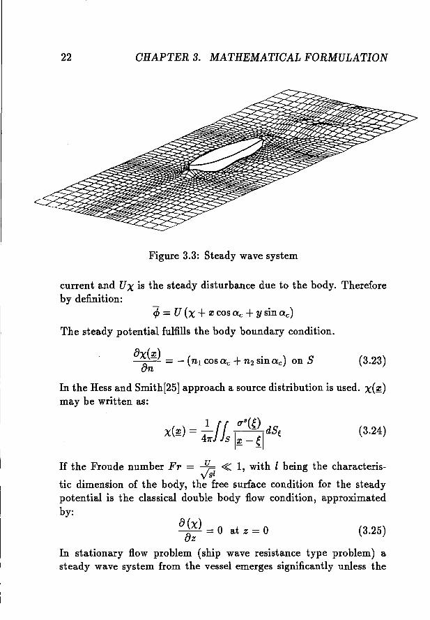
Figure 3.3: Steady wave system
current and UX is the steady disturbance due to the body. Thereforeby definition:
(fJ = U (X+z cos a c +y sin a c )
The steady potential fulfills the body boundary condition.
8~~~) = _ (nl cos a c +n2 sin a c ) on S
In the Hess and Smith[25] approach a source distribution is used. X(~)
may be written as:
(3.24)
If the Froude number Fr = ~ ~ 1, with I being the charaeteris-v 91
tic dimension of the body, the free surface condition for the steadypotential is the classical double body flow condition, approximatedby:
8(x) = 0 at z = 0 (3.25)8z
In stationary flow problem (ship wave resistance type problem) asteady wave system from the vessel emerges significantly unless the
3.5. THE STEADY POTENTIAL 23
Fn is very small. As an example of such a wave system the wavepattern around a vessel is depicted in figure 3.3. Now we can write:
with r = I~ - {I. From this expression it is evident that we only needtwo independent updates of the source strength with respect to thecurrent direction. The source strength for any other current directioncan then be readily determined. Denoting the source strength forO:c = 0 as lT~ and O:c = 90 as lTi, it follows that:
8() 8 8 .IT O:c = IT0 cos O:c + ITI sin O:c
To compute the body boundary condition we need an expressionfor the derivatives of the steady potential. The first derivatives of thesteady potential or the velocities can be determined without any difficulty from the expression of the potential as a source distribution. Inorder to determine the second order derivatives of the steady potential, use is made of a numerical differentiation schemeThe advantage of using a source distribution over a Morino formulation originates from the fact that the steady velocity is determinedwith the same accuracy as the source strength. Here the numericaldifferentiation is taken of the steady velocity. In the work of Prins[56] for the solution of the ship motion problem in time domain, use ismade of a numerical scheme to determine the double derivative of thesteady potential. He reports that this must be done with great care.
24 CHAPTER 3. MATHEMATIOAL FORMULATION
Chapter 4
Expansion of the potential
In this chapter the expansion of the potential is derived, using theintegral formulation (the free surface condition, equation (3.16)) andthe Green function of chapter 5.The first section treats the way Hermans and Huijsmans[24] derivedthe potential using a source distribution. The last section deals withthe amplitude of the potential for the far field.
4.1 The integral equation
First the source strength is computed by using the free surface conditions. An expansion of source strength is then derived. With thesource strength we are able to compute an expansion of the potential.
Combining the formulation inside and outside the ship, equations(3.16) and (3.19), we obtain a description of the potential functiondefined outside S by means of the source and vortex distribution. Theformulation is an extension of the one found in Brard [8].
/'r f) /'r 2iwUr- ls ,({) f)n G(~,{)dSe+ ls O"({)G(~,{)dSe - -9-1WL ,({)G(~,{)d"l+
+~2 fwL [1'({) :eG(." o- {Qn,({) +QT1'T({)}G(." o1d'1+
25

26 CHAPTER 4. EXPANSION OF THE POTENTIAL
U21 2iwufi+- anO"(e)G(~,e)d."+- G(~,e)D(x,¢)dSe = 41l"¢(~)9 WL - - 9 FS -
where at = cos(O:v,t), aT = cos(O:v, T) , an = cos(O:V,1!) and where nis the normal and t the tangent to the waterline, and T = t x n thebi-normal. Here G(~, {) is the Green's function satisfying the homogeneous free surface boundary condition.
(4.1)
i!=O
(4.2)
Figure 4.1: Coordinates at waterline.
It is clear that with the choice ,(f) = 0 the integral along the waterline gives no contribution up to order U. The source distributionwe obtain this way is not a proper distribution, because it expressesthe function ¢ in a source distribution along the free surface with astrength proportional to derivatives of the same function ¢. In orderto include the effect of the operator D on the integral equation, aniterative approach should be adopted. Based on updates of the potential ¢ and the velocity V¢ in the free surface an iterative procedurecould be formulated, but this approach has not been followed here.However, the formulation is linear in U and the integrand tends tozero rapidly for increasing distance R.So finally we arrive at the formulation:
f £O"({)G(~, {)dSe+ ~2 fWL anO"({)G(~,{)d."+
2iwUfi+- G(~,e)D(X,¢)dSe= 41l"¢(~)9 FS -
4.1. THE INTEGRAL EQUATION 27
Using the body boundary conditions, which are worked out in equation(3.22), at the mean position of the hull
8~~~) = v«. '!! = V(~) at ~ E S (4.3)
and taking a~., of equation (4.2) and taking the limit of :v E De toXES.
(4.4)
D(X, <jJ) is the linear differential operator acting on <jJ as defined inappendix (A). The quadratic terms in X are neglected. So D(X, <jJ) is- \lX\l<jJ - ~<jJ(Xxx +Xyy)·
The normal derivative -aa means the normal derivative with re-n.,sped to ~ = (:v, y, z).The formulation obtained thus far does not give any new view onthe integral equation with forward speed, except that the free surface term has been added. Apart from the steady potential influenceequation (4.4) is equivalent to the formulations used by Inglis [34] orBougis [6]. The Green's function as it appears in equation (4.4) isstill the translating oscillating source as formulated by Wehausen andLaitone [74] and subsequently used for the ship motion problem byInglis, Bougis and others. One of the main drawbacks of the use ofthis Green's function formulation is the rather cumbersome way it iscomputed. To date little progress has been made in trying to compute this Green function as efficiently as, for example; in the zerospeed Green's function demonstrated by Newman [46] or Telste andNoblesse [66]. Therefore, we shall impose an additional restriction onthe use ofthis Green's function: it will only be applied for low speedsor more correctly for low Brard numbers (r = wgu ~ 1/4).
It is interesting to note that in classical forward speed formulation,in which the steady potential is neglected, a contribution over the
28 CHAPTER 4. EXPANSION OF THE POTENTIAL
waterline is seen. Careful analysis by Nossen [52] did show that thisterm is cancelled once the steady potential is taken into account.
We consider small values of U, such that T = ~w < ~. The sourcestrength and potential function will be expanded as follows:
o"j({,U)
¢;(~, U)O"jO(e)+TO"j1 (e) +O(T2
)- -¢jo(~) +T¢j1(~) +O(T2
)
(4.5)
(4.6)
And for the Green's function we write:
G(~,{) = Go(~,{) + T"p1(~'{) +~o(~,{) (4.7)
where Go(~,{) is the zero speed Green's function.
1Go(~, {) = - +"po(~, {)- r -
We now can write equation (4.4), at ~ E S, for j = 1, ... ,7:
(4.8)
and
(4.9)
(4.10)
(4.11)j = 1, ... ,6j=7
where Go(~,{) = : +"po(~,{), with"po is the zero speed pulsating wavesources, and l-j(~jU) = l-jo(~) +Tl-j1(~)+O(T2 ) as in equation (3.22).
{-iwnj j = 1, ... ,6-~~ j = 7
{~ij;s a~z GoD(X, ¢o)dSeThe subscripts jO and j1 mean respectively the zero- and first-orderexpansion in the jth mode of motion.
4.1. THE INTEGRAL EQUATION 29
In solving the integral equations (4.8) and (4.9) we encounter theproblem of the irregular frequency phenomena. The existence of theseirregular frequencies for the water wave problem dates back to thepublications of John [37, 36] in 1950.
Since the ship motion problem is formulated at forward speed, thisgives rise to encounter frequencies higher than the frequencies normally used in the ship motion problem at zero speed for head andbow quartering waves. As will be made clear later on, the effect of" irregular frequencies" will influence the numerical solution of theproblem. These so-called irregular frequencies tend to enter the shipmotion problem at higher frequencies (this however actually also depends on the geometry of the vessel). Therefore attention will be paidto reduce the effect of the irregular frequencies on the ship motionproblem.
For V7 we see that cPo depends of wand wo, which in turn dependson the speed of the vessel. Since cPo does not satisfy the free surfacecondition (3.8) we correct the cP7 in order to let cP7 + cPo satisfy thefree surface condition (3.8). From the analysis in chapter 3 we seethat the last term in (4.11) gives the necessary correction. We have totake care that w does not become too small, because then the factor Jl
wbecomes too large. When we use an asymptotic expansion, the termsof the expansion have to be of the same order. So a small w makes thefirst order term become much larger than the zero order term. In thatcase we are trying to make an asymptotic expansion for both smallT as well as small w. A similar approach, but for small w, has beengiven by Van de Stoep [71].
The potential function equation (4.6) now becomes:
cPjo(~) 4~JIs O"jo({)Go(~, {)dSe (4.12)
cPjl(~) 4~JIs O"jo({Nh(~,{)dSe +4~JIs O"jl({)Go(~,{)dSe
+2i J' r Go(~,e)D(X,cPjo)dSe1[" JF S -
(4.13)
So when we compute O"jO and O"jl with the equations (4.8) and (4.9),
30 CHAPTER 4. EXPANSION OF THE POTENTIAL
we can evaluate ¢jO and ¢j1 from the equations (4.12) and (4.13).
From the body boundary condition can be seen that the second derivative of the steady potential must be computed. Section 3.5 describeshow we arrive at a numerical value of these quantities.
The integral equations for the source strength 0'0 and 0'1 are solvedusing a conventional panel method. We approximate the mean wetted surface of the body by quadrilateral panels for which we assumeconstant source strength over the panel. The integration of the rankine source part of the Green's function was discussed by Fang [15].Because of some misprints in his original publication, the integrationover a panel of 1fr and :n (lfr) is reiterated in the appendix C. Thefrequency dependent part of the Green's function is integrated usingEuler. The algebraic equations that follow after the discretization ofthe integral equations can be solved either using classical LU decomposition or by using an iterative solver. The latter is more useful if onerequires large number of panels. The iterative scheme used is basedon a method published by Sonneveld [65]. His method pivots aroundthe use of conjugated gradient type of methods for non-self adjointoperators. For a review of these type of methods one is referred to thework of Van de Vorst [73, 72].
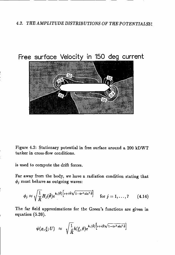
In the right hand side of the integral equation (4.9) for O'}, anintegration has to be made over the entire free surface around thebody. The extent of this integration over the free surface is, however,limited due to the fact that the steady potential disturbance behaveslike a dipole, the integrand decays like R-4 with R being the polardistance to the vessel. An example of the extent of the influence ofthe stationary potential over the free surface is given in figure 4.2.
4.2 The amplitude distributions of thepotentials
In this section the far field potential is described. We define Hj as theamplitude of this potential. We need this amplitude to compute thefirst and second order wave forces in chapter 6. The sum of the Hi's
4.2. THE AMPLITUDE DISTRIBUTIONS OF THE POTENTIALS31
Free surface Velocity in 150 deg current
Figure 4.2: Stationary potential in free surface around a 200 kDWTtanker in cross-flow conditions.
is used to compute the drift forces.
Far away from the body, we have a radiation condition stating that<Pi must behave as outgoing waves:
,/.,J' ~ flR
1_HJ·(()-)ek1(6) [z+iRV1-472
sin2 0]
'I' . - VR for j = 1, ... , 7 (4.14)
The far field approximations for the Green's functions are given inequation (5.30).
32 CHAPTER 4. EXPANSION OF THE POTENTIAL
with the amplitude
h(e, 8) = rs;k1(8)ek 1(0) [c+ie( - cos 0-2Tsin2 O)+il'/(- SinO+2T cos osin0)]+i-I
- V---;;:where
k1(8) = K(l +2r cos 8)+O( r 2) (4.15)
The function H results from the asymptotic expansion of the far fieldpotentials in equation (4.2).
471"4>j(~) = +/LO"({)G(~, {)dSe+
+2irJ' f G(~, e)D(X,4>jo)dSe}FS -
So the amplitude H of the potentials becomes
Hj(8) = +4~ / L O"j({)h(e, 8)dSe+
+~: / ks h(e,8)D(X, 4>io)dSe (4.16)
with h(e,8) as in equation (5.31).
The amplitude of potential H is the result of the following equation:
471"4>j = J' f [4> 0 o"p -"p o4>j] dS +ls J on on
+2ir/ks[4>jD(x,4>j)]dS (4.17)
So the amplitude H of the potentials becomes, with Tuck's theorem:
H·(6) = +~J'r [4> oOh - (h-~V(X+Z)Vh)no]dS+J 471" ) S J on 7,K J
-tn [4>jD(X,h)]dS (4.18)271" }FS
H7(8) = +4~JL4>D~~dS+ ~:JLs4>DD(x,h)dS (4.19)
We need the sum of the H/s to compute the drift forces. We define:6
H(8) = H7 +iw L H(j)(jj=l
(4.20)
Chapter 5
The Green's function
To solve the integral equation (equation (4.4) ), we have to computethe Green's function. Once the expression for the Green's function isfound we then can compute the source and the potential distributions.The first section of this chapter! gives the asymptotic expansion of theGreen's function. In the second section the zero order Green's function 'l/Jo is treated. The third section gives two ways to compute thefirst order Green function 'l/Jl: a transformation in the complex planeand an expression based on the derivatives of the zero order Green'sfunction. The fourth section deals with the non-uniformity of the firstorder Green function. In the last section we derived the derivativesof the first-order Green's function. We need these derivatives for thepotential expansions in the next chapter.
5.1 The expansion of the Green's function
In this section we present an asymptotic expansion of the Green'sfunction. The Green's function has to satisfy the conditions on thevelocity potential ~(:z:,y,z,t)= G(~,{;U)exp(-iwt):
IThe subscripts 0 and 1 in this chapter are the terms of the asymptotic expansion and not the modes of motion as in the preceeding chapter.
33
34 CHAPTER 5. THE GREEN'S FUNCTION
1. V 2<.L> = 0, z < 0, (X,y,Z) =I- (e,"1,() (Laplace's equation)
2. <.L>tt + 2U<.L>xt +U2<.L>xx +g<.L>z(x,y,O,t) =°at mean water level
3. <.L>(x,y,z,t) = co~wt +~(x,y,z,t),
-t/J harmonic everywhere in z <°4. limz--+_ oo V<.L> = 0 for all x, y, t (no flux on the sea-floor)
5. limR--+oo V<.L> = ° for all t,R2 = (x -e)2 + (y-"1)2
6. <.L>(x,y, 0, 0) = <.L>t(x,y, 0, 0) = °In accordance with Wehausen [74] we introduce:
1 1G(~,eiU) = - - - +'ljJ(~,e;U) (5.1)
- r rl -
where r = I~ - {I and rl = I~ - e'l·e' is the image of ewith respect to the free surface. This means with{ = (e,"1,(), r~ = ex - e)2 + (y - ",)2 + (z + ()2.
The Green's function follows from the oscillatory translating sourcefunction presented in Wehausen and Laitone[74]. In the case T < ~,
where T = w;r, the function .,p(~, {; U) is written as follows:
'ljJ(~, ei U) = 2g f!j dO f dk F(0,k) + 2g t' dO f dk F(0,k) (5.2)- 7r 10 1£1 7r 1!j 1£2
where
k . ek[z+e+i(x-e) cosO] cos[k(y - ",) sin 0]F(O, k) = ( ) (5.3)gk - w +kU cos 0 2
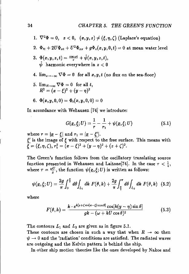
The contours L 1 and L 2 are given as in figure 5.1.These contours are chosen in such a way that when R ~ 00 then'ljJ ~ °and the 'radiation' conditions are satisfied. The radiated wavesare outgoing and the Kelvin pattern is behind the ship.
In other ship motion theories like the ones developed by Nakos and
5.1. THE EXPANSION OF THE GREEN'S FUNCTION 35
k1 k2
\J G .. ot1k3 k4 ot2\J V ..
Figure 5.1: Contours of integration.
1't < 4
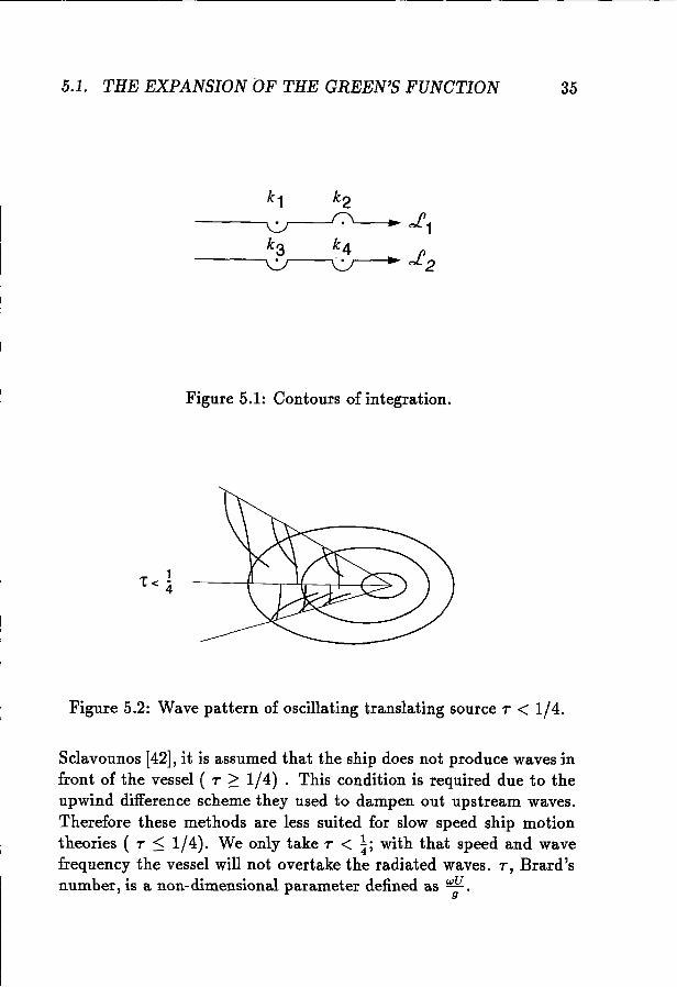
Figure 5.2: Wave pattern of oscillating translating source T < 1/4.
Sclavounos [42], it is assumed that the ship does not produce waves infront of the vessel ( T 2: 1/4) . This condition is required due to theupwind difference scheme they used to dampen out upstream waves.Therefore these methods are less suited for slow speed ship motiontheories ( T :::; 1/4). We only take T < ~j with that speed and wavefrequency the vessel will not overtake the radiated waves. T, Brard'snumber, is a non-dimensional parameter defined as w~.
36 OHAPTER 5. THE GREEN'S FUNCTION
The values k, are the poles of F((},k). So: gki - (w +kiU cos (})2 = O.We have to pay attention to the value of cos (} in both the integrals inequation (5.2): in the first integral 0 ~ (} ~ j, so cos (} is negative andin the other integral cos (} is positive.The values of k; behave as follows:
Jgkb Jgk3
J9k2 , -~
1 - VI - 4r cos (}------w
2r cos (}1 +Vl- 4rcos(}----'-----w
2r cos ()For small values of r these poles behave as follows:
../gk1 ,~ rv W +O(r)} 0r::r fN as r -+J9!i;., -v gn;4 rv TCOS(} +0(1)
(5.4)
(5.5)
(5.8)
(5.7)
A careful analysis of the asymptotic behaviour of "p(~, {; U) for smallvalues of r leads to a regular and an irregular part.
_ U2 _
"p(~,e; U) = .,po(~,e) + r.,p1(~,e) + ... + .,po(~,O + -.,p1(~,e) + .. '5.6)- - - - 9 -
In Hermans and Huijsmans [24] (see appendix F) it is shown thatdue to the highly oscillatory behaviour the influence of "fio may beneglected in our first order correction for small values of r .
The behaviour of k1 and k3 gives rise to a regular perturbation serieswith respect to r . In contrast, k2 and k4 originates a highly oscillatingcontribution which gives rise to a non-uniform expansion. However,the position of the last two poles moves to infinity, therefore it can betreated separately. If r -+ 0, the contours L1 and L2 become the same(figure 5.3). With K = ~2 it follows:
r kek(z+c).,po(~,{) = 2JL k _ K Jo(kR)dk
r k2ek(z+c)
"p1(~' {) =4i cos (}'JL (k _ K)2 J1(kR)dk
where (}' = arctan ~=e 'or in an other way R cos (}' = :l: - e.
5.2. THE ZERO ORDER GREEN'S FUNOTION "po
k=K ----..k
Figure 5.3: Contours of integration.
37
5.2 The zero order Green's function "po
In this section the zero-order Green's function of the asymptotic ex-. . .pansion IS given.
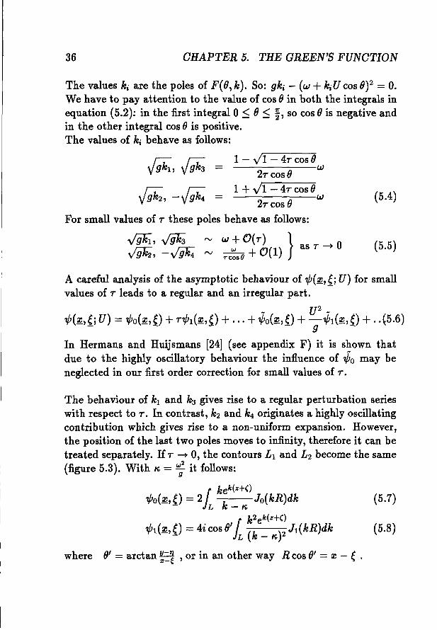
The equation (5.7) for"po can be split into the residue and the principalvalue integral.
,r k k(z+C)7ri {2kek(z+c) Jo(kR)}k=K. +2 . PVjL ~ _ n Jo(kR)dk =
l. kek(z+c)27rineK.(z+C)Jo(nR) +2· PV k Jo(kR)dk (5.9)
L - n
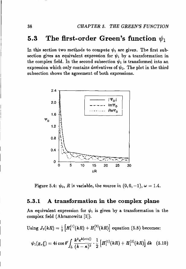
The zero-order Green's function, without the Rankine singularity ~ iscomputed in the algorithm FINGREEN, derived by Newman [45].So in FINGREEN (;1 + "po) is computed. Figure 5.4 shows the behaviour of the amplitude of 1.. +"po, the real and imaginary part (in
T1
the figure respectively "po, Re"po and Im"po).
38 CHAPTER 5. THE GREEN'S FUNCTION
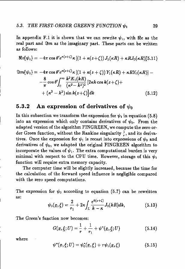
5.3 The first-order Green's function "p1
In this section two methods to compute 'l/Jl are given. The first subsection gives an equivalent expression for 'l/Jl by a transformation inthe complex field. In the second subsection 'l/Jl is transformed into anexpression which only contains derivatives of'l/Jo. The plot in the thirdsubsection shows the agreement of both expressions.
30252015
kR
I 'flo I----- Im'l'o... - - ... - . Re'l'0
105
I
\~\~:\:\: \'''''-.',-" .".. '....... .."... ';"""'.,(..."" ~- .. - ............ -
• '., J"'''' •• ' _,/ ... .-. _....-:. _;--'.:....
0+---~-~-~------':"~--1
o
2.4
2.0
1.6'flo
1.2
0.8
0.4
Figure 5.4: 'l/Jo, R is variable, the source in (0,0, -1), w = 1.4.
5.3.1 A transformation in the complex plane
An equivalent expression for 'l/Jl is given by a transformation in thecomplex field (Abramowitz [1]).
Using J1(kR) = ~ [HIl)(kR) +HI2)(kR)] equation (5.8) becomes:
5.3. THE FIRST-ORDER GREEN'S FUNCTION .,pI 39
In appendix F.1 it is shown that we can rewrite .,pI, with ~e as thereal part and S'm as the imaginary part. These parts can be writtenas follows:
S'm{.,pI} = -471" cos ()'elt(z+() K[(1 +K( z +()) Yi (KR) +KRYO( KR)] -8 ,(00 v KI (kR)
-; cos ()'Jo (K2 - k2 ) 2 [2Kkcosk(z+()+
+ (K2- k2)sink(z+()]dk (5.12)
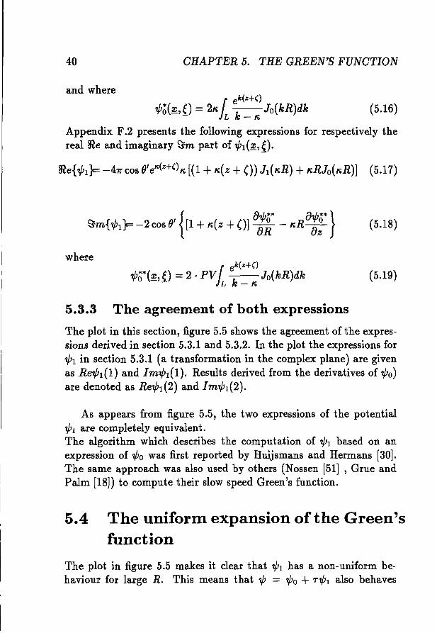
5.3.2 An expression of derivatives of 'l/Jo
In this subsection we transform the expression for.,pI in equation (5.8)into an expression which only contains derivatives of .,po. From theadapted version of the algorithm FINGREEN, we compute the zero order Green function, without the Rankine singularity ~, and its derivatives. Once the expression for .,pI is recast into expressions of .,po andderivatives of .,po, we adapted the original FINGREEN algorithm toincorporate the values of .,pl' The extra computational burden is veryminimal with respect to the CPU time. However, storage of this .,pIfunction will require extra memory capacity.
The computer time will be slightly increased, because the time forthe calculation of the forward speed influence is negligible comparedwith the zero speed computations.
The expression for .,po according to equation (5.7) can be rewrittenas:
2 /, ek(z+().,po(~,e) = - +2K k Jo(kR)dk,
- 1'1 L - K
The Green's function now becomes:
where
(5.13)
(5.14)
(5.15)
40
and where
CHAPTER 5. THE GREEN'S FUNCTION
rek(z+()
.,p~(~,{) = 2K1£ k _ K JO( kR)dk (5.16)
Appendix F.2 presents the following expressions for respectively thereal ~e and imaginary ~m part of .,pl(~'{)'
{8.,p** 8.,p** }
~m{.,pIF -2 cos 0' [1+K( Z +0] 8~ - KR 8;
where .r k(z+().,p~*(~,{) = 2· PVJLe
k_ K Jo(kR)dk
5.3.3 The agreement of both expressions
(5.18)
(5.19)
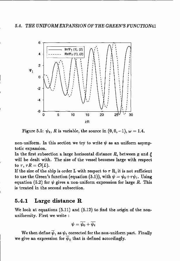
The plot in this section, figure 5.5 shows the agreement of the expressions derived in section 5.3.1 and 5.3.2. In the plot the expressions for.,pI in section 5.3.1 (a transformation in the complex plane) are givenas Re.,pl (1) and Im.,pI(1). Results derived from the derivatives of .,po)are denoted as Re.,pl(2) and Im.,pI(2).
As appears from figure 5.5, the two expressions of the potential.,pI are completely equivalent.The algorithm which describes the computation of .,pI based on anexpression of .,po was first reported by Huijsmans and Hermans [30].The same approach was also used by others (Nossen [51] , Grue andPalm [18]) to compute their slow speed Green's function.
5.4 The uniform expansion of the Green'sfunction
The plot in figure 5.5 makes it clear that .,pI has a non-uniform behaviour for large R. This means that .,p = .,po + T.,pl also behaves
5.4. THE UNIFORM EXPANSION OF THE GREEN'S FUNCTION41
6,'\
I \ ,4
I I I------ I II I
I I I I II I I I, I I I2 , I I II I I I
'1'1 I I I II
,I ,
\ I I I0 I I ,
II I ,
II r I II I I ,I I I I
-2 I,
I II
,I I, I I II I II ,
I-4 \ I
I
" I
I I
\,
\,
-60 5 10 15 \1 30
kR
Figure 5.5: 'l/;b R is variable, the source in (0,0, -1), w = 1.4.
non-uniform. In this section we try to write 'I/; as an uniform asymptotic expansion.In the first subsection a large horizontal distance R, between ~ and {will be dealt with. The size of the vessel becomes large with respectto r , r R = O(L).If the size of the ship is order L with respect to r R, it is not sufficientto use the Green's function (equation (5.1)), with 'I/; = 'l/;0+r'l/;1' Usingequation (5.2) for 'I/; gives a non-uniform expression for large R. Thisis treated in the second subsection.
5.4.1 Large distance R
We look at equations (5.11) and (5.12) to find the origin of the nonuniformity. First we write:
We then define '1/;1 as '1/;1 corrected for the non-uniform part. Finallywe give an expression for '1/;0 that is defined accordingly.
42 OHAPTER 5. THE GREEN'S FUNOTION
The first-order Green's function can be written as.,pI = ~e{.,pl} +i . S'm{.,pl}' This gives:
.,pl(~'{) = -411"cosO'elt(z+C) [~H}I)(~R) + ~2(z +()HP)(K,R)
+ K,2RH~I)(K,R)] -
8i , roo k2K1(kR)--:; cos 0 1
0(K,2 _ k2)2 {2K,k cos k(z+()
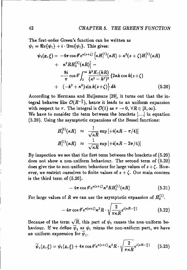
+ (_k2+ K,2) sin k(z+O} dk (5.20)
According to Hermans and Huijsmans [29], it turns out that the integral behaves like O(R-~), hence it leads to an uniform expansionwith respect to T. The integral is 0(1) as T -+ 0, VR E [0,00).We have to consider the term between the brackets [...] in equation(5.20). Using the asymptotic expansions of the Bessel functions:
HJI) (K,R)
HP)(",R)
~ ~ exp [+i(K,R -11"/4)]vK,R
~ ~ exp [+i(K,R - 311"/4)]vK,R
By inspection we see that the first term between the brackets of (5.20)does not show a non-uniform behaviour. The second term of (5.20)does give rise to non-uniform behaviour for large values of z +(. However, we restrict ourselves to finite values of z +(. Our main concernis the third term of (5.20).
- 411" cos O'eK(z+C)K,2 RHJI) (K,R) (5.21)
For large values of R we can use the asymptotic expansion of Hd l) .
- 411" cos 0'elt(z+C) K,2 R . V2 ei(KR-·V (5.22)1I"~R
Because of the term VR, this part of .,pI causes the non-uniform behaviour. If we define .,pI as .,pI minus the non-uniform part, we havean uniform expression for .,pl'
.,pl(~' e) = .,pl(~' 0 + 411" cos O'elt(z+C) K,2 R· V2R ei(ItR-i) (5.23)- - 1I"K,
5.4. THE UNIFORM EXPANSION OF THE GREEN'S FUNCTION43
6
5
1------4 LV'¥1
'1'1 '1'1
3
2
"I \, "I --- ---- ------------------
10 15 20 25 30
kR
5O-l---~-~-~-~-----1
o
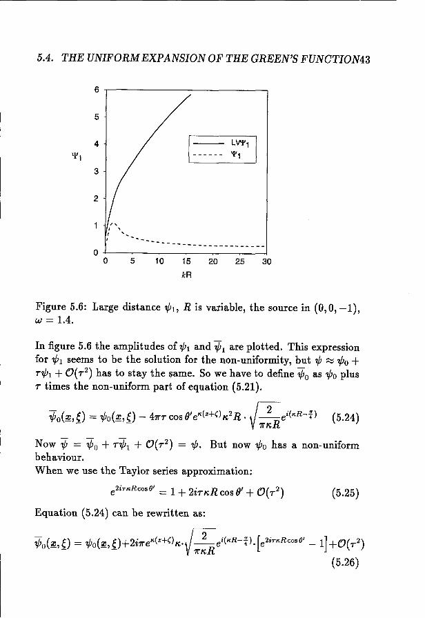
Figure 5.6: Large distance wj , R is variable, the source in (0,0,-1),w = 1.4.
In figure 5.6 the amplitudes of .,pI and .,pI are plotted. This expressionfor .,pI seems to be the solution for the non-uniformity, but .,p ~ .,po +T.,pI + O(T2) has to stay the same. So we have to define .,po as .,po plusT times the non-uniform part of equation (5.21) .
.,po(~, e) = .,po(~, e) - 47l"T cos f)' elt(z+() /'i,2 R • V 2R ei(ItR-1) (5.24)- - 7l"K
Now .,p = .,po + T.,pI + 0(T2) =.,p. But now.,po has a non-uniformbehaviour.When we use the Taylor series approximation:
(5.25)
Equation (5.24) can be rewritten as:
.,poC~,{) = .,po(~,{)+2i7l"elt(z+')/'i,·V7l"~Rei(ItR-1L[e2iTItRCOS8' -1]+0(T2)
(5.26)
44 CHAPTER 5. THE GREEN'S FUNCTION
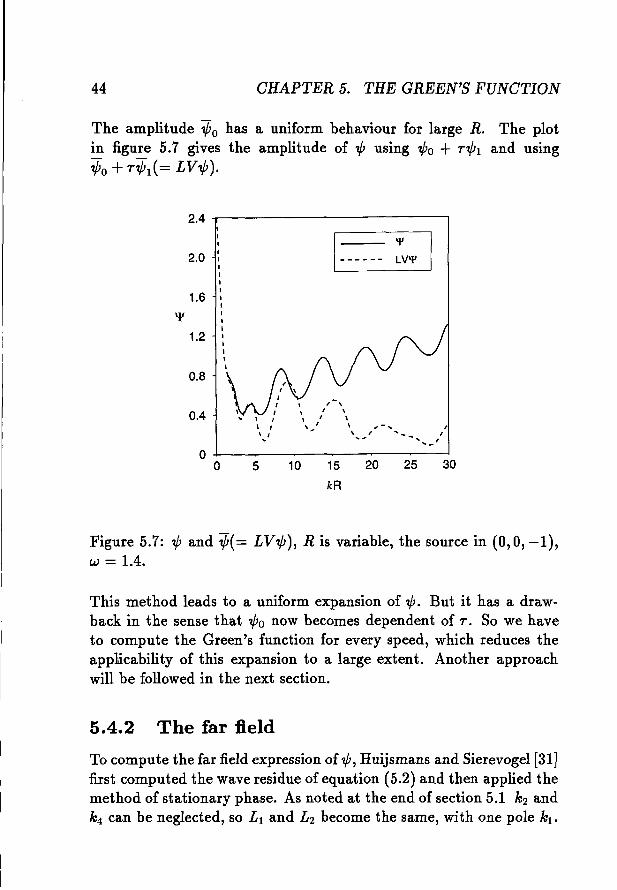
The amplitude "po has a uniform behaviour for large R. The plotin figure 5.7 gives the amplitude of "p using "po + T"p1 and using"po + T"p1(= LV"p).
2.4 ,----------------,
2.0'I'
LV'I'
1.6
'¥
1.2
0.8
0.4\ '\ I\ I
\ ~ I
\\\
', r > ....,~
,I, ,
,~
10 15 20 25 30
kR
5O-l----~---~--~---I
o
Figure 5.7: "p and "p(= LV"p), R is variable, the source in (0,0, -1),w = 1.4.
This method leads to a uniform expansion of"p. But it has a drawback in the sense that "po now becomes dependent of T. SO we haveto compute the Green's function for every speed, which reduces theapplicability of this expansion to a large extent. Another approachwill be followed in the next section.
5.4.2 The far field
To compute the far field expression of"p, Huijsmans and Sierevogel [31]first computed the wave residue of equation (5.2) and then applied themethod of stationary phase. As noted at the end of section 5.1 k2 andk4 can be neglected, so L1 and L2 become the same, with one pole k1 •
5.4. THE UNIFORM EXPANSION OF THE GREEN'S FUNCTION45
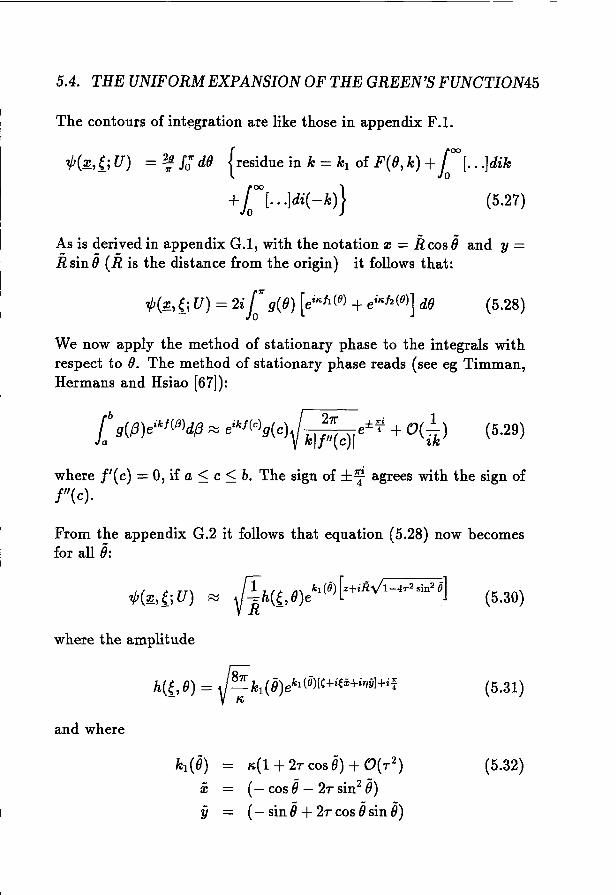
The contours of integration are like those in appendix F.1.
'lj;(;J1, {; U) = ~ fo1r dO {residue in k = k1 of F(0,k) +1000
[ •• •]dik
+1000
[•••]di(-k)} (5.27)
As is derived in appendix G.l, with the notation :I: = Rcos 8 and y =Rsin 8 (R is the distance from the origin) it follows that:
(5.28)
We now apply the method of stationary phase to the integrals withrespect to e. The method of stationary phase reads (see eg Timman,Hermans and Hsiao [67]):
(5.29)
where f'(c) = 0, if a:::; c:::; b. The sign of ±~i agrees with the sign off"(C).
From the appendix G.2 it follows that equation (5.28) now becomesfor all 8:
(5.30)
where the amplitude
and where
(5.31)
y
K(1 +2r cos 0) +O(r 2)
(- cos B- 2r sin2 8)(- sin 8+2r cos fJ sin fJ)
(5.32)

46 CHAPTER 5. THE GREEN'S FUNCTION
2.4 x'f- ---,
302515 20
kR
10
- - -* --
w
I
,X .... """ "X ~ I "xx" \ ,
~\ " '\,' '>l.I \ I \ I
I \)< XI )(,
5O~-~-_-~~-'--~"'--'__'--L.--l
o
0.4
2~O IIIII
1.6 ~IIIIII
0.8
'I'
1.2
Figure 5.8: "p and FF"p, R is variable, the source in (0,0, -1), w = 1.4.
In figure 5.8 the amplitudes of"p and the far field approximation of"p(= FF"p) are given.
It is clear that the far field expression for "p is an uniform expression. But we have the same problem as in subsection 5.4.1: we haveto compute the Green's function for every speed, because we cannotexpand "p like "po + r"pI'
The following solution is adopted: we only use the asymptotic expansion at a finite distance from the source point. When IKRI > 1 thesecond order Green's function has a non-uniform behaviour, but thefar field Green function can be described by the zero order Green'sfunction "po. So when IKRI > 1 we can set "pI equal to 0.Once the expressions for "pI are found, the derivatives of "pI with respect to Rand Z can then determined. The complete expressions aregiven in appendix F.
5.5. SUPPRESSION OF IRREGULAR FREQUENCIES 47
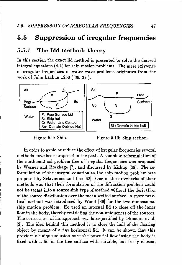
5.5 Suppression of irregular frequencies
5.5.1 The Lid method: theory
In this section the exact lid method is presented to solve the derivedintegral equations (4.4) for ship motion problems. The mere existenceof irregular frequencies in water wave problems originates from thework of John back in 1950 ([36, 37]).
Surface
Free
S
ISi : Domain inside hull
Water
Air
F: Free Surface LidS: Ship hullC: Water Line ContourSo: Domain Outside Hull
Water
Air
Free_~--~
Surface
Figure 5.9: Ship. Figure 5.10: Ship section.
In order to avoid or reduce the effect of irregular frequencies severalmethods have been proposed in the past. A complete reformulation ofthe mathematical problem free of irregular frequencies was proposedby Werner and Brakhage [7], and discussed by Kirkup [39]. The reformulation of the integral equation to the ship motion problem wasproposed by Sc1avounos and Lee [62]. One of the drawbacks of theirmethods was that their formulation of the diffraction problem couldnot be recast into a source sink type of method without the derivationof the source distribution over the mean wetted surface. A more practical method was introduced by Wood [80] for the two-dimensionalship motion problem. He used an internal lid to close off the innerflow in the body, thereby restricting the non-uniqueness of the sources.The correctness of his approach was later justified by Ohmatsu et al.[2]. The idea behind this method is to close the hull of the floatingobject by means of a flat horizontal lid. It can be shown that thisprovides a unique solution once the potential flow inside the body isfixed with a lid in the free surface with suitable, but freely chosen,
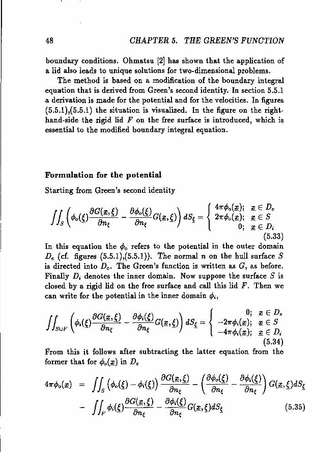
48 OHAPTER 5. THE GREEN'S FUNOTION
boundary conditions. Ohmatsu [2] has shown that the application ofa lid also leads to unique solutions for two-dimensional problems.
The method is based on a modification of the boundary integralequation that is derived from Green's second identity. In section 5.5.1a derivation is made for the potential and for the velocities. In figures(5.5.1),{5.5.1) the situation is visualized. In the figure on the righthand-side the rigid lid F on the free surface is introduced, which isessential to the modified boundary integral equation.
Formulation for the potential
Starting from Green's second identity
~ E De~ES
~ E D i
(5.33)In this equation the cPo refers to the potential in the outer domainDe (cf. figures (5.5.1),(5.5.1)). The normal n on the hull surface Sis directed into De. The Green's function is written as G, as before.Finally D, denotes the inner domain. Now suppose the surface S isclosed by a rigid lid on the free surface and call this lid F. Then wecan write for the potential in the inner domain cPi,
f1 (cPi{{) 8G8~' {) - 8:~{) G(~,{)) dS{ = { -27rcPi(~~~ : ~ ~esuF e e -47rcPi{~); ~ E D,
(5.34)From this it follows after subtracting the latter equation from theformer that for cPo{~) in De
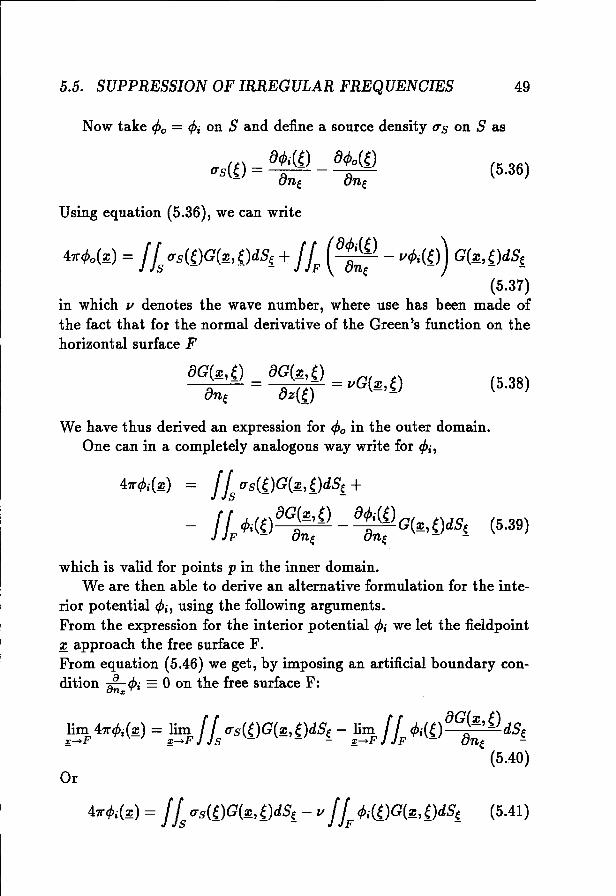
5.5. SUPPRESSION OF IRREGULAR FREQUENOIES 49
Now take cPo = cPi on S and define a source density Us on S as
(5.36)
Using equation (5.36), we can write
t f j' f (8cPi(e) )47l"cPoC~) = Js us({)G(~, {)dS{ + JF 8n; - VcPi({) G(~, {)dS{
(5.37)in which v denotes the wave number, where use has been made ofthe fact that for the normal derivative of the Green's function on thehorizontal surface F
8G(~1 {) = 8G(~, {) = G( t)8ne 8z({) v~,~
(5.38)
We have thus derived an expression for cPo in the outer domain.One can in a completely analogous way write for cPi'
which is valid for points p in the inner domain.We are then able to derive an alternative formulation for the inte
rior potential cPi' using the following arguments.From the expression for the interior potential cPi we let the fieldpoint~ approach the free surface F.From equation (5.46) we get, by imposing an artificial boundary condition -aa4>i - 0 on the free surface F:n.,
:5 47l"4>i(~) = :51Is us({)G(~, {)dS{ - :51L4>i({)8~:; e) dS{
(5.40)Or
(5.41)
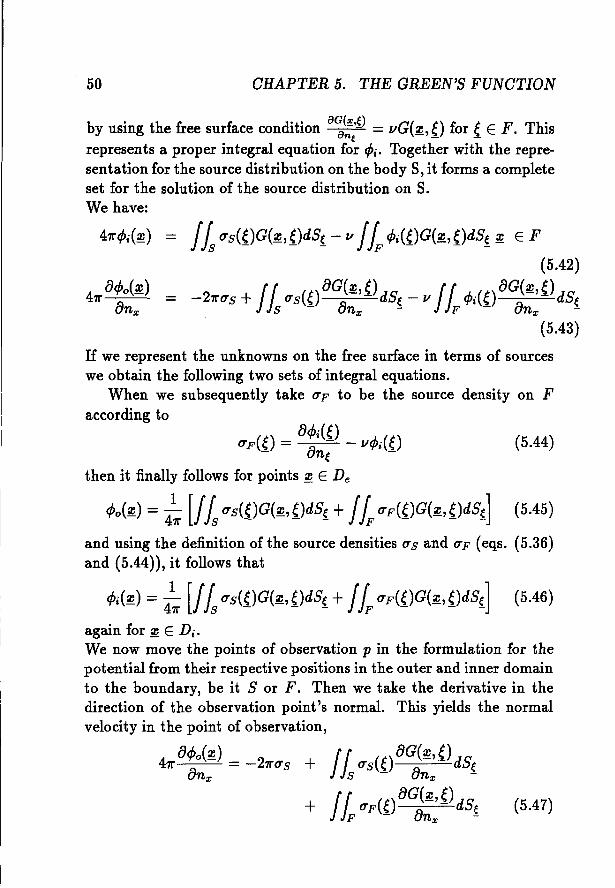
50 CHAPTER 5. THE GREEN'S FUNCTION
by using the free surface condition 8~~~) =vG(~,{) for { E F. Thisrepresents a proper integral equation for cPi. Together with the representation for the source distribution on the body S, it forms a completeset for the solution of the source distribution on S.We have:
/Is U8({)G(~, {)dS~ - v / LcPi({)G(~, {)dS~ ~ E F
(5.42)
-27r0"8 + f'r O"s(e) 8G(~, e) is, - v f' r(h(e) 8G(~, e)es,Js - 8nx - JF - 8nx -
(5.43)
If we represent the unknowns on the free surface in terms of sourceswe obtain the following two sets of integral equations.
When we subsequently take UF to be the source density on Faccording to
O"F({) = 8:~:) -V¢i({) (5.44)
then it finally follows for points ~ E De
cPo(~) = 4~ [/Is O"s({)G(~,{)dS~ +/LO"F({)G(~,{)dS~] (5.45)
and using the definition of the source densities as and O"F (eqs. (5.36)and (5.44)), it follows that
cPi(~) = 4~ [/Is O"s({)G(~, {)dS~ +/LO"F({)G(~, {)dS{] (5.46)
(5.47)
/Is O"s({)8~~~ {) dS{
+ /LO"F({) 8~':~ {) dS{
again for ~ E Di.We now move the points of observation p in the formulation for thepotential from their respective positions in the outer and inner domainto the boundary, be it S or F. Then we take the derivative in thedirection of the observation point's normal. This yields the normalvelocity in the point of observation,
4 8cPo(~) 2 +7r 8 = - 7rO"s
n x
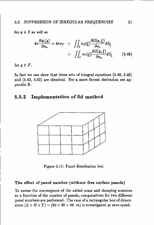
5.5. SUPPRESSION OF IRREGULAR FREQUENOIES 51
for ~ E S as well as
(5.48)
for ~ E F.
In fact we can show that these sets of integral equations (5.48, 5.48)and (5.42, 5.43) are identical. For a more formal derivation see appendix B.
5.5.2 Implementation of lid method
Figure 5.11: Panel distribution box
The effect of panel number (without free surface panels)
To assess the convergence of the added mass and damping matricesas a function of the number of panels, computations for two differentpanel numbers are performed. The case of a rectangular box of dimensions (L x B x T) = (90 x 90 x 40 m) is investigated at zero-speed.
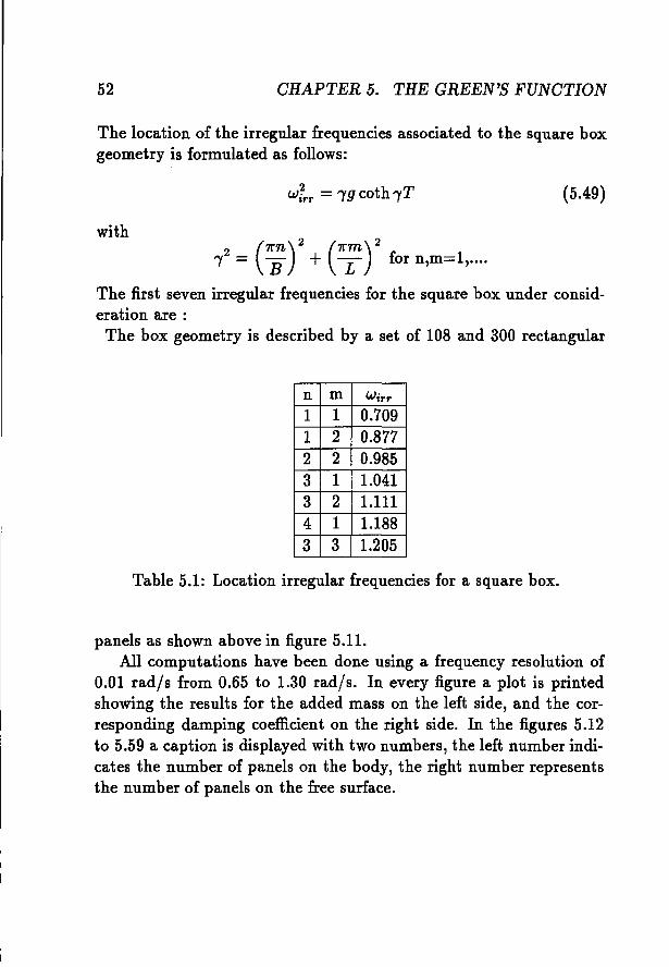
52 OHAPTER 5. THE GREEN'S FUNOTION
The location of the irregular frequencies associated to the square boxgeometry is formulated as follows:
with
W;rr = "'(9 coth "'(T (5.49)
(7rn)2 (7rm) 2"'(2 = Ii + L for n,m=l,....
The first seven irregular frequencies for the square box under consideration are :
The box geometry is described by a set of 108 and 300 rectangular
n m Wirr
1 1 0.7091 2 0.8772 2 0.9853 1 1.0413 2 1.1114 1 1.1883 3 1.205
Table 5.1: Location irregular frequencies for a square box.
panels as shown above in figure 5.11.All computations have been done using a frequency resolution of
0.01 rad/s from 0.65 to 1.30 rad/s. In every figure a plot is printedshowing the results for the added mass on the left side, and the corresponding damping coefficient on the right side. In the figures 5.12to 5.59 a caption is displayed with two numbers, the left number indicates the number of panels on the body, the right number representsthe number of panels on the free surface.
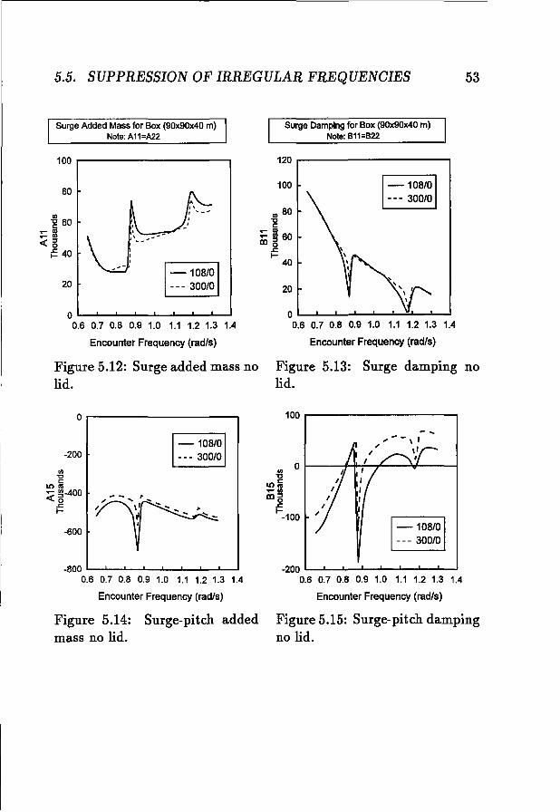
5.5. SUPPRESSION OF IRREGULAR FREQUENCIES 53
Surge Added Mass for Box(90x90x40m)Note:A11=A22
100 r--------------,
80
.g 60..... 111..... 1/1
«B~ 40
20
0'--........---1.-................---''--'---'-----'
0.6 0.7 0.8 0.9 1.0 1.1 1.2 1.3 1.4
Encounter Frequency (rad/s)
Surge Dampingfor Box(90x90x40m)Note:611=622
120 ...-------------,
100
1/1 80"t:l<:
..... 111
..... 1/1 60!DBs:I-
40
20
OL..-....L..---L_.l.-........ ......J--::................---I
0.6 0.7 0.8 0.9 1.0 1.1 1.2 1.3 1.4
Encounter Frequency (rad/s)
Figure 5.12: Surge added mass nolid.
Or----------...,
-200
1/1"t:l<:
It) III
:;;( g-400s:I-
-600
-800 '---I---I._.1---L.......J_................---1
0.6 0.7 0.8 0.9 1.0 1.1 1.2 1.3 1.4
Encounter Frequency (rad/s)
Figure 5.14: Surge-pitch addedmass no lid.
Figure 5.13: Surge damping nolid.
100 r-------------,
1/1 0 I-----j"""'"-;-+----...f-----l"t:l
It):ij..... 1/1
!DBs:I
-100
-200 L..-....L..---L_.l.--L.......J_................---1
0.6 0.7 0.8 0.9 1.0 1.1 1.2 1.3 1.4
Encounter Frequency (rad/s)
Figure 5.15: Surge-pitch dampingno lid.
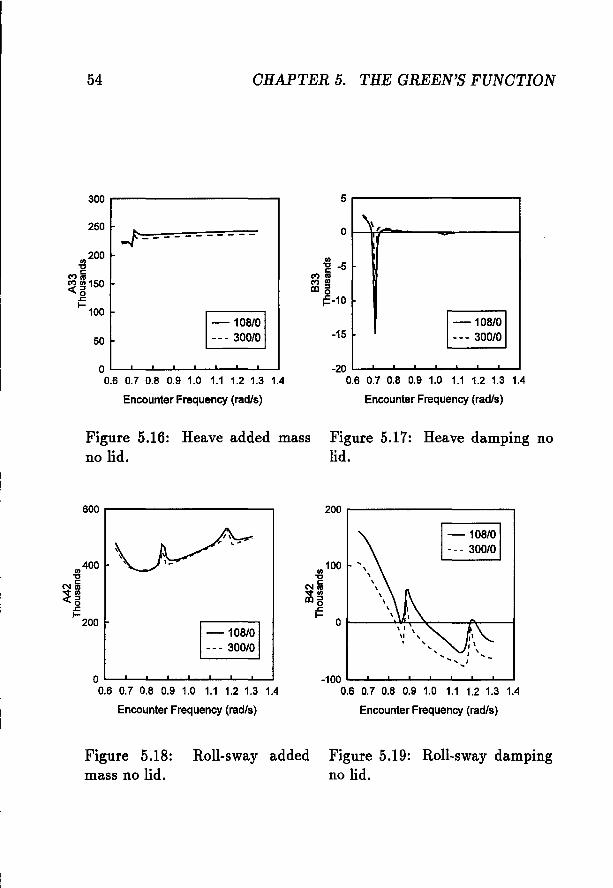
54 CHAPTER 5. THE GREEN'S FUNCTION
300 .--------------, 5r------------,
250
<11200
"CC')e::
~~150os:
I- 100
50
..,t-----------<II
C') ~ -5C')<II
IDS~-10
-151
- 108/0 1--- 300/01
OL...-.........--L_......................_..I-.--L---'
0.6 0.7 0.8 0.9 1.0 1.1 1.2 1.3 1.4
Encounter Frequency (rad/s)
Figure 5.16: Heave added massno lid.
600 .--------------.
-20 L...-.........--L_......................_ .......--L---'
0.6 0.7 0.8 0.9 1.0 1.1 1.2 1.3 1.4
Encounter Frequency (radis)
Figure 5.17: Heave damping nolid.
200 r-----------...,
~\ .
~ ",, ,\,
1-
108/0 1
-- - 300/0
OL...-.........--L_......................'--..I-.--L---'
0.6 0.7 0.8 0.9 1.0 1.1 1.2 1.3 1.4
Encounter Frequency (rad/s)
<II 100"C
(\Ie::
vlJlIDS~
OI---"'-¥L~lIt_--~-_1
-100 L...-.........--L_.............---L_.......-'-.......
0.6 0,7 0.8 0.9 1.0 1.1 1.2 1.3 1.4
Encounter Frequency (rad/s)
Figure 5.18:mass no lid.
Roll-sway added Figure 5.19: Roll-sway dampingno lid.
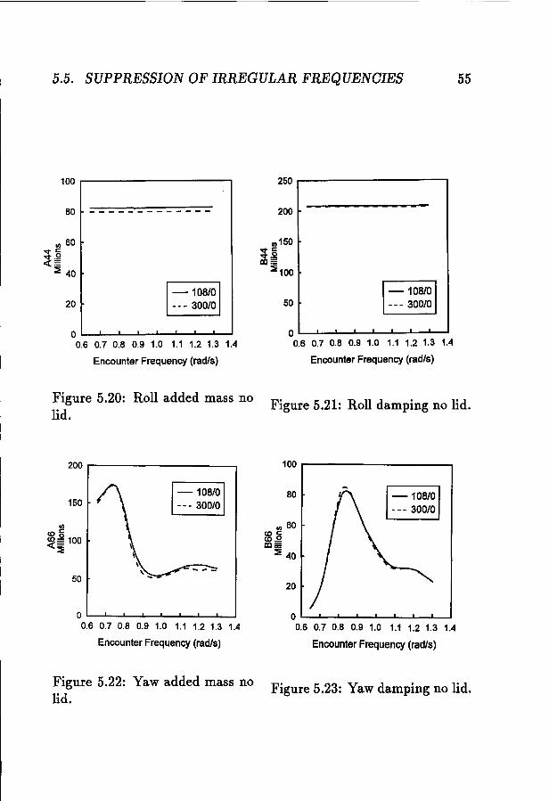
5.5. SUPPRESSION OF IRREGULAR FREQUENCIES 55
100 .--------------, 250 .--------------,
80 --- ---------
OL.--..L--L----l._.&..-...I---L---lL.--l
0.6 0.7 0.8 0.9 1.0 1.1 1.2 1.3 1.4
Encounter Frequency (radls)
ell 60..... 1:-e .2«=
:ii 40
201
- 108/0--- 300/0
200
50
OL.--..L-.....L.--L_L.-.......-L---"--'
0.6 0.7 0.8 0.9 1.0 1.1 1.2 1.3 1.4
Encounter Frequency (radls)
Figure 5.20: Roll added mass nolid.
200 .-------------.
150
ell
C05co= 100«:E
50
OL..-.............L.--L_L.-..L--L---L--J
0.6 0.7 0.8 0.9 1.0 1.1 1.2 1.3 1.4
Encounter Frequency (radls)
Figure 5.22: Yaw added mass nolid.
Figure 5.21: Roll damping no lid.
100 .--------------.
80
ell 60COl:co.2!Xl =
:ii 40
20
OL..-..L-.....L.--L_.L..-.......-L----l.---l
0.6 0.7 0.8 0.9 1.0 1.1 1.2 1.3 1.4
Encounter Frequency (radls)
Figure 5.23: Yaw damping no lid.
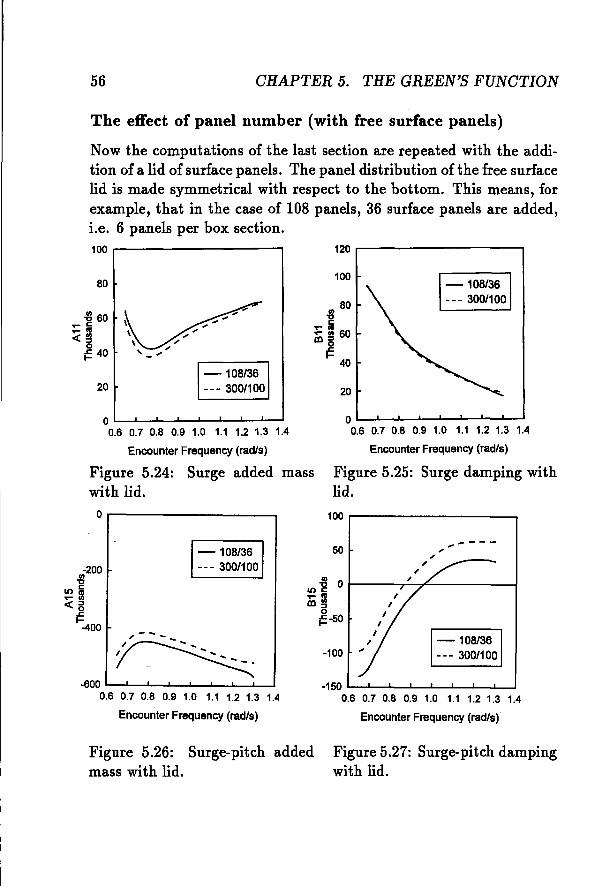
56 CHAPTER 5. THE GREEN'S FUNCTION
The effect of panel number (with free surface panels)
Now the computations of the last section are repeated with the addition of a lid of surface panels. The panel distribution of the free surfacelid is made symmetrical with respect to the bottom. This means, forexample, that in the case of 108 panels, 36 surface panels are added,i.e. 6 panels per box section.100 120
80100
~80
~ 60rI)"0
... c C... 1\1... 1\1 \ ,," ... Ul 60
«~\ " COs
~ 40 , " .cI- -" I-
40
1-108136 II20 --- 300/100 20
O~....L.......L---..L-J.-~~--J--J
0.6 0.7 0.8 0.9 1.0 1.1 1.2 1.3 1.4
Encounter Frequency (rad/s)
Figure 5.24: Surge added masswith lid.
O~..L-......I----,"-l-......L.........I---.L--I
0.6 0.7 0.8 0.9 1.0 1.1 1.2 1.3 1.4
Encounter Frequency (rad/s)
Figure 5.25: Surge damping withlid.
o,-------------, 100 r-------------,
-600 '"-................---l_J.-~-..L.--J--J0.6 0.7 0.8 0.9 1.0 1.1 1.2 1.3 1.4
Encounter Frequency (rad/s)
-150 l-....L-......I----'"_l-......L.......L----..1----l
0.6 0.7 0.8 0.9 1.0 1.1 1.2 1.3 1.4
Encounter Frequency (radls)
.,..----50
-100
~0r_--_r__r----____4IDC
"'lllCO::Jo~-50
1
- 108136 1--- 300/100
~" . - - - -
I -- -- -.
-200Ul"0
IDc
... lll«::Jo~-400
Figure 5.26: Surge-pitch addedmass with lid.
Figure 5.27: Surge-pitch dampingwith lid.
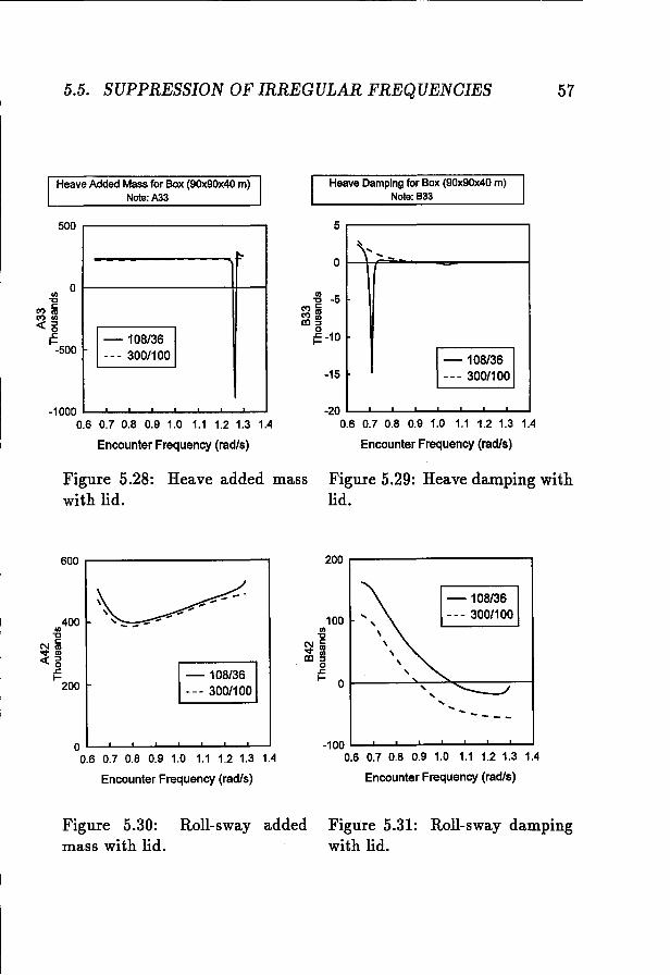
5.5. SUPPRESSION OF IRREGULAR FREQUENCIES 57
HeaveAddedMassfor Box (90x90x40 m)Note:A33
HeaveDamping for Box (90x90x40 m)Note: B33
5r--------------,500
oUl
"C(')1:(,)lJl«::Io~-500
~
1-108/361-- - 300/100
\'o '-
{l -5~l6mgj
o~-10
-15 \
- 108/36 I- - - 300/100I
-10000.6 0.7 0.8 0.9 1.0 1.1 1.2 1.3 1.4
Encounter Frequency (rad/s)
Figure 5.28: Heave added masswith lid.
600 r-----------......,
-20 L..-....L......L_J.-....L..----l_..L-.....L----I
0.6 0.7 0.8 0.9 1.0 1.1 1.2 1.3 1.4
Encounter Frequency (radls)
Figure 5.29: Heave damping withlid.
200 r--------------,
400Ul
"C
Nl6"ItUl«::Io~
200
~.
\ ..,--\ ......, ......---
1
- 108/36 1--- 300/100
100Ul
"C
~l6mgj
o~
Ol--------:!'-:-~"":::---~---I
---oL-..L.........L---JL...-..L.........L---JL...-..L-......
0.6 0.7 0.8 0.9 1.0 1.1 1.2 1.3 1.4
Encounter Frequency (rad/s)
-100 L..-....L......L_J.-....L..----l_...............----'
0.6 0.7 0.8 0.9 1.0 1.1 1.2 1.3 1.4
Encounter Frequency (rad/s)
Figure 5.30: Roll-sway addedmass with lid.
Figure 5.31: Roll-sway dampingwith lid.
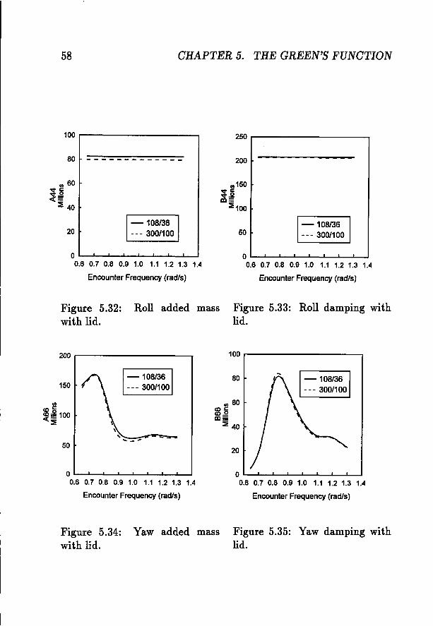
58 CHAPTER 5. THE GREEN'S FUNCTION
100 r-----------,
80 -------------
UI 60
~~~ 40
250 r----------,
200
20 50-108/36- - - 300/100
O'---'--.......---I._"---....&---L.......---J
0.6 0.7 0.8 0.9 1.0 1.1 1.2 1.3 1.4
EncounterFrequency(radls)
Figure 5.32: Roll added masswith lid.
0'---'--...............-'---'---.&..---1.---1
0.6 0.7 0.8 0.9 1.0 1.1 1.2 1.3 1.4
EncounterFrequency (radls)
Figure 5.33: Roll damping withlid.
200 ,..------------,
150
50
0"----'--.......---1.-"---........-.&..---1.---1
0.6 0.7 0.8 0.9 1.0 1.1 1.2 1.3 1.4
EncounterFrequency (radls)
100 ,..-----------,
80
UI 60cocco.S!10=~ 40
20
0'---'--.......---1.-"---........-.&..---1.----1
0.6 0.7 0.8 0.9 1.0 1.1 1.2 1.3 1.4
EncounterFrequency (radls)
Figure 5.34: Yaw added masswith lid.
Figure 5.35: Yaw damping withlid.
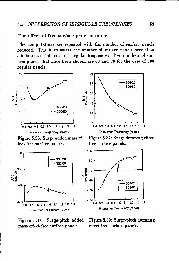
5.5. SUPPRESSION OF IRREGULAR FREQUENOIES 59
80
OL.-...L--L.---"_.L-.--....L.........L.---L----l0.6 0.7 0.8 0.9 1.0 1.1 1.2 1.3 1.4
Encounter Frequency (radls)
Figure 5.37: Surge damping effectfree surface panels.
100
20
o-g 60.... l'II.... 0al~o
t= 40- 300/20--- 300/60
0.----------.,
20
OL.-....L--L_.L-.--....L--L_.L-.--....L........J0.6 0.7 0.8 0.9 1.0 1.1 1.2 1.3 1.4
Encounter Frequency (radls)
Figure 5.36: Surge added mass effect free surface panels.
The effect of free surface panel number
The computations are repeated with the number of surface panelsreduced. This is to assess the number of surface panels needed toeliminate the influence of irregular frequencies. Two numbers of surface panels that have been chosen are 60 and 20 for the case of 300regular panels.80 100 .------------,
\
- 300120 I--- 300/60 I
-200til"'C
IO C.... l'II«~o.c
1---400
50
.g 0 I----r--i------jIOl'II.... 0alS
i!= -50
-100
.600 L....L...-L_I.---'--.-L.....J.........I--.....J0.6 0.7 0.8 0.9 1.0 1.1 1.2 1.3 1.4
Encounter Frequency (rad/s)
-150 l-...L--L.---"_.L--....L.........L.---L--'0.6 0.7 0.8 0.9 1.0 1.1 1.2 1.3 1.4
Encounter Frequency (radls)
Figure 5.38: Surge-pitch addedmass effect free surface panels.
Figure 5.39: Surge-pitch dampingeffect free surface panels.
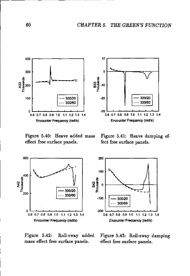
60 CHAPTER 5. THE GREEN'S FUNCTION
-20
400
300 JII)"tJ c-::-e::
Mill
~ ~200.&:I-
100
OL-..I----L_"----'-........---''--''''--....
0.6 0.7 0.8 0.9 1.0 1.1 1.2 1.3 1.4
Encounter Frequency (rad/s)
10 r----------,
-30 "----'-......--L_.L..-...............--'---'
0.6 0.7 0.8 0.9 1.0 1.1 1.2 1.3 1.4
Encounter Frequency (rad/s)
Figure 5.40: Heave added masseffect free surface panels.
600 ...----------....,
Figure 5.41: Heave damping effect free surface panels.
200...----------...,
400{l
Ni~gj
~200
0"----'-........---"----'-........---''--''''--.......0.6 0.7 0.8 0.9 1.0 1.1 1.2 1.3 1.4
EncounterFrequency(rad/s)
II)"tJ
Ne::..,.1ll01----""""I:"'"""---t---1~_l
m~
-100
-200 "----'-........---''--''''--.................- ...........0.6 0.7 0.8 0.9 1.0 1.1 1.2 1.3 1.4
EncounterFrequency (rad/s)
Figure 5.42: Roll-sway addedmass effect free surface panels.
Figure 5.43: Roll-sway dampingeffect free surface panels.
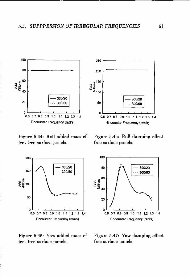
5.5. SUPPRESSION OF IRREGULAR FREQUENCIES 61
0'--....L--L---1_.L..-...J---L.---I1.-...J0.6 0.7 0.8 0.9 1.0 1.1 1.2 1.3 1.4
Encounter Frequency (radls)
250 ,..------------.
50
200
20
100 r------------,
80
OL....-.........-L---1_.L..-...J---L.--l1.-...J0.6 0.7 0.8 0.9 1.0 1.1 1.2 1.3 1.4
EncounterFrequency (radls)
III 60"01'1:"OI'.Qc(=~ 40
Figure 5.44: Roll added mass effect free surface panels.
Figure 5.45: Roll damping effectfree surface panels.
200 ,..-------------,
150
III
C05co= 100c(:E
50
100 r--------------,
80
III 60col:co.Qm=~ 40
20
OL.--...L--L---1_.L.-...J-......L..---1---10.6 0.7 0.8 0.9 1.0 1.1 1.2 1.3 1.4
Encounter Frequency (radls)
OL....-.........-L---I._.L.-...L--L---1---10.6 0.7 0.8 0.9 1.0 1.1 1.2 1.3 1.4
Encounter Frequency (radls)
Figure 5.46: Yaw added mass effect free surface panels.
Figure 5.47: Yaw damping effectfree surface panels.
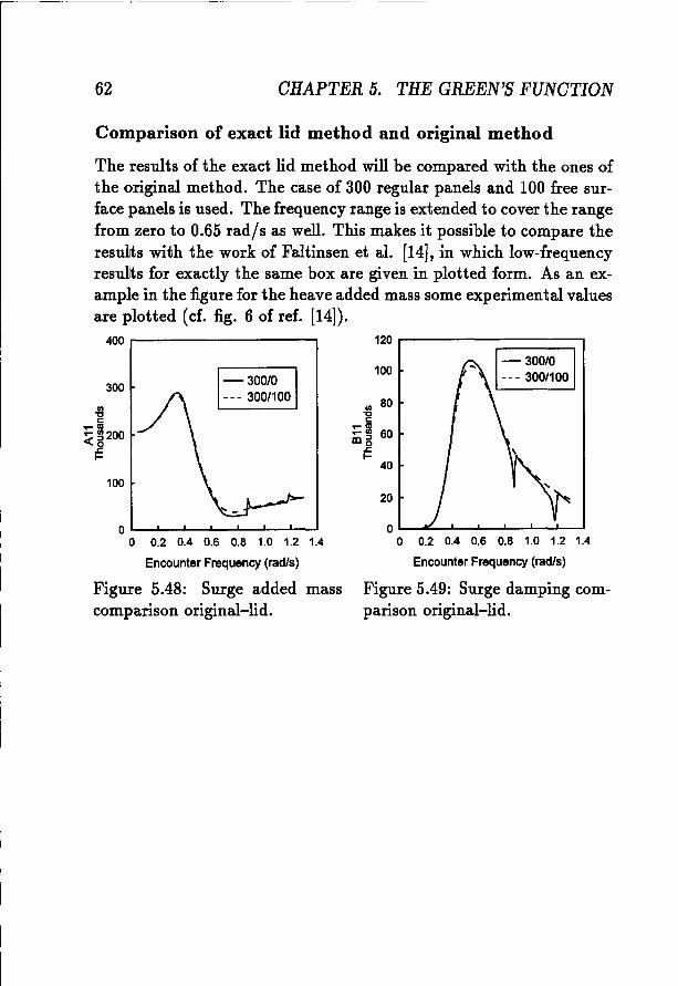
62 CHAPTER 5. THE GREEN'S FUNCTION
Comparison of exact lid method and original method
The results of the exact lid method will be compared with the ones ofthe original method. The case of 300 regular panels and 100 free surface panels is used. The frequency range is extended to cover the rangefrorm zero to 0.65 radfs as well. This makes it possible to compare theresulits with the work of Faltinsen et al. [14], in which low-frequencyresults for exactly the same box are given in plotted form. As an example in the figure for the heave added mass some experimental valuesare plotted (cf. fig. 6 of ref. [14]).
a L-........I'.---'-_.L...-.....r-----'-_'---.....
a 0.2 0.4 0.6 0.8 1.0 1.2 1.4
Encounter Frequency (rad/s)
Figure 5.49: Surge damping comparison original-lid.
20
0.2 0.4 0.6 0.8 1.0 1.2 1.4
Encounter Frequency (raclls)
Figure 5.48: Surge added masscomparison original-lid.
400 120
100
300
'" '" 80"'C "'CC c
.... 11I ~m 60:;(g200 alSs: s:l- I-
40
100
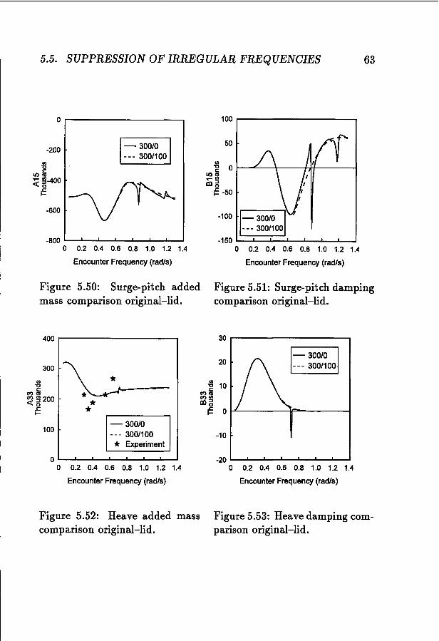
5.5. SUPPRESSION OF IRREGULAR FREQUENCIES 63
o r----------...,
-200
<II"C
LOlij::;c ~-400
.c::I-
-600
-800 L..-......L._.L.-......L.._.L.-......L.._I..-....lo 0.2 0.4 0.6 0.8 1.0 1.2 1.4
Encounter Frequency (rad/s)
100 r----------...,
50
<II
~ 0 r-----r--ffi'-----;LOllims~ -50
-100
-150 L::::L::::;::~----l_..L-.-....L...-..Jo 0.2 0.4 0.6 0.8 1.0 1.2 1.4
Encounter Frequency (radls)
Figure 5.50: Surge-pitch addedmass comparison original-lid.
Figure 5.51: Surge-pitch dampingcomparison original-lid.
400 r----------...,
OL-......L._.L.-......L._.L.-......L._.L.-....Jo 0.2 0.4 0.6 0.8 1.0 1.2 1.4
Encounter Frequency (rad/s)
20
30 .--------------,
-10
-20 L-......L._.L.-......L._.L.-......L._.L.-.......o 0.2 0.4 0.6 0.8 1.0 1.2 1.4
Encounter Frequency (radls)
Ul"C 10
C")lijC')Ulcog
f=. 0 j-L-----;p------t
- 30010--- 300/100* Experiment
300
100
til"Cl:C")lll
~ ~200s:I-
Figure 5.52: Heave added masscomparison original-lid.
Figure 5.53: Heave damping comparison original-lid.
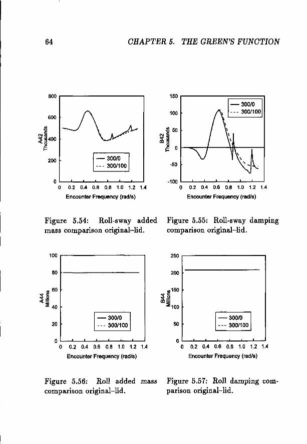
64 CHAPTER 5. THE GREEN'S FUNCTION
800 .------------.....,
600
.,"C
NC
~~400o~
200
OL...-.....L.......J"--'----L_....L---L----'
o 0.2 0.4 0.6 0.8 1.0 1.2 1.4
EncounterFrequency(radls)
Figure 5.54: Roll-sway addedmass comparison original-lid.
150 .-----;:::======:;,100
~ 50
~!ilD:::J
,g 0 I-.......,..--+---+!\------II-
-50
-100 L-.....L._.L..--L._.L..--L._L...-....l
o 0.2 0.4 0.6 0.8 1.0 1.2 1.4
EncounterFrequency (rad/s)
Figure 5.55: Roll-sway dampingcomparison original-lid.
80 ~----------
100 ...----------...,
., 60
~~::iE 40
201
- 300/0 I- - - 300/100
250 r-----------...,
200
10 150
~~:i 100
50
OL..-.....L._.L..-.....L._.L..---I.._.L..-.....J
o 0.2 0.4 0.6 0.8 1.0 1.2 1.4
EncounterFrequency(rad/s)
Figure 5.56: Roll added masscomparison original-lid.
OL.-.....L.......J_....L----L_..I..---L---l
o 0.2 0.4 0.6 0.8 1.0 1.2 1.4
Encounter Frequency (rad/s)
Figure 5.57: Roll damping comparison original-lid.
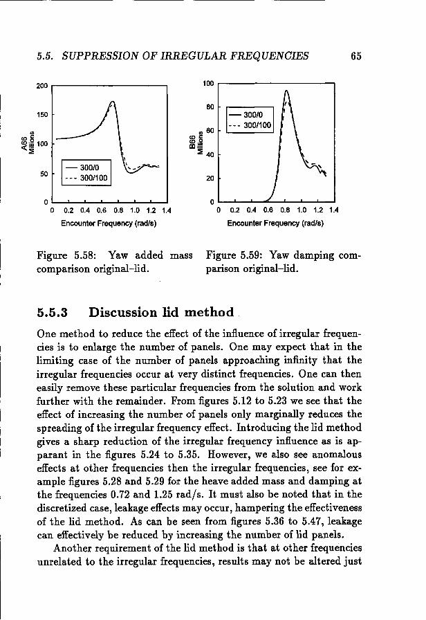
5.5. SUPPRESSION OF IRREGULAR FREQUENCIES 65
200 r------------,
150
50
o L...-....L..--'-_.L..-....L..--'-_.L..-...J
o 0.2 0.4 0.6 0.8 1.0 1.2 1.4
EncounterFrequency (rad/s)
100 r-----------,
80
III 60CDC::CD.S!al::~ 40
20
0.2 0.4 0.6 0.8 1.0 1.2 1.4
EncounterFrequency(radls)
Figure 5.58: Yaw added masscomparison original-lid.
Figure 5.59: Yaw damping comparison original-lid.
5.5.3 Discussion lid method
One method to reduce the effect of the influence of irregular frequencies is to enlarge the number of panels. One may expect that in thelimiting case of the number of panels approaching infinity that theirregular frequencies occur at very distinct frequencies. One can theneasily remove these particular frequencies from the solution and workfurther with the remainder. From figures 5.12 to 5.23 we see that theeffect of increasing the number of panels only marginally reduces thespreading of the irregular frequency effect. Introducing the lid methodgives a sharp reduction of the irregular frequency influence as is apparant in the figures 5.24 to 5.35. However, we also see anomalouseffects at other frequencies then the irregular frequencies, see for example figures 5.28 and 5.29 for the heave added mass and damping atthe frequencies 0.72 and 1.25 rad/s. It must also be noted that in thediscretized case, leakage effects may occur, hampering the effectivenessof the lid method. As can be seen from figures 5.36 to 5.47, leakagecan effectively be reduced by increasing the number of lid panels.
Another requirement of the lid method is that at other frequenciesunrelated to the irregular frequencies, results may not be altered just

66 CHAPTER 5. THE GREEN'S FUNCTION
by using a lid in the free surface. From figures 5.48 to 5.59 we seethat there is little influence of the application of the lid method atfrequencies below the lowest irregular frequency.
Chapter 6
The forces on the body
Once the velocity potential is known, we are able to compute thehydrodynamic forces using pressure integration.In the first section we derive the added mass and the damping bycomputing the reaction forces. The second section gives the waveforces, computed by direct pressure integration and by the Haskindrelation. Also, the motions due to these forces are computed. Inthe third section we compute the mean drift forces. The forces andmotions are computed for a half-immersed sphere and compared withthe results of Nossen [52] and Zhao and Faltinsen [82].
6.1 Added mass and damping
In this section we derive the reaction forces, F; i = 1, ... ,6, usingpressure integration. With these reaction forces we are able to compute the added mass and the damping.
Once the potentials cPo(~) and cPl (s) are known, the pressure is determined from Bernoulli's equation.
1p(~, t) = -pgz - p<I>t(~, t) - 2PV<I>(~, t) . V<I>(~, t) +Po +C(t) (6.1)
The pressure is then expanded using the same expansion scheme as isused for the sources and velocity potentials. Using the expressions for
67
68 CHAPTER 6. THE FORCES ON THE BODY
<) and linearizing with respect to ~ we have:
p(~,t) = -pgz - P~t +pU~x - pU(VX' V~) (6.2)
The linearized pressure 1 can be written as:
(6.3)
with
PO(~' t) _p8~o~:, t) (6.4)
_/~~:,t) +~ [8~~=,t) _ VX(i11)' V~(~,t)]
(6.5)
The static pressure part comes from the pgz term. Integration of thepressure over the mean wetted surface results in the hydrodynamicreaction forces in the usual coordinate system fixed to the ship.
(6.6)
Fki is the reaction force in the kth mode due to a unit oscillation in thejth mode. Substitution of the pressure expansion and using equations(6.4) and (6.5) gives:
FkiO -ipw/ Is <Pio . nkdS
Fkil -ipw/ Is <Pil . nkdS
-: /Is (8<P~~~) - VX(~) . V <PiO(~)) . nkdS
(6.7)
with(6.8)
lSubscripts 0 and 1 denote the zero speed and the first order speed correction
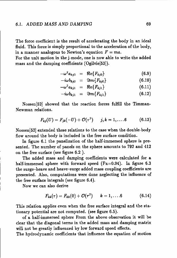
6.1. ADDED MASS AND DAMPING 69
The force coefficient is the result of accelerating the body in an idealfluid. This force is simply proportional to the acceleration of the body,in a manner analogous to Newton's equation F = maoFor the unit motion in the j-mode, one is now able to write the addedmass and the damping coefficients (Ogilvie[53]).
2-w akjO
-iwbkjO2-w akjl
-iwbkj1
~e{FkjO}
S'm{Fkj o}
~e{Fkjl}
S'm{Fkj1}
(6.9)
(6.10)
(6.11)(6.12)
Nossen[52] showed that the reaction forces fulfill the TimmanNewman relations.
(6.13)
Nossen[52] extended these relations to the case when the double-bodyflow around the body is included in the free surface condition.
In figure 6.1 the panelization of the half-immersed sphere is presented. The number of panels on the sphere amounts to 792 and 412on the free surface (see figure 6.2 ).
The added mass and damping coefficients were calculated for ahalf-immersed sphere with forward speed (Fn=0.04). In figure 6.3the surge-heave and heave-surge added mass coupling coefficients arepresented. Also, computations were done neglecting the influence ofthe free surface integrals (see figure 6.4).
Now we can also derive
k = 1, ....6 (6.14)
This relation applies even when the free surface integral and the stationary potential are not computed. (see figure 6.5).
of a half-immersed sphere From the above observation it will beclear that the diagonal terms in the added mass and damping matrixwill not be greatly influenced by low forward speed effects.The hydrodynamic coefficients that influence the equation of motion
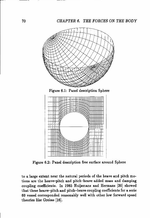
70 CHAPTER 6. THE FORCES ON THE BODY
Figure 6.1: Panel description Sphere
Figure 6.2: Panel description free surface around Sphere
to a large extent near the natural periods of the heave and pitch motions are the heave-pitch and pitch-heave added mass and dampingcoupling coefficients. In 1985 Huijsmans and Hermans [30] showedthat these heave-pitch and pitch-heave coupling coefficients for a serie60 vessel corresponded reasonably well with other low forward speedtheories like Grekas [16].
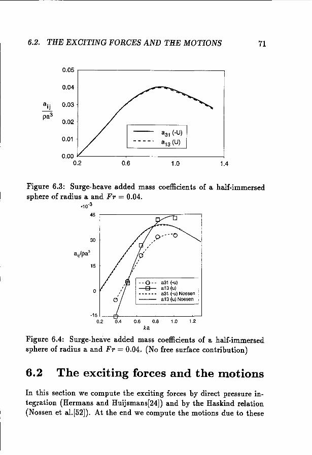
6.2. THE EXCITING FORGES AND THE MOTIONS 71
0.05
0.04
aij 0.03
pa30.02
a31 (-U)0.01 a13 (U)
0.000.2 0.6 1.0 1.4
Figure 6.3: Surge-heave added mass coefficients of a half-immersedsphere of radius a and Fr = 0.04.
*10-3
o
a31 (-u)a13 (u)a31 (-u) Nossena13 (u) Nossen
o
15
-15 L----I'!i'---~-~-~-~0.2 0.4 0.6 0.8 1.0 1.2
ka
45 ,.-----------::::=------,
30
Figure 6.4: Surge-heave added mass coefficients of a half-immersedsphere of radius a and Fr = 0.04. (No free surface contribution)
6.2 The exciting forces and the motions
In this section we compute the exciting forces by direct pressure integration (Hermans and Huijsmans[24]) and by the Haskind relation(Nossen et al.[52]). At the end we compute the motions due to these
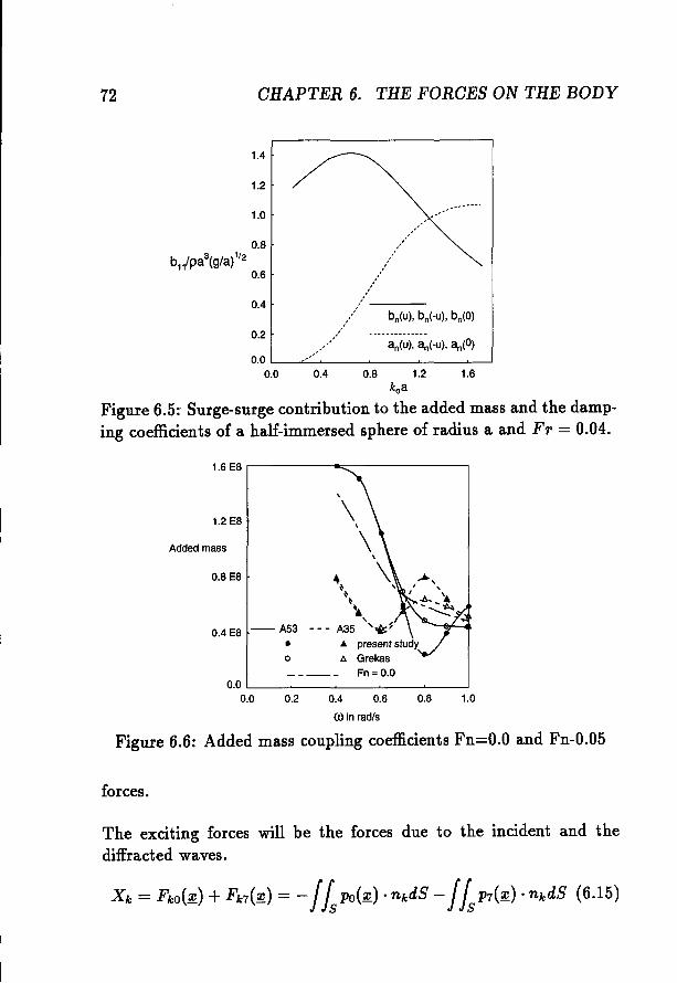
72 CHAPTER 6. THE FORCES ON THE BODY
1.4
1.2
1.0
0.8
b, /pa3(g/a)'/2
0.6
0.4
1.60.80.4
0.0 L.---"':'~__~_~__~---.J
0.0
0.2
1.2koa
Figure 6.5: Surge-surge contribution to the added mass and the damping coefficients of a half-immersed sphere of radius a and Fr = 0.04.
1.6 E8 ,--------=----------,
1.2 E8
Added mass
0.8 E8 4~~~
)., ~I
0.4 E8 - A53 - - - A35 '-t::'• ... present study
o Ii. Grekas____ Fn = 0.0
1.00.80.60.40.20.0 L.-_~_~__~_~_--.J
0.0
0) in rad/s
Figure 6.6: Added mass coupling coefficients Fn=O.O and Fn-0.05
forces.
The exciting forces will be the forces due to the incident and thediffracted waves.
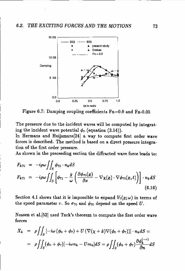
6.2. THE EXCITING FORCES AND THE MOTIONS 73
15 E8 ,.....--------------,
- 653 ._-- 635• ... present study
o '" Grekas____ Fn=O.O
10 E8
Damping
5 E8
1.00.750.25
0.0 L-__~__~_~_--J
0.0
Figure 6.7: Damping coupling coefficients Fn=O.O and Fn-O.05
The pressure due to the incident waves will be computed by integrating the incident wave potential <Po (equation (3.14)).In Hermans and Huijsmans[24] a way to compute first order waveforces is described. The method is based on a direct pressure integration of the first order pressure.As shown in the preceeding section the diffracted wave force leads to:
Fk70 -ipw!Is <P70 . nkdS
Fon -ipw/ J. [<p71 - : (1J<P;;;i11) - VX(i11) • V.p,.(i11, t))] . nodS
(6.16)
Section 4.1 shows that it is impossible to expand V7(~;w) in terms ofthe speed parameter T. SO U70 and <P70 depend on the speed U.
Nossen et al.[52] used Tuck's theorem to compute the first order waveforces
x, = p!Is [-iw (<Po + <P7) +U (V(x + z)V(<po +<P7))] . nkdS ={)<p(-T)
p!1(<Po + <P7)[-iwnk - Umk]dS = p!1(<PO + <P7) ;n dB
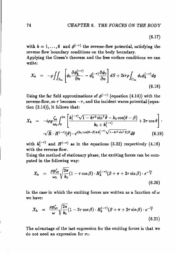
74 CHAPTER 6. THE FORGES ON THE BODY
(6.17)
with k = 1, ... ,6 and </J(-T) the reverse-flow potential, satisfying thereverse flow boundary conditions on the body boundary.Applying the Green's theorem and the free surface conditions we canwrite:
x, - -pit [<Poof) -<Pl-<J:] dS+2irp!c- Ml-<)dy
(6.18)
Using the far field approximations of </J(-T) (equation (4.14)) with thereverse-flow, so r becomes -r, and the incident waves potential (equation (3.14)), it follows that:
. (a 10211' [kJ-
T)v'l - 4r2 sin2 8 - kocos(8 - (3) 0]-zpg- +2r cos .Wo 0 ko +kl-T
)
...fR. H(-T)(8). ei(kocos(9-,B)+k~-T\h-4T2sin29)Rd8 (6.19)
with kl-T) and H(-T) as in the equations (5.32) respectively (4.16)with the reverse-How.Using the method of stationary phase, the exciting forces can be computed in the following way:
X k = pg(a {2;k1l'"(1 - r cos(3) . H~-T)({3 + 11'" +2r sin(3) . e-ifWo VI;;
(6.20)
In the case in which the exciting forces are written as a function of wwe have:
x, = P~(a fi(1- 2r cos(3) . H~-T)({3 + 11'" +2r sin(3) . e-if
(6.21)
The advantage of the last expression for the exciting forces is that wedo not need an expression for (1'7'
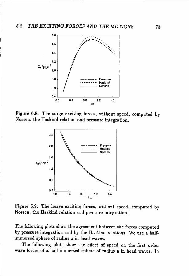
6.2. THE EXCITING FORCES AND THE MOTIONS 75
PressureHaskindNossen
0.8
1.6
1.8 ,---------=--------,
0.6
1.4
1.61.20.80.4
0.4 L-_~__~__~_~---'
0.0ka
Figure 6.8: The surge exciting forces, without speed, computed byNossen, the Haskind relation and pressure integration.
2.4
2.0
0.8
\\\\
\\
\\
\\
\\ ,,,
"~
'c
~
PressureHaskindNossen
1.61.20.80.4
0.4 L-_~__~__~_~---,
0.0ka
Figure 6.9: The heave exciting forces, without speed, computed byNossen, the Haskind relation and pressure integration.
The following plots show the agreement between the forces computedby pressure integration and by the Haskind relations. We use a halfimmersed sphere of radius a in head waves.
The following plots show the effect of speed on the first orderwave forces of a half-immersed sphere of radius a in head waves. In
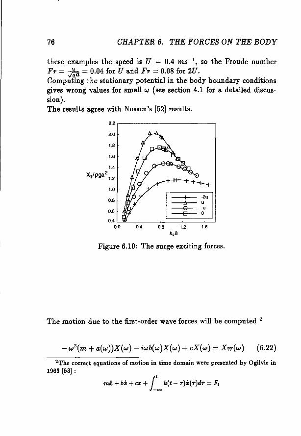
76 CHAPTER 6. THE FORCES ON THE BODY
these examples the speed is U = 0.4 ms-1 , so the Froude numberFr = via = 0.04 for U and Er = 0.08 for 2U.Computing the stationary potential in the body boundary conditionsgives wrong values for small w (see section 4.1 for a detailed discussion).The results agree with Nossen's [52] results.
2.2 ,---------------,
IAa0
0.4 0.8 1.2 1.6koa
1.6
2.0
1.8
1.0
0.8
0.6
0.4 LJ1lL~_~=======~0.0
Figure 6.10: The surge exciting forces.
The motion due to the first-order wave forces will be computed 2
- w2(m +a(w))X(w) - iwb(w)X(w) +cX(w) = Xw(w) (6.22)
2The correct equations of motion in time domain were presented by Ogilvie in1963 [53] :
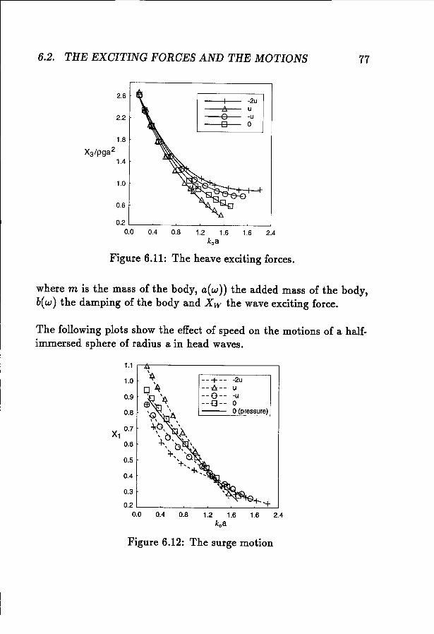
6.2. THE EXCITING FORCES AND THE MOTIONS 77
2.6I -zuA u
2.2 0 -uD 0
1.8
X3 /pga2
1.4
1.0
0.6
0.20.0 0.4 0.8 1.2 1.6 1.6 2.4
koa
Figure 6.11: The heave exciting forces.
where m is the mass of the body, a(w)) the added mass of the body,b(w) the damping of the body and X w the wave exciting force.
The following plots show the effect of speed on the motions of a halfimmersed sphere of radius a in head waves.
1.1
1.0
0.9
0.8
X10.7
0.6
0.5
0.4
0.3
0.20.0 0.4 0.8
--+-- -2u---ts-- u--0-- -u--0-- 0
o(pressure)
1.2 1.6 1.6 2.4koa
Figure 6.12: The surge motion
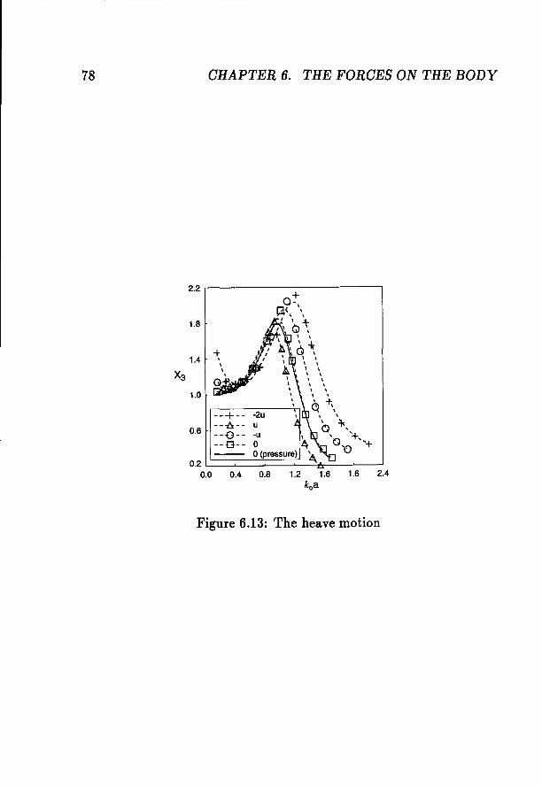
78 CHAPTER 6. THE FORCES ON THE BODY
2.2 ,---------------,
1.8
1.0
--+-- -2u
0.6---6,-- u--0-- -u \
--0-- 0 ~o(pressure) '.\0.2
0.0 0.4 0.8 1.2 1.6 1.6 2.4
koa
Figure 6.13: The heave motion
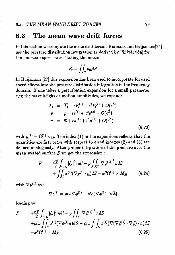
6.3. THE MEAN WAVE DRIFT FORGES
6.3 The mean wave drift forces
79
In this section we compute the mean drift forces. Hermans and Huijsmans[24)use the pressure distribution integration as derived by Pinkster[54] forthe non-zero speed case. Taking the mean:
In Huijsmans [27] this expression has been used to incorporate forwardspeed effects into the pressure distribution integration in the frequencydomain. If one takes a perturbation expansion for a small parameter€,eg the wave height or motion amplitudes, we expand:
F; Ft +€FP) + €2 FP) +O(€3)
p P+€p(l) + €2p(2) +O( €3)
n n + €n(l) + €2n(2) +O(€3)
(6.23)
with n.(t) = n(l) x n.. The index (1) in the expansions reflects that thequantities are first order with respect to € and indexes (2) and (3) aredefined analogously. After proper integration of the pressure over themean wetted surface S we get the expression :
F = Pi fWL ICrl 2n.dl- PfbIvc/P)1
2
n.dS
+fb X(l)(Vp(l) . n.)dS - W2n (1) X M~
with Vp(1) as :
(6.24)
leading to:
F = +Pi fWL ICrl2n.dl- Pfb IV 4J(1)!2n.dS
+piw fb x(l)(V4J(1)n.)dS - piwf b:rP)(V(V4J(l). v(f». n.)dS
_w2n (1) X M~ (6.25)
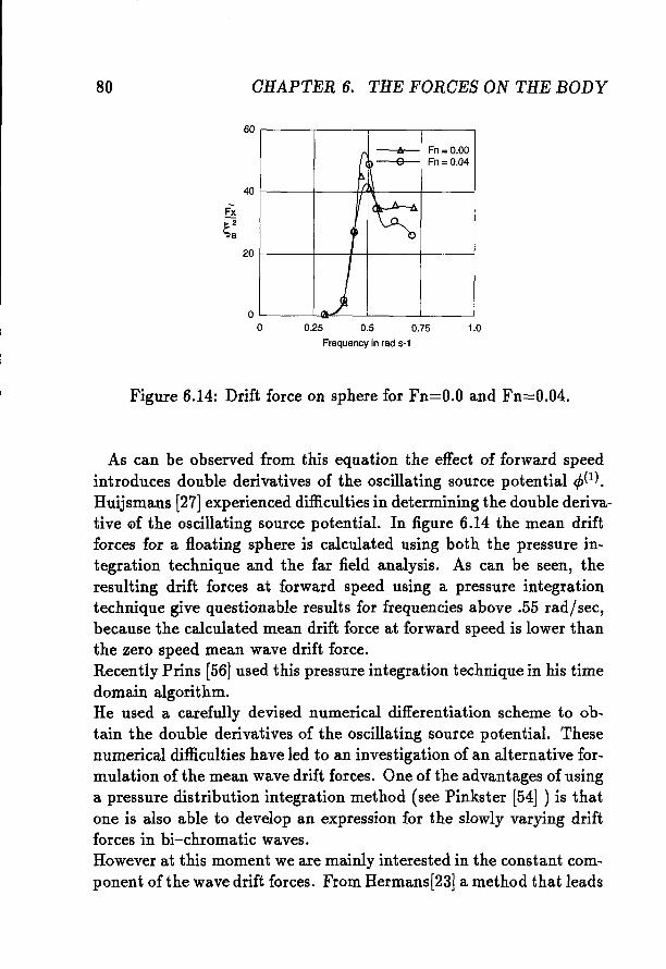
80 OHAPTER 6. THE FORCES ON THE BODY
1.00.25 0.5 0.75
Frequency in rad s-t
Ir -----A- Fn = 0.00
p --e--- Fn = 0.04
~\\
~
Joo
40
20
60
Fx
S=
Figure 6.14: Drift force on sphere for Fn=O.O and Fn=0.04.
As can be observed from this equation the effect of forward speedintroduces double derivatives of the oscillating source potential </J(l).
Huijsmans [27] experienced difficulties in determining the double derivative of the oscillating source potential. In figure 6.14 the mean driftforces for a floating sphere is calculated using both the pressure integration technique and the far field analysis. As can be seen, theresulting drift forces at forward speed using a pressure integrationtechnique give questionable results for frequencies above .55 rad/sec,because the calculated mean drift force at forward speed is lower thanthe zero speed mean wave drift force.Recently Prins [56] used this pressure integration technique in his timedomain algorithm.He used a carefully devised numerical differentiation scheme to obtain the double derivatives of the oscillating source potential. Thesenumerical difficulties have led to an investigation of an alternative formulation of the mean wave drift forces. One of the advantages of usinga pressure distribution integration method (see Pinkster [54] ) is thatone is also able to develop an expression for the slowly varying driftforces in bi-chromatic waves.However at this moment we are mainly interested in the constant component of the wave drift forces. From Hermans[23] a method that leads
6.3. THE MEAN WAVE DRIFT FORCES 81
to results that are possibly more accurate numerically, is recapitulated.
From the rate of change of the linear and angular momentum withinthe fluid domain bounded by the free surface, the wetted part of thevessel and a control surface at infinity, we can formulate an expressionof the mean work done by the vessel in regular waves.
(6.26)
Taking into account the free surface condition, the fixed control surfaceSoo (giving Un = 0 on Soo ) and the vanishing pressure at the freesurface we have:
which leads to:
This results in the mean drift force F given by
F = - / Loo(PI! + pVV • ,!!!.)dS
where the line above means time-average.
(6.28)
Grue and Palm[18] derived independently the same expression for thedrift forces as Hermans[22]. They used not only the Bernoulli equation, but also included the conservation of mass.F x consists of two parts. The first one FJ!), behaves like R-i, whilethe second term FJ2), the wave drift force, behaves like R:",
FP) A~ . ~e{H*(f3*)e1} cosf3 +0(7"2) (6.29)
FP) -~Kr IH(0)12 [cos0 - 27" sin2 0] dO +0(7"2) (6.30)
82 CHAPTER 6. THE FORCES ON THE BODY
We also have two terms for F II'
with
F(l)II
F(2)II
- Af#. fle{Ir(p')eit} sinp +O(T') (6.31)
__eK, r: IH(8)12[sin8 +2rsin8cos8] d8 +O(r2X6.32)4 10
pw2
A --C2wo a
H* - the complex conjugate of H
{3* - {3 - 2r sin{3
(6.33)
The following plots show the effect of speed on the drift forces of ahalf-immersed sphere of radius a in head waves. In these examples thespeed is U = OAms- l , so the Froude number Fr = Ja = 0.04 for Uand Fr = 0.08 for 2U.Nossen[52] gives the drift forces on the restrained sphere. The effect ofthe stationary potential on these forces can be neglected. The resultsfrom figure 6.15 coincide with the results of Zhao and Faltinsen [82].
We also give the drift forces on a free floating sphere for zero speed;by definition these results are equivalent to the results of Pinkster[54]. The effect of the stationary potential is small, but can not beneglected, so both figures are plotted.
The wave drift damping will be computed with the derivative ofthe forces to the speed. Figure 6.18 is an outline of the damping,derived from the preceeding figure. The line u is derived from thedifference between the zero and u lines of the preceeding figure. So-u is between 0 and -u.
To arrive at a proper wave drift damping coefficient, one shouldtake a smaller step in the froude number, which will reduce the inaccuary from the numerical differentiation.
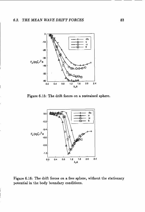
6.3. THE MEAN WAVE DRIFT FORGES
0
I -2u-10 A u
0 -u0 0
-20
-30
Fx/pg~a28-40
-SO
-600.0 0.4 0.8 1.2 1.6 2.0 2.4
ko8
Figure 6.15: The drift forces on a restrained sphere.
0.0 -2uu-u
-0.2 0
-0.4
Fx/pg~a28-0.6
-0.8
-1.0
0.0 0.4 0.8 1.2 1.6 2.0 2.4ko8
83
Figure 6.16: The drift forces on a free sphere, without the stationarypotential in the body boundary conditions.
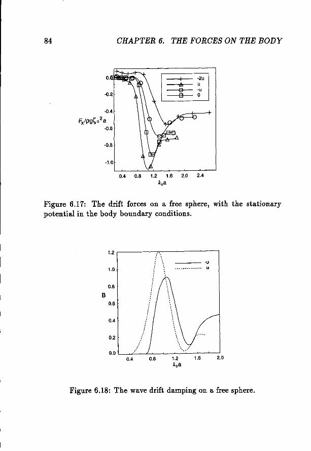
84 CHAPTER 6. THE FORCES ON THE BODY
-0.2
-0.4
Fx/pgsa2a-0.6
-0.8
-1.0
oo
-2uu-uo
0.4 0.8 1.2 1.6 2.0 2.4koa
Figure 6.17: The drift forces on a free sphere, with the stationarypoten.tial in the body boundary conditions.
1.6
___ -u_•. • u
0.80.4
0.2
0.4
1.0
1.2 r------:"'"------,
0.8
B0.6
Figure 6.18: The wave drift damping on a free sphere.
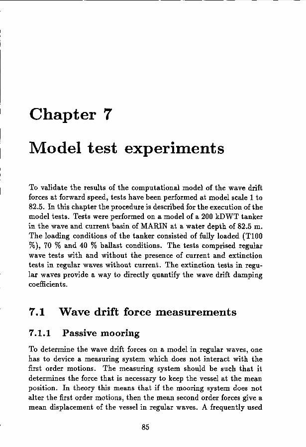
Chapter 7
Model test experiments
To validate the results of the computational model of the wave driftforces at forward speed, tests have been performed at model scale 1 to82.5. In this chapter the procedure is described for the execution of themodel tests. Tests were performed on a model of a 200 kDWT tankerin the wave and current basin of MARIN at a water depth of 82.5 m,The loading conditions of the tanker consisted of fully loaded (TlOO%), 70 % and 40 % ballast conditions. The tests comprised regularwave tests with and without the presence of current and extinctiontests in regular waves without current. The extinction tests in regular waves provide a way to directly quantify the wave drift dampingcoefficients.
7.1 Wave drift force measurements
7.1.1 Passive mooring
To determine the wave drift forces on a model in regular waves, onehas to device a measuring system which does not interact with thefirst order motions. The measuring system should be such that itdetermines the force that is necessary to keep the vessel at the meanposition. In theory this means that if the mooring system does notalter the first order motions, then the mean second order forces give amean displacement of the vessel in regular waves. A frequently used
85
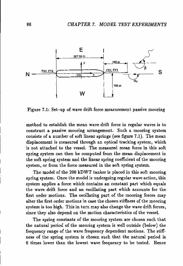
86 CHAPTER 7. MODEL TEST EXPERIMENTS
N
E327.53 m
y 785m
\FX1 FY1FX2 FY2 .......CG x ./ .......
785m
W .-
s
Figure 7.1: Set-up of wave drift force measurement passive mooring
method to establish the mean wave drift force in regular waves is toconstruct a passive mooring arrangement. Such a mooring systemconsists of a number of soft linear springs (see figure 7.1). The meandisplacement is measured through an optical tracking system, whichis not attached to the vessel. The measured mean force in this softspring system can then be computed from the mean displacement inthe soft spring system and the linear spring coefficient of the mooringsystem, or from the force measured in the soft spring system.
The model of the 200 kDWT tanker is placed in this soft mooringspring system. Once the model is undergoing regular wave action, thissystem applies a force which contains an constant part which equalsthe wave drift force and an oscillating part which accounts for thefirst order motions. The oscillating part of the mooring forces mayalter the first order motions in case the chosen stiffness of the mooringsystem is too high. This in turn may also change the wave drift forces,since they also depend on the motion characteristics of the vessel.
The spring constants of the mooring system are chosen such thatthe natural period of the mooring system is well outside (below) thefrequency range of the wave frequency dependent motions. The stiffness of the spring system is chosen such that the natural period is6 times lower than the lowest wave frequency to be tested. Hence
7.1. WAVE DRIFT FORGE MEASUREMENTS 87
no real influence on the first order motions and consequently on thewave drift forces is to be expected from the chosen soft mooring system. Following the observation made by Pinkster [54], the measuring
t
RAO mooring
Wave spectrum
regular wave
Figure 7.2: Spring characteristics mooring system.
devices can be either ship-fixed or earth-fixed as long as the angularmotions are not too large. In the current set-up a ship-fixed forcetransducer was chosen.
The current is generated in N-S direction; changing the heading ofthe model also changes the heading of the current with respect to theship. (see figure 7.1) The waves can be generated with an arbitraryangle to the model.
7.1.2 Active mooring
One of the disadvantages of the passive mooring set-up is that it isdifficult to control the heading of the vessel, once the vessel respondsto the actions of the waves and the current. One has to correct themean heading angle to the desired heading angle manually. An elegantway to overcome these difficulties is to use a dynamic mooring systemor dynamic positioning system. Such a dynamic positioning systemrelies on algorithms to maintain a certain predefined position in thehorizontal space. The dynamic positioning system must than be capa-
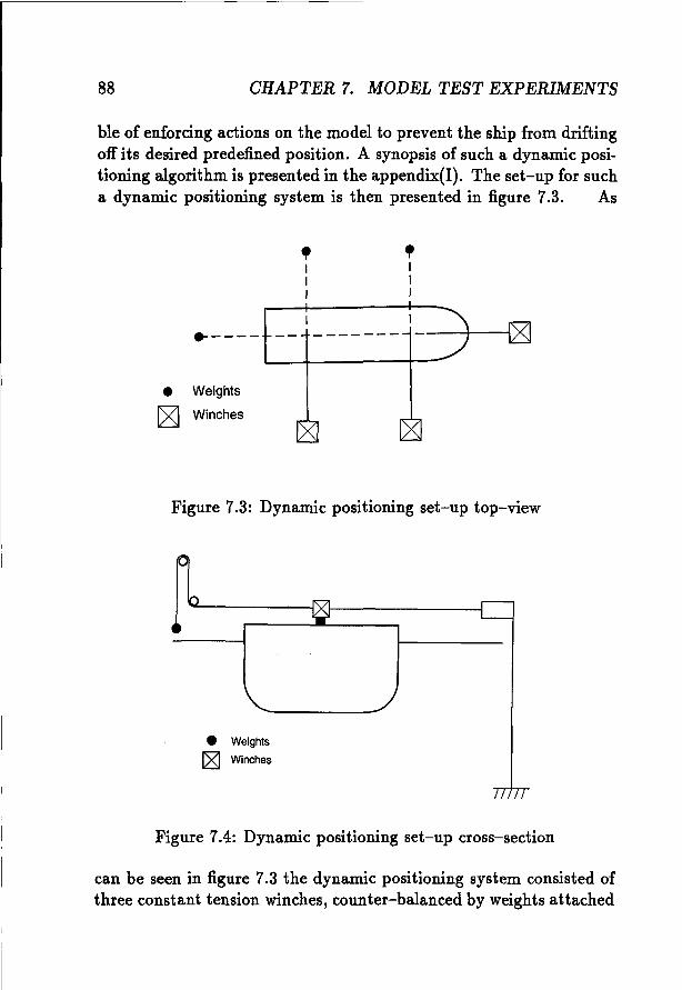
~------------------ -_.. - --
88 OHAPTER 7. MODEL TEST EXPERIMENTS
ble of enforcing actions on the model to prevent the ship from driftingoff its desired predefined position. A synopsis of such a dynamic positioning algorithm is presented in the appendix(I). The set-up for sucha dynamic positioning system is then presented in figure 7.3. As
•III
•III
-- ------- ---~~~.----• Weights
~ Winches
Figure 7.3: Dynamic positioning set-up top-view
• Weights
C8J Winches
Figure 7.4: Dynamic positioning set-up cross-section
can be seen in figure 7.3 the dynamic positioning system consisted ofthree constant tension winches, counter-balanced by weights attached
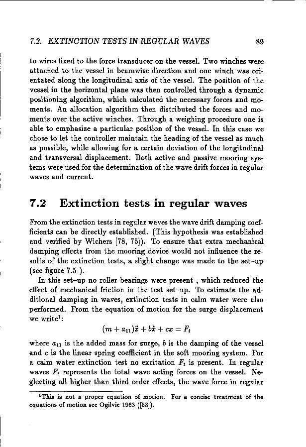
7.2. EXTINCTION TESTS IN REGULAR WAVES 89
to wires fixed to the force transducer on the vessel. Two winches wereattached to the vessel in beamwise direction and one winch was orientated along the longitudinal axis of the vessel. The position of thevessel in the horizontal plane was then controlled through a dynamicpositioning algorithm, which calculated the necessary forces and moments. An allocation algorithm then distributed the forces and moments over the active winches. Through a weighing procedure one isable to emphasize a particular position of the vessel. In this case wechose to let the controller maintain the heading of the vessel as muchas possible, while allowing for a certain deviation of the longitudinaland transversal displacement. Both active and passive mooring systems were used for the determination of the wave drift forces in regularwaves and current.
7.2 Extinction tests in regular waves
From the extinction tests in regular waves the wave drift damping coefficients can be directly established. (This hypothesis was establishedand verified by Wichers [78, 75]). To ensure that extra mechanicaldamping effects from the mooring device would not influence the results of the extinction tests, a slight change was made to the set-up(see figure 7.5 ).
In this set-up no roller bearings were present, which reduced theeffect of mechanical friction in the test set-up. To estimate the additional damping in waves, extinction tests in calm water were alsoperformed. From the equation of motion for the surge displacementwe writel:
(m +all):i: +bi; +ce = Ft
where all is the added mass for surge, b is the damping of the vesseland c is the linear spring coefficient in the soft mooring system. Fora calm water extinction test no excitation Ft is present. In regularwaves Ft represents the total wave acting forces on the vessel. Neglecting all higher than third order effects, the wave force in regular
IThis is not a proper equation of motion. For a concise treatment of theequations of motion see Ogilvie 1963 ([53]).
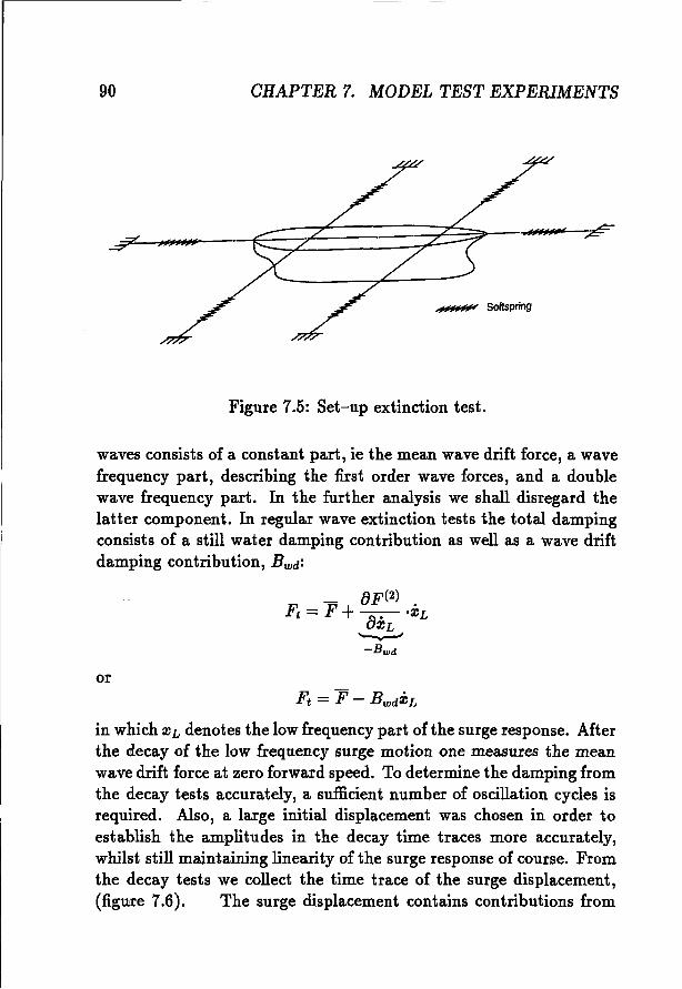
90 OHAPTER 7. MODEL TEST EXPERIMENTS
~ Soltspring
Figure 7.5: Set-up extinction test.
waves consists of a constant part, ie the mean wave drift force, a wavefrequency part, describing the first order wave forces, and a doublewave frequency part. In the further analysis we shall disregard thelatter component. In regular wave extinction tests the total dampingconsists of a still water damping contribution as well as a wave driftdamping contribution, Bwd :
orFt = F- BwdZL
in which Z L denotes the low frequency part of the surge response. Afterthe decay of the low frequency surge motion one measures the meanwave drift force at zero forward speed. To determine the damping fromthe decay tests accurately, a sufficient number of oscillation cycles isrequired. Also, a large initial displacement was chosen in order toestablish the amplitudes in the decay time traces more accurately,whilst still maintaining linearity of the surge response of course. Fromthe decay tests we collect the time trace of the surge displacement,(figure 7.6). The surge displacement contains contributions from
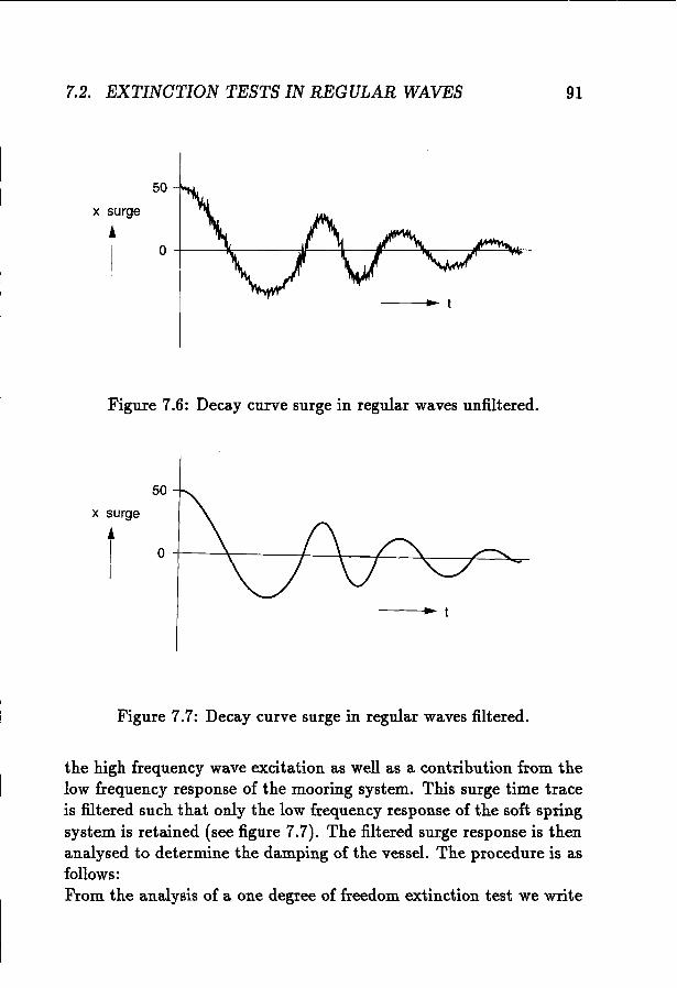
7.2. EXTINOTION TESTS IN REGULAR WAVES
50
x surge
• t
Figure 7.6: Decay curve surge in regular waves unfiltered.
50
x surge
·t
Figure 7.7: Decay curve surge in regular waves filtered.
91
the high frequency wave excitation as well as a contribution from thelow frequency response of the mooring system. This surge time traceis filtered such that only the low frequency response of the soft springsystem is retained (see figure 7.7). The filtered surge response is thenanalysed to determine the damping of the vessel. The procedure is asfollows:From the analysis of a one degree of freedom extinction test we write
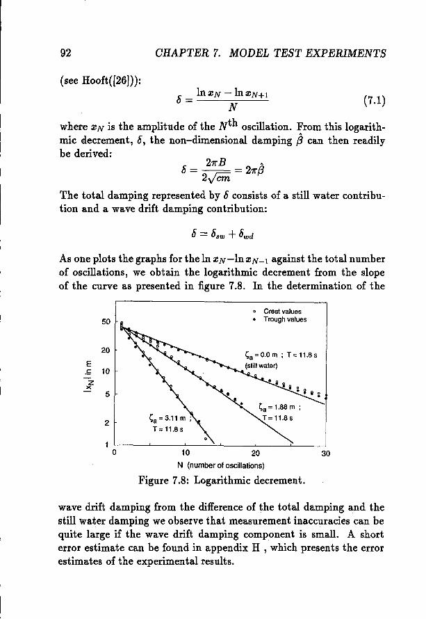
92 CHAPTER 7. MODEL TEST EXPERIMENTS
(see Hooft([26])):
6 = InzN -lnzN+l (7.1)N
where ZN is the amplitude of the Nth oscillation. From this logarithmic decrement, 6, the non-dimensional damping ~ can then readilybe derived:
6 = 21rB = 21r~2y'Cm
The total damping represented by 6 consists of a still water contribution and a wave drift damping contribution:
As ORe plots the graphs for the In Z N-In Z N -1 against the total numberof oscillations, we obtain the logarithmic decrement from the slopeof the curve as presented in figure 7.8. In the determination of the
30
o Crest values• Trough values
10 20
N (number of oscillations)
Figure 7.8: Logarithmic decrement.
1'----'------''---....:......<-_----'-__---L:__--.J
o
2
5
20
50
E.£ 10zx
wave drift damping from the difference of the total damping and thestill water damping we observe that measurement inaccuracies can bequite large if the wave drift damping component is small. A shorterror estimate can be found in appendix H , which presents the errorestimates of the experimental results.
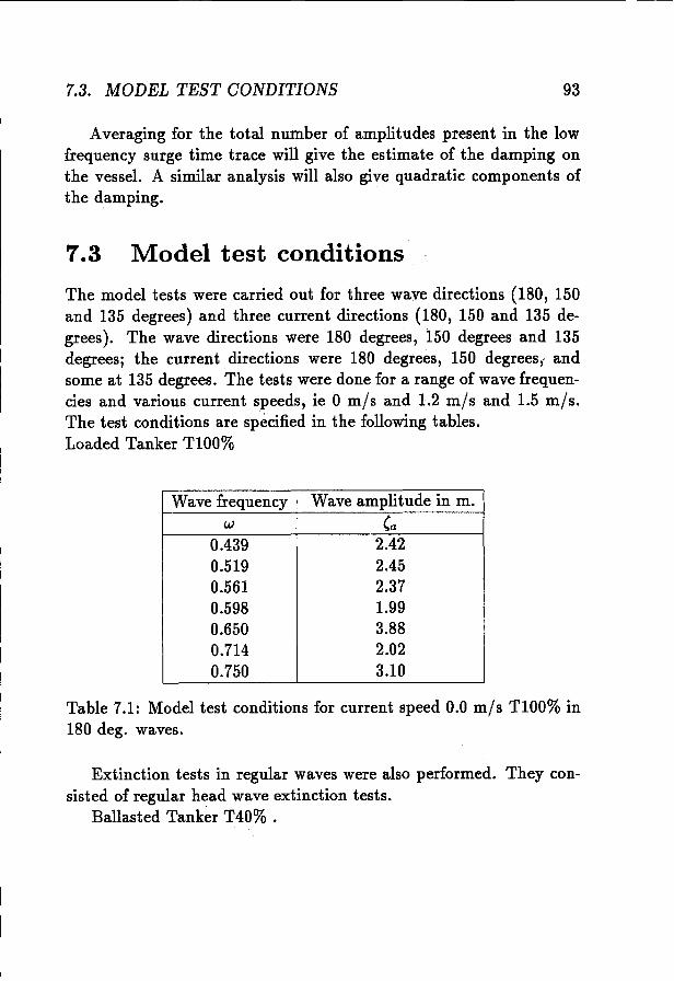
7.3. MODEL TEST CONDITIONS 93
Averaging for the total number of amplitudes present in the lowfrequency surge time trace will give the estimate of the damping onthe vessel. A similar analysis will also give quadratic components ofthe damping.
7.3 Model test conditions
The model tests were carried out for three wave directions (180, 150and 135 degrees) and three current directions (180, 150 and 135 degrees). The wave directions were 180 degrees, 150 degrees and 135degrees; the current directions were 180 degrees, 150 degrees, andsome at 135 degrees. The tests were done for a range of wave frequencies and various current speeds, ie 0 mls and 1.2 mls and 1.5 ta]«.The test conditions are specified in the following tables.Loaded Tanker TlOO%
Wave frequency Wave amplitude in m.w (a
0.439 2.420.519 2.450.561 2.370.598 1.990.650 3.880.714 2.020.750 3.10
Table 7.1: Model test conditions for current speed 0.0 mls TlOO% in180 deg. waves.
Extinction tests in regular waves were also performed. They consisted of regular head wave extinction tests.
Ballasted Tanker T40% .
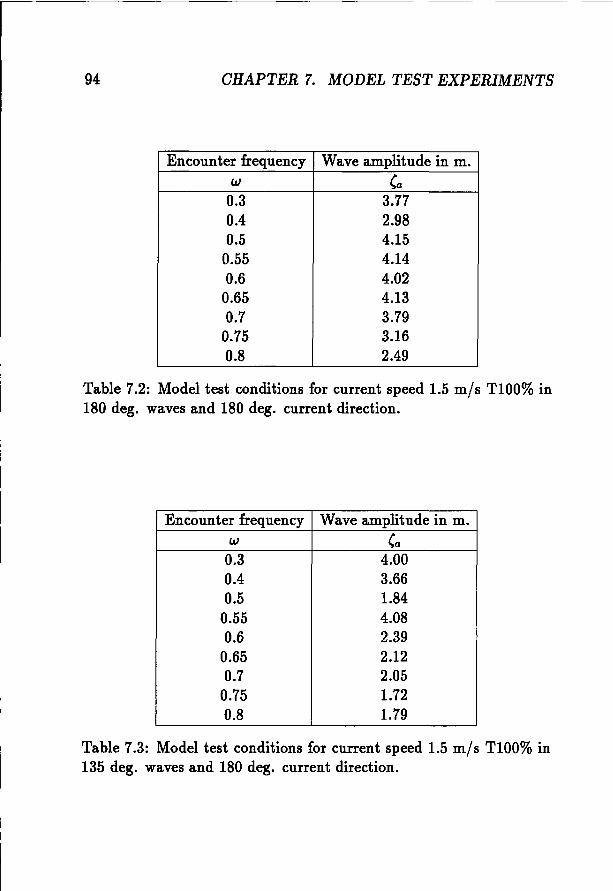
d 1.5 m/s TlOO% in
de in m.
de in m.
ST EXPERIMENTS
2.392.122.051.721.79
0.60.650.7
0.750.8
94 CHAPTER 7. MODEL TE
Encounter frequency Wave amplituw (a
0.3 3.770.4 2.980.5 4.15
0.55 4.140.6 4.02
0.65 4.130.7 3.79
0.75 3.160.8 2.49
Table 7.2: Model test conditions for current spee180 deg. waves and 180 deg. current direction.
Encounter frequency Wave amplituw (a
0.3 4.000.4 3.660.5 1.84
0.55 4.08
Table 7.3: Model test conditions for current speed 1.5 m/s TlOO% in135 deg. waves and 180 deg. current direction.
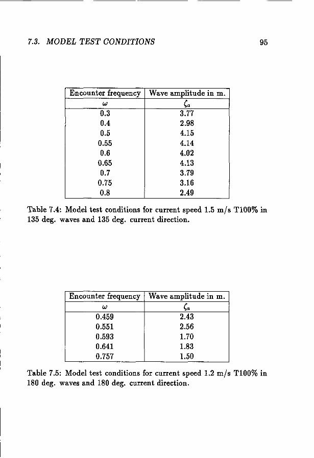
7.3. MODEL TEST CONDITIONS
Encounter frequency Wave amplitude in m.w (a
0.3 3.770.4 2.980.5 4.15
0.55 4.140.6 4.02
0.65 4.130.7 3.79
0.75 3.160.8 2.49
95
Table 7.4: Model test conditions for current speed 1.5 m/s TlOO% in135 deg, waves and 135 deg. current direction.
Encounter frequency Wave amplitude in m,w (a
0.459 2.430.551 2.560.593 1.700.641 1.830.757 1.50
Table 7.5: Model test conditions for current speed 1.2 mjs TlOO% in180 deg. waves and 180 deg. current direction.
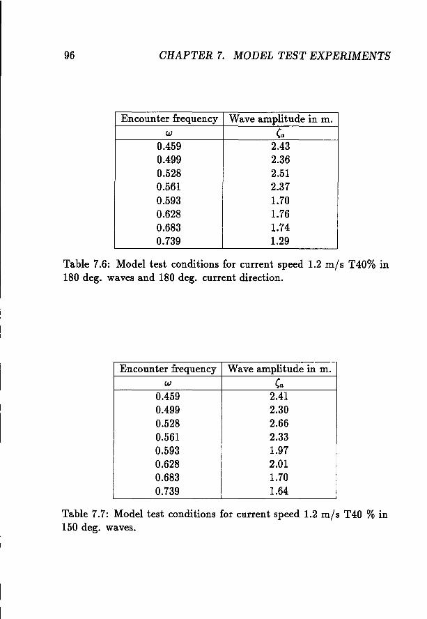
96 CHAPTER 7. MODEL TEST EXPERIMENTS
Encounter frequency Wave amplitude in m.w (a
0.459 2.430.499 2.360.528 2.510.561 2.370.593 1.700.628 1.760.683 1.740.739 1.29
Table 7.6: Model test conditions for current speed 1.2 ta]« T40% in180deg. waves and 180 deg. current direction.
Encounter frequency Wave amplitude in m.w (a
0.459 2.410.499 2.300.528 2.660.561 2.330.593 1.970.628 2.010.683 1.700.739 1.64
Table 7.7: Model test conditions for current speed 1.2 m/s T40 %in150 deg. waves.
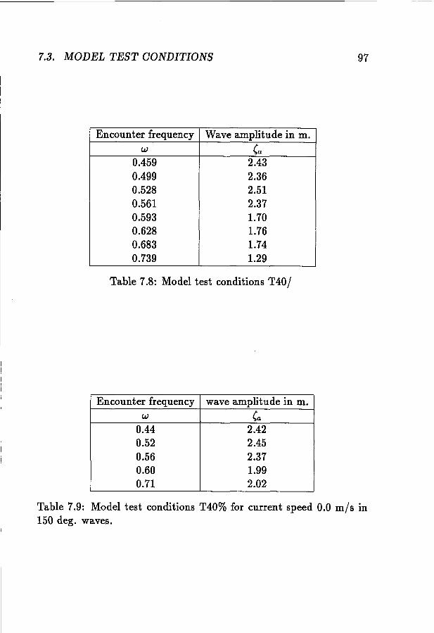
7.3. MODEL TEST CONDITIONS
Encounter frequency Wave amplitude in m,w Ca
0.459 2.430.499 2.360.528 2.510.561 2.370.593 1.700.628 1.760.683 1.740.739 1.29
Table 7.8: Model test conditions T40/
Encounter frequency wave amplitude in m.w Ca
0.44 2.420.52 2.450.56 2.370.60 1.990.71 2.02
97
Table 7.9: Model test conditions T40% for current speed 0.0 m/s in150 deg. waves.
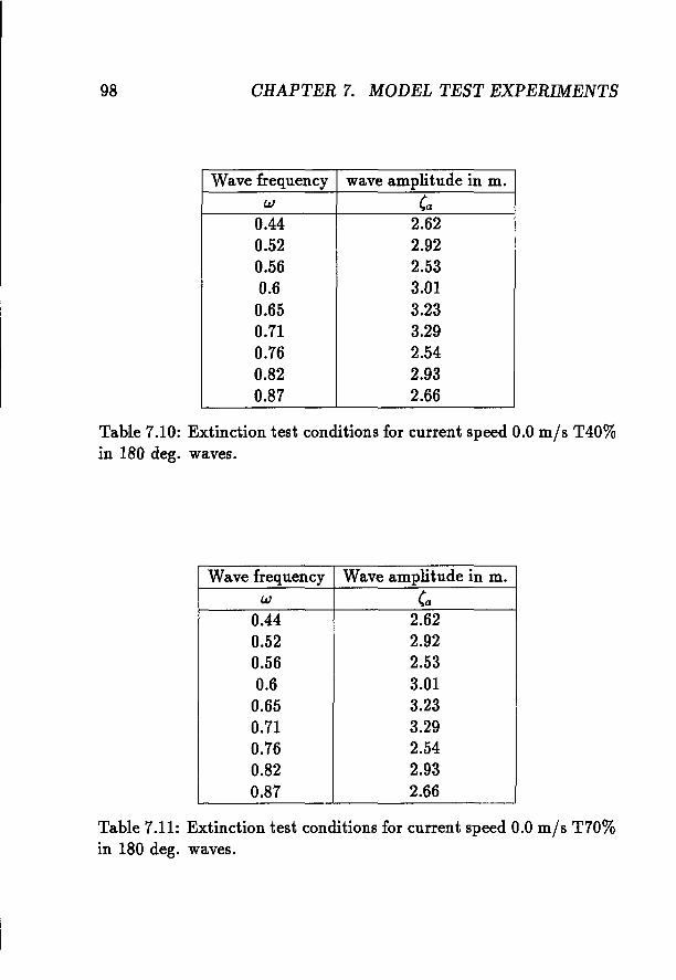
98 OHAPTER 7. MODEL TEST EXPERIMENTS
Wave frequency wave amplitude in m.w (a
0.44 2.620.52 2.920.56 2.530.6 3.010.65 3.230.71 3.290.76 2.540.82 2.930.87 2.66
Table 7.10: Extinction test conditions for current speed 0.0 m/s T40%in 180 deg. waves.
Wave frequency Wave amplitude in m.w (a
0.44 2.620.52 2.920.56 2.530.6 3.01
0.65 3.230.71 3.290.76 2.540.82 2.930.87 2.66
Table 7.11: Extinction test conditions for current speed 0.0 m/s T70%in 180 deg. waves.
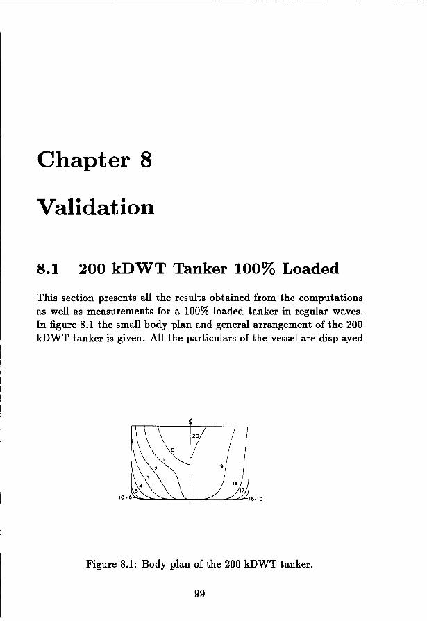
Chapter 8
Validation
8.1 200 kDWT Tanker 100% Loaded
This section presents all the results obtained from the computationsas well as measurements for a 100% loaded tanker in regular waves.In figure 8.1 the small body plan and general arrangement of the 200kDWT tanker is given. All the particulars of the vessel are displayed
Figure 8.1: Body plan of the 200 kDWT tanker.
99
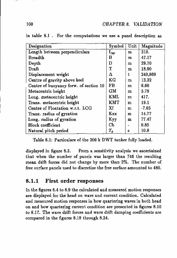
100 CHAPTER 8. VALIDATION
in table 8.1 For the computations we use a panel description as
Designation Symbol Unit MagnitudeLength between perpendiculars Lpp m 310.Breadth B m 47.17Depth D m 29.70Draft T m 18.90Displacement weight A- t 240,869Centre of gravity above keel KG m 13.32Centre of buoyancy forw. of section 10 FB m 6.60Metacentric height GM m 5.78Long. metacentric height KML m 417.Trans. metacentric height KMT m 19.1Centre of Floatation w.r.t. LCG Xf m -7.05Trans. radius of gyration Kxx m 14.77Long. radius of gyration Kyy m 77.47Block coeffi.cient Cb - 0.85Natural pitch period Tq, s 10.8
Table 8.1: Particulars of the 200 k DWT tanker fully loaded.
displayed in figure 8.3. From a sensitivity analysis we ascertainedthat when the number of panels was larger than 746 the resultingmean drift forces did not change by more than 2%. The number offree surface panels used to discretize the free surface amounted to 480.
8.1.1 First order responses
In the figures 8.4 to 8.9 the calculated and measured motion responsesare displayed for the head on wave and current condition. Calculatedand measured motion responses in bow quartering waves in both headon and bow quartering current condition are presented in figures 8.10to 8.17. The wave drift forces and wave drift damping coefficients arecompared in the figures 8.18 through 8.24.
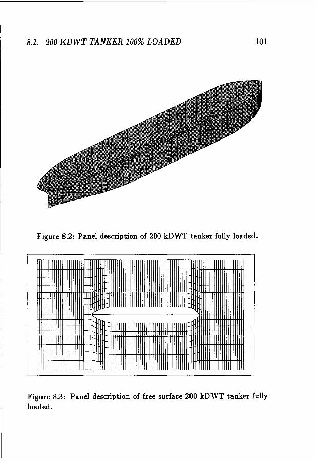
8.1. 200 KDWT TANKER 100% LOADED 101
Figure 8.2: Panel description of 200 kDWT tanker fully loaded.
Figure 8.3: Panel description of free surface 200 kDWT tanker fullyloaded.
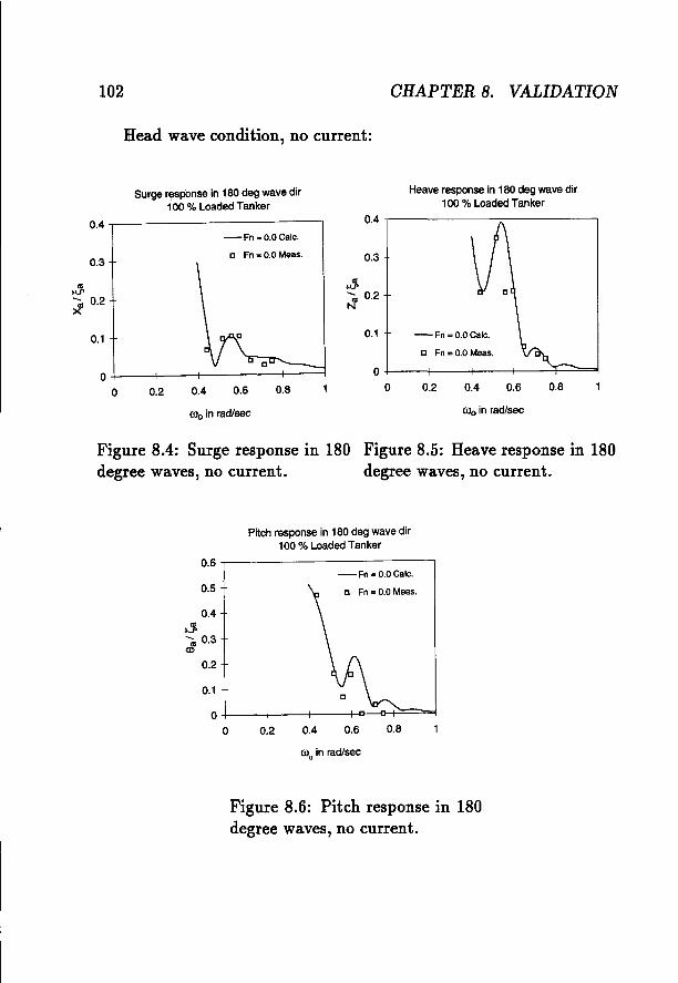
102 CHAPTER 8. VALIDATION
Head wave condition, no current:
0.4 -,---------------,
0.80.60.40.2
- Fn = 0.0 Calc.
e Fn =0.0 Meas.
Heave response in 180 deg wave dir100 % Loaded Tanker
O.J---+---+----+-~J==::==l
o
0.4 -,--------:----------,
0.3
0.1
.:J..... 0.2N
0.80.6
- Fn = 0.0 Calc.
e Fn =0.0 Meas.
0.40.2
Surge response in 180 deg wave dir100 % Loaded Tanker
0+---+-----1f----l---+---i
o
0.1
0.3
.:J.~ 0.2
roo in rad/sec rooin rad/sec
Figure 8.4: Surge response in 180 Figure 8.5: Heave response in 180degree waves, no current. degree waves, no current.
Pitch response in 180 deg wave dir100 % Loaded Tanker
0.6 -,--------------,
0.5
0.4J,.... 0.3a>
0.2
0.1
-Fn = 0.0 Calc.
e Fn = 0.0 Meas.
0.80.60.40.2
O-J.-...---+---+---t-o----cr+=~
oroo in rad/sec
Figure 8.6: Pitch response in 180degree waves, no current.
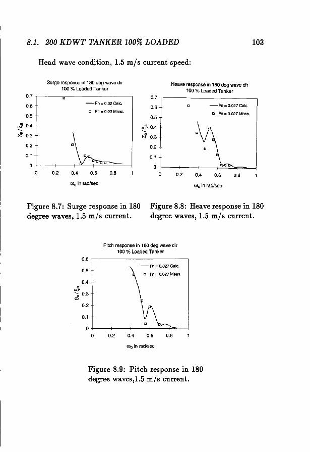
8.1. 200 KDWT TANKER 100% LOADED 103
Head wave condition, 1.5 tu]s current speed:
Surge response in 180 deg wave dir100 % Loaded Tanker
- Fn= 0.027 Calc.
e Fn = 0.027 Meas.
e
Heave response in 180 deg wave dir100 % Loaded Tanker
0.7 -r----------------,
0.6
0.5n Fn= 0.02 Meas.
-Fn =0.02 Calc.e0.7 -,-----------.,---------------,
0.6
0.5
0.80.60.40.2
0.2
0.1
O+----+----1f-----r-::~~==---I
o
.,'J. 0.4.....r-1 0.3
0.80.60.40.2
0.2
0.1
O+----+---+-=--f---+---'-----jo
.,'J. 0.4.....~ 0.3
000 in rad/sec 000 in radlsec
Figure 8.7: Surge response in 180degree waves, 1.5 m/s current.
Figure 8.8: Heave response in 180degree waves, 1.5 m/s current.
Pilch response in 180 deg wave dir100 % Loaded Tanker
0.6 -,---------------,
0.5
0.4..u.J'"'m 0.3CI)
0.2
0.1
- Fn= 0.027 Calc.
e Fn= 0.027 Meas.
0.80.60.40.2
O+----+---+-----.--,f-----t==-----jo
000 in radlsec
Figure 8.9: Pitch response in 180degree waves,1.5 m/s current.
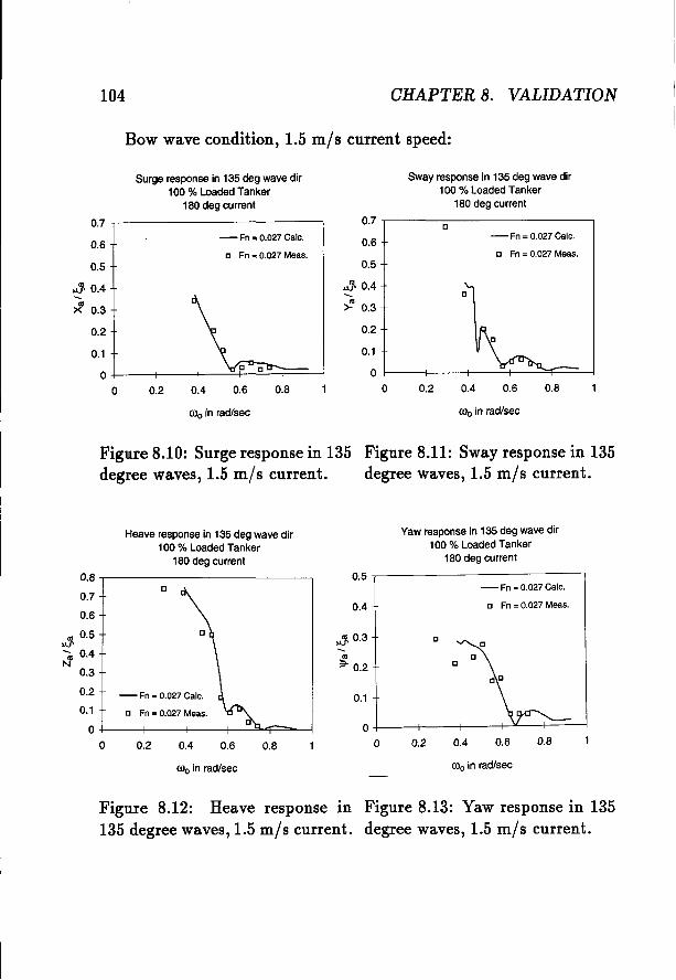
104 CHAPTER 8. VALIDATION
Bow wave condition, 1.5 ta]« current speed:
Surge response in 135deg wavedir100 % LoadedTanker
180deg current
Sway response in 135deg wave dir100% LoadedTanker
180deg current
- Fn =0.027 Calc.
D Fn = 0.027 Meas. D Fn = 0.027 Meas.
- Fn = 0.027 Calc.D
0.7 -,-----------------,
0.6
0.5
0.7.,-------------,
0.6
0.5
0.80.60.40.2
0.2
0.1
O+----+---+----=-+-----=~==____J
o
.:J. 0.4-~ 0.3
0.80.60.40.2
0.2
0.1
0-l---+--+------2:!...F---!:!..:::.....+==-!o
.:J. 0.4-~ 0.3
000 in rad/sec 000 in radlsec
Figure 8.10: Surge response in 135 Figure 8.11: Sway response in 135degree waves, 1.5 mls current. degree waves, 1.5 ta]« current.
Heaveresponse in 135deg wavedir100 % LoadedTanker
180 deg current
0.80.6
- Fn = 0.027 Calc.
D Fn = 0.027 Meas.
0.4
D
D
0.2
o+----t---f---+~-+-
o
Yaw response in 135deg wavedir100 % LoadedTanker
180 deg current
0.5..,---------------,
0.1
0.4
.:J. 0.3-'";;T 0.2
0.80.60.4
D
0.2
- Fn = 0.027 Calc.
D Fn = 0.027 Meas.
0.3
0.2
0.1
O+----+---+---+------!:""'I==~
o
0.8 -,-----------------,
0.7
0.6
'" 0.5>J..J'..... 0.4N
000 in radlsec 000 in rad/sec
Figure 8.12: Heave response in Figure 8.13: Yaw response in 135135 degree waves, 1.5 mls current. degree waves, 1.5 mls current.
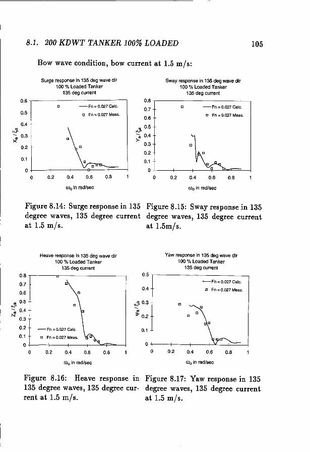
8.1. 200 KDWT TANKER 100% LOADED 105
Bow wave condition, bow current at 1.5 m/s:
Surge response in 135deg wavedir100% LoadedTanker
135 deg current
Sway response in 135 deg wave dir100 % LoadedTanker
135 deg current0.6 -,----------------,
0.80.6
- Fn = 0.027 Calc.
e Fn = 0.027 Meas.
0.4
e
0.2
0.8 -,-------------
0.7
0.6
III 0.5uP
"m 0.4>-
0.3
0.2
0.1
O-!----j---+-----'f----"''''''F=----lo0.80.6
- Fn = 0.027 Calc.
e Fn =0.027 Meas.
0.4
e
0.2
O-!----j---+-----I:j----t-------,
o
0.1
0.2
0.4
0.5
,:J.~ 0.3X
())o in radlsec ())o in rad/sec
Figure 8.14: Surge response in 135degree waves, 135 degree currentat 1.5 m/s.
Figure 8.15: Sway response in 135degree waves, 135 degree currentat 1.5m/s.
Heaveresponse in 135 deg wavedir100% LoadedTanker
135deg current
Yaw response in 135 degwavedir100% LoadedTanker
135 deg current
0.80.6
- Fn =0.027 Calc.
e Fn = 0.027 Meas.
en
e
0.4
e
0.20+----+----+---1---"--+--.1
o
0.5 ,--------------,
0.4
0.1
,:J. 0.3.....
III
~ 0.2
0.80.60.40.2
- Fn = 0.027 Calc.
e Fn = 0.027 Meas.
0.8 ,-----.:,---------~
0.7
0.6
0.3
0.2
0.1
O+---j---f-----t----O"""'f:=",----l
o
III 0.5uP
"m 0.4N
())o in rad/sec ())o in rad/sec
Figure 8.16: Heave response in135 degree waves, 135 degree current at 1.5 tn]«.
Figure 8.17: Yaw response in 135degree waves, 135 degree currentat 1.5 tii]«.
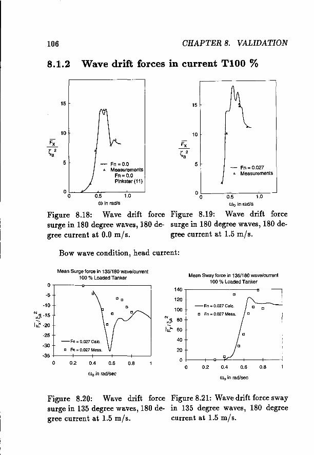
106 CHAPTER 8. VALIDATION
8.1.2 Wave drift forces in current TIOO %
15
10
15
10
- Fn=0.027.. Measurements
0.5 1.0COo in rad/s
OL-----'-----,'-::----'o
5- Fn=O.O.. Measurements
Fn=O.OPinkster(11)
0.5 1.0coin rad/s
5
Figure 8.18: Wave drift forcesurge in 180 degree waves, 180 degree current at 0.0 m/s,
Figure 8.19: Wave drift forcesurge in 180 degree waves, 180 degree current at 1.5 m/s.
Bow wave condition, head current:
MeanSurgeforce in 135/180 wave/current100 % Loaded Tanker MeanSwayforcein 135/180 wave/current
100 % Loaded Tanker
140a
120
100- Fn =0.027 Calc. a
a Fn =0.027 Meas.
'"'" 80>JJ'
t;z.. 60
40a
20a
00 0.2 0.4 0.6 0.8
0>0 in rad/sec
0.8
a a
0.60.40.2
- Fn = 0.027 Calc.
a Fn = 0.027 Meas.
roo in rad/sec
-25
-30
-35 +---+--+---+--+-----1o
O~----o-----------,
-5
-10
~-15.....
I al: -20
Figure 8.20: Wave drift forcesurge in 135 degree waves, 180 degree current at 1.5 ta]«,
Figure 8.21: Wave drift force swayin 135 degree waves, 180 degreecurrent at 1.5 m/s.
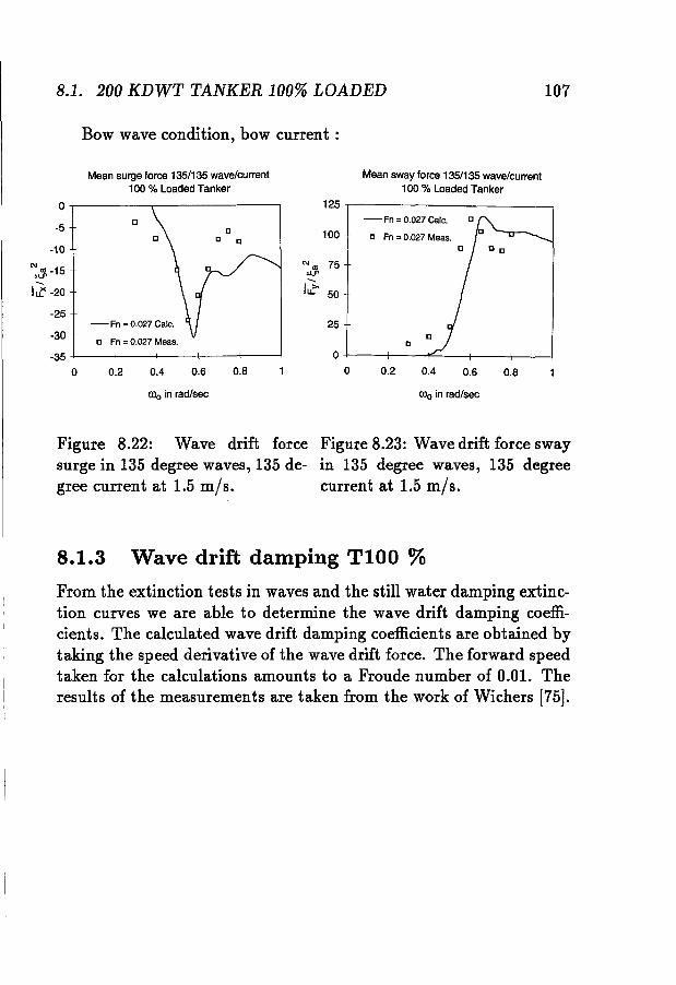
8.1. 200 KDWT TANKER 100% LOADED 107
Bow wave condition, bow current:
Meansurge force 135/135wave/current100 % LoadedTanker
Meansway force 135/135wave/current100 % LoadedTanker
0.80.60.40.2
O+----+-----l~-_+_-__+_-_1
o
en
25
125 -,----------_----,- Fn=0.027 Calc.
100 n Fn= 0.027 Meas.
"'11l 75u.J'
I:?- 50
0.80.6
e
0.4
e
0.2
- Fn= 0.027 Calc.
e Fn = 0.027 Meas.
-25
-30
-35 +--__+_-~f---_I_-_+-____1
o
0-.----------.------------,
-5
-10
":J, -15
I~ -20
0>0 in rad/sec 0>0 in rad/sec
Figure 8.22: Wave drift forcesurge in 135 degree waves, 135 degree current at 1.5 tsi]«.
Figure 8.23: Wave drift force swayin 135 degree waves, 135 degreecurrent at 1.5 m/s.
8.1.3 Wave drift damping TIOO %From the extinction tests in waves and the still water damping extinction curves we are able to determine the wave drift damping coefficients. The calculated wave drift damping coefficients are obtained bytaking the speed derivative of the wave drift force. The forward speedtaken for the calculations amounts to a Froude number of 0.01. Theresults of the measurements are taken from the work of Wichers [75].
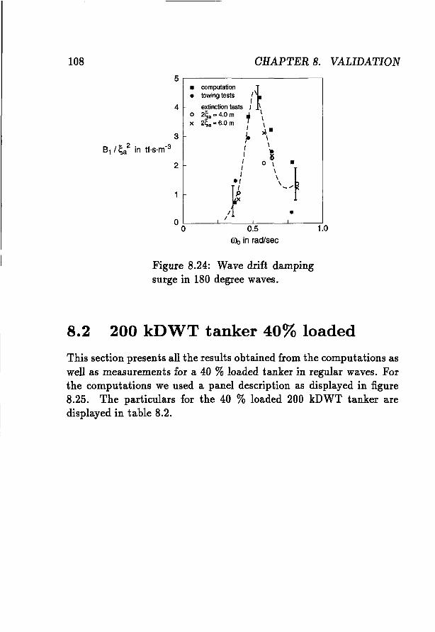
108 CHAPTER 8. VALIDATION5 ,---------------,
1.00.5roo in rad/sec
• computation t.• towing tests 1\
4 extinction tests : \o 21;. = 4.0 m , \x 2~a=6.0 m \
t >4.~ \t \, ~i O\}
I
2
O:.------"--_-=-'::-__.L-_-;-'o
3
8 1/ ~a2 in tf·s·m-3
Figure 8.24: Wave drift dampingsurge in 180 degree waves.
8.2 200 kDWT tanker 40% loaded
This section presents all the results obtained from the computations aswell as measurements for a 40 %loaded tanker in regular waves. Forthe computations we used a panel description as displayed in figure8.25. The particulars for the 40 % loaded 200 kDWT tanker aredisplayed in table 8.2.
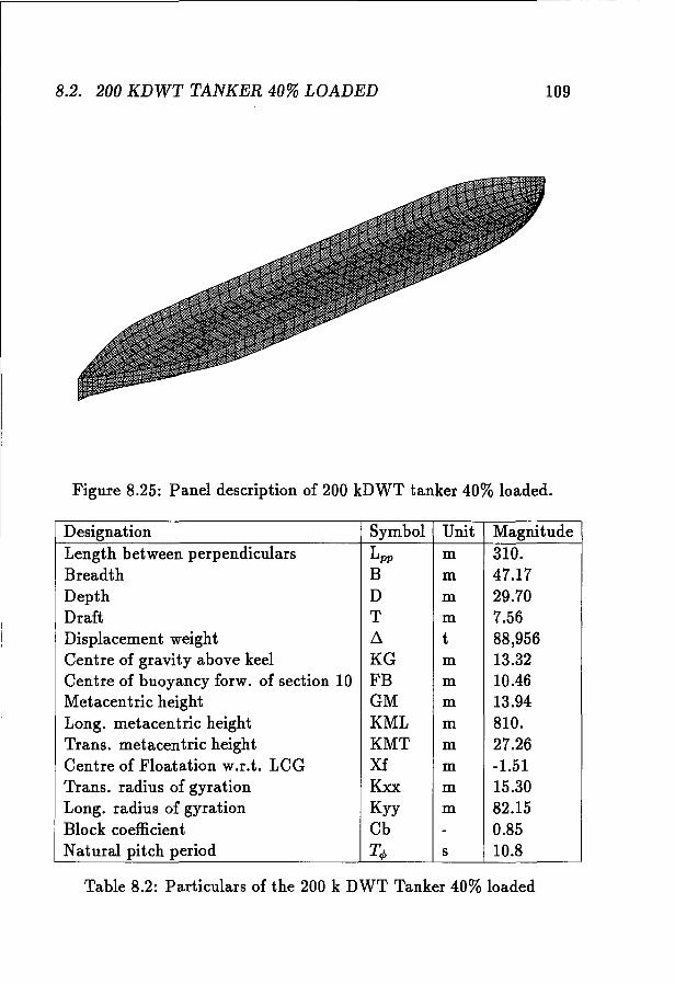
8.2. 200 KDWT TANKER 40% LOADED 109
Figure 8.25: Panel description of 200 kDWT tanker 40% loaded.
Designation Symbol Unit MagnitudeLength between perpendiculars Lpp m 310.Breadth B m 47.17Depth D m 29.70Draft T m 7.56Displacement weight .6- t 88,956Centre of gravity above keel KG m 13.32Centre of buoyancy forw. of section 10 FB m 10.46Metacentric height GM m 13.94Long. metacentric height KML m 810.Trans. metacentric height KMT m 27.26Centre of Floatation w.r.t. LCG Xf m -1.51Trans. radius of gyration Kxx m 15.30Long. radius of gyration Kyy m 82.15Block coefficient Cb - 0.85Natural pitch period T¢ s 10.8
Table 8.2: Particulars of the 200 k DWT Tanker 40% loaded
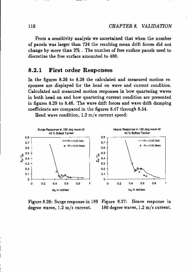
110 OHAPTER 8. VALIDATION
From a sensitivity analysis we ascertained that when the numberof panels was larger than 724 the resulting mean drift forces did notchange by more than 2% . The number of free surface panels used todiscretize the free surface amounted to 480.
8.2.1 First order Responses
In the figures 8.26 to 8.28 the calculated and measured motion responses are displayed for the head on wave and current condition.Calculated and measured motion responses in bow quartering wavesin both head on and bow quartering current condition are presentedin figures 8.29 to 8.46. The wave drift forces and wave drift dampingcoefficients are compared in the figures 8.47 through 8.54.
Head wave condition, 1.2 tix]s current speed:
SurgeResponse in 180deg wavedir40 % BalastTanker
HeaveResponse in 180 deg wavedir40 % BallastTanker
0.6 0.8
a Fn = 0.02 Meas.
- Fn = 0.02 Calc.
0.40.2
0.8~------------,
0.7
0.6
0.3
0.2
0.1
0..J---+---+--t----+-~---1
o
.. 0.5>JJ'
~ 0.4N
0.80.6
- Fn =0.02 Calc.
a Fn = 0.02 Meas.
0.40.2
0.8.,---------------,
0.7
0.6
.. 0.5>JJ'
~ 0.4
0.3
0.2
0.1
o+--I---t~~~=t===-__1o
(00 in radlsec (00 in rad/sec
Figure 8.26: Surge response in 180 Figure 8.27: Heave response indegree waves, 1.2 mls current. 180 degree waves, 1.2 mls current.
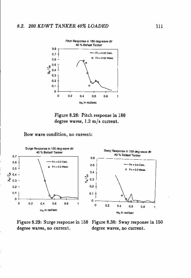
B.2. 200 KDWT TANKER 40% LOADED 111
Pitch Response in 180 deg wave dir40 % BallastTanker
0.80.6
- Fn = 0.02 Calc.
c Fn = 0.02 Meas.
0.40.2
0.8,----------------,
0.7
0.6
'" 0.5u..1'
~ 0.4Q)
0.3
0.2
0.1
0+----+---+---/----+----1o
COo in radlsec
Figure 8.28: Pitch response in 180degree waves, 1.2 mls current.
Bow wave condition, no current:
COo in rad/sec
Surge Response in 150 deg wavedir40 % BallastTanker
0.80.6
-Fn =0.0 Calc.
c Fn =0.0 Meas.
0.4
(00 in rad/sec
0.2
0.61
- - ---,
SwayResponse in 150 deg wavedir40 % BallastTanker
0.5
0.4
0.2
0.1
.:J.~ 0.3>-
0.80.6
- Fn = 0.0 Calc.
c Fn = 0.0 Meas.
0.40.2
0.7,----------------,
0.6
0.5
0.2
0.1
o -l--+---+---~4_..l!::=+====1
o
.:J. 0.4--~ 0.3
Figure 8.29: Surge response in 150 Figure 8.30: Sway response in 150degree waves, no current. degree waves, no current.
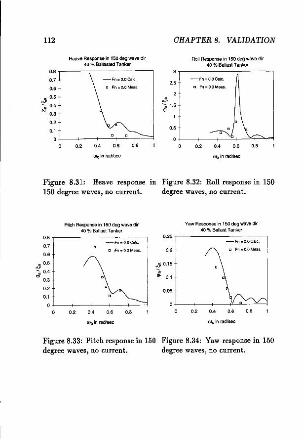
112 CHAPTER 8. VALIDATION
HeaveResponse in 150 deg wavedir40 % Ballasted Tanker
Roll Response in 150 deg wavedir40 % BallastTanker
0.80.60.2 0.4
- Fn = 0.0 Calc.
c Fn = 0.0 Meas.
O+---+---+--~I------==~----=:,~
o
3,.---------------,
2
2.5
0.5
.:J...., 1.59-
0.6 0.8
c
-Fn = 0.0 Calc.
c Fn = 0.0 Meas.
0.40.2
0.8 ,---------------,
0.7
0.6
.:J. 0.5..., 0.4N
0.3
0.2
0.1
0+---+---+---1__---+---'1
o000 in rad/sec 000 in rad/sec
Figure 8.31: Heave response In Figure 8.32: Roll response in 150150 degree waves, no current. degree waves, no current.
PitchResponse in 150 deg wavedir40 % BallastTanker
0.80.60.40.2
0+---+--+---+!!..-~+--~---1
o
0.2
- Fn = 0.0 Calc.
YawResponse in 150 deg wavedir40 % BallastTanker
0.25 ,.----------------,
0.05
.:J. 0.15-....~ 0.1
0.80.6
-Fn = 0.0 Calc.
c Fn =0.0 Meas.c
0.40.2
0.3
0.2
0.1
0+---+--+------1f----+------1
o
0.8,.---------------,
0.7
0.6
.:J. 0.5..., 0.4a:>
000 in rad/sec 000 in rad/sec
Figure 8.33: Pitch response in 150 Figure 8.34: Yaw response in 150degree waves, no current. degree waves, no current.
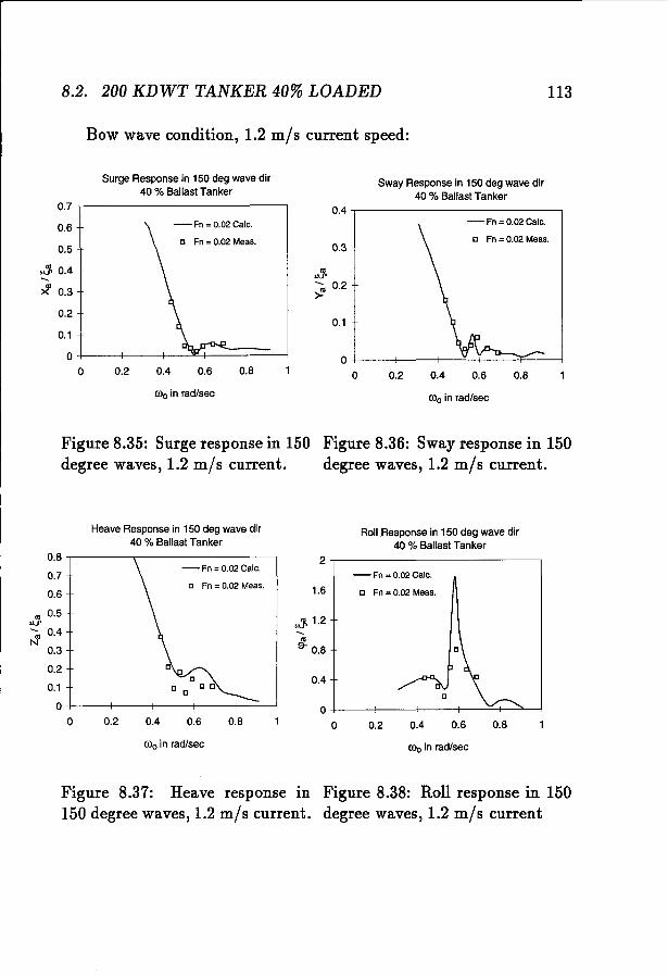
8.2. 200 KDWT TANKER 40% LOADED 113
Bow wave condition, 1.2 m/s current speed:
0.80.6
- Fn = 0.02 Calc.
e Fn = 0.02 Meas.
0.40.2
Sway Response in 150 deg wave dir40 % Ballast Tanker
o +---+-----+-~~~=::::~=_______.j
o
0.1
0.4 ,----------------,
0.3
.,j,-m 0.2>-
0.80.6
- Fn = 0.02 Calc.
n Fn = 0.02 Meas.
0.40.2
Surge Response in 150 deg wave dir40 % Ballast Tanker
0.2
0.1
o +----t-----+--.-.'::~.=...:::::::;:==-___.j
o
0.7 ,------------------,
0.6
0.5
.,j, 0.4
--~ 0.3
000 in radlsec 000 in rad/sec
Figure 8.35: Surge response in 150 Figure 8.36: Sway response in 150degree waves, 1.2 tix]« current. degree waves, 1.2 m/s current.
Heave Response in 150 deg wave dir40 % Ballast Tanker
0.80.60.40.2
- Fn = 0.02 Calc.
e Fn =0.02 Meas.
O+----t---+---t------'=:....t---"''---io
Roll Response in 150 deg wave dir40 % Ballast Tanker
2,----------------,
0.4
1.6
.,j, 1.2
-'"9- 0.8
0.8
n Fn = 0.02 Meas.
0.6
- Fn = 0.02 Calc.
0.40.2
0.3
0.2
0.1
O-l---+---+------1f----+-------1o
0.8 -,-------.----------------,
0.7
0.6
'" 0.5>V'-m 0.4N
000 in rad/sec 000 in radlsec
Figure 8.37: Heave response in Figure 8.38: Roll response in 150150 degree waves, 1.2 m/s current. degree waves, 1.2 m/s current
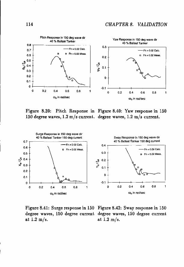
114 CHAPTER 8. VALIDATION
Pitch Responsein 150deg wave dir40 % BallastTanker
0.80.6
- Fn = 0.02 Calc.
n Fn =0.02 Meas.
0.40.2
Yaw Responsein 150deg wave dir40 % BallastTanker
-0.1 -1----+---+---1----+----1o
0.3
0.2
oJuP-.. 0.1~
0
0.80.6
- Fn = 0.02 Calc.
e e Fn =0.02 Meas.
0.40.2
0.8,-----------------,
0.7
0.6
oJ 0.5uP..... 0.4a>
0.3
0.2
0.1
0-1----+---+---1----+----1o
COo in rad/sec <00 in rad/sec
Figure 8.39: Pitch Response in Figure 8.40: Yaw response in 150150 degree waves, 1.2 mls current. degree waves, 1.2 mls current.
Surge Responsein 150deg wave dir40 % BallastTanker 150 deg current
0.80.6
- Fn = 0.02 Calc.
e Fn = 0.02 Meas.
0.40.2
Sway Responsein 150deg wave dir40 % BallastTanker 150deg current
0.4
0.3
oJ 0.2uP-..~ 0.1
0
-0.1
00.80.6
- Fn =0.02 Calc.
e Fn = 0.02 Meas.
0.40.2
0.7 ,---------------,
0.6
0.5
0.2
0.1
o -l-------1f----+--.J~-===+===-__1
o
.:J. 0.4-..~ 0.3
<00 in rad/sec COo in rad/sec
Figure 8.41: Surge response in 150degree waves, 150 degree currentat 1.2 tsi]«.
Figure 8.42: Sway response in 150degree waves, 150 degree currentat 1.2 m/s.
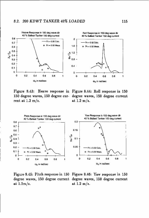
8.2. 200 KDWT TANKER 40% LOADED 115
Heave Responsein 150 deg wave dir40 % BallastTanker 150 deg current
0.80.60.40.2
Roll Responsein 150 deg wave dir40 % BallastTanker 150 deg current
- Fn = 0.02 Calc.
e Fn = 0.02 Meas.
0+---t---t---f------===-r-----"''---1
o
2-,---------------,
1.6
0.4
.,"j. 1.2-...9- 0.8
0.8
- Fn = 0.02 Calc.
e Fn = 0.02 Meas.
n
0.4 0.60.2
0.3
0.2
0.1
O-+---t---j---f----+----='-----1
o
0.8 -,----.....-----------,
0.7
0.6
.. 0.5UJ'
--m 0.4N
0)0 in rad/sec 0)0 in rad/sec
Figure 8.43: Heave response in150 degree waves, 150 degree current at 1.2 m/s,
Figure 8.44: Roll response in 150degree waves, 150 degree currentat 1.2 tii]»,
Pitch Responsein 150 deg wave dir40 % BallastTanker 150 deg current
0.80.60.2 0.4
e Fn = 0.02 Meas.
- Fn = 0.02 Calc.
0-+----+---+---+--0---+--'-----1
o
0.2 -,------=------------,
0.15
Yaw Responsein 150deg wave dir40 % BallastTanker 150 deg current
0.05
..UJ'
--m 0.1~
0.8
ee
0.60.2 0.4
- Fn = 0.02 Calc.
n Fn = 0.02 Meas.
0.3
0.2
0.1
O+----+---+---+----+-------i
o
0.8 -,---------------,
0.7
0.6
.. 0.5UJ'
--m 0.4a:>
0)0 in rad/sec 0)0 in rad/sec
Figure 8.45: Pitch response in 150degree waves, 150 degree currentat 1.2m/s.
Figure 8.46: Yaw response in 150degree waves, 150 degree currentat 1.2 m/s.
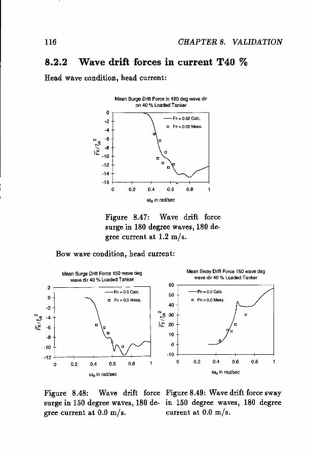
116 CHAPTER 8. VALIDATION
8.2.2 Wave drift forces in current T40 %Head wave condition, head current:
MeanSurgeDrift Forcein 180deg wavediron 40 % Loaded Tanker
0.80.6
[] Fn = 0.02 Meas.
- Fn=0.02 Calc.
0.40.2
0-.------......,.-----------,
-2
-4
'" m -6>lJ'- -8
ILl:: -10
-12
-14
-16 +---+--+----1--=--+----1o
COo in rad/sec
Figure 8.47: Wave drift forcesurge in 180 degree waves, 180 degree current at 1.2 m/s.
Bow wave condition, head current:
MeanSurgeDriftForce150 wavedegwavedir 40 % Loaded Tanker
- Fn = 0.0 Calc.
e Fn = 0.0 Meas.
0.80.60.40.2
- Fn=0.0 Calc.
[] Fn=0.0 Meas.
MeanSwayDriftForee 150 wavedegwavedir 40 % Loaded Tanker
60 -,---------------,
50
40
~ 30-Jat 20
10
o-10 -l---+---t---+--+------j
o0.80.60.40.2
2
0
-2
"'m -4>lJ'-ILl:: -6
-8
-10
-12
0
COo in rad/sec COo in rad/sec
Figure 8.48: Wave drift forcesurge in 150 degree waves, 180 degree current at 0.0 tu] s.
Figure 8.49: Wave drift force swayin 150 degree waves, 180 degreecurrent at 0.0 tsi]«.
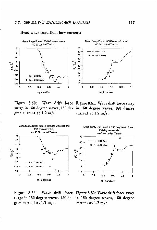
8.2. 200 KDWT TANKER 40% LOADED 117
Head wave condition, bow current:
Mean Surge Force 150/180 wave/current40 % Loaded Tanker
Mean Sway Force 150/180 wave/current40 % Loaded Tanker
0.80.60.40.2
- Fn =0.02 Calc.
e Fn = 0.02 Meas.
90 -.-------------~
80
70
60
"'m 50>J..1'-. 40lat 30
20
10
o-10 +----j---+---+---+-----j
o0.80.60.2 0.4
- Fn = 0.02 Calc.
n Fn = 0.02 Meas.
o-.--------.;;:-------~
-2
-4
'" -6.:J.-. -8
IXu, -10
-12
-14
-16 +---+---+---1---+----;o
(00 in rad/sec COo in rad/sec
Figure 8.50: Wave drift forcesurge in 150 degree waves, 180 degree current at 1.2 m/s.
Figure 8.51: Wave drift force swayin 150 degree waves, 180 degreecurrent at 1.2 m/s.
Mean Surge Drift Force in 150 deg wave dir and150 deg current dir
on 40 % Loaded Tanker
0.80.60.40.2
- Fn = 0.02 Calc.
u Fn = 0.02 Meas.
e
Mean Sway Drift Force in 150 deg wave dir and150 deg current dir
on 40 % Loaded Tanker
40
30"'m
>J..1'-. 20lat
10
0
-10
00.8
e
e
0.60.2 0.4
- Fn = 0.02 Calc.
n Fn = 0.02 Meas.
o-,-----~o;:__------~
-2
-4
'" m -6'!:!' -8IXu, -10
-12
-14
-16 +---+--+-----1r-----"--+-----Io
(00 in rad/sec(00 in rad/sec
Figure 8.52: Wave drift forcesurge in 150 degree waves, 150 degree current at 1.2 ta]«.
Figure 8.53: Wave drift force swayin 150 degree waves, 150 degreecurrent at 1.2 m/s.
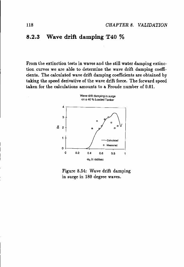
118 GHAPTER 8. VALIDATION
8.2.3 Wave drift damping T40 %
From the extinction tests in waves and the still water damping extinction curves we are able to determine the wave drift damping coefficients. The calculated wave drift damping coefficients are obtained bytaking the speed derivative of the wave drift force. The forward speedtaken for the calculations amounts to a Froude number of 0.01.
Wavedrift dampingin surgeon a 40 % LoadedTanker
4.,------- ------,
3
n
0.80.60.40.20+---+-......:;1----+----+--1
o
<00 in rad/sec
Figure 8.54: Wave drift dampingin surge in 180 degree waves.
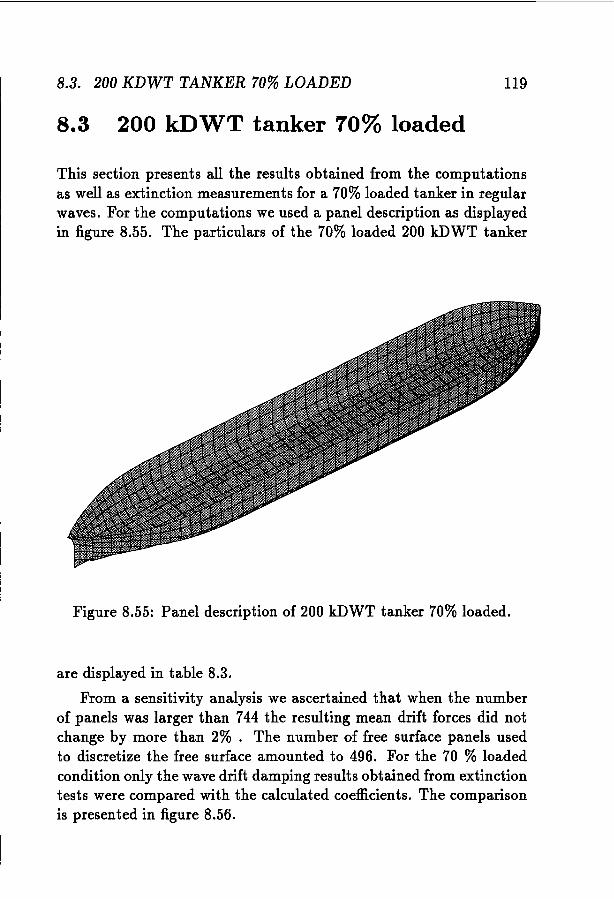
8.3. 200 KDWT TANKER 70% LOADED
8.3 200 kDWT tanker 70% loaded
119
This section presents all the results obtained from the computationsas well as extinction measurements for a 70% loaded tanker in regularwaves. For the computations we used a panel description as displayedin figure 8.55. The particulars of the 70% loaded 200 kDWT tanker
Figure 8.55: Panel description of 200 kDWT tanker 70% loaded.
are displayed in table 8.3.
From a sensitivity analysis we ascertained that when the numberof panels was larger than 744 the resulting mean drift forces did notchange by more than 2%. The number of free surface panels usedto discretize the free surface amounted to 496. For the 70 % loadedcondition only the wave drift damping results obtained from extinctiontests were compared with the calculated coefficients. The comparisonis presented in figure 8.56.
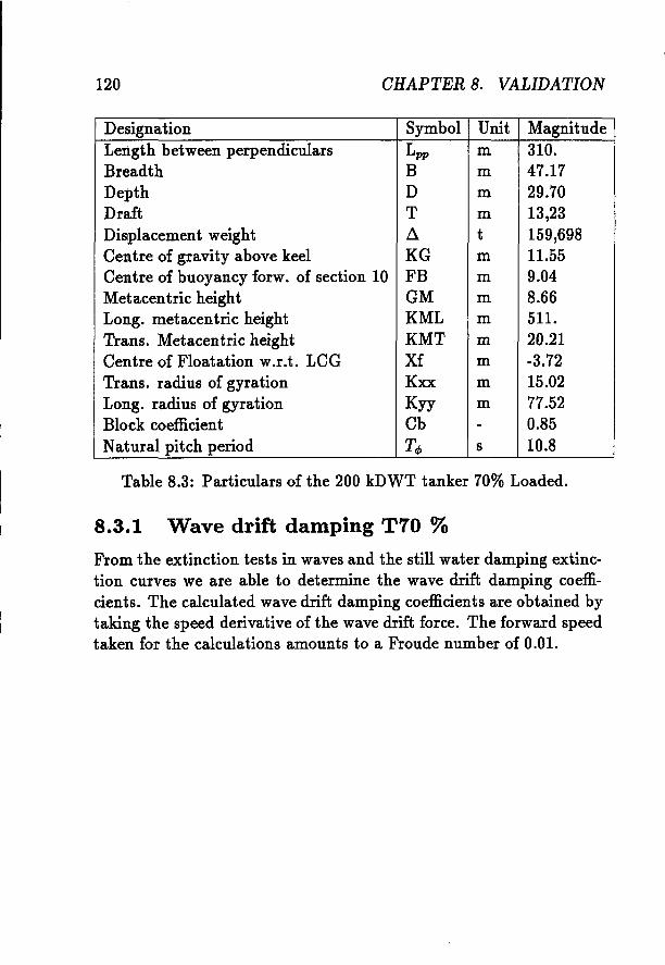
120 CHAPTER 8. VALIDATION
Designation Symbol Unit MagnitudeLength between perpendiculars Lpp m 310.Breadth B m 47.17Depth D m 29.70Draft T m 13,23Displacement weight ~ t 159,698Centre of gravity above keel KG m 11.55Centre of buoyancy forw. of section 10 FB m 9.04Metacentric height GM m 8.66Long. metacentric height KML m 511.Trans. Metacentric height KMT m 20.21Centre of Floatation w.r.t. LCG Xf m -3.72Trans. radius of gyration Kxx m 15.02Long. radius of gyration Kyy m 77.52Block coefficient Cb - 0.85Natural pitch period Tcf> s 10.8
Table 8.3: Particulars of the 200 kDWT tanker 70% Loaded.
8.3.1 Wave drift damping T70 %From the extinction tests in waves and the still water damping extinction curves we are able to determine the wave drift damping coefficients. The calculated wave drift damping coefficients are obtained bytaking the speed derivative of the wave drift force. The forward speedtaken for the calculations amounts to a Froude number of 0.01.
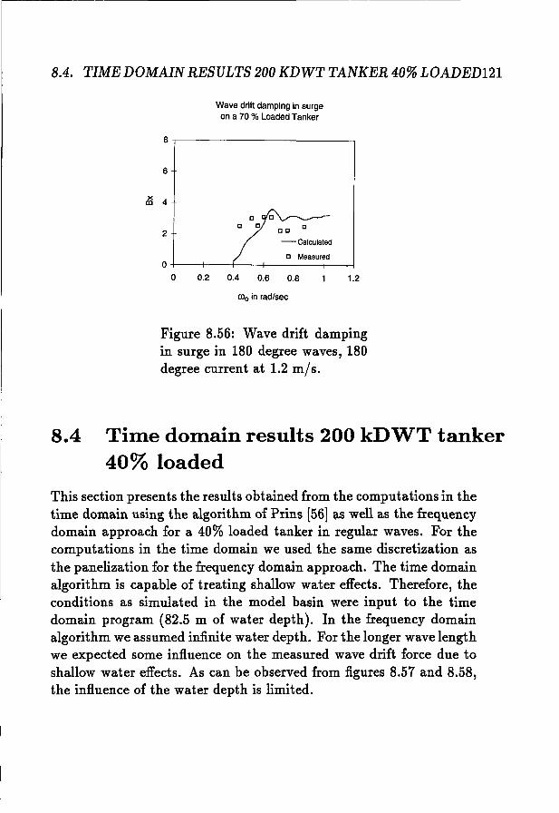
8.4. TIME DOMAIN RESULTS 200 KDWT TANKER 40% LOADED121
Wave drift damping in surgeon a 70 % Loaded Tanker
8-.-----------------,
6
DO 02
o 0 ,......--~-
o 0
-Calculated
n Measured0+--f---t----.,r----t-----j---1
o 0.2 0.4 0.6 0.8 1.2
COo in radlsec
Figure 8.56: Wave drift dampingin surge in 180 degree waves, 180degree current at 1.2 m/s.
8.4 Time domain results 200 kDWT tanker40% loaded
This section presents the results obtained from the computations in thetime domain using the algorithm of Prins [56] as well as the frequencydomain approach for a 40% loaded tanker in regular waves. For thecomputations in the time domain we used the same discretization asthe panelization for the frequency domain approach. The time domainalgorithm is capable of treating shallow water effects. Therefore, theconditions as simulated in the model basin were input to the timedomain program (82.5 m of water depth). In the frequency domainalgorithm we assumed infinite water depth. For the longer wave lengthwe expected some influence on the measured wave drift force due toshallow water effects. As can be observed from figures 8.57 and 8.58,the influence of the water depth is limited.
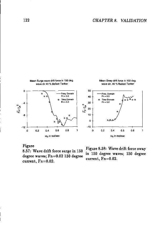
122 OHAPTER 8. VALIDATION
Mean Surge wave drift force in 150 deg.wave dir 40 % Ballast Tanker
Mean Sway drift force in 150 deg.wave dir. 40 % Ballast Tanker
0.80.60.40.2
- Freq. DomainFn =0.0
D Time DomainFn = 0.0
50
40
30"'..>JJ'- 20lat
10
0
-10
00.8
- Freq. DomainFn = 0.0
D Time DomainFn =0.0
0.60.4
D
0.2
-12 +-_-+__-+-__f---..:e.-f----i
o
0
-4"'..>JJ'-I~
-8
0)0 in rad/sec 0)0 in rad/sec
Figure8.57: Wave drift force surge in 150degree waves; Fn=0.02 150 degreecurrent, Fn=0.02.
Figure 8.58: Wave drift force swayin 150 degree waves; 150 degreecurrent, Fn=0.02.
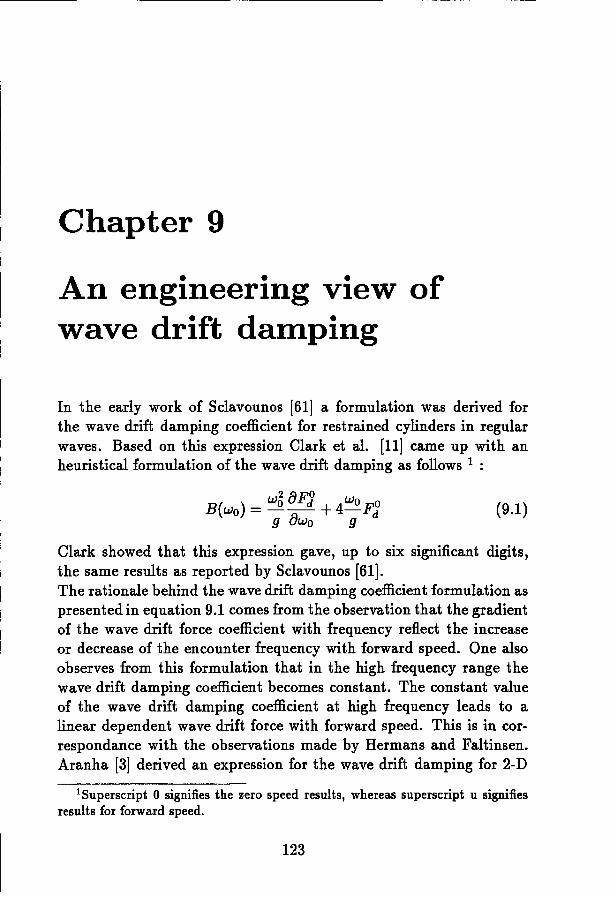
Chapter 9
An engineering view ofwave drift damping
In the early work of Sclavounos [61] a formulation was derived forthe wave drift damping coefficient for restrained cylinders in regularwaves. Based on this expression Clark et al. [11] came up with anheuristical formulation of the wave drift damping as follows 1 :
B( ) - w5 0FS 4woFoWo - --- + -
9 owo 9 d(9.1)
Clark showed that this expression gave, up to six significant digits,the same results as reported by Sclavounos [61].The rationale behind the wave drift damping coefficient formulation aspresented in equation 9.1 comes from the observation that the gradientof the wave drift force coefficient with frequency reflect the increaseor decrease of the encounter frequency with forward speed. One alsoobserves from this formulation that in the high frequency range thewave drift damping coefficient becomes constant. The constant valueof the wave drift damping coefficient at high frequency leads to alinear dependent wave drift force with forward speed. This is in correspondance with the observations made by Hermans and Faltinsen.Aranha [3] derived an expression for the wave drift damping for 2-D
lSuperscript 0 signifies the zero speed results, whereas superscript u signifiesresults for forward speed.
123
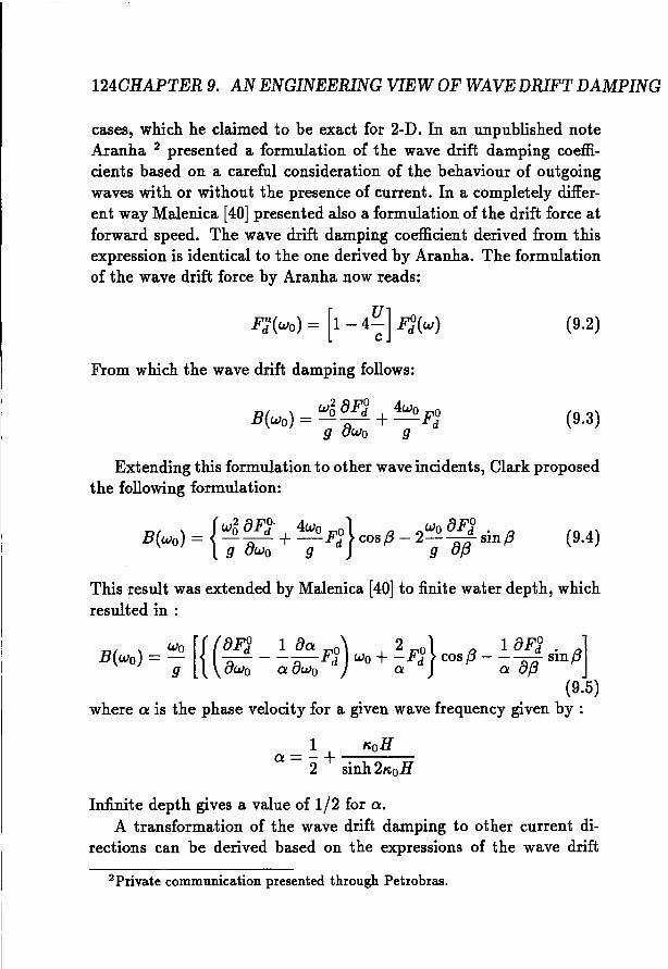
124QHAPTER 9. AN ENGINEERING VIEW OF WAVE DRIFT DAMPING
cases, which he claimed to be exact for 2-D. In an unpublished noteAranha 2 presented a formulation of the wave drift damping coefficients based on a careful consideration of the behaviour of outgoingwaves with or without the presence of current. In a completely different way Malenica [40] presented also a formulation of the drift force atforward speed. The wave drift damping coefficient derived from thisexpression is identical to the one derived by Aranha. The formulationof the wave drift force by Aranha now reads:
From which the wave drift damping follows:
B( ) _ w5 8F~ 4woFoWo ----+- d
9 8wo 9
(9.2)
(9.3)
Extending this formulation to other wave incidents, Clark proposedthe following formulation:
B( ) - {W5 8F~· 4WOFO} a 2wo8F~ . aWo - --- +- d cOSfJ - ---SlllfJ9 8wo 9 9 8{3
(9.4)
This result was extended by Malenica [40] to finite water depth, whichresulted in :
Wo [{ (8F~ 1 Ba 0) 2 o} 1 8Fi. ]B(wo) = - -- - --Fd Wo +-Fd cos{3 - -- Slll{39 8wo a 8wo a a 8{3
(9.5)where a is the phase velocity for a given wave frequency given by :
1 K.oHa=-+----2 sinh2K.oH
Infinite depth gives a value of 1/2 for a.A transformation of the wave drift damping to other current di
rections can be derived based on the expressions of the wave drift
2Private communication presented through Petrobras.
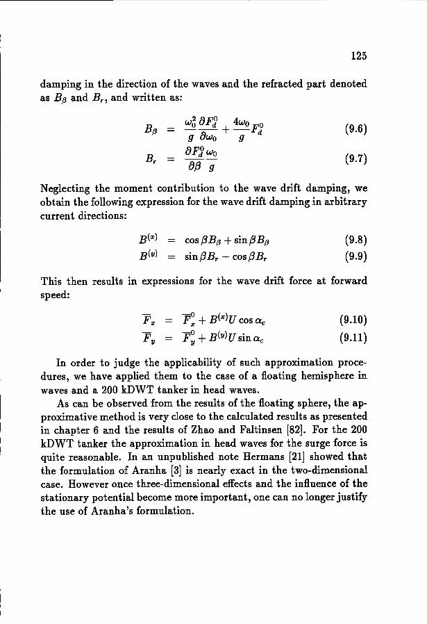
125
damping in the direction of the waves and the refracted part denotedas Bf3 and Br , and written as:
Bf3w~ 8Fi + 4wo FO (9.6)9 8wo 9 d
Br8Fi wo (9.7)- ---8{3 9
Neglecting the moment contribution to the wave drift damping, weobtain the following expression for the wave drift damping in arbitrarycurrent directions:
cos {3Bf3 + sin{3Bf3
sin{3Br - cos{3Br
(9.8)(9.9)
This then results in expressions for the wave drift force at forwardspeed:
v: +B(x)U cos ax C
po +B(Y)U sin aY C
(9.10)
(9.11)
In order to judge the applicability of such approximation procedures, we have applied them to the case of a floating hemisphere inwaves and a 200 kDWT tanker in head waves.
As can be observed from the results of the floating sphere, the approximative method is very close to the calculated results as presentedin chapter 6 and the results of Zhao and Faltinsen [82]. For the 200kDWT tanker the approximation in head waves for the surge force isquite reasonable. In an unpublished note Hermans [21] showed thatthe formulation of Aranha [3] is nearly exact in the two-dimensionalcase. However once three-dimensional effects and the influence of thestationary potential become more important, one can no longer justifythe use of Aranha's formulation.
1260HAPTER 9. AN ENGINEERING VIEW OF WAVE DRIFT DAMPING
30 ,-----------------, 10 .----------------,
- 2Fx/Sa
20
10
o
.. ..-------
u '" 0, calcEst, Aranhau=o
Aranhacamp
"' .. 0U..1'-I~
-10
-20
-20 -30 L-_...L-_-'-_----L_----.l._--'
0.3 0.35 0.4 0.45 0.5 0.55 0.6 0.2 0.4 0.6 0.8 1.0 1.2
(00 in racllsec
Figure 9.1: Approximation wavedrift damping surge usingAranha's expression for a floatingsphere.
roo in rad/sec
Figure 9.2: Approximation wavedriftdamping surge using Aranha's expression for a 200 kDWT in headwaves and current.
Chapter 10
Discussion
As other studies have already shown ([54, 69]), accurate knowledgeof the body motion for the estimation of wave drift forces is quiteimportant. In this study, as well as in the previous cases, the Froudenumber is low. Therefore, the main effect of the Froude number on theship motions at forward speed is concentrated on the shift from wavefrequencies to encounter frequencies. In an earlier study this was alsoobserved by Huijsmans et al. [28] for ship motions in shallow water atforward speed. From the computations and measurements of the shipmotions for both the 100% and 40% loaded tanker we get a similaragreement as was found in studies on ship motions at zero Froudenumber [54, 69]. However, even small changes in forward speed maylead to a considerable increase in wave drift forces, as can e.g, be foundin the figures 8.18 and 8.19.. Accuracy in measuring the increase of thedrift force in current is hampered by the fact that in the analysis, theconstant current force has to be substracted from the total measuredmean force. The same holds true for the estimation of the wave driftdamping coefficient through extinction tests in regular waves. One ofthe main driving forces behind this study was to get reliable estimatesof the wave drift damping coefficients. The hypothesis behind thewave drift damping concept is that this wave drift damping coefficientcan also be obtained from the increase of the drift force due to thepresence of forward speed. So far no rigorous theoretical proof hasbeen given to substantiate the hypothesis. In the study of Wichers
127
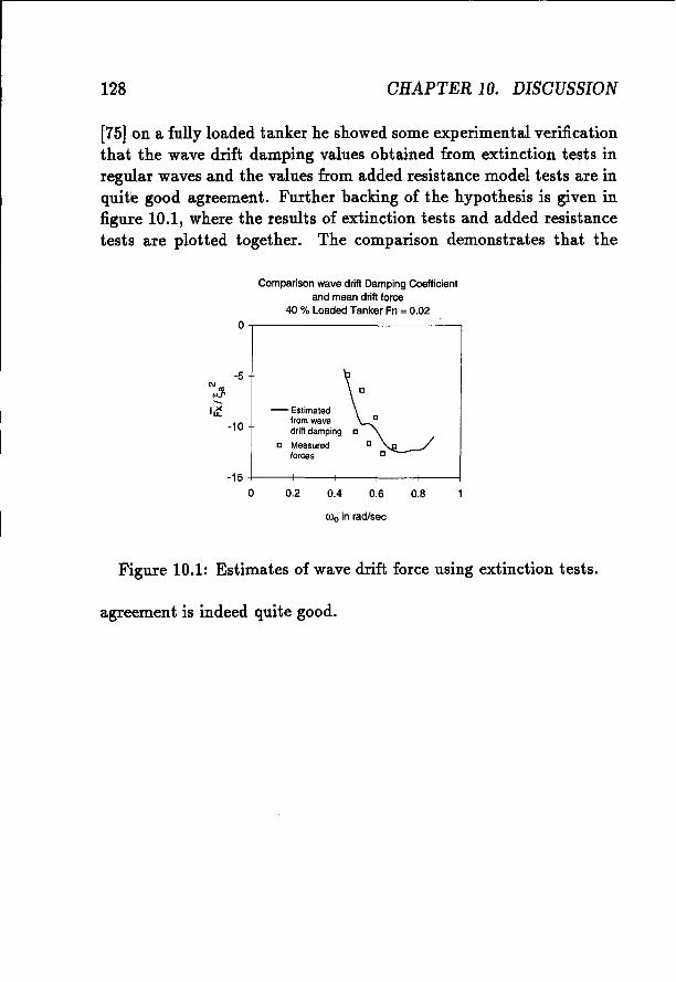
128 CHAPTER 10. DISCUSSION
[75] on a fully loaded tanker he showed some experimental verificationthat the wave drift damping values obtained from extinction tests inregular waves and the values from added resistance model tests are inquite good agreement. Further backing of the hypothesis is given infigure 10.1, where the results of extinction tests and added resistancetests are plotted together. The comparison demonstrates that the
Comparison wave drift Damping Coefficientand mean drift force
40 % Loaded Tanker Fn = 0.02
o,------------~
-5
·10 -.-Estimatedfromwave ndrift damping c
c Measured cforces D
0.80.60.40.2
-15 -l----t-----If----+---+------.j
o
COo in rad/sec
Figure 10.1: Estimates of wave drift force using extinction tests.
agreement is indeed quite good.
Chapter 11
Conclusions
From the observations of the analysis in this study we may concludethe following:
It is possible to formulate a mathematical model of the wave driftforces in current using linearized potential How formulations.
Expansion of the integral equations with respect to forward speed ispossible.
Non-uniformities arising in the expansion of the Green function withrespect to forward speed can be effectively eliminated.
The forward speed expansion of the Green function can be completelyrecast into a zero speed Green function formulation. This gives a verylarge computational advantage over the direct solution of the translating oscillating source potential.
Although the algorithm for solving the integral equations requires alarge amount of computer memory, the computational efficiency of thealgorithm for solving the integral equations is eminent.
From the measurements of the wave drift damping obtained from extinction tests in regular waves and added resistance tests, it becomesevident that the increase in damping due to the low frequency motionsof the vessel can be regarded in a quasi-static manner.
129
130 CHAPTER 11. CONCLUSIONS
The expansion scheme with respect to forward speed does not allowfor very low encounter frequencies. This limits the applicability of thealgorithm to beam and head wave conditions.
If one does not have an algorithm for the computation of the influenceof forward speed on the wave drift forces, one may caustiously as anengineering approach the formulations like those given by Aranha [3]and Malenica [40].
The lid method for three-dimensional floating bodies is efficacious, andit does not require a considerable increase in computational efforts.
The focus of further research can be to:
Derive asymptotic expressions for the forward speed Green function,applicable to shallow water conditions;
Investigate numerically the wave drift damping concept using timedomain approaches, like those formulated by Prins [56] .

Bibliography
[1] M. Abramowitz. Handbook of mathematical functions. DoverPublications, 1972.
[2] H. Adachi and S. Ohmatsu. On the irregular frequencies in the integral equation solution of time-dependent free-surface flow problems. Journal of Engineering Mathematics, 16(2), 1979.
[3] J .A.P. Aranha. A formula for wave drift damping in the drift ofa floating body. Journal of Fluid Mechanics, 275, 1994.
[4] R. B. beck. Time domain simulations of non linear ship motions.Journal of Applied Ocean Research, 34, 1993.
[5] A. Benschop, A.J. Hermans, and R.H.M Huijsmans. Second orderdiffraction forces on a ship in irregular waves. Journal of AppliedOcean Research, 9, 1987.
[6] J. Bougis. Etude de la diffraction radiation dans le cas d'un flotieur indeformiable anime par une boule sinusoidole de faible amplitude. PhD thesis, Universite de Nantes, 1980.
[7] H. Brakhage and P. Werner. Ueber das dirichletsche aussenraumproblem fuer die helmholzsche schwingungsgleichung. Arch Math.Basel, 16, 1965.
[8] R. Brard. The representation of a given ship form by singularitydistributions when the free surface condition is linearized. Journal of Ship Research, 16, 1972.
131
132 BIBLIOGRAPHY
[9] J. Broeze. Numerical modelling on non-linear free surface waves.PhD thesis, Twente University of Technology, 1992.
[10] M.S. Chang. Computation of 3-d ship motions with forwardspeed. In Second Int. Conf. on Numerical Ship HydroDynamics,1977.
[11] P. Clark, B. Molin, and M. Malenica. An heuristic approach towave drift damping. Journal ofApplied Ocean Research, 15, 1992.
[12] W.E. Cummins. The impulse response function and ship motions.Schiffstechnik, 9, 1962.
[13] C.W. Dawson. A practical computer method for solving shipwave problems. In Second Int. Conf. on numerical Ship Hydrodynamics, 1977.
[14] O. Faltinsen and F. Michelsen. Motions of large Structures inwaves at zero Froude number. In The Dynamics of Marine Vehicles and Structures in waves, 1974.
[15] Fang Zhong-Sheng. A new method for calculating the fundamental potential functions induced by a source/dipole polygon.Applied Mathematics and Mechanics, 6(7), July 1985.
[16] A. Grekas and G. Delhommeau. Diffraction-radiation en presence d'un courant. In Proceedings of the ATMA conference Paris,1983.
[17] J. Grue. Drift forces and moments on ships advancing with smallforward speed. Ship Technology Research, 1992.
[18] J. Grue and E. Palm. Current and wave forces on ships and Marine Structures. In Proceedings of Dynamics of Marine Vehiclesand Structures in Waves, 1991.
[19] J. Grue and E. Palm. Currents and wave forces on ships and Marine Structures. In Dynamics of Marine uerhicles and Structuresin waves, 1991.
BIBLIOGRAPHY 133
[20] J. Grue and E. Palm. The mean drift force and yaw momenton Marine Structures in waves and current. Journal of FluidMechanics, 1993.
[21] A.J. Hermans. A discussion on the second order wave forces andwave drift damping. Discussion on Aranha's and Clark's wavedrift damping formulation.
[22] A.J. Hermans. Second order wave forces and wave drift damping.Report 91-34, Delft university of technology, 1991.
[23] A.J. Hermans. Second order wave forces and wave drift damping.Ship Technology Research, 38, 1991.
[24] A.J. Hermans and R.H.M. Huijsmans. The effect of moderatespeed on the motion of floating bodies. Schiffstechnik, 1987.
[25] J.L. Hess and A.M.O. Smith. Calculation of non-lifting potentialflow about arbitrary three-dimensional bodies. Report E.S.40622,Douglas Aircraft Co, Califonia, 1962.
[26] J.P. Hooft. Advanced Dynamics of Marine Structures. J.WileyIntersience, 1982.
[27] R.H.M. Huijsmans. Wave drift forces in current. In 16th Conf.on Naval HydroDynamics,Berkeley, 1986.
[28] R.H.M. Huijsmans and R.P. Dallinga, Non-linear shipmotions inshallow water. In Ship and Platform Motion Symposium, Berkeley, 1983.
[29] R.H.M. Huijsmans and A.J. Hermans. The effect of the steadyperturbation potential on the motion of a ship sailing in randomseas. In Fifth Int. Conf.on Numerical Ship HydroDynamics, Hiroshima 1989.
[30] R.H.M. Huijsmans and A.J. Hermans. A fast algorithme forthe calculation of 3- d shipmotions at moderate forward speed.In Proceedings of Fourth Numerical Ship Hydrodynamic Conference,Washington 1985.
134 BIBLIOGRAPHY
[31] R.H.M. Huijsmans and L. Sierevogel. Wave drift forces on a vessel in cross-flow conditions. In Twentieth Symposium on navalHydrodynamics, Santa Barbara USA, 1994.
[32] R.H.M. Huijsmans and J.E.W. Wichers. Computation model ona chain-turret moored tanker in irregular seas. In Proceedingsof the Twenty-second Annual Offshore Technology Conference,Houston, 1991,. paper No. 6594.
[33] E. Huse. Influence of mooring line damping upon rig motions.In Proceedings of the OTC Conference paper no. 5204, Houston1986.
[34] R. Inglis. A 3-d analysis of the motion of a rigid ship in waves.PhD thesis, University college London, 1980.
[35] G. Jensen, V. Bertram, and H. Soding. Ship resistance computations. In Fifth Int. Conf.on Numerical Ship HydroDynamics,Hiroshima 1989.
[36] F. John. On the motion of floating bodies 1. Communicationson the pure and applied Mathematics, 2, 1949.
[37] F. John. On the motion of floating bodies 2. Communicationson the pure and applied Mathematics, 3, 1950.
[38] M.H. Kim and D.K. Vue. Slowly varying wave drift forces inshort crested irregular seas. Journal of Applied Ocean Research,1, 1989.
[39] M. Kirkup. Solution of exterior acoustic problems by the boundaryelement Method. PhD thesis, Brighton Polytechnic UK, 1989.
[40] M. Malenica. Diffraction de troisieme ordre et interaction boulecourant pour un cylindre vertical et profondeur infinie. PhD thesis, Universite de Paris VI, 1994.
[41] H. Maruo. The drift of a body floating on waves. Journal of ShipResearch, 4, 1960.
BIBLIOGRAPHY 135
[42] P Nakos and P Sclavounos. On steady and unsteady ship wavepatterns. Journal of Fluid Mechanics, 215, 1990.
[43] J.N. Newman. Distribution of sources and normal dipoles over aquadrilateral panel. Journal of Engineering Mathematics, 20:113- 126, 1986.
[44] J.N. Newman. The drift force and moment on a ship in waves.Journal of Ship Research, 10, 1967.
[45] J.N. Newman. The evaluation of the free surface green function.In Fourth international conference on numerical ship Hydrodynamics, Washington, 1985.
[46] J.N. Newman. An expansion of the oscillatory source potential.Applied Ocean Research, 6(2), 1984.
[47] J.N. Newman. Marine Hydrodynamics. The MIT press, 1977.
[48] J.N. Newman. Second order slowly varying forces on vessels inirregular waves. In proceedings of the International symposium onthe Dynamics of Marine Vehicles and Structures in waves London, 1974.
[49] J.N. Newman. The theory of ships motions. Advances in AppliedMathematics, Vol.18, 1978.
[50] P. Noblesse. The green function in the theory of radiation anddiffraction of regular water waves by a body. Journal of Engineering Mathematics, 16, 1982.
[51] J. Nossen. Wave drift forces at small forward speed. PhD thesis,University of Oslo, 1989.
[52] J. Nossen, J. Grue, and E. Palm. Wave forces on threedimensional floating bodies with small forward speed. Journalof Fluid Mechanics, Vol.227, 1991.
[53] T.F. Ogilvie. Recent progress towards understanding and prediction of ship motions. In Proceedings of the fifth symposium onNaval HydroDynamics, Bergen, 1964.
136 BIBLIOGRAPHY
[54] J.A. Pinkster. Low frequency second order wave exciting forceson floating Structures. PhD thesis, Technical University of Delft,1980.
[55] H. Prins and A.J. Hermans. Time domain calculations of thesecond order drift forces on a tanker in current and waves. InTwentieth Symposium on Naval Hydrodynamics, Santa BarbaraUSA, 1994.
[56] H. J. Prins. Time domain calculation of Wave drift forces andmoments. PhD thesis, Technical University of Delft, 1995.
[57] H.C. Raven. Variations on a theme by dawson: recent improvements of a potential flow calculation method for ships. In 17thNaval HydroDynamics Symposium, The Hague 1988.
[58] Hermans A.J. Remery a.F. Slow drift oscillations of a mooredobject in random seas. In Proceedings of the offshore technologyconference, Houston 1971. 1500.
[59] J. Romate. Local error analysis in 3-d panel methods. Journalof Engineering Math., 22, 1988.
[60] J. Romate. The numerical simulation of non-linear gravitywaves. PhD thesis, Twente University of Technology, 1988.
[61] P. Sclavonous. The slow drift wavedamping of floating bodies.In Fourth Int. Workshop on Water Waves and Floating Bodies,1989.
[62] P. Sclavounos and C. Lee. Irregular frequenc suppression inboundary element methods. Journal of Fluid Mechanics, 531,1991.
[63] L. Sierevogel. Absorbing boundary condition for the floating twodimensional objects in current and waves. Accepted for publication. Journal of Engineering Mathematics, 1996.
BIBLIOGRAPHY 137
[64] L. Sierevogel, A.J. Hermans, and R.H.M. Huijsmans. Time domain calculations of first and second order forces on a sailingvessel in waves. In Proceedings of the 21rst conference on NavalHydroDynamics, Santa Barbara 1996.
[65] P. Sonneveld. cas a fast Lanczos-type solver for nonsymmetric linear systems. Technical Report 84-16, Technical UniversityDelft, 1984.
[66] J. Telste and F. Noblesse. Numerical evaluation of green's functions of water wave diffraction and radiation. Journal of ShipResearch, 1111, 1987.
[67] R. Timman, A. J. Hermans, and C. Hsiao. Water wave diffractionon floating bodies. Martinus Nijhof Publications, 1985.
[68] R. Timman and J.N. Newman. The coupled damping coefficentsof a symmetric ship. Journal of Ship Research, 1962.
[69] Oortmerssen G. van. The motions of a moored ship in waves.PhD thesis, Technical University Delft, 1976.
[70] E.F.G. Van Daalen. Studies of water waves and floating bodies.PhD thesis, Twente University of Technology, 1992.
[71] C. Van der Stoep. A three dimensional method for the calculation of the unsteady ship wave pattern using a Neumann Kelvinapproach. PhD thesis, Delft University of Technology, 1991.
[72] H. Van der Vorst. The convergance behaviour of preconditionedcg and cgs in the presence of rounding errors. In Proceedings ofthe pca conference, Nijmwegen June 1989.
[73] H. Van der Vorst and P. Sonneveld. Krylov subspaces for cas.Technical Report, Reports of the Faculty of Technical Mathematics and Informatics, Delft 1990.
[74] J. Wehausen and E. Laitone. Surface Waves. Volume 9 of Handbucli der Physik, Springer Verlag, 1960.
138 BIBLIOGRAPHY
[75] J.E.W. Wichers. A simulation model for a single point mooredtanker. PhD thesis, Technical University of Delft, 1988.
[76] J.E.W. Wichers and R.H.M. Huijsmans. The contribution of hydrodynamic damping induced by mooring chains on low frequencyvessel motions. In Proceedings of the Twenty-first Annual Offshore Technology Conference, Houston 1990,. paper No. 6218.
[77] J.E.W. Wichers and R.H.M. Huijsmans. On the low frequencyhydrodynamic damping force acting on offshore moored vessels.In Offshore Technology Conference, Houston, 1984. Paper No.4813.
[78] J.E.W. Wichers and M.F. van Sluijs. The influence of waves onthe low frequency hydrodynamic coefficients of moored vessels.In Proceedings of the eleventh Annual Offshore Technology Conference, Houston 1979,. paper No. 3625.
[79] Huijsmans R.H.M. Wichers J.E.W. Considerations on wavedriftdamping of a moored tanker for zero and non-zero driftangles. InProceedings of the PRADS symposium, Trondheim, 1987.
[80] P. Woods. Lid method for suppression of irregular frequencies.Journal of Fluid Mechanics, 531, 1962.
[81] G. Wu. A numerical scheme for the calculation of the mj termsin wave current body interaction problem. Journal of AppliedOcean Research, 13, 1991.
[82] R. Zhao and O. Faltinsen. Interaction between current wave andMarine Structures. In Fifth International Conference on Numerical Ship Hydrodynamics., Hiroshima, 1989.
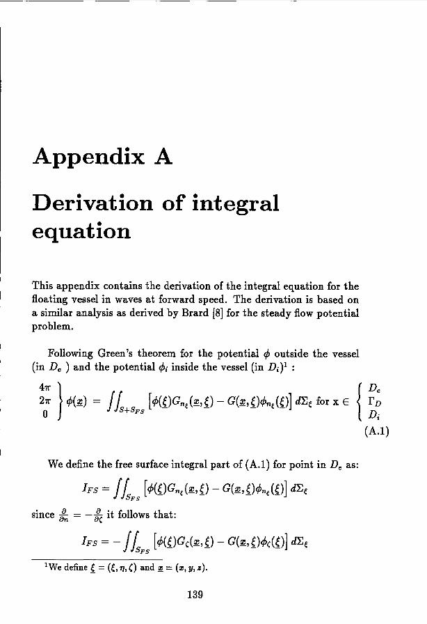
Appendix A
Derivation of integralequation
This appendix contains the derivation of the integral equation for thefloating vessel in waves at forward speed. The derivation is based ona similar analysis as derived by Brard [8] for the steady flow potentialproblem.
Following Green's theorem for the potential ¢ outside the vessel(in De ) and the potential ¢i inside the vessel (in DiP :
;: } ¢(~) = Jfs+SFS [¢({)Gne(~,{) - G(~, {)¢ne ({)] d~e for x E { ~;o ~
(A.1)
We define the free surface integral part of (A.1) for point in De as:
IFs = !hFS [¢({)Gne(~'{) - G(~,{)¢ne({)] d~e
since :n = - ;, it follows that:
lWe define { = (e, 1], C) and ~ =(z, y, z).
139
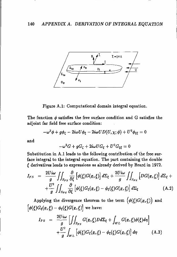
140 APPENDIX A. DERIVATION OF INTEGRAL EQUATION
Figure A.1: Computational domain integral equation.
The function ifJ satisfies the free surface condition and G satisfies theadjoint far field free surface condition:
_w2 ifJ +gifJ, - 2iwUifJe - 2iwUD(U, Xi ifJ) +U2 ifJee = 0
and-w2G +gG, +2iwUGe+U2G
ee = 0
Substitution in A.1leads to the following contribution of the free surface integral to the integral equation. The part containing the doubleederivatives leads to expressions as already derived by Brard in 1972.
IFs = 2Uiw j'r aac [¢({)G(~,{)] d}1e + 2Uiw j' r [DG(~,{)] d}1e +9 }SFS f" 9 }SFS
+~21hFS ~ [¢({)Ge(~,{)- ifJe({)G(~,{)] d}1e (A.2)
Applying the divergence theorem to the term (¢({)G(~,{)) and
[4>({)Ge(~,{) - ¢e({)G(~,{)] we have:
IFs = 2~iW [IhFS
G(~,{)Dd}1e + IWL G(~,{)ifJ({)d17]
+~21wL [4>({)Ge(~,{) - 4>e({)G(~,{)] d17 (A.3)
141
For the potential inside the vessel (Pi we write:
(A.4)
We remark that (Pi satifies the free surface condition with D == O.Combining A.l and AA and defining ,(e) = ¢i(e) - ¢(e) and u(e) =¢in(e) - ¢n(e) we have: - -
47l"¢(.~) - - Is ,({)Gne(.~, {)d~e + Is u({)G(~, {)d~e
2Uiw l. 2Uiw h- - G(~,e)Dd~e +- ,(e)G(~,e)dTJ9 ~ - 9 WL - -
+ ~2 fWL [r({)Ge(~,{)- ,e({)G(~,{)] dTJ for x E ~.5)
or :
(A.B)
where at = cos(Ox,t), or = cos(Ox,T) , an = cos(Ox,nJwhere n is the normal and t the tangent to the waterline and T = t x nthe bi-normal.
142 APPENDIX A. DERNATION OF INTEGRAL EQUATION
Choosing i({) = 0 on S and the free surface:
(A.7)
Appendix B
Integral equation irregularfrequencies
Reiterating the formulation of the integral equations described bysource distributions:
f'f us(e) 8G(~, {) ssis - Bn; {
f'f UF(e) 8G(~, e) as+ iF - 8nx {
for ~ E S as well as
(E.1)
for ~ E F.
The latter equation is already equivalent to equation (5.46)We have by definition:
143
144APPENDIX B. INTEGRAL EQUATION IRREGULAR FREQUENOIES!
using -aa4>i =0 on F we reformulate B.1 into:n",
ll. aG(:z:,e) ll. aG(:z:,e)411'"v4>iC~) = -v 1F4>i({) a;;'x dS{+ l»O's({) a;;'x dS{~ E o.
(B.3)In this equation we need an expression of the z-derivative of the Greenfunction at the free surface. In order to arrive at the correct derivativesof the Green function at z = 0 we make the following reasoning, seealso Noblesse section 9 [50] :the Green function G(~, {) can be written as:
G(~, e) = -1/1'+1/1'1+vh+(X, Z') = -1/1'-1/1'1 +vh-(X, Z') (BA)
in which X = vJ(:z: - ep + (y -11)2, Z' = v(z +() and Z = v(z - ()
From B.4 it then follows:
Gz - vG = (-1/1' - l/1't}z + h; - v (-1/1' +1/1't} - vh+ (B.5)
SInce
(-1/1' -l/1'I)z = V (-1/1' +1/1'1) = 0 for z =0,( < 0
We see by inspection that the functions h+ and h- are only dependenton Z'. Therefore b; - vh+ == 0 throughout the whole fluid domain forz <O. Which leaves:
Gz - vG = (-1/1' - l/1't}z - V (-1/1' +1/1't) for z ~ 0, ( < 0
Suppose we write for the Green function:
G = -1/1' + v-¢J-
It then follows for the z-derivative of G:
(B.6)
This equation is valid throughout the fluid domain. For the integration of the kernel as displayed in ( B.2) we need the derivative with
e.i. INTEGRATION OF FREE SURFACE PANEL 145
(B.7)
respect to the field point z; Applying this equation with respect tothe free surface (( = 0) we find:
2 _ 2z /Gz =v"p + 3" - v r*
r*
in which r* = viR2 + Z2 and R is the horizontal distance.If we take the limit of equation (B.3) for ~ --+ F and the observationthat Gz = vG + 2z/r~ for ~ E F.The integral
j'f (J'F(e) 8G(~, e) dSiF - 8nx e
has to be interpreted in the sense of principle value. Therefore wehave:
41rv4>i(~) = _v2Jh. 4>i({)G(~, {)dS~ +vJL(J's({)G(~, {)dSfl) E F
(B.8)From the last equation we see that the integral equation (5.48) isidentical to the integral equation (5.42).
The remaining terms can be integrated analytically over a panel aswell; the function "p- also has a logarithmic singularity of the following type In(vrt - Z'). This remaining logarithmic singularity in thefrequency dependent part of the Green function can be integrated onthe free surface as will be shown in the next section. The ~ term inr.the integration will lead to a contribution of 21rvRf for a circular panelof radius R], In the interior domain D, or in the interior free surfaceF we are free to chose a proper boundary condition for the interiorpotential 4>i. Since we have reformulated the potential problem into asource distribution, we have to chose a boundary condition for -aa 4>i.
n",
In the remainder we have set -aa 4>i =O.n",
B.l Integration of free surface panel
The singular integral used in computing the contribution from the freesurface panels is presented in this section. The interesting case occurswhen the self-induction of free surface panels has to be determined.
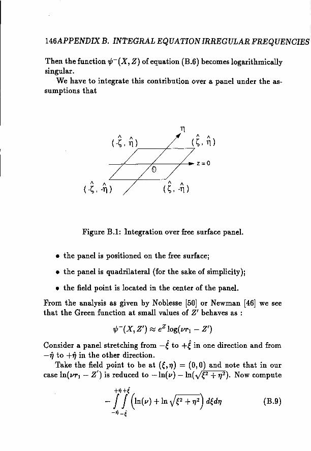
I46A.PPENDIX B. INTEGRAL EQUATION IRREGULAR FREQUENOIES
1
Then the function 'f/r(X, Z) of equation (B.6) becomes logarithmicallysingular.
We have to integrate this contribution over a panel under the assumptions that
--+----+----/----.. z =0
Figure B.I: Integration over free surface panel.
• the panel is positioned on the free surface;
• the panel is quadrilateral (for the sake of simplicity);
• the field point is located in the center of the panel.
From the analysis as given by Noblesse [50] or Newman [46] we seethat the Green function at small values of Z' behaves as :
?/J-(X, Z') ~ eZlog(V1'l - Z')
Consider a panel stretching from -t to +t in one direction and from-iJ to +iJ in the other direction.
Take the field point to be at (e,11) = (0,0) and note that in ourcase In(V1'l - Z') is reduced to -In(v) -In(Je + 112 ) . Now compute
+ii+e- / / (In(v) +In Je 2 + 112
) ded11-11-e
(B.9)
B.I. INTEGRATION OF FREE SURFACE PANEL 147
After some algebra this yields the expression
- 4l7} In(v) +212 aretan(7}!l) +27}2 aretan(l/7}) +2l7} In(l2 +7}2) - 6{rJ(B.10)
148APPENDIX B. INTEGRAL EQUATION IRREGULAR FREQUENCIES
Appendix C
Integration rankine source
This appendix contains the computation of the integration of the singular part ofthe Green function. The formulae are basically derived by Fang ( [15]), but arereiterated here because of the several misprints in his original publication.
The integration of the rankine part of the Green function is takenover a quadrilateral. The derivation for triangular panels is basicallyanalogous to the following derivation. Define I:
where !:fJ..Sj is split up into: P is the field point and P' is the projectionof P onto the panel j (ABCD). We distinguish the contributions fromthe four triangles AQB,BQC,CQD,DQA. which leads to :
r dSQ _ r dSQ + r dSQ + r dSQ + r dSQ
JASj I~p _{QI - JQAB T JQBC T JQCD T JQDA T
Integration over the triangle QAB now gives [15],[43] :
hAB d~Q = dlog (~~ :~: ~ ~)+ Ihl [arctan (01. p~ - p~ + ..\2)
d 2Pl..\
(Ihl p2 _ p2 + ..\2) ]+ arctan d' 2 2p~..\ - signed) . (J (C.1)
149
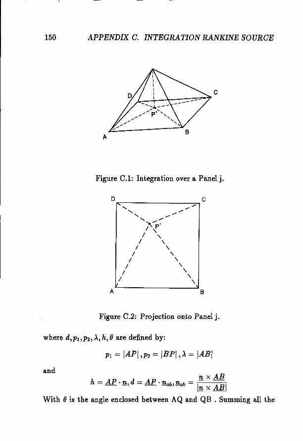
150 APPENDIX C. INTEGRATION RANKINE SOURCE
A
c
Figure C.1: Integration over a Panel j.
o c" ....-""-, ....-, ....-""-, ....-
~""-p'/ \
/ \/ \
/ \/ \
/ \/ \
/ \/ \
I \
A B
Figure C.2: Projection onto Panel j.
where d,PI,P2,>.,h,() are defined by:
PI = IAPI ,P2 = IBPI,>' = IABI
andnxAB
h = AP '!h d = AP . 11ab,11ab = I; x AHIWith () is the angle enclosed between AQ and QB . Summing all the
151
four contributions will result for the angle (J:
P' inside ABCDP' on one of the sides of ABCDP' outside ABCD
Care should be taken once the arguments of the arctangent functionsbecome very small.For the sake of completeness, we give the expression for the normalderivative of the Green function.
[ (Ihl p2_ 2+ A2)
sign(h) arctan d' 1 2=:A
(Ihl p2_p2+A2) 1+ arctan d' 2 2P:A - sign(d) . (Ji
+ log (PI +P2 +A) (C.2)PI +P2 - A
152 APPENDIX C. INTEGRATION RANKINE SOURCE

(D.l)
Appendix D
The fsc for the radiationpotential
This appendix contents the computation of the free surface conditionfor the non-steady part of the velocity potential.The boundary condition is (equation (3.6)) at z = 0:
1<Ptt+ g<Pz+ (V<p .V<p)t-- (<pt +V<P· V<p).
9
(V<P . V<P )·(<ptt+g<Pzt+V<P·V 2 =0+0((2)
In this condition we have to fill in the total velocity potential, whichis split into a steady and a non-steady part (equation (3.11)).
<p(~, t) = ¢(~; U) +~(~, t; U) (D.2)
¢ satisfies the free surface condition, so g¢z + (V¢ . V¢)t + V¢ .V (V4>;V4» = o.
For clearness, equation (D.l) will be split into four parts. The partswill be added together at the end of this appendix.We will assume for the time being that the ship travels in head ondirection, which means that we represent the steady potential as:
153
l54APPENDIX D. THE FSC FOR THE RADIATION POTENTIAL
We also assume that quadratic or higher order terms in ¢ are neglegible. The first and second term of equation (D.l) become by usingequation (D.2):
q)tt +gq)z = ¢tt +g¢z
The third term of equation (D.I) becomes:
(D.3)
(Vq). Vq)t = 2 (V¢. V¢t)
= -2U¢xt+ (2VX ,V¢)t (DA)
Thefourth term becomes, with V2¢ = 0:
-~¢t (¢ttz +g¢zz +g¢zz) z
= ¢t (¢xx +¢yy) (D.5)
The last term gives:
V q) . V q) = V¢ . V¢ +V¢ . V¢ +2V¢ . V¢ (D.6)
Taking V of equation (D.6):
V (Vq);Vq)) V(V¢.V~
- UV(VX' V¢) - UV¢x (D.7)
For the further computations we need to rewrite the derivatives of(VX· V¢). .
(VX . V¢) x = Xxx¢x +Xx¢xx +XYX¢y +Xy¢XY
(VX· V¢) y = Xyy¢y +Xy¢yy +XYX¢X +Xx¢XY
(VX . V¢) z = Xx¢zx +XlJ¢ZY
(D.S)
(D.9)
(D.IO)
Multiplying equation (D.7) and V cP will lead to terms that are quadraticin X and ¢. Neglecting most of the quadratic terms and U squaredterms will lead to the final free surface condition:
- - - - 2-cPtt +gcPz - 2UcPxt +2UVX . V cPt +U cPxx +
+ ¢t (Xxx +Xyy) = 0 (D.ll)
In short:
155
~tt +g~z - 2U~xt + U2~xx +D(U;x,¢) = 0
with D(U; x,¢) = +2UV X ' V~t + ~t (Xxx +Xyy) (D.12)

156APPENDIX D. THE rsc FOR THE RADIATION POTENTIAL
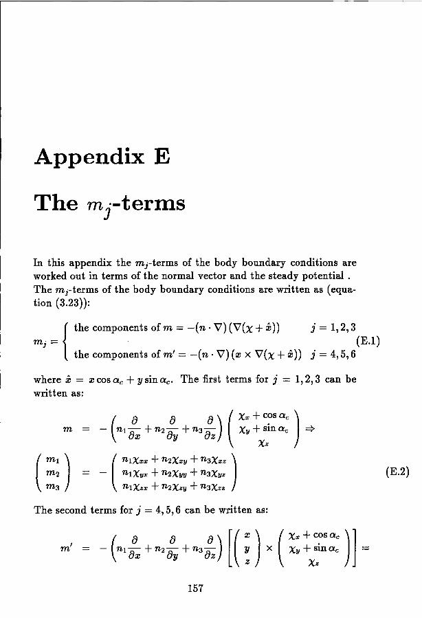
Appendix E
In this appendix the mj-terms of the body boundary conditions areworked out in terms of the normal vector and the steady potential.The mj-terms of the body boundary conditions are written as (equation (3.23)):
{
the components of m = -(n. V) (V(x + i:))
mj = the components of m' = -(n. V)(x X VeX + i:))
j = 1,2,3(E.l)
j = 4,5,6
where i: = x cos a c + y sin ac • The first terms for j = 1,2,3 can bewritten as:
The second terms for j = 4,5,6 can be written as:
(E.2)
m'
157
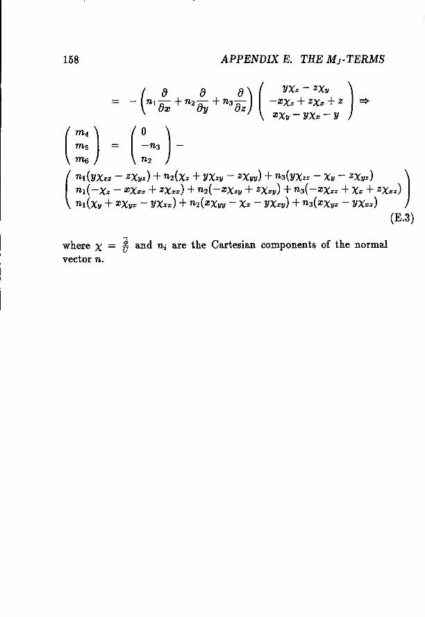
158 APPENDIX E. THE MJ - TERMS
(
YXz - ZXy )-:Z:Xz +ZXX +Z '*:Z:Xy - YXx - Y
(
nl(YXzx - ZXyz) +n2(Xz +YXzy - ZXyy)+n3(YXzz - Xy - ZXyz) )nl( -Xz - :Z:Xxz +ZXxx) +n2( -:Z:Xzy +ZXXY) +n3( -:Z:Xzz +Xx +ZXxz)nl(XY + :Z:Xyx - YXxx) +n2(:Z:XYy - Xx - YXXy) +n3(:Z:Xyz - YXxz)
(E.3)
where X = ~ and ni are the Cartesian components of the normalvector n.
Appendix F
The computations of 'l/Jl
In this appendix the computations of the expressions for "pI, used in sections 5.3.1
and 5.3.2, are given.
F.1 A transformation in the complex plane
We have (equation (5.10)):
The Hankel functions H~l) and H~2) have the asymptotic expansionrespectively ei kR and e- i kR , when IkRI ---t 00. So the contour Lbecomes in the complex plane just like the one shown in figure F.1.If the poles in z = Zo are second order singularities of f( z), the residuehas to be written as:
(Residue at z = zo) = lim dd [(z - ZO)2 • f(z)] (F.2)z-+zo z
If R ---t 00 integration of the arcs goes to zero, because with k = ReiO,H~I)(RReiO) behaves like JReiRRei9.
For the integration of the contour of Hi l) we have to add the contour
at the imaginary axis, by using k = ik, and the residue in k = K. The
159
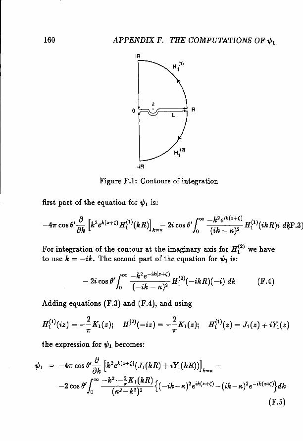
160 APPENDIX F. THE COMPUTATIONS OF"pI
iR
-iR
Figure F.1: Contours of integration
first part of the equation for "pI is:
For integration of the contour at the imaginary axis for H?) we haveto use k = -ik. The second part of the equation for "pI is:
lOO _Pe-ik(z+c)
- 2i cos Of (. )2 Hi2) ( -ikR)(-i) dk
o -'£k - /'i,
Adding equations (F.3) and (FA), and using
(FA)
the expression for "pI becomes:
"pI = -47r cos Of~ [k2ek(z+C) (JI (kR) + iYj (kR))] k=x -
-2 cos Of roo -k2.~KI(kR) {(-ik-/'i, )2 eik(z+c) _ (ik-/'i,)2 e-ik(z+C)}dk
10 (/'i,2-k2 )2(F.5)
F.2. AN EXPRESSION OF DERIVATIVES ore; 161
We have to work out tk[" .]. The derivative of the Bessel and Weberfunction can be compute with the help of the recurrence relations:
8JI = RJo _ J I and 8Yi = RYO _ Yi8k k 8k k
We also have to work out the term between the delimiters.
{ ...} = {l-k2 + K,2 + 2iK,k] - [_k 2 + K,2 - 2iK,kl} cos k(z +()++ {[_k2 +K2+2iKk] + [_k 2 +K2
- 2iKk]}isink(z +() =
2[2iKk cos k(z +()+ i( _k2+ K,2) sin k(z +()] (F.6)
The equation for .,pI can be split into a real ~e and an imaginary~part. These equations can be written as follows:
S:m{'l/JI} -47rcosO'elt(z+()K[(1 +K(Z +()Yi(KR) +KRYO(KR)]
8 r k2 KI(kR) [-; cos 0'Jo (K2 _ k2)2 2Kk cos k(z+() + (_k
2+
+K2)sin k(z+()]dk
(F.8)
F.2 An expression of derivatives of 'l/Jo
For the further computations we only use the principal value of theintegral in equation (5.16). In order to derive a relation between equation (5.16) and equation (5.8) we introduce the non-dimensional parameters.
kK=-j X=KRj Z=-K(Z+()
K
Using these non-dimensional parameters, the expressions for 'l/Joand.,pI can be written as:
r -ZK'l/J~(~,{) = 2KJL ; -1 Jo(XK)dK (F.9)
162 APPENDIX F. THE OOMPUTATIONS OF'l/Jl
r K 2e- ZK'l/Jl(~'{) = 4i cos O'KJL (K _1)2J1(XK)dK (F.1D)
To compute the derivatives of'l/Jij we need the derivatives of the Besselfunctions as given in Abramowitz [1].
8Jo(XK) = -KJ (XK)' 8J1(XK) = X~ (XK) _ J1(X K )8X 1, 8K 0 K
(F.ll)The derivatives of 'l/Jij become:
8'l/Jij8X8'l/Jij8Z
iK -ZK
- 2K - K e J1(XK)dKL -1
iK -ZK
2K - K e Jo(XK)dK =L -1
2K r e-ZK- X J
LK -1 [-KdJ1(XK) - J1(XK)dK] =
__ 2K re-ZK[ZK(K -1) +K]J1(XK)dKX JL (K -1)2
(F.12)
(F.13)
The last step of !!Ii is reached by partial integration.The principal value of the expression for 'l/Jl (~, {) can now be computedas:
Because the principal value of'l/Jo is real, the principal value of 'l/Jl (~,{)is purely imaginary. The real part of 'l/Jl(~, {) is equal to the residueof the integral, as computed in section 5.3.1.So in this section we have the following expressions for respectivelythe real ~e and imaginary ~m part of 'l/Jl(~'{):
~e{ 'l/Jl} = -471" cos 0'elt(z+c)K[(1 +K(Z+(n J1(KR)+
+KRJo(KR)] (F.15)
{8'l/J* 8'l/J* }
-2 cos 0' [K(Z +()+ 1] K8~ +KR -K;Z (F.16)
r ek(z+c)2KPV JL k _ K Jo(kR)dk (F.17)
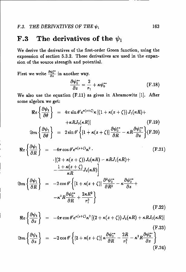
F.3. THE DERIVATIVES OF THE 1/;1
F.3 The derivatives of the "pI
163
We derive the derivatives of the first-order Green function, using theexpression of section 5.3.2. These derivatives are used in the expansion of the source strength and potential.
+KRJO(KR)] (F.19)
2 sinO' {[I +K(Z +()] 8:~* - KR8:;*}(F.20)
471" sinO'elt(z+C)K [(1 +K(Z +e))J1(KR)+
First we write a~r in another way.
81/;0* 2 ftJ.**-- = - +K'f'O8z Tl
We also use the equation (F.ll) as given in Abramowitz [1].some algebra we get:
~e {8~1}
~m{8~1} =
~e { ~~} = -471" cos 0'e't(z+C) K2
•
(F.18)
After
(F.21)
(F.22)
-471" cos 0'elt(z+C)K2[(2 + K(Z +en J1(KR) +KRJO(KR)]
(F.23)
{81/;** 2R 81/;** }-2 cos 0' [2+K(Z +e)] K_O_ - - - K2R_O_8R T~ 8z
(F.24)
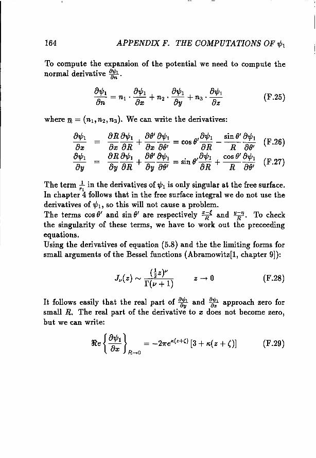
164 APPENDIX F. THE COMPUTATIONS OF "pI
To compute the expansion of the potential we need to compute thenormal derivative ~.
(F.25)
where 11 = (nt,n2,n3)' We can write the derivatives:
(F.26)
(F.27)
The term l in the derivatives of .,pI is only singular at the free surface.rl
In chapter 4 follows that in the free surface integral we do not use thederivatives of "pI, so this will not cause a problem.The terms cos Of and sin Of are respectively 7t and 1lif. To checkthe singularity of these terms, we have to work out the preceedingequations.Using the derivatives of equation (5.8) and the the limiting forms forsmall arguments of the Bessel functions (Abramowitz[l, chapter 9]):
z-+O (F.28)
It follows easily that the real part of eatl and ~ approach zero forsmall R. The real part of the derivative to z does not become zero,but we can write:
(F.29)

F.3. THE DERIVATIVES OF THE '1/;1
To compute the imaginary parts we use equation (F.18) and
which gives after some algebra:
165
(F.30)
(F.31)
{0'1/;**
-21\'; (1 + (1+ I\';(z +(n cos2 0') 'I/;~* +R cos2 0' o~ +
+ l + l\';(z + ( )( 20' . 20')0'l/;~* +------'-~ cos - SIn --
1\';2R oR
21 + I\';(z + ()cosO' z+(2 O'}+ - -- cosI\';r l 1\';2r~
Newman[46] gives the integral 'I/;~* as an ascending series expansion.Using this series and its derivatives the singular behaviours of 'Ij;~* andits derivatives are:
'Ij;~*
o'l/;~*
oR1 o'l/;~*---R ou
-21n(l\';(rl + Iz +(In2R
(F.32)
Using these equations it follows:
(F.33)
Using the same method, it follows that the imaginary part of the 8/:and 8tl becomes zero for R -4' O.
166 APPENDIX F. THE OOMPUTATIONS OF "pI
Appendix G
The far field expansion
In this appendix the far field expansion of the Green function is computed. In the first section the residue is computed and in the secondsection the method of stationary phase is applied.
G.1 The residue of 'ljJ
For the residue in k = k1 of F(9,k) (equation (5.3)) the denominatorof F(O,k) has to be zero. Equation (5.4) gives:
k1(O) = K,' 1- 27 cosO - ""1- 47COSO (G.1)272 cos2 ()
The residue in k = k1 of F (0, k) becomes:
{residue in k = k1 of F(O,k)} =
= 27ri { k - k1 kek[z+(+i(x-e) COS 8] cos[k(y -1/) sin O]}gk - (w + kU cos 0)2 k=k
1
(G.2)
Using the rule of l'Hospital:
{residue in k = k1 of F(O,k)} =
= 27ri 1 k1ekdz+(+i(x-e) COS 8] cos[k1(y - 1/) sin 0] =9 - 2U cos O(w + k1Ucos 0)
167
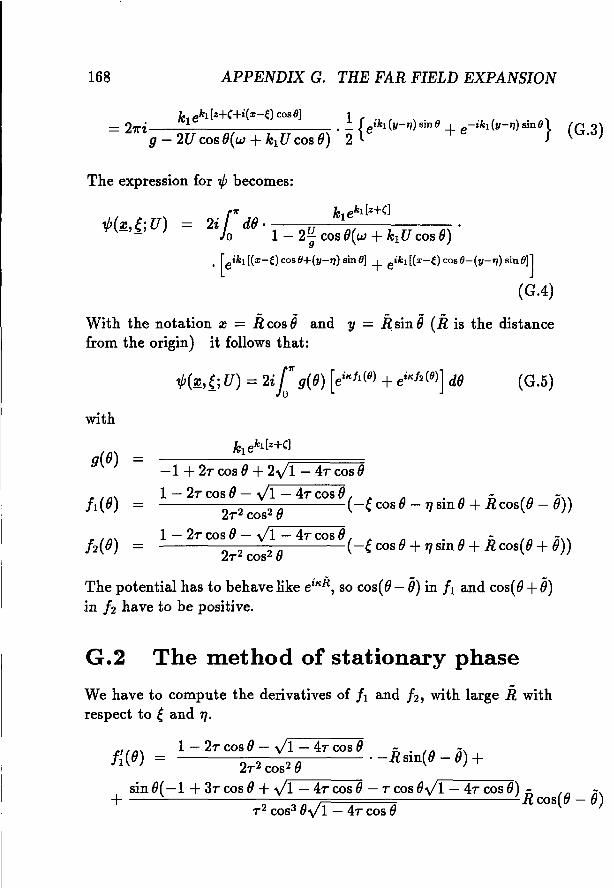
168 APPENDIX G. THE FAR FIELD EXPANSION
.,p(~,{j U) =
The expression for .,p becomes:
l'lt" kl ekdz+Cl
2i dO· .o 1-2¥cosO(w+k1UcosO)
• [eikd(x-e)cOS8+(Y-l1)sinol + eikd(x-e) cosO-(Y-l1) sinOl]
(GA)
With the notation z = il cos 8 and Y = it sin 8 (il is the distancefrom the origin) it follows that:
with
g(O)
12(0)
-1 +2Tcos 0 +2J1 - 4T cos 0
1- 2Tcos 0 - J1- 4TCOSO( cO' 0 R- (0 0-))--------,------- -10 cos - '" sin + cos -
2T2 cos2 01 - 2Tcos 0 - yr71---4-:-T-c-o-s-"0 --
22 2 0 (-e cos 0+'" sin 0 +R cos(0 +0))
T cos
The potential has to behave like eiK.R, so cos(0 - 8) in /1 and cos(0+8)in 12 have to be positive.
G.2 The method of stationary phase
We have to compute the derivatives of /1 and 12, with large il withrespect to eand n,
IHO) = 1 - 2Tcos20
2- J210
- 4Tcos 0 . -ilsin(O - 6)+T cos
sinO(-1 +3Tcos 0 + y~1---4"""'T-c-o-s-=0 - T cos OJ1 - 4T cos 0) - (0 -)+ Rcos - 0T2 cos'' OJ1 - 4Tcos 0
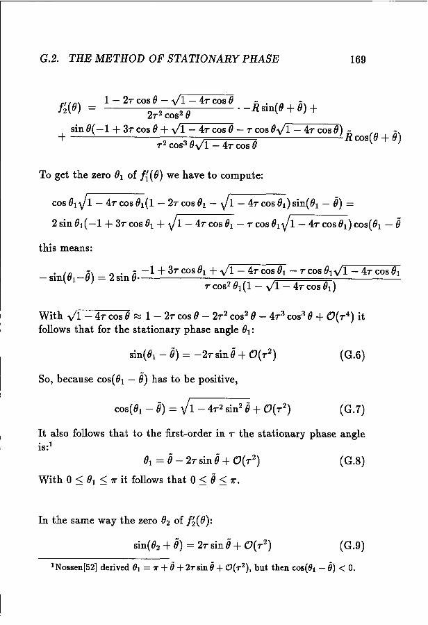
G.2. THE METHOD OF STATIONARY PHASE 169
f ' ((J) 1 - 2r cos (J - VI - 4r cos (J R-' ((J (J-)2 = 2 2 2(J • - sin + +
r COS
+ sin (J(-1 +3r cos (J +V'-"""I---4;-r-co-s----;;(J - r cos (JVl - 4r cos (J)Rcos( (J +8)
r 2 cos'' (JVl - 4r cos (J
To get the zero (Jl of f{ ((J) we have to compute:
cos(Jn/1 - 4rcos(Jl(l- 2rcos(Jl- Vl- 4rcos(Jl)sin((Jl - 8) =
2 sin (Jl( -1 +3r cos (Jl + VI - 4r cos (Jl - r cos (JlVI - 4r cos (Jd COS((JI - 8
this means:
. ((J (J-) 2' (J- -1 +3r cos (Jl +VI - 4r cos (Jl - r cos (JlVI - 4r cos (Jl- SIn 1- = SIn .------~-;;-;:---r.=====;:====;~-----
r cos2 (Jl(1 - VI - 4r cos (Jl)
With VI - 4r cos (J ::::::: 1 - 2r cos (J - 2r2 cos2 (J - 4r3 cos" (J +O(r 4 ) itfollows that for the stationary phase angle (Jl:
(G.6)
So, because cos((Jl - 8) has to be positive,
It also follows that to the first-order in r the stationary phase angleis:1
(Jl = 8 - 2rsin8 +0(r2)
With 0 < (Jl :s; 7r it follows that 0 <8 :s; 7r.
In the same way the zero (J2 of fH(J):
sin( (J2 +8) = 2r sin 8 +O(r 2)
(G.8)
(G.9)
1 Nossen[52] derived (h = 1r +8+ 2T sin 8+ CJ(T 2 ) , but then cos(/h - 8) < O.
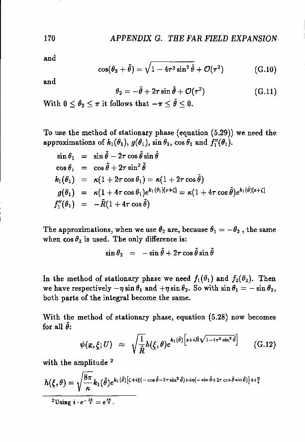
170
and
APPENDIX G. THE FAR FIELD EXPANSION
and
(G.lO)
82 = -0 +2r sin 0+O(r2)
With 0 ~ 82 < 71" it follows that -71" <0<O.
(G.ll)
To use the method of stationary phase (equation (5.29)) we need theapproximations of k1(8t), g(81 ) , sin 81, cos 81 and f{'(81 ) .
sin 81
cos 81
k1(81 )
g(01)f~'(( 1 )
sin 0- 2r cos 0sin 0cos 0+ 2r sin2 0K(l +2r cos ( 1 ) = K(l +2r cos 0)K(l +4r cos (1)ekd8d[z+Cl = K(1 +4r cos O)ekt(O)[z+Cl
-R(1 +4r cos 0)
The approximations, when we use O2 are, because 01 = -02 , the samewhen cos O2 is used. The only difference is:
sin O2 = - sin 0+2r cos 0sin 0
In the method of stationary phase we need h(01) and h(02)' Thenwe have respectively -11sin 01 and +11 sin 92 , So with sin 01 = - sin O2 ,
both parts of the integral become the same.
With the method of stationary phase, equation (5.28) now becomesfor all 0:
?/J(~,e;U) ~ ~h<e,O)/t(9)[Z+iRJ1-4T2sin29] (G.l2)- YR -with the amplitude 2
h(e,9) = rs;k1(O)ekdO) [C+ie(- cos0-2T sin2 6)+ifj( - sin 6+2T cos9sin6)]+if- y-;;
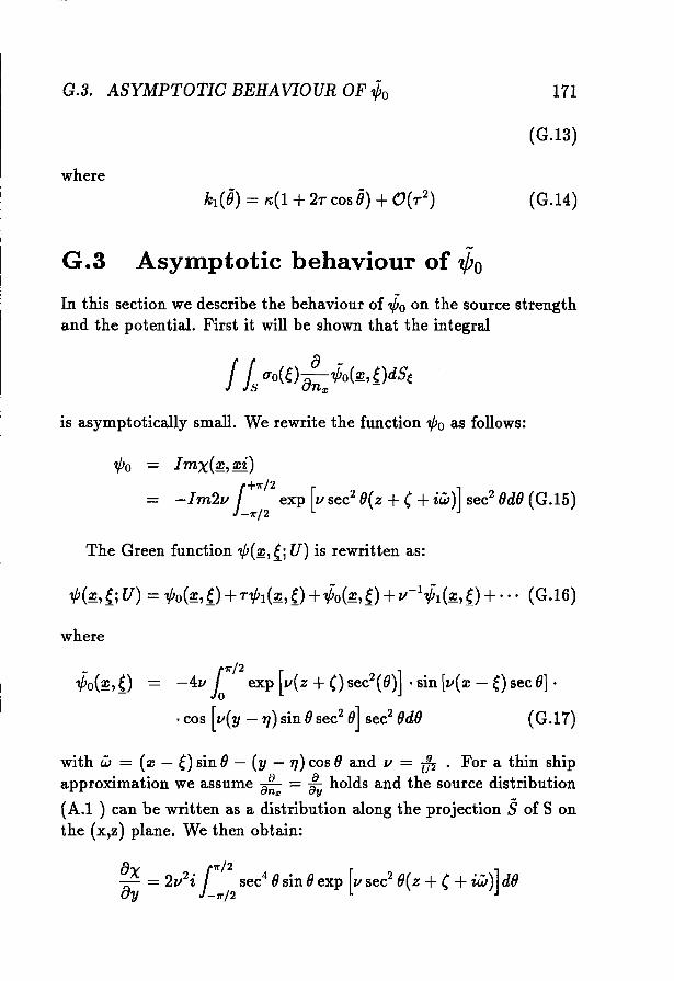
G.3. ASYMPTOTIC BEHAVIOUR OF-¢;o
where
G.3 Asymptotic behaviour of "po
171
(G.13)
(G.14)
In this section we describe the behaviour of {Jo on the source strengthand the potential. First it will be shown that the integral
is asymptotically small. We rewrite the function "po as follows:
"po Imx(~, xi)
r:-Im2v exp [v sec2 O(z +, + iW)] sec2 OdO (G.15)-7r/2
The Green function "p(~, {j U) is rewritten as:
where
r/2
-4v 10 exp [v( z +()sec2( 0)] . sin [v(x - e)sec 0] .
. cos [v(y - 1]) sin 0sec2 0] sec2 OdO (G .17)
with W = (x - e) sin 0 - (y -1]) cos 0 and v = ih . For a thin shipapproximation we assume -aa = aa holds and the source distribution
n", y
(A.I ) can be written as a distribution along the projection Sof S onthe (x,z) plane. We then obtain:
aaX = 2v2i r': sec4 0sin 0exp [v sec2 O(z +, + iW)] dOY L7r/2
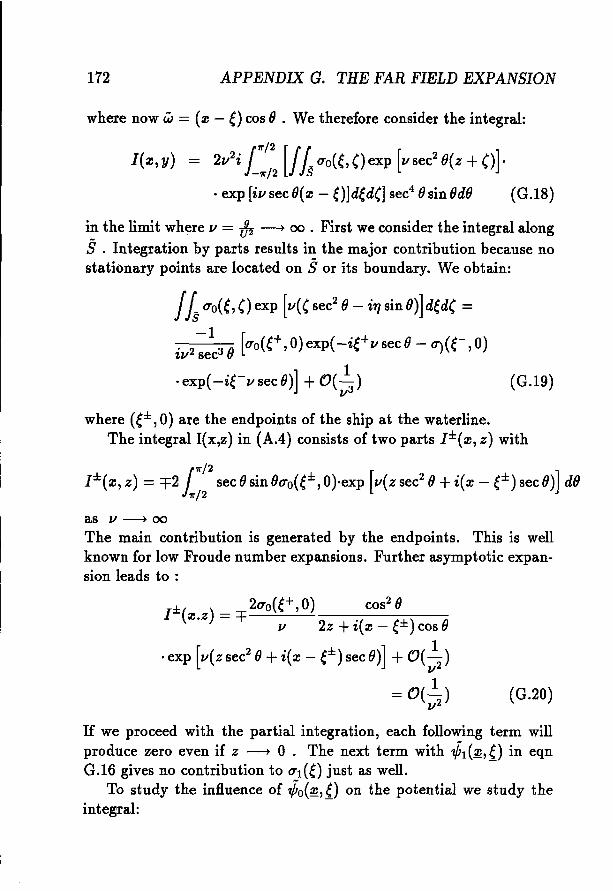
172 APPENDIX G. THE FAR FIELD EXPANSION
where now w= (z - e) cos8 . We therefore consider the integral:
Ii», y) = 2v2i r. [I' t. uo(e,oexp [vsec2 8(z +()].-1r/2 is
. exp [iv sec 8(z - e)]ded(] sec" 8 sin 8d8 (G.18)
in the limit where v = ih ---+ 00 • First we consider the integral alongS . Integration by parts results in the major contribution because nostationary points are located on S or its boundary. We obtain:
fIs uo(e, () exp [v(( sec2 8 - i", sin8)]ded( =
. 2-138 [uo(e+,0)exp(-ie+vsec8 - U)(e-,O)~v sec
. exp( -ie-v sec e)] +O(~) (G.19)v 3
where (e±, 0) are the endpoints of the ship at the waterline.The integral I(x,z) in (A.4) consists of two parts I±(z, z) with
as v ---+ 00
The main contribution is generated by the endpoints. This is wellknown for low Froude number expansions. Further asymptotic expansion leads to :
J±(z.z) = =f2uo(e+,0) cos2 e
v 2z +i( z - e±)cos e
. exp [v(z sec2e+i(z - e±)sec e)] +O(:2)= O(~)
v2(G.20)
If we proceed with the partial integration, each following term willproduce zero even if z ---+ °. The next term with "fil (.~, e) in eqnG.16 gives no contribution to Ul(e) just as well.
To study the influence of "fio(~,{) on the potential we study theintegral:
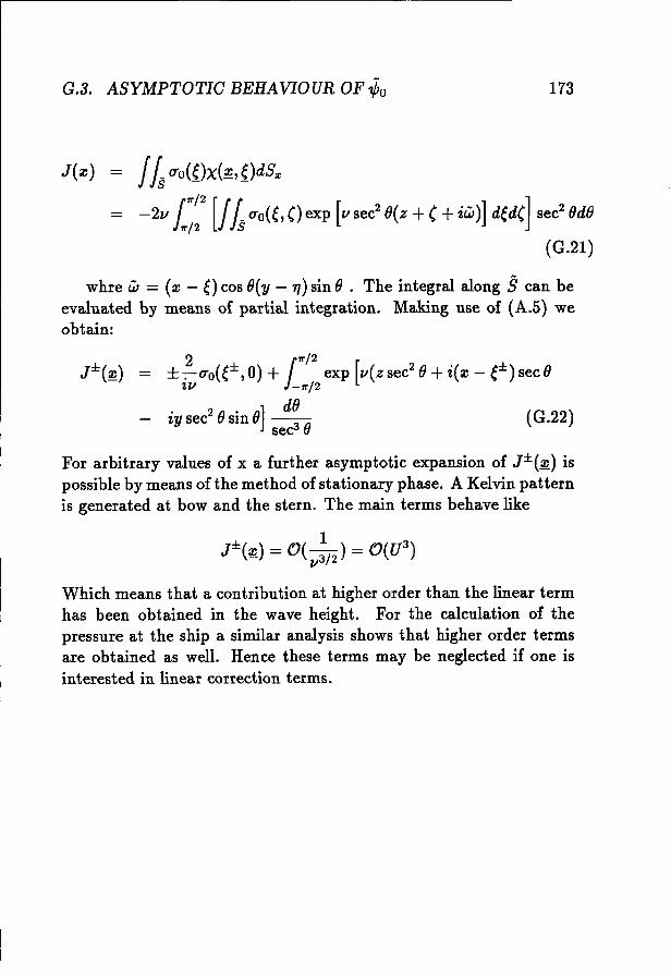
G.3. ASYMPTOTIO BEHAVIOUR OF ;jJo 173
J( z) / Is tTo({)X(~, {)dSx
-2v L~~2 [/£tTo(e, oexp l- sec2 O(z + (+ iW)] ded(] sec20dO
(G.21)
whre W = (z - e)cos O(y - 1/) sin 0 . The integral along § can beevaluated by means of partial integration. Making use of (A.5) weobtain:
For arbitrary values of x a further asymptotic expansion of J±(~) ispossible by means of the method of stationary phase. A Kelvin patternis generated at bow and the stern. The main terms behave like
Which means that a contribution at higher order than the linear termhas been obtained in the wave height. For the calculation of thepressure at the ship a similar analysis shows that higher order termsare obtained as well. Hence these terms may be neglected if one isinterested in linear correction terms.
174 APPENDIX G. THE FAR FIELD EXPANSION
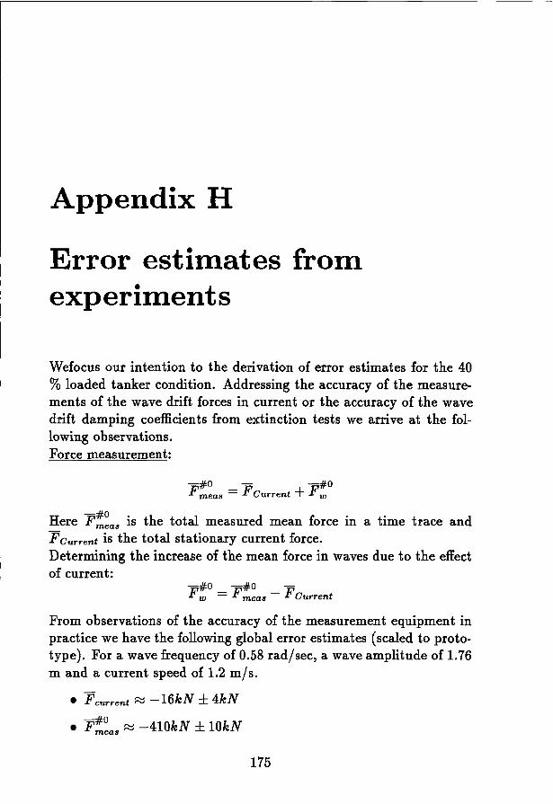
Appendix H
Error estimates fromexperiments
Wefocus our intention to the derivation of error estimates for the 40% loaded tanker condition. Addressing the accuracy of the measurements of the wave drift forces in current or the accuracy of the wavedrift damping coefficients from extinction tests we arrive at the following observations.Force measurement:
-#0 - -#0F meas = F Current +F w
Here rz: is the total measured mean force in a time trace andF Current is the total stationary current force.Determining the increase of the mean force in waves due to the effectof current:
-#0 -#0 -F w = F meas - F Current
From observations of the accuracy of the measurement equipment inpractice we have the following global error estimates (scaled to prototype). For a wave frequency of 0.58 rad/sec, a wave amplitude of 1.76m and a current speed of 1.2 tsi]«.
• F current ~ -16kN ± 4kN-#0
• F meas ~ -410kN ± 10kN
175
176 APPENDIX H. ERROR ESTIMATES FROM EXPERIMENTS
Assuming the zero speed wave drift force ( F:o = -222kN) at thisfrequency and wave height to be exact, we then arrive at the followingerror estimate of the wave drift damping:
- -#0 --0where AF is defined as F w - F: or Bwd = 60kNs/ m3 ± 5kNs/ m3
•
Extinction tests:In the direct estimation of the wave drift damping coefficient we makeuse of extinction tests in regular waves. In the assesment of the accuracies of the damping coefficient we assume that the spring system inthe tests is linear and we used an approximation of the added mass ofthe tanker in surge direction of 10% of its own mass. From the extiction tests the damping coefficients were obtained with the followingaccuracy. We use as an example the results for the test in .65 rad/secwaves with a wave amplitude of 3.1 m.The wave drift damping coefficient is then obtained from:
where 8sw is the damping in still water and 8m eas is the total measureddamping in regular waves.
• 8m eas = .259 ± 0.008
• 8sw = .117 ± 0.008
This leads to the approximate error in the wave drift damping coefficient of 0.142 ± 0.016, which is approximately 15% . For smaller measured values of the total damping, the relative error estimate increasesconsiderably. Apart from these stochastical errors also systematic errors may occur. For example the heading control may not be perfectfor bow quartering waves and current.
Appendix I
Dynamic positioning atmodel scale
1.1 Global set-up
At MARIN a system was developed which incorporates all possibilitiesof simulation into one system. For that purpose a universally applicable simulator/simulation program RUNSIM was developed. With thisprogram it is possible to run an arbitrary mathematical model or aphysical model in the model basin in conjunction with an automaticor manual control system.The processes represent the considered problem. In the present caseonly the following processes are used.
• FYSMOD
• AUTCON
• GRAPHICS
• TERMINAL
FYSMOD represents the physical model and includes the AD (analog- digital) and DA (digital - analog) conversions.AUTCON embodies the control process.TERMINAL is used to change parameters on-line and to start theprocess.
177
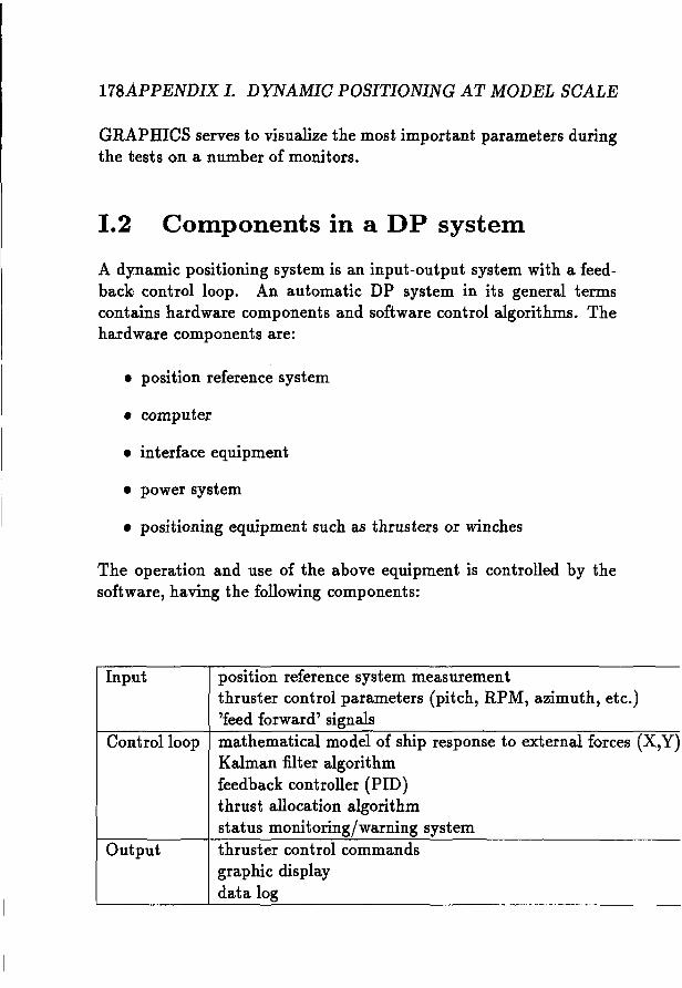
178APPENDIX 1. DYNAMIC POSITIONING AT MODEL SCALE
GRAPHICS serves to visualize the most important parameters duringthe tests on a number of monitors.
1.2 Components in a DP system
A dynamic positioning system is an input-output system with a feedback control loop. An automatic DP system in its general termscontains hardware components and software control algorithms. Thehardware components are:
• position reference system
• computer
• interface equipment
• power system
• positioning equipment such as thrusters or winches
The operation and use of the above equipment is controlled by thesoftware, having the following components:
Input position reference system measurementthruster control parameters (pitch, RPM, azimuth, etc.)'feed forward' signals
Control loop mathematical model of ship response to external forces (X,Y)Kalman filter algorithmfeedback controller (PID)thrust allocation algorithmstatus monitoring/warning system
Output thruster control commandsgraphic displaydata log
1.3. THE OONTROL LOOP
1.3 The control loop
179
The principal features of the control loop are those algorithms whichare needed for position correction measures on the basis of the measured reference. Other software parts, related to monitoring and statuslogging, are basically needed for tuning the system and for performance evaluation. These will not be discussed here.
1.3.1 Mathematical model of the ship
The motions of a ship can be described by a set of differential equations. For DPeontrol, only the mean and low frequency (drift) motionsin the horizontal plane are considered. The excitation of the motionsis caused by second order wave effects, wind and current, while themotions themselves induce fluid reaction forces. The mathematicalmodel of the behaviour of a tanker under the influence of wind, wavedrift forces and current is given by Wichers [75] . Incorporation ofthruster action or action by the winches leads to the following equations of motion:
in which:
MiC LF +D(xLF)xLF = X(2) + ~·X(2) .- - - -HD I-EXT,I (1.1)
• xL F = xLF , yLF, 'lj;LF, the low frequency motions: surge, swayand yaw
• x~b = second order hydrodynamic reaction forces
• x~lT,i = other low frequency varying exciting forces (wind,thrusters, wave drift and current forces)
• M = mass matrix
• D = LF damping matrix due to coupling
Note that in the low frequency time domain, the first order (linear)damping may be neglected.
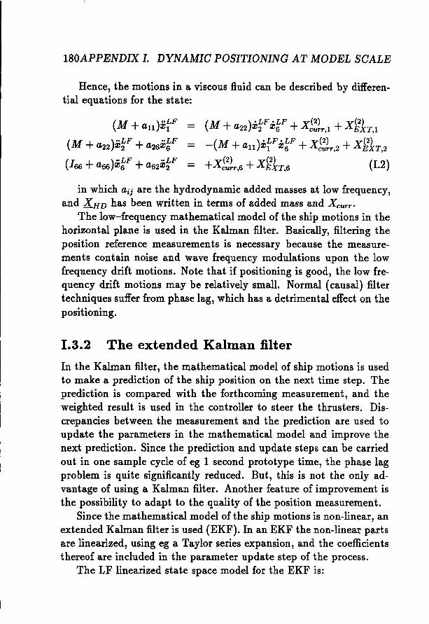
180APPENDIX 1. DYNAMIO POSITIONING AT MODEL SOALE
Hence, the motions in a viscous fluid can be described by differential equations for the state:
(M +a22):i:fF:i:~F +X~~~r,l +X1~T,1
-(M +all):i:fF:i:~F +X~:~r,2 +xJJ1T,2
+X(2) +X(2) (I 2)curr,6 EXT,6 •
in which aij are the hydrodynamic added masses at low frequency,and X H D has been written in terms of added mass and X curr.
The low-frequency mathematical model of the ship motions in thehorizontal plane is used in the Kalman filter. Basically, filtering theposition reference measurements is necessary because the measurements contain noise and wave frequency modulations upon the lowfrequency drift motions. Note that if positioning is good, the low frequency drift motions may be relatively small. Normal (causal) filtertechniques suffer from phase lag, which has a detrimental effect on thepositioning.
1.3.2 The extended Kalman filter
In the Kalman filter, the mathematical model of ship motions is usedto make a prediction of the ship position on the next time step. Theprediction is compared with the forthcoming measurement, and theweighted result is used in the controller to steer the thrusters. Discrepancies between the measurement and the prediction are used toupdate the parameters in the mathematical model and improve thenext prediction. Since the prediction and update steps can be carriedout in one sample cycle of eg 1 second prototype time, the phase lagproblem is quite significantly reduced. But, this is not the only advantage of using a Kalman filter. Another feature of improvement isthe possibility to adapt to the quality of the position measurement.
Since the mathematical model of the ship motions is non-linear, anextended Kalman filter is used (EKF). In an EKF the non-linear partsare linearized, using eg a Taylor series expansion, and the coefficientsthereof are included in the parameter update step of the process.
The LF linearized state space model for the EKF is:
1.3. THE CONTROL LOOP
~k+l Ak~k +I', +FWk
1!..k - C~k + Vk
181
(1.3)
in which the first line describes the prediction of the LF positionand heading and their derivatives ~ on time step k-l-1 from the statuson time step k and the external forces r k • The second line representsthe position measurements at time step k. In both equations the noisein the process is incorporated: W k is the noise due to inaccuracy in themathematical model and V k represents the noise in the measurement.Both noise functions are assumed to have a Gaussian distribution withzero mean. The matrices F and C represent the transfer of Wand Vto the dimensions of the vectors ~ and 1!.. respectively.
The solution of the EKF equations takes place in a one-step tran-sition scheme with:
• State predictor ~k+llk = Ak~k +r k
• State corrector ~k+l = ~k+llk +Kk+l (Yk+1 - C~k+1Ik)
• Covariance predictor Pk+Ilk = AkPkAf +FkQkF[
• Kalman filter gain K k+I = Pk+llkCT (C Pk+llkCT + Rk+l) - l
• Covariance corrector Pk+I = Pk+l1k - Kk+IC Pk+Ilk
in which it is assumed that the matrix C is constant. The matricesQ and R represent the covariance of the two noise signals Wk and Vi.It is assumed that there is no noise interaction.
In the recursive scheme the following particulars are present:
• If the mathematical model of the process is incomplete or disturbed, the value of the covariance of Wk will be large, whichleads to an increase of the Kalman gain K k • In that case thestate estimates rely more on the measurements.
• If the measurements of the position from the reference systemare disturbed, the covariance of Vk is large. This tends to decrease the gain matrix and the estimates will rely more on themathematical prediction.
182APPENDIX 1. DYNAMIO POSITIONING AT MODEL SOALE
1.3.i3 The controller
Various options are available for the controller. In this section onewill be presented, the PID controller. The PID controller is basicallyan algorithm which multiplies the position error and drift speed witha spring restoring ('P') and a damping factor ('D'). An integrationroutine ('1') may be applied to compensate for an offset in the meanvalue. The position estimate of the EKF, and its derivative (the driftspeed estimate) is input to the PID controller as follows:
Fi = PiZi +Dizi +Ii! Zi.dt (1.4)
in which Fi represents the total required force vector on the shipthat has to be generated by the thrusters. The subscripts i stand forthe three modes of motion in the horizontal plane x, y and 't/J • Thecoefficients of the PID controller have to be selected and optimisedfor a good positioning performance. A significant change of sea stateor loading condition are the most important reasons to update thesettings. Therefore, the need to adapt the PID control coefficients isa drawback of this approach.
In the linearized state space model for the EKF, the externalforcesf'j, are replaced by:
(1.5)
in which the input vector Uk represents the required thruster forcesand wtet the low frequency exciting forces on the ship.
A PID controller is used and selection of controller settings is carried out in a series of test runs in representative environmental conditions, prior to the actual testing.
The output of the controller is the required forces and momenton the ship. The thrust allocation algorithm, in which the thrusterlayout and thrust degradation effects are defined, takes care that theserequired total forces and moment are properly distributed over theavail-able thrusters. In the current lay-out of the measuring systemthe thrusters are modelled using constant tension winches.
Samenvatting
In deze studie worden resultaten gepresenteerd van het onderzoek vande gemiddelde golfdriftkrachten op een schip in stroom en golven. Inde hoofdstukken 3 en 5 zijn de wiskundige uitgangspunten van derandintegraal methode weergegeven voor de berekening van de eersteen tweede orde golfkrachten op vrij drijvende objeeten met lage snelheid. Onder gebruikmaking van de stelling van Green is een bronsterkte formulering afgeleid. De Greens funktie voor een oscillerendeen translerende bron funktie en de bronbelegging zijn gelinearizeerdmet betrekking tot de voorwaartse snelheid. De eerste twee termen uit de asymptotische benadering voorde bronsterkten wordenbepaald door middel van twee integraal vergelijkingen, die dezelfdekernel bezitten. In vergelijking tot het snelheid nul diffraktie probleemspeelt nu het vrije oppervlak een rol in de randvoorwaarden van deintegraal vergelijking voor de bronsterkten. Aanpassingen zijn gedaanvan de gelinearizeerde Greens funktie om tot een goede asymptotischebenadering te komen van de Greens funktie voor het verre veld. In hetgeval van diffraktie van golven op een schip met voorwaartse snelheidspeelt de ontmoetingsfrequentie een grote rol. Deze ontmoetingsfrequenties zijn hoger dan bij snelheid nul voor voorinkomende of schuinvoorinkomende golfkondities. Echter bij deze hogere frequenties geeftde randintegraal methode aanleiding tot onnauwkeurige resultaten bijspecifieke frequenties, ook wel 'irregular frequencies' genoemd. Omdit probleem aan te pakken is een 'lid methode' ontwikkeld. De resulaten van de 'lid methode' laten zien dat deze effectief is voor hetonderdrukken van de 'irregular frequencies'.De methode van berekening van de gemiddelde driftkrachten is gebaseerdop een methode van behoud van impulse. De resultaten van de driftkrachtberekening op een drijvende bol kwamen goed overeen met de resultaten uit de study van Zhao en faltinsen [82]. Ter validatie van deontwikkelde methode voor de berekening van de driftkrachten zijnook model proeven uitgevoerd op een 200 kDWT tanker in zowel volbeladen als ook in ballast konditie. Uit de resultaten van de modelproeven kan men konkluderen dat de gelinearizeerde voorwaartse snelheids aanpak goed werkt voor de stroom recht van voren en de geteste
183

schuin voorinkomende golfrichtingen. Een minder goede overeenkomstis gekonstateerd voor die situaties met de stroom onder een hoek vaninval met de tanker.
184
Acknowledgement
First of all I would like to give my thanks to my promotor Prof. Dr.Jr. A. J. Hermans who offered continuously his support and adviceduring the progress of the work.
Further I want to thank the board of directors of the Maritime Research Institute Netherlands, who supported the work by providingtime and funds for me to perform the work.
Special thanks are in order to the many members of the staff ofMARIN for helping with the experiments, numerical calculations andnumerous discussions on the topic of this thesis.
I also gratefully acknowledge the support of the sponsoring companiesof the Cooperative Research on Ships group and their permission touse some of the interesting results from the 'irregular frequency' problem study.
Also a warm word of thanks is in order for the people how helped withthe last finishing touches of the thesis, especially G. Radstaat and C.Visser for their effort for making the final touches on the figures.
Lastly and most importantly I wish to thank my wife Gretha and myson Jeroen and daughter Inge for putting up with my nearly foreverduring absent mindedness.
185
186
Curriculum Vitae
The author was born on December 211951 in Breda, the Netherlands.After graduation in 1969 of the HBS-B in Arnhem he started his study of mathematics atthe Twente University of Technology. He finshed his study in Januari 1976 ona topic related to multivariate control problems. Since then he joined the staffof the Maritime Research Institute of the Netherlands as project manager in theshallow water basin. He has been working in the R&D department and theOffshore Research division of MARlN as a senoir project manager.
187