Magnetic Fields inside Extremely Fast Shock Waves · Magnetic Fields inside Extremely Fast Shock...
259
Magnetic Fields inside Extremely Fast Shock Waves Jorrit Wiersma 2007
Transcript of Magnetic Fields inside Extremely Fast Shock Waves · Magnetic Fields inside Extremely Fast Shock...
Magnetic Fields insideExtremely Fast Shock Waves
Jorrit Wiersma2007
ISBN 978-90-393-4532-0
Magnetic Fields insideExtremely Fast Shock Waves
Magnetische velden in extreem snelle schokgolven
(met een samenvatting in het Nederlands)
Proefschrift
ter verkrijging van de graad van doctor aan de Universiteit Utrechtop gezag van de rector magnificus, prof.dr. W.H. Gispen,
ingevolge het besluit van het college voor promotiesin het openbaar te verdedigen op
dinsdag 29 mei 2007 des ochtends te 10.30 uur
doorJorrit Wiersma
geboren op 7 mei 1977te de Bilt
Promotor: Prof.dr. A. Achterberg
Dit proefschrift werd (mede) mogelijk gemaakt met financiele steun van deNederlandse Onderzoekschool voor Astronomie (NOVA).
Preface
The world around us is made up of microscopic particles. Solid objects mayappear solid and the air we breath may appear intangible, but both are madeup of atoms and molecules, the only difference being how strongly they areheld together. It has always fascinated me how almost all physical phenomenacan be explained as the interaction between particles. How even the light ofthe Sun is produced from the energy that is freed as particles deep inside theSun fuse together.
This fascination is the reason why the subject of my PhD research appealsto me. My research also concerns the interaction of particles, although theparticles considered here have extraordinary properties. They travel almostwith the speed of light, something that Earthly particles do not do outside ofman-made laboratories. And they are part of a plasma: a gas of electricallycharged particles, such as the gas inside a fluorescent lamp or in the Earth’supper atmosphere.
But what really makes these particles interesting is that, together, they forma shock wave, whose interaction with the interstellar material produces somuch radiation that, although they can be billions of light years distant, theybriefly become the brightest sources of gamma-rays in our sky. I have spentfive years at the University of Utrecht investigating how these particles wouldinteract according to the theories of modern-day physics to help explain howthey produce the radiation that we see.
In this thesis [99]1 I present the results of my research. I have tried to struc-ture it in a convenient way for you, the reader. There are three parts. Thefirst part contains an introduction, in which I explain the physical principlesthat are important for the subject matter of the rest of my thesis. I have tried
1Numbers in square brackets refer to entries in the bibliography included near the end of thisthesis.
5
6
to keep it understandable for everyone, even if you do not have a backgroundin physics or astronomy. If you do have a background in astronomy then it mayserve as a refresher. The second part contains the results of my research. Mostof the chapters in this part are also published in (or submitted to) the profes-sional European astronomy journal Astronomy & Astrophysics. Therefore, thetext is aimed at astronomers who are at home with the subject matter. I havepreceded each chapter with a short summary of its contents and an indicationof its relation to the other chapters. This should provide you with enough in-formation to skim these chapters and to just read the details you are interestedin. The third and last part contains a discussion of the conclusions that I drawfrom the results of my research. It also contains a summary in Dutch and acurriculum vitae.
The five years at the ‘Sterrekundig Instituut Utrecht’ have been very pleas-ant and I would like to use this opportunity to thank everyone for the goodtime. In particular, I would like to thank Bram for his guidance as my pro-motor. Whenever I had a question he was available to help and as far as Ican remember he could always point me to some article or a chapter in somebook to provide me with more information. I would also like to thank Marc,Pui Kei, Jeroen and Sung-Chul, who were my roommates during (part of) mytime at the Institute. Thanks also go to Marion for doing so much for the in-stitute, especially organizing the social activities such as Sinterklaas and thegame evenings. And also thanks to Rob Rutten, for being a fun professor toassist in his courses and for keeping me, a little bit, involved with the solarphysics research. Thanks to Selma, Evert, Cees and Gemma for the good timesat the game evenings and to Axel for the good times in general.
Most thanks of all and a lot of love go to my wife Saskia. I can imagine thatsitting next to me when I was working on my thesis with my laptop on thecouch wasn’t the most romantic thing imaginable. Yet you did so much to giveme the time I needed to finish it.
The illustration on the cover was made by my five-year-old daughter Silkeon 24 February 2007 and is a Zon die kapot is (‘Sun that is broken’), which ishow we tried to describe the subject of my research to her.
Contents
I Introduction 13
1 Overview 15
2 Relativistic shocks and magnetic fields 17
3 Basic Physics 193.1 Shock waves . . . . . . . . . . . . . . . . . . . . . . . . . . . . . . 203.2 The theory of relativity . . . . . . . . . . . . . . . . . . . . . . . . 21
3.2.1 The light cone . . . . . . . . . . . . . . . . . . . . . . . . . 223.2.2 Proper time and proper density . . . . . . . . . . . . . . . 233.2.3 Relativistic Doppler shift . . . . . . . . . . . . . . . . . . 243.2.4 Relativistic momentum and energy . . . . . . . . . . . . 24
3.3 Electricity and Magnetism . . . . . . . . . . . . . . . . . . . . . . 263.3.1 Light . . . . . . . . . . . . . . . . . . . . . . . . . . . . . . 273.3.2 Charged Particles in electromagnetic fields . . . . . . . . 273.3.3 Interaction of particles and electromagnetic radiation . . 28
3.4 The Weibel or filamentation instability . . . . . . . . . . . . . . . 29
4 Gamma-ray Bursts 334.1 Observational facts . . . . . . . . . . . . . . . . . . . . . . . . . . 354.2 Properties derived from observations . . . . . . . . . . . . . . . 364.3 The sources of Gamma-ray Bursts . . . . . . . . . . . . . . . . . . 38
II Research 43
5 Relativistic Shock Conditions 45
7
8 CONTENTS
5.1 Introduction . . . . . . . . . . . . . . . . . . . . . . . . . . . . . . 465.2 Theory: Magnetohydrodynamics . . . . . . . . . . . . . . . . . . 47
5.2.1 MHD description of the plasma . . . . . . . . . . . . . . 475.2.2 Physics of MHD Plasmas . . . . . . . . . . . . . . . . . . 485.2.3 Approximations . . . . . . . . . . . . . . . . . . . . . . . 50
5.3 Shock conditions and their solutions . . . . . . . . . . . . . . . . 515.3.1 General situation . . . . . . . . . . . . . . . . . . . . . . . 515.3.2 Perpendicular Shocks . . . . . . . . . . . . . . . . . . . . 525.3.3 Non-perpendicular shocks . . . . . . . . . . . . . . . . . 65
5.4 Discussion of the results . . . . . . . . . . . . . . . . . . . . . . . 685.4.1 General results . . . . . . . . . . . . . . . . . . . . . . . . 685.4.2 Internal structure of the shock . . . . . . . . . . . . . . . 68
6 Linear theory of the Weibel instability 716.1 Introduction . . . . . . . . . . . . . . . . . . . . . . . . . . . . . . 726.2 Covariant formulation of plasma dispersion . . . . . . . . . . . . 74
6.2.1 Polarization tensor in the fluid approximation . . . . . . 756.2.2 Polarization tensor in the kinetic description . . . . . . . 776.2.3 The cold plasma limit . . . . . . . . . . . . . . . . . . . . 78
6.3 The beam-driven Weibel instability . . . . . . . . . . . . . . . . . 786.4 Non-relativistic cold beam limit . . . . . . . . . . . . . . . . . . . 806.5 Weibel instability driven by two symmetric beams . . . . . . . . 826.6 The case of ultra-relativistic beams . . . . . . . . . . . . . . . . . 856.7 Ultra-relativistic background gas . . . . . . . . . . . . . . . . . . 896.8 Magnetized Weibel instability . . . . . . . . . . . . . . . . . . . . 93
6.8.1 When can non-magnetic results be used? . . . . . . . . . 966.9 The asymmetric case . . . . . . . . . . . . . . . . . . . . . . . . . 1006.10 Conclusions . . . . . . . . . . . . . . . . . . . . . . . . . . . . . . 1046.11 Covariant formulation of plasma response . . . . . . . . . . . . 105
6.11.1 Plasma response in the fluid approach . . . . . . . . . . . 1076.11.2 Plasma response in the kinetic approach . . . . . . . . . . 109
6.12 Covariant dispersion relation . . . . . . . . . . . . . . . . . . . . 1116.13 The components of the dispersion tensor . . . . . . . . . . . . . 113
6.13.1 Fluid approximation . . . . . . . . . . . . . . . . . . . . . 1136.13.2 Kinetic theory . . . . . . . . . . . . . . . . . . . . . . . . . 1146.13.3 Waterbag approximation . . . . . . . . . . . . . . . . . . 117
6.14 Magnetized Weibel instability . . . . . . . . . . . . . . . . . . . . 118
CONTENTS 9
7 Variations on the Weibel instability 1217.1 Introduction . . . . . . . . . . . . . . . . . . . . . . . . . . . . . . 1227.2 Counterstreaming beam model . . . . . . . . . . . . . . . . . . . 122
7.2.1 Initial condition . . . . . . . . . . . . . . . . . . . . . . . . 1227.2.2 Background plasma . . . . . . . . . . . . . . . . . . . . . 1237.2.3 Maxwell’s equations . . . . . . . . . . . . . . . . . . . . . 124
7.3 Instability analysis . . . . . . . . . . . . . . . . . . . . . . . . . . 1247.3.1 Linear response of the beams . . . . . . . . . . . . . . . . 1247.3.2 Linear response of the background plasma . . . . . . . . 1257.3.3 Dispersion relation . . . . . . . . . . . . . . . . . . . . . . 1267.3.4 The “Normal” Weibel instability . . . . . . . . . . . . . . 1277.3.5 Dispersion relation for spatial modes . . . . . . . . . . . 1277.3.6 Weibel instability for oblique propagation . . . . . . . . . 129
7.4 Discussion . . . . . . . . . . . . . . . . . . . . . . . . . . . . . . . 132
8 Proton Weibel instability 1358.1 Introduction . . . . . . . . . . . . . . . . . . . . . . . . . . . . . . 1368.2 Simple model for a relativistic shock . . . . . . . . . . . . . . . . 137
8.2.1 The proton velocity distribution . . . . . . . . . . . . . . 1388.2.2 The shock conditions for the electrons . . . . . . . . . . . 138
8.3 The Weibel instability . . . . . . . . . . . . . . . . . . . . . . . . . 1398.3.1 The dispersion relation . . . . . . . . . . . . . . . . . . . . 1398.3.2 Stabilization of the Weibel instability . . . . . . . . . . . . 1448.3.3 The equipartition parameter . . . . . . . . . . . . . . . . 147
8.4 Discussion . . . . . . . . . . . . . . . . . . . . . . . . . . . . . . . 1478.5 Conclusions . . . . . . . . . . . . . . . . . . . . . . . . . . . . . . 1488.6 Asymmetric beams . . . . . . . . . . . . . . . . . . . . . . . . . . 149
9 The end of the Weibel instability 1539.1 Introduction . . . . . . . . . . . . . . . . . . . . . . . . . . . . . . 1549.2 Stabilization mechanisms: an overview . . . . . . . . . . . . . . 1589.3 Fluid model for the beam response . . . . . . . . . . . . . . . . . 160
9.3.1 Dynamics of the beam particles . . . . . . . . . . . . . . . 1649.3.2 Reduced set of Maxwell’s equations . . . . . . . . . . . . 1669.3.3 Linear response of the beam plasma . . . . . . . . . . . . 1689.3.4 The nonlinear response for single modes: the effect of
wave breaking . . . . . . . . . . . . . . . . . . . . . . . . 1699.3.5 Influence of the background plasma . . . . . . . . . . . . 171
9.4 Kinetic stabilization due to quiver motion . . . . . . . . . . . . . 174
10 CONTENTS
9.4.1 Broadening of the momentum distribution . . . . . . . . 1759.4.2 Effect on the beam response . . . . . . . . . . . . . . . . . 178
9.5 Current channel coalescence . . . . . . . . . . . . . . . . . . . . . 1799.5.1 Maximum current for a cylindrical channel: the Alfven
current . . . . . . . . . . . . . . . . . . . . . . . . . . . . . 1799.5.2 Simple model for field growth . . . . . . . . . . . . . . . 1819.5.3 The effect of screening currents . . . . . . . . . . . . . . . 1839.5.4 Equation of motion for two attracting screened filaments 1859.5.5 The coalescence time scale . . . . . . . . . . . . . . . . . . 186
9.6 Implications for ultra-relativistic shocks . . . . . . . . . . . . . . 1889.6.1 Thermalization through the Weibel instability . . . . . . 1909.6.2 Thermalization of protons . . . . . . . . . . . . . . . . . . 193
9.7 Conclusions . . . . . . . . . . . . . . . . . . . . . . . . . . . . . . 197
10 Computer simulations 19910.1 Introduction . . . . . . . . . . . . . . . . . . . . . . . . . . . . . . 20010.2 The simulated system . . . . . . . . . . . . . . . . . . . . . . . . . 20110.3 Basic equations . . . . . . . . . . . . . . . . . . . . . . . . . . . . 20110.4 Particle in Cell method . . . . . . . . . . . . . . . . . . . . . . . . 20310.5 Weibel instability theory . . . . . . . . . . . . . . . . . . . . . . . 204
10.5.1 Linear response of the beam particles . . . . . . . . . . . 20610.5.2 Linear response of the background particles . . . . . . . 20710.5.3 Dispersion relation . . . . . . . . . . . . . . . . . . . . . . 20910.5.4 Saturation of the instability . . . . . . . . . . . . . . . . . 213
10.6 Simulation results . . . . . . . . . . . . . . . . . . . . . . . . . . . 21610.7 Conclusions . . . . . . . . . . . . . . . . . . . . . . . . . . . . . . 22110.8 Numerical approach . . . . . . . . . . . . . . . . . . . . . . . . . 224
10.8.1 Dimensionless form of the equations . . . . . . . . . . . . 22410.8.2 Solution method: particles . . . . . . . . . . . . . . . . . . 22510.8.3 Solution method: electromagnetic fields . . . . . . . . . . 225
III Discussion and summary 229
11 Discussion and conclusions 231
CONTENTS 11
12 Samenvatting in het Nederlands 23512.1 Inleiding . . . . . . . . . . . . . . . . . . . . . . . . . . . . . . . . 23512.2 Gamma-ray Bursts . . . . . . . . . . . . . . . . . . . . . . . . . . 23512.3 Schokgolven en magnetische velden . . . . . . . . . . . . . . . . 23812.4 Simulaties . . . . . . . . . . . . . . . . . . . . . . . . . . . . . . . 23912.5 De sterkte van het magnetische veld . . . . . . . . . . . . . . . . 24112.6 Vergelijking met waarnemingen . . . . . . . . . . . . . . . . . . . 243
13 Curriculum Vitae 245
12 CONTENTS
Part I
Introduction
13

Chapter 1
Overview
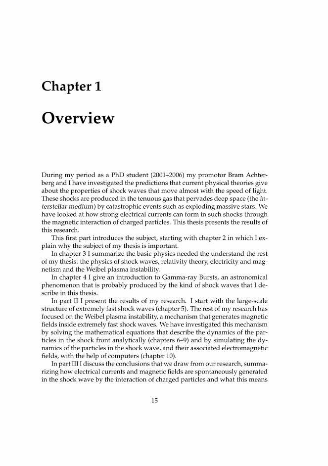
During my period as a PhD student (2001–2006) my promotor Bram Achter-berg and I have investigated the predictions that current physical theories giveabout the properties of shock waves that move almost with the speed of light.These shocks are produced in the tenuous gas that pervades deep space (the in-terstellar medium) by catastrophic events such as exploding massive stars. Wehave looked at how strong electrical currents can form in such shocks throughthe magnetic interaction of charged particles. This thesis presents the results ofthis research.
This first part introduces the subject, starting with chapter 2 in which I ex-plain why the subject of my thesis is important.
In chapter 3 I summarize the basic physics needed the understand the restof my thesis: the physics of shock waves, relativity theory, electricity and mag-netism and the Weibel plasma instability.
In chapter 4 I give an introduction to Gamma-ray Bursts, an astronomicalphenomenon that is probably produced by the kind of shock waves that I de-scribe in this thesis.
In part II I present the results of my research. I start with the large-scalestructure of extremely fast shock waves (chapter 5). The rest of my research hasfocused on the Weibel plasma instability, a mechanism that generates magneticfields inside extremely fast shock waves. We have investigated this mechanismby solving the mathematical equations that describe the dynamics of the par-ticles in the shock front analytically (chapters 6–9) and by simulating the dy-namics of the particles in the shock wave, and their associated electromagneticfields, with the help of computers (chapter 10).
In part III I discuss the conclusions that we draw from our research, summa-rizing how electrical currents and magnetic fields are spontaneously generatedin the shock wave by the interaction of charged particles and what this means
15
16 CHAPTER 1. OVERVIEW
for models that try to explain how Gamma-ray Bursts are formed. I also dis-cuss the limitations of our research and how future research can advance thefield.
Part III also contains a summary of this thesis in Dutch and a CurriculumVitae.
Chapter 2
Relativistic Shock Waves andMagnetic Fields
Fast shock waves occur in the tenuous gas that pervades deep space (the inter-stellar medium) around catastrophic events such as exploding massive stars.When the shock waves are so strong that they reach speeds close to the speed oflight we call them relativistic shock waves because the effects described by Rel-ativity Theory become important for their dynamics. Such extremely fast shockwaves form an important part of the favored explanation for the high-energyradiation (X rays and gamma rays) and particles (cosmic rays) produced in andaround several astronomical phenomena, such as Gamma-ray Bursts, PulsarWinds, and Active Galactic Nuclei.
Because relativistic shock waves occur around sources at great distancesfrom the Earth and the solar system, much is still unclear about the physicalprocesses in and near them. The typical length scale1 on which the processesthat I have studied take place is more than a kilometer, making them too largeto study directly in the laboratory. Theoretical research such as my PhD re-search provides predictions about the physical processes in relativistic shocks.These predictions can then be tested by astronomical observations or by labo-ratory experiments on a smaller scale.
Relativistic shocks will form when a very fast outflow of matter interactswith material surrounding the object. Such a very fast outflow can be pro-duced, for example by an exploding massive star or by a very compact, rapidlyspinning energetic object like a pulsar or a black hole.
At the front of the shock wave a violent change in pressure and tempera-ture takes place. It causes the material that it leaves behind to glow brightly,
1Here, with typical length scale I mean the plasma skin depth.
17
18 CHAPTER 2. RELATIVISTIC SHOCKS AND MAGNETIC FIELDS
producing among others high-energy radiation like X rays and gamma rays.Although the interstellar medium is very tenuous, and the compressed gas leftbehind by the shock is as well, the effect of relativistic shocks is strong enoughto produce radiation that is visible on Earth even from the distant universe.
The gas in the shock front consists of atoms, ions and electrons. These parti-cles are very small, and because the gas is so tenuous the particles rarely collidewith each other. Instead, they interact through electromagnetic forces becausethey are electrically charged. Therefore, we refer to such shock waves as colli-sionless shocks. Because the force between individual particles is very weak,relativistic shocks must form by the collective interaction of large groups ofthese particles. This thesis is mostly concerned with these collective interac-tions.
Observations of astronomical objects that involve relativistic shocks showthat magnetic fields play a key role. Due to the large speed of the shock, con-centrations of charged particles produce strong electrical currents and mag-netic fields. The magnetic fields act as a catalyst allowing the particles in theshock to use the outflow energy to produce radiation and particle emissions.
To investigate the formation of these electrical currents I have looked atthe collective behavior of the different particle populations in a shock front:shocked and unshocked electrons and protons. This can, eventually, give acomplete description of the formation and the structure of the shock, but withcurrent techniques it is impossible to create complete models for the wholeshock transition from interstellar medium to post-shock medium. Our modelsapply to the very start of the shock transition, and serve as a starting point forfurther investigations into the rest of the structure of relativistic shock waves.
We have found that the generation of magnetic fields through the formationof electrical currents is a general phenomenon in the initial phase of the shocks.The electrical currents that produce the magnetic fields can consist of electronsand of heavier charged particles such as protons, but when both kinds of par-ticles are present, the strength of the proton currents is limited by the presenceof the electrons.
Much remains unclear, however. Astronomical observations only provideindirect clues about these shock waves because we can only compare them tomodels for the sources of high energy radiation and cosmic rays. Laboratoryexperiments cannot reach the scale of astronomical phenomena. Theoreticalresearch, such as the research that I present in this thesis, can provide the glueneeded to make further progress, by connecting results from these two fields2.
2This has also recently been discussed by Medvedev [57].
Chapter 3
Basic Physics
In this chapter I introduce the basic physical concepts concerning shock waves,relativity theory and electromagnetism. At the end of this chapter (section 3.4)I give an introduction to the Weibel plasma instability, which is a mechanismthat can generate magnetic fields in relativistic shock waves. In the rest of mythesis I work out the properties of the Weibel instability in relativistic shockwaves in more detail.
19
20 CHAPTER 3. BASIC PHYSICS
3.1 Shock waves[A shock wave is a] strong pressure wave in any elastic medium
such as air, water, or a solid substance, produced by supersonic air-craft, explosions, lightning, or other phenomena that create violentchanges in pressure. Shock waves differ from sound waves in thatthe wave front, in which compression takes place, is a region of sud-den and violent change in stress, density, and temperature. Becauseof this, shock waves propagate in a manner different from that ofordinary acoustic waves. In particular, shock waves travel fasterthan sound, and their speed increases as the amplitude is raised;but the intensity of a shock wave also decreases faster than doesthat of a sound wave, because some of the energy of the shock waveis expended to heat the medium in which it travels.
From: Encyclopaedia Britannica
Waves are collective motion: they only exist through the collective behavior ofa large amount of particles. Take the example of the wave that travels througha rope when you flick one of its ends. The disturbance travels from the end thatyou flicked to the other because each part of the rope passes the disturbanceon to the next. In this sense, wave motion is very different from the motionof a projectile or the flow of water: as long as the wave’s amplitude is small,the rope itself will not have moved once the wave has passed. Rather, it is thedisturbance that moved through it.
Sound and shock waves are examples of pressure waves. Some source, suchas the human vocal cords or an explosion, produces a disturbance of the localpressure in an elastic medium (such as air) and this disturbance is passed on tothe surrounding medium, thus traveling outwards. Although this disturbancetravels very fast (the speed of sound is of the order of a thousand kilometersper hour) the particles in the air barely move (during normal speech, the typicalflow velocity of the involved air is only one fiftieth of a centimeter per second).Therefore, when a typical sound wave has passed it leaves the properties of theair practically unchanged.
However, when the intensity of a sound wave is very high (well above thehuman pain threshold), the effect on the air it passes through becomes notice-able, typically in the form of what is called radiation pressure pushing awayfrom the source of the sound (this phenomenon is often exaggerated for hu-morous effect in TV ads or in music videos in which huge loudspeakers blowaway everything in front of them).
Magnetic Fields inside Extremely Fast Shock Waves by Jorrit Wiersma 21
When the source of the waves involves an even stronger pressure distur-bance (for example, due to an explosion) it produces a shock wave that causesa noticeable change in the medium through which it travels. Instead of havinga smooth wave profile, a shock wave consists of a sharp change in pressure ina narrow region.
Such a sharp change is formed in strong waves because they involve verystrong disturbances of the pressure. Because the velocity of each part of a wavedepends on the pressure, it influences its own velocity. The points of the wavewhere the pressure is highest move faster than the rest of the wave causing apile-up of wave fronts. The result is that the pressure and temperature increasesharply at the front of the wave. As stated in the quote at the start of thissection, such shock waves have higher velocities than normal sound waves,with stronger waves traveling faster. The shock waves that I discuss in thisthesis are so extremely strong that they even approach the light speed.
3.2 The theory of relativityThe speed of light (or of any electromagnetic wave) is special in the sense thatthe speed of light is a universal constant. Normally, the perceived velocity of awave (or any velocity) will depend on the velocity of the observer: when youare surfing near some tropical island, the waves will seem to be almost at restwith respect to your surfboard, even though they are crashing on to the beachwith high velocities. The big exception are light waves: the speed of light infree space is a constant, independent of the velocity of the observer. WhenEinstein formulated his relativity theory this was one of his postulates and ithas since been confirmed by physical experiments like the Michelson–Morleyexperiment and subsequent work1.
Considerations of whether and how the laws of physics change when youcompare observations of observers moving relative to each other, are what isdenoted by the term relativity theory. In 1905 Einstein worked out the conse-quences of the fact that the velocity of light is independent of the motion ofthe observer if you assume that all physical laws should be the same for allobservers that move inertially (without being accelerated). This theory is usu-ally referred to as the special theory of relativity2. Some of its consequencesare counter-intuitive. For example: events that happen simultaneously for oneobserver do not necessarily happen simultaneously for another; no matter how
1For a historical perspective see [71]2Einstein also formulated a general theory of relativity in 1915, which connects the phe-
nomenon of gravitational attraction with the structure of space and time
22 CHAPTER 3. BASIC PHYSICS
much energy you give to an object, it can never go faster than light; and massand energy turn out to be interchangeable quantities.
The fact that the speed of light is constant means that if a surfer turns on aflash light, then he sees the light flying away from him with exactly the samevelocity as someone who is at rest on the beach. Even though these two ob-servers move relative to each other they assign equal velocities with respectto themselves to the same light beam. In everyday life we do not notice suchcurious effects because the speed of, say, a typical surfer (of the order of 10 to20 kilometers per hour) is much smaller than the speed of light (of the orderof a billion kilometers per hour). In the case of a shock wave moving almostat the speed of light, however, the effects become significant. From the pointof view of the shock wave any light emitted by the particles in the shock waveis flying away from it with the speed of light, but to a distant observer who isat rest the relative speed between the shock and the light emitted by it seemsto be very small. The perception of space and time is very different from thepoint of view of someone moving with the shock and from the point of viewof a distant observer.
The rest of this section discusses some of the consequences of the relativityof space and time to keep in mind when considering the physics of relativisti-cally moving shock fronts.
3.2.1 The light coneIn any system of particles (for example, the particles in a shock front), the ve-locity of light is an upper bound on both the velocities of the particles and onthe speed at which physical interactions between particles can take place. Thismeans that, given a certain time span into the future, only a certain region ofspace around each particle is causally connected to it: within that time span aparticle can only influence other particles that fall within this region. Similarly,given a time span into the past, only a certain region of space around a parti-cle can have influenced it. These regions are called the light cone of a particle(because they are cone-shaped in a space–time diagram).
The light cone puts a limit on the size of a fluctuating phenomenon. Becauseit is unlikely that parts of an object fluctuate in the same way unless they arecausally connected, the object cannot be larger than the distance light travelson the timescale of the fluctuations. We use this, for example, to estimate thesize of the source of Gamma-ray Bursts in chapter 4.
Magnetic Fields inside Extremely Fast Shock Waves by Jorrit Wiersma 23
3.2.2 Proper time and proper densityOne of the consequences of the relativity of space and time is time dilation (ortime dilatation). A relativistically moving particle experiences time differentlyfrom observers at rest. At each instantaneous point in time the rate of the par-ticle’s clock is different from the observer’s clock. Time as it is experienced bythe particle itself is called the proper time of the particle. At each point in timethe observer will see the proper time of the particle running slow with respectto the observer’s own clock by a factor equal to the instantaneous Lorentz fac-tor, denoted by γ and defined by
γ =1√
1− v2/c2, (3.1)
where v/c is the ratio of the speed of the particle and the light speed. Thephysical processes that happen in a frame of reference that moves with respectto the observer therefore occur in slow-motion from the point of view of theobserver.
I should note, however, that the observed effect is different if the sourceis moving directly towards the observer with a speed close to the light speed.The source then moves towards the observer with about the same speed as thelight it emits. Because each subsequent photon travels a shorter distance to theobserver, the light emitted over a certain time-span arrives at the observer ina much shorter time span. After correcting for the time dilation mentioned inthe previous paragraph, the net effect is that the observed fluctuations in thelight from a relativistic shock moving towards us happen faster than in the restframe of the shock.
Another relativistic effect is that lengths along the direction of movementare compressed. If two particles are at a certain distance L from each otheralong their direction of movement (as perceived by the particles) then to a sta-tionary observer they will seem to be closer to each other by the Lorentz factorin equation (3.1):
Lobserved = L/γ. (3.2)
Distances perpendicular to the direction of movement are not compressed.This also means that the number density (the number of particles per unit
volume) of a group of particles with a certain average velocity will seem to belarger by a Lorentz factor than the number density in the frame of referencein which their average velocity is zero, which we call the proper density. Af-ter all, smaller apparent distance between the particles means higher apparentdensity.
24 CHAPTER 3. BASIC PHYSICS
3.2.3 Relativistic Doppler shiftThe fact that space and time are different for particles with different veloci-ties means that they also see the wavelength and frequency of (light) wavesdifferently.
The cause of the classic Doppler effect is that if you move with respect tothe source of a wave then you will see the wave crests passing you with adifferent frequency than the source frequency. This is what causes the siren ofan ambulance to appear to change pitch as the vehicle passes you by.
If the relative velocity between the observer and the source of the wave islarge enough, relativistic effects will happen on top of these classical Dopplereffects. The number of wave crests in a wave is an absolute quantity, but sincetime and space are different for observers with different velocities, this absolutenumber of wave crests must fit in a different time or length span for differentobservers. In particular, the time difference means that the frequency of thewave is even different if the observer is moving perpendicularly to the wave.
These effects on the appearance of a wave are called the relativistic Dopplershift and will affect the observed spectral energy distribution of the radiationfrom relativistic shocks.
3.2.4 Relativistic momentum and energyConservation of momentum and energy is a basic postulate of physics. En-ergy measures the capacity of an object to do work and depends (among otherthings) on the velocity of the object: a fast moving car has the potential of caus-ing a more catastrophic accident than a slow moving car3. Momentum is ameasure of the direction and magnitude of the motion of an object. In particu-lar, it measures how much force would be needed to be applied for how longin which direction to bring the object to rest4.
Because energy and momentum depend on the velocity of a particle andtherefore on the space–time reference frame of the observer (because velocitymeasures the distance traveled by an object through space during a certaintime) the definitions of energy and momentum have to be adapted in situationswhere relativity theory applies to make sure that conservation of energy andmomentum still holds for all observers. Both theory and experiment show thatthe momentum of a relativistically moving particle is like the momentum of
3One could even say (like the author of the entry on energy in the Encyclopaedia Britannica)that all energy is associated with some kind of motion, either potentially or actually.
4In mathematical terms, energy is the spatial integral of the force applied to a particle (alongthe path of the particle), and momentum is the temporal integral of the force.
Magnetic Fields inside Extremely Fast Shock Waves by Jorrit Wiersma 25
a non-relativistic particle but that its mass m seems to be larger than its restmass m0 by a Lorentz factor. Its energy E is given by the famous equation
E = mc2 = γm0c2, (3.3)
where c is the light speed and again its mass m is larger than its rest mass m0by a Lorentz factor (see equation 3.1). The particle always possesses a certainamount of energy, even when it is at rest. This energy m0c2 is called the restenergy of the particle.
Note that the Lorentz factor, and therefore also the energy and momentumof a particle, become infinite as the particle’s velocity approaches the speedof light. This means that it costs more and more force to change a particlesvelocity or its direction of motion as it approaches the speed of light.
26 CHAPTER 3. BASIC PHYSICS
3.3 Electricity and MagnetismElectricity is the phenomenon associated with positively and
negatively charged particles of matter at rest and in motion, indi-vidually or in great numbers. [...] Because every atom contains bothpositively and negatively charged particles, electricity cannot be di-vorced from the physical properties of matter, which include suchdiverse phenomena as magnetism, conductivity and crystal struc-ture; from chemical reaction; or from the waves of electromagneticradiation, which include visible light.
From: Encyclopaedia Britannica
The particles making up the shocks that I discuss in this thesis are charged,and their behavior is dominated by electromagnetic effects.
Electricity concerns the attractive or repelling force between charged (elec-trified) bodies. Separating opposite charges requires work resulting in poten-tial energy (electric energy) that can be released by bringing the charges to-gether again. This can happen in the form of a spark jumping between thecharged bodies or in the form of a flow of charges through a conducting ma-terial connecting the bodies. The tendency of an electric charge to attract op-posite charges (or to repel same charges) is often represented as a force fieldaround the charge: the electric field.
Magnetism concerns the force between electrical currents. However, mostpeople will be more familiar with the magnetic forces working between mag-netic dipoles such as the Earth magnetic field and a compass needle. The mag-netic force tends to (anti-)align magnetic dipoles (or rather, it tends to align a(small) magnetic dipole with the local direction of the magnetic field ) causing acompass needle to always point to the (magnetic) north pole of the Earth. Mag-netic dipoles involve rotating charges (that is, closed electrical current loops)and the forces between these current loops cause the magnetic effects. Themagnetic force causes parallel currents to attract one another and anti-parallelcurrents to repel.
One of the most important experimental discoveries in the field of electro-magnetism, by Michael Faraday (1791–1867), was that just as electrical currentsproduce magnetic effects, changing magnetic fields produce electrical effectsthat can drive an electrical current (this phenomenon forms the basis of sim-ple dynamos). In addition, it was found that a changing electric field (oftenreferred to as a displacement current ) also produces magnetic effects, a phe-nomenon that was first hypothesized by Maxwell in 1865 to complete his the-ory of electromagnetism. These two discoveries showed the strong connection
Magnetic Fields inside Extremely Fast Shock Waves by Jorrit Wiersma 27
between electric and magnetic phenomena and led to the theory of electromag-netic energy conservation (known as Poynting’s Theorem, 1884), which led tothe conclusion that both electricity and magnetism are forms of energy. Thesum of all the effects just described ensures that charged particles and theirassociated electric and magnetic fields form an energy conserving system.
Because electric and magnetic phenomena are associated with charged par-ticles respectively at rest or in motion, we have to be especially careful aboutframes of reference when discussing electromagnetic interactions. The chargeof a particle is independent of its velocity as far as experiments have been ableto determine5. But a particle that is at rest with respect to one observer will beseen to be in motion by another observer who moves with respect to the first.As a result, even for observers moving non-relativistically the electromagneticfields they see will be different.
3.3.1 LightLight is a form of energy that travels freely6 through empty space (with a con-stant speed of 299 792 458 m/s).
It was Maxwell (in 1865) who presented a theory that light and radiant heatare electromagnetic disturbances in the form of waves. The laws Maxwell de-veloped prescribed that in empty space a change in the electric field strengthmust always be accompanied by a change in magnetic field strength in such away that an electromagnetic disturbance can propagate freely through (empty)space. This opened the possibility of self-sustaining electromagnetic waves infree space with exactly the same wave velocity as the experimentally deter-mined velocity of light. Since then it is generally accepted that light is simplya particular form of electromagnetic radiation.
3.3.2 Charged Particles in electromagnetic fieldsMuch of my thesis is concerned with the behavior of charged particles in elec-tromagnetic fields (which are formed by the surrounding particles).
The effect of an electric field on a charged particle is to accelerate (or de-celerate) it. This way, an electric field also increases (or decreases) the kineticenergy of charged particles.
5Whereas the (effective) mass of a particle depends on its velocity (relative to the observer). Seethe previous section.
6Most other forms of energy can only be transported by transport of the matter associated withthem.
28 CHAPTER 3. BASIC PHYSICS
The effect of a magnetic field on a charged particle is to change its directionof motion. However, magnetic fields do not change the speed of the parti-cle and therefore do not (directly) influence its energy. The way in which amagnetic field deflects the trajectory of a charged particle is such that in a ho-mogeneous, constant magnetic field the particle will spiral around magneticfield lines (but its velocity parallel to the field lines is not influenced).
A (moving) charged particle will induce electric and magnetic fields aroundit. This way, charged particles can interact. When the particles move with re-spect to each other with a relativistic velocity one has to take into account thatthese electromagnetic fields propagate with the finite velocity of light. There-fore the fields at one particle depend on the position of the other particle at anearlier time. This contrasts with the non-relativistic interaction, which can beconsidered to be instantaneous. (See also the discussion of the light cone insection 3.2.1).
3.3.3 Interaction of particles and electromagnetic radiationOne of the basic properties of charged particles is that they emit electromag-netic radiation when they are accelerated. Every charged particle causes elec-tromagnetic fields in its surroundings, but the electromagnetic field of an ac-celerated charge becomes an electromagnetic wave far away from the particle.Through this emission of radiation the accelerated particle loses energy. Thishappens both when their velocity is increased or decreased (acceleration alongthe direction of the particle’s motion) and when their trajectory is deflected(acceleration perpendicular to the particle’s motion).7
The radiation is emitted roughly perpendicularly to the direction of accel-eration for a particle that moves non-relativistically. When a particle movesrelativistically, the transformation of space-time from its rest frame to the ob-server frame causes the emission to be skewed towards its direction of motion.When the Lorentz factor is noticeably larger than unity, this relativistic effectdominates the emission pattern and practically all the emission is concentratedwithin a narrow angle (in radians of the order of one divided by the Lorentzfactor) with the direction of motion.
Also, for a relativistic particle the power radiated for a force applied per-pendicularly to the particle’s direction of motion is the square of the Lorentzfactor larger than for the same force applied in parallel. So for very relativisticparticles the acceleration perpendicular to the direction of motion is the deter-mining factor for the emitted radiation.
7Jackson [41], chapter 14 discusses radiation by moving charges in more depth.
Magnetic Fields inside Extremely Fast Shock Waves by Jorrit Wiersma 29
We can observe relativistic shock waves through the radiation that the par-ticles in the shock wave emit as they are accelerated by their interaction. Espe-cially when the particles produce the radiation through their collective electro-magnetic interaction (groups of particles interacting; see the next section) willthe emitted radiation be visible.
When charged particles interact with electromagnetic waves that were gen-erated by some other source, they will scatter these waves. The wave fieldscoming from the external source will cause the particle to oscillate so that theparticle absorbs energy. The corresponding acceleration of the particle will,however, cause it to emit radiation and the particle loses part or all of the ab-sorbed energy again. This also happens in shock waves when the radiationfrom particles behind the shock front is scattered by the particles inside theshock front.
3.4 The Weibel or filamentation instabilityIn a shock wave moving almost with the speed of light, the magnetic interac-tion of the particles will be more important then their electric interaction. Thereare two reasons for this. Firstly, electrical currents induce magnetic fields andcharged particles moving at such large velocities can produce strong electricalcurrents. Secondly, the magnetic force (Lorentz force) on a charged particle isalso proportional to its speed. In other words, the charged particles in an ex-tremely fast shock wave can produce strong electrical currents that will interactstrongly through their magnetic fields.
This strong magnetic interaction will cause the plasma to become unstable.The starting situation may be in equilibrium, but a small perturbation of theplasma will quickly grow much stronger. This is similar, for example, to a ballon top of a hill. As long as the ball lies still, nothing will happen, but if you givethe ball a small push it will quickly roll down the hill faster and faster. As I willexplain below, in a fast moving shock front in outer space a small disturbanceof the magnetic field will quickly grow in strength in the same way.
This unstable magnetic interaction can provide a way for the particles todissipate energy in the shock front. As a shock front plows through the ma-terial in front of it, its kinetic energy forms a source of free energy. Randominteractions of the particles in the shock front can dissipate this energy, causingthe gas in the shock front to heat up, to become magnetically charged and toemit radiation.
This phenomenon is known as equipartition of energy: initially, all the en-ergy is in the movement of the particles along the propagation direction of the
30 CHAPTER 3. BASIC PHYSICS
shock wave, but random processes have the tendency to distribute this energyover all the available degrees of freedom of the system. In a system of chargedparticles these degrees of freedom are thermal motions of the particles and theelectromagnetic field.
To reach conditions with a magnetic energy density that is comparable tothe total energy density in the shock wave the charged particles in the shockmust generate magnetic fields collectively. Whether, and how, this might bepossible is the main subject of this thesis. The main idea is that the chargedparticles (collectively called a plasma) in the shock wave are unstable in sucha way that a small concentration of the charged particles will quickly grow.Because of the high velocity of the particles, this charge concentration will pro-duce a strong electrical current, which deflects more and more charges towardsit through the magnetic field that it generates.
The electrical currents that correspond to the random concentrations ofcharge in the plasma merge because parallel currents attract each other. Thisprocess cannot go on indefinitely: at some point the magnetic forces becomeso strong that they would disrupt the motion of the particles that make up theelectrical currents themselves if they were to grow stronger. The end result ofthe whole process is that plasma in the shock breaks up into filaments, eachcarrying a strong electrical current. You can see this clearly in the computersimulations in chapter 10.
This mechanism is known as the filamentation instability (often also calledthe Weibel instability) and can cause the magnetic field to quickly grow instrength. The strength of the magnetic field produced by the instability de-pends on the size of these filaments. We can make a simple estimate by usingthe Biot-Savart law for magnetic fields: this law states that the magnetic fieldstrength B produced by an electrical current I that is contained in a filament ofsize d will be
B =2Icd
, (3.4)
here c is the speed of light. When the number density of relativistically movingcharged particles with charge q is n then the electrical current contained withina cylinder of radius d is I = qnπd2c so that the magnetic field at the edge of thecylinder is
B = 2πqnd. (3.5)
Although this is a very coarse estimate of the strength of the magnetic fieldthat can be produced, we can see that, in theory, larger filaments (larger d) canproduce stronger magnetic fields (larger B). In chapters 8 and 9 we give more
Magnetic Fields inside Extremely Fast Shock Waves by Jorrit Wiersma 31
sophisticated estimates of the magnetic field strength and we show how theplasma in the shock wave (the electrons in particular) determines the maxi-mum size of the filaments.
In 1959 Erich S. Weibel proved the existence of this kind of self-excitedtransverse electromagnetic waves in plasmas having velocity distributions thatdeviate from an isotropic distribution, and Burton D. Fried explained the mech-anism of their formation [98, 25]. In the 1970s the first computer simulationsof these mechanisms were presented, for example by Davidson et al. [16], whoshowed that the amplitude of the instability is limited by magnetic trappingof the particles taking part in the instability, and by Lee & Lampe [52], whoshowed that the instability causes filamentation of plasma beams and subse-quent recombination into larger filaments. These results were confirmed inmore detail by Yang et al. [104] in 1994. The first fully 3D computer simulationsof the Weibel instability were done by Fonseca et al. at the start of this cen-tury [21] and after that Frederiksen et al. simulated how the Weibel instabilitycan develop in a (relativistic) shock front [24]. In their PhD theses Hededal [35]and Haugbølle [34] present larger computer experiments that are working to-wards covering the full shock ramp.
The Weibel instability is also of interest to laboratory experiments involv-ing a high-power laser that produces a relativistic beam of electrons. AlthoughSilva et al. [89] showed that the effect in practical applications is probably low,Wei et al. [97] detected the filamentation of electron beams in an actual experi-ment.
In astrophysics, there are several applications of the Weibel instability: inpulsar winds [45], in the jets of active galactic nuclei (AGN) [69], and in coldfronts [70] and shocks [87, 26] in galaxy clusters. Medvedev & Loeb [58] andBrainerd [9] suggested that the Weibel instability can also help to explain theradiation mechanisms responsible for Gamma-ray Bursts and their afterglows(see also the next chapter). The role of the Weibel instability in this scenariois to produce magnetic fields, and the rest of my thesis discusses this subjectin more detail. I should note that it is still unclear whether these magneticfields can survive long enough to really explain Gamma-ray Bursts. For exam-ple, Gruzinov [31] presented arguments why they might not, but Jaroschek etal. [42] presented arguments in favor.
In chapter 6 we discuss how the Weibel instability starts with the sponta-neous generation of magnetic fields. In chapter 7 we show that the associatedelectrical currents will mainly be directed perpendicularly to the shock front.In chapter 8 we estimate that the magnetic energy density will reach about0.01 % of the total energy density in a typical shock wave (see section 8.3.3). In
32 CHAPTER 3. BASIC PHYSICS
chapter 9 we explain that the attainable magnetic field strength is limited as aresult of two mechanisms: firstly, the particles become trapped in the magneticfields that they generate themselves, and secondly the electrons in the plasmatend to shield the magnetic fields that the protons produce. These effects limitthe scale of the magnetic fields that the Weibel instability can produce, basi-cally because the length-scale d in equation (3.5) cannot become very large. Weconfirm the validity of these results with computer simulations of the behaviorof the particles in chapter 10.
The importance of this research is to determine how (the particles in) shockwaves moving almost with the speed of light can lose their energy, aided by theWeibel instability, producing radiation with a non-thermal energy distribution.This is known as collisionless dissipation because the particles lose their energynot through collisions with each other but through their electromagnetic inter-action. In most astrophysical plasmas this is the only way to dissipate energybecause the particle densities are so low that collisions between particles arevery rare.
A large fraction of the literature concerning relativistic shock waves hasconcentrated on the application in models for Gamma-ray Burst sources. Thisis probably attributable to the large amount of astronomical observations ofGamma-ray Bursts (see the next chapter), to which we can compare the the-oretical predictions about the evolution of relativistic shock waves. Althoughmuch of my thesis discusses general results about relativistic shock waves Iwill mainly compare my results to what we know from Gamma-ray Bursts forthe same reason. Unfortunately, we can draw no firm conclusions yet, and itremains unclear whether the estimate for the magnetic field strength that fol-lows from our results is sufficient to explain the brightness of Gamma-ray Burstsources (see the discussion in chapter 11).
Chapter 4
Gamma-ray Bursts
At the moment, the most important application of the theory of relativisticshock waves is in explaining the radiation from Gamma-ray Burst sources. Iwill briefly introduce the phenomenon of Gamma-ray Bursts, what we knowabout them from observations and then discuss the role that relativistic shocksplay in the models for the source of Gamma-ray Bursts.
Gamma radiation is a form of light that consists of photons carrying abouta million times as much energy as the photons that make up visible light. Be-cause the earth’s atmosphere is relatively opaque to gamma radiation (com-pared to visible light) the detection of gamma radiation from outer space be-came possible only recently, in the 1970s, through the launch of satellites withgamma-ray detectors on board. Today, special-purpose astronomical satellitesdetect exceptionally bright bursts of gamma radiation about once a day (usu-ally outshining for a brief time all other sources of gamma radiation in the sky)that seem to come from completely arbitrary directions. We call these strong,one-time bursts Gamma-ray Bursts (often abbreviated to GRB). Although it ishard to investigate such an unpredictable phenomenon, there is strong evi-dence that these Gamma-ray Bursts are formed by the relativistic shocks pro-duced by very strong explosions in the distant universe1. In this chapter I willdiscuss some of the relevant observational evidence and theoretical considera-tions pointing in this direction2.
There are several classes of short-lived gamma-ray sources in the sky. AsI mentioned in the previous paragraph the strongest of these are the Gamma-
1The most distant known Gamma-ray Burst originated from a redshift distance (see footnote 6)z ∼ 6.5, which means that it was produced when the universe was just one sixth of the age that itis today.
2Peter Meszaros wrote a review about this subject in Science [64]. Tsvi Piran wrote two, moretechnical, reviews [76, 75].
33
34 CHAPTER 4. GAMMA-RAY BURSTS
ray Bursts, which are strictly one-time events. There seem to be two classesof Gamma-ray Bursts: long ones that typically last longer than a few secondsand short ones that last shorter than a few seconds. Although the divisionbetween the two classes is not very sharp (and the explanation for both in-volves relativistic shocks), there is evidence that they are formed by distinctclasses of sources. I will come back to this point in section 4.3 below3. An-other class of transient gamma-ray sources is known as soft gamma-ray re-peaters. These can sometimes be confused with Gamma-ray Bursts but, un-like Gamma-ray Bursts, are recurring events. The evidence is strong that softgamma-ray repeaters are neutron stars and therefore quite different from thesources of Gamma-ray Bursts but the possibility exists that they very rarelyemit giant flares of gamma radiation that do actually look like short Gamma-ray Bursts [39, 51]. Lastly there are, of course, also transient gamma-ray sourcesthat are unexplained. Most of this chapter applies to the class of long Gamma-ray Bursts.
3Also, Nature recently reported a breakthrough in the observations of short bursts [77, 22].
Magnetic Fields inside Extremely Fast Shock Waves by Jorrit Wiersma 35
4.1 Observational factsWe cannot predict when and where a Gamma-ray Burst will occur. Therefore,special purpose satellites have been built that can observe a large part of the(gamma-ray) sky. Examples of such satellites are HETE 2 [48] and SWIFT [29].
Gamma-ray detectors are not very accurate at determining the position ofthe source of the radiation. However, sources of gamma rays typically alsoemit a certain amount of X rays. Therefore, these satellites also carry X-raydetectors (and in the case of SWIFT also a telescope that observes ultra-violetlight) that are automatically pointed in the (general) direction of any bursts ofgamma-rays in order to determine the position of the source more accurately.The positioning information of the detectors is quickly transmitted to Earth sothat telescopes on the Earth’s surface can try to detect other forms of radiationfrom the source, such as visible light and radio waves.
Gamma-ray Bursts come from all directions in the sky (Piran [75], sec-tion II.C.3). Current detectors typically observe fewer than one Gamma-rayBurst per day, and they are conveniently named after the day they were ob-served: for instance, the gamma-ray burst observed on 29 March 2003 is namedGRB030329.
The initial burst of gamma rays and high energy X rays (the prompt emis-sion) is sometimes followed by an afterglow that can be detected much longer(hours, days or even months after the initial burst) in other wavelength bands(visible light and radio, for example).
During the prompt emission phase most observed Gamma-ray Bursts are,for a fraction of a second to a few seconds, the brightest source in the sky. To bevisible from such a large distance, the energy output at the source must be solarge that they are the most luminous objects known to exist. The prompt emis-sion can vary wildly, peaking repeatedly on a timescale of fractions of a second.Typically the intensity during each peak rises quickly and falls off more grad-ually (fast-rise, exponential decay). There is, however, great variety in vari-ability: some Gamma-ray Bursts are just a single (long) peak, whereas otherscan consist of hundreds of sub-peaks, sometimes interspersed with quiescentperiods. The total duration of the Gamma-ray Burst (excluding the afterglow)ranges from a few milliseconds to hundreds of seconds.
The spectral energy distribution of the prompt radiation clearly points toa radiation mechanism that is not thermal: it comprises X and gamma raysspanning a large range of photon energies. For thermal emission the amountof (high-energy) photons falls off exponentially4 with increasing photon en-
4Proportional to exp (−βE) with some constant β.
36 CHAPTER 4. GAMMA-RAY BURSTS
ergy E, but the high-energy spectrum of Gamma-ray Bursts typically falls offas a (broken) power-law5 instead. This spectrum quickly deviates many ordersof magnitude from the thermal energy distribution.
X-ray satellites and optical and radio telescopes detected Gamma-ray Burstafterglows for the first time in 1997, when the technology became available forpinpointing the Gamma-ray Burst sources quickly [14, 94, 23]. Although X-rayafterglows are practically always detected when a Gamma-ray Burst is locatedquickly enough, not all Gamma-ray Bursts have a detectable optical afterglow.The reason for this is still unclear (Piran [75], section II.B.3).
When an afterglow is detected, the X-ray afterglow is the strongest signal.The optical (visible light) and radio afterglow are weaker (and therefore harderto detect). The optical afterglow sometimes reaches its peak intensity only aday after the burst, and can typically be detected for a few weeks or longer be-fore it becomes dimmer than the galaxy in which the Gamma-ray Burst sourceis located. The radio afterglow typically only reaches its peak intensity after anumber of weeks, and the brightest afterglows remain visible in radio wavesfor more than a year.
We usually describe this evolution of the afterglow at different wavelengthsas a signature of the progressive cooling of the source: although the total lu-minosity becomes smaller, a cooler light source will emit more light in low-energy radiation (such as radio waves). However, cooling is not really theright word because the spectral energy distribution of the afterglow is dis-tinctly non-thermal (again with a power-law dependence on photon energythat differs widely from a thermal distribution [103, 102]). As I will explainbelow, we think that the afterglow is produced by shock waves from a largeexplosion, and that the afterglow fades and ‘cools’ because the shock wavebecomes less vigorous over time.
4.2 Properties derived from observationsWith the detection of the optical (visible light) afterglow of Gamma-ray Burststheir location in the sky became known much more accurately than before.In many cases observations showed that the position of the Gamma-ray Burstoverlapped with a distant galaxy. Most likely the sources of those Gamma-rayBursts are located inside those distant galaxies: the chance that the Gamma-ray Bursts are actually in front of the host galaxy and that the superpositionis purely coincidental is very small. In a number of cases these galaxies were
5Proportional to E−α with some constant α.
Magnetic Fields inside Extremely Fast Shock Waves by Jorrit Wiersma 37
bright enough to determine their distance, which then also yields the distanceof the Gamma-ray Burst.
The distance of the host galaxy can be determined by an identification ofcertain features in the spectral energy distribution of its light. When objectsare very far away then these features are shifted towards longer wavelengthswith respect to their normal position, which is known as redshift. This shift isan effect of the expansion of the universe because the light takes a certain timeto travel from the source to us6. Host galaxies of (long) Gamma-ray Burstscan be very far away: a distance of ten billion light years is not uncommon7.Gamma-ray Bursts sources are detected from such great distances so often be-cause of their brightness: there is simply much more space far away from usthan close to us. The typical distance of short Gamma-ray Bursts is not wellknown because they are harder to detect, but evidence is mounting that theyare intrinsically dimmer than long Gamma-ray Bursts, and are therefore onlydetected from relatively smaller distances8.
The location of the Gamma-ray Burst sources inside their host galaxies in-dicates that they mostly appear in regions where new stars are forming. How-ever, the evidence is not conclusive yet (Piran [75], section II.C.1).
When the distance of a Gamma-ray Burst is known, we can also calculatehow much energy was emitted by the source (in the form of radiation) fromthe detected flux. However, because we do not know whether the Gamma-rayBurst emitted its radiation in all directions equally, this is only an estimate andprobably an upper limit.
These energy estimates are similar to or larger than the energy emitted bya typical supernova, sometimes up to a thousand times larger. The differencewith a supernova is that a Gamma-ray Burst lasts much shorter (seconds in-stead of weeks) and involves much more energetic photons. This means thateither the sources of Gamma-ray Bursts are much shorter lived than super-novae, or that the light is produced by something moving towards us with anextremely large velocity as explained on page 23. In the following section I willexplain that we believe that the latter is the case.
Long Gamma-ray Bursts do seem to be associated with supernovae. Thereare two definite cases in which a supernova was detected at the same position
6The redshift is measured by a parameter z, which indicates that the universe has expanded bya factor 1 + z since the emission of the radiation. Nearby sources have z ' 0 but many Gamma-rayBurst host galaxies have z > 1 [75, section II.C].
7A distance of a lightyear indicates that the source is so far away that the light from it had totravel a year to reach us. A lightyear is approximately 10 trillion kilometers (1012 km).
8A number of articles on the subject recently appeared in Nature [77, 22].
38 CHAPTER 4. GAMMA-RAY BURSTS
in the sky as a Gamma-ray Burst when the much faster fading afterglow al-lowed the light from the supernova to be seen9. At least a number of the longGamma-ray Bursts are therefore associated with the death of massive stars10
(Piran [75], section II.C.4).A last important clue about the nature of Gamma-ray Burst sources came
from the afterglow of GRB970508. The radio waves in this afterglow were ob-served to twinkle in the first four weeks after the burst. This phenomenon issimilar to the twinkling of stars in the night sky, which is caused by the Earth’satmosphere. However, the twinkling of radio waves can only be caused bymaterial in outer space between us and the source and it only occurs whenthe source of the radio waves is smaller than a certain size, so Frail et al. [23]were able to determine that the Gamma-ray Burst source had to be smallerthan 1012 kilometers in the first four weeks after the burst and larger than thissize after that. This is the only direct estimate of the size of Gamma-ray Burstsources independent of any model for their formation.
4.3 The sources of Gamma-ray BurstsBased on the observational properties of Gamma-ray Bursts that I have de-scribed so far we can make some guesses about the possible sources of theseinteresting phenomena. The most general property seems to be that they areexplosive: they are very bright for a very short period of time11. This alsomeans that the source is compact: it is physically impossible to light up a largeobject in such a short time because of the finite speed of light (see section 3.2.1).The sources of Gamma-ray Bursts that show variability on a timescale of mil-liseconds cannot be larger than (a few) thousand kilometers, which is quitesmall for an astronomical object: the Sun is about a million kilometers acrossand even the Earth is ten thousand kilometers across. Apparently, Gamma-rayBursts involve an object smaller than the Earth producing, in a few seconds,more energy than the Sun produces in its lifetime12.
Another constraint is the energy requirement. I mentioned earlier that thetotal emitted energy inferred from observations is of the same order as (orlarger than) the energy involved in a supernova. Not many phenomena could
9These cases are GRB980425 [27] and GRB030329 [37].10At least ten times more massive than the Sun.11Although explosive models are favored by current theories, other models have also been pro-
posed that are based on a central engine that emits strongly over a longer period of time, but isonly pointing in our direction for the duration of the ‘burst.’
12Gamma-ray Bursts seem to emit a total amount of energy of around 1051–52erg, whereas theSun has produced around 1050erg in radiation during its lifetime.
Magnetic Fields inside Extremely Fast Shock Waves by Jorrit Wiersma 39
produce so much energy in such a short time. Most likely a Gamma-ray Burstinvolves the destruction of a massive star, just like a supernova.
In view of these considerations the most popular model for long Gamma-ray Bursts involves the destruction of a very massive star by the collapse of itscore into a black hole13. As we will see below, the ‘fireball’ model for the mech-anism that produces the Gamma-ray Burst emission and its afterglow requiresthat the source expels matter at almost the speed of light, causing strong shockwaves in its surroundings14.
The most popular model for short Gamma-ray Bursts involves a binarystar consisting of two neutron stars (or a neutron star and a black hole) thatis destroyed when the neutron stars collide with each other15. Such an eventwould also produce strong, extremely fast shock waves in its surroundings.
Something that puzzled astronomers when Gamma-ray Bursts were justdiscovered is the non-thermal spectrum of the radiation. Although several ra-diation mechanisms can explain the shape of the spectral distribution of theradiation, this can only explain Gamma-ray Burst spectra if the light can es-cape rapidly from the source. The problem is that the maximum size derivedfrom the time variability of the bursts is so small and the involved energy is solarge that one would expect a very dense, hot, and opaque ‘fireball’ to form.The radiation from such a fireball should carry a thermal signature that is verydifferent from the observed radiation (figure 4.1). This problem is known asthe compactness problem.
A solution was suggested by Martin Rees and Peter Meszaros [79]. The fire-ball is so dense that radiation can hardly escape from it, and instead it expandswith almost the speed of light sending shock waves into its surroundings. Reesand Meszaros suggested that these shock waves could produce the observedGamma-ray Burst and its afterglow instead. The shock waves would be sloweddown by the material surrounding the source and processes inside the shockwould convert its kinetic energy into radiation16.
These shock waves are probably not emitted isotropically in all directions.The evolution in time of the afterglow radiation indicates that the ejected mate-rial that causes the shock wave to form is initially confined to a jet. In particular,the decline in the intensity of the radiation indicates that the material spreadsout as it travels away from the source [83].
13See Piran [75, section IX] for more information about Gamma-ray Burst progenitors.14For other models based on a similar idea, see for example [15].15This would happen because such a binary loses energy to gravitational waves, causing it to
collapse inevitably.16Meszaros wrote a short overview of the model recently [64].
40 CHAPTER 4. GAMMA-RAY BURSTS
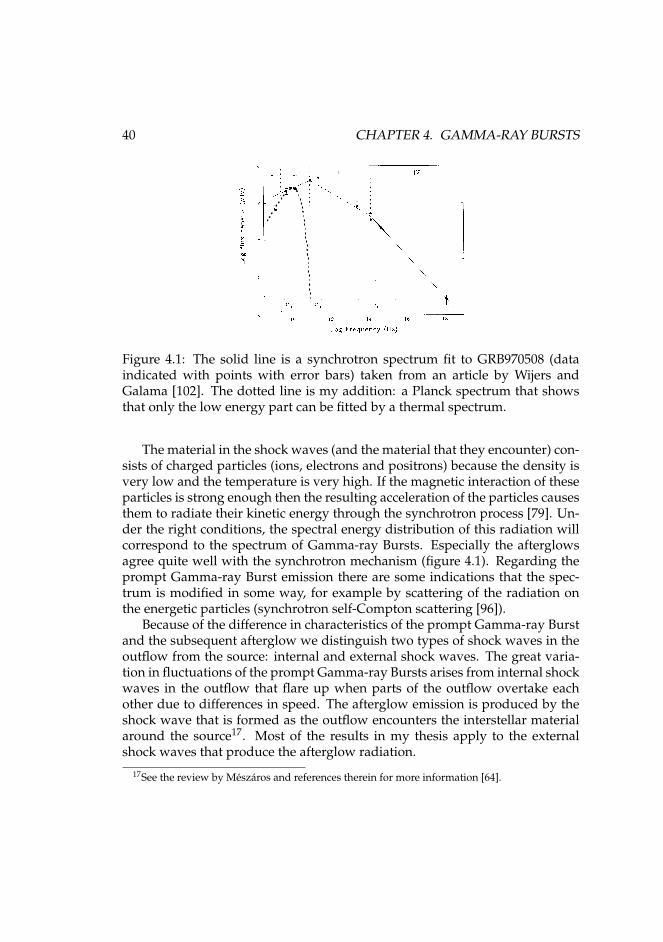
Figure 4.1: The solid line is a synchrotron spectrum fit to GRB970508 (dataindicated with points with error bars) taken from an article by Wijers andGalama [102]. The dotted line is my addition: a Planck spectrum that showsthat only the low energy part can be fitted by a thermal spectrum.
The material in the shock waves (and the material that they encounter) con-sists of charged particles (ions, electrons and positrons) because the density isvery low and the temperature is very high. If the magnetic interaction of theseparticles is strong enough then the resulting acceleration of the particles causesthem to radiate their kinetic energy through the synchrotron process [79]. Un-der the right conditions, the spectral energy distribution of this radiation willcorrespond to the spectrum of Gamma-ray Bursts. Especially the afterglowsagree quite well with the synchrotron mechanism (figure 4.1). Regarding theprompt Gamma-ray Burst emission there are some indications that the spec-trum is modified in some way, for example by scattering of the radiation onthe energetic particles (synchrotron self-Compton scattering [96]).
Because of the difference in characteristics of the prompt Gamma-ray Burstand the subsequent afterglow we distinguish two types of shock waves in theoutflow from the source: internal and external shock waves. The great varia-tion in fluctuations of the prompt Gamma-ray Bursts arises from internal shockwaves in the outflow that flare up when parts of the outflow overtake eachother due to differences in speed. The afterglow emission is produced by theshock wave that is formed as the outflow encounters the interstellar materialaround the source17. Most of the results in my thesis apply to the externalshock waves that produce the afterglow radiation.
17See the review by Meszaros and references therein for more information [64].
Magnetic Fields inside Extremely Fast Shock Waves by Jorrit Wiersma 41
Although we now have solid observational grounds for the hypothesis thatthe synchrotron process produces the Gamma-ray Burst and afterglow radia-tion, we are still left with the question whether it is theoretically possible thatthe synchrotron process occurs in these shock waves.
The models that can reproduce the synchrotron spectrum (as in figure 4.1)require a population of charged particles with a power-law distribution fortheir kinetic energy that extends to much higher energies than a thermal distri-bution. This, in turn, requires some kind of mechanism in the shock waves thataccelerates the particles to such high energies. Particle acceleration in shocks isa hairy subject, but the consensus of researchers seems to be that particles doget accelerated in shocks to a power-law energy distribution. The details of themechanism responsible for the acceleration is still the subject of debate in theliterature (Piran [75], section V.B).
A second requirement for explaining the synchrotron spectrum is a strongmagnetic interaction of the charged particles in the shock wave18. In chapter 5I will discuss how the compression of plasma in the shock front will alwaysboost the magnetic field strength by a certain factor. However, this boost is notenough to explain the synchrotron spectra of Gamma-ray Burst afterglows. AsI described earlier in section 3.4 we do however expect that the magnetic inter-action in the shock front is strong because of plasma instabilities. Therefore, inthe rest of my thesis I investigate these processes in more detail.
To summarize, Gamma-ray Bursts have only been known for a short timeand form an important test for modern physics. To observe them we depend onmodern techniques to detect high-energy radiation and cosmic rays with satel-lites and with detectors on Earth. To explain them we use modern physicaltheories like the Special Theory of Relativity (physics at velocities approachingthe speed of light), plasma physics (physics of charged particles and their in-teractions) and particle physics (the physics of particles at large energies). Thisthesis discusses an important part of their explanation: the magnetic interac-tion of charged particles in relativistic shocks.
18The strength of the magnetic interaction is generally measured through the ratio of magneticenergy density to total energy density in the shock wave. The synchrotron model requires thisratio to be at least 1–10 % [96, 32].

42 CHAPTER 4. GAMMA-RAY BURSTS
Part II
Research
43

Chapter 5
Relativistic Shock Conditions
Like all physical phenomena a shock wave must obey certain conservationlaws such as conservation of energy and momentum. This restricts the pos-sible ways in which a shock wave can change the gas that passes through it:for each quantity that is conserved, the same amount must come out of theshock transition as goes into it. In this chapter I use this fact to derive relationsbetween the properties of the material behind the shock and the properties ofthe material in front of the shock. We call these relations ‘shock conditions.’
In relativistic collisionless shock waves we have to take into account thatprocesses such as plasma instabilities inside the shock wave can use part ofthe available energy to produce electromagnetic fields. The total energy isconserved, but the division into kinetic, thermal and electromagnetic energydepends on the processes that work inside the shock transition. In this chapter,this introduces an uncertainty into the properties of the material behind theshock wave: based purely on the conservation laws we cannot say how largethe magnetic energy density behind the shock is, so this quantity is left as afree parameter εB. In later chapters (such as chapters 8 and 9) we will see howa study of the Weibel instability can yield an estimate for this parameter.
45
46 CHAPTER 5. RELATIVISTIC SHOCK CONDITIONS
5.1 IntroductionRelativistic shock waves in astrophysical plasmas are considerably more com-plex than classical shock waves in gases. Apart from relativistic effects and theinfluence of electromagnetic fields, processes inside the shock transition caninclude particle creation [73] and magnetic field generation [58], so that massand magnetic flux conservation might no longer apply across the shock front.In this chapter I will analyze how this affects the properties of the shockedmaterial.
A shock is a location of sudden change in flow properties such as density,pressure, temperature, and magnetic field strength. A transition occurs froman unshocked flow to a shocked flow. In this chapter I will discuss the prob-lem of finding the properties of the shocked material if the properties of theunshocked material and the shock speed are given.
In astrophysical shocks, the change in plasma properties across the shockfront and the internal structure of the shock front is controlled by plasma insta-bilities rather than by collision-dominated processes such as viscosity and heatconduction. The plasma is so tenuous that particle collisions are unimportant(collisionless plasma). Exchange of energy and momentum with electromag-netic fields plays a much larger role (see [92] for a book on non-relativisticcollisionless shocks). Medvedev and Loeb [58] have shown that this can in-volve the generation of magnetic fields, particularly when relativistic speedsare involved (see also [11]).
Jump conditions give the properties of a shock transition independent ofits internal structure in the limit of an infinitesimally thin shock. In that case,the state of the shocked plasma is related to the state of the unshocked plasmathrough conservation laws: when a quantity is conserved, the same amountmust flow out of the shock front as flows into it.
Relativistic shock conditions have been studied in the literature. Bland-ford & McKee [8] have given an explicit form of the hydrodynamical shockconditions for strong relativistic shocks (without a magnetic field). Kennel &Coroniti [46] have given shock conditions in the presence of a magnetic fieldin the ideal MHD approximation and Lichnerowicz [53] has given a covariantformulation for ideal MHD shock conditions. Kirk & Duffy [47] have written areview of the theory of relativistic shocks.
In this chapter I will give a derivation of the shock conditions that leavesopen the possibility of magnetic field generation in the shock so that magneticflux conservation does not apply. The derivation starts with the conservationlaws of magnetohydrodynamics (section 5.2.1), which can be simplified us-
Magnetic Fields inside Extremely Fast Shock Waves by Jorrit Wiersma 47
ing suitable approximations. The most important approximation is to take themagnetic field perpendicular to the direction in which the shock moves. I willsolve the shock conditions in this case and give a justification for the approx-imation of a perpendicular magnetic field (section 5.3). In the last section Idiscuss the assumptions made and the general properties of the results (sec-tion 5.4).
5.2 Theory: Magnetohydrodynamics5.2.1 MHD description of the plasmaI will examine the plasma on a length-scale that is much larger than the length-scale associated with the plasma instabilities in the shock transition. In thislimit we can view the plasma as an ideally conducting, compressible fluid.Its properties are described by the theory of relativistic magnetohydrodynam-ics (MHD) [53].
MHD treats the collection of charged particles that makes up the plasma asa continuum. The flow velocity v is then the bulk velocity of the particles (mea-sured throughout this chapter in units of the light-speed) and the proper massdensity ρ is measured in the frame where the velocity v is zero (the ‘fluid restframe’). The velocity field has an associated Lorentz factor γ = 1/
√1− |v|2,
four-velocity uα = (γ, γv) and mass flux ρuα.The proper internal energy density e consists of the rest mass energy den-
sity and the kinetic energy density in thermal motions. The pressure P de-notes the momentum flux density in thermal motions. The associated energy-momentum tensor in the fluid rest frame is (e.g., [49])
Tgas = diag(e, P, P, P). (fluid rest frame) (5.1)
The electromagnetic properties of the plasma are described through macro-scopic electromagnetic fields. In an ideal (infinitely good conducting) plasmathe electric field vanishes in the fluid rest frame. This is the MHD assumption.The magnetic field B does not vanish and has an associated four-vector Bα =(0, B) in the fluid rest frame.
The total energy momentum tensor (gas plus electromagnetic fields) forsuch a plasma can be written as (see Lichnerowicz [53], section 33):
Tαβ = (w +B2
4π)uαuβ − (P +
B2
8π)gαβ − BαBβ
4π, (5.2)
where gαβ = diag(1,−1,−1,−1) is the Minkowski metric tensor, w is the en-thalpy density in the fluid rest frame, and B is the magnetic field strength in
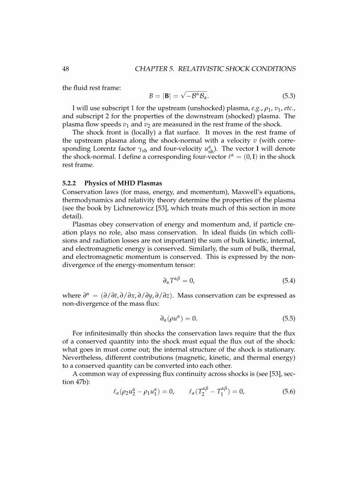
48 CHAPTER 5. RELATIVISTIC SHOCK CONDITIONS
the fluid rest frame:B = |B| =
√−BαBα. (5.3)
I will use subscript 1 for the upstream (unshocked) plasma, e.g., ρ1, v1, etc.,and subscript 2 for the properties of the downstream (shocked) plasma. Theplasma flow speeds v1 and v2 are measured in the rest frame of the shock.
The shock front is (locally) a flat surface. It moves in the rest frame ofthe upstream plasma along the shock-normal with a velocity v (with corre-sponding Lorentz factor γsh and four-velocity uα
sh). The vector l will denotethe shock-normal. I define a corresponding four-vector `α = (0, l) in the shockrest frame.
5.2.2 Physics of MHD PlasmasConservation laws (for mass, energy, and momentum), Maxwell’s equations,thermodynamics and relativity theory determine the properties of the plasma(see the book by Lichnerowicz [53], which treats much of this section in moredetail).
Plasmas obey conservation of energy and momentum and, if particle cre-ation plays no role, also mass conservation. In ideal fluids (in which colli-sions and radiation losses are not important) the sum of bulk kinetic, internal,and electromagnetic energy is conserved. Similarly, the sum of bulk, thermal,and electromagnetic momentum is conserved. This is expressed by the non-divergence of the energy-momentum tensor:
∂αTαβ = 0, (5.4)
where ∂α = (∂/∂t, ∂/∂x, ∂/∂y, ∂/∂z). Mass conservation can be expressed asnon-divergence of the mass flux:
∂α(ρuα) = 0. (5.5)
For infinitesimally thin shocks the conservation laws require that the fluxof a conserved quantity into the shock must equal the flux out of the shock:what goes in must come out; the internal structure of the shock is stationary.Nevertheless, different contributions (magnetic, kinetic, and thermal energy)to a conserved quantity can be converted into each other.
A common way of expressing flux continuity across shocks is (see [53], sec-tion 47b):
`α(ρ2uα2 − ρ1uα
1) = 0, `α(Tαβ2 − Tαβ
1 ) = 0, (5.6)
Magnetic Fields inside Extremely Fast Shock Waves by Jorrit Wiersma 49
which ensures that the flux along the shock-normal is continuous. These equa-tions are a restraint on the jump in density, pressure, energy density and flowspeed across the shock and are therefore called the jump conditions.
The electromagnetic fields are constrained by Maxwell’s equations. Forideal MHD these can be reduced to one covariant equation which expressesconservation of magnetic flux:
∂α(uαBβ − Bαuβ) = 0. (5.7)
We can apply this equation across the shock:
`α(uα2B
β2 − B
α2 uβ
2 ) = `α(uα1B
β1 − B
α1 uβ
1 ). (frozen) (5.8)
However, this assumes that the ideal MHD approximation applies across thewhole shock front. I will indicate equations that depend on this assumptionwith the keyword ‘frozen’ since it means that the magnetic field lines are frozento the plasma.
Mass and magnetic flux conservation might not apply if particle creationand magnetic field generation play a role in the shock transition. One way todrop these two conservation laws is to consider the mass density and magneticfield strength behind the shock to be given quantities instead of variables. Al-ternatively, to take particle creation into account, a parameter η = ρcons
2 /ρ2can be introduced that gives the ratio of conserved number of particles to totalnumber of particles behind the shock (see Kirk and Duffy [47]). For the mag-netic field I will show in section 5.3.2 how to find shock conditions assumingthat the ratio of magnetic to internal energy εB ≡ B2
2/(8πe2) is a given quan-tity. However, these are ad hoc solutions and a full solution requires a theoryfor the internal shock structure that gives ρ2 and B2 as a function of the shockparameters (see also the discussion in section 5.4).
The density, pressure, and internal energy are thermodynamic quantitiesthat can be related through an equation of state. A simple equation of state,which I will use here, is:
P = (Γ− 1)(e− ρ), (5.9)
where Γ is the specific heat ratio, which is equal to 5/3 for a cold plasma and4/3 for a relativistically hot plasma (see the the next subsection for the defini-tion of hot and cold plasma). For intermediate cases another equation of stateshould be used (Kirk and Duffy [47] discuss how to use a Synge equation ofstate).
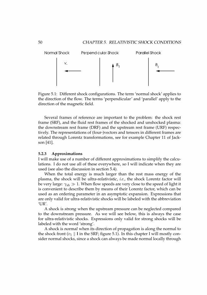
50 CHAPTER 5. RELATIVISTIC SHOCK CONDITIONS
Figure 5.1: Different shock configurations. The term ‘normal shock’ applies tothe direction of the flow. The terms ‘perpendicular’ and ‘parallel’ apply to thedirection of the magnetic field.
Several frames of reference are important to the problem: the shock restframe (SRF), and the fluid rest frames of the shocked and unshocked plasma:the downstream rest frame (DRF) and the upstream rest frame (URF) respec-tively. The representations of (four-)vectors and tensors in different frames arerelated through Lorentz transformations, see for example Chapter 11 of Jack-son [41].
5.2.3 ApproximationsI will make use of a number of different approximations to simplify the calcu-lations. I do not use all of these everywhere, so I will indicate when they areused (see also the discussion in section 5.4).
When the total energy is much larger than the rest mass energy of theplasma, the shock will be ultra-relativistic , i.e., the shock Lorentz factor willbe very large: γsh 1. When flow speeds are very close to the speed of light itis convenient to describe them by means of their Lorentz factor, which can beused as an ordering parameter in an asymptotic expansion. Expressions thatare only valid for ultra-relativistic shocks will be labeled with the abbreviation‘UR’.
A shock is strong when the upstream pressure can be neglected comparedto the downstream pressure. As we will see below, this is always the casefor ultra-relativistic shocks. Expressions only valid for strong shocks will belabeled with the word ‘strong’.
A shock is normal when its direction of propagation is along the normal tothe shock front (v1 ‖ l in the SRF; figure 5.1). In this chapter I will mostly con-sider normal shocks, since a shock can always be made normal locally through
Magnetic Fields inside Extremely Fast Shock Waves by Jorrit Wiersma 51
a change of reference frame.When magnetic fields are involved, important classes of shocks are those
of perpendicular and parallel shocks (figure 5.1). When the magnetic field isparallel to the propagation direction of the shock (B ‖ l in the SRF) a shock isparallel. When the magnetic field is perpendicular to this direction it is per-pendicular (B ⊥ l in the SRF). I will show below that ultra-relativistic shockscan almost always be considered to be perpendicular.
Certain approximations can also be made regarding the properties of theup- or downstream plasma. The plasma is said to be cold when the thermalmotions of the particles are negligible. This means that the pressure and ther-mal energy density are not important for the dynamics: P ρ, e ' ρ. A plasmais relativistically hot when its thermal energy density is much larger than itsrest mass density: e ρ. In this case the adiabatic constant is Γ = 4/3 and theequation of state (5.9) can be approximated by P ' e/3. Lastly, the plasma issaid to be unmagnetized when the influence of the magnetic field can be ne-glected (i.e., when the Larmor radius of the particles is much larger than anyrelevant length scale of the problem).
5.3 Shock conditions and their solutions5.3.1 General situationThe goal of this chapter is to find the properties of the shocked plasma giventhe properties of the unshocked plasma and the shock (figure 5.2). To do thisanalytically I will simplify the situation by assuming that the shock is ultra-relativistic (γsh 1).
For ultra-relativistic shocks the magnetic field can almost always be consid-ered to be perpendicular to the shock-normal. I will prove this in section 5.3.3but it can be anticipated because of the following. In general, the magnetic fieldin the unshocked material will be at an inclination angle i to the shock-normalwith parallel and perpendicular components B‖ = B cos i and B⊥ = B sin i (Iwill put the x-axis along B‖, and the y-axis along B⊥). A Lorentz transforma-tion with boost v gives the situation in the shock rest frame (e.g., Jackson [41],Section 11.10):
Bsrf⊥ = γshB sin i, Bsrf
‖ = B cos i. (5.10)
The perpendicular component is amplified by a Lorentz factor, whereas theparallel component remains unchanged. Therefore we can expect the perpen-dicular component to dominate unless sin i <∼ 1/γsh.
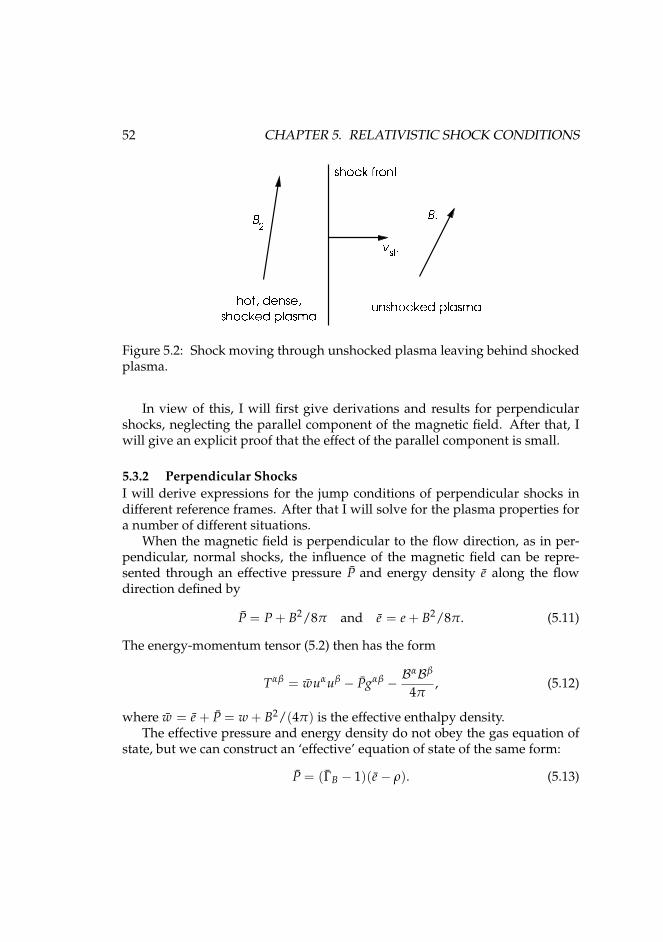
52 CHAPTER 5. RELATIVISTIC SHOCK CONDITIONS
Figure 5.2: Shock moving through unshocked plasma leaving behind shockedplasma.
In view of this, I will first give derivations and results for perpendicularshocks, neglecting the parallel component of the magnetic field. After that, Iwill give an explicit proof that the effect of the parallel component is small.
5.3.2 Perpendicular ShocksI will derive expressions for the jump conditions of perpendicular shocks indifferent reference frames. After that I will solve for the plasma properties fora number of different situations.
When the magnetic field is perpendicular to the flow direction, as in per-pendicular, normal shocks, the influence of the magnetic field can be repre-sented through an effective pressure P and energy density e along the flowdirection defined by
P = P + B2/8π and e = e + B2/8π. (5.11)
The energy-momentum tensor (5.2) then has the form
Tαβ = wuαuβ − Pgαβ − BαBβ
4π, (5.12)
where w = e + P = w + B2/(4π) is the effective enthalpy density.The effective pressure and energy density do not obey the gas equation of
state, but we can construct an ‘effective’ equation of state of the same form:
P = (ΓB − 1)(e − ρ). (5.13)
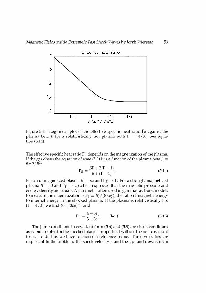
Magnetic Fields inside Extremely Fast Shock Waves by Jorrit Wiersma 53
Figure 5.3: Log-linear plot of the effective specific heat ratio ΓB against theplasma beta β for a relativistically hot plasma with Γ = 4/3. See equa-tion (5.14).
The effective specific heat ratio ΓB depends on the magnetization of the plasma.If the gas obeys the equation of state (5.9) it is a function of the plasma beta β ≡8πP/B2:
ΓB =βΓ + 2(Γ− 1)
β + (Γ− 1). (5.14)
For an unmagnetized plasma β → ∞ and ΓB → Γ. For a strongly magnetizedplasma β → 0 and ΓB → 2 (which expresses that the magnetic pressure andenergy density are equal). A parameter often used in gamma-ray burst modelsto measure the magnetization is εB ≡ B2
2/(8πe2), the ratio of magnetic energyto internal energy in the shocked plasma. If the plasma is relativistically hot(Γ = 4/3), we find β = (3εB)−1 and
ΓB =4 + 6εB
3 + 3εB. (hot) (5.15)
The jump conditions in covariant form (5.6) and (5.8) are shock conditionsas is, but to solve for the shocked plasma properties I will use the non-covariantform. To do this we have to choose a reference frame. Three velocities areimportant to the problem: the shock velocity v and the up- and downstream
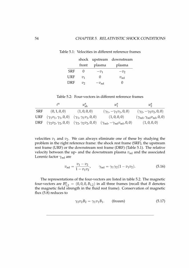
54 CHAPTER 5. RELATIVISTIC SHOCK CONDITIONS
Table 5.1: Velocities in different reference frames
shock upstream downstreamfront plasma plasma
SRF 0 −v1 −v2
URF v1 0 vrel
DRF v2 −vrel 0
Table 5.2: Four-vectors in different reference frames
`α uαsh uα
1 uα2
SRF (0, 1, 0, 0) (1, 0, 0, 0) (γ1,−γ1v1, 0, 0) (γ2,−γ2v2, 0, 0)URF (γ1v1, γ1, 0, 0) (γ1, γ1v1, 0, 0) (1, 0, 0, 0) (γrel, γrelvrel, 0, 0)DRF (γ2v2, γ2, 0, 0) (γ2, γ2v2, 0, 0) (γrel,−γrelvrel, 0, 0) (1, 0, 0, 0)
velocities v1 and v2. We can always eliminate one of these by studying theproblem in the right reference frame: the shock rest frame (SRF), the upstreamrest frame (URF) or the downstream rest frame (DRF) (Table 5.1). The relativevelocity between the up- and the downstream plasma vrel and the associatedLorentz factor γrel are
vrel =v1 − v2
1− v1v2, γrel = γ1γ2(1− v1v2). (5.16)
The representations of the four-vectors are listed in table 5.2. The magneticfour-vectors are Bα
1,2 = (0, 0, 0, B1,2) in all three frames (recall that B denotesthe magnetic field strength in the fluid rest frame). Conservation of magneticflux (5.8) reduces to
γ2v2B2 = γ1v1B1. (frozen) (5.17)
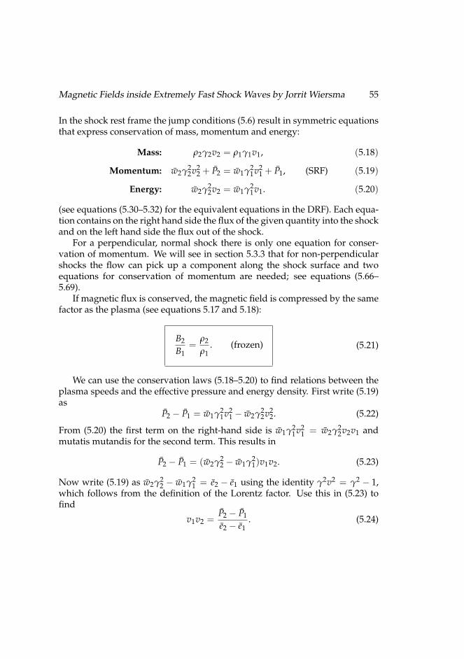
Magnetic Fields inside Extremely Fast Shock Waves by Jorrit Wiersma 55
In the shock rest frame the jump conditions (5.6) result in symmetric equationsthat express conservation of mass, momentum and energy:
Mass: ρ2γ2v2 = ρ1γ1v1, (5.18)
Momentum: w2γ22v2
2 + P2 = w1γ21v2
1 + P1, (SRF) (5.19)
Energy: w2γ22v2 = w1γ2
1v1. (5.20)
(see equations (5.30–5.32) for the equivalent equations in the DRF). Each equa-tion contains on the right hand side the flux of the given quantity into the shockand on the left hand side the flux out of the shock.
For a perpendicular, normal shock there is only one equation for conser-vation of momentum. We will see in section 5.3.3 that for non-perpendicularshocks the flow can pick up a component along the shock surface and twoequations for conservation of momentum are needed; see equations (5.66–5.69).
If magnetic flux is conserved, the magnetic field is compressed by the samefactor as the plasma (see equations 5.17 and 5.18):
B2
B1=
ρ2
ρ1. (frozen) (5.21)
We can use the conservation laws (5.18–5.20) to find relations between theplasma speeds and the effective pressure and energy density. First write (5.19)as
P2 − P1 = w1γ21v2
1 − w2γ22v2
2. (5.22)
From (5.20) the first term on the right-hand side is w1γ21v2
1 = w2γ22v2v1 and
mutatis mutandis for the second term. This results in
P2 − P1 = (w2γ22 − w1γ2
1)v1v2. (5.23)
Now write (5.19) as w2γ22 − w1γ2
1 = e2 − e1 using the identity γ2v2 = γ2 − 1,which follows from the definition of the Lorentz factor. Use this in (5.23) tofind
v1v2 =P2 − P1
e2 − e1. (5.24)
56 CHAPTER 5. RELATIVISTIC SHOCK CONDITIONS
I will show below that ultra-relativistic shocks have P2 P1, e2 e1, ande2 ρ2 so that (with v1 ' 1 and equation of state (5.13)):
v2 = P2/e2 = ΓB − 1. (UR) (5.25)
For a hot downstream plasma equation (5.15) gives ΓB and the downstreamflow speed varies from v2 = 1/3 for an unmagnetized plasma to v2 → 1 fora strongly magnetized plasma (in a strongly magnetized plasma the shock isan electromagnetic wave and propagates at the speed of light in all referenceframes).
Returning to the general case, we can now eliminate v1 or v2. For example,start again with equation (5.22), and use w2γ2
2v22 = w1γ2
1v2v1 (see equation 5.20)to find
P2 − P1 = w1γ21(v2
1 − v2v1)
= w1γ21
(v2
1 −P2 − P1
e2 − e1
).
(5.26)
Eliminating the Lorentz factor through γ21 = (1 − v2
1)−1 we find an equation
that can be solved for v1:
v1 =
√(P2 − P1)(e2 + P1)(e2 − e1)(e1 + P2)
. (5.27)
Because of the symmetry of the jump conditions under the exchange of theindices 1 and 2 we also find
v2 =
√(P2 − P1)(e1 + P2)(e2 − e1)(e2 + P1)
. (5.28)
We can use these results to express the Lorentz factor γrel of the relativevelocity between the up- and downstream plasma in P and e. Equation (5.16)yields after some algebra:
γrel =
√(e2 + P1)(e1 + P2)(e1 + P1)(e2 + P2)
. (5.29)
Magnetic Fields inside Extremely Fast Shock Waves by Jorrit Wiersma 57
Now I will derive the jump conditions in the rest frame of the downstreamplasma. The equations in the upstream rest frame are the same, but with sub-scripts 1 and 2 interchanged. Note that these equations are equivalent to thosein the shock rest frame, equations (5.18–5.20). The jump conditions (5.6) yieldin the downstream rest frame:
Mass: ρ2v2 = ρ1γrelv2 + ρ1γrelvrel, (5.30)
Momentum: P2 = w1γ2relvrelv2 + w1γ2
relv2rel + P1, (DRF) (5.31)
Energy: e2v2 = (e1 + P1v2rel)γ2
relv2 + (e1 + P1)γ2relvrel, (5.32)
where a factor γ2 has been eliminated from all three equations. The equationscontain on the left hand side the flux of each quantity out of the shock. Thedownstream plasma is at rest and v2 enters the equations not as a flow speedbut as the speed of the shock. The movement of the shock front causes a flux ofdensity× shock speed, e.g., the mass flux is ρ2v2. The only contribution to themomentum flux out of the shock is the effective pressure P2 because the bulkmomentum density behind the shock is zero in this reference frame. Both themovement of the shock and the movement of the upstream plasma contributeto the flux into the shock on the right hand side (the first and second termsrespectively). The momentum flux also has a contribution from the pressure P1.
The equations contain the downstream quantities ρ2, e2 and P2 in a simpleway and we can work out some properties of these quantities.
We can write mass conservation as
X ≡ ρ2
γrelρ1= 1 +
vrelv2
. (5.33)
The quantity X plays an important role in later calculations. For ultra-relati-vistic shocks vrel → 1 and 1/3 <∼ v2 <∼ 1 (see above) so that 2 <∼ X <∼ 4. Thecompression ratio ρ2/ρ1 will be of order γrel because X is of order 1.
To get a relation between the Lorentz factor γrel of the relative velocity be-tween the up- and downstream plasma and the Lorentz factor γsh of the shockvelocity we can use mass conservation in the URF:
ρ1v = ρ2γrel(v− vrel). (URF) (5.34)
Rewriting this as (γrelρ2 − ρ1)v = ρ2γrelvrel and squaring both sides to elimi-nate the velocities in favor of the Lorentz factors, we find after some straight-
58 CHAPTER 5. RELATIVISTIC SHOCK CONDITIONS
forward algebra
γ2sh =
(Xγ2rel − 1)2
(X − 2)Xγ2rel + 1
. (5.35)
For ultra-relativistic shocks both γsh and γrel are large and provided X 6= 2 weget the approximate expression
γ2sh =
XX − 2
γ2rel. (UR) (5.36)
For ultra-relativistic shocks γrel will therefore be of the same order as γsh.This enables us to find the order of the downstream plasma properties from theDRF equations (5.30–5.32): the density ρ2 is of order γrel, the energy densityand pressure are of order γ2
rel, and a frozen-in magnetic field is of order γrel,see equation (5.21).
Now I will solve for the downstream plasma properties v2, ρ2, e2, P2, and B2.For a unique solution we need five equations. The conservation laws of mass,momentum, energy, and magnetic flux provide four equations and the down-stream equation of state the fifth.
First I will give a derivation for the strong unmagnetized shock solutiongiven by Blandford and McKee [8]. Then I will give a derivation for magne-tized ultra-relativistic shocks with conserved magnetic flux (similar to solu-tions found in [46] and [30]). Finally, I will give a solution for a fixed εB.
Unmagnetized shocks. Blandford & McKee [8] have given an analytic solutionfor strong unmagnetized shocks. I will derive their results (see table 5.3 fornotational differences).
The idea is to find a relation for e2/ρ2 and to use this with the equation ofstate to eliminate e2 and P2. The resulting equation can be solved to find ρ2 asa function of γrel. The last step is to relate γrel to the shock Lorentz factor.
The jump conditions (5.30–5.32) give
ρ2 = γrelρ1(1 + vrel/v2), (5.37)
P2 − P1 = γ2relw1vrel(v2 + vrel), (5.38)
(e2 + P1) = γ2relw1(1 + vrel/v2), (5.39)
Magnetic Fields inside Extremely Fast Shock Waves by Jorrit Wiersma 59
Table 5.3: Notation used by Blandford & McKee [8]
This chapter Blandford & McKee
adiabatic const. Γ γ2
shock Lorentz factor γsh Γrelative L. factor γrel γ2
mass density ρ m n
where I have dropped the ¯ accents. The only non-trivial change is in thelast equation where I used the identity γ2
relv2rel = γ2
rel − 1. Equations (5.37)and (5.39) yield
e2 + P1
ρ2= γrel
w1
ρ1. (5.40)
Note that this equation is exact and that it is also valid with the subscripts 1and 2 interchanged. For strong shocks P2 P1 and therefore e2 P1 so thatwe can approximate equation (5.40) with
e2
ρ2= γrel
w1
ρ1. (strong) (5.41)
This is equation (3) of Blandford and McKee [8]. It expresses that the energyper unit mass behind the shock is equal to the energy per unit mass in front.
To derive equations (4) and (5) of Blandford and McKee [8] we need the ex-tra assumption that the upstream plasma is cold, P1 ρ1 (Blandford & McKeedo not mention this explicitly). In a cold plasma we have w1 ' e1 ' ρ1 so thate2 ' γrelρ2 and (5.38) becomes
P2 = γ2relρ1vrel(v2 + vrel). (strong) (5.42)
After some manipulation, mass conservation (5.37) gives
v2 + vrel =ρ2vrel
(ρ2 − γrelρ1). (5.43)
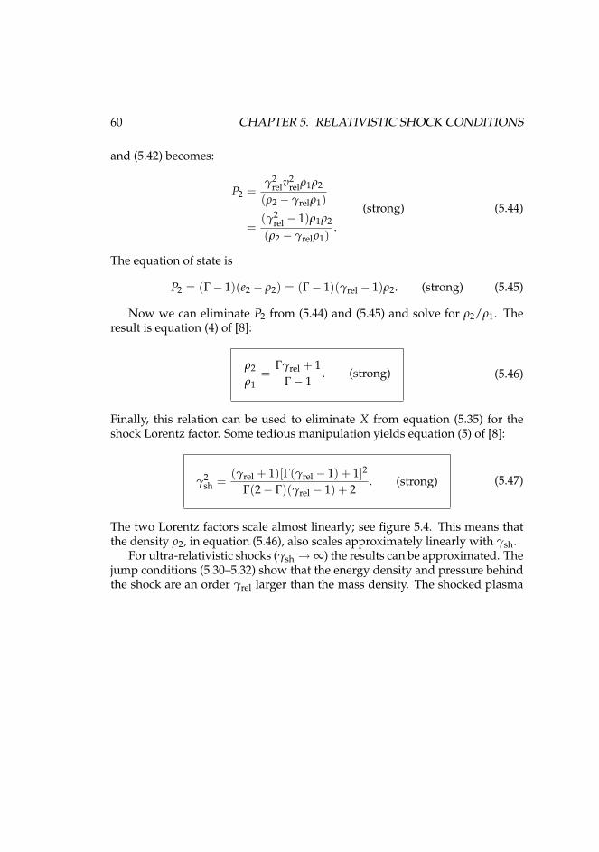
60 CHAPTER 5. RELATIVISTIC SHOCK CONDITIONS
and (5.42) becomes:
P2 =γ2
relv2relρ1ρ2
(ρ2 − γrelρ1)
=(γ2
rel − 1)ρ1ρ2
(ρ2 − γrelρ1).
(strong) (5.44)
The equation of state is
P2 = (Γ− 1)(e2 − ρ2) = (Γ− 1)(γrel − 1)ρ2. (strong) (5.45)
Now we can eliminate P2 from (5.44) and (5.45) and solve for ρ2/ρ1. Theresult is equation (4) of [8]:
ρ2
ρ1=
Γγrel + 1Γ− 1
. (strong) (5.46)
Finally, this relation can be used to eliminate X from equation (5.35) for theshock Lorentz factor. Some tedious manipulation yields equation (5) of [8]:
γ2sh =
(γrel + 1)[Γ(γrel − 1) + 1]2
Γ(2− Γ)(γrel − 1) + 2. (strong) (5.47)
The two Lorentz factors scale almost linearly; see figure 5.4. This means thatthe density ρ2, in equation (5.46), also scales approximately linearly with γsh.
For ultra-relativistic shocks (γsh → ∞) the results can be approximated. Thejump conditions (5.30–5.32) show that the energy density and pressure behindthe shock are an order γrel larger than the mass density. The shocked plasma
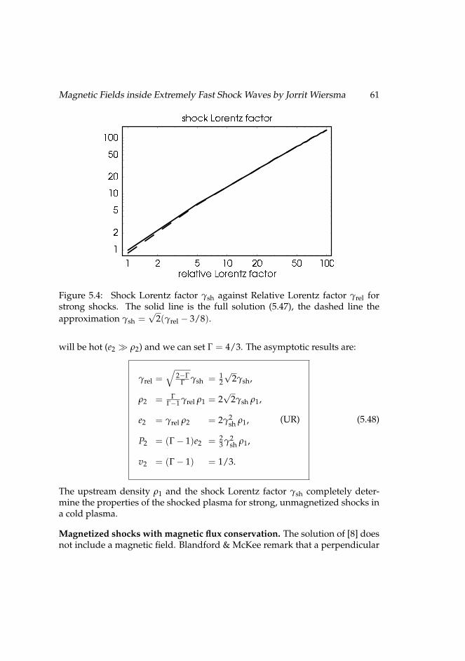
Magnetic Fields inside Extremely Fast Shock Waves by Jorrit Wiersma 61
Figure 5.4: Shock Lorentz factor γsh against Relative Lorentz factor γrel forstrong shocks. The solid line is the full solution (5.47), the dashed line theapproximation γsh =
√2(γrel − 3/8).
will be hot (e2 ρ2) and we can set Γ = 4/3. The asymptotic results are:
γrel =√
2−ΓΓ γsh = 1
2
√2γsh,
ρ2 = ΓΓ−1 γrel ρ1 = 2
√2γsh ρ1,
e2 = γrel ρ2 = 2γ2sh ρ1,
P2 = (Γ− 1)e2 = 23 γ2
sh ρ1,
v2 = (Γ− 1) = 1/3.
(UR) (5.48)
The upstream density ρ1 and the shock Lorentz factor γsh completely deter-mine the properties of the shocked plasma for strong, unmagnetized shocks ina cold plasma.
Magnetized shocks with magnetic flux conservation. The solution of [8] doesnot include a magnetic field. Blandford & McKee remark that a perpendicular
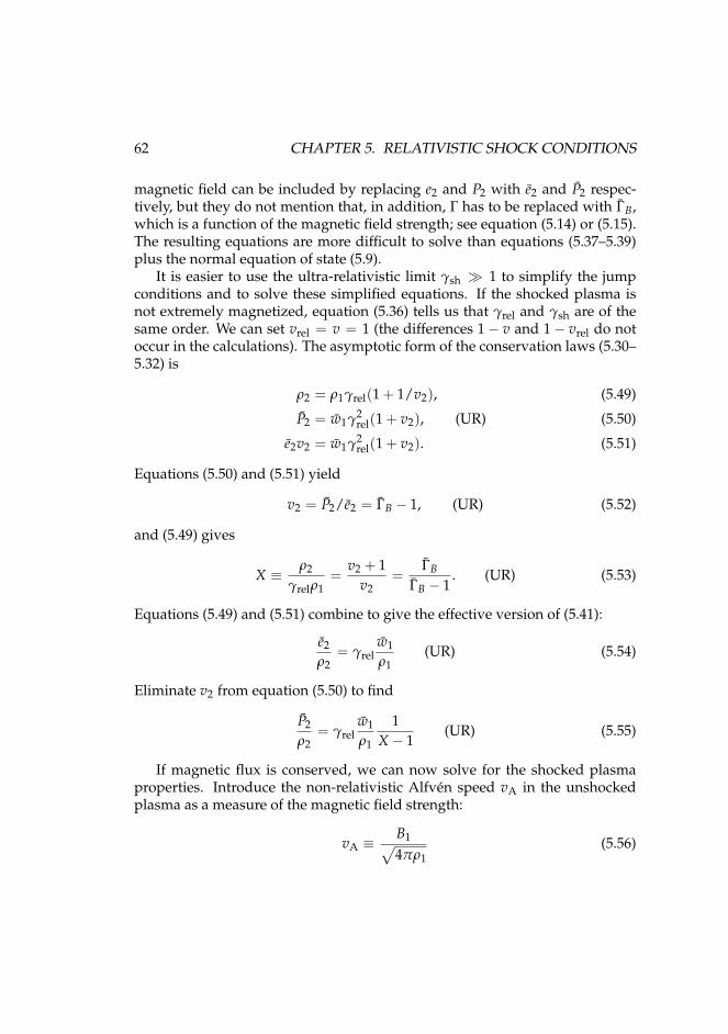
62 CHAPTER 5. RELATIVISTIC SHOCK CONDITIONS
magnetic field can be included by replacing e2 and P2 with e2 and P2 respec-tively, but they do not mention that, in addition, Γ has to be replaced with ΓB,which is a function of the magnetic field strength; see equation (5.14) or (5.15).The resulting equations are more difficult to solve than equations (5.37–5.39)plus the normal equation of state (5.9).
It is easier to use the ultra-relativistic limit γsh 1 to simplify the jumpconditions and to solve these simplified equations. If the shocked plasma isnot extremely magnetized, equation (5.36) tells us that γrel and γsh are of thesame order. We can set vrel = v = 1 (the differences 1− v and 1− vrel do notoccur in the calculations). The asymptotic form of the conservation laws (5.30–5.32) is
ρ2 = ρ1γrel(1 + 1/v2), (5.49)
P2 = w1γ2rel(1 + v2), (UR) (5.50)
e2v2 = w1γ2rel(1 + v2). (5.51)
Equations (5.50) and (5.51) yield
v2 = P2/e2 = ΓB − 1, (UR) (5.52)
and (5.49) gives
X ≡ ρ2
γrelρ1=
v2 + 1v2
=ΓB
ΓB − 1. (UR) (5.53)
Equations (5.49) and (5.51) combine to give the effective version of (5.41):
e2
ρ2= γrel
w1
ρ1(UR) (5.54)
Eliminate v2 from equation (5.50) to find
P2
ρ2= γrel
w1
ρ1
1X − 1
(UR) (5.55)
If magnetic flux is conserved, we can now solve for the shocked plasmaproperties. Introduce the non-relativistic Alfven speed vA in the unshockedplasma as a measure of the magnetic field strength:
vA ≡B1√4πρ1
(5.56)
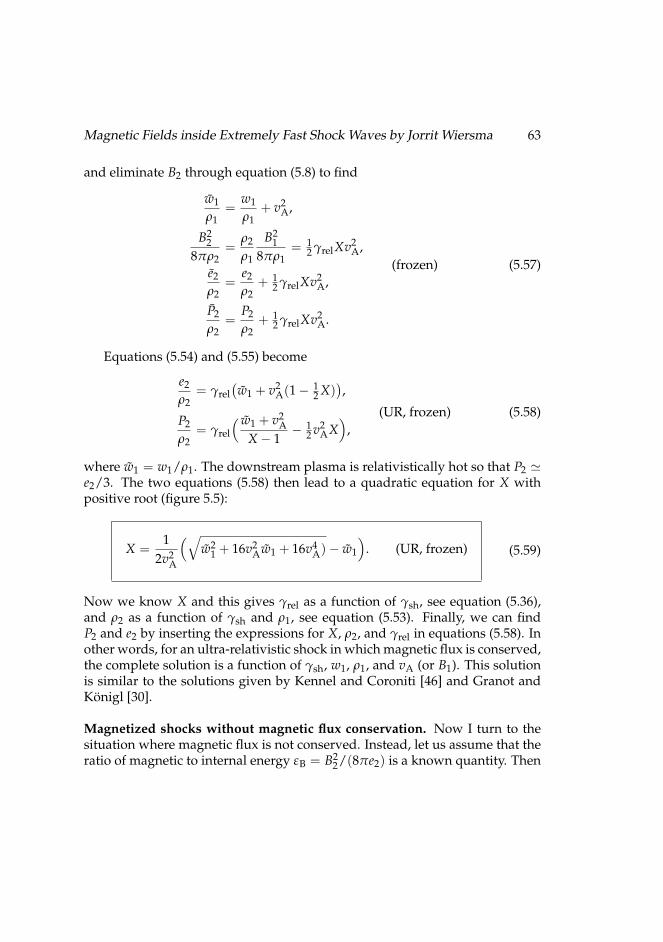
Magnetic Fields inside Extremely Fast Shock Waves by Jorrit Wiersma 63
and eliminate B2 through equation (5.8) to find
w1
ρ1=
w1
ρ1+ v2
A,
B22
8πρ2=
ρ2
ρ1
B21
8πρ1= 1
2 γrelXv2A,
e2
ρ2=
e2
ρ2+ 1
2 γrelXv2A,
P2
ρ2=
P2
ρ2+ 1
2 γrelXv2A.
(frozen) (5.57)
Equations (5.54) and (5.55) become
e2
ρ2= γrel
(w1 + v2
A(1− 12 X)
),
P2
ρ2= γrel
( w1 + v2A
X − 1− 1
2 v2AX)
,(UR, frozen) (5.58)
where w1 = w1/ρ1. The downstream plasma is relativistically hot so that P2 'e2/3. The two equations (5.58) then lead to a quadratic equation for X withpositive root (figure 5.5):
X =1
2v2A
(√w2
1 + 16v2Aw1 + 16v4
A)− w1
). (UR, frozen) (5.59)
Now we know X and this gives γrel as a function of γsh, see equation (5.36),and ρ2 as a function of γsh and ρ1, see equation (5.53). Finally, we can findP2 and e2 by inserting the expressions for X, ρ2, and γrel in equations (5.58). Inother words, for an ultra-relativistic shock in which magnetic flux is conserved,the complete solution is a function of γsh, w1, ρ1, and vA (or B1). This solutionis similar to the solutions given by Kennel and Coroniti [46] and Granot andKonigl [30].
Magnetized shocks without magnetic flux conservation. Now I turn to thesituation where magnetic flux is not conserved. Instead, let us assume that theratio of magnetic to internal energy εB = B2
2/(8πe2) is a known quantity. Then
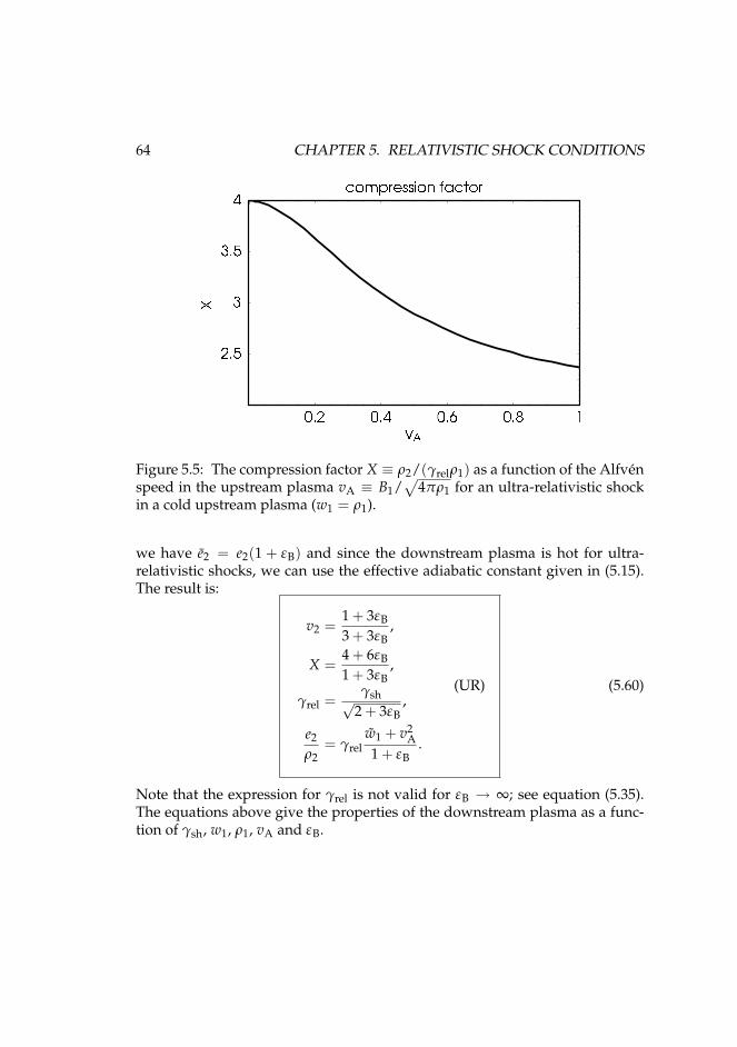
64 CHAPTER 5. RELATIVISTIC SHOCK CONDITIONS
Figure 5.5: The compression factor X ≡ ρ2/(γrelρ1) as a function of the Alfvenspeed in the upstream plasma vA ≡ B1/
√4πρ1 for an ultra-relativistic shock
in a cold upstream plasma (w1 = ρ1).
we have e2 = e2(1 + εB) and since the downstream plasma is hot for ultra-relativistic shocks, we can use the effective adiabatic constant given in (5.15).The result is:
v2 =1 + 3εB
3 + 3εB,
X =4 + 6εB
1 + 3εB,
γrel =γsh√
2 + 3εB,
e2
ρ2= γrel
w1 + v2A
1 + εB.
(UR) (5.60)
Note that the expression for γrel is not valid for εB → ∞; see equation (5.35).The equations above give the properties of the downstream plasma as a func-tion of γsh, w1, ρ1, vA and εB.
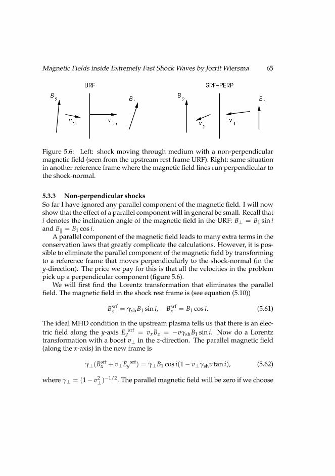
Magnetic Fields inside Extremely Fast Shock Waves by Jorrit Wiersma 65
Figure 5.6: Left: shock moving through medium with a non-perpendicularmagnetic field (seen from the upstream rest frame URF). Right: same situationin another reference frame where the magnetic field lines run perpendicular tothe shock-normal.
5.3.3 Non-perpendicular shocksSo far I have ignored any parallel component of the magnetic field. I will nowshow that the effect of a parallel component will in general be small. Recall thati denotes the inclination angle of the magnetic field in the URF: B⊥ = B1 sin iand B‖ = B1 cos i.
A parallel component of the magnetic field leads to many extra terms in theconservation laws that greatly complicate the calculations. However, it is pos-sible to eliminate the parallel component of the magnetic field by transformingto a reference frame that moves perpendicularly to the shock-normal (in they-direction). The price we pay for this is that all the velocities in the problempick up a perpendicular component (figure 5.6).
We will first find the Lorentz transformation that eliminates the parallelfield. The magnetic field in the shock rest frame is (see equation (5.10))
Bsrfz = γshB1 sin i, Bsrf
x = B1 cos i. (5.61)
The ideal MHD condition in the upstream plasma tells us that there is an elec-tric field along the y-axis Ey
srf = vxBz = −vγshB1 sin i. Now do a Lorentztransformation with a boost v⊥ in the z-direction. The parallel magnetic field(along the x-axis) in the new frame is
γ⊥(Bsrfx + v⊥Ey
srf) = γ⊥B1 cos i(1− v⊥γshv tan i), (5.62)
where γ⊥ = (1− v2⊥)−1/2. The parallel magnetic field will be zero if we choose
66 CHAPTER 5. RELATIVISTIC SHOCK CONDITIONS
v⊥ =1
γshv tan i. (5.63)
Note that this is only possible if γshv > 1/ tan i.We can now calculate the shock conditions in this new frame of reference.
To do this, we must use two Lorentz transformations (one to the SRF and onein the perpendicular direction) on the relevant four-vectors. For example, theupstream four-velocity becomes
uα1 = (γ⊥γsh,−γshv, 0, γshγ⊥v⊥) (5.64)
and the magnetic four-vector becomes
Bα1 = (−γ⊥γshB1 cos i/v, γshB1 cos i, 0, γ⊥B1/ sin i). (5.65)
In the ultra-relativistic limit γsh → ∞, v → 1, v⊥ → 0, and γ⊥ → 1. The jumpconditions (5.6) yield
Mass: ρ1γ1v‖1 = ρ2γ2v‖2, (5.66)
Par. momentum: w1γ21v2‖1 + P1 = w2γ2
2v2‖2 + P2, (5.67)
Perp. momentum: w1γ21v⊥1v‖1 = w2γ2
2v⊥2v‖2, (UR) (5.68)
Energy: w1γ21v‖1 = w2γ2
2v‖2, (5.69)
where v‖ is the parallel velocity in this special frame with v‖1 = v/γ⊥. Theperpendicular component v⊥1 = v⊥ is given in equation (5.63). The result onlydiffers from the jump conditions (5.18–5.20) for perpendicular shocks throughthe extra conservation law of perpendicular momentum.
I will now relate v⊥2 to v⊥ to show that v⊥2 is small for ultra-relativisticshocks. Conservation of perpendicular momentum gives
v⊥2
v⊥1=
w1γ21v‖1
w2γ22v‖2
. (5.70)
Eliminate the parallel velocities using energy conservation to find:
v⊥2
v⊥1=
w2
w1× w1
w2. (5.71)
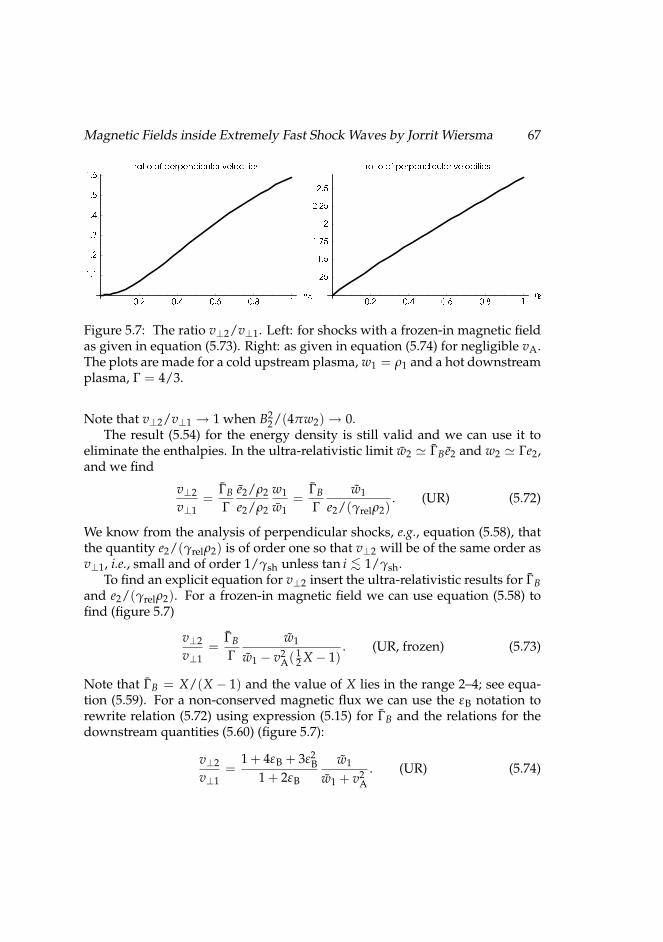
Magnetic Fields inside Extremely Fast Shock Waves by Jorrit Wiersma 67
Figure 5.7: The ratio v⊥2/v⊥1. Left: for shocks with a frozen-in magnetic fieldas given in equation (5.73). Right: as given in equation (5.74) for negligible vA.The plots are made for a cold upstream plasma, w1 = ρ1 and a hot downstreamplasma, Γ = 4/3.
Note that v⊥2/v⊥1 → 1 when B22/(4πw2) → 0.
The result (5.54) for the energy density is still valid and we can use it toeliminate the enthalpies. In the ultra-relativistic limit w2 ' ΓB e2 and w2 ' Γe2,and we find
v⊥2
v⊥1=
ΓBΓ
e2/ρ2
e2/ρ2
w1
w1=
ΓBΓ
w1
e2/(γrelρ2). (UR) (5.72)
We know from the analysis of perpendicular shocks, e.g., equation (5.58), thatthe quantity e2/(γrelρ2) is of order one so that v⊥2 will be of the same order asv⊥1, i.e., small and of order 1/γsh unless tan i <∼ 1/γsh.
To find an explicit equation for v⊥2 insert the ultra-relativistic results for ΓBand e2/(γrelρ2). For a frozen-in magnetic field we can use equation (5.58) tofind (figure 5.7)
v⊥2
v⊥1=
ΓBΓ
w1
w1 − v2A( 1
2 X − 1). (UR, frozen) (5.73)
Note that ΓB = X/(X − 1) and the value of X lies in the range 2–4; see equa-tion (5.59). For a non-conserved magnetic flux we can use the εB notation torewrite relation (5.72) using expression (5.15) for ΓB and the relations for thedownstream quantities (5.60) (figure 5.7):
v⊥2
v⊥1=
1 + 4εB + 3ε2B
1 + 2εB
w1
w1 + v2A
. (UR) (5.74)
68 CHAPTER 5. RELATIVISTIC SHOCK CONDITIONS
The last step is to transform back to the shock rest frame where the up-stream plasma flows along the shock-normal. Since v⊥1 is small we can use aGalilean transformation instead of a Lorentz transformation and simply sub-tract v⊥1 from v⊥2:
vsrf⊥2 =
(v⊥2
v⊥1− 1) 1
γshv tan i(UR, SRF) (5.75)
where v⊥2/v⊥1 follows either from equation (5.73) or (5.74).The conclusion is that the difference between perpendicular and non-per-
pendicular shocks is that in non-perpendicular shocks the downstream plasmapicks up a velocity in the direction perpendicular to the shock-normal. Thisvelocity is of order 1/(γsh tan i) and will be small if γsh 1/ tan i.
5.4 Discussion of the results5.4.1 General resultsConservation laws constrain the change in plasma properties across a shockfront. I have formulated these constraints in the previous section for ultra-relativistic shocks as relations between the up- and downstream plasma prop-erties (equations (5.18–5.20), (5.30–5.32) or (5.66–5.69)) and as solutions for thedownstream plasma properties (equations (5.48), (5.59), or (5.60)). The solu-tions give the downstream plasma properties (energy density, mass density,flow speed, and magnetic field strength) as a function of the upstream plasmaproperties (mass density, enthalpy density, magnetic field strength) and theshock Lorentz factor.
I have shown that we can consider the magnetic field to be perpendicular tothe shock-normal except when the shock moves almost parallel to the upstreammagnetic field lines.
The downstream plasma is hot so that the equation of state is well approxi-mated by one with a ratio of specific heats Γ = 4/3, because the internal energydensity is an order of the Lorentz factor larger than the mass density.
The shock is strong (P2 P1) because the downstream pressure is at leasttwo orders of the Lorentz factor larger than the upstream pressure.
5.4.2 Internal structure of the shockThese shock properties result from conservation of mass, momentum, energyand magnetic flux. This large scale treatment does not specify the internal pro-cesses that are responsible for the dissipation of bulk kinetic energy to inter-
Magnetic Fields inside Extremely Fast Shock Waves by Jorrit Wiersma 69
nal energy in the shock transition. These processes might involve particle cre-ation and magnetic field generation and could influence the properties of theshocked plasma.
If particle creation plays a role in the shock transition the mass density be-hind the shock is higher. Nevertheless, many of the results do not depend onconservation of mass and therefore still apply.
It is likely that the assumption of magnetic flux conservation is also incor-rect because plasma instabilities that violate the MHD assumption occur in theshock transition.
The processes that involve such particle creation or plasma instabilities re-quire a closer look at the internal structure of the shock. A first study of theinfluence of plasma instabilities on the magnetic field in relativistic shockswas given, e.g., by Medvedev & Loeb [58] and by Brainerd [9]. In this chap-ter the magnetic energy density was treated as a free parameter εB; see equa-tions (5.60). In the following chapters we investigate the plasma instabilitiesthat determine this parameter εB in more depth.
70 CHAPTER 5. RELATIVISTIC SHOCK CONDITIONS
Chapter 6
Linear theory of the Weibelinstability
As the pre- and post-shock particles mix in the shock front they form a plasmawith wildly differing particle velocities: seen from the point of view of theshock, the pre-shock particles will move into the shock front with a high ve-locity. Such a situation is unstable and because of the Weibel instability theparticles will arrange themselves into separated electrical currents. These cur-rents will generate a small-scale magnetic field.
In this chapter we show how the initial growth of the Weibel instability onlydepends on how diffuse the velocity distribution is and on the strength of theincoming plasma flow compared to the (shocked) background plasma.
Because a relativistic collisionless shock wave is formed by electromagneticinteraction instead of particle collisions the previous chapter introduced thequestion of how much energy will end up in electromagnetic energy. In chap-ters 8 and 9 we will see how the growth of the magnetic field strength will bestopped, which will lead to an estimate of the magnetic energy density.
This chapter has been submitted to Astronomy & Astrophysics [3].
71
72 CHAPTER 6. LINEAR THEORY OF THE WEIBEL INSTABILITY
6.1 IntroductionThe Weibel instability is an electromagnetic instability of low-frequency per-turbations in a plasma where one (or more) of the particle species has an aniso-tropic momentum distribution. In its original form, as discussed by Weibel[98], this anisotropy is caused by different values of the kinetic temperature ofthe particles in two mutually orthogonal directions. More recent astrophysi-cal applications, see for instance [32], [31], [58] and [24], have concentrated onthe anisotropy caused by the presence of bulk plasma motions in the form ofbeams in a (thermal) background plasma.
In relativistic shocks, which propagate into a cold medium with bulk speedVsh ∼ c, this version of the instability could be important as the collisionlessrelaxation mechanism in the ’transition layer’ where the shock-heated and in-coming (unshocked) plasma mix. As this instability has its most rapid growthin the low-frequency regime, so that |ω| kc with k = 2π/λ the wave num-ber, it generates an electromagnetic field (δE , δB) that is dominated by themagnetic component: |δB| |δE|.
Generation of magnetic fields is a necessary ingredient in those models thatexplain the prompt gamma-rays, and the broad-band afterglow emission fromGamma Ray Bursts as (Lorentz-boosted) synchrotron radiation. These syn-chrotron models must assume that the magnetic field is strong in the sense thatthe ratio of magnetic to internal energy is of order B2/8πe ≈ 0.01− 0.1. HereB the magnetic field strength with corresponding energy density eB = B2/8π,and e is the internal energy density of the radiating plasma. Details of the ar-guments leading to this estimate can be found in the reviews by Piran [74, 75]and Meszaros [65, 66], and in the references therein.
The compression of existing interstellar (or circumstellar) magnetic fieldsby a relativistic shock leads to an insufficient field strength, with εB 1. Infact, without additional field amplification one finds that the pre- and post-shock values of εB ≡ B2/8πe are of similar magnitude, see equation (6.4) be-low. For an exterior shock, propagating into a cold astrophysical plasma withproper mass density ρ, the upstream energy density is dominated by the restenergy density of the hadrons: e ' ρc2. Therefore, the pre-shock value of theequipartition parameter εB1 is small:
εB1 ≈ B21/8πρ1c2 =
(V2
A/2c2)
1 1 . (6.1)
Here VA = B/√
4π ρ is the (non-relativistic) Alfven velocity. Here (and in whatfollows) we use the subscript 1 (2) to denote the pre-shock (post-shock) valuesof physical quantities.
Magnetic Fields inside Extremely Fast Shock Waves by Jorrit Wiersma 73
In the best possible case, where the pre-shock magnetic field is tangentialto the shock surface with strength Bt, the shock jump conditions (in particularmass conservation and magnetic flux conservation) imply that the pre- andpost shock magnetic fields are related by
Bt1
ρ1=
Bt2
ρ2. (6.2)
Since the upstream magnetic field is dynamically unimportant (equation 6.1),one can apply the approximate hydrodynamic jump conditions of Blandford
and McKee [8]. For an ultra-relativistic shock with γsh = 1/√
1−V2sh/c2 1,
propagating into a cold medium with mass density ρ1 and pressure P1 ρ1c2,the relativistically hot post-shock gas has a proper mass density ρ2, pressure P2and a thermal energy density e2 given by:
ρ2
ρ1= 2
√2 γsh , e2 = 3P2 = 2γ2
shρ1c2 . (6.3)
Relations (6.2) and (6.3) imply that the post-shock ratio of magnetic and ther-mal energy densities is
εB2 ≡B2
t28πe2
≈B2
t12πρ1c2 ≈ 4εB1 1 . (6.4)
This shows that the pre- and post shock values are of similar magnitude. Clear-ly an additional mechanism is needed to generate a post-shock magnetic fieldwith εB2 ∼ 0.1–1.
This chapter is concerned with the linear stage of the Weibel instability,where the electromagnetic field amplitudes grow exponentially, |δE| , δ|B| ∝exp(σt), with σ = Im(ω) the growth rate. We present a detailed analysis of thedispersion relation that determines the growth rate starting from first princi-ples of the fluid description of the plasma and of a kinetic waterbag descriptionof the plasma. These results are important for the analysis of the non-linearstage of the relativistic Weibel instability, which depends sensitively on the dis-persion in the plasma; see chapter 9. From the dispersion relation we derive ex-pressions for the growth rate σ using various approximations: non-relativisticand ultrarelativistic; with and without a background magnetic field. The aimis to determine the basic parameters that characterize the solution.
In section 6.2 we introduce the covariant formalism employed here and thegeneral form of the plasma response. In section 6.3 we derive the linear disper-sion relation for the beam-driven Weibel instability from two points of view: a
74 CHAPTER 6. LINEAR THEORY OF THE WEIBEL INSTABILITY
fully relativistic fluid plasma version and a kinetic version, both for two coun-terstreaming beams. In the latter case we employ a mathematically convenientmodel for the momentum distribution of the beam particles: the waterbag dis-tribution. In section 6.4 we consider the case of cold relativistic beams and thenon-relativistic limit, showing that our results agree with those available forthese two cases in the literature. In section 6.5 we discuss the Weibel instabilitydriven by two symmetric, counterstreaming beams. There we show that thefluid and kinetic results are closely related and are characterized by only twoparameters: the ratio of effective plasma frequencies of beams and backgroundplasma and an effective Mach number of the beam plasma with respect to thebackground plasma. In section 6.6 we consider the ultra-relativistic limit wherethe beam velocity is close to c and the beam Lorentz factor satisfies γb 1. Insection 6.7 we consider the effect of anomalous dispersion that occurs whenthe background plasma is relativistically hot, and in section 6.8 we discuss themagnetized Weibel instability for beams aligned with the magnetic field. Therewe show that in the ultra-relativistic case the influence of the background mag-netic field is small for typical parameters. In section 6.9 we briefly discuss theasymmetric case, where the instability is driven by relativistic beams of un-equal density. Conclusions are presented in section 6.10. The Appendices 6.11through 6.14 contain the necessary mathematical details.
6.2 Covariant formulation of plasma dispersionAnticipating our application to relativistic shocks, we use a fully relativistic(covariant) formulation that is valid in any (conveniently chosen) referenceframe. This has the advantage that we can decompose the dispersion tensorof the plasma into normal modes based on a set of polarization vectors, post-poning considerations of the choice of a specific reference frame as long aspossible (see below). Co- and contravariant vector and tensor componentsare related in the usual fashion, e.g. Jµ = ηµν Jν and α
µν = ηµσ ασν, with
ηµν = ηµν ≡ diag(1 , −1 , −1 , −1) the Minkowski metric tensor of flat space-time, which satisfies η
µν = δ
µν.
The covariant description employed here (and by others, see the referencesbelow) expresses the linear electromagnetic response of the plasma in terms ofthe wave four-current Jµ(k) = (ρ , J(k)) and the wave four-potential Aµ(k) =(Φ(k) , A(k)) in the Fourier domain through a tensorial relation of the form [e.g.61]
4π Jµ(k) = αµν(k) Aν(k) . (6.5)
Magnetic Fields inside Extremely Fast Shock Waves by Jorrit Wiersma 75
The polarization tensor αµν (k) contains all information about the plasma re-
sponse. Here, and in what follows, we employ a tilde (∼) to denote the four-potential and four-current density in the Fourier domain (see definition 6.92 inAppendix 6.11), which depend on the wavenumber four-vector kµ = (ω/c , k).Greek indices are used to denote the components of four-vectors.
The dispersion relation for the linear electromagnetic wave modes in theplasma follows from using (6.5) in the covariant set of Maxwell equations,equation (6.90) of Appendix 6.11. The resulting set of linear relations in theFourier domain takes the form Dµν(k) Aν(k) = 0, with Dµν(k) ≡ (k · k) ηµν −kµkν + αµν(k), see Appendix 6.12. This leads to three independent physicalwave modes. It is convenient to expand the four-potential of the three physicaldegrees of freedom in terms of three mutually orthogonal polarization vectors:Aµ(k) = Ai(k) eµ
i , with i = 1 , 2 , 3. The dispersion relation, which is the so-lution condition for the system of equations, then takes the form D(ω , K) =det(Dij) = 0, where the 3 × 3 matrix Dij is defined in terms of α
µν, kµ and
the three polarization vectors eµi of the linear wave modes, see Appendix 6.12,
equation (6.134). If one chooses a Lorentz gauge for the electromagnetic fields,kµ Aµ = 0, Dij takes the form:
Dij(k) = (k · k) gij + αij(k) . (6.6)
Here we employ the notation A · B ≡ ηµν AµBν for the scalar product of twofour-vectors, and introduce the quantities gij ≡ (ei · ej), and αij ≡ eµ
i αµν eνj . We
also adhere to the Einstein summation convention for double indices.This covariant formulation of the linear electromagnetic response of the
plasma is based on the work of Melrose [62], see also [61] and [18], and is veryconvenient for this problem. As it is not commonly used, we provide a full setof definitions together with the necessary mathematical details in the Appen-dices 6.11 and 6.12. Appendix 6.13 contains full expressions for the dispersiontensor for the different approaches presented below.
6.2.1 Polarization tensor in the fluid approximationMany of the properties of the beam-driven Weibel instability can be under-stood from a simple fluid model. Consider a plasma consisting of several par-ticle species, with charge qs, rest mass ms and four-velocity Uµ
s ≡ (γs , γsVs)for each particle species s. The proper density of species s is ns, the rest massdensity is ρs = nsms, the thermal energy density is es and the pressure is Ps.We will use units with c = 1 so that the Lorentz factor is γs = 1/
√1− |Vs|2.
76 CHAPTER 6. LINEAR THEORY OF THE WEIBEL INSTABILITY
However, we will retain c in some expressions for clarity. For the moment,we will neglect the influence of an ambient magnetic field, in effect treatingan unmagnetized plasma. The magnetized case will be considered briefly insection 6.8.
The calculation of the linear response of each species involves the lineariza-tion of the covariant equation of motion for species s in a charged fluid,
(ρ + e + P)s (Us · ∂) Uµs = hµν
s ∂νPs + nsqsFµνUsν . (6.7)
Here hµνs ≡ ηµν − Uµ
s Uνs is the tensor that projects onto the hyperplane per-
pendicular to the four-velocity Uµs . Fµν = ∂µ Aν − ∂ν Aµ is the Faraday tensor
of the electromagnetic field. Equation of motion (6.7) is supplemented by thecontinuity equation and an equation of state,
∂µ
(nsUµ
s
)= 0 , Ps ∝ nΓs
s . (6.8)
This procedure leads to a polarization tensor αµν = ∑s(α
µν)s, where the con-
tribution from species s takes the form (see equation (6.112) in the appendix):
(α
µν
)s= −ω2
ps Pµsα
(δα
β −C2
s kαkβ
(k ·Us)2 − K2s⊥C2
s
)P†β
sν . (6.9)
The projection tensor Pµsν ≡ δ
µν − Uµ
s kν/(k · Us) and its transpose appear asa result of charge conservation and the invariance of the current density Jµ
under electromagnetic gauge transformations [18], see Appendix 6.11 for a fulldiscussion. From here onwards Uµ
s is the unperturbed four-velocity of speciess.
The relativistic plasma frequency ωps and the sound speed Cs of species sare respectively defined by:
ω2ps ≡
4πn2s q2
s(ρ + e + P)s
, C2s ≡
ΓsPs
(ρ + e + P)s. (6.10)
The quantity K2s⊥ is the absolute value of the length of the space-like four-
vector kµs⊥ ≡ hµν
s kµ = kµ − (k ·Us)Uµs :
K2s⊥ ≡ −ks⊥ · ks⊥ = (k ·Us)2 − k · k . (6.11)
Choosing the manifestly covariant Lorentz gauge kµ Aµ = 0 and using the re-sulting properties of the three polarization vectors e1 − e3 (see Appendix 6.12,
Magnetic Fields inside Extremely Fast Shock Waves by Jorrit Wiersma 77
equations (6.129–6.131), it follows from expression (6.9) that the contributionof species s to αij ≡ eµ
i αµν eνj is
(αij)
s = −ω2ps
gij +
(k · k)(1− C2
s)
UsiUsj
(k ·Us)2 − K2s⊥C2
s
, (6.12)
where Usi ≡ Us · ei and gij = ei · ej.
6.2.2 Polarization tensor in the kinetic descriptionAlthough the fluid approach of the previous section is mathematically easier,a more adequate description of the waves and oscillations in the plasma isgiven by the kinetic approach. This is especially relevant since we will considerplasmas with a finite temperature in the following sections. We will compareresults for the two approaches in section 6.5.
In the kinetic description, one describes the multi-species plasma using thecovariant Vlasov equation for the phase-space distribution functionFs(xµ , pµ)of each species in the plasma:
dFs
dτ≡ dxµ
dτ
∂Fs
∂xµ +qs
msFµν pν
∂Fs
∂pµ = 0 , (6.13)
cf. equations (6.113) and (6.114) of Appendix 6.11. As before, Fµν = ∂µ Aν −∂ν Aµ is the Faraday tensor of the electromagnetic field. The position four vec-tor xµ and momentum four vector pµ satisfy dxµ/dτ = pµ/ms, with τ theproper time.
Linearizing the Vlasov equation in the Fourier domain, and calculating thefour-current density Jµ resulting from the linear perturbation, one can calculatethe polarization tensor (α
µν)s for each species.
As was the case in the fluid description, it is convenient to work with therepresentation αij of the polarization tensor in the Lorentz gauge. The contri-bution to this tensor from species s, (αij)s, can be written as (see Appendix 6.13,equations 6.143 and 6.144):
(αij)
s = −ω2ps
∫d3pγ(p)
f0s(p)(
gij +(k · k) pi pj
(k · p)2
). (6.14)
Here f0s(p) is the ordinary Vlasov distribution of the particles in three-momen-tum space, normalized to unity, and ns is the density of the particle species s inthe lab frame, so that ns f0s(p) d3p is the lab-frame number density of particles
78 CHAPTER 6. LINEAR THEORY OF THE WEIBEL INSTABILITY
with their three-momentum in an infinitesimal momentum space volume d3paround p. The frequency ωps is defined by
ω2ps =
4πq2s ns
ms, (6.15)
and is the plasma frequency based on the density of species s in the lab frame.As before gij ≡ ei · ej and we define pi = p · ei, with pµ = (E , p) the four-momentum vector.
6.2.3 The cold plasma limitBecause cold plasmas are already well-studied in the literature we will checkour results in later sections by taking the cold limit. In this section we will givean expression for the polarization tensor in the cold limit.
It is well-known [e.g. 63] that the fluid approach and the kinetic approachyield the same answer for a cold plasma. Our expressions for αij satisfy thissimple requirement. The cold plasma assumption corresponds to putting Cs =0 in expression (6.12), and to putting f0s(p) = δ3(p− ps) in expression (6.14).Here ps ≡ γsmsVs is the bulk momentum of particle species s, where we stillallow for relativistic bulk motion with Lorentz factor γs = 1/
√1−V2
s 1.In that case one has ns = γsns due to Lorentz-contraction, and the two plasmafrequencies defined above are related by:
ω2ps =
ω2ps
γs=
4πq2s ns
ms. (6.16)
The cold plasma polarization tensor is then given by
(αij)
cold = −∑s
ω2ps
(gij +
(k · k) UsiUsj
(k ·Us)2
), (6.17)
where the sum is over all plasma species, and Uµs = pµ
s /ms = γs(1 , Vs) is thefour-velocity of the bulk motion of species s.
6.3 The beam-driven Weibel instabilityWe now consider the case of a plasma with the following components: a (multi-species) ‘background’ plasma at rest in the lab frame with bulk four-velocity
Magnetic Fields inside Extremely Fast Shock Waves by Jorrit Wiersma 79
Uµs = (1 , 0 , 0 , 0), and two counterstreaming beams of charged particles mov-
ing along the z-axis, with an associated four-velocity
Uµ± = γb (1 , 0 , 0 , ±Vb) . (6.18)
The beam Lorentz factor is γb = 1/√
1−V2b . The beam particles have a rest
mass mb and a charge qb. The two beams have a proper density
n± =1± ∆
2nb . (6.19)
The parameter ∆ ≤ 1 measures the asymmetry in the strength of the two coun-terstreaming beams, with the symmetric case of two equal density beams cor-responding to ∆ = 0. For simplicity we assume that the beams consist of asingle particle species, and that the temperature of the two beams, quantifiedby the sound speed Cb of the beam plasma in the fluid description or by thevelocity dispersion in the kinetic description (see below), is identical. The caseof beams consisting of more than one particle species is a straightforward gen-eralization of the results presented here.
We limit the discussion to the case of waves with a wave vector k = Kxperpendicular to the beam direction, corresponding with a wave four-vectorkµ = (ω , K , 0 , 0) in the lab frame. This choice implies that, for species be-longing to the background plasma, one has k ·Us = ω, and Ks⊥ = |K|. In thiscase the three polarization vectors can be chosen as eµ
1 = (K , ω , 0 , 0)/√|k · k|,
eµ2 = (0 , 0 , 1 , 0) and eµ
3 = (0 , 0 , 0 , 1), see Appendix 6.12. These three vec-tors all satisfy k · ei = 0, ensuring that Aµ(k) = ∑i Ai(k) eµ
i satisfies the Lorentzgauge.
For this choice of k, the only non-zero components of the tensor Dij as de-fined in equation (6.6) are: D11, D22, D33 and D13 = D∗31. The dispersion rela-tion D(ω , K) ≡ det(Dij) = 0 factors into
D(ω , K) = D22
(D11D33 − |D31|2
)= 0 . (6.20)
Here |D31|2 = D31D∗31 = D31D13. The explicit expressions for the non-zerocomponents of Dij are listed in Appendix 6.13.
The solution D22 = 0 corresponds to a stable, purely electromagnetic modewith E ⊥ k and E ⊥ Vb in the lab frame, with Vb = ±Vbz the beam veloc-ity. This mode is unaffected by the bulk motion of the forward and backwardbeam. It will not be considered further.
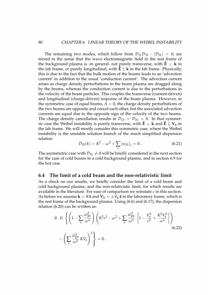
80 CHAPTER 6. LINEAR THEORY OF THE WEIBEL INSTABILITY
The remaining two modes, which follow from D11D33 − |D31| = 0, aremixed in the sense that the wave electromagnetic field in the rest frame ofthe background plasma is -in general- not purely transverse, with E ⊥ k inthe lab frame, or purely longitudinal, with E ‖ k in the lab frame. Physically,this is due to the fact that the bulk motion of the beams leads to an ‘advectioncurrent’ in addition to the usual ‘conduction current’. The advection currentarises as charge density perturbations in the beam plasma are dragged alongby the beams, whereas the conduction current is due to the perturbations inthe velocity of the beam particles. This couples the transverse (current-driven)and longitudinal (charge-driven) response of the beam plasma. However, inthe symmetric case of equal beams, ∆ = 0, the charge density perturbations ofthe two beams are opposite and cancel each other, but the associated advectioncurrents are equal due to the opposite sign of the velocity of the two beams.The charge density cancellation results in D13 = D31 = 0. In that symmet-ric case the Weibel instability is purely transverse, with E ⊥ k and E ‖ Vb inthe lab frame. We will mostly consider this symmetric case, where the Weibelinstability is the unstable solution branch of the much simplified dispersionrelation
D33(k) = K2 −ω2 + ∑s
(α33)s = 0 . (6.21)
The asymmetric case withD31 6= 0 will be briefly considered in the next sectionfor the case of cold beams in a cold background plasma, and in section 6.9 forthe hot case.
6.4 The limit of a cold beam and the non-relativistic limitAs a check on our results, we briefly consider the limit of a cold beam andcold background plasma, and the non-relativistic limit, for which results areavailable in the literature. For ease of comparison we reinstate c in this section.As before we assume k = Kx and Vb = ±Vb z in the laboratory frame, which isthe rest frame of the background plasma. Using (6.6) and (6.17), the dispersionrelation (6.20) can be written as:
|k · k|
(1−∑
s
ω2ps
ω2
)(K2c2 −ω2 + ∑
s
ω2ps
ω2
[1− V2
sc2 +
K2V2s
ω2
])(6.22)
−
(∑s
ω2ps
ω2 KVs
)2 = 0 .
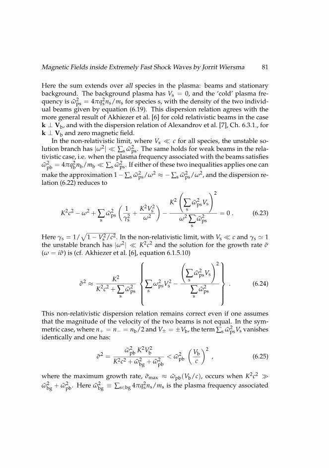
Magnetic Fields inside Extremely Fast Shock Waves by Jorrit Wiersma 81
Here the sum extends over all species in the plasma: beams and stationarybackground. The background plasma has Vs = 0, and the ‘cold’ plasma fre-quency is ω2
ps = 4πq2s ns/ms for species s, with the density of the two individ-
ual beams given by equation (6.19). This dispersion relation agrees with themore general result of Akhiezer et al. [6] for cold relativistic beams in the casek ⊥ Vb, and with the dispersion relation of Alexandrov et al. [7], Ch. 6.3.1., fork ⊥ Vb and zero magnetic field.
In the non-relativistic limit, where Vs c for all species, the unstable so-lution branch has |ω2| ∑s ω2
ps. The same holds for weak beams in the rela-tivistic case, i.e. when the plasma frequency associated with the beams satisfiesω2
pb = 4πq2bnb/mb ∑s ω2
ps. If either of these two inequalities applies one can
make the approximation 1−∑s ω2ps/ω2 ≈ −∑s ω2
ps/ω2, and the dispersion re-lation (6.22) reduces to
K2c2 −ω2 + ∑s
ω2ps
(1
γ2s
+K2V2
sω2
)−
K2
(∑s
ω2psVs
)2
ω2 ∑s
ω2ps
= 0 . (6.23)
Here γs = 1/√
1−V2s /c2. In the non-relativistic limit, with Vs c and γs ' 1
the unstable branch has |ω2| K2c2 and the solution for the growth rate σ(ω = iσ) is (cf. Akhiezer et al. [6], equation 6.1.5.10)
σ2 ≈ K2
K2c2 + ∑s
ω2ps
∑s
ω2psV2
s −
(∑s
ω2psVs
)2
∑s
ω2ps
. (6.24)
This non-relativistic dispersion relation remains correct even if one assumesthat the magnitude of the velocity of the two beams is not equal. In the sym-metric case, where n+ = n− = nb/2 and V± = ±Vb, the term ∑s ω2
psVs vanishesidentically and one has:
σ2 =ω2
pb K2V2b
K2c2 + ω2bg + ω2
pb< ω2
pb
(Vbc
)2, (6.25)
where the maximum growth rate, σmax ≈ ωpb(Vb/c), occurs when K2c2 ω2
bg + ω2pb. Here ω2
bg ≡ ∑s∈bg 4πq2s ns/ms is the plasma frequency associated
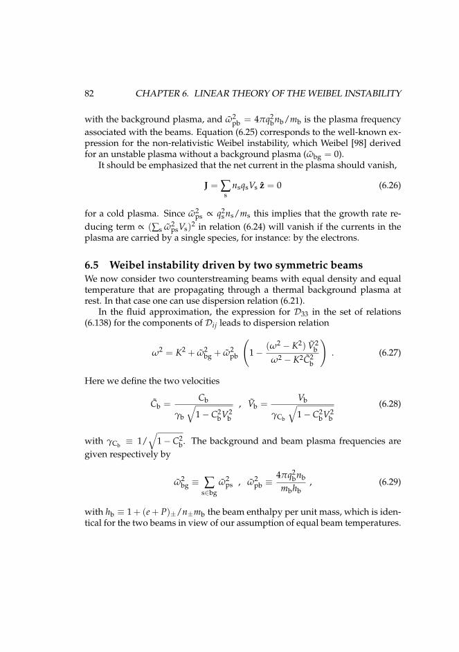
82 CHAPTER 6. LINEAR THEORY OF THE WEIBEL INSTABILITY
with the background plasma, and ω2pb = 4πq2
bnb/mb is the plasma frequencyassociated with the beams. Equation (6.25) corresponds to the well-known ex-pression for the non-relativistic Weibel instability, which Weibel [98] derivedfor an unstable plasma without a background plasma (ωbg = 0).
It should be emphasized that the net current in the plasma should vanish,
J = ∑s
nsqsVs z = 0 (6.26)
for a cold plasma. Since ω2ps ∝ q2
s ns/ms this implies that the growth rate re-ducing term ∝ (∑s ω2
psVs)2 in relation (6.24) will vanish if the currents in theplasma are carried by a single species, for instance: by the electrons.
6.5 Weibel instability driven by two symmetric beamsWe now consider two counterstreaming beams with equal density and equaltemperature that are propagating through a thermal background plasma atrest. In that case one can use dispersion relation (6.21).
In the fluid approximation, the expression for D33 in the set of relations(6.138) for the components of Dij leads to dispersion relation
ω2 = K2 + ω2bg + ω2
pb
(1−
(ω2 − K2) V2b
ω2 − K2C2b
). (6.27)
Here we define the two velocities
Cb =Cb
γb
√1− C2
bV2b
, Vb =Vb
γCb
√1− C2
bV2b
(6.28)
with γCb≡ 1/
√1− C2
b. The background and beam plasma frequencies aregiven respectively by
ω2bg ≡ ∑
s∈bgω2
ps , ω2pb ≡
4πq2bnb
mbhb, (6.29)
with hb ≡ 1 + (e + P)±/n±mb the beam enthalpy per unit mass, which is iden-tical for the two beams in view of our assumption of equal beam temperatures.
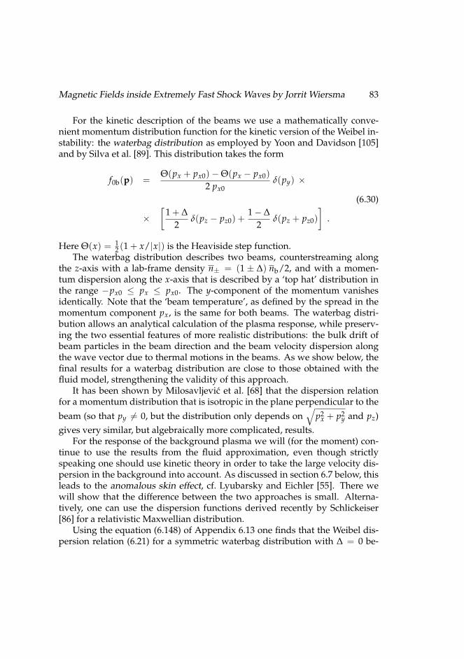
Magnetic Fields inside Extremely Fast Shock Waves by Jorrit Wiersma 83
For the kinetic description of the beams we use a mathematically conve-nient momentum distribution function for the kinetic version of the Weibel in-stability: the waterbag distribution as employed by Yoon and Davidson [105]and by Silva et al. [89]. This distribution takes the form
f0b(p) =Θ(px + px0)−Θ(px − px0)
2 px0δ(py) ×
(6.30)
×[
1 + ∆2
δ(pz − pz0) +1− ∆
2δ(pz + pz0)
].
Here Θ(x) = 12 (1 + x/|x|) is the Heaviside step function.
The waterbag distribution describes two beams, counterstreaming alongthe z-axis with a lab-frame density n± = (1 ± ∆) nb/2, and with a momen-tum dispersion along the x-axis that is described by a ‘top hat’ distribution inthe range −px0 ≤ px ≤ px0. The y-component of the momentum vanishesidentically. Note that the ‘beam temperature’, as defined by the spread in themomentum component px, is the same for both beams. The waterbag distri-bution allows an analytical calculation of the plasma response, while preserv-ing the two essential features of more realistic distributions: the bulk drift ofbeam particles in the beam direction and the beam velocity dispersion alongthe wave vector due to thermal motions in the beams. As we show below, thefinal results for a waterbag distribution are close to those obtained with thefluid model, strengthening the validity of this approach.
It has been shown by Milosavljevic et al. [68] that the dispersion relationfor a momentum distribution that is isotropic in the plane perpendicular to the
beam (so that py 6= 0, but the distribution only depends on√
p2x + p2
y and pz)gives very similar, but algebraically more complicated, results.
For the response of the background plasma we will (for the moment) con-tinue to use the results from the fluid approximation, even though strictlyspeaking one should use kinetic theory in order to take the large velocity dis-persion in the background into account. As discussed in section 6.7 below, thisleads to the anomalous skin effect, cf. Lyubarsky and Eichler [55]. There wewill show that the difference between the two approaches is small. Alterna-tively, one can use the dispersion functions derived recently by Schlickeiser[86] for a relativistic Maxwellian distribution.
Using the equation (6.148) of Appendix 6.13 one finds that the Weibel dis-persion relation (6.21) for a symmetric waterbag distribution with ∆ = 0 be-
84 CHAPTER 6. LINEAR THEORY OF THE WEIBEL INSTABILITY
comes
ω2 = K2 + ω2bg + ω2
pb
(Gb +
K2V2z0
ω2 − K2V2x0
). (6.31)
Here we define the following characteristic beam parameters: the beam plasmafrequency ωpb, the characteristic Lorentz factor γ0 and the two velocities Vx0and Vz0:
ω2pb =
ω2pb
γ0=
4πq2bnb
γ0mb, γ0 =
√1 +
p2x0
m2bc2
+p2
z0m2
bc2,
(6.32)
Vx0 =px0
γ0mb, Vz0 =
pz0
γ0mb.
The function Gb(px0 , pz0) is given by:
Gb(px0 , pz0) =1
2Vx0ln(
1 + Vx0
1−Vx0
)−
p2z0
p2z0 + m2
b. (6.33)
When Vx0 1 (so that γ0 ' γb) the frequency ωpb reduces to the beam plasmafrequency ωpb based on the proper density nb ≈ nb/γb of the beam particles.The beam contribution to D33 (the last term on the right-hand side of equation6.31) has been derived before by Silva et al. [89].
The two dispersion relations (6.27) and (6.31) can both be written as a bi-quadratic equation for ω of the form
ω4 − B(K) ω2 + C(K) = 0 , (6.34)
Such a bi-quadratic equation for ω occurs often in the theory of the Weibelinstability [98, 84]. The two coefficients B(K) and C(K) are:
B(K) =
ω2
bg + ω2pb
(1− V2
b
)+ K2
(1 + C2
b
)(fluid model)
ω2bg + ω2
pb Gb + K2(
1 + V2x0
)(waterbag model)
(6.35)
and
C(K) =
(
ω2bg + K2
)K2C2
b − ω2pb K2
(V2
b − C2b
)(fluid model)
(ω2
bg + K2)
K2V2x0 − ω2
pbK2(
V2z0 − Gb V2
x0
)(waterbag model)
(6.36)
Magnetic Fields inside Extremely Fast Shock Waves by Jorrit Wiersma 85
The analogy between these two sets of expressions is clear. The solution for ω,
ω2± = 1
2B ±12
√B2 − 4C , (6.37)
has an unstable branch with ω2− < 0, i.e. ω− = iσ with σ > 0, provided
C(K) < 0. This condition defines a maximum unstable wavenumber Kmax sothat perturbations with
K2 < K2max =
ω2
pb
(M2 − 1
)− ω2
bg (fluid model)
ω2pb
(M2 − Gb
)− ω2
bg (waterbag model)(6.38)
are unstable and will grow. Here we define an effective ‘Mach number’ for thebeams by
M ≡
Vb
Cb=
γbVbγCb
Cb(fluid model)
Vz0
Vx0=
pz0
px0(waterbag model)
(6.39)
for the fluid and waterbag model respectively. This shows the stabilizing influ-ence of the thermal motion of beam particles in the direction of the wave vectork = Kx, suppressing the instability at sufficiently large values of |K|.
6.6 The case of ultra-relativistic beamsWe now concentrate on the ultra-relativistic case, of importance for the Weibelinstability in the shock transition layer of shocks with bulk velocity Vsh suchthat γsh = 1/(1− V2
sh)1/2 1. In the frame of the hot (shocked) plasma, theunshocked material forms a relativistic beam. This implies γb ∼ γsh 1 andVb Cb in the fluid case and pz0 mb, pz0 px0 in the waterbag case. Itis then possible to describe the properties of the symmetric Weibel instabilityusing two parameters. The first is the ‘Mach number’ M defined in equation(6.39) that now satisfies1 M2 ∼ (γb/γCbCb)2 1. The second parameter is ameasure of the strength of the two beams, defined by
η ≡
ω2
pb/ω2bg (fluid model)
ω2pb/ω2
bg (waterbag model)(6.40)
1For an ideal gas one has Cb < 1/√
3 and γCbCb < 1/√
2
86 CHAPTER 6. LINEAR THEORY OF THE WEIBEL INSTABILITY
The ultra-relativistic limit of the fluid model has Cb ' 1/M 1, Vb ' Vb ' 1,and in the waterbag model one has Gb 1 and Vx0 ' 1/M Vz0 ≈ Vb ' 1.To leading order, the expressions (6.35) and (6.36) become identical in bothmodels. In terms of η and M one can write:
B(K) ' ω2bg + K2 ,
(6.41)
C(K) ' K2
(ω2
bg + K2
M2 − η ω2bg
).
Terms of order 1/γ2b, C2
b or V2x0 have been consistently neglected with respect
to unity.
If we define a dimensionless growth rate σ and a dimensionless wavenumberκ by
σ2 = −ω2/ω2bg , κ = K/ωbg , (6.42)
dispersion relation (6.34) can be written as
σ4 +(
1 + κ2)
σ2 −κ2 (κ2
max − κ2)M2 = 0 . (6.43)
Here we use that ω is either real (stable modes) or purely imaginary with ω2 <0. The dimensionless maximum wavenumber κmax (see equation 6.38) of theunstable modes equals in the ultra-relativistic limit:
κmax ≈√
η M2 − 1 . (6.44)
The Weibel instability occurs only if ηM2 > 1 for 0 ≤ |κ| < κmax. The unstablebranch has a growth rate
σ2 =
√(1 + κ2
2
)2
+κ2 (κ2
max − κ2)M2 − 1 + κ2
2. (6.45)
In many cases expression (6.45) can be simplified further. Provided that(1 + κ2)2 4κ2 (κ2
max − κ2) /M2 one can expand the root in (6.45). This yields:
σ2 'κ2(
κ2max − κ2
)M2
(1 + κ2
) . (6.46)
Magnetic Fields inside Extremely Fast Shock Waves by Jorrit Wiersma 87
This approximation corresponds to the neglect of the σ4 term in dispersionrelation (6.43), and is valid for all unstable wavelengths if the beams are weakin the sense that η 1. In that case one has σ2 < η 1. For η of order unity(ωpb , ωpb ∼ ωbg) the approximated solution (6.46) is valid everywhere exceptin the vicinity of |κ| = 1 where σ ≈ 1. For very strong beams with η 1 onehas to use the full solution (6.45) except when √η |κ| ≤ κmax ∼
√ηM.
Figure 6.1 gives the growth rate of the Weibel instability in units of thebackground plasma frequency as a function of the dimensionless wavenumberκ (= Kc/ωbg if one uses units with c 6= 1). The curves are labeled by the pairof parameters (η, M). This figure shows that the dimensionless growth rateσ = Im(ω)/ωbg has the following properties:
• For κ = K/ωbg 1 it grows as σ ∝ κ. If the approximated solution (6.46)applies one has
σ ≈ κκmax
M≈ √
η κ . (6.47)
The last approximation is valid if η < 1.
• Around κ ∼ 1 the growth rate saturates. If κmax 1 the growth rate hasa nearly constant value for 1 κ κmax which, in the approximation(6.46), equals:
σ ≈ κmax
M≈ √
η . (6.48)
• The growth rate rapidly decreases to zero at κ ≈ κmax ≈√
η M.
Comparing the ultra-relativistic result (6.46) to the classic non-relativisticresult for a cold plasma (6.25) we can identify the following differences:
• The cold plasma result does not have a cut-off wave number κmax.
• The denominator of the non-relativistic expression contains an extra ω2pb
term because one can not apply the limit η ≤ 1, γb 1 in that case.The corresponding term in the ultra-relativistic case is ω2
pb/γ2b, which has
been neglected with respect to ω2bg. That is allowed whenever η γ2
b.
• In the relativistic case it is important to use the appropriate relativisticexpressions for the plasma frequencies.
Note, however, that the peak value of the growth rate σ ≈ √η for the ultra-
relativistic case is the relativistic equivalent for Vb ' c of the maximum growthrate for the non-relativistic case.
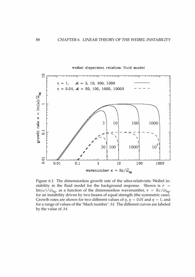
88 CHAPTER 6. LINEAR THEORY OF THE WEIBEL INSTABILITY
~
~
3 10 100 1000
30 100 1000 104
Figure 6.1: The dimensionless growth rate of the ultra-relativistic Weibel in-stability in the fluid model for the background response. Shown is σ =Im(ω)/ωbg, as a function of the dimensionless wavenumber, κ = Kc/ωbg,for an instability driven by two beams of equal strength (the symmetric case).Growth rates are shown for two different values of η, η = 0.01 and η = 1, andfor a range of values of the ‘Mach number’M. The different curves are labeledby the value of M.
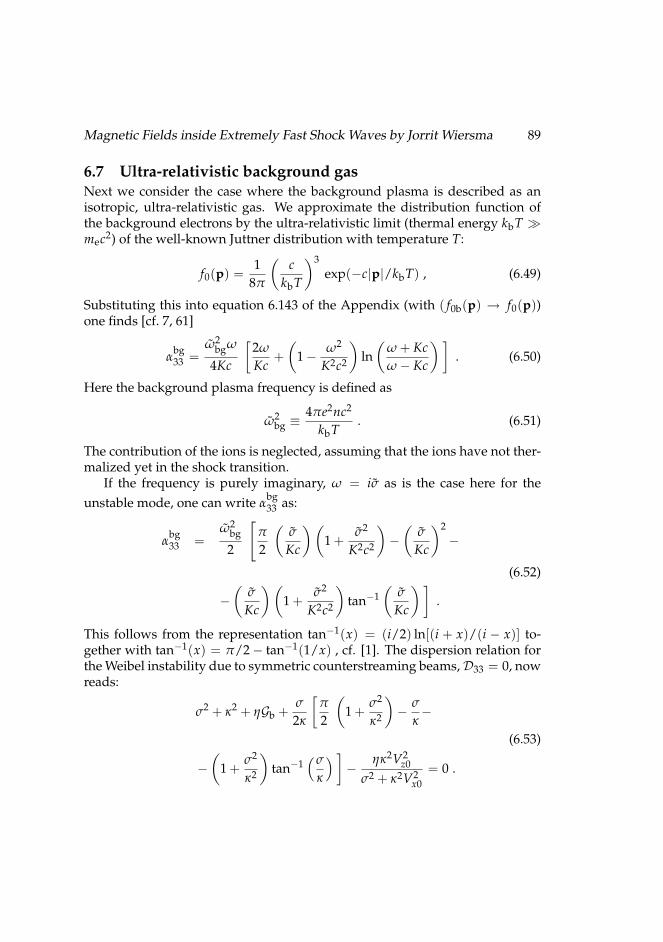
Magnetic Fields inside Extremely Fast Shock Waves by Jorrit Wiersma 89
6.7 Ultra-relativistic background gasNext we consider the case where the background plasma is described as anisotropic, ultra-relativistic gas. We approximate the distribution function ofthe background electrons by the ultra-relativistic limit (thermal energy kbT mec2) of the well-known Juttner distribution with temperature T:
f0(p) =1
8π
(c
kbT
)3exp(−c|p|/kbT) , (6.49)
Substituting this into equation 6.143 of the Appendix (with ( f0b(p) → f0(p))one finds [cf. 7, 61]
αbg33 =
ω2bgω
4Kc
[2ω
Kc+(
1− ω2
K2c2
)ln(
ω + Kcω − Kc
) ]. (6.50)
Here the background plasma frequency is defined as
ω2bg ≡
4πe2nc2
kbT. (6.51)
The contribution of the ions is neglected, assuming that the ions have not ther-malized yet in the shock transition.
If the frequency is purely imaginary, ω = iσ as is the case here for theunstable mode, one can write α
bg33 as:
αbg33 =
ω2bg
2
[π
2
(σ
Kc
)(1 +
σ2
K2c2
)−(
σ
Kc
)2−
(6.52)
−(
σ
Kc
)(1 +
σ2
K2c2
)tan−1
(σ
Kc
) ].
This follows from the representation tan−1(x) = (i/2) ln[(i + x)/(i − x)] to-gether with tan−1(x) = π/2− tan−1(1/x) , cf. [1]. The dispersion relation forthe Weibel instability due to symmetric counterstreaming beams,D33 = 0, nowreads:
σ2 + κ2 + ηGb +σ
2κ
[π
2
(1 +
σ2
κ2
)− σ
κ−
(6.53)
−(
1 +σ2
κ2
)tan−1
(σ
κ
) ]−
ηκ2V2z0
σ2 + κ2V2x0
= 0 .
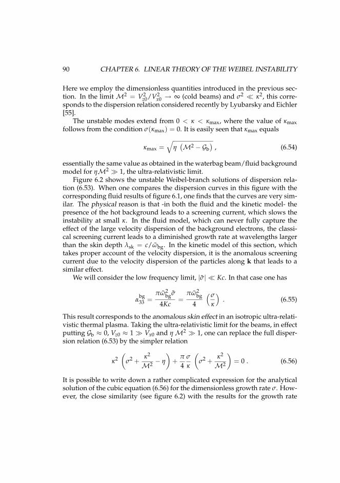
90 CHAPTER 6. LINEAR THEORY OF THE WEIBEL INSTABILITY
Here we employ the dimensionless quantities introduced in the previous sec-tion. In the limit M2 = V2
z0/V2x0 → ∞ (cold beams) and σ2 κ2, this corre-
sponds to the dispersion relation considered recently by Lyubarsky and Eichler[55].
The unstable modes extend from 0 < κ < κmax, where the value of κmaxfollows from the condition σ(κmax) = 0. It is easily seen that κmax equals
κmax =√
η(M2 − Gb
), (6.54)
essentially the same value as obtained in the waterbag beam/fluid backgroundmodel for ηM2 1, the ultra-relativistic limit.
Figure 6.2 shows the unstable Weibel-branch solutions of dispersion rela-tion (6.53). When one compares the dispersion curves in this figure with thecorresponding fluid results of figure 6.1, one finds that the curves are very sim-ilar. The physical reason is that -in both the fluid and the kinetic model- thepresence of the hot background leads to a screening current, which slows theinstability at small κ. In the fluid model, which can never fully capture theeffect of the large velocity dispersion of the background electrons, the classi-cal screening current leads to a diminished growth rate at wavelengths largerthan the skin depth λsk = c/ωbg. In the kinetic model of this section, whichtakes proper account of the velocity dispersion, it is the anomalous screeningcurrent due to the velocity dispersion of the particles along k that leads to asimilar effect.
We will consider the low frequency limit, |σ| Kc. In that case one has
αbg33 =
πω2bgσ
4Kc=
πω2bg
4
(σ
κ
). (6.55)
This result corresponds to the anomalous skin effect in an isotropic ultra-relati-vistic thermal plasma. Taking the ultra-relativistic limit for the beams, in effectputting Gb ≈ 0, Vz0 ≈ 1 Vx0 and η M2 1, one can replace the full disper-sion relation (6.53) by the simpler relation
κ2(
σ2 +κ2
M2 − η
)+
π
4σ
κ
(σ2 +
κ2
M2
)= 0 . (6.56)
It is possible to write down a rather complicated expression for the analyticalsolution of the cubic equation (6.56) for the dimensionless growth rate σ. How-ever, the close similarity (see figure 6.2) with the results for the growth rate
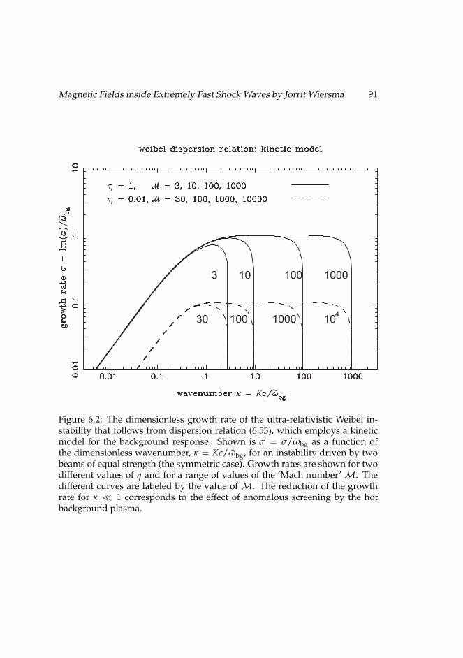
Magnetic Fields inside Extremely Fast Shock Waves by Jorrit Wiersma 91
3 10 100 1000
30 100 1000 104
K
~
~
Figure 6.2: The dimensionless growth rate of the ultra-relativistic Weibel in-stability that follows from dispersion relation (6.53), which employs a kineticmodel for the background response. Shown is σ = σ/ωbg as a function ofthe dimensionless wavenumber, κ = Kc/ωbg, for an instability driven by twobeams of equal strength (the symmetric case). Growth rates are shown for twodifferent values of η and for a range of values of the ‘Mach number’ M. Thedifferent curves are labeled by the value of M. The reduction of the growthrate for κ 1 corresponds to the effect of anomalous screening by the hotbackground plasma.
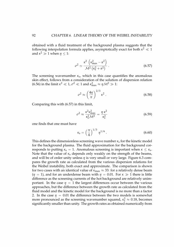
92 CHAPTER 6. LINEAR THEORY OF THE WEIBEL INSTABILITY
obtained with a fluid treatment of the background plasma suggests that thefollowing interpolation formula applies, asymptotically exact for both κ2 1and κ2 1 when η ≤ 1:
σ2 'κ2(
κ2max − κ2
)M2
(κ2
s + κ2) . (6.57)
The screening wavenumber κs, which in this case quantifies the anomalousskin effect, follows from a consideration of the solution of dispersion relation(6.56) in the limit κ2 1, σ2 1 and κ2
max ≈ ηM2 1:
σ2 ≈(
4η
π
)2/3κ2 . (6.58)
Comparing this with (6.57) in this limit,
σ2 ≈ κ2κ2max
κ2sM2 =
η κ2
κ2s
(6.59)
one finds that one must have
κs =(π
4
)1/3η1/6 . (6.60)
This defines the dimensionless screening wave number κs for the kinetic modelfor the background plasma. The fluid approximation for the background cor-responds to putting κs = 1. Anomalous screening is important when κ ≤ κs.Note that the value of κs depends only weakly on the strength of the beams,and will be of order unity unless η is very small or very large. Figure 6.3 com-pares the growth rate as calculated from the various dispersion relations forthe Weibel instability, both exact and approximate. The comparison is shownfor two cases with an identical value of κmax ≈ 33: for a relatively dense beam(η = 1), and for an underdense beam with η = 0.01. For κ 1 there is littledifference as the screening currents of the hot background are relatively unim-portant. In the case η = 1 the largest differences occur between the variousapproaches, but the difference between the growth rate as calculated from thefluid model and the kinetic model for the background is no more than a factor2. In the case η = 0.01 the difference between the two models is somewhatmore pronounced as the screening wavenumber squared, κ2
s ≈ 0.18, becomessignificantly smaller than unity. The growth rates as obtained numerically from
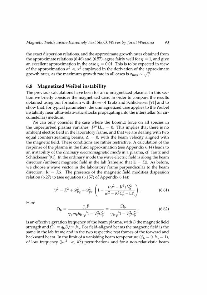
Magnetic Fields inside Extremely Fast Shock Waves by Jorrit Wiersma 93
the exact dispersion relations, and the approximate growth rates obtained fromthe approximate relations (6.46) and (6.57), agree fairly well for η = 1, and givean excellent approximation in the case η = 0.01. This is to be expected in viewof the approximation σ2 κ2 employed in the derivation of the approximategrowth rates, as the maximum growth rate in all cases is σmax ∼
√η.
6.8 Magnetized Weibel instabilityThe previous calculations have been for an unmagnetized plasma. In this sec-tion we briefly consider the magnetized case, in order to compare the resultsobtained using our formalism with those of Tautz and Schlickeiser [91] and toshow that, for typical parameters, the unmagnetized case applies to the Weibelinstability near ultra-relativistic shocks propagating into the interstellar (or cir-cumstellar) medium.
We can only consider the case where the Lorentz force on all species inthe unperturbed plasma vanishes: FµνUsν = 0. This implies that there is noambient electric field in the laboratory frame, and that we are dealing with twoequal counterstreaming beams, ∆ = 0, with the beam velocity aligned withthe magnetic field. These conditions are rather restrictive. A calculation of theresponse of the plasma in the fluid approximation (see Appendix 6.14) leads toan instability of the ordinary electromagnetic mode in a plasma, cf. Tautz andSchlickeiser [91]. In the ordinary mode the wave electric field is along the beamdirection/ambient magnetic field in the lab frame so that E = Ez. As before,we choose a wave vector in the laboratory frame perpendicular to the beamdirection: k = Kx. The presence of the magnetic field modifies dispersionrelation (6.27) to (see equation (6.157) of Appendix 6.14):
ω2 = K2 + ω2bg + ω2
pb
(1−
(ω2 − K2) V2b
ω2 − K2C2b − Ω2
b
). (6.61)
HereΩb =
qbB
γbmbhb
√1−V2
b C2b
≡ Ωb
γb
√1−V2
b C2b
, (6.62)
is an effective gyration frequency of the beam plasma, with B the magnetic fieldstrength and Ωb ≡ qbB/mbhb. For field-aligned beams the magnetic field is thesame in the lab frame and in the two respective rest frames of the forward andbackward beam. In the limit of a vanishing beam temperature (Cb = 0, hb = 1),of low frequency (|ω2| K2) perturbations and for a non-relativistic beam
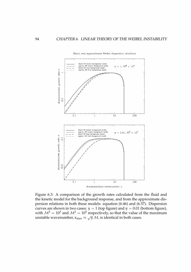
94 CHAPTER 6. LINEAR THEORY OF THE WEIBEL INSTABILITY
Figure 6.3: A comparison of the growth rates calculated from the fluid andthe kinetic model for the background response, and from the approximate dis-persion relations in both these models: equation (6.46) and (6.57). Dispersioncurves are shown in two cases: η = 1 (top figure) and η = 0.01 (bottom figure),with M2 = 103 and M2 = 105 respectively, so that the value of the maximumunstable wavenumber, κmax ≈
√η M, is identical in both cases.
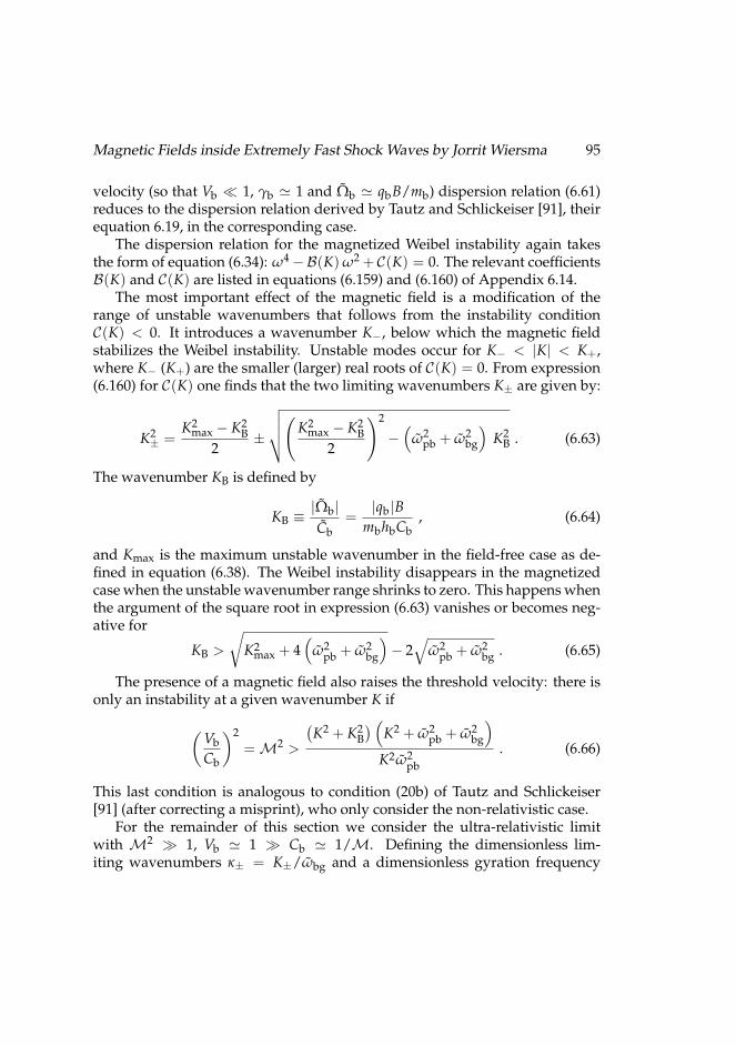
Magnetic Fields inside Extremely Fast Shock Waves by Jorrit Wiersma 95
velocity (so that Vb 1, γb ' 1 and Ωb ' qbB/mb) dispersion relation (6.61)reduces to the dispersion relation derived by Tautz and Schlickeiser [91], theirequation 6.19, in the corresponding case.
The dispersion relation for the magnetized Weibel instability again takesthe form of equation (6.34): ω4 −B(K) ω2 + C(K) = 0. The relevant coefficientsB(K) and C(K) are listed in equations (6.159) and (6.160) of Appendix 6.14.
The most important effect of the magnetic field is a modification of therange of unstable wavenumbers that follows from the instability conditionC(K) < 0. It introduces a wavenumber K−, below which the magnetic fieldstabilizes the Weibel instability. Unstable modes occur for K− < |K| < K+,where K− (K+) are the smaller (larger) real roots of C(K) = 0. From expression(6.160) for C(K) one finds that the two limiting wavenumbers K± are given by:
K2± =
K2max − K2
B2
±
√√√√(K2max − K2
B2
)2
−(
ω2pb + ω2
bg
)K2
B . (6.63)
The wavenumber KB is defined by
KB ≡|Ωb|Cb
=|qb|B
mbhbCb, (6.64)
and Kmax is the maximum unstable wavenumber in the field-free case as de-fined in equation (6.38). The Weibel instability disappears in the magnetizedcase when the unstable wavenumber range shrinks to zero. This happens whenthe argument of the square root in expression (6.63) vanishes or becomes neg-ative for
KB >
√K2
max + 4(
ω2pb + ω2
bg
)− 2√
ω2pb + ω2
bg . (6.65)
The presence of a magnetic field also raises the threshold velocity: there isonly an instability at a given wavenumber K if
(VbCb
)2= M2 >
(K2 + K2
B) (
K2 + ω2pb + ω2
bg
)K2ω2
pb. (6.66)
This last condition is analogous to condition (20b) of Tautz and Schlickeiser[91] (after correcting a misprint), who only consider the non-relativistic case.
For the remainder of this section we consider the ultra-relativistic limitwith M2 1, Vb ' 1 Cb ' 1/M. Defining the dimensionless lim-iting wavenumbers κ± = K±/ωbg and a dimensionless gyration frequency
96 CHAPTER 6. LINEAR THEORY OF THE WEIBEL INSTABILITY
σB = Ωb/ωbg, the growth rate of the unstable solution can be represented bythe analogue for the magnetized case of relation (6.45):
σ2 =
√√√√(1 + κ2 + σ2B
2
)2
+
(κ2 − κ2
−) (
κ2+ − κ2)
M2 −1 + κ2 + σ2
B2
. (6.67)
The magnetized equivalent of approximate relation (6.46), valid when (1 + κ2 +σ2
B)2 4(κ2 − κ2−)(κ2
+ − κ2) /M2, reads:
σ2 ≈(κ2 − κ2
−) (
κ2+ − κ2)
M2(1 + κ2 + σ2
B) . (6.68)
In the ultra-relativistic limit with Cb 1 and M2 1 one has KB 'M (Ωb/γB) and Kmax ' M ωpb. If K2
max ω2pb + ω2
bg (ηM2 1 + η) theWeibel instability vanishes according to (6.65) if the magnetic field gets so largethat KB ≈ Kmax, or equivalently
|Ωb|γb
' |qb|Bγbmb
≈ ωpb . (6.69)
In figure 6.4 we show the solution for the dimensionless growth rate σ(κ) ofthe unstable Weibel mode (ordinary mode) in the magnetized case.
6.8.1 When can non-magnetic results be used?We are mostly interested in the application of the Weibel instability to the ultra-relativistic shocks associated with Gamma Ray Bursts. The influence of themagnetic field on the Weibel instability will be small if K− ωbg (κ− 1), sothat both the maximum growth rate and the range of unstable wavenumbersare comparable with their values in the field-free case, see figure 6.4. Fromthe discussion above, and in particular from equation (6.63), it is clear that thissituation occurs if KB Kmax. In the ultra-relativistic regime, the growth rateof the instability, σ = Im(ω), is then roughly constant over a wide wavelengthrange, with
σ ≈ ωpbVb for ωbg < K < ωpb M , (6.70)
assuming ηM2 1. This should be compared with the gyration frequency ofbeam particles, which for a relativistic cold beam with Cb 1 is
|qb|B/γbmb ≈ |Ωb|/γb , (6.71)
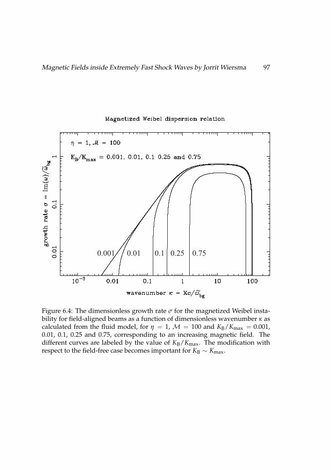
Magnetic Fields inside Extremely Fast Shock Waves by Jorrit Wiersma 97
0.001 0.01 0.1 0.25 0.75
~
~
Figure 6.4: The dimensionless growth rate σ for the magnetized Weibel insta-bility for field-aligned beams as a function of dimensionless wavenumber κ ascalculated from the fluid model, for η = 1, M = 100 and KB/Kmax = 0.001,0.01, 0.1, 0.25 and 0.75, corresponding to an increasing magnetic field. Thedifferent curves are labeled by the value of KB/Kmax. The modification withrespect to the field-free case becomes important for KB ∼ Kmax.
98 CHAPTER 6. LINEAR THEORY OF THE WEIBEL INSTABILITY
The ratio of the gyration frequency and typical Weibel growth rate is therefore
|Ωb|γbσ
≈ |Ωb|γbωpbVb
≈ KB
Kmax. (6.72)
This shows that the condition KB Kmax also ensures that the growth rate ofthe instability is much larger than the gyration frequency of the beam particles.
Taking the beam material to be the unshocked (cold) hydrogen plasma in-terpenetrating the (hot) shocked plasma, the ratio of the beam gyration fre-quency and growth rate of the Weibel instability equals:
|Ωb|γbωpb
≈
3× 10⁻⁴ BµG
γb√
ne(electrons)
7× 10⁻⁵ BµG
γb√np
(protons)
(6.73)
Here BµG is the strength of the pre-existing magnetic field in the shock tran-sition layer in units of micro-Gauss, and ne (np) is the proper density of theelectron (proton) beam. This proper density is always of the same order as thedensity of the particles in the pre-shock medium. The magnetic field strengthin the transition layer depends on the orientation of the pre-shock magneticfield. For a magnetic field parallel to the shock normal (the case for which themagnetized Weibel dispersion relation was derived) there is no field amplifi-cation due to shock compression, and the ambient magnetic field in the transi-tion layer equals the upstream field, even after a Lorentz transformation to therest frame of the hot post-shock material. In that case, the ratio |Ωb|/γbωpbis always much smaller than unity for typical parameters: BµG ∼ 1 − 100,γb ∼ γsh/
√2 ∼ 100 and ne,p ∼ 1− 100 cm−3. That implies that in this case
the effect of the magnetic field can be neglected altogether: the growth of theWeibel instability is so rapid that particles do not get a chance to start gyratingaround the ambient (pre-existing) magnetic field. Their dynamics can be de-scribed as being unmagnetized, and the range of unstable wavenumbers andinstability growth rate are hardly affected in this case.
If there is a component Bt of the magnetic field along the shock surface, itcould be amplified considerably, with Bt2 ≈ 2
√2 γshBt1 upon completion of the
shock transition according to the relativistic MHD shock jump conditions (seesection 6.1). But even then one has Bt2/γb ≈
√2Bt2/γsh ∼ 4Bt1. Here we have
used that γb ≈ γrel ≈ γsh/√
2, where γrel is the Lorentz factor associated with
Magnetic Fields inside Extremely Fast Shock Waves by Jorrit Wiersma 99
the relative motion between the up- and downstream flow. We may speculatethat -at least for the light electrons- the growth rate of a Weibel-like instabilityin this case is still much larger than the gyrofrequency for typical parametersand the unmagnetized treatment of the instability is still a good approximation,while at the same time the growth of the electron-driven Weibel instability israpid enough that the large-scale electric fields due to ion/electron charge sep-aration in the shockfront play only a minor role in the local electron dynamics.We reiterate however that this case, where the beams are not (anti)parallel withthe magnetic field, has not been treated here. In fact, the plasma dynamics neara perpendicular relativistic shock may very well involve quite different plasmainstabilities, in particular for the thermalization of the heavier ions, such as theion-driven gyroresonant instability discussed by Spitkovsky and Arons [90] inthe context of the relativistic shocks in the pulsar wind that creates the CrabNebula.
Some support for the relative unimportance of the magnetic field in the rel-ativistic case when KB Kmax comes from the simulations of Hededal andNishikawa [36]. Because of numerical limitations they can only follow theelectron-driven Weibel instability. In the case of field-aligned beams they findthat the Weibel instability develops unhindered if ωpb Ωb/γb, and that theinstability is totally suppressed if the beam plasma frequency and the beamgyrofrequency become of equal: ωpb ∼ Ωb/γb in our notation. In the caseof a magnetic field that is perpendicular to the beam they find a significantmodification of the plasma behavior when Ωb/γb > 0.05 ωpb.
It should be pointed out that a similar conclusion does not necessarily holdfor the non-relativistic version of the Weibel instability. If the beam velocitysatisfies Vb c, the maximum growth rate (for a cold beam) is (see equation6.25):
σ = ωpb
(Vbc
). (6.74)
The ratio of this growth rate and the typical gyration frequency Ωb = qbB/mbcof the beam particles is now
σ
Ωb≈ Vb
VAb, (6.75)
where VAb ≡ B/√
4πnbmb is an Alfven velocity associated with the beams. Inthis case one needs Vb VAb in order for the unmagnetized result to apply.This is not guaranteed, especially for light particles such as electrons. Also, the
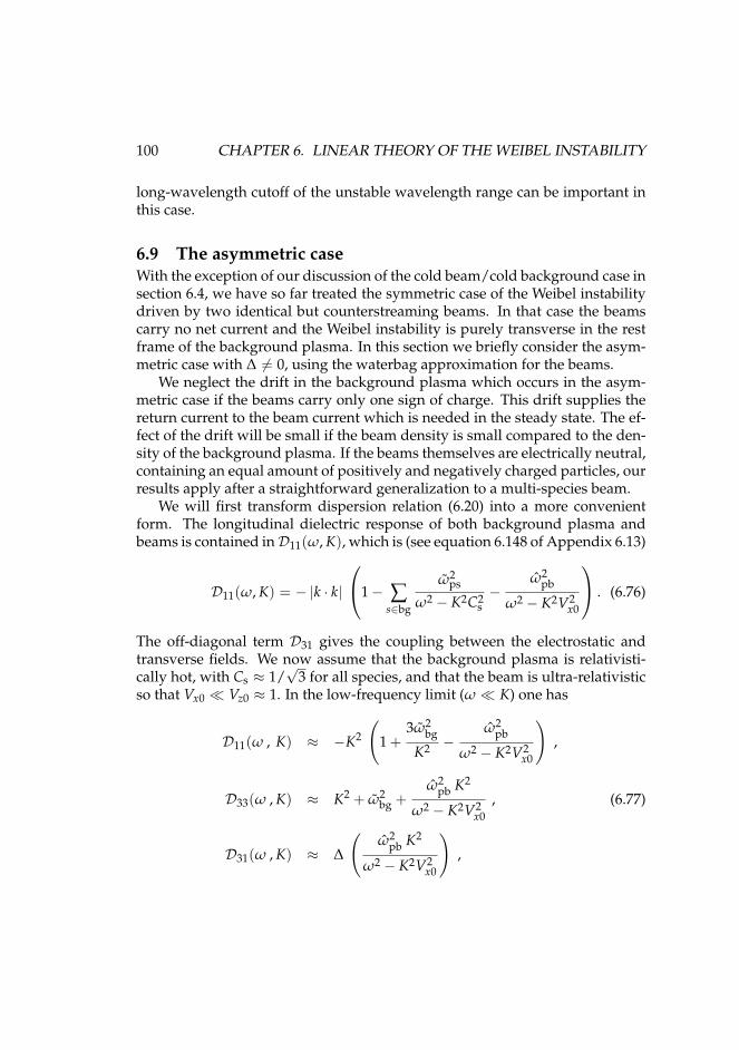
100 CHAPTER 6. LINEAR THEORY OF THE WEIBEL INSTABILITY
long-wavelength cutoff of the unstable wavelength range can be important inthis case.
6.9 The asymmetric caseWith the exception of our discussion of the cold beam/cold background case insection 6.4, we have so far treated the symmetric case of the Weibel instabilitydriven by two identical but counterstreaming beams. In that case the beamscarry no net current and the Weibel instability is purely transverse in the restframe of the background plasma. In this section we briefly consider the asym-metric case with ∆ 6= 0, using the waterbag approximation for the beams.
We neglect the drift in the background plasma which occurs in the asym-metric case if the beams carry only one sign of charge. This drift supplies thereturn current to the beam current which is needed in the steady state. The ef-fect of the drift will be small if the beam density is small compared to the den-sity of the background plasma. If the beams themselves are electrically neutral,containing an equal amount of positively and negatively charged particles, ourresults apply after a straightforward generalization to a multi-species beam.
We will first transform dispersion relation (6.20) into a more convenientform. The longitudinal dielectric response of both background plasma andbeams is contained inD11(ω, K), which is (see equation 6.148 of Appendix 6.13)
D11(ω, K) = − |k · k|
1− ∑s∈bg
ω2ps
ω2 − K2C2s−
ω2pb
ω2 − K2V2x0
. (6.76)
The off-diagonal term D31 gives the coupling between the electrostatic andtransverse fields. We now assume that the background plasma is relativisti-cally hot, with Cs ≈ 1/
√3 for all species, and that the beam is ultra-relativistic
so that Vx0 Vz0 ≈ 1. In the low-frequency limit (ω K) one has
D11(ω , K) ≈ −K2
(1 +
3ω2bg
K2 −ω2
pb
ω2 − K2V2x0
),
D33(ω , K) ≈ K2 + ω2bg +
ω2pb K2
ω2 − K2V2x0
, (6.77)
D31(ω , K) ≈ ∆
(ω2
pb K2
ω2 − K2V2x0
),
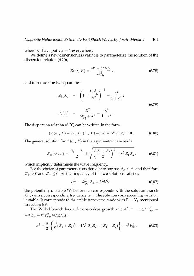
Magnetic Fields inside Extremely Fast Shock Waves by Jorrit Wiersma 101
where we have put Vz0 = 1 everywhere.We define a new dimensionless variable to parameterize the solution of the
dispersion relation (6.20),
Z(ω , K) ≡ω2 − K2V2
x0ω2
pb, (6.78)
and introduce the two quantities
Z1(K) =
(1 +
3ω2bg
K2
)−1
=κ2
3 + κ2 ;
(6.79)
Z2(K) =K2
ω2bg + K2
=κ2
1 + κ2 .
The dispersion relation (6.20) can be written in the form
(Z(ω , K)−Z1) (Z(ω , K) + Z2) + ∆2 Z1Z2 = 0 . (6.80)
The general solution for Z(ω , K) in the asymmetric case reads
Z±(ω , K) =Z1 −Z2
2±
√(Z1 + Z2
2
)2− ∆2 Z1Z2 , (6.81)
which implicitly determines the wave frequency.For the choice of parameters considered here one hasZ2 > Z1 and therefore
Z+ > 0 and Z− ≤ 0. As the frequency of the two solutions satisfies
ω2± = ω2
pb Z± + K2V2x0 , (6.82)
the potentially unstable Weibel branch corresponds with the solution branchZ−, with a corresponding frequency ω−. The solution corresponding with Z+is stable. It corresponds to the stable transverse mode with E ⊥ Vb mentionedin section 6.3.
The Weibel branch has a dimensionless growth rate σ2 ≡ −ω2−/ω2
bg =
−η Z− − κ2V2x0, which is :
σ2 =η
2
√(Z1 + Z2)
2 − 4∆2 Z1Z2 − (Z1 −Z2)− κ2V2
x0 . (6.83)
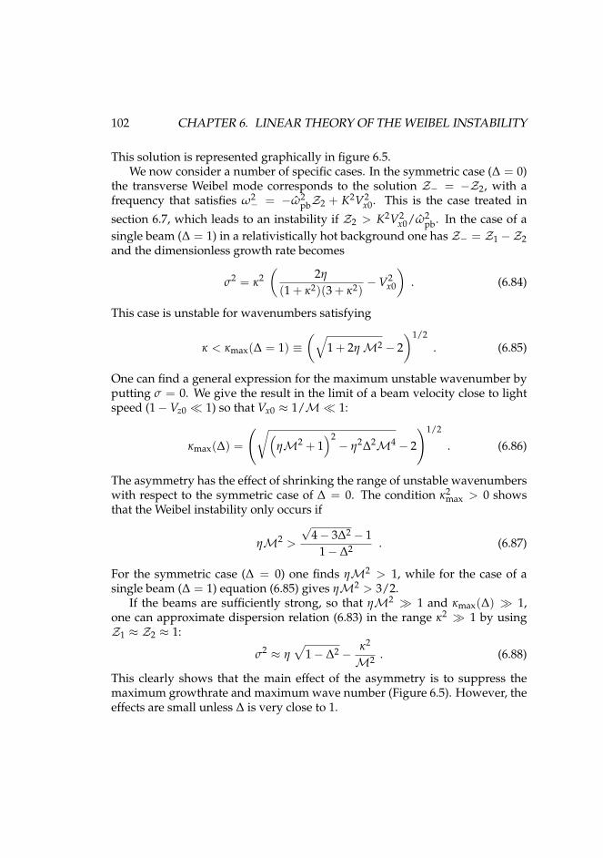
102 CHAPTER 6. LINEAR THEORY OF THE WEIBEL INSTABILITY
This solution is represented graphically in figure 6.5.We now consider a number of specific cases. In the symmetric case (∆ = 0)
the transverse Weibel mode corresponds to the solution Z− = −Z2, with afrequency that satisfies ω2
− = −ω2pbZ2 + K2V2
x0. This is the case treated in
section 6.7, which leads to an instability if Z2 > K2V2x0/ω2
pb. In the case of asingle beam (∆ = 1) in a relativistically hot background one has Z− = Z1 −Z2and the dimensionless growth rate becomes
σ2 = κ2(
2η
(1 + κ2)(3 + κ2)−V2
x0
). (6.84)
This case is unstable for wavenumbers satisfying
κ < κmax(∆ = 1) ≡(√
1 + 2η M2 − 2)1/2
. (6.85)
One can find a general expression for the maximum unstable wavenumber byputting σ = 0. We give the result in the limit of a beam velocity close to lightspeed (1−Vz0 1) so that Vx0 ≈ 1/M 1:
κmax(∆) =
(√(ηM2 + 1
)2− η2∆2M4 − 2
)1/2
. (6.86)
The asymmetry has the effect of shrinking the range of unstable wavenumberswith respect to the symmetric case of ∆ = 0. The condition κ2
max > 0 showsthat the Weibel instability only occurs if
ηM2 >
√4− 3∆2 − 1
1− ∆2 . (6.87)
For the symmetric case (∆ = 0) one finds ηM2 > 1, while for the case of asingle beam (∆ = 1) equation (6.85) gives ηM2 > 3/2.
If the beams are sufficiently strong, so that ηM2 1 and κmax(∆) 1,one can approximate dispersion relation (6.83) in the range κ2 1 by usingZ1 ≈ Z2 ≈ 1:
σ2 ≈ η√
1− ∆2 − κ2
M2 . (6.88)
This clearly shows that the main effect of the asymmetry is to suppress themaximum growthrate and maximum wave number (Figure 6.5). However, theeffects are small unless ∆ is very close to 1.
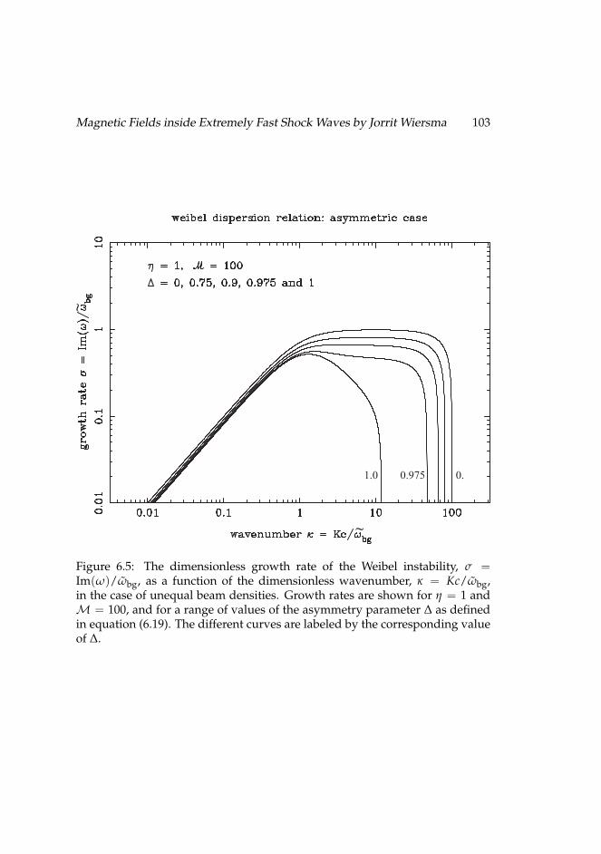
Magnetic Fields inside Extremely Fast Shock Waves by Jorrit Wiersma 103
1.0 0.975 0.
~
~
Figure 6.5: The dimensionless growth rate of the Weibel instability, σ =Im(ω)/ωbg, as a function of the dimensionless wavenumber, κ = Kc/ωbg,in the case of unequal beam densities. Growth rates are shown for η = 1 andM = 100, and for a range of values of the asymmetry parameter ∆ as definedin equation (6.19). The different curves are labeled by the corresponding valueof ∆.
104 CHAPTER 6. LINEAR THEORY OF THE WEIBEL INSTABILITY
6.10 ConclusionsWe have discussed the Weibel instability of relativistic beams in a relativisti-cally hot background plasma. We have based our calculations on the first prin-ciples of the fluid and the Vlasov description of the plasma. Our calculationsgeneralize and extend the results existing in the literature by presenting a de-tailed analysis of the dispersion relation in tensor form. Our aims have been,in particular:
• to obtain accurate expressions to use in further non-linear calculationswhich we present in chapter 9;
• to determine the basic parameters that characterize the dispersion in theplasma;
• and to estimate whether background magnetic fields or asymmetry playan important role.
We have shown that the linear growth rate in the relativistic limit is char-acterized by only two parameters in the symmetric case of identical but coun-terstreaming beams: the ratio η = ω2
pb/ω2bg of the effective plasma frequencies
of beams and background plasma, and an effective Mach-number M, which isa measure for the ratio of the momentum of beam particles in the beam direc-tion and the typical momentum of the thermal motion (velocity dispersion) inthe direction along the wave vector. The latter component is a measure for thepressure in the beam plasma. These conclusions are independent of the precisemodel, fluid or kinetic, that is used to describe the beam-plasma system.
For ultra-relativistic beams (γb 1) the maximum growth rate is of or-der Im(ω) ≈ √
η ωbg, and the maximum unstable wavenumber is Kmax ≈√
η M2 (ωbg/c).The presence of an ambient magnetic field does not change the behavior
of the Weibel instability unless the field is so strong that the beam plasma fre-quency and the gyration frequency of the beam particles become comparable inmagnitude: ωpb ' |qb|B/γbmb. A similar conclusion was reached by Hededaland Nishikawa [36] on the basis of numerical simulations. For the typical pa-rameters associated with the ultra-relativistic shocks of Gamma Ray Bursts (ex-ternal shocks) that propagate into the interstellar or circumstellar medium theunmagnetized treatment of the Weibel instability is a good approximation.
In the asymmetric case, characterized by the additional parameter ∆ =(n+ − n−)/(n+ + n−) where n± are the densities of the two counterstream-ing beams, the main effect of the asymmetry is that the range of unstable
Magnetic Fields inside Extremely Fast Shock Waves by Jorrit Wiersma 105
wavenumbers shrinks, with the maximum unstable wavenumber and maxi-mum growth rate scaling as Im(ω)max , Kmax ∝ (1− ∆2)1/4 (cf. equation 6.88)in the ultra-relativistic limit with Kc/ωbg 1.
The beam-driven Weibel instability will lead to the generation of magneticfields over a wide range of wavelengths, as also discussed by references [32],[31], [58], [24] and [68]. In this respect it behaves not unlike the original versionof the instability, driven by temperature anisotropies [98]. The next step isa detailed study of the stabilization mechanisms that terminate the phase ofexponential growth of the instability discussed here. A first discussion of thesestabilization mechanisms can be found in chapter 8. Chapter 9 discusses themin more detail.
6.11 Appendix: Covariant formulation of plasma responseThe usual procedure for determining the response of a plasma to small-ampli-tude electromagnetic field, which is found in any book on plasma physics[e.g. 40, 63] relates the electric field E and the current density J it induces inthe plasma by solving the linearized plasma equations. This determines theconductivity tensor σ. In the Fourier domain the amplitudes of the currentdensity and the electric field are related by Ji(ω , k) = σij(ω , k) Ej(ω , k),where (i, j) enumerate the spatial components and a tilde (∼) is used to denoteFourier amplitudes. One then calculates the susceptibility tensor, χij(ω , k) =4πiω σij(ω , k), and the dielectric tensor εij(ω , k) = δij + χij in the Fourier do-
main. The dispersion relation of the various linear wave modes that the plasmasupports follows from Maxwell’s equations as
det(c2/ω2)(kik j − k2 δij) + εij(ω, k) = 0. (6.89)
The electromagnetic response of a plasma can also be formulated covari-antly [62, 61, 18]. This has the advantage of immediately yielding results thatare valid for an arbitrary choice of reference frame. The starting point for sucha formulation is the covariant set of Maxwell’s equations,
∂µFµν = 4π Jν , ∂µ
(εµναβ Fαβ
)= 0 , (6.90)
with Fµν the Faraday tensor defined in terms of the electromagnetic four-poten-tial Aµ ≡ (Φ , A) as [e.g. 41]
Fµν = ∂µ Aν − ∂ν Aµ , (6.91)
106 CHAPTER 6. LINEAR THEORY OF THE WEIBEL INSTABILITY
and where εµναβ is the totally antisymmetric (Levi-Cevita) tensor. For linearwave phenomena, this set of equations will be completed by a linear relationbetween the four-current Jµ and the electromagnetic fields.
It is convenient to formulate the linear response in terms of the four-poten-tial perturbation δAµ(x) and the associated four-current perturbation δJµ(x).Assuming plane waves, one can represent these perturbed quantities in termsof a Fourier integral with the Fourier amplitudes Aµ(k) and Jµ(k): δAµ(x)
δJµ(x)
=∫
d4k(2π)4
Aµ(k)
Jµ(x)
exp(−ik · x) . (6.92)
Here (and in what follows) a tilde ∼ is used to denote Fourier amplitudes ofthe wave-like perturbations in the various physical fields.
The Fourier-amplitude of the linearized four-current perturbation carriedby some species s in a multi-species plasma can be related to the Fourier am-plitude of the four-potential through
4π Jµs (k) =
(α
µν
)s(k) Aν(k) . (6.93)
The quantity αµνs (k) is the polarization tensor. The Faraday tensor associated
with the waves, δFµν = ∂µδAν − ∂νδAµ, has the Fourier amplitude
Fµν(k) = i(kν Aµ − kµ Aν
), (6.94)
which follows from the replacement ∂µ −→ −ikµ when going from configu-ration space to Fourier space. As a result, the first set of Maxwell’s equations(6.90) reads in the Fourier domain
(k · A)kµ − (k · k)Aµ = 4π ∑s
Jµs = ∑
s
(α
µν
)s
Aν . (6.95)
The polarization tensor has a number of simple properties, which are relatedto charge conservation and to the gauge freedom of the electromagnetic field.Charge conservation of each species s reads ∂ · δJµ
s = 0, which in the Fourierdomain becomes
kµ Jµs (k) = 0 . (6.96)
Also, the four-current of each individual species should be invariant under ageneral gauge transformation of the form
δAµ =⇒ δAµ + ∂µχ ⇐⇒ Aµ =⇒ Aµ − ikµχ . (6.97)
Magnetic Fields inside Extremely Fast Shock Waves by Jorrit Wiersma 107
equations (6.96) and (6.97) together imply that the polarization tensor mustsatisfy the relations
kµαµνs (k) = α
µνs (k)kν = 0 . (6.98)
6.11.1 Plasma response in the fluid approachIf one calculates the plasma response in the fluid approximation the two con-ditions (6.98) imply that the linear polarization tensor of species s can alwaysbe written in the form [cf. 18, 61, Ch. 4](
αµ
ν
)s= Pµ
sα
(Πα
β
)sP†β
sν , (6.99)
with
Pµsν ≡ δ
µν −
Uµs kν
k ·Us, P†µ
sν ≡ δµν −
kµUsν
k ·Us. (6.100)
Here Uµs is the four-velocity of the frame where species s is at rest, apart from
the thermal motions, so that the unperturbed mass current of species s is Σµ =ns0msUµ
s , with ns0 the proper density and ms the rest mass of the species. Theprojection tensor Pµ
sν and its transpose P†µsν project to the hyperplane perpen-
dicular to k, and satisfy
kµ Pµsν = P†µ
sν kν = 0 , PµsνUν
s = UsµP†µsν = 0 . (6.101)
The determination of αµνs in the fluid approach can then be reduced to the cal-
culation of (Παβ)s.
Linearizing the covariant fluid equation (equation 6.7 of the main paper) tofirst order in perturbed quantities, assuming that there is no electromagneticfield in the unperturbed state and that the unperturbed state is uniform andtime-independent, yields:
(ρ + e + P)s (Us · ∂) δUµs = hµν
s ∂ν δPs + nsqs (δFµν) Usν . (6.102)
Here (and in what follows) ρs, es, Ps and Uµs are the unperturbed (equilibrium)
values of the proper density, internal energy density, pressure and four-velocityof species s, and hµν
s = ηµν −Uµs Uν
s is the projection tensor based on the unper-turbed four-velocity. In the Fourier domain, using ∂µ −→ −ikµ, this linearizedequation of motion becomes:
i(k ·Us) (ρ + e + P)s Uµs = ikµ
⊥Ps − nsqsUsν Fµν . (6.103)
108 CHAPTER 6. LINEAR THEORY OF THE WEIBEL INSTABILITY
Herekµ
s⊥ ≡ hµν kν = kµ − (k ·Us) Uµs . (6.104)
Note thatk ·Us = γs (ω − k · vs) (6.105)
is a Doppler-shifted frequency that corresponds to the wave frequency in therest frame of species s.
The continuity equation (see equation 6.8 of the main paper) upon lineariza-tion becomes
(Us · ∂) δns = −ns (∂ · δUs) , (6.106)
and the equation of state yields
δPs = ΓsPs
(δns
ns
). (6.107)
These two relations yield expressions for the density perturbation ns and pres-sure perturbation Ps in the Fourier domain:
ns = −ns
(k · Us
k ·Us
).
(6.108)
Ps = −ΓsPs
(k · Us
k ·Us
).
If one substitutes these two relations into equation (6.103), and substitutes re-lation (6.94) for the Fourier amplitude Fµν of the Faraday tensor, one obtains aset of four linear relations between the components of the two four vectors Uµ
sand Aν:
(ρ + e + P)s (k ·Us)Uµs + ΓsPs
(k · Us
k ·Us
)kµ
s⊥
(6.109)= nsqs
(Us · A) kµ − (k ·Us) Aµ
.
However, one of these relations is redundant as the unit normalization of thetotal four-velocity implies that Uµ
s ·Usµ = 0, as is easily checked by contractingequation (6.109) with Usµ.
The contribution of species s to the linear current four-vector is:
Jµs = qsns Uµ
s + qsns Uµs . (6.110)
Magnetic Fields inside Extremely Fast Shock Waves by Jorrit Wiersma 109
The first term in this expression is the advection current due to charge densityperturbations advected by the unperturbed flow. This contribution to the cur-rent density is responsible for the occurrence of the Weibel instability. The sec-ond term is the conduction current due to the velocity perturbations inducedby the electromagnetic fields. Using the first relation of equation (6.108), onecan write the Fourier amplitude of the four-current density as
Jµs (k) =
qsns
k ·Us
(k ·Us) Uµ
s − (k · Us) Uµs
. (6.111)
Solving equation (6.109), in effect expressing the components of Uµs in terms
of the components of Aµ, and substituting the resulting expressions into equa-tion (6.111), one can calculate the linearized current density Js in terms of A,and from that read off the components of the corresponding polarization tensor(α
µν )s. We just give the final result in terms of the tensor (Πα
β)s:
(Πα
β
)s= −ω2
ps
(δα
β −C2
s kαkβ
(k ·Us)2 − K2s⊥C2
s
). (6.112)
For a cold plasma one has C2s = 0, so that (Πα
β)s = −ω2ps δα
β with ω2ps =
4πq2s ns/ms. The cold plasma result has been derived previously by Dewar
[18], his equations 95 and 114.
6.11.2 Plasma response in the kinetic approachIn the kinetic approach one must solve the covariant Vlasov equation. LetFs(xµ , pµ) d4x d4 p be the number of particles of species s in the infinitesimalvolume d4x in space-time and four-momentum interval d4 p. The covariantVlasov equation is
dFs
dτ≡ dxµ
dτ
∂Fs
∂xµ +dpµ
dτ
∂Fs
∂pµ = 0 . (6.113)
Here τ is the proper time, and
dxµ
dτ= uµ =
pµ
ms,
dpµ
dτ= qsFµ
νuν (6.114)
are the four-velocity and the Lorentz force acting on a particle with mass msand charge qs. We assume a plane-wave perturbation of the distribution func-tion and all electromagnetic fields with the perturbations represented by a
110 CHAPTER 6. LINEAR THEORY OF THE WEIBEL INSTABILITY
Fourier integral. The total Vlasov distribution can be written as
F (x , p) = F0(p) +∫
d4k(2π)4 F (k , p) exp(−ik · x) , (6.115)
and the linearized Vlasov equation yields:
−i(k · u) Fs(k , p) = − qs
msFµ
ν pν ∂F0s(p)∂pµ . (6.116)
Here we have assumed that the unperturbed distribution F0(p) is uniform inspace-time and that there is no unperturbed electromagnetic field. The linearcurrent density associated with this perturbation has an amplitude
Jµs (k) =
qs
ms
∫d4 p pµFs(k , p) (6.117)
for particle species s. Using equation (6.94) for the Faraday tensor Fµν and solv-
ing (6.116) for F (k, p) and substituting the resulting expression one finds:
4π Jµs =
4πq2s
ms
∫d4 p pµ
(Aν − (A · p)
(k · p)kν
)∂F0s(p)
∂pν. (6.118)
After a partial integration one can write (6.118) in the form 4π Jµs = (α
µν)s Aν,
which defines the polarization tensor of species s in the kinetic approach:(α
µν
)s≡ −4πq2
sms
∫d4 p F0s(p) Mµ
ν(k , p) , (6.119)
with
Mµν(k , p) = δ
µν −
kµ pν + pµkν
(k · p)+
(k · k) pµ pν
(k · p)2 . (6.120)
This result is in fact closely related to the fluid results (6.99) and (6.100). Thiscan be seen by writing (6.119) in the form(
αµν
)s(k) =
∫d4 p F0s(p)
[Pµ
α(k , p)(
Παβ
)sP†β
ν (k , p)]
, (6.121)
with
Pµα(k , p) = δ
µα −
pµkα
(k · p)(6.122)
P†βν (k , p) = δ
βν −
kβ pν
(k · p)
Magnetic Fields inside Extremely Fast Shock Waves by Jorrit Wiersma 111
and (Πα
β
)s= −4πq2
sms
δαβ . (6.123)
In the case of cold beams the fluid and kinetic results are completely equivalent.Result (6.119) was derived in a different context by Achterberg [2], and also
corresponds to expression 227 of Dewar [18] and the corresponding expressionin Melrose [61], Ch. 4.1, for the response tensor of an unmagnetized plasma.These relations show explicitly that both charge conservation, and the invari-ance of the current density under gauge transformations of the vector potential,are once again ensured.
6.12 Appendix: Covariant dispersion relationThe linear dispersion relation for modes supported by the plasma follows fromequation (6.95), which can be written as
Dµν(k) Aν(k) = 0 . (6.124)
Here we defineDµν(k) ≡ (k · k) ηµν − kµkν + αµν(k) (6.125)
with αµν(k) ≡ ∑s(αµν)s(k). However, this set of equations is not linearly in-dependent. The tensor Dµν satisfies (see equation 6.98): kµ Dµν = Dµν kν = 0.This means that the determinant of the 4× 4 matrix Dµν vanishes identically:det[Dµν ] = 0.
The dispersion relation for linear waves can be obtained by noting that onecan factor equation (6.124) as:(
δµα −
kµkα
(k · k)
)[(k · k) ηαν + ααν ] Aν = 0 , (6.126)
since kα ααν = 0. The first factor leads to the vanishing determinant of Dµν.Therefore, the dispersion relation for the waves in the plasma follows from therequirement that the determinant of the second factor vanishes identically:
det
[(k · k) ηµν + ∑
sα
µνs (k)
]= 0 . (6.127)
The problem of determining the wave properties therefore corresponds to de-termining the polarization tensor αµν and solving dispersion relation (6.127)
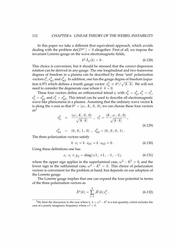
112 CHAPTER 6. LINEAR THEORY OF THE WEIBEL INSTABILITY
In this paper we take a different (but equivalent) approach, which avoidsdealing with the problem det[Dµν ] = 0 altogether. First of all, we impose theinvariant Lorentz-gauge on the wave electromagnetic fields,
kµ Aµ(k) = 0 . (6.128)
This choice is convenient, but it should be stressed that the correct dispersionrelation can be derived in any gauge. The one longitudinal and two transversedegrees of freedom in a plasma can be described by three ‘unit’ polarizationvectors eµ
` , eµtr1 and eµ
tr2. In addition, one has the gauge degree of freedom (equa-tion 6.97) which defines a fourth gauge vector: eµ
G ≡ kµ/√|k · k|. We will not
need to consider the degenerate case where k · k = 0.These four vectors define an orthonormal tetrad ei with eµ
0 = eµG, eµ
1 = eµ` ,
eµ2 = eµ
tr1 and eµ3 = eµ
tr2. This tetrad can be used to describe all electromagneticwave-like phenomena in a plasma. Assuming that the ordinary wave vector kis along the x-axis so that kµ = (ω , K , 0 , 0), we can choose these four vectorsas2
eµG =
(ω , K , 0 , 0)√|k · k|
, eµ` =
(K , ω , 0 , 0)√|k · k|
,
(6.129)eµ
tr1 = (0 , 0 , 1 , 0) , eµtr2 = (0 , 0 , 0 , 1) .
The three polarization vectors satisfy
k · e` = k · etr1 = k · etr2 = 0 . (6.130)
Using these definitions one has
ei · ej ≡ gij = diag(±1 , ∓1 , −1 , −1), (6.131)
where the upper sign applies in the superluminal case, ω2 − K2 > 0, and thelower sign in the subluminal case, ω2 − K2 < 0. This choice of polarizationvectors is convenient for the problem at hand, but depends on our adoption ofthe Lorentz gauge.
The Lorentz gauge implies that one can expand the four-potential in termsof the three polarization vectors as
Aµ(k) =3
∑j=1Aj(k) eµ
j . (6.132)
2We limit the discussion to the case where k · k = ω2 − K2 is a real quantity, which includes thecase of a purely imaginary frequency where ω2 < 0.
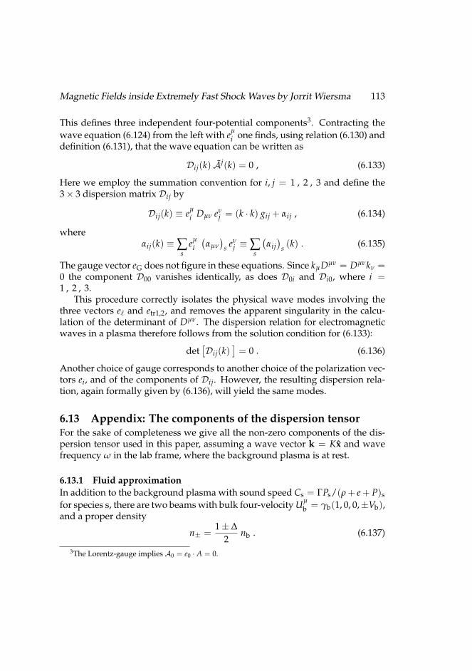
Magnetic Fields inside Extremely Fast Shock Waves by Jorrit Wiersma 113
This defines three independent four-potential components3. Contracting thewave equation (6.124) from the left with eµ
i one finds, using relation (6.130) anddefinition (6.131), that the wave equation can be written as
Dij(k) Aj(k) = 0 , (6.133)
Here we employ the summation convention for i, j = 1 , 2 , 3 and define the3× 3 dispersion matrix Dij by
Dij(k) ≡ eµi Dµν eν
j = (k · k) gij + αij , (6.134)
whereαij(k) ≡ ∑
seµ
i(αµν
)s eν
j ≡ ∑s
(αij)
s (k) . (6.135)
The gauge vector eG does not figure in these equations. Since kµDµν = Dµνkν =0 the component D00 vanishes identically, as does D0i and Di0, where i =1 , 2 , 3.
This procedure correctly isolates the physical wave modes involving thethree vectors e` and etr1,2, and removes the apparent singularity in the calcu-lation of the determinant of Dµν. The dispersion relation for electromagneticwaves in a plasma therefore follows from the solution condition for (6.133):
det[Dij(k)
]= 0 . (6.136)
Another choice of gauge corresponds to another choice of the polarization vec-tors ei, and of the components of Dij. However, the resulting dispersion rela-tion, again formally given by (6.136), will yield the same modes.
6.13 Appendix: The components of the dispersion tensorFor the sake of completeness we give all the non-zero components of the dis-persion tensor used in this paper, assuming a wave vector k = Kx and wavefrequency ω in the lab frame, where the background plasma is at rest.
6.13.1 Fluid approximationIn addition to the background plasma with sound speed Cs = ΓPs/(ρ + e + P)sfor species s, there are two beams with bulk four-velocity Uµ
b = γb(1, 0, 0,±Vb),and a proper density
n± =1± ∆
2nb . (6.137)
3The Lorentz-gauge implies A0 = e0 · A = 0.
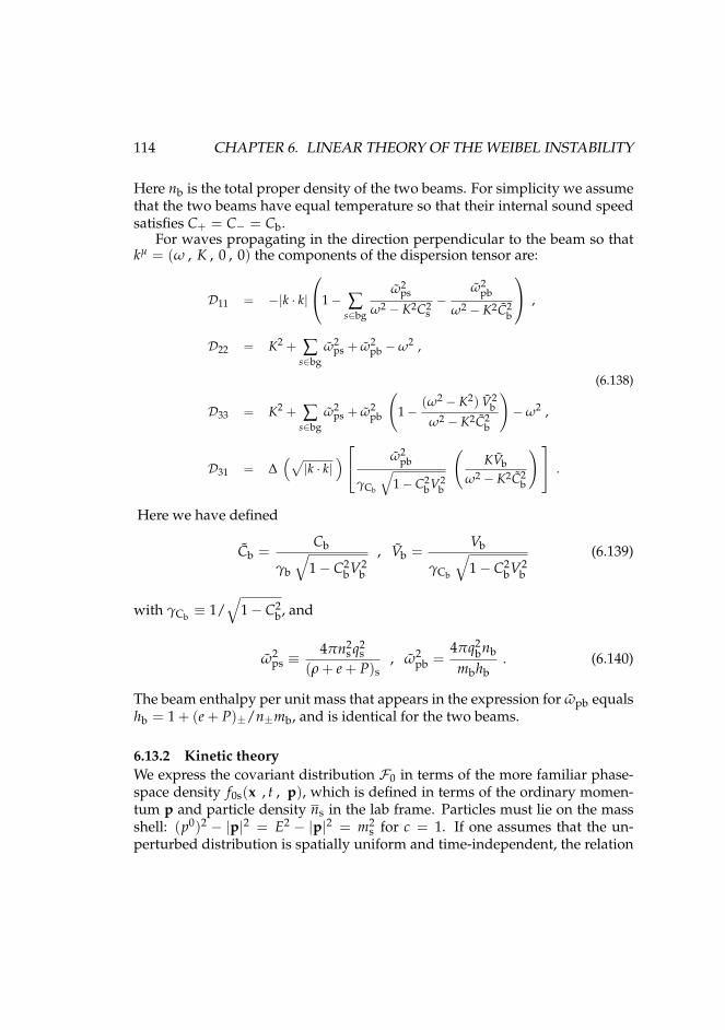
114 CHAPTER 6. LINEAR THEORY OF THE WEIBEL INSTABILITY
Here nb is the total proper density of the two beams. For simplicity we assumethat the two beams have equal temperature so that their internal sound speedsatisfies C+ = C− = Cb.
For waves propagating in the direction perpendicular to the beam so thatkµ = (ω , K , 0 , 0) the components of the dispersion tensor are:
D11 = −|k · k|
1− ∑s∈bg
ω2ps
ω2 − K2C2s−
ω2pb
ω2 − K2C2b
,
D22 = K2 + ∑s∈bg
ω2ps + ω2
pb −ω2 ,
(6.138)
D33 = K2 + ∑s∈bg
ω2ps + ω2
pb
(1−
(ω2 − K2) V2b
ω2 − K2C2b
)−ω2 ,
D31 = ∆(√
|k · k|) ω2
pb
γCb
√1− C2
bV2b
(KVb
ω2 − K2C2b
) .
Here we have defined
Cb =Cb
γb
√1− C2
bV2b
, Vb =Vb
γCb
√1− C2
bV2b
(6.139)
with γCb≡ 1/
√1− C2
b, and
ω2ps ≡
4πn2s q2
s(ρ + e + P)s
, ω2pb =
4πq2bnb
mbhb. (6.140)
The beam enthalpy per unit mass that appears in the expression for ωpb equalshb = 1 + (e + P)±/n±mb, and is identical for the two beams.
6.13.2 Kinetic theoryWe express the covariant distribution F0 in terms of the more familiar phase-space density f0s(x , t , p), which is defined in terms of the ordinary momen-tum p and particle density ns in the lab frame. Particles must lie on the massshell: (p0)2 − |p|2 = E2 − |p|2 = m2
s for c = 1. If one assumes that the un-perturbed distribution is spatially uniform and time-independent, the relation
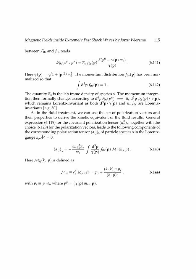
Magnetic Fields inside Extremely Fast Shock Waves by Jorrit Wiersma 115
between F0s and f0s reads
F0s(xµ , pµ) = ns f0s(p)δ(p0 − γ(p) ms)
γ(p). (6.141)
Here γ(p) =√
1 + |p|2/m2s . The momentum distribution f0s(p) has been nor-
malized so that ∫d3p f0s(p) = 1 . (6.142)
The quantity ns is the lab frame density of species s. The momentum integra-tion then formally changes according to d4 p F0s(pµ) =⇒ ns d3p f0s(p)/γ(p),which remains Lorentz-invariant as both d3p/γ(p) and ns f0s are Lorentz-invariants [e.g. 50].
As in the fluid treatment, we can use the set of polarization vectors andtheir properties to derive the kinetic equivalent of the fluid results. Generalexpression (6.119) for the covariant polarization tensor (α
µν )s, together with the
choice (6.129) for the polarization vectors, leads to the following components ofthe corresponding polarization tensor (αij)s of particle species s in the Lorentz-gauge kµ Aµ = 0:
(αij)
s = −4πq2s ns
ms
∫d3pγ(p)
f0s(p)Mij(k , p) . (6.143)
Here Mij(k , p) is defined as
Mij ≡ eµi Mµν eν
j = gij +(k · k) pi pj
(k · p)2 , (6.144)
with pi ≡ p · ei, where pµ = (γ(p) ms , p).
116 CHAPTER 6. LINEAR THEORY OF THE WEIBEL INSTABILITY
The components of the polarization tensor with kµ = (ω , K , 0 , 0) followas
αb11 = |k · k|
4πq2bnb
mb
∫d3pγ(p)
f0b(p)
1− v2x
(ω − Kvx)2
,
αb22 =
4πq2bnb
mb
∫d3pγ(p)
f0b(p) ,
(6.145)
αb33 =
4πq2bnb
mb
∫d3pγ(p)
f0b(p)
1−
v2z(ω2 − K2)
(ω − Kvx)2
,
αb31 = αb∗
13
= −√|k · k|
4πq2bnb
mb
∫d3pγ(p)
f0b(p)
vz (K −ωvx)
(ω − Kvx)2
.
Here v = p/γmb is the velocity of beam particles with momentum p.It can be shown by partial integration that this is equivalent with
αb11 = −
4πq2bnb|k · k|K2
∫d3p
K
∂ f0b(p)∂px
ω − Kvx
,
αb33 =
4πq2bnb
mb
∫d3pγ(p)
f0b(p)(
1− v2z
)−4πq2
bnb
∫d3p
v2
zω − Kvx
(K
∂ f0b(p)∂px
),
(6.146)
αb31 =
√|k · k|ω
[4πq2
bnb
mb
∫d3pγ(p)
f0b(p) vxvz
+ 4πq2bnb
∫d3p
vxvz
ω − Kvx
(K
∂ f0b(p)∂px
)].
This particular form is convenient in the waterbag approximation discussedbelow.
Magnetic Fields inside Extremely Fast Shock Waves by Jorrit Wiersma 117
6.13.3 Waterbag approximationWe use a momentum distribution for the beams of the form
f0b(p) =Θ(px + px0)−Θ(px − px0)
2 px0δ(py) ×
(6.147)
×[
1 + ∆2
δ(pz − pz0) +1− ∆
2δ(pz + pz0)
].
For the background we continue to use the fluid approximation.Substituting (6.147) into (6.146) the evaluation of the αb
ij is straightforwardas the px-derivatives in these expressions convert the Heaviside step functionsin (6.147) into Dirac delta functions. The resulting components of the disper-sion tensor are:
D11 = −|k · k|
1− ∑s∈bg
ω2ps
ω2 − K2C2s−
ω2pb
ω2 − K2V2x0
,
D22 = K2 + ∑s∈bg
ω2ps + ω2
pb Gb −ω2 ,
(6.148)
D33 = K2 + ∑s∈bg
ω2ps + ω2
pb
(Gb +
K2V2z0
ω2 − K2V2x0
)−ω2 ,
D31 = ∆(√
|k · k|) [ ω2
pb KVz0
ω2 − K2V2x0
].
Here we define the beam plasma frequency by
ω2pb =
4πq2bnb
γ0mb, (6.149)
define a characteristic Lorentz-factor and velocity components
γ0 =
√1 +
p2x0
m2bc2
+p2
z0m2
bc2,
(6.150)
Vx0 =px0
γ0mb, Vz0 =
pz0
γ0mb,
118 CHAPTER 6. LINEAR THEORY OF THE WEIBEL INSTABILITY
and introduce the two functions
Gb = γ0
∫d3pγ(p)
f0b(p) =1
2Vx0ln[
1 + Vx0
1−Vx0
](6.151)
Gb = γ0
∫d3pγ(p)
f0b(p)(
1− v2z
)= Gb −
p2z0
p2z0 + m2
bc2.
The result for the beam contribution to the polarization tensor, αbij, has been
derived by Silva et al. [89], using a somewhat different notation.
6.14 Appendix: Magnetized Weibel instabilityWe briefly consider the magnetized case, in order to compare the results ob-tained with the present formalism with those of Tautz and Schlickeiser [91].We limit the discussion to the case where the electric field vanishes in the lab-oratory frame (the rest frame of the background plasma), and where the beamvelocity is along the magnetic field in the z-direction. The beam trajectory thenremains straight, and we do not have to deal with the much more difficult caseof oscillator beams that gyrate around the ambient magnetic field. This meansthat the Lorentz force on all components vanishes in the unperturbed state: ina covariant notation
FµνUsν = 0 . (6.152)
In both the laboratory frame and the rest frame of the beams, moving with ve-locity±Vb along the z-axis, the only non-vanishing components of the Faradaytensor are F21 = −F12 = B, with B the strength of the magnetic field B = Bz inthe laboratory frame.
In the fluid approximation the linearized equation of motion for small per-turbations in the four-velocity of species s now reads, when transformed to theFourier domain:
(ρ + e + P)s (k ·Us)Uµs + ΓsPs
(k · Us
k ·Us
)kµ
s⊥ − insqsFµνUsµ
(6.153)= nsqs
(Us · A) kµ − (k ·Us) Aµ
.
Magnetic Fields inside Extremely Fast Shock Waves by Jorrit Wiersma 119
The last term on the left-hand side gives the first-order Lorentz force. Solvingthis equation, expressing the four-velocity perturbation in terms of the vectorpotential Aµ, and calculating the associated four-current density, one finds thepolarization tensor α
µν . As before, we express the final result in terms of the
tensor (Παβ)s for each species in the plasma:
(Πα
β
)s
= −ω2
ps
N(k)
(k ·Us)2
[(k ·Us)2 − K2
s⊥C2s
]δα
β
−i (k ·Us) Ωs
[(k ·Us)2 − (k · b)2C2
s
]εα
βµνUµs bν
(6.154)
+i (k ·Us) Ωs(k · b)C2s
[εα
νµλkνUµs bλbβ − bαεβνµλkνUµ
s bλ]
− (k ·Us)2 C2s kαkβ + (k ·Us)2 Ω2
s bαbβ
In this expression we define
N(k) ≡ (k ·Us)2[(k ·Us)2 − K2
s⊥C2s
]−Ω2
s
[(k ·Us)2 − (k · b)2C2
s
](6.155)
andΩs ≡
nsqsB(ρ + e + P)s
, (6.156)
which is an effective gyrofrequency with B the magnetic field strength in thelab frame. In this particular case it is also the strength of the magnetic field inthe rest frame of the beams, as follows from the Lorentz-transformations of theelectromagnetic field, e.g. Jackson [41], Ch. 11. The quantity K2
s⊥ is definedin equation (6.11) of the main paper. The quantity εαβγδ is the totally antisym-metric Levi-Cevita tensor, and the four-vector bµ = (0 , B/B) corresponds toa space-like vector whose spatial component is along the magnetic field in thelab frame, where it takes the form bµ = (0 , 0 , 0 , 1). It is easily checked that werecover the earlier result (A.23) for the unmagnetized case by putting Ωs = 0.
We limit the discussion to the case where the wavevector k = Kx in the lab-oratory frame is perpendicular to the magnetic field B = Bz (and the beam ve-locity) so that (k · b) = 0. We assume two symmetric counterstreaming beams.The Weibel instability then corresponds to the instability of the ordinary mode,
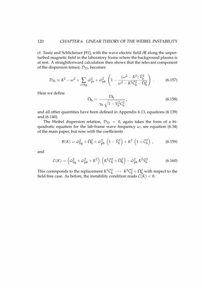
120 CHAPTER 6. LINEAR THEORY OF THE WEIBEL INSTABILITY
cf. Tautz and Schlickeiser [91], with the wave electric field δE along the unper-turbed magnetic field in the laboratory frame where the background plasma isat rest. A straightforward calculation then shows that the relevant componentof the dispersion tensor, D33, becomes:
D33 ≡ K2 −ω2 + ∑s∈bg
ω2ps + ω2
pb
(1−
(ω2 − K2) V2b
ω2 − K2C2b − Ω2
b
). (6.157)
Here we defineΩb =
Ωb
γb
√1−V2
b C2b
, (6.158)
and all other quantities have been defined in Appendix 6.13, equations (6.139)and (6.140).
The Weibel dispersion relation, D33 = 0, again takes the form of a bi-quadratic equation for the lab-frame wave frequency ω, see equation (6.34)of the main paper, but now with the coefficients
B(K) = ω2bg + Ω2
b + ω2pb
(1− V2
b
)+ K2
(1 + C2
b
), (6.159)
and
C(K) =(
ω2bg + ω2
pb + K2) (
K2C2b + Ω2
b
)− ω2
pb K2V2b . (6.160)
This corresponds to the replacement K2C2b −→ K2C2
b + Ω2b with respect to the
field-free case. As before, the instability condition reads C(K) < 0.
Chapter 7
Variations on the Weibelinstability
In the previous chapter we saw how, in a relativistic shock front, the Weibelinstability will cause the magnetic field strength to grow in time. However,seen from the point of view of the shock wave one might expect a stationarysituation instead, with the magnetic field becoming stronger as you go deeperinto the shock front.
In this chapter we briefly show that the two points of view yield equivalentresults. We also show that the Weibel instability preferentially produces elec-trical currents oriented perpendicularly to the shock front, which justifies theone-dimensional assumption that we make in much of the rest of this thesis.
121
122 CHAPTER 7. VARIATIONS ON THE WEIBEL INSTABILITY
7.1 IntroductionOne can model plasma instabilities, like the Weibel instability, with solutionsthat grow in time (the usual approach) but also with solutions that grow inspace, the relevant approach being dictated by the initial situation and bound-ary conditions that are used. The normal approach of looking for (exponen-tially) growing solutions of the equations that describe the plasma determineswhether a certain situation is unstable at all, and determines such basic quan-tities as the typical length scale of the unstable perturbations and the growthrate. In recent theoretical research of relativistic collisionless shock waves, theinstability analysis is taken a step further: the rapid growth of instabilities isused to model the shock ramp, the initial sudden increase in internal energydensity and especially in magnetic energy density at the shock front [104, 58].To model the (quasi-stationary) situation in the shock rest frame one wouldbe interested in a spatially growing solution for the instability rather than onegrowing in time. In particular, depending on the boundary conditions, onewould expect such a quasi-stationary state to form (after a certain time) in nu-merical simulations that use a constant inflow of particles (e.g., as in Frederik-sen et al. [24]; see also Hededal [35, chapter 4]).
The Weibel or filament instability is one of a few known mechanisms thatare capable of increasing the magnetic field strength in collisionless shocks. En-hancement of the magnetic energy density is necessary, for example, to explainGamma-ray Burst afterglows with the synchrotron (or jitter) radiation mecha-nism [e.g. 32].
To see if a Weibel-like instability might also produce a region of spatiallygrowing magnetic field we will derive a dispersion relation for a plasma whoseproperties are allowed to vary in two spatial directions. In Sect. 7.3.5 we willshow that the spatially growing solution for two counterstreaming beams ofplasma is almost the same as the normal Weibel instability.
This analysis also yields equations describing a temporally growing Weibel-like instability with a wave vector that is not strictly perpendicular to the beamdirection, i.e., a mixed transverse/longitudinal mode, and we will show thatthis mixed instability only occurs for wave vectors that fall outside a certaincone around the shock normal (Sect. 7.3.6).
7.2 Counterstreaming beam model7.2.1 Initial conditionWe consider the stability of a system consisting of two counterstreaming beamsof charged particles. Such a situation is similar to what we believe to exist in
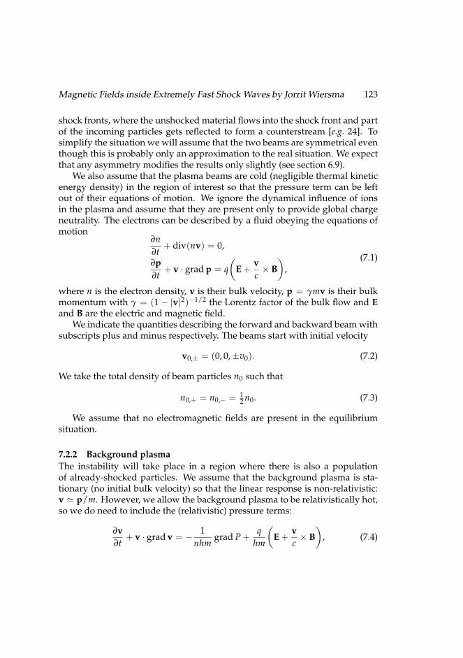
Magnetic Fields inside Extremely Fast Shock Waves by Jorrit Wiersma 123
shock fronts, where the unshocked material flows into the shock front and partof the incoming particles gets reflected to form a counterstream [e.g. 24]. Tosimplify the situation we will assume that the two beams are symmetrical eventhough this is probably only an approximation to the real situation. We expectthat any asymmetry modifies the results only slightly (see section 6.9).
We also assume that the plasma beams are cold (negligible thermal kineticenergy density) in the region of interest so that the pressure term can be leftout of their equations of motion. We ignore the dynamical influence of ionsin the plasma and assume that they are present only to provide global chargeneutrality. The electrons can be described by a fluid obeying the equations ofmotion
∂n∂t
+ div(nv) = 0,
∂p∂t
+ v · grad p = q(
E +vc× B
),
(7.1)
where n is the electron density, v is their bulk velocity, p = γmv is their bulkmomentum with γ = (1− |v|2)−1/2 the Lorentz factor of the bulk flow and Eand B are the electric and magnetic field.
We indicate the quantities describing the forward and backward beam withsubscripts plus and minus respectively. The beams start with initial velocity
v0,± = (0, 0,±v0). (7.2)
We take the total density of beam particles n0 such that
n0,+ = n0,− = 12 n0. (7.3)
We assume that no electromagnetic fields are present in the equilibriumsituation.
7.2.2 Background plasmaThe instability will take place in a region where there is also a populationof already-shocked particles. We assume that the background plasma is sta-tionary (no initial bulk velocity) so that the linear response is non-relativistic:v ' p/m. However, we allow the background plasma to be relativistically hot,so we do need to include the (relativistic) pressure terms:
∂v∂t
+ v · grad v = − 1nhm
grad P +q
hm
(E +
vc× B
), (7.4)
124 CHAPTER 7. VARIATIONS ON THE WEIBEL INSTABILITY
where P is the pressure and the quantity h is the enthalpy per unit mass givenby
h = 1 +e + Pnmc2 , (7.5)
where e is the internal energy density of the plasma.The equation given above is formally only valid when the plasma is well
described with a fluid model. For a relativistically hot plasma a kinetic modelwould actually be more appropriate: see section 6.7. However, in chapter 6we showed that the differences between results for the two approaches aresmall, so in this chapter we will favor the fluid description because it keeps themathematics simpler.
7.2.3 Maxwell’s equationsWe describe the electromagnetic fields through a scalar potential φ and a vectorpotential A in the Lorentz gauge:
E = − grad φ− 1c
∂A∂t
, B = curl A. (7.6)
Maxwell’s equations reduce to (e.g., Jackson [41, equations 6.37,38])
∇2φ− 1c2
∂2φ
∂t2 = −4πq(n− n0),
∇2A− 1c2
∂2A∂t2 = −4π
cJ,
(7.7)
where n0 is the equilibrium density and J is the total current density in theplasma.
7.3 Instability analysis7.3.1 Linear response of the beamsAssume that the instability is a small-amplitude, plane wave perturbation ontop of the equilibrium situation. We substitute n → n0 + n exp(ikxx + ikzz −iωt) and similarly for all the other quantities. We assume that there are noinitial electromagnetic fields (E0 = B0 = 0). We neglect the electrostatic po-tential (φ = 0), and concentrate on the electromagnetic response of the plasmainstead.
For small perturbations the response of the plasma to the electromagneticfield can be expressed as a linear relation between the current density J and

Magnetic Fields inside Extremely Fast Shock Waves by Jorrit Wiersma 125
the vector potential A. The derivation of this expression from the equationsof motion (7.1) can be found, for example in Melrose [60], Sect. 2.1 (see alsoexercise 1.2). The current density for each beam becomes:
J± = − q2n0,±γ0mc
I± k v0 + v0 k
ω ∓ k · v0+
(k2 −ω2)v0 v0/c2
(ω ∓ k · v0)2
·A, (7.8)
where I is the identity tensor, k2 = |k|2 and we have indicated the expressionsfor the forward and backward beam with the ± signs. The total contributionof both beams is Jb = J+ + J−:
Jb = − q2n0
γ0mc
I +
(k · v0)(k v0 + v0 k)ω2 − (k · v0)2
+(k2 −ω2/c2)(ω2 + (k · v0)2)v0 v0
(ω2 − (k · v0)2)2
·A.
(7.9)
7.3.2 Linear response of the background plasmaThe background plasma will also contribute to the current density. Linearizingthe equation of motion (7.4) for the background plasma yields an expressionfor the velocity perturbation of the background plasma:
−iωv = −ikP
n0h0m+ iω
qh0mc
A. (7.10)
To eliminate the pressure perturbation P we make use of a polytropic equationof state P0 + P = P0 (n/n0)Γ, where Γ is the adiabatic index of the backgroundplasma. Linearizing this equation of state gives
P = ΓP0nn0
. (7.11)
The density perturbation is given by the continuity equation (remember thatv0 = 0 for the background plasma):
n = n0k · v
ω. (7.12)
Substituting equations (7.11) and (7.12) into the equation of motion (7.10) yields
v− C2s(k · v)k
ω2 = − qh0mc
A, (7.13)
126 CHAPTER 7. VARIATIONS ON THE WEIBEL INSTABILITY
where C2s = ΓP0/(n0h0m) is the relativistic sound speed. To solve (7.13) for
v we need to eliminate the k · v term and we can do that by first taking thedot-product with k to get an expression for k · v:
k · v = − qh0mc
ω2
ω2 − k2C2s
k ·A. (7.14)
Eliminating k · v from equation (7.13) now gives an expression for v whichwe can use to find the contribution of the background plasma to the currentdensity:
Jbg = qn0v = − q2n0
h0mc
I +
C2s k k
ω2 − k2C2s
·A. (7.15)
7.3.3 Dispersion relationThe electromagnetic field must satisfy Maxwell’s equations (7.7) with both thebackground and beam contributions as sources:(
ω2
c2 − k2
)A = −4π
c(Jb + Jbg). (7.16)
To get Weibel-like modes we will take k = (kx, 0, kz) and v0 = (0, 0, v0). Notethat we leave kz 6= 0 to allow for the possibility of solutions growing in thez-direction. We can then write the dispersion equation (7.16) as M · A = 0involving the vector A = (Ax, Az) and the 2× 2 matrix M with components:
Mxx = k2c2 −ω2 + ω2pbg + ω2
pb + ω2pbg
C2s k2
xω2 − k2C2
s
Mxz = Mzx = ω2pbg
C2s kxkz
ω2 − k2C2s
+ ω2pb
v20kxkz
ω2 − k2zv2
0,
Mzz = k2c2 −ω2 + ω2pbg + ω2
pb + ω2pbg
C2s k2
zω2 − k2C2
s
+ ω2pb
[2v2
0k2z
ω2 − k2zv2
0+
(ω2 + k2zv2
0)(k2 −ω2/c2)v20
(ω2 − k2zv2
0)2
],
(7.17)
where
ω2pb ≡
4πnbq2
γ0m, ω2
pbg ≡4πnbgq2
h0m. (7.18)
Magnetic Fields inside Extremely Fast Shock Waves by Jorrit Wiersma 127
7.3.4 The “Normal” Weibel instabilityThe “normal” transverse Weibel instability growing in time follows from thedispersion equation of the previous section by taking kz = 0. In that caseMxz = Mzx = 0 so the dispersion equation det M = 0 factors into
Mxx Mzz = 0. (7.19)
The longitudinal mode with Mxx = 0 is always stable and the transverse modewith Mzz = 0 contains the Weibel instability. It obeys the dispersion equation
Mzz = k2xc2 −ω2 + ω2
pbg + ω2pb + ω2
pb(k2
x −ω2/c2)v20
ω2 = 0. (7.20)
We can write this asω4 + Bω2 + C = 0, (7.21)
withB = −
(k2
xc2 + ω2pbg + ω2
pb(1− v20/c2)
),
C = −ω2pbk2
xv20.
(7.22)
The solution is
ω2 =−B±
√B2 − 4C
2. (7.23)
Note that both B and C are negative, so the unstable solution ω2 < 0 is thesolution with the minus sign. For ω k2
xc2 we can neglect the ω4 term inequation (7.21) and the solution is approximated by
ω2 = −CB
= −ω2
pbk2xv2
0
k2xc2 + ω2
pbg + ω2pb(1− v2
0). (7.24)
7.3.5 Dispersion relation for spatial modesIn this section we will calculate the allowed growth length of stationary per-turbations. If we take ω = 0 the components of M in equation (7.17) simplifyto
Mxx = k2c2 + ω2pb + ω2
pbg − ω2pbg
k2x
k2 ,
Mxz = −
(ω2
pbg
k2 +ω2
pb
k2z
)kxkz,
Mzz = k2c2 + ω2pb + ω2
pbg −
(ω2
pbg
k2 +ω2
pb
k2z
)k2
z + ω2pb
k2x
k2z
.
(7.25)
128 CHAPTER 7. VARIATIONS ON THE WEIBEL INSTABILITY
We can conveniently represent the matrix with
M =(
D + Fk2x Fkxkz
Fkxkz D + Fk2z
)(7.26)
where
D = k2c2 + ω2pb + ω2
pbg + ω2pb
k2x
k2z
,
F = −
(ω2
pbg
k2 +ω2
pb
k2z
).
(7.27)
There is only a nontrivial solution for A when det M = 0:
det M = D2 + DFk2 = Dk2c2 = 0, (7.28)
where we have used D + Fk2 = k2c2. For k2 6= 0 we obtain
k4z + B′k2
z + C′ = 0. (7.29)
where
B′ = k2x +
ω2pb + ω2
pbg
c2 ,
C′ =ω2
pb
c2 k2x.
(7.30)
The solution is
k2z =
−B′ ±√
B′2 − 4C′
2. (7.31)
The solution with the minus sign corresponds to a plasma skin effect as we cansee by considering the case without beams (ωpb = 0). The solution with theplus sign contains a spatially growing solution with purely imaginary kz thatresembles the Weibel instability:
k2z ' −C′/B′ = −
ω2pbk2
x
k2xc2 + ω2
pbgfor k2
z k2x. (7.32)
The imaginary part of kz has a simple dependence on kx (Fig. 7.1): for smallkx it grows linearly with kx, for large kx it reaches a plateau. In more realisticmodels the instability will be cut off at large kx due to a thermal spread inthe momentum (cf. chapter 6 and reference [105]). Section 7.4 discusses thedifferences and similarities with the temporally growing solution (7.24).
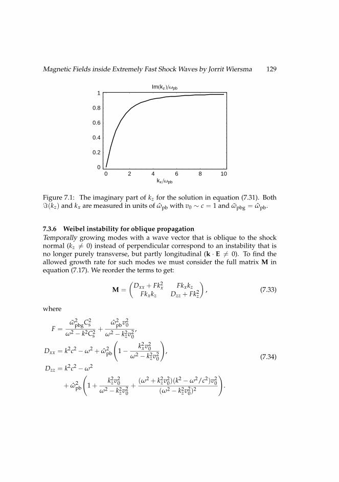
Magnetic Fields inside Extremely Fast Shock Waves by Jorrit Wiersma 129
0 2 4 6 8 10kx Ωpb
0
0.2
0.4
0.6
0.8
1ImHkz LΩpb
Figure 7.1: The imaginary part of kz for the solution in equation (7.31). Both=(kz) and kx are measured in units of ωpb with v0 ∼ c = 1 and ωpbg = ωpb.
7.3.6 Weibel instability for oblique propagationTemporally growing modes with a wave vector that is oblique to the shocknormal (kz 6= 0) instead of perpendicular correspond to an instability that isno longer purely transverse, but partly longitudinal (k · E 6= 0). To find theallowed growth rate for such modes we must consider the full matrix M inequation (7.17). We reorder the terms to get:
M =(
Dxx + Fk2x Fkxkz
Fkxkz Dzz + Fk2z
), (7.33)
where
F =ω2
pbgC2s
ω2 − k2C2s
+ω2
pbv20
ω2 − k2zv2
0,
Dxx = k2c2 −ω2 + ω2pb
(1−
k2xv2
0ω2 − k2
zv20
),
Dzz = k2c2 −ω2
+ ω2pb
(1 +
k2zv2
0ω2 − k2
zv20
+(ω2 + k2
zv20)(k2 −ω2/c2)v2
0(ω2 − k2
zv20)
2
).
(7.34)
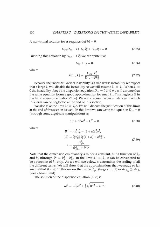
130 CHAPTER 7. VARIATIONS ON THE WEIBEL INSTABILITY
A non-trivial solution for A requires det M = 0:
DxxDzz + F(Dxxk2z + Dzzk2
x) = 0. (7.35)
Dividing this equation by Dxx + Fk2x we can write it as
Dzz + G = 0, (7.36)
where
G(ω, k) ≡ DxxFk2z
Dxx + Fk2x
. (7.37)
Because the “normal” Weibel instability is a transverse instability we expectthat a large kz will disable the instability so we will assume kz kx. When kz =0 the instability obeys the dispersion equation Dzz = 0 and we will assume thatthe same equation forms a good approximation for small kz. This neglects G inthe full dispersion equation (7.36). We will discuss the circumstances in whichthis term can be neglected at the end of this section.
We also take the limit ω kxc. We will discuss the justification of this limitat the end of this section as well. In this limit we can write the equation Dzz = 0(through some algebraic manipulation) as
ω4 + B′′ω2 + C′′ = 0, (7.38)
whereB′′ = αk2
xv20 − (2 + α)k2
zv20,
C′′ = k2zv4
0
k2z(1 + α) + αk2
x
,
α =ω2
pb
ω2pbg + k2c2
.
(7.39)
Note that the dimensionless quantity α is not a constant, but a function of kxand kz (through k2 = k2
x + k2z). In the limit kz kx it can be considered to
be a function of kx only. As we will see below, α determines the scaling of allthe different terms. We will show that the approximations that we made so farare justified if α 1: this means that kc ωpb (large k limit) or ωpbg ωpb(weak beam limit).
The solution of the dispersion equation (7.38) is
ω2 = − 12 B′′ ± 1
2
√B′′2 − 4C′′. (7.40)
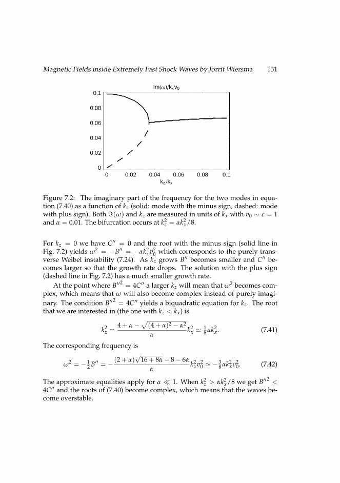
Magnetic Fields inside Extremely Fast Shock Waves by Jorrit Wiersma 131
0 0.02 0.04 0.06 0.08 0.1kz kx
0
0.02
0.04
0.06
0.08
0.1ImHΩLkxv0
Figure 7.2: The imaginary part of the frequency for the two modes in equa-tion (7.40) as a function of kz (solid: mode with the minus sign, dashed: modewith plus sign). Both =(ω) and kz are measured in units of kx with v0 ∼ c = 1and α = 0.01. The bifurcation occurs at k2
z = αk2x/8.
For kz = 0 we have C′′ = 0 and the root with the minus sign (solid line inFig. 7.2) yields ω2 = −B′′ = −αk2
xv20 which corresponds to the purely trans-
verse Weibel instability (7.24). As kz grows B′′ becomes smaller and C′′ be-comes larger so that the growth rate drops. The solution with the plus sign(dashed line in Fig. 7.2) has a much smaller growth rate.
At the point where B′′2 = 4C′′ a larger kz will mean that ω2 becomes com-plex, which means that ω will also become complex instead of purely imagi-nary. The condition B′′2 = 4C′′ yields a biquadratic equation for kz. The rootthat we are interested in (the one with kz < kx) is
k2z =
4 + α−√
(4 + α)2 − α2
αk2
x ' 18 αk2
x. (7.41)
The corresponding frequency is
ω2 = − 12 B′′ = − (2 + α)
√16 + 8α− 8− 6α
αk2
xv20 ' − 3
8 αk2xv2
0. (7.42)
The approximate equalities apply for α 1. When k2z > αk2
x/8 we get B′′2 <4C′′ and the roots of (7.40) become complex, which means that the waves be-come overstable.
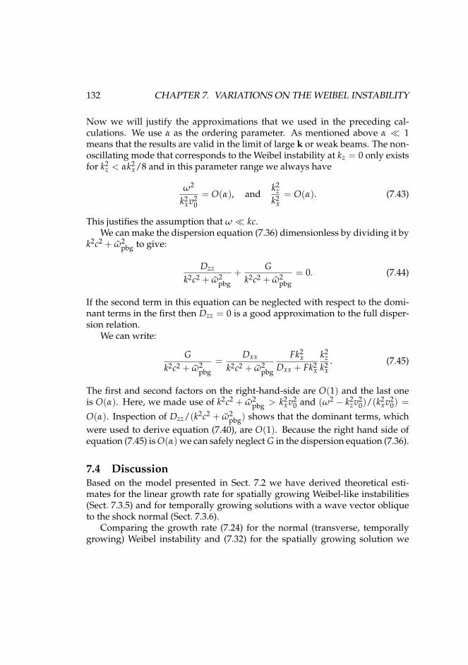
132 CHAPTER 7. VARIATIONS ON THE WEIBEL INSTABILITY
Now we will justify the approximations that we used in the preceding cal-culations. We use α as the ordering parameter. As mentioned above α 1means that the results are valid in the limit of large k or weak beams. The non-oscillating mode that corresponds to the Weibel instability at kz = 0 only existsfor k2
z < αk2x/8 and in this parameter range we always have
ω2
k2xv2
0= O(α), and
k2z
k2x
= O(α). (7.43)
This justifies the assumption that ω kc.We can make the dispersion equation (7.36) dimensionless by dividing it by
k2c2 + ω2pbg to give:
Dzz
k2c2 + ω2pbg
+G
k2c2 + ω2pbg
= 0. (7.44)
If the second term in this equation can be neglected with respect to the domi-nant terms in the first then Dzz = 0 is a good approximation to the full disper-sion relation.
We can write:
Gk2c2 + ω2
pbg=
Dxx
k2c2 + ω2pbg
Fk2x
Dxx + Fk2x
k2z
k2x
. (7.45)
The first and second factors on the right-hand-side are O(1) and the last oneis O(α). Here, we made use of k2c2 + ω2
pbg > k2xv2
0 and (ω2 − k2zv2
0)/(k2xv2
0) =
O(α). Inspection of Dzz/(k2c2 + ω2pbg) shows that the dominant terms, which
were used to derive equation (7.40), are O(1). Because the right hand side ofequation (7.45) is O(α) we can safely neglect G in the dispersion equation (7.36).
7.4 DiscussionBased on the model presented in Sect. 7.2 we have derived theoretical esti-mates for the linear growth rate for spatially growing Weibel-like instabilities(Sect. 7.3.5) and for temporally growing solutions with a wave vector obliqueto the shock normal (Sect. 7.3.6).
Comparing the growth rate (7.24) for the normal (transverse, temporallygrowing) Weibel instability and (7.32) for the spatially growing solution we
Magnetic Fields inside Extremely Fast Shock Waves by Jorrit Wiersma 133
see that they resemble each other closely. In particular, in the case of an ultra-relativistic streaming velocity the term containing (1 − v2
0) drops out of thedenominator of equation (7.24) and the only remaining difference is the factorv2
0 in the numerator. This proportionality of the growth rate with the streamingvelocity is one of the main properties of the Weibel instability. The co-movinggrowth rate ikzv0 with kz given by equation (7.32) has the same proportionality.
That the spatial Weibel instability so closely resembles the “normal” Weibelinstability may be an expected result, but there are some subtleties. For one,whereas the normal Weibel instability is an instability with wave vector k per-pendicular to the streaming velocity v0, this is not strictly true for the spatialcase because it has an imaginary component of k along v0. This is reflectedby the matrix M having non-zero off-diagonal components in the spatial case;see equation (7.25). The eigenvectors of the normal Weibel instability resultin a vector potential with only a z-component producing a transverse electricfield E = iωA/c and magnetic field B = ik×A, whereas the spatial instabilityinvolves a vector potential A = (Ax, 0, Az) and no electric field since ω = 0.Nevertheless, the dispersion relations (7.21) and (7.29) for the pertinent modesturn out almost identical, but only through a fortuitous cancellation of terms.
The calculations in this chapter do not include temperature effects. For anumerical solution of the oblique dispersion equation including temperatureeffects see the work of Bret et al. [10].
The presence of counterstreaming beams in a plasma modifies the skin ef-fect (the root in equation (7.31) with the minus sign) and creates the possibilityof a spatially growing mode that closely resembles the Weibel instability (theroot with the plus sign). We expect that this Weibel-like mode can model thequasi-stationary start of the shock ramp in collisionless shocks. With a suit-able model for the saturation level, our results might also help in numericalsimulations of the collisionless shock ramp as a starting point to speed the con-vergence to a quasi-stationary state.
In Sect. 7.3.6 we have also presented results for the temporally growingWeibel-like mode with a wave vector that is not strictly perpendicular to thebeam direction (kz 6= 0). The growth rate of the instability decreases slightlywith increasing kz (Fig. 7.2) up to kz/kx = (α/8)1/2, where α is defined inequation (7.39). At this value of kz the growth rate drops sharply and insteadof a purely growing instability, the modes change to overstable (growing os-cillating) waves. In most applications of the Weibel instability one either hasweak beams or large wave vectors (because the fast-growing modes typicallyhave small wave lengths) so that α is small. This implies that the dominantinstability only allows small kz. This shows that the linear theory predicts that
134 CHAPTER 7. VARIATIONS ON THE WEIBEL INSTABILITY
the initial Weibel instability is mostly transverse and produces steadily grow-ing currents parallel to the beam direction, which agrees with the results ofnumerical simulations [24, for example].
Chapter 8
Proton Weibel instability
In the previous two chapters we considered how the Weibel instability canproduce exponentially growing magnetic fields. What we are interested in nowis when the growth of the magnetic field will stop. In this chapter I present anestimate for the attainable magnetic field for the specific case of protons in abackground of electrons. This case is interesting because we expect that thekinetic energy of the electrons can get thermalized much more quickly thanthe kinetic energy of the protons because electrons are so much lighter in mass.However, most of the kinetic energy is carried by the protons because of theirlarge mass so we might expect the instability to continue for the protons whenthe instability of the electrons has already ended.
In this chapter I show how magnetic trapping of the protons predicts thatthe proton currents cannot grow much stronger than the electron currents sothat surprisingly little of the kinetic energy of the protons can be used by theWeibel instability to produce magnetic fields. In chapter 9 we present moregeneral results regarding the end of the Weibel instability and a more in-depthlook at the mechanisms responsible for this chapter’s result.
This chapter was published in Astronomy & Astrophysics [100].
135
136 CHAPTER 8. PROTON WEIBEL INSTABILITY
8.1 IntroductionMagnetic field generation in relativistic shocks in a hydrogen (electron-proton)plasma is important for the fireball model for Gamma-ray Bursts [79, for ex-ample]. This model proposes that the non-thermal radiation we observe in theprompt and afterglow emission from the Gamma-ray Burst is synchrotron ra-diation from collisionless relativistic shocks. To explain the observed intensityof the afterglows as synchrotron emission, the models need a magnetic fieldstrength B of at least ten per cent of the equipartition field strength [32, 72].This means that the magnetic energy density must contribute about one to tenper cent to the total energy density of the plasma behind the shock: B2/8π ∼(0.01− 1)× e, with e the post-shock thermal energy density. In electron-protonplasmas this implies a much stronger magnetic field than in pair plasmas be-cause the energy density in an ultra-relativistic shock propagating into a coldmedium (where nmc2 P, with n the number density, m the rest mass and Pthe thermal pressure) is roughly proportional to the rest mass m of the particles.In this chapter, we look at what happens in a plasma consisting of particles ofwidely different mass.
In collisionless shocks, plasma instabilities can generate magnetic fields.Within the shock transition layer the relative motion of the mixing pre- andpost-shock plasma produces very anisotropic velocity distributions for all par-ticle species concerned. Fluctuating electromagnetic fields deflect the incomingcharged particles and act as the effective collisional process needed to completethe shock transition [e.g., 38]. These fluctuating fields occur naturally becauseanisotropic velocity distributions are unstable against several plasma instabil-ities, such as the electrostatic two-stream instability and the electromagneticWeibel instability. The first is an instability of (quasi-)longitudinal charge den-sity perturbations and leads to fluctuating electric fields satisfying |E| |B|where E and B are the fluctuating electric and magnetic fields. The second isan instability of the advection currents (proportional to the beam velocity) thatresult from charge bunching in the beams, and leads to spontaneously growingtransverse waves [98] with |B| ≥ |E|. In a relativistic shock, where the relativevelocity of the pre- and post-shock plasma approaches the velocity of light, theWeibel instability dominates because it has the largest growth rate [12].
As both analytical estimates and numerical simulations show, the Weibelinstability in pair plasmas can produce a magnetic field of near-equipartitionstrength [21, 33, 45, 58, 104]. In numerical simulations, the magnetic field gen-eration always undergoes an exponentially growing phase that agrees with theestimates from linear analytical theory, and enters a nonlinear phase after that.
Magnetic Fields inside Extremely Fast Shock Waves by Jorrit Wiersma 137
Yang et al. [104] have shown that in pair plasmas, the magnetic field strengthreaches its maximum value at the end of the linear phase of the instability. Thequestion arises whether the same holds true for the Weibel instability operat-ing in an electron-proton plasma [58]. Numerical simulations [24] show thatthe nonlinear phase may be more important in electron-ion plasmas.
In this chapter we present an analytical estimate that shows that the lin-ear phase of the instability ends much earlier for proton beams in a hydrogenplasma than for electron(-positron) beams in a pair plasma. We do not presenta full self-consistent shock model: rather we consider the plasma processes thatcould generate a magnetic field in a plasma with properties such as one expectsnear the front of a collisionless relativistic shock. The chapter is organized asfollows. In section 8.2 we define a model for the shock situation in terms ofthe momentum distributions of the particles. We calculate the conditions forthe instability in section 8.3.1 and the magnetic field strength at the end of thelinear phase of the instability in section 8.3.2. In section 8.3.3, we comparethe energy density associated with this magnetic field strength with the totalavailable energy density associated with the beams. Section 8.4 contains thediscussion and section 8.5 the conclusions.
8.2 A simple model for a relativistic shock transitionIn an electron-proton plasma, the protons dominate the shock energetics be-cause they have a much larger rest mass than the electrons. Therefore, we willstudy the proton-driven Weibel instability. In this section we present a simplemodel for the plasma in the transition layer at the front of the shock.
The plasma in an astrophysical relativistic shock does not necessarily be-have as a single fluid. Coulomb collisions between electrons and protons arenot sufficiently fast to create thermal equilibrium between the protons and elec-trons. This problem of the non-equilibration of the electron and ion energiesalready exists in the much slower (∼ 1000 km/s) shocks associated with Su-pernova Remnants [19, 95].
We assume that scattering by plasma waves is far more efficient for thelight electrons than for the heavy ions so that when the trajectories of the in-coming protons start to become significantly perturbed, the electrons have al-ready undergone the fast-growing electron Weibel instability [24, 58], whichhas converted the kinetic energy of their bulk motion into the thermal energyof a relativistically hot electron plasma with an (almost) isotropic thermal ve-locity distribution. The incoming protons form, seen from the rest frame of thehot electrons, a relativistic beam. We also assume that part of the protons are
138 CHAPTER 8. PROTON WEIBEL INSTABILITY
reflected further downstream although that assumption is not critical for ourfinal conclusions (see section 8.6).
The electron-driven Weibel instability produces a weak fluctuating mag-netic field with B2/8π ∼ ee, with ee the energy density of the shocked elec-trons. We ignore this magnetic field in the calculations for proton beams, but itcould serve as a seed perturbation for the proton-driven Weibel instability.
8.2.1 The proton velocity distributionA simple model for the anisotropic proton velocity distribution within theshock transition layer is a waterbag distribution [89, 105]. We consider a similarsituation as in Fig. 6 of Frederiksen et al. [24]: we take two counter-streamingproton beams moving along the z-direction, with a small velocity spread in thex-direction to model thermal motions:
F(p) =np
4px0[Θ(px + px0)−Θ(px − px0)]
× δ(py) [δ(pz − pz0) + δ(pz + pz0)] .(8.1)
Here np is the total proton density, pz0 is the bulk momentum of the protonbeams, px0 is the maximum momentum in thermal motions and Θ(x) = (1 +x/|x|)/2 is the Heaviside step function. The assumption of two beams of equalstrength is mathematically convenient, but not essential (see section 8.6).
This is a simple model that mimics the properties of non-relativistic col-lisionless shocks [see the Microstructure section in 93] in which (partial) re-flection of the ions occurs as a result of deflection by an electrostatic potentialjump in the shock transition, or by ‘overshoots’ in the strong magnetic fieldin the wake of the shock. In addition, the waterbag model accounts for partialion heating by including a velocity dispersion in the direction perpendicular toboth the beam direction and the wave magnetic field. This direction lies alongthe wave vector of the unstable modes (the x-direction in our configuration).
8.2.2 The shock conditions for the electronsWe assume that the electrons have (almost) completed the shock transition sothat their properties obey the relativistic shock conditions [8], which followfrom the generally valid conservation laws for particle number, energy andmomentum (see chapter 5).
Here and below, we will label properties of the post-shock electron plasmawith subscript 2, and those of the pre-shock plasma with subscript 1. We willassume that the pre-shock plasma is cold in the sense that ee,1 ne,1mec2. Then
Magnetic Fields inside Extremely Fast Shock Waves by Jorrit Wiersma 139
the shock conditions for the proper density ne and the proper energy density eefor the electrons are:
ne,2 = (4γrel + 3)ne,1,
ee,2 = (4γrel + 3)γrelne,1mec2,(8.2)
where γ2rel = 1 + u2
z0 is the Lorentz factor of the relative velocity between thepre- and post-shock plasma (with uz0 = pz0/mpc).
We neglect the dynamical influence of a pre-shock magnetic field on theelectron-fluid jump conditions. This influence will be small if VAe,1 c whereVAe,1 ≡ B1/
√4πne,1me is the Alfven speed based on the electron mass (instead
of the proton mass). We also neglect any large-scale electrostatic field in theshock that might accelerate the electrons to higher energies while deceleratingthe incoming protons.
8.3 The Weibel instability8.3.1 The dispersion relationWe consider the instability of a purely transverse electromagnetic wave withwave vector k = kex and frequency ω. The instability will grow with a rateequal to the imaginary part of the wave frequency: σ = =(ω).
The Weibel instability for the model of the previous section obeys a disper-sion relation of the form [e.g., 89]
k2c2 −ω2 [ 1 + χzz(ω, k) ] = 0, (8.3)
where χzz(ω, k) ≡ χzz,e(ω, k) + χzz,p(ω, k) is the zz-component1 of the plasmasusceptibility tensor, which contains contributions of both the electrons and theprotons.
Since the electrons have a relativistically hot thermal velocity distributiontheir contribution is
χzz,e(ω, k) = −ω2
pe
ω2 , (8.4)
where ωpe is the electron plasma frequency (in Gaussian units):
ω2pe =
4πq2ne,2
meh, (8.5)
1Note that we have changed the notation (x ↔ z) from the published article to be consistentwith the rest of this thesis.
140 CHAPTER 8. PROTON WEIBEL INSTABILITY
with ne the electron proper density, q the electron charge, me the electron massand h = (ee + Pe)/(nemec2) ' 4ee/(3nemec2) the electron enthalpy per unitrest energy for the relativistically hot electrons with ee ' 3Pe nemec2. If weassume that the electrons are fully shocked, the shock conditions (8.2) enableus to express ωpe in terms of the pre-shock electron number density:
ω2pe =
12πq2ne,1
me
(4γrel + 3
4γrel
). (8.6)
The factor between brackets approaches unity in ultra-relativistic shocks withγrel 1.
The proton contribution to dispersion relation (8.3) is [see 89]
χzz,p(ω, k) = −ω2
pp
γb0 ω2
(F +
k2v2z0
ω2 − k2v2x0
), (8.7)
with
F =c
2vx0ln(
c + vx0
c− vx0
)−
u2z0
1 + u2z0
. (8.8)
(see also chapter 6). Here ωpp =√
4πq2np/mp is the (non-relativistic) protonplasma frequency based on the density in the lab frame, mp is the proton restmass, ui = pi/(mpc), γb0 = (1 + u2
x0 + u2z0)
1/2 and vi = uic/γb0. To ensurequasi-neutrality of the plasma we must have
np ≈ ne,2, (8.9)
and the associated plasma frequency is
ω2pp = (4γrel + 3)
4πq2ne,1
mp. (8.10)
For what follows it is convenient to introduce the frequency ωpp defined by
ω2pp =
ω2pp
γb0. (8.11)
If the velocity dispersion in the beam is small, which is always true for aWeibel-unstable proton distribution (see the end of this section), we have γb0 'γrel so that
ω2pp
ω2pe' 4me
3mp. (8.12)
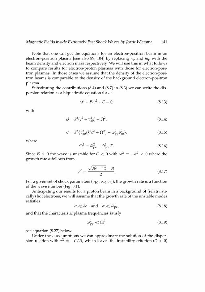
Magnetic Fields inside Extremely Fast Shock Waves by Jorrit Wiersma 141
Note that one can get the equations for an electron-positron beam in anelectron-positron plasma [see also 89, 104] by replacing np and mp with thebeam density and electron mass respectively. We will use this in what followsto compare results for electron-proton plasmas with those for electron-posi-tron plasmas. In those cases we assume that the density of the electron-posi-tron beams is comparable to the density of the background electron-positronplasma.
Substituting the contributions (8.4) and (8.7) in (8.3) we can write the dis-persion relation as a biquadratic equation for ω:
ω4 − Bω2 + C = 0, (8.13)
with
B = k2(c2 + v2x0) + Ω2, (8.14)
C = k2v2x0(k2c2 + Ω2)− ω2
ppv2z0, (8.15)
whereΩ2 ≡ ω2
pe + ω2pp F . (8.16)
Since B > 0 the wave is unstable for C < 0 with ω2 ≡ −σ2 < 0 where thegrowth rate σ follows from
σ2 =
√B2 − 4C − B
2. (8.17)
For a given set of shock parameters (γb0, vx0, n0), the growth rate is a functionof the wave number (Fig. 8.1).
Anticipating our results for a proton beam in a background of (relativisti-cally) hot electrons, we will assume that the growth rate of the unstable modessatisfies
σ kc and σ ωpe, (8.18)
and that the characteristic plasma frequencies satisfy
ω2pp Ω2, (8.19)
see equation (8.27) below.Under these assumptions we can approximate the solution of the disper-
sion relation with σ2 ' −C/B, which leaves the instability criterion (C < 0)
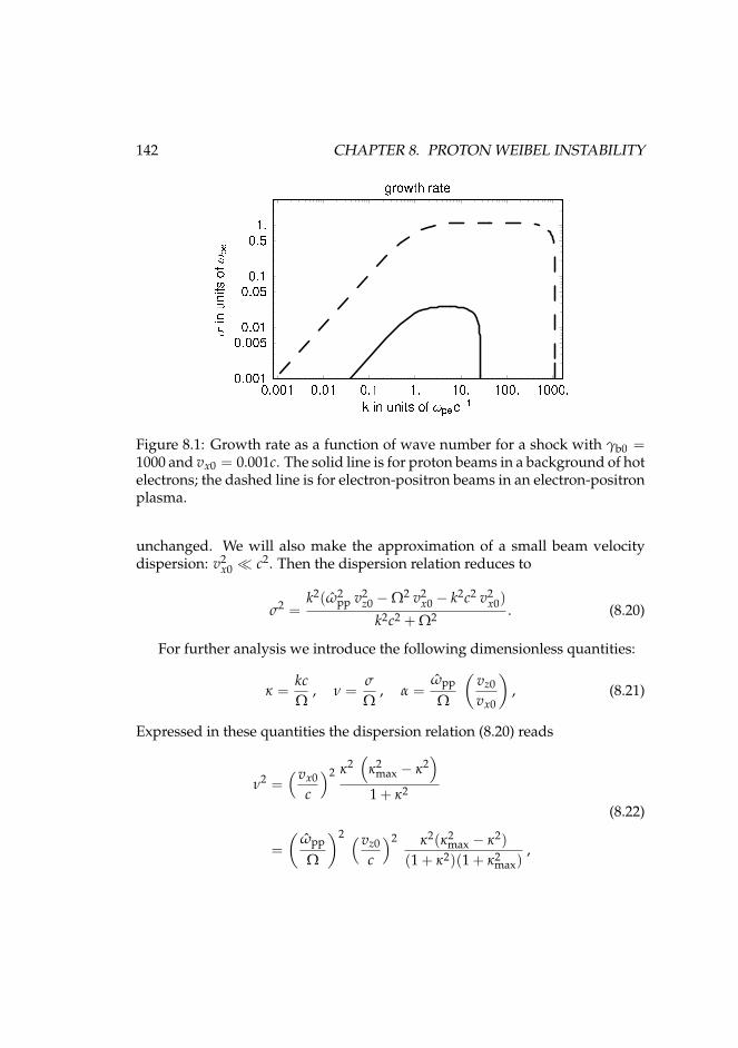
142 CHAPTER 8. PROTON WEIBEL INSTABILITY
Figure 8.1: Growth rate as a function of wave number for a shock with γb0 =1000 and vx0 = 0.001c. The solid line is for proton beams in a background of hotelectrons; the dashed line is for electron-positron beams in an electron-positronplasma.
unchanged. We will also make the approximation of a small beam velocitydispersion: v2
x0 c2. Then the dispersion relation reduces to
σ2 =k2(ω2
pp v2z0 −Ω2 v2
x0 − k2c2 v2x0)
k2c2 + Ω2 . (8.20)
For further analysis we introduce the following dimensionless quantities:
κ =kcΩ
, ν =σ
Ω, α =
ωpp
Ω
(vz0
vx0
), (8.21)
Expressed in these quantities the dispersion relation (8.20) reads
ν2 =(vx0
c
)2 κ2(
κ2max − κ2
)1 + κ2
=(
ωpp
Ω
)2 (vz0
c
)2 κ2(κ2max − κ2)
(1 + κ2)(1 + κ2max)
,
(8.22)
Magnetic Fields inside Extremely Fast Shock Waves by Jorrit Wiersma 143
where we have eliminated vx0 using the definition of α and we define
κmax ≡√
α2 − 1, (8.23)
which is the limiting wavenumber of the Weibel instability: the instability con-dition is satisfied for κ < κmax. The parameter α is a measure for the rangeof unstable wave numbers. The Weibel instability occurs only if α > 1. Thiscondition poses a restriction on the velocity spread vx0:
vx0
vz0<
ωpp
Ω. (8.24)
The quantity Ω depends on vx0 through equations (8.16) and (8.8), but a quickinspection shows that F and Ω are increasing functions of vx0 so if condi-tion (8.24) holds, then we also have
vx0
vz0<
ωpp
Ω|vx0=0=
ωpp
(ω2pe + ω2
pp/γ2rel)
1/2. (8.25)
It follows that for relativistic shocks with vz0 → c the proton-driven instabilityrequires vx0 c so that
F ' 1γ2
b0+
v2x0
3c2 1, (8.26)
andΩ ' ωpe ωpp (8.27)
(see equation 8.12).The largest growth rate occurs for a mode with wave number k∗, which fol-
lows from (dσ/dk)k=k∗ = 0. Using the approximated dispersion relation (8.22)we find that this wavenumber equals
k∗cΩ
≡ κ∗(α) =√
α− 1 , (8.28)
with the corresponding growth rate
σ(k∗)Ω
≡ ν∗ = (α− 1)vx0
c
=α− 1
α
(ωpp
Ω
)vz0
c.
(8.29)
144 CHAPTER 8. PROTON WEIBEL INSTABILITY
In the last equality we have used the definition of α. For a strong, relativisticshock we find σ(k∗) ' ωpp.
In view of this fact and equation (8.27), conditions (8.18) and (8.19) auto-matically hold for the proton-driven Weibel instability.
8.3.2 Stabilization of the Weibel instabilityThe linear phase of the Weibel instability (during which perturbations growexponentially with time) ends when the generated electromagnetic fields sig-nificantly perturb the trajectories of the particles taking part in the instability.Because the magnetic fields generated by the instability are inhomogeneous,the particles will quiver under the influence of the Lorentz force. When theamplitude of these quiver motions exceeds the wavelength of the instability,the linear theory breaks down. Yang et al. [104] give a full treatment of thesequiver motions and show that this criterion agrees with the magnetic trappingargument, which says that the instability will stop when the wave magneticfield becomes so strong that it traps the beam particles (see also chapter 9).
The linearized equation describing the quiver motions in the x-direction fora beam particle in a magnetic field B(x, t) ey reads:
d2ξx
dt2 =qvz0 B(x, t)
γb0mpc, (8.30)
where ξx is the displacement. In the linear stage of the instability the wavemagnetic field varies as B(x, t) = |B| exp(σt) sin(kx) for a wave with wavenumber k and growth rate σ, so the amplitude of the quiver motion is
|ξx| ∼q|B|vz0
γb0mpcσ2 . (8.31)
The trapping criterion k|ξx| < 1 corresponds to |B| < Btrap with
Btrap =γb0mpcσ2(k)
kvz0q. (8.32)
This corresponds to equation (18) of Yang et al. [104]. Assuming that trappingsaturates the Weibel instability at all wavelengths we get the typical field am-plitude as a function of wavenumber (Fig. 8.2).
The maximum field amplitude is reached at those wave numbers whereσ2/k has the maximum value. For dispersion relation (8.22) this maximum is
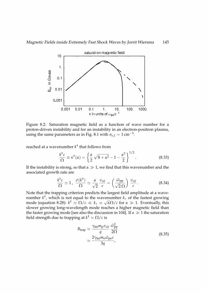
Magnetic Fields inside Extremely Fast Shock Waves by Jorrit Wiersma 145
Figure 8.2: Saturation magnetic field as a function of wave number for aproton-driven instability and for an instability in an electron-positron plasma,using the same parameters as in Fig. 8.1 with ne,1 = 1 cm−3.
reached at a wavenumber k† that follows from
k†cΩ
≡ κ†(α) =
α
2
√8 + α2 − 1− α2
2
1/2
. (8.33)
If the instability is strong, so that α 1, we find that this wavenumber and theassociated growth rate are
k†cΩ
' 1 ,σ(k†)
Ω' α√
2vx0
c=(
ωpp√2 Ω
)vz0
c. (8.34)
Note that the trapping criterion predicts the largest field amplitude at a wave-number k†, which is not equal to the wavenumber k∗ of the fastest growingmode (equation 8.28): k† ' Ω/c k∗ '
√αΩ/c for α 1. Eventually, this
slower growing long-wavelength mode reaches a higher magnetic field thanthe faster growing mode [see also the discussion in 104]. If α 1 the saturationfield strength due to trapping at k† ' Ω/c is
Btrap 'γb0mpvz0
qω2
pp
2Ω
'2γb0meωpec
3q,
(8.35)
146 CHAPTER 8. PROTON WEIBEL INSTABILITY
where we have used equations (8.12) and (8.27) to eliminate ωpp and Ω.For parameters typical for the external shock associated with Gamma-ray
Bursts we haveBtrap ' 3.7
√n1 γ1000 Gauss, (8.36)
with n1 = n0/(1 cm−3) and γ1000 = γb0/1000.We should note that Medvedev and Loeb [58] use a different method for
estimating B: they propose that the instability saturates when the beam ionsbecome magnetized. This happens when the Larmor radius rL = γvmc2/qBof the beam particles in the generated magnetic field becomes smaller thanthe wavelength of the fastest growing mode of the instability. This criterionk∗rL < 1 corresponds to |B| < Bmagn with
Bmagn =γb0vz0mpck∗
q, (8.37)
with k∗ given by equation (8.28). However, the trapping argument predicts thesmallest saturation amplitude |B|. In particular, we have
Btrap
Bmagn=
σ2(k†)k†k∗v2
z0=(
ωpp
Ω
)2Φ(α), (8.38)
where
Φ(α) ≡ κ†(α)α2√
α− 1
(3α−
√8 + α2
√8 + α2 − α
). (8.39)
To derive this relation we have used definition (8.21) to write
vx0/vz0 = ωpp/(αΩ).
For a proton beam in a hot electron background we have ω2pp/Ω2 1 and
Φ(α) < 0.3 for all α ≥ 1. For a strong instability with α 1 we have Φ(α) '(4α)−1/2 1. Therefore, trapping occurs well before the field can totally mag-netize a proton beam with a density comparable to the density of the hot back-ground electrons. In view of this we will use Btrap as an estimate of the satura-tion magnetic field strength (see also section 9.2).
The criteria (8.32) and (8.37) predict the typical amplitude of the magneticfield as one particular wave mode k saturates. In a realistic situation the in-stability will involve a superposition of wave modes and one should interpretB as the amplitude that follows from the power spectrum IB(k) of the field
Magnetic Fields inside Extremely Fast Shock Waves by Jorrit Wiersma 147
fluctuations: B2/8π ∼ kIB(k) with k ≈ k∗ for magnetization and k ≈ k† fortrapping. The total magnetic energy in the unstable modes is
UB =B2
8π=∫ kmax
0dk IB(k). (8.40)
8.3.3 The equipartition parameterA measure of the strength of the magnetic field is the equipartition parameter,which compares the energy density in the magnetic field with the total energydensity.
The protons dominate the energy budget, and the total available energydensity is
ep =∫
dp F(p)γ(p)mpc2 ' γb0npmpc2, (8.41)
where the approximation is valid for vx0 vz0.We define the proton equipartition parameter as
εB =B2
trap
8πep. (8.42)
Using equation (8.35) for the magnetic field, with the definition (8.11) for ωppand the approximation vz0 ' c for relativistic shocks we get
εB =ω2
pp
8Ω2 . (8.43)
Then from equations (8.12) and (8.27) we have
εB 'me
6mp∼ 10−4 . (8.44)
8.4 DiscussionThe small value of the equipartition parameter (8.44) implies that the proton-driven Weibel instability in a background of relativistically hot electrons sat-urates long before the magnetic field reaches equipartition with the availableproton free energy. Equation (8.25) demonstrates that the proton-driven Weibelinstability in a hydrogen plasma is not a suitable candidate for the mechanismresponsible for ‘thermalization’ of the incoming protons in the shock layer. In
148 CHAPTER 8. PROTON WEIBEL INSTABILITY
electron(-positron) beams in a hot pair background the instability condition,α > 1, allows a large beam velocity dispersion: vx0/vz0 ≤ 1 if the number den-sities in the beam and in the hot background are of similar magnitude [see also105]. Therefore, the Weibel instability is in principle capable of randomizing asignificant fraction of the beam momentum of an electron(-positron) beam, asasserted in section 8.2, whereas this is not true for a proton beam in a hydrogenplasma.
In the limit of a cold, relativistic proton beam the properties of the elec-trons and not those of the protons determine many of the results. The electronplasma frequency determines the wave number (8.33) of the mode with themaximum magnetic field so that the electron skin depth c/ωpe sets the lengthscale of the dominant mode. This happens because the low inertia of the elec-trons makes them very responsive to the perturbations of the protons. Thedispersion relation for the Weibel modes (Fig. 8.1), also supports this view:the plateau around the maximum growth rate starts roughly at a wave num-ber k ∼ ωpe/c. Studies that do not include the response of the backgroundelectrons (by treating the protons as an isolated system) miss this point. Thepeak magnetic field (8.35) does not contain any parameters connected withthe protons. Therefore, proton beams in a hydrogen plasma generate nearlythe same magnetic field strength as electron(-positron) beams in an electron-positron plasma (Fig. 8.2) despite the larger kinetic energy of the protons.
Gruzinov [31] anticipated this when he excluded the case where a smallparameter in the theory might be important in his analysis of the Weibel in-stability: our analysis shows that the relevant small parameter is ω2
pp/Ω2 ∼4me/3mp. The result is a small equipartition parameter (8.44). In this respectour result is similar to the one found by Sagdeev [82, p. 88], who argued for theWeibel instability in a non-relativistic plasma that the electrons have a quench-ing effect on the ion instability.
In our analysis we have excluded electrostatic waves, which could also playan important role in the shock transition zone [88]. In that case electrostaticBremsstrahlung could be an alternative explanation for the Gamma-ray Burstafterglow emission [85], relaxing the need in synchrotron models for a highmagnetic field strength.
8.5 ConclusionsWe have presented an analytical estimate of the magnetic field produced atthe end of the linear phase of the Weibel instability at the front of an ultra-relativistic shock propagating into a cold hydrogen plasma, a situation that
Magnetic Fields inside Extremely Fast Shock Waves by Jorrit Wiersma 149
applies to the external shocks that produce gamma-ray burst afterglows inthe fireball model [79]. The magnetic field strength that we find is too weakto explain the observed synchrotron radiation [32]: the equipartition parame-ter (equation 8.44) is at least two orders of magnitude too small. This is radi-cally different from the results for the Weibel instability in pair plasmas. Thereason is that the contribution of the electrons to the electromagnetic responseof the plasma inhibits the instability of the protons.
The saturation magnetic field (8.35) which this low equipartition parame-ter corresponds to is the magnetic field at the point where the linear approx-imation breaks down and where non-linear trapping effects start to limit thegrowth of the unstable Weibel mode. After this happens, it is likely that the in-stability enters a nonlinear phase or that another type of instability takes over:numerical simulations [24] of similar plasmas show near-equipartition mag-netic fields behind the Weibel-unstable region in the shock transition. The non-linear phase would then be the dominant phase in electron-ion plasmas anddeserves further study to determine the physical mechanism and the proper-ties of the resulting magnetic field.
8.6 Appendix: Asymmetric beamsWe consider asymmetric proton beams and show that we can neglect the ef-fect of the asymmetry for typical parameters. We replace the proton distribu-tion (8.1) by
F(p) =np
2px0
[1 + ∆
2δ(pz − pz0) +
1− ∆2
δ(pz + pz0)]
× δ(py) [Θ(px + px0)−Θ(px − px0)] ,(8.45)
with 0 ≤ ∆ ≤ 1 the parameter measuring the asymmetry between the twobeams. This asymmetry changes the dispersion relation of the waves to [6]:
k2c2 −ω2[
1 + χzz(ω, k)− χ2zx(ω, k)
1 + χxx(ω, k)
]= 0. (8.46)
The extra term ∝ χ2zx appears in relation (8.46) because the waves are no longer
transverse: the charge bunching of asymmetric beams produces a net chargedensity, leading to a component of the wave electric field along the wave vec-tor.
We will give the extra components of the susceptibility tensor and publisha derivation elsewhere (see chapter 6). The proton contribution to χzz(ω, k) is
150 CHAPTER 8. PROTON WEIBEL INSTABILITY
the same as in the symmetric case. For a thermal electron background with anisotropic momentum distribution, only the two proton beams contribute to theoff-diagonal components of the susceptibility tensor so that
χzx(ω, k) = χzx,p(ω, k) =∆ ω2
pp
ω2 − k2v2x0
kvz0
ω. (8.47)
This off-diagonal component vanishes in the symmetric case (∆ = 0). Thelongitudinal response of the beam-plasma system is contained in
1 + χxx(ω, k) = 1−ω2
pe
ω2 − k2C2e−
ω2pp
ω2 − k2v2x0
. (8.48)
Here C2e = 4Pe/3nemeh is the effective sound speed in the hot electron gas.
In the ultra-relativistic case one has Ce ' c/√
3. For proton beams in a hotelectron background one has ω2
pe ω2pp and |ω| ≤ ωpp kCe for the Weibel
instability (see section 8.3.1). This implies that
1 + χxx ' 1 +ω2
pe
k2C2e−
ω2pp
ω2 − k2v2x0
. (8.49)
The resulting dispersion relation can be written in terms of the dimension-less variable
Z(ω, k) ≡ω2 − k2v2
x0ω2
pp. (8.50)
One finds(Z −Z1) (Z + Z2)− ∆2 Z1Z2 = 0. (8.51)
Here Z1,2 are defined by
Z1 =k2C2
ek2C2
e + ω2pe
, Z2 =k2v2
z0k2c2 + Ω2 (8.52)
with Z2 > Z1 for the parameters considered here. The solution of this quadra-tic equation,
Z± =Z1 −Z2
2±
√(Z1 + Z2
2
)2− ∆2 Z1Z2, (8.53)
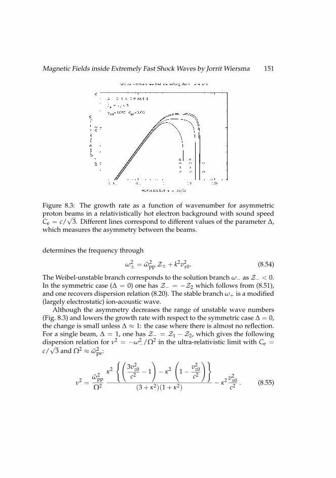
Magnetic Fields inside Extremely Fast Shock Waves by Jorrit Wiersma 151
Figure 8.3: The growth rate as a function of wavenumber for asymmetricproton beams in a relativistically hot electron background with sound speedCe = c/
√3. Different lines correspond to different values of the parameter ∆,
which measures the asymmetry between the beams.
determines the frequency through
ω2± = ω2
pp Z± + k2v2x0. (8.54)
The Weibel-unstable branch corresponds to the solution branch ω− as Z− < 0.In the symmetric case (∆ = 0) one has Z− = −Z2 which follows from (8.51),and one recovers dispersion relation (8.20). The stable branch ω+ is a modified(largely electrostatic) ion-acoustic wave.
Although the asymmetry decreases the range of unstable wave numbers(Fig. 8.3) and lowers the growth rate with respect to the symmetric case ∆ = 0,the change is small unless ∆ ≈ 1: the case where there is almost no reflection.For a single beam, ∆ = 1, one has Z− = Z1 − Z2, which gives the followingdispersion relation for ν2 = −ω2
−/Ω2 in the ultra-relativistic limit with Ce =c/√
3 and Ω2 ≈ ω2pe:
ν2 =ω2
pp
Ω2
κ2
(3v2
z0c2 − 1
)− κ2
(1−
v2z0
c2
)(3 + κ2)(1 + κ2)
− κ2 v2x0
c2 . (8.55)

152 CHAPTER 8. PROTON WEIBEL INSTABILITY
Chapter 9
The end of the Weibelinstability
When the particles inside a shock front undergo the Weibel instability theywill, at some point, start to feel the influence of the magnetic field that theygenerated themselves. This chapter considers some of the resulting effects:how the particles become trapped in the magnetic field, and how the sloshingmotion of the particles in the magnetic field diffuses the velocity distribution.These processes signal the end of the Weibel instability.
The electrical currents that the instability produces can keep growing if theymerge into larger currents, but we also show that this process will not providemuch additional gain because the plasma has the tendency to shield the inter-action of the electrical currents when they become too large.
This shows that the order of magnitude of the magnetic field strength pro-duced by the Weibel instability is of the order of the well-known magnetictrapping estimate, confirming the estimate in the previous chapter.
In the last sections of this chapter we discuss what this means for the roleof the Weibel instability in relativistic shock fronts. In particular, we discusshow the Weibel instability can cause the electrons in the shock front to converttheir energy into heat. The free energy of the heavier particles in the shockfront (protons and ions) cannot be converted into heat by the Weibel instability.Instead, these particles will heat up more slowly through their interaction withthe magnetic field that the Weibel instability leaves behind. The thermalizationlength scale of these heavy particles will determine the thickness of the shockfront.
This chapter has been submitted to Astronomy & Astrophysics [5].
153
154 CHAPTER 9. THE END OF THE WEIBEL INSTABILITY
9.1 IntroductionThe Weibel instability is a plasma instability that arises in plasmas with ananisotropic velocity distribution. This chapter discusses the nonlinear dynam-ics of the plasma in the late stages of this instability in the relativistic shockfronts that are produced by Gamma Ray Burst sources.
The prompt and afterglow emission from Gamma Ray Bursts (GRBs) is of-ten interpreted as synchrotron emission or as jitter radiation [56] from rela-tivistic electrons in a magnetic field. In order to explain the observed intensity,the magnetic field in the emission region must have a strength of 1 to 10% ofthe equipartition field strength Be, e.g. [102], which is defined in terms of theinternal (thermal) energy e of the plasma as
Be =√
8πe . (9.1)
This holds true for both the emission from internal shocks [see 80], which arebelieved to be responsible for the prompt emission, and for the emission fromexternal shocks [e.g. 79] which are believed to be the source of the afterglowemission. A full account of the observations and theory of GRBs can be foundin the reviews of Piran [74, 75] and of Meszaros [65, 66].
The strong magnetic fields associated with GRBs must somehow be self-generated by the strong (relativistic) shocks invoked in GRB models. In partic-ular for the external shocks the compression of interstellar/circumstellar mag-netic fields in a relativistic shock leads to B Be in the post-shock plasma (seesection 6.1).
It has been proposed (see [58] and [31]) that a plasma instability, the Weibelinstability, leads to the generation of the necessary magnetic fields. The ba-sic picture is that this instability operates in the shock transition layer, wherethe unshocked incoming plasma mixes with the (relativistically) hot shockedplasma. The mixture is unstable against the generation of low-frequency elec-tromagnetic waves with |ω| kc, where ω is the wave frequency and k =2π/λ is the wave number. This instability is due to the anisotropy of the mo-mentum distribution of the incoming plasma, which looks like a beam in thereference frame of the shocked plasma. Since Maxwell’s equations imply thatthe Fourier amplitudes E and B of the electric and magnetic fields associatedwith the instability satisfy the relation |E| ∼ (|ω|/kc) |B| |B|, the resultingturbulent electromagnetic field is almost purely magnetic.
Although it is now long known that the Weibel instability can generatemagnetic fields in relativistic shock fronts, estimates of the attainable magneticfield strength have been mostly restricted to ad hoc arguments. In this chapter
Magnetic Fields inside Extremely Fast Shock Waves by Jorrit Wiersma 155
we present an in-depth look into the nonlinear dynamics of a Weibel-unstableplasma to obtain a reliable foundation for our estimates of the attainable mag-netic field strength. In addition, we discuss the mechanisms that contribute tothe stabilization of the Weibel instability and the subsequent thermalization ofthe plasma.
Our calculations concentrate on the case of ultra-relativistic shocks (withLorentz factor γ 1). We will assume that we can model the plasma in theshock front with two symmetric counterstreaming plasmas because the effectof asymmetries is small (see section 6.9). We also take the beams to be cold, asone would expect in a shock front encountering the cold interstellar medium.At various points, we will take into account the presence of a relativisticallyhot stationary background plasma that corresponds to the already thermalizedpost-shock plasma. We discuss kinetic and fluid processes that take place ontime and length scales of the order of the plasma frequency and the plasmaskin depth respectively.
In the companion paper [3, chapter 6 in this thesis] we have consideredthe linear phase of the Weibel instability, where the magnetic field grows ex-ponentially in time. The main conclusions of chapter 6 can be summarized asfollows:
The growth rate of the instability due to two equal but counterstreaming beamsin the presence of a (hot) background plasma is mostly determined by twoparameters: η and M. The first parameter is defined as
η =(
ωpb/ωbg
)2, (9.2)
the square of the ratio of the effective plasma frequency ωpb of the beam parti-cles and the the plasma frequency ωbg of thermal background. In a hydrogenplasma, the background plasma frequency is almost entirely determined by thecontribution of the hot electrons and one has
ω2bg '
4πe2ne
mehe. (9.3)
Here he is the enthalpy per unit rest energy of the electron gas, with he ≈ 1 ifthe electron gas is cold so that kbTe mec2, and he ' kbTe/mec2 1 for arelativistically hot electron gas. The beam plasma frequency is
ω2pb =
4πq2bnb
mbhb, (9.4)
156 CHAPTER 9. THE END OF THE WEIBEL INSTABILITY
in terms of the charge qb and mass mb of the beam particles, their proper den-sity nb and the enthalpy per unit rest energy hb. When the beams are cold wehave hb ' 1.
The parameterM can be thought of as an effective ‘beam Mach Number’: itis a measure for the importance of the velocity dispersion in the beam plasma inthe direction perpendicular to the beam direction, which we will take along thez-axis. If the momentum of the directed motion of the beam particles is pz0 andif the typical momentum associated with the velocity dispersion perpendicularto the beam direction is px0, one has:
M ∼ pz0/px0 . (9.5)
A full set of definitions can be found in section 6.5, where both a fluid modeland a waterbag model employing kinetic theory are employed to describe thebeams. If the beams are cold one has M→ ∞. As we will see below, the valueof M together with η determines the range of unstable wavenumbers, and ηdetermines the maximum growth rate.
In the symmetric case the beam particles are distributed over two counter-streaming but otherwise identical beams, each with proper density nb/2. Inthis case there is a simple approximation for the growth rate of the instabilityin the limit of perturbations with the wavevector perpendicular to the beamdirection: k ·Vb = 0. This approximation is almost universally valid for ultra-relativistic beams (with pz0 mbc) if M 1, η ≤ 1 and ηM2 1, and stillgives a rather good approximation for η ∼ M ∼ 1. In terms of a dimensionlessgrowth rate and wavenumber, defined as1
σ ≡ Im(ω)/ωbg , κ ≡ kc/ωbg , (9.6)
one finds (chapter 6, equation 6.57):
σ2(κ) ≈ κ2
κ2s + κ2
(κ2
max − κ2
M2
). (9.7)
Here κs is the (dimensionless) wavenumber below which screening currentsin the background plasma slow the growth of the instability, see section 6.6,equation (6.46) and section 6.7, equations (6.57) and (6.60). In our applicationto ultra-relativistic beams one has κs ∼ 0.1− 1.
1Note that in this chapter we write k (rather than K as in chapter 6) for the wave number in thelaboratory frame, which coincides with the rest frame of the thermal plasma.
Magnetic Fields inside Extremely Fast Shock Waves by Jorrit Wiersma 157
The wavenumber κmax is the maximum unstable wavenumber that, in thelimit ηM2 1 that concerns us here, equals
κmax ≡√
ηM2 − 1 ≈ √η M . (9.8)
The maximum growth rate, which follows from dσ/dκ = 0, occurs at awavenumber κ∗, which for dispersion relation (9.7) is given by
κ∗ =(
κs
√κ2
max + κ2s − κ2
s
)1/2≈√
κsκmax . (9.9)
It equals σ(κ∗) ≡ σ∗, which is:
σ∗ =
√κ2
s + κ2max − κs
M≈ κmax
M=√
η . (9.10)
In these two expressions the last approximate terms on the right-hand side arevalid in the limit ηM2 1, when κmax κs.
This implies that the Weibel instability is most vigorous at wavelengthsshorter than the effective skin depth λsk ∼ c/ωbgκs of the hot backgroundplasma. The linear growth rate is almost independent of wavenumber, andclose to σ∗, on a broad ‘plateau’ in the wavenumber range corresponding toκs < κ < κmax, see figures 6.1 and 6.2 in chapter 6. The maximum unsta-ble wavelength is determined by the ‘temperature’ of the beam plasma, whichdetermines the value of M through the velocity dispersion of beam particlesalong the wave vector.
In the rest of this chapter we will discuss the stabilization of the Weibel in-stability and the subsequent evolution of the plasma. In section 9.2 we startoff with an overview of stabilization mechanisms that have already been dis-cussed in the literature. In section 9.3 we present a fluid model for the non-linear wave breaking of a single wave mode of the Weibel instability. In sec-tion 9.4 we briefly consider a kinetic model for the nonlinear dynamics of theWeibel-unstable plasma once a broad-band spectrum of unstable modes hasbeen excited. In section 9.5 we estimate whether and for how long the electri-cal currents can keep growing stronger after the instability itself has stabilized.Section 9.6 discusses the implications of our results for the plasma in an ultra-relativistic shock front, considering thermalization of the electrons and the ionsin the plasma separately. For the ions we estimate the thermalization lengthscale due to scattering in the turbulent magnetic fields produced by the Weibelinstability. In section 9.7 we summarize the conclusions that we draw from ourresults.
158 CHAPTER 9. THE END OF THE WEIBEL INSTABILITY
9.2 Stabilization mechanisms: an overviewA number of stabilization mechanisms have been proposed for the beam-dri-ven Weibel instability in an astrophysical context. In this section we comparetwo mechanisms employed in recent literature to estimate the attainable mag-netic field strength of the Weibel instability: magnetization of the plasma andmagnetic trapping of particles in the plasma wave fields. We will show thatthe latter gives the most stringent limit on the attainable magnetic field for theparameter regime that we are interested in.
Medvedev and Loeb [58] have proposed that the deflection of beam parti-cles in the self-generated magnetic field stabilizes the instability if the Larmorradius in this field becomes of the order of the wavelength of the most unstablemode. This essentially means that the beam particles become magnetized. Forsimplicity we consider the case of a cold beam.
The gyration radius rg of beam particles of mass mb, beam velocity Vb, bulk
(beam) Lorentz factor γb = 1/√
1−V2b /c2 and charge qb is of order:
rg =γbmbcVb
qbB=
VbΩg
. (9.11)
Here Ωg = qbB/γbmbc is the gyration frequency of the beam particles in amagnetic field of strength B. The corresponding stabilization criterion accord-ing to Medvedev and Loeb [58] reads:
k∗rg =k∗VbΩg
∼ 1 , (9.12)
with k∗ the wavenumber of the fastest growing mode. We will refer to this asthe magnetization criterion.
Alternatively, Yang et al. [104] have proposed that magnetic trapping ofparticles in the waves stabilizes the Weibel instability. This stabilization mech-anism was already considered by Davidson et al. [16] for the non-relativisticWeibel instability in a plasma with a temperature anisotropy. The same stabi-lization mechanism was briefly discussed by Gruzinov [31] in the context ofmagnetic field generation in GRB shocks.
The electromagnetic field of the waves produced by the instability willcause the beam particles to ‘quiver’. Trapping occurs when the amplitude ofthe quiver motion in the direction of the wave vector reaches an amplitudecomparable to the wavelength of the unstable mode. This quiver motion isinduced by the Lorentz force on the beam particles due to the wave magnetic
Magnetic Fields inside Extremely Fast Shock Waves by Jorrit Wiersma 159
field B = B(x , t) y. The equation of motion to first order in the wave amplitudereads (see also the more complete treatment below)
d2ξx
dt2 = − qbVbBγbmbc
, (9.13)
with ξx the displacement of a beam particle in the x-direction. For a magneticfield varying as B(x , t) = B0 exp(σt) sin(kx), with σ = Im(ω) > 0 the growthrate of the instability, one finds that the typical amplitude of the quiver motionis
|ξx| ≈∣∣∣∣ qbVbBγbmbcσ2
∣∣∣∣ . (9.14)
The stabilization condition reads [e.g. 17]
|k ξx| =∣∣∣∣k qbVbB
γbmbcσ2
∣∣∣∣ ∼ 1 . (9.15)
which we will refer to as the trapping criterion.As we pointed out in chapter 8, the trapping criterion (9.15) is the most
stringent criterion of the two for external GRB shocks, which have η ≤ 1, Vb 'c and M 1. This is easily checked for dispersion relation (9.7). From (9.12)and (9.15) one finds that the field amplitudes Bm and Btr predicted respectivelyby these two criteria are:
Bm ∼ γbmbc k∗Vbqb
, Btr ∼ γbmbc σ2(k†)qbk†Vb
. (9.16)
Here k† is the wavenumber where σ2(k)/k reaches its maximum value. Wedefine a third characteristic dimensionless parameter,
α ≡
√1 +
κ2maxκ2
s, (9.17)
with the beam-driven Weibel instability occurring for α > 1. The character-istic dimensionless wavenumbers κ∗ = k∗c/ωbg, κ† = k†c/ωbg and κmax =kmaxc/ωbg can be written in terms of α as
κmax = κs
√α2 − 1 , κ∗ = κs
√α− 1 , κ† = κs S(α) , (9.18)
160 CHAPTER 9. THE END OF THE WEIBEL INSTABILITY
with S(α) for dispersion relation (9.7) given by:
S(α) ≡
α
2
√8 + α2 − 1− α2
2
1/2
. (9.19)
The ratio of the field amplitudes Btr and Bm can be written for Vb ' c as
Btr
Bm =σ2
†κ†κ∗
=S(α)√
α− 1M2
(3α−
√8 + α2
√8 + α2 − α
), (9.20)
where σ† = σ(k†)/ωbg. For α 1 (ηM2 1) one has κmax ' α κs = √ηM,
κ∗ '√
α κs, κ† ' κs and σ† ' κmax/√
2M =√
η/2. In that case (9.20) reducesto
Btr
Bm ' η
2√
ακ2s
=η3/4
2κ3/2s M1/2
. (9.21)
For GRB external shocks, with η ≤ 1, α 1, M 1 and κs ≤ 1 one hasBtr Bm, and trapping rather than magnetization stabilizes the beam-drivenWeibel instability.
For the Weibel instability operating in the transition layer of an ultra-relati-vistic shock one expects η ≈ 1 for an electron(-positron) beam, and
η ≈ 4me/3mp ' 7× 10⁻⁴
for a proton beam in a hot electron background, see chapter 8 for more details.Since one must have M > 1 + 1/η for an instability to occur this implies thattrapping will occur long before the beam particles are fully magnetized so thatthe exponential growth of the magnetic field saturates at |B| ' Btr.
Figure 9.1 shows the characteristic wavenumbers κ∗ and κ† and κmax, andthe ratio of the field amplitudes at trapping and magnetization, Btr/Bm =σ2
† /κ†κ∗, all as a function of the parameter α for M = 100.
9.3 Nonlinear effects: fluid model for the beam responseWe now present calculations that justify the order-of-magnitude estimates ofthe previous section for two different situations. In this section we consider thenonlinear effects due to the Weibel instability using a fluid model. This allowsus to investigate the effect of nonlinear coupling, and in particular of wavebreaking of the Weibel mode when only a single dominant mode is present.In the next section we will consider the kinetic theory, which is appropriate
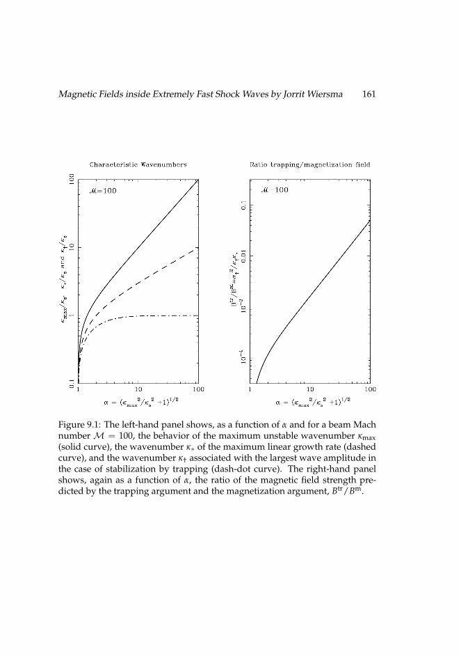
Magnetic Fields inside Extremely Fast Shock Waves by Jorrit Wiersma 161
Figure 9.1: The left-hand panel shows, as a function of α and for a beam Machnumber M = 100, the behavior of the maximum unstable wavenumber κmax(solid curve), the wavenumber κ∗ of the maximum linear growth rate (dashedcurve), and the wavenumber κ† associated with the largest wave amplitude inthe case of stabilization by trapping (dash-dot curve). The right-hand panelshows, again as a function of α, the ratio of the magnetic field strength pre-dicted by the trapping argument and the magnetization argument, Btr/Bm.

162 CHAPTER 9. THE END OF THE WEIBEL INSTABILITY
for a broad-band spectrum of unstable modes, and where phase mixing of thequiver motion in the collection of waves is the dominant stabilization process.
We will show that the wave breaking considered in this section will slowdown the exponential growth of individual wave modes and could even re-verse the growth. This wave breaking will, however, inevitably excite higherwave modes, leading to a broad-band spectrum of wave modes. When thathappens the stabilization mechanisms considered in the next section will de-scribe the plasma dynamics more accurately.
Note that for stable plasma modes (with a real frequency ω) a fluid calcula-tion such as presented below would yield the well-known equations for modecoupling, see for instance [28]. This leads to resonant interactions between dif-ferent waves (normal modes) of the form k1 ± k2 = k3, ω1 ± ω2 = ω3, wherethe indices enumerate the different wave modes. However, in the case of theunstable Weibel modes considered here such resonances do not occur as ω ispurely imaginary, and the interactions are qualitatively different. In particular,we will show below that the dominant effect is through the nonlinear distor-tion of the wave profile, not unlike what happens to large-amplitude electronplasma oscillations in a cold plasma, see Davidson [17], Ch. 3. This is a non-resonant process.
In order to keep the mathematics tractable we make a number of simplify-ing assumptions:
1. We treat the symmetric case with two oppositely directed beams of equalstrength propagating along the z-axis with velocity V± = ±Vb z. In thatcase the linear Weibel mode is purely electromagnetic. We also assumethat all electromagnetic fields vary as plane waves in the x-direction (k =k x), so that E(x , t), B(x , t) ∝ exp(ikx − iωt). The Fourier amplitudes Band E⊥ of the electromagnetic field then satisfy
B = B(k , ω) y , E⊥ = E⊥(k , ω) z = −ω
kcB(k , ω) z . (9.22)
The last relation follows from Faraday’s law: c(curl E) + ∂B/∂t = 0. Herewe use the subscript ⊥ to distinguish the transverse electric field (withk · E⊥ = 0) from the longitudinal electric field E‖ that is introduced below.
2. We consider the wavelength range where |ω|/kc 1. For the low-frequency electromagnetic Weibel mode this implies that the magnetic
Magnetic Fields inside Extremely Fast Shock Waves by Jorrit Wiersma 163
field amplitude is much larger than the amplitude of the transverse elec-tric field: ∣∣B(k, ω)
∣∣ =∣∣∣∣ kc
ω
∣∣∣∣ ∣∣E⊥(k, ω)∣∣ ∣∣E⊥(k, ω)
∣∣ .
3. For the moment we will neglect pressure effects in the beam dynamics,putting the kinetic temperature of the beam particles equal to zero.
In this case, the equation of motion for the fluid of beam particles is formallythe same as that for a single particle of mass mb and charge qb:
dpdt
= qb
(E +
V× Bc
). (9.23)
Here p(x , t) is the momentum of the fluid, defined as usual in terms of thefluid velocity V(x , t) as
p = γmbV =mbV√
1−V2/c2. (9.24)
The time-derivative in equation (9.23) should be interpreted as the convective(Lagrangian) time derivative,
ddt≡ ∂
∂t+ V · grad . (9.25)
We consider the symmetric case with two counterstreaming but otherwiseidentical beams, directed along the z-axis. Each beam has an unperturbed lab-oratory frame density n+ = n− = nb/2. Here, and in what follows, we use asubscript ± to distinguish quantities associated with the forward beam (withunperturbed velocity V = +Vb z) and the backward beam (with unperturbedvelocity V = −Vb z) . The density satisfies the continuity equation,
∂n±∂t
+ div (n±V±) = 0 . (9.26)
Note that the proper density of each of the two beams is n0± = n±/γ±. Finally,the charge density and current density associated with the two beams is
ρ± = qbn± , J± = qbn± V± . (9.27)
164 CHAPTER 9. THE END OF THE WEIBEL INSTABILITY
9.3.1 Dynamics of the beam particlesThe equation of motion in the x and z direction reads respectively:
(∂
∂t+ Vx
∂
∂x
)px = qb
(E‖ −
Vz
cB)
; (9.28)
(∂
∂t+ Vx
∂
∂x
)pz = qb
(E⊥ +
Vx
cB)
. (9.29)
The y-component reads dpy/dt = 0, and we can put py = 0.The transverse electromagnetic fields are associated with the Weibel mode,
and can be written in terms of a vector potential A = A(x , t) z:
E⊥ = −1c
∂A∂t
, B = −∂A∂x
. (9.30)
The longitudinal electric field can be derived from a scalar potential Φ(x , t):
E‖ = −∂Φ∂x
. (9.31)
In the Weibel instability of two counterstreaming beams of equal density (n+ =n−) this longitudinal field is absent in the linear approximation, and can onlybe nonlinearly excited by the beams (see section 6.3).
If one substitutes these definitions into the z-component of the equation ofmotion (equation 9.29) one finds that it can be written as(
∂
∂t+ Vx
∂
∂x
)(pz +
qbc
A)
=dPz
dt= 0 , (9.32)
with Pz ≡ pz + qbc A the z-component of the canonical momentum. This can
immediately be integrated to
Pz = pz +qbc
A = constant , (9.33)
the conservation of the canonical momentum in the z-direction, which arises asz is an ignorable coordinate. If one turns on the waves adiabatically, it followsthat one must have
(Pz)± = ±mbγbVb , (9.34)
Magnetic Fields inside Extremely Fast Shock Waves by Jorrit Wiersma 165
i.e. the canonical momentum in the z-direction equals the unperturbed beammomentum.
We expand all fields as plane waves by defining the Fourier amplitudes forthe vector and scalar potentials: A(x , t)
Φ(x , t)
=∫
dk dω
(2π)2
A(k, ω)
Φ(k, ω)
exp(ikx− iωt) . (9.35)
Maxwell’s equations imply that the Fourier components of the electric andmagnetic field are
E⊥ =iωc
A , B = −ik A , E‖ = −ik Φ . (9.36)
In addition, we will assume that the beams are ultra-relativistic, with γb 1.It is easily checked that the motion induced by the low-frequency Weibel
mode in an ultra-relativistic beam is almost one-dimensional with the per-turbed velocity directed along the x-axis. One can use a standard perturba-tion expansion [e.g. 60, Ch. 2] in terms of the field amplitudes, by writing themomentum of beam particles as
p = ±γbmb Vb z + p(1) + p(2) + · · · (9.37)
and solving the equation of motion order-by-order. Here |p(n)| ∝ |A|n is then-th order momentum perturbation. A similar expansion can be written downfor the velocity: V = ±Vb z + V(1) + V(2) + · · · , where one must use V =
cp/√
p2 + m2bc2 to relate the terms in the momentum and velocity expansions.
The first-order terms in this expansion can be found written out explicitly inMelrose [60], p. 18. In our application of the theory we will exploit the fact thatthere are (by assumption) two small parameters: 1/γb 1 and |ω/kc| 1.Using this, one finds from the general perturbation expansion that the first-order velocity perturbations in the beam satisfy∣∣∣∣∣ V(1) z(k , ω)
V(1) x(k , ω)
∣∣∣∣∣ =1
γ2b
∣∣∣∣ ω
kVb
∣∣∣∣ ≈ 1γ2
b
∣∣∣ω
kc
∣∣∣ 1. (9.38)
Here V(1)(k, ω) is the Fourier component of the linear velocity perturbation,defined in a manner analogous to equation (9.35). This implies that one can
166 CHAPTER 9. THE END OF THE WEIBEL INSTABILITY
neglect the wave-induced motion along the beam direction (along the z-axis) tofirst order. It can be shown that a similar conclusion holds for the higher-ordervelocity perturbations V(2)(k, ω) , V(3)(k, ω) · · · . This allows one to approxi-mate the equation of motion (9.28) by(
∂
∂t+ V±
∂
∂x
)V±(x , t) =
qbE±(x , t)γbmb
. (9.39)
Here we have written V±(x , t) for the x-component Vx(x , t) of the velocity forthe forward and backward beam. Note that this velocity component vanishesfor the unperturbed beam, so that V± = V±(1) + V±(2) + · · · in a perturbationexpansion. We also define
E±(x , t) = E‖ ∓Vbc
B ≈ E‖ ∓ B . (9.40)
The last approximation follows from our assumption γb 1.The approximate equation of motion (9.39) neglects the relatively small
nonlinear contributions to the Lorentz force due to variations in Vz, and alsothe equally small nonlinear variations in γ, keeping only the dominant non-linearity due to ponderomotive effects, which is associated with the advectiveterm, V± (∂V±/∂x), in the equation of motion (9.39).
In the same limit, the current density carried by the beams is almost en-tirely due to the advection current that is associated with the charge densityperturbations in the beams:
Jb ≈ qb (n+ − n−) Vb ez . (9.41)
The conduction current, which is induced by the perturbations in the z-compo-nent of the beam velocity, is a factor ∼ |ω/γbkc|2 1 smaller, and will beneglected in what follows.
9.3.2 Reduced set of Maxwell’s equationsIn the low-frequency limit |ω| kc one can employ a set of reduced Maxwellequations to describe the plasma response: Ampere’s Law neglecting the dis-placement current, curl B = (4π/c) J, and Poisson’s equation div E = 4πρ forthe longitudinal electric field. Here ρ and J are the charge and current densities.For the moment we will neglect the effect of the background plasma, exceptas an infinitely massive neutralizing agent that compensates the charge of the
Magnetic Fields inside Extremely Fast Shock Waves by Jorrit Wiersma 167
beam particles in the unperturbed state, carrying a charge density ρbg = −qbnbin the laboratory frame. In this case Maxwell’s equations reduce to
∂E‖∂x
= 4πqb (n+ + n− − nb)
(9.42)∂B∂x
= 4πqbVbc
(n+ − n−) ' 4πqb (n+ − n−) .
Using the definition (9.40) for E± one finds that the reduced set of Maxwell’sequations is equivalent to
∂E±∂x
= 8πqb
(n∓ − 1
2 nb
). (9.43)
The density of the two beams satisfies the continuity equation:
∂n±∂t
+∂
∂x(n±V±) = 0 . (9.44)
Together with relation (9.43) this implies:
∂2E±∂x∂t
= −8πqb∂
∂x(n∓V∓) . (9.45)
This last relation can be integrated to
∂E±∂t
= C±(t)− 8πqbn∓V∓ . (9.46)
Here the C±(t) are arbitrary functions of time, but do not depend on the po-sition x. For waves periodic in x it is easily checked by averaging over onewavelength that these two integration constants must vanish: C+ = C− = 0.In that case one can combine equations (9.43) and (9.46) to show that E+ andE− satisfy:
D−E+ = −4πqbnb V− , D+E− = −4πqbnb V+ . (9.47)
Here we use the following notation for the convective derivatives associatedwith the two beams:
D± ≡∂
∂t+ V±
∂
∂x. (9.48)
168 CHAPTER 9. THE END OF THE WEIBEL INSTABILITY
In this notation the equations of motion (9.39) read:
D+V+ =qbE+
γbmb, D−V− =
qbE−γbmb
. (9.49)
The coupled set of nonlinear equations (9.47) and (9.49) describes oscillationsin the beam plasma. Note that all the nonlinear effects are in the left-hand sidesof these four coupled equations: the right-hand sides are all linear! The nonlin-earities are associated with the V±(∂V±/∂x) terms in the convective derivativesD±. Also, these equations exhibit a remarkable symmetry that we will employbelow.
By operating with D− on the first equation of (9.49) and with D+ on thesecond equation one can reduce the system further: one finds two coupledequations for V±:
D−D+V+ = −ω2pb V− , D+D−V− = −ω2
pb V+ . (9.50)
Here the constant beam plasma frequency is defined as
ω2pb =
4πq2bnb
γbmb. (9.51)
9.3.3 Linear response of the beam plasmaIf one neglects nonlinear effects one can put D+ = D− = ∂/∂t. The set of twoequations (9.50) is then equivalent with the single equation
∂4V±∂t4 = ω4
pb V± , (9.52)
Assuming V± ∝ exp(iωt) one finds that ω4 = ω4pb, and the solutions are
ω = ±ωpb , ω = ±iωpb . (9.53)
The first two solutions are symmetric in the sense that V+ = V−, as is easilyseen by substituting the solution back into the original set of equations. In thelinear case this implies E+ = E−, so that one must have E‖ 6= 0 and B = 0.These are stable electrostatic (longitudinal) plasma waves in the beam plasma.The second set of solutions for ω correspond to an exponentially growing andan exponentially decaying mode. Both these solutions are antisymmetric inthe sense that V+ = −V−. The Weibel instability in the short-wavelength limit
Magnetic Fields inside Extremely Fast Shock Waves by Jorrit Wiersma 169
corresponds to the growing mode. In this case E+ = −E−, so that one musthave E‖ = 0 and B 6= 0, and the waves are transverse. In this limit, wherewe have assumed that terms of order |ω/kc| and 1/γb can be neglected withrespect to unity, these two transverse modes are purely magnetic.
9.3.4 The nonlinear response for single modes: the effect of wave breakingAs argued above, the dominant nonlinearity for |ω| kc and γb 1 is as-sociated with the V± (∂V±/∂x) terms in the convective derivatives D±. Theseterms describe the distortion of the waves from the initial sinusoidal shape bythe process of wave breaking. One usually defines the displacement of beamparticles in the x-direction by
ξ±(r± , t) = x±(t)− r± with r± ≡ x±(t = 0) . (9.54)
The r± are Lagrangian labels that are carried along by the particles. The con-vective derivative and the velocity in the x-direction can be reinterpreted interms of these labels as [cf. 81, Ch. 1.7]
D± =(
∂
∂t
)r±
, V± = D±ξ± =(
∂ξ±∂t
)r±
. (9.55)
Using these definitions it follows that the formal solution of the two equations(9.47) for E± reads:
E+(r− + ξ− , t) = −4πqbnb ξ−(r− , t) ,(9.56)
E−(r+ + ξ+ , t) = −4πqbnb ξ+(r+ , t) .
This shows that (in this limit) the E+-field is determined by the motion of theparticles in the −-beam, and vice versa. This result is important for the rest ofthe discussion.
Consider now the motion of particles in one of the two beams, say the for-ward (+) beam. The equation of motion can be written as(
∂2ξ+
∂t2
)r+
=qb
γbmbE+(r+ + ξ+ , t) . (9.57)
In the linear approximation one puts r+ + ξ+ ≈ r+ ≈ r−, neglecting the differ-ence between the orbits followed by the particles in the forward and backward
170 CHAPTER 9. THE END OF THE WEIBEL INSTABILITY
beam. Consider now the case of the initial condition r+ = r− ≡ r. In the linearstage of the Weibel instability one can put
ξ+(r , t) = −ξ−(r , t) = a(t) sin(kr) , (9.58)
which describes a plane wave in the Lagrangian coordinate r with wavelength2π/k. The amplitude a(t) grows initially as a(t) ∝ exp(ωpbt).
As the beam particles move in x, the wave is distorted from its initial sinu-soidal shape. From (9.56) and (9.58) one has:
E+(r + ξ+ , t) ≈ E+(r + ξ− + 2ξ+ , t)
= −4πqbnb ξ−(r + 2ξ+ , t) (9.59)
≈ 4πqbnb a(t) sin (kr + 2ka(t) sin(kr)) .
With the help of an expansion in terms of the Bessel functions of integer order2,
sin(kr + 2ka sin(kr)) =∞
∑m=−∞
Jm(2ka) sin([m + 1]kr) , (9.60)
one sees that 1. higher spatial harmonics are generated by the nonlinearitythrough the m 6= 0 terms and 2. that there is a phase shift due to wave breaking,which ultimately slows the instability.
Some insight into the nonlinear development can be gained by consider-ing the initially dominant m = 0 term. The motion of the beam particles isapproximately described by:
∂2a∂t2 ≈ ω2
pba(t) J0(2ka(t)) , (9.61)
neglecting the higher spatial harmonics (i.e. the terms with m 6= 0). Using theproperty
x J0(x) =d
dx(x J1(x)) (9.62)
2This result follows from the better-known expansion eib sin θ = ∑m Jm(b) exp(imθ), togetherwith sin z = (eiz − e−iz)/2i and Jm(−b) = (−1)m Jm(b) = J−m(b).
Magnetic Fields inside Extremely Fast Shock Waves by Jorrit Wiersma 171
of the zero-order Bessel function J0(x), it is easily checked that equation (9.61)corresponds to motion in a potential, with an energy integral that can be ex-pressed as
12
(dadt
)2+ V(a) = constant , (9.63)
where a = 2ka and t = ωpbt, and the potential is
V(a) = −a J1(a) . (9.64)
The form of the potential (see figure 9.2) is such that, after the initially almostexponential growth of a(t), a stable nonlinear oscillation results whenever theamplitude of the initial perturbation is small. If the instability starts with |a| 1 and |da/dt| 1, the integration constant in (9.63) will be close to zero asV(0) = 0. In that case the two turning points of the motion of a will be locatedclose to the first zeroes of J1(a), which are at
|amax| = 2k |amax| ≈ 3.83 . (9.65)
This simplified analysis predicts that the distortion of the wave profile, to-gether with the relative shift ∆ξ = ξ+ − ξ− ≈ 2ξ+ between the orbits of theparticles in the two beams, stabilizes the instability, and leads to oscillationswith an amplitude
|a| ≈ 3.832k
≈ 0.3 λ , (9.66)
where λ = 2π/k is the wavelength of the original perturbation.This result shows that wave breaking will limit the amplitude of the dis-
placement ξ± of the beam particles, see equation (9.58). Because this displace-ment is directly related to the electromagnetic fields through equation (9.56),this also yields a limit on the electromagnetic field strength. However, to getan accurate estimate of the resulting magnetic field strength we have to takethe influence of the background plasma into account, which we will do in thenext section.
9.3.5 Influence of the background plasmaSo far we have neglected the response of the background plasma, treating itin effect as an infinitely massive neutralizing background. We will now relaxthis assumption. The main effect of the background is to introduce screeningcurrents and charges that slow the growth of the Weibel instability. We will
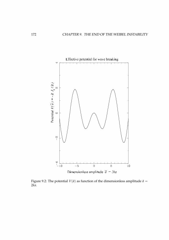
172 CHAPTER 9. THE END OF THE WEIBEL INSTABILITY
Figure 9.2: The potential V(a) as function of the dimensionless amplitude a =2ka.
Magnetic Fields inside Extremely Fast Shock Waves by Jorrit Wiersma 173
describe the background as an isotropic plasma. Since the Weibel instability ismainly magnetic, we will only need the transverse response of the plasma. TheFourier-transformed reduced Maxwell equations that include the backgroundresponse replace the equation for the Fourier-amplitude of the magnetic field,ik B ' 4πqb (n+ − n−), by
ikε⊥(k , ω)B = 4πqb (n+ − n−) . (9.67)
Here ε⊥(k, ω) is the transverse response (dielectric) function of the backgroundplasma. We have again assumed a relativistic beam with Vb ' c. In terms ofthe components αij of the polarization tensor defined in chapter 6 (equation 6.5)one has:
ε⊥(k , ω) = 1 +α
bg33 (k , ω)
k2c2 . (9.68)
It gives the effect of screening currents carried by the background plasma. Inthe linear approximation, where E+ ≈ −E− = −B, equation (9.67) togetherwith the equation of motion and the continuity equation of the beam particlesimply that the electromagnetic fields in the Fourier domain that are associatedwith the unstable Weibel mode now satisfy:
E±(k, ω) ≈ − 4πqbnbε⊥(k , ω)
ξ∓(k, ω) . (9.69)
As shown in chapter 6, the effect of screening currents can be described in agood approximation by putting
ε⊥(k , ω) ≈ κ2 + κ2s
κ2 , (9.70)
with κ = kc/ωbg with ωbg the plasma frequency of the background plasma,and where κs is the dimensionless screening wavenumber. The equation forthe Weibel mode with a given wavelength λ = 2π/k is then equivalent with
∂2ξ±(k , t)∂t2 =
ω2pb
ε⊥(k)ξ±(k , t) . (9.71)
Again this leads to an exponentially growing amplitude, ξ±(t) ∝ exp(σWt),where
σW(k) =ωpb√ε⊥(k)
=κ√
κ2 + κ2s
ωpb . (9.72)
174 CHAPTER 9. THE END OF THE WEIBEL INSTABILITY
The factor 1/√
ε⊥(k) shows that the background response lowers the growthrate of the linear instability. Expression (9.72) is exactly the growth rate thatfollows from equation (9.7) in the case of cold beams (M → ∞) as consideredhere. For κ κs the effect of the background plasma is very small.
The presence of screening currents does not influence the stabilization ar-gument of the previous section. The analysis presented there (e.g. equation9.65) predicts that the Weibel instability saturates at a level where
k∣∣ξ±∣∣ ' 1.9 . (9.73)
From (9.69) one has∣∣E±∣∣ ≈ ∣∣B∣∣ ≈ 4πqbnbε⊥(k)
∣∣ξ±∣∣ ≈ 8πqbnbk ε⊥(k)
. (9.74)
It is easily checked that this estimate is equivalent to the standard trappingargument (see, for example, chapter 8).
9.4 Kinetic theory: stabilization due to quiver motionWe now consider the stabilization of the Weibel instability from the point-of-view of kinetic theory. We assume a broad-band spectrum of unstable modeswith a bandwidth ∆k ∼ k, in contrast to the calculation of the previous sectionwhich assumed a single (dominant) mode.
Such a broad-band spectrum leads to phase mixing of the particle motion(the so-called quiver motion) in the collection of waves. This ultimately resultsin a broadening of the momentum distribution function fb(p) of the beam par-ticles in phase space. Traditionally this process is described as ‘fake diffusion’[e.g. 17], where the term ‘fake’ refers to the fact that this process, unlike truediffusion, is in principle reversible! In more modern incarnations of the theoryof wave-particle interactions one uses oscillation center theory to define theaverage distribution function in the presence of waves, see for instance Caryand Kaufman [13]. Since the linear Weibel instability has Re(ω) = 0, thereare no resonant non-linear effects, such as resonant wave-wave coupling as al-ready discussed above, or such typical kinetic nonlinear resonant processes asnonlinear Landau damping. These processes usually dominate the non-lineardynamics of plasma waves with |Re(ω)| |Im(ω)|.
This broadening of the momentum distribution effectively heats the plasmaand it is well known that heating of the plasma will stabilize the Weibel in-stability. In this section we will first estimate the broadening of the velocity
Magnetic Fields inside Extremely Fast Shock Waves by Jorrit Wiersma 175
distribution in terms of the amplitude of the magnetic field generated by theinstability. Using this estimate we will calculate the effect on the response ofthe beam particles and derive the magnetic field strength at the point wherethe broadening slows down the instability appreciably.
9.4.1 Broadening of the momentum distributionOnce again we consider the case of two counterstreaming and ultra-relativisticbeams that propagate along the z-axis. The dispersion relation for the Weibelinstability as derived in chapter 6 reads, in the limit |ω2| k2c2:
c2k2 + αbg33 (ω , k) + αb
33(ω , k) = 0 , (9.75)
where the polarization tensor component α33 has a contribution αbg33 (ω , k) due
to the background plasma, and αb33(k , ω) due to the beams. This last contribu-
tion is (chapter 6, appendix, equation 6.145):
αb33(ω , k) =
4πq2bnb
mb
∫d3pγ(p)
f0b(p)(
1− v2z
c2
)(9.76)
−4πq2bnb
∫d3p
v2
zω − kvx
(k
∂ f0b(p)∂px
).
Here f0b(p) is the average phase-space density of the beam particles, normal-ized to ∫
d3p f0b(p) = 1 , (9.77)
and γ(p) =√
1 + |p|2/m2bc2.
The effect of the quiver motion is a broadening of the mean distributionfunction. We will denote the spatially averaged distribution function of thebeam particles by f0b, to be distinguished from the exact distribution fb, whichincludes a fluctuating part. In the limit |ω| kc and for k = kx and B = B ythe Vlasov equation for the exact distribution fb(x , t , p) can be approximatedby
∂ fb∂t
+ vx∂ fb∂x
−(
qb vzBc
)∂ fb∂px
= 0 . (9.78)
Here fb(x , t , px , py , Pz) is taken to be a function of the x-coordinate and time,of the momentum components px and py perpendicular to the beam direction
176 CHAPTER 9. THE END OF THE WEIBEL INSTABILITY
(which equal the canonical momentum components Px and Py because Ax =Ay = 0) and the (conserved) canonical momentum Pz = pz + qb A/c. Usingstandard techniques of weak plasma turbulence [e.g. 17, Ch. 8], one can showthat the mean distribution function f0b satisfies a diffusion equation of the form
∂ f0b∂t
=∂
∂px
( qbvz
c
)2∫
dk dω
(2π)2σ⟨|B(k, ω)|2
⟩(ωr − kvx)2 + σ2
∂ f0b∂px
. (9.79)
This equation gives the effect of the quiver motion on the mean distributionfunction. Here the wave frequency is written in terms of its real and imagi-nary part as ω(k) = ωr + iσ. For a broad-band spectrum of normal modes theensemble average satisfies⟨
|B(k, ω)|2⟩
= B2(k) 2πδ(ω −ω(k)) , (9.80)
with ω(k) the wave frequency as determined by the solution of the dispersionrelation (9.75).
We now make the assumption of beams that are initially cold in the direc-tion perpendicular to the beam direction so that |kvx| |ω|. In the linear stageof the Weibel instability the amplitude of the magnetic perturbations grows as
∂B2(k)∂t
= 2σ(k) B2(k) , (9.81)
and ωr = Re(ω) = 0. In this limit, equation (9.79) can be approximated by
∂ f0b∂t
=∫
dk2π
∂B2(k)∂t
∂
∂px
q2
bv2z
2σ2c2∂ f0b∂px
. (9.82)
In the linear stage of the Weibel instability, the growth rate σ for kc/ωbg >1 is almost independent of wavenumber. In addition we have f0b ∝ δ(Pz +γbmbVb) + δ(Pz − γbmbVb) (see equation 9.34) and pz ≈ Pz, so we can putvz = ±Vb. We define the typical magnetic field strength B by the relation
B2 =∫
dk2π
B2(k) . (9.83)
Together, equations (9.81), (9.82) and (9.83) imply that f0b satisfies a diffusionequation of the form:
∂ f0b
∂(B2)=
∂ f0b/∂t∂(B2)/∂t
=∂
∂px
q2
bV2b
2σ2c2∂ f0b∂px
. (9.84)
Magnetic Fields inside Extremely Fast Shock Waves by Jorrit Wiersma 177
If the beams are ultra-relativistic and cold at t = 0, the momentum distributionis given by:
f0b(t = 0) = δ(px) δ(py)×(9.85)
× 12 [δ(Pz + γbmbVb) + δ(Pz − γbmbVb)] .
Using γb 1 the solution to equation (9.84) can then be written as a quasi-Maxwellian distribution in vx = px/γbmb:
f0b(t) =1√
2π γbmbvqe−(v2
x/2v2q) δ(py)×
(9.86)× 1
2 [δ(Pz + γbmbVb) + δ(Pz − γbmbVb)] .
Here the quiver velocity vq is defined by:
v2q ≈
q2bV2
b B2
2γ2bm2
bσ2c2. (9.87)
This explicitly shows how the mean distribution in vx (with associated mo-mentum px ≈ γbmbvx) broadens due to phase mixing of the quiver motion asthe rms magnetic field grows. The above procedure generalizes a similar resultderived by [43], p. 25, for electrostatic waves.
If we relax the assumption that the wave vector k is in the x-direction, andallow for ky 6= 0, Bx 6= 0 while keeping kz = 0, a similar broadening occurs inthe distribution of the y-component of momentum. If the situation is cylindri-cally symmetric around the beam direction, with
B2x(k) = B2
y(k) ≡ B2(k) , (9.88)
expression (9.86) is replaced by
f0b(t) =1
2π (γbmb vq)2 e−(v2x+v2
y)/2v2q ×
(9.89)× 1
2 [δ(Pz + γbmbVb) + δ(Pz − γbmbVb)] .
In conclusion: the effect of the phase mixing of the quiver motion is to heat thebeam plasma, in particular by creating a quasi-Maxwellian distribution of thecomponents of the particle momentum in the xy-plane, the plane perpendicu-lar to the beam direction.
178 CHAPTER 9. THE END OF THE WEIBEL INSTABILITY
9.4.2 Effect on the beam responseThe change in the beam momentum distribution also changes the contributionof the beam to the polarization tensor component α33(ω , k) that figures in thedispersion relation for the Weibel instability. Using distribution function (9.89)in definition (9.76) gives the beam contribution to α33 in the limit vq c so thatpx ≈ γbmbvx:
αb33 = ω2
pb
(1
γ2b
+4v2
q
c2
)− ω2
pbk2V2
bω2 Z2 W(Z) . (9.90)
Here Z ≡ ω/kvq and W(Z) is the plasma dispersion function defined by Ichi-maru [40],
W(Z) ≡ 1√2π
∫ +∞
−∞dx
x exp(−x2/2
)x− Z
, (9.91)
and ω2pb = 4πq2
bnb/γbmb is the effective plasma frequency associated with thebeams. To obtain result (9.90) we have used
1− v2z
c2 =1
γ2 +v2
xc2 +
v2y
c2 . (9.92)
Initially vq |ω/k| c and |Z| 1, and we can use the expansion (valid forσ = Im(ω) > 0):
W(Z) ≈ − 1Z2 −
3Z4 (9.93)
For kVb ∼ kc |ω|, γb 1 and vq c we can neglect the first term in (9.90),and the dispersion relation (9.75) can be approximated by:
k2c2 + αbg33 (iσ , k)− ω2
pbk2V2
bσ2
(1−
3k2v2q
σ2
)= 0 . (9.94)
Here we put ω = iσ. This approximate dispersion relation shows that theinstability slows down appreciably if kvq ∼ σ, or equivalently when
kvq
σ≈ kqbVbB
γbmbcσ2 ≈ 1. (9.95)
This is essentially the trapping criterion (9.15), with the quiver amplitude ξq =vq/σ as the typical amplitude. A similar argument for the stabilization of the
Magnetic Fields inside Extremely Fast Shock Waves by Jorrit Wiersma 179
Weibel instability has been proposed previously by Gruzinov [31]. A more pre-cise evaluation of the dispersion relation using expression (9.90) for αb
33 needsan evaluation of W(Z) = W(ω/kvq) in the complex plane, and is beyond thescope of this paper.
9.5 Further field growth through current channel coalescenceIn the previous two sections we have calculated how the exponential phase ofthe Weibel instability is terminated when the amplitude of the magnetic fieldbecomes comparable with the trapping field B ∼ Btr, see equation (9.16). If asingle (dominant) wave mode of given wavenumber k is present, the stabiliza-tion can be understood as the effect of wave breaking. In a broad-band spec-trum of unstable modes the broadening of the average distribution functionessentially gives the beam plasma a finite temperature in the plane perpendic-ular to the beam direction. Since wave breaking generates higher harmonics,the single-mode case will evolve naturally into a broad-band spectrum.
Once trapping finishes the quasi-exponential growth of the magnetic field,further field amplification is still possible. The numerical simulations of Leeand Lampe [52], and more recently by Frederiksen et al. [24] show how thefilamentary currents generated by the Weibel instability merge into larger cur-rent channels. Physically, this coalescence is the result of the attractive force be-tween parallel currents. Medvedev et al. [59] have considered a simple modelof this coalescence phase, assuming that the process can be approximated bytreating the current channels as thin current wires with a magnetic field at a dis-tance r from the wire axis equal to B(r) = 2I/cr. Their calculation neglects thescreening currents of a background plasma which, at least in the exponentialstage of the instability, play an important role in determining the wavenumberk† at which the trapping field reaches the maximum value (see equation 9.18).
In this section we will include the effect of screening currents. In particular,we investigate how the presence of the hot background plasma influences thecoalescence process. We will show that the screening currents supported bythis background slow the coalescence process once the typical transverse sizeof the current channels becomes comparable with the skin depth, c/ωbg, of thehot background.
9.5.1 Maximum current for a cylindrical channel: the Alfven currentFollowing Kato [44] we define typical currents and the associated magneticfields for a cylindrical current filament of a given radius r0. A single beam of
180 CHAPTER 9. THE END OF THE WEIBEL INSTABILITY
charged particles with lab frame density nb, with charge qb per particle andwith a bulk velocity Vb can carry a maximum current equal to
Ib = πr20qbnbVb . (9.96)
If the current channels result from the Weibel instability, the typical size of thechannels will be r0 ≤ c/ωbg. If one neglects screening currents, the typicalmagnetic field at the outer edge of the filament is
Bb =2Ibcr0
=2πqbnbc
ωbg
(Vbc
) (r0
(c/ωbg)
). (9.97)
The Alfven current follows (up to factors of order unity) from the requirementthat the gyration radius of the beam particles, with an energy E = γbmbc2, inthe self-generated magnetic field becomes equal to the radius of the currentchannel:
rg =γbmbcVb
qbB∼ r0 . (9.98)
Using B ≈ 2I/cr0 this gives the critical Alfven current,
IA =γbmbc2Vb
2qb. (9.99)
The associated magnetic field is equal to
BA =γbmbcVb
qbr0
(9.100)
=4πqbnbc
ωbg
(ω2
bg
ω2pb
)(Vbc
) (r0
(c/ωbg)
)−1
.
One has Bb(r0) < BA(r0) for r0 <√
2 (c/ωpb).The trapping condition (9.15) implies that the magnetic field amplitude for
a wave mode with a wavenumber k = 2π/λ at the end of the phase of expo-nential growth is
Btr(k) =γbmbc
qb
(σ2
kVb
). (9.101)
This trapping field serves as an initial condition for the coalescence phase ofmagnetic field growth. Using the expression for the growth rate of the Weibel
Magnetic Fields inside Extremely Fast Shock Waves by Jorrit Wiersma 181
instability in the ultra-relativistic limit 3 , equation (9.7), one has for k kmax,hb ≈ 1 (cold beam) and Vb ≈ c:
Btr(k) ≈ 4πqbγbnbk
(k2
k2 + k2s
). (9.102)
The maximum field amplitude occurs at a wavenumber close to the screeningwavenumber: k ∼ k† ∼ ks = ωbgκs/c. For typical parameters (see below) onehas κs ≈ 0.25− 1. For the order-of-magnitude estimates we will use the fluidresult: κs = 1. Note that the field amplitude Btr is independent of the mass ofthe beam particles for k ks.
For relativistic beams with Vb ≈ c and for a wavenumber k ≥ ωbg/c thetrapping field is comparable to the field of a cylindrical current with a radiusequal to r0 = 1/k = λ/2π:
Bb(r0) ∼ Btr(k = 1/r0) . (9.103)
The magnetic field associated with the critical Alfven current equals
BA(r0) ∼Btr(k = 1/r0)η (ωbgr0/c)2 =
Btr(k = 1/r0)(ωpbr0/c)2 . (9.104)
Here we have used definition (9.2) for η. The current channels created by theWeibel instability typically have r0 ∼ 1/k† ≤ c/ωbg.
The estimates (9.103) and (9.104) have immediate consequences for the co-alescence of the current filaments created by the Weibel instability that we willexplore in section 9.6.
9.5.2 Simple model for field growthThe growth of the small-scale field can be estimated using the toy model forcurrent merging of Medvedev et al. [59]. This model considers the mergingof identical and cylindrical current channels with radius rm and cross sectionπr2
m after the m-th merger. After m mergers of currents with the same initialscale r0 and current I0, the resulting current filament carries a current Im, hasa radius rm and a magnetic field Bm = 2Im/crm at its outer edge, which aregiven by [59]
Im = 2m I0 , rm = 2m/2 r0 , Bm = 2m/2 B0 . (9.105)3Although formally expression (9.7) for the growth rate σ has been derived under the assump-
tion σ kc, it turns out that it gives a good approximation even if σ ∼ kc.
182 CHAPTER 9. THE END OF THE WEIBEL INSTABILITY
This calculation neglects screening currents, which is a reasonable approxima-tion for rm c/ωbg, and uses mass conservation and current conservation.Combining the last two relations of (9.105) one has
Bm =(
rm
r0
)B0 . (9.106)
We first consider the merging of electron current filaments. At this stage of thedevelopment of the instability, the electrons are already (partially) thermalized,and η ≈ 1, see also the discussion in Section 9.6 below. Using as an initialcondition for the merger process the trapping field generated at the end of theexponential phase of the Weibel instability, B0 = Btr(k = 1/r0) ≈ Bb(r0), thisyields for rm ≤ c/ωbg:
Bm =2πqbnbc
ωbg
ωbgrm
c≈ Bb(rm) ≈ Btr(k ∼ 1/rm) . (9.107)
This simple merging model gives a magnetic field of the merged current fila-ments of size rm that is comparable with the trapping field at the same scale,which equals the field created by the exponential Weibel instability at thatscale. When, after multiple mergers, the radius of the resulting filament be-comes comparable with the skin depth, rm ∼ c/ωbg, the Alfven limit Btr(r =c/ωbg) ∼ BA is reached as ωbg ∼ ωpb for the electrons. The electron currentcan not grow beyond the (radius-independent) Alfven limit (9.99), and the as-sociated magnetic field (9.100) will decay as r−1
m if merging continues.We will argue below that further merging to filaments of a transverse size
larger than the skin depth is slowed down considerably by the screening cur-rents generated in the background plasma. This means that for all intents andpurposes the merging almost stops when rm ∼ c/ωbg when the magnetic fieldhas a magnitude Bb ∼ BA ∼ Btr. The decay of the field due to further merging,Bm ∝ r−1
m for Bm > BA, is present, but proceeds at a much slower rate than thegrowth of the field in the Weibel instability.
Protons have η = ηp ∼ me/mp 1. This means that the Alfven field satis-fies BA ∼ Btr/η Btr at r ' c/ωbg. Merging of proton current filaments couldtherefore in principle lead to continuing magnetic field growth. However, thescreening currents act here also, slowing down the merging rate. Therefore,the additional field growth will be limited.
Magnetic Fields inside Extremely Fast Shock Waves by Jorrit Wiersma 183
9.5.3 The effect of screening currentsThe hot background plasma that one expects to be present in shock transitionlayers will influence the coalescence process because it supports screening cur-rents, which diminish both the total current of a filament and the resultingmagnetic field outside the filament. The latter determines the strength of theforce between adjacent current filaments. In this section we calculate the in-fluence of the screening currents on the merger rate, and how they modify theresults of the simple merger model employed above for rm > c/ωbg.
The magnitude of the screening current in the z-direction (along the beams)that is carried by the background can be readily calculated from the z-compo-nent of the equation of motion for species s in the hot background. This equa-tion is formally identical to the corresponding equation (9.29) for the beamparticles. The only difference is that the effective inertia of a hot plasma is mshswith hs the enthalpy per unit rest energy, cf. [49]. One has:
mshsd (γsVsz)
dt= qs
(E +
V× Bc
)z
. (9.108)
In a cylindrically symmetric situation around a filament aligned with the z-axis, with B = B(r) eφ and ∂/∂φ = 0, one has B(r) = −∂A/∂r, (V × B)z =VrB(r), Ez = −(1/c)(∂A/∂t) and d/dt = ∂/∂t + Vr (∂/∂r). Here A = A(r) zis the vector potential, r is the cylindrical radius centered on the filament axisand φ is the azimuthal angle around the filament. In that case equation (9.108)can be integrated to
mshsγsVsz +qs A
c= constant ≡ Psz , (9.109)
which is the equivalent of relation (9.33) for a species belonging to the back-ground plasma. For a growing field the integration constant Psz can be ne-glected. Solving for Vsz with Psz = 0 one finds the screening current due to thebackground:
Jbg = ∑s
qsnsVsz z
(9.110)
= −∑s
q2s ns
mshscA√
1 +(
qs Amshsc2
)2.
184 CHAPTER 9. THE END OF THE WEIBEL INSTABILITY
In what follows we will neglect the non-linearity in this relation due to therelativistic mass correction, replacing (9.110) by its non-relativistic equivalent
Jbg ≈ −∑s
q2s ns
mshscA = −
ω2bg
4πcA . (9.111)
This is allowed if Js nsqsc, which is formally satisfied if the beam densitysatisfies nb ns, or if the beam-current filaments have a size r0 c/ωbg sothat the screening currents remain small. For the fields created by the Weibelinstability this last condition is (marginally) satisfied. Nevertheless, our resultsshould remain qualitatively valid even when Js ≈ nsqsc.
We note in passing that relation (9.110) implies that Js < nsqsc, a limit whichis physically obvious. Therefore, in a situation where the beam density is muchlarger than the density of the species in the background plasma so that nb nsfor all species, screening currents are always much smaller than the maximumcurrent density that can be carried by the beam, Jb = nbqbc. In that case screen-ing can be much less effective. In what follows we will assume that (at most)nb ≈ ns, and that this particular situation does not occur.
In a quasi-steady state, where the fields only depend on the distance r fromthe filament axis and A = A(r) z, Maxwell’s equation for the vector potentialcurl(curl A) = (4π/c) J [e.g. 41, Ch. 6.4] reads, with approximation (9.111),
1r
∂
∂r
(r
∂A∂r
)−
ω2bg
c2 A = −4π
cJb . (9.112)
Here Jb is the current density due to the beam particles in a current filament.The screening current of the background plasma corresponds to the secondterm on the left-hand side of the equation.
Let us calculate the magnetic field due to a single cylindrical current fil-ament embedded in a background plasma with a uniform background den-sity ns and pressure Ps. This last assumption is a reasonable approximationas long as the radial gradients in pressure and density induced by the radialmagnetic pinching force remain small. This will be the case if B2/8π Ps.In the relativistic case this condition is met when the field amplitude is muchless than the equipartition field: B Be. As a first approximation, the currentdensity carried by the beam is taken to be constant over the cross section ofthe filament of radius r0, Jb = J0 for r ≤ r0, and vanishes outside the filament:Jb = 0 for r > r0.
Magnetic Fields inside Extremely Fast Shock Waves by Jorrit Wiersma 185
Equation (9.112) is readily solved for constant ωbg in terms of the modifiedBessel functions of integer order In and Kn:
A(r) =4π J0
ck2s×
1− ksr0 K1(ksr0)I0(ksr) for r ≤ r0;
ksr0 I1(ksr0)K0(ksr) for r > r0
(9.113)
Here ks ≡ ωbg/c is the inverse skin depth. The magnetic field as a function ofcylindrical radius r follows from B(r) = −∂A/∂r:
B(r) = 2B0 ×
K1(ksr0)I1(ksr) for r ≤ r0;
I1(ksr0)K1(ksr) for r > r0
(9.114)
Here B0 = 2I0/cr0 = 2πr0 J0/c is the field at the outer radius r0 of an un-screened current filament with a total beam current I0 = πr2
0 J0. The totalcurrent contained within a cylindrical radius r0 equals
Itot =cr0 B(r0)
2= 2I0 I1(ksr0)K1(ksr0) . (9.115)
For a large current filament, with a radius such that ksr0 1, Itot decays withincreasing filament radius as
Itot ≈ I0/ksr0 , (9.116)
while the magnetic field for r > r0 falls off rapidly:
B(r) ≈ B0e−ks(r−r0)
ks√
rr0. (9.117)
9.5.4 Equation of motion for two attracting screened filamentsNow consider two identical and parallel current filaments of radius r0, withtheir axes at a distance d > 2r0. As an admittedly crude model let us assumethat we can describe the interaction between the two current filaments as theinteraction between two current wires, with a total current equal to the par-tially screened current Itot of equation (9.115), and with a magnetic field out-side the filament given by equation (9.114). The attractive interaction force perunit length between the current wires equals dF/d` = −ItotB(d)/c, which is
dFd`
= −8I2
0c2r0
I21 (ksr0)K1(ksr0)K1(ksd) . (9.118)
186 CHAPTER 9. THE END OF THE WEIBEL INSTABILITY
For ksr0 1 and ksd 1 we can use the expansion of the modified Besselfunctions for a small argument: I1(ξ) ≈ ξ/2 and K1(ξ) ≈ 1/ξ. In that caseequation (9.118) reduces to the well-known result dF/d` = −2I2
0 /c2d.The mass per unit length of a current filament is approximately equal to
µ ≡ dmd`
≈ πr20 (nemehe + γbmbnb) . (9.119)
Here we have used that the effective mass of the hot electron backgroundequals meff ≈ mehe, and that the effective mass of the beam particles for mo-tions perpendicular to the beam direction is γbmb. This assumes that the beamcurrents and the hot electron background, which provides the screening cur-rent, move together inside the filament.
The equation of motion for a filament is
µd2ddt2 = −
8I20
c2r0I21 (ksr0)K1(ksr0)K1(ksd) . (9.120)
The modified Bessel function K0 satisfies dK0(ξ)/dξ = −K1(ξ). This meansthat the force on the right-hand side of equation (9.120) can be written in theform −∂Vint/∂d, where the interaction potential Vint(d) is given by:
Vint(d) = −8I2
0ksc2r0
I21 (ksr0)K1(ksr0)K0(ksd) . (9.121)
9.5.5 The coalescence time scaleIf the filaments start from rest at an initial distance di, the equation of motionhas an energy integral:
µ
2
(dddt
)2+ Vint(d) = Vint(di) . (9.122)
The coalescence time now follows as
tcoal(di) =∫ di
2r0
dr√2µ
[Vint(di)−Vint(r) ]
. (9.123)
Here we end the coalescence phase when the filaments touch so that d = 2r0.Defining dimensionless variables
$ ≡ ksd , $0 ≡ ksr0 , (9.124)
Magnetic Fields inside Extremely Fast Shock Waves by Jorrit Wiersma 187
one finds
tcoal($i) = T0
∫ $i
2$0
d$√K0($)− K0($i)
, (9.125)
with a characteristic time T0 given by
T0 ≡
(16I2
0 ks
µc2 r0
)−1/2 (I21 ($0)K1($0)
)1/2
(9.126)
=1
2ωpb
(c
Vb
) (1 +
nemehe
nbmbγb
)1/2 ( B0
Bb
)−1ψ($0) .
Here we defineψ($0) ≡ 1/
√$0 I2
1 ($0)K1($0) , (9.127)
normalize the beam current with the maximum current (9.96) and use I0/Ib =B0/Bb. Note that for current filaments left by the Weibel instability the trap-ping argument predicts that B0 ≈ Bb and that Vb ' c for the relativistic beamswe are considering. In that case (for typical values of the parameters) one hasT0 ' 1/ωpb for r0 ∼ c/ωbg, and the time scale of the merging process and thegrowth time of the preceding Weibel instability, tW ∼ 1/σ ' 1/ωpb, are of thesame order.
In what follows we will neglect the factor√
1 + nemehe/nbγbmb, which isalways of order unity in our applications. Assuming $0 1 and $i 1 wecan use the asymptotic expansion of the modified Bessel functions for largearguments, In($) ≈ e$/
√2π$ and Kn($) ≈
√π/2$ e−$. In that case
ψ($0) ≈ (8π$0)1/4 e−$0/2 , (9.128)
and the integral appearing in (9.125) can be approximated by(2π
)1/4 ∫ $i
2$0
d$ $1/4 e$/2√1− ($/$i)1/2 e$−$i
≡ K . (9.129)
In its present form the integral can not be evaluated analytically. However, for2$0 1 an excellent approximation can be derived. To that end we define anew variable,
ζ ≡(
$
$i
)1/4e($−$i)/2 . (9.130)
188 CHAPTER 9. THE END OF THE WEIBEL INSTABILITY
With a little algebra it is easy to show that the integral (9.129) can be rewrittenas
K = 2(
2$i
π
)1/4e$i/2
∫ 1
ζ0
dζ√1− ζ2 (1 + 1/2$(ζ))
. (9.131)
For $ 1 we can safely neglect 1/2$ in the factor (1 + 1/2$), and the integralbecomes
K ≈ 2(
2$i
π
)1/4e$i/2
(π
2− sin−1(ζ0)
). (9.132)
Together with (9.125), (9.126) and (9.128) this gives the coalescence time forζ0 = (2$0/$i)1/4 exp[(2$0 − $i)/2 ] 1:
tcoal ≈2π
ωpb
(B0
Bb
)−1 ( cVb
)($0$i)
1/4 e($i−2$0)/2 . (9.133)
For $i − $0 ≥ $0 1 the coalescence time grows exponentially with increasingdistance between the two filaments. This behavior is illustrated in figure 9.3,which was obtained through direct numerical integration of the equation ofmotion (9.120) for B0 = Bb, Vb ≈ c and nbmbγb nemehe.
These calculations imply that the coalescence slows down appreciably assoon as the distance between current filaments exceeds the skin depth of thehot background, ksdi > 1. Note that in the simple model of Medvedev et al. [59]the distance between pairwise merging current wires increases as dm = 2md0after the m-th merger, if the process starts with an initial collection of wiresthat are separated by a distance d0. The ratio of the distance between the wiresand their radius scales therefore as dm/rm ∝ 2m/2. This means that, as soonas screening currents become important when ksrm ∼ 1, the coalescence rateslows rapidly in the following steps of the merger process, and the coalescenceof current filaments effectively ‘stalls’ after a few additional steps.
9.6 Implications for ultra-relativistic shocksWe now consider the implications of the results of the previous sections forthe generation of magnetic fields near ultra-relativistic shocks. In particularwe discuss the shock transition layer, where the kinetic energy of the incom-ing ions (with mass mi) and electrons (and possibly positrons, both with massme) is thermalized, creating a relativistically hot plasma. Since we are deal-ing with a collisionless plasma, the behavior of the ions and electrons must beconsidered separately.
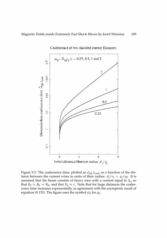
Magnetic Fields inside Extremely Fast Shock Waves by Jorrit Wiersma 189
Figure 9.3: The coalescence time, plotted as ωpb tcoal, as a function of the dis-tance between the current wires in units of their radius: di/r0 = $i/$0. It isassumed that the beam consists of heavy ions with a current equal to Ib, sothat B0 ≈ Bb ≈ Btr, and that Vb ≈ c. Note that for large distances the coales-cence time increases exponentially, in agreement with the asymptotic result ofequation (9.133). The figure uses the symbol v0 for $0.
190 CHAPTER 9. THE END OF THE WEIBEL INSTABILITY
9.6.1 Thermalization through the Weibel instabilityWe first consider the effect of the electron-driven Weibel instability. Simu-lations (e.g., [24]) show that the electron-driven Weibel instability developsrapidly in a shock transition. The ion-driven instability also occurs, but has amaximum growth rate that is a factor (ωpb)e/(ωpb)p ≈
√mp/me ∼ 43 slower
than the electron-driven instability. Here we assume a hydrogen plasma withthe ion mass equal to the proton mass: mi = mp. Incidentally: simulations of-ten use (for computational reasons) a much smaller ion-electron mass ratio, ofthe order mi/me ∼ 16 corresponding to
√mi/me ∼ 4. Therefore, the difference
in the growth rates of the electron- and ion-driven instabilities is not nearly aspronounced in these simulations as in reality.
If the electrons form their own ‘subshock’, then the shock jump conditionsshould apply to the electron fluid. For ultra-relativistic shocks, where the in-coming flow in the shock frame has a Lorentz factor γsh 1 and the incomingelectron gas is cold in the sense that kbT1 mec2, the relation for the veloc-ity difference vrel = (v1 − v2)(1− v1v2/c2) between the up- and downstreamflow is purely kinematic, cf. Blandford and McKee [8]. The corresponding
Lorentz-factor is γrel ' γsh/√
2 with γsh = 1/√
1− v21/c2, independent of the
mass of the particles that make up the plasma. It is natural to associate γrelwith the beam Lorentz factor γb in the rest of the discussion. For γsh 1proper densities on both sides of the shock are related by n2/n1 ' 4 γrel, andthe downstream temperature T2 follows from e2 ' 3P2 = 3n2kbT2 ' γreln2mc2,with m the rest mass of the particles involved. For electrons or positrons thisimplies kbT2 ≈ γrelmec2/3. Here we have used a subscript 1 (2) to denote thepre-shock (post-shock) state. Below we will take these post-shock values asindicative values for the thermal electron background.
Initially, the electron-driven Weibel instability will proceed almost as in thecase of no background, the limit η 1, or equivalently (ωpb)2
e ω2bg. This
implies that the instability grows over a wide range of wavelengths, with agrowth rate σ ' (ωpb)e. As the beam(s) get further and further behind theshock front, the quiver motion in the self-generated magnetic field will growin amplitude, and the electron-driven instability starts to stabilize, starting atthe longer wavelengths. The typical amplitude of the magnetic field (equation9.102) for perturbations with wavelength λ = 2π/k equals, with Vb ' c
B ∼ Btr ≈ 4πeγbne
k. (9.134)
where ne ≈ n1 is the proper density of the electron beams and where we have
Magnetic Fields inside Extremely Fast Shock Waves by Jorrit Wiersma 191
put he = 1 as the electrons are initially cold. The amplitude of the quivervelocity that corresponds with this field amplitude is quite large. From theapproximate expression (9.87) with σ = (ωpb)e and Vb ' c one finds
(vq
c
)e∼
(ωpb)e√2 kc
, (9.135)
which is of order unity for k ∼ (ωpb)e/c, implying that waves with k <(ωpb)e/c stabilize first. The electron-driven Weibel instability should be ca-pable of completely thermalizing the electrons. The perturbations with k >(ωpb)e/c will continue to grow even when the electron plasma is partially ther-malized, with a typical value of the parameter ηe ∼ 1.
The electron beam plasma frequency, and the downstream electron plasmafrequency once the electrons are fully thermalized, are similar in magnitude(see also the discussion in chapter 8). We express them in terms of the plasmafrequency ωpe =
√4πe2ne/me of the cold upstream electron gas with density
n1 = ne. Using the above shock relations one finds:(ωpb
)2
e' 4πe2ne
me= ω2
pe ,(
ωbg
)2
e=
4πe2n2c2
kbT2' 12 ω2
pe . (9.136)
In view of our discussion in section 9.5.1, these estimates imply that the trap-ping magnetic field and the Alfven critical field for electrons are of the sameorder at a scale comparable to the effective skin depth: c/(ωbg)e ∼ c/(ωpb)e.As a result further magnetic field growth due to coalescence of the current fila-ments created by the electron-driven Weibel instability at a scale r0 ' c/(ωbg)ewill stall after a few mergers because of the exponential increase of the coa-lescence time, as calculated in section 9.5.5. Filaments created at r0 ∼ 1/k c/(ωbg)e will merge almost unimpeded, but the scaling laws (9.106) and (9.107)imply that the resulting magnetic field strength at some scale r > r0 is compa-rable to the magnetic field that was created initially at that scale by the quasi-exponential phase of the Weibel instability. However, the filling factor of thecurrent filaments decreases as merging proceeds further and further.
The ion-driven Weibel instability develops more slowly, and takes placemostly in the hot background of the already thermalized (shocked) electrons.A complication is the fact that there will possibly be strong effects in the transi-tion layer due to electrostatic potentials generated by electron-ion charge sep-aration, and due to a strong overshoot of the compressed magnetic field. Wecan not treat these effects, but point out that, for typical parameters, magnetic
192 CHAPTER 9. THE END OF THE WEIBEL INSTABILITY
effects on the Weibel instability are estimated to be small, as discussed in sec-tion 6.8.
The ion-driven instability is weak in the sense that η 1: for a hydrogenplasma one has
ηp =(ωpb)2
p
(ωbg)2e' me
mp 1 . (9.137)
The precise numerical constant in front of the electron-proton mass ratio inrelation (9.137) is difficult to predict without a complete shock model, but willbe of order unity. If one assumes charge neutrality it equals 4/3. The presenceof screening currents in the hot electron background impedes the ion-drivenWeibel instability for wavelengths larger than the effective electron skin depth.The screening wavenumber is ks = [(ωbg)e/c] κs, where (see chapter 6)
κs =
1 fluid background model,
(π
4
)1/3η1/6
p ≈ 0.26 kinetic background model.. (9.138)
In that case relation (9.102) applies, the maximum trapping field in the ion-driven instability occurs at k ∼ ks, and the typical field amplitude for k > ks(up to factors of order unity) is again given by (equation 9.134), assuming np ≈ne ' n1. This also implies that for protons(vq
c
)p∼
(ωpb)p√2 kc
≤ηp√
2 1 . (9.139)
Unlike what happens with the electrons, the Weibel instability is therefore notcapable of immediately thermalizing the incoming protons on a scale of a fewtimes c/(ωpb)p.
A second important difference with the electron-driven case is that the trap-ping field is smaller than the critical Alfven field BA for the ions at the samescale, a consequence of the larger ion mass, which makes them more difficultto deflect. One has BA ∼ Btr/ηp at r0 ∼ c/(ωbg)e with ηp 1. This means thatmerging of ion current filaments, and the associated growth of the magneticfield, is possible in principle. However, the calculations in the preceding sec-tion show that, analogous to what happens with the linear ion-driven Weibelinstability at wavelengths exceeding the skin depth, further merging is im-peded by the screening currents in the (now thermalized) electron backgroundplasma. The merging rate slows down strongly once the radius of the filaments
Magnetic Fields inside Extremely Fast Shock Waves by Jorrit Wiersma 193
becomes larger than a few times the plasma skin depth c/(ωbg)e ' c/(ωpb)e.The overall conclusion therefore is that the ion-driven Weibel instability doesnot generate magnetic fields that are much stronger than the ones already cre-ated by the faster electron-driven instability.
9.6.2 Thermalization of protonsBecause the ions will thermalize well after the electrons do, the overall widthof the shock transition is now determined by the ion thermalization length.To a large extent, the implications of this have already been investigated byLyubarsky and Eichler [55]. Here we refine their calculation.
Ion thermalization takes place due to scattering in the magnetic fields thathave been generated by the electron-driven Weibel instability. This processcan be described as diffusion of the direction of flight unit vector n = p/p =(nx , ny , nz), where p is the proton momentum. The equation of motion for anultra-relativistic proton with energy E can be written as
dnds
=eE
(n× B) . (9.140)
Here s is the path length along the orbit of the proton. We neglect the influenceof the shock-compressed background magnetic field as the amplitude of theWeibel-generated field is much larger: from relation (9.134) with ks ∼ (ωbg)e/cand (9.136) one finds:
Btr
B2≈ 1
4√
3
(ωpe
ωce
)= 4.6× 10² √ne1 B−1
1 (µG) . (9.141)
Here ωce = eB1/mec is the upstream value of the electron gyrofrequency,where we have used B2 = 4γrelBt1 ≈ 2γrelB1 for the strength of the shock-compressed magnetic field.
The vector n will diffuse with a diffusion coefficient Dij ≡⟨∆ni∆nj
⟩/2∆s,
where the angular brackets denote an ensemble average. A standard quasi-linear calculation, which uses the unperturbed (ballistic) particle orbits, leadsto a diffusion coefficient of the form
Dij =πe2
E2
∫d3k
(2π)3
(nn :
⟨AA∗⟩ (k)
)kik j δ(k · n) . (9.142)
The dyadic correlation tensor⟨AA∗⟩ in this expression is the correlation tensor
of the Fourier components of the vector potential A. The Fourier components
194 CHAPTER 9. THE END OF THE WEIBEL INSTABILITY
of the vector potential and of the turbulent magnetic field are related in theusual manner: B = ik × A. The correlation tensor follows from the randomphase approximation [e.g. 17, p. 135] for the ensemble average of the turbulentfields: ⟨
A(k)A∗(k′)⟩
=⟨AA∗⟩ (k)(2π)3 δ3(k + k′) . (9.143)
Beam protons initially have n ≈ z. In that case the only non-vanishing com-ponents of the diffusion tensor Dij are Dxx = Dyy = D0, if we assume that themagnetic turbulence is axisymmetric around the beam direction. The scalardiffusion coefficient D0 equals
D0 =πe2
2E2
∫ ∞
0
dk⊥k⊥(2π)2
⟨AA∗⟩
zz (k⊥ , k‖ = 0) k2⊥ . (9.144)
Here k⊥ =√
k2x + k2
y is the wave vector component perpendicular to the beamdirection, and k‖ = kz the component along the beam direction. The trivialintegration over k‖ has been performed, using δ(k · n) = δ(k‖).
So far, we have considered the Weibel instability in the limit k‖ = 0. In thatcase the quasilinear diffusion approximation for the direction of flight n doesnot apply, as the unperturbed orbit never leaves a single current filament. For-tunately, the assumption k‖ = 0 can be relaxed, as the Weibel instability persistsfor k‖ 6= 0. The theory in this case is rather complicated, see for instance thediscussion in [10]. An approximate calculation (not reproduced here) showsthat the dispersion relation for |k‖| k⊥ leads to a dimensionless growth ratefor κ κmax (compare equation 9.7):
σ2 ≈ ηκ2 sin2 θ
κ2s + κ2 − 3κ2 cos2 θ . (9.145)
Here sin θ = k⊥/k, cos θ = k‖/k. The growth rate will be reduced well belowthe value for θ = π/2, sin θ = 1 when tan2 θ ' 3 (κ2 + κ2
s )/η ∼ 6/η, where thelast equality is for κ ≈ κs ' 1. For the electron-driven instability one has (atleast initially) ηe ≈ 1, and the instability will act with a growth rate close to themaximum value for wavevectors inclined at an angle θ > 68 degrees with thebeam direction. This corresponds with | cos θ| ≤ 0.37 ≡ cos θc.
A simple model for the turbulent power spectrum of the Weibel-generatedmagnetic field is
⟨|B|2
⟩(k) = k2
⊥⟨AA∗⟩
zz (k⊥ , k‖) = (2π)2 B(k⊥)L‖ e−k2
‖L2‖/2
√2πk⊥
. (9.146)
Magnetic Fields inside Extremely Fast Shock Waves by Jorrit Wiersma 195
Here L‖ is the correlation length of the magnetic turbulence in the beam direc-tion, corresponding to a bandwidth ∆|k‖| = 1/L‖. The case k‖ = 0 correspondswith the limit L‖ −→ ∞. With this definition the rms amplitude of the turbulentmagnetic field follows from:
B2rms =
∫ dk‖dk⊥k⊥(2π)2
⟨|B|2
⟩(k⊥ , k‖) =
∫ ∞
0dk⊥B(k⊥) . (9.147)
The power spectrum B(k⊥) can be calculated by noting that the trapping fieldBtr(k) (see equation 9.102) at some wavenumber k⊥ is related to the magneticpower spectrum B(k⊥) by (Btr(k ' k⊥))2 ≈ k⊥ B(k⊥). This yields for k⊥ kmax:
B(k⊥) =B2
0ks
k⊥/ks(1 + (k⊥/ks)2
)2 . (9.148)
Here we defineB0 =
4πeγbne
ks(9.149)
with ne the density of the electron beam and ks = κs(ωbg)e/c the screeningwave number. It is easy to show that this spectrum has B2
rms = B20/2. This
spectrum falls of as B(k⊥) ∝ k−3⊥ for k⊥ ks, so the restriction k⊥ < kmax is
not very important for the evaluation of integrals over the power spectrum aslong as ks kmax.
Using this magnetic power spectrum in expression (9.144) for the scalardiffusion coefficient one finds:
D0 =
√πL‖
2√
2
∫ ∞
0dk⊥ B(k⊥) =
√π
4√
2
(eB0
E
)2L‖ . (9.150)
One sees from this expression that L‖ = 1/∆|k‖| plays the role of a correlationlength. It also shows, as argued above, that the limit k‖ = 0, L‖ = ∞ is formallyill-defined.
If we define a gyroradius rg = E/eB0 one has:
D0 =√
π
4√
2
L‖r2
g. (9.151)
Lyubarsky and Eichler [55] arrive at a similar expression, in effect putting L‖ ∼1/ks and neglecting the numerical constant. In view of our discussion above
196 CHAPTER 9. THE END OF THE WEIBEL INSTABILITY
of the behavior of the Weibel instability for θ < π/2 the obvious choice for L‖is
L‖ ∼1
ks cos θc≈ 2.65
ks. (9.152)
Here we use the fact that the largest contribution to the integral over the powerspectrum comes from the region k⊥ ' ks. This gives
D0 = 0.83
(rsk
r2g
), (9.153)
with rsk = 1/ks the effective skin depth of the hot electron background, whichaccording to (9.136) equals
rsk 'c
(ωbg)e=
12√
3c
ωpe. (9.154)
As protons are scattered by the random fields the components of the direc-tion of flight satisfy [cf. 4]⟨
n2x
⟩=⟨
n2y
⟩≈ 2D0s ,
⟨n2
z
⟩≈ 1− 4D0s , (9.155)
where the brackets indicate an average over the distribution. This shows thatthe thermalization length is
`th =1
6D0' 0.2
(r2
g(E)
rsk
), (9.156)
the distance where according to (9.155) one has⟨n2
x⟩
=⟨
n2y
⟩=⟨n2
z⟩
= 1/3,corresponding to an isotropic distribution of momenta. The more precise the-ory in Achterberg et al. [4] shows that `th is indeed the relevant length scale:the initial correlation of the momentum direction of the beam particles decayswith distance s due to scattering as exp(−6D0s).
Using (9.149) with ks ' (ωbg)e/c ' 2√
3 ωpe/c (as κs ' 1 in the electron-driven instability) one has for beam protons with energy E ' γbmpc2:
rg 'mpc2ks
4πe2np=
c (ωbg)e
(ωpb)2p' 2
√3(
mp
me
)c
ωpe. (9.157)
Magnetic Fields inside Extremely Fast Shock Waves by Jorrit Wiersma 197
Here np is the density of beam protons, which equals ne because of quasi-neutrality in the upstream flow, and we have used relation (9.136). This givesthe proton thermalization length in terms of the upstream electron skin depth:
`pth = 8.3
(mp
me
)2 cωpe
' 1.5× 10¹³n−1/2e cm. (9.158)
Apart from the numerical factor ∼ 8, this is the same result as derived byLyubarsky and Eichler [55].
9.7 ConclusionsIn this chapter we have presented two detailed non-linear calculations of theWeibel instability in the ultra-relativistic limit. The first uses a relativistic fluidapproximation to calculate the response of the beam particles, while the sec-ond uses kinetic plasma theory for the beam plasma. Although the physicsof the two calculations is subtly different, pertaining respectively to the caseof a single dominant mode where wave breaking occurs and to fake diffusionin a broad-band collection of waves due to the quiver motion that ‘heats’ thebeam plasma in the plane perpendicular to the beam direction, these calcu-lations both confirm that the Weibel instability due to relativistic beams willend the phase of exponential growth when particle trapping occurs, i.e. whenthe amplitude of the quiver motion, driven by the Lorentz force of the wave-generated magnetic field, becomes comparable with the wavelength of the un-stable modes. A similar conclusion was reached by Davidson et al. [16] for theWeibel instability in a non-relativistic plasma with a temperature anisotropy,by Yang et al. [104] for the Weibel instability in a magnetized electron-positronplasma, and our results also confirm the estimate of Gruzinov [31] (see alsochapter 8) for this particular case. This means that the typical field strengthat the end of the quasi-exponential phase of the instability is independent ofthe mass of the beam particles in a hydrogen plasma. The fast electron-drivenWeibel instability creates a field that is approximately two orders of magni-tude larger than the shock-compressed magnetic field, see equation (9.141). Itsvalue is set by the skin depth (inertial length) c/ωpe and density of the up-stream electron plasma, B ∼ πene(c/ωpe), independent of the shock Lorentzfactor. The slower proton-driven instability is impeded by the presence of thenow thermalized post-shock electron gas. The trapping argument shows thatthe typical field strength associated with this instability is of the same orderas the field generated by the electron-driven instability: the electron screening
198 CHAPTER 9. THE END OF THE WEIBEL INSTABILITY
currents result in a the trapping field that is independent of the mass of thebeam particles driving the instability.
We have also considered the subsequent evolution of the magnetic fieldsgenerated by the Weibel instability. We point out that the merging of currentfilaments [as proposed by 59] and the associated algebraic growth of the mag-netic field associated with these filaments, is slowed down drastically by theeffects of screening currents once the the transverse size of the filaments andthe filament-filament separation distance becomes comparable with, or largerthan with the electron skin depth. The coalescence time increases exponentiallyas the merged filaments are further and further apart. This limits any furtherfield amplification (or decay) at scales larger than the skin depth. At smallerscales, the merging is essentially unimpeded, but the resulting magnetic fieldat some scale r has an amplitude comparable to the trapping field left behindby the Weibel instability at that scale. Therefore, the magnetic field strengthnever grows much beyond the trapping field.
We have used our results to calculate the effect of the magnetic turbulenceon the ion beams that, in contrast to what happens to the electrons, are notdirectly thermalized by the Weibel instability. This happens indirectly, notthrough phase-mixing of the quiver motion, but by the slow scattering on theturbulent magnetic fields. Our calculation of the thermalization length con-firms the basic idea of [55], albeit with a thermalization length that is one orderof magnitude larger than their value.
Chapter 10
Computer simulations of theWeibel instability
To improve our understanding of the theoretical processes discussed in theprevious chapters we have simulated the behavior of the charged particles inthe Weibel instability with the help of computers. The simulations show howthe Weibel instability causes the magnetic field strength to grow exponentially,stopping when the particles become trapped in the magnetic field. The sim-ulations also show how the electrical currents continually merge to becomelarger and stronger and how the plasma shields the currents when they be-come strong. This supports the theory presented in the previous chapters.
This chapter will be submitted to Astronomy & Astrophysics [101].
199
200 CHAPTER 10. COMPUTER SIMULATIONS
10.1 IntroductionThis chapter describes Particle-In-Cell (PIC) computer simulations of the evo-lution of the relativistic Weibel instability driven by two (symmetric) relativis-tic beams. The simulations consider the evolution of this instability in a 1D2Vapproach, where variations in one spatial dimension (x), transverse to the beamdirection, are considered for a plasma with a two-dimensional momentum dis-tribution, with momentum components px (pz) transverse (along) the directionof the beams. We consider the linear properties of the beam-driven Weibel in-stability for this configuration, and show that its properties are virtually thesame as in the fully three-dimensional case.
The beam-driven Weibel instability (or filamentation instability) is an im-portant process in the shock front of relativistic collisionless shock waves [58,9]. The mixing of pre- and post-shock plasma in collisionless shock fronts pro-duces a plasma with an anisotropic velocity distribution. Such distributionsare known to be unstable to the spontaneous generation of transverse electro-magnetic waves [98].
The Weibel instability leads to filamentary, charge-separated electrical cur-rent channels that initially grow exponentially in strength. The exponentialgrowth is terminated when wave braking and particle trapping in the wave-generated magnetic field occur (see chapter 9). After the exponential phase,the current channels merge to form larger units [52].
This merging process increases the transverse size of the current channels,amplifies the associated magnetic field and thereby suppresses diffusion of themagnetic field [59]. However, when the instability takes place in a stationarythermal background plasma, the background tends to shield the current chan-nels and suppresses the merging process when the length scale grows beyondthe skin depth of the background plasma, see the discussion in chapter 9. Thisis particularly important when one considers the instability in the shock tran-sition layer of an electron-proton plasma: the Weibel instability in the electroncomponent grows much faster than the proton-driven instability. As a result,the directed momentum of the electron beams is thermalized, and the elec-trons quickly form a very responsive quasi-thermal background plasma. Thethermal electron background will lower the amplitude of the magnetic fieldthat the slower proton-driven instability generates (see chapters 8 and 9). Inthis article we present a number of 1D2V PIC simulations to test and confirmthe analytical estimates derived from instability theory in previous analyticalmodels (chapter 9).
We note that a number of groups have reported fully two- and three-dimen-
Magnetic Fields inside Extremely Fast Shock Waves by Jorrit Wiersma 201
sional computer simulations of the processes described in this article [21, 24,69]. Such 2D and 3D simulations include phenomena, in particular turbulentbehavior, that is suppressed by the one-dimensional nature of the simulationswe present below. The primary goal of our simulations is not to provide acomplete description of the long-term behavior of a realistic plasma, but tomake it easier to compare simulation results with the analytical estimates forthe behavior immediately following the phase of exponential growth, and soto confirm the underlying theory.
10.2 The simulated systemOur code computes the evolution of transverse perturbations in a collisionlessplasma that contains both a hot background and two counterstreaming beamsof particles. We allow the perturbations to be inhomogeneous in the directionperpendicular to the direction of propagation of the beams. In this situation theWeibel instability is purely electromagnetic, and involves growing transversewaves with a wave vector perpendicular to the direction of propagation of thebeams: E ⊥ B and k · E = 0, with k the wave vector (see chapter 6). In thenon-linear stage of the instability, there is a longitudinal component of electricfield along k.
In the unperturbed state, two homogeneous counterstreaming beams ofcharged particles travel along the z-direction through a background of station-ary particles. When the motion of the beam particles is perturbed, the result-ing charge density perturbations (charge bunching) lead to an advection cur-rent Jadv
z due to the bulk motion in the z-direction. This current perturbationwill be the source for a magnetic field perturbation in the direction perpen-dicular to both the propagation direction of the beams and the direction ofinhomogeneity.
We will assume that the perturbations vary along the x-direction, and thatthe magnetic field points in the y-direction. Consequently the electric field is inthe x–z plane. We use a finite grid, and assume periodic boundary conditionsin the x-direction in order to simulate a much larger plasma.
10.3 Basic equationsConsider a particle with velocity v and charge q, moving in an electric field Eand a magnetic field B. The particle position r and momentum p will evolve
202 CHAPTER 10. COMPUTER SIMULATIONS
according to:drdt
= v,
dpdt
= q(E +
vc× B
),
(10.1)
where v = p/γm with γ = (1 + |p|2/m2c2)1/2 the Lorentz factor, and m is theparticle mass. In our configuration the momentum equations are
dpx
dt= q(Ex −
vz
cBy),
dpy
dt= 0,
dpz
dt= q(Ez +
vx
cBy).
(10.2)
For simplicity, and without the loss of generality, we will assume that py = 0in what follows.
The electric and magnetic fields follow from Maxwell’s equations, with thecharge and current densities in the system acting as a source for the fields. Thecharge and current density have contributions from the beam particles, as wellas from any background plasma:
ρtot = ρbg + ∑i
ρi ,
Jtot = Jbg + ∑i
Ji ,(10.3)
where the sum is taken over all beam particles with each particle contributing(e.g., [41], equation 12.138)
ρi(x, t) = q δ(x− ri(t)),Ji(x, t) = qvi(t) δ(x− ri(t)).
(10.4)
We denote the average density of simulated beam particles with n0, and use astatic neutralizing background so that the total charge density vanishes in theunperturbed system: ρbg = −qn0. We will assume that this neutralizing staticbackground consists of very heavy (unresponsive) ions.
We will initialize the plasma in such a way that the average initial cur-rent density associated with the beams vanishes, so the background current
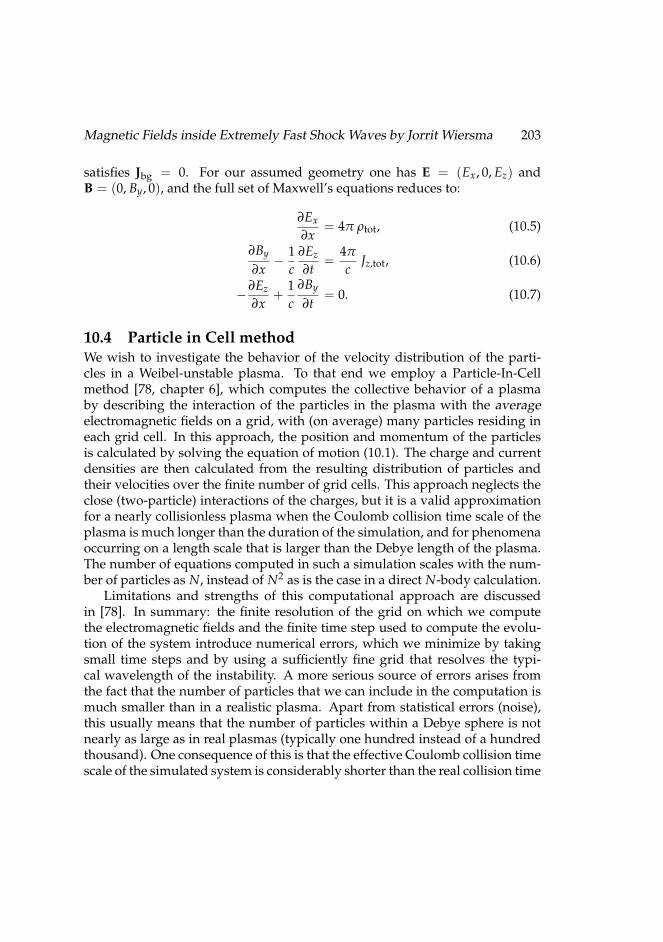
Magnetic Fields inside Extremely Fast Shock Waves by Jorrit Wiersma 203
satisfies Jbg = 0. For our assumed geometry one has E = (Ex, 0, Ez) andB = (0, By, 0), and the full set of Maxwell’s equations reduces to:
∂Ex
∂x= 4π ρtot, (10.5)
∂By
∂x− 1
c∂Ez
∂t=
4π
cJz,tot, (10.6)
−∂Ez
∂x+
1c
∂By
∂t= 0. (10.7)
10.4 Particle in Cell methodWe wish to investigate the behavior of the velocity distribution of the parti-cles in a Weibel-unstable plasma. To that end we employ a Particle-In-Cellmethod [78, chapter 6], which computes the collective behavior of a plasmaby describing the interaction of the particles in the plasma with the averageelectromagnetic fields on a grid, with (on average) many particles residing ineach grid cell. In this approach, the position and momentum of the particlesis calculated by solving the equation of motion (10.1). The charge and currentdensities are then calculated from the resulting distribution of particles andtheir velocities over the finite number of grid cells. This approach neglects theclose (two-particle) interactions of the charges, but it is a valid approximationfor a nearly collisionless plasma when the Coulomb collision time scale of theplasma is much longer than the duration of the simulation, and for phenomenaoccurring on a length scale that is larger than the Debye length of the plasma.The number of equations computed in such a simulation scales with the num-ber of particles as N, instead of N2 as is the case in a direct N-body calculation.
Limitations and strengths of this computational approach are discussedin [78]. In summary: the finite resolution of the grid on which we computethe electromagnetic fields and the finite time step used to compute the evolu-tion of the system introduce numerical errors, which we minimize by takingsmall time steps and by using a sufficiently fine grid that resolves the typi-cal wavelength of the instability. A more serious source of errors arises fromthe fact that the number of particles that we can include in the computation ismuch smaller than in a realistic plasma. Apart from statistical errors (noise),this usually means that the number of particles within a Debye sphere is notnearly as large as in real plasmas (typically one hundred instead of a hundredthousand). One consequence of this is that the effective Coulomb collision timescale of the simulated system is considerably shorter than the real collision time
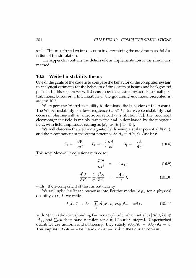
204 CHAPTER 10. COMPUTER SIMULATIONS
scale. This must be taken into account in determining the maximum useful du-ration of the simulation.
The Appendix contains the details of our implementation of the simulationmethod.
10.5 Weibel instability theoryOne of the goals of the code is to compare the behavior of the computed systemto analytical estimates for the behavior of the system of beams and backgroundplasma. In this section we will discuss how this system responds to small per-turbations, based on a linearization of the governing equations presented insection 10.2.
We expect the Weibel instability to dominate the behavior of the plasma.The Weibel instability is a low-frequency (ω kc) transverse instability thatoccurs in plasmas with an anisotropic velocity distribution [98]. The associatedelectromagnetic field is mainly transverse and is dominated by the magneticfield, with field amplitudes scaling as |By| |Ez| |Ex|.
We will describe the electromagnetic fields using a scalar potential Φ(x, t),and the z-component of the vector potential A: Az ≡ A(x, t). One has:
Ex = −∂Φ∂x
, Ez = −1c
∂A∂t
, By = −∂A∂x
. (10.8)
This way, Maxwell’s equations reduce to:
∂2Φ∂x2 = −4π ρ, (10.9)
∂2 A∂x2 −
1c2
∂2 A∂t2 = −4π
cJ, (10.10)
with J the z-component of the current density.We will split the linear response into Fourier modes, e.g., for a physical
quantity A(x , t) we write
A(x , t) → A0 + ∑k
A(ω , k) exp(ikx− iωt) , (10.11)
with A(ω , k) the corresponding Fourier amplitude, which satisfies |A(ω, k)| |A0|, and ∑k a short-hand notation for a full Fourier integral. Unperturbedquantities are uniform and stationary: they satisfy ∂A0/∂t = ∂A0/∂x = 0.This implies ∂A/∂t → −iω A and ∂A/∂x → ik A in the Fourier domain.
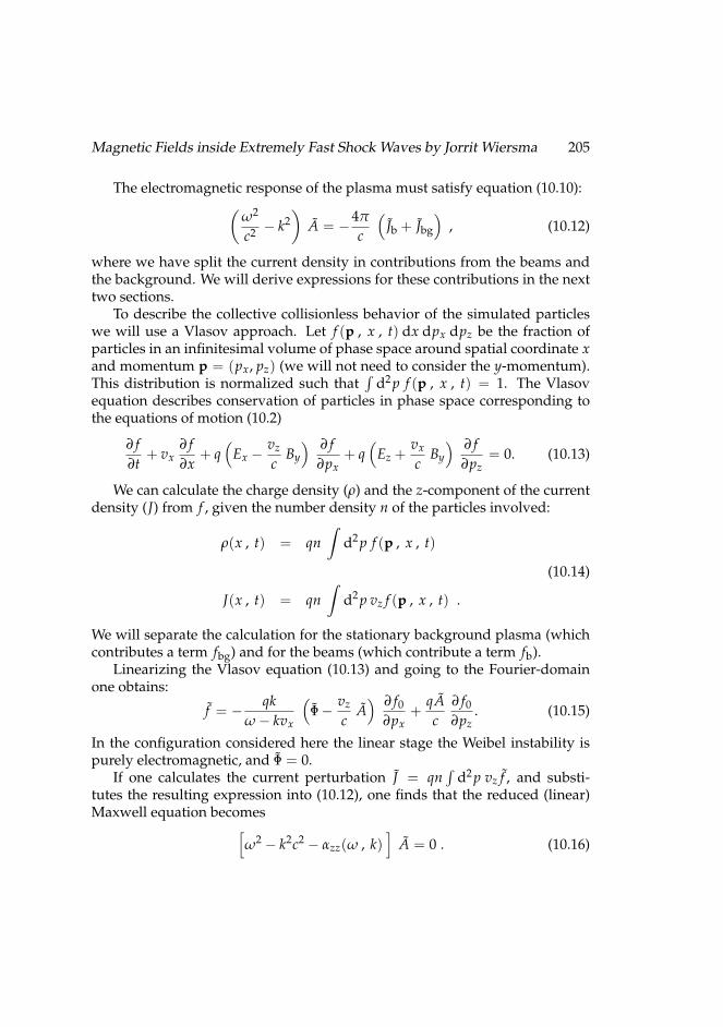
Magnetic Fields inside Extremely Fast Shock Waves by Jorrit Wiersma 205
The electromagnetic response of the plasma must satisfy equation (10.10):(ω2
c2 − k2)
A = −4π
c
(Jb + Jbg
), (10.12)
where we have split the current density in contributions from the beams andthe background. We will derive expressions for these contributions in the nexttwo sections.
To describe the collective collisionless behavior of the simulated particleswe will use a Vlasov approach. Let f (p , x , t) dx dpx dpz be the fraction ofparticles in an infinitesimal volume of phase space around spatial coordinate xand momentum p = (px, pz) (we will not need to consider the y-momentum).This distribution is normalized such that
∫d2 p f (p , x , t) = 1. The Vlasov
equation describes conservation of particles in phase space corresponding tothe equations of motion (10.2)
∂ f∂t
+ vx∂ f∂x
+ q(
Ex −vz
cBy
) ∂ f∂px
+ q(
Ez +vx
cBy
) ∂ f∂pz
= 0. (10.13)
We can calculate the charge density (ρ) and the z-component of the currentdensity (J) from f , given the number density n of the particles involved:
ρ(x , t) = qn∫
d2 p f (p , x , t)
(10.14)
J(x , t) = qn∫
d2 p vz f (p , x , t) .
We will separate the calculation for the stationary background plasma (whichcontributes a term fbg) and for the beams (which contribute a term fb).
Linearizing the Vlasov equation (10.13) and going to the Fourier-domainone obtains:
f = − qkω − kvx
(Φ− vz
cA) ∂ f0
∂px+
qAc
∂ f0
∂pz. (10.15)
In the configuration considered here the linear stage the Weibel instability ispurely electromagnetic, and Φ = 0.
If one calculates the current perturbation J = qn∫
d2 p vz f , and substi-tutes the resulting expression into (10.12), one finds that the reduced (linear)Maxwell equation becomes[
ω2 − k2c2 − αzz(ω , k)]
A = 0 . (10.16)
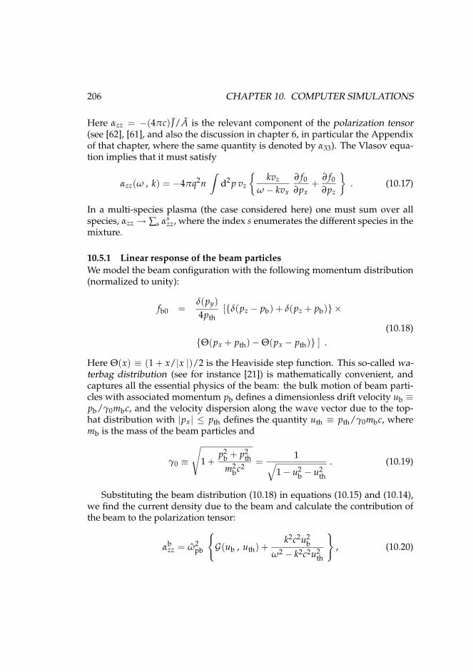
206 CHAPTER 10. COMPUTER SIMULATIONS
Here αzz = −(4πc) J/A is the relevant component of the polarization tensor(see [62], [61], and also the discussion in chapter 6, in particular the Appendixof that chapter, where the same quantity is denoted by α33). The Vlasov equa-tion implies that it must satisfy
αzz(ω , k) = −4πq2n∫
d2 p vz
kvz
ω − kvx
∂ f0
∂px+
∂ f0
∂pz
. (10.17)
In a multi-species plasma (the case considered here) one must sum over allspecies, αzz → ∑s αs
zz, where the index s enumerates the different species in themixture.
10.5.1 Linear response of the beam particlesWe model the beam configuration with the following momentum distribution(normalized to unity):
fb0 =δ(py)4pth
[δ(pz − pb) + δ(pz + pb)×
(10.18)Θ(px + pth)−Θ(px − pth) ] .
Here Θ(x) ≡ (1 + x/|x |)/2 is the Heaviside step function. This so-called wa-terbag distribution (see for instance [21]) is mathematically convenient, andcaptures all the essential physics of the beam: the bulk motion of beam parti-cles with associated momentum pb defines a dimensionless drift velocity ub ≡pb/γ0mbc, and the velocity dispersion along the wave vector due to the top-hat distribution with |px| ≤ pth defines the quantity uth ≡ pth/γ0mbc, wheremb is the mass of the beam particles and
γ0 ≡
√1 +
p2b + p2
thm2
bc2=
1√1− u2
b − u2th
. (10.19)
Substituting the beam distribution (10.18) in equations (10.15) and (10.14),we find the current density due to the beam and calculate the contribution ofthe beam to the polarization tensor:
αbzz = ω2
pb
G(ub , uth) +
k2c2u2b
ω2 − k2c2u2th
, (10.20)
Magnetic Fields inside Extremely Fast Shock Waves by Jorrit Wiersma 207
where nb is the number density of the beam particles,
ω2pb =
4πq2nbγ0mb
(10.21)
is the beam plasma frequency squared, and
G(ub , uth) ≡ γ0
∫d2 p
γ
(1− vz
2
c2
)fb0
=1
2uthln
(1 + uth1− uth
)−
γ20u2
b1 + γ2
0u2b
(10.22)
=1
2uthln
(1 + uth1− uth
)−
u2b
1− u2th
.
This function follows from the term involving ∂ f0/∂pz in expression (10.17),after partial integration with respect to pz, and using ∂vz/∂pz = (1/γm)(1−v2
z/c2).
10.5.2 Linear response of the background particlesBecause the background particles have an isotropic distribution with no bulkvelocity the easiest approach to calculate their linear response to electromag-netic perturbations is to use a fluid description. From standard linear theory(chapter 6) we know that the linear current density perpendicular to k is givenby
Jbg = −ω2
p,fl
4πcA, (10.23)
where ωp,fl is the relativistic plasma frequency in the fluid model:
ω2p,fl =
4πq2 nbg
hbgm. (10.24)
Here nbg is the density of the background and hbg is the enthalpy per unit mass,which is given by
hbg = 1 +e + P
nbgmc2 , (10.25)
208 CHAPTER 10. COMPUTER SIMULATIONS
with P the pressure and e the internal (thermal) energy of the backgroundplasma. For an N-dimensional Maxwellian plasma with temperature T, in theultra-relativistic limit kbT mc2, one has e = NP = NnbgkbT and hbg ≈(N + 1)kbT/mc2. In that case the plasma frequency (10.24) in the fluid approx-imation becomes:
ω2p,fl ≈
4πq2nbgc2
(N + 1) kbT. (10.26)
In this model the polarization αzz is constant:
αflzz = ω2
p,fl . (10.27)
The simple fluid approach does not take account of the effect of the large ve-locity dispersion of the background plasma (in particular of the electrons orpositrons) that arises when the background becomes relativistically hot, e.g.,[55]. To take these effects into account we will use kinetic theory for the back-ground plasma. In chapter 6 we found for the three-dimensional Weibel insta-bility that the difference between the two approaches is small. Here we brieflyderive the corresponding results for a two-dimensional thermal backgroundplasma.
In the two-dimensional case considered here one can use a two-dimensionalultra-relativistic Maxwellian distribution, approximating the particle energyby E ≈ pc, which is
f Maxwbg0 (p) =
1
2π(
pthbg
)2 e−p/pthbg . (10.28)
Here p =√
p2x + p2
y, and
pthbg ≡ kbT/c (10.29)
is the typical thermal momentum, with T the temperature of the backgroundplasma and kb Boltzmann’s constant. In that case the background contributionto αzz for a purely growing mode, with ω = iσ equals:
αbgzz = ω2
pbg
(σ
kc
) [√1 +
σ2
k2c2 −σ
kc
]. (10.30)
The background plasma frequency squared in this case equals
ω2pbg =
4πq2nbgc
pthbg
=4πq2nbgc2
kbT. (10.31)
Magnetic Fields inside Extremely Fast Shock Waves by Jorrit Wiersma 209
In the simulations we use, for computational convenience, a two-dimensionalGaussian momentum distribution for the background particles of the form
fbg0(p) =1
2π(pthbg)2
exp(−(p/2pth
bg)2)
, (10.32)
This distribution leaves the functional form (10.30) of αbgzz (σ , k) unchanged,
and only leads to a small change in the value of the background plasma fre-quency, by a factor
√π/2 ≈ 1.25:
ω2pbg −→
√π
24πq2nbgc
pthbg
. (10.33)
We assume once again that pthbg mc.
10.5.3 Dispersion relation
Substituting αzz ≡ αbgzz + αb
zz into dispersion relation (10.16) gives the disper-sion relation for the unstable electromagnetic mode. The resulting dispersionrelation is very similar to results obtained in chapter 6 for the case of a fullythree-dimensional thermal background. Following the conventions introducedin chapter 6, we define the dimensionless growth rate σ and the dimensionlesswave number κ, measured in units of the background plasma frequency ωpbgand inverse skin depth respectively:
σ = σ/ωpbg , κ = kc/ωpbg . (10.34)
If one uses a fluid model for the background (either 2D or 3D in momentumspace), the dispersion relation is the one derived in chapter 6:
σ4 + B σ2 − C = 0, (10.35)
withB = κ2
(1 + u2
th
)+ (1 + η G),
C = κ2u2th
η M2 −
(κ2 + η G + 1
) .
(10.36)
Hereη ≡ ω2
pb/ω2pbg (10.37)
210 CHAPTER 10. COMPUTER SIMULATIONS
andM ≡ ub/uth = pb/pth. (10.38)
are the two fundamental parameters that determine the growth rate and therange of unstable wavenumbers of the instability, see chapter 6.
This mode is has an unstable solution (with σ > 0) when C > 0. The growthrate σ is then given by
σ2 =
√B2 + 4C − B
2. (10.39)
The instability condition C > 0 leads to the condition κ < κmax on the wave-number, where
κ2max = η(M2 − G)− 1. (10.40)
For ultra-relativistic shocks (γ0 1) the expression simplify because uth ub ∼ 1 and G 1. We then get
B ' 1 + κ2,
C ' κ2
M2
(η M2 − κ2 − 1
), (10.41)
κ2max ' ηM2 − 1.
The dispersion relation of the instability in the fluid model is characterized bythe two parameters η and M, see chapter 6. The parameter η measures thestrength of the beam plasma compared to the background plasma, the param-eterMmeasures the importance of the thermal motions in the beams. As such,η determines the (maximum) growth rate of the instability, and η and M to-gether determine the range of wavelengths that are unstable, as is illustratedin figures 10.1 and 10.2.
The 2D kinetic model for the background response yields a dispersion rela-tion that can be written as
σ2 + κ2 +(σ
κ
) [√1 +
σ2
κ2 −σ
κ
]− ηκ2
σ2 + κ2/M2 = 0 . (10.42)
This will give an instability with σ > 0 for κ <√
ηM. Dispersion rela-tion (10.42) can only be solved numerically. In the low-frequency limit, σ2 κ2, one can expand the square root, and the leading terms give an approximatedispersion relation of the form
κ2(
σ2 +κ2
M2 − η
)+
σ
κ
(σ2 +
κ2
M2
)= 0 . (10.43)
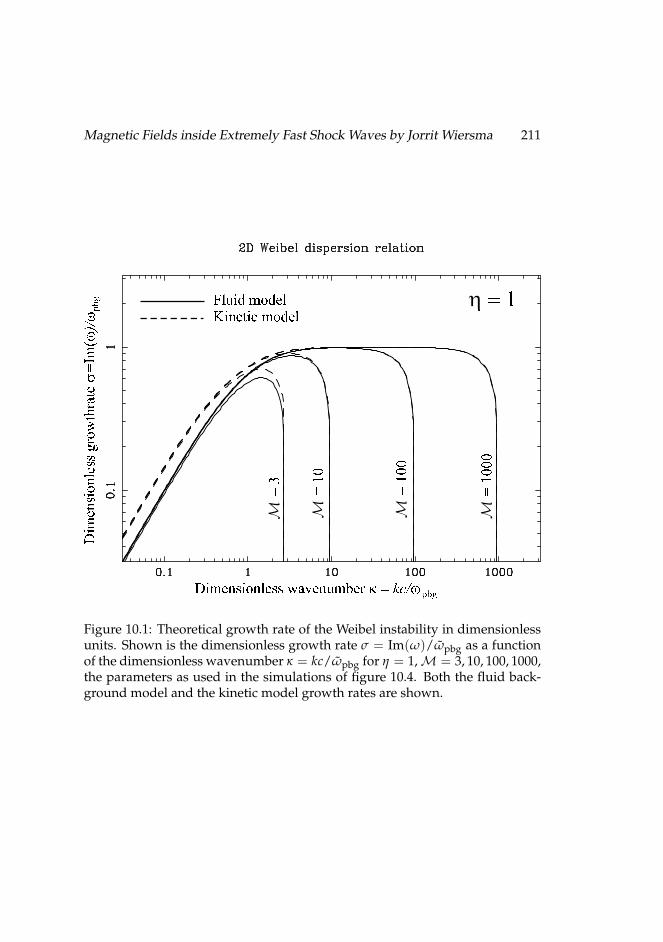
Magnetic Fields inside Extremely Fast Shock Waves by Jorrit Wiersma 211
Figure 10.1: Theoretical growth rate of the Weibel instability in dimensionlessunits. Shown is the dimensionless growth rate σ = Im(ω)/ωpbg as a functionof the dimensionless wavenumber κ = kc/ωpbg for η = 1,M = 3, 10, 100, 1000,the parameters as used in the simulations of figure 10.4. Both the fluid back-ground model and the kinetic model growth rates are shown.
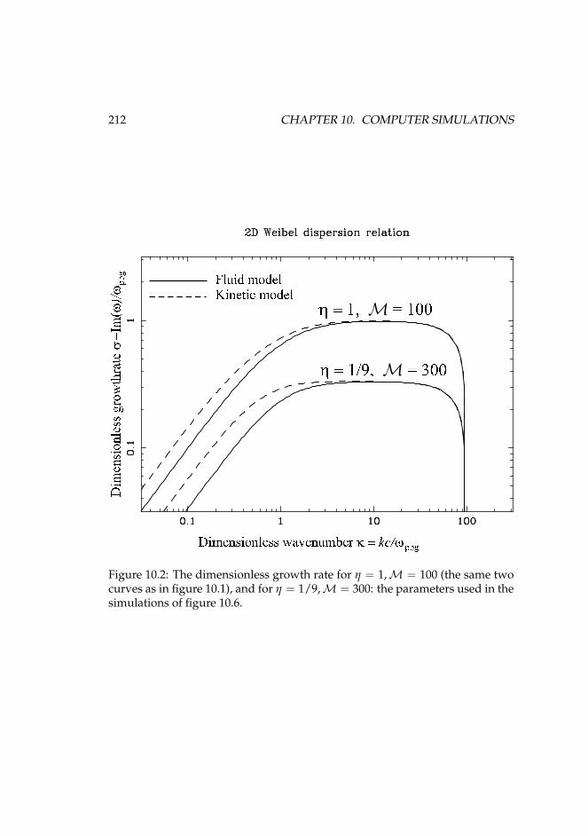
212 CHAPTER 10. COMPUTER SIMULATIONS
Figure 10.2: The dimensionless growth rate for η = 1,M = 100 (the same twocurves as in figure 10.1), and for η = 1/9,M = 300: the parameters used in thesimulations of figure 10.6.
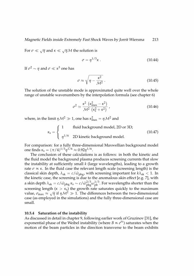
Magnetic Fields inside Extremely Fast Shock Waves by Jorrit Wiersma 213
For σ √η and κ √
ηM the solution is
σ = η1/3κ . (10.44)
If σ2 ∼ η and σ κ3 one has
σ ≈√
η − κ2
M2 . (10.45)
The solution of the unstable mode is approximated quite well over the wholerange of unstable wavenumbers by the interpolation formula (see chapter 6)
σ2 'κ2 (κ2
max − κ2)M2
(κ2
s + κ2) , (10.46)
where, in the limit ηM2 1, one has κ2max = ηM2 and
κs =
1 fluid background model, 2D or 3D;
η1/6 2D kinetic background model.(10.47)
For comparison: for a fully three-dimensional Maxwellian background modelone finds κs = (π/4)1/3η1/6 ≈ 0.92η1/6.
The conclusion of these calculations is as follows: in both the kinetic andthe fluid model the background plasma produces screening currents that slowthe instability at sufficiently small k (large wavelengths), leading to a growthrate σ ∝ κ. In the fluid case the relevant length scale (screening length) is theclassical skin depth, λsk = c/ωpbg, with screening important for kλsk < 1. Inthe kinetic case, the screening is due to the anomalous skin effect [e.g. 7], witha skin depth λsk = c/ωpbg κs ∼ c/ω2/3
pbgω1/3pb . For wavelengths shorter than the
screening length (κ > κs) the growth rate saturates quickly to the maximumvalue, σmax ≈
√η if ηM2 1. The differences between the two-dimensional
case (as employed in the simulations) and the fully three-dimensional case aresmall.
10.5.4 Saturation of the instabilityAs discussed in detail in chapter 9, following earlier work of Gruzinov [31], theexponential phase of the Weibel instability (where B ∝ eσt) saturates when themotion of the beam particles in the direction transverse to the beam exhibits
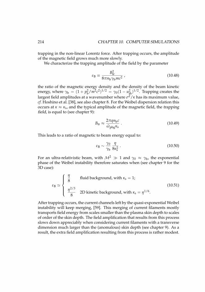
214 CHAPTER 10. COMPUTER SIMULATIONS
trapping in the non-linear Lorentz force. After trapping occurs, the amplitudeof the magnetic field grows much more slowly.
We characterize the trapping amplitude of the field by the parameter
εB ≡B2
tr8πnbγbmc2 , (10.48)
the ratio of the magnetic energy density and the density of the beam kineticenergy, where γb = (1 + p2
b/m2c2)1/2 = γ0(1− u2th)1/2. Trapping creates the
largest field amplitudes at a wavenumber where σ2/κ has its maximum value,cf. Hoshino et al. [38], see also chapter 8. For the Weibel dispersion relation thisoccurs at κ ≈ κs, and the typical amplitude of the magnetic field, the trappingfield, is equal to (see chapter 9):
Btr ≈2πqnbcωpbgκs
. (10.49)
This leads to a ratio of magnetic to beam energy equal to:
εB ∼γ0
γb
η
8κ2s
. (10.50)
For an ultra-relativistic beam, with M2 1 and γ0 ≈ γb, the exponentialphase of the Weibel instability therefore saturates when (see chapter 9 for the3D case):
εB '
η
8fluid background, with κs = 1;
η2/3
82D kinetic background, with κs = η1/6.
(10.51)
After trapping occurs, the current channels left by the quasi-exponential Weibelinstability will keep merging, [59]. This merging of current filaments mostlytransports field energy from scales smaller than the plasma skin depth to scalesof order of the skin depth. The field amplification that results from this processslows down appreciably when considering current filaments with a transversedimension much larger than the (anomalous) skin depth (see chapter 9). As aresult, the extra field amplification resulting from this process is rather modest.
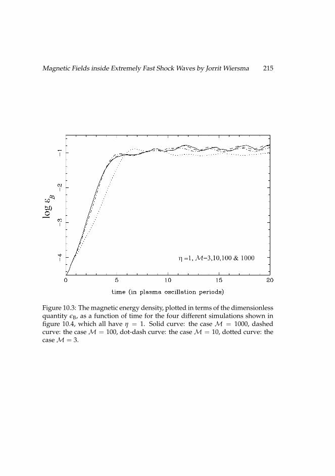
Magnetic Fields inside Extremely Fast Shock Waves by Jorrit Wiersma 215
Figure 10.3: The magnetic energy density, plotted in terms of the dimensionlessquantity εB, as a function of time for the four different simulations shown infigure 10.4, which all have η = 1. Solid curve: the case M = 1000, dashedcurve: the case M = 100, dot-dash curve: the case M = 10, dotted curve: thecase M = 3.
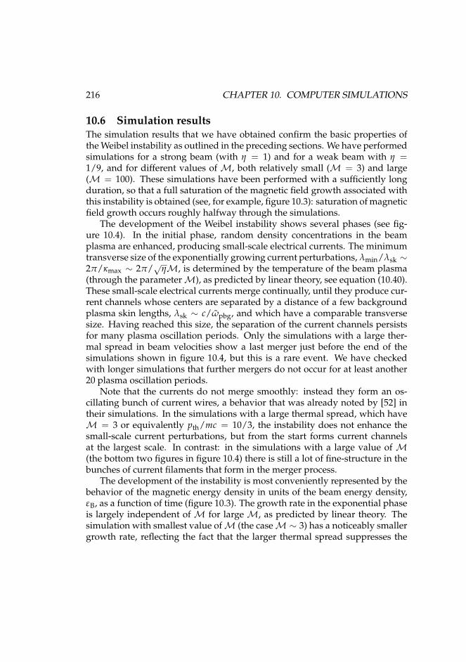
216 CHAPTER 10. COMPUTER SIMULATIONS
10.6 Simulation resultsThe simulation results that we have obtained confirm the basic properties ofthe Weibel instability as outlined in the preceding sections. We have performedsimulations for a strong beam (with η = 1) and for a weak beam with η =1/9, and for different values of M, both relatively small (M = 3) and large(M = 100). These simulations have been performed with a sufficiently longduration, so that a full saturation of the magnetic field growth associated withthis instability is obtained (see, for example, figure 10.3): saturation of magneticfield growth occurs roughly halfway through the simulations.
The development of the Weibel instability shows several phases (see fig-ure 10.4). In the initial phase, random density concentrations in the beamplasma are enhanced, producing small-scale electrical currents. The minimumtransverse size of the exponentially growing current perturbations, λmin/λsk ∼2π/κmax ∼ 2π/√ηM, is determined by the temperature of the beam plasma(through the parameter M), as predicted by linear theory, see equation (10.40).These small-scale electrical currents merge continually, until they produce cur-rent channels whose centers are separated by a distance of a few backgroundplasma skin lengths, λsk ∼ c/ωpbg, and which have a comparable transversesize. Having reached this size, the separation of the current channels persistsfor many plasma oscillation periods. Only the simulations with a large ther-mal spread in beam velocities show a last merger just before the end of thesimulations shown in figure 10.4, but this is a rare event. We have checkedwith longer simulations that further mergers do not occur for at least another20 plasma oscillation periods.
Note that the currents do not merge smoothly: instead they form an os-cillating bunch of current wires, a behavior that was already noted by [52] intheir simulations. In the simulations with a large thermal spread, which haveM = 3 or equivalently pth/mc = 10/3, the instability does not enhance thesmall-scale current perturbations, but from the start forms current channelsat the largest scale. In contrast: in the simulations with a large value of M(the bottom two figures in figure 10.4) there is still a lot of fine-structure in thebunches of current filaments that form in the merger process.
The development of the instability is most conveniently represented by thebehavior of the magnetic energy density in units of the beam energy density,εB, as a function of time (figure 10.3). The growth rate in the exponential phaseis largely independent of M for large M, as predicted by linear theory. Thesimulation with smallest value ofM (the caseM ∼ 3) has a noticeably smallergrowth rate, reflecting the fact that the larger thermal spread suppresses the
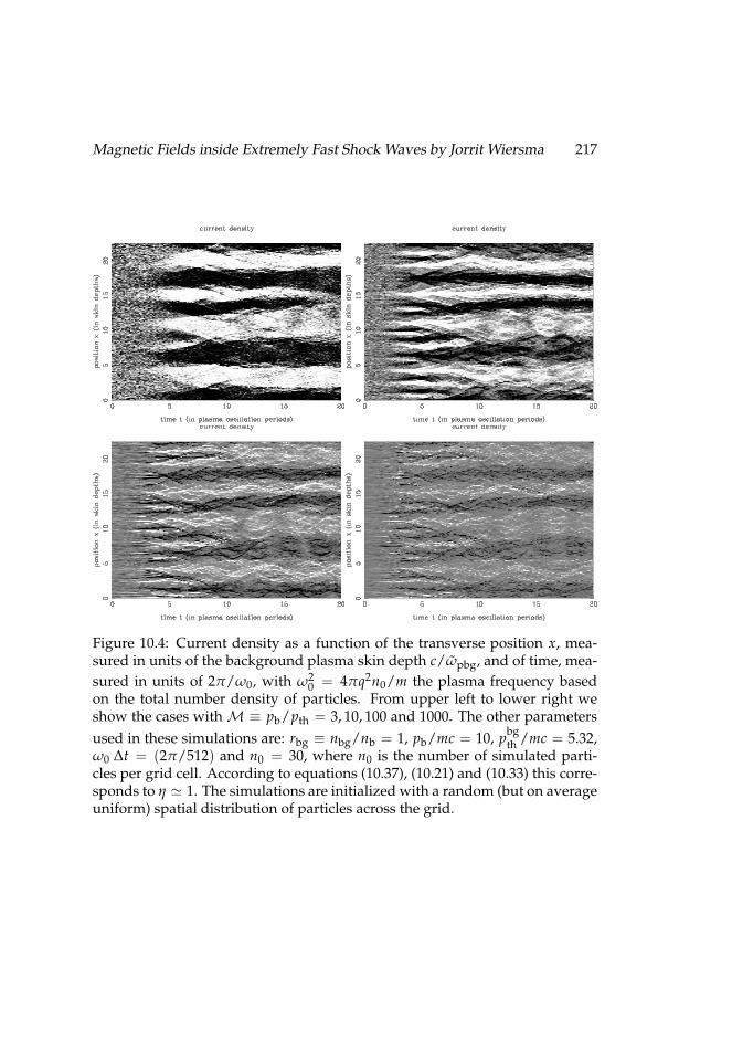
Magnetic Fields inside Extremely Fast Shock Waves by Jorrit Wiersma 217
Figure 10.4: Current density as a function of the transverse position x, mea-sured in units of the background plasma skin depth c/ωpbg, and of time, mea-sured in units of 2π/ω0, with ω2
0 = 4πq2n0/m the plasma frequency basedon the total number density of particles. From upper left to lower right weshow the cases with M ≡ pb/pth = 3, 10, 100 and 1000. The other parametersused in these simulations are: rbg ≡ nbg/nb = 1, pb/mc = 10, pbg
th /mc = 5.32,ω0 ∆t = (2π/512) and n0 = 30, where n0 is the number of simulated parti-cles per grid cell. According to equations (10.37), (10.21) and (10.33) this corre-sponds to η ' 1. The simulations are initialized with a random (but on averageuniform) spatial distribution of particles across the grid.
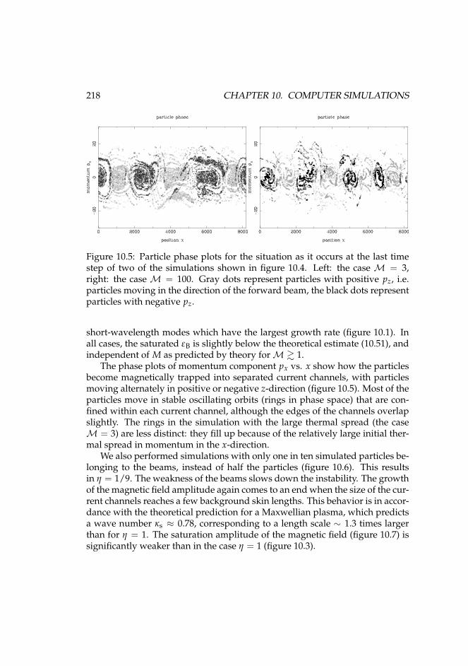
218 CHAPTER 10. COMPUTER SIMULATIONS
Figure 10.5: Particle phase plots for the situation as it occurs at the last timestep of two of the simulations shown in figure 10.4. Left: the case M = 3,right: the case M = 100. Gray dots represent particles with positive pz, i.e.particles moving in the direction of the forward beam, the black dots representparticles with negative pz.
short-wavelength modes which have the largest growth rate (figure 10.1). Inall cases, the saturated εB is slightly below the theoretical estimate (10.51), andindependent of M as predicted by theory for M & 1.
The phase plots of momentum component px vs. x show how the particlesbecome magnetically trapped into separated current channels, with particlesmoving alternately in positive or negative z-direction (figure 10.5). Most of theparticles move in stable oscillating orbits (rings in phase space) that are con-fined within each current channel, although the edges of the channels overlapslightly. The rings in the simulation with the large thermal spread (the caseM = 3) are less distinct: they fill up because of the relatively large initial ther-mal spread in momentum in the x-direction.
We also performed simulations with only one in ten simulated particles be-longing to the beams, instead of half the particles (figure 10.6). This resultsin η = 1/9. The weakness of the beams slows down the instability. The growthof the magnetic field amplitude again comes to an end when the size of the cur-rent channels reaches a few background skin lengths. This behavior is in accor-dance with the theoretical prediction for a Maxwellian plasma, which predictsa wave number κs ≈ 0.78, corresponding to a length scale ∼ 1.3 times largerthan for η = 1. The saturation amplitude of the magnetic field (figure 10.7) issignificantly weaker than in the case η = 1 (figure 10.3).
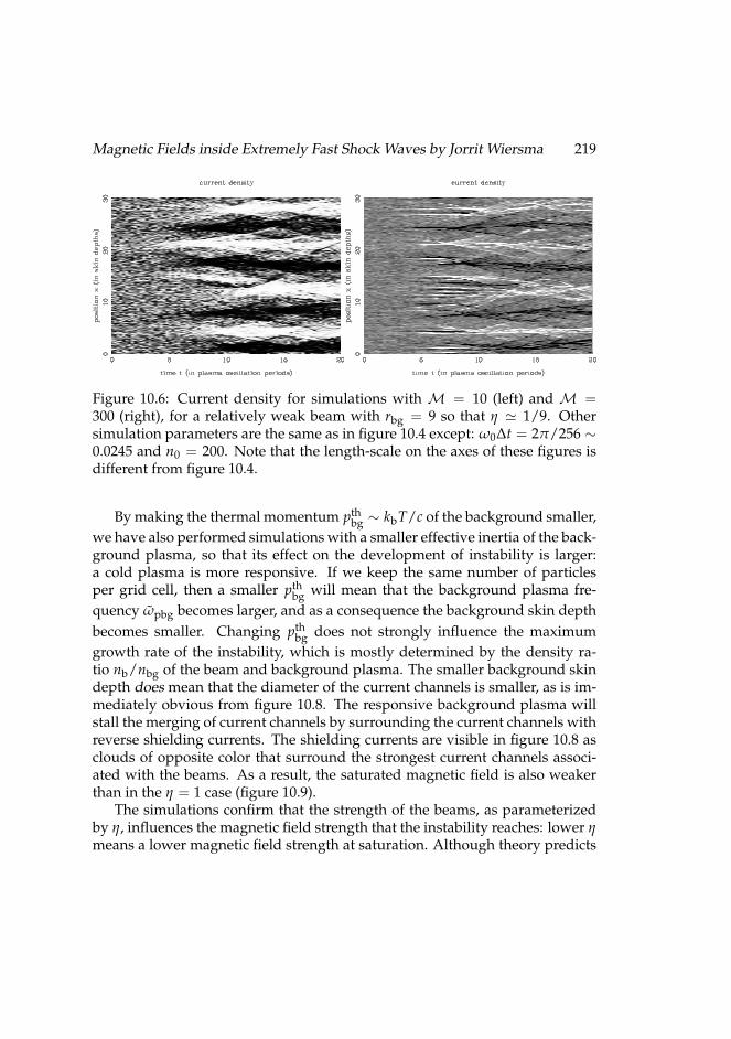
Magnetic Fields inside Extremely Fast Shock Waves by Jorrit Wiersma 219
Figure 10.6: Current density for simulations with M = 10 (left) and M =300 (right), for a relatively weak beam with rbg = 9 so that η ' 1/9. Othersimulation parameters are the same as in figure 10.4 except: ω0∆t = 2π/256 ∼0.0245 and n0 = 200. Note that the length-scale on the axes of these figures isdifferent from figure 10.4.
By making the thermal momentum pthbg ∼ kbT/c of the background smaller,
we have also performed simulations with a smaller effective inertia of the back-ground plasma, so that its effect on the development of instability is larger:a cold plasma is more responsive. If we keep the same number of particlesper grid cell, then a smaller pth
bg will mean that the background plasma fre-quency ωpbg becomes larger, and as a consequence the background skin depthbecomes smaller. Changing pth
bg does not strongly influence the maximumgrowth rate of the instability, which is mostly determined by the density ra-tio nb/nbg of the beam and background plasma. The smaller background skindepth does mean that the diameter of the current channels is smaller, as is im-mediately obvious from figure 10.8. The responsive background plasma willstall the merging of current channels by surrounding the current channels withreverse shielding currents. The shielding currents are visible in figure 10.8 asclouds of opposite color that surround the strongest current channels associ-ated with the beams. As a result, the saturated magnetic field is also weakerthan in the η = 1 case (figure 10.9).
The simulations confirm that the strength of the beams, as parameterizedby η, influences the magnetic field strength that the instability reaches: lower ηmeans a lower magnetic field strength at saturation. Although theory predicts
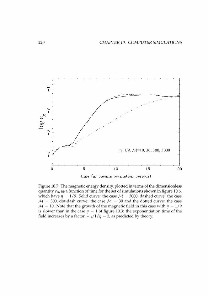
220 CHAPTER 10. COMPUTER SIMULATIONS
Figure 10.7: The magnetic energy density, plotted in terms of the dimensionlessquantity εB, as a function of time for the set of simulations shown in figure 10.6,which have η = 1/9. Solid curve: the case M = 3000, dashed curve: the caseM = 300, dot-dash curve: the case M = 30 and the dotted curve: the caseM = 10. Note that the growth of the magnetic field in this case with η = 1/9is slower than in the case η = 1 of figure 10.3: the exponentiation time of thefield increases by a factor ∼
√1/η = 3, as predicted by theory.
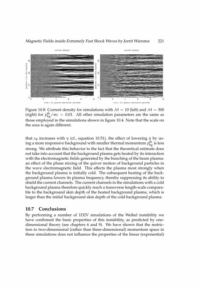
Magnetic Fields inside Extremely Fast Shock Waves by Jorrit Wiersma 221
Figure 10.8: Current density for simulations with M = 10 (left) and M = 300(right) for pth
bg/mc = 0.01. All other simulation parameters are the same asthose employed in the simulations shown in figure 10.4. Note that the scale onthe axes is again different.
that εB increases with η (cf., equation 10.51), the effect of lowering η by us-ing a more responsive background with smaller thermal momentum pth
bg is lessstrong. We attribute this behavior to the fact that the theoretical estimate doesnot take into account that the background plasma gets heated by its interactionwith the electromagnetic fields generated by the bunching of the beam plasma:an effect of the phase mixing of the quiver motion of background particles inthe wave electromagnetic field. This affects the plasma most strongly whenthe background plasma is initially cold. The subsequent heating of the back-ground plasma lowers its plasma frequency, thereby suppressing its ability toshield the current channels. The current channels in the simulations with a coldbackground plasma therefore quickly reach a transverse length-scale compara-ble to the background skin depth of the heated background plasma, which islarger than the initial background skin depth of the cold background plasma.
10.7 ConclusionsBy performing a number of 1D2V simulations of the Weibel instability wehave confirmed the basic properties of this instability, as predicted by one-dimensional theory (see chapters 6 and 9). We have shown that the restric-tion to two-dimensional (rather than three-dimensional) momentum space inthese simulations does not influence the properties of the linear (exponential)
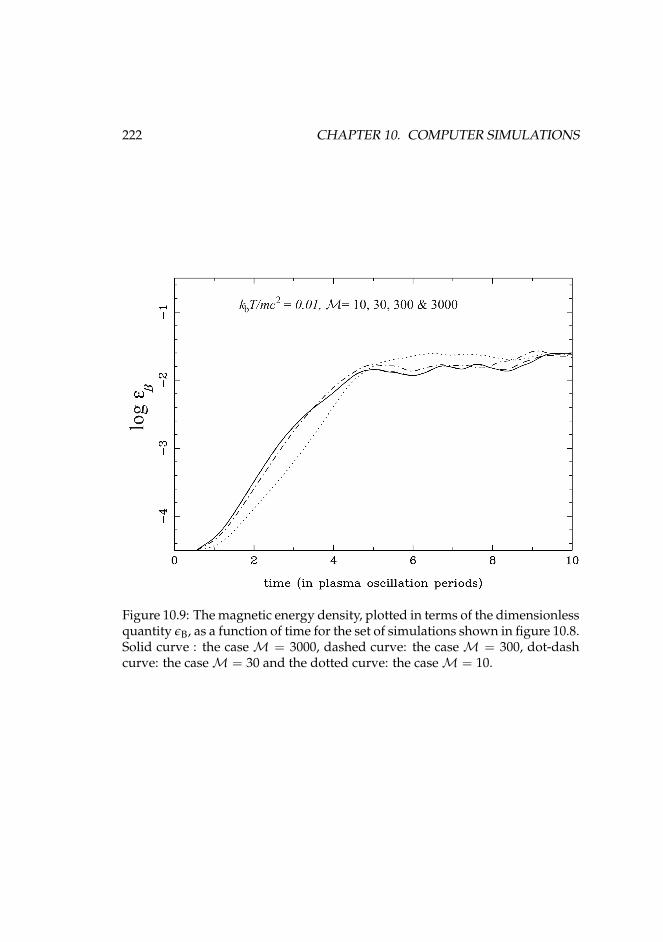
222 CHAPTER 10. COMPUTER SIMULATIONS
Figure 10.9: The magnetic energy density, plotted in terms of the dimensionlessquantity εB, as a function of time for the set of simulations shown in figure 10.8.Solid curve : the case M = 3000, dashed curve: the case M = 300, dot-dashcurve: the case M = 30 and the dotted curve: the case M = 10.
Magnetic Fields inside Extremely Fast Shock Waves by Jorrit Wiersma 223
phase of the instability: the growth rate σ and range of unstable wavenum-bers behave the same as in the case where the background has three degreesof freedom in momentum space. The waterbag model for the beam plasma,on which our analytical estimates are based, is intrinsically two-dimensionalin momentum space.
The Weibel instability produces electrical current channels, whose strengthis limited by the magnetic trapping of the particles inside the current channels.A dense and hot (stationary) background plasma inhibits the merging of thethe parallel electrical currents produced by the instability due to its screeningaction, thereby reducing the magnetic field strength that the instability ulti-mately produces.
The influence of a strong background plasma is particularly important forthe development of the Weibel instability for proton beams in a backgroundplasma containing electrons. The low mass of the electrons implies that theyform a very responsive background plasma, so that effectively η 1. This willinhibit the merging of proton currents by shielding of the current channels asin our simulations with a cold background plasma.
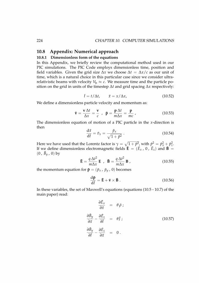
224 CHAPTER 10. COMPUTER SIMULATIONS
10.8 Appendix: Numerical approach10.8.1 Dimensionless form of the equationsIn this Appendix, we briefly review the computational method used in ourPIC simulations. The PIC Code employs dimensionless time, position andfield variables. Given the grid size ∆x we choose ∆t = ∆x/c as our unit oftime, which is a natural choice in this particular case since we consider ultra-relativistic beams with velocity Vb ≈ c. We measure time and the particle po-sition on the grid in units of the timestep ∆t and grid spacing ∆x respectively:
t = t/∆t, x = x/∆x, (10.52)
We define a dimensionless particle velocity and momentum as:
v =v ∆t∆x
=vc
, p =p ∆tm∆x
=p
mc, (10.53)
The dimensionless equation of motion of a PIC particle in the x-direction isthen
dxdt
= vx =px√
1 + p2. (10.54)
Here we have used that the Lorentz factor is γ =√
1 + p2, with p2 = p2x + p2
z .If we define dimensionless electromagnetic fields E = (Ex , 0 , Ez) and B =(0 , By , 0) by
E =q ∆t2
m∆xE , B =
q ∆t2
m∆xB , (10.55)
the momentum equation for p = ( px , py , 0) becomes
dpdt
= E + v× B . (10.56)
In these variables, the set of Maxwell’s equations (equations (10.5 - 10.7) of themain paper) read:
∂Ex
∂x= θ ρ ;
∂By
∂x− ∂Ez
∂t= θ J ; (10.57)
∂By
∂t− ∂Ez
∂x= 0 .
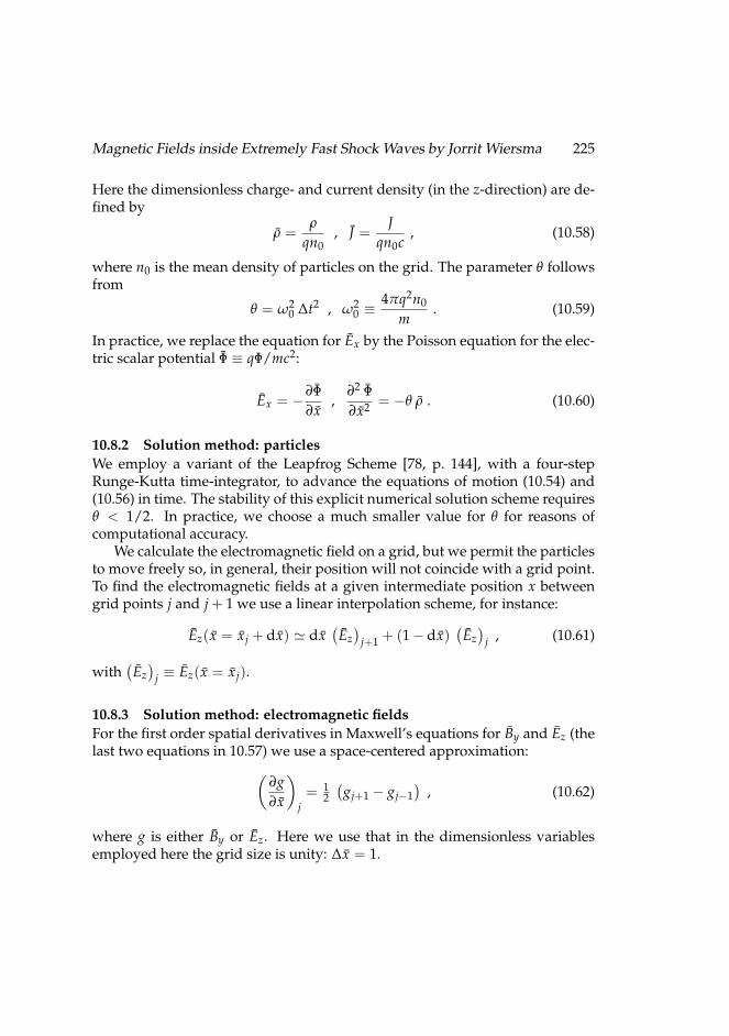
Magnetic Fields inside Extremely Fast Shock Waves by Jorrit Wiersma 225
Here the dimensionless charge- and current density (in the z-direction) are de-fined by
ρ =ρ
qn0, J =
Jqn0c
, (10.58)
where n0 is the mean density of particles on the grid. The parameter θ followsfrom
θ = ω20 ∆t2 , ω2
0 ≡4πq2n0
m. (10.59)
In practice, we replace the equation for Ex by the Poisson equation for the elec-tric scalar potential Φ ≡ qΦ/mc2:
Ex = −∂Φ∂x
,∂2 Φ∂x2 = −θ ρ . (10.60)
10.8.2 Solution method: particlesWe employ a variant of the Leapfrog Scheme [78, p. 144], with a four-stepRunge-Kutta time-integrator, to advance the equations of motion (10.54) and(10.56) in time. The stability of this explicit numerical solution scheme requiresθ < 1/2. In practice, we choose a much smaller value for θ for reasons ofcomputational accuracy.
We calculate the electromagnetic field on a grid, but we permit the particlesto move freely so, in general, their position will not coincide with a grid point.To find the electromagnetic fields at a given intermediate position x betweengrid points j and j + 1 we use a linear interpolation scheme, for instance:
Ez(x = xj + dx) ' dx(Ez)
j+1 + (1− dx)(Ez)
j , (10.61)
with(Ez)
j ≡ Ez(x = xj).
10.8.3 Solution method: electromagnetic fieldsFor the first order spatial derivatives in Maxwell’s equations for By and Ez (thelast two equations in 10.57) we use a space-centered approximation:(
∂g∂x
)j= 1
2(
gj+1 − gj−1)
, (10.62)
where g is either By or Ez. Here we use that in the dimensionless variablesemployed here the grid size is unity: ∆x = 1.
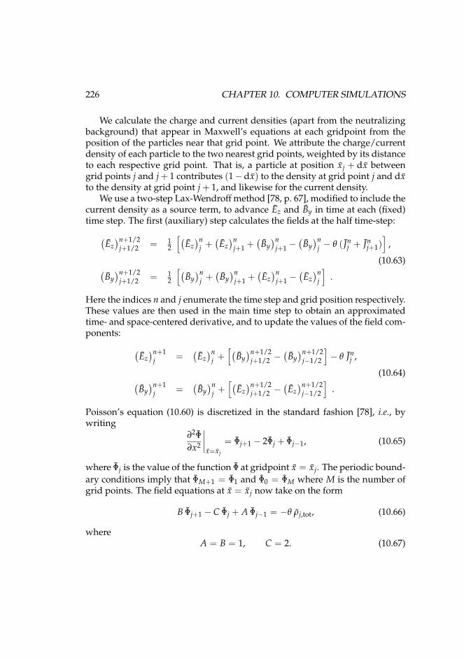
226 CHAPTER 10. COMPUTER SIMULATIONS
We calculate the charge and current densities (apart from the neutralizingbackground) that appear in Maxwell’s equations at each gridpoint from theposition of the particles near that grid point. We attribute the charge/currentdensity of each particle to the two nearest grid points, weighted by its distanceto each respective grid point. That is, a particle at position xj + dx betweengrid points j and j + 1 contributes (1− dx) to the density at grid point j and dxto the density at grid point j + 1, and likewise for the current density.
We use a two-step Lax-Wendroff method [78, p. 67], modified to include thecurrent density as a source term, to advance Ez and By in time at each (fixed)time step. The first (auxiliary) step calculates the fields at the half time-step:(
Ez)n+1/2
j+1/2 = 12
[(Ez)n
j +(Ez)n
j+1 +(
By)n
j+1 −(
By)n
j − θ ( Jnj + Jn
j+1)]
,
(10.63)(By)n+1/2
j+1/2 = 12
[(By)n
j +(
By)n
j+1 +(Ez)n
j+1 −(Ez)n
j
].
Here the indices n and j enumerate the time step and grid position respectively.These values are then used in the main time step to obtain an approximatedtime- and space-centered derivative, and to update the values of the field com-ponents: (
Ez)n+1
j =(Ez)n
j +[(
By)n+1/2
j+1/2 −(
By)n+1/2
j−1/2
]− θ Jn
j ,
(10.64)(By)n+1
j =(
By)n
j +[(
Ez)n+1/2
j+1/2 −(Ez)n+1/2
j−1/2
].
Poisson’s equation (10.60) is discretized in the standard fashion [78], i.e., bywriting
∂2Φ∂x2
∣∣∣∣x=xj
= Φj+1 − 2Φj + Φj−1, (10.65)
where Φj is the value of the function Φ at gridpoint x = xj. The periodic bound-ary conditions imply that ΦM+1 = Φ1 and Φ0 = ΦM where M is the number ofgrid points. The field equations at x = xj now take on the form
B Φj+1 − C Φj + A Φj−1 = −θ ρj,tot, (10.66)
whereA = B = 1, C = 2. (10.67)
Magnetic Fields inside Extremely Fast Shock Waves by Jorrit Wiersma 227
Poisson’s finite-difference equation (10.66) for the scalar potential Φ can besolved with the Forward Elimination–Backward Substitution Method [54, sec-tion 13.2.2]. For stability, this method requires
A > 0, B > 0, C > A + B . (10.68)
Formally, the last requirement is not satisfied by our equations because C =A + B = 2. To remedy this, we have added a small positive quantity to C, in ef-fect putting C =⇒ 2 + ε with ε 1. The effect of this replacement is to slightlyenhance the Debye shielding of the electric field. As such, it is equivalent withadding a massive background plasma with a Debye length much larger thanthat of the gas of simulated particles. This ‘fix’ does not influence the solutionon the scale that we are interested in: the skin depth of the simulated plasma.

228 CHAPTER 10. COMPUTER SIMULATIONS
Part III
Discussion and summary
229

Chapter 11
Discussion and conclusions
In this thesis I have presented an in-depth look at the physical processes thatwe expect to be at work in shock fronts that move with a speed very close tothe speed of light. These shock waves only occur in deep space near extremelyviolent phenomena such as the explosion of stars many times heavier than theSun or near compact objects such as neutron stars or black holes. The con-ditions in these environments are very different from conditions on Earth. Inshock waves in normal air, such as the sonic boom of a jet plane traveling fasterthan sound, the physical processes producing the shock wave are dominatedby collisions of the particles in the air. In most astrophysical situations, the gasdensity is so low that particle collisions are too rare to be of any importance.
We can still say something about the global properties of the shock tran-sition if we assume that there are other processes than particle collisions thatcan produce the shock transition (chapter 5). However, because the particlesin astrophysical gases (plasma) are electrically charged, we have to allow forthe influence of electromagnetic fields. This introduces an uncertainty that wehave now partly resolved.
Electromagnetic interaction plays a crucial role in these shock waves. Imag-ine a charged particle flying freely in deep space, part of the interstellar mate-rial that pervades all of space. When such a particle is overtaken by a relativis-tic shock wave it will be practically unaffected at first because the density ofparticles is so low, and they are so far separated from each other, that the par-ticle hardly feels the electromagnetic field of the particles in the shock wave.However, if a concentration of charges occurs in the plasma, and this couldhappen purely by chance, then the cumulative electromagnetic field could bestrong enough to influence the particle.
Because we are talking about relativistic shock waves the particles movevery fast and a moving concentration of charges constitutes an electrical cur-
231
232 CHAPTER 11. DISCUSSION AND CONCLUSIONS
rent. If the particle that we are considering is moving in such a way thatit would contribute to the electrical current of the random concentration ofcharge then it will be attracted by it (and repelled if it is moving in the oppo-site direction). The existence of this process of self-enhancing electrical currentswas already proven by Erich S. Weibel in 1959 [98] and is therefore commonlyreferred to as the Weibel instability. The bulk of this thesis has dealt with a the-oretical study of the role of the Weibel instability in relativistic shock waves.
When the instability starts from random variations in the plasma, then theelectrical currents will grow most quickly at the smallest length scales. Thesmallest length scale on which the instability can grow is determined by therandomness of the velocities of the particles: a larger velocity spread inhibitsgrowth at the smallest scales (chapters 6 and 10).
From the point of view of the shock wave the Weibel instability has thetendency to concentrate the charged particles that the shock sweeps up intoelectrical current channels directed mostly perpendicularly to the shock front(chapter 7).
The instability creates concentrations of electrons and protons, but the elec-tron concentrations grow much quicker. Because electrons are almost twothousand times lighter in mass than protons, they react much more quicklythan the protons. The protons, however, possess much more kinetic energythan the electrons because they are heavier, but the Weibel instability cannotuse the energy of the protons as efficiently as the energy of the electrons (chap-ters 8 and 9).
When a particle gets incorporated in the electrical currents produced by theWeibel instability, it can become trapped in the magnetic field that the currentchannel produces (chapters 9 and 10). Because the particle picks up a velocityperpendicular to the electrical current as it moves towards the current, it willinitially just move through the current channel. However, when the particle isabout to leave the current channel, the magnetic field produced by the currentchannel will deflect it back. The oscillations that the particle undergoes in thisway take on the nature of a thermal velocity spread (also referred to as ‘fakediffusion’ or ‘quiver motions’; chapter 9). Such thermal motions inhibit furthergrowth of the instability.
As the electrical currents grow stronger they will start to attract other cur-rent channels as a whole instead of only attracting individual particles. Thismerging process provides an additional way for the current channels to growin strength (chapters 9 and 10).
An important factor to take into account when considering the Weibel in-stability in a shock front is that particles that have already undergone the shock
233
transition (in particular electrons) form a background of charged particles thatalso react to the electromagnetic fields that the instability produces. This slowsthe instability down and puts an upper limit on the size of the electrical cur-rents (chapters 6 and 10). It will also limit the distance between the currentchannels: the background plasma acts as a conducting material that tends toshield the electromagnetic fields of the current channels in such a way thatmerging of the current channels is slowed down dramatically when the dis-tance between them becomes larger than the skin depth of the backgroundplasma (chapters 9 and 10).
Magnetic field generation through the Weibel instability is an inevitableprocess in relativistic shock waves, but it produces small-scale magnetic fields.The typical size and distance of the electrical currents that the instability pro-duces and the typical length-scale of the associated magnetic field are limitedby the skin depth of the plasma in the shock wave. This limitation is partic-ularly important when we consider the electrical currents that the protons inthe shock wave can produce. Because the protons have a much larger massthan the electrons, they could in theory produce much larger and, therefore,stronger electrical currents than the electrons. Our results show that the elec-trons in the plasma suppress this because they will serve as a backgroundplasma that only allows much smaller current channels to form (chapters 8and 9).
We have studied the Weibel instability from its initial exponential growth tothe end of the merging of the electrical currents produced by the instability.However, the development of the shock wave does not stop there. The insta-bility provides the reason why the charged particles inside the shock transitionbunch together. The collective electromagnetic interaction of these groups ofparticles can then provide the dissipation needed to complete the shock transi-tion. This collective interaction provides ‘effective collisions’ between groupsof particles, which play the same role as particle collisions play in shock wavesin normal air.
We expect this dissipation to take the form of a turbulent process. Pre-liminary computer simulations presented by Hededal [35] in chapter 4 of hisPhD thesis show that a hot, dense thermalization region develops behind theWeibel-unstable region. In these simulations the magnetic field that the Weibelinstability produces survives through the turbulent region to end up frozeninto clumps of material left behind by the shock front. There are no theoreticalmodels for these processes yet and the implications for the radiation producedby relativistic shock waves are unclear.
234 CHAPTER 11. DISCUSSION AND CONCLUSIONS
Another challenge is the application of this knowledge to models for Gamma-ray Burst sources (chapter 4). The Weibel instability produces magnetic fieldswith a strength that is a fraction of equipartition (the ratio of magnetic energydensity to total energy density is εB ∼ 10−4; chapter 8). This is lower than thevalue that is obtained in some studies, for example by Wijers and Galama [102],that fit observations of Gamma-ray Bursts and their afterglows to models ex-plaining the radiation with the synchrotron mechanism. However, from whatI have seen in the literature and from talking to those researchers that do thesefits, I have got the impression that there is a large scatter in the estimates for εBand that this parameter is not very tightly constrained by the observations [20,for example]. We can therefore say that the Weibel-produced magnetic fieldscould well be consistent with the observations.
Particles moving through the Weibel-produced magnetic field in relativisticshock waves could produce this synchrotron radiation. However, whether thiswould be sufficiently strong to explain Gamma-ray Bursts is still unclear. Thispoint has caused some debate in the astrophysical journals with some authors,like Gruzinov [31], arguing that the Weibel produced fields are too small-scaleand short-lived, and others, like Jaroschek et al. [42] arguing for the oppositepoint. The resolution of this issue requires a better understanding of what hap-pens after the end of the Weibel instability. Another possibility is that dynamoprocesses on a larger scale produce additional magnetic fields (see the workby Milosavljevic and Nakar [67], for example).
In conclusion, our understanding of the physical processes in relativisticshock waves is far from complete. Therefore, I believe that new develop-ments such as new observations of Gamma-ray Bursts, theoretical advances,advances in computing power, and application to other astronomical phenom-ena, such as Active Galactic Nuclei and Pulsar Winds, will ensure that the in-terest in this field of research will remain high for many years to come.
Jorrit WiersmaMay 7, 2007
Utrecht
Hoofdstuk 12
Samenvatting in hetNederlands
12.1 InleidingDit proefschrift bevat de belangrijkste resultaten van het onderzoek dat ik delaatste vijf jaar heb gedaan naar natuurkundige theorien over schokgolven meteen snelheid in de buurt van de snelheid van licht. Hierbij heb ik vooral beke-ken hoe sterke elektrische stromen kunnen ontstaan in het schokfront. Dit isvan belang voor de verklaring van explosieve sterrenkundige fenomenen zoalsGamma-ray Bursts.
Omdat dit soort schokgolven alleen voorkomen op grote afstand van deaarde en het zonnestelsel kunnen we ze niet van dichtbij bestuderen. Boven-dien zijn dit soort schokgolven zo groot en energetisch dat we ze niet in eenlaboratorium kunnen opwekken. Om deze redenen kunnen we onze kennisvan deze schokgolven alleen vergroten door de voorspellingen van theoretischonderzoek, zoals het onderzoek dat in dit proefschrift wordt beschreven, tevergelijken met de waarnemingen van sterrenkundige objecten zoals Gamma-ray Bursts.
12.2 Gamma-ray BurstsGamma-ray Bursts (Gammaflitsen) zijn uitbarstingen van zeer intense gam-mastraling waarvan er ongeveer elke dag een door speciale satellieten wordtgeregistreerd. Veel van deze uitbarstingen zijn waarschijnlijk afkomstig van deontploffing van zeer zware sterren: een hypernova. Dit zijn ontploffende ster-ren waarvan de kern zo zwaar is dat hij instort door zijn eigen zwaartekracht(een Core Collapse Supernova). Alleen als de massa van de oorspronkelijke
235
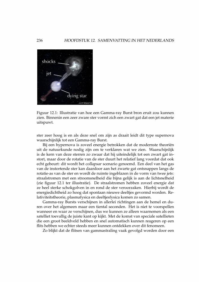
236 HOOFDSTUK 12. SAMENVATTING IN HET NEDERLANDS
shocks
jet
dying star
Figuur 12.1: Illustratie van hoe een Gamma-ray Burst bron eruit zou kunnenzien. Binnenin een zeer zware ster vormt zich een zwart gat dat een jet materieuitspuwt.
ster zeer hoog is en als deze snel om zijn as draait leidt dit type supernovawaarschijnlijk tot een Gamma-ray Burst.
Bij een hypernova is zoveel energie betrokken dat de modernste theorienuit de natuurkunde nodig zijn om te verklaren wat we zien. Waarschijnlijkis de kern van deze sterren zo zwaar dat hij uiteindelijk tot een zwart gat in-stort, maar door de rotatie van de ster duurt het relatief lang voordat dat ookecht gebeurt: dit wordt het collapsar scenario genoemd. Een deel van het gasvan de instortende ster kan daardoor aan het zwarte gat ontsnappen langs derotatie-as van de ster en wordt de ruimte ingeblazen in de vorm van twee jets :straalstromen met een stroomsnelheid die bijna gelijk is aan de lichtsnelheid(zie figuur 12.1 ter illustratie). De straalstromen hebben zoveel energie datze heel sterke schokgolven in en rond de ster veroorzaken. Hierbij wordt deenergiedichtheid zo hoog dat spontaan nieuwe deeltjes gevormd worden. Re-lativiteitstheorie, plasmafysica en deeltjesfysica komen zo samen.
Gamma-ray Bursts verschijnen in allerlei richtingen aan de hemel en du-ren over het algemeen maar een tiental seconden. Het is niet te voorspellenwanneer en waar ze verschijnen, dus we kunnen ze alleen waarnemen als eensatelliet toevallig de juiste kant op kijkt. Met de komst van speciale satellietendie een groot beeldveld hebben en snel automatisch kunnen reageren op eenflits hebben we echter steeds meer kunnen ontdekken over dit fenomeen.
Zo blijkt dat de flitsen van gammastraling vaak gevolgd worden door een
Magnetic Fields inside Extremely Fast Shock Waves by Jorrit Wiersma 237
soort nagloeien van de bron waardoor we ook rontgenstraling, zichtbaar lichten zelfs radiostraling kunnen opvangen. Dit nagloeien nemen we lang niet al-tijd waar, waarschijnlijk door de grote afstand waarop de Gamma-ray Burstsplaatsvinden. Het nagloeien verschaft ons echter veel informatie over de bron-nen van Gamma-ray Bursts. Uit de verdeling van de straling over de verschil-lende golflengten hebben we kunnen afleiden dat de straling gevormd wordtonder de invloed van magnetische velden: het stralingsspectrum lijkt meer opdat van synchrotronprocessen, waarbij snel bewegende elektronen door eenmagnetisch veld gaan, dan op het Planckspectrum van thermische stralings-processen. Waarom de straling deze eigenschappen heeft blijkt echter moeilijkte verklaren.
Een eerste probleem is de hevigheid van de gammastraling. Een Gamma-ray Burst zendt in een paar seconden evenveel energie uit in gammastraling alseen supernova in totaal uitstraalt. Supernovae zijn ook ontploffende sterren envertonen ook een explosieve groei in helderheid, maar ze stralen gedurendeeen periode van weken en hun straling is verdeeld over een veel groter golf-lengtebereik. Bij een Gamma-ray Burst explosie verwacht je dat een nog veelhetere en compacte vuurbal wordt gevormd dan bij een supernova waardoorthermische straling compleet overheerst in plaats van de synchrotron stralingdie we waarnemen. De verklaring waarom dit niet gebeurt is dat de stralingniet afkomstig is van de explosie zelf: deze is waarschijnlijk zo compact dat hetniet lukt om efficient gammastraling te produceren. In plaats daarvan wordtde gammastraling gevormd in de schokgolven die de explosie in zijn omge-ving veroorzaakt. Dit model voor de bron van Gamma-ray Bursts wordt hetfireball model genoemd1.
Een tweede probleem is waar het benodigde magnetische veld vandaankomt dat nodig is voor de stralingsprocessen die we waarnemen. Een mo-gelijke verklaring waar de laatste paar jaar veel onderzoek naar is gedaan isdat het magnetische veld spontaan ontstaat door de elektromagnetische wis-selwerking van de deeltjes in de schokgolf. Dit proefschrift beschrijft wat ik uitde theorie van deze wisselwerking heb kunnen afleiden.
Overigens bestaat er ook een klasse Gamma-ray Bursts die gemiddeld kor-ter duren (enkele seconden in plaats van tientallen seconden). De eigenschap-pen van deze kortdurende Gamma-ray Bursts kunnen we beter verklaren meteen model waarbij twee neutronsterren (sterren zo zwaar als de zon met deomvang van de aarde) samensmelten nadat ze lange tijd om elkaar heen ge-draaid hebben in een dubbelster systeem. Dit gebeurt omdat deze dubbelster-
1Het idee voor het fireball model is van Rees and Meszaros [79].
238 HOOFDSTUK 12. SAMENVATTING IN HET NEDERLANDS
systemen langzaam ineenstorten doordat ze energie verliezen via het uitzen-den van zwaartekrachtstralen. Deze Gamma-ray Burst bronnen zijn dus heelanders dan de instortende zware sterren die de langdurige Gamma-ray Burstsveroorzaken. In dit proefschrift heb ik me alleen bezig gehouden met de mo-dellen voor de langdurige Gamma-ray Bursts.
12.3 Schokgolven en magnetische veldenSchokgolven ontstaan in een gas door grote drukverschillen, bijvoorbeeld bijexplosies. Een schokgolf is ook eigenlijk niets anders dan een scherpe veran-dering in druk die zich voortplant door het gas. Doordat de druk achter deschokgolf zo hoog is sleurt de schokgolf gas met zich mee en daarbij wordt destromingsenergie omgezet in warmte. In de schokgolf zijn de druk, de dicht-heid en de temperatuur dan ook veel hoger dan ervoor.
Het gas waar de schokgolven die ik heb bestudeerd doorheen gaan is gro-tendeels geıoniseerd: het bestaat vrijwel geheel uit geladen deeltjes. Dit wordteen plasma genoemd. De geladen deeltjes zorgen ervoor dat het plasma eengoede elektrische geleider is. Vanwege deze eigenschap leidt de verhoging vande plasmadichtheid in de schokgolf ook tot een verhoging van de magnetischeveldsterkte. Het probleem is echter dat de magnetische veldsterkte in de ruim-te rond Gamma-ray Bursts over het algemeen niet zo hoog is, en dat de schok-golfcompressie van dit interstellaire magnetische veld niet voldoende is om desynchrotronstraling die we waarnemen te verklaren. Bij ons onderzoek willenwe daarom bepalen of er ook een ander mechanisme is dat het magnetischeveld kan versterken.
Het is namelijk niet zo vreemd dat magnetische velden een belangrijke rolspelen. Dit ligt aan de grote snelheid die de schokgolven bereiken (bijna delichtsnelheid). De snel bewegende, geladen deeltjes kunnen namelijk sterkeelektrische stromen vormen die weer sterke magnetische velden in het plas-ma veroorzaken. Bovendien is de magnetische Lorentzkracht op een geladendeeltje ook nog eens evenredig met de snelheid.
Het idee is nu dat het plasma onstabiel is: dat wil zeggen dat kleine versto-ringen van het plasma in de schokgolf snel uit zullen groeien tot veel sterkereverstoringen. Instabiliteiten komen in allerlei situaties voor. Een makkelijk tebegrijpen voorbeeld is een auto die zonder handrem op de top van een heuvelis geparkeerd. Zolang de auto stilstaat is dat geen probleem, maar als iemandhem een heel klein zetje geeft zal de auto ineens heel snel van de heuvel afrol-len. Op dezelfde manier zijn schokgolven die met zeer hoge snelheid door deruimte bewegen onstabiel in de zin dat kleine verstoringen van het magneti-
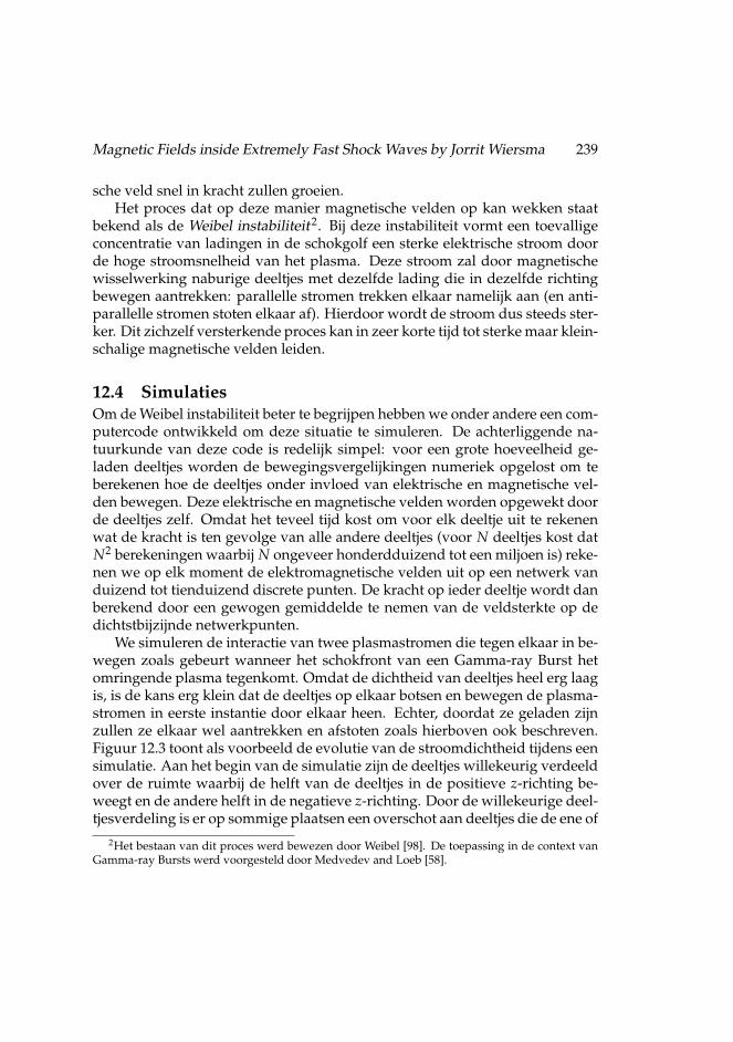
Magnetic Fields inside Extremely Fast Shock Waves by Jorrit Wiersma 239
sche veld snel in kracht zullen groeien.Het proces dat op deze manier magnetische velden op kan wekken staat
bekend als de Weibel instabiliteit2. Bij deze instabiliteit vormt een toevalligeconcentratie van ladingen in de schokgolf een sterke elektrische stroom doorde hoge stroomsnelheid van het plasma. Deze stroom zal door magnetischewisselwerking naburige deeltjes met dezelfde lading die in dezelfde richtingbewegen aantrekken: parallelle stromen trekken elkaar namelijk aan (en anti-parallelle stromen stoten elkaar af). Hierdoor wordt de stroom dus steeds ster-ker. Dit zichzelf versterkende proces kan in zeer korte tijd tot sterke maar klein-schalige magnetische velden leiden.
12.4 SimulatiesOm de Weibel instabiliteit beter te begrijpen hebben we onder andere een com-putercode ontwikkeld om deze situatie te simuleren. De achterliggende na-tuurkunde van deze code is redelijk simpel: voor een grote hoeveelheid ge-laden deeltjes worden de bewegingsvergelijkingen numeriek opgelost om teberekenen hoe de deeltjes onder invloed van elektrische en magnetische vel-den bewegen. Deze elektrische en magnetische velden worden opgewekt doorde deeltjes zelf. Omdat het teveel tijd kost om voor elk deeltje uit te rekenenwat de kracht is ten gevolge van alle andere deeltjes (voor N deeltjes kost datN2 berekeningen waarbij N ongeveer honderdduizend tot een miljoen is) reke-nen we op elk moment de elektromagnetische velden uit op een netwerk vanduizend tot tienduizend discrete punten. De kracht op ieder deeltje wordt danberekend door een gewogen gemiddelde te nemen van de veldsterkte op dedichtstbijzijnde netwerkpunten.
We simuleren de interactie van twee plasmastromen die tegen elkaar in be-wegen zoals gebeurt wanneer het schokfront van een Gamma-ray Burst hetomringende plasma tegenkomt. Omdat de dichtheid van deeltjes heel erg laagis, is de kans erg klein dat de deeltjes op elkaar botsen en bewegen de plasma-stromen in eerste instantie door elkaar heen. Echter, doordat ze geladen zijnzullen ze elkaar wel aantrekken en afstoten zoals hierboven ook beschreven.Figuur 12.3 toont als voorbeeld de evolutie van de stroomdichtheid tijdens eensimulatie. Aan het begin van de simulatie zijn de deeltjes willekeurig verdeeldover de ruimte waarbij de helft van de deeltjes in de positieve z-richting be-weegt en de andere helft in de negatieve z-richting. Door de willekeurige deel-tjesverdeling is er op sommige plaatsen een overschot aan deeltjes die de ene of
2Het bestaan van dit proces werd bewezen door Weibel [98]. De toepassing in de context vanGamma-ray Bursts werd voorgesteld door Medvedev and Loeb [58].
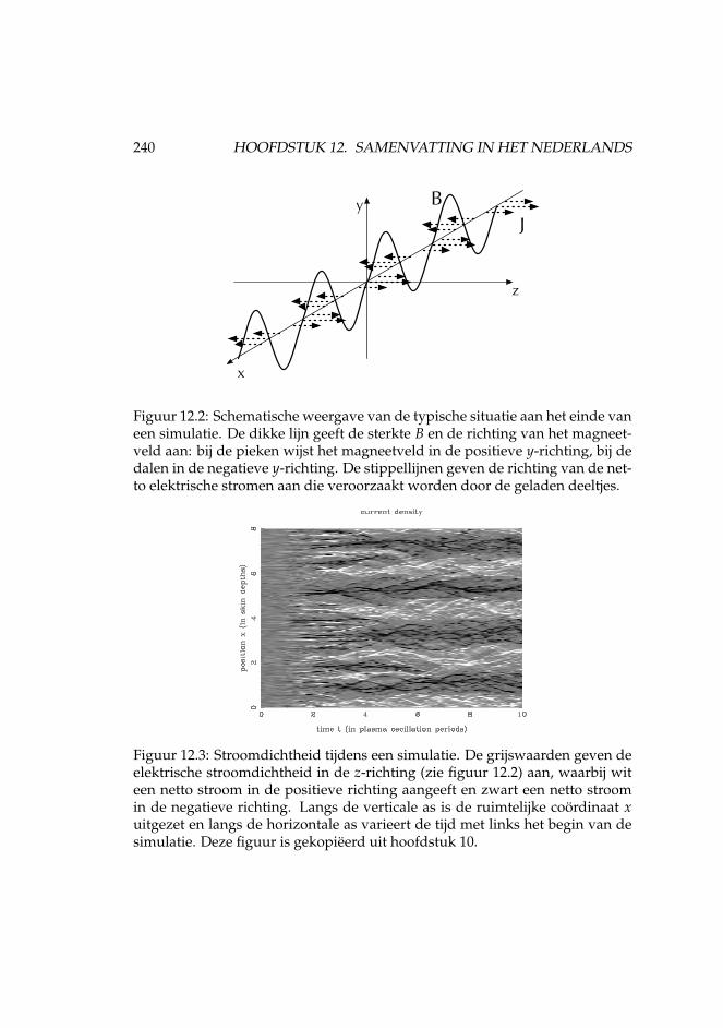
240 HOOFDSTUK 12. SAMENVATTING IN HET NEDERLANDS
y
z
x
BJ
Figuur 12.2: Schematische weergave van de typische situatie aan het einde vaneen simulatie. De dikke lijn geeft de sterkte B en de richting van het magneet-veld aan: bij de pieken wijst het magneetveld in de positieve y-richting, bij dedalen in de negatieve y-richting. De stippellijnen geven de richting van de net-to elektrische stromen aan die veroorzaakt worden door de geladen deeltjes.
Figuur 12.3: Stroomdichtheid tijdens een simulatie. De grijswaarden geven deelektrische stroomdichtheid in de z-richting (zie figuur 12.2) aan, waarbij witeen netto stroom in de positieve richting aangeeft en zwart een netto stroomin de negatieve richting. Langs de verticale as is de ruimtelijke coordinaat xuitgezet en langs de horizontale as varieert de tijd met links het begin van desimulatie. Deze figuur is gekopieerd uit hoofdstuk 10.
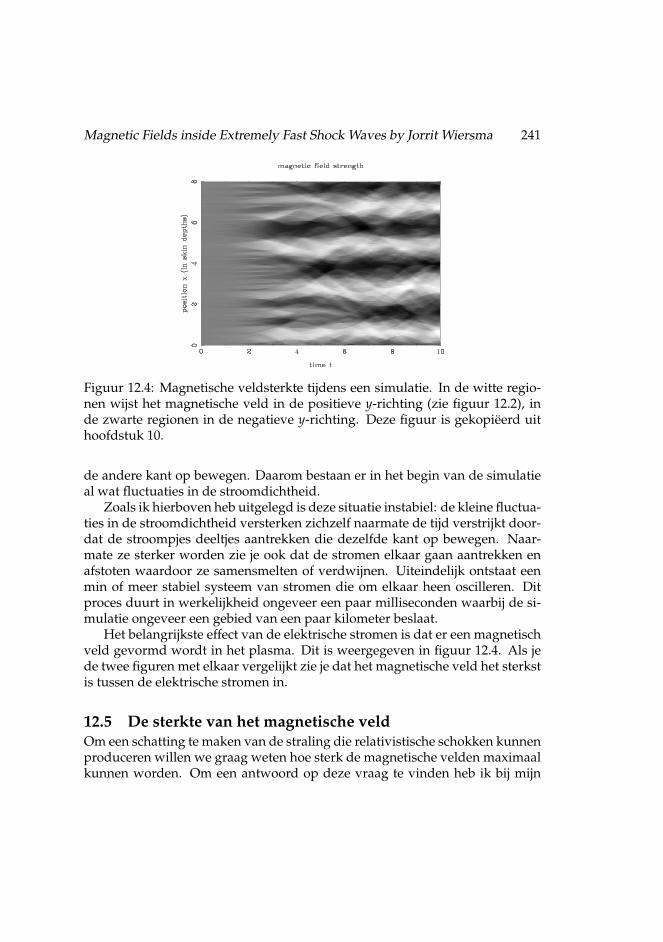
Magnetic Fields inside Extremely Fast Shock Waves by Jorrit Wiersma 241
Figuur 12.4: Magnetische veldsterkte tijdens een simulatie. In de witte regio-nen wijst het magnetische veld in de positieve y-richting (zie figuur 12.2), inde zwarte regionen in de negatieve y-richting. Deze figuur is gekopieerd uithoofdstuk 10.
de andere kant op bewegen. Daarom bestaan er in het begin van de simulatieal wat fluctuaties in de stroomdichtheid.
Zoals ik hierboven heb uitgelegd is deze situatie instabiel: de kleine fluctua-ties in de stroomdichtheid versterken zichzelf naarmate de tijd verstrijkt door-dat de stroompjes deeltjes aantrekken die dezelfde kant op bewegen. Naar-mate ze sterker worden zie je ook dat de stromen elkaar gaan aantrekken enafstoten waardoor ze samensmelten of verdwijnen. Uiteindelijk ontstaat eenmin of meer stabiel systeem van stromen die om elkaar heen oscilleren. Ditproces duurt in werkelijkheid ongeveer een paar milliseconden waarbij de si-mulatie ongeveer een gebied van een paar kilometer beslaat.
Het belangrijkste effect van de elektrische stromen is dat er een magnetischveld gevormd wordt in het plasma. Dit is weergegeven in figuur 12.4. Als jede twee figuren met elkaar vergelijkt zie je dat het magnetische veld het sterkstis tussen de elektrische stromen in.
12.5 De sterkte van het magnetische veldOm een schatting te maken van de straling die relativistische schokken kunnenproduceren willen we graag weten hoe sterk de magnetische velden maximaalkunnen worden. Om een antwoord op deze vraag te vinden heb ik bij mijn
242 HOOFDSTUK 12. SAMENVATTING IN HET NEDERLANDS
promotie-onderzoek een gedetailleerde analyse uitgevoerd van de hierbovenbeschreven processen. Ik zal deze hier kort samenvatten.
Om te beginnen kunnen we een grove schatting maken gebaseerd op ele-mentaire natuurkunde. De Biot-Savart wet vertelt ons dat het magnetischeveld rond een elektrische stroom I met straal d een sterkte B heeft met
B =2Icd
, (12.1)
waarbij c de lichtsnelheid is. Omdat de deeltjes maximaal met de lichtsnelheidkunnen bewegen is de maximale stroomsterkte ongeveer I = qnπd2c waarbijq de lading van de deeltjes is en n de dichtheid. De factor nπd2c geeft hetmaximum aantal deeltjes dat per seconde door een doorsnede met straal d heenbeweegt. De magnetische veldsterkte wordt dan
B = 2πqnd. (12.2)
Hoewel dit een heel grove schatting is, blijkt de waarde die uit vergelij-king (12.2) volgt wel ongeveer overeen te komen met wat we in de simulatieszien. We hebben dus onder andere gezien dat de geschatte magnetische veld-sterkte evenredig is met de typische lengteschaal d. Naarmate de processenop grotere schaal plaatsvinden kan er dus (theoretisch) een sterker magnetischveld gevormd worden. Door het gedrag van de geladen deeltjes volgens deplasmatheorie te bestuderen hebben we echter nog betere schattingen gemaaktvan de verwachte magnetische veldsterkte.
Bij ons onderzoek hebben we deze processen wiskundig beschreven doorde stroomdichtheidsverdeling te modelleren met een som van golfmodes (eenFourier-som). De stroomdichtheid van elke golfmode varieert als sin 2πx/λmet verschillende golflengte λ voor verschillende modes (de golflengte is deafstand tussen de pieken in figuur 12.2). Aan het begin van het proces groeiende fluctuaties in de stroomdichtheid onafhankelijk van naburige fluctuaties. Inde wiskundige beschrijving komt dat overeen met golfmodes die onafhanke-lijk van elkaar in sterkte groeien (hoofdstukken 6 en 7). Zodra de fluctuatieselkaar echter gaan beınvloeden komt dat er in de wiskundige beschrijving meeovereen dat de golfmodes met elkaar wisselwerken (hoofdstuk 9).
Uit onze berekeningen blijkt dat de in vergelijking (12.2) gegeven schattingvoor de magnetische veldsterkte een bovengrens is. De geladen deeltjes rakennamelijk gevangen in het magnetische veld dat ze zelf opwekken waardoor deinstabiliteit en de bijgebehorende groei van de magnetische veldsterkte op eengegeven moment stopt.
Magnetic Fields inside Extremely Fast Shock Waves by Jorrit Wiersma 243
Door de magnetische aantrekkingskracht kunnen de geproduceerde elek-trische stromen echter nog wel groeien door met elkaar samen te smelten enzo de magnetische veldsterkte nog verder te vergroten. Toch zal dit samen-smelten niet heel lang doorgaan. Het plasma werkt als een elektrische geleiderdie de neiging heeft de magnetische aantrekkingskracht af te schermen. Ditis met name van belang voor elektrische stromen die uit protonen bestaan.Door hun hoge massa kunnen protonen heel veel energie met zich mee dra-gen. Deze energie kunnen ze echter niet efficient omzetten in magnetische vel-den omdat de veel lichtere elektronen in het plasma heel sterk reageren op demagnetische velden die de protonen produceren. De elektronen schermen zohet magnetische veld van de protonbundels af en vertragen het samensmelten(zie hoofdstukken 8 en 9). Ook de protonbundels kunnen daardoor geen grotedoorsnede bereiken en dat beperkt de magnetische veldsterkte, zoals gegevendoor vergelijking (12.2).
In hoofdstukken 8 en 9 bespreken wij ook een belangrijk verschil tussen on-ze resultaten en die van eerdere onderzoeken zoals van Medvedev & Loeb [58].In modellen zoals die van Medvedev & Loeb wordt aangenomen dat het mag-netische veld uiteindelijk zo sterk wordt dat het de dynamica van de deeltjes inhet plasma gaat overheersen en daaruit wordt dan een schatting voor de mag-netische veldsterkte afgeleid. Onze resultaten tonen aan dat de effecten die ikin de vorige paragrafen heb beschreven al optreden voordat het magnetischeveld totaaloverheersend wordt. Dit is een belangrijk gegeven alhoewel het detheorie van deze schokgolven wel complexer maakt: de door ons afgeleide ef-fecten zullen er namelijk voor zorgen dat de deeltjes in het plasma turbulentof chaotisch gedrag gaan vertonen. Toekomstig onderzoek zal een uitgebreideanalyse van dit laatste gedrag moeten uitvoeren.
12.6 Vergelijking met waarnemingenUit de waarnemingen van Gamma-ray Bursts en hun nagloeien kunnen weiets afleiden over de magnetische veldsterkte die in de relativistische schokkenmoet heersen. De intensiteit van de straling en de verdeling over de verschil-lende golflengten hangt daar namelijk mee samen. Het blijkt dat de schattingenop basis van de waarnemingen en die op basis van de theorie heel redelijk metelkaar overeenkomen.
Toch kunnen we nog niet zeggen dat we het probleem helemaal opgelosthebben. Naast de sterkte van het magnetische veld is ook de typische leng-teschaal van belang voor de stralingsprocessen. Hoewel de processen die wijgesimuleerd hebben plaatsvinden op een schaal van kilometers, is dat in de
244 HOOFDSTUK 12. SAMENVATTING IN HET NEDERLANDS
context van de sterrenkunde nog steeds heel klein.Een tweede probleem is dat het magnetische veld, nadat het gevormd is,
waarschijnlijk ook weer zal vervagen door chaotische processen in het plas-ma. Het is op dit moment nog niet duidelijk of dat zo snel gebeurt dat er nietgenoeg straling gevormd kan worden om de waarnemingen te verklaren.
Een laatste open vraag betreft het effect van de aanwezigheid van deeltjesmet verschillende massa’s. Het meeste onderzoek op dit gebied heeft zich ge-concentreerd op elektronenplasma’s omdat de berekeningen het simpelst zijnals alle deeltjes dezelfde (elektron)massa hebben. In een realistisch model zou-den echter ook zwaardere deeltjes zoals protonen opgenomen moeten worden.Deze gedragen zich echter heel anders dan de elektronen doordat zwaarde-re deeltjes trager reageren op de elektromagnetische krachten (zie ook hoofd-stuk 8).
De oplossing voor deze problemen zal meer gedetailleerde simulaties enbetere theoretische modellen vereisen voor de complexe processen die plaats-vinden na de eerste toename in magnetische veldsterkte. Om een echte schok-golf te vormen moet de kinetische energie van de deeltjes omgezet worden inwarmte (en magnetische velden). Door de Weibel instabiliteit raken de deel-tjes samengeklonterd in groepen en door de elektromagnetische interactie vandeze groepen deeltjes kan warmte opgewekt worden. Dit is waarschijnlijk eenturbulent proces en er zijn nog geen theorien voor de details hiervan.
Er zouden misschien ook grootschaligere dynamoprocessen in de schokgolfop kunnen treden ten gevolge van turbulentie. Daarbij leiden wervelingen inhet plasma tot de groei van magnetische velden.
Meer begrip van de rol van magnetisme in schokgolven is hoe dan ook no-dig om de vorming van de straling die wij als Gamma-ray Bursts aan de hemelzien te begrijpen. Daarnaast zal deze kennis ook belangrijk zijn voor het on-derzoek naar andere sterrenkundige fenomenen, zoals actieve sterrenstelsels(Active Galactic Nuclei) en pulsar winden, waarvan we ook vermoeden dat zerelativistische schokgolven veroorzaken. Om deze redenen verwacht ik dat ditonderzoeksveld nog lange tijd actief zal blijven.
Chapter 13
Curriculum Vitae
I was born in Bilthoven, in the centre of the Netherlands, on the seventh of May1977, a mother’s day gift to my mother. For a few years we continued livingin Bilthoven and then moved to Hilversum, a few kilometers to the north. InHilversum I attended the Gemeentelijk Gymnasium. My interest in astronomystarted in those teen years.
In 1995 I started as a student at the faculty of Physics and Astronomy at theUniversity of Utrecht. My intention was to take physics as my major becauseof the career prospects, but already in my second year I was pulled towardsastrophysics mainly because astrophysics so elegantly blends multiple fieldsof physics. In January 2001 I graduated cum laude with a Master’s degreein both Theoretical Physics and Theoretical Astrophysics neither of which hasparticularly good (commercial) career prospects :-).
I continued in Astrophysics as a PhD student until January 2006 and thisthesis is the result of my research. During those years I also attended severalconferences, two of which were held outside of the Netherlands: in Santa Fe(sunny, empty desert and thunderstorms) and in Rome (sunny, good food andwine, much traffic and soot). I also got married and was blessed with a daugh-ter (chronologically in the opposite order).
At the time of printing this thesis I am no longer working in the field ofastrophysics. Instead I am working as a software developer at a medium-sizedsoftware company in Utrecht that develops business-critical software for largeinsurance companies and banks.
245
246 CHAPTER 13. CURRICULUM VITAE
Bibliography
[1] M. Abramowitz and I. A. Stegun. Handbook of Mathematical Functions. DoverPublications, New York, 1970.
[2] A. Achterberg. Covariant ponderomotive hamiltonian. J. Plasma Phys., 35:257,1986.
[3] A. Achterberg and J. Wiersma. The Weibel instability in relativistic plasmas I:Linear theory. Submitted to A&A, 2007.
[4] A. Achterberg, Y. A. Gallant, J. P. Rachen, C. A. Norman, and D. B. Melrose. Sub-mitted to MNRAS, 2003.
[5] A. Achterberg, J. Wiersma, and C. A. Norman. The Weibel instability in relativisticplasmas II: Nonlinear theory and stabilization mechanism. Submitted to A&A,2007.
[6] A. I. Akhiezer, I. A. Akhiezer, R. V. Polovin, A. G. Sitenko, and K. N. Stepanov.Plasma Electrodynamics, v. 1. Linear theory, volume 68 of International series ofmonographs in natural philosophy. Pergamon Press, Oxford, 1975. ISBN 0-08-017783-2.
[7] A. F. Alexandrov, L. S. Bogdankevich, and A. A. Rukhadze. Principles of PlasmaElectrodynamics. Springer, 1984.
[8] R. D. Blandford and C. F. McKee. Fluid dynamics of relativistic blast waves.Physics of Fluids, 19(8):1130–1138, Aug. 1976.
[9] J. J. Brainerd. A plasma instability theory of Gamma-ray Burst emission. ApJ,538:628–637, Aug. 2000.
[10] A. Bret, M.-C. Firpo, and C. Deutsch. Bridging the gap between two stream andfilamentation instabilities. Laser and Particle Beams, 23:375–383, 2005.
247
248 BIBLIOGRAPHY
[11] F. Califano, F. Pegoraro, S. V. Bulanov, and A. Mangeney. Kinetic saturation of theWeibel instability in a collisionless plasma. Physical Review E, 57(6):7048–7059,June 1998.
[12] F. Califano, T. Cecchi, and C. Chiuderi. Nonlinear kinetic regime of the Weibelinstability in an electron-ion plasma. Physics of Plasmas, 9(2):451–457, Feb. 2002.
[13] J. R. Cary and A. N. Kaufman. Ponderomotive effects in collisionless plasma: aLie transform approach. Physics of Fluids, 24:1238–1250, July 1981.
[14] E. Costa, F. Frontera, J. Heise, M. Feroci, J. in ’t Zand, F. Fiore, M. N. Cinti, D. dalFiume, et al. Discovery of an X-ray afterglow associated with the gamma-rayburst of 28 February 1997. Nature, 387:783–785, June 1997.
[15] S. Dado, A. Dar, and A. D. Rujula. On the optical and X-ray afterglows of gammaray bursts. A&A, 388:1079–1105, 2002. On the cannonball model.
[16] R. C. Davidson, D. A. Hammer, I. Haber, and C. E. Wagner. Nonlinear develop-ment of electromagnetic instabilities in anisotropic plasmas. Physics of Fluids, 15(2):317–333, Feb. 1972.
[17] R. J. Davidson. Methods in Nonlinear Plasma Theory. Academic Press, NewYork, Feb. 1972.
[18] R. L. Dewar. Energy-momentum tensors for dispersive electromagnetic waves.Aust. J. Phys., 30:533–575, 1977.
[19] B. T. Draine and C. F. McKee. Theory of interstellar shocks. ARA&A, 31:373–432,1993.
[20] D. Eichler and E. Waxman. The efficiency of electron acceleration in collisionlessshocks and Gamma-ray Burst energetics. ApJ, 627:861–867, July 2005.
[21] R. A. Fonseca, L. O. Silva, J. W. Tonge, W. B. Mori, and J. M. Dawson. Three-dimensional Weibel instability in astro-physical scenarios. Physics of Plasmas, 10(5):1979–1984, May 2003.
[22] D. B. Fox, D. A. Frail, P. A. Price, S. R. Kulkarni, E. Berger, T. Piran, A. M. Soder-berg, S. B. Cenko, et al. The afterglow of GRB 050709 and the nature of the short-hard γ-ray bursts. Nature, 437:845–850, Oct. 2005.
[23] D. A. Frail, S. R. Kulkarni, L. Nicastro, M. Feroci, and G. B. Taylor. The radioafterglow from the γ-ray burst of 8 May 1997. Nature, 389:261–263, Sept. 1997.
[24] J. T. Frederiksen, C. B. Hededal, T. Haugbølle, and A. Nordlund. Magnetic fieldgeneration in collisionless shocks: pattern growth and transport. ApJ, 608:L13–L16, June 2004.
BIBLIOGRAPHY 249
[25] B. D. Fried. Mechanism for instability of transverse plasma waves. Physics ofFluids, 2:337, 1959.
[26] Y. Fujita and T. Kato. A possible origin of magnetic fields in galaxies and clusters:strong magnetic fields at z ∼ 10? MNRAS, 364:247–252, 2005.
[27] T. J. Galama, P. M. Vreeswijk, J. van Paradijs, C. Kouveliotou, T. Augusteijn,H. Bohnhardt, J. P. Brewer, V. Doublier, et al. An unusual supernova in the er-ror box of the gamma-ray burst of 25 April 1998. Nature, 395:670–672, 1998.
[28] A. A. Galeev and R. Z. Sagdeev. Nonlinear plasma theory. In M. A. Leontovich,editor, Reviews of Plasma Physics, volume 7, page 1. Consultants Bureau, NewYork, 1979.
[29] N. Gehrels, G. Chincarini, P. Giommi, K. O. Mason, J. A. Nousek, A. A. Wells,N. E. White, S. D. Barthelmy, et al. The Swift Gamma-Ray Burst Mission. ApJ,611:1005–1020, Aug. 2004.
[30] J. Granot and A. Konigl. Radiative hydromagnetic shocks in relativistic outflowsources. ApJ, 560:145–159, Oct. 2001.
[31] A. Gruzinov. Gamma-ray Burst phenomenology, shock dynamo, and the firstmagnetic fields. ApJ, 563:L15–L18, Dec. 2001.
[32] A. Gruzinov and E. Waxman. Gamma-ray burst afterglow: Polarization and ana-lytic light curves. ApJ, 511:852–861, Feb. 1999.
[33] T. Haruki and J.-I. Sakai. Generation of magnetic field and electrostatic shockwave driven by counterstreaming pair plasmas. Physics of Plasmas, 10(2):392–397, Feb. 2003.
[34] T. Haugbølle. Modelling Relativistic Astrophysics and the Large and Small Scale.PhD thesis, University of Copenhagen, Denmark, May 2005.
[35] C. B. Hededal. Gamma-ray Bursts, Collisionless Shocks and Synthetic Spectra.PhD thesis, University of Copenhagen, Denmark, May 2005.
[36] C. B. Hededal and K.-I. Nishikawa. The influence of an ambient magnetic fieldon relativistic collisionless plasma shocks. ApJ, 623:L89–L92, Apr. 2005.
[37] J. Hjorth, J. Sollerman, P. Møller, J. P. U. Fynbo, S. E. Woosley, C. Kouveliotou,N. R. Tanvir, J. Greiner, et al. A very energetic supernova associated with theγ-ray burst of 29 March 2003. Nature, 423:847–850, June 2003.
[38] M. Hoshino, J. Arons, Y. A. Gallant, and A. B. Langdon. Relativistic magnetosonicshock waves in synchrotron sources: shock structure and nonthermal accelerationof positrons. ApJ, 390:454–479, May 1992.
250 BIBLIOGRAPHY
[39] K. Hurley, S. E. Boggs, D. M. Smith, R. C. Duncan, R. Lin, A. Zoglauer, S. Krucker,G. Hurford, et al. An exceptionally bright flare from SGR 1806-20 and the originsof short-duration γ-ray bursts. Nature, 434:1098–1103, Apr. 2005.
[40] S. Ichimaru. Basic Principles of Plasma Physics: A Statistical Approach. W.A.Benjamin Inc., Reading, Ma., USA, 1973. ISBN 0805387536.
[41] J. D. Jackson. Classical Electrodynamics. John Wiley & Sons, New York, secondedition, 1975. ISBN 0-471-43132-X.
[42] C. H. Jaroschek, H. Lesch, and R. A. Treumann. Self-consistent diffusive lifetimesof Weibel magnetic fields in Gamma-ray Bursts. ApJ, 616:1065–1071, Dec. 2004.
[43] B. B. Kadomtsev. Plasma Turbulence. Academic Press, London, 1965.
[44] T. N. Kato. Saturation mechanism of the Weibel instability in weakly magnetizedplasmas. Physics of Plasmas, 12:080705, Aug. 2005.
[45] Y. Kazimura, J. I. Sakai, T. Neubert, and S. V. Bulanov. Generation of a small-scale quasi-static magnetic field and fast particles during the collision of electron-positron plasma clouds. ApJ, 498:L183–L186, May 1998.
[46] C. F. Kennel and F. V. Coroniti. Confinement of the crab pulsar’s wind by itssupernova remnant. ApJ, 283:694–709, Aug. 1984.
[47] J. G. Kirk and P. Duffy. Particle acceleration and relativistic shocks. J. Phys. G:Nucl. Part. Phys., 25:R163–R194, 1999. Topical Review.
[48] D. Q. Lamb, G. R. Ricker, J.-L. Atteia, C. Barraud, M. Boer, J. Braga, N. Butler,T. Cline, et al. Scientific highlights of the HETE-2 mission. Nuclear Physics BProceedings Supplements, 132:279–288, June 2004.
[49] L. D. Landau and E. M. Lifschitz. Fluid Mechanics. Pergamon Press, Oxford,1975. ISBN 0-08-091040-8.
[50] L. D. Landau and E. M. Lifschitz. The Classical Theory of Fields. Pergamon Press,Oxford, fourth edition, 1975. ISBN 0080181767.
[51] D. Lazzati. A certain flare. Nature, 434:1075–1076, Apr. 2005.
[52] R. Lee and M. Lampe. Electromagnetic instabilities, filamentation and focusing ofrelativistic electron beams. Physical Review Letters, 31(23):1390–1393, Dec. 1973.
[53] A. Lichnerowicz. Relativistic Hydrodynamics and Magnetohydrodynamics. W.A. Benjamin, Inc., New York, 1967.
BIBLIOGRAPHY 251
[54] A. S. Lipatov. The Hybrid Multiscale Simulation Technology. Springer, 2002.ISBN 3-540-41734-6.
[55] Lyubarsky and Eichler. Are gamma-ray burst shocks mediated by the weibelinstability? ApJ, 647:1250–1254, 2006.
[56] M. V. Medvedev. Theory of “jitter” radiation from small-scale random magneticfields and prompt emission from gamma-ray burst shocks. ApJ, 540:704–714,2000.
[57] M. V. Medvedev. Weibel turbulence in laboratory experiments and GRB/SNshocks. Astrophysics and Space Science, Online First, Jan. 2007.
[58] M. V. Medvedev and A. Loeb. Generation of magnetic fields in the relativisticshock of gamma-ray burst sources. ApJ, 526:697–706, Dec. 1999.
[59] M. V. Medvedev, M. Fiore, R. A. Fonseca, L. O. Silva, and W. B. Mori. Long-timeevolution of magnetic fields in relativistic Gamma-ray Burst shocks. ApJ, 618:L75–L78, Jan. 2005.
[60] D. Melrose. Instabilities in Space and Laboratory Plasmas. Cambridge UniversityPress, 1986. ISBN 0-521-30541-1.
[61] D. B. Melrose. Quantum plasma dynamics, 2001. URL http://www.physics.usyd.edu.au/∼melrose/qpd.html.
[62] D. B. Melrose. A covariant formulation of wave dispersion. Plasma Phys., 15:99–106, 1973.
[63] D. B. Melrose. Plasma Astrophysics: Nonthermal Processes in Diffuse Magne-tized Plasmas, volume 1. Gordon and Breach Publ., New York, 1980. ISBN0677034903.
[64] P. Meszaros. Gamma-ray bursts: Accumulating afterglow implications, progeni-tor clues, and prospects. Science, 291:79–84, Jan. 2001.
[65] P. Meszaros. Theories of gamma-ray bursts. ARA&A, 40:137–169, 2002. Reviewof fireball shock model.
[66] P. Meszaros. Gamma-ray bursts. Rep. Prog. Phys., 69:2259–2321, 2006.
[67] M. Milosavljevic and E. Nakar. The cosmic ray precursor of relativistic collision-less shocks: a missing link in Gamma-ray Burst afterglows. ApJ, 651:979–984,Nov. 2006.
252 BIBLIOGRAPHY
[68] M. Milosavljevic, E. Nakar, and A. Spitkovsky. Steady state electrostatic layersfrom Weibel instability in relativistic collisionless shocks. ApJ, 637:765–773, Feb.2006.
[69] K.-I. Nishikawa, P. Hardee, G. Richardson, R. Preece, H. Sol, and G. J. Fishman.Particle acceleration in relativistic jets due to weibel instability. ApJ, 595:555–563,Sept. 2003.
[70] N. Okabe and M. Hattori. Spontaneous generation of the magnetic field andsuppression of the heat conduction in cold fronts. ApJ, 599:964–970, Dec. 2003.
[71] A. Pais. Subtle is the Lord: The Science and the Life of Albert Einstein. OxfordUniversity Press, 1983. ISBN 0-19-520438-7.
[72] A. Panaitescu and P. Kumar. Properties of relativistic jets in Gamma-ray Burstafterglows. ApJ, 571:779–789, June 2002.
[73] P. O. Petrucci, G. Henri, and G. Pelletier. Pair creation at shocks: Application tothe high energy emission of compact objects. A&A, 374:719–732, 2001.
[74] T. Piran. Gamma-ray bursts – a puzzle being resolved. Physics Reports, 333:529–553, 2000.
[75] T. Piran. The physics of gamma-ray bursts. Rev. Mod. Phys., 76:1143–1210, Oct.2004.
[76] T. Piran. Gamma-ray Bursts and the fireball model. Physics Reports, 314:575–667,1999.
[77] L. Piro. Short-burst sources. Nature, 437:822–823, Oct. 2005.
[78] D. Potter. Computational Physics. John Wiley & Sons, New York, 1973. ISBN0-471-69555-6.
[79] M. J. Rees and P. Meszaros. Relativistic fireballs: energy conversion and time-scales. MNRAS, 258:41P, Sept. 1992.
[80] M. J. Rees and P. Meszaros. Unsteady outflow models for cosmological gamma-ray bursts. ApJ, 430:L93–L96, Aug. 1994.
[81] P. H. Roberts. An Introduction to Magnetohydrodynamics. Longmans, Greenand Co. Ltd, London, 1967.
[82] R. Z. Sagdeev. Cooperative phenomena and shock waves in collisionless plasmas.Reviews of Plasma Physics, 4:23–91, 1966.
BIBLIOGRAPHY 253
[83] R. Sari, T. Piran, and J. Halpern. Jets in gamma-ray bursts. ApJ, 519:L17–L20, July1999.
[84] U. Schaefer-Rolffs, I. Lerche, and R. Schlickeiser. The relativistic kinetic weibelinstability: General arguments and specific illustrations. Physics of Plasmas, 13:012107, 2006.
[85] R. Schlickeiser. Nonthermal radiation from jets of active galactic nuclei: Electro-static bremsstrahlung as alternative to synchrotron radiation. A&A, 410:397–414,2003.
[86] R. Schlickeiser. Covariant kinetic dispersion theory of linear waves in anisotropicplasmas. I. Physics of Plasmas, 11(12):5532–5546, Dec. 2004.
[87] R. Schlickeiser and P. K. Shukla. Cosmological magnetic field generation by theWeibel instability. ApJ, 599:L57–L60, Dec. 2003.
[88] R. Schlickeiser, R. Vainio, M. Bottcher, I. Lerche, M. Pohl, and C. Schuster. Con-version of relativistic pair energy into radiation in the jets of active galactic nuclei.A&A, 393:69–87, 2002.
[89] L. O. Silva, R. A. Fonseca, J. W. Tonge, W. B. Mori, and J. M. Dawson. On therole of the purely transverse Weibel instability in fast ignitor scenarios. Physicsof Plasmas, 9(6):2458–2461, June 2002.
[90] A. Spitkovsky and J. Arons. Time dependence in relativistic collisionless shocks:theory of the variable “wisps” in the Crab nebula. ApJ, 603:669–681, Mar. 2004.
[91] R. C. Tautz and R. Schlickeiser. Counterstreaming magnetized plasmas. II. per-pendicular wave propagation. Physics of Plasmas, 13:062901, 2006.
[92] D. A. Tidman and N. A. Krall. Shock Waves in Collisionless Plasmas. Wiley-Interscience, New York, 1971.
[93] B. T. Tsurutani and R. G. Stone, editors. Collisionless Shocks in the Heliosphere:Reviews of Current Research, volume 35 of Geophysical Monograph. AmericanGeophysical Union, 1985.
[94] J. van Paradijs, P. J. Groot, T. Galama, C. Kouveliotou, R. G. Strom, J. Telting,R. G. M. Rutten, G. J. Fishman, et al. Transient optical emission from the error boxof the gamma-ray burst of 28 February 1997. Nature, 386:686–689, 1997.
[95] J. Vink. Shocks and particle acceleration in supernova remnants: observationalfeatures. Advances in Space Research, 33(4):356–365, 2004.
254 BIBLIOGRAPHY
[96] E. Waxman. Gamma-ray-burst afterglow: supporting the cosmological fireballmodel, contraining parameters, and making predictions. ApJ, 485:L5–L8, Aug.1997.
[97] M. S. Wei, F. N. Beg, A. E. Dangor, A. Gopal, M. Tatarakis, K. Krushelnick, E. L.Clark, P. A. Norreys, et al. Experimental observations of the Weibel instability inhigh intensity laser solid interactions. Annual Report of Central Laser Facility,Rutherford Appleton Laboratory, pages 7–9, 2001/2002.
[98] E. S. Weibel. Spontaneously growing transverse waves in a plasma due to ananisotropic velocity distribution. Physical Review Letters, 2(3):83–84, Feb. 1959.
[99] J. Wiersma. Magnetic fields inside extremely fast shock waves. PhD thesis, Uni-versity of Utrecht, The Netherlands, May 2007.
[100] J. Wiersma and A. Achterberg. Magnetic field generation in relativistic shocks- an early end of the exponential weibel instability in electron-proton plasmas.A&A, 428:365–371, Dec. 2004.
[101] J. Wiersma and A. Achterberg. Particle-In-Cell simulations of the Weibel instabil-ity. To be submitted to A&A, 2007.
[102] R. A. M. J. Wijers and T. J. Galama. Physical parameters of GRB 970508 and GRB971214 from their afterglow synchrotron emission. ApJ, 523:177–186, Sept. 1999.
[103] R. A. M. J. Wijers, M. J. Rees, and P. Meszaros. Shocked by GRB 970228: theafterglow of a cosmological fireball. MNRAS, 288:L51–L56, 1997.
[104] T.-Y. B. Yang, J. Arons, and A. B. Langdon. Evolution of the Weibel instability inrelativistically hot electron-positron plasmas. Physics of Plasmas, 1(9):3059–3077,Sept. 1994.
[105] P. H. Yoon and R. C. Davidson. Exact analytical model of the classical weibelinstability in a relativistic anisotropic plasma. Physical Review A, 35(6):2718–2721, Mar. 1987. Brief report.
Index
E = mc2, 251D2V approach, 2003D simulations, 201
1905, 21
active galactic nuclei, 31advection current, 80, 109, 166, 201afterglow, 35, 36, 154AGN, 31Alfven critical field, 191, 192Alfven current, 180Alfven velocity, 72Ampere’s Law, 166anomalous skin effect, 90asymmetric beams, 79, 100, 102, 104,
149
background particles, 207background plasma, 123, 125, 171, 233
relativistic, 89background plasma frequency, 155background response, 174background skin depth, 219beam plasma frequency, 155beam-driven Weibel instability, 78Bessel functions, 170
expansion for modified, 186boundary conditions, 122, 201Bremsstrahlung, 148
canonical momentum, 164causality, 22charge and current density, 226charge conservation, 106charged particles, 27close (two-particle) interactions, 203coalescence, 179
slowing of, 188coalescence time scale, 186cold background plasma, 80cold beams, 80, 111cold plasma, 49, 51, 59, 78, 109, 219collisionless plasma, 46compactness problem, 39compression ratio, 57, 60computational method, 203, 224computer simulations, 200, 201conduction current, 80, 109conductivity tensor, 105conservation laws, 48, 54, 68continuity equation, 108, 163, 167Coulomb collision time scale, 203covariant description, 74covariant response, 75, 105current channels, 179
Debye length, 203Debye shielding, 227dielectric tensor, 105diffusion, 193
255
256 INDEX
diffusion equation, 176dilatation, 23dispersion relation, 75, 80, 83, 105,
126, 127, 139, 209asymmetric beams, 101linear, 111magnetized, 95magnetized Weibel, 120non-relativistic, 81relativistic background, 89
dispersion tensorfluid approximation, 114waterbag approximation, 117
displacement current, 26Doppler effect, 24downstream rest frame, 57downstream velocity, 56
perpendicular component, 68
effective collisional process, 136effective equation of state, 52effective plasma frequency, 155effective pressure, 52effective skin depth, 157effective specific heat ratio, 53Einstein, 21electricity, 26electromagnetic interaction, 231electromagnetic mode, 79electron current filaments, 182electron-driven Weibel instability,
190, 197electrostatic waves, 148, 168energy, 24, 59equation of motion, 123, 202, 224
covariant, 76fluid, 163for displacement, 159linearized, 107
equation of state, 49, 51, 68, 108equipartition, 136, 147equipartition field strength, 154equipartition parameter, 147external GRB shocks, 159
fake diffusion, 174, 232Faraday tensor, 105filamentary currents, 179filamentation instability, 30fireball model, 39, 237fluid model, 75, 107, 160, 207fluid rest frame, 47Forward Elimination–Backward
Substitution Method, 227four-current, 106four-potential, 106Fourier integral, 106frames of reference, 50
galaxy clusters, 31gamma radiation, 33Gamma-ray Bursts, 31, 33, 136, 234,
235long, 34naming scheme, 35possible sources, 38short, 34
Gammaflitsen, 235gauge freedom, 106Gaussian distribution, 209generation of magnetic fields, 46GRB, see Gamma-ray Burstsgrid, 225grid cell, 203growth rate, 87, 92, 127, 141, 156, 210,
216asymmetric beams, 101magnetized, 96
INDEX 257
oblique, 130spatially growing solution, 128
gyration frequency, 96, 119gyration radius, 158, 180
harmonics, 170heating, 174, 221HETE 2, 35host galaxy, 36hot, 51, 68hot background, 191hydrogen, 136
ideal MHD approximation, 49initial situation, 122internal structure, 69ion thermalization length, 193ion-driven Weibel instability, 191ions, 89
jitter radiation, 154jump conditions, 46, 55, 57Juttner distribution, 89
kinetic approach, 77, 109kinetic theory, 174, 208
laboratory experiments, 31Lagrangian labels, 169Landau damping, 174Larmor radius, 158Lax-Wendroff method, 226Leapfrog Scheme, 225Levi-Cevita tensor, 106light cone, 22limiting wavenumber, 143linear results, 104longitudinal electric field, 164Lorentz factor, 23, 57, 84Lorentz gauge, 76, 77, 112, 124
Lorentz transformations, 50low-frequency limit, 72, 162
Mach number, 85, 104, 156magnetic energy density, 136, 216, 234magnetic field, 18, 30, 51, 55, 61, 68, 96
ambient, 104non-perpendicular, 65shock compression, 72
magnetic field generation, 49magnetic field strength, 154magnetic flux conservation, 62magnetic trapping, 144, 158, 218, 232magnetism, 26magnetization, 158magnetization criterion, 146, 158magnetized shocks, 46, 61, 63magnetized Weibel instability, 93, 118magnetohydrodynamics, 47Mass and magnetic flux conservation,
49massive star, 39maximum growth rate, 143, 157maximum unstable wavenumber, 157Maxwell, 26Maxwell’s equations, 49, 106, 124,
202, 204, 224covariant, 105reduced, 166
Maxwellian distribution, 177, 208merging of current channels, 179, 216,
219ion current filaments, 192
metric tensor, 47Minkowski metric tensor, 74mode coupling, 162momentum, 24
net current, 82
258 INDEX
neutron stars, 39non-covariant, 53non-equilibration, 137non-relativistic limit, 80nonlinear coupling, 160nonlinearity, 149, 169normal, 50
oblique Weibel instability, 129, 133optical afterglow, 36oscillating orbits, 218oscillation center theory, 174
parallel magnetic field, 65parallel shock, 51particle creation, 49, 69Particle-In-Cell method, 200, 203perpendicular momentum, 66perpendicular relativistic shock, 99perpendicular shock, 51, 68perturbation expansion, 165phase mixing, 174phase plots, 218phase shift, 170phase-space distribution function, 77PIC, see Particle-In-Cell method, 224plane waves, 106plasma frequency, 78, 82, 84
beam, 117relativistic, 76
plasma instabilities, 46, 136plasma speeds, 55Poisson’s equation, 166, 226polarization tensor, 76, 77, 106, 206
cold limit, 78kinetic approach, 116magnetized, 119
polarization vectors, 79, 112ponderomotive effects, 166
potentialnonlinear, 171
Poynting’s Theorem, 27projection tensor, 76, 107prompt emission, 35, 154proper density, 23proper time, 23proton current filaments, 182, 223proton-driven instability, 197protons, 135, 233pulsar winds, 31
quiver motion, 144, 158, 174, 176, 232quiver velocity, 177
radio afterglow, 36radio waves, 35ratio of magnetic to internal energy,
49, 53, 63, 72ratio of specific heats, 68redshift, 37reference frame, 53relative velocity, 54, 56relativistic shocks, 17, 46, 72relativistic speeds, 46relativistically hot plasma, 49relativity, 21resonant interactions, 162response of the background plasma,
83response of the plasma, 105, 124, 205
covariant, 105responsive, 219return current, 100Runge-Kutta time-integrator, 225
satellites, 35saturation, 160, 216saturation field, 145
INDEX 259
scalar potential, 204screening currents, 173, 179, 183, 192,
213screening wavenumber, 173shock conditions, 45, 138shock rest frame, 55, 122shock solutions, 58shock transition, 46shock transition layer, 154, 188, 200shock wave, 17, 20
non-perpendicular, 65, 66simulation results, 216skin effect, 133solutions, 68sound speed
relativistic, 76space-centered approximation, 225spatially growing solution, 132specific heat ratio, 49speed of light, 21stabilization, 174stabilization mechanisms, 158statistical errors, 203strong, 50, 59, 68strong background plasma, 223strong unmagnetized shocks, 58supernovae, 37susceptibility tensor, 105SWIFT, 35symmetric beams, 82, 102, 156, 162synchrotron radiation, 40, 136, 154,
234
temperature of the beam plasma, 216thermal motion, 85thermalization, 147, 188, 221thermalization length, 193, 196, 198time dilatation, 23total energy momentum tensor, 47
toy model for current merging, 181trapping condition, 135, 159, 178, 180trapping magnetic field, 191
ion-driven Weibel instability, 192turbulence, 233turbulent power spectrum, 194
ultra-relativistic beams, 104ultra-relativistic limit, 50, 60, 62, 66,
85, 90, 210ultra-relativistic solution, 63, 64unmagnetized plasma, 51
vector potential, 164, 204velocity perturbations, 165Vlasov equation, 205
covariant, 77, 109linearized, 110
waterbag distribution, 83, 138, 206wave breaking, 160, 170wave modes, 113wave-particle interactions, 174wavenumber
maximum unstable, 104weak beams, 218Weibel instabiliteit, 239Weibel instability, 30, 72, 136, 154,
201, 204, 232asymmetric, 100electron-driven, 190growth rate, 87ion-driven, 191magnetized, 93merging current channels, 232non-relativistic, 82single beam, 102ultra-relativistic, 85
X rays, 35


![Research Article Neural Virtual Sensors for Adaptive Magnetic …downloads.hindawi.com/archive/2014/394038.pdf · 2019. 7. 31. · [ ],Internet-of- ings(IoT),Cyber-Physical-Systems(CPS),](https://static.fdocuments.nl/doc/165x107/5fe9bcff291fb213251d7e1b/research-article-neural-virtual-sensors-for-adaptive-magnetic-2019-7-31-internet-of-.jpg)