
kaft-1/4 -Dujardin et al.
100
KONINKLIJKE VLAAMSE ACADEMIE VAN BELGIE VOOR WETENSCHAPPEN EN KUNSTEN CONTACTFORUM ACTUARIAL AND FINANCIAL MATHEMATICS CONFERENCE Interplay between Finance and Insurance February 4-5, 2010 Michèle Vanmaele, Griselda Deelstra, Ann De Schepper, Jan Dhaene, Wim Schoutens & Steven Vanduffel (Eds.)
Transcript of kaft-1/4 -Dujardin et al.
KONINKLIJKE VLAAMSE ACADEMIE VAN BELGIE
VOOR WETENSCHAPPEN EN KUNSTEN
CONTACTFORUM
ACTUARIAL AND FINANCIALMATHEMATICS CONFERENCE
Interplay between Finance and Insurance
February 4-5, 2010
Michèle Vanmaele, Griselda Deelstra, Ann De Schepper, Jan Dhaene, Wim Schoutens & Steven Vanduffel (Eds.)
aCtuarIaL anD fInanCIaLmatHEmatICS ConfErEnCE
Interplay between finance and Insurance
february 4-5, 2010
michèle Vanmaele, Griselda Deelstra, ann De Schepper, Jan Dhaene, Wim Schoutens & Steven Vanduffel (Eds.)
KONINKLIJKE VLAAMSE ACADEMIE VAN BELGIE
VOOR WETENSCHAPPEN EN KUNSTEN
ContaCtforum

Handelingen van het contactforum “Actuarial and Financial Mathematics Conference. Interplay between Finance and
Insurance” (4-5 februari 2010, hoofdaanvrager : Prof. M. Vanmaele, UGent) gesteund door de Koninklijke Vlaamse
Academie van België voor Wetenschappen en Kunsten.
Afgezien van het afstemmen van het lettertype en de alinea’s op de richtlijnen voor de publicatie van de
handelingen heeft de Academie geen andere wijzigingen in de tekst aangebracht. De inhoud, de volgorde en de
opbouw van de teksten zijn de verantwoordelijkheid van de hoofdaanvrager (of editors) van het contactforum.
KONINKLIJKE VLAAMSE ACADEMIE VAN BELGIE
VOOR WETENSCHAPPEN EN KUNSTEN
Paleis der Academiën
Hertogsstraat 1
1000 Brussel
Niets uit deze uitgave mag worden verveelvoudigd en/of
openbaar gemaakt door middel van druk, fotokopie,
microfilm of op welke andere wijze ook zonder
voorafgaande schriftelijke toestemming van de uitgever.
No part of this book may be reproduced in any form, by
print, photo print, microfilm or any other means without
written permission from the publisher.
Printed by Universa Press, 9230 Wetteren, Belgium
© Copyright 2010 KVABD/2010/0455/17
ISBN 9789065690722
V
KONINKLIJKE VLAAMSE ACADEMIE VAN BELGIE
VOOR WETENSCHAPPEN EN KUNSTEN
Actuarial and Financial Mathematics Conference
Interplay between finance and insurance
CONTENTS
Invited talk
Supervisory accounting: comparison between Solvency II and coherent risk measures . 3
Ph. Artzner, K.-Th. Eisele
Contributed talks
Pricing of a catastrophe bond related to seasonal claims . . . . . . . . . . . . . . . . . . . . . . . . . . 17
D. Hainaut
CMS spread options in the multi-factor HJM framework . . . . . . . . . . . . . . . . . . . . . . . . . 33
P. Hanton, M. Henrard
Strong Taylor approximation of stochastic differential equations and application to the
Lévy LIBOR model . . . . . . . . . . . . . . . . . . . . . . . . . . . . . . . . . . . . . . . . . . . . . . . . . . . . . . 47
A. Papapantoleon, M. Siopacha
Extended Abstracts / Poster session
Threshold proportional reinsurance: an alternative strategy to reduce the initial
investment in a non-life insurance portfolio . . . . . . . . . . . . . . . . . . . . . . . . . . . . . . . . . . . 65
A. Castañer, M.M. Claramunt, M. Mármol
Local volatility pricing models for long-dated FX derivatives . . . . . . . . . . . . . . . . . . . . . 71
G. Deelstra, G. Rayée
Pricing and hedging of interest rate derivatives in a Lévy driven term structure model . 75
K. Glau, N. Vandaele, M. Vanmaele
Optimal trading strategies and the Bessel process . . . . . . . . . . . . . . . . . . . . . . . . . . . . . . . 81
J. Ruf
The term structure of interest rates and implied inflation . . . . . . . . . . . . . . . . . . . . . . . . . 87
S. Sahin, A.J.G. Cairns, T. Kleinow, A.D. Wilkie

VI
VII
KONINKLIJKE VLAAMSE ACADEMIE VAN BELGIE
VOOR WETENSCHAPPEN EN KUNSTEN
Actuarial and Financial Mathematics Conference
Interplay between Finance and Insurance
PREFACE
On February 4 and 5, the contactforum “Actuarial and Financial Mathematics Conference”
(AFMathConf2010) took place in the buildings of the Royal Flemish Academy of Belgium for
Science and Arts in Brussels. The main goal of this conference is to strengthen the ties between
researchers in actuarial and financial mathematics from Belgian universities and from abroad
on the one side, and professionals of the banking and insurance business on the other side. The
conference attracted 124 participants from 12 different countries, illustrating the large interest
from academia as well as from practitioners.
For this 2010 edition, we have organized the first conference day as a thematic day on “Market
Consistent Valuation in Insurance”, which is a hot topic at the moment among academics and
practitioners. During the first day, we welcomed four internationally esteemed invited
speakers : Eckhard Platen (University of Technology – Sydney, Australia), Philippe Artzner
(Université de Strasbourg, France), Ragnar Norberg (London School of Economics, U.K.)
and Antoon Pelsser (Maastricht University, the Netherlands). They all gave first-class lectures
throwing more light on several aspects of Market Consistent Valuation. Together with
Guy Roelandt (CEO Dexia Insurance Services, Belgium), they afterwards participated in an
animated panel discussion, moderated by Steven Vanduffel (Vrije Universiteit Brussel,
Belgium). The second day, the attendants had the opportunity to listen to four more invited
speakers: Hansjoerg Albrecher (Université de Lausanne, Switzerland), Maria de Lourdes
Centeno (Technical University of Lisbon, Portugal), Dilip Madan (University of Maryland,
USA) and Monique Jeanblanc (Université d’Evry Val d’Essonne, France), as well as to seven
interesting contributions from Donatien Hainaut (ESC Rennes, France), Daniel Alai (ETH
Zurich, Switzerland), Katrien Antonio (University of Amsterdam, the Netherlands), Robert
Salzmann (ETH Zurich, Switzerland), Marc Henrard (Dexia Bank, Belgium), Antonis
Papapantoleon (QP Lab and TU Berlin, Germany) and Mateusz Maj (Vrije Universiteit
Brussel, Belgium). In addition, nine researchers presented a poster during an appreciated poster
session. We thank them all for their enthusiasm and their nice presentations which made the
conference a great success.
The present proceedings give an overview of the activities at the conference. They contain
comments on one of the invited talks, three papers corresponding to contributed talks, and five
short communications of posters presented during the poster sessions on both conference days.

We are much indebted to the members of the scientific committee, Freddy Delbaen (ETH
Zurich, Switzerland), Rob Kaas (University of Amsterdam, the Netherlands), Ernst Eberlein
(University of Freiburg, Germany), Michel Denuit (Université Catholique de Louvain,
Belgium), Noel Veraverbeke (Universiteit Hasselt, Belgium) and Griselda Deelstra (Université
Libre de Bruxelles & Vrije Universiteit Brussel, Belgium), for the excellent scientific support.
We also thank Wouter Dewolf (Ghent University, Belgium), for the administrative work.
We cannot forget our sponsors, who made it possible to organise this event in a very agreeable
and inspiring environment. We are very grateful to the Royal Flemish Academy of Belgium for
Science and Arts, the Research Foundation – Flanders (FWO), the Scientific Research Network
(WOG) “Fundamental Methods and Techniques in Mathematics”, le Fonds de la Recherche
Scientific (FNRS), the KULeuven Fortis Chair in Financial and Actuarial Risk Management
and the ESF program “Advanced Mathematical Methods in Finance” (AMaMeF).
The success of the meeting encourages us to go on with the organisation of this contactforum.
We are sure that continuing this event will provide more opportunities to facilitate the exchange
of ideas and results in our fascinating research field.
The editors:
Griselda Deelstra
Ann De Schepper
Jan Dhaene
Wim Schoutens
Steven Vanduffel
Michèle Vanmaele
The other members of the organising committee:
Pierre Devolder
Paul Van Goethem
David Vyncke
VIII

INVITED TALK
1

SUPERVISORY ACCOUNTING:
COMPARISON BETWEEN SOLVENCY II AND COHERENT RISK MEASURES
Philippe Artzner1 and Karl-Theodor Eisele
Institut de Recherche Mathematique Avancee, Universite de Strasbourg et CNRS, etLaboratoire de Recherches en Gestion, Strasbourg, FranceEmail: [email protected], [email protected]
Abstract
We examine the ingredients of Solvency II, namely its free capital, provision and solvencycapital requirement. They are of course linked by the accounting equality but we claim thatthey should be more deeply related to each other since solvency naturally should require pos-itivity of available capital. Taken in general, this condition indeed almost dictates a formulato derive provision from free capital. The derivation suggests the property of market consis-tency of provision and the definition of optimal replicating portfolio. This does not show up inactual building of Solvency II, while we show that coherent risk measures allow an integratedconstruction.
1. INTRODUCTION AND NOTATION
1.1. Introductory remarks
The following is essentially a sequence of comments on the actual presentation at the Actuarial andFinancial Mathematics Conference, Brussels, Feb. 4-5, 2010, and it incorporates some feedbackreceived during the conference. The presentation itself was based on the paper Artzner and Eisele(2010).The paper intended to draw connections between academia, in particular the theory of risk mea-sures, and industry in looking for a definition of “solvency”, further exploring the reason andmethod for studying “provision” as well as the deduced requirement on available capital.The current comments go one step further with respect to Solvency II by reviewing its ingredients(see Subsection 2.1) and by asking how related they are or should be. A first link is of course theaccounting equality:
1Partial support from AERF/CKER, The Actuarial Foundation is gratefully acknowledged.
3
4 Ph. Artzner and K.-Th. Eisele
free capital + provision + capital requirement = initial asset value
where the free capital is chosen by the assessment procedure, like the 0.5% quantile of the net(cash-flow) position whose positivity is taken as definition of solvency. Solvency is usually re-phrased as:
available capital (= initial asset value − provision) ≥ capital requirement
which strongly suggests that available capital must be positive when solvency is reached.This fact in turn puts a condition on the definition of provision via the positivity of free capitalsince market possibilities show up in this procedure: roughly speaking definition of the provisionfunctional (on random obligation cash-flows) is mandated by the free capital functional (see Defi-nition 2.2). This is a first, very powerful instrument to judge a solvency system.Unfortunately, the construction of Solvency II by a VaR-operator reveals a number of seriousdifficulties, in particular the possibility of supervisory arbitrage. We show these lacks in someexamples.The much spoken about property of “market consistency” of obligation assessments is defined andshown to result from the definition of provision out of free capital.Guided by these observations on Solvency II, we juxtapose the “top-down” approach provided bythe test probabilities at the basis of coherent risk measurement (see Artzner and Eisele (2010)). Itstarts from the free capital functional (Section 3.1.1) then obtains the provision (Section 3.2) eitherby an infimum of the price of asset portfolios “covering” the company’s obligations and providingpositive free capital (the method of Definition 2.2), or by a characterization of market consis-tency in terms of the trading-risk neutral test probabilities. Finally it recovers the requirementon available capital from an asset-liability management approach as well as from the supervisoryaccounting equality.
1.2. Notations
1.2.1. PROBABILISTIC FRAMEWORK
We deal with a one-period model with t = 0 and t = 1. Based on a finite probability space(Ω,F , P), a random variable X is interpreted as a “risky position” in date 1 money. By Z1 ≥ 0we denote an obligation cash-flow at date 1 and by A1 an asset cash-flow at date 1 in a financialmarket, described as follows:
1.2.2. FINANCIAL MARKETS
For i = 0, . . . , d, assets Si are given as random variables: Si1(ω) is the cash-flow of date 1 money
in state ω. Si0 is the initial market price of Si. We take S0
1 = r as the “numeraire”, assuming r > 0and S0
0 = 1. Now, the asset cash flow A1 has the form of a traded portfolio: A1 =∑d
i=0 αiSi1,
αi ∈ R, with initial market value A0 = π(A1) :=∑d
i=0 αiSi0. The pricing functional is denoted as
π.The set M of “trading-risk neutral” probabilities Q is
M :=Q | EQ
[Si
1
/r]
= Si0 for all i = 1, . . . , d
,
Supervisory Accounting 5
such thatπ(A1) = EQ [A1/r] for all Q ∈ M and all tradeable A1. (1)
The set of zero-cost portfolios is
NM := D | D is a traded portfolio with π(D) = 0 . (2)
Thus, a self-financed rebalancing of the insurance’s asset choice is possible at date 0 by passingfrom A1 to A1 + D with D ∈ NM.
1.2.3. BUSINESS PLAN OF AN INSURANCE COMPANY
A business plan (A1, Z1) of a company consists of an asset cash flow A1 and an obligation cash-flow Z1. The obligation Z1 is exogenously given by the company’s signed contracts and in generalnot tradeable, while the asset cash flow A1 is tradeable and subject to the choice of the company’smanagement. So C1 := A1−Z1 is the “net position”. We call D1 := A1−r ·A0 the “trading-riskexposure”, where A0 = π(A1).
2. SOLVENCY II REVISITED
2.1. Components of Solvency II
2.1.1. FREE CAPITAL
Solvency II is mainly based on a quantile approach since it requires the future net cash-flowA1 − Z1 to satisfy the following “solvency” condition:
P [A1 − Z1 ≥ 0] ≥ 99.5%. (3)
We define the quantile F0(A1, Z1) = q0.5%((A1 − Z1)/r). Relation (3) is a requirement on F0,namely F0(A1, Z1) ≥ 0. We read F0(A1, Z1) as the company’s “free capital” since the companysatisfies the solvency condition as long as F0(A1, Z1) remains positive.In principle the solvency condition says all about the supervisor’s opinion on the risky positionA1 − Z1. However, one main task of accounting in general and also of supervisory accounting isto distinguish between commitments with respect to third parties and those with respect to share-holders.
2.1.2. PROVISION
Provision (also called “liability”) is thought of as an assessment of the obligation Z1 contractedby the company with respect to the contingent creditor, namely the policyholder. At one point ofthe elaboration of Solvency II it was defined as:
L0(Z1) is the 75%- quantile of Z1/r : P[Z1/r > L0(Z1)
]≤ 25%. (4)
6 Ph. Artzner and K.-Th. Eisele
We remark that L0 bears no formal relation to F0, and that it is independent of the financial market,except for r.
2.1.3. SOLVENCY CAPITAL REQUIREMENT
The definitions of the free capital F0(A1, Z1) and the provision L0(Z1) give an implicit definitionof the “solvency capital requirement” M0(A1, Z1) via the (supervisory) accounting equality
π = L0 + M0 + F0. (5)
This is an equality of functionals on the couple (A1, Z1).
Remark 2.1 We denote M0(A1, Z1) by the traditional “Solvency capital requirement” (SCR),though it is only the definition of an amount of capital, rather then a requirement. The requirementlies in the condition π(A1) ≥ L0(Z1) + M0(A1, Z1). Personally we would prefer for M0(A1, Z1)the name “required solvency capital”.
Sometimes the solvency capital requirement is also defined using a sort of asset-liability manage-ment approach, by considering net asset values at date t = 0 and t = 1 and their difference. Thequantile flavour of free capital is reflected in the definition of M0 as the (negative) quantile:
P[NAV1/r − NAV0 ≥ −M0(A1, Z1)
]≥ 99.5%. (6)
In the one-period model, we have NAV1 = A1 − Z1 and NAV0 = A0 − L0(Z1). Using (5) , it iseasily seen that (6) is equivalent to the accounting equality definition of M0.Rewriting (5) as π − L0 = F0 + M0 shows that the required positivity of both the free capitalF0(A1, Z1) and M0(A1, Z1) implies the positivity of the “available capital” A0 − L0(Z1). Weshall see in Example 2.1 below that the converse is not true.
2.2. Positivity of the available capital
We now examine the interdependence between the roles of free capital and of provision. A verynatural requirement on the provision as assessment of obligations is the fact that if solvency isgranted by the supervision, then the market value of assets should be at least equal to the provisioni.e. available capital, assets minus liabilities, should be positive. We show that this is not alwayssatisfied by a quantile based definition of provision.In the following we write random variables and probabilities on a finite probability space as rowvectors.
Example 2.1 Let Ω = ω1, ω2, ω3, ω4 with probability vector P = (0.005, 0.245, 0.25, 0.5) andS0
1 = r = (1, 1, 1, 1). We assume that P is also a market-risk neutral probability. At date 1, thecompany’s obligation will be Z1 = (60, 1000/49, 40, 0) and its asset value A1 = (0, 1000/49, 40, 0).Obviously the company satisfies the “solvency” condition (3), since its free capital F0(A1−Z1) =
Supervisory Accounting 7
0. By (4), the provision is L0(Z1) = 40 while the initial asset value is A0 = 15. Thus, the companydoes not satisfy the requirement of the positivity of the available capital: both the available capitaland the solvency capital requirement are equal to −25.Only for the sake of completeness, we mention that if we replace A1 by A′
1 = (0, 2000/49, 100, 10),we get A′
0 = 40 such that the available capital A′0−L0(Z1) = 0 is non-negative, while P[A′
1−Z1 =
(−60, 1000/49, 60, 10) ≥ 10] = 99.5% shows that the solvency capital requirement M0(A′1, Z1) =
−10 is negative.
2.3. Attempting a systematic approach to supervisory provision
In existing solvency regulations and in the insurance industry there exists a great number of def-initions of provision. In some of them it is sometimes not clear which part covers the firm’sobligations with respect to the policyholder and which part serves as protection against other un-certainties, for example shareholders’ risks.
Remark 2.2 In this paper, as in Artzner and Eisele (2010), we study exclusively the notion ofsupervisory provision, in the following shortly called provision. But we emphasize the fact thatsupervisory provision has to be distinguished from other notions of provision, in particular thosedefined by a cost-of-capital method. This is a matter of ongoing research.
We believe that any notion of provision should satisfy the following two conditions:
Conditions 2.1
1. (Independence): Any two companies having the same obligation Z1 with respect to thepolicyholders should have the same provision.
2. (Positivity of available capital): If an insurance company is acceptable to the supervisor,then its initial asset value should be at least as great as the provision.
The quantile approach of Solvency II given in (3) and (4) does not satisfy the positivity of availablecapital condition above, as the Example 2.1 has shown.Based on the requirements above, a general and natural derivation of provision from a solvencyassessment would be as follows:We suppose that Ψ is a functional, called free capital, on random variables such that a net positionA1 − Z1 satisfies the solvency condition if and only if
Ψ(A1 − Z1) ≥ 0.
Definition 2.2 (Derivation of supervisory provision from the free capital functional Ψ)The provision LΨ(Z1) of an obligation Z1 deduced from the free capital functional Ψ is the minimalinitial value A0 = π(A1) of a tradeable portfolio A1 such that A1 − Z1 satisfies the solvencycondition:
LΨ(Z1) = inf π(A1) | A1 tradeable with Ψ(A1 − Z1) ≥ 0 . (7)
As is evident from the formulation, LΨ depends on the whole external market structure (but isdefined without reference to an asset portfolio). We shall even show below that it defines a marketconsistent assessment.
8 Ph. Artzner and K.-Th. Eisele
2.4. Market consistent assessment
At the Oberwolfach miniworkshop on the Mathematics of Solvency, Cheridito et al. (2008) pre-sented a definition of a market consistent functional (see also Malamud et al. (2008)). In fact, it isa generalization of cash-invariance: Ψ(X + c · r) = Ψ(X) + c.
Definition 2.3 (Market Consistency)An assessment Ψ is market consistent (MC) if and only if for each X and each traded U :
Ψ(X + U) = Ψ(X) + π(U). (8)
Proposition 2.1 For any functional Ψ defining the solvency condition, the provision LΨ is marketconsistent:
LΨ(Z1 + U) = LΨ(Z1) + π(U) (9)
for all obligations Z1 and all traded U .
Proof. If U is a traded position, then
LΨ(Z1 + U) = inf π(A1) | A1 tradeable with Ψ(A1 − Z1 − U) ≥ 0= inf π(A′
1 + U) | A′1 tradeable with Ψ(A′
1 − Z1) ≥ 0 = LΨ(Z1) + π(U).
Example 2.2 We resume Example 2.1 with Z1 = (60, 1000/49, 40, 0), S01 = r = (1, 1, 1, 1),
S11 = (0, 1000/49, 40, 1) and S2
1 = (300, 900/49, 38, 0) such that S10 = S2
0 = 15.5. It follows thatD = S1
1 − S21 = (−300, 100/49, 2, 1) is a zero-cost portfolio with a short position in S2.
Since Z1 − D1 = (360, 900/49, 38,−1), we find
L0(Z1 − D1) = 38 6= L0(Z1) = 40.
This shows that L0 is not market consistent.
2.5. Supervisory arbitrage
We consider Example 2.1 once more.
Example 2.3 Define Z1 and D1 as before. Now for any asset value A1 = (a1, a2, a3, a4), we get
A1 + λD1 − Z1 = (a1 − 300λ − 60, a2 + 100/49λ − 1000/49, a3 + 2λ − 40, a4 + λ).
Therefore, a company with the arbitrary asset value A1 can satisfy the solvency condition (3) byputting at zero cost a sufficiently large amount of the contract D into its portfolio:
P [A1 + λD1 − Z1 ≥ 0] ≥ 99.5%
for λ > 0 sufficiently large.
Supervisory Accounting 9
Remark 2.3 The example shows that the solvency condition (3) allows supervisory arbitrage. Thiscan be expressed as LF0
≡ −∞.One may argue that such “abstract” examples do not reflect the real situation of an insurancecompany. However, recent experiences show that astute people soon may find out these deficienciesand create special financial products (like D above), allowing companies having difficulties to passthe solvency condition, no matter how bad their situation is.We shall find the same problem in the second part of this paper where we discuss supervisoryaccounting by a coherent risk-adjusted assessment. However, there the simple assumption 3.1prevents the existence of supervisory arbitrage, while in the situation of Solvency II it seems verydifficult, if not impossible, to avoid supervisory arbitrage.
3. SUPERVISION BY COHERENT RISK-ADJUSTED ASSESSMENT
The observations on Solvency II comfort us into the “top-down” approach provided by the testprobabilities at the basis of coherent risk measurement. We shall start from the free capital func-tional, the negative of a coherent risk measure (Section 3.1.1). We then obtain the provision(Section 3.2) by an infimum of the price of asset portfolios “covering” the company’s obligationsand providing positive free capital (the method of Definition 2.2), and identify it explicitly as amarket consistent functional. Finally we shall recover the requirement on available capital from anasset-liability management approach as well as from the supervisory accounting equality.
3.1. Coherent risk-adjusted assessment
3.1.1. ACCEPTABILITY AND FREE CAPITAL
For a (closed, convex) set P of “test probabilities” (“scenarios”, “stress tests”), we define therisk-adjusted assessment2 ΦP,r for each random variable X by
ΦP,r(X) := infQ∈P
EQ [X/r] . (10)
Definition 3.1 A risky position X is acceptable w.r.t. (P , r) if and only if
ΦP,r(X) ≥ 0.
According to Section 2.1.1, we get the free capital of a business plan:
Definition 3.2 The free capital of (A1, Z1) is
F0(C1) := ΦP,r(A1 − Z1) = infQ∈P
EQ [(A1 − Z1)/r] . (11)
2 −ΦP,r is called risk measure in Artzner et al. (1999).
10 Ph. Artzner and K.-Th. Eisele
3.1.2. NO SUPERVISORY ARBITRAGE
It is intuitive that the set P of test probabilities cannot be chosen completely independent of themarket situation if we want to avoid situations like in Example 2.2 (see also Remark 2.3). Forexample assume that there exists a traded D with
π(D) = 0 and ΦP,r(D) = α > 0. (12)
Then, for any X , there exists a λ large enough such that
ΦP,r(X + λ · D) ≥ ΦP,r(X) + λ · α > 0,
i.e. “any X can be made acceptable in a self-financed way”. It has been shown in Artzner et al.(1999), Section 4.3 and Delbaen (2000), Chapter 7, that (12) is equivalent to P ∩M = ∅. There-fore, we make the following assumption:
Assumption 3.1 (No Supervisory Arbitrage)
P ∩M 6= ∅. (13)
Though we want (13), it would not be wise to have the other extreme P ⊂ M, since then ΦP,r
would not distinguish government bonds from dot.com shares in equally priced portfolios A1,A′
1 respectively. A meaningful set of test probabilities P would therefore satisfy both relationsP ∩M 6= ∅ and P \M 6= ∅.
3.2. Two definitions of provision
3.2.1. FIRST DEFINITION OF THE PROVISION OF AN OBLIGATION
Let us apply the Definition 2.2 to the risk-adjusted assessment ΦP,r:
Definition 3.3 (Provision L0)
L0 (Z1) = inf π(A1) | A1 tradeable with ΦP,r(A1 − Z1) ≥ 0 . (14)
L0(Z1) is market consistent by Proposition 2.1.
3.2.2. SOLVABILITY CONDITION ON (A0, Z1)
Definition 3.4 (Solvability Condition)(A0, Z1) is solvable if and only if the available capital A0 − L0(Z1) is positive.
We shall see by Equation (17) below that an acceptable business plan (A1, Z1) not only realizesthe solvability condition for (A0, Z1), but even satisfies the stronger condition of the positivity ofthe solvency capital requirement.
Supervisory Accounting 11
3.2.3. SECOND DEFINITION OF PROVISION
We know by Proposition 2.1 that the provision L0 is market consistent. Here we give an explicitrepresentation of L0 in terms of the trading-risk neutral test probabilities. Indeed, one can showthat a coherent risk-assessment ΦP ′,r is market consistent if and only if P ′ ⊂ M. The last twophrases give a hint to the fact that L0 should be in relation to ΦP∩M,r. In fact we have the followingequality.
Proposition 3.2L0(Z1) = −ΦP∩M,r(−Z1) = sup
Q∈P∩MEQ[Z1/r]. (15)
The proof of (15), given in Artzner and Eisele (2010), is based on the fact that ΦP∩M,r is theconvolution of ΦP,r and ΦM,r.
Remark 3.1 The positivity of the available capital A0 − L0(Z1) can be written as the conditionΦP∩M,r(A0 · r − Z1) ≥ 0.
3.3. ALM-risk and solvency capital requirement
Solvency II has already shown a duality of approaches to solvency capital requirement: accountingequality or asset-liability considerations. We have the same opportunity here, with more detailsfor the ALM approach, which we therefore describe first. Asset-Liability-Management (ALM)is guided by the adequacy of coverage between the actual A1 and Z1. They are both “centered”around A0 · r and L0(Z1) · r respectively. Recalling C1 = A1 − Z1, we therefore introduce thefollowing definition.
Definition 3.5 The ALM-risk is given by
A1 − A0 · r − (Z1 − L0(Z1) · r) = C1 − ΦP∩M,r(C1) · r. (16)
Its risk-adjusted assessment
M0(A1 − Z1) = M0(C1) := −ΦP,r (C1 − ΦP∩M,r(C1) · r)= ΦP∩M,r(C1) − ΦP,r(C1) ≥ 0 (17)
is the solvency capital requirement (SCR) (see Remark 2.1).
By its very definition, the solvency capital requirement is positive, which implies for an acceptablebusiness plan (A1, Z1) the positivity of the available capital.
Remark 3.2 Since M0 only deals with “centered” risks, M0(A1−Z1) = M0(A1+a·r−(Z1+b·r))for a and b constant, that is SCR only deals with “unforeseen losses” (CEIOPS, CP20).
12 Ph. Artzner and K.-Th. Eisele
3.4. Supervisory accounting equality
The market consistent definition of provision L0(Z1) = −ΦP∩M,r(−Z1) and the definition of thesolvency capital requirement M0(C1) = A0 + ΦP∩M,r(−Z1) − ΦP,r(C1) add up to:
Proposition 3.3 The supervisory accounting equality is
A0 = L0(Z1) + M0(C1) + F0(C1). (18)
As a consequence of (18) and (15), we find the following equivalences:
Corollary 3.4 The business plan (A1, Z1) is acceptable if and only if
A0 ≥ L0(Z1) + M0(C1), (19)
or equivalently, if the available capital A0 − L0(Z1) is greater than the solvency capital require-ment M0(C1).
3.5. Optimal replicating portfolios
Since ΦP∩M,r is the convolution of ΦP,r and ΦM,r, one can show that
ΦP∩M,r(X) = supD∈NM
ΦP,r(X + D).
Applying (15) givesL0(Z1) = inf
D∈NM− ΦP,r(D − Z1). (20)
In general, even for a finite probability space, the infimum in (20) is not attained. For a condi-tion which guarantees the existence of an optimal replicating portfolio, we refer to Artzner andEisele (2010). Nevertheless, it is important to specify portfolios whose trading-risk exposure D∗
minimizes (20):
Definition 3.6 An asset portfolio A∗1 = r ·A0 +D∗
1 whose trading-risk exposure D∗1 = A∗
1 − r ·A0
for −Z1 satisfiesL0(Z1) = −ΦP,r(D
∗ − Z1), (21)
is called an optimal replicating portfolio for the obligation Z1.
We have two characterizations of an optimal replicating portfolio.
Proposition 3.5 A∗1 is an optimal replicating portfolio for Z1 if and only if one of the following
equivalent conditions is satisfied:
1. the free capital is equal to the available capital:
ΦP,r(A∗1 − Z1) = A0 − L0(Z1), (22)
2. the solvency capital requirement is zero:
M0(A∗1 − Z1) = 0. (23)
It is remarkable that, in the context of the “cost of capital principle”, the Swiss Solvency Test(SST) refers to optimal replicating portfolios as portfolios which “immunize the liability cash-flows against all changes in the underlying market risk factors”.
Supervisory Accounting 13
3.6. Three different regions of solvency
The question whether the initial asset value A0 is sufficient to cover provision and solvency capitalrequirement or not determines, for any solvency system, three regions described below in termsof the available capital. Moreover, the use of coherent risk measures allows to introduce at somepoint the risk management choice of “more capital brought by shareholders” or “rebalancing theasset portfolio”.
1. The region of negative available capital:
A0 − L0(Z1) < 0. (24)
Since the positivity of the available capital is a “conditio sine qua non”, the only possibilityto avoid closure of the company by the supervisor is to gather (from the shareholders) a newamount of cash of at least c ≥ L0(Z1) − A0 and thus to meet this condition.
2. Region of positive available capital, but not satisfying the solvency condition:
0 ≤ A0 − L0(Z1) < M0(A1 − Z1). (25)
There are now two possible solutions:
(a) Under appropriate assumptions on the set P of test probabilities, the solvency capi-tal requirement M0(A1 − Z1) can be diminished to zero by rebalancing the assets toan equally priced optimal replicating portfolio A∗
1. Thus, one satisfies the solvencycondition:
A0 − L0(Z1) ≥ M0(A∗1 − Z1)︸ ︷︷ ︸=0
.
(b) If the company does not want to change its trading-risk exposure D1 = A1 − A0 · r,it has to get an additional amount of cash c ≥ −ΦP,r(D1 − Z1) − A0 from the capitalmarket, and to invest c in the numeraire r. The risk exposure D1 is then left unchangedand
ΦP,r(A1 + c · r − Z1) = A0 + c + ΦP,r(D1 − Z1) ≥ 0.
The company thereby avoids a new assessment of the final future net position and,possibly, a new requirement!
3. If A0 − L0(Z1) ≥ M0(A1 − Z1), the company meets the solvency condition.
Remark 3.3 Roughly speaking, the three regions above correspond in Solvency II to
1. A0 < technical provision + minimum capital requirement (MCR) ,
2. technical provision + MCR ≤ A0 < technical provision + solvency capital requirement(SCR),
3. technical provision + SCR ≤ A0.
14 Ph. Artzner and K.-Th. Eisele
4. CONCLUSION
Starting from an analysis of Solvency II, we realized that free capital is the key concept in solvencyconsiderations. We think that a supervisory assessment of obligation has to be deduced from thefree capital functional, the supervisory assessment of future cash flows. Such a derivation willimmediately provide market consistency of provisions.Value-at-risk methods present difficulties along these lines, which coherent risk measures do not.
References
Ph. Artzner and K.-Th. Eisele. Supervisory insurance accounting: mathematics for provision –and solvency capital – requirements. To appear, Astin Bulletin, available at http://www-irma.u-strasbg.fr/∼eisele/, 2010.
Ph. Artzner, F. Delbaen, J.-M. Eber, and D. Heath. Coherent risk measures. Mathematical Finance,9:203–228, 1999.
P. Cheridito, D. Filipovic, and M. Kupper. Dynamic risk measures, valuations and optimal div-idends for insurance. Technical report, Oberwolfach MiniWorkshop on the Mathematics ofSolvency, February 15, 2008.
F. Delbaen. Coherent Risk Measures. Lectures Scuola Normale Superiore, Pisa, 2000.
H. Follmer and Schied A. Stochastic Finance, 2nd ed. de Gruyter, Berlin, 2004.
S. Malamud, E. Trubowitz, and M. Wuthrich. Market consistent pricing of insurance products.ASTIN Bulletin, 38:483–526, 2008.

CONTRIBUTED TALKS
15

PRICING OF A CATASTROPHE BOND RELATED TO SEASONAL CLAIMS
Donatien Hainaut†
†Department of Finance and Operations, ESC Rennes School of Business, Rennes, FranceEmail: [email protected]
Abstract
This paper proposes a method to price catastrophe bonds paying multiple coupons, when thenumber of claims is under the influence of a stochastic seasonal effect. The claim arrivalprocess is modeled by a Poisson Process whose intensity is the sum of an Ornstein Uhlenbeckprocess and a periodic function. The size of claims is assumed to be a positive random variable,independent of the intensity process. The expected number of claims is deduced from theprobability generating function, while the calculation of the fair coupon relies on the FourierTransform.
1. INTRODUCTION
During the last two decades, we have attended to the emergence of a new category of assets, pri-marily developed to hedge the costs of insuring natural catastrophes. In this context, catastropheinsurance derivatives have been introduced at the Chicago Board of Trade in the early nineties. Thevalue of those securities is directly related to indexes that account for the total insurance losses dueto natural catastrophes in US, by regions. Reinsurers have also started to propose a wide range ofinsurance bonds, based upon the mechanism of securitization. Those products offer two advan-tages. Firstly, they transfer a part of insurance risks from the reinsurers to other potential investors,allowing to increase the reinsurers’ volume of transactions. Secondly, insurance derivatives are ef-ficient diversification tools for institutional investors, which are in their core business not exposedto catastrophe risks. Indeed, contrary to credit derivatives, the securities linked to insurance eventsare not at all correlated with financial markets.
However, the valuation of catastrophe derivatives is obviously more complex compared tothe pricing of purely financial securities. The first problematic element is the incompletenessof the insurance linked securities. It does not make sense to appraise those contracts based onnon arbitrage arguments, given that the underlying risks are not tradeable, by nature. This pointhas been underlined by many authors, see e.g. Murmann (2001) and Charpentier (2008). Tosummarize, the incompleteness entails that there exist more than one risk neutral measure, and
17
18 D. Hainaut
that the price is not unique. A second issue related to pricing is the complexity of the aggregatelosses process, that could hardly be modeled by standard financial tools. The first attempts ofpricing were done by Cummins and Geman (1994) and Geman and Yor (1997). They modelthe underlying catastrophe indexes by a geometric Brownian motion with jumps. Aase (1999,2001) and Christensen and Schmidli (2000) have proposed to model the aggregated losses as acompound Poisson process with stochastic size of claims. In a recent work, Biagini et al. (2008)have studied the valuation of catastrophe derivatives on a loss index but with a reestimation ofthe total aggregated claims. In those papers, the intensity of the Poisson process determining thenumber of claims, is either constant or a deterministic function of time. Jang (2000) and Dassiosand Jang (2003) have improved the modeling of the aggregated losses by assuming that the claimsarrival process is driven by a Poisson process whose intensity is a stochastic shot noise process.The pricing of the insurance derivatives is done under the Esscher measure.
The contribution of this paper is to propose a method to price an insurance bond which paysmultiple coupons and whose nominal depends upon claims under the influence of a stochasticseasonal effect. The interest for modeling the seasonality is particularly obvious for claims such ashurricanes, storms, flooding or even car accidents, which are more frequent during certain periodsof the year. For long term insurance securities, it is then crucial to integrate this trend in the pricing.To achieve this goal, the claims arrival process is modeled by a doubly stochastic process, whoseintensity is the sum of one deterministic seasonal function and of one mean reverting stochasticprocess. This mean reversibility can also be useful to model the influence of long term climatechanges on claims frequency.
In the following section, we present details on the claims arrival process and we provide arecursion to compute the expected number of claims. In section 3, the aggregated claims processand the insurance bond are defined, and the general formula to value the coupon rate of such bondsis presented. In section 4, we explain how the Fast Fourier Transform can help us to price bonds.Finally, this paper includes a numerical application that underlines the feasibility of our approach.
2. THE CLAIMS ARRIVAL PROCESS
In this paper it is assumed that the number of claims observed till time t is a Poisson process,denoted by Nt, with stochastic intensity. This class of processes is called doubly stochastic. It hasalready been widely used to model the process of credit events, and it seems well adapted to modelthe arrivals of claims. The process Nt is defined on a filtration Ft, in a probability space Ω coupledto a probability measure, denoted by Q. This measure is assumed to be the risk neutral measure,used for pricing purposes (the relation between the modeling under P , the real measure, and Q isdeveloped in Appendix B). The intensity of Nt is a non observable stochastic process, denoted byλt. It is defined on a filtration Ht such that, conditionally to Ht ∨ F0, the process Nt is a Poissonprocess for which the probability of observing k jumps is given by the formula:
P (Nt = k |Ht ∨ F0) =
(∫ t
0λudu
)k
k!e−
∫ t
0λudu. (1)
Pricing of Catastrophic bonds 19
For more details on doubly stochastic processes, the interested reader is referred to Bremaud(1981) and Bielecki and Rutkowski (2004), chapter 6. The frequency of many claims exhibitsboth stochasticity and seasonality. This is obviously the case for claims related to natural calami-ties such as storms or floodings, but it is also the case for car accidents for which the frequencyclimbs during the winter period. In order to capture this double characteristic, stochasticity andseasonality, in the pricing of insurance bonds, the intensity of our Poisson Process is modeled asthe sum of a cyclical deterministic function λ(t) and a stochastic process λOU
t :
λt = λ(t) + λOUt . (2)
The deterministic cyclical function is defined by three real constant parameters δ, β, γ ∈ R :
λ(t) = δ + β cos ((t + γ)2π) , (3)
while the stochastic component of the intensity, λOUt , is an Ornstein Uhlenbeck process, whose
speed, level of mean reversion and volatility are real constants, respectively denoted as a, b, σ ∈ R.The dynamics of λOU
t is ruled by the following stochastic differential equation:
dλOUt = a(b − λOU
t )dt + σdWt, (4)
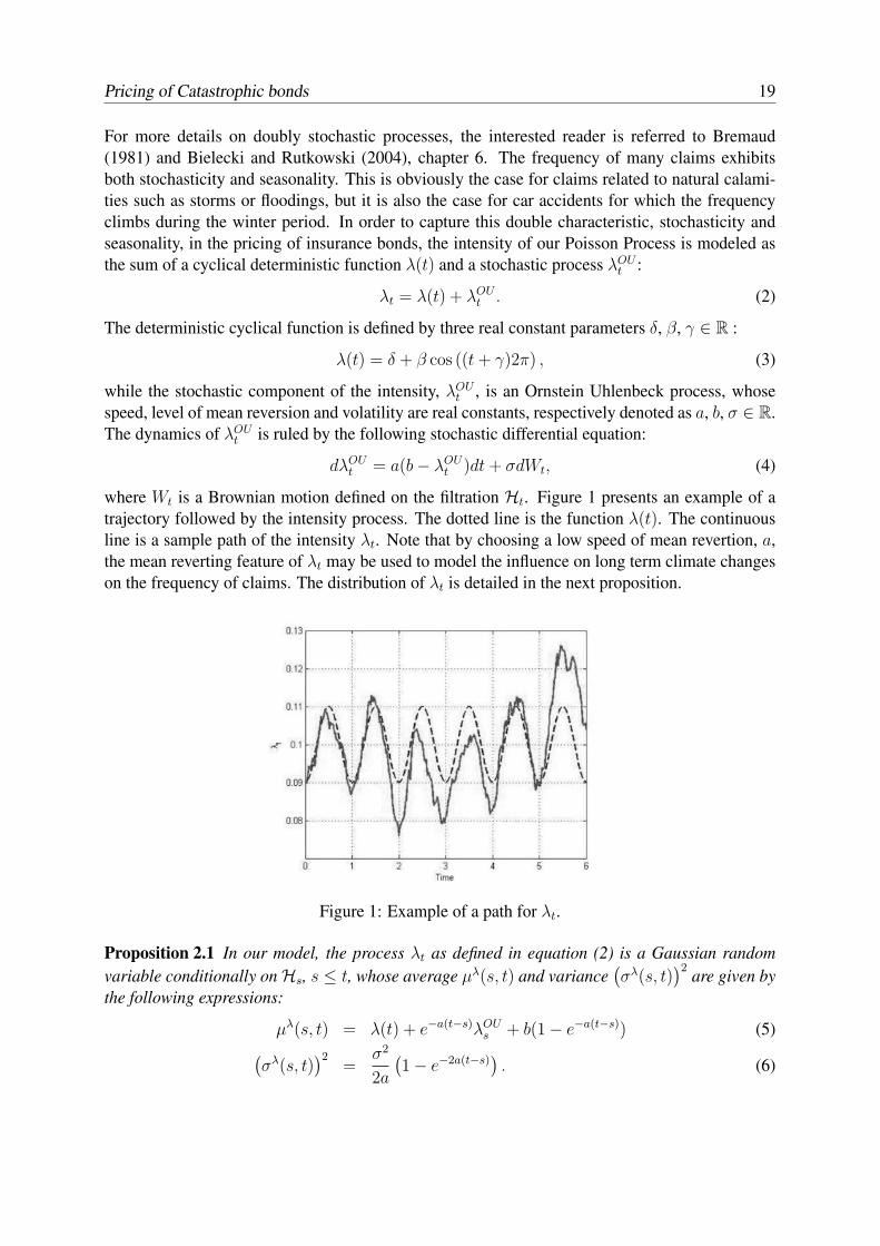
where Wt is a Brownian motion defined on the filtration Ht. Figure 1 presents an example of atrajectory followed by the intensity process. The dotted line is the function λ(t). The continuousline is a sample path of the intensity λt. Note that by choosing a low speed of mean revertion, a,the mean reverting feature of λt may be used to model the influence on long term climate changeson the frequency of claims. The distribution of λt is detailed in the next proposition.
Figure 1: Example of a path for λt.
Proposition 2.1 In our model, the process λt as defined in equation (2) is a Gaussian randomvariable conditionally on Hs, s ≤ t, whose average µλ(s, t) and variance
(σλ(s, t)
)2are given by
the following expressions:
µλ(s, t) = λ(t) + e−a(t−s)λOUs + b(1 − e−a(t−s)) (5)
(σλ(s, t)
)2=
σ2
2a
(1 − e−2a(t−s)
). (6)
20 D. Hainaut
Proof. We just sketch the proof because this result is rather standard and we refer the reader toMusiela and Rutkowski (1997), chapter 12 - p.289, for details. The first step consists of differenti-ating the process Zt = eat(b − λOU
t ) to show that
Zt = Zs −
∫ t
s
eauσdWu; (7)
as λOUt = b − e−atZt, one infers from equation (7), that
λOUt = e−a(t−s)λOU
s + b(1 − e−a(t−s)) +
∫ t
s
e−a(t−u)σdWu. (8)
The results of the proposition directly follow from this last relation.
The intensity process λt defined in equations (2) and (4), is a Gaussian random variable, andthe probability of observing a negative value for this process differs from zero. However, if theannual average level δ of λ(t) and level of mean reversion b are sufficiently high compared to thevolatility σ, this probability should be nearly zero, and λt may be used as intensity for Nt. We nowpresent two propositions that will allow us to determine the probability generating function of Nt.
Proposition 2.2 The integral of λu from t1 to t2, is a Gaussian random variable conditionally onHs, s ≤ t1 ≤ t2, whose average µ
∫λdu(s, t1, t2) and variance
(σ
∫λdu(s, t1, t2)
)2are given by the
following expressions:
µ∫
λdu(s, t1, t2) = δ(t2 − t1) +1
2πβ sin (2π(t2 + γ)) −
1
2πβ sin (2π(t1 + γ))
+λOUs e−a(t1−s)B(t1, t2) + b
((t2 − t1) − e−a(t1−s)B(t1, t2)
)(9)
(
σ∫
λdu(s, t1, t2))2
=σ2
2aB(t1, t2)
2(1 − e−2a(t1−s)
)
+σ2
a2
(
(t2 − t1) − B(t1, t2) −1
2a B(t1, t2)
2
)
, (10)
where the function B(t1, t2) is defined as follows:
B(t1, t2) =1
a
(1 − e−a(t2−t1)
).
Proof. The integral of λu is the sum of the integrals of λ(u) and of λOUu . The integral of λ(u) from
t1 to t2 is worth:∫ t2
t1
λ(u)du = δ(t2 − t1) +1
2πβ sin (2π(t2 + γ)) −
1
2πβ sin (2π(t1 + γ)) , (11)
whereas the integral of the process λOUu is obtained by integrating equation (8) from t1 to t2:
∫ t2
t1
λOUu du = λOU
s e−a(t1−s)B(t1, t2) + b((t2 − t1) − e−a(t1−s)B(t1, t2)
)
+
∫ t1
s
σ
a
(e−at1 − e−at2
)eaudWu +
∫ t2
t1
σB(u, t2)dWu. (12)
Pricing of Catastrophic bonds 21
The results of the proposition directly follow from this last relation.
According to equation (1), the process Nt2 − Nt1 is a Poisson process conditionally on Ht2 ∨Ft1 ⊃ Fs. This property allows us to deduce that the probability of observing k jumps in a certaininterval of time is equal to the following expectation, where I is an indicator variable:
P (Nt2 − Nt1 = k | Fs) = E[INt2
−Nt1=k| Fs
]
= E
[
E[INt2
−Nt1=k|Ht2 ∨ Ft1
]∣∣∣Fs
]
= E
[
P (Nt2 − Nt1 = k |Ht2 ∨ Ft1)∣∣∣Fs
]
= E
(∫ t2
t1λudu
)k
k!e−
∫ t2t1
λudu
∣∣∣∣∣Fs
. (13)
Except for k = 0, no analytical expression exists for this last expectation. However, it will beshown in the remainder of this section that the probabilities of observing k > 0 jumps, can becomputed by means of an iterative procedure based upon the probability generating function (pgf)of Nt as defined in the next proposition.
Proposition 2.3 The pgf of Nt defined by
pgf(x, s, t1, t2) = E
[
xNt2−Nt1
∣∣∣Fs
]
(14)
with s ≤ t1 ≤ t2 is given by
pgf(x, s, t1, t2) = E
[
e∫ t2
t1λudu (x−1)
∣∣∣Fs
]
= exp
(
(x − 1)µ∫
λdu(s, t1, t2) +1
2(x − 1)2
(
σ∫
λdu(s, t1, t2))2
)
. (15)
Proof. Given that Ht2 ∨ Ft1 ⊃ Fs, one can rewrite the probability generating function as follows:
pgf(x, s, t1, t2) = E[xNt2
−Nt1 |Fs
]= E
[
E[xNt2
−Nt1 |Ht2 ∨ Ft1
]
∣∣∣∣∣Fs
]
.
Conditionally on Ht2 ∨ Ft1 , the jump process is Poisson with known pgf, resulting in
pgf(x, s, t1, t2) = E
[
E[xNt2
−Nt1 |Ht2 ∨ Ft1
]∣∣∣Fs
]
= E
[
e∫ t2
t1λudu (x−1)
∣∣∣Fs
]
. (16)
The integral of the intensity is Gaussian according to proposition 2.2, and therefore the expectationin equation (16) is the expectation of a lognormal variable, as given in equation (15).
The pgf is a powerful tool that gives us the possibility to infer by a recursive method theprobabilities of jumps of Nt2 − Nt1 , conditionally on the filtration Fs at time s ≤ t1 ≤ t2.
22 D. Hainaut
Proposition 2.4 The probability not to observe any jumps in the interval of time [t1, t2], condition-ally on Fs, s ≤ t1 ≤ t2, is equal to
P (Nt2 − Nt1 = 0 | Fs) = pgf(x, s, t1, t2)
∣∣∣∣∣x=0
= exp
(
−µ∫
λdu(s, t1, t2) +1
2
(
σ∫
λdu(s, t1, t2))2
)
. (17)
The probability that the process Nt exhibits exactly one jump in the interval of time [t1, t2] is equalto:
P (Nt2 − Nt1 = 1 | Fs) =∂
∂xpgf(x, s, t1, t2)
∣∣∣∣x=0
= P (Nt2 − Nt1 = 0 | Fs)
(
µ∫
λdu(s, t1, t2) −(
σ∫
λdu(s, t1, t2))2
)
. (18)
The probability of observing more than one jump can be computed iteratively as follows:
P (Nt2 − Nt1 = k | Fs) =1
k!
∂k
∂xkpgf(x, s, t1, t2)
∣∣∣∣x=0
, (19)
where
∂k
∂xkpgf(x, s, t1, t2)
∣∣∣∣x=0
=
(
µ∫
λdu(s, t1, t2) −(
σ∫
λdu(s, t1, t2))2
)∂k−1
∂xk−1pgf(x, s, t1, t2)
∣∣∣∣x=0
+(k − 1)(
σ∫
λdu(s, t1, t2))2 ∂k−2
∂xk−2pgf(x, s, t1, t2)
∣∣∣∣x=0
. (20)
Proof. The proof of this proposition directly results from the exponential form of the probabilitygenerating function.
Proposition 2.4 provides us with an important tool in order to calibrate our model parameters(δ, β, γ, a, b, σ) to real data. The calibration can be done by maximizing the likelihood of observednumbers of claims observed during several seasons.
3. THE SIZE OF CLAIMS AND THE PRICING OF BONDS
The risk faced by an insurance bondholder is inherent to his exposure to accumulated insuredproperty losses. This process of accumulated losses, which is denoted by Xt in the sequel of thiswork, depends both on the frequency of the claims Nt and on the magnitude of the claims. The sizeof the jth claim, occurring at time tj , is modeled by a positive random variable, Yj , defined on the
Pricing of Catastrophic bonds 23
filtration Ftj , but assumed to be independent from previous claims and from the frequency. Thereare no other constraints on the choice of Yj . As for the claims arrival process Nt, we directly workwith the distribution of Yt under the risk neutral measure Q (again we refer the interested readerto appendix B for details about the relation between the modeling under P , the real measure, andQ). The process of aggregated losses, is defined by the following expression:
Xt =∑
tj<t
Yj =Nt∑
i=1
Yj.
We now describe the characteristics of an insurance bond and introduce the method to price suchkind of assets. The insurance bond periodically pays a coupon equal to a constant percentage ofthe nominal, reduced by the amount of aggregated losses, exceeding a certain trigger level. Atmaturity, what is left of the nominal value is repaid. In order to compensate for this eventual lossof the nominal value, the coupon rate always exceeds the risk free rate. In case a few claims occur,the bondholder is then rewarded at a higher rate than the one obtained by investing in risk freeassets with the same maturities. On the contrary, in case of catastrophic losses, the nominal of thebond can fall to zero and the payment of coupons can be interrupted. In order to understand howthe spread of this bond is priced, we need to introduce some additional mathematical notations.
Let us use the notation BN for the initial nominal value of the bond. The level above whichthe excess of aggregated losses is deduced from the nominal, is denoted by K1. If the total insuredlosses reach the amount of K2 = K1 +BN before maturity, the bond stops to deliver coupons andthe nominal is depleted. The bond, issued at time t0, pays n coupons, at regular intervals of time,∆t, ranging from t1 to tn. The coupon rate is the sum of the constant risk free rate with maturity tn,and of a spread: they are respectively denoted as r and sp. The coupons paid at times ti, i = 1...n,are denoted as cp(ti) and defined as follows:
cp(ti) = (r + sp) ∆t
[
(K2 − K1) IXti∈[0,K1] + (K2 − Xti) IXti
∈(K1,K2]
]
︸ ︷︷ ︸
BNti
. (21)
The term between brackets is the (stochastic) nominal of the bond at time ti and is written as BNti
in the sequel of our developments. Note that BNt0 is equal to BN . Based upon the principleof absence of arbitrage, the spread of the insurance bond is chosen such that the expectations offuture discounted spreads and of future discounted cutbacks of nominal are equal under the riskneutral pricing Q. The expectations of future discounted spreads and reductions of nominal arerespectively called the “spreads leg” and the “claims leg” (this terminology is in fact inspired fromthe one for credit derivatives). These legs are defined by the following expressions:
SpreadLeg(t0) = sp ∆t
tn∑
ti=t1
e−r (ti−t0)E [BNti | Ft0 ] , (22)
ClaimsLeg(t0) =tn∑
ti=t1
e−r (ti−t0)E
[BNti−1
− BNti | Ft0
]. (23)
24 D. Hainaut
By equating equation (22) with equation (23), we infer the following fair spread rate that shouldbe added to the risk free rate, at the issuance of the insurance bond:
sp =
∑tnti=t1
e−r (ti−t0)E
[BNti−1
− BNti | Ft0
]
∆t∑tn
ti=t1e−r (ti−t0)E [BNti | Ft0 ]
. (24)
Despite the apparent simplicity of this last expression, the expected future nominals are not calcu-lable by means of a closed form expression, and we have to rely on numerical methods to appraisethem. Among the numerical tools available, we have chosen to use the Fourier transform.
4. PRICING BY FOURIER TRANSFORM
As explained in the previous paragraph, the pricing of an insurance bond requires the valuation ofthe expected future value of nominal. According to equation (21), this expectation may be splitinto two components,
E [BNti | Ft0 ] = E[BN IXti
∈[0,K1] | Ft0
]+ E
[(K2 − Xti) IXti
∈(K1,K2] | Ft0
]. (25)
As done by Carr and Madan (1999), each component can be reformulated in terms of their Fouriertransforms. The two next propositions deal with this point.
Proposition 4.1 If α1 is a strictly positive real constant, chosen to ensure the stability of subse-quent numerical computations, the following holds:
E[BN IXti
∈[0,K1] | Ft0
]
=BN
π
∫ +∞
0
ϕ1(u)e−(α1+iu)Xt0
+∞∑
k=0
P (Nti − Nt0 = k)(
E[e−(α1+iu)Y
])k
du, (26)
where ϕ1(u) is the Fourier transform of the function eα1xIx∈[0,K1] , x ∈ R+,
ϕ1(u) =1
α1 + iu
(e(α1+iu)K1 − 1
). (27)
The probabilities P (Nti −Nt0 = k) can be retrieved from proposition 2.4 whereas the expectationE
[e−(α1+iu)Y
]is the Laplace transform of the claim size Y , evaluated at α1 + iu.
Proof. Let us denote by qXti|Ft0
(x) the density of the aggregated losses process Xti , conditionallyon the filtration Ft0 . If we choose a positive constant α1, the expectation in equation (34) can bewritten as follows:
E[IXti
∈[0,K1] | Ft0
]= E
[e−α1Xti eα1Xti IXti
∈[0,K1] | Ft0
].
=
∫ +∞
0
e−α1x eα1x Ix∈[0,K1] qXti|Ft0
(x) dx. (28)

Pricing of Catastrophic bonds 25
Now, define ϕ1(u) as the Fourier transform of the function eα1xIx∈[0,K1] , x ∈ R+:
ϕ1(u) =
∫ +∞
−∞
eα1xIx∈[0,K1]eiuxdx;
it can be easily checked that this last integral is equal to the expression in equation (27). If α1 isstrictly positive, the function ϕ1(u) is well defined for u = 0. The function eα1xIx∈[0,K1] can beretrieved by inverting the Fourier transform ϕ1(u):
eα1xIx∈[0,K1] =1
2π
∫ +∞
−∞
ϕ1(u)e−iuxdu
=1
π
∫ +∞
0
ϕ1(u)e−iuxdu, (29)
where the second equality results from the symmetry of the integrand, which is itself due to thefact that the function eα1xIx∈[0,K1] is real (no imaginary component). The combination of equation(28) and equation (29) allows us to infer that:
E[IXti
∈[0,K1] | Ft0
]=
1
π
∫ +∞
0
∫ +∞
0
ϕ1(u)e−(α1+iu)x qXti|Ft0
(x) dx du
=1
π
∫ +∞
0
ϕ1(u) E[e−(α1+iu)Xti | Ft0
]du. (30)
The integrand of this last equation contains the Laplace transform of the aggregated losses process,evaluated at α1 + iu. This can be worked out as follows:
E[e−(α1+iu)Xti | Ft0
]= e−(α1+iu)Xt0E
[
e−(α1+iu)
∑Ntii=Nt0
Yi
∣∣∣Ft0
]
= e−(α1+iu)Xt0
+∞∑
k=0
P (Nti − Nt0 = k)(
E[e−(α1+iu)Y
])k
. (31)
Proposition 4.2 If α2 is a strictly positive real constant, chosen to ensure the stability of subse-quent numerical computations, the following holds:
E[(K2 − Xti) IXti
∈(K1,K2] | Ft0
]
=1
π
∫ +∞
0
ϕ2(u)e−(α2+iu)Xt0
+∞∑
k=0
P (Nti − Nt0 = k)(
E[e−(α2+iu)Y
])k
du, (32)
where ϕ2(u) is the Fourier transform of the function eα2x (K2 − x) Ix∈[K1,K2] , x ∈ R+,
ϕ2(u) =K1
α2 + iue(α2+iu)K1 −
K2
α2 + iue(α2+iu)K1
+1
(α2 + iu)2
(e(α2+iu)K2 − e(α2+iu)K1
). (33)
The probabilities P (Nti −Nt0 = k) can be retrieved from proposition 2.4 whereas the expectationE
[e−(α1+iu)Y
]is the Laplace transform of the claim size Y , valued at α1 + iu.
26 D. Hainaut
Proof. The proof is analogous to the proof of proposition 4.1. It may be checked quickly thatϕ2(u), the Fourier transform of the function eα2x (K2 − x) Ix∈[K1,K2], x ∈ R
+, or
ϕ2(u) =
∫ +∞
−∞
eα2x (K2 − x) Ix∈[K1,K2]eiuxdx,
is equal to the expression of equation (33). Moreover it is true that for α2 strictly positive, thefunction ϕ2(u) is well defined for u = 0.
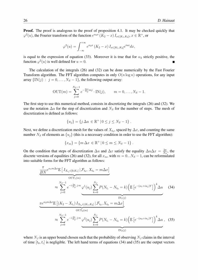
The calculation of the integrals (26) and (32) can be done numerically by the Fast FourierTransform algorithm. The FFT algorithm computes in only O(n log n) operations, for any inputarray IN(j) : j = 0, . . . , NS − 1, the following output array:
OUT(m) =
NS−1∑
j=0
e− 2πi
NSmj
· IN(j), m = 0, . . . , NS − 1.
The first step to use this numerical method, consists in discretizing the integrals (26) and (32). Weuse the notation ∆u for the step of discretization and NS for the number of steps. The mesh ofdiscretization is defined as follows:
uj = j ∆u ∈ R+ | 0 ≤ j ≤ NS − 1 .
Next, we define a discretization mesh for the values of Xt0 , spaced by ∆x, and counting the samenumber NS of elements as uj (this is a necessary condition in order to use the FFT algorithm):
xm = m ∆x ∈ R+ | 0 ≤ m ≤ NS − 1 .
On the condition that steps of discretization ∆u and ∆x satisfy the equality ∆u∆x = 2πNS
, thediscrete versions of equalities (26) and (32), for all xm, with m = 0...NS − 1, can be reformulatedinto suitable forms for the FFT algorithm as follows:
π
BNeα1m∆x
E[IXti
∈[0,K1] | Ft0 , Xt0 = m∆x]
︸ ︷︷ ︸
OUT1(m)
≈
NS−1∑
j=0
e−i 2π
NSj m
ϕ1(uj)
NJ∑
k=0
P (Nti − Nt0 = k)(
E[e−(α1+iuj)Y
])k
∆u
︸ ︷︷ ︸
IN1(j)
(34)
πeα2m∆xE
[(K2 − Xti) IXti
∈(K1,K2] | Ft0 , Xt0 = m∆x]
︸ ︷︷ ︸
OUT2(m)
≈
NS−1∑
j=0
e−i 2π
NSj m
ϕ2(uj)
NJ∑
k=0
P (Nti − Nt0 = k)(
E[e−(α2+iuj)Y
])k
∆u
︸ ︷︷ ︸
IN2(j)
, (35)
where NJ is an upper bound chosen such that the probability of observing NJ claims in the intervalof time [t0, ti] is negligible. The left hand terms of equations (34) and (35) are the output vectors

Pricing of Catastrophic bonds 27
computed by a standard FFT algorithm. By combining them, one can calculate the expected valuesof future nominal, for a wide range of initial values for Xt0 (see equation (25)):
E [BNti | Ft0 , Xt0 = m∆x] =BN
πe−α1m∆x OUT1(m) +
1
πe−α1m∆x OUT2(m), (36)
∀m = 1, ..., NS − 1. Note that the calculation of the spread by equation (24) at the issuance ofthe bond, only requires to determine the expected future nominal when Xt0 = 0. However, theknowledge of expected future nominal when Xt0 > 0, may be useful to reappraise an insurancebond, issued before t0, and also when some claims already occurred.
5. NUMERICAL APPLICATIONS
This section illustrates by means of a numerical example the feasibility of the pricing methoddeveloped in the first part of this paper. In particular, we compute the fair spreads that insurancebonds of maturities ranging from 1 to 3 years should pay above the risk free rate, here set at 3%.The nominal, NB, is of 70 million. This nominal is decreased if the aggregated losses rise above10 million. The coupons are paid annually. Other bonds characteristics are summarized in table 1.
r 3% tn 1,2,3K1 10 t1 1K2 80 ∆t 1
Table 1: Parameters of bonds.
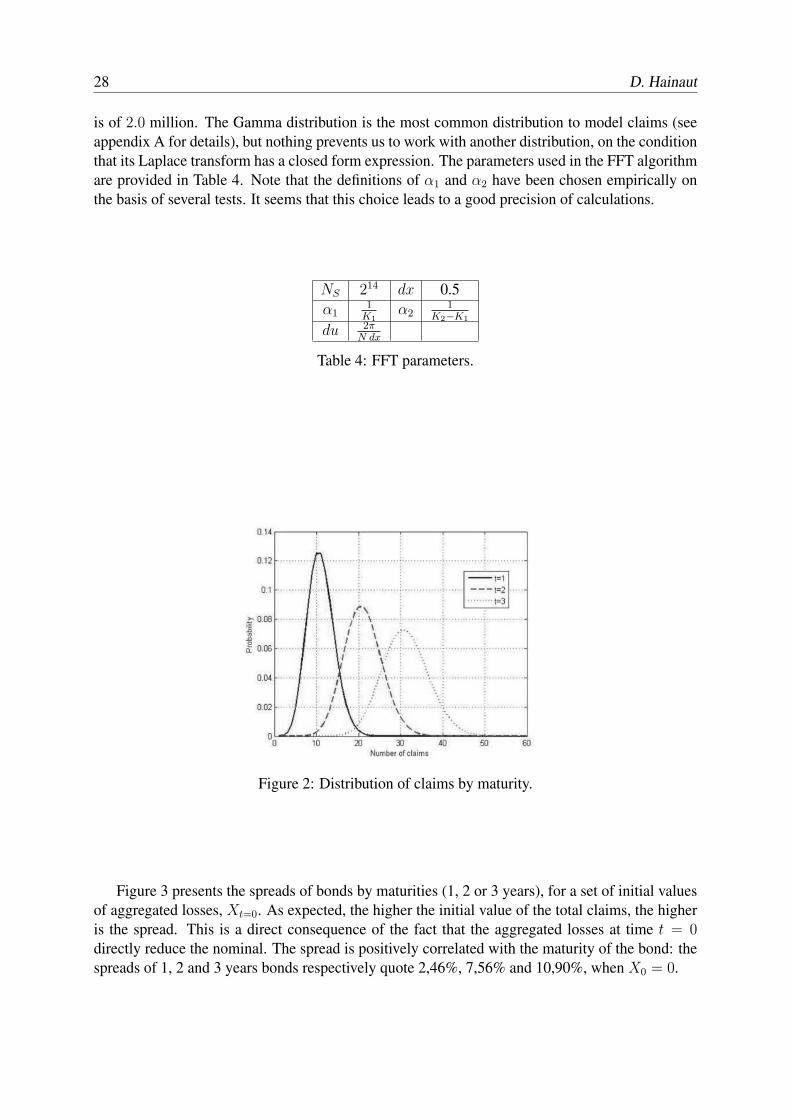
Table 2 presents the parameters chosen for the claims arrival process. From Proposition 2.4,we can deduce the probability density function of Nt after 1, 2 and 3 years. The densities areplotted in figure 2. From these densities, we can calculate the averages and standard deviations ofthe number of claims, after 1, 2 and 3 years; these presented in Table 3. Per year, one foresees onaverage 11 claims, and the one-year volatility is situated around 3 claims.
α 0.4 δ 10b 0.1 β 0.01σ 0.01 γ 0.5
Table 2: Parameters of the claims arrival process.
t = 1 t = 2 t = 3E(Nt) 11.02 21.06 31.13σ(Nt) 3.17 4.48 5.49
Table 3: Means and deviations of Nt.
We have chosen to model the size of claims by a Gamma random variable whose parametersare θ = 2 and k = 0.5. The average size of claims is of 1.0 million and the standard deviation
28 D. Hainaut
is of 2.0 million. The Gamma distribution is the most common distribution to model claims (seeappendix A for details), but nothing prevents us to work with another distribution, on the conditionthat its Laplace transform has a closed form expression. The parameters used in the FFT algorithmare provided in Table 4. Note that the definitions of α1 and α2 have been chosen empirically onthe basis of several tests. It seems that this choice leads to a good precision of calculations.
NS 214 dx 0.5α1
1K1
α21
K2−K1
du 2πN dx
Table 4: FFT parameters.
Figure 2: Distribution of claims by maturity.
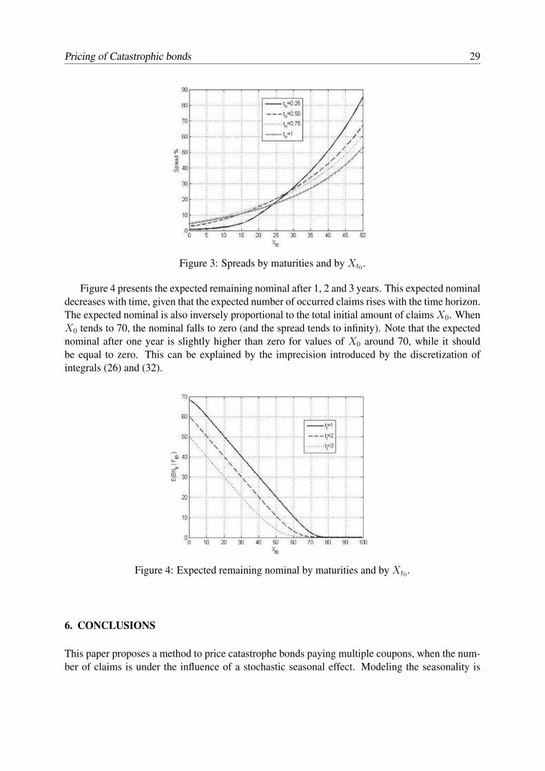
Figure 3 presents the spreads of bonds by maturities (1, 2 or 3 years), for a set of initial valuesof aggregated losses, Xt=0. As expected, the higher the initial value of the total claims, the higheris the spread. This is a direct consequence of the fact that the aggregated losses at time t = 0directly reduce the nominal. The spread is positively correlated with the maturity of the bond: thespreads of 1, 2 and 3 years bonds respectively quote 2,46%, 7,56% and 10,90%, when X0 = 0.
Pricing of Catastrophic bonds 29
Figure 3: Spreads by maturities and by Xt0 .
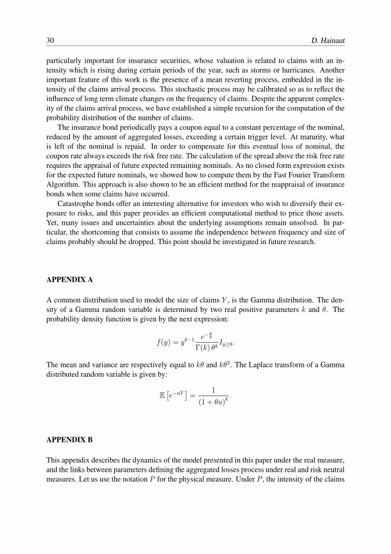
Figure 4 presents the expected remaining nominal after 1, 2 and 3 years. This expected nominaldecreases with time, given that the expected number of occurred claims rises with the time horizon.The expected nominal is also inversely proportional to the total initial amount of claims X0. WhenX0 tends to 70, the nominal falls to zero (and the spread tends to infinity). Note that the expectednominal after one year is slightly higher than zero for values of X0 around 70, while it shouldbe equal to zero. This can be explained by the imprecision introduced by the discretization ofintegrals (26) and (32).
Figure 4: Expected remaining nominal by maturities and by Xt0 .
6. CONCLUSIONS
This paper proposes a method to price catastrophe bonds paying multiple coupons, when the num-ber of claims is under the influence of a stochastic seasonal effect. Modeling the seasonality is
30 D. Hainaut
particularly important for insurance securities, whose valuation is related to claims with an in-tensity which is rising during certain periods of the year, such as storms or hurricanes. Anotherimportant feature of this work is the presence of a mean reverting process, embedded in the in-tensity of the claims arrival process. This stochastic process may be calibrated so as to reflect theinfluence of long term climate changes on the frequency of claims. Despite the apparent complex-ity of the claims arrival process, we have established a simple recursion for the computation of theprobability distribution of the number of claims.
The insurance bond periodically pays a coupon equal to a constant percentage of the nominal,reduced by the amount of aggregated losses, exceeding a certain trigger level. At maturity, whatis left of the nominal is repaid. In order to compensate for this eventual loss of nominal, thecoupon rate always exceeds the risk free rate. The calculation of the spread above the risk free raterequires the appraisal of future expected remaining nominals. As no closed form expression existsfor the expected future nominals, we showed how to compute them by the Fast Fourier TransformAlgorithm. This approach is also shown to be an efficient method for the reappraisal of insurancebonds when some claims have occurred.
Catastrophe bonds offer an interesting alternative for investors who wish to diversify their ex-posure to risks, and this paper provides an efficient computational method to price those assets.Yet, many issues and uncertainties about the underlying assumptions remain unsolved. In par-ticular, the shortcoming that consists to assume the independence between frequency and size ofclaims probably should be dropped. This point should be investigated in future research.
APPENDIX A
A common distribution used to model the size of claims Y , is the Gamma distribution. The den-sity of a Gamma random variable is determined by two real positive parameters k and θ. Theprobability density function is given by the next expression:
f(y) = yk−1 e−y
θ
Γ(k) θkIy≥0.
The mean and variance are respectively equal to kθ and kθ2. The Laplace transform of a Gammadistributed random variable is given by:
E[e−uY
]=
1
(1 + θu)k.
APPENDIX B
This appendix describes the dynamics of the model presented in this paper under the real measure,and the links between parameters defining the aggregated losses process under real and risk neutralmeasures. Let us use the notation P for the physical measure. Under P , the intensity of the claims
Pricing of Catastrophic bonds 31
arrival process is given by :λP
t = λP (t) + λOU,Pt ,
where λP (t) is defined by three real constant parameters δP , βP , γP ∈ R :
λ(t) = δP + βP cos((t + γP )2π
),
and where λOU,Pt is an Ornstein Uhlenbeck process, whose speed, level of mean reversion and
volatility are real constants, respectively denoted by aP , bP , σP ∈ R. The dynamics of λOU,Pt is
ruled by the following stochastic differential equation:
dλOUt = aP (bP − λOU
t )dt + σP dW Pt . (37)
Under P , the size of claims are positive random variables with density fPY (y). The changes of
measure from P to a risk neutral measure Q leading to the model developed in section 2 and 3, aredefined by the following Radon-Nikodym derivative (for details see e.g. Shreve (2004), chapter11):
dQ
dP= exp
(Nt∑
k=1
ln(κg(Yk)) +
∫ t
0
λu(1 − κ)du
)
· exp
(
−1
2
∫ t
0
ξ2du −
∫ t
0
ξdW Pu
)
,
where κ is a nonnegative constant and ξ is here a real constant. The function g(.) is measurableg : R
+ → R and satisfies the relation∫ +∞
0
g(y)fP (y)dy = 1.
Under Q, dWu = dW Pu + ξdu is a Brownian motion, the intensity of the claims arrival process is
multiplied by κ and the probability density function of claims is multiplied by g(y). The followingrelations between twe parameters of our model under Q and P then hold:
δ = κδP a = aP
β = κβP b = κ(
bP − σP ξ
aP
)
γ = γP σ = κσP .
The probability density function of Yt under Q is equal to:
f(y) = g(y)fP (y).
References
K. Aase. An equilibrium model of catastrophe insurance futures and spreads. Geneva papers onrisk and insurance theory, 24:69–96, 1999.
32 D. Hainaut
K. Aase. A Markov model for the pricing of catastrophe insurance futures and spreads. Journal ofRisk and Insurance, 68(1):25–50, 2001.
F. Biagini, Y. Bregman, and T. Meyer-Brandis. Pricing of catastrophe insurance options written ona loss index with reestimation. Insurance: Mathematics and Economics, 43:214–222, 2008.
T.R. Bielecki and M. Rutkowski. Credit Risk: Modeling, Valuation and Hedging. Springer Fi-nance, 2004.
P. Bremaud. Point processes and queues martingales dynamics. Springer Verlag, New York, 1981.
M. Carr and D.B. Madan. Option valuation using the Fast Fourier transform. Journal of Compu-tational Finance, 2(4):61–73, 1999.
A. Charpentier. Pricing catastrophe options. In M. Vanmaele, G. Deelstra, A. De Schepper,J. Dhaene, H. Reynaerts, W. Schoutens, and P. Van Goethem, editors, Handelingen Contact-forum Actuarial and Financial Mathematics Conference, February 7-8, 2008, pages 19–31.Koninklijke Vlaamse Academie van Belgie voor Wetenschappen en Kunsten, 2008.
C.V. Christensen and H. Schmidli. Pricing catastrophe insurance products based on actually re-ported claims. Insurance: Mathematics and Economics, 27:189–200, 2000.
J.D. Cummins and H. Geman. An Asian option approach to valuation of insurance futures con-tracts. Review futures markets, 13:517–557, 1994.
A. Dassios and J. Jang. Pricing of catastrophe reinsurance and derivatives using the Cox processwith shot noise intensity. Finance and Stochastics, 7(1):73–95, 2003.
H. Geman and M. Yor. Stochastic time changes in catastrophe option pricing. Insurance: mathe-matics and economics, 21:185–193, 1997.
J-W. Jang. Doubly stochastic poisson process and the pricing of catastrophe reinsurance contract.ASTIN Colloquium, 2000.
A. Murmann. Pricing catastrophe insurance derivatives. Technical Report 400, Financial MarketsGroup and The Wharton School, Discussion Paper, 2001.
M. Musiela and M. Rutkowski. Martingale Methods in Financial Modelling. Springer Finance,1997.
S. Shreve. Stochastic Calculus for Finance II: Continuous-time Models. Springer Finance, 2004.
CMS SPREAD OPTIONS IN THE MULTI-FACTOR HJM FRAMEWORK
Pierre Hanton and Marc Henrard
Interest Rate Modelling, Dexia Bank Belgium, 1000 Brussels, BelgiumEmail: [email protected], [email protected]
Abstract
Constant maturity swaps (CMS) and CMS spread options are analyzed in the multi-factorHeath-Jarrow-Morton (HJM) framework. For Gaussian models, which include some LiborMarket Models (LMM) and the G2++ model, explicit approximated pricing formulae are pro-vided. Two approximating approaches are proposed: an exact solution to an approximatedequation and an approximated solution to the exact equation. The first approach borrows fromprevious literature on other models; the second is new. The price approximation errors aresmaller than in the previous literature and negligible in practice. The approach is being usedhere to price standard CMS and CMS spreads and can be used for some European exoticproducts.
1. INTRODUCTION
Constant Maturity Swap (CMS) spread options are relatively popular. Their pay-off depends onthe difference between two swap rates. Models where only the global level of the curve is modeledwould not do a good job in pricing those instruments. Quite naturally one uses two-factor (or moregenerally multi-factor) models to price those instruments.
The pricing of rate spread instruments in the HJM framework was considered in Fu (1996)and Miyazaki and Yoshida (1998). The former considers the spread between zero-coupon rateswith annual compounding, payment on exercise date and strike 0. The options are analyzed in aGaussian two-factor HJM model. The latter considers a very specific Gaussian two-factor HJMmodel and spread between continuously compounded zero coupon rates. Due to convention andpayment dates, those results can not be used to price actual CMS spread options.
More recently Wu and Chen (2009) analyzed the spread options in the log-normal LMM. Theoptions they consider have strike 0 and payment on exercise date. In practice the payment takesplace at the end of an accrual period and not on the fixing date. Their results would need to beadapted to be used in practice. Moreover the majority of spread options are dealt at non-zerostrikes. In Antonov and Arneguy (2009), CMS products are analyzed in a LMM with stochastic
33
34 P. Hanton and M. Henrard
volatility. The instruments analyzed have non-zero strike and a payment lag. Due to the modelcomplexity their results are not fully explicit and require a characteristic function and one or two-dimensional Laplace transforms.
The CMS spread instruments depend, as their name indicates, on swap rates. One approach isto obtain approximated dynamics for the swap rates in the model. If the approximated dynamics aresimple enough, the spread options can be valued as an exchange option. This is the technique usedin Wu and Chen (2009) in the log-normal LMM model where the swap rates are approximatelylog-normal. In Antonov and Arneguy (2009), the swap dynamics are obtained through a techniquecalled Markov projection.
A standard approach to price CMS options is to use replication arguments. In that case the priceis based on the prices of vanilla cash-settled swaptions (see for example Hagan (2003) or Mercurioand Pallavicini (2005)). Based on the CMS prices and the implied CMS rate, one often prices theCMS spreads as the spread on two log-normal assets with correlation (see for example Berrahoui(2004)). Our proposal could replace this approach. A two-factor model could be calibrated toCMS and CMS spread prices and could be used to price more exotic products. Our approach givesmore freedom on the pay-off description than the standard bi-log-normal approach.
Here we first develop results in the G2++ model using the approximated rate dynamics ap-proach. The swap rate dynamics are approximately normal. The exact option price in the approxi-mated dynamics is the first price approximation proposed. The price formula is explicit and similarto the Bachelier formula. The options we consider have a free strike, use the market conventionand have a free payment date. The first result is interesting in itself. In particular the smile of theG2++ model is closer to the market smile than a flat log-normal LMM (absence of) smile.
Then we move one step further. We would like to obtain similar results in a general Gaussianseparable multi-factor HJM framework. This framework contains in particular the LMM versioncalled Bond Market Model and the G2++ model. In that model very efficiently approximated Euro-pean swaption prices are available, as described in Henrard (2008b). One could extend the approxi-mated swap dynamics methodology; the drawback is that one can only price instruments dependenton (one or two) swap rates; the pay-offs are limited to pay-offs of the form f(S1, S2)1(g(S1,S2)>0).We work in a term-structure model, modeling the full yield curve but our approach would restrictus to use only two of those rates. This, for example, excludes a swaption with CMS spread trigger,i.e with pay-off
∑ciP (θ, ti)1(S1−S2>0), or similar products.
For that reason we propose a second approach where we use an approximated solution to theexact equation. The exact solution of the discount bond in the HJM framework is computed.With those exact solutions, the pay-offs are too complex to lead to explicit solutions. We usepay-off approximations (to the first and second order) to obtain explicit prices. The price formulacontains terms similar to the Bachelier formula for the first order and some additional terms for thesecond order. The approximating explicit solution to exotic options contrasts with the Monte-Carlotechniques often used in that context.

CMS spreads in the multi-factor HJM framework 35
2. MODELS
In general, a term structure model describes the behavior of P (t, u), the price in t of the zero-coupon bond paying 1 in u (0 ≤ t ≤ u ≤ T ). When the discount curve P (t, .) is differentiable (ina weak sense), there exists f(t, u) such that
P (t, u) = exp
(−
∫ u
t
f(t, s)ds
). (1)
Let Nt = exp(∫ t
0rsds) be the cash-account numeraire with (rs)0≤s≤T the short rate rt = f(t, t).
Except if otherwise stated, the model equations are in the numeraire measure associated to Nt.
2.1. G2++
The G2++ model is a two-factor interest rate model which can be viewed as a two-factor extendedVasicek model. The model is usually introduced as a short rate model with
rt = x1t + x2
t + φ(t)
where the stochastic processes are given by
dxit = −aix
itdt + ηi(t)dW i
t .
The Brownian processes W 1t and W 2
t are correlated with correlation ρ. The initial values of theprocesses are xi
0 = 0. The ai are two positive constants and the functions ηi are deterministic. Thedeterministic function φ(t) is given by the initial interest rate curve. The description of the modeland its analytical formulae can be found in Brigo and Mercurio (2006).
2.2. Gaussian HJM (multi-factor)
The idea of Heath et al. (1992) was to model f with a stochastic differential equation
df(t, u) = σ(t, u) · (ρν(t, u)) dt + σ(t, u) · dWt
whereν(t, u) =
∫ u
t
σ(t, s)ds
for some suitable σ. The random processes Wt = (W 1t , . . . ,W n
t ) are Brownian motions withcorrelation matrix ρ. The special form of the drift is required to ensure the arbitrage-free property.Note that with respect to standard writing we use a correlated Brownian motion to simplify thewriting in the developments. This is the origin of the correlation matrix appearing in the drift term.The volatility and the Brownian motion are n-dimensional while the rates are 1-dimensional. Themodel technical details can be found, among other places, in the original paper or in the chapterDynamical term structure model of Hunt and Kennedy (2004).
36 P. Hanton and M. Henrard
We study this model under the separability hypothesis, see e.g. Henrard (2008a)
σi(s, u) = gi(s)hi(u).
Separability conditions have been widely used in interest rate modeling. The results cover theMarkov processes in Carverhill (1994), explicit swaption formulas in Gaussian HJM models inHenrard (2003) and efficient approximations for LMM in Pelsser et al. (2004) and Bennett andKennedy (2005).
In line with the separability hypothesis, we denote
γi,j =
∫ θ
0
gi(s)gj(s)ds and Hi(t) =
∫ t
0
hi(s)ds.
So we obtain that the price of a zero-coupon bond can be written (Henrard 2007, Lemma A.1),after a change of numeraire to P (., θ) as
P (θ, u)=P (0, u)
P (0, θ)exp
(−
n∑
j=1
αj(u)Xj −1
2τ 2(u)
)(2)
with
α2j (u) =
∫ θ
0
(νj(s, u) − νj(s, θ))2ds = (Hj(u) − Hj(θ))
2γj,j
and∫ θ
0
(ν(s, u) − ν(s, θ)) · dW θs =
n∑
j=1
(Hj(u) − Hj(θ))
∫ θ
0
gj(s)dW θ,js =
n∑
j=1
αj(u)Xj,
with Brownian motion W θs , and where τ 2(u) = αT (u)ρα(u) is the total variance with the correla-
tion ρ is given byρj,k = ρj,k
γj,k√γj,j
√γk,k
,
and the random variable X = (X1, . . . , Xn) ∼ N (0, ρ). Notice that X is the same for all paymentdates u.
The G2++ model is a special case of the HJM framework with
σi(s, u) = ηi(s) exp(−ai(u − s)).
Those functions satisfy the separability condition σi(s, u) = gi(s)hi(u) with gi(s) = ηi(s) exp(ais)and hi(u) = exp(−aiu). In the numerical tests, a piecewise constant G2++ is considered. Theequivalence of G2++ to the special HJM case described above is analyzed in (Brigo and Mercurio2006, Section 5.2).
3. CMS PRODUCTS DESCRIPTION
The CMS underlying is a swap with a given tenor and the market conventions. For a tenor k, thepayment dates are denoted tk,i (1 ≤ i ≤ nk) with nk the number of payments. The settlement date,

CMS spreads in the multi-factor HJM framework 37
used for the first floating period, is denoted t0. For a fixing date, the settlement date is the samefor all swaps and there is no need to index the settlement date by the tenor. The associated accrualfractions (i.e. the coverage of the interval [tk,i−1, tk,i]) is denoted δk,i. We will denote the swap(forward) rate for tenor k at the date θ by Sk,θ. The swap rate is given by
Sk,θ =P (θ, t0) − P (θ, tk,nk
)∑nk
i=1 δk,iP (θ, tk,i).
3.1. CMS options
A CMS option is characterized by an expiry or fixing date θ, a CMS underlying, a strike K anda payment date tp ≥ θ. The pay-off is (Sk,θ − K)+ paid in tp. The generic value in the P (., θ)numeraire is
P (0, θ) Eθ[P (θ, tp)(Sk,θ − K)+
].
3.2. CMS spread options
A CMS spread option is characterized by an expiry date θ, two CMS underlyings with weights(β1, β2), a strike K and a payment date tp ≥ θ. The CMS underlyings are swaps with given tenorsand the market convention. The tenors are denoted by k1 and k2. The pay-off is (β1Sk1,θ−β2Sk2,θ−K)+ paid in tp.
4. APPROXIMATED EQUATION
4.1. CMS options
In the numeraire P (., tp), the option on a CMS fixed at time θ is
P (0, tp) Etp[(Sk,θ − K)+
].
Defining the Libor forward rate Lk,is between tk,i and tk,i+1, observed at time s, the swap rate is
Sk,θ =
nk∑
i=1
wk,iθ Lk,i−1
θ with wk,iθ =
δk,iP (θ, tk,i)∑nk
j=1 δk,jP (θ, tk,j).
As the coefficients wk,iθ have small variabilities compared to Lk,i
θ ’s variabilities (see LognormalSwap Rate model in Brigo and Mercurio (2006)), the swap rate can be approximated by
Sk,θ 'nk∑
i=1
wk,i0 Lk,i−1
θ (3)
where the wk,i0 are computed with the initial zero coupon curve.
38 P. Hanton and M. Henrard
To compute the distribution of Sk,θ, we compute the discrete forward rate process in a G2++model. The link between the discrete forward rate Lk,i−1
s and the instantaneous forward rate f(t, u)is
Lk,i−1s =
1
δk,i
[e
∫ tk,itk,i−1
f(s,u)du − 1
].
From the analytical zero-coupon bond price in the G2++ model, see e.g. Brigo and Mercurio(2006), the process of Lk,i−1
s can be deduced.Omitting the variables (t, T ) and introducing deterministic functions Pi, Qi1, Qi2, with ρ the
correlation between the two Brownian motions Wtp,1t , W
tp,2t which are Brownian motions defined
in Section 2.1, under the tp-measure
dLk,i−1t =
(1 + δk,iL
k,i−1t
δk,i
)
×[(
Pk,i +1
2Q2
k,i1 +1
2Q2
k,i2 + ρQk,i1Qk,i2
)dt + Qk,i1dW
tp,1t + Qk,i2dW
tp,2t
].
The equation evolution can be approximated by freezing the first term to some acceptable value.As the moments of the distribution will be computed under the numeraire P (., tp), the idea isto replace the stochastic variable Lk,i−1
t in the first term by its expectation under the numeraireP (., tp). On a first order approximation, the drift is neglected
Etp[Lk,i−1
t
]' Lk,i−1
0 .
Equation (3) leads then to a Gaussian Swap Rate process
dSk,θ 'nk∑
i=1
(1 + δk,iL
k,i−10
δk,i
)wk,i
0
[(Pk,i +
1
2Q2
k,i1 +1
2Q2
k,i2 + ρQk,i1Qk,i2
)dt
+Qk,i1dWtp,1t + Qk,i2dW
tp,2t
]
' µk,θ(t)dt + σk,θ1 (t)dW
tp,1t + σk,θ
2 (t)dWtp,2t ,
where the functions µk,θ(t) and σk,θj (t) are properly defined. In order to obtain a Black normal for-
mula, we need the first two moments of the Sk,θ distribution, which can be computed analytically,namely
M = Etp [Sk,θ] = Sk,0 +
∫ θ
0
µk,θ(u)du,
V 2 = Vartp [Sk,θ] =
∫ θ
0
(σk,θ
1 (u))2
du +
∫ θ
0
(σk,θ
2 (u))2
du + 2ρ
∫ θ
0
σk,θ1 (u)σk,θ
2 (u)du.
Knowing the mean and standard deviation of the Gaussian distribution leads to simple analyticalprices for CMS options and CMS spread options.

CMS spreads in the multi-factor HJM framework 39
Theorem 4.1 The price of the CMS option with an approximated Gaussian swap rate is given by
P (0, tp)
[(M − K)Φ
(M − K
V
)+
V√2π
e−12(
M−KV )
2]
(4)
with K the option strike, M the mean and V 2 the variance of the swap rate. Φ(·) denotes asusually the cumulative density function of the standard normal law.
4.2. CMS spread options
The same technique can be used to compute the distribution of a spread of CMS rates. Withthe same approximation, the spread Sθ = Sk1,θ − Sk2,θ is also a Gaussian process which can becomputed analytically.
Theorem 4.2 The price of the CMS spread option with an approximated Gaussian swap rate isgiven by
P (0, tp)
[(M − K)Φ
(M − K
V
)+
V√2π
e−12(
M−KV )
2]
(5)
with K the option strike, M = Etp [Sk1,θ]−Etp [Sk2,θ] the mean and V 2 the variance of the spreadgiven by
V 2 = Vartp [Sθ] =
∫ θ
0
(σk1,θ
1 (u) − σk2,θ1 (u)
)2
du +
∫ θ
0
(σk1,θ
2 (u) − σk2,θ2 (u)
)2
du
+ 2ρ
∫ θ
0
(σk1,θ
1 (u) − σk2,θ1 (u)
) (σk1,θ
2 (u) − σk2,θ2 (u)
)du.
5. APPROXIMATED SOLUTION
5.1. CMS options
In the multifactor HJM model, the CMS rate in θ is, from Equation (2),
Sk,θ(X)
=P (0, t0) exp(−
∑αj(t0)Xj − τ 2(t0)/2) − P (0, tk,nk
) exp(−∑
αj(tk,nk)Xj − τ 2(tk,nk
)/2)∑nk
i=1 P (0, tk,i) exp(−∑
αj(tk,i)Xj − τ 2(tk,i)/2).
The CMS rate will be approximated by a first or second order Taylor approximation:
Sk,θ(X) − K ' A + BX +1
2XT CX.
To clarify some computations, we make a change of variable. Let Y = (Y1, . . . , Yn) be dis-tributed as a standard normal with b1Y1 = BX (i.e. b1 = BT ρB). The change of variable isdenoted by Y = DX . After the change of variables, one has
Sk,θ(X) − K ' A + bY +1
2Y T cY
40 P. Hanton and M. Henrard
with b = (b1, 0, . . . , 0) and c = (D−1)T CD−1. The CMS option condition is Sk,θ(X) − K > 0which is approximated to the first order by Y1 > − A
b1= κ. Let −α(tp)D
−1 = e. Using the firstorder approximation for the exercise condition and the second order approximation for the pay-off,the price of the CMS option is given by
P (0, tp) Eθ
[(A + b1Y1 +
1
2Y T cY
)1Y1>κ exp
(eY − 1
2τ 2p
)],
where τp denotes in the following τ(tp).The value of the expected value is written in the form of a technical lemma.
Lemma 5.1 If Y is a standard (multivariate) normal distribution,
E
[(A + b1Y1 +
1
2Y T cY )1Y1>κ exp
(eY − 1
2τ 2p
)]
= exp
(−1
2τ 2p +
1
2e2
)[(b1 + c1,.e +
1
2c1,1(κ − e1)
)1√2π
exp
(−1
2(κ − e1)
2
)
+
(A + b1e1 −
1
2eT ce +
1
2
n∑
j=1
cj,j
)Φ(e1 − κ)
].
Proof. The expected value is expressed by using two nested integrals
1
(2π)n/2
∫
y1≥κ
∫
Rn−1
(A + b1y1 +
1
2yT cy
)exp
(ey − 1
2τ 2p
)exp
(−1
2|y|2)
dy2dy1.
The first step is to compute the inner integral over Rn−1 taking advantage of the symmetries. Wefirst write all the integrands in terms of y − e:(
A + b1y1 +1
2(y − e)T c(y − e) + (y − e)T ce − 1
2eT ce
)exp
(−1
2(y − e)2
)exp
(1
2e2 − 1
2τ 2p
).
Using the integrals over the n − 1 dimensional space, the remaining integrand is((
A + b1e1 −1
2eT ce +
1
2
n∑
j=2
cj,j
)+ (b1 + c1,.e)(y1−e1) +
1
2c1,1(y1−e1)
2
)exp
(−1
2(y1−e1)
2
).
The result is obtained by decomposing the above integral on y1 ≥ κ in three parts accordingto the approximation order. The definition of cumulative normal distribution is used together withthe integral of the normal density against order one and two exponent. In particular for order twowe use 1√
2π
∫∞κ
x2 exp(−1
2x2)dx = 1√
2πκ exp(−κ2/2) + N(−κ).
Theorem 5.2 The price of the CMS option is approximated to the second order by
P (0, tp) exp
(−1
2τ 2p +
1
2e2
)[(b1 + c1,.e +
1
2c1,1κ
)1√2π
exp
(−1
2κ2
)
+
(A + e1b1 −
1
2eT ce +
1
2
n∑
j=1
cj,j
)Φ(−κ))
]
where κ = κ − e1, A, b, c and e are described above.
CMS spreads in the multi-factor HJM framework 41
Note that if the first order approximation is used (C = 0) the price formula structure is verysimilar to the one in Baviera (2006) and the one presented in the previous section. The (small)multiplicative adjustment is different and the coefficients are slightly different depending on thefreeze technique used in the approach.
5.2. CMS spread options
In the previous section a second order approximation is used for the CMS rate. As the second orderapproximation of a difference is the difference of the approximations, the same technique can beused for CMS spreads:
β1Sk1,θ(X) − β2Sk2,θ(X) − K ' A + BX +1
2XT CX.
Theorem 5.3 The price of the CMS spread option is approximated to the second order by
P (0, tp) exp
(−1
2τ 2p +
1
2e2
)[(b1 + c1,.e +
1
2c1,1κ
)1√2π
exp
(−1
2κ2
)
+
(A + e1b1 −
1
2eT ce +
1
2
n∑
j=1
cj,j
)Φ(−κ))
]
where κ = κ − e1, A, b, c and e are computed as in the CMS option case.
6. NUMERICAL RESULTS ANALYSIS
The quality of the different approximations is analyzed. The analysis is done for the G2++ model.In Figure 1(a) the level curves for Sk,θ(X) − A are displayed for a four standard deviation square.The level curves are similar to lines and the first order approximation for them may be justified.In the second graph the level curves of Sk,θ(X) − (A + BX) are represented. The first orderboundary is represented in white. Second order and higher terms have little impact around theexercise boundary, justifying the use of the first order boundary. In the perpendicular direction, thehigher order terms have a non negligible effect, justifying the second order approximation usage.
The first option analyzed is a cap fixing in five years on a ten years CMS with payment oneyear after fixing. The market data are as of 31 July 2009. The model is calibrated to the at-the-money 5Yx10Y volatility. The parameters are a1 = 0.10, a2 = 0.01, η1 = 0.27%, η2 = 0.81% andρ = −0.30. For the graphs, the strike is one percent below the money. Table 1 proposes the pricesfor strikes in a four percent range.
The error with the approximated equation is below 0.50 basis point in price which correspondsroughly to 0.1 ATM Black vega. The first order approximation with the second method has aslightly larger error, which corresponds to 0.2 vega. The error with the second order approximationis below 0.01 basis point and almost invisible; it is certainly more than good enough for anypractical purpose.
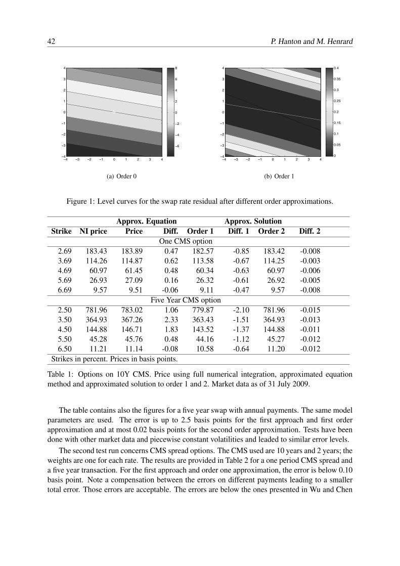
42 P. Hanton and M. Henrard
!4 !3 !2 !1 0 1 2 3 4!4
!3
!2
!1
0
1
2
3
4
!6
!4
!2
0
2
4
6
8
(a) Order 0
!4 !3 !2 !1 0 1 2 3 4!4
!3
!2
!1
0
1
2
3
4
0
0.05
0.1
0.15
0.2
0.25
0.3
0.35
0.4
(b) Order 1
Figure 1: Level curves for the swap rate residual after different order approximations.
Approx. Equation Approx. SolutionStrike NI price Price Diff. Order 1 Diff. 1 Order 2 Diff. 2
One CMS option2.69 183.43 183.89 0.47 182.57 -0.85 183.42 -0.0083.69 114.26 114.87 0.62 113.58 -0.67 114.25 -0.0034.69 60.97 61.45 0.48 60.34 -0.63 60.97 -0.0065.69 26.93 27.09 0.16 26.32 -0.61 26.92 -0.0056.69 9.57 9.51 -0.06 9.11 -0.47 9.57 -0.008
Five Year CMS option2.50 781.96 783.02 1.06 779.87 -2.10 781.96 -0.0153.50 364.93 367.26 2.33 363.43 -1.51 364.93 -0.0134.50 144.88 146.71 1.83 143.52 -1.37 144.88 -0.0115.50 45.28 45.76 0.48 44.16 -1.12 45.27 -0.0126.50 11.21 11.14 -0.08 10.58 -0.64 11.20 -0.012
Strikes in percent. Prices in basis points.
Table 1: Options on 10Y CMS. Price using full numerical integration, approximated equationmethod and approximated solution to order 1 and 2. Market data as of 31 July 2009.
The table contains also the figures for a five year swap with annual payments. The same modelparameters are used. The error is up to 2.5 basis points for the first approach and first orderapproximation and at most 0.02 basis points for the second order approximation. Tests have beendone with other market data and piecewise constant volatilities and leaded to similar error levels.
The second test run concerns CMS spread options. The CMS used are 10 years and 2 years; theweights are one for each rate. The results are provided in Table 2 for a one period CMS spread anda five year transaction. For the first approach and order one approximation, the error is below 0.10basis point. Note a compensation between the errors on different payments leading to a smallertotal error. Those errors are acceptable. The errors are below the ones presented in Wu and Chen
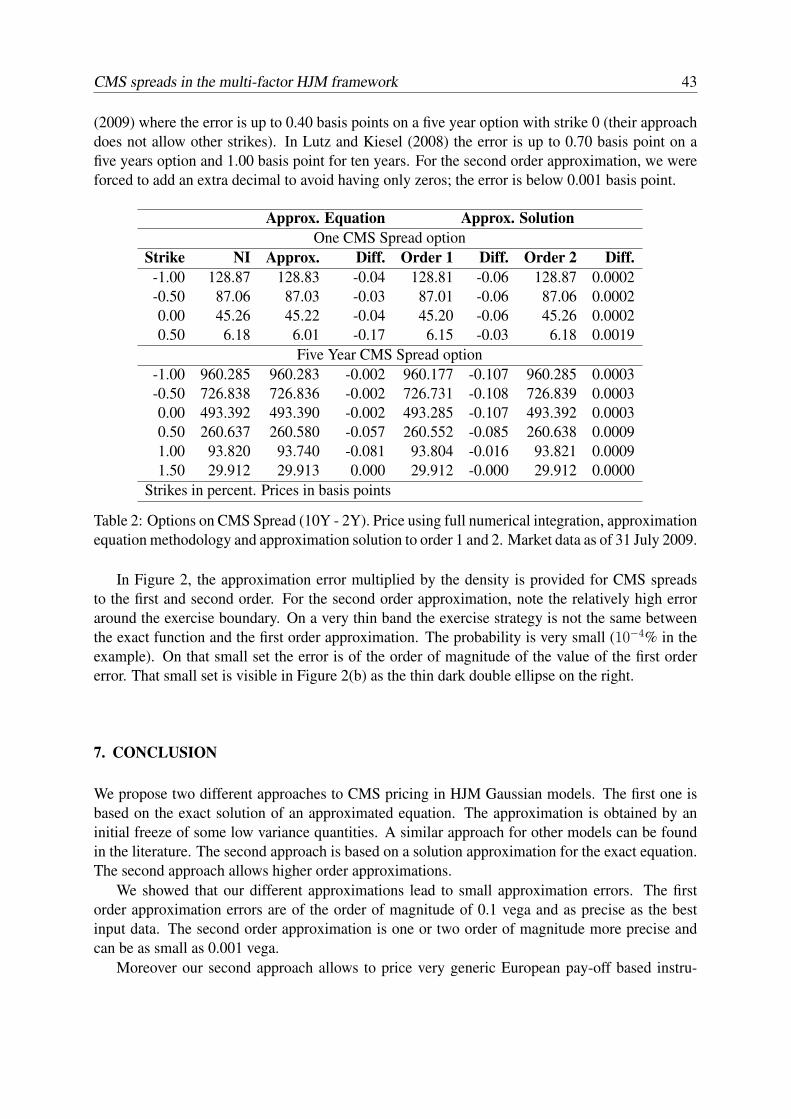
CMS spreads in the multi-factor HJM framework 43
(2009) where the error is up to 0.40 basis points on a five year option with strike 0 (their approachdoes not allow other strikes). In Lutz and Kiesel (2008) the error is up to 0.70 basis point on afive years option and 1.00 basis point for ten years. For the second order approximation, we wereforced to add an extra decimal to avoid having only zeros; the error is below 0.001 basis point.
Approx. Equation Approx. SolutionOne CMS Spread option
Strike NI Approx. Diff. Order 1 Diff. Order 2 Diff.-1.00 128.87 128.83 -0.04 128.81 -0.06 128.87 0.0002-0.50 87.06 87.03 -0.03 87.01 -0.06 87.06 0.00020.00 45.26 45.22 -0.04 45.20 -0.06 45.26 0.00020.50 6.18 6.01 -0.17 6.15 -0.03 6.18 0.0019
Five Year CMS Spread option-1.00 960.285 960.283 -0.002 960.177 -0.107 960.285 0.0003-0.50 726.838 726.836 -0.002 726.731 -0.108 726.839 0.00030.00 493.392 493.390 -0.002 493.285 -0.107 493.392 0.00030.50 260.637 260.580 -0.057 260.552 -0.085 260.638 0.00091.00 93.820 93.740 -0.081 93.804 -0.016 93.821 0.00091.50 29.912 29.913 0.000 29.912 -0.000 29.912 0.0000
Strikes in percent. Prices in basis points
Table 2: Options on CMS Spread (10Y - 2Y). Price using full numerical integration, approximationequation methodology and approximation solution to order 1 and 2. Market data as of 31 July 2009.
In Figure 2, the approximation error multiplied by the density is provided for CMS spreadsto the first and second order. For the second order approximation, note the relatively high erroraround the exercise boundary. On a very thin band the exercise strategy is not the same betweenthe exact function and the first order approximation. The probability is very small (10−4% in theexample). On that small set the error is of the order of magnitude of the value of the first ordererror. That small set is visible in Figure 2(b) as the thin dark double ellipse on the right.
7. CONCLUSION
We propose two different approaches to CMS pricing in HJM Gaussian models. The first one isbased on the exact solution of an approximated equation. The approximation is obtained by aninitial freeze of some low variance quantities. A similar approach for other models can be foundin the literature. The second approach is based on a solution approximation for the exact equation.The second approach allows higher order approximations.
We showed that our different approximations lead to small approximation errors. The firstorder approximation errors are of the order of magnitude of 0.1 vega and as precise as the bestinput data. The second order approximation is one or two order of magnitude more precise andcan be as small as 0.001 vega.
Moreover our second approach allows to price very generic European pay-off based instru-
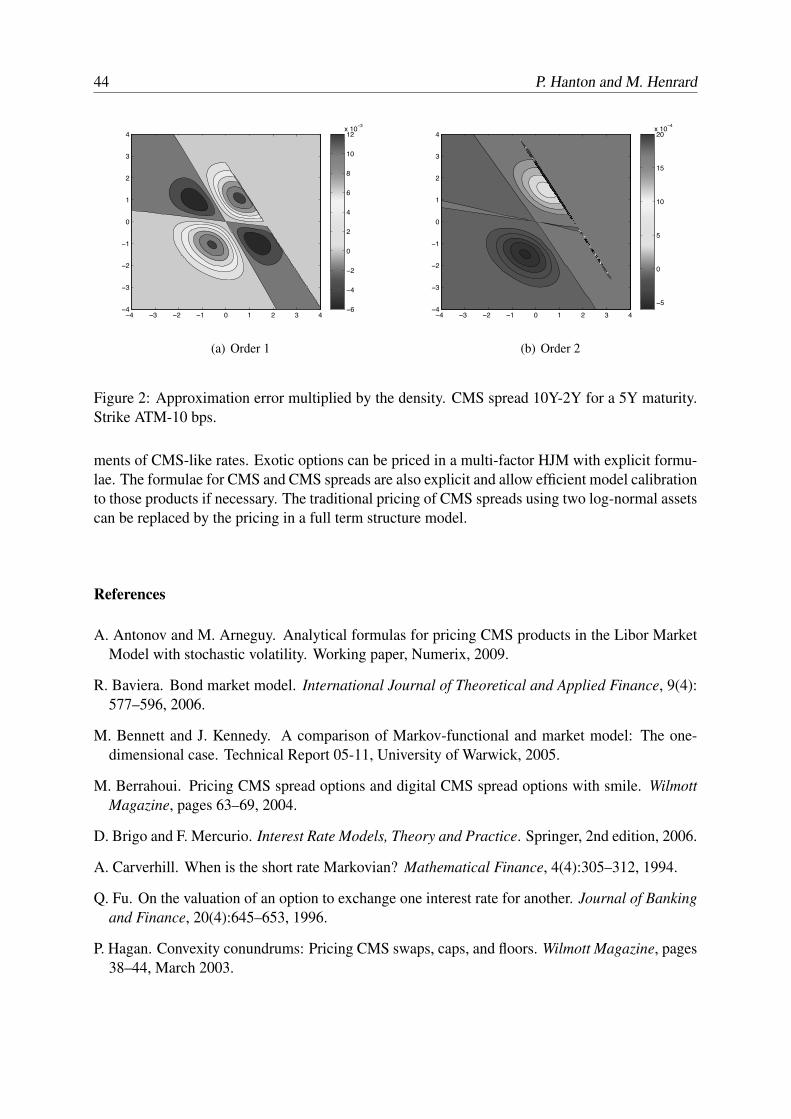
44 P. Hanton and M. Henrard
!4 !3 !2 !1 0 1 2 3 4!4
!3
!2
!1
0
1
2
3
4
!6
!4
!2
0
2
4
6
8
10
12x 10
!3
(a) Order 1
!4 !3 !2 !1 0 1 2 3 4!4
!3
!2
!1
0
1
2
3
4
!5
0
5
10
15
20x 10
!4
(b) Order 2
Figure 2: Approximation error multiplied by the density. CMS spread 10Y-2Y for a 5Y maturity.Strike ATM-10 bps.
ments of CMS-like rates. Exotic options can be priced in a multi-factor HJM with explicit formu-lae. The formulae for CMS and CMS spreads are also explicit and allow efficient model calibrationto those products if necessary. The traditional pricing of CMS spreads using two log-normal assetscan be replaced by the pricing in a full term structure model.
References
A. Antonov and M. Arneguy. Analytical formulas for pricing CMS products in the Libor MarketModel with stochastic volatility. Working paper, Numerix, 2009.
R. Baviera. Bond market model. International Journal of Theoretical and Applied Finance, 9(4):577–596, 2006.
M. Bennett and J. Kennedy. A comparison of Markov-functional and market model: The one-dimensional case. Technical Report 05-11, University of Warwick, 2005.
M. Berrahoui. Pricing CMS spread options and digital CMS spread options with smile. WilmottMagazine, pages 63–69, 2004.
D. Brigo and F. Mercurio. Interest Rate Models, Theory and Practice. Springer, 2nd edition, 2006.
A. Carverhill. When is the short rate Markovian? Mathematical Finance, 4(4):305–312, 1994.
Q. Fu. On the valuation of an option to exchange one interest rate for another. Journal of Bankingand Finance, 20(4):645–653, 1996.
P. Hagan. Convexity conundrums: Pricing CMS swaps, caps, and floors. Wilmott Magazine, pages38–44, March 2003.
CMS spreads in the multi-factor HJM framework 45
D. Heath, R. Jarrow, and A. Morton. Bond pricing and the term structure of interest rates: A newmethodology for contingent claims valuation. Econometrica, 60(1):77–105, January 1992.
M. Henrard. Explicit bond option and swaption formula in Heath-Jarrow-Morton one-factor model.International Journal of Theoretical and Applied Finance, 6(1):57–72, February 2003.
M. Henrard. Skewed Libor Market Model and Gaussian HJM explicit approaches to rolled depositoptions. The Journal of Risk, 9(4), 2007.
M. Henrard. Bermudan swaptions in Gaussian HJM one-factor model: Analyticaland numerical approaches. Working Paper 1287982, SSRN, 2008a. Available athttp://ssrn.com/abstract=1287982.
M. Henrard. Swaptions in Libor Market Model with local volatility. Working Paper 1098420,SSRN, 2008b. To appear in Wilmott Journal. Available at http://ssrn.com/abstract=1098420.
P. Hunt and J. Kennedy. Financial Derivatives in Theory and Practice. John Wiley & Sons Inc.,2nd edition, 2004. ISBN 0-470-86359-5.
M. Lutz and R. Kiesel. Efficient pricing of CMS spread options in a stochastic volatility LMM.Working Paper 1418571, SSRN, 2008. Available at http://ssrn.com/abstract=1418571.
F. Mercurio and A. Pallavicini. Swaption skews and convexity adjustments. Technical report,Banca IMI, 2005.
K. Miyazaki and T. Yoshida. Valuation model of yield-spread options in the HJM framework. TheJournal of Financial Engineering, 7(2):89–107, 1998.
A. Pelsser, R. Pietersz, and M. van Regenmortel. Fast drift-approximated pricing in BGM model.Journal of Computational Finance, 8(1):93–124, 2004.
T.P. Wu and S.N. Chen. Valuation of interest rate spread options in a multifactor LIBOR marketmodel. The Journal of Derivatives, Spring:38–52, 2009.

STRONG TAYLOR APPROXIMATION OF STOCHASTIC DIFFERENTIALEQUATIONS AND APPLICATION TO THE LEVY LIBOR MODEL
Antonis Papapantoleon† and Maria Siopacha§
†Institute of Mathematics, TU Berlin, Straße des 17. Juni 136, 10623 Berlin, Germany & Quanti-tative Products Laboratory, Deutsche Bank AG, Alexanderstr. 5, 10178 Berlin, Germany§Raiffeisen Zentralbank Osterreich AG, Market Risk, Am Stadtpark 9, 1030 Vienna, AustriaEmail: [email protected], [email protected]
Abstract
In this article we develop a method for the strong approximation of stochastic differential equa-tions (SDEs) driven by Levy processes or general semimartingales. The main ingredients ofour method is the perturbation of the SDE and the Taylor expansion of the resulting parameter-ized curve. We apply this method to develop strong approximation schemes for LIBOR marketmodels. In particular, we derive fast and precise algorithms for the valuation of derivatives inLIBOR models which are more tractable than the simulation of the full SDE. A numericalexample for the Levy LIBOR model illustrates our method.
1. INTRODUCTION
The main aim of this paper is to develop a general method for the strong approximation of stochas-tic differential equations (SDEs) and to apply it to the valuation of options in LIBOR models. Themethod is based on the perturbation of the initial SDE by a real parameter, and then on the Taylorexpansion of the resulting parameterized curve around zero. Thus, we follow the line of thought ofSiopacha and Teichmann (2010) and extend their results from continuous to general semimartin-gales. The motivation for this work comes from LIBOR market models; in particular, we considerthe Levy LIBOR model as the basic paradigm for the development of this method.
The LIBOR market model has become a standard model for the pricing of interest rate deriva-tives in recent years. The main advantage of the LIBOR model in comparison to other approachesis that the evolution of discretely compounded, market-observable forward rates is modeled di-rectly and not deduced from the evolution of unobservable factors. Moreover, the log-normalLIBOR model is consistent with the market practice of pricing caps according to Black’s formula(cf. Black (1976)). However, despite its apparent popularity, the LIBOR market model has certainwell-known pitfalls.
47
48 A. Papapantoleon and M. Siopacha
On the one hand, the log-normal LIBOR model is driven by a Brownian motion, hence itcannot be calibrated adequately to the observed market data. An interest rate model is typicallycalibrated to the implied volatility surface from the cap market and the correlation structure of at-the-money swaptions. Several extensions of the LIBOR model have been proposed in the literatureusing jump-diffusions, Levy processes or general semimartingales as the driving motion (cf. e.g.Glasserman and Kou (2003), Eberlein and Ozkan (2005), Jamshidian (1999)), or incorporatingstochastic volatility effects (cf. e.g. Andersen and Brotherton-Ratcliffe (2005)).
On the other hand, the dynamics of LIBOR rates are not tractable under every forward measuredue to the random terms that enter the dynamics of LIBOR rates during the construction of themodel. In particular, when the driving process has continuous paths the dynamics of LIBOR ratesare tractable under their corresponding forward measure, but they are not tractable under any otherforward measure. When the driving process is a general semimartingale, then the dynamics ofLIBOR rates are not even tractable under their very own forward measure. Consequently:
1. if the driving process is a continuous semimartingale caplets can be priced in closed form,but not swaptions or other multi-LIBOR derivatives;
2. if the driving process is a general semimartingale, then even caplets cannot be priced inclosed form.
The standard remedy to this problem is the so-called “frozen drift” approximation, where onereplaces the random terms in the dynamics of LIBOR rates by their deterministic initial values; itwas first proposed by Brace et al. (1997) for the pricing of swaptions and has been used by severalauthors ever since. Brace et al. (2001), Dun et al. (2001) and Schlogl (2002) argue that freezingthe drift is justified, since the deviation from the original equation is small in several measures.
Although the frozen drift approximation is the simplest and most popular solution, it is well-known that it does not yield acceptable results, especially for exotic derivatives and longer hori-zons. Therefore, several other approximations have been developed in the literature; in one lineof research Daniluk and Gatarek (2005) and Kurbanmuradov et al. (2002) are looking for the bestlognormal approximation of the forward LIBOR dynamics; cf. also Schoenmakers (2005). Otherauthors have been using linear interpolations and predictor-corrector Monte Carlo methods to geta more accurate approximation of the drift term (cf. e.g. Pelsser et al. (2005), Hunter et al. (2001)and Glasserman and Zhao (2000)). We refer the reader to Joshi and Stacey (2008) for a detailedoverview of that literature, and for some new approximation schemes and numerical experiments.
Although most of this literature focuses on the lognormal LIBOR market model, Glassermanand Merener (2003a,b) have developed approximation schemes for the pricing of caps and swap-tions in jump-diffusion LIBOR market models.
In this article we develop a general method for the approximation of the random terms thatenter into the drift of LIBOR models. In particular, by perturbing the SDE for the LIBOR ratesand applying Taylor’s theorem we develop a generic approximation scheme; we concentrate hereon the first order Taylor expansion, although higher order expansions can be considered in the sameframework. At the same time, the frozen drift approximation can be embedded in this method as thezero-order Taylor expansion, thus offering a theoretical justification for this approximation. Themethod we develop yields more accurate results than the frozen drift approximation, while beingcomputationally simpler than the simulation of the full SDE for the LIBOR rates. Moreover, ourmethod is universal and can be applied to any LIBOR model driven by a general semimartingale.
Taylor Approximation of SDE and Levy LIBOR model 49
However, we focus on the Levy LIBOR model as a characteristic example of a LIBOR modeldriven by a general semimartingale.
The article is structured as follows: in section 2 we review time-inhomogeneous Levy process,and in section 3 we revisit the Levy LIBOR model. In section 4 we describe the dynamics oflog-LIBOR rates under the terminal martingale measure and express them as a Levy-driven SDE.In section 5 we develop the strong Taylor approximation method and apply it to the Levy LIBORmodel. Finally, section 6 contains a numerical illustration.
2. LEVY PROCESSES
Let (Ω,F ,F, IP) be a complete stochastic basis, where F = FT∗ and the filtration F = (Ft)t∈[0,T∗]
satisfies the usual conditions; we assume that T∗ ∈ R>0 is a finite time horizon. The drivingprocess H = (Ht)0≤t≤T∗ is a process with independent increments and absolutely continuouscharacteristics; this is also called a time-inhomogeneous Levy process. That is, H is an adapted,cadlag, real-valued stochastic process with independent increments, starting from zero, where thelaw of Ht, t ∈ [0, T∗], is described by the characteristic function
IE[eiuHt
]= exp
(∫ t
0
[ibsu − cs
2u2 +
∫
R(eiux − 1 − iux)Fs(dx)
]ds
); (1)
here bt ∈ R, ct ∈ R>0 and Ft is a Levy measure, i.e. satisfies Ft(0) = 0 and∫
R(1∧|x|2)Ft(dx) <∞, for all t ∈ [0, T∗]. In addition, the process H satisfies Assumptions (AC) and (EM) givenbelow.
Assumption (AC). The triplets (bt, ct, Ft) satisfy
∫ T∗
0
(|bt| + ct +
∫
R(1 ∧ |x|2)Ft(dx)
)dt < ∞.
Assumption (EM). There exist constants M, ε > 0 such that for every u ∈ [−(1 + ε)M, (1 +ε)M ] =: M ∫ T∗
0
∫
|x|>1euxFt(dx)dt < ∞.
Moreover, without loss of generality, we assume that∫|x|>1 euxFt(dx) < ∞ for all t ∈ [0, T∗]
and u ∈ M.
These assumptions render the process H = (Ht)0≤t≤T∗ a special semimartingale, thereforeit has the canonical decomposition (cf. Jacod and Shiryaev (2003, II.2.38), and Eberlein et al.(2005))
H =
∫ ·
0
bsds +
∫ ·
0
√csdWs +
∫ ·
0
∫
Rx(µH − ν)(ds, dx), (2)
50 A. Papapantoleon and M. Siopacha
where µH is the random measure of jumps of the process H , ν is the IP-compensator of µH , andW = (Wt)0≤t≤T∗ is a IP-standard Brownian motion. The triplet of predictable characteristics ofH with respect to the measure IP, T(H|IP) = (B, C, ν), is
B =
∫ ·
0
bsds, C =
∫ ·
0
csds, ν([0, ·] × A) =
∫ ·
0
∫
A
Fs(dx)ds,
where A ∈ B(R); the triplet (b, c, F ) represents the local characteristics of H . In addition,the triplet of predictable characteristics (B, C, ν) determines the distribution of H , as the Levy–Khintchine formula (1) obviously dictates.
We denote by κs the cumulant generating function associated to the infinitely divisible distri-bution with Levy triplet (bs, cs, Fs), i.e. for z ∈ M and s ∈ [0, T∗]
κs(z) := bsz +cs
2z2 +
∫
R(ezx − 1 − zx)Fs(dx). (3)
Using Assumption (EM) we can extend κs to the complex domain C, for z ∈ C with <z ∈ M,and the characteristic function of Ht can be written as
IE[eiuHt
]= exp
( ∫ t
0
κs(iu)ds
). (4)
If H is a Levy process, i.e. time-homogeneous, then (bs, cs, Fs) – and thus also κs – do not dependon s. In that case, κ equals the cumulant (log-moment) generating function of H1.
3. THE LEVY LIBOR MODEL
The Levy LIBOR model was developed by Eberlein and Ozkan (2005), following the seminalarticles of Sandmann et al. (1995), Miltersen et al. (1997) and Brace et al. (1997) on LIBORmarket models driven by Brownian motion; see also Glasserman and Kou (2003) and Jamshidian(1999) for LIBOR models driven by jump processes and general semimartingales respectively. TheLevy LIBOR model is a market model where the forward LIBOR rate is modeled directly, and isdriven by a time-inhomogeneous Levy process.
Let 0 = T0 < T1 < · · · < TN < TN+1 = T∗ denote a discrete tenor structure where δi =Ti+1 − Ti, i ∈ 0, 1, . . . , N. Consider a complete stochastic basis (Ω,F ,F, IPT∗) and a time-inhomogeneous Levy process H = (Ht)0≤t≤T∗ satisfying Assumptions (AC) and (EM). Theprocess H has predictable characteristics (0, C, νT∗) or local characteristics (0, c, F T∗), and itscanonical decomposition is
H =
∫ ·
0
√csdW T∗
s +
∫ ·
0
∫
Rx(µH − νT∗)(ds, dx), (5)
where W T∗ is a IPT∗-standard Brownian motion, µH is the random measure associated with thejumps of H and νT∗ is the IPT∗-compensator of µH . We further assume that the following condi-tions are in force.
Taylor Approximation of SDE and Levy LIBOR model 51
(LR1) For any maturity Ti there exists a bounded, continuous, deterministic function λ(·, Ti) :[0, Ti] → R, which represents the volatility of the forward LIBOR rate process L(·, Ti).Moreover,
N∑
i=1
∣∣λ(s, Ti)∣∣ ≤ M,
for all s ∈ [0, T∗], where M is the constant from Assumption (EM), and λ(s, Ti) = 0 for alls > Ti.
(LR2) The initial term structure B(0, Ti), 1 ≤ i ≤ N + 1, is strictly positive and strictly decreas-ing. Consequently, the initial term structure of forward LIBOR rates is given, for 1 ≤ i ≤ N ,by
L(0, Ti) =1
δi
(B(0, Ti)
B(0, Ti + δi)− 1
)> 0.
The construction starts by postulating that the dynamics of the forward LIBOR rate with thelongest maturity L(·, TN) is driven by the time-inhomogeneous Levy process H and evolve asa martingale under the terminal forward measure IPT∗ . Then, the dynamics of the LIBOR ratesfor the preceding maturities are constructed by backward induction; they are driven by the sameprocess H and evolve as martingales under their associated forward measures.
Let us denote by IPTi+1the forward measure associated to the settlement date Ti+1, 0 ≤ i ≤ N .
The dynamics of the forward LIBOR rate L(·, Ti), for an arbitrary Ti, is given by
L(t, Ti) = L(0, Ti) exp
(∫ t
0
bL(s, Ti)ds +
∫ t
0
λ(s, Ti)dHTi+1s
), (6)
where HTi+1 is a special semimartingale with canonical decomposition
HTi+1
t =
∫ t
0
√csdW Ti+1
s +
∫ t
0
∫
Rx(µH − νTi+1)(ds, dx). (7)
Here W Ti+1 is a IPTi+1-standard Brownian motion and νTi+1 is the IPTi+1
-compensator of µH . Thedynamics of an arbitrary LIBOR rate again evolves as a martingale under its corresponding forwardmeasure; therefore, we specify the drift term of the forward LIBOR process L(·, Ti) as
bL(s, Ti) = −1
2λ2(s, Ti)cs −
∫
R
(eλ(s,Ti)x − 1 − λ(s, Ti)x
)F Ti+1
s (dx). (8)
The forward measure IPTi+1, which is defined on (Ω,F , (Ft)0≤t≤Ti+1
), is related to the terminalforward measure IPT∗ via
dIPTi+1
dIPT∗
=N∏
l=i+1
1 + δlL(Ti+1, Tl)
1 + δlL(0, Tl)=
B(0, T∗)
B(0, Ti+1)
N∏
l=i+1
(1 + δlL(Ti+1, Tl)) . (9)
52 A. Papapantoleon and M. Siopacha
The IPTi+1-Brownian motion W Ti+1 is related to the IPT∗-Brownian motion via
WTi+1
t = WTi+2
t −∫ t
0
α(s, Ti+1)√
csds = . . .
= W T∗t −
∫ t
0
(N∑
l=i+1
α(s, Tl)
)√
csds, (10)
where
α(t, Tl) =δlL(t−, Tl)
1 + δlL(t−, Tl)λ(t, Tl). (11)
The IPTi+1-compensator of µH , νTi+1 , is related to the IPT∗-compensator of µH via
νTi+1(ds, dx) = β(s, x, Ti+1)νTi+2(ds, dx) = . . .
=
(N∏
l=i+1
β(s, x, Tl)
)νT∗(ds, dx), (12)
where
β(t, x, Tl, ) =δlL(t−, Tl)
1 + δlL(t−, Tl)
(eλ(t,Tl)x − 1
)+ 1. (13)
Remark 3.1 Notice that the process HTi+1 , driving the forward LIBOR rate L(·, Ti), and H =HT∗ have the same martingale part and differ only in the finite variation part (drift). An applicationof Girsanov’s theorem for semimartingales yields that the IPTi+1
-finite variation part of H is
∫ ·
0
cs
N∑
l=i+1
α(s, Tl)ds +
∫ ·
0
∫
Rx
(N∏
l=i+1
β(s, x, Tl) − 1
)νT∗(ds, dx).
Remark 3.2 The process H = HT∗ driving the most distant LIBOR rate L(·, TN) is – by assump-tion – a time-inhomogeneous Levy process. However, this is not the case for any of the processesHTi+1 driving the remaining LIBOR rates, because the random terms δlL(t−,Tl)
1+δlL(t−,Tl)enter into the
compensators νTi+1 during the construction; see equations (12) and (13).
4. TERMINAL MEASURE DYNAMICS AND LOG-LIBOR RATES
In this section we derive the stochastic differential equation that the dynamics of log-LIBOR ratessatisfy under the terminal measure IPT∗ . This will be the starting point for the approximationmethod that will be developed in the next section. Of course, we could consider the SDE as thedefining point for the model, as is often the case in stochastic volatility LIBOR models, cf. e.g.Andersen and Brotherton-Ratcliffe (2005).
Taylor Approximation of SDE and Levy LIBOR model 53
Starting with the dynamics of the LIBOR rate L(·, Ti) under the forward martingale measureIPTi+1
, and using the connection between the forward and terminal martingale measures (cf. eqs.(10)–(13) and Remark 3.1), we have that the dynamics of the LIBOR rate L(·, Ti) under the termi-nal measure are given by
L(t, Ti) = L(0, Ti) exp
(∫ t
0
b(s, Ti)ds +
∫ t
0
λ(s, Ti)dHs
), (14)
where H = (Ht)0≤t≤T∗ is the IPT∗-time-inhomogeneous Levy process driving the LIBOR rates, cf.(5). The drift term b(·, Ti) has the form
b(s, Ti) = −1
2λ2(s, Ti)cs − csλ(s, Ti)
N∑
l=i+1
δlL(s−, Tl)
1 + δlL(s−, Tl)λ(s, Tl)
−∫
R
((eλ(s,Ti)x − 1
) N∏
l=i+1
β(s, x, Tl) − λ(s, Ti)x
)F T∗
s (dx), (15)
where β(s, x, Tl) is given by (13). Note that the drift term of (14) is random, therefore we aredealing with a general semimartingale, and not with a Levy process. Of course, L(·, Ti) is not aIPT∗-martingale, unless i = N (where we use the conventions
∑0l=1 = 0 and
∏0l=1 = 1).
Let us denote by Z the log-LIBOR rates, that is
Z(t, Ti) := log L(t, Ti)
= Z(0, Ti) +
∫ t
0
b(s, Ti)ds +
∫ t
0
λ(s, Ti)dHs, (16)
where Z(0, Ti) = log L(0, Ti) for all i ∈ 1, . . . , N. We can immediately deduce that Z(·, Ti)is a semimartingale and its triplet of predictable characteristics under IPT∗ , T(Z(·, Ti)|IPT∗) =(Bi, Ci, νi), is described by
Bi =
∫ ·
0
b(s, Ti)ds
Ci =
∫ ·
0
λ2(s, Ti)csds (17)
1A(x) ∗ νi = 1A
(λ(s, Ti)x
)∗ νT∗ , A ∈ B(R\0).
The assertion follows from the canonical decomposition of a semimartingale and the triplet ofcharacteristics of the stochastic integral process; see, for example, Proposition 1.3 in Papapan-toleon (2007).
Hence, the log-LIBOR rates satisfy the following linear SDE
dZ(t, Ti) = b(t, Ti)dt + λ(t, Ti)dHt, (18)
with initial condition Z(0, Ti) = log L(0, Ti).
Remark 4.1 Note that the martingale part of Z(·, Ti), i.e. the stochastic integral∫ ·
0λ(s, Ti)dHs,
is a time-inhomogeneous Levy process. However, the random drift term destroys the Levy propertyof Z(·, Ti), as the increments are no longer independent.

54 A. Papapantoleon and M. Siopacha
5. STRONG TAYLOR APPROXIMATION AND APPLICATIONS
The aim of this section is to strongly approximate the stochastic differential equations for thedynamics of LIBOR rates under the terminal measure. This pathwise approximation is based onthe strong Taylor approximation of the random processes L(·, Tl), i + 1 ≤ l ≤ N in the driftb(·, Ti) of the semimartingale driving the LIBOR rates L(·, Ti); cf. equations (14)–(16). The ideabehind the strong Taylor approximation is the perturbation of the initial SDE by a real parameterand a classical Taylor expansion around this parameter, with usual conditions for convergence (cf.Definition 5.1).
5.1. Definition
We introduce a parameter ε ∈ R and will approximate the terms
L(t−, Tl)
which cause the drift term to be random, by their first-order strong Taylor approximation; cf.Lemma 5.1. Note that the map x 7→ δlx
1+δlx, appearing in the drift, is globally Lipschitz with
Lipschitz constant δ∗ = maxl δl.The following definition of the strong Taylor approximation is taken by Siopacha (2006); see
also Siopacha and Teichmann (2010). Consider a smooth curve ε 7→ Wε, where ε ∈ R andWε ∈ L2(Ω; R).
Definition 5.1 A strong Taylor approximation of order n ≥ 0 is a (truncated) power series
Tn(Wε) :=n∑
k=0
εk
k!
∂k
∂εk
∣∣∣ε=0
Wε
such that
IE [|Wε − Tn(Wε)|] = o(εn),
holds true as ε → 0.
Then, for Lipschitz functions f : R → R>0 with Lipschitz constant k we get the followingerror estimate:
IE[|f(Wε) − f(Tn(Wε))|] ≤ kIE[|Wε − Tn(Wε)|] = ko(εn). (19)
Remark 5.1 It is important to point out that motivated by the idea of the Taylor series we performan expansion around ε = 0 and the estimate (19) is valid. However, for the pathwise approximationof LIBOR rates we are interested in the region ε ≈ 1, and hope that the expansion yields adequateresults; for ε = 0 we would simply recover the “frozen drift” approximation. Numerical experi-ments show that this approach indeed yields better results than the “frozen drift” approximation;cf. section 6.
Taylor Approximation of SDE and Levy LIBOR model 55
5.2. Strong Taylor approximation
In this section we develop a strong Taylor approximation scheme for the dynamics of log-LIBORrates. Let us introduce the auxiliary process Xε(·, Ti) = (Xε(t, Ti))0≤t≤Ti
with initial valuesXε(0, Ti) = L(0, Ti) for all i ∈ 0, . . . , N and all ε ∈ R. The dynamics of Xε(·, Ti) is describedby perturbing the SDE of the log-LIBOR rates by the perturbation parameter ε ∈ R:
dXε(t, Ti) = ε(b(t, Ti; X
ε(t))dt + λ(t, Ti)dHt
), (20)
where the drift term b(·, Ti; Xε(·)) is given by (15). The term Xε(·) in b(·, Ti; X
ε(·)) emphasizesthat the drift term depends on all subsequent processes Xε(·, Ti+1), . . . , X
ε(·, TN), which are alsoperturbed by ε. Note that for ε = 1 the processes X1(·, Ti) and Z(·, Ti) are indistinguishable.
Remark 5.2 In the sequel we will use the notation T as shorthand for T1.
Lemma 5.1 The first-order strong Taylor approximation of the random variable Xε(t, Ti) is givenby:
T(Xε(t, Ti)
)= log L(0, Ti) + ε
∂
∂ε
∣∣ε=0
Xε(t, Ti), (21)
where the first variation process ∂∂ε|ε=0X
ε(·, Ti) =: Y (·, Ti) of Xε(·, Ti) is a time-inhomogeneousLevy process with local characteristics
bYis = b(s, Ti; X(0))
cYis = λ2(s, Ti)cs (22)∫
1A(x)F Yis (dx) =
∫1A
(λ(s, Ti)x
)F T∗
s (dx), A ∈ B(R).
Proof. By definition, the first-order strong Taylor approximation is given by the truncated powerseries
T(Xε(t, Ti)
)= X0(t, Ti) + ε
∂
∂ε
∣∣ε=0
Xε(t, Ti). (23)
Since the curves ε 7→ Xε(t, Ti) are smooth, and Xε(t, Ti) ∈ L2(Ω) by Assumption (EM), we getthat strong Taylor approximations of arbitrary order can always be obtained, cf. Kriegl and Michor(1997, Chapter 1). In particular, for the first-order expansion we have that
IE[|Xε(t, Ti) − T
(Xε(t, Ti)
)|]
= o(ε).
The zero-order term of the Taylor expansion trivially satisfies
X0(t, Ti) = X0(0, Ti) for all t, since dX0(t, Ti) = 0.
Of course, the initial values of the perturbed SDE coincide with the initial values of the un-perturbed SDE, hence X0(0, Ti) = L(0, Ti) =: X(0, Ti).
The first variation process of Xε(·, Ti) with respect to ε is derived by differentiating (20); hence,the dynamics is
d( ∂
∂ε
∣∣∣ε=0
Xε(t, Ti))
= b(t, Ti; Xε(t))|ε=0dt + λ(t, Ti)dHt
= b(t, Ti; X(0))dt + λ(t, Ti)dHt. (24)
56 A. Papapantoleon and M. Siopacha
We can immediately notice that in the drift term b(·, Ti; X(0)) of the first variation process, therandom terms Xε(t, Ti) are replaced by their deterministic initial values X(0, Ti) = Z(0, Ti).
Let us denote by Y (·, Ti) the first variation process of Xε(·, Ti). The solution of the linear SDE(24) describing the dynamics of the first variation process yields
Y (t, Ti) =
∫ t
0
b(s, Ti; X(0))ds +
∫ t
0
λ(s, Ti)dHs. (25)
Since the drift term is deterministic and H is a time-inhomogeneous Levy process we can concludethat Y (·, Ti) is itself a time-inhomogeneous Levy process. The local characteristics of Y (·, Ti) aredescribed by (22).
To summarize, by setting ε = 1 in Lemma 5.1, we have developed the following approximationscheme for the logarithm of the random terms X1(·, Ti) = Z(·, Ti) entering the drift:
TX(t, Ti) = log L(0, Ti) +
∫ t
0
b(s, Ti; X(0))ds +
∫ t
0
λ(s, Ti)dHs. (26)
Comparing (26) with (16) it becomes evident that we are approximating the semimartingale Z(·, Ti)with the time-inhomogeneous Levy process TX(·, Ti).
Remark 5.3 A consequence of this approximation scheme is that we can embed the “frozen drift”approximation into our method. Indeed, the “frozen drift” approximation is the zero-order Taylorapproximation, i.e. X1(t, Ti) ≈ log L(0, Ti). The dynamics of LIBOR rates using this approxima-tion will be denoted by L0(·, Ti).
5.3. Application to LIBOR models
In this section, we will apply the strong Taylor approximation of the log-LIBOR rates Z(·, Ti) byTX(·, Ti) in order to derive a strong, i.e. pathwise, approximation for the dynamics of log-LIBORrates. That is, we replace the random terms in the drift b(·, Ti; Z(·)) by the Levy process TX(·, Ti)instead of the semimartingale Z(·, Ti). Therefore, the dynamics of the approximate log-LIBORrates Z(·, Ti) are given by
Z(t, Ti) = Z(0, Ti) +
∫ t
0
b(s, Ti;TX(s))ds +
∫ t
0
λ(s, Ti)dHs, (27)
where the drift term is provided by
b(s, Ti;TX(s)) = −1
2λ2(s, Ti)cs − csλ(s, Ti)
N∑
l=i+1
δleTX(s−,Tl)
1 + δleTX(s−,Tl)λ(s, Tl)
−∫
R
((eλ(s,Ti)x − 1
) N∏
l=i+1
β(s, x, Tl) − λ(s, Ti)x
)F T∗
s (dx), (28)
with
β(t, x, Tl, ) =δl exp
(TX(t−, Tl)
)
1 + δl exp(TX(t−, Tl)
)(eλ(t,Tl)x − 1
)+ 1. (29)
Taylor Approximation of SDE and Levy LIBOR model 57
T 0.5 Y 1 Y 1.5 Y 2 Y 2.5 YB(0, T ) 0.9833630 0.9647388 0.9435826 0.9228903 0.9006922
T 3 Y 3.5 Y 4 Y 4.5 Y 5 YB(0, T ) 0.8790279 0.8568412 0.8352144 0.8133497 0.7920573
Table 1: Euro zero coupon bond prices on February 19, 2002.
The main advantage of the strong Taylor approximation is that the resulting SDE for Z(·, Ti)can be simulated more easily than the equation for Z(·, Ti). Indeed, looking at (18) and (15)again, we can observe that each LIBOR rate L(·, Ti) depends on all subsequent rates L(·, Tl),i + 1 ≤ l ≤ N . Hence, in order to simulate L(·, Ti), we should start by simulating the furthestrate in the tenor and proceed iteratively from the end. On the contrary, the dynamics of Z(·, Ti)depend only on the Levy processes TX(·, Tl), i+1 ≤ l ≤ N , which are independent of each other.Hence, we can use parallel computing to simulate all approximate LIBOR rates simultaneously.This significantly increases the speed of the Monte Carlo simulations while, as the numericalexample reveals, the empirical performance is very satisfactory.
Remark 5.4 Let us point out that this method can be applied to any LIBOR model driven by ageneral semimartingale. Indeed, the properties of Levy processes are not essential in the proof ofLemma 5.1 or in the construction of the LIBOR model. If we start with a LIBOR model driven by ageneral semimartingale, then the structure of this semimartingale will be “transferred” to the firstvariation process, and hence also to the dynamics of the strong Taylor approximation.
6. NUMERICAL ILLUSTRATION
The aim of this section is to demonstrate the accuracy and efficiency of the Taylor approximationscheme for the valuation of options in the Levy LIBOR model compared to the “frozen drift”approximation. We will consider the pricing of caps and swaptions, although many other interestrate derivatives can be considered in this framework.
We revisit the numerical example in Kluge (2005, pp. 76-83). That is, we consider a tenorstructure T0 = 0, T1 = 1
2, T2 = 1 . . . , T10 = 5 = T∗, constant volatilities
λ(·, T1) = 0.20 λ(·, T2) = 0.19 λ(·, T3) = 0.18
λ(·, T4) = 0.17 λ(·, T5) = 0.16 λ(·, T6) = 0.15
λ(·, T7) = 0.14 λ(·, T8) = 0.13 λ(·, T9) = 0.12
and the discount factors (zero coupon bond prices) as quoted on February 19, 2002; cf. Table 1.The tenor length is constant and denoted by δ = 1
2.
The driving Levy process H is a normal inverse Gaussian (NIG) process with parametersα = δ = 1.5 and µ = β = 0. We denote by µH the random measure of jumps of H and byν(dt, dx) = F (dx)dt the IPT∗-compensator of µH , where F is the Levy measure of the NIG pro-
58 A. Papapantoleon and M. Siopacha
cess. The necessary conditions are satisfied because M = α, hence∑9
i=1 |λ(·, Ti)| = 1.44 < αand λ(·, Ti) < α
2, for all i ∈ 1, . . . , 9.
The NIG Levy process is a pure-jump Levy process and, for µ = 0, has the canonical decom-position
H =
∫ ·
0
∫
Rx(µH − ν)(ds, dx).
The cumulant generating function of the NIG distribution is
κ(u) = δα − δ√
α2 − u2,
for all u ∈ C with |<u| ≤ α.
6.1. Caplets
The price of a caplet with strike K maturing at time Ti, using the relationship between the terminaland the forward measures cf. (9), can be expressed as
C0(K, Ti) = δB(0, Ti+1) IEIPTi+1[(L(Ti, Ti) − K)+]
= δB(0, Ti+1) IEIPT∗
[dIPTi+1
dIPT∗
∣∣FTi
(L(Ti, Ti) − K)+]
= δB(0, T∗) IEIPT∗
[ N∏
l=i+1
(1 + δL(Ti, Tl)
)(L(Ti, Ti) − K)+
]. (30)
This equation will provide the actual prices of caplets corresponding to simulating the full SDE forthe LIBOR rates. In order to calculate the first-order Taylor approximation prices for a caplet wehave to replace L(·, T·) in (30) with L(·, T·). Similarly, for the frozen drift approximation priceswe must use L0(·, T·) instead of L(·, T·).
We will compare the performance of the strong Taylor approximation relative to the frozendrift approximation in terms of their implied volatilities. In Figure 1 we present the differencein implied volatility between the full SDE prices and the frozen drift prices, and between the fullSDE prices and the strong Taylor prices. One can immediately observe that the strong Taylorapproximation method performs much better than the frozen drift approximation; the difference inimplied volatilities is very low across all strikes and maturities. Indeed, the difference in impliedvolatility between the full SDE and the strong Taylor prices lies always below the 1% threshold,which deems this approximation accurate enough for practical implementations. On the contrary,the difference in implied volatilities for the frozen drift approximation exceeds the 1% level forin-the-money options.
6.2. Swaptions
Next, we will consider the pricing of swaptions. Recall that a payer (resp. receiver) swaption canbe viewed as a put (resp. call) option on a coupon bond with exercise price 1; cf. section 16.2.3

Taylor Approximation of SDE and Levy LIBOR model 59
0.020.03
0.040.05
0.060.07
01
23
4
50
0.5
1
1.5
2
2.5
3
0.020.03
0.040.05
0.060.07
01
23
4
5−0.2
−0.15
−0.1
−0.05
0
0.05
0.1
0.15
Figure 1: Difference in implied volatility between the full SDE and the frozen drift prices (left),and the full SDE and the strong Taylor prices (right).
and 16.3.2 in Musiela and Rutkowski (1997). Consider a payer swaption with strike rate K, wherethe underlying swap starts at time Ti and matures at Tm (i < m ≤ N ). The time-Ti value is
STi(K, Ti, Tm) =
(1 −
m∑
k=i+1
ckB(Ti, Tk)
)+
=
(1 −
m∑
k=i+1
(ck
k−1∏
l=i
1
1 + δL(Ti, Tl)
))+
, (31)
where
ck =
K, i + 1 ≤ k ≤ m − 1,1 + K, k = m.
Then, the time-0 value of the swaption is obtained by taking the IPTi-expectation of its time-Ti
value, that is
S0 = S0(K, Ti, Tm)
= B(0, Ti) IEIPTi
(
1 −m∑
k=i+1
(ck
k−1∏
l=i
1
1 + δL(Ti, Tl)
))+
= B(0, T∗) IEIPT∗
N∏
l=i
(1 + δL(Ti, Tl)
)(
1 −m∑
k=i+1
(ck
k−1∏
l=i
1
1 + δL(Ti, Tl)
))+ ,
hence
S0 = B(0, T∗) IEIPT∗
(−
m∑
k=i
(ck
N∏
l=k
(1 + δL(Ti, Tl))
))+ , (32)
where ci := −1. Once again, this equation will provide the actual prices of swaptions correspond-ing to simulating the full SDE for the LIBOR rates. In order to calculate the first-order Taylor
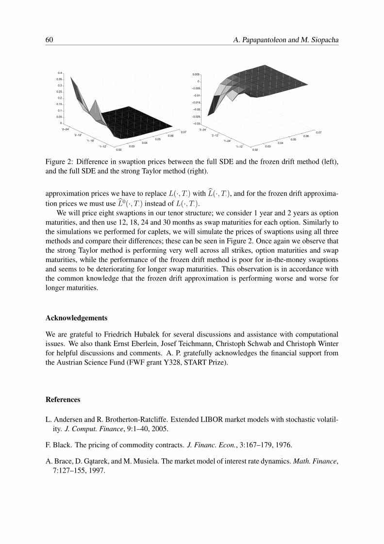
60 A. Papapantoleon and M. Siopacha
0.020.03
0.040.05
0.060.07
’1−12’
’1−18’
’2−12’
’2−24’
0
0.05
0.1
0.15
0.2
0.25
0.3
0.35
0.4
0.02
0.030.04
0.050.06
0.07
’1−12’
’1−24’
’2−12’
’2−24’
−0.03
−0.025
−0.02
−0.015
−0.01
−0.005
0
0.005
Figure 2: Difference in swaption prices between the full SDE and the frozen drift method (left),and the full SDE and the strong Taylor method (right).
approximation prices we have to replace L(·, T·) with L(·, T·), and for the frozen drift approxima-tion prices we must use L0(·, T·) instead of L(·, T·).
We will price eight swaptions in our tenor structure; we consider 1 year and 2 years as optionmaturities, and then use 12, 18, 24 and 30 months as swap maturities for each option. Similarly tothe simulations we performed for caplets, we will simulate the prices of swaptions using all threemethods and compare their differences; these can be seen in Figure 2. Once again we observe thatthe strong Taylor method is performing very well across all strikes, option maturities and swapmaturities, while the performance of the frozen drift method is poor for in-the-money swaptionsand seems to be deteriorating for longer swap maturities. This observation is in accordance withthe common knowledge that the frozen drift approximation is performing worse and worse forlonger maturities.
Acknowledgements
We are grateful to Friedrich Hubalek for several discussions and assistance with computationalissues. We also thank Ernst Eberlein, Josef Teichmann, Christoph Schwab and Christoph Winterfor helpful discussions and comments. A. P. gratefully acknowledges the financial support fromthe Austrian Science Fund (FWF grant Y328, START Prize).
References
L. Andersen and R. Brotherton-Ratcliffe. Extended LIBOR market models with stochastic volatil-ity. J. Comput. Finance, 9:1–40, 2005.
F. Black. The pricing of commodity contracts. J. Financ. Econ., 3:167–179, 1976.
A. Brace, D. Gatarek, and M. Musiela. The market model of interest rate dynamics. Math. Finance,7:127–155, 1997.
Taylor Approximation of SDE and Levy LIBOR model 61
A. Brace, T. Dun, and G. Barton. Towards a central interest rate model. In E. Jouini, J. Cvitanic,and M. Musiela, editors, Option pricing, interest rates and risk management, pages 278–313.Cambridge University Press, 2001.
A. Daniluk and D. Gatarek. A fully log-normal LIBOR market model. Risk, 18(9):115–118, 2005.
T. Dun, G. Barton, and E. Schlogl. Simulated swaption delta-hedging in the lognormal forwardLIBOR model. Int. J. Theor. Appl. Finance, 4:677–709, 2001.
E. Eberlein and F. Ozkan. The Levy LIBOR model. Finance Stoch., 9:327–348, 2005.
E. Eberlein, J. Jacod, and S. Raible. Levy term structure models: no-arbitrage and completeness.Finance Stoch., 9:67–88, 2005.
P. Glasserman and S. G. Kou. The term structure of simple forward rates with jump risk. Math.Finance, 13:383–410, 2003.
P. Glasserman and N. Merener. Numerical solution of jump-diffusion LIBOR market models.Finance Stoch., 7:1–27, 2003a.
P. Glasserman and N. Merener. Cap and swaption approximations in LIBOR market models withjumps. J. Comput. Finance, 7:1–36, 2003b.
P. Glasserman and X. Zhao. Arbitrage-free discretization of lognormal forward LIBOR and swaprate models. Finance Stoch., 4:35–68, 2000.
C. Hunter, P. Jackel, and M. Joshi. Getting the drift. Risk, 14:81–84, 2001.
J. Jacod and A. N. Shiryaev. Limit Theorems for Stochastic Processes. Springer, 2nd edition, 2003.
F. Jamshidian. LIBOR market model with semimartingales. Working Paper, NetAnalytic Ltd.,1999.
M. Joshi and A. Stacey. New and robust drift approximations for the LIBOR market model. Quant.Finance, 8:427–434, 2008.
W. Kluge. Time-inhomogeneous Levy processes in interest rate and credit risk models. PhD thesis,Univ. Freiburg, 2005.
A. Kriegl and P. W. Michor. The Convenient Setting of Global Analysis. American MathematicalSociety, 1997.
O. Kurbanmuradov, K. Sabelfeld, and J. Schoenmakers. Lognormal approximations to LIBORmarket models. J. Comput. Finance, 6:69–100, 2002.
K. R. Miltersen, K. Sandmann, and D. Sondermann. Closed form solutions for term structurederivatives with log-normal interest rates. J. Finance, 52:409–430, 1997.
M. Musiela and M. Rutkowski. Martingale Methods in Financial Modelling. Springer, 1997.
62 A. Papapantoleon and M. Siopacha
A. Papapantoleon. Applications of semimartingales and Levy processes in finance: duality andvaluation. PhD thesis, Univ. Freiburg, 2007.
A. Pelsser, R. Pietersz, and M. van Regenmortel. Bridging Brownian LIBOR. Wilmott Mag., 18:98–103, 2005.
K. Sandmann, D. Sondermann, and K. R. Miltersen. Closed form term structure derivatives in aHeath–Jarrow–Morton model with log-normal annually compounded interest rates. In Proceed-ings of the Seventh Annual European Futures Research Symposium Bonn, pages 145–165, 1995.Chicago Board of Trade.
E. Schlogl. A multicurrency extension of the lognormal interest rate market models. FinanceStoch., 6:173–196, 2002.
J. Schoenmakers. Robust LIBOR Modelling and Pricing of Derivative Products. Chapman &Hall/CRC, 2005.
M. Siopacha. Taylor expansions of option prices by means of Malliavin calculus. PhD thesis,Vienna University of Technology, 2006.
M. Siopacha and J. Teichmann. Weak and strong Taylor methods for numerical solutions ofstochastic differential equations. Quant. Finance, 2010. (forthcoming, arXiv/0704.0745).

POSTER SESSION
63

THRESHOLD PROPORTIONAL REINSURANCE: AN ALTERNATIVE STRATEGYTO REDUCE THE INITIAL INVESTMENT IN A NON-LIFE
INSURANCE PORTFOLIO
Anna Castaner†, M. Merce Claramunt† and Maite Marmol†
†Department of Actuarial, Financial and Economic Mathematics, University of Barcelona, Av.Diagonal 690, 08034 Barcelona, SpainEmail: [email protected], [email protected], [email protected]
We introduce a dynamic proportional reinsurance strategy in a non-life portfolio in which theretention level k, instead of being constant, depends on the level of the surplus. With this strategythe insurer can reduce the probability of ruin for some predetermined level of initial capital relativeto the option of not reinsuring and the option of applying a proportional reinsurance. Therefore,if the manager of the portfolio chooses this dynamic reinsurance strategy, a reduction in the initialcapital investment can be achieved while maintaining the solvency level.
1. INTRODUCTION
In a non-life insurance portfolio, the manager must make decisions that ensure the business’stechnical solvency, i.e., that ensure a sufficient level of technical reserves to cover the paymentof claims. Ruin theory models allow taking the long-term view in analyzing a portfolio’s currentsolvency and making the necessary decisions. In this sense, these models are in many aspectssuperior to models that focus on the short term. In particular, classical ruin theory represents thelevel of reserves R(t) at any given time t as
R(t) = u + ct − S(t)
where u is the initial level of reserves, i.e., the initial capital which allows the portfolio to operate,c is the cash inflow rate from premiums on the portfolio at each instant, and S(t) is the sum of theclaims that have occurred up to time t. The aggregate sum of the claims up to time t is estimated
as S(t) =N(t)∑
i=1
Xi, where N(t) is the stochastic process of the number of claims up to time t, and
Xi the amount of the ith claim. The classical hypotheses are that the amounts of the individualclaims are identical and independently distributed, and that they are independent of the number of
65
66 A. Castaner et al.
claims, so that S(t) is a compound process. If it also assumed, as is usual, that N(t) is a Poissonprocess of rate λ, then S(t) is a compound Poisson process.
The premium is calculated as the expected loss rate increased by a “loading” coefficient, ρ > 0to satisfy the “net profit” condition, and is given by
c = λE[X](1 + ρ).
One of the measures used to assess the solvency of the portfolio is the probability of ruin ψ(u),i.e., the probability that the reserves are negative,
ψ(u) = P [R(t) < 0|R(0) = u].
With a reinsurance treaty (or contract), the insurer cedes a part of the premiums to the reinsur-ers, and accordingly also a part of the losses. In a proportional treaty, the insurer keeps a certainfraction of all claims k ∈ (0, 1], the retention ratio, and the reinsurers takes the remaining (1 − k).
In their treaty with the insurer, the reinsurers also apply a loading coefficient ρR > 0, so thatthe net reinsurance premium for the insurer is
c′ = c− (1 − k)(1 + ρR)λE[X].
It is normally assumed that ρR > ρ > 0, because if ρR ≤ ρ, the insurer would simply cede hisentire portfolio to the reinsurers, a situation which would be senseless. This net premium thusdefines a new real loading coefficient for the insurer,
ρN =c′
kλE[X]− 1 = ρR −
ρR − ρ
k.
The “net profit” condition for the loading coefficient (ρN > 0) imposes a natural limit on theproportion retained by the insurer, so that
ρR − ρ
ρR
< k ≤ 1, ρR > ρ > 0.
Studies of the effect of reinsurance strategy on solvency measures have concentrated theirattention on the ultimate ruin probability. Several of them analyze the effect of reinsurance onthe adjustment coefficient or Lundberg exponent, see Waters (1979), Centeno (2002), Hesselager(1990).
Many authors have considered the problem of determining the optimal level and/or type ofreinsurance, where optimal is defined in terms of some stability criterion, mainly the probabilityof ruin, see e.g. Waters (1983), Goovaerts et al. (1989), Verlaak and Beirlant (2003), Schmidli(2002), Hipp and Vogt (2003), Taksar and Markussen (2003).
The reinsurance strategy considered may be static or dynamic. In the first case, it is assumedthat the level and type of reinsurance remain constant throughout the period considered, where thisperiod in many cases is infinite, see Centeno (2005), Dickson and Waters (1996). In the dynamiccase, we can find papers assuming that for a fixed type of reinsurance the level of reinsurance canchange continuously, see Hojgaard and Taksar (1998), Schmidli (2002), Hipp and Vogt (2003). Inthese papers, optimal stochastic control tools in continuous time are used. Dickson and Waters

Threshold proportional reinsurance 67
(2006) assume that the insurer can change the type and/or level of reinsurance at the start of eachyear, so they studied a discrete time stochastic control problem.
In this paper we introduce a dynamic reinsurance strategy and we obtain the ruin probabilitywhen the individual claim amount is distributed exponentially. Before that, we remind the ex-pression of ruin probability when the individual claim amount follows a unit-mean exponentialdistribution,
ψ(u) =1
1 + ρe− ρ
1+ρu, ∀u ≥ 0. (1)
If we include a proportional reinsurance, the ruin probability can be obtained directly from (1),
ψR(u, k) =1
1 + ρN
e−
ρNk(1+ρN )
u, ∀u ≥ 0.
If the manager’s objective is to optimize the portfolio’s solvency by minimizing the probability ofruin, the control variable related to reinsurance is the retention ratio.
2. THRESHOLD PROPORTIONAL REINSURANCE
In this paper we introduce a dynamic proportional reinsurance strategy in which the retention ratio,k, instead of being constant, depends on the level of the surplus. Then the threshold proportionalstrategy we define is as follows: the retention ratio applied is k1 whenever the reserves are lessthan a determined threshold b, and k2 otherwise.
Since, for the insurer, reinsurance is a tool for controlling the solvency of the portfolio, it seemsnatural that the retention ratio should depend on the current level of surplus. The threshold pro-portional reinsurance strategy that we propose is a straightforward and transparent way to includethis dependence. The fractions k1 and k2 define two new net premium loading coefficients for theinsurer, ρ1 and ρ2. For a graphical illustration, see Figure 1.
( )R t2k X
b 2c
k X
2
2k X
u 1c 1k X1k X
t01T 2T 3T 4T
kk
1k
2k
1
t01T 2T 3T 4T
Figure 1: Threshold Proportional Reinsurance
68 A. Castaner et al.
With this new reinsurance strategy, the probability of ruin behaves differently, depending onwhether its initial surplus u is below or above the level b,
ψ(u) =
ψ1(u) 0 ≤ u < b
ψ2(u) u ≥ b .
The explicit expression of the ruin probability can be found in Marmol et al. (2009) when theindividual claim amount is distributed as an exponential with unitary mean.
Threshold proportional reinsurance includes standard proportional reinsurance (k1 = k2 = k)as a particular case, and therefore also the option of not reinsuring (k1 = k2 = k = 1).
For fixed values of the parameters (λ, ρ and ρR), we can find the optimal threshold proportionalreinsurance that minimize the probability of ruin in a numerical way. In the optimal solution, k1
is different from k2, so with this new threshold reinsurance strategy the insurer can reduce hisprobability of ruin for some predetermined level of initial capital relative to the other options:no reinsurance or applying proportional reinsurance. This optimality of threshold proportionalreinsurance also implies that, if the manager wants to obtain this minimal probability of ruin butwith proportional reinsurance or no reinsurance, he will need more initial capital. The relativeincrease in the initial reserves to achieve this optimal probability of ruin can be considered as thecost of the options of proportional reinsurance and no reinsurance as against threshold proportionalreinsurance. For example, when λ = 1, ρ = 0.15 and ρR = 0.25, for u = 4, if the managerchooses the optimal threshold proportional reinsurance he achieves a probability of ruin of 49.8%.If he chooses proportional reinsurance with the optimal fixed retention percentage, to achieve thisprobability of ruin he will need a 4.075% more initial capital, and if he chooses not to reinsure, hisfinancial requirement to initiate the business would be increased by 6.8%.
3. CONCLUSION
The threshold proportional reinsurance strategy consists of applying a retention ratio that dependson the level of reserves. It allows a better management of the initial capital compared with theoptions of proportional reinsurance and no reinsurance. With this new strategy, one achieves eithera higher level of solvency while maintaining the same initial capital invested in the portfolio, or areduction in the initial capital investment while maintaining the same level of solvency.
References
L. Centeno. Measuring the effects of reinsurance by the adjustment coefficient in the Sparre An-derson model. Insurance: Mathematics and Economics, 30(1):37–49, 2002.
L. Centeno. Dependent risks and excess of loss reinsurance. Insurance: Mathematics and Eco-nomics, 37(2):229–238, 2005.
D.C.M Dickson and H.R. Waters. Reinsurance and ruin. Insurance: Mathematics and Economics,19(1):61–80, 1996.
Threshold proportional reinsurance 69
D.C.M Dickson and H.R. Waters. Optimal dynamic reinsurance. Astin Bulletin, 36(2):415–432,2006.
M.J. Goovaerts, A.E. Van Heervaarden, and R. Kaas. Optimal reinsurance in relation to orderingof risk. Insurance: Mathematics and Economics, 8(1):11–17, 1989.
O. Hesselager. Some results on optimal reinsurance in terms of the adjustment coefficient. Scan-dinavian Actuarial Journal, 1990(1-2):80–95, 1990.
C. Hipp and M. Vogt. Optimal dynamic XL reinsurance. Astin Bulletin, 33(2):193–207, 2003.
B. Hojgaard and M. Taksar. Optimal proportional reinsurance policies for diffusion models withtransaction costs. Insurance: Mathematics and Economics, 22(1):41–51, 1998.
M. Marmol, M.M. Claramunt, and A. Castaner. Investigaciones en Seguros y Gestion de Riesgos:RIESGO 2009, chapter Efectos de la estrategia de reaseguro proporcional de umbral en la prob-abilidad de ruina del asegurador, pages 331–344. Number 136 in Cuadernos de la Fundacion.Fundacion Mapfre, Madrid, 2009.
H. Schmidli. On minimizing the ruin probability by investment and reinsurance. The Annals ofApplied Probability, 12(3):890–907, 2002.
M. Taksar and C. Markussen. Optimal dynamic reinsurance policies for large insurance portfolios.Finance and Stochastics, 7(1):97–121, 2003.
R. Verlaak and J. Beirlant. Optimal reinsurance programs: an optimal combination of severalreinsurance protections on a heterogeneous insurance portfolio. Insurance: Mathematics andEconomics, 33(2):381–403, 2003.
H.R. Waters. Excess of loss reinsurance limits. Scandinavian Actuarial Journal, 1979(1):37–43,1979.
H.R. Waters. Some mathematical aspects of reinsurance. Insurance: Mathematics and Economics,2(1):17–26, 1983.

LOCAL VOLATILITY PRICING MODELS FOR LONG-DATED FX DERIVATIVES
Griselda Deelstra and Gregory Rayee
Department of Mathematics, Universite Libre de Bruxelles, Boulevard du Triomphe, CP 210, Brus-sels 1050, BelgiumEmail: [email protected], [email protected]
In recent years the market in long-dated FX options has grown considerably. Currently themost traded and liquid long-dated FX Hybrid products are so-called Power-Reverse Dual-Currencyswaps (PRDC) (see for example Piterbarg (2006)) as well as vanilla or exotic long-dated productssuch as barrier options. While for short-dated options (less than 1 year), assuming constant inter-est rates does not lead to significant mispricing, for long-dated options the effect of interest ratevolatility becomes increasingly pronounced with increasing maturity and can become as importantas FX spot volatility. Most dealers are using a three-factor pricing model for long-dated FX prod-ucts where the FX spot is locally governed by a geometric Brownian motion, and where each ofthe domestic and foreign interest rates follows a Hull-White one factor Gaussian model (Hull andWhite (1993)). However using such a model does not allow the volatility smile and skew effectencountered in the FX market to be taken into account, and is therefore not appropriate to priceand hedge long-dated FX products.
Different methods exist to incorporate smile and skew effects in the three-factor pricing model.In the literature, one can find different approaches which consist of either using a stochastic volatil-ity for the FX spot or a local volatility. There are many processes that can be used for the stochasticvolatility and their choices will generally depend on their tractability. Before being used for pric-ing all these models should be calibrated over the market. In general the calibration is based oncalculating prices of liquid products for different strikes and maturity and the parameters of themodel are adjusted until these prices match sufficiently with the market. However, in most cases itis difficult to derive analytical formulae, and consequently the calibration procedure often remainsapproximative or computationally demanding.
Local volatility models were introduced in 1994 by Dupire (Dupire (1994)) and Derman andKani (Derman and Kani (1994)) for equity based products. As compared to stochastic volatil-ity models they have the advantage that they are Markovian in only one factor (because the localvolatility is a deterministic function of both the FX spot and time) implying that they are moreappropriate for hedging strategies. Local volatility models also have the advantage that they arecalibrated on the complete implied volatility surface, and hence they usually capture more pre-cisely the surface of the implied volatilities than stochastic volatility models. However, a local
71

72 G. Deelstra and G. Rayee
volatility model has the drawback that it predicts unrealistic dynamics for the stock volatility sincethe volatilities observed in the market are really stochastic, capable of rising without a movementin spot FX prices. In Bossens et al. (2006), the authors compare short-dated barrier option mar-ket prices with the corresponding prices derived from either a Dupire local volatility or a Hestonstochastic volatility model both calibrated on the vanilla smile and skew. It appears from their studythat in a simplified world, where exotic option prices are derived either from Dupire local volatil-ity or from a Heston stochastic volatility dynamics, an FX market characterised by a mild skew(USDCHF) exhibits mainly a stochastic volatility behavior, and that FX markets characterised bya dominantly skewed implied volatility (USDJPY) exhibit a stronger local volatility component.This observation also underlines that calibrating a stochastic model to the vanilla market is by nomeans a guarantee that exotic options will be priced correctly (Schoutens et al. (2004)). This isbecause the vanilla market carries no information about the smile dynamics. The market dynamicscould be better approximated by a hybrid volatility model that contains both stochastic volatilitydynamics and local volatility ones. To the best of our knowledge this approach has never beenstudied in a stochastic interest rates framework, but it is also known that it provides positive resultsfor short dated options when interest rates are assumed to be constant (see for example Lipton(2002), Lipton and McGhee (2002), Madan et al. (2007), Tavella et al. (2006)). Once the localvolatility surface is available, the new mixed volatility can be computed by multiplying this localvolatility with a ratio of integrals that depend on the joint density of the FX spot and the stochasticvolatility. This density can be determined by numerically solving the associated Kolmogorov for-ward PDE.
The study of the local volatility and its calibration to a three-factor model can then be moti-vated by hedging arguments but is also considerably useful for the calibration of hybrid volatilitymodels. In Deelstra and Rayee (2010), we derive the Dupire’s like formula in a three-factor modelwhere we have three sources of randomness: the FX spot with a local volatility and the domesticas well as the foreign interest rates. We present two ways to derive the expression of the localvolatility. The first one is based on the method used by Dupire in a simple one factor Gaussianmodel (Dupire (1994)) and consists of deriving the call prices with respect to the strike and thematurity. In the second approach we use the results of Atlan (Atlan (2006)) as well as Tanaka’sformula, to show that we can also obtain the Dupire’s like formula for the three-factor model withlocal volatility.
In a one-factor Gaussian model, the local volatility surface is generally built by using theDupire’s formula where partial derivatives of call options with respect to strikes and maturities arecalculated by finite differences and where the real implied volatility surface is an interpolation ofa finite set of market call prices. In a three-factor framework with local volatility, the Dupire’slike formula becomes more complicated. This is because it also depends on a particularly com-plicated expectation for which no closed form expression exists and which is not directly relatedto European call prices or other liquid products. Of course such expectation can be evaluated us-ing numerical integration methods. Then, to enable realisations of the numerical integrations oneneeds the forward probability distribution of the spot FX rate and the domestic and foreign interestrates up to maturity. In Deelstra and Rayee (2010), we have derived the forward PDE associatedto this forward probability density function. However, in a three factor framework, numerical inte-gration methods and PDE solvers are computationally demanding: numerical resolutions of high

Local Volatility Pricing Models for Long-dated FX Derivatives 73
dimensional PDEs are sometimes unstable.
An alternative approach is to calibrate the local volatility from stochastic volatility models byestablishing links between local and stochastic volatility. Extracting the local volatility surfacefrom a stochastic volatility model rather than using the market implied volatility surface seemsto be a preferred approach. Indeed, let us first observe that the market implied volatility surfacecan in practice only be an interpolation of a finite set of available market data. Consequently alocal volatility surface built from an approximative implied volatility surface is often unstable. Incontrast stochastic volatility models can be calibrated by using fast algorithms like Fast FourierTransforms (FFT) (see for example van Haastrecht et al. (2008)) and the local volatility surfaceextracted from the calibrated stochastic volatility model will be really smooth. In Deelstra andRayee (2010), we present some mimicking properties that links the three-factor model with a localvolatility to the same model with a stochastic volatility rather than a local volatility. These proper-ties will allow us to obtain explicit expressions to construct the local volatility surface.
Finally, we study two different extensions of the local volatility model with stochastic interestrates. First, following the ideas developed by Derman and Kani (1998) and by Dupire (2004), weassume that the dynamic behavior of the local volatility obeys a stochastic process driven by someadditional Brownian motion. Second, using Gyongy’s result (Gyongy (1986)), we derive somelinks between the three-factor model with local volatility and a hybrid volatility model where thevolatility of the spot FX rate mixes a stochastic volatility with a local volatility. Knowing the localvolatility function associated to the three-factor model with local volatility, we propose a calibra-tion method for the local volatility in the four-factor hybrid volatility model.
The paper Deelstra and Rayee (2010) is organised as follows. We begin by defining the three-factor model with local volatility. Then, we derive the local volatility expression for this modelby using two different techniques. First, we derive the Fokker-Plank equation for the forwardprobability density function of the FX spot and the domestic and foreign interest rates at maturity.This PDE is used in the derivation of the local volatility function by differentiating European callprice expressions with respect to the strike and the maturity. The second approach is based onTanaka’s formula.
Afterwards, we focus on the calibration of this local volatility function. We obtain a linkbetween the local volatility function derived in a three-factor framework and the one that stemsfrom the simple one-factor Gaussian model.
Next, we derive a link between the three factor model with a stochastic volatility for the spotFX rate and the one where the spot FX rate volatility is a local volatility. This link provides arelationship between our local volatility function and future instantaneous spot FX rate volatilities.We also propose two extensions of the three-factor model with local volatility. The first extensionis obtained by introducing a stochastic structure on the local volatility surface. We show that inthat case local volatilities are risk-adjusted expectations of future instantaneous volatilities withrespect to the K-strike and T -maturity forward risk-adjusted measure.
Finally, we consider a hybrid volatility model, where the volatility of the spot FX rate is theproduct of a local volatility and a stochastic volatility. Thanks to Gyongy’s result we obtain equa-tions that link the local volatility function associated to the three-factor model with the local volatil-ity function of the four-factor hybrid volatility model and propose a calibration procedure for the
74 G. Deelstra and G. Rayee
local volatility function associated to this four-factor hybrid volatility model.
References
M. Atlan. Localizing volatilities. Working paper, Universite Pierre et Marie Curie, 2006.
F. Bossens, G. Rayee, N.S. Skantzos, and G. Deelstra. Vanna-Volga methods applied to FX deriva-tives: from theory to market practice. Working paper, Universite Libre de Bruxelles, 2006.
G. Deelstra and G. Rayee. Local Volatility Pricing Models for Long-Dated FX Derivatives. Work-ing paper, Universite Libre de Bruxelles, 2010.
E. Derman and I. Kani. Riding on a smile. Risk, pages 32–39, 1994.
E. Derman and I. Kani. Stochastic implied trees: Arbitrage pricing with stochastic term and strikestructure of volatility. International Journal of Theoretical and Applied Finance, 1:61–110,1998.
B. Dupire. Pricing with a smile. Risk, pages 18–20, 1994.
B. Dupire. A unified theory of volatility. In P. Carr, editor, Derivatives Pricing: The ClassicCollection, chapter 6, pages 185–196. Risk Books, 2004.
I. Gyongy. Mimicking the one-dimensional marginal distributions of processes having an Ito dif-ferential. Probability Theory and Related Fields, 71:501–516, 1986.
J. Hull and A. White. One factor interest rate models and the valuation of interest rate derivativesecurities. Journal of Financial and Quantitative Analysis, 28:235–254, 1993.
A. Lipton. The vol smile problem. Risk Magazine, 15:61–65, 2002.
A. Lipton and W. McGhee. Universal barriers. Risk Magazine, 15:81–85, 2002.
D. Madan, M. Qian Qian, and Y. Ren. Calibrating and pricing with embedded local volatilitymodels. Risk, 2007.
V. Piterbarg. Smiling hybrids. Risk, pages 66–71, 2006.
W. Schoutens, E. Simons, and J. Tistaert. A perfect calibration! Now what? Wilmott Magazine,2004.
D. Tavella, A. Giese, and D. Vermeiren. Hybrid stochastic volatility calibration. The Best ofWilmott, 2:221–228, 2006.
A van Haastrecht, R. Lord, A. Pelsser, and D. Schrager. Pricing long-maturity equity and FXderivatives with stochastic interest rates and stochastic volatility. Working paper, 2008.
PRICING AND HEDGING OF INTEREST RATE DERIVATIVES IN A LEVY DRIVENTERM STRUCTURE MODEL
Kathrin Glau†, Nele Vandaele§ and Michele Vanmaele§
†Department of Mathematical Stochastics, University of Freiburg, Eckerstrasse 1, 79100 Freiburg,Germany§Department of Applied Mathematics and Computer Science, Ghent University, Krijgslaan 281,S9, 9000 Gent, BelgiumEmail: [email protected], [email protected],
We study the pricing of forward payer swaptions and derive hedging strategies for these on the basisof investments in zero-coupon bonds. As framework we consider the Levy driven Heath-Jarrow-Morton model for the term structure and we determine the delta-hedge and the mean-variancehedge which is a quadratic hedge. The pricing formula and the hedging strategies are derived asclosed-form expressions in terms of Fourier transforms.
1. INTRODUCTION
Nowadays models for the term structure of interest rates that are driven by the Brownian motion arewidely used in practice. However serious shortcomings of those models, in particular concerningthe smile effect, are well known. Therefore Eberlein and Kluge (2006) extended the Heath-Jarrow-Morton model of Heath et al. (1992), to a model in which the forward rate is driven by a time-inhomogeneous Levy process. Kluge (2005) showed that such a model allows to reproduce theso-called smile surface.In this article we will investigate pricing and hedging of swaptions, which are options on swaps.Our contribution to the pricing of these products, see e.g. Eberlein and Kluge (2006), consistsin a compact representation of the price by using the Jamshidian decomposition, introduced inJamshidian (1989) for a Vasicek model.Further, we will focus on hedging strategies with investments in zero-coupon bonds. In particularwe will examine delta-hedges, which are mainly used in practice and which make the portfoliorisk-neutral for changes in the underlying of the claim.In literature many other hedging approaches are discussed, such as utility minimization and quadra-tic strategies. These methods are based on quantifying the risk and minimizing it over a certainset of strategies. We will study the quadratic strategies that minimize the square of the difference
75

76 K. Glau et al.
between the claim at maturity and the portfolio. This so-called mean-variance hedging strategyhas the appealing advantage of being self-financing.We will state here the main results. For the proofs we refer to Glau et al. (2010) and Vandaele(2010).
2. LEVY DRIVEN HEATH–JARROW–MORTON MODEL
We assume that the stochastic basis (Ω,F , F, P) is given. We give a short introduction of the modelunder consideration. Denote by T ∗ > 0 the fixed horizon date, this means that trading will onlyhappen during the interval [0, T ∗]. The value at time t of a zero-coupon bond paying 1 unit atmaturity T is given by B(t, T ) and, of course, B(T, T ) equals 1. The forward interest rate at datet ≤ T , f(t, T ), is the instantaneous risk-free interest rate for borrowing or lending at time T seenfrom time t. When we have a family of forward interest rates f(t, T ), we can easily derive the
prices of the zero-coupon bonds: B(t, T ) = exp
(−
∫ T
t
f(t, u)du
). The short-term interest rate
rt is described by f(t, t) and Bt = exp(∫ t
0rudu) represents the savings account.
Denote by F the natural filtration generated by the one-dimensional time-(in)homogeneous Levyprocess L with Levy-Khintchine triplet (bs, cs, Fs) and associated cumulant θs such that
∫ T ∗
0
(|bs| + |cs| +
∫
R(x2 ∧ 1)Fs(dx)
)ds < ∞.
Then, the dynamics of the forward interest rates and the zero-coupon bonds under the measure Pare given by
df(t, T ) =α(t, T )dt − σ(t, T )dLt
B(t, T ) =B(0, T ) exp(
∫ t
0
(rs − A(s, T ))ds +
∫ t
0
Σ(s, T )dLs), (1)
with α, σ R-valued adapted stochastic processes and, for s belonging to [0, T ∗],
A(s, T ) =
∫ T
s∧T
α(s, u)du and Σ(s, T ) =
∫ T
s∧T
σ(s, u)du. (2)
The dynamics of the zero-coupon bonds can be rewritten as:
B(t, T ) =B(0, T )
B(0, t)exp
(−
∫ t
0
(A(s, T ) − A(s, t))ds +
∫ t
0
(Σ(s, T ) − Σ(s, t))dLs
). (3)
We assume the following integrability condition on the measures Fs to ensure in particular that Lis an exponential special semimartingale:
Axiom 1 (EM) There are constants M, ε > 0 such that for every u ∈ [−(1 + ε)M, (1 + ε)M ]:∫ T ∗
0
∫
|x|>1exp(ux)Fs(dx)ds < ∞.
Hedging swaptions 77
The discounted bond prices are martingales and, hence, the model is described under the uniquemartingale measure P∗, also called the spot martingale measure, see Eberlein et al. (2005), if
A(s, T ) = θs(Σ(s, T )) ∀T ∈ [0, T ∗]. (4)
Concerning the volatility structure we impose the following additional axioms.
Axiom 2 (DET) The volatility structure σ is bounded and deterministic. Furthermore we assume
0 ≤ Σ(s, T ) ≤ M ′ < M for all 0 ≤ s, T ≤ T ∗
with M the constant defined in Axiom 1 and Σ given in (2).
Axiom 3 (VOL) For all T ∈ [0, T ∗] we assume that σ(· , T ) 6≡ 0 and
σ(s, T ) = σ1(s)σ2(T ) 0 ≤ s ≤ T,
where σ1 : [0, T ∗] → R+ and σ2 : [0, T ∗] → R+ are continuously differentiable. Furthermore weassume that infs∈[0,T ∗] σ1(s) ≥ σ1 > 0.
Important for pricing and hedging interest rate derivative products is the forward measure.
Definition 2.1 The forward measure is linked with a settlement date T , such that the forward priceof any financial asset (in our case any zero-coupon bond) is a (local) martingale. The forward priceat time t of an asset S is given by St/B(t, T ).
The change of measure from the spot martingale measure P∗, which equals P in our setting, to theforward martingale measure linked with the settlement date T is according to (1)
dPT
dP
∣∣∣∣Ft
=B(t, T )
BtB(0, T )= exp
(−
∫ t
0
A(s, T )ds +
∫ t
0
Σ(s, T )dLs
). (5)
From Proposition 10 and Lemma 11 of Eberlein and Kluge (2006) we conclude that L is also atime-inhomogeneous Levy process under the forward measure PT , that L is again special underthis measure and its characteristics (bPT
s , cPTs , F PT
s ) under PT can be expressed in terms of thoseunder P.
3. PAYER SWAPTION
A (plain vanilla) interest rate swap is a contract to exchange a fixed interest rate against a floatingreference rate, like the Libor. Both rates are based on the same notional amount and for the sameperiod of time. In the case of a payer swap the investor pays the fixed rate and receives the floatingrate, where the fixed rate is chosen such that the contract is worth zero at the initial date.A forward swap is an agreement to enter into a swap at a future date T0 with a pre-specified fixedrate κ, while a payer swaption gives the owner the right to enter the forward payer swap at T0.Musiela and Rutkowski (2004) showed that the payer swaption can be seen as a put option withstrike price 1 on a coupon-bearing bond. Therefore we can write the payer swaption’s payoff as(1 −
∑nj=1 cjB(T0, Tj))
+, where T1 < T2 < . . . < Tn are the payment dates of the swap withT1 > T0. We denote the length of the accrual periods [Tj−1, Tj], j = 1, . . . , n by δj := Tj − Tj−1.The coupons ci equal ci = κδi for i = 1, . . . , n − 1 and cn = 1 + κδn where κ is the fixed interestrate of the swap.
78 K. Glau et al.
4. PRICING OF THE PAYER SWAPTION
We present the derivation for the payer swaption in a slightly different way than in Eberlein andKluge (2006) to make the application of the so called Jamshidian trick more visible. This allows tointerpret the payer swaption as a weighted sum of put options with different strikes on bonds withdifferent maturities. This was already noticed by Annaert et al. (2007) in a continuous setting fora general interest rate model where the zero-coupon bond prices are comonotonic.The fair price of the payer swaption is given by PSt = BtE[ 1
BT0(1 −
∑nj=1 cjB(T0, Tj))
+|Ft],where the expectation is taken under the risk-neutral measure P. We change to the forward measurePT0 eliminating the instantaneous interest rate BT0 under the expectation in this way:
PSt =B(t, T0)EPT0
[(1 −
n∑
j=1
cjB(T0, Tj))+∣∣∣Ft
]= B(t, T0)E
PT0
[(1 −
n∑
j=1
cjDTj
T0eΣ
TjT0
XT0 )+∣∣∣Ft
]
with according to (2), (3), (4) and Axiom 3
DTj
T0=
B(0, Tj)
B(0, T0)exp
(∫ T0
0
[θs(Σ(s, T0)) − θs(Σ(s, Tj))] ds
)
ΣTj
T0=
∫ Tj
T0
σ2(u)du and XT0 =
∫ T0
0
σ1(s)dLs.
Theorem 4.1 Under the Axioms 1, 2, 3 and if |σ1| < σ1 for a certain σ1 ∈ R, the price at time tof a forward payer swaption is given by a weighted sum of put options on bonds
PSt =B(t, T0)n∑
j=1
cjEPT0
[(bj − B(T0, Tj))
+∣∣Ft
]
=B(t, T0)n∑
j=1
cje−RXt
2π
∫
ReiuXtϕ
PT0XT0
−Xt(u + iR)vj(−u − iR)du, (6)
where ϕPT0XT0
−Xtis the characteristic function of XT0 − Xt under the measure PT0 and where
vj(−u − iR) =bje
(−iu+R)z∗ΣTj
T0
(−iu + R)(−iu + ΣTj
T0+ R)
for R in ]0, Mσ1
] and bj such that g(T0, Tj, z∗) = bj , where z∗ is the solution to the equation
∑nj=1 cjg(T0, Tj, z
∗) = 1 with g the non-decreasing function defined as g(s, t, x) = Dtse
Σtsx.
5. DELTA-HEDGING OF THE PAYER SWAPTION
We determine the delta-hedge for a short position in the payer swaption when one zero-couponbond is used for hedging.
Hedging swaptions 79
Theorem 5.1 Under the axioms of Theorem 4.1 and if |u|·|ϕPT0XT0
−Xt(u+iR)| is integrable then the
optimal amount, denoted by ∆jt , to invest in the zero-coupon bond with maturity Tj to delta-hedge
a short position in the forward payer swaption is given by:
∆jt = − B(t, T0)
B(t, Tj)ΣTj
t
n∑
k=1
ck
(ΣT0
t Hk(t, Xt) +∂
∂Xt
Hk(t, Xt)),
with
Hk(t, Xt) =e−RXt
2π
∫
ReiuXtϕ
PT0XT0
−Xt(u + iR)vk(−u − iR)du.
∂Hk(t, Xt)
∂Xt
=1
2π
∫
Re(−R+iu)Xtϕ
PT0XT0
−Xt(u + iR)vk(−u − iR)(−R + iu)du.
The integrability condition of Theorem 5.1 is satisfied for a wide range of processes, see Glau et al.(2010).
6. MEAN-VARIANCE HEDGING STRATEGY FOR THE PAYER SWAPTION
In the interest rate derivatives market it is unrealistic to hedge with the risk-free interest rate productin contrast to the stock market. Therefore we choose the bond B(·, T0) as numeraire to develop ahedging strategy for the payer swaption.For the explicit determination of the strategy in terms of the cumulant process we use ideas ofHubalek et al. (2006) adapted to our setting. They determine the variance-optimal hedging strategyfor an exponential Levy process, which is not necessarily a martingale. We work under the forwardmeasure PT0 which ensures that the discounted asset B(·, Tj)/B(·, T0) is a martingale. Hencedetermining the strategy reduces to finding the Galtchouk-Kunita-Watanabe decomposition of theclaim H .On the other hand Hubalek et al. use time-homogeneous processes, while the driving process inour setting is a time-inhomogeneous Levy process. Instead of generalizing the argumentationgiven in Hubalek et al. (2006), we give a new proof in Glau et al. (2010) based on properties ofthe cumulant process of time-inhomogeneous Levy processes and the Galtchouk-Kunita-Watanabedecomposition.Following a mean-variance hedging strategy we determine the optimal number we have to investin the zero-coupon bond with maturity Tj to hedge the forward swaption:
Theorem 6.1 Under the assumptions of Theorem 4.1 and if 3M ′ ≤ M and if R is chosen in theinterval ]0, M
2σ1] then the Galtchouk-Kunita-Watanabe decomposition of the forward payer swap-
tion (6) exists. The optimal number to invest in the zero-coupon bond with maturity Tj is accordingto the mean-variance hedging strategy given by
ξjt =
∫
Rexp
(∫ T0
t
κXj
s
( iu − R
ΣTj
T0
)ds
)B(t−, Tj)
iu−R
ΣTjT0
−1κXj
t
(iu−R
ΣTjT0
+ 1)− κXj
t
(iu−R
ΣTjT0
)
κXj
t (2)Π(du),
80 K. Glau et al.
with
κXj
s (w) = θs(wΣ(s, Tj) + (1 − w)Σ(s, T0)) − wθs(Σ(s, Tj)) − (1 − w)θs(Σ(s, T0)),
Π(du) =n∑
k=1
ck
2π(f j
T0)
iu−R
ΣTjT0 vk(−u − iR)du,
f jT0
=B(0, T0)
B(0, Tj)exp
(∫ T0
0
[θs(Σ(s, Tj)) − θs(Σ(s, T0))]ds
).
Acknowledgements
Kathrin Glau acknowledges travel grant 2751 and 3119 received from the European Science Foun-dation (ESF) for the activity entitled ‘Advanced Mathematical Methods for Finance’. Nele Van-daele would like to acknowledge the financial support by the Research Foundation-Flanders.
References
J. Annaert, G. Deelstra, D. Heyman, and Vanmaele M. Risk management of a bond portfolio usingoptions. Insurance: Mathematics and Economics, 41(3):299–316, 2007.
E. Eberlein and W. Kluge. Exact pricing formulae for caps and swaptions in a Levy term structuremodel. Journal of Computational Finance, 9:99–125, 2006.
E. Eberlein, J. Jacod, and S. Raible. Levy term structure models: no-arbitrage and completeness.Finance and Stochastics, 9:67–88, 2005.
K. Glau, N. Vandaele, and M. Vanmaele. Hedging of swaptions in the Levy driven Heath-Jarrow-Morton model. Working paper, University of Freiburg and Ghent University, 2010.
D. Heath, R. Jarrow, and A. Morton. Bond pricing and the term structure of interest rates: a newmethodology for contingent claim valuation. Econometrica, 60:77–105, 1992.
F. Hubalek, J. Kallsen, and L. Krawczyk. Variance-optimal hedging for processes with stationaryindependent increments. Annals of Applied Probability, 16:853–885, 2006.
F. Jamshidian. An exact bond option formula. The Journal of Finance, 44(1):205–209, 1989.
W. Kluge. Time-inhomogeneous Levy processes in interest rate and credit risk models. PhD thesis,University of Freiburg, 2005.
M. Musiela and M. Rutkowski. Martingale Methods in Financial Modelling. Number 36 inStochastic Modelling and Applied Probability. Springer, 2004.
N. Vandaele. Quadratic hedging in finance and insurance. PhD thesis, Ghent University, 2010.
OPTIMAL TRADING STRATEGIES AND THE BESSEL PROCESS
Johannes Ruf1
Department of Statistics, Columbia University, 1255 Amsterdam Avenue, New York, NY 10027,USAEmail: [email protected]
It is shown that delta hedging provides the optimal trading strategy in terms of minimal requiredinitial capital to replicate a given terminal payoff in a continuous-time Markovian context. Thisholds true in market models where no equivalent local martingale measure exists but only a square-integrable market price of risk. A new probability measure is constructed, which takes the placeof an equivalent local martingale measure. In order to ensure the existence of the delta hedge,sufficient conditions are derived for the necessary differentiability of expectations indexed over theinitial market configuration. For a precise statement of the assumptions, proofs of the statements,further references and results we refer to Ruf (2010).
1. STOCK PRICE MODEL AND WEALTH PROCESSES
We use the notation Rn+ := s =
(s1 · · · sn
)T ∈ Rn, si > 0, for all i = 1, . . . , n, fix a timehorizon T and assume a market where the stock price processes are modelled as positive continuousMarkovian semimartingales. That is, we consider a financial market S(·) =
(S1(·) · · · Sn(·)
)Tof the form
dSi(t) =Si(t)
(µi(t, S(t))dt +
n∑
k=1
σi,k(t, S(t))dWk(t)
)(1)
for all i = 1, . . . , n and t ∈ [0, T ] starting at S(0) ∈ Rn+ and a money market B(·). Here µ :
[0, T ]×Rn+ → Rn denotes the mean rate of return and σ : [0, T ]×Rn
+ → Rn×n the volatility. Bothfunctions are assumed to be measurable. For the sake of convenience we only look at discounted(forward) prices and set the interest rates constant to zero, that is, B(·) ≡ 1. The flow of informa-tion is modelled by a right-continuous filtration F(·) such that W (·) =
(W1(·) · · · Wn(·)
)T isan n-dimensional Brownian motion with independent components. We only consider mean ratesof return µ and volatilities σ which imply that the stock prices S1(·), . . . , Sn(·) exist and are unique
1I am grateful to Ioannis Karatzas and Ekaterina Vinkovskaya for their support of this project.
81
82 J. Ruf
and strictly positive. We denote by a(·, ·) = σ(·, ·)σT(·, ·) the covariance process of the stocks inthe market.
Furthermore, we assume here that σ(t, S(t)) is invertible for all t ∈ [0, T ] and that the marketprice of risk
θ(t, S(t)) := σ−1(t, S(t))µ(t, S(t))
satisfies the integrability condition∫ T
0‖θ(t, S(t))‖2dt < ∞ almost surely.
Based upon the market price of risk, we are now ready to define the stochastic discount factoras
Zθ(t) := exp
(−
∫ t
0
θT(u, S(u))dW (u) − 1
2
∫ t
0
‖θ(u, S(u))‖2du
)
for all t ∈ [0, T ]. In classical no-arbitrage theory, Zθ(·) represents the Radon-Nikodym derivativewhich translates the “real-world” measure into the generic “risk-neutral” measure with the moneymarket as the underlying. Since in this work we explicitly want to allow a “Free Lunch withVanishing Risk”, we shall not assume that the stochastic discount factor Zθ(·) is a true martingale.Thus, we can only rely on a local martingale property of Zθ(·).
We denote the number of shares held by an investor with initial capital v > 0 at time t byη(t) =
(η1(t) · · · ηn(t)
)T and the associated wealth process by V v,η(·). To wit,
dV v,η(t) =n∑
i=1
ηi(t)dSi(t)
for all t ∈ [0, T ]. We call η a trading strategy or in short, a strategy. To ensure that V v,η(·) iswell-defined and to exclude doubling strategies we restrict ourselves to progressively measurabletrading strategies which satisfy V 1,η(t) ≥ 0 for all t ∈ [0, T ].
If Y is a nonnegative F(T )-measurable random variable such that E[Y |F(t)] is a function ofS(t) for all t ∈ [0, T ], we use the Markovian structure of S(·) to denote conditioning on the eventS(t) = s by Et,s[Y ].
2. HEDGING
In the following, we shall call (t, s) ∈ [0, T ] × Rn+ a point of support for S(·) if there exists some
ω ∈ Ω such that S(t, ω) = s. We define for any measurable function p : Rn+ → [0,∞) a candidate
hp : [0, T ] × Rn+ → [0,∞) for the hedging price of the corresponding European option:
hp(t, s) := Et,s
[Zθ(T )
Zθ(t)p(S(T ))
]. (2)
Equation (2) has appeared as the “real-world pricing formula” in the Benchmark approach, com-pare Platen and Heath (2006), Equation (9.1.30). Applying Ito’s rule to Equation (2) yields thefollowing result. Here we write Di and D2
i,j for the partial derivatives with respect to the vari-able s.
Optimal trading strategies 83
Theorem 2.1 (Markovian representation for non path-dependent European claims) Assumethat we have a contingent claim of the form p(S(T )) ≥ 0 and that the function hp of Equa-tion (2) is sufficiently differentiable, or more precisely, for all points of support (t, s) for S(·) wehave hp ∈ C1,2(Ut,s) for some neighborhood Ut,s of (t, s). Then, with ηp
i (t, s) := Dihp(t, s), for
all i = 1, . . . , n and (t, s) ∈ [0, T ] × Rn+, and with vp := hp(0, S(0)), we get
V vp,ηp
(t) = hp(t, S(t))
for all t ∈ [0, T ]. The strategy ηp is optimal in the sense that for any v > 0 and for any strategy ηwhose associated wealth process is nonnegative and satisfies V v,η(T ) ≥ p(S(T )), we have v ≥ vp.Furthermore, hp satisfies the PDE
∂
∂thp(t, s) +
1
2
n∑
i=1
n∑
j=1
sisjai,j(t, s)D2i,jh
p(t, s) = 0 (3)
at all points of support (t, s) for S(·).
Next, we will provide sufficient conditions under which the function hp is sufficiently smooth. Forthat we need the following definition.
Definition 2.1 (Locally Lipschitz and bounded) We call a function f : [0, T ] × Rn+ → R locally
Lipschitz and bounded on Rn+ if for all s ∈ Rn
+ the function t → f(t, s) is right-continuous withleft limits and for all M > 0 there exists some C(M) < ∞ such that
sup1M
≤‖y‖,‖z‖≤My 6=z
|f(t, y) − f(t, z)|‖y − z‖
+ sup1M
≤‖y‖≤M
|f(t, y)| ≤ C(M),
for all t ∈ [0, T ].
Using the theory of stochastic flows and Schauder estimates, we obtain the necessary differentia-bility of hp.
Theorem 2.2 We assume that the functions θk and σi,k are for all i, k = 1, . . . , n locally Lipschitzand bounded. We furthermore assume that for all points of support (t, s) for S(·) there existC1, C2 > 0 and some neighborhood U of (t, s) such that
∑ni,j=1 ai,j(u, y)ξiξj > C1‖ξ‖2 for all
ξ ∈ Rn and hp(u, y) ≤ C2 for all (u, y) ∈ U . Then, there exists for all points of support (t, s) forS(·) some neighborhood U of (t, s) such that the function hp defined in Equation (2) is in C1,2(U).
3. CHANGE OF MEASURE
To simplify the computation of hp, one can perform a change of measure after making some tech-nical assumptions. For that, we rely on the techniques developed by Follmer (1972), Meyer (1972),and Delbaen and Schachermayer (1995), Section 2.

84 J. Ruf
Theorem 3.1 (Generalized change of measure) There exists a measure Q such that for all F(T )-measurable random variables Y ≥ 0 we have
EP [Zθ(T )Y
]= EQ
[Y 11/Zθ(T )>0
]
where EQ denotes the expectation with respect to the new measure Q. That is, P is absolutely
continuous with respect to Q. Under this measure Q, the process W (·) =(W1(·) · · · Wn(·)
)T
with
Wk(t ∧ τ θ) := Wk(t ∧ τ θ) +
∫ t∧τθ
0
θk(u, S(u))du
for all k = 1, . . . , n and t ∈ [0, T ] is an n-dimensional Brownian motion stopped at time τ θ :=limi→∞ inft ∈ [0, T ] : Zθ(t) ≥ i.
Furthermore, it is now easy to show that we have, up to the stopping time τ θ, the following dy-namics for S(·) and 1/Zθ(·) under Q:
dSi(t) = Si(t)n∑
k=1
σi,k(t, S(t))dWk(t),
d
(1
Zθ(t)
)=
1
Zθ(t)
n∑
k=1
θk(t, S(t))dWk(t),
for all i = 1, . . . , n and t ∈ [0, T ]. One can also prove a generalization of Bayes’ rule for Girsanov-type measure changes to the measure change suggested by Theorem 3.1.
4. THREE-DIMENSIONAL BESSEL PROCESS
We illustrate the techniques presented here with a toy model. Let n = 1 and S(·) be a three-dimensional Bessel process. To wit,
dS(t) =1
S(t)dt + dW (t)
for all t ∈ [0, T ]. For any payoff function p(·) ≥ 0 we obtain from Theorem 3.1 that hp(t, s) :=EQ,t,s[p(S(T ))1S(T )>0], where S(·) is now a Q-Brownian motion stopped at zero. For example,if p(s) ≡ s, that is, the stock itself, then hp(t, s) = EQ,t,s[S(T )] = s. To wit, the hedging price ofthe stock is exactly its price and the optimal strategy is to hold the stock. However, if p(s) ≡ 1,then we compute
hp(t, s) = Qt,s(S(T ) > 0) = 2Φ
(s√
T − t
)− 1 < 1.
There is a trading strategy ηp, which yields exactly one monetary unit at time T and costs hp(0, s)at time 0 if the stock price equals s. By Theorem 2.1, there is no other strategy which needs less

Optimal trading strategies 85
initial capital and leads to a nonnegative wealth process. Furthermore, we have the representation
ηp(t, s) =2√
T − tφ
(s√
T − t
),
where φ denotes the standard normal density function.
5. FURTHER RESULTS AND A VERY INCOMPLETE LIST OF REFERENCES
The hedging results of Theorem 2.1 also hold when the number of Brownian motions is largerthan the number of stocks. However, in this case one has to pay attention to the choice of themarket price of risk, which is no longer unique. The PDE (3) usually allows for several solutionssatisfying the same boundary conditions and being of polynomial growth. The function hp can becharacterized as the minimal nonnegative solution of that PDE.
This work is motivated by the desire to better understand the question of hedging in stochasticportfolio theory and in the Benchmark process. For an overview of the former, we recommendthe survey paper by Fernholz and Karatzas (2009). Furthermore, in Fernholz and Karatzas (2010)optimal trading strategies to hold the market portfolio at time horizon T are discussed. For an in-troduction to the Benchmark process, developed by Eckhard Platen and co-authors, we refer to themonograph by Platen and Heath (2006). In particular, Theorem 2.1 generalizes Platen and Hulley(2008), Proposition 3, where the same statement is shown for a one-dimensional market with atime-transformed squared Bessel process of dimension four modelling the stock price process.
The results presented here also yield optimal trading strategies for models where the stock pricehas a bubble. A stock is said to have a bubble if its price does not equal its “intrinsic value”. Werefer to Jarrow et al. (2007) for a precise definition and further references.
Theorem 2.2 generalizes recent Feynman-Kac type theorems by Heath and Schweizer (2000),Janson and Tysk (2006), and Ekstrom and Tysk (2009) for the stock price models presented here.
References
F. Delbaen and W. Schachermayer. Arbitrage possibilities in Bessel processes and their relationsto local martingales. Probability Theory and Related Fields, 102(3):357–366, 1995.
E. Ekstrom and J. Tysk. Bubbles, convexity and the Black-Scholes equation. Annals of AppliedProbability, 19(4):1369–1384, 2009.
D. Fernholz and I. Karatzas. On optimal arbitrage. Annals of Applied Probability, forthcoming,2010.
E. R. Fernholz and I. Karatzas. Stochastic portfolio theory: a survey. In A. Bensoussan, editor,Handbook of Numerical Analysis, volume Mathematical Modeling and Numerical Methods inFinance. Elsevier, 2009.
86 J. Ruf
H. Follmer. The exit measure of a supermartingale. Zeitschrift fur Wahrscheinlichkeitstheorie undVerwandte Gebiete, 21:154–166, 1972.
D. Heath and M. Schweizer. Martingales versus PDEs in finance: an equivalence result withexamples. Journal of Applied Probability, 37:947–957, 2000.
S. Janson and J. Tysk. Feynman-Kac formulas for Black-Scholes-type operators. Bulletin of theLondon Mathematical Society, 38(2):269–282, 2006.
R. Jarrow, P. Protter, and K. Shimbo. Asset price bubbles in complete markets. In Michael C.Fu, Robert A. Jarrow, Ju-Yi J. Yen, and Robert J. Elliott, editors, Advances in MathematicalFinance, volume in honor of Dilip Madan, pages 97–121. Birkhauser, 2007.
P. Meyer. La mesure de H. Follmer en theorie de surmartingales. Seminare de Probabilites, 6,1972.
E. Platen and D. Heath. A Benchmark Approach to Quantitative Finance. Springer, 2006.
E. Platen and H. Hulley. Hedging for the long run. Research Paper Series 214, Quantitative FinanceResearch Centre, University of Technology, Sydney, 2008.
J. Ruf. Hedging under arbitrage. 2010.
THE TERM STRUCTURE OF INTEREST RATES AND IMPLIED INFLATION
Sule Sahin, Andrew J.G. Cairns, Torsten Kleinow and A. David Wilkie
Department of Actuarial Mathematics and Statistics, Heriot-Watt University, EdinburghEH14 4AS, Scotland, UKEmail: [email protected]
The yield-curve models developed by macroeconomists and financial economists are very differentin form and fit due to particular demands and different motives. While macroeconomists focus onthe role of expectations of inflation and future real economic activity in the determination of yields,financial economists avoid any explicit role for such determinants. These different attitudes causea gap between the yield curve models developed. A joint macro-finance modelling strategy wouldprovide the most comprehensive understanding of the term structure of interest rates (Diebold et al.2005). There are various recent papers which aim to bridge this gap by formulating and estimatinga yield curve model that integrates macroeconomic and financial factors (Dewachter and Lyrio(2006), Diebold et al. (2006), Diebold and Li (2006), Diebold et al. (2007), Lildholdt et al. (2007),Ang et al. (2008)).
The starting point of most of the macro-finance models is the short-term interest rates. Short-term interest rates have different meanings from a macroeconomic perspective and a finance per-spective. From a macroeconomic perspective, the short-term interest rate is a policy instrumentdirectly controlled by the central bank to achieve its economic stabilization goals. From a financeperspective, the short rate is a fundamental building block for yields of other maturities, which arejust risk-adjusted averages of expected future short rates. Focusing on short-term interest rates toconstruct a yield-macro model is consistent with the Taylor (1993) policy rules. The Taylor ruleis a monetary-policy rule that stipulates how much the central bank should change the nominal in-terest rate in response to divergences of actual gross domestic product (GDP) from potential GDPand of actual inflation rates from target inflation rates.
This study aims to model the UK term structures of interest rates and the term structure ofimplied inflation simultaneously using the additional macroeconomic variables in a way that isconsistent with macroeconomic theory. To construct such a model which we will call ‘yield-macro’model, we use nominal government spot rates extracted from the conventional gilt market and realand implied inflation spot rates extracted from the index-linked gilt market by the Bank of England.We use all available maturities i.e. 50 different maturities for nominal rates (starting from 6 monthand ending with 25 years) and 46 maturities for real rates and implied inflation (starting from2.5 years and ending with 25 years). As for the macroeconomic variables we use annual realizedinflation obtained from the UK Retail Price Index and the output gap (= actual GDP−potential GDP
potential GDP)
provided by the OECD Economic Outlook publications.
87

88 S. Sahin et al.
1. FITTING THE CAIRNS MODEL ON YIELD CURVES
In order to fill in the gaps in the data we fit the Cairns (1997) model described in Equation (1)below before applying any analysis to the term structures. The curve is a flexible model with fourexponential terms and nine parameters in total. However, four of these parameters (the exponentialrates) are fixed which reduces the risk of multiple solutions. If the value of ci where i = 1, 2, 3, 4 issmall then the relevant value of bi affects all durations whereas if ci is large then the relevant valueof bi only affects the shortest durations.
R(t, t + s) = b0(t) + b1(t)1 − e−c1s
c1s+ b2(t)
1 − e−c2s
c2s+ b3(t)
1 − e−c3s
c3s+ b4(t)
1 − e−c4s
c4s(1)
where R(t, t+s) is the spot rate at time t whose maturity is t+s. We fit the Cairns model on to thedaily nominal spot rates to decide the best set of exponential parameters (C = (0.1, 0.2, 0.4, 0.8))for the nominal yield curve and use this set of parameters for the other yield curves (impliedinflation and real spot rates) as well. We use fitted curves to construct the yield-macro model.
2. PRINCIPAL COMPONENT ANALYSIS ON YIELD CURVES
Principal component analysis (PCA) attempts to describe the behaviour of a range of correlatedrandom variables (in this case, the various spot yields for different times to maturity) in terms of asmall number of uncorrelated principal components. This approach was first applied to bond yieldsby Litterman and Scheinkman (1991), who found three common factors called ‘level’, ‘slope’ and‘curvature’ which influenced the returns on all treasury bonds.
To construct a yield-macro model, we decreased the dimension of the yield curves by applyingPCA on quarterly values of nominal, real and implied inflation spot rates for the period 1995 and2007. Therefore, we extract the three most important components of these yield curves. Figure 1shows the loadings of these principal components. According to the PCA, the first three factorsexplain more than 99.9% of the variability for each yield curve.
0 10 20 30 40 50
−0.6
−0.4
−0.2
0.00.2
0.4
Levels
Maturity
NominalImpliedReal
0 10 20 30 40 50
−0.6
−0.4
−0.2
0.00.2
0.4
Slopes
Maturity
NominalImpliedReal
0 10 20 30 40 50
−0.6
−0.4
−0.2
0.00.2
0.4
Curvatures
Maturity
NominalImpliedReal
Figure 1: Loadings of the PCs
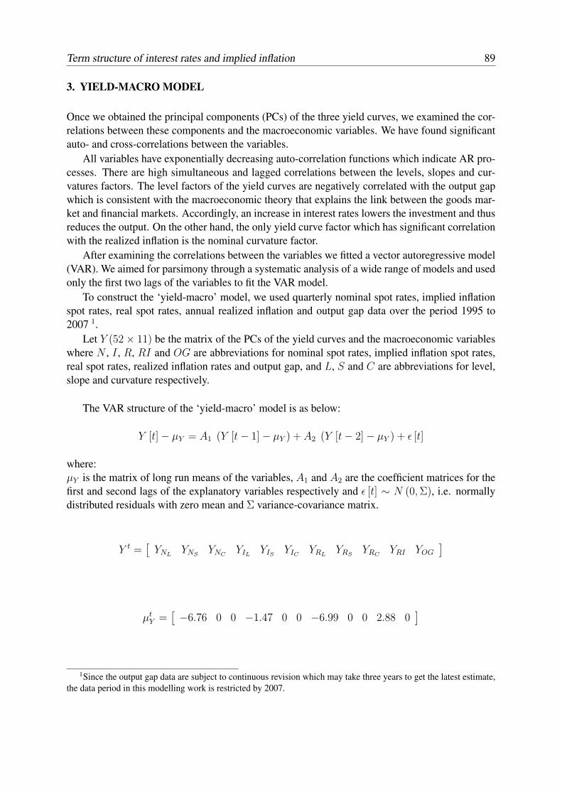
Term structure of interest rates and implied inflation 89
3. YIELD-MACRO MODEL
Once we obtained the principal components (PCs) of the three yield curves, we examined the cor-relations between these components and the macroeconomic variables. We have found significantauto- and cross-correlations between the variables.
All variables have exponentially decreasing auto-correlation functions which indicate AR pro-cesses. There are high simultaneous and lagged correlations between the levels, slopes and cur-vatures factors. The level factors of the yield curves are negatively correlated with the output gapwhich is consistent with the macroeconomic theory that explains the link between the goods mar-ket and financial markets. Accordingly, an increase in interest rates lowers the investment and thusreduces the output. On the other hand, the only yield curve factor which has significant correlationwith the realized inflation is the nominal curvature factor.
After examining the correlations between the variables we fitted a vector autoregressive model(VAR). We aimed for parsimony through a systematic analysis of a wide range of models and usedonly the first two lags of the variables to fit the VAR model.
To construct the ‘yield-macro’ model, we used quarterly nominal spot rates, implied inflationspot rates, real spot rates, annual realized inflation and output gap data over the period 1995 to2007 1.
Let Y (52 × 11) be the matrix of the PCs of the yield curves and the macroeconomic variableswhere N , I , R, RI and OG are abbreviations for nominal spot rates, implied inflation spot rates,real spot rates, realized inflation rates and output gap, and L, S and C are abbreviations for level,slope and curvature respectively.
The VAR structure of the ‘yield-macro’ model is as below:
Y [t] − µY = A1 (Y [t − 1] − µY ) + A2 (Y [t − 2] − µY ) + ε [t]
where:µY is the matrix of long run means of the variables, A1 and A2 are the coefficient matrices for thefirst and second lags of the explanatory variables respectively and ε [t] ∼ N (0, Σ), i.e. normallydistributed residuals with zero mean and Σ variance-covariance matrix.
Y t =[
YNLYNS
YNCYIL
YISYIC
YRLYRS
YRCYRI YOG
]
µtY =
[−6.76 0 0 −1.47 0 0 −6.99 0 0 2.88 0
]
1Since the output gap data are subject to continuous revision which may take three years to get the latest estimate,the data period in this modelling work is restricted by 2007.

90 S. Sahin et al.
A1 =
0.92 0 0 0 0 0 0 0 0 0 00 0.78 0 0 0 0 0 0 0 0 00 0 0.96 0 0 0 0 0 0 −0.15 00 0 0 0.89 0 0 0 0 0 0 00 0 0 0 0.56 0 0 0 0 0 00 0 0 0 0 0.62 0 0 0 0 00 0 0 0 0 0 0.95 0 0 0 00 0.27 0 0 0 0 0 0.49 0 0 00 0 0 0 0 0 0 0 0.86 0 00 0 0 0 0 0 0 0 0 0.92 00 −0.04 0 0 0 0 0 0 0 0 0.89
A2 =
0 0 0 0 0 0 0 0 0 0 00 0 0 0 0 0 0 0 −1.21 0 −0.410 0 −0.34 0 0 0 0 0 0 0 00 0 0 0 0 0 0 0 0 0 00 0 0 0 −0.32 0 0 0 1.38 0 00 0 0 0 0 0 0 −0.09 0 0 00 0 0 0 0 0 0 0 0 0 00 0 0 0 0 0 0 0 0 0 00 0 0 0 0 0 0 0 0 0 00 0 0.34 0 0 0 0 0 0 0 −0.200 0 0 0 0 0 0 0 0 0 0
Σ =
4.54−0.62 0.76−0.50 0.07 0.142.51 −0.22 −0.30 2.28−0.17 0.25 0.07 −0.18 0.270.09 −0.11 0.01 0.07 −0.05 0.081.88 −0.30 −0.19 0.20 0.05 0.00 1.61−0.53 0.30 0.05 −0.10 −0.02 0.02 −0.40 0.29−0.20 0.06 0.03 −0.02 −0.02 −0.02 −0.17 0.05 0.050.07 0.10 −0.05 0.07 0.03 −0.01 0.02 0.02 −0.01 0.17−0.03 0.03 0.01 0.04 0.01 0.01 −0.06 0.02 0.01 0.02 0.06
As A1 and A2 indicate, the level factors and the curvature factor of real interest rates can bemodelled as AR(1) processes. The diagonal structure of A1 and the few values in A2 can beexplained by the existence of the high autocorrelations in the variables.
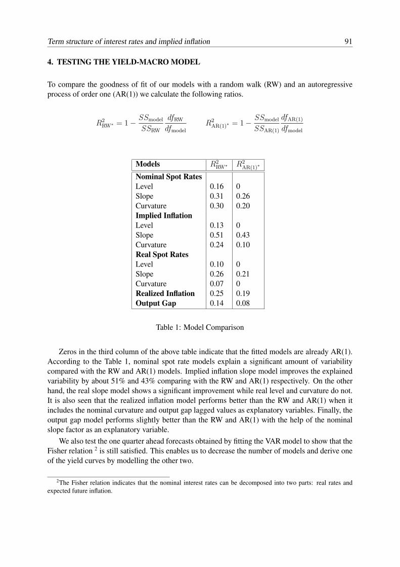
Term structure of interest rates and implied inflation 91
4. TESTING THE YIELD-MACRO MODEL
To compare the goodness of fit of our models with a random walk (RW) and an autoregressiveprocess of order one (AR(1)) we calculate the following ratios.
R2RW∗ = 1 −
SSmodel
SSRW
dfRW
dfmodel
R2AR(1)∗ = 1 −
SSmodel
SSAR(1)
dfAR(1)
dfmodel
Models R2RW∗ R2
AR(1)∗
Nominal Spot RatesLevel 0.16 0Slope 0.31 0.26Curvature 0.30 0.20Implied InflationLevel 0.13 0Slope 0.51 0.43Curvature 0.24 0.10Real Spot RatesLevel 0.10 0Slope 0.26 0.21Curvature 0.07 0Realized Inflation 0.25 0.19Output Gap 0.14 0.08
Table 1: Model Comparison
Zeros in the third column of the above table indicate that the fitted models are already AR(1).According to the Table 1, nominal spot rate models explain a significant amount of variabilitycompared with the RW and AR(1) models. Implied inflation slope model improves the explainedvariability by about 51% and 43% comparing with the RW and AR(1) respectively. On the otherhand, the real slope model shows a significant improvement while real level and curvature do not.It is also seen that the realized inflation model performs better than the RW and AR(1) when itincludes the nominal curvature and output gap lagged values as explanatory variables. Finally, theoutput gap model performs slightly better than the RW and AR(1) with the help of the nominalslope factor as an explanatory variable.
We also test the one quarter ahead forecasts obtained by fitting the VAR model to show that theFisher relation 2 is still satisfied. This enables us to decrease the number of models and derive oneof the yield curves by modelling the other two.
2The Fisher relation indicates that the nominal interest rates can be decomposed into two parts: real rates andexpected future inflation.
92 S. Sahin et al.
5. CONCLUSIONS
In this work, the three term structures (nominal, implied inflation and real spot rates) and twomacroeconomic variables (realized inflation and output gap) have been modelled by consideringthe bidirectional relations between the two sets of variables. The correlations between the variablesshow that the yield curve factors highly depend on their lagged values and the other yield curves’corresponding factors as well as the output gap. A parsimonious VAR model has been fitted to thedata to forecast the yield curves simultaneously. The VAR model has performed better than the RWand AR(1) processes in terms of the explained variability in the data. One quarter ahead forecastsare well within the 95% confidence limits for all yield curves and maturities. Furthermore, themodel is consistent with the Fisher relation.
References
A. Ang, G. Bekaert, and M. Wei. The term structure of real rates and expected inflation. Centrefor Economic Policy Research Discussion Papers, 2008.
A.J.G. Cairns. Descriptive bond yield and forward-rate models for the British Government Secu-rities’ market. British Actuarial Journal, 4(2):265–321 and 350–383, 1997.
H. Dewachter and M. Lyrio. Macro factors and the term structure of interest rates. Journal ofMoney Credit and Banking, 38(1):119–140, 2006.
F.X. Diebold and C. Li. Forecasting the term structure of government bond yields. Journal ofEconometrics, 130:337–364, 2006.
F.X. Diebold, M. Piazzesi, and G.D. Rudebusch. Modeling bond yields in finance and macroeco-nomics. American Economic Review, 95:415–420, 2005.
F.X. Diebold, G.D. Rudebusch, and S.B. Aruoba. The macroeconomy and the yield curve: Adynamic latent factor approach. Journal of Econometrics, 131:309–338, 2006.
F.X. Diebold, C. Li, and V.Z. Yue. Global yield curve dynamics and interactions: A dynamicNelson-Siegel approach. Journal of Econometrics, 146(2):351–363, 2007.
P. Lildholdt, N. Panigirtzoglou, and C. Peacock. An-affine macro-factor model of the UK yieldcurve. Bank of England Working Paper, 322, 2007.
R. Litterman and J. Scheinkman. Common factors affecting bond returns. The Journal of FixedIncome, 1(1):54–61, 1991.
J.B. Taylor. Discretion versus policy rules in practice. Carnegie-Rochester Conference Series onPublicPolicy, 39:195–214, 1993.
De Koninklijke Vlaamse Academie van België voor Wetenschappen en Kunsten coördineertjaarlijks tot 25 wetenschappelijke bijeenkomsten, ook contactfora genoemd, in de domeinenvan de natuurwetenschappen (inclusief de biomedische wetenschappen), menswetenschappenen kunsten. De contactfora hebben tot doel Vlaamse wetenschappers of kunstenaars te vereni-gen rond specifieke thema’s.
De handelingen van deze contactfora vormen een aparte publicatiereeks van de Academie.
Contactforum “Actuarial and Financial Mathematics Conference” (4-5 februari 2010, Prof.M. Vanmaele)
De “Actuarial and Financial Mathematics Conference 2010” was de 8ste editie van het “Actuarial and
Financial Mathematics” contactforum dat ondertussen zijn plaats veroverd heeft tussen de internationale
conferenties die focussen op de wisselwerking tussen financieel en actuarieel wiskundige technieken.
De eerste dag was opgebouwd rond het thema Market Consistent Valuation met voordrachten door
gerenommeerde internationale sprekers gevolgd door een leerrijke en levendige paneldiscussie. Op dag
twee mochten we naast genodigde sprekers ook sprekers uit de praktijk verwelkomen met onderwerpen
zoals Solvency II en spread opties. Gedurende beide dagen was er ook een postersessie tijdens de welke
jonge onderzoekers de mogelijkheid kregen om hun onderzoeksresultaten voor te stellen aan een
ruim publiek bestaande uit academici uit binnen- en buitenland alsook collega's uit de bank- en
verzekerings wereld. In deze publicatie vindt u een samenvatting van een van de voordrachten over
Market Consistent Valuation. Verder zijn er bijdragen over het prijzen van afgeleide producten zoals
catastrophe bonds, spread options en swaptions, over optimal trading strategies, proportional reinsur-
ance, strong Taylor approximation of stochastic differential equations en implied inflation.