Distributed Source Coding in

Wireless Sensor Networks

JOHANNES KARLSSON

Master’s Degree ProjectStockholm, Sweden 2006-06-30

XR-EE-KT 2006:006

Abstract

The advent of wireless sensor networks adds new requirements when design-ing communication schemes. Not only should the sensor nodes be energyefficient but they should preferably also be small and cheap. In the light ofthis a joint source-channel coding design that is utilizing a basic method ofdistributed source coding is investigated. An iterative algorithm for designingsuch system for two correlated Gaussian sources is proposed and evaluated. Itis shown that the proposed system finds a way of using the correlation of thesources to both reduce the quantization distortion and introduce protectionagainst channel errors.

i

ii

Acknowledgments

The work presented in this thesis was conducted during the spring of 2006in the Communication Theory group at the Department of Signals, Sensorsand Systems (S3) at the Royal Institute of Technology (KTH).

I would first of all like to thank my supervisor Niklas Wernersson for all ofhis help throughout the work with this thesis. Also big thanks to my examinerProf. Mikael Skoglund for letting me do my thesis in the CommunicationTheory group.

Finally I would like to thank my family and all my friends who have beensupporting me through my years of studies, and also thanks to my HeavenlyFather for all his blessings!

iii

iv

Contents

1 Introduction 11.1 Quantization . . . . . . . . . . . . . . . . . . . . . . . . . . . 21.2 Source Optimized Scalar Quantization . . . . . . . . . . . . . 31.3 Channel Optimized Scalar Quantization . . . . . . . . . . . . 4

1.3.1 Optimal Quantizer Design for Noisy Channels . . . . . 61.4 Distributed Source Coding . . . . . . . . . . . . . . . . . . . . 9

2 Channel Optimized Scalar Quantization of Correlated Sources 132.1 Problem Formulation . . . . . . . . . . . . . . . . . . . . . . . 132.2 Analysis . . . . . . . . . . . . . . . . . . . . . . . . . . . . . . 14

2.2.1 Finding the Optimal Encoder q1 . . . . . . . . . . . . . 152.2.2 Finding the Optimal Decoder g1 . . . . . . . . . . . . . 162.2.3 Algorithm . . . . . . . . . . . . . . . . . . . . . . . . . 17

2.3 Numerical Results . . . . . . . . . . . . . . . . . . . . . . . . . 182.3.1 Channel Mismatch . . . . . . . . . . . . . . . . . . . . 202.3.2 Correlation-SNR Mismatch . . . . . . . . . . . . . . . 22

3 Reducing Complexity 253.1 Multistage Quantization . . . . . . . . . . . . . . . . . . . . . 25

3.1.1 Analysis . . . . . . . . . . . . . . . . . . . . . . . . . . 253.1.2 Numerical Results . . . . . . . . . . . . . . . . . . . . 27

3.2 Dual COSQ with Optimal Decoders . . . . . . . . . . . . . . . 283.2.1 Analysis . . . . . . . . . . . . . . . . . . . . . . . . . . 283.2.2 Numerical Results . . . . . . . . . . . . . . . . . . . . 29

4 Conclusions 314.1 Comments on the Results . . . . . . . . . . . . . . . . . . . . 314.2 Future Work . . . . . . . . . . . . . . . . . . . . . . . . . . . . 32

A Derivations 33A.1 pdf of a Gaussian Variable . . . . . . . . . . . . . . . . . . . . 33

v

A.2 pdf of the Sum of Two Gaussian Variables . . . . . . . . . . . 34A.3 Conditional pdf of a Gaussian Variable . . . . . . . . . . . . . 34A.4 P (i2 |x1) . . . . . . . . . . . . . . . . . . . . . . . . . . . . . . 35A.5 Reconstruction Points . . . . . . . . . . . . . . . . . . . . . . 36

B Numerical Results 37

Bibliography 42

vi

Chapter 1

Introduction

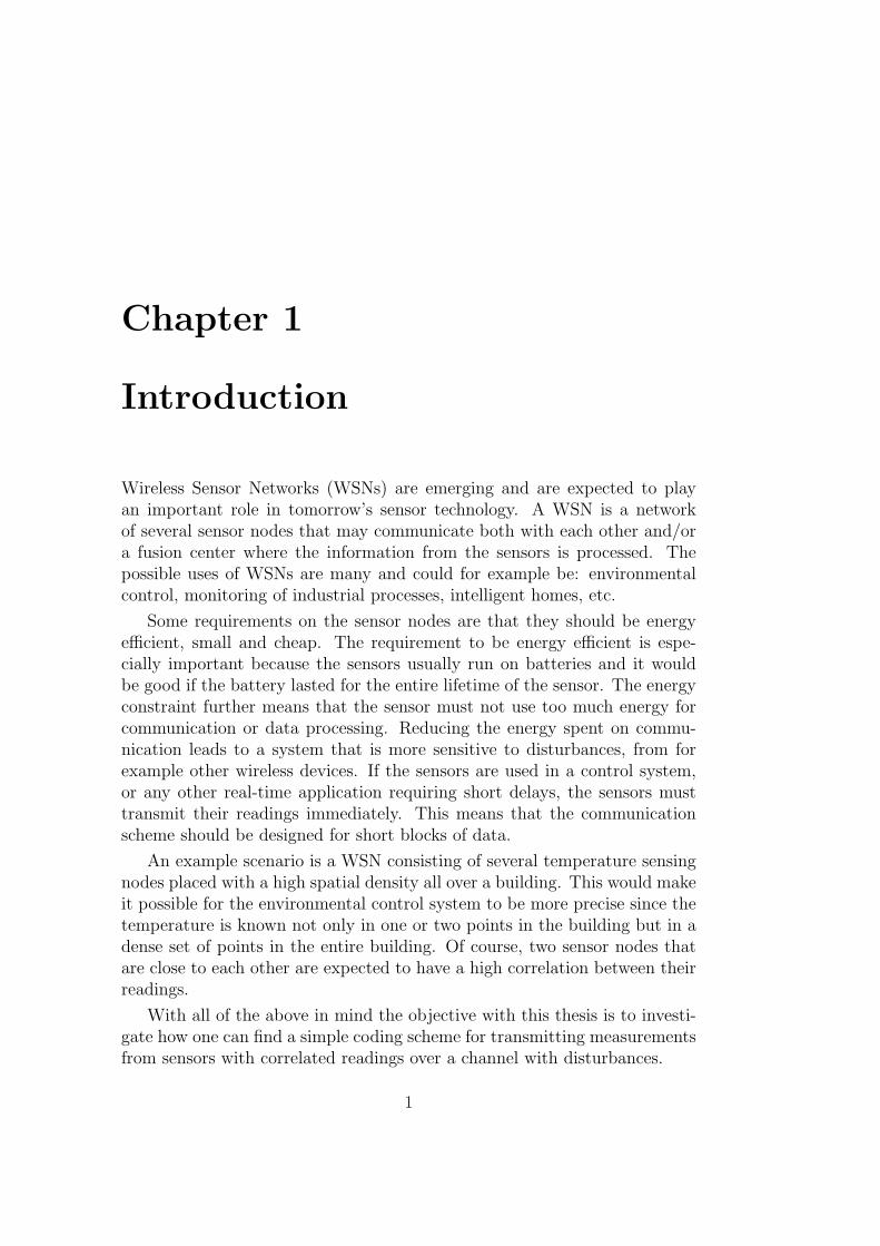
Wireless Sensor Networks (WSNs) are emerging and are expected to playan important role in tomorrow’s sensor technology. A WSN is a networkof several sensor nodes that may communicate both with each other and/ora fusion center where the information from the sensors is processed. Thepossible uses of WSNs are many and could for example be: environmentalcontrol, monitoring of industrial processes, intelligent homes, etc.

Some requirements on the sensor nodes are that they should be energyefficient, small and cheap. The requirement to be energy efficient is espe-cially important because the sensors usually run on batteries and it wouldbe good if the battery lasted for the entire lifetime of the sensor. The energyconstraint further means that the sensor must not use too much energy forcommunication or data processing. Reducing the energy spent on commu-nication leads to a system that is more sensitive to disturbances, from forexample other wireless devices. If the sensors are used in a control system,or any other real-time application requiring short delays, the sensors musttransmit their readings immediately. This means that the communicationscheme should be designed for short blocks of data.

An example scenario is a WSN consisting of several temperature sensingnodes placed with a high spatial density all over a building. This would makeit possible for the environmental control system to be more precise since thetemperature is known not only in one or two points in the building but in adense set of points in the entire building. Of course, two sensor nodes thatare close to each other are expected to have a high correlation between theirreadings.

With all of the above in mind the objective with this thesis is to investi-gate how one can find a simple coding scheme for transmitting measurementsfrom sensors with correlated readings over a channel with disturbances.

1

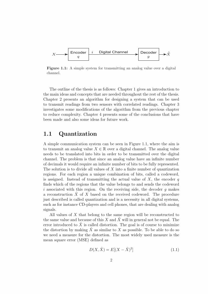
Figure 1.1: A simple system for transmitting an analog value over a digitalchannel.

The outline of the thesis is as follows: Chapter 1 gives an introduction tothe main ideas and concepts that are needed throughout the rest of the thesis.Chapter 2 presents an algorithm for designing a system that can be usedto transmit readings from two sensors with correlated readings. Chapter 3investigates some modifications of the algorithm from the previous chapterto reduce complexity. Chapter 4 presents some of the conclusions that havebeen made and also some ideas for future work.

1.1 Quantization

A simple communication system can be seen in Figure 1.1, where the aim isto transmit an analog value X ∈ R over a digital channel. The analog valueneeds to be translated into bits in order to be transmitted over the digitalchannel. The problem is that since an analog value have an infinite numberof decimals it would require an infinite number of bits to be fully represented.The solution is to divide all values of X into a finite number of quantizationregions. For each region a unique combination of bits, called a codeword,is assigned. Instead of transmitting the actual value of X, the encoder qfinds which of the regions that the value belongs to and sends the codewordi associated with this region. On the receiving side, the decoder g makesa reconstruction X of X based on the received codeword. The procedurejust described is called quantization and is a necessity in all digital systems,such as for instance CD-players and cell phones, that are dealing with analogsignals.

All values of X that belong to the same region will be reconstructed tothe same value and because of this X and X will in general not be equal. Theerror introduced to X is called distortion. The goal is of course to minimizethe distortion by making X as similar to X as possible. To be able to do sowe need a measure for the distortion. The most widely used measure is themean square error (MSE) defined as

D(X, X) = E[(X − X)2] (1.1)

2

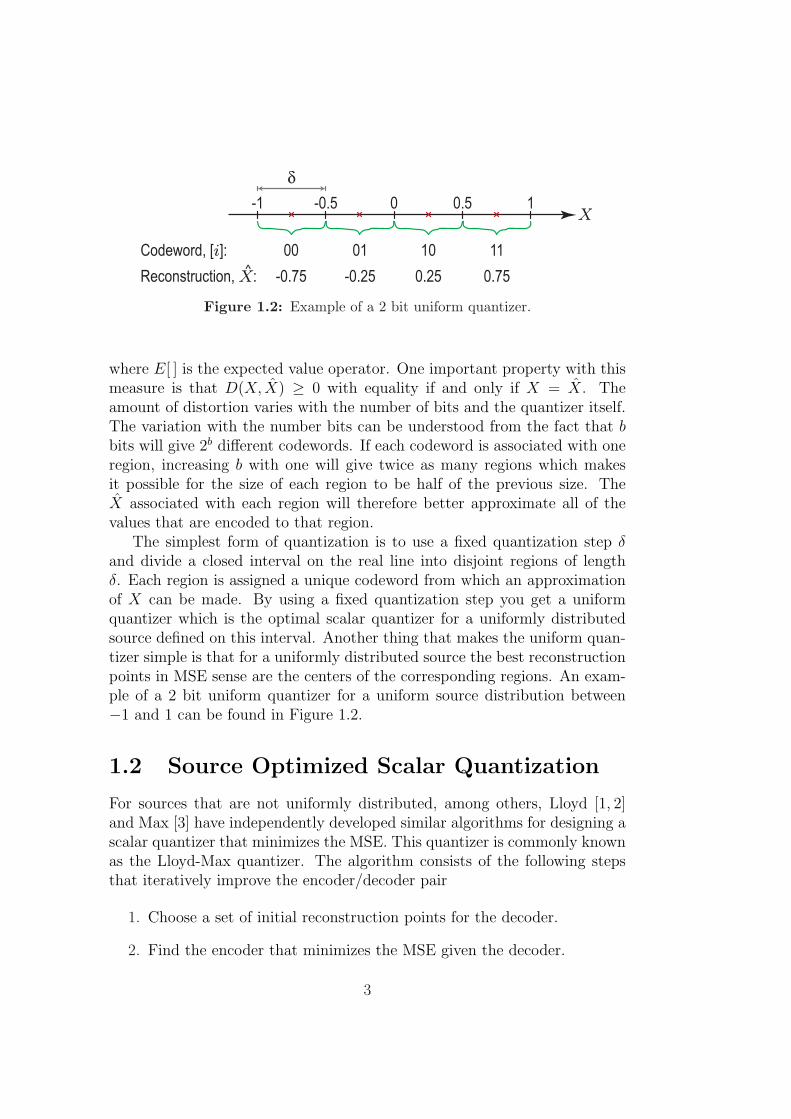
Figure 1.2: Example of a 2 bit uniform quantizer.

where E[ ] is the expected value operator. One important property with thismeasure is that D(X, X) ≥ 0 with equality if and only if X = X. Theamount of distortion varies with the number of bits and the quantizer itself.The variation with the number bits can be understood from the fact that bbits will give 2b different codewords. If each codeword is associated with oneregion, increasing b with one will give twice as many regions which makesit possible for the size of each region to be half of the previous size. TheX associated with each region will therefore better approximate all of thevalues that are encoded to that region.

The simplest form of quantization is to use a fixed quantization step δand divide a closed interval on the real line into disjoint regions of lengthδ. Each region is assigned a unique codeword from which an approximationof X can be made. By using a fixed quantization step you get a uniformquantizer which is the optimal scalar quantizer for a uniformly distributedsource defined on this interval. Another thing that makes the uniform quan-tizer simple is that for a uniformly distributed source the best reconstructionpoints in MSE sense are the centers of the corresponding regions. An exam-ple of a 2 bit uniform quantizer for a uniform source distribution between−1 and 1 can be found in Figure 1.2.

1.2 Source Optimized Scalar Quantization

For sources that are not uniformly distributed, among others, Lloyd [1, 2]and Max [3] have independently developed similar algorithms for designing ascalar quantizer that minimizes the MSE. This quantizer is commonly knownas the Lloyd-Max quantizer. The algorithm consists of the following stepsthat iteratively improve the encoder/decoder pair

1. Choose a set of initial reconstruction points for the decoder.

2. Find the encoder that minimizes the MSE given the decoder.

3

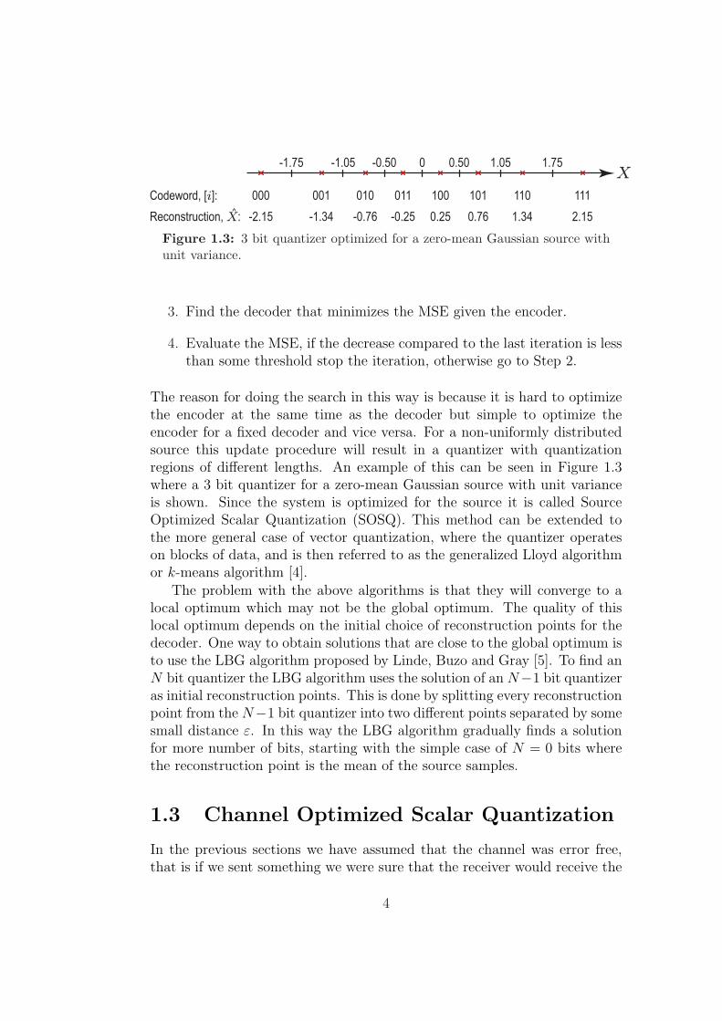
Figure 1.3: 3 bit quantizer optimized for a zero-mean Gaussian source withunit variance.

3. Find the decoder that minimizes the MSE given the encoder.

4. Evaluate the MSE, if the decrease compared to the last iteration is lessthan some threshold stop the iteration, otherwise go to Step 2.

The reason for doing the search in this way is because it is hard to optimizethe encoder at the same time as the decoder but simple to optimize theencoder for a fixed decoder and vice versa. For a non-uniformly distributedsource this update procedure will result in a quantizer with quantizationregions of different lengths. An example of this can be seen in Figure 1.3where a 3 bit quantizer for a zero-mean Gaussian source with unit varianceis shown. Since the system is optimized for the source it is called SourceOptimized Scalar Quantization (SOSQ). This method can be extended tothe more general case of vector quantization, where the quantizer operateson blocks of data, and is then referred to as the generalized Lloyd algorithmor k-means algorithm [4].

The problem with the above algorithms is that they will converge to alocal optimum which may not be the global optimum. The quality of thislocal optimum depends on the initial choice of reconstruction points for thedecoder. One way to obtain solutions that are close to the global optimum isto use the LBG algorithm proposed by Linde, Buzo and Gray [5]. To find anN bit quantizer the LBG algorithm uses the solution of an N−1 bit quantizeras initial reconstruction points. This is done by splitting every reconstructionpoint from the N−1 bit quantizer into two different points separated by somesmall distance ε. In this way the LBG algorithm gradually finds a solutionfor more number of bits, starting with the simple case of N = 0 bits wherethe reconstruction point is the mean of the source samples.

1.3 Channel Optimized Scalar Quantization

In the previous sections we have assumed that the channel was error free,that is if we sent something we were sure that the receiver would receive the

4

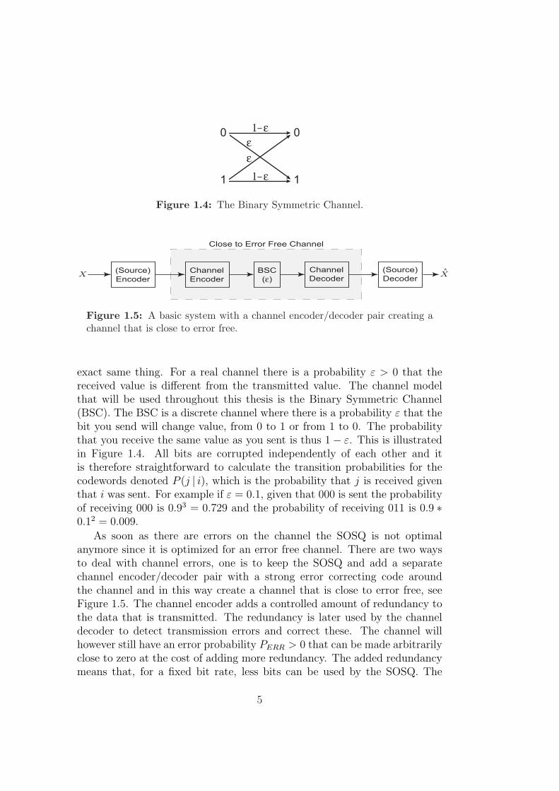
Figure 1.4: The Binary Symmetric Channel.

Figure 1.5: A basic system with a channel encoder/decoder pair creating achannel that is close to error free.

exact same thing. For a real channel there is a probability ε > 0 that thereceived value is different from the transmitted value. The channel modelthat will be used throughout this thesis is the Binary Symmetric Channel(BSC). The BSC is a discrete channel where there is a probability ε that thebit you send will change value, from 0 to 1 or from 1 to 0. The probabilitythat you receive the same value as you sent is thus 1− ε. This is illustratedin Figure 1.4. All bits are corrupted independently of each other and itis therefore straightforward to calculate the transition probabilities for thecodewords denoted P (j | i), which is the probability that j is received giventhat i was sent. For example if ε = 0.1, given that 000 is sent the probabilityof receiving 000 is 0.93 = 0.729 and the probability of receiving 011 is 0.9 ∗0.12 = 0.009.

As soon as there are errors on the channel the SOSQ is not optimalanymore since it is optimized for an error free channel. There are two waysto deal with channel errors, one is to keep the SOSQ and add a separatechannel encoder/decoder pair with a strong error correcting code aroundthe channel and in this way create a channel that is close to error free, seeFigure 1.5. The channel encoder adds a controlled amount of redundancy tothe data that is transmitted. The redundancy is later used by the channeldecoder to detect transmission errors and correct these. The channel willhowever still have an error probability PERR > 0 that can be made arbitrarilyclose to zero at the cost of adding more redundancy. The added redundancymeans that, for a fixed bit rate, less bits can be used by the SOSQ. The

5

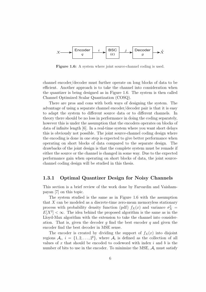
Figure 1.6: A system where joint source-channel coding is used.

channel encoder/decoder must further operate on long blocks of data to beefficient. Another approach is to take the channel into consideration whenthe quantizer is being designed as in Figure 1.6. The system is then calledChannel Optimized Scalar Quantization (COSQ).

There are pros and cons with both ways of designing the system. Theadvantage of using a separate channel encoder/decoder pair is that it is easyto adapt the system to different source data or to different channels. Intheory there should be no loss in performance in doing the coding separately,however this is under the assumption that the encoders operates on blocks ofdata of infinite length [6]. In a real-time system where you want short delaysthis is obviously not possible. The joint source-channel coding design wherethe encoding is done in one step is expected to give better performance whenoperating on short blocks of data compared to the separate design. Thedrawbacks of the joint design is that the complete system must be remade ifeither the source or the channel is changed in some way. Due to the expectedperformance gain when operating on short blocks of data, the joint source-channel coding design will be studied in this thesis.

1.3.1 Optimal Quantizer Design for Noisy Channels

This section is a brief review of the work done by Farvardin and Vaisham-payan [7] on this topic.

The system studied is the same as in Figure 1.6 with the assumptionthat X can be modeled as a discrete-time zero-mean memoryless stationaryprocess with probability density function (pdf) fX(x) and variance σ2

X =E[X2] < ∞. The idea behind the proposed algorithm is the same as in theLloyd-Max algorithm with the extension to take the channel into consider-ation. That is, given the decoder g find the best encoder q and given theencoder find the best decoder in MSE sense.

The encoder is created by dividing the support of fX(x) into disjointregions Ai, i = {1, 2, . . . , 2b}, where Ai is defined as the collection of allvalues of x that should be encoded to codeword with index i and b is thenumber of bits to use in the encoder. To minimize the MSE, Ai must satisfy

6

Ai = {x : E[(x− X)2 | q(x)= i] ≤ E[(x− X)2 | q(x)=k], ∀k 6= i}. (1.2)

This can equivalently be expressed as

Ai =2b⋂

k=1k 6=i

Aik (1.3)

where Aik is defined as

Aik = {x : E[(x− X)2 | q(x)= i] ≤ E[(x− X)2 | q(x)=k]}. (1.4)

The set Aik specifies all points x that will give a lower or equal MSE ifthey are mapped to codeword i instead of codeword k. By expanding thesquares and rearranging the terms in (1.4), it can be seen that the inequalityis between two functions that are linear in x. In [7] it is further shown thatbecause of this Ai must be an interval and an analytical expression for findingthe endpoints of the interval for a given decoder is derived.

It is a well known fact from estimation theory that in order to minimizethe MSE the decoder is calculated as the expected value of x given that acertain codeword j is received

x(j) = E[X | j]. (1.5)

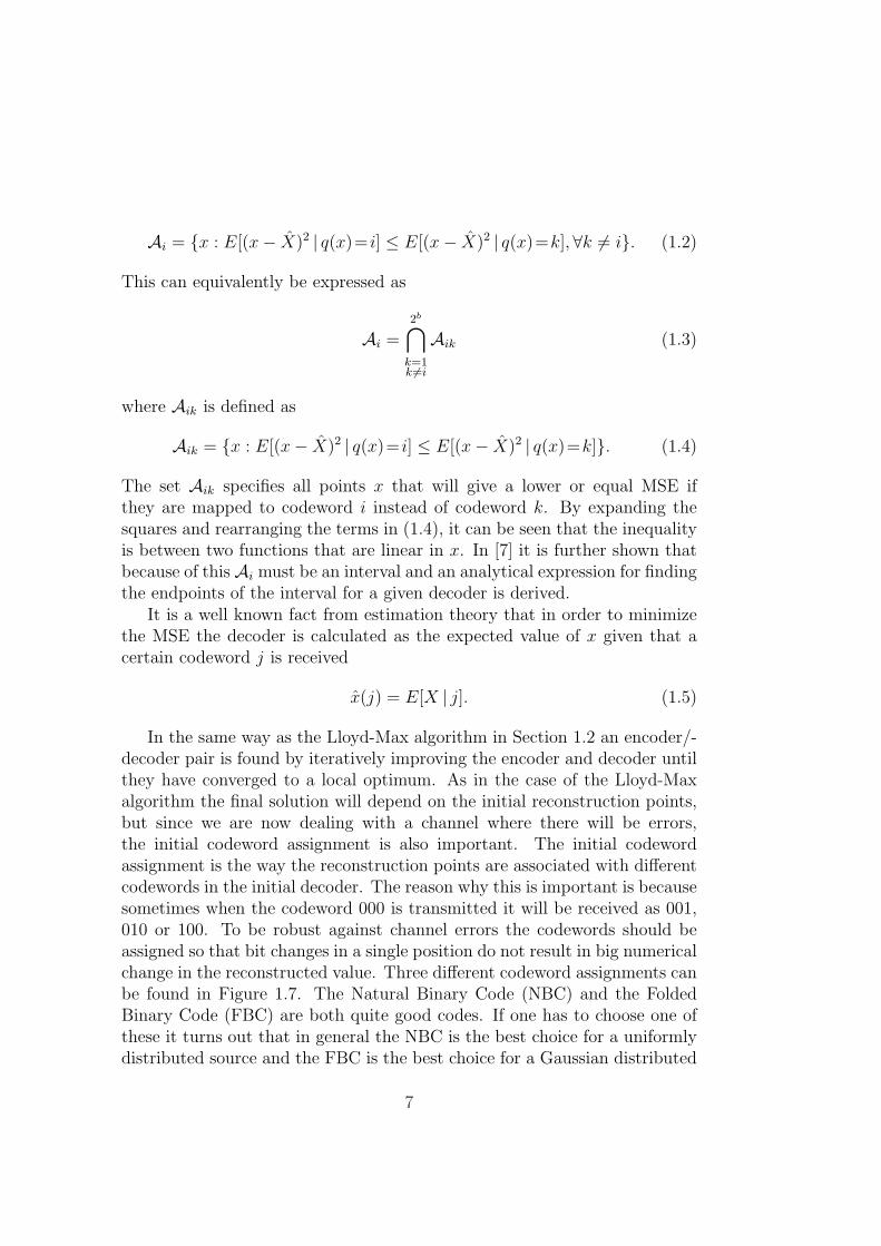
In the same way as the Lloyd-Max algorithm in Section 1.2 an encoder/-decoder pair is found by iteratively improving the encoder and decoder untilthey have converged to a local optimum. As in the case of the Lloyd-Maxalgorithm the final solution will depend on the initial reconstruction points,but since we are now dealing with a channel where there will be errors,the initial codeword assignment is also important. The initial codewordassignment is the way the reconstruction points are associated with differentcodewords in the initial decoder. The reason why this is important is becausesometimes when the codeword 000 is transmitted it will be received as 001,010 or 100. To be robust against channel errors the codewords should beassigned so that bit changes in a single position do not result in big numericalchange in the reconstructed value. Three different codeword assignments canbe found in Figure 1.7. The Natural Binary Code (NBC) and the FoldedBinary Code (FBC) are both quite good codes. If one has to choose one ofthese it turns out that in general the NBC is the best choice for a uniformlydistributed source and the FBC is the best choice for a Gaussian distributed

7

Figure 1.7: A 3 bit quantizer with different codeword assignments.

source [7]. The Bad Code in the figure is an example of a code that shouldnot be used. All bit changes in a single position will result in a reconstructionwhere even the sign is wrong.

To be able to compare the performance of different systems we use theSignal-to-Distortion Ratio (SDR), defined as

SDR = 10 log10

(E[X2]

E[(X − X)2]

). (1.6)

It can easily be seen that this is nothing but the ratio between the varianceof the source and the MSE of the reconstructed signal. SDR = 0 dB meansthat the MSE is as large as the signal itself and SDR = ∞ dB means thatthe signal is perfectly reconstructed.

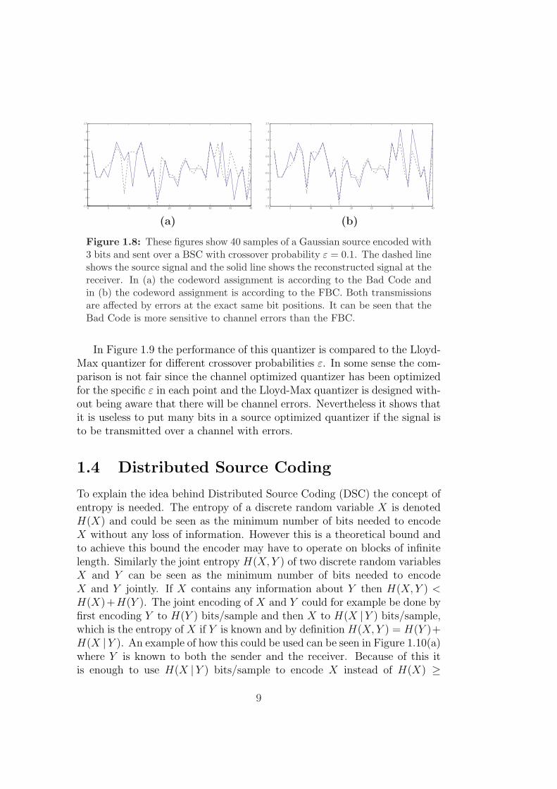
An example of how channel errors affect different codeword assignmentscan be seen in Figure 1.8 where the Bad Code from the previous example iscompared to the FBC. 1000000 samples of a zero-mean Gaussian source hasbeen encoded with a SOSQ and sent over a channel with crossover probabilityε = 0.1. The SDR is 2.2 dB for the FBC, 1.6 dB for the NBC and −0.9 dBfor the Bad Code. In other words, in this case the Bad Code is so bad that itwould have been better to neglect the received value and decode everythingto 0 since this would have given an SDR of 0 dB.

Something that is different compared to the Lloyd-Max quantizer is that,for high crossover probability ε, some of the sets Ai are empty, which meansthat the corresponding codeword will never be transmitted. For example inthe case when ε = 0.1 and 4 bits/sample are used, only 6 of the 16 availablecodewords are used by the encoder. When the receiver receives any of the10 codewords that never are transmitted X is reconstructed as the expectedvalue of X given the received codeword (as is always the case) according to(1.5). The codewords that are not used are such that they, by single biterrors, would be mistaken for the 6 codewords that are used. This showshow the joint design finds a tradeoff between quantization distortion androbustness against channel errors in order to minimize the MSE.

8

(a) (b)

Figure 1.8: These figures show 40 samples of a Gaussian source encoded with3 bits and sent over a BSC with crossover probability ε = 0.1. The dashed lineshows the source signal and the solid line shows the reconstructed signal at thereceiver. In (a) the codeword assignment is according to the Bad Code andin (b) the codeword assignment is according to the FBC. Both transmissionsare affected by errors at the exact same bit positions. It can be seen that theBad Code is more sensitive to channel errors than the FBC.

In Figure 1.9 the performance of this quantizer is compared to the Lloyd-Max quantizer for different crossover probabilities ε. In some sense the com-parison is not fair since the channel optimized quantizer has been optimizedfor the specific ε in each point and the Lloyd-Max quantizer is designed with-out being aware that there will be channel errors. Nevertheless it shows thatit is useless to put many bits in a source optimized quantizer if the signal isto be transmitted over a channel with errors.

1.4 Distributed Source Coding

To explain the idea behind Distributed Source Coding (DSC) the concept ofentropy is needed. The entropy of a discrete random variable X is denotedH(X) and could be seen as the minimum number of bits needed to encodeX without any loss of information. However this is a theoretical bound andto achieve this bound the encoder may have to operate on blocks of infinitelength. Similarly the joint entropy H(X, Y ) of two discrete random variablesX and Y can be seen as the minimum number of bits needed to encodeX and Y jointly. If X contains any information about Y then H(X,Y ) <H(X)+H(Y ). The joint encoding of X and Y could for example be done byfirst encoding Y to H(Y ) bits/sample and then X to H(X |Y ) bits/sample,which is the entropy of X if Y is known and by definition H(X, Y ) = H(Y )+H(X |Y ). An example of how this could be used can be seen in Figure 1.10(a)where Y is known to both the sender and the receiver. Because of this itis enough to use H(X |Y ) bits/sample to encode X instead of H(X) ≥

9

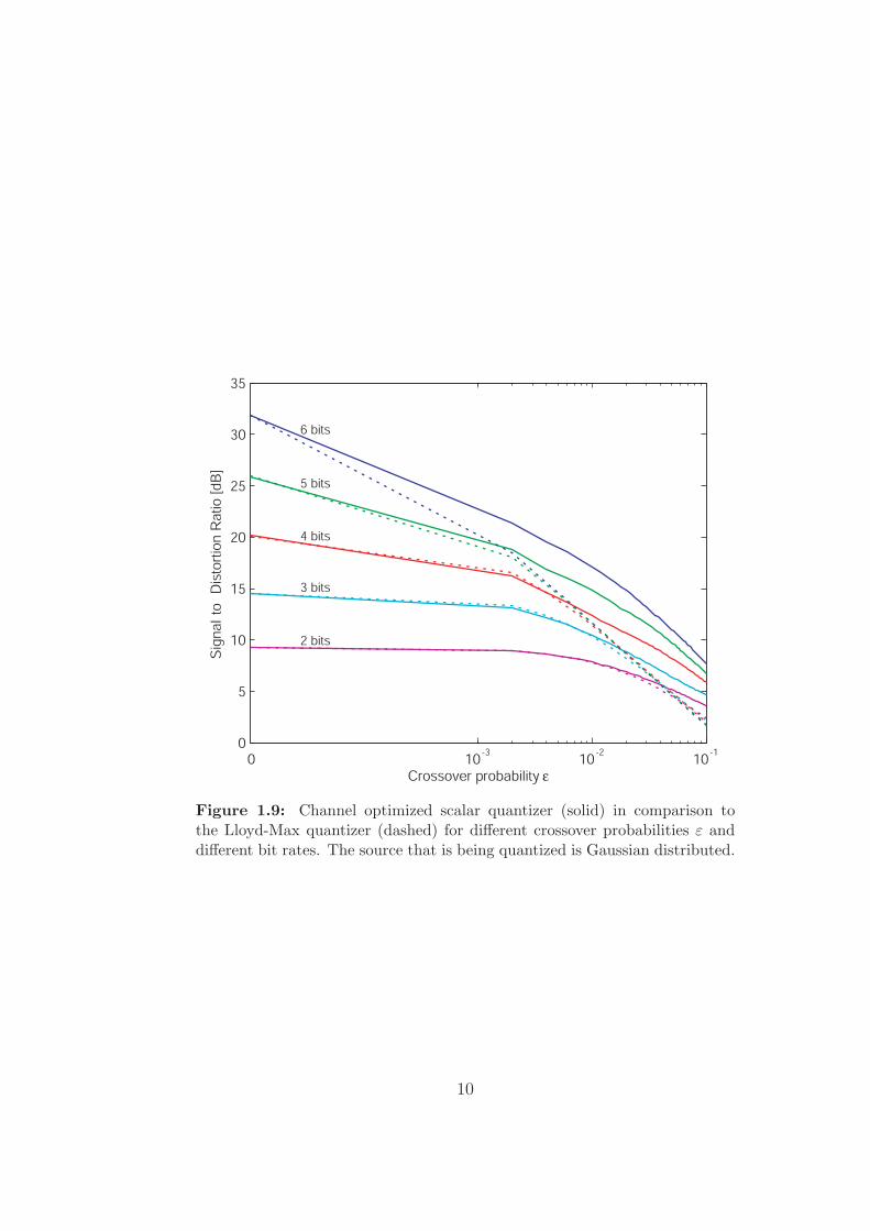
Figure 1.9: Channel optimized scalar quantizer (solid) in comparison tothe Lloyd-Max quantizer (dashed) for different crossover probabilities ε anddifferent bit rates. The source that is being quantized is Gaussian distributed.

10

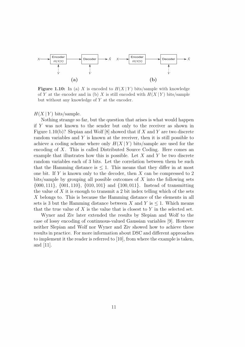
(a) (b)

Figure 1.10: In (a) X is encoded to H(X |Y ) bits/sample with knowledgeof Y at the encoder and in (b) X is still encoded with H(X |Y ) bits/samplebut without any knowledge of Y at the encoder.

H(X |Y ) bits/sample.Nothing strange so far, but the question that arises is what would happen

if Y was not known to the sender but only to the receiver as shown inFigure 1.10(b)? Slepian and Wolf [8] showed that if X and Y are two discreterandom variables and Y is known at the receiver, then it is still possible toachieve a coding scheme where only H(X |Y ) bits/sample are used for theencoding of X. This is called Distributed Source Coding. Here comes anexample that illustrates how this is possible. Let X and Y be two discreterandom variables each of 3 bits. Let the correlation between them be suchthat the Hamming distance is ≤ 1. This means that they differ in at mostone bit. If Y is known only to the decoder, then X can be compressed to 2bits/sample by grouping all possible outcomes of X into the following sets{000, 111}, {001, 110}, {010, 101} and {100, 011}. Instead of transmittingthe value of X it is enough to transmit a 2 bit index telling which of the setsX belongs to. This is because the Hamming distance of the elements in allsets is 3 but the Hamming distance between X and Y is ≤ 1. Which meansthat the true value of X is the value that is closest to Y in the selected set.

Wyner and Ziv later extended the results by Slepian and Wolf to thecase of lossy encoding of continuous-valued Gaussian variables [9]. Howeverneither Slepian and Wolf nor Wyner and Ziv showed how to achieve theseresults in practice. For more information about DSC and different approachesto implement it the reader is referred to [10], from where the example is taken,and [11].

11

12

Chapter 2

Channel Optimized ScalarQuantization of CorrelatedSources

2.1 Problem Formulation

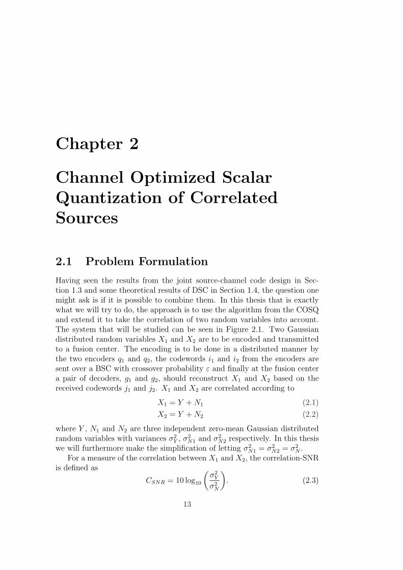
Having seen the results from the joint source-channel code design in Sec-tion 1.3 and some theoretical results of DSC in Section 1.4, the question onemight ask is if it is possible to combine them. In this thesis that is exactlywhat we will try to do, the approach is to use the algorithm from the COSQand extend it to take the correlation of two random variables into account.The system that will be studied can be seen in Figure 2.1. Two Gaussiandistributed random variables X1 and X2 are to be encoded and transmittedto a fusion center. The encoding is to be done in a distributed manner bythe two encoders q1 and q2, the codewords i1 and i2 from the encoders aresent over a BSC with crossover probability ε and finally at the fusion centera pair of decoders, g1 and g2, should reconstruct X1 and X2 based on thereceived codewords j1 and j2. X1 and X2 are correlated according to

X1 = Y + N1 (2.1)

X2 = Y + N2 (2.2)

where Y , N1 and N2 are three independent zero-mean Gaussian distributedrandom variables with variances σ2

Y , σ2N1 and σ2

N2 respectively. In this thesiswe will furthermore make the simplification of letting σ2

N1 = σ2N2 = σ2

N .For a measure of the correlation between X1 and X2, the correlation-SNR

is defined as

CSNR = 10 log10

(σ2

Y

σ2N

). (2.3)

13

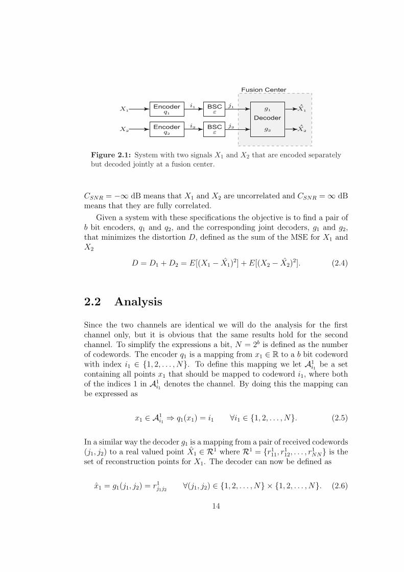
Figure 2.1: System with two signals X1 and X2 that are encoded separatelybut decoded jointly at a fusion center.

CSNR = −∞ dB means that X1 and X2 are uncorrelated and CSNR = ∞ dBmeans that they are fully correlated.

Given a system with these specifications the objective is to find a pair ofb bit encoders, q1 and q2, and the corresponding joint decoders, g1 and g2,that minimizes the distortion D, defined as the sum of the MSE for X1 andX2

D = D1 + D2 = E[(X1 − X1)2] + E[(X2 − X2)

2]. (2.4)

2.2 Analysis

Since the two channels are identical we will do the analysis for the firstchannel only, but it is obvious that the same results hold for the secondchannel. To simplify the expressions a bit, N = 2b is defined as the numberof codewords. The encoder q1 is a mapping from x1 ∈ R to a b bit codewordwith index i1 ∈ {1, 2, . . . , N}. To define this mapping we let A1

i1be a set

containing all points x1 that should be mapped to codeword i1, where bothof the indices 1 in A1

i1denotes the channel. By doing this the mapping can

be expressed as

x1 ∈ A1i1⇒ q1(x1) = i1 ∀i1 ∈ {1, 2, . . . , N}. (2.5)

In a similar way the decoder g1 is a mapping from a pair of received codewords(j1, j2) to a real valued point X1 ∈ R1 where R1 = {r1

11, r112, . . . , r

1NN} is the

set of reconstruction points for X1. The decoder can now be defined as

x1 = g1(j1, j2) = r1j1j2

∀(j1, j2) ∈ {1, 2, . . . , N} × {1, 2, . . . , N}. (2.6)

14

With these definitions the distortion D1 can be written as

D1 =

∫

x1

fX1(x1)N∑

j1=1

P (j1 | q1(x1))N∑

i2=1

P (i2 |x1)

N∑j2=1

P (j2 | i2)(x1 − g1(j1, j2))2 dx1 (2.7)

and D2, from the perspective of channel 1, becomes

D2 =

∫

x1

fX1(x1)N∑

j1=1

P (j1 | q1(x1))

∫

x2

fX2(x2 |x1)

N∑j2=1

P (j2 | q2(x2))(x2 − g2(j1, j2))2 dx2 dx1. (2.8)

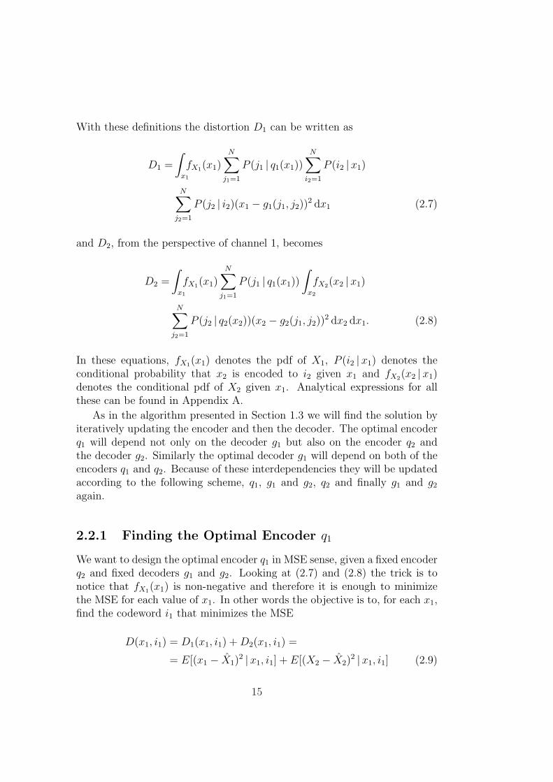
In these equations, fX1(x1) denotes the pdf of X1, P (i2 | x1) denotes theconditional probability that x2 is encoded to i2 given x1 and fX2(x2 |x1)denotes the conditional pdf of X2 given x1. Analytical expressions for allthese can be found in Appendix A.

As in the algorithm presented in Section 1.3 we will find the solution byiteratively updating the encoder and then the decoder. The optimal encoderq1 will depend not only on the decoder g1 but also on the encoder q2 andthe decoder g2. Similarly the optimal decoder g1 will depend on both of theencoders q1 and q2. Because of these interdependencies they will be updatedaccording to the following scheme, q1, g1 and g2, q2 and finally g1 and g2

again.

2.2.1 Finding the Optimal Encoder q1

We want to design the optimal encoder q1 in MSE sense, given a fixed encoderq2 and fixed decoders g1 and g2. Looking at (2.7) and (2.8) the trick is tonotice that fX1(x1) is non-negative and therefore it is enough to minimizethe MSE for each value of x1. In other words the objective is to, for each x1,find the codeword i1 that minimizes the MSE

D(x1, i1) = D1(x1, i1) + D2(x1, i1) =

= E[(x1 − X1)2 |x1, i1] + E[(X2 − X2)

2 | x1, i1] (2.9)

15

where

D1(x1, i1) =N∑

j1=1

P (j1 | i1)N∑

i2=1

P (i2 | x1)

N∑j2=1

P (j2 | i2)(x1 − g1(j1, j2))2 (2.10)

D2(x1, i1) =N∑

j1=1

P (j1 | i1)∫

x2

fX2(x2 |x1)

N∑j2=1

P (j2 | q2(x2))(x2 − g2(j1, j2))2 dx2. (2.11)

The set A1i1

can now be defined as

A1i1

= {x1 : D(x1, i1) ≤ D(x1, i1), ∀i1 6= i1} ∀i1 ∈ {1, 2, . . . , N}. (2.12)

Unfortunately this inequality is not linear in x1 and there are no indi-cations that the sets A1

i1will be intervals as in the single source case in

Section 1.3. Instead of trying to find an analytical expression for the encoderthe approach is to do a full search and evaluate the distortion for all val-ues of x1 and all codewords. The encoder is then designed by choosing thecodeword that resulted in the lowest distortion for each value of x1.

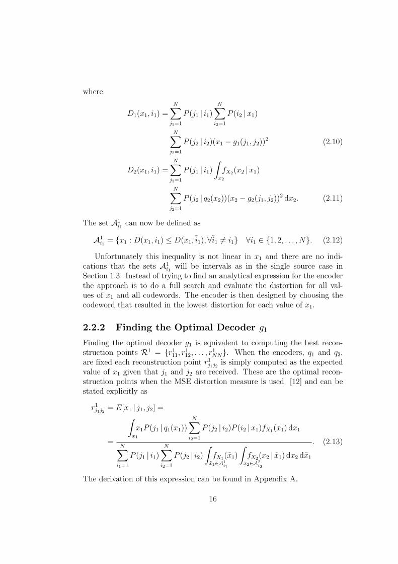
2.2.2 Finding the Optimal Decoder g1

Finding the optimal decoder g1 is equivalent to computing the best recon-struction points R1 = {r1

11, r112, . . . , r

1NN}. When the encoders, q1 and q2,

are fixed each reconstruction point r1j1j2

is simply computed as the expectedvalue of x1 given that j1 and j2 are received. These are the optimal recon-struction points when the MSE distortion measure is used [12] and can bestated explicitly as

r1j1j2

= E[x1 | j1, j2] =

=

∫

x1

x1P (j1 | q1(x1))N∑

i2=1

P (j2 | i2)P (i2 |x1)fX1(x1) dx1

N∑i1=1

P (j1 | i1)N∑

i2=1

P (j2 | i2)∫

x1∈A1i1

fX1(x1)

∫

x2∈A2i2

fX2(x2 | x1) dx2 dx1

. (2.13)

The derivation of this expression can be found in Appendix A.

16

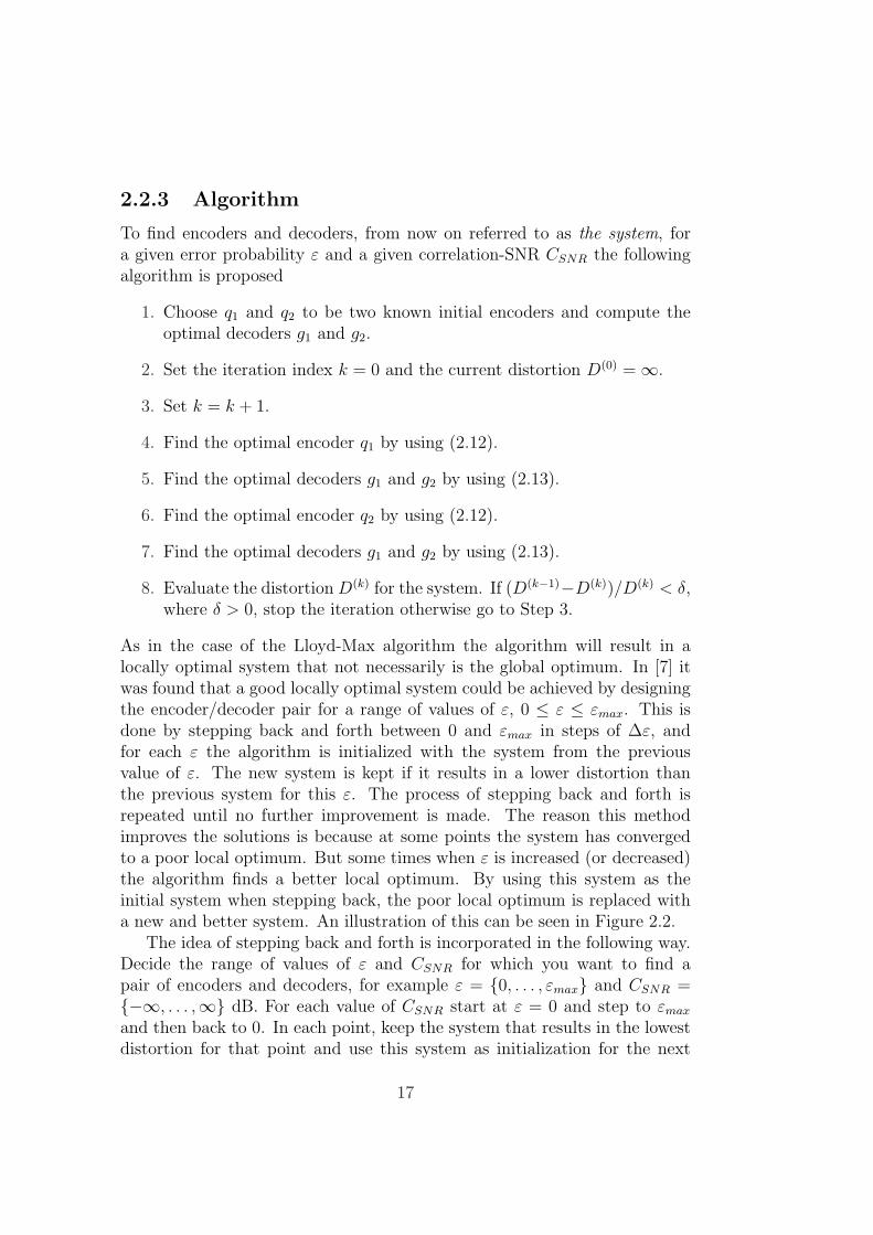
2.2.3 Algorithm

To find encoders and decoders, from now on referred to as the system, fora given error probability ε and a given correlation-SNR CSNR the followingalgorithm is proposed

1. Choose q1 and q2 to be two known initial encoders and compute theoptimal decoders g1 and g2.

2. Set the iteration index k = 0 and the current distortion D(0) = ∞.

3. Set k = k + 1.

4. Find the optimal encoder q1 by using (2.12).

5. Find the optimal decoders g1 and g2 by using (2.13).

6. Find the optimal encoder q2 by using (2.12).

7. Find the optimal decoders g1 and g2 by using (2.13).

8. Evaluate the distortion D(k) for the system. If (D(k−1)−D(k))/D(k) < δ,where δ > 0, stop the iteration otherwise go to Step 3.

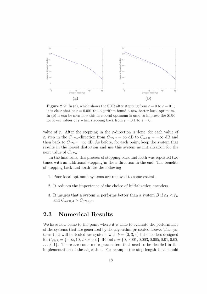
As in the case of the Lloyd-Max algorithm the algorithm will result in alocally optimal system that not necessarily is the global optimum. In [7] itwas found that a good locally optimal system could be achieved by designingthe encoder/decoder pair for a range of values of ε, 0 ≤ ε ≤ εmax. This isdone by stepping back and forth between 0 and εmax in steps of ∆ε, andfor each ε the algorithm is initialized with the system from the previousvalue of ε. The new system is kept if it results in a lower distortion thanthe previous system for this ε. The process of stepping back and forth isrepeated until no further improvement is made. The reason this methodimproves the solutions is because at some points the system has convergedto a poor local optimum. But some times when ε is increased (or decreased)the algorithm finds a better local optimum. By using this system as theinitial system when stepping back, the poor local optimum is replaced witha new and better system. An illustration of this can be seen in Figure 2.2.

The idea of stepping back and forth is incorporated in the following way.Decide the range of values of ε and CSNR for which you want to find apair of encoders and decoders, for example ε = {0, . . . , εmax} and CSNR ={−∞, . . . ,∞} dB. For each value of CSNR start at ε = 0 and step to εmax

and then back to 0. In each point, keep the system that results in the lowestdistortion for that point and use this system as initialization for the next

17

(a) (b)

Figure 2.2: In (a), which shows the SDR after stepping from ε = 0 to ε = 0.1,it is clear that at ε = 0.001 the algorithm found a new better local optimum.In (b) it can be seen how this new local optimum is used to improve the SDRfor lower values of ε when stepping back from ε = 0.1 to ε = 0.

value of ε. After the stepping in the ε-direction is done, for each value ofε, step in the CSNR-direction from CSNR = ∞ dB to CSNR = −∞ dB andthen back to CSNR = ∞ dB. As before, for each point, keep the system thatresults in the lowest distortion and use this system as initialization for thenext value of CSNR.

In the final runs, this process of stepping back and forth was repeated twotimes with an additional stepping in the ε-direction in the end. The benefitsof stepping back and forth are the following

1. Poor local optimum systems are removed to some extent.

2. It reduces the importance of the choice of initialization encoders.

3. It insures that a system A performs better than a system B if εA < εB

and CSNR,A > CSNR,B.

2.3 Numerical Results

We have now come to the point where it is time to evaluate the performanceof the systems that are generated by the algorithm presented above. The sys-tems that will be tested are systems with b = {2, 3, 4} bit encoders designedfor CSNR = {−∞, 10, 20, 30,∞} dB and ε = {0, 0.001, 0.003, 0.005, 0.01, 0.02,. . . , 0.1}. There are some more parameters that need to be decided in theimplementation of the algorithm. For example the step length that should

18

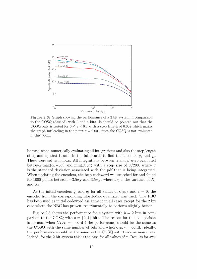
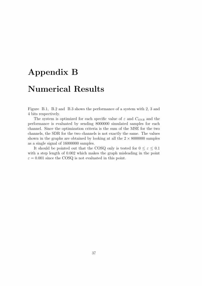
Figure 2.3: Graph showing the performance of a 2 bit system in comparisonto the COSQ (dashed) with 2 and 4 bits. It should be pointed out that theCOSQ only is tested for 0 ≤ ε ≤ 0.1 with a step length of 0.002 which makesthe graph misleading in the point ε = 0.001 since the COSQ is not evaluatedin this point.

be used when numerically evaluating all integrations and also the step lengthof x1 and x2 that is used in the full search to find the encoders q1 and q2.These were set as follows. All integrations between α and β were evaluatedbetween max(α,−5σ) and min(β, 5σ) with a step size of σ/200, where σis the standard deviation associated with the pdf that is being integrated.When updating the encoders, the best codeword was searched for and foundfor 1000 points between −3.5σX and 3.5σX , where σX is the variance of X1

and X2.

As the initial encoders q1 and q2 for all values of CSNR and ε = 0, theencoder from the corresponding Lloyd-Max quantizer was used. The FBChas been used as initial codeword assignment in all cases except for the 2 bitcase where the NBC has proven experimentally to perform slightly better.

Figure 2.3 shows the performance for a system with b = 2 bits in com-parison to the COSQ with b = {2, 4} bits. The reason for this comparisonis because when CSNR = −∞ dB the performance should be the same asthe COSQ with the same number of bits and when CSNR = ∞ dB, ideally,the performance should be the same as the COSQ with twice as many bits.Indeed, for the 2 bit system this is the case for all values of ε. Results for sys-

19

tems with 3 bits and 4 bits can be found in Appendix B. When the numberof bits is increased the performance gain of the distributed approach is notas good for all values of ε. But as soon as ε ≥ 0.003 the two curves coincideeven for the case of 4 bits. It should however be pointed out that the system,that for fully correlated sources and ε = 0, obtains the same performanceas the COSQ with twice as many bits is highly structured and therefore noteasy to find with a greedy search algorithm.

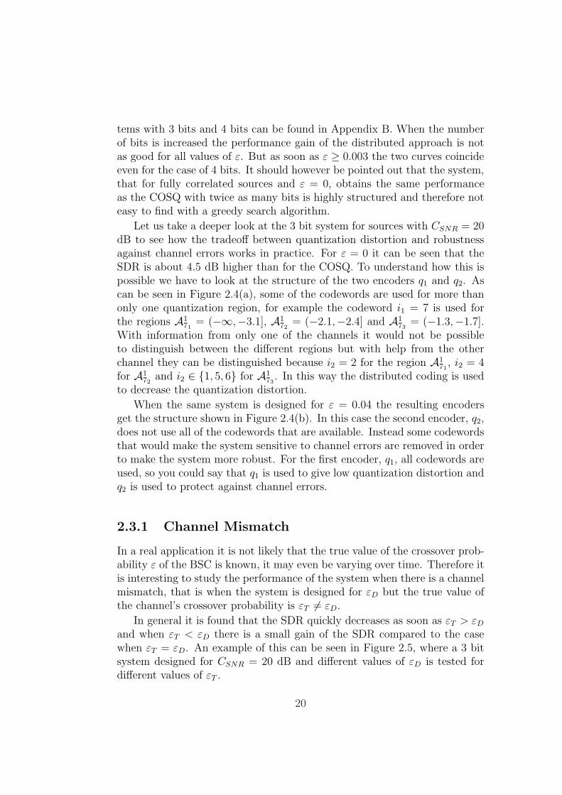
Let us take a deeper look at the 3 bit system for sources with CSNR = 20dB to see how the tradeoff between quantization distortion and robustnessagainst channel errors works in practice. For ε = 0 it can be seen that theSDR is about 4.5 dB higher than for the COSQ. To understand how this ispossible we have to look at the structure of the two encoders q1 and q2. Ascan be seen in Figure 2.4(a), some of the codewords are used for more thanonly one quantization region, for example the codeword i1 = 7 is used forthe regions A1

71= (−∞,−3.1], A1

72= (−2.1,−2.4] and A1

73= (−1.3,−1.7].

With information from only one of the channels it would not be possibleto distinguish between the different regions but with help from the otherchannel they can be distinguished because i2 = 2 for the region A1

71, i2 = 4

for A172

and i2 ∈ {1, 5, 6} for A173

. In this way the distributed coding is usedto decrease the quantization distortion.

When the same system is designed for ε = 0.04 the resulting encodersget the structure shown in Figure 2.4(b). In this case the second encoder, q2,does not use all of the codewords that are available. Instead some codewordsthat would make the system sensitive to channel errors are removed in orderto make the system more robust. For the first encoder, q1, all codewords areused, so you could say that q1 is used to give low quantization distortion andq2 is used to protect against channel errors.

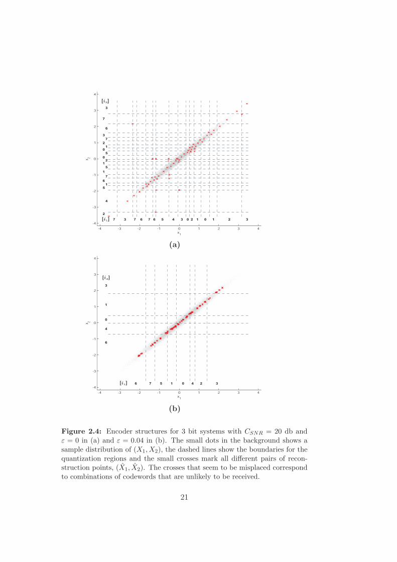
2.3.1 Channel Mismatch

In a real application it is not likely that the true value of the crossover prob-ability ε of the BSC is known, it may even be varying over time. Therefore itis interesting to study the performance of the system when there is a channelmismatch, that is when the system is designed for εD but the true value ofthe channel’s crossover probability is εT 6= εD.

In general it is found that the SDR quickly decreases as soon as εT > εD

and when εT < εD there is a small gain of the SDR compared to the casewhen εT = εD. An example of this can be seen in Figure 2.5, where a 3 bitsystem designed for CSNR = 20 dB and different values of εD is tested fordifferent values of εT .

20

(a)

(b)

Figure 2.4: Encoder structures for 3 bit systems with CSNR = 20 db andε = 0 in (a) and ε = 0.04 in (b). The small dots in the background shows asample distribution of (X1, X2), the dashed lines show the boundaries for thequantization regions and the small crosses mark all different pairs of recon-struction points, (X1, X2). The crosses that seem to be misplaced correspondto combinations of codewords that are unlikely to be received.

21

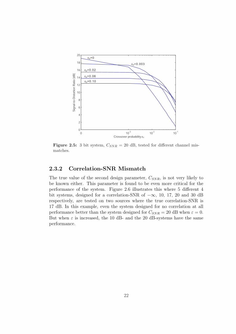
Figure 2.5: 3 bit system, CSNR = 20 dB, tested for different channel mis-matches.

2.3.2 Correlation-SNR Mismatch

The true value of the second design parameter, CSNR, is not very likely tobe known either. This parameter is found to be even more critical for theperformance of the system. Figure 2.6 illustrates this where 5 different 4bit systems, designed for a correlation-SNR of −∞, 10, 17, 20 and 30 dBrespectively, are tested on two sources where the true correlation-SNR is17 dB. In this example, even the system designed for no correlation at allperformance better than the system designed for CSNR = 20 dB when ε = 0.But when ε is increased, the 10 dB- and the 20 dB-systems have the sameperformance.

22

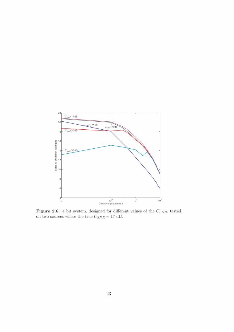
Figure 2.6: 4 bit system, designed for different values of the CSNR, testedon two sources where the true CSNR = 17 dB.

23

24

Chapter 3

Reducing Complexity

The algorithm presented in Chapter 2 works very well in practice, but thecomplexity for finding the encoders and the decoders grows exponentiallywith the number of bits that are used. Because of this problem we willinvestigate some methods that reduce the complexity which makes it possibleto increase the bit rate.

3.1 Multistage Quantization

The first approach is inspired from the field of vector quantization where itis common to use several stages of quantization. That is, instead of doingthe quantization in a single step with for example 20 bits, the quantization isdivided into two stages where you first use a 10 bit quantizer and then use asecond stage with another 10 bits to quantize the error from the first stage.

When adapting this method to correlated sources the idea is to use thesystem from Chapter 2 in the first stage of each channel and use two inde-pendent COSQ from Section 1.3.1 in the second stages. The complete systemcan be seen in Figure 3.1.

3.1.1 Analysis

Let us focus on the first channel with the encoders q11 and q12 and thedecoders g11 and g12. The most important thing to realize is that the valuethat should be sent to the second stage encoder q12 is X1 − E[X11 |X1]. Aproof of this can be constructed in the following way. First of all, let us groupthe encoder q11, the BSC and the decoder g11 into a single unit called Q11.Let us further assume that we are allowed to add a value A to the outputof Q11 where A is a function of X1 as seen in Figure 3.2. For each value of

25

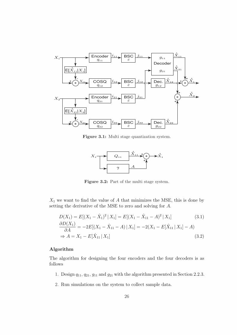
Figure 3.1: Multi stage quantization system.

Figure 3.2: Part of the multi stage system.

X1 we want to find the value of A that minimizes the MSE, this is done bysetting the derivative of the MSE to zero and solving for A.

D(X1) = E[(X1 − X1)2 |X1] = E[(X1 − X11 − A)2 |X1] (3.1)

∂D(X1)

∂A= −2E[(X1 − X11 − A) |X1] = −2(X1 − E[X11 |X1]− A)

⇒ A = X1 − E[X11 |X1] (3.2)

Algorithm

The algorithm for designing the four encoders and the four decoders is asfollows

1. Design q11, q21, g11 and g21 with the algorithm presented in Section 2.2.3.

2. Run simulations on the system to collect sample data.

26

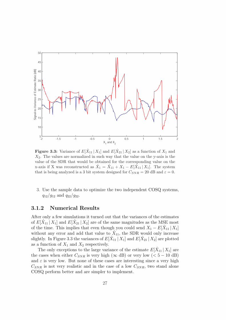
Figure 3.3: Variance of E[X11 |X1] and E[X21 |X2] as a function of X1 andX2. The values are normalized in such way that the value on the y-axis is thevalue of the SDR that would be obtained for the corresponding value on thex-axis if X was reconstructed as X1 = X11 + X1 − E[X11 |X1]. The systemthat is being analyzed is a 3 bit system designed for CSNR = 20 dB and ε = 0.

3. Use the sample data to optimize the two independent COSQ systems,q12/g12 and q22/g22.

3.1.2 Numerical Results

After only a few simulations it turned out that the variances of the estimatesof E[X11 |X1] and E[X21 |X2] are of the same magnitudes as the MSE mostof the time. This implies that even though you could send X1 − E[X11 |X1]without any error and add that value to X11, the SDR would only increaseslightly. In Figure 3.3 the variances of E[X11 |X1] and E[X21 |X2] are plottedas a function of X1 and X2 respectively.

The only exceptions to the large variance of the estimate E[X11 |X1] arethe cases when either CSNR is very high (∞ dB) or very low (< 5− 10 dB)and ε is very low. But none of these cases are interesting since a very highCSNR is not very realistic and in the case of a low CSNR, two stand aloneCOSQ perform better and are simpler to implement.

27

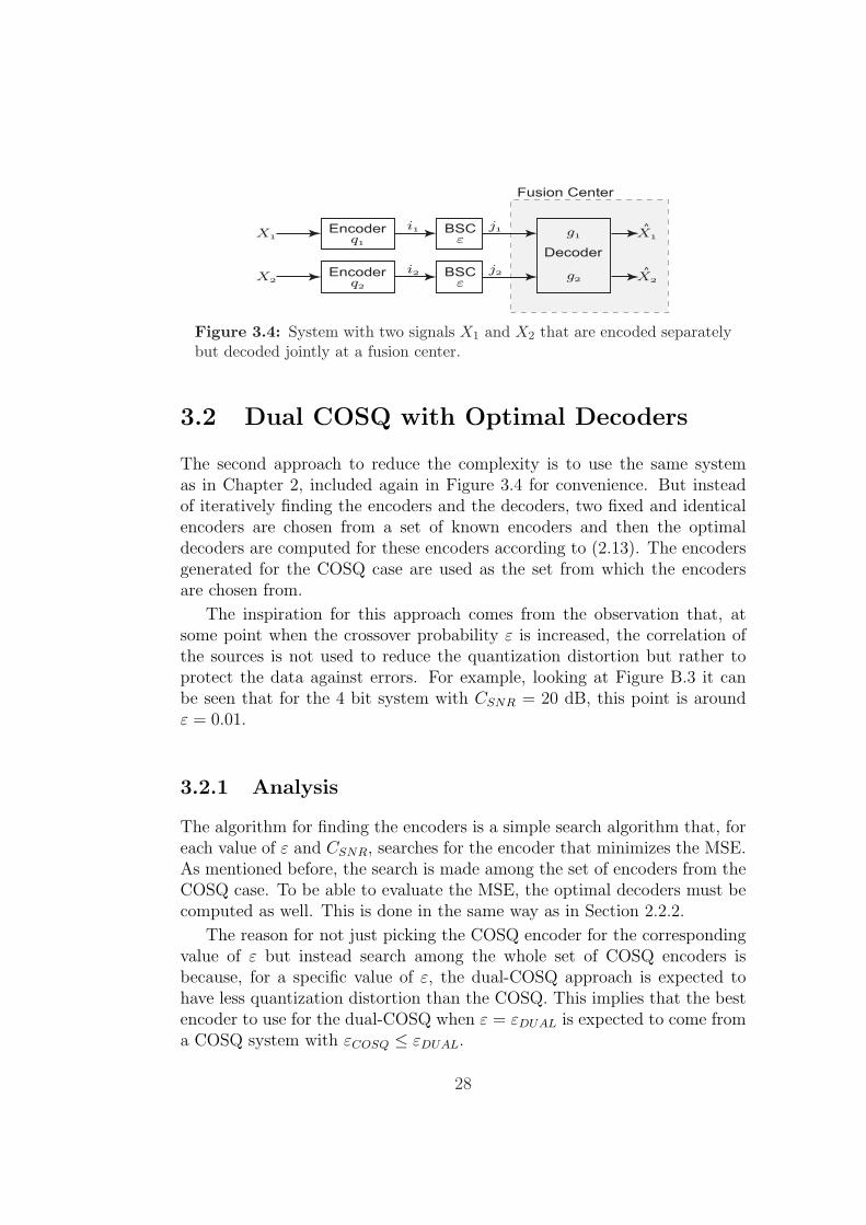
Figure 3.4: System with two signals X1 and X2 that are encoded separatelybut decoded jointly at a fusion center.

3.2 Dual COSQ with Optimal Decoders

The second approach to reduce the complexity is to use the same systemas in Chapter 2, included again in Figure 3.4 for convenience. But insteadof iteratively finding the encoders and the decoders, two fixed and identicalencoders are chosen from a set of known encoders and then the optimaldecoders are computed for these encoders according to (2.13). The encodersgenerated for the COSQ case are used as the set from which the encodersare chosen from.

The inspiration for this approach comes from the observation that, atsome point when the crossover probability ε is increased, the correlation ofthe sources is not used to reduce the quantization distortion but rather toprotect the data against errors. For example, looking at Figure B.3 it canbe seen that for the 4 bit system with CSNR = 20 dB, this point is aroundε = 0.01.

3.2.1 Analysis

The algorithm for finding the encoders is a simple search algorithm that, foreach value of ε and CSNR, searches for the encoder that minimizes the MSE.As mentioned before, the search is made among the set of encoders from theCOSQ case. To be able to evaluate the MSE, the optimal decoders must becomputed as well. This is done in the same way as in Section 2.2.2.

The reason for not just picking the COSQ encoder for the correspondingvalue of ε but instead search among the whole set of COSQ encoders isbecause, for a specific value of ε, the dual-COSQ approach is expected tohave less quantization distortion than the COSQ. This implies that the bestencoder to use for the dual-COSQ when ε = εDUAL is expected to come froma COSQ system with εCOSQ ≤ εDUAL.

28

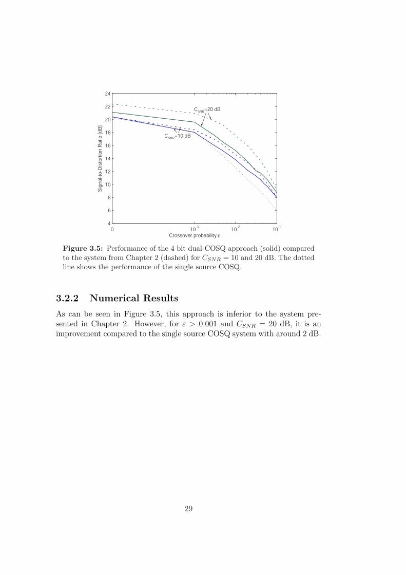
Figure 3.5: Performance of the 4 bit dual-COSQ approach (solid) comparedto the system from Chapter 2 (dashed) for CSNR = 10 and 20 dB. The dottedline shows the performance of the single source COSQ.

3.2.2 Numerical Results

As can be seen in Figure 3.5, this approach is inferior to the system pre-sented in Chapter 2. However, for ε > 0.001 and CSNR = 20 dB, it is animprovement compared to the single source COSQ system with around 2 dB.

29

30

Chapter 4

Conclusions

4.1 Comments on the Results

The algorithm presented in Chapter 2 works very well in practice. Somewhatsurprisingly the resulting encoders even use the same codeword for severalregions so that the quantization distortion is reduced for the case of small ε.For higher values of ε the correlation is instead used for protection againstchannel errors.

If the COSQ is assumed to be a good scalar quantizer then this systemseems to be a good scalar quantizer for correlated sources. This is becausethe systems designed for full correlation have the same performance as theCOSQ with twice as many bits. The only exception to this is when ε < 0.003.

The complexity is an issue. Of course the implementation of the designalgorithm can certainly be done in a more efficient way, but unfortunatelythat does not change the complexity of the underlying equations. If moresources were added the complexity would increase even more.

The multistage system presented in Section 3.1 does not give any signif-icant improvement of the performance. Even if there would have been animprovement there is a substantial increase in complexity to implement suchencoding system.

The dual-COSQ system presented in Section 3.2 works satisfyingly. Thesystem is of course suboptimal but the number of bits used by the encodercan be increased and a higher SDR may thereby be obtained.

To avoid poor performance because of mismatches between the designparameters for the system and the true values of these parameters, ε andCSNR should be chosen with some margins. This proves to be especiallyimportant for the CSNR as seen in the example in Section 2.3.2. But alsoε should be chosen with care, if there is any doubt whether the channel is

31

error free or not, the system should be designed for ε > 0.

4.2 Future Work

This section contains some ideas for future work and improvements thatcould be made.

First of all, the complexity of the design algorithm could be decreased byonly looking at single bit errors for each transmitted codeword. For low valuesof ε these are most likely to occur. It is also possible that the complexitycould be reduced by enforcing some kind of structure to the encoders.

For the use in WSNs, the number of possible sources should be increased.One way to do this without increasing the complexity too much is to decodethe data from correlated sensors in pairs. The final estimate of the sensor’sreading could then be calculated as a weighted sum of the readings from allpair of sensors, with less weight put on values that seem unreasonable.

32

Appendix A

Derivations

All derivations are done for the following system

X1 = Y + N1 (A.1)

X2 = Y + N2 (A.2)

where Y , N1 and N2 are three independent Gaussian distributed randomvariables with variances σ2

Y , σ2N1, σ2

N2 and means mY , mN1 , mN2 respectively.

A.1 pdf of a Gaussian Variable

The pdf, fY (y), of the Gaussian variable Y is defined as

fY (y) =1√

2πσ2Y

exp

(− (y −mY )2

2σ2Y

). (A.3)

33

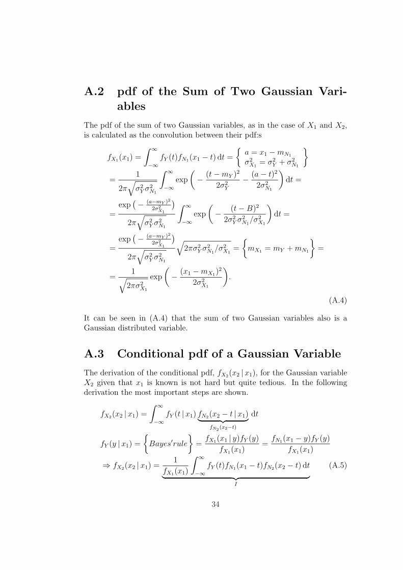
A.2 pdf of the Sum of Two Gaussian Vari-

ables

The pdf of the sum of two Gaussian variables, as in the case of X1 and X2,is calculated as the convolution between their pdf:s

fX1(x1) =

∫ ∞

−∞fY (t)fN1(x1 − t) dt =

{a = x1 −mN1

σ2X1

= σ2Y + σ2

N1

}

=1

2π√

σ2Y σ2

N1

∫ ∞

−∞exp

(− (t−mY )2

2σ2Y

− (a− t)2

2σ2N1

)dt =

=exp

(− (a−mY )2

2σ2X1

)

2π√

σ2Y σ2

N1

∫ ∞

−∞exp

(− (t−B)2

2σ2Y σ2

N1/σ2

X1

)dt =

=exp

(− (a−mY )2

2σ2X1

)

2π√

σ2Y σ2

N1

√2πσ2

Y σ2N1

/σ2X1

=

{mX1 = mY + mN1

}=

=1√

2πσ2X1

exp

(− (x1 −mX1)

2

2σ2X1

).

(A.4)

It can be seen in (A.4) that the sum of two Gaussian variables also is aGaussian distributed variable.

A.3 Conditional pdf of a Gaussian Variable

The derivation of the conditional pdf, fX2(x2 |x1), for the Gaussian variableX2 given that x1 is known is not hard but quite tedious. In the followingderivation the most important steps are shown.

fX2(x2 |x1) =

∫ ∞

−∞fY (t |x1) fN2(x2 − t |x1)︸ ︷︷ ︸

fN2(x2−t)

dt

fY (y |x1) =

{Bayes′rule

}=

fX1(x1 | y)fY (y)

fX1(x1)=

fN1(x1 − y)fY (y)

fX1(x1)

⇒ fX2(x2 |x1) =1

fX1(x1)

∫ ∞

−∞fY (t)fN1(x1 − t)fN2(x2 − t) dt

︸ ︷︷ ︸I

(A.5)

34

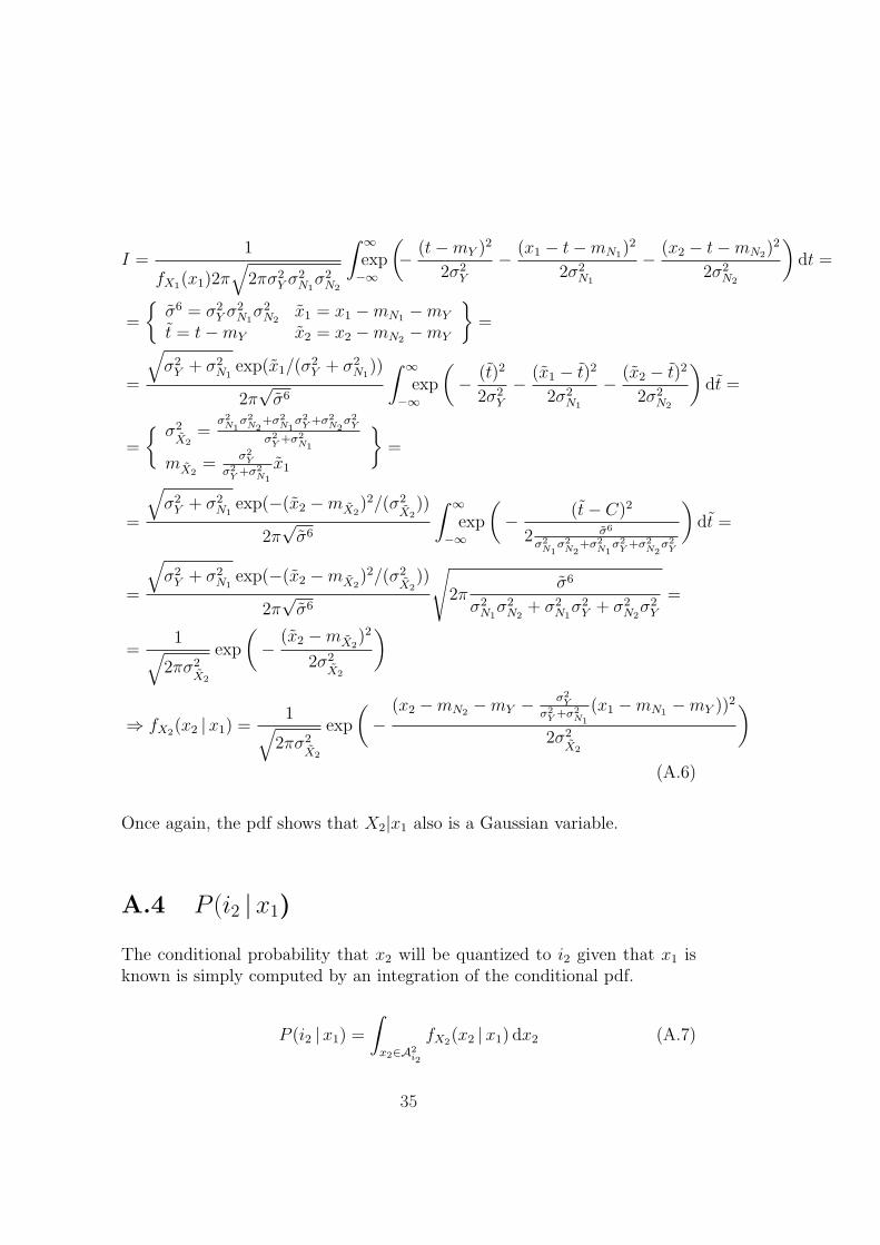
I =1

fX1(x1)2π√

2πσ2Y σ2

N1σ2

N2

∫ ∞

−∞exp

(− (t−mY )2

2σ2Y

− (x1 − t−mN1)2

2σ2N1

− (x2 − t−mN2)2

2σ2N2

)dt =

=

{σ6 = σ2

Y σ2N1

σ2N2

x1 = x1 −mN1 −mY

t = t−mY x2 = x2 −mN2 −mY

}=

=

√σ2

Y + σ2N1

exp(x1/(σ2Y + σ2

N1))

2π√

σ6

∫ ∞

−∞exp

(− (t)2

2σ2Y

− (x1 − t)2

2σ2N1

− (x2 − t)2

2σ2N2

)dt =

=

{ σ2X2

=σ2

N1σ2

N2+σ2

N1σ2

Y +σ2N2

σ2Y

σ2Y +σ2

N1

mX2=

σ2Y

σ2Y +σ2

N1

x1

}=

=

√σ2

Y + σ2N1

exp(−(x2 −mX2)2/(σ2

X2))

2π√

σ6

∫ ∞

−∞exp

(− (t− C)2

2 σ6

σ2N1

σ2N2

+σ2N1

σ2Y +σ2

N2σ2

Y

)dt =

=

√σ2

Y + σ2N1

exp(−(x2 −mX2)2/(σ2

X2))

2π√

σ6

√2π

σ6

σ2N1

σ2N2

+ σ2N1

σ2Y + σ2

N2σ2

Y

=

=1√

2πσ2X2

exp

(− (x2 −mX2

)2

2σ2X2

)

⇒ fX2(x2 |x1) =1√

2πσ2X2

exp

(−

(x2 −mN2 −mY − σ2Y

σ2Y +σ2

N1

(x1 −mN1 −mY ))2

2σ2X2

)

(A.6)

Once again, the pdf shows that X2|x1 also is a Gaussian variable.

A.4 P (i2 |x1)

The conditional probability that x2 will be quantized to i2 given that x1 isknown is simply computed by an integration of the conditional pdf.

P (i2 |x1) =

∫

x2∈A2i2

fX2(x2 | x1) dx2 (A.7)

35

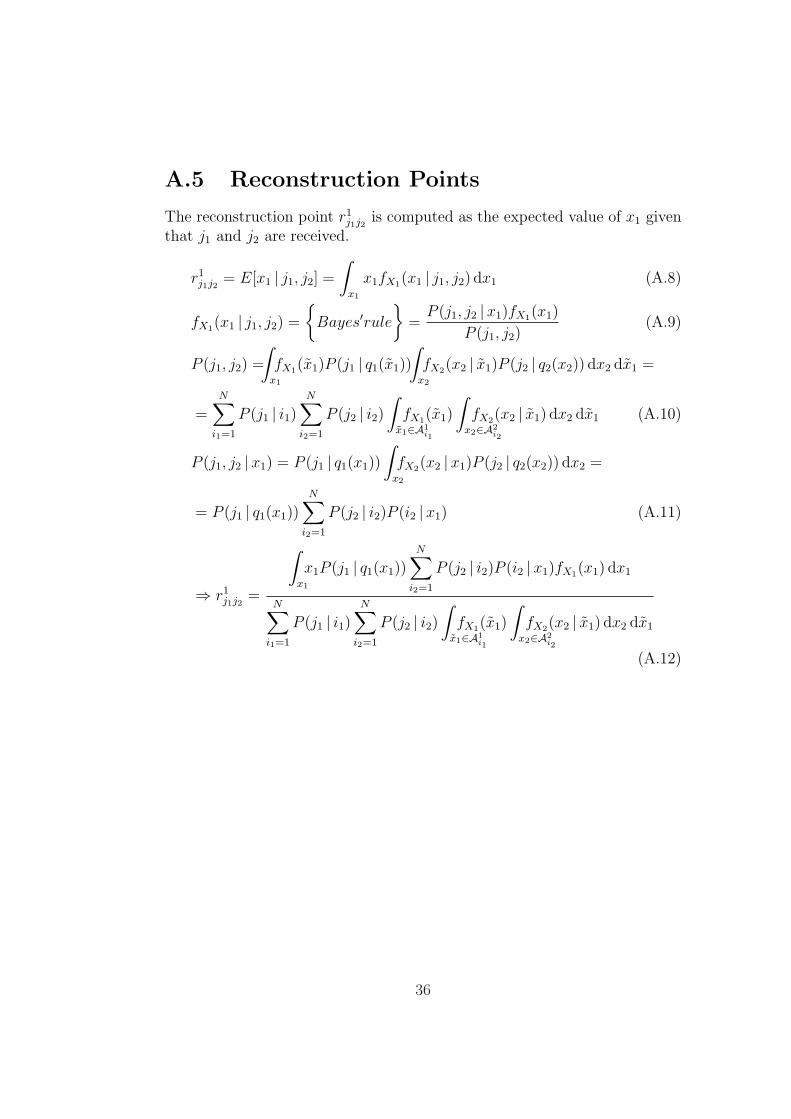
A.5 Reconstruction Points

The reconstruction point r1j1j2

is computed as the expected value of x1 giventhat j1 and j2 are received.

r1j1j2

= E[x1 | j1, j2] =

∫

x1

x1fX1(x1 | j1, j2) dx1 (A.8)

fX1(x1 | j1, j2) =

{Bayes′rule

}=

P (j1, j2 |x1)fX1(x1)

P (j1, j2)(A.9)

P (j1, j2) =

∫

x1

fX1(x1)P (j1 | q1(x1))

∫

x2

fX2(x2 | x1)P (j2 | q2(x2)) dx2 dx1 =

=N∑

i1=1

P (j1 | i1)N∑

i2=1

P (j2 | i2)∫

x1∈A1i1

fX1(x1)

∫

x2∈A2i2

fX2(x2 | x1) dx2 dx1 (A.10)

P (j1, j2 | x1) = P (j1 | q1(x1))

∫

x2

fX2(x2 |x1)P (j2 | q2(x2)) dx2 =

= P (j1 | q1(x1))N∑

i2=1

P (j2 | i2)P (i2 |x1) (A.11)

⇒ r1j1j2

=

∫

x1

x1P (j1 | q1(x1))N∑

i2=1

P (j2 | i2)P (i2 | x1)fX1(x1) dx1

N∑i1=1

P (j1 | i1)N∑

i2=1

P (j2 | i2)∫

x1∈A1i1

fX1(x1)

∫

x2∈A2i2

fX2(x2 | x1) dx2 dx1

(A.12)

36

Appendix B

Numerical Results

Figure B.1, B.2 and B.3 shows the performance of a system with 2, 3 and4 bits respectively.

The system is optimized for each specific value of ε and CSNR and theperformance is evaluated by sending 8000000 simulated samples for eachchannel. Since the optimization criteria is the sum of the MSE for the twochannels, the SDR for the two channels is not exactly the same. The valuesshown in the graphs are obtained by looking at all the 2× 8000000 samplesas a single signal of 16000000 samples.

It should be pointed out that the COSQ only is tested for 0 ≤ ε ≤ 0.1with a step length of 0.002 which makes the graph misleading in the pointε = 0.001 since the COSQ is not evaluated in this point.

37

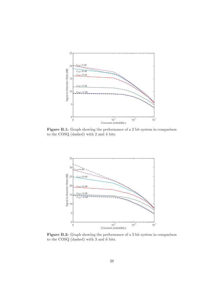
Figure B.1: Graph showing the performance of a 2 bit system in comparisonto the COSQ (dashed) with 2 and 4 bits.

Figure B.2: Graph showing the performance of a 3 bit system in comparisonto the COSQ (dashed) with 3 and 6 bits.

38

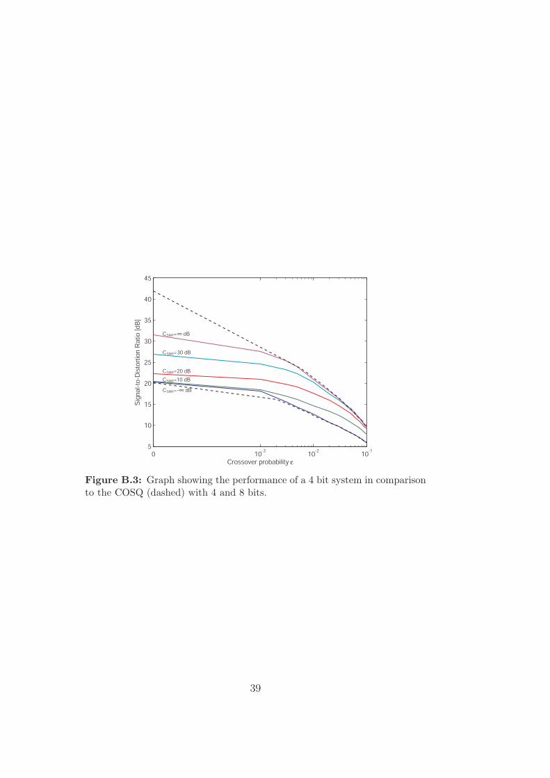
Figure B.3: Graph showing the performance of a 4 bit system in comparisonto the COSQ (dashed) with 4 and 8 bits.

39

40

Bibliography

[1] S. P. Lloyd, “Least Squares Quantization in PCM,” Bell TelephoneLaboratories Paper, 1957.

[2] S. P. Lloyd, “Least Squares Quantization in PCM,” IEEE Trans. onInformation Theory, vol. IT-28, no. 2, pp. 129–137, March 1982.

[3] J. Max, “Quantizing for Minimum Distortion,” IRE Trans. on Infor-mation Theory, vol. IT-6, pp. 7–12, March 1960.

[4] A. Acero X. Huang and H.W. Hon, Spoken Language Processing,Prentice-Hall, Upper Saddle River, New Jersey 07458, USA, 2001.

[5] Y. Linde, A. Buzo and R. M. Gray, “An Algorithm for Vector QuantizerDesign,” IEEE Trans. on Communications, vol. COM-28, no. 1, pp. 84–95, January 1980.

[6] T. M. Cover and J. A. Thomas, Elements of Information Theory, Wiley-Interscience, 1991.

[7] N. Farvardin and V. Vaishampayan, “Optimal Quantizer Design forNoisy Channels: An Approach to Combined Source-Channel Coding.,”IEEE Trans. on Information Theory, vol. 33, no. 6, pp. 827–838, Novem-ber 1987.

[8] D. Slepian and J. K. Wolf, “Noiseless Coding of Correlated InformationSources.,” IEEE Trans. on Information Theory, vol. IT-19, no. 4, pp.471–480, July 1973.

[9] A. D. Wyner and J. Ziv, “The Rate-Distortion Function for Source Cod-ing with Side Information at the Decoder,” IEEE Trans. on InformationTheory, vol. IT-22, no. 1, pp. 1–10, January 1976.

[10] S. S. Pradhan, J. Kusuma and K. Ramchandran, “Distributed Com-pression in a Dense Microsensor Network,” IEEE Trans. on Signal Pro-cessing, vol. 19, no. 2, pp. 51–60, March 2002.

41

[11] Z. Xiong, A. D. Liveris and S. Cheng, “Distributed Source Coding forSensor Networks,” IEEE Trans. on Signal Processing, vol. 21, no. 5, pp.80–94, September 2004.

[12] B. Kleijn, A Basis for Source Coding, KTH (Royal Institue of Technol-ogy), 100 44 Stockholm, Sweden, 2004.

42