
Invariant Manifolds and Applications for Functional Differential Equations of Mixed Type
265
Invariant Manifolds and Applications for Functional Differential Equations of Mixed Type Proefschrift ter verkrijging van de graad van Doctor aan de Universiteit Leiden, op gezag van de Rector Magnificus prof. mr. P. F. van der Heijden, volgens besluit van het College voor Promoties te verdedigen op donderdag 12 juni 2008 klokke 11.15 uur door Hermen Jan Hupkes geboren te Gouda in 1981
Transcript of Invariant Manifolds and Applications for Functional Differential Equations of Mixed Type
Invariant Manifolds and Applications forFunctional Differential Equations of Mixed Type
Proefschrift
ter verkrijging vande graad van Doctor aan de Universiteit Leiden,
op gezag van de Rector Magnificusprof. mr. P. F. van der Heijden,
volgens besluit van het College voor Promotieste verdedigen op donderdag 12 juni 2008
klokke 11.15 uurdoor
Hermen Jan Hupkes
geboren te Goudain 1981
Samenstelling van de promotiecommissie:
promotor: Prof. dr. S. M. Verduyn Lunel
referent: Prof. dr. B. Sandstede (University of Surrey, UK)
overige leden: Prof. dr. ir. L. A. PeletierDr. S. C. HilleProf. dr. O. Diekmann (Universiteit Utrecht)Prof. dr. P. Stevenhagen
Invariant Manifolds and Applications for
Functional Differential Equations of
Mixed Type
Hupkes, Hermen Jan, 1981-Invariant Manifolds and Applications for Functional Differential Equations of Mixed TypePrinted by Universal Press - VeenendaalAMS 2000 Subj. class. code: 34K18, 34K17, 34K19, 37G15NUR: 921ISBN-13: 978-90-9023127-3
email: [email protected]
THOMAS STIELTJES INSTITUTE
FOR MATHEMATICS
c© H.J. Hupkes, Leiden 2008.
All rights reserved. No part of this publication may be reproduced in any formwithout prior written permission from the author.
Contents
Preface iii
1. Introduction 11.1. Travelling Waves in Lattice Systems . . . . . . . . . . . . . . . . . . . . . 51.2. Classical Construction of Invariant Manifolds . . . . . . . . . . . . . . . . 101.3. Invariant Manifolds for MFDEs . . . . . . . . . . . . . . . . . . . . . . . 181.4. Optimal Control Capital Market Dynamics . . . . . . . . . . . . . . . . . . 221.5. Economic Life-Cycle Model . . . . . . . . . . . . . . . . . . . . . . . . . 271.6. Monetary Cycles with Endogenous Retirement . . . . . . . . . . . . . . . 301.7. Frenkel-Kontorova models . . . . . . . . . . . . . . . . . . . . . . . . . . 351.8. Numerical Methods . . . . . . . . . . . . . . . . . . . . . . . . . . . . . . 36
2. Center Manifolds Near Equilibria 412.1. Introduction . . . . . . . . . . . . . . . . . . . . . . . . . . . . . . . . . . 412.2. Main Results . . . . . . . . . . . . . . . . . . . . . . . . . . . . . . . . . 432.3. Linear Inhomogeneous Equations . . . . . . . . . . . . . . . . . . . . . . 472.4. The State Space . . . . . . . . . . . . . . . . . . . . . . . . . . . . . . . . 512.5. Pseudo-Inverse for Linear Inhomogeneous Equations . . . . . . . . . . . . 542.6. A Lipschitz Smooth Center Manifold . . . . . . . . . . . . . . . . . . . . . 592.7. Smoothness of the center manifold . . . . . . . . . . . . . . . . . . . . . . 622.8. Dynamics on the Center Manifold . . . . . . . . . . . . . . . . . . . . . . 692.9. Parameter Dependence . . . . . . . . . . . . . . . . . . . . . . . . . . . . 712.10. Hopf Bifurcation . . . . . . . . . . . . . . . . . . . . . . . . . . . . . . . 722.11. Example: Double Eigenvalue At Zero . . . . . . . . . . . . . . . . . . . . 78
3. Center Manifolds for Smooth Differential-Algebraic Equations 813.1. Introduction . . . . . . . . . . . . . . . . . . . . . . . . . . . . . . . . . . 813.2. Main Results . . . . . . . . . . . . . . . . . . . . . . . . . . . . . . . . . 833.3. Preliminaries . . . . . . . . . . . . . . . . . . . . . . . . . . . . . . . . . 863.4. The state space . . . . . . . . . . . . . . . . . . . . . . . . . . . . . . . . 903.5. Linear Inhomogeneous Equations . . . . . . . . . . . . . . . . . . . . . . 933.6. The pseudo-inverse . . . . . . . . . . . . . . . . . . . . . . . . . . . . . . 983.7. The Center Manifold . . . . . . . . . . . . . . . . . . . . . . . . . . . . . 100
ii Contents
4. Center Manifolds near Periodic Orbits 1074.1. Introduction . . . . . . . . . . . . . . . . . . . . . . . . . . . . . . . . . . 1074.2. Main Results . . . . . . . . . . . . . . . . . . . . . . . . . . . . . . . . . 1104.3. Preliminaries . . . . . . . . . . . . . . . . . . . . . . . . . . . . . . . . . 1124.4. Linear inhomogeneous equations . . . . . . . . . . . . . . . . . . . . . . . 1154.5. The state space . . . . . . . . . . . . . . . . . . . . . . . . . . . . . . . . 1194.6. Time dependence . . . . . . . . . . . . . . . . . . . . . . . . . . . . . . . 1234.7. The center manifold . . . . . . . . . . . . . . . . . . . . . . . . . . . . . . 1284.8. Smoothness of the center manifold . . . . . . . . . . . . . . . . . . . . . . 132
5. Travelling Waves Close to Propagation Failure 1415.1. Introduction . . . . . . . . . . . . . . . . . . . . . . . . . . . . . . . . . . 1415.2. Linear Functional Differential Equations of Mixed Type . . . . . . . . . . . 1445.3. Global Structure . . . . . . . . . . . . . . . . . . . . . . . . . . . . . . . . 1495.4. The Algorithm . . . . . . . . . . . . . . . . . . . . . . . . . . . . . . . . 1595.5. Examples . . . . . . . . . . . . . . . . . . . . . . . . . . . . . . . . . . . 1645.6. Extensions . . . . . . . . . . . . . . . . . . . . . . . . . . . . . . . . . . . 168
5.6.1. Ising models . . . . . . . . . . . . . . . . . . . . . . . . . . . . . 1685.6.2. Higher Dimensional Systems . . . . . . . . . . . . . . . . . . . . . 170
5.7. Proof of Theorem 5.2.10 . . . . . . . . . . . . . . . . . . . . . . . . . . . 1725.8. Implementation Issues . . . . . . . . . . . . . . . . . . . . . . . . . . . . 179
6. Lin’s Method and Homoclinic Bifurcations 1816.1. Introduction . . . . . . . . . . . . . . . . . . . . . . . . . . . . . . . . . . 1816.2. Main Results . . . . . . . . . . . . . . . . . . . . . . . . . . . . . . . . . 1846.3. Preliminaries . . . . . . . . . . . . . . . . . . . . . . . . . . . . . . . . . 1906.4. Exponential Dichotomies . . . . . . . . . . . . . . . . . . . . . . . . . . . 1966.5. Parameter-Dependent Exponential Dichotomies . . . . . . . . . . . . . . . 2036.6. Lin’s Method for MFDEs . . . . . . . . . . . . . . . . . . . . . . . . . . . 2106.7. The remainder term . . . . . . . . . . . . . . . . . . . . . . . . . . . . . . 2166.8. Derivative of the remainder term . . . . . . . . . . . . . . . . . . . . . . . 222
Appendix 227A. Embedded Contractions . . . . . . . . . . . . . . . . . . . . . . . . . . . . 227B. Fourier and Laplace Transform . . . . . . . . . . . . . . . . . . . . . . . . 230C. Hopf Bifurcation Theorem . . . . . . . . . . . . . . . . . . . . . . . . . . 231D. Nested Differentiation . . . . . . . . . . . . . . . . . . . . . . . . . . . . . 232
Samenvatting 247
Curriculum Vitae 253

Preface
Throughout a significant portion of recorded history, mankind has expressed a fascinationfor the concepts of motion and change. In 1600 BC the Babylonians had already constructedstar charts based on detailed observations of the rising of celestial bodies. They used thesecharts to determine the best harvesting and planting times. Ever since the Jewish peopleemerged from their wanderings through the Sinai desert, they needed to keep track of lu-nar cycles to calculate the exact dates for their numerous feasts. They knew that God hadpromised Noah (in Genesis 8:22, King James Bible):
While the earth remaineth, seedtime and harvest, and cold and heat,and summer and winter, and day and night shall not cease.
The ancient Greeks started studying the subject from a more philosophical point ofview. The famous quote παντα ρει is due to Heraclitus (540 BC), who argued that theworld around us is always in motion. This assertion was pulled apart masterfully by Zenoof Elea (450 BC), who laid down the groundwork for modern calculus through his deviousparadoxes. The most well-known of these is probably the story of Achilles who shouldnever be able to overtake the tortoise, a mind-teaser that still sharpens the minds of children,students and scholars alike.
Mathematical Models
In The Almagest, Ptolemaeus (150 AD) proposed the first comprehensive mathematical sys-tem to describe the planetary motions. His predictions were actually quite accurate, in spiteof the fact that they were based upon a stationary earth, fixed at the center of the cosmos. Hismodel found widespread favour for more than a thousand years, until increasingly accurateobservations and work by Oresme, Copernicus, Galileo and Kepler led to the acceptance ofthe heliocentric point of view in the seventeenth century. The crowning achievement of thisgolden age of astronomy was undoubtedly the formulation by Newton of the differentialequations that describe the laws of gravity and the subsequent development of calculus byNewton and Leibniz. The realization that very complex and puzzling behaviour over longperiods of time could be described by simple rules governing rates of change on extremelysmall timescales, led to the birth of dynamical systems theory as we know it today.
The eighteenth and nineteenth century witnessed the development of a relatively com-plete theory for linear ordinary differential equations. In addition, perturbation methods
iv Preface
were developed and applied to systems with weak nonlinear interactions. The study of gen-eral nonlinear systems far from equilibria however long remained a barren area. At the endof the nineteenth century Poincare and Lyapunov both added new impetus to the subjectby abandoning the search for explicit solutions to differential equations in favour of a morequalitative approach. In particular, Poincare introduced topological methods to the theory,treating the full trajectory traversed by the components of a dynamical system as a singlegeometrical object. He was the first to use Poincare sections to analyze the behaviour of sys-tems near periodic orbits and fixed points, locally reducing the continuous-time dynamics toa discrete iteration map. His subsequent research on the behaviour of intersections of stableand unstable manifolds allowed him to prove that the solar system is highly unstable andmarked the birth of the modern theory of chaos. Lyapunov on the other hand laid the basisfor the current theory of stability, by providing definitions that are still important today andpioneering the use of energy methods.
The marriage between geometry and analysis thus initiated proved to be particularlyfruitful. Major contributions to the current relatively complete theory for planar systemswere made by Birkhoff [22] and Andronov et al. [2, 3, 4, 5]. Import advances in chaoticsystems were sparked by the oscillators studied by Duffing [48] and van der Pol [157], themeteorological problem considered by Lorentz [107] and important results for integrablesystems obtained by Arnold [6, 7, 8]. Readers that are interested in detailed accounts of thedevelopment of the finite dimensional theory should consult the books by Guckenheimerand Holmes [71] and Katok and Hasselblatt [91].
Infinite dimensional systems
In the later part of the twentieth century there has been an increasing tendency to fit partialdifferential equations into the framework of dynamical systems. For elliptic PDEs this wasinitiated by Kirchgassner [94], who studied nonlinear boundary value problems in infiniteelliptic cylinders, treating the unbounded spatial direction as a temporal coordinate. Thesedevelopments have lead to the formation of an active research community in the area ofinfinite dimensional systems. We refer to [138, Chapter 1] for a nice light-weight overviewof the history of this subject, which touches upon most of the major tools and techniquesthat have been developed. By contrast, our short presentation here will merely highlightsome aspects that have a direct connection to the subject of this thesis. Hopefully, this willassist the reader in viewing the developments described throughout this work in the broadcontext of infinite dimensional evolution equations.
The most important obstacle that has to be overcome in an infinite dimensional setting,is the fact that Banach spaces lack many of the desirable properties that are taken for grantedin finite dimensional spaces. This causes many geometric arguments that work beautifully inRn to break down. Furthermore, one needs to worry about domains of operators, regularityof solutions and ill-posedness of initial value problems, which all tend to make many argu-ments very technical. A logical first step in the development of the theory would of coursebe to identify the parts of the powerful finite dimensional toolbox that can be salvaged foruse in Banach space settings. Indeed, this is still one of the main themes of research in thisarea.
Preface v
Early on in the twentieth century the foundations for linear semigroup theory were al-ready being laid, in an effort to generalize the matrix exponentials that appear ubiquitouslywhen studying ODEs. The theory reached maturity in 1948 with the formulation of theHille Yosida generation theorem [79, 169], which provides criteria to determine if a givenlinear operator can be exponentiated in a sensible fashion. Since then the use of semigroupshas branched out considerably and they now play an important role in many applications,including stochastic processes, partial differential equations, quantum mechanics, infinite-dimensional control theory and integro-differential equations [55].
Even though the use of semigroups has proved to be extremely successful, there is stilla wide class of systems in which the machinery cannot be so readily applied. As an impor-tant example, we mention situations where the linear operator describing the infinitesimalchange of a system has unbounded spectrum both to the left and right of the imaginaryaxis. One cannot define a strongly continuous semigroup that behaves as the exponentialof such an operator. This difficulty can often be circumvented by splitting the state spaceof the system into two separate parts, that both do allow the construction of a semigroup.One of these will however only be defined in backward time. Such a splitting is referred toas an exponential dichotomy. Work on this subject in finite dimensions can be traced backto Lyapunov [109] and Perron [124], but Coppel established the important fact that suchsplittings are robust under perturbations [37]. Results on exponential splittings in infinitedimensional systems were obtained by Sacker and Sell [133], Henry [77], Pliss and Sell[125] and Sandstede and Scheel [135].
As in the finite dimensional situation, invariant manifolds play a fundamental role in thestudy of nonlinear systems. A very important structure in this respect is the so-called centermanifold, which according to Vanderbauwhede and Iooss forms one of the cornerstones ofthe theory of infinite dimensional dynamical systems [158]. The reason for this is that smallamplitude variations near non-hyperbolic equilibria can be captured by a flow on a smoothinvariant center manifold, which typically is finite dimensional. In addition, this flow canoften be explicitly computed up to arbitrary order. In view of the considerations above itshould be clear that such a reduction from an infinite to a finite dimensional setting can beextremely powerful. As a consequence many different authors have worked on the subjectfrom many different perspectives. We mention here the constructions for elliptic PDEs dueto Mielke [118, 119], the results on semilinear PDEs by Bates and Jones [14] and the workby Diekmann and van Gils [44] on Volterra integral equations. To be fair, we should alsonote that infinite dimensional center manifolds can also be encountered, see e.g. a paper byScarpellini [136].
When considering a dissipative evolution equation, it becomes feasible to study theglobal attractor associated to the system. This object attracts all bounded sets and hencecaptures the long-term behaviour of any orbit. It has been established in quite some gen-erality that this global object has finite Hausdorff dimension [110, 116], although little isknown about its geometry, which often has a fractal nature. Important topics in this areainclude smooth approximations of these attractors [64], classifications based on connectionequivalence using Morse index theory [60, 61] and estimates of attractor dimensions fromsystem parameters [154].
vi Preface
Retarded Functional Differential Equations
In the study of evolution equations, the underlying principal of causality states that the futurestate of the system is independent of the past states and is determined solely by the present.Many physical systems however feature feedback mechanisms with a non-negligible timelag. Of course, this can still be fitted into the evolution equation framework by extendingthe state space to include the relevant portion of the system’s past. The price one has to payis that this extended state space will be infinite dimensional, even if the original state spaceis finite dimensional. In addition, a naive application of this approach raises major technicalcomplications if one wishes to add small perturbations to the original equations.
These issues are addressed by the theory of retarded functional differential equations,which was pioneered by Volterra [161]. Many authors have since contributed to the theoryand a comprehensive overview can now be found in the monographs by Hale and VerduynLunel [72] and Diekmann et al. [45]. The main technical tool exhibited in the latter work,is the development of a sun-star semigroup calculus that allows the (finite dimensional)original state space to be separated in a sense from the part of the extended state space thatkeeps track of the ”past” of the system. This technique paved the way for the construction ofinvariant manifolds and consequently opened up the development of the nonlinear theory.
Functional Differential Equations of Mixed Type
Functional differential equations of mixed type (MFDEs) generalize the retarded equationsmentioned above, in the sense that the rate of change of a system is allowed to depend onfuture states as well as past states. MFDEs have attracted considerable attention over the pasttwo decades. This interest has been sparked chiefly due to the importance of MFDEs in thestudy of travelling wave solutions to differential equations posed on lattices (LDEs). Theselattice based systems arise naturally when modelling systems that possess a discrete spatialstructure. In addition, MFDEs play a major role in a number of applications from economictheory. We refer to Chapter 1 for an extensive discussion on these modelling aspects.
The Fredholm theory for linear MFDEs was developed by Mallet-Paret [112], whileimportant results concerning exponential dichotomies were obtained by Rustichini [130]for autonomous systems. The latter work was later extended to nonautonomous systemssimultaneously by Mallet-Paret and Verduyn Lunel [115] on the one hand and Harterichand Sandstede [75] on the other.
This thesis should be seen as a continuation of these efforts to prepare the rich con-cepts and techniques currently available in infinite dimensional systems theory for use inthe context of MFDEs and LDEs. In particular, we focus heavily on the construction ofinvariant manifolds for MFDEs. Major difficulties that need to be overcome in this respectare the absence of a semiflow and the ill-posedness of the natural initial value problem. Thisprecludes the direct application of the ideas developed for retarded functional differentialequations, which at first sight would appear to be closely related to MFDEs. A lengthierdiscussion concerning these dissimilarities can be found in Chapter 1. As a consequence,the methods employed here differ somewhat from those in [45]. They may best be de-scribed as a mixture of the classical Lyapunov-Perron techniques with those that were usedby Mielke for elliptic PDEs [118]. In particular, in Chapter 2 we provide a center manifold

Preface vii
framework for autonomous MFDEs, while the same is done for autonomous differential-algebraic functional equations in Chapter 3. In a similar spirit, Chapter 4 is concerned withthe development of Floquet theory for periodic MFDEs. In Chapter 6 we move on to studyhomoclinic bifurcations. We also pay a considerable amount of attention to the applicationrange of these results, discussing and numerically analyzing models from economic theory,solid state physics and biology in Chapters 1 and 5.

Chapter 1
Introduction
This thesis is focussed entirely on the study of functional differential equations of mixedtype. Such equations can be written in the form
x ′(ξ) = G(xξ ), (1.1)
in which x is a continuous function, G is a nonlinear mapping from C([−1, 1],Cn) intoCn and the state xξ ∈ C([−1, 1],Cn) is defined by xξ (θ) = x(ξ + θ) for all ξ ∈ R. Thenonlinearity G thus typically depends on both advanced and retarded arguments of x , whichdistinguishes our setting from the by now extensively studied area of delay differential equa-tions.
We will be specially interested in versions of (1.1) that depend on one or more param-eters. In particular, we wish to study changes in the behaviour of (1.1) that arise as theseparameters are varied. Such changes are commonly referred to as bifurcations and through-out the present work they will be explored from both a theoretical and a numerical point ofview. A significant portion of the research described here was motivated directly by prob-lems encountered in the modelling community. To illustrate this, we will demonstrate theapplication range of our results by discussing several such examples.
Although equations of the form (1.1) have appeared haphazardly in the literature forat least forty years, active interest in these functional differential equations of mixed type(MFDEs) has been limited to the last two decades. Surprisingly enough, this increase inactivity was sparked more or less simultaneously by developments in two at first sight com-pletely unrelated subject areas, namely physical and biological modelling on the one sideand economic theory on the other. We will explain both developments here in some detail.
Lattice-based Modelling
Motivated by the study of physical structures such as crystals, grids of neurons and popu-lation patches, an increasing demand has arisen over the last few decades for mathematicalmodelling techniques that reflect the spatial discreteness that such systems possess. In the
2 1. Introduction
past, the additional complexity of the resulting equations often posed as a deterrent to de-viate from the classical models, which were most often based on ordinary and partial dif-ferential equations. The increase of computer power during the last few decades howeverhas served to remove this obstacle. As a consequence, a wave of numerical investigationshas been initiated, focussing on the evolution of patterns that live on discrete lattices. Thespectacular results that have been obtained have in fact opened up some thriving new areasin the field of dynamical systems theory.
-14 -12 -10 -8 -6 -4 -2 0 2 4
-1.2
-1.0
-0.8
-0.6
-0.4
-0.2
0.0
0.2
0.4
0.6
0.8
1.0
1.2
ρ = 0.90
ρ = 0.70
ρ = 0.54
ρ = 0.36
ρ = 0.30
ρ = 0.20
ρ = 0.10
ρ = 0.08
ρ = 0.00
φ(ξ
)
ξ
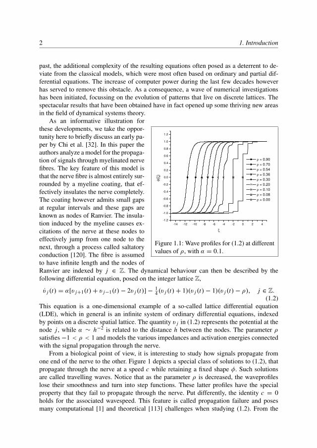
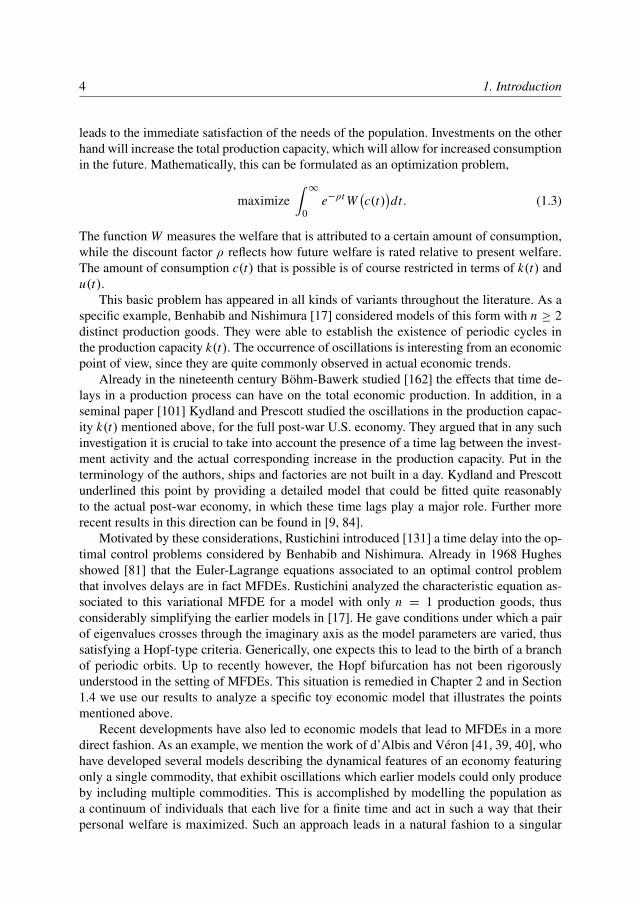
Figure 1.1: Wave profiles for (1.2) at differentvalues of ρ, with α = 0.1.
As an informative illustration forthese developments, we take the oppor-tunity here to briefly discuss an early pa-per by Chi et al. [32]. In this paper theauthors analyze a model for the propaga-tion of signals through myelinated nervefibres. The key feature of this model isthat the nerve fibre is almost entirely sur-rounded by a myeline coating, that ef-fectively insulates the nerve completely.The coating however admits small gapsat regular intervals and these gaps areknown as nodes of Ranvier. The insula-tion induced by the myeline causes ex-citations of the nerve at these nodes toeffectively jump from one node to thenext, through a process called saltatoryconduction [120]. The fibre is assumedto have infinite length and the nodes ofRanvier are indexed by j ∈ Z. The dynamical behaviour can then be described by thefollowing differential equation, posed on the integer lattice Z,
v j (t) = α[v j+1(t)+ v j−1(t)− 2v j (t)]− 14 (v j (t)+ 1)(v j (t)− 1)(v j (t)− ρ), j ∈ Z.
(1.2)This equation is a one-dimensional example of a so-called lattice differential equation(LDE), which in general is an infinite system of ordinary differential equations, indexedby points on a discrete spatial lattice. The quantity v j in (1.2) represents the potential at thenode j , while α ∼ h−2 is related to the distance h between the nodes. The parameter ρsatisfies−1 < ρ < 1 and models the various impedances and activation energies connectedwith the signal propagation through the nerve.
From a biological point of view, it is interesting to study how signals propagate fromone end of the nerve to the other. Figure 1 depicts a special class of solutions to (1.2), thatpropagate through the nerve at a speed c while retaining a fixed shape φ. Such solutionsare called travelling waves. Notice that as the parameter ρ is decreased, the waveprofileslose their smoothness and turn into step functions. These latter profiles have the specialproperty that they fail to propagate through the nerve. Put differently, the identity c = 0holds for the associated wavespeed. This feature is called propagation failure and posesmany computational [1] and theoretical [113] challenges when studying (1.2). From the
3
modelling perspective, this phenomenon can be understood in terms of an energy barriercaused by the gaps, which must be overcome in order to allow propagation. Indeed, theeffect disappears when passing to the PDE version of (1.2), where one takes the limit h → 0for the internode distance h. These issues will be explored in depth in Chapter 5, wheretechniques are contributed that aid the numerical computations in the regime where c ∼ 0.
This biological example already hints towards the complex dynamical behaviour thatLDEs may possess. The uncovering of this diverse behaviour has been a major drivingissue in the early phases of the investigation into such equations. A pioneering examplein this respect is formed by the work of Chua et al, who devised grid-based algorithms toidentify edges and corners in pixelized digital images [36]. Using the original image as astarting point, they constructed electronic circuits that allowed each pixel to interact withits neighbours. By carefully selecting interactions that enhance only the required patterns,they were able to extract the outlines of shapes in noisy photographs quite successfully. Thecircuits used by Chua and his coworkers can be modelled by a lattice differential equation.Since a circuit-based approach is by nature massively parallel, they were able to obtainresults which at the time would not have been possible using direct computer simulations ofthis underlying LDE.
The interesting features that these grid-like algorithms were thus shown to possess in-spired many authors to work on LDEs, both from a numerical and theoretical point of view.As a result, numerous studies have by now firmly established that LDEs admit very richdynamic and pattern-forming behaviour. Even the class of equilibrium solutions to an LDEmay be full of interesting structure. Mallet-Paret for example proved that the balance be-tween regular and chaotic spatial patterns in the set of equilibria for a simplified version ofthe circuit LDE described above may depend in a delicate fashion upon the parameters ofthe system [111]. In the sequel we will emphasize this point further, by discussing anotherproperty that distinguishes an LDE from its continuous counterpart, the partial differentialequation.
The ability to include discrete effects into models, together with their interesting dy-namical features, have been a tremendous stimulation for the development of lattice-basedmodels. As a consequence, they can now be encountered in a wide variety of scientificdisciplines, including chemical reaction theory [57, 104], image processing [36], materialscience [13, 25] and biology [15, 32, 92, 93]. We refer to Section 1.1 for a further discussionon LDEs and a detailed list of references.
Capital Market Dynamics
Optimal control problems are ubiquitous in economic theory, due to the simple fact thatthe behaviour of individuals and groups is almost always governed by a wish to maximizeoverall profit or welfare. As a very simple example to set the stage, let us consider an isolatedcountry that comes into existence at time t = 0 and has an infinite life-span. Let us writek(t) for the total production capacity at a certain point in time, which is a direct measure forthe amount of economic output in the form of goods and services that can be produced. Thecrucial point is that at each moment in time, one must decide how to split the productioncapacity between investments u(t) and consumption c(t). On the one hand, consumption
4 1. Introduction
leads to the immediate satisfaction of the needs of the population. Investments on the otherhand will increase the total production capacity, which will allow for increased consumptionin the future. Mathematically, this can be formulated as an optimization problem,
maximize∫∞
0e−ρt W
(c(t)
)dt. (1.3)
The function W measures the welfare that is attributed to a certain amount of consumption,while the discount factor ρ reflects how future welfare is rated relative to present welfare.The amount of consumption c(t) that is possible is of course restricted in terms of k(t) andu(t).
This basic problem has appeared in all kinds of variants throughout the literature. As aspecific example, Benhabib and Nishimura [17] considered models of this form with n ≥ 2distinct production goods. They were able to establish the existence of periodic cycles inthe production capacity k(t). The occurrence of oscillations is interesting from an economicpoint of view, since they are quite commonly observed in actual economic trends.
Already in the nineteenth century Bohm-Bawerk studied [162] the effects that time de-lays in a production process can have on the total economic production. In addition, in aseminal paper [101] Kydland and Prescott studied the oscillations in the production capac-ity k(t) mentioned above, for the full post-war U.S. economy. They argued that in any suchinvestigation it is crucial to take into account the presence of a time lag between the invest-ment activity and the actual corresponding increase in the production capacity. Put in theterminology of the authors, ships and factories are not built in a day. Kydland and Prescottunderlined this point by providing a detailed model that could be fitted quite reasonablyto the actual post-war economy, in which these time lags play a major role. Further morerecent results in this direction can be found in [9, 84].
Motivated by these considerations, Rustichini introduced [131] a time delay into the op-timal control problems considered by Benhabib and Nishimura. Already in 1968 Hughesshowed [81] that the Euler-Lagrange equations associated to an optimal control problemthat involves delays are in fact MFDEs. Rustichini analyzed the characteristic equation as-sociated to this variational MFDE for a model with only n = 1 production goods, thusconsiderably simplifying the earlier models in [17]. He gave conditions under which a pairof eigenvalues crosses through the imaginary axis as the model parameters are varied, thussatisfying a Hopf-type criteria. Generically, one expects this to lead to the birth of a branchof periodic orbits. Up to recently however, the Hopf bifurcation has not been rigorouslyunderstood in the setting of MFDEs. This situation is remedied in Chapter 2 and in Section1.4 we use our results to analyze a specific toy economic model that illustrates the pointsmentioned above.
Recent developments have also led to economic models that lead to MFDEs in a moredirect fashion. As an example, we mention the work of d’Albis and Veron [41, 39, 40], whohave developed several models describing the dynamical features of an economy featuringonly a single commodity, that exhibit oscillations which earlier models could only produceby including multiple commodities. This is accomplished by modelling the population asa continuum of individuals that each live for a finite time and act in such a way that theirpersonal welfare is maximized. Such an approach leads in a natural fashion to a singular
1.1. Travelling Waves in Lattice Systems 5
version of (1.1), where the derivative x ′(ξ) on the left hand side is replaced by zero. Such amodel is described and analyzed in detail in Section 1.6, using theory that is developed inChapter 3.
Chapter Overview
This introductory chapter is organized as follows. In Section 1.1 we discuss the connectionbetween lattice differential equations and mixed type functional differential equations that isprovided through the study of travelling waves. The main subject of this thesis is introducedin Section 1.2, where we discuss the important role that invariant manifolds play in thefield of dynamical systems. We unfold in an informal manner how the construction of theseobjects proceeds in the setting of ordinary and delay differential equations. The difficultiesthat arise when lifting this framework to MFDEs are described in Section 1.3. In addition,we give an overview of the main results concerning invariant manifolds that are obtained inthis thesis. These results are illustrated by four worked-out examples, which are presented inSections 1.4 to 1.7. Throughout these sections, we comment on open problems and possiblegeneralizations of our results. Finally, the numerical methods that were employed to solvethe MFDEs arising in the examples are addressed in Section 1.8.
1.1. Travelling Waves in Lattice SystemsIn this section we give a brief overview featuring recent developments in the study of latticedifferential equations. We will focus particularly on issues related to the search for travellingwave solutions to LDEs, since these waves connect LDEs to functional differential equationsof mixed type. It is common practice to distinguish two separate types of LDEs, based onthe possibility of defining an energy-type quantity that is conserved over time. Systems thatadmit such an energy functional are called Hamiltonian, while the other class of LDEs iscalled dissipative.
Dissipative systems
Many lattice systems that have been considered in the literature can be captured by the fol-lowing general form, which is posed here on the integer lattice Z2 for presentation purposes,
ui, j = α((J ∗ u)i, j
)− f (ui, j , ρ), (i, j) ∈ Z2. (1.4)
Here α ∈ R, while f : R× (−1, 1)→ R typically is a bistable nonlinearity of the form
f (u, ρ) = (u − ρ)(u2− 1), (1.5)
for some parameter−1 < ρ < 1. The convolution J , which mixes the different lattice sites,is given by
(J ∗ u)i, j =∑
(l,m)∈Z2\{0}
J (l,m)[ui+l, j+m − ui, j ], (1.6)
6 1. Introduction
with∑(l,m)∈Z2\{0} J (l,m) = 1. Typically the support of the discrete kernel J is limited
to close neighbours of 0 ∈ Z2, but we specifically mention here the work of Bates [12],who analyzed a model incorporating infinite range interactions. In many applications, Jrepresents a discrete version of the Laplacian operator. As an example, we introduce thenearest neighbour Laplacian 1+ that is defined by
(1+u)i, j =14
[ui+1, j + ui−1, j + ui, j+1 + ui, j−1 − 4ui, j
]. (1.7)
With this choice for J , (1.4) turns into the discrete Nagumo equation, given by
ui, j =α
4
[ui+1, j + ui−1, j + ui, j+1 + ui, j−1 − 4ui, j
]− f (ui, j , ρ). (1.8)
This equation is one of the most well-known examples of a lattice differential equation andit has served as a prototype for investigating the properties of dissipative LDEs.
Of course, many other choices for J are possible. In [53], the authors introduce thenext-to-nearest neighbour Laplacian 1× given by
(1×u)i, j =14
[ui+1, j+1 + ui+1, j−1 + ui−1, j−1 + ui−1, j+1 − 4ui, j
](1.9)
and numerically study (1.4) with linear combinations of 1+ and 1×. In [13] Bates et al.show how an Ising spin model from material science leads to lattice equations (1.4) inwhich the coefficients of J corresponding to the shifted lattice sites may have both signs. Inaddition, the kernel J may even lose the natural point symmetry J (i, j) = J (−i,− j).
The discrete Nagumo equation (1.4) with α = 4h−2 arises when one discretizes the twodimensional reaction diffusion equation,
ut = 1u − f (u, ρ), (1.10)
on a rectangular lattice with spacing h. In the analysis of the PDE (1.10), travelling wavesolutions of the form u(x, t) = φ(k · x − ct) have played a crucial role and thus have beenstudied extensively, starting with the classic work by Fife and McLeod [62]. The unit vectork indicates the propagation direction of the wave and c is the unknown wavespeed, whichhas to be determined along with the waveprofile φ. Following this approach, we can alsostudy travelling wave solutions to equation (1.8). Substituting the travelling wave ansatzui, j (t) = φ(ik1 + jk2 − ct) into (1.8), we arrive at a mixed type functional differentialequation of the form
−cφ′(ξ) =α
4
(φ(ξ+k1)+φ(ξ−k1)+φ(ξ+k2)+φ(ξ−k2)−4φ(ξ)
)− f (φ(ξ), ρ). (1.11)
In [35] results are given concerning the asymptotic stability of travelling wave solutions to(1.8), showing that it is indeed worth while to study this class of solutions. The existenceof heteroclinic solutions to (1.11) that connect the stable zeroes ±1 of the nonlinearity f isestablished in [113].
Many authors have studied the discrete Nagumo equation and other similar LDEs [73,111, 167, 170, 172]. It is by now well known that away from the continuous limit, i.e.,
1.1. Travelling Waves in Lattice Systems 7
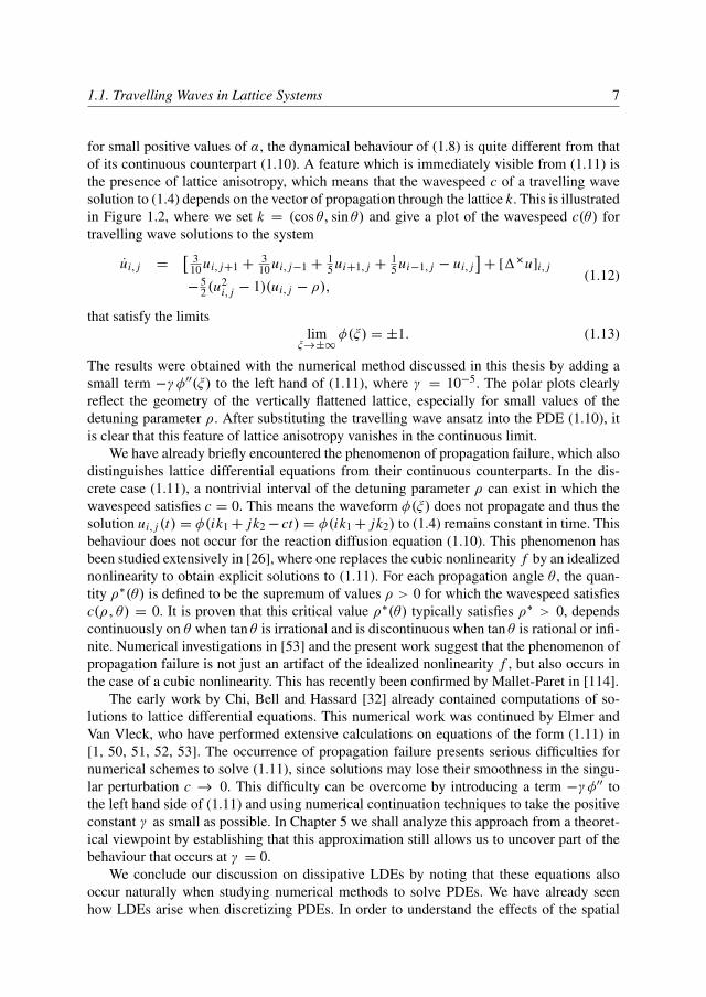
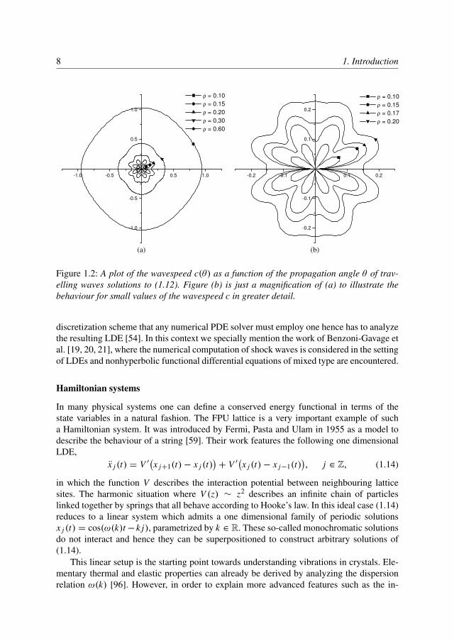
for small positive values of α, the dynamical behaviour of (1.8) is quite different from thatof its continuous counterpart (1.10). A feature which is immediately visible from (1.11) isthe presence of lattice anisotropy, which means that the wavespeed c of a travelling wavesolution to (1.4) depends on the vector of propagation through the lattice k. This is illustratedin Figure 1.2, where we set k = (cos θ, sin θ) and give a plot of the wavespeed c(θ) fortravelling wave solutions to the system
ui, j =[ 3
10 ui, j+1 +310 ui, j−1 +
15 ui+1, j +
15 ui−1, j − ui, j
]+ [1×u]i, j
−52 (u
2i, j − 1)(ui, j − ρ),
(1.12)
that satisfy the limitslim
ξ→±∞φ(ξ) = ±1. (1.13)
The results were obtained with the numerical method discussed in this thesis by adding asmall term −γφ′′(ξ) to the left hand of (1.11), where γ = 10−5. The polar plots clearlyreflect the geometry of the vertically flattened lattice, especially for small values of thedetuning parameter ρ. After substituting the travelling wave ansatz into the PDE (1.10), itis clear that this feature of lattice anisotropy vanishes in the continuous limit.
We have already briefly encountered the phenomenon of propagation failure, which alsodistinguishes lattice differential equations from their continuous counterparts. In the dis-crete case (1.11), a nontrivial interval of the detuning parameter ρ can exist in which thewavespeed satisfies c = 0. This means the waveform φ(ξ) does not propagate and thus thesolution ui, j (t) = φ(ik1+ jk2− ct) = φ(ik1+ jk2) to (1.4) remains constant in time. Thisbehaviour does not occur for the reaction diffusion equation (1.10). This phenomenon hasbeen studied extensively in [26], where one replaces the cubic nonlinearity f by an idealizednonlinearity to obtain explicit solutions to (1.11). For each propagation angle θ , the quan-tity ρ∗(θ) is defined to be the supremum of values ρ > 0 for which the wavespeed satisfiesc(ρ, θ) = 0. It is proven that this critical value ρ∗(θ) typically satisfies ρ∗ > 0, dependscontinuously on θ when tan θ is irrational and is discontinuous when tan θ is rational or infi-nite. Numerical investigations in [53] and the present work suggest that the phenomenon ofpropagation failure is not just an artifact of the idealized nonlinearity f , but also occurs inthe case of a cubic nonlinearity. This has recently been confirmed by Mallet-Paret in [114].
The early work by Chi, Bell and Hassard [32] already contained computations of so-lutions to lattice differential equations. This numerical work was continued by Elmer andVan Vleck, who have performed extensive calculations on equations of the form (1.11) in[1, 50, 51, 52, 53]. The occurrence of propagation failure presents serious difficulties fornumerical schemes to solve (1.11), since solutions may lose their smoothness in the singu-lar perturbation c → 0. This difficulty can be overcome by introducing a term −γφ′′ tothe left hand side of (1.11) and using numerical continuation techniques to take the positiveconstant γ as small as possible. In Chapter 5 we shall analyze this approach from a theoret-ical viewpoint by establishing that this approximation still allows us to uncover part of thebehaviour that occurs at γ = 0.
We conclude our discussion on dissipative LDEs by noting that these equations alsooccur naturally when studying numerical methods to solve PDEs. We have already seenhow LDEs arise when discretizing PDEs. In order to understand the effects of the spatial
8 1. Introduction
-1.0 -0.5 0.5 1.0
-1.0
-0.5
0.5
1.0
ρ = 0.10
ρ = 0.15
ρ = 0.20
ρ = 0.30
ρ = 0.60
(a)
-0.2 -0.1 0.1 0.2
-0.2
-0.1
0.1
0.2
ρ = 0.10
ρ = 0.15
ρ = 0.17
ρ = 0.20
(b)
Figure 1.2: A plot of the wavespeed c(θ) as a function of the propagation angle θ of trav-elling waves solutions to (1.12). Figure (b) is just a magnification of (a) to illustrate thebehaviour for small values of the wavespeed c in greater detail.
discretization scheme that any numerical PDE solver must employ one hence has to analyzethe resulting LDE [54]. In this context we specially mention the work of Benzoni-Gavage etal. [19, 20, 21], where the numerical computation of shock waves is considered in the settingof LDEs and nonhyperbolic functional differential equations of mixed type are encountered.
Hamiltonian systems
In many physical systems one can define a conserved energy functional in terms of thestate variables in a natural fashion. The FPU lattice is a very important example of sucha Hamiltonian system. It was introduced by Fermi, Pasta and Ulam in 1955 as a model todescribe the behaviour of a string [59]. Their work features the following one dimensionalLDE,
x j (t) = V ′(x j+1(t)− x j (t)
)+ V ′
(x j (t)− x j−1(t)
), j ∈ Z, (1.14)
in which the function V describes the interaction potential between neighbouring latticesites. The harmonic situation where V (z) ∼ z2 describes an infinite chain of particleslinked together by springs that all behave according to Hooke’s law. In this ideal case (1.14)reduces to a linear system which admits a one dimensional family of periodic solutionsx j (t) = cos(ω(k)t−k j), parametrized by k ∈ R. These so-called monochromatic solutionsdo not interact and hence they can be superpositioned to construct arbitrary solutions of(1.14).
This linear setup is the starting point towards understanding vibrations in crystals. Ele-mentary thermal and elastic properties can already be derived by analyzing the dispersionrelation ω(k) [96]. However, in order to explain more advanced features such as the in-
1.1. Travelling Waves in Lattice Systems 9
terplay between vibrations of separate frequencies or the temperature dependance of theelastic constants, it is essential to include higher order terms in the potential V . Modelsthat involve nonlinear versions of the FPU system (1.14) and the very similar Klein-Gordonequation have already been used to describe crystal dislocations [97], localized excitationsin ionic crystals [146] and even thermal denaturation of DNA [42].
The Hamiltonian structure of (1.14), together with the evident symmetries present inthis equation, have stimulated and facilitated the mathematical analysis of the FPU lattice.To give a recent example, Guo et al. [132] used a Lyapunov-Schmidt reduction to show thatgenerically, a family of small amplitude monochromatic solutions persists for the nonlinearproblem (1.14). In addition, under an appropriate resonance condition, two sufficiently smallmonochromatic solutions that are exactly in or out of phase may be added together to yielda two-parameter family of small bichromatic solutions. These results can be seen in thespirit of the multiscale expansion approach [63, 127, 156], which postulates the existenceof solutions to (1.14) of the form
x j (t) = εA(ε2t, ε( j − ct)
)cos(ω(k)t − k j)+O(ε2). (1.15)
It can be easily verified that the envelope function A must now satisfy the nonlinearSchrodinger equation, which has already been widely studied. Formally, the LDE (1.14)has thus been reduced to a PDE. However, this reduction has as yet only been made precisefor finite time intervals [70].
Another successful technique that directly uses the Hamiltonian structure of (1.14), re-lies on the observation that any travelling wave solution x j (t) = φ( j − ct) will necessarilybe a critical point of the action functional
S(φ) :=∫∞
−∞
[12
c2φ′(ξ)2 − V(φ(ξ + 1)− φ(ξ)
)]dξ. (1.16)
One can use so-called mountain pass methods to characterize the critical points of Sand construct travelling wave solutions to (1.14). Results in this direction for a num-ber of different monotonicity and growth conditions on the potential V can be found in[67, 123, 137, 150]. It is interesting to note that in Section 1.4 we take the exact oppositeroute, since we will look for the critical points of a similar functional by solving the MFDEthat arises from the associated variational problem.
Iooss and Kirchgassner provided an additional important tool in [87], where a centermanifold reduction for (1.14) is established. This has allowed for the construction of smallamplitude solutions to (1.14) [85, 86, 88, 147, 148]. These results all rely on normal formtheory to analyze the reversible system of ODEs that arises after performing the centerreduction. We remark here that the techniques that the authors use in [87] to construct thecenter manifold are tailored specifically for the particular system (1.14) under consideration.By contrast, in Chapter 2 we develop a center manifold framework that holds for arbitrarysystems of mixed type. This will allow the normal form computations discussed here to beperformed in a far broader setting.
10 1. Introduction
1.2. Classical Construction of Invariant Manifolds
Invariant manifolds have played a fundamental role in the theory of dynamical systems.They can be used to simplify the analysis of complex systems by considerably reducing therelevant dimensions. As we shall see, this may even involve the transformation of infinitedimensional problems into finite dimensional ones. Since invariant manifolds are often ro-bust under modifications of system parameters, they play an important role when analyzingbifurcations and singular perturbations. As an example, Lin described [106] how the ex-istence of multi-hump solutions of large period bifurcating from heteroclinic connectionscan be established by employing geometric arguments involving intersections between sta-ble and unstable manifolds. In a similar spirit, Fenichel provided three important theorems[58] that facilitate the analysis of dynamics in systems that possess two different naturaltimescales. In particular, these theorems allow one to robustly link together the dynamicsobtained by treating each timescale separately. This is done by exploiting the fact that un-der suitable conditions the so-called slow manifolds, which are invariant under the slowdynamics, persist when turning on the fast dynamics.
In this section we give a short introduction to the concepts of local stable, unstable andcenter manifolds. We briefly review how one can prove the existence of these structureswhen studying ordinary and delay differential equations. This overview will help to identifythe issues that need to be resolved if one wishes to consider these manifolds in the contextof functional differential equations of mixed type.
Ordinary Differential Equations
For simplicity, we start by considering the following nonlinear ordinary differential equa-tion,
x ′(ξ) = G(x(ξ)), (1.17)
in which x is a Cn-valued function. Let us suppose that the nonlinearity G : Cn→ Cn is
sufficiently smooth, so that for any initial state w ∈ Cn there exist constants 0 < ξ+ ≤ ∞and−∞ ≤ ξ− < 0 together with a unique solution xw : (ξ−, ξ+)→ Cn that satisfies (1.17)on the interval (ξ−, ξ+), with x(0) = w. This allows us to define a flow 8 : Cn
× R→ Cn
that maps (w, ξ) to xw(ξ). Care has to be taken that this may not be defined for all ξ ∈ R,but we will ignore this issue here.
In order to get a grasp of the behaviour of (1.17), an intuitive first step would be todivide the state space into parts that remain invariant under this flow 8 in some sense. Infact, smooth sets that have such a property are precisely the invariant manifolds in whichwe are interested. Consider first any point x ∈ Cn for which G(x) = 0. Such a point iscalled an equilibrium for (1.17) and obviously it is already an invariant manifold by itself.Two other important examples are given by the stable and unstable manifolds associated tox , which are defined as
W s(x) = {w ∈ Cn : 8(w, ξ)→ x as ξ →∞} ,W u(x) = {w ∈ Cn : 8(w, ξ)→ x as ξ →−∞} . (1.18)
1.2. Classical Construction of Invariant Manifolds 11
In order to understand the structure of the stable and unstable manifolds near the equi-librium point x , one needs to linearize (1.17) around this equilibrium. This yields the linearODE
v′(ξ) = Lv(ξ) := DG(x)v(ξ), (1.19)
in which L is an n × n matrix with complex coefficients. The analysis of (1.19) starts bylooking for special solutions of the form
v(ξ) = exp(zξ)w, (1.20)
with z ∈ C and w ∈ Cn . Substitution of this Ansatz into (1.19) shows that z must satisfythe well-known characteristic equation 1(z) = det(z I − L) = 0, implying that z is aneigenvalue for the matrix L . Since 1 is a polynomial of degree n, it can be factored as
1(z) =∏i=1
(z − λi )αi , (1.21)
in which each λi ∈ C is a distinct eigenvalue. The integers αi are called the algebraic multi-plicities of the eigenvalues λi . The Cayley-Hamilton theorem states that1 is an annihilatingpolynomial for the matrix L , which means 1(L) = 0. One may show that there exists anannihilating polynomial P 6= 0 that divides every other such polynomial. It is obvious thatthis minimal polynomial P must admit the following factorization,
P(z) =∏i=1
(z − λi )νi . (1.22)
The integers νi are called the ascents of the eigenvalues λi and necessarily satisfy1 ≤ νi ≤ αi . The well-known Jordan decomposition of the square matrix L gives us thefollowing powerful decomposition of the state space,
Cn=
⊕i=1
N (λi I − L)νi . (1.23)
The kernel N (λi I − L)νi is called the generalized eigenspace associated to λi . A usefulbasis for these eigenspaces can be constructed by computing so-called Jordan chains, whichare sequences of n-dimensional vectors w0, . . . , wk that satisfy the relations Lw0 = λw0and Lw j = λw j+w j−1 for 1 ≤ j ≤ k. The constituents of a Jordan chain are automaticallylinearly independent. In fact, the entire generalized eigenspace can be spanned by combin-ing a number of such chains. To appreciate the power of this setup, let us solve (1.19) withthe initial condition v(0) = w j . One may easily verify that the unique solution is given byv = v j , with
v j (ξ) = eλξ [w j + ξw j−1 + . . .+ξ j
j!w0]. (1.24)
The decomposition in (1.23) implies that this observation is sufficient to solve (1.19) withany initial condition. It is easy to check that (1.24) yields an efficient way to compute the
12 1. Introduction
matrix exponential exp(ξL), using which the general solution of (1.19) can be compactlywritten as
v(ξ) = eξLv(0). (1.25)
The inhomogeneous linear ODE
v′(ξ) = Lv(ξ)+ f (ξ) (1.26)
can now be solved using the variation-of-constants formula, which yields
v(ξ) = exp(ξL)v(0)+∫ ξ
0e(ξ−ξ
′)L f (ξ ′)dξ ′. (1.27)
Assume for the moment that the linearization around x has no eigenvalues on the imag-inary axis. In this case the equilibrium is called hyperbolic. Let us write Cn
= X+⊕ X−, inwhich X+ is the generalized eigenspace corresponding to the eigenvalues with positive realpart and X− is the generalized eigenspace corresponding to the eigenvalues with negativereal part. Write Q± for the associated spectral projections from Cn onto X± and note thatobviously Q+ + Q− = I .
Any initial conditionw− ∈ X− can be extended to an exponentially decaying solution ofthe linearized homogeneous equation (1.19) on the half-line [0,∞), namely x(ξ) = eξLw−.The analogous statement holds for initial conditions w+ ∈ X+, which can be extended tosolutions on (−∞, 0]. Such a splitting is called an exponential dichotomy and plays animportant role when studying invariant manifolds, as we shall see.
Intuitively speaking, the behaviour of (1.17) near equilibria will be fully dominated bythe linear part of the nonlinearity G. In view of this, one may hope that the stable manifoldW s(x) will locally remain close to the hyperplane x + X− ⊂ Cn . To shed some light onthis issue, we introduce the Banach space BC(R+,Cn) as the set of bounded continuousCn-valued functions that are defined on the half-line [0,∞), equipped with the supremumnorm. We also introduce a functional G : BC(R+,Cn)× X−→ BC(R+,Cn), defined by
G(u, w)(ξ) = eξLw +∫ ξ
0 e(ξ−ξ′)L Q−[G
(x + u(ξ ′)
)− Lu(ξ ′)]dξ ′
+∫ ξ∞
e(ξ−ξ′)L Q+[G
(x + u(ξ ′)
)− Lu(ξ ′)]dξ ′.
(1.28)
There are three key features to note regarding this definition. The first is that the splittingof the integral into a part acting on X− in forward time and a part acting on X+ in back-ward time ensures that G indeed maps into BC(R+,Cn) and not merely into C(R+,Cn).This is where the exponential dichotomy mentioned above comes into play. One may evenshow that G maps into the set of exponentially decaying functions. The second observationis that for all arguments (u, w) ∈ BC(R+,Cn) × X−, we have Q−G(u, w)(0) = w. Fi-nally, there is a bijection between solutions u ∈ BC(R+,Cn) to the fixed point equationu = G(u, Q−u(0)) and solutions x ∈ BC(R+,Cn) of the nonlinear equation (1.17), via thecorrespondance x(ξ) = u(ξ) + x . To see this, consider any solution x ∈ BC(R+,Cn) to(1.17). Then u = x − x satisfies
u′(ξ) = G(x(ξ)) = Lu(ξ)+[G
(u(ξ)+ x
)− Lu(ξ)
]. (1.29)
1.2. Classical Construction of Invariant Manifolds 13
However, by construction also G(u, 0) is a solution to the above equation. This impliesthat u = G(u, 0) + y for some solution y ∈ BC(R+,Cn) of the homogeneous equation(1.19). As a consequence, we must have y(ξ) = eξL Q−y(0) = eξL Q−u(0), which impliesu = G(u, Q−u(0)). Conversely, any solution of this fixed point equation satisfies (1.17) byconstruction.
We have hence reduced the description of the stable manifold W s(x) to the task ofsolving a nonlinear fixed point problem. Unfortunately, this is in general still an intractableprocedure. However, notice that the nonlinearity in (1.28) is governed by the expressionG
(x + u(ξ ′)
)− DG(x)u(ξ ′), which is of order O(u(ξ ′)2) for small u. This key fact allows
one to at least partially construct the stable manifold W s(x). More precisely, we will con-struct the local stable manifold W s
loc(x) ⊂ W s(x), which contains all w ∈ W s(x) with theadditional property that |8(w, ξ)− x | < ε for all ξ ≥ 0. Here ε > 0 is a sufficiently smallconstant.
At the heart of this construction lies the observation that for all sufficiently smallw ∈ X−, the map G(·, w) is a contraction on a closed and bounded subset of the spaceBC(R+,Cn). This implies that for all such w ∈ X−, a unique fixpoint u∗(w) has to exist,which then satisfies u∗(w) = G(u∗(w),w). This means that u∗(w) solves (1.17) and decaysexponentially. Hence W s
loc(x) can be written as a graph over the small ball Bδ(0) ⊂ X− ofradius δ > 0 around 0 ∈ X−, by means of the map w 7→ x + [u∗(w)](0). One maynow easily observe from a Taylor expansion of (1.28) that W s
loc(x) is indeed tangent to thehyperplane x + X−.
The unstable manifold W u(x) can of course be analyzed in a similar fashion. How-ever, when hyperbolicity is lost, i.e., when (1.19) admits eigenvalues on the imaginary axis,somewhat more care needs to be taken. Indeed, in this situation the qualitative large timebehaviour of solutions may depend in a subtle fashion on the higher order terms in the Tay-lor expansion of G. A very powerful tool in this context is the center manifold reduction[30]. To describe this reduction, let us decompose the state space as
Cn= X− ⊕ X0 ⊕ X+, (1.30)
in which X± are defined as before and X0 is the generalized eigenspace associatedto the eigenvalues on the imaginary axis. One may show that there exists a functionh : X0 → X− ⊕ X+, with h(0) = 0 and Dh(0) = 0, such that the dynamical behaviour of(1.17) in a sufficiently small neighbourhood of the equilibrium x is fully determined by thebehaviour of the following ODE
y′(ξ) = L |X0 y(ξ)+ Q0[G
(x + y(ξ)+ h(y(ξ))
)− DG(x)
(y(ξ)+ h(y(ξ)
)]. (1.31)
Notice that this ODE is defined on the subspace X0 ⊂ Cn . Stated more precisely, the centermanifold theorem guarantees that there exists an ε > 0 such that any solution x to (1.17)that has |x(ξ)| < ε for all ξ ∈ R, yields a solution y to (1.31) via the correspondencey(ξ) = Q0[x(ξ)− x]. Conversely, if y satisfies (1.31) on an interval I ⊂ R with |y(ξ)| < εfor all ξ ∈ I, then the function x defined by x(ξ) = y(ξ)+ h(y(ξ))+ x satisfies (1.17) onthe interval I.
The proof of this center reduction proceeds much along the lines of the procedure out-lined above to obtain the local stable and unstable manifolds. There are however a number
14 1. Introduction
of additional technical complications that have to be addressed. These are all related to thefact that there may exist initial conditions w ∈ X0 such that the function eξLw grows ina polynomial fashion as |ξ | → ∞. One has to compensate for this possibility by work-ing in exponentially weighted function spaces instead of BC(R,Cn), which in turn causesproblems when studying the smoothness of the center manifold.
To appreciate the true power of this center manifold reduction, we need to look at pa-rameter dependent versions of (1.17). Let us therefore consider the extended system
{x ′(ξ) = G(x(ξ), µ),µ′ = 0, (1.32)
which should be seen as a version of (1.17) parametrized by a single parameter µ ∈ R. Letus suppose for simplicity that x = 0 is a parameter independent equilibrium value, whichmeans G(0, µ) = 0 for all µ ∈ R. The eigenvalues of the linearization
v′(ξ) = DG(0, µ)v(ξ) (1.33)
will now depend on µ. Generically speaking, we expect that eigenvalues will lie on theimaginary axis only at isolated values of µ. Furthermore, it is reasonable to expect thatwhenever (1.33) does in fact fail to be hyperbolic, there will only be a small number ofpurely imaginary eigenvalues.
In general, eigenvalues that cross through the imaginary axis as parameters are variedcause a change in the qualitative behaviour of (1.32). Such changes are referred to as bi-furcations and their detection and classification play a fundamental role in the theory ofdynamical systems [34]. By considerably reducing the dimension of the system that hasto be analyzed, the computational and geometric analysis of bifurcations becomes a muchmore feasible task. In addition, since the physical dimension of the system under investi-gation becomes almost irrelevant, it becomes worthwhile to isolate commonly occurringbifurcation scenarios and give a standardized treatment for each. Such analyses are coveredby the realm of normal form theory.
To give an example, suppose that the hyperbolicity of (1.33) is lost when µ = 0, dueto a complex conjugate pair of eigenvalues with algebraic multiplicity one that cross theimaginary axis. We can then construct a 2+1 dimensional center manifold for the extendedsystem (1.32) that captures the behaviour of sufficiently small solutions x to the first compo-nent of (1.32), for all small parametersµ. A detailed analysis of this low dimensional systemshows that a branch of periodic solutions to (1.31) occurs either for µ > 0 or µ < 0, withamplitudes of order O(
√|µ|) as µ→ 0. These periodic solutions can then be lifted back to
the full equation (1.33). A simple sign condition involving the second and third order deriva-tives of G determines whether these periodic orbits occur for µ positive or negative. Thisfamous result is known as the Hopf bifurcation theorem and by now many generalizationsto more complex root crossing scenarios have appeared in the literature.
1.2. Classical Construction of Invariant Manifolds 15
Delay Differential Equations
Let us now turn our attention to delay equations. For simplicity, we will consider the fol-lowing nonlinear equation with a single point delay,
x ′(ξ) = G(x(ξ), x(ξ − 1)
). (1.34)
We will always assume that x is a continuous Cn-valued function defined on some interval.In this context the state space X is given by X = C([−1, 0],Cn). We recall the notationxξ (θ) = x(ξ + θ) for the state xξ ∈ X of x at ξ . The linearization around an equilibrium xis given by
v′(ξ) = Lvξ := D1G(x)v(ξ)+ D2G(x)v(ξ − 1). (1.35)
We again look for solutions to (1.35) of the form v(ξ) = w exp(ξ z), with w ∈ Cn . Asbefore, one must have 1(z)w = 0, but the characteristic matrix 1 is now given by
1(z) = z I − D1G(x)− D2G(x)e−z . (1.36)
Due to the presence of the exponential in (1.36), there will in general be an infinite numberof roots to the characteristic equation det1(z) = 0. However, it is still the case that onecan capture all the roots to the left of a vertical line in the complex plane, i.e., there existsa number γ+ ∈ R such that all roots z have Re z < γ+. Another important observation isthat the number of eigenvalues in a vertical strip is finite, i.e., for any pair of reals ν− < ν+,there are only finitely many z with ν− < Re z < ν+ and det1(z) = 0.
Similarly as in the ODE case, for any root z of the characteristic equation det1(z) = 0one may compute a Jordan basis for the null space N
(1(z)
)and use the expression (1.24)
to construct solutions to the homogeneous equation (1.35). These solutions have the formv(ξ) = p(ξ)ezξ for polynomials p and are called eigensolutions to (1.35) for the eigenvaluez. Let us write V ⊂ C([−1, 0],Cn) for the span of all these eigensolutions, ranging over alleigenvalues z. There are two important questions that now arise naturally. The first is if anyinitial condition φ ∈ C([−1, 0],Cn) can be written in terms of these eigensolutions. Statedmore precisely, do we have the identity V = C([−1, 0],Cn). The second question concernsthe construction of the natural projections Q±, which map initial conditions onto parts thatcan be extended to bounded solutions of (1.35) on the half-lines R±.
To answer these questions (1.35) needs to be embedded into a more abstract framework.To prepare for this, let us first consider an arbitrary φ ∈ C([−1, 0],Cn) and attempt to solve(1.35) on the interval [0, 1], with the initial condition x0 = φ. One easily sees that this isequivalent to solving the following initial value problem on [0, 1],{
v′(ξ) = D1G(x)v(ξ)+ D2G(x)φ(ξ − 1),v(0) = φ(0). (1.37)
This can be readily solved to yield
vφ(ξ) = exp[D1G(x)ξ ]φ(0)+∫ ξ
0exp[D1G(x)(ξ − ξ ′)]D2G(x)φ(ξ ′ − 1)dξ ′ (1.38)
16 1. Introduction
for all 0 ≤ ξ ≤ 1. This construction can then be repeated on the interval [1, 2]. Continuingin this fashion, one can compute a solution vφ to (1.35) on the entire half-line R+. Thisprocedure has adequately been named the method of steps [45].
We now proceed by considering the setup above from a more abstract point of view.For every ξ ≥ 0 we have constructed a linear operator T (ξ) : X → X that maps an initialcondition φ ∈ X to the state (vφ)ξ ∈ X . Put in other words, we have vφ(ξ) = [T (ξ)φ](0)for all ξ ≥ 0. One may easily verify that T (0) = I and T (ξ + ξ ′) = T (ξ)T (ξ ′) for allpositive ξ and ξ ′, which means that T is in fact a semigroup.
The operators T (ξ) should be seen as the generalization of the matrix exponen-tials exp[Lξ ] encountered above in the ODE setting. A major difference however isthat T (ξ) is only defined for positive ξ . Indeed, any initial condition φ ∈ X that isnot differentiable can never be extended in backward time. Notice that in the ODE set-ting, the matrix L can be recovered from the matrix exponential by means of the limitLw = limh→0 h−1[exp(Lh)w − w], which exists for all w ∈ Cn . Inspired by this, thegenerator A of the semigroup T is defined by setting Aφ = limh↓0 h−1[T (h)φ − φ], forall φ ∈ X for which this limit exists. In an infinite dimensional setting this last existencecondition becomes important and in general, the domain D(A) is indeed a proper subset ofthe state space X . Using our solution (1.38) it is not hard to explicitly calculate the generatorA : D(A) ⊂ X → X . It is closed, densely defined and given by
Aφ = φ′,
D(A) ={φ ∈ C1([−1, 0],Cn) | φ′(0) = Lφ = D1G(x)φ(0)+ D2G(x)φ(−1)
}.
(1.39)Any z ∈ C for which z I − A : D(A)→ X is bijective is said to be in the resolvent set of A,denoted by ρ(A). Due the closed graph theorem, for any z ∈ ρ(A) the inverse (z I − A)−1,called the resolvent of A at z, is automatically bounded. The spectrum of A is defined as thecomplement of the resolvent set, i.e., σ(A) = C \ ρ(A).
As can be inferred by the ODE case, the properties of the semigroup T are intimatelyconnected to those of the generator A. An important example of such a connection is relatedto the splitting of the state space X into parts that are invariant under the action of the semi-group T . Let us suppose that λ ∈ σ(A) is an isolated pole of finite order m for the functionz 7→ (z I−A)−1. Let us also defineMλ(A) = N
((λI−A)m
)andRλ(A) = R
((λI−A)m
).
A standard result [45, Theorem IV.2.5] states that the spaces thus defined are maximal, inthe sense that N
((λI − A)k
)=Mλ(A) and R
((λI − A)k
)= Rλ(A) hold for the kernel
and range of (λI − A)k for all larger integers k ≥ m. Furthermore, bothMλ(A) andRλ(A)are closed and invariant under the action of the semigroup T . Finally, one has the spectraldecomposition
X =Mλ(A)⊕Rλ(A), (1.40)
with a corresponding spectral projection Qλ onto Mλ(A) that is given by the Dunfordintegral
Qλ =1
2π i
∫0λ
(z I − A)−1dz. (1.41)
Here the contour 0λ ⊂ ρ(A) is a small circle around λ that contains no other points of σ(A)in its interior.
1.2. Classical Construction of Invariant Manifolds 17
For the delay equation (1.35) under consideration, the resolvent (z I − A)−1 : X → Xmay be explicitly computed to be
[(z I − A)−1φ](θ) = ezθ ( ∫ 0θ e−zσφ(σ)dσ
+1(z)−1[φ(0)+ D2G(x)e−z ∫ 0−1 e−zσφ(σ)dσ
]).
(1.42)
This expression provides the link between the eigensolutions that we constructed in an ad-hoc fashion using the characteristic matrix1 and the abstract spectral theory outlined abovefor the generator A. In particularly, using the theory for characteristic matrices developed in[89], one can show that the structure and dimension of the generalized eigenspaceMλ(A) iscompletely determined by the structure of the nullspaceN (1(λ)), via the expression (1.24).In addition, the spectral projection operators Qλ can be expressed in terms of residues atz = λ of terms involving the matrix-inverse 1(z)−1. For example, if z = λ is a simple rootof the characteristic equation det1(z) = 0, there exists a matrix-valued function H that isanalytic at z = λ, such that
1(z)−1= (z − λ)−1 H(z). (1.43)
Using this identity, the spectral projection (1.41) reduces to
[Qλφ](θ) = eλθ H(λ)[φ(0)+ DG2e−λ
∫ 0
−1e−zσφ(σ)dσ
]. (1.44)
Further examples and a description of a systematic procedure for the explicit computationof spectral projections in a general setting can be found in [65].
It remains to address the question whether the set of all generalized eigensolutions iscomplete. Results in this direction were first given in [160]. It is possible to establish thefollowing decomposition for the state space,
X = V ⊕ S, (1.45)
in which the subspace S is related to the resolvent of A, via
S ={φ ∈ X | z 7→ (z I − A)−1φ is entire
}. (1.46)
Initial conditions in S are related to solutions to (1.35) that become identically zero aftera finite time. The existence of these so-called small solutions can be verified directly from(1.35). Indeed, one may show that S is empty if and only if det D2G(x) 6= 0.
Now that the linear homogeneous equation (1.35) has been addressed, we need to moveon to the inhomogeneous problem{
v′(ξ) = Lvξ + f (ξ),v0 = φ.
(1.47)
We note first that in principle the method of steps can again be used to find a solution.However, we are interested here in the construction of invariant manifolds as describedabove for ODEs. The task at hand is to generalize the variation-of-constants formula (1.27)
18 1. Introduction
that was developed for ODEs, now using the semigroup T instead of the matrix exponentialexp[ξL]. Even at first glance one already runs into serious difficulties. Indeed, one needs tocompensate for the fact that the inhomogeneity f no longer maps into the state space X , butmerely into Cn .
This difficulty has been overcome by the introduction of sun-star calculus. In par-ticular, instead of looking at X we turn our attention to an extended state spaceX�? = Cn
× L∞([rmin, 0],Cn). Note that X ↪→ X�? via the natural inclusionφ 7→ (φ(0), φ). By the nature of the construction, the semigroup T generalizes to a weak-*continuous semigroup T�? on X�?. The inhomogeneity f can be naturally extended to amap F : R→ X�? via F(ξ) = ( f (ξ), 0). This leads to the variation-of-constants formula
vξ = T (ξ − ξ0)φ +
∫ ξ
ξ0
T�?(ξ − ξ ′)F(ξ ′)dξ ′. (1.48)
One may show that this is well-defined in the sense that the righthand side is again an ele-ment in the original state space X and that v thus defined satisfies the initial value problem(1.47).
With the development of this variation-of-constants formula the road towards invariantmanifold theory for delay equations was opened up. The construction of the stable and un-stable manifolds proceeds quite similarly as in the ODE case outlined above. When studyingthe center manifold, extra precautions need to be taken due to the fact that smooth cut-offfunctions are generally unavailable in an infinite dimensional setting.
1.3. Invariant Manifolds for MFDEsWe are now ready to move on to functional differential equations of mixed type. For sim-plicity, we will consider the following nonlinear equation with two shifted arguments,
x ′(ξ) = G(x(ξ), x(ξ − 1), x(ξ + 1)
). (1.49)
We will again assume that x is a continuous Cn-valued function defined on some appropriateinterval. The state space X is now given by X = C([−1, 1],Cn) and the linearization aroundan equilibrium x can be written as
v′(ξ) = Lvξ := D1G(x)v(ξ)+ D2G(x)v(ξ − 1)+ D3G(x)v(ξ + 1). (1.50)
To start the discussion, we consider a simple illustrative example, due to Harterich et al.[75]. Consider the linear homogeneous MFDE
v′(ξ) = v(ξ + 1)− v(ξ − 1), (1.51)
with the initial condition v0 = 1. One easily sees that for all ξ ∈ (1, 3) one must havev(ξ) = −1, which in turn implies that v(ξ) = 1 for all ξ ∈ (3, 5). The continuity of theinitial condition is hence lost. In other words, (1.50) with an initial condition v0 = φ isill-posed as an initial value problem.
1.3. Invariant Manifolds for MFDEs 19
The construction of the semigroup T for delay equations thus breaks done and cannotbe repaired. This fact already exhibits itself when analyzing the characteristic matrix
1(z) = z I − D1G(x)− D2G(x)e−z− D3G(x)ez . (1.52)
The presence of the two exponential functions with oppositive signs in their arguments willin general cause the characteristic equation det1(z) = 0 to have an infinite set of roots bothto the right and left of the imaginary axis. In contrast, the spectrum of semigroup generatorscan always be contained in a left half plane. The asymptotic location of eigenvalues for(1.50) was analyzed in early work by Bellman and Cooke [16]. An important observation isthat any vertical strip {z ∈ C : ν− < Re z < ν+} contains only finitely many roots.
Although it is now no longer the generator of a semigroup, one can still study the op-erator A that was defined for delay equations by (1.39). In this fashion one can still obtainspectral decompositions of the state space X and the associated spectral projections. How-ever, the relation between the spectral splittings thus obtained and the dynamics of (1.50) isnow no longer immediately clear.
The ill-posedness of the initial value problem (1.50) has long limited our understand-ing of the full nonlinear system (1.49). It was only during the last decade that significanttheoretical progress has been made. An important step in this respect was the constructionof exponential dichotomies for (1.50). One can show that there exists a closed subspaceP← ⊂ X such that for every φ ∈ P←, there exists a function xφ defined on (−∞, 1], withx0 = φ, that satisfies (1.50) on the interval (−∞, 0]. Similarly, there exists a closed sub-space P→ ⊂ X such that every φ ∈ P→ can be extended to a solution of (1.50) on [0,∞).More importantly, one has the decomposition
X = P→ ⊕ P←. (1.53)
A first result in this direction was obtained in 1989 by Rustichini [130]. Only very recentlyhowever, the existence of exponential dichotomies was established for non-autonomous ver-sions of (1.50). These results were obtained independently and simultaneously by Mallet-Paret et al. [115] and Harterich et al. [75].
Another important result concerns the linearization of (1.54) around heteroclinic orbits.In particular, consider any solution x that satisfy the limits limξ→±∞ x(ξ) = x±, in whichboth x± ∈ Cn are equilibria for the nonlinearity G. Linearizing (1.49) around this solutionyields 3v = 0, in which the linear operator 3 : W 1,∞(R,Cn)→ L∞(R,Cn) is given by
[3v](ξ) = v′(ξ)− D1G(xξ )v(ξ)− D2G(xξ )v(ξ − 1)− D3G(xξ )v(ξ + 1). (1.54)
Notice that since x is a heteroclinic orbit, one can define the limiting operatorsA±j = limξ→±∞ D j G(xξ ) for 0 ≤ j ≤ 2 and consider the limiting systems
v′(ξ) = L±vξ =2∑
j=0
A±j v(ξ + r j ). (1.55)
When both limiting systems do not have eigenvalues on the imaginary axis, we saythat 3 is asymptotically hyperbolic. Assuming this condition, Mallet-Paret was able
20 1. Introduction
to establish Fredholm properties for the operator 3 [112]. In particular, the kernelK(3) ⊂ W 1,∞(R,Cn) is finite dimensional, while the rangeR(3) ⊂ L∞(R,Cn) is closedand has finite codimension. In addition, one has the following useful characterization forthe range of 3,
R(3) ={
f ∈ L∞(R,Cn) |
∫∞
−∞
x∗(ξ) f (ξ) = 0 for all x ∈ K(3∗)}, (1.56)
in which the adjoint 3∗ : W 1,∞(R,Cn)→ L∞(R,Cn) is given by
[3∗v](ξ) = v′(ξ)+ D1G(xξ )∗v(ξ)+ D2G(xξ+1)v(ξ + 1)+ D3G(xξ−1)v(ξ − 1). (1.57)
In the special case that x is constant, the operator3 is an isomorphism and a Greens functionG exists such that for any f ∈ L∞(R,Cn), the equation 3v = f is solved by the function
v(ξ) =
∫∞
−∞
G(ξ − ξ ′) f (ξ ′)dξ ′. (1.58)
The linear theory outlined above can be seen as the appropriate generalization of theconcepts discussed previously for ordinary and delay differential equations. However, ithas not been firmly established how these results can be lifted to a nonlinear setting. Inparticular, it is unclear whether a version of the sun-star calculus can be developed thatallows for the natural embedding of Cn-valued nonlinearities into the state space X .
The approach followed in this thesis circumvents this difficulty by rewriting the relevantfixed point equations discussed in the previous section in such a way, that only the inverse3−1 is needed. Of course, care must be taken when choosing the correct function spaceson which to define the problem, in order to ensure that this inverse does indeed exist. Inaddition, we use Laplace transform techniques to obtain the connection between the spectralproperties of the operator A discussed above and solutions to the homogeneous equation3v = 0.
In Chapter 2 we combine this technique with a fibred contraction argument due to Van-derbauwhede and Van Gils [159]. In particular, we show how a finite dimensional centermanifold can be constructed that captures the dynamics of (1.49) near an equilibrium x forG. We illustrate how one can explicitly calculate a Taylor expansion of the resulting ODE(1.31) up to any desired order. In particular, we provide explicit conditions, directly in termsof derivatives of G, under which super and subcritical Hopf bifurcations arise. In Section1.4 we show how easily these conditions can be explicitly verified in practice. This yieldsthe first result for the occurrence of Hopf bifurcations for general systems of the form (1.1).
In view of the economic modelling problems that are described in the sequel, it is impor-tant to extend these results to a slight variant of (1.49). In particular, we need to understandthe following algebraic problem of mixed type,
0 = F(xξ ), (1.59)
under a smoothness condition that ensures that any solution x to (1.59) automatically sat-isfies an accompanying differential equation (1.49). We attack this problem in Chapter 3.
1.3. Invariant Manifolds for MFDEs 21
In particular, we show that the smoothness condition is sufficient to ensure that (1.59) canstill be reduced to an ODE, upon restricting the equation to a small neighbourhood aroundan equilibrium. Again, one can explicitly compute the Taylor expansion of this ODE up toarbitrary order and we give an example of such a computation in Section 1.6.
One can use the results discussed above to establish the existence of periodic solutionsto (1.49) under suitable conditions. Of course, the next interesting question that arises iswhether the dynamics around these periodic solutions can be analyzed in a similar fashion.This brings us into the realm of Floquet theory. To set the stage, let us return briefly to theODE (1.17), under the assumption that this equation admits a 2π -periodic solution p. ThePoincare return map is the key mathematical structure that is used to analyze the dynamics of(1.17) in a neighbourhood of p. It is constructed by fixing a hyperplaneH that contains p(0)and is transversal to Dp(0). Any w ∈ H is then mapped to the first subsequent intersectionof the orbit through w with this hyperplane H, which is well-defined for all w sufficientlyclose to p(0). In this fashion, the dynamics in a neighbourhood of the orbit p can be capturedby a discrete dynamical system.
The analysis of the Poincare return-map proceeds by considering the linearization of theODE (1.17) around p, yielding
v′(ξ) = L(ξ)v(ξ) := DG(pξ )v(ξ) (1.60)
in which the periodic matrix-valued operator L : R → Cn×n shares the period of p. Onenow analyzes the monodromy map T2π : X → X associated to (1.60). This operator mapsinitial conditions w ∈ Cn onto the translate vw(2π) ∈ Cn , where vw solves (1.60) withv(0) = w. Eigenvalues of the monodromy map are called Floquet multipliers, while thecorresponding solutions to (1.60) are called Floquet solutions. As can be expected, the sta-bility properties of the Poincare return map depend heavily on the location of this Floquetspectrum. The presence of Floquet multipliers on the unit circle is of particular interest whenone is looking for bifurcations that affect a branch of periodic solutions.
The ill-posedness of (1.49) implies that we need to develop a different line of attackwhen studying MFDEs, since both the Poincare map and the monodromy operator cannot bedirectly defined. These issues are explored in Chapter 4, where we provide a center manifoldframework that can be used to capture the dynamics of (1.49) near periodic solutions. Thetechniques used in this chapter were chiefly inspired by those used by Mielke [119], whowas also faced with the absence of a semiflow in his work on elliptic PDEs.
The key point is that one can no longer search directly for Floquet multipliers by study-ing the monodromy operator. However, it is still possible to look for solutions to the lin-earization
v′(ξ) = L(ξ)vξ := DG1(pξ )v(ξ)+ DG2(pξ )v(ξ − 1)+ DG3(pξ )v(ξ + 1), (1.61)
that have the special Floquet form v(ξ) = eλξq(ξ). Here p is a periodic solution to (1.49),λ ∈ C is the Floquet exponent and q a continuous periodic function that has the sameperiod as p. In Sections 1.7 and 1.8 we shall see how this feature affects the numericalcomputations of Floquet multipliers.
Finally, in Chapter 6 we discuss a second mechanism via which periodic orbits canappear. In particular, we use exponential dichotomies to lift Lin’s method [106] to the setting
22 1. Introduction
of MFDEs. This allows us to study bifurcations from homoclinic solutions to nonlinearMFDEs that depend upon parameters. The so-called ‘blue sky catastrophe’ is an exampleof such a bifurcation. It describes how a branch of periodic solutions, that have increasinglylarge period, may suddenly disappear and turn into a homoclinic solution, as the parametersof the system are varied. Many interesting results have been obtained concerning homoclinicbifurcations in ODE settings. In Chapter 6 we show how our framework can be used totranslate some of these results to our infinite dimensional system. We explicitly describe theorbit-flip bifurcation, which can lead to very complicated behaviour in the neighbourhoodof a homoclinic orbit [134]. In particular, we give conditions for the existence of symbolicdynamics for MFDEs.
1.4. Optimal Control Capital Market DynamicsFollowing Rustichini [131] and Benhabib et al. [17], we consider a simple model for thedynamics of a capital market. The economy starts at time t = 0 and has a fixed populationof unit size. Exactly n + 1 distinct types of products are produced. One of these can onlybe used for consumption purposes while the other n are capital goods that facilitate themanufacture of the consumption good.
We will write k(t) ∈ Rn for the total amount of capital goods that are available at time t .By u(t) ∈ Rn we will denote the total investments in capital. In order to model effects suchas decay and maintenance costs, we introduce a positive constant g as the capital decay rateand obtain the following relation between investments and capital,
k(t) = u(t)− gk(t). (1.62)
At any given moment, the total consumption C naturally depends upon the availableproduction facilities, viz the total amount of capital goods k. Since any investment in capitalgoods will necessarily divert resources from the production of the consumption good, theconsumption C also depends upon the investments u. We thus write C = C(u, k). Thewelfare W (t) of the society in our model at any given time t is related to the total amountof consumption via W (t) = ln C(t).
The dynamic behaviour of the capital market can be found by maximizing the functional
J (k, k) =∫∞
0e−ρt ln C
(u(t), k(t)
)=
∫∞
0e−ρt ln C
(k(t)+ gk(t), k(t)
). (1.63)
The parameter ρ > 0 represents the discount rate, quantifying the fact that welfare in thepresent is rated higher than its counterpart in the future.
The Euler-Lagrange equations provide the classic tool for solving (1.63) and lead to thesecond order ODE
e−ρt [C(k(t)+ gk(t), k(t)
)]−1[gD1C
(k(t)+ gk(t), k(t)
)+ D2C
(k(t)+ gk(t), k(t)
)]
=ddt
[e−ρt [C
(k(t)+ gk(t), k(t)
)]−1 D1C
(k(t)+ gk(t), k(t)
)].
(1.64)
1.4. Optimal Control Capital Market Dynamics 23
In [17, 18, 131] it is argued that, under some weak assumptions on the function C , periodicsolutions to (1.64) are in fact optimal solutions to (1.63). This type of solution is henceparticularly interesting from an economic point of view.
It still remains to specify the consumer function C(u, k). Following [17], it can be foundby solving the optimization problem
C(u, k) = max{Yc(Lc, K c) | Yu(Lu, K u) = u,
Lc+
∑ni=1 Lu
i = 1, Lc≥ 0,
Lui ≥ 0, 1 ≤ i ≤ n,
K c+
∑ni=1 K u
i = k, K c≥ 0,
K ui ≥ 0, 1 ≤ i ≤ n
}.
(1.65)
We take Yc and Yu to be standard Cobb-Douglas production functions [47], which have theform
Y (L , K ) = βLαL K αK (1.66)
for positive parameters αL , αK and β. The conditions in the maximization problem (1.65)reflect the fact that the total available labour l = 1 and capital k have to be divided over theproduction of the consumption good and capital goods in such a way, that the output of theconsumption good is maximal, while the capital good production matches the investmentsu.
Benhabib et al. found periodic solutions to (1.63) in markets that contain more than oneproduction good, i.e., where n > 1 [17]. Rustichini however fixed n = 1, but introducedtime delays into the problem to account for the fact that both the investment activity and theproduction of the consumption good take time [131]. In particular, (1.63) is modified to takethe form
J (k, k) =∫∞
0 e−ρt ln C(u(t − τ), k(t − σ)
),
k(t) = u(t − τ)− gk(t − τ).(1.67)
In Hughes [81] the Euler-Lagrange equations were generalized to problems that containdelays. In particular, the functional
J (y) =∫ b
af(t, y(t − τ), y(t), y(t − τ), y(t)
)dt (1.68)
was considered, in which y ranges over the class of piecewise smooth solutions on theinterval [a − τ, b] that satisfy an initial condition y(s) = α(s) for s ∈ [a − τ, a] and aboundary condition y(b) = β. Solutions that maximize J were shown to satisfy the Euler-Lagrange equation
D3 f (t, x, y, x, y)+ D2 f (t + τ, y, z, y, z) = ddt [D5 f (t, x, y, x, y)+D4 f (t + τ, y, z, y, z)]
(1.69)
on the interval [a, b − τ ], in which x(·) = y(· − τ) and z(·) = y(· + τ).
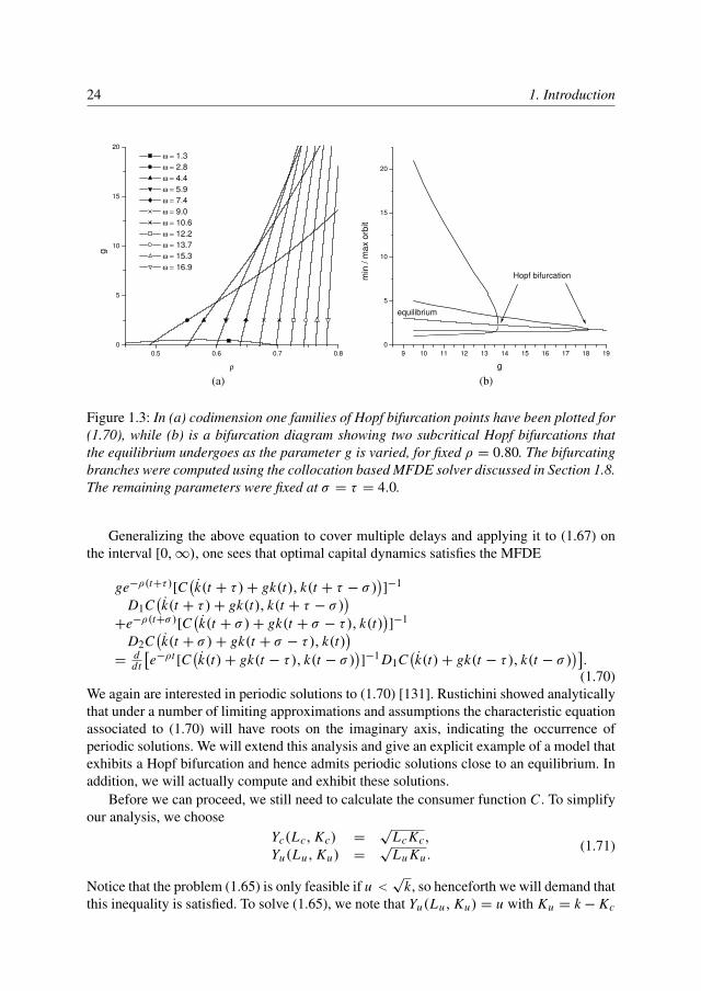
24 1. Introduction
0.5 0.6 0.7 0.8
0
5
10
15
20
ω = 1.3
ω = 2.8
ω = 4.4
ω = 5.9
ω = 7.4
ω = 9.0
ω = 10.6
ω = 12.2
ω = 13.7
ω = 15.3
ω = 16.9
g
ρ
(a)
9 10 11 12 13 14 15 16 17 18 19
0
5
10
15
20
equilibrium
Hopf bifurcationmin
/ m
ax o
rbit
g
(b)
Figure 1.3: In (a) codimension one families of Hopf bifurcation points have been plotted for(1.70), while (b) is a bifurcation diagram showing two subcritical Hopf bifurcations thatthe equilibrium undergoes as the parameter g is varied, for fixed ρ = 0.80. The bifurcatingbranches were computed using the collocation based MFDE solver discussed in Section 1.8.The remaining parameters were fixed at σ = τ = 4.0.
Generalizing the above equation to cover multiple delays and applying it to (1.67) onthe interval [0,∞), one sees that optimal capital dynamics satisfies the MFDE
ge−ρ(t+τ)[C(k(t + τ)+ gk(t), k(t + τ − σ)
)]−1
D1C(k(t + τ)+ gk(t), k(t + τ − σ)
)+e−ρ(t+σ)[C
(k(t + σ)+ gk(t + σ − τ), k(t)
)]−1
D2C(k(t + σ)+ gk(t + σ − τ), k(t)
)=
ddt
[e−ρt [C
(k(t)+ gk(t − τ), k(t − σ)
)]−1 D1C
(k(t)+ gk(t − τ), k(t − σ)
)].(1.70)
We again are interested in periodic solutions to (1.70) [131]. Rustichini showed analyticallythat under a number of limiting approximations and assumptions the characteristic equationassociated to (1.70) will have roots on the imaginary axis, indicating the occurrence ofperiodic solutions. We will extend this analysis and give an explicit example of a model thatexhibits a Hopf bifurcation and hence admits periodic solutions close to an equilibrium. Inaddition, we will actually compute and exhibit these solutions.
Before we can proceed, we still need to calculate the consumer function C . To simplifyour analysis, we choose
Yc(Lc, Kc) =√
Lc Kc,Yu(Lu, Ku) =
√Lu Ku .
(1.71)
Notice that the problem (1.65) is only feasible if u <√
k, so henceforth we will demand thatthis inequality is satisfied. To solve (1.65), we note that Yu(Lu, Ku) = u with Ku = k− Kc
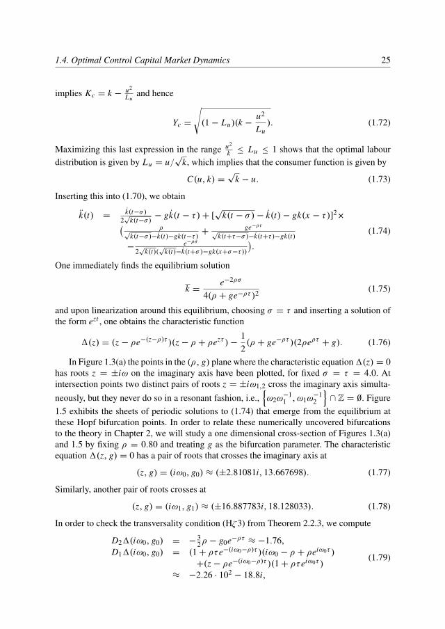
1.4. Optimal Control Capital Market Dynamics 25
implies Kc = k − u2
Luand hence
Yc =
√(1− Lu)(k −
u2
Lu). (1.72)
Maximizing this last expression in the range u2
k ≤ Lu ≤ 1 shows that the optimal labourdistribution is given by Lu = u/
√k, which implies that the consumer function is given by
C(u, k) =√
k − u. (1.73)
Inserting this into (1.70), we obtain
k(t) = k(t−σ)2√
k(t−σ)− gk(t − τ)+ [
√k(t − σ)− k(t)− gk(x − τ)]2
×( ρ√
k(t−σ)−k(t)−gk(t−τ)+
ge−ρτ√
k(t+τ−σ)−k(t+τ)−gk(t)
−e−ρσ
2√
k(t)(√
k(t)−k(t+σ)−gk(x+σ−τ))
).
(1.74)
One immediately finds the equilibrium solution
k =e−2ρσ
4(ρ + ge−ρτ )2(1.75)
and upon linearization around this equilibrium, choosing σ = τ and inserting a solution ofthe form ezt , one obtains the characteristic function
1(z) = (z − ρe−(z−ρ)τ )(z − ρ + ρezτ )−12(ρ + ge−ρτ )(2ρeρτ + g). (1.76)
In Figure 1.3(a) the points in the (ρ, g) plane where the characteristic equation1(z) = 0has roots z = ±iω on the imaginary axis have been plotted, for fixed σ = τ = 4.0. Atintersection points two distinct pairs of roots z = ±iω1,2 cross the imaginary axis simulta-
neously, but they never do so in a resonant fashion, i.e.,{ω2ω
−11 , ω1ω
−12
}∩ Z = ∅. Figure
1.5 exhibits the sheets of periodic solutions to (1.74) that emerge from the equilibrium atthese Hopf bifurcation points. In order to relate these numerically uncovered bifurcationsto the theory in Chapter 2, we will study a one dimensional cross-section of Figures 1.3(a)and 1.5 by fixing ρ = 0.80 and treating g as the bifurcation parameter. The characteristicequation 1(z, g) = 0 has a pair of roots that crosses the imaginary axis at
(z, g) = (iω0, g0) ≈ (±2.81081i, 13.667698). (1.77)
Similarly, another pair of roots crosses at
(z, g) = (iω1, g1) ≈ (±16.887783i, 18.128033). (1.78)
In order to check the transversality condition (Hζ3) from Theorem 2.2.3, we compute
D21(iω0, g0) = −32ρ − g0e−ρτ ≈ −1.76,
D11(iω0, g0) = (1+ ρτe−(iω0−ρ)τ )(iω0 − ρ + ρeiω0τ )
+(z − ρe−(iω0−ρ)τ )(1+ ρτeiω0τ )
≈ −2.26 · 102− 18.8i,
(1.79)
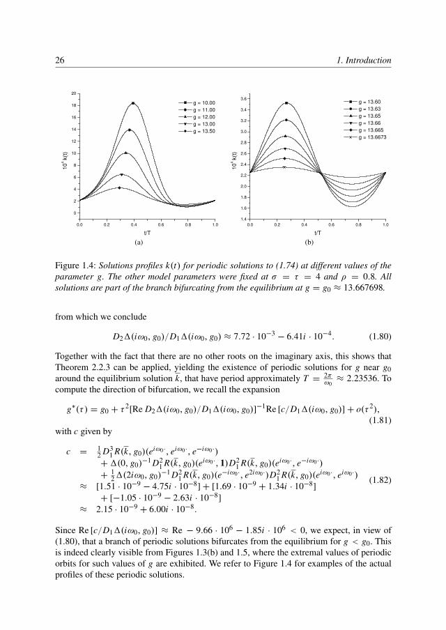
26 1. Introduction
0.0 0.2 0.4 0.6 0.8 1.0
0
2
4
6
8
10
12
14
16
18
20
g = 10.00
g = 11.00
g = 12.00
g = 13.00
g = 13.50
10
4 k
(t)
t/T
(a)
0.0 0.2 0.4 0.6 0.8 1.0
1.4
1.6
1.8
2.0
2.2
2.4
2.6
2.8
3.0
3.2
3.4
3.6 g = 13.60
g = 13.63
g = 13.65
g = 13.66
g = 13.665
g = 13.6673
10
4 k
(t)
t/T
(b)
Figure 1.4: Solutions profiles k(t) for periodic solutions to (1.74) at different values of theparameter g. The other model parameters were fixed at σ = τ = 4 and ρ = 0.8. Allsolutions are part of the branch bifurcating from the equilibrium at g = g0 ≈ 13.667698.
from which we conclude
D21(iω0, g0)/D11(iω0, g0) ≈ 7.72 · 10−3− 6.41i · 10−4. (1.80)
Together with the fact that there are no other roots on the imaginary axis, this shows thatTheorem 2.2.3 can be applied, yielding the existence of periodic solutions for g near g0around the equilibrium solution k, that have period approximately T = 2π
ω0≈ 2.23536. To
compute the direction of bifurcation, we recall the expansion
g∗(τ ) = g0 + τ2[Re D21(iω0, g0)/D11(iω0, g0)]−1Re [c/D11(iω0, g0)]+ o(τ 2),
(1.81)with c given by
c =12 D3
1 R(k, g0)(eiω0·, eiω0·, e−iω0·)
+1(0, g0)−1 D2
1 R(k, g0)(eiω0·, 1)D21 R(k, g0)(eiω0·, e−iω0·)
+121(2iω0, g0)
−1 D21 R(k, g0)(e−iω0·, e2iω0·)D2
1 R(k, g0)(eiω0·, eiω0·)
≈ [1.51 · 10−9− 4.75i · 10−8]+ [1.69 · 10−9
+ 1.34i · 10−8]+ [−1.05 · 10−9
− 2.63i · 10−8]≈ 2.15 · 10−9
+ 6.00i · 10−8.
(1.82)
Since Re [c/D11(iω0, g0)] ≈ Re − 9.66 · 106− 1.85i · 106 < 0, we expect, in view of
(1.80), that a branch of periodic solutions bifurcates from the equilibrium for g < g0. Thisis indeed clearly visible from Figures 1.3(b) and 1.5, where the extremal values of periodicorbits for such values of g are exhibited. We refer to Figure 1.4 for examples of the actualprofiles of these periodic solutions.
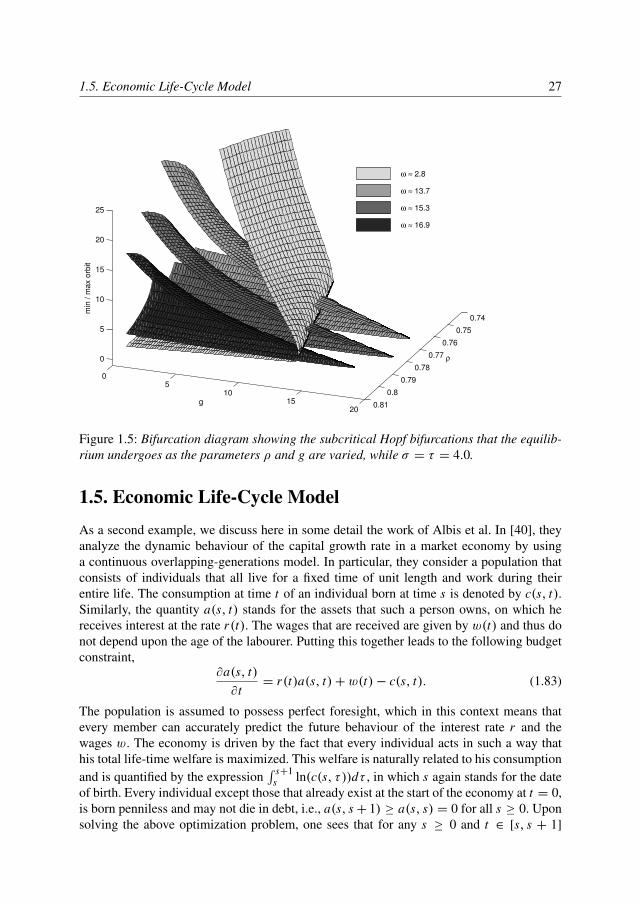
1.5. Economic Life-Cycle Model 27
0.74
0.75
0.76
0.77
0.78
0.79
0.8
0.81
05
1015
20
0
5
10
15
20
25
ρ
g
min
/ m
ax o
rbit
ω ≈ 2.8
ω ≈ 13.7
ω ≈ 15.3
ω ≈ 16.9
Figure 1.5: Bifurcation diagram showing the subcritical Hopf bifurcations that the equilib-rium undergoes as the parameters ρ and g are varied, while σ = τ = 4.0.
1.5. Economic Life-Cycle Model
As a second example, we discuss here in some detail the work of Albis et al. In [40], theyanalyze the dynamic behaviour of the capital growth rate in a market economy by usinga continuous overlapping-generations model. In particular, they consider a population thatconsists of individuals that all live for a fixed time of unit length and work during theirentire life. The consumption at time t of an individual born at time s is denoted by c(s, t).Similarly, the quantity a(s, t) stands for the assets that such a person owns, on which hereceives interest at the rate r(t). The wages that are received are given by w(t) and thus donot depend upon the age of the labourer. Putting this together leads to the following budgetconstraint,
∂a(s, t)∂t
= r(t)a(s, t)+ w(t)− c(s, t). (1.83)
The population is assumed to possess perfect foresight, which in this context means thatevery member can accurately predict the future behaviour of the interest rate r and thewages w. The economy is driven by the fact that every individual acts in such a way thathis total life-time welfare is maximized. This welfare is naturally related to his consumptionand is quantified by the expression
∫ s+1s ln(c(s, τ ))dτ , in which s again stands for the date
of birth. Every individual except those that already exist at the start of the economy at t = 0,is born penniless and may not die in debt, i.e., a(s, s+ 1) ≥ a(s, s) = 0 for all s ≥ 0. Uponsolving the above optimization problem, one sees that for any s ≥ 0 and t ∈ [s, s + 1]
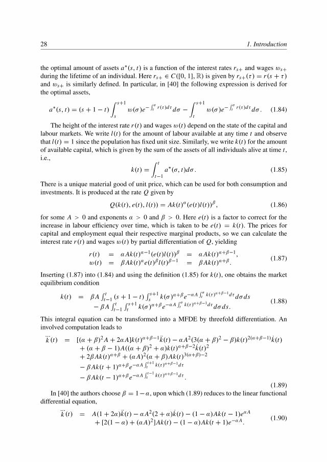
28 1. Introduction
the optimal amount of assets a∗(s, t) is a function of the interest rates rs+ and wages ws+during the lifetime of an individual. Here rs+ ∈ C([0, 1],R) is given by rs+(τ ) = r(s + τ)and ws+ is similarly defined. In particular, in [40] the following expression is derived forthe optimal assets,
a∗(s, t) = (s + 1− t)∫ s+1
sw(σ)e−
∫ σt r(τ )dτdσ −
∫ s+1
tw(σ)e−
∫ σt r(τ )dτdσ . (1.84)
The height of the interest rate r(t) and wages w(t) depend on the state of the capital andlabour markets. We write l(t) for the amount of labour available at any time t and observethat l(t) = 1 since the population has fixed unit size. Similarly, we write k(t) for the amountof available capital, which is given by the sum of the assets of all individuals alive at time t ,i.e.,
k(t) =∫ t
t−1a∗(σ, t)dσ . (1.85)
There is a unique material good of unit price, which can be used for both consumption andinvestments. It is produced at the rate Q given by
Q(k(t), e(t), l(t)) = Ak(t)α(e(t)l(t))β , (1.86)
for some A > 0 and exponents α > 0 and β > 0. Here e(t) is a factor to correct for theincrease in labour efficiency over time, which is taken to be e(t) = k(t). The prices forcapital and employment equal their respective marginal products, so we can calculate theinterest rate r(t) and wages w(t) by partial differentiation of Q, yielding
r(t) = αAk(t)α−1(e(t)l(t))β = αAk(t)α+β−1,
w(t) = βAk(t)αe(t)βl(t)β−1= βAk(t)α+β .
(1.87)
Inserting (1.87) into (1.84) and using the definition (1.85) for k(t), one obtains the marketequilibrium condition
k(t) = βA∫ t
t−1 (s + 1− t)∫ s+1
s k(σ )α+βe−αA∫ σ
t k(τ )α+β−1dτdσds− βA
∫ tt−1
∫ s+1t k(σ )α+βe−αA
∫ σt k(τ )α+β−1dτdσds.
(1.88)
This integral equation can be transformed into a MFDE by threefold differentiation. Aninvolved computation leads to
...k (t) = [(α + β)2 A + 2αA]k(t)α+β−1k(t)− αA2(3(α + β)2 − β)k(t)2(α+β−1)k(t)
+ (α + β − 1)A((α + β)2 + α)k(t)α+β−2k(t)2
+ 2βAk(t)α+β + (αA)2(α + β)Ak(t)3(α+β)−2
− βAk(t + 1)α+βe−αA∫ t+1
t k(τ )α+β−1dτ
− βAk(t − 1)α+βe−αA∫ t−1
t k(τ )α+β−1dτ .(1.89)
In [40] the authors choose β = 1−α, upon which (1.89) reduces to the linear functionaldifferential equation,
...k (t) = A(1+ 2α)k(t)− αA2(2+ α)k(t)− (1− α)Ak(t − 1)eαA
+ [2(1− α)+ (αA)2]Ak(t)− (1− α)Ak(t + 1)e−αA.(1.90)
1.5. Economic Life-Cycle Model 29
This equation matches the expression derived in [40] by substituting α + β = 1 directly in(1.87). Since (1.90) is linear, the global behaviour of the capital market can be analyzed bystudying the roots of the characteristic equation
1(z, α, A) := (z − αA)3 − (1− α)A[(z − αA)2 + 2− e−(z−αA)− ez−αA] = 0. (1.91)
This was performed in [40], where the authors proved that, apart from the triple root atz = αA, there is precisely one real root g(A) and all other roots satisfy Re z 6= g(A). Weremark here that insertion of k(t) = (A0 + A1t + A2t2)eαAt into (1.88) yields k(t) = 0,which is why this root needs to be excluded. However, k(t) ∼ egt does indeed yield asolution to (1.88). Demanding furthermore that k(t) should remain strictly positive, onesees that the capital dynamics may exhibit oscillations at the start of the economy, but willfinally converge to the balanced growth path [40].
We now shift our attention to the case that α+β 6= 1 and look for non-zero equilibriumsolutions to (1.88). It is convenient to introduce the new variable y = αAe(α+β−1) ln k .Substitution into (1.88) and setting all derivatives to zero yields the equilibrium conditionf (y) = 0, in which the function f is given by
f (y) = (α + β)y2+ 2β(1− cosh y). (1.92)
Lemma 1.5.1. For all parameters α > 0 and β > 0, the equation f (y) = 0 has a uniquestrictly positive solution y = y(A, α, β) > 0.
Proof. Notice that f (0) = f ′(0) = 0. In addition, we calculate
f ′′(y) = 2(α + β(1− cosh y)),f ′′′(y) = −2β sinh y, (1.93)
which implies that f ′′(0) = 2α > 0 and f ′′′(y) < 0 for all y > 0. The claim nowimmediately follows upon observing that limy→∞ f (y) = −∞.
We emphasize here that the equilibrium y found above does not translate into a valid equi-librium k for the capital when α + β = 1, since the corresponding variable transformationis ill-defined.
Linearizing (1.89) around an equilibrium y and using the condition f (y) = 0 yields thefollowing characteristic function,
α1(z) = α(z − y)3 + y(α − (α + β)2
)(z − y)2
− (α + β)y2(1− (α + β))(z − y)− (α + β)y
((α + β − 1)y2
+ 2β)
+ z−1[2β y((α + β)(z − y)+ y
)cosh(z − y)
+ y2(α + β − 1)((α + β)y2
+ 2β)].
(1.94)Invoking the equilibrium condition f (y) = 0, one can easily see that the apparent singular-ity at z = 0 in the above expression is in fact removable. Furthermore, a short calculationshows that 1(y) = 0, but for similar reasons as in the linear case this root needs to beexcluded.
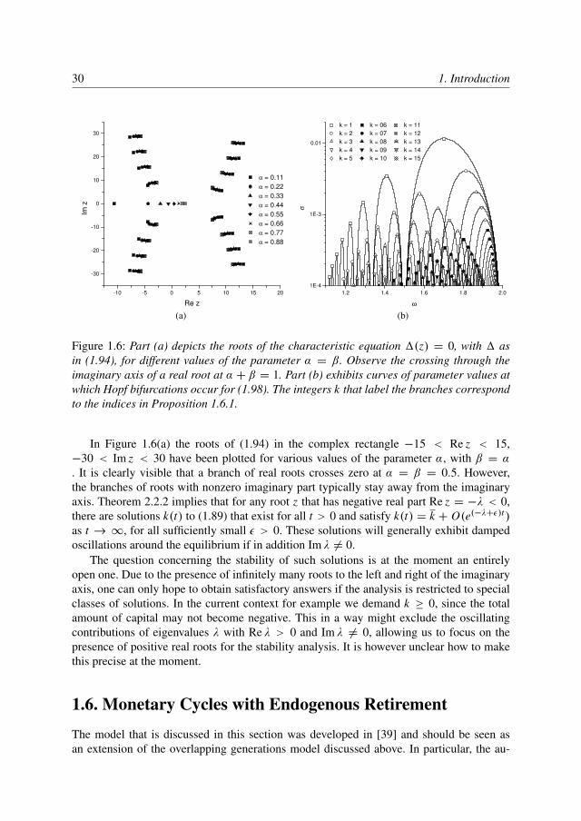
30 1. Introduction
-10 -5 0 5 10 15 20
-30
-20
-10
0
10
20
30
α = 0.11
α = 0.22
α = 0.33
α = 0.44
α = 0.55
α = 0.66
α = 0.77
α = 0.88
Im z
Re z
(a)
1.2 1.4 1.6 1.8 2.0
1E-4
1E-3
0.01
k = 1 k = 06 k = 11
k = 2 k = 07 k = 12
k = 3 k = 08 k = 13
k = 4 k = 09 k = 14
k = 5 k = 10 k = 15
σω
(b)
Figure 1.6: Part (a) depicts the roots of the characteristic equation 1(z) = 0, with 1 asin (1.94), for different values of the parameter α = β. Observe the crossing through theimaginary axis of a real root at α + β = 1. Part (b) exhibits curves of parameter values atwhich Hopf bifurcations occur for (1.98). The integers k that label the branches correspondto the indices in Proposition 1.6.1.
In Figure 1.6(a) the roots of (1.94) in the complex rectangle −15 < Re z < 15,−30 < Im z < 30 have been plotted for various values of the parameter α, with β = α. It is clearly visible that a branch of real roots crosses zero at α = β = 0.5. However,the branches of roots with nonzero imaginary part typically stay away from the imaginaryaxis. Theorem 2.2.2 implies that for any root z that has negative real part Re z = −λ < 0,there are solutions k(t) to (1.89) that exist for all t > 0 and satisfy k(t) = k + O(e(−λ+ε)t )as t → ∞, for all sufficiently small ε > 0. These solutions will generally exhibit dampedoscillations around the equilibrium if in addition Im λ 6= 0.
The question concerning the stability of such solutions is at the moment an entirelyopen one. Due to the presence of infinitely many roots to the left and right of the imaginaryaxis, one can only hope to obtain satisfactory answers if the analysis is restricted to specialclasses of solutions. In the current context for example we demand k ≥ 0, since the totalamount of capital may not become negative. This in a way might exclude the oscillatingcontributions of eigenvalues λ with Re λ > 0 and Im λ 6= 0, allowing us to focus on thepresence of positive real roots for the stability analysis. It is however unclear how to makethis precise at the moment.
1.6. Monetary Cycles with Endogenous Retirement
The model that is discussed in this section was developed in [39] and should be seen asan extension of the overlapping generations model discussed above. In particular, the au-
1.6. Monetary Cycles with Endogenous Retirement 31
thors again consider a fixed size population of individuals, that now live for the longer timeω > 1, with the restriction that every labourer retires at unit age. In terms of the model com-ponents, this means that the wages w(s, t) now do depend upon the time of birth and satisfyw(s, t) = 1 for t ∈ [s, s + 1] and w(s, t) = 0 otherwise. As before, everybody receivesinterest at the rate r(t) on their assets a(s, t) while consuming c(s, t). These observationslead to the modified budget constraint
∂a(s, t)∂t
= r(t)a(s, t)+ w(s, t)− c(s, t). (1.95)
A second variant in this model is that the utility u(s) as perceived by the generation born attime s is now given by
u(s) =∫ s+ω
s
c(s, t)1−σ−1
1− σ−1 dt. (1.96)
As usual, every individual acts in such a way that his utility is maximized, subject to both(1.95) and the natural budget constraints a(s, s) = 0 and a(s, s + ω) ≥ 0. In (1.96) theparameter σ stands for the elasticity of intertemporal substitution and is required to satisfyσ > 0. The economy features a single, nonstorable consumption good, which we willassume to be produced at exactly the rate required by the consumer market. In terms of ourmodel variables, this means that for all time t the following identity must hold,∫ t
t−ωw(σ, t)dσ =
∫ t
t−ωc(σ, t)dσ. (1.97)
The rules above are sufficient to fix the dynamical behaviour of the economy and following[39], one easily derives the difference equation F(rt ) = 0 for the interest rate r(t), with Fgiven by
F(rt ) = 1−∫ t
t−ω
∫ s+1s exp[−
∫ vt r(u)du]dv∫ s+ω
s exp[−(1− σ)∫ v
t r(u)du]dvds. (1.98)
Notice that r = 0 is an equilibrium solution of (1.98). The linearization around thisequilibrium is given by
0 = −1ω
∫ t
t−ω
∫ s+1
s
∫ v
tx(u)du dv ds +
1− σω2
∫ t
t−ω
∫ s+ω
s
∫ v
tx(u)du dv ds. (1.99)
Inserting x(u) = exp(zu) yields the characteristic function
1(z, σ, ω) = −1
ω2z3 [−ωez+ (1− σ)ezω
+ (ωez− ω + 1− σ)e−zω
+(ω − 2+ 2σ)+ σω2z2].(1.100)
The following result, which was partially proven in [39], shows that the characteristic equa-tion 1(z) = 0 admits simple roots on the imaginary axis that satisfy the conditions associ-ated with the Hopf bifurcation theorem. The proof is deferred to the end of this section.
Proposition 1.6.1. Consider any ω > 1 such that (ω − 1)−1 /∈ N. There exists an infinitesequence of pairs (σk, qk) parametrized by k ∈ N, with σk > 0 and qk > 0, such that thefollowing properties are satisfied.
32 1. Introduction
(i) One has the limits σk → 0 and qk →∞ as k →∞.
(ii) The characteristic equation 1(z, σk, ω) = 0 has two simple roots at z = ±iqk .
(iii) For all k ∈ N and m ∈ Z \ {±1}, the inequality 1(imqk, σk, ω) 6= 0 holds.
(iv) For every k ∈ N, the branch of roots z(σ ) of the characteristic equation1(z, σ, ω) = 0 through z = iqk at σ = σk crosses the imaginary axis with posi-tive speed, i.e.,
ReD21(iqk, σk, ω)
D11(iqk, σk, ω)6= 0. (1.101)
Conversely, if ω = 1+ n−1 for some n ∈ N, then for all σ > 0 the characteristic equation1(z, σ, ω) = 0 admits no roots with Re z = 0.
Fixing any suitable ω > 1 and treating σ as a bifurcation parameter, the result abovewill allow us to conclude that the algebraic equation (1.98) admits a branch of periodic so-lutions bifurcating from the equilibrium r = 0 at σ = σk , for all k ∈ N. Similarly, anysufficiently small solution of (1.98) with σ near σk can be captured on such a branch. Tovalidate this claim using our main theorem in Section 3.2, we note that twofold differenti-ation of (1.98) and simplification using the identity (1.98), yields the following mixed typefunctional differential equation,
r(t) = G(rt ), with−σG(rt ) = −σ 2r(t)2 + [
∫ t+ωt eσ (v)dv]−1[e(t + 1)− 1]
−[∫ t+ω
t eσ (v)dv]−2[eσ (t + ω)− 1]∫ t+1
t e(v)dv+[
∫ tt−ω eσ (v)dv]−2[1− eσ (t − ω)]
∫ t−ω+1t−ω e(v)dv
−[∫ t
t−ω eσ (v)dv]−1[e(t − ω + 1)− e(t − ω)],
(1.102)
in which we have made the abbreviations
e(w) = exp(−
∫ wt r(u)du
),
eσ (w) = exp(− (1− σ)
∫ wt r(u)du
).
(1.103)
Linearizing (1.102) around r = 0 yields
−σ x(t) = −1ω
∫ t+1t x(u)du + 1
ω
∫ t−ω+1t−ω x(u)du
+1−σω2
∫ t+ωt x(u)du + 1−σ
ω2
∫ t−ωt x(u)du.
(1.104)
Inserting x(u) = exp(zu) and normalizing, we find the characteristic function
1M (z, σ, ω) = 1σω2z [σω2z2
− ω(ez− 1)+ ω(ez
− 1)e−ωz
+(1− σ)(eωz+ e−ωz
− 2)]= −
z2
σ 1(z, σ, ω),(1.105)
which immediately implies that condition (HL) in Section 3.2 is satisfied. Using the ex-pressions above, all the other conditions of Theorem 3.2.2 can easily be verified as well.
1.6. Monetary Cycles with Endogenous Retirement 33
Hence upon fixing an appropriate ω > 1 and considering any pair (σ0, q0) generatedby Proposition 1.6.1, we can establish the existence of a 2 + 1 dimensional center mani-fold u∗ : X0 × R →
⋂η>0 BC1
η(R,Cn) directly for the difference equation (1.98). HereX0 = span(eiq0·, e−iq0·) and the extra dimension arises by including the bifurcation param-eter σ = σ − σ0 in the center space. The dynamical behaviour of σ on the center manifoldis trivial, while the evolution of ψ(ξ) = x(ξ)eiq0· + y(ξ)e−iq0· ⊂ X0 is governed by theODE
x ′ = iq0x + f1(x, y, σ )+ O((|x | + |y|)3 + |σ | (|x | + |y|)(|σ | + |x | + |y|)
),
y′ = −iq0 y + f2(x, y, σ )+ O((|x | + |y|)3 + |σ | (|x | + |y|)(|σ | + |x | + |y|)
),
(1.106)in which the second order terms are given by
f1(x, y, σ ) = −D21(iq0, σ0)D11(iq0, σ0)−1σ x
+12 D11(iq0, σ0)
−1(αxx x2+ 2αxy xy + αyy y2)
+1
2iq0D11(iq0, σ0)
−1(1(2iq0, σ0)(βxx − 4 q2
0σ0αxx )x2
−21(0, σ0)βxy xy − 131(−2iq0, σ0)(βyy − 4 q2
0σ0αyy)y2
),
f2(x, y, σ ) = −D21(−iq0, σ0)D11(−iq0, σ0)−1σ y
+12 D11(−iq0, σ0)
−1(αxx x2+ 2αxy xy + αyy y2)
+1
2iq0D11(−iq0, σ0)
−1(
131(2iq0, σ0)(βxx − 4 q2
0σ0αxx )x2
+21(0, σ0)βxy xy −1(−2iq0, σ0)(βyy − 4 q20σ0αyy)y2
)(1.107)
and the quantities αxx through βyy can be calculated by using
αxx = D21F(0, σ0)(eiq0·, eiq0·), βxx = D2
1G(0, σ0)(eiq0·, eiq0·),
αxy = D21F(0, σ0)(eiq0·, e−iq0·), βxy = D2
1G(0, σ0)(eiq0·, e−iq0·),
αyy = D21F(0, σ0)(e−iq0·, e−iq0·), βyy = D2
1G(0, σ0)(e−iq0·, e−iq0·).(1.108)
Using the transversality condition (iv) from Proposition 1.6.1, it is easily seen that the ODE(1.106) undergoes a Hopf bifurcation at σ = σ0. This yields a branch of periodic orbits thatcan be lifted back to periodic solutions of our initial problem (1.98), which establishes ourclaim above.
Notice that 1M (z) = 0 has a double root at z = 0 for all valid parameters ω andσ , which arises as an artifact of the differentiation operations needed to derive (1.102).This double root prevents the direct application of the Hopf bifurcation result developed inChapter 2 to the MFDE (1.102). To give a detailed analysis of the local behaviour of thisequation, one would hence have to revert to a complicated normal form reduction. Theorem3.2.2 has allowed us to circumvent this difficulty by analyzing (1.98) directly.
In Figure 1.6(b) the parameter values at which (1.98) undergoes a Hopf bifurcation havebeen visualized. The nested structure of the curves and the location of the gaps can beunderstood from the proof of Proposition 1.6.1, which exploits the rare fact that the rootsof (1.100) can be explicitly described. By contrast, the actual computation of the arisingperiodic orbits is far more challenging due to the presence of the doubly nested integrals in
34 1. Introduction
(1.102). The results in Figure 1.7(a) were computed by using a fine equidistributed grid of21 thousand mesh points and invoking the non-adaptive Kronrod 21-point rule [43] on eachmesh interval to compute the integrals.
Proof of Proposition 1.6.1. For convenience, we write 1(z, σ, ω) = −ω2z31(z, σ, ω).First note that 1(z, σ, ω) = 1
2ω2(ω− 1)z3
+ O(z4) around z = 0, which implies that z = 0is not a root of 1(z, σ0, ω) for ω > 1. For any q ∈ R, we write I (q) = Im 1(iq, σ, ω) andcompute
I (q) = ω(sinωq + sin(1− ω)q − sin q) = 4ω sinωq2
sin(1− ω)q
2sin
q2. (1.109)
Similarly, writing R(q) = Re 1(iq, σ, ω), we compute
R(q) = −ω cos q + 2(1− σ)(cosωq − 1)+ ω(1− cosωq)+ω cos(1− ω)q − σω2q2
= 2ω(sin2 q2 + sin2 ωq
2 − sin2 (1−ω)q2 )− 4 sin2 ωq
2 + σ(4 sin2 ωq2 − ω
2q2).(1.110)
Notice that for any l ∈ N and q(l) = 2lπω−1 , we have sin (1−ω)q(l)
2 = 0, while
sin2 q(l)2 = sin2 ωq(l)
2 . This implies that
R(q(l)) = 4(ω − 1) sin2 q(l)
2+ σ(4 sin2 q(l)
2− (ωq(l))2). (1.111)
Now assume that (ω − 1)−1 /∈ N, which implies that π1−ω 6≡ 0 mod π . There hence
exists a strictly increasing sequence of integers lk > 0, parametrized by k ∈ N, such thatsk = sin2 q(lk )
2 > 14 . Choose qk = q(lk ) and write
σk =ω − 1
ω2 q2k
4sk− 1
> 0, (1.112)
where the last inequality follows from ω > 1 and the fact that |sin θ | < |θ | for θ 6= 0.By construction, we have 1(iqk, σk, ω) = 0. Suppose that for any m ∈ Z \ {0,±1} wehave 1(imqk, σk, ω) = 0, then using mqk = q(mlk ) and setting R(q(mlk )) = 0, we find thatsin2 q(mlk )
2 = skm2 > 14 m2 > 1, which is impossible. To prove the claim (iv) involving the
derivatives of 1, note that
Ds1(iqk, σk, ω) =i
ω2q3k
Ds1(iqk, σk, ω) (1.113)
for s = 1, 2. In addition,
D21(iqk, σk, ω) = 2(1− cosωqk)− ω2q2
k = 4sk − ω2q2
k < 0. (1.114)
It hence suffices to compute
Re D11(iqk, σk, ω) = −ω cos qk + ω(1− ω) cos(1− ω)qk + ω2 cosωqk
= 2ω(1− ω)sk 6= 0.(1.115)
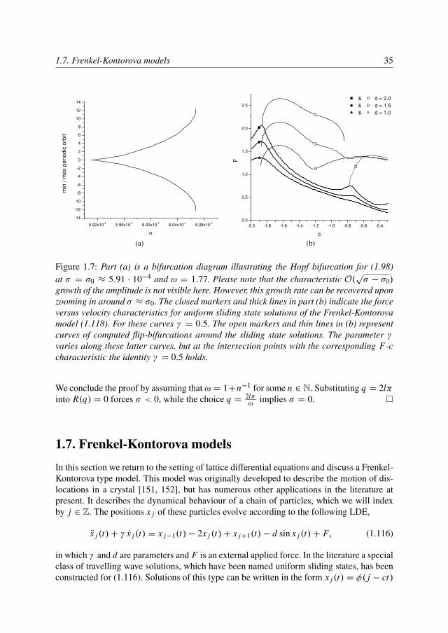
1.7. Frenkel-Kontorova models 35
5.92x10⁻⁴
5.96x10⁻⁴
6.00x10⁻⁴
6.04x10⁻⁴
6.08x10⁻⁴
-14
-12
-10
-8
-6
-4
-2
0
2
4
6
8
10
12
14
min
/ m
ax p
eri
od
ic o
rbit
σ
(a)
-2.0 -1.8 -1.6 -1.4 -1.2 -1.0 -0.8 -0.6 -0.4
0.0
0.5
1.0
1.5
2.0
2.5
& d = 2.0
& d = 1.5
& d = 1.0
Fc
(b)
Figure 1.7: Part (a) is a bifurcation diagram illustrating the Hopf bifurcation for (1.98)at σ = σ0 ≈ 5.91 · 10−4 and ω = 1.77. Please note that the characteristic O(
√σ − σ0)
growth of the amplitude is not visible here. However, this growth rate can be recovered uponzooming in around σ ≈ σ0. The closed markers and thick lines in part (b) indicate the forceversus velocity characteristics for uniform sliding state solutions of the Frenkel-Kontorovamodel (1.118). For these curves γ = 0.5. The open markers and thin lines in (b) representcurves of computed flip-bifurcations around the sliding state solutions. The parameter γvaries along these latter curves, but at the intersection points with the corresponding F-ccharacteristic the identity γ = 0.5 holds.
We conclude the proof by assuming that ω = 1+n−1 for some n ∈ N. Substituting q = 2lπinto R(q) = 0 forces σ < 0, while the choice q = 2lπ
ω implies σ = 0.
1.7. Frenkel-Kontorova models
In this section we return to the setting of lattice differential equations and discuss a Frenkel-Kontorova type model. This model was originally developed to describe the motion of dis-locations in a crystal [151, 152], but has numerous other applications in the literature atpresent. It describes the dynamical behaviour of a chain of particles, which we will indexby j ∈ Z. The positions x j of these particles evolve according to the following LDE,
x j (t)+ γ x j (t) = x j−1(t)− 2x j (t)+ x j+1(t)− d sin x j (t)+ F, (1.116)
in which γ and d are parameters and F is an external applied force. In the literature a specialclass of travelling wave solutions, which have been named uniform sliding states, has beenconstructed for (1.116). Solutions of this type can be written in the form x j (t) = φ( j − ct)
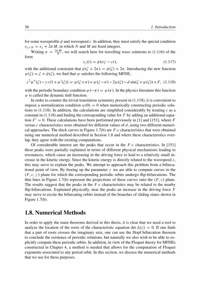
36 1. Introduction
for some waveprofile φ and wavespeed c. In addition, they must satisfy the special conditionx j+N = x j + 2πM , in which N and M are fixed integers.
Writing σ = 2πMN , we will search here for travelling wave solutions to (1.116) of the
formx j (t) = φ(σ j − ct), (1.117)
with the additional constraint that φ(ξ + 2π) = φ(ξ) + 2π . Introducing the new functionψ(ξ) = ξ + φ(ξ), we find that ψ satisfies the following MFDE,
c2ψ ′′(ξ)−γ c(1+ψ ′(ξ)) = ψ(ξ+σ)+ψ(ξ−σ)−2ψ(ξ)−d sin(ξ+ψ(ξ))+F, (1.118)
with the periodic boundary conditionψ(−π) = ψ(π). In the physics literature this functionψ is called the dynamic hull function.
In order to counter the trivial translation symmetry present in (1.118), it is convenient toimpose a normalization condition ψ(0) = 0 when numerically constructing periodic solu-tions to (1.118). In addition, the calculations are simplified considerably by treating c as aconstant in (1.118) and finding the corresponding value for F by adding an additional equa-tion F ′ = 0. These calculations have been performed previously in [1] and [151], where Fversus c characteristics were obtained for different values of d, using two different numeri-cal approaches. The thick curves in Figure 1.7(b) are F-c characteristics that were obtainedusing our numerical method described in Section 1.8 and where these characteristics over-lap, they agree with the existing computations.
Of considerable interest are the peaks that occur in the F-c characteristics. In [151]these peaks were partially explained in terms of different physical mechanisms leading toresonances, which cause an increasing in the driving force to lead to a relatively small in-crease in the kinetic energy. Since the kinetic energy is directly related to the wavespeed c,this may serve to explain the peaks. We attempt to approach this problem from a bifurca-tional point of view. By freeing up the parameter γ we are able to compute curves in the(F, c, γ ) plane for which the corresponding periodic orbits undergo flip-bifurcations. Thethin lines in Figure 1.7(b) represent the projections of these curves onto the (F, c) plane.The results suggest that the peaks in the F-c characteristics may be related to the nearbyflip-bifurcations. Explained physically, near the peaks an increase in the driving force Fmay serve to excite the bifurcating orbits instead of the branches of sliding states shown inFigure 1.7(b).
1.8. Numerical MethodsIn order to apply the main theorems derived in this thesis, it is clear that we need a tool toanalyze the location of the roots of the characteristic equation det1(z) = 0. If one findsthat a pair of roots crosses the imaginary axis, one can use the Hopf bifurcation theoremto conclude the existence of periodic solutions, but naturally we also wish to be able to ex-plicitly compute these periodic orbits. In addition, in view of the Floquet theory for MFDEsconstructed in Chapter 4, a method is needed that allows for the computation of Floquetexponents associated to any period orbit. In this section, we discuss the numerical methodsthat we use for these purposes.
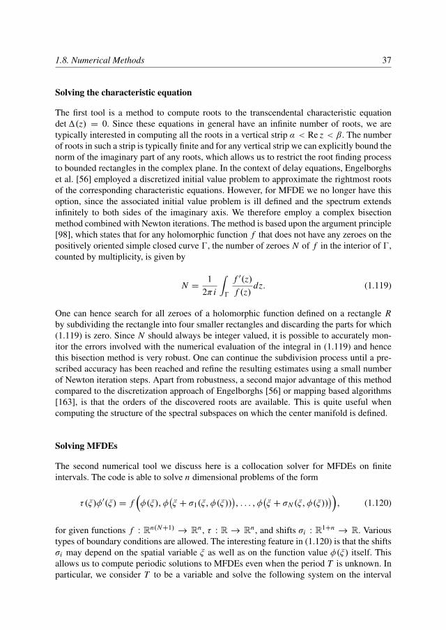
1.8. Numerical Methods 37
Solving the characteristic equation
The first tool is a method to compute roots to the transcendental characteristic equationdet1(z) = 0. Since these equations in general have an infinite number of roots, we aretypically interested in computing all the roots in a vertical strip α < Re z < β. The numberof roots in such a strip is typically finite and for any vertical strip we can explicitly bound thenorm of the imaginary part of any roots, which allows us to restrict the root finding processto bounded rectangles in the complex plane. In the context of delay equations, Engelborghset al. [56] employed a discretized initial value problem to approximate the rightmost rootsof the corresponding characteristic equations. However, for MFDE we no longer have thisoption, since the associated initial value problem is ill defined and the spectrum extendsinfinitely to both sides of the imaginary axis. We therefore employ a complex bisectionmethod combined with Newton iterations. The method is based upon the argument principle[98], which states that for any holomorphic function f that does not have any zeroes on thepositively oriented simple closed curve 0, the number of zeroes N of f in the interior of 0,counted by multiplicity, is given by
N =1
2π i
∫0
f ′(z)f (z)
dz. (1.119)
One can hence search for all zeroes of a holomorphic function defined on a rectangle Rby subdividing the rectangle into four smaller rectangles and discarding the parts for which(1.119) is zero. Since N should always be integer valued, it is possible to accurately mon-itor the errors involved with the numerical evaluation of the integral in (1.119) and hencethis bisection method is very robust. One can continue the subdivision process until a pre-scribed accuracy has been reached and refine the resulting estimates using a small numberof Newton iteration steps. Apart from robustness, a second major advantage of this methodcompared to the discretization approach of Engelborghs [56] or mapping based algorithms[163], is that the orders of the discovered roots are available. This is quite useful whencomputing the structure of the spectral subspaces on which the center manifold is defined.
Solving MFDEs
The second numerical tool we discuss here is a collocation solver for MFDEs on finiteintervals. The code is able to solve n dimensional problems of the form
τ(ξ)φ′(ξ) = f(φ(ξ), φ
(ξ + σ1(ξ, φ(ξ))
), . . . , φ
(ξ + σN (ξ, φ(ξ))
)), (1.120)
for given functions f : Rn(N+1)→ Rn , τ : R → Rn , and shifts σi : R1+n
→ R. Varioustypes of boundary conditions are allowed. The interesting feature in (1.120) is that the shiftsσi may depend on the spatial variable ξ as well as on the function value φ(ξ) itself. Thisallows us to compute periodic solutions to MFDEs even when the period T is unknown. Inparticular, we consider T to be a variable and solve the following system on the interval
38 1. Introduction
[0, 1],
φ′(ξ) = T f(φ(ξ), φ(ξ + r1/T mod 1), . . . , φ(ξ + rN/T mod 1)
),
T ′(ξ) = 0,φ(0) = φ(1),P(φ) = 0.
(1.121)
Here P(φ) is a phase condition to counter the shift invariance of periodic solutions. Weremark here that the computations of periodic solutions with unknown periods that can befound in this chapter are actually novel to the field of MFDEs.
The system (1.121) is solved by dividing the interval [0, 1] into L subintervals [ti , ti+1]and representing φ(ξ) on each subinterval in terms of a standard Runge-Kutta monomialbasis. The representation is required to be continuous at the boundary points between subin-tervals and in addition to satisfy (1.121) at the Ld collocation points ti + (ti+1 − ti )c j , fori = 1 . . . L and j = 1 . . . d , where 0 < c1 < . . . < cd < 1 are the Gaussian collocationpoints of degree d for some d ≥ 3. Using Newton iterations such a piecewise polynomial φcan be found, given a sufficiently close initial estimate. For further details and a convergenceanalysis of this method, we refer to Chapter 5.
Floquet exponents
In [56] and [153] Floquet exponents associated to periodic solutions were computed byconstructing the monodromy matrix, otherwise known as the T2π -map, for the linearizationaround the periodic solutions. However, in the case of MFDEs this monodromy matrix is nolonger available, since the equation is ill-defined and hence a different technique is needed.
Our approach will be to look for Floquet multipliers on the unit circle by direct construc-tion of the associated Floquet eigenfunction. In particular, given a periodic solution p wewill look for functions of the form v(ξ) = eλξq(ξ) with λ ∈ iR and periodic q ∈ C(R,Rn)with q(ξ) = q(ξ + 2π), that solve the linearized equation
v′(ξ) = D f (pξ )vξ . (1.122)
This can be solved within our framework of periodic solutions, by solving (1.122) onthe interval [0, 2π ] with the boundary condition v(2π) = e2πλv(0) and an appropriaterule v(ξ + σ) = e2kπλv(ξ + σ − 2kπ), where k ∈ Z needs to be chosen such thatξ + σ − 2kπ ∈ [0, 2π ].
Generalized Floquet functions can be found in a similar fashion. From Section 4.6, weknow that for any Jordan block associated to a Floquet exponent λ, a basis of generalizedFloquet eigenfunctions {yk} with 0 ≤ k ≤ d can be constructed, with
yk(ξ) = eλξqk(ξ)−
k−1∑`=0
(−ξ)k−`
(k − `)!y`(ξ). (1.123)
Here d + 1 is the dimension of the Jordan block and the functions qk∈ C(R,Rn) are
periodic with qk(ξ + 2π) = qk(ξ) for all ξ ∈ R.
1.8. Numerical Methods 39
Proposition 1.8.1. Consider a floquet exponent λ and let a basis for the generalizedeigenspace be given by (1.123). Then we have
yk(ξ + 2π) = e2πλk∑`=0
y`(ξ)(2π)k−`
(k − `)!. (1.124)
Proof. We use induction on the integer k. For k = 0 the statement is clear directly from(1.123). For k > 0, we assume that (1.124) holds for all integers 0 ≤ ` < k and compute
yk(ξ + 2π) = e2πλeλξqk(ξ + 2π)− e2πλ∑k−1`=0
(−ξ−2π)k−`(k−`)!
∑`j=0 y j (ξ) (2π)
`− j
(`− j)!
= e2πλ[eλξqk(ξ)−∑k−1
j=0 y j (ξ)∑k−1`= j
(−ξ−2π)k−`(k−`)!
(2π)`− j
(`− j)!
]= e2πλ[eλξqk(ξ)−
∑k−1j=0 y j (ξ) 1
(k− j)! [(−ξ)k− j− (2π)k− j ]
]= e2πλ[yk(ξ)+
∑k−1j=0 y j (ξ) (2π)
k− j
(k− j)!
],
(1.125)which completes the proof.
In practice, it is convenient to compute the periodic solution p simultaneously with theassociated Floquet exponents. In order to detect the presence of a Jordan block of dimensiond + 1 associated to a Floquet exponent λ, one would hence solve the following system onthe interval [0, 2π ],
p′(ξ) =T
2π f(
p(ξ), p(ξ + 2πr1/T mod 2π), . . . , p(ξ + 2πrN/T mod 2π)),
T ′(ξ) = 0,
yk′(ξ) =T
2π D f(
p(ξ), p(ξ + 2πr1/T mod 2π), . . . ,
p(ξ + 2πrN/T mod 2π))
evξ yk,
p(2π) = p(0),P(p) = 0,yk(2π) = e2πλ∑k
`=0 y`(0) (2π)k−`
(k−`)! ,
Y (y0) = 0,(1.126)
in which k = 0 . . . d . The last condition is a normalization on y0. The expression evξ yk
should be interpreted as the vector(yk(ξ), yk(ξ + 2πr1/T ), . . . , yk(ξ + 2πrN/T )
), which
needs to be evaluated using repeated application of (1.124) to translate the arguments intothe interval [0, 2π ].

Chapter 2
Center Manifolds Near Equilibria
This chapter has been published as: H.J. Hupkes and S.M. Verduyn Lunel, “Center ManifoldTheory for Functional Differential Equations of Mixed Type”, Journal of Dynamics andDifferential Equations, Vol. 19 (2007), 497–560.
Abstract. We study the behaviour of solutions to nonlinear autonomous functional differ-ential equations of mixed type in the neighbourhood of an equilibrium. We show that allsolutions that remain sufficiently close to an equilibrium can be captured on a finite dimen-sional invariant center manifold, that inherits the smoothness of the nonlinearity. In addition,we provide a Hopf bifurcation theorem for such equations.
2.1. IntroductionThe purpose of this chapter is to provide a tool to analyze the behaviour of solutions to anonlinear functional differential equation of mixed type
x ′(ξ) = G(xξ ), (2.1)
in the neighbourhood of an equilibrium x . Here x is a continuous Cn-valued function andfor any ξ ∈ R the state xξ ∈ C([rmin, rmax],Cn) is defined by xξ (θ) = x(ξ + θ). We allowrmin ≤ 0 and rmax ≥ 0, hence the nonlinearity G may depend on advanced and retardedarguments simultaneously.
We establish a center manifold theorem for solutions to (2.1) close to x , that is, we showthat all sufficiently small solutions to the equation
u′(ξ) = DG(x)uξ + (G(x + uξ )− DG(x)uξ ) (2.2)
can be captured on a finite dimensional invariant manifold and we explicitly describe thedynamics on this manifold. This reduction allows us to establish a Hopf bifurcation theo-rem for (2.1), yielding a very powerful tool to perform a bifurcation analysis on parameterdependent versions of this equation. If the linearization u′(ξ) = DG(x)uξ has no bounded
42 2. Center Manifolds Near Equilibria
solutions on the line, we say that the equilibrium x is hyperbolic and in this case the centermanifold contains only the zero function. We will thus be particularly interested in situa-tions where the linear operator DG(x) has eigenvalues on the imaginary axis, implying thatx is a nonhyperbolic equilibrium.
The study of center manifolds in infinite dimensions forms one of the cornerstones of thetheory of dynamical systems. During the last two decades, many authors have contributedtowards developing the general theory. We mention specially the comprehensive overviewby Iooss and Vanderbauwhede [158] and the work of Mielke on elliptic partial differentialequations [118, 119], in which linear unbounded operators that have infinite spectrum tothe right and left of the imaginary axis were analyzed. This type of operator also ariseswhen studying (2.1), but our approach in this chapter is more closely related to the ideasdeveloped in [45], where the theory of semigroups was used to succesfully construct centermanifolds for delay equations.
When studying the nonlinear mixed-type functional differential equation (2.1), it is es-sential to have results for linear systems
x ′(ξ) = L(ξ)xξ + f (ξ). (2.3)
Mallet-Paret provided the basic theory in [112], showing that a Fredholm alternative theo-rem holds for hyperbolic systems (2.3) and providing exponential estimates for solutionsto such equations. Later, the existence of exponential dichotomies for (2.3) was estab-lished independently by Mallet-Paret and Verduyn Lunel [115] and Harterich et al. [75].In the present work, we extend the framework developed in [112] to nonhyperbolic butautonomous versions of (2.3), which allows us to generalize the center manifold theorydeveloped for delay equations in [45] to equations of mixed type.
Our main results are stated in Section 2.2 and proved in Sections 2.3 through 2.10, wherethe necessary theory is developed. In particular, in Section 2.3 we discuss and apply the re-sults of Mallet Paret to linear systems (2.3) that violate the hyperbolicity condition neededin [112]. In Section 2.4 we introduce an operator associated with (2.3) on the state spaceX = C([rmin, rmax],Cn), that in the case of delay equations reduces to the generator of thesemigroup associated with the homogeneous version of (2.3). Laplace transform techniquesare used in Section 2.5 to combine the results from the previous two sections in order todefine a pseudo-inverse K for (2.3), in the sense that inhomogeneities f are mapped to theircorresponding solutions x = K f modulo a finite dimensional set of solutions to (2.3) withf = 0. This set is isomorphic to a finite dimensional subspace X0 ⊂ X and the operatorK is used in Section 2.6 in a fixed point argument to construct small solutions u∗φ to thenonlinear equation (2.2) for any small φ ∈ X0. This map u∗ is shown to be of class Ck
in Section 2.7, while Section 2.8 shows that these small solutions can in fact be describedas solutions to a finite dimensional ordinary differential equation. This reduction is used inSection 2.10 to establish a Hopf bifurcation theorem for parameter dependent versions of(2.2). Finally, in Section 2.11 we discuss some examples and explicitly describe the dynam-ics on the center manifold for a functional differential equation of mixed type that admitsa double eigenvalue at zero after linearization. In particular, we exhibit a Takens-Burganovbifurcation and show that for delay equations the results from [45] can be recovered fromour framework.
2.2. Main Results 43
2.2. Main ResultsConsider for some N ≥ 0 the functional differential equation of mixed type
x ′(ξ) =N∑
j=0
A j x(ξ + r j )+ R(x(ξ + r0), . . . , x(ξ + rN )), (2.4)
in which x is a mapping from R into Cn for some integer n ≥ 1 and each A j is a n × nmatrix with complex entries. The shifts r j ∈ R may be both positive and negative andfor convenience we assume that they are ordered and distinct, i.e., r0 < r1 < . . . < rN .Defining rmin = r0 and rmax = rN , we require rmin ≤ 0 ≤ rmax.
The space X = C([rmin, rmax],Cn) of continuous Cn-valued functions defined on theinterval [rmin, rmax] will serve as a state space when analyzing (2.4). In particular, for anyx ∈ C(R,Cn) and any ξ ∈ R, we define the state xξ ∈ X as the function xξ (θ) = x(ξ + θ)for any rmin ≤ θ ≤ rmax. Introducing the bounded linear operator L : X → Cn given by
Lφ =N∑
j=0
A jφ(r j ), (2.5)
one can rewrite (2.4) asx ′(ξ) = Lxξ + R(xξ ). (2.6)
In our analysis of (2.6) we will be particularly interested in the scale of Banach spaces
BCη(R,Cn) =
{x ∈ C(R,Cn) | sup
ξ∈Re−η|ξ | |x(ξ)| <∞
}, (2.7)
parametrized by η ∈ R. The corresponding norm is given by ‖x‖η = supξ∈R e−η|ξ | |x(ξ)|.We also need the Banach spaces
BC1η(R,C
n) ={
x ∈ BCη(R,Cn) ∩ C1(R,Cn) | x ′ ∈ BCη(R,Cn)}, (2.8)
with corresponding norm ‖x‖BC1η= ‖x‖η +
∥∥x ′∥∥η. Notice that we have continuous inclu-
sionsBCη1(R,Cn) ↪→ BCη2(R,Cn) and BC1
η1(R,Cn) ↪→ BC1
η2(R,Cn) for any pair
η2 ≥ η1. We will write Jη2η1 and J 1η2η1
respectively for the corresponding embeddingoperators.
In the analysis of (2.6), it is essential to study the behaviour of the homogeneous linearequation
x ′(ξ) = Lxξ . (2.9)
Associated with this system (2.9) one has the characteristic matrix 1 : C → Cn×n , givenby
1(z) = z I −N∑
j=0
A j ezr j . (2.10)
44 2. Center Manifolds Near Equilibria
A value of z such that det1(z) = 0 is called an eigenvalue for the system (2.9). In order toformulate our main results, we need the following proposition.
Proposition 2.2.1. For any homogeneous linear equation of the form (2.9), there exists afinite dimensional linear subspace X0 ⊂ X with the following properties.
(i) Suppose x ∈⋂η>0 BC1
η(R,Cn) is a solution of (2.9). Then for any ξ ∈ R we havexξ ∈ X0.
(ii) For any φ ∈ X0, we have φ′ ∈ X0.
(iii) For any φ ∈ X0, there is a solution x = Eφ ∈⋂η>0 BCη(R,Cn) of (2.9) that has
x0 = φ. This solution is unique in the set⋃η>0 BCη(R,Cn).
We will write Q0 for the projection operator from X onto X0, which will be definedprecisely in the sequel. The following two assumptions on the nonlinearity R : X → Cn
will be needed in our results.
(HR1) The nonlinearity R is Ck-smooth for some k ≥ 1.
(HR2) We have R(0) = 0 and DR(0) = 0.
We remark here that the smoothness requirement in condition (HR1) in fact refers to theFrechet differentiability of R, since this operator is defined on the infinite dimensionalspace X . This technicality should be implicitly understood throughout the remainder ofthis chapter. However, one should note that this issue becomes irrelevant when consideringnonlinearities R as in (2.4), which have a finite dimensional domain.
Theorem 2.2.2. Consider the nonlinear equation (2.6) and assume that (HR1) and (HR2)are satisfied. Then there exists γ > 0 such that the characteristic equation det1(z) = 0has no roots with 0 < |Re z| < γ . Fix an interval I = [ηmin, ηmax] ⊂ (0, γ )such that ηmax > kηmin, with k as introduced in (HR1). Then there exists a mappingu∗ : X0 →
⋂η>0 BC1
η(R,Cn) and constants ε > 0, ε∗ > 0 such that the followingstatements hold.
(i) For any η ∈ (kηmin, ηmax], the function u∗ viewed as a map from X0 into BC1η(R,Cn)
is Ck-smooth.
(ii) Suppose for some ζ > 0 that x ∈ BC1ζ (R,C
n) is a solution of (2.6) withsupξ∈R |x(ξ)| < ε∗. Then we have x = u∗(Q0x0). In addition, the function8 : R → X0 defined by 8(ξ) = Q0xξ ∈ X0 is of class Ck+1 and satisfies theordinary differential equation
8′(ξ) = A8(ξ)+ f (8(ξ)), (2.11)
in which A : X0 → X0 is the linear operator φ → φ′ for φ ∈ X0. The functionf : X0 → X0 is Ck-smooth with f (0) = 0 and D f (0) = 0 and is explicitly given by
f (ψ) = Q0(L(u∗ψ − Eψ)θ + R((u∗ψ)θ )
), (2.12)
in which the projection Q0 is taken with respect to the variable θ . Finally, we havexξ = (u∗8(ξ))0 for all ξ ∈ R.
2.2. Main Results 45
(iii) For any φ ∈ X0 such that supξ∈R |(u∗φ)(ξ)| < ε∗, the function u∗φ satisfies (2.6).
(iv) For any continuous function 8 : R → X0 that satisfies (2.11) and has ‖8(ξ)‖ < εfor all ξ ∈ R, we have that x = u∗8(0) is a solution of (2.6). In addition, we havexξ = (u∗8(ξ))0 for any ξ ∈ R.
(v) Consider the interval I = (ξ−, ξ+), where ξ− = −∞ and ξ+ = ∞ are allowed.Let 8 : I → X0 be a continuous function that satisfies (2.11) for every ξ ∈ I andin addition has ‖8(ξ)‖ < ε for all such ξ . Then for any ζ ∈ (ξ−, ξ+) we havethat x(ξ) = (u∗8(ζ))(ξ − ζ ) satisfies (2.6) for all ξ ∈ I . In addition, we havexξ = (u∗8(ξ))0 for all ξ ∈ I .
The results above should be compared to similar results for delay differential equations,see e.g. [45, Chp. VIII and IX]. When considering delay equations, it is possible to captureall sufficiently small solutions defined only on the half lines R± on invariant manifolds.This feature is absent when considering mixed type equations, due to the fact that (2.9) isill-posed as an initial value problem. We believe that the same ill-posedness can be used toexplain the fact that the nonlinearity (2.12) on the center manifold cannot immediately besimplified to its delay equation counterpart [45, (IX.8.3)].
An interesting application of statement (v) above arises when one considers functionaldifferential equations of mixed type on finite intervals. This situation arises for examplewhen studying numerical methods to solve such equations on the line, as in Chapter 5.These methods typically truncate the problem to a finite interval, possibly introducing ex-tra solutions. The center manifold reduction will allow us to at least partially analyze thepresence of such solutions. Other preliminary research in this area can be found in [115].
In order to state the Hopf bifurcation theorem, it is necessary to include parameter de-pendance into our framework. In particular, we introduce an open parameter set � ⊂ Rd
for some integer d ≥ 1 and consider for µ ∈ � the equation
x ′(ξ) = L(µ)xξ + R(xξ , µ), (2.13)
in which R is a nonlinear mapping from X � into Cn and
L(µ)φ =N∑
j=0
A j (µ)φ(r j ). (2.14)
We will need the following assumptions on the system (2.13).
(HLµ) The mapping (µ, φ)→ L(µ)φ from�×X into Cn is Ck-smooth for some k ≥ 1.
(HRµ1) The nonlinearity R : X ×�→ Cn is Ck-smooth for some k ≥ 1.
(HRµ2) We have R(0, µ) = 0 and D1 R(0, µ) = 0 for all µ ∈ �.
These assumptions are sufficient in order to rewrite the parameter dependent equation (2.13)as an equation of the form (2.6) that satisfies the assumptions of Theorem 2.2.2. This impliesthat for fixed µ0 ∈ � and corresponding subspace X0 = X0(µ0) ⊂ X , it is possible to
46 2. Center Manifolds Near Equilibria
define a mapping u∗ : X0×�→⋂ζ>0 BC1
ζ (R,Cn) that is Ck-smooth when considered as
a map into BC1η(R,Cn) for suitable values of η. To establish the Hopf bifurcation theorem,
we also need the following.
(Hζ1) The parameter space is one-dimensional, i.e., d = 1. In addition, the matricesA j (µ) have real valued coefficients and the nonlinearity R maps into Rn . Finally,in (HLµ) and (HRµ1) we have k ≥ 2.
(Hζ2) For some µ0 ∈ � and ω0 > 0, the characteristic equation det1(z, µ0) = 0 hassimple roots at z = ±iω0 and no other root belongs to iω0Z.
(Hζ3) Letting p, q ∈ Cn be non-zero vectors such that 1(iω0, µ0)p = 0 and1(iω0, µ0)
T q = 0, normalized such that qT D11(iω0, µ0)p = 1, we have thatRe qT D21(iω0, µ0)p 6= 0.
With p as in (Hζ3), we can define the functions φ = peiω0· and φ = pe−iω0· and it is easyto see that both functions are solutions to the homogeneous equation x ′ = L(µ0)xξ .
Theorem 2.2.3. Consider the nonlinear equation (2.13) and assume that (HLµ), (HRµ1),(HRµ2) and (Hζ1) -(Hζ3) all hold. There exist Ck−1-smooth functions τ → µ∗(τ ),τ → ρ∗(τ ) and τ → ω∗(τ ) taking values in R and a mapping τ → ψ∗(τ ) taking values inX0, all defined for τ sufficiently small, such that x∗(τ ) = u∗(ρ∗(τ )(φ+φ+ψ∗(τ )), µ∗(τ ))is a periodic solution of (2.13) at µ = µ∗(τ ) with period 2π
ω∗(τ ) . Moreover, µ∗(τ ) and ω∗(τ )are even in τ , µ∗(0) = µ0 and if x is any sufficiently small periodic solution of (2.13)with µ close to µ0 and period close to 2π
ω0, then µ = µ∗(τ ) for some τ and there exists
ξ0 ∈ [0, 2πω∗(τ ) ) such that x(· + ξ0) = x∗(τ )(·). Finally, we have ρ∗(τ ) = τ + o(τ ) and
ψ∗(τ ) = o(1) as τ → 0.
We wish to emphasize here that the corresponding result for delay equations [45, ChpX] can be recovered almost verbatim from the conditions and statement above by makingthe appropriate restrictions. Our last main theorem establishes a result on the direction ofthe Hopf bifurcation.
Theorem 2.2.4. Consider the nonlinear equation (2.13) and assume that (HLµ), (HRµ1),(HRµ2) and (Hζ1) -(Hζ3) all hold, but with k ≥ 3 in (Hζ1). Let µ∗(τ ) be as defined inTheorem 2.2.3. Then we have µ∗(τ ) = µ0 + µ2τ
2+ o(τ 2), with
µ2 =Re c
Re qT D21(iω0, µ0)p, (2.15)
in which
c =12 qT D3
1 R(0, µ0)(φ, φ, φ)
+ qT D21 R(0, µ0)(φ, 11(0, µ0)
−1 D21 R(0, µ0)(φ, φ))
+12 qT D2
1 R(0, µ0)(φ, e2iω0·1(2iω0, µ0)−1 D2
1 R(0, µ0)(φ, φ)).
(2.16)
We conclude this section by remarking that the restriction to point delays in (2.4) ismerely a notational convenience to improve the readability of our arguments. In fact, allresults carry over almost verbatim to the more general system (2.6) with arbitrary linearL : X → Cn and nonlinear R : X → Cn .
2.3. Linear Inhomogeneous Equations 47
2.3. Linear Inhomogeneous EquationsIn this section we develop some results for linear inhomogeneous functional differentialequations of mixed type,
x ′(ξ) = Lxξ + f (ξ). (2.17)
The techniques used here should be compared to similar ones employed in the context ofdelay equations, see e.g. [11, 90].
For the moment we take x ∈ W 1,1loc (R,C
n) ∩ C(R,Cn) and f ∈ L1loc(R,C
n), with thebounded linear operator L as defined in (2.5). Associated to the system (2.17) we define alinear operator 3 : W 1,1
loc (R,Cn) ∩ C(R,Cn)→ L1
loc(R,Cn) by
(3x)(ξ) = x ′(ξ)− Lxξ . (2.18)
We recall the characteristic matrix 1(z) associated to (2.17) as defined in (2.10),
1(z) = z I −N∑
j=0
A j ezr j . (2.19)
The following result establishes some elementary properties concerning the behaviour of1(z) on vertical strips in the complex plane.
Lemma 2.3.1. Consider any closed vertical strip S = {z ∈ C | γ− ≤ Re z ≤ γ+} andfor any ρ > 0 define Sρ = {z ∈ S | |Im z| > ρ}. Then there exist K , ρ > 0 such thatdet1(z) 6= 0 for all z ∈ Sρ and in addition
∣∣1(z)−1∣∣ < K
|Im z| for each such z. In particular,there are only finitely many zeroes of det1(z) in S. Furthermore, if det1(z) 6= 0 for allz ∈ S, then for any α /∈ S the function Rα(z) = 1(z)−1
− (z − α)−1 I is holomorphic in anopen neighbourhood of S and in addition there exists K > 0 such that |Rα(z)| ≤ K
1+|Im z|2
for all z ∈ S.
Proof. For any z ∈ S, define A(z) =∑N
j=0 A j ezr j and A = supz∈S |A(z)| < ∞. For any
z ∈ S with |z| > 2A, we have that 1(z) = z(I − A(z)z ) is invertible. The inverse is given by
1(z)−1=
1z
∞∑j=0
A(z) j
z j , (2.20)
and satisfies the bound ∣∣∣1(z)−1∣∣∣ ≤ 1
|z| (1− 1|z| |A(z)|)
≤2|z|. (2.21)
Now consider the case that det1(z) 6= 0 for all z ∈ S. Since all zeroes of det1(z) areisolated, there exists an open neighbourhood of S on which 1(z)−1 and hence Rα(z) isholomorphic. Note that for |z| > 2A we have
|Rα(z)| =∣∣∣ α
z(α−z) I + 1z∑∞
j=1A(z) j
z j
∣∣∣ ≤ |α||z(z−α)| +
|A(z)||z|2
11− |A(z)|
|z|
≤|α|
|z(z−α)| +2A|z|2,
(2.22)
48 2. Center Manifolds Near Equilibria
which yields the final estimate using the fact that Rα(z) is bounded on the set{z ∈ S | |z| < 2A
}.
The inhomogeneous system (2.17) has been analyzed with respect to the space
W 1,∞(R,Cn) ={
x ∈ L∞(R,Cn) | x is absolutely continuous and x ′ ∈ L∞(R,Cn)}
(2.23)by Mallet-Paret in [112], where he obtained the following result.
Theorem 2.3.2 (Mallet-Paret). Consider the operator L in (2.5) and suppose that the char-acteristic equation det1(z) = 0 has no roots on the imaginary axis. Then the operator 3defined in (2.18) is a bounded linear isomorphism from W 1,∞(R,Cn) onto L∞(R,Cn). Inparticular, there exists a Green’s function G : R → Cn×n such that the equation 3x = fhas the unique solution
x(ξ) =∫∞
−∞
G(ξ − s) f (s)ds. (2.24)
In addition, we have G ∈ L p(R,Cn×n) for any 1 ≤ p ≤ ∞ and the following identityholds for the Fourier transform (B.1) of G,
G(η) = 1(iη)−1. (2.25)
Corollary 2.3.3. Fix an a− < 0 and a+ > 0 such that det1(z) 6= 0 for all a− ≤ Re z ≤ a+and choose an α < a−. Then we have
|G(ξ)| ≤{(1+ K (a−))ea−ξ for all ξ ≥ 0,K (a+)ea+ξ for all ξ < 0,
(2.26)
in which
K (a) =1
2π
∫∞
−∞
|Rα(a + iω)| dω. (2.27)
In particular, we have the estimate
∥∥∥3−1∥∥∥ ≤ 1+ (
1+ K (a−)−a−
+K (a+)
a+)(1+
N∑j=0
∣∣A j∣∣). (2.28)
Finally, suppose f satisfies a growth condition f (ξ) = O(e−λξ ) as ξ → ∞ for some0 < λ < −a−. Then also x = 3−1 f satisfies x(ξ) = O(e−λξ ) as ξ →∞. The analogousstatement also holds for ξ →−∞.
Proof. Write 1(z)−1= (z − α)−1 I + Rα(z). Writing E(ξ) for the inverse transform of
(z − α)−1, we have that E(ξ) = eαξ for ξ > 0 while E(ξ) = 0 for ξ < 0. We thus obtainfor ξ > 0
G(ξ) = eαξ I+1
2π
∫∞
−∞
eiξωRα(iω)dω = eαξ I+ea−ξ
2π
∫∞
−∞
eiξωRα(a− + iω)dω, (2.29)
2.3. Linear Inhomogeneous Equations 49
where the integration contour was shifted to the line Re z = a− in the last step. A similarestimate can be obtained for ξ < 0 by shifting the integration contour to Re z = a+. Lemma2.3.1 ensures that both Rα(a−+ iω) and Rα(a++ iω) are integrable and this concludes theproof of the exponential decay of G.
Consider the equation 3x = f and notice that ‖x‖L∞ ≤ ‖G‖L1 ‖ f ‖L∞ . Using theestimates above we compute ‖G‖L1 ≤
1+K (a−)−a−
+K (a+)
a+. The differential equation (2.17)
now implies
‖x‖W 1,∞ = ‖x‖L∞ +∥∥x ′
∥∥L∞ ≤ ‖x‖L∞ + ‖ f ‖L∞ +
N∑j=0
∣∣A j∣∣ ‖x‖L∞ , (2.30)
from which the bound for∥∥3−1
∥∥ follows.Finally, if f (ξ) = O(e−λξ ) as ξ →∞, there exists M > 0 such that | f (ξ)| ≤ Me−λξ
for all ξ > 0. Hence for all such ξ we compute
x(ξ) =∫∞
−∞G(ξ − s) f (s)ds ≤ 1+K (a−)
−a−ea−ξ ‖ f ‖∞ +
∫∞
0 G(ξ − s) f (s)ds
≤1+K (a−)−a−
ea−ξ ‖ f ‖∞ + (1+ K (a−))ea−ξ M−a−−λ
(e(−a−−λ)ξ − 1
)+
Mλ+a+
K (a+)e−λξ ,(2.31)
which concludes the proof.
In order to proceed, we need to generalize the results above to the situation where thecharacteristic equation does have roots on the imaginary axis. The key observation whichwe shall use is that one can shift the roots of the characteristic equation by multiplying thefunctions in (2.17) by a suitable exponential. In order to make this precise, we introduce thenotation eν f = eν· f (·) for any ν ∈ R and any f ∈ L1
loc(R,Cn).
Taking any y ∈ W 1,1loc (R,C
n) ∩ C(R,Cn), one can compute
(e−η3eηy
)(ξ) = y′(ξ)+ ηy(ξ)−
N∑j=0
A j eηr j y(ξ + r j ). (2.32)
Upon defining the linear operator 3η : W 1,1loc (R,C
n) ∩ C(R,Cn)→ L1loc(R,C
n) by
(3ηx)(ξ) = x ′(ξ)− ηx(ξ)−N∑
j=0
A j e−ηr j x(ξ + r j ) (2.33)
and writing 1η(z) for the corresponding characteristic matrix, we see that for anyx ∈ W 1,1
loc (R,Cn) ∩ C(R,Cn) we have
3ηeηx = eη3x and 1η(z) = (z − η)I −∑N
j=0 A j e(z−η)r j = 1(z − η). (2.34)
In view of these observations we introduce for any η ∈ R the Banach spaces
L∞η (R,Cn) ={
x ∈ L1loc(R,C
n) | e−ηx ∈ L∞(R,Cn)},
W 1,∞η (R,Cn) =
{x ∈ L1
loc(R,Cn) | e−ηx ∈ W 1,∞(R,Cn)
},
(2.35)
50 2. Center Manifolds Near Equilibria
with norms given by ‖x‖L∞η =∥∥e−ηx
∥∥L∞ and similarly ‖x‖W 1,∞
η=
∥∥e−ηx∥∥
W 1,∞ . The nextproposition provides the appropriate generalization of Theorem 2.3.2.
Proposition 2.3.4. Fix η ∈ R. Consider the operator L in (2.5) and suppose that thecharacteristic function 1(z) has no eigenvalues with Re z = η. The operator 3 is abounded linear isomorphism from W 1,∞
η (R,Cn) onto L∞η (R,Cn), with inverse given by
3−1 f = eη3−1−ηe−η f . In particular, we have
∥∥3−1∥∥ = ∥∥∥3−1
−η
∥∥∥. In addition, there existsε0 > 0 such that 1(z) has no eigenvalues in the strip η − ε0 < Re z < η + ε0. Finally,for any 0 < ε < ε0 and f ∈ L∞η (R,Cn), we have the following explicit expression forx = 3−1 f ,
x(ξ) =1
2π i
∫ η+ε+i∞
η+ε−i∞eξ z1(z)−1 f+(z)dz +
12π i
∫ η−ε+i∞
η−ε−i∞eξ z1(z)−1 f−(z)dz, (2.36)
where the Laplace transforms f+ and f− are as defined in Appendix B.
Proof. Note that1−η has no eigenvalues on the imaginary axis and hence3−η is an isomor-phism from W 1,∞(R,Cn) onto L∞(R,Cn). Since eη is an isometric isomorphism betweenW 1,∞(R,Cn) and W 1,∞
η (R,Cn) and also between L∞(R,Cn) and L∞η (R,Cn), this provesthat 3 is an isomorphism and yields the supplied bound for the norm of the inverse.
Now let f ∈ L∞η (R,Cn) and consider x = 3−1 f ∈ W 1,∞η (R,Cn). Write f = f++ f−
with f+(ξ) = 0 for ξ < 0 and f−(ξ) = 0 for ξ ≥ 0. Let x± = 3−1 f± = eη3−1−ηe−η f±. Us-
ing the exponential decay (2.26) of G for a = ε0+ε2 , we easily see that x+(ξ) = O(e(η+a)ξ )
as ξ → −∞, and similarly x−(ξ) = O(e(η−a)ξ ) as ξ → ∞. Using the differential equa-tion (2.17) one sees that similar asymptotic estimates apply for x ′±. This implies that bothx± = e−(η±ε)x± and their first derivatives have exponential decay at both ±∞ and in par-ticular satisfy x± ∈ W 1,∞(R,Cn) ∩W 1,2(R,Cn) ∩W 1,1(R,Cn). Similarly, upon definingf ± = e−(η±ε) f±, we easily see f ± ∈ L∞(R,Cn) ∩ L1(R,Cn) ∩ L2(R,Cn). Using theidentity (2.34) and the fact that both 3−(η±ε) are isomorphisms from W 1,∞(R,Cn) ontoL∞(R,Cn), we have x± = 3−1
−(η±ε) f ± . Since x±, f ± ∈ L2(R,Cn) ∩ L1(R,Cn) we maytake the Fourier transform and obtain
x±(k) = 1−1−(η±ε)(ik) f ±(k). (2.37)
Inversion yields
x±(ξ) =1
2π
∫∞
−∞
eikξ1−1−(η±ε)(ik) f ±(k)dk. (2.38)
Writing z = η ± ε + ik and noting 1−(η±ε)(ik) = 1(z) together with
f +(k) =∫∞
0 e−ikξ e−(η+ε)ξ f+(ξ)dξ = f+(z),f −(k) =
∫ 0−∞
e−ikξ e−(η−ε)ξ f−(ξ)dξ = f−(z),(2.39)
we obtain
x±(ξ) =1
2π i
∫ η±ε+i∞
η±ε−i∞ezξ1(z)−1 f±(z)dz. (2.40)
2.4. The State Space 51
2.4. The State Space
In this section we focus our attention on the state space X = C([rmin, rmax],Cn). We definea closed and densely defined operator A : D(A) ⊂ X → X , via
D(A) ={φ ∈ X ∩ C1([rmin, rmax],Cn) | φ′(0) = Lφ =
∑Nj=0 A jφ(r j )
},
Aφ = φ′.(2.41)
Note that the closedness of A can be easily established using the fact that differentiation is aclosed operation, together with the continuity of L . The density of the domainD(A) followsfrom the density of C1-smooth functions in X , together with the fact that for any ε > 0 andany neighbourhood of zero, one can modify an arbitrary C1 function φ in such a way thatφ′(0) can be set at will, while φ(0) remains unchanged and ‖φ‖X changes by at most ε.The first lemma of this section shows that X is indeed a state space for the homogeneousequation 3x = 0 in some sense, even though one cannot view this equation as an initialvalue problem.
Lemma 2.4.1. Suppose that for some x ∈ W 1,1loc (R,C
n) ∩ C(R,Cn) we have the identity3x = 0 with xξ0 = 0 for some ξ0 ∈ R. If x satisfies the growth condition x(ξ) = O(ebξ ) asξ →∞ for any b ∈ R, then x(ξ) = 0 for all ξ ≥ ξ0 + rmin. Similarly, if x(ξ) = O(ebξ ) asξ →−∞, then x(ξ) = 0 for all ξ ≤ ξ0 + rmax.
Proof. Without loss of generality take ξ0 = 0 and assume that the growth condition at +∞holds. Introducing the function y with y(ξ) = 0 for all ξ ≤ 0 and y(ξ) = x(ξ) for all ξ > 0,we see that3y = 0. Consider any η > b such that det1(z) 6= 0 for all z ∈ C with Re z = ηand notice that y ∈ W 1,∞
η (R,Cn). It now follows from Proposition 2.3.4 that y = 0.
The next lemma establishes the relationship between the characteristic equationdet1(z) = 0 and the spectrum of A.
Lemma 2.4.2. The operator A has only point spectrum, withσ(A) = σp(A) = {λ ∈ C | det1(λ) = 0}. In addition, for z ∈ ρ(A), the resolventof A is given by
(z I − A)−1ψ = e·z K (·, z, ψ), (2.42)
in which K : [rmin, rmax]× C× X → Cn is given by
K (θ, z, ψ) =∫ 0
θe−zσψ(σ)dσ +1(z)−1(ψ(0)+ N∑
j=0
A j ezr j
∫ 0
r j
e−zσψ(σ)dσ). (2.43)
Proof. Fix ψ ∈ X and consider the equation (z I − A)φ = ψ for φ ∈ D(A), which isequivalent to the system
φ′ = zφ − ψ,φ′(0) =
∑Nj=0 A jφ(r j ).
(2.44)
52 2. Center Manifolds Near Equilibria
Suppose det1(z) 6= 0. Solving the first equation yields
φ(θ) = eθ zφ(0)+ eθ z∫ 0
θe−zσψ(σ)dσ (2.45)
and hence using the second equation
φ′(0) = zφ(0)− ψ(0) =N∑
j=0
A j ezr j (φ(0)+∫ 0
r j
e−zσψ(σ)dσ). (2.46)
Thus if we set
φ(0) = 1(z)−1(ψ(0)+ N∑j=0
A j ezr j
∫ 0
r j
e−zσψ(σ)dσ), (2.47)
we see that (2.45) yields a solution to (2.44), showing that indeed z ∈ ρ(A). On the otherhand, consider any z ∈ C such that det1(z) = 0. Choosing a non-zero v ∈ Rn such that1(z)v = 0, one sees that the function φ(θ) = ezθv satisfies φ ∈ D(A) and Aφ = zφ. Thisshows that z ∈ σp(A), completing the proof.
The next lemma enables us to compute spectral projections corresponding to sets ofeigenvalues in vertical strips in the complex plane. We will particularly be interested in theprojection operator corresponding to all eigenvalues on the imaginary axis.
Lemma 2.4.3. For any pair µ, ν ∈ R with µ < ν, set6 = 6µ,ν = {z ∈ σ(A) | µ < Re z < ν}. Then 6 is a finite set, consisting of polesof (z I − A)−1 that all have finite order. Furthermore, we have the decompositionX =M6 ⊕R6 , where M6 is the generalized eigenspace corresponding to the eigenval-ues in 6. For any µ < γ− < γ+ < ν such that 6γ−,γ+ = 6, the spectral projection Q6
onto M6 along R6 is given by
(Q6φ)(θ) =1
2π i
∫ γ++i∞
γ+−i∞eθ z K (θ, z, φ)dz +
12π i
∫ γ−−i∞
γ−+i∞eθ z K (θ, z, φ)dz. (2.48)
If there are no z ∈ σ(A) with Re z = µ, then γ− = µ is allowed. Similary, one may chooseγ+ = ν if there are no z ∈ σ(A) with Re z = ν.
Proof. Lemma 2.3.1 shows that 6 is finite. Since det1(z) is a non-zero entire functionall zeroes are of finite order, hence the representation (2.42) implies that (z I − A)−1 hasa pole of order k ≤ k0 at λ0 if λ0 is a zero of det1(z) of order k0. It now follows fromstandard spectral theory (see e.g. [45, Theorem IV.2.5]) that we have the decompositionX =M6 ⊕R6 , for some closed linear subspace M6 . Using Dunford calculus, it followsthat for any Jordan path 0 ⊂ ρ(A) with int(0) ∩ σ(A) = 6, we have
Q6 =1
2π i
∫0(z I − A)−1dz. (2.49)
2.4. The State Space 53
For any ρ > 0 such that |Im λ| < ρ for any λ ∈ 6, we introduce the path0ρ = 0
↑ρ ∪ 0
←ρ ∪ 0
↓ρ ∪ 0
→ρ , in which we have introduced the line segments
0↑ρ = seg[γ+ − iρ, γ+ + iρ], 0
↓ρ = seg[γ− + iρ, γ− − iρ],
0←ρ = seg[γ+ + iρ, γ− + iρ], 0→ρ = seg[γ− − iρ, γ+ − iρ].(2.50)
Note that the proof is completed if we show that for every θ ∈ [rmin, rmax], we have
limρ→∞
∫0
�ρ
eθ z( ∫ 0
θe−zσφ(σ)dσ +1(z)−1(φ(0)+ N∑
j=0
A j ezr j
∫ 0
r j
e−zσφ(σ)dσ))
dz = 0.
(2.51)We treat the case for 0←, as the other case is analogous. First note that for some K > 0 wehave the uniform bound∣∣∣∣∣∣eθ z(φ(0)+ N∑
j=0
A j ezr j
∫ 0
r j
e−zσφ(σ)dσ)∣∣∣∣∣∣ ≤ K (2.52)
in the strip γ− ≤ Re z ≤ γ+, while by Lemma 2.3.1 1(z)−1= O(|Im z|−1) uniformly in
this strip. In addition, using Fubini to change the order of integration and applying LemmaB.1, we compute
limρ→∞
∫ γ−
γ+
∫ 0
θe(iρ+w)(θ−σ)φ(σ)dσdw = lim
ρ→∞
∫ 0
θeiρv eγ−v − eγ+v
vφ(θ − v)dv = 0,
(2.53)which concludes the proof.
In order to show that M6 is finite dimensional, we introduce a new operator A on thelarger space X = Cn
× X ,
D( A) ={(c, φ) ∈ X | φ′ ∈ X, c = φ(0)
},
A(c, φ) = (Lφ, φ′).(2.54)
Writing j : X → X for the continuous embedding φ → (φ(0), φ), we see that the part ofA in j X is equivalent to A and that the closure of D( A) is given by j X . Hence the spectralanalysis of A and A is one and the same. The next lemma shows that1(z) is a characteristicmatrix for A, in the sense of [45, Def. IV.4.17].
Lemma 2.4.4. Consider the holomorphic functions E : C → L(X ,D( A)) andF : C→ L(X , X) given by
E(z)(c, ψ)(θ) = (c, eθ zc + eθ z ∫ 0θ e−zσψ(σ)dσ),
F(z)(c, ψ)(θ) = (c +∑N
j=0 A j ezr j∫ 0
r je−zσψ(σ)dσ ,ψ(θ)),
(2.55)
in which D( A) is considered as a Banach space with the graph norm. Then E(z) and F(z)are bijective for every z ∈ C and we have the identity(
1(z) 00 I
)= F(z)(z I − A)E(z). (2.56)
54 2. Center Manifolds Near Equilibria
Proof. Writing E2(z) for the projection of E(z) onto the X component of X , we compute
ψ(θ) = zE2(z)(c, ψ)(θ)− D(E2(z)(c, ψ))(θ). (2.57)
On the other hand, using partial integration we find
E2(z)(ψ(0), (z I − D)ψ) = eθ zψ(0)+ eθ z∫ 0
θe−zσ (zψ(σ)− ψ ′(σ ))dσ = ψ(θ), (2.58)
from which it easily follows that E(z) is bijective for all z ∈ C. The bijectivity of F(z) isalmost immediate. The last identity in the statement of the lemma follows easily by usingthe definition of 1(z) and computing
(z I − A)E(z)(c, ψ) = ((z −N∑
j=0
A j ezr j )c −N∑
j=0
A j ezr j
∫ 0
r j
e−zσψ(σ)dσ ,ψ). (2.59)
Using the theory of characteristic matrices (see e.g. [45, Theorem IV.4.18], one nowobtains the following result.
Corollary 2.4.5. For any6 as in the statement of Lemma 2.4.3, the generalized eigenspaceM6 is finite dimensional.
We conclude this section by referring the reader to [11, 66], where similar results areobtained in the framework of delay equations.
2.5. Pseudo-Inverse for Linear Inhomogeneous EquationsThe goal of this section is to define a pseudo-inverse K : BCη(R,Cn)→ BC1
η(R,Cn) forthe linear inhomogeneous equation (2.17) in the spirit of Theorem 2.3.2, that however canstill be defined when the system has eigenvalues on the imaginary axis.
We first need to introduce two families of Banach spaces, parametrized by µ, ν ∈ R,that describe distributions that have controlled exponential growth at ±∞.
B Xµ,ν(R,Cn) ={
x ∈ L1loc(R,C
n) | ‖x‖B Xµ,ν := supξ<0 e−µξ |x(ξ)|
+ supξ≥0 e−νξ |x(ξ)| <∞},
B X1µ,ν(R,Cn) =
{x ∈ W 1,1
loc (R,Cn) ∩ C(R,Cn) | ‖x‖B X1
µ,ν:= ‖x‖B Xµ,ν
+∥∥x ′
∥∥B Xµ,ν
<∞}.
(2.60)
For any η > 0, we have continuous inclusions
i±η : W 1,∞±η (R,C
n) ↪→ B X1−η,η(R,C
n), (2.61)
2.5. Pseudo-Inverse for Linear Inhomogeneous Equations 55
with∥∥i±η
∥∥ ≤ 2+ |η|. Indeed, this can be seen by considering x ∈ W 1,∞±η (R,Cn), defining
y = e∓ηx ∈ W 1,∞(R,Cn) and noting that∣∣∣e−η|ξ |x ′(ξ)∣∣∣ = ∣∣∣e−η|ξ |D(e±ηξ y(ξ))∣∣∣ = ∣∣∣e±ηξ−η|ξ |(y′(ξ)± ηy(ξ))
∣∣∣ ≤ (1+ η) ‖y‖W 1,∞ .
(2.62)The following important result allows us to relate the projection operators Q6 as defined in(2.48) to the solution operator (2.36).
Proposition 2.5.1. Consider any x ∈ B X1µ,ν(R,Cn) and write 3x = f ∈ B Xµ,ν(R,Cn).
Then for any γ+ > ν and γ− < µ such that the characteristic equation det1(z) = 0 hasno roots with Re z = γ±, and for any ξ ∈ R, we have
x(ξ) = 12π i
∫ γ++i∞γ+−i∞ eξ z(K (ξ, z, x)+1(z)−1 f+(z)
)dz
+1
2π i
∫ γ−−i∞γ−+i∞ eξ z(K (ξ, z, x)−1(z)−1 f−(z)
)dz,
(2.63)
in which the operator K defined in (2.43) has been canonically extended toR×C×B X1
µ,ν(R,Cn). The Laplace transforms f+ and f− are again as defined in AppendixB.
Proof. An application of Lemma B.2 shows that
12
x(ξ) =1
2π i
∫ γ++i∞
γ+−i∞eξ z
( ∫ 0
ξe−zσ x(σ )dσ + x+(z)
)dz. (2.64)
Taking the Laplace transform of (2.17) yields
zx+(z)− x(0) =∑N
j=0 A j∫∞
0 e−zu x(u + r j )du + f+(z)=
∑Nj=0 A j ezr j
(x+(z)+
∫ 0r j
e−zσ x(σ )dσ)+ f+(z)
(2.65)
and thus after rearrangement we have
x+(z) = 1(z)−1(
x(0)+N∑
j=0
A j ezr j
∫ 0
r j
e−zσ x(σ )dσ + f+(z)). (2.66)
Now define y(ξ) = x(−ξ) and notice that y satisfies the following equation on [0,∞),
y′(ξ) = − f (−ξ)−N∑
j=0
A j y(ξ − r j ). (2.67)
Taking the Laplace transform of this identity yields
z y+(z)− y(0) = −N∑
j=0
A j e−zr j(y+(z)+
∫ 0
−r j
e−zσ y(σ )dσ)− f−(−z) (2.68)
56 2. Center Manifolds Near Equilibria
and thus after rearrangement
y+(z) = 1(−z)−1(− y(0)+
N∑j=0
A j e−zr j
∫ 0
−r j
e−zσ y(σ )dσ + f−(−z)). (2.69)
Reasoning as in the derivation of (2.64) we obtain the identity
12
y(ξ) =1
2π i
∫−γ−+i∞
−γ−−i∞eξ z
( ∫ 0
ξe−zσ y(σ )dσ + y+(z)
)dz (2.70)
and thus 12 x(ξ) = 1
2π i
∫ −γ−+i∞−γ−−i∞ e−ξ z(9(ξ, z)+1(−z)−1 f−(−z))dz, with
9(ξ, z) =∫ 0
−ξe−zσ x(−σ)dσ −1(−z)−1(x(0)−
N∑j=0
A j e−zr j
∫ 0
−r j
e−zσ x(−σ)dσ).
(2.71)Substituting z → −z, we obtain 1
2 x(ξ) = 12π i
∫ γ−−i∞γ−+i∞ eξ z(9(ξ,−z)−1(z)−1 f−(z))dz
with
9(ξ,−z) =∫ 0
ξe−zσ x(σ )dσ +1(z)−1(x(0)+
N∑j=0
A j ezr j
∫ 0
r j
e−zσ x(σ )dσ), (2.72)
which follows from (2.71) after the substitution σ →−σ and concludes the proof.
Using Lemma 2.3.1 one sees that there exists γ > 0 such that (2.17) has no eigenvaluesz with 0 < |Re z| < γ . Throughout the rest of this section we fix an arbitrary η ∈ (0, γ ).We introduce L∞(R,Cn×n) functions χ± such that χ+(ξ) = I for ξ ≥ 0, χ−(ξ) = I forξ < 0 and χ+ + χ− = I . Associated with these functions we define bounded linear cutoffoperators 8± : BCη(R,Cn) → L∞±η(R,Cn) by 8±x(ξ) = χ±(ξ)x(ξ) and notice that8+ +8− = IBCη(R,Cn).
Using Proposition 2.3.4 we can define the isomorphisms3± = 3
(η)± : W 1,∞
±η (R,Cn) → L∞±η(R,Cn) and a linear operatorPη : BC1
η(R,Cn)→ BC1η(R,Cn) by
Pηx = 3−1+ 8+3x +3−1
− 8−3x . (2.73)
Notice that Pη is well defined, since3Pηx = 8+3x+8−3x = 3x ∈ BCη(R,Cn), whichtogether with the differential equation (2.17) implies that the derivative of Pηx is continous,yielding Pηx ∈ BC1
η(R,Cn) instead of merely Pηx ∈ B X1−η,η(R,Cn). Define the space
Rη ⊂ BC1η(R,Cn) as the range of Pη and the space N0 ⊂ BC1
η(R,Cn) as the kernel ofPη. Notice that the set of eigenvalues 6 = 6−ζ,ζ is independent of ζ for 0 < ζ < γ . Weintroduce the projection Q0 : X → X with Q0 = Q6 and define the finite dimensionallinear subspace X0 =M6 ⊂ X .
2.5. Pseudo-Inverse for Linear Inhomogeneous Equations 57
Proposition 2.5.2. The operator Pη defined above is bounded and in addition is a projec-tion, i.e., it satisfies P2
η = Pη. The range Rη is a closed linear subspace of BC1η(R,Cn)
and for any x ∈ Rη we have Q0x0 = 0. The kernel N0 is finite dimensional and does notdepend on η, with dimN0 = dim X0. In particular, for any x ∈ N0 we have xξ ∈ X0 for allξ ∈ R and conversely, for any φ ∈ X0 there exists a unique x = Eφ in N0 with x0 = φ.For any ζ0 > 0, we have that E viewed as a linear operator from X0 into BC1
ζ0(R,Cn) is
bounded with norm ‖E‖ζ0 that satisfies ‖E‖ζ1 ≤ ‖E‖ζ0 for ζ1 ≥ ζ0.
Proof. The boundedness of Pη follows from the boundedness of 3, 8± and 3−1± , to-
gether with the continuous embeddings i±η : W 1,∞±η (R,Cn) ↪→ B X1
−η,η(R,Cn). For allx ∈ BC1
η(R,Cn), we notice
3Pηx = 8+3x +8−3x = 3x, (2.74)
which yieldsP2η x = 3−1
+ 8+3Pηx +3−1− 8−3Pηx
= 3−1+ 8+3x +3−1
− 8−3x = Pηx .(2.75)
The range Rη can now immediately be seen to be closed, since if Pηxn → z, thenP2η xn = Pηxn → z, but also Pηxn → Pηz, yielding Pηz = z and thus z ∈ Rη. Con-
sider any x ∈ Rη and write f = 8+3x and g = 8−3x . It is clear that f−(z) = 0 andsimilarly g+(z) = 0. Combining Propositions 2.3.4 and 2.5.1, we conclude that Q0x0 = 0.
Now consider any x ∈ N0. It follows from Proposition 2.5.1 that x0 = Q0x0 and sinceN0 is invariant under translation, we see xξ = Q0xξ for any ξ ∈ R. Let y0 ∈ N0 be suchthat y0 = x0, then x − y ∈ N0 with (x − y)0 = 0, but then Lemma 2.4.1 implies thatx = y. We thus have dimN0 ≤ dim X0. On the other hand, any φ ∈ X0 has the formφ(θ) =
∑Mj=0 p j (θ)eλ j θ with Re λ j = 0 and polynomials p j and can thus be extended to
a function x = Eφ on the line, with x ∈ N0 and x0 = φ. Thus dimN0 = dim X0 and theproperties of E easily follow from the specific form of φ(ξ). This completes the proof.
We remark here that all the statements in Proposition 2.2.1 have now been proved. Fur-thermore, we currently have all the ingredients we need to define a bounded pseudo-inversefor 3. We thus introduce the operator Kη : BCη(R,Cn)→ Rη, given by
Kηx = 3−1+ 8+x +3−1
− 8−x . (2.76)
Notice that the range of Kη is indeed contained in Rη, since x = 3Kηx and henceKηx = PηKηx . This also immediately shows the injectivity of Kη, since if Kηx = 0,we have x = 3(0) = 0. The surjectivity of Kη follows from the identity y = Pηy = Kη3yfor any y ∈ Rη. The following result shows that Kη behaves nicely on the scale of Banachspaces BCζ (R,Cn).
Lemma 2.5.3. Consider any pair 0 < η1 < η2 < γ . Then for any f ∈ BCη1(R,Cn) wehave
Kη1 f = Kη2 f. (2.77)
58 2. Center Manifolds Near Equilibria
Proof. Note that f + = e−η28+ f ∈ L∞(R,Cn) satisfies a growth conditionf +(ξ) = O(e−(η2−η1)ξ ) as ξ → ∞ and hence x+ = 3−1
−η2f + shares this
growth condition by Corollary 2.3.3. This implies that the function x+ = eη2 x+satisfies x+ = O(eη1ξ ) as ξ → ∞ and since x+ is bounded on R, we havex+ = O(e−η2|ξ |) as ξ → −∞. Using the differential equation (2.17) it follows thatx+ ∈ W 1,∞
η1(R,Cn) ∩ W 1,∞
η2(R,Cn). Since 3x+ = 8+ f ∈ L1
η1(R,Cn) ∩ L1
η2(R,Cn),
we see that x+ = (3(η1)+ )−18+ f = (3
(η2)+ )−18+ f . A similar argument for 8− f com-
pletes the proof.
The next lemma shows that Kη and the translation operator do not commute.
Lemma 2.5.4. For any f ∈ BCη(R,Cn) and ξ0 ∈ R, define the function y ∈ BC1η(R,Cn)
byy(ξ) = (Kη f )(ξ0 + ξ)− (Kη f (ξ0 + ·))(ξ). (2.78)
Then we have y ∈ N0. In particular, we have the identity
(I − Q0)(Kη f )ξ0 = (Kη f (ξ0 + ·))0. (2.79)
Proof. Define functions x0(ξ) = (Kη f )(ξ0 + ξ) and x1(ξ) = (Kη f (ξ0 + ·))(ξ). Noticethat for all ξ ∈ R we have (3x0)(ξ) = f (ξ0 + ξ) but also (3x1)(ξ) = f (ξ0 + ξ). Thisimplies 3(x0 − x1) = 0 and hence y = x0 − x1 ∈ N0. The final statement follows fromthe fact that Q0 yξ = yξ for any y ∈ N0 together with the identity Q0(Kη f )0 = 0 for anyf ∈ BCη(R,Cn).
For notational convenience, we introduce the quantity
w = max(e−rmin , ermax) ≥ 1 (2.80)
and note that for any η > 0, ξ ∈ R and rmin ≤ θ ≤ rmax, we have e−η|ξ |eη|ξ+θ | ≤ wη. Thisin turn implies that for any x ∈ BCη(R,Cn) and any ξ ∈ R, we have∥∥xξ
∥∥ = suprmin≤θ≤rmax
eη|ξ+θ |e−η|ξ+θ | |x(ξ + θ)| ≤ eη|ξ |wη ‖x‖η . (2.81)
The following corollary to Lemma 2.5.4 shows that the hyperbolic component of K f re-mains bounded whenever f is bounded, which in the sequel will allow us to restrict ourattention to the growth rate on the center component.
Corollary 2.5.5. Suppose that f ∈ BC0(R,Cn). Then for any ξ ∈ R we have∥∥(I − Q0)(Kη f )ξ∥∥ ≤ wη ∥∥Kη
∥∥ ‖ f ‖0 . (2.82)
Proof. Using Lemma 2.5.4 we compute∥∥(I − Q0)(Kη f )ξ∥∥ = ∥∥(Kη f (ξ + ·))0
∥∥ ≤ wη ∥∥Kη∥∥ ‖ f (ξ + ·)‖η . (2.83)
The statement now follows from the observation ‖ f (ξ + ·)‖η ≤ ‖ f (ξ + ·)‖0 = ‖ f ‖0.
2.6. A Lipschitz Smooth Center Manifold 59
Finally, we show that we can bound the norm of Kη uniformly on closed intervals.
Lemma 2.5.6. Consider any interval I = [η−, η+] ⊂ (0, γ ). Then∥∥Kη∥∥ is uniformly
bounded for η ∈ I .
Proof. In view of the bounds∥∥i±η
∥∥ ≤ 2 + |η| for the embedding opera-tors introduced in (2.61), it is enough to show that we can uniformly boundB±η =
∥∥∥3−1±
∥∥∥L(L∞±η(R,Cn),W 1,∞
±η )(R,Cn). We here concentate on the + case, as the re-
maining case follows analogously. From Proposition 2.3.4 we know Bη =∥∥3−η∥∥. Fix
a = min( 12η−,
12 ( γ −η+)) and choose any α < −a. Using Corollary 2.3.3 and the fact that
the norms∣∣A j eηr j
∣∣ are uniformly bounded, we see it is enough to show that the quantitiesK±η are uniformly bounded for η ∈ I , where
K±η =1
2π
∫∞
−∞
∣∣∣1−η(±a + i z)−1−
1z−α I
∣∣∣ dz
=1
2π
∫∞
−∞
∣∣∣1(±a + η + i z)−1−
1z−α I
∣∣∣ dz.(2.84)
This however follows immediately from Lemma 2.3.1.
2.6. A Lipschitz Smooth Center Manifold
Using the pseudo-inverse K defined in the previous section for the inhomogeneous linearequation (2.17), we are now in a position to construct a Lipschitz smooth center manifoldfor the nonlinear equation (2.6). Throughout this section we consider a fixed nonlinearityR : X → Cn that satisfies the assumptions (HR1) and (HR2). In order to employ theBanach contraction theorem, we need to modify the nonlinearity R so that it becomes glob-ally Lipschitz continuous with a sufficiently small Lipschitz constant. To this end, we letχ : [0,∞)→ R be any C∞-smooth function that satisfies χ(ξ) = 0 for ξ ≥ 2, χ(ξ) = 1for ξ ≤ 1 and 0 ≤ χ(ξ) ≤ 1 for all 1 ≤ ξ ≤ 2. For any δ > 0, we define χδ : [0,∞)→ Rby χδ(ξ) = χ(
ξδ ). Following the approach in [45], we modify the nonlinearity separately in
the hyperbolic and nonhyperbolic directions and define Rδ : X → Cn by
Rδ(φ) = χδ(‖Q0φ‖)χδ(‖(I − Q0)φ‖)R(φ). (2.85)
Lemma 2.6.1. Let E and F be Banach spaces and let f : E → F with f (0) = 0 bea Lipschitz continuous mapping with Lipschitz constant L(δ) on on the ball of radius δ.Let V,W ∈ L(E, E) with V + W = I . Then there exists C > 0 such that for all δ > 0the mapping x → χδ(‖V x‖)χδ(‖W x‖) f (x) is globally Lipschitz continuous with Lipschitzconstant (4C ‖V ‖ + 4C ‖W‖ + 1)L(4δ).
Proof. There exists C > 0 such that χδ is globally Lipschitz continuous with Lipschitzconstant C/δ. Introduce the shorthands fx = f (x), χV
x = χδ(‖V x‖) and χWx = χδ(‖W x‖)
60 2. Center Manifolds Near Equilibria
and the corresponding notations for y. We obtain the following estimate,
1 = ‖ f (x)χδ(‖V x‖)χδ(‖W x‖)− f (y)χδ(‖V y‖)χδ(‖W y‖)‖
=
∥∥∥ fxχVx χ
Wx − fyχ
Vy χ
Wy
∥∥∥≤
∥∥ fx − fy∥∥χV
y χWy + ‖ fx‖
∣∣∣χVx − χ
Vy
∣∣∣χWy + ‖ fx‖χ
Vx
∣∣∣χWx − χ
Wy
∣∣∣ . (2.86)
We now treat the three different cases. Suppose that both χVx χ
Wx = 0 and χV
y χWy = 0, then
it immediately follows that 1 = 0. Now suppose that both χVx χ
Wx 6= 0 and χV
y χWy 6= 0,
which implies ‖x‖ , ‖y‖ ≤ 4δ. This means ‖ fx‖ ,∥∥ fy
∥∥ ≤ 4δL(4δ) and hence
1 ≤ L(4δ) ‖x − y‖ + 4δL(4δ)Cδ ‖V ‖ ‖x − y‖ + 4δL(4δ)C
δ ‖W‖ ‖x − y‖= (4C ‖V ‖ + 4C ‖W‖ + 1)L(4δ) ‖x − y‖ .
(2.87)
Notice the only case left to consider is the situation where χVx χ
Wx 6= 0 but χV
y χWy = 0,
since x and y are interchangeable. We obtain
1 ≤ 4δL(4δ)Cδ ‖V ‖ ‖x − y‖ + 4δL(4δ)C
δ ‖W‖ ‖x − y‖= (4C ‖V ‖ + 4C ‖W‖)L(4δ) ‖x − y‖ .
(2.88)
Corollary 2.6.2. The mappings Rδ : X → Cn are globally Lipschitz continuous withLipschitz constants L Rδ that go to zero as δ goes to zero. In addition, ‖Rδ(φ)‖ ≤ 4δL Rδ forall φ ∈ X.
Proof. The first statement follows from assumption (HR2). The second statement followsby noting that if Rδ(φ) 6= 0, then ‖φ‖ ≤ ‖Q0φ‖ + ‖(I − Q0)φ‖ ≤ 2δ + 2δ = 4δ.
We observe here that the nonlinearity Rδ induces a map Rδ : C(R,Cn) → C(R,Cn)via substitution, i.e.,
Rδx(ξ) = Rδxξ . (2.89)
Notice that Rδ is well-defined, since ix : R → X which sends ξ → xξ is a continuousmapping for any continuous x and hence the same holds for Rδx = Rδ ◦ ix . The next lemmashows that Rδ inherits the global Lipschitz continuity of Rδ .
Lemma 2.6.3. For any η ∈ R, the substitution operator Rδ viewed as an operator fromBCη(R,Cn) into BCη(R,Cn) is globally Lipschitz continuous with Lipschitz constantwηL Rδ .
Proof. Write x = Rδu, y = Rδv and compute
e−η|ξ | |y(ξ)− x(ξ)| = e−η|ξ |∣∣Rδuξ − Rδvξ
∣∣ ≤ e−η|ξ |L Rδ∥∥uξ − vξ
∥∥≤ wηL Rδ ‖u − v‖η .
(2.90)
2.6. A Lipschitz Smooth Center Manifold 61
We are now ready to construct solutions to the system (2.6) with the modified nonlinear-ity Rδ substituted for R. This will be done by employing a fixed point argument. To this end,we recall the extension operator E : X0 →
⋂ζ>0 BC1
ζ (R,Cn) introduced in Proposition
2.5.2 and define an operator G : BC1η(R,Cn)× X0 → BC1
η(R,Cn) via
G(u, φ) = Eφ +Kη Rδ(u). (2.91)
Choose δ > 0 small enough to guarantee
wηL Rδ∥∥Kη∥∥ < 1
2. (2.92)
Note that if ‖E‖η ‖φ‖ <ρ2 , then G(·, φ) leaves the ball with radius ρ in BC1
η(R,Cn)
invariant. Notice in addition that G(·, φ) is Lipschitz continuous with Lipschitz constant 12 .
Since ρ can be chosen arbitrarily, the following theorem can be established using standardarguments.
Theorem 2.6.4. Consider the system (2.6) and suppose that the conditions (HR1) and(HR2) are satisfied. Fix γ > 0 such that the characteristic equation det1(z) = 0 has noroots with 0 < |Re z| < γ . Fix any η ∈ (0, γ ) and choose δ > 0 such that (2.92) is satisfied.Then there exists a globally Lipschitz continuous mapping u∗η from X0 into BC1
η(R,Cn)
such that u = u∗ηφ is the unique solution in BC1η(R,Cn) of the equation
u = G(u, φ). (2.93)
The following results show that the family of mappings u∗ζ defined above behaves ap-propriately under translations and under shifts of the parameter ζ .
Lemma 2.6.5. Consider the setting of Theorem 2.6.4 and let φ ∈ X0. Then for any ξ0 ∈ Rwe have the identity
(u∗ηφ)(ξ0 + ·) = (u∗ηQ0(u∗ηφ)ξ0)(·). (2.94)
Proof. Using Lemma 2.5.4 we compute
ψ := Q0(u∗ηφ)ξ0 = (Eφ)ξ0 + (Kη Rδ(u∗ηφ))ξ0 − (Kη Rδ((u∗ηφ)(ξ0 + ·)))0, (2.95)
hence upon defining
y(ξ) = Eφ(ξ0 + ξ)+Kη Rδ(u∗ηφ)(ξ0 + ξ)−Kη Rδ((u∗ηφ)(ξ0 + ·))(ξ), (2.96)
we conclude that y ∈ N0 by Lemma 2.5.4 and in addition that y = Eψ . Upon calculating
G((u∗ηφ)(ξ0 + ·), ψ)(ξ) = y(ξ)+Kη Rδ((u∗ηφ)(ξ0 + ·))(ξ)
= Eφ(ξ0 + ξ)+Kη Rδ(u∗ηφ)(ξ0 + ξ) = (u∗ηφ)(ξ0 + ξ),(2.97)
we see that due to uniquess of solutions we must have
(u∗ηψ)(ξ) = (u∗ηφ)(ξ0 + ξ), (2.98)
from which the claim follows.
62 2. Center Manifolds Near Equilibria
Combining Lemma 2.5.3 and Corollary 2.6.2 immediately yields the final result of thissection.
Lemma 2.6.6. Consider any pair 0 < η1 < η2 < γ and suppose that (2.92) holds for bothη1 and η2. Then we have u∗η2
= J 1η2η1
u∗η1.
2.7. Smoothness of the center manifoldIn the previous section we saw that the mapping u∗η : X0 → BC1
η(R,Cn) is Lipschitzcontinuous. In this section we will extend this result and show that u∗η inherits the Ck-smoothness of the nonlinearity R. More precisely, we shall establish the following theorem.
Theorem 2.7.1. Consider the system (2.6) and suppose that the conditions (HR1) and(HR2) are satisfied. Fix γ > 0 such that the characteristic equation det1(z) = 0 hasno roots with 0 < |Re z| < γ and consider any interval [ηmin, ηmax] ⊂ (0, γ ) withkηmin < ηmax, where k is as defined in (HR1). Then there exists δ > 0 such that thefollowing statements hold.
(i) For any η ∈ [ηmin, ηmax], we have the inequality
wηL Rδ∥∥Kη∥∥ < 1
4. (2.99)
(ii) For each integer 1 ≤ p ≤ k and for each η ∈ (pηmin, ηmax], the mappingJ 1ηηmin◦ u∗ηmin
: X0 → BC1η(R,Cn) is of class C p, where u∗ζ for ζ ∈ [ηmin, ηmax]
is as defined in Theorem 2.6.4 with the above value for δ.
We remark here that the arguments in this section follow closely the lines of [45, SectionIX.7]. Throughout this entire section we consider a fixed system (2.6) that satisfies theconditions (HR1) and (HR2), i.e., we shall use the corresponding integer k and Ck-smoothnonlinearity R without further comment in our results.
As a first step towards proving the above theorem, we need to find a suitable domain ofdefinition for Rδ to ensure that this operator becomes sufficiently smooth. Due to the pres-ence of the cutoff function on the infinite dimensional complement of X0, the nonlinearityRδ loses the Ck-smoothness on X and becomes merely Lipschitz continuous. In view ofthese observations, we introduce for any η > 0 the space
V 1η (R,C
n) =
{u ∈ BC1
η(R,Cn) | sup
ξ∈R
∥∥Qhuξ∥∥ <∞}
, (2.100)
in which Qh = (I − Q0) is the projection onto the hyperbolic part of X . We provide theabove space with the norm
‖u‖V 1η= supξ∈R
e−η|ξ |∥∥Q0uξ
∥∥+ supξ∈R
∥∥Qhuξ∥∥+ ∥∥u′
∥∥η, (2.101)
2.7. Smoothness of the center manifold 63
with which V 1η (R,Cn) is a Banach space that has continuous inclusions
V 1η (R,Cn) ↪→ BC1
η(R,Cn). In addition, for any δ > 0 we define the open set
V 1,δη =
{u ∈ BC1
η(R,Cn) | sup
ξ∈R
∥∥Qhuξ∥∥ < δ
}⊂ V 1
η (R,Cn). (2.102)
Since X0 is finite dimensional, we have that Rδ is of class Ck on the setBhδ = {φ ∈ X | ‖Qhφ‖ < δ}. In addition, the norms ‖D p Rδφ‖ are uniformly bounded on
Bhδ for all 0 ≤ p ≤ k. Thus, for any u ∈ C(R,Cn) for which supξ∈R
∥∥Qhuξ∥∥ < δ and any
0 ≤ p ≤ k, we can define a map R(p)δ (u) ∈ L(p)(C(R,Cn),C(R,Cn)) by
R(p)δ (u)(v1, . . . , vp)(ξ) = D p Rδ(uξ )((v1)ξ , . . . , (vp)ξ
). (2.103)
Here the symbol L(p)(Y1 × . . . × Yp, Z) denotes the space of p-linear mappings fromY1× . . .×Yp into Z . If Y1 = . . . = Yp = Y , we use the shorthand L(p)(Y, Z). Note that themap R(p)δ (u) defined above is well defined, since D p Rδ is a continuous map from Bh
δ × X p
into Cn , as is the map ix : R→ X which sends ξ → xξ , for any x ∈ C(R,Cn).The next lemma shows that for sufficiently small δ, the operator u∗η maps precisely into
the region on which the modification of R in the hyperbolic direction is trivial, which meansthat Rδ is Ck-smooth on this region.
Lemma 2.7.2. Let δ > 0 be so small that for some 0 < η0 < γ ,
wη0 L Rδ < (4∥∥Kη0
∥∥)−1. (2.104)
Then for any φ ∈ X0 and 0 < η < γ , we have that for all ξ ∈ R,∥∥∥Qh(u∗ηφ)ξ∥∥∥ < δ. (2.105)
Proof. Note first that the cutoff function ensures that∥∥∥Rδ(u∗ηφ)∥∥∥
0≤ 4δL Rδ . (2.106)
Since Lemma 2.5.3 guarantees thatKη andKη0 agree on BC0(R,Cn), we can use Corollary2.5.5 to compute∥∥∥Qh(u∗ηφ)ξ
∥∥∥ = ∥∥∥QhKη0(Rδ(u∗ηφ))ξ
∥∥∥ ≤ wη0∥∥Kη0
∥∥ 4δL Rδ . (2.107)
The next series of results establishes conditions under which the mapsRδ : V 1,δ
σ (R,Cn) → BC1ζ (R,C
n) are smooth. In the remainder of this section wewill for convenience adopt the shorthand BC1
ζ = BC1ζ (R,C
n), together with similar onesfor the other function spaces.
64 2. Center Manifolds Near Equilibria
Lemma 2.7.3. Let 1 ≤ p ≤ k, ζi > 0 for 1 ≤ i ≤ p, ζ = ζ1 + . . . + ζp and η ≥ ζ . Thenfor any u ∈ C(R,Cn) such that supξ∈R
∥∥Qhuξ∥∥ < δ, we have
R(p)δ (u) ∈ L(p)(BC1ζ1× . . .× BC1
ζp, BCη), (2.108)
where the norm is bounded by∥∥∥R(p)δ
∥∥∥L(p)≤ wζ sup
ξ∈Re−(η−ζ )|ξ |
∥∥D p Rδ(uξ )∥∥ <∞. (2.109)
If η > ζ and σ > 0, then in addition u → R(p)δ (u) is continuous as a map from V 1,δσ into
L(p)(BC1ζ1× . . .× BC1
ζp, BCη).
Finally, in the statements above, any subset of the BC1ζi
spaces may be replaced by V 1ζi
.
Proof. We define r = supξ∈R∥∥Qhuξ
∥∥ < δ. The bound for∥∥∥R(p)δ
∥∥∥L(p)
follows from the
estimates∥∥(vi )ξ
∥∥ ≤ wζi eζi |ξ | ‖vi‖ζi and ‖vi‖ζi ≤ ‖vi‖BC1ζi
. Since ‖D p Rδ‖ is uniformly
bounded on Bhδ , the norm above can be seen to be finite and hence R(p)δ (u) is well defined.
We now consider the case that η > ζ and prove the continuity of u → R(p)δ (u). LetB ⊂ V 1
σ be the open ball of radius δ − r and note that for any 0 < ε < 1, we have
supg∈B
∥∥∥R(p)δ (u + εg)− R(p)δ (u)∥∥∥L(p)
≤ supg∈B supξ∈R e−(η−ζ )|ξ |∥∥D p Rδ(uξ + εgξ )− D p Rδ(uξ )
∥∥ . (2.110)
Fix an arbitrary κ > 0. Exploiting the fact that D p Rδ is uniformly bounded on Bhδ , we
choose an A > 0 such that
2e−(η−ζ )A supφ∈Bh
δ
∥∥D p Rδ(φ)∥∥ ≤ κ, (2.111)
which implies
supg∈B
sup|ξ |≥A
e−(η−ζ )|ξ |∥∥D p Rδ(uξ + εgξ )− D p Rδ(uξ )
∥∥ ≤ κ. (2.112)
Due to the compactness of the interval [−A, A], we can choose a finite open coveringCov =
⋃Mj=1 Bρ j (uξ j ) ⊂ Bh
δ ⊂ X , with standard open balls Bρ(ψ) ⊂ X , such thatuξ ∈ Cov for all ξ ∈ [−A, A] and in addition
∥∥D p Rδ(φ)− D p Rδ(uξ j )∥∥ ≤ κ
2 for allφ ∈ B2ρ j (uξ j ). Choose any ε > 0 such that εwσ eσ A(δ− r) < min
{ρ j | 1 ≤ j ≤ M
}. This
implies that for every g ∈ B and any 1 ≤ j ≤ M we have∥∥εgξ∥∥ ≤ εwσ eσ |ξ | ‖g‖V 1
σ< ρ j
and hence∥∥D p Rδ(uξ + εgξ )− D p Rδ(uξ )∥∥ ≤
∥∥∥D p Rδ(uξ + εgξ )− D p Rδ(uξ j0)∥∥∥
+
∥∥∥D p Rδ(uξ j0)− D p Rδ(uξ )
∥∥∥≤
κ2 +
κ2 = κ,
(2.113)
2.7. Smoothness of the center manifold 65
where we have chosen j0 such that uξ ∈ Bρ j0(uξ j0
). Since ξ > 0 was arbitrary, we have that
u → R(p)δ (u) is indeed continuous as a map from V 1,δσ into L(p)(BC1
ζ1× . . .× BC1
ζp, BCη).
Finally, note that the arguments above carry over upon replacing any subset of the BC1ζi
spaces by their corresponding V 1ζi
spaces.
Lemma 2.7.4. Let 0 ≤ p < k, ζi > 0 for 1 ≤ i ≤ p, ζ = ζ1 + . . . + ζp and η > ζ + σ .Then the map R(p)δ : V 1,δ
σ → L(p)(BC1ζ1× . . .× BC1
ζp, BCη) is of class C1 with derivative
DR(p)δ (u) = R(p+1)δ (u) ∈ L(p+1)(BC1
ζ1× . . .× BC1
ζp× V 1
σ , BCη). (2.114)
In addition, the same statement holds upon replacing any subset of the BC1ζi
spaces withthe corresponding V 1
ζispaces.
Proof. Pick an arbitrary u ∈ V 1,δσ and write r = supξ∈R
∥∥Qhuξ∥∥ < δ. Write B ⊂ V 1
σ forthe open ball with radius δ − r and note that for any 0 < ε < 1, we have
supg∈B1ε
∥∥∥R(p)δ (u + εg)− R(p)δ (u)− ε R(p+1)δ (u)g
∥∥∥= supg∈B supξ∈R sup‖v1‖BC1
ζ1=1 . . . sup‖vp‖BC1
ζp=1
1ε ||D
p Rδ(uξ )((v1)ξ , . . . , (vm)ξ )
−D p Rδ(uξ + εgξ )((v1)ξ , . . . , (vp)ξ )+ εD p+1 Rδ(uξ )((v1)ξ , . . . , (vp)ξ , gξ )||η≤ supξ∈R supφ∈Bh
(ξ)wζ+σ e(−η+ζ+σ)|ξ |
∥∥D p+1 Rδ(uξ + εφ)− D p+1 Rδ(uξ )∥∥ ,
(2.115)where we have defined Bh
(ξ) ={φ ∈ X | ‖φ‖ < (δ − r)wσ eσ |ξ | and ‖Qhφ‖ < δ − r
}.
Since the exponent −η + ζ + σ is negative, one can reason as in the proof of Lemma2.7.3 to conclude that the last expression tends to zero as ε → 0. This impliesDR(p)δ (u) = R(p+1)
δ (u) as an operator in L(p+1)(BC1ζ1× BC1
ζp× V 1
σ , BCη). Lemma 2.7.3
ensures that this derivative u → R(p+1)δ (u) is continuous. Again, the arguments above carry
over upon replacing any subset of the BC1ζi
spaces by their corresponding V 1ζi
spaces.
Corollary 2.7.5. Let η2 > kη1 > 0 and 1 ≤ p ≤ k. Then the mapping Rδ : V 1,δη1→ BCη2
is of class Ck with
D p Rδ(u) = R(p)δ (u) ∈ L(p)(V 1η1, BCη2) ∩ L
(p)(BC1η1, BCη2). (2.116)
Proof. The fact that Rδ is of class Ck follows by repeated application of Lemma 2.7.4.In addition, Lemma 2.7.3 implies that the derivatives R(p)δ (u) ∈ L(p)(V 1
η1, BCη2) can be
naturally extended to elements in L(p)(BC1η1, BCη2).
Corollary 2.7.6. Let 1 ≤ p ≤ k, ζi > 0 for 1 ≤ i ≤ p,ζ = ζ1 + . . . + ζp and η > ζ + (k − p)σ for some σ > 0. Then the mappingR(p)δ : V 1,δ
σ → L(p)(BC1ζ1× . . .× BC1
ζp, BCη) is of class Ck−p.
66 2. Center Manifolds Near Equilibria
Lemma 2.7.7. Let 1 ≤ p < k, ζi > 0 for 1 ≤ i ≤ p, ζ = ζ1 + . . .+ ζp and η > ζ + σ forsome σ > 0. Let8 be a mapping of class C1 from X0 into V 1,δ
σ . Then the mapping R(p)δ ◦8
from X0 into L(p)(BC1ζ1, . . . , BC1
ζp, BCη) is of class C1 with
D(R(p)δ ◦8)(φ)(v1, . . . vp, ψ) = R(p+1)(8(φ))(v1, . . . , vp,8′(φ)ψ). (2.117)
Proof. Let M = supφ∈Bhδ
∥∥D(p+1)Rδ(φ)∥∥. Fix v = (v1, . . . , vp), with ‖vi‖ηi = 1. Observe
that if
S(ξ) = R(p)δ (8(φ))(v)(ξ)− R(p)δ (8(ψ))(v)(ξ)− R(p+1)(8(ψ))(v,8′(ψ)(φ − ψ))(ξ),(2.118)
then S can be written as S(ξ) = S1(ξ)+ S2(ξ), with
S1(ξ) =∫ 1
0
(D p+1 Rδ(θ8(φ)ξ + (1− θ)8(ψ)ξ )−D p+1 Rδ(8(ψ)ξ )
)(vξ , (8′(ψ)(φ − ψ))ξ
)dθ,
S2(ξ) =∫ 1
0 D p+1 Rδ(θ8(φ)ξ + (1− θ)8(ψ)ξ )(vξ ,8(φ)ξ −8(ψ)ξ − (8′(ψ)(φ − ψ))ξ
)dθ.
(2.119)
Define I (ξ) =∫ 1
0
∥∥D p+1 Rδ(θ8(φ)ξ + (1− θ)8(ψ)ξ )− D p+1 Rδ(8(ψ)ξ )∥∥ dθ and cal-
culate
e−η|ξ | |S1(ξ)| ≤ wζ+σ e(−η+ζ+σ)|ξ | ‖φ − ψ‖∥∥8′(ψ)∥∥V 1
σI (ξ)
≤ wζ+σ ‖φ − ψ‖∥∥8′(ψ)∥∥V 1
σ
max{2Me(−η+ζ+σ)A, supξ∈[−A,A] I (ξ)
},
e−η|ξ | |S2(ξ)| ≤ Mwζ+σ e(−η+ζ+σ)|ξ |∥∥8(φ)−8(ψ)−8′(ψ)(φ − ψ)∥∥V 1
σ
≤ Mwζ+σ∥∥8(φ)−8(ψ)−8′(ψ)(φ − ψ)∥∥V 1
σ.
(2.120)Fixing some ε > 0 and letting A > 0 be such that 2Me(−η+ζ+σ)A < ε, we define
� ={8(ψ)ξ | ξ ∈ [−A, A]
}⊂ X. (2.121)
We can argue as in the proof of Lemma 2.7.3 to show that there exists δ1 > 0 such that∥∥∥D p+1 Rδ(φ + ψ)− D p+1 Rδ(φ)∥∥∥ < ε (2.122)
for any φ ∈ � and∥∥ψ∥∥ < δ1. Since supξ∈[−A,A]
∥∥8(φ)ξ −8(ψ)ξ∥∥ → 0 as φ → ψ ,there exists δ2 > 0 such that ‖φ − ψ‖ < δ2 implies
∥∥8(φ)ξ −8(ψ)ξ∥∥ < δ1 for allξ ∈ [−A, A]. In addition, as 8 is differentiable at ψ , there exists δ3 > 0 such that∥∥8(φ)−8(ψ)−8′(ψ)(φ − ψ)∥∥V 1
σ≤ ‖φ − ψ‖ ε whenever ‖φ − ψ‖ < δ3. Together
this implies that if ‖φ − ψ‖ < min(δ2, δ3), we have
‖S(·)‖η ≤ ‖φ − ψ‖wσ+ζ (M +
∥∥8′(ψ)∥∥V 1σ)ε, (2.123)
which proves that R(p) ◦8 is differentiable. The continuity of this derivative follows fromthe fact that 8 is of class C1 together with the continuity of the mapping u → R(p+1)(u)from V 1,δ
σ into L(p+1)(BC1ζ1× . . .× BC1
ζp× V 1
σ , BCη).
2.7. Smoothness of the center manifold 67
Corollary 2.7.8. Consider any pair 0 < η1 < η2 < γ . Then the map from V 1,δη1
into BC1η2
defined byu → J 1
η2η1Kη1 Rδ(u) (2.124)
is of class C1 with derivative u → J 1η2η1◦ Kη1 ◦ R(1)δ (u), which maps into
L(V 1η1, BC1
η2) ∩ L(BC1
η1, BC1
η2).
Proof. Using Lemma 2.5.3 and Corollary 2.6.2 we observe thatJ 1η2η1
Kη1 Rδ(u) = Kη2 Rδ(u). This last map is C1-smooth by Lemma 2.7.4 and thefact that Kη2 is a bounded linear operator from BCη2 into BC1
η2, with derivative
Kη2 ◦ R(1)δ (u). The proof is completed upon noting that R(1)δ (u) in fact maps BC1η1
intoBCη1 by Lemma 2.7.3.
Proof of Theorem 2.7.1. In view of Lemma 2.5.6 we can choose the constant δ > 0 insuch a way that both (2.99) and (2.104) are satisfied. We start with the case k = 1.Let η ∈ (ηmin, ηmax]. We will apply Lemma A.2 with the Banach spaces Y0 = V 1
ηmin,
Y = BC1ηmin
, Y1 = BC1η with the corresponding natural inclusions and 30 = 3 = X0.
We fix �0 = V 1,δηmin⊂ V 1
ηmin, recall the extension operator E : X0 →
⋂ζ>0 BC1
ζ (R,Cn)
introduced in Proposition 2.5.2 and choose
F(u, φ) = Eφ +Kηmin Rδ(u), φ ∈ X0, u ∈ BC1ηmin
,
F (1)(u, φ) = Kηmin ◦ R(1)δ (u) ∈ L(BC1ηmin
), φ ∈ X0, u ∈ V 1,δηmin
,
F (1)1 (u, φ) = Kη ◦ R(1)δ (u) ∈ L(BC1η), φ ∈ X0, u ∈ V 1,δ
ηmin.
(2.125)
In the context of Lemma A.2, we have that G : V 1,δηmin× X0 → BC1
η is defined by
G(u, φ) = Eφ + J 1ηηmin
Kηmin Rδ(u), (2.126)
and hence using Corollary 2.7.8 and Lemma 2.7.3 we see that condition (HC1) is satis-fied. Since supφ∈Bh
δ‖DRδ(φ)‖ ≤ L Rδ , we see that (2.99) in combination with Lemma
2.7.3 implies condition (HC2). Condition (HC3) follows from Corollary 2.7.8, (HC4) isevident since D2G(u, φ)ψ = Eψ ∈ BC1
ηmin, (HC5) follows from (2.99) and finally
(HC6) follows from Lemma 2.7.2. We conclude that J 1ηηmin◦ u∗ηmin
is of class C1 and that
D(J 1ηηmin◦ u∗ηmin
)(φ) = J 1ηηmin◦ u∗(1)ηmin(φ) ∈ L(X0, BC1
η), where u∗(1)ηmin(φ) is the uniquesolution of the equation
u(1) = Kηmin ◦ R(1)(u∗ηmin(φ))u(1) + E (2.127)
in the space L(X0, BC1ηmin
).We now assume that k ≥ 2 and use induction on p. Let 1 ≤ p < k and suppose that
for all 1 ≤ q ≤ p and all η ∈ (qηmin, ηmax], the mapping J 1ηηmin◦ u∗ηmin
is of class Cq
with Dq(J 1ηηmin◦u∗ηmin
) = J 1η qηmin
u∗(q)ηmin , for some map u∗(q)ηmin : X0 → L(q)(X0, BC1qηmin
). In
addition, assume that u∗(p)ηmin (φ) is the unique solution at η = ηmin of an equation of the form
u(p) = Kpη ◦ R(1)δ (u∗ηmin(φ))u(p) + H (p)
η (φ) = F (p)η (u(p), φ), (2.128)
68 2. Center Manifolds Near Equilibria
in L(p)(X0, BC1pη). Here we have H (1)(φ) = E and for p ≥ 2 we can write H (p)
η (φ) as afinite sum of terms of the form
Kpη ◦ R(q)δ (u∗ηmin(φ))(u∗(e1)
ηmin(φ), . . . , u
∗(eq )ηmin (φ)) (2.129)
with 2 ≤ q ≤ p and integers ei ≥ 1 such that e1 + . . . + eq = p. Notice that theseconditions ensure that F (p)η : L(p)(X0, BC1
pη)× X0 → L(p)(X0, BC1pη) is well-defined for
all η ∈ [ηmin,1pηmax] and, in addition, is a uniform contraction for these values of η. We now
fix η ∈ ((p+1)ηmin, ηmax] and choose σ and ζ such that ηmin < σ < (p+1)σ < ζ < η. Wewish to apply Lemma A.2 in the setting�0 = Y0 = L(p)(X0, BC1
pσ ), Y = L(p)(X0, BC1ζ ),
Y1 = L(p)(X0, BC1η) with the corresponding natural inclusions and 3 = X0. We use the
functions
F(u(p), φ) = Kζ ◦ R(1)δ (u∗ηmin(φ))u(p) + H (p)
ζ/p(φ),
φ ∈ X0, u(p) ∈ L(p)(X0, BC1ζ ),
F (1)(u(p), φ) = Kζ ◦ R(1)δ (u∗ηmin(φ)) ∈ L(L(p)(X0, BC1
ζ )),
φ ∈ X0, u(p) ∈ L(p)(X0, BC1pσ ),
F (1)1 (u(p), φ) = Kη ◦ R(1)δ (u∗ηmin(φ)) ∈ L(L(p)(X0, BC1
η)),
φ ∈ X0, u(p) ∈ L(p)(X0, BC1pσ ).
(2.130)
To check (HC1), we need to show that the mapG : L(p)(X0, BC1
pσ )× X0 → L(p)(X0, BC1η) given by
G(u(p), φ) = J 1ηζ ◦Kζ ◦ R(1)δ (u∗ηmin
(φ))u(p) + J 1ηζ H (p)
ζ/p(φ) (2.131)
is of class C1. In view of the linearity of this map with respect to u(p), it is sufficient toshow that φ → Kζ ◦ R(1)δ (u∗ηmin
(φ)) is of class C1 as a map from X0 into L(BC1pσ , BC1
ζ )
and, in addition, that φ → H (p)ζ/p(φ) is of class C1 as a map from X0 into L(p)(X0, BC1
ζ ).The first fact follows from Lemma 2.7.7 using ζ > (p+ 1)σ and the C1-smoothness of themap φ → J 1
σηminu∗ηmin
φ. To verify the second fact, we use Lemma 2.7.7 and the chain ruleto compute
DφKζ ◦ R(q)δ (u∗ηminφ)(u∗(e1)
ηmin (φ), . . . , u∗(eq )ηmin (φ))
= Kζ ◦ R(q+1)δ (u∗ηmin
φ)(u∗(e1)ηmin (φ), . . . , u
∗(eq )ηmin (φ), u∗(1)ηmin(φ))
+∑q
j=1Kζ ◦ R(q)(u∗ηminφ)(u∗(e1)
ηmin (φ), . . . , u∗(e j+1)ηmin (φ), . . . , u
∗(eq )ηmin (φ)),
(2.132)
in which each occurrence of u∗( j)ηmin is understood to map into BC1
jσ . An application ofLemma 2.7.3 with ζ > (p + 1)σ , shows that the above map is indeed continuous fromX0 into L(p+1)(X0, BC1
ζ ). These arguments immediately show that also (HC4) is satisfied.
Condition (HC3) can be verified by writing J 1ηζ ◦ Kζ ◦ R(1)δ (u∗ηmin
φ) = Kη ◦ R(1)δ (u∗ηminφ)
and applying Lemma 2.7.3 to conclude that φ → R(1)δ (u∗ηminφ) ∈ L(BC1
ζ , BCη) is con-tinuous. Conditions (HC2) and (HC5) again follow from (2.99) and Lemma 2.7.3 and
2.8. Dynamics on the Center Manifold 69
(HC6) follows from the fact that the fixed point of (2.128) lies in L(p)(X0, BC1pσ ) since
pσ > pηmin. We thus conclude from Lemma A.2 that J 1η pηmin
◦ u∗(p)ηmin is of class C1 with
D(J 1η pηmin
◦ u∗(p)ηmin )(φ) = J 1ηζ ◦ u∗(p+1)(φ), in which u∗(p+1)(φ) is the unique solution of
the equationu(p+1)
= Kζ ◦ R(1)δ (u∗ηmin(φ))u(p+1)
+ H (p+1)ζ/(p+1)(φ) (2.133)
in L(p+1)(X0, BC1ζ ), with
H (p+1)ζ/(p+1)(φ) = Kζ ◦ R(2)δ (u∗ηmin
φ)(u∗(p)(φ), u∗(1)(φ))+ DH (p)ζ/p(φ). (2.134)
The arguments in the first part of this proof show that the fixed pointu∗(p+1)(φ) is also contained in L(p+1)(X0, BC1
(p+1)ηmin). We can hence write
u∗(p+1)ηmin = u∗(p+1)(φ) ∈ L(p+1)(X0, BC1
(p+1)ηmin), upon which the proof is completed.
Corollary 2.7.9. Consider the setting of Theorem 2.7.1. Then for any ζ ∈ [ηmin, ηmax] andany ξ ∈ R, the mapping φ→ (u∗ζφ)ξ from X0 into X is Ck-smooth.
Proof. For any η ∈ (kηmin, ηmax], we have (u∗ζφ)ξ = (u∗ηφ)ξ . The latter mapping is Ck-smooth as a consequence of Theorem 2.7.1 and the fact that the evaluation at ξ is a boundedlinear mapping.
As a conclusion of this section, we use the explicit expression (2.133) for the derivativesof u∗, together with the fact that u∗η(0) = 0, to compute the Taylor expansion of u∗ηφ aroundφ = 0 up to second order. This can be done if k ≥ 2 and yields
u∗ηφ = Eφ +12KηD2 Rδ(0)((Eφ)ξ , (Eφ)ξ )+ o(‖φ‖2), (2.135)
in which the operator Kη acts with respect to the variable ξ .
2.8. Dynamics on the Center ManifoldIn this section we show that the dynamics on the center manifold can be described by anordinary differential equation. In addition, this reduction will be used to supply the proof ofTheorem 2.2.2.
Theorem 2.8.1. Consider the setting of Theorem 2.7.1 and choose η ∈ (kηmin, ηmax]. Thenfor any φ ∈ X0, the function 8 : R→ X0 given by 8(ξ) = Q0(u∗ηφ)ξ is Ck+1-smooth andsatisfies an ordinary differential equation
8′(ξ) = A8(ξ)+ f (8(ξ)). (2.136)
Here the function f : X0 → X0 is Ck-smooth and is explicitly given by
f (ψ) = Q0(L(u∗ηψ − Eψ)θ + Rδ((u∗ηψ)θ )), (2.137)
where the projection Q0 is taken with respect to the variable θ . Finally, we have f (0) = 0and D f (0) = 0.
70 2. Center Manifolds Near Equilibria
Proof. Notice first that 8 is a continuous function, since ξ → (u∗ηφ)ξ is continuous. Wecalculate
8′(ξ)(θ) = limh→01h (8(ξ + h)(θ)−8(ξ)(θ))
= limh→01h (Q0(u∗ηφ)ξ+h(θ)− Q0(u∗ηφ)ξ (θ))
= Q0(D(u∗ηφ)(ξ + ·))(θ),(2.138)
where the continuity of the projection Q0 together with the fact that Kη maps intoC1(R,Cn) was used in the last step. Using the definition of Kη we compute
D(u∗ηφ)(ξ + θ) = L(u∗ηφ)ξ+θ + Rδ((u∗ηφ)ξ+θ ). (2.139)
For convenience, define ψ = 8(ξ). Lemma 2.6.5 implies that (u∗ηφ)ξ+θ = (u∗ηψ)θ . TheODE (2.136) now follows upon noting that
Q0(L(Eψ)θ ) = Q0(ψ′(θ)) = Q0((Aψ)(θ)) = Aψ. (2.140)
The fact that f is Ck-smooth follows from the fact that the Ck-smooth functionu∗η : X0 → BC1
η(R,Cn) maps into a region on which Rδ is itself Ck-smooth by Corol-lary 2.7.5. It is easy to see that f (0) = 0 and from (HR2) and the Taylor expansion (2.135),it follows that D f (0) = 0. The fact that 8 is Ck+1-smooth follows from repeated differen-tiation of (2.136).
In order to lift solutions of (2.136) back to the original equation (2.6), we need to estab-lish that the nonlinearity in (2.12) agrees with the version in (2.137) in a small neighbour-hood of zero. The next lemma shows that this can indeed be realized.
Lemma 2.8.2. Let δ > 0 and ε > 0 be so small that for some 0 < η0 < γ ,
L Rδ (w2η0 + wη0) < (8
∥∥Kη0
∥∥)−1,
εw2η0 ‖E‖η0 < 12δ,
(2.141)
with the Lipschitz constant L Rδ as introduced in Corollary 2.6.2 and the extension operatorE as defined in Proposition 2.5.2. Then for any 0 < η < γ and any φ ∈ X0 with ‖φ‖ < ε,we have for all rmin ≤ θ ≤ rmax that∥∥∥Q0(u∗ηφ)θ
∥∥∥ < δ. (2.142)
Proof. Similarly as in the proof of Lemma 2.7.2, we compute
Q0(u∗ηφ)θ = (Eφ)θ + (Kη0 Rδ(u∗ηφ))θ − (Kη0 Rδ((u∗ηφ)(θ + ·)))0 (2.143)
and hence using (2.81) we obtain∥∥∥Q0(u∗ηφ)θ∥∥∥ ≤ wη0wη0 ‖E‖η0 ‖φ‖ + 4δL Rδ (w
η0wη0∥∥Kη0
∥∥+ wη0∥∥Kη0
∥∥) < δ, (2.144)
which completes the proof.
2.9. Parameter Dependence 71
Proof of Theorem 2.2.2. Choose δ > 0 such that (2.99), (2.104) and (2.141) are all satisfiedand fix the constant ε∗ > 0 such that ε∗max(‖Q0‖ , ‖I − Q0‖) < δ. Fix 0 < ε < δ suchthat (2.141) is satisfied, pick any η ∈ (kηmin, ηmax] and write u∗ = u∗η.
(i) This follows from Theorem 2.7.1 together with u∗ = u∗ζ = J 1ζηmin
u∗ηminfor any
ζ ∈ (kηmin, ηmax].
(ii) First note that (i) and the conditions (HR1)-(HR2) imply that f is Ck-smooth withf (0) = 0 and D f (0) = 0. Since ξ 7→ xξ maps into the subset of X on whichR and Rδ agree, we have 3x = Rδ(x) and hence Px = Kη3x = Kη Rδ(x).Since Px = x − E Q0x0 we see that G(x, Q0x0) = x and hence due to unique-ness of solutions we indeed have x = u∗Q0x0. Note that for all ξ ∈ R we have‖8(ξ)‖ < δ, which by Lemma 2.6.5 implies that ‖Q0(u∗8(ξ))θ‖ < δ for any ξ ∈ Rand θ ∈ [rmin, rmax]. Thus the function f defined in (2.137) agrees with (2.12) andhence an application of Theorem 2.8.1 shows that 8 satisfies the ODE (2.11). Anapplication of Lemma 2.6.5 completes the proof.
(iii) This is clear from the fact that ξ → (u∗φ)ξ maps into the subset of X on which Rand Rδ agree.
(iv) See (v) with ξ− = −∞ and ξ+ = +∞.
(v) Define the function 9(ξ) = Q0(u∗8(ζ))ξ−ζ and note that it satisfies (2.136) on R,with 9(ζ) = 8(ζ). Note further that Lemmas 2.7.2 and 2.8.2 imply that the non-linearities (2.12) and (2.137) agree on the set {φ ∈ X0 | ‖φ‖ < ε}. Since both non-linearities are locally Lipschitz continuous, this implies that in fact 9(ξ) = 8(ξ)for all ξ ∈ (ξmin, ξmax). Thus defining x(ξ) = (u∗8(ζ))(ξ − ζ ), we see thatQ0xξ = 9(ξ) and hence
∥∥Q0xξ∥∥ < ε < δ for all ξ ∈ (ξmin, ξmax). Since
(3x)(ξ) = Rδ(xξ ) = R(xξ ) for all such ξ , we see that x indeed satisfies (2.6) onthe interval (ξmin, ξmax). Finally, Lemma 2.6.5 shows that for any ξ in this interval wehave xξ = (u∗9(ξ))0 = (u∗8(ξ))0.
2.9. Parameter DependenceWe now wish to incorporate parameter dependent equations into our framework. In partic-ular, we will study equations of the form
x ′(ξ) = L(µ)xξ + R(xξ , µ) (2.145)
for parameters µ ∈ � ⊂ Cd in some open subset � and linearities
L(µ)φ =N∑
j=0
A j (µ)φ(r j ). (2.146)
72 2. Center Manifolds Near Equilibria
We assume here that the conditions (HLµ), (HRµ1) and (HRµ2) all hold. Suppose that forsome µ0 ∈ � we have that det1L(µ0)(z) = 0 has roots on the imaginary axis. Introducingnew coordinates ν = µ− µ0 and defining y = (x, ν), we obtain the system
y′(ξ) = Lyξ + R(yξ ), (2.147)
in which L = (L(µ0), 0) and R((φ, ν)) = ((L(µ0 + ν) − L(µ0))φ + R(φ, µ0 + ν), 0).Notice that R satisfies the assumptions (HR1) and (HR2), which enables the application ofthe theory developed above. Notice that for any x ∈ N0, we have that y = (x, ν) satisfiesy′(ξ) = Lyξ and hence we have the identity X0 = X0×Cd for the respective center spaces.
From now on we will simply write u∗ for the function u∗η defined in Theorem 2.6.4. Wesplit off the part of this operator which acts on the state space for the parameter ν and writeu∗ = (u∗1, u∗2), with u∗2(φ, ν) = ν. The first component of the differential equation (2.11)on the center manifold in our setting becomes
8′(ξ) = A8(ξ)+ f (8(ξ), ν), (2.148)
for 8 : R→ X0, where f : X0 × Cd→ X0 is given by
f (ψ, ν) = Q0(L(u∗1(ψ, ν)− Eψ)θ + (L(µ0 + ν)− L(µ0))(u∗1(ψ, ν))θ+R((u∗1(ψ, ν))θ , µ0 + ν)),
(2.149)
in which the projection Q0 is taken with respect to the variable θ . We finish by computingthe Taylor expansion of u∗1 to second order, which is possible if k ≥ 2. We have
u∗1(φ, ν) = Eφ +K(L ′(µ0)ν(Eφ)ξ +
12
D21 R(0, µ0)((Eφ)ξ , (Eφ)ξ )
)+ o((|ν| + |φ|)2),
(2.150)in which K acts with respect to the variable ξ .
2.10. Hopf BifurcationIn this section we use the projection on the center manifold to apply the finite dimensionalHopf bifurcation theorem to our infinite dimensional setting. In particular, we will considera system of the form (2.13) that depends on a parameter µ ∈ R. We will assume that forsome µ0 ∈ R the linear operator L = L(µ0) has simple eigenvalues at ±iω0 for someω0 > 0 and we write X0 for the center subspace at this parameter value µ0. We will lookfor small continuous periodic solutions 8 : R→ X0 to the equation
8′(ξ) = A8(ξ)+ f (8(ξ), ν), (2.151)
for small values of ν, with f as in (2.149). Using Theorem 2.2.2 these solutions can be liftedto periodic solutions of the original equation (2.13).
Before we can apply Theorem C.1, we need to study the generalized eigenspace of Afor simple eigenvalues.
2.10. Hopf Bifurcation 73
Lemma 2.10.1. Consider the system (2.6) and suppose that the characteristic equationdet1(z) = 0 has a simple root at z = iω0. Then the matrix valued function
H(z) = (z − iω0)1(z)−1 (2.152)
is analytic in a neighbourhood of z = iω0. In addition, there exist p, q ∈ Cn such that1(iω0)p = 1(iω0)
T q = 0, while qT1′(iω0)p 6= 0. For any such pair the functionφ = eiω0· p is an eigenvector of the operator A defined in (2.41) corresponding to thealgebraically simple eigenvalue iω0 and in addition we have the identities
H(iω0) = pqT (qT1′(iω0)p)−1,
Qφψ = eiω0·H(iω0)(ψ(0)+∑N
j=0 A j eiω0r j∫ 0
r je−iω0σψ(σ)dσ). (2.153)
Here Qφ : X0 → X0 denotes the spectral projection onto the generalized eigenspace of Afor the eigenvalue iω0.
Proof. Since 1(z) is a characteristic matrix for A and det1(z) = 0 has a simple rootat z = iω0, it follows from the theory of characteristic matrices (see e.g. [45, TheoremIV.4.18]) that 1(z) has a pole of order one at z = iω0 and A has a simple eigenvalue atz = iω0. This proves that H(z) is analytic in a neigbourhood of z = iω0. It also followsthat the nullspace N (1(iω0)) is the one dimensional span of some p ∈ Cn . Similarly, wehave N (1(iω0)
T ) = span{q} for some q ∈ Cn . It is easy to check that φ = eiω0· p isindeed a corresponding eigenvector for A. Using residue calculus and the formula (2.42)for the resolvent of A to simplify the Dunford integral (2.49), the expression (2.153) for thespectral projection follows easily.
It remains to derive the explicit expression (2.153) for H(iω0). To this end, observe that
1(z)H(z) = H(z)1(z) = (z − iω0)I, (2.154)
which implies RH(iω0) ⊂ N1(iω0) and RH(iω0)T⊂ N1(iω0)
T . From this it followsthat H(iω0) = CpqT for some constant C . Expanding (2.154) in a Taylor series we obtain
I = H ′(iω0)1(iω0)+ H(iω0)1′(iω0) = 1
′(iω0)H(iω0)+1(iω0)H ′(iω0),0 = H ′′(iω0)1(iω0)+ 2H ′(iω0)1
′(iω0)+ H(iω0)1′′(iω0).
(2.155)Noting that p = H(iω0)1
′(iω0)p = CpqT1′(iω0)p completes the proof.
Since we are interested in real valued functions, we need to treat the two complex eigen-values at ±iω0 together. To this end, we introduce the real valued functions ψ± ∈ X0 via
ψ+(θ) =12 (φ(θ)+ φ(θ)),
ψ−(θ) = −i2 (φ(θ)− φ(θ))
(2.156)
and we note that the part of A on this basis takes the form( 0ω0
−ω00
). On the other hand, we
consider the two dimensional real ODE(y′+y′−
)=
(a11
a21
a12
a22
)(y+y−
)(2.157)
74 2. Center Manifolds Near Equilibria
and observe that under the complexification z = y+ + iy−, this system is transformed into
z′ =12(a11 + a22 + i(a21 − a12))z +
12(a11 + a22 + i(a12 − a21))z. (2.158)
The only nontrivial hypothesis we need to check before we can apply Theorem C.1 is thecondition (HH3), i.e. Re Dσ(µ0) 6= 0 for the branch σ(µ) of eigenvalues of D1g(0, µ)through iω0 at µ = µ0. The following lemma indicates how this quantity can be explicitlycalculated.
Lemma 2.10.2. Consider real m × m matrices M0 and M1(ν) for some integer m ≥ 2,where each entry M (i j)
1 (ν) of M1(ν) is a C1-smooth function of the real parameter ν withM (i j)
1 (0) = 0 for all 1 ≤ i ≤ m and 1 ≤ j ≤ m. Suppose that for some ω0 ∈ R and(m−2)×(m−2)matrix B we have M0 = diag(A(ω0), B) with A(ω0) =
( 0ω0
−ω00
). Suppose
further that the matrices B±iω0 I are both invertible, i.e., M0 has simple eigenvalues±iω0.Write σ(ν) for the branch of eigenvalues of M = M0 + M1(ν) through iω0 at ν = 0. Thenwe have Re Dσ(0) = 1
2 (M(11)1 (0)+ M (22)
1 (0)), in which the dot denotes differentiation withrespect to ν.
Proof. We define the function 1(ν, λ) = det(M0 + M1(ν)− (iω0 + λ)I ) and note that wehave the identity1(ν, σ (ν)− iω0) = 0 for small ν. Using implicit differentiation it followsthat
Dσ(0) = −D11(0, 0)/D21(0, 0) (2.159)
and hence it suffices to compute
D11(0, 0) =(− iω0 M (11)
1 (0)− iω0 M (22)1 (0)− ω0 M (12)
1 (0)+ ω0 M (21)1 (0)
)det(B − iω0 I ),
D21(0, 0) = 2iω0 det(B − iω0 I ),(2.160)
from which the claim immediately follows.
Thus in order to calculate Dσ(µ0), it suffices to expand (2.151) up to terms involvingO(νφ), i.e.,
8′ = A8+ Q0h(8, ν)+ O(|8|2 + |ν|2 + (|8| + |ν|)3), (2.161)
where h : X0 × R→ X is the bilinear operator
h(ψ, ν)(θ) = (LevθK + pevθ )(νL ′(µ0)ev(·)Eψ
), (2.162)
in which we have introduced the evaluation function evθ ′ f (·) = fθ ′ and the point evaluationpevθ ′ f (·) = f (θ ′). In view of Lemma 2.10.2, the specific form of the transformation of thereal ODE (2.157) into (2.158) and the fact that φ = ψ+ + iψ−, it is clear that
Re Dσ(0) = Re QφQ0h(φ/ν, ν), with Qφ = φ Qφ . (2.163)
2.10. Hopf Bifurcation 75
In order to evaluate (2.163), we need to calculate Keiω0·v for arbitrary v ∈ Cn . As a prepa-ration, we compute
Qφeiω0θv = eiω0·H(iω0)1′(iω0)v,
Qφθeiω0θv = 12 eiω0·H(iω0)1
′′(iω0)v,(2.164)
in which the projections Qφ were taken with respect to the variable θ .
Lemma 2.10.3. Consider (2.6) and suppose that the characteristic equation det1(z) = 0has a simple root at z = iω0. Let H(z), p and q be as in Lemma 2.10.1. Then for arbitraryv ∈ Cn we have
(Keiω0·v)(ξ) = eiω0ξ (H(iω0)ξ + H ′(iω0))v + (Eψ)(ξ), (2.165)
for some ψ ∈ X0 with Qφψ = 0. In addition, we have
Qφ((LevθK + pevθ )eiω0·v) = φqT v(qT1′(iω0)p)−1. (2.166)
Proof. For convenience, define 9(ξ) = eiω0ξ (H(iω0)ξ + H ′(iω0))v. We first check thatthe function above indeed satisfies the differential equation. We compute
9 ′(ξ) = eiω0ξ ((iω0ξ + 1)H(iω0)+ iω0 H ′(iω0))v. (2.167)
Similarly, we compute
L9ξ = eiω0ξ((iω0 −1(iω0))H(iω0)ξ + (I −1′(iω0))H(iω0)
+(iω0 −1(iω0))H ′(iω0))v
= eiω0ξ((iω0ξ + 1)H(iω0)+ iω0 H ′(iω0)− I
)v,
(2.168)
from which we see that indeed (39)(ξ) = 9 ′(ξ) − L9ξ = eiω0ξv. In addition, using(2.155) we can calculate
e−iω0·Qφ90 = ( 12 H(iω0)1
′′(iω0)H(iω0)+ H(iω0)1′(iω0)H ′(iω0))v
= −12 H(iω0)1(iω0)H ′′(iω0)v = 0,
(2.169)
as required. Finally, we compute
Qφ(L9θ + eiω0θv) = Qφ(eiω0θ ((iω0θ + 1)H(iω0)+ iω0 H ′(iω0))v)
= eiω0·( 12 iω0 H(iω0)1
′′(iω0)H(iω0)+H(iω0)1
′(iω0)(H(iω0)+ iω0 H ′(iω0)))v
= eiω0·H(iω0)1′(iω0)H(iω0)v
= φqT v(qT1′(iω0)p)−1.
(2.170)
Using the above lemma we can now calculate
Re Dσ(0) = Re QφQ0((LevθK + pevθ )L′(µ0)φ)
= −Re Qφ((LevθK + pevθ )D21(iω0, µ0)eiω0· p)= −Re qT D21(iω0, µ0)p(qT1′(iω0)p)−1.
(2.171)
76 2. Center Manifolds Near Equilibria
Proof of Theorem 2.2.3. We apply Theorem C.1 to the ODE (2.151). Conditions (HH1)-(HH2) are immediate from the assumptions on (2.13) and (HH3) follows from (Hζ3) and(2.171). Restricting the allowed values of τ in Theorem C.1 to a small interval I aroundzero such that |µ∗(τ )− µ0| <
ε2 and |x∗(τ )(ξ)| < ε
2 for all ξ ∈ R and τ ∈ I , with ε as inthe statement of Theorem 2.2.2, it follows from part (iv) of this theorem that each x∗(τ ) canbe lifted to a periodic solution of (2.13). Similarly, every small periodic solution of (2.13)corresponds to a small periodic solution of (2.151), which is captured by Theorem C.1.
We now set out to compute the direction of bifurcation using Theorem C.2. Notice firstthat (Eφ)(ξ) = peiω0ξ and similarly (Eφ)(ξ) = pe−iω0ξ . In particular, this implies that(Eφ)ξ = eiω0ξφ ∈ X0 and similarly (Eφ)ξ = e−iω0ξφ ∈ X0. In order to evaluate theconstant c appearing in Theorem C.2, we need to calculate Keiζω0θv for arbitrary v ∈ Cn
and ζ ∈ R such that det1(iζω0) 6= 0. We obtain the following result.
Lemma 2.10.4. Consider (2.6) and suppose that the characteristic equation det1(z) = 0has a simple root at z = iω0. Let H(z), p and q be as in Lemma 2.10.1. Then for arbitraryv ∈ Cn and ζ ∈ R such that det1(iζω0) 6= 0, we have
(Keiζω0·v)(ξ) = eiζω0ξ1(iζω0)−1v − Q0(eiζω0·1(iζω0)
−1v). (2.172)
In addition, we have the identity
Q0((LevθK + pevθ )eiζω0·v) = (iζω0 − A)Q0(eiζω0·1(iζω0)
−1v). (2.173)
Proof. For convenience, define 9(ξ) = eiζω0ξ1(iζω0)−1v. First note that
L9ξ = eiζω0ξ (iζω0 −1(iζω0))1(iζω0)−1v = iζω09(ξ)− eiζω0ξv, (2.174)
from which it follows that
(39)(ξ) = iζω09(ξ)− L9ξ = eiζω0ξv, (2.175)
which implies the first claim. To substantiate the second claim, note that
Q0((LevθK + pevθ )eiζω0·v) = Q0(L9θ + eiζω0θv − L(E Q0(eiζω0·1(iζω0)
−1v))θ )
= Q0(iζω0eiζω0θ1(iζω0)−1v
− AQ0(eiζω0·1(iζω0)−1v))
= (iζω0)Q0(eiζω0θ1(iζω0)−1v)
− AQ0(eiζω0·1(iζω0)−1v)
= (iζω0 − A)Q0(eiζω0·1(iζω0)−1v).
(2.176)
To explicitly calculate c, we write the nonlinearity f : X0 × R→ X0 in (2.151) in theform
f (ψ, ν) = Q0((LevθK + pevθ )R1(u∗1(ψ, ν), ν)), (2.177)
2.10. Hopf Bifurcation 77
in which R1 is the substitution operator associated with the first component of the compoundoperator R defined in (2.147). We thus need to compute
D31(R1 ◦ u∗)(0, 0)(ψ1, ψ2, ψ3)(ξ)
= D31 R(0, µ0)((Eψ1)ξ , (Eψ2)ξ , (Eψ3)ξ )
+ D21 R(0, µ0)((Eψ1)ξ , evξKD2
1 R(0, µ0)((Eψ2)(·), (Eψ3)(·)))
+ D21 R(0, µ0)((Eψ2)ξ , evξKD2
1 R(0, µ0)((Eψ3)(·), (Eψ1)(·)))
+ D21 R(0, µ0)((Eψ3)ξ , evξKD2
1 R(0, µ0)((Eψ1)(·), (Eψ2)(·)))
(2.178)
and hence substituting ψ1 = ψ2 = φ and ψ3 = φ, we obtain
D31(R1 ◦ u∗)(0, 0)(φ, φ, φ)(ξ)= eiω0ξ D3
1 R(0, µ0)(φ, φ, φ)
+ 2eiω0ξ D21 R(0, µ0)
(φ, 11(0)−1 D2
1 R(0, µ0)(φ, φ))
− 2D21 R(0, µ0)
((Eφ)ξ , evξ E Q0(11(0)−1 D2
1 R(0, µ0)(φ, φ)))
+ eiω0ξ D21 R(0, µ0)
(φ,1(2iω0)
−1 D21 R(0, µ0)(φ, φ)
)− D2
1 R(0, µ0)((Eφ)ξ , evξ E Q0(e2iω0·1(2iω0)
−1 D21 R(0, µ0)(φ, φ))
).
(2.179)
In addition, using Lemma 2.10.4 we calculate,
D21 f (0, µ0)(φ, φ) = Q0((LevθK + pevθ )e
2iω0·D21 R(0, µ)(φ, φ))
= (2iω0 − A)Q0(e2iω0·1(2iω0)−1 D2
1 R(0, µ)(φ, φ)).(2.180)
A similar computation shows that
D21 f (0, µ0)(φ, φ) = −AQ0(11(0)−1 D2
1 R(0, µ0)(φ, φ)). (2.181)
Using these identities we can write
D21(R1 ◦ u∗)(0, µ0)(φ,−A−1 D2
1 f (0, µ0)(φ, φ))(ξ)
= D21(R1 ◦ u∗)(0, µ0)
(φ, Q0(11(0)−1 D2
1 R(0, µ0)(φ, φ)))
= D21 R(0, µ0)
((Eφ)ξ , evξ E Q0(11(0)−1 D2
1 R(0, µ0)(φ, φ))) (2.182)
and similarly
D21(R1 ◦ u∗)(0, µ0)(φ, (2iω0 − A)−1 D2
1 f (0, µ0)(φ, φ))(ξ)
= D21 R(0, µ0)
((Eφ)ξ , evξ E Q0(e2iω0·1(2iω0)
−1 D21 R(0, µ0)(φ, φ))
).
(2.183)
Putting all our calculations together, we arrive at
cφ = QφQ0((LevθK + pevθ )9(·)), (2.184)
in which
9(ξ) = 12 eiω0ξ D3
1 R(0, µ0)(φ, φ, φ)
+ eiω0ξ D21 R(0, µ0)(φ, 11(0)−1 D2
1 R(0, µ0)(φ, φ))
+12 eiω0ξ D2
1 R(0, µ0)(φ, e2iω0·1(2iω0)−1 D2
1 R(0, µ0)(φ, φ)).
(2.185)
78 2. Center Manifolds Near Equilibria
Finally, an application of Lemma 2.10.3 yields
(qT1′(iω0)p)c =12 qT D3
1 R(0, µ0)(φ, φ, φ)
+ qT D21 R(0, µ0)(φ, 11(0)−1 D2
1 R(0, µ0)(φ, φ))
+12 qT D2
1 N (0, µ0)(φ, e2iω0·1(2iω0)−1 D2
1 R(0, µ0)(φ, φ)).(2.186)
Proof of Theorem 2.2.4. Using Theorem C.2, the statement follows immediately from theformulas (2.171) and (2.186).
2.11. Example: Double Eigenvalue At ZeroWe here give a concrete example of the power of the finite dimensional reduction by con-sidering a functional differential equation of mixed type that depends on four parameters.For certain values of the parameters the equation reduces to a delay equation, which hasalready been studied in [45]. This example hence allows us to check that our frameworkyields reproducable results when restricting to delay equations. The equation we considerhas the origin as an equilibrium and in addition has a double eigenvalue at zero with geo-metric multiplicity one, for certain critical parameter values. This means that the origin is aTakens-Bogdanov point and it is known that for such equilibria only the second order termsare needed to determine the local phase portrait.
In particular, we consider the equation
x ′(ξ) = αx(ξ)+ β−g(x(ξ − 1), µ)+ β+g(x(ξ − 1), µ), (2.187)
for some g ∈ C3(R × R,R). We enforce the conditions β+ + β− 6= 0 and β+ − β− 6= 0.Suppose that g(0, µ) = 0 for any µ ∈ R and in addition g′(0, µ) = µ. Linearization aroundthe zero equilibrium yields
x ′(ξ) = αx(ξ)+ β−µx(ξ − 1)+ β+µx(ξ + 1) (2.188)
and with a short calculation one can verify that this equation has a double eigenvalue zeroat (α, µ) = (α0, µ0) := (β−+β+β−−β+
, 1β+−β−
), with corresponding eigenvectors φ0 = 1 andφ1 = {θ 7→ θ}. The projection operator Q0 : X → X0 onto the span of φ0 and φ1 can becalculated by using residue calculus on the resolvent equation (2.42). We find
(Q0φ)(θ) =2θ(β−−β+)2+ 2
3 (β−−β+)2
(β++β−)2ψ(0)
+β−
(β++β−)2
∫ 0−1
(2(σ − θ)(β+ + β−)+ 8
3β+ +43β−
)ψ(σ)dσ
+β+
(β++β−)2
∫ 10
(2(θ − σ)(β+ + β−)+ 8
3β− +43β+
)ψ(σ)dσ.
(2.189)
We introduce parameters λ = α − α0 and ν = µ− µ0 and investigate (2.187) for smallvalues of λ and ν, keeping β+ and β− fixed. Writing
R(φ, λ, ν) = β−g(φ(−1), µ0 + ν)− β−(µ0 + ν)φ(−1)+ β+g(φ(+1), µ0 + ν)− β+(µ0 + ν)φ(+1)
=β−2 g′′(0, µ0 + ν)(φ(−1))2 + β+
2 g′′(0, µ0 + ν)(φ(+1))2 + O(‖φ‖3),(2.190)
2.11. Example: Double Eigenvalue At Zero 79
equation (2.187) transforms into the system
x ′(ξ) = β++β−β−−β+
x(ξ)+ β−β+−β−
x(ξ − 1)+ β+β+−β−
x(ξ + 1)+ λx(ξ)+ νβ−x(ξ − 1)+ νβ+x(ξ + 1)+ R(xξ , λ, ν),
(2.191)
which satisfies the conditions (HRµ1)-(HRµ2) and (HLµ). Using the explicit form of Rand the linear part of (2.191), we see that the first component of the second order Taylorexpansion (2.150) in our case becomes
u∗1(φ, λ, ν) = Eφ +K(λ(Eφ)(·)+ β−ν(Eφ)(· − 1)+ β+ν(Eφ)(· + 1)
+β−2 g′′(0, µ0)((Eφ)(· − 1))2
)+
β+2 g′′(0, µ0)((Eφ)(· + 1))2)
+ O(|φ|3 + (|ν| + |λ|) |φ| (|ν| + |λ| + |φ|)).(2.192)
We now set out to calculate the differential equation that is satisfied on the center manifoldup to and including second order terms. Using Theorem 2.8.1 we calculate
8′ = A8+ f (8)+ O(|8|3 + (|λ| + |ν|) |8| (|λ| + |ν| + |8|)), (2.193)
in which Aφ1 = φ0, Aφ0 = 0 and f : X0 → X0 is the function
f (ψ) = Q0(β−−β+β−+β+
pevθK +β−
β+−β−pevθ−1K +
β+β+−β−
pevθ+1K + pevθ )(λ(Eψ)(·)+ β−ν(Eψ)(· − 1)+ β+ν(Eψ)(· + 1)+
β−2 g′′(0, µ0)((Eψ)(· − 1))2 + β+
2 g′′(0, µ0)((Eψ)(· + 1))2),
(2.194)
in which the projection Q0 is taken with respect to the variable θ . We introduce coordinates8(ξ)(θ) = u(ξ) + v(ξ)θ on the center space X0. Fixing a value of ξ ∈ R and writingψ = 8(ξ), u = u(ξ) and v = v(ξ), we compute
λ(Eψ)(ξ ′)+ β−ν(Eψ)(ξ ′ − 1)+ β+ν(Eψ)(ξ ′ + 1)+
β−2 g′′(0, µ0)((Eψ)(ξ ′ − 1))2 + β+
2 g′′(0, µ0)((Eψ)(ξ ′ + 1))2
= C0 + C1ξ′+ C2(ξ
′)2,
(2.195)
in which
C0 = λu + β−ν(u − v)+ β+ν(u + v)+β−2 g′′(0, µ0)(u − v)2
+β+2 g′′(0, µ0)(u + v)2,
C1 = (λ+ (β− + β+)ν)v + β−g′′(0, µ0)v(u − v)+ β+g′′(0, µ0)v(u + v),C2 =
β−+β+2 g′′(0, µ0)v
2.(2.196)
In order to proceed, we need to calculate the action of the pseudo-inverse K on the powersof ξ ′. This can be done by using a polynomial ansatz and projecting out the X0 component
80 2. Center Manifolds Near Equilibria
at zero. We obtain
(K1)(ξ) =β−−β+β++β−
ξ2+
2(β+−β−)2
3(β++β−)2ξ +
(β−−β+)(−14β−β++β2−+β
2+)
18(β++β−)3,
(Kξ ′)(ξ) =β−−β+
3(β++β−)ξ3+
(β−−β+)2
3(β++β−)2ξ2+
(β−−β+)(−14β−β++β2−+β
2+)
18(β++β−)3ξ
+(β−−β+)(81β−β2
+−81β2−β+−β
3−+β
3+)
270(β++β−)4,
(K(ξ ′)2)(ξ) = β−−β+6(β++β−)
ξ4+
2(β−−β+)2
9(β++β−)2ξ3+ ( β+−β−
6(β++β−)+
2(β−−β+)3
9(β++β−)3)ξ2
+(β−−β+)(81β−β2
+−81β2−β+−β
3−+β
3+)
135(β++β−)4ξ
+(β+−β−)(212β−β3
+−858β2−β
2++212β+β3
−+β4−+β
4+)
1620(β++β−)5.
(2.197)
Inserting (2.195) and (2.197) into (2.193), calculating the relevant projections and perform-ing some extensive formula manipulation now yields the system
u′ = v + 23(β−−β+)
2
(β−+β+)2h(u, v, λ, ν)
v′ = 2β−−β+β−+β+h(u, v, λ, ν),
(2.198)
with
h(u, v, λ, ν) = β−2 g′′(0, µ0)(u − v)2 +
β+2 g′′(0, µ0)(u + v)2 + λu
+β−ν(u − v)+ β+ν(u + v)+O((|u| + |v|)3 + (|λ| + |ν|)(|u| + |v|)(|λ| + |ν| + |u| + |v|)).
(2.199)If we choose β− = 1 and β+ = 0, equation (2.187) reduces to a delay equation that hasbeen studied in [45]. The differential equation on the center manifold that was found thereusing specific delay equation techniques, matches the equation (2.198) derived here.
Chapter 3
Center Manifolds for SmoothDifferential-Algebraic Equations
This chapter has been published as: H.J. Hupkes, E. Augeraud-Veron and S.M. VerduynLunel, “Center Projections for Smooth Difference Equations of Mixed Type”, Journal ofDifferential Equations, Vol. 244 (2008), 803-835.
Abstract. We study a class of mixed type difference equations that enjoy a specialsmoothening property, in the sense that solutions automatically satisfy an associated func-tional differential equation of mixed type. Using this connection, a finite dimensional centermanifold is constructed that captures all solutions that remain sufficiently close to an equi-librium. The results enable a rigorous analysis of a recently developed model in economictheory, that exhibits periodic oscillations in the interest rates of a simple economy of over-lapping generations.
3.1. Introduction
The purpose of this chapter is to develop a center manifold framework that will enable usto analyze the behaviour of near-equilibrium solutions to a class of nonlinear differenceequations of mixed type,
F(xξ ) = 0, (3.1)
that enjoy a special smoothening property. In particular, we require that any solution to (3.1)automatically satisfies an associated functional differential equation of mixed type (MFDE),which we will denote by
x ′(ξ) = G(xξ ). (3.2)
In the above x is a continuous Cn-valued function and for any ξ ∈ R the statexξ ∈ C([rmin, rmax],Cn) is defined by xξ (θ) = x(ξ + θ). We allow rmin ≤ 0 and rmax ≥ 0,
82 3. Center Manifolds for Smooth Differential-Algebraic Equations
thus the nonlinearities F and G may depend on advanced and retarded arguments simulta-neously.
Our main equation (3.1) should be seen as an infinite dimensional version of adifferential-algebraic equation (DAE), i.e., an equation of the form f (y(ξ), y′(ξ), ξ) = 0that yields an ODE after a finite number of differentiations. Such equations have beenstudied extensively during the last two decades [23, 28, 29], primarily because they havearisen in many scientific disciplines, including chemical engineering [24, 99], mechanics[76, 117, 121], fluid dynamics [166] and electrical circuit theory [27, 122, 139, 155]. Wespecially emphasize the applications in the latter area, since the incorporation of time delaysinto the governing model equations turns out to be an important step towards understandingthe dynamical behaviour of many circuits [105]. Inclusion of such delayed arguments in aDAE may lead to equations of the form (3.1).
However, at present our primary motivation for the study of (3.1) comes from the area ofeconomic research, where recent developments have led to models involving such equations.In particular, we mention the work of d’Albis and Veron [41, 39, 40], who have developedseveral models describing the dynamical features of an economy featuring only a singlecommodity, that exhibit oscillations which earlier models could only produce by includingmultiple commodities. We refer to Section 1.6 for a detailed discussion of such a model,which describes the effects of retirement on the dynamics of the interest rate. The resultsfrom this chapter are used there to establish the existence of periodic cycles for the inter-est rate. This is accomplished by constructing a smooth local invariant manifold for (3.1)that captures all solutions that remain sufficiently close to an equilibrium and subsequentlyinvoking the Hopf bifurcation theorem.
We remark here that from an economic point of view, periodic cycles are in generalconsidered to be very interesting, since they can be readily observed in actual markets. Tra-ditionally, the Hopf theorem has been widely used to establish the existence of such cyclesfor economic models involving ODEs. The results developed here allow for the statementof such a theorem in the infinite dimensional setting of (3.1), merely in terms of an explicitfinite dimensional characteristic function associated to this equation.
We recall that in Chapter 2 a center manifold was constructed for the MFDE (3.2), basedupon earlier work by Mallet-Paret [112], Diekmann et al. [45] and Vanderbauwhede et al.[159]. Writing x for any equilibrium G(x) = 0, this construction allows us to relate thedynamics of any sufficiently small solution to the equation
u′(ξ) = DG(x)uξ + (G(x + uξ )− DG(x)uξ ), (3.3)
to orbits of a differential equation on a finite dimensional spaceNG . This spaceNG containsall the solutions of the linearized equation u′(ξ) = DG(x)uξ that can be bounded by apolynomial. However, if one attempts to analyze the difference equation (3.1) by usingthe center manifold construction on the associated MFDE, difficulties arise due to the factthat is is unclear how to lift solutions of (3.2) back to solutions of (3.1). In addition, thestructure of the spaceNG will in general differ fromNF , the space of polynomially boundedsolutions to 0 = DF(x)uξ . This implies that extra dynamical behaviour may be observedon the center manifold of (3.2) that is not observed in (3.1). For example, in Section 1.6 theparameter dependent characteristic equation associated to the MFDE (3.2) admits a double
3.2. Main Results 83
root at z = 0, which is absent when studying (3.1) directly. The presence of this ubiquitousdouble root is troublesome as it adds a resonance to eigenvalues that cross through theimaginary axis as the parameters are varied. The analysis of (3.2) would hence involvestudying complicated zero-Hopf bifurcations [68, 74, 100, 102, 103], a situation one wouldprefer to avoid.
These issues can be resolved by constructing a center manifold directly for (3.1). Wewill show that the extra smoothness properties provided by (3.2) enable this reduction tobe performed and in addition allow us to describe the dynamics on this center manifold bya differential equation, which of course will be related to the nonlinearity G in (3.2). Thisprocedure is performed systematically in Sections 3.4 and further, mainly in the spirit ofChapter 2. The results that we obtained in this fashion are formulated in Section 3.2.
3.2. Main ResultsConsider the following difference equation of mixed type,
0 = Lxξ + R(xξ ), ξ ∈ R, (3.4)
in which x is a continuous mapping from R into Cn for some integer n ≥ 1, the operators Land R are a linear respectively nonlinear map from the state space X = C([−1, 1],Cn) intoCn and the state xξ ∈ X is defined by xξ (θ) = x(ξ + θ) for any −1 ≤ θ ≤ 1. Notice that interms of the terminology of (3.1), this means that we have fixed rmin = −1 and rmax = 1.As a consequence of the Riesz representation theorem, there exists a unique Cn×n-valuednormalized function of bounded variation µ ∈ NBV([−1, 1],Cn×n), such that for all φ ∈ Xwe have the identity
Lφ =∫ 1
−1dµ(σ)φ(σ ). (3.5)
We recall here that the normalization of µ implies that µ is right-continuous on (−1, 1)and satisfies µ(−1) = 0. Throughout this section, the reader may wish to keep in mind thefollowing typical example equation,
x(ξ) =∫ 1
−1x(ξ + σ)dσ +
( ∫ 1
−1x(ξ + σ)dσ
)2. (3.6)
As in Chapter 2, we will be particularly interested in the following families of Banachspaces during our analysis of (3.4),
BCη(R,Cn) ={
x ∈ C(R,Cn) | ‖x‖η := supξ∈R e−η|ξ | |x(ξ)| <∞},
BC1η(R,Cn) =
{x ∈ BCη(R,Cn) ∩ C1(R,Cn) | x ′ ∈ BCη(R,Cn)
},
(3.7)
parametrized by η ∈ R, with the standard norm ‖x‖BC1η= ‖x‖η +
∥∥x ′∥∥η. Notice that for
any pair η2 ≥ η1, there exist continuous inclusions Jη2η1 : BCη1(R,Cn) ↪→ BCη2(R,Cn)and J 1
η2η1: BC1
η1(R,Cn) ↪→ BC1
η2(R,Cn).
84 3. Center Manifolds for Smooth Differential-Algebraic Equations
In order to construct a center manifold for (3.4), it is essential to consider the homoge-neous linear equation
0 = Lxξ . (3.8)
Associated to this system (3.8) one has the characteristic matrix 1 : C→ Cn×n , given by
1(z) = −∫ 1
−1dµ(σ)ezσ . (3.9)
The minus sign is included here to ensure notational consistency with the characteristicmatrix for MFDEs. A value of z such that det1(z) = 0 is called an eigenvalue for thesystem (3.8). In order to state our main results, we need to impose the following conditionon the operator L and the corresponding characteristic matrix 1.
(HL) There exists a linear operator M : X → Cn , an integer ` > 0 and constantsαM , βM ∈ C with βM 6= 0 such that
1(z) = β−1M (z − αM )
−`1M (z), (3.10)
where1M (z) is the characteristic matrix corresponding to the homogeneous linearfunctional differential equation of mixed type x ′(ξ) = Mxξ .
This condition is related to the fact that we need any solution of the difference equation (3.4)to additionally satisfy a differential equation of mixed type. The operator M should be seenas the linear part of this latter MFDE. For the example equation (3.6) one may conclude that(HL) holds with αM = 0, βM = 1 and ` = 1, by computing
1(z) = 1−1z(ez− e−z) =
1z(z − ez
+ e−z) = 1M (z)/z, (3.11)
in which Mφ = φ(1) − φ(−1). It is easy to see that this choice for M indeed yieldsx ′(ξ) = Mxξ whenever Lxξ = 0.
Alternatively, the condition (HL) can be verified directly in terms of the measure dµassociated to L via (3.5). In particular, we will show in Section 3.3 that (HL) is equivalentto the following condition, which roughly states that the first non-smooth derivative of µmay only have a jump at zero.
(HL′) There exists an integer ` > 0 such that µ ∈ W `−1,1loc ([−1, 1],Cn×n). In addi-
tion, there exist a constant κ 6= 0 and a normalized function of bounded variationζ ∈ NBV([−1, 1],Cn×n), such that
D`−1µ(σ) = κ I H(σ )+∫ σ−1 ζ(τ )dτ, −1 ≤ σ ≤ 1, (3.12)
in which H denotes the Heaviside function. Finally, for all 1 ≤ s ≤ `− 1, we havethe identity Dsµ(±1) = 0.
Note that when ` ≥ 2 in (HL′), it follows directly from (3.12) thatµ ∈ C`−2([−1, 1],Cn×n), which ensures that the last condition involving Dsµ(±1)is well-defined.
The following proposition, which will be proved in Section 3.4, exhibits the finite di-mensional space X0 on which the center manifold will be defined.
3.2. Main Results 85
Proposition 3.2.1. For any homogeneous linear equation (3.8) that satisfies the condition(HL), there exists a finite dimensional linear subspace X0 ⊂ X with the following proper-ties.
(i) Suppose x ∈⋂η>0 BCη(R,Cn) is a solution of (3.8). Then for any ξ ∈ R we have
xξ ∈ X0.
(ii) For any φ ∈ X0, we have Dφ ∈ X0.
(iii) For any φ ∈ X0, there is a solution x ∈⋂η>0 BC1
η(R,Cn) of (3.8) that has x0 = φ.This solution is unique in the set
⋃η>0 BCη(R,Cn) and will be denoted by Eφ.
We write Q0 for the projection operator from X onto X0, which will be defined preciselyin the sequel. Before stating our main result, we introduce two conditions on the nonlinearityR : X → Cn , which again are related to the MFDE that any solution of (3.4) satisfies.
(HR1) For any x ∈ C(R,Cn), the function f : ξ 7→ R(xξ ) satisfies f ∈ C`(R,Cn),where ` is as introduced in (HL). In addition, there exist operators R(s) : X → Cn
for 0 ≤ s ≤ `, with R(0) = R, such that
Ds f (ξ) = R(s)(xξ ), for 0 ≤ s ≤ `. (3.13)
(HR2) The functions R(s) are Ck-smooth for some integer k ≥ 1 and all 0 ≤ s ≤ `. Inaddition, we have R(s)(0) = DR(s)(0) = 0 for all 0 ≤ s ≤ `.
Theorem 3.2.2. Consider the nonlinear equation (3.4) and assume that (HL), (HR1)and (HR2) are satisfied. Then there exists γ > 0 such that the characteristic equationdet1M (z) = 0 has no roots with 0 < |Re z| < γ . Fix an interval I = [ηmin, ηmax] ⊂ (0, γ )such that ηmax > kηmin, with k as introduced in (HR2). Then there exists a mappingu∗ : X0 →
⋂η>0 BC1
η(R,Cn), together with constants ε > 0 and ε∗ > 0, such thatthe following statements hold.
(i) For any η ∈ (kηmin, ηmax], the function u∗ viewed as a map from X0 into BC1η(R,Cn)
is Ck-smooth.
(ii) Suppose for some ζ > 0 that x ∈ BC1ζ (R,C
n) is a solution of (3.4) withsupξ∈R |x(ξ)| < ε∗. Then we have x = u∗(Q0x0). In addition, the function8 : R → X0 defined by 8(ξ) = Q0xξ ∈ X0 is of class Ck+1 and satisfies theordinary differential equation
8′(ξ) = A8(ξ)+ f (8(ξ)), (3.14)
in which A : X0 → X0 is the linear operator φ 7→ Dφ for φ ∈ X0. The functionf : X0 → X0 is Ck-smooth with f (0) = 0 and D f (0) = 0 and is explicitly given by
f (ψ) = Q0χψ , (3.15)
86 3. Center Manifolds for Smooth Differential-Algebraic Equations
in which the state χψ ∈ X is given by
χψ (σ ) = M(u∗(ψ))σ − M(Eψ)σ + βM (D − αM )`R
((u∗(ψ))σ
), (3.16)
for σ ∈ [−1, 1]. Here the expression DsR(·) should be interpreted as R(s)(·) for
0 ≤ s ≤ `; see also the remark at the end of this section. Finally, we havexξ =
(u∗(8(ξ))
)0 for all ξ ∈ R.
(iii) For any φ ∈ X0 such that supξ∈R |u∗(φ)(ξ)| < ε∗, the function u∗(φ) satisfies (3.4).
(iv) For any continuous function 8 : R → X0 that satisfies (3.14) with ‖8(ξ)‖ < ε forall ξ ∈ R, we have that x = u∗(8(0)) is a solution of (3.4). In addition, we havexξ =
(u∗(8(ξ))
)0 for any ξ ∈ R.
We conclude this section by noting that (3.16) indeed makes sense, since both u∗(ψ)and Eψ are continuous functions on the line, which ensures that the states (u∗(ψ))σ and(Eψ)σ belong to X and depend continuously on σ ∈ [−1, 1]. This allows the operators Mand R(s) to be applied, yielding a continuous Cn-valued function χψ on [−1, 1], as required.
3.3. Preliminaries
In this section we provide some preliminary results regarding the linear operators L andM that appeared in Section 3.2. We start by showing that (HL) and (HL′) are equiva-lent conditions that automatically provide smoothness properties for functions of the formξ 7→ −Lxξ , which will be encountered frequently in the sequel.
Proposition 3.3.1. Recall the linear operator L : X → Cn defined by (3.5). The conditions(HL) and (HL ′) on L with equal values of the integer ` > 0 are equivalent. In addition,when these conditions are satisfied the following properties hold.
(i) For any x ∈ C(R,Cn), the function f defined by f (ξ) = −Lxξ satisfiesf ∈ C`−1(R,Cn).
(ii) There exists a constant C > 0 such that for any x ∈ C(R,Cn), we have|Ds f (ξ)| ≤ C
∥∥xξ∥∥ for all 0 ≤ s ≤ `− 1, where f is again given by f (ξ) = −Lxξ .
(iii) If the function f : ξ 7→ −Lxξ associated to any x ∈ C(R,Cn) satisfiesf ∈ C`(R,Cn), then we must have x ∈ C1(R,Cn).
Proof. We first show that (HL′) implies (HL) and the properties (i) through (iii) listed inthe statement of this result. We proceed by induction on the integer `. Consider there-fore an operator L : X → Cn with corresponding NBV function µ that satisfies(HL′) with ` = 1. Consider any x ∈ C(R,Cn) and let the function f : R → Cn
be defined by f (ξ) = −Lxξ . The identity (3.12) in (HL′) now implies that we have
3.3. Preliminaries 87
− f (ξ) = κx(ξ) +∫ ξ+1ξ−1 ζ(σ − ξ)x(σ )dσ , from which (i) and (ii) immediately follow.
If in fact f ∈ C1(R,Cn), then differentiation of the above identity yields
κDx(ξ) = −D f (ξ)− ζ(1)x(ξ + 1)+ ζ(−1)x(ξ − 1)+∫ 1
−1dζ(σ )x(ξ + σ), (3.17)
showing that x ∈ C1(R,Cn) and hence establishing (iii). An easy calculation involving inte-gration by parts allows us to establish that also condition (HL) holds, with the correspondingoperator M : X → Cn given by Mφ = κ−1(ζ(−1)φ(−1)− ζ(1)φ(1)+
∫ 1−1 dζ(σ )φ(σ )
).
Indeed, choosing αM = 0 and βM = −κ−1, we may compute
−1(z) =∫ 1−1 dµ(σ)ezσ
= κ I +∫ 1−1 ζ(σ )e
zσdσ= κ I + 1
z (ζ(1)ez− ζ(−1)e−z
−∫ 1−1 dζ(σ )ezσ )
=κz (z I − Mez·) = −β−1
M z−11M (z),(3.18)
which shows that (3.10) in (HL) is satisfied.Now let p > 1 and consider an operator L with corresponding NBV function µ that
satisfies (HL′) with ` = p. Observe that (3.12) implies that Dµ ∈ L1loc([−1, 1],Cn×n) is
also a NBV function. Therefore it induces the operator L ′ : X → Cn given by
L ′φ =∫ 1
−1d[Dµ](σ )φ(σ ) (3.19)
and one may easily verify that L ′ satisfies the condition (HL′) with ` = p− 1. In particular,using our induction hypothesis this means that for some operator M ′ : X → Cn , condition(HL) with ` = p − 1 is satisfied by L ′, together with the properties (i) through (iii) listedabove.
Now as before, consider an arbitrary x ∈ C(R,Cn) and its corresponding function fgiven by f (ξ) = −Lxξ . We may compute
−D f (ξ) = D[∫ 1−1 dµ(σ)x(ξ + σ)] = D[
∫ ξ+1ξ−1 Dµ(σ − ξ)x(σ )dσ ]
= Dµ(1)x(ξ + 1)− Dµ(−1)x(ξ − 1)−∫ 1−1 d[Dµ](σ )x(ξ + σ)
= −∫ 1−1 d[Dµ](σ )x(ξ + σ) = −L ′xξ ,
(3.20)
where the penultimate equality follows from the conditions in (HL′) on Dµ. Properties (i)through (iii) with ` = p now follow immediately from the fact that these properties with` = p − 1 are satisfied by L ′. To show that L also satisfies the condition (HL), one maycompute
−1(z) =∫ 1−1 Dµ(σ)ezσdσ = 1
z
(Dµ(1)ez
− Dµ(−1)e−z−
∫ 1−1 d[Dµ](σ )ezσ )
= −1z
∫ 1−1 d[Dµ](σ )ezσ
=1z β−1M ′ z−p+11M ′(z).
(3.21)We now proceed to show that condition (HL) implies (HL′). Without loss of generality
we will assume βM = 1. Using induction on ` we will show that if z 7→ (z − α)−`1M (z)
88 3. Center Manifolds for Smooth Differential-Algebraic Equations
is a holomorphic function, then there exists a NBV function µ that meets the conditions in(HL′) and in addition satisfies the identity−
∫ 1−1 dµ(σ)ezσ
= (z−α)−`1M (z). Writing ζM
for the NBV function associated with M , we introduce the corresponding NBV function ζassociated to the operator M : X → Cn given by φ 7→ Mφ − αφ(0). Consider the case` = 1, write f (z) = (z − α)−11M (z) and use repeated integration by parts to compute
f (z) = (z − α)−1(z −∫ 1−1 dζM (σ )ezσ ) = (z − α)−1(z − α −
∫ 1−1 d ζ (σ )ezσ )
= (z − α)−1ez−α(α ∫ 1−1 eασ ζ (σ )dσ − ζ (1)eα
)+1− α
∫ 1−1 e(z−α)σ
∫ σ−1 eατ ζ (τ )dτdσ +
∫ 1−1 ezσ ζ (σ )dσ,
(3.22)in which we recall the normalization ζ (−1) = 0. Since f is a holomorphic function, onesees that the following identity must hold,
α
∫ 1
−1eασ ζ (σ )dσ = ζ (1)eα. (3.23)
From this it follows that the induction hypothesis is satisfied for the NBV function µ givenby
µ(σ) = −H(σ )−∫ σ
−1ζ (τ )dτ + α
∫ σ
−1e−ατ
∫ τ
−1eαu ζ (u)dudτ. (3.24)
Now consider an integer p > 1 and consider a holomorphic function of the formf (z) = (z − α)−p1M (z). Assume that our induction hypothesis is satisfied for ` = p − 1,which implies that (z − α) f (z) = −
∫ 1−1 dν(σ )ezσ for some NBV function ν that satisfies
(HL′) at ` = p − 1. We can thus compute
f (z) = −(z − α)−1 ∫ 1−1 dν(σ )ezσ
= (z − α)−1ez−α(α ∫ 1−1 eασ ν(σ )dσ − ν(1)eα
)+
∫ 1−1 ezσ ν(σ )dσ − α
∫ 1−1 e(z−α)σ
∫ σ−1 eατν(τ)dτdσ.
(3.25)
Again, since f is holomorphic, (3.23) must hold with ν instead of ζ and one may readilyverify that the induction hypothesis is satisfied at ` = p, for the NBV function
µ(σ) = α
∫ σ
−1e−ατ
∫ τ
−1eαuν(u)dudτ −
∫ σ
−1ν(τ)dτ, (3.26)
which concludes the proof.
We now recall the characteristic matrix 1M associated to the homogeneous equationx ′(ξ) = Mxξ that features in condition (HL) and repeat some useful properties of 1M thatwere established in Chapter 2.
Lemma 3.3.2. Consider any closed vertical strip S = {z ∈ C | γ− ≤ Re z ≤ γ+} andfor any ρ > 0 define Sρ = {z ∈ S | |Im z| > ρ}. Then there exist C, ρ > 0 such that
3.3. Preliminaries 89
det1M (z) 6= 0 for all z ∈ Sρ and in addition∣∣1M (z)−1
∣∣ < C|Im z| for each such z. In partic-
ular, there are only finitely many zeroes of det1M (z) in S. Furthermore, if det1M (z) 6= 0for all z ∈ S, then for any α /∈ S the function
Rα(z) = 1M (z)−1− (z − α)−1 I (3.27)
is holomorphic in an open neighbourhood of S and in addition there exists C ′ > 0 such that|Rα(z)| ≤ C ′
1+|Im z|2for all z ∈ S.
The final result of this section uses Laplace transform techniques to characterize solu-tions to −Lxξ = f that have controlled exponential growth at ±∞.
Proposition 3.3.3. Consider the operator L defined by (3.5) and suppose that the condition(HL) is satisfied. Fix constants η−, η+ ∈ R and consider any x ∈ C(R,Cn) that satisfiesx(ξ) = O(eη±ξ ) as ξ → ±∞. Define the function f : ξ 7→ −Lxξ . Then for any γ+ > η+and γ− < η− such that the characteristic equation det1M (z) = 0 has no roots withRe z = γ± and for any ξ ∈ R, we have
x(ξ) = 12π i
∫ γ++i∞γ+−i∞ eξ z(K (ξ, z, x)+1(z)−1 f+(z)
)dz
+1
2π i
∫ γ−−i∞γ−+i∞ eξ z(K (ξ, z, x)−1(z)−1 f−(z)
)dz,
(3.28)
in which K : R× C× C(R,Cn)→ Cn is given by
K (ξ, z, x) =∫ 0
ξe−zτ x(τ )dτ +1(z)−1
∫ 1
−1dµ(σ)ezσ
∫ 0
σe−zτ x(τ )dτ. (3.29)
The Laplace transforms f+ and f− are as defined in (B.4) and (B.5).
Proof. Note that Proposition 3.3.1 implies that f shares the growth rate of x at ±∞. Anapplication of Lemma B.2 hence shows that
12
x(ξ) =1
2π i
∫ γ++i∞
γ+−i∞eξ z( ∫ 0
ξe−zτ x(τ )dτ + x+(z)
)dz. (3.30)
Taking the Laplace transform of the identity −Lxξ = f (ξ) yields
0 = f+(z)+∫ 1
−1dµ(σ)ezσ (
x+(z)+∫ 0
σe−zτ x(τ )dτ
)(3.31)
and thus after rearrangement
x+(z) = 1(z)−1( f+(z)+∫ 1
−1dµ(σ)ezσ
∫ 0
σe−zτ x(τ )dτ
). (3.32)
As in Chapter 2, a similar argument applied to the function y(ξ) = x(−ξ) completes theproof.
90 3. Center Manifolds for Smooth Differential-Algebraic Equations
3.4. The state spaceIn this section we study the state space X = C([−1, 1],Cn) in the spirit of the correspond-ing treatment for MFDEs employed in Chapter 2. We recall the linear operator L : X → Cn
defined by (3.5) and define a closed operator A : D(A) ⊂ X → X , via
D(A) ={φ ∈ X | φ is C1-smooth and satisfies 0 = Lφ =
∫ 1−1 dµ(σ)φ(σ )
},
Aφ = Dφ.(3.33)
Notice that the domain D(A) now differs from the corresponding definition in Chapter 2and in addition, A is no longer densely defined. Nevertheless, it is still possible to relate theresolvent of A to the characteristic matrix 1. We refer to [89] for a general discussion oncharacteristic matrices for unbounded operators.
Lemma 3.4.1. The operator A defined in (3.33) has only point spectrum withσ(A) = σp(A) = {z ∈ C | det1(z) = 0}. In addition, for z ∈ ρ(A), the resolvent of Ais given by
(z I − A)−1ψ = e·z K (·, z, ψ), (3.34)
in which K : [−1, 1]×C×X → Cn is the appropriate restriction of the operator K definedin (3.29).
Proof. Fix ψ ∈ X and consider the equation (z I − A)φ = ψ for φ ∈ D(A), which isequivalent to the system
Dφ = zφ − ψ,0 =
∫ 1−1 dµ(σ)φ(σ ).
(3.35)
Suppose that det1(z) 6= 0. Solving the first equation yields
φ(θ) = eθ zφ(0)+ eθ z∫ 0
θe−zτψ(τ)dτ (3.36)
and hence the fullfillment of the second equation requires
0 =∫ 1
−1dµ(σ)ezσ (φ(0)+
∫ 0
σe−zτψ(τ)dτ). (3.37)
Thus setting
φ(0) = 1(z)−1∫ 1
−1dµ(σ)ezσ
∫ 0
σe−zτψ(τ)dτ, (3.38)
we see that z ∈ ρ(A). On the other hand, choosing a non-zero v ∈ Rn such that 1(z)v = 0for some root z of det1(z) = 0, one sees that the function φ(θ) = ezθv satisfies φ ∈ D(A)and Aφ = zφ. This shows that z ∈ σp(A), completing the proof.
For any pair of reals γ− < γ+ such that the characteristic equation det1(z) = 0 has noroots with Re z = γ±, define the set 6 = 6γ−,γ+ = {z ∈ σ(A) | γ− < Re z < γ+}. Using
3.4. The state space 91
Lemma 3.3.2 it is easy to see that 6 is a finite set. Furthermore, the representation (3.34)implies that (z I − A)−1 has a pole of finite order at z = λ0 for every λ0 ∈ 6. Standardspectral theory [45, Theorem IV.2.5] now yields the decomposition X = M6 ⊕ R6 forsome closed linear subspace M6 , together with a spectral projection Q6 : X → M6 ,which is explicitly given by
Q6 =1
2π i
∫0(z I − A)−1dz, (3.39)
for any Jordan path 0 ⊂ ρ(A) with int(0) ∩ σ(A) = 6. The following result gives con-ditions under which this Dunford integral can be related to the integral representation in(3.28).
Lemma 3.4.2. Consider an operator L of the form (3.5) that satisfies (HL). Suppose thatφ ∈ C`−1([−1, 1],Cn) satisfies L Dsφ = 0 for all 0 ≤ s ≤ ` − 2, with ` as introduced in(HL). Then the spectral projection Q6φ defined above is given by
(Q6φ)(θ) =1
2π i
∫ γ++i∞
γ+−i∞eθ z K (θ, z, φ)dz +
12π i
∫ γ−−i∞
γ−+i∞eθ z K (θ, z, φ)dz, (3.40)
with K as defined in (3.29).
Proof. For any ρ > 0 such that |Im λ| < ρ for any λ ∈ 6, we introduce the path0ρ = 0
↑ρ ∪ 0
←ρ ∪ 0
↓ρ ∪ 0
→ρ , consisting of the line segments
0↑ρ = seg[γ+ − iρ, γ+ + iρ], 0
↓ρ = seg[γ− + iρ, γ− − iρ],
0←ρ = seg[γ+ + iρ, γ− + iρ], 0→ρ = seg[γ− − iρ, γ+ − iρ].(3.41)
Note that it suffices to show that for every θ ∈ [−1, 1], we have
limρ→∞
∫0
�ρ
eθ z∫ 0
θe−zτφ(τ)dτdz +
∫0
�ρ
eθ z9(z, φ)dz = 0, (3.42)
with 9(z, φ) given by
9(z, φ) = βM (z − αM )`1M (z)−1
∫ 1
−1dµ(σ)ezσ
∫ 0
σe−zτφ(τ)dτ . (3.43)
The first integral in (3.42) can be shown to converge to zero as in Chapter 2. To treat thesecond integral, use integration by parts to compute∫ 0
σe−zτφ(τ)dτ =
1z`−1
∫ 0
σe−zτ D`−1φ(τ)dτ +
`−2∑k=0
1zk+1
(e−zσ Dkφ(σ)− Dkφ(0)
).
(3.44)Using the fact that L Dsφ = 0 for 0 ≤ s ≤ `− 2, we conclude that 9(z, φ) can be rewrittenas
9(z, φ) =∑`−2
k=0Dkφ(0)
zk+1 +βM (z−αM )
`−1
z`−1
( z−αMz−α + (z − αM )Rα(z)
)∫ 1−1 dµ(σ)ezσ ∫ 0
σ e−zτ D`−1φ(τ)dτ,(3.45)
92 3. Center Manifolds for Smooth Differential-Algebraic Equations
where Rα(z) = O(1/ |z|2) as Im z → ±∞, uniformly in vertical strips. Ignoring the termsin 9(z, φ) that behave as O(1/z) as Im z→±∞, it remains to show that
limρ→∞
∫0
�ρ
eθ z∫ 1
−1dµ(σ)ezσ
∫ 0
σe−zτ D`−1φ(τ)dτdz = 0. (3.46)
This however can also be established using the arguments in Chapter 2.
In order to show that M6 is finite dimensional, we introduce a new operator A on thelarger space X = Cn
× X ,
D( A) ={(c, φ) ∈ X | Dφ ∈ X and c = φ(0)
},
A(c, φ) = (Lφ + Dφ(0), Dφ).(3.47)
We write j : X → X for the canonical continuous embedding φ 7→ (φ(0), φ). The readershould note that the definition of A given here differs from the corresponding definition inChapter 2. However, this construction ensures that the part of A in j X is equivalent to Aand that the closure of D( A) is given by j X . Hence the spectral analysis of A and A is oneand the same. The next result shows that 1(z) is a characteristic matrix for A, in the senseof [45, Def. IV.4.17].
Lemma 3.4.3. Consider the holomorphic functions E : C → L(X ,D( A)) andF : C→ L(X , X), given by
E(z)(c, ψ)(θ) = (c, eθ zc + eθ z ∫ 0θ e−zτψ(τ)dτ),
F(z)(c, ψ)(θ) = (c − ψ(0)+∫ 1−1 dµ(σ)ezσ ∫ 0
σ e−zτψ(τ)dτ, ψ(θ)),(3.48)
in which D( A) is considered as a Banach space with the graph norm. Then E(z) and F(z)are bijective for every z ∈ C and we have the identity(
1(z) 00 I
)= F(z)(z I − A)E(z). (3.49)
Proof. The bijectivity of E(z) follows as in Chapter 2, while the bijectivity of F(z) isalmost immediate. The last identity in the statement of the lemma follows easily by usingthe definition of 1(z) and computing
(z I − A)E(z)(c, ψ) = (ψ(0)−∫ 1
−1dµ(σ)ezσ c −
∫ 1
−1dµ(σ)ezσ
∫ 0
σe−zτψ(τ)dτ, ψ).
(3.50)
In Chapter 2 similar results were obtained for the system x ′(ξ) = Mxξ . In particular,writing 6M
= 6Mγ−,γ+
= {z ∈ C | det1M (z) = 0 and γ− < Re z < γ+}, the decomposi-tion X =M6M ⊕R6M was obtained, together with a projection QM
6 : X →M6M . Using(HL) it is easy to see that6 ⊂ 6M . In addition, the next result exhibits how the generalizedeigenspaces are related.
3.5. Linear Inhomogeneous Equations 93
Proposition 3.4.4. Consider the operator L defined in (3.5) and suppose that (HL) holds.Then we have the inclusion M6 ⊂M6M , together with the identity QM
6M ◦ Q6 = Q6 .
Proof. First recall from Chapter 2 that 1M (z) is a characteristic matrix for the operatorAM : D( A) → X given by AM (c, φ) = (Mφ, Dφ). As in the proof of [45, TheoremIV.4.18], a basis for M6 can be constructed using maximal generalized Jordan chains. Ithence suffices to show that every such chain for 1 at z = λ is also a Jordan chain for 1Mat the same value of z. Indeed, for any such chain v0, . . . , vm−1 of length m we have bydefinition
1(z)(v0 + (z − λ)v1 + . . .+ (z − λ)m−1vm−1) = O((z − λ)m), (3.51)
which immediately implies that also
1M (z)(v0 + (z − λ)v1 + . . .+ (z − λ)m−1vm−1)
= βM (z − αM )`1(z)(v0 + (z − λ)v1 + . . .+ (z − λ)m−1vm−1) = O((z − λ)m).
(3.52)The inclusionM6 ⊂M6M now easily follows, which in turn implies that QM
6M acts as theidentity on M6 , upon which the proof is complete.
Proof of Proposition 3.2.1. Choose γ > 0 such that det1M (z) = 0 has no roots with0 < |Re z| ≤ γ and write X0 = M6−γ,γ , together with Q0 = Q6−γ,γ . Consider anyx ∈
⋂η>0 BCη(R,Cn) that satisfies 0 = Lxξ . Using Proposition 3.3.1 it follows that
x ∈ C1(R,Cn). However, this implies that also Lx ′ξ = 0 for all ξ ∈ R and repeatedapplication of this argument shows that in fact x ∈ C∞(R,Cn). We can hence combineProposition 3.3.3 with Lemma 3.4.2 to conclude that Q0x0 = x0 and hence by shifting xalong the line, Q0xξ = xξ for all ξ ∈ R. Due to the fact that a basis for X0 can be constructedusing functions of the form p(θ)eλθ , in which p is a polynomial and det1M (λ) = 0, onesees that any φ ∈ X0 can be extended to a solution x = Eφ of Lxξ = 0 on the line,with x0 = φ. To see the uniqueness of this extension, suppose that both x1 and x2 satisfyx1
0 = x20 = φ, with 0 = Lx1
ξ = Lx2ξ for all ξ ∈ R. Write y(ξ) = x1(ξ) − x2(ξ) for ξ ≥ 0
and y(ξ) = 0 for ξ < 0. Then y ∈ C(R,Cn) satisfies 0 = Lyξ , with y(ξ) = O(eζ ξ ) asξ → ±∞ for some ζ > 0, which can be chosen in such a way that there are no roots ofdet1M (z) = 0 in the strip ζ −ε ≤ Re z ≤ ζ +ε, for some ε > 0. This however implies thatfor all ξ ∈ R, we have yξ = Q6ζ−ε,ζ+ε yξ = Q{0}yξ = 0, i.e., y = 0. A similar constructionfor ξ ≤ 0 completes the proof.
3.5. Linear Inhomogeneous Equations
In this section we study the interplay between the linear inhomogeneous equations
0 = Lxξ + f (ξ),y′(ξ) = Myξ + g(ξ), (3.53)
94 3. Center Manifolds for Smooth Differential-Algebraic Equations
with L as defined in (3.5) and M as in (HL). Associated to these equations we define thelinear operators 3 : C(R,Cn)→ C`−1(R,Cn) and 3M : W 1,1
loc (R,Cn)→ L1
loc(R,Cn) by
(3x)(ξ) = −Lxξ(3M x)(ξ) = x ′(ξ)− Mxξ .
(3.54)
The operator 3M has been extensively studied in [112] and we will use these results tofacilitate our treatment of 3. We will be particularly interested in the spaces
W `,p(R,Cn) ={
x ∈ L p(R,Cn) | Ds x ∈ L p(R,Cn) for all 1 ≤ s ≤ `}, (3.55)
with p = 2 or p = ∞. In the first result we choose p = 2, which enables us to use Fouriertransform techniques to define an inverse for3 on the space W `,2(R,Cn). This inverse willturn out to be closely related to the inverse of 3M .
Lemma 3.5.1. Consider the operator L defined in (3.5) and assume that (HL) is satisfied.Suppose further that the characteristic equation det1M (z) = 0 has no roots with Re z = 0.Then 3 is a bounded linear isomorphism from W 1,2(R,Cn) onto W `,2(R,Cn), with
(D − αM )`3x = β−1
M 3M x (3.56)
for x ∈ W 1,2(R,Cn), in which D denotes the differentiation operator. Conversely, supposex = 3−1 f for f ∈ W `,2(R,Cn), then x is given by
x(η) = 1(iη)−1 f (η). (3.57)
In addition, there is a representation
x(ξ) =∫∞
−∞
G(ξ − s)((D − αM )` f )(s)ds = βM
(3−1
M (D − αM )` f
)(ξ), (3.58)
with a Green’s function G that satisfies G ∈ L p(R,Cn×n) for all 1 ≤ p ≤ ∞ and whoseFourier tranform is given by
G(η) = (iη − αM )−`1(iη)−1
= βM1M (iη)−1. (3.59)
The function G decays exponentially at both ±∞. In particular, fixing a− < 0 and a+ > 0such that det1M (z) 6= 0 for all a− ≤ Re z ≤ a+ and choosing an α < a−, we have theestimate
|G(ξ)| ≤{βM (1+ K (a−))ea−ξ for all ξ ≥ 0,βM K (a+)ea+ξ for all ξ < 0,
(3.60)
in which
K (a) =1
2π
∫∞
−∞
|Rα(a + iω)| dω, (3.61)
with Rα as introduced in (3.27).Finally, suppose that f and its derivatives satisfies a growth condition
Ds f (ξ) = O(e−λξ ) as ξ → ∞ for some 0 < λ < −a− and all 0 ≤ s ≤ `. Thenalso x = 3−1 f satisfies x(ξ) = O(e−λξ ) as ξ → ∞, with the same estimate for x ′. Theanalogous statement also holds for ξ →−∞.
3.5. Linear Inhomogeneous Equations 95
Proof. Suppose that 3x = 0 for some x ∈ W 1,2(R,Cn). Due to the Sobolev embeddingW 1,2(R,Cn) ⊂ C(R,Cn) ∩ L∞(R,Cn), we know that x is bounded, hence we can applyProposition 3.2.1 with X0 = {0} to conclude x = 0. Recall the fact that f ∈ W `,2(R,Cn)is equivalent to η 7→ (1 + |η| + . . . + |η|`) f (η) ∈ L2(R,Cn). The fact that 3 mapsW 1,2(R,Cn) into W `,2(R,Cn) now follows after noting that for some constants C , C ′ andC ′′, we have
(1+ |η| + . . .+ |η|`)F+3x(η) = (1+ |η| + . . .+ |η|`)β−1M (iη − αM )
−`
1M (iη)x(η)≤ C1M (iη)x(η) ≤ (C ′ |η| + C ′′)x(η).
(3.62)
Observe also that the identity (D − αM )`3x = β−1
M 3M x follows immediately from
F+((D − αM )
`3x)(η) = (iη − αM )
`1(iη)x(η) = β−1M 1M (iη)x(η). (3.63)
To show that 3 is invertible, fix any f ∈ W `,2(R,Cn) and define x ∈ W 1,2(R,Cn) by
x(η) = 1(iη)−1 f (η) = 1M (iη)−1βM (iη − αM )` f (η)
= βM1M (iη)−1F+((D − αM )` f )(η).
(3.64)
It is clear that indeed 3x = f and the remaining statements now follow easily from thisidentity together with the theory developed in Chapter 2 for the operator 3M .
As in Chapter 2, we need to obtain results on the behaviour of 3 on the exponentiallyweighted spaces
W `,∞η (R,Cn) =
{x ∈ L1
loc(R,Cn) | e−η·x(·) ∈ W `,∞(R,Cn)
}. (3.65)
To ease notation, we introduce the function eν f = eν· f (·) for any f ∈ L1loc(R,C
n) andν ∈ R. Upon defining a transformed operator 3η : C(R,Cn)→ C`−1(R,Cn) by
(3ηx)(ξ) = −∫ 1
−1dµ(σ)e−ησ x(ξ + σ), (3.66)
one may easily verify the following identity,
3ηeηx = eη3x . (3.67)
The corresponding transformation of the characteristic matrix is given by
1η(z) = −∫ 1
−1e(z−η)σdµ(σ) = 1(z − η) = (z − αη,M )−`1η,M (z), (3.68)
with αη,M = αM + η and 1η,M (z) = 1M (z − η).We now wish to use the fact that 3 is invertible as a map from W 1,2(R,Cn) into
W `,2(R,Cn) to prove a similar result when considering 3 as a map from W 1,∞η (R,Cn)
96 3. Center Manifolds for Smooth Differential-Algebraic Equations
into W `,∞η (R,Cn). An inverse for 3 will be constructed by writing any f ∈ W `,∞
η (R,Cn)
as a sum of functions in W `,2ζ (R,Cn) for appropriate values of ζ , on which we can use
the inverse of 3 defined in Lemma 3.5.1. In contrast to the situation in Chapter 2, wherewe merely needed to consider f ∈ L∞(R,Cn), care has to be taken when splitting theinhomogeneity f to ensure that the components remain sufficiently smooth.
To accomodate this, we choose C∞-smooth basis functions χi for0 ≤ i ≤ ` − 1 that have compact support contained in [−1, 1], such thatDiχ j (0) = δi j for 0 ≤ i, j ≤ ` − 1. We now define the finite dimensionalspace BC�(R,Cn) = span {χi | 0 ≤ i ≤ `− 1} ⊂ C∞c (R,Cn) and an operator8� : W `,1
loc (R,Cn)→ BC�(R,Cn) by
8� f =`−1∑i=0
χi Di f (0). (3.69)
Notice that Di8� f (0) = Di f (0) for all 0 ≤ i ≤ ` − 1, which ensures that we can definethe cutoff operators 8± : W `,1
loc → W `,1loc via
8+ f (ξ) = H(ξ)( f −8� f )(ξ) 8− f (ξ) = (1− H(ξ))( f −8� f )(ξ), (3.70)
where H(ξ) denotes the Heaviside function, i.e., H(ξ) = 1 for ξ ≥ 0 and H(ξ) = 0 forξ < 0.
Proposition 3.5.2. Consider any η ∈ R and ε0 > 0 such that there are no roots ofdet1M (z) = 0 in the strip η − ε0 ≤ Re z ≤ η + ε0. Then the operator 3 is an iso-morphism from W 1,∞
η (R,Cn) onto W `,∞η (R,Cn). In addition, for any 0 < ε < ε0 and
any f ∈ W 1,∞η (R,Cn) such that 8� f = 0, we have the following integral expression for
x = 3−1 f ,
x(ξ) =1
2π i
∫ η+ε+i∞
η+ε−i∞eξ z1(z)−1 f+(z)dz +
12π i
∫ η−ε+i∞
η−ε−i∞eξ z1(z)−1 f−(z)dz, (3.71)
where the Laplace transforms f+ and f− are defined as in Section 3.3. Finally, for anyf ∈ W `,∞
η (R,Cn), we have the following Green’s formula for x = 3−1 f ,
x(ξ) = eηξ∫∞
−∞
G−η(ξ − s)e−ηs((D − αM )` f )(s)ds = βM3
−1M (D − αM )
` f, (3.72)
in which G−η has exponential decay at both ±∞ and is given by
F+G−η(k) = βM1M (ik + η)−1. (3.73)
Proof. We first show that we can indeed define an inverse for3 on the space W `,∞η (R,Cn).
Pick any 0 < ε < ε0 and use the cutoff operators introduced above to definef± ∈ W `,∞
η (R,Cn) by f± = 8± f and similarly f� = 8� f . Note that f� ∈ W `,2η (R,Cn)
and hence we can define x� = eηx� ∈ W 1,2η (R,Cn), with x� = 3−1
−ηe−η f�. Since
3.5. Linear Inhomogeneous Equations 97
e−η f� ∈ C∞c (R,Cn), one can use the Green’s function representation (3.58) to concludethat also x� and its derivative are uniformly bounded, showing that x� ∈ W 1,∞
η (R,Cn).It remains to invert the functions f±. To this end, we define
f ± = e−(η±ε) f± ∈ W `,2(R,Cn) ∩W `,∞(R,Cn) ∩W `,∞∓ε (R,C
n), (3.74)
which allows us to introduce the functions x± = eη±εx±, in which
x± = 3−1−η∓ε f ± ∈ W 1,2(R,Cn) ∩W 1,∞(R,Cn) ∩W 1,∞
∓ε (R,Cn), (3.75)
where the last two inclusions follow from the Green’s function representation of 3−1 inLemma 3.5.1. This shows that indeed x± ∈ W 1,∞
η (R,Cn) and hence x = x� + x+ + x−satisfies3x = f . The integral expression (3.71) now follows upon applying the substitutionz = η ± ε + ik to the equality
F+x±(k) = 1−1−η∓ε(ik)F+ f ±(k) = 1
−1(ik + η ± ε) f±(ik + η ± ε). (3.76)
The injectivity of 3 can be shown in exactly the same manner as the correspondingresult in Lemma 3.5.1. Notice that Proposition 3.3.1 immediately implies that 3 mapsW 1,∞η (R,Cn) into W `−1,∞
η (R,Cn) ∩ W `,1loc (R,C
n). To show that the mapping is actuallyinto W `,∞
η (R,Cn), we notice that in a similar fashion as above, any y ∈ W 1,∞η (R,Cn)
can be split into y = y� + y+ + y− with y� ∈ C∞c (R,Cn) and y± ∈ W 1,2η±ε(R,Cn).
Applying Lemma 3.5.1 to these individual functions and using (3.67), we find that again(D − αM )
`3y = β−1M 3M y ⊂ L∞η (R,Cn), which together with Proposition 3.3.1 shows
that also D`3y ∈ L∞η (R,Cn).Finally, we show that the Green’s formula representation (3.58) continues to hold. For
convenience, we write ζ = η + ε and note that for any f ∈ W `,1loc (R,C
n) the identityDeζ f = eζ (D + ζ ) f implies that
eζ (D − α−ζ,M )`e−(η+ε) f = eη+ε(D − αM + η + ε)`e−ζ f
= eζ ((D − ζ )− αM + ζ )` f
= (D − αM )` f.
(3.77)
This allows us to compute
x+(ξ) = (eζ3−1−ζ e−ζ f+)(ξ)
= eζ ξ∫∞
−∞G−ζ (ξ − s)e−ζ s(D − αM )
` f+(s)ds= eηξ
∫∞
−∞eε(ξ−s)G−ζ (ξ − s)e−ηs(D − αM )
` f+(s)ds.(3.78)
Now noticing that F+eεG−ζ (k) = G−ζ (k + iε), we find,
F+eεG−ζ (k) = (ik − ε − α−ζ,M )−`1−ζ (ik − ε)−1
= (ik − αM + η)−`1(ik + η)−1
= G−η(k),(3.79)
upon which the proof can be completed using similar identities for x− and x�.
98 3. Center Manifolds for Smooth Differential-Algebraic Equations
3.6. The pseudo-inverseThe goal of this section is to define a pseudo-inverse for the linear inhomogeneous equation3x = f in the spirit of Chapter 2. However, the construction here will differ from the corre-sponding construction in Chapter 2, due to the fact that we cannot modify the nonlinearitiesR(s) to become globally Lipschitz continuous in such a way that the differentiation structurein (HR1) is preserved. To bypass this difficulty, we need to decouple the inhomogeneity ffrom its derivatives, allowing us to replace the vector of functions ( f, D f, . . . , D` f ) bygeneral vectors (g0, . . . , g`) for which there is no relation between the components. Thisdecoupling should be seen in the context of so-called jet manifolds, which play a role whenstudying PDEs and DAEs from an algebraic point of view, see e.g. [126].
To formalize this construction, we introduce the product spaces
L∞,×(`+1)η (R,Cn) = L∞η (R,C
n)× . . .× L∞η (R,Cn)︸ ︷︷ ︸
`+1 times
,
BC×(`+1)η (R,Cn) = BCη(R,Cn)× . . .× BCη(R,Cn)︸ ︷︷ ︸
`+1 times
(3.80)
and the canonical inclusions BC`η(R,Cn) ↪→ BC×(`+1)
η (R,Cn) and
W `,∞η (R,Cn) ↪→ L∞,×(`+1)
η (R,Cn) via J x = (x, Dx, . . . , D`x). For any 0 ≤ s ≤ `
write Ds : L∞,×(`+1)η (R,Cn) → L∞η (R,Cn) for the canonical extensions of the dif-
ferentiation operators and similarly define 8� : BC×(`+1)η (R,Cn) → C∞c (R,Cn) and
8± : BC×(`+1)η (R,Cn)→ L∞,×(`+1)
±η (R,Cn). Using the explicit representation (3.72) for3−1 : W `,∞
η (R,Cn) → W 1,∞η (R,Cn), we can naturally expand the domain of definition
to obtain an operator 3−1 : L∞,×(`+1)η (R,Cn)→ W 1,∞
η (R,Cn), given by
3−1f = βM3−1M (D − αM )
`f, f ∈ L∞,×(`+1)η (R,Cn). (3.81)
We will use the longer notation 3−1(η) for this operator whenever we wish to emphasize the
η-dependence of the underlying exponentially weighted function spaces.Pick any γ > 0 such that there are no roots of det1M (z) = 0 with 0 < |Re z| ≤ γ
and fix an η ∈ (0, γ ). Using the construction above we can define the bounded linearoperators 3−1
± = 3−1(±η) : L∞,×(`+1)
±η (R,Cn)→ W 1,∞±η (R,Cn). As in the proof of Proposi-
tion 3.2.1, we write X0 =M6−γ,γ for the generalized eigenspace corresponding to roots ofdet1(z) = 0 on the imaginary axis and Q0 = Q6−γ,γ for the corresponding spectral projec-tion. Similarly, we introduce X M =M6M
−γ,γand QM = QM
6−γ,γfor the analogues of X0 and
Q0 associated to the operator3M . Recalling the extension operator E : X0 → BC1η(R,Cn)
from Proposition 3.2.1, we have all the ingredients we need to define the pseudo-inverseKη : BC×(`+1)
η (R,Cn)→ BC1η(R,Cn). It is given explicitly by the formula
Kηf = 3−1+ (
12 8�f+ 8+f)+3−1
− (12 8�f+ 8−f)
−E Q0ev0[3−1+ (
12 8�f+ 8+f)+3−1
− (12 8�f+ 8−f)
],
(3.82)
3.6. The pseudo-inverse 99
in which we have introduced the evaluation function evξ x = xξ ∈ X . Note that by con-struction we have the identity Q0ev0Kηf = 0. In addition, from (3.81) together with theinclusion X0 ⊂ X M , we see that 3MKηf = βM (D − αM )
`f. The following result showsthat K is well-behaved on the scale of Banach spaces BC×(`+1)
ζ (R,Cn).
Lemma 3.6.1. Consider any pair η1, η2 ∈ R with 0 < η1 < η2 < γ . Then for anyf ∈ BC×(`+1)
η1 (R,Cn), we haveKη1 f = Kη2 f. (3.83)
Proof. We will merely establish (3.83) under the assumption f = 8+f, not-ing that the remaining components of f can be treated in a similar fashion. Notethat h+ = e−η2(D − αM )
`8+f ∈ L∞(R,Cn) satisfies a growth conditionh+(ξ) = O(e−(η2−η1)ξ ) as ξ → ∞ and hence x+ = βM3
−1−η2,M
h+ shares this growthrate by Corollary 2.3.3. This implies that the function x+ = eη2 x+ satisfies x+ = O(eη1ξ )as ξ → ∞. We can hence argue x+ ∈ W 1,∞
η1(R,Cn) ∩ W 1,∞
η2(R,Cn), from which we
conclude3−1(η1)8+f = 3−1
(η2)8+f, (3.84)
which directly implies that also (3.83) holds.
The final result of this section should be seen as the analogue of Lemma 2.5.4. Theconclusions here are however somewhat weaker, due to the fact that in this more generalsetting we no longer have an automatic interpretation of Kηf in terms of the operator 3.The consequences of this fact shall become clear in Section 3.7, during the analysis of thedynamics on the center manifold.
Lemma 3.6.2. For any f ∈ BC×(`+1)η (R,Cn) and ξ0 ∈ R, define the function
y ∈ BC1η(R,Cn) by
y(ξ) = (Kηf)(ξ + ξ0)− (Kηf(ξ0 + ·))(ξ). (3.85)
Then we have 3M y = 0. In particular, we have the identity
(I − QM )evξ0Kηf = (I − QM )ev0Kηf(ξ0 + ·). (3.86)
In addition, suppose that for all integers s with 0 ≤ s ≤ ` we have
(fs)|J = Ds g (3.87)
for some g ∈ C`(J,Cn), with J = [−1− |ξ0| , 1+ |ξ0|]. Then in fact 3y = 0 and
(I − Q0)evξ0Kηf = ev0Kηf(ξ0 + ·). (3.88)
Proof. We can no longer as in Chapter 2 apply3 directly to the definition ofK. Instead, weintroduce the shift operator Tξ0 that acts as (Tξ0 f )(ξ) = f (ξ + ξ0) and compute
y = x + Tξ03−1(η)[
12 8� + 8+]f−3−1
(η)[12 8� + 8+]Tξ0 f
+Tξ03−1(−η)[
12 8� + 8−]f−3−1
(−η)[12 8� + 8−]Tξ0 f
= x +3−1(η)g+ +3
−1(−η)g−
(3.89)
100 3. Center Manifolds for Smooth Differential-Algebraic Equations
for some x ∈ BC1η(R,Cn) with 3x = 0. Using the fact that Tξ0 and 3−1
± commute, we canwrite
g+ = Tξ0 [ 12 8� + 8+]f− [ 1
2 8� + 8+]Tξ0 fg− = Tξ0 [ 1
2 8� + 8−]f− [ 12 8� + 8−]Tξ0 f.
(3.90)
Now using the identity I = 8� + 8+ + 8−, one easily sees that g+ = −g−. Using (3.81)it now easily follows that indeed 3M y = 0.
Now suppose that the differentiability condition (3.87) holds. Since(Tξ08±f)(ξ) = (8±Tξ0 f)(ξ) = f(ξ + ξ0) for all ξ ≥ max(1, 1 − ξ0) andξ ≤ min(−1,−1 − ξ0), it follows that both g± have compact support and in addi-tion satisfy g± = J g∗ for some g∗ ∈ C`(R,Cn). In this case the conclusion 3y = 0 isimmediate from (3.89).
3.7. The Center ManifoldWe are now in a position in which we can use the pseudo-inverse defined in the previoussection to construct a center manifold for the nonlinear equation (3.4). In order to applythe Banach contraction theorem, we consider the set of nonlinearities R(s) for 0 ≤ s ≤ `introduced in condition (HR1) and modify them simultaneously to become globally Lip-schitz continuous with a sufficiently small Lipschitz constant. We choose a C∞-smoothcutoff-function χ : [0,∞) → R with ‖χ‖∞ = 1 that satisfies χ(ξ) = 0 for ξ ≥ 2 whileχ(ξ) = 1 for ξ ≤ 1. For any δ > 0 we define χδ(ξ) = χ(ξ/δ). We use the projection QMdefined in the previous section to modify the nonlinearities separately in the hyperbolic andnonhyperbolic directions and define Rδ : X → Cn×(`+1) componentwise by
Rδ(φ)s = χδ(‖QMφ‖)χδ(‖(I − QM )φ‖)R(s)(φ), 0 ≤ s ≤ `. (3.91)
The fact that we use QM instead of Q0 is motivated by (3.86), which allows us to controlthe growth of ξ 7→ (I − QM )evξK on the center manifold.
The map Rδ induces the map Rδ : BCη(R,Cn) → BC×(`+1)η (R,Cn) via
Rδx(ξ) = Rδxξ . Notice that Rδ is well-defined, since ix : R→ X which sends ξ 7→ xξ is acontinuous mapping for any continuous x and hence the same holds for Rδx = Rδ ◦ ix . Thenext lemma follows directly from Section 2.6 and shows that the construction above indeedyields a globally Lipschitz smooth substitution operator Rδ .
Lemma 3.7.1. For any η ∈ R, the substitution operator Rδ viewed as an operator fromBCη(R,Cn) into BC×(`+1)
η (R,Cn) is globally Lipschitz continuous with Lipschitz constantexp(|η|)Lδ , in which Lδ → 0 as δ→ 0. In addition, we have |(Rδφ)s | ≤ 4δLδ for all φ ∈ Xand integers s with 0 ≤ s ≤ `.
We will apply a fixed point argument to the operatorG : BC1
η(R,Cn)× X0 → BC1η(R,Cn), defined by
G(u, φ) = Eφ +KηRδ(u). (3.92)
3.7. The Center Manifold 101
Theorem 3.7.2. Consider the system (3.4) and suppose that the conditions (HL), (HR1)and (HR2) are all satisfied. Fix γ > 0 such that the characteristic equation det1M (z) = 0has no roots with 0 < |Re z| < γ and consider any interval [ηmin, ηmax] ⊂ (0, γ ) withkηmin < ηmax, where k is as defined in (HR2). Then there exist constants 0 < ε < δ suchthat
(i) For all η ∈ [ηmin, ηmax] and for any φ ∈ X0, the fixed point equation u = G(u, φ)has a unique solution u = u∗η(φ) ∈ BC1
η(R,Cn).
(ii) For any pair ηmin ≤ η1 < η2 ≤ ηmax, we have that u∗η2= J 1
η2η1u∗η1
.
(iii) For all ξ ∈ R and all φ ∈ X0, we have∥∥∥(I − QM )evξu∗η(φ)∥∥∥ < δ. (3.93)
(iv) For any φ ∈ X0 with ‖φ‖ < ε, we have for all −2 ≤ θ ≤ 2 that∥∥∥QM evθu∗η(φ)∥∥∥ < δ. (3.94)
(v) For all η ∈ (kηmin, ηmax], the mapping J 1ηηmin◦ u∗ηmin
: X0 → BC1η(R,Cn) is of class
Ck and admits the Taylor expansion
u∗η(φ) = Eφ +12KηD2Rδ(0)(evξ Eφ, evξ Eφ)+ o(‖φ‖2), (3.95)
if k ≥ 2, in which Kη acts on the variable ξ .
Proof. (i) First note that as in Chapter 2 we can use the Green’s function representation(3.72) to uniformly bound
∥∥Kη∥∥ for η ∈ [ηmin, ηmax], hence it is possible to choose δin such a way that for all such η we have
exp(η)Lδ∥∥Kη∥∥ < 1
4. (3.96)
This ensures that G(·, φ) is Lipschitz continuous with constant 14 . Since G(·, φ) leaves
the ball with radius ρ in BC1η(R,Cn) invariant when ‖E‖η ‖φ‖ <
ρ2 , the mapping
u∗η : X0 → BC1η(R,Cn) can be defined using the contraction mapping theorem. By
computing∥∥∥u∗η(φ1)− u∗η(φ2)∥∥∥
BC1η
≤ ‖E‖η ‖φ1 − φ2‖
+∥∥Kη∥∥ exp(η)Lδ
∥∥∥u∗η(φ1)− u∗η(φ2)∥∥∥
BC1η
≤ ‖E‖η ‖φ1 − φ2‖ +14
∥∥∥u∗η(φ1)− u∗η(φ2)∥∥∥
BC1η
,
(3.97)it is clear that u∗η is in fact Lipschitz continuous.
102 3. Center Manifolds for Smooth Differential-Algebraic Equations
(ii) Observing that∣∣∣Rδ(evξu∗η(φ)
)s
∣∣∣ ≤ 4δLδ for all 0 ≤ s ≤ `, Lemma 3.6.1 implies that
Kη2 Rδ(u∗η1(φ)) = Kη1Rδ(u∗η1
(φ)), from which the result follows immediately.
(iii) If δ > 0 is chosen sufficiently small to ensure that for some 0 < η0 < γ
‖I − QM‖ exp(η0)Lδ < (4∥∥Kη0
∥∥)−1, (3.98)
then we can use Lemma 3.6.2 and Lemma 3.6.1 to compute∥∥∥(I − QM )evξu∗η(φ)∥∥∥ =
∥∥∥(I − QM )evξKη0 Rδ(u∗η(φ))∥∥∥
=
∥∥∥(I − QM )ev0Kη0Rδ(u∗η(φ))(· + ξ)∥∥∥
≤ ‖I − QM‖ exp(η0)∥∥Kη0
∥∥ 4δLδ < δ.
(3.99)
(iv) If δ > 0 and ε > 0 are chosen sufficiently small to ensure that for some 0 < η0 < γ
(8∥∥Kη0
∥∥)−1 > Lδ(exp(3η0)+ ‖I − QM‖ exp(η0)) and12δ > ε exp(3η0) ‖E‖η0 ,
(3.100)
then we can compute
QM evθu∗η(φ) = evθ Eφ + evθKη0 Rδ(u∗η(φ))−(I − QM )ev0Kη0Rδ
(u∗η(φ)(θ + ·)
) (3.101)
and hence
QM evθu∗η(φ) ≤ exp(2η0) exp(η0) ‖E‖η0 ‖φ‖
+4δLδ(
exp(2η0) exp(η0) ‖K‖η0+‖I − QM‖ exp(η0) ‖K‖η0
)< δ.
(3.102)
(v) Notice that item (iii) ensures that u∗η maps precisely into the region on which themodification of R in the infinite dimensional hyperbolic direction is trivial, whichmeans that Rδ is Ck-smooth in this region. This fact ensures that we can follow theapproach in Chapter 2 to prove that u∗ is in fact Ck-smooth, in the sense definedabove.
In order to show that u∗η behaves appropriately under translations, we need to be able tocontrol the size of the center part of u∗η(φ), as is made precise in the next result.
Lemma 3.7.3. Consider the setting of Theorem 3.7.2 and let φ ∈ X0. Consider any ξ0 ∈ Rsuch that
∥∥∥QM evξu∗η(φ)∥∥∥ < δ for all −1− |ξ0| ≤ ξ ≤ 1+ |ξ0|. Then the following identity
holds,u∗η(φ)(ξ0 + ·) =
[u∗η
(Q0evξ0 u∗η(φ)
)](·). (3.103)
3.7. The Center Manifold 103
Proof. Due to item (iii) of Theorem 3.7.2, we have∥∥∥(I − QM )evξu∗η(φ)
∥∥∥ < δ for all ξ ∈ R.From (HR1), the definition of Rδ in (3.91) and the condition in the statement of the lemma,it now follows that Rδ(u∗η(φ))|J = J g for some g ∈ C`(J,Cn), where J denotes theinterval J = [−1 − |ξ0| , 1 + |ξ0|]. We can hence apply Lemma 3.6.2 to conclude that thefunction
y(ξ) = Eφ(ξ0 + ξ)+KηRδ(u∗η(φ))(ξ0 + ξ)−KηRδ(u∗η(φ)(ξ0 + ·)
)(ξ) (3.104)
satisfies 3y = 0, with y = Eψ for ψ = Q0evξ0 u∗η(φ). Upon calculating
G(u∗η(φ)(ξ0 + ·), ψ
)(ξ) = y(ξ)+KηRδ
(u∗η(φ)(ξ0 + ·)
)(ξ)
= Eφ(ξ0 + ξ)+KηRδ(u∗η(φ))(ξ0 + ξ)
= u∗η(φ)(ξ0 + ξ),
(3.105)
the conclusion follows from the uniqueness of fixed points for G.
We are now ready to construct the ODE that describes the dynamics on the center man-ifold. Note that in contrast to the situation in Chapter 2, this is no longer possible globally,but upon combining the results in Lemma 3.7.3 and item (iv) of Theorem 3.7.2 the ODE canat least be defined locally. Nevertheless, the next result will turn out to be strong enough tolift sufficiently small solutions of the ODE (3.106) back to solutions of (3.4).
Proposition 3.7.4. Consider for any φ ∈ X0 the function 8 : R → X0, given by8(ξ) = Q0evξu∗η(φ). Suppose that for some ξ0 > 0 we have ‖8(ξ)‖ < ε for allξ ∈ (−ξ0, ξ0). Then 8 satisfies the following ODE on the interval (−ξ0, ξ0),
8′(ξ) = A8(ξ)+ fδ(8(ξ)). (3.106)
Here the function fδ : X0 → X0 is Ck-smooth and is explicitly given by
fδ(ψ) = Q0(Mevθ (u∗η(ψ)− Eψ)+ βM (D − αM )
`Rδ(evθu∗η(ψ))), (3.107)
in which the projection Q0 is taken with respect to the variable θ and the expression DsRδ(·)
should be read as Rδ(·)s . Finally, we have fδ(0) = 0 and D fδ(0) = 0.
Proof. Notice first that 8 is a continuous function, since ξ 7→ evξu∗η(φ) is continuous. Wecalculate
8′(ξ)(σ ) = limh→01h (8(ξ + h)(σ )−8(ξ)(σ ))
= limh→01h
([Q0evξ+hu∗η(φ)](σ )− [Q0evξu∗η(φ)](σ )
)=
[Q0[Du∗η(φ)](ξ + ·)
](σ ),
(3.108)
where the continuity of the projection Q0, together with the fact that Kη maps intoC1(R,Cn), was used in the last step. Using the definition of Kη, we compute
[Du∗η(φ)](ξ + θ) = Mevξ+θu∗η(φ)+ βM (D − αM )`Rδ
(evξ+θu∗η(φ)
). (3.109)
104 3. Center Manifolds for Smooth Differential-Algebraic Equations
Assume for the moment that for all ξ ∈ (−ξ0, ξ0) and all −1 ≤ θ ≤ 1 we have thatevξ+θu∗η(φ) = evθu∗η(ψ), where ψ = 8(ξ). Then the ODE (3.106) follows upon notingthat
Q0(Mevθ Eψ) = Q0(Dψ(θ)) = Q0((Aψ)(θ)) = Aψ, (3.110)
in which Q0 acts on the variable θ . The fact that f is Ck-smooth follows from the fact thatthe Ck-smooth function u∗η : X0 → BC1
η(R,Cn) maps into a region on which Rδ is itselfCk-smooth by part (iii) of Theorem 3.7.2. It is easy to see that fδ(0) = 0 and from (HR2)and the Taylor expansion (3.95), it follows that D fδ(0) = 0. The fact that8 is Ck+1-smoothfollows from repeated differentiation of (3.106).
To conclude the proof, write φ = 8(0) and notice that ‖φ‖ < ε, which by (iv) ofTheorem 3.7.2 implies that
∥∥∥QM evξu∗η(φ)∥∥∥ < δ for all −2 ≤ ξ ≤ 2. This allows us to
apply Lemma 3.7.3 to conclude that for all −1 ≤ ξ ′ ≤ 1 and all θ ∈ R, we have
evξ ′+θu∗η(φ) = evθu∗η(Q0evξ ′u∗η(φ)
)= evθu∗η(8(ξ
′)). (3.111)
Since also∥∥8(ξ ′)∥∥ < ε for all −ξ0 ≤ ξ ′ ≤ ξ0, the above identity implies that also∥∥∥QM evξu∗η(φ)
∥∥∥ < δ for all −min(ξ0, 1) − 2 ≤ ξ ≤ min(ξ0, 1) + 2, implying (3.111)
for all −min(ξ0, 1)− 1 ≤ ξ ′ ≤ 1+min(ξ0, 1). Repeating this procedure a sufficient num-ber of times ensures that in fact (3.111) holds for all ξ ′ ∈ (−ξ0, ξ0), as required.
Proof of Theorem 3.2.2. We choose δ > ε > 0 as in the statement of Theorem 3.7.2and fix the constant ε∗ > 0 such that ε∗max(‖QM‖ , ‖Q0‖ , ‖I − QM‖) < ε. Pick anyη ∈ (kηmin, ηmax] and write u∗ = u∗η.
(i) This follows from Theorem 3.7.2 together with u∗ = u∗ζ = J 1ζηmin
u∗ηminfor any
ζ ∈ (kηmin, ηmax].
(ii) The conditions (HR1) and (HR2) together with (i) imply that f is Ck-smooth withf (0) = D f (0) = 0. Since ξ 7→ xξ maps into the subset of X on which R andRδ agree, it is easy to see that G(x, Q0x0) = x which due to the uniqueness offixed points immediately implies x = u∗(Q0x0). An application of Lemma 3.7.3shows that indeed xξ = ev0u∗(8(ξ)). Note that for all ξ ∈ R we have ‖8(ξ)‖ < ε,which implies that 8 satisfies the ODE (3.106) on the line. It hence suffices to showf and fδ agree on all 8(ξ). This however follows immediately from the fact that‖QM evθu∗(8(ξ))‖ =
∥∥QM xξ+θ∥∥ < ε < δ.
(iii) This is clear from the fact that ξ 7→ evξu∗(φ) maps into the subset of x on which Rand Rδ agree.
(iv) Define the function 9(ξ) = Q0evξu∗(8(0)). Since ‖9(0)‖ = ‖8(0)‖ < ε, thereexists an interval (−ξ0, ξ0) with ξ0 > 0, on which the ODE (3.106) is satisfied for9. However, since f and fδ agree on the set {φ ∈ X0 | ‖φ‖ < ε} and both nonlin-earities are Lipschitz continuous, we can conclude that in fact (3.106) is satisfied onthe line, with 9(ξ) = 8(ξ) for all ξ ∈ R. Thus defining x = u∗(8(0)), we have by
3.7. The Center Manifold 105
construction that 8(ξ) = Q0xξ . It remains to show that∥∥QM xξ
∥∥ < δ for all ξ ∈ Rand xξ = ev0u∗(8(ξ)). Writing φ = 8(0), note that ‖φ‖ < ε which implies that∥∥QM evξu∗(φ)
∥∥ < δ for all −2 ≤ ξ ≤ 2. This allows us to apply Lemma 3.7.3 toconclude that for all −1 ≤ ξ ′ ≤ 1 and all θ ∈ R, we have
evξ ′+θu∗η(φ) = evθu∗η(Q0evξ ′u∗η(φ)
)= evθu∗η(9(ξ
′)) = evθu∗η(8(ξ′)). (3.112)
Arguing as in Proposition 3.7.4 we can extend the conclusions above to ξ ∈ R andξ ′ ∈ R, which concludes the proof.

Chapter 4
Center Manifolds near PeriodicOrbits
This chapter has been accepted for publication in the Journal of Differential Equations as:H.J. Hupkes and S.M. Verduyn Lunel, “Center Manifolds for Periodic Functional Differen-tial Equations of Mixed Type”.
Abstract. We study the behaviour of solutions to nonlinear functional differential equa-tions of mixed type (MFDEs), that remain sufficiently close to a prescribed periodic so-lution. Under a discreteness condition on the Floquet spectrum, we show that all such so-lutions can be captured on a finite dimensional invariant center manifold, that inherits thesmoothness of the nonlinearity. This generalizes the results that were obtained in Chapter 2for bifurcations around equilibrium solutions to MFDEs.
4.1. IntroductionIn this chapter we provide a tool to analyze the behaviour of solutions to a functional differ-ential equation of mixed type (MFDE),
x ′(ξ) = G(xξ ), (4.1)
that lie in the vicinity of a prescribed periodic solution. Here x is a continuous Cn-valued function and for any ξ ∈ R, the state xξ ∈ C([rmin, rmax],Cn) is defined byxξ (θ) = x(ξ + θ). We allow rmin ≤ 0 and rmax ≥ 0, hence the operator G may depend onadvanced and retarded arguments simultaneously.
In Chapter 1 we have seen how lattice differential equations present a strong motivationfor the study of MFDEs. As a specific example which is interesting in view of our mainequation (4.1), we recall a Frenkel-Kontorova type model that was analyzed numerically in[1]. This model was originally developed to describe the motion of dislocations in a crystal
108 4. Center Manifolds near Periodic Orbits
[151, 152], but now has numerous other applications in the literature. In particular, considera chain of particles that have positions xk , with k ∈ Z. The dynamics are given by the LDE
xk(t)+ γ xk(t) = xk−1(t)− 2xk(t)+ xk+1(t)− d sin xk(t)+ F, (4.2)
in which γ and d are parameters and F is an external applied force. In the literature a spe-cial class of travelling wave solutions, which have been named uniform sliding states, hasbeen constructed for (4.2). Such solutions can be written in the form xk(t) = φ(k − ct)for some waveprofile φ and wavespeed c and in addition satisfy the special conditionxk+N = xk + 2πM , in which N and M are fixed integers. It is not hard to see that (4.2)can be restated in such a way that these states become periodic and hence the study ofbifurcations from these solutions can be fitted into the framework developed here.
In a previous chapter, a center manifold approach was developed to capture all solu-tions of (4.1) that remain sufficiently close to a given equilibrium x , based upon earlierwork by several authors [45, 112, 159]. It was shown that the dimension and linear struc-ture on the center manifold are entirely determined by the holomorphic characteristic matrix1 : C→ Cn×n associated to the linearized system v′(ξ) = DG(x)vξ . This matrix is explic-itly given by1(z) = z I − DG(x) exp(z·) and is thus relatively straightforward to constructand analyze in many practical applications, see e.g. Chapter 1 and [41]. As an illustration ofthe strength of this reduction, consider a parameter dependent family of MFDEs,
x ′(ξ) = G(xξ , µ), (4.3)
that admit a common equilibrium x . In addition, suppose that a pair of roots of the char-acteristic equation det1(z, µ) = 0 crosses the imaginary axis at a certain parameter valueµ0. Under suitable conditions the Hopf bifurcation theorem can be lifted to the infinite di-mensional setting of (4.3) and hence one may conclude the existence of a branch of periodicsolutions to (4.3) bifurcating from the equilibrium x for µ ∼ µ0. In Section 1.4 this ap-proach was used to analyze an economic optimal control problem involving delays. Thisproblem was proposed by Rustichini in order to simplify a model describing the dynam-ics of a capital market [131], whilst still retaining the periodic orbits that are compulsoryfor any such model. The existence of these periodic orbits was established by numericallyanalyzing the resulting characteristic equation and looking for root-crossings through theimaginary axis.
The main goal of this chapter is to facilitate a similar bifurcation analysis around peri-odic solutions p to (4.1). In order to do this, we will set out to capture all sufficiently smallsolutions to the equation
y′(ξ) = DG(pξ )yξ +(G(pξ + yξ )− DG(pξ )yξ − G(pξ )
)(4.4)
on a finite dimensional center manifold, hence generalizing the approach in Chapter 2 forequilibria p = x . Our results should be seen in the setting of Floquet theory in infinite di-mensions. In particular, the linear dynamics and structure on the center manifold are relatedto Floquet solutions of the linear part of (4.4), i.e., functions v of the form v(ξ) = eλξq(ξ)that satisfy
v′(ξ) = DG(pξ )vξ . (4.5)
4.1. Introduction 109
Here q is a periodic function that has the same period as p and λ ∈ C is called a Floquetexponent. In particular, we will be interested in linearized equations that admit Floquetexponents on the imaginary axis.
In contrast to the autonomous case, the construction and subsequent analysis of a char-acteristic matrix for (4.5) in general poses a significant challenge. In the study of delayequations, at least two approaches have been developed to deal with this problem. The firstapproach uses the fact that a delay equation may be seen as an initial value problem on thestate space C([rmin, 0],Cn), which allows one to define a monodromy map on this space. Itis possible to show that this map is compact, which immediately implies that the set of Flo-quet exponents is discrete [45]. Applying the theory developed in [89] to the monodromymap, Szalai et al. were able to construct a characteristic matrix for general periodic delayequations (4.5), which in addition can be used efficiently for numerical computations [153].However, an explicit form for this matrix can only be given in very special cases. In ad-dition, this approach fails whenever rmax > 0, since in general MFDEs are ill-defined asinitial value problems [75].
If the operator DG(pξ ) : C([rmin, rmax],Cn)→ Cn can be written in the form
DG(pξ )φ =N∑
j=0
A j (ξ)φ(ξ + r j ) (4.6)
and if the sizes of the shifts r j in (4.6) are all rationally related to the period of p, theFloquet exponents can be studied in a more direct fashion. This is done by substitutingq(ξ) = e−λξv(ξ) into (4.5) and looking for periodic solutions q. The resulting equation canbe transformed into an ODE by introducing new variables qk(ξ) = q(ξ + kr∗), for some r∗that divides all the shifts r j . In [149, 164], the authors use this reduction to analyze a scalardelay differential equation with a single delay,
x ′(ξ) = −µx(ξ)+ f (x(ξ − 1)), (4.7)
in which f is an odd C1-smooth nonlinearity. In particular, a characteristic matrix wasconstructed for the Floquet exponents associated to the special class of periodic orbits p thatsatisfy p(ξ+r) = −p(ξ), for some r > 0 and all ξ ∈ R. Under some additional restrictionson f and p it was possible to explicitly verify the presence of Floquet exponents on theimaginary axis. In general however, such an approach will quickly become intractable. Onewill hence have to resort to numerical calculations in the spirit of [108, 153] to detect Floquetexponents that cross through the imaginary axis as the parameters of a system are varied.
To state our results we will need to assume that the Floquet spectrum of (4.5) is discretein some sense. In Section 4.3 we will use the ODE reduction described above to verifythis condition in a number of special cases, but at the moment it is unclear if this holds forgeneral MFDEs. Our main results are formulated in Section 4.2 and the necessary linearmachinery is developed in Sections 4.4 through 4.6. We remark here that the approachin Section 4.4 was chiefly motivated by the work of Mielke. In [119], he constructed acenter manifold to study bifurcations in the setting of elliptic PDEs and hence also had tocope with the absence of a time evolution map. However, we will need to deviate fromhis approach considerably, for reasons which should become clear in the sequel. In Section
110 4. Center Manifolds near Periodic Orbits
4.7 we use the Lyapunov–Perron technique to define the center manifold and derive theassociated flow, much along the lines of [45]. Finally, in Section 4.8 we use techniquesdeveloped by Vanderbauwhede and van Gils [159] to address the smoothness of the centermanifold.
4.2. Main ResultsConsider the following functional differential equation of mixed type,
x ′(ξ) = L(ξ)xξ + R(ξ, xξ ), ξ ∈ R, (4.8)
in which x is a continuous mapping from R into Cn for some integer n ≥ 1 and theoperators L(ξ) and R(ξ, ·) are a linear respectively nonlinear map from the state spaceX = C([rmin, rmax],Cn) into Cn . The state xξ ∈ X is defined by xξ (θ) = x(ξ + θ)for any rmin ≤ θ ≤ rmax, with rmin ≤ 0 ≤ rmax. Furthermore, we require through-out this chapter that L and R are periodic, in the sense that L(ξ + 2π)φ = L(ξ)φ andR(ξ + 2π, φ) = R(ξ, φ) for all ξ ∈ R and φ ∈ X . For ease of notation, we will present ourresults for (4.8) under the assumption that L acts on point delays only, i.e., we assume thatfor some integer N the operator L(ξ) : X → Cn can be written in the form
L(ξ)φ =N∑
j=0
A j (ξ)φ(r j ), (4.9)
for Cn×n-valued functions A j and shifts rmin = r0 < r1 . . . < rN = rmax. We remark how-ever that the arguments developed here can easily be extended to arbitrary L(ξ) : X → Cn .
As in Chapter 2, we will employ the following families of Banach spaces,
BCη(R,Cn) ={
x ∈ C(R,Cn) | ‖x‖η := supξ∈R e−η|ξ | |x(ξ)| <∞},
BC1η(R,Cn) =
{x ∈ BCη(R,Cn) ∩ C1(R,Cn) | x ′ ∈ BCη(R,Cn)
},
(4.10)
parametrized by η ∈ R, with the standard norm ‖x‖BC1η= ‖x‖η +
∥∥x ′∥∥η. Notice that for
any pair η2 ≥ η1, there exist continuous inclusions Jη2η1 : BCη1(R,Cn) ↪→ BCη2(R,Cn)and J 1
η2η1: BC1
η1(R,Cn) ↪→ BC1
η2(R,Cn).
An essential step towards understanding the behaviour of (4.8) is the study of the homo-geneous linear equation
x ′(ξ) = L(ξ)xξ . (4.11)
In particular, we are interested in the special class of solutions to (4.11) that can be writtenin the form x(ξ) = eλξ p(ξ) with p ∈ Cper
2π (R,Cn), i.e., p is a periodic continuous function
with p(ξ +2π) = p(ξ) for all ξ ∈ R. The parameter λ ∈ C is called a Floquet exponent for(4.11) if and only if any such solution exists. We need to impose the following restrictionson (4.11).
(HL) The map R→ L(X,Cn) given by ξ 7→ L(ξ) is of class Cr , for some integer r ≥ 3.
4.2. Main Results 111
(HF) There exist γ− < 0 and γ+ > 0 such that (4.11) has no Floquet exponents λ ∈ Cwith Re λ ∈ {γ−, γ+}.
When studying delay equations, which in our context means rmax = 0, one can show that(HF) is always satisfied [72]. However, the proof requires the existence of an evolution mapdefined on the entire state space X and hence fails to work when rmax > 0. At the moment,it is unclear if equations (4.11) exist for which (HF) fails. However, in Section 4.3 we givesome criteria which will help establish (HF) in the case where all the shifts r j appearing in(4.9) are rationally related to the period 2π .
The following proposition, which will be proved throughout Sections 4.5 and 4.6, ex-hibits the finite dimensional space X0 on which the center manifold will be defined.
Proposition 4.2.1. Consider any homogeneous linear equation (4.11) that satisfies the con-ditions (HL) and (HF) and pick a constant γ with 0 < γ < |γ±|, in which γ± are as intro-duced in (HF). Then there exists a finite dimensional linear subspace X0 ⊂ X, a Cr -smoothoperator 5 : R→ L(X, X0) and a matrix W ∈ L(X0), such that the following propertieshold.
(i) Suppose x ∈⋂η>0 BCη(R,Cn) is a solution of (4.11). Then for any ` ∈ Z we have
x2π` ∈ X0.
(ii) For any φ ∈ X0, there is a unique solution x = Eφ ∈ BCγ (R,Cn) of (4.11) suchthat x0 = φ. Moreover, we have that x ∈ BC1
η(R,Cn) for any η > 0.
(iii) For any φ ∈ X0 we have 5(ξ)(Eφ)ξ = eξWφ.
We also need to impose the following assumptions on the periodic nonlinearity R, afterwhich we are ready to state our main results.
(HR1) The nonlinearity R is Ck-smooth as a function R × X → Cn , for some integerk ≥ 2.
(HR2) For all ξ ∈ R we have R(ξ, 0) = 0 and D2 R(ξ, 0) = 0.
Theorem 4.2.2. Consider the nonlinear equation (4.8) and assume that (HL), (HF), (HR1)and (HR2) are satisfied. Then there exists γ > 0 such that (4.11) has no Floquet expo-nents λ with 0 < |Re λ| < γ . Fix an interval I = [ηmin, ηmax] ⊂ (0, γ ) such thatηmax > min(r, k)ηmin, with r and k as introduced in (HL) and (HR2). Then there existsa mapping u∗ : X0 × R →
⋂η>0 BC1
η(R,Cn) and constants ε > 0, ε∗ > 0 such that thefollowing statements hold.
(i) For any η ∈ (min(r, k)ηmin, ηmax], the function u∗ viewed as a map from X0×R intoBC1
η(R,Cn) is Cmin(r,k)-smooth.
(ii) Suppose for some ζ > 0 that x ∈ BC1ζ (R,C
n) is a solution of (4.8) withsupξ∈R |x(ξ)| < ε∗. Then we have x = u∗(5(0)x0, 0). In addition, the function
112 4. Center Manifolds near Periodic Orbits
8 : R → X0 defined by 8(ξ) = 5(ξ)xξ ∈ X0 is of class Cmin(r,k+1) and satisfiesthe ordinary differential equation
8′(ξ) = W8(ξ)+ f (ξ,8(ξ)). (4.12)
Here the function f : R × X0 → X0 is Cmin(r−1,k)-smooth with f (ξ, 0) = 0 andD f (ξ, 0) = 0 for all ξ ∈ R. Furthermore, it is periodic in the first variable, withf (ξ + 2π,ψ) = f (ξ, ψ) for all (ξ, ψ) ∈ R× X0 and given explicitly by
f (ξ, ψ) = [D5(ξ)][u∗(ψ, ξ)− Ee−ξWψ]ξ+5(ξ)χ1(ψ, ξ)
+5(ξ)χ2(ψ, ξ).
(4.13)
Here the states χ i (ψ, ξ) ∈ X, for i = 1, 2, are defined as
χ1(ψ, ξ)(σ ) = L(ξ + σ)[u∗(ψ, ξ)− Ee−ξWψ]ξ+σχ2(ψ, ξ)(σ ) = R(ξ + σ, (u∗(ψ, ξ))ξ+σ ).
(4.14)
Finally, we have xξ =(u∗(8(ξ), ξ)
)ξ
for any pair ξ, ξ ∈ R that satisfies
ξ − ξ ∈ 2πZ.
(iii) For any φ ∈ X0 such that supξ∈R |u∗(φ, 0)(ξ)| < ε∗, the function u∗(φ, 0) satisfies
(4.8).
(iv) For any continuous function 8 : R → X0 that satisfies (4.12) with ‖8(ξ)‖ < ε forall ξ ∈ R, we have that x = u∗(8(0), 0) is a solution of (4.8). In addition, we havexξ =
(u∗(8(ξ), ξ)
)ξ
for any pair ξ, ξ ∈ R that satisfies ξ − ξ ∈ 2πZ.
(v) Consider the interval I = (ξ−, ξ+), where ξ− = −∞ and ξ+ = ∞ are allowed.Let 8 : I → X0 be a continuous function that satisfies (4.12) for every ξ ∈ Iand in addition has ‖8(ξ)‖ < ε for all such ξ . Then for any ζ ∈ (ξ−, ξ+) wehave that x = u∗(8(ζ ), ζ ) satisfies (4.8) for all ξ ∈ I . In addition, we havexξ =
(u∗(8(ξ), ξ)
)ξ
for any pair (ξ, ξ) ∈ I × R that satisfies ξ − ξ ∈ 2πZ.
4.3. PreliminariesIn addition to the spaces BCη(R,Cn) that contain continuous functions, we introduce twoextra families of Banach spaces, parametrized by µ, ν ∈ R, that contain distributions thathave controlled exponential growth at ±∞,
B Xµ,ν(R,Cn) ={
x ∈ L1loc(R,C
n) | ‖x‖B Xµ,ν := supξ<0 e−µξ |x(ξ)|
+ supξ≥0 e−νξ |x(ξ)| <∞},
B X1µ,ν(R,Cn) =
{x ∈ W 1,1
loc (R,Cn) ∩ C(R,Cn) | ‖x‖B X1
µ,ν:= ‖x‖B Xµ,ν
+∥∥x ′
∥∥B Xµ,ν
<∞}.
(4.15)
4.3. Preliminaries 113
In order to improve the readability of our arguments, we also introduce the notationevξ x = xξ ∈ X for any x ∈ C(R,Cn) and ξ ∈ R, together with the shift operators Tξdefined by Tξ f (·) = f (· + ξ), for any f ∈ L1
loc(R,Cn).
Consider the linear operator L(ξ) : X → Cn appearing in (4.8). One may split thisoperator into an autonomous part and a periodic part, i.e., write L(ξ) = Laut+ Lper(ξ) with
Lautφ =∑N
j=0 A jautφ(r j ),
Lper(ξ)φ =∑N
j=0 B j (ξ)φ(r j ).(4.16)
We recall the characteristic matrix1(z) = z I−∑N
j=0 A jaute
zr j associated to Laut and repeatsome useful properties of 1 that were established in Chapter 2.
Lemma 4.3.1. Consider any closed vertical strip S = {z ∈ C | a− ≤ Re z ≤ a+} andfor any ρ > 0 define Sρ = {z ∈ S | |Im z| > ρ}. Then there exist C, ρ > 0 such thatdet1(z) 6= 0 for all z ∈ Sρ and in addition
∣∣1(z)−1∣∣ < C
|Im z| for each such z. In particular,there are only finitely many zeroes of det1(z) in S.
Notice that the splitting (4.16) is obviously ambiguous, in the sense that Laut can be cho-sen freely. We will use this freedom to ensure that the characteristic equation det1(z) = 0has no roots in a small strip around the imaginary axis, which will allow us to solve linearsystems of the form
x ′(ξ) = L(ξ)xξ + f (ξ), (4.17)
for suitable classes of inhomogeneities f . As a final matter of notation, for any function xwe will write Lx to represent the function ξ 7→ L(ξ)xξ .
We conclude this section by discussing the assumption (HF) concerning the Floquetexponents for the system (4.11). We provide a number of results with which this criterioncan be verified.
Lemma 4.3.2. Consider any system of the form (4.11) that has the property that all theshifts are rationally related to the period, i.e., we have r j ∈ πQ for all 0 ≤ j ≤ N. Theneither every λ ∈ C is a Floquet exponent, or (HF) is satisfied.
Proof. Choose r∗ = 2πM ∈ R such that for some numbers m j ∈ Z we have r j = m jr∗
for all 0 ≤ j ≤ N . Suppose that λ ∈ C is a Floquet exponent and let p ∈ Cper2π (R,C
n) bethe corresponding nontrivial periodic function, such that u′ = Lu for u : ξ 7→ eλξ p(ξ).Associated to p we introduce the (Cn)M -valued function p, the Cn-valued components ofwhich are defined by pi (ξ) = p(ξ + ir∗) for 0 ≤ i ≤ M − 1. Since p is periodic, itis clear that pi (r∗) = pi+1modM (0) for all 0 ≤ i ≤ M − 1, which can be reformulatedas p(r∗) = In ⊗ T p(0), in which In is the n × n identity matrix and the M × M-matrixT is defined by Ti, j = δ j,i+1modM . After an appropriate shift one may assume p(0) 6= 0.Furthermore, a quick calculation shows that p satisfies the ODE
p′(ξ) = F(ξ, λ)p(ξ), (4.18)
in which F is given by
(F(ξ, λ)v)i = −λvi +∑N
j=0 eλr j A j (ξ + ir∗)vi+m j modM . (4.19)
114 4. Center Manifolds near Periodic Orbits
Writing �(ξ, λ) for the fundamental matrix for the ODE (4.18), we have�(r∗, λ)p(0) = In ⊗ T p(0) and hence
det[�(r∗, λ)− In ⊗ T ] = 0. (4.20)
Since the coefficients of the ODE (4.18) depend analytically on λ ∈ C, it follows that forany fixed ξ ∈ R the matrix �(ξ, ·) is an entire function in the second variable [46, Section10.7]. This however implies that either (4.20) is satisfied for all λ ∈ C, or the set of solutionsis discrete. To complete the proof, observe that λ ∈ Cn is a Floquet exponent if and only ifλ + i is a Floquet exponent, which means that the set of real parts of Floquet exponents isdiscrete whenever the set of Floquet exponents is discrete.
In some special cases we can get extra information on the fundamental matrix � andshow that not all λ ∈ C can be Floquet exponents.
Corollary 4.3.3. Consider any scalar system of the form (4.11) that has the property thatall shifts are integer multiples of the period, i.e., we have r j ∈ 2πZ for all 0 ≤ j ≤ N.Then (HF) is satisfied.
Proof. In this case (4.18) is scalar and the fundamental matrix reduces to�(2π, λ) = exp[−2πλ +
∑Nj=0 eλr j
∫ 2π0 A j (σ )dσ ], hence the set of roots of (4.20) is
discrete.
Corollary 4.3.4. Consider any system of the form (4.11) that has the property that all shiftsare rationally related to the period, i.e., we have r j ∈ πQ for all 0 ≤ j ≤ N. Suppose thatthere exists a vector v ∈ (Cn)M that is an eigenvector for the adjoint matrix F∗(ξ, λ) forall ξ and all λ, with F and r∗ as given in (4.19). Then (HF) is satisfied.
Proof. Observe that the complex conjugate of the eigenvalue µ = µ(ξ, λ) corresponding tothe eigenvector v of F∗(ξ, λ) is given by
µ∗ = −λ+ P(ξ)(exp(λr∗))+ Q(ξ)(exp(−λr∗)), (4.21)
in which P(ξ)(·) and Q(ξ)(·) are polynomials for every ξ ∈ R, with P(ξ + 2π) = P(ξ)and Q(ξ +2π) = Q(ξ). Introducing the scalar function q(ξ) = v∗p, we may now calculate
q ′(ξ) = v∗F(ξ, λ)p = µ∗v∗p= −λq(ξ)+
[P(ξ)(exp(λr∗))+ Q(ξ)(exp(−λr∗))
]q(ξ). (4.22)
This means that
q(2π) = exp[−2πλ+∫ 2π
0 P(σ )(exp(λr∗))dσ +∫ 2π
0 Q(σ )(exp(−λr∗))dσ ]q(0)= q(0),
(4.23)which concludes the proof.
4.4. Linear inhomogeneous equations 115
As an example to illustrate the result above, consider the equation
x ′(ξ) = sin(ξ)x(ξ − π)+ sin(ξ)x(ξ + π). (4.24)
If λ ∈ C is a Floquet exponent for (4.24) with corresponding scalar p ∈ Cper2π (R,C
n), thenthe R2-valued function p(ξ) = (p0(ξ), p1(ξ)) = (p(ξ), p(ξ + π)) satisfies the system
p′0(ξ) = −λp0(ξ)+ sin(ξ)[e−πλ + eπλ]p1(ξ),p′1(ξ) = −λp1(ξ)− sin(ξ)[e−πλ + eπλ]p0(ξ).
(4.25)
Writing q(ξ) = p0(ξ)+ i p1(ξ), we find that q solves the scalar ODE
q ′(ξ) = −λq(ξ)− i sin(ξ)[e−πλ + eπλ]q(ξ) (4.26)
and satisfies q(0) = q(2π). Using the variation-of-constants formula for q it is clear that(HF) must be satisfied.
4.4. Linear inhomogeneous equations
We introduce the linear operator 3 : W 1,1loc (R,C
n) ∩ C(R,Cn)→ L1loc(R,C
n), given by
(3x)(ξ) = x ′(ξ)− L(ξ)xξ . (4.27)
In this section we set out to solve equations of the form 3x = f and hence define aninverse for 3. Using Fourier transform techniques, we will first show that 3 is invertiblewhen considered as an operator from W 1,2(R,Cn) into L2(R,Cn). This result can then beextended to compute 3−1 f for f ∈ L∞(R,Cn).
Due to the periodicity of L(ξ), the transform F+[Lx](η0) will only involve x(η1) whenη1 − η0 ∈ Z. It will hence be fruitful to follow the approach employed by Mielke [119] andintroduce the sequence space
`2 ={w = (wk)k∈Z | wk ∈ Cn and ‖w‖22 :=
∑k∈Z|wk |
2 <∞}. (4.28)
Recalling the splitting (4.16), we need to solve
x ′(ξ) =N∑
j=0
A jautx(ξ + r j )+
N∑j=0
B j (ξ)x(ξ + r j )+ f (ξ). (4.29)
Since B j∈ Cr (R,Cn×n) with B j (ξ + 2π) = B j (ξ), we may write
B j (ξ) =∑∞
k=−∞ B jk eikξ , (4.30)
in which the coefficients satisfy the estimate∣∣∣B jk
∣∣∣ ≤ C/(1+ |k|)r , (4.31)
116 4. Center Manifolds near Periodic Orbits
for some C > 0. For any 0 ≤ j ≤ N , define the convolution operator B j : `2 → `2 by
(B jw)n =∑
k∈Z ei(n−k)r j B jkwn−k, (4.32)
together with Bz : `2 → `2 given by Bz =∑N
j=0 ezr j B j . To see that B j is well-definedand bounded, use the Cauchy-Schwartz inequality and the estimate (4.31) to compute∥∥B jw
∥∥22 =
∑n∈Z
∣∣∣∑m∈Z ei(n−m)r j B jmwn−m
∣∣∣2
≤∑
n∈Z[ ∑
m∈Z
∣∣∣B jm
∣∣∣ 12∣∣∣B j
m
∣∣∣ 12|wn−m |
]2
≤∑
n∈Z(∑
m∈Z
∣∣∣B jm
∣∣∣)(∑m∈Z
∣∣∣B jm
∣∣∣ |wn−m |2)
= (∑
m∈Z
∣∣∣B jm
∣∣∣)2 ‖w‖22 .(4.33)
Note that it is possible to choose Laut in such a way that det1(z) = 0 has no roots in astrip |Re z| < ε. For any such z, we can hence define a multiplication operator1z : `2 → `2by
(1zw)n = 1(z + in)−1wn . (4.34)
We claim that 1z is compact. To see this, consider any bounded sequence {wn}n∈N ⊂ `2,
write vn= 1zw
n and use a diagonal argument to pass to a subsequence for which eachcomponent vn
k converges as n→∞. For any K > 0 we find∥∥vn− vm∥∥2
2 ≤∑|k|<K
∣∣vnk − v
mk
∣∣2+ (1+ K )−1
∑|k|≥K
(1+ |k|)∣∣vn
k − vmk
∣∣2. (4.35)
Fixing any ε > 0 and noting that the estimate in Lemma 4.3.1 implies that the second sumcan be bounded independently of K , n and m, we can choose K > 0 sufficiently largeto ensure that the entire second term on the righthand side of (4.35) is bounded by ε/2.Similarly, for such a choice of K we can choose a M > 0 such that the first term is boundedby ε/2 for any n ≥ M and m ≥ M , which shows that 1z is indeed compact.
For any τ ∈ R, consider a function f : τ + iR → Cn such thatη 7→ f (τ + iη) ∈ L2(R,Cn). For any complex z with Re z = τ , define the sequence(Jz f )k = f (z + ik). Notice that for almost all such z, we have Jz f ∈ `2. Finally, for anyw ∈ `2, define evnw = wn ∈ Cn and (Tnw)k = wk+n . With these preparations we areready to provide the inverse 3−1 f for f ∈ L2(R,Cn).
Proposition 4.4.1. Suppose that (4.29) admits no Floquet exponents λ with Re λ = 0. Then3 is an isomorphism from W 1,2(R,Cn) onto L2(R,Cn), with inverse given by
3−1 f =1
2π i
∫ i∞
−i∞ezξ ev0[I −1z Bz]−11zJz[ f+(·)+ f−(·)]dz. (4.36)
In addition, there exists a Green’s function G : R × R → Cn×n such that for ev-ery ξ ∈ R, the function G(ξ, ·) ∈ L2(R,Cn×n) satisfies (4.29) in the sense of dis-tributions, with f (ξ ′) = δ(ξ ′ − ξ)I . In addition, G(ξ, ·) is bounded, admits a jumpG(ξ, ξ+)− G(ξ, ξ−) = I and is C1-smooth on R \ {ξ}.
4.4. Linear inhomogeneous equations 117
Proof. First consider any sequence w ∈ `2 such that w = 1z Bzw. Then the functionu(ξ) = ezξ ∑
n∈Z einξwn satisfies 3u = 0. In addition, since (nwn) ∈ `2, we have that theperiodic function p(ξ) = e−zξu(ξ) satisfies p ∈ W 1,2([0, 2π ],Cn) ⊂ C([0, 2π ],Cn). Wehence conclude that z must be a Floquet exponent. Due to the absence of Floquet exponentson the imaginary axis, the Fredholm alternative now implies that 1 −1z Bz is invertible asa map from `2 onto `2 for all z ∈ iR. Since both z 7→ 1z and z 7→ Bz are continuous,the same holds for z 7→ [1 − 1z Bz]−1. Notice in addition that one has Bz+i = T1 BzT−1,together with a similar identity for 1z . This implies that the norm
∥∥[1−1z Bz]−1∥∥ can be
bounded independently of z for z ∈ iR.Taking the Fourier transform of (4.29), we arrive at
1(iη)x(η) = f (η)+N∑
j=0
∞∑k=−∞
ei(η−k)r j B jk x(η − k). (4.37)
This identity can be inverted by introducing the sequence f θ ∈ `2 via f θn = f (θ+n) wherethis is well-defined and choosing, for θ ∈ [0, 1) and n ∈ Z,
x(θ + n) = evn[1−1iθ Biθ ]−11iθ f θ . (4.38)
It remains to show that x thus constructed is in fact an L2 function. We calculate∫∞
−∞
∣∣x(η)∣∣2 dη =∫ 1
0∑
n∈Z∣∣x(θ + n)
∣∣2 dθ
=∫ 1
0
∥∥∥[1−1iθ Biθ ]−11iθ f θ∥∥∥2
2dθ
≤ C∫ 1
0
∥∥∥1iθ f θ∥∥∥2
2dθ = C
∫∞
−∞
∣∣∣1(iη)−1 f (η)∣∣∣2
dη
≤ C ′∥∥∥ f
∥∥∥2.
(4.39)
In addition, using (4.37) together with the estimate (4.31) it follows that η 7→ ηx(η) isan L2 function, from which we conclude x ∈ W 1,2(R,Cn), as desired. To show that 3 isinjective, consider any x ∈ W 1,2(R,Cn) with 3x = 0. There exists a θ ∈ R such thatxθ ∈ `2 with xθ 6= 0 and using (4.37) it follows that iθ must be Floquet exponent, whichyields a contradiction.
Without loss of generality, we will prove the statements concerning the Green’s functionG only for ξ = 0. To this end, note that the construction above remains valid if we takef = 1 and G(0, ·) = 3−1δ(·). The only modification that is required is the last inequalityin (4.39), which can be replaced by∫
∞
−∞
∣∣G(η)∣∣2 dη ≤ C∫∞
−∞
∣∣∣1−1(iη)∣∣∣2
dη = C∥∥∥1−1(i ·)
∥∥∥L2≤ C ′. (4.40)
In view of this, we merely have G(0, ·) ∈ L2(R,Cn×n), but using the differential equationwe find G(0, ·) ∈ W 1,2((0,∞),Cn×n) ∪ W 1,2((−∞, 0),Cn×n) and hence G(0, ·) is C1-smooth on R \ {0}, as required. The remaining properties also follow from the distributionaldifferential equation that G satisfies.
118 4. Center Manifolds near Periodic Orbits
Since we are specially interested in situations where (4.29) does admit Floquet ex-ponents λ with Re λ = 0, we will need a tool to shift such exponents off the imagi-nary axis. To this end, we introduce the notation eν f = eν· f (·) for any ν ∈ R andany f ∈ L1
loc(R,Cn). In addition, for η ∈ R we define the shifted linear operator
3η : W 1,1loc (R,C
n) ∩ C(R,Cn)→ L1loc(R,C
n), by
(3ηx)(ξ) = x ′(ξ)− ηx(ξ)−N∑
j=0
[A jaut + B j (ξ)]e−ηr j x(ξ + r j ). (4.41)
One may check that eη3e−ηx = 3ηx and hence for any Floquet exponent λ associated to3η, one has that λ+ η is a Floquet exponent associated to 3.
In view of these observations, we introduce, for any η ∈ R and p ∈ {2,∞}, the Banachspaces
L pη (R,Cn) =
{x ∈ L1
loc(R,Cn) | e−ηx ∈ L p(R,Cn)
},
W 1,pη (R,Cn) =
{x ∈ L1
loc(R,Cn) | e−ηx ∈ W 1,p(R,Cn)
},
(4.42)
with norms given by ‖x‖L pη=
∥∥e−ηx∥∥
L p and similarly ‖x‖W 1,pη=
∥∥e−ηx∥∥
W 1,p . The fol-lowing result now follows immediately from Proposition 4.4.1.
Corollary 4.4.2. Suppose that (4.29) admits no Floquet exponents λ with Re λ = η. Then3 is an isomorphism from W 1,2
η (R,Cn) onto L2η(R,Cn), with inverse given by
3−1 f =1
2π i
∫ η+i∞
η−i∞ezξ ev0[I −1z Bz]−11zJz[ f+(·)+ f−(·)]dz. (4.43)
In addition, there exists a Green’s function G : R × R → Cn×n such that for everyξ ∈ R, the function G(ξ, ·) ∈ L2
η(R,Cn×n) satisfies (4.29) in the sense of distributions,with f (ξ ′) = δ(ξ ′ − ξ)I . In addition, e−ηG(ξ, ·) is bounded, while G(ξ, ·) admits a jumpG(ξ, ξ+)− G(ξ, ξ−) = I and is C1-smooth on R \ {ξ}.
In order to avoid confusion, we will write 3−1(η) for the inverse of 3 when consid-
ered as a map from W 1,2η (R,Cn) onto L2
η(R,Cn) and similarly G(η) for the correspond-ing Green’s function. In the next section we will use these inverses to construct 3−1 f forf ∈ L∞(R,Cn), by writing f as a sum of two functions in L2
±η(R,Cn) for appropriateη ∈ R. The next result paves the road for this approach, by showing that 3−1 f respectsthe growth rate of f . As a preparation, we emphasize that on the space W 1,2
η (R,Cn) one
can also define a norm ‖x‖2W 1,2η
:=∥∥e−ηx
∥∥22 +
∥∥e−ηx ′∥∥2
2, which is equivalent to the norm
‖x‖W 1,2η
defined above.
Proposition 4.4.3. Consider any η ∈ R and ε > 0 such that (4.29) admits no Floquetexponents λ with Re λ ∈ {η − ε, η + ε} and assume that 3−1
(η+ε)g = 3−1(η−ε)g for all
g ∈ L2η+ε(R,Cn) ∩ L2
η−ε(R,Cn). Then for any f ∈ L∞η (R,Cn) ∩ L2η+ε(R,Cn), we have
3−1(η+ε) f ∈ W 1,∞
η (R,Cn), with a similar result for f ∈ L∞η (R,Cn) ∩ L2η−ε(R,Cn).
4.5. The state space 119
Proof. Our arguments here are an adaptation of those presented by Mielke in [119] forelliptic PDEs. Without loss of generality, we will assume that η = 0 and that time has beenrescaled to ensure that L(ξ) has period one. Now consider any f ∈ L∞(R,Cn)∩L2
ε(R,Cn)and define x = 3−1 f ∈ W 1,2
ε (R,Cn).For any n ∈ Z, let χn denote the indicator function for the interval [n, n + 1]. Writing
fn = χn f , we see that fn ∈ L2ε(R,Cn) ∩ L2
−ε(R,Cn), with∑
n∈Z fn → f in L2ε(R,Cn).
We can hence define xn = 3−1 fn and observe that xn ∈ W 1,2
ε (R,Cn)∩W 1,2−ε (R,Cn), again
with∑
n∈Z xn → x in W 1,2ε (R,Cn). The periodicity of the system (4.29) and the rescaling
of time ensure that Tn and3−1 commute, i.e., Tn3−1(±ε) = 3
−1(±ε)Tn . We can exploit this fact
to compute
‖xn‖W 1,2([m,m+1]) = [∫ m+1
m xn(ξ)2+ x ′n(ξ)
2dξ ]1/2
= [∫ m−n+1
m−n xn(ξ + n)2 + x ′n(ξ + n)2dξ ]1/2
≤ [∫ m−n+1
m−n (xn(ξ + n)eεξ )2 + (eεξ x ′n(ξ + n))2dξ ]1/2e−ε(m−n)
≤ e−ε(m−n) ‖Tn xn‖W 1,2−ε≤ Cεe−ε(m−n) ‖Tn xn‖W 1,2
−ε
≤ Cε∥∥∥3−1
(−ε)
∥∥∥ e−ε(m−n) ‖Tn fn‖L2−ε
≤ Cε∥∥∥3−1
(−ε)
∥∥∥ e−ε(m−n)eε ‖Tn fn‖L2
≤ Cε∥∥∥3−1
(−ε)
∥∥∥ e−ε(m−n)eε ‖χn f ‖∞
≤ Cε∥∥∥3−1
(−ε)
∥∥∥ e−ε(m−n)eε ‖ f ‖∞ .(4.44)
In a similar fashion, we obtain
‖xn‖W 1,2([m,m+1]) ≤ [∫ m−n+1
m−n (xn(ξ + n)e−εξ )2 + (e−εξ x ′n(ξ + n))2dξ ]1/2
e+ε(m−n+1)
≤ eε(m−n+1) ‖Tn xn‖W 1,2ε
≤ Cε∥∥∥3−1
(ε)
∥∥∥ eε(m−n)eε ‖ f ‖∞ .
(4.45)
Using a Sobolev embedding it now follows that there exists a constant C > 0, independentof n and m, such that ‖χm xn‖∞ ≤ Ce±ε(m−n) ‖ f ‖∞. Summing this identity over n ∈ Z,we obtain
‖χm x‖∞ ≤ C ‖ f ‖∞[ ∑
n≥m eε(m−n)+
∑n<m eε(n−m)]
≤2C
1−e−ε ‖ f ‖∞ .(4.46)
This bound does not depend on m, hence x ∈ L∞(R,Cn), as desired. The differentialequation now implies that in fact x ∈ W 1,∞(R,Cn).
4.5. The state spaceThe main goal of this section is to analyze solutions to the homogeneous equation 3x = 0and to provide a pseudo-inverse for 3 that projects out these solutions in some sense. We
120 4. Center Manifolds near Periodic Orbits
start by using the Laplace transform to characterize any solution x that satisfies 3x = f ,even though x may no longer be unique. As a preparation, we introduce the cutoff operators8± : L1
loc(R,Cn)→ L1
loc(R,Cn), defined via [8+ f ](ξ) = 0 for all ξ < 0, [8− f ](ξ) = 0
for all ξ ≥ 0 and 8+ f +8− f = f .
Proposition 4.5.1. Consider a linear equation of the form (4.29) that satisfies the assump-tion (HL) and admits no Floquet exponents λ on the lines Re λ = γ±, for some constantsγ±. Fix a pair γ− < µ < ν < γ+, consider any function x ∈ B X1
µ,ν(R,Cn) and write3x = f . Then the following identity holds,
x = 3−1(γ+)
8+ f +3−1(γ−)
8− f + Pγ−,γ+x0, (4.47)
in which Pγ−,γ+ : X → B X1γ−,γ+
(R,Cn) is given by
(Pγ−,γ+φ)(ξ) = 12π i
∫ γ−+i∞γ+−i∞ ezξ ev0(I −1z Bz)
−11zJzhφ(·)dz
+1
2π i
∫ γ−−i∞γ−+i∞ ezξ ev0(I −1z Bz)
−11zJzhφ(·)dz,(4.48)
with
hφ(z′) = φ(0)+N∑
j=0
ez′r j
∫ 0
r j
e−σ z′(A jaut + B j (σ − r j )
)φ(σ)dσ. (4.49)
In addition, we have the representation
(Pγ−,γ+φ)(ξ) = [3−1(γ+)
gφ −3−1(γ−)
gφ](ξ)+ [G(γ+)(0, ξ)− G(γ−)(0, ξ)]φ(0),(4.50)
in which gφ ∈ L2(R,Cn) has compact support, is bounded on [−rmax,−rmin] and is givenby
gφ(ξ) =∑
r j>0(
A jaut + B j (ξ)
)φ(ξ + r j )χ[−r j ,0](ξ)
+∑
r j<0(
A jaut + B j (ξ)
)φ(ξ + r j )χ[0,−r j ](ξ).
(4.51)
Proof. Taking the Laplace transform of 3x = f yields
zx+(z) = x(0)+∑N
j=0 A jaut
∫∞
0 e−zu x(u + r j )du+
∑Nj=0
∫∞
0 e−zu B j (u)x(u + r j )du + f+(z)= x(0)+
∑Nj=0 A j
autezr j
(x+(z)+
∫ 0r j
e−zσ x(σ )dσ)+ f+(z)
+∑N
j=0 ezr j( ∫∞
0 e−zu B j (u − r j )x(u)du+
∫ 0r j
e−zσ B j (σ − r j )x(σ )dσ)
= x(0)+∑N
j=0 A jaute
zr j(x+(z)+
∫ 0r j
e−zσ x(σ )dσ)+ f+(z)
+∑N
j=0 ezr j[ ∑
k∈Z e−ikr j B jk x+(z − ik)
+∫ 0
r je−zσ B j (σ − r j )x(σ )dσ
](4.52)
and thus after rearrangement we have
1(z)x+(z) = x(0)+∑
k∈Z∑N
j=0 e(z−ik)r j B jk x+(z − ik)+ f+(z)
+∑N
j=0 ezr j∫ 0
r je−zσ (
A jaut + B j (σ − r j )
)x(σ )dσ.
(4.53)
4.5. The state space 121
Upon defining y(ξ) = x(−ξ) a similar identity may be obtained for y+(z). Similarly as inChapter 2, an application of the inversion formula (B.7) now yields the desired result (4.48),upon observing that∫ γ++i∞
γ+−i∞eξ z
∫ 0
ξe−zσ x(σ )dσdz +
∫ γ−−i∞
γ−+i∞eξ z
∫ 0
ξe−zσ x(σ )dσdz = 0. (4.54)
We now establish the representation (4.50), by taking an arbitrary φ ∈ X , writing g = gφand computing g+ and g−. This yields
g+(z) =∫∞
0 e−zξ g(ξ)dξ =∑
r j<0∫ −r j
0 e−zξ (A jaut + B j (ξ)
)φ(ξ + r j )dξ
=∑
r j<0 ezr j∫ 0
r je−zξ ′(A j
aut + B j (ξ ′ − r j ))φ(ξ ′)dξ ′,
g−(z) =∫∞
0 ezξ g(−ξ)dξ =∑
r j>0∫ r j
0 ezξ (A jaut + B j (−ξ)
)φ(−ξ + r j )dξ
=∑
r j>0 ezr j∫ 0
r je−zξ ′′(A j
aut + B j (ξ ′′ − r j ))φ(ξ ′′)dξ ′′,
(4.55)
in which we used the substitutions ξ ′ = ξ + r j and ξ ′′ = −ξ + r j . The result followsusing Corollary 4.4.2, together with the observation that the bounded function gφ has com-pact support, which means gφ ∈ L2
γ±(R,Cn). Finally, using (4.50) and the embeddings
W 1,2γ±(R,Cn) ⊂ L∞γ±(R,C
n), another application of Corollary 4.4.2 shows that Pγ−,γ+ in-deed maps into B X1
γ−,γ+.
We now study the set of solutions to the homogeneous equation (4.11) that have con-trolled exponential growth. We will therefore consider the spaces
Nµ,ν ={
x ∈ B X1µ,ν(R,Cn) | 3x = 0
},
Xµ,ν ={φ ∈ X | φ = x0 for some x ∈ Nµ,ν
},
(4.56)
with µ and ν as in Proposition 4.5.1. From the representation (4.47) it follows immediatelythat for every φ ∈ Xµ,ν there is a unique x ∈ Nµ,ν with x0 = φ, which we will denoteas x = Eφ. Using a standard shifting argument, it is clear that for all x ∈ Nµ,ν andany k ∈ Z, we also have T2kπ x ∈ Nµ,ν . We can hence define the monodromy operatorsM±2π : Xµ,ν → Xµ,ν by φ 7→ ev±2π Eφ, which satisfy M2πM−2π = M−2πM2π = I .
Lemma 4.5.2. Consider a homogeneous linear equation (4.11) that satisfies (HL). Supposefurther that for two constants γ− < γ+, this equation (4.11) admits no Floquet exponentsλ on the lines Re λ = γ±. Then for any pair γ− < µ < ν < γ+, we have that M2π is acompact operator on Xµ,ν and Nµ,ν is finite dimensional.
Proof. The representation (4.50) implies that for some C > 0 we have a bound‖M2πφ‖ ≤ C ‖φ‖ for all φ ∈ Xµ,ν , which using the differential equation implies thatalso ‖DM2πφ‖ ≤ C ′ ‖φ‖. An application of the Ascoli-Arzela theorem shows that M2π iscompact. However, since M2π has a bounded inverse, the unit ball in Xµ,ν is compact andhence this space is finite dimensional.
122 4. Center Manifolds near Periodic Orbits
Since M2π is invertible, we can define a matrix W such that e2πW= M2π . Consider
any ψ ∈ Xµ,ν , then the continuous function Pψ : R → Cn given by Pψ = Ee−ξWψ isperiodic, since
Pψ (ξ + 2π) = [Ee−(ξ+2π)Wψ](ξ + 2π) = [Eev2π E M−2πe−ξWψ](ξ)= [E M2πM−2πe−ξWψ](ξ) = Pψ (ξ).
(4.57)
Consider a Jordan chain φ0, . . . , φ` of length ` + 1 for W at some eigenvalue λ,i.e., Wφ0
= λφ0 and Wφi= λφi
+ φi−1 for 1 ≤ i ≤ `. Recall thateW ξφi
=∑i
j=01j!ξ
j eλξφi− j . Writing x i= Eφi , we now obtain that
eλξ Pφi (ξ) =
i∑j=0
1j!(−ξ) j x i− j (ξ). (4.58)
This can be inverted, yielding x0= eλξ Pφ0 , which implies that λ is a Floquet multiplier.
Similarly, we have
x i (ξ) = eλξ Pφi (ξ)−
i∑j=1
1j!(−ξ) j x i− j (ξ). (4.59)
We hence conclude that Nµ,ν is spanned by functions that can be written as sums ofterms of the form eλξ ξ j p(ξ), with p ∈ Cper
2π (R,Cn) and λ a Floquet exponent with
µ ≤ Re λ ≤ ν. This important observation gives a criterion for the existence of an inversefor 3 : W 1,∞
η (R,Cn)→ L∞η (R,Cn), merely in terms of Floquet exponents.
Proposition 4.5.3. Consider an equation of the form (4.29) that satisfies (HL). Con-sider any η ∈ R and ε0 > 0 such that (4.29) has no Floquet exponents λ in the stripη − ε0 < Re λ < η + ε0. Then the operator 3 is an isomorphism from W 1,∞
η (R,Cn) ontoL∞η (R,Cn). For any 0 < ε < ε0, the inverse is given by
3−1 f = 3−1(η+ε)8+ f +3−1
(η−ε)8− f. (4.60)
Proof. Notice first that the assumptions of Proposition 4.4.3 are satisfied. Indeed, forany function g ∈ L2
η+ε(R,Cn) ∩ L2η−ε(R,Cn), write x = 3−1
(η+ε)g − 3−1(η−ε)g, then
x ∈ B X1η−ε,η+ε(R,Cn) with 3x = 0, i.e., x ∈ Nη−ε,η+ε. However, the condition on
the Floquet exponents implies that Nη−ε,η+ε = {0}, hence x = 0 as desired. Proposition4.4.3 now shows that3−1 defined above indeed maps into W 1,∞
η (R,Cn). The injectivity of3 again follows from the condition on the Floquet multipliers.
The finite dimensionality of Xµ,ν can be exploited to define a projection from X ontothis subspace, using the operator P appearing in (4.47).
Lemma 4.5.4. Consider any set of constants γ− < γ− < γ+ < γ+ such that the equation(4.29) has no Floquet exponents λ with Re λ ∈ {γ±, γ±}. Suppose further that (HL) issatisfied. Then the operator P = Pγ−,γ+ : X → X defined by Pφ = ev0Pγ−,γ+φ is aprojection, with R(Pγ−,γ+) = Xγ−,γ+ .
4.6. Time dependence 123
Proof. Notice first that the set of real parts of Floquet exponents between γ− and γ+ isdiscrete, hence there exist γ− < µ < ν < γ+ such that Xγ−,γ+ = Xµ,ν . Now (4.50) impliesthatR(Pγ−,γ+) ⊂ Nγ−,γ+ = Nµ,ν , henceR(Pγ−,γ+) ⊂ Xµ,ν . In addition, for any φ ∈ Xµ,νwrite x = Eφ ∈ B X1
µ,ν(R,Cn) and notice that (4.47) implies x = Pγ−,γ+φ, yielding
φ = x0 = ev0Pγ−,γ+φ = Pγ−,γ+φ. (4.61)
This shows that indeed R(Pγ−,γ+) = Xµ,ν = Xγ−,γ+ and hence also P2= P .
From now on fix γ > 0 such that there are no Floquet exponents with 0 < |Re λ| < γ .For any 0 < µ < γ , define X0 = X−µ,µ, N0 = N−µ,µ and Q0 = P−µ,µ. Note that thesedefinitions are independent of the particular choice of µ. In addition, for any 0 < η < γ ,define the pseudo-inverse K = Kη : BCη(R,Cn)→ BC1
η(R,Cn) by
Kη f = 3−1(η)8+ f +3−1
(−η)8− f. (4.62)
Notice that if 0 < η0 < η1 < γ , then (Kη1)|BCη0 (R,Cn) = Kη0 . This can be verified bymeans of the same reasoning used to established Proposition 4.5.3. In combination with(4.47), this allows us to compute
Kη0 f = Kη13Kη0 f + P−η1,η1 ev0Kη0 f = Kη1 f + P−η1,η1 ev0Kη0 f= Kη0 f + P−η1,η1 ev0Kη0 f (4.63)
for any f ∈ BCη0(R,Cn), which yields the important identity
Q0ev0Kη0 f = 0. (4.64)
4.6. Time dependenceFor any τ ∈ R, consider the shifted mixed type functional differential equation
x ′(ξ) = Lτ (ξ)xξ + f (ξ) = L(ξ + τ)xξ + f (ξ) (4.65)
and write X τ0 ,N τ0 ,3τ , Qτ
0 and Kτ for the spaces and operators associated to (4.65) that arethe counterparts of those defined for the original unshifted equation (4.29).
Lemma 4.6.1. Consider a linear homogeneous equation of the form (4.11) that satisfies(HL). Fix two constants τ0, τ1 ∈ R and suppose that there exists a γ > 0 such that (4.11)admits no Floquet exponents λ in the strip 0 < |Re λ| < γ . Then for any φ ∈ X τ0
0 , there isa unique extension x = Eφ ∈ N τ0
0 with the property that x0 = φ. In addition, we have thatTτ1−τ0 x ∈ N τ1
0 , i.e.,Qτ1
0 evτ1−τ0 Eφ = evτ1−τ0 Eφ. (4.66)
Finally, for any 0 < η < γ and any function f ∈ BCη(R,Cn), the following identity holds,
Kτ0+τ1η Tτ1 f = Tτ1K
τ0η f − E Qτ0+τ1
0 evτ1Kτ0η f. (4.67)
124 4. Center Manifolds near Periodic Orbits
Proof. First, consider any φ ∈ X τ00 and write u = Eφ, which means that
u′(ξ) = L(ξ + τ0)uξ for all ξ ∈ R. Defining ψ = uτ1−τ0 , notice that the function v = Eψhas v(ξ) = u(ξ + τ1 − τ0) and hence satisfies v′(ξ) = L(ξ + τ1)vξ , showing that ψ ∈ X τ1
0as required. Now consider the function y defined by
y = Tτ1Kτ0η f −Kτ0+τ1
η Tτ1 f. (4.68)
It is easy to compute
y′(ξ) = L(ξ + τ0 + τ1)yξ + f (ξ + τ1)− f (ξ + τ1) = L(ξ + τ0 + τ1)yξ (4.69)
and hence y ∈ N τ0+τ10 . The final statement now follows from y = Ey0, together with the
computation
y0 = Qτ0+τ10 y0 = Qτ0+τ1
0 evτ1Kτ0η f − Qτ0+τ1
0 ev0Kτ0+τ1η Tτ1 f
= Qτ0+τ10 evτ1K
τ0η f,
(4.70)
where (4.64) was used in the last identity.
An elementary observation that follows from this result and the uniqueness of continu-ations, is that if y ∈ N τ
0 for any τ ∈ R, then
evξ Eevξ ′ y = evξ+ξ ′ y. (4.71)
We will need the ability to relate the different subspaces X τ0 to one another in a naturalfashion. To this end, we recall the matrix W ∈ L(X0) that is related to the monodromyoperator M2π by M2π = e2πW . For all τ ∈ R, we define the bounded linear operators5τ→ : X0 → X τ0 and 5τ← : X τ0 → X0, via
5τ→φ = evτ Ee−τWφ,
5τ←ψ = eτW ev−τ Eψ.(4.72)
In addition, we define a mapping 5 : R→ L(X, X0) by
5(τ) = 5τ←Qτ0 . (4.73)
Using the definition of W and the identity (4.71), it is clear that all three operators de-fined above are periodic, i.e., 5τ+2π
← = 5τ← and similarly for 5→ and 5. Notice also that5τ→5
τ← = I and 5τ←5
τ→ = 5(τ)5
τ→ = I .
In the remainder of this section we will show that the operator 5 inherits the Cr -smoothness of the linear operator L . In [119] this was obtained directly, using an equiva-lence between the Floquet spectrum and the spectrum of an operator3′per, that in our setting
should be seen as the restriction of3 to the space W 1,1loc (R,C
n)∩C2πper(R,Cn). In particular,
any eigensolution 3′peru = −λu would lead to a Floquet exponent λ via x(ξ) = eλξu(ξ).However, this last observation is only valid in the absence of delayed and advanced argu-ments in (4.9). This fact forces us to pursue an alternate approach.
4.6. Time dependence 125
Lemma 4.6.2. Consider a linear equation of the form (4.29) that satisfies the assumption(HL) and suppose that this equation admits no Floquet exponents on the imaginary axis.Then the function 3−1 : R → L(L2(R,Cn),W 1,2(R,Cn)) given by τ 7→ (3τ )−1 is C1-smooth. The derivative is given by
D3−1(τ ) = 3−1(τ )[DLτ ]3−1(τ ). (4.74)
In addition, for any ξ ∈ R, the function G : R → L2(R,Cn×n) given by τ 7→ Gτ (ξ, ·) isC1-smooth. The derivative is given by
DG(τ ) = 3−1(τ )[DLτ ]G(τ ). (4.75)
Proof. Let us first recall the convolution operators B j defined in (4.32). For any 0 ≤ j ≤ Nwe now introduce the translated operators B j,τ
∈ L(`2, `2), which are given by
(B j,τw)n =∑k∈Z
ei(n−k)r j eikτ B jkwn−k . (4.76)
We claim that τ 7→ B j,τ is differentiable at τ = 0 and that the derivative is generated bythe operator DB j
∈ L(X,Cn). Indeed, a similar estimate as in (4.33) yields∥∥∥[B j,τ− B j
− τ DB j ]w∥∥∥2
2=
∑n∈Z
∣∣∣∑m∈Z ei(n−m)r j [eiτm− imτ − 1]B j
mwn−m
∣∣∣2
≤ (∑
m∈Z
∣∣∣[eiτm− imτ − 1]B j
m
∣∣∣)2 ‖w‖22 .(4.77)
Now fix ε > 0 and choose ε′ = ε[2∑
m∈Z
∣∣∣m B jm
∣∣∣]−1 > 0. Since the exponential function
is differentiable, there exists a δ′ > 0 such that∣∣ez− z − 1
∣∣ < ε′ |z| (4.78)
for all |z| < δ′. Now let M > 0 be so large that ( 2δ′ + 1)
∑|m|>M
∣∣∣m B jm
∣∣∣ < ε2 . Finally, fix
δ = δ′
M . For any 0 < |τ | < δ, write 1 =∑
m∈Z
∣∣∣[eiτm− imτ − 1]B j
m
∣∣∣ and compute
1 =∑|m|≤ δ′
|τ |
∣∣∣[eiτm− imτ − 1]B j
m
∣∣∣+∑|m|> δ′
|τ |
∣∣∣[eiτm− imτ − 1]B j
m
∣∣∣≤
∑|m|≤ δ′
|τ |ε′ |τ |
∣∣∣m B jm
∣∣∣+∑|m|> δ′
|τ |(2+ |m| |τ |)
∣∣∣B jm
∣∣∣≤ |τ | ε′
∑m∈Z
∣∣∣m B jm
∣∣∣+∑|m|> δ′
|τ |( 2δ′ + 1) |m| |τ |
∣∣∣B jm
∣∣∣≤
ε2 |τ | + |τ |
∑|m|>M (
2δ′ + 1)
∣∣∣m B jm
∣∣∣ < ε |τ | .
(4.79)
This proves the differentiability of τ 7→ B j,τ at τ = 0 and the same argument can be usedto establish this fact for all τ ∈ R. Since 1z does not depend on τ , this shows that the mapτ 7→ I − 1z Bτz ∈ L(`2) and its inverse are differentiable in the variable τ , uniformly forz ∈ iR. We find
D[τ 7→ (I −1z Bτz )
−1]= τ 7→ [I −1z Bτz ]−11z[DB]τz [I −1z Bτz ]−1. (4.80)
An estimate analogous to (4.39) now completes the proof.
126 4. Center Manifolds near Periodic Orbits
The explicit forms (4.74) and (4.75) allow repeated differentiation of 3−1 and G, up tothe point that the differentiability of L is lost. This observation leads to the following result.
Corollary 4.6.3. Consider a linear equation of the form (4.29) that satisfies the assumption(HL) and suppose that this equation admits no Floquet exponents on the imaginary axis.Then the functions 3−1 : R → L(L2(R,Cn),W 1,2(R,Cn)) and G : R → L2(R,Cn×n)are Cr -smooth. For any 1 ≤ ` ≤ r there exist constants c( f1,..., fq ) such that the followingidentities hold,
D`3−1(τ ) =∑( f1,..., fq )
c( f1,..., fq )3−1(τ )[D f1 Lτ ]3−1(τ ) . . .
3−1(τ )[D fq Lτ ]3−1(τ ),
D`G(τ ) =∑( f1,..., fq )
c( f1,..., fq )3−1(τ )[D f1 Lτ ]3−1(τ ) . . .
3−1(τ )[D fq Lτ ]G(τ ).
(4.81)
Here the sums are taken over tuples ( f1, . . . , fq) with fi ≥ 1 and f1 + . . .+ fq = `.
We will use the representation (4.50) in order to establish the smoothness of 5.We hence need to extend the results above to show the differentiability of 3−1 whenviewed as an operator that maps into the space of Cr+1-smooth functions. To do this, letK ′ ⊂ R be a compact interval and consider the set C0(K ′,Cn) of continuous functionsf with support contained in K ′, i.e., supp( f ) ⊂ K ′. Fixing any bounded open interval� ⊂ R, we now define operators 0 = 0(η) : R → L(C0(K ′,Cn),Cr+1(�,Cn)) andH = H (η) : R→ Cr+1(�,Cn×n) via
0(τ) f = 3−1(η)(τ ) f −3−1
(−η)(τ ) f,H(τ ) = G(η)(τ )− G(−η)(τ ).
(4.82)
Notice that indeed 0(τ) f ∈ Cr+1(�,Cn), since 3τ0(τ) f = 0. Throughout the remainderof this chapter, we will use the symbol Dξ to exclusively represent differentiation withrespect to a time-like real-valued variable. The details should be clear from the context. Wewill also write Dτ for the derivative with respect to the variable τ .
For any suitable integer s, a quick calculation shows that Dsξ D`
τ3−1(τ ) can be written
as a sum of elements of the form
D(e1,...ep)3( f1,... fq ), (4.83)
for integers 0 ≤ p ≤ s, ei ≥ 0 and fi ≥ 1 that satisfy f1 + . . . + fq ≤ ` andp + e1 + . . .+ ep + f1 + . . .+ fq = s + `, in which
D(e1,...ep) = [De1 Lτ ] . . . [Dep Lτ ],3( f1,... fq ) = 3−1(τ )[D f1 Lτ ]3−1(τ ) . . . 3−1(τ )[D fq Lτ ]3−1(τ ),
(4.84)
together with elements of the form
[De1 Lτ ] . . . [Dep Lτ ]D fξ , (4.85)
4.6. Time dependence 127
with ei ≥ 0, f ≥ 0 and p+ e1+ . . .+ ep+ f + 1 = s+ `. Now for any tuples (e1, . . . , ep)and ( f1, . . . , fq), define the sets
(e1, . . . , ep)⊕ 1 ={(e1 + 1, e2, . . . , ep), (e1, e2 + 1, . . . , ep), . . . ,(e1, . . . , ep + 1)
},
( f1, . . . , fq)� 1 = ( f1, . . . , fq)⊕ 1∪
{(1, f1, . . . , fq), ( f1, 1, . . . , fq), . . . , ( f1, . . . , fq , 1)
}.
(4.86)If q ≥ 1, an easy calculation shows that
Dξ D(e1,...,ep)3( f1,..., fq ) = D(e1,...,ep)⊕13( f1,..., fq )
+D(e1,...,ep,0)3( f1,..., fq )
+D(e1,...,ep, f1)3( f2,..., fq )
Dτ Dξ D(e1,...,ep)3( f1,..., fq ) = D(e1,...,ep)⊕1⊕13( f1,..., fq )
+D(e1,...,ep)⊕13( f1,..., fq )�1+D(e1,...,ep,0)⊕13( f1,..., fq )
+D(e1,...,ep,0)3( f1,..., fq )�1+D(e1,...,ep, f1)⊕13( f2,..., fq )
+D(e1,...,ep, f1)3( f2,..., fq )�1,
(4.87)
upon understanding that 3∅ = 3−1(τ ) and noting that for any set E , one should readDE =
∑e∈E De. If q = 0, then the same identity holds if one writes f1 = 0,3( f2,..., fq ) = id
and 3( f2,..., fq )�1 = 0. The important observation, which can be verified by a simple calcu-lation, is that Dτ and Dξ commute on elements of the form (4.83), i.e.,
Dτ Dξ D(e1,...,ep)3( f1,..., fq ) = Dξ Dτ D(e1,...,ep)3( f1,..., fq ). (4.88)
Lemma 4.6.4. Consider a linear equation of the form (4.29) that satisfies the assump-tion (HL) and suppose that for some γ > 0 this equation admits no Floquet expo-nents λ with 0 < |Re λ| < γ . Consider an integer 0 ≤ ` ≤ r and a parameterη ∈ (0, γ ). Then the maps 0` = 0(η),` : R → L(C0(K ,Cn),Cr+1−`(�,Cn)) andH ` = H (η),` : R→ Cr+1−`(�,Cn×n) are C`-smooth.
Proof. We will only treat the map 0`, since the differentiability of H ` follows in a similarfashion. For any τ ∈ R, consider the map 8`(τ ) : C0(K ,Cn)→ Cr+1−`(�,Cn) given by
8`(τ ) f = [D`τ3−1(+η)](τ ) f − [D`
τ3−1(−η)](τ ) f. (4.89)
In order to see that indeed 8`(τ ) f ∈ Cr+1−`(�,Cn), notice first that due to the spe-cial form of 8`(τ ) we can ignore all the terms of the form (4.85) in the expansion of[Dr+1−`
ξ D`τ3−1(±η)](τ ). We hence only need to consider the terms of the form (4.83) with
s = r + 1− `. However, since ei ≤ r for all 1 ≤ i ≤ p, these terms will yield a continuousfunction when applied to f , as desired.
For convenience, we will treat each of the r + 1 − ` components of 0` f sepa-rately in order to show that 8` is indeed the `-th derivative of 0`. To this end, de-fine for all 0 ≤ s ≤ r + 1 − `, the map 0(s)(τ ) : C0(K ,Cn) → C(�,Cn),
128 4. Center Manifolds near Periodic Orbits
given by 0(s)(τ ) f = Dsξ0`(τ ) f . Observe first that due to the Sobolev embeddings
W 1,2±η (R,Cn) ⊂ L∞±η(R,Cn), Corollary 4.6.3 implies that D`
τ0(0)= 8` when viewing 8`
as a function mapping into C(�,Cn). Now due to the commutation relation (4.88), one mayuse a similar argument to show that for all 0 ≤ s ≤ r + 1− `, 0(s) is `-fold differentiable,with
[D`τ0
(s)](τ ) f = [Dsξ D`
τ3−1(+η) − Ds
ξ D`τ3−1(−η)](τ ) f ∈ C(�,Cn). (4.90)
The continuity of 8` follows from the continuity of 3−1(±η) as maps
R→ L(L2±η(R,Cn),W 1,2
±η (R,Cn)).
Corollary 4.6.5. Consider the setting of Lemma 4.6.4. The function τ 7→ 5(τ) is Cr -smooth as a map from R into L(X, X0).
Proof. It is sufficient to show that τ 7→ ev−τ E Qτ0 is Cr -smooth as a map from
R → L(X). For an appropriate open �′ ⊂ R, notice that the evaluation function�′ → L(C`+1(�,Cn), X) defined by ξ 7→ evξ is C`-smooth. In view of Lemma 4.6.4and the representation (4.50), the Cr -smoothness of 5 now follows from Lemma D.1.
4.7. The center manifoldWe are now ready to construct the center manifold for the nonlinear equation (4.8). Asa preparation, we need to modify the nonlinearity R so that it becomes globally Lipschitzcontinuous. This can be realized by choosing a C∞-smooth cutoff function χ : [0,∞)→ Rwith ‖χ‖∞ = 1, that satisfies χ(ξ) = 0 for ξ ≥ 2, while χ(ξ) = 1 for ξ ≤ 1. Wesubsequently define for any δ > 0 the nonlinearity Rδ : R× X → Cn , given by
Rδ(ξ, φ) = χ(‖5(ξ)φ‖ /δ′)χ(∥∥∥(I − Qξ
0)φ∥∥∥ /δ)R(ξ, φ), (4.91)
in which δ′ = δ supξ∈R∥∥∥5ξ→∥∥∥. As in Chapter 2, one can show that this map is bounded and
globally Lipschitz continuous in the second variable. In particular, the Lipschitz constantLδ is independent of ξ ∈ R and satisfies Lδ → 0 as δ → 0, while one has the estimate|Rδ(ξ, φ)| ≤ 4δLδ for all ξ ∈ R and φ ∈ X . Associated to Rδ one can define the substitutionmap Rδ : BCη(R,Cn)→ BCη(R,Cn), given by [Rδx](ξ) = Rδ(ξ, xξ ). The Lipschitz con-stant associated to this substitution map Rδ is given by wηLδ , in which we have introducedthe quantity
w = max(e−rmin , ermax) ≥ 1. (4.92)
Following these preliminaries, we introduce the operatorG : BC1
η(R,Cn)× X0 × R→ BC1η(R,Cn) that acts as
G(u, φ, τ ) = Ee−τW [φ −5(τ)evτK Rδ(u)
]+K Rδ(u). (4.93)
Notice that any fixed point u = G(u, φ, τ ) will satisfy the equationu′(ξ) = L(ξ)uξ + Rδ(ξ, uξ ), with Qτ
0uτ = 5τ→φ. For this reason, we set out toshow that for any fixed pair (φ, τ ) ∈ X0 × R, the map G(·, φ, τ ) is a contraction onBC1
η(R,Cn), yielding a fixed point u = u∗η(φ, τ ).
4.7. The center manifold 129
Theorem 4.7.1. Consider the nonlinear equation (4.8) and assume that the conditions (HL),(HF), (HR1) and (HR2) are all satisfied. Pick any γ > 0 such that there are no Floquet ex-ponents λ with 0 < |Re λ| < γ and consider any interval [ηmin, ηmax] ⊂ (0, γ ) withmin(k, r)ηmin < ηmax. Then there exist constants 0 < ε < δ such that the following prop-erties hold.
(i) For all η ∈ [ηmin, ηmax] and for any pair (φ, τ ) ∈ X0 × R, the fixed point equationu = G(u, φ, τ ) has a unique solution u = u∗η(φ, τ ) ∈ BC1
η(R,Cn).
(ii) For any pair ξ, ξ ∈ R with ξ − ξ ∈ 2πZ, we have
u∗(5(ξ)evξu∗(φ, τ ), ξ
)= Tξ−ξu∗(φ, τ ). (4.94)
(iii) For any pair ηmin ≤ η1 < η2 ≤ ηmax, one has the identity u∗η2= J 1
η2η1u∗η1
.
(iv) For any pair (φ, τ ) ∈ X0 × R, we have the inequality∥∥∥(I − Qξ0)evξu∗η(φ, τ )
∥∥∥ < δ, (4.95)
for all ξ ∈ R.
(v) Consider a pair (φ, τ ) ∈ X0 × R that has ‖φ‖ < ε. Then the following inequalityholds for all rmin ≤ θ ≤ rmax,∥∥∥5(τ + θ)evτ+θu∗η(φ, τ )
∥∥∥ < δ. (4.96)
(vi) For all η ∈ (min(k, r)ηmin, ηmax], the mappingJ 1ηηmin◦ u∗ηmin
: X0 × R→ BC1η(R,Cn) is of class Cmin(k,r).
We need a preparatory result to prove this theorem, which allows us to restrict the pa-rameter τ to the interval [0, 2π ]. This in turn will enable us to choose the parameters δ andε independently of τ ∈ R, simplifying the analysis considerably.
Proposition 4.7.2. Let u satisfy u = G(u, φ, τ ). Consider any τ with τ − τ ∈ 2πZ and letv = Tτ−τu. Then v satisfies the fixed point equation v = G(v, φ, τ ).Proof. First note that Lemma 4.6.1 implies
K Rδ(v) = Tτ−τK Rδ(u)− E Q0evτ−τK Rδ(u), (4.97)
using which we compute
Tτ−τG(v, φ, τ ) = Tτ−τ Ee−τW [φ −5(τ)evτ [Tτ−τK Rδ(u)− E Q0evτ−τK Rδ(u)]
]+K Rδ(u)− Tτ−τ E Q0evτ−τK Rδ(u)
= Ee−τW [φ −5(τ)evτK Rδ(u)
]+K Rδ(u)
+Ee−τW5(τ)evτ E Q0evτ−τK Rδ(u)−Ee(τ−τ)W Q0evτ−τK Rδ(u)
= u + Ee−τW5τ←Qτ05
τ→eτW Q0evτ−τK Rδ(u)
−Ee(τ−τ)W Q0evτ−τK Rδ(u)= u.
(4.98)
130 4. Center Manifolds near Periodic Orbits
We are now ready to prove items (i) through (v) of Theorem 4.7.1. The remaining item(vi) will be treated in Section 4.8, where the necessary machinery is developed.
Partial proof of Theorem 4.7.1. In view of Proposition 4.7.2, we may assume throughoutthe proof that τ ∈ [0, 2π ].
(i) Choose δ > 0 in such a way that for all η ∈ [ηmin, ηmax] and all σ ∈ R, we have
wη∥∥Kη∥∥ Lδ
[1+ ‖E‖η e2π |W |
‖5(σ)‖wηe2πη] < 14. (4.99)
Then for any pair (φ, τ ) ∈ X0 × [0, 2π ] and all η ∈ [ηmin, ηmax], we have theinequality
‖G(u1, φ, τ )− G(u2, φ, τ )‖BC1η≤
14‖u1 − u2‖BC1
η. (4.100)
In addition, if ρ ≥ 2 ‖E‖η e2π |W | ‖φ‖, then G(·, φ, τ ) maps the ball with radius ρ inBC1
η(R,Cn) into itself. We can hence use the contraction mapping theorem to definethe unique solution u = u∗η(φ, τ ) of the fixed point equation u = G(u, φ, τ ) forτ ∈ [0, 2π ].
(ii) We first write ψ = 5(ξ)evξu∗(φ, τ ) and compute
ψ = 5(ξ)evξ Ee−τWφ −5(ξ)evξ Ee−τW5(τ)evτK Rδ(u∗(φ, τ ))+5(ξ)evξK Rδ(u∗(φ, τ ))
= e(ξ−τ)Wφ − e(ξ−τ)W5(τ)evτK Rδ(u∗(φ, τ ))+5(ξ)evξK Rδ(u∗(φ, τ )).
(4.101)
Now writing u = u∗(φ, τ ) and v = Tξ−ξu, it suffices to show thatu = Tξ−ξG(v, ψ, ξ). We can closely follow the computation (4.98) in Proposition4.7.2 and substitute (4.101) to obtain
Tξ−ξG(v, ψ, ξ) = Ee−ξW [ψ −5(ξ)evξK Rδ(u)
]+K Rδ(u)
= Ee−τW [φ −5(τ)evτK Rδ(u)]+K Rδ(u) = u.(4.102)
(iii) This follows immediately using the fact that Kη1 and Kη2 agree on BC0(R,Cn),together with the estimate
∣∣Rδ(ξ, evξu∗(φ, τ ))∣∣ ≤ 4δLδ , which holds for all ξ ∈ R.
(iv) If δ > 0 is chosen sufficiently small to ensure that for some 0 < η0 < γ and allσ ∈ R we have
wη0 Lδ < (4∥∥∥Kση0
∥∥∥)−1, (4.103)
then we may use Lemma 4.6.1 to compute
(I − Qξ0)evξu∗(φ, τ ) = (I − Qξ
0)evξ Ee−ξW [φ −5(ξ)evξKη0 Rδ(u∗(φ, τ ))
]+(I − Qξ
0)evξKη0 Rδ(u∗(φ, τ ))= (I − Qξ
0)evξKη0 Rδ(u∗(φ, τ ))= ev0Kξη0 Tξ Rδ(u∗(φ, τ ))
(4.104)
4.7. The center manifold 131
and hence∥∥∥(I − Qξ0)evξu∗(φ, τ )
∥∥∥ ≤ wη0
∥∥∥Kξη0
∥∥∥ ∥∥Tξ Rδ(u∗(φ, τ ))∥∥η0
≤ wη0
∥∥∥Kξη0
∥∥∥ 4δLδ < δ.(4.105)
(v) Choose δ > 0 and ε > 0 sufficiently small to ensure that for some 0 < η0 < γ andall τ, τ ′ ∈ R,
w2η0 e2πη0 ‖E‖η0 e2π |W |∥∥5τ←∥∥ ε < 1
2δ,
4Lδ∥∥Kη0
∥∥w2η0 e2πη0[‖5(τ)‖
+e2π |W |∥∥5(τ ′)∥∥ e2πη0wη0 ‖E‖η0
∥∥5τ←∥∥ ]< 1
2δ.
(4.106)
Recalling that τ ∈ [0, 2π ] and writing 1 = ‖5(τ + θ)evτ+θu∗(φ, τ )‖, we compute
1 =∥∥5τ+θ← evτ+θ Ee−τW [
φ −5(τ)evτKη0 Rδ(u)]
+5(τ + θ)evτ+θKη0 Rδ(u)∥∥
≤∥∥5τ+θ← ∥∥wη0wη0 e2πη0 ‖E‖η0 e2π |W |[ε + ‖5(τ)‖ e2πη0wη0
∥∥Kη0
∥∥ 4δLδ]
+‖5(τ + θ)‖wη0wη0 e2πη0∥∥Kη0
∥∥ 4δLδ< δ
2 +δ2 .
(4.107)
In the remainder of this section we will derive an ODE that is satisfied on the finitedimensional center manifold. To this end, we consider an arbitrary pair (φ, τ ) ∈ X0 × Rand introduce the function 8 : R→ X0, given by
8(ξ) = 5(ξ)evξu∗(φ, τ ). (4.108)
Notice that we can apply the identity (4.94) to invert this and express u∗(φ, τ ) in terms of8(ξ). In particular, for any ξ for which ξ − ξ ∈ 2πZ, we find
u∗(φ, τ ) = Tξ−ξu∗(8(ξ), ξ
). (4.109)
Setting out to obtain an ODE for 8, we introduce the shorthand u = u∗(φ, τ ) anddifferentiate (4.108) to find
8′(ξ) = [D5(ξ)]evξu +5(ξ)D[evξu]= [D5(ξ)]evξu +5(ξ)evξ Du= [D5(ξ)]evξu +5(ξ)evξ Lu +5(ξ)evξ Rδ(u)= [D5(ξ)]evξu∗(8(ξ), ξ)+5(ξ)evξ Lu∗(8(ξ), ξ)
+5(ξ)evξ R(u∗(8(ξ), ξ))= [D5(ξ)]evξ Ee−ξWψ +5(ξ)evξ L Ee−ξWψ + f (ξ,8(ξ)).
(4.110)
Here the nonlinearity f (ξ, ψ) is of order O(‖ψ‖2) as ψ → 0 and is explicitly given by
f (ξ, ψ) = [D5(ξ)]evξ [u∗(ψ, ξ)− Ee−ξWψ]+5(ξ)evξ L[u∗(ψ, ξ)− Ee−ξWψ]+5(ξ)evξ Rδ(u∗(ψ, ξ)).
(4.111)
132 4. Center Manifolds near Periodic Orbits
Using Proposition 4.7.2 one easily sees that f is 2π -periodic in the first variable, i.e.,f (ξ + 2π,ψ) = f (ξ, ψ) for all ξ ∈ R and ψ ∈ X0. In addition, the Cr -smoothnessof 5 and the Cmin(r,k)-smoothness of u∗ imply that f ∈ Cmin(r−1,k)(R× X0, X0).
It remains to treat the linear part of (4.110). Defining y = Ee−ξWψ ∈ N0, notice that
[D5(ξ)]evξ y +5(ξ)evξ Ly = [D5(ξ)]evξ y +5(ξ)evξ Dy= [D5(ξ)]evξ y +5(ξ)Devξ y= D[5(ξ)evξ y] = D[eξW ev−ξ Eevξ y]= D[eξW ev0 y] = W eξW ev0 y= Wψ.
(4.112)
We have hence established the following result.
Proposition 4.7.3. Consider the setting of Theorem 4.7.1. For any (φ, τ ) ∈ X0 ×R, definethe function8 : R→ X0 given by8(ξ) = 5(ξ)evξu∗(φ, τ ). Then8 is Cmin(r,k+1)-smoothand satisfies the ordinary differential equation
8′(ξ) = W8(ξ)+ f (ξ,8(ξ)). (4.113)
Here the function f : R × X0 → X0, which is explicitly given by (4.111), is Cmin(r−1,k)-smooth and satisfies f (ξ + 2π,ψ) = f (ξ, ψ) for all (ξ, ψ) ∈ R × X0. Finally, we havef (ξ, 0) = 0 and D2 f (ξ, 0) = 0 for all ξ ∈ R.
In a standard fashion, one may now use the ODE derived above in conjunction with theproperties of u∗ established in Theorem 4.7.1 to prove our main results in Theorem 4.2.2.As a final remark, we observe that in the constant coefficient situation where L(ξ) = L , wehave Tξu∗(·, ξ) = u∗(·, 0) and5(ξ) = Q0 for all ξ ∈ R, which shows that the definition off reduces correctly to the form derived in Chapter 2.
4.8. Smoothness of the center manifoldIn this section we address the smoothness of the center manifold established above. In par-ticular, we set out to prove item (vi) of Theorem 4.7.1. Throughout this section we considera fixed system (4.8) that satisfies the conditions (HL), (HF), (HR1) and (HR2) and recall thecorresponding integers r and k. In addition, we fix an interval [ηmin, ηmax] ⊂ (0, γ ) as inthe setting of Theorem 4.7.1. In order to ease notation we will assume that r ≥ k, but weremark that upon interchanging k and r all our arguments here remain valid when in factr < k. Our arguments here are based on the strategy developed in [45, Section IX.7] andwill extend the proof given in Chapter 2 for autonomous versions of (4.8).
Due to the presence of the cutoff function on the infinite dimensional complement ofX0, the nonlinearity Rδ loses the Ck-smoothness on X and becomes merely Lipschitz con-tinuous. To correct for this situation, we introduce for any η > 0 the Banach space
V 1η (R,Cn) =
{u ∈ BC1
η(R,Cn) | ‖u‖V 1η
:= supξ∈R e−η|ξ |∥∥5(ξ)uξ∥∥
+ supξ∈R∥∥∥(I − Qξ
0)uξ∥∥∥+ ∥∥u′
∥∥η<∞
},
(4.114)
4.8. Smoothness of the center manifold 133
which is continuously embedded in BC1η(R,Cn), together with the open set
V 1,δη (R,Cn) =
{u ∈ BC1
η(R,Cn) | sup
ξ∈R
∥∥∥(I − Qξ0)uξ
∥∥∥ < δ}⊂ V 1
η (R,Cn). (4.115)
We start by establishing conditions under which the substitution mapsRδ : V 1,δ
σ (R,Cn) → BC1ζ (R,C
n) are smooth. Notice that Rδ is of class Ck on theset Bh
δ , in which
Bhδ =
{(ξ, φ) ∈ R× X |
∥∥∥(I − Qξ0)φ
∥∥∥ < δ}. (4.116)
Considering any pair of integers p ≥ 0, q ≥ 0 with p + q ≤ k, observe that thenorms
∥∥D p1 Dq
2 Rδ(ξ, φ)∥∥ are uniformly bounded on Bh
δ . Thus, for any u ∈ C(R,Cn)
for which supξ∈R∥∥∥(I − Qξ
0)uξ∥∥∥ < δ and for any 0 ≤ p ≤ k, we can define a map
R(p,q)δ (u) ∈ L(q)(C(R,Cn),C(R,Cn)) by
R(p,q)δ (u)(v1, . . . , vq)(ξ) = D p1 Dq
2 Rδ(ξ, uξ )((v1)ξ , . . . , (vq)ξ
). (4.117)
Here the symbol L(q)(Y, Z) denotes the space of q-linear mappings from Y × . . .× Y intoZ . Note that the map R(p,q)δ (u) defined above is well-defined, since D p
1 Dq2 Rδ is a contin-
uous map from Bhδ × Xq into Cn , as is the map ix : R → X which sends ξ 7→ xξ , for
any x ∈ C(R,Cn). Throughout the remainder of this section we will adopt the shorthandBC1
ζ = BC1ζ (R,C
n), together with analogous ones for the other function spaces. In addi-tion, we write BC`
ζ for the space of C`-smooth functions f that have D j f ∈ BCζ for all0 ≤ j ≤ `. The following two results are stated without proof, as they are very similar totheir counterparts in Chapter 2.
Proposition 4.8.1. Let p ≥ 0 and q ≥ 0 be positive integers with p + q ≤ k. Pickη ≥ qζ > 0. Then for any u ∈ C(R,Cn) such that supξ∈R
∥∥∥(I − Qξ0)uξ
∥∥∥ < δ, we have
R(p,q)δ (u) ∈ L(q)(BC1ζ , BCη) ∩ L(q)(V 1
ζ , BCη), (4.118)
where the norm is bounded by∥∥∥R(p,q)δ
∥∥∥L(q)≤ wζ sup
ξ∈Re−(η−qζ )|ξ | ∥∥D p
1 Dq2 Rδ(ξ, uξ )
∥∥ <∞. (4.119)
Furthermore, consider any 0 ≤ ` ≤ k − (p + q) and any σ > 0. If η > qζ + `σ , thenin addition the map u 7→ R(p,q)δ (u) from V 1,δ
σ into L(q)(BC1ζ , BCη) is C`-smooth, with
D` R(p,q)δ = R(p,q+l)δ . The same holds when considering u 7→ R(p,q)δ (u) as a map from
V 1,δσ into L(q)(V 1
ζ , BCη).
Finally, if p + q < k, consider any u ∈ V 1,δσ . Then for any q-tuple of functions
134 4. Center Manifolds near Periodic Orbits
v1, . . . , vq ∈ BC1ζ , we have R(p,q)δ (u)(v1, . . . , vq) ∈ C1(R,Cn), with
Dξ R(p,q)δ (u)(v1, . . . , vq) = R(p+1,q)δ (u)(v1, . . . , vq)+ R(p,q+1)
δ (u)(u′, v1, . . . , vq)
+R(p,q)δ (u)(v′1, v2, . . . , vq)+ . . .
+R(p,q)δ (u)(v1, v2, . . . , v′q).
(4.120)
Proposition 4.8.2. Consider integers p ≥ 0 and q ≥ 0 with p + q < k. Let η > qζ + σfor some ζ > 0 and σ > 0. Let 8 be a mapping of class C1 from X0 × R into V 1,δ
σ . Thenthe mapping R(p,q)δ ◦8 from X0 × R into L(q)(BC1
ζ , BCη) is of class C1 with
D(R(p,q)δ ◦8)(φ, τ)(v1, . . . , vq , (ψ, ξ)) = R(p,q+1)(8(φ, τ))(v1, . . . , vq , D8(φ, τ)(ψ, ξ)).
(4.121)
For convenience, we introduce for any η ∈ [ηmin, ηmax] the functionE : V 1,δ
η × (X0 × [0, 2π ])→ BC1η via
E(u, (φ, τ )
)= Ee−τW [
φ −5(τ)evτK Rδ(u)]. (4.122)
One may compute the partial derivatives
D1E(u, (φ, τ )
)= −Ee−τW5(τ)evτK R(0,1)δ (u),
D2E(u, (φ, τ )
)= Ee−τW
×
(− EW e−τW [φ −5(τ)evτK Rδ(u)]
−Ee−τW [D5(τ)]evτK Rδ(u)
+5(τ)evτ [LK Rδ(u)+ Rδ(u)]) (4.123)
and easily conclude that these are both continuous functions. This means that Eis at least C1-smooth and in addition this enables us to define the continuousauxiliary functions F1 : X0 × [0, 2π ] → L(V 1
η , BC1η) ∩ L(BC1
η, BC1η) and
F2 : X0 × [0, 2π ]→ L(X0 × R, BC1η) by
F1(φ, τ ) = D1E(u∗(φ, τ ), (φ, τ )
),
F2(φ, τ ) = D2E(u∗(φ, τ ), (φ, τ )
).
(4.124)
Notice that Proposition 4.8.1 implies that F1 is indeed well-defined as a map intoL(BC1
η, BC1η).
We will employ an induction approach towards establishing the smoothness of u∗. Thenext result serves as a starting point by obtaining the C1-smoothness.
Proposition 4.8.3. For all η ∈ (ηmin, ηmax], the functionJ 1ηηmin
u∗ηmin: X0×[0, 2π ]→ BC1
η
is C1-smooth. In addition, for each 1 ≤ p ≤ k and all η ∈ (pηmin, ηmax], the function
(φ, τ ) 7→ J 1η pηmin
D pξ u∗ηmin
(φ, τ ), (4.125)
which maps X0 × [0, 2π ] into BC1η , is continuous.
4.8. Smoothness of the center manifold 135
Proof. Consider any η ∈ (ηmin, ηmax]. We will apply Lemma A.2 in the setting Y0 = V 1ηmin
,Y = BC1
ηminand Y1 = BC1
η , together with their natural inclusions. Furthermore, wechoose �0 = V 1,δ
ηmin⊂ V 1
ηminand let 3 = X0 × R with 30 = X0 × [0, 2π ]. For any
(φ, τ ) ∈ X × [0, 2π ], the operators featuring in Appendix A are defined by
F(u, φ, τ ) = E(u, (φ, τ ))+Kηmin Rδ(u), u ∈ BC1ηmin
,
F (1)(u, φ, τ ) = D1E(u, (φ, τ ))+Kηmin ◦ R(0,1)δ (u) ∈ L(BC1ηmin
), u ∈ V 1,δηmin
,
F (1)1 (u, φ, τ ) = D1E(u, (φ, τ ))+Kη ◦ R(0,1)δ (u) ∈ L(BC1η), u ∈ V 1,δ
ηmin.
(4.126)In the context of Lemma A.2 this means that G : V 1,δ
ηmin× X0 × [0, 2π ]→ BC1
η is definedby
G(u, φ, τ ) = E(u, (φ, τ ))+ J 1ηηmin
Kηmin Rδ(u)= E(u, (φ, τ ))+Kη Rδ(u),
(4.127)
in which the final equality follows from the fact that Kηmin and Kη agree on BC0.Conditions (HC1), (HC3) and (HC4) are satisfied due to the C1-smoothness of E ,
together with Proposition 4.8.1. The inequality (4.99) implies (HC2) and (HC5), while(HC6) follows from (4.103). We conclude that J 1
ηηmin◦ u∗ηmin
is of class C1 and that
D(J 1ηηmin◦ u∗ηmin
)(φ, ξ) = J 1ηηmin◦ u∗(1)ηmin(φ, ξ) ∈ L(X0 × R, BC1
η), where u∗(1)ηmin(φ, ξ)is the unique solution of the equation
u(1) = [F1(φ, τ )+Kηmin ◦ R(0,1)(u∗ηmin(φ, τ ))]u(1) + F2(φ, τ ) (4.128)
in the space L(X0 × R, BC1ηmin
). We compute
Dξu∗ηmin(φ, τ ) = Lu∗ηmin
(φ, τ )+ Rδ(u∗ηmin(φ, τ ))
D2ξu∗ηmin
(φ, τ ) = [DL]u∗ηmin(φ, τ )+ L[Dξu∗ηmin
(φ, τ )]+R(1,0)(u∗ηmin
(φ, ξ))+ R(0,1)(u∗ηmin(φ, τ ))Dξu∗ηmin
(φ, τ )
(4.129)
and hence (φ, τ ) 7→ J 1ηηmin
Dξu∗ηmin(φ, τ ) is continuous. It is easy to see that (4.129) can be
differentiated another k − 1 times, showing that in general (φ, τ ) 7→ J 1η `ηmin
D`ξu∗ηmin
(φ, τ )is continuous for 1 ≤ ` ≤ k.
In the interest of clarity, we specify in some detail the induction hypothesis that weuse prior to performing the induction step, To this end, consider any integer ` that satisfies1 ≤ ` < k and suppose that for all 1 ≤ q ≤ `, there exist mappings
u∗(q)ηmin: X0 × [0, 2π ]→ L(q)(X0 × R, BC1
qηmin), (4.130)
such that the following properties are satisfied.
(IH1) For all 1 ≤ q ≤ ` and for all η ∈ (qηmin, ηmax], the mapping J 1ηηmin◦ u∗ηmin
is ofclass Cq with
Dq(J 1ηηmin◦ u∗ηmin
) = J 1η qηmin
◦ u∗(q)ηmin. (4.131)
136 4. Center Manifolds near Periodic Orbits
(IH2) For all integer pairs (p, q) with 0 ≤ q ≤ ` and 1 ≤ p ≤ k − q and allη ∈ ((p + q)ηmin, ηmax], the function X0 × [0, 2π ] → L(q)(X0 × R, BC1
η),defined by
(φ, τ ) 7→ J 1η (p+q)ηmin
D pξ u∗(q)(φ, τ ), (4.132)
is continuous.
(IH3) For any pair (φ, τ ) ∈ X0 × [0, 2π ], the map u∗(`)ηmin(φ, τ ) is the unique solution atη = ηmin of an equation of the form
u(`) = F (`)η (u(`), φ, τ ) (4.133)
in the space L(`)(X0 × R, BC1`η), with
F (`)η (u(`), φ, τ ) =[F1(φ, τ )+K`η ◦ R(0,1)δ (u∗ηmin
(φ, τ ))]u(`)
+D`−1F2(φ, ξ)+ H (`)η (φ, τ ).
(4.134)
Here we have H (1)(φ, τ ) = 0 and for ` ≥ 2 we can write H (`)η (φ, τ ) as a finite
sum of terms of two different forms, the first of which is given by
K`η ◦ R(0,q)δ (u∗ηmin(φ, τ ))(u∗(e1)
ηmin (φ, τ ), . . . , u∗(eq )ηmin (φ, τ )), (4.135)
with 2 ≤ q ≤ ` and integers ei ≥ 1 such that e1 + . . .+ eq = `. The second formcan be written as
D f1F1(φ, τ )u∗( f2)ηmin (φ, τ ), (4.136)
with integers f1 ≥ 1 and f2 ≥ 1 that satisfy f1 + f2 = `.
Using Proposition 4.8.3 it is easily verified that the assumptions above are satisfied for` = 1. Before proceeding with the remaining cases, we need to study the smoothness of theoperators F1 and F2.
Proposition 4.8.4. Suppose that for some integer 1 ≤ ` < k the induction as-sumptions (IH1) through (IH3) all hold. Then for any η ∈ [ηmin, ηmax], the functionsF1 : X0 × [0, 2π ] → L(BC`
η, BC1η) and F2 : X0 × [0, 2π ] → L(X0 × R, BC1
η) areC`-smooth.
Proof. Upon defining E ′(u, (φ, τ )) = E(u, (φ, τ )) − Ee−τWφ, we remark that it is suffi-cient to establish the claim for the operators F ′1 and F ′2 associated to E ′. Observe first thatfor i = 1, 2 we can write D`F ′i (φ, τ ) as a sum of terms of the form
Dα11 Dα2
2 E′(u∗(φ, τ ), (φ, τ ))u∗(β1)(φ, τ ) . . . u∗(βnβ )(φ, τ ), (4.137)
in which β j ≥ 1 for 1 ≤ j ≤ nβ . If i = 1, then we have in addition that α1 ≥ 1,nβ = α1− 1 and α2+β1+ . . .+βnβ = `. If however i = 2, then we have α2 ≥ 1, nβ = α1and α2 + β1 + . . .+ βnβ = `+ 1.
4.8. Smoothness of the center manifold 137
Now notice that the only nonzero component of Dα11 Dα2
2 E′(u, (φ, τ )) can be written as
a sum of terms of the form
EW γ0 e−τW (Dγ15)(τ)evτ Dγ2ξ K R(0,α1)
δ (u), (4.138)
in which γ j ≥ 0 for 0 ≤ j ≤ 2 with γ0 + γ1 + γ2 = α2. Setting out to compute thederivatives with respect to ξ appearing in (4.138), notice first that
DξK R(0,α1)δ (u) = LK R(0,α1)
δ (u)+ R(0,α1)δ (u). (4.139)
Generalizing, we obtain that Dγ2ξ K R(0,α1)
δ (u) can be written as a sum of terms of two dif-ferent forms, the first of which is given by
[De1 L] . . . [Dene L]R(p,α1+q)(u)(D f1ξ u, . . . , D
fqξ u)(Dg1
ξ , . . . , Dgα1ξ ), (4.140)
in which we have p ≥ 0, q ≥ 0 and ne ≥ 0, together with e j ≥ 0 for all 1 ≤ j ≤ ne,f j ≥ 1 for all 1 ≤ j ≤ q and g j ≥ 0 for all 1 ≤ j ≤ α1. In addition, we must have
1+ ne + e1 + . . .+ ene + p + f1 + . . .+ fq + g1 + . . .+ gα1 = γ2. (4.141)
The second form is given by
[De1 L] . . . [Dene L]K R(0,α1)δ (u), (4.142)
in which ne ≥ 0, e j ≥ 0 for all 1 ≤ j ≤ ne and
ne + e1 + . . .+ ene = γ2. (4.143)
Indeed, this can be verified directly for γ2 = 1 and differentiation of the terms in (4.140)and (4.142) again gives terms of these forms.
It remains to show that the terms (4.140) and (4.142) are continuous after substitutingu = u∗(φ, τ ). In view of Proposition (IH2), it suffices to check that we have α1+ p+q ≤ k,e j ≤ r for 1 ≤ j ≤ ne, f j ≤ ` for 1 ≤ j ≤ q and g j +β j ≤ ` for 1 ≤ j ≤ nβ . If in fact wehave i = 1, i.e., we are considering D`F ′1, then we in addition need gα1 ≤ ` − 1 to ensurethat BC`
η is mapped into BC1η under the operator D
gα1ξ . All these inequalities can easily be
verified by using the conditions (4.141) and (4.143).
Proof of item (vi) of Theorem 4.7.1. Assume that for some 1 ≤ ` < k, the induc-tion assumptions (IH1) through (IH3) are satisfied. Notice that these conditions en-sure that F (`)η : L(`)(X0, BC1
`η) × X0 → L(`)(X0, BC1`η) is well-defined for all
η ∈ [ηmin,1`ηmax] and, in addition, is a uniform contraction for these values of η. We now
fix η ∈ ((` + 1)ηmin, ηmax] and choose σ and ζ such that ηmin < σ < (` + 1)σ < ζ < η.We wish to apply Lemma A.2 in the setting �0 = Y0 = L(`)(X0 × R, BC1
`σ ),Y = L(`)(X0 × R, BC1
ζ ), Y1 = L(`)(X0 × R, BC1η) with the corresponding natural in-
clusions, with the parameter space given by 30 = X0 × [0, 2π ] with 30 ⊂ 3 = X0 × R.
138 4. Center Manifolds near Periodic Orbits
For any (φ, τ ) ∈ X0 × [0, 2π ], we define the functions
F(u(`), φ, τ ) = [F1(φ, τ )+Kζ ◦ R(0,1)δ (u∗ηmin(φ, τ ))]u(`) + D`−1F2(φ, τ )
+H (`)ζ/`(φ),
F (1)(u(`), φ, τ ) = F1(φ, τ )+Kζ ◦ R(0,1)δ (u∗ηmin(φ, τ )) ∈ L(L(`)(X0 × R, BC1
ζ )),
F (1)1 (u(`), φ, τ ) = F1(φ, τ )+Kη ◦ R(0,1)δ (u∗ηmin(φ, τ )) ∈ L(L(`)(X0 × R, BC1
η)),(4.144)
in which we take u(`) ∈ L(`)(X0 × R, BC1ζ ) in the definition of F and
u(`) ∈ L(`)(X0 × R, BC1`σ ) for F (1) and F (1)1 . To check (HC1), we need to show that
the map G : L(`)(X0 × R, BC1`σ )× X0 × [0, 2π ]→ L(`)(X0, BC1
η) given by
G(u(`), φ, τ ) =[F1(φ, τ )+ J 1
ηζ ◦Kζ ◦ R(0,1)δ (u∗ηmin(φ, τ ))
]u(`)
+D`−1F2(φ, τ )+ J 1ηζ H (`)
ζ/`(φ, τ )(4.145)
is of class C1. In view of the linearity of this map with respect to u(`), together with thesmoothness of F1 and F2 as established in Proposition 4.8.4, it is sufficient to show that(φ, τ ) 7→ Kζ ◦ R(0,1)δ (u∗ηmin
(φ, τ )) is of class C1 as a map from X0×R into L(BC1`σ , BC1
ζ )
and, in addition, that (φ, τ ) 7→ H (`)ζ/`(φ, τ ) is of class C1 as a map from X0 × R into
L(`)(X0 × R, BC1ζ ). The first fact follows from Proposition 4.8.2 using ζ > (` + 1)σ and
the C1-smoothness of the map (φ, τ ) 7→ J 1σηmin
u∗ηmin(φ, τ ). To verify the second fact, we
again use Proposition 4.8.2 to differentiate the components of H (`) given in (4.135) and(4.136). The first component yields
DKζ ◦ R(0,q)δ (u∗ηmin(φ, τ ))(u∗(e1)
ηmin (φ, τ ), . . . , u∗(eq )ηmin (φ, τ ))
= Kζ ◦ R(0,q+1)δ (u∗ηmin
(φ, τ ))(u∗(e1)ηmin (φ, τ ), . . . , u
∗(eq )ηmin (φ, τ ), u∗(1)ηmin(φ, τ ))
+∑q
j=1Kζ ◦ R(0,q)(u∗ηmin(φ, τ ))(u∗(e1)
ηmin (φ, τ ), . . . , u∗(e j+1)ηmin (φ, τ ), . . . , u
∗(eq )ηmin (φ, τ )),
(4.146)in which each occurrence of u∗( j)
ηmin is understood to map into BC1jσ . An application of Propo-
sition 4.8.1 with ζ > (`+1)σ , shows that the above map is indeed continuous from X0×Rinto L(`+1)(X0 × R, BC1
ζ ). The second component can be treated using similar argumentsin conjunction with Proposition 4.8.4. These arguments immediately show that also (HC4)is satisfied. Conditions (HC2), (HC3) and (HC5) can be verified much as before. Finally,(HC6) follows from the fact that L(`)(X0 × R, BC1
`ηmin) ⊂ L(`)(X0 × R, BC1
`σ ).
We thus conclude from Lemma A.2 that J 1η `ηmin
◦ u∗(`)ηmin is of class C1 with
D(J 1η `ηmin
◦u∗(`)ηmin)(φ, τ ) = J 1ηζ ◦u
∗(`+1)(φ, τ ), in which u∗(`+1)(φ, τ ) is the unique solutionof the equation
u(`+1)=
[F1(φ, τ )+Kζ ◦ R(0,1)δ (u∗ηmin
(φ, τ ))]u(`+1)
+ D`F2(φ, τ )
+H (`+1)ζ/(`+1)(φ, τ )
(4.147)
4.8. Smoothness of the center manifold 139
in L(`+1)(X0 × R, BC1ζ ), with
H (`+1)ζ/(`+1)(φ, τ ) = Kζ ◦ R(0,2)δ (u∗ηmin
(φ, τ ))(u∗(`)ηmin(φ, τ ), u∗(1)ηmin(φ, τ ))
+DH (`)ζ/`(φ, τ ).
(4.148)
However, the definition (4.148) remains valid upon writing ζ = (` + 1)ηmin. This al-lows one to define H (`+1)
ηmin ∈ L(`+1)(X0 × R, BC1(`+1)ηmin
) in a natural fashion, with
H (`+1)ζ/(`+1) = J 1
ζ (`+1)ηminH (`+1)ηmin . We hence conclude that the fixed point u∗(`+1)(φ, τ )
of (4.147) is also contained in L(`+1)(X0 × R, BC1(`+1)ηmin
). We can hence define
u∗(`+1)ηmin = u∗(`+1)(φ, τ ) ∈ L(`+1)(X0 × R, BC1
(`+1)ηmin). In order to complete the proof,
it remains only to consider the statements in (IH2) that involve the Dξ derivatives. How-ever, these follow from inspection, repeatedly using DξK f = LK f + f together with(4.120).

Chapter 5
Travelling Waves Close toPropagation Failure
This chapter has been published as: H.J. Hupkes and S.M. Verduyn Lunel, “Analysis ofNewton’s Method to Compute Travelling Waves in Discrete Media”, Journal of Dynamicsand Differential Equations, Vol. 17 (2005), 523–572.
Abstract. We analyze a variant of Newton’s Method for computing travelling wave solu-tions to scalar bistable lattice differential equations. We prove that the method converges toa solution, obtain existence and uniqueness of solutions to such equations with a small sec-ond order term and study the limiting behaviour of such solutions as this second order termtends to zero. The robustness of the algorithm will be discussed using numerical examples.These results will also be used to illustrate phenomena like propagation failure, which areencountered when studying lattice differential equations. We finish by discussing the broadapplication range of the method and illustrate that higher dimensional systems exhibit richerbehaviour than their scalar counterparts.
5.1. IntroductionThe main purpose of this chapter is to analyze a numerical method to solve families of scalarbistable differential difference equations of the form
−γφ′′(ξ)− cφ′(ξ) = F(φ(ξ), φ(ξ + r1), . . . , φ(ξ + rN ), ρ
). (5.1)
Here γ ≥ 0 is a fixed parameter, c is an unknown wavespeed, ρ can be thought of asa detuning parameter and the diagonal function −F(x, . . . , x, ρ) is an N-shaped functionwhich depends C1-smoothly on ρ. The numbers ri are shifts which may have either sign.
The algorithm we discuss consists of a combination of a Newton-type method withparameter continuation techniques and is based upon ideas proposed in [1, 10, 53]. Our maincontribution here is to give a detailed analysis of the method. In particular, we shall show that
142 5. Travelling Waves Close to Propagation Failure
the algorithm converges to a solution of (5.1) and use numerical examples to discuss some ofthe issues involved when solving (5.1). In addition, we shall obtain existence and uniquenessof connecting solutions to (5.1) and prove that these solutions depend C1-smoothly on thedetuning parameter ρ. These results extend earlier results obtained by Mallet-Paret in [113],where the γ = 0 case was treated. To relate this interesting and widely studied case to thenumerically feasible situation where γ > 0, we shall also prove that a sequence of solutionsto (5.1) with γ tending to zero converges to a solution with γ = 0.
The primary motivation for the study of our main equation (5.1) comes from the anal-ysis of travelling wave solutions to lattice differential equations, as explained in detail inChapter 1. The early work by Chi, Bell and Hassard [32] already contained computationsof solutions to LDEs and Elmer and Van Vleck have performed extensive calculations onequations of the form (5.1) in [50, 51, 52, 53]. In their early works [50, 51], the nonlinearityf was replaced by an idealized nonlinearity, but this restriction was lifted in [53], where alarger class of bistable functions f is considered. At present, they are pursuing a collocationapproach to solve a class of functional differential equations which includes the family (5.1)[1]. We note here that when applying the methods in [1, 53] to (5.1), one essentially per-forms a series of Newton iterations of the same type as those studied in this chapter, whichmeans that the theory developed here can be directly applied to this situation. Our resultsshould thus be seen as a first step towards establishing a general theoretical background forthe numerical analysis of (5.1).
Notice that the equation (1.11) which governs the behaviour of travelling wave solutionsto LDEs does not contain a second derivative term, in contrast to the family (5.1) where γmay be strictly positive. As we have seen in Sectin 1.1 while discussing the phenomenonof propagation failure, very interesting features of lattice differential equations arise whenγ = 0 and the wavespeed c satisfies c ≈ 0. Unfortunately, the possible lack of continuityproperties of the solutions in this regime makes it extremely difficult to numerically solve(5.1) directly, as all known methods would require handling singularly perturbed boundaryvalue problems. However, setting γ > 0 in (5.1) has a smoothening effect on solutions,ensuring every solution to be at least twice differentiable. This allows the succesfull ap-plication of numerical techniques to solve (5.1) even as c → 0, but immediately raises thequestion if the rich behaviour in the limit γ, c→ 0 can still be uncovered. In this chapter wegive rigorous theoretical and numerical evidence that this is indeed the case. In particular, weprove in Theorem 5.3.12 that solutions to (5.1) with increasingly small γ converge to a solu-tion with γ = 0. We strengthen the argument in Sections 5.5 and 5.6 by discussing a numberof numerical examples which clearly exhibit the phenomenon of propagation failure. Theseexamples also illustrate the important fact that the convergence proved in Theorem 5.3.12already occurs at numerically feasible values of γ .
In addition to the technical reasons mentioned above, there is also a physical reason tointroduce a second order term in (5.1). Such a term arises naturally if we consider systemswhich have local as well as nonlocal interactions and it allows us to perform continuationfrom systems with a continuous Laplacian to systems with a discrete Laplacian. As an ex-ample in solid-state physics, we mention the Frenkel-Kontorova type equations discussedin [151, 152].
The numerical method discussed in this chapter combines the merits of both the strate-
5.1. Introduction 143
gies employed in [1, 53]. In particular, we remark here that the direct collocation techniqueemployed in [1] is numerically robuster than the method used in [53], but also requiressignificantly more computer time and storage space to execute a Newton iteration step. InSection 5.4 we show that away from the continuous limit, i.e., for small values of α in(1.11), the approach in [53] can be expected to work best. In Section 5.5 this information iscombined with our continuation techniques to give a more thorough investigation into thephenomenon of propagation failure than previously possible. On the other hand, in Section5.6.2 we numerically solve a two dimensional periodic diffusion problem, which requiresthe robustness of the direct collocation technique along with our path following strategies.
This chapter is organized as follows. In Section 5.2 we recall the general Fredholmtheory developed in [112] for linear functional equations of mixed type and apply it to scalarsecond order equations. In Section 5.3, we set out to establish existence and uniqueness ofsolutions to (5.1). We introduce the operator G : W 2,∞
0 × R × V → L∞ associated with(5.1) and given by
G(φ, c, ρ)(ξ) = −γφ′′(ξ)− cφ′(ξ)− F(φ(ξ), φ(ξ + r1), . . . , φ(ξ + rN ), ρ
). (5.2)
Solutions to (5.1) correspond to zeroes of G. In the first part of Section 5.3, Theorem 5.2.10is used to prove that the Frechet derivative D1,2G of G, evaluated at a solution (φ, c) to(5.1) at some parameter ρ0, is, in fact, an isomorphism from W 2,∞
0 ×R to L∞ (Proposition5.3.8). This allows us to make a smooth local continuation
(φ(ρ), c(ρ)
)of solutions around
ρ = ρ0. In the second part of Section 5.3, we establish the uniqueness of solutions andprove Theorem 5.3.12. This enables us to turn the local continuation from the first part intoa global continuation. In order to obtain the existence of solutions, we solve an explicitequation of the form (5.1) and use a homotopy of systems to extend this solution to anarbitrary family (5.1).
Having developed the underlying theory, we discuss the algorithm in Section 5.4 andwe prove its convergence to a solution of (5.1). The algorithm is a modified Newton itera-tion, which uses the inverse of a linear operator D1,2F that is closely related to the operatorD1,2G, but with a relaxation on the shifted terms. Our analysis of the method relies heav-ily on the isomorphism result in Proposition 5.3.8, which can be extended to the operatorD1,2F . In Section 5.5 we use our algorithm to calculate solutions to a specific family (5.1).The results are used to illustrate some of the technical difficulties involved in the applicationof our method. Considerable attention is devoted to the phenomenon of propagation failureand the issue of approaching the solutions in the singular perturbation limit γ → 0 andc→ 0.
Finally, in Section 5.6, we address some issues connected to a possible generalizationof the theory developed in this chapter. In particular, the numerical method can handle abroader class of equations than those analyzed here. We illustrate this by numerically com-puting solutions to a differential difference equation that arises when studying Ising mod-els, which are very important for applications in the material sciences [13]. In addition,we discuss higher dimensional systems of the form (5.1) and show numerically that herethe uniqueness of solutions breaks down, indicating that higher dimensional systems have aricher structure than their one dimensional counterparts. In future work this will be analyzedin a more theoretical setting.
144 5. Travelling Waves Close to Propagation Failure
5.2. Linear Functional Differential Equations of MixedType
In this section we apply the results obtained in [112] to second order scalar linear functionaldifferential equations of mixed type
−γ x ′′(ξ)− cx ′(ξ) =N∑
j=0
A j (ξ)x(ξ + r j )+ h(ξ). (5.3)
Here x , A j and h represent real valued functions and the parameter γ is assumed to satisfyγ 6= 0 throughout this section. In the homogeneous case we have h = 0 and (5.3) reducesto
−γ x ′′(ξ)− cx ′(ξ) =N∑
j=0
A j (ξ)x(ξ + r j ). (5.4)
Linear equations of the form (5.3) arise when one considers the linearization of (5.1)around a particular solution φ(ξ). In order to investigate the nonlinear equation (5.1) itwill turn out to be crucial to understand the properties of the associated linear differentialdifference equation. Results in this direction will be given in this section, after we haveintroduced the terminology we shall need.
Throughout this section we will assume that the coefficients A j : J → R are measurableand uniformly bounded on some (usually infinite) interval J and that the inhomogeneityh : J → R is locally integrable. The quantities r j , the so-called shifts, can have eithersign. As a technical restriction we shall assume r0 = 0 and ri 6= r j whenever i 6= j .For convenience we demand that N ≥ 1. It should be noted that in this case this is not arestriction on (5.3), as we can always take any coefficient A j to vanish identically on J .
Following the standard notation for differential difference equations as introduced in[112], we define the quantities
rmin = min{r j | j = 0 . . . N
},
rmax= max{r j | j = 0 . . . N
} (5.5)
and observe that rmin ≤ 0 ≤ rmax and rmin < rmax. We also define the statexξ ∈ C([rmin, rmax],R) of a solution by xξ (θ) = x(ξ + θ) for θ ∈ [rmin, rmax]. Thisallows us to rewrite (5.3) as
−γ x ′′(ξ)− cx ′(ξ) = L(ξ)xξ + h(ξ). (5.6)
Here L(ξ), for almost every ξ ∈ J , denotes the bounded linear functional
L(ξ)φ =N∑
j=0
A j (ξ)φ(r j ), φ ∈ C([rmin, rmax],R) (5.7)
from C([rmin, rmax],R) into R. When the function h is absent, we have the homogeneoussystem
−γ x ′′(ξ)− cx ′(ξ) = L(ξ)xξ . (5.8)
5.2. Linear Functional Differential Equations of Mixed Type 145
A special case of (5.7) occurs when all the matrix functions A j (ξ) are constants, giving riseto the constant coefficient operator
L0(φ) =
N∑j=0
A j,0φ(r j ) (5.9)
and the homogeneous constant coefficient system
−γ x ′′(ξ)− cx ′(ξ) = L0xξ . (5.10)
Definition 5.2.1. A solution to equation (5.6) on an interval J is a continuously differen-tiable function x : J #
→ R, defined on the larger interval
J #= {ξ + θ | ξ ∈ J and θ ∈ [rmin, rmax]} , (5.11)
such that both x and x ′ are absolutely continuous on J and x satisfies (5.6) for almost everyξ ∈ J .
From now on we shall assume J = R, unless explicitly stated otherwise. We will beparticularly interested in the spaces
W 1,∞=
{f ∈ L∞ | f is absolutely continuous and f ′ ∈ L∞
},
W 2,∞=
{f ∈ L∞ | f is absolutely continuous and f ′ ∈ W 1,∞}
,(5.12)
where we have used the shorthand L∞ = L∞(R,R).Associated to the homogeneous equation (5.8) we have the bounded linear operator
3c,γ,L : W 2,∞→ L∞ defined by
(3c,γ,L x)(ξ) = −γ x ′′(ξ)− cx ′(ξ)− L(ξ)xξ . (5.13)
The adjoint equation of (5.8) is given by
−γ y′′(ξ)+ cy′(ξ) = −L∗(ξ)yξ , (5.14)
in which
L∗(ξ)φ = −N∑
j=0
A j (ξ − r j )φ(−r j ), φ ∈ C([−rmax,−rmin],R). (5.15)
The corresponding adjoint operator 3∗c,γ,L : W 2,∞→ L∞ is defined by
(3∗c,γ,L y)(ξ) = −γ y′′(ξ)+ cy′(ξ)+ L∗(ξ)yξ (5.16)
and one can indeed easily verify that for test functions x and y we have(x,3c,γ,L y) = (3∗c,γ,L x, y), where ( , ) denotes the standard inner product(x, y) =
∫∞
−∞x(ξ)y(ξ)dξ .
146 5. Travelling Waves Close to Propagation Failure
Associated to the constant coefficient system (5.10) is the characteristic equation, givenby
1c,γ,L0(s) = 0, (5.17)
where 1c,γ,L0 , called the characteristic function, is given by
1c,γ,L0(s) = −γ s2− cs −
N∑j=0
A j,0esr j . (5.18)
We recall that a number λ ∈ C is an eigenvalue of the constant coefficient system (5.10) ifand only if it satisfies the characteristic equation, i.e.,1c,γ,L0(λ) = 0. Elementary solutionsy(ξ) of the constant coefficient system (5.10) corresponding to the eigenvector λ can bewritten as y(ξ) = Re eλξ p(ξ), for some complex polynomial p. We will also refer to thesesolutions as eigensolutions.
Definition 5.2.2. The constant coefficient system (5.10) is called hyperbolic in case1c,γ,L0(iη) 6= 0 for all η ∈ R, i.e., there are no eigenvalues on the imaginary axis.
We shall often write the operator L(ξ) in (5.7) as a sum
L(ξ) = L0 + M(ξ) (5.19)
of a constant coefficient operator L0 and a perturbation operatorM(ξ) : C([rmin, rmax],R) → R and we will be specially interested in cases whereM(ξ) vanishes as ξ →±∞.
Definition 5.2.3. The system (5.8) (or more simply L) is asymptotically autonomous at±∞if there exist L0 and M as in (5.19), for which
limξ→±∞
‖M(ξ)‖ = 0. (5.20)
In this case (5.10) is called the limiting equation at ±∞. If in addition this limiting equa-tion is hyperbolic, then we say that (5.8) is asymptotically hyperbolic at ±∞. If (5.8) isasymptotically autonomous or hyperbolic at both ±∞, then we simply drop the suffix “at±∞”.
We are now ready to state the main theorem of this section which establishes usefulproperties of the operator 3c,γ,L . In addition, two important propositions concerning theasymptotic behaviour of solutions to (5.6) are included. These results can be seen as exten-sions of the main results from [112] to second order scalar systems and are derived in [82]by embedding the second order equation (5.3) into a first order two-dimensional systemwhich is covered by the results in [112].
Theorem 5.2.4 (The Fredholm Alternative). Assume the homogeneous equation (5.8) isasymptotically hyperbolic. Then the operator 3c,γ,L from W 2,∞ to L∞ is a Fredholm op-erator and its range R(3c,γ,L) ⊆ L∞ is given by
R(3c,γ,L ) =
{h ∈ L∞ |
∫∞
−∞
y(ξ)h(ξ)dξ = 0 for all y ∈ K(3∗c,γ,L)}. (5.21)
5.2. Linear Functional Differential Equations of Mixed Type 147
In particular,
dimK(3∗c,γ,L) = codimR(3c,γ,L), dimK(3c,γ,L) = codimR(3∗c,γ,L),ind(3c,γ,L) = −ind(3∗c,γ,L),
(5.22)where ind denotes the Fredholm index. Furthermore, the Fredholm index of 3c,γ,L dependsonly on the limiting operators L±, namely the limits of L(ξ) as ξ → ±∞. Finally, if Lρfor −1 ≤ ρ ≤ 1 is a continuously varying one-parameter family of hyperbolic constantcoefficient operators (5.9) with L±1 = L±, then ind(3c,γ,L) = 0.
The next proposition will turn out to be extremely useful when obtaining asymptoticestimates on solutions to (5.1). It enables us to turn the detailed information about the eigen-values of (5.8) which we shall obtain for our class of differential difference equations intovery precise statements concerning the decay rate of the solutions. However, this result doesnot rule out the existence of solutions which decay superexponentially, as defined below.
Definition 5.2.5. Let x : J → R be a continuous function on the interval J = [τ,∞) forsome τ ∈ R. Then we say x decays superexponentially or has superexponential decay at+∞ if
limξ→∞
ebξ x(ξ) = 0 (5.23)
for every b ∈ R. We define superexponential decay at −∞ analogously. We will drop thedistinction ”at ±∞” if this is clear from the context.
Proposition 5.2.6. Let x : J #→ R be a solution to equation (5.8) on the interval
J = [τ,∞) for some τ ∈ R. Assume that x does not decay superexponentially and that(5.8) is asymptotically autonomous at +∞, with L written as in (5.19). Also assume forsome real number a and some positive number k > 0, that
x(ξ) = O(e−aξ ), x ′(ξ) = O(e−aξ ), ‖M(ξ)‖ = O(e−kξ ), ξ →∞. (5.24)
Then there exist b ≥ a and ε > 0 such that
x(ξ) = y(ξ)+ O(e−(b+ε)ξ ), ξ →∞,
x ′(ξ) = y′(ξ)+ O(e−(b+ε)ξ ), ξ →∞,(5.25)
where y is a nontrivial eigensolution of the limiting equation (5.10) corresponding to thenonempty set of eigenvalues with Re λ = −b.
In light of Proposition 5.2.6, the following lemma will be useful when studying theasymptotic behaviour of solutions to the linear homogeneous equation (5.8).
Lemma 5.2.7. Consider a real-valued function x : [τ,∞)→ R of the form
x(ξ) = y(ξ)+ O(e−(b+ε)ξ ), ξ →∞, (5.26)
for some b ∈ R and ε > 0, where y is a nontrivial solution of the constant coefficientsystem (5.10) with γ 6= 0, given by a finite sum of eigensolutions corresponding to a set 3
148 5. Travelling Waves Close to Propagation Failure
of eigenvalues λ, all of which satisfy Re λ = −b. If Im λ 6= 0 for all λ ∈ 3, then there existarbitrarily large ξ for which x(ξ) > 0 and arbitrarily large ξ for which x(ξ) < 0. On theother hand, if 3 = {−b}, then x(ξ) 6= 0 for all large ξ . The analogous result for ξ → −∞also holds.
The next proposition shows that solutions to (5.8) which are in W 2,∞ decay exponen-tially. Note that it is not required here that the coefficients A j (ξ) approach their limits ex-ponentially fast.
Proposition 5.2.8. Assume that equation (5.6) is asymptotically hyperbolic at +∞. Thenthere exist positive quantities K , K ′ and a such that for all pairs of functions x ∈ W 2,∞
and h ∈ L∞ which satisfy 3L x = h, the estimate(x(ξ)2 + x ′(ξ)2
) 12≤ K e−aξ
(‖x‖2L∞ +
∥∥x ′∥∥2
L∞
) 12+ K ′ ‖h‖L∞ (5.27)
holds for all ξ ≥ 0.
Due to the conditions we impose on our nonlinear equation (5.1), the linear equations(5.3) encountered in the sequel often satisfy the following conditions.
Assumption 5.2.9. The parameter γ satisfies γ > 0 and the function h : J → R is acontinuous function satisfying h(ξ) ≥ 0 for all ξ ∈ J . In addition, for every 0 ≤ j ≤ N,the function A j (ξ) is continuous on J and there exist constants α j , β j such that
α j ≤ A j (ξ) ≤ β j , ξ ∈ J. (5.28)
In addition, we have α j > 0 for 1 ≤ j ≤ N.
The final theorem of this section concerns homogeneous equations (5.4) that satisfythe above conditions and will be the main ingredient for establishing the results in the nextsection. The proof is deferred to Appendix 5.7, where the necessary machinery is developed.
Theorem 5.2.10. Consider the homogeneous linear equation (5.4) and suppose that As-sumption (5.2.9) is satisfied. Assume that equation (5.4) is asymptotically autonomous andthat in addition the limiting equations are approached at an exponential rate, so∣∣A j (ξ)− A j±
∣∣ = O(e−k|ξ |), ξ →±∞, j = 0 . . . N (5.29)
for some k > 0. Also assume that each of the sums A6± given below, of the limiting coeffi-cients at ±∞, is negative, namely
A6± =N∑
j=0
A j± < 0. (5.30)
Finally, assume that there exists a nontrivial solution x = p(ξ) ∈ W 2,∞ to (5.4) whichsatisfies p(ξ) ≥ 0 for all ξ ∈ R. Then equation (5.4) is asymptotically hyperbolic and theassociated operator 3c,γ,L : W 2,∞
→ L∞ is a Fredholm operator. In addition, we have
dimK(3c,γ,L) = dimK(3∗c,γ,L) = codimR(3c,γ,L) = 1, ind(3c,γ,L) = 0. (5.31)
5.3. Global Structure 149
The element p ∈ K(3c,γ,L) is strictly positive,
p(ξ) > 0, ξ ∈ R (5.32)
and there exists an element p∗ ∈ K(3∗c,γ,L) which is strictly positive,
p∗(ξ) > 0, ξ ∈ R. (5.33)
5.3. Global StructureIn this section we study the family of autonomous differential difference equations intro-duced in the introduction,
−cx ′(ξ)− γ x ′′(ξ) = F(x(ξ + r0), x(ξ + r1), x(ξ + r2), . . . , x(ξ + rN ), ρ
), (5.34)
in which γ > 0. As in the previous section, we demand that r0 = 0, ri 6= r j if i 6= j andri 6= 0 for i = 1 . . . N , where N ≥ 1. Here we take ρ ∈ V to be a parameter, where V isan open subset of R. We shall prove existence and uniqueness of solutions to (5.34) undercertain conditions and establish the C1-dependence of the solutions on the parameter ρ.
We start out by making precise the requirements given in the introduction and give a listof conditions on the function F which we will assume to hold throughout this section.
(b1) The nonlinearity F : RN+1× V → R is C1-smooth in RN+1 and V .
(b2) The derivative D1 F : RN+1×V → RN+1 with respect to the first argument v ∈ RN+1
is locally Lipschitz in v.
(b3) For each ρ ∈ V and for j = 1, . . . , N , we have, writingv = (v0, v1, . . . , vN ) ∈ RN+1, that either
∂F(v,ρ)∂v j
≡ 0, or ∂F(v,ρ)∂v j
> 0, (5.35)
that is, either F is totally independent of v j or is strictly increasing in v j . Further-more, for each ρ ∈ V there is at least one j , satisfying 1 ≤ j ≤ N , for which thenonlinearity F is not totally independent of v j .
(b4) Let 8 : R× V → R be defined as
8(φ, ρ) = F(φ, φ, . . . , φ, ρ). (5.36)
Then for some quantity q = q(ρ) ∈ [−1, 1] we have that
8(−1, ρ) = 8(q(ρ), ρ) = 8(1, ρ) = 0,8(φ, ρ) > 0, φ ∈ (−∞,−1) ∪ (q, 1),8(φ, ρ) < 0, φ ∈ (−1, q) ∪ (1,∞).
(5.37)
In case ρ ∈ V we demand q(ρ) ∈ (−1, 1).
150 5. Travelling Waves Close to Propagation Failure
(b5) We have for q = q(ρ) that
D18(−1, ρ) < 0 if q 6= −1,D18(q, ρ) > 0 if q ∈ (−1, 1),D18(1, ρ) < 0 if q 6= 1,
(5.38)
with D1 denoting the derivative with respect to the first argument x ∈ R.
Condition (b3) allows us to consider families in which the shifts r j may vary with ρ, byadding extra shifts r j which do not affect the value of F for certain values of ρ.
In (5.34) the wavespeed c is an unknown parameter. From the above conditions we seethat equation (5.34) has exactly three constant equilibrium solutions, namely x = ±1 andx = q(ρ). We will be interested in solutions to (5.34) joining the two equilibrium points±1. As (5.34) is autonomous, we see that all translates of a solution x(ξ) to (5.34) are alsosolutions. We can use this freedom to demand that x(0) = 0. It will turn out that after thisnormalization the solution to (5.34) is unique. We thus seek our solutions in the space
W 2,∞0 =
{x ∈ W 2,∞
| x(0) = 0}. (5.39)
It will be useful to introduce the operator G : W 2,∞0 × R× V → L∞ defined by
G(φ, c, ρ)(ξ) = −γφ′′(ξ)− cφ′(ξ)− F(φ(ξ + r0), φ(ξ + r1), . . . , φ(ξ + rN ), ρ
). (5.40)
We are now ready to define the concept of a connecting solution to (5.34).
Definition 5.3.1. Given ρ ∈ V , a connecting solution to the nonlinear autonomous differ-ential difference equation (5.34) is a pair (φ, c) ∈ W 2,∞
0 ×R that satisfies (5.34) and joinsthe two equilibrium solutions ±1, i.e., for which the limits
limξ→±∞
φ(ξ) = ±1 (5.41)
hold.
Please note that we will continue to use the term ”solution” to indicate a functionx ∈ W 2,∞ satisfying the equation (5.34), but not necessarily joining the two equilibria±1 and not necessarily having x(0) = 0.
We are now in a position to state the main theorem of this section.
Theorem 5.3.2. Consider a family of autonomous differential difference equations (5.34)that satisfies the conditions (b1) through (b5). There exist C1-smooth functions c : V → Rand P : V → W 2,∞
0 such that for all ρ0 ∈ V , the pair(P(ρ0), c(ρ0)
)is a connecting
solution to equation (5.34). Moreover, these are the only connecting solutions to (5.34).
Before proceeding with the proof of the main theorem, let us consider the differentialdifference equation (5.34) with fixed parameters c, γ and ρ. If x1 and x2 are two bounded
5.3. Global Structure 151
solutions of this equation (5.34), then the difference y(ξ) = x1(ξ)−x2(ξ) satisfies the linearhomogeneous equation (5.8) with coefficients given by
A j (ξ) =
∫ 1
0
∂F(u, ρ)∂u j
∣∣∣∣u=tπ(x1,ξ)+(1−t)π(x2,ξ)
dt . (5.42)
Here π is the state projection
π(φ, ξ) =(φ(ξ + r0), . . . , φ(ξ + rN )
)∈ RN+1. (5.43)
This can easily be seen by using the formula
F(v, ρ)− F(w, ρ) =∫ 1
0d F(tv+(1−t)w,ρ)
dt dt
=∑N
j=0
(∫ 10∂F(tv+(1−t)w,ρ)
∂u jdt
)(v j − w j ).
(5.44)
Similarly, suppose that x : R→ R is any solution to (5.34) for some ρ ∈ V . Then x ′(ξ)is a solution of the linearization around x , that is, the linear equation (5.8) with coefficients
A j (ξ) =∂F(u, ρ)∂u j
∣∣∣∣u=π(x,ξ)
. (5.45)
The linearization around the three equilibrium solutions x = ±1 and x = q(ρ) are constantcoefficient equations given by (5.10). We shall write L+, L− and L� for the associated linearoperators (5.9) and shall refer to the corresponding constant coefficients as
A j±(ρ) =∂F(u,ρ)∂u j
∣∣∣u=κ(±1)
,
A j�(ρ) =∂F(u,ρ)∂u j
∣∣∣u=κ(q(ρ))
,(5.46)
where κ is the diagonal map κ(x) = (x, . . . , x) ∈ RN+1. Writing A6± =∑N
j=0 A j±, wehave the identity
A6± = D18(±1, ρ). (5.47)
Note that when ρ ∈ V , condition (b5) in combination with Lemma 5.7.4 implies that thelinearization of (5.34) around x = ±1 is asymptotically hyperbolic at ±∞.
The proof of Theorem 5.3.2 will be given in two parts. First we shall concentrate on theexistence of functions P(ρ) and c(ρ) as in the statement of Theorem 5.3.2 in a small neigh-bourhood of the detuning parameter ρ0, given a connecting solution (P0, c0) for ρ = ρ0.After we have established the existence of this local continuation in Proposition 5.3.3, weshow that it can be extended to all ρ ∈ V and thus prove the existence and uniquenessclaims in the statement of Theorem 5.3.2.
Proposition 5.3.3. Let (P0, c0) ∈ W 2,∞0 × R be a connecting solution to (5.34) for
some ρ0 ∈ V and for some c0 ∈ R. Then for each ρ near ρ0 there exists an unique(P, c) =
(P(ρ), c(ρ)
)∈ W 2,∞
0 × R, that depends C1-smoothly on ρ, for whichG(P(ρ), c(ρ), ρ
)= 0, with c(ρ0) = c0 and P(ρ0) = P0. This function P(ρ) satisfies
the boundary conditions limξ→±∞ P(ρ)(ξ) = ±1 and thus(P(ρ), c(ρ)
)is a connecting
solution to (5.34).
152 5. Travelling Waves Close to Propagation Failure
Our approach to proving the result above will be to invoke the implicit function theoremon the operator G defined by (5.40). Consequently, in Proposition 5.3.8 we study the Frechetderivative of G, which is given by
D1,2G(P0, c0, ρ0)(ψ, b)(ξ) = −bP ′0(ξ)+ (3c0,γ,Lψ)(ξ), (5.48)
where 3c0,γ,L is the linear operator associated to the linearization of (5.34) around thesolution P0. We shall establish that Theorem 5.2.10 applies to the operator 3c0,γ,L andthat the derivative P ′0 is strictly positive (Lemma 5.3.7). In particular, this means thatP ′0 /∈ R(3c0,γ,L) and K(3c0,γ,L) ∩ W 2,∞
0 = ∅. From this it is easy to see that D1,2Gis an isomorphism from W 2,∞
0 × R onto L∞, which legitimizes the use of the implicitfunction theorem.
We shall need the following technical lemma to prove that solutions to (5.34) which areclose to connecting solutions in the W 2,∞ norm are in fact also connecting solutions. Theproof of this result closely follows the corresponding argument for γ = 0 and we thereforerefer to [82] for the details.
Lemma 5.3.4. Let x : R→ R be a solution to (5.34) for some ρ ∈ V and c ∈ R. Define
µ− = infξ∈R
x(ξ), µ+ = supξ∈R
x(ξ), (5.49)
and assume that both µ± are finite. Then
µ− ∈ [−1, q(ρ)] ∪ {1}, µ+ ∈ {−1} ∪ [q(ρ), 1]. (5.50)
The same conclusion (5.50) holds for
µ− = lim infξ→∞
x(ξ), µ+ = lim supξ→∞
x(ξ) (5.51)
and similarly for the lim inf and lim sup at −∞.
Corollary 5.3.5. If (P, c) ∈ W 2,∞0 × R is a connecting solution to (5.34), then
−1 < P(ξ) < 1, ξ ∈ R. (5.52)
Proof. Lemma 5.3.4 implies that −1 ≤ P(ξ) ≤ 1 for all ξ ∈ R. The strict inequalities nowfollow from an application of Lemma 5.7.9.
Lemma 5.3.6. Let (P0, c0) ∈ W 2,∞0 ×R be a connecting solution to (5.34). Then for some
quantities C± > 0 and ε > 0 we have that
P0(ξ) =
{−1+ C−eλ
u−ξ + O(e(λ
u−+ε)ξ ), ξ →−∞,
1− C+eλs+ξ + O(e(λ
s+−ε)ξ ), ξ →∞,
(5.53)
where λu− ∈ (0,∞) is the unique positive eigenvalue of the linearization of (5.34) about
x = −1 and λs+ ∈ (−∞, 0) is the unique negative eigenvalue of the linearization about
x = 1. The formulae for P ′(ξ) obtained by formally differentiating (5.53) also hold.
5.3. Global Structure 153
Proof. We consider only the limit ξ →∞, as the proofs of the results for ξ →−∞ are sim-ilar. Defining y(ξ) = 1− P(ξ), we see that y satisfies the linear equation (5.4) with coeffi-cients A j (ξ) given by (5.42) with x1 = 1 and x2 = P . Note that limξ→∞ A j (ξ) = A j+(ρ),thus this linear equation is asymptotically hyperbolic. Proposition 5.2.8 now implies thaty(ξ) decays exponentially. Using the expression (5.42) together with the Lipschitz condi-tion (b2) on the derivative of F , it follows that the coefficients A j (ξ) approach their limitsexponentially fast. One can now proceed as in the proof of Theorem 5.2.10 to establish theclaim.
Lemma 5.3.7. If (P, c) ∈ W 2,∞0 ×R is a connecting solution to (5.34), then P ′(ξ) > 0 for
all ξ ∈ R.
Proof. We note that it is sufficient to prove that P ′(ξ) ≥ 0 for all ξ ∈ R, since Corollary5.7.8 then immediately implies the strict positivity P ′(ξ) > 0.
By (5.53) we see that there exists τ > 0 such that P ′(ξ) > 0 whenever |ξ | ≥ τ and suchthat P(−τ) < P(ξ) < P(τ ) whenever |ξ | < τ . From this we have P(ξ + k) > P(ξ) forall ξ ∈ R, provided that k ≥ 2τ . Now suppose that P ′(ξ) < 0 for some ξ and set
k0 = inf {k > 0 | P(ξ + k) > P(ξ) for all ξ ∈ R} . (5.54)
Certainly k0 > 0. Also, k0 ≤ 2τ and P(ξ + k0) ≥ P(ξ) for all ξ ∈ R. If 0 < k < k0 thenP(ξ + k) ≤ P(ξ) for some ξ , where necessarily |ξ | ≤ τ . Therefore, there exists some ξ0,with |ξ0| ≤ τ , for which P(ξ0 + k0) = P(ξ0). We can now define x1(ξ) = P(ξ + k0) andx2(ξ) = P(ξ). Because x1(ξ) ≥ x2(ξ) for all ξ ∈ R and x1(ξ0) = x2(ξ0), Lemma 5.7.9implies that P(ξ + k0) = P(ξ) for all ξ ∈ R. This is a contradiction, because P ′(ξ) > 0 forall large |ξ |.
Proposition 5.3.8. Let (P0, c0) ∈ W 2,∞0 × R be a connecting solution to (5.34) for some
ρ0 ∈ V and for some c0 ∈ R. Consider the linearization (5.4) of equation (5.34) about P0and let3c0,γ,L denote the associated linear operator from W 2,∞ to L∞. Then the derivativeof G,
D1,2G(P0, c0, ρ0) : W 2,∞0 × R→ L∞, (5.55)
at the solution (P0, c0), with respect to the first two arguments, is given by
D1,2G(P0, c0, ρ0)(ψ, b)(ξ) = −bP ′0(ξ)+ (3c0,γ,Lψ)(ξ) (5.56)
and is an isomorphism from W 2,∞0 × R onto L∞.
Proof. The fact that G is C1-Frechet differentiable follows from the fact that F is a C1-function and the explicit formula (5.56) follows by direct differentiation of (5.40). The oper-ator3c0,γ,L can be easily seen to satisfy all the conditions of Theorem 5.2.10. In particular,x(ξ) = P ′0(ξ) satisfies the linear equation (5.4), which by Lemma 5.3.7 gives the strictlypositive p = P ′0 ∈ Kc0,γ,L in the statement of Theorem 5.2.10. Thus, by Theorem 5.2.10,the kernel Kc0,γ,L of 3c0,γ,L is precisely the one-dimensional span of P ′0. The strict posi-tivity P ′0(0) > 0 implies that P ′0 /∈ W 2,∞
0 , hence K(3c0,γ,L) ∩ W 2,∞0 = ∅. In addition, the
154 5. Travelling Waves Close to Propagation Failure
presence of the strictly positive p∗ ∈ K(3∗c0,γ,L) guarantees P ′0 /∈ R(3c0,γ,L) by Theorem
5.2.4, which establishes the claim.
Proof of Proposition 5.3.3. The local continuation follows from the implicit function the-orem, together with Lemma 5.3.8. The limit at +∞ follows from the observation that thequantity µ−(ρ) in (5.51) for P(ρ) varies continuously with ρ, together with µ−(ρ0) = 1and the identity (5.50). The limit at −∞ follows similarly.
We now set out to give the proof of Theorem 5.3.2. Lemma 5.3.9 establishes the unique-ness claim in Theorem 5.3.2. Theorem 5.3.12 will allow us to extend the local continuationin Proposition 5.3.3 to a global continuation for all ρ ∈ V , by proving that limits of connect-ing solutions are connecting solutions to the limiting differential difference equation. Thismeans that once we have established the existence of a connecting solution to (5.34) for onevalue of the detuning parameter, ρ0 ∈ V , we know that (5.34) has a connecting solutionfor all values ρ ∈ V . This is why we give an explicit solution to a prototype differentialdifference equation in Lemma 5.3.13. By constructing a new family (5.34), which mixes theoriginal differential difference equation and the prototype system, we can combine Theo-rem 5.3.12 and Proposition 5.3.3 to establish the existence of a connecting solution to ouroriginal family (5.34) at one value of the detuning parameter ρ, as required.
We merely state the following lemma and refer to [82] for the complete proof, whichclosely follows the corresponding argument for the γ = 0 case.
Lemma 5.3.9. For each ρ ∈ V there exists at most one value c ∈ R such that equation(5.34) possesses a monotone increasing solution x = P(ξ), satisfying the boundary condi-tions
limξ→±∞
x(ξ) = ±1. (5.57)
For each c ∈ R and ρ ∈ V there exists at most one solution x = P(ξ) of (5.34), up totranslation, satisfying the boundary conditions (5.57).
The following result, concerning the linearization around the (unstable) equilibriumq(ρ), will prove to be useful in establishing the boundary conditions x(±∞) = ±1 forlimits of connecting solutions xn .
Lemma 5.3.10. For every ρ ∈ V , γ ∈ R≥0 and c ∈ R there do not exist two monotoneincreasing solutions x± : R→ R of equation (5.34) such that
limξ→−∞ x−(ξ) = −1, limξ→∞ x−(ξ) = q(ρ),limξ→−∞ x+(ξ) = q(ρ), limξ→∞ x+(ξ) = 1. (5.58)
Proof. The case where γ = 0 was considered in [113, Lemma 7.1], so we will assumeγ > 0. First notice that
1c,γ,L�(ρ)(0) = −A6�(ρ) = −D18(q(ρ), ρ) < 0, (5.59)
which by Lemma 5.7.5 implies that there do not simultaneously exist eigenvaluesλu� < 0 < λs
� for the constant coefficient system L� defined in (5.46).
5.3. Global Structure 155
Now assume that there exist monotone increasing x− and x+ satisfying conditions(5.58). Consider y(ξ) = q(ρ) − x−(ξ), which is a monotone decreasing function on thereal line, satisfying (5.4) with coefficients given by (5.42), with x1 = q(ρ) and x2 = x−(ξ).This linear equation satisfies all the assumptions of Lemma 5.7.1 and thus reasoning as inthe proof of this lemma we see that for all ξ ∈ R,
y′(ξ) ≥ −By(ξ) (5.60)
for some B > 0. Now take any sequence ξn →∞, and let zn(ξ) = y(ξ + ξn)/y(ξn). Theneach zn also satisfies z′n(ξ) ≥ −Bzn(ξ) on R. As zn(0) = 1, we conclude that the sequenceof functions zn is uniformly bounded and equicontinuous on each compact interval and sowithout loss we have that zn(ξ) → z(ξ) uniformly on compact intervals. From the differ-ential equation (5.34) we see that we can use the uniform bound on z′n to obtain a uniformbound on z′′n(ξ), thus concluding that also z′n(ξ) is equicontinuous on each compact interval.One now easily sees that z satisfies the autonomous limiting constant coefficient equationassociated to L�. Moreover, −Bz(ξ) ≤ z′(ξ) ≤ 0 for all ξ ∈ R, with z(0) = 1, so z(ξ) > 0and z does not decay faster than exponentially. We may now apply Proposition 5.2.6 to thesolution z. We conclude that z(ξ) = w(ξ)+ O(e−(b+ε)ξ ) as ξ →∞, where w is a nontriv-ial sum of eigensolutions corresponding to a set of eigenvalues with Re λ = −b ≤ 0. Thepositivity of z, together with Lemma 5.2.7, implies that the linearization about x = q(ρ)possesses a nonpositive eigenvalue λs
� ≤ 0. Since 1c,γ,L�(ρ)(0) < 0 we have λs� < 0. We
can use similar reasoning applied to x+(ξ) to conclude that the linearization about x = q(ρ)must also possess a positive eigenvalue λu
� > 0. This yields a contradiction.
Remark 5.3.11. In the above proof we could not apply Proposition 5.2.6 directly to thefunction y(ξ), as it may not be the case that y(ξ) approaches its limits y(±∞) exponentiallyfast.
The next theorem enables us to take limits of connecting solutions, which will be crucialin establishing global existence of solutions.
Theorem 5.3.12. Let ρn ∈ V and γn ∈ R>0 be two sequences satisfying γn → γ0 andρn → ρ0 as n →∞, possibly with γ0 = 0. Let (Pn(ξ), cn) denote any connecting solutionto (5.34) with ρ = ρn and γ = γn . Then, after possibly passing to a subsequence, the limit
limn→∞
Pn(ξ) = P0(ξ) (5.61)
exists pointwise and also the limitlim
n→∞cn = c0 (5.62)
exists, with |c0| <∞. Furthermore, P0(ξ) satisfies the limiting differential difference equa-tion
−γ0 P ′′0 (ξ)− c0 P ′0(ξ) = F(P0(ξ), P0(ξ + r1), . . . , P0(ξ + rN ), ρ0
)(5.63)
almost everywhere. In addition, we have the limits
limξ→±∞
P0(ξ) = ±1. (5.64)
156 5. Travelling Waves Close to Propagation Failure
Proof. Using the fact that the functions Pn(ξ) satisfy P ′n > 0, we may argue in a standardfashion that, after passing to a subsequence, the pointwise limit P0(ξ) = limn→∞ Pn(ξ)exists for all ξ ∈ R. Due to the limits limn→∞ Pn(ξ) = ±1, we have
∫∞
−∞P ′n(s)ds = 2.
Writing F(ξ) = lim infn→∞ P ′n(ξ) we obtain, using Fatou’s Lemma,∫∞
−∞
F(s)ds ≤ 2. (5.65)
In particular, this implies that the measure of the set for which F(s) = ∞ is zero. Lettingβn be any sequence with βn → 0 as n→∞, we have that, if we choose ξ0 appropriately,
lim infn→∞
βn(P ′n(ξ)− P ′n(ξ0)) = 0 almost everywhere . (5.66)
Now suppose that lim infn→∞ |cn| = ∞. Without loss assume cn > 0. Write q0 = q(ρ0)and fix a point
q∗ ∈ (q0, 1). (5.67)
Let xn(ξ) = Pn(cnξ+ξn), where ξn ∈ R is such that Pn(ξn) = q∗. Then (5.34) in integratedform gives us
−γnc−2n
(x ′n(ξ)− x ′n(ξ0)
)=
∫ ξξ0
F(xn(s), xn(s + r1c−1
n ), . . . ,
xn(s + rN c−1n ), ρn
)ds +
(xn(ξ)− xn(ξ0)
).
(5.68)
Again, because the xn are monotonically increasing functions, we can pass to a subsequencefor which the pointwise limit x(ξ) = limn→∞ xn(ξ) exists and is continuous at all butcountably many points. We have seen above that lim infn→∞ βnc−1
n x ′n(ξ) = 0 almost ev-erywhere, for a sequence βn → 0. After taking the limit lim infn→∞ we thus obtain, usingβn = c−1
n → 0,
−(x(ξ)− x(ξ0)
)=
∫ ξ
ξ0
F(x(s), x(s), . . . , x(s), ρ0
)ds, (5.69)
which holds almost everywhere. By redefining x on a set of measure zero, which does notaffect the right hand side of (5.69), we can assume this identity to hold everywhere. Fromthis identity we also see that x(ξ) is differentiable and satisfies
−x ′(ξ) = 8(x(ξ), ρ0). (5.70)
Since x(ξ) ≤ q∗ for almost all ξ ≤ 0, we cannot have x(ξ) = 1 for some ξ , as this wouldimply x(ξ) = 1 for all ξ . Now xn(ξ) ≥ q∗ for all ξ ≥ 0, hence also 1 > x(ξ) ≥ q∗ forξ ≥ 0 and thus x ′(ξ) = −8(x(ξ), ρ0) < 0 whenever ξ ≥ 0. On the other hand, x ′n(ξ) > 0,hence x ′(ξ) ≥ 0, for all ξ . This contradiction implies that lim infn→∞ |cn| <∞. Thus, afterpassing to a subsequence, the limit c0 = limn→∞ cn exists.
Integration of (5.34) yields
−γn(P ′n(ξ)− P ′n(ξ0)
)=
∫ ξξ0
F(Pn(s), Pn(s + r1), . . . ,
Pn(s + rN ), ρn)ds + cn
(Pn(ξ)− Pn(ξ0)
).
(5.71)
5.3. Global Structure 157
Consider the case where γ0 > 0. Notice that yn(ξ) = 1−Pn(ξ) is a monotone decreasingfunction on the real line, which satisfies the linear equation (5.3) with coefficients given by(5.42), with x1 = 1 and x2 = Pn . Referring to these coefficients as A j,n(ξ), we see that(5.4) satisfies the conditions of Lemma 5.7.1 and we hence obtain from the proof of thislemma
y′n(ξ) ≥ −Bn yn(ξ), (5.72)
in which Bn =
√c2
n4γ 2
n−
α0,nγn+
cnγn
. Now there exists α0 such that 0 ≥ α0,n ≥ α0, as the
functions yn(ξ) are uniformly bounded and D1 F is a continuous function, which attainsits maxima and minima on compact sets. This means that the constants Bn are bounded,0 ≤ Bn ≤ B for some B. From (5.72) we now see that y′n and hence P ′n are uniformlybounded. From the differential equation (5.34) it now also follows that the functions P ′′n areuniformly bounded. Thus P ′n is an equicontinuous family, allowing us to pass to a subse-quence for which P ′n(ξ)→ P ′0(ξ) and Pn(ξ)→ P0(ξ) uniformly on compact intervals.
Thus, taking the limit lim infn→∞ in (5.71), we now obtain for all γ0 ≥ 0
−γ0(P ′0(ξ)− P ′0(ξ0)
)=
∫ ξξ0
F(P0(s), P0(s + r1), . . . ,
P0(s + rN ), ρ0)ds + c0
(P0(ξ)− P0(ξ0)
),
(5.73)
which holds for all ξ ∈ R if γ0 6= 0 and almost everywhere if γ0 = 0. In case γ0 = 0 andc0 6= 0 we can again by redefining P0 on a set of measure zero ensure that (5.73) holdsfor all ξ ∈ R. After differentiation we see that P0(ξ) satisfies the differential differenceequation stated in the theorem.
We now set out to prove the limits (5.64). Because P0(ξ) is a bounded monotonically in-creasing function, the limits limξ→±∞ P0(ξ) exist. We will refer to these limits as P0(±∞).When c0 6= 0, the function P ′0(ξ) decays exponentially, and when γ0 6= 0, the functionP ′′0 (ξ) decays exponentially. Taking the limits ξ →±∞ in equation (5.63) we obtain
0 = F(P0(±∞), P0(±∞), . . . , P0(±∞), ρ0
)= 8
(P0(±∞), ρ0
), (5.74)
which implies thatP0(±∞) ∈ {−1, q(ρ0), 1} . (5.75)
Since we know that Pn(ξ) < 0 if ξ < 0 and Pn(ξ) > 0 if ξ > 0, we have that P0(ξ) ≤ 0if ξ < 0 and P0(ξ) ≥ 0 if ξ > 0 almost everywhere. In particular, if q(ρ0) = ±1 then theproof is complete as then necessarily P0(±∞) = ±1. Thus assume that q(ρ0) ∈ (−1, 1).Fix any points q1 and q2 satisfying −1 < q1 < q(ρ0) < q2 < 1 and let ξn, ζn ∈ R be suchthat
Pn(ξ) ≤ q1 for ξ < ζn, q1 ≤ Pn(ξ) ≤ q2 for ζn < ξ < ξn,Pn(ξ) ≥ q2 for ξ > ξn .
(5.76)
Without loss (we may always pass to a subsequence) we may assume that the limits ξn → ξ0and ζn → ζ0 both exist, although they may possibly be infinite. It is enough to show thatthe difference ξn − ζn is bounded. Indeed, if this is the case, and if ξn and hence alsoζn are bounded themselves, so that ξ0 and ζ0 are both finite, then P0(ξ) ≤ q1 for all
158 5. Travelling Waves Close to Propagation Failure
ξ < ζ0 and P0(ξ) ≥ q2 for all ξ > ξ0, which with (5.75) implies the limits (5.64). Thecase ξ0 = ζ0 = ±∞ cannot occur, since then either P0(ξ) ≤ q1 or P0(ξ) ≥ q2, henceP0(ξ) = ±1 for all ξ ∈ R, which is a contradiction.
To prove that ξn − ζn is bounded, assume ξn − ζn →∞ and define
xn+(ξ) = Pn(ξ + ξn), xn−(ξ) = Pn(ξ + ζn). (5.77)
Upon passing to a subsequence and taking limits xn± → x± as above, we obtain solutionsof (5.63) which satisfy the four boundary conditions in (5.58) with q(ρ0) replacing q(ρ).However, this is impossible by Lemma 5.3.10.
Lemma 5.3.13. Suppose that the function q : V → R associated to (5.34) satisfiesq(ρ∗) = 0 for some ρ∗ ∈ V . Then (5.34) with ρ = ρ∗ has a connecting solution (P(ξ), c)for some c ∈ R.
Proof. First we consider the specific equation for some k > 0,
−γ x ′′(ξ)− x ′(ξ) = β−1(x(ξ − k)− x(ξ))− f
(x(ξ)
), (5.78)
in which f is given by
f (x) =βx(x2
− 1)1− βx
+ 2γ x(x2− 1), β = tanh k, (5.79)
for x ∈ [−1, 1]. Outside this interval f is modified to be a nonzero C1 function on the realline. It is routine to check that x = tanh ξ satisfies (5.78).
Now let g : [0, 1] → [0, 1] be any C1 smooth function satisfying g( 14 ) = 0 and
g( 34 ) = 1 and consider the family of equations
−γ x ′′(ξ)− cx ′(ξ) = (1− g(ρ))(β−1(x(ξ − k)− x(ξ)
)− f
(x(ξ)
))+g(ρ)F
(x(ξ + r0), . . . , x(ξ + rN ), ρ
∗) (5.80)
for ρ ∈ [0, 1]. It is easy to see that this family satisfies the conditions (b1) through (b5), withq(ρ) = 0 for all ρ ∈ [0, 1]. We know that at ρ = 1
4 the equation (5.80) has a connectingsolution, namely c = 1, x = tanh ξ . Due to Proposition 5.3.3, we see that solutions to (5.80)exist in a neighbourhood of ρ = 1
4 and Theorem 5.3.12 allows us to extend this continuationto the interval (0, 1). This proves the claim, as at ρ = 3
4 the system reduces to the specifiedequation (5.34) with ρ = ρ∗.
In case there is no value ρ∗ for which q(ρ∗) = 0, the following lemma shows that wecan choose an arbitrary value ρ0 ∈ V and embed the differential difference equation (5.34)with ρ = ρ0 into a new family which does have q(ρ∗) = 0 for some ρ∗. We can then applythe same reasoning as in the proof of Lemma 5.3.13 to the new family to obtain a connectingsolution to our original family at ρ = ρ0.
5.4. The Algorithm 159
Lemma 5.3.14 (see [113, Lemma 8.6] ). Consider the system
−γ x ′′(ξ)− cx ′(ξ) = F0(x(ξ + r0), . . . , x(ξ + rN )
)(5.81)
satisfying the conditions (b1) through (b5) without the parameter ρ. Assume thatq = q0 ∈ (−1, 1) for the quantity in condition (b5). Then there exists a family (5.34),with V = (−1, 1) and q(ρ) = ρ, satisfying the conditions (b1) through (b5), which reducesto (5.81) at ρ = q0.
We now have all the ingredients to complete the proof of Theorem 5.3.2.
Proof of Theorem 5.3.2. One can use Lemma’s 5.3.13 and 5.3.14 to establish the existenceof a solution at some parameter ρ∗ ∈ V , after which a global continuation for all ρ ∈ Vof this solution can be constructed using Theorem 5.3.12 and Proposition 5.3.3. Unique-ness follows from Lemma 5.3.9. Here we have assumed V is connected, if not, use thisconstruction for each connected component of V .
5.4. The AlgorithmIn this section we present and analyze a numerical method for solving the nonlinear au-tonomous differential difference equation
−γ x ′′(ξ)− cx ′(ξ) = F(x(ξ), x(ξ)
), (5.82)
where we have introduced the notation φ(ξ) =(φ(ξ+r1), φ(ξ+r2), . . . , φ(ξ+rN )
)∈ RN .
As in the previous section, we demand that γ > 0, ri 6= r j if i 6= j and ri 6= 0 fori = 1 . . . N , where N ≥ 1. Throughout this section we will also assume F satisfies theconditions (b1) through (b5) from Section 5.3.
Following Definition 5.3.1, a connecting solution to (5.82) is a pair (φ, c) ∈ W 2,∞0 ×R
that satisfies (5.82) and has the limits
limξ→±∞
φ(ξ) = ±1. (5.83)
Solutions to (5.82) correspond to zeroes of the operator G defined in (5.84), which in thepresent notation is given by
G(φ, c)(ξ) = −γφ′′(ξ)− cφ′(ξ)− F(φ(ξ), φ(ξ)
). (5.84)
The numerical method we use to solve the differential difference equation (5.82) consistsof applying a variant of Newton’s method to find a zero of the operator G which satisfiesthe boundary conditions (5.83). Normally, applying Newton’s method to seek a zero of Gwould involve an iteration step of the form
(φn+1, cn+1) = (φn, cn)− [D1,2G(φn, cn)]−1G(φn, cn). (5.85)
160 5. Travelling Waves Close to Propagation Failure
To execute this step one would have to solve the linear differential difference equation
D1,2G(φn, cn)(φn+1, cn+1) = D1,2G(φn, cn)(φn, cn)− G(φn, cn). (5.86)
Since this is a computationally expensive procedure due to the presence of the shifted argu-ments [1], we want to reduce their contribution as much as possible. To this end, we fix a re-laxation parameterµ ∈ [0, 1] and introduce the linear operator D1,2Fµ : W 2,∞
×R→ L∞,given by
D1,2Fµ(φ, c)(ψ, b)(ξ) = −γψ ′′(ξ)− cψ ′(ξ)− D1 F(φ, φ)ψ(ξ)−µD2 F(φ, φ)ψ(ξ)− bφ′(ξ).
(5.87)
Here D1 F(x, x) denotes the derivative of F with respect to the first unshifted argumentand D2 F(x, x) denotes the derivative with respect to the shifted arguments. This operatorD1,2Fµ(φ, c) will play an important role in the variant of Newton’s method we employto solve (5.82). In particular, the iteration step in our method consists of solving the lineardifferential difference equation
D1,2Fµ(φn, cn)(φn+1, cn+1) = D1,2Fµ(φn, cn)(φn, cn)− G(φn, cn). (5.88)
We note here that when µ = 1, the iteration step (5.88) is equivalent to the Newton iterationdefined in (5.85). However, when µ = 0, (5.88) is just an ordinary differential equation,which can be solved efficiently using standard techniques.
It will be useful to rewrite (5.88) in the form
(φn+1, cn+1) = (φn, cn)− [D1,2Fµ(φn, cn)]−1G(φn, cn). (5.89)
At this point it is not yet clear if this iteration step is well-defined. In particular, we willshow that for µ close enough to 1, the operator D1,2Fµ(φ∗, c∗) is invertible for all pairs(φ∗, c∗) sufficiently close to the solution (φ, c). The main theorem of this section roughlystates that the numerical method introduced above converges to a solution of (5.82). In orderto make this precise, we need to define what we mean by a point of attraction of the Newtoniteration (5.88).
Definition 5.4.1. A pair (φ, c) ∈ W 2,∞0 ×R is a point of attraction of the Newton iteration
(5.88) if there is an open neighbourhood S ⊆ W 2,∞0 ×R, with (φ, c) ∈ S, such that for any
(φ0, c0) ∈ S, the iterates defined by (5.88) all lie in W 2,∞0 × R and converge to (φ, c).
Theorem 5.4.2. Let (φ, c) ∈ W 2,∞0 × R be a connecting solution to the nonlinear au-
tonomous differential difference equation (5.82). Then there exists ε > 0 such that (φ, c) isa point of attraction for the Newton iteration (5.88) for all µ satisfying |µ− 1| < ε.
Theorem 5.4.2 will be proved in a number of steps. We first prove that the Newtoniteration (5.88) is well-defined for appropriate choices of the parameter µ and the initialcondition (φ0, c0). Then we will consider the linearization of (5.89) around the solution(φ, c) and prove that the spectral radius of this linearized operator is smaller than one,which will allow us to complete the proof.
The first two lemma’s use the fact that D1,2G(φ, c) is an isomorphism to show that thisalso holds for the operator D1,2Fµ(φ∗, c∗), for pairs (φ∗, c∗) sufficiently close to (φ, c).
5.4. The Algorithm 161
Lemma 5.4.3. Let (φ, c) ∈ W 2,∞0 ×R be a connecting solution to (5.82). Then there exists
ε > 0 such that D1,2Fµ(φ, c) is an isomorphism for all µ satisfying |µ− 1| < ε.
Proof. We start out by noting that D1,2F1(φ, c) = D1,2G(φ, c), which is an isomorphismfrom W 2,∞
0 × R onto L∞. It follows from [128, Theorem 5.10] that [D1,2G(φ, c)]−1 is abounded linear operator. We can thus write v =
∥∥[D1,2G(φ, c)]−1∥∥ and since D1,2G(φ, c)
is a nontrivial operator, 0 < v <∞ must hold. Noticing that∥∥[D1,2Fµ1(φ, c)]− [D1,2Fµ2(φ, c)]∥∥ = |µ1 − µ2|
∥∥D2 F(φ, φ)∥∥ (5.90)
and using the fact that∥∥D2 F(φ, φ)
∥∥ < ∞ as φ is bounded, we see that we can chooseε > 0 such that ∥∥[D1,2Fµ(φ, c)]− [D1,2G(φ, c)]
∥∥ < 12v
(5.91)
whenever |µ− 1| < ε. Now fix µ ∈ (1 − ε, 1 + ε) and let I be the identity operator onW 2,∞
0 × R. Since∥∥I − [D1,2G(φ, c)]−1[D1,2Fµ(φ, c)]∥∥
=∥∥[D1,2G(φ, c)]−1([D1,2G(φ, c)]− [D1,2Fµ(φ, c)])
∥∥ ≤ 12v v =
12 < 1,
(5.92)
Neumann’s Lemma implies that [D1,2G(φ, c)]−1[D1,2Fµ(φ, c)] is invertible and henceD1,2Fµ(φ, c) has a left inverse. Because D1,2G(φ, c) is an isomorphism, it has a left andright inverse and so by an analogous argument involving the identity operator on L∞ theexistence of a right inverse for D1,2Fµ(φ, c) can be established. This completes the proofthat D1,2Fµ(φ, c) is an isomorphism.
For convenience, we define open balls Bψ,b,δ in W 2,∞0 × R given by
Bψ,b,δ ={(φ∗, c∗) ∈ W 2,∞
× R | ‖(ψ, b)− (φ∗, c∗)‖ < δ}. (5.93)
Lemma 5.4.4. Let (φ, c) ∈ W 2,∞0 ×R be a connecting solution to (5.82). Then there exists
ε > 0, such that for all µ ∈ R with |µ− 1| < ε, there is an open ball B = Bφ,c,δ , for someδ > 0, with the property that the linear operator D1,2Fµ(φ∗, c∗) is an isomorphism for all(φ∗, c∗) ∈ B.
Proof. The proof is analogous to the proof of Lemma 5.4.3. One uses the fact thatD1,2Fµ(φ, c) is invertible and the observation that
∥∥D1,2Fµ(φ, c)∥∥ is continuous with
respect to (φ, c) in the norm on W 2,∞0 × R. To establish this, one needs the local Lip-
schitz condition (b2) on the derivatives of F , which implies the global Lipschitz con-tinuity of D1 F on compact subsets of RN+1. Together with the boundedness of allφ∗ ∈ W 2,∞
0 , this establishes that for fixed φ∗ and for all φ∗∗ with ‖φ∗∗ − φ∗‖ ≤ C , wehave
∣∣D1 F(φ∗, φ∗)(ξ)− D1 F(φ∗∗, φ∗∗)(ξ)∣∣ ≤ D ‖φ∗ − φ∗∗‖ for some D <∞. With this
estimate and a similar one for D2 F , the continuity is easily established.
162 5. Travelling Waves Close to Propagation Failure
We remark that Lemma 5.4.4 guarantees that for µ close enough to 1, there existsδ > 0 such that the Newton iteration step given by (5.88) is well-defined whenever(φn, cn) ∈ Bφ,c,δ . We can now define the operator Hµ : Bφ,c,δ → W 2,∞
0 × R givenby
Hµ(φ∗, c∗) = (φ∗, c∗)− [D1,2Fµ(φ∗, c∗)]−1G(φ∗, c∗). (5.94)
Lemma 5.4.5. Let (φ, c) ∈ W 2,∞0 ×R be a connecting solution to (5.82). Then there exists
ε > 0 such that for all µ satisfying |µ− 1| < ε, the operator Hµ defined by (5.94) isFrechet differentiable at (φ, c). For these values of µ, the corresponding derivative withrespect to φ∗ and c∗ at this point is given by
D1,2 Hµ(φ, c) = I − [D1,2Fµ(φ, c)]−1 D1,2G(φ, c). (5.95)
Proof. From Lemma 5.4.3 we know that there exists ε > 0 such that for all µ satisfying|µ− 1| < ε, D1,2Fµ(φ, c) is an isomorphism. From the proof of Lemma 5.4.3 we alsoknow that for such µ we have
∥∥I − [D1,2G(φ, c)]−1 D1,2Fµ(φ, c)∥∥ < 1. Now fix µ satis-
fying |µ− 1| < ε.Fix β > 0. We know that G is Frechet-differentiable at (φ, c), hence there exists δ1 such
that∥∥G(φ∗, c∗)− G(φ, c)− D1,2G(φ, c)[(φ∗, c∗)− (φ, c)]∥∥ ≤ β ‖(φ∗, c∗)− (φ, c)‖ (5.96)
for all (φ∗, c∗) ∈ Bφ,c,δ1 . From Lemma 5.4.4 we know that there exists δ2 such thatD1,2Fµ(φ∗, c∗) is an isomorphism for all (φ∗, c∗) ∈ Bφ,c,δ2 . In the proof of Lemma 5.4.4we have seen that
∥∥D1,2Fµ(φ∗, c∗)∥∥ is continuous in φ∗ and c∗. Using this and the conti-
nuity of the inverse, we see that there exists δ3 > 0 such that∥∥∥[[D1,2Fµ(φ, c)]−1− [D1,2Fµ(φ∗, c∗)]−1][D1,2G(φ, c)]
∥∥∥ ≤ β (5.97)
whenever ‖(φ, c)− (φ∗, c∗)‖ < δ3. From (5.97) it also follows that when‖(φ, c)− (φ∗, c∗)‖ < δ3 we have∥∥∥[D1,2Fµ(φ∗, c∗)]−1[D1,2G(φ, c)]
∥∥∥ ≤ β + ∥∥∥[D1,2Fµ(φ, c)]−1[D1,2G(φ, c)]∥∥∥ = β + C
(5.98)for some finite constant C . Using the identity
[D1,2Fµ(φ∗, c∗)]−1= [D1,2Fµ(φ∗, c∗)]−1[D1,2G(φ, c)][D1,2G(φ, c)]−1, (5.99)
we see that∥∥[D1,2Fµ(φ∗, c∗)]−1
∥∥ ≤ D(β + C) for some finite constant D, whenever‖(φ, c)− (φ∗, c∗)‖ < δ3.
Now choose δ = min(δ1, δ2, δ3). Using the fact that (φ, c) = Hµ(φ, c) we obtain forall (φ∗, c∗) ∈ Bφ,c,δ∥∥Hµ(φ∗, c∗)− Hµ(φ, c)− [I − [D1,2Fµ(φ, c)]−1 D1,2G(φ, c)][(φ∗, c∗)− (φ, c)]
∥∥=
∥∥[D1,2Fµ(φ, c)]−1 D1,2G(φ, c)[(φ∗, c∗)− (φ, c)]− [D1,2Fµ(φ∗, c∗)]−1G(φ∗, c∗)∥∥
≤∥∥−[D1,2Fµ(φ∗, c∗)]−1[G(φ∗, c∗)− G(φ, c)− D1,2G(φ, c)[(φ∗, c∗)− (φ, c)]]
∥∥+
∥∥[[D1,2Fµ(φ, c)]−1− [D1,2Fµ(φ∗, c∗)]−1][D1,2G(φ, c)[(φ∗, c∗)− (φ, c)]]
∥∥≤ (D(β + C)β + β) ‖(φ∗, c∗)− (φ, c)‖ .
(5.100)
5.4. The Algorithm 163
This completes the proof that Hµ is Frechet differentiable.
We can now use the fact that D1,2Fµ(φ, c) is an isomorphism to establish the crucialfact that the spectral radius of the linear operator D1,2 Hµ(φ, c) is less than one.
Lemma 5.4.6. Let (φ, c) ∈ W 2,∞0 × R be a connecting solution to (5.82). Let σµ denote
the spectral radius of D1,2 Hµ(φ, c). Then there exists ε > 0, such that for all µ satisfying|µ− 1| < ε, we have σµ < 1.
Proof. Writing out the eigenvalue problem for D1,2 Hµ(φ, c), we obtain the equation
(1− µ)[D1,2Fµ(φ, c)]−1[D2 F(φ, φ)ψ]− λ(ψ, b) = (0, 0), (5.101)
where λ is the eigenvalue and (ψ, b) are the eigenfunctions. After applying D1,2Fµ(φ, c)and using the explicit form of D1,2Fµ this is equivalent to
−D1,2F µ(λ)(φ, c)(ψ, b) = 0, (5.102)
in which
µ(λ) = µ+1− µλ
. (5.103)
We know from Lemma 5.4.3 that there exists δ > 0 such that D1,2Fµ(φ, c) is an isomor-phism for all µ satisfying |µ− 1| < δ. If we now choose ε = δ
2 , we see that for all µsatisfying |µ− 1| < ε and for all |λ| ≥ 1,
|µ(λ)− 1| ≤δ
2+δ
2|λ|−1
≤ δ. (5.104)
In particular, this means that for these µ and λ equation (5.102) has only the zero solution,as D1,2F µ(λ)(φ, c) is an isomorphism. Thus for these µ there cannot be any eigenvalues λwith |λ| ≥ 1, proving that σµ < 1.
We are now ready to complete the proof of Theorem 5.4.2.
Proof of Theorem 5.4.2. Fix β > 0 such that for all µ satisfying |µ− 1| < β, wehave that the operator Hµ is well-defined in a neighbourhood of (φ, c) and Frechetdifferentiable at (φ, c), together with the inequality σµ < 1, where σµ is the spec-tral radius of D1,2 Hµ(φ, c). Now fix µ satisfying |µ− 1| < β, write H = Hµ andσ = σµ and choose ε > 0 such that σ + ε < 1. Let H p be the p-fold iterate of H .Since H is Frechet-differentiable at (φ, c), so is H p. From the chain rule it follows thatD1,2 H p(φ, c) = [D1,2 H(φ, c)]p.
From the Gelfand and Mazur formula [129, Theorem 10.13] for the spectral radius σ , itfollows that we may choose p such that∥∥[D1,2 H(φ, c)]p
∥∥ ≤ (σ + ε)p,(σ + ε)p
+ ε < 1. (5.105)
164 5. Travelling Waves Close to Propagation Failure
Let s be an integer. From the Frechet-differentiability of H s we know that there exists δ > 0,such that for all (φ∗, c∗) ∈ Bφ,c,δ and for all 1 ≤ s ≤ p,∥∥H s(φ∗, c∗)− H s(φ, c)− [D1,2 H(φ, c)]s[(φ∗, c∗)− (φ, c)]
∥∥ ≤ ε ‖(φ∗, c∗)− (φ, c)‖ .(5.106)
With this we can compute
‖H s(φ∗, c∗)− (φ, c)‖ ≤∥∥H s(φ∗, c∗)− H s(φ, c)−[D1,2 H(φ, c)]s[(φ∗, c∗)− (φ, c)]
∥∥+
∥∥[D1,2 H(φ, c)]s∥∥ ‖(φ∗, c∗)− (φ, c)‖
≤ (∥∥[D1,2 H(φ, c)]s
∥∥+ ε) ‖(φ∗, c∗)− (φ, c)‖ .
(5.107)
Writingw = max
(ε,max
{∥∥[D1,2 H(φ, c)]s∥∥ | s = 1 . . . p} ), (5.108)
we see that we can ensure H s(φ0, c0) ∈ Bφ,c,δ∗ for s = 1 . . . p by choosing(φ0, c0) ∈ Bφ,c,δ∗/2w. For s = p equation (5.107) reduces to∥∥H p(φ∗, c∗)− (φ, c)
∥∥ ≤ [(σ + ε)p+ ε] ‖(φ∗, c∗)− (φ, c)‖ . (5.109)
Combining everything, we see that by choosing (φ0, c0) ∈ Bφ,c,δ/2w all the Newton iterateslie in the ball Bφ,c,δ . Now choosing δ > 0 so small that H is well-defined on Bφ,c,δ , we seethat the Newton process is well-defined and satisfies
limn→∞‖(φn, cn)− (φ, c)‖ ≤ lim
n→∞(2w)
((σ+ε)p
+ε)⌊
np
⌋‖(φ0, c0)− (φ, c)‖ = 0. (5.110)
This concludes the proof of the theorem.
Remark 5.4.7. It is not clear if Theorem 5.4.2 holds for µ = 0. Setting µ = 0 in the Newtoniteration step (5.88) is easily seen to be equivalent to making the approximation φn+1 = φn .Intuitively, this approximation should become increasingly accurate as the iterates φn con-verge to the solution of (5.82). In addition, the equations (5.90) and (5.91) from the proof ofLemma 5.4.3 give us information about the values of ε which satisfy the claim in Theorem5.4.2. In particular, smaller values of ‖D2 F‖ give us larger possible values for ε. Referringback to (1.11), we see there that ‖D2 F‖ is proportional to the parameter α. Since we areinterested in solutions to (1.11) far from the continuous limit, i.e., for small values of theparameter α, these observations lead us to believe we can take µ = 0 in many cases ofinterest. See Section 5.5 for a further discussion and some numerical examples.
5.5. ExamplesIn this section we present some numerical results obtained by our algorithm in order toillustrate some of the key phenomena encountered in the qualitative study of lattice differ-ential equations, together with some of the technical difficulties involved with the numericalcomputation of solutions to such equations. We note here that all the Newton iteration steps
5.5. Examples 165
(5.88) which were executed in order to obtain the results in this section were performed withµ = 0.
In the literature it has by now become somewhat classic to study travelling wave solu-tions to the spatially discretized reaction diffusion equation (1.8). The simplest correspond-ing differential difference equation is given by
−cφ′(ξ) = α(φ(ξ + 1)+ φ(ξ − 1)− 2φ(ξ)
)− (φ(ξ)2 − 1)(φ(ξ)− ρ), (5.111)
where α > 0 and ρ ∈ (−1, 1) is a detuning parameter. It has been widely studied bothnumerically and theoretically [1, 15, 35, 51, 53, 93, 170, 171]. The relative simplicity of(5.111) and the fact that solutions exhibit many of the interesting features mentioned in theintroduction ensure that this equation is an ideal test problem for any differential differenceequation solver.
In [82] (5.111) was solved numerically by adding a small diffusion term −γφ′′(ξ) tothe left-hand side of (5.111) and our results were compared to previously established so-lutions in [1, 53]. In particular, we remark that our implementation allows us to chooseγ = 3× 10⁻¹⁰, while up to now the smallest possible choice for γ was given by γ = 10−6
[1]. The phenomenon of propagation failure is clearly visible from the results for α = 0.1and the corresponding wave profiles already reach their limiting forms at γ = 10−5.
We wish to empasize here that, in contrast to the presentation in [53], the formulationof the algorithm given in the previous section allows us to consider differential differenceequations which involve a nonlinear mixing of shifted terms and ordinary terms. In thissection we illustrate this feature by numerically studying the differential difference equation
−γφ′′(ξ)− cφ′(ξ) = 2α tanh(1
2φ(ξ + 1)+
12φ(ξ − 1)− φ(ξ)
)−
14
f (φ(ξ), ρ). (5.112)
Here γ, α > 0 are two positive parameters and f is the cubic nonlinearity given by
f (x, ρ) = (x2− 1)(x − ρ), (5.113)
where ρ ∈ (−1, 1) is a continuation parameter. The solutions of (5.112) were required tosatisfy the limits
limξ→−∞
φ(ξ) = −1, limξ→∞
φ(ξ) = 1 (5.114)
and were normalized to have φ(0) = 0. Equations similar to (5.112) play an important rolewhen studying Glauber type Ising models [49] in material science.
It is easy to verify that the family (5.112) satisfies all the requirements (b1) through (b5).Also note that if φ(ξ) is a solution to the problem (5.112) satisfying the limits (5.114) atsome parameter ρ = ρ0 with wavespeed c = c0, then ψ(ξ) = −φ(−ξ) is a solution to thesame problem with ρ = −ρ0 and wavespeed c = −c0 and also satisfies the limits (5.114).
The phenomenon of propagation failure has been studied extensively in [113]. In par-ticular, in Corollary 2.5 of [113] it is shown that for our family (5.112) with γ = 0, thereexist quantities −1 ≤ ρ− ≤ ρ+ ≤ 1, such that (5.112) only has connecting solutions withwavespeed c = 0 for ρ− ≤ ρ ≤ ρ+. It may happen that ρ− < ρ+, that is, that there isa nontrivial interval of the detuning parameter ρ for which the wavespeed vanishes. In this
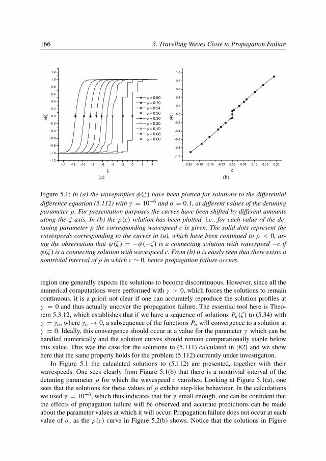
166 5. Travelling Waves Close to Propagation Failure
-14 -12 -10 -8 -6 -4 -2 0 2 4
-1.2
-1.0
-0.8
-0.6
-0.4
-0.2
0.0
0.2
0.4
0.6
0.8
1.0
1.2
ρ = 0.90
ρ = 0.70
ρ = 0.54
ρ = 0.36
ρ = 0.30
ρ = 0.20
ρ = 0.10
ρ = 0.08
ρ = 0.00
φ(ξ
)
ξ
(a)
-0.20 -0.15 -0.10 -0.05 0.00 0.05 0.10 0.15 0.20
-1.0
-0.8
-0.6
-0.4
-0.2
0.0
0.2
0.4
0.6
0.8
1.0
ρ(c
)c
(b)
Figure 5.1: In (a) the waveprofiles φ(ξ) have been plotted for solutions to the differentialdifference equation (5.112) with γ = 10−6 and α = 0.1, at different values of the detuningparameter ρ. For presentation purposes the curves have been shifted by different amountsalong the ξ -axis. In (b) the ρ(c) relation has been plotted, i.e., for each value of the de-tuning parameter ρ the corresponding wavespeed c is given. The solid dots represent thewavespeeds corresponding to the curves in (a), which have been continued to ρ < 0, us-ing the observation that ψ(ξ) = −φ(−ξ) is a connecting solution with wavespeed −c ifφ(ξ) is a connecting solution with wavespeed c. From (b) it is easily seen that there exists anontrivial interval of ρ in which c ∼ 0, hence propagation failure occurs.
region one generally expects the solutions to become discontinuous. However, since all thenumerical computations were performed with γ > 0, which forces the solutions to remaincontinuous, it is a priori not clear if one can accurately reproduce the solution profiles atγ = 0 and thus actually uncover the propagation failure. The essential tool here is Theo-rem 5.3.12, which establishes that if we have a sequence of solutions Pn(ξ) to (5.34) withγ = γn , where γn → 0, a subsequence of the functions Pn will convergence to a solution atγ = 0. Ideally, this convergence should occur at a value for the parameter γ which can behandled numerically and the solution curves should remain computationally stable belowthis value. This was the case for the solutions to (5.111) calculated in [82] and we showhere that the same property holds for the problem (5.112) currently under investigation.
In Figure 5.1 the calculated solutions to (5.112) are presented, together with theirwavespeeds. One sees clearly from Figure 5.1(b) that there is a nontrivial interval of thedetuning parameter ρ for which the wavespeed c vanishes. Looking at Figure 5.1(a), onesees that the solutions for these values of ρ exhibit step-like behaviour. In the calculationswe used γ = 10−6, which thus indicates that for γ small enough, one can be confident thatthe effects of propagation failure will be observed and accurate predictions can be madeabout the parameter values at which it will occur. Propagation failure does not occur at eachvalue of α, as the ρ(c) curve in Figure 5.2(b) shows. Notice that the solutions in Figure
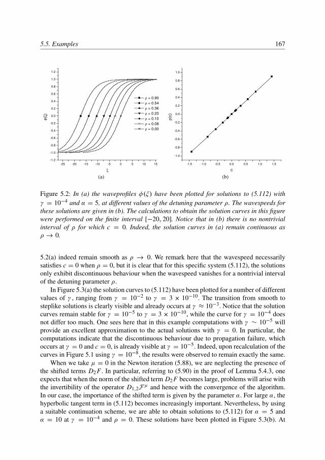
5.5. Examples 167
-25 -20 -15 -10 -5 0 5 10 15
-1.2
-1.0
-0.8
-0.6
-0.4
-0.2
0.0
0.2
0.4
0.6
0.8
1.0
1.2
ρ = 0.90
ρ = 0.54
ρ = 0.36
ρ = 0.20
ρ = 0.10
ρ = 0.08
ρ = 0.00
φ(ξ
)
ξ
(a)
-1.5 -1.0 -0.5 0.0 0.5 1.0 1.5
-1.0
-0.8
-0.6
-0.4
-0.2
0.0
0.2
0.4
0.6
0.8
1.0
ρ(c
)c
(b)
Figure 5.2: In (a) the waveprofiles φ(ξ) have been plotted for solutions to (5.112) withγ = 10−4 and α = 5, at different values of the detuning parameter ρ. The wavespeeds forthese solutions are given in (b). The calculations to obtain the solution curves in this figurewere performed on the finite interval [−20, 20]. Notice that in (b) there is no nontrivialinterval of ρ for which c = 0. Indeed, the solution curves in (a) remain continuous asρ → 0.
5.2(a) indeed remain smooth as ρ → 0. We remark here that the wavespeed necessarilysatisfies c = 0 when ρ = 0, but it is clear that for this specific system (5.112), the solutionsonly exhibit discontinuous behaviour when the wavespeed vanishes for a nontrivial intervalof the detuning parameter ρ.
In Figure 5.3(a) the solution curves to (5.112) have been plotted for a number of differentvalues of γ , ranging from γ = 10−2 to γ = 3 × 10⁻¹⁰. The transition from smooth tosteplike solutions is clearly visible and already occurs at γ ≈ 10−3. Notice that the solutioncurves remain stable for γ = 10−5 to γ = 3 × 10⁻¹⁰, while the curve for γ = 10−4 doesnot differ too much. One sees here that in this example computations with γ ∼ 10−5 willprovide an excellent approximation to the actual solutions with γ = 0. In particular, thecomputations indicate that the discontinuous behaviour due to propagation failure, whichoccurs at γ = 0 and c = 0, is already visible at γ = 10−5. Indeed, upon recalculation of thecurves in Figure 5.1 using γ = 10−8, the results were observed to remain exactly the same.
When we take µ = 0 in the Newton iteration (5.88), we are neglecting the presence ofthe shifted terms D2 F . In particular, referring to (5.90) in the proof of Lemma 5.4.3, oneexpects that when the norm of the shifted term D2 F becomes large, problems will arise withthe invertibility of the operator D1,2Fµ and hence with the convergence of the algorithm.In our case, the importance of the shifted term is given by the parameter α. For large α, thehyperbolic tangent term in (5.112) becomes increasingly important. Nevertheless, by usinga suitable continuation scheme, we are able to obtain solutions to (5.112) for α = 5 andα = 10 at γ = 10−4 and ρ = 0. These solutions have been plotted in Figure 5.3(b). At
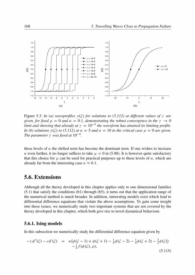
168 5. Travelling Waves Close to Propagation Failure
-16 -14 -12 -10 -8 -6 -4 -2 0 2 4 6
-1.2
-1.0
-0.8
-0.6
-0.4
-0.2
0.0
0.2
0.4
0.6
0.8
1.0
1.2
γ = 1e-2
γ = 1e-3
γ = 1e-4
γ = 1e-5
γ = 1e-6
γ = 1e-8
γ = 3e-10
φ(ξ
)
ξ
(a)
-20 -10 0 10 20
-1.2
-1.0
-0.8
-0.6
-0.4
-0.2
0.0
0.2
0.4
0.6
0.8
1.0
1.2
α = 5
α = 10
φ(ξ
)ξ
(b)
Figure 5.3: In (a) waveprofiles y(ξ) for solutions to (5.112) at different values of γ aregiven, for fixed ρ = 0 and α = 0.1, demonstrating the robust convergence in the γ → 0limit and showing that already at γ = 10−5 the waveform has attained its limiting profile.In (b) solutions y(ξ) to (5.112) at α = 5 and α = 10 in the critical case ρ = 0 are given.The parameter γ was fixed at 10−4.
these levels of α the shifted term has become the dominant term. If one wishes to increaseα even further, it no longer suffices to take µ = 0 in (5.88). It is however quite satisfactorythat this choice for µ can be used for practical purposes up to these levels of α, which arealready far from the interesting case α ≈ 0.1.
5.6. ExtensionsAlthough all the theory developed in this chapter applies only to one dimensional families(5.1) that satisfy the conditions (b1) through (b5), it turns out that the application range ofthe numerical method is much broader. In addition, interesting models exist which lead todifferential difference equations that violate the above assumptions. To gain some insightinto these issues, we numerically study two important systems that are not covered by thetheory developed in this chapter, which both give rise to novel dynamical behaviour.
5.6.1. Ising models
In this subsection we numerically study the differential difference equation given by
−γφ′′(ξ)− cφ′(ξ) = α(φ(ξ − 1)+ φ(ξ + 1)− 1
4φ(ξ − 2)− 14φ(ξ + 2)− 3
2φ(ξ))
−14 f (φ(ξ), ρ),
(5.115)
5.6. Extensions 169
-14 -12 -10 -8 -6 -4 -2 0 2 4
-1.2
-1.0
-0.8
-0.6
-0.4
-0.2
0.0
0.2
0.4
0.6
0.8
1.0
1.2
ρ = 0.60
ρ = 0.50
ρ = 0.40
ρ = 0.30
ρ = 0.20
ρ = 0.10
ρ = 0.00
φ(ξ
)
ξ
(a)
-0.06 -0.04 -0.02 0.00 0.02 0.04 0.06
-0.6
-0.4
-0.2
0.0
0.2
0.4
0.6
ρ(c
)c
(b)
Figure 5.4: In (a) the waveprofiles φ(ξ) have been plotted for solutions to (5.115) withγ = 10−6 and α = 0.042, at different values of the detuning parameter ρ. The correspond-ing wavespeeds for these solutions are given in (b).
where f again denotes the bistable cubic nonlinearity f (x, ρ) = (x2− 1)(x − ρ) for some
parameter ρ ∈ (−1, 1) and α > 0 is a strictly positive parameter. We again impose thelimits φ(±∞) = ±1 and the normalization condition φ(0) = 0 and again take µ = 0when performing the iteration steps (5.88). The interesting feature in (5.115) is that thecoefficients in front of the shifted terms φ(ξ ± 2) are now negative, which implies that thisequation does not satisfy the assumption (b3) introduced in Section 5.3. In particular, we nolonger have any guarantee that (5.115) in fact has a solution or that the numerical methodwill be able to find it.
Equation (5.115) with γ = 0 is an example of a class of differential difference equa-tions which was proposed in [13] to provide a discrete convolution model for Ising-likephase transitions. The equation was derived by considering groups of atoms arranged on alattice and computing the gradient flow of a Helmholtz free energy functional. This energyfunctional takes into account interactions within each group of atoms together with inter-actions between groups, thus incorporating both local and non-local effects into the model.Due to the nature of the physical forces involved, the long-range interaction coefficients canbe both positive and negative.
Unnormalized solutions to (5.115) with γ = 0, c = 0, fixed ρ and sufficiently smallα > 0 were analyzed in [13]. In particular, for each sufficiently small α > 0 it wasshown that there exist three intervals I j (α) for 1 ≤ j ≤ 3, such that for any two disjointsets S1, S2 ⊂ Z, there exists a unique (unnormalized) solution u to (5.115) that satisfiesu(x) ∈ Ii whenever bxc ∈ Si , for all 1 ≤ i ≤ 3. Here we have defined S3 = Z \
(S1 ∪ S2
).
We remark here that −1 ∈ int(I1) and 1 ∈ int(I2). From this it is clear that the set ofsolutions to (5.115) with γ = c = 0 has a rich structure.
In Figure 5.4 the results of an application of the numerical method to (5.115) with
170 5. Travelling Waves Close to Propagation Failure
-14 -12 -10 -8 -6 -4 -2 0 2 4 6
-1.2
-1.0
-0.8
-0.6
-0.4
-0.2
0.0
0.2
0.4
0.6
0.8
1.0
1.2
φo ρ = 0.70
φe ρ = 0.70
φo ρ = 0.50
φe ρ = 0.50
φo ρ = 0.30
φe ρ = 0.30
φo ρ = 0.20
φe ρ = 0.20
φ(ξ
)
ξ
(a)
-6 -4 -2 0 2 4
-1.2
-1.0
-0.8
-0.6
-0.4
-0.2
0.0
0.2
0.4
0.6
0.8
1.0
1.2
φo ρ = 0.10
φe ρ = 0.10
φo ρ = 0.08
φe ρ = 0.08
φo ρ = 0.00
φe ρ = 0.00
φ(ξ
)ξ
(b)
Figure 5.5: Waveprofiles φo(ξ) and φe(ξ) have been plotted for solutions to (5.118) withαo = 1.5, αe = 1.7 and γ = 10−5. In addition to the global shift for different values of ρ,the curves for φe in (a) have been shifted by 1 along the ξ -axis relative to their accompany-ing φo curves. This additional shift has not been applied to the curves in (b).
γ = 10−6 and α = 0.042 are displayed. The transition from smooth solution curves todiscontinuous step functions as ρ approaches the critical value ρ = 0 is clearly illustrated.Notice that in contrast to the results from the previous section, the solution curves are nolonger monotonic and in addition are no longer restricted to the interval [−1, 1]. The valuestaken by the step functions in Figure 5.4 are in agreement with the predictions from [13]and these results again illustrate that the algorithm is robust enough to be able to uncoversome of the behaviour at γ = 0.
5.6.2. Higher Dimensional SystemsUp to now all the theory has been developed for scalar differential difference equations ofthe form (5.34). The question of course immediately arises if the results can be extendedto higher dimensional systems and if the numerical method is able to handle them as well.In this subsection we briefly discuss some of the issues involved, using a bistable reaction-diffusion equation on a one dimensional lattice with spatially varying diffusion coefficientsas an example. Specifically, we will study the system
u j (t) = α j(u j+1(t)+ u j−1(t)− 2u j (t)
)−
154
(u2
j (t)− 1)(
u j (t)− ρ), j ∈ Z, (5.116)
where ρ ∈ (−1, 1) is a detuning parameter and the coefficients α j are periodic with periodtwo, i.e., we have α j+2 = α j for all j ∈ Z.
Lattice differential equations of the form (5.116) arise naturally when modelling dif-fusion processes in discrete systems which are spatially periodic. As a specific biological
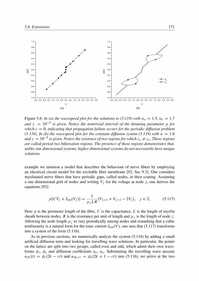
5.6. Extensions 171
-3.5 -3.0 -2.5 -2.0 -1.5 -1.0 -0.5 0.0 0.5 1.0 1.5 2.0 2.5 3.0 3.5
-1.0
-0.8
-0.6
-0.4
-0.2
0.0
0.2
0.4
0.6
0.8
1.0
ρ(c
)
c
(a)
-3.5 -3.0 -2.5 -2.0 -1.5 -1.0 -0.5 0.0 0.5 1.0 1.5 2.0 2.5 3.0 3.5
-1.0
-0.8
-0.6
-0.4
-0.2
0.0
0.2
0.4
0.6
0.8
1.0
ce
co
ρ(c
)c
(b)
Figure 5.6: In (a) the wavespeed plot for the solutions to (5.118) with αo = 1.5, αe = 1.7and γ = 10−5 is given. Notice the nontrivial interval of the detuning parameter ρ forwhich c = 0, indicating that propagation failure occurs for the periodic diffusion problem(5.116). In (b) the wavespeed plot for the constant diffusion system (5.119) with α = 1.6and γ = 10−5 is given. Notice the existence of two regions for which ce 6= co. These regionsare called period two bifurcation regions. The presence of these regions demonstrates that,unlike one dimensional systems, higher dimensional systems do not necessarily have uniquesolutions.
example we mention a model that describes the behaviour of nerve fibers by employingan electrical circuit model for the excitable fiber membrane [92, Sec 9.3]. One considersmyelinated nerve fibers that have periodic gaps, called nodes, in their coating. Assuminga one dimensional grid of nodes and writing V j for the voltage at node j , one derives theequations [92]
p(CV j + Iion(V j )
)=
1µ j L R
(V j+1 + V j−1 − 2V j
), j ∈ Z. (5.117)
Here p is the perimeter length of the fibre, C is the capacitance, L is the length of myelinsheath between nodes, R is the resistance per unit of length and µ j is the length of node j .Allowing the node length µ j to vary periodically among nodes and remarking that a cubicnonlinearity is a natural form for the ionic current Iion(V ), one sees that (5.117) transformsinto a system of the form (5.116).
As in previous sections, we numerically analyze the system (5.116) by adding a smallartificial diffusion term and looking for travelling wave solutions. In particular, the pointson the lattice are split into two groups, called even and odd, which admit their own wave-forms φe, φo and diffusion coefficients αe, αo. Substituting the travelling wave anszatzu2k(t) = φe(2k − ct) and u2k+1 = φo(2k + 1 − ct) into (5.116), we arrive at the two
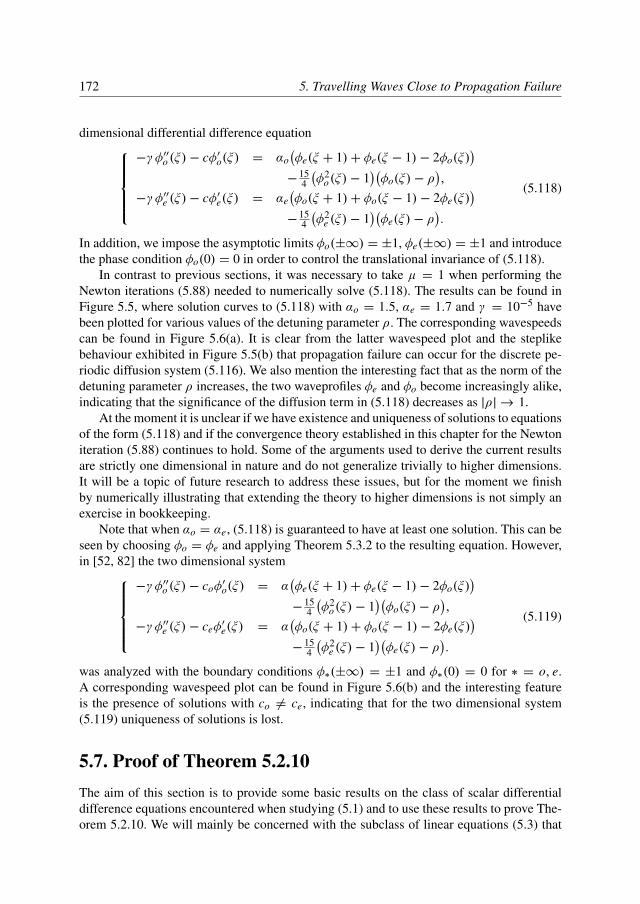
172 5. Travelling Waves Close to Propagation Failure
dimensional differential difference equation−γφ′′o (ξ)− cφ′o(ξ) = αo
(φe(ξ + 1)+ φe(ξ − 1)− 2φo(ξ)
)−
154
(φ2
o(ξ)− 1)(φo(ξ)− ρ
),
−γφ′′e (ξ)− cφ′e(ξ) = αe(φo(ξ + 1)+ φo(ξ − 1)− 2φe(ξ)
)−
154
(φ2
e (ξ)− 1)(φe(ξ)− ρ
).
(5.118)
In addition, we impose the asymptotic limits φo(±∞) = ±1, φe(±∞) = ±1 and introducethe phase condition φo(0) = 0 in order to control the translational invariance of (5.118).
In contrast to previous sections, it was necessary to take µ = 1 when performing theNewton iterations (5.88) needed to numerically solve (5.118). The results can be found inFigure 5.5, where solution curves to (5.118) with αo = 1.5, αe = 1.7 and γ = 10−5 havebeen plotted for various values of the detuning parameter ρ. The corresponding wavespeedscan be found in Figure 5.6(a). It is clear from the latter wavespeed plot and the steplikebehaviour exhibited in Figure 5.5(b) that propagation failure can occur for the discrete pe-riodic diffusion system (5.116). We also mention the interesting fact that as the norm of thedetuning parameter ρ increases, the two waveprofiles φe and φo become increasingly alike,indicating that the significance of the diffusion term in (5.118) decreases as |ρ| → 1.
At the moment it is unclear if we have existence and uniqueness of solutions to equationsof the form (5.118) and if the convergence theory established in this chapter for the Newtoniteration (5.88) continues to hold. Some of the arguments used to derive the current resultsare strictly one dimensional in nature and do not generalize trivially to higher dimensions.It will be a topic of future research to address these issues, but for the moment we finishby numerically illustrating that extending the theory to higher dimensions is not simply anexercise in bookkeeping.
Note that when αo = αe, (5.118) is guaranteed to have at least one solution. This can beseen by choosing φo = φe and applying Theorem 5.3.2 to the resulting equation. However,in [52, 82] the two dimensional system
−γφ′′o (ξ)− coφ′o(ξ) = α
(φe(ξ + 1)+ φe(ξ − 1)− 2φo(ξ)
)−
154
(φ2
o(ξ)− 1)(φo(ξ)− ρ
),
−γφ′′e (ξ)− ceφ′e(ξ) = α
(φo(ξ + 1)+ φo(ξ − 1)− 2φe(ξ)
)−
154
(φ2
e (ξ)− 1)(φe(ξ)− ρ
).
(5.119)
was analyzed with the boundary conditions φ∗(±∞) = ±1 and φ∗(0) = 0 for ∗ = o, e.A corresponding wavespeed plot can be found in Figure 5.6(b) and the interesting featureis the presence of solutions with co 6= ce, indicating that for the two dimensional system(5.119) uniqueness of solutions is lost.
5.7. Proof of Theorem 5.2.10The aim of this section is to provide some basic results on the class of scalar differentialdifference equations encountered when studying (5.1) and to use these results to prove The-orem 5.2.10. We will mainly be concerned with the subclass of linear equations (5.3) that
5.7. Proof of Theorem 5.2.10 173
arises when linearizing (5.1) around solutions. However, we shall also provide a number ofcomparison principles for solutions to the nonlinear equation (5.1) which can directly beapplied to the linear equations mentioned above.
The first result gives conditions under which (5.4) admits no positive solutions whichdecay superexponentially. This is especially useful in combination with Proposition 5.2.6,as in the absence of superexponentially decaying solutions this Proposition allows us toobtain asymptotic descriptions of the solutions to (5.4).
Lemma 5.7.1. Consider the homogeneous equation (5.4) and let x : J #→ R be a solution
to this equation on J = [τ,∞) for some τ ∈ R. Suppose that Assumption 5.2.9 holds,possibly with α j = 0 for one or more 1 ≤ j ≤ N. Assume further that x(ξ) ≥ 0 for allξ ∈ J #, but that there does not exist an R > 0 such that x(ξ) = 0 for all ξ ≥ R. Then xdoes not decay superexponentially. The analogous result for J = (−∞, τ ] also holds.
Proof. Without loss we shall also assume J = [τ,∞), as the case of J = (−∞, τ ] canbe treated by a change of variables ξ → −ξ , which does not change the sign of γ . Forconvenience, we introduce the quantity α0 = min(α0,
c2
4γ − ε), where ε > 0 is an arbitrarynumber.
We start out by noting that we can rescale equation (5.8) by defining y(ξ) = eλξ x(ξ),where λ can be chosen appropriately. It is easy to see that y(ξ) satisfies the following dif-ferential difference equation
y′′(ξ) = (2λ−cγ)y′(ξ)− λ(λ−
cγ)y(ξ)−
1γ
N∑j=0
A j (ξ)e−λr j y(ξ + r j ). (5.120)
Since y(ξ) ≥ 0 for all ξ ∈ J #, we have the inequality
y′′(ξ) ≤ (2λ−cγ)y′(ξ)+
(− λ(λ−
cγ)−
α0
γ
)y(ξ). (5.121)
Now choosing λ = c2γ we obtain
y′′(ξ) ≤ By(ξ), ξ ∈ J, (5.122)
in which B = c2
4γ 2 −α0γ > 0. Using a standard argument for ordinary differential equations
which can be found in [82, Lemma A.1], one sees that for arbitrary ξ0 ∈ J ,
y(ξ) ≤ C1e√
B(ξ−ξ0) + C2e−√
B(ξ−ξ0) (5.123)
holds for all ξ ≥ ξ0. The coefficients C1 and C2 in this expression are given by
C1 =1
2√
B
(y′(ξ0)+
√B y(ξ0)
),
C2 =1
2√
B
(− y′(ξ0)+
√B y(ξ0)
).
(5.124)
174 5. Travelling Waves Close to Propagation Failure
From the nonnegativity of y(ξ) we see that we must have C1 ≥ 0, as otherwise (5.123)would imply that y(ξ) < 0 for sufficiently large ξ . From this we conclude
y′(ξ0) ≥ −√
B y(ξ0), ξ0 ∈ J, (5.125)
which immediately implies that y(ξ) and hence x(ξ) cannot have superexponential decay.
The following lemma will be crucial to establish comparison principles for solutions tothe nonlinear equation (5.1). It can be easily derived by employing the scaling argumentintroduced in the proof of Lemma 5.7.1.
Lemma 5.7.2. Let x : J #→ R be a solution to (5.3) on J = [τ,∞) for some τ ∈ R and
suppose that Assumption 5.2.9 holds, possibly with α j = 0 for one or more 1 ≤ j ≤ N.Assume further that x(ξ) ≥ 0 for all ξ ∈ J #. Then if x(ξ0) = 0 for some ξ0 ∈ J , we havex(ξ) = 0 for all ξ ≥ ξ0.
We now restrict ourselves to constant coefficient equations
−γ x ′′(ξ)− cx ′(ξ)− L0(xξ ) = 0 (5.126)
that satisfy Assumption 5.2.9. Our goal will be to obtain detailed information about theeigenvalues of such systems. This will allow us to give precise asymptotic descriptions ofsolutions to the nonautomatous linear equation (5.8) and to provide conditions for which(5.126) is hyperbolic. To this end, we introduce the quantity
A6 = −1c,γ,L0(0) =N∑
j=0
A j,0, (5.127)
associated to the constant coefficient operator L0. The following lemma relates the existenceof complex eigenvalues of (5.126) to the sign of the characteristic function 1c,γ,L0(s) forreal values of s.
Lemma 5.7.3. Consider the constant coefficient equation (5.126), suppose that Assump-tion 5.2.9 holds and in addition assume that A6 < 0. Consider an arbitrary a ∈ R. If1c,γ,L0(a) ≥ 0, then there do not exist any eigenvalues λ ∈ C such that Re λ = a exceptpossibly λ = a itself.
Proof. Note that A0,0 < 0, since A6 < 0 and A j,0 > 0 for 1 ≤ j ≤ N . Writing λ = a+ iηwith a, η ∈ R, we compute∣∣cλ+ γ λ2
+ A0,0∣∣2=
∣∣ca + γ a2− γ η2
+ A0,0 + i(2aγ η + cη)∣∣2
=∣∣ca + γ a2
+ A0,0∣∣2
+η2(η2γ 2+ 2aγ c + 2a2γ 2
+ c2− 2γ A0,0)
=∣∣ca + γ a2
+ A0,0∣∣2+ η2 p(a),
5.7. Proof of Theorem 5.2.10 175
where p is a second degree polynomial. It is elementary to see that
p(a) ≥12
c2+ η2γ 2
− 2γ A0 ≥ η2γ 2≥ 0.
We thus have ∣∣∣cλ+ γ λ2+ A0,0
∣∣∣ ≥ ∣∣∣ca + γ a2+ A0,0
∣∣∣ , (5.128)
with equality if and only if λ = a.Now suppose that λ = a + iη satisfies 1c,γ,L0(λ) = 0 for some real η and that
1c,γ,L0(a) ≥ 0. Then using (5.128), we arrive at∣∣ca + γ a2+ A0,0
∣∣ ≤ ∣∣cλ+ γ λ2+ A0,0
∣∣ = ∣∣∣∑Nj=1 A j,0eλr j
∣∣∣≤
∑Nj=1 A j,0ear j
≤ −(ca + γ a2+ A0,0).
(5.129)
By examining the first and last terms in (5.129), we see that the three inequalities have to beequalities. This can only be if λ = a, from which the claim immediately follows.
Notice that under the assumptions of the previous lemma, we have 1c,γ,L0(0) > 0 and1′′c,γ,L0
< 0. The behaviour of the characteristic function is thus easy to analyze on thereal line and we can use the result above to establish the following two claims about theeigenvalues of (5.126).
Lemma 5.7.4. Consider the equation (5.126) and suppose that A6 < 0 and Assump-tion 5.2.9 is satisfied. Then equation (5.126) is hyperbolic. Furthermore, there exists pre-cisely one real positive eigenvalue λ+ ∈ (0,∞) and precisely one real negative eigenvalueλ− ∈ (−∞, 0) and each of these eigenvalues is simple. The eigenvalues λ− and λ+ dependC1 smoothly on c and the coefficients A j,0. In addition, we have that
∂λ−
∂c< 0 and
∂λ+
∂c< 0. (5.130)
All the remaining eigenvalues satisfy
Re λ ∈ (−∞, λ−) ∪ (λ+,∞), Im λ 6= 0. (5.131)
Lemma 5.7.5. Consider the equation (5.126) and suppose that A6 > 0 and Assumption5.2.9 is satisfied. Then either all real eigenvalues of (5.126) lie in (0,∞), or else they all liein (−∞, 0).
We now shift our focus to nonlinear differential difference equations of the form
−γ x ′′(ξ)− cx ′(ξ) = G(ξ, x(ξ), x(ξ + r1), . . . , x(ξ + rN )
). (5.132)
In the automatous case we write
−γ x ′′(ξ)− cx ′(ξ) = F(x(ξ), x(ξ + r1), . . . , x(ξ + rN )
). (5.133)
We will impose the following conditions on (5.132).
176 5. Travelling Waves Close to Propagation Failure
Assumption 5.7.6. The parameter γ satisfies γ > 0 and the shifts satisfy ri 6= r j wheni 6= j and ri 6= 0. There is at least one shifted argument, i.e. N ≥ 1. The functionG : R × RN+1
→ R, written as G(ξ, u), where u = (u0, u1, . . . , uN ), is C1 smoothand the derivative D2G of G with respect to the second argument u ∈ RN+1 is locallyLipshitz in u. In addition, for every ξ ∈ R we have that
∂G(ξ, u)∂u j
> 0, u ∈ RN+1, 1 ≤ j ≤ N . (5.134)
The following lemma roughly states that solutions to (5.133) are uniquely specified bytheir initial conditions. The proof is almost completely analogous to that in [113], so weomit it.
Lemma 5.7.7. Let x j : J → R for j = 1, 2 be two solutions of equation (5.132) with thesame parameters c and γ on some interval J . Suppose that Assumption 5.7.6 holds and that
x1(ξ) = x2(ξ), τ + rmin ≤ ξ ≤ τ + rmax, (5.135)
for some τ ∈ J for which [τ + rmin, τ + rmax] ⊆ J . Then
x1(ξ) = x2(ξ), ξ ∈ J #. (5.136)
We remark here that in combination with Lemma 5.7.2 the above result yields the fol-lowing useful corollary.
Corollary 5.7.8. Consider the linear differential difference equation (5.3) and suppose thatAssumption 5.2.9 holds. Let x j : J → R for j = 1, 2 be two solutions to (5.3) with thesame parameters c and γ on the interval J = [τ,∞) for some τ ∈ R. If for all ξ ∈ J # wehave
x1(ξ) ≥ x2(ξ), (5.137)
with equality x1(ξ0) = x2(ξ0) for some ξ0 ∈ J , then we have
x1(ξ) = x2(ξ), ξ ∈ J #. (5.138)
Suppose that x1 and x2 are both bounded solutions of the nonlinear autonomous differ-ential difference equation (5.133) with the same parameters c and γ , where γ > 0. We haveseen in Section 5.3 that the difference y(ξ) = x1(ξ)−x2(ξ) satisfies the linear homogeneousequation (5.4) with coefficients given by
A j (ξ) =
∫ 1
0
∂F(u)∂u j
∣∣∣∣u=tπ(x1,ξ)+(1−t)π(x2,ξ)
dt . (5.139)
If Assumption 5.7.6 holds for the equation (5.133), it is easy to see that A j (ξ) > 0 forall ξ ∈ R and for all 1 ≤ j ≤ N . Since the derivatives ∂F(u)
∂u jare continuous, we can use the
fact that x1(ξ) and x2(ξ) are uniformly bounded to establish that the coefficients A j (ξ) are
5.7. Proof of Theorem 5.2.10 177
uniformly bounded for 0 ≤ j ≤ N . The continuity of these coefficients follows from theLipschitz condition on the partial derivatives of F . This means that our linear equation (5.4)with coefficients (5.139) satisfies all the assumptions of Lemma 5.7.2. Applying this resultto the difference x1(ξ) − x2(ξ) and invoking Lemma 5.7.7, we obtain the following usefulcomparison principle.
Lemma 5.7.9. Let x j : J #→ R for j = 1, 2 be two bounded solutions of the nonlinear
differential difference equation (5.133) with the same parameters c and γ on the intervalJ = [τ,∞) for some τ ∈ R. Suppose also that Assumption 5.7.6 holds and that
x1(ξ) ≥ x2(ξ), ξ ∈ J #. (5.140)
Then if x1(ξ0) = x2(ξ0) for some ξ0, we have x1(ξ) = x2(ξ) for all ξ ∈ J #.
In order to establish uniqueness of solutions to (5.1), we shall need a comparison prin-ciple for solutions to (5.133) which have different wavespeeds.
Lemma 5.7.10. Let x j : J #→ R for j = 1, 2 be two bounded solutions of the nonlinear
autonomous differential difference equation (5.133) with parameters γ = γ j and c = c j onsome interval J = [τ,∞) for some τ ∈ R. Suppose that Assumption 5.7.6 holds and thatγ1 = γ2 > 0, but that c1 > c2. Also assume that
x1(ξ) ≥ x2(ξ), ξ ∈ J # (5.141)
and that x2(ξ) is monotonically increasing. Then if x1(ξ0) = x2(ξ0) for some ξ0, we havethat x1(ξ) = x2(ξ) is constant for all ξ ≥ ξ0.
Proof. We start out by noticing that the difference y(ξ) = x1(ξ)− x2(ξ) satisfies the linearequation
y′′(ξ) = −c1
γx ′1(ξ)+
c2
γx ′2(ξ)−
1γ
N∑j=0
A j (ξ)y(ξ + r j ), (5.142)
where the coefficients A j are again given by (5.139).We have already seen that the coefficients A j (ξ) are uniformly bounded for 0 ≤ j ≤ N
and that A j (ξ) > 0 for all ξ ∈ R and for 1 ≤ j ≤ N . We can thus write A0(ξ) ≥ α0, forsome α0 < 0. Now using the fact that x ′2(ξ) ≥ 0, we have
c2
γx ′2(ξ) ≤
c1
γx ′2(ξ), (5.143)
which allows us to conclude
y′′(ξ) ≤ −c1
γy′(ξ)−
α0
γy(ξ). (5.144)
Upon defining z(ξ) = ec12γ ξ y(ξ), we obtain
z′′(ξ) ≤ (c2
14γ 2 −
α0
γ)z(ξ) = Bz(ξ), (5.145)
178 5. Travelling Waves Close to Propagation Failure
where B > 0. We now proceed as in the proof of Lemma 5.7.1 to conclude that z(ξ) = 0 forall ξ ≥ ξ0, which implies x1(ξ) = x2(ξ) for all ξ ≥ ξ0. Referring back to (5.133), we seethat for ξ ≥ ξ0 + rmin we must have c1x ′1(ξ) = c2x ′2(ξ). However, as also x ′1(ξ) = x ′2(ξ),we must have x ′1(ξ) = x ′2(ξ) = 0. This establishes the claim.
We are now ready to provide the proof of Theorem 5.2.10 and we note here that thepreparations in this section allow us to follow closely the proof of [113, Theorem 4.1].
Proof of Theorem 5.2.10. Denote the limiting constant coefficient operators at ±∞ byL±. Then it follows from Lemma 5.7.4 that the equations (5.126) with L± are both hy-perbolic. In fact, the same result holds for the family of constant coefficient operators12
((1 − ρ)L− + (1 + ρ)L+
)for −1 ≤ ρ ≤ 1, which connects L− to L+. Theorem 5.2.4
thus guarantees that 3c,γ,L is a Fredholm operator with ind(3c,γ,L) = 0. Corollary 5.7.8immediately implies that the nontrivial solution p satisfies p > 0. Using Proposition 5.2.6and Lemma 5.7.4, we obtain the asymptotic expressions
p(ξ) ={
C p−eλ
u−ξ + O(e(λ
u−+ε)ξ ), ξ →−∞,
C p+eλ
s+ξ + O(e(λ
s+−ε)ξ ), ξ →∞,
(5.146)
for some ε > 0, with finite exponents
−∞ < λs+ < 0 < λu
− <∞. (5.147)
Since p does not decay superexponentially and is strictly positive, Proposition 5.2.6 andLemma 5.2.7 imply that both C p
± > 0. Suppose that there exists some x ∈ K(3c,γ,L)which is linearly independent of p. By adding some multiple of p and replacing x by −xif necessary, we may assume that x satisfies a similar asymptotic expansion (5.146) withC x− ≤ 0 and C x
+ = 0. Because x is not identically zero, Lemma 5.7.7 implies that there existarbitrarily large ξ for which x(ξ) 6= 0. If x(ξ) ≤ 0 for all large ξ , then the same reasoningas applied above to conclude that C p
+ > 0 in the expansion (5.146) leads to a contradictionwith C x
+ = 0. This means there even are arbitrarily large ξ for which x(ξ) > 0. From this itimmediately follows that there exists µ0 > 0 such that
p(ξ)− µ0x(ξ) < 0, (5.148)
for some ξ ∈ R. We now consider the family p − µx ∈ Kc,γ,L for 0 ≤ µ ≤ µ0. Theasymptotic expressions for p and x ensure that there exist τ, K , λ ∈ R such that
p(ξ)− µx(ξ) ≥ K e−λ|ξ | > 0, |ξ | > τ, 0 ≤ µ ≤ µ0. (5.149)
Now define
µ∗ = sup {µ ∈ [0, µ0] | p(ξ)− µx(ξ) ≥ 0 for all ξ ∈ R} . (5.150)
By definition it follows from (5.148) that µ∗ < µ0. Obviously, we have the inequalityµ∗x(ξ) ≤ p(ξ) for all ξ ∈ R, but actually it is easy to see that also µ∗x(ξ0) = p(ξ0) forsome ξ0 ∈ [−τ, τ ]. From Corollary 5.7.8 it now immediately follows that µ∗x(ξ) = p(ξ),
5.8. Implementation Issues 179
but this contradicts the linear independence of x and p, establishing dimK(3c,γ,L) = 1. Tocomplete the proof, it is enough to show that there exists a p∗ ∈ K(3∗c,γ,L) which satisfiesp∗ ≥ 0, as the strict positivity then follows immediately from Corollary 5.7.8. Thus assumeto the contrary that p∗(ξ1) > 0 > p∗(ξ2) for some ξ1, ξ2 ∈ R. Lemma 5.7.7 guaranteesthat we may assume that |ξ1 − ξ2| ≤ rmax − rmin. This means that there exists a continuousfunction h : R → R such that
∫∞
−∞p∗(ξ)h(ξ)dξ = 0, with supp(h) ⊂ [τ1, τ2] for some
τ1, τ2 ∈ R satisfying τ2 − τ1 < rmax − rmin. Theorem 5.2.4 now implies that there exists anx ∈ W 2,∞ such that3c,γ,L x = h. We now consider the family of such solutions x+µp forµ ∈ R. Noting that x satisfies the homogeneous equation (5.4) for large |ξ | and using similararguments as above, one argues that there exists a µ∗ ∈ R such that y = x + µ∗ p satisfiesy ≥ 0 and y(ξ0) = 0 for some ξ0 ∈ R. Since (−∞, τ1 + rmax] ∪ [τ2 + rmin,∞) = R, wemay use Lemma 5.7.7 to conclude that y(ξ) does not vanish for all large |ξ |. By possiblymaking the substitution ξ → −ξ , we may assume y(ξ) does not vanish for all large ξ .However, Lemma 5.7.2 now implies y(ξ) = 0 for all ξ ≥ ξ0, which gives the desiredcontradiction.
5.8. Implementation Issues
Performing the iteration step defined in (5.88) with µ = 0 amounts to solving a bound-ary value problem on the real line. This observation in principle allows one to performthe Newton iterations requiring the help of a boundary value problem solver for ordinarydifferential equations only, if one truncates the problem to some appropriate finite interval[T−, T+] with T− < 0 < T+. In our C++ implementation, the boundary value problem solverCOLMOD [31] was used at each iteration step. Since the boundary value problem whichhas to be solved has degree three, three boundary conditions need to be specified at eachstep. These conditions were chosen to be φ(T±) = ±1 and φ(0) = 0, in order to pick outthe unique translate. In addition, when evaluating the delay and advanced terms in (5.88),the iterates were taken to satisfy φ(ξ) = −1 whenever ξ ≤ T− and φ(ξ) = 1 for ξ ≥ T+. Inthe literature, other sets of boundary conditions have been proposed, which require that atthe boundary points ξ = T± solutions are matched up with the exponential eigenfunctionsof the corresponding linearization. However, since solutions have exponential behaviour at±∞, the distinction between these two sets of boundary conditions vanishes numerically ifthe interval is chosen to be large enough.
In order to perform the iteration (5.88) with µ 6= 0, the COLMOD code was adapted,roughly along the lines of [1, 10], to collocate the delay and advance terms directly. Thisrequired the usage of extra memory space to accomodate the larger matrices involved andthe use of a different linear system solver to allow for non block-diagonal matrices.
It remains to specify how a suitable starting value (φ0, c0) can be supplied for the New-ton iterations. It turns out that this is very hard in general: very often the algorithm requiresa very accurate initial guess to converge. One has to use the technique of continuation toarrive at a suitable starting value. In general, this means that one starts by solving an ”easy”problem to a certain degree of accuracy and gradually moves toward the ”hard” problem,using the solution of one problem as the starting value for the next problem which lies

180 5. Travelling Waves Close to Propagation Failure
”nearby”. As an example, we mention that a continuation scheme for the family (5.112) caninvolve varying combinations of the detuning parameter ρ, the size of the delay term α andthe size of γ . The continuity in parameter space which was established in Proposition 5.3.3shows that this is indeed a feasible strategy.
Chapter 6
Lin’s Method and HomoclinicBifurcations
This chapter has been submitted as: H.J. Hupkes and S.M. Verduyn Lunel, “Lin’s Methodand Homoclinic Bifurcations for Functional Differential Equations of Mixed Type”.
Abstract. We extend Lin’s method for use in the setting of parameter-dependent nonlin-ear functional differential equations of mixed type (MFDEs). We show that the presence ofM-homoclinic and M-periodic solutions that bifurcate from a prescribed homoclinic con-nection, can be detected by studying a finite dimensional bifurcation equation. As an appli-cation, we describe the codimension two orbit-flip bifurcation in the setting of MFDEs.
6.1. IntroductionThe main purpose of this chapter is to provide a framework that facilitates the detection ofsolutions to a parameter-dependent nonlinear functional differential equation of mixed type
x ′(ξ) = G(xξ , µ), (6.1)
that bifurcate from a prescribed homoclinic or heteroclinic connection. Here x is a contin-uous Cn-valued function and for any ξ ∈ R the state xξ ∈ C([rmin, rmax],Cn) is definedby xξ (θ) = x(ξ + θ). We allow rmin ≤ 0 and rmax ≥ 0, hence the nonlinearity G maydepend on advanced and retarded arguments simultaneously. The parameter µ is taken froman open subset of Rp, for some integer p ≥ 1.
The fact that travelling wave solutions to lattice differential equations are described byfunctional differential equations of mixed type (MFDEs), forms one of the primary motiva-tions for this chapter. As exhibited in detail in Chapter 1, lattice differential equations havemany modelling applications in a wide range of scientific disciplines. As a consequencethey are attracting a considerable amount of interest, both from an applied as well as a the-oretical perspective. One of the driving forces in these investigations is the desire to apply
182 6. Lin’s Method and Homoclinic Bifurcations
the powerful tools that are currently available for ODEs to the infinite dimensional settingof (6.1). The constructions in previous chapters concerning finite dimensional center man-ifolds, which describe the behaviour of solutions to (6.1) in the vicinity of equilibria andperiodic solutions, should be seen in this light.
In the present work we continue this approach, by studying solutions to (6.1) that remainorbitally close to a prescribed homoclinic or heteroclinic solution q that solves (6.1) atµ = µ0. We will be particularly interested in the construction of M-homoclinic and M-periodic orbits, which loosely speaking wind around the principal orbit q exactly M times,before converging to an equilibrium or repeating their pattern. More precisely, we will fixa Poincare section that intersects the trajectory of q at q0 in a transverse fashion and studysolutions that pass through this section M times. We will show that for µ sufficiently closeto µ0, one may construct solutions that satisfy these winding properties, up to M possiblediscontinuities that occur exactly at the Poincare section. Moreover, our construction willforce these jumps to be contained in some finite dimensional subset of this section. Thiscrucial reduction allows us to search for M-homoclinic and M-periodic orbits by studyingthe roots of M finite dimensional bifurcation equations, that effectively measure the size ofthe jumps.
This construction is known as Lin’s method and was originally developed by Lin [106]in order to study systems that depend upon a single parameter. Sandstede generalized themethod in such a way that bifurcations with higher codimensions could also be incorpo-rated [134]. Our approach here should be seen as a subsequent generalization of this latterframework to the infinite dimensional context of (6.1). In addition, we will show that thebifurcation equations that describe the size of the jumps have a similar asymptotic form asthose derived for the ODE version of (6.1). This provides a bridge that will allow classi-cal bifurcation results obtained for ODEs to be directly lifted to the mixed type functionaldifferential equation (6.1).
We mention here that very recently Lin’s method was used to study homoclinic solutionsto a reversible lattice differential equation, in the neighbourhood of a prescribed symmetrichomoclinic connection [69]. The approach in [69] however cannot be used to detect bifur-cating periodic solutions. In addition, the choice to use Cn
× L2([rmin, rmax],Cn) as a statespace for (6.1), causes the nonlinearity to have a domain and therefore requires the use of aproper functional-analytic setup. In contrast to our approach, this prevents the smoothnessof the nonlinearity to be carried over to the bifurcation equations.
Historically, the primary motivation for the work by Lin and Sandstede mentionedabove, was the classification of the bifurcations that homoclinic solutions to genericODEs with one or two parameters may undergo. In a sequence of papers, Shilnikov[140, 141, 142, 143, 144, 145] presented an alternative for generic ODE versions of (6.1)with p = 1. In particular, the ODE either admits precisely one branch of large-period pe-riodic solution that bifurcates from the homoclinic orbit q for µ > µ0 or µ < µ0, or elseadmits symbolic dynamics for all µ sufficiently close to µ0. The existence of the unique pe-riodic orbit was generalized to semilinear parabolic PDEs and delay equations by Chow andDeng [33] using semigroup techniques. Sandstede lifted the result concerning the presenceof symbolic dynamics to parabolic PDEs that have a sectorial linear part [134].
According to Yanagida [168], the generic bifurcations of codimension two that a hyper-
6.1. Introduction 183
bolic homoclinic solution to an ODE may undergo, are the inclination-flip and the orbit-flip bifurcations. The former of these has been analyzed by several authors [80, 95] usingLyapunov-Schmidt techniques, that unfortunately break down when studying the orbit-flipbifurcation. However, employing the adaptation of Lin’s method discussed above, Sandst-ede obtained a general description of this bifurcation for ODEs in [134]. In Section 6.2 wewill use our bridge to lift this result and characterize the orbit-flip bifurcation for (6.1).
The first obstacle that needs to be overcome in any bifurcation analysis involvingMFDEs, is that the linearized problems one encounters are ill-posed and therefore donot generate a semiflow. It is known that exponential dichotomies form a very powerfultool when dealing with ill-posed problems, since they split the state space into separateparts that do admit a semiflow. The existence of such exponential splittings for parameter-independent homogeneous linear MFDEs, was established independently and simultane-ously by Verduyn Lunel and Mallet-Paret [115] on the one hand and Harterich and cowork-ers [75] on the other, using very different methods. A second obstacle is that there is noimmediate way to write down a variation-of-constants formula that solves inhomogeneousMFDEs. This is caused by the fact that the inhomogeneity will simply be a Cn-valued func-tion, while the projections associated to the exponential dichotomies act on the state spaceC([rmin, rmax],Cn). In view of this fact, a third obstacle arises when one wishes to studysystems that depend on a parameter, since robustness theorems for exponential dichotomiesare generally established using a variation-of-constants formula.
In previous chapters, the absence of a variation-of-constants formula was circumventedby utilizing variants of the Greens function that was constructed by Mallet-Paret for au-tonomous MFDEs [112]. Continuing in this spirit, we will use the Fredholm theory devel-oped in [112] for nonautonomous MFDEs, to construct inverses for inhomogeneous MFDEson half-lines. By carefully combining these inverses with the exponential splittings devel-oped in [115], we are able to construct exponential dichotomies for parameter-dependentMFDEs without using a variation-of-constants formula. In addition, this setup will allowus to obtain precise estimates on the speed at which the projections associated to these di-chotomies approach the limiting spectral projections at ±∞. We will also be able to isolatethe portion of the state space that corresponds to a specific eigenvalue of one of these spec-tral projections. These results can be found in Sections 6.3 to 6.5 and provide the machinerythat we require to construct the bridge between ODEs and MFDEs.
In Section 6.2 we state our main results, which describe Lin’s method in the settingof MFDEs and give an explicit expression for the leading order terms in the bifurcationequations. In addition, we characterize the orbit-flip bifurcation for MFDEs. In Section 6.6we construct the candidate M-homoclinic and M-periodic orbits, that satisfy (6.1) up to Mjumps. Our approach in that section broadly follows the presentation in [134], but we avoidthe smooth coordinates changes that are used there, since these are often problematic inan infinite dimensional setting. Instead, these coordinate changes are only applied after theproblem has been reduced to a finite dimensional one. Finally, in Sections 6.7 and 6.8 weobtain estimates on the size of the error that is made, if one only considers the leading orderterms when measuring the size of the M jumps.
184 6. Lin’s Method and Homoclinic Bifurcations
6.2. Main ResultsConsider for some integer N ≥ 0 the general nonlinear functional differential equation ofmixed type
x ′(ξ) = G(x(ξ + r0), . . . , x(ξ + rN ), µ) = G(xξ , µ), (6.2)
in which x should be seen as a mapping from R into Cn for some n ≥ 1. The shifts r j ∈ Rmay have either sign and we will assume that they are ordered as r0 < . . . < rN , with r0 ≤ 0and rN ≥ 0. Introducing rmin = r0 and rmax = rN , we write X = C([rmin, rmax],Cn) for thestate space associated to (6.2). The state of a function x at ξ ∈ R will be denoted by xξ ∈ Xor alternatively evξ x ∈ X and is defined by xξ (θ) = x(ξ + θ) for rmin ≤ θ ≤ rmax. Theparameterµ is taken from an open subset U ⊂ Rp for some integer p ≥ 1. For convenience,we will use both of the representations for G that were introduced in (6.2) interchangeablythroughout the sequel, but the details should be clear from the context.
We will need the following assumptions on the nonlinearity G. We remark that theparameter-independence of the equilibria is not a real restriction, as this can always beachieved by means of a change of variables.
(HG) The nonlinearity G : X ×U → Cn is Ck+2 smooth for some integer k ≥ 2. In ad-dition, it admits D distinct equilibria q∗ ∈ Cn , which we label as q(1)∗ through q(D)∗ .These equilibria do not depend on the parameter µ, i.e., we have G(q(i)∗ , µ) = 0for all µ ∈ U and all integers 1 ≤ i ≤ D.
It is important to understand the linearizations of (6.2) around these equilibrium solutions.To this end, we define L(i)(µ) = D1G(q(i)∗ , µ) and consider the homogeneous linear MFDE
x ′(ξ) = L(i)(µ)xξ =N∑
j=0
A(i)j (µ)x(ξ + r j ). (6.3)
Associated to this linear MFDE one has the characteristic matrix
1(i)(z, µ) = z I − L(i)(µ)ez·= z I −
N∑j=0
A(i)j ezr j . (6.4)
We will need the following assumption on the linearizations, which basically states that allequilibria are hyperbolic.
(HL) For all integers 1 ≤ i ≤ D, the linearization L(i)(µ) does not depend on µ. Inaddition, the characteristic equation det1(i)(z) = 0 admits no roots with Re z = 0.
Now let us assume that for µ = µ0, equation (6.2) has a heteroclinic solution q thatconnects the equilibria q−∗ and q+∗ . Inserting x(ξ) = q(ξ) + v(ξ) into (6.2), we find thevariational MFDE
v′(ξ) = D1G(qξ , µ0)vξ + R(ξ, vξ , µ), (6.5)
6.2. Main Results 185
which is no longer autonomous. Associated to the linear part of this equation we define theoperator 3 : W 1,1
loc (R,Cn)→ L1
loc(R,Cn) that is given by
[3v](ξ) = v′(ξ)− D1G(qξ , µ0)vξ = v′(ξ)−
N∑j=0
A j (ξ)v(ξ + r j ), (6.6)
with A j (ξ) = D j G(q(ξ + r0), . . . , q(ξ + rN ), µ0
). It is possible to define an operator
3∗ : W 1,1loc (R,C
n)→ L1loc(R,C
n) that can be interpreted as an adjoint for3 under suitableconditions. This adjoint is given by
[3∗w](ξ) = w′(ξ)+N∑
j=0
A j (ξ − r j )∗w(ξ − r j ). (6.7)
We will write Y = C([−rmax,−rmin],Cn) for the state space associated to the adjoint(6.7) and ev∗ξ for the associated evaluation operator, which now maps into Y . The couplingbetween 3 and 3∗ is provided through the Hale inner product, which is given by
〈ψ, φ〉ξ = ψ(0)∗φ(0)−N∑
j=0
∫ r j
0ψ(θ − r j )
∗A j (ξ + θ − r j )φ(θ)dθ, (6.8)
for any φ ∈ X and ψ ∈ Y . The following condition on the operator 3 ensures that the Haleinner product is nondegenerate, in the sense that if 〈ψ, φ〉ξ = 0 for all ψ ∈ Y and someφ ∈ X , then φ = 0. A proof for this fact can be found in [115].
(HB) The matrices A0(ξ) and AN (ξ) are nonsingular for every ξ ∈ R.
Let I ⊂ R be an interval. To state our results, we use the following family of Banachspaces, parametrized by η ∈ R,
BCη(I,Cn) ={
x ∈ C(I,Cn) | ‖x‖η := supξ∈I e−ηξ |x(ξ)| <∞}. (6.9)
We also need to consider the finite dimensional kernels
K ={b ∈ BC0(R,Cn) | 3b = 0
},
K∗ ={d ∈ BC0(R,Cn) | 3∗d = 0
}.
(6.10)
Let us write X0 = {φ ∈ X | φ = b0 for some b ∈ K} and choose X in such a way thatX = X ⊕ X0. In addition, we write Y0 = {ψ ∈ Y | ψ = d0 for some d ∈ K∗} and definethe space
X⊥ ={φ ∈ X | 〈ψ, φ〉0 = 0 for all ψ ∈ Y0
}. (6.11)
We note that X⊥ ⊂ X is closed and of finite codimension, which allows us to fix a finitedimensional complement 0 and write X = X0 ⊕ X⊥ ⊕ 0.
Proposition 6.2.1. Consider the nonlinear equation (6.2) and suppose that (HG), (HL) and(HB) are satisfied. There exists a small neighbourhood U ′ ⊂ U, with µ0 ∈ U ′, a smallconstant ε > 0 and two Ck+1-smooth maps u− : U ′ → BC+ε
((−∞, rmax],Cn)
andu+ : U ′→ BC−ε
([rmin,∞),Cn)
, such that the following properties are satisfied.
186 6. Lin’s Method and Homoclinic Bifurcations
(i) For anyµ ∈ U ′, the function x(ξ) = q(ξ)+u−(µ)(ξ) satisfies the nonlinear equation(6.2) for all ξ ≤ 0. In addition, the function x(ξ) = q(ξ) + u+(µ)(ξ) satisfies (6.2)for all ξ ≥ 0.
(ii) For all µ ∈ U ′, we have the identities
ev0u−(µ) ∈ X⊥ ⊕ 0,ev0u+(µ) ∈ X⊥ ⊕ 0.
(6.12)
(iii) For all µ ∈ U ′, we have ξ∞(µ) := ev0u−(µ)− ev0u+(µ) ∈ 0.
(iv) For any d ∈ K∗, we have the Melnikov identity
Dµ[〈ev∗0d, ξ∞(µ)〉0]|µ=µ0 =
∫∞
−∞
d(ξ ′)∗D2G(qξ ′ , µ0)dξ ′. (6.13)
These maps are locally unique, in the sense that there exists δ > 0 such thatany pair (u+, u−) that satisfies (i) through (iii) for some µ ∈ U ′ and also hasu+ ∈ BC−ε
([rmin,∞),Cn)
, u− ∈ BC+ε((−∞, rmax],Cn)
and∥∥u±
∥∥0 < δ, must satisfy
u+ = u+(µ) and u− = u−(µ).
We remark that the condition (HB) ensures that the Hale inner product is nondegenerate,which means that the inner product appearing in (6.13) is a valid way of measuring the gapbetween the local stable and unstable manifolds of (6.2). If one is merely interested instudying heteroclinic orbits that bifurcate from a prescribed heteroclinic connection, thenProposition 6.2.1 already reduces this problem to a finite dimensional one. Indeed, item (iii)implies that one has to search for the roots of a Ck+1-smooth function defined on 0.
For the purpose of this chapter however, let us consider a family of heteroclinic con-nections {q j } j∈J , in which J ⊂ Z is a possibly infinite set of subsequent integers. Weemphasize here that these connections need not be distinct, thus any heteroclinic connec-tion can appear in the family an arbitrary number of times. We write J ∗ ⊂ Z + 1
2 for theset of half-integers J ∗ = { j ± 1
2 } j∈J , that will be related to the boundary conditions thattie the connections together. In particular, we will assume that the family {q j } j∈J connectsthe equilibria {q∗` }`∈J ∗ , i.e.,
limξ→±∞
q j (ξ) = q∗j± 1
2. (6.14)
Our aim is to construct solutions x to (6.2) that subsequently intersect the Poincare sectionsev0q j + X⊥ +0 close to ev0q j at prescribed times T j . To this end, we look for solutions to(6.2) that can be written as
x(T j + ξ) = q j (ξ)+ u−j (µ)(ξ)+ v−
j (µ)(ξ), ω−j + rmin ≤ ξ ≤ rmax,
x(T j + ξ) = q j (ξ)+ u+j (µ)(ξ)+ v+
j (µ)(ξ), rmin ≤ ξ ≤ ω+
j + rmax,(6.15)
in which we will take ω+j = −ω−
j+1 = ω j+ 12, for some family {ω`}`∈J ∗ that has
T j+1 − T j = 2ω j+ 12, wherever this is defined. If J is finite, i.e., J = {1, . . . ,M},
6.2. Main Results 187
then we can supply boundary conditions by requiring either limξ→−∞ x(ξ) = q∗12
and
limξ→∞ x(ξ) = q∗M+ 1
2if we are looking for a heteroclinic connection or evω−1 x = evω+M x
if we are interested in periodic orbits.The main result of this chapter shows that if the prescribed crossing times T j are suffi-
ciently far apart, the search for solutions x of the form (6.15) is equivalent to the search forroots of a smooth function defined on the collection of finite dimensional spaces {0( j)
} j∈J .
Theorem 6.2.2. Consider the nonlinear equation (6.2) and suppose that (HG), (HL) and(HB) are satisfied. Furthermore, consider a family of heteroclinic connections {q j } j∈J thatsatisfies (6.14). There exists an � > 0 and an open neighbourhood U ′ ⊂ U, with µ0 ∈ U ′,such that for any family {ω`}`∈J ∗ that has ω` ≥ � for all ` ∈ J ∗, there exist two families offunctions v−j : U ′ → C
([ω−j + rmin, rmax],Cn)
and v+j : U ′ → C([rmin, ω
+
j + rmax],Cn),
defined for j ∈ J , that satisfy the following properties.
(i) For any µ ∈ U ′ and j ∈ J , the function x(ξ) = q j (ξ) + u−j (µ)(ξ) + v−
j (µ)(ξ)
satisfies the nonlinear equation (6.2) for all ω−j ≤ ξ ≤ 0. In addition, the functionx(ξ) = q j (ξ)+ u+j (µ)(ξ)+ v
+
j (ξ) satisfies (6.2) for all 0 ≤ ξ ≤ ω+j .
(ii) For any µ ∈ U ′ and any j ∈ J , we have ev0v−
j (µ) ∈ X ( j)⊥⊕ 0( j) and similarly
ev0v+
j (µ) ∈ X ( j)⊥⊕ 0( j).
(iii) For any µ ∈ U ′ and j ∈ J , the following boundary conditions are satisfied,
evω−j+1v−j+1(µ)−evω+j v
+
j (µ) = evω+j [q j+u+j (µ)]−evω−j+1[q j+1+u−j+1(µ)]. (6.16)
If the family J is finite with M elements and −∞ < ω−1 = −ω+
M , then v−M+1 shouldbe read as v−1 . If however ω−1 = −∞ and ω+M = ∞, then (6.16) holds for all1 ≤ j < M and one has the additional limits
limξ→−∞ v−
1 (µ)(ξ) = 0, limξ→∞ v+
M (µ)(ξ) = 0. (6.17)
(iv) For any µ ∈ U ′ and any j ∈ J , we have ξ j (µ) ∈ 0( j), in which ξ j (µ) denotes the
gap ev0[v−j (µ)− v+
j (µ)].
The two families {v±j } j∈J are locally unique in a sense similar to the one described inProposition 6.2.1. In addition, these functions v±j depend Ck-smoothly on µ, while the shiftsξ j depend Ck-smoothly on the pair (µ, {ω`}`∈J ∗). Finally, for any d ∈ K∗ and j ∈ J , wecan estimate ξ j (µ) according to
〈ev∗0d, ξ j (µ)〉0 = 〈ev∗ω+j
d, evω−j+1[q j+1 + u−j+1(µ)− q∗
j+ 12]〉ω+j
− 〈ev∗ω−j
d, evω+j−1[q j−1 + u+j−1(µ)− q∗
j− 12]〉ω−j +R j .
(6.18)
The error term R j enjoys the following estimate, for some positive constants C1 and C2,
R j ≤∥∥ev∗0d
∥∥ [C1 |µ− µ0| e−2αω+ C2e−3αω]. (6.19)
188 6. Lin’s Method and Homoclinic Bifurcations
Here we have introduced ω = min`∈J ∗{ω`}, while α > 0 is sufficiently small to ensure thatthe characteristic equations det1(i)z = 0 have no roots with |Re z| ≤ α for all 1 ≤ i ≤ D.
We note here that sharper estimates for the remainder termsR j can be found in Sections6.7 and 6.8, where we also provide estimates on the derivatives ofR j with respect to µ andthe family {ω`}`∈J ∗ . In combination with these estimates, Theorem 6.2.2 allows bifurcationproblems for the infinite dimensional system (6.2) to be treated on a similar footing asbifurcation problems for ODEs.
The orbit-flip bifurcation
To illustrate the application range of Theorem 6.2.2, we lift a result obtained by Sandstede[134] that describes the homoclinic orbit-flip bifurcation for ODEs. We proceed by statingthe assumptions on the system (6.2) that we will need.
(OF1) The nonlinearity G is Ck+2-smooth with k ≥ 2. The parameter space U is twodimensional and contains the origin, i.e., 0 ∈ U ⊂ R2. The nonlinear differentialequation (6.2) has an equilibrium at x = 0 for all µ ∈ U . The linearizationD1G(0, µ) around this equilibrium does not depend on µ.
(OF2) There exist constants η f− < 0 and η f
+ > 0, such that the characteristic equationdet1(z) = 0 associated to the equilibrium of (6.2) at x = 0 has precisely twoeigenvalues z = λ± in the strip η f
− ≤ Re z ≤ ηf+. These eigenvalues are sim-
ple roots of the characteristic equation and there exist constants ηs± such that the
following inequalities are satisfied,
ηf− < λ− < ηs
− < 0 < ηs+ < λ+ < η
f+. (6.20)
(OF3) There exists a homoclinic solution q to (6.2) at µ = 0 that satisfieslimξ→±∞ q(ξ) = 0. The kernel K = K(3) ⊂ BC0(R,Cn) associated to thelinearization (6.6) of the nonlinear equation (6.2) around this orbit q, is one di-mensional and satisfies
K = span{q ′
}. (6.21)
(OF4) The kernel K∗ = K(3∗) associated to the adjoint of the linearization (6.6) is onedimensional, i.e., for some d ∈ BC0(R,Cn) we have
K∗ = span{d}. (6.22)
The spectral splitting in (OF2) ensures that we can decompose the state spaces X and Y as
X =Mc ⊕Mλ− ⊕Mλ+ , Y =M∗c ⊕M∗−λ− ⊕M∗−λ+
, (6.23)
in which Mλ± are the one dimensional eigenspaces associated to the eigenvalues λ± andMc is a closed complement, while the starred spaces are defined similarly. The spectral
6.2. Main Results 189
projections 5Mλ±and 5M∗
−λ±onto these eigenspaces can be written in terms of the Hale
inner product [72]. More precisely, there exist ψ± ∈ Y and φ± ∈ X such that
5Mλ±φ = 〈ψ±, φ〉∞φ±, 5M∗
−λ±ψ = 〈ψ, φ±〉∞ψ±. (6.24)
Let us now consider the functions u±(µ) introduced in Proposition 6.2.1, together with thejump ξ∞(µ). We also need to introduce the function 8± : U ′→ R given by
8±(µ) = limξ→±∞ e−λ∓ξ 〈ψ∓, evξ(q + u±(µ)
)〉±∞. (6.25)
In a similar fashion we define the scalars
8∗± = limξ→±∞ eλ±ξ 〈ev∗ξd, φ±〉±∞. (6.26)
Using arguments very similar to those given in [112, Section 7], one may show that both8± depend Ck-smoothly on µ.
(OF5) We have the identities 8+(0) = 0, 8−(0) 6= 0 and 8∗± 6= 0. In particular, qapproaches its limit in forward time at an exponential rate faster than η f
−, butbehaves generically as ξ →−∞, while d behaves generically at both ±∞.
(OF6) The Melnikov integral∫∞
−∞d(ξ ′)∗D2G(qξ ′ , 0)dξ ′ ∈ R2 and the derivative
[D8+](0) ∈ R2 are linearly independent.
This condition allows us to redefine the coordinates on the parameter space U to ensure that
µ1 = 8+(µ1, µ2),µ2 = 〈d, ξ∞(µ1, µ2)〉0.
(6.27)
In the event that λ+ > −ηf− we need to strengthen the condition (OF2) and give a more
detailed description of the negative part of the spectrum associated to the limiting equation.
(OF7) There exist constants η f f− < η
f− < 0 and η f
+ > 0 such that the characteristic equa-tion det1(z) = 0 associated to the equilibrium of (6.2) at x = 0 has preciselythree eigenvalues z = λ± and z = λ f
− in the strip η f f− ≤ Re z ≤ η f
+. These eigen-values are simple roots of the characteristic equation and there exist constants ηs
±
such that the following inequalities are satisfied,
ηf f− < λ
f− < η
f− < λ− < ηs
− < 0 < ηs+ < λ+ < η
f+. (6.28)
Writing 8 f+ and 8∗ f
− for the quantities associated to this eigenvalue λ f− that are
analogous to those defined for λ± in (6.25) and (6.26), we have 8 f+(0) 6= 0 and
8∗ f− 6= 0.
After all these preparations, we are almost ready to apply Theorem 6.2.2 and describe theorbit-flip bifurcation for functional differential equations of mixed type. It merely remains
190 6. Lin’s Method and Homoclinic Bifurcations
to define the type of solutions to (6.2) in which we are interested. To this end, considerany pair of positive constants (δ,�), where δ should be seen as small and � as large.Let us consider a solution x to (6.2) that satisfies the limits limξ→±∞ x(ξ) = 0. Sup-pose that x remains δ-close to q , in the sense that for any ξ ∈ R there is a ξ ′ ∈ R suchthat
∥∥evξ x − evξ ′q∥∥ < δ. Suppose furthermore that there exist exactly M distinct values
{ξ j }Mj=1 for which evξ j x ∈ ev0q + X⊥ + 0, with
∥∥evξ j x − ev0q∥∥ < δ. Finally, suppose
that for any pair 1 ≤ j1, j2 ≤ M , we have∣∣ξ j1 − ξ j2
∣∣ > �. Then we will refer to x as a(δ,�,M)-homoclinic solution. Similarly, let us consider a periodic solution x to (6.2) withminimal period ω. If x also satisfies the conditions above, where the values ξ j should nowbe interpreted modulo ω, then we will call x a (δ,�,M)-periodic solution.
Theorem 6.2.3. Consider the nonlinear equation (6.2) and assume that the conditions(OF1) through (OF6) and (HB) are satisfied, with λ+ 6= −λ−. In the event that λ+ ≥ −η
f−,
assume furthermore that (OF7) is satisfied and that λ+ 6= −λf−. Then upon fixing δ > 0
sufficiently small and � > 0 sufficiently large, one of the following three alternatives musthold.
(A) (Homoclinic Continuation) We have λ+ < −λ−. For all sufficiently small pairs(µ1, µ2), with µ2 > 0, equation (6.2) admits precisely one (δ,�, 1)-periodic so-lution. For all sufficiently small |µ1|, there exists precisely one (δ,�, 1)-homoclinicsolution to (6.2) withµ2 = 0. For all integers M ≥ 2, there are no (δ,�,M)-periodicand (δ,�,M)-homoclinic solutions to (6.2).
(B) (Homoclinic Doubling) We have−λ− < λ+ < −ηf−. Excluding the lineµ2 = 0, there
are two curves that extend from the origin in parameter space on which codimensionone bifurcations occur. More precisely, there is a branch of (δ,�, 2)-homoclinic so-lutions that passes through the origin and a curve emanating from the origin at whicha period-doubling bifurcation takes place, turning (δ,�, 1)-periodic solutions into(δ,�, 2)-periodic solutions.
(C) (Homoclinic Cascade) We have −λ f− < λ+. For every M ≥ 1 there is a branch of
(δ, ω,M)-homoclinic solutions to (6.2) that emerges from the origin in parameterspace. In addition, branches of codimension-one period-fold and period-doubling bi-furcations emerge from the origin and there is an open wedge in parameter space inwhich (6.2) admits symbolic dynamics.
We refer to [134] for a more graphic description of these three bifurcation scenarios.
6.3. PreliminariesIn this section we recall the basic linear theory that was developed for the linear inhomoge-neous system
x ′(ξ) = L(ξ)xξ + f (ξ) =N∑
j=0
A j (ξ)x(ξ + r j )+ f (ξ), (6.29)
6.3. Preliminaries 191
in which we take x ∈ W 1,∞(R,Cn) and f ∈ L∞(R,Cn). We will assume throughout thissection that the complex n×n matrix valued functions A j are continuous and that the shiftsr j are ordered according to r0 < . . . < rN , again with r0 ≤ 0 and rN ≥ 0.
The system (6.29) is said to be asymptotically hyperbolic if the limitsA±j = limξ→±∞ A j (ξ) exist for all integers 0 ≤ j ≤ N , while the characteristic equa-tions det1±(z) = 0 associated to these limiting equations do not have any roots on theimaginary axis. Here we have defined
1±(z) = z I −N∑
j=0
A±j ezr j . (6.30)
We recall the linear operator 3 : W 1,∞(R,Cn) → L∞(R,Cn) associated to (6.29) that isgiven by
[3x](ξ) = x ′(ξ)−N∑
j=0
A j (ξ)x(ξ + r j ), (6.31)
together with the formal adjoint 3∗ : W 1,∞(R,Cn)→ L∞(R,Cn) that acts as
[3∗y](ξ) = y′(ξ)+N∑
j=0
A j (ξ − r j )∗y(ξ − r j ). (6.32)
The following important result, that describes the relation between the Fredholm operators3 and 3∗, is due to Mallet-Paret and can be found in [112].
Theorem 6.3.1. Assume that (6.29) is asymptotically hyperbolic. Then both 3 and 3∗ areFredholm operators, with Fredholm indices given by
ind(3) = −ind(3∗) = dimK(3)− dimK(3∗). (6.33)
Every element in the kernelsK(3) andK(3∗) decays exponentially as ξ →±∞, while therelation between 3 and 3∗ is given by the following identities,
R(3) ={h ∈ L∞(R,Cn) |
∫∞
−∞d(ξ ′)∗h(ξ ′)dξ ′ = 0 for every d ∈ K(3∗)
},
R(3∗) ={h ∈ L∞(R,Cn) |
∫∞
−∞b(ξ ′)∗h(ξ ′)dξ ′ = 0 for every b ∈ K(3)
}.(6.34)
In the special case that the functions A j (ξ) do not depend on ξ , the operator3 is invertibleand there exists a Greens function G : R→ Cn×n such that
[3−1 f ](ξ) =∫∞
−∞
G(ξ − ξ ′) f (ξ ′)dξ ′. (6.35)
The Fourier transform of the function G is given by G(η) = 1−1(iη), which implies that Gdecays exponentially at both ±∞.
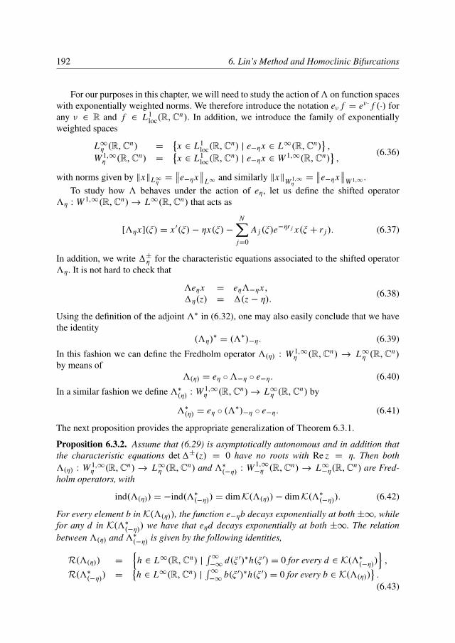
192 6. Lin’s Method and Homoclinic Bifurcations
For our purposes in this chapter, we will need to study the action of3 on function spaceswith exponentially weighted norms. We therefore introduce the notation eν f = eν· f (·) forany ν ∈ R and f ∈ L1
loc(R,Cn). In addition, we introduce the family of exponentially
weighted spaces
L∞η (R,Cn) ={
x ∈ L1loc(R,C
n) | e−ηx ∈ L∞(R,Cn)},
W 1,∞η (R,Cn) =
{x ∈ L1
loc(R,Cn) | e−ηx ∈ W 1,∞(R,Cn)
},
(6.36)
with norms given by ‖x‖L∞η =∥∥e−ηx
∥∥L∞ and similarly ‖x‖W 1,∞
η=
∥∥e−ηx∥∥
W 1,∞ .To study how 3 behaves under the action of eη, let us define the shifted operator
3η : W 1,∞(R,Cn)→ L∞(R,Cn) that acts as
[3ηx](ξ) = x ′(ξ)− ηx(ξ)−N∑
j=0
A j (ξ)e−ηr j x(ξ + r j ). (6.37)
In addition, we write 1±η for the characteristic equations associated to the shifted operator3η. It is not hard to check that
3eηx = eη3−ηx,1η(z) = 1(z − η). (6.38)
Using the definition of the adjoint 3∗ in (6.32), one may also easily conclude that we havethe identity
(3η)∗= (3∗)−η. (6.39)
In this fashion we can define the Fredholm operator 3(η) : W 1,∞η (R,Cn) → L∞η (R,Cn)
by means of3(η) = eη ◦3−η ◦ e−η. (6.40)
In a similar fashion we define 3∗(η) : W 1,∞η (R,Cn)→ L∞η (R,Cn) by
3∗(η) = eη ◦ (3∗)−η ◦ e−η. (6.41)
The next proposition provides the appropriate generalization of Theorem 6.3.1.
Proposition 6.3.2. Assume that (6.29) is asymptotically autonomous and in addition thatthe characteristic equations det1±(z) = 0 have no roots with Re z = η. Then both3(η) : W 1,∞
η (R,Cn)→ L∞η (R,Cn) and 3∗(−η) : W 1,∞−η (R,Cn)→ L∞−η(R,Cn) are Fred-
holm operators, with
ind(3(η)) = −ind(3∗(−η)) = dimK(3(η))− dimK(3∗(−η)). (6.42)
For every element b in K(3(η)), the function e−ηb decays exponentially at both ±∞, whilefor any d in K(3∗(−η)) we have that eηd decays exponentially at both ±∞. The relationbetween 3(η) and 3∗(−η) is given by the following identities,
R(3(η)) =
{h ∈ L∞(R,Cn) |
∫∞
−∞d(ξ ′)∗h(ξ ′) = 0 for every d ∈ K(3∗(−η))
},
R(3∗(−η)) ={h ∈ L∞(R,Cn) |
∫∞
−∞b(ξ ′)∗h(ξ ′) = 0 for every b ∈ K(3(η))
}.
(6.43)
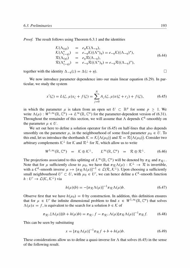
6.3. Preliminaries 193
Proof. The result follows using Theorem 6.3.1 and the identities
K(3(η)) = eηK(3−η),K(3∗(−η)) = e−ηK((3∗)η) = e−ηK((3−η)∗),R(3(η)) = eηR(3−η),R(3∗(−η)) = e−ηR((3∗)η) = e−ηR((3−η)∗),
(6.44)
together with the identity 1−η(z) = 1(z + η).
We now introduce parameter dependence into our main linear equation (6.29). In par-ticular, we study the system
x ′(ξ) = L(ξ, µ)xξ + f (ξ) =N∑
j=0
A j (ξ, µ)x(ξ + r j )+ f (ξ), (6.45)
in which the parameter µ is taken from an open set U ⊂ Rp for some p ≥ 1. Wewrite 3(µ) : W 1,∞(R,Cn)→ L∞(R,Cn) for the parameter-dependent version of (6.31).Throughout the remainder of this section, we will assume that 3 depends Ck-smoothly onthe parameter µ ∈ U .
We set out here to define a solution operator for (6.45) on half-lines that also dependssmoothly on the parameter µ, in the neighbourhood of some fixed parameter µ0 ∈ U . Tothis end, let us introduce the shorthandsK = K
(3(µ0)
)andR = R
(3(µ0)
). Consider two
arbitrary complements K⊥ for K and R⊥ for R, which allow us to write
W 1,∞(R,Cn) = K⊕K⊥, L∞(R,Cn) = R⊕R⊥. (6.46)
The projections associated to this splitting of L∞(R,Cn) will be denoted by πR and πR⊥ .Note that for µ sufficiently close to µ0, we have that πR3(µ) : K⊥ → R is invertible,with a Ck-smooth inverse µ 7→ [πR3(µ)]−1
∈ L(R,K⊥). Upon choosing a sufficientlysmall neighbourhood U ′ ⊂ U , with µ0 ∈ U ′, we can hence define a Ck-smooth functionh : U ′→ L(K,K⊥) via
h(µ)(b) = −[πR3(µ)]−1πR3(µ)b. (6.47)
Observe first that we have h(µ0) = 0 by construction. In addition, this definition ensuresthat for µ ∈ U ′ the infinite dimensional problem to find x ∈ W 1,∞(R,Cn) that solves3(µ)x = f , is equivalent to the search for a solution b ∈ K of
πR⊥ [3(µ)](b + h(µ)b) = πR⊥ f − πR⊥3(µ)[πR3(µ)]−1πR f. (6.48)
This can be seen by substituting
x = [πR3(µ)]−1πR f + b + h(µ)b. (6.49)
These considerations allow us to define a quasi-inverse for 3 that solves (6.45) in the senseof the following result.
194 6. Lin’s Method and Homoclinic Bifurcations
Proposition 6.3.3. Consider the parameter-dependent inhomogeneous system (6.45) andfix a parameter µ0 ∈ U for which (6.45) is asymptotically hyperbolic. Then there exists anopen subset U ′ ⊂ U, with µ0 ∈ U ′, together with a Ck-smooth function
C : U ′→ L(L∞(R,Cn),R⊥
)(6.50)
and a Ck-smooth quasi-inverse
3qinv : U ′→ L(L∞(R,Cn),W 1,∞(R,Cn)
), (6.51)
such that the following properties hold.
(i) For all µ ∈ U ′ we have
dimK(3(µ)
)≤ dimK
(3(µ0)
). (6.52)
(ii) For all µ ∈ U ′ and all f ∈ L∞(R,Cn) we have the identity
3(µ)3qinv(µ) f = f + C(µ) f. (6.53)
In addition, the restriction of C(µ0) to the set R vanishes identically.
Proof. Item (i) can be confirmed by noting that
dimK(3(µ)) = dimK − rankπR⊥3(µ)[I + h(µ)] ≤ dimK. (6.54)
To establish item (ii), we choose C and 3qinv according to
3qinv(µ) f = [πR3(µ)]−1πR f,C(µ) f = −πR⊥ f + πR⊥3(µ)[πR3(µ)]
−1πR f.(6.55)
A simple calculation is now sufficient to conclude the proof.
In order to define a solution operator for (6.45) on half-lines, we will need to utilizethe freedom we still have to choose the complements K⊥ and R⊥ in a special fashion.To do this, we will need to assume that condition (HB) holds, i.e., we demand that bothdet A0(ξ, µ0) and det AN (ξ, µ0) are non-zero for all ξ ∈ R.
Lemma 6.3.4. Consider the parameter-dependent linear system (6.45) and supposethat condition (HB) holds for this system at µ = µ0, for some µ0 ∈ U. Writend = dimK
(3∗(µ0)
)and choose a basis {d i
}ndi=1 for K
(3∗(µ0)
). For any ξ ∈ R there
exists a set of functions {ψ i}ndi=1 ⊂ Y such that for any pair of integers 1 ≤ i, j ≤ nd we
have ∫−rmin
−rmax
d i (ξ + θ)∗ψ j (θ)dθ = δi j . (6.56)
6.3. Preliminaries 195
Proof. First notice that the condition (HB) implies that the set of elements {ev∗ξd i}ndi=d ⊂ Y
is linearly independent. In particular, this means that the nd × nd matrix Z with entriesZi j =
(ev∗ξd i , ev∗ξd j ) is invertible, where (, ) denotes the integral inner product
(ψ, φ) =
∫−rmin
−rmax
ψ(θ)∗φ(θ)dθ. (6.57)
For any integer 1 ≤ j ≤ nd we now choose
ψ j=
nd∑k=1
ev∗ξdk Z−1k j . (6.58)
A simple calculation shows that indeed
(ev∗ξd i , ψ j ) =
nd∑k=1
(ev∗ξd i , ev∗ξdk)Z−1k j =
nd∑k=1
Zik Z−1k j = δi j . (6.59)
We will use Lemma 6.3.4 to explicitly construct a representation for πR and πR⊥ . In-deed, let us write r = rmax− rmin and fix an arbitrary ξ0 ≤ −4r . In addition, for any integer1 ≤ i ≤ nd we let gi
∈ L∞(R,Cn) denote the function that has ev∗ξ0gi= ψ i , while
gi (ξ ′) = 0 for all ξ ′ < ξ0 − rmax and ξ ′ > ξ0 − rmin. Here the functions {ψ i}ndi=1 ⊂ Y
arise from an application of Lemma 6.3.4 with ξ = ξ0. Since the set {gi}ndi=1 is linearly
independent, we can now explicitly define the projection
πR⊥ f =∑nd
i=1[∫∞
−∞d i (ξ ′)∗ f (ξ ′)dξ ′]gi . (6.60)
This enables us to define an inverse for 3(µ) on the positive half-line. Indeed, consider theoperator 3−1
+ (µ) : L∞([0,∞),Cn)
→ W 1,∞([rmin,∞),Cn)
given by
3−1+ (µ) f = 3qinv(µ)E f, (6.61)
in which [E f ](ξ) = 0 for all ξ < 0 and [E f ](ξ) = f (ξ) for all ξ ≥ 0. Since gi (ξ) = 0 forall ξ ≥ 0 and all integers 1 ≤ i ≤ nd , an application of (6.53) immediately implies that forall ξ ≥ 0 we have
[3(µ)3−1+ (µ) f ](ξ) = f (ξ). (6.62)
In a similar fashion an inverse 3−1− (µ) : L∞
((−∞, 0],Cn)
→ W 1,∞((−∞, rmax],Cn)
can be constructed for the negative half-line. Both these inverses depend Ck-smoothly onthe parameter µ ∈ U ′.
196 6. Lin’s Method and Homoclinic Bifurcations
6.4. Exponential Dichotomies
In this section we study exponential splittings for the homogeneous counterpart of the linearsystem (6.29), which we will write as
x ′(ξ) = L(ξ)xξ =N∑
j=0
A j (ξ)x(ξ + r j ). (6.63)
Throughout this entire section we will assume that the functions A j are continuous. Inaddition, we will assume that (6.63) is asymptotically hyperbolic and that the condition(HB) holds. We start by stating the main theorem which we set out to prove in this section.We remark that a similar result was previously obtained in a Hilbert space setting [75].
Theorem 6.4.1. Consider the linear system (6.63). There exist constants K > 0, αS > 0and αQ > 0, such that for every ξ ≥ 0 there is a splitting
X = Q(ξ)⊕ S(ξ), (6.64)
such that each φ ∈ Q(ξ) can be extended to a solution Eφ ∈ C([ξ + rmin,∞),Cn)
of thehomogeneous equation (6.63) on the interval [ξ,∞), while each ψ ∈ S(ξ) can be extendedto a function Eψ ∈ C
((−∞, ξ + rmax],Cn)
that satisfies the homogeneous equation (6.63)on the interval [0, ξ ]. In addition, we have the exponential estimates∣∣[Eφ](ξ ′)
∣∣ ≤ K e−αQ|ξ′−ξ| ‖φ‖ for every φ ∈ Q(ξ) and ξ ′ ≥ ξ,∣∣[Eψ](ξ ′)
∣∣ ≤ K e−αS|ξ′−ξ| ‖ψ‖ for every ψ ∈ S(ξ) and 0 ≤ ξ ′ ≤ ξ.
(6.65)These spaces are invariant, in the sense that for any 0 ≤ ξ ′ ≤ ξ and any ψ ∈ S(ξ), we haveevξ ′Eψ ∈ S(ξ ′), together with a similar identity for φ ∈ Q(ξ). Finally, the projections5Q(ξ) and 5S(ξ) depend continuously on ξ ≥ 0 and there exists a constant C such that∥∥5Q(ξ)
∥∥ ≤ C and∥∥5S(ξ)
∥∥ ≤ C for all ξ ≥ 0.
Throughout this section, we will follow the notation employed in [115]. In particular,we introduce the spaces
P(ξ) ={
x ∈ BC0((−∞, ξ + rmax],Cn)
| x ′(ξ ′) = L(ξ ′)vξ ′ for all ξ ′ ∈ (−∞, ξ ]},
Q(ξ) ={
x ∈ BC0([ξ + rmin,∞),Cn)
| x ′(ξ ′) = L(ξ ′)vξ ′ for all ξ ′ ∈ [ξ,∞)},
P(ξ) ={
x ∈ P(ξ) |∫ min(ξ+rmax,0)−∞
b(ξ ′)∗x(ξ ′)dξ ′ = 0 for all b ∈ K},
Q(ξ) ={
x ∈ Q(ξ) |∫ max(ξ+rmin,0)+∞
b(ξ ′)∗x(ξ ′)dξ ′ = 0 for all b ∈ K}.
(6.66)We remark here that these definitions of P and Q differ slightly from those given in [115],in the sense that the upper bounds of the defining integrals are now constant for ξ ≥ 0respectively ξ ≤ 0. All the results obtained in [115] remain unaffected by this choice,which we make here to ensure that P(ξ) is invariant on the positive half-line and Q(ξ) isinvariant on the negative half-line. As in [115], we also introduce the following spaces, that
6.4. Exponential Dichotomies 197
describe the initial conditions associated to the spaces above and the kernels K and K∗.
P(ξ) ={φ ∈ X | φ = xξ for some x ∈ P(ξ)
},
Q(ξ) ={φ ∈ X | φ = xξ for some x ∈ Q(ξ)
},
P(ξ) ={φ ∈ X | φ = xξ for some x ∈ P(ξ)
},
Q(ξ) ={φ ∈ X | φ = xξ for some x ∈ Q(ξ)
},
B(ξ) ={φ ∈ X | φ = bξ for some b ∈ K
},
B∗(ξ) ={φ ∈ Y | φ = dξ for some d ∈ K∗
}.
(6.67)
The following result was obtained in [115] and shows that P(ξ) and Q(ξ) together span Xup to a finite dimensional complement, that can be described explicitly in terms of the Haleinner product.
Proposition 6.4.2. Consider the homogeneous linear system (6.63). For any ξ ∈ R, letZ(ξ) ⊂ X be the closed subspace of finite codimension that is given by
Z(ξ) ={φ ∈ X | 〈ψ, φ〉ξ = 0 for every ψ ∈ B∗(ξ)
}. (6.68)
Then we have the direct sum decomposition
Z(ξ) = P(ξ)⊕ Q(ξ)⊕ B(ξ). (6.69)
Our main contribution in this section is to provide an explicit complement for Z(ξ)that will allow us to enlarge the space P(ξ) and obtain a set S(ξ) that satisfies theproperties in Theorem 6.4.1. To do this, we will employ a very useful property ofthe Hale inner product. In particular, fix an interval [ξ−, ξ+] and consider an arbi-trary function z ∈ W 1,1
loc ([ξ− − rmax, ξ+ − rmin]) together with an arbitrary functionx ∈ W 1,1
loc [ξ− + rmin, ξ+ + rmax]. Then for every ξ ∈ [ξ−, ξ+], we can perform the compu-tation
Dξ 〈ev∗ξ z, evξ x〉ξ = Dξ[z(ξ)∗x(ξ)−
∑Nj=0
∫ ξ+r jξ z(θ − r j )
∗A j (θ − r j )x(θ)dθ]
= z′(ξ)∗x(ξ)+ z(ξ)∗x ′(ξ)−∑N
j=0 z(ξ)∗A j (ξ)x(ξ + r j )
+z(ξ − r j )∗A j (ξ − r j )x(ξ)
= z(ξ)∗[3x](ξ)+ [3∗z](ξ)∗x(ξ).(6.70)
Lemma 6.4.3. Consider the homogeneous linear system (6.63). Let {d i}ndi=1 be a basis for
the kernel K∗ and recall the constant r = rmax − rmin. Then for every ξ ≥ 0 and everyinteger 1 ≤ i ≤ nd , there exists a function yi
(ξ) ∈ C((−∞, ξ + rmax],Cn)
that satisfies thefollowing properties.
(i) For every ξ ≥ 0 and every integer 1 ≤ i ≤ nd , we have [3yi(ξ)](ξ
′) = 0 for allξ ′ ≥ −3r and all ξ ′ ≤ −5r .
(ii) For any pair 0 ≤ ξ ′ ≤ ξ and any pair of integers 1 ≤ i, j ≤ nd , we have the identity
〈ev∗ξ ′di , evξ ′ y
j(ξ)〉ξ
′ = δi j . (6.71)
198 6. Lin’s Method and Homoclinic Bifurcations
(iii) Fix an integer 1 ≤ i ≤ nd and a constant 0 ≤ ξ ′. Then the function ξ 7→ evξ ′ yi(ξ)
depends continuously on ξ , for ξ ′ ≤ ξ .
(iv) Consider any triple 0 ≤ ξ ′ ≤ ξ1 ≤ ξ2. Then for any integer 1 ≤ i ≤ nd we have
evξ ′ [yi(ξ1)− yi
(ξ2)] ∈ P(ξ ′). (6.72)
(v) For every ξ ≥ 0 and every integer 1 ≤ i ≤ nd , we have the integral condition∫ 0
−∞
b(ξ ′)∗y(ξ)(ξ ′)dξ ′ = 0, (6.73)
which holds for all b ∈ K(3).
Proof. Fix ξ0 = −4r and consider the functions {ψ i}ndi=1 ⊂ Y that were constructed in
Lemma 6.3.4 for ξ = ξ0. As in Section 6.3, define the functions gi∈ L∞(R,Cn) that
have ev∗ξ0gi= ψ i , while gi
= 0 elsewhere. For the remainder of this proof, fix an integer
1 ≤ i ≤ nd . Consider a sequence ξk = k →∞ and define y(k) = 3−1(k)g
i , where the inverse
3−1(k) should be interpreted as the analogue of 3−1
− for the half-line (−∞, ξk]. Note that byadding an appropriate element in K to y(k) we can ensure that the integral condition (6.73)is satisfied. For any integer 1 ≤ j ≤ nd we can use (6.70) together with the exponentialdecay of d j at −∞ to compute
〈ev∗ξd j , evξ y(k)〉ξ =∫ ξ
−∞
d j (ξ ′)∗[3y(k)](ξ ′)dξ ′ = (ev∗ξ0d j , ψ i ) = δi j . (6.74)
Choose a continuous function χ : [0,∞) → [0, 1] such that χ is zero near even integersand one near odd integers. Write
y(ξ) = χ(2ξ)y(dξe) + [1− χ(2ξ)]y(dξ+ 12 e), (6.75)
in which dξe denotes the smallest integer that is larger or equal to ξ . With this definition itis easy to see that the properties (i) through (v) all hold.
The functions defined in Lemma 6.4.3 are sufficient to construct the space S(ξ) appear-ing in Theorem 6.4.1. Indeed, we will use the spaces
S(ξ) = P(ξ)⊕ span{yi(ξ)}
ndi=1,
S(ξ) = P(ξ)⊕ span{evξ yi(ξ)}
ndi=1.
(6.76)
The following result should be seen as the appropriate generalization of Theorem 4.2 in[115] and shows that functions in S automatically decay exponentially.
Proposition 6.4.4. Consider the homogeneous linear system (6.63). Let the sets S(ξ) ⊂ Xfor ξ ≥ 0 be defined as in (6.76). Then there exist constants K > 0 and αS > 0 such thatfor all ξ ≥ 0 and all ξ ′ ≤ ξ , we have∣∣x(ξ ′)∣∣ ≤ K e−αS(ξ−ξ
′)∥∥xξ
∥∥ , (6.77)
for every x ∈ S(ξ).
6.4. Exponential Dichotomies 199
Proof. As in [115] it suffices to prove the following two statements.
(i) There exists σ > −rmax such that for all ξ ≥ 0 and all y ∈ S(ξ), we have∣∣y(ξ ′)∣∣ ≤ 12
sups<ξ+rmax|y(s)| for all ξ ′ ≤ ξ − σ. (6.78)
(ii) There exists K > 0 such that for all ξ ≥ 0 and all y ∈ S(ξ), we have∣∣y(ξ ′)∣∣ ≤ K∥∥evξ y
∥∥ for all ξ ′ ≤ ξ + rmax. (6.79)
Assuming that (i) fails, we have sequences σ j→∞, ξ j
≥ 0 and y j∈ S(ξ j ) such that∣∣y j (−σ j
+ ξ j )∣∣ ≥ 1
2 , sups<ξ j+rmax
∣∣y j (s)∣∣ = 1. (6.80)
Suppose first that −σ j+ ξ j is unbounded, i.e., −σ j
+ ξ j→ ±∞ after passing to a
subsequence. Writing z j (ξ ′) = y j (ξ ′− σ j+ ξ j ), an application of Ascoli’s theorem yields
a convergent subsequence z j→ z. Notice that z(0) ≥ 1
2 , which means that z is a nontrivialbounded solution on R of one of the limiting equations at ±∞. This situation is howeverprecluded by the hyperbolicity of this limiting equation.
Now suppose that, possibly after passing to a subsequence, we have −σ j+ ξ j
→ β0.Using the fact that [3y j ](ξ ′) = 0 for ξ ≥ rmin, together with the limit ξ j
→ ∞, we mayapply Ascoli-Arzela to conclude that y j
→ y∗ uniformly on compact subsets of [rmin,∞).Since we also have [3y∗](ξ ′) = 0 for all ξ ′ ≥ 0, we conclude that ev0 y∗ ∈ Q(0). However,this immediately implies that for any ψ ∈ B∗(0) we have 〈ψ, ev0 y∗〉0 = 0. In view of theidentity
3y j=
nd∑i=1
gi〈ev∗0d i , ev0 y j
〉0, (6.81)
this however implies that 3y j→ 0 uniformly on every compact subset of R. This allows
us to apply Ascoli-Arzela on the entire line, by means of which we obtain the convergencey j→ y∗, which is again uniform on compacta. In addition, we have 3y∗ = 0, which now
means that y∗ ∈ K. However, this is precluded by the integral condition (6.73).Let us now suppose that (ii) fails, which implies that for some sequence K j
→ ∞,ξ j≥ 0 and y j
∈ S(ξ j ), we have
sups<ξ j+rmax
∣∣∣y j (s)∣∣∣ = K j
∥∥∥evξ j y j∥∥∥ = 1. (6.82)
In view of (i), this means that there exists a sequence σ j∈ [−rmin, σ ] such that∣∣y j (−σ j
+ ξ j )∣∣ = 1.
Suppose that ξ j is unbounded. We find y j (ξ ′ + ξ j ) → z(ξ ′) wherez : (−∞, rmax] → Cn is a bounded solution of the limiting equation at +∞. Since thesequence σ j is bounded, z does not vanish identically. Since
∥∥evξ j y j∥∥ = 1/K j
→ 0, wehave ‖z0‖ = 0 and hence z can be extended to a bounded nontrivial solution of the limit-ing equation at +∞ on the entire line. Again, this is precluded by the hyperbolicity of thislimiting equation.
200 6. Lin’s Method and Homoclinic Bifurcations
Now assume that, possibly after passing to a subsequence, we have ξ j→ ξ∗ ≥ 0. Since
evξ j y j→ 0, we can use Ascoli-Arzela to find the convergence y j
→ y∗, which is nowuniform on the interval [−r + rmin, ξ
∗+ rmax]. In addition, we have [3y∗](ξ ′) = 0 for all
ξ ′ ∈ [−r, ξ∗]. If ξ∗ ≥ σ , this fact is precluded by the non-degeneracy condition (HB), sincewe also have evξ∗ y∗ = 0. In the case where ξ∗ < σ , we can again use (6.81) to obtain theconvergence y j
→ y∗, which this time is uniform on compact subsets of (−∞, ξ∗ + rmax].As before, the condition (HB) now leads to a contradiction.
Notice that we have now obtained a splitting
X = S(ξ)⊕ Q(ξ) (6.83)
that satisfies nearly all of the properties stated in Theorem 6.4.1. It remains only to considerthe statements concerning the projections 5S(ξ) and 5Q(ξ). We will address these issues inthe remainder of this section by establishing the continuity of these projections and studyingthe limiting behaviour as ξ →∞. To this end, we recall the splitting
X = P(∞)⊕ Q(∞) (6.84)
associated to the autonomous limit of (6.63) at +∞, which was established in [115].
Lemma 6.4.5. Consider the linear homogeneous system (6.63). The following limit holdsin the spaces L(S(ξ), X),
[I −5P(∞)]|S(ξ)→ 0 as ξ →∞. (6.85)
In addition, in the spaces L(Q(ξ), X) we have the similar limit
[I −5Q(∞)]|Q(ξ)→ 0 as ξ →∞. (6.86)
Proof. The second limit was established in [115], so we restrict ourselves to the first limithere. Choose an arbitrarily small ε > 0 and fix C > 0 sufficiently large to ensure that forall ξ ∈ R, the inequality
N∑j=0
∣∣A j (ξ)eαSr j∣∣ ≤ C (6.87)
holds. Recalling the constants K and αS from Proposition 6.4.4, pick ξ0 > 0 sufficientlylarge to ensure that 4(1+ C)2 K exp(−αSξ0) <
ε2 and also
N∑j=0
∣∣∣A j (ξ′)− A+j
∣∣∣ < ε
2K(6.88)
for all ξ ′ ≥ ξ0. Fix any ξ ≥ 2ξ0 + rmax. Consider an arbitrary y ∈ S(ξ) and writeφ = evξ y ∈ S(ξ). Notice first that φ|[rmin,0] ∈ C1([rmin, 0],Cn). We can hence approximateφ with a sequence of C1-smooth functions φk that have φk(θ) = φ(θ) for all θ ∈ [−1, 0].Let us extend these functions to C1-smooth functions yk on the line, with evξ yk
= φk but
6.4. Exponential Dichotomies 201
also yk(ξ ′) = y(ξ ′) for all 0 ≤ ξ ′ ≤ ξ . Notice that we may construct the functions yk insuch a way to ensure that the following estimate holds for all ξ ′ ≤ 0,∣∣∣Dyk(ξ ′)
∣∣∣+ ∣∣∣yk(ξ ′)∣∣∣ ≤ 2[
∣∣∣Dyk(0)∣∣∣+ ∣∣∣yk(0)
∣∣∣]. (6.89)
In particular, this means that for all ξ ′ ≤ ξ we have the bound∣∣∣Dyk(ξ ′)∣∣∣+ ∣∣∣yk(ξ ′)
∣∣∣ ≤ 2K (1+ C)[e−αSξ + e−αS(ξ−ξ′)]
∥∥∥φk∥∥∥ . (6.90)
Now, for any C1-smooth function y we have the representation
5Q(∞)evξ y = evξ3−1∞ [I − Hξ ]3∞y, (6.91)
in which we have introduced the notation [3∞x](ξ ′) = x ′(ξ ′) −∑N
j=0 A+j x(ξ ′ + r j ),together with the Heaviside function Hξ that satisfies Hξ (ξ ′) = I if ξ ′ ≥ ξ and zerootherwise. Observing that
[3∞yk](ξ ′) = [3yk](ξ ′)+N∑
j=0
[A j (ξ′)− A+j ]evξ ′ yk, (6.92)
we may compute∥∥[I − Hξ ]3∞yk∥∥
L∞(R,Cn)≤ supξ ′≤ξ0
Dyk(ξ ′)+ C∥∥evξ ′ yk
∥∥+ supξ0≤ξ ′≤ξ
ε2K
∥∥evξ ′ yk∥∥
≤ 4K (1+ C)2e−αSξ0∥∥φk
∥∥+ ε2
∥∥φk∥∥
≤ ε∥∥φk
∥∥ .(6.93)
This however means that for some constant C ′ > 0 we have∥∥∥5Q(∞)φk∥∥∥ ≤ εC ′ ∥∥∥φk
∥∥∥ , (6.94)
which concludes the proof due to the continuity of 5Q(∞).
Lemma 6.4.6. Consider the system (6.63) and suppose that (HB) is satisfied. Fix an arbi-trary ξ ≥ 0. Write 0(ξ) = span{evξ yi
(ξ)}ndi=1 and consider the splitting
X = P(ξ)⊕ 0(ξ)⊕ Q(ξ) (6.95)
with the corresponding projection operators 5P(ξ), 50(ξ) and 5Q(ξ). Then we have thefollowing limits,
[I −5P(ξ0)]|P(ξ) → 0 as ξ → ξ0,
[I −5Q(ξ0)]|Q(ξ) → 0 as ξ → ξ0,[I −50(ξ0)]|0(ξ) → 0 as ξ → ξ0.
(6.96)
Proof. The statements concerning P(ξ) and Q(ξ) were established in [115]. The limit in-volving 0(ξ) follows easily using the finite dimensionality of 0(ξ) and item (iii) in Lemma6.4.3.
202 6. Lin’s Method and Homoclinic Bifurcations
Lemma 6.4.7. Consider an arbitrary ξ0 ≥ 0. The projections 5Q(ξ) can be uniformlybounded for all ξ ≥ ξ0.
Proof. Assuming the statement is false, let us consider a sequence ξ j and φ j∈ X that has
ξ j≥ ξ0 and
∥∥φ j∥∥ = 1 for all integers j ≥ 1, while
∥∥5Q(ξ j )φj∥∥→∞ as j →∞. Let us
first assume that ξ j is bounded, which after passing to a subsequence implies that ξ j→ ξ∗
for some ξ∗ ≥ ξ0. Let us write σ j= 50(ξ j )φ
j , p j= 5P(ξ j )φ
j and q j= 5Q(ξ j )φ
j . Defin-ing κ j =
∥∥σ j∥∥ + ∥∥p j
∥∥ + ∥∥q j∥∥, let us also introduce the bounded sequence σ j
= κ−1j σ j
and similarly defined sequences p j and q j . In addition, we introduce σ j∗ = 50(ξ∗)σ
j andsimilarly p j
∗ = 5P(ξ∗) p j and q j∗ = 5Q(ξ∗)q
j . Using Lemma 6.4.6 we obtain the followinglimits as j →∞,
σ j+ p j
+ q j→ 0,
σ j− σ
j∗ → 0,
p j− p j∗ → 0,
q j− q j∗ → 0.
(6.97)
Since 0(ξ∗) is finite dimensional, we can pass to a subsequence and obtain σ j∗ → σ∗ This
implies the following limit as j →∞,
σ∗ + p j∗ + q j
∗ → 0. (6.98)
We now introduce the truncation operators π+ : X → C([0, rmax],Cn)
andπ− : X → C
([rmin, 0],Cn)
. Using the exponential estimates on Q(ξ∗) and P(ξ∗), it isnot hard to see that the restriction of π+ to Q(ξ∗) is compact, as is the restriction of π− toP(ξ∗). After passing to a subsequence, we thus find that π+q j
∗ and hence also π+ p j∗ con-
verge uniformly on [0, rmax]. Invoking a similar argument involving π− we conclude thatas j →∞, we must have p j
∗ → p∗ and q j∗ → q∗ for some p∗ ∈ P(ξ∗) and q∗ ∈ Q(ξ∗). In
view of (6.98), this leads to a contradiction, since ‖σ∗‖ + ‖p∗‖ + ‖q∗‖ = 1.It remains to consider the case that ξ j
→ ∞. However, using the splittingX = S(ξ) ⊕ Q(ξ) and the limits in Lemma 6.4.5, we can obtain a contradiction in thesame fashion as above.
Corollary 6.4.8. Consider the linear homogeneous system (6.63) and recall the splittings
X = S(ξ)⊕ Q(ξ), (6.99)
that hold for ξ ≥ 0. The projections 5S(ξ) and 5Q(ξ) depend continuously on ξ ∈ R. Inaddition, we have the limits
limξ→∞
∥∥5Q(ξ) −5Q(∞)∥∥ = 0, limξ→∞
∥∥5S(ξ) −5P(∞)∥∥ = 0. (6.100)
Proof. The limit for 5Q(ξ) as ξ →∞ can be seen by writing
5Q(ξ) −5Q(∞) = [I −5Q(∞)]5Q(ξ) − [I −5P(∞)]5S(ξ) (6.101)
and using the limits in Lemma 6.4.5, together with the uniform bounds for5Q(ξ) and5S(ξ)that follow from Lemma 6.4.7. The other statements follow analogously.

6.5. Parameter-Dependent Exponential Dichotomies 203
6.5. Parameter-Dependent Exponential DichotomiesIn this section we show how homogeneous linear systems of the form
x ′(ξ) = L(ξ, µ)xξ =N∑
j=0
A j (ξ, µ)x(ξ + r j ), (6.102)
which depend on a parameter µ ∈ U , can be incorporated into the framework developedin the previous section. Throughout this section we will assume that the linear operators3(µ) : W 1,∞(R,Cn) → L∞(R,Cn) associated to (6.102) by means of (6.31), dependCk-smoothly on the parameter µ. In addition, we will assume that (HB) holds for someparameter µ0 ∈ U . Our main result shows that the exponential splittings can be constructedin such a way, that the relevant spaces and projections depend smoothly on the parameterµ. The price we have to pay is that we lose the invariance of S(ξ, µ), but for our purposesthis will be irrelevant.
Theorem 6.5.1. Consider the linear homogeneous system (6.102). There exists an openneighbourhood U ′ ⊂ U, with µ0 ∈ U ′, such that for all µ ∈ U ′ and all ξ ≥ 0 we have thesplitting
X = Q(ξ, µ)⊕ S(ξ, µ). (6.103)
In addition, there exist constants K > 0, αS > 0 and αQ > 0, such that each φ ∈ Q(ξ, µ)can be extended to a solution Eφ of the homogeneous equation (6.102) on [ξ,∞), whileeach ψ ∈ S(ξ, µ) can be extended to a function Eψ that is defined on the inter-val [rmin, ξ + rmax] and satisfies the homogeneous equation (6.102) on [0, ξ ]. The mapsµ 7→ 5Q(ξ,µ) and µ 7→ 5S(ξ,µ) are Ck-smooth and all derivatives can be bounded inde-pendently of ξ ≥ 0. Moreover, we have the following exponential estimates for all integers0 ≤ ` ≤ k,∥∥D`evξ ′E5Q(ξ,µ)
∥∥ ≤ K e−αQ|ξ′−ξ| for every ξ ′ ≥ ξ,∥∥D`evξ ′E5S(ξ,µ)
∥∥ ≤ K e−αS|ξ′−ξ| for every 0 ≤ ξ ′ ≤ ξ,
(6.104)
in which the differentiation operator D acts with respect to the parameter µ.
Our approach towards establishing Theorem 6.5.1 will be to construct the parameter-dependent spaces Q(ξ, µ) and S(ξ, µ) separately, using the implicit function theorem torepresent these spaces as graphs over Q(ξ, µ0) and S(ξ, µ0). The exponential estimates willfollow essentially from those established in the previous section for (6.102) with µ = µ0.
Lemma 6.5.2. Consider the exponential splitting X = Q(ξ) ⊕ S(ξ) for ξ ≥ 0, as de-fined in Theorem 6.4.1 for the system (6.102) with µ = µ0. Then there exists an openneighbourhood U ′ ⊂ U, with µ0 ∈ U ′, together with a family of Ck-smooth functionsu∗Q(ξ) : U ′ → L(Q(ξ), X), parametrized by ξ ≥ 0, such that for all µ ∈ U ′ we haveR(u∗Q(ξ)(µ)) = Q(ξ, µ), with 5Q(ξ)u∗Q(ξ)(µ) = I and [I − 5Q(ξ)]u∗Q(ξ)(µ) → 0 asµ → µ0, uniformly for ξ ≥ 0. In addition, there exist constants K > 0 and αQ > 0 suchthat for all µ ∈ U ′, all pairs ξ ′ ≥ ξ ≥ 0 and all integers 0 ≤ ` ≤ k, we have∥∥∥D`evξ ′Eu∗Q(ξ)(µ)
∥∥∥L(Q(ξ),X)
≤ K e−αQ|ξ′−ξ|. (6.105)
204 6. Lin’s Method and Homoclinic Bifurcations
Proof. We recall the Ck-smooth operator
C : U ′→ L(L∞(R,Cn),R(3(µ0))
⊥)
(6.106)
defined in Proposition 6.3.3 and we choose a basis for R(3(µ0))⊥ in such a way that the
support of each basis function is contained in [−4r − rmax,−4r − rmin] ⊂ (−∞, 0). Wealso recall the constants K > 0 and αQ > 0 obtained by an application of Theorem 6.4.1 tothe system (6.102) at µ = µ0.
For any ξ ≥ 0, let us consider the map G : U → L(BC−αQ ([rmin + ξ,∞),Cn)
)that is
given by
G(µ)u = 3qinv(−αQ)
(µ0)[L(µ)− L(µ0)]u − E5Q(ξ)evξ3qinv(−αQ)
(µ0)[L(µ)− L(µ0)]u.(6.107)
Here we have introduced the notation [L(µ)u](ξ) = L(ξ, µ)uξ . We first note that G is well-defined, since the extension operator E indeed maps Q(ξ) into BC−αQ
([rmin + ξ,∞),Cn)
due to the exponential estimates in Theorem 6.4.1. To be more precise, note that theL
(Q(ξ), BC−αQ ([rmin + ξ,∞),Cn)
)-norm of this extension is given by
‖E‖ ≤ K eαQξ . (6.108)
Notice also that for some constant C1 > 0 the L(BC−αQ ([rmin + ξ,∞),Cn), X
)-norm of
the evaluation operator evξ ′ is bounded by∥∥evξ ′∥∥ ≤ C1e−αQξ
′
. (6.109)
The Ck-smoothness of µ 7→ L(µ) now implies that G is Ck-smooth as a map from Uinto L
(BC−αQ ([rmin+ξ,∞),Cn)
). By taking µ sufficiently close to µ0 we can achieve the
following bounds, simultaneously for all ξ ≥ 0 and every integer 1 ≤ ` ≤ k,
‖G(µ)‖ ≤12 ,∥∥D`G(µ)
∥∥ ≤ C2,(6.110)
in which we have introduced a constant C2 > 0. The first estimate in (6.110) implies thatfor all µ sufficiently close to µ0 and all ξ ≥ 0, we can define the linear maps
v∗Q(ξ)(µ) : Q(ξ)→ BC−αQ
([rmin + ξ,∞),Cn)
, φ 7→ [1− G(µ)]−1 Eφ, (6.111)
together with u∗Q(ξ)(µ) = evξv∗Q(ξ)(µ). The exponential estimates (6.105) follow directlyfrom this representation of u∗Q(ξ)(µ), together with (6.108), (6.109) and (6.110). In addition,it is immediately clear from our choice of G that 5Q(ξ)u∗Q(ξ)(µ) = I . The remainder termcan be bounded using the identity
[I −5Q(ξ)]u∗Q(ξ)(µ) = evξ[[I − G(µ)]−1
− I]E, (6.112)
which approaches 0 as µ → µ0. Again, this limit can be obtained simultaneously for allξ ≥ 0 by using (6.108) and (6.109).
6.5. Parameter-Dependent Exponential Dichotomies 205
We now set out to prove that R(v∗Q(ξ)(µ)
)= Q(ξ, µ). Suppose therefore that
u = v∗Q(ξ)(µ)φ for some φ ∈ Q(ξ). Notice that u necessarily satisfies the following identityfor all ξ ′ ≥ ξ ,
[3(µ)u](ξ ′) = [L(ξ ′, µ0)− L(ξ ′, µ)]evξ ′Eφ + [L(ξ ′, µ)− L(ξ ′, µ0)]evξ ′u+ [L(ξ ′, µ0)− L(ξ ′, µ)]evξ ′3
qinv(−αQ)
(µ0)[L(µ)− L(µ0)]u− [L(ξ ′, µ0)− L(ξ ′, µ)]evξ ′E5Q(ξ)evξ3
qinv(−αQ)
(µ0)[L(µ)− L(µ0)]u= [L(ξ ′, µ0)− L(ξ ′, µ)]evξ ′u + [L(ξ ′, µ)− L(ξ ′, µ0)]evξ ′u = 0.
(6.113)This means that v∗Q(ξ)(µ) indeed maps into Q(ξ, µ).
It remains to show that Q(ξ, µ) ⊂ R(v∗Q(ξ)(µ)
). Supposing this is not the case, pick
q1µ ∈ Q(ξ, µ) with q1
µ /∈ R(v∗Q(ξ)(µ)
)and write φ = 5Q(ξ)evξq1
µ and q2µ = v∗Q(ξ)(µ)φ.
Writing qµ = q1µ − q2
µ, we have qµ ∈ Q(ξ, µ) with 5Q(ξ)evξqµ = 0. Noticing that[L(µ)− L(µ0)]qµ = 3(µ0)qµ, we find that for some qµ0 ∈ Q(ξ) we must have
G(µ)qµ = qµ + qµ0 − E5Q(ξ)evξ [qµ + qµ0 ]= qµ + qµ0 − qµ0 = qµ
(6.114)
and hence qµ ∈ K(I − G(µ)
)= {0}, which concludes the proof.
In the next proposition, a similar approach is used to construct S(ξ, µ). Notice howeverthat this construction will be treated as a definition, as there is no canonical way to defineS(ξ, µ) as was possible for Q(ξ, µ).
Lemma 6.5.3. Consider the exponential splitting X = Q(ξ) ⊕ S(ξ) for ξ ≥ 0 as de-fined in Theorem 6.4.1 for the system (6.102) with µ = µ0. Then there exists an openneighbourhood U ′ ⊂ U, with µ0 ∈ U ′, together with a family of Ck-smooth functionsu∗S(ξ) : U → L(S(ξ, µ0), X), parametrized by ξ ≥ 0, such that for all µ ∈ U ′ we have5S(ξ)u∗S(ξ)(µ) = I and [I −5S(ξ)]u∗S(ξ)(µ)→ 0 as µ→ µ0, uniformly for ξ ≥ 0. In addi-tion, there exist constants K > 0 and αS > 0, such that for all µ ∈ U ′, all pairs 0 ≤ ξ ′ ≤ ξand all integers 0 ≤ ` ≤ k, we have∥∥∥D`evξ ′Eu∗S(ξ)(µ)
∥∥∥L(S(ξ),X)
≤ K e−αS|ξ′−ξ|. (6.115)
Finally, for all µ ∈ U ′ and all ξ ≥ 0, the range R(u∗S(ξ)(µ)
)⊂ X is closed.
Proof. We can proceed in the same fashion as in the proof of Lemma 6.5.2, although wehere need to use the function space BCαS
([rmin, ξ + rmax],Cn)
. To see that R(u∗S(ξ)(µ)
)is
closed, consider a sequence φ j∈ S(ξ), write ψ j
= u∗S(ξ)(µ)φj and assume that ψ j
→ ψ∗.Since 5S(ξ)ψ
j= φ j , we also have φ j
→ 5S(ξ)ψ∗ := φ∗. Since u∗S(ξ)(µ) is bounded, wehave u∗S(ξ)(µ)[φ
j− φ∗]→ 0 and hence ψ∗ = u∗S(ξ)(µ)φ∗.
206 6. Lin’s Method and Homoclinic Bifurcations
Proof of Theorem 6.5.1. We first establish the splitting X = Q(ξ, µ)⊕S(ξ, µ). To this end,consider the family of maps U∗ξ : U ′→ L
(Q(ξ)⊕ S(ξ)
)defined by
U∗ξ (µ)(φ,ψ) =(5Q(ξ)
[u∗Q(ξ)(µ)φ + u∗S(ξ)(µ)ψ
],5S(ξ)
[u∗Q(ξ)(µ)φ + u∗S(ξ)(µ)ψ
]).
(6.116)Since 5Q(ξ)u∗S(ξ) → 0 as µ → µ0 and similarly 5S(ξ)u∗Q(ξ) → 0, uniformly for ξ ≥ 0,we find that by choosing the neighbourhood U ′ small enough, we can ensure that U∗ξ (µ) isinvertible for all µ ∈ U ′ and all ξ ≥ 0, with a bound on the inverse and the first k derivativesof this inverse with respect to µ that is uniform for µ ∈ U and ξ ≥ 0. This allows us todefine the projections
5S(ξ,µ) = u∗S(ξ)(µ)5S(ξ)[U∗ξ (µ)]−1,
5Q(ξ,µ) = u∗Q(ξ)(µ)5Q(ξ)[U∗ξ (µ)]−1.
(6.117)
It is easy to see that indeed 52Q(ξ,µ) = 5Q(ξ,µ) and similarly 52
S(ξ,µ) = 5S(ξ,µ). Also5Q(ξ,µ) + 5S(ξ,µ) = I . These functions µ 7→ 5Q(ξ,µ) and µ 7→ 5S(ξ,µ) are Ck-smoothas functions U ′ → L(X), which follows from the Ck-smoothness of u∗Q(ξ), u∗S(ξ) and U∗ξ .In addition, since we have estimates on the first k derivatives of these functions with respectto µ, that are uniform for µ ∈ U ′ and ξ ≥ 0, the same holds for the derivatives of theprojections. The exponential estimates (6.104) now follow from (6.105) and (6.115).
Throughout the remainder of this section we will consider the limiting behaviour of theprojections 5S(ξ,µ) and 5Q(ξ,µ) as ξ → ∞. The next result describes the speed at whichthese projections approach their limiting values 5P(∞) and 5Q(∞).
Theorem 6.5.4. Consider the linear system (6.102) and suppose that for some α− < 0, thecharacteristic equation det1+(z) = 0 has no roots in the strip α− ≤ Re z ≤ 0, where 1+
is the characteristic matrix associated to the limiting system at +∞. Suppose furthermorethat for some α f
− ≤ α−, all ξ ∈ R, all µ ∈ U ′ and some constant C > 0 we have the bound∥∥L(ξ, µ)− L+∥∥L(X,Cn)
≤ C[|µ− µ0| eα−ξ + eα
f−ξ
], (6.118)
in which L+ denotes the linear operator (6.29) associated to the limiting system at +∞.Then there exists a constant K > 0, such that the following bound holds for all ξ ≥ 0,∥∥5Q(ξ,µ) −5Q(∞)
∥∥ ≤ K[|µ− µ0| eα−ξ + e(α−−αS)ξ + eα
f−ξ
]. (6.119)
In addition, suppose that for some C > 0 and all integers 0 ≤ ` ≤ k, we have∥∥∥D`[L(ξ, µ)− L+]∥∥∥L(X,Cn)
≤ C[|µ− µ0| eα−ξ + eα
f−ξ
]. (6.120)
Then there exists a constant K > 0, such that for all integers 0 ≤ ` ≤ k and all ξ ≥ 0, wehave the bound∥∥∥D`[5Q(ξ,µ) −5Q(∞)]
∥∥∥ ≤ K[|µ− µ0| eα−ξ + e(α−−αS)ξ + eα
f−ξ
]. (6.121)
6.5. Parameter-Dependent Exponential Dichotomies 207
Our approach towards proving these bounds, will be to provide sharper versions ofthe results previously established in Lemma 6.4.5. We will need to study the quantity5Q(ξ,µ) −5Q(∞) separately from its derivatives D`5Q(ξ,µ) for 1 ≤ ` ≤ k.
Lemma 6.5.5. Consider the setting of Theorem 6.5.4 and suppose that (6.118) holds. Thenthere exists a constant K1 such that
[I −5P(∞)]|S(ξ,µ) ≤ K1[|µ− µ0| eα−ξ + eα
f−ξ + e(α−−αS)ξ
], (6.122)
for all µ ∈ U ′ and ξ ≥ 0.
Proof. Consider a φ ∈ S(ξ, µ). We recall the sequences φ j and y j of C1-smooth functionsthat were introduced in the proof of Lemma 6.4.5, with φ j
→ φ as j →∞ and evξ y j= φ j .
We will give a detailed estimate of the quantity evξ z j defined by
z j= 3−1
∞ [I − Hξ ]3∞y j . (6.123)
To this end, we recall the Greens function G from Theorem 6.3.1 that satisfiesG(ξ) ≤ K2eα−ξ for ξ ≥ 0 and allows us to write
3−1∞ f =
∫∞
−∞
G(ξ − s) f (s)ds. (6.124)
Using this representation, we introduce the shorthands z = z j and y = y j and calculate
z(ξ) =∫ 0−∞
G(ξ − s)[3∞y](s)+∫ ξ
0 G(ξ − s)[3∞y](s)ds≤ K3e−αSξ ‖φ‖
∫ 0−∞
eα−(ξ−s)ds +∫ ξ
0 eα−(ξ−s)∥∥L(ξ, µ)− L+
∥∥ evs yds≤ K4e−αSξ eα−ξ ‖φ‖
+ K5 ‖φ‖∫ ξ
0 eα−(ξ−s)[|µ− µ0| eα−s+ eα
f−s]e−αS(ξ−s)ds
≤ K4e(α−−αS)ξ ‖φ‖
+ K6 ‖φ‖ e(α−−αS)ξ[|µ− µ0| [eαSξ − 1]+ [e(αS+α
f−−α−)ξ − 1]
].
(6.125)Similar estimates for z(ξ + θ), with rmin ≤ θ ≤ rmax, complete the proof.
Lemma 6.5.6. Consider the setting of Theorem 6.5.4 and suppose that (6.118) holds. Thenthere exists a constant K1 > 0 such that
[I −5Q(∞)]|Q(ξ,µ) ≤ K1[|µ− µ0| eα−ξ + eα
f−ξ
](6.126)
for all µ ∈ U ′ and all ξ ≥ 0.
Proof. Consider a similar setup as in the proof of Lemma 6.5.5, now with y j∈ Q(ξ, µ).
This time, we need to estimate the quantity evξ z j , with
z j= 3−1
∞ Hξ3∞y j . (6.127)
For all ξ ′ ≥ ξ we compute
[3∞yk](ξ ′) = [3(µ)y j ](ξ ′)+ [L(ξ ′, µ)− L+]y jξ ′ = [L(ξ ′, µ)− L+]y j
ξ ′ , (6.128)
since y j∈ Q(ξ, µ). The estimate is now immediate.
208 6. Lin’s Method and Homoclinic Bifurcations
Lemma 6.5.7. Consider the setting of Theorem 6.5.4 and suppose that (6.120) holds. Thenthere exists a constant K1 > 0, such that for all integers 1 ≤ ` ≤ k, we have∥∥∥D`u∗S(ξ)
∥∥∥ ≤ K1[|µ− µ0| eα−ξ + eα
f−ξ + e(α−−αS)ξ
], (6.129)
for all µ ∈ U ′ and ξ ≥ 0.
Proof. We will be interested in the derivatives of u∗S(ξ)(µ) with respect to µ. To get theestimates we need, we will work in the space BCα−
([rmin, ξ + rmax],Cn)
. By contrast, ourconstruction of u∗S(ξ) involved the function space BCαS
([rmin, ξ + rmax],Cn)
. Indeed, let usrecall the family of operators G(µ) defined by
G(µ)u = 3qinv(αS)
(µ0)[L(µ)− L(µ0)]u − E5S(ξ)evξ3qinv(αS)
(µ0)[L(µ)− L(µ0)]u. (6.130)
For our purposes here we wish to consider G(µ) as an operator inL
(BCα−([rmin, ξ + rmax],Cn)
). The key point is that there are no roots of the char-
acteristic equation det1+(z) = 0 in the strip α− ≤ Re z ≤ αS , from which we concludethat 3qinv
(αS)and 3qinv
(α−)agree on the space BCα−
([rmin,∞),Cn)
. The norm of the extensionoperator E in the space L
(S(ξ), BCα−([rmin, ξ + rmax],Cn)
)can now be bounded by
‖E‖ ≤ K2e−α−ξ . (6.131)
In addition, the norm of the evaluation operator evξ in the spaceL
(BCα−([rmin, ξ + rmax],Cn), X
)can be bounded by∥∥evξ ′
∥∥ ≤ K3eα−ξ′
. (6.132)
This means that we can again bound the family G(µ) uniformly for µ ∈ U ′ and ξ ≥ 0,with a norm that goes to zero as µ→ µ0. Now, recall that v∗S(ξ)(µ) = [I − G(µ)]−1 E . Inparticular, for any integer 1 ≤ ` ≤ k, this allows us to compute
D`v∗S(ξ)(µ) =∑( f1,... fq )
c( f1,..., fq )[I − G(µ)]−1[D f1G][I − G(µ)]−1
. . . [I − G(µ)]−1[D fqG][I − G(µ)]−1 E=
∑( f1,... fq )
c( f1,..., fq )[I − G(µ)]−1[D f1G][I − G(µ)]−1
. . . [I − G(µ)]−1[D fqG]v∗S(ξ),
(6.133)
in which the sum is taken over tuples ( f1, . . . , fq) with fi ≥ 1 and f1 + . . . + fq = `.We will focus on the last part of this expression, namely [D fqG]v∗S(ξ) and consider this as alinear operator from S(ξ) into BCα−([rmin, ξ + rmax],Cn). In particular, we compute
e−α−ξ′∣∣∣[[D fqG]v∗S(ξ)φ
](ξ ′)
∣∣∣ ≤ K4e−α−ξ′∣∣∣[D fq L(ξ ′, µ)]evξ ′v∗S(ξ)(µ)φ
∣∣∣≤ K5e−α−ξ
′[|µ− µ0| eα−ξ
′
+ eαf−ξ′]
e−αS(ξ−ξ′) ‖φ‖ ,
(6.134)
6.5. Parameter-Dependent Exponential Dichotomies 209
which, after taking the supremum over 0 ≤ ξ ′ ≤ ξ + rmax, implies that∥∥∥[D fq L(ξ ′, µ)]u∗S(ξ)φ∥∥∥α−≤ K6
[|µ− µ0| + e−αSξ + e(α
f−−α−)ξ
]‖φ‖ . (6.135)
Upon using the uniform bounds of the operators [I − G(µ)]−1 and D fiG(µ) acting on thespace BCα−
([rmin, ξ + rmax],Cn)
, we finally find the bound∥∥∥D`u∗S(ξ)(µ)∥∥∥ ≤ K1
[|µ− µ0| eα−ξ + e(α−−αS)ξ + eα
f−ξ
], (6.136)
which holds for all µ ∈ U ′ and all ξ ≥ 0, as desired.
Lemma 6.5.8. Consider the setting of Theorem 6.5.4 and suppose that (6.120) holds. Thenthere exists a constant K1 > 0, such that for all integers 1 ≤ ` ≤ k, we have∥∥∥D`u∗Q(ξ)
∥∥∥ ≤ K1[|µ− µ0| eα−ξ + eα
f−ξ
], (6.137)
for all µ ∈ U ′ and ξ ≥ 0.
Proof. We can proceed much as in the proof of Lemma 6.5.7, but now we may work directlyin the space BCα−
([ξ + rmin,∞),Cn)
, which simplifies the analysis considerably.
Theorem 6.5.4 now follows easily from the results above by invoking the identity(6.101). To conclude this section, we show how we can isolate the part of S(ξ, µ) thatdecays at the rate of the leading positive eigenvalue of the characteristic matrix 1+. To thisend, consider any ν > 0 such that the characteristic equation det1+(z) = 0 has no rootswith Re z = ν. This allows us to perform the spectral decomposition
X = Pν(∞)⊕ Q(∞)⊕ 00,ν, (6.138)
in which 00,ν is the finite dimensional generalized eigenspace associated to the roots ofdet1+(z) = 0 that have 0 < Re z < ν. By nature of the spectral projection, we have theidentity 500,ν +5Pν (∞) = 5P(∞).
Let us now introduce the operator Uξ ∈ L(Pν(∞)⊕ 00,ν ⊕ Q(∞)
), that is defined by
(ψ, γ, φ) 7→ [5Pν (∞) ⊕500,ν ⊕ Q(∞)][5Sν (ξ,µ)ψ +5S(ξ,µ)γ +5Q(ξ,µ)φ].(6.139)
Here we have introduced the space Sν(ξ, µ), that should be seen as the analogue of S(ξ, µ)after application of an exponential shift e−ν to the system (6.102). We claim that Uξ is closeto the identity for ξ large enough. To see this, we compute
5Pν (∞)Uξ (ψ, γ, φ) = ψ +5Pν (∞)[5Sν (ξ,µ) −5Pν (∞)]ψ+5Pν (∞)[5S(ξ,µ) −5P(∞)]γ+5Pν (∞)[5Q(ξ,µ) −5Q(∞)]φ.
(6.140)
Similar estimates for the other projections complete the proof of the claim. This allows usto obtain the following splitting, for all sufficiently large ξ ,
X = S f (ξ, µ)⊕ Ss(ξ, µ)⊕ Q(ξ, µ), (6.141)
210 6. Lin’s Method and Homoclinic Bifurcations
in which we have 5S f (ξ,µ) +5Ss (ξ,µ) −5P(∞) → 0 as ξ →∞. In addition, we have theidentities
S f (ξ, µ) = 5Sν (ξ,µ)(Pν(∞)
),
Ss(ξ, µ) = 5S(ξ,µ)(00,ν
).
(6.142)
6.6. Lin’s Method for MFDEsNow that the necessary machinery for linear systems has been developed, we are ready toconsider the nonlinear functional differential equation of mixed type,
x ′(ξ) = G(xξ , µ) (6.143)
and study bifurcations from heteroclinic connections. Our approach in this section wasstrongly inspired by the presentation in [134], but the notation here will differ somewhat.This is primarily due to the fact that we have to adapt the framework developed by Sandst-ede to an infinite dimensional setting and need to avoid the use of a variation-of-constantsformula.
To set the stage, let q be a heteroclinic solution to (6.143) at some parameter µ = µ0,that connects the two equilibria q± ∈ Cn . We set out to find solutions to (6.143) that remainclose to q , for parameters that have µ ≈ µ0. We therefore write x = q + u and find thevariational equation
u′(ξ) = G(qξ + uξ , µ)− q ′(ξ)= G(qξ + uξ , µ)− G(qξ , µ0)= [G(qξ + uξ , µ)− G(qξ , µ0)− D1G(qξ , µ0)uξ − D2G(qξ , µ0)(µ− µ0)]
+ D1G(qξ , µ0)uξ + D2G(qξ , µ0)(µ− µ0)= N (ξ, uξ , µ)+ D1G(qξ , µ0)uξ + D2G(qξ , µ0)(µ− µ0),
(6.144)in which the nonlinearity N is given explicitly by
N (ξ, φ, µ) = G(qξ+φ,µ)−G(qξ , µ0)−D1G(qξ , µ0)φ−D2G(qξ , µ0)(µ−µ0). (6.145)
Throughout this entire section we will assume that the conditions (HG), (HL) and (HB) aresatisfied. We therefore obtain the bound N (ξ, φ, µ) = O
((|µ− µ0| + ‖φ‖)
2) as µ→ µ0and φ→ 0. This estimate holds uniformly for all ξ ∈ R, due to the fact that the heteroclinicconnection q can be uniformly bounded.
We write 3 for the operator (6.6) associated to the linear part of (6.144), i.e., foru ∈ W 1,1
loc (R,Cn) we have
[3u](ξ) = u′(ξ)− D1G(qξ , µ0)uξ . (6.146)
Throughout the sequel, we use the following splitting of the state space X , that is associatedto the linearization (6.146),
X = P(0)⊕ Q(0)⊕ B(0)⊕ 0(0). (6.147)
6.6. Lin’s Method for MFDEs 211
We pick two constants α− < 0 < α+ in such a way that the characteristic equationsdet1±(z) = 0 associated to (6.146) have no roots in the strip α− ≤ Re z ≤ α+. To ease thenotation throughout this section, we now introduce the shorthands
BC+α− = BCα−([0,∞),Cn)
, BC−α+ = BCα+((−∞, 0],Cn)
,
BC⊕α− = BCα−([rmin,∞),Cn)
, BCα+ = BCα+((−∞, rmax],Cn)
.(6.148)
We recall the inverses for 3 on half-lines that were constructed in (6.61). In particular,we will use the appropriately defined inverses 3−1
+ = 3qinv(α−)
(µ0) to ensure that for anyf ∈ BC+α− we can find x ∈ BC⊕α− with 3x = f on [0,∞), with the analogous properties
for 3−1− = 3
qinv(α+)
(µ0).
Lemma 6.6.1. Consider the linearization (6.146). For every pair of functions (g−, g+) thathas g− ∈ BC−α+ and g+ ∈ BC+α− , there exists a unique pair (u−, u+) = L1(g−, g+), withu− ∈ BCα+ and u+ ∈ BC⊕α− , such that the following properties hold.
(i) We have the identities
[3u−](ξ ′) = g−(ξ ′) for all ξ ′ ≤ 0,[3u+](ξ ′) = g+(ξ ′) for all ξ ′ ≥ 0. (6.149)
(ii) We have ev0u− ∈ P(0)⊕ Q(0)⊕ 0(0) and similarly ev0u+ ∈ P(0)⊕ Q(0)⊕ 0(0).
(iii) We have ev0[u− − u+] ∈ 0(0), with
〈ev∗0d, ev0[u− − u+]〉0 =∫ 0
−∞
d(ξ ′)∗g−(ξ ′)dξ ′ +∫∞
0d(ξ ′)∗g+(ξ ′)dξ ′, (6.150)
for any d ∈ K(3∗).
The linear map L1 is bounded as a map from BC−α+ × BC+α− into BCα+ × BC⊕α− .
Proof. One may easily check that the choice
u− = 3−1− g− − E5B(0)ev03
−1− g− + E5P(0)[3
−1+ g+ −3−1
− g−],u+ = 3−1
+ g+ − E5B(0)ev03−1+ g+ + E5Q(0)[3
−1− g− −3−1
+ g+],(6.151)
ensures that all the required properties hold, using the identity (6.70) to verify (iii).
Proof of Proposition 6.2.1. In order to find the functions u−(µ) and u+(µ) that satisfy theproperties stated in Proposition 6.2.1, it suffices to solve the nonlinear fixed point problem
(u−, u+) = L1(N (u−, µ)+ D2G(q, µ0)(µ− µ0),N (u+, µ)+ D2G(q, µ0)(µ− µ0)
).
(6.152)Here the maps N and D2G should be viewed as substitution operators, i.e., for any ξ ′ ≥ 0we haveN (u+, µ)(ξ ′) = N (ξ ′, evξ ′u+, µ), together with similar identities for D2G(q, µ0)and N (u−, µ). By construction we have that (0, 0) is a solution to this problem at µ = µ0.
212 6. Lin’s Method and Homoclinic Bifurcations
The definition of N in (6.145) ensures that, by taking µ sufficiently close to µ0 and byrestricting u+ to a small ball in BC⊕α− , we may achieve∥∥[D2N ](ξ, evξu+, µ)
∥∥ ≤ C[∥∥evξu+
∥∥+ |µ− µ0|] (6.153)
for all ξ ≥ 0. Now consider the ball Bδ(0) ⊂ BCα+ × BC⊕α− around the pair (0, 0) thathas radius δ > 0. Choosing δ sufficiently small, (6.153) implies that the right hand side of(6.152) is a contraction on Bδ(0). In addition, choosing a sufficiently small neighbourhoodU ′ ⊂ U ensures that the right hand side of (6.152) maps Bδ(0) into itself. Together with theimplicit function theorem, these observations show that for each µ ∈ U ′, equation (6.152)has a unique solution in Bδ(0), that depends Ck+1- smoothly on µ. We lose one orderof smoothness here, due to the fact that the substitution operator N is only Ck+1-smooth[134].
We now proceed towards establishing Theorem 6.2.2. In order to meet the boundaryconditions in item (iii), we will need to insert x± = q(ξ) + u±(µ)(ξ) + v±(ξ) into thenonlinear equation (6.143). We find that v± must solve the equations
[Dξv−](ξ) = M−(ξ, evξv−, µ)+ D1G(qξ + evξu−(µ), µ)evξv−, ξ ≤ 0,[Dξv+](ξ) = M+(ξ, evξv+, µ)+ D1G(qξ + evξu+(µ), µ)evξv+, ξ ≥ 0,
(6.154)in which the nonlinearities M± are given by
M±(ξ, φ, µ) = G(qξ + evξu±(µ)+ φ,µ
)− D1G
(qξ + evξu±(µ), µ
)φ
− G(qξ + evξu±, µ). (6.155)
Let us write 3(µ) for the operator (6.6) associated to the inhomogeneous linearization
v′(ξ) = D1G(qξ + evξu(µ), µ
)vξ + f (ξ), (6.156)
in which we have evξu(µ) = evξu+(µ) for ξ ≥ 0 and evξu(µ) = evξu−(µ) for ξ ≤ 0.We remark here that the matrix-valued functions A j (ξ, µ) associated to (6.156) that wereintroduced in (6.45) are no longer continuous at ξ = 0 for µ 6= µ0, but this will not matterfor our purposes here. For convenience, we introduce the following shorthands for ω+ > 0and ω− < 0,
C+(ω+)
= C([0, ω+],Cn)
, C−(ω−)
= C([ω−, 0],Cn)
,
C⊕(ω+)
= C([rmin, ω
++ rmax],Cn)
, C(ω−)
= C([ω− + rmin, rmax],Cn)
.
(6.157)We also recall the splitting X = Q(ξ, µ) ⊕ S(ξ, µ) that holds for all ξ ≥ 0. Similarly, forall ξ ≤ 0 we will use the splitting X = P(ξ, µ) ⊕ R(ξ, µ). Here we have introduced thespaces R(ξ, µ), that should be seen as the natural counterparts of S(ξ, µ) on the negativehalf-line.
Lemma 6.6.2. Consider the parameter-dependent inhomogeneous linear system (6.156).Then there exists a neighbourhood U ′ ⊂ U, with µ0 ∈ U ′ and a constant � > 0,such that for every µ ∈ U ′, every pair ω− < −� < � < ω+, every pair(g−, g+) ∈ C−
(ω−)× C+
(ω+)and every pair (φ−, φ+) ∈ Q(−∞) × P(∞), there exists a
unique pair (v−, v+) ∈ C(ω−)× C⊕
(ω+)that satisfies the following properties.
6.6. Lin’s Method for MFDEs 213
(i) The functions v± satisfy the linear system
[3(µ)v−](ξ ′) = g−(ξ ′) for all ω− ≤ ξ ′ ≤ 0,[3(µ)v+](ξ ′) = g+(ξ ′) for all 0 ≤ ξ ′ ≤ ω+. (6.158)
(ii) We have ev0v−(µ) ∈ P(0) ⊕ Q(0) ⊕ 0(0) and similarly
ev0v+(µ) ∈ P(0)⊕ Q(0)⊕ 0(0).
(iii) The gap between v− and v+ at zero satisfies ev0[v−(µ)− v+(µ)] ∈ 0(0).
(iv) The functions v± satisfy the boundary conditions
5Q(−∞)evω−v− = φ−,5P(∞)evω+v+ = φ+.
(6.159)
This pair (v−, v+) will be denoted by
(v−, v+) = L3(g−, g+, φ−, φ+, µ, ω−, ω+
), (6.160)
in which L3 is a linear operator with respect to the first four variables that depends Ck+1-smoothly on µ, with a norm that can be bounded independently of ω±.
In addition, consider any d ∈ K∗ and write d+ = Eu∗Q∗(0)ev∗0d and d− = Eu∗P∗(0)ev∗0d.Then the following identity holds for the gap at zero,
〈ev∗0d−, ev0v−〉0,µ = 〈ev∗0d+, ev0v
+〉0,µ
+ 〈ev∗ω−
d−, evω−v−〉ω−,µ − 〈ev∗ω+
d+, evω+v+〉ω+,µ+
∫ 0ω− d−(ξ ′)∗g−(ξ ′)dξ ′ +
∫ ω+0 d+(ξ ′)∗g+(ξ ′)dξ ′.
(6.161)
Proof. We first define the functions w+ = 3−1+ (µ)g
+ and w− = 3−1− (µ)g
−. In order tosatisfy the conditions (ii) through (iv), we now set out to find ψ B+
∈ B(0), ψ B−∈ B(0),
ψ Q∈ Q(0), ψ P
∈ P(0), ψ S∈ P(∞) and ψ R
∈ Q(−∞) that satisfy the linear system
−5B(0)w+
0 = ψ B++5B(0)ev0 E5S(ω+,µ)ψ
S,
−5B(0)w−
0 = ψ B−+5B(0)ev0 E5R(ω−,µ)ψ
R,
−5Q(0)[w−
0 − w+
0 ] = −ψ Q+5Q(0)u
∗
P(0)(µ)[ψP+ ψ B−]
+5Q(0)[ev0 E5R(ω−,µ)ψ
R− ev0 E5S(ω+,µ)ψ
S],
−5P(0)[w−
0 − w+
0 ] = ψ P−5P(0)u
∗
Q(0)(µ)[ψQ+ ψ B+]
+5P(0)[ev0 E5R(ω−,µ)ψ
R− ev0 E5S(ω+,µ)ψ
S],
5P(∞)[φ+ − w+ω+ ] = ψ S+5P(∞)evω+Eu∗Q(0)(µ)[ψ
Q+ ψ B+]
+5P(∞)[5S(ω+,µ) −5P(∞)]ψ S,
5Q(−∞)[φ− − w−ω− ] = ψ R+5Q(−∞)evω−Eu∗P(0)(µ)[ψ
P+ ψ B−]
+5Q(−∞)[5R(ω−,µ) −5Q(−∞)]ψ R .(6.162)
214 6. Lin’s Method and Homoclinic Bifurcations
Then upon writing ψQ= ψ Q
+ ψ B+ and ψ P= ψ P
+ ψ B− and defining
v+ = w+ + u∗Q(0)(µ)ψQ+ E5S(ω+,µ)ψ
S,
v− = w− + u∗P(0)(µ)ψP+ E5R(ω−,µ)ψ
R,(6.163)
we see that the properties (i) through (iv) are satisfied. The exponential estimates in Theorem6.5.1, together with the results established in Lemma 6.5.2 and Theorem 6.5.4, ensure thatby choosing a sufficiently small neighbourhood U ′ ⊂ U , with µ0 ∈ U ′ and a sufficientlylarge constant� > 0, the system (6.162) can always be solved. Moreover, the inverse of thelinear operator associated to (6.162) depends Ck+1-smoothly on µ.
To verify the identity (6.161), it suffices to observe that for any continuous function dthat satisfies 3(µ)d = 0 on the interval [0, ξ ], we have
〈ev∗0d, ev0x〉0,µ = 〈ev∗ξd, evξ x〉ξ,µ +∫ 0ξ d(ξ ′)∗[3(µ)x](ξ ′)dξ ′. (6.164)
To see the uniqueness of the pair (v−, v+) that has now been constructed, consider any con-tinuous function y ∈ C⊕
(ω+)that has 3(µ)y = 0 on [0, ω+]. Writing z = E5S(ω+,µ)evω+ y,
we find that3(µ)(y− z) = 0 on [0, ω+], while evω+ [y− z] ∈ Q(ω+, µ). This implies thatev0[y − z] ∈ Q(0, µ), which in turn means y ∈ Q(0, µ) + S(ω+, µ), with some abuse ofnotation. It is thus sufficient to show that
S(ω+, µ) = 5S(ω+,µ)(P(∞)
),
R(ω−, µ) = 5R(ω−,µ)(Q(−∞)
),
(6.165)
but these identities follow directly from the discussion at the end of Section 6.5.
We are now ready to consider a family of heteroclinic connections {q j } j∈J that connectthe equilibria {q∗` }`∈J ∗ , i.e.,
limξ→±∞
q j (ξ) = q∗j± 1
2. (6.166)
For any j ∈ J , let us write 3( j)(µ) for the linear operator (6.156) that is associated to theheteroclinic connection q j .
Lemma 6.6.3. Consider the nonlinear equation (6.143) and a family of heteroclinic connec-tions {q j } j∈J that satisfy (6.166). Then there exists a neighbourhood U ′ ⊂ U, withµ0 ∈ U ′
and a constant � > 0, such that for every µ ∈ U ′, every family {ω`}`∈J ∗ that has ω` > �for all ` ∈ J ∗, every family {g−j , g+j } j∈J with (g−j , g+j ) ∈ C−
(ω−j )×C+
(ω+j ), and every family
{8`}`∈J ∗ ∈ XJ∗
, there is a unique family {v−j , v+
j } j∈J with (v−j , v+
j ) ∈ C(ω−j )× C⊕
(ω+j ),
that satisfies the following properties.
(i) For every j ∈ J , the pair (v−j , v+
j ) solves the linear system
[3(µ)v−j ](ξ ′) = g−j (ξ′) for all ω−j ≤ ξ
′≤ 0,
[3(µ)v+j ](ξ ′) = g+j (ξ′) for all 0 ≤ ξ ′ ≤ ω+j .
(6.167)
6.6. Lin’s Method for MFDEs 215
(ii) For every j ∈ J , we have ev0v−
j ∈ P(0) ⊕ Q(0) ⊕ 0(0) and similarlyev0v
+
j ∈ P(0)⊕ Q(0)⊕ 0(0).
(iii) For every j ∈ J , the gap between v±j at zero satisfies ev0[v−j − v+
j ] ∈ 0(0).
(iv) For every ` ∈ J ∗, we have the boundary condition
evω+`− 1
2
v+`− 1
2− evω−
`+ 12
v−`+ 1
2= 8`, (6.168)
which should be interpreted in the sense of item (iii) in Theorem 6.2.2.
This family {v−j , v+
j } will be denoted by
{v−j , v+
j } = L4({g−j , g+j }, {8`}, µ, {ω`}
), (6.169)
in which L4 is a linear operator with respect to the first two variables that depends Ck+1-smoothly on µ, with a norm that can be bounded independently of the family {ω`}.
Proof. It suffices to choose a family {φ−j , φ+
j } j∈J , with φ−j ∈ Q( j)(−∞)
and φ+j ∈ P( j)(∞), such that the family of solutions defined by(v−j , v
+
j ) = L3(g−j , g+j , φ−
j , φ+
j , µ, ω−
j , ω+
j)
satisfies the following boundary condi-tion for every ` ∈ J ∗,
5(`− 1
2 )
P(∞)
[8` + evω−
`+ 12
L−3 (g−
`+ 12, g+`+ 1
2, 0, 0)
]= φ+
`− 12+ K+
`− 12
(φ−`+ 1
2, φ+
`+ 12
),
5(`+ 1
2 )
Q(−∞)
[evω+
`− 12
L+3 (g−
`− 12, g+`− 1
2, 0, 0)−8`
]= φ−
`+ 12+ K−
`+ 12
(φ−`− 1
2, φ+
`− 12
).
(6.170)Here we have introduced the obvious shorthand L3 = (L−3 , L+3 ) and dropped the depen-dence of L3 on µ and ω±. For any j ∈ J we can inspect (6.162) and obtain the bounds∥∥∥K+j
∥∥∥ ≤ K1eαPω−
j+1 + K2
∥∥∥∥5( j+1)R(ω−j+1,µ)
−5( j+1)Q(−∞)
∥∥∥∥ ,∥∥∥K−j∥∥∥ ≤ K1e−αQω
+
j−1 + K2
∥∥∥∥5( j−1)S(ω+j−1,µ)
−5( j−1)P(∞)
∥∥∥∥ , (6.171)
which ensures that the right hand side of (6.170) is close to the identity, for sufficiently large� > 0 and a sufficiently small neighbourhood U ′ ⊂ U .
With this result we are ready to establish the existence of the family {v−j , v+
j } j∈J thatappears in Theorem 6.2.2. We will defer the proof of the estimates (6.19) to the next section.
Proof of Theorem 6.2.2. In order to find the family {v−j , v+
j }, we will first fix the family{ω`} and solve the fixed point problem
{v−j , v+
j } = L4({M−(v−j , µ),M
+(v+j , µ)}, {8`}, µ, {ω`}). (6.172)
216 6. Lin’s Method and Homoclinic Bifurcations
First note that for some C > 0 we can make the estimate
∥∥D2M+(ξ, φ, µ)∥∥ ≤ C ‖φ‖ , (6.173)
uniformly for ξ ≥ 0 and µ ∈ U ′. This allows us to proceed as in the proof of Proposition6.2.1, to obtain families v±j
({8`}, µ, {ω`}
)that solve (6.172), for small values of {8`} and
µ sufficiently close to µ0. Moreover, these families depend Ck-smoothly on {8`} and µ,where we have again lost an order of smoothness due to our use of the substitution operatorsM±. Upon choosing a sufficiently large constant � > 0 and subsequently using (6.16) topick the appropriate (small) values for 8` = 8`(µ), the fixed point of (6.172) will satisfythe properties (i) through (iv) in Theorem 6.2.2. Since 8`(µ) depends Ck-smoothly on µ,the fixed point of (6.172) will share this property.
It remains to consider the smoothness of the jumps with respect to the family {ω`}. Let ustherefore fix a sufficiently large � > � and reconsider the setting of Lemma 6.6.2. Insteadof looking for a pair (v−, v+) ∈ C
(ω−)× C⊕
(ω+)that satisfies the properties (i) through (iv),
we will look for a pair (v−, v+) ∈ C(−�)× C⊕
(�)that satisfies these properties, still with
the original quantities ω± that have∣∣ω±∣∣ < �. In order to solve this modified problem,
let us adapt the action of the extension operator E on the space S(ω+, µ), to ensure thatEψ ∈ C⊕
�forψ ∈ S(ω+, µ), with a similar modification for the space R(ω−, µ). The exact
details are irrelevant, as long as we still have 3(µ)Eψ = 0 on the interval [0, ω+]. Afterthis modification, it again suffices to solve the linear system (6.162). To see that 5S(ω+,µ)depends smoothly on ω+, we note that for any ω∗ we can redefine the space S(ω∗, µ)so that it contains solutions to (6.102) on the slightly larger half-line [−1, ω∗]. We canthen obtain solutions to (6.102) on the interval [0, ω+] with ω+ = ω∗ + 1ω, by solving(6.102) with A j (ξ, µ,1ω) = A j (ξ + 1ω,µ) and shifting the resulting function to theright by 1ω. This observation allows us to treat the parameter ω+ on the same footing asµ. We emphasize that these modifications do not affect the pair (v−, v+) when viewed asfunctions in C⊕
(ω−)× C
(ω+), due to the uniqueness result in Lemma 6.6.2. Applying similar
modifications to Lemma 6.6.3 and the construction above now completes the proof, usingthe estimates for R j that are obtained in the next section.
6.7. The remainder term
Our goal in this section is to obtain estimates on the size of the remainder term R j thatfeatures in (6.18). To set the stage, assume that for some j ∈ J we have d ∈ K
((3( j))∗
)with
∥∥ev∗0d∥∥ = 1. We also recall the functions d+(µ) ∈ Q∗(0, µ) and d−(µ) ∈ P∗(0, µ)
that are defined by
d+(µ) = Eu∗Q∗(0)(µ)ev∗0d,d−(µ) = Eu∗P∗(0)(µ)ev∗0d. (6.174)
6.7. The remainder term 217
In this section, we will study the slightly modified remainder term R j , that is given by
R j = 〈ev∗0d−, ev0v−〉0,µ − 〈ev∗0d+, ev0v
+〉0,µ
− 〈ev∗ω+j
d+, evω−j+1[q j+1 + u−j+1(µ)− q∗
j+ 12]〉ω+j ,µ
+ 〈ev∗ω−j
d−, evω+j−1[q j−1 + u+j−1(µ)− q∗
j− 12]〉ω−j ,µ.
(6.175)
In the terminology of Theorem 6.2.2, we see that the difference satisfies∣∣R j −R j∣∣ = O(|µ− µ0| e−2αω). To simplify our arguments, we introduce the fol-
lowing quantities that are associated to the boundary conditions in (6.16).
2±j = evω±j [q j + u±j (µ)− q∗j± 1
2],
8+j = 5( j)P(∞)
(evω+j [q j + u+j (µ)]− evω−j+1
[q j+1 + u−j+1(µ)]),
8−j = 5( j)Q(−∞)
(evω−j [q j + u−j (µ)]− evω+j−1
[q j−1 + u+j−1(µ)]).
(6.176)
We also introduce the supremum norms ‖2‖ = sup j∈J
∥∥∥2±j ∥∥∥ and similarly
‖8‖ = sup j∈J
∥∥∥8±j ∥∥∥. In addition, we introduce the terms
r+j =
∥∥∥5S(ω+j ,µ)−5P(∞)
∥∥∥+ ∥∥∥D[5S(ω+j ,µ)−5P(∞)]
∥∥∥ ,r−j =
∥∥∥5R(ω−j ,µ)−5Q(−∞)
∥∥∥+ ∥∥∥D[5R(ω−j ,µ)−5Q(−∞)]
∥∥∥ , (6.177)
in which D denotes differentiation with respect to the pairs (ω±, µ). Our main focus will beto study the rate at which the error terms R j decay as the quantities {ω`}`∈J ∗ tend towardsinfinity. In order to eliminate the need to keep track of constants, we introduce the notation
a(µ, {ω`}
)≤∗ b
(µ, {ω`}
)(6.178)
to indicate that there exists a constant C > 0 such that for all µ ∈ U ′ and families {ω`} thathave ω` > � for all ` ∈ J ∗, we have the inequality
a(µ, {ω`}
)≤ Cb
(µ, {ω`}
). (6.179)
As a final preparation, we will assume that for every j ∈ J we have obtained the splittings
X = Ss(ω+j , µ)⊕ S f (ω+j , µ)⊕ Q(ω+j , µ),X = Rs(ω−j , µ)⊕ R f (ω−j , µ)⊕ P(ω−j , µ),
(6.180)
as introduced at the end of Section 6.5. We write α fS and α f
R for the exponential rates asso-ciated to the fast spaces S f (ω+, µ) and R f (ω−, µ). In view of this more detailed splitting,we modify the definition of v± in (6.163) to make it read
v+ = w+ + u∗Q(0)(µ)φQ+ E5S f (ω+,µ)ψ
S+ E5Ss (ω+,µ)ψ
S,
v− = w− + u∗P(0)(µ)φP+ E5R f (ω−,µ)ψ
S+ E5Rs (ω−,µ)ψ
R .(6.181)
218 6. Lin’s Method and Homoclinic Bifurcations
Our first goal will be to fix a j ∈ J , consider small boundary values φ+ and φ− and getestimates on the solution of the nonlinear fixed point problem
(v−, v+) = L3(M−(v−),M+(v+), φ−, φ+, µ, ω−, ω+
), (6.182)
in terms of φ+ and φ−. We proceed by introducing the notation w− = (w−, ψ R, ψ P ),w+ = (w+, ψQ, ψ S) and w = (w−, w+) ∈W, where W denotes the space
W = C(ω−)× C⊕
(ω+)× Q(−∞)× P(0)× Q(0)× P(∞). (6.183)
The problem (6.182) can now be written as
w = [I − K ]−1(
[J0 B0 + J1 B1 + J2 B2](M−(w−),M+(w+)
)+ J3(φ
−, φ+)), (6.184)
in which the operators B0, B1 and B2 act as
B0(g−, g+) = (3−1− (µ)g
−,3−1+ (µ)g
+),B1(g−, g+) = ev0 B0(g−, g+),B2(g−, g+) =
(evω− , evω+
)B0(g−, g+),
(6.185)
while the precise form of the operators K ∈ L(W) and Ji can be found by inspection of(6.162). Note that for any b ∈W we have the bound∥∥∥[I − K ]−1b− [I + K ]b
∥∥∥ ≤ [I − ‖K‖]−1‖K‖ ‖K b‖ . (6.186)
Now consider the first order estimate w0 = [I − K ]−1 J3(φ−, φ+). Upon introducing
the quantities
T+0 = e−αSω+ ∥∥5Ss (ω+,µ)φ
+∥∥+ e−α
fS ω+ ∥∥φ+∥∥ ,
T−0 = eαRω− ∥∥5Rs (ω−,µ)φ
−∥∥+ eα
fRω− ∥∥φ−∥∥ ,
T+1 = r+e−αSω+ ∥∥φ+∥∥ ,
T−1 = r−eαRω− ∥∥φ−∥∥ ,
(6.187)
together with T0 = T−0 + T+0 and T1 = T−1 + T+1 , we find w0 = (0, 0, ψ R, ψ P , ψQ, ψ S),with ∥∥ψ R
− φ−∥∥ ≤∗ r−
∥∥φ−∥∥+ eαPω−
[T0 + T+1 ],∥∥ψ P∥∥ ≤∗ T0 + T1,∥∥ψQ∥∥ ≤∗ T0 + T1,∥∥ψ S− φ+
∥∥ ≤∗ r+∥∥φ+∥∥+ e−αQω
+
[T0 + T−1 ].
(6.188)
In order to see that these are in fact all the terms, we note that we can use a separate normon W for each of the components. In particular, the operator K remains bounded, indepen-dently of ω+ ≥ � and ω− ≤ −�, after the scalings ψ S
∼ e−αSω+
ψ S and ψ R∼ eαRω
−
ψ R ,which allows us to get the estimates on ψ P and ψQ . To obtain the estimate on ψ S , one canuse the scalings ψQ
∼ e−αQω+
ψQ , ψ P∼ e−αQω
+
ψ P and ψ R= eαRω
−
e−αQω+
ψ R .
6.7. The remainder term 219
We now include the higher order terms using the expansion
w = w0 + [I − K ]−1[J0 B0 + J1 B1 + J2 B2](M−(w−0 ),M
+(w+0 ))
+ (V−, V+),(6.189)
in which∥∥V±
∥∥0 ≤∗ ‖φ‖3. We thus find that the fixed point
w = (w−, w+, ψ R, ψ P , ψQ, ψ S) of (6.184) can be bounded by
∥∥w−∥∥0 ≤∗ e−2αSω
+
‖φ‖2 ,∥∥w−∥∥−αR
≤∗ eαRω−
‖φ‖2 ,∥∥w+∥∥0 ≤∗ e2αRω
−
‖φ‖2 ,∥∥w+∥∥αS
≤∗ e−αSω+
‖φ‖2 ,∥∥ψ R− φ−
∥∥ ≤∗ r−∥∥φ−∥∥+ eαPω
−
[T0 + T+1 ]+ ‖φ‖2 ,∥∥ψ P∥∥ ≤∗ T0 + T1 + e−αSω
+
‖φ‖2 + eαRω−
‖φ‖2 ,∥∥ψQ∥∥ ≤∗ T0 + T1 + e−αSω
+
‖φ‖2 + eαRω−
‖φ‖2 ,∥∥ψ S− φ+
∥∥ ≤∗ r+∥∥φ+∥∥+ e−αQω
+
[T0 + T−1 ]+ ‖φ‖2 ,
(6.190)
in which we have split w± = w± + w±. Adding higher order terms does not change theseestimates.
We are now ready to move on to the full system. We will use (6.170) to find the family{φ−j , φ
+
j } in terms of the boundary conditions {8−j } and {8+j }. To this end, we reformulate(6.170) as follows,
φ+j = 8+j +5P(∞)[evω−j+1
w−j+1 + evω−j+1u∗P(0)ψ
Pj+1
]+5P(∞)[5Rs (ω−j+1,µ)
+5R f (ω−j+1,µ)−5Q(−∞)]ψ R
j+1,
φ−j = 8−j +5Q(−∞)[evω+j−1
w+j−1 + evω+j−1u∗Q(0)ψ
Qj−1
]+5Q(−∞)[5Ss (ω+j−1,µ)
+5S f (ω+j−1,µ)−5P(∞)]ψ S
j−1.
(6.191)
We first set out to find the lowest order terms, i.e., we compute
{φ(1)−j , φ
(1)+j } = [D{φ−j , φ
+
j }](0)({8−j }, {8
+
j })= [I −K]−1({8−j }, {8
+
j }), (6.192)
for some linear operator K. We can use the estimate (6.190) to bound the components of K
220 6. Lin’s Method and Homoclinic Bifurcations
by ∣∣∣K+j ({c−}, {c+})∣∣∣ ≤∗ r−j+1
∥∥∥c−j+1
∥∥∥+ r−j+1eαPω−
j+1e−αSω+
j+1
∥∥∥c+j+1
∥∥∥+ eαPω
−
j+1eαRω−
j+1
∥∥∥5Rs (ω−j+1,µ)c−j+1
∥∥∥+ eαPω
−
j+1e−αSω+
j+1
∥∥∥5Ss (ω+j+1,µ)c+j+1
∥∥∥+ eαPω
−
j+1 [eαfRω−
j+1
∥∥∥c−j+1
∥∥∥+ e−αfS ω+
j+1
∥∥∥c+j+1
∥∥∥]
+ eαPω−
j+1eαRω−
j+1r−j+1
∥∥∥c−j+1
∥∥∥+ eαPω
−
j+1e−αSω+
j+1r+j+1
∥∥∥c+j+1
∥∥∥ ,∣∣∣K−j ({c−}, {c+})∣∣∣ ≤∗ r+j−1
∥∥∥c+j−1
∥∥∥+ r+j−1e−αQω+
j−1 eαRω−
j−1
∥∥∥c−j−1
∥∥∥+ e−αQω
+
j−1 eαRω−
j−1
∥∥∥5Rs (ω−j−1,µ)c−j−1
∥∥∥+ e−αQω
+
j−1 e−αSω+
j−1
∥∥∥5Ss (ω+j+1,µ)c+j−1
∥∥∥]
+ e−αQω+
j−1 [eαfRω−
j−1
∥∥∥c−j−1
∥∥∥+ e−αfS ω+
j−1
∥∥∥c+j−1
∥∥∥]
+ e−αQω+
j−1 eαRω−
j−1r−j−1
∥∥∥c−j−1
∥∥∥+ e−αQω
+
j−1 e−αSω+
j−1r+j−1
∥∥∥c+j−1
∥∥∥ .
(6.193)
Let us now introduce the scaling factors
φ+j ∼ e−αPω−
j+1φ+j ,
φ−j ∼ eαQω+
j−1φ−j .(6.194)
In terms of these scaled variables, the operator K can still be bounded independentlyof the family {ω`}`∈J ∗ , as long as ω` > � for all ` ∈ J ∗. We wish to in-voke the general estimate (6.186) using these scaled variables. Let us therefore split upK({8−}, {8+}) = {a−, a+} + {b−, b+}, in which∥∥∥b−j
∥∥∥ ≤∗ r+j−1
∥∥∥8+j−1
∥∥∥ ,∥∥∥b+j∥∥∥ ≤∗ r−j+1
∥∥∥8−j+1
∥∥∥ , (6.195)
while the family {a−, a+} can be estimated using the scaled norm according to∥∥{a−, a+}∥∥
sc ≤∗ S0, (6.196)
where we have introduced the quantity
S0 = sup j∈J{
eαRω−
j
∥∥∥5Rs (ω−j ,µ)8−j
∥∥∥+ e−αSω+
j
∥∥∥5Ss (ω+j ,µ)8+j
∥∥∥+ eα
fRω−
j
∥∥∥8−j ∥∥∥+ e−αfS ω+
j
∥∥∥8+j ∥∥∥+ eαRω
−
j [r−j + r+j ]∥∥∥8−j ∥∥∥+ e−αSω
+
j [r+j + r−j ]∥∥∥8+j ∥∥∥
+ eαRω−
j r+j−1
∥∥∥8+j−1
∥∥∥+ e−αSω+
j r−j+1
∥∥∥8−j+1
∥∥∥ }.
(6.197)
6.7. The remainder term 221
We now compute K({b−, b+}) = {e−, e+} + { f −, f +} and obtain the bounds∥∥∥e−j∥∥∥ ≤∗ r+j−1r−j
∥∥∥8−j ∥∥∥ ,∥∥∥e+j∥∥∥ ≤∗ r−j+1r+j
∥∥∥8+j ∥∥∥ ,∥∥{ f −, f +}∥∥
sc ≤∗ S0.
(6.198)
Since the family {e−, e+} is now bounded componentwise by the family {8−,8+}, we maywrite ∥∥∥φ(1)−j −8−j
∥∥∥ ≤∗ r+j−1
∥∥∥8+j−1
∥∥∥+ e−αQω+
j−1 S0,∥∥∥φ(1)+j −8+j
∥∥∥ ≤∗ r−j+1
∥∥∥8−j+1
∥∥∥+ eαPω−
j+1 S0.(6.199)
Adding the second order terms, we arrive at∥∥∥φ−j −8−j ∥∥∥ ≤∗ r+j−1[∥∥∥8+j−1
∥∥∥+ ‖8‖2]+ e−αQω+
j−1 [S0 + ‖8‖2],∥∥∥φ+j −8+j ∥∥∥ ≤∗ r−j+1[
∥∥∥8−j+1
∥∥∥+ ‖8‖2]+ eαPω−
j+1 [S0 + ‖8‖2].
(6.200)
We are now finally in a position to estimate the error term. To this end, we writeR j = R+j + R
−
j and represent the two parts in the following manner,
R−j =∫ 0ω−j
d−(ξ ′)M−(ξ ′, evξ ′v−
j , µ)dξ′+ 〈ev∗
ω−jd−, φ−j −8
−
j 〉ω−j ,µ
+ 〈ev∗ω−j
d−, [5R(ω−j ,µ)−5Q(−∞)]evω−j v
−
j 〉ω−j ,µ
− 〈ev∗ω−j
d−, [5R(ω−j ,µ)−5Q(−∞)][2−j −2
+
j−1]〉ω−j ,µ+ 〈ev∗
ω−jd−,5R(ω−j ,µ)
2−j 〉ω−j ,µ,
R+j =∫ ω+j
0 d+(ξ ′)M+(ξ ′, evξ ′v+
j , µ)dξ′− 〈ev∗
ω+jd+, φ+j −8
+
j 〉ω+j ,µ
− 〈ev∗ω+j
d+, [5S(ω+j ,µ)−5P(∞)]evω+j v
+
j 〉ω+j ,µ
+ 〈ev∗ω+j
d+, [5S(ω+j ,µ)−5P(∞)][2+j −2
−
j+1]〉ω+j ,µ− 〈ev∗
ω+jd+,5S(ω+j ,µ)
2+j 〉ω+j ,µ.
(6.201)
In order to complete our estimate, observe that 5S(ω+j ,µ)2+j ≤∗ ‖2‖
2, because the func-
tion q j +u+j (µ) is contained in the stable manifold of q∗j+ 1
2. Notice also that for some small
constant ε > 0, we may write d+(ξ) = O(e−(αS+ε)ξ ) as ξ → ∞, since the character-istic equation det1+(z) = 0 associated to the equilibrium q∗
j+ 12
has no roots in the strip
0 ≤ Re z ≤ αS . Putting everything together we obtain the following result, which completesthe proof of Theorem 6.2.2.
Lemma 6.7.1. Consider the setting of Theorem 6.2.2. For every j ∈ J , we have the fol-lowing estimate for the error term R j that is defined in (6.175),
R j ≤∗ e−αSωj+ [‖2‖2 + (r−j+1 + r+j ) ‖2‖ + eαPω
−
j+1 S0]
+eαRω−
j [‖2‖2 + (r+j−1 + r−j ) ‖2‖ + e−αQω+
j−1 S0].(6.202)

222 6. Lin’s Method and Homoclinic Bifurcations
6.8. Derivative of the remainder term
The main goal of this section is to provide an estimate for the quantities Dω`R j , forj ∈ J and ` ∈ J ∗. Recalling the fixed point problem (6.184), together with the solutionw = w(φ−, φ+, ω−, ω+) ∈ W, we set out to compute the derivatives Dφ±w and Dω±w.We start with the observation
Dω±w = [I − K ]−1[Dω±K ]w+ [I − K ]−1 J2 Dω±[B2
(M−(w−),M+(w+)
)].
(6.203)Inspection of (6.162) yields the identities
[Dω−Kψ R ]w ≤∗ r−∥∥ψ R
∥∥+ eαPω− ∥∥ψ P
∥∥ ,[Dω−Kψ P ]w ≤∗ eαRω
− ∥∥5Rs (ω−,µ)ψR∥∥+ eα
fRω− ∥∥ψ R
∥∥ ,[Dω+Kψ P ]w ≤∗ e−αSω
+ ∥∥5Ss (ω+,µ)ψS∥∥+ e−α
fS ω+ ∥∥ψ S
∥∥ ,[Dω−KφQ ]w ≤∗ eαRω
− ∥∥5Rs (ω−,µ)ψR∥∥+ eα
fRω− ∥∥ψ R
∥∥ ,[Dω+KφQ ]w ≤∗ e−αSω
+ ∥∥5Ss (ω+,µ)ψS∥∥+ e−α
fS ω+ ∥∥ψ S
∥∥ ,[Dω+Kψ S ]w ≤∗ r+
∥∥ψ S∥∥+ e−αQω
+ ∥∥ψQ∥∥ .
(6.204)
Let us write Dw±0 = [I − K ]−1[Dω±K ]w. Utilizing the bounds (6.190) and performing acalculation in the spirit of the previous section now yields the estimates
(Dw+0 )ψ R ≤∗ eαPω−[
T+0 + T+1 + e−αSω+
e−αQω+
[T−0 + T−1 ]+ e−αSω+
‖φ‖2],
(Dw+0 )ψ P ≤∗ T+0 + T+1 + e−αSω+
e−αQω+
[T−0 + T−1 ]+ e−αSω+
‖φ‖2 ,
(Dw+0 )ψQ ≤∗ T+0 + T+1 + e−αSω+
e−αQω+
[T−0 + T−1 ]+ e−αSω+
‖φ‖2 ,
(Dw+0 )ψ S ≤∗ r+∥∥φ+∥∥+ e−αQω
+
[T0 + T−1 ]+ ‖φ‖2 .(6.205)
Inserting this back into (6.203), we find the following estimate for the derivative Dω+w,where w = (w−, w+, ψ R, ψ P , ψQ, ψ S) is the solution of the fixed point problem (6.184),
∥∥Dω+w−∥∥
0 ≤∗ e−αSω+
[e−αSω+
+ eαRω−
] ‖φ‖2 ,∥∥Dω+w−∥∥−αR
≤∗ eαRω−
eαPω−
e−αSω+
‖φ‖2 ,∥∥Dω+w+∥∥
0 ≤∗ e−αSω+
[e−αSω+
+ eαRω−
] ‖φ‖2 ,∥∥Dω+w+∥∥αS
≤∗ e−αSω+
r+ ‖φ‖2 ,∥∥Dω+ψ R∥∥ ≤∗ eαPω
−[T+0 + T+1 + e−αSω
+
e−αQω+
[T−0 + T−1 ]]
+ e−αSω+
[e−αSω+
+ eαRω−
+ eαPω−
] ‖φ‖2 ,∥∥Dω+ψ P∥∥ ≤∗ T+0 + T+1 + e−αSω
+
e−αQω+
[T−0 + T−1 ]+ e−αSω+
‖φ‖2 ,∥∥Dω+ψQ∥∥ ≤∗ T+0 + T+1 + e−αSω
+
e−αQω+
[T−0 + T−1 ]+ e−αSω+
‖φ‖2 ,∥∥Dω+ψ S∥∥ ≤∗ r+
∥∥φ+∥∥+ e−αQω+
[T0 + T−1 ]+ ‖φ‖2 .(6.206)
6.8. Derivative of the remainder term 223
Using a similar calculation, we also obtain
∥∥[Dφw−](1φ+,1φ−)∥∥
0 ≤∗ e−2αSω+
‖φ‖ ‖1φ‖ ,∥∥[Dφw−](1φ+,1φ−)∥∥−αR
≤∗ eαRω−
‖φ‖ ‖1φ‖ ,∥∥[Dφw+](1φ+,1φ−)∥∥
0 ≤∗ e2αRω−
‖φ‖ ‖1φ‖ ,∥∥[Dφw+](1φ+,1φ−)∥∥αS
≤∗ e−αSω+
‖φ‖ ‖1φ‖ ,∥∥[Dφψ R](1φ+,1φ−)∥∥ ≤∗
∥∥1φ−∥∥+ e−αSω+
eαPω− ∥∥1φ+∥∥
+ e−αSω+
‖φ‖ ‖1φ‖ ,∥∥[Dφψ P ](1φ+,1φ−)∥∥ ≤∗ 1T0 +1T1 + [e−αSω
+
+ eαRω−
] ‖φ‖ ‖1φ‖ ,∥∥[DφψQ](1φ+,1φ−)∥∥ ≤∗ 1T0 +1T1 + [e−αSω
+
+ eαRω−
] ‖φ‖ ‖1φ‖ ,∥∥[Dφψ S](1φ+,1φ−)∥∥ ≤∗
∥∥1φ+∥∥+ eαRω−
e−αQω+ ∥∥1φ−∥∥
+ eαRω−
‖φ‖ ‖1φ‖ .(6.207)
These expressions can be used to determine the derivatives Dω`φ±
j for j ∈ J and` ∈ J ∗ using the boundary conditions in (6.191). Let us therefore fix some j∗ ∈ J anddetermine the family {b−j , b+j } j∈J that describes the derivatives of the family {φ−, φ+}with
respect to ω+j∗ up to first order in ‖8‖, i.e.,∥∥∥Dω+j∗
φ±j − b±j∥∥∥ ≤∗ ‖8‖2. Careful inspection
of (6.191) shows that we must solve the coupled system
b+j = B+j + L+j(b−j+1, b+j+1
),
b−j = B−j + L−j(b−j−1, b+j−1
),
(6.208)
in which the norms of L±j share the estimates for K±j given in (6.193), while the initial valueB can be bounded as
∥∥∥B+j − δ j j∗Dω+j∗8+j∗
∥∥∥ ≤∗ δ j, j∗−1[eαPω
−
j∗∥∥∥Dω+j∗
ψ Pj∗
∥∥∥+ r−j∗∥∥∥Dω+j∗
ψ Rj∗
∥∥∥ ]∥∥∥B−j∥∥∥ ≤∗ δ j, j∗+1e−αQω
+
j∗ [∥∥∥ψQ
j∗
∥∥∥+ ∥∥∥Dω+j ψQj∗
∥∥∥]
+ δ j, j∗+1r+j∗ [∥∥∥ψ S
j∗
∥∥∥+ ∥∥∥Dω+j∗ψ S
j
∥∥∥].
(6.209)
As in the previous section, a small number of applications of the operator family {L−j , L+j },together with the scaling (6.194), enables us to obtain an estimate on the solution to thecoupled system (6.208). We obtain
∥∥∥b+j − δ j j∗Dω+j∗8+j∗
∥∥∥ ≤∗ δ j j∗r−j∗+1r+j∗∥∥∥φ+j∗∥∥∥+ eαPω
−
j+1E,∥∥∥b−j∥∥∥ ≤∗ δ j, j∗+1[r+j∗
∥∥∥Dω+j∗8+j∗
∥∥∥+ r+j∗∥∥∥φ+j∗∥∥∥]+ e−αQω
+
j−1 E,(6.210)
224 6. Lin’s Method and Homoclinic Bifurcations
in which we have defined the quantity
E = E+( j∗) = T j∗0 + T j∗
1 + r+j∗eαRω
−
j∗+1
∥∥∥φ+j∗∥∥∥+ r−j∗e−αSω
+
j∗∥∥∥φ+j∗∥∥∥
+ e−αSω+
j∗∥∥∥5Ss (ω+j∗ ,µ)
Dω+j∗8+j∗
∥∥∥+ e−αfS ω+
j∗∥∥∥Dω+j∗
8+j∗
∥∥∥+ [e−αSω
+
j∗ + eαRω−
j∗+1 ]r+j∗∥∥∥Dω+j∗
8+j∗
∥∥∥+ r−j∗e
−αSω+
j∗∥∥∥Dω+j∗
8+j∗
∥∥∥ .(6.211)
Of course, similar estimates can be obtained for the derivatives with respect to ω−j∗+1. Inorder to combine these estimates, we now fix `∗ ∈ J ∗ and introduce the following quantitiesfor any ` ∈ J ∗,
|8`|1 =
∣∣∣∣8+`− 12
∣∣∣∣+ ∣∣∣∣8−`+ 12
∣∣∣∣+ ∣∣∣∣Dω`∗8+
`− 12
∣∣∣∣+ ∣∣∣∣Dω`∗8−
`+ 12
∣∣∣∣ ,∣∣8S`
∣∣1,s =
∣∣∣∣5Ss (ω`,µ)8+
`− 12
∣∣∣∣+ ∣∣∣∣5Ss (ω`,µ)Dω`∗8+
`− 12
∣∣∣∣ ,∣∣8R`
∣∣1,s =
∣∣∣∣5Rs (−ω`,µ)8−
`+ 12
∣∣∣∣+ ∣∣∣∣5Rs (−ω`,µ)Dω`∗8−
`+ 12
∣∣∣∣ ,r` = r+
`− 12+ r−
`+ 12.
(6.212)
We also introduce the quantity S1, which should be seen as the sum of the quantitiesE+(`∗− 1
2 )+ E−
(`∗+ 12 )
, after insertion of the inequalities (6.200),
S1 = e−αSω`∗∣∣8S
`∗
∣∣1,s + e−αRω`∗
∣∣8R`∗
∣∣1,s
+ [e−αfS ω`∗ + e−α
fRω`∗ ] |8`∗ |1
+ [e−αSω`∗ + e−αRω`∗ ]r` |8`∗ |1+ e−αRω`∗−1
∣∣8R`∗−1
∣∣1,s + e−α
fRω`∗−1 |8`∗−1|1 + r`∗−1e−αRω`∗−1 |8`∗−1|1
+ e−αSω`∗+1∣∣8S
`∗+1
∣∣1,s + e−α
fS ω`∗+1 |8`∗+1|1 + r`∗+1e−αSω`∗+1 |8`∗+1|1
+ e−αSω`∗ e−αPω`∗ S0 + e−αRω`∗−1 e−αQω`∗−1 S0+ e−αRω`∗ e−αQω`∗ S0 + e−αSω`∗+1 e−αPω`∗+1 S0+ ‖8‖2 .
(6.213)
We are now ready to put everything together. Using (6.210) together with the definitions
6.8. Derivative of the remainder term 225
above and inserting the second order terms in the appropriate places, we obtain the estimates∥∥∥∥Dω`∗ [φ+
`∗− 12−8+
`∗− 12]∥∥∥∥ ≤∗ e−αPω`∗ S1 + r−
`∗+ 12|8`∗ |1
+ r−`∗+ 1
2[e−αQω`∗ S0 + r+
`∗− 12e−αPω`∗ S0]+ ‖8‖2 ,∥∥∥∥Dω`∗ [φ
−
`∗+ 12−8−
`∗+ 12]∥∥∥∥ ≤∗ e−αQω`∗ S1 + r+
`∗− 12|8`∗ |1
+ r+`∗− 1
2[e−αPω`∗ S0 + r−
`∗+ 12e−αQω`∗ S0]+ ‖8‖2 ,∥∥∥Dω`∗φ
+
j
∥∥∥ ≤∗ eαPω−
j+1 S1, for all j 6= `∗ − 12 ,∥∥∥Dω`∗φ
−
j
∥∥∥ ≤∗ e−αQω+
j−1 S1, for all j 6= `∗ + 12 .
(6.214)With these estimates in hand, we can move on and analyze (6.201) in order to obtain
estimates for the quantities Dω`∗ R j . Care has to be taken to distinguish the terms in (6.201)that depend directly on ω`∗ , from those that only depend on this quantity through the familyof boundary terms {φ−, φ+}. Using methods similar to those employed here to estimate thederivatives
∣∣DµR j∣∣ and
∣∣∣DµDω∗` R j
∣∣∣, we obtain the following result.
Lemma 6.8.1. Consider the setting of Theorem 6.2.2 and recall the error terms (6.175). Fixan `∗ ∈ J ∗ and let j ∈ J be such that j 6= `∗ ± 1
2 . Then the following estimates hold forthe error terms {R},∣∣∣Dω`∗ R`∗− 1
2
∣∣∣ ≤∗ ∣∣∣R`∗− 12
∣∣∣+ e−αSω`∗ [‖2‖ + r`∗ ] |8`|1+ e−αSω`∗ e−αPω`∗ S1+ e−αRω`∗−1 e−αQω`∗−1 S1,∣∣∣Dω`∗ R`∗+ 1
2
∣∣∣ ≤∗ ∣∣∣R`∗+ 12
∣∣∣+ e−αRω`∗ [‖2‖ + r`∗ ] |8`|1+ e−αRω`∗ e−αQω`∗ S1+ e−αSω`∗+1e−αPω`∗+1 S1,∣∣Dω`∗ R j
∣∣ ≤∗ e−αSω+
j eαPω−
j+1 S1 + eαRω−
j e−αQω+
j−1 S1.
(6.215)
In addition, for all j ∈ J we have the estimates∣∣DµR j∣∣ ≤∗ e−3αω,∣∣∣DµDω∗` R j
∣∣∣ ≤∗ e−3αω,(6.216)
in which α and ω are defined as in Theorem 6.2.2.
We are now ready to consider the orbit-flip bifurcation for (6.2). An application of The-orem 6.2.2 to the setting of Theorem 6.2.3 yields a finite dimensional bifurcation equation,that is very similar to the one obtained in Chapter 4 of [134]. The calculations contained inthat chapter carry over to our setting and can hence be used to establish Theorem 6.2.3.

Appendix
A. Embedded Contractions
In this appendix we outline a version of the embedded contraction theorem which we usedto prove that center manifolds are Ck-smooth. The presentation given here contains slightadaptations of results given in [159].
Let Y0, Y , Y1 and 3 be Banach spaces with norms denoted respectively by
‖·‖0 , ‖·‖ , ‖·‖1 and |·| , (A.1)
and suppose that we have continuous embeddings J0 : Y0 ↪→ Y and J : Y ↪→ Y1. Let�0 ⊂ Y0 and 30 ⊂ 3 be two convex open subsets of Y0 respectively 3. We consider thefixed-point equation
y = F(y, λ) (A.2)
for some F : Y ×3→ Y . Associated to F we define a function F0 : �0 ×30 → Y via
F0(y0, λ0) = F(J0 y0, λ0) (A.3)
and also a function G : �0 × 30 → Y1 by G = J ◦ F0. The situation is illustrated by thefollowing commutative diagram.
�0 ×30G //
F0
$$HHHHHH
HHHH
J0×I��
Y1
Y ×3 F // Y
J
OO (A.4)
We shall need the following assumptions on F and G.
(HC1) The function G is of class C1. Fix any ω0 ∈ �0 and λ0 ∈ 30 and consider the par-tial derivative D1G(ω0, λ0) ∈ L(Y0, Y1). Then there exist F (1)(ω0, λ0) ∈ L(Y )
228 Appendix
and F (1)1 (ω0, λ0) ∈ L(Y1) such that the following diagram is commutative,
Y0J0
wwooooooooooooooo
D1G
�����������������
Y
F (1)
��
J// Y1
F (1)1��
YJ // Y1
(A.5)
i.e., for any v0 ∈ Y0 we have
D1G(ω0, λ0)v0 = J F (1)(ω0, λ0)J0v0,
J F (1)(ω0, λ0)y = F (1)1 (ω0, λ0)J y.(A.6)
(HC2) There exists some κ1 ∈ [0, 1) such that for all ω0 ∈ �0 and λ0 ∈ 30 we have∥∥F (1)(ω0, λ0)∥∥L(Y ) ≤ κ1 and
∥∥∥F (1)1 (ω0, λ0)∥∥∥L(Y1)
≤ κ1. (A.7)
(HC3) The mapping (ω0, λ0) 7→ J ◦ F (1)(ω0, λ0) is continuous as a map from �0 ×30into L(Y, Y1).
(HC4) The function F0 has a continuous partial derivative
D2 F0 : �0 ×30 → L(3, Y ). (A.8)
(HC5) There exists some κ2 ∈ [0, 1) such that for all y, y ∈ Y and all λ0 ∈ 30 we have
‖F(y, λ0)− F(y, λ0)‖ ≤ κ2 ‖y − y‖ . (A.9)
It follows from (HC5) that (A.2) has for each λ0 ∈ 30 a unique solution 9 = 9(λ0). Weassume that
(HC6) For some continuous 8 : 30 → �0 we have 9 = J0 ◦8.
We define κ = max(κ1, κ2).
Lemma A.1. Assume that assumptions (HC1) through (HC6) hold, except possibly (HC3).Then 9 is locally Lipschitz continuous.
Proof. We calculate
‖9(λ0)−9(µ0)‖ = ‖F(9(λ0), λ0)− F(9(µ0), µ0)‖≤ ‖F(9(λ0), λ0)− F(9(µ0), λ0)‖
+‖F0(8(µ0), λ0)− F0(8(µ0), µ0)‖≤ |λ0 − µ0| sups∈[0,1] ‖D2 F0(8(µ0), sλ0 + (1− s)µ0)‖
+κ ‖9(λ0)−9(µ0)‖ .(A.10)
A. Embedded Contractions 229
Now fix some λ0 ∈ 30 and let C(λ0) > ‖D2 F0(8(λ0), λ0)‖. Since both D2 F0 and 8 arecontinuous, there exists some δ > 0 such that for all µ0 ∈ 3 with |µ0 − λ0| < δ we haveµ0 ∈ 30 and
sups∈[0,1]
‖D2 F0(8(µ0), sλ0 + (1− s)µ0)‖ ≤ C(λ0). (A.11)
Using (A.10) we immediately conclude that for such µ0 we have
‖9(λ0)−9(µ0)‖ ≤ C(λ0)(1− κ)−1|λ0 − µ0| , (A.12)
which concludes the proof.
Assuming that (HC1) through (HC6) hold, we can consider the following equation forA ∈ L(3, Y ),
A = F (1)(8(λ0), λ0)A + D2 F0(8(λ0), λ0). (A.13)
Since∥∥F (1)
∥∥L(Y ) ≤ κ < 1 by (HC2), we see that I − F (1)(8(λ0), λ0) is invertible in L(Y )
and hence for each λ0 ∈ 30 (A.13) has a unique solution A = A(λ0) ∈ L(3, Y ).
Lemma A.2. Assume that (HC1) through (HC6) hold. Then the mapping J ◦ 9 is of classC1 and D(J ◦9)(λ0) = J ◦A(λ0) for all λ0 ∈ 30.
Proof. Fix λ0 ∈ 30. For anyµ0 ∈ 30 write S(µ0) = J9(µ0)−J9(λ0)−JA(λ0)(µ0−λ0)and calculate
S(µ0) = J F(9(µ0), µ0)− J F(9(λ0), λ0)− J F (1)(8(λ0), λ0)A(λ0)(µ0 − λ0)− J D2 F0(8(λ0), λ0)(µ0 − λ0)
= G(8(µ0), µ0)− G(8(λ0), λ0)− J F (1)(8(λ0), λ0)A(λ0)(µ0 − λ0)− D2G(8(λ0), λ0)(µ0 − λ0)
= G(8(µ0), µ0)− G(8(λ0), µ0)− J F (1)(8(λ0), λ0)A(λ0)(µ0 − λ0)+ G(8(λ0), µ0)− G(8(λ0), λ0)− D2G(8(λ0), λ0)(µ0 − λ0)
= J F (1)(8(λ0), λ0)[9(µ0)−9(λ0)−A(λ0)(µ0 − λ0)]+ R(λ0, µ0)
= F (1)1 (8(λ0), λ0)[J9(µ0)− J9(λ0)− JA(λ0)(µ0 − λ0)]+ R(λ0, µ0),(A.14)
where
R(λ0, µ0) =∫ 1
0 [J F (1)(s8(µ0)+ (1− s)8(λ0), µ0
)− J F (1)(8(λ0), λ0)]
[9(µ0)−9(λ0)]ds+
∫ 10 [D2G(8(λ0), sµ0 + (1− s)λ0)− D2G(8(λ0), λ0)]
[µ0 − λ0]ds.
(A.15)
Using (HC3) and the continuity of D2G and 8, for each ε > 0 we can find some δ > 0such that
sups∈[0,1]∥∥J F (1)(s8(µ0)+ (1− s)8(λ0), µ0)− J F (1)(8(λ0), λ0)
∥∥ < ε,sups∈[0,1] ‖D2G(8(λ0), sµ0 + (1− s)λ0)− D2G(8(λ0), λ0)‖ < ε,
(A.16)
whenever |µ0 − λ0| < δ. Letting C(λ0) be a Lipschitz constant for 9 in a neighbourhoodof λ0, we obtain
‖R(λ0, µ0)‖ ≤ ε(C(λ0)+ 1) |µ0 − λ0| (A.17)
230 Appendix
for |µ0 − λ0| < δ. From (A.14) and (HC2) it now follows that for such values of µ0 wehave
‖S(µ0)‖1 ≤ εC(λ0)+ 1
1− κ|µ0 − λ0| , (A.18)
which shows that J ◦9 is differentiable at λ0 with D(J ◦9)(λ0) = J ◦A(λ0). It remainsto show that λ0 7→ J ◦A(λ0) is continuous. Since
JA(λ0)− JA(µ0) = J F (1)(8(λ0), λ0)A(λ0)+ D2G(8(λ0), λ0)
− J F (1)(8(µ0), µ0)A(µ0)− D2G(8(µ0), µ0)
= F (1)1 (J08(λ0), λ0)(JA(λ0)− JA(µ0))
+(J F (1)(8(λ0), λ0)− J F (1)(8(λ0), µ0)
)A(µ0)
+(J F (1)(8(λ0), µ0)− J F (1)(8(µ0), µ0)
)A(µ0)
+ D2G(8(λ0), λ0)− D2G(8(µ0), µ0),
(A.19)
it follows that
(1− κ) ‖JA(λ0)− JA(µ0)‖ ≤∥∥J F (1)(8(λ0), λ0)− J F (1)(8(λ0), µ0)
∥∥‖A(µ0)‖
+∥∥J F (1)(8(λ0), µ0)− J F (1)(8(µ0), µ0)
∥∥‖A(µ0)‖+‖D2G(8(λ0), λ0)− D2G(8(µ0), µ0)‖ .
(A.20)Using the continuity of 8, D2G and J F (1), the continuity of λ0 7→ J ◦ A(λ0) now easilyfollows.
B. Fourier and Laplace TransformWe recall here the definitions of the Fourier transform f (k) of an L2(R,Cn) function f andthe inverse Fourier transform g(ξ) for any g ∈ L2(R,Cn), given by
f (k) =∫∞
−∞e−ikξ f (ξ)dξ, g(ξ) = 1
2π
∫∞
−∞eikξ g(k)dk. (B.1)
We remark here that the integrals above are well defined only if f, g ∈ L1(R,Cn). If thisis not the case, the integrals have to be understood as integrals in the Fourier sense, i.e., thefunctions
hn(k) =∫ n
−ne−ikξ f (ξ)dξ (B.2)
satisfy hn → f in L2(R,Cn) and in addition there is a subsequence {n′} such thathn′(k) → f (k) almost everywhere. We recall that the Fourier transform takes convolu-tions into products, i.e., ( f ∗ g)(k) = f (k)g(k) for almost every k. As another useful tool,we state the Riemann Lebesgue lemma [78, Thm. 21.39].
Lemma B.1. For any f ∈ L1(R+,Cn), we have
limω→±∞
∣∣∣∣∫ ∞0
eiωξ f (ξ)dξ∣∣∣∣ = 0. (B.3)
C. Hopf Bifurcation Theorem 231
Suppose f : R → Cn satisfies f (ξ) = O(e−aξ ) as ξ → ∞. Then for any z withRe z > −a, define the Laplace transform
f+(z) =∫∞
0e−zξ f (ξ)dξ . (B.4)
Similarly, if f (ξ) = O(ebξ ) as ξ →−∞, then for any z with Re z < b, define
f−(z) =∫∞
0ezξ f (−ξ)dξ . (B.5)
The inverse transformation is described in the next result, which can be found in the standardliterature on Laplace transforms [165, 7.3-5].
Lemma B.2. Let f : R→ Cn satisfy a growth condition f (ξ) = O(e−aξ ) as ξ →∞ andsuppose that f is of bounded variation on bounded intervals. Then for any γ > −a andξ > 0 we have the inversion formula
f (ξ+)+ f (ξ−)2
= limω→∞
12π i
∫ γ+iω
γ−iωezξ f+(z)dz, (B.6)
whereas for ξ = 0 we have
f (0+)2= limω→∞
12π i
∫ γ+iω
γ−iωezξ f+(z)dz. (B.7)
C. Hopf Bifurcation TheoremIn this appendix we state the Hopf bifurcation theorem for the finite dimensional system ofODE’s
x ′ = g(x, µ), (C.1)
for µ ∈ R and x ∈ Rn , where g satisfies the following assumptions.
(HH1) For some integer k ≥ 2 we have g ∈ Ck(Rn× R,Rn), with g(0, µ) = 0 for all
µ ∈ R.
(HH2) For some µ0 ∈ R the matrix A = D1g(0, µ0) has simple (i.e. of algebraic multi-plicity one) eigenvalues at ±iω0, where ω0 > 0. In addition, no other eigenvalueof A belongs to iω0Z.
(HH3) Writing σ(µ) for the branch of eigenvalues of D1g(0, µ) through iω0 at µ = µ0,we have Re Dσ(µ0) 6= 0.
Finally, we define the non-zero vector v ∈ Rn to be an arbitrary eigenvector of the matrix Aat the eigenvalue iω0 and we letw ∈ Rn be an arbitrary eigenvector of AT at iω0 normalizedsuch that wT v = 1, i.e., the spectral projection Piω0 corresponding to the eigenvalue iω0 isgiven by Piω0 x = vwT x . The following results are stated as in [45] and we refer to a paperby Crandall and Rabinowitz [38] for proofs and additional information.
232 Appendix
Theorem C.1. Consider (C.1) and suppose that (HH1)-(HH3) are satisfied. Then there ex-ist Ck−1-smooth functions τ → µ∗(τ ) ∈ R, τ → ω∗(τ ) ∈ R and τ → x∗(τ ) ∈ C(R,Rn),all defined for τ sufficiently small, such that at µ = µ∗(τ ), x∗(τ ) is a 2π
ω∗(τ ) pe-riodic solution of (C.1). Moreover, µ∗ and ω∗ are even, µ(0) = µ0, ω(0) = ω0,x∗(−τ)(ξ) = x∗(τ )(ξ + π
ω∗(τ ) ) and x∗(τ )(ξ) = τRe (eiω0ξv)+ o(τ ), as τ → 0, uniformlyon compact subsets of R. In addition, if x is a small periodic solution of this equation withµ close to µ0 and minimal period close to 2π
ω0, then x(ξ) = x∗(τ )(ξ + ξ0) and µ = µ∗(τ )
for some τ and ξ0 ∈ [0, 2π/ω∗(τ )), with τ unique modulo its sign.
We conclude this appendix with a result on the direction of bifurcation.
Theorem C.2. Consider (C.1) and suppose that (HH1)-(HH3) are satisfied, but with k ≥ 3.Let µ∗ be as defined in Theorem C.1. Then we have µ∗(τ ) = µ0 + µ2τ
2+ o(τ 2), with
µ2 = −Re c
Re Dσ(µ0). (C.2)
The constant c is uniquely determined by the following identity
cv = 12 Piω0 D3
1 g(0, µ0)(v, v, v)
+ Piω0 D21 g(0, µ0)(v,−D1g(0, µ0)
−1 D21 g(0, µ0)(v, v))
+12 Piω0 D2
1 g(0, µ0)(v, (2iω0 − D1g(0, µ0))−1 D2
1 g(0, µ0)(v, v)).
(C.3)
D. Nested DifferentiationWe conclude the appendix with the following result on differentiation in nested spaces.
Lemma D.1. Consider an integer ` > 1 and a sequence of Banach spacesY0 ⊂ Y1 ⊂ . . . ⊂ Y`, in which each inclusion J j i : Yi → Y j with j > i is continu-ous. Let Z0 and Z1 be Banach spaces and [a, b] ⊂ R be an interval. Consider functionsM : [a, b]→ L(Z0, Y0) and L : [a, b]→ L(Y`, Z1) with the following properties.
(i) For each 0 ≤ j ≤ `, we have that the map [a, b] → L(Z0, Y j ) given byξ 7→ J j0 M(ξ) is C j -smooth.
(ii) For every 0 ≤ q ≤ j , we have that
DqJ j0 M(ξ) = J jq DqJq0 M(ξ). (D.1)
(iii) For each 0 ≤ j ≤ `, we have that the restriction map [a, b] → L(Y j , Z1) given byξ 7→ (L(ξ))|Y j is C`− j -smooth.
Then the map [a, b]→ L(Z0, Z1) given by ξ 7→ L(ξ)J`0 M(ξ) is C`-smooth.
Proof. For convenience, define the maps L j = L |Y j and M j = J j0 M . Notice first that forany p ≥ 0 and q ≥ 0 with p+q ≤ `, we have that the function W p,q : [a, b]→ L(Z0, Z1)defined by
W p,q(ξ) = Dq L p(ξ)D p Mp(ξ) (D.2)
D. Nested Differentiation 233
is well-defined and continuous. Associated to a given C j -smooth operator S : [a, b]→ �,we define the usual remainder functions R( j)
S : [a, b]× [a, b]→ � by
R( j)S (ξ, ξ ′) = S(ξ ′)−
j∑k=0
Dk S(ξ)(ξ ′ − ξ)k
k!(D.3)
and observe that∥∥∥R( j)
S (ξ, ξ ′)∥∥∥ = o(
∣∣ξ − ξ ′∣∣ j).
Now notice that
L(ξ ′)M`(ξ′) = L(ξ ′)R(`)M`
(ξ, ξ ′)+∑`
k=0 L(ξ ′)Dk M`(ξ)(ξ ′−ξ)k
k!
= L(ξ ′)R(`)M`(ξ, ξ ′)+
∑`k=0 L(ξ ′)J`k Dk Mk(ξ)
(ξ ′−ξ)k
k!
= L(ξ ′)R(`)M`(ξ, ξ ′)+
∑`k=0 Lk(ξ
′)Dk Mk(ξ)(ξ ′−ξ)k
k! .
(D.4)
Recalling that
Lk(ξ′) = R(`−k)
Lk(ξ, ξ ′)+
∑`−km=0 Dm Lk(ξ)
(ξ ′−ξ)m
m! , (D.5)
one can write
L(ξ ′)M`(ξ′)− L(ξ)M`(ξ) =
∑(p≥0,q≥0)|1≤p+q≤` cp,q W p,q(ξ ′ − ξ)p+q
+∑`
k=0 R(`−k)Lk
(ξ, ξ ′)Dk Mk(ξ)(ξ′− ξ)k 1
k!+L(ξ ′)R(`)M`
(ξ, ξ ′),
(D.6)
for appropriate constants cp,q , which shows that indeed D`[LJ`0 M] can be properly de-fined in a continuous fashion.

Bibliography
[1] K. A. Abell, C. E. Elmer, A. R. Humphries, and E. S. Van Vleck (2005), Computationof Mixed Type Functional Differential Boundary Value Problems. SIAM J. Appl.Dyn. Sys. 4, 755–781.
[2] A. A. Andronov, E. A. Leontovich, I. I. Gordon, and A. G. Maier (1971), Theory ofBifurcations of Dynamic Systems on a Plane. Israel Program of Scientific Transla-tions, Jerusalem.
[3] A. A. Andronov, E. A. Leontovich, I. I. Gordon, and A. G. Maier (1973), Theory ofDynamic Systems on a Plane. Israel Program of Scientific Translations, Jerusalem.
[4] A. A. Andronov and L. Pontryagin (1937), Systemes Grossiers. Dokl. Akad. Nauk.SSSR 14, 247–251.
[5] A. A. Andronov, E. A. Vitt, and S. E. Khaiken (1966), Theory of Oscillators. Perga-mon Press, Oxford.
[6] V. I. Arnold (1973), Ordinary Differential Equations. M.I.T. Press, Cambrige, MA(Russian original, Moscow, 1971).
[7] V. I. Arnold (1978), Mathematical Methods of Classical Mechanics. Springer-Verlag,New York, Heidelberg, Berlin (Russian original, Moscow, 1974).
[8] V. I. Arnold (1982), Geometrical Methods in the Theory of Ordinary Differen-tial Equations. Springer-Verlag, New York, Heidelberg, Berlin (Russian original,Moscow, 1977).
[9] P. K. Asea and P. J. Zak (1999), Time-to-Build and Cycles. J. Econ. Dyn. and Contr.23, 1155–1175.
[10] G. Bader (1985), Solving Boundary Value Problems for Functional DifferentialEquations by Collocation. In: U. M. Ascher and R. D. Russel (eds.): Proceedingsin Scientific Computing, Numerical Boundary Value ODEs, Vol. 5. pp. 227–243.
[11] H. Bart, I. Gohberg, and M. A. Kaashoek (1986), Wiener-Hopf Factorization, InverseFourier Transforms and Exponentially Dichotomous Operators. J. Funct. Anal. 68,1–42.
236 Bibliography
[12] P. W. Bates, X. Chen, and A. Chmaj (2003), Traveling Waves of Bistable Dynamicson a Lattice. SIAM J. Math. Anal. 35, 520–546.
[13] P. W. Bates and A. Chmaj (1999), A discrete Convolution Model for Phase Transi-tions. Arch. Rational Mech. Anal. 150, 281–305.
[14] P. W. Bates and C. K. Jones (1989), Invariant Manifolds for Semilinar Partial Differ-ential Equations. Dynamics Reported 2, 1–38.
[15] J. Bell (1981), Some Threshold Results for Models of Myelinated Nerves. Math.Biosciences 54, 181–190.
[16] R. Bellman and K. Cooke (1963), Differential Difference Equations. Academic Press,New York.
[17] J. Benhabib and K. Nishimura (1979), The Hopf Bifurcation and the Existence andStability of Closed Orbits in Multisector Models of Optimal Economic Growth. J.Econ. Theory 21, 421–444.
[18] L. M. Benveniste and J. A. Scheinkman (1982), Duality Theory for Dynamic Op-timization Models of Economics: The Continuous Time Case. J. Econ. Theory 27,1–19.
[19] S. Benzoni-Gavage (1998), Semi-Discrete Shock Profiles for Hyperbolic Systems ofConservation Laws. Physica D 115, 109–124.
[20] S. Benzoni-Gavage and P. Huot (2002), Existence of Semi-Discrete Shocks. DiscreteContin. Dyn. Syst. 8, 163–190.
[21] S. Benzoni-Gavage, P. Huot, and F. Rousset (2003), Nonlinear Stability of Semidis-crete Shock Waves. SIAM J. Math. Anal. 35, 639–707.
[22] G. D. Birkhoff (1966), Dynamical Systems, With an addendum by Jurgen Moser.American Mathematical Society Colloquium Publications, Vol. IX. American Math-ematical Society, Providence, R.I.
[23] K. E. Brenan, S. L. Campbell, and L. R. Petzold (1996), Numerical Solution of Initial-Value Problems in Differential-Algebraic Equations. Society for Industrial and Ap-plied Mathematics, Philadelphia.
[24] G. D. Byrne and P. R. Ponzi (1988), Differential-Algebraic Systems, Their Applica-tions and Solutions. Comput. Chem. Engineering 12, 377–382.
[25] J. W. Cahn (1960), Theory of Crystal Growth and Interface Motion in CrystallineMaterials. Acta Met. 8, 554–562.
[26] J. W. Cahn, J. Mallet-Paret, and E. S. Van Vleck (1999), Traveling Wave Solutionsfor Systems of ODE’s on a Two-Dimensional Spatial Lattice. SIAM J. Appl. Math.59, 455–493.
Bibliography 237
[27] S. L. Campbell (1980), Singular Systems of Differential Equations, Vol. 40 of Re-search Notes in Mathematics. Pitman Pub. Ltd., London.
[28] S. L. Campbell (1994), Numerical Methods for Unstructured Higher Index DAEs.Ann. Numer. Math. 1, 265–277.
[29] S. L. Campbell and W. Marszalek (1997), DAEs Arising from Traveling Wave Solu-tions of PDEs. J. Comp. Applied Math. 82, 41–58.
[30] J. Carr (1981), Applications of Centre Manifold Theory, Vol. 35 of Applied Mathe-matical Sciences. Springer-Verlag, New York.
[31] J. R. Cash, G. Moore, and R. W. Wright (1995), An Automatic Continuation Strategyfor the Solution of Singularly Perturbed Linear Two-Point Boundary Value Prob-lems. J. Comp. Phys. 122, 266–279.
[32] H. Chi, J. Bell, and B. Hassard (1986), Numerical Solution of a Nonlinear Advance-Delay-Differential Equation from Nerve Conduction Theory. J. Math. Bio. 24, 583–601.
[33] S. N. Chow and B. Deng (1989), Bifurcation of a Unique Periodic Orbit from aHomoclinic Orbit in Infinite-Dimensional Systems. Trans. Amer. Math. Soc. 312,539–587.
[34] S. N. Chow and J. K. Hale (1982), Methods of Bifurcation Theory. Springer-Verlag,New York.
[35] S. N. Chow, J. Mallet-Paret, and W. Shen (1998), Traveling Waves in Lattice Dynam-ical Systems. J. Diff. Eq. 149, 248–291.
[36] L. O. Chua and T. Roska (1993), The CNN paradigm. IEEE Trans. Circ. Syst. 40,147–156.
[37] W. A. Coppel (1978), Dichotomies in Stability Theory, Vol. 629 of Lecture Notes inMathematics. Springer Verlag, New York.
[38] M. C. Crandall and P. H. Rabinowitz (1978), The Hopf Bifurcation Theorem in Infi-nite Dimensions. Arch. Rat. Mech. Anal. 67, 53–72.
[39] H. d’Albis and E. Augeraud-Veron, Endogenous Retirement and Monetary Cycles.Preprint.
[40] H. d’Albis and E. Augeraud-Veron (2004), Competitive Growth in a Life-CycleModel: Existence and Dynamics. Preprint.
[41] H. d’Albis and E. Augeraud-Veron (2007), Balanced Cycles in an OLG Model witha Continuum of Finitely-lived Individuals. J. Econ. Theory 30, 181–186.
[42] T. Dauxois, M. Peyrard, and A. R. Bishop (1993), Dynamics and Thermodynamicsof a Nonlinear Model for DNA Denaturation. Phys. Rev. E 47, 684–695.
238 Bibliography
[43] P. J. Davis and P. Rabinowitz (1975), Methods of Numerical Integration. AcademicPress, New York.
[44] O. Diekmann and S. A. van Gils (1984), Invariant Manifolds for Volterra IntegralEquations. J. Diff. Eq. 54, 139–180.
[45] O. Diekmann, S. A. van Gils, S. M. Verduyn-Lunel, and H. O. Walther (1995), DelayEquations. Springer-Verlag, New York.
[46] J. Dieudonne (1960), Foundations of Modern Analysis. Academic Press, New York.
[47] P. H. Douglas (1948), Are there Laws of Production? American Economic Review38, 1–41.
[48] G. Duffing (1918), Erzwungene Schwingungen bei Veranderlicher Eigenfrequenz.Braunschweig, Vieweg.
[49] C. M. Elliott, A. R. Gardiner, I. Kostin, and B. Lu (1994), Mathematical and Numeri-cal Analaysis of a Mean-Field Equation for the Ising Model with Glauber Dynamics.In: Chaotic Numerics, AMS, Vol. 172. pp. 217–242.
[50] C. E. Elmer and E. S. Van Vleck (1996), Computation of Traveling Waves for Spa-tially Discrete Bistable Reaction-Diffusion Equations. Appl. Numer. Math. 20, 157–169.
[51] C. E. Elmer and E. S. Van Vleck (1999), Analysis and Computation of TravelingWave Solutions of Bistable Differential-Difference equations. Nonlinearity 12, 771–798.
[52] C. E. Elmer and E. S. Van Vleck (2001), Traveling Wave Solutions for Bistable Dif-ferential Difference Equations with Periodic Diffusion. SIAM J. Appl. Math. 61,1648–1679.
[53] C. E. Elmer and E. S. Van Vleck (2002), A Variant of Newton’s Method for theComputation of Traveling Waves of Bistable Differential-Difference Equations. J.Dyn. Diff. Eq. 14, 493–517.
[54] C. E. Elmer and E. S. Van Vleck (2005), Dynamics of Monotone Travelling Frontsfor Discretizations of Nagumo PDEs. Nonlinearity 18, 1605–1628.
[55] K. J. Engel and R. Nagel (2000), One-Parameter Semigroups for Linear EvolutionEquations, Vol. 194 of Graduate Texts in Mathematics. Springer-Verlag, New York.
[56] K. Engelborghs, T. Luzyanina, and D. Roose (2002), Numerical Bifurcation Anal-ysis of Delay Differential Equations using DDE-BIFTOOL. ACM Transactions onMathematical Software 28, 1–21.
[57] T. Erneux and G. Nicolis (1993), Propagating Waves in Discrete Bistable Reaction-Diffusion Systems. Physica D 67, 237–244.
Bibliography 239
[58] N. Fenichel (1979), Geometric Singular Perturbation Theory for Ordinary Differen-tial Eequations. J. Diff. Eq. 31, 53–98.
[59] E. Fermi, J. Pasta, and S. Ulam (1955), Studies of Nonlinear Problems. TechnicalReport LA-1940, Los Alamos National Laboratory.
[60] B. Fiedler (1994), Global Attractors of One-Dimensional Parabolic Equations: Six-teen Examples. Tatra Mountains Math. Publ. 4, 67–92.
[61] B. Fiedler and C. Rocha (1996), Heteroclinic Orbits of Semilinear Parabolic Equa-tions. J. Diff. Eq. 125, 239–281.
[62] P. Fife and J. McLeod (1977), The Approach of Solutions of Nonlinear DiffusionEquations to Traveling Front Solutions. Arch. Rat. Mech. Anal. 65, 333–361.
[63] N. Flytzanis, S. Pnevmatikos, and M. Remoissenet (1985), Kink, Breather and Asym-metric Envelope or Dark Solitons in Nonlinear Chains. I Monoatomic Chain. J. Phys.C 18, 4603–4629.
[64] C. Foias and R. Temam (1994), Approximation of Attractos by Algebraic or AnalyticSets. SIAM J. Math. Anal. 25, 1269–1302.
[65] M. V. S. Frasson (2005), Large Time Behaviour of Neutral Delay Systems. PhDThesis.
[66] M. V. S. Frasson and S. M. Verduyn-Lunel (2003), Large Time Behaviour of LinearFunctional Differential Equations. Integral Eq. and Operator Theory 47, 91–121.
[67] G. Friesecke and J. A. Wattis (1994), Existence Theorem for Solitary Waves on Lat-tices. Comm. Math. Phys. 161, 391–418.
[68] N. K. Gavrilov (1987), Bifurcations of an Equilibrium State with One Zero Root anda Pair of Purely Imaginary Roots and Additional Degeneration. In: E. A. Leontovich-Andronova (ed.): Methods of the Qualitative Theory of Differential Equations. Gor′
kov. Gos. Univ., Gorki, pp. 43–51.
[69] M. Georgi (2008), Bifurcations from Homoclinic Orbits to Non-Hyperbolic Equilib-ria in Reversible Lattice Differential Equations. Nonlinearity 21, 735–763.
[70] J. Giannoulis and A. Mielke (2004), The Nonlinear Schrodinger Equation as a Macro-scopic limit for an oscillator chain with Cubic Nonlinearities. Nonlinearity 17, 551–565.
[71] J. Guckenheimer and P. Holmes (1983), Nonlinear Oscillations, Dynamical Sys-tems, and Bifurcations of Vector Fields, Vol. 42 of Applied Mathematical Sciences.Springer-Verlag, New York.
[72] J. K. Hale and S. M. Verduyn-Lunel (1993), Introduction to Functional DifferentialEquations. Springer–Verlag, New York.
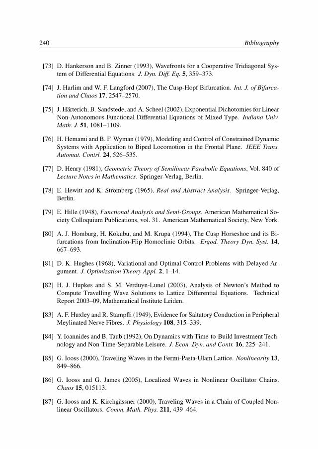
240 Bibliography
[73] D. Hankerson and B. Zinner (1993), Wavefronts for a Cooperative Tridiagonal Sys-tem of Differential Equations. J. Dyn. Diff. Eq. 5, 359–373.
[74] J. Harlim and W. F. Langford (2007), The Cusp-Hopf Bifurcation. Int. J. of Bifurca-tion and Chaos 17, 2547–2570.
[75] J. Harterich, B. Sandstede, and A. Scheel (2002), Exponential Dichotomies for LinearNon-Autonomous Functional Differential Equations of Mixed Type. Indiana Univ.Math. J. 51, 1081–1109.
[76] H. Hemami and B. F. Wyman (1979), Modeling and Control of Constrained DynamicSystems with Application to Biped Locomotion in the Frontal Plane. IEEE Trans.Automat. Contrl. 24, 526–535.
[77] D. Henry (1981), Geometric Theory of Semilinear Parabolic Equations, Vol. 840 ofLecture Notes in Mathematics. Springer-Verlag, Berlin.
[78] E. Hewitt and K. Stromberg (1965), Real and Abstract Analysis. Springer-Verlag,Berlin.
[79] E. Hille (1948), Functional Analysis and Semi-Groups, American Mathematical So-ciety Colloquium Publications, vol. 31. American Mathematical Society, New York.
[80] A. J. Homburg, H. Kokubu, and M. Krupa (1994), The Cusp Horseshoe and its Bi-furcations from Inclination-Flip Homoclinic Orbits. Ergod. Theory Dyn. Syst. 14,667–693.
[81] D. K. Hughes (1968), Variational and Optimal Control Problems with Delayed Ar-gument. J. Optimization Theory Appl. 2, 1–14.
[82] H. J. Hupkes and S. M. Verduyn-Lunel (2003), Analysis of Newton’s Method toCompute Travelling Wave Solutions to Lattice Differential Equations. TechnicalReport 2003–09, Mathematical Institute Leiden.
[83] A. F. Huxley and R. Stampfli (1949), Evidence for Saltatory Conduction in PeripheralMeylinated Nerve Fibres. J. Physiology 108, 315–339.
[84] Y. Ioannides and B. Taub (1992), On Dynamics with Time-to-Build Investment Tech-nology and Non-Time-Separable Leisure. J. Econ. Dyn. and Contr. 16, 225–241.
[85] G. Iooss (2000), Traveling Waves in the Fermi-Pasta-Ulam Lattice. Nonlinearity 13,849–866.
[86] G. Iooss and G. James (2005), Localized Waves in Nonlinear Oscillator Chains.Chaos 15, 015113.
[87] G. Iooss and K. Kirchgassner (2000), Traveling Waves in a Chain of Coupled Non-linear Oscillators. Comm. Math. Phys. 211, 439–464.
Bibliography 241
[88] G. James and Y. Sire (2005), Traveling Breathers with Exponentially Small Tails ina Chain of Nonlinear Oscillators. Comm. Math. Phys. 257, 51–85.
[89] M. A. Kaashoek and S. M. Verduyn-Lunel (1992), Characteristic Matrices and Spec-tral Properties of Evolutionary Systems. Trans. Amer. Math. Soc. 334, 479–517.
[90] M. A. Kaashoek and S. M. Verduyn-Lunel (1994), An Integrability Condition on theResolvent for Hyperbolicity of the Semigroup. J. Diff. Eq. 112, 374–406.
[91] A. Katok and B. Hasselblatt (1995), Introduction to the Modern Theory of DynamicalSystems. Cambridge University Press, Cambridge, NY.
[92] J. Keener and J. Sneed (1998), Mathematical Physiology. Springer–Verlag, NewYork.
[93] J. P. Keener (1987), Propagation and its Failure in Coupled Systems of Discrete Ex-citable Cells. SIAM J. Appl. Math. 47, 556–572.
[94] K. Kirchgassner (1982), Wave Solutions of Reversible Systems and Applications. J.Diff. Eqns. 45, 113–127.
[95] M. Kisaka, H. Kokubu, and H. Oka (1993), Bifurcation to N -homoclinic Orbits andN -periodic orbits in Vector Fields. J. Dyn. Diff. Eq. 5, 305–358.
[96] C. Kittel (1996), Introduction to Solid State Physics. Wiley, New York.
[97] T. A. Kontorova and Y. J. Frenkel (1938), On the Theory of Plastic Deformation andTwinning. Zh. Eksp. Teor. Fiz. 8, 1340–1348.
[98] S. G. Krantz (1999), Handbook of Complex Variables. Birkhauser, Boston, MA.
[99] A. Kumar and P. Daoutidis (1997), High Index DAE Systems in Modeling and Con-trol of Chemical Processes. In: Preprints of IFAC Conf. on Control of IndustrialSystems, Vol. 1. pp. 518–523.
[100] Y. Kuznetsov (2004), Elements of Applied Bifurcation Theory, Vol. 112 of AppliedMathematical Sciences. Springer–Verlag, New York.
[101] F. E. Kydland and E. C. Prescott (1982), Time to Build and Aggregate Fluctuations.Econometrica 50, 1345–1370.
[102] W. F. Langford (1983), A Review of Interactions of Hopf and Steady-State Bifurca-tions. In: G. I. Barenblatt, G. Iooss, and D. D. Joseph (eds.): Nonlinear Dynamicsand Turbulence. Pitman, Boston, MA, pp. 215–237.
[103] W. F. Langford (1984), Numerical Studies of Torus Bifurcations. In: T. Kupper, H. D.Mittelman, and H. Weber (eds.): Numerical Methods for Bifurcation Problems, Vol.ISNM 70. pp. 285–295.
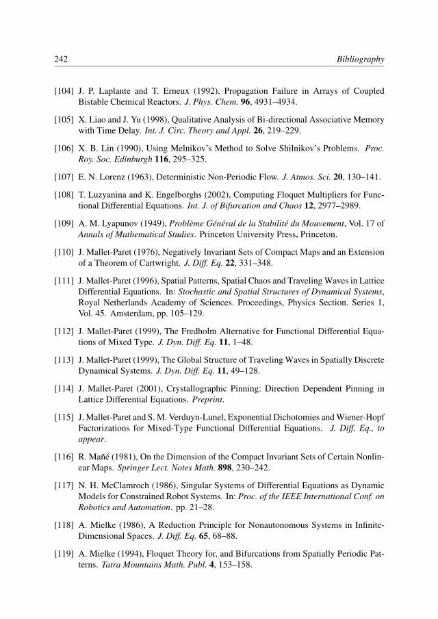
242 Bibliography
[104] J. P. Laplante and T. Erneux (1992), Propagation Failure in Arrays of CoupledBistable Chemical Reactors. J. Phys. Chem. 96, 4931–4934.
[105] X. Liao and J. Yu (1998), Qualitative Analysis of Bi-directional Associative Memorywith Time Delay. Int. J. Circ. Theory and Appl. 26, 219–229.
[106] X. B. Lin (1990), Using Melnikov’s Method to Solve Shilnikov’s Problems. Proc.Roy. Soc. Edinburgh 116, 295–325.
[107] E. N. Lorenz (1963), Deterministic Non-Periodic Flow. J. Atmos. Sci. 20, 130–141.
[108] T. Luzyanina and K. Engelborghs (2002), Computing Floquet Multipliers for Func-tional Differential Equations. Int. J. of Bifurcation and Chaos 12, 2977–2989.
[109] A. M. Lyapunov (1949), Probleme General de la Stabilite du Mouvement, Vol. 17 ofAnnals of Mathematical Studies. Princeton University Press, Princeton.
[110] J. Mallet-Paret (1976), Negatively Invariant Sets of Compact Maps and an Extensionof a Theorem of Cartwright. J. Diff. Eq. 22, 331–348.
[111] J. Mallet-Paret (1996), Spatial Patterns, Spatial Chaos and Traveling Waves in LatticeDifferential Equations. In: Stochastic and Spatial Structures of Dynamical Systems,Royal Netherlands Academy of Sciences. Proceedings, Physics Section. Series 1,Vol. 45. Amsterdam, pp. 105–129.
[112] J. Mallet-Paret (1999), The Fredholm Alternative for Functional Differential Equa-tions of Mixed Type. J. Dyn. Diff. Eq. 11, 1–48.
[113] J. Mallet-Paret (1999), The Global Structure of Traveling Waves in Spatially DiscreteDynamical Systems. J. Dyn. Diff. Eq. 11, 49–128.
[114] J. Mallet-Paret (2001), Crystallographic Pinning: Direction Dependent Pinning inLattice Differential Equations. Preprint.
[115] J. Mallet-Paret and S. M. Verduyn-Lunel, Exponential Dichotomies and Wiener-HopfFactorizations for Mixed-Type Functional Differential Equations. J. Diff. Eq., toappear.
[116] R. Mane (1981), On the Dimension of the Compact Invariant Sets of Certain Nonlin-ear Maps. Springer Lect. Notes Math. 898, 230–242.
[117] N. H. McClamroch (1986), Singular Systems of Differential Equations as DynamicModels for Constrained Robot Systems. In: Proc. of the IEEE International Conf. onRobotics and Automation. pp. 21–28.
[118] A. Mielke (1986), A Reduction Principle for Nonautonomous Systems in Infinite-Dimensional Spaces. J. Diff. Eq. 65, 68–88.
[119] A. Mielke (1994), Floquet Theory for, and Bifurcations from Spatially Periodic Pat-terns. Tatra Mountains Math. Publ. 4, 153–158.
Bibliography 243
[120] P. Morrel and W. T. Norton (1980), Myeline. Scientific American 242, 88–118.
[121] P. C. Muller (1997), Linear Mechanical Descriptor Systems: Identification, Analysisand Design. In: Preprints of IFAC Conf. on Control of Industrial Systems, Vol. 1. pp.501–506.
[122] R. W. Newcomb (1981), The Semistatic Description of Nonlinear Time-Variable Cir-cuits. IEEE Trans. Circ. Syst. 28, 62–71.
[123] A. Pankov and K. Pfluger (2000), Travelling Waves in Lattice Dynamical Systems.Math. Meth. Appl. Sci 23, 1223–1235.
[124] O. Perron (1928), Uber Stabilitat und Asymptotisches Verhalten der Integrale vonDifferentialgleichungssystemen. Math Zeit 29, 129–160.
[125] V. Pliss and G. R. Sell (1999), Robustness of Exponential Dichotomies in Infinite-Dimensional Dynamical Systems. J. Dyn. Diff. Eq. 11, 471–513.
[126] J. F. Pommaret (1983), Differential Galois Theory. Gordon & Breach Science Pub-lishers, New York.
[127] M. Remoissenet (1986), Low-Amplitude Breather and Envelope Solitons in Quasi-One-Dimensional Physical Models. Phys. Rev. B 33, 2386–2392.
[128] W. Rudin (1974), Real and Complex Analysis. McGraw–Hill, New York.
[129] W. Rudin (1991), Functional Analysis. McGraw–Hill, New York.
[130] A. Rustichini (1989), Functional Differential Equations of Mixed Type: the LinearAutonomous Case. J. Dyn. Diff. Eq. 11, 121–143.
[131] A. Rustichini (1989), Hopf Bifurcation for Functional-Differential Equations ofMixed Type. J. Dyn. Diff. Eq. 11, 145–177.
[132] J. S. W. L. S. Guo and B. W. Rink (2007), Branching Patterns of Wave Trains in theFPU Lattice. Preprint.
[133] R. J. Sacker and G. R. Sell (1994), Dichotomies for Linear Evolutionary Equationsin Banach Spaces. J. Diff. Eq. 113, 17–67.
[134] B. Sandstede (1993), Verzweigungstheorie Homokliner Verdopplungen. PhD Thesis.
[135] B. Sandstede and A. Scheel (2001), On the Structure of Spectra of Modulated Trav-elling Waves. Math. Nachr. 232, 39–93.
[136] B. Scarpellini (1991), Center Manifolds of Infinite Dimensions I: Main Results andApplications. Z. Angew. Math. Phys. 42, 1–32.
[137] H. Schwetlick and J. Zimmer (2007), Solitary Waves for Nonconvex FPU Lattices.J. Nonlinear Science 17, 1–12.
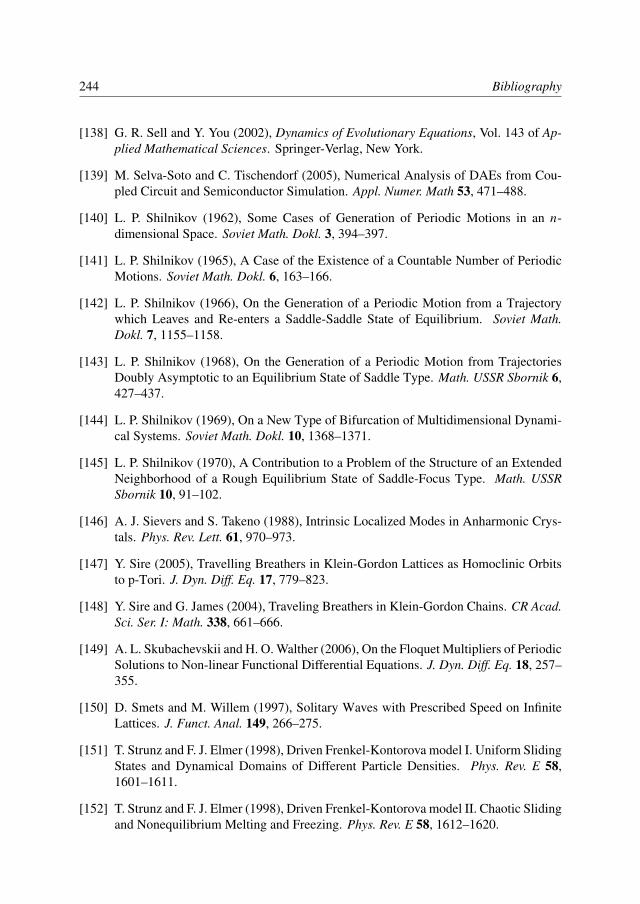
244 Bibliography
[138] G. R. Sell and Y. You (2002), Dynamics of Evolutionary Equations, Vol. 143 of Ap-plied Mathematical Sciences. Springer-Verlag, New York.
[139] M. Selva-Soto and C. Tischendorf (2005), Numerical Analysis of DAEs from Cou-pled Circuit and Semiconductor Simulation. Appl. Numer. Math 53, 471–488.
[140] L. P. Shilnikov (1962), Some Cases of Generation of Periodic Motions in an n-dimensional Space. Soviet Math. Dokl. 3, 394–397.
[141] L. P. Shilnikov (1965), A Case of the Existence of a Countable Number of PeriodicMotions. Soviet Math. Dokl. 6, 163–166.
[142] L. P. Shilnikov (1966), On the Generation of a Periodic Motion from a Trajectorywhich Leaves and Re-enters a Saddle-Saddle State of Equilibrium. Soviet Math.Dokl. 7, 1155–1158.
[143] L. P. Shilnikov (1968), On the Generation of a Periodic Motion from TrajectoriesDoubly Asymptotic to an Equilibrium State of Saddle Type. Math. USSR Sbornik 6,427–437.
[144] L. P. Shilnikov (1969), On a New Type of Bifurcation of Multidimensional Dynami-cal Systems. Soviet Math. Dokl. 10, 1368–1371.
[145] L. P. Shilnikov (1970), A Contribution to a Problem of the Structure of an ExtendedNeighborhood of a Rough Equilibrium State of Saddle-Focus Type. Math. USSRSbornik 10, 91–102.
[146] A. J. Sievers and S. Takeno (1988), Intrinsic Localized Modes in Anharmonic Crys-tals. Phys. Rev. Lett. 61, 970–973.
[147] Y. Sire (2005), Travelling Breathers in Klein-Gordon Lattices as Homoclinic Orbitsto p-Tori. J. Dyn. Diff. Eq. 17, 779–823.
[148] Y. Sire and G. James (2004), Traveling Breathers in Klein-Gordon Chains. CR Acad.Sci. Ser. I: Math. 338, 661–666.
[149] A. L. Skubachevskii and H. O. Walther (2006), On the Floquet Multipliers of PeriodicSolutions to Non-linear Functional Differential Equations. J. Dyn. Diff. Eq. 18, 257–355.
[150] D. Smets and M. Willem (1997), Solitary Waves with Prescribed Speed on InfiniteLattices. J. Funct. Anal. 149, 266–275.
[151] T. Strunz and F. J. Elmer (1998), Driven Frenkel-Kontorova model I. Uniform SlidingStates and Dynamical Domains of Different Particle Densities. Phys. Rev. E 58,1601–1611.
[152] T. Strunz and F. J. Elmer (1998), Driven Frenkel-Kontorova model II. Chaotic Slidingand Nonequilibrium Melting and Freezing. Phys. Rev. E 58, 1612–1620.
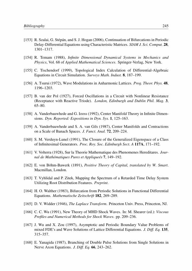
Bibliography 245
[153] R. Szalai, G. Stepan, and S. J. Hogan (2006), Continuation of Bifurcations in PeriodicDelay-Differential Equations using Characteristic Matrices. SIAM J. Sci. Comput. 28,1301–1317.
[154] R. Temam (1988), Infinite Dimensional Dynamical Systems in Mechanics andPhysics, Vol. 68 of Applied Mathematical Sciences. Springer-Verlag, New York.
[155] C. Tischendorf (1999), Topological Index Calculation of Differential-AlgebraicEquations in Circuit Simulation. Surveys Math. Indust. 8, 187–199.
[156] A. Tsurui (1972), Wave Modulations in Anharmonic Lattices. Prog. Theor. Phys. 48,1196–1203.
[157] B. van der Pol (1927), Forced Oscillations in a Circuit with Nonlinear Resistance(Receptance with Reactive Triode). London, Edinburgh and Dublin Phil. Mag. 3,65–80.
[158] A. Vanderbauwhede and G. Iooss (1992), Center Manifold Theory in Infinite Dimen-sions. Dyn. Reported: Expositions in Dyn. Sys. 1, 125–163.
[159] A. Vanderbauwhede and S. A. van Gils (1987), Center Manifolds and Contractionson a Scale of Banach Spaces. J. Funct. Anal. 72, 209–224.
[160] S. M. Verduyn-Lunel (1991), The Closure of the Generalized Eigenspace of a Classof Infinitesimal Generators. Proc. Roy. Soc. Edinburgh Sect. A 117A, 171–192.
[161] V. Volterra (1928), Sur la Theorie Mathematique des Phenomenes Hereditares. Jour-nal de Mathematiques Pures et Appliquees 7, 149–192.
[162] E. von Bohm-Bawerk (1891), Positive Theory of Capital, translated by W. Smart.Macmillan, London.
[163] T. Vyhlidal and P. Zitek, Mapping the Spectrum of a Retarded Time Delay SystemUtilizing Root Distribution Features. Preprint.
[164] H. O. Walther (1983), Bifurcation from Periodic Solutions in Functional DifferentialEquations. Mathematische Zeitschrift 182, 269–289.
[165] D. V. Widder (1946), The Laplace Transform. Princeton Univ. Press, Princeton, NJ.
[166] C. C. Wu (1991), New Theory of MHD Shock Waves. In: M. Shearer (ed.): ViscousProfiles and Numerical Methods for Shock Waves. pp. 209–236.
[167] J. Wu and X. Zou (1997), Asymptotic and Periodic Boundary Value Problems ofmixed FDE’s and Wave Solutions of Lattice Differential Equations. J. Diff. Eq. 135,315–357.
[168] E. Yanagida (1987), Branching of Double Pulse Solutions from Single Solutions inNerve Axon Equations. J. Diff. Eq. 66, 243–262.
246 Bibliography
[169] K. Yosida (1948), On the Differentiability and the Representation of One-ParameterSemi-Group of Linear Operators. J. Math. Soc. Japan 1, 15–21.
[170] B. Zinner (1992), Existence of Traveling Wavefront Solutions for the DiscreteNagumo Equation. J. Diff. Eq. 96, 1–27.
[171] B. Zinner (1992), Stability of Traveling Wavefronts for the Discrete Nagumo Equa-tion. J. Diff. Eq. 96, 1–27.
[172] B. Zinner, G. Harris, and W. Hudson (1993), Traveling Wavefronts for the DiscreteFisher’s Equations. J. Diff. Eq. 105, 46–62.
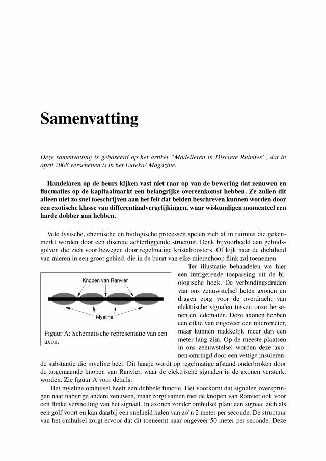
Samenvatting
Deze samenvatting is gebaseerd op het artikel “Modelleren in Discrete Ruimtes”, dat inapril 2008 verschenen is in het Eureka! Magazine.
Handelaren op de beurs kijken vast niet raar op van de bewering dat zenuwen enfluctuaties op de kapitaalmarkt een belangrijke overeenkomst hebben. Ze zullen ditalleen niet zo snel toeschrijven aan het feit dat beiden beschreven kunnen worden dooreen exotische klasse van differentiaalvergelijkingen, waar wiskundigen momenteel eenharde dobber aan hebben.
Vele fysische, chemische en biologische processen spelen zich af in ruimtes die geken-merkt worden door een discrete achterliggende structuur. Denk bijvoorbeeld aan geluids-golven die zich voortbewegen door regelmatige kristalroosters. Of kijk naar de dichtheidvan mieren in een groot gebied, die in de buurt van elke mierenhoop flink zal toenemen.
Myeline
Knopen van Ranvier
Figuur A: Schematische representatie van eenaxon.
Ter illustratie behandelen we hiereen intrigerende toepassing uit de bi-ologische hoek. De verbindingsdradenvan ons zenuwstelsel heten axonen endragen zorg voor de overdracht vanelektrische signalen tussen onze herse-nen en ledematen. Deze axonen hebbeneen dikte van ongeveer een micrometer,maar kunnen makkelijk meer dan eenmeter lang zijn. Op de meeste plaatsenin ons zenuwstelsel worden deze axo-nen omringd door een vettige insuleren-
de substantie die myeline heet. Dit laagje wordt op regelmatige afstand onderbroken doorde zogenaamde knopen van Ranvier, waar de elektrische signalen in de axonen versterktworden. Zie figuur A voor details.
Het myeline omhulsel heeft een dubbele functie. Het voorkomt dat signalen oversprin-gen naar naburige andere zenuwen, maar zorgt samen met de knopen van Ranvier ook vooreen flinke versnelling van het signaal. In axonen zonder omhulsel plant een signaal zich alseen golf voort en kan daarbij een snelheid halen van zo’n 2 meter per seconde. De structuurvan het omhulsel zorgt ervoor dat dit toeneemt naar ongeveer 50 meter per seconde. Deze
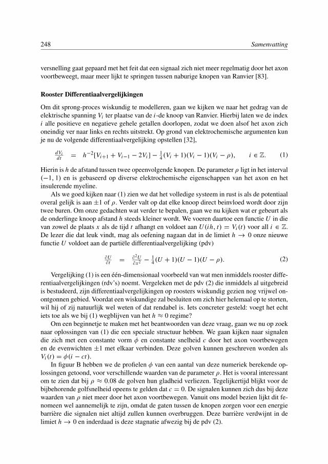
248 Samenvatting
versnelling gaat gepaard met het feit dat een signaal zich niet meer regelmatig door het axonvoortbeweegt, maar meer lijkt te springen tussen naburige knopen van Ranvier [83].
Rooster Differentiaalvergelijkingen
Om dit sprong-proces wiskundig te modelleren, gaan we kijken we naar het gedrag van deelektrische spanning Vi ter plaatse van de i-de knoop van Ranvier. Hierbij laten we de indexi alle positieve en negatieve gehele getallen doorlopen, zodat we doen alsof het axon zichoneindig ver naar links en rechts uitstrekt. Op grond van elektrochemische argumenten kunje nu de volgende differentiaalvergelijking opstellen [32],
dVidt = h−2[Vi+1 + Vi−1 − 2Vi ]− 1
4 (Vi + 1)(Vi − 1)(Vi − ρ), i ∈ Z. (1)
Hierin is h de afstand tussen twee opeenvolgende knopen. De parameter ρ ligt in het interval(−1, 1) en is gebaseerd op diverse elektrochemische eigenschappen van het axon en hetinsulerende myeline.
Als we goed kijken naar (1) zien we dat het volledige systeem in rust is als de potentiaaloveral gelijk is aan ±1 of ρ. Verder valt op dat elke knoop direct beinvloed wordt door zijntwee buren. Om onze gedachten wat verder te bepalen, gaan we nu kijken wat er gebeurt alsde onderlinge knoop afstand h steeds kleiner wordt. We voeren daartoe een functie U in dievan zowel de plaats x als de tijd t afhangt en voldoet aan U (ih, t) = Vi (t) voor all i ∈ Z.De lezer die dat leuk vindt, mag als oefening nagaan dat in de limiet h → 0 onze nieuwefunctie U voldoet aan de partiele differentiaalvergelijking (pdv)
∂U∂t =
∂2U∂x2 −
14 (U + 1)(U − 1)(U − ρ). (2)
Vergelijking (1) is een een-dimensionaal voorbeeld van wat men inmiddels rooster diffe-rentiaalvergelijkingen (rdv’s) noemt. Vergeleken met de pdv (2) die inmiddels al uitgebreidis bestudeerd, zijn differentiaalvergelijkingen op roosters wiskundig gezien nog vrijwel on-ontgonnen gebied. Voordat een wiskundige zal besluiten om zich hier helemaal op te storten,wil hij of zij natuurlijk wel weten of dat rendabel is. Iets concreter gesteld: voegt het echtiets toe als we bij (1) wegblijven van het h ≈ 0 regime?
Om een beginnetje te maken met het beantwoorden van deze vraag, gaan we nu op zoeknaar oplossingen van (1) die een speciale structuur hebben. We gaan kijken naar signalendie zich met een constante vorm φ en constante snelheid c door het axon voortbewegenen de evenwichten ±1 met elkaar verbinden. Deze golven kunnen geschreven worden alsVi (t) = φ(i − ct).
In figuur B hebben we de profielen φ van een aantal van deze numeriek berekende op-lossingen getoond, voor verschillende waarden van de parameter ρ. Het is vooral interessantom te zien dat bij ρ ≈ 0.08 de golven hun gladheid verliezen. Tegelijkertijd blijkt voor debijbehorende golfsnelheid opeens te gelden dat c = 0. De signalen kunnen zich dus bij dezewaarden van ρ niet meer door het axon voortbewegen. Vanuit ons model bezien lijkt dit fe-nomeen wel aannemelijk te zijn, omdat de gaten tussen de knopen zorgen voor een energiebarriere die signalen niet altijd zullen kunnen overbruggen. Deze barriere verdwijnt in delimiet h → 0 en inderdaad is deze stagnatie afwezig bij de pdv (2).
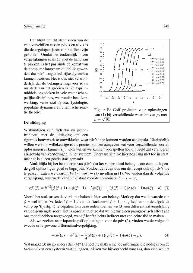
Samenvatting 249
-14 -12 -10 -8 -6 -4 -2 0 2 4
-1.2
-1.0
-0.8
-0.6
-0.4
-0.2
0.0
0.2
0.4
0.6
0.8
1.0
1.2
ρ = 0.90
ρ = 0.70
ρ = 0.54
ρ = 0.36
ρ = 0.30
ρ = 0.20
ρ = 0.10
ρ = 0.08
ρ = 0.00
φ(ξ
)
ξ
Figuur B: Golf profielen voor oplossingenvan (1) bij verschillende waarden van ρ, meth =√
10.
Het blijkt dat dit slechts een van devele verschillen tussen pdv’s en rdv’s isdie de afgelopen jaren aan het licht zijngekomen. Omdat het ondoenlijk is omvergelijkingen zoals (1) met de hand aante pakken, is het pas sinds de komst vande computer langzaam duidelijk gewor-den dat rdv’s ongekend rijke dynamicakunnen bezitten. Het is dus niet verwon-derlijk dat de belangstelling voor rdv’snu sterk aan het groeien is. Ze zijn in-middels opgedoken in vele wetenschap-pelijke disciplines, waaronder beeldver-werking, vaste stof fysica, fysiologie,populatie dynamica en chemische reac-tie theorie.
De uitdaging
Wiskundigen zien zich dus nu gecon-fronteerd met de uitdaging om eenrigoreus bouwwerk te ontwikkelen waar rdv’s mee kunnen worden aangepakt. Uiteindelijkwillen we voor willekeurige rdv’s precies kunnen aangeven wat voor verschillende soortenoplossingen er kunnen zijn. Ook willen we kunnen voorspellen hoe dit beeld zal veranderenals gevolg van verstoringen in het systeem. Uiteraard zijn we hier nog lang niet toe in staat,maar er is al een goede start gemaakt.
Vaak blijkt bij het bestuderen van pdv’s dat het van cruciaal belang is om eerst de lopen-de golf oplossingen goed te begrijpen. Voldoende reden dus om dit recept ook op rdv’s toete passen. Laten we daarom Vi (t) = φ(i − ct) invullen in (1). We vinden dan de volgendevergelijking, waarin de variable ξ staat voor de combinatie ξ = i − ct ,
−cφ′(ξ) = h−2[φ(ξ + 1)+ φ(ξ − 1)− 2φ(ξ)]−
14(φ(ξ)+ 1)(φ(ξ)− 1)(φ(ξ)− ρ). (3)
Vooral het stuk tussen de vierkante haken is hier van belang. Merk op dat we de waarde vanφ zowel in het ‘verleden’ ξ − 1 als in de ‘toekomst’ ξ + 1 nodig hebben om de afgeleidevan φ op ‘tijdstip’ ξ te bepalen. Om deze reden noemen we (3) een differentiaalvergelijkingvan de gemengde soort. Het is absoluut niet zo dat we hiermee een paragnostisch effect aanons model hebben toegevoegd, want ξ heeft slechts indirect met een echte tijd te maken.
Als we zoeken naar lopende golf oplossingen voor de pdv (2), vinden we de volgendetweede orde gewone differentiaalvergelijking,
−cφ′(ξ) = φ′′(ξ)−14(φ(ξ)+ 1)(φ(ξ)− 1)(φ(ξ)− ρ). (4)
Wat maakt (3) nu zo anders dan (4)? Dit heeft te maken met de informatie die nodig is om detoestand van een systeem vast te leggen. Kijken we bijvoorbeeld naar (4), dan zien we dat
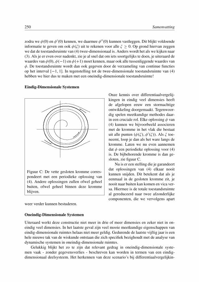
250 Samenvatting
zodra we φ(0) en φ′(0) kennen, we daarmee φ′′(0) kunnen vastleggen. Dit blijkt voldoendeinformatie te geven om ook φ(ξ) uit te rekenen voor alle ξ ≥ 0. Op grond hiervan zeggenwe dat de toestandsruimte van (4) twee-dimensionaal is. Anders wordt het als we kijken naar(3). Als je er even over nadenkt, zie je al snel dat om iets soortgelijks te doen, je uiteraard dewaardes van φ(0), φ(−1) en φ(+1)moet kennen, maar ook alle tussenliggende waardes vanφ. De toestandsruimte wordt dan ook gegeven door de verzameling van continue functiesop het interval [−1, 1]. In tegenstelling tot de twee-dimensionale toestandsruimte van (4)hebben we hier dus te maken met een oneindig-dimensionale toestandsruimte!
Eindig-Dimensionale Systemen
Figuur C: De vette gesloten kromme corres-pondeert met een periodieke oplossing van(4). Andere oplossingen zullen ofwel geheelbuiten, ofwel geheel binnen deze krommeblijven.
Onze kennis over differentiaalvergelij-kingen in eindig veel dimensies heeftde afgelopen eeuw een stormachtigeontwikkeling doorgemaakt. Tegenwoor-dig spelen meetkundige methodes daar-in een cruciale rol. Elke oplossing φ van(4) kunnen we bijvoorbeeld associerenmet de kromme in het vlak die bestaatuit alle punten (φ(ξ), φ′(ξ)). Als ξ toe-neemt, loop je dan als het ware langs dekromme. Laten we nu even aannemendat φ een periodieke oplossing voor (4)is. De bijbehorende kromme is dan ge-sloten, zie figuur C.
Nu is er een stelling die je garandeertdat oplossingen van (4) elkaar nooitkunnen snijden. Dit betekent dat als jeeenmaal in de gesloten kromme zit, jenooit naar buiten kan komen en vica ver-sa. Hiermee is de totale toestandsruimteal gereduceerd naar twee afzonderlijkecomponenten, die we vervolgens apart
weer verder kunnen bestuderen.
Oneindig-Dimensionale Systemen
Uiteraard werkt deze constructie niet meer in drie of meer dimensies en zeker niet in on-eindig veel dimensies. In het laatste geval zijn veel mooie meetkundige eigenschappen vaneindig-dimensionale ruimtes helaas niet meer geldig. Gedurende de laatste vijftig jaar is eenhele nieuwe tak van de wiskunde ontstaan die zich specifiek bezighoudt met de analyse vandynamische systemen in oneindig-dimensionale ruimtes.
Gelukkig blijkt het zo te zijn dat relevant gedrag in oneindig-dimensionale syste-men vaak - zonder gegevensverlies - beschreven kan worden in termen van een eindig-dimensionaal deelsysteem. Het herkennen van deze scenario’s bij differentiaalvergelijkin-
Samenvatting 251
gen van de gemengde soort en het ontwikkelen van technieken om deze deelsystemen ookdaadwerkelijk te beschrijven, vormen samen het hart van dit proefschrift. We hebben bij-voorbeeld een krachtige stelling die oorspronkelijk is ontwikkeld voor twee dimensies, ge-schikt gemaakt voor gebruik in onze oneindig-dimensionale context. Hiermee kunnen wevoorspellen bij welke waarden van de parameter ρ vergelijking (3) kleine oscillaties om eenvan de evenwichten zal toestaan.
Maximale Welvaart
Als afsluiting is het interessant om op te merken dat differentiaalvergelijkingen van de ge-mengde soort op onverwachte wijze ook bij optimalisatie problemen om de hoek komenkijken. Economen gebruiken vaak het volgende welvaarts-optimalisatie model om ontwik-kelingen op de kapitaalmarkt te bestuderen [17],
maximaliseer∫∞
0W (c(t))dt. (5)
Hierbij staat c(t) voor de totale consumptie op een bepaald tijdstip t en W voor de welvaartdie dit oplevert. Uiteraard hangt de mogelijkheid om te consumeren af van de investerin-gen in de productiecapaciteit die in het verleden zijn verricht. Fabrieken worden immersniet in een dag gebouwd. Al sinds 1968 is bekend dat deze tijdsvertraging betekent dat deEuler-Lagrange vergelijkingen die de oplossing van (5) typeren, niets anders zijn dan dif-ferentiaalvergelijkingen van de gemengde soort [81]. Als wiskundigen zijn we nu dus weernet iets beter in staat om ook de economen de technieken aan te reiken die ze nodig hebben.


Curriculum Vitae
De auteur van dit proefschrift werd geboren op 25 januari 1981 te Gouda. Hij bezocht vanaf1992 het Rijnlands Lyceum te Oegstgeest, waar hij in 1998 het VWO diploma behaalde. Indatzelfde jaar begon hij met de studies wiskunde en natuurkunde aan de Universiteit Lei-den. In 2003 schreef hij onder begeleiding van prof. dr. S. M. Verduyn Lunel de scriptieAnalysis of Newton’s Method to Compute Travelling Wave Solutions to Lattice DifferentialEquations, waarmee hij cum laude afstudeerde in de wiskunde. In de zomer van 2003 werk-te hij drie maanden bij CERN in Geneve, waar hij bijdroeg aan het ijken van de ATLASdetector. De studie natuurkunde rondde hij in 2004 cum laude af met een onderzoek naar deveiligheid van quantum cryptografische systemen.
In januari 2004 begon hij met zijn promotie onderzoek bij prof. dr. S. M. Verduyn Lunel.Naast het schrijven van de artikelen die in dit proefschrift zijn opgenomen, was hij intensiefbetrokken bij het onderwijs van de wiskunde opleiding in Leiden. Hij begeleidde diversewerkgroepen en verzorgde ook een introductie college wiskunde voor eerstejaars studentenvan de studie Life, Science and Technology. Verder gaf hij voordrachten op diverse nationaleen internationale congressen en colloquia.
Eind 2007 werd aan hem een Rubicon subsidie toegewezen door NWO. Hiermee heefthij de mogelijkheid gekregen om in de periode 2008-2010 verder te werken aan de uitbrei-ding en toepassing van de in dit proefschrift ontwikkelde theorie. Het is de bedoeling dat ditonderzoek onder begeleiding van prof. dr. B. Sandstede zal worden uitgevoerd aan BrownUniversity in de Verenigde Staten.