Intersection Type Disciplines P Lambda Calculussvb/Research/Papers/PhD2up.pdf · Intersection Type...
105
C ✕ ❑ ML ✕ ✕ Myc R ❑ ✕ RE ✸ CD ② ❖ CDVR ✕ CDV P ❨ CDV ✸ S ✍ ❦ -ω ✛ BCD E ❲ E CE ISBN 90-9005752-8 Intersection Type Disciplines in Lambda Calculus and Applicative Term Rewriting Systems een wetenschappelijke proeve op het gebied van de Wiskunde en Informatica. Proefschrift ter verkrijging van de graad van doctor aan de Katholieke Universiteit Nijmegen, volgens besluit van het College van Decanen in het openbaar te verdedigen op woensdag 3 februari 1993 des namiddags te 1.30 uur precies door Stephanus Johannes van Bakel Mathematisch Centrum, Amsterdam
-
Upload
phungkhuong -
Category
Documents
-
view
220 -
download
0
Transcript of Intersection Type Disciplines P Lambda Calculussvb/Research/Papers/PhD2up.pdf · Intersection Type...
!C
!"
!ML
!!!Myc
#
!R
"
!
!RE
$
!CD
% &!CDVR
!
!CDVP
'!CDV
$
!S
(
)
!"!
*!BCD
!E
+
,!E!CE
ISBN 90-9005752-8
Intersection Type Disciplines
in
Lambda Calculus
and
Applicative Term Rewriting Systems
een wetenschappelijke proeve op het gebied van de Wiskunde en Informatica.
Proefschrift
ter verkrijging van de graad van doctor aan de Katholieke Universiteit Nijmegen,
volgens besluit van het College van Decanen in het openbaar te verdedigen op
woensdag 3 februari 1993 des namiddags te 1.30 uur precies
door
Stephanus Johannes van Bakel
Mathematisch Centrum, Amsterdam
Promotores
Prof. M. Dezani-Ciancaglini
Dipartimento di Informatica, Universita degli Studi di Torino, Italia.
Prof. H.P. Barendregt.
Co-promotor
Dr. Ir. M.J. Plasmeijer.
‘Castigo te non quod odio habeam, sed quod AMEM.
I chastize thee not out of hatred, but out of love.’
– Henry Fielding, Tom Jones, Book III (1749)
Voor mijn moeder
Manuscriptcommissie
Prof. S. Ronchi della Rocca
Dipartimento di Informatica, Universita degli Studi di Torino, Italia.
Dr. Ir. C. Hemerik
Vakgroep Theoretische Informatica, Technische Universiteit Eindhoven, Nederland.
Contents
Preface xi
Introduction 1
Chapter 1 The Curry Type Assignment System 9
Chapter 2 Intersection Type Assignment Systems 13
2.1 The Coppo-Dezani Type Assignment System 13
2.2 The Coppo-Dezani-Venneri Type Assignment Systems 15
2.2.1 The systems of [Coppo et al. ’81] 15
2.2.2 The system of [Coppo et al. ’80] 18
2.3 The Barendregt-Coppo-Dezani Type Assignment System 24
2.3.1 Completeness of type assignment 26
2.3.2 Principal type schemes 29
Chapter 3 The Milner - and Mycroft Type Assignment Systems 33
3.1 The Milner Type Assignment System 33
3.2 The Mycroft Type Assignment System 37
3.3 The difference between Milner’s and Mycroft’s system 39
Chapter 4 The Strict Type Assignment System 41
4.1 Strict type assignment 41
4.2 The strict filter lambda model 45
4.3 The relation between !S and !BCD 50
4.4 Soundness and completeness of strict type assignment 52
Chapter 5 The Essential Intersection Type Assignment System 55
5.1 Essential type assignment 55
5.2 The relation between !S , !E and !BCD 59
5.3 Soundness and completeness of essential type assignment 59
Chapter 6 Principal Type Schemes for the Strict Type Assignment System 63
6.1 Principal pairs for terms in "#-normal form 65
6.2 Operations on pairs 68
6.2.1 Strict substitution 68
6.2.2 Strict expansion 70
viii Contents
6.2.3 Lifting 77
6.3 Completeness for lambda terms 81
6.3.1 Soundness and completeness for terms in "#-normal form 82
6.3.2 Principal pairs for lambda terms 85
6.4 Principal pairs for the essential type assignment system 86
Chapter 7 The Barendregt-Coppo-Dezani Type Assignment System without ! 87
7.1 !-free derivations 88
7.2 The relation between !!! and !BCD 90
7.3 The type assignment without ! is complete for the "I-calculus 92
7.4 Strong normalization result for the system without ! 93
Chapter 8 The Rank 2 Intersection Type Assignment System 99
8.1 Coppo-Dezani type assignment versus ML type assignment 100
8.2 Rank 2 intersection type assignment 102
8.3 Operations on pairs 104
8.3.1 Rank 2 substitution 104
8.3.2 Duplication 106
8.3.3 Type-chains 107
8.4 Principal type property 108
8.4.1 Unification of intersection types of Rank 2 108
8.4.2 Principal pairs for terms 110
Chapter 9 Applicative Term Rewriting Systems 115
9.1 The defined symbol of rewrite rules 117
9.2 Partial type assignment 118
9.3 Definitions 119
9.4 Tree-representation of terms and rewrite rules 123
Chapter 10 Partial Intersection Type Assignment in Applicative Term Rewriting Sys-
tems 125
10.1 Essential type assignment in ATRS’s 126
10.2 Soundness of strict operations 132
10.3 The loss of the subject reduction property 137
10.4 About recursion 141
Chapter 11 Partial Curry Type Assignment in Left Linear Applicative Term Rewriting
Systems 145
11.1 Curry type assignment in LLATRS’s 146
11.2 The principal pair for a term 149
Contents ix
11.3 A necessary and sufficient condition for subject reduction 151
Chapter 12 Partial Rank 2 Intersection Type Assignment in Applicative Term Rewrit-
ing Systems 155
12.1 Operations on pairs 156
12.2 Rank 2 type assignment in ATRS’s 158
12.3 Soundness of operations on pairs 161
12.4 Principal type property 163
12.5 A sufficient condition for subject reduction 168
12.6 Implementation aspects of Rank 2 type assignment in ATRS’s 171
Summary 175
Comparing the different notions of type assignment 177
Using Intersection Types for Term Graph Rewriting Systems 179
Conclusion 180
References 183
Index 189
Samenvatting 193
x Contents
Preface
The work on intersection type assignment systems presented in this thesis grew between 1988
and 1992. I first encountered intersection types in 1986 in an introductory course on Lambda
Calculus by professor Henk Barendregt at the University of Nijmegen. Under his supervision I
wrote a master’s thesis [van Bakel ’88], in which a first version of the Strict Type Assignment
System was presented. After my MSc-graduation in 1988 I worked with professors
Mariangiola Dezani-Ciancaglini, Mario Coppo and Simonetta Ronchi della Rocca in Turin,
Italy, from February 15 until July 15 1988. This resulted in a paper [van Bakel ’92a] that
appeared in the June 1992 issue of Theoretical Computer Science. The results presented in this
paper can be found in the chapters four and seven of this thesis.
In the first half of 1989 I implemented an intersection type inference algorithm for lambda
terms, reported on in [van Bakel ’90]. It led to the proof that the Strict Type Assignment
System has the principal type property. This proof was presented in [van Bakel ’91], which is
submitted for publication to the journal Logic and Computation. The results presented in that
paper can be found in chapter six.
In March 1991 I visited Turin. In a discussion with Mariangiola Dezani-Ciancaglini and
Mario Coppo the observation was made that in Term Rewriting Systems, types are not
preserved under rewriting. This problem was successfully tackled and reported on in the paper
[van Bakel et al. ’92] which appeared in the February 1992 proceedings of CAAP ’92,
Colloquium on Trees in Algebra and Programming, Rennes, France. Part of the results of that
paper can be found in the chapters nine and eleven. The design of the Applicative Term
Rewriting Systems and the notion of type assignment as presented in that paper was the result
of a cooperation between Sjaak Smetsers of the University of Nijmegen, Simon Brock of the
University of East Anglia, Norwich, U.K., and myself. In the second half of 1991 I
generalized this notion of type assignment to the system that uses intersection types of Rank 2,
which resulted in [van Bakel ’92c], that is submitted for publication to the Journal of
Functional Programming. The results of that paper can be found in chapters eight and twelve.
When writing this thesis I defined the Essential Type Assignment System, both for Lambda
Calculus and Applicative Term Rewriting Systems. These two notions of type assignment
were also presented in [van Bakel ’92b]. The former has been submitted to LICS ’93, Logic In
Computer Science, Montreal, Canada, and can be found in chapter five, the latter will appear
xii Preface
as [van Bakel ’93] in the March 1993 proceedings of TLCA ’93, Typed Lambda Calculi and
Applications, Utrecht, the Netherlands, and can be found in chapter ten.
The research presented in this thesis was supported by:
• The Dutch Organisation for the Advancement of Pure Research (N.W.O.), grant NF-68.
• The Esprit Basic Research Action 3074 ‘Semantics and Pragmatics of Generalized Graph
Rewriting (Semagraph)’.
• N.W.O.-project ‘Design and implementation of a type system based on intersection types
for the functional graph rewriting language Concurrent Clean’, grant 612-316-027.
Preface xiii
Prerequisites
I assume the reader to be familiar with the lambda calculus, including notions like normal
forms, reduction strategies, "-models, etc. For definitions and notions used here, see
[Barendregt ’84].
Notations
This section is given as a point of return while reading the thesis; its contents is not intended as
something to read before studying the chapters of the thesis.
In this thesis, the symbol # (often indexed, like in #i) will be a type-variable; when writing
a type-variable #i, I will sometimes use the index i only, so as to obtain more readable types.
Greek symbols like $, %, &, µ, ', (, ), * and + (often indexed) will range over types, and ,
will be used for principal types. To avoid parentheses in the notation of types, I will assume
that ‘$’ associates to the right – so right-most, outer-most brackets will be omitted – and I
will assume that, as in logic, ‘!’ binds stronger than ‘$’. So *!+$)!µ$& means
((*!+ )$(()!µ)$&)). I use the word ‘subtype’ to express that one type is a syntactic
component of another or the type itself.
I use M , N for lambda terms, x, y, z for term-variables and A for terms in "#-normal
form. F , G, H , I , etc. are used for function symbols, Q for constants and T for terms in
rewriting systems.
I use B for bases, B\x for the basis obtained from B by erasing the statements that have x
as subject, and P for principal bases. Two types (bases, pairs of basis and type) are disjoint if
and only if they have no type-variables in common.
Notions of type assignment are defined as ternary relations on bases, terms and types, that
are denoted by ! . I use B !I M :* for the statement ‘M can be typed with the type * starting
from a basis B using the set of derivation rules that is indicated by I’. If in a notion of type
assignment for M there are basis B and type * such that B ! M :*, or a node or edge in the
tree-representation of terms is labelled with a type *, then the term (node, edge) is typed with
*, and * is assigned to it.
I use O for operations on types, bases and pairs of basis and type; I use D for duplications, E
for expansions, L for liftings, S for substitutions, and W for weakenings.
I use the symbol to mark the end of a proof.
xiv Preface
Acknowledgements
The first person I would like to thank is Mariangiola Dezani, for the encouragement, support
and many helpful suggestions on the various papers (and the various versions of them) I wrote.
Visiting Turin has always been stimulating because of her: without her, this thesis would not
have been written. I would also like to thank Henk Barendregt for the enlightening
discussions, and Rinus Plasmeijer for creating the perfect working environment.
I thank my parents Gon van Bakel-van Heumen and Jan van Bakel for teaching me that the
most important things in life are tolerance towards other people and to follow one’s own ideas;
in research, both attitudes proved valuable.
Introduction
Over the last decade the popularity of functional programming has increased. A large and still
growing number of people is becoming interested in functional programming languages: com-
puter scientists and logicians on the scientific side as well as hard- and software manufacturers
on the applied side. Unfortunately for the major part of people working in computer science or
companies, functional programming languages are but a toy, since programs written in the av-
erage functional language take a long time to execute. Nevertheless impressive improvements
are achieved in implementing these languages (reaching nfib-numbers of over one million for
the functional programming language Clean on an Apple Macintosch IIFX) and it seems just a
matter of time before they will become a practical tool in program development.
In recent years several paradigms were investigated for the implementation of functional
programming languages. Not only the Lambda Calculus [Barendregt ’84], but also Term
Rewriting Systems [Klop ’90] and Term Graph Rewriting Systems [Barendregt et al. ’87] were
topics of research. Lambda Calculus (or rather combinator systems) constitutes the underly-
ing model for the functional programming language Miranda [Turner ’85]. Term Rewriting
Systems were used in the underlying model for the language OBJ [Futatsugi et al. ’85], and
Term Graph Rewriting Systems were the model for the language Clean [Brus et al. ’87, Nocker
et al. ’91].
The extension from Lambda Calculus to Term Rewriting Systems is done via combinator
systems. Term rewrite rules are written very much like the definitions of combinators, the
difference being that a formal parameter can be a pattern: it is allowed to have structure and it
need not be a term-variable. Term Graph Rewriting Systems are obtained from Term Rewriting
Systems by writing terms as trees, and allowing cyclic structures as well as sharing of nodes.
The Lambda Calculus, Term Rewriting Systems and Graph Rewriting Systems themselves are
type free, whereas in programming the notion of types plays an important role. Type assignment
to programs and objects is in fact a way of performing abstract interpretation that provides nec-
essary information for both compilers and programmers. Types are essential to obtain efficient
machine code when compiling a program and are also used to make sure that the program-
mer has a clearer understanding of the programs that are written. Since Lambda Calculus is a
fundamental basis for many functional programming languages, a type assignment system for
2 Introduction
pure untyped Lambda Calculus capable of deducing meaningful and expressive types has been
a topic of research for many years.
There are various ways to deal with the problem of handling types in programming lan-
guages. These can roughly be divided in the ‘typed’ and ‘untyped’ approaches. The ‘typed’ ap-
proach can be found in programming languages that have explicit typing: objects in a program
have types provided by the programmer, and the type-algorithm incorporated in the compiler
for the language checks if these are used consistently. The ‘untyped’ approach is used in lan-
guages that allow programmers to write programs without any type-specification at all, and it is
the task of the type-algorithm to infer types for objects and to check consistency.
There exists a well-understood and well-defined notion of type assignment on lambda terms,
known as the Curry Type Assignment System [Curry & Feys ’58, Curry ’34]), which expressed
abstraction and application. Many of the now existing type assignment systems for functional
programming languages that use the ‘untyped’ approach are based on (extensions of) Curry’s
system. For example, the functional programming language ML [Milner ’78] is in fact an
extended lambda calculus and its type system is based on Curry’s system.
It is well known that in Curry’s system, the problem of typeability
Given a term M , are there basis B and type * such that B !M :*?
is decidable. This system also has the principal type property: M is typeable if and only if there
are a basis P , and type ,, such that
P !M :,, and for every pair %B, *& such that B ! M :*, there exists an operation O
(from a specified set of operations) such that O (%P , ,&) = %B, *&.
The type , is then called a ‘principal type for M ’. In general it is undecidable whether such
an operation exists in the specified collection, except for certain special cases. For Curry’s sys-
tem the operation O consists entirely of substitutions, i.e. operations that replace type-variables
by types. Principal type schemes for Curry’s system were defined in [Hindley ’69].
The existence of a principal type within a type assignment system for a typeable lambda
term M shows an internal coherence between all types that can be assigned to M . Since sub-
stitution is an easy operation, the set { %B, *& | B ! M :* } can be computed in Curry’s system
easily from the principal pair for M . The principal type property plays an important role in the
‘untyped’ approach, since, in an implementation, it allows of the use of the principal type of M
to find the right types for the various occurrences of M without deriving the type for M over
and over again; this property constitutes the basis for the notion of ‘polymorphic functions’ in
programming languages like ML.
In some type assignment systems it is uncertain whether or not this property holds. For
Introduction 3
example, for the Polymorphic Type Discipline [Girard ’86] there is no natural way to obtain the
types ('#.#)$('#.#) and ('#.#$#)$('#.#$#), both types for the lambda term ("x.xx)
from a single type (see [Giannini & Ronchi della Rocca ’88]). In any case, there exists no type
* derivable for "x.xx such that both types can be obtained from * by substitution.
In [Milner ’78] an extension of Curry’s system is presented, which can be seen as a restric-
tion of the Polymorphic Type Discipline. Type assignment in this system is decidable and it has
the principal type property. It is designed to formalize the notion of polymorphic functions as
used in functional programming languages like ML and Miranda. (In [Mycroft ’84] a slightly
more general extension of this system was presented in which type assignment is no longer
decidable, but that is nevertheless used for type checking in Miranda.)
Although frequently used in functional programming languages, the Curry Type Assignment
System has some drawbacks. In this system it is, for example, not possible to assign a type to
the term ("x.xx). Moreover, although the lambda terms ("cd.d) and (("xyz.xz(yz))("ab.a))
are %-equal, the principal type schemes for these terms are different.
The Intersection Type Discipline as presented in [Coppo et al. ’81, Barendregt et al. ’83] is
an extension of Curry’s system that does not have these drawbacks. The extension to Curry’s
system is essentially that term-variables are allowed to have more than one type. Intersection
types are constructed by adding, next to the type constructor ‘$’, the type constructor ‘!’ and
the type constant ‘!’. This yields a type assignment system that is very powerful: it is closed
under %-equality:
If B ! M :* and M =" N , then B ! N :*.
Because of this power, type assignment in this system is undecidable.
As stated above, if a type assignment system with intersection types is desired – instead of
Curry’s system – for the construction of a type inference system for an untyped functional
programming language, then such a system should at least have the principal pair property.
(Of course decidability of type assignment is also convenient.) There are two intersection type
assignment systems for which this property is proved.
In [Coppo et al. ’80] principal type schemes were defined for a type assignment system that
is a restriction of the one presented in [Coppo et al. ’81]. This system has as a disadvantage
that it is not an extension of Curry’s system: if B !M :+ , and the variable x does not occur
in B, then for "x.M only the type !$+ can be derived. Therefore, it is impossible to derive
#0$#1$#0 for the lambda term "ab.a. This type is derivable for that term in Curry’s system.
For the BCD-system defined in [Barendregt et al. ’83], principal type schemes can be de-
fined as in [Ronchi della Rocca & Venneri ’84]. In [Ronchi della Rocca ’88] a unification
4 Introduction
semi-algorithm for intersection types was presented, together with a semi-algorithm that finds
the principal type for every strongly normalizable lambda term. These algorithms are called
‘semi-algorithms’, because they do not terminate for every possible input.
The BCD-system has as a disadvantage that it is too general: in this system there are several
ways to deduce a desired result, due to the presence of the derivation rules (!I), (!E) and (().
These rules not only allow of superfluous steps in derivations, but they also make it possible to
give essentially different derivations for the same result. Moreover, in [Barendregt et al. ’83]
the relation ( induced an equivalence relation ) on types. Equivalence classes are big (for
example: ! ) *$!, for all types *) and type assignment is closed for ) . And although the set
{ %B, *& | B !M :* } can be generated using the operations specified in [Ronchi della Rocca
& Venneri ’84], the problem of type-checking
Given a term M and type *, is there a B such that B !M :*?
is complicated.
Although the BCD-system has the principal type property, it is not used in type checkers
for functional languages at the present time, as type assignment is undecidable in this system.
In order to obtain a terminating type checker based on this system, some restrictions have
to be made. There are of course limitations of the BCD-system that provide decidable type
assignment and efficient implementation (the trivial one being the restriction to Curry’s system).
Another possibility is the one suggested in [Leivant ’83]: limiting the set of types to intersection
types of Rank 2.
Because of the similarity between this system and the one for ML, this system got little
attention from the functional programming world in the past. This is surprising, considering
the several advantages of the Rank 2 system over the one for ML. Not only the class of ty-
peable terms is significantly extended when intersection types of Rank 2 are used, but also
more accurate types can be deduced for terms. Moreover, when using the ML-type checker it
is possible that a program (correct in the programmers mind) is rejected because of occurring
type conflicts, while on the other hand it could be accepted after the programmer has rewritten
the specification. Such a rewrite would not be necessary if Rank 2 types were used.
Most functional programming languages, for instance Miranda, allow programmers to specify
an algorithm (function) as a set of rewrite rules. It is remarkable that little is known – apart from
the algebraic approach [Dershowitz & Jouannaud ’90] – about type assignment in Term Rewrit-
ing Systems. The type assignment systems incorporated in most term rewriting languages are
in fact extensions of type assignment systems for a(n extended) lambda calculus, and although
it seems straightforward to generalize those systems to the (significantly larger) world of Term
Rewriting Systems, it is at first glance not evident that those borrowed systems still have all the
Introduction 5
properties they possessed in the world of Lambda Calculus. For example, type assignment in
Term Rewriting Systems in general does not satisfy the subject reduction property: i.e. types
are not preserved under rewriting. In order to be able to study the details of type assignment
for Term Rewriting Systems, a formal notion of type assignment on Term Rewriting Systems is
needed, that is closer to the approach of type assignment in Lambda Calculus than the algebraic
one.
The aim of the research presented in this thesis is develop to type assignment systems with
intersection types for the Lambda Calculus and for Term Rewriting Systems, in order to in-
vestigate and understand their structure and properties and to see whether the definition of a
type-checker for a functional programming language with intersection types is feasible. Inter-
section types are examined because they are a good means to perform abstract interpretation:
better than Curry types, also even better than the kind of types used in languages like ML. Also,
the presented formalisms could be extended to the world of Term Graph Rewriting Systems,
which is favourable as in that world intersection types are the natural tool to type nodes that are
shared. Moreover, intersection types seem to be promising for use in functional programming
languages, since they seem to provide a good formalism to express overloading. The results
of this research can be used as a guideline to develop type-inferencing (and type-checking)
algorithms using intersection types in functional programming languages.
There is a great number of notions of type assignment presented in this thesis (fifteen in total),
each defined as a ternary relation on bases, terms and types and denoted by ! , indexed with
information to be able to distinguish them.
In chapters one through three a short overview of various type disciplines will be given.
It starts with the presentation of the Curry Type Assignment System ( !C ) in chapter one.
Chapter two will contain the development of the Intersection Type Discipline, by presenting the
several systems that were published in the past. In section 2.1 the Coppo-Dezani System ( !CD )
will be discussed, and in section 2.2 three Coppo-Dezani-Venneri Systems ( !CDV , !CDVR,
!CDVP). In section 2.3 the Barendregt-Coppo-Dezani System ( !BCD ) will be discussed. In
chapter three a short overview of the Milner Type Assignment System [Milner ’78] ( !ML ) will
be given – that will be compared to the Rank 2 Intersection Type Assignment System in chapter
eight – and the Mycroft Type Assignment System [Mycroft ’84] ( !Myc ).
In chapters four through eight intersection type disciplines for the Lambda Calculus will
be studied. In chapter four the Strict Type Assignment System ( !S ) will be presented, a
restriction of the BCD-system that satisfies all major properties of that full system, for which
in chapter six will be proved that the principal type property holds. In chapter five the Essential
Intersection Type Assignment System ( !E ) will be defined, a slight generalization of the strict
6 Introduction
one and also a restriction of the BCD-system. The intersection type assignment system without
the type constant ! ( !!! ) will be presented in chapter seven. It will be shown that all three
restrictions yield undecidable systems. So these attempts to restrict the system in preparation
for the construction of a type checker will fail. In chapter eight the Rank 2 Intersection Type
Assignment System ( !R ) will be defined, the smallest restriction of the Intersection Type
Discipline that contains intersection types. It will be shown that in this system type assignment
is decidable and that it has the principal type property.
In chapters nine through twelve intersection type disciplines will be studied for Applicative
Term Rewriting Systems, that will be defined in chapter nine. In chapter ten a formal notion
of type assignment ( !E ) will be presented that uses strict intersection types. Chapters eleven
and twelve will be presented in such a way that they can be read independently from the other
chapters in this thesis, although it is advisable to study chapter eight before reading chapter
twelve. Those chapters aim to present type assignment systems that can be used in functional
programming languages, so not only will be shown that the presented systems have the principal
type property, but also will be shown that type assignment is decidable in those systems by
presenting (terminating) unification algorithms that should be implemented when such a system
is used.
In chapter eleven a formal notion of type assignment on left linear Applicative Term Rewrit-
ing Systems will be presented ( !CE ) that uses Curry types, and the way of dealing with recur-
sion of the extension defined by Mycroft of Curry’s system. This chapter aims to give formal
motivation for the type system of Miranda, and to provide a formal type system for all languages
that use pattern matching and have type systems based on Mycroft’s extension of Curry’s sys-
tem.
In chapter twelve a type assignment system for Applicative Term Rewriting Systems will
be defined that uses intersection types of Rank 2 ( !RE ). The Rank 2 system is very close to the
Milner Type Assignment System, as discussed in chapter eight, so should show the advantages
of intersection types over Curry types (or ML types).
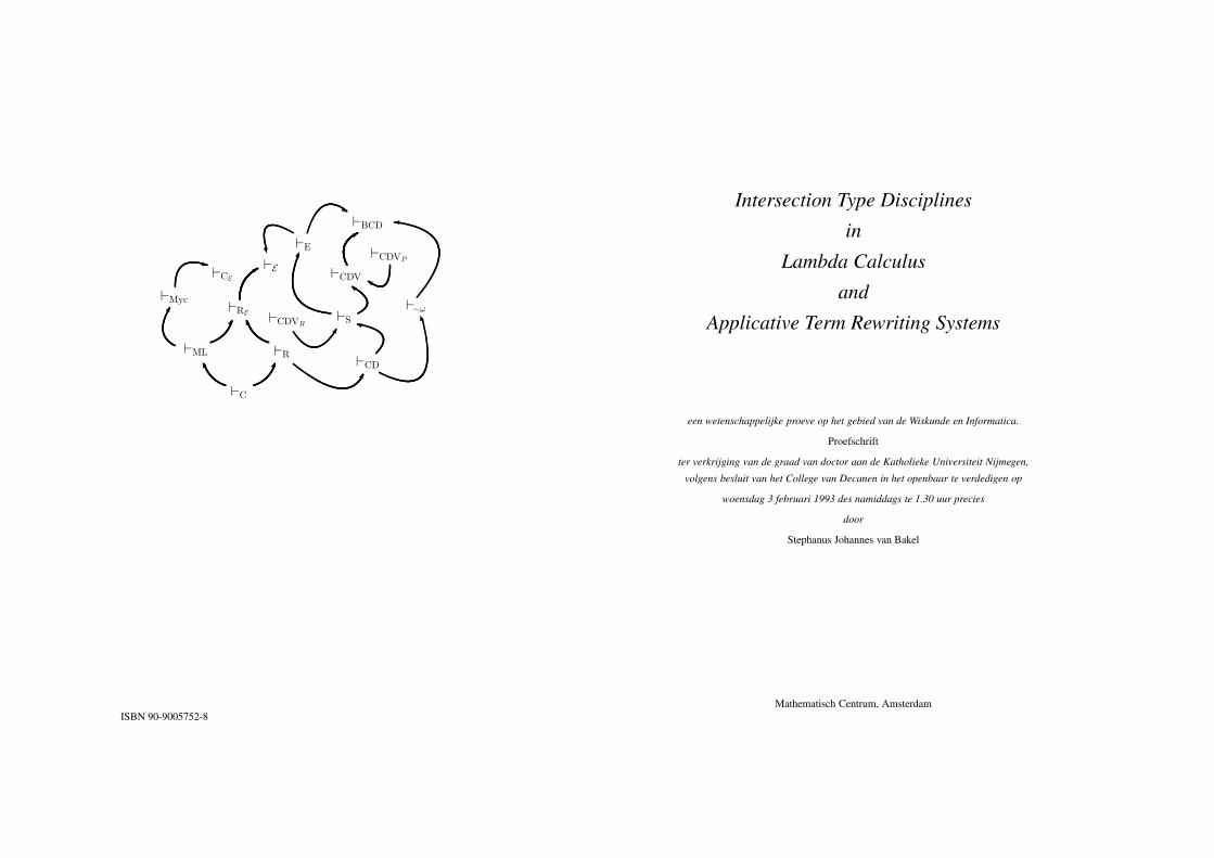
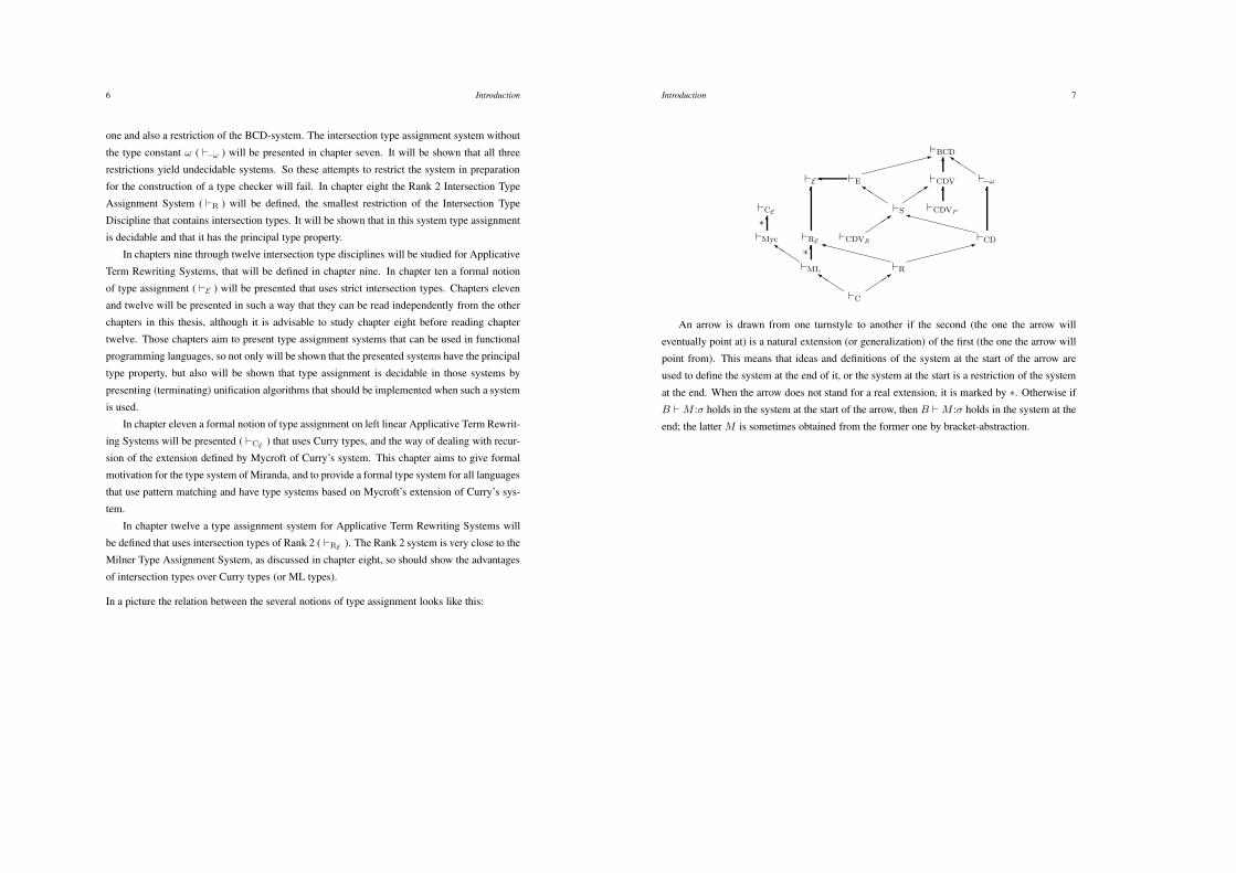
In a picture the relation between the several notions of type assignment looks like this:
Introduction 7
!C!
!!"###$
!ML!
!!" %*!Myc
%*!CE
!RE
%!E
!R&&&&&&&'
((((((()!CD
&&&&&&&'
%
!CDVR
###$
!S!
!!"###$
!CDVP
%!E
* ((((((()
!CDV
%!!!
!!!"
!BCD
An arrow is drawn from one turnstyle to another if the second (the one the arrow will
eventually point at) is a natural extension (or generalization) of the first (the one the arrow will
point from). This means that ideas and definitions of the system at the start of the arrow are
used to define the system at the end of it, or the system at the start is a restriction of the system
at the end. When the arrow does not stand for a real extension, it is marked by *. Otherwise if
B ! M :* holds in the system at the start of the arrow, then B ! M :* holds in the system at the
end; the latter M is sometimes obtained from the former one by bracket-abstraction.
Chapter 1 The Curry Type Assignment System
Type assignment for the Lambda Calculus was first studied in [Curry ’34]. (See also [Curry
& Feys ’58].) Curry’s system – the first and most primitive one – expresses abstraction and
application and has as its major advantage that the problem of type assignment (given a term
M , are there B, * such that B !C M :*) is decidable. In this chapter we will present the main
definitions and results for this system, using a notation that will be used throughout this thesis.
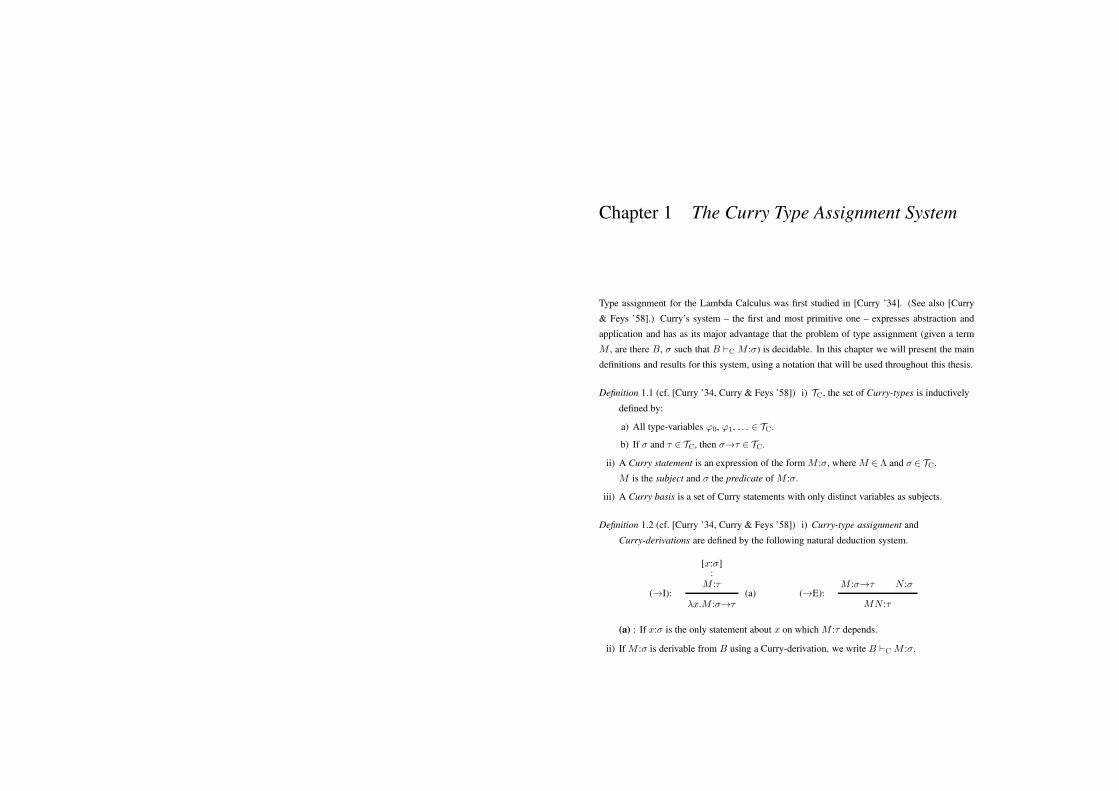
Definition 1.1 (cf. [Curry ’34, Curry & Feys ’58]) i) TC, the set of Curry-types is inductively
defined by:
a) All type-variables #0, #1, . . . + TC.
b) If * and + + TC, then *$+ + TC.
ii) A Curry statement is an expression of the form M :*, where M +! and * + TC.
M is the subject and * the predicate of M :*.
iii) A Curry basis is a set of Curry statements with only distinct variables as subjects.
Definition 1.2 (cf. [Curry ’34, Curry & Feys ’58]) i) Curry-type assignment and
Curry-derivations are defined by the following natural deduction system.
[x:*]:
M :+($I): (a)
"x.M :*$+
M :*$+ N :*($E):
MN :+
(a) : If x:* is the only statement about x on which M :+ depends.
ii) If M :* is derivable from B using a Curry-derivation, we write B !C M :*.
10 Chapter 1 The Curry Type Assignment System
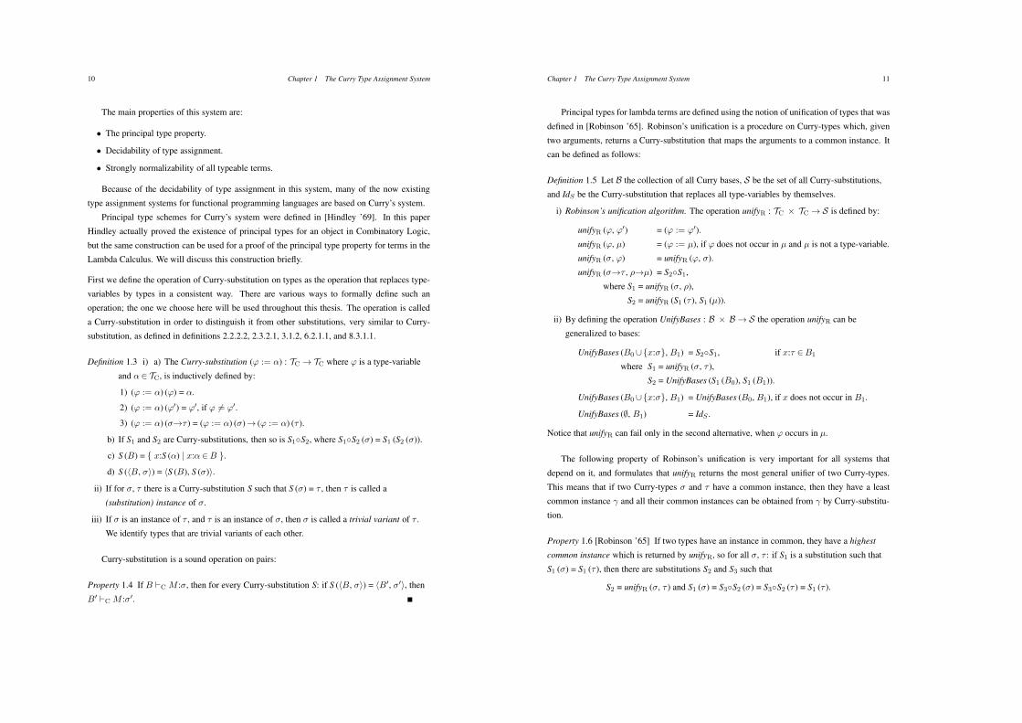
The main properties of this system are:
• The principal type property.
• Decidability of type assignment.
• Strongly normalizability of all typeable terms.
Because of the decidability of type assignment in this system, many of the now existing
type assignment systems for functional programming languages are based on Curry’s system.
Principal type schemes for Curry’s system were defined in [Hindley ’69]. In this paper
Hindley actually proved the existence of principal types for an object in Combinatory Logic,
but the same construction can be used for a proof of the principal type property for terms in the
Lambda Calculus. We will discuss this construction briefly.
First we define the operation of Curry-substitution on types as the operation that replaces type-
variables by types in a consistent way. There are various ways to formally define such an
operation; the one we choose here will be used throughout this thesis. The operation is called
a Curry-substitution in order to distinguish it from other substitutions, very similar to Curry-
substitution, as defined in definitions 2.2.2.2, 2.3.2.1, 3.1.2, 6.2.1.1, and 8.3.1.1.
Definition 1.3 i) a) The Curry-substitution (# := $) : TC $ TC where # is a type-variable
and $ + TC, is inductively defined by:
1) (# := $) (#) = $.
2) (# := $) (#") = #", if # ,= #".
3) (# := $) (*$+ ) = (# := $) (*)$ (# := $) (+ ).
b) If S1 and S2 are Curry-substitutions, then so is S1-S2, where S1-S2 (*) = S1 (S2 (*)).
c) S (B) = { x:S ($) | x:$ +B }.
d) S (%B, *&) = %S (B), S (*)&.
ii) If for *, + there is a Curry-substitution S such that S (*) = + , then + is called a
(substitution) instance of *.
iii) If * is an instance of + , and + is an instance of *, then * is called a trivial variant of + .
We identify types that are trivial variants of each other.
Curry-substitution is a sound operation on pairs:
Property 1.4 If B !C M :*, then for every Curry-substitution S: if S (%B, *&) = %B", *"&, then
B" !C M :*".
Chapter 1 The Curry Type Assignment System 11
Principal types for lambda terms are defined using the notion of unification of types that was
defined in [Robinson ’65]. Robinson’s unification is a procedure on Curry-types which, given
two arguments, returns a Curry-substitution that maps the arguments to a common instance. It
can be defined as follows:
Definition 1.5 Let B the collection of all Curry bases, S be the set of all Curry-substitutions,
and IdS be the Curry-substitution that replaces all type-variables by themselves.
i) Robinson’s unification algorithm. The operation unifyR : TC . TC $ S is defined by:
unifyR (#, #") = (# := #").
unifyR (#, µ) = (# := µ), if # does not occur in µ and µ is not a type-variable.
unifyR (*, #) = unifyR (#, *).
unifyR (*$+ , )$µ) = S2-S1,
where S1 = unifyR (*, )),
S2 = unifyR (S1 (+ ), S1 (µ)).
ii) By defining the operation UnifyBases : B . B $ S the operation unifyR can be
generalized to bases:
UnifyBases (B0 /{x:*}, B1) = S2-S1, if x:+ +B1
where S1 = unifyR (*, + ),
S2 = UnifyBases (S1 (B0), S1 (B1)).
UnifyBases (B0 /{x:*}, B1) = UnifyBases (B0, B1), if x does not occur in B1.
UnifyBases (0, B1) = IdS .
Notice that unifyR can fail only in the second alternative, when # occurs in µ.
The following property of Robinson’s unification is very important for all systems that
depend on it, and formulates that unifyR returns the most general unifier of two Curry-types.
This means that if two Curry-types * and + have a common instance, then they have a least
common instance & and all their common instances can be obtained from & by Curry-substitu-
tion.
Property 1.6 [Robinson ’65] If two types have an instance in common, they have a highest
common instance which is returned by unifyR, so for all *, + : if S1 is a substitution such that
S1 (*) = S1 (+ ), then there are substitutions S2 and S3 such that
S2 = unifyR (*, + ) and S1 (*) = S3-S2 (*) = S3-S2 (+ ) = S1 (+ ).
12 Chapter 1 The Curry Type Assignment System
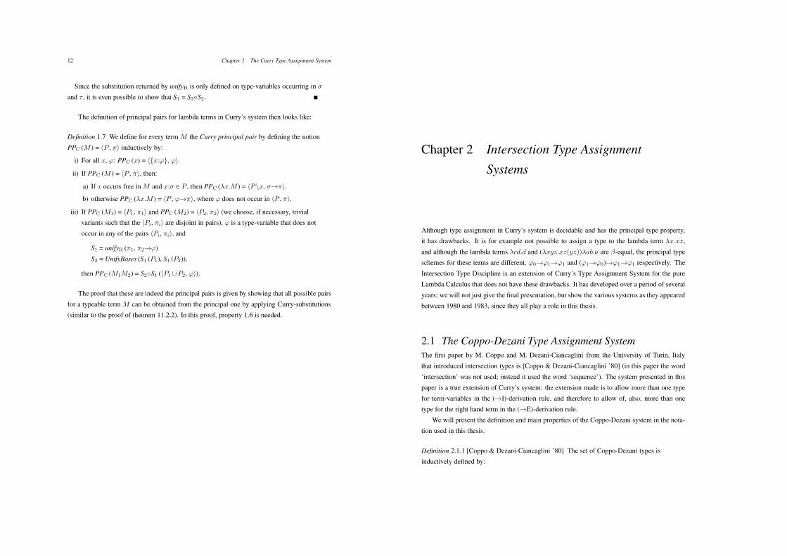
Since the substitution returned by unifyR is only defined on type-variables occurring in *
and + , it is even possible to show that S1 = S3-S2.
The definition of principal pairs for lambda terms in Curry’s system then looks like:
Definition 1.7 We define for every term M the Curry principal pair by defining the notion
PPC (M ) = %P , ,& inductively by:
i) For all x, #: PPC (x) = %{x:#}, #&.
ii) If PPC (M ) = %P , ,&, then:
a) If x occurs free in M and x:* + P , then PPC ("x.M ) = %P\x, *$,&.
b) otherwise PPC ("x.M ) = %P , #$,&, where # does not occur in %P , ,&.
iii) If PPC (M1) = %P1, ,1& and PPC (M2) = %P2, ,2& (we choose, if necessary, trivial
variants such that the %Pi, ,i& are disjoint in pairs), # is a type-variable that does not
occur in any of the pairs %Pi, ,i&, and
S1 = unifyR (,1, ,2$#)
S2 = UnifyBases (S1 (P1), S1 (P2)),
then PPC (M1M2) = S2-S1 (%P1 /P2, #&).
The proof that these are indeed the principal pairs is given by showing that all possible pairs
for a typeable term M can be obtained from the principal one by applying Curry-substitutions
(similar to the proof of theorem 11.2.2). In this proof, property 1.6 is needed.
Chapter 2 Intersection Type Assignment
Systems
Although type assignment in Curry’s system is decidable and has the principal type property,
it has drawbacks. It is for example not possible to assign a type to the lambda term "x.xx,
and although the lambda terms "cd.d and ("xyz.xz(yz))"ab.a are %-equal, the principal type
schemes for these terms are different, #0$#1$#1 and (#1$#0)$#1$#1 respectively. The
Intersection Type Discipline is an extension of Curry’s Type Assignment System for the pure
Lambda Calculus that does not have these drawbacks. It has developed over a period of several
years; we will not just give the final presentation, but show the various systems as they appeared
between 1980 and 1983, since they all play a role in this thesis.
2.1 The Coppo-Dezani Type Assignment SystemThe first paper by M. Coppo and M. Dezani-Ciancaglini from the University of Turin, Italy
that introduced intersection types is [Coppo & Dezani-Ciancaglini ’80] (in this paper the word
‘intersection’ was not used; instead it used the word ‘sequence’). The system presented in this
paper is a true extension of Curry’s system: the extension made is to allow more than one type
for term-variables in the ($I)-derivation rule, and therefore to allow of, also, more than one
type for the right hand term in the ($E)-derivation rule.
We will present the definition and main properties of the Coppo-Dezani system in the nota-
tion used in this thesis.
Definition 2.1.1 [Coppo & Dezani-Ciancaglini ’80] The set of Coppo-Dezani types is
inductively defined by:
14 Chapter 2 Intersection Type Assignment Systems
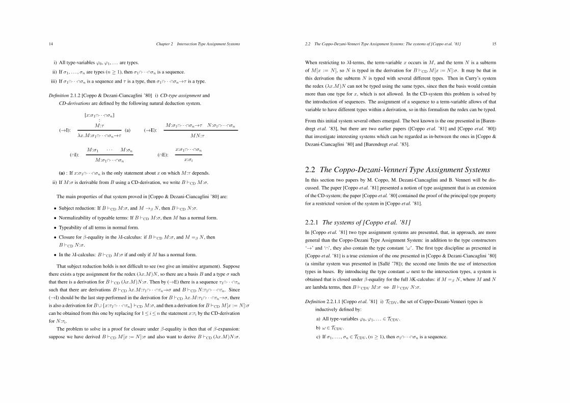
i) All type-variables #0, #1, . . . are types.
ii) If *1, . . . , *n are types (n 1 1), then *1!· · ·!*n is a sequence.
iii) If *1!· · ·!*n is a sequence and + is a type, then *1!· · ·!*n$+ is a type.
Definition 2.1.2 [Coppo & Dezani-Ciancaglini ’80] i) CD-type assignment and
CD-derivations are defined by the following natural deduction system.
[x:*1!· · ·!*n]:
M :+($I): (a)
"x.M :*1!· · ·!*n$+
M :*1!· · ·!*n$+ N :*1!· · ·!*n($E):
MN :+
M :*1 · · · M :*n(!I):
M :*1!· · ·!*n
x:*1!· · ·!*n(!E):
x:*i
(a) : If x:*1!· · ·!*n is the only statement about x on which M :+ depends.
ii) If M :* is derivable from B using a CD-derivation, we write B !CD M :*.
The main properties of that system proved in [Coppo & Dezani-Ciancaglini ’80] are:
• Subject reduction: If B !CD M :*, and M $" N , then B !CD N :*.
• Normalizability of typeable terms: If B !CD M :*, then M has a normal form.
• Typeability of all terms in normal form.
• Closure for %-equality in the "I-calculus: if B !CD M :*, and M =" N , then
B !CD N :*.
• In the "I-calculus: B !CD M :* if and only if M has a normal form.
That subject reduction holds is not difficult to see (we give an intuitive argument). Suppose
there exists a type assignment for the redex ("x.M)N , so there are a basis B and a type * such
that there is a derivation for B !CD ("x.M)N :*. Then by ($E) there is a sequence +1!· · ·!+n
such that there are derivations B !CD "x.M :+1!· · ·!+n$* and B !CD N :+1!· · ·!+n. Since
($I) should be the last step performed in the derivation for B !CD "x.M :+1!· · ·!+n$*, there
is also a derivation for B/{x:+1!· · ·!+n} !CD M :*, and then a derivation for B !CD M [x := N ]:*
can be obtained from this one by replacing for 1( i(n the statement x:+i by the CD-derivation
for N :+i.
The problem to solve in a proof for closure under %-equality is then that of %-expansion:
suppose we have derived B !CD M [x := N ]:* and also want to derive B !CD ("x.M)N :*.
2.2 The Coppo-Dezani-Venneri Type Assignment Systems: The systems of [Coppo et al. ’81] 15
When restricting to "I-terms, the term-variable x occurs in M , and the term N is a subterm
of M [x := N ], so N is typed in the derivation for B !CD M [x := N ]:*. It may be that in
this derivation the subterm N is typed with several different types. Then in Curry’s system
the redex ("x.M)N can not be typed using the same types, since then the basis would contain
more than one type for x, which is not allowed. In the CD-system this problem is solved by
the introduction of sequences. The assignment of a sequence to a term-variable allows of that
variable to have different types within a derivation, so in this formalism the redex can be typed.
From this initial system several others emerged. The best known is the one presented in [Baren-
dregt et al. ’83], but there are two earlier papers ([Coppo et al. ’81] and [Coppo et al. ’80])
that investigate interesting systems which can be regarded as in-between the ones in [Coppo &
Dezani-Ciancaglini ’80] and [Barendregt et al. ’83].
2.2 The Coppo-Dezani-Venneri Type Assignment SystemsIn this section two papers by M. Coppo, M. Dezani-Ciancaglini and B. Venneri will be dis-
cussed. The paper [Coppo et al. ’81] presented a notion of type assignment that is an extension
of the CD-system; the paper [Coppo et al. ’80] contained the proof of the principal type property
for a restricted version of the system in [Coppo et al. ’81].
2.2.1 The systems of [Coppo et al. ’81]
In [Coppo et al. ’81] two type assignment systems are presented, that, in approach, are more
general than the Coppo-Dezani Type Assignment System: in addition to the type constructors
‘$’ and ‘!’, they also contain the type constant ‘!’. The first type discipline as presented in
[Coppo et al. ’81] is a true extension of the one presented in [Coppo & Dezani-Ciancaglini ’80]
(a similar system was presented in [Salle ’78]); the second one limits the use of intersection
types in bases. By introducing the type constant ! next to the intersection types, a system is
obtained that is closed under %-equality for the full "K-calculus: if M =" N , where M and N
are lambda terms, then B !CDV M :* 23 B !CDV N :*.
Definition 2.2.1.1 [Coppo et al. ’81] i) TCDV, the set of Coppo-Dezani-Venneri types is
inductively defined by:
a) All type-variables #0, #1, . . . + TCDV.
b) ! + TCDV.
c) If *1, . . . , *n + TCDV, (n 1 1), then *1!· · ·!*n is a sequence.
16 Chapter 2 Intersection Type Assignment Systems
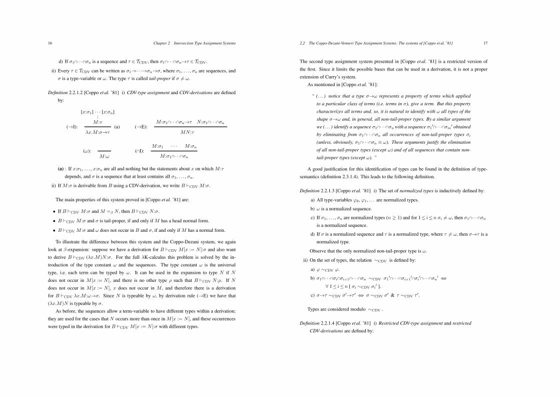
d) If *1!· · ·!*n is a sequence and + + TCDV, then *1!· · ·!*n$+ + TCDV.
ii) Every + + TCDV can be written as *1$· · ·$*n$*, where *1, . . . , *n are sequences, and
* is a type-variable or !. The type + is called tail-proper if * ,= !.
Definition 2.2.1.2 [Coppo et al. ’81] i) CDV-type assignment and CDV-derivations are defined
by:
[x:*1] · · · [x:*n]:
M :+($I): (a)
"x.M :*$+
M :*1!· · ·!*n$+ N :*1!· · ·!*n($E):
MN :+
(!):M :!
M :*1 · · · M :*n(!I):
M :*1!· · ·!*n
(a) : If x:*1, . . . , x:*n are all and nothing but the statements about x on which M :+
depends, and * is a sequence that at least contains all *1, . . . , *n.
ii) If M :* is derivable from B using a CDV-derivation, we write B !CDV M :*.
The main properties of this system proved in [Coppo et al. ’81] are:
• If B !CDV M :* and M =" N , then B !CDV N :*.
• B !CDV M :* and * is tail-proper, if and only if M has a head normal form.
• B !CDV M :* and ! does not occur in B and *, if and only if M has a normal form.
To illustrate the difference between this system and the Coppo-Dezani system, we again
look at %-expansion: suppose we have a derivation for B !CDV M [x := N ]:* and also want
to derive B !CDV ("x.M)N :*. For the full "K-calculus this problem is solved by the in-
troduction of the type constant ! and the sequences. The type constant ! is the universal
type, i.e. each term can be typed by !. It can be used in the expansion to type N if N
does not occur in M [x := N ], and there is no other type ) such that B !CDV N :). If N
does not occur in M [x := N ], x does not occur in M , and therefore there is a derivation
for B !CDV "x.M :!$*. Since N is typeable by !, by derivation rule ($E) we have that
("x.M)N is typeable by *.
As before, the sequences allow a term-variable to have different types within a derivation;
they are used for the cases that N occurs more than once in M [x := N ], and these occurrences
were typed in the derivation for B !CDV M [x := N ]:* with different types.
2.2 The Coppo-Dezani-Venneri Type Assignment Systems: The systems of [Coppo et al. ’81] 17
The second type assignment system presented in [Coppo et al. ’81] is a restricted version of
the first. Since it limits the possible bases that can be used in a derivation, it is not a proper
extension of Curry’s system.
As mentioned in [Coppo et al. ’81]:
“ (. . . ) notice that a type *$! represents a property of terms which applied
to a particular class of terms (i.e. terms in *), give a term. But this property
characterizes all terms and, so, it is natural to identify with ! all types of the
shape *$! and, in general, all non-tail-proper types. By a similar argument
we (. . . ) identify a sequence *1!· · ·!*n with a sequence *1"!· · ·!*m" obtained
by eliminating from *1!· · ·!*n all occurrences of non-tail-proper types *i
(unless, obviously, *1!· · ·!*n 4 !). These arguments justify the elimination
of all non-tail-proper types (except !) and of all sequences that contain non-
tail-proper types (except !). ”
A good justification for this identification of types can be found in the definition of type-
semantics (definition 2.3.1.4). This leads to the following definition.
Definition 2.2.1.3 [Coppo et al. ’81] i) The set of normalized types is inductively defined by:
a) All type-variables #0, #1, . . . are normalized types.
b) ! is a normalized sequence.
c) If *1, . . . , *n are normalized types (n 1 1) and for 1( i(n *i ,= !, then *1!· · ·!*n
is a normalized sequence.
d) If * is a normalized sequence and + is a normalized type, where + ,= !, then *$+ is a
normalized type.
Observe that the only normalized non-tail-proper type is !.
ii) On the set of types, the relation )CDV is defined by:
a) # )CDV #.
b) *1!· · ·!*i!*i+1!· · ·!*n )CDV *1"!· · ·!*i+1
"!*i"!· · ·!*n" 23
' 1( i(n [ *i )CDV *i" ].
c) *$+ )CDV *"$+ " 23 * )CDV *" & + )CDV + ".
Types are considered modulo )CDV .
Definition 2.2.1.4 [Coppo et al. ’81] i) Restricted CDV-type assignment and restricted
CDV-derivations are defined by:
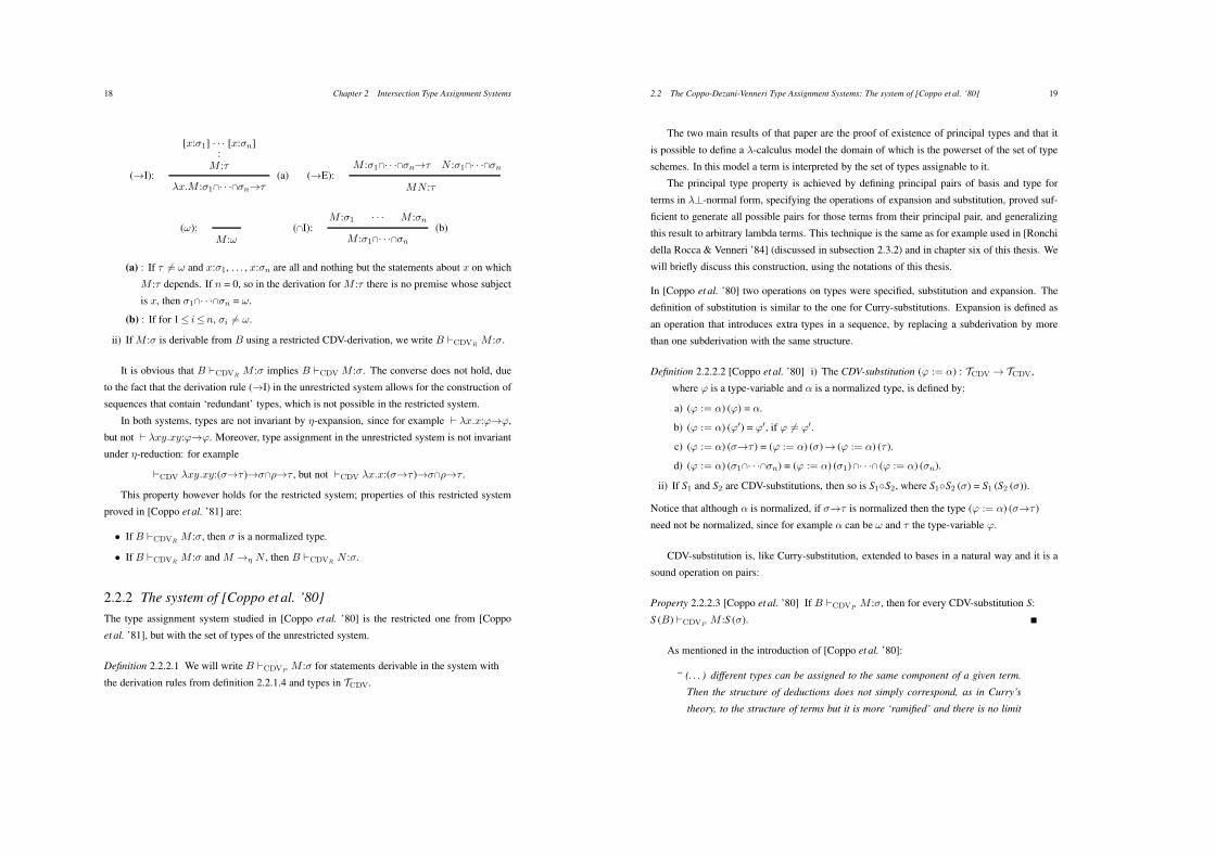
18 Chapter 2 Intersection Type Assignment Systems
[x:*1] · · · [x:*n]:
M :+($I): (a)
"x.M :*1!· · ·!*n$+
M :*1!· · ·!*n$+ N :*1!· · ·!*n($E):
MN :+
(!):M :!
M :*1 · · · M :*n(!I): (b)
M :*1!· · ·!*n
(a) : If + ,= ! and x:*1, . . . , x:*n are all and nothing but the statements about x on which
M :+ depends. If n = 0, so in the derivation for M :+ there is no premise whose subject
is x, then *1!· · ·!*n = !.
(b) : If for 1( i(n, *i ,= !.
ii) If M :* is derivable from B using a restricted CDV-derivation, we write B !CDVRM :*.
It is obvious that B !CDVRM :* implies B !CDV M :*. The converse does not hold, due
to the fact that the derivation rule ($I) in the unrestricted system allows for the construction of
sequences that contain ‘redundant’ types, which is not possible in the restricted system.
In both systems, types are not invariant by (-expansion, since for example ! "x.x:#$#,
but not ! "xy.xy:#$#. Moreover, type assignment in the unrestricted system is not invariant
under (-reduction: for example
!CDV "xy.xy:(*$+ )$*!)$+ , but not !CDV "x.x:(*$+ )$*!)$+ .
This property however holds for the restricted system; properties of this restricted system
proved in [Coppo et al. ’81] are:
• If B !CDVRM :*, then * is a normalized type.
• If B !CDVRM :* and M $# N , then B !CDVR
N :*.
2.2.2 The system of [Coppo et al. ’80]
The type assignment system studied in [Coppo et al. ’80] is the restricted one from [Coppo
et al. ’81], but with the set of types of the unrestricted system.
Definition 2.2.2.1 We will write B !CDVPM :* for statements derivable in the system with
the derivation rules from definition 2.2.1.4 and types in TCDV.
2.2 The Coppo-Dezani-Venneri Type Assignment Systems: The system of [Coppo et al. ’80] 19
The two main results of that paper are the proof of existence of principal types and that it
is possible to define a "-calculus model the domain of which is the powerset of the set of type
schemes. In this model a term is interpreted by the set of types assignable to it.
The principal type property is achieved by defining principal pairs of basis and type for
terms in "#-normal form, specifying the operations of expansion and substitution, proved suf-
ficient to generate all possible pairs for those terms from their principal pair, and generalizing
this result to arbitrary lambda terms. This technique is the same as for example used in [Ronchi
della Rocca & Venneri ’84] (discussed in subsection 2.3.2) and in chapter six of this thesis. We
will briefly discuss this construction, using the notations of this thesis.
In [Coppo et al. ’80] two operations on types were specified, substitution and expansion. The
definition of substitution is similar to the one for Curry-substitutions. Expansion is defined as
an operation that introduces extra types in a sequence, by replacing a subderivation by more
than one subderivation with the same structure.
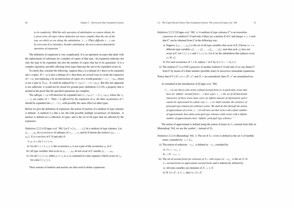
Definition 2.2.2.2 [Coppo et al. ’80] i) The CDV-substitution (# := $) : TCDV $ TCDV,
where # is a type-variable and $ is a normalized type, is defined by:
a) (# := $) (#) = $.
b) (# := $) (#") = #", if # ,= #".
c) (# := $) (*$+ ) = (# := $) (*)$ (# := $) (+ ).
d) (# := $) (*1!· · ·!*n) = (# := $) (*1)!· · ·! (# := $) (*n).
ii) If S1 and S2 are CDV-substitutions, then so is S1-S2, where S1-S2 (*) = S1 (S2 (*)).
Notice that although $ is normalized, if *$+ is normalized then the type (# := $) (*$+ )
need not be normalized, since for example $ can be ! and + the type-variable #.
CDV-substitution is, like Curry-substitution, extended to bases in a natural way and it is a
sound operation on pairs:
Property 2.2.2.3 [Coppo et al. ’80] If B !CDVPM :*, then for every CDV-substitution S:
S (B) !CDVPM :S (*).
As mentioned in the introduction of [Coppo et al. ’80]:
“ (. . . ) different types can be assigned to the same component of a given term.
Then the structure of deductions does not simply correspond, as in Curry’s
theory, to the structure of terms but it is more ‘ramified’ and there is no limit
20 Chapter 2 Intersection Type Assignment Systems
to its complexity. With the only operation of substitution we cannot obtain, for
a given term, all types whose deduction are more complex than the one of the
type on which we are doing the substitution. (. . . ) (This) difficulty (. . . ) can
be overcome if we introduce, besides substitution, the new (context-dependent)
operation of expansion. ”
The definition of expansion is very complicated. It is an operation on types that deals with
the replacement of (sub)types by a number of copies of that type. An expansion indicates not
only the type to be expanded, but also the number of copies that has to be generated. It is a
complex operation, possibly affecting more types than just the one to be expanded occurs in.
To clarify this, consider the following: suppose that µ is a subtype of * that is to be expanded
into n copies. If +$µ is also a subtype of *, then there are several ways to create the expansion
of +$µ: just replacing µ by an intersection of copies of µ would generate +$1!· · ·!µn, which
is not a type in TCDV. It could be replaced by (+$µ1) !· · ·! (+$µn). But this last approach
is not sufficient: it would not be closed for ground pairs (definition 2.2.2.8), a property that is
needed in the proof that the specified operations are complete.
The subtype +$µ will therefore be expanded into (+ 1$µ1)!· · ·! (+n$µn), where the +1,
. . . , +n are copies of + . Then + is affected by the expansion of µ; all other occurrences of +
should be expanded into 1!· · ·!+n, with possibly the same effect on other types.
Before we give the definition of expansion, the notion of nucleus of a multiset of type schemes
is defined. A multiset is a like a set, but with possibly multiple occurrences of elements. A
nucleus is defined on a collection of types, and is the set of all types that are affected by the
expansion.
Definition 2.2.2.4 [Coppo et al. ’80] Let C = {+1, . . . , +n} be a multiset of type schemes. Let
)1, . . . , )m be occurrences of subtypes of +1, . . . , +n and let E denote the multiset {)1, . . . ,
)m}. E is a nucleus of C if and only if:
i) )i ,= ! for 1( i(m.
ii) for all 1 ( i ,= j ( m the occurrence )i is not a part of the occurrence )j in C.
iii) all type-variables that occur in )1, . . . , )m do not occur in C outside )1, . . . , )m.
iv) for all 1( i(m, either )i 4 +j or )i is contained in some sequence which occurs in +j ,
for some 1( j(n.
These notions of multiset and nucleus are then used to define expansions.
2.2 The Coppo-Dezani-Venneri Type Assignment Systems: The system of [Coppo et al. ’80] 21
Definition 2.2.2.5 [Coppo et al. ’80] i) A multiset of type schemes C" is an immediate
expansion of a multiset C if and only if there are a nucleus E of C and integer n 1 1 such
that C" can be obtained from C in the following way:
a) Suppose {#1, . . . , #m} is the set of all type-variables that occur in E. Choose m. n
different type-variables #11, . . . , #n
1 , . . . , #1m, . . . , #n
m, such that each #ij does not
occur in C, for 1( i(n and 1( j(m. Let Si be the substitution that replaces every
#j by #ij .
b) For each occurrence of + + E, replace + in C by S1 (+ )!· · ·! Sn (+ ).
ii) The multiset C" is a CDV-expansion of another multiset C if and only if we can obtain C"
from C by means of a finite number (possible none) of successive immediate expansions.
Notice that if C (%B, *&) = %B", *"& and B, * are normalized, then B", *" are normalized too.
As remarked in the introduction of [Coppo et al. ’80]:
“ (. . . ) in our theory also terms without normal form or, in particular, terms that
have an ‘infinite’ normal form (. . . ) have types. (. . . ) the set of all functional
characters of these terms must carry an infinite amount of information and it
cannot be represented in a finite way. (. . . ) we shall consider the existence of
principal type schemes for arbitrary terms. We shall do this through the notion
of approximant of a term. (. . . ) It will turn out that terms with a finite number
of approximants have finite principal type schemes while terms with a infinite
number of approximants have ‘infinite’ principal type schemes. ”
The notion of approximant is defined using the notion of terms in "#-normal form (like in
[Barendregt ’84], we use the symbol # instead of ").
Definition 2.2.2.6 [Barendregt ’84] i) The set of !#-terms is defined as the set ! of lambda
terms, extended by: #+!#.
ii) The notion of reduction $"# is defined as $" , extended by:
a) "x.#$"# #.
b) #M $"# #.
iii) The set of normal forms for elements of !# with respect to $"# is the set N of
"#-normal forms or approximate normal forms and is inductively defined by:
a) All term-variables are elements of N , #+N .
b) If A +N , A ,= #, then "x.A +N .
22 Chapter 2 Intersection Type Assignment Systems
c) If A1, . . . , An +N , then xA1 . . . An +N .
iv) A+N is a direct approximant of M +!, if A matches M except for occurrences of #.
v) A+N is an approximant of M +! (notation: A 5 M ) if there is an M " =" M such that
A is a direct approximant of M ".
vi) A(M) = {A + N | A 5 M}.
The type assignment rules are generalized by allowing for the terms to be elements of !#.
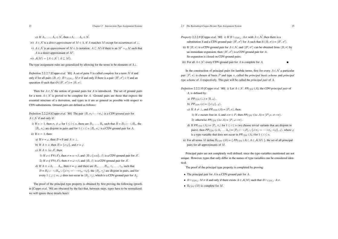
Definition 2.2.2.7 [Coppo et al. ’80] A set of pairs V is called complete for a term M if and
only if for all pairs %B, *&: B !CDVPM :* if and only if there is a pair %B", *"& + V and an
operation O such that O (%B", *"&) = %B, *&.
Then for A +N the notion of ground pairs for A is introduced. The set of ground pairs
for a term A+N is proved to be complete for A. Ground pairs are those that express the
essential structure of a derivation, and types in it are as general as possible with respect to
CDV-substitutions. Ground pairs are defined as follows:
Definition 2.2.2.8 [Coppo et al. ’80] The pair %B, *1!· · ·!*n& is a CDV-ground pair for
A+N if and only if:
i) If n > 1, then *i ,= ! for 1( i(n, there are B1, . . . , Bn such that B = B1/· · ·/Bn, the
%Bi, *i& are disjoint in pairs and for 1( i(n %Bi, *i& is a CDV-ground pair for A.
ii) If n = 1, then:
a) If * = !, then B = 0 and A 4 #.
b) If A 4 x, then B = {x:#}, and * = #.
c) If A 4 "x.A", then:
1) If x+ FV(A"), then * = $$%, and %B /{x:$}, %& is a CDV-ground pair for A".
2) If x ,+ FV(A"), then * = !$%, and %B, %& is a CDV-ground pair for A".
d) If A 4 xA1 . . . Am, then * = #, and there are B1, . . . , Bm, +1, . . . , +m such that
B = B1/· · ·/Bm/{x:+1$· · ·$+m$#}, the %Bj , +j& are disjoint in pairs, and for
every 1( j(m, # does not occur in %Bj , +j&, which is a CDV-ground pair for Aj .
The proof of the principal type property is obtained by first proving the following (proofs
in [Coppo et al. ’80] are obscured by the fact that, between steps, types have to be normalized;
we will ignore these details here):
2.3 The Barendregt-Coppo-Dezani Type Assignment System 23
Property 2.2.2.9 [Coppo et al. ’80] i) If B !CDVPA:* with A +N , then there is a
substitution S and a CDV-ground pair %B", *"& for A such that S (%B, *&) = %B", *"&.
ii) If %B, *& is a CDV-ground pair for A+N , and %B", *"& can be obtained from %B, *& by
an immediate expansion, then %B", *"& is a CDV-ground pair for A.
So expansion is closed on CDV-ground pairs.
iii) For all A+N : every CDV-ground pair for A is complete for A.
In the construction of principal pairs for lambda terms, first for every A+N a particular
pair %P , ,& is chosen of basis P and type ,, called the principal basis scheme and principal
type scheme of A respectively. This pair will be called the principal pair of A.
Definition 2.2.2.10 [Coppo et al. ’80] i) Let A +N . PPCDV (A), the CDV-principal pair of
A, is defined by:
a) PPCDV (#) = %0, !&.
b) PPCDV (x) = %{x:#}, #&.
c) If A ,= #, and PPCDV (A) = %P , ,&, then:
1) If x occurs free in A, and x:* + P , then PPCDV ("x.A) = %P\x, *$,&.
2) otherwise PPCDV ("x.A) = %P , !$,&.
d) If PPCDV (Ai) = %Pi, ,i& for 1( i(n (we choose trivial variants that are disjoint in
pairs), then PPCDV (xA1 . . . An) = %P1/· · ·/Pn /{x:,1$· · ·$,n$#}, #&, where #
is a type-variable that does not occur in PPCDV (Ai) for 1( i(n.
ii) For all terms M define #CDV (M ) = { PPCDV (A) | A+A(M) }, the set of all principal
pairs for all approximants of M .
Principal pairs are not completely well defined, since the type-variables mentioned are not
unique. However, types that only differ in the names of type-variables can be considered iden-
tical.
The proof of the principal type property is completed by proving:
• The principal pair for A is a CDV-ground pair for A.
• B !CDVPM :* if and only if there exists A+A(M) such that B !CDVP
A:*.
• #CDV (M ) is complete for M .
24 Chapter 2 Intersection Type Assignment Systems
2.3 The Barendregt-Coppo-Dezani Type Assignment SystemThe type assignment system presented in [Barendregt et al. ’83] by H. Barendregt, M. Coppo
and M. Dezani-Ciancaglini is based on the system as presented in [Coppo et al. ’81]. This
system was strengthened further by extending the set of types to TBCD and introducing a par-
tial order relation ‘(’ on types, as well as adding the type assignment rule ((), and a more
general form of the rules concerning intersection. The rule (() is mainly introduced to prove
completeness of type assignment.
In this paper, it was shown that the set of types derivable for a lambda term in the extended
system is a filter, i.e. a set closed under intersection and right-closed for ( (if * ( + and * + d
where d is a filter, then + + d.) The interpretation of a lambda term by the set of types derivable
for it – [[M ]]$ – is defined in the standard way, and gives a filter lambda model F . The main
result of that paper is that, using this model, completeness is proved by proving the statement:
!BCD M :* 23 [[M ]] + -(*), where - : TBCD $ F is a simple type interpretation as defined
in [Hindley ’83]. In order to prove the 2-part of this statement (completeness), the relation ( is
needed. Other interesting use of filter lambda models can be found in [Coppo et al. ’84], [Coppo
et al. ’87], [Dezani-Ciancaglini & Margaria ’84], and [Dezani-Ciancaglini & Margaria ’86].
In this subsection we give the definition of the Intersection Type Discipline as presented in
[Barendregt et al. ’83], together with its major features.
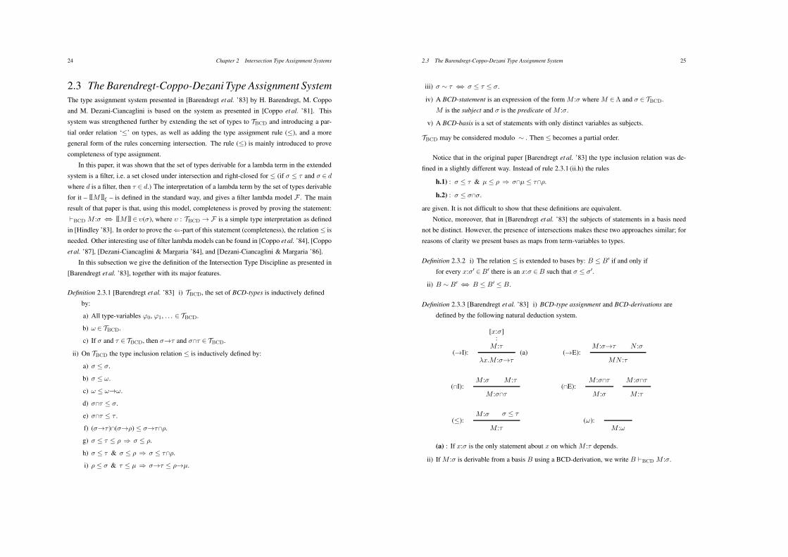
Definition 2.3.1 [Barendregt et al. ’83] i) TBCD, the set of BCD-types is inductively defined
by:
a) All type-variables #0, #1, . . . + TBCD.
b) ! + TBCD.
c) If * and + + TBCD, then *$+ and *!+ + TBCD.
ii) On TBCD the type inclusion relation ( is inductively defined by:
a) * ( *.
b) * ( !.
c) ! ( !$!.
d) *!+ ( *.
e) *!+ ( + .
f) (*$+ )!(*$)) ( *$+!).
g) * ( + ( ) 3 * ( ).
h) * ( + & * ( ) 3 * ( +!).
i) ) ( * & + ( µ 3 *$+ ( )$µ.
2.3 The Barendregt-Coppo-Dezani Type Assignment System 25
iii) * ) + 23 * ( + ( *.
iv) A BCD-statement is an expression of the form M :* where M +! and * + TBCD.
M is the subject and * is the predicate of M :*.
v) A BCD-basis is a set of statements with only distinct variables as subjects.
TBCD may be considered modulo ) . Then ( becomes a partial order.
Notice that in the original paper [Barendregt et al. ’83] the type inclusion relation was de-
fined in a slightly different way. Instead of rule 2.3.1 (ii.h) the rules
h.1) : * ( + & µ ( ) 3 *!µ ( +!).
h.2) : * ( *!*.
are given. It is not difficult to show that these definitions are equivalent.
Notice, moreover, that in [Barendregt et al. ’83] the subjects of statements in a basis need
not be distinct. However, the presence of intersections makes these two approaches similar; for
reasons of clarity we present bases as maps from term-variables to types.
Definition 2.3.2 i) The relation ( is extended to bases by: B ( B" if and only if
for every x:*" +B" there is an x:* +B such that * ( *".
ii) B ) B" 23 B ( B" ( B.
Definition 2.3.3 [Barendregt et al. ’83] i) BCD-type assignment and BCD-derivations are
defined by the following natural deduction system.
[x:*]:
M :+($I): (a)
"x.M :*$+
M :*$+ N :*($E):
MN :+
M :* M :+(!I):
M :*!+
M :*!+(!E):
M :*
M :*!+
M :+
M :* * ( +(():
M :+(!):
M :!
(a) : If x:* is the only statement about x on which M :+ depends.
ii) If M :* is derivable from a basis B using a BCD-derivation, we write B !BCD M :*.
26 Chapter 2 Intersection Type Assignment Systems
In the BCD-system there are several ways to deduce a desired result, due to the presence
of the derivation rules (!I), (!E) and ((), which allow superfluous steps in derivations. In
the CDV-system these rules are not present and there is a one-one relationship between terms
and skeletons of derivations. In other words: that system is syntax directed. The BCD-type
discipline has the same expressive power as the previous unrestricted CDV-system: all solvable
terms have types other than !, and a term has a normal form if and only if it has a type without
! occurrences.
• The set of normalizable terms can be characterized in the following way:
6 B, * [ B !BCD M :* & B, * !-free ] 23 M has a normal form.
• The set of terms having a head normal form can be characterized in the following way:
6 B, * [ B !BCD M :* & * ,= ! ] 23 M has a head normal form.
The following properties of the BCD-system, used in this thesis, are listed here so as to
refer to them easily:
Property 2.3.4 i) [Barendregt et al. ’83].2.8 (i): B !BCD MN :+ 3
6 * + TBCD [ B !BCD M :*$+ & B !BCD N :* ].
ii) [Barendregt et al. ’83].2.8 (iii): B !BCD "x.M :*$+ 23 B\x/{x:*} !BCD M :+ .
iii) [Barendregt et al. ’83].4.13 (i): 6 B, * [ B !BCD M :* & * ,= ! ] 23
M has a head normal form.
iv) [Barendregt et al. ’83].4.13 (ii): 6 B, * [ B !BCD M :* & B, * !-free ] 23
M has a normal form.
v) [Barendregt et al. ’83].2.7 (ii): B !BCD x:+ 3 6 x:* +B [ * ( + ].
vi) [Dezani-Ciancaglini & Margaria ’86].5.6: ) ( +1!· · ·!+n$* 3
) = (+11$· · ·$+ sn$*1)!· · ·!(+ s1$· · ·$+ sn$*s) !)", for some + j1 , . . . , + jn, *j , )" such that
+ ji 1 +i with 1( i(n, 1( j ( s and *1!· · ·!*s ( *.
2.3.1 Completeness of type assignment
The main result of [Barendregt et al. ’83] is the proof for completeness of type assignment.
This is achieved by showing that the set of types derivable for a lambda term is a filter, i.e. a
set closed under intersection and right closed for (. The construction of a filter lambda model
and the definition of a map from types to elements of this model (a simple type interpretation)
2.3 The Barendregt-Coppo-Dezani Type Assignment System: Completeness of type assignment 27
make the proof of completeness possible: if the interpretation of the term M is an element of
the interpretation of the type *, then M is typeable with *.
Filters and the filter "-model F are defined by:
Definition 2.3.1.1 [Barendregt et al. ’83] i) A BCD-filter is a subset d 7 TBCD such that:
a) ! + d.
b) *, + + d 3 *!+ + d.
c) * 1 + + d 3 * + d
ii) F = { d | d is a BCD-filter }.
iii) For d1, d2 +F define d1 ·d2 = { + + TBCD | 6 * + d2 [ *$+ + d1 ] }.
The following properties are proved in [Barendregt et al. ’83]:
• 'M +! [ { * | 6 B [ B !BCD M :* ] } +F ].
• Let . be a valuation of term-variables in F , and B$ = { x:* | * + . (x) }.
For M +! define [[M ]]$ = { * | B$ !BCD M :* }. Using the method of Hindley and
Longo [Hindley & Longo ’80] it is shown that %F , · , [[ ]]& is a "-model.
The following two definitions were absent [Barendregt et al. ’83]. They are presented here
so as to compare the construction of the completeness proof in [Barendregt et al. ’83] with that
of chapter four.
In constructing a complete system, the semantics of types play a crucial role. As in [Dezani-
Ciancaglini & Margaria ’86], [Mitchell ’88] and essentially following [Hindley ’82], a distinc-
tion can be made between several notions of type interpretations and semantic satisfiability.
There are, roughly, three notions of type semantics that differ in the meaning of an arrow type
scheme: inference type interpretations, simple type interpretations and F type interpretations.
These different notions of type interpretations induce of course different notions of semantic
satisfiability.
Following essentially [Mitchell ’88], we distinguish several kinds of type interpretations.
Definition 2.3.1.2 i) Let %D, · , /& be a continuous lambda model.
A mapping -: TBCD $ 0(D) = {X | X 7 D} is a type interpretation if and only if:
a) { / ·d | ' e [ e+ -(*) 3 d · e+ -(+ ) ] } 7 -(*$+ ).
b) -(*$+ ) 7 { d | ' e [ e+ -(*) 3 d · e+ -(+ ) ] }.
c) -(*!+ ) = -(*)8 -(+ ).
28 Chapter 2 Intersection Type Assignment Systems
ii) Following [Hindley ’83] we say that a type interpretation is simple if and only if:
-(*$+ ) = { d | ' e [ e + -(*) 3 d · e + -(+ ) ] }.
iii) On the other hand, a type interpretation is called an F type interpretation if it satisfies:
-(*$+ ) = { / ·d | ' e [ e + -(*) 3 d · e + -(+ ) ] }.
Notice that, in part (ii), the containment relation 7 of part (i.b) is replaced by =, and that in
part (iii) the same is done with regard to part (i.a).
These notions of type interpretation lead, naturally, to the following definitions for semantic
satisfiability (called inference-, simple- and F-semantics, respectively).
Definition 2.3.1.3 i) Let M = %D, · , [[ ]]& be a "-model, and . a valuation.
Then [[M ]]M$ +D is the interpretation of M in M via ..
ii) We define !! by: (where M is a lambda model, . a valuation and - a type interpretation)
a) M, ., - !! M :* 23 [[M ]]M$ + -(*).
b) M, ., - !! B 23 M, ., - !! x:* for every x:* +B.
c) 1) B !!M :* 23 ' M, ., - [ M, ., - !! B 3 M, ., - !!M :* ].
2) B !!s M :* 23
'M, ., simple type interpretations - [ M, ., - !! B 3 M, ., - !! M :* ].
3) B !!F M :* 23
'M, ., F type interpretations - [ M, ., - !! B 3 M, ., - !!M :* ].
If no confusion is possible, we will omit the superscript on [[ ]].
The method followed in [Barendregt et al. ’83] is to define a simple type interpretation -
and to use it for the proof of completeness.
Definition 2.3.1.4 (cf. [Barendregt et al. ’83]) The type interpretation - : TBCD $ 0(F) is
defined as follows:
i) - (!) = F .
ii) - (#) = { d +F | #+ d }.
iii) - (*$+ ) = { d+F | ' e+ - (*) [ d · e+ - (+ ) ] }.
iv) - (*!+ ) = - (*)8 - (+ ).
Notice that because of part (iii), - is a simple type interpretation. For -, the following
properties are proved:
2.3 The Barendregt-Coppo-Dezani Type Assignment System: Principal type schemes 29
• For all types *: - (*) = { d+F | * + d }.
• If [[M ]]$B + - (*), then * + [[M ]]$B , where .B (x) = { * + TBCD | B !BCD x:* }.
The main result of [Barendregt et al. ’83] is obtained by proving, using the following prop-
erties:
Property 2.3.1.5 [Barendregt et al. ’83] i) Soundness. B !BCD M :* 3 B !!s M :*.
ii) Completeness. B !!s M :* 3 B !BCD M :*.
The proof of completeness is obtained in a way very similar to the one of theorem 4.4.5.
Since the type interpretation - is simple, the results of [Barendregt et al. ’83] in fact show that
type assignment in the BCD-system is complete with respect to simple type semantics.
2.3.2 Principal type schemes
For the system as defined in [Barendregt et al. ’83], principal type schemes can be defined as
done by S. Ronchi della Rocca and B. Venneri in [Ronchi della Rocca & Venneri ’84]. In
this paper, three operations are provided: substitution, expansion, and rise. These are sound
and sufficient to generate all suitable pairs for a term M from its principal pair. This result is
achieved in a way similar to that of [Coppo et al. ’80], as discussed in subsection 2.2.2. (Like
in the CDV-system the type assignment rules of the BCD-system are generalized by allowing
for the terms to be elements of !#.)
We will briefly discuss the construction of [Ronchi della Rocca & Venneri ’84]. In this
paper, all constructions and definitions are made modulo the equivalence relation ) .
The first operation defined is substitution; it is a natural extension of Curry-substitution and
CDV-substitution.
Definition 2.3.2.1 [Ronchi della Rocca & Venneri ’84] i) The RV-substitution (# := $) :
TBCD $ TBCD, where # is a type-variable and $ + TBCD, is defined by:
a) (# := $) (#) ) $.
b) (# := $) (#") ) #", if # ,= #".
c) (# := $) (*$+ ) ) (# := $) (*)$ (# := $) (+ ).
d) (# := $) (*1!· · ·!*n) ) (# := $) (*1) !· · ·! (# := $) (*n).
ii) If S1 and S2 are RV-substitutions, then so is S1-S2, where S1-S2 (*) = S1 (S2 (*)).
30 Chapter 2 Intersection Type Assignment Systems
Notice that a RV-substitution is defined without restriction: the type $ that is to be substituted
can be every element of TBCD.
Next, the operation of expansion is defined, which is a generalization of the CDV-expansion.
Definition 2.3.2.2 [Ronchi della Rocca & Venneri ’84] For every µ+ TBCD, n 1 2, the pair
%µ,n& determines an RV-expansion E$µ,n% that is constructed as follows:
i) Let Le(B, + ) be the set of type schemes defined as follows:
a) µ +Le(B, + ).
b) If * +Le(B, + ), any proper subtype of * belongs to Le(B, + ).
c) For each type scheme *, such that * is a subtype of either + or a predicate in B:
1) If either * ) $$% or * ) $$%!& and % +Le(B, + ), then * +Le(B, + ).
2) If * ) $!% and $, % +Le(B, + ), then * +Le(B, + ).
ii) Suppose Le(B, + ) is the list obtained by ordering the elements of Le(B, + ) in decreasing
order according to the number of symbols (if two type schemes have the same number of
symbols, their mutual order is unimportant).
iii) Let V = {#1, . . . , #m} be all the variables occurring in Le(B, + ). Choose m. n different
type-variables #11, . . . , #n
1 , . . . , #1m, . . . , #n
m, such that each #ij does not occur in %B, +&,
for 1( i(n and 1( j(m. Let Si be the substitution that replaces every #j by #ij .
iv) For every * + TBCD, E$µ,n% (*) is obtained from * by examining in order each element of
Le(B, + ), and each time an element $ is found that is a subtype of *, by replacing $, in
*, by S1 ($) !· · ·! Sn ($).
The set Le(B, + ) is the equivalent of the nucleus in definition 2.2.2.4.
Substitution and expansions are in the natural way extended to operations on bases and
pairs. The third operation defined is the operation of rise: it consists of adding applications of
the derivation rule (() to a derivation.
Definition 2.3.2.3 [Ronchi della Rocca & Venneri ’84] A rise R is an operation denoted by a
pair of pairs <<B0, +0&, %B1, +1>> such that +0 ( +1 and B1 ( B0, and is defined by:
i) a) R (*) ) +1, if * ) +0.
b) R (*) ) *, otherwise.
ii) a) R (B) ) B1, if B ) B0.
b) R (B) ) B, otherwise.
2.3 The Barendregt-Coppo-Dezani Type Assignment System: Principal type schemes 31
iii) R (%B, *&) ) %R (B), R (*)&.
The following property is proved; it shows that all defined operations are sound:
Property 2.3.2.4 [Ronchi della Rocca & Venneri ’84] Let A +N , %B, *& be such that
B !BCD A:*, and let O be an operation of substitution, expansion or rise.
Then O (B) !BCD A:O (*).
As in [Coppo et al. ’80], principal types are defined for terms in "#-normal form.
Definition 2.3.2.5 [Ronchi della Rocca & Venneri ’84] i) Let A+N . PPRV (A), the
RV-principal pair of A, is defined by:
a) PPRV (#) ) %0, !&.
b) PPRV (x) ) %{x:#}, #&.
c) If A ,= #, and PPRV (A) ) %P , ,&, then:
1) If x occurs free in A, and x:* + P , then PPRV ("x.A) ) %P\x, *$,&.
2) otherwise PPRV ("x.A) ) %P , !$,&.
d) If PPRV (Ai) ) %Pi, ,i& for 1( i(n (we choose trivial variants that are disjoint in
pairs), then PPRV (xA1 . . . An) ) %P1/· · ·/Pn/{x:,1$· · ·$,n$#}, #&, where #
is a type-variable that does not occur in PPRV (Ai) for 1( i(n.
ii) PRV = {%P , ,& | 6 A +N [ PPRV (A) ) %P , ,& ] }.
Notice that this definition is almost the same as definition 2.2.2.10 (apart from the notion of
sequence and the relation )).
Definition 2.3.2.6 (cf. [Ronchi della Rocca & Venneri ’84]) i) Linear chains of operations are
defined as sequences of operations that start with a number of expansions, followed by a
number of substitutions, and that end with one rise.
ii) Let M be a term. As in [Coppo et al. ’80] let #RV (M ) be the set of all RV-principal pairs
for all approximants of M : #RV (M ) = { PPRV (A) | A+A(M) }.
iii) On PRV is it possible to to define the preorder relation 5! by:
%P , ,& 5! %P ", ,"& 23
6 #1, . . . , #n [ %P , ,& = (#1 := !)-· · ·-(#n := !) (%P ", ,"&) ],
and PRV, 5! is a meet semilattice isomorphic to N , (.
iv) #RV (M ) is an ideal in PRV and therefore:
32 Chapter 2 Intersection Type Assignment Systems
a) If #RV (M ) is finite, there exists a pair %P , ,& =!#RV (M ), where %P , ,& +PRV.
This pair is then called the principal pair of M .
b) If #RV (M ) is infinite,!#RV (M ) does not exist in PRV.
The principal pair of M is then the infinite set of pairs #RV (M ).
In [Ronchi della Rocca & Venneri ’84], linear chains are defined as those sequences of
operations that start with a number of expansions, followed by a number of substitutions or
rises. Both are allowed. This definition is not complete: that the chain ends with one rise is
essential in the proof for completeness.
Property 2.3.2.7 B !BCD M :* if and only if there exists A+A(M) such that
B !BCD A:*.
The proof of the principal type property is completed by proving:
• Let A+N and %P , ,& be the RV-principal pair for A. For any pair %B, *& such that
B !BCD A:* there exists a linear chain C such that C (%P , ,&) = %B, *&.
• – A(M ) is finite. Let %P , ,& be the RV-principal pair of M . Then there exists a chain C
such that C (%P , ,&) = %B, *&.
– A(M ) is infinite. Then there exist a pair %P , ,& +#RV (M ) and a chain C such that
C (%P , ,&) = %B, *&.
Chapter 3 The Milner - and Mycroft Type
Assignment Systems
In this chapter we focus on some aspects of two type assignment systems that were defined for
a simple applicative language called Exp that is in fact an extended lambda calculus.
The first, defined by R. Milner, has become very famous and is implemented in a type
checker that is embedded in the functional programming language ML. The second one is a
generalization of Milner’s system presented by A. Mycroft, which is defined by allowing a
more permissive rule for recursion. Both systems are present in the implementation of the
functional programming language Miranda. Milner’s system is used when the Miranda type
assignment algorithm infers a type for an object; Mycroft’s system is used when the type as-
signment algorithm does type checking, i.e. when the programmer has specified a type for an
object. These two systems will play an important role in the third part of this thesis.
3.1 The Milner Type Assignment SystemIn [Milner ’78], a formal type discipline was presented for polymorphic procedures in a simple
programming language called Exp, designed to express that certain procedures work well on
objects of a wide variety. This kind of procedures is called (shallow) polymorphic, and they are
essential to obtain enough flexibility in programming. To illustrate the need for polymorphic
procedures, consider the following example.
Suppose we have a programming language in which we can write the following program:
I x = x
I I
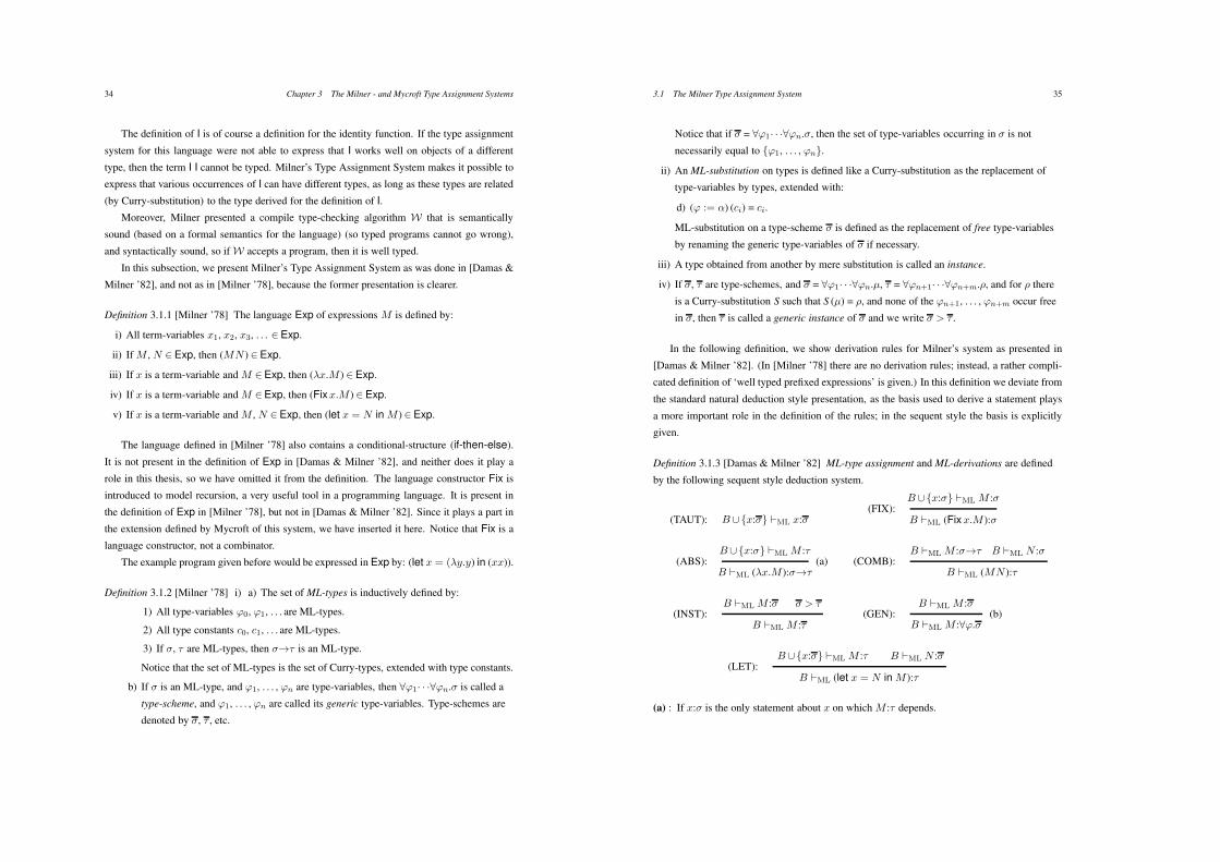
34 Chapter 3 The Milner - and Mycroft Type Assignment Systems
The definition of I is of course a definition for the identity function. If the type assignment
system for this language were not able to express that I works well on objects of a different
type, then the term I I cannot be typed. Milner’s Type Assignment System makes it possible to
express that various occurrences of I can have different types, as long as these types are related
(by Curry-substitution) to the type derived for the definition of I.
Moreover, Milner presented a compile type-checking algorithm W that is semantically
sound (based on a formal semantics for the language) (so typed programs cannot go wrong),
and syntactically sound, so if W accepts a program, then it is well typed.
In this subsection, we present Milner’s Type Assignment System as was done in [Damas &
Milner ’82], and not as in [Milner ’78], because the former presentation is clearer.
Definition 3.1.1 [Milner ’78] The language Exp of expressions M is defined by:
i) All term-variables x1, x2, x3, . . . + Exp.
ii) If M , N + Exp, then (MN ) + Exp.
iii) If x is a term-variable and M +Exp, then ("x.M ) + Exp.
iv) If x is a term-variable and M +Exp, then (Fixx.M ) + Exp.
v) If x is a term-variable and M , N + Exp, then (let x = N in M ) + Exp.
The language defined in [Milner ’78] also contains a conditional-structure (if-then-else).
It is not present in the definition of Exp in [Damas & Milner ’82], and neither does it play a
role in this thesis, so we have omitted it from the definition. The language constructor Fix is
introduced to model recursion, a very useful tool in a programming language. It is present in
the definition of Exp in [Milner ’78], but not in [Damas & Milner ’82]. Since it plays a part in
the extension defined by Mycroft of this system, we have inserted it here. Notice that Fix is a
language constructor, not a combinator.
The example program given before would be expressed in Exp by: (let x = ("y.y) in (xx)).
Definition 3.1.2 [Milner ’78] i) a) The set of ML-types is inductively defined by:
1) All type-variables #0, #1, . . . are ML-types.
2) All type constants c0, c1, . . . are ML-types.
3) If *, + are ML-types, then *$+ is an ML-type.
Notice that the set of ML-types is the set of Curry-types, extended with type constants.
b) If * is an ML-type, and #1, . . . , #n are type-variables, then '#1· · ·'#n.* is called a
type-scheme, and #1, . . . , #n are called its generic type-variables. Type-schemes are
denoted by *, + , etc.
3.1 The Milner Type Assignment System 35
Notice that if * = '#1· · ·'#n.*, then the set of type-variables occurring in * is not
necessarily equal to {#1, . . . , #n}.
ii) An ML-substitution on types is defined like a Curry-substitution as the replacement of
type-variables by types, extended with:
d) (# := $) (ci) = ci.
ML-substitution on a type-scheme * is defined as the replacement of free type-variables
by renaming the generic type-variables of * if necessary.
iii) A type obtained from another by mere substitution is called an instance.
iv) If *, + are type-schemes, and * = '#1· · ·'#n.µ, + = '#n+1· · ·'#n+m.), and for ) there
is a Curry-substitution S such that S (µ) = ), and none of the #n+1, . . . , #n+m occur free
in *, then + is called a generic instance of * and we write * > + .
In the following definition, we show derivation rules for Milner’s system as presented in
[Damas & Milner ’82]. (In [Milner ’78] there are no derivation rules; instead, a rather compli-
cated definition of ‘well typed prefixed expressions’ is given.) In this definition we deviate from
the standard natural deduction style presentation, as the basis used to derive a statement plays
a more important role in the definition of the rules; in the sequent style the basis is explicitly
given.
Definition 3.1.3 [Damas & Milner ’82] ML-type assignment and ML-derivations are defined
by the following sequent style deduction system.
(TAUT): B/ {x:*} !ML x:*
B/{x:*} !ML M :*(FIX):
B !ML (Fixx.M ):*
B/{x:*} !ML M :+(ABS): (a)
B !ML ("x.M ):*$+
B !ML M :*$+ B !ML N :*(COMB):
B !ML (MN ):+
B !ML M :* * > +(INST):
B !ML M :+
B !ML M :*(GEN): (b)
B !ML M :'#.*
B/{x:*} !ML M :+ B !ML N :*(LET):
B !ML (let x = N in M ):+
(a) : If x:* is the only statement about x on which M :+ depends.
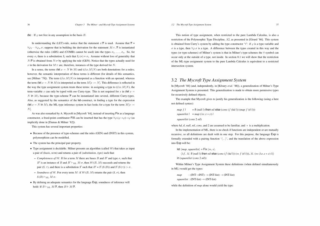
36 Chapter 3 The Milner - and Mycroft Type Assignment Systems
(b) : If # not free in any assumption in the basis B.
In understanding the (LET)-rule, notice that the statement x:* is used. Assume that * =
'#1· · ·'#n.*; suppose that in building the derivation for the statement M :+ , * is instantiated
(otherwise the rules (ABS) and (COMB) cannot be used) into the types *1, . . . , *n. So, for
every *i there is a substitution Si such that Si (*) = *i. Assume without loss of generality that
N :* is obtained from N :* by applying the rule (GEN). Notice that the types actually used for
x in the derivation for M :+ are, therefore, instances of the type derived for N .
In a sense, the terms (let x = N in M ) and (("x.M)N ) are both denotations for a redex;
however, the semantic interpretation of these terms is different (for details of this semantics,
see [Milner ’78]). The term (("x.M)N ) is interpreted as a function with an operand, whereas
the term (let x = N in M ) is interpreted as the term M [x := N ]. This difference is reflected in
the way the type assignment system treats these terms: in assigning a type to (("x.M)N ), the
term-variable x can only be typed with one Curry-type. This is not required for x in (let x =
N in M ), because the type-scheme * can be instantiated into several, different Curry-types.
Also, as suggested by the semantics of the let-construct, in finding a type for the expression
(let x = N in M ), the ML-type inference system in fact looks for a type for the term M [x :=
N ].
As was also remarked by A. Mycroft in [Mycroft ’84], instead of inserting Fix as a language
constructor, a fixed-point combinator FIX can be inserted that has the type '#.(#$#)$# (as
implicitly done in [Damas & Milner ’82]).
This system has several important properties:
• Because of the presence of type-schemes and the rules (GEN) and (INST) in this system,
polymorphism can be modelled.
• The system has the principal pair property.
• Type assignment is decidable. Milner presents an algorithm (called W) that takes as input
a pair of (basis, term) and returns a pair of (substitution, type) such that:
– Completeness of W . If for a term M there are bases B and B" and type *, such that
B" is an instance of B and B" !ML M :*, then W (B, M ) succeeds and returns the
pair (S, + ), and there is a substitution S" such that B" = S" (S (B)) and S" (S (+ )) > *.
– Soundness of W . For every term M : if W (B, M ) returns the pair (S, *), then
S (B) !ML M :*.
• By defining an adequate semantics for the language Exp, soundness of inference will
hold: If B !ML M :*, then B !!M :*.
3.2 The Mycroft Type Assignment System 37
This notion of type assignment, when restricted to the pure Lambda Calculus, is also a
restriction of the Polymorphic Type Discipline, !2, as presented in [Girard ’86]. This system
is obtained from Curry’s system by adding the type constructor ‘'’: if # is a type-variable and
* is a type, then '#.* is a type. A difference between the types created in this way and the
types (or type-schemes) of Milner’s system is that in Milner’s type-schemes the '-symbol can
occur only at the outside of a type, not inside. In section 8.1 we will show that the restriction
of the ML-type assignment system to the pure Lambda Calculus is equivalent to a restricted
intersection system.
3.2 The Mycroft Type Assignment SystemIn [Mycroft ’84] (and, independently, in [Kfoury et al. ’88]), a generalization of Milner’s Type
Assignment System is presented. This generalization is made to obtain more permissive types
for recursively defined objects.
The example that Mycroft gives to justify his generalization is the following (using a here
not defined syntax):
map f l = if (null l) then nil else (cons (f (hd l)) (map f (tl l)))
squarelist l = map ("x.x * x) l
squarelist (cons 2 nil)
where hd, tl, null, nil, cons, and 2 are assumed to be familiar, and * is a multiplication.
In the implementation of ML, there is no check if functions are independent or are mutually
recursive, so all definitions are dealt with in one step. For this purpose, the language Exp is
formally extended with a pairing function ‘% , &’, and the translation of the above expression
into Exp will be:
let %map, squarelist& = Fix %m, s&.
%"f . "l. if (null l) then nil else (cons (f (hd l)) (m f (tl l))), "l. (m ("x.x * x) l)&
in (squarelist (cons 2 nil))
Within Milner’s Type Assignment System these definitions (when defined simultaneously
in ML) would get the types:
map : (INT$INT) $ (INT-list) $ (INT-list)
squarelist : (INT-list) $ (INT-list)
while the definition of map alone would yield the type:
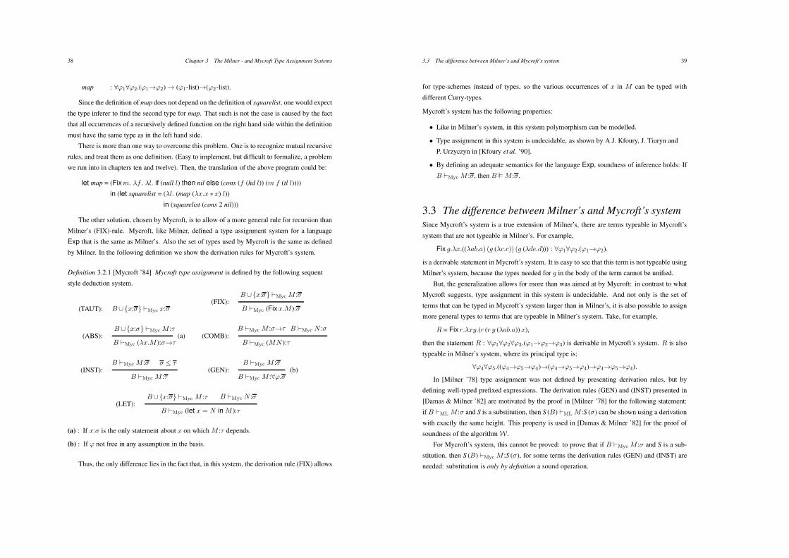
38 Chapter 3 The Milner - and Mycroft Type Assignment Systems
map : '#1'#2.(#1$#2) $ (#1-list)$(#2-list).
Since the definition of map does not depend on the definition of squarelist, one would expect
the type inferer to find the second type for map. That such is not the case is caused by the fact
that all occurrences of a recursively defined function on the right hand side within the definition
must have the same type as in the left hand side.
There is more than one way to overcome this problem. One is to recognize mutual recursive
rules, and treat them as one definition. (Easy to implement, but difficult to formalize, a problem
we run into in chapters ten and twelve). Then, the translation of the above program could be:
let map = (Fixm. "f . "l. if (null l) then nil else (cons (f (hd l)) (m f (tl l))))
in (let squarelist = ("l. (map ("x.x * x) l))
in (squarelist (cons 2 nil)))
The other solution, chosen by Mycroft, is to allow of a more general rule for recursion than
Milner’s (FIX)-rule. Mycroft, like Milner, defined a type assignment system for a language
Exp that is the same as Milner’s. Also the set of types used by Mycroft is the same as defined
by Milner. In the following definition we show the derivation rules for Mycroft’s system.
Definition 3.2.1 [Mycroft ’84] Mycroft type assignment is defined by the following sequent
style deduction system.
(TAUT): B/ {x:*} !Myc x:*
B/ {x:*} !Myc M :*(FIX):
B !Myc (Fixx.M ):*
B/ {x:*} !Myc M :+(ABS): (a)
B !Myc ("x.M ):*$+
B !Myc M :*$+ B !Myc N :*(COMB):
B !Myc (MN ):+
B !Myc M :* * ( +(INST):
B !Myc M :+
B !Myc M :*(GEN): (b)
B !Myc M :'#.*
B/{x:*} !Myc M :+ B !Myc N :*(LET):
B !Myc (let x = N in M ):+
(a) : If x:* is the only statement about x on which M :+ depends.
(b) : If # not free in any assumption in the basis.
Thus, the only difference lies in the fact that, in this system, the derivation rule (FIX) allows
3.3 The difference between Milner’s and Mycroft’s system 39
for type-schemes instead of types, so the various occurrences of x in M can be typed with
different Curry-types.
Mycroft’s system has the following properties:
• Like in Milner’s system, in this system polymorphism can be modelled.
• Type assignment in this system is undecidable, as shown by A.J. Kfoury, J. Tiuryn and
P. Urzyczyn in [Kfoury et al. ’90].
• By defining an adequate semantics for the language Exp, soundness of inference holds: If
B !Myc M :*, then B !! M :*.
3.3 The difference between Milner’s and Mycroft’s systemSince Mycroft’s system is a true extension of Milner’s, there are terms typeable in Mycroft’s
system that are not typeable in Milner’s. For example,
Fix g."x.(("ab.a) (g ("c.c)) (g ("de.d))) : '#1'#2.(#1$#2).
is a derivable statement in Mycroft’s system. It is easy to see that this term is not typeable using
Milner’s system, because the types needed for g in the body of the term cannot be unified.
But, the generalization allows for more than was aimed at by Mycroft: in contrast to what
Mycroft suggests, type assignment in this system is undecidable. And not only is the set of
terms that can be typed in Mycroft’s system larger than in Milner’s, it is also possible to assign
more general types to terms that are typeable in Milner’s system. Take, for example,
R = Fix r."xy.(r (r y ("ab.a)) x),
then the statement R : '#1'#2'#3.(#1$#2$#3) is derivable in Mycroft’s system. R is also
typeable in Milner’s system, where its principal type is:
'#4'#5.((#4$#5$#4)$(#4$#5$#4)$#4$#5$#4).
In [Milner ’78] type assignment was not defined by presenting derivation rules, but by
defining well-typed prefixed expressions. The derivation rules (GEN) and (INST) presented in
[Damas & Milner ’82] are motivated by the proof in [Milner ’78] for the following statement:
if B !ML M :* and S is a substitution, then S (B) !ML M :S (*) can be shown using a derivation
with exactly the same height. This property is used in [Damas & Milner ’82] for the proof of
soundness of the algorithm W .
For Mycroft’s system, this cannot be proved: to prove that if B !Myc M :* and S is a sub-
stitution, then S (B) !Myc M :S (*), for some terms the derivation rules (GEN) and (INST) are
needed: substitution is only by definition a sound operation.
40 Chapter 3 The Milner - and Mycroft Type Assignment Systems
For example, to show in Milner’s system that any substitution instance of the type
$ = (#4$#5$#4)$(#4$#5$#4)$#4$#5$#4
is a correct type for R, it is sufficient to take the derivation for
{r:$} !ML "xy.(r (r y ("ab.a)) x) : $,
just substitute the types in this derivation, and apply the (FIX)-derivation rule.
For Mycroft’s system this construction does not yield correct derivations. If the derivation
for the statement
{r : '#1'#2'#3.(#1$#2$#3)} !Myc "xy.(r (r y ("ab.a)) x) : #1$#2$#3
were taken and, for example, the type-variable #2 were replaced by #1, then the (FIX)-derivation
rule cannot be applied because the type in the conclusion of the derivation is affected by
the substitution, but the type '#1'#2'#3.(#1$#2$#3) in the basis is not. The only way
to obtain !Myc R : #1$#1$#3 is by using the derivation rule (INST) on the derivation for
!Myc R : '#1'#2'#3.(#1$#2$#3).
Chapter 4 The Strict Type Assignment System
In this chapter we present the Strict Type Assignment System, a restricted version of the BCD-
system. Compared to the BCD-system, the major feature of this restricted system is the absence
of the derivation rule ((). It is based on a set of strict types, which correspond to the normalized
types of the CDV-system. We will show that these two together give rise to a strict filter lambda
model that is essentially different from F . We will show that the Strict Type Assignment System
is the nucleus of the BCD-system, i.e. for every derivation in the BCD-type discipline there is
a derivation in which (() is used only at the very end. Finally we will prove that strict type
assignment is complete for inference semantics.
4.1 Strict type assignmentIn this section we will present the Strict Type Assignment System, together with the set of strict
types. These two together will yield a lambda model FS, with which we prove completeness of
type assignment without the derivation rule (().
The elimination of ( induces a set of strict types, a restriction of the set of types used in the
BCD-system. Strict types are the types that are strictly needed to assign a type to a term in the
BCD-system. The set of strict types is a true subset of set TBCD; intersection type schemes and
the type constant ! play a limited role in the Strict Type Assignment System. We will assume
that ! is the same as an intersection over zero elements: if n = 0, then *1!· · ·!*n = !, so
! does not occur in an intersection subtype. Moreover, intersection type schemes (so also !)
occur in strict types only as subtypes at the left hand side of an arrow type scheme. We could
have omitted the type constant ! completely from the presentation of the system, because we
can always assume that n = 0 in *1!· · ·!*n, but some of the definitions and the results we
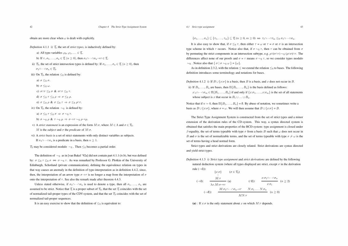
42 Chapter 4 The Strict Type Assignment System
obtain are more clear when ! is dealt with explicitly.
Definition 4.1.1 i) Ts, the set of strict types, is inductively defined by:
a) All type-variables #0, #1, . . . + Ts.
b) If + , *1, . . . , *n + Ts (n 1 0), then *1!· · ·!*n$+ + Ts.
ii) TS, the set of strict intersection types is defined by: If *1, . . . , *n + Ts (n 1 0), then
*1!· · ·!*n + TS.
iii) On TS, the relation (S is defined by:
a) * (S *.
b) * (S !.
c) *!+ (S * & *!+ (S + .
d) * (S + (S ) 3 * (S ).
e) * (S ) & * (S + 3 * (S )!+ .
iv) On TS, the relation )S is defined by:
a) * (S + (S * 3 * )S + .
b) * )S ) & + )S µ 3 *$+ )S )$µ.
v) A strict statement is an expression of the form M :*, where M +! and * + TS.
M is the subject and * the predicate of M :*.
vi) A strict basis is a set of strict statements with only distinct variables as subjects.
If *1!· · ·!*n is a predicate in a basis, then n 1 1.
TS may be considered modulo )S . Then (S becomes a partial order.
The definition of )S as in [van Bakel ’92a] did not contain part 4.1.1 (iv.b), but was defined
by: * (S + (S * 23 * )S + . As was remarked by Professor G. Plotkin of the University of
Edinburgh, Schotland (private communication), defining the equivalence relation on types in
that way causes an anomaly in the definition of type-interpretation as in definition 4.4.2, since,
then, the interpretation of an arrow type *$+ is no longer a map from the interpretation of *
onto the interpretation of + . See also the remark made after theorem 4.4.3.
Unless stated otherwise, if *1!· · ·!*n is used to denote a type, then all *1, . . . , *n are
assumed to be strict. Notice that Ts is a proper subset of TS, that the set Ts coincides with the set
of normalized tail-proper types of the CDV-system, and that the set TS coincides with the set of
normalized tail-proper sequences.
It is an easy exercise to show that the definition of (S is equivalent to:
4.1 Strict type assignment 43
{*1, . . . , *n} 7 {+1, . . . , +m} 7 Ts (n 1 0, m 1 0) 23 +1!· · ·!+m (S *1!· · ·!*n.
It is also easy to show that, if * (S + , then either + = ! or + = * or * is an intersection
type scheme in which + occurs. Notice also that, if * )S + , then + can be obtained from *
by permuting the strict components in an intersection subtype, e.g. )!(*!+ ) )S ()!*)!+ . The
differences affect none of our proofs and * = + means * )S + , so we consider types modulo
)S . Notice also that { * | * )S ! } = {!}.
As in definition 2.3.2, with the relation ( we extend the relation (S to bases. The following
definition introduces some terminology and notations for bases.
Definition 4.1.2 i) If B/{x:*} is a basis, then B is a basis, and x does not occur in B.
ii) If B1, . . . , Bn are bases, then #{B1, . . . , Bn} is the basis defined as follows:
x:1!· · ·!*m +#{B1, . . . , Bn} if and only if {x:*1, . . . , x:*m} is the set of all statements
whose subject is x that occur in B1/ . . . /Bn.
Notice that if n = 0, then #{B1, . . . , Bn} = 0. By abuse of notation, we sometimes write a
basis as B/{x:*}, where * = !. We will then assume that B/ {x:*} = B.
The Strict Type Assignment System is constructed from the set of strict types and a minor
extension of the derivation rules of the CD-system. This way, a syntax directed system is
obtained that satisfies the main properties of the BCD-system: type assignment is closed under
%-equality, the set of terms typeable with type * from a basis B such that ! does not occur in
B and * is the set of normalizable terms, and the set of terms typeable with type * ,= ! is the
set of terms having a head normal form.
Strict types and strict derivations are closely related. Strict derivations are syntax directed
and yield strict types.
Definition 4.1.3 i) Strict type assignment and strict derivations are defined by the following
natural deduction system (where all types displayed are strict, except * in the derivation
rule ($I)):[x:*] (* + TS)
:M :+
($I): (a)"x.M :*$+
x:*1!· · ·!*n(!E): (n 1 2)
x:*i
M :*1!· · ·!*n$+ N :*1 . . . N :*n($E): (n 1 0)
MN :+
(a) : If x:* is the only statement about x on which M :+ depends.
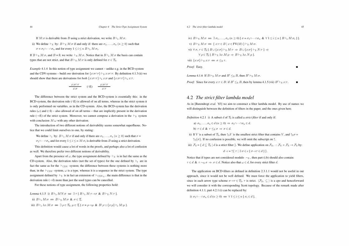
44 Chapter 4 The Strict Type Assignment System
If M :* is derivable from B using a strict derivation, we write B !s M :*.
ii) We define !S by: B !S M :* if and only if: there are *1, . . . , *n (n 1 0) such that
* = *1!· · ·!*n and for every 1( i(n B !s M :*i.
If B !S M :*, and B = 0, we write !S M :*. Notice that in B !s M :* the basis can contain
types that are not strict, and that B !S M :* is only defined for * + TS.
Example 4.1.4 In this notion of type assignment we cannot – unlike e.g. in the BCD-system
and the CDV-systems – build one derivation for {x:*!+} !S x:*!+ . By definition 4.1.3 (ii) we
should show that there are derivations for both {x:*!+} !s x:* and {x:*!+} !s x:+ .
x:*!+
x:*(!E)
x:*!+
x:+
The difference between the strict system and the BCD-system is essentially this: in the
BCD-system, the derivation rule (!E) is allowed of on all terms, whereas in the strict system it
is only performed on variables, as in the CD-system. Also, the BCD-system has the derivation
rules (!) and (!I) – also allowed of on all terms – that are implicitly present in the derivation
rule ($E) of the strict system. Moreover, we cannot compose a derivation in the !S system
with conclusion M :! with any other derivation.
The introduction of two different notions of derivability seems somewhat superfluous. No-
tice that we could limit ourselves to one, by stating:
We define !s by: B !s M :* if and only if there are *1, . . . , *n (n 1 0) such that * =
*1!· · ·!*n and for every 1( i(nM :*i is derivable from B using a strict derivation.
This definition would cause a lot of words in the proofs, and perhaps also a lot of confusion
as well. We therefore prefer two different notions of derivability.
Apart from the presence of !, the type assignment defined by !S is in fact the same as the
CD-system. Also, the derivation rules (not the set of types) for the one defined by !s are in
fact the same as for the !CDV -system; the difference between these systems is nothing more
than, in the !CDV -system, ! is a type, whereas it is a sequence in the strict system. The type
assignment defined by !S is in fact an extension of !CDVR, the main difference is that in the
derivation rule ($I) more than just the used types can be cancelled.
For these notions of type assignment, the following properties hold:
Lemma 4.1.5 i) B !s MN :* 23 6 + [ B !s M :+$* & B !S N :+ ].
ii) B !s M :* 23 B !S M :* & * + Ts.
iii) B !s "x.M :* 23 6 )+ TS, µ + Ts [ * = )$µ & B\x/{x:)} !s M :µ ].
4.2 The strict filter lambda model 45
iv) B !S M :* 23 6 *1, . . . , *n (n 1 0) [ * = *1!· · ·!*n & ' 1( i(n [ B !s M :*i ] ].
v) B !S M :* 23 { x:+ +B | x+ FV(M ) } !S M :*.
vi) ' *, + + TS [ B/ {x:*} !S M :+ 3 B /{x:*} !S N :+ ] 3
' )+ TS [ B !S "x.M :) 3 B !S "x.N :) ].
vii) {x:*} !S x:+ 23 * (S + .
Proof: Easy.
Lemma 4.1.6 If B !S M :* and B" (S B, then B" !S M :*.
Proof: Since for every x:+ +B: if B" (S B, then by lemma 4.1.5 (vii) B" !S x:+ .
4.2 The strict filter lambda modelAs in [Barendregt et al. ’83] we aim to construct a filter lambda model. By use of names we
will distinguish between the definition of filters in the paper, and the ones given here.
Definition 4.2.1 i) A subset d of TS is called a strict filter if and only if:
a) *1, . . . , *n + d (n 1 0) 3 *1!· · ·!*n + d.
b) + + d & + (S * 3 * + d.
ii) If V is a subset of TS, then 9SV is the smallest strict filter that contains V , and 9S* =
9S{*}. If no confusion is possible, we will omit the subscript on 9.
iii) FS = { d 7 TS | d is a strict filter }. We define application on FS, · : FS . FS $ FS by:
d · e = 9{ + | 6 * + e [ *$+ + d ] }.
Notice that if types are not considered modulo )S , then part (i.b) should also contain:
+ + d & + )S * 3 * + d. Notice also that ! + d, for every strict filter d.
The application on BCD-filters as defined in definition 2.3.1.1 would not be useful in our
approach, since it would not be well defined. We must force the application to yield filters,
since in each arrow type scheme *$+ + TS, + is strict. %FS, 7 & is a cpo and henceforward
we will consider it with the corresponding Scott topology. Because of the remark made after
definition 4.1.1, part 4.2.1 (i) can be replaced by:
i) *1!· · ·!*n + d (n 1 0) 23 ' 1( i(n [ *i + d ].
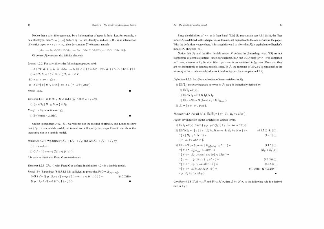
46 Chapter 4 The Strict Type Assignment System
Notice that a strict filter generated by a finite number of types is finite. Let, for example, *
be a strict type, then 9* = {*, !} (where by )S we identify * and *!*). If * is an intersection
of n strict types, * = *1!· · ·!*n, then 9* contains 2n elements, namely:
{ *1, . . . , *n, *1!*2, *1!*3, . . . , *n!1!*n, *1!*2!*3, . . . , *1!· · ·!*n, ! }.
Of course FS contains also infinite elements.
Lemma 4.2.2 For strict filters the following properties hold:
i) * + 9V & V 7 Ts 23 6 *1, . . . , *n (n 1 0) [ * = *1!· · ·!*n & ' 1( i(n [*i + V ] ].
ii) * + Ts & * + 9V & V 7 Ts 3 * + V .
iii) * + 9+ 23 + (S *.
iv) * + 9{ + | B !s M :+ } 23 * + { + | B !S M :+ }.
Proof: Easy.
Theorem 4.2.3 i) If B !S M :* and * (S + , then B !S M :+ .
ii) { * + TS | B !S M :* } +FS.
Proof: i) By induction on (S .
ii) By lemma 4.2.2 (iv).
Unlike [Barendregt et al. ’83], we will not use the method of Hindley and Longo to show
that %FS, · & is a lambda model, but instead we will specify two maps F and G and show that
these give rise to a lambda model.
Definition 4.2.4 We define F: FS $ [FS $ FS] and G: [FS $ FS] $ FS by:
i) F d e = d · e.
ii) G f = 9{ *$+ + TS | + + f (9*) }.
It is easy to check that F and G are continuous.
Theorem 4.2.5 %FS, · & with F and G as defined in definition 4.2.4 is a lambda model.
Proof: By [Barendregt ’84].5.4.1 it is sufficient to prove that F-G = id[FS&FS].
F-G f d = 9{ µ | 6 )+ d [ )$µ + 9{ *$+ | + + f (9*) } ] } = (4.2.2 (ii))
9{ µ | 6 )+ d [ µ + f (9)) ] } = f (d).
4.2 The strict filter lambda model 47
Since the definition of )S as in [van Bakel ’92a] did not contain part 4.1.1 (iv.b), the filter
model FS as defined in this chapter is, as domain, not equivalent to the one defined in the paper.
With the definition we gave here, it is straightforward to show that FS is equivalent to Engeler’s
model DA [Engeler ’81].
Notice that FS and the filter lambda model F defined in [Barendregt et al. ’83] are not
isomorphic as complete lattices, since, for example, in F the BCD-filter 9*!+$* is contained
in 9*$*, whereas in FS the strict filter 9S*!+$* is not contained in 9S*$*. Moreover, they
are not isomorphic as lambda models, since, in F , the meaning of "xy.xy is contained in the
meaning of "x.x, whereas this does not hold in FS (see the examples in 4.2.9).
Definition 4.2.6 Let . be a valuation of term-variables in FS.
i) [[M ]]$ , the interpretation of terms in FS via . is inductively defined by:
a) [[x]]$ = .(x).
b) [[MN ]]$ = F [[M ]]$[[N ]]$ .
c) [["x.M ]]$ = G ("" v +FS.[[M ]]$(v/x)).
ii) B$ = { x:* | * + .(x) }.
Theorem 4.2.7 For all M , .: [[M ]]$ = { * + TS | B$ !S M :* }.
Proof: By induction on the structure of lambda terms.
i) [[x]]$ = .(x). Since { y:) | ) + .(y) } !S x:* 23 * + .(x).
ii) [[MN ]]$ = 9{ + | 6 * [ B$ !s M :*$+ & B$ !S N :* ] } = (4.1.5 (i) & (ii))
9{ + | B$ !s MN :+ } = (4.2.3 (ii))
{ + | B$ !S MN :+ }.
iii) [["x.M ]]$ = 9{ *$+ | B$(9%/x) !S M :+ } = (4.1.5 (ii))
9{ *$+ | B$(9%/x) !s M :+ } = (B$! = B$\x)
9{ *$+ | B$! /{x:µ | µ + 9*} !s M :+ } =
9{ *$+ | B$! /{x:*} !s M :+ } = (4.1.5 (iii))
9{ *$+ | B$! !s "x.M :*$+ } = (4.1.5 (v))
9{ *$+ | B$ !s "x.M :*$+ } = (4.1.5 (iii) & 4.2.2 (iv))
{ ) | B$ !S "x.M :) }.
Corollary 4.2.8 If M =" N and B !S M :*, then B !S N :*, so the following rule is a derived
rule in !S :
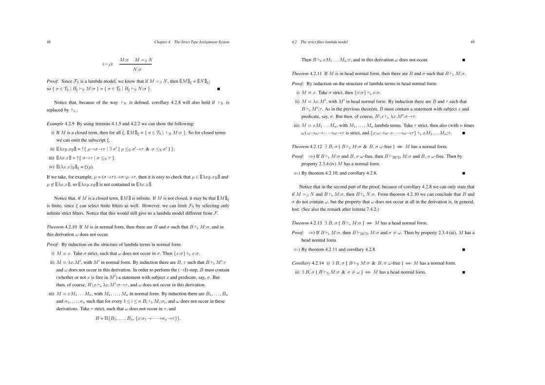
48 Chapter 4 The Strict Type Assignment System
M :* M =" N(="):
N :*
Proof: Since FS is a lambda model, we know that if M =" N , then [[M ]]$ = [[N ]]$;
so { * + TS | B$ !S M :* } = { * + TS | B$ !S N :* }.
Notice that, because of the way !S is defined, corollary 4.2.8 will also hold if !S is
replaced by !s .
Example 4.2.9 By using lemmas 4.1.5 and 4.2.2 we can show the following:
i) If M is a closed term, then for all ., [[M ]]$ = { * + TS | !S M :* }. So for closed terms
we can omit the subscript ..
ii) [["xy.xy]] = 9{ )$*$+ | 6 *" [ ) (S *"$+ & * (S *" ] }.
iii) [["x.x]] = 9{ *$+ | * (S + }.
iv) [[("x.x)y]]$ = .(y).
If we take, for example, µ = (*$+ )$*!)$+ , then it is easy to check that µ + [["xy.xy]] and
µ ,+ [["x.x]], so [["xy.xy]] is not contained in [["x.x]].
Notice that, if M is a closed term, [[M ]] is infinite. If M is not closed, it may be that [[M ]]$
is finite, since . can select finite filters as well. However, we can limit FS by selecting only
infinite strict filters. Notice that this would still give us a lambda model different from F .
Theorem 4.2.10 If M is in normal form, then there are B and * such that B !s M :*, and in
this derivation ! does not occur.
Proof: By induction on the structure of lambda terms in normal form.
i) M 4 x. Take * strict, such that ! does not occur in *. Then {x:*} !s x:*.
ii) M 4 "x.M ", with M " in normal form. By induction there are B, + such that B !s M ":+
and ! does not occur in this derivation. In order to perform the ($I)-step, B must contain
(whether or not x is free in M ") a statement with subject x and predicate, say, *. But
then, of course, B\x !s "x.M ":*$+ , and ! does not occur in this derivation.
iii) M 4 xM1 . . .Mn, with M1, . . . , Mn in normal form. By induction there are B1, . . . , Bn
and *1, . . . , *n such that for every 1( i(n Bi !s Mi:*i, and ! does not occur in these
derivations. Take + strict, such that ! does not occur in + , and
B = #{B1, . . . , Bn, {x:*1$· · ·$*n$+}}.
4.2 The strict filter lambda model 49
Then B !s xM1 . . .Mn:+ , and in this derivation ! does not occur.
Theorem 4.2.11 If M is in head normal form, then there are B and * such that B !s M :*.
Proof: By induction on the structure of lambda terms in head normal form.
i) M 4 x. Take * strict, then {x:*} !s x:*.
ii) M 4 "x.M ", with M " in head normal form. By induction there are B and + such that
B !s M ":+ . As in the previous theorem, B must contain a statement with subject x and
predicate, say, *. But then, of course, B\x !s "x.M ":*$+ .
iii) M 4 xM1 . . .Mn, with M1, . . . , Mn lambda terms. Take + strict, then also (with n times
!) !$!$· · ·$!$+ is strict, and {x:!$!$· · ·$!$+} !s xM1 . . .Mn:+ .
Theorem 4.2.12 6 B, * [ B !s M :* & B, * !-free ] 23 M has a normal form.
Proof: 3) If B !s M :* and B, * !-free, then B !BCD M :* and B, * !-free. Then by
property 2.3.4 (iv) M has a normal form.
2) By theorem 4.2.10, and corollary 4.2.8.
Notice that in the second part of the proof, because of corollary 4.2.8 we can only state that
if M =" N and B !s M :*, then B !s N :*. From theorem 4.2.10 we can conclude that B and
* do not contain !, but the property that ! does not occur at all in the derivation is, in general,
lost. (See also the remark after lemma 7.4.2.)
Theorem 4.2.13 6 B, * [ B !s M :* ] 23 M has a head normal form.
Proof: 3) If B !s M :*, then B !BCD M :* and * ,= !. Then by property 2.3.4 (iii), M has a
head normal form.
2) By theorem 4.2.11 and corollary 4.2.8.
Corollary 4.2.14 i) 6 B, * [ B !S M :* & B, * !-free ] 23 M has a normal form.
ii) 6 B, * [ B !S M :* & * ,= ! ] 23 M has a head normal form.
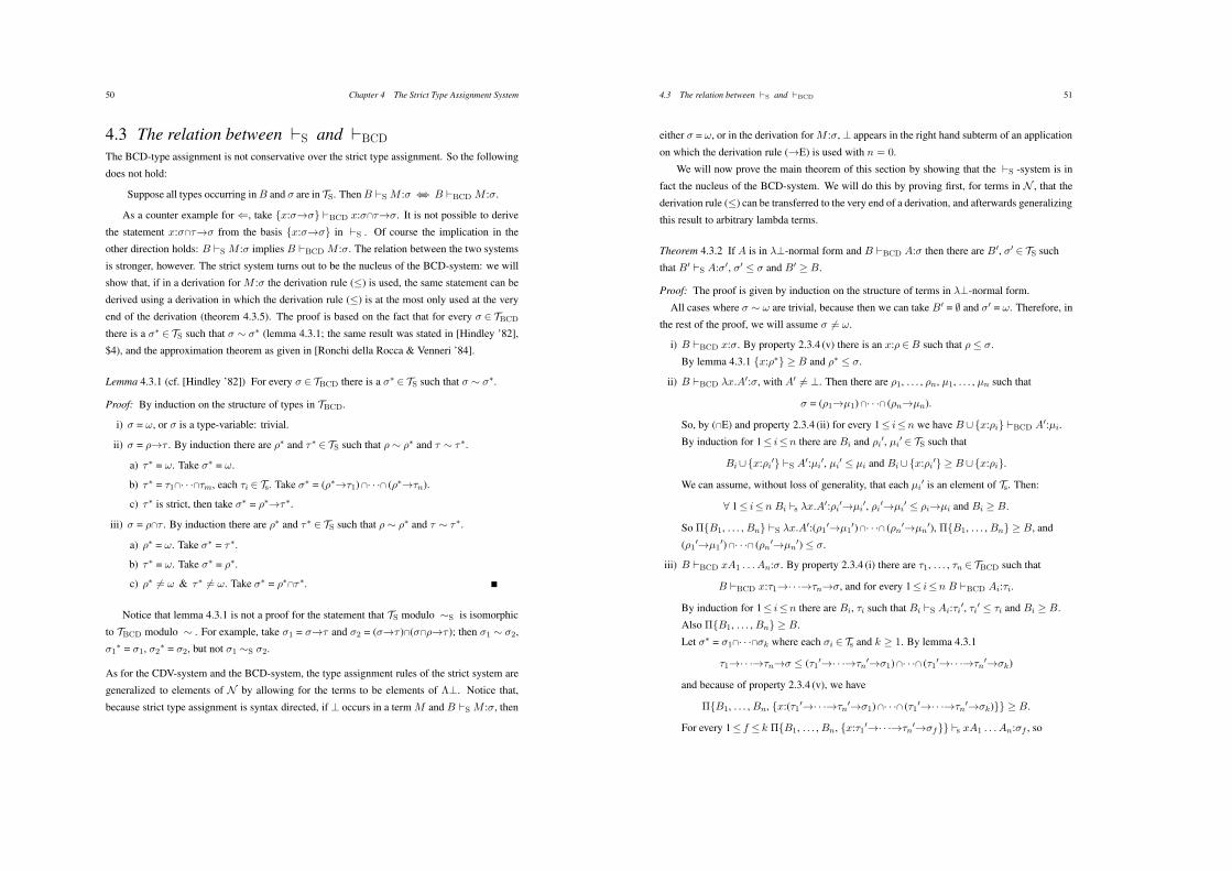
50 Chapter 4 The Strict Type Assignment System
4.3 The relation between !S and !BCD
The BCD-type assignment is not conservative over the strict type assignment. So the following
does not hold:
Suppose all types occurring in B and * are in TS. Then B !S M :* 23 B !BCD M :*.
As a counter example for 2, take {x:*$*} !BCD x:*!+$*. It is not possible to derive
the statement x:*!+$* from the basis {x:*$*} in !S . Of course the implication in the
other direction holds: B !S M :* implies B !BCD M :*. The relation between the two systems
is stronger, however. The strict system turns out to be the nucleus of the BCD-system: we will
show that, if in a derivation for M :* the derivation rule (() is used, the same statement can be
derived using a derivation in which the derivation rule (() is at the most only used at the very
end of the derivation (theorem 4.3.5). The proof is based on the fact that for every * + TBCD
there is a *' + TS such that * ) *' (lemma 4.3.1; the same result was stated in [Hindley ’82],
$4), and the approximation theorem as given in [Ronchi della Rocca & Venneri ’84].
Lemma 4.3.1 (cf. [Hindley ’82]) For every * + TBCD there is a *' + TS such that * ) *'.
Proof: By induction on the structure of types in TBCD.
i) * = !, or * is a type-variable: trivial.
ii) * = )$+ . By induction there are )' and +' + TS such that ) ) )' and + ) +'.
a) +' = !. Take *' = !.
b) +' = +1!· · ·!+m, each +i + Ts. Take *' = ()'$+1)!· · ·! ()'$+n).
c) +' is strict, then take *' = )'$+'.
iii) * = )!+ . By induction there are )' and +' + TS such that ) ) )' and + ) +'.
a) )' = !. Take *' = +'.
b) +' = !. Take *' = )'.
c) )' ,= ! & +' ,= !. Take *' = )'!+'.
Notice that lemma 4.3.1 is not a proof for the statement that TS modulo )S is isomorphic
to TBCD modulo ) . For example, take *1 = *$+ and *2 = (*$+ )!(*!)$+ ); then *1 ) *2,
*1' = *1, *2
' = *2, but not *1 )S *2.
As for the CDV-system and the BCD-system, the type assignment rules of the strict system are
generalized to elements of N by allowing for the terms to be elements of !#. Notice that,
because strict type assignment is syntax directed, if # occurs in a term M and B !S M :*, then
4.3 The relation between "S and "BCD 51
either * = !, or in the derivation for M :*, # appears in the right hand subterm of an application
on which the derivation rule ($E) is used with n = 0.
We will now prove the main theorem of this section by showing that the !S -system is in
fact the nucleus of the BCD-system. We will do this by proving first, for terms in N , that the
derivation rule (() can be transferred to the very end of a derivation, and afterwards generalizing
this result to arbitrary lambda terms.
Theorem 4.3.2 If A is in "#-normal form and B !BCD A:* then there are B", *" + TS such
that B" !S A:*", *" ( * and B" 1 B.
Proof: The proof is given by induction on the structure of terms in "#-normal form.
All cases where * ) ! are trivial, because then we can take B" = 0 and *" = !. Therefore, in
the rest of the proof, we will assume * ,= !.
i) B !BCD x:*. By property 2.3.4 (v) there is an x:)+B such that ) ( *.
By lemma 4.3.1 {x:)'} 1 B and )' ( *.
ii) B !BCD "x.A":*, with A" ,= #. Then there are )1, . . . , )n, µ1, . . . , µn such that
* = ()1$µ1) !· · ·! ()n$µn).
So, by (!E) and property 2.3.4 (ii) for every 1( i(n we have B/{x:)i} !BCD A":µi.
By induction for 1( i(n there are Bi and )i", µi
" + TS such that
Bi/{x:)i"} !S A":µi
", µi" ( µi and Bi/ {x:)i
"} 1 B /{x:)i}.
We can assume, without loss of generality, that each µi" is an element of Ts. Then:
' 1( i(n Bi !s "x.A":)i"$µi
", )i"$µi
" ( )i$µi and Bi 1 B.
So #{B1, . . . , Bn} !S "x.A":()1
"$µ1")!· · ·! ()n
"$µn"), #{B1, . . . , Bn} 1 B, and
()1"$µ1
") !· · ·! ()n"$µn
") ( *.
iii) B !BCD xA1 . . . An:*. By property 2.3.4 (i) there are +1, . . . , +n + TBCD such that
B !BCD x:+1$· · ·$+n$*, and for every 1( i(n B !BCD Ai:+i.
By induction for 1( i(n there are Bi, +i such that Bi !S Ai:+i", +i
" ( +i and Bi 1 B.
Also #{B1, . . . , Bn} 1 B.
Let *' = *1!· · ·!*k where each *i + Ts and k 1 1. By lemma 4.3.1
+1$· · ·$+n$* ( (+1"$· · ·$+n
"$*1)!· · ·! (+1"$· · ·$+n
"$*k)
and because of property 2.3.4 (v), we have
#{B1, . . . , Bn, {x:(+1"$· · ·$+n
"$*1) !· · ·! (+1"$· · ·$+n
"$*k)}} 1 B.
For every 1( f ( k #{B1, . . . , Bn, {x:+1"$· · ·$+n
"$*f}} !s xA1 . . . An:*f , so
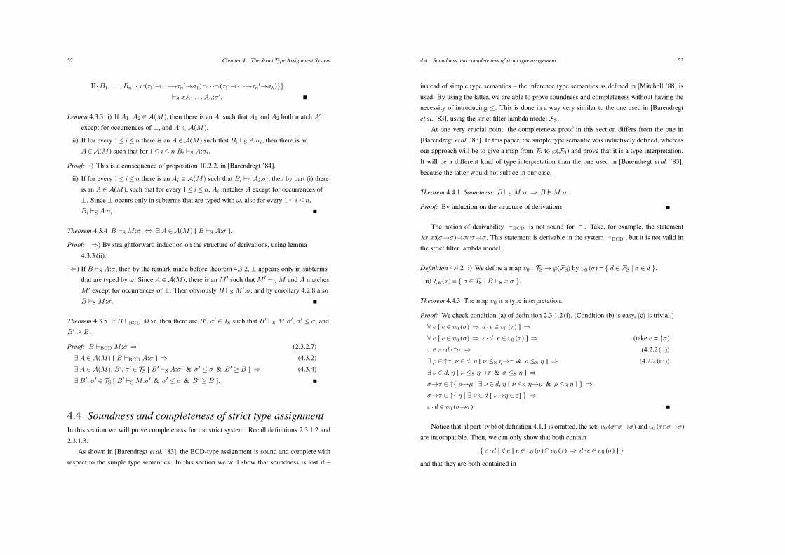
52 Chapter 4 The Strict Type Assignment System
#{B1, . . . , Bn, {x:(+1"$· · ·$+n
"$*1) !· · ·! (+1"$· · ·$+n
"$*k)}}
!S xA1 . . . An:*".
Lemma 4.3.3 i) If A1, A2 +A(M), then there is an A" such that A1 and A2 both match A"
except for occurrences of #, and A" +A(M).
ii) If for every 1( i(n there is an A +A(M ) such that Bi !S A:*i, then there is an
A+A(M ) such that for 1( i(n Bi !S A:*i.
Proof: i) This is a consequence of proposition 10.2.2, in [Barendregt ’84].
ii) If for every 1( i(n there is an Ai + A(M) such that Bi !S Ai:*i, then by part (i) there
is an A+A(M ), such that for every 1( i(n, Ai matches A except for occurrences of
#. Since # occurs only in subterms that are typed with !, also for every 1( i(n,
Bi !S A:*i.
Theorem 4.3.4 B !S M :* 23 6 A +A(M) [ B !S A:* ].
Proof: 3) By straightforward induction on the structure of derivations, using lemma
4.3.3 (ii).
2) If B !S A:*, then by the remark made before theorem 4.3.2, # appears only in subterms
that are typed by !. Since A +A(M ), there is an M " such that M " =" M and A matches
M " except for occurrences of #. Then obviously B !S M ":*, and by corollary 4.2.8 also
B !S M :*.
Theorem 4.3.5 If B !BCD M :*, then there are B", *" + TS such that B" !S M :*", *" ( *, and
B" 1 B.
Proof: B !BCD M :* 3 (2.3.2.7)
6 A +A(M) [ B !BCD A:* ] 3 (4.3.2)
6 A +A(M), B", *" + TS [ B" !S A:*" & *" ( * & B" 1 B ] 3 (4.3.4)
6 B", *" + TS [ B" !S M :*" & *" ( * & B" 1 B ].
4.4 Soundness and completeness of strict type assignmentIn this section we will prove completeness for the strict system. Recall definitions 2.3.1.2 and
2.3.1.3.
As shown in [Barendregt et al. ’83], the BCD-type assignment is sound and complete with
respect to the simple type semantics. In this section we will show that soundness is lost if –
4.4 Soundness and completeness of strict type assignment 53
instead of simple type semantics – the inference type semantics as defined in [Mitchell ’88] is
used. By using the latter, we are able to prove soundness and completeness without having the
necessity of introducing (. This is done in a way very similar to the one used in [Barendregt
et al. ’83], using the strict filter lambda model FS.
At one very crucial point, the completeness proof in this section differs from the one in
[Barendregt et al. ’83]. In this paper, the simple type semantic was inductively defined, whereas
our approach will be to give a map from TS to 0(FS) and prove that it is a type interpretation.
It will be a different kind of type interpretation than the one used in [Barendregt et al. ’83],
because the latter would not suffice in our case.
Theorem 4.4.1 Soundness. B !S M :* 3 B !!M :*.
Proof: By induction on the structure of derivations.
The notion of derivability !BCD is not sound for !! . Take, for example, the statement
"x.x:(*$*)$*!+$*. This statement is derivable in the system !BCD , but it is not valid in
the strict filter lambda model.
Definition 4.4.2 i) We define a map -0 : TS $ 0(FS) by -0 (*) = { d +FS | * + d }.
ii) .B(x) = { * + TS | B !S x:* }.
Theorem 4.4.3 The map -0 is a type interpretation.
Proof: We check condition (a) of definition 2.3.1.2 (i). (Condition (b) is easy, (c) is trivial.)
' e [ e + -0 (*) 3 d · e+ -0 (+ ) ] 3
' e [ e + -0 (*) 3 / ·d · e+ -0 (+ ) ] 3 (take e = 9*)
+ + / ·d · 9* 3 (4.2.2 (ii))
6 )+ 9*, ' + d, ( [ ' (S ($+ & ) (S ( ] 3 (4.2.2 (iii))
6 ' + d, ( [ ' (S ($+ & * (S ( ] 3
*$+ + 9{ )$µ | 6 ' + d, ( [ ' (S ($µ & ) (S ( ] } 3
*$+ + 9{ ( | 6 ' + d [ '$( + /] } 3
/ ·d+ -0 (*$+ ).
Notice that, if part (iv.b) of definition 4.1.1 is omitted, the sets -0 (*!+$*) and -0 (+!*$*)
are incompatible. Then, we can only show that both contain
{ / ·d | ' e [ e + -0 (*)8 -0 (+ ) 3 d · e+ -0 (*) ] }
and that they are both contained in
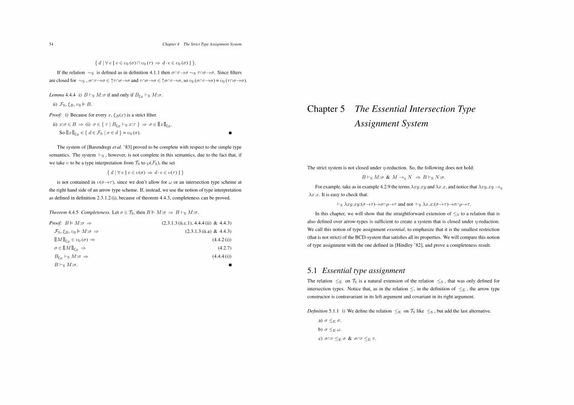
54 Chapter 4 The Strict Type Assignment System
{ d | ' e [ e + -0 (*)8 -0 (+ ) 3 d · e+ -0 (*) ] }.
If the relation )S is defined as in definition 4.1.1 then *!+$* )S +!*$*. Since filters
are closed for )S , *!+$* + 9+!*$* and +!*$* + 9*!+$*, so -0 (*!+$*) = -0 (+!*$*).
Lemma 4.4.4 i) B !S M :* if and only if B$B !S M :*.
ii) FS, .B, -0 !! B.
Proof: i) Because for every x, .B(x) is a strict filter.
ii) x:* +B 3 (i) * + { + | B$B !S x:+ } 3 * + [[x]]$B .
So [[x]]$B + { d+FS | * + d } = -0 (*).
The system of [Barendregt et al. ’83] proved to be complete with respect to the simple type
semantics. The system !S , however, is not complete in this semantics, due to the fact that, if
we take - to be a type interpretation from TS to 0(FS), the set
{ d | ' e [ e + -(*) 3 d · e + -(+ ) ] }
is not contained in -(*$+ ), since we don’t allow for ! or an intersection type scheme at
the right hand side of an arrow type scheme. If, instead, we use the notion of type interpretation
as defined in definition 2.3.1.2 (i), because of theorem 4.4.3, completeness can be proved.
Theorem 4.4.5 Completeness. Let * + TS, then B !!M :* 3 B !S M :*.
Proof: B !!M :* 3 (2.3.1.3 (ii.c.1), 4.4.4 (ii) & 4.4.3)
FS, .B, -0 !! M :* 3 (2.3.1.3 (ii.a) & 4.4.3)
[[M ]]$B + -0 (*) 3 (4.4.2 (i))
* + [[M ]]$B 3 (4.2.7)
B$B !S M :* 3 (4.4.4 (i))
B !S M :*.
Chapter 5 The Essential Intersection Type
Assignment System
The strict system is not closed under (-reduction. So, the following does not hold:
B !S M :* & M $# N 3 B !S N :*.
For example, take as in example 4.2.9 the terms "xy.xy and "x.x, and notice that "xy.xy $#
"x.x. It is easy to check that:
!S "xy.xy:(*$+ )$*!)$+ and not !S "x.x:(*$+ )$*!)$+ .
In this chapter, we will show that the straightforward extension of (S to a relation that is
also defined over arrow-types is sufficient to create a system that is closed under (-reduction.
We call this notion of type assignment essential, to emphasize that it is the smallest restriction
(that is not strict) of the BCD-system that satisfies all its properties. We will compare this notion
of type assignment with the one defined in [Hindley ’82], and prove a completeness result.
5.1 Essential type assignmentThe relation (E on TS is a natural extension of the relation (S , that was only defined for
intersection types. Notice that, as in the relation (, in the definition of (E , the arrow type
constructor is contravariant in its left argument and covariant in its right argument.
Definition 5.1.1 i) We define the relation (E on TS like (S , but add the last alternative.
a) * (E *.
b) * (E !.
c) *!+ (E * & *!+ (E + .
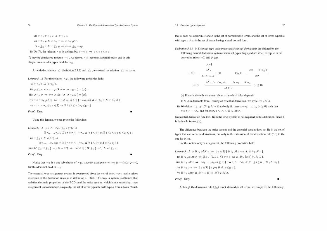
56 Chapter 5 The Essential Intersection Type Assignment System
d) * (E + (E ) 3 * (E ).
e) * (E ) & * (E + 3 * (E )!+ .
f) ) (E * & + (E µ 3 *$+ (E )$µ.
ii) On TS, the relation )E is defined by: * )E + 23 * (E + (E *.
TS may be considered modulo )E . As before, (E becomes a partial order, and in this
chapter we consider types modulo )E .
As with the relations ( (definition 2.3.2) and (S , we extend the relation (E to bases.
Lemma 5.1.2 For the relation (E , the following properties hold:
i) * (S + 3 * (E + .
ii) # (E * 23 * = #. So { * | * )E # } = {#}.
iii) ! (E * 23 * = !. So { * | * )E ! } = {!}.
iv) *$+ (E )+ Ts 23 6 $+ TS, % + Ts [ ) = $$% & $ (E * & + (E % ].
v) *1!· · ·!*n (E + + Ts 3 6 1( i(n [ *i (E + ].
Proof: Easy.
Using this lemma, we can prove the following:
Lemma 5.1.3 i) *1!· · ·!*n (E + + TS 3
6 +1, . . . , +m + Ts [ + = +1!· · ·!+m & ' 1( j (m 6 1( i(n [ *i (E +j ] ].
ii) * (E + & * + Ts 3
6 +1, . . . , +m (m 1 0) [ + = +1!· · ·!+m & ' 1( j(m [ * (E +j ] ].
iii) B" (E B (S {x:*} & * + Ts 3 6 *" + Ts [ B" (S {x:*"} & *" (E * ].
Proof: Easy.
Notice that )S is a true subrelation of )E , since for example *$+ )E (*$+ )!(*!)$+ ),
but this does not hold in )S .
The essential type assignment system is constructed from the set of strict types, and a minor
extension of the derivation rules as in definition 4.1.3 (i). This way, a system is obtained that
satisfies the main properties of the BCD- and the strict system, which is not surprising: type
assignment is closed under %-equality, the set of terms typeable with type * from a basis B such
5.1 Essential type assignment 57
that ! does not occur in B and * is the set of normalizable terms, and the set of terms typeable
with type * ,= ! is the set of terms having a head normal form.
Definition 5.1.4 i) Essential type assignment and essential derivations are defined by the
following natural deduction system (where all types displayed are strict, except * in the
derivation rules ($I) and ((E)):
[x:*]:
M :+($I): (a)
"x.M :*$+
x:* * (E +((E):
x:+
M :*1!· · ·!*n$+ N :*1 . . . N :*n($E): (n 1 0)
MN :+
(a) If x:* is the only statement about x on which M :+ depends.
If M :* is derivable from B using an essential derivation, we write B !e M :*.
ii) We define !E by: B !E M :* if and only if: there are *1, . . . , *n (n 1 0) such that
* = *1!· · ·!*n, and for every 1( i(n, B !e M :*i.
Notice that derivation rule (!E) from the strict system is not required in this definition, since it
is derivable from ((E).
The difference between the strict system and the essential system does not lie in the set of
types that can occur in derivations, but only in the extension of the derivation rule (!E) to the
one for ((E).
For this notion of type assignment, the following properties hold:
Lemma 5.1.5 i) B !e MN :* 23 6 + + TS [ B !e M :+$* & B !E N :+ ].
ii) B !e "x.M :* 23 6 )+ TS, µ+ Ts [ * = )$µ & B/{x:)} !e M :µ ].
iii) B !E M :* 23 6 *1, . . . , *n (n 1 0) [ * = *1!· · ·!*n & ' 1( i(n [ B !e M :*i ] ].
iv) B !E x:* 23 6 )+ TS [ x:)+B & ) (E * ].
v) B !E M :* & B" (E B 3 B" !E M :*.
Proof: Easy.
Although the derivation rule ((E) is not allowed on all terms, we can prove the following:
58 Chapter 5 The Essential Intersection Type Assignment System
Lemma 5.1.6 If B !E M :*, and * (E + , then B !E M :+ .
Proof: By induction on !E .
i) * = !. Then by lemma 5.1.2 (iii) + = !. Obviously B !E M :+ .
ii) * = *1!· · ·!*n. Then by lemma 5.1.5 (iii), for every 1( i(n, B !e M :*i. By lemma
5.1.3 (i) there are +1, . . . , +m + Ts such that + = +1!· · ·!+m, and for every 1( j(m there
is a 1( i(n such that *i (E +j . By induction for every 1( j(m B !e M :+j . But then
B !E M :+ .
iii) * + Ts. This part is proved by induction on M .
a) M 4 x. Then B (E {x:*} (E {x:+}, so by lemma 5.1.5 (iv) B !E x:+ .
b) M 4 "x.M ". Then by lemma 5.1.5 (ii), there are ) + TS, µ + Ts such that * = )$µ,
and B/{x:)} !e M ":µ. By lemmas 5.1.3 (ii) and 5.1.2 (iv), there are )1, . . . , )n, µ1,
. . . , µn such that + = ()1$µ1) !· · ·! ()n$µn), and for 1( i(n )i (E ) and
µ (E µi. By lemma 5.1.5 (v), for 1( i(n B/{x:)i} !e M ":µ, and by induction
B/{x:)i} !e M ":µi. So by lemma 5.1.5 (ii), for every 1( i(n B !e "x.M ":)i$µi,
so B !E "x.M ":+ .
c) M 4M1M2. Then by lemma 5.1.5 (i), there is a µ+ TS such that B !e M1:µ$*, and
B !E M2:µ. Since * (E + , also µ$* (E µ$+ , and by induction B !e M1:µ$+ .
But then, by lemma 5.1.5 (i), B !E M1M2:+ .
Now it is easy to prove that type assignment in this system is closed under (-reduction.
Theorem 5.1.7 If B !E M :* and M $# N , then B !E N :*.
Proof: We will only show the part * + Ts. The proof is completed by induction on the
definition of $# , of which we only show the part "x.Mx $# M , where x does not occur
free in M . The other parts are dealt with by straightforward induction.
B !e "x.Mx:* 3 (5.1.5 (ii))
6 ), µ [ * = )$µ & B/ {x:)} !e Mx:µ ] 3 (5.1.5 (i))
6 + , ), µ [ * = )$µ & B/{x:)} !e M :+$µ & B/{x:)} !E x:+ ] 3
(5.1.5 (iv), x not in M )
6 + , ), µ [ * = )$µ & B !e M :+$µ & ) (E + ] 3 (5.1.1)
6 + , ), µ [ * = )$µ & B !e M :+$µ & +$µ (E )$µ ] 3 (5.1.6)
B !e M :*.
It is easy to check that !E "xy.xy:(*$+ )$*!)$+ and !E "x.x:(*$+ )$*!)$+ .
5.3 Soundness and completeness of essential type assignment 59
5.2 The relation between !S , !E and !BCD
As with the BCD-type assignment system and the strict system, essential type assignment is not
conservative over strict type assignment. So the following does not hold:
B !S M :* 23 B !E M :*.
As a counter example for 2, take {x:*$*} !E x:*!+$*. Notice that *$* (E *!+$*.
It is not possible to derive the statement x:*!+$* from the basis {x:*$*} in !S . Of course
the implication in the other direction holds: B !S M :* implies B !E M :*.
In a way similar to that of section 4.3, we can show that the essential type assignment system
is the nucleus of the BCD-system; we can also show that the strict system is the nucleus of the
essential system. The relation between the different notions of type assignment is formulated
as follows:
Theorem 5.2.1 i) If B !BCD M :*, then there are B", *" such that B" !E M :*", * ) *" and
B ) B".
ii) If B !E M :*, then there are B", *" such that B" !S M :*", *" (E * and B (E B".
Proof: i) As the proof of theorem 4.3.5.
ii) By easy induction, using lemma 5.1.5.
In part (i) in particular *" ( * and B ( B".
As in the previous chapter, it is possible to prove that the essential type assignment system
satisfies the main properties of the BCD-system and of the strict system.
Property 5.2.2 i) B !E M :* & M =" N 3 B !E N :*.
ii) 6 B, * [ B !E M :* & B, * !-free ] 23 M has a normal form.
iii) 6 B, * [ B !E M :* & * ,= ! ] 23 M has a head normal form.
5.3 Soundness and completeness of essential type assign-
mentFor this essential system, it is possible to prove completeness of type assignment with respect
to the simple type semantics the same way as done in [Barendregt et al. ’83]. Since such a proof
would be obtained in exactly the same way as in [Barendregt et al. ’83], we will not present it
here. Instead, we will prove a completeness result using results proven in [Hindley ’82]. In this
60 Chapter 5 The Essential Intersection Type Assignment System
paper, some restrictions of the BCD-system were investigated, and one of them proved to be
essentially the same as the BCD-system.
Definition 5.3.1 [Hindley ’82] i) The set TN of normal intersection types is defined by:
a) Type-variables and ! are in TN.
b) If *, + + TN – {!}, then *!+ + TN.
c) If * + TN, and + + TN-{!, intersections}, then *$+ + TN.
ii) On TN, the relation (N is obtained by restricting the definition of ( to TN.
iii) The notion of type assignment !N is defined as !BCD , but by adding:
a) All types are in TN.
b) Derivation rule (!E) never immediately follows (!I).
c) Derivation rules (!E) and ((N) are only used with atomic subjects.
It is straightforward to show that TN = TS, and (N = (E .
Proposition 5.3.2 (cf. [Hindley ’82]) i) If *, + + TS, then * ( + 23 * (E + .
ii) Let ' be defined as in lemma 4.3.1. B !BCD M :* 23 B' !N M :*'.
We will now prove that BCD-type assignment is conservative over essential type assign-
ment.
Theorem 5.3.3 Conservativity. Let B and * contain types in TS. If B !BCD M :*, then
B !E M :*.
Proof: B !BCD M :* 3 (5.2.1 (i))
6 B", *" [ B" !E M :*" & *" ) * & B ) B" ] 3 (5.3.2 (i))
6 B", *" [ B" !E M :*" & *" (E * & B (E B" ] 3 (5.1.5 (v) & 5.1.6)
B !E M :*.
Of course the implication in the other direction also holds: If B !E M :*, then B !BCD M :*.
We will now show that !N and !E are equivalent.
Theorem 5.3.4 B !N M :* 23 B !E M :*.
Proof: 3) B !N M :* 3 (5.3.2 (ii)) B !BCD M :* 3 (5.3.3) B !E M :*.
2) B !E M :* 3 B !BCD M :* 3 (5.3.2 (ii)) B !N M :*.
5.3 Soundness and completeness of essential type assignment 61
Now, soundness and completeness of essential type assignment are easy to prove.
Theorem 5.3.5 Soundness and completeness of essential type assignment. Let B and * contain
types in TS. Then B !E M :* 23 B !!s M :*.
Proof: 3) B !E M :* 3 B !BCD M :* 3 (2.3.1.5 (i)) B !!s M :*.
2) B !!s M :* 3 (2.3.1.5 (ii)) B !BCD M :* 3 (5.3.3) B !E M :*.
Since !N and !E are equivalent, soundness and completeness of essential type assign-
ment could also be proved using a similar result proved in [Hindley ’82] for !N .
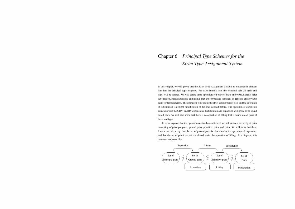
Chapter 6 Principal Type Schemes for the
Strict Type Assignment System
In this chapter, we will prove that the Strict Type Assignment System as presented in chapter
four has the principal type property. For each lambda term the principal pair (of basis and
type) will be defined. We will define three operations on pairs of basis and types, namely strict
substitution, strict expansion, and lifting, that are correct and sufficient to generate all derivable
pairs for lambda terms. The operation of lifting is the strict counterpart of rise, and the operation
of substitution is a slight modification of the ones defined before. The operation of expansion
coincides with the CDV- and RV-expansions. Substitution and expansion will prove to be sound
on all pairs; we will also show that there is no operation of lifting that is sound on all pairs of
basis and type.
In order to prove that the operations defined are sufficient, we will define a hierarchy of pairs
consisting of principal pairs, ground pairs, primitive pairs, and pairs. We will show that these
form a true hierarchy, that the set of ground pairs is closed under the operation of expansion,
and that the set of primitive pairs is closed under the operation of lifting. In a diagram, this
construction looks like:
!"
#$
Set of
Principal pairs
% &+
Expansion
:,=
!"
#$
Set of
Ground pairs'( Expansion
)*
*
% &+
Lifting
:,=
!"
#$
Set of
Primitive pairs'( Lifting
)*
*
% &+
Substitution
:,=
!"
#$
Set of
Pairs'( Substitution
)*
*
64 Chapter 6 Principal Type Schemes for the Strict Type Assignment System
There is an arrow from one set of pairs to another, if the operation mentioned above the
arrow maps a pair in the set at the beginning of the arrow to a pair in the set at the end. When
these sets are different, the result of applying the operation in general is not a pair in the set at
the beginning of the arrow. The symbols between the sets indicate that the set on the left is a
true subset of the set on the right.
The principal pair for a lambda term M in the Strict Type Assignment System, PPS (M ),
turns out to be the same as PPCDV (M ) and PPRV (M ); the definition of ground pairs coincides
with the one for CDV-ground pairs. As will be shown in this chapter, the results of [Coppo
et al. ’80] and [Ronchi della Rocca & Venneri ’84] do not provide principal types for the strict
system. Although the type assignment systems differ only in details, none of the results of
either paper can be applied to the strict system. All results presented in this chapter with proofs
are therefore new, although we are using techniques that are similar to the ones used in these
two papers.
Since the strict system is closed under %-equality, type assignment in this system is not
decidable, but semi-decidable. This means that, in an implementation of the strict system, some
restrictions have to be made, as is done, for example, in [Coppo & Giannini ’92].
We will show that the three operations defined in this chapter are complete: if %B, *& is a
suitable pair for a term A in "#-normal form, and %P , ,& is the principal pair for A, then there
are an operation of lifting L, sequences of operations of expansion 1E, and substitution 1S, such
that %B, *& = 1S (L (1E (%P , ,&))).
We will generalize these results to arbitrary lambda terms, and, finally, show that also the
essential type assignment system has the principal type property.
In proving that the strict system has the principal pair property, we could have used the same
technique as [Margaria & Zacchi ’90]. In this paper, principal typings for the type assignment
system as presented in [Jacobs et al. ’92] were studied. This system is a combination of the
BCD-system and the polymorphic type discipline as presented in [Girard ’86]. This combina-
tion can be seen as an extension of the BCD-system by adding the type constructor ‘'’: if #
is a type-variable and * is a type, then '#.* is a type. Also, the type inclusion relation ( is
extended in a natural way. The type assignment rules consist of ($I), ($E), ('I), (!I), ((),
and (!). The rules (!E) and ('E) are omitted since they can be derived from (().
The technique used in [Margaria & Zacchi ’90] is the following: For every A in "#-normal
form, a relation 7A is defined on the inductively defined set of pairs %B, *& admissible for A
(i.e. such that B ! A:*). This relation satisfies: if %B1, *1& 7A %B2, *2&, then %B1, *1& and
%B2, *2& are both admissible pairs for A. The principal pairs of terms in "#-normal form are
defined by induction on the structure of such terms (similar to definitions 2.2.2.10, 2.3.2.5 and
6.1 Principal pairs for terms in !#-normal form 65
6.1.3 of this thesis). The proof is completed by showing that, if %B, *& is an admissible pair for
A, and %P , ,& is the principal pair of A, then %P , ,& 7A %B, *&.
A major difference between this technique and the one used in this chapter, is that the latter
yields, given an admissible pair %B, *& for A, a sequence of operations that will transform the
principal pair of A into %B, *&. The technique of [Margaria & Zacchi ’90] is sufficient to show
that, for every term in "#-normal form, there exists a principal type; it does not specify how to
create an admissible pair from the principal one.
6.1 Principal pairs for terms in !#-normal formIn [Coppo et al. ’80], principal pairs were defined for a type assignment system that is, at first
sight, very similar to the strict system, and in [Ronchi della Rocca & Venneri ’84] principal pairs
were defined for the BCD-system. In order to understand the necessity of defining principal
pairs for the the strict system, we focus on the small but important differences between the
strict system and the other two.
In the type assignment system as presented in [Coppo et al. ’80], the types that occur in
bases can only be type-variables or arrow types. Instead of using intersections in bases, it
is allowed for to let a basis contain several statements the subject of which is a variable. If
B !CDVPM :+ , and x occurs in B, the ($I)-rule of this system collects all types that are
predicates for x and are used in the derivation of M :+ . This system does not contain an (!E)-
rule of any kind, so, in this system, it is impossible to derive the type #0!#1$#0 for the lambda
term "x.x. This type is derivable for this term in the strict system.
Moreover, if B !CDVPM :+ , and the variable x does not occur in B, then for "x.M only
the type !$+ can be derived. Therefore, in that system it is impossible to derive #0$#1$#0
for the lambda term "ab.a. This type is derivable for this term in the strict system.
The restriction being made from the BCD-system to the strict system consists of eliminating
the derivation rule ((). This rule plays an important part in [Ronchi della Rocca & Venneri ’84],
in which the derivation rule (!E) of the BCD-system is left out because it is in fact derivable
from ((). In this system, the statement "x.x:#0!#1$#0 can be derived by applying the (()-
rule to the derivation for
!BCD "x.x:#0$#0
(allowed for since #0$#0 ( #0!#1$#0). Similarly, the statement "ab.a:#0$#1$#0 can be
derived by applying the (()-rule to the derivation for
!BCD "ab.a:#0$!$#0
66 Chapter 6 Principal Type Schemes for the Strict Type Assignment System
(since #0$!$#0 ( #0$#1$#0). Although the (()-rule is not allowed in the strict system,
it could of course be that the operation of rise – which works on pairs and produces pairs – is
sound for strict pairs. This, however, is not true. Take, for example, the rise
R = %%0, #0$!$#0&, %0, #0$#1$#0&&.
Then R (%{x:#0$!$#0}, #0$!$#0&) = %{x:#0$!$#0}, #0$#1$#0&. It is not possible
to derive x:#0$#1$#0 from the basis {x:#0$!$#0} in the strict system.
So, the results of [Coppo et al. ’80] and [Ronchi della Rocca & Venneri ’84] do not provide
principal types for the strict system. The technique used in these papers to construct the princi-
pal pairs and to define the operations that generate all other derivable pairs for a lambda term,
is, however, similar to the one used here.
Before we come to the definition of principal pairs, we introduce the notion of a basis used
for a statement. The idea is that, in an average derivation, a number of types attached to term-
variables in the basis is not needed in the derivation at all: there is, for example, no (!E)-rule
that selects these types. In constructing a used basis of a derivation, we collect all (and nothing
but) the types that are actually used in the derivation. This notion makes the proofs of subsection
6.2.2 easier.
Definition 6.1.1 i) The used bases of B !S M :* are inductively defined by:
a) If * = *1!· · ·!*n (n 1 0), then for every 1( i(n B !s M :*i. Let, for every
1( i(n, Bi be a used basis of B !s M :*i. Take #{B1, . . . , Bn}.
b) * + Ts.
1) M 4 x. Take {x:*}.
2) M 4 "x.M ". Then * = $$%, and B/{x:$} !S M ":%. Let B" be a used basis of
B /{x:$} !S M ":%. If x:$" +B", take B"\x, otherwise take B".
3) M 4 M1M2. Then there is a + such that B !s M1:+$* and B !S M2:+ .
Let B1 be a used basis of B !s M1:+$*, and B2 be a used basis of B !S M2:+ .
Take #{B1, B2}.
ii) A basis B is used for M :* if and only if there is a basis B" such that B" !S M :*, and B
is a used basis of B" !S M :*.
Notice that in part (i.a), if n = 0, then * = !, and #{B1, . . . , Bn} = 0.
Notice that constructing a used basis from a derivation is not the same as constructing
the minimal basis needed to derive the conclusion of the derivation. Also, a used basis for a
derivable statement M :* is not unique, but depends on the derivation used. This is caused by
6.2 Operations on pairs 67
the fact that in part (i.b.3), for example, the type + is not fixed. Choosing another suitable +
could give another used basis. The results we present with used bases do not depend on the
actual structure of a used basis, however; they only depend on its existence.
For used bases, the following properties hold.
Lemma 6.1.2 i) If B is used for M :*, then B !S M :*.
ii) B !S M :* 23 6 B" [ B (S B" & B" is used for M :* ].
iii) B is used for "x.M :*$+ 23 6 *" [ * (S *" & B /{x:*"} is used for M :+ ].
iv) B is used for xM1 . . .Mn:* 23 6 B1, . . . , Bn, *1, . . . , *n [ ' 1( i(n [ Bi is used for
Mi:*i ] & B = #{B1, . . . , Bn, {x:*1$· · ·$*n$*}} ].
Proof: By lemmas 4.1.5 and 4.1.6, and definition 6.1.1.
Principal pairs for the Strict Type Assignment System are defined by:
Definition 6.1.3 i) Let A+N . PPS (A), the strict principal pair of A, is defined by:
a) PPS (#) = %0, !&.
b) PPS (x) = %{x:#}, #&.
c) If A ,= #, and PPS (A) = %P , ,&, then:
1) If x occurs free in A, and x:* + P , then PPS ("x.A) = %P\x, *$,&.
2) Otherwise PPS ("x.A) = %P , !$,&.
d) If PPS (Ai) = %Pi, ,i& for 1( i(n (we choose trivial variants that are disjoint in
pairs), then PPS (xA1 . . . An) = %#{P1, . . . , Pn, {x:,1$· · ·$,n$#}}, #&, where #
is a type-variable that does not occur in PPS (Ai) for 1( i(n.
ii) PS = {%P , ,& | 6 A+N [ PPS (A) = %P , ,& ] }.
Notice that, this definition is, apart from the notion of sequence, the same as the definition for
PPCDV (M ), and equivalent to the one for PPRV (M ), so we can say that PS = PRV.
Notice that, if %P , ,& +PS, then , + Ts, and that if PPS (A) = %P , ,&, then P is used for
A:,. The notion of principal pairs for "#-normal forms will be generalized to arbitrary lambda
terms in subsection 6.3.2. This is done the same way as in [Coppo et al. ’80] and [Ronchi della
Rocca & Venneri ’84].

68 Chapter 6 Principal Type Schemes for the Strict Type Assignment System
6.2 Operations on pairsIn this section, we present three different operations on pairs of %basis, type&, namely strict
substitution, strict expansion, and lifting. The operation of strict substitution is a slight modifi-
cation of the one normally used; this modification is required to make sure that substitution is
closed on strict types. The operation of strict expansion coincides with the one given in [Coppo
et al. ’80, Ronchi della Rocca & Venneri ’84]. The operation of lifting forms the strict counter-
part of the operation of rise. It deals with the introduction of extra (types to) statements in the
basis of a derivation, or introduces extra types to term-variables that are bound.
For the operations of substitution and expansion we will prove soundness: for every A +N ,
if B !S A:*, and %B", *"& can be obtained from %B, *& by an operation of substitution or
expansion, then B" !S A:*". For the operation of lifting we will prove a more restricted result:
if %B, *& is a primitive pair for A (then also B !S A:*), and %B", *"& can be obtained from
%B, *& by lifting, then %B", *"& is a primitive pair for A. We will also show that there is no
operation of lifting that is sound on all pairs.
We will define a hierarchy of pairs, consisting of (in order): principal pairs, ground pairs,
and primitive pairs. We will show that the set of ground pairs is closed under the operation
of expansion, and that the set of primitive pairs is closed under the operation of lifting. These
results are required in the completeness proof of section 6.3.
6.2.1 Strict substitution
Substitution on types is normally defined as the operation that replaces type-variables by types.
For strict types, this definition would not be correct. For example, the replacement of # by
! would transform *$# (or *!#) into *$! (*!!), which is not a strict type. Therefore,
substitution on strict types is not defined as an operation that replaces type-variables by types,
but as a mapping from types to types.
Definition 6.2.1.1 i) The strict substitution (# := $) : TS $ TS, where # is a type-variable
and $+ Ts/ {!}, is defined by:
a) (# := $) (#) = $.
b) (# := $) (#") = #", if # ,= #".
c) (# := $) (*$+ ) = !, if (# := $) (+ ) = !.
d) (# := $) (*$+ ) = (# := $) (*)$ (# := $) (+ ), if (# := $) (+ ) ,= !.
e) (# := $) (*1!· · ·!*n) = (# := $) (*1") !· · ·! (# := $) (*m
"),
where {*1", . . . , *m"} = { *i + {*1, . . . , *n} | (# := $) (*i) ,= ! }.
6.2 Operations on pairs: Strict substitution 69
ii) If S1 and S2 are strict substitutions, then so is S1-S2, where S1-S2 (*) = S1 (S2 (*)).
iii) S (B) = { x:S ($) | x:$ +B & S ($) ,= ! }.
iv) S (%B, *&) = %S (B), S (*)&.
Notice that in part (i.e), if for 1( i(n (# := $) (*i) = !, then (# := $) (*1!· · ·!*n) = !.
Since no confusion is possible, we will throughout this chapter speak of ‘substitution’ in-
stead of ‘strict substitution’. For substitutions, the following properties hold:
Lemma 6.2.1.2 Let S be a substitution.
i) If * (S + , then S (*) (S S (+ ).
ii) If * + Ts, then S (*) ,= ! 3 S (*) + Ts.
Proof: Easy.
The following lemma is needed in the proof of theorem 6.3.1.2.
Lemma 6.2.1.3 Let S be a substitution such that S (+ ) = + ", + + Ts, and + " ,= !, then:
i) If S (B/{x:*}) = B"/{x:*"}, then S (%B, *$+&) = %B", *"$+ "&.
ii) If, for every 1( i(n, S (%Bi, *i&) = %Bi", *i
"&, then
S (%#{B1, . . . , Bn, {x:*1$ · · ·$*n$+}}, +&) =
%#{B1", . . . , Bn
", {x:*1"$· · ·$*n
"$+ "}}, + "&.
Proof: Immediately by definition 6.2.1.1.
We will now prove that the operation of substitution is sound on all pairs of basis and type.
Theorem 6.2.1.4 If B !S A:*, then for every substitution S: if S (%B, *&) = %B", *"&, then
B" !S A:*".
Proof: By induction on the definition of !S .
i) B !S A:!. S (!) = !, and obviously B" !S A:!.
ii) B !S A:*1!· · ·!*n. Then, for every 1( i(n, B !s A:*i. Let *1", . . . , *m
" be the
elements in {*1, . . . , *n} such that S (*i") ,= !. By induction and lemma 6.2.1.2 (ii), for
every 1( i(m, B" !s A:S (*i"). Then B" !S A:S (*1
")!· · ·! S (*m"), so B" !S A:S (*).
iii) B !s A:*. Then * + Ts. This part is proven by induction on elements of N . The case
S (*) = ! is trivial, so in the rest of the proof S (*) ,= !, so by lemma 6.2.1.2 (ii) S (*) + Ts.
70 Chapter 6 Principal Type Schemes for the Strict Type Assignment System
a) A 4 x. Then there is an $ such that x:$ +B, and $ (S *.
Then x:S ($) +B", and, by lemma 6.2.1.2 (i), S ($) (S S (*) + Ts, so B" !s x:S (*).
b) A 4 "x.A". Then * = $$%, B/{x:$} !s A":%, and
S (%B /{x:$}, %&) = %B"/{x:S ($)}, S (%)&.
Since S (*) + Ts, also S (%) + Ts, so by induction: B"/{x:S ($)} !s A":S (%), so
B" !s "x.A":S ($)$ S (%), and, therefore, B" !s "x.A":S (*).
c) A 4 xA1 . . . Am. Then there are +1, . . . , +m, such that x:+1$· · ·$+m$* +B, and
for every 1( j(mB !S Aj :+j . S (*) + Ts, so x:S (+1)$· · ·$S (+m)$S (*) +B". By
induction for every 1( j(m, B" !S Aj:S (+j). But then also
B" !S xA1 . . . Am:S (*).
6.2.2 Strict expansion
The operation of strict expansion as defined in this subsection corresponds to the CDV-expansion,
and is a simplified version of the RV-expansion. It is an operation on types that deals with the
replacement of (sub)types by an intersection of a number of copies of that type. Strict expan-
sion on types corresponds to the duplication of (sub)derivations: a subderivation in either the
right hand side of an ($E)-step – or the final step in a derivation in !S – is expanded by copy-
ing. In this process, the types that occur in the subderivation are also copied: the types in the
conclusion and the ones in the basis of the subderivation will be instantiated into a number of
copies.
A strict expansion not only indicates the type to be expanded, but also the number of copies
that has to be generated. Like in the original definition, strict expansion is a complex operation,
possibly affecting more types than just the one which is to be expanded occurs in. Suppose that
µ is a subtype of * that is to be expanded into n copies. If +$µ is also a subtype of *, then,
just replacing µ by an intersection of copies of µ would generate +$1!· · ·!µn. This is not a
legal strict type.
Defining an operation of strict expansion by saying that it should replace the subtype +$µ
by (+$µ1)!· · ·! (+$µn) (which is by definition of ( a type equivalent to +$1!· · ·!µn) would
give an expansion that is sound, but not sufficient: it would not be closed for ground pairs, a
property we need in the proof of theorem 6.3.1.2.
Therefore, the subtype +$µ will be expanded into (+ 1$µ1) !· · ·! (+n$µn), where +1,
. . . , +n are copies of + . This means that all other occurrences of + should also be expanded into
1!· · ·!+n, with possibly the same effect on other types. Moreover, if # is a type-variable that
occurs in µ (or + ), then all occurrences of # outside µ (+ ) will be expanded into 1!· · ·!#n, and
6.2 Operations on pairs: Strict expansion 71
all types of the shape )$# will be expanded into ()1$#1)!· · ·! ()n$#n), etc.
So, again the strict expansion of µ can have a more than local effect on *. Therefore, the
strict expansion of a type is defined in a such a way that, before replacing types by intersections,
all type-variables are collected that are affected by the strict expansion of µ. Then, types are
traversed top down, and subtypes are replaced if they end with one of the type-variables found.
The definition of the operation of strict expansion can be found in definition 6.2.2.6; it
is based on the definition of a type-expansion, as given in definition 6.2.2.2. The definition
of expansion as presented here is slightly different from the ones given in definitions 2.2.2.5
and 2.3.2.2. In those definitions subtypes are collected, whereas this definition collects type-
variables.
Definition 6.2.2.1 i) a) The last type-variable of a strict type is defined by:
1) The last type-variable of # is #.
2) The last type-variable of *1!· · ·!*n$+ (n 1 0) is the last type-variable of + .
b) A strict type * is said to end with #, if # is the last type-variable of *.
ii) If B is a basis and * + TS, then T$B,%% is the set of all strict subtypes occurring in the pair
%B, *&.
Definition 6.2.2.2 For every µ + Ts, n 1 2, basis B and * + TS, the quadruple %µ,n,B,*&
determines a type-expansion T$µ,n,B,%% : TS $ TS, that is constructed as follows.
i) The set of type-variables Vµ(%B, *&) is constructed by:
a) If # occurs in µ, then #+ Vµ(%B, *&).
b) Let + + T$B,%% with last type-variable #0. If #0 + Vµ(%B, *&), then for all
type-variables # that occur in + : # + Vµ(%B, *&).
ii) Suppose Vµ(%B, *&) = {#1, . . . , #m}. Choose m. n different type-variables #11, . . . , #n
1 ,
. . . , #1m, . . . , #n
m, such that each #ij does not occur in T$B,%%, for 1( i(n and 1( j (m.
Let Si be the substitution that replaces every #j by #ij .
iii) a) T$µ,n,B,%% ($) = S1 ($) !· · ·! Sn ($), if the last type-variable of $ is in Vµ(%B, *&).
b) T$µ,n,B,%% ($$%) = T$µ,n,B,%% ($)$T$µ,n,B,%% (%), if the last type-variable of % is not
in Vµ(%B, *&).
c) T$µ,n,B,%% (#) = #, if # ,+ Vµ(%B, *&).
d) T$µ,n,B,%% ($1!· · ·!$n) = T$µ,n,B,%% ($1) !· · ·!T$µ,n,B,%% ($n).
iv) T$µ,n,B,%% (B") = { x:T$µ,n,B,%% ()) | x:)+B" }.
v) T$µ,n,B,%% (%B", *"&) = %T$µ,n,B,%% (B"), T$µ,n,B,%%(*")&.
72 Chapter 6 Principal Type Schemes for the Strict Type Assignment System
Instead of T$µ,n,B,%% we will write %µ,n,B,*&.
For an operation of type-expansion the following properties hold:
Lemma 6.2.2.3 Let T = %µ,n,B,*& be a type-expansion.
i) If + + T$B,%%, then either:
a) T (+ ) = +1!· · ·!+n with for every 1( i(n +i is a trivial variant of + , or:
b) T (+ ) + Ts.
ii) T (#{B1, . . . , Bn}) = #{T (B1), . . . , T (Bn)}.
iii) If + (S ), then T (+ ) (S T ()).
iv) If B" (S B"", then T (B") (S T (B"").
Proof: Immediately by 6.2.2.2.
Variants of the following lemmas are proved in [Coppo et al. ’80] and [Ronchi della Rocca
& Venneri ’84]. They are needed in the proofs of the following theorems.
Lemma 6.2.2.4 Let B" be used for A:+ , where + + Ts, and %µ,n,B,*& be a type-expansion
such that T$B!, &% 7 T$B,%%. If + ends with #+ Vµ(%B, *&), then, for every type-variable #" that
occurs in %B", +&, #" + Vµ(%B, *&).
Proof: By induction on elements of N .
i) A 4 x, then B" = {x:+}. Since the last type-variable of + is in Vµ(%B, *&), and
+ + T$B!, &% 7 T$B,%%, all type-variables that occur in + are in Vµ(%B, *&).
ii) A 4 "x.A", then + = $$%. Since B" is used for "x.A":$$%, there is an $" such that
$ (S $", and B"/{x:$"} is used for A":%. Because the last type-variable of $$% is in
Vµ(%B, *&), and $$% + T$B!, '&"% 7 T$B,%%, all type-variables of $$% are
in Vµ(%B, *&). Since the last type-variable of $$% is the last type-variable of %, and
T$B!({x:'!}, "% 7 T$B!({x:'}, "% 7 T$B!, '&"% 7 T$B,%%,
by induction: all type-variables in %B/ {x:$"}, %& are in Vµ(%B, *&). So all
type-variables in %B, $$%& are in Vµ(%B, *&).
iii) A 4 xA1 . . . Am. Then there are +1, . . . , +m, and B1, . . . , Bm, such that for every
1( j(mBj is used for Aj :+j and B" = #{B1, . . . , Bm, {x:+1$· · ·$+m$+}}. Since
the last type-variable of + is in Vµ(%B, *&), and
+1$· · ·$+m$+ + T$B!, &% 7 T$B,%%,
6.2 Operations on pairs: Strict expansion 73
every type-variable in +1$· · ·$+m$+ is in Vµ(%B, *&). Assume, without loss of
generality, that each +j + Ts, then for every 1( j (m the last type-variable of +j is in
Vµ(%B, *&), and
T$Bj , &j% 7 T$B!, &% 7 T$B,%%,
so by induction all type-variables in %Bj , +j& are in Vµ(%B, *&). So all type-variables in
%#{B1, . . . , Bm, {x:+1$· · ·$+m $+}}, +& are in Vµ(%B, *&).
Lemma 6.2.2.5 Let B" be used for A:+ , where + + Ts, and %µ,n,B,*& be a type-expansion
such that T$B!, &% 7 T$B,%%. Then
i) There are B1, . . . , Bn, +1!· · ·!+n, such that
%µ,n,B,*& (%B", +&) = %#{B1, . . . , Bn}, +1!· · ·!+n&
and for every 1( i(n %Bi, +i& is a trivial variant of %B", +&, or
ii) %µ,n,B,*& (%B", +&) = %B"", + "&, with + " + Ts.
Proof: By lemma 6.2.2.4.
Notice that in particular this lemma holds for the case that %B", +& = %B, *&.
We will now define the operation of strict expansion, that maps pairs to pairs.
Definition 6.2.2.6 Let Pairs be the set of all pairs of basis and type. For every µ + Ts and
n 1 2, the pair %µ,n& determines a strict expansion E$µ,n% : Pairs $ Pairs, defined by:
E$µ,n% (%B, *&) = %µ,n,B,*& (%B, *&).
Instead of E$µ,n% we write %µ,n&, and we will say expansion instead of strict expansion.
The following lemma is needed in the proofs of theorems 6.2.2.10 and 6.3.1.2.
Lemma 6.2.2.7 Let E be an expansion, and + + Ts.
i) E (%B/ {x:*}, +&) = %B"/{x:*"}, + "&, where + " + Ts, if and only if
E (%B, *$+&) = %B", *"$+ "&.
ii) Let E (%Bi, *i&) = %Bi", *i
"& for every 1( i(n. Then
E (%#{B1, . . . , Bn, {x:*1$ · · ·$*n$#}}, #&) =
%#{B1", . . . , Bn
", {x:*1"$· · ·$*n
"$#}}, #&.
Proof: Easy, using definitions 6.2.2.6 and 6.2.2.2, and lemma 6.2.2.3 (ii).
74 Chapter 6 Principal Type Schemes for the Strict Type Assignment System
We will now prove that the operation of expansion is closed on the set of strict ground pairs,
as defined in the next definition. This property is needed in the proof that the operations defined
in this chapter are complete (as given in subsection 6.3.1).
Definition 6.2.2.8 The pair %B, *& is a strict ground pair for A+N if and only if:
i) If * = !, then B = 0 and A 4 #.
ii) If * = *1!· · ·!*n, then there are B1, . . . , Bn such that B = #{B1, . . . , Bn}, the %Bi, *i&
are disjoint in pairs and for 1( i(n %Bi, *i& is a ground pair for A.
iii) If * + Ts, then:
a) If A 4 x, then * = #, and B = {x:#}.
b) If A 4 "x.A", then:
1) If x+ FV(A"), then * = $$%, and %B /{x:$}, %& is a ground pair for A".
2) If x ,+ FV(A"), then * = !$%, and %B, %& is a ground pair for A".
c) If A 4 xA1 . . . Am, then * = #, and there are B1, . . . , Bm, +1, . . . , +m such that
B = #{B1, . . . , Bm, {x:+1$· · ·$+m$#}}, the %Bj , +j& are disjoint in pairs, and for
every 1( j(m # does not occur in %Bj , +j&, and %Bj , +j& is a ground pair for Aj .
Notice that this definition is the same as the one for CDV-ground pairs (apart from the notion
of sequence).
Lemma 6.2.2.9 i) If %B, *& is a ground pair for A, then B is used for A:*.
ii) For every A, PPS (A) is a ground pair for A.
Proof: Easy.
The following theorem states that expansion is closed on the set of ground pairs.
Theorem 6.2.2.10 If %B, *& is a ground pair for A, and %µ,n& (%B, *&) = %B", *"&,
then %B", *"& is a ground pair for A.
Proof: By induction on the definition of ground pairs. We will only show the part * + Ts.
Notice that, because of lemma 6.2.2.9 (i), we already know that B is used for A:*, and,
therefore, by lemma 6.2.2.5 either:
i) *" = *1!· · ·!*n, B" = #{B1, . . . , Bn} where each %Bi, *i& is a trivial variant of %B, *&
and, therefore, a ground pair for A. Because of definition 6.2.2.6, the %Bi, *i& are disjoint
in pairs. So %B", *"& is a ground pair for A.
6.2 Operations on pairs: Strict expansion 75
ii) *" + Ts. This part is proved by induction on elements of N . Notice that we need not
consider the case that A 4 #.
a) A 4 x, B = {x:#}, and * = #.
Since *" + Ts, # ,+ Vµ(%B, *&) and %B", *"& = %{x:#}, #&.
b) A 4 "x.A", * = $$%, and %B/{x:$}, %& is a ground pair for A". Let *" = $"$%".
(Notice that if x ,+ FV(A"), then $ = $" = !). By lemma 6.2.2.7 (i)
%µ,n& (%B /{x:$}, %&) = %B"/{x:$"}, %"&,
which is by induction a ground pair for A". Because %" + Ts, also %B", $"$%"& is a
ground pair for "x.A".
c) A 4 xA1 . . . Am, * = #, and B = #{B1, . . . , Bm, {x:+1$· · ·$+m$#}}, the
(disjoint in pairs) %Bj , +j& are ground pairs for Aj , in which # does not occur.
Since *" + Ts, *" = #. Let for every 1( j (m
%µ,n& (%Bj , +j&) = %Bj", +j
"&,
which is by induction a ground pair for Aj . Then by lemma 6.2.2.7 (ii)
%µ,n& (%#{B1, . . . , Bm, {x:+1$· · ·$+m$#}}, #&) =
%#{B1", . . . , Bm
", {x:+1"$· · ·$+m
"$#}}, #&.
Since the %Bj , +j& are disjoint in pairs, the %Bj", +j
"& are too, because of definition
6.2.2.6, and # does not occur in any of the %Bj", +j
"&. So
%#{B1", . . . , Bm
", {x:+1"$· · ·$+m
"$#}}, #&
is a ground pair for xA1 . . . Am.
Example 6.2.2.11 (cf. [Coppo et al. ’80]) Take the pair %0, (!$(#0$#0)$#1)$#1&, which
is the principal pair of "x.x#("y.y).
[x:!$(#0$#0)$#1] [y:#0]
"y.y:#0$#0x#:(#0$#0)$#1
x#("y.y):#1
"x.x#("y.y):(!$(#0$#0)$#1)$#1
Take the expansion E = %#0$#0, 2&. Then V(0&(0(%0, (!$(#0$#0)$#1)$#1&) = {#0}
and E (%0, (!$(#0$#0)$#1)$#1&) = %0, (!$(#2$#2)!(#3$#3)$#1)$#1&, which is by
the previous lemma a ground pair for the term "x.x#("y.y).
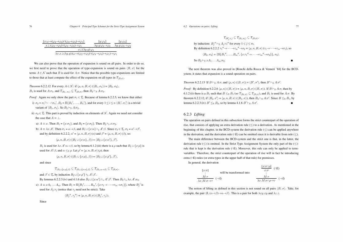
76 Chapter 6 Principal Type Schemes for the Strict Type Assignment System
[x:!$(#2$#2)!(#3$#3)$#1] [y:#2]
"y.y:#2$#2
[y:#3]
"y.y:#3$#3x#:(#2$#2)!(#3$#3)$#1
x#("y.y):#1
"x.x#("y.y):(!$(#2$#2)!(#3$#3)$#1)$#1
We can also prove that the operation of expansion is sound on all pairs. In order to do so,
we first need to prove that the operation of type-expansion is sound on pairs %B, *& for the
terms A+N such that B is used for A:*. Notice that the possible type-expansions are limited
to those that at least compute the effect of the expansion on all types in T$B,%%.
Theorem 6.2.2.12 For every A+N : if %µ,n,B,*& (%B1, *1&) = %B2, *2&,
B1 is used for A:*1, and T$B1, %1% 7 T$B,%%, then B2 !S A:*2.
Proof: Again we only show the part *1 + Ts. Because of lemma 6.2.2.5, we know that either:
i) *2 = *1"!· · ·!*n", B2 = #{B1
", . . . , Bn"}, and for every 1( i(n %Bi
", *i"& is a trivial
variant of %B1, *1&. So B2 !S A:*2.
ii) *2 + Ts. This part is proved by induction on elements of N . Again we need not consider
the case that A 4 #.
a) A 4 x. Then B1 = {x:*1}, and B2 = {x:*2}. Then B2 !s x:*2.
b) A 4 "x.A". Then *1 = $$%, and B1/{x:$} !s A":%. Since *2 + Ts, *2 = $"$%",
and by definition 6.2.2.2, $" = %µ,n,B,*& ($) and %" = %µ,n,B,*& (%), so:
%µ,n,B,*& (%B1 /{x:$}, %&) = %B2/{x:$"}, %"&.
B1 is used for "x.A":$$%, so by lemma 6.1.2 (iii) there is a ) such that B1/ {x:)} is
used for A":%, and $ (S ). Let )" = %µ,n,B,*& ()), then
%µ,n,B,*& (%B1/ {x:)}, %&) = %B2/{x:)"}, %"&,
and since
T$B1({x:)},"% 7 T$B1({x:'},"% 7 T$B1,'&"% 7 T$B,%%,
and %" + Ts, by induction B2/ {x:)"} !s A":%".
By lemmas 6.2.2.3 (iv) and 4.1.6 also B2/{x:$"} !s A":%". Then B2 !s "x.A":*2.
c) A 4 xA1 . . . Am. Then B1 = #{B1", . . . , Bm
", {x:+1$· · ·$+m$*1}}, where Bj" is
used for Aj :+j (notice that +j need not be strict). Take
%Bj"", +j
""& = %µ,n,B,*& (%Bj", +j&).
Since
6.2 Operations on pairs: Lifting 77
T$B!j ,&j%
7 T$B1,%1% 7 T$B,%%,
by induction: Bj"" !S Aj :+i
"" for every 1( j(m.
By definition 6.2.2.2 +1""$· · · $+m
""$*2 = %µ,n,B,*& (+1$· · ·$+m$*1), so
%B2, *2& = %#{B1"", . . . , Bm
"", {x:+1""$· · · $+m
""$*2}}, *2&.
So B2 !S xA1 . . . Am:*2.
The next theorem was also proved in [Ronchi della Rocca & Venneri ’84] for the BCD-
ystem; it states that expansion is a sound operation on pairs.
Theorem 6.2.2.13 If B !S A:*, and %µ,n& (%B, *&) = %B", *"&, then B" !S A:*".
Proof: By definition 6.2.2.6 %µ,n& (%B, *&) = %µ,n,B,*& (%B, *&). If B !S A:*, then by
6.1.2 (ii) there is a B1 such that B (S B1 (so T$B1,%% 7 T$B,%%), and B1 is used for A:*. By
theorem 6.2.2.12, if %B2, *"& = %µ,n,B,*& (%B1, *&), then B2 !S A:*". Since B (S B1, by
lemma 6.2.2.3 (iv) B" (S B2, so by lemma 4.1.6 B" !S A:*".
6.2.3 Lifting
The operation on pairs defined in this subsection forms the strict counterpart of the operation of
rise, that consists of applying an extra derivation rule (() to a derivation. As mentioned in the
beginning of this chapter, in the BCD-system the derivation rule (() can be applied anywhere
in the derivation, and the derivation rule (!E) can be omitted since it is derivable from rule (().
The main difference between the BCD-system and the strict one is that, in the latter, the
derivation rule (() is omitted. In the Strict Type Assignment System the only part of the (()-
rule that is kept is the derivation rule (!E). Moreover, this rule can only be applied to term-
variables. Therefore, the strict counterpart of the operation of rise will in fact be introducing
extra (!E)-rules (or extra types in the upper half of that rule) for premisses.
In general, the derivation
[x:*]:
M :+($I)
"x.M :*$+
will be transformed into:
[x:*!)](!E)
x:*:
M :+($I)
"x.M :*!)$+
The notion of lifting as defined in this section is not sound on all pairs %B, *&. Take, for
example, the pair %0, ($$%)$$$%&. This is a pair for both "xy.xy and "z.z.
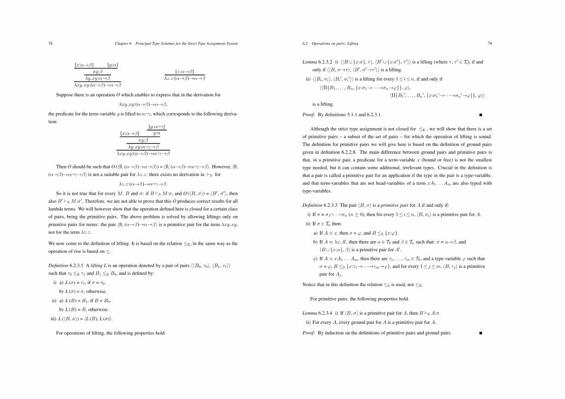
78 Chapter 6 Principal Type Schemes for the Strict Type Assignment System
[x:$$%] [y:$]
xy:%
"y.xy:$$%
"xy.xy:($$%)$$$%
[z:$$%]
"z.z:($$%)$$$%
Suppose there is an operation O which enables to express that in the derivation for
"xy.xy:($$%)$$$%,
the predicate for the term-variable y is lifted to $!&, which corresponds to the following deriva-
tion:[y:$!&]y:$[x:$$%]
xy:%
"y.xy:$!&$%
"xy.xy:($$%)$$!&$%
Then O should be such that O (%0, ($$%)$$$%&) = %0, ($$%)$$!&$%&. However, %0,
($$%)$$!&$%& is not a suitable pair for "z.z: there exists no derivation in !S for
"z.z:($$%)$$!&$%.
So it is not true that for every M , B and *: if B !S M :*, and O (%B, *&) = %B", *"&, then
also B" !S M :*". Therefore, we are not able to prove that this O produces correct results for all
lambda terms. We will however show that the operation defined here is closed for a certain class
of pairs, being the primitive pairs. The above problem is solved by allowing liftings only on
primitive pairs for terms: the pair %0, ($$%)$$$%& is a primitive pair for the term "xy.xy,
not for the term "z.z.
We now come to the definition of lifting. It is based on the relation (E, in the same way as the
operation of rise is based on (.
Definition 6.2.3.1 A lifting L is an operation denoted by a pair of pairs %%B0, +0&, %B1, +1&&
such that +0 (E +1 and B1 (E B0, and is defined by:
i) a) L (*) = +1, if * = +0.
b) L (*) = *, otherwise.
ii) a) L (B) = B1, if B = B0.
b) L (B) = B, otherwise.
iii) L (%B, *&) = %L (B), L (*)&.
For operations of lifting, the following properties hold:
6.2 Operations on pairs: Lifting 79
Lemma 6.2.3.2 i) %%B /{x:*}, +&, %B"/ {x:*"}, + "&& is a lifting (where + , + " + Ts), if and
only if %%B, *$+&, %B", *"$+ "&& is a lifting.
ii) %%Bi, *i&, %Bi", *i
"&& is a lifting for every 1( i(n, if and only if
%%#{B1, . . . , Bn, {x:*1$· · ·$*n$#}}, #&,
%#{B1", . . . , Bn
", {x:*1"$· · ·$*n
"$#}}, #&&
is a lifting.
Proof: By definitions 5.1.1 and 6.2.3.1.
Although the strict type assignment is not closed for (E , we will show that there is a set
of primitive pairs – a subset of the set of pairs – for which the operation of lifting is sound.
The definition for primitive pairs we will give here is based on the definition of ground pairs
given in definition 6.2.2.8. The main difference between ground pairs and primitive pairs is
that, in a primitive pair, a predicate for a term-variable x (bound or free) is not the smallest
type needed, but it can contain some additional, irrelevant types. Crucial in the definition is
that a pair is called a primitive pair for an application if the type in the pair is a type-variable,
and that term-variables that are not head-variables of a term xA1 . . . Am are also typed with
type-variables.
Definition 6.2.3.3 The pair %B, *& is a primitive pair for A if and only if:
i) If * = *1!· · ·!*n (n 1 0), then for every 1( i(n, %B, *i& is a primitive pair for A.
ii) If * + Ts, then:
a) If A 4 x, then * = #, and B (S {x:#}.
b) If A 4 "x.A", then there are $ + TS and % + Ts, such that: * = $$%, and
%B /{x:$}, %& is a primitive pair for A".
c) If A 4 xA1 . . . Am, then there are +1, . . . , +m + TS, and a type-variable # such that
* = #, B (S {x:+1$· · ·$+m$#}, and for every 1( j(m, %B, +j& is a primitive
pair for Aj .
Notice that in this definition the relation (S is used, not (E.
For primitive pairs, the following properties hold.
Lemma 6.2.3.4 i) If %B, *& is a primitive pair for A, then B !S A:*.
ii) For every A, every ground pair for A is a primitive pair for A.
Proof: By induction on the definitions of primitive pairs and ground pairs.
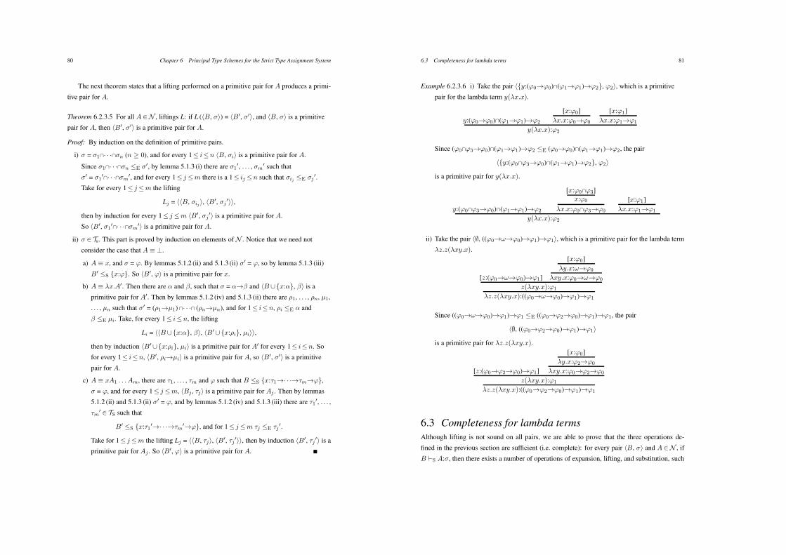
80 Chapter 6 Principal Type Schemes for the Strict Type Assignment System
The next theorem states that a lifting performed on a primitive pair for A produces a primi-
tive pair for A.
Theorem 6.2.3.5 For all A +N , liftings L: if L (%B, *&) = %B", *"&, and %B, *& is a primitive
pair for A, then %B", *"& is a primitive pair for A.
Proof: By induction on the definition of primitive pairs.
i) * = *1!· · ·!*n (n 1 0), and for every 1( i(n %B, *i& is a primitive pair for A.
Since *1!· · ·!*n (E *", by lemma 5.1.3 (i) there are *1", . . . , *m
" such that
*" = *1"!· · ·!*m", and for every 1( j(m there is a 1( ij (n such that *ij (E *j
".
Take for every 1( j(m the lifting
Lj = %%B, *ij&, %B", *j
"&&,
then by induction for every 1( j(m %B", *j"& is a primitive pair for A.
So %B", *1"!· · ·!*m"& is a primitive pair for A.
ii) * + Ts. This part is proved by induction on elements of N . Notice that we need not
consider the case that A 4 #.
a) A 4 x, and * = #. By lemmas 5.1.2 (ii) and 5.1.3 (ii) *" = #, so by lemma 5.1.3 (iii)
B" (S {x:#}. So %B", #& is a primitive pair for x.
b) A 4 "x.A". Then there are $ and %, such that * = $$% and %B /{x:$}, %& is a
primitive pair for A". Then by lemmas 5.1.2 (iv) and 5.1.3 (ii) there are )1, . . . , )n, µ1,
. . . , µn such that *" = ()1$µ1)!· · ·! ()n$µn), and for 1( i(n, )i (E $ and
% (E µi. Take, for every 1( i(n, the lifting
Li = %%B/ {x:$}, %&, %B"/{x:)i}, µi&&,
then by induction %B"/{x:)i}, µi& is a primitive pair for A" for every 1( i(n. So
for every 1( i(n, %B", )i$µi& is a primitive pair for A, so %B", *"& is a primitive
pair for A.
c) A 4 xA1 . . . Am, there are +1, . . . , +m and # such that B (S {x:+1$· · ·$+m$#},
* = #, and for every 1( j(m, %Bj , +j& is a primitive pair for Aj . Then by lemmas
5.1.2 (ii) and 5.1.3 (ii) *" = #, and by lemmas 5.1.2 (iv) and 5.1.3 (iii) there are +1", . . . ,
+m" + TS such that
B" (S {x:+1"$· · ·$+m
"$#}, and for 1( j(m +j (E +j".
Take for 1( j(m the lifting Lj = %%B, +j&, %B", +j"&&, then by induction %B", +j
"& is a
primitive pair for Aj . So %B", #& is a primitive pair for A.
6.3 Completeness for lambda terms 81
Example 6.2.3.6 i) Take the pair %{y:(#0$#0)!(#1$#1)$#2}, #2&, which is a primitive
pair for the lambda term y("x.x).
[x:#0]
"x.x:#0$#0
[x:#1]
"x.x:#1$#1y:(#0$#0)!(#1$#1)$#2
y("x.x):#2
Since (#0!#3$#0)!(#1$#1)$#2 (E (#0$#0)!(#1$#1)$#2, the pair
%{y:(#0!#3$#0)!(#1$#1)$#2}, #2&
is a primitive pair for y("x.x).
[x:#0!#3]x:#0
"x.x:#0!#3$#0
[x:#1]
"x.x:#1$#1y:(#0!#3$#0)!(#1$#1)$#2
y("x.x):#2
ii) Take the pair %0, ((#0$!$#0)$#1)$#1&, which is a primitive pair for the lambda term
"z.z("xy.x).
[x:#0]
"y.x:!$#0
"xy.x:#0$!$#0[z:(#0$!$#0)$#1]
z("xy.x):#1
"z.z("xy.x):((#0$!$#0)$#1)$#1
Since ((#0$!$#0)$#1)$#1 (E ((#0$#2$#0)$#1)$#1, the pair
%0, ((#0$#2$#0)$#1)$#1&
is a primitive pair for "z.z("xy.x).
[x:#0]
"y.x:#2$#0
"xy.x:#0$#2$#0[z:(#0$#2$#0)$#1]
z("xy.x):#1
"z.z("xy.x):((#0$#2$#0)$#1)$#1
6.3 Completeness for lambda termsAlthough lifting is not sound on all pairs, we are able to prove that the three operations de-
fined in the previous section are sufficient (i.e. complete): for every pair %B, *& and A +N , if
B !S A:*, then there exists a number of operations of expansion, lifting, and substitution, such
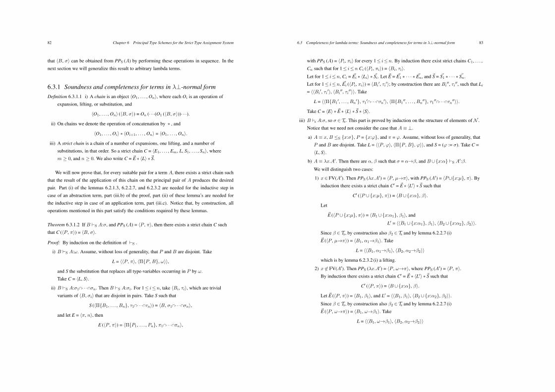
82 Chapter 6 Principal Type Schemes for the Strict Type Assignment System
that %B, *& can be obtained from PPS (A) by performing these operations in sequence. In the
next section we will generalize this result to arbitrary lambda terms.
6.3.1 Soundness and completeness for terms in !#-normal form
Definition 6.3.1.1 i) A chain is an object %O1, . . . , On&, where each Oi is an operation of
expansion, lifting, or substitution, and
%O1, . . . , On& (%B, *&) = On (· · ·(O1 (%B, *&))· · ·).
ii) On chains we denote the operation of concatenation by * , and
%O1, . . . , Oi& * %Oi+1, . . . , On& = %O1, . . . , On&.
iii) A strict chain is a chain of a number of expansions, one lifting, and a number of
substitutions, in that order. So a strict chain C = %E1, . . . , Em, L, S1, . . . , Sn&, where
m 1 0, and n 1 0. We also write C = 1E * %L& *1S.
We will now prove that, for every suitable pair for a term A, there exists a strict chain such
that the result of the application of this chain on the principal pair of A produces the desired
pair. Part (i) of the lemmas 6.2.1.3, 6.2.2.7, and 6.2.3.2 are needed for the inductive step in
case of an abstraction term, part (iii.b) of the proof, part (ii) of these lemma’s are needed for
the inductive step in case of an application term, part (iii.c). Notice that, by construction, all
operations mentioned in this part satisfy the conditions required by these lemmas.
Theorem 6.3.1.2 If B !S A:*, and PPS (A) = %P , ,&, then there exists a strict chain C such
that C (%P , ,&) = %B, *&.
Proof: By induction on the definition of !S .
i) B !S A:!. Assume, without loss of generality, that P and B are disjoint. Take
L = %%P , ,&, %#{P , B}, !&&,
and S the substitution that replaces all type-variables occurring in P by !.
Take C = %L, S&.
ii) B !S A:*1!· · ·!*n. Then B !S A:*i. For 1( i(n, take %Bi, +i&, which are trivial
variants of %B, *i& that are disjoint in pairs. Take S such that
S (%#{B1, . . . , Bn}, +1!· · ·!+n&) = %B, *1!· · ·!*n&,
and let E = %,, n&, then
E (%P , ,&) = %#{P1, . . . , Pn}, ,1!· · ·!,n&,
6.3 Completeness for lambda terms: Soundness and completeness for terms in !#-normal form 83
with PPS (A) = %Pi, ,i& for every 1( i(n. By induction there exist strict chains C1, . . . ,
Cn such that for 1( i(n Ci (%Pi, ,i&) = %Bi, +i&.
Let for 1( i(n, Ci = 1Ei * %Li& * 1Si. Let 1E = 1E1 * · · · * 1En, and 1S = 1S1 * · · · * 1Sn.
Let for 1( i(n, 1Ei (%Pi, ,i&) = %Bi", +i
"&; by construction there are Bi"", +i
"", such that Li
= %%Bi", +i
"&, %Bi"", +i
""&&. Take
L = %%#{B1", . . . , Bn
"}, +1"!· · ·!+n"&, %#{B1
"", . . . , Bn""}, +1
""!· · ·!+n""&&.
Take C = %E& * 1E * %L& *1S * %S&.
iii) B !s A:*, so * + Ts. This part is proved by induction on the structure of elements of N .
Notice that we need not consider the case that A 4 #.
a) A 4 x, B (S {x:*}, P = {x:#}, and , = #. Assume, without loss of generality, that
P and B are disjoint. Take L = %%P , #&, %#{P , B}, #&&, and S = (# := *). Take C =
%L, S&.
b) A 4 "x.A". Then there are $, % such that * = $$%, and B/ {x:$} !S A":%.
We will distinguish two cases:
1) x + FV(A"). Then PPS ("x.A") = %P , µ$,&, with PPS (A") = %P/{x:µ}, ,&. By
induction there exists a strict chain C" = 1E * %L"& *1S such that
C" (%P /{x:µ}, ,&) = %B /{x:$}, %&.
Let
1E (%P /{x:µ}, ,&) = %B1/{x:$1}, %1&, and
L" = %%B1 /{x:$1}, %1&, %B2/{x:$2}, %2&&.
Since % + Ts, by construction also %2 + Ts and by lemma 6.2.2.7 (i)
1E (%P , µ$,&) = %B1, $1$%1&. Take
L = %%B1, $1$%1&, %B2, $2$%2&&
which is by lemma 6.2.3.2 (i) a lifting.
2) x ,+ FV(A"). Then PPS ("x.A") = %P , !$,&, where PPS (A") = %P , ,&.
By induction there exists a strict chain C" = 1E * %L"& *1S such that
C" (%P , ,&) = %B/{x:$}, %&.
Let 1E (%P , ,&) = %B1, %1&, and L" = %%B1, %1&, %B2/ {x:$2}, %2&&.
Since % + Ts, by construction also %2 + Ts and by lemma 6.2.2.7 (i)
1E (%P , !$,&) = %B1, !$%1&. Take
L = %%B1, !$%1&, %B2, $2$%2&&
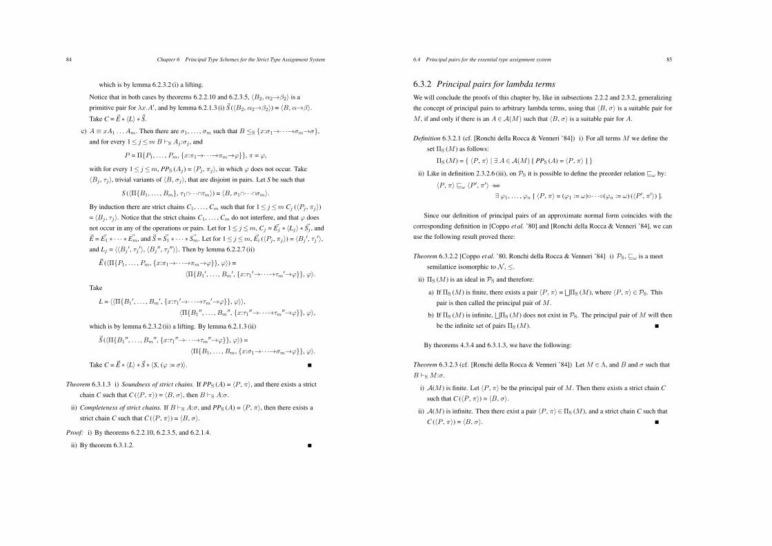
84 Chapter 6 Principal Type Schemes for the Strict Type Assignment System
which is by lemma 6.2.3.2 (i) a lifting.
Notice that in both cases by theorems 6.2.2.10 and 6.2.3.5, %B2, $2$%2& is a
primitive pair for "x.A", and by lemma 6.2.1.3 (i) 1S (%B2, $2$%2&) = %B, $$%&.
Take C = 1E * %L& *1S.
c) A 4 xA1 . . . Am. Then there are *1, . . . , *m such that B (S {x:*1$· · ·$*m$*},
and for every 1( j(mB !S Aj :*j , and
P = #{P1, . . . , Pm, {x:,1$· · ·$,m$#}}, , = #,
with for every 1( j(m, PPS (Aj) = %Pj , ,j&, in which # does not occur. Take
%Bj , +j&, trivial variants of %B, *j&, that are disjoint in pairs. Let S be such that
S (%#{B1, . . . , Bm}, +1!· · ·!+m&) = %B, *1!· · ·!*m&.
By induction there are strict chains C1, . . . , Cm such that for 1( j(m Cj (%Pj , ,j&)
= %Bj , +j&. Notice that the strict chains C1, . . . , Cm do not interfere, and that # does
not occur in any of the operations or pairs. Let for 1( j(m, Cj = 1Ej * %Lj& * 1Sj , and
1E = 1E1 * · · · * 1Em, and 1S = 1S1 * · · · * 1Sm. Let for 1( j(m, 1Ei (%Pj , ,j&) = %Bj", +j
"&,
and Lj = %%Bj", +j
"&, %Bj"", +j
""&&. Then by lemma 6.2.2.7 (ii)
1E (%#{P1, . . . , Pm, {x:,1$· · ·$,m$#}}, #&) =
%#{B1", . . . , Bm
", {x:+1"$· · ·$+m
"$#}}, #&.
Take
L = %%#{B1", . . . , Bm
", {x:+1"$· · ·$+m
"$#}}, #&&,
%#{B1"", . . . , Bm
"", {x:+1""$· · ·$+m
""$#}}, #&,
which is by lemma 6.2.3.2 (ii) a lifting. By lemma 6.2.1.3 (ii)
1S (%#{B1"", . . . , Bm
"", {x:+1""$· · ·$+m
""$#}}, #&) =
%#{B1, . . . , Bm, {x:*1$· · ·$*m$#}}, #&.
Take C = 1E * %L& *1S * %S, (# := *)&.
Theorem 6.3.1.3 i) Soundness of strict chains. If PPS (A) = %P , ,&, and there exists a strict
chain C such that C (%P , ,&) = %B, *&, then B !S A:*.
ii) Completeness of strict chains. If B !S A:*, and PPS (A) = %P , ,&, then there exists a
strict chain C such that C (%P , ,&) = %B, *&.
Proof: i) By theorems 6.2.2.10, 6.2.3.5, and 6.2.1.4.
ii) By theorem 6.3.1.2.
6.4 Principal pairs for the essential type assignment system 85
6.3.2 Principal pairs for lambda terms
We will conclude the proofs of this chapter by, like in subsections 2.2.2 and 2.3.2, generalizing
the concept of principal pairs to arbitrary lambda terms, using that %B, *& is a suitable pair for
M , if and only if there is an A+A(M) such that %B, *& is a suitable pair for A.
Definition 6.3.2.1 (cf. [Ronchi della Rocca & Venneri ’84]) i) For all terms M we define the
set #S (M ) as follows:
#S (M ) = { %P , ,& | 6 A+A(M) [ PPS (A) = %P , ,& ] }
ii) Like in definition 2.3.2.6 (iii), on PS it is possible to define the preorder relation 5! by:
%P , ,& 5! %P ", ,"& 23
6 #1, . . . , #n [ %P , ,& = (#1 := !)-· · ·-(#n := !) (%P ", ,"&) ].
Since our definition of principal pairs of an approximate normal form coincides with the
corresponding definition in [Coppo et al. ’80] and [Ronchi della Rocca & Venneri ’84], we can
use the following result proved there:
Theorem 6.3.2.2 [Coppo et al. ’80, Ronchi della Rocca & Venneri ’84] i) PS, 5! is a meet
semilattice isomorphic to N , (.
ii) #S (M ) is an ideal in PS and therefore:
a) If #S (M ) is finite, there exists a pair %P , ,& =!#S (M ), where %P , ,& +PS. This
pair is then called the principal pair of M .
b) If #S (M ) is infinite,!#S (M ) does not exist in PS. The principal pair of M will then
be the infinite set of pairs #S (M ).
By theorems 4.3.4 and 6.3.1.3, we have the following:
Theorem 6.3.2.3 (cf. [Ronchi della Rocca & Venneri ’84]) Let M +!, and B and * such that
B !S M :*.
i) A(M ) is finite. Let %P , ,& be the principal pair of M . Then there exists a strict chain C
such that C (%P , ,&) = %B, *&.
ii) A(M ) is infinite. Then there exist a pair %P , ,& +#S (M ), and a strict chain C such that
C (%P , ,&) = %B, *&.
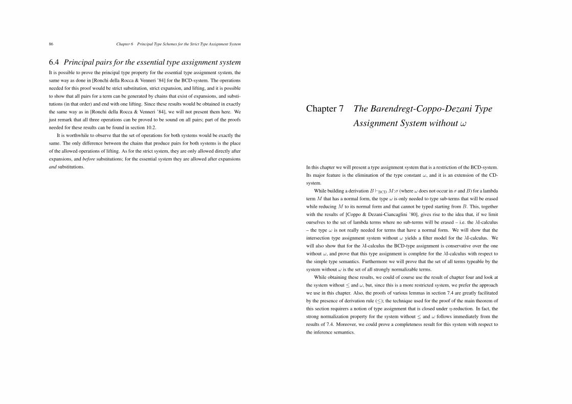
86 Chapter 6 Principal Type Schemes for the Strict Type Assignment System
6.4 Principal pairs for the essential type assignment systemIt is possible to prove the principal type property for the essential type assignment system, the
same way as done in [Ronchi della Rocca & Venneri ’84] for the BCD-system. The operations
needed for this proof would be strict substitution, strict expansion, and lifting, and it is possible
to show that all pairs for a term can be generated by chains that exist of expansions, and substi-
tutions (in that order) and end with one lifting. Since these results would be obtained in exactly
the same way as in [Ronchi della Rocca & Venneri ’84], we will not present them here. We
just remark that all three operations can be proved to be sound on all pairs; part of the proofs
needed for these results can be found in section 10.2.
It is worthwhile to observe that the set of operations for both systems would be exactly the
same. The only difference between the chains that produce pairs for both systems is the place
of the allowed operations of lifting. As for the strict system, they are only allowed directly after
expansions, and before substitutions; for the essential system they are allowed after expansions
and substitutions.
Chapter 7 The Barendregt-Coppo-Dezani Type
Assignment System without "
In this chapter we will present a type assignment system that is a restriction of the BCD-system.
Its major feature is the elimination of the type constant !, and it is an extension of the CD-
system.
While building a derivation B !BCD M :* (where ! does not occur in * and B) for a lambda
term M that has a normal form, the type ! is only needed to type sub-terms that will be erased
while reducing M to its normal form and that cannot be typed starting from B. This, together
with the results of [Coppo & Dezani-Ciancaglini ’80], gives rise to the idea that, if we limit
ourselves to the set of lambda terms where no sub-terms will be erased – i.e. the "I-calculus
– the type ! is not really needed for terms that have a normal form. We will show that the
intersection type assignment system without ! yields a filter model for the "I-calculus. We
will also show that for the "I-calculus the BCD-type assignment is conservative over the one
without !, and prove that this type assignment is complete for the "I-calculus with respect to
the simple type semantics. Furthermore we will prove that the set of all terms typeable by the
system without ! is the set of all strongly normalizable terms.
While obtaining these results, we could of course use the result of chapter four and look at
the system without ( and !, but, since this is a more restricted system, we prefer the approach
we use in this chapter. Also, the proofs of various lemmas in section 7.4 are greatly facilitated
by the presence of derivation rule ((); the technique used for the proof of the main theorem of
this section requirers a notion of type assignment that is closed under (-reduction. In fact, the
strong normalization property for the system without ( and ! follows immediately from the
results of 7.4. Moreover, we could prove a completeness result for this system with respect to
the inference semantics.
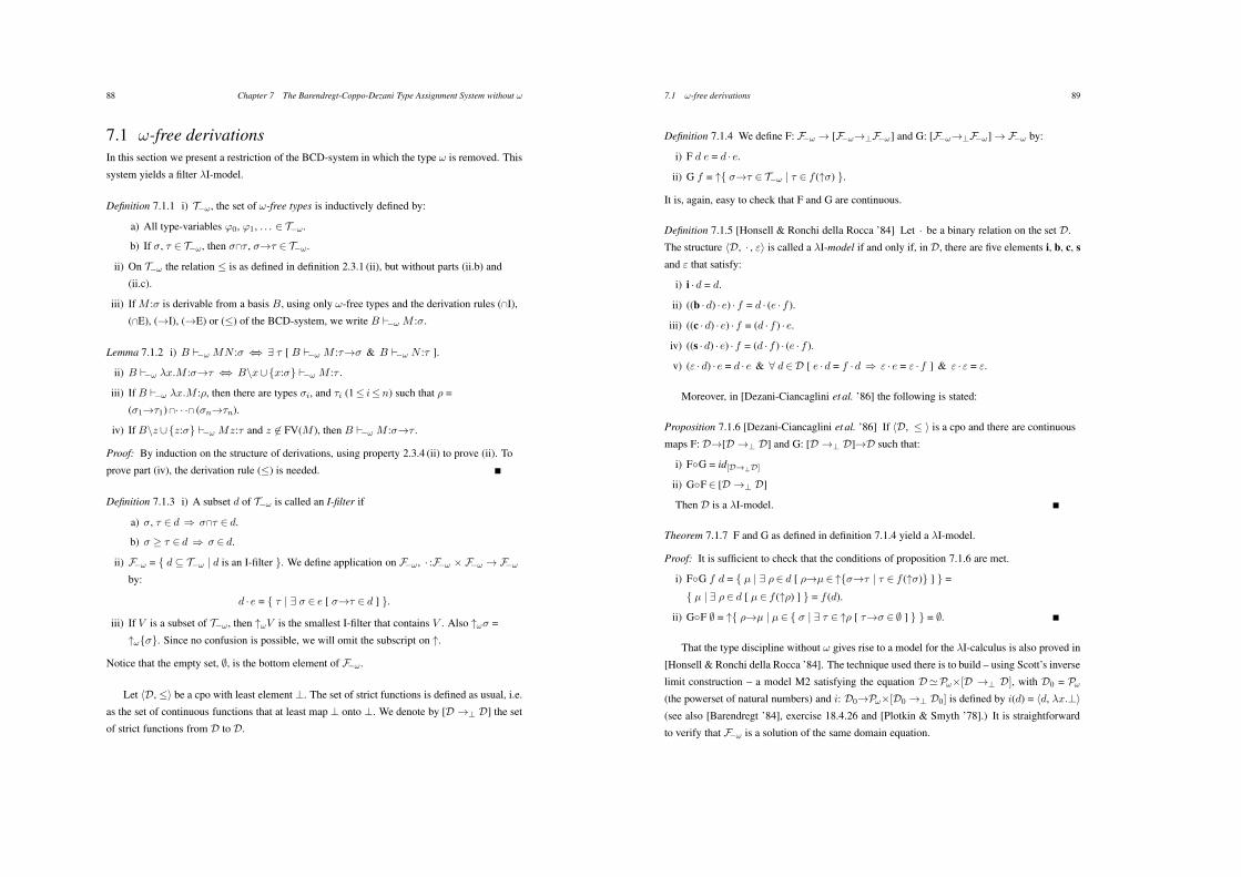
88 Chapter 7 The Barendregt-Coppo-Dezani Type Assignment System without "
7.1 "-free derivationsIn this section we present a restriction of the BCD-system in which the type ! is removed. This
system yields a filter "I-model.
Definition 7.1.1 i) T!!, the set of !-free types is inductively defined by:
a) All type-variables #0, #1, . . . + T!!.
b) If *, + + T!!, then *!+ , *$+ + T!!.
ii) On T!! the relation ( is as defined in definition 2.3.1 (ii), but without parts (ii.b) and
(ii.c).
iii) If M :* is derivable from a basis B, using only !-free types and the derivation rules (!I),
(!E), ($I), ($E) or (() of the BCD-system, we write B !!! M :*.
Lemma 7.1.2 i) B !!! MN :* 23 6 + [ B !!! M :+$* & B !!! N :+ ].
ii) B !!! "x.M :*$+ 23 B\x/{x:*} !!! M :+ .
iii) If B !!! "x.M :), then there are types *i, and +i (1( i(n) such that ) =
(*1$+1)!· · ·! (*n$+n).
iv) If B\z/{z:*} !!! Mz:+ and z ,+ FV(M ), then B !!! M :*$+ .
Proof: By induction on the structure of derivations, using property 2.3.4 (ii) to prove (ii). To
prove part (iv), the derivation rule (() is needed.
Definition 7.1.3 i) A subset d of T!! is called an I-filter if
a) *, + + d 3 *!+ + d.
b) * 1 + + d 3 * + d.
ii) F!! = { d 7 T!! | d is an I-filter }. We define application on F!!, · :F!! . F!! $ F!!
by:
d · e = { + | 6 * + e [ *$+ + d ] }.
iii) If V is a subset of T!!, then 9!V is the smallest I-filter that contains V . Also 9!* =
9!{*}. Since no confusion is possible, we will omit the subscript on 9.
Notice that the empty set, 0, is the bottom element of F!!.
Let %D, (& be a cpo with least element #. The set of strict functions is defined as usual, i.e.
as the set of continuous functions that at least map # onto #. We denote by [D $# D] the set
of strict functions from D to D.
7.1 "-free derivations 89
Definition 7.1.4 We define F: F!! $ [F!!$#F!!] and G: [F!!$#F!!] $ F!! by:
i) F d e = d · e.
ii) G f = 9{ *$+ + T!! | + + f (9*) }.
It is, again, easy to check that F and G are continuous.
Definition 7.1.5 [Honsell & Ronchi della Rocca ’84] Let · be a binary relation on the set D.
The structure %D, · , /& is called a "I-model if and only if, in D, there are five elements i, b, c, s
and / that satisfy:
i) i ·d = d.
ii) ((b ·d) · e) · f = d · (e · f ).
iii) ((c ·d) · e) · f = (d · f ) · e.
iv) ((s ·d) · e) · f = (d · f ) · (e · f ).
v) (/ ·d) · e = d · e & ' d +D [ e ·d = f ·d 3 / · e = / · f ] & / · / = /.
Moreover, in [Dezani-Ciancaglini et al. ’86] the following is stated:
Proposition 7.1.6 [Dezani-Ciancaglini et al. ’86] If %D, ( & is a cpo and there are continuous
maps F: D$[D $# D] and G: [D $# D]$D such that:
i) F-G = id[D&"D]
ii) G-F + [D $# D]
Then D is a "I-model.
Theorem 7.1.7 F and G as defined in definition 7.1.4 yield a "I-model.
Proof: It is sufficient to check that the conditions of proposition 7.1.6 are met.
i) F-G f d = { µ | 6 )+ d [ )$µ + 9{*$+ | + + f (9*)} ] } =
{ µ | 6 )+ d [ µ + f (9)) ] } = f (d).
ii) G-F 0 = 9{ )$µ | µ + { * | 6 + + 9) [ +$* + 0 ] } } = 0.
That the type discipline without ! gives rise to a model for the "I-calculus is also proved in
[Honsell & Ronchi della Rocca ’84]. The technique used there is to build – using Scott’s inverse
limit construction – a model M2 satisfying the equation D;P!.[D $# D], with D0 = P!
(the powerset of natural numbers) and i: D0$P!.[D0 $# D0] is defined by i(d) = %d, "x.#&
(see also [Barendregt ’84], exercise 18.4.26 and [Plotkin & Smyth ’78].) It is straightforward
to verify that F!! is a solution of the same domain equation.
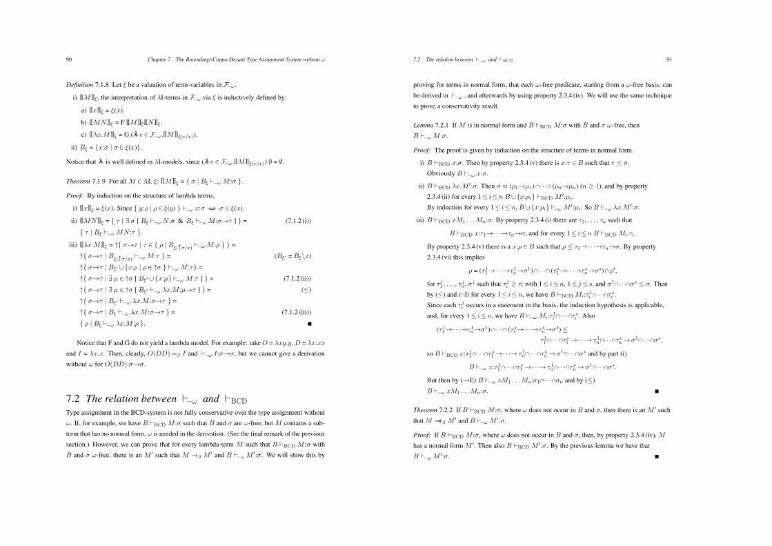
90 Chapter 7 The Barendregt-Coppo-Dezani Type Assignment System without "
Definition 7.1.8 Let . be a valuation of term-variables in F!! .
i) [[M ]]$ , the interpretation of "I-terms in F!! via . is inductively defined by:
a) [[x]]$ = .(x).
b) [[MN ]]$ = F [[M ]]$[[N ]]$ .
c) [["x.M ]]$ = G ("" v +F!! .[[M ]]$(v/x)).
ii) B$ = {x:* | * + .(x)}.
Notice that "" is well defined in "I-models, since ("" v +F!!.[[M ]]$(v/x)) 0 = 0.
Theorem 7.1.9 For all M +!I, .: [[M ]]$ = { * | B$ !!! M :* }.
Proof: By induction on the structure of lambda terms.
i) [[x]]$ = .(x). Since { y:) | ) + .(y) } !!! x:* 23 * + .(x).
ii) [[MN ]]$ = { + | 6 * [ B$ !!! N :* & B$ !!! M :*$+ ] } = (7.1.2 (i))
{ + | B$ !!! MN :+ }.
iii) [["x.M ]]$ = 9{ *$+ | + + { ) | B$(9%/x) !!! M :) } } =
9{ *$+ | B$(9%/x) !!! M :+ } = (B$! = B$\x)
9{ *$+ | B$! /{x:) | )+ 9* } !!! M :+} =
9{ *$+ | 6 µ + 9* [ B$! / {x:µ} !!! M :+ ] } = (7.1.2 (ii))
9{ *$+ | 6 µ + 9* [ B$! !!! "x.M :µ$+ ] } = (()
9{ *$+ | B$! !!! "x.M :*$+ } =
9{ *$+ | B$ !!! "x.M :*$+ } = (7.1.2 (iii))
{ ) | B$ !!! "x.M :) }.
Notice that F and G do not yield a lambda model. For example: take O = "xy.y, D = "x.xx
and I = "x.x. Then, clearly, O(DD) =" I and !!! I:*$*, but we cannot give a derivation
without ! for O(DD):*$*.
7.2 The relation between !"" and !BCD
Type assignment in the BCD-system is not fully conservative over the type assignment without
!. If, for example, we have B !BCD M :* such that B and * are !-free, but M contains a sub-
term that has no normal form, ! is needed in the derivation. (See the final remark of the previous
section.) However, we can prove that for every lambda-term M such that B !BCD M :* with
B and * !-free, there is an M " such that M $" M " and B !!! M ":*. We will show this by
7.2 The relation between "#! and "BCD 91
proving for terms in normal form, that each !-free predicate, starting from a !-free basis, can
be derived in !!! , and afterwards by using property 2.3.4 (iv). We will use the same technique
to prove a conservativity result.
Lemma 7.2.1 If M is in normal form and B !BCD M :* with B and * !-free, then
B !!! M :*.
Proof: The proof is given by induction on the structure of terms in normal form.
i) B !BCD x:*. Then by property 2.3.4 (v) there is x:+ +B such that + ( *.
Obviously B !!! x:*.
ii) B !BCD "x.M ":*. Then * 4 ()1$µ1)!· · ·! ()n$µn) (n 1 1), and by property
2.3.4 (ii) for every 1( i(n B/{x:)i} !BCD M ":µi.
By induction for every 1( i(n, B /{x:)i} !!! M ":µi. So B !!! "x.M ":*.
iii) B !BCD xM1 . . .Mn:*. By property 2.3.4 (i) there are +1, . . . , +n such that
B !BCD x:+1$· · ·$+n$*, and for every 1( i(n B !BCD Mi:+i.
By property 2.3.4 (v) there is a x:) +B such that ) ( +1$· · ·$+n$*. By property
2.3.4 (vi) this implies
) = (+11$· · ·$+1n$*1)!· · ·! (+ s1$· · ·$+ sn$*s)! )",
for + j1 , . . . , + jn, *j such that + ji 1 +i with 1( i(n, 1( j( s, and *1!· · ·!*s ( *. Then
by (() and (!I) for every 1( i(n, we have B !BCD Mi:+1i !· · ·!+
si .
Since each + ji occurs in a statement in the basis, the induction hypothesis is applicable,
and, for every 1( i(n, we have B !!! Mi:+1i !· · ·!+
si . Also
(+11$· · ·$+1n$*1)!· · ·! (+ s1$· · ·$+ sn$*s) (
+11!· · ·!+s1 $· · ·$ +1n!· · ·!+
sn$*1!· · ·!*s,
so B !BCD x:+11!· · ·!+s1 $· · ·$ +1n!· · ·!+
sn$*1!· · ·!*s and by part (i)
B !!! x:+11!· · ·!+s1 $· · ·$ +1n!· · ·!+
sn$*1!· · ·!*s.
But then by ($E) B !!! xM1 . . .Mn:*1!· · ·!*n and by (()
B !!! xM1 . . .Mn:*.
Theorem 7.2.2 If B !BCD M :*, where ! does not occur in B and *, then there is an M " such
that M $$" M " and B !!! M ":*.
Proof: If B !BCD M :*, where ! does not occur in B and *, then, by property 2.3.4 (iv), M
has a normal form M ". Then also B !BCD M ":*. By the previous lemma we have that
B !!! M ":*.
92 Chapter 7 The Barendregt-Coppo-Dezani Type Assignment System without "
As was remarked in the beginning of this chapter, if we are interested in deriving types
without ! occurrences, the type constant ! will only be needed in the BCD-system to type
sub-terms N of M that will be erased while reducing M . In fact, if there is a type ) such that
B !!! N :), then, even for this N , we would not need !. Unfortunately, there are lambda terms
M that contain a sub-term N that must be typed with ! in B !BCD M :*, even if ! does not
occur in B and *. We can even find strongly normalizable lambda terms that contain such a
sub-term (see also the remark made after lemma 7.4.2). So, to prove theorem 7.2.2 we have to
go down all the way to the set of lambda terms in normal form, since only these do not contain
sub-terms that will be erased.
Theorem 7.2.3 Conservativity. If M is a "I-term and B !BCD M :* where ! does not occur in
B and *, then B !!! M :*.
Proof: If B !BCD M :* and B, * are !-free, then, by property 2.3.4 (iv), M has a normal
form M ". Then, also, B !BCD M ":*. By lemma 7.2.1 we have B !!! M ":*. Because M and
M " are "I-terms, by corollary 7.4.3 we obtain B !!! M :*.
7.3 The type assignment without " is complete for the !I-
calculusIn this section, completeness of type assignment without ! for the "I-calculus will be proved
using the method of [Barendregt et al. ’83]. The notions of type interpretation as defined in
definition 2.3.1.2 lead also for the "I-calculus in a natural way to the following definitions for
semantic satisfiability.
Definition 7.3.1 As in definition 2.3.1.3, we define !! by: (where M is a "I-model, . a
valuation and - a type interpretation)
i) M, ., - !!M :* 23 [[M ]]M$ + -(*).
ii) M, ., - !! B 23 M, ., - !! x:* for every x:* +B.
iii) a) B !! M :* 23 'M, ., - [ M, ., - !! B 3 M, ., - !! M :* ].
b) B !!s M :* 23
'M, ., simple type interpretations - [ M, ., - !! B 3 M, ., - !!M :* ].
c) B !!F M :* 23 'M, ., F type interpretations - [ M, ., - !! B 3 M, ., - !! M :* ].
7.4 Strong normalization result for the system without " 93
We will only consider the simple type semantics, since !!! is not sound for all type inter-
pretations. For example: {y:(#1!#2$#3)$#4, x:#1$#3} !!! yx:#4, but this is not seman-
tically valid for all type interpretations.
Theorem 7.3.2 Soundness. If B !!! M :* then B !!s M :*.
Proof: By induction on the structure of derivations.
Definition 7.3.3 i) We define a map -1 : T!! $ 0(F!!) by -1 (*) = { d +F!! | * + d }.
ii) .B(x) = { * + T!! | B !!! x:* }.
Theorem 7.3.4 i) The map -1 is a simple type interpretation.
ii) B !!! M :* 23 B$B !!! M :*.
iii) F!!, .B, -1 !!s B.
Proof: i) Easy.
ii) Because for every x, .B(x) is an I-filter.
iii) x:* +B 3 * + { + | B$B !!! x:+ } 3 * + [[x]]$B .
So [[x]]$B + { d+F!! | * + d }.
Theorem 7.3.5 Completeness. Let M be a "I-term, and suppose ! does not occur in B and *.
If B !!s M :*, then B !!! M :*.
Proof: B !!s M :* 3 (7.3.1 (iii.b), 7.3.4 (i) & 7.3.4 (iii))
F!!, .B, -1 !!s M :* 3 (7.3.1 (i) & 7.3.4 (i))
[[M ]]$B + -1 (*) 3 (7.3.3 (i))
* + [[M ]]$B 3 (7.1.9)
B$B !!! M :* 3 (7.3.4 (ii))
B !!! M :*.
7.4 Strong normalization result for the system without "In this section, we show that the set of lambda terms typeable by means of the derivation rules
(!I), (!E), ($I) and ($E) of the BCD-system is exactly the set of strongly normalizable terms.
The same result was presented in [Coppo et al. ’81], [Leivant ’83] and [Pottinger ’80]. However,
the proof in [Leivant ’83] was too brief, the proof in [Pottinger ’80] gave few details and the
94 Chapter 7 The Barendregt-Coppo-Dezani Type Assignment System without "
proof in [Coppo et al. ’81] was not complete. In this section, we will present a complete and
formal proof. The same result has also been proved in [Krivine ’90], using the technique of
saturated sets.
In order to prove that each term typeable by the rules (!I), (!E), ($I) and ($E) is strongly
normalizable, we will prove even more: we will show that if B !!! M :* (i.e. using derivation
rule (() as well), then M is strongly normalizable. In [Ronchi della Rocca ’88], a similar
result was proved: B !!! M :* 23 M is strongly normalizable. In this paper, this result was
given in corollary 6.3 and was obtained from the theorem that the procedure PP’ (as defined in
[Ronchi della Rocca ’88], section 6) finds a principal pair for all and nothing but the strongly
normalizable terms. In this section, we will present a proof for the same result, different from
the one given in [Ronchi della Rocca ’88]. The proof that all strongly normalizable terms are
typeable in the system without ! and (() will be given in theorem 7.4.4.
Notice that an I-filter can be empty. A direct result of the main theorem of this section
will be that [[· · ·]] as defined in definition 7.1.8 will map all unsolvable terms onto the empty
filter (‘unsolvable’ in the "I-calculus equals to ‘not having a normal form,’ as well as that
‘normalizable’ and ‘strongly normalizable’ coincide).
Notice, also, that we no longer restrict ourselves to the "I-terms, but prove the statement for
the full "K-calculus.
Fact 7.4.1 In the sequel, we will accept the following without proof:
i) If xM1 . . .Mn and N are strongly normalizable, then so is xM1 . . .MnN .
ii) If Mz is strongly normalizable (where z does not occur free in M ), then so is M .
iii) If M [x := N ] and N are strongly normalizable, then so is ("x.M)N .
Lemma 7.4.2 If B !!! C[M [x := N ]]:+ and B !!! N :), then B !!! C[("x.M)N ]:+ ,
where C[· · ·] is the notation for a context.
Proof: By induction on the structure of contexts. We will omit the case that the context is an
application, since it is trivial.
i) C[M [x := N ]] 4M [x := N ]. We can assume that x does not occur in B.
a) N occurs n times in M [x := N ], each time typed by, say, *i.
B !!! M [x := N ]:+ 3
B/{x:*1!· · ·!*n} !!! M :+ & B !!! N :*1!· · ·!*n 3
B !!! "x.M :*1!· · ·!*n$+ & B !!! N :*1!· · ·!*n 3
B !!! ("x.M)N :+ .
7.4 Strong normalization result for the system without " 95
b) N does not occur in M [x := N ], so x ,+ FV(M ).
B !!! M :+ & B !!! N :) 3 (x ,+ FV(M ))
B/{x:)} !!! M :+ & B !!! N :) 3
B !!! "x.M :)$+ & B !!! N :) 3
B !!! ("x.M)N :+ .
ii) B !!! "y.C[M [x := N ]]:+ & B !!! N :) 3 (7.1.2 (ii) & (iii))
6 )1, . . . , )n, µ1, . . . , µn [ + = ()1$µ1) !· · ·! ()n$µn) &
' 1( i(n [ B/{y:)i} !!! C[M [x := N ]]:µi ] ] & B !!! N :) 3 (IH)
6 )1, . . . , )n, µ1, . . . , µn [ + = ()1$µ1) !· · ·! ()n$µn) &
' 1( i(n [ B/{y:)i} !!! C[("x.M)N ]:µi ] ] 3
B !!! "y.C[("x.M)N ]:+ .
Notice that the condition B !!! N :) in the formulation of the lemma is essential. As a
counter example, take the two lambda terms "yz.("b.z)(yz) and "yz.z. Notice that the first
strongly reduces to the latter. We know that
{z:*, y:+} !!! z:*,
but it is impossible to give a derivation for ("b.z)(yz):* from the same basis without using !.
This is caused by the fact that we can only type ("b.z)(yz) in the system without ! from a basis
in which the predicate for y is an arrow type scheme. We can, for example, derive
{z:*, y:*$+} !!! ("b.z)(yz):*.
We can therefore only state that we can derive
!!! "yz.("b.z)(yz):(*$+ )$*$* and !!! "yz.z:+$*$*
but that we are not able to give a derivation without ! for the statement
"yz.("b.z)(yz):+$*$*.
So the type assignment without ! is not closed for %-equality, but of course this is not
imperative. We only want to be able to derive a type for each strongly normalizable term,
no matter what basis or type is used. Notice that, for the "I-calculus, part 7.4.2 (i.b) is not
applicable and the condition B !!! N :) is not needed. So, the following is an immediate
result:
Corollary 7.4.3 Let M and M " be "I-terms, such that M $$" M ", and there are B and * such
that B !!! M ":*. Then B !!! M :*.
96 Chapter 7 The Barendregt-Coppo-Dezani Type Assignment System without "
Lemma 7.4.2 is also essentially the proof for the statement that each strongly normalizable
term can be typed in the system !!! .
Theorem 7.4.4 If M is strongly normalizable, then there are B and * such that B !!! M :*
and in this derivation the rule (() is not used.
Proof: If M is strongly normalizable, then the normal form of M will be reached using the
inside-out reduction strategy (see [Barendregt ’84].14.2.11). This strategy has the special
property that a redex ("x.M)N can only be contracted if N is in normal form. The proof is
completed by induction on the inside-out reduction path, using lemma 7.4.2 and theorem
4.2.10.
In order to prove that each term typeable in !!! is strongly normalizable, we will introduce
a notion of computability. We will abbreviate ‘M is strongly normalizable’ by SN(M ).
Definition 7.4.5 (cf. [Pottinger ’80]) Comp (B, M , )) is inductively defined by:
i) Comp (B, M , #) 23 B !!! M :# & SN(M ).
ii) Comp (B, M , *$+ ) 23 (Comp (B", N , *) 3 Comp (B /B", MN , + )).
iii) Comp (B, M , *!+ ) 23 (Comp (B, M , *) & Comp (B, M , + )).
Lemma 7.4.6 Take *, and + such that * ( + . Then Comp (B, M , *) 3 Comp (B, M , + ).
Proof: By straightforward induction on the definition of (.
Theorem 7.4.7 i) B !!! xM1 . . .Mn:) & SN(xM1 . . .Mn) 3 Comp (B, xM1 . . .Mn, )).
ii) Comp (B, M , )) 3 B !!! M :) & SN(M ).
Proof: Simultaneously by induction on the structure of types. The only interesting case is
when ) = *$+ ; the other cases are dealt with by induction.
i) B !!! xM1 . . .Mn:*$+ & SN(xM1 . . .Mn) 3 ((ii))
(Comp (B", N , *) 3
B !!! xM1 . . .Mn:*$+ & SN(xM1 . . .Mn) & B" !!! N :* & SN(N )) 3
(7.4.1 (i))
(Comp (B", N , *) 3 B/B" !!! xM1 . . .MnN :+ & SN(xM1 . . .MnN )) 3
(IH)
(Comp (B", N , *) 3 Comp (B /B", xM1 . . .MnN , + )) 3 (7.4.5 (ii))
Comp (B, xM1 . . .Mn, *$+ ).
7.4 Strong normalization result for the system without " 97
ii) Comp (B, M , *$+ ) & z ,+ FV(M ) 3 ((i))
Comp (B, M , *$+ ) & Comp ({z:*}, z, *) & z ,+ FV(M ) 3 (7.4.5 (ii))
Comp (B/{z:*}, Mz, + ) & z ,+ FV(M ) 3 (IH)
B/{z:*} !!! Mz:+ & SN(Mz) & z ,+ FV(M ) 3 (7.1.2 (iv) & 7.4.1 (ii))
B !!! M :*$+ & SN(M ).
Lemma 7.4.8 Comp (B/B", C[M [x := N ]], *) & Comp (B", N , )) 3
Comp (B/B", C[("x.M)N ], *).
Proof: By induction on the structure of types. We will only consider the case that * is a
type-variable:
Comp (B/B", C[M [x := N ]], #) & Comp (B", N , )) 3 (7.4.7 (ii))
B/B" !!! C[M [x := N ]]:# & SN(C[M [x := N ]]) & B" !!! N :) & SN(N ) 3
(7.4.2 & 7.4.1 (iii))
B/B" !!! C[("x.M)N ]:# & SN(C[("x.M)N ]) 3 (7.4.5 (i))
Comp (B/B", C[("x.M)N ], #).
Theorem 7.4.9 If B = {x1:µ1, . . . , xn:µn} and for every 1( i(n Comp (Bi, Ni, µi) and
B !!! M :*, then Comp (B1/ · · ·/Bn, M [x1 := N1, . . . , xn := Nn], *).
Proof: By induction on the structure of derivations. We will only show the non-trivial parts.
i) ($I). Then M 4 "y.M ", * = )$+ , and B/ {y:)} !!! M ":+ .
B = {x1:µ1, . . . , xn:µn} &
' 1( i(n [Comp (Bi, Ni, µi)] & B/{y:)} !!! M ":+ 3 (IH)
(Comp (B", N , )) 3
Comp (B1/· · ·/Bn/B", M "[x1 := N1, . . . , xn := Nn, y := N ], + )) 3 (7.4.8)
(Comp (B", N , )) 3
Comp (B1/· · ·/Bn/B", ("y.M "[x1 := N1, . . . , xn := Nn])N , + )) 3
(7.4.5 (ii))
Comp (B1/· · ·/Bn, ("y.M ")[x1 := N1, . . . , xn := Nn], )$+ ).
ii) ($E). Then M 4M1M2, B !!! M1:)$+ and B !!! M2:).
B = {x1:µ1, . . . , xn:µn} & ' 1( i(n [Comp (Bi, Ni, µi)] &
B !!! M1:)$+ & B !!! M2:) 3 (IH)
Comp (B1/· · ·/Bn, M1[x1 := N1, . . . , xn := Nn], )$+ ) &
Comp (B1/· · ·/Bn, M2[x1 := N1, . . . , xn := Nn], )) 3 (7.4.5 (ii))
Comp (B1/· · ·/Bn, (M1M2)[x1 := N1, . . . , xn := Nn], + ).
98 Chapter 7 The Barendregt-Coppo-Dezani Type Assignment System without "
Theorem 7.4.10 If B !!! M :*, then SN(M ).
Proof: B !!! M :* 3 (7.4.9) Comp (B, M , *) 3 (7.4.7 (ii)) SN(M ).
We can now prove the main theorem of this section.
Theorem 7.4.11 {M | M is typeable by means of the derivation rules (!I), (!E), ($I) and
($E)} = {M | M is strongly normalizable}.
Proof: 7 ) If M is typeable by means of the derivation rules (!I), (!E), ($I) and ($E), then
certainly B !!! M :*. Then, by theorem 7.4.10, M is strongly normalizable.
< ) If M is strongly normalizable, then, by theorem 7.4.4, there are B, * such that
B !!! M :*; in this derivation the derivation rule (() is not used.
Chapter 8 The Rank 2 Intersection Type
Assignment System
The notion of type assignment presented in this chapter will be based on the strict type as-
signment system (restricted to intersection types of Rank 2, as suggested by D. Leivant in
[Leivant ’83]), and the CD-system. We will define intersection types of Rank 2, and we will
present two operations on pairs of basis and type, namely Rank 2 substitution and duplication.
We will show that the presented notion of type assignment has the principal type property: for
every typeable term M , there are a basis P and type , such that the pair %P , ,& is the prin-
cipal pair for M , and P !R M :,. We will show that for every basis B and type * such that
B !R M :*, there is a type-chain of operations C (consisting of nothing but substitutions and
duplications) such that C (%P , ,&) = %B, *&. We will obtain this result by defining a unification
algorithm for intersection types of Rank 2; using this algorithm, for every term M we define
the principal pair for M .
The system presented in this chapter is perhaps more general than needed to obtain Rank 2
intersection type assignment for the lambda calculus. For example, the definition of duplication
in definition 8.3.2.1 could be formulated in a slightly simplified way. However, in chapter
twelve we will formulate a notion of type assignment based on the one presented in this chapter,
for which this more general approach is appropriate.
To avoid confusion, we would like to point out that there also exists a notion of type as-
signment that is called the Rank 2 polymorphic type assignment system, defined in [Kfoury &
Tiuryn ’89]. This system is an extension of Milner’s system, by allowing the '-type constructor
to occur on the left hand side of an arrow type as well, instead of only at top level. (It is also
a restriction of the polymorphic type discipline [Girard ’86], in which types are restricted to
polymorphic types of Rank 2.) The definition of types allowed in this system is similar to that
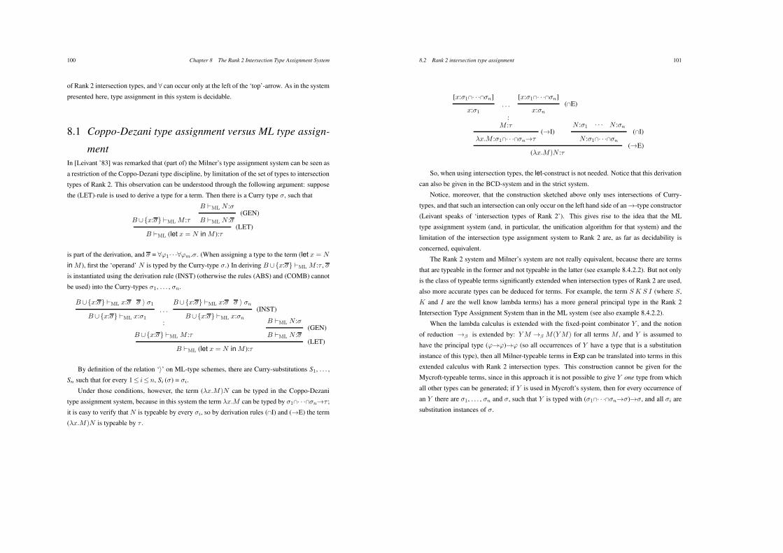
100 Chapter 8 The Rank 2 Intersection Type Assignment System
of Rank 2 intersection types, and ' can occur only at the left of the ‘top’-arrow. As in the system
presented here, type assignment in this system is decidable.
8.1 Coppo-Dezani type assignment versus ML type assign-
mentIn [Leivant ’83] was remarked that (part of) the Milner’s type assignment system can be seen as
a restriction of the Coppo-Dezani type discipline, by limitation of the set of types to intersection
types of Rank 2. This observation can be understood through the following argument: suppose
the (LET)-rule is used to derive a type for a term. Then there is a Curry type *, such that
B /{x:*} !ML M :+
B !ML N :*(GEN)
B !ML N :*(LET)
B !ML (let x = N in M ):+
is part of the derivation, and * = '#1· · ·'#m.*. (When assigning a type to the term (let x = N
in M ), first the ‘operand’ N is typed by the Curry-type *.) In deriving B/{x:*} !ML M :+ , *
is instantiated using the derivation rule (INST) (otherwise the rules (ABS) and (COMB) cannot
be used) into the Curry-types *1, . . . , *n.
B/{x:*} !ML x:* * & *1
B/ {x:*} !ML x:*1· · ·
B/{x:*} !ML x:* * & *n
B/{x:*} !ML x:*n(INST)
:
B/{x:*} !ML M :+
B !ML N :*(GEN)
B !ML N :*(LET)
B !ML (let x = N in M ):+
By definition of the relation ‘&’ on ML-type schemes, there are Curry-substitutions S1, . . . ,
Sn such that for every 1( i(n, Si (*) = *i.
Under those conditions, however, the term ("x.M)N can be typed in the Coppo-Dezani
type assignment system, because in this system the term "x.M can be typed by *1!· · ·!*n$+ ;
it is easy to verify that N is typeable by every *i, so by derivation rules (!I) and ($E) the term
("x.M)N is typeable by + .
8.2 Rank 2 intersection type assignment 101
[x:*1!· · ·!*n]
x:*1· · ·
[x:*1!· · ·!*n](!E)
x:*n:
M :+($I)
"x.M :*1!· · ·!*n$+
N :*1 · · · N :*n(!I)
N :*1!· · ·!*n($E)
("x.M)N :+
So, when using intersection types, the let-construct is not needed. Notice that this derivation
can also be given in the BCD-system and in the strict system.
Notice, moreover, that the construction sketched above only uses intersections of Curry-
types, and that such an intersection can only occur on the left hand side of an $-type constructor
(Leivant speaks of ‘intersection types of Rank 2’). This gives rise to the idea that the ML
type assignment system (and, in particular, the unification algorithm for that system) and the
limitation of the intersection type assignment system to Rank 2 are, as far as decidability is
concerned, equivalent.
The Rank 2 system and Milner’s system are not really equivalent, because there are terms
that are typeable in the former and not typeable in the latter (see example 8.4.2.2). But not only
is the class of typeable terms significantly extended when intersection types of Rank 2 are used,
also more accurate types can be deduced for terms. For example, the term S K S I (where S,
K and I are the well know lambda terms) has a more general principal type in the Rank 2
Intersection Type Assignment System than in the ML system (see also example 8.4.2.2).
When the lambda calculus is extended with the fixed-point combinator Y , and the notion
of reduction $" is extended by: YM $" M(YM) for all terms M , and Y is assumed to
have the principal type (#$#)$# (so all occurrences of Y have a type that is a substitution
instance of this type), then all Milner-typeable terms in Exp can be translated into terms in this
extended calculus with Rank 2 intersection types. This construction cannot be given for the
Mycroft-typeable terms, since in this approach it is not possible to give Y one type from which
all other types can be generated; if Y is used in Mycroft’s system, then for every occurrence of
an Y there are *1, . . . , *n and *, such that Y is typed with (*1!· · ·!*n$*)$*, and all *i are
substitution instances of *.
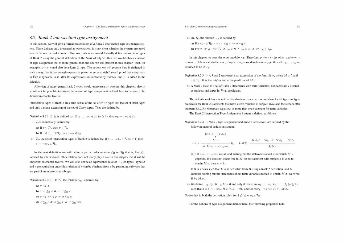
102 Chapter 8 The Rank 2 Intersection Type Assignment System
8.2 Rank 2 intersection type assignmentIn this section, we will give a formal presentation of a Rank 2 intersection type assignment sys-
tem. Since Leivant only presented an observation, it is not clear whether the system presented
here is the one he had in mind. Moreover, when we would formally define intersection types
of Rank 2 using the general definition of the ‘rank of a type’, then we would obtain a notion
of type assignment that is more general than the one we will present in this chapter: then, for
example, !$* would also be a Rank 2 type. The system we will present here is designed in
such a way, that it has enough expressive power to get a straightforward proof that every term
in Exp is typeable in it, after let-expressions are replaced by redexes, and Y is added to the
calculus.
Allowing of more general rank 2 types would unnecessarily obscure this chapter; also, it
would not be possible to extend the notion of type assignment defined here to the one to be
defined in chapter twelve.
Intersection types of Rank 2 are a true subset of the set of BCD-types and the set of strict types
and only a minor extension of the set of Curry-types. They are defined by:
Definition 8.2.1 i) T1 is defined by: If *1, . . . , *n + TC (n 1 1), then *1!· · ·!*n + T1.
ii) T2 is inductively defined by:
a) If * + TC, then * + T2.
b) If * + T1, + + T2, then *$+ + T2.
iii) TR, the set of intersection types of Rank 2 is defined by: if *1, . . . , *n + T2 (n 1 1) then
*1!· · ·!*n + TR.
In the next definition we will define a partial order relation (R on TR that is, like (S,
induced by intersections. This relation does not really play a role in this chapter, but it will be
important in chapter twelve. We will also define an equivalence relation )R on types. Types *
and + are equivalent under this relation, if * can be obtained from + by permuting subtypes that
are part of an intersection subtype.
Definition 8.2.2 i) On TR, the relation (R is defined by:
a) * (R *.
b) *!+ (R * & *!+ (R + .
c) * (R + (R ) 3 * (R ).
d) * (R ) & * (R + 3 * (R )!+ .
8.2 Rank 2 intersection type assignment 103
ii) On TR, the relation )R is defined by:
a) For *, + + TR: * (R + (R * 3 * )R + .
b) For *$+ , )$µ + TR: * )R ) & + )R µ 3 *$+ )R )$µ.
In this chapter we consider types modulo )R. Therefore, )!(*!+ ) = ()!*)!+ , and *$+ =
*!*$+ . Unless stated otherwise, if *1!· · ·!*n is used to denote a type, then all *1, . . . , *n are
assumed to be in T2.
Definition 8.2.3 i) A Rank 2 statement is an expression of the form M :*, where M +! and
* + TR. M is the subject and * the predicate of M :*.
ii) A Rank 2 basis is a set of Rank 2 statements with term-variables, not necessarily distinct,
as subjects and types in TC as predicates.
The definition of bases is not the standard one, since we do not allow for all types in TR as
predicates for Rank 2 statements that have a term-variable as subject. (See also the remark after
theorem 8.4.2.5.) Moreover, we allow of more than one statement for term-variables.
The Rank 2 Intersection Type Assignment System is defined as follows:
Definition 8.2.4 i) Rank 2 type assignment and Rank 2 derivations are defined by the
following natural deduction system:
[x:*1] · · · [x:*n]:
M :+($I): (a)
"x.M :*1!· · ·!*n$+
M :*1!· · ·!*n$+ N :*1 . . . N :*n($E):
MN :+
(a) : If x:*1, . . . , x:*n are all and nothing but the statements about x on which M :+
depends. If x does not occur free in M , so no statement with subject x is used to
obtain M :+ , then n = 1.
If B is a basis such that M :* is derivable from B using a Rank 2 derivation, and B
contains nothing but the statements about term-variables needed to obtain M :*, we write
B !2 M :*.
ii) We define !R by: B !R M :* if and only if: there are *1, . . . , *n, B1, . . . , Bn (n 1 1)
such that * = *1!· · ·!*n, B = B1/· · ·/Bn and for every 1( i(n Bi !2 M :*i.
Notice that in both the derivation rules, for 1( i(n, *i + TC.
For the notions of type assignment defined here, the following properties hold:
104 Chapter 8 The Rank 2 Intersection Type Assignment System
Lemma 8.2.5 i) B !2 "x.M :* 23 6 +1, . . . , +n + TC, + + T2 [ * = +1!· · ·!+n$+ &
( x+ FV(M ) 3 B/{x:+1, . . . , x:+n} !2 M :+ ) &
( x ,+ FV(M ) 3 B !2 M :+ & n = 1 ) ].
ii) B !2 MN :* 23 6 + + T1, B1, B2 [ B1 !2 M :+$* & B2 !R N :+ & B = B1/B2 ].
Proof: Immediately from definition 8.2.4.
Notice that the notion ‘B !2 M :*’ is a more restricted relation between basis, term and
type than in the previous chapters. In these chapters, it was sufficient for a basis to just contain
all types needed in the derivation, while in the Rank 2 intersection system we must require
that a basis contain nothing more than these types. (So for this notion of type assignment, the
definition of ‘B is used for M :*’ would be superfluous.) If we drop this restriction, then we
should also be more permissive in the constraints on derivation rule ($I), and, for example,
allow of derivations for
{x:#1, x:#2} !2 x:#1, and !2 "x.x:#1!#2$#1.
Since it is not possible to derive this last type for "x.x in Milner’s system, we have chosen
not to allow it for the Rank 2 Intersection Type Assignment System. Notice that being more
permissive forces to define an operation of lifting, something not needed in the approach taken
here. In fact this restriction is only needed for the Rank 2 Intersection Type Assignment System
for the lambda calculus. We will drop it in chapter twelve, in which we will extend the system
defined in this chapter to one for Term Rewriting Systems.
8.3 Operations on pairsIn this section we will define two operations on pairs of basis and type, namely substitution and
duplication. In theorem 8.3.3.3 (i) we will prove that these operations are sound, and in theorem
8.4.2.5 we will prove that these are complete (i.e. are sufficient to generate all pairs for a term
from its principal pair).
8.3.1 Rank 2 substitution
In this chapter, substitution will be defined as a Curry-substitution, the operation that replaces
type-variables by elements of TC. Although perhaps this is a more restricted kind of substitution
than could be expected, it is a sound operation and will prove to be sufficient.
8.3 Operations on pairs: Rank 2 substitution 105
Definition 8.3.1.1 i) The Rank 2 substitution (# := $) : TR $ TR, where # is a type-variable
and $+ TC, is defined by:
a) (# := $) (#) = $.
b) (# := $) (#") = #", if # ,= #".
c) (# := $) (*$+ ) = (# := $) (*)$ (# := $) (+ ).
d) (# := $) (*1!· · ·!*n) = (# := $) (*1)!· · ·! (# := $) (*n).
ii) If S1 and S2 are Rank 2 substitutions, then so is S1-S2, where S1-S2 (*) = S1 (S2 (*)).
iii) S (B) = {x:S (*) | x:* +B}.
iv) S (%B, *&) = %S (B), S (*)&.
Substitution is normally defined as the operation that replaces type-variables by types, with-
out restriction. This definition would not be correct for the Rank 2 system, since, for example,
the replacement of the type-variable # in #$# by the type (*$+ )!*$+ would give a type
that is not an element of TR. It is easy to verify that the above defined operation is well defined.
For substitutions, the following properties hold:
Lemma 8.3.1.2 Let S be a Rank 2 substitution. Then:
i) If * (R + , then S (*) (R S (+ ).
ii) If * + TC (T1, T2, TR), then S (*) + TC (T1, T2, TR).
Proof: Easy.
Notice that, because of part (ii) of this lemma, substitution is well defined on bases.
The following theorem will show that substitution is a sound operation.
Theorem 8.3.1.3 Soundness of substitution. If B !R M :*, then for every Rank 2 substitution
S: S (B) !R M :S (*).
Proof: i) * + T2, so B !2 M :*. By induction on the structure of M .
a) M 4 x, so B = {x:*}, and * + TC. Then S (*) + TC, and S (B) !2 x:S (*).
b) M 4 "x.M ". Then by lemma 8.2.5 (i) there are +1, . . . , +n + TC, + + T2 such that
* = +1!· · ·!+n$+ and either
1) x + FV(M ). Then B/{x:+1, . . . , x:+n} !2 M":+ . By induction
S (B/{x:+1, . . . , x:+n}) !2 M":S(+ ),
106 Chapter 8 The Rank 2 Intersection Type Assignment System
so by definition 8.3.1.1 S (B)/{x:S (+1), . . . , x:S (+n)} !2 M":S(+ ), so by lemma
8.2.5 (i) and definition 8.3.1.1 S (B) !2 "x.M :S (*).
2) x ,+ FV(M ). Then B !2 M":+ , and n = 1. By induction S (B) !2 M
":S (+ ), and by
lemma 8.2.5 (i) S (B) !2 "x.M":S (+1)$ S (+ ), so by definition 8.3.1.1
S (B) !2 "x.M :S (*).
c) M 4M1M2. By lemma 8.2.5 (ii) there are B1, B2 and + + T1, such that:
B = B1/B2, B1 !2 M1:+$*, and B2 !R M2:+ .
Then S (B) = S (B1)/S (B2), and by lemma 8.3.1.2 (ii) S (+ ) + T1, and since S (+$*)
= S (+ )$ S (*), also by induction:
S (B1) !2 M1:S (+ )$ S (*) and S (B2) !R M2:S (+ ).
Then by lemma 8.2.5 (ii) S (B) !2 M1M2:S (*).
ii) * + TR. Then by definition 8.2.4 (ii) there are *1, . . . , *n, B1, . . . , Bn (n 1 1) such that
* = *1!· · ·!*n, and B = B1/· · ·/Bn and for every 1( i(n Bi !2 M :*i.
Then S (B) = S (B1)/ · · ·/S (Bn), and by induction for 1( i(n S (Bi) !2 M :S (*i).
Again by definition 8.2.4 (ii) we have S (B) !2 M :S (*).
8.3.2 Duplication
We now come to the definition of duplication. It can be seen as a very simple version of the
various operations of expansion as defined before; duplication is a total expansion, that is not
‘computed’: all type-variables occurring in basis and type are copied.
Definition 8.3.2.1 Let B be a basis, * + TR, and n 1 1. The triple %n, B, *& determines a
duplication D$n,B,%% : TR $ TR, which is constructed as follows:
i) a) Suppose V = {#1, . . . , #m} is the set of all type-variables occurring in %B, *&. Choose
m. n different type-variables #11, . . . , #n
1 , . . . , #1m, . . . , #n
m, such that each #ij
(1( i(n, 1( j(m) does not occur in V. Let Si be the substitution that replaces
every #j by #ij .
b) D$n,B,%% (+ ) = S1 (+ )!· · ·! Sn (+ ).
ii) D$n,B,%% (B") = S1 (B")/ · · ·/Sn (B").
iii) D$n,B,%% (%B", *"&) = %D$n,B,%% (B"), D$n,B,%% (*")&.
Instead of D$n,B,%%, we will simply write %n, B, *&.
8.3 Operations on pairs: Type-chains 107
Notice that if + does not contain type-variables that occur in V, then %n, B, *& (+ ) = +!· · ·!+ ,
which is by definition of )R the same as + .
For an operation of duplication, the following properties hold:
Lemma 8.3.2.2 Let D = %n, B, *&.
i) If ) (R + , then D ()) (R D (+ ).
ii) D (%B", *"&) = %B1/· · ·/Bn, *1!· · ·!*n& with for every 1( i(n there is a substitution
Si such that Si (%B", *"&) = %Bi, *i&.
iii) D (%B, *&) = %B1/· · ·/Bn, *1!· · ·!*n&, with for every 1( i(n, %Bi, *i& is a trivial
variant of %B, *&, and the %Bi, *i& are disjoint in pairs.
iv) If + + TC (T1, T2, TR), then D (+ ) + T1 (T1, TR, TR).
Proof: Immediately by definition 8.3.2.1.
We will now prove that the operation of duplication is sound.
Theorem 8.3.2.3 Soundness of duplication. If B !R M :*, then for every duplication D:
If D (%B, *&) = %B", *"&, then B" !R M :*".
Proof: By lemma 8.3.2.2 (ii) there are B1, . . . , Bn, *1, . . . , *n such that: %B", *"& =
%B1/· · ·/Bn, *1!· · ·!*n&, and for every 1( i(n there is a substitution Si such that
Si (%B, *&) = %Bi, *i&. The proof is completed by theorem 8.3.1.3.
8.3.3 Type-chains
As before we will define chains as sequences of operations. To avoid confusion, we will call
the chains needed in this chapter type-chains.
Definition 8.3.3.1 A type-chain is a chain %O1, . . . , On&, where each Oi is an operation of
Rank 2 substitution or duplication.
Type-chains have the following effect on types.
Lemma 8.3.3.2 Let C be a type-chain.
i) If * (R + , then C (*) (R C (+ ).
ii) If + + TC (T1, T2, TR), then C (+ ) + T1 (T1, TR, TR).
108 Chapter 8 The Rank 2 Intersection Type Assignment System
iii) If + + TC, and C (+ ) + TC, then there is a substitution S such that C (+ ) = S (+ ). Without
loss of generality, we can even assume that there is also a type-chain C" such that
C = %S& * C".
Proof: By lemmas 8.3.1.2 and 8.3.2.2.
Type-chains have the following effect on pairs.
Theorem 8.3.3.3 Let C be a type-chain.
i) Soundness of type-chains. If B !R M :* and C (%B, *&) = %B", *"&, then B" !R M :*".
ii) If C (%B\x/{x:*1, . . . , x:*n}, *&) = %B"\x/{x:+1, . . . , x:+m}, +&, and + + T2, then
C (%B\x, *1!· · ·!*n$*&) = %B"\x, +1!· · ·!+m$+&.
Proof: i) By theorems 8.3.1.3 and 8.3.2.3.
ii) By definitions 8.3.1.1 and 8.3.2.1.
8.4 Principal type propertyIn this section, we will show that the Rank 2 Intersection Type Assignment System has the
principal type property: for every typeable term M there exists a pair PPR (M ), the principal
pair of M , and for every pair %B, *& such that B !R M :*, there exists a type-chain C such that
C (PPR (M )) = %B, *&.
As for the Curry type assignment system, principal types for terms will be defined using a
notion of unification.
8.4.1 Unification of intersection types of Rank 2
Unification is a procedure normally used to find a common instance for demanded and provided
types for application, i.e.: if M1 has type *$+ , and M2 has type $, then unification will look
for a common instance of both the types * and $, such that M1M2 can be typed properly.
The unification algorithm unify1 we will present in the next definition deals with just that
problem. This means that it is not a full unification algorithm for intersection types of Rank 2,
but only an algorithm that finds the most general unifying type-chain for demanded and pro-
vided type. It is defined using Robinson’s unification algorithm unifyR.
The algorithm is used in the definition of principal pairs for M ; in finding the principal pair
for the term M1M2 by construction, the demanded type * in *$+ is in T1 and the provided
8.4 Principal type property: Unification of intersection types of Rank 2 109
type $ is in T2. The unification algorithm looks for types that can be assigned to the terms
M1 and M2, such that the derivation rule ($E) can be applied. Therefore, the result of the
unification of * and $ – a type-chain C – should always be such that C ($) + T1. However, by
lemma 8.3.3.2 (ii), if $ ,+ TC, then C ($) ,+ T1. To overcome this difficulty, we have inserted an
extra algorithm toTC that, when called with the type $, returns a type-chain of operations that
removes, if possible, intersections in $, and unify1 is called with the types * and $", the latter
being $ in which the intersections are removed, so $" = toTC ($) ($).
It is possible that * ,+ TC, so it can be that $" must be duplicated. Since such an operation
affects the basis as well, the third argument of unify1 is a basis.
Definition 8.4.1.1 Rank 2 unification. Let B be the set of all bases, C the set of all type-chains,
and let IdS be the substitution that replaces all type-variables by themselves.
i) unify1 : T1. TC.B $ C
unify1 (*, $, B) = unifyR (*, $), if * + TC
unify1 (*1!· · ·!*n, $, B) = %D, S1, . . . , Sn&, otherwise
where D = %n, B, $&,
$1!· · ·!$n = D ($),
Si = unifyR (%S1, . . . , Si!1& (*i), $i) for every 1( i(n.
ii) toTC : T2 $ C
toTC (*) = IdS , if * + TC
toTC (*1!· · ·!*n$*) = %S1, . . . , Sn!1& * C, otherwise
where Si = unifyR (%S1, . . . , Si!1& (*1), %S1, . . . , Si!1& (*i+1))
for every 1( i(n-1,
C = toTC (%S1, . . . , Sn!1& (*)) .
Notice that unify1 and toTC may fail because unifyR may fail, and that %n, B, $& never fails.
Because of this relation between unify1 and toTC, and unifyR, the procedures defined here are
terminating and type assignment in the system defined in this chapter is decidable.
Lemma 8.4.1.2 i) For every * + T2, type-chain C: if C (*) = + + T1, then there is a type-chain
C" such that: toTC (*) * C" (*) = + . (Without loss of generality, we can assume that
C = toTC (*) * C".)
ii) For every * + T1, $ + TC that are disjoint: if there is a type-chain C such that C (*) =
C ($), then for every basis B that shares no type-variables with * there is a type-chain C"
110 Chapter 8 The Rank 2 Intersection Type Assignment System
such that
C (*) = unify1 (*, $, B) * C" (*) = unify1 (*, $, B) * C" ($) = C ($).
(Without loss of generality, we can assume that C = unify1 (*, $, B) * C".)
Proof: By induction on definition 8.4.1.1, using property 1.6.
8.4.2 Principal pairs for terms
The definition of principal pairs for lambda terms in the Rank 2 system will then look like:
Definition 8.4.2.1 We define, for every term M , the Rank 2 principal pair by defining the
notion PPR (M ) = %P , ,& inductively by:
i) For all x, #: PPR (x) = %{x:#}, #&.
ii) If PPR (M ) = %P , ,&, then:
a) If x occurs free in M and P = P\x/{x:*1, . . . , x:*n}, then
PPR ("x.M ) = %P\x, *1!· · ·!*n$,&.
b) otherwise PPR ("x.M ) = %P , #$,&, where # is a type-variable that does not occur in
%P , ,&.
iii) If PPR (M1) = %P1, ,1& and PPR (M2) = %P2, ,2& (we choose if necessary trivial variants
such that the %Pi, ,i& are disjoint in pairs), and S2 = toTC (,2), then
a) If ,1 = #, then:
PPR (M1M2) = %S2, S1& (%P1/P2, #"&),
where S1 = unifyR (#, S2 (,2)$#")
and #" is a type-variable not occurring in any other type.
b) If ,1 = *$+ , then:
PPR (M1M2) = %S2& * C (%P1/P2, +&),
where C = unify1 (*, S2 (,2), S2 (P2)).
Example 8.4.2.2 Using Rank 2 intersection types, the term S K S I (where S, K and I are the
well known lambda terms) has a smaller principal type than using Curry types. Notice that:
PPR (S) = (1$2$3)$(4$2)$1!4$3,
PPR (K) = 5$6$5, and
PPR (I) = 7$7,
8.4 Principal type property: Principal pairs for terms 111
and by definition 8.4.2.1 it is easy but laborious to check that PPR (S K S I) = 8$8 (in
Curry’s system – and in ML – this term has the principal type (9$10)$9$10).
If we define D = "x.xx, then we can even check that for example PPR (D (S K S I)) =
PPR (D I) = 9$9. Notice that the term I D is not typeable in this system.
Lemma 8.4.2.3 If PPR (M ) = %P , ,&, then P !2 M :,, so , + T2.
Proof: By induction on the definition of PPR (M ), using lemma 8.3.3.2.
The following lemma is needed in the proof of theorem 8.4.2.5, and formulates that if a
type-chain maps the principal pairs of terms in an application to pairs that allow the use of
derivation rule ($E), then these pairs can also be obtained by first performing a unification.
Lemma 8.4.2.4 Let * + T2, and for i = 1, 2 PPR (Mi) = %Pi, ,i&, such that these pairs are
disjoint, and let C be a type-chain such that:
C (PPR (M1)) = %B1, +$*&, and C (PPR (M2)) = %B2, +&.
Then there are type-chains Cg and C", and type $+ T2 such that:
PPR (M1M2) = Cg (%P1/P2, $&), and C" (PPR (M1M2)) = %B1/B2, *&.
Proof: Since C (,2) + T1, by lemma 8.4.1.2 (i) there is a C1 such that C = %S2& * C1,
with S2 = toTC (,2).
i) ,1 = #. Take S1 = unifyR (#, S2 (,2)$#"), where #" is a type-variable not occurring in
any other type. Assume, without loss of generality, that C1 (#") = *. Then by definition
8.4.2.1 (iii.a)
PPR (M1M2) = %S2, S1& (%P1/P2, #"&).
Since #+ TC and +$* + T2, by lemma 8.3.3.2 (ii) +$* + T1, so +$* + TC and + + TC.
So C1 (S2 (,2)$#") + TC, and by lemma 8.3.3.2 (iii) there are a substitution S3 and a
type-chain C2 such that:
S3 (S2 (,2)$#") = +$*, and C1 = %S3& * C2.
Assume, without loss of generality, that S3 (#) = +$*. Then by property 1.6 there is a
substitution S4 such that S3 = S4-S1. So
C = %S2& * C1 = %S2& * %S3& * C2 = %S2, S1& * %S4& * C2.
Take Cg = %S2, S1&, C" = %S4& * C2 and $ = #".
ii) ,1 = )$µ. Since the pairs %P1, )$µ& and %P2, ,2& are disjoint, C1 ()$µ) = +$*.
112 Chapter 8 The Rank 2 Intersection Type Assignment System
Since C1 ()) = C1 (S2 (,2)), and S2 (P2) shares no type-variables with ), by lemma
8.4.1.2 (ii) there are type-chains Cu and C2 such that
Cu = unify1 (), S2 (,2), S2 (P2)), and C1 = Cu * C2.
By definition 8.4.2.1 (iii.b)
PPR (M1M2) = %S2& * Cu (%P1/P2, µ&).
Then C = %S2& * C1 = %S2& * Cu * C2. Take Cg = %S2& * Cu, C" = C2, and $ = µ.
The following theorem will show that type-chains are sufficient to generate all possible
pairs for a typeable term.
Theorem 8.4.2.5 Completeness of type-chains. If B !R M :*, then there are a basis P , type ,
and a type-chain C such that PPR (M ) = %P , ,&, and C (%P , ,&) = %B, *&.
Proof: i) * + T2. By induction on the structure of M .
a) M 4 x. Then B = {x:*}, * + TC, and PPR (x) = %{x:#}, #&.
Take C = %(# := *)&.
b) M 4 "x.M ". Then by lemma 8.2.5 (i) either:
1) x occurs free in M " and there are +1, . . . , +n + TC, + + T2 such that
* = +1!· · ·!+n$+ , and B/{x:+1, . . . , x:+n} !2 M":+ .
By induction there are P , ,, and a type-chain C such that
PPR (M ") = %P , ,&, and C (%P , ,&) = %B/{x:+1, . . . , x:+n}, +&.
By definition 8.4.2.1 (ii.a) there are *1, . . . , *m (m ( n) such that
P = P\x/ {x:*1, . . . , x:*m} and PPR (M ) = %P\x, *1!· · ·!*m$,&.
Since C (%P\x/ {x:*1, . . . , x:*m}, ,&) = %B/ {x:+1, . . . , x:+n}, +&, by theorem
8.3.3.3 (ii) C (%P\x, *1!· · ·!*m$,&) = %B, *&.
2) x does not occur free in M " and there are +1 + TC, + + T2 such that
* = +1$+ , and B !2 M":+ .
By induction there are P , ,, and a type-chain C" such that
PPR (M ") = %P , ,&, and C" (%P , ,&) = %B, +&.
By definition 8.4.2.1 (ii.b) there is a # not occurring in %P , ,& such that
PPR (M ) = %P , #$,&.
Take C = (# := +1) * C", then C (%P , #$,&) = %B, *&.
8.4 Principal type property: Principal pairs for terms 113
c) M 4M1M2. Then by lemma 8.2.5 (ii) there are a + + T1 and B1, B2 such that:
B1 !2 M1:+$*, B2 !R M2:+ , and B = B1/B2.
By induction for i = 1, 2 there are Pi, ,i, and type-chains Ci such that:
PPR (M1) = %P1, ,1&, C1 (PPR (M1)) = %B1, +$*&,
PPR (M2) = %P2, ,2&, and C2 (PPR (M2)) = %B2, +&.
Assume, without loss of generality, that the pairs %Pi, ,i& are disjoint. Then the
type-chains Ci do not interfere, so
C1 * C2 (PPR (M1)) = %B1, +$*&, and C1 * C2 (PPR (M2)) = %B2, +&.
Then, by lemma 8.4.2.4 there is a type-chain C such that C (PPR (M1M2)) = %B, *&.
ii) * = *1!· · ·!*n. By definition 8.2.4 (ii) there are B1, . . . , Bn such that B = B1/· · ·/Bn,
and for every 1( i(n, Bi !2 M :*i. Take pairs %Bi", *i
"&, trivial variants of %Bi, *i& and
disjoint in pairs. Take S such that
S (%B1"/· · ·/Bn
", *1"!· · ·!*n"&) = %B1/· · ·/Bn, *1!· · ·!*n&.
By induction there are P , ,, such that PPR (M ) = %P , ,&. Let D = %n, P , ,&, then
D (%P , ,&) = %P1/· · ·/Pn, ,1!· · ·!,n&,
and by lemma 8.3.2.2 (iii) the %Pi, ,i& are disjoint in pairs, and for 1( i(n
PPR (M ) = %Pi, ,i&. By induction there are type-chains C1, . . . , Cn such that
for 1( i(n Ci (%Pi, ,i&) = %Bi", *i
"&.
Since the %Pi, ,i& and the %Bi", *i
"& are disjoint in pairs, the Ci do not interfere.
Take C = %D& * C1 * · · · * Cn * %S&.
At this stage, we can more clearly explain why we choose to define a basis as in definition
8.2.3 (ii). Take the term xy. If all types were allowed for term-variables, then the following
would be a correct statement:
{x:*!+$), y:*, y:+} !2 xy:).
Notice that
PPR (xy) = %{x:1$2, y:1}, 2&.
If we want our notion of principal pair to be correct, we should show that we have a way of
obtaining the first pair for xy from its principal one, so we need a type-chain of operations C
such that:
C (%{x:1$2, y:1}, 2&) = %{x:*!+$), y:*, y:+}, )&.
114 Chapter 8 The Rank 2 Intersection Type Assignment System
However, there exists no type-chain of operations as defined in this chapter that can replace
the type 1$2 by *!+$); therefore, we have chosen to restrict the possible predicates for
statements that have a term-variable as subject to types in TC.
Chapter 9 Applicative Term Rewriting Systems
In this chapter we will define Applicative Term Rewriting Systems (ATRS), a slight extension
of the Term Rewriting Systems as defined in [Klop ’90], as term rewriting systems that con-
tain a special binary operator Ap. The Applicative Term Rewriting Systems to be defined in
this chapter are extensions to those suggested by most functional programming languages, in
that they do not discriminate against the varieties of function symbols that can be used in pat-
terns. As such, there is no distinction between function symbols (e.g. append and plus) and
constructor symbols (e.g. cons and succ); the extension made consists of allowing not only
constructor-symbols in the operand space of the left hand side of rewrite rules, but all function
symbols.
The definition of applicative systems as will be done in this chapter is motivated by the
following observation: there is a clear translation (embedding) of combinator systems into
Term Rewriting Systems, in which the implicit application of the world of combinators is made
explicit. The kind of term rewriting system that is needed for such a translation contains only
one function symbol, called Ap, and is therefore often called an applicative term rewriting
system. A translation of, for example, Combinatory Logic (CL)
S x y z = x z (y z)
K x y = x
I x = x
into such a term rewriting system then looks like:
Ap (Ap (Ap (S, x), y), z) $ Ap (Ap (x, z), Ap (y, z))
Ap (Ap (K,x), y) $ x
Ap (I, x) $ x
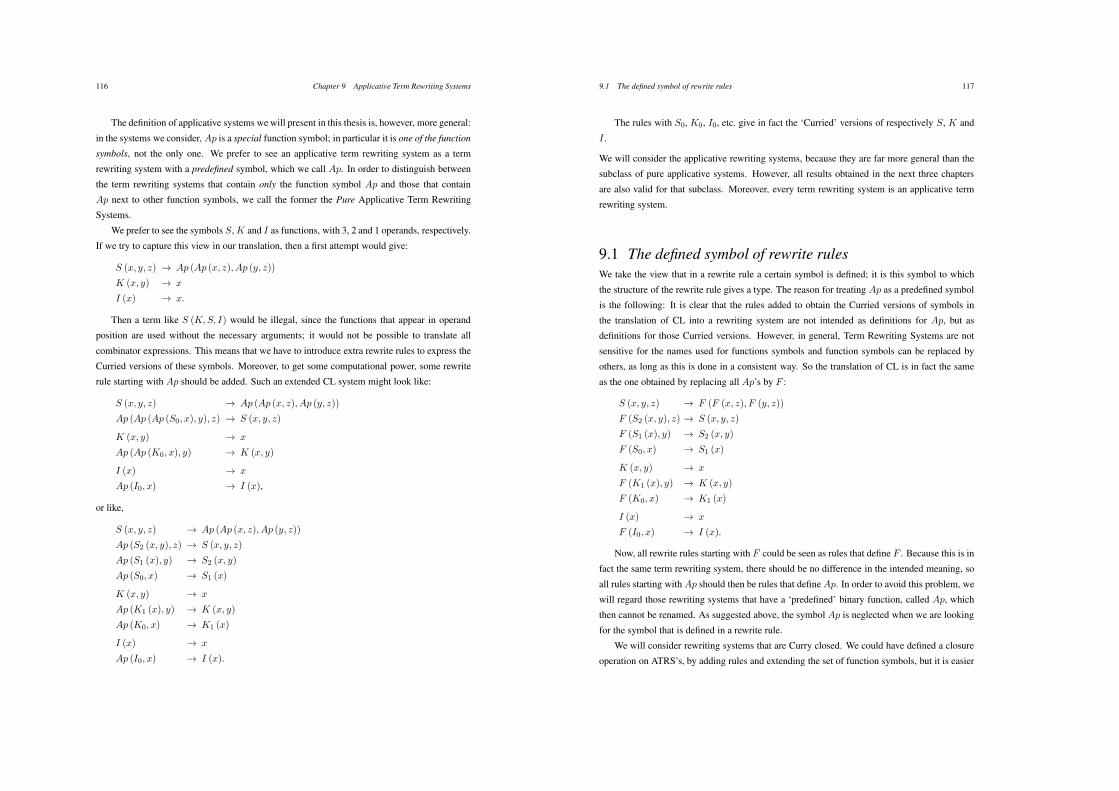
116 Chapter 9 Applicative Term Rewriting Systems
The definition of applicative systems we will present in this thesis is, however, more general:
in the systems we consider, Ap is a special function symbol; in particular it is one of the function
symbols, not the only one. We prefer to see an applicative term rewriting system as a term
rewriting system with a predefined symbol, which we call Ap. In order to distinguish between
the term rewriting systems that contain only the function symbol Ap and those that contain
Ap next to other function symbols, we call the former the Pure Applicative Term Rewriting
Systems.
We prefer to see the symbols S, K and I as functions, with 3, 2 and 1 operands, respectively.
If we try to capture this view in our translation, then a first attempt would give:
S (x, y, z) $ Ap (Ap (x, z), Ap (y, z))
K (x, y) $ x
I (x) $ x.
Then a term like S (K,S, I) would be illegal, since the functions that appear in operand
position are used without the necessary arguments; it would not be possible to translate all
combinator expressions. This means that we have to introduce extra rewrite rules to express the
Curried versions of these symbols. Moreover, to get some computational power, some rewrite
rule starting with Ap should be added. Such an extended CL system might look like:
S (x, y, z) $ Ap (Ap (x, z), Ap (y, z))
Ap (Ap (Ap (S0, x), y), z) $ S (x, y, z)
K (x, y) $ x
Ap (Ap (K0, x), y) $ K (x, y)
I (x) $ x
Ap (I0, x) $ I (x),
or like,
S (x, y, z) $ Ap (Ap (x, z), Ap (y, z))
Ap (S2 (x, y), z) $ S (x, y, z)
Ap (S1 (x), y) $ S2 (x, y)
Ap (S0, x) $ S1 (x)
K (x, y) $ x
Ap (K1 (x), y) $ K (x, y)
Ap (K0, x) $ K1 (x)
I (x) $ x
Ap (I0, x) $ I (x).
9.1 The defined symbol of rewrite rules 117
The rules with S0, K0, I0, etc. give in fact the ‘Curried’ versions of respectively S, K and
I .
We will consider the applicative rewriting systems, because they are far more general than the
subclass of pure applicative systems. However, all results obtained in the next three chapters
are also valid for that subclass. Moreover, every term rewriting system is an applicative term
rewriting system.
9.1 The defined symbol of rewrite rulesWe take the view that in a rewrite rule a certain symbol is defined; it is this symbol to which
the structure of the rewrite rule gives a type. The reason for treating Ap as a predefined symbol
is the following: It is clear that the rules added to obtain the Curried versions of symbols in
the translation of CL into a rewriting system are not intended as definitions for Ap, but as
definitions for those Curried versions. However, in general, Term Rewriting Systems are not
sensitive for the names used for functions symbols and function symbols can be replaced by
others, as long as this is done in a consistent way. So the translation of CL is in fact the same
as the one obtained by replacing all Ap’s by F :
S (x, y, z) $ F (F (x, z), F (y, z))
F (S2 (x, y), z) $ S (x, y, z)
F (S1 (x), y) $ S2 (x, y)
F (S0, x) $ S1 (x)
K (x, y) $ x
F (K1 (x), y) $ K (x, y)
F (K0, x) $ K1 (x)
I (x) $ x
F (I0, x) $ I (x).
Now, all rewrite rules starting with F could be seen as rules that define F . Because this is in
fact the same term rewriting system, there should be no difference in the intended meaning, so
all rules starting with Ap should then be rules that define Ap. In order to avoid this problem, we
will regard those rewriting systems that have a ‘predefined’ binary function, called Ap, which
then cannot be renamed. As suggested above, the symbol Ap is neglected when we are looking
for the symbol that is defined in a rewrite rule.
We will consider rewriting systems that are Curry closed. We could have defined a closure
operation on ATRS’s, by adding rules and extending the set of function symbols, but it is easier

118 Chapter 9 Applicative Term Rewriting Systems
to assume that every ATRS is closed. When presenting a rewrite system, however, we will only
show the rules that are essential; we will not show the rules that define the Curried versions.
9.2 Partial type assignmentThe type assignment systems we will present in the next three chapters are partial systems in the
sense of [Pfenning ’88]. Not only will we define how terms and rewrite rules can be typed, but
we will also assume that every function symbol already has a type, which structure is usually
motivated by a rewrite rule. There are several reasons to do so.
First of all a term rewriting system can contain a symbol that is not the defined symbol of a
rewrite rule (such a symbol is called a constant). A constant can appear in a rewrite rule more or
less as a symbol that ‘has to be there’, but for which it is impossible to determine any functional
characterization, apart from what is demanded by the immediate context. If we provide a type
for every constant, then we can formulate some consistency requirement by saying that the
types used for a constant must be related to the provided type.
Moreover, even for every defined symbol there must be some way of determining what
type can be used for an occurrence. Normally the rewrite rules that define such a symbol are
investigated, and from analyzing the structure of those rules the ‘most general type’ for that
symbol can be constructed. Instead of investigating all the defining rules for a defined symbol
every time the symbol is encountered, we can store the type of the symbol in a mapping from
symbols to types, and use this mapping instead. Of course it makes no difference to assume the
existence from the start of such a mapping from symbols (both defined and constant) to types,
and to define type assignment using that mapping (in the following such a mapping is called an
‘environment’).
In fact, the approach we take here is very much the same as the one taken by Hindley in
[Hindley ’69], where he defines the principal Curry-type scheme of an object in Combinatory
Logic. Even his notion of type assignment could be regarded as a partial one. Moreover,
since combinator systems can easily be translated into (Left Linear) Applicative Term Rewriting
Systems, the results of chapter eleven (when restricting the allowed rewrite rules to those that
correspond to combinators), are the same as in [Hindley ’69].
9.3 Definitions 119
9.3 DefinitionsThe following definitions will be based on definitions given in [Klop ’90]. Definition 9.3.1 will
define Applicative Term Rewriting Systems the same way as the definition given by Klop for
Term Rewriting Systems, extended with part (i.c) to express the existence of the predefined
symbol Ap. Definition 9.3.2 will define a notion of rewriting on Applicative Term Rewriting
Systems, the same way as the definition of rewriting given by Klop for Term Rewriting Systems,
extended with part (ii.a.3) to express that the possible use of the symbol Ap in the left hand side
is restricted, and part (iii) to define the notion of defined symbol of a rewrite rule. In fact, parts
(ii.a.3) and (iii) are related. Part (iv) is added to express that only Curry closed rewrite systems
are considered.
We will introduce in some parts a notation different from Klop’s, because some of the sym-
bols or definitions Klop used were already used in this thesis with a different meaning. For
example, we will use the word ‘replacement’ for the operation that replaces term-variables
by terms, instead of the word ‘substitution’, which was used for operations that replace type-
variables by types. (Substitution and replacement are also operations defined in [Curry &
Feys ’58]. They both are defined as operations on terms; substitution was defined as the oper-
ation that replaces term-variables by terms, and replacement was defined as the operation that
replaces occurrences of subterms by terms. Note that our definition therefore differs also from
the one given in [Curry & Feys ’58].) To denote a replacement, we will use capital characters
like ‘R’, instead of Greek characters like ‘*’, which were used to denote types. We will use the
symbol ‘$’ for the rewriting symbol, instead of ‘$’ which was used as a type constructor. We
will use the notion ‘constant symbol’ for a symbol that cannot be rewritten (for which there is
no rewrite rule that defines that symbol), instead of for a function symbol with arity 0.
Definition 9.3.1 (cf. [Klop ’90]) An Applicative Term Rewriting System (ATRS) is a pair ($,
R) of an alphabet or signature $ and a set of rewrite rules R.
i) The alphabet $ consists of:
a) A countable infinite set of variables x1, x2, x3, . . . (or x, y, z, x", y", . . . ).
b) A non empty set F of function symbols or operator symbols F , G, . . . , each equipped
with an ‘arity’ (a natural number), i.e. the number of ‘arguments’ it is supposed to
have. We have 0-ary, unary, binary, ternary etc. function symbols.
c) A special binary operator, called application (Ap).
ii) The set of terms (or expressions) ‘over’ $ is T(F,X ) and is defined inductively:
a) x, y, z, . . . + T(F,X ).
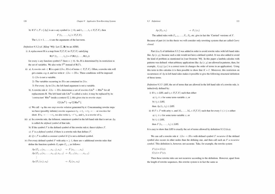
120 Chapter 9 Applicative Term Rewriting Systems
b) If F +F / {Ap} is an n-ary symbol (n 1 0), and t1, . . . , tn + T(F,X ), then
F (t1, . . . , tn) + T(F,X ).
The ti (i = 1, . . . , n) are the arguments of the last term.
Definition 9.3.2 (cf. [Klop ’90]) Let ($, R) be an ATRS.
i) A replacement R is a map from T(F,X ) to T(F,X ) satisfying
R(F (t1, . . . , tn)) = F (R(t1), . . . , R(tn))
for every n-ary function symbol F (here n 1 0). So, R is determined by its restriction to
the set of variables. We also write TR instead of R(T ).
ii) a) A rewrite rule + R is a pair (Lhs, Rhs) of terms + T(F,X ). Often, a rewrite rule will
get a name, e.g. r, and we write r : Lhs$ Rhs. Three conditions will be imposed:
1) Lhs is not a variable.
2) The variables occurring in Rhs are contained in Lhs.
3) For every Ap in Lhs, the left hand argument is not a variable.
b) A rewrite rule r : Lhs$ Rhs determines a set of rewrites LhsR $ RhsR for all
replacements R. The left hand side LhsR is called a redex; it may be replaced by its
‘contractum’ RhsR inside a context C[ ]; this gives rise to rewrite steps:
C[ LhsR ] $r C[ RhsR ].
c) We call $r the one-step rewrite relation generated by r. Concatenating rewrite steps
we have (possibly infinite) rewrite sequences t0 $ t1 $ t2 $ · · · or rewrites for
short. If t0 $ · · · $ tn we also write t0 $' tn, and tn is a rewrite of t0.
iii) a) In a rewrite rule, the leftmost, outermost symbol in the left hand side that is not an Ap,
is called the defined symbol of that rule.
b) If the symbol F is the defined symbol of the rewrite rule r, then r defines F .
c) F is a defined symbol, if there is a rewrite rule that defines F .
d) Q +F is called a constant symbol if Q is not a defined symbol.
iv) For every defined symbol F with arity n 1 1, there are n additional rewrite rules that
define the function symbols F0 upto Fn!1 as follows:
Ap (Fn!1 (x1, . . . , xn!1), xn) $ F (x1, . . . , xn)
Ap (Fn!2 (x1, . . . , xn!2), xn!1) $ Fn!1 (x1, . . . , xn!1)...
Ap (F1 (x1), x2) $ F2 (x1, x2)
9.3 Definitions 121
Ap (F0, x1) $ F1 (x1)
The added rules with Fn!1, . . . , F1, F0, etc. give in fact the ‘Curried’-versions of F .
Because of part (iv) in this thesis we will consider only rewriting systems that are called Curry
closed.
Part (ii.a.3) of definition 9.3.2 was added in order to avoid rewrite rules with left hand sides
like Ap (x, y), because such a rule would not have a defined symbol. It was also added to avoid
the kind of problem as mentioned in [van Oostrom ’90]. In this paper a lambda calculus with
patterns was defined: when arbitrary applications like Ap (x, y) are allowed in patterns, then, for
example, "(xy).(yx) is a correct term (it changes the order of terms in an application). Using
this term in this calculus it is then possible to show that K = I . Moreover, this restriction on
occurrences of Ap in left hand sides makes it possible to give the following structural definition
of those terms.
Definition 9.3.3 LHS, the set of terms that are allowed in the left hand side of a rewrite rule, is
inductively defined by:
i) If t1 + LHS, and t2 + T(F,X ) such that either:
a) t2 4 x for some term-variable x, or
b) t2 + LHS,
then Ap (t1, t2) + LHS.
ii) If F +F with arity n, and M1, . . . , Mn + T(F,X ) such that for every 1( i(n either:
a) ti 4 x for some term-variable x, or
b) ti + LHS,
then F (t1, . . . , tn) + LHS.
It is easy to show that LHS is exactly the set of terms allowed by definition 9.3.2 (ii.a).
We can call a rewrite rule r : Lhs $ Rhs with defined symbol F recursive if the defined
symbol also occurs in other nodes than the defining one, and then call such an F a recursive
symbol. This definition is, however, not accurate. Take, for example, the rewrite system
F (x) = G (x)
G (x) = F (x).
Then these rewrite rules are not recursive according to the definition. However, apart from
the length of rewrite sequences, this rewrite system is in fact the same as
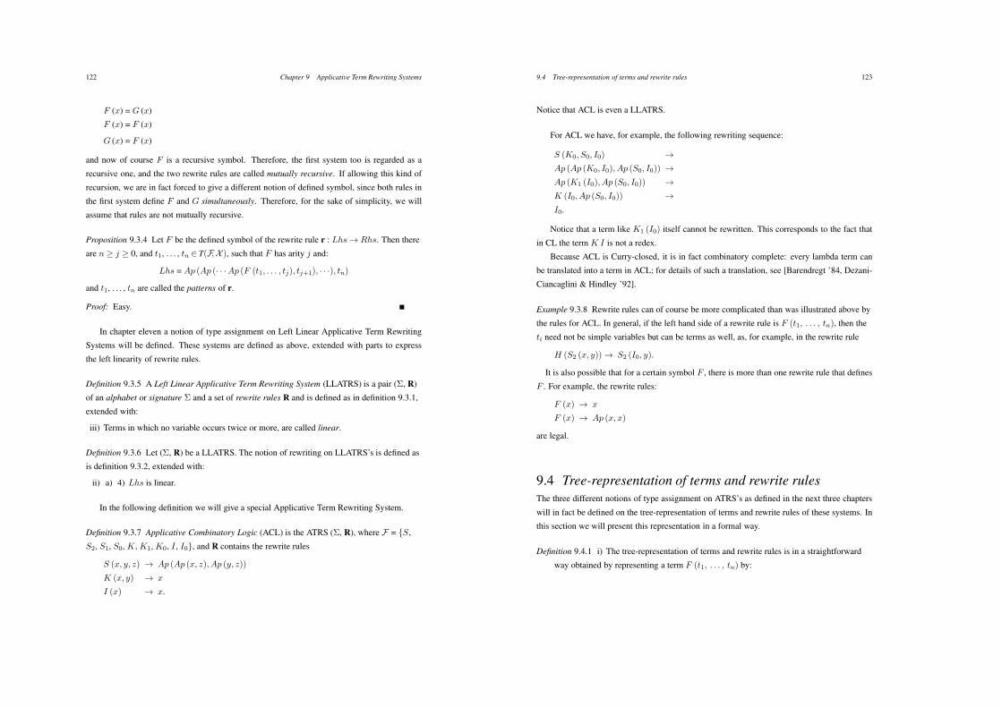
122 Chapter 9 Applicative Term Rewriting Systems
F (x) = G (x)
F (x) = F (x)
G (x) = F (x)
and now of course F is a recursive symbol. Therefore, the first system too is regarded as a
recursive one, and the two rewrite rules are called mutually recursive. If allowing this kind of
recursion, we are in fact forced to give a different notion of defined symbol, since both rules in
the first system define F and G simultaneously. Therefore, for the sake of simplicity, we will
assume that rules are not mutually recursive.
Proposition 9.3.4 Let F be the defined symbol of the rewrite rule r : Lhs$ Rhs. Then there
are n 1 j 1 0, and t1, . . . , tn + T(F,X ), such that F has arity j and:
Lhs = Ap (Ap (· · ·Ap (F (t1, . . . , tj), tj+1), · · ·), tn)
and t1, . . . , tn are called the patterns of r.
Proof: Easy.
In chapter eleven a notion of type assignment on Left Linear Applicative Term Rewriting
Systems will be defined. These systems are defined as above, extended with parts to express
the left linearity of rewrite rules.
Definition 9.3.5 A Left Linear Applicative Term Rewriting System (LLATRS) is a pair ($, R)
of an alphabet or signature $ and a set of rewrite rules R and is defined as in definition 9.3.1,
extended with:
iii) Terms in which no variable occurs twice or more, are called linear.
Definition 9.3.6 Let ($, R) be a LLATRS. The notion of rewriting on LLATRS’s is defined as
is definition 9.3.2, extended with:
ii) a) 4) Lhs is linear.
In the following definition we will give a special Applicative Term Rewriting System.
Definition 9.3.7 Applicative Combinatory Logic (ACL) is the ATRS ($, R), where F = {S,
S2, S1, S0, K , K1, K0, I , I0}, and R contains the rewrite rules
S (x, y, z) $ Ap (Ap (x, z), Ap (y, z))
K (x, y) $ x
I (x) $ x.
9.4 Tree-representation of terms and rewrite rules 123
Notice that ACL is even a LLATRS.
For ACL we have, for example, the following rewriting sequence:
S (K0, S0, I0) $
Ap (Ap (K0, I0), Ap (S0, I0)) $
Ap (K1 (I0), Ap (S0, I0)) $
K (I0, Ap (S0, I0)) $
I0.
Notice that a term like K1 (I0) itself cannot be rewritten. This corresponds to the fact that
in CL the term K I is not a redex.
Because ACL is Curry-closed, it is in fact combinatory complete: every lambda term can
be translated into a term in ACL; for details of such a translation, see [Barendregt ’84, Dezani-
Ciancaglini & Hindley ’92].
Example 9.3.8 Rewrite rules can of course be more complicated than was illustrated above by
the rules for ACL. In general, if the left hand side of a rewrite rule is F (t1, . . . , tn), then the
ti need not be simple variables but can be terms as well, as, for example, in the rewrite rule
H (S2 (x, y)) $ S2 (I0, y).
It is also possible that for a certain symbol F , there is more than one rewrite rule that defines
F . For example, the rewrite rules:
F (x) $ x
F (x) $ Ap (x, x)
are legal.
9.4 Tree-representation of terms and rewrite rulesThe three different notions of type assignment on ATRS’s as defined in the next three chapters
will in fact be defined on the tree-representation of terms and rewrite rules of these systems. In
this section we will present this representation in a formal way.
Definition 9.4.1 i) The tree-representation of terms and rewrite rules is in a straightforward
way obtained by representing a term F (t1, . . . , tn) by:
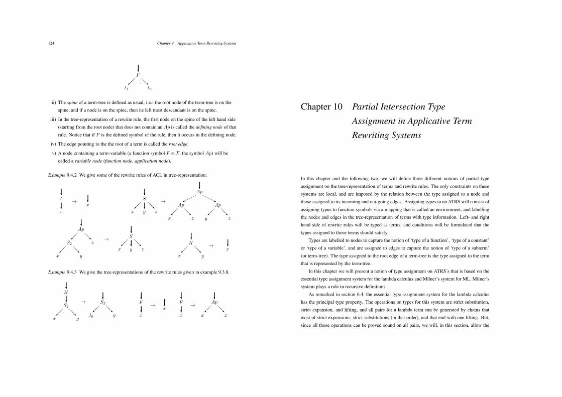
124 Chapter 9 Applicative Term Rewriting Systems
+F
,,-t1
../tn
· · ·
ii) The spine of a term-tree is defined as usual, i.e.: the root node of the term-tree is on the
spine, and if a node is on the spine, then its left most descendant is on the spine.
iii) In the tree-representation of a rewrite rule, the first node on the spine of the left hand side
(starting from the root node) that does not contain an Ap is called the defining node of that
rule. Notice that if F is the defined symbol of the rule, then it occurs in the defining node.
iv) The edge pointing to the the root of a term is called the root edge.
v) A node containing a term-variable (a function symbol F +F , the symbol Ap) will be
called a variable node (function node, application node).
Example 9.4.2 We give some of the rewrite rules of ACL in tree-representation:
+I
+x
$ +x
+S
,,-x
+y
../z
$
+Ap
00012223
Ap
,,-x
../z
Ap
,,-y
../z
+Ap
,,-S2
../z
,,-x
../y
$
+S
,,-x
+y
../z
+K
,,-x
../y
$ +x
Example 9.4.3 We give the tree-representations of the rewrite rules given in example 9.3.8.
+H
+S2
,,-x
../y
$+
S2
,,-I0
../y
+F
+x
$ +x
+F
+x
$
+Ap
,,-x
../x
Chapter 10 Partial Intersection Type
Assignment in Applicative Term
Rewriting Systems
In this chapter and the following two, we will define three different notions of partial type
assignment on the tree-representation of terms and rewrite rules. The only constraints on these
systems are local, and are imposed by the relation between the type assigned to a node and
those assigned to its incoming and out-going edges. Assigning types to an ATRS will consist of
assigning types to function symbols via a mapping that is called an environment, and labelling
the nodes and edges in the tree-representation of terms with type information. Left- and right
hand side of rewrite rules will be typed as terms, and conditions will be formulated that the
types assigned to those terms should satisfy.
Types are labelled to nodes to capture the notion of ‘type of a function’, ‘type of a constant’
or ‘type of a variable’, and are assigned to edges to capture the notion of ‘type of a subterm’
(or term-tree). The type assigned to the root edge of a term-tree is the type assigned to the term
that is represented by the term-tree.
In this chapter we will present a notion of type assignment on ATRS’s that is based on the
essential type assignment system for the lambda calculus and Milner’s system for ML. Milner’s
system plays a role in recursive definitions.
As remarked in section 6.4, the essential type assignment system for the lambda calculus
has the principal type property. The operations on types for this system are strict substitution,
strict expansion, and lifting, and all pairs for a lambda term can be generated by chains that
exist of strict expansions, strict substitutions (in that order), and that end with one lifting. But,
since all those operations can be proved sound on all pairs, we will, in this section, allow the
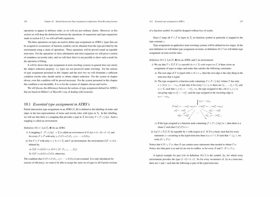
126 Chapter 10 Partial Intersection Type Assignment in Applicative Term Rewriting Systems
operations to appear in arbitrary order, so we will use just ordinary chains. Moreover, in this
section we will drop the distinction between the operations of expansions and type-expansions
made in section 6.2.2; we will call both expansions.
The three operations on types are used to define type assignment on ATRS’s: types that can
be assigned to occurrences of function symbols can be obtained from the type provided by the
environment using a chain of operations. These operations will be proved sound on typeable
term-trees. For the operations of strict substitution and strict expansion we will prove a notion
of soundness on rewrite rules, and we will show that it is not possible to show such a result for
the operation of lifting.
It will be shown that type assignment in term rewriting systems in general does not satisfy
the subject reduction property: i.e. types are not preserved under rewriting. For the notions
of type assignment presented in this chapter and the next two we will formulate a sufficient
condition rewrite rules should satisfy to obtain subject reduction. For the system of chapter
eleven, even this condition will be proved necessary. For the system presented in this chapter
this condition is not decidable. It is so for the systems of chapters eleven and twelve.
We will discuss the differences between the notions of type assignment defined for ATRS’s
that are based on Milner’s or Mycroft’s way of dealing with recursion.
10.1 Essential type assignment in ATRS’sPartial intersection type assignment on an ATRS ($, R) is defined as the labelling of nodes and
edges in the tree-representation of terms and rewrite rules with types in TS. In this labelling,
we will use that there is a mapping that provides a type in Ts for every F +F /{Ap}. Such a
mapping is called an environment.
Definition 10.1.1 Let ($, R) be an ATRS.
i) A mapping E : F /{Ap} $ Ts is called an environment if E(Ap) = (1$2)$1$2, and
for every F +F with arity n, E (F ) = E (Fn!1) = · · · = E(F0).
ii) For F +F with arity n 1 0, * + Ts, and E an environment, the environment E[F := *] is
defined by:
a) E[F :=*] (G) = *, if G+ {F , Fn!1, . . . , F0}.
b) E[F :=*] (G) = E (G), otherwise.
The condition that E (F ) = E (Fn!1) = · · · = E(F0) is not essential. It is only introduced for
reasons of efficiency; we want to be able to assign the same set of types to all Curried versions
10.1 Essential type assignment in ATRS’s 127
of a function symbol. It could be dropped without loss of results.
Since E maps all F +F to types in Ts, no function symbol in particular is mapped to the
type constant !.
Type assignment on applicative term rewriting systems will be defined in two stages. In the
next definition we will define type assignment on terms, in definition 10.1.7 we will define type
assignment on term rewrite rules.
Definition 10.1.2 Let ($, R) be an ATRS, and E an environment.
i) We say that T + T(F,X ) is typeable by * + TS with respect to E , if there exists an
assignment of types to edges and nodes that satisfies the following constraints:
a) The root edge of T is typed with *; if * = !, then the root edge is the only thing in the
term-tree that is typed.
b) The type assigned to a function node containing F +F /{Ap} (where F has arity
n 1 0) is +1!· · ·!+m, if and only if for every 1( i(m there are *i1, . . . , *i
n + TS, and
*i + Ts, such that +i = *i1$· · ·$*i
n$*i, the type assigned to the j-th (1( j (n)
out-going edge is *1j!· · ·!*
mj , and the type assigned to the incoming edge is
*1!· · ·!*m.
+*1!· · ·!*m
F :(*11$· · ·$*1
n$*1)!· · ·! (*m1 $· · ·$*m
n $*m)000001
*11!· · ·!*
m1 4
44
445*12!· · ·!*
m2
666667*1n!1!· · ·!*
mn!1
222223*1n!· · ·!*
mn
. . .
c) If the type assigned to a function node containing F +F /{Ap} is + , then there is a
chain C such that C (E (F )) = + .
ii) Let T + T(F,X ) be typeable by * with respect to E . If B is a basis such that for every
statement x:+ occurring in the typed term-tree there is a x:+ " +B such that + " (E + , we
write B !E T :*.
Notice that if B !E T :*, then B can contain more statements than needed to obtain T :*.
Notice also that parts (i.a) and (ii) are not in conflict, so for every B and T : B !E T :!.
A typical example for part (i.b) of definition 10.1.2 is the symbol Ap, for which every
environment provides the type (1$2)$1$2. So for every occurrence of Ap in a term-tree,
there are * and + such that the following is part of the typed term-tree.
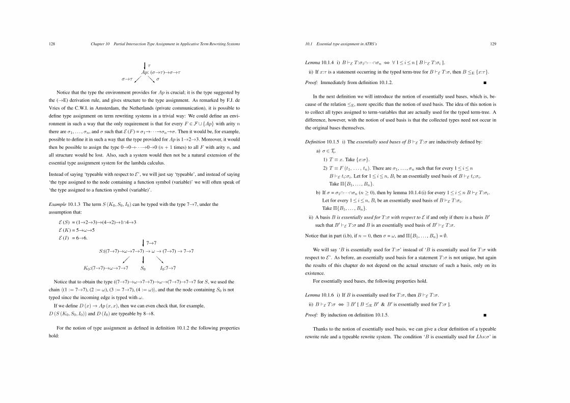
128 Chapter 10 Partial Intersection Type Assignment in Applicative Term Rewriting Systems
++Ap: (*$+ )$*$+
,,-*$+ ../ *
Notice that the type the environment provides for Ap is crucial; it is the type suggested by
the ($E) derivation rule, and gives structure to the type assignment. As remarked by F.J. de
Vries of the C.W.I. in Amsterdam, the Netherlands (private communication), it is possible to
define type assignment on term rewriting systems in a trivial way: We could define an envi-
ronment in such a way that the only requirement is that for every F +F /{Ap} with arity n
there are *1, . . . , *n, and * such that E (F ) = *1$· · ·$*n$*. Then it would be, for example,
possible to define it in such a way that the type provided for Ap is 1$2$3. Moreover, it would
then be possible to assign the type 0$0$· · ·$0$0 (n + 1 times) to all F with arity n, and
all structure would be lost. Also, such a system would then not be a natural extension of the
essential type assignment system for the lambda calculus.
Instead of saying ‘typeable with respect to E’, we will just say ‘typeable’, and instead of saying
‘the type assigned to the node containing a function symbol (variable)’ we will often speak of
‘the type assigned to a function symbol (variable)’.
Example 10.1.3 The term S (K0, S0, I0) can be typed with the type 7$7, under the
assumption that:
E (S) = (1$2$3)$(4$2)$1!4$3
E (K) = 5$!$5
E (I) = 6$6.
+7$7
S:((7$7)$!$7$7) $ ! $ (7$7) $ 7$7
,,-K0:(7$7)$!$7$7
+S0
../I0:7$7
Notice that to obtain the type ((7$7)$!$7$7)$!$(7$7)$7$7 for S, we used the
chain %(1 := 7$7), (2 := !), (3 := 7$7), (4 := !)&, and that the node containing S0 is not
typed since the incoming edge is typed with !.
If we define D (x) $ Ap (x, x), then we can even check that, for example,
D (S (K0, S0, I0)) and D (I0) are typeable by 8$8.
For the notion of type assignment as defined in definition 10.1.2 the following properties
hold:
10.1 Essential type assignment in ATRS’s 129
Lemma 10.1.4 i) B !E T :*1!· · ·!*n 23 ' 1( i(n [ B !E T :*i ].
ii) If x:+ is a statement occurring in the typed term-tree for B !E T :*, then B (E {x:+}.
Proof: Immediately from definition 10.1.2.
In the next definition we will introduce the notion of essentially used bases, which is, be-
cause of the relation (E, more specific than the notion of used basis. The idea of this notion is
to collect all types assigned to term-variables that are actually used for the typed term-tree. A
difference, however, with the notion of used basis is that the collected types need not occur in
the original bases themselves.
Definition 10.1.5 i) The essentially used bases of B !E T :* are inductively defined by:
a) * + Ts.
1) T 4 x. Take {x:*}.
2) T 4 F (t1, . . . , tn). There are *1, . . . , *n such that for every 1( i(n
B !E ti:*i. Let for 1( i(n, Bi be an essentially used basis of B !E ti:*i.
Take #{B1, . . . , Bn}.
b) If * = *1!· · ·!*n (n 1 0), then by lemma 10.1.4 (i) for every 1( i(n B !E T :*i.
Let for every 1( i(n, Bi be an essentially used basis of B !E T :*i.
Take #{B1, . . . , Bn}.
ii) A basis B is essentially used for T :* with respect to E if and only if there is a basis B"
such that B" !E T :* and B is an essentially used basis of B" !E T :*.
Notice that in part (i.b), if n = 0, then * = !, and #{B1, . . . , Bn} = 0.
We will say ‘B is essentially used for T :*’ instead of ‘B is essentially used for T :* with
respect to E’. As before, an essentially used basis for a statement T :* is not unique, but again
the results of this chapter do not depend on the actual structure of such a basis, only on its
existence.
For essentially used bases, the following properties hold.
Lemma 10.1.6 i) If B is essentially used for T :*, then B !E T :*.
ii) B !E T :* 23 6 B" [ B (E B" & B" is essentially used for T :* ].
Proof: By induction on definition 10.1.5.
Thanks to the notion of essentially used basis, we can give a clear definition of a typeable
rewrite rule and a typeable rewrite system. The condition ‘B is essentially used for Lhs:*’ in
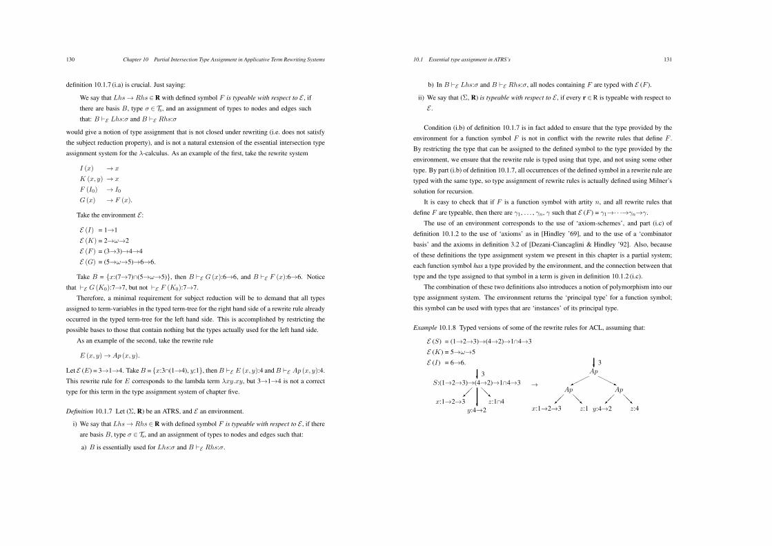
130 Chapter 10 Partial Intersection Type Assignment in Applicative Term Rewriting Systems
definition 10.1.7 (i.a) is crucial. Just saying:
We say that Lhs $ Rhs + R with defined symbol F is typeable with respect to E , if
there are basis B, type * + Ts, and an assignment of types to nodes and edges such
that: B !E Lhs:* and B !E Rhs:*
would give a notion of type assignment that is not closed under rewriting (i.e. does not satisfy
the subject reduction property), and is not a natural extension of the essential intersection type
assignment system for the "-calculus. As an example of the first, take the rewrite system
I (x) $ x
K (x, y) $ x
F (I0) $ I0
G (x) $ F (x).
Take the environment E :
E (I) = 1$1
E (K) = 2$!$2
E (F ) = (3$3)$4$4
E (G) = (5$!$5)$6$6.
Take B = {x:(7$7)!(5$!$5)}, then B !E G (x):6$6, and B !E F (x):6$6. Notice
that !E G (K0):7$7, but not !E F (K0):7$7.
Therefore, a minimal requirement for subject reduction will be to demand that all types
assigned to term-variables in the typed term-tree for the right hand side of a rewrite rule already
occurred in the typed term-tree for the left hand side. This is accomplished by restricting the
possible bases to those that contain nothing but the types actually used for the left hand side.
As an example of the second, take the rewrite rule
E (x, y) $ Ap (x, y).
Let E (E) = 3$1$4. Take B = {x:3!(1$4), y:1}, then B !E E (x, y):4 and B !E Ap (x, y):4.
This rewrite rule for E corresponds to the lambda term "xy.xy, but 3$1$4 is not a correct
type for this term in the type assignment system of chapter five.
Definition 10.1.7 Let ($, R) be an ATRS, and E an environment.
i) We say that Lhs$ Rhs + R with defined symbol F is typeable with respect to E , if there
are basis B, type * + Ts, and an assignment of types to nodes and edges such that:
a) B is essentially used for Lhs:* and B !E Rhs:*.
10.1 Essential type assignment in ATRS’s 131
b) In B !E Lhs:* and B !E Rhs:*, all nodes containing F are typed with E (F ).
ii) We say that ($, R) is typeable with respect to E , if every r + R is typeable with respect to
E .
Condition (i.b) of definition 10.1.7 is in fact added to ensure that the type provided by the
environment for a function symbol F is not in conflict with the rewrite rules that define F .
By restricting the type that can be assigned to the defined symbol to the type provided by the
environment, we ensure that the rewrite rule is typed using that type, and not using some other
type. By part (i.b) of definition 10.1.7, all occurrences of the defined symbol in a rewrite rule are
typed with the same type, so type assignment of rewrite rules is actually defined using Milner’s
solution for recursion.
It is easy to check that if F is a function symbol with artity n, and all rewrite rules that
define F are typeable, then there are &1, . . . , &n, & such that E (F ) = &1$· · ·$&n$&.
The use of an environment corresponds to the use of ‘axiom-schemes’, and part (i.c) of
definition 10.1.2 to the use of ‘axioms’ as in [Hindley ’69], and to the use of a ‘combinator
basis’ and the axioms in definition 3.2 of [Dezani-Ciancaglini & Hindley ’92]. Also, because
of these definitions the type assignment system we present in this chapter is a partial system;
each function symbol has a type provided by the environment, and the connection between that
type and the type assigned to that symbol in a term is given in definition 10.1.2 (i.c).
The combination of these two definitions also introduces a notion of polymorphism into our
type assignment system. The environment returns the ‘principal type’ for a function symbol;
this symbol can be used with types that are ‘instances’ of its principal type.
Example 10.1.8 Typed versions of some of the rewrite rules for ACL, assuming that:
E (S) = (1$2$3)$(4$2)$1!4$3
E (K) = 5$!$5
E (I) = 6$6.
+3S:(1$2$3)$(4$2)$1!4$3
,,-x:1$2$3 +
y:4$2
../z:1!4
$
+3Ap
00012223
Ap
,,-x:1$2$3
../z:1
Ap
,,-y:4$2
../z:4
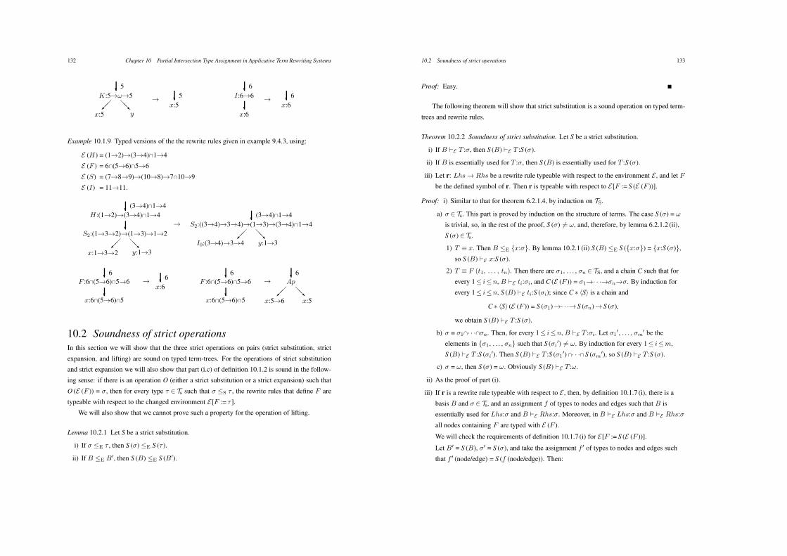
132 Chapter 10 Partial Intersection Type Assignment in Applicative Term Rewriting Systems
+5
K:5$!$5,,-
x:5
../y
$ +5
x:5
+6
I:6$6
+x:6
$ +6
x:6
Example 10.1.9 Typed versions of the the rewrite rules given in example 9.4.3, using:
E (H) = (1$2)$(3$4)!1$4
E (F ) = 6!(5$6)!5$6
E (S) = (7$8$9)$(10$8)$7!10$9
E (I) = 11$11.
+(3$4)!1$4
H:(1$2)$(3$4)!1$4
+S2:(1$3$2)$(1$3)$1$2
,,-x:1$3$2
../y:1$3
$+(3$4)!1$4
S2:((3$4)$3$4)$(1$3)$(3$4)!1$4
,,-I0:(3$4)$3$4
../y:1$3
+6
F :6!(5$6)!5$6
+x:6!(5$6)!5
$ +6
x:6
+6
F :6!(5$6)!5$6
+x:6!(5$6)!5
$+6
Ap
,,-x:5$6
../x:5
10.2 Soundness of strict operationsIn this section we will show that the three strict operations on pairs (strict substitution, strict
expansion, and lifting) are sound on typed term-trees. For the operations of strict substitution
and strict expansion we will also show that part (i.c) of definition 10.1.2 is sound in the follow-
ing sense: if there is an operation O (either a strict substitution or a strict expansion) such that
O (E (F )) = *, then for every type + + Ts such that * (S + , the rewrite rules that define F are
typeable with respect to the changed environment E[F := + ].
We will also show that we cannot prove such a property for the operation of lifting.
Lemma 10.2.1 Let S be a strict substitution.
i) If * (E + , then S (*) (E S (+ ).
ii) If B (E B", then S (B) (E S (B").
10.2 Soundness of strict operations 133
Proof: Easy.
The following theorem will show that strict substitution is a sound operation on typed term-
trees and rewrite rules.
Theorem 10.2.2 Soundness of strict substitution. Let S be a strict substitution.
i) If B !E T :*, then S (B) !E T :S (*).
ii) If B is essentially used for T :*, then S (B) is essentially used for T :S (*).
iii) Let r: Lhs$ Rhs be a rewrite rule typeable with respect to the environment E , and let F
be the defined symbol of r. Then r is typeable with respect to E [F := S (E (F ))].
Proof: i) Similar to that for theorem 6.2.1.4, by induction on TS.
a) * + Ts. This part is proved by induction on the structure of terms. The case S (*) = !
is trivial, so, in the rest of the proof, S (*) ,= !, and, therefore, by lemma 6.2.1.2 (ii),
S (*) + Ts.
1) T 4 x. Then B (E {x:*}. By lemma 10.2.1 (ii) S (B) (E S ({x:*}) = {x:S (*)},
so S (B) !E x:S (*).
2) T 4 F (t1, . . . , tn). Then there are *1, . . . , *n + TS, and a chain C such that for
every 1( i(n, B !E ti:*i, and C (E (F )) = *1$· · ·$*n$*. By induction for
every 1( i(n, S (B) !E ti:S (*i); since C * %S& is a chain and
C * %S& (E (F )) = S (*1)$· · ·$ S (*n)$ S (*),
we obtain S (B) !E T :S (*).
b) * = *1!· · ·!*n. Then, for every 1( i(n, B !E T :*i. Let *1", . . . , *m
" be the
elements in {*1, . . . , *n} such that S (*i") ,= !. By induction for every 1( i(m,
S (B) !E T :S (*i"). Then S (B) !E T :S (*1
") !· · ·! S (*m"), so S (B) !E T :S (*).
c) * = !, then S (*) = !. Obviously S (B) !E T :!.
ii) As the proof of part (i).
iii) If r is a rewrite rule typeable with respect to E , then, by definition 10.1.7 (i), there is a
basis B and * + Ts, and an assignment f of types to nodes and edges such that B is
essentially used for Lhs:* and B !E Rhs:*. Moreover, in B !E Lhs:* and B !E Rhs:*
all nodes containing F are typed with E (F ).
We will check the requirements of definition 10.1.7 (i) for E [F := S (E (F ))].
Let B" = S (B), *" = S (*), and take the assignment f " of types to nodes and edges such
that f " (node/edge) = S (f (node/edge)). Then:
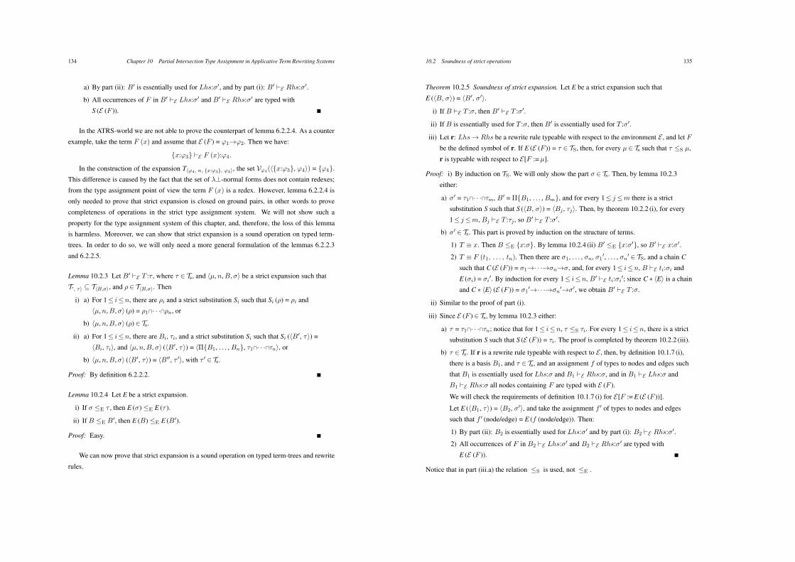
134 Chapter 10 Partial Intersection Type Assignment in Applicative Term Rewriting Systems
a) By part (ii): B" is essentially used for Lhs:*", and by part (i): B" !E Rhs:*".
b) All occurrences of F in B" !E Lhs:*" and B" !E Rhs:*" are typed with
S (E (F )).
In the ATRS-world we are not able to prove the counterpart of lemma 6.2.2.4. As a counter
example, take the term F (x) and assume that E (F ) = #1$#2. Then we have:
{x:#3} !E F (x):#4.
In the construction of the expansion T$(4, n, {x:(3}, (4%, the set V(4(%{x:#3}, #4&) = {#4}.
This difference is caused by the fact that the set of "#-normal forms does not contain redexes;
from the type assignment point of view the term F (x) is a redex. However, lemma 6.2.2.4 is
only needed to prove that strict expansion is closed on ground pairs, in other words to prove
completeness of operations in the strict type assignment system. We will not show such a
property for the type assignment system of this chapter, and, therefore, the loss of this lemma
is harmless. Moreover, we can show that strict expansion is a sound operation on typed term-
trees. In order to do so, we will only need a more general formulation of the lemmas 6.2.2.3
and 6.2.2.5.
Lemma 10.2.3 Let B" !E T :+ , where + + Ts, and %µ,n,B,*& be a strict expansion such that
T!, &% 7 T$B,%%, and )+ T$B,%%. Then
i) a) For 1( i(n, there are )i and a strict substitution Si such that Si ()) = )i and
%µ,n,B,*& ()) = )1!· · ·!)n, or
b) %µ,n,B,*& ()) + Ts.
ii) a) For 1( i(n, there are Bi, +i, and a strict substitution Si such that Si (%B", +&) =
%Bi, +i&, and %µ,n,B,*& (%B", +&) = %#{B1, . . . , Bn}, +1!· · ·!+n&, or
b) %µ,n,B,*& (%B", +&) = %B"", + "&, with + " + Ts.
Proof: By definition 6.2.2.2.
Lemma 10.2.4 Let E be a strict expansion.
i) If * (E + , then E (*) (E E (+ ).
ii) If B (E B", then E (B) (E E (B").
Proof: Easy.
We can now prove that strict expansion is a sound operation on typed term-trees and rewrite
rules.
10.2 Soundness of strict operations 135
Theorem 10.2.5 Soundness of strict expansion. Let E be a strict expansion such that
E (%B, *&) = %B", *"&.
i) If B !E T :*, then B" !E T :*".
ii) If B is essentially used for T :*, then B" is essentially used for T :*".
iii) Let r: Lhs$ Rhs be a rewrite rule typeable with respect to the environment E , and let F
be the defined symbol of r. If E (E (F )) = + + TS, then, for every µ + Ts such that + (S µ,
r is typeable with respect to E[F :=µ].
Proof: i) By induction on TS. We will only show the part * + Ts. Then, by lemma 10.2.3
either:
a) *" = +1!· · ·!+m, B" = #{B1, . . . , Bm}, and for every 1( j (m there is a strict
substitution S such that S (%B, *&) = %Bj , +j&. Then, by theorem 10.2.2 (i), for every
1( j(m, Bj !E T :+j , so B" !E T :*".
b) *" + Ts. This part is proved by induction on the structure of terms.
1) T 4 x. Then B (E {x:*}. By lemma 10.2.4 (ii) B" (E {x:*"}, so B" !E x:*".
2) T 4 F (t1, . . . , tn). Then there are *1, . . . , *n, *1", . . . , *n
" + TS, and a chain C
such that C (E (F )) = *1$· · ·$*n$*, and, for every 1( i(n, B !E ti:*i and
E (*i) = *i". By induction for every 1( i(n, B" !E ti:*i
"; since C * %E& is a chain
and C * %E& (E (F )) = *1"$· · ·$*n
"$*", we obtain B" !E T :*.
ii) Similar to the proof of part (i).
iii) Since E (F ) + Ts, by lemma 10.2.3 either:
a) + = +1!· · ·!+n; notice that for 1( i(n, + (S +i. For every 1( i(n, there is a strict
substitution S such that S (E (F )) = +i. The proof is completed by theorem 10.2.2 (iii).
b) + + Ts. If r is a rewrite rule typeable with respect to E , then, by definition 10.1.7 (i),
there is a basis B1, and + + Ts, and an assignment f of types to nodes and edges such
that B1 is essentially used for Lhs:* and B1 !E Rhs:*, and in B1 !E Lhs:* and
B1 !E Rhs:* all nodes containing F are typed with E (F ).
We will check the requirements of definition 10.1.7 (i) for E[F := E (E (F ))].
Let E (%B1, +&) = %B2, *"&, and take the assignment f " of types to nodes and edges
such that f " (node/edge) = E (f (node/edge)). Then:
1) By part (ii): B2 is essentially used for Lhs:*" and by part (i): B2 !E Rhs:*".
2) All occurrences of F in B2 !E Lhs:*" and B2 !E Rhs:*" are typed with
E (E (F )).
Notice that in part (iii.a) the relation (S is used, not (E .
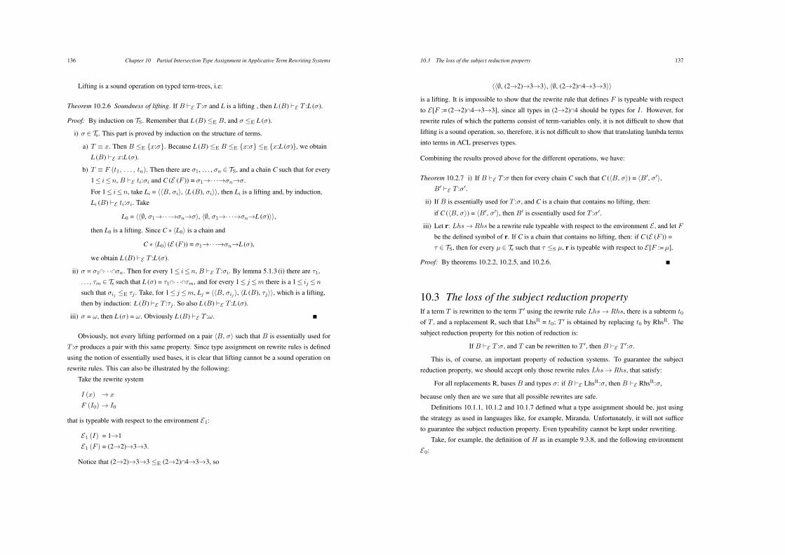
136 Chapter 10 Partial Intersection Type Assignment in Applicative Term Rewriting Systems
Lifting is a sound operation on typed term-trees, i.e:
Theorem 10.2.6 Soundness of lifting. If B !E T :* and L is a lifting , then L (B) !E T :L (*).
Proof: By induction on TS. Remember that L (B) (E B, and * (E L (*).
i) * + Ts. This part is proved by induction on the structure of terms.
a) T 4 x. Then B (E {x:*}. Because L (B) (E B (E {x:*} (E {x:L (*)}, we obtain
L (B) !E x:L (*).
b) T 4 F (t1, . . . , tn). Then there are *1, . . . , *n + TS, and a chain C such that for every
1( i(n, B !E ti:*i and C (E (F )) = *1$· · ·$*n$*.
For 1( i(n, take Li = %%B, *i&, %L (B), *i&&, then Li is a lifting and, by induction,
Li (B) !E ti:*i. Take
L0 = %%0, *1$· · ·$*n$*&, %0, *1$· · ·$*n$L (*)&&,
then L0 is a lifting. Since C * %L0& is a chain and
C * %L0& (E (F )) = *1$· · ·$*n$L (*),
we obtain L (B) !E T :L (*).
ii) * = *1!· · ·!*n. Then for every 1( i(n, B !E T :*i. By lemma 5.1.3 (i) there are +1,
. . . , +m + Ts such that L (*) = +1!· · ·!+m, and for every 1( j(m there is a 1( ij (n
such that *ij (E +j . Take, for 1( j(m, Lj = %%B, *ij &, %L (B), +j&&, which is a lifting,
then by induction: L (B) !E T :+j . So also L (B) !E T :L (*).
iii) * = !, then L (*) = !. Obviously L (B) !E T :!.
Obviously, not every lifting performed on a pair %B, *& such that B is essentially used for
T :* produces a pair with this same property. Since type assignment on rewrite rules is defined
using the notion of essentially used bases, it is clear that lifting cannot be a sound operation on
rewrite rules. This can also be illustrated by the following:
Take the rewrite system
I (x) $ x
F (I0) $ I0
that is typeable with respect to the environment E1:
E1 (I) = 1$1
E1 (F ) = (2$2)$3$3.
Notice that (2$2)$3$3 (E (2$2)!4$3$3, so
10.3 The loss of the subject reduction property 137
%%0, (2$2)$3$3&, %0, (2$2)!4$3$3&&
is a lifting. It is impossible to show that the rewrite rule that defines F is typeable with respect
to E[F := (2$2)!4$3$3], since all types in (2$2)!4 should be types for I . However, for
rewrite rules of which the patterns consist of term-variables only, it is not difficult to show that
lifting is a sound operation, so, therefore, it is not difficult to show that translating lambda terms
into terms in ACL preserves types.
Combining the results proved above for the different operations, we have:
Theorem 10.2.7 i) If B !E T :* then for every chain C such that C (%B, *&) = %B", *"&,
B" !E T :*".
ii) If B is essentially used for T :*, and C is a chain that contains no lifting, then:
if C (%B, *&) = %B", *"&, then B" is essentially used for T :*".
iii) Let r: Lhs$ Rhs be a rewrite rule typeable with respect to the environment E , and let F
be the defined symbol of r. If C is a chain that contains no lifting, then: if C (E (F )) =
+ + TS, then for every µ + Ts such that + (S µ, r is typeable with respect to E [F :=µ].
Proof: By theorems 10.2.2, 10.2.5, and 10.2.6.
10.3 The loss of the subject reduction propertyIf a term T is rewritten to the term T " using the rewrite rule Lhs $ Rhs, there is a subterm t0
of T , and a replacement R, such that LhsR = t0; T " is obtained by replacing t0 by RhsR. The
subject reduction property for this notion of reduction is:
If B !E T :*, and T can be rewritten to T ", then B !E T ":*.
This is, of course, an important property of reduction systems. To guarantee the subject
reduction property, we should accept only those rewrite rules Lhs$ Rhs, that satisfy:
For all replacements R, bases B and types *: if B !E LhsR:*, then B !E RhsR:*,
because only then are we sure that all possible rewrites are safe.
Definitions 10.1.1, 10.1.2 and 10.1.7 defined what a type assignment should be, just using
the strategy as used in languages like, for example, Miranda. Unfortunately, it will not suffice
to guarantee the subject reduction property. Even typeability cannot be kept under rewriting.
Take, for example, the definition of H as in example 9.3.8, and the following environment
E0:
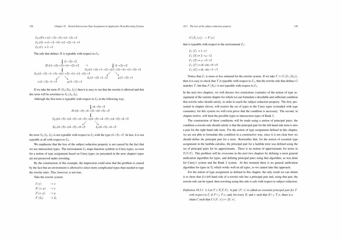
138 Chapter 10 Partial Intersection Type Assignment in Applicative Term Rewriting Systems
E0 (H) = ((1$2)$3)$(1$2)$2
E0 (S) = (1$2$3)$(1$2)$1$3
E0 (I) = 1$1
The rule that defines H is typeable with respect to E0:
+(1$2)$2
H:((1$2)$3)$(1$2)$2
+S2:((1$2)$1$3)$((1$2)$1)$(1$2)$3
,,-x:(1$2)$1$3
../y:(1$2)$1
$ +(1$2)$2
S2:((1$2)$1$2)$((1$2)$1)$(1$2)$2
,,-I0:(1$2)$1$2
../y:(1$2)$1
If we take the term H (S2 (K0, I0)) then it is easy to see that the rewrite is allowed and that
this term will be rewritten to S2 (I0, I0).
Although the first term is typeable with respect to E0 in the following way:
+(4$5)$5
H:((4$5)$4$5)$(4$5)$5
+S2:((4$5)$(4$5)$4$5)$((4$5)$4$5)$(4$5)$4$5
,,-K0:(4$5)$(4$5)$4$5
../I0:(4$5)$4$5
the term S2 (I0, I0) is not typeable with respect to E0 with the type (4$5)$5. In fact, it is not
typeable at all with respect to E0.
We emphasize that the loss of the subject reduction property is not caused by the fact that
we use intersection types. The environment E0 maps function symbols to Curry-types, so even
for a notion of type assignment based on Curry-types (as presented in the next chapter) types
are not preserved under rewriting.
By the construction of this example, the impression could arise that the problem is caused
by the fact that an environment is allowed to select more complicated types than needed to type
the rewrite rules. This, however, is not true.
Take the rewrite system:
I (x) $ x
K (x, y) $ x
Z (x, y) $ y
F (I0) $ I0
10.3 The loss of the subject reduction property 139
G (Z1 (x)) $ F (x)
that is typeable with respect to the environment E1:
E1 (I) = 1$1
E1 (K)= 2$!$2
E1 (Z) = !$3$3
E1 (F ) = (4$4)$5$5
E1 (G) = (6$6)$7$7.
Notice that E1 is more or less minimal for the rewrite system. If we take T 4 G (Z1 (K0)),
then it is easy to check that T is typeable with respect to E1, that the rewrite rule that defines G
matches T , but that F (K0) is not typeable with respect to E1.
In the next two chapters, we will discuss two restrictions (variants) of the notion of type as-
signment of the current chapter for which we can formulate a decidable and sufficient condition
that rewrite rules should satisfy, in order to reach the subject reduction property. The first, pre-
sented in chapter eleven, will restrict the set of types to the Curry types (extended with type
constants); for this system we will even prove that the condition is necessary. The second, in
chapter twelve, will limit the possible types to intersection types of Rank 2.
The construction of these conditions will be made using a notion of principal pairs; the
condition a rewrite rule should satisfy is that the principal pair for the left hand side term is also
a pair for the right hand side term. For the notion of type assignment defined in this chapter,
we are not able to formulate this condition in a constructive way, since it is not clear how we
should define the principal pair for a term. Remember that, for the notion of essential type
assignment in the lambda calculus, the principal pair for a lambda term was defined using the
set of principal pairs for its approximants. There is no notion of approximants for terms in
T(F,X ). This problem will be overcome in the next two chapters by defining a most general
unification algorithm for types, and defining principal pairs using that algorithm, as was done
for Curry’s system and the Rank 2 system. At this moment there is no general unification
algorithm for types in TS which works well on all types, so we cannot take this approach.
For the notion of type assignment as defined in this chapter, the only result we can obtain
is to show that if a left hand side of a rewrite rule has a principal pair and, using that pair, the
rewrite rule can be typed, then rewriting using this rule is safe with respect to subject reduction.
Definition 10.3.1 i) Let T + T(F,X ). A pair %P , ,& is called an essential principal pair for T
with respect to E , if P !E T :,, and, for every B, and * such that B !E T :*, there is a
chain C such that C (%P , ,&) = %B, *&.
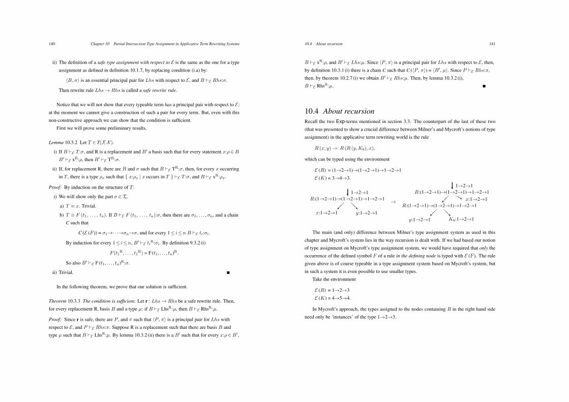
140 Chapter 10 Partial Intersection Type Assignment in Applicative Term Rewriting Systems
ii) The definition of a safe type assignment with respect to E is the same as the one for a type
assignment as defined in definition 10.1.7, by replacing condition (i.a) by:
%B, *& is an essential principal pair for Lhs with respect to E , and B !E Rhs:*.
Then rewrite rule Lhs $ Rhs is called a safe rewrite rule.
Notice that we will not show that every typeable term has a principal pair with respect to E ;
at the moment we cannot give a construction of such a pair for every term. But, even with this
non-constructive approach we can show that the condition is sufficient.
First we will prove some preliminary results.
Lemma 10.3.2 Let T + T(F,X ).
i) If B !E T :*, and R is a replacement and B" a basis such that for every statement x:)+B
B" !E xR:), then B" !E TR:*.
ii) If, for replacement R, there are B and * such that B !E TR:*, then, for every x occurring
in T , there is a type )x such that { x:)x | x occurs in T } !E T :*, and B !E xR:)x.
Proof: By induction on the structure of T .
i) We will show only the part * + Ts.
a) T 4 x. Trivial.
b) T 4 F (t1, . . . , tn). If B !E F (t1, . . . , tn):*, then there are *1, . . . , *n, and a chain
C such that
C (E (F )) = *1$· · ·$*n$*, and for every 1( i(n B !E ti:*i.
By induction for every 1( i(n, B" !E tiR:*i. By definition 9.3.2 (i)
F (t1R, . . . , t1R) = F (t1, . . . , tn)R.
So also B" !E F (t1, . . . , tn)R:*.
ii) Trivial.
In the following theorem, we prove that our solution is sufficient.
Theorem 10.3.3 The condition is sufficient. Let r : Lhs $ Rhs be a safe rewrite rule. Then,
for every replacement R, basis B and a type µ: if B !E LhsR:µ, then B !E RhsR:µ.
Proof: Since r is safe, there are P , and , such that %P , ,& is a principal pair for Lhs with
respect to E , and P !E Rhs:,. Suppose R is a replacement such that there are basis B and
type µ such that B !E LhsR:µ. By lemma 10.3.2 (ii) there is a B" such that for every x:)+B",
10.4 About recursion 141
B !E xR:), and B" !E Lhs:µ. Since %P , ,& is a principal pair for Lhs with respect to E , then,
by definition 10.3.1 (i) there is a chain C such that C (%P , ,&) = %B", µ&. Since P !E Rhs:,,
then, by theorem 10.2.7 (i) we obtain B" !E Rhs:µ. Then, by lemma 10.3.2 (i),
B !E RhsR:µ.
10.4 About recursionRecall the two Exp-terms mentioned in section 3.3. The counterpart of the last of these two
(that was presented to show a crucial difference between Milner’s and Mycroft’s notions of type
assignment) in the applicative term rewriting world is the rule
R (x, y) $ R (R (y,K0), x),
which can be typed using the environment
E (R) = (1$2$1)$(1$2$1)$1$2$1
E (K) = 3$4$3.
+1$2$1R:(1$2$1)$(1$2$1)$1$2$1
,,-x:1$2$1
../y:1$2$1
$
+1$2$1R:(1$2$1)$(1$2$1)$1$2$1
,,-223 x:1$2$1
R:(1$2$1)$(1$2$1)$1$2$1
,,-y:1$2$1
../K0:1$2$1
The main (and only) difference between Milner’s type assignment system as used in this
chapter and Mycroft’s system lies in the way recursion is dealt with. If we had based our notion
of type assignment on Mycroft’s type assignment system, we would have required that only the
occurrence of the defined symbol F of a rule in the defining node is typed with E (F ). The rule
given above is of course typeable in a type assignment system based on Mycroft’s system, but
in such a system it is even possible to use smaller types.
Take the environment
E (R) = 1$2$3
E (K) = 4$5$4.
In Mycroft’s approach, the types assigned to the nodes containing R in the right hand side
need only be ‘instances’ of the type 1$2$3.
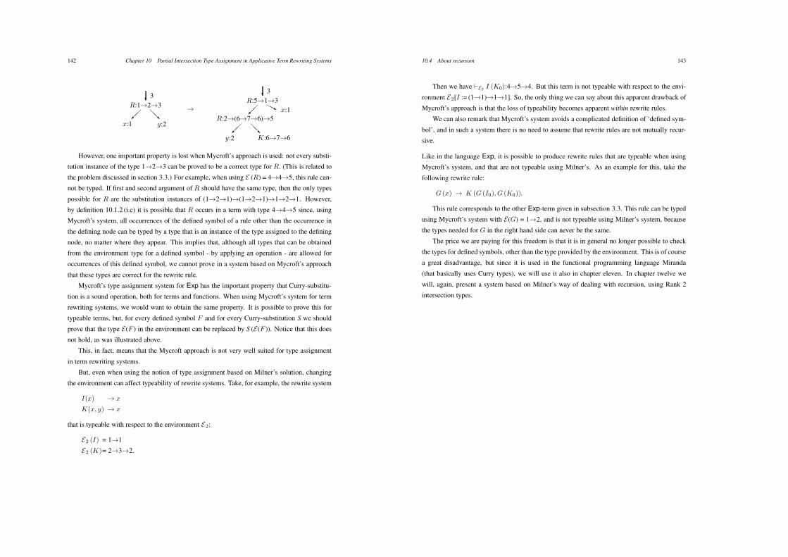
142 Chapter 10 Partial Intersection Type Assignment in Applicative Term Rewriting Systems
+3
R:1$2$3,,-
x:1
../y:2
$
+3
R:5$1$3,,-
223 x:1R:2$(6$7$6)$5
,,-y:2
../K:6$7$6
However, one important property is lost when Mycroft’s approach is used: not every substi-
tution instance of the type 1$2$3 can be proved to be a correct type for R. (This is related to
the problem discussed in section 3.3.) For example, when using E (R) = 4$4$5, this rule can-
not be typed. If first and second argument of R should have the same type, then the only types
possible for R are the substitution instances of (1$2$1)$(1$2$1)$1$2$1. However,
by definition 10.1.2 (i.c) it is possible that R occurs in a term with type 4$4$5 since, using
Mycroft’s system, all occurrences of the defined symbol of a rule other than the occurrence in
the defining node can be typed by a type that is an instance of the type assigned to the defining
node, no matter where they appear. This implies that, although all types that can be obtained
from the environment type for a defined symbol - by applying an operation - are allowed for
occurrences of this defined symbol, we cannot prove in a system based on Mycroft’s approach
that these types are correct for the rewrite rule.
Mycroft’s type assignment system for Exp has the important property that Curry-substitu-
tion is a sound operation, both for terms and functions. When using Mycroft’s system for term
rewriting systems, we would want to obtain the same property. It is possible to prove this for
typeable terms, but, for every defined symbol F and for every Curry-substitution S we should
prove that the type E(F ) in the environment can be replaced by S (E(F )). Notice that this does
not hold, as was illustrated above.
This, in fact, means that the Mycroft approach is not very well suited for type assignment
in term rewriting systems.
But, even when using the notion of type assignment based on Milner’s solution, changing
the environment can affect typeability of rewrite systems. Take, for example, the rewrite system
I(x) $ x
K(x, y) $ x
that is typeable with respect to the environment E2:
E2 (I) = 1$1
E2 (K)= 2$3$2.
10.4 About recursion 143
Then we have !E2 I (K0):4$5$4. But this term is not typeable with respect to the envi-
ronment E2[I := (1$1)$1$1]. So, the only thing we can say about this apparent drawback of
Mycroft’s approach is that the loss of typeability becomes apparent within rewrite rules.
We can also remark that Mycroft’s system avoids a complicated definition of ‘defined sym-
bol’, and in such a system there is no need to assume that rewrite rules are not mutually recur-
sive.
Like in the language Exp, it is possible to produce rewrite rules that are typeable when using
Mycroft’s system, and that are not typeable using Milner’s. As an example for this, take the
following rewrite rule:
G (x) $ K (G (I0), G (K0)).
This rule corresponds to the other Exp-term given in subsection 3.3. This rule can be typed
using Mycroft’s system with E(G) = 1$2, and is not typeable using Milner’s system, because
the types needed for G in the right hand side can never be the same.
The price we are paying for this freedom is that it is in general no longer possible to check
the types for defined symbols, other than the type provided by the environment. This is of course
a great disadvantage, but since it is used in the functional programming language Miranda
(that basically uses Curry types), we will use it also in chapter eleven. In chapter twelve we
will, again, present a system based on Milner’s way of dealing with recursion, using Rank 2
intersection types.
Chapter 11 Partial Curry Type Assignment in
Left Linear Applicative Term
Rewriting Systems
In this chapter we will present a formal notion of type assignment on Left Linear Applica-
tive Term Rewriting Systems, which is based on the extension defined by Mycroft of Curry’s
type assignment system. Since we use Mycroft’s approach, the system of this chapter is not a
restriction of the type assignment system of the previous chapter.
We will show that Curry-substitution is a sound operation: for every basis B, term T , type
* and Curry-substitution S: if B !CE T :*, then also S (B) !CE T :S (*). We will show that, for
every typeable term T , there is a principal pair %P , ,& for T ; i.e. P !CE T :,, and for every pair
%B, *& such that B !CE T :* there is a Curry-substitution S such that S (%P , ,&) = %B, *&.
We will formulate a condition that typeable rewrite rules should satisfy in order to guarantee
the subject reduction property. This condition could be used to prove that all rewrite rules that
can be defined in a language like Miranda are safe in this respect. Another result presented is
that, if %P , ,& is the principal pair for T , T " is obtained from T by replacing (in a consistent
way) term-variables by terms, and T " is typeable by + , then there is a Curry-substitution S such
that: S (,) = + , and for every x:) occurring in P the replacement of x is typeable by S ()). Using
this result we will prove the formulated condition to be necessary and sufficient.
The most important difference between the notion of type assignment we will introduce in
this chapter and Curry’s type assignment system is the following: In Curry’s system, a basis is
defined as a mapping from term-variables to types, or, equivalently, as a set of statements with
distinct term-variables as subjects. However, the bases allowed in the system we will present
in this chapter can contain several different statements for the same term-variable. So, in the
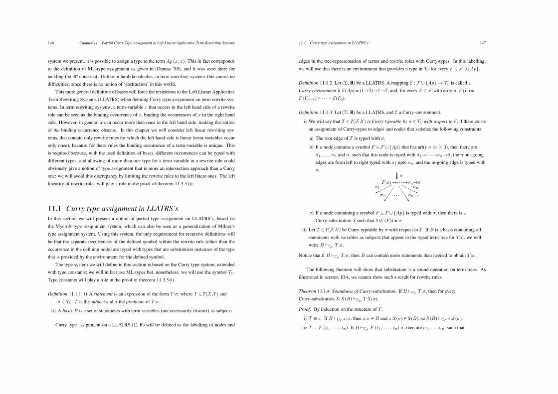
146 Chapter 11 Partial Curry Type Assignment in Left Linear Applicative Term Rewriting Systems
system we present, it is possible to assign a type to the term Ap (x, x). This in fact corresponds
to the definition of ML-type assignment as given in [Damas ’85], and it was used there for
tackling the let-construct. Unlike in lambda calculus, in term rewriting systems this causes no
difficulties, since there is no notion of ‘abstraction’ in this world.
This more general definition of bases will force the restriction to the Left Linear Applicative
Term Rewriting Systems (LLATRS) when defining Curry type assignment on term rewrite sys-
tems. In term rewriting systems, a term-variable x that occurs in the left hand side of a rewrite
rule can be seen as the binding occurrence of x, binding the occurrences of x in the right hand
side. However, in general x can occur more than once in the left hand side, making the notion
of the binding occurrence obscure. In this chapter we will consider left linear rewriting sys-
tems, that contain only rewrite rules for which the left hand side is linear (term-variables occur
only once), because for these rules the binding occurrence of a term-variable is unique. This
is required because, with the used definition of bases, different occurrences can be typed with
different types, and allowing of more than one type for a term variable in a rewrite rule could
obviously give a notion of type assignment that is more an intersection approach than a Curry
one: we will avoid this discrepancy by limiting the rewrite rules to the left linear ones. The left
linearity of rewrite rules will play a role in the proof of theorem 11.3.5 (i).
11.1 Curry type assignment in LLATRS’sIn this section we will present a notion of partial type assignment on LLATRS’s, based on
the Mycroft type assignment system, which can also be seen as a generalization of Milner’s
type assignment system. Using this system, the only requirement for recursive definitions will
be that the separate occurrences of the defined symbol within the rewrite rule (other than the
occurrence in the defining node) are typed with types that are substitution instances of the type
that is provided by the environment for the defined symbol.
The type system we will define in this section is based on the Curry type system, extended
with type constants; we will in fact use ML-types but, nonetheless, we will use the symbol TC.
Type constants will play a role in the proof of theorem 11.3.5 (i).
Definition 11.1.1 i) A statement is an expression of the form T :*, where T + T(F,X ) and
* + TC. T is the subject and * the predicate of T :*.
ii) A basis B is a set of statements with term-variables (not necessarily distinct) as subjects.
Curry type assignment on a LLATRS ($, R) will be defined as the labelling of nodes and
11.1 Curry type assignment in LLATRS’s 147
edges in the tree-representation of terms and rewrite rules with Curry-types. In this labelling,
we will use that there is an environment that provides a type in TC for every F +F / {Ap}.
Definition 11.1.2 Let ($, R) be a LLATRS. A mapping E : F /{Ap}$ TC is called a
Curry-environment if E(Ap) = (1$2)$1$2, and, for every F +F with arity n, E (F ) =
E (Fn!1) = · · · = E(F0).
Definition 11.1.3 Let ($, R) be a LLATRS, and E a Curry-environment.
i) We will say that T + T(F,X ) is Curry typeable by * + TC with respect to E , if there exists
an assignment of Curry-types to edges and nodes that satisfies the following constraints:
a) The root edge of T is typed with *.
b) If a node contains a symbol F +F /{Ap} that has arity n (n 1 0), then there are
*1, . . . , *n and *, such that this node is typed with *1$· · ·$*n$*, the n out-going
edges are from left to right typed with *1 upto *n, and the in-going edge is typed with
*.
+*F :*1$· · ·$*n$*
00001*1 4
4445
*2
66667*n!1
22223*n
· · ·
c) If a node containing a symbol F +F /{Ap} is typed with *, then there is a
Curry-substitution S such that S (E (F )) = *.
ii) Let T + T(F,X ) be Curry typeable by * with respect to E . If B is a basis containing all
statements with variables as subjects that appear in the typed term-tree for T :*, we will
write B !CE T :*.
Notice that if B !CE T :*, then B can contain more statements than needed to obtain T :*.
The following theorem will show that substitution is a sound operation on term-trees. As
illustrated in section 10.4, we cannot show such a result for rewrite rules.
Theorem 11.1.4 Soundness of Curry-substitution. If B !CE T :*, then for every
Curry-substitution S: S (B) !CE T :S (*).
Proof: By induction on the structure of T .
i) T 4 x. If B !CE x:*, then x:* +B and x:S (*) + S (B), so S (B) !CE x:S (*).
ii) T 4 F (t1, . . . , tn). If B !CE F (t1, . . . , tn):*, then are *1, . . . , *n, such that
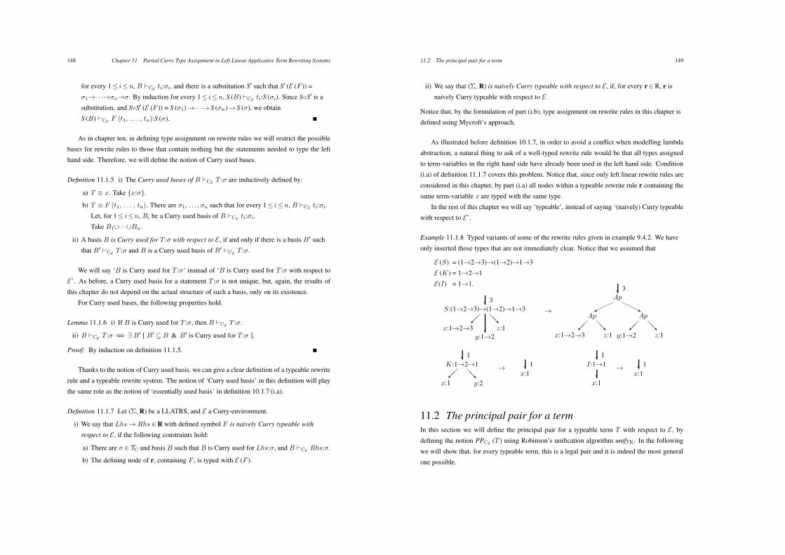
148 Chapter 11 Partial Curry Type Assignment in Left Linear Applicative Term Rewriting Systems
for every 1( i(n, B !CE ti:*i, and there is a substitution S" such that S" (E (F )) =
*1$· · ·$*n$*. By induction for every 1( i(n, S (B) !CE ti:S (*i). Since S-S" is a
substitution, and S-S" (E (F )) = S (*1)$· · ·$ S (*n)$ S (*), we obtain
S (B) !CE F (t1, . . . , tn):S (*).
As in chapter ten, in defining type assignment on rewrite rules we will restrict the possible
bases for rewrite rules to those that contain nothing but the statements needed to type the left
hand side. Therefore, we will define the notion of Curry used bases.
Definition 11.1.5 i) The Curry used bases of B !CE T :* are inductively defined by:
a) T 4 x. Take {x:*}.
b) T 4 F (t1, . . . , tn). There are *1, . . . , *n such that for every 1( i(n, B !CE ti:*i.
Let, for 1( i(n, Bi be a Curry used basis of B !CE ti:*i.
Take B1/· · ·/Bn.
ii) A basis B is Curry used for T :* with respect to E , if and only if there is a basis B" such
that B" !CE T :* and B is a Curry used basis of B" !CE T :*.
We will say ‘B is Curry used for T :*’ instead of ‘B is Curry used for T :* with respect to
E’. As before, a Curry used basis for a statement T :* is not unique, but, again, the results of
this chapter do not depend on the actual structure of such a basis, only on its existence.
For Curry used bases, the following properties hold.
Lemma 11.1.6 i) If B is Curry used for T :*, then B !CE T :*.
ii) B !CE T :* 23 6 B" [ B" 7 B & B" is Curry used for T :* ].
Proof: By induction on definition 11.1.5.
Thanks to the notion of Curry used basis, we can give a clear definition of a typeable rewrite
rule and a typeable rewrite system. The notion of ‘Curry used basis’ in this definition will play
the same role as the notion of ‘essentially used basis’ in definition 10.1.7 (i.a).
Definition 11.1.7 Let ($, R) be a LLATRS, and E a Curry-environment.
i) We say that Lhs $ Rhs + R with defined symbol F is naively Curry typeable with
respect to E , if the following constraints hold:
a) There are * + TC and basis B such that B is Curry used for Lhs:*, and B !CE Rhs:*.
b) The defining node of r, containing F , is typed with E (F ).
11.2 The principal pair for a term 149
ii) We say that ($, R) is naively Curry typeable with respect to E , if, for every r + R, r is
naively Curry typeable with respect to E .
Notice that, by the formulation of part (i.b), type assignment on rewrite rules in this chapter is
defined using Mycroft’s approach.
As illustrated before definition 10.1.7, in order to avoid a conflict when modelling lambda
abstraction, a natural thing to ask of a well-typed rewrite rule would be that all types assigned
to term-variables in the right hand side have already been used in the left hand side. Condition
(i.a) of definition 11.1.7 covers this problem. Notice that, since only left linear rewrite rules are
considered in this chapter, by part (i.a) all nodes within a typeable rewrite rule r containing the
same term-variable x are typed with the same type.
In the rest of this chapter we will say ‘typeable’, instead of saying ‘(naively) Curry typeable
with respect to E’.
Example 11.1.8 Typed variants of some of the rewrite rules given in example 9.4.2. We have
only inserted those types that are not immediately clear. Notice that we assumed that
E (S) = (1$2$3)$(1$2)$1$3
E (K) = 1$2$1
E(I) = 1$1.
+3
S:(1$2$3)$(1$2)$1$3
,,-x:1$2$3 +
y:1$2
../z:1
$
+3Ap
00012223
Ap
,,-x:1$2$3
../z:1
Ap
,,-y:1$2
../z:1
+1
K:1$2$1,,-
x:1
../y:2
$ +1
x:1
+1
I:1$1
+x:1
$ +1
x:1
11.2 The principal pair for a termIn this section we will define the principal pair for a typeable term T with respect to E , by
defining the notion PPCE (T ) using Robinson’s unification algorithm unifyR. In the following
we will show that, for every typeable term, this is a legal pair and it is indeed the most general
one possible.
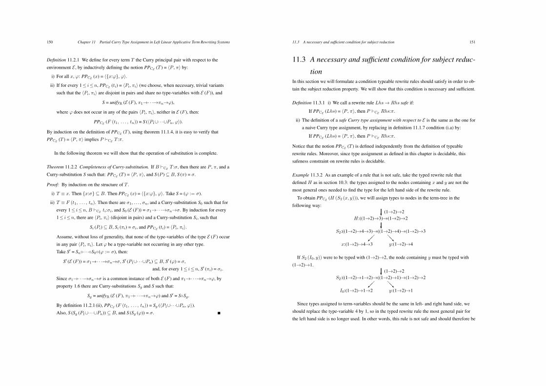
150 Chapter 11 Partial Curry Type Assignment in Left Linear Applicative Term Rewriting Systems
Definition 11.2.1 We define for every term T the Curry principal pair with respect to the
environment E , by inductively defining the notion PPCE (T ) = %P , ,& by:
i) For all x, #: PPCE (x) = %{x:#}, #&.
ii) If for every 1( i(n, PPCE (ti) = %Pi, ,i& (we choose, when necessary, trivial variants
such that the %Pi, ,i& are disjoint in pairs and share no type-variables with E (F )), and
S = unifyR (E (F ), ,1$· · ·$,n$#),
where # does not occur in any of the pairs %Pi, ,i&, neither in E (F ), then:
PPCE (F (t1, . . . , tn)) = S (%P1/· · ·/Pn, #&).
By induction on the definition of PPCE (T ), using theorem 11.1.4, it is easy to verify that
PPCE (T ) = %P , ,& implies P !CE T :,.
In the following theorem we will show that the operation of substitution is complete.
Theorem 11.2.2 Completeness of Curry-substitution. If B !CE T :*, then there are P , ,, and a
Curry-substitution S such that: PPCE (T ) = %P , ,&, and S (P ) 7 B, S (,) = *.
Proof: By induction on the structure of T .
i) T 4 x. Then {x:*} 7 B. Then PPCE (x) = %{x:#}, #&. Take S = (# := *).
ii) T 4 F (t1, . . . , tn). Then there are *1, . . . , *n, and a Curry-substitution S0 such that for
every 1( i(n, B !CE ti:*i, and S0 (E (F )) = *1$· · ·$*n$*. By induction for every
1( i(n, there are %Pi, ,i& (disjoint in pairs) and a Curry-substitution Si, such that
Si (Pi) 7 B, Si (,i) = *i, and PPCE (ti) = %Pi, ,i&.
Assume, without loss of generality, that none of the type-variables of the type E (F ) occur
in any pair %Pi, ,i&. Let # be a type-variable not occurring in any other type.
Take S" = Sn-· · ·-S0-(# := *), then:
S" (E (F )) = *1$· · ·$*n$*, S" (P1/· · ·/Pn) 7 B, S" (#) = *,
and, for every 1( i(n, S" (,i) = *i.
Since *1$· · ·$*n$* is a common instance of both E (F ) and ,1$· · ·$,n$#, by
property 1.6 there are Curry-substitutions Sg and S such that:
Sg = unifyR (E (F ), ,1$· · ·$,n$#) and S" = S-Sg .
By definition 11.2.1 (ii), PPCE (F (t1, . . . , tn)) = Sg (%P1/· · ·/Pn, #&).
Also, S (Sg (P1/· · ·/Pn)) 7 B, and S (Sg (#)) = *.
11.3 A necessary and sufficient condition for subject reduction 151
11.3 A necessary and sufficient condition for subject reduc-
tionIn this section we will formulate a condition typeable rewrite rules should satisfy in order to ob-
tain the subject reduction property. We will show that this condition is necessary and sufficient.
Definition 11.3.1 i) We call a rewrite rule Lhs$ Rhs safe if:
If PPCE (Lhs) = %P , ,&, then P !CE Rhs:,.
ii) The definition of a safe Curry type assignment with respect to E is the same as the one for
a naive Curry type assignment, by replacing in definition 11.1.7 condition (i.a) by:
If PPCE (Lhs) = %P , ,&, then P !CE Rhs:,.
Notice that the notion PPCE (T ) is defined independently from the definition of typeable
rewrite rules. Moreover, since type assignment as defined in this chapter is decidable, this
safeness constraint on rewrite rules is decidable.
Example 11.3.2 As an example of a rule that is not safe, take the typed rewrite rule that
defined H as in section 10.3: the types assigned to the nodes containing x and y are not the
most general ones needed to find the type for the left hand side of the rewrite rule.
To obtain PPCE (H (S2 (x, y))), we will assign types to nodes in the term-tree in the
following way:
+(1$2)$2
H:((1$2)$3)$(1$2)$2
+S2:((1$2)$4$3)$((1$2)$4)$(1$2)$3
,,-x:(1$2)$4$3
../y:(1$2)$4
If S2 (I0, y)) were to be typed with (1$2)$2, the node containing y must be typed with
(1$2)$1.
+(1$2)$2
S2:((1$2)$1$2)$((1$2)$1)$(1$2)$2
,,-I0:(1$2)$1$2
../y:(1$2)$1
Since types assigned to term-variables should be the same in left- and right hand side, we
should replace the type-variable 4 by 1, so in the typed rewrite rule the most general pair for
the left hand side is no longer used. In other words, this rule is not safe and should therefore be
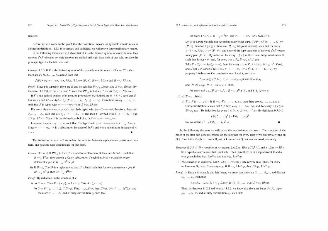
152 Chapter 11 Partial Curry Type Assignment in Left Linear Applicative Term Rewriting Systems
rejected.
Before we will come to the proof that the condition imposed on typeable rewrite rules as
defined in definition 11.3.1 is necessary and sufficient, we will prove some preliminary results.
In the following lemma we will show that, if F is the defined symbol of a rewrite rule, then
the type E (F ) dictates not only the type for the left and right hand side of that rule, but also the
principal type for the left hand side.
Lemma 11.3.3 If F is the defined symbol of the typeable rewrite rule r : Lhs$ Rhs, then
there are P , B, *1, . . . , *n, and * such that
E(F ) = *1$· · ·$*n$*, PPCE (Lhs) = %P , *&, B !CE Lhs:* and B !CE Rhs:*.
Proof: Since r is typeable, there are B and * such that B !CE Lhs:*, and B !CE Rhs:*. By
theorem 11.2.2 there are P , ,, and S, such that PPCE (Lhs) = %P , ,&, S (P ) 7 B, S (,) = *.
If F is the defined symbol of r, then, by proposition 9.3.4, there are n 1 j 1 0 such that F
has arity j and Lhs = Ap (· · ·Ap (F (t1, . . . , tj), tj+1) · · ·, tn). Then there are *1, . . . , *j , µ
such that F is typed with *1$· · ·$*j$µ in B !CE Lhs:*.
For every Ap there are $, % such that Ap is typed with ($$%)$$$%; therefore, there are
*j+1, . . . , *n, such that µ = *j+1$· · ·$*n$*. But then F is typed with *1$· · ·$*n$* in
B !CE Lhs:*. Since F is the defined symbol of r, E(F ) = *1$· · ·$*n$*.
Likewise, there are +1, . . . , +n such that F is typed with +1$· · ·$+n$, in P !CE Lhs:,.
Since +1$· · ·$+n$, is a substitution instance of E(F ), and * is a substitution instance of ,,
* = ,.
The following lemma will formulate the relation between replacements performed on a
term, and possible type assignments for that term.
Lemma 11.3.4 i) If PPCE (T ) = %P , ,&, and for replacement R there are B and * such that
B !CE TR:*, then there is a Curry-substitution S such that S (,) = *, and for every
statement x:)+ P B !CE xR:S ()).
ii) If B !CE T :*, R is a replacement, and B" a basis such that for every statement x:) +B
B" !CE xR:), then B" !CE TR:*.
Proof: By induction on the structure of T .
i) a) T 4 x. Then P = {x:#}, and , = #. Take S = (# := *).
b) T 4 F (t1, . . . , tn). If B !CE F (t1, . . . , tn)R:*, then B !CE F (t1R, . . . , t1R):*, and
there are *1, . . . , *n, and a Curry-substitution S0 such that
11.3 A necessary and sufficient condition for subject reduction 153
for every 1( i(n, B !CE tiR:*i, and *1$· · ·$*n$* = S0 (E (F )).
Let # be a type-variable not occurring in any other type. If PPCE (F (t1, . . . , tn)) =
%P , ,&, then for 1( i(n, there are %Pi, ,i& (disjoint in pairs), such that for every
1( i(n, PPCE (ti) = %Pi, ,i&, and none of the type-variables of the type E (F ) occur
in any pair %Pi, ,i&. By induction for every 1( i(n, there is a Curry- substitution Si
such that Si (,i) = *i, and, for every x:$ +Pi, B !CE xR:Si ($).
Take S" = Sn-· · ·-S0-(# := *), then, for every x:$ + P1/· · ·/Pn, B !CE xR:S" ($),
and S" (#) = *. Since S" (E (F )) = *1$· · ·$*n$* = S" (,1$· · ·$,n$#), by
property 1.6 there are Curry-substitutions S and Sg such that
Sg = unifyR (E (F ), ,1$· · ·$,n$#), and S" = S-Sg
and %P , ,& = Sg (%P1/· · ·/Pn, #&). Then,
for every x:% + Sg(P1/· · ·/Pn), B !CE xR:S (%), and S (Sg (#)) = *.
ii) a) T 4 x. Trivial.
b) T 4 F (t1, . . . , tn). If B !CE F (t1, . . . , tn):*, then there are *1, . . . , *n, and a
Curry-substitution S such that S (E (F )) = *1$· · ·$*n$*, and, for every 1( i(n,
B !CE ti:*i. By induction for every 1( i(n, B" !CE tiR:*i. By definition 9.3.6 (i)
F (t1R, . . . , t1R) = F (t1, . . . , tn)R.
So, we obtain B" !E F (t1, . . . , tn)R:*.
In the following theorem we will prove that our solution is correct. The structure of the
proof of the first part depends greatly on the fact that for every type * we can trivially find an
Q +F such that E (Q) = *: we will just pick a constant Q that was not used previously.
Theorem 11.3.5 i) The condition is necessary. Let Lhs, Rhs + T(F,X ), and r : Lhs$ Rhs
be a typeable rewrite rule that is not safe. Then there there exist a replacement R and a
type µ, such that !CE LhsR:µ and not !CE RhsR:µ.
ii) The condition is sufficient. Let r : Lhs $ Rhs be a safe rewrite rule. Then, for every
replacement R, basis B and a type µ, if B !CE LhsR:µ, then B !CE RhsR:µ.
Proof: i) Since r is typeable and left linear, we know that there are %1, . . . , %n, + , and distinct
x1, . . . , xn, such that:
{x1:%1, . . . , xn:%n} !CE Lhs:+ & {x1:%1, . . . , xn:%n} !CE Rhs:+ .
Then, by theorem 11.2.2 and lemma 11.3.3, we know that there are bases Pl, Pr, types
)1, . . . , )n, ,r and a Curry-substitution S0, such that:
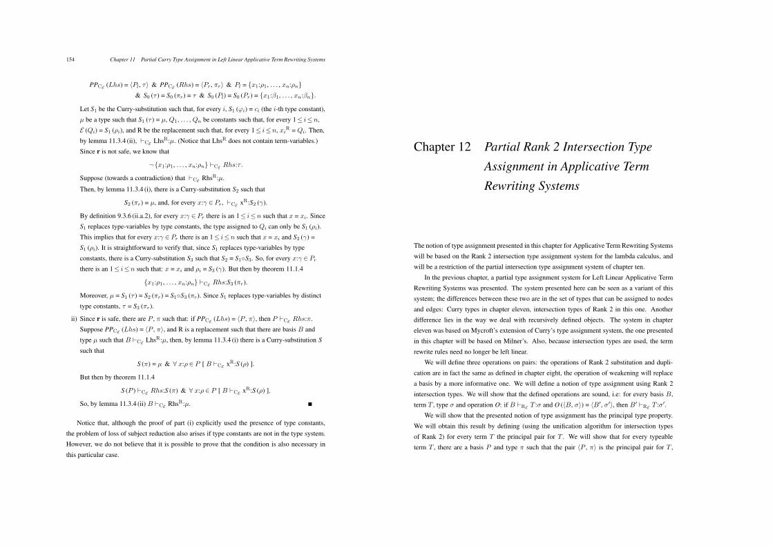
154 Chapter 11 Partial Curry Type Assignment in Left Linear Applicative Term Rewriting Systems
PPCE (Lhs) = %Pl, +& & PPCE (Rhs) = %Pr , ,r& & Pl = {x1:)1, . . . , xn:)n}
& S0 (+ ) = S0 (,r) = + & S0 (Pl) = S0 (Pr) = {x1:%1, . . . , xn:%n}.
Let S1 be the Curry-substitution such that, for every i, S1 (#i) = ci (the i-th type constant),
µ be a type such that S1 (+ ) = µ, Q1, . . . , Qn be constants such that, for every 1( i(n,
E (Qi) = S1 ()i), and R be the replacement such that, for every 1( i(n, xiR = Qi. Then,
by lemma 11.3.4 (ii), !CE LhsR:µ. (Notice that LhsR does not contain term-variables.)
Since r is not safe, we know that
¬{x1:)1, . . . , xn:)n} !CE Rhs:+ .
Suppose (towards a contradiction) that !CE RhsR:µ.
Then, by lemma 11.3.4 (i), there is a Curry-substitution S2 such that
S2 (,r) = µ, and, for every x:& + Pr, !CE xR:S2 (&).
By definition 9.3.6 (ii.a.2), for every x:& + Pr there is an 1( i(n such that x = xi. Since
S1 replaces type-variables by type constants, the type assigned to Qi can only be S1 ()i).
This implies that for every x:& + Pr there is an 1( i(n such that x = xi and S2 (&) =
S1 ()i). It is straightforward to verify that, since S1 replaces type-variables by type
constants, there is a Curry-substitution S3 such that S2 = S1-S3. So, for every x:& + Pr
there is an 1( i(n such that: x = xi and )i = S3 (&). But then by theorem 11.1.4
{x1:)1, . . . , xn:)n} !CE Rhs:S3 (,r).
Moreover, µ = S1 (+ ) = S2 (,r) = S1-S3 (,r). Since S1 replaces type-variables by distinct
type constants, + = S3 (,r).
ii) Since r is safe, there are P , , such that: if PPCE (Lhs) = %P , ,&, then P !CE Rhs:,.
Suppose PPCE (Lhs) = %P , ,&, and R is a replacement such that there are basis B and
type µ such that B !CE LhsR:µ, then, by lemma 11.3.4 (i) there is a Curry-substitution S
such that
S (,) = µ & ' x:)+ P [ B !CE xR:S ()) ].
But then by theorem 11.1.4
S (P ) !CE Rhs:S (,) & ' x:)+ P [ B !CE xR:S ()) ].
So, by lemma 11.3.4 (ii) B !CE RhsR:µ.
Notice that, although the proof of part (i) explicitly used the presence of type constants,
the problem of loss of subject reduction also arises if type constants are not in the type system.
However, we do not believe that it is possible to prove that the condition is also necessary in
this particular case.
Chapter 12 Partial Rank 2 Intersection Type
Assignment in Applicative Term
Rewriting Systems
The notion of type assignment presented in this chapter for Applicative Term Rewriting Systems
will be based on the Rank 2 intersection type assignment system for the lambda calculus, and
will be a restriction of the partial intersection type assignment system of chapter ten.
In the previous chapter, a partial type assignment system for Left Linear Applicative Term
Rewriting Systems was presented. The system presented here can be seen as a variant of this
system; the differences between these two are in the set of types that can be assigned to nodes
and edges: Curry types in chapter eleven, intersection types of Rank 2 in this one. Another
difference lies in the way we deal with recursively defined objects. The system in chapter
eleven was based on Mycroft’s extension of Curry’s type assignment system, the one presented
in this chapter will be based on Milner’s. Also, because intersection types are used, the term
rewrite rules need no longer be left linear.
We will define three operations on pairs: the operations of Rank 2 substitution and dupli-
cation are in fact the same as defined in chapter eight, the operation of weakening will replace
a basis by a more informative one. We will define a notion of type assignment using Rank 2
intersection types. We will show that the defined operations are sound, i.e: for every basis B,
term T , type * and operation O: if B !RE T :* and O (%B, *&) = %B", *"&, then B" !RE T :*".
We will show that the presented notion of type assignment has the principal type property.
We will obtain this result by defining (using the unification algorithm for intersection types
of Rank 2) for every term T the principal pair for T . We will show that for every typeable
term T , there are a basis P and type , such that the pair %P , ,& is the principal pair for T ,
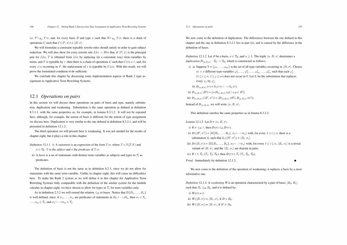
156 Chapter 12 Partial Rank 2 Intersection Type Assignment in Applicative Term Rewriting Systems
i.e. P !RE T :,, and, for every basis B and type * such that B !RE T :*, there is a chain of
operations C such that C (%P , ,&) = %B, *&.
We will formulate a constraint typeable rewrite rules should satisfy in order to gain subject
reduction. We will also show for every rewrite rule Lhs $ Rhs that, if %P , ,& is the principal
pair for Lhs, T is obtained from Lhs by replacing (in a consistent way) term-variables by
terms, and T is typeable by + , then there is a chain of operations C such that C (,) = + , and, for
every x:$ occurring in P , the replacement of x is typeable by C ($). With this result, we will
prove the formulated condition to be sufficient.
We conclude this chapter by discussing some implementation aspects of Rank 2 type as-
signment in Applicative Term Rewriting Systems.
12.1 Operations on pairsIn this section we will discuss three operations on pairs of basis and type, namely substitu-
tion, duplication and weakening. Substitution is the same operation as defined in definition
8.3.1.1, with the same properties as, for example, in lemma 8.3.1.2. It will not be repeated
here, although, for example, the notion of basis is different for the notion of type assignment
we discuss here. Duplication is very similar to the one defined in definition 8.3.2.1, and will be
presented in definition 12.1.2.
The third operation we will present here is weakening. It was not needed for the results of
chapter eight, but it plays a role in this chapter.
Definition 12.1.1 i) A statement is an expression of the form T :*, where T + T(F,X ) and
* + TR. T is the subject and * the predicate of T :*.
ii) A basis is a set of statements with distinct term-variables as subjects and types in T1 as
predicates.
The definition of basis is not the same as in definition 8.2.3, since we do not allow for
statements with the same term-variable. Unlike in chapter eight, this will cause no difficulties
here. To make the Rank 2 system as we will define it in this chapter for Applicative Term
Rewriting Systems fully comparable with the definition of the similar system for the lambda
calculus in chapter eight, we have chosen to allow for types in T1 for term-variables only.
As in definition 2.3.2 we will extend the relation (R to bases. Notice that #{B1, . . . , Bn}
is well defined, since, if *1, . . . , *m are predicates of statements in B1/· · ·/Bn, then *1 + T1,
. . . , *m + T1, and *1!· · ·!*m + T1.
12.1 Operations on pairs 157
We now come to the definition of duplication. The differences between the one defined in this
chapter and the one in definition 8.3.2.1 lies in part (ii), and is caused by the difference in the
definition of bases.
Definition 12.1.2 Let B be a basis, * + TR, and n 1 1. The triple %n, B, *& determines a
duplication D$n,B,%% : TR $ TR, which is constructed as follows:
i) a) Suppose V = {#1, . . . , #m} is the set of all type-variables occurring in %B, *&. Choose
m. n different type-variables #11, . . . , #n
1 , . . . , #1m, . . . , #n
m, such that each #ij
(1( i(n, 1( j(m) does not occur in V. Let Si be the substitution that replaces
every #j by #ij .
b) D$n,B,%% (+ ) = S1 (+ )!· · ·! Sn (+ ).
ii) D$n,B,%% (B") = {x:D$n,B,%% ()) | x:)+B"}.
iii) D$n,B,%% (%B", *"&) = %D$n,B,%% (B"), D$n,B,%% (*")&.
Instead of D$n,B,%%, we will write %n, B, *&.
This definition satisfies the same properties as in lemma 8.3.2.2.
Lemma 12.1.3 Let D = %n, B, *&.
i) If * (R + , then D (*) (R D (+ ).
ii) D (%B", *"&) = %#{B1, . . . , Bn}, *1!· · ·!*n& with, for every 1( i(n, there is a
substitution Si such that Si (%B", *"&) = %Bi, *i&.
iii) D (%B, *&) = %#{B1, . . . , Bn}, *1!· · ·!*n& with, for every 1( i(n, %Bi, *i& is a trivial
variant of %B, *&, and the %Bi, *i& are disjoint in pairs.
iv) If + + TC (T1, T2, TR), then D (+ ) + T1 (T1, TR, TR).
Proof: Immediately by definition 12.1.2.
We now come to the definition of the operation of weakening; it replaces a basis by a more
informative one.
Definition 12.1.4 A weakening W is an operation characterized by a pair of bases %B0, B1&
such that B1 (R B0, and it is defined by:
i) W (*) = *.
ii) W (%B, *&) = %B1, *&, if B = B0.
iii) W (%B, *&) = %B, *&, if B ,= B0.
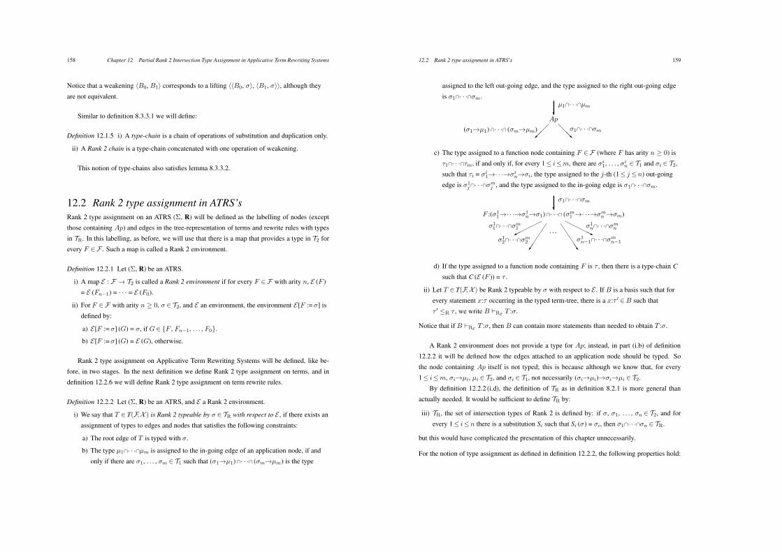
158 Chapter 12 Partial Rank 2 Intersection Type Assignment in Applicative Term Rewriting Systems
Notice that a weakening %B0, B1& corresponds to a lifting %%B0, *&, %B1, *&&, although they
are not equivalent.
Similar to definition 8.3.3.1 we will define:
Definition 12.1.5 i) A type-chain is a chain of operations of substitution and duplication only.
ii) A Rank 2 chain is a type-chain concatenated with one operation of weakening.
This notion of type-chains also satisfies lemma 8.3.3.2.
12.2 Rank 2 type assignment in ATRS’sRank 2 type assignment on an ATRS ($, R) will be defined as the labelling of nodes (except
those containing Ap) and edges in the tree-representation of terms and rewrite rules with types
in TR. In this labelling, as before, we will use that there is a map that provides a type in T2 for
every F +F . Such a map is called a Rank 2 environment.
Definition 12.2.1 Let ($, R) be an ATRS.
i) A map E : F $ T2 is called a Rank 2 environment if for every F +F with arity n, E (F )
= E (Fn!1) = · · · = E (F0).
ii) For F +F with arity n 1 0, * + T2, and E an environment, the environment E[F := *] is
defined by:
a) E[F :=*] (G) = *, if G+ {F , Fn!1, . . . , F0}.
b) E[F :=*] (G) = E (G), otherwise.
Rank 2 type assignment on Applicative Term Rewriting Systems will be defined, like be-
fore, in two stages. In the next definition we define Rank 2 type assignment on terms, and in
definition 12.2.6 we will define Rank 2 type assignment on term rewrite rules.
Definition 12.2.2 Let ($, R) be an ATRS, and E a Rank 2 environment.
i) We say that T + T(F,X ) is Rank 2 typeable by * + TR with respect to E , if there exists an
assignment of types to edges and nodes that satisfies the following constraints:
a) The root edge of T is typed with *.
b) The type µ1!· · ·!µm is assigned to the in-going edge of an application node, if and
only if there are *1, . . . , *m + T1 such that (*1$µ1)!· · ·! (*m$µm) is the type
12.2 Rank 2 type assignment in ATRS’s 159
assigned to the left out-going edge, and the type assigned to the right out-going edge
is *1!· · ·!*m.
+µ1!· · ·!µm
Ap
,,,-
(*1$µ1) !· · ·! (*m$µm) .../*1!· · ·!*m
c) The type assigned to a function node containing F +F (where F has arity n 1 0) is
+1!· · ·!+m, if and only if, for every 1( i(m, there are *i1, . . . , *i
n + T1 and *i + T2,
such that +i = *i1$· · ·$*i
n$*i, the type assigned to the j-th (1( j (n) out-going
edge is *1j!· · ·!*
mj , and the type assigned to the in-going edge is *1!· · ·!*m.
+*1!· · ·!*m
F :(*11$· · ·$*1
n$*1)!· · ·! (*m1 $· · ·$*m
n $*m)000001
*11!· · ·!*
m1 4
44
445*12!· · ·!*
m2
666667*1n!1!· · ·!*
mn!1
222223*1n!· · ·!*
mn
. . .
d) If the type assigned to a function node containing F is + , then there is a type-chain C
such that C (E (F )) = + .
ii) Let T + T(F,X ) be Rank 2 typeable by * with respect to E . If B is a basis such that for
every statement x:+ occurring in the typed term-tree, there is a x:+ " +B such that
+ " (R + , we write B !RE T :*.
Notice that if B !RE T :*, then B can contain more statements than needed to obtain T :*.
A Rank 2 environment does not provide a type for Ap; instead, in part (i.b) of definition
12.2.2 it will be defined how the edges attached to an application node should be typed. So
the node containing Ap itself is not typed; this is because although we know that, for every
1( i(m, *i$µi, µi + T2, and *i + T1, not necessarily (*i$µi)$*i$µi + T2.
By definition 12.2.2 (i.d), the definition of TR as in definition 8.2.1 is more general than
actually needed. It would be sufficient to define TR by:
iii) TR, the set of intersection types of Rank 2 is defined by: if *, *1, . . . , *n + T2, and for
every 1( i(n there is a substitution Si such that Si (*) = *i, then *1!· · ·!*n + TR.
but this would have complicated the presentation of this chapter unnecessarily.
For the notion of type assignment as defined in definition 12.2.2, the following properties hold:
160 Chapter 12 Partial Rank 2 Intersection Type Assignment in Applicative Term Rewriting Systems
Lemma 12.2.3 i) B !RE T :*1!· · ·!*n if and only if for every 1( i(n, B !RE T :*i.
ii) If x:+ is a statement occurring in the typed term-tree for B !RE T :*, then B (R {x:+}.
Proof: Immediately from definition 12.2.2.
Because of part (i) of this lemma, in most proofs over B !RE T :* we will only show the
part that assumes * + T2.
As in chapter ten in defining type assignment on rewrite rules, we will restrict the possible
bases for rewrite rules to those that contain nothing but the statements needed to type the left
hand side. In the next definition we will introduce the notion of Rank 2 used bases, which is
similar to that of used bases. This notion will be convenient in several proofs and definitions in
the rest of this chapter.
Definition 12.2.4 i) The Rank 2 used bases of B !RE T :* are inductively defined by:
a) * + T2.
1) T 4 x. Take {x:*}.
2) T 4 Ap (t1, t2). Then there is a + such that B !RE t1:+$*, and B !RE t2:+ . Let
B1 be a Rank 2 used basis of B !RE t1:+$*, and B2 be a Rank 2 used basis of
B !RE t2:+ . Take #{B1, B2}.
3) T 4 F (t1, . . . , tn). Then there are *1, . . . , *n such that, for every 1( i(n,
B !RE ti:*i. Let, for 1( i(n, Bi be a Rank 2 used basis of B !RE ti:*i.
Take #{B1, . . . , Bn}.
b) If * = *1!· · ·!*n, then, by lemma 12.2.3 (i), for every 1( i(n, B !RE T :*i. Let, for
every 1( i(n, Bi be a Rank 2 used basis of B !RE T :*i. Take #{B1, . . . , Bn}.
ii) A basis B is Rank 2 used for T :* with respect to E if and only if there is a basis B" such
that B" !RE T :*, and B is a Rank 2 used basis of B" !RE T :*.
We will say ‘B is Rank 2 used for T :*’ instead of ‘B is Rank 2 used for T :* with respect to E’.
As before, a Rank 2 used basis for a statement T :* is not unique, but, again, the results of
this chapter do not depend on the actual structure of a Rank 2 used basis, only on its existence.
For Rank 2 used bases, the following properties hold.
Lemma 12.2.5 i) If B is Rank 2 used for T :*, then B !RE T :*.
ii) B !RE T :* 23 6 B" [ B (R B" & B" is Rank 2 used for T :* ].
Proof: By induction on definition 12.2.4.
12.3 Soundness of operations on pairs 161
Thanks to the notion of Rank 2 used basis, we can give a clear definition of a typeable
rewrite rule and a typeable rewrite system. Notice that this notion plays the same role in this
definition as the notion of ‘essentially used basis’ did in definition 10.1.7.
Definition 12.2.6 Let ($, R) be an ATRS, and E a Rank 2 environment.
i) We say that Lhs $ Rhs + R with defined symbol F is Rank 2 typeable with respect to
E , if there are basis B, type * + T2, such that
a) B is Rank 2 used for Lhs:* and B !RE Rhs:*.
b) In B !RE Lhs:* and B !RE Rhs:*, all nodes containing F are typed with E (F ).
ii) We say that ($, R) is Rank 2 typeable with respect to E , if every r + R is Rank 2 typeable
with respect to E .
Proposition 12.2.7 Let x be a term-variable occurring in the rewrite rule r: Lhs $ Rhs, and
let r be typeable with basis B and type *. If *1, . . . , *m are all and nothing but the types
assigned to the nodes containing x in the typed term-tree for B !RE Lhs:*, and +1, . . . , +n are
those for B !RE Rhs:*, then x:*1!· · ·!*m +B and *1!· · ·!*m (R +1!· · ·!+n.
Proof: By definition 12.2.4 and lemma 12.2.3 (ii).
Notice that, in the above case, not necessarily *1!· · ·!*m = +1!· · ·!+n.
12.3 Soundness of operations on pairsIn this section we will prove that the three operations on pairs of basis and type (substitution,
duplication and weakening) are sound on typed term-trees. We will also show that part (i.d) of
definition 12.2.2 is sound: if there is a type-chain C such that C (E (F )) = *, then, for every type
+ + T2 such that * (R + , the rewrite rules that define F are typeable with respect to a changed
environment, in which E (F ) is replaced by + .
The following lemma will show that Rank 2 substitution is a sound operation on typed term-
trees and rewrite rules.
Theorem 12.3.1 Soundness of Rank 2 substitution. Let S be a Rank 2 substitution.
i) If B !RE T :*, then S (B) !RE T :S (*).
ii) If B is Rank 2 used for T :*, then S (B) is Rank 2 used for T :S (*).
162 Chapter 12 Partial Rank 2 Intersection Type Assignment in Applicative Term Rewriting Systems
iii) Let r: Lhs$ Rhs be a rewrite rule typeable with respect to the environment E , and let F
be the defined symbol of r. Then r is typeable with respect to E [F := S (E (F ))].
Proof: Very much like the one for theorem 10.2.2. We will, therefore, only show the proof of
part (i), which is given by induction on the structure of T . (Assume * + T2.)
a) T 4 x. Then by lemma 12.2.3 (ii) B (R {x:*}.
By lemma 8.3.1.2 (i) S (B) (R S ({x:*}), so by 12.2.2 (ii) S (B) !RE x:S (*).
b) T 4 Ap (t1, t2). As part (i.c) of the proof of theorem 8.3.1.3.
c) T 4 F (t1, . . . , tn). By definition 12.2.2 (i) there are *1, . . . , *n + T1, and a type-chain C
such that C (E (F )) = *1$· · ·$*n$*, and, for every 1( i(n, B !RE ti:*i.
By induction for every 1( i(n, S (B) !RE ti:S (*i), and, by lemma 8.3.1.2 (ii),
S (*i) + T1. Since C * %S& is also a type-chain, and S (*1$· · ·$*n$*) =
S (*1)$· · ·$ S (*n)$ S (*), we have S (B) !RE F (t1, . . . , tn):S (*).
We will now prove that the operation of duplication is sound on typed term-trees and rewrite
rules.
Theorem 12.3.2 Soundness of duplication. Let D be a duplication such that D (%B", *"&) =
%B"", *""&.
i) If B" !RE T :*", then B"" !RE T :*"".
ii) If B" is Rank 2 used for T :*", then B"" is Rank 2 used for T :*"".
iii) Let r: Lhs$ Rhs be a rewrite rule typeable with respect to the environment E , and let F
be the defined symbol of r. If D (E (F )) = + + TR, then, for every µ + T2 such that
+ (R µ, r is typeable with respect to E [F :=µ].
Proof: Very much like the proof of theorem 10.2.5, but easier since duplication is a simplified
version of strict expansion.
i) By lemma 12.1.3 (i), there are B1, . . . , Bn, *1, . . . , *n such that
%B", *"& = %#{B1, . . . , Bn}, *1!· · ·!*n&,
and for every 1( i(n there is a substitution Si such that Si (%B, *&) = %Bi, *i&.
Notice that for all F +F occurring in T by definition 12.2.2 (i.d), there is a type-chain C
such that F is typed with C (E (F )). Since C * %D& is also a type-chain, F can be typed
with the type D (C (E (F ))).
The proof is completed by theorem 12.3.1 (i) and lemma 12.2.3 (i).
ii) As the proof of part (i).
12.4 Principal type property 163
iii) For every µ + T2 such that + (R µ, by definition 12.1.2 there is a substitution S such that
µ = S (E (F )). The proof is completed by theorem 12.3.1 (iii).
The next theorem states that a weakening performed on a arbitrary pair, will produce a
correct result.
Theorem 12.3.3 Soundness of weakening. For every T + T(F,X ): if B !RE T :*, then for
every weakening W: if W (%B, *&) = %B", *"&, then B" !RE T :*".
Proof: By definition 12.2.2 (ii), for every x:+ occurring in the typed term-tree for T :* there is
a x:µ +B such that µ (R *. By definition 12.1.4, B" (R B, and *" = *. For every x:$ +B
there is a x:$" +B" such that $" (R $. But then for every x:+ occurring in the typed term-tree
for T :*, there is a x:µ" +B" such that µ" (R + , so B" !RE T :*.
Combining the results proved above, we know that Rank 2 chains and type-chains will have
the following effect on pairs and rewrite rules:
Lemma 12.3.4 i) If B !RE T :*, and C is a Rank 2 chain such that C (%B, *&) = %B", *"&, then
B" !RE T :*".
ii) If B is Rank 2 used for T :*, C is a type-chain, and C (%B, *&) = %B", *"&, then B" is
Rank 2 used for T :*".
iii) Let r: Lhs$ Rhs be a rewrite rule typeable with respect to the environment E , and let F
be the defined symbol of r. If C is a type-chain and C (E (F )) = + + TR, then, for every
µ + T2 such that + (R µ, r is typeable with respect to E[F :=µ].
Proof: By theorems 12.3.1, 12.3.2 and 12.3.3.
12.4 Principal type propertyIn this section we will show that the partial Rank 2 type assignment system has the principal type
property, by defining, for every typeable term T , a principal pair with respect to the environment
E , PPRE (T ), and by showing that, for all pairs %B, *& such that B !RE T :*, there is a Rank 2
chain C such that C (PPRE (T )) = %B, *&.
We will define the principal pair for a term T with respect to E , consisting of basis P and
type ,, by defining PPRE (T ) using the operations unify1 and unifyR. In theorem 12.4.8 we will
show that, for every term, this is indeed the principal one.
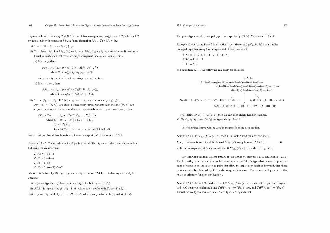
164 Chapter 12 Partial Rank 2 Intersection Type Assignment in Applicative Term Rewriting Systems
Definition 12.4.1 For every T + T(F,X ) we define (using unify1, unifyR, and toTC) the Rank 2
principal pair with respect to E by defining the notion PPRE (T ) = %P , ,& by:
i) T 4 x. Then %P , ,& = %{x:#}, #&.
ii) T 4 Ap (t1, t2). Let PPRE (t1) = %P1, ,1&, PPRE (t2) = %P2, ,2&, (we choose if necessary
trivial variants such that these are disjoint in pairs), and S2 = toTC (,2), then:
a) If ,1 = #, then:
PPRE (Ap (t1, t2)) = %S2, S1& (%#{P1, P2}, #"&),
where S1 = unifyR (#, S2 (,2)$#").
and #" is a type-variable not occurring in any other type.
b) If ,1 = *$+ , then:
PPRE (Ap (t1, t2)) = %S2& * C (%#{P1, P2}, +&),
where C = unify1 (*, S2 (,2), S2 (P2)).
iii) T 4 F (t1, . . . , tn). If E (F ) = &1$· · ·$&n$&, and for every 1( i(n,
PPRE (ti) = %Pi, ,i&, (we choose if necessary trivial variants such that the %Pi, ,i& are
disjoint in pairs and these pairs share no type-variables with &1$· · ·$&n$&), then:
PPRE (F (t1, . . . , tn)) = C (%#{P1, . . . , Pn}, &&),
where C = %S1, . . . , Sn& * C1 * · · · * Cn,
Si = toTC (,i),
Ci = unify1 (C1 * · · · * Ci!1 (&i), Si (,i), Si (Pi)).
Notice that part (ii) of this definition is the same as part (iii) of definition 8.4.2.1.
Example 12.4.2 The typed rules for F (as in example 10.1.9) seem perhaps somewhat ad hoc,
but using the environment:
E (K) = 1$2$1
E (Z) = 3$4$4
E (I) = 5$5
E (F ) = 7!(6$7)!6$7
where Z is defined by Z(x, y) $ y, and using definition 12.4.1, the following can easily be
checked:
i) F (I0) is typeable by 8$8, which is a type for both I0 and I (I0).
ii) F (Z0) is typeable by (8$8)$8$8, which is a type for both Z0 and Z1 (Z0).
iii) F (K0) is typeable by (8$9)$9$8$9, which is a type for both K0 and K1 (K0).
12.4 Principal type property 165
The given types are the principal types for respectively F (I0), F (Z0), and F (K0).
Example 12.4.3 Using Rank 2 intersection types, the term S (K0, S0, I0) has a smaller
principal type than using Curry types. With the environment
E (S) = (1$2$3)$(4$2)$1!4$3
E (K) = 5$6$5
E (I) = 7$7
and definition 12.4.1 the following can easily be checked:
+8$8
S:((8$8)$(((9$10)$9)$(9$10)$10)$8$8) $(((9$10)$9$10)$((9$10)$9)$(9$10)$10) $
(8$8)!((9$10)$9$10) $ 8$8
,,-K0:(8$8)$(((9$10)$9)$(9$10)$10)$8$8
+S0:((9$10)$9$10)$((9$10)$9)$(9$10)$10
../I0:(8$8)!((9$10)$9$10)
If we define D (x) $ Ap (x, x), then we can even check that, for example,
D (S (K0, S0, I0)) and D (I0) are typeable by 11$11.
The following lemma will be used in the proofs of the next section.
Lemma 12.4.4 If PPRE (T ) = %P , ,&, then P is Rank 2 used for T :,, and , + T2.
Proof: By induction on the definition of PPRE (T ), using lemma 12.3.4 (ii).
A direct consequence of this lemma is that if PPRE (T ) = %P , ,&, then P !RE T :,.
The following lemmas will be needed in the proofs of theorem 12.4.7 and lemma 12.5.3.
The first will give a result similar to the one of lemma 8.4.2.4: if a type-chain maps the principal
pairs of terms in an application to pairs that allow the application itself to be typed, then these
pairs can also be obtained by first performing a unification. The second will generalize this
result to arbitrary function applications.
Lemma 12.4.5 Let * + T2, and for i = 1, 2 PPRE (ti) = %Pi, ,i& such that the pairs are disjoint,
and let C be a type-chain such that C (PPRE (t1)) = %B1, +$*&, and C (PPRE (t2)) = %B2, +&.
Then there are type-chains Cg and C" and type $ + T2 such that
166 Chapter 12 Partial Rank 2 Intersection Type Assignment in Applicative Term Rewriting Systems
PPRE (Ap (t1, t2)) = Cg (%#{P1, P2}, $&), and
C" (PPRE (Ap (t1, t2))) = %#{B1, B2}, *&.
Proof: Like the one for lemma 8.4.2.4.
Lemma 12.4.6 Let * + T2, and for every 1( i(n, PPRE (ti) = %Pi, ,i&, such that the pairs
%Pi, ,i& and the type E (F ) = &1$· · ·$&n$& are disjoint, and let C be a type-chain such that
C (E (F )) = *1$· · ·$*n$* and, for every 1( i(n, C (%Pi, ,i&) = %Bi, *i&.
Then there are type-chains Cg and Cp such that
PPRE (F (t1, . . . , tn)) = Cg (%#{P1, . . . , Pn}, &&), and
Cp (PPRE (F (t1, . . . , tn))) = %#{B1, . . . , Bn}, *&.
Proof: Let, for 1( i(n, Si = toTC (,i). Since for every 1( i(n, C (,i) = *i + T1, by lemma
8.4.1.2 (i), for every 1( i(n there is a Ci" such that C = %Si& * Ci
". Since the ,i are disjoint,
the Si do not interfere, so, without loss of generality we can assume that there is a C" such that
C = %S1, . . . , Sn& * C", and for 1( i(n, C" (&i) = *i.
We will finish the proof by showing by induction on i that for every 0( i(n there are
type-chains Ci, Cu1 , . . . , Cu
i such that C" = Cu1 * · · · * Cu
i * Ci, and for 1( j( i the Cuj are not
defined on type-variables occurring in Sk (,k), with k.
i) i = 0. Take C0 = C".
ii) Since C" (&i) = C" (Si (,i)), by induction:
Ci!1 (Cu1 * · · · * Cu
i!1 (&i)) = Ci!1 (Cu1 * · · · * Cu
i!1 (Si (,i))) = Ci!1 (Si (,i)).
Si (Pi) shares no type-variables with Cu1 * · · · * Cu
i!1 (&i), so by lemma 8.4.1.2 (ii) there is
a type-chain Ci such that Ci!1 = unify1 (Cu1 * · · · * Cu
i!1 (&i), Si (,i), Si (Pi)) * Ci.
Take Cui = unify1 (Cu
1 * · · · * Cui!1 (&i), Si (,i), Si (Pi)).
Take Cg = %S1, . . . , Sn& * Cu1 * · · · * Cu
n, then by definition 12.4.1 (iii) we have
PPRE (F (t1, . . . , tn)) = Cg (%#{P1, . . . , Pn}, &&).
Take Cp = Cn.
The following theorem will show that type-chains are sufficient to generate all possible
pairs %B, *& for a typeable term T such that B is Rank 2 used for T :*.
Theorem 12.4.7 If B is Rank 2 used for T :*, then there are a basis P , type , and a type-chain
C such that PPRE (T ) = %P , ,&, and C (%P , ,&) = %B, *&.
Proof: i) * + T2. By induction on the structure of T .
12.4 Principal type property 167
a) T 4 x. Then B = {x:*}. Then * + TC, and PPRE (x) = %{x:#}, #&.
Take C = %(# := *)&.
b) T 4 Ap (t1, t2). Then, by definition 12.2.4 (i.a.2), there are + + T1 and B1, B2 such
that B1 is Rank 2 used for t1:+$*, B2 is Rank 2 used for t2:+ , and B = #{B1, B2}.
By induction for i = 1, 2, there are Pi, ,i, and type-chains Ci such that
PPRE (t1) = %P1, ,1&, C1 (PPRE (t1)) = %B1, +$*&, and
PPRE (t2) = %P2, ,2&, C2 (PPRE (t2)) = %B2, +&.
Since the pairs %Pi, ,i& are disjoint, the type-chains Ci do not interfere, so
C1 * C2 (PPRE (t1)) = %B1, +$*&, and C1 * C2 (PPRE (t2)) = %B2, +&.
Then, by lemma 12.4.5, there are type-chains C and Cu, and type $ such that
PPRE (Ap (t1, t2)) = Cu (%#{P1, P2}, $&), and C (PPRE (Ap (t1, t2))) = %B, *&.
c) T 4 F (t1, . . . , tn). By definition 12.2.4 (i.a.3), there are B1, . . . , Bn, and *1, . . . , *n
such that B = #{B1, . . . , Bn}, and, for every 1( i(n, Bi is Rank 2 used for ti:*i.
By definition 12.2.2 (i.d), there is a type-chain CF such that
CF (E (F )) = *1$· · ·$*n$*.
By induction for 1( i(n, there are %Pi, ,i& (disjoint in pairs) and type-chains Ci,
such that
PPRE (ti) = %Pi, ,i&, and Ci (PPRE (ti)) = %Bi, *i&.
Since the pairs %Pi, ,i& are disjoint, the type-chains Ci do not interfere. Assume,
without loss of generality, that none of the type-variables occurring in E (F ) occur in
any of the pairs %Pi, ,i&. Let C" = CF * C1 * · · · * Cn. Since, for every 1( i(n,
C" (%Pi, ,i&) = %Bi, *i&, and C" (E (F )) = *1$· · ·$*n$*, then, by lemma 12.4.6,
there are type-chains C and Cu such that
PPRE (F (t1, . . . , tn)) = Cu (%#{P1, . . . , Pn}, &&),
and C (PPRE (F (t1, . . . , tn))) = %B, *&.
ii) * = *1!· · ·!*n. By lemma 12.2.4 (i.b), for every 1( i(n there is a Bi such that Bi is
Rank 2 used for T :*i, and B = #{B1, . . . , Bn}. Take %Bi", *i
"&, trivial variants of
%Bi, *i& that are disjoint in pairs. Take S such that
S (%#{B1", . . . , Bn
"}, *1"!· · ·!*n"&) = %#{B1, . . . , Bn}, *1!· · ·!*n&.
By induction there are P , ,, such that PPRE (T ) = %P , ,&. Let D = %n, P , ,&, then
D (%P , ,&) = %#{P1, . . . , Pn}, ,1!· · ·!,n&, with PPRE (T ) = %Pi, ,i&.
168 Chapter 12 Partial Rank 2 Intersection Type Assignment in Applicative Term Rewriting Systems
By induction there are type-chains C1, . . . , Cn such that
for 1( i(n, Ci (%Pi, ,i&) = %Bi", *i
"&.
Since the %Pi, ,i& and the %Bi", *i
"& are disjoint in pairs, the Ci do not interfere.
Take C = %D& * C1 * · · · * Cn * %S&.
Theorem 12.4.8 Principal pair property.
i) Soundness. If PPRE (T ) = %P , ,&, and C a Rank 2 chain such that C (%P , ,&) = %B, *&,
then B !RE T :*.
ii) Completeness. If B !RE T :*, then there are P and ,, such that PPRE (T ) = %P , ,&, and a
Rank 2 chain C such that C (%P , ,&) = %B, *&.
Proof: i) By lemmas 12.2.5 and 12.4.4 and theorem 12.3.4 (i).
ii) If B !RE T :*, then there is a B" such that B (R B" and B" is Rank 2 used for T :*.
By theorem 12.4.7 there exist P , ,, and a type-chain C" such that PPRE (T ) = %P , ,&, and
C" (%P , ,&) = %B", *&. Take the weakening W = %B", B&, then W (%B", *&) = %B, *&. Take
C = C" * %W&.
12.5 A sufficient condition for subject reductionIn this section we will formulate a condition typeable rewrite rules should satisfy in order to
obtain subject reduction. This condition will be the same as the one formulated for the type
assignment system presented in the previous chapter. We will show that this condition is suffi-
cient.
Definition 12.5.1 i) We call a rewrite rule Lhs$ Rhs safe if:
If PPRE (Lhs) = %P , ,&, then P !RE Rhs:,.
ii) The definition of ‘safely Rank 2 typeable with respect to E " is the same as given in
definition 12.2.2 and 12.2.6, by replacing condition (i.a) of definition 12.2.6 by:
If %P , ,& = PPRE (Lhs), then P !RE Rhs:,.
Notice that the notion PPRE (T ) is defined independently from the definition of typeable
rewrite rules. Moreover, since type assignment as defined in this chapter is decidable, this
safeness constraint on rewrite rules is decidable too.
12.5 A sufficient condition for subject reduction 169
Before we come to the proof that the condition is sufficient, we will prove some preliminary
results.
The following lemmas will formulate the relation between replacements performed on a
term that is the left hand side of a rewrite rule, and possible type assignments for that term.
The construction of the proof of lemma 12.5.3 will in fact be one of the motivations for the
limitation of the possible left hand sides, as given in definition 9.3.2 (ii.a).
Lemma 12.5.2 If B !RE T :*, and R is a replacement and B" a basis such that for every
statement x:$ +B B" !RE xR:$, then B" !RE TR:*.
Proof: By easy induction on the structure of T (see the proof of lemma 11.3.4 (ii)).
Lemma 12.5.3 If T + LHS, for the replacement R there are B and * such that B is Rank 2
used for TR:*, and PPRE (T ) = %P , ,&, then there is a type-chain C, such that C (,) = *, and,
for every statement x:$ + P , B !RE xR:C ($).
Proof: By induction on the structure of LHS.
i) T 4 Ap (t1, t2). Since Ap (t1, t2)R = Ap (t1
R, t2R), by definition 12.2.4 (i.a.2) there are
+ + T1, and B1, B2 such that B1 is Rank 2 used for t1R:+$*, and B2 is Rank 2 used for
t2R:+ . By theorem 12.4.7 for i = 1, 2, there are disjoint %Pi, ,i& = PPRE (ti).
Since t1 + LHS, by induction there is a type-chain C1 such that C1 (,1) = +$*, and, for
every statement x:$ + P1, B1 !RE xR:C1 ($). For t2 we have either:
a) t2 4 x, so %P2, ,2& = %{x:#}, #& for some #. Take C2 = unify1 (+ , #, {x:#}), then + =
C2 (#). B2 is Rank 2 used for xR:+ , so by lemma 12.2.5 (i), for every statement
x:$ + P2, B2 !RE xR:C2 ($).
b) t2 + LHS, so by induction there is a type-chain C2 such that C2 (,2) = + , and, for
every statement x:$ + P2, B2 !RE xR:C2 ($).
Since the pairs %Pi, ,i& are disjoint, the chains Ci do not interfere. Let
C1 * C2 (%P1, ,1&) = %B1", +$*& and C1 * C2 (%P2, ,2&) = %B2
", +&.
Let Cg and , be such that
PPRE (Ap (t1, t2)) = %Cg (#{P1, P2}), ,&,
then by lemma 12.4.5 there is a C such that
C (%Cg (#{P1, P2}), ,&) = %#{B1", B2
"}, *&.
Also: ' x:$ + P1 [ B1 !RE xR:C1 ($) ] & ' x:$ + P2 [ B2 !RE xR:C2 ($) ] 3
' x:$ +#{P1, P2} [ #{B1, B2} !RE xR:Cg * C ($) ] 3
170 Chapter 12 Partial Rank 2 Intersection Type Assignment in Applicative Term Rewriting Systems
' x:$ + Cg (#{P1, P2}) [ #{B1, B2} !RE xR:C ($) ].
ii) T 4 F (t1, . . . , tn). Since F (t1, . . . , tn)R = F (t1R, . . . , tn
R), by definition 12.2.4 (i.a.3),
there are B1, . . . , Bn, *1, . . . , *n such that, for every 1( i(n, Bi is Rank 2 used for
tiR:*i, and B = #{B1, . . . , Bn}. By definition 12.2.2 (i.d) there is a type-chain CF such
that CF (E (F )) = *1$· · ·$*n$*.
Let E (F ) = &1$· · ·$&n$&. By theorem 12.4.7 and definition 12.4.1 (iii) there is a
type-chain Cg and %Pi, ,i& (1( i(n, disjoint in pairs) such that, for every 1( i(n,
PPRE (ti) = %Pi, ,i&, and PPRE (F (t1, . . . , tn)) = Cg (%#{P1, . . . , Pn}, &&).
Assume that none of the type-variables occurring in &1$· · ·$&n$& occur in any of the
pairs %Pi, ,i&. Then for every 1( i(n either:
a) ti 4 x, so %Pi, ,i& = %{x:#}, #& for some #. Take Ci = unify1 (*i, #, {x:#}), then *i
= Ci (#). Bi is Rank 2 used for xR:*i, so, by lemma 12.2.5 (i), for every statement
x:$ + Pi, Bi !RE xR:Ci ($).
b) ti + LHS, so by induction there is a type-chain Ci such that Ci (,i) = *i, and, for every
statement x:$ + Pi, Bi !RE xR:Ci ($).
In any case, for every 1( i(n there is a type-chain Ci such that Ci (,i) = *i, and for
every statement x:$ + Pi, Bi !RE xR:Ci ($).
Let C" = CF * C1 * · · · * Cn. Since for every 1( i(n, C" (%Pi, ,i&) = %Bi, *i&, and
C" (&1$· · ·$&n$&) = *1$· · ·$*n$*,
by lemma 12.4.6 there is a type-chain C such that
C (PPRE (F (t1, . . . , tn))) = %#{B1, . . . , Bn}, *&.
Also: If for every 1( i(n, x:$ +Pi, Bi !RE xR:Ci ($) then
for every x:$ +#{P1, . . . , Pn}, #{B1, . . . , Bn} !RE xR:Cg * C ($)
so for every x:$ + Cg (#{P1, . . . , Pn}), #{B1, . . . , Bn} !RE xR:C ($).
In the following theorem, we will prove that our solution is sufficient.
Theorem 12.5.4 The condition is sufficient. Let r : Lhs $ Rhs be a safe rewrite rule. Then
for every replacement R, basis B and type µ: if B !RE LhsR:µ, then B !RE RhsR:µ.
Proof: (Assume µ + T2.) Let PPRE (Lhs) = %P , ,&. Since r is safe, P !RE Rhs:,.
Suppose R is a replacement such that there are B, µ such that B !RE LhsR:µ. By lemma
12.2.5 (ii) we can assume that B is Rank 2 used for LhsR:µ, so by lemma 12.5.3 there is a
type-chain C such that C (,) = µ & ' x:$ + P [ B !RE xR:C ($) ].
By lemma 12.3.4 (i) C (P ) !RE Rhs:C (,), so C (P ) !RE Rhs:µ, and
12.6 Implementation aspects of Rank 2 type assignment in ATRS’s 171
' x:$ + P [ B !RE xR:C ($) ] 3 ' x:$ + C (P ) [ B !RE xR:$ ].
So by lemma 12.5.2 B !RE RhsR:µ.
In the previous chapter it was also shown that the condition formulated in that chapter is
necessary. This result was achieved by extending the set of types with type constants, and for
every rewrite rule that was not safe, a specific replacement that gives the counterexample was
created. In this construction it was used that every type * can be inhabited in a trivial way: just
pick a constant Q, not already used, and assume that E (Q) = *.
In the notion of type assignment as defined in this chapter we cannot give this construction,
because we cannot let every type be trivially inhabited. The environment of this chapter returns
types in T2, and a function symbol F can only have an intersection type $!% if there exists
a type chain C such that C (E (F )) = $!%. This means that we cannot show that there is, for
example, a function symbol that can be assigned the type #0!(#1$#0).
12.6 Implementation aspects of Rank 2 type assignment in
ATRS’sThe results of this chapter could be used to implement a type-check algorithm for ATRS’s. It
should be noted that the notion of type assignment as defined here is really a type-check system.
Take, for example, the rewrite rule
I (x) $ x.
The smallest environment possible for this rule maps I to the type 1$1. We have shown
that all types that can be obtained from this one by substitution or duplication are allowed for
the rewrite rule, but the set of types that can be used is larger that just the set obtained by those
operations. For example, the rewrite rule can also be typed using the type 1!2$1. To obtain
a type-inference algorithm an operation should be inserted that allows of more specific types
than generated by substitution and duplication. Take, for example, the rewrite rules:
F (x) $ x
F (x) $ Ap (x, x).
A type-inference algorithm could, for example, type both alternatives separately and com-
bine the results found. For the first rule it would find E (F ) = 1$1, for the second E (F ) =
(2$3)!2$3. These types cannot be unified using operations defined in this chapter. To obtain
the correct type for F , 6!(5$6)!5$6, an operation is needed that inserts extra types in the left
172 Chapter 12 Partial Rank 2 Intersection Type Assignment in Applicative Term Rewriting Systems
hand side of the top arrow type constructor. It is not at all easy to define such an operation that
is sound in all cases.
Another thing to notice is that, although type assignment (and type-checking) by the notion
of type assignment defined here is decidable, the complexity of type-checking is bigger than for
a system based on Curry-types. The biggest problem will arise when checking a type provided
for a function symbol. Suppose Lhs $ Rhs is a rewrite rule. One way to implement type-
checking for this rule would be to construct the principal pair %P , ,& for the term Lhs, and to
try and type Rhs using this pair. Let *1!· · ·!*n be the type assigned to the term-variable x in
P . Then, for every occurrence of x in Rhs, some selection of the types in *1!· · ·!*n should
be made. In the worst case, the number of possibilities that must be tried is huge: 2n. There are
some more efficient ways to type-check a rule, but the complexity is still exponential. However,
in every day programming life n will rarely be larger than 2.
The concept of overloading in programming languages is normally used to express that dif-
ferent objects (typically procedures) can have the same identifier. (For another approach to
overloading, see [Castagna et al. ’92].) At first sight, it seems to be nothing but a tool to obtain
programming convenience, but the implementational aspects of languages with overloading are
not at all trivial. In functional programming languages, functions are first order citizens, which
means that they can be handled as any object, like, for example, numbers. In particular, a func-
tion can be passed as an argument to another one, or could constitutes its result. Especially
in the first case it can occur that, at compile time, it cannot be decided which of the several
function definitions for an overloaded identifier is really needed. If this decision cannot be
made, the compiler should generate code that contains all possible functions, and some kind
of case-construct that makes it possible to select at runtime which is the code to use. For rea-
sons of efficiency, and to avoid run-time checks on function types, it seems natural to allow of
overloaded objects only if at compile time, it can be decided which of the different function
definitions is meant, since then the compiler can decide for every occurrence of an overloaded
symbol which of the several function definitions should be linked into the object code.
The intersection type constructor is a good candidate to express this kind of overloading
(see also [Pierce ’91]). It seems natural to say, for example, that the type for addition Add
is (int$int$int)!(real$real$real). Incorporating the notion of overloading into a formal
system for type assignment as defined in this chapter implies that the restriction on types that can
be provided by a Rank 2 environment should be dropped; in such a formalism, types provided
by the environment should be in TR, not just T2.
Selection of one of the function definitions for an overloaded identifier can be accomplished
by defining, similar to definition 12.2.2 (i.d) how a type for a function symbol can be obtained
12.6 Implementation aspects of Rank 2 type assignment in ATRS’s 173
from the one provided by the environment, in the following way:
If the type assigned to a function node containing F is + , then there is a * + T2 such
that E (F ) (R *, and a type chain C such that C (*) = + .
This selection will then be reflected in the way intersection types are unified. Since only
one of the types in an ‘overloaded’ type can be used, the unification should try to unify the
demanded type with each individual type occurring in the provided type. Using this definition,
the notion of ‘principal pair’ becomes slightly more complicated. This is best explained by
discussing the implementation of the type-checker that is looking for such a pair. Take the
function foldr that is defined by
foldr f i [] = i
foldr f i (a:b) = f a (foldr f i b)
and can be typed by (1$2$2)$2$[1]$2. If we take the term ‘foldr Add 1 [2, 3, 4]’, then it is
clear that this term should be typeable by the type int. When constructing the type assignment
for this term, the subterm ‘foldr Add’ is typed. As such, the type needed for Add cannot be
uniquely determined for this term: it is the second argument of foldr that forces the selection.
Since there is a chance of success, the type-checker should postpone the decision to reject
the term, and consider both possibilities simultaneously. This means that, formally, the term
foldr Add has two principal types (which is not the same as saying that its principal type is an
intersection).
175
Summary
”When you know how to do it, Zuck, it’s very easy.
It’s like riding a bike.”
”No, no, people tend to devalue the sophistication of
their own special field.
It’s easy only because of all you know.”
– Philip Roth, The Anatomy Lesson (1983)
This thesis deals with a number of different notions of
type assignment that use intersection types, and it can
roughly be divided in three parts. The first part briefly
discusses definitions and properties of a number of
type assignment systems that were developed in the
past by other authors. The second and third part
contain results of the author’s research; notions of type
assignment defined for the lambda calculus are
presented in the second part and for Term Rewriting
Systems in the third part.
In the first chapter, Curry’s Type Assignment
System is discussed, the oldest en most elementary
type assignment system, in which type assignment is
decidable and all typeable terms are strongly
normalizable. This system has the principal type
property: all possible types for a term can be generated
from a specific type, by means of operations chosen
from a predefined collection. For Curry’s system this
collection consists entirely of type substitutions.
In chapter two a number of intersection type
assignment systems is discussed. The Coppo-Dezani
Type Assignment System (CD) in section 2.1 is a
generalization of Curry’s system in which it is possible
to type term-variables with more than one type. If the
set of terms is limited to those from the !I-calculus,
type assignment in this system is closed for
beta-equality. In section 2.2 three different
Coppo-Dezani-Venneri Type Assignment Systems
(CDV) are discussed; the main difference between
these and the CD-system is the addition of the type
constant ". These systems are closed for beta-equality
for the full lambda calculus, and, therefore, type
assignment in these systems is undecidable. It is
possible to characterize the normalizing terms and the
terms that have a head normal form by means of the
assignable types. For one of these systems the
principal type property is proved; in order to do so,
restrictions have to be made. Next to type substitutions
the collection of operations allowed for this system
contains expansions on types as well.
In section 2.3 the Barendregt-Coppo-Dezani Type
Assignment System (BCD) is discussed, a
generalization of the CDV-systems in which it is
possible to give the same characterization of typeable
terms as in the CDV-systems. The generalization made
consists of treating ‘!’ as a normal type constructor
and introducing a partial type inclusion relation ($),
and it is made in order to prove completeness of type
assignment. The set of typeable terms is exactly the
same as in the CDV-systems, only the set of types that
can be assigned to a term is significantly bigger. The
construction of a filter lambda model and the definition
of a map from types to elements of this model (a
simple type interpretation) make the proof of
completeness possible: if the interpretation of the term
M is an element of the interpretation of the type #,
then M is typeable with #. Also, the BCD-system has
the principal type property. Next to type substitutions
and expansions on types the collection of operations
allowed for the BCD-system contains rises as well.
In chapter three two notions of type assignment are
discussed, the Milner Type Assignment System and
the Mycroft Type Assignment System, that are defined
for a primitive applicative (functional) programming
language. They differ from Curry’s system in the
extension of the lambda calculus with new syntactic
constructors that enable to express recursion and
polymorphism. Both systems have the principal type
property. Type assignment in Milner’s system is
decidable, in Mycroft’s system it is not.
The second part of this thesis starts with chapter
four, which contains the presentation of the Strict
Intersection Type Assignment System. It is a slight
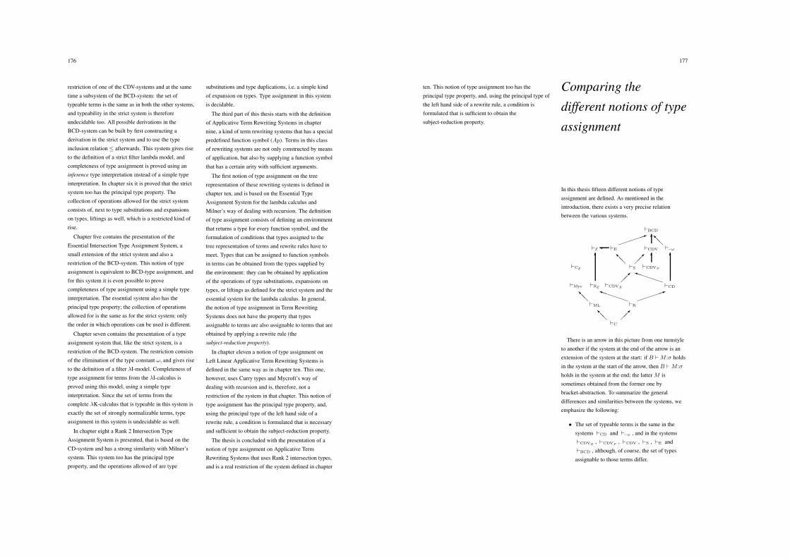
176
restriction of one of the CDV-systems and at the same
time a subsystem of the BCD-system: the set of
typeable terms is the same as in both the other systems,
and typeability in the strict system is therefore
undecidable too. All possible derivations in the
BCD-system can be built by first constructing a
derivation in the strict system and to use the type
inclusion relation $ afterwards. This system gives rise
to the definition of a strict filter lambda model, and
completeness of type assignment is proved using an
inference type interpretation instead of a simple type
interpretation. In chapter six it is proved that the strict
system too has the principal type property. The
collection of operations allowed for the strict system
consists of, next to type substitutions and expansions
on types, liftings as well, which is a restricted kind of
rise.
Chapter five contains the presentation of the
Essential Intersection Type Assignment System, a
small extension of the strict system and also a
restriction of the BCD-system. This notion of type
assignment is equivalent to BCD-type assignment, and
for this system it is even possible to prove
completeness of type assignment using a simple type
interpretation. The essential system also has the
principal type property; the collection of operations
allowed for is the same as for the strict system; only
the order in which operations can be used is different.
Chapter seven contains the presentation of a type
assignment system that, like the strict system, is a
restriction of the BCD-system. The restriction consists
of the elimination of the type constant ", and gives rise
to the definition of a filter !I-model. Completeness of
type assignment for terms from the !I-calculus is
proved using this model, using a simple type
interpretation. Since the set of terms from the
complete !K-calculus that is typeable in this system is
exactly the set of strongly normalizable terms, type
assignment in this system is undecidable as well.
In chapter eight a Rank 2 Intersection Type
Assignment System is presented, that is based on the
CD-system and has a strong similarity with Milner’s
system. This system too has the principal type
property, and the operations allowed of are type
substitutions and type duplications, i.e. a simple kind
of expansion on types. Type assignment in this system
is decidable.
The third part of this thesis starts with the definition
of Applicative Term Rewriting Systems in chapter
nine, a kind of term rewriting systems that has a special
predefined function symbol (Ap). Terms in this class
of rewriting systems are not only constructed by means
of application, but also by supplying a function symbol
that has a certain arity with sufficient arguments.
The first notion of type assignment on the tree
representation of these rewriting systems is defined in
chapter ten, and is based on the Essential Type
Assignment System for the lambda calculus and
Milner’s way of dealing with recursion. The definition
of type assignment consists of defining an environment
that returns a type for every function symbol, and the
formulation of conditions that types assigned to the
tree representation of terms and rewrite rules have to
meet. Types that can be assigned to function symbols
in terms can be obtained from the types supplied by
the environment: they can be obtained by application
of the operations of type substitutions, expansions on
types, or liftings as defined for the strict system and the
essential system for the lambda calculus. In general,
the notion of type assignment in Term Rewriting
Systems does not have the property that types
assignable to terms are also assignable to terms that are
obtained by applying a rewrite rule (the
subject-reduction property).
In chapter eleven a notion of type assignment on
Left Linear Applicative Term Rewriting Systems is
defined in the same way as in chapter ten. This one,
however, uses Curry types and Mycroft’s way of
dealing with recursion and is, therefore, not a
restriction of the system in that chapter. This notion of
type assignment has the principal type property, and,
using the principal type of the left hand side of a
rewrite rule, a condition is formulated that is necessary
and sufficient to obtain the subject-reduction property.
The thesis is concluded with the presentation of a
notion of type assignment on Applicative Term
Rewriting Systems that uses Rank 2 intersection types,
and is a real restriction of the system defined in chapter
177
ten. This notion of type assignment too has the
principal type property, and, using the principal type of
the left hand side of a rewrite rule, a condition is
formulated that is sufficient to obtain the
subject-reduction property.
Comparing the
different notions of type
assignment
In this thesis fifteen different notions of type
assignment are defined. As mentioned in the
introduction, there exists a very precise relation
between the various systems.
"C
..8 ,,9
"ML
..8
"Myc
"CE
"RE
%"E
"R
:::::;<<<<<=
"CD
:::::;
%
"CDVR
,,9
"S
..8 ,,9"CDVP
%"E
* <<<<<=
"CDV
%"#!
..8
"BCD
There is an arrow in this picture from one turnstyle
to another if the system at the end of the arrow is an
extension of the system at the start: if B "M :# holds
in the system at the start of the arrow, then B " M :#
holds in the system at the end; the latter M is
sometimes obtained from the former one by
bracket-abstraction. To summarize the general
differences and similarities between the systems, we
emphasize the following:
• The set of typeable terms is the same in the
systems "CD and "#! , and in the systems
"CDVR, "CDVP
, "CDV , "S , "E and
"BCD , although, of course, the set of types
assignable to those terms differ.
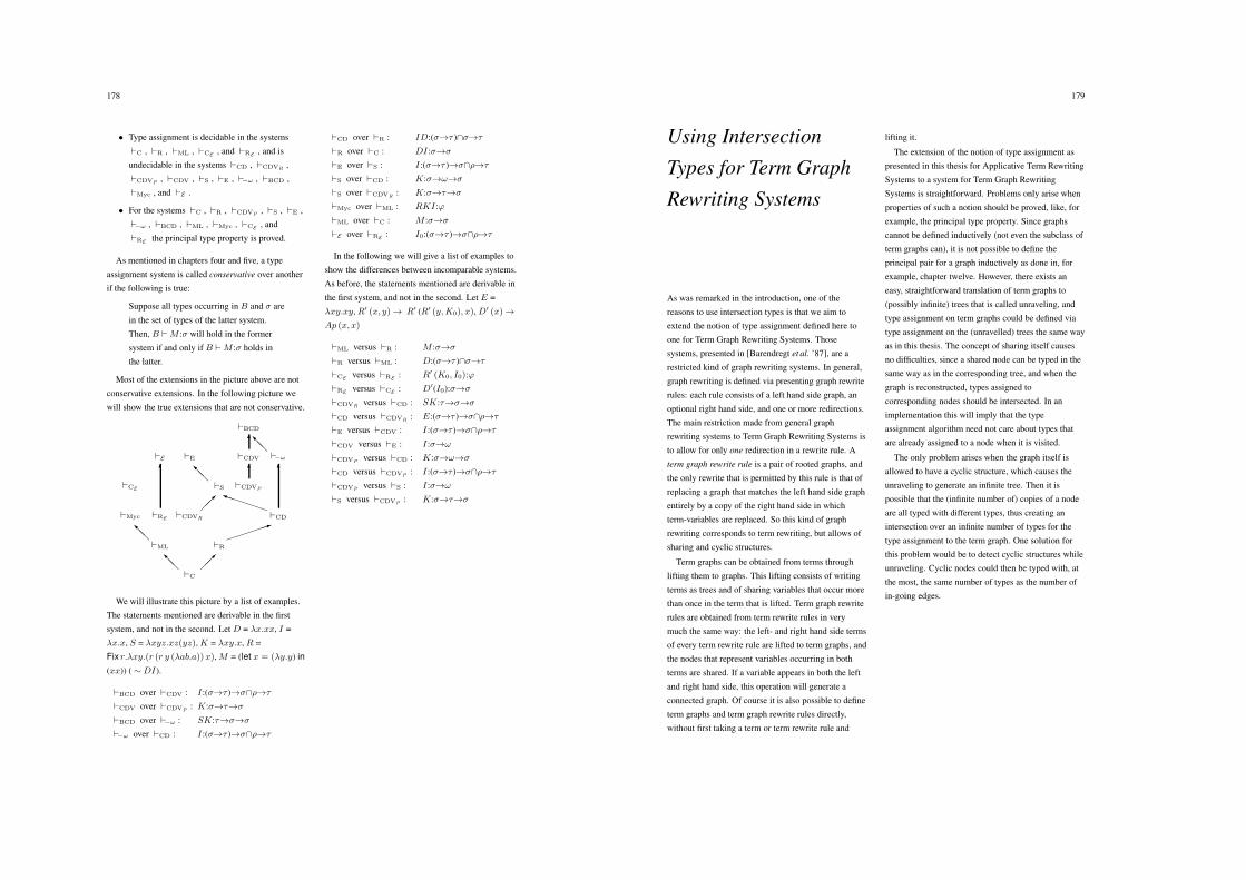
178
• Type assignment is decidable in the systems
"C , "R , "ML , "CE, and "RE
, and is
undecidable in the systems "CD , "CDVR,
"CDVP, "CDV , "S , "E , "#! , "BCD ,
"Myc , and "E .
• For the systems "C , "R , "CDVP, "S , "E ,
"#! , "BCD , "ML , "Myc , "CE, and
"REthe principal type property is proved.
As mentioned in chapters four and five, a type
assignment system is called conservative over another
if the following is true:
Suppose all types occurring in B and # are
in the set of types of the latter system.
Then, B " M :# will hold in the former
system if and only if B " M :# holds in
the latter.
Most of the extensions in the picture above are not
conservative extensions. In the following picture we
will show the true extensions that are not conservative.
"C
..8 ,,9
"ML
..8
"Myc
"CE
"RE
%"E
"R
<<<<<="CD
:::::;
%
"CDVR
,,9
"S
..8"CDVP
%"E "CDV
%"#!
..8
"BCD
We will illustrate this picture by a list of examples.
The statements mentioned are derivable in the first
system, and not in the second. Let D = !x.xx, I =
!x.x, S = !xyz.xz(yz), K = !xy.x, R =
Fix r.!xy.(r (r y (!ab.a))x), M = (let x = (!y.y) in
(xx)) ( %DI).
"BCD over "CDV : I :(#&$ )&#!%&$
"CDV over "CDVP: K:#&$&#
"BCD over "#! : SK:$&#&#
"#! over "CD : I :(#&$ )&#!%&$
"CD over "R : ID:(#&$ )!#&$
"R over "C : DI :#&#
"E over "S : I :(#&$ )&#!%&$
"S over "CD : K:#&"&#
"S over "CDVR: K:#&$&#
"Myc over "ML : RKI :&
"ML over "C : M :#&#
"E over "RE: I0:(#&$ )&#!%&$
In the following we will give a list of examples to
show the differences between incomparable systems.
As before, the statements mentioned are derivable in
the first system, and not in the second. Let E =
!xy.xy, R! (x, y)& R! (R! (y,K0), x), D! (x)&
Ap (x, x)
"ML versus "R : M :#&#
"R versus "ML : D:(#&$ )!#&$
"CEversus "RE
: R! (K0, I0):&
"REversus "CE
: D!(I0):#&#
"CDVRversus "CD : SK:$&#&#
"CD versus "CDVR: E:(#&$ )&#!%&$
"E versus "CDV : I :(#&$ )&#!%&$
"CDV versus "E : I :#&"
"CDVPversus "CD : K:#&"&#
"CD versus "CDVP: I :(#&$ )&#!%&$
"CDVPversus "S : I :#&"
"S versus "CDVP: K:#&$&#
179
Using Intersection
Types for Term Graph
Rewriting Systems
As was remarked in the introduction, one of the
reasons to use intersection types is that we aim to
extend the notion of type assignment defined here to
one for Term Graph Rewriting Systems. Those
systems, presented in [Barendregt et al. ’87], are a
restricted kind of graph rewriting systems. In general,
graph rewriting is defined via presenting graph rewrite
rules: each rule consists of a left hand side graph, an
optional right hand side, and one or more redirections.
The main restriction made from general graph
rewriting systems to Term Graph Rewriting Systems is
to allow for only one redirection in a rewrite rule. A
term graph rewrite rule is a pair of rooted graphs, and
the only rewrite that is permitted by this rule is that of
replacing a graph that matches the left hand side graph
entirely by a copy of the right hand side in which
term-variables are replaced. So this kind of graph
rewriting corresponds to term rewriting, but allows of
sharing and cyclic structures.
Term graphs can be obtained from terms through
lifting them to graphs. This lifting consists of writing
terms as trees and of sharing variables that occur more
than once in the term that is lifted. Term graph rewrite
rules are obtained from term rewrite rules in very
much the same way: the left- and right hand side terms
of every term rewrite rule are lifted to term graphs, and
the nodes that represent variables occurring in both
terms are shared. If a variable appears in both the left
and right hand side, this operation will generate a
connected graph. Of course it is also possible to define
term graphs and term graph rewrite rules directly,
without first taking a term or term rewrite rule and
lifting it.
The extension of the notion of type assignment as
presented in this thesis for Applicative Term Rewriting
Systems to a system for Term Graph Rewriting
Systems is straightforward. Problems only arise when
properties of such a notion should be proved, like, for
example, the principal type property. Since graphs
cannot be defined inductively (not even the subclass of
term graphs can), it is not possible to define the
principal pair for a graph inductively as done in, for
example, chapter twelve. However, there exists an
easy, straightforward translation of term graphs to
(possibly infinite) trees that is called unraveling, and
type assignment on term graphs could be defined via
type assignment on the (unravelled) trees the same way
as in this thesis. The concept of sharing itself causes
no difficulties, since a shared node can be typed in the
same way as in the corresponding tree, and when the
graph is reconstructed, types assigned to
corresponding nodes should be intersected. In an
implementation this will imply that the type
assignment algorithm need not care about types that
are already assigned to a node when it is visited.
The only problem arises when the graph itself is
allowed to have a cyclic structure, which causes the
unraveling to generate an infinite tree. Then it is
possible that the (infinite number of) copies of a node
are all typed with different types, thus creating an
intersection over an infinite number of types for the
type assignment to the term graph. One solution for
this problem would be to detect cyclic structures while
unraveling. Cyclic nodes could then be typed with, at
the most, the same number of types as the number of
in-going edges.
180
Conclusion
There is a great number of intersection type
assignment systems defined in this thesis. For the
greater part, only the syntactical aspects of type
assignment are investigated, like the set of typeable
terms, the principal type property, and decidability of
type assignment.
We have seen that Curry’s Type Assignment System
has the principal type property, type assignment is
decidable, and all typeable terms are strongly
normalizable; unfortunately, however, the set of
typeable terms is rather small.
The various intersection type assignment systems
(like the Coppo-Dezani system, the three different
Coppo-Dezani-Venneri systems, and the
Barendregt-Coppo-Dezani system) are all far more
general type assignment systems than Curry’s system.
The set of terms typeable in the latter two with a type
different from the type constant " is just the set of
terms having a head normal form, and the set of terms
typeable without " in basis and conclusion is the set of
normalizable terms. Moreover, the CDV- and
BCD-systems are closed for '-equality. The results of
chapter seven show that, if " is not used at all (like in
the CD-system), the set of terms typeable is exactly the
set of strongly normalizable terms. We have seen the
development of those intersection type assignment
systems of which the BCD-system was the final one,
and it is also the most frequently used and quoted.
From the functional languages point of view the
disadvantages of these intersection systems are,
however, great. Type assignment in all those systems is
undecidable, and especially the BCD-system is very
general: because of the $-relation on types it is not
easy to really understand the relation between all types
assignable to a term. The Strict Type Assignment
System, which is defined as a restriction of the
BCD-system a couple of years after the BCD-paper
was published, is in fact closer to the CDV-systems
than to the BCD-system. It is strict in more than one
aspect: it is strict in the sense that it has just enough
power to type all CDV- and BCD-typeable terms, and
is restricted since it is not closed for (-reduction.
The results of chapters four and six actually show
that the extension made in the CDV-systems to obtain
the BCD-system was to general. To obtain the major
results of the BCD-paper, it is sufficient to treat " not
as a type-variable as done in the CDV-systems but as
an empty intersection, and to use a relation on types
that is induced in a natural way by intersections and by
defining " as the universal type. To prove
completeness of type assignment it is sufficient to use
the strict filter lambda model (Engeler’s model DA)
and the inference type semantics. The results of
chapter five for the Essential Type Assignment System
show that even if the simple type semantics are
preferred, the completeness result can be obtained via
a filter lambda model that is defined using a relation on
types that is just a small extension of the relation
defined for the strict system.
Even the fact that the BCD-system has the principal
type property does not speak in its favour, since both
the strict system and the essential one have the same
property.
Implementation of type inference algorithms using
intersection types is complicated. Even implementing
a partial type assignment algorithm that is only
supposed to terminate on terms that have a normal
form is not as straightforward as in other systems; the
main source of the problems is the operation of
expansion. There are various ways of restricting
intersection type assignment systems in order to obtain
decidable type assignment. The one studied in this
thesis, the Rank 2 system, is the smallest restriction
imaginable to have intersection types. It has the
following advantages: the complexity of this system is
manageable, it has the principal type property, type
assignment is decidable, it is close to Milner’s notion
of type assignment, it is sufficiently powerful to
express overloading operators, and it can type a larger
class of objects. Therefore, it seems reasonable to use
this notion of type assignment in (functional)
181
programming languages.
The notions of type assignment on Applicative Term
Rewriting Systems as defined in this thesis use the
approach for similar systems for the lambda calculus.
They show that it is possible to define such a notion for
reduction systems that are more general than that
calculus, and that are more close to (functional)
programming languages. The Applicative Term
Rewriting Systems differ from these languages in that
there are almost no restrictions on the structure of
possible left hand sides of function definitions. The
results of chapter ten show that defining such a notion
is straightforward, but that, unfortunately, the
subject-reduction property is lost. Since this property
is vital for reduction systems, two less general notion
of type assignment are defined in chapters eleven and
twelve. The first is very close to notions of type
assignment used for functional programming
languages at this moment and a condition is
formulated that typeable rewrite rules should satisfy in
order to obtain subject reduction. In these systems type
assignment is decidable, both these notions of type
assignment have the principal type property, and, using
the principal type of the left hand side of a rewrite rule,
a condition is formulated that is sufficient to obtain the
subject-reduction property.
References
S. van Bakel, S. Smetsers, and S. Brock.
’92 Partial Type Assignment in Left Linear
Applicative Term Rewriting Systems. In J.-C.
Raoult, editor, Proceedings of CAAP ’92. 17th
Colloquim on Trees in Algebra and
Programming, Rennes, France, volume 581 of
Lecture Notes in Computer Science, pages
300–321. Springer-Verlag, 1992.
S. van Bakel.
’88 Derivations in Type Assignment Systems.
Master’s thesis, University of Nijmegen, 1988.
’90 A first attempt in polymorphic type assignment
using intersection types. The problem of
unification. Technical Report 90-9, Department
of Computer Science, University of Nijmegen,
1990.
’91 Principal type schemes for the Strict Type
Assignment System. Technical Report 91-6,
Department of Computer Science, University of
Nijmegen, 1991.
’92a Complete restrictions of the Intersection Type
Discipline. Theoretical Computer Science,
102:135–163, 1992.
’92b Essential Intersection Type Assignment.
Technical Report 92-28, Department of Computer
Science, University of Nijmegen, 1992.
’92c Partial Intersection Type Assignment of Rank 2
in Applicative Term Rewriting Systems.
Technical Report 92-03, Department of Computer
Science, University of Nijmegen, 1992.
’93 Partial Intersection Type Assignment in
Applicative Term Rewriting Systems. In
Proceedings of TLCA ’93. International
Conference on Typed Lambda Calculi and
Applications, Lecture Notes in Computer
Science. Springer-Verlag, 1993.To appear.
H. Barendregt, M. Coppo, and M. Dezani-Ciancaglini.
’83 A filter lambda model and the completeness of
type assignment. The Journal of Symbolic Logic,
48(4):931–940, 1983.
H.P. Barendregt, M.C.J.D. van Eekelen, J.R.W.
Glauert, J.R. Kennaway, M.J. Plasmeijer, and
M.R. Sleep.
’87 Term graph rewriting. In Proceedings of PARLE,
Parallel Architectures and Languages Europe,
Eindhoven, The Netherlands, volume 259-II of
Lecture Notes in Computer Science, pages
141–158. Springer-Verlag, 1987.
H. Barendregt.
’84 The lambda calculus: its syntax and semantics.
North-Holland, Amsterdam, revised edition,
1984.
T. Brus, M.C.J.D. van Eekelen, M.O. van Leer, and
M.J. Plasmeijer.
’87 Clean - A Language for Functional Graph
Rewriting. In Proceedings of the Third
International Conference on Functional
Programming Languages and Computer
Architecture, Portland, Oregon, USA, volume 274
of Lecture Notes in Computer Science, pages
364–368. Springer-Verlag, 1987.
G. Castagna, G. Ghelli, and G. Longo.
’92 A Calculus for Overloaded Functions with
Subtyping. Technical Report LIENS-92-4,
Laboratoire d’Informatique de l’Ecole Normale
Superieure, 1992.
M. Coppo and M. Dezani-Ciancaglini.
’80 An Extension of the Basic Functionality Theory
for the !-Calculus. Notre Dame, Journal of
184 References
Formal Logic, 21(4):685–693, 1980.
M. Coppo and P. Giannini.
’92 A complete type inference algorithm for simple
intersection types. In J.-C. Raoult, editor,
Proceedings of CAAP ’92. 17th Colloquim on
Trees in Algebra and Programming, Rennes,
France, volume 581 of Lecture Notes in
Computer Science, pages 102–123.
Springer-Verlag, 1992.
M. Coppo, M. Dezani-Ciancaglini, and B. Venneri.
’80 Principal type schemes and !-calculus semantics.
In J. R. Hindley and J. P. Seldin, editors, To H. B.
Curry, Essays in combinatory logic,
lambda-calculus and formalism, pages 535–560.
Academic press, New York, 1980.
’81 Functional characters of solvable terms.
Zeitschrift fur Mathematische Logik und
Grundlagen der Mathematik, 27:45–58, 1981.
M. Coppo, M. Dezani-Ciancaglini, F. Honsell, and
G. Longo.
’84 Extended type structures and filter lambda
models. In G. Lolli, G. Longo, and A. Marcja,
editors, Logic Colloquium 82, pages 241–262,
Amsterdam, 1984.
M. Coppo, M. Dezani-Ciancaglini, and M. Zacchi.
’87 Type Theories, Normal Forms and
D$-Lambda-Models. Information and
Computation, 72(2):85–116, 1987.
H.B. Curry and R. Feys.
’58 Combinatory Logic. volume 1. North-Holland,
Amsterdam, 1958.
H.B. Curry.
’34 Functionality in combinatory logic. In Proc. Nat.
Acad. Sci. U.S.A., volume 20, pages 584–590,
1934.
L. Damas and R. Milner.
’82 Principal type-schemes for functional programs.
In Proceedings 9th ACM Symposium on
Principles of Programming Languages, pages
207–212, 1982.
L.M.M. Damas.
’85 Type Assignment in Programming Languages.
PhD thesis, University of Edinburgh, Department
of Computer Science, Edinburgh, 1985.Thesis
CST-33-85.
N. Dershowitz and J.P. Jouannaud.
’90 Rewrite systems. In J. van Leeuwen, editor,
Handbook of Theoretical Computer Science,
volume B, chapter 6, pages 245–320.
North-Holland, 1990.
M. Dezani-Ciancaglini and J.R. Hindley.
’92 Intersection types for combinatory logic.
Theoretical Computer Science, 100:303–324,
1992.
M. Dezani-Ciancaglini and I. Margaria.
’84 F-semantics for intersection type discipline. In
G. R. Kahn, D. B. Macqueen, and G. Plotkin.,
editors, Sematics of data types. International
symposium Sophia - Antipolis, France, volume
173 of Lecture Notes in Computer Science, pages
279–300. Springer-Verlag, 1984.
’86 A characterisation of F-complete type
assignments. Theoretical Computer Science,
45:121–157, 1986.
M. Dezani-Ciancaglini, F. Honsell, and S. Ronchi
della Rocca.
’86 Models for theories of functions strictly
depending on all their arguments. Stanford ASL
Summer Meeting ’85. Journal of Symbolic Logic,
51 (2):845–846, 1986.abstract.
References 185
E. Engeler.
’81 Algebras and combinators. Algebra universalis,
13(3):389–392, 1981.
K. Futatsugi, J. Goguen, J.P. Jouannaud, and
J. Meseguer.
’85 Principles of OBJ2. In Proceedings 12th ACM
Symposium on Principles of Programming
Languages, pages 52–66, 1985.
P. Giannini and S. Ronchi della Rocca.
’88 Characterization of Typings in Polymorphic
Type Discipline. In Proceedings of the Third
Annual Symposium on Logic in Computer
Science, pages 61–70, 1988.
J.Y. Girard.
’86 The System F of Variable Types, Fifteen years
later. Theoretical Computer Science, 45:159–192,
1986.
R. Hindley and G. Longo.
’80 Lambda calculus models and extensionality.
Zeitschrift fur Mathematische Logik und
Grundlagen der Mathematik, 26:289–310, 1980.
J.R. Hindley.
’69 The principal type scheme of an object in
combinatory logic. Transactions of the American
Mathematical Society, 146:29–60, 1969.
’82 The simple semantics for Coppo-Dezani-Salle
type assignment. In M. Dezani and U. Montanari,
editors, International symposium on
programming, volume 137 of Lecture Notes in
Computer Science, pages 212–226.
Springer-Verlag, 1982.
’83 The Completeness Theorem for Typing !-terms.
Theoretical Computer Science, 22(1):1–17, 1983.
F. Honsell and S. Ronchi della Rocca.
’84 Models for theories of functions strictly
depending on all their arguments. Internal report,
Department of Computer Science, Turin, Italy,
1984.
B. Jacobs, I. Margaria, and M. Zacchi.
’92 Filter Models with Polymorphic Types.
Theoretical Computer Science, 95:143–158,
1992.
A.J. Kfoury and J. Tiuryn.
’89 Typeability in the polymorphic !-calculus of
Rank 2 is decidable. 1989.Preliminary Report.
A.J. Kfoury, J. Tiuryn, and P. Urzyczyn.
’88 A proper extension of ML with an effective
type-assignment. In Proceedings of the Fifteenth
Annual ACM SIGACT-SIGPLAN Symposium on
Principles of Programming Languages, pages
58–69, San Diego, California, 1988.
’90 ML Typability is Dexptime-Complete. In
A. Arnold, editor, Proceedings of CAAP ’90. 15th
Colloquim on Trees in Algebra and
Programming, Copenhagen, Denmark, volume
431 of Lecture Notes in Computer Science, pages
206–220. Springer-Verlag, 1990.
J.W. Klop.
’90 Term Rewriting Systems. Report CS-R9073,
Centre for Mathematics and Computer Science,
Amsterdam, 1990.
J-L. Krivine.
’90 Lambda-calcul types et modeles. Masson, Paris,
1990.
D. Leivant.
’83 Polymorphic Type Inference. In Proceedings
10th ACM Symposium on Principles of
Programming Languages, Austin Texas, pages
88–98, 1983.
186 References
I. Margaria and M. Zacchi.
’90 Principal Typing in a '!-Discipline. Internal
report, Dipartimento di Informatica dell’
Universita de Torino, 1990.
R. Milner.
’78 A theory of type polymorphism in programming.
Journal of Computer and System Sciences,
17:348–375, 1978.
J.C. Mitchell.
’88 Polymorphic Type Inference and Containment.
Information and Computation, 76:211–249,
1988.
A. Mycroft.
’84 Polymorphic type schemes and recursive
definitions. In Proceedings of the International
Symposium on Programming, Toulouse, volume
167 of Lecture Notes Computer Science, pages
217–239. Springer-Verlag, 1984.
E.G.J.M.H. Nocker, J.E.W. Smetsers, M.C.J.D. van
Eekelen, and M.J. Plasmeijer.
’91 Concurrent Clean. In Proceedings of PARLE ’91,
Parallel Architectures and Languages Europe,
Eindhoven, The Netherlands, volume 506-II of
Lecture Notes in Computer Science, pages
202–219. Springer-Verlag, 1991.
V. van Oostrom.
’90 Lambda Calculus with Patterns. Technical
Report IR-228, Faculteit der Wiskunde en
Informatica, Vrije Universiteit Amsterdam, 1990.
F. Pfenning.
’88 Partial Polymorphic Type Inference and
Higher-Order Unification. In Proceedings of the
1988 conference on LISP and Functional
Programming Languages, volume 201 of Lecture
Notes in Computer Science, pages 153–163.
Springer-Verlag, 1988.
B.C. Pierce.
’91 Programming with Intersection Types and
Bounded Polymorphism. PhD thesis, Carnegie
Mellon University, School of Computer Science,
Pitssburgh, 1991.CMU-CS-91-205.
G.D. Plotkin and M.B. Smyth.
’78 The category-theoretic solution of recursive
domain equations. DAI Research Report 60,
University of Edinburgh, Scotland, 1978.
G. Pottinger.
’80 A type assignment for the strongly normalizable
!-terms. In J. R. Hindley and J. P. Seldin, editors,
To H. B. Curry, Essays in combinatory logic,
lambda-calculus and formalism, pages 561–577.
Academic press, New York, 1980.
J.A. Robinson.
’65 A machine-oriented logic based on the resolution
principle. Journal of the ACM, 12(1):23–41,
1965.
S. Ronchi della Rocca and B. Venneri.
’84 Principal type schemes for an extended type
theory. Theoretical Computer Science,
28:151–169, 1984.
S. Ronchi della Rocca.
’88 Principal type scheme and unification for
intersection type discipline. Theoretical
Computer Science, 59:181–209, 1988.
P. Salle.
’78 Une extension de la theorie des types. In
G. Ausiello and C. Bohm, editors, Automata,
languages and programming. Fifth Colloquium,
Udine, Italy, volume 62 of Lecture Notes in
References 187
Computer Science, pages 398–410.
Springer-Verlag, 1978.
D.A. Turner.
’85 Miranda: A non-strict functional language with
polymorphic types. In Proceedings of the
conference on Functional Programming
Languages and Computer Architecture, volume
201 of Lecture Notes in Computer Science, pages
1–16. Springer-Verlag, 1985.
Index
TypesBarendregt-Coppo-Dezani types 2.3.1
Coppo-Dezani types 2.1.1
Coppo-Dezani-Venneri types 2.2.1.1
Curry types 1.1
Environment 10.1.1
Curry environment 11.1.2
Rank 2 environment 12.2.1
Filter
BCD-filter 2.3.1.1
I-filter 7.1.3
Strict-filter 4.2.1
Generic instance 3.1.2
Highest common instance 1.6
Intersection types of Rank 2 8.2.1
Last type-variable 6.2.2.1
ML-types 3.1.2
Normalized types 2.2.1.3
"-free types 7.1.1
Strict types 4.1.1
Tail-proper types 2.2.1.1
Type-schemes 3.1.2
E[F :=#] 10.1.1, 12.2.1
(S 4.2.1
(! 7.1.3
#% 4.3.1
F 2.3.1.1
F#! 7.1.3
FS 4.2.1
TBCD 2.3.1
T&B,"' 6.2.2.1
TC 1.1
TCDV 2.2.1.1
T#! 7.1.1
TR, T2, T1 8.2.1
TS, Ts 4.1.1
Relations on types (pairs)%CDV 2.2.1.3
> 3.1.2
$, % 2.3.1, 7.1.1
$E, %E 5.1.1
$R, %R 8.2.2
$S, %S 4.1.1
)! 2.3.2.6, 6.3.2.1
Type assignment systemsBarendregt-Coppo-Dezani type assignment 2.3.3
Coppo-Dezani type assignment 2.1.2
Coppo-Dezani-Venneri type assignment 2.2.1.2
Restricted - 2.2.1.4
Curry type assignment 1.2
Essential type assignment 5.1.4
Naively Curry typeable with respect to E 11.1.7
ML type assignment 3.1.3
Mycroft type assignment 3.2.1
"-free type assignment 7.1.1
Rank 2 type assignment 8.2.4
Safe type assignment with respect to E 10.3.1
Safe Curry type assignment with
respect to E 11.3.1
Safe Rank 2 type assignment with
respect to E 12.5.1
Strict type assignment 4.1.3
Typeable with respect to E 10.1.2, 10.1.7
Curry typeable with respect to E 11.1.3
Rank 2 typeable with respect to E 12.2.2, 12.2.6
"BCD 2.3.3
"C 1.2
"CD 2.1.2
"CDV 2.2.1.2
"CDVP2.2.2.1
"CDVR2.2.1.4
"CE11.1.3
"E , "e 5.1.4
"E 10.1.2
"#! 7.1.1
"ML 3.1.3
"Myc 3.2.1
190 Index
"R , "2 8.2.4
"RE12.2.2
"S , "s 4.1.3
Notions of basesUsed basis 6.1.1
Curry used basis 11.1.5
Essentially used basis 10.1.5
Rank 2 used basis 12.2.4
!{B1, . . . , Bn} 4.1.2
PairsGround pairs
CDV-ground pair 2.2.2.8
Strict ground pair 6.2.2.8
Primitive pairs 6.2.3.3
Principal pairs
CDV-principal pair 2.2.2.10
Curry principal pair 1.7
Curry principal pair with respect to E 11.2.1
Essential principal pair with respect to E 10.3.1
Rank 2 principal pair 8.4.2.1
Rank 2 principal pair with respect to E 12.4.1
RV-principal pair 2.3.2.5
Strict principal pair 6.1.3
PPC (M ) 1.7
PPCDV (A) 2.2.2.10
PPCE(T ) 11.2.1
PPR (A) 8.4.2.1
PPRE(T ) 12.4.1
PPRV (A), PRV 2.3.2.5
PPS (A), PS 6.1.3
!CDV 2.2.2.10
!RV 2.3.2.6
!S 6.3.2.1
Operations on types (pairs)Chain 6.3.1.1
Linear chain 2.3.2.6
Rank 2 chain 12.1.5
Strict chain 6.3.1.1
Type chain 8.3.3.1, 12.1.5
Duplication 8.3.2.1, 12.1.2
Expansion
CDV-expansion 2.2.2.5
Immediate expansion 2.2.2.5
RV-expansion 2.3.2.2
Strict expansion 6.2.2.6
Type-expansion 6.2.2.2
Lifting 6.2.3.1
Rise 2.3.2.3
Substitution
CDV-substitution 2.2.2.2
Curry-substitution 1.3
ML-substitution 3.1.2
Rank 2 substitution 8.3.1.1
RV-substitution 2.3.2.1
Strict substitution 6.2.1.1
Unification
Rank 2 unification 8.4.1.1
Robinson’s unification algorithm 1.5
Weakening 12.1.4
(& := )) 1.3, 2.2.2.2, 2.3.2.1, 6.2.1.1, 8.3.1.1
*µ,n+, E&µ,n' 2.3.2.2, 6.2.2.6
*µ,n,B,#+, T&µ,n,B,"' 6.2.2.2
*n, B, #+, D&n,B,"' 8.3.2.1, 12.1.2
toTC 8.4.1.1
unifyR, UnifyBases 1.5
unify1 8.4.1.1
**B0, #0+, *B1, #1++ 2.3.2.3, 6.2.3.1
*B0, B1+ 12.1.4
Term Rewriting NotionsATRS, Applicative Term Rewriting
System 9.3.1, 9.3.2
Curry closed 9.3.2
Defining node 9.4.1
Defined symbol, constant 9.3.2
LHS 9.3.3
LLATRS, Left Linear Applicative Term
Rewriting System 9.3.5, 9.3.6
Pattern 9.3.4
Rewrite rule 9.3.2
Index 191
Safe rewrite rule 10.3.1, 11.3.1, 12.5.1
", T(F,X ) 9.3.1
Auxiliary notionsApproximant 2.2.2.6
Nucleus 2.2.2.4
Semantics (inference -, simple -, F -) 2.3.1.3
Type interpretation (simple -, F -) 2.3.1.2
A(M) 2.2.2.6
Exp 3.1.1
##-terms, !#-normal form, N 2.2.2.6
Vµ(*B, #+)
6.2.2.2
Le(B, $ ), Le(B, $ ) 2.3.2.2
"" , ""s , ""F 2.3.1.3, 7.3.1
Samenvatting
Dit proefschrift behandelt een aantal verschillende
noties van typering die gebruik maken van
intersectietypes en kan ruwweg worden opgedeeld in
drie onderdelen. Het eerste deel behandelt in het kort
de definities en eigenschappen van een aantal
typeringssystemen die door andere auteurs in het
verleden zijn ontwikkeld. Het tweede en derde deel
bevatten het resultaat van eigen onderzoek en
presenteren noties van typering gedefinieerd voor de
lambda calculus in het tweede deel en noties voor
termherschrijfsystemen in het derde deel.
In het eerste hoofdstuk wordt Curry’s
typeringssysteem besproken, het oudste en meest
simpele typeringssysteem, waarin typering beslisbaar
is en alle typeerbare termen strek normaliserend zijn.
Dit systeem heeft de voornaamste typeeigenschap
(principal type property): alle mogelijke types voor
een term kunnen uit een zeker gegeven type worden
gegenereerd door middel van operaties gekozen uit een
vooraf gedefinieerde collectie. Voor Curry’s systeem
bestaat deze collectie volledig uit typesubstituties.
In hoofdstuk twee worden een aantal
intersectietyperingssystemen besproken. Het Coppo -
Dezani systeem (CD) in sectie 2.1 is een generalisatie
van Curry’s systeem waarin het mogelijk is
termvariabelen met meer dan een type te typeren.
Wanneer de verzameling termen beperkt wordt tot die
uit de !I-calculus, is typering in dit systeem gesloten
voor beta-gelijkheid. In sectie 2.2 worden drie
verschillende Coppo - Dezani - Venneri systemen
(CDV) besproken; het belangrijkste verschil tussen
deze en het CD-systeem is de toevoeging van de
typeconstante ". Deze systemen zijn gesloten voor
beta-gelijkheid voor de volledige lambda calculus, en
daarmee is typering binnen deze systemen
onbeslisbaar. Het is mogelijk de normaliserende
termen en de termen die een kop-normaal vorm (head
normal form) hebben, te karakteriseren door middel
van de toewijsbare types. Voor een van deze systemen
wordt de voornaamste typeeigenschap bewezen;
daartoe moeten echter aan het systeem beperkingen
worden opgelegd. De collectie van toegestane
operaties voor dit systeem bestaat buiten
typesubstituties ook uit expansies op types.
In sectie 2.3 wordt het Barendregt - Coppo - Dezani
systeem (BCD) besproken, een generalisatie van de
CDV-systemen waarin het mogelijk is eenzelfde
karakterisering van typeerbare termen te geven. De
uitgevoerde generalisatie bestaat uit het behandelen
van ‘!’ als een volwaardige typeconstructor en het
introduceren van een partiele type inclusie relatie ($)
en wordt gemaakt teneinde volledigheid van
typetoekenning te bewijzen. De verzameling van
typeerbare termen is exact gelijk aan die van de
CDV-systemen, alleen de verzameling van de types die
kunnen worden toegekend aan een term is beduidend
groter. De constructie van een filter lambda model en
de definitie van een afbeelding van types naar
elementen van dit model (een simpele
typeınterpretatie) maakt het bewijs voor volledigheid
mogelijk: als de interpretatie van de term M een
element is van de interpretatie van het type #, dan is
M typeerbaar met #. Ook het BCD-systeem bezit de
voornaamste typeeigenschap. De collectie van
toegestane operaties voor het BCD-systeem bestaat
buiten typesubstituties en expansies op types ook uit
typeverheffingen.
In hoofdstuk drie worden twee noties van typering
besproken, het Milner systeem en het Mycroft
systeem, die gedefinieerd zijn voor een primitieve
applicatieve (functionele) programeertaal. Ze
onderscheiden zich van Curry’s systeem door de
uitbreiding van de lambda calculus met nieuwe
syntactische constructoren voor het kunnen uitdrukken
van recursie en polymorfie. Beide systemen bezitten de
voornaamste typeeigenschap. Typering binnen Milners
systeem is beslisbaar, binnen Mycrofts systeem niet.
Het tweede deel van dit proefschrift begint met
hoofdstuk vier, dat de presentatie van het stricte
intersectietype systeem bevat, welk een lichte
beperking vormt van een van de CDV-systemen en
194 Samenvatting
daarmee een deelsysteem is van het BCD-systeem: de
verzameling van de typeerbare termen is dezelfde als
in beide andere systemen en typeerbaarheid in het
stricte systeem is daarmee dan ook onbeslisbaar. Alle
mogelijke afleidingen binnen het BCD-systeem
kunnen worden opgebouwd door eerst een afleiding in
het stricte systeem te maken en daarna de type inclusie
relatie ‘$’ te gebruiken. Dit systeem geeft aanleiding
tot de definitie van een strict filter lambda model en
volledigheid van typetoekenning wordt bewezen door
in plaats van een simpele typeınterpretatie de inferentie
typeınterpretatie te gebruiken. In hoofdstuk zes wordt
aangetoond dat ook het stricte systeem de voornaamste
typeeigenschap bezit. De collectie van toegestane
operaties voor het stricte systeem bestaat buiten
typesubstituties en expansies op types ook uit
typeoptillingen, een beperkte vorm van
typeverheffingen.
Hoofdstuk vijf bevat de presentatie van het
essentiele intersectie systeem, een kleine uitbreiding
van het stricte systeem en eveneens een beperking van
het BCD-systeem. Deze notie van typering is
equivalent aan BCD-typering en het is mogelijk zelfs
voor dit systeem volledigheid van typetoekenning te
bewijzen met behulp van een simpele typeınterpretatie.
Eveneens het essentiele systeem bezit de voornaamste
typeeigenschap; de collectie van toegestane operaties
is dezelfde als voor het stricte systeem, alleen de
volgorde waarin operaties mogen worden toegepast
verschilt.
Hoofdstuk zeven bevat de presentatie van een
typeringssysteem dat, zoals het stricte systeem, een
beperking vormt van het BCD-systeem. De beperking
bestaat uit het verwijderen van de typeconstante ", en
geeft aanleiding tot de definitie van een filter
!I-model. Volledigheid van typetoekenning voor
termen uit de !I-calculus wordt met behulp van dit
model bewezen, gebruikmakend van een simpele
typeınterpretatie. De verzameling termen uit de
volledige !K-calculus die typeerbaar zijn binnen dit
systeem is precies de verzameling van de sterk
normaliserende termen, en daarmee is ook binnen dit
systeem typering onbeslisbaar.
In hoofdstuk acht wordt een rang 2
intersectietyperingssysteem gepresenteerd, dat
gebaseerd is op het CD-systeem en sterke
overeenkomst vertoont met het Milner systeem. Ook
dit systeem heeft de voornaamste typeeigenschap, en
de toegestane operaties zijn typesubstituties en
typeduplicaties, een eenvoudige vorm van expansie
van types. Typering binnen dit systeem is beslisbaar.
Het derde deel van dit proefschrift begint met de
definitie van applicatieve termherschrijfsystemen in
hoofdstuk negen, een soort termherschrijfsystemen die
een speciaal, voorgedefinieerd functiesymbool (Ap)
bevatten. Termen in deze klasse van
herschrijfsystemen worden niet alleen door middel van
applicatie geconstrueerd, maar ook door een
functiesymbool met een zekere ariteit van voldoende
argumenten te voorzien.
De eerste notie van typering op de
boomrepresentatie van deze herschrijfsystemen wordt
gedefinieerd in hoofdstuk tien, en is gebaseerd op het
essentiele typeringssysteem voor de lambda calculus
en de manier van omgaan met recursie zoals gebruikt
in Milners systeem. De definitie van typering bestaat
uit het geven van een omgeving die voor elk
functiesymbool een type levert en het formuleren van
condities waaraan types toegekend aan de
boomrepresentatie van termen en herschrijfregels
moeten voldoen. De types die kunnen worden
toegekend aan functiesymbolen in termen kunnen
worden verkregen uit de types geleverd door de
omgeving: ze kunnen worden verkregen door
toepassing van de operaties typesubstituties, expansies
op types en typeoptillingen zoals gedefinieerd voor het
stricte systeem en het essentiele systeem voor de
lambda calculus. In het algemeen bezit de notie van
typering in termhershrijf systemen niet de eigenschap
dat types toekenbaar aan termen ook toekenbaar zijn
aan termen die ontstaan door het toepassen van een
herschrijfregel (de subject-reductie eigenschap).
In hoofdstuk elf wordt op dezelfde manier als in
hoofdstuk tien een notie van typering op links lineaire
applicatieve termherschrijfsystemen gedefinieerd.
Deze maakt echter gebruik van Curry types en de
manier van omgaan met recursie zoals gebruikt in
Mycrofts systeem en vormt daarom dan ook geen
Samenvatting 195
beperking van het systeem uit dat hoofdstuk. Deze
notie van typering bezit de voornaamste
typeeigenschap en met behulp van het voornaamste
type van de linkerkant van een herschrijfregel wordt
een conditie geformuleerd die noodzakelijk en
voldoende is voor het verkrijgen van de
subject-reductie eigenschap.
Het proefschrift wordt afgesloten met de presentatie
van een notie van typering op applicatieve
termherschrijfsystemen dat gebruik maakt van rang 2
intersectietypes en een echte beperking is van het
systeem gedefinieerd in hoofdstuk twaalf. Ook deze
notie van typering bezit de voornaamste
typeeigenschap en met behulp van het voornaamste
type van de linkerkant van een herschrijfregel wordt
een conditie geformuleerd die voldoende is voor het
verkrijgen van de subject-reductie eigenschap.
Curriculum Vitae
15 februari 1958: Geboren te Doetinchem.
1970 – 1977: Atheneum-B aan het Nebo-Marienbosch-Gabriel College te Nijmegen, afgesloten
met het behalen van het diploma in 1977.
1977 – 1984: Studie Wiskunde aan de Katholieke Universiteit van Nijmegen.
1 september 1982 - 29 januari 1988: Studie Informatica aan de Katholieke Universiteit van
Nijmegen, afgesloten met het behalen van het doctoraaldiploma.
1979 – 1987: Diverse studentassistentschappen, zowel binnen de studie Wiskunde als binnen
de studie Informatica.
1 januari 1986 – 31 juli 1987: In dienst van de afdeling Computer Architectuur onder leiding
van professor R. Boute.
15 februari 1988 – 15 juli 1988: Verblijf aan de Universiteit van Turijn, Italie, onderste-
und door de Nederlandse Organisatie voor Wetenschappelijk Onderzoek (N.W.O.),
beschikking NF-68, onder leiding van professor M. Dezani.
1 september 1988 – 31 december 1988: In dienst van de afdeling Computer Architectuur onder
leiding van professor R. Boute.
1 januari 1989 – Heden: Als toegevoegd onderzoeker in dienst van de afdeling Theoretische
Informatica en Berekeningsmodellen onder leiding van Dr.Ir. R. Plasmeijer, onders-
teund door Esprit Basic Research Action 3074 ‘Semantics and Pragmatics of Gen-
eralized Graph Rewriting (Semagraph)’ (1 juli 1989 - 31 december 1991), en de
Nederlandse Organisatie voor Wetenschappelijk Onderzoek (N.W.O.), beschikking
612-316-027 (1 februari 1990 - 1 februari 1994).
1 mei 1989 – 31 december 1991: In dienst als toegevoegd docent bij de Post-Doctorale Oplei-
ding Informatica.
1 september 1989 – 31 december 1989: In dienst van de afdeling Computer Architectuur onder
leiding van professor R. Boute.