
Integrated mixed logit and latent variable models - Lirias
24
DEPARTMENT OF DECISION SCIENCES AND INFORMATION MANAGEMENT (KBI) Faculty of Business and Economics KBI
Transcript of Integrated mixed logit and latent variable models - Lirias

Integrated mixed logit and latent variable models
Vishva M. Danthurebandara, Martina Vandebroek and Jie Yu
DEPARTMENT OF DECISION SCIENCES AND INFORMATION MANAGEMENT (KBI)
Faculty of Business and Economics
KBI 1208

Integrated mixed logit and latent variable models
Vishva M. Danthurebandara
Faculty of Business and Economics, Katholieke Universiteit Leuven, Naamsestraat 69, B-3000
Leuven, Belgium.
Email: [email protected]
Tel: +32 (0)16 32 69 63
Fax: +32 (0)16 32 66 24
Martina Vandebroek
Faculty of Business and Economics & Leuven Statistics Research Centre, Katholieke Universiteit
Leuven, Naamsestraat 69, B-3000 Leuven, Belgium.
Email: [email protected]
Tel: +32 (0)16 32 69 75
Fax: +32 (0)16 32 66 24
Jie Yu
Faculty of Business and Economics, Katholieke Universiteit Leuven, Naamsestraat 69, B-3000
Leuven, Belgium.
Email: [email protected]
Tel: +32 (0)16 32 69 62
Fax: +32 (0)16 32 66 24
1
Integrated mixed logit and latent variable models ∗
Vishva M. Danthurebandara†, Martina Vandebroek‡ and Jie Yu§
Abstract
A traditional discrete choice model assumes that an individual's decision-making process is
based on utility maximization and that the systematic part of the utility function depends on some
observable attributes and covariates. These attributes and covariates however can only explain part
of the utility and a large part remains unexplained. In recent years, researchers have recognized
that psychological factors such as attitudes, lifestyle and values can aect an alternative's utility
and hence the individual's choices. Therefore, extending the traditional discrete choice model by
incorporating those latent or unobservable factors, can help to better understand the individual's
decision making process and therefore to yield more reliable part-worth estimates and market share
predictions.
Several integrated choice and latent variable (ICLV) models which merge the conditional logit
model with a structural equation model exist in the literature. They assume homogeneity in the
part-worths and use latent variables to model the heterogeneity among the respondents. The
current research uses the mixed logit model that describes the heterogeneity in the part-worths
and uses the latent variables to decrease the unexplained part of the heterogeneity. The empirical
study that we conducted to assess student preferences on mobile phone features shows these ICLV
models perform very well with respect to model t and prediction.
Furthermore, we compare the dierent estimation procedures that exist in the literature. Re-
sults show that, as expected, the simultaneous procedure where we estimate the structural equation
model (SEM) and the choice model simultaneously, gives better model t and more accurate pre-
dictions compared to the sequential procedure that estimates the SEM rst and then the choice
model taking the estimated factor scores into account. But the gain of the simultaneous proce-
dure is relatively small. Therefore one can use the easier sequential procedure without losing much
eciency if needed.
Keywords: Discrete choice models; Structural equation models; Hierarchical Bayesian estima-
tion; Panel mixed logit model; Heterogeneity distribution
JEL Codes: C11, C25, C90
∗This work was supported by the Katholieke Universiteit Leuven, Belgium.†Katholieke Universiteit Leuven, E-mail: [email protected]‡Katholieke Universiteit Leuven, E-mail: [email protected]§Katholieke Universiteit Leuven, E-mail: [email protected]
2
1 Introduction
In recent years, discrete choice models (DCM) have become increasingly popular for collecting and
studying consumer preferences in many dierent disciplines such as marketing, transportation, and
health economics. A traditional DCM assumes that an individual's decision-making process is based
on utility maximization and that the utility can be modeled as a function of some observable attributes
as well as the individuals' socio-demographics. For example, in their marketing application to explain
the consumers choices of mobile phones, Head and Ziolkowski (2010) consider product attributes such as
mobile phone functions (text messaging, web browsing, downloading ringtones) and features (calendar,
alarm clock, personal notes) as well as the consumers' individual characteristics (income, age, gender).
DCM link these observed inputs (attributes and covariates) to the observed outputs (choice data) by
assuming that the individual's internal process during decision formation is implicitly captured well
by the model (Ben-Akiva et al., 2002). However, in all disciplines, the attributes and covariates fail
to capture the true inner process of a decision maker. Therefore, research has been devoted to using
psychometric data that represent the true decision process of the respondent and, hence, to capture at
least part of the previously unexplained utility.
Several researchers have illustrated how psychological factors such as attitudes, lifestyle, perception
and values can aect an individual's decision making process (Ben-Akiva et al., 2002; Walker and
Ben-Akiva, 2002; Timme et al., 2008). Olson and Zanna (1993) explain how these latent variables
inuence information processing and show the importance of taking these factors into account in order
to improve the utility model. Ben-Akiva et al. (2002) discuss the importance of these factors in choice
experiments and present a solid literature review. In their empirical application in transportation,
Temme et al. (2008) extend the classical travel mode choice model to incorporate individuals' attitudes
and values and show that the choice model that incorporates these latent factors clearly outperforms
the traditional conditional logit model with respect to parameter estimation. La Paix et al. (2011)
give an application in the travel domain, where they study the impact of the propensity to travel on the
choice of dierent tour structures for three primary activities (home, work/study, shopping). Moreover,
Ashok et al. (2002) present two empirical applications, one in marketing where they study the inuence
of satisfaction and barriers on the selection of cable TV providers and one in health care where they
study the inuence of the satisfaction with cost and coverage on the choice of a health care plan.
To model the impact of latent variables on choice, integrated choice and latent variable (ICLV) models
have been developed which merge classical choice models with structural equation models (SEM). These
ICLV models can be found in dierent model parametrizations, both with respect to the choice model
and to the structural equation model. In all of these empirical applications, the ICLV model was based
on the conditional logit model and the market heterogeneity was modelled by incorporating individual-
specic latent factors. Nowadays, the mixed logit model is often used to model the market heterogeneity
(for example, Bliemer et al., 2009; Yu et al., 2011; Danthurebandara et al., 2011). Though it models
3
individual specic part-worths, the mixed logit model can still be improved by including individual-
specic latent factors that model the decision making process. In this paper we will compare ICLV
models based on the conditional logit model and on the mixed logit model with models that do not
include latent factors.
Furthermore, the current paper considers two dierent ways of incorporating the latent variables in
the choice model. In the latent covariate model (Ben-Akiva et al., 2002; Temme et al., 2008), latent
factors are included into the systematic part of the random utility model as extra individual covariates,
while in the random scale latent variable model (Hess and Stathopoulos, 2011) the latent factors are
assumed to inuence the scale parameter. The rst parametrization is a homoscedastic model since the
scale factor is assumed constant. This model assumes that respondents have the same error variance
or precision and uses individual latent factors to increase the explained part of the utility. The second
parametrization yields a heteroscedastic model since the scale parameter now is a function of individual-
specic latent factors. In this model, latent variables are used to explain dierences in precision across
respondents.
For the ICLV models, two prominent estimation methods can be found in the literature: sequential and
simultaneous. The easier sequential method is a two stage approach where the SEM is estimated rst
and then the choice model incorporates the estimated factor scores (Ashok et al., 2002). However, Ben-
Akiva et al. (2002) show that the sequential approach results in inconsistent and inecient estimates.
Alternatively, the integrated model can be estimated simultaneously resulting in ecient estimates but
this approach is computationally much more demanding, especially for the ICLV models based on the
mixed logit model and, as the number of latent variable increases, this approach gives convergence
and identication problems. We will compare these dierent estimation methods and study the gain
of using the full information simultaneous approach over the limited information sequential approach.
We show how WinBUGS can be used to estimate the dierent ICLV models both sequentially and
simultaneously.
To wrap up, this paper provides methodological and empirical contributions. We extend the classical
ICLV models to the mixed logit model which models individual specic part-worths. We also introduce
hierarchical Bayesian estimation and illustrate how this can be implemented in WinBUGS. Finally, in
the empirical application we compare the dierent models and estimation procedures in a study on
mobile phone features.
The following section introduces the generalized ICLV model and the dierent estimation approaches.
Section 3 presents the results of an empirical study we conducted to compare the dierent models and
estimation procedures, and Section 4 summarizes the key ndings of the paper.
4
2 Methodology
The ICLV model consists of two major components: a structural equation model and a choice model. In
this section we rst introduce these components in detail and then present the dierent parametrizations
of the combined ICLV model.
2.1 The structural equation model (SEM)
The standard SEM, also called LISREL model (Joreskog and Sorbom, 1996), consist of two sub-
models. The rst one is the measurement model which is a conrmatory factor model that relates the
endogeneous and exogeneous latent variables to their corresponding indicators or manifest variables
while taking the measurement error into account. The second is a structural model that represents
the interrelationships among the latent endogeneous variables and also relates the latent endogeneous
variables to the latent exogeneous variables and the observed exogeneous variables if present.
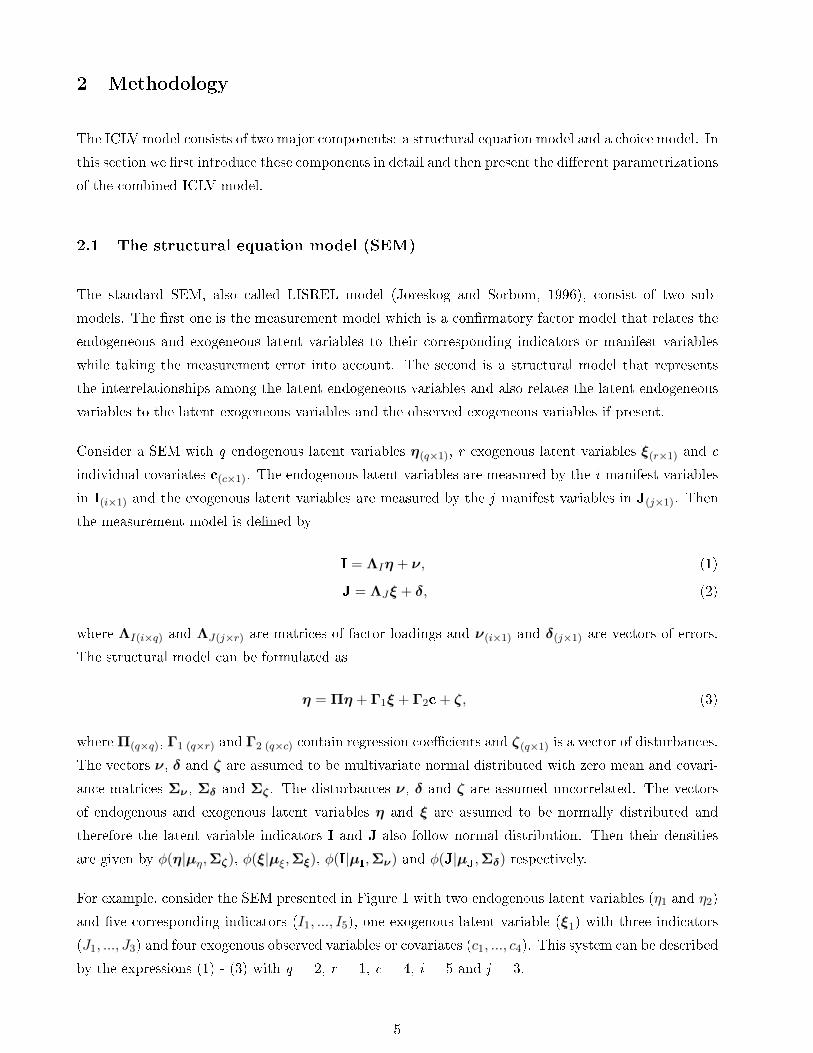
Consider a SEM with q endogenous latent variables η(q×1), r exogenous latent variables ξ(r×1) and c
individual covariates c(c×1). The endogenous latent variables are measured by the i manifest variables
in I(i×1) and the exogenous latent variables are measured by the j manifest variables in J(j×1). Then
the measurement model is dened by
I = ΛIη + ν, (1)
J = ΛJξ + δ, (2)
where ΛI(i×q) and ΛJ(j×r) are matrices of factor loadings and ν(i×1) and δ(j×1) are vectors of errors.
The structural model can be formulated as
η = Πη + Γ1ξ + Γ2c+ ζ, (3)
whereΠ(q×q), Γ1 (q×r) and Γ2 (q×c) contain regression coecients and ζ(q×1) is a vector of disturbances.
The vectors ν, δ and ζ are assumed to be multivariate normal distributed with zero mean and covari-
ance matrices Σν , Σδ and Σζ . The disturbances ν, δ and ζ are assumed uncorrelated. The vectors
of endogenous and exogenous latent variables η and ξ are assumed to be normally distributed and
therefore the latent variable indicators I and J also follow normal distribution. Then their densities
are given by φ(η|µη,Σζ), φ(ξ|µξ,Σξ), φ(I|µI,Σν) and φ(J|µJ,Σδ) respectively.
For example, consider the SEM presented in Figure 1 with two endogenous latent variables (η1 and η2)
and ve corresponding indicators (I1, ..., I5), one exogenous latent variable (ξ1) with three indicators
(J1, ..., J3) and four exogenous observed variables or covariates (c1, ..., c4). This system can be described
by the expressions (1) - (3) with q = 2, r = 1, c = 4, i = 5 and j = 3.
5
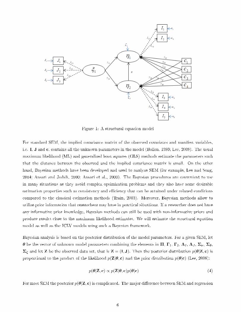
Figure 1: A structural equation model
For standard SEM, the implied covariance matrix of the observed covariates and manifest variables,
i.e. I, J and c, contains all the unknown parameters in the model (Bollen, 1989; Lee, 2008). The usual
maximum likelihood (ML) and generalized least squares (GLS) methods estimate the parameters such
that the distance between the observed and the implied covariance matrix is small. On the other
hand, Bayesian methods have been developed and used to analyze SEM (for example, Lee and Song,
2004; Ansari and Jedidi, 2000; Ansari et al., 2000). The Bayesian procedures are convenient to use
in many situations as they avoid complex optimization problems and they also have some desirable
estimation properties such as consistency and eciency that can be attained under relaxed conditions
compared to the classical estimation methods (Train, 2003). Moreover, Bayesian methods allow to
utilize prior information that researchers may have in practical situations. If a researcher does not have
any informative prior knowledge, Bayesian methods can still be used with non-informative priors and
produce results close to the maximum likelihood estimates. We will estimate the structural equation
model as well as the ICLV models using such a Bayesian framework.
Bayesian analysis is based on the posterior distribution of the model parameters. For a given SEM, let
θ be the vector of unknown model parameters combining the elements in Π, Γ1, Γ2, ΛI , ΛJ , Σν , Σδ,
Σζ and let Z be the observed data set, that is Z = (I,J). Then the posterior distribution p(θ|Z, c) isproportional to the product of the likelihood p(Z|θ, c) and the prior distribution p(θ|c) (Lee, 2008):
p(θ|Z, c) ∝ p(Z|θ, c)p(θ|c) (4)
For most SEM the posterior p(θ|Z, c) is complicated. The major dierence between SEM and regression
6
and simultaneous equation models is the presence of latent variables. If the factor scores in a SEM
were not random but observed data, then the SEM would simplify to a simultaneous equation model
and the posterior distribution simplies. The key idea in the Bayesian estimation procedure for SEM
is data augmentation, initially proposed by Tanner and Wong (1987), which is an iterative procedure
which starts with some initial values for the latent variables. Tanner and Wong (1987) give a complete
description about calculating posterior distributions by data augmentation. By using this method
in SEM, we treat the latent variables as hypothetical missing data and augment the observed data
with imputed values for the latent variables. Then the posterior distribution based on the complete
data set is relatively easy to deal with. Specically, instead of working with p(θ|Z, c), we work with
the posterior distribution p(θ,Ω|Z, c) where Ω contains the latent variables, Ω = (η, ξ). Lee (2008)
provides a detailed theoretical explanation of this Bayesian method for SEM. The posterior distribution
is then given as:
p(θ,Ω|Z, c) ∝ p(Z|θ, c)p(Ω|θ, c)p(θ|c). (5)
In order to approximate the mean and other useful statistics of this posterior distribution, we use
a Gibbs sampler (Geman and Geman, 1984) where we use full conditional Monte-Carlo draws. The
Gibbs sampler at the (j+1)th iteration is:
(i) generate Ωj+1 from p(Ω | θj , Z, c)
(ii) generate θj+1 from p(θ | Ωj+1, Z, c)
More details on the conditional distributions p(Ω|θ,Z, c) and p(θ|Ω,Z, c), based on the model and
the distributional properties of the model parameters and the observed and unobserved data, can be
found in Lee (2008). The conditional distributions used in this Gibbs sampler are non-standard in
most of the cases. Therefore we implement these models in WinBUGS (Lunn et al., 2009) such that we
do not have to specify these conditional distributions explicitly. WinBUGS uses the Gibbs sampling
method to sample from a given joint posterior distribution and it uses the Metropolis-Hastings sampler
(Metropolis et al., 1953; Hastings, 1970) when the full conditional distribution is not available in closed
form. For more details about Bayesian methods for SEM refer for example to Lee (2008).
2.2 The mixed logit model
The mixed logit model is nowadays often used to model the market heterogeneity in conjoint choice
studies. This section introduces the mixed logit model without considering the latent factors, and in
the next section we extend it to take the factors into account. In case all respondents are assumed to
have the same part-worths, the mixed logit model simplies to the conditional logit model. For more
details about the conditional logit model, refer for example to Sándor and Wedel (2001) and Yu et al.
7
(2008).
Consider the random utility model:
uksn = Vksn(x) + εksn = x′ksnβn + εksn (6)
where uksn is the utility that respondent n obtains by choosing alternative k from choice set s, Vksn(x) is
called the systematic part of the utility which is assumed to be a linear function of the attribute values
and corresponding utility coecients or part-worths and xksn is the p-dimensional vector containing
the attribute values of alternative k in choice set s for respondent n. The preferences of respondent n
are represented by the individual-specic utility coecient vector βn. The probability that respondent
n chooses alternative k (k = 1,...,K) in choice set s (s = 1,...,S) is
pksn(βn) =exp (µ x′ksnβn)∑Ki=1 exp (µ x′isnβn)
, (7)
where µ is the scale factor. The scale factor is derived as π/√6σ, where σ is the standard deviation of
ε. To avoid identication problems we usually set µ = 1.
Denote by yn the K × S-dimensional individual-specic vector containing the S choices from re-
spondent n that correspond to the S choice sets of K alternatives. Conditional on βn, the likelihood
function for a given yn can be written as
L(yn|X,βn) =S∏s=1
K∏k=1
(pksn(βn))yksn , (8)
where yksn, element of yn, is 1 if respondent n chooses alternative k in choice set s and 0 otherwise
and X is a matrix containing the attribute values of each alternative in the S choice sets.
We assume that the coecient vector βn is randomly drawn from a p-variate normal distribution with
mean µβ and covariance matrix Σβ, that is N(βn | µβ,Σβ). Then the likelihood of a given sequence
of choices yn, unconditional on βn, for respondent n is
L(yn|X,µβ,Σβ) =
ˆL(yn|X,βn) φ(βn | µβ,Σβ) dβn,
=
ˆ(
S∏s=1
K∏k=1
(pksn(βn))yksn) φ(βn | µβ,Σβ) dβn.
(9)
The probabilities of a single respondent in multiple choice situations will be correlated and the above
formulation takes this dependency into account. That is, the coecient vector βn for a given respondent
n appears in all choice sets and ensures that the model captures the correlation across repeated choices.
The likelihood of the choices of all N respondents, unconditional on βn, is denoted by L(yfull|X,µβ,Σβ)
8
and dened as
L(yfull|X,µβ,Σβ) =N∏n=1
L(yn|X,µβ,Σβ) (10)
where yfull contains the responses of all N respondents.
The choice model can also be considered as a SEM. In the random utility model, the utility is a latent
variable and the observed choices are indicators or manifest variables of this utility. The measurement
model is here given by a non-linear relationship between the observed choices and the latent utility,
i.e. for a given choice set s and a respondent n,
yisn =
1, if uisn = maxj(ujsn), j = 1, ...,K
0, otherwise
This indicates that respondent n chooses alternative i from choice set s containing K alternatives if
and only if the alternative i yields maximum utility. The random utility model in equation (6) can
then be seen as a structural model that represents the relationship between observed attribute levels
and the latent utility.
The mixed logit model is frequently estimated through a Hierarchical Bayes approach which also avoids
the dicult optimization of the likelihood function (Toubia et al., 2004; Arora and Huber, 2001; Rossi
et al., 1996). Here also we use the Gibbs sampler to draw from the posterior density. The Gibbs
sampler at the (j + 1)th iteration is:
(i) generate µj+1β from p(µβ | βjn, Σ
jβ)
(ii) generate Σj+1β from p(Σβ | βjn, µ
j+1β )
(iii) generate βj+1n from p(βn | µj+1
β , Σj+1β )
Train (2003) contains the derivation of conditional distributions based on non-informative priors. We
use these non-informative priors for choice model parameters in our WinBUGS programs. A detailed
discussion on HB estimation for mixed logit models can be found in Train (2003).
2.3 Integrated choice and latent variable (ICLV) models
Now that we have introduced the two major components of the ICLV model, we can present the general
form of the ICLV model and look at two parametrizations: the latent covariate model and the random
scale latent variable model. To express that the factors are individual specic we introduce the index
n in the measurement and structural equations of the SEM. Then the measurement and the structural
equations become:
ηn = Πηn + Γ1ξn + Γ2cn + ζn,
9
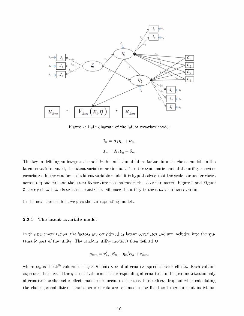
Figure 2: Path diagram of the latent covariate model
In = ΛIηn + νn,
Jn = ΛJξn + δn,
The key in dening an integrated model is the inclusion of latent factors into the choice model. In the
latent covariate model, the latent variables are included into the systematic part of the utility as extra
covariates. In the random scale latent variable model it is hypothesized that the scale parameter varies
across respondents and the latent factors are used to model the scale parameter. Figure 2 and Figure
3 clearly show how these latent constructs inuence the utility in these two parametrization.
In the next two sections we give the corresponding models.
2.3.1 The latent covariate model
In this parametrization, the factors are considered as latent covariates and are included into the sys-
tematic part of the utility. The random utility model is then dened as
uksn = x′ksnβn + ηn′αk + εksn,
where αk is the kth column of a q × K matrix α of alternative specic factor eects. Each column
expresses the eect of the q latent factors on the corresponding alternative. In this parametrization only
alternative-specic factor eects make sense because otherwise, those eects drop out when calculating
the choice probabilities. These factor eects are assumed to be xed and therefore not individual
10
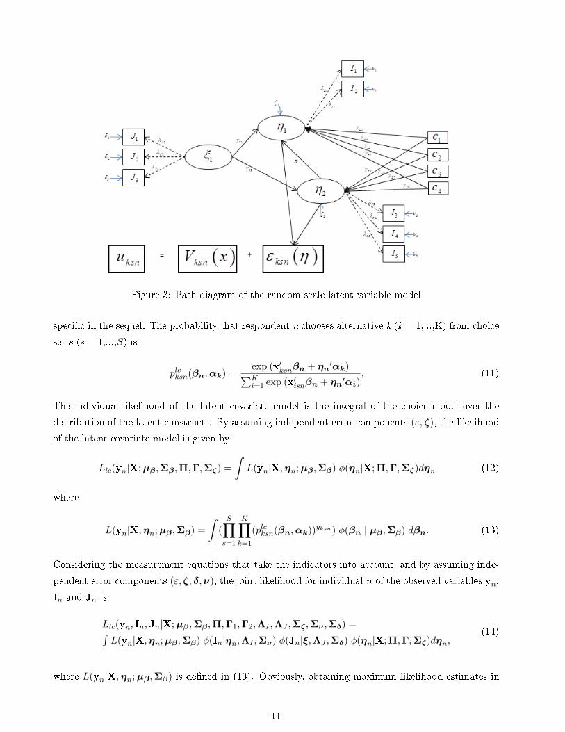
Figure 3: Path diagram of the random scale latent variable model
specic in the sequel. The probability that respondent n chooses alternative k (k = 1,...,K) from choice
set s (s = 1,...,S) is
plcksn(βn,αk) =exp (x′ksnβn + ηn
′αk)∑Ki=1 exp (x′isnβn + ηn′αi)
, (11)
The individual likelihood of the latent covariate model is the integral of the choice model over the
distribution of the latent constructs. By assuming independent error components (ε, ζ), the likelihood
of the latent covariate model is given by
Llc(yn|X;µβ,Σβ,Π,Γ,Σζ) =
ˆL(yn|X,ηn;µβ,Σβ) φ(ηn|X;Π,Γ,Σζ)dηn (12)
where
L(yn|X,ηn;µβ,Σβ) =ˆ
(
S∏s=1
K∏k=1
(plcksn(βn,αk))yksn) φ(βn | µβ,Σβ) dβn. (13)
Considering the measurement equations that take the indicators into account, and by assuming inde-
pendent error components (ε, ζ, δ,ν), the joint likelihood for individual n of the observed variables yn,
In and Jn is
Llc(yn, In,Jn|X;µβ,Σβ,Π,Γ1,Γ2,ΛI ,ΛJ ,Σζ ,Σν ,Σδ) =´L(yn|X,ηn;µβ,Σβ) φ(In|ηn,ΛI ,Σν) φ(Jn|ξ,ΛJ ,Σδ) φ(ηn|X;Π,Γ,Σζ)dηn,
(14)
where L(yn|X,ηn;µβ,Σβ) is dened in (13). Obviously, obtaining maximum likelihood estimates in
11
this case is dicult. We use this likelihood together with the prior distributions of the model parameters
to obtain Bayesian estimates. The estimation method and the software implementation of the latent
covariate model will be presented in section 2.4.
2.3.2 The random scale latent variable model
Hess and Stathopoulos (2011) use latent factors to explain the variation across respondents in the scale
parameter of the choice model. For example, in their empirical research, they consider the scale factor
as a function of the respondents' survey engagement. The model hypothesizes that dierences across
respondents in survey engagement yield dierences in precisions and therefore scale heterogeneity.
In this case, the probability that respondent n chooses alternative k (k = 1,...,K) in choice set s
(s = 1,...,S) can be formulated as
prslvksn (βn,α) =exp (µn x
′ksnβn)∑K
i=1 exp (µn x′isnβn)
, (15)
where µn = eηn′α and α is a q × 1 vector of xed factor eects.
Similar to the latent covariate model, the individual joint likelihood of the observed variables yn, In
and Jn is
Lrslv(yn, In,Jn|X;µβ,Σβ,Π,Γ1,Γ2,ΛI ,ΛJ ,Σζ ,Σν ,Σδ) =´L(yn|X,ηn;µβ,Σβ) φ(In|ηn,ΛI ,Σν) φ(Jn|ξ,ΛJ ,Σδ) φ(ηn|X;Π,Γ,Σζ)dηn,
(16)
where
L(yn|X,ηn;µβ,Σβ) =ˆ(S∏s=1
K∏k=1
(prslvksn (βn,α))yksn) φ(βn | µβ,Σβ) dβn. (17)
The Bayesian estimation method where we use this individual joint likelihood together with prior
distributions of model parameters and the software implementation of the random scale latent variable
model will be presented in the next section.
2.4 Estimation
The sequential approach is the simplest way to estimate the ICLV models. In this case we estimate
the structural equation model rst and then estimate the choice model incorporating the estimated
factor scores. This method is known to be easy and straightforward because researchers can use readily
12
available software for SEM (for example LISREL, AMOS, EQS, SAS) and for the choice model (for
example SAS, NLOGIT, STATA). The sequential method considers the estimated factor scores as
non-stochastic variables and includes them into the utility model as exogenous variables. This brings
measurement error into the model and therefore results in inconsistent and inecient estimates (Ben-
Akiva et al., 2002). The alternative simultaneous approach provides consistent and ecient estimates
but, as the number of latent factors increases, this approach becomes numerically cumbersome. To
perform simultaneous estimation, one can program the joint likelihood in a exible software package
such as GAUSS (Ashok et al., 2002), Mplus (Temme et al., 2008), Ox (Hess and Stathopoulos, 2011),
BIOGOME(La Paix et al., 2011) and also in SAS, R or Matlab.
In this research, the Hierarchical Bayes method is used to estimate the latent covariate and the random
scale latent variable models. For each model parametrization, the posterior distribution is proportional
to the product of the corresponding likelihood given by the expression (14) or (16) and the prior dis-
tributions of the corresponding model parameters. Obviously, for the integrated model, this posterior
is much more complex than the posteriors for SEM and for the choice model. A large number of
non-standard conditional distributions have to be calculated during the estimation process. There-
fore, we implement these models in WinBUGS which is freely available software for Bayesian analysis
(Spiegelhalter et al., 2003; Lunn et al., 2009). The key advantage of using WinBUGS here is that we
do not have to specify the conditional distributions explicitly. WinBUGS uses Markov chain Monte
Carlo (MCMC) methods such as the Gibbs sampler (Geman and Geman, 1984) and the Metropolis
Hastings algorithm (Metropolis et al., 1953; Hastings, 1970), which help to avoid the complex integra-
tion problems in ML methods. For each model, we perform 100,000 iterations in total, 70,000 which
are used for burn-in and the remaining 30,000 draws, which are thinned by selecting every 10th draw
to remove the auto-correlation, are used to determine the parameter estimates.
3 Student preference on mobile phone features
In this section we present the choice experiment we conducted to compare the dierent integrated
models introduced previously. In the next section, the choice experiment is explained in detail: the
study domain, the data collection and the models estimated, and section 3.2 contains the results.
3.1 Data and models
Mobile phone use has grown rapidly throughout the world. Srivastava (2005) gives a rich overview
of how the mobile phone has moved beyond being a simple technical device to becoming a key social
object. In Belgium, the number of mobile phone subscribers has increased by 68% from 2000 to 2005.
This rapid quantitative growth of consumers leads to a signicant qualitative improvement of mobile
13
phones. A large number of mobile phone features and applications are launched everyday to capture
the users' attention. Our conjoint experiment is designed to assess the relative preferences for these
mobile phone features. Obviously, teenagers and young adults constitute the largest consumer group
in the mobile phone market (McClatchy, 2006) and hence is the major target group of mobile phone
manufactures. Therefore, the experiment is conducted with undergraduate and graduate students
at the Faculty of Business and Economics of the Katholieke Universiteit Leuven, Belgium. A near
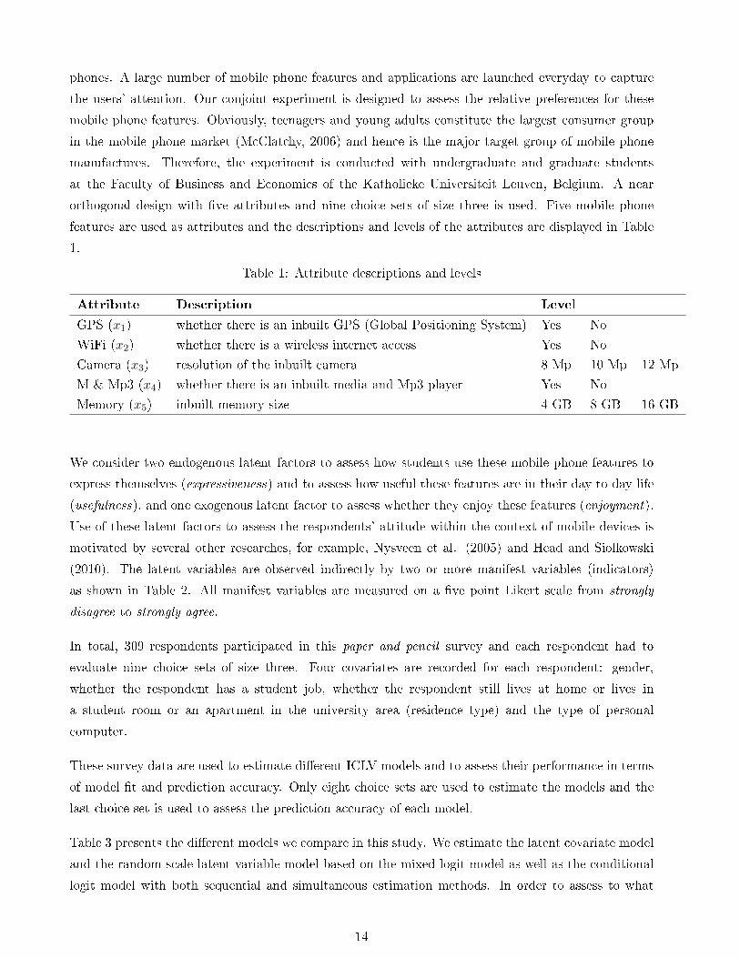
orthogonal design with ve attributes and nine choice sets of size three is used. Five mobile phone
features are used as attributes and the descriptions and levels of the attributes are displayed in Table
1.
Table 1: Attribute descriptions and levels
Attribute Description Level
GPS (x1) whether there is an inbuilt GPS (Global Positioning System) Yes No
WiFi (x2) whether there is a wireless internet access Yes No
Camera (x3) resolution of the inbuilt camera 8 Mp 10 Mp 12 Mp
M & Mp3 (x4) whether there is an inbuilt media and Mp3 player Yes No
Memory (x5) inbuilt memory size 4 GB 8 GB 16 GB
We consider two endogenous latent factors to assess how students use these mobile phone features to
express themselves (expressiveness) and to assess how useful these features are in their day to day life
(usefulness), and one exogenous latent factor to assess whether they enjoy these features (enjoyment).
Use of these latent factors to assess the respondents' attitude within the context of mobile devices is
motivated by several other researches, for example, Nysveen et al. (2005) and Head and Siolkowski
(2010). The latent variables are observed indirectly by two or more manifest variables (indicators)
as shown in Table 2. All manifest variables are measured on a ve point Likert scale from strongly
disagree to strongly agree.
In total, 309 respondents participated in this paper and pencil survey and each respondent had to
evaluate nine choice sets of size three. Four covariates are recorded for each respondent: gender,
whether the respondent has a student job, whether the respondent still lives at home or lives in
a student room or an apartment in the university area (residence type) and the type of personal
computer.
These survey data are used to estimate dierent ICLV models and to assess their performance in terms
of model t and prediction accuracy. Only eight choice sets are used to estimate the models and the
last choice set is used to assess the prediction accuracy of each model.
Table 3 presents the dierent models we compare in this study. We estimate the latent covariate model
and the random scale latent variable model based on the mixed logit model as well as the conditional
logit model with both sequential and simultaneous estimation methods. In order to assess to what
14
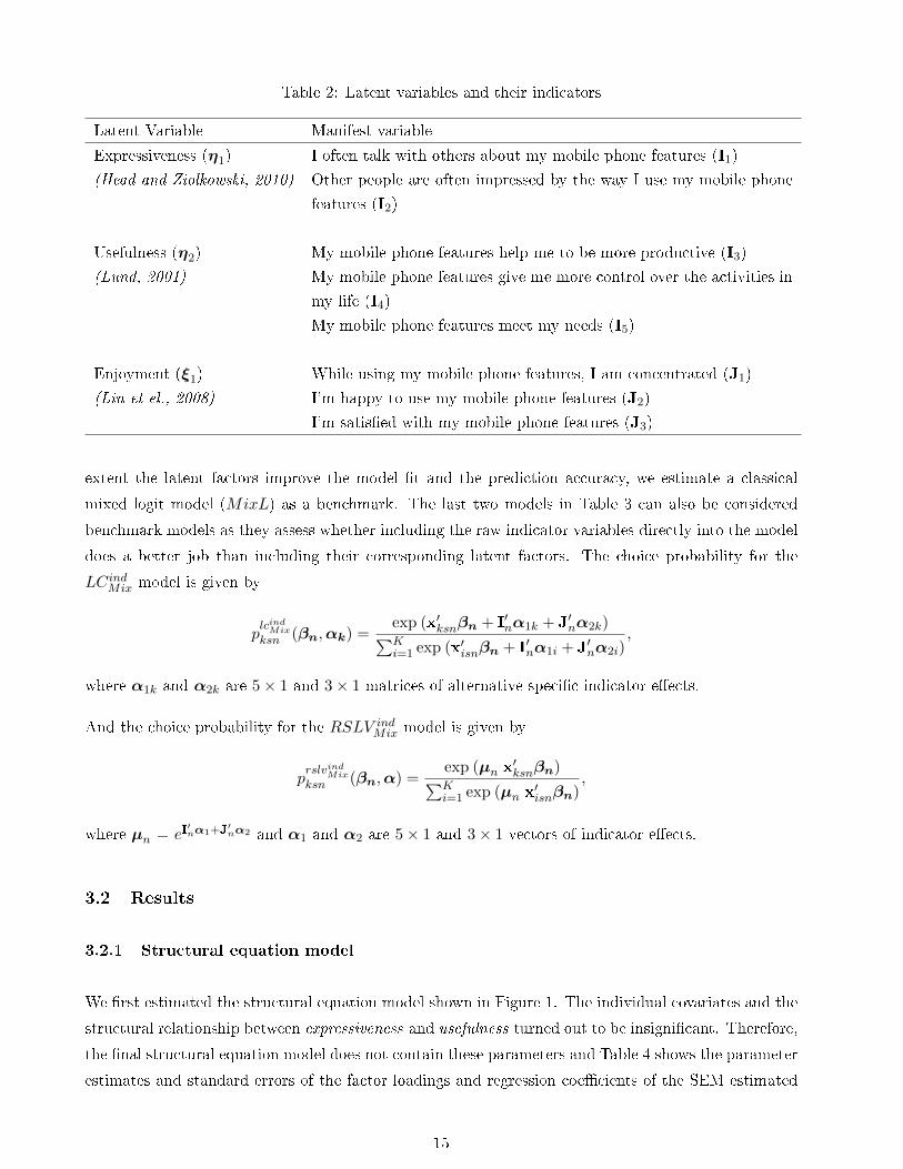
Table 2: Latent variables and their indicators
Latent Variable Manifest variable
Expressiveness (η1) I often talk with others about my mobile phone features (I1)
(Head and Ziolkowski, 2010) Other people are often impressed by the way I use my mobile phone
features (I2)
Usefulness (η2) My mobile phone features help me to be more productive (I3)
(Lund, 2001) My mobile phone features give me more control over the activities in
my life (I4)
My mobile phone features meet my needs (I5)
Enjoyment (ξ1) While using my mobile phone features, I am concentrated (J1)
(Lin et el., 2008) I'm happy to use my mobile phone features (J2)
I'm satised with my mobile phone features (J3)
extent the latent factors improve the model t and the prediction accuracy, we estimate a classical
mixed logit model (MixL) as a benchmark. The last two models in Table 3 can also be considered
benchmark models as they assess whether including the raw indicator variables directly into the model
does a better job than including their corresponding latent factors. The choice probability for the
LCindMix model is given by
plcind
Mixksn (βn,αk) =
exp (x′ksnβn + I′nα1k + J′nα2k)∑Ki=1 exp (x′isnβn + I′nα1i + J′nα2i)
,
where α1k and α2k are 5× 1 and 3× 1 matrices of alternative specic indicator eects.
And the choice probability for the RSLV indMix model is given by
prslvind
Mixksn (βn,α) =
exp (µn x′ksnβn)∑K
i=1 exp (µn x′isnβn)
,
where µn = eI′nα1+J
′nα2 and α1 and α2 are 5× 1 and 3× 1 vectors of indicator eects.
3.2 Results
3.2.1 Structural equation model
We rst estimated the structural equation model shown in Figure 1. The individual covariates and the
structural relationship between expressiveness and usefulness turned out to be insignicant. Therefore,
the nal structural equation model does not contain these parameters and Table 4 shows the parameter
estimates and standard errors of the factor loadings and regression coecients of the SEM estimated
15
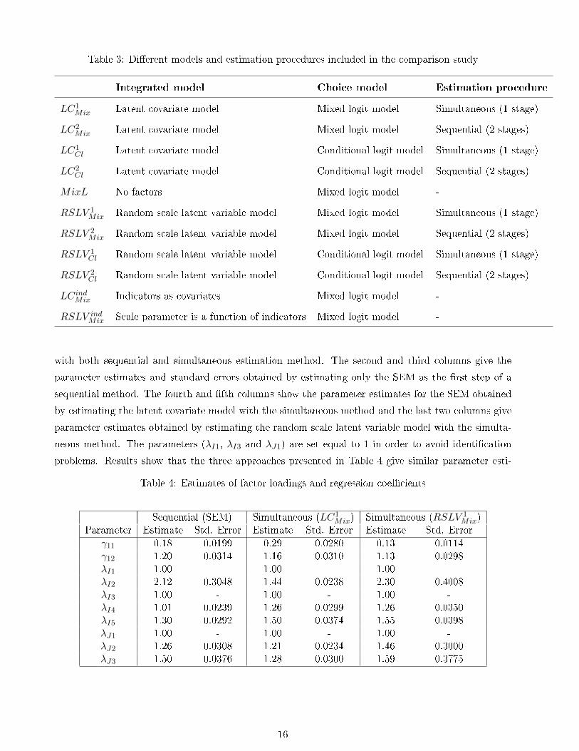
Table 3: Dierent models and estimation procedures included in the comparison study
Integrated model Choice model Estimation procedure
LC1Mix Latent covariate model Mixed logit model Simultaneous (1 stage)
LC2Mix Latent covariate model Mixed logit model Sequential (2 stages)
LC1Cl Latent covariate model Conditional logit model Simultaneous (1 stage)
LC2Cl Latent covariate model Conditional logit model Sequential (2 stages)
MixL No factors Mixed logit model -
RSLV 1Mix Random scale latent variable model Mixed logit model Simultaneous (1 stage)
RSLV 2Mix Random scale latent variable model Mixed logit model Sequential (2 stages)
RSLV 1Cl Random scale latent variable model Conditional logit model Simultaneous (1 stage)
RSLV 2Cl Random scale latent variable model Conditional logit model Sequential (2 stages)
LCindMix Indicators as covariates Mixed logit model -
RSLV indMix Scale parameter is a function of indicators Mixed logit model -
with both sequential and simultaneous estimation method. The second and third columns give the
parameter estimates and standard errors obtained by estimating only the SEM as the rst step of a
sequential method. The fourth and fth columns show the parameter estimates for the SEM obtained
by estimating the latent covariate model with the simultaneous method and the last two columns give
parameter estimates obtained by estimating the random scale latent variable model with the simulta-
neous method. The parameters (λI1, λI3 and λJ1) are set equal to 1 in order to avoid identication
problems. Results show that the three approaches presented in Table 4 give similar parameter esti-
Table 4: Estimates of factor loadings and regression coecients
Sequential (SEM) Simultaneous (LC1Mix) Simultaneous (RSLV 1
Mix)Parameter Estimate Std. Error Estimate Std. Error Estimate Std. Error
γ11 0.18 0.0199 0.29 0.0280 0.13 0.0114γ12 1.20 0.0314 1.16 0.0310 1.13 0.0298λI1 1.00 - 1.00 - 1.00 -λI2 2.12 0.3048 1.44 0.0238 2.30 0.4008λI3 1.00 - 1.00 - 1.00 -λI4 1.01 0.0239 1.26 0.0299 1.26 0.0350λI5 1.30 0.0292 1.50 0.0374 1.55 0.0398λJ1 1.00 - 1.00 - 1.00 -λJ2 1.26 0.0308 1.21 0.0234 1.46 0.3000λJ3 1.50 0.0376 1.28 0.0300 1.59 0.3775
16
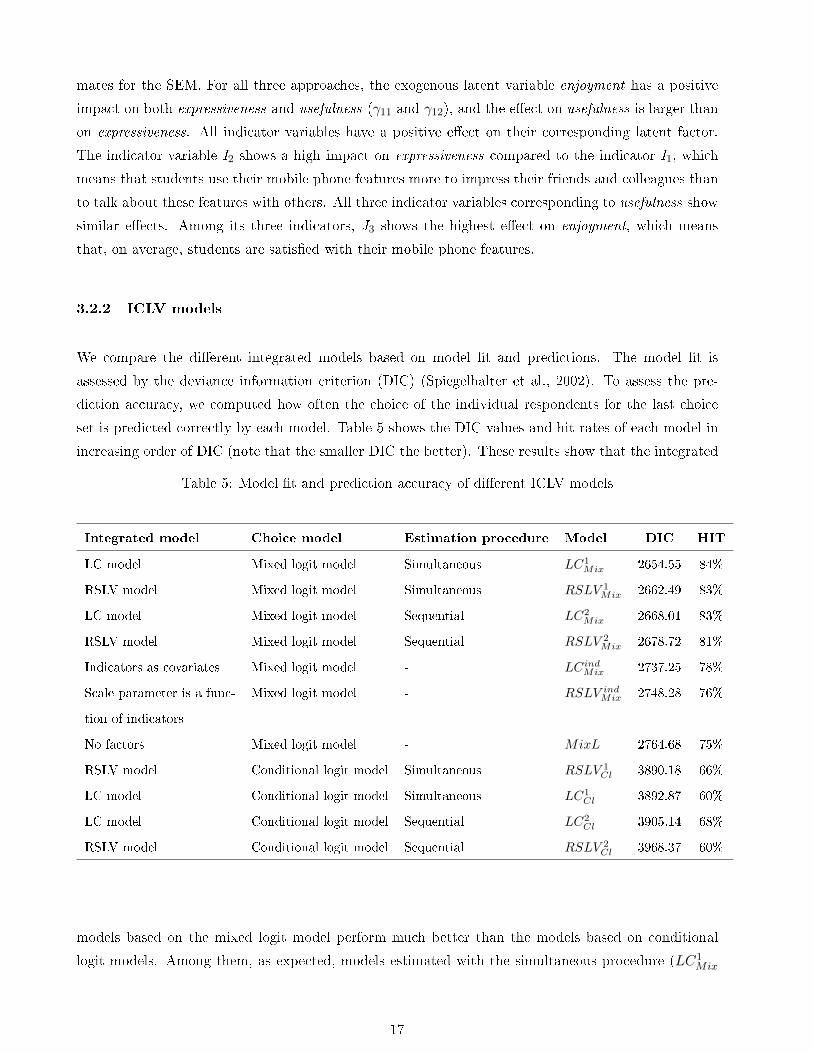
mates for the SEM. For all three approaches, the exogenous latent variable enjoyment has a positive
impact on both expressiveness and usefulness (γ11 and γ12), and the eect on usefulness is larger than
on expressiveness. All indicator variables have a positive eect on their corresponding latent factor.
The indicator variable I2 shows a high impact on expressiveness compared to the indicator I1, which
means that students use their mobile phone features more to impress their friends and colleagues than
to talk about these features with others. All three indicator variables corresponding to usefulness show
similar eects. Among its three indicators, J3 shows the highest eect on enjoyment, which means
that, on average, students are satised with their mobile phone features.
3.2.2 ICLV models
We compare the dierent integrated models based on model t and predictions. The model t is
assessed by the deviance information criterion (DIC) (Spiegelhalter et al., 2002). To assess the pre-
diction accuracy, we computed how often the choice of the individual respondents for the last choice
set is predicted correctly by each model. Table 5 shows the DIC values and hit rates of each model in
increasing order of DIC (note that the smaller DIC the better). These results show that the integrated
Table 5: Model t and prediction accuracy of dierent ICLV models
Integrated model Choice model Estimation procedure Model DIC HIT
LC model Mixed logit model Simultaneous LC1Mix 2654.55 84%
RSLV model Mixed logit model Simultaneous RSLV 1Mix 2662.49 83%
LC model Mixed logit model Sequential LC2Mix 2668.01 83%
RSLV model Mixed logit model Sequential RSLV 2Mix 2678.72 81%
Indicators as covariates Mixed logit model - LCindMix 2737.25 78%
Scale parameter is a func-
tion of indicators
Mixed logit model - RSLV indMix 2748.28 76%
No factors Mixed logit model - MixL 2764.68 75%
RSLV model Conditional logit model Simultaneous RSLV 1Cl 3890.18 66%
LC model Conditional logit model Simultaneous LC1Cl 3892.87 60%
LC model Conditional logit model Sequential LC2Cl 3905.14 68%
RSLV model Conditional logit model Sequential RSLV 2Cl 3968.37 60%
models based on the mixed logit model perform much better than the models based on conditional
logit models. Among them, as expected, models estimated with the simultaneous procedure (LC1Mix
17

and RSLV 1Mix) show better t and better predictions than the models estimated with the sequential
method. However, the gain of using the simultaneous method over the sequential method is rather
small. Therefore, we can conclude that, one can use the easier sequential approach to estimate the
integrated model without losing much eciency. Although these two models (LC1Mix and RSLV 1
Mix)
have rather dierent interpretations they have very similar t and predictions. We can also conclude
that including all observed indicators into the model directly is worse than including the latent factors
both with respect to the model t and the prediction accuracy. Furthermore, the mixed logit model
without latent variables can model the heterogeneity better than the integrated models based on the
conditional logit model.
Next we present the parameter estimates of the two best models LC1Mix and RSLV
1Mix in Table 5. The
latent covariate model contains alternative specic factor eects. In each choice set of the design three
alternatives are arranged according to the camera resolution: the rst alternative with low resolution,
the second with medium resolution and the third with high resolution. The utilities of the three mobile
alternatives are given by:
u1sn = βgpsn x
gps1sn +βwifi
n xwifi1sn +βcam
n xcam1sn +βmp3
n xmp31sn +βmem
n xmem1sn +αexpres
1 ηexpresn +αuseful
2 ηusefuln + ε1sn,
u2sn = βgpsn x
gps2sn +βwifi
n xwifi2sn +βcam
n xcam2sn +βmp3
n xmp32sn +βmem
n xmem2sn +αexpres
3 ηexpresn +αuseful
4 ηusefuln + ε2sn,
u3sn = βgpsn x
gps3sn + βwifi
n xwifi3sn + βcam
n xcam3sn + βmp3
n xmp33sn β
memn x
mem3sn + ε3sn.
The factor eects are interpreted as dierential eects: for example, αexpres1 is the dierential eect of
expressiveness on the utility of the rst alternative (low camera resolution) compared to the alternative
with high resolution.
The random utility for the random scale latent variable model is given by:
uksn = e(αexpresηexpres
n +αusefulηusefuln )(βgpsn x
gpsksn+β
wifin x
wifiksn +βcamn x
camksn +βmp3n x
mp3ksn β
memn x
memksn )+εksn.
For this model parametrization, the factor eects are interpreted as eects of latent variables on the
scale parameter, hence on the precision.
Table 6 presents the estimated population means of the attributes and the estimated factor eects for
the LC1Mix and RSLV
1Mix models.
Both models indicate that WiFi, M&Mp3 and GPS are the most preferred mobile phone features
on average among students. The camera resolution is the least important attribute. Notice that, in
the latent covariate model, the eects of expressiveness on the utilities have positive signs. Since the
alternatives are arranged from low to high resolution, these parameters were expected to be negative.
This would represent that a mobile with higher camera resolution is preferred over a mobile with
lower camera resolution. Though the model gives unexpected results about the eects of the latent
factors on the model, it has improved the prediction accuracy by 10% compared to the mixed logit
18
Table 6: Population mean and factor eects estimates
LC1Mix RSLV 1
Mix
Parameter Estimate Std. Error Estimate Std. Error
µGPS 1.9283 0.1820 1.2053 0.3478
µWiFi 4.1280 0.2907 5.3640 0.9674
µCamera 0.4142 0.1249 0.2995 0.0849
µMp3 2.1654 0.2557 2.3237 0.7709
µMemory 0.6635 0.0876 1.3940 0.1962
αexpress1 0.2273 0.0197 - -
αuseful2 -0.3792 0.0219 - -
αexpress3 0.1618 0.0152 - -
αuseful4 -0.1295 0.0138 - -
αexpress - - 1.6404 0.1010
αuseful - - 0.4333 0.0910
model estimated without latent factors. For the RSLV 1Mix model both expressiveness and usefulness
has positive eect on the scale and the expressiveness has the highest eect. This indicates that an
increase in the latent variable leads to an increase in scale, hence an increase in precision. This is
expected, since if a respondent sees these mobile phone features as highly useful to express himself and
to be more productive in his day to day life then the respondent will make more consistent choices and
this will be reected by a small error variance.
Figure 4 shows the heterogeneity distributions of the attribute coecients estimated by LC1Mix and
RSLV 1Mix models. It can be concluded that the WiFi attribute which is on average most preferred,
exhibits the highest heterogeneity. The camera resolution on the other hand is least preferred on
average and exhibits only a small heterogeneity. We can therefore conclude that respondents have
neglected the camera resolution attribute in their decision making process which may explain the
unexpected sign of the factor eects.
19
Figure 4: Heterogeneity distributions of attribute coecients estimated by (a) LC1Mix and (b)RSLV
1Mix
4 Discussion and Conclusions
The current research proposes an integrated mixed logit and latent variable model to model market
heterogeneity based on choice experiments. Researchers often use a conditional logit model that as-
sumes homogeneity in the part-worths and consider individual specic latent factors to model the
market heterogeneity. We extend the classical mixed logit model which assumes market heterogene-
ity in the part-worths by incorporating latent factors and study whether this improves model t and
predictions. We also considered two parametrization of the ICLV model: the latent covariate model
where we consider these latent quantities as covariates and include them into the systematic part of
the utility and the random scale latent variable model where the latent factors aect the scale factor.
This paper compares dierent ICLV models based on a empirical marketing experiment. Results for
this particular experiment show that the proposed integrated mixed logit and latent variable models
outperform all other models we considered. In both model parametrization, the integrated mixed logit
models estimated with the simultaneous procedure yield best model t and the highest prediction
accuracy. It was also shown that the classical mixed logit model can model the market heterogeneity
better than the ICLV models based on the conditional logit model which uses the factors to capture
the heterogeneity.
Regarding the parameter estimates, the best two models (LC1Mix and RSLV
1Mix) give similar estimates
for the population means of the attribute coecients and also give similar estimated heterogeneity
distributions. Both models indicate that WiFi, M&Mp3 and GPS are on average the most preferred
mobile phone features for these respondents.
20
References
Ansari, A. and K. Jedidi, 2000. Bayesian Factor Analysis for Multilevel Binary Observations. Psy-
chometrika. 65 475-497.
Ansari, A. and K. Jedidi, and S. Jagpal, 2000. A Hierarchical Bayesian Methodology for Treating
heterogeneity in Structural Equation Models. Marketing Science. 19 328-347.
Arora, N., J. Huber, 2001. Improving Parameter Estimates and Model Prediction by Aggregate Cus-
tomization in Choice Experiments. Journal of Consumer Research. 28 273-283.
Ashok, K., W.R. Dillon, and S. Yuan, 2002. Extending Discrete Choice Models to Incorporate Attitu-
dinal and Other Latent Variables. Journal of Marketing Research. 39(1) 31-46.
Ben-Akiva, M., J. Walker, A. Bernardino, D. Gopinath, T. Morikawa, and A. Polydoropoulou, 2002.
Integration of Choice and Latent Variable Models, in (H. Mahmassani, Ed.) In Perpetual Motion:
Travel Behaviour Research Opportunities and Application Challenges. Elsevier Science. 431-470.
Bierlaire, M. and M. Ben-Akiva, 2010. Lecture notes in Discrete Choice Analysis. EPFL, Lausanne,
Switzerland.
Bliemer, M.C.J., J.M. Rose, 2010. Construction of Experimental Designs for Mixed Logit Models
Allowing for Correlation Across Choice Observations. Transportation Research Part B: Methodological.
44 720-734.
Bollen, K. A., 1989. Structural Equation Models with latent Variables. John Wiley & Sons, Inc.
Danthurebandara, V. M., J. Yu, and M. Vandebroek, 2011. Sequential Choice Designs to Estimate
the Heterogeneity Distribution of Willingness-to-pay. Quantitative Marketing and Economics. 9(4)
429-448.
Geman, S. and D. Geman, 1984. Stochastic Relaxation, Gibbs Distribution and the Bayesian Restora-
tion of Images. IEEE Transactions on Pattern Analysis and Machine Intelligence. 6 721-741.
Hastings, W. K., 1970. Monte Carlo Samplin Methods Using Markov Chains and Their Applications.
Biometrika. 57 97-109.
Head, M., N. Ziolkowski, 2010. Understanding student attitudes of mobile phone applications and
tools: A study using conjoint, cluster and SEM analyses. Proceedings of the 18th European Conference
on Information Systems (ECIS 2010), Pretoria, South Africa.
Hess, S., and A. Stathopoulos, 2010. Linking Response Quality to Survey Engagement: A Combined
Random Scale and Latent Variable Approach. Proceedings of the European Transport Conference (ETC
2010), Glasgow, Scotland, UK.
21
Joreskog, K. G., and D. Sorbom, 1996. LISREL 8: Structural Equation Modelling with the SIMPLIS
Command Language. Hove and London: Scientic Software International.
La Paix, L., M. Bierlaire, E. Cherchi, and A. Monzón, 2011. How Urban Environment Aects Travel
Behaviour? Integrated Choice and Latent Variable Model for Travel Schedules. Proceedings of the
Second International Choice Modelling Conference (ICMC 2011), Leeds, North England, UK.
Lee, S. Y. and Song, X. Y., 2004. Evaluation of Bayesian and Maximum Likelihood Approaches in
Analysing Structural Equation Models with Small Sample Sizes. Multivariate Behavioural Research.
39 653-686.
Lee, S. Y., 2008. Structural Equation Modelling: A Bayesian Approach. John Wiley & Sons, Inc.
Lin, A., S. Gregor and M. Ewing, 2008. Developing a scale to measure the enjoyment of web experiences.
Journal of Interactive Marketing. 22.
Lund, A., 2001. Measuring usability with the USE questionnaire. STC Usability SIG Newsletter. 8(2).
Lunn, D., D. J. Spiegelhalter, A. Thomas and N. Best, 2009. The BUGS project: Evolution, critique
and future directions. Statistics in Medicine. 28 3049 - 3067.
McClatchey, S., 2006. The consumption of mobile services by Australian university students. Aus-
tralian College Students. 1(1) 2-9.
Mels, G., 2006. LISREL for Windows: Getting Started Guide. Lincolnwood, IL: Scientic Software
International, Inc.
Metropolis, N., 1953. Equations of State Calculation by Fast Computing Machine. Journal of Chemical
Physics. 21 1087-1091.
Nysveen, H., Per E. Pedersen and H. Thorbjornsen, 2005. Intentions to use mobile services: antecedents
and cross-service comparisons. Journal of the Academy of Marketing Science. 33(3) 330-356.
Olson, J. M., and M. P. Zanna, 1993. Attitudes and attitude change. Annual Review of Psychology.
44 117-154.
Rossi, P.E., R.E. McCulloch, and G.M. Allenby, 1996. The Value of Purchase History Data in Target
Marketing. Marketing Science. 15 321-340.
Rungie, C. M., L. V. Coote, and J. Louviere, 2011. Structural Choice Modeling: Theory and Appli-
cations to Combining Choice experiments. Proceedings of the Second International Choice Modelling
Conference (ICMC 2011), Leeds, North England, UK.
22
Sándor, Z., M. Wedel, 2001. Designing conjoint choice experiments using managers' prior beliefs.
Journal of Marketing Research. 38 430-444.
Spiegelhalter, D. J., N. G. Best, B. P. Carlin and A. van der Linde, 2002. Bayesian measures of model
complexity and t. Journal of the Royal Statistical Society, Series B. 64 583-639.
Spiegelhalter, D. J., A. Thomas, N. G. Best, and D. Lunn, 2003. WinBUGS User Manual. Version
1.4. Cambridge, England. MRC Biostatistics Unit.
Srivastava, L., 2005. Mobile phones and the evolution of social behaviour. Behaviour and Information
technology. 24(2) 111-129.
Tanner, M. A. and W. H. Wong, 1987. The calculation of posterior distributions by data augmentation
(with discussion). Journal of the American Statistical Association. 82 528-550.
Temme, D., M. Paulssen, and T. Dannewald, 2008. Incorporating Latent Variables into Discrete Choice
Models - A Simultaneous Estimation Approach Using SEM Software. Business Research. 1(2) 220-237.
Toubia, O., J. R. Hauser, and D. I. Simester, 2004. Polyhedral Methods for Adaptive Choice-Based
Conjoint Analysis. Journal of Marketing Research. 41 116-131.
Train, K., 2003. Discrete choice methods with simulation. Cambridge University Press.
Walker, J. and M. Ben-Akiva, 2002. Generalized Random Utility Model. Mathematical Social Sciences.
43(3) 303-343.
Yu, J., Goos, P., Vandebroek, M., 2008. Model Robust Design of Conjoint Choice Experiments.
Journal of Communications in Statistics - Simulations and Computations. 37 1603-1621.
Yu, J., Goos, P., Vandebroek, M., 2011. Individually adapted sequential Bayesian conjoint-choice
designs in the presence of consumer heterogeneity. Submitted for publication.
23