If You Are So Smart, Why Aren�t You Rich? The E¤ects of

Education, Financial Literacy and Cognitive Ability on

Financial Market Participation

Shawn Cole and Gauri Kartini Shastry�

November 2008

Abstract

Household �nancial market participation a¤ects asset prices and household welfare. Yet,our understanding of this decision is limited. Using an instrumental variables strategy anddataset new to this literature, we provide the �rst precise, causal estimates of the e¤ects ofeducation on �nancial market participation. We �nd a large e¤ect, even controlling for in-come. Examining mechanisms, we demonstrate that cognitive ability increases participation;however, and in contrast to previous research, �nancial literacy education does not a¤ectdecisions. We conclude by discussing how education may a¤ect decision-making through:personality, borrowing behavior, discount rates, risk-aversion, and the in�uence of employersand neighbors.

�Harvard Business School (scole@hbs.edu), and University of Virginia (shastry@virginia.edu), respectively.We thank the editor, associate editor, two referees, and Josh Angrist, Malcolm Baker, Daniel Bergstresser, CarolBertaut, David Cutler, Robin Greenwood, Caroline Hoxby, Michael Kremer, Annamaria Lusardi, Erik Sta¤ord,Jeremy Tobacman, Petia Topalova, Peter Tufano, and workshop participants at Harvard, the Federal ReserveBoard of Governors, the University of Virginia and the Boston Federal Reserve for comments and suggestions.

1

1 Introduction

Individuals face an increasingly complex menu of �nancial product choices. The shift from

de�ned bene�t to de�ned contribution pension plans, and the growing importance of private

retirement accounts, require individuals to choose the amount they save, as well as the mix

of assets in which they invest. Yet, participation in �nancial markets is far from universal in

the United States. Moreover, we have only a limited understanding of what factors cause

participation.

Using a very large dataset new to the literature, this paper studies the determinants of �-

nancial market participation. Exploiting exogenous variation in education caused by changes in

schooling laws, we provide a precise, causal estimate of the e¤ect of education on participation.

One year of schooling increases the probability of �nancial market participation by 7-8%, hold-

ing other factors, including income, constant. The size of this e¤ect is larger than previously

identi�ed correlates of behavior, such as trust (Guiso, Sapienza, and Zingales, 2008), peer ef-

fects (Hong, Kubik, and Stein, 2004), or life experience from the stock market (Malmendier and

Nagel, 2007).

We then turn to explore why this is so. A leading hypothesis is that students receive �nancial

education in school, which changes behavior. Indeed, states increasingly require high schools to

teach �nancial literacy. Twenty-eight states have mandatory �nancial literacy content standards

for high school students; many other high schools o¤er optional courses. Exploiting a natural

experiment studied in an in�uential paper by Bernheim, Garrett, and Maki (2001), we test

whether �nancial literacy education a¤ects participation. Using a sample several orders of

magnitude larger than theirs, with a more �exible speci�cation, we �nd in fact that high school

�nancial literacy programs did not a¤ect participations.

A second possibility is that education a¤ects cognitive ability, which in turn increases par-

ticipation. By exploiting within-sibling group variation in cognitive ability, we show that indeed

higher levels of cognitive ability leads to greater �nancial market participation. Importantly,

these estimates are not confounded by unobserved background and family characteristics.

Finally, we explore other ways in which education might a¤ect �nancial behavior, including

e¤ects on personality, borrowing behavior, discount rates, risk-aversion, and the in�uence of

2

employers and neighbors.

This paper adds to a growing literature on the correlates and determinants of �nancial

participation. Participation is important for many reasons. For the household, participation

facilitates asset accumulation and consumption smoothing, with potentially signi�cant e¤ects

on welfare. For the �nancial system as a whole, the depth and breadth of participation are

important determinants of the equity premium and the volatility of markets, and household

expenditure (Mankiw and Zeldes, 1991; Heaton and Lucas, 1999; Vissing-Jorgensen, 2002; and

Brav, Constantinides, and Gezcy, 2002). Participation may also a¤ect the political economy

of �nancial regulation, as those holding �nancial assets may have di¤erent attitudes towards

corporate and investment income tax policy than those without such assets, as well as di¤erent

attitudes towards risk-sharing and redistribution.

The 2004 Survey of Consumer Finances indicates that the share of households holding stock,

either directly or indirectly, was only 48.6% in 2004, down three percentage points from 2001

(Bucks, Kennickell, and Moore, 2006). Some view this limited participation as a puzzle: Haliassos

and Bertaut (1995) consider and reject risk aversion, belief heterogeneity, and other potential ex-

planations, instead favoring �departures from expected-utility maximization.�Guiso, Sapienza,

and Zingales (2008) �nd that individuals lack of trust may limit participation in �nancial mar-

kets. Others argue that limited participation may be rationally explained, by small �xed costs

of participation. Vissing-Jorgensen (2002), using data from a household survey, estimates that

an annual participation cost of $275 (in 2003 dollars) would be enough to explain the non-

participation of 75% of households. This paper sheds some light on this debate by examining

whether exogenous shifts in education, and cognitive ability, and �nancial literacy training a¤ect

participation decisions.

This paper proceeds as follows. The next section introduces our main source of data, the

U.S. census, which has not yet been used to study �nancial market participation. Sections 3,

4, and 5 examine how �nancial market participation is a¤ected by education, �nancial literacy

education, and cognitive ability, respectively. Section 6 discusses additional mechanisms through

which education could a¤ect participation, and section 7 concludes.

3

2 Patterns in Financial Market Participation

2.1 Data

We introduce new data for use in analyzing �nancial market participation decisions. The U.S.

census, a decennial survey conducted by the U.S. government, asks questions of households

that Congress has deemed necessary to administer U.S. government programs. One out of

six households is sent the �long form,�which includes detailed questions about an individual,

including information on education, race, occupation, and income. We use a 5% sample from

the Public Use Census Data, which is a random representative sample drawn from the United

States population.

There are several important advantages to using census data. First and foremost, by com-

bining data from 1980, 1990, and 2000, our baseline speci�cation contains more than 14 million

observations. This allows precise estimates, and most importantly, enables us to use instrumen-

tal variable strategies that would simply not be possible with other data sets. The large sample

size also allows non-parametric controls for most variables of interest, and the inclusion of state,

cohort, and age �xed-e¤ects.

The census does not collect any information on �nancial wealth, but does collect detailed

questions on household income. The main measure of �nancial market participation we will use is

�income from interest, dividends, net rental income, royalty income, or income from estates and

trusts,�received during the previous year which we will term �investment income.�Households

are instructed to �report even small amounts credited to an account.�(Ruggles et al., 2004). A

second type of income we use is �retirement, survivor, or disability pensions,� received during

the previous year which we term �retirement income.�This is distinct from Social Security and

Supplemental Security Income, both of which are reported on separate lines.1

1Two data points deserve mention. First, one may be concerned that small amounts of investment incomesimply represent interest from savings accounts. As a robustness check, we rerun our analysis considering onlythose who receive income greater than $500 (or, alternatively, $1000) in investment income as "participating."The results are very similar (available on request).Second, to preclude the possibility of revealing personal information, the Census �top-codes�values for very rich

individuals. Speci�cally, they replace the income variable for individuals with investment income or retirementincome above a year-speci�c limit with the median income of all individuals in that state earning above thatlimit. The limits for investment income are $75,000, $40,000 and $50,000 in 1980, 1990 and 2000 respectively.The limits for retirement income are $30,000 and $52,000 in 1990 and 2000 respectively. (The 1980 Census didnot separate retirement income from other sources of income.) The percentage of topcoded observations is verylow: 0.47% for investment income and 0.22% for retirement income. Of course, using as a dependent variable

4

A limitation of using the amount of investment income, rather than amount invested, is that

the level of investment need not be monotonically related to the level of income from investments.

An individual with $10,000 in bonds may well report more investment income than a household

with $30,000 in equity. This would make it di¢ cult to use the data for structural estimates of

investment levels (such as estimates of participation costs). In this work, we focus primarily on

the decision to participate in �nancial markets, for which we de�ne a dummy variable equal to one

if the household reports any positive investment income. Approximately 22% of respondents do

so, which is close to 21.3% of families that report holding equity in the 2001 Survey of Consumer

Finances (Bucks, Kennickell, and Moore, 2006), but lower than the 33% of households reporting

any investment income in the 2001 SCF. The data appendix compares the data from the SCF

and the Census in greater detail.

We report results for both the level of investment income (in 2000 dollars), and place of that

individual in the overall distribution of investment income. The latter term we measure by the

household�s percentile rank in the distribution of investment income divided by total income.

The limitations of the data on household wealth are counterbalanced by the size of the

dataset: a sample of 14 million observations allows for non-parametric analysis along multiple

dimensions, as well as the use of innovative identi�cation strategies to measure causal e¤ects.

2.2 Patterns of Participation

Correlates of participation in �nancial markets are well understood. Campbell (2006) provides

a careful, recent review of this literature. Previous work has demonstrated that participation is,

not surprisingly, increasing in income, as well as education (Bertaut and Starr-McCluer, 2001,

among others), measured �nancial literacy (Lusardi and Mitchell, 2007, and Rooij, Lusardi, and

Alessie, 2007), social connections (Hong, Kubik, and Stein, 2004), and trust (Guiso, Sapienza,

and Zingales, 2008), and experience with the stock market (Malmendier and Nagel, 2007).

Tortorice (2008), however, �nds that income and education only slightly reduce the likelihood

that individuals make expectational errors regarding macroeconomic variables, and that these

errors adversely a¤ect buying attitudes and �nancial decisions.

�any investment income�avoids the top-coding problem entirely. Nevertheless, as an alternative approach, we runTobit regressions, and �nd very similar results (available upon request).

5

In this section, we explore the link between �nancial market participation, income, age, and

education. Taking advantage of the large size of the census dataset, we employ non-parametric

analysis. There are at least two signi�cant advantages of non-parametric analysis. First, instead

of imposing a linear (or polynomial) functional form, it allows the data to decide the shape of the

relationship between variables. This yields the correct non-linear relationship. Second, and more

importantly, if a parametric model is not correctly speci�ed, it biases the estimates of all the

parameters in the model. Allowing an arbitrary relationship between income and participation,

for example, ensures that the education variable is not simply picking up non-linear loading on

income.

The left three graphs of Figure 1 depict simple means, indicating how participation varies

with age, educational attainment, and earned income. The solid line indicates the share reporting

investment income, while the dotted line indicates the average amount (right axis). Throughout

the paper, households with no reported investment income are kept in the data, including when

we calculate average investment income. Because education and income are strongly correlated,

these graphs confound those two factors. As an alternative method, we take advantage of

the large sample size of the census, and instead estimate non-parametric relationships, in the

following manner. We regress measures of �nancial market participation, y, on categorical

variables for age, �i, level of education, i, and amount of income, �i. We use a separate

dummy for each $1,000 income range, e.g., a dummy �0 indicates income between $0 and $999,

while �1 indicates income between $1,000 and $2,000, etc.:

yi = �a + e + �w + "i (1)

These relationships, all derived from estimating equation 1, are presented in the right three

graphs of Figure 1. Again, the solid line gives the share reporting income, while the dotted line

gives the amount. These graphs give the incremental e¤ect of one factor (e.g., age), controlling

for the other two factors (income and education).

Participation in �nancial markets increases strongly with age. Approximately 17 percent of

individuals report positive investment income at the age of 35; this number increases by about

11 points by age 55. Controlling for wealth and education do not a¤ect this relationship: the

6

top-right panel gives the regression coe¢ cients �j , describing the incremental increase for each

year of age, for a given level of wealth and education. Average investment income also increases

with age, consistent with the life cycle hypothesis.

The share reporting investment income, and amount, increases steadily with education,

though this relationship is tempered when age and income are controlled for. Averages for

various levels of education are graphed in the second row2. Moving from a high-school education

to a college degree, for example, is associated with a 10 percentage point increase in participation.

Finally, the bottom two graphs indicate how investment income varies with total individual

income. The share of individuals who participate in �nancial markets increases at a decreasing

rate with total income, reaching a peak of approximately 60% for households with earned income

levels of $150,000. The bottom-right plot, which controls for age and education, looks quite

similar for �nancial market participation, but describes a much steeper relationship between

earned income and earned investment income than if one does not control for age and education.

Of course, even careful partial correlations do not imply causal relationships, as unobserved

factors, such as ability, may a¤ect education, income, and �nancial market participation. One

important factor, which we cannot measure, is the intergenerational transmission of saving and

investment behavior. Mandell (2007) �nds that high school students cite their parents as their

primary source of information on �nancial matters, and �nds that students who score high on

�nancial literacy tests come from well-o¤, well-educated households. Charles and Hurst (2003)

�nd that investment behavior transmitted from parent to child explains a substantial fraction

of the correlation of wealth across generations.

In the remainder of the paper, we develop precise causal estimates of the relative importance

of factors that a¤ect �nancial market participation.

2They are 5th through 8th grade, 9th grade; 10th grade; 11th grade; 12th grade but no diploma, high-schooldiploma or GED, some college (HS+), associate degree-occupational program (C1), associate degree-academicprogram (C2), bachelor�s (B.A.), master�s (M.A.), professional degree (M.A.+), and doctorate (Ph.D.).

7

3 The E¤ect of Education on Financial Market Participation

3.1 Empirical Strategy

The patterns described in section 2 strongly suggest that households with higher levels of educa-

tion are more likely to participate in �nancial markets. Campbell (2006), for example, notes that

educated households in Sweden diversify their portfolios more e¢ ciently. However, the simple re-

lationship between �nancial decisions and education levels omits many other important factors,

such as ability or family background, that likely in�uence the decisions. Unbiased estimates

of the e¤ect of education on investment behavior can be identi�ed by exploiting variation in

education that is not correlated with any of these unobserved characteristics. In this section, we

exploit an instrumental variables strategy identi�ed by Acemoglu and Angrist (2000)- changes

in state compulsory education laws - to provide exogenous variation in education. Revisions

in state laws a¤ected individuals�education attainment, but are not correlated with individual

ability, parental characteristics, or other potentially confounding factors.

In particular, we use changes in state compulsory education laws between 1914 and 1978.

We follow the strategy used in Lochner and Moretti (2004, hereafter LM), who use changes in

schooling requirements to measure the e¤ect of education on incarceration rates. The principle

advantage of following LM closely is that they have conducted a battery of speci�cation checks,

demonstrating the validity of using compulsory schooling laws as a natural experiment. For

example, LM show that there is no clear trend in years of schooling in the years prior to changes

in schooling laws and that compulsory schooling laws do not a¤ect college attendance.

The structural equation of interest is the following,

yi = �+ �si + Xi + "i (2)

where si is years of education for individual i, and Xi is a set of controls, including age, gender,

race, state of birth, state of residence, census year, cohort of birth �xed e¤ects and a cubic

polynomial in earned income. Age e¤ects are de�ned as dummies for each 3-year age group from

20 to 75, while year e¤ects are dummies for each census year. Following LM, we exclude people

born in Alaska and Hawaii but include those born in the District of Columbia; thus we have 49

8

state of birth dummies, but 51 state of residence dummies. When the sample includes blacks,

we also include state of birth dummies interacted with a dummy variable for cohorts born in the

South who turn 14 in or after 1958 to allow for the impact of Brown vs. Board of Education.

Cohort of birth is de�ned, following LM, as 10-year birth intervals. Standard errors are corrected

for intracluster correlation within state of birth-year of birth. The outcome variable is either

an indicator for having any investment or retirement income or the actual level of investment

or retirement income. When studying the amount of income, we drop observations that were

top-coded by the survey; in 1980 (1990; 2000) these individuals reported amounts greater than

$50,000 ($40,000; $75,000) for investment income and $52,000 ($30,000) for retirement income.

We account for endogeneity in educational attainment by using exogenous variation in school-

ing that comes from changes in state compulsory education laws. These compulsory schooling

laws usually set one or more of the following: the earliest age a child is required to be enrolled

in school, the latest age she is required to be in school and the minimum number of years she

is required to be enrolled. Following Acemoglu and Angrist and LM, we de�ne the years of

mandated schooling as the di¤erence between the latest age she is required to stay in school

and earliest age she is required to enroll when states do not set the minimum required years of

schooling. When these two measures disagree, we take the maximum. We then create dummy

variables for whether the years of required schooling are 8 or less, 9, 10, and 11 or more. These

dummies are based on the law in place in an individual�s state of birth when an individual

turns 14 years of age. As LM note, migration between birth and age 14 will add noise to this

estimation, but the IV strategy is still valid. The �rst stage for the IV strategy can then be

written as

si = �+ �9 � Comp9 + �10 � Comp10 + �11 � COMP11 +Xi + "i (3)

These laws were changed numerous times from 1914 to 1978, even within a state and not

always in the same direction. It is important to note that while state-mandated compulsory

schooling may be correlated at the state or individual level with preferences for savings, risk

preferences or discount rates or ability, the validity of these instruments rests solely on the

assumption that the timing of these law changes is orthogonal to these unobserved characteristics

9

conditional on state of birth, cohort of birth, state of residence and census year. An alternate

explanation would have to account for how these unobserved characteristics changed discretely

for a cohort born exactly 14 years before the law change relative to those born a year earlier in

the same state.

Our sample di¤ers from LM in two ways. First, LM limit their attention to census data from

1960, 1970 and 1980, as their study requires information on whether the respondent resides in

a correctional institution. Investment income is available in a later set of census years; data are

available from 1980-2000. We describe results from pooled data from 1980, 1990 and 2000. The

second di¤erence from LM is in the sample selection: we include individuals as old as 75, rather

than limiting analysis to individuals aged 20-60. The addition of older cohorts also allows us to

study reported retirement income where we focus on individuals between the ages of 50 and 75.

Individuals in our sample are aged 18 - 75.

The census does not code a continuous measure of years of schooling, but rather identi�es

categories of educational attainment: preschool, grades 1-4, grades 5-8, grade 9, grade 10, grade

11, grade 12, 1-3 years of college, and college or more. We translate these categories into years

of schooling by assigning each range of grades the highest years of schooling. This should not

a¤ect our estimates since individuals who fall within the ranges of grades 1-8 and 1-3 years of

college will not be in�uenced by the compulsory schooling laws.

Finally, it is worth noting that the estimates produced here are Local Average Treatment

E¤ects, which measure the e¤ect of education on participation for those who were a¤ected by the

compulsory education laws.3 We note that those who are in fact a¤ected by the laws are likely

to have low levels of participation, and thus constitute a relevant study population. Moreover,

we draw some comfort from Oreopoulos (2006), who studies a compulsory schooling reform that

a¤ected a very large fraction of the population in the UK. While Oreopoulos focuses on earnings

rather than �nancial market participation, he �nds that the relationship between schooling and

earnings estimated in the United States from a small fraction of the population is quite similar

to the relationship in the United Kingdom, which was estimated using a very large fraction of

the population.

3 Imbens and Angrist (1994) provides a discussion of Local Average Treatment E¤ects.

10

3.2 Results

OLS estimates of equation (2) are presented in Table 1. Panel A presents the results for the

linear probability model, using �any income�as the dependent variable and panel B studies the

level of total income. In panel C the left-hand side variable is the individual�s location in the

nationwide distribution of the ratio of investment income to total income.4 The sample size

varies between 4 million and 14 million observations, depending on the sample used (we restrict

attention to those over 50 for retirement income). In addition to years of schooling, we include

(but do not report) race and gender dummies, age (3-year age groups), birth cohort (10 year

cohorts), state of birth, state of residence, census year and a cubic polynomial in earned income.

Regressions also include state of residence �xed e¤ects interacted with a dummy variable for

being born in the South and turning age 14 in 1958 or later to account for the impact of Brown

vs. Board of Education for blacks. This speci�cation mimics Lochner and Moretti.

The OLS results have the expected sign and are precisely estimated. An additional year

of education is associated with a 3.55 percentage point higher probability of �nancial market

participation, and a 2.4 percentage point increase for retirement income. An additional year

of schooling is associated with approximately $273 more in investment income, and $548 more

in retirement income, which represent an approximately 3.4 and 2.3 percentage point increase

in the distribution of investment and retirement income. We caution that these estimates are

likely plagued by omitted variables bias - educational attainment is correlated with unobserved

individual characteristics that may also a¤ect savings. We therefore implement the IV strategy

described above.

For an instrument to be valid it must a¤ect education: we �rst present evidence that com-

pulsory schooling laws did increase human capital accumulation. The results are presented in

Table 2, where we include only observations which contain information on investment income.

The omitted group is states with no compulsory attendance laws or laws that require 8 or fewer

years of schooling. Clearly, the state laws do in�uence some individuals - when states mandate a

greater number of years of schooling, some individuals are forced to attain more education than

they otherwise would have acquired. A 9th year or 10th year of mandated schooling increases

4That is, all individuals are sorted by total investment income / total income, and are assigned a percentileranking.

11

years of completed education by 0.2 years, while requiring 11 years of education increases ed-

ucation by 0.26 years. In fact, forcing students to remain in school for even one more year (9

years of required schooling) increases the probability of graduating high school by 3.8%. The

average years of schooling and the share of high school graduates are monotonic in the required

number of years. These estimates are similar to those in Table 4 of LM�s work.5

Table 3 presents 2SLS estimates of equation (2). Panel A reveals that an additional year of

schooling increases the probability of having any investment income by 7.6%. For retirement

investments, an additional year of schooling increases the probability of non-zero income by

about 5.9%. These estimates are somewhat larger than the OLS estimates in table 1, suggesting

a downward bias in the OLS.

In panel B, we study the amount of income from these assets and �nd a large and signi�cant

e¤ect on both types of investment income. The magnitudes are quite large, substantially larger

than the OLS estimates; an additional year of schooling increases investment income and retire-

ment income by $1767 and $979 respectively.6 Education also improves an individual�s position

in the distribution of investment income (as a percentage of total income) as shown in panel C.

These results are robust to using high school completion, rather than years of schooling, as the

measure of educational attainment. Including a cubic in earned income (which includes wages

and income from one�s own business or farm) as a control does not a¤ect the results appreciably.

The striking fact is that no matter how many income controls we include, we �nd persistent,

large, di¤erences in participation by education.

To get a sense of these point estimates, we conduct a back-of-the-envelope calibration exer-

cise. This calibration also helps us to understand the source of the increase: does education raise

investment earnings simply because households earn more money, while keeping the fraction of

income saved constant, or does it a¤ect the savings rate as well?

The average individual in our sample is 49 years old. To simplify the algebra, we assume he

earned a constant $20,000 (the average income for high school graduates in our sample) since

he was 20 years old,7 saved a constant 10% of his income at the end of each year and earned a

5�Weak instrument�bias is not a problem in this context. We report the F-statistics of the excluded instrumentsin Table 3. The F-statistics range from 44.5 to 49.9, well above the critical values proposed by Stock and Yogo(2005).

6Using IV Tobit for investment income yields very similar results; results are available on request.7Using the average income at each age gives very similar estimates.

12

5% return on his assets. Assuming one additional year of schooling boosts wage income by of

7% (an estimate from Acemoglu and Angrist 2000), if the individual�s savings rate did not vary

with schooling, an additional year would increase his savings by ($20,000)*(0.07)*(0.1) = $140

per year. At the age of 49, his accumulated savings would be greater by about $9,000, and his

income from investments approximately $450 higher.8

In contrast, if we assume that the year of education also increased our hypothetical 49-year-

old�s savings rate by 1 percentage point, his annual savings would increase by $354, yielding an

approximately $22,500 greater asset base by age 49, and a corresponding increase in income of

$1,200.9

The point estimates on investment income, $1,769 per year, are much closer to this latter

�gure, suggesting education a¤ected the savings rate. Finally, it is also possible that education

a¤ects the choice of asset allocation: better educated individuals choose portfolios that yield

higher returns, perhaps with lower fees and less tax impact.

4 Financial Literacy and Financial Market Participation

Having identi�ed causal e¤ects of education on �nancial market participation, it is important

to understand the mechanisms through which education may matter. One possibility is that

education increases participation through actual content: �nancial education may increase �nan-

cial literacy. A growing literature has found strong links between �nancial literacy and savings

and investment behavior. Lusardi and Mitchell (2007), for example, show that households with

higher levels of �nancial literacy are more likely to plan for retirement, and that planners arrive

at retirement with substantially more assets than non-planners. Other work links higher levels

of �nancial literacy to more responsible �nancial behavior, such as writing fewer bounced checks,

and paying lower interest rates on mortgages (see Mandell 2007, among others, for an overview).

For these reasons, improving �nancial literacy has become an important goal of policy makers

and businesses alike. Governments fund dozens of �nancial literacy training programs, aimed at

the general population (e.g., high school �nancial education courses), as well as speci�c target

8140 � (1�exp(0:05�(49�20)))(1�exp(0:05)) � $9000: A 5% return would yield approximately $450.

9These estimates do not depend on the assumed savings rate of 10%, but on a function of the two savingsrates and the return to education: If an individual saved 5% of his income each year, and one year of schoolingincreased this rate to 6.3%, the estimates would be identical.

13

groups (e.g., low-income individuals, �rst-time home buyers, etc.). Businesses provide �nancial

guidance to employees, with an emphasis, but not exclusive focus, on how and how much to

save for retirement.

There is some evidence suggesting that �nancial literacy education can a¤ect both levels

of �nancial literacy and �nancial behavior.10 Bernheim and Garrett (2003) examine whether

employees who attend employer-sponsored retirement seminars are more likely to save for re-

tirement, and �nd they do, after controlling for a wide variety of characteristics. However,

as Caskey (2006) points out, it is di¢ cult to interpret this evidence as causal, as �stable �rms

tend to o¤er �nancial education and people who are most future-oriented in their thinking are

attracted to stable �rms� (p. 24). Indeed, any study that compares individuals who received

training to those who did not receive training is likely to su¤er from selection problems: unless

the training is randomly assigned, the �treatment�and �comparison�groups will almost surely

vary along observable or unobservable characteristics.11 This may explain why other studies �nd

con�icting e¤ects of literacy training programs. Comparing students who participated in any

high school program to those who did not, Mandell (2007) �nds no e¤ect of high school �nancial

literacy programs. In contrast, FDIC (2007) �nd that a �Money Smart� �nancial education

course has measurable e¤ects on household savings.

One of the most methodologically compelling studies that links �nancial education to savings

behavior is Bernheim, Garrett, and Maki (2001, BGM hereafter). BGM use the imposition of

state-mandated �nancial education to study the e¤ects of �nancial literacy training on household

savings. The advantage of this study, which uses a di¤erence-in-di¤erence approach, is that if

the state laws are unrelated to trends in household savings behavior, then the estimated e¤ects

can be given a causal interpretation.

BGM begin by noting that between 1957 and 1982, 14 states imposed the requirement

that high school students take a �nancial education course prior to graduation. Working with

Merrill Lynch, they conducted a telephone survey of 3,500 households, eliciting information on

exposure to �nancial literacy training, and savings behavior. They �nd that the mandates were

10For a careful and thorough review of this literature, see Caskey (2006).11Glazerman, Levy, and Myers (2003) make this point forcefully when they compare a dozen non-experimental

studies to experimental studies, and �nd that non-experimental methods often provide signi�cantly incorrectestimates of treatment e¤ects.

14

e¤ective, and that individuals who graduated following their imposition were more likely to have

been exposed to �nancial education. They also �nd that those individuals save more, with those

graduating �ve years after the imposition of the mandate reporting a savings rate 1.5 percentage

points higher than those not exposed.

In this section, we �rst use census data to replicate the �ndings of BGM. Using their speci-

�cation, we �nd positive and signi�cant e¤ects of �nancial education. We then extend BGM�s

research in two directions. First, the large sample size allows the inclusion of state �xed e¤ects,

as well as non-parametric controls for age and education levels. Second, we are able to carefully

test whether the identi�cation assumption necessary for their approach to be valid holds.

4.1 Bernheim, Garret, and Maki Replication

The main results from BGM are reproduced in column (1) of Table 4. BGM estimate the

following equation, with individual savings rates as the dependent variable yi :

yis = �0+�0�Treats+�1�(MandY earsis)+�2�Marriedi+�3�Collegei+�4�Agei+�5�Earningsi+"i(4)

Treats is a dummy for whether state s ever required students to take �nancial literacy education,

MandYearsis indicates the number of years �nancial literacy mandates had been in place when

the individual graduated from high school, Marriedi and Collegei are indicator variables for

marital status and college education, and earnings is total earnings / 100,000. Column (1)

gives the results for savings rate percentile, compared to peers, which BGM use to reduce the

in�uence of outliers. Consistent with the patterns reported above and elsewhere, BGM �nd

savings increases in education and earnings. They suggest that the strong relationship between

age and income explains why the savings rate is not correlated with age.

The main regressor of interest, �1, is positive and signi�cant, suggesting that exposure to

�nancial literacy education leads to an increased savings rate. Graduating �ve years following

the mandate would induce an individual to move approximately 4.5 percentage points up in the

distribution of savings rate, equivalent to a 1.5 percentage points shift in savings rate. BGM also

note that the fact that �0 is statistically indistinguishable from zero supports the identi�cation

strategy: treated states were not di¤erent from non-treated states prior to the imposition of the

15

mandate.

In columns (2) - (5) we replicate BGM�s results, estimating equation (4) using data from

the census. There are two important di¤erences between the census data and the BGM sample.

First, the BGM sample was collected in 1995, �ve years prior to the 2000 census. Our sample

is aged 35-54 in 2000. When using the census data, we focus on households born in the same

years as the BGM sample, so the birth-cohorts are �ve years older.12 Second, the census sample

size is substantially larger, at 3.6 million, compared to BGM�s 1,900 respondents. We cluster

standard errors at the state of birth-year of birth level.

The primary dependent variable used by BGM was the savings rate, de�ned as unspent

take-home pay plus voluntary deferrals, divided by income. This information is not available in

the census. Instead, we focus on reported income from savings and investments, dividends and

rental payments, which should be informative of the level of assets held by the household.

Columns (2) and (3) in Table 4 present the estimation of equation (4) using �any investment

income�, a dummy equal to 1 if the household reports any income from investment or savings,

as the dependent variable. Column (2) estimates a linear regression model, while column (3)

estimates probit. Similar to BGM, we �nd a positive relationship between savings behavior and

age, income, college education, and total income.

The main coe¢ cient of interest, on years since mandate, is positive and statistically signi�-

cant, at the one percent level. The point estimate, in column (2) 0.33, suggests that each year

the mandate had been in e¤ect the share of households reporting savings income increased by

0.33 percentage points. The mean level of participation is 22.13 percentage points, while the

standard deviation is 41 percentage points. The e¤ect is therefore modest: the e¤ect, �ve years

following the imposition of mandates, would be 1.5 percentage points, or approximately 0.05

standard deviation. However, the e¤ect is highly statistically signi�cant (t-stat 5.18). Column

(4) reports the coe¢ cients from the probit regression. The size of the marginal e¤ect is nearly

identical, at 0.37 percentage points, evaluated at the mean dependent variables.

Column (4) estimates equation 4 using the dollar value of investment income as the dependent

variable. This regression suggests that an additional year of mandate exposure increases savings

12We do not think it likely that any of the di¤erences from our �ndings and BGM are attributable to the timingof the data collection. Using census data from 1990 (or 1980) gives very similar results.

16

income by approximately $19. The average amount of investment income is $1199, while the

median amount is $0. Assuming a return on investments of 5%, an increase of $18 would suggest

an increase in total savings of about $360 for each year of exposure to the mandate. The average

individual that had been exposed to the mandate in the sample had been exposed for �ve years,

suggesting a roughly $1,800 increase in total savings.

Finally, we use the households placement in the entire distribution of investment income to

total income. This is close to BGM�s percentile rating, though it is based on investment income,

rather than savings rate. Again, we �nd a positive and statistically signi�cant e¤ect of exposure

to �nancial education.

The results are, at �rst glance, encouragingly consistent with BGM. One notable di¤erence

is that the coe¢ cient on Treat, �0, is negative, and statistically and economically signi�cant, in

all regressions. A crucial assumption for the BGM approach to be valid is that cohorts in the

states in which the mandates were imposed were not trending di¤erently than those in which

the mandates were not imposed. While a negative �0 does not necessarily indicate the BGM

identi�cation strategy is not valid, it does raise a cautionary �ag. In the next section, we expand

on the BGM methodology, taking advantage of a substantially increased sample size, to examine

how savings behavior of individual cohorts varies with the timing of the mandates.

4.2 A More Flexible Approach

4.2.1 Empirical Strategy

In this section, we improve upon the BGM identi�cation strategy in several ways. First, we add

state �xed-e¤ects, which will control for any unobserved, time-invariant heterogeneity in savings

behavior across states. Second, rather than include a linear trend for age, we include a �xed

e¤ect for each birth-year cohort �a, controlling for both age and cohort e¤ects. Finally, and most

importantly, the extremely large sample size allows for a much more careful measurement of the

impact of literacy education. Rather than a standard di¤erence-in-di¤erence, which compares

the average in the �post� to the average in the �pre,� we include event-year dummies, which

estimate the average level of participation individually for each event-year before and after the

implementation of the mandates. This strategy is perhaps best conveyed graphically, in Figure

2. The line plots average participation for cohorts that were not exposed (left of the vertical

17

line) and exposed (right of the vertical line) to the mandates.

We do this by de�ning a set of 11 dummy variables, D�5isb ; D�4isb ,..D

0isb; D

1isb; :::; D

4isb; D

5plusisb ;

which divide our sample into eleven groups. The omitted group is individuals who were born in

states in which mandates did not go into e¤ect, or who would have graduated from high school

more than �ve years before the mandates kicked in; all 11 dummies are zero. D0isb indicates that

an individual graduated in the year the mandates took e¤ect; D1isb in the �rst year after the

mandates took e¤ect. D2isb �D4isb are de�ned analogously, while D5pisb is set to 1 if an individual

graduates �ve or more years after the �rst cohort in that state was a¤ected by the mandate. We

use �ve as a cut-o¤ for simplicity and because BGM suggest the mandate would have achieved

maximal e¤ect �in short order (within a couple of years)�13. An important test of a di¤erence-

in-di¤erence strategy is that there are no pre-existing trends. D�1isb is set to one for the last

cohort to graduate before mandates took e¤ect, with D�kisb de�ned analogously for cohorts born

2-5 years before the mandate took e¤ect. We thus estimate the following equation:

yisb = �s + b +

4Xk=�5

kDkisb + 5pD

5pisb + �Xi + "isb (5)

The vector Xi includes controls for race, college education, whether the household is married,

and household income. To account for within-cohort correlation, standard errors are clustered

at the state of birth-year of birth level.

Using dummies, rather than a single variable, has two important advantages: �rst, it provides

a clear and compelling test of the identi�cation strategy: were cohorts in states in which the

mandate was eventually to be imposed similar to those in which no mandate was imposed.

Second, it allows the data to decide how the e¢ cacy of �nancial literacy a¤ects savings behavior:

the e¤ect can be constant, increasing, or decreasing. By usingMandY ears, BGM constrain the

e¤ect to be linear in years since the mandate was imposed.

A �nding consistent with the results from BGM would be the following: the coe¢ cients Dkisb;

for k<0, would be statistically indistinguishable from zero and the coe¢ cients on D0isb;...D4isb

and D5pisb would start out small (perhaps indistinguishable from zero), but increase over time,

and be positive and statistically signi�cant for higher values of k. In other words, prior to the

13p. 12. Very similar patterns obtain if a ten year window is used.

18

imposition of the mandates, savings behavior was not trending up or down in states in which

the mandate was imposed and the imposition of �nancial literacy education led to increased

savings over time.

4.2.2 Results

Table 5 presents results from equation (5). Column (1) presents the estimates for the linear

probability model, with �any investment income�as the dependent variable. Column (2) uses

the level of total investment income14 on the left-hand side, and column (3) uses the individual�s

location in the nationwide distribution of investment income to total income as the dependent

variable.

Figure 2 plots each k coe¢ cient, along with a 95% con�dence interval. These coe¢ cients

represent the di¤erence in �nancial participation between the particular cohort, and the cohorts

that graduated more than �ve years prior to the imposition of mandates. (These changes are

not time or age e¤ects, since the birth year dummies absorb any common change in savings

behavior). The red vertical line indicates the �rst cohort that was a¤ected by the mandate,with

cohorts not a¤ected (born earlier) to the left, and cohorts a¤ected (born later) to the right.

The results, presented in Table 5, discon�rm the �ndings of BGM: the �nancial literacy

mandates did not increase savings. Consider the results for the dependent variable �any invest-

ment income.�Individuals born in states both before and after the mandates were imposed are

substantially more likely to report investment income, relative to those born in states in which

mandates were not imposed. Most importantly, there is no increase in investment income for

cohorts that were born after the mandate. We can formally test this hypothesis by compar-

ing the average participation in treated states just before to just after the mandates.15. For

�nancial participation, the average value of k is 1.12 for k2 f�4;�3;�2; and -1g ; and 1.15

for k2 f1; 2; 3; 4g : An F-test (reported in the �nal two rows of Table 5) indicates that �nancial

participation did not change following the mandates. The two rows test the hypothesis that the

sum of the four �pre�year coe¢ cients are equal to the sum of four �post�coe¢ cients, and fail to

reject equality.

14 It is not obvious that the e¤ect would be a level e¤ect, rather than a proportional e¤ect. However, becausemany observations are zero or negative, we do not use log income as a dependent variable.15Formally, we test 1

4

� �4 + �3 + �2 + �1

�= 1

4( 1 + 2 + 3 + 4)

19

Column (2) of Table 5 performs an identical analysis, using the level of investment income

as the dependent variable. Again, troublingly for the BGM identi�cation strategy, investment

income is above average for cohorts graduating prior to the imposition of the mandate. There is

an apparent general upward trend, but no clear trend break at the time of the imposition of the

mandate. A test of the four pre k against the four post k indicates that the latter are signi�-

cantly higher. However, given that there is positive trend before the mandates are implemented,

and that the e¤ect appears to disappear after four years ( 5p is statistically indistinguishable

from zero), the results do not suggest the mandates had an e¤ect.

Finally, column (3) performs the same analysis, using the percentile rank of where the

household falls in the percentile distribution of investment income to total income. The observed

patterns are quite similar to those for any investment income.

While there is no e¤ect when using the entire population, perhaps the e¤ect is heterogenous.

Households with lower levels of education may bene�t most from basic �nancial literacy training

provided in high schools. To test the hypothesis, we re-estimate equation 5 using only data from

individuals who report a maximum educational attainment of 11th or 12th grade, or some college.

Results (not reported) are very similar in this subsample: there is no e¤ect of the mandates on

savings behavior.

Similar �ndings hold when data from the 1980 or 1990 census are used, or when the sample

is restricted to blacks only or whites only. All estimates display the same pattern, �nancial

market participation is above historic levels prior to the imposition of mandates, and does not

increase following the mandate.

As a �nal check of the identi�cation strategy, we use state-level GDP growth data to examine

whether the imposition of mandates was correlated with states�economic situation. The data,

from the Bureau of Economic Analysis, for 1963-1990 are used, giving 1,296 observations.16 We

estimate an equation very similar to 5:

ysy =4X

k=�5 kD

ksy + 5pD

5psy + "sy; (6)

where ysy is GDP growth in state s in year y, and Dksy is a dummy for whether the state s

16As before, DC, Hawaii, and Alaska are excluded. This exclusion makes no di¤erence.

20

imposed a mandate that �rst a¤ected the graduating high school class in year k. Results are

presented in Table 6. The �rst column suggests why participation was increasing both before

and after the mandates became e¤ective: the mandates were passed after periods of abnormally

high economic growth. The average growth rate in the �ve years leading up to the mandates

was 0.26 log points higher than previous years. Similarly, in the four following years, growth

was 0.125 log points higher than the base period, while in the period more than �ve years after

the imposition of mandates, growth was on average 0.2 log points lower than the base period.

Mandates were passed during periods of strong growth in states. The patterns in GDP growth

are similar to those observed for �nancial participation, and may well explain why �nancial

participation increased prior to the passage of the mandates.

Columns (2)-(5) of Table 6 add, progressively, state �xed e¤ects, and linear, quadratic and

�xed-e¤ect controls for time. The last three rows of the table jointly test various combinations of

the Dksy coe¢ cients. The most �exible speci�cation includes year and state �xed-e¤ects. Neither

the �pre�dummies taken together, nor the �post�dummies, are jointly statistically signi�cant.

However, the joint hypothesis that Dksy = 0 for all k can be rejected at the 1% level. (p-value

<.0001). The evidence therefore suggests that both cross-sectional and panel estimates should

be treated with caution.

5 Cognitive Ability and Savings

Recent evidence suggests that the primary value of education is to increase cognitive ability

(Hanushek and Woessman, 2008). Financial decisions are often complicated. The household

mortgage decision is tremendously important for the average household. Individuals regularly

make costly mistakes when deciding whether to re�nance their mortgage (Schwartz, 2007). Even

decisions such as which credit card to use, which bank to use, or in which mutual fund to invest,

can involve complex trade-o¤s that require a nuanced understanding of probability, compound

interest, etc.

Some evidence in favor of the hypothesis that cognitive ability matters for �nancial decision

making has already been collected. Chevalier and Ellison (1999) �nd that mutual fund managers

who graduated from institutions with high average SAT scores outperform those who graduated

21

from less selective institutions. Stango and Zinman (2007) show that households who exhibit

the cognitive bias of systematically miscalculating interest rates from information on nominal

repayment levels hold loans with higher interest rates, controlling for individual characteristics.

Korniotis and Kumar (2007a) examine portfolio choice of individual investors, and �nd that

stock-selection ability declines dramatically after the age of 64, which is approximately when

cognitive ability declines. Korniotis and Kumar (2007b) compare the stock-selection performance

of individuals likely to have high cognitive abilities to those likely to have low cognitive abilities,

and �nd that those likely to have higher cognitive abilities earn higher risk-adjusted returns.

Agarwal et al. (2007) �nd that individuals��nancial sophistication varies over the life-cycle,

peaking at 53, and note that this pattern is similar to the relationship between cognitive ability

and age. Zagorsky (2007) �nds that IQ test scores are positively correlated with income and

related to measures of �nancial distress such as trouble paying bills or going bankrupt, but not

correlated with wealth. Finally, Dhar and Zhu (2006) �nd individuals in professional occupations

are less likely to exhibit the disposition e¤ect in their trading.

Only one other study, to our knowledge, links actual measures of cognitive ability to invest-

ment decisions. Christelis, Jappelli, and Padula (2006) use a survey of households in Europe,

which directly measured household cognitive ability using math, verbal,and recall tests. They

�nd that cognitive abilities are strongly correlated with investment in the stock market. These

results are correlations, and the degree to which causal interpretation may be assigned depends

on the determinants of cognitive ability.

A limitation of that approach is that cognitive ability itself is correlated with other factors

that also a¤ect �nancial decision making. Bias could occur if, for example, measured cognitive

ability is correlated with wealth or the transfer of human capital from parent to child. This is

likely the case. Plomin and Petrill (1997), in a survey of the literature �nd that both genetic

variation and shared environment play a signi�cant role in explaining variation in measured cog-

nitive ability.17 The importance of background suggests that the coe¢ cient from a regression of

investment behavior on measured IQ which does not correctly control for parental circumstances

17For example, the correlation between parental IQ and children reared apart is approximately 0.24, provid-ing evidence that genes in�uence IQ. Similarly, the correlation between two unrelated individuals (at least oneadopted) raised in the same household is approximately 0.25.

22

may be biased upwards.18

5.1 Empirical Strategy

One compelling way to overcome the potential confound of environment is to study sibling pairs,

who grew up with similar backgrounds. Labor economists have used this technique extensively

to identify the e¤ect of education on earnings (see, e.g., Ashenfelter and Rouse 1998). Including

a sibling group �xed-e¤ect provides a substantial advantage, as it controls for a wide range of

observed and unobserved characteristics. Most of the remaining variation in cognitive ability is

thus attributable to the random allocation of genes to each particular child.19

There are limitations to this approach as well. Only children are of course excluded. The

errors-in-variables bias is potentially exacerbated when di¤erencing between siblings (Griliches

1979). Finally, as demonstrated in Bound and Solon (1999), if all the endogenous variation is not

eliminated when comparing between siblings, the resulting bias may constitute an even larger

proportion of the remaining variation than in traditional cross-sectional studies. This concern

is mitigated in the case of cognitive ability because educational attainment is a choice variable,

while cognitive ability is not. While unobserved characteristics such as motivation and discount

rates may a¤ect how many years of schooling di¤erent siblings get, these are unlikely to a¤ect

measures of their cognitive ability.

Benjamin and Shapiro (2007) employ this method to study how cognitive ability is correlated

with various behaviors, including �nancial market participation, using data from the National

Longitudinal Survey of Youth (NLSY). They regress a dummy for stock market participation

on a set of controls, a sibling group �xed-e¤ect, and a measure of cognitive ability. We expand

this analysis in several directions. We look at a range of �nancial assets, we consider both the

extensive and intensive margins, and �nally we unpack cognitive ability into two components,

�knowledge�and �ability.� The former is meant to capture factual aspects of cognitive ability

that are are taught, such as general science (what is an eclipse?). The latter captures functional

abilities, which may or may not be taught: mathematical skills, or coding speed (how fast can

18Mayer (2002) surveys evidence on the relationship between parental income and childhood outcomes, anddescribes a strong consensus that higher parental income and education is associated with higher measuredcognitive ability among children.19Plomin and Petrill (1997) note that the correlation in IQ of monozygotic (identical) twins raised together is

much higher than dizygotic (fraternal) twins raised together.

23

the respondent look up a number in a table).

Following Benjamin and Shapiro (hereafter, BS), we use the National Longitudinal Survey

of Youth from 1979. The NLSY79 is a survey of 12,686 Americans aged 14 to 22 in 1979, with

annual follow-ups until 1994, and biennial follow-ups afterwards. In 1980, survey respondents

took the Armed Services Vocational Aptitude Battery (ASVAB), a set of 10 exams that measure

ability and knowledge, and calculated an estimate of the respondent�s percentile score in the

Armed Forces Qualifying Test (AFQT). The AFQT comprises mostly questions that measure

reasoning abilities, such as math skills, paragraph comprehension and numerical operations. To

calculate a measure of knowledge that may have been acquired in school, we include ASVAB test

scores such as general science, auto and shop information and electronics information. These

scores are then normalized by subtracting the mean and dividing by the standard deviation.

Further details are provided in the data appendix.

Using these test scores, we estimate the e¤ect of cognitive ability, knowledge and education

on �nancial decision making (yit) with the following equation

yit = �1knowledgei + �2abilityi + �educationit + Xit + SGi + "it (7)

where abilityi is a measure of innate ability, knowledgei is a measure of acquired knowledge,

educationit is the highest grade individual i has completed by year t and Xit includes age, race,

gender and survey year e¤ects, and SGi are sibling-group �xed e¤ects. Standard errors are

corrected for intracluster correlation within an individual over time. We proxy for permanent

income by controlling for the log of family income20 in every available survey year from 1979 to

2002 and including dummy variables for missing data. 21

20We actually take log (family income + $1) so as to not drop individuals with zero income.21We also drop all observations which are top-coded; the cut-o¤ varies by year and outcome variable, but

typically does not exclude many individuals. We do not include individuals who are cousins, step-siblings, adoptedsiblings or only related by marriage and we also drop households that only have one respondent.To ensure that our results are not driven by large cognitive di¤erences between siblings due to mental handicaps,

we cut the data in two ways. Our results are robust to dropping all households where any individual is determinedto be mentally handicapped at any time between 1988 and 1992 when the question was asked. In addition, ourresults are robust to dropping siblings with a cognitive ability di¤erence greater than 1 standard deviation of thesample by race.

24

5.2 Results

Results are presented in Table 7. For each type of asset (column), panel A provides estimates

when the outcome variable is whether the individual has any money in this type of asset (multi-

plied by 100), panel B examines how cognitive ability impacts how much money the individual

has in this type of asset and panel C uses the individual�s position in the distribution of asset

accumulation. The �rst two columns in panel A replicate the results found in BS. Column (1)

uses as an outcome variable a dummy for whether the respondent answers �something left over"

to the following NLSY question: �Suppose you [and your spouse] were to sell all of your major

possessions (including your home), turn all of your investments and other assets into cash, and

pay all of your debts. Would you have something left over, break even, or be in debt?�We �nd a

signi�cantly positive e¤ect of both knowledge and ability - an increase of one standard deviation

in knowledge (22 points out of 120 or 18%) increases the propensity to have accumulated assets

by about 2.6% while an increase in one standard deviation in ability (41 points out of 214 or

19%) increases the propensity by about 3.6%. Note that this result is after controlling for edu-

cation. The point estimate on education alone is not statistically signi�cant. Respondents were

then asked to estimate how much money would be left over - we �nd that neither ability nor

knowledge has an e¤ect on this amount (column (1) in panel B) or on the individual�s position

in the overall distribution (column (1) in panel C).

The second column in Table 7 examines stock market participation. The NLSY question is

�Not counting any individual retirement accounts (IRA or Keogh) 401K or pre-tax annuities...

Do you [or your spouse] have any common stock, preferred stock, stock options, corporate or

government bonds, or mutual funds?� There is a positive and signi�cant e¤ect: a one stan-

dard deviation increase in knowledge or ability increases the participation margin by 3.4% for

knowledge and 1.8% for ability. Education also has a strongly signi�cant e¤ect on stock market

participation of about 1.5% per year of additional education. Column (2) in panels B and C

demonstrates that ability is not signi�cantly associated with how much money an individual has

in stocks, bonds or mutual funds or the individual�s rank in the distribution of such assets, but

knowledge and education are.

We extend the analysis in BS by studying a number of other outcomes regarding whether

and how much individuals save in di¤erent �nancial instruments. In column (3) we study how

25

respondents�answer the following question �Do you [and your spouse] have any money in savings

or checking accounts, savings & loan companies, money market funds, credit unions, U.S. savings

bonds, individual retirement accounts (IRA or Keogh), or certi�cates of deposit, common stock,

stock options, bonds, mutual funds, rights to an estate or investment trust, or personal loans to

others or mortgages you hold (money owed to you by other people)?22�Innate ability increases

an individual�s propensity to save: one standard deviation increases the propensity to save by

5%. Education increases the share with positive savings by 1.65% per year of education. Ability

and education also increase the amount of savings and an individual�s position in the distribution

of savings as a percent of income.

We �nd similar results when we focus on savings in 401Ks and pre-tax annuities (column

(5)). Ability and knowledge are not individually signi�cant, but are jointly signi�cant at the ten

percent level. Education has a signi�cant e¤ect on savings in IRAs and Keogh accounts (column

(4)). Ability increases participation in tax-deferred accounts such as 401Ks by 5%. One year

of schooling increases both participation in IRAs and Keogh accounts by 1% and participation

in tax-deferred accounts by 1.3% per. The e¤ects are substantially smaller for certi�cates of

deposit, loans and mortgage assets (column (6)).

Column (7) presents the results for the question of whether the respondent expects to re-

ceive inheritance (estate or investment trust), shedding light on the interpretation of our results.

If parents treated children with di¤erent cognitive abilities di¤erently, the mechanism through

which cognitive ability matters may not be individual decisions, but rather increased (or de-

creased) parental transfers. The coe¢ cients in this column are not statistically distinguishable

from zero, suggesting that parents do not treat children with di¤erent cognitive ability di¤erently.

Finally, in column (8) we look at an outcome variable, classi�ed as �other income� from

1979 to 2002, which includes income from investment and other sources of income,23 which

22 In following years, respondents were asked a variant of this question - each few years, the list of types ofsavings changes slightly. For example, in 1988 and 1989, respondents were no longer asked about savings & loancompanies while stocks, bonds and mutual funds were asked in a separate question. While our survey year �xede¤ects should take these changes into account, we also test the robustness of this speci�cation by recoding a newvariable with a consistent list of assets. The estimates are almost identical to those reported in Table 7.23The question asks �(Aside from the things you have already told me about,) During [year], did you [or your

(husband/wife) receive any money, even if only a small amount, from any other sources such as the ones on thiscard? For example: things like interest on savings, payments from social security, net rental income, or any otherregular or periodic sources of income.�The list of assets changes slightly from year to year, but always includes interest on savings, net rental income,

any regular or periodic sources of income. In 1987, the question also lists worker�s compensation, veteran�s

26

corresponds closely to our measure of investment income from the census. Ability, knowledge

and education all have a positive and signi�cant e¤ect on income from these sources: one standard

deviation in knowledge increases the probability of having any such income by 5.3%, one standard

deviation in ability increases the probability by about 4% and one year of schooling by 1.5%.

Similarly, ability, knowledge and education increase the individual�s percentile ranking in such

income, although only education a¤ects the amount earned.

These results suggest that both ability and knowledge acquired in school and education in-

crease participation in �nancial markets. 24 Acquired knowledge matters only for one investment

class (stocks, bonds, and mutual funds), while cognitive ability is associated with all assets and

methods of investing measured in the data. The F-statistics at the bottom of Panel A indicate

that knowledge and ability are always jointly signi�cant at either the �ve or ten percent level.

Our �nding that cognitive ability is more important than acquired knowledge is consistent

with a growing recognition of the key role of cognitive ability in determining economic outcomes

(Hanushek and Woessman, 2008). Our analysis suggests one channel by which schooling may

matter: it a¤ects cognitive ability, which in turn a¤ects savings and investment decisions. The

magnitudes of the e¤ects we identify are large, and may well account for a substantial fraction

of unexplained variation in �nancial market participation.

6 Other Mechanisms

How else might education a¤ect �nancial market participation? We begin this last section by

exploring whether education a¤ects borrowing behavior, whether it matters because of peer

e¤ects at home or at work. Finally, we examine whether education may a¤ect preferences and

beliefs, such as attitudes towards risk, and feelings of control..

Education changes the set of job opportunities available to individuals. For example, a

high-school degree may lead an employee to obtain a salaried job at a large corporation, which

facilitates �nancial market participation. We test for this in the following manner. We iden-

bene�ts, estates or trusts and up until 1987, also includes payments from social security. From 1987 to 2002, theinterviewer also listed interest on bonds, dividends, pensions or annuities, royalties.Due to the wording of the question (asking for �any other source�of income), we treat this question as constant.

The results are robust to focusing only on questions which ask about precisely the same set of assets.24Columns (1)-(3) of Appendix Table A4 demonstrate that the relationship between schooling and cognitive

ability holds in sibling pairs.

27

tify the share of individuals aged 65-70 in each occupation in each state receiving a pension,

using data from the 1970 census. We use the 1970 census because it includes the individuals�

occupation from 5 years prior to the survey.25 We use this fraction as a measure of the pen-

sion probability for each individual in our dataset from 1980, 1990, and 2000, and regress this

probability on education, using state laws as an instrument, as in equation (2). The result is

presented in Table 8, column (1). We �nd a positive relationship between education and the

probability of �nding a job in which a pension is o¤ered, statistically signi�cant at the 1 percent

level. One year of schooling would increase the probability of receiving a pension by 1%. All of

the estimates in Table 8 mimic the education speci�cation, with controls for age, cohort, birth

state, state of residence, gender, race, and income.

Hong et al. (2004) �nd that peer e¤ects are important determinants of �nancial market

participation. To test this channel, we use a similar approach: we calculate the percent of

individuals aged 65 and older in every "neighborhood" in the U.S. who received retirement

income, and use this as the dependent variable in equation (2). Neighborhoods are de�ned as

county groups, single counties or census-de�ned "places" with a population of approximately

100,000. Results are presented in column (2) of Table 8. We �nd a remarkably similar e¤ect to

that in column (1): one year of schooling increases the share of retired neighbors with retirement

income other than Social Security income by 1 percentage point.26

A commonly advanced view is that education tempers impatience. Indeed, in a �eld study,

Harrison (2002) �nds that discount rates are strongly negatively correlated with levels of educa-

tion. Of course, this correlation is hard to interpret: does education reduce discount rates, or do

more impatient individuals select to enter the labor market earlier? While we cannot measure

discount rates, we do observe whether households take out �rst and second mortgages. We �nd

that education does not have an e¤ect on whether a household takes out a �rst mortgage (col-

umn 3), but does signi�cantly reduce the likelihood a household takes out a second mortgage

25The 1970 census does not include the retirement income variable we have been using this far. Instead, itgroups pension income into "income from other sources," such as unemployment compensation, child supportand alimony. We therefore de�ne an individual over 65 as having a pension if they received more than $1000 (in1970 dollars) in other income during the previous year. The results are robust to using $2,500, $5,000 or $10,000instead.26The F-statistic of the excluded instruments in this column is much lower than that in previous results because

we lose data from 1980 when more people were a¤ected by the laws. The 1980 census does not include the publicuse microdata area identi�ers. This suggests this result may su¤er from weak instruments bias.

28

(column 4).

As a �nal direct mechanism, we explore whether education a¤ects individuals�willingness to

take risks. Halek and Eisenhauer (2001) �nd a strong negative correlation between risk aversion

and education. We do not have a good measure of attitudes towards risk from the census. One

important risk an individual can take is to move, in search of better opportunities. We �nd no

evidence that individuals are more likely to move away from their city (column 5) or state (not

reported) in the past �ve years. We �nd evidence that more educated individuals are less likely

to have moved into a di¤erent house within the city in the previous �ve years.

It is also possible that education a¤ects �nancial market participation through beliefs and

attitudes. Graham et al. (2005) �nd that educated investers report higher levels of con�dence

and invest more abroad. Puri and Robinson (2007) show that optimistic individuals invest a

greater share of their portfolio in equities, as compared to other �nancial instruments. We do

not have a view on how education a¤ects optimism; it may well foster discipline and views on

achieving speci�c goals, by changing individuals beliefs and self-control. While few datasets

consider personality and investment decisions in detail, the NLSY does ask respondents to

indicate their agreement with the statement �I have little control over the things that happen

to me,�with 1 indicating strong disagreement and 4 indicating strong agreement. Individuals

who feel more in control (or have greater self-control) may well be more likely to participate in

�nancial markets.

Appendix Table A4, using the same within-family identi�cation strategy, provides evidence

from the NLSY that feelings of lack of control are greater among less educated individuals, and

weakly more larger among individuals with lower levels of cognitive ability.

To examine the relationship between self control and �nancial market participation, we focus

on investment decisions made after 1993, the year the personality measure was taken, using the

same identi�cation strategy as for cognitive ability. Results are presented in Table 9. Comparing

two siblings within the same family, we �nd that those who report di¢ culty with self control

are less likely to have money left at the end of the month, less likely to report investment

income, and less likely to report having a positive savings balance (Panel A). The magnitudes

are quite substantial: moving from strong disagreement to strong agreement with the statement

is associated with an individual being 4.3 percentage points less likely to have investment income,

29

and 8 percentage points less likely to report having money left at the end of the month.

7 Conclusion

Household participation in �nancial markets is limited. While over 90% of households have

transactions accounts, the fraction of families that own bonds (17.6%), stock (20.7%), and other

assets is relatively small. While participation has been increasing substantially over the previous

�fty years, this increase seems to have stalled: direct ownership of stock declined slightly from

2001 to 2004, as did the fraction of families with retirement accounts.

This paper contributes to a growing body of literature exploring the importance of non-neo-

classical factors to household investment decisions. We explore three important determinants

of participation in �nancial markets, with a focus on discovering causal mechanisms. We begin

by studying the e¤ect of education and �nd that education signi�cantly increases investment

income. Individuals with one more year of schooling are 7.6% more likely to report positive

investment income. Similarly, those graduating from high school are signi�cantly more likely to

report income from retirement savings than those not graduating. We next explore the direct

mechanisms through which education may a¤ect investment decisions.

The �rst mechanism we study is that education may a¤ect savings behavior through actual

content: students acquire �nancial literacy in school. We show that a set of �nancial literacy

education programs, mandated by state governments, did not have an e¤ect on individual savings

decisions. Those who graduated just prior to the imposition of mandates (and therefore were not

exposed to �nancial literacy education) have identical participation rates as those who graduated

following the mandates (and were therefore exposed to the program).

Next, we �nd that cognitive ability is important. Controlling for family background, those

with higher test scores are more likely to hold a wide variety of �nancial instruments, including

stocks, bonds, and mutual funds, savings accounts, tax-deferred accounts, and CDs. When

cognitive ability is decomposed into innate abilities and acquired abilities or knowledge, the

innate abilities matter for a greater number of �nancial instruments, but both types of ability

a¤ect key measures of �nancial market participation such as having any accumulated assets and

owning any stocks, bonds or mutual funds.

30

The point estimates on education suggest that it is a very important determinant of partic-

ipation. A convenient metric to compare the relative importance across di¤erent studies is the

�e¤ect size�, which is the e¤ect of a one standard deviation change in dependent variable on

participation. The �e¤ect size� of education is 19.8 percentage points, which compares to an

e¤ect size of trust (Guiso, Sapienza, and Zingales) of 4 percentage points, peer e¤ects (Hong

and Stein) of 1.15 percentage points, and experience with stock market returns (Malmendier

and Nagel) of 4.2 percentage points.

Three studies serve as potential benchmark of these e¤ect. Du�o and Saez (2003) present

evidence from a randomized evaluation that minor incentives ($20 for university sta¤ attending

a bene�ts fair) can increase TDA participation rates by 1.25 percentage points. Du�o et al.

(2006) o¤ered low-income tax �lers randomly assigned amounts of matching to contribute to

IRAs. They �nd that an o¤er of a 50 percent match increased participation by 14 percentage

points, which compares to two years of education in our measure. No proposed determinants of

participation have been found to be more e¤ective than simply changing the default enrollment

status for 401(k) plans. Beshears et al. (2006) �nd changing the default to �enroll� increases

participation by as much as 35 percentage points.

We conclude with a brief policy discussion. First, we point out that because education a¤ects

�nancial market participation, studies that focus on wage earnings may in fact underestimate

the returns to investment in human capital; this suggests adjusting earlier cost-bene�t analyses

of educational programs. Second, do our results suggest that �nancial education is not worth

pursuing? Between 1998 and 2007, an additional 19 states have implemented content standards

for �nancial education in high schools.27 Given that we �nd an e¤ect of education, but not

�nancial literacy education, one might reasonably ask whether the substantial �nancial resources

devoted to �nancial literacy education are well spent? We do not feel that the data warrant this

conclusion. We �nd education e¤ective, but an additional year of schooling is potentially life-

changing event. In contrast, �nancial literacy courses tend to be short, covering basic topics.

However, we do feel it is imperative to conduct rigorous evaluations of these programs to measure

their e¢ cacy. The best and most compelling evidence would come from randomized evaluations.

27�Economic, Personal Finance & Entreprenuership Education in Our Nation�s Schools in 2007,�National Coun-cil on Economics Education, http://www.ncee.net/about/survey2007/NCEESurvey2007.pdf, accessed 10/1/2008.p. 3.

31

8 Bibliography

Acemoglu, Daron, and Joshua Angrist, 2000, How Large are Human-Capital Externalities?Evidence from Compulsory Schooling Laws, in Ben S. Bernanke and Kenneth Rogo¤ eds.:NBER Macroeconomics Annual 2000. (MIT Press, Volume 15. Cambridge and London)9-59.

Agarwal, Sumit, John Driscoll, Xavier Gabaix, and David Laibson, 2007, The Age of Reason:Financial Decisions Over the Lifecycle, NBER Working Paper Number 13191.

Ashenfelter, Orley, and Cecilia Rouse, 1998, Income, Schooling, and Ability: Evidence from aNew Sample of Identical Twins, Quarterly Journal of Economics 113, 253-284.

Benjamin, Daniel, and Jesse Shapiro, 2007, Who is �Behavioral?�Cognitive Ability and Anom-alous Preferences, Working Paper, University of Chicago Graduate School of Business.

Bernheim, B. D., and Daniel M. Garrett, 2003, The E¤ects of Financial Education in theWorkplace: Evidence from a Survey of Households, Journal of Public Economics 87, 1487-1519.

Bernheim, B. D., Daniel M. Garrett, and Dean M. Maki, 2001, Education and Saving: TheLong-Term E¤ects of High School Financial Curriculum Mandates, Journal of Public Eco-nomics 80, 435-465.

Bertaut, Carol C., and Martha Starr-McCluer, 2001, Household Portfolios in the United States,in Luigi Guiso, Michael Haliassos, and Tullio Jappelli eds.: Household Portfolios. (MITPress, Cambridge and London) 181-217.

Beshears, John, Jame Choi, David Laibson, and Brigitte Madrian, 2006, The Importance ofDefault Options for Retirement Savings Outcomes: Evidence from the United States,mimeo, Harvard University.

Brav, Alon, George M. Constantinides, and Christopher C. Geczy, 2002, Asset Participationwith Heterogenous Consumers and Limited Participation: Empirical Evidence, Journal ofPolitical Economy, 110, 793-824.

Bound, John, and Gary Solon, 1999, Double Trouble: On the Value of Twins-Based Estimationof the Return to Schooling, Economics of Education Review 18, 169-182.

Bucks, Brian K., Arthur B. Kennickell, and Kevin B. Moore, 2006, Recent Changes in U.S.Family Finances: Evidence from the 2001 and 2004 Survey of Consumer Finances, FederalReserve Bulletin 92, A1-38.

Calvet, Laurent E., John Y. Campbell, and Paolo Sodini, 2007, Down Or Out: Assessingthe Welfare Costs of Household Investment Mistakes, Journal of Political Economy 115,707-747.

Campbell, John Y., 2006, Household Finance, Journal of Finance 61, 1553-1604.

32

Caskey, John, 2006, Can Personal Financial Management Education Promote Asset Accumu-lation by the Poor, in: Assessing Adult Financial Literacy and Why it Matters, (IndianaState University).

Charles, Kerwin K., and Erik Hurst, 2003, The Correlation of Wealth Across Generations,Journal of Political Economy 111, 1155-1182.

Chevalier, Judith, and Glenn Ellison, 1999, Are some Mutual Fund Managers Better thanOthers? Cross-Sectional Patterns in Behavior and Performance, Journal of Finance 54,875-899.

Christelis, Dimitris, Tullio Jappelli, and Mario Padula, 2006, Cognitive Abilities and PortfolioChoice, Manuscript, University of Salerno.

Dhar, Ravi and Ning Zhu, 2006, Up Close and Personal: Investor Sophistication and theDisposition E¤ect, Management Science 52, 726-740.

Du�o, Esther, and Emmanuel Saez, 2003, The Role of Information and Social Interactions inRetirement Plan Decisions: Evidence from a Randomized Experiment, Quarterly Journalof Economics 118, 815-842.

Du�o, Esther, William Gale, Je¤rey Liebman, Peter Orszag, and Emmanuel Saez, 2006, SavingIncentives for Low- and Middle-Income Families: Evidence from a Field Experiment withH&R Block, Quarterly Journal of Economics 121, 1311-1346.

FDIC, 2007, A Longitudinal Evaluation of the Immediate-Term Impact of MoneySmart Finan-cial Education Curriculum upon Consumers�Behavior and Con�dence.

Glazerman, Steven, Dan M. Levy, and David Myers, 2003, Nonexperimental Versus Experi-mental Estimates of Earnings Impacts, Annals of the American Academy of Political andSocial Science 589, 63-93.

Graham, John R., Campbell R. Harvey, and Hai Huang, 2005, Investor Competence, TradingFrequency, and Home Bias, Manuscript.

Griliches, Zvi, 1979, Sibling Models and Data in Economics: Beginnings of a Survey, Journalof Political Economy 87, S37-64.

Guiso, Luigi, Paola Sapienza, and Luigi Zingales, 2008, Trusting the Stock Market, Journal ofFinance 63: 2557-2600.

Hanushek, Eric, and Ludger Woessmann, 2008, The Role of Cognitive Skills in EconomicDevelopment, Journal of Economic Literature 46, 607-668.

Haliassos, Michael, and Carol C. Bertaut, 1995, Why do so Few Hold Stocks? EconomicJournal 105, 1110-1129.

Heaton, John, and Deborah Lucas, 1999, Stock prices and fundamentals, NBER Macroeco-nomics Annual 14, 213-242.

33

Harrison, Glenn W., Morten I. Lau, and Melonie B. Williams, 2002, Estimating IndividualDiscount Rates in Denmark: A Field Experiment, American Economic Review 92, 1606-1617.

Hong, Harrison, Je¤rey D. Kubik, and Jeremy C. Stein, 2004, Social Interaction and Stock-Market Participation, Journal of Finance 59, 137-163.

Imbens, GuidoW., and Joshua D. Angrist, 1994, Identi�cation and Estimation of Local AverageTreatment E¤ects, Econometrica 62, 467-475.

Korniotis, George, and Alok Kumar, 2007a, Does Investment Skill Decline due to CognitiveAging Or Improve with Experience? Mimeo, University of Texas at Austin.

� . 2007b, Superior Information Or a Psychological Bias? A Uni�ed Framework with CognitiveAbilities Resolves Three Puzzles, Mimeo, University of Texas at Austin.

Lochner, Lance, and Enrico Moretti, 2004, The E¤ect of Education on Crime: Evidence fromPrison Inmates, Arrests, and Self-Reports, American Economic Review 94, 155-189.

Lusardi, Annamaria, and Olivia S. Mitchell, 2007, Baby Boomer Retirement Security: TheRoles of Planning, Financial Literacy, and Housing Wealth, Journal of Monetary Eco-nomics 54, 205-224.

Malmendier, Ulrike, and Stefan Nagel, Depression Babies: Do Macroeconomic ExperiencesA¤ect Risk-Taking? Manuscript, UC Berkeley.

Mandell, Lewis, 2007, Financial Education in High School, in Annamaria Lusardi ed.: Over-coming the Saving Slump: How to Increase the E¤ectiveness of Financial Education andSaving Programs (SUNY-Bu¤alo Press).

Mankiw, N. G., and Stephen P. Zeldes, 1991, The Consumption of Stockholders and Nonstock-holders, Journal of Financial Economics, 29, 97-112.

Mayer, Susan, 2002, The In�uence of Parental Income on Children�s Outcomes, Ministry ofSocial Development (Wellington, New Zealand).

Oreopoulos, Philip, 2006, Estimating Average and Local Average Treatment E¤ects of Edu-cation when Compulsory Schooling Laws really Matter, American Economic Review 96,152-175.

Plomin, Robert, and Stephen A. Petrill, 1997, Genetics and Intelligence: What�s New?, Intel-ligence, 24, 53-77.

Puri, Manju, and David T. Robinson, 2007, Optimism and Economic Choice, Journal of Fi-nancial Economics 86, 71-99.

Ruggles, Steven, Matthew Sobek, Trent Alexander, Catherine A. Fitch, Ronald Goeken, Patri-cia Kelly Hall, Miriam King, and Chad Ronnander, 2004, Integrated Public use MicrodataSeries: Version 3.0, Machine-Readable Database (Minneapolis, MN: Minnesota Popula-tion Center).

34

Schwartz, Allie, 2007, Household Re�nancing Behavior in Fixed Rate Mortgages, Mimeo Har-vard University.

Stango, Victor, and Johathon Zinman, 2007, Exponential Growth Bias and Household Finance,forthcoming, Journal of Finance.

Stock, James H., and Motohiro Yogo, 2005, Testing for Weak Instruments in Linear IV Re-gression, in Donald W. K. Andrews and James H. Stock eds.: Identi�cation and Inferencefor Econometric Models: Essays in Honor of Thomas Rothenberg (Cambridge UniversityPress) 80-108.

Tortorice, Daniel L., 2008, Unemployment Expectations and the Business Cycle, Mimeo Bran-deis University.

van Rooij, Maarten, Annamaria Lusardi, and Rob Alessie, 2007, Financial Literacy and StockMarket Participation, Manuscript.

Vissing-Jogensen, Annette, 2002, Limited Asset Market Participation and the Elasticity ofIntertemporal Substitution, Journal of Political Economy 110, 825-853.

Zagorsky, Jay L., 2007, Do you have to be smart to be rich? The impact of IQ on wealth,income and �nancial distress, Intelligence 35, 489-501.

9 Data Appendix

9.1 Comparison of Census and Survey of Consumer Finances Data

Census data have not been used much to track investment income, and one may naturally haveconcerns about the reliability of the data, as well as comparability with standard data sources. Inthis appendix, we compare the means and distributions of the variables of interest, and describethe relationship between investment income and �nancial wealth. In the census data, we use thevariable �INCINVST�as a measure of investment income, and the variable �INCRETIR� forretirement income (see Ruggles et. al, 2004). For the survey of consumer �nances, we use thesum of non-taxable investment income (x5706), other interest income (x5708), dividends (x5710),and income from net rent, trusts, or royalties (x5714). In both the census and the SCF, reportednumbers appear to be pre-tax income, though the census �gures are less precise. Neither theSCF nor Census measure includes capital gains. (The income portion of the questionnaire forthe census is reproduced in Appendix 2). Retirement income is measured in the SCF as the sumof current account-type pension bene�ts and non-account-type bene�ts.28

Appendix Table A1 presents the means, standard deviations, ranges, and percentiles for theinvestment income and retirement income variables. Analysis is limited to a sample of householdsaged 35-75, who earn investment income below $50,000. (This is the same sample used toevaluate the e¤ect of education on investment income.) Relative to the SCF, census respondentsappear to underreport both investment and retirement income. The mean investment income is17 percent lower, at $1,264, compared to the SCF average �gure of $1,515. A nearly identical

28The former are, x6464, x6469, x6474, x6479, x6484, and x6489, and the latter are x5326, x5326,x5334, x5418,x5426, x5434. All values are converted to annual �gures, in 2000 dollars.

35

percent fewer report receiving any invesment income: the �gure is 33% in the SCF, and 27%in the Census. We speculate that the reason for this is that the survey of consumer �nancesis much more detailed than the census, and that the SCF is done in person. Nonetheless, thedistributions appear to be comparable, with a median of zero in both datasets, and 75th,, 90th,and 99th percentiles

The apparent underreporting of retirement income in the U.S. Census is more severe: theaverage reported in the census is approximately 30% lower than the average in the SCF, andapproximately twenty percent fewer individuals report any retirement income in the U.S. census:22 percent, against 27 percent in the SCF. Nonetheless, again the two distributions appear totrack one another reasonably closely.

The results suggest that the dollar �gures estimated from the census may not be preciselycorrect. Nevertheless, the two data sources are not strikingly di¤erent, and the e¤ect on es-timated coe¢ cients is likely relatively small. The patterns described in section 2 correspondclosely with those observed using other datasets.

An alternative check of the comparability of the two datasets is to regress the dependentvariables used in our main paper on individual characteristics, such as age, income, race,andeducation level. The coe¢ cients obtained from the SCF and Census are quite similar. Indeed,equality cannot be rejected for 35 out of 36 demographic variables. (Results not reported.)

A second potential concern with the use of census data is that information is available oninvestment income, not �nancial wealth. In particular, if the relationship between �nancialwealth and investment income is highly non-linear, results using one measure may not translatewell to the other. Figure A1 plots the relationship between investment income and �nancialwealth, from a Fan local linear regression, using data from the 2001 Survey of Consumer Fi-nances. While visual inspection reveals a slight increase in slope around the point of $25,000(consistent with evidence from Calvet, Campbell, and Sodini, 2007, that investors with higherincome achieve higher risk-adjusted returns), to a �rst approximation, the relationship is linear.The use of location in the distribution of investment and retirement income should also serve tomitigate concerns about non-linear e¤ects.

9.2 Census Income Questions

We reproduce here the questions on income from the 2000 Census �long form.�

31. INCOME IN 1999 - Mark [X] the �Yes" box for each income source received during1999 and enter the total amount received during 1999 to a maximum of $999,999. Mark[X] the �No" box if the income source was not received. If net income was a loss, enter theamount and mark [X] the �Loss" box next to the dollar amount.

For income received jointly, report, if possible, the appropriate share for each person;otherwise, report the whole amount for only one person and mark the �No" box for theother person. If exact amount is not known, please give best estimate.

a. Wages, salary, commissions, bonuses, or tips from all jobs - Report amount beforedeductions for taxes, bonds, dues, or other items.

O YesAnnual amount - Dollars$[ ][ ][ ],[ ][ ][ ].00

36

O Nob. Self-employment income from own nonfarm businesses or farm businesses, including

proprietorships and partnerships - Report NET income after business expenses.OYesAnnual amount - Dollars$[ ][ ][ ],[ ][ ][ ].00O NoO Lossc. Interest, dividends, net rental income, royalty income, or income from estates and

trusts - Report even small amounts credited to an account.O YesAnnual amount - Dollars$[ ][ ][ ],[ ][ ][ ].00O Nod. Social Security or Railroad RetirementO YesAnnual amount - Dollars$[ ][ ][ ],[ ][ ][ ].00O Noe. Supplemental Security Income (SSI)O YesAnnual amount - Dollars$[ ][ ][ ],[ ][ ][ ].00O Nof. Any public assistance or welfare payments from the state or local welfare o¢ ceO YesAnnual amount - Dollars$[ ][ ][ ],[ ][ ][ ].00O Nog. Retirement, survivor, or disability pensions - Do NOT include Social Security.O YesAnnual amount - Dollars$[ ][ ][ ],[ ][ ][ ].00O Noh. Any other sources of income received regularly such as Veterans�(VA) payments, un-

employment compensation, child support, or alimony - Do NOT include lump-sum paymentssuch as money from an inheritance or sale of a home.

O YesAnnual amount - Dollars$[ ][ ][ ],[ ][ ][ ].00O No32. What was this person�s total income in 1999? Add entries in questions 31 a-31 h;

subtract any losses. If net income was a loss, enter the amount and mark [X] the �Loss" boxnext to the dollar amount.

O None OR Annual amount - Dollars

37

$[ ][ ][ ],[ ][ ][ ].00O Loss

9.3 National Longitudinal Survey of Youth 1979

The NLSY79 cohort is a nationally representative sample of young people aged 14-22 when thesurvey began in 1979. Respondents were interviewed annually until 1994 and then bienniallysince 1996. While each survey contains di¤erent questions and often special sets of questionson topics such as military participation, time-use or alcohol and substance abuse, each surveycontains a core set of questions on respondents�labor force experience, labor market attachment,investments in education and training. Summary statistics on the variables used in this paperare available in Appendix Table A2.

From these questions, sta¤ at the Center for Human Resource Research create consistentlycoded variables on a number of demographic characteristics. Two such variables are used in theestimates above. Information on educational attainment and enrollment has been used to createa variable for highest grade completed as of May 1 of the survey year. Separate questions onincome from various sources have been used to create a consistent estimate of �total net familyincome". This variable summarizes all income received in the household, and does not accountfor taxes or other adjustments. From 1979 to 1986 total net family income was calculated froma Household Interview administered to parents for respondents who lived with their parents.While 19 sources of income are asked separately (such as wages, military income, farm income,business income, inheritance and gifts), income from investments is included in the �OtherIncome" category: �Aside from the things you have already told me about, during 19XX, didyou (or your spouse/partner) receive any money from any other sources such as the ones onthis card? For example, things like interest on savings, payments from social security, net rentalincome, or any other regular or periodic sources of income?" Questions on di¤erent types ofassets, such as IRAs and Keogh accounts or 401Ks and pre-tax annuities, di¤er slightly acrossyears, resulting in question-speci�c sample periods.

In 1980, respondents in the NLSY79 sample were adminstered the Armed Services VocationalAptitude Battery (ASVAB) in a joint e¤ort of the U.S. Departments of Defense and MilitaryServices to update the ASVAB norms. In total, 11,914 NLSY79 respondents (94% of the sam-ple) participated in the test. The ASVAB measures di¤erent aspects of ability, knowledge andskill in 10 tests, each in one of the following areas: general science, arithmetic reasoning, wordknowledge, paragraph comprehension, numerical operations, coding speed, auto and shop infor-mation, mathematics knowledge, mechanical comprehension and electronics information. Scoreson these tests are used to estimate each respondent�s percentile score in the Armed Forces Qual-ifying Test (AFQT), as well as our measures of knowledge and ability. The AFQT score is afunction of the individual�s score on tests in arithmetic reasoning, word knowledge, paragraphcomprehension and numerical operations. Our measure of innate ability uses these tests plus atest in coding speed, while our measure of acquired knowledge includes tests in general science,auto and shop information, mathematics knowledge, mechanical comprehension and electronicsinformation. Our results are robust to slightly di¤erent decompositions.

38

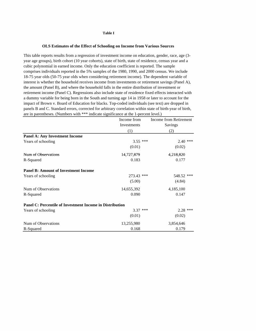
Panel A: Any Investment IncomeYears of schooling 3.55 *** 2.40 ***

(0.01) (0.02)

Num of Observations 14 727 879 4 218 820

This table reports results from a regression of investment income on education, gender, race, age (3-year age groups), birth cohort (10 year cohorts), state of birth, state of residence, census year and a cubic polynomial in earned income. Only the education coefficient is reported. The sample comprises individuals reported in the 5% samples of the 1980, 1990, and 2000 census. We include 18-75 year olds (50-75 year olds when considering retirement income). The dependent variable of interest is whether the household receives income from investments or retirement savings (Panel A), the amount (Panel B), and where the household falls in the entire distribution of investment or retirement income (Panel C). Regressions also include state of residence fixed effects interacted with a dummy variable for being born in the South and turning age 14 in 1958 or later to account for the impact of Brown v. Board of Education for blacks. Top-coded individuals (see text) are dropped in panels B and C. Standard errors, corrected for arbitrary correlation within state of birth-year of birth, are in parentheses. (Numbers with *** indicate significance at the 1-percent level.)

Table I

(2)

OLS Estimates of the Effect of Schooling on Income from Various Sources

(1)

Income from Retirement Savings

Income from Investments

Num of Observations 14,727,879 4,218,820R-Squared 0.183 0.177

Panel B: Amount of Investment IncomeYears of schooling 273.43 *** 548.52 ***

(5.00) (4.84)

Num of Observations 14,655,392 4,185,100R-Squared 0.090 0.147

Panel C: Percentile of Investment Income in DistributionYears of schooling 3.37 *** 2.28 ***

(0.01) (0.02)

Num of Observations 13,255,980 3,854,646R-Squared 0.168 0.179

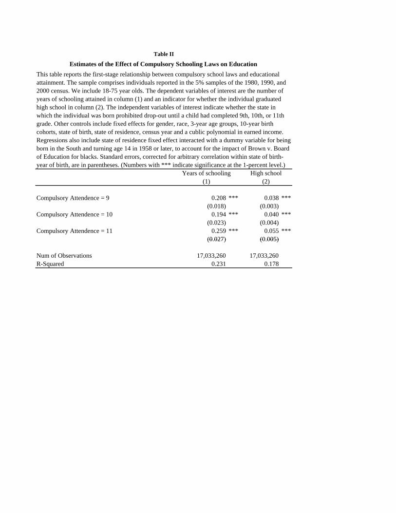
Compulsory Attendence = 9 0.208 *** 0.038 ***(0.018) (0.003)

Compulsory Attendence = 10 0.194 *** 0.040 ***(0.023) (0.004)

Compulsory Attendence = 11 0.259 *** 0.055 ***(0 027) (0 005)

(2)(1)

Estimates of the Effect of Compulsory Schooling Laws on EducationTable II

Years of schooling

This table reports the first-stage relationship between compulsory school laws and educational attainment. The sample comprises individuals reported in the 5% samples of the 1980, 1990, and 2000 census. We include 18-75 year olds. The dependent variables of interest are the number of years of schooling attained in column (1) and an indicator for whether the individual graduated high school in column (2). The independent variables of interest indicate whether the state in which the individual was born prohibited drop-out until a child had completed 9th, 10th, or 11th grade. Other controls include fixed effects for gender, race, 3-year age groups, 10-year birth cohorts, state of birth, state of residence, census year and a cublic polynomial in earned income. Regressions also include state of residence fixed effect interacted with a dummy variable for being born in the South and turning age 14 in 1958 or later, to account for the impact of Brown v. Board of Education for blacks. Standard errors, corrected for arbitrary correlation within state of birth-year of birth, are in parentheses. (Numbers with *** indicate significance at the 1-percent level.)

High school

(0.027) (0.005)

Num of Observations 17,033,260 17,033,260R-Squared 0.231 0.178

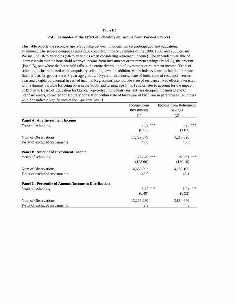
Panel A: Any Investment IncomeYears of schooling 7.59 *** 5.93 ***

(0.51) (1.03)

Num of Observations 14,727,879 4,218,820F stat of excluded instruments 47 0 45 6

with *** indicate significance at the 1-percent level.)

Table III

This table reports the second-stage relationship between financial market participation and educational attainment. The sample comprises individuals reported in the 5% samples of the 1980, 1990, and 2000 census. We include 18-75 year olds (50-75 year olds when considering retirement income). The dependent variable of interest is whether the household receives income from investments or retirement savings (Panel A), the amount (Panel B), and where the household falls in the entire distribution of investment or retirement income. Years of schooling is instrumented with compulsory schooling laws. In addition, we include as controls, but do not report, fixed effects for gender, race, 3-year age groups, 10-year birth cohorts, state of birth, state of residence, census year and a cubic polynomial in earned income. Regressions also include state of residence fixed effects interacted with a dummy variable for being born in the South and turning age 14 in 1958 or later to account for the impact of Brown v. Board of Education for blacks. Top-coded individuals (see text) are dropped in panels B and C. Standard errors, corrected for arbitrary correlation within state of birth-year of birth, are in parentheses. (Numbers

(1)

2SLS Estimates of the Effect of Schooling on Income from Various Sources

Income from Investments

Income from Retirement Savings

(2)

F-stat of excluded instruments 47.0 45.6

Panel B: Amount of Investment IncomeYears of schooling 1767.49 *** 979.61 ***

(128.66) (130.10)

Num of Observations 14,655,392 4,185,100F-stat of excluded instruments 46.9 45.1

Panel C: Percentile of Amount/Income in DistributionYears of schooling 7.64 *** 5.43 ***

(0.49) (0.92)

Num of Observations 13,255,980 3,854,646F-stat of excluded instruments 49.9 44.5

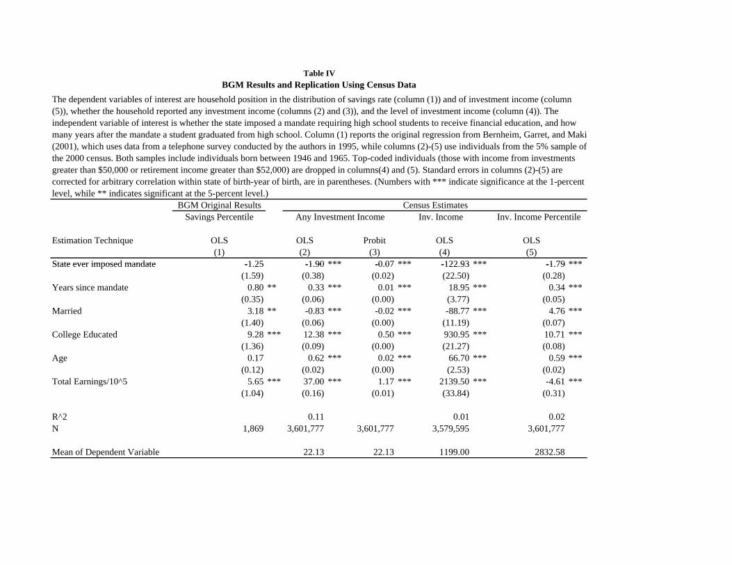
Savings Percentile Inv. Income Inv. Income Percentile

Estimation Technique OLS OLS Probit OLS OLS(1) (2) (3) (4) (5)

State ever imposed mandate -1 25 -1 90 *** -0 07 *** -122 93 *** -1 79 ***

Table IV

BGM Original Results Census EstimatesAny Investment Income

The dependent variables of interest are household position in the distribution of savings rate (column (1)) and of investment income (column (5)), whether the household reported any investment income (columns (2) and (3)), and the level of investment income (column (4)). The independent variable of interest is whether the state imposed a mandate requiring high school students to receive financial education, and how many years after the mandate a student graduated from high school. Column (1) reports the original regression from Bernheim, Garret, and Maki (2001), which uses data from a telephone survey conducted by the authors in 1995, while columns (2)-(5) use individuals from the 5% sample of the 2000 census. Both samples include individuals born between 1946 and 1965. Top-coded individuals (those with income from investments greater than $50,000 or retirement income greater than $52,000) are dropped in columns(4) and (5). Standard errors in columns (2)-(5) are corrected for arbitrary correlation within state of birth-year of birth, are in parentheses. (Numbers with *** indicate significance at the 1-percent level, while ** indicates significant at the 5-percent level.)

BGM Results and Replication Using Census Data

State ever imposed mandate -1.25 -1.90 *** -0.07 *** -122.93 *** -1.79 ***(1.59) (0.38) (0.02) (22.50) (0.28)

Years since mandate 0.80 ** 0.33 *** 0.01 *** 18.95 *** 0.34 ***(0.35) (0.06) (0.00) (3.77) (0.05)

Married 3.18 ** -0.83 *** -0.02 *** -88.77 *** 4.76 ***(1.40) (0.06) (0.00) (11.19) (0.07)

College Educated 9.28 *** 12.38 *** 0.50 *** 930.95 *** 10.71 ***(1.36) (0.09) (0.00) (21.27) (0.08)

Age 0.17 0.62 *** 0.02 *** 66.70 *** 0.59 ***(0.12) (0.02) (0.00) (2.53) (0.02)

Total Earnings/10^5 5.65 *** 37.00 *** 1.17 *** 2139.50 *** -4.61 ***(1.04) (0.16) (0.01) (33.84) (0.31)

R^2 0.11 0.01 0.02N 1,869 3,601,777 3,601,777 3,579,595 3,601,777

Mean of Dependent Variable 22.13 22.13 1199.00 2832.58

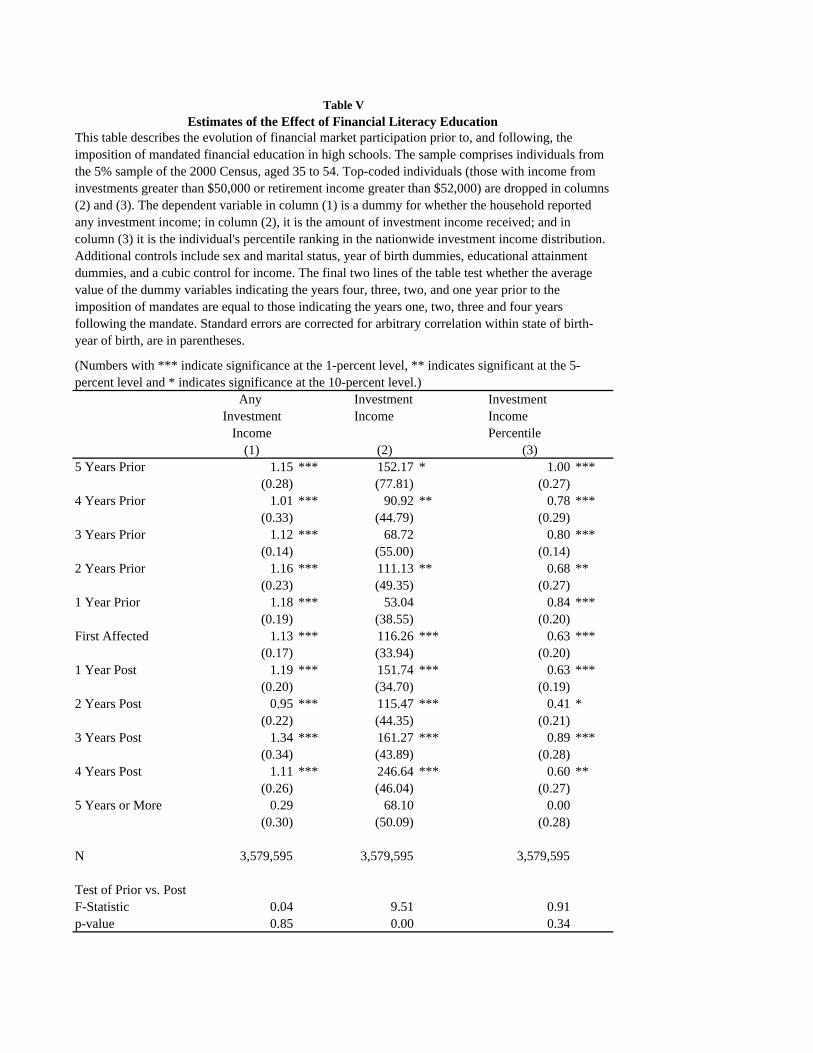
Any Investment InvestmentInvestment Income Income

Income Percentile(1) (2) (3)

5 Years Prior 1.15 *** 152.17 * 1.00 ***(0.28) (77.81) (0.27)

Table VEstimates of the Effect of Financial Literacy Education

(Numbers with *** indicate significance at the 1-percent level, ** indicates significant at the 5-percent level and * indicates significance at the 10-percent level.)

This table describes the evolution of financial market participation prior to, and following, the imposition of mandated financial education in high schools. The sample comprises individuals from the 5% sample of the 2000 Census, aged 35 to 54. Top-coded individuals (those with income from investments greater than $50,000 or retirement income greater than $52,000) are dropped in columns (2) and (3). The dependent variable in column (1) is a dummy for whether the household reported any investment income; in column (2), it is the amount of investment income received; and in column (3) it is the individual's percentile ranking in the nationwide investment income distribution. Additional controls include sex and marital status, year of birth dummies, educational attainment dummies, and a cubic control for income. The final two lines of the table test whether the average value of the dummy variables indicating the years four, three, two, and one year prior to the imposition of mandates are equal to those indicating the years one, two, three and four years following the mandate. Standard errors are corrected for arbitrary correlation within state of birth-year of birth, are in parentheses.

( ) ( ) ( )4 Years Prior 1.01 *** 90.92 ** 0.78 ***

(0.33) (44.79) (0.29)3 Years Prior 1.12 *** 68.72 0.80 ***

(0.14) (55.00) (0.14)2 Years Prior 1.16 *** 111.13 ** 0.68 **

(0.23) (49.35) (0.27)1 Year Prior 1.18 *** 53.04 0.84 ***

(0.19) (38.55) (0.20)First Affected 1.13 *** 116.26 *** 0.63 ***

(0.17) (33.94) (0.20)1 Year Post 1.19 *** 151.74 *** 0.63 ***

(0.20) (34.70) (0.19)2 Years Post 0.95 *** 115.47 *** 0.41 *

(0.22) (44.35) (0.21)3 Years Post 1.34 *** 161.27 *** 0.89 ***

(0.34) (43.89) (0.28)4 Years Post 1.11 *** 246.64 *** 0.60 **

(0.26) (46.04) (0.27)5 Years or More 0.29 68.10 0.00

(0.30) (50.09) (0.28)

N 3,579,595 3,579,595 3,579,595

Test of Prior vs. PostF-Statistic 0.04 9.51 0.91p-value 0.85 0.00 0.34

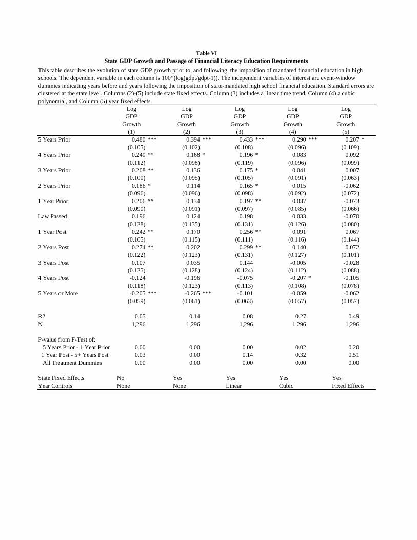
Log Log Log Log LogGDP GDP GDP GDP GDP

Growth Growth Growth Growth Growth(1) (2) (3) (4) (5)

5 Years Prior 0.480 *** 0.394 *** 0.433 *** 0.290 *** 0.207 *(0.105) (0.102) (0.108) (0.096) (0.109)

4 Years Prior 0.240 ** 0.168 * 0.196 * 0.083 0.092(0.112) (0.098) (0.119) (0.096) (0.099)

3 Years Prior 0.208 ** 0.136 0.175 * 0.041 0.007(0.100) (0.095) (0.105) (0.091) (0.063)

2 Years Prior 0.186 * 0.114 0.165 * 0.015 -0.062(0.096) (0.096) (0.098) (0.092) (0.072)

1 Year Prior 0.206 ** 0.134 0.197 ** 0.037 -0.073(0.090) (0.091) (0.097) (0.085) (0.066)

Law Passed 0.196 0.124 0.198 0.033 -0.070(0.128) (0.135) (0.131) (0.126) (0.080)

1 Year Post 0.242 ** 0.170 0.256 ** 0.091 0.067(0.105) (0.115) (0.111) (0.116) (0.144)

2 Years Post 0.274 ** 0.202 0.299 ** 0.140 0.072(0 122) (0 123) (0 131) (0 12 ) (0 101)

Table VIState GDP Growth and Passage of Financial Literacy Education Requirements

This table describes the evolution of state GDP growth prior to, and following, the imposition of mandated financial education in high schools. The dependent variable in each column is 100*(log(gdpt/gdpt-1)). The independent variables of interest are event-window dummies indicating years before and years following the imposition of state-mandated high school financial education. Standard errors are clustered at the state level. Columns (2)-(5) include state fixed effects. Column (3) includes a linear time trend, Column (4) a cubic polynomial, and Column (5) year fixed effects.

(0.122) (0.123) (0.131) (0.127) (0.101)3 Years Post 0.107 0.035 0.144 -0.005 -0.028

(0.125) (0.128) (0.124) (0.112) (0.088)4 Years Post -0.124 -0.196 -0.075 -0.207 * -0.105

(0.118) (0.123) (0.113) (0.108) (0.078)5 Years or More -0.205 *** -0.265 *** -0.101 -0.059 -0.062

(0.059) (0.061) (0.063) (0.057) (0.057)

R2 0.05 0.14 0.08 0.27 0.49N 1,296 1,296 1,296 1,296 1,296

P-value from F-Test of: 5 Years Prior - 1 Year Prior 0.00 0.00 0.00 0.02 0.20 1 Year Post - 5+ Years Post 0.03 0.00 0.14 0.32 0.51 All Treatment Dummies 0.00 0.00 0.00 0.00 0.00

State Fixed Effects No Yes Yes Yes YesYear Controls None None Linear Cubic Fixed Effects

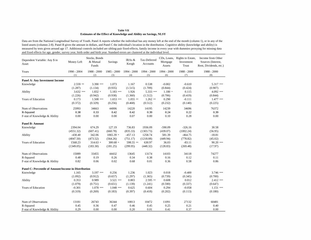
Dependent Variable: Any $ in Asset

Years

Panel A: Any Investment IncomeKnowledge 2.559 ** 3.390 *** 1.073 1.167 0.538 -0.002 -0.610 5.317 ***

(1.287) (1.134) (0.935) (1.515) (1.709) (0.844) (0.424) (0.907)Ability 3.632 *** 1.832 * 5.183 *** 1.926 5.333 *** 1.180 * 0.115 4.092 ***

(1.226) (0.942) (0.938) (1.360) (1.512) (0.706) (0.419) (0.844)Years of Education 0.173 1.508 *** 1.653 *** 1.055 ** 1.262 ** 0.290 -0.111 1.477 ***

(0.372) (0.329) (0.256) (0.468) (0.512) (0.232) (0.140) (0.225)

Num of Observations 25993 34663 44006 14220 14195 14239 34696 76372R-Squared 0 38 0 33 0 42 0 42 0 39 0 24 0 22 0 39

Table VII

Income from Other Sources (Interest,

Rent, Dividends, etc.)

IRAs & Keogh

Estimates of the Effect of Knowledge and Ability on Savings, NLSY

Data are from the National Longitudinal Survey of Youth. Panel A reports whether the individual has any money left at the end of the month (column 1), or in any of the listed assets (columns 2-8). Panel B gives the amount in dollars, and Panel C the individual's location in the distribution. Cognitive ability (knowledge and ability) is measured by tests given around age 17. Additional controls included are sibling-pair fixed-effects, family income in every year with dummies proxying for missing data and fixed effects for age, gender, survey year, birth order and birth year. Standard errors are clustered at the individual level.

Money Left SavingsCDs, Loans,

Mortgage Assets

(6)1990 - 2004 1988 - 2000

(7)1988 - 2000

(1) (2) (3) (4)

Stocks, Bonds & Mutual

Funds

(8)1985 - 2000 1988 - 2000

Rights to Estate, Investment

Trust

Tax-Deferred Accounts

1994 - 2000 1994 - 20001994 - 2000(5)

R-Squared 0.38 0.33 0.42 0.42 0.39 0.24 0.22 0.39F-stat of Knowledge & Ability 0.00 0.00 0.00 0.07 0.00 0.10 0.28 0.00

Panel B: AmountKnowledge 2394.04 674.29 127.19 736.83 1936.09 -590.09 -326.16 30.58

(4551.32) (607.41) (660.78) (835.33) (1303.73) (439.07) (1002.24) (56.95)Ability -430.40 342.06 1065.39 * -457.13 1258.74 581.39 -464.75 -18.81

(4047.50) (473.52) (564.26) (751.17) (1218.08) (449.94) (778.82) (45.02)Years of Education 1568.23 314.63 * 300.68 * 598.55 ** 630.97 36.03 -83.11 90.20 ***

(1349.05) (183.30) (181.25) (299.95) (448.32) (128.83) (269.48) (17.97)

Num of Observations 15089 33455 44432 13645 13174 14103 34118 74277R-Squared 0.48 0.19 0.26 0.34 0.38 0.16 0.12 0.11F-stat of Knowledge & Ability 0.82 0.06 0.02 0.68 0.01 0.36 0.58 0.86

Panel C: Percentile of Amount/Income in DistributionKnowledge 1.165 3.197 *** 0.256 1.236 1.023 0.018 -0.400 3.746 ***

(1.092) (0.912) (0.657) (1.297) (1.365) (0.739) (0.345) (0.700)Ability 0.353 0.989 3.521 *** 0.803 2.595 ** 0.608 0.012 2.412 ***

(1.079) (0.751) (0.651) (1.139) (1.241) (0.590) (0.337) (0.647)Years of Education -0.301 1.078 *** 1.048 *** 0.625 0.604 0.294 -0.058 1.151 ***

(0.319) (0.269) (0.183) (0.397) (0.418) (0.202) (0.113) (0.180)

Num of Observations 13181 26743 36344 10813 10472 11091 27132 60481R-Squared 0.45 0.36 0.47 0.46 0.45 0.25 0.21 0.40F-stat of Knowledge & Ability 0.29 0.00 0.00 0.20 0.01 0.41 0.37 0.00

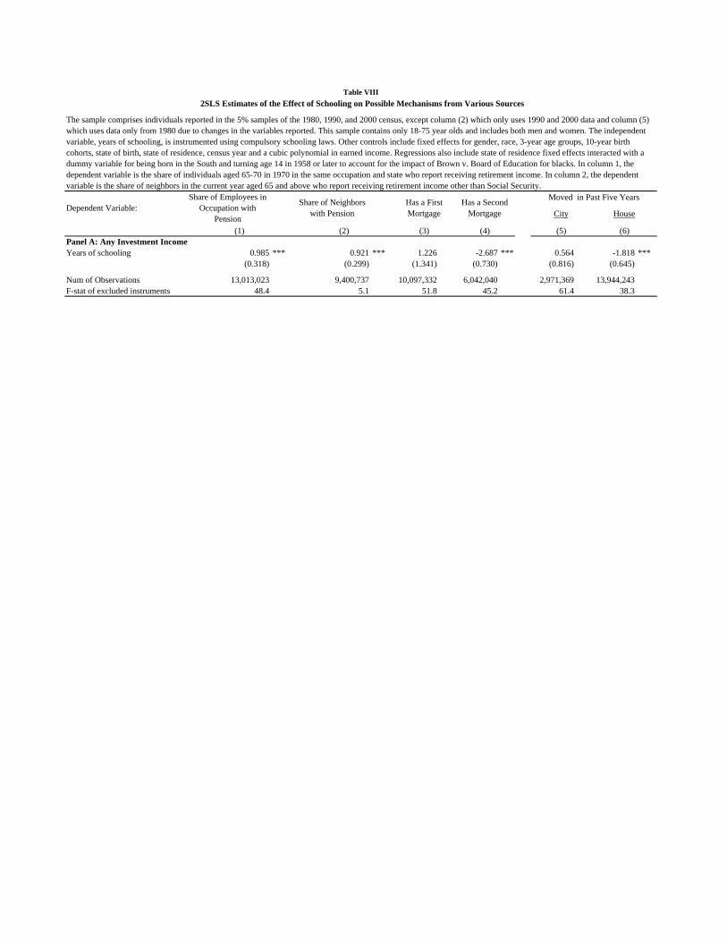
Panel A: Any Investment IncomeYears of schooling 0.985 *** 0.921 *** 1.226 -2.687 *** 0.564 -1.818 ***

(0.318) (0.299) (1.341) (0.730) (0.816) (0.645)

Num of Observations 13,013,023 9,400,737 10,097,332 6,042,040 2,971,369 13,944,243F-stat of excluded instruments 48.4 5.1 51.8 45.2 61.4 38.3

(6)

Has a First Mortgage

Has a Second Mortgage

Moved in Past Five Years

Table VIII2SLS Estimates of the Effect of Schooling on Possible Mechanisms from Various Sources

Dependent Variable:Share of Employees in

Occupation with Pension

(1)

City

(5)(2)

The sample comprises individuals reported in the 5% samples of the 1980, 1990, and 2000 census, except column (2) which only uses 1990 and 2000 data and column (5) which uses data only from 1980 due to changes in the variables reported. This sample contains only 18-75 year olds and includes both men and women. The independent variable, years of schooling, is instrumented using compulsory schooling laws. Other controls include fixed effects for gender, race, 3-year age groups, 10-year birth cohorts, state of birth, state of residence, census year and a cubic polynomial in earned income. Regressions also include state of residence fixed effects interacted with a dummy variable for being born in the South and turning age 14 in 1958 or later to account for the impact of Brown v. Board of Education for blacks. In column 1, the dependent variable is the share of individuals aged 65-70 in 1970 in the same occupation and state who report receiving retirement income. In column 2, the dependent variable is the share of neighbors in the current year aged 65 and above who report receiving retirement income other than Social Security.

Share of Neighbors with Pension

(3) (4)

House

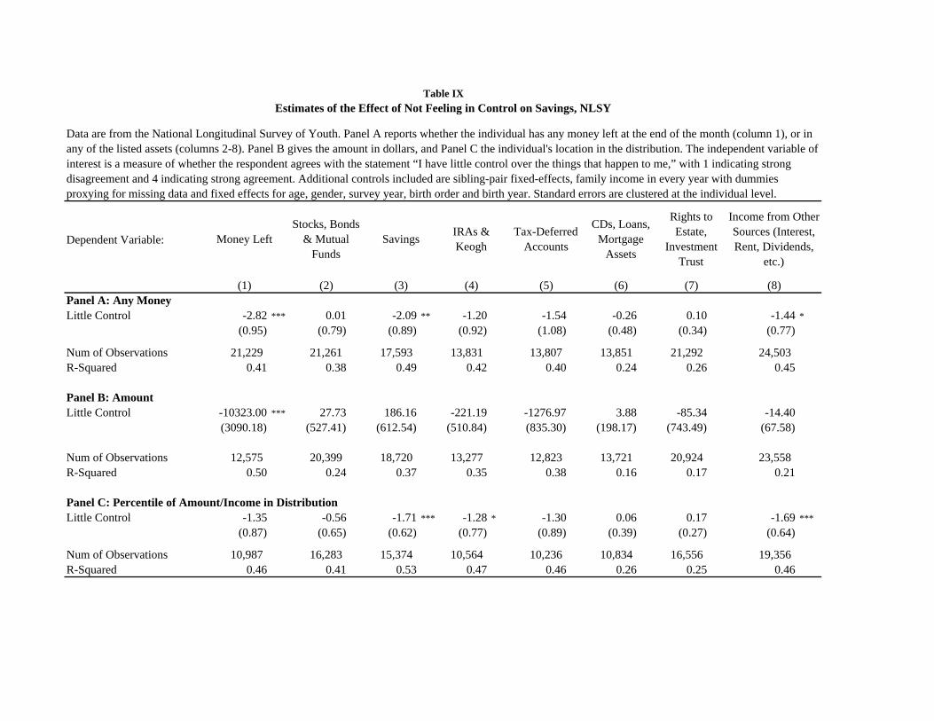
Dependent Variable:

Panel A: Any Money Little Control -2.82 *** 0.01 -2.09 ** -1.20 -1.54 -0.26 0.10 -1.44 *

(0.95) (0.79) (0.89) (0.92) (1.08) (0.48) (0.34) (0.77)

Table IX

Data are from the National Longitudinal Survey of Youth. Panel A reports whether the individual has any money left at the end of the month (column 1), or in any of the listed assets (columns 2-8). Panel B gives the amount in dollars, and Panel C the individual's location in the distribution. The independent variable of interest is a measure of whether the respondent agrees with the statement “I have little control over the things that happen to me,” with 1 indicating strong disagreement and 4 indicating strong agreement. Additional controls included are sibling-pair fixed-effects, family income in every year with dummies proxying for missing data and fixed effects for age, gender, survey year, birth order and birth year. Standard errors are clustered at the individual level.

(4) (5) (7)

Stocks, Bonds & Mutual

Funds

(2)

Money Left Tax-Deferred Accounts

Rights to Estate,

Investment Trust

Estimates of the Effect of Not Feeling in Control on Savings, NLSY

Income from Other Sources (Interest, Rent, Dividends,

etc.)

(8)(1) (3)

Savings IRAs & Keogh

CDs, Loans, Mortgage

Assets

(6)

( ) ( ) ( ) ( ) ( ) ( ) ( ) ( )

Num of Observations 21,229 21,261 17,593 13,831 13,807 13,851 21,292 24,503 R-Squared 0.41 0.38 0.49 0.42 0.40 0.24 0.26 0.45

Panel B: AmountLittle Control -10323.00 *** 27.73 186.16 -221.19 -1276.97 3.88 -85.34 -14.40

(3090.18) (527.41) (612.54) (510.84) (835.30) (198.17) (743.49) (67.58)

Num of Observations 12,575 20,399 18,720 13,277 12,823 13,721 20,924 23,558 R-Squared 0.50 0.24 0.37 0.35 0.38 0.16 0.17 0.21

Panel C: Percentile of Amount/Income in DistributionLittle Control -1.35 -0.56 -1.71 *** -1.28 * -1.30 0.06 0.17 -1.69 ***

(0.87) (0.65) (0.62) (0.77) (0.89) (0.39) (0.27) (0.64)

Num of Observations 10,987 16,283 15,374 10,564 10,236 10,834 16,556 19,356 R-Squared 0.46 0.41 0.53 0.47 0.46 0.26 0.25 0.46

Mean St. Dev.(1) (2)

DemographicYears of schooling 13.19 2.62High school graduation 0.85 0.36Compulsory Attendence = 9 0.40 0.49Compulsory Attendence = 11 0.11 0.31Compulsory Attendence = 10 0.36 0.48Age 48.89 13.05Male 0.48 0.50Black 0.10 0.30

Income from InvestmentsAny 28.23 45.01Amount 1302.94 4659.14Percentile 25.92 39.12

Income from Retirement SavingsAny 10.85 31.11

Appendix Table A1 Summary Statistics, Census

Whole Sample

This table reports summary statistics from the 5% sample of the census, from 1980, 1990, and 2000, for individuals aged. We include individuals aged 36-75.

yAmount 1278.63 4928.85Percentile 11.10 30.30

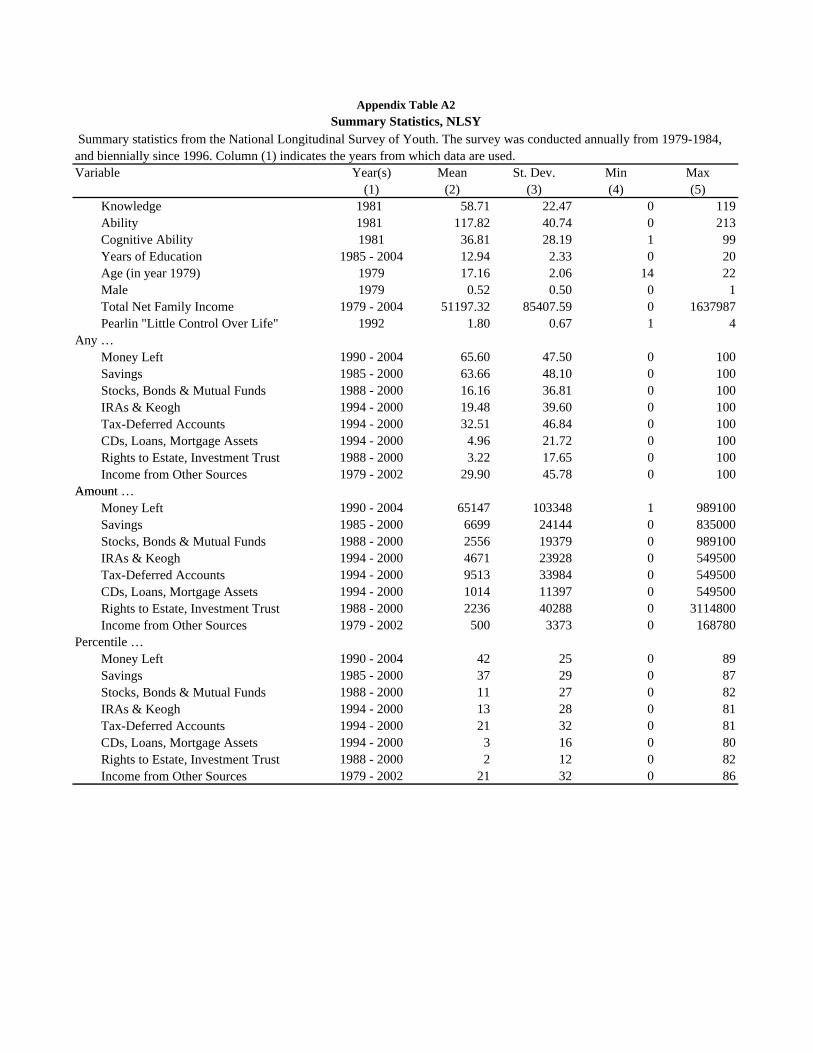
Variable Year(s) Mean St. Dev. Min Max(1) (2) (3) (4) (5)

Knowledge 1981 58.71 22.47 0 119Ability 1981 117.82 40.74 0 213Cognitive Ability 1981 36.81 28.19 1 99Years of Education 1985 - 2004 12.94 2.33 0 20Age (in year 1979) 1979 17.16 2.06 14 22Male 1979 0.52 0.50 0 1Total Net Family Income 1979 - 2004 51197.32 85407.59 0 1637987Pearlin "Little Control Over Life" 1992 1.80 0.67 1 4

Any …Money Left 1990 - 2004 65.60 47.50 0 100Savings 1985 - 2000 63.66 48.10 0 100Stocks, Bonds & Mutual Funds 1988 - 2000 16.16 36.81 0 100IRAs & Keogh 1994 - 2000 19.48 39.60 0 100Tax-Deferred Accounts 1994 - 2000 32.51 46.84 0 100CDs, Loans, Mortgage Assets 1994 - 2000 4.96 21.72 0 100Rights to Estate, Investment Trust 1988 - 2000 3.22 17.65 0 100Income from Other Sources 1979 - 2002 29.90 45.78 0 100

Amount

Appendix Table A2Summary Statistics, NLSY

Summary statistics from the National Longitudinal Survey of Youth. The survey was conducted annually from 1979-1984, and biennially since 1996. Column (1) indicates the years from which data are used.

Amount …Money Left 1990 - 2004 65147 103348 1 989100Savings 1985 - 2000 6699 24144 0 835000Stocks, Bonds & Mutual Funds 1988 - 2000 2556 19379 0 989100IRAs & Keogh 1994 - 2000 4671 23928 0 549500Tax-Deferred Accounts 1994 - 2000 9513 33984 0 549500CDs, Loans, Mortgage Assets 1994 - 2000 1014 11397 0 549500Rights to Estate, Investment Trust 1988 - 2000 2236 40288 0 3114800Income from Other Sources 1979 - 2002 500 3373 0 168780

Percentile …Money Left 1990 - 2004 42 25 0 89Savings 1985 - 2000 37 29 0 87Stocks, Bonds & Mutual Funds 1988 - 2000 11 27 0 82IRAs & Keogh 1994 - 2000 13 28 0 81Tax-Deferred Accounts 1994 - 2000 21 32 0 81CDs, Loans, Mortgage Assets 1994 - 2000 3 16 0 80Rights to Estate, Investment Trust 1988 - 2000 2 12 0 82Income from Other Sources 1979 - 2002 21 32 0 86

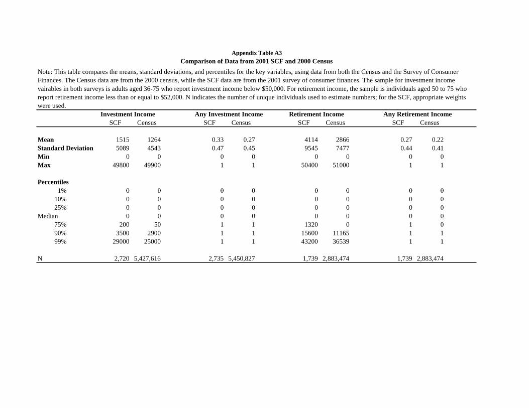
Investment Income Any Investment Income Retirement Income Any Retirement IncomeSCF Census SCF Census SCF Census SCF Census

Mean 1515 1264 0.33 0.27 4114 2866 0.27 0.22Standard Deviation 5089 4543 0.47 0.45 9545 7477 0.44 0.41Min 0 0 0 0 0 0 0 0Max 49800 49900 1 1 50400 51000 1 1

Percentiles1% 0 0 0 0 0 0 0 0

Appendix Table A3Comparison of Data from 2001 SCF and 2000 Census

Note: This table compares the means, standard deviations, and percentiles for the key variables, using data from both the Census and the Survey of Consumer Finances. The Census data are from the 2000 census, while the SCF data are from the 2001 survey of consumer finances. The sample for investment income vairables in both surveys is adults aged 36-75 who report investment income below $50,000. For retirement income, the sample is individuals aged 50 to 75 who report retirement income less than or equal to $52,000. N indicates the number of unique individuals used to estimate numbers; for the SCF, appropriate weights were used.

1% 0 0 0 0 0 0 0 010% 0 0 0 0 0 0 0 025% 0 0 0 0 0 0 0 0

Median 0 0 0 0 0 0 0 075% 200 50 1 1 1320 0 1 090% 3500 2900 1 1 15600 11165 1 199% 29000 25000 1 1 43200 36539 1 1

N 2,720 5,427,616 2,735 5,450,827 1,739 2,883,474 1,739 2,883,474

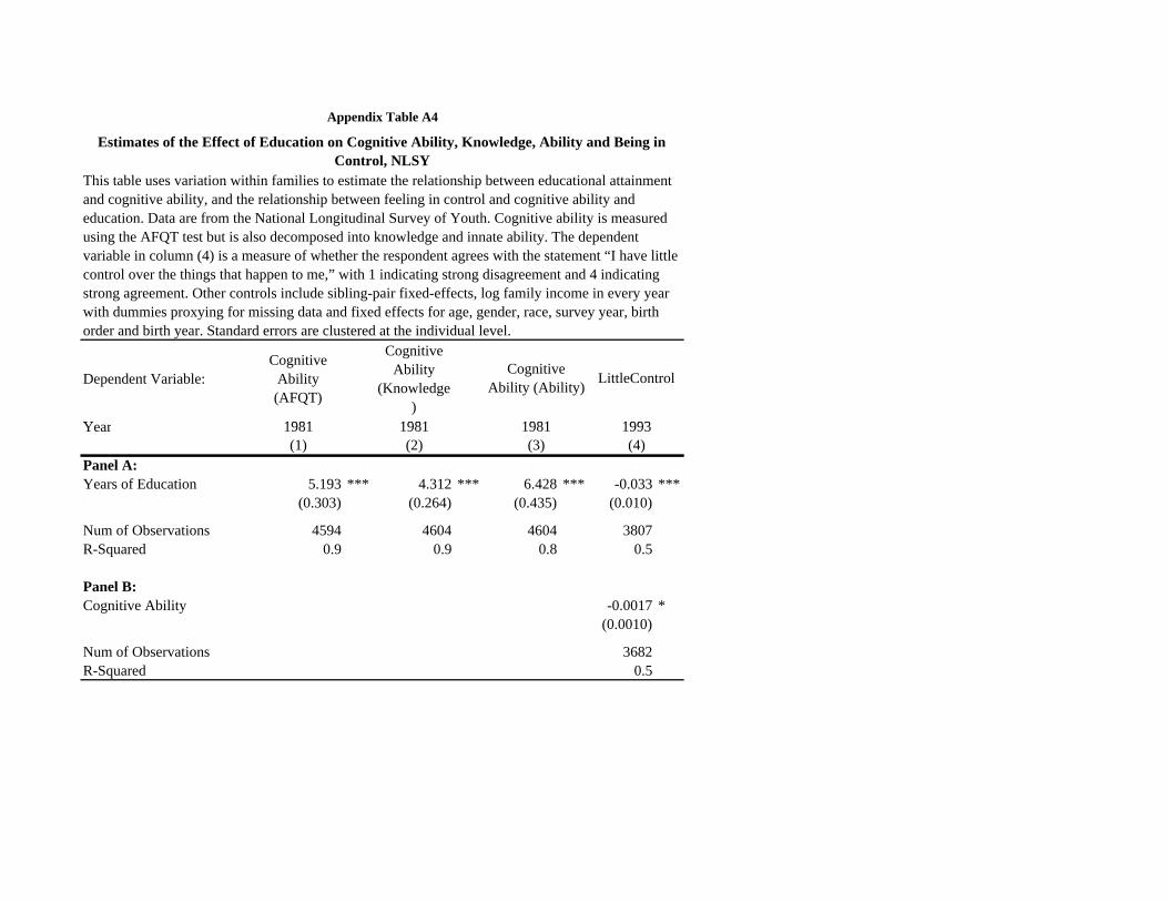
Dependent Variable:Cognitive

Ability (AFQT)

Cognitive Ability

(Knowledge)

Y 1981 1981

Appendix Table A4

1981

Cognitive Ability (Ability) LittleControl

1993

Estimates of the Effect of Education on Cognitive Ability, Knowledge, Ability and Being in Control, NLSY

This table uses variation within families to estimate the relationship between educational attainment and cognitive ability, and the relationship between feeling in control and cognitive ability and education. Data are from the National Longitudinal Survey of Youth. Cognitive ability is measured using the AFQT test but is also decomposed into knowledge and innate ability. The dependent variable in column (4) is a measure of whether the respondent agrees with the statement “I have little control over the things that happen to me,” with 1 indicating strong disagreement and 4 indicating strong agreement. Other controls include sibling-pair fixed-effects, log family income in every year with dummies proxying for missing data and fixed effects for age, gender, race, survey year, birth order and birth year. Standard errors are clustered at the individual level.

Year 1981 1981(1) (2)

Panel A:Years of Education 5.193 *** 4.312 *** 6.428 *** -0.033 ***

(0.303) (0.264) (0.435) (0.010)

Num of Observations 4594 4604 4604 3807R-Squared 0.9 0.9 0.8 0.5

Panel B:Cognitive Ability -0.0017 *

(0.0010)

Num of Observations 3682R-Squared 0.5

(4)(3)1981 1993

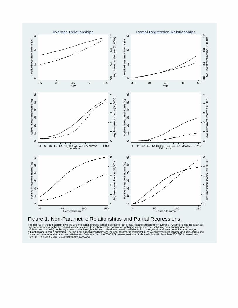
0.0

0.4

0.8

1.2

Avg

. inv

estm

ent i

ncom

e ($

1,00

0s)

010

2030

Pos

itive

inve

stm

ent i

ncom

e (%

)

35 40 45 50 55Age

Average Relationships

0.0

0.4

0.8

1.2

Avg

. inv

estm

ent i

ncom

e ($

1,00

0s)

010

2030

Pos

itive

inve

stm

ent i

ncom

e (%

)

35 40 45 50 55Age

Partial Regression Relationships

01

23

45

Avg

. inv

estm

ent i

ncom

e ($

1,00

0s)

010

2030

4050

60P

ositi

ve in

vest

men

t inc

ome

(%)

01

23

45

Avg

. inv

estm

ent i

ncom

e ($

1,00

0s)

010

2030

4050

60P

ositi

ve in

vest

men

t inc

ome

(%)

8 9 10 11 12 HSHS+C1 C2 BA MAMA+ PhDEducation

8 9 10 11 12 HSHS+C1 C2 BA MAMA+ PhDEducation

01

23

45

Avg

. inv

estm

ent i

ncom

e ($

1,00

0s)

010

2030

4050

60P

ositi

ve in

vest

men

t inc

ome

(%)

0 50 100 150Earned Income

01

23

45

Avg

. inv

estm

ent i

ncom

e ($

1,00

0s)

010

2030

4050

60P

ositi

ve in

vest

men

t inc

ome

(%)

0 50 100 150Earned Income

Figure 1. Non-Parametric Relationships and Partial Regressions.The figures in the left column give the unconditional average (smoothed using Fan's local linear regression) for average investment income (dashedline corresponding to the right-hand vertical axis) and the share of the population with investment income (solid line corresponding to theleft-hand vertical axis). In the right column the lines give the (smoothed) estimated coefficients from a regression of investment income on age,education and income dummies. The top-right panel gives therefore the non-parametric relationship between investment income and age, controllingfor earned income and educational attainment. Data are from the 2000 US census, restricted to households with less than $50,000 in investmentincome. The sample size is approximately 3,200,000.

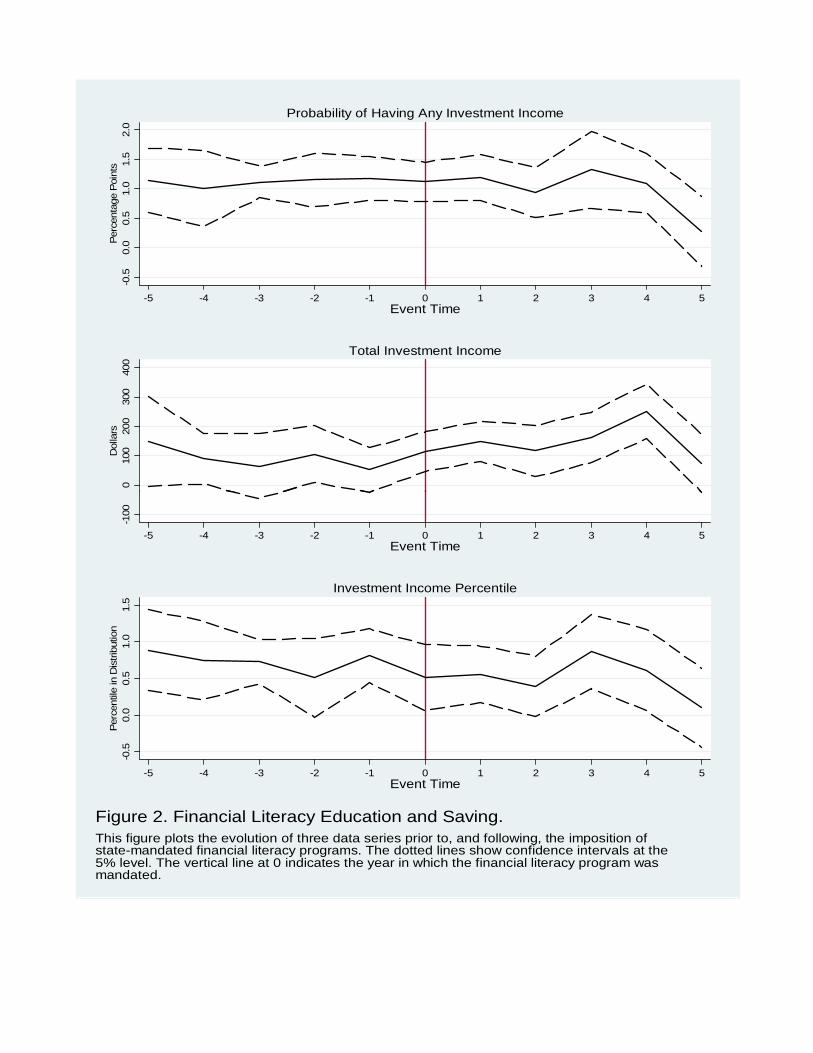
-0.5

0.0

0.5

1.0

1.5

2.0

Perc

enta

ge P

oint

s

-5 -4 -3 -2 -1 0 1 2 3 4 5Event Time

Probability of Having Any Investment Income0

100

200

300

400

Dol

lars

Total Investment Income

-100

-5 -4 -3 -2 -1 0 1 2 3 4 5Event Time

-0.5

0.0

0.5

1.0

1.5

Perc

entil

e in

Dis

tribu

tion

-5 -4 -3 -2 -1 0 1 2 3 4 5Event Time

Investment Income Percentile

Figure 2. Financial Literacy Education and Saving.This figure plots the evolution of three data series prior to, and following, the imposition ofstate-mandated financial literacy programs. The dotted lines show confidence intervals at the5% level. The vertical line at 0 indicates the year in which the financial literacy program wasmandated.

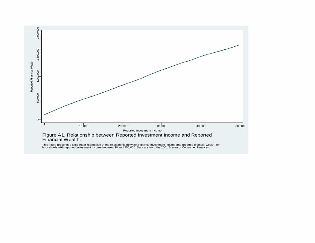
500,

000

1,00

0,00

01,

500,

000

2,00

0,00

0

Rep

orte

d Fi

nanc

ial W

ealth

0

0 10,000 20,000 30,000 40,000 50,000

Reported Investment Income

Figure A1. Relationship between Reported Investment Income and ReportedFinancial Wealth.This figure presents a local linear regression of the relationship between reported investment income and reported financial wealth, forhouseholds with reported investment income between $0 and $50,000. Data are from the 2001 Survey of Consumer Finances.