High Performance Computational Hemodynamics with the ...
114
High Performance Computational Hemodynamics with the Lattice Boltzmann Method
Transcript of High Performance Computational Hemodynamics with the ...

High Performance
Computational Hemodynamics
with the Lattice Boltzmann
Method


High Performance
Computational Hemodynamics
with the Lattice Boltzmann
Method
ACADEMISCH PROEFSCHRIFT
ter verkrijging van de graad van doctoraan de Universiteit van Amsterdamop gezag van de Rector Magnificus
prof. dr. D. C. van den Boomten overstaan van een door het college voor promoties ingestelde
commissie, in het openbaar te verdedigen in de Agnietenkapelop dinsdag 18 December 2007, te 10:00 uur
door
Lilit Axner
geboren te Yerevan, Armenie
Promotiecommissie:
Promotor: prof. dr. P. M. A. SlootCo-promotor: dr. A. G. HoekstraOverige leden: Prof. Dr. J.H.C. Reiber
Prof. Dr. M.T. BubakProf. Dr. J.A.E. SpaanProf. Dr. B. ChopardProf. Dr. P.A.J. Hilbers
Faculteit: Faculteit der Natuurwetenschappen, Wiskunde en Informatica
Section Computational Science
Universiteit van Amsterdam
The work described in this thesis has been carried out in the Section ComputationalScience of the University of Amsterdam, with financial support of:
• University of Amsterdam,• Netherlands Organisation for Scientific Research – Distributed Interactive Medical Ex-
ploratory for 3D Medical Images (NWO–DIME) project (634.000.024),
Copyright c© 2007 Lilit Axner.
ISBN 978-90-5776-170-6
Typeset with LATEX 2ε.Printed by PrintPartners Ipskamp B. V., Enschede.
Author contact: [email protected]

To my mother, Anna...


Contents
1 Introduction 11.1 High performance computing and computational hemodynamics 1
1.1.1 Computational hemodynamics 11.1.2 High performance computing 41.1.3 Merge of two worlds 6
1.2 Lattice Boltzmann method in computational hemodynamics 61.2.1 The model 81.2.2 Parallel Lattice Boltzmann method 91.2.3 Unstructured Lattice Boltzmann 10
1.3 Research overview and motivation 12
2 HemoSolve - A Problem Solving Environment for Image-Based Computa-tional Hemodynamics 152.1 Introduction 152.2 The first step towards HemoSolve 15
2.2.1 Medical Data Segmentation 162.2.2 3D Editor and Mesh Generator 192.2.3 Hemodynamic Solver 192.2.4 Validation of Lattice Boltzmann Method 192.2.5 Flow Analyses 23
2.3 Examples 232.3.1 Aneurysm 232.3.2 Abdominal aorta 24
2.4 Discussions and Conclusions 24
3 Efficient LBM for Time Harmonic Flows 273.1 Introduction 273.2 Lattice Boltzmann Method 28
vii
viii CONTENTS
3.3 Constraint Optimization Scheme 283.3.1 Asymptotic error analysis 303.3.2 Experimental results 31
3.4 Stability of Time Harmonic LBM Simulations 353.5 Harmonic Flow in Human Abdominal Aorta 363.6 Regularized time-harmonic LBGK 373.7 Accuracy and Stability of RL-BGK 38
3.7.1 Numerical stability of R-LBGK 393.8 Conclusions 40
4 High Performance Lattice Boltzmann Computing 434.1 Introduction 434.2 Sparse LB Implementation 444.3 The Graph Partitioning Algorithms 444.4 The Performance Prediction Model 454.5 Results 49
4.5.1 Basic parameters 514.5.2 Performance Measurements of the Lattice Boltzmann application 54
4.6 Conclusions 55
5 Towards Decision Support in Vascular Surgery through Computational Hemo-dynamics 635.1 Introduction 635.2 HemoSolve and the new enhancements 64
5.2.1 Medical Data Segmentation 645.2.2 3D Editor and Mesh Generator 655.2.3 Hemodynamic Solver - Sparse Lattice Boltzmann Method 665.2.4 Flow Analyses 66
5.3 Carotid Artery with Severe Stenosis - with and without Bypass 675.4 Conclusion 68
6 Conclusion 736.1 Discussion 736.2 Future work 75
Summary 77
Nederlandse samenvatting 79
Summary in Armenian 81

CONTENTS ix
Acknowledgments 85
Publications 89
Bibliography 91
Index 101

Introduction
1.1 High performance computing and computational hemo-dynamics
1.1.1 Computational hemodynamicsFluid dynamics is one of the major scientific disciplines describing the behavior of oneof the main materials of nature: Water. The earth has liquid water on 70% of its surface,and the volume of blood of an average human is about 5 liters and fluids are engaged inalmost all our daily activities. Thus fluid is an immediate requirement of life and deepknowledge of its behavior is a way to recognize and predict its influence on us and ourenvironment.
Specifically, in the last decades there is a growing interest towards the details of theflow behavior of blood in the human vascular system, e.g. blood dynamics called hemo-dynamics.
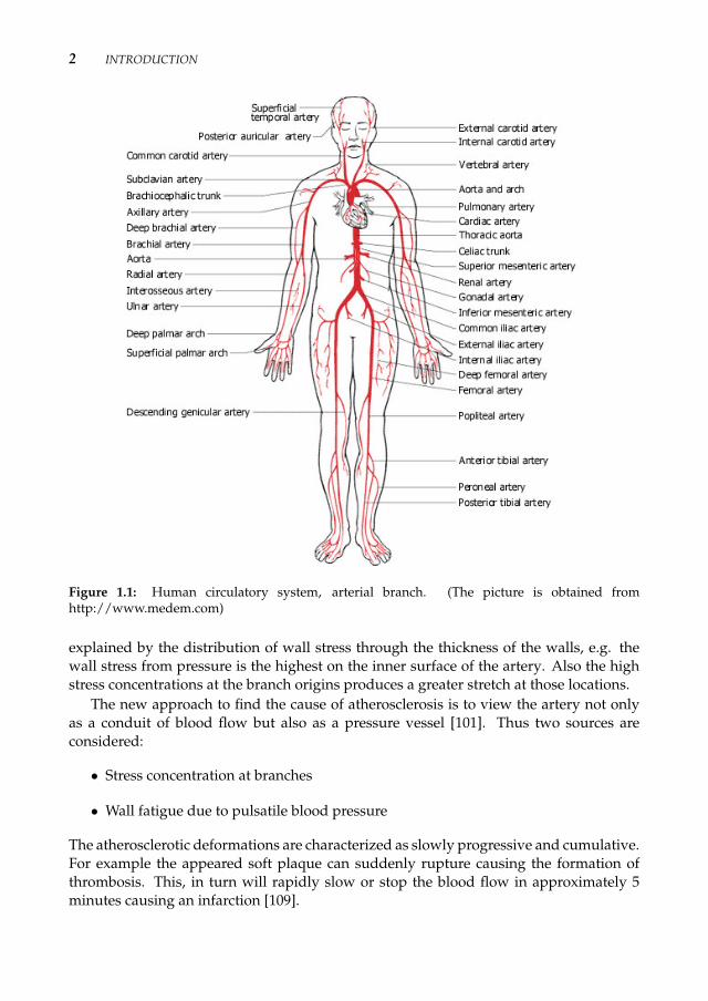
The human cardiovascular system is very complex: The blood is pumped by heart,through the large arteries, such as the abdominal aorta, to the smaller diameter arteriescalled arterioles (see Fig. 1.1). These arterioles become capillaries and eventually venules,where the deoxygerated blood passes through veins back to heart, imposing a circularroad-map through whole body [30]. Due to the pumping of the heart the blood pulsatesover time, thus it is characterized as time-harmonic.
Atherosclerosis is the most common cardiovascular disease that affects the arterial bloodvessel [4, 98, 100]. It is the formation of yellowish plaques containing fatty substancesthat are formed within the intima and inner media of arteries [101]. The plaque causesthe hardening of the arteries and destructs or in some cases it completely blocks the nor-mal time-harmonic blood flow (see Fig. 1.2 (right)). As described by M. Thubrikar [101],atherosclerosis begins as intimal lipid deposits in childhood and adolescence and in somearterial parts those lipid deposits convert into fibrous plaques by continued accumula-tion of lipid smooth muscle and connective tissue. In middle age, after 30 or more yearssince the beginning of the process, some of fibrous plaques produce occlusion, ischemaand clinical disease. It should be noted that only few of the lipid deposits convert intoatherosclerotic lesions.
Atherosclerosis usually appears at the origins of tributaries, bifurcations and curva-tures of the arteries. Moreover, it primarily affects the luminal side of them. This is
1
2 INTRODUCTION
Figure 1.1: Human circulatory system, arterial branch. (The picture is obtained fromhttp://www.medem.com)
explained by the distribution of wall stress through the thickness of the walls, e.g. thewall stress from pressure is the highest on the inner surface of the artery. Also the highstress concentrations at the branch origins produces a greater stretch at those locations.
The new approach to find the cause of atherosclerosis is to view the artery not onlyas a conduit of blood flow but also as a pressure vessel [101]. Thus two sources areconsidered:
• Stress concentration at branches
• Wall fatigue due to pulsatile blood pressure
The atherosclerotic deformations are characterized as slowly progressive and cumulative.For example the appeared soft plaque can suddenly rupture causing the formation ofthrombosis. This, in turn will rapidly slow or stop the blood flow in approximately 5minutes causing an infarction [109].

1.1 HIGH PERFORMANCE COMPUTING AND COMPUTATIONAL HEMODYNAMICS 3
Aneurysm is a balloon enlargement of the aorta (see Fig. 1.2 (left)). Most commonlyit appears in abdominal aorta and cerebral arteries (at the base of the brain, known asthe Circle of Willis), rarely in ascending aorta and descending thoracic aorta (see Fig. 1.1)and sometimes it may cover several segments of the aorta. Aneurysm appears due tothe same mechanism as atherosclerosis when the smooth muscle cells of the artery areunable to proliferate [101].
Figure 1.2: Aneurysm and stenosis in the abdominal aorta. (The pictures are obtained fromhttp://www.medcyclopaedia.com)
The modeling of blood flow in human cardiovascular structures helps to obtain anextensive knowledge about its behavior and to create solutions for preventing the ac-tual death caused by atherosclerotic diseases or aneurysms. It can be done by using theNavier-Stokes equation.
The Navier-Stokes equation was derived by Claude Louis M.H. Navier (1785-1836)and Sir George Gabriel Stokes (1819-1903). Although it is capable to describe such com-plex phenomena as solitons, von Karman vortex streets and turbulence, it is still ham-pered by two major limitations: the non-straight forward applicability to complex ge-ometries and the high compute intensity.
One approach to overcome these limitations is to use cellular automata, more pre-cisely lattice gas automata (LGA), to model the microscopic properties of the blood flowwhile exploring its macroscopic properties [90]. Historically the successor of LGA is thelattice Boltzmann method (LBM) and thus both methods are mesoscopic methods. Themain idea behind LBM is the mapping of the average motion of the fluid/blood particleson the lattice. An introduction to the LBM method is given in the subsection 1.2. Anotherapproach is the numerical discretion of Navier-Stokes equation. The finite element andthe finite volume methods are examples of this approach.

4 INTRODUCTION
In either way the final step is the integration of chosen approach into the state-of-the-art high performance computers. This we call computational hemodynamics.
In the further development of this thesis we use LBM as computational hemodynam-ics method. The locality of the LBM update scheme makes its parallelization straightfor-ward while the optimal distribution/decomposition of the geometry over the multipleprocessors is the main bottleneck for high performance computing. This will be one ofthe problems addressed in later chapters.
1.1.2 High performance computingThree dimensional simulations in computational hemodynamics as well as in any com-putational fluid dynamics problem require huge computer resources, both in memoryand speed. Thus in CFD always the most powerful computers available have been used.
The term "Super computing" was first used by the New York World newspaper in1920 about the IBM large custom-build tabulators for Columbia university [96]. Super-computers first appeared in 1960s designed by Seymour Cray at Control Data Corpo-ration. In 1970s most of the supercomputers were dedicated to vector computing. In1980s and 1990s massive parallel processing systems with thousands of CPUs appeared.Nowadays, supercomputers typically are "off the shell" server-class microprocessors, e.g.computer clusters with commodity processors [3].
As of June 2007, the fastest machine is Blue Gene/L with 65.536 nodes, each with twoprocessors , each with two data stream connectivity [3].
In this work we use two different types of CPU architectures: Vector machines andStreaming SIMD Extension2 (SSE2). We chose vector machines as they are known toproduce the highest number of lattice updates per second while the architecture of SSE2clusters is the best suited for the storage of the complex geometry data.
• Vector architectureVector processor is a CPU design that implements mathematical operations on mul-tiple data elements simultaneously. This type of processors were first introducedby Westinghouse through Solomon project in 1960s [49]. The first successful imple-mentation of vector processors was CDC STAR-100 and The Texas Instrument Ad-vance Scientific Computer. These processors reached approximately 20 MFLOPSpeak performance, however they took very long times decoding the vector instruc-tions and to run the process. Next, Cray introduced the Cray-1 machine, wherethere were eight vector registers and the vector instructions were applied betweenregisters, thus accelerating the processing. Also Cray-1 had a separate pipelinefor addition/subtraction and separate for multiplication, thus applying the vectorchaining technique. Cray-1 reached from 80 to 240 MFLOPS peak performance.Later different Japanese companies, one of which was NEC, started to producesimilar vector machines. Due to the special super-scalar implementation, vectormachines perform most efficient, when the amount of data to work on is signifi-cantly large [79].

1.1 HIGH PERFORMANCE COMPUTING AND COMPUTATIONAL HEMODYNAMICS 5
The NEC SX-8 supercomputers are the latest generation of NEC SX-series of su-percomputers. They are build from SMP machines each with 8 vector processors.More detailed specifications of the NEC SX-8 are given in Table 4.1 of Chapter 4.(See also [1]).
• Streaming SIMD Extension2
SSE2 is an addition to SIMD technique. SIMD processors are a single instruction,multiple data general purpose processors.They are are used to achieve data levelparallelism and are handling only data manipulation. The first widely used SIMDarchitecture supercomputers were Intel MMX x86 architectures [108].
The SSE2 extension is based on SIMD architecture, which also includes a set ofcache-control instructions and a system of numerical format conversion instruc-tions. The SSE2 was first introduced by Intel Pentium 4 processor. Moreover,in addition to SSE2 an instruction pipeline technique is used in Pentium 4 pro-cessors, which allows to reduce the cycle time of a processor and increase the in-struction throughput. The hyper threading technology (HTT) that enables multiplethreads to run simultaneously, improves reaction and response time, and increasesthe number of users a server can support is also combined in later models of Pen-tium 4 [108].
In this work we use the Dutch national compute cluster Lisa , based on 2Intel Xeon2architecture at SARA Computing and Networking Service center [2]. The Intel Xeoncluster Lisa has an identical architecture to Pentium 4. More detailed specificationsof this cluster are given in Table 4.2 of Chapter 4. (See also [2])
As was mentioned in previous subsection, one of the main issues in high performanceimplementation of computational hemodymanics is the optimal decomposition of thegeometry, especially when the geometry is complex.
During the last decade a lot of decomposition algorithms have been developed forboth the discretized Navier-Stokes (FEM,FVM) and the mesoscopic (LBM) methods. Ex-amples of such algorithms are geometric schemes, spectral methods, combinatoric schemes,multilevel schemes, orthogonal bisectioning method, cell-based method etc. [15, 33, 47,55, 110, 111]. All these schemes have their advantages and disadvantages. For example,geometric schemes use the geometric information of the data to find a good partition-ing. They tend to be fast but produce worse quality partitions than those by multilevelschemes. Spectral methods are known to produce perfect partitions, however they arevery expensive since they require the computation of the eigenvectors correspondingto the second smallest eigenvalue (Fiedler method) [62].As for multilevel schemes, theytend to give quite reasonable, although not excellent partitions at a comparatively lowcost. One of the known libraries that use multilevel graph partitioning is METIS [62].The method as well as its advantages and disadvantages will be described further in thethesis.

6 INTRODUCTION
1.1.3 Merge of two worldsIn vivo measurements of hemodynamic quantities give very detailed information aboutblood flow characteristics, however they are very difficult to obtain. Thus one of thechallenges of computational hemodynamics is the implementation of numerical modelsin large datasets and the simulation/validation of flow dynamics.
The practice showed that the non-linear equations of fluid flows can only be solvedanalytically for special simplified cases. Those cases comprise deep physical insights,thus the following step is the application of these knowledge on the non-linear problems.
There have been several studies discussing the aspects of development of computa-tional hemodynamics [21, 64, 98, 100, 118]. In all these studies it is explicitly pointed outthat computational hemodynamics problems are known to be extensive and requiringlarge computational resources. Thus the transfer to high performance computing is avery natural step of development [16, 36, 119].
As mentioned by Taylor et al. [100],in order to realize the benefits of the merge ofthese two worlds we need to cite the major barriers and the ways to overcome:
1. Creation of complex hemodynamics models can be time consuming and a tremen-dous process - to model time-harmonic blood flow in the human vascular systemone can use the Navier-Stokes equations and discretize them to create a computeralgorithm.
2. Mesh generation from medical data is time consuming and complex - several meshgeneration algorithms/softwares are created for these purposes.
3. The generated discrete problems can involve millions of equations for thousandof timesteps - the generated algorithmic blocks can be integrated into high perfor-mance computing [21, 90].
To these and other more detailed aspects we will refer in the further development ofthe thesis.
1.2 Lattice Boltzmann method in computational hemody-namics
In 1872 Ludwig Boltzmann derived the Boltzmann equation (Eq. 1.1) to describe the sta-tistical distribution of particles in fluids.
∂ f∂t +
∂ f∂x ∗ p
m +∂ f∂p F =
∂ f∂t (1.1)
here m and p are the mass and momentum of the fluid particle, ∂x and ∂t are the spaceand time steps respectively. f (x, p, t) is the probability density function and F is the forceacting on the particles and making them propagate and collide [97].

1.2 LATTICE BOLTZMANN METHOD IN COMPUTATIONAL HEMODYNAMICS 7
One of the methods to simulate a Newtonian fluid flow is the lattice Boltzmannmethod (LBM) [17, 23, 25, 97] which can be derived from continuous Boltzmann equa-tion [45,122]. In LBM models the fluid flow in the sense of particles performing propaga-tion and collision over a discrete lattice. Some of the positive characteristics of LBM aree.g. its ability to incorporate complex boundary conditions. On the other hand it is ham-pered by slow convergence [42, 59, 106], caused by the demand of a low Mach number(Ma) ( to suppress compressibility error ) and the fulfillment of a Courant-Friedrich-Levycondition for numerical stability.
Historically LBM comes from lattice gas automata (LGA) [25, 81, 89] which are basedon Boolean particle numbers and is a simplified model for particle dynamics. AlthoughLGA is a good method for modeling fluid flow it suffers from the lack of Galilean in-variance and statical noise due to its Boolean nature. In the transformation to LBM, theBoolean particle numbers are replaced by density distribution functions thus eliminatingthe statistical noise [7,97]. Moreover, from density distributions it is possible to derive thepressure field, hence there is no need to solve the Poisson equation as in the other CFDmodels. The further modification of lattice Boltzmann method is the approximation of itscollision operator with the Bhatnagar-Gross-Krook (BGK) relaxation term [24,123]. It hasbeen proved using Chapman-Enskog analysis it is possible to recover the Navier-Stokesequations from LBM. The chart in the Fig. 1.3 shows the complete tree from Newtonianflow to lattice Boltzmann model and to Navier-Stokes equations.
Lattice Gas Automata
Ensemble Average
Boltzmann Equation
Lattice BoltzmannEquation
Navier - Stokes Equations
Chapman-Enskog
Figure 1.3: From Newtonian flow to discretized velocity lattice Boltzmann method and Navier-Stokes equations.
8 INTRODUCTION
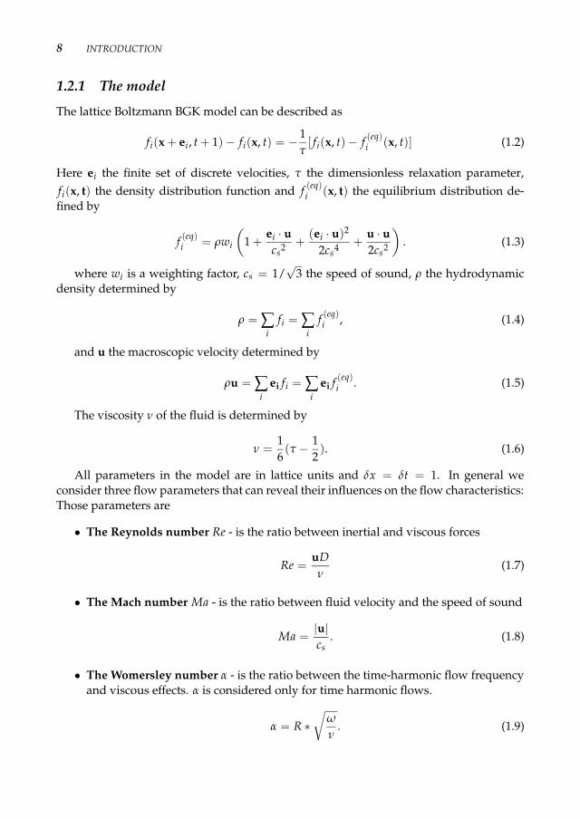
1.2.1 The modelThe lattice Boltzmann BGK model can be described as
fi(x + ei, t + 1) − fi(x, t) = − 1τ
[ fi(x, t) − f (eq)i (x, t)] (1.2)
Here ei the finite set of discrete velocities, τ the dimensionless relaxation parameter,fi(x, t) the density distribution function and f (eq)
i (x, t) the equilibrium distribution de-fined by
f (eq)i = ρwi
(1 +
ei · ucs2 +
(ei · u)2
2cs4 +u · u2cs2
). (1.3)
where wi is a weighting factor, cs = 1/√
3 the speed of sound, ρ the hydrodynamicdensity determined by
ρ = ∑i
fi = ∑i
f (eq)i , (1.4)
and u the macroscopic velocity determined by
ρu = ∑i
ei fi = ∑i
ei f (eq)i . (1.5)
The viscosity ν of the fluid is determined by
ν =16 (τ − 1
2 ). (1.6)
All parameters in the model are in lattice units and δx = δt = 1. In general weconsider three flow parameters that can reveal their influences on the flow characteristics:Those parameters are
• The Reynolds number Re - is the ratio between inertial and viscous forces
Re =uDν
(1.7)
• The Mach number Ma - is the ratio between fluid velocity and the speed of sound
Ma =|u|cs
. (1.8)
• The Womersley number α - is the ratio between the time-harmonic flow frequencyand viscous effects. α is considered only for time harmonic flows.
α = R ∗√
ω
ν. (1.9)
1.2 LATTICE BOLTZMANN METHOD IN COMPUTATIONAL HEMODYNAMICS 9
In all these equations D = 2R is a typical length scale of the flow problem, cs is the speedof sound and ω is the flow frequency.
In all our further studies we first run our simulations for the simple cases and comparethe results with analytical solutions such as the Womersley solution [117] for the time-harmonic flows. After being satisfied with the outcome we transfer our simulations tothe real and more complex applications.
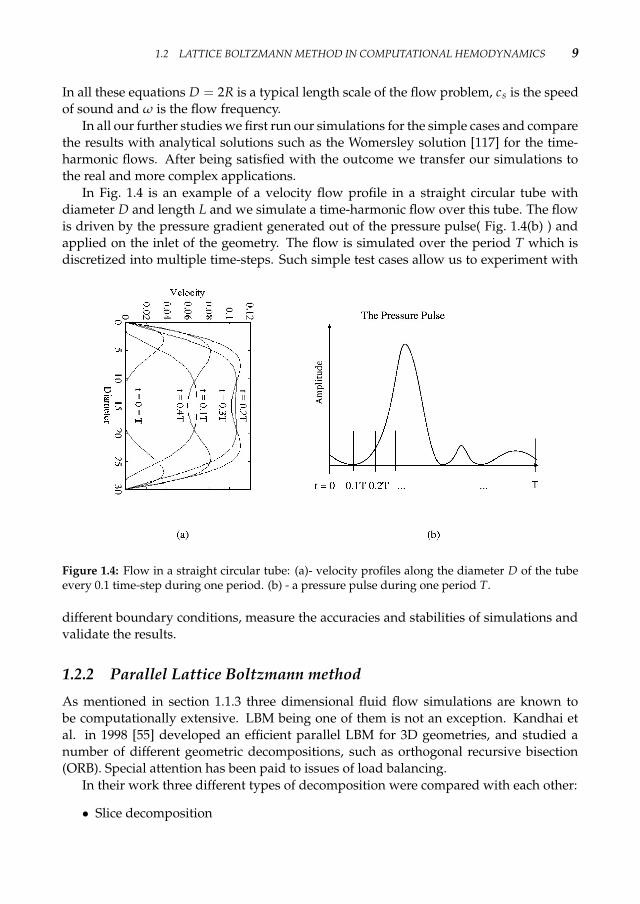
In Fig. 1.4 is an example of a velocity flow profile in a straight circular tube withdiameter D and length L and we simulate a time-harmonic flow over this tube. The flowis driven by the pressure gradient generated out of the pressure pulse( Fig. 1.4(b) ) andapplied on the inlet of the geometry. The flow is simulated over the period T which isdiscretized into multiple time-steps. Such simple test cases allow us to experiment with
Figure 1.4: Flow in a straight circular tube: (a)- velocity profiles along the diameter D of the tubeevery 0.1 time-step during one period. (b) - a pressure pulse during one period T.
different boundary conditions, measure the accuracies and stabilities of simulations andvalidate the results.
1.2.2 Parallel Lattice Boltzmann methodAs mentioned in section 1.1.3 three dimensional fluid flow simulations are known tobe computationally extensive. LBM being one of them is not an exception. Kandhai etal. in 1998 [55] developed an efficient parallel LBM for 3D geometries, and studied anumber of different geometric decompositions, such as orthogonal recursive bisection(ORB). Special attention has been paid to issues of load balancing.
In their work three different types of decomposition were compared with each other:
• Slice decomposition
10 INTRODUCTION
• Box decomposition
• ORB decomposition
For the presenter geometry it was shown that in case of slice and box decompositionsthe workload was not balanced at all. The preference was given to ORB decomposition.Although the obtained results were 10− 60% better than slice or box decomposition, ORBhas a main disadvantage of the complicated communication scheme.
Later, in 1999 Dupuis et al. decomposed a two dimensional (2D) lattice by usinga graph partitioning library called METIS (see Sec. 1.1.3) for any Lattice Gas applica-tion [33]. They proposed to represent the 2D lattice as a vector of cells instead of ma-trix, where every cell knows the indexes of its neighboring cells. This approach has twoadvantages. First it allows to exclude the unused areas from lattice, second the latticetraversal is simple to execute. It was concluded that the performance of this approach isa factor of two slower than the classical approach.
In the same year Satofuka and Nishioka [84] compared the three horizontal, verti-cal and checker board domain decomposition methods for LBM simulations. They con-cluded, that the vertical decomposition gives the highest speedup. In the case of hor-izontal decomposition the longer the number of lattice units in horizontal direction ofeach subdomain, the shorter the CPU time. The measurements were performed for 2Dsimulations and considering the outcome the vertical decomposition was applied for 3Dsimulations. Even better results of speed-up were obtained for the 3D case.
In 2005 Wang et al. [111] proposed another approach, the so called cell-based decom-position method. Unlike other methods, the cell-based method performs the load balancefirst to divide the total number of fluid cells into a number of subdomains, where the dif-ference of fluid cells in each subdomain is either 0 or 1, depending on if the total numberof fluid cells is a multiple of the processor numbers. This cell-based method recovers theinterface rather than the load balance; it does not need iteration and gives an exact loadbalance. The performance of the results showed that it reached the theoretical parallelefficiency.
Detailed performance analysis on three SMP clusters were performed by Wu et al. [121]in 2006 based on a parallel multiblock method proposed by Yu et al. [124]. In this methodthe entire computational domain is divided into blocks, where each block is a segment inthe x-, y-, and z-dimensions, respectively. Each block is assigned to a processor. The gridsizes in each block can be different. Only the communication along the border layers isnecessary. The performance results showed that the large size problems scale well on theSMP clusters using the multiblock decomposition method.
1.2.3 Unstructured Lattice BoltzmannOriginally, LBM was formulated only on geometries that are discretized into uniformgrids. Very soon, the potential of LB as an alternative method for complex fluid flowsimulations became appreciated. There was a need to improve the method in order toapply it on more complex grids such as partially refined or nested grids. These types of

1.2 LATTICE BOLTZMANN METHOD IN COMPUTATIONAL HEMODYNAMICS 11
grids are especially useful to discretization of complex geometries, such as, in our case,the human vascular system.
First, the idea of making LBM applicable for non-uniform/unstructured grids waspointed out by Higuera in 1990 [48]. He proposed to use a coarse-grained distributionfunction which is defined at the center of the cell, which in its turn contains several nodesof the regular fine-grained grid.
In 1992 the Finite-Volume LB method (FV-LBM) was first introduced [17, 75]. Main ad-vantages of FV-LBM are the fact that the mass and momentum conservations remain wellposed as in standard LBM and that it is able to cover the same Reynolds number rangeas standard LBM. However, its major disadvantages are the complicated implementationand loss of computational locality, which essentially increase the computational cost, es-pecially for parallelization.
Next He, Luo and Dembo [46] modified LBM by adding a technique based on point-wise interpolation. In this new algorithm, the computational mesh is uncoupled fromthe discretization of momentum space and it can have an arbitrary shape. Collisions stilltake place on the grid points of the computational mesh. After a collision, the densitydistributions move according to their velocities. Although the density distributions atthe grid sites now may not be exactly determined, they can always be calculated usinginterpolation. After interpolation, collision and advection steps are repeated [46]. Herethe accuracy of LBM is of second order both in time and space and the error introducedby quadratic interpolation is more sufficient as it is small for any grid size. But due to thefact that in the scheme the interpolation distance has an impact on numerical viscosity, itincreases the numerical error.
Later several modifications were applied on FV-LBM [22, 74, 77]. It has been appliedon bilinear quadrilateral and triangular cells. Here the influence of interpolation distanceon numerical error have been reduced. Moreover, in 2005 Stieber et al. applied the up-wind discretization scheme on FV-LBM [95]. This scheme is based on the method of Penget al. [74, 77] but improves the stability and computational efficiency. However, in thisscheme the linear reconstructional step is as expensive as the collision and propagationsteps, which make the total cell update cost 50% higher.
Another adaptation of LBM is the Multiscale LB schemes (M-LBM) that have been pre-sented by Filippova and Heanel [35]. The scheme is based on a coarse grid covering thewhole integration domain. In a critical region, detected either by adaptation criteria ordefined a priori, a finer grid is superposed to the basic, coarser grid. The calculation pro-ceeds with large time steps accordingly to the coarser grid while on the finer grids severaltime-steps are performed to advance to the same time level [35]. This method is appliedto LBGK. Here the collision step on the shared grid nodes is adjusted by correcting thenon-equilibrium part of the particle distribution for the different time discretization andrelaxation parameter on both grids. This assumption, however, is not entirely correct,because the non-equilibrium part depends on the relaxation parameter (in the case ofLBGK scheme) and the time step. Without rescaling the non-equilibrium part, an error isintroduced in the local components of the stress tensor.
A different modification of LBM is the Finite Difference LB scheme (FD-LBM) first pointedout in 2002 by Yu et al. [125]. This scheme is developed based on the fact that the common
12 INTRODUCTION
LBM just one specific discrete representation of the Boltzmann equation. And as it doesnot use a different discretization of the space and time derivatives, one is free in choosingthe type of grid. A multi-block method is developed and an accurate, conservative inter-face treatment between neighboring blocks is adopted, and demonstrated that it satisfiesthe continuity of mass, momentum, and stresses across the interface. The present multi-block method can substantially improve the accuracy and computational efficiency of theLBE method for viscous flow computations.
In 2000 Kandhai et al. applied FD-LBGK on nested grids [60]. The discrete velocityBoltzmann equation is solved numerically on each sub-lattice and interpolation betweenthe interfaces is carried out in order to couple the sub-grids consistently. The computa-tional domain is basically built up of a number of sub-domains which can have differentgrid resolutions. On each sub-domain the discrete velocity Boltzmann equation is solvedand the adjacent sub-domains are coupled with each other by appropriate interpolationat the boundaries of the sub-domains. But again the presented finite-difference meth-ods can accommodate only relatively smooth variations of the flow field because largedeformations of the nonuniform mesh may result in numerical instabilities [73].
During the same period Tölke et al. [107] introduced implicit discretization and a non-uniform mesh refinement approach for the LBGK method. The results of the numericalexamples shown in this work indicate that the use of implicit discretization methods forthe LBGK equations may be of significant advantage at least for stationary flows of highReynolds numbers in geometries of moderate complexity [107]. But stability and consis-tency issues of implicit methods for LBGK equations are far from being fully explored.
Recently a new idea of Locally Embedded Grids (LEG) is explored by Martin Rohde [82].The idea of using the volumetric description of the grid for mass conservation is still ap-plied here but no interpolation technique or rescaling of the non-equilibrium distributionis required to obtain accurate results. Furthermore, the technique is not restricted to asingle-relaxation scheme, but can be used for any LB scheme, because the communica-tion between the coarse and the fine grids takes place after the propagation step [82].
1.3 Research overview and motivationThe main goals of this thesis are
• to create a complete and enhanced computer-based simulation environment forimage-based computational hemodynamics problems, using the LBM,
• to integrate it into a high performance computing environment,
• to apply it for visualization and understanding of biomechanical processes in com-plex vascular systems.
These will result to the creation of a comprehensive and efficient PSE that will answerto the "What if ..." questions concerning the biomechanical effects of complex vascularreconstruction processes, and that may also serve as a decision support system.

1.3 RESEARCH OVERVIEW AND MOTIVATION 13
As was mentioned in section 1 during the last years the number of deaths caused bycardiovascular diseases has essentially increased, especially due to the vascular disor-ders caused by atherosclerotic diseases. The development of a computer-based problemsolving environment (PSE) that provides all the computational facilities needed to solvea target class of problems is a necessity [50, 98].
For this type of PSE a major important component is a sophisticated time-harmonicflow simulator. As discussed in section 1.1.3 for fluid flow simulations besides traditionalNavier-Stokes equations one can use the LBM method. However, as any CDF method ithas its disadvantages, like slow convergence, pointed out in section 1.2. Thus the chal-lenge for us is to create a scheme which will help to overcome this problem.
Moreover, the optimal parallelization of LBM is a developing issue and an interestingdirection to investigate. Even though LBM is simple to parallelize due to the locality of itscomputations, there still can be complications connected with the discretization methodsand workload imbalance. In section 1.1 the main concepts of high performance comput-ing were introduced, while in section 1.1.3 their influences on the simulation model werediscussed. The short description of existing parallelization schemes gives us clear indica-tion that there are several ways of their optimization. Especially for the cases where thegeometry discretization is inhomogeneous as described in section 1.2.3.
The thesis is constructed in the following way:In the current chapter is a general introduction to the main concepts and a short pre-
sentation of the state of the art.In Chapter 2 we describe the PSE that we have created for image-based computational
Hemodynamics called HemoSolve. Also we give a complete evaluation of the LBM bycomparing it to with the other CFD methods such as Finite Element Method (FEM).
After evaluation of LBM, we continue with its improvement in the Chapter 3. Wedefine a constraint optimization scheme which helps to speed-up its convergence. Alsoanother improvement of is a new proposed variation of LBM called regularized LBM. Asubstantive comparison of these two methods is presented.
Next in Chapter 4 we integrate LBM into high performance computing. We show acomplete set of experiments and comparisons of both discretization methods and per-formance aspects. Moreover, inspired by previous studies we develop a performanceprediction model that can be used to evaluate the execution costs of the model.
In Chapter 5 we combine our results in a new and highly enhanced version of PSE,HemoSolve2.0.
At the end, in Chapter 6 we summarize the work presented in this thesis, draw ourconclusions and discuss the future development possibilities.


HemoSolve - A Problem SolvingEnvironment for Image-Based
Computational Hemodynamics∗
2.1 Introduction"A problem solving environment (PSE) is a computer system that provides all the com-putational facilities necessary to solve a target class of problems" [39, 50]. The targetclass of problems that we chose in our study is associated with cardiovascular diseases,a predominant cause of death [4, 98, 101]. In particular our attention is concentrated onvascular disorders caused by atherosclerosis. The goal of our PSE, which we call Hemo-Solve, is to provide a fully integrated environment for simulation of blood flow in patientspecific arteries.
Because of the complex structure of the human vascular system it is not always ob-vious for surgeons how to solve the problem of bypass and/or stent placement on thedeformed part, or to decide on specific treatment alternatives. Having a completely in-tegrated computational hemodynamics environment like HemoSolve can serve as a pre-operational planning tool for surgeons, but also as a useful experimental system for med-ical students to enlarge their practical skills [93, 104]. It also serves as a environment forbiomedical engineers that study e.g. new stent designs.
Moreover, HemoSolve is merged with Grid technology, thus offering a unified accessto different and distant computational and instrumental resources [104]. This is one ofthe desirable abilities of PSEs in general [50].
2.2 The first step towards HemoSolveIn ref. [93] Steinman argues that a need exists for robust and user-friendly techniquesthat can help an operator turn a set of medical images into computational fluid dynamics
∗This chapter is partly based on: L. Abrahamyan, J. A. Schaap, A. G. Hoekstra, D. Shamonin, F. M.A. Box,R. J. van der Geest, J. H.C. Reiber, P. M.A. Sloot. A Problem Solving Environment for Image-Based Computa-tional Hemodynamics. In LNCS 3514, p.287, April (2005).
15

16 HEMOSOLVE - A PROBLEM SOLVING ENVIRONMENT FOR IMAGE-BASED COMPUTATIONALHEMODYNAMICS
(CFD) input file in a matter of minutes. HemoSolve not only has this ability but also is atool which allows to simulate pulsatile (systolic) flows in arteries.
The whole system consists of the following components (See Fig. 2.1):
1. Medical data segmentation to obtain arteries of interest;
2. 3D editing and mesh generation, to prepare for the flow simulation;
3. Flow simulation, computing of blood flow during systole;
4. Analysis of the flow, pressure, and stress fields.
Figure 2.1: Functional design of HemoSolve.
Figure 2.2: (a) - is the pathline and the centerline crossing an axial slice, (b) - is a stack of slicesresampled along the centerline.
2.2.1 Medical Data SegmentationThe goal of the segmentation process is to automatically find the lumen border betweenthe blood and non-blood, i.e. the vessel wall, thrombus or calcified plaque. The algorithm

2.2 THE FIRST STEP TOWARDS HEMOSOLVE 17
Figure 2.3: Aneurysm: main stages of HemoSolve. First segmentation of the raw medical data (a).Then the segmented data (b) is first cropped (c) and inlet/outlet layers are added (d) and the meshis generated (e). Simulation results of created mesh are presented (f).
Figure 2.4: Abdominal aorta: main stages of HemoSolve. Segmented data (a) is first cropped (b)and inlet/outlet layers are added (c) and the mesh is generated (d). Simulation results of the createdmesh are presented (e).
18 HEMOSOLVE - A PROBLEM SOLVING ENVIRONMENT FOR IMAGE-BASED COMPUTATIONALHEMODYNAMICS
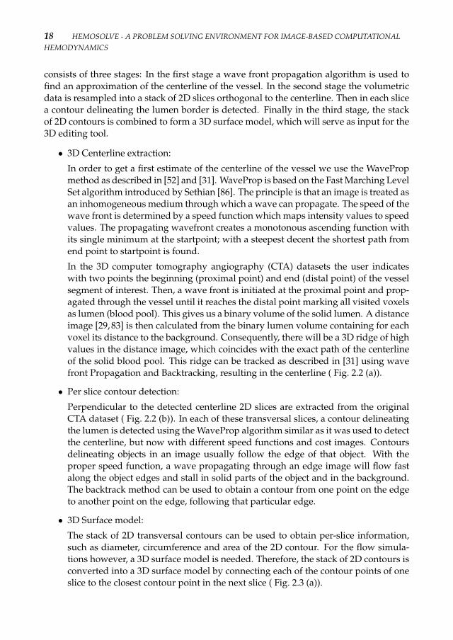
consists of three stages: In the first stage a wave front propagation algorithm is used tofind an approximation of the centerline of the vessel. In the second stage the volumetricdata is resampled into a stack of 2D slices orthogonal to the centerline. Then in each slicea contour delineating the lumen border is detected. Finally in the third stage, the stackof 2D contours is combined to form a 3D surface model, which will serve as input for the3D editing tool.
• 3D Centerline extraction:In order to get a first estimate of the centerline of the vessel we use the WavePropmethod as described in [52] and [31]. WaveProp is based on the Fast Marching LevelSet algorithm introduced by Sethian [86]. The principle is that an image is treated asan inhomogeneous medium through which a wave can propagate. The speed of thewave front is determined by a speed function which maps intensity values to speedvalues. The propagating wavefront creates a monotonous ascending function withits single minimum at the startpoint; with a steepest decent the shortest path fromend point to startpoint is found.In the 3D computer tomography angiography (CTA) datasets the user indicateswith two points the beginning (proximal point) and end (distal point) of the vesselsegment of interest. Then, a wave front is initiated at the proximal point and prop-agated through the vessel until it reaches the distal point marking all visited voxelsas lumen (blood pool). This gives us a binary volume of the solid lumen. A distanceimage [29, 83] is then calculated from the binary lumen volume containing for eachvoxel its distance to the background. Consequently, there will be a 3D ridge of highvalues in the distance image, which coincides with the exact path of the centerlineof the solid blood pool. This ridge can be tracked as described in [31] using wavefront Propagation and Backtracking, resulting in the centerline ( Fig. 2.2 (a)).
• Per slice contour detection:Perpendicular to the detected centerline 2D slices are extracted from the originalCTA dataset ( Fig. 2.2 (b)). In each of these transversal slices, a contour delineatingthe lumen is detected using the WaveProp algorithm similar as it was used to detectthe centerline, but now with different speed functions and cost images. Contoursdelineating objects in an image usually follow the edge of that object. With theproper speed function, a wave propagating through an edge image will flow fastalong the object edges and stall in solid parts of the object and in the background.The backtrack method can be used to obtain a contour from one point on the edgeto another point on the edge, following that particular edge.
• 3D Surface model:The stack of 2D transversal contours can be used to obtain per-slice information,such as diameter, circumference and area of the 2D contour. For the flow simula-tions however, a 3D surface model is needed. Therefore, the stack of 2D contours isconverted into a 3D surface model by connecting each of the contour points of oneslice to the closest contour point in the next slice ( Fig. 2.3 (a)).

2.2 THE FIRST STEP TOWARDS HEMOSOLVE 19
2.2.2 3D Editor and Mesh Generator3D editing is the second component after the segmentation. The 3D stereoscopic imagecan easily be maintained in this user-friendly editing tool. Here surgeons and studentscan execute their experimental visualization studies on realistic arterial geometries. Theycan crop parts of the artery, where important factors in the study of hemodynamics exist,with the help of a clipping instrument. They can add inlet and outlet layers on the end-points of the arterial geometry and can enhance it with structures like bypasses or stents.Also this component allows them to define the geometrical features ( e.g. width, length,placement positions ) of these structures. Thus, the 3D editing tool allows surgeons andstudents to mimic the real surgical processes.
The final stage of this component is mesh generation. The prepared arterial geometry,including aneurysms, bifurcations, bypasses and stents, is converted into a computa-tional mesh in several minutes. The mesh could be coarse or fine depending on the wishof user.
The mesh is then ready to be used in flow simulators.
2.2.3 Hemodynamic SolverAs a computational hemodynamic solver the Lattice Boltzmann Method(LBM) is used inHemoSolve: In this solver the flow is time-harmonic and after simulation the pressure,velocity, and shear stress fields during one full harmonic period are produced and can bevisualized. LBM receives the input geometry mesh from the 3D editing tool.
LBM is a mesoscopic method based on a discretized Boltzmann equation with simpli-fied collision operator [97]. Here the flow is considered Newtonian. We have shown thatLBM is capable of solving hemodynamic flows in the range of Reynolds and Womers-ley numbers ofhttp://www.google.com/ interest [9, 13, 14]. To run the simulator, exceptthe input data file from 3D editing tool, one should define several patient-specific freeparameters such as the Reynolds number.
2.2.4 Validation of Lattice Boltzmann Method† The complexity of the human vascular system and the time-harmonic character of theblood flow make it very difficult to analyze and predict the behavior of flow after surgicalinterference. In order to exactly mimic this behavior in HemoSolve, well-established flowsolvers need to be used.
In order to show that LBM is a comprehensive method to simulate time-harmonicblood flow in the human vascular system we compare it with Finite Element Method(FEM). Several studies of comparison between LBM and FEM methods have shownpromising results [40, 54]. Although, in all those studies, whether in 2D or 3D geome-tries, the fluid flow has been time-independent.
†The geometry and FEM data are kindly provided by Dr. Rod Hose and Dr. Adam Jeays, Department ofMedical Physics and Clinical Engineering, University of Sheffield.
20 HEMOSOLVE - A PROBLEM SOLVING ENVIRONMENT FOR IMAGE-BASED COMPUTATIONALHEMODYNAMICS
We compare LBM and FEM solvers for a time-harmonic flow in realistic 3D geometry.As an application we choose to analyze the blood flow in the superior mesenteric artery(SMA). SMA is the part of artery that starts from the anterior surface of the abdominalaorta (AA), distal to the root of the celiac trunk (see Fig. 1.1). Although atheroscleroticdisease is rare in this part of the artery its occlusion at SMA leads to the death of patientin the 80% of cases [80].
The analysis between these two methods have been done through:
• comparison of velocity profiles at three different cross sections along AA and SMA
• comparison of pressure profiles at the outlet of SMA
• fixation of a time and place of flow characteristics such as vortex formation next tothe bifurcation
In Fig. 2.5 (left) the surface of the superior mesenteric artery is shown.The data is obtained from MRI scan and a triangular mesh is generated to be used
in the FEM solver [53]. The 3D mesh for FEM consists of total 100465 nodes, with 650nodes on the AA inlet, 295 on the AA outlet and 207 on the SMA outlet. From this mesha voxel mesh is generated for LBM using the 3D editing and mesh generation tool with694 nodes on the AA inlet, 316 on the AA outlet and 224 on the SMA outlet. FLOTRAN(ANSYS Inc.) is used as a FEM solver for simulating the 3D Navier-Stokes equationsas (see Jeays et al. [53]). As the artery is relatively large the following flow parametersare applied in FEM: the density of the blood ρ is 1000kgm−3, Newtonian viscosity ν is4mPa.s, the cardiac cycle duration T is 0.86s with five milliseconds time-steps δt and theblood is considered incompressible. The maximum velocity u of 0.8m/s at a peak sys-tole in the aorta, combined with the diameter D of 0.0165m, gives a maximum Reynoldsnumber (Re) of 3300 [53]. In order to apply the same flow condition in the LBM solverwe have converted all the parameters into dimensionless units and applied a constraintoptimization scheme (see sec. 3.3). This resulted in D = 30 lattice points, T = 17200 andν = 0.0065 with Re = 3300 for α = 11.
As inlet/outlet boundary conditions we applied the same as described in Jeays etal. [53]. The velocities (created using Womersley’s solution [117]) are specified at theproximal AA opening, the pressure waveform (created using the Westerhof model [114])is specified at the distal AA opening and a free flow boundary condition is applied at theoutflow of SMA.
In Fig. 2.6 we depicted the velocity profiles at peak systole in the last cardiac cycle ex-ecuted, when beat to beat convergence had been achieved, along the cutting plane shownin Fig. 2.5 (right). Here we clearly see the expected flow behavior and the formation ofvoxel in the top of SMA just below the outer wall.
As shown in Fig. 2.5 we compare the obtained velocity profiles along the three A, Band C lines after simulations by both solvers. The flow profiles at regions A and B areshown in Fig 2.7 (left) and (right) respectively and for region C in Fig 2.8.
We see a very good agreement between velocity profiles of FEM and LBM. Our mea-surements show that the difference between velocities next to the walls is maximum0.078m/s while in the middle it is about 0.018m/s. Moreover, we see that the maximum

2.2 THE FIRST STEP TOWARDS HEMOSOLVE 21
Figure 2.5: The surface of the superior mesenteric artery (left) and a simulated velocity profile init(right) at Re = 3300 with α = 11. Here red and blue are the high and low velocities respectively.A, B and C are the cutting planes along which we look into the velocity profiles in detail further on.
Figure 2.6: The simulated velocity profiles depicted during one systole every 700 time-step (left)and the stream-lines showing the formation of vortex (right).

22 HEMOSOLVE - A PROBLEM SOLVING ENVIRONMENT FOR IMAGE-BASED COMPUTATIONALHEMODYNAMICS
0 5 10 15 20 250
0.2
0.4
0.6
0.8
D
Vel
ocity
0 5 10 15 20 250
0.2
0.4
0.6
0.8
D
Vel
ocity
Figure 2.7: Comparison of the velocity profiles between LBM (bullets) and FEM (solid lines) at theregion A(left) and B (right)(see Fig. 2.5) for every 0.05s timestep. Velocities are presented in m/s.
1 2 3 40
0.03
0.06
0.09
0.12
0.15
D
Vel
ocity
0 5 10 15 20 250
0.2
0.4
0.6
0.8
D
Vel
ocity
Figure 2.8: Comparison of the velocity profiles between LBM (bullets) and FEM (solid lines) forSMA (left) and AA (right) at the region C (see Fig. 2.5) every 0.05s timestep. Velocities are presentedin m/s.
velocity in Fig. 2.7, e.g. before the bifurcation, is tilted to the left while in Fig. 2.8 (right),e.g. after bifurcation, it is near the right side. This indicates a spiraling of the flow in AA.The same effect we see during the flow visualization. This is one of the two interestingcharacteristics of the flow noted by Jeays et al. [53] for FEM comparable to our obser-vations for LBM. Furthermore, we noted that the flow in the SMA is directed from thebifurcation towards the outer wall, which causes the creation of a vortex at the highestlevel of the SMA just below the outer wall (see Fig. 2.6). This vortex formation is due tothe angle that the SMA forms with the AA [53].
In Fig. 2.9 we have also plotted the pressure profile at the outlet of SMA for both meth-ods during one complete heart beat. Here we also see a very good agreement betweenboth methods.
We have shown a good agreement between velocity as well as pressure profiles ofFEM and LBM at all three cross sections. We have also presented the similarities of

2.3 EXAMPLES 23
0 0.2 0.4 0.6 0.81
1.05
1.1
1.15
1.2
1.25
1.3
1.35
1.4
1.45x 10⁴
time (sec.)
Pres
sure
(Pa)
Figure 2.9: Comparison of the pressure profiles between LBM (dash line) and FEM (solid line) atthe outlet of SMA during one systole. Pressure is presented in Pa.
flow characteristics, such as the precise timestep and coordinates of vortex formation,for both methods. Thus, based on these arguments we conclude that LBM is a quite eligi-ble method to use as a solver of Navier-Stokes equation for simulations of time-harmonicblood flows in human vascular system.
2.2.5 Flow AnalysesIn order to analyze the blood flow in arteries its velocity, pressure and shear stress profilesneed to be examined. Several methods exist for it and among them visualization of theflow is one of the advanced methods that helps to understand the meaning and behaviorof flow better. Also visualization techniques are different and can show different featuresof flow. One of the visualization techniques we use in HemoSolve is based on simulatedpathline visualization [92].
2.3 ExamplesAs an application example of using HemoSolve we present two case studies with com-plex geometries representing parts of the human vascular system:
• Aneurysm in the upper part of abdominal aorta;
• Whole abdominal aorta.
2.3.1 AneurysmWe consider the case of an aneurysm ( ballooning out of the artery ) in the upper part ofthe aorta. First the medical data of the upper part of a patient’s abdominal aorta with ananeurysm is segmented by applying the segmentation algorithm ( Fig. 2.3 (a,b) ). Then

24 HEMOSOLVE - A PROBLEM SOLVING ENVIRONMENT FOR IMAGE-BASED COMPUTATIONALHEMODYNAMICS
the segmented part which includes the aneurysm, is transfered into the 3D editing toolwhere the user crops the structurally interesting part ( Fig. 2.3 (c) ) and defines inlet andoutlet layers ( Fig. 2.3 (d) ). These layers are easy to control, that is to change the planeof their position by simply moving the normal vector in the middle of each layer or tochange the size by movement of corner points. In this example there is one inlet at thetop and one outlet at the bottom layer. Finally the mesh is generated depending on theconstructed geometry ( Fig. 2.3 (e) ). The mesh is then used as input data for the CFDsolver. The presented flow is the velocity profile of blood flow simulated by LBM method.The Reynolds number applied to this blood flow is 500. The size of the generated meshis 146x73x55 lattice points and the simulation time is about 20 minutes on 16 processors.As a result three frames during the cardiac systole are captured ( Fig. 2.3 (f) ).
2.3.2 Abdominal aortaNext we consider the full lower abdominal aorta down to the bifurcation. Again themedical data is segmented by applying the segmentation algorithm ( Fig. 2.4 (a) ). Thenthe same steps as in the first example are applied ( Fig. 2.4 (b) ), except for the outlet layersthat are six now and are in different planes ( Fig. 2.4 (c) ) and the sizes of generated meshesare bigger ( Fig. 2.4 (d) ). The ready mesh then used as an input data for CFD solver. Thepresented flow is the velocity profile of blood flow simulated by LBM method with thesame Reynolds number 500. The size of the generated mesh is 355x116x64 lattice pointsand the simulation time is 85 minutes on 16 processors. As a result three frames duringthe cardiac systole are captured ( Fig. 2.4 (e) ).
2.4 Discussions and ConclusionsThe field of image based hemodynamics needs integrated PSEs, especially to enhancethe preparation of computational meshes, and to allow non-specialists to enlarge theirpractical skills. HemoSolve consists of several components that make it a complete sys-tem. Thus biomedical engineers, surgeons or novice surgeons can take raw medical datafrom a patients’ vascular system and after several simple steps within a quite short pe-riod get completed flow fields ( velocity, pressure, shear stress) which they can analyzewith different visualization tools. One of this tools is the personal space station (PSS)which supports 3D visualization and interaction [126]. Moreover with the help of the3D editing tool potential users can add bypasses or stents to vessels and examine theblood flow profile in them. The biomechanists of University of Amsterdam and LeidenUniversity Medical Center have already used HemoSolve in their scientific research. Aswas reported by Zudilova and Sloot [126], two different projection modularities: a virtualreality and a desktop have been tested and compared for vascular reconstruction simula-tion systems. These studies have been conducted based on the visualization componentsof HemoSolve. They have reported that the results of user profiling showed that thecombination of the virtual reality and desktop capabilities within the same environmentis the best solution for potential users.

2.4 DISCUSSIONS AND CONCLUSIONS 25
Another study have been conducted by Twente University to estimate the usefulnessof environments like HemoSolve for the university students. It has been reported thatvirtual learning environments hold great promise as a tool for medical education [70].
An important feature of HemoSolve is also the fact that it is integrated into Grid en-vironment. It is an environment that supports a uniform access to distributed data (im-ages), compute power and, visualization and interaction [102–104]. If the data (CT scanin the hospital), simulation (high performance computing center) and visualization (stu-dent desktop) are situated in different geographical places, Grid is the environment tocombine them. That is why the fact of HemoSolve being integrated into Grid is one of itsimportant attributes.
In order to estimate the efficiency of HemoSolve we compare its main features withthe requirements of users from PSEs in general. Those characteristics are [39, 50] :
• Simple human-computer interaction - It is enhanced by graphical user interfacewhich is easy accessible even for inexperienced users [126].
• Complete and accurate numerical models - Numerical model used in this PSE isLBM [9] which is complete and quite accurate for simulation of blood flow in hu-man vascular system.
• Parallel and distributed computing environment - The solvers in PSE are fully par-allelized [57] .
• Geographically distributed data - This image-based PSE is completely integratedinto a Grid environment, which gives huge abilities not only to distribute the databut also to do simulations and diagnoses by grid computing [104] .
• Usefulness for university students - The potential users of this PSE are considerednovice surgeons who can first practice their knowledge by doing an operation onPSE and afterward apply their experience on patients.
We conclude that HemoSolve is a well defined, easy applicable environment for image-based hemodynamics research of time-harmonic blood flow in the human vascular sys-tem.

Efficient LBM for Time Harmonic Flows∗
3.1 IntroductionThe lattice Boltzmann method (LBM) is a well recognized method in computational fluiddynamics and has attracted much attention [17, 23, 25, 97]. It is widely used in simu-lations of fluid flow in complex geometries such as fluid flow through porous mediae.g. [26, 56, 63] or time-harmonic blood flow e.g. [9, 10, 27, 34, 43]. However, LBM is ham-pered by slow convergence [42, 59, 106], caused by the demand of low Mach number(Ma)( to suppress compressibility error ) and the fulfillment of the Courant-Friedrich-Levy condition for numerical stability. In order to meet these constraints the number oftime-steps for reaching steady state needs to be large, and so is the execution time. Forthis reason we must carefully choose simulation parameters that, given flow propertiesand a target simulation error, minimize the execution time. We call this the constraintoptimization problem for LBM simulations.
In this chapter we propose a solution to the constraint optimization problem for time-harmonic flows. For validation of the constraint optimization scheme we compare resultsof time-harmonic flow simulations with analytical Womersley solutions [117]. We alsoperform stability analysis for a range of Reynolds (Re) and Womersley (α) numbers.
Moreover, it is known that L-BGK suffers from numerical instabilities at high Reynoldsnumbers (Re). Several solutions have been proposed to improve the method in this re-spect [6, 66]. In this chapter we follow another route, we choose to use the regularizationscheme proposed by Latt and Chopard [68]. In this RL-BGK scheme, the simulated ki-netic variables are submitted to a small correction (the regularization), after which theyonly depend on the local density, velocity, and momentum flux. This correction is im-mediately followed by the usual L-BGK collision term. The effect of the regularizationstep is to eliminate non-hydrodynamic terms, known as "ghost variables", and to enforcea closer relationship between the discrete, kinetic dynamics and the macroscopic Navier-Stokes equation.
We study the performance of the RL-BGK through a numerical simulation of the time-harmonic Womersley [117] flow for 3D geometries. Further, we analyze the accuracy of
∗This chapter is partly based on: L. Axner, A. G. Hoekstra, and P. M. A. Sloot. Simulating time-harmonicflows with the lattice Boltzmann method. In Phys Rev. E, 75,3, p.036709, (2007), and partly on: L. Axner, J. Latt,A. G. Hoekstra, B. Chopard, and P. M. A. Sloot. Simulating time-harmonic flows with the Regularized L-BGKMethod In Int. J. Mod. Phys. C, 18,4, p.661, (2007).
27
28 EFFICIENT LBM FOR TIME HARMONIC FLOWS
the scheme by comparison of the simulation results with analytical solution. We alsopresent stability analysess of the model for some benchmark flows.
3.2 Lattice Boltzmann MethodWe apply the three dimensional 19-velocity (D3Q19) model [123] for time harmonic flows [9].The fluid flow is quasi-incompressible and all simulations in this chapter (except those insubsection 3.5) are performed on a straight circular tube with rigid walls. On the wallswe use Bouzidi boundary conditions (BBC) [19]. For the experiments on the straight tubewe use periodic inlet/outlet boundary conditions and the flow was driven by a time-harmonic body force [10]. As we confirmed earlier for time-harmonic flows [11] BBC ismore stable and accurate than the bounce back on links boundary condition, especiallyfor high Mach numbers (Ma). For the simulations we use a previously developed highlyefficient parallel code. [55].
We define an average simulation error (Er) as
Er =1T ∑
t
∑x |uth(x, t) − ulb(x, t)|∑x |uth(x, t)| , (3.1)
where uth(t) is the analytical Womersley solution, ulb(t) is the simulated velocity, andT is the number of time steps per period. For uth we use the Womersley [117] solution.For flow in an infinite tube driven by pressure gradient Aeiωt,
uth =AR2
ν
1i3α2
{1 − J0(αi3/2x)
J0(αi3/2)
}eiωt, (3.2)
where R is the radius of the tube, x is defined as x = r/R, ω = 2πT is the circle
frequency, J0 is the zero order Bessel function, ν is the viscosity and α is the Womersleynumber as defined in Eqs 1.6 and 1.9 Here D = 2R is the diameter of the tube.
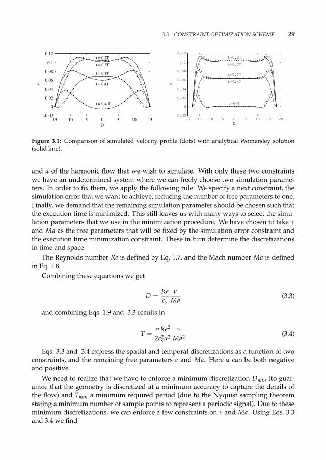
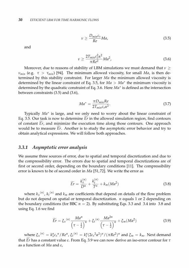
As an example, we show in Fig. 3.1 simulation results together with analytical solu-tions, for Re = 10, α = 6 and Re = 3000, α = 16 respectively. Other examples, and moredetailed comparisons can be found in [8–10].
The agreement in the case of low Re number is good while for Re = 3000 the agree-ment is less good, especially near the walls. The simulation error in the first case isEr = 0.002, while for the second case is Er = 0.092.
3.3 Constraint Optimization SchemeIn LBM simulations for time-harmonic flows one must specify four free parameters: thediameter D, the period T, the relaxation parameter τ (or related viscosity ν) and the Machnumber Ma. The choice of these four parameters not only influences the accuracy of themethod, but also other features like stability, convergence and execution time. We willnow address the question how to optimally choose these parameters. First we specify Re
3.3 CONSTRAINT OPTIMIZATION SCHEME 29
−15 −10 −5 0 5 10 15−0.02
0
0.02
0.04
0.06
0.08
0.1
0.12
v
D
t = 0 = T
t = 0.1T
t = 0.2Tt = 0.3T
t = 0.4T
−20 −15 −10 −5 0 5 10 15 20−0.02
0
0.02
0.04
0.06
0.08
0.1
0.12
v
D
t=0=T
t=0.1T
t=0.2T
t=0.3T
t=0.4T
Figure 3.1: Comparison of simulated velocity profile (dots) with analytical Womersley solution(solid line).
and α of the harmonic flow that we wish to simulate. With only these two constraintswe have an undetermined system where we can freely choose two simulation parame-ters. In order to fix them, we apply the following rule. We specify a next constraint, thesimulation error that we want to achieve, reducing the number of free parameters to one.Finally, we demand that the remaining simulation parameter should be chosen such thatthe execution time is minimized. This still leaves us with many ways to select the simu-lation parameters that we use in the minimization procedure. We have chosen to take τand Ma as the free parameters that will be fixed by the simulation error constraint andthe execution time minimization constraint. These in turn determine the discretizationsin time and space.
The Reynolds number Re is defined by Eq. 1.7, and the Mach number Ma is definedin Eq. 1.8.
Combining these equations we get
D =Recs
ν
Ma (3.3)
and combining Eqs. 1.9 and 3.3 results in
T =πRe2
2c2s α2ν
Ma2 (3.4)
Eqs. 3.3 and 3.4 express the spatial and temporal discretizations as a function of twoconstraints, and the remaining free parameters ν and Ma. Here u can be both negativeand positive.
We need to realize that we have to enforce a minimum discretization Dmin (to guar-antee that the geometry is discretized at a minimum accuracy to capture the details ofthe flow) and Tmin a minimum required period (due to the Nyquist sampling theoremstating a minimum number of sample points to represent a periodic signal). Due to theseminimum discretizations, we can enforce a few constraints on ν and Ma. Using Eqs. 3.3and 3.4 we find
30 EFFICIENT LBM FOR TIME HARMONIC FLOWS
ν ≥ DmincsRe Ma, (3.5)
and
ν ≥ 2Tminc2s α2
πRe2 Ma2, (3.6)
Moreover, due to reasons of stability of LBM simulations we must demand that ν ≥νmin (e.g. τ > τmin) [94]. The minimum allowed viscosity, for small Ma, is then de-termined by this stability constraint. For larger Ma the minimum allowed viscosity isdetermined by the linear constraint of Eq. 3.5, for Ma > Ma∗ the minimum viscosity isdetermined by the quadratic constraint of Eq. 3.6. Here Ma∗ is defined as the intersectionbetween constraints (3.5) and (3.6),
Ma∗ =πDminRe2Tmincsα2 . (3.7)
Typically Ma∗ is large, and we only need to worry about the linear constraint ofEq. 3.5. Our task is now to determine Er in the allowed simulation region, find contoursof constant Er, and minimize the execution time along those contours. One approachwould be to measure Er. Another is to study the asymptotic error behavior and try toobtain analytical expressions. We will follow both approaches.
3.3.1 Asymptotic error analysisWe assume three sources of error, due to spatial and temporal discretization and due tothe compressibility error. The errors due to spatial and temporal discretizations are offirst or second order, depending on the boundary conditions [11]. The compressibilityerror is known to be of second order in Ma [51, 72]. We write the error as
Er =k(n)
xDn +
k(n)t
Tn + km(Ma2) (3.8)
where kx(n), kt
(n) and km are coefficients that depend on details of the flow problembut do not depend on spatial or temporal discretization. n equals 1 or 2 depending onthe boundary conditions (for BBC n = 2). By substituting Eqs. 3.3 and 3.4 into 3.8 andusing Eq. 1.6 we find
Er = ξx(n) Man
(τ − 1
2
)n + ξt(n) Ma2n
(τ − 1
2
)n + ξm(Ma2) (3.9)
where ξx(n) = kn
xcsn/Ren, ξt(n) = kn
t (2cs2α2)n/(πRe2)n and ξm = km. Next demandthat Er has a constant value ε. From Eq. 3.9 we can now derive an iso-error contour for τas a function of Ma and ε,
3.3 CONSTRAINT OPTIMIZATION SCHEME 31
τ = Ma(
ξx + ξt Ma2
ε − ξm Ma2
)1/n+
12 . (3.10)
The execution time Texec for LBM for time-harmonic flows can be written as
Texec = NpTp, (3.11)
where Np is the number of periods needed to achieve a stable time-harmonic solutionand Tp = Ttiter is the execution time per period, with titer the execution time for oneLBM iteration. Finally, titer = D3tnode, where tnode is the time spent to update one nodein the lattice. For our simulations we assume that we have D3 nodes. From previousexperiments [11] we know that Np hardly depends on other parameters and for our casewe assume that it is constant. Thus Eq. 3.11 can be written as
Texec = NpTD3tnode = CtTD3, (3.12)
where Ct is a constant. If we substitute Eqs. 3.3 and 3.4 into 3.12 and use Eq. 3.9 weget
Texec = CtπRe5
2cs5α21
Ma
(ξx + ξt Ma2
ε − ξm Ma2
)4/n. (3.13)
Independent of n, Texec goes to infinity for Ma decreasing to 0 (because T then goes toinfinity, see Eq. 3.4) and for Ma reaching the value
√ε
ξm(because ν, and therefore D goes
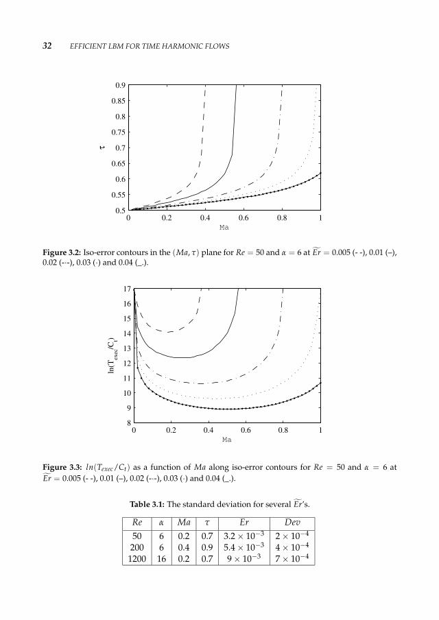
to infinity, see Eq. 3.3 and 3.10) Texec has a minimum between these two limiting values.Later we will compare our experimental results to these analytical solutions. Plots of theasymptotic iso-error contours are shown in Fig. 3.2. Here we assume kx = kt = 1 andkm = 0.05, and second order boundary conditions, i. e. n = 2.
Using Eq. 3.13 we have plotted in Fig. 3.3 ln(Texec/Ct) as a function of Ma along theanalytical iso-error curves. Each of the contours has a minimum point which correspondsto the optimal value of Ma for a certain Er. For example for Er = 0.005, Texec has itsminimum at Ma = 0.18 and as Ma increase towards
√ε
ξm, Texec grows to infinity.
3.3.2 Experimental resultsWe performed three sets of experiments: Re = 50, α = 6, Re = 200, α = 6 and Re = 1200,α = 16. We measured the error on every timestep for a range of values of Ma and τ andfrom that we compute the average error Er and its standard deviation of Er. In Table 3.1the standard deviations for Er = 0.0032, 0.0054 and 0.009 are shown. Note that Er ismeasured at each time step and averaged over the period.
Fig. 3.4 shows the experimental iso-error curves (markers) for Re = 50, α = 6. Theseexperimental results suggest that the Ma - τ correlation is linear. In the limit of small MaEq. 3.10 can be written as
32 EFFICIENT LBM FOR TIME HARMONIC FLOWS
0 0.2 0.4 0.6 0.8 10.5
0.55
0.6
0.65
0.7
0.75
0.8
0.85
0.9
Ma
τ
Figure 3.2: Iso-error contours in the (Ma, τ) plane for Re = 50 and α = 6 at Er = 0.005 (- -), 0.01 (–),0.02 (-·-), 0.03 (·) and 0.04 (_.).
0 0.2 0.4 0.6 0.8 18
9
10
11
12
13
14
15
16
17
Ma
ln(T
exec
/Ct)
Figure 3.3: ln(Texec/Ct) as a function of Ma along iso-error contours for Re = 50 and α = 6 atEr = 0.005 (- -), 0.01 (–), 0.02 (-·-), 0.03 (·) and 0.04 (_.).
Table 3.1: The standard deviation for several Er’s.
Re α Ma τ Er Dev50 6 0.2 0.7 3.2 × 10⁻³ 2 × 10⁻⁴
200 6 0.4 0.9 5.4 × 10⁻³ 4 × 10⁻⁴
1200 16 0.2 0.7 9 × 10⁻³ 7 × 10⁻⁴
3.3 CONSTRAINT OPTIMIZATION SCHEME 33
τ =
(ξxε
)1/nMa +
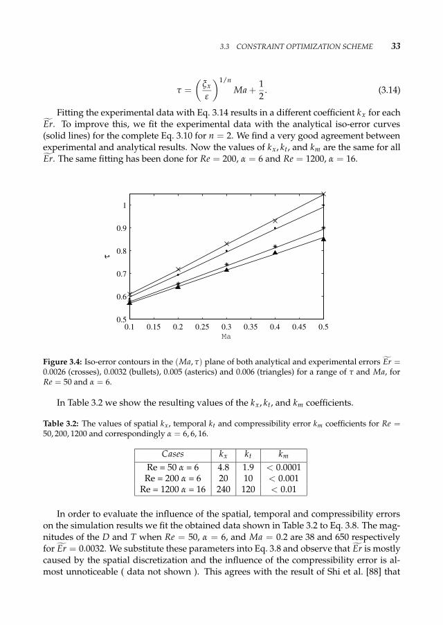
12 . (3.14)
Fitting the experimental data with Eq. 3.14 results in a different coefficient kx for eachEr. To improve this, we fit the experimental data with the analytical iso-error curves(solid lines) for the complete Eq. 3.10 for n = 2. We find a very good agreement betweenexperimental and analytical results. Now the values of kx, kt, and km are the same for allEr. The same fitting has been done for Re = 200, α = 6 and Re = 1200, α = 16.
0.1 0.15 0.2 0.25 0.3 0.35 0.4 0.45 0.50.5
0.6
0.7
0.8
0.9
1
Ma
τ
Figure 3.4: Iso-error contours in the (Ma, τ) plane of both analytical and experimental errors Er =0.0026 (crosses), 0.0032 (bullets), 0.005 (asterics) and 0.006 (triangles) for a range of τ and Ma, forRe = 50 and α = 6.
In Table 3.2 we show the resulting values of the kx, kt, and km coefficients.
Table 3.2: The values of spatial kx, temporal kt and compressibility error km coefficients for Re =50, 200, 1200 and correspondingly α = 6, 6, 16.
Cases kx kt kmRe = 50 α = 6 4.8 1.9 < 0.0001
Re = 200 α = 6 20 10 < 0.001Re = 1200 α = 16 240 120 < 0.01
In order to evaluate the influence of the spatial, temporal and compressibility errorson the simulation results we fit the obtained data shown in Table 3.2 to Eq. 3.8. The mag-nitudes of the D and T when Re = 50, α = 6, and Ma = 0.2 are 38 and 650 respectivelyfor Er = 0.0032. We substitute these parameters into Eq. 3.8 and observe that Er is mostlycaused by the spatial discretization and the influence of the compressibility error is al-most unnoticeable ( data not shown ). This agrees with the result of Shi et al. [88] that
34 EFFICIENT LBM FOR TIME HARMONIC FLOWS
the simulation error is almost not influenced by compressibility error. The results con-firm the second order behavior in time and space as demonstrated in [8, 60]. The valuesof km in the Table 3.2 are quite small and are the threshold ones, for higher values thefitting breaks down and for smaller ones it does not improve. We measured the standarddeviation of the fitting error and for this specific case they are small, e.g. for space dis-cretization it is approximately 0.006. This shows that we have a good agreement betweenanalytical and experimental results.
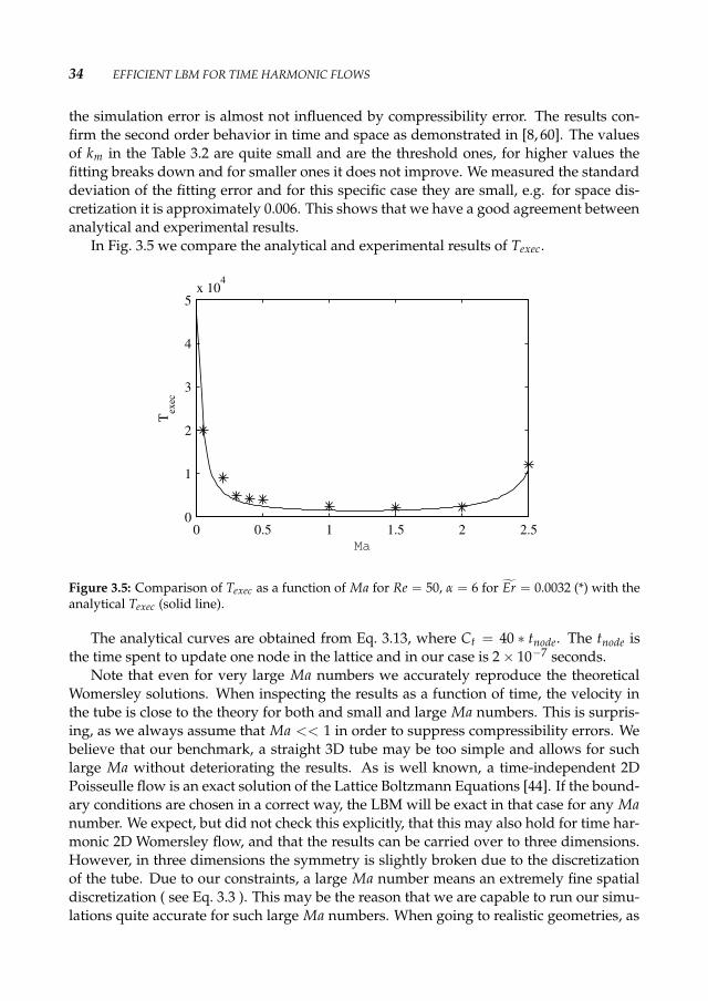
In Fig. 3.5 we compare the analytical and experimental results of Texec.
0 0.5 1 1.5 2 2.50
1
2
3
4
5x 10⁴
Ma
T exec
Figure 3.5: Comparison of Texec as a function of Ma for Re = 50, α = 6 for Er = 0.0032 (*) with theanalytical Texec (solid line).
The analytical curves are obtained from Eq. 3.13, where Ct = 40 ∗ tnode. The tnode isthe time spent to update one node in the lattice and in our case is 2 × 10⁻⁷ seconds.
Note that even for very large Ma numbers we accurately reproduce the theoreticalWomersley solutions. When inspecting the results as a function of time, the velocity inthe tube is close to the theory for both and small and large Ma numbers. This is surpris-ing, as we always assume that Ma << 1 in order to suppress compressibility errors. Webelieve that our benchmark, a straight 3D tube may be too simple and allows for suchlarge Ma without deteriorating the results. As is well known, a time-independent 2DPoisseulle flow is an exact solution of the Lattice Boltzmann Equations [44]. If the bound-ary conditions are chosen in a correct way, the LBM will be exact in that case for any Manumber. We expect, but did not check this explicitly, that this may also hold for time har-monic 2D Womersley flow, and that the results can be carried over to three dimensions.However, in three dimensions the symmetry is slightly broken due to the discretizationof the tube. Due to our constraints, a large Ma number means an extremely fine spatialdiscretization ( see Eq. 3.3 ). This may be the reason that we are capable to run our simu-lations quite accurate for such large Ma numbers. When going to realistic geometries, as

3.4 STABILITY OF TIME HARMONIC LBM SIMULATIONS 35
the aorta, we expect that we must keep the Ma number at more familiar values, i.e. < 1.Both plots in Fig. 3.5 have similar behavior, that is for a specific parameter set there
exists a minimum Texec. One should be aware of this behavior in order to chose optimalsimulation parameters with minimum Texec under the given constraints.
As a conclusion we confirm that using the constraint optimization scheme it is pos-sible to find a parameter set that gives the minimum Texec for a desired Er. Also in ourasymptotic error analysis we have shown the second order behavior of Er. From detailedcomparisons of experimental and analytical results we showed that the Ma − τ correla-tion is linear and observed that the error is not influenced by compressibility error. Thismay be due to the complete symmetry of the geometry, for real cases we expect to see arelevant influence of the compressibility error.
3.4 Stability of Time Harmonic LBM SimulationsNumerical stability of LBM has been studied by many authors e.g. [66, 76, 94, 120]. Thesestudies are mainly performed assuming uniform, time independent background flow.The stability of LBM depends on three conditions [94]. First, the relaxation time τ mustbe ≥ 0.5 corresponding to positive shear viscosity. Second, the mean flow velocity mustbe below a maximum stable velocity and third, as τ increases from 0.5 the maximumstable velocity increases monotonically until some fixed velocity is reached, which doesnot change for larger τ.
In our experiments we fix Ma (u = 0.1) and for a range of α we push Re to its highestpossible values by decreasing ν. Divergence of momentum profiles is considered to be adefinite sign of instability in the system. In order to have a large range of Re number wechose three different cases D = 24, 36, and 48.
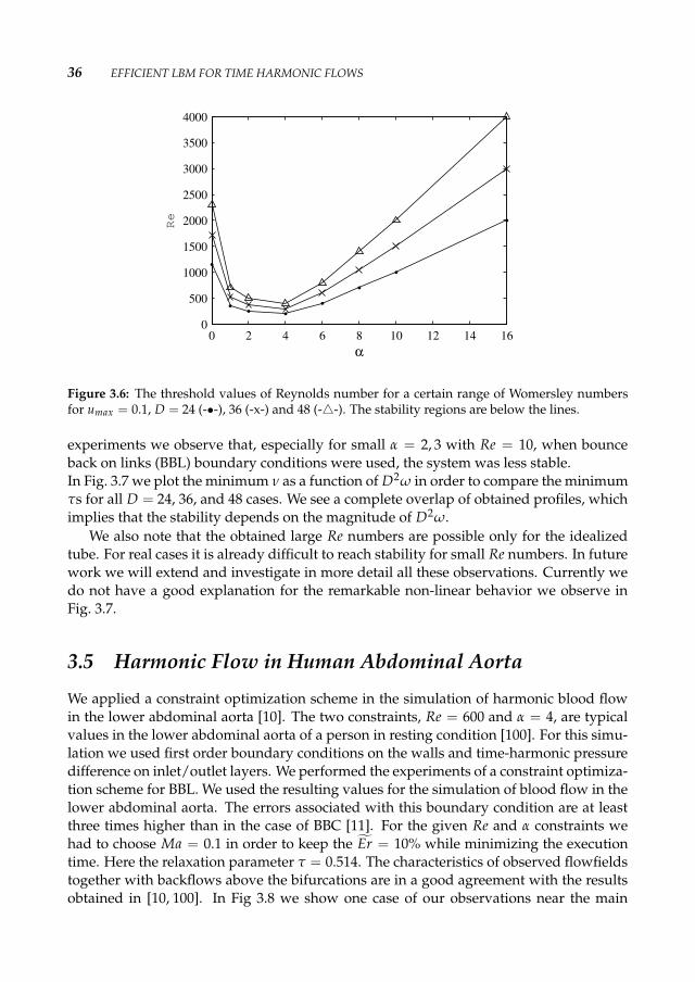
In Fig. 3.6 the highest attained Re numbers as a function of α are plotted. We observethe growth of the stability limit for Re with increasing α. As we can see from the plotsthe maximum Re we reached for static flows is 2300 for D = 48. This indicates that thesystem is still stable for τ = 0.506 and u = 0.1. This is comparable to the 2D resultsobtained by Lallemand and Luo [66].
The threshold values of Re for time-dependent flows are much higher, e.g. Re = 4000for D = 48 as α = 16.
It is known that the transition into turbulence appears at high Re numbers. The tran-sition starts at Reδ ∼ 850, where Reδ is the Reynold number based on the Stokes layerthickness [27]. Moreover, experimental results of Shemer [87] indicate that the thresholdvalue of transition into turbulence in a slowly pulsating pipe flow is Re = 4000. Theseresults confirm that we observe numerical instabilities in this laminar regime.
In the graph for larger values of α we see almost linear behavior. The interesting partis when the value of α is ≤ 6 while the viscous forces are dominating. Here the limitingmagnitude of Re can be quite small. This non-linear behavior for small values of α isremarkable and not understood at all.
With these measurements we confirm that for time-harmonic flows it is possible toreach high Re numbers especially with second order wall boundary conditions. From our
36 EFFICIENT LBM FOR TIME HARMONIC FLOWS
0 2 4 6 8 10 12 14 160
500
1000
1500
2000
2500
3000
3500
4000
α
Re
Figure 3.6: The threshold values of Reynolds number for a certain range of Womersley numbersfor umax = 0.1, D = 24 (-•-), 36 (-x-) and 48 (-4-). The stability regions are below the lines.
experiments we observe that, especially for small α = 2, 3 with Re = 10, when bounceback on links (BBL) boundary conditions were used, the system was less stable.In Fig. 3.7 we plot the minimum ν as a function of D2ω in order to compare the minimumτs for all D = 24, 36, and 48 cases. We see a complete overlap of obtained profiles, whichimplies that the stability depends on the magnitude of D2ω.
We also note that the obtained large Re numbers are possible only for the idealizedtube. For real cases it is already difficult to reach stability for small Re numbers. In futurework we will extend and investigate in more detail all these observations. Currently wedo not have a good explanation for the remarkable non-linear behavior we observe inFig. 3.7.
3.5 Harmonic Flow in Human Abdominal AortaWe applied a constraint optimization scheme in the simulation of harmonic blood flowin the lower abdominal aorta [10]. The two constraints, Re = 600 and α = 4, are typicalvalues in the lower abdominal aorta of a person in resting condition [100]. For this simu-lation we used first order boundary conditions on the walls and time-harmonic pressuredifference on inlet/outlet layers. We performed the experiments of a constraint optimiza-tion scheme for BBL. We used the resulting values for the simulation of blood flow in thelower abdominal aorta. The errors associated with this boundary condition are at leastthree times higher than in the case of BBC [11]. For the given Re and α constraints wehad to choose Ma = 0.1 in order to keep the Er = 10% while minimizing the executiontime. Here the relaxation parameter τ = 0.514. The characteristics of observed flowfieldstogether with backflows above the bifurcations are in a good agreement with the resultsobtained in [10, 100]. In Fig 3.8 we show one case of our observations near the main
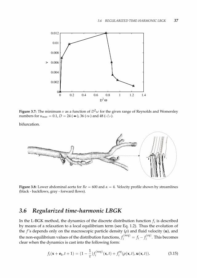
3.6 REGULARIZED TIME-HARMONIC LBGK 37
0 0.2 0.4 0.6 0.8 1 1.2 1.40
0.002
0.004
0.006
0.008
0.01
0.012
D2
ν
ω
Figure 3.7: The minimum ν as a function of D2ω for the given range of Reynolds and Womersleynumbers for umax = 0.1, D = 24 (-•-), 36 (-x-) and 48 (-4-).
bifurcation.
Figure 3.8: Lower abdominal aorta for Re = 600 and α = 4. Velocity profile shown by streamlines(black - backflows, gray - forward flows).
3.6 Regularized time-harmonic LBGKIn the L-BGK method, the dynamics of the discrete distribution function f i is describedby means of a relaxation to a local equilibrium term (see Eq. 1.2). Thus the evolution ofthe f ’s depends only on the macroscopic particle density (ρ) and fluid velocity (u), andthe non-equilibrium values of the distribution functions, f (neq)
i = fi − f (eq)i . This becomes
clear when the dynamics is cast into the following form:
fi(x + ei, t + 1) = (1 − 1τ
) f (neq)i (x, t) + f eq
i (ρ(x, t), u(x, t)). (3.15)
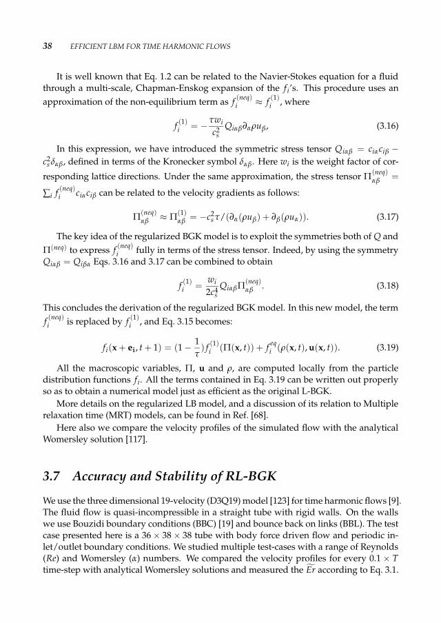
38 EFFICIENT LBM FOR TIME HARMONIC FLOWS
It is well known that Eq. 1.2 can be related to the Navier-Stokes equation for a fluidthrough a multi-scale, Chapman-Enskog expansion of the f i’s. This procedure uses anapproximation of the non-equilibrium term as f (neq)
i ≈ f (1)i , where
f (1)i = −τwi
c2sQiαβ∂αρuβ, (3.16)
In this expression, we have introduced the symmetric stress tensor Qiαβ = ciαciβ −c2
s δαβ, defined in terms of the Kronecker symbol δαβ. Here wi is the weight factor of cor-responding lattice directions. Under the same approximation, the stress tensor Π
(neq)αβ =
∑i f (neq)i ciαciβ can be related to the velocity gradients as follows:
Π(neq)αβ ≈ Π
(1)αβ = −c2
s τ/(∂α(ρuβ) + ∂β(ρuα)). (3.17)
The key idea of the regularized BGK model is to exploit the symmetries both of Q andΠ(neq) to express f (neq)
i fully in terms of the stress tensor. Indeed, by using the symmetryQiαβ = Qiβα Eqs. 3.16 and 3.17 can be combined to obtain
f (1)i =
wi2c4s
QiαβΠ(neq)αβ . (3.18)
This concludes the derivation of the regularized BGK model. In this new model, the termf (neq)i is replaced by f (1)
i , and Eq. 3.15 becomes:
fi(x + ei, t + 1) = (1 − 1τ
) f (1)i (Π(x, t)) + f eq
i (ρ(x, t), u(x, t)). (3.19)
All the macroscopic variables, Π, u and ρ, are computed locally from the particledistribution functions fi. All the terms contained in Eq. 3.19 can be written out properlyso as to obtain a numerical model just as efficient as the original L-BGK.
More details on the regularized LB model, and a discussion of its relation to Multiplerelaxation time (MRT) models, can be found in Ref. [68].
Here also we compare the velocity profiles of the simulated flow with the analyticalWomersley solution [117].
3.7 Accuracy and Stability of RL-BGKWe use the three dimensional 19-velocity (D3Q19) model [123] for time harmonic flows [9].The fluid flow is quasi-incompressible in a straight tube with rigid walls. On the wallswe use Bouzidi boundary conditions (BBC) [19] and bounce back on links (BBL). The testcase presented here is a 36 × 38 × 38 tube with body force driven flow and periodic in-let/outlet boundary conditions. We studied multiple test-cases with a range of Reynolds(Re) and Womersley (α) numbers. We compared the velocity profiles for every 0.1 × Ttime-step with analytical Womersley solutions and measured the Er according to Eq. 3.1.
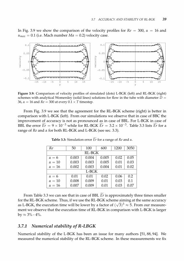
3.7 ACCURACY AND STABILITY OF RL-BGK 39
In Fig. 3.9 we show the comparison of the velocity profiles for Re = 300, α = 16 andumax = 0.1 (i.e. Mach number Ma = 0.2) velocity case.
-15 -10 -5 0 5 10 15y
-0.1
-0.05
0
0.05
0.1
velocity
-15 -10 -5 0 5 10 15y
-0.1
-0.05
0
0.05
0.1
velocity
Figure 3.9: Comparison of velocity profiles of simulated (dots) L-BGK (left) and RL-BGK (right)schemes with analytical Womersley (solid lines) solutions for flow in the tube with diameter D =36, α = 16 and Re = 300 at every 0.1 × T timestep.
From Fig. 3.9 we see that the agreement for the RL-BGK scheme (right) is better incomparison with L-BGK (left). From our simulations we observe that in case of BBC theimprovement of accuracy is not as pronounced as in case of BBL. For L-BGK in case ofBBL the error Er = 9 × 10⁻³ while for RL-BGK Er = 3.2 × 10⁻³. Table 3.3 lists Er for arange of Re and α for both RL-BGK and L-BGK (see sec. 3.3).
Table 3.3: Simulation error Er for a range of Re and α.
Re 50 100 600 1200 3050RL-BGK
α = 6 0.003 0.004 0.005 0.02 0.05α = 10 0.003 0.003 0.005 0.01 0.03α = 16 0.002 0.003 0.004 0.01 0.02
L-BGKα = 6 0.01 0.01 0.02 0.06 0.2α = 10 0.008 0.009 0.01 0.03 0.1α = 16 0.007 0.009 0.01 0.03 0.07
From Table 3.3 we can see that in case of BBL Er is approximately three times smallerfor the RL-BGK scheme. Thus, if we use the RL-BGK scheme aiming at the same accuracyas L-BGK, the execution time will be lower by a factor of (
√3)3 ≈ 5. From our measure-
ment we observe that the execution time of RL-BGK in comparison with L-BGK is largerby ≈ 3% - 4%.
3.7.1 Numerical stability of R-LBGKNumerical stability of the L-BGK has been an issue for many authors [51, 88, 94]. Wemeasured the numerical stability of the RL-BGK scheme. In these measurements we fix
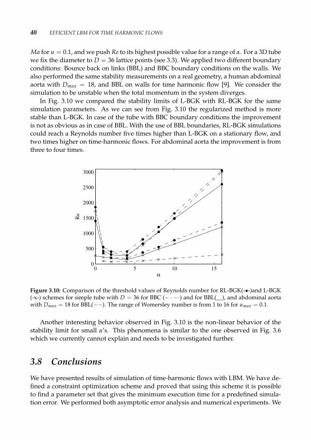
40 EFFICIENT LBM FOR TIME HARMONIC FLOWS
Ma for u = 0.1, and we push Re to its highest possible value for a range of α. For a 3D tubewe fix the diameter to D = 36 lattice points (see 3.3). We applied two different boundaryconditions: Bounce back on links (BBL) and BBC boundary conditions on the walls. Wealso performed the same stability measurements on a real geometry, a human abdominalaorta with Dmax = 18, and BBL on walls for time harmonic flow [9]. We consider thesimulation to be unstable when the total momentum in the system diverges.
In Fig. 3.10 we compared the stability limits of L-BGK with RL-BGK for the samesimulation parameters. As we can see from Fig. 3.10 the regularized method is morestable than L-BGK. In case of the tube with BBC boundary conditions the improvementis not as obvious as in case of BBL. With the use of BBL boundaries, RL-BGK simulationscould reach a Reynolds number five times higher than L-BGK on a stationary flow, andtwo times higher on time-harmonic flows. For abdominal aorta the improvement is fromthree to four times.
0 5 10 150
500
1000
1500
2000
2500
3000
α
Re
Figure 3.10: Comparison of the threshold values of Reynolds number for RL-BGK(-•-)and L-BGK(-x-) schemes for simple tube with D = 36 for BBC (− · −·) and for BBL(__), and abdominal aortawith Dmax = 18 for BBL(−−). The range of Womersley number is from 1 to 16 for umax = 0.1.
Another interesting behavior observed in Fig. 3.10 is the non-linear behavior of thestability limit for small α’s. This phenomena is similar to the one observed in Fig. 3.6which we currently cannot explain and needs to be investigated further.
3.8 ConclusionsWe have presented results of simulation of time-harmonic flows with LBM. We have de-fined a constraint optimization scheme and proved that using this scheme it is possibleto find a parameter set that gives the minimum execution time for a predefined simula-tion error. We performed both asymptotic error analysis and numerical experiments. We
3.8 CONCLUSIONS 41
conclude that the simulation error is hardly influenced by compressibility error. Fromstability measurements of the system, we found a unique dependence of the minimumallowed viscosity as a function of D2ω. This needs further study. Finally, we applied theconstraint optimization scheme on our simulations of blood flow in the lower abdomi-nal aorta. We have performed examinations of flow profiles and showed a qualitativeagreement with experimental results.
We also have presented numerical simulation results of time-harmonic Womersleyflow in a 3D tube by applying the regularized L-BGK scheme. We compared the velocityprofiles from simulations with the analytical Womersley solution. We showed that the ac-curacy associated with RL-BGK is higher than with L-BGK by comparing the simulationerrors. This implies that if we use the RL-BGK scheme with the same accuracy as L-BGKthe execution time will decrease significantly (see Table 3.3). We also presented the stabil-ity measurements for the RL-BGK scheme where we reached higher Reynolds numbersthan in case of the L-BGK scheme. For a 3D time-harmonic flow we achieved three tofive times higher Reynolds numbers which is comparable with the results obtained inRef. [68] for 2D cavity flow. The algorithm can be used to more efficiently calculate 3Dtime-harmonic flows like blood flow in abdominal aorta.

High Performance Lattice BoltzmannComputing∗
4.1 IntroductionThe lattice Boltzmann method (LBM) is a well established scheme in ComputationalFluid Dynamics (CFD) [22, 97, 123] and has proven to be a promising and reliable solverfor fluid flow simulations in complex geometries such as porous media, fissured rocksand geometries from medical applications [9, 10, 24, 26–28, 34, 56, 63]. However, for suchlarge and complex geometries the simulations are known to be computationally inten-sive. This is why there is an ongoing interest towards optimal LBM simulation codes andefficient parallelization strategies [11, 32, 33, 57, 58, 67, 69, 78, 85, 105, 113]. Key to achievean optimum in parallel performance is the correct choice of the domain decompositionmethod, to preserve the workload balance and to minimize the interprocessor communi-cations.
A new LBM approach based on sparse matrix linear algebra is proposed by Schulzet al. [85]. Here the computational domain is mapped on an unstructured grid, wherethe geometrical ordering of nodes is rearranged and a new index list of only fluid nodesis composed. Thus each fluid node has an adjacency index list of its neighboring fluidnodes, while the solid nodes are completely eliminated. This method requires storageof three one-dimensional arrays: two for density distributions (as a double buffering isused) and the other one for neighbor node indices. Next, domain decomposition has beenperformed for this scheme by using the METIS partitioning library [5, 61, 62]. With thisparallelized sparse-LBM approach memory consumption is essentially minimized and ahighly optimized parallel performance can be achieved.
In this chapter we extend this initial parallelized sparse-LBM approach by performingdetailed analysis of domain decomposition methods within the METIS library and theircomparison to a one-dimensional decomposition. This is done in terms of estimationof the number of edge-cuts (to find the amount of data that needs to be communicatedbetween processors) and an estimation of the amount of fluid nodes per processors (to
∗This chapter is based on: L. Axner, J. Bernsdorf, T. Zeiser, P. Lammers, J. Linxweiler and A.G. HoekstraPerformance evaluation of a parallel sparse Lattice Boltzmann solver (submitted for publication in J. of Comp.Phys.)
43
44 HIGH PERFORMANCE LATTICE BOLTZMANN COMPUTING
assess the load imbalance). Further we analyze performance results in terms of paral-lel scalability, and find the sources of loss of parallel efficiency, as well as predict thebehavior of the solver for other geometries and/or on other systems using a detailedperformance prediction model. This model includes both details of the parallel architec-ture (single node performance, point-to-point communication) and details of the domaindecomposition. The sources of loss of efficiency are estimated in terms of fractional over-head functions [37, 38].
In section 4.2 we give a short overview of our sparse-LB implementation, section 4.3describes the general idea behind partitioning methods. In section 4.4 we develop theperformance prediction model and in section 4.5 we show the results of the parallel per-formance on different machine architectures and compare with the scalability predictionmodel. In section 4.6 we present our conclusions.
4.2 Sparse LB ImplementationThe lattice Boltzmann method is said to be very efficient and easy to implement. But inmost cases, a simple full matrix implementation is used, where not only the fluid andboundary nodes, but also the solid fraction is allocated in computer memory. Dependingon the geometry, this is a considerable waste of resources, and also of CPU-cycles due tothe long loops over solid nodes in order to reach the fluid ones. In the framework of asimple full-matrix implementation, the density distribution array for the whole boundingbox is allocated in memory. This results in 2 ∗ 19 ∗ lx ∗ ly ∗ lz REAL numbers for the D3Q19model for a lx ∗ ly ∗ lz lattice [18, 112].
Well-known methods from sparse matrix linear algebra were first applied to the latticeBoltzmann method by Schulz et al. [85]. Here the storage of the density distribution isonly for the fluid nodes and thus the complete domain is mapped on an unstructuredgrid. Instead of geometrical ordering of those fluid nodes, a new index list is composed,where each node has the index list of its neighboring fluid nodes. In this method all datais stored in 1D arrays, where only 2 ∗ N ∗ 19 REAL numbers are stored for the densitydistribution (N is the number of fluid nodes) and N ∗ 18 INTEGERs for the adjacency list.This approach allows to save a considerable amount of memory.
4.3 The Graph Partitioning AlgorithmsThe goal of the graph partitioning algorithms is to partition large and complex graphssuch that the edge-cut is minimized (and thus the related communication overhead)while trying to keep the number of nodes on the sub graphs as balanced as possible(thus minimizing load imbalance). In sparse LBM the computational domain is mappedon a graph, where graph vertexes represent the fluid nodes and edges are the links con-necting the fluid nodes. From this graph the 1D array of fluid nodes and adjacency indexlist, as described in section 4.2, are constructed.
In previous studies, the METIS graph partitioning library was used to compute par-titions from the graphs [33, 85]. However, in neither of these studies one can find in-

4.4 THE PERFORMANCE PREDICTION MODEL 45
formation or an evident objective for the chosen function from the multiple partitioningfunctions of METIS.
The METIS partitioning library contains different functions for graph and mesh par-titioning. METIS reduces the size of the original graph by collapsing vertices and edges,partitions a smaller graph and then uncoarsens it to construct a partition for the origi-nal graph [5, 61, 62]. In this way it produces high quality partitions and in addition isextremely fast. The partitioning functions are mainly based on the combination of twoalgorithms: modified Kernighan-Lin and Fiduccia-Mattheyses.
The Kernighan-Lin starts with an initial bipartition of the reduced size graph suchthat each half contains roughly half of the weight of the original graph and each furtheriteration it searches a subset of vertices/nodes from each part of the graph, such that theirswapping will create a partition with smaller edge-cut [62]. The algorithm continues untilit cannot find any two such subsets. The Kernighan-Lin algorithm takes O(|E|log|E|) timewhile Fiduccia-Mattheyses takes O(E) [61], where E is the number of edge-cuts.
Fiduccia-Mattheyses can work with multiple partitions instead of two. The mainachievement of this algorithm is its ability of analyzing the effect of moving a singlevertex. That is, it can compute the change of the number of edge-cuts, caused by themovement of the current vertex from one partition to another, which is called gain. Thealgorithm repeats by selecting the vertex with the largest gain from the larger partitionand moves it to another partition. To prevent the same vertex from moving in the samedirection the algorithm marks the vertex [62].
In METIS the Kernighan-Lin partitioning algorithm is modified by the gain comput-ing quality of the Fiduccia-Mattheyses algorithm. Moreover, the coarsening, partitioningand uncoarsening phases are also enhanced with a number of improvements. Thus, de-pending on the demands of the fluid flow solver one can adjust the parameters of thepartitioning functions to achieve an approximate balance between maximum load bal-ance and minimum communication amount. Moreover, METIS allows to use a (heavily)weighted graph, i.e. a graph with labels on nodes and/or edges, to strengthen the differ-ent features of partitions. The weights on edges of the graph can be used to strengthenthe connection between nodes thus to help to minimize the communication amounts. Theweights on the nodes can be used to strictly preserve the load balance between partitions.
We use two different functions of the METIS partitioning library: Multilevel K-wayand Multilevel Recursive Bisectioning (RB). The difference is that the multilevelRB ap-proach computes a k-way partitioning by performing recursive bisectioning on all phasesof the multilevel graph partitioning. On the other hand, the multilevelK − way performscoarsening only once, then the coarsest graph is directly partitioned into k parts andfinally the uncoarsening phase is also performed only once, during which a k-way parti-tioning refinement algorithm is applied to improve the quality of the partitions [62].
4.4 The Performance Prediction ModelIn order to analyze the parallel scalability of the sparse LB solver and to find the sources ofloss of parallel efficiency we develop a performance prediction model. Using this model
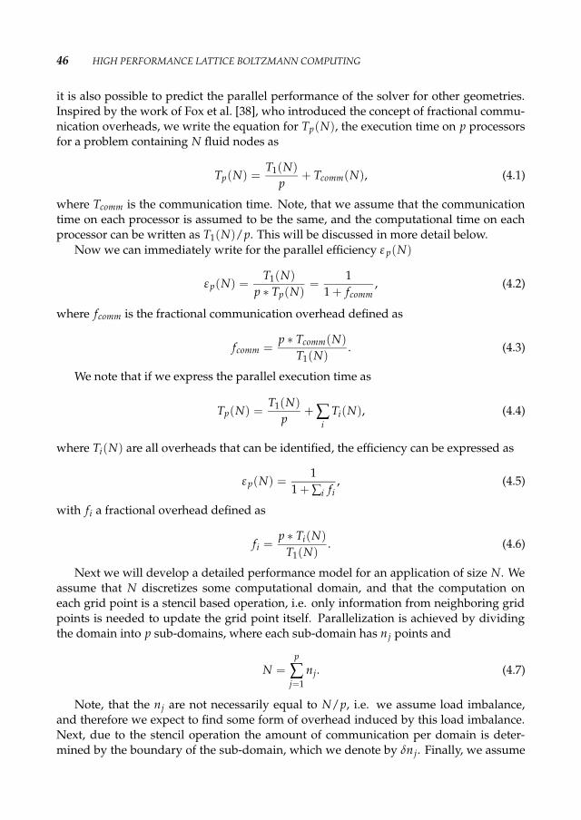
46 HIGH PERFORMANCE LATTICE BOLTZMANN COMPUTING
it is also possible to predict the parallel performance of the solver for other geometries.Inspired by the work of Fox et al. [38], who introduced the concept of fractional commu-nication overheads, we write the equation for Tp(N), the execution time on p processorsfor a problem containing N fluid nodes as
Tp(N) =T1(N)
p + Tcomm(N), (4.1)
where Tcomm is the communication time. Note, that we assume that the communicationtime on each processor is assumed to be the same, and the computational time on eachprocessor can be written as T1(N)/p. This will be discussed in more detail below.
Now we can immediately write for the parallel efficiency ε p(N)
ε p(N) =T1(N)
p ∗ Tp(N)=
11 + fcomm
, (4.2)
where fcomm is the fractional communication overhead defined as
fcomm =p ∗ Tcomm(N)
T1(N). (4.3)
We note that if we express the parallel execution time as
Tp(N) =T1(N)
p + ∑i
Ti(N), (4.4)
where Ti(N) are all overheads that can be identified, the efficiency can be expressed as
ε p(N) =1
1 + ∑i fi, (4.5)
with fi a fractional overhead defined as
fi =p ∗ Ti(N)
T1(N). (4.6)
Next we will develop a detailed performance model for an application of size N. Weassume that N discretizes some computational domain, and that the computation oneach grid point is a stencil based operation, i.e. only information from neighboring gridpoints is needed to update the grid point itself. Parallelization is achieved by dividingthe domain into p sub-domains, where each sub-domain has n j points and
N =p
∑j=1
nj. (4.7)
Note, that the nj are not necessarily equal to N/p, i.e. we assume load imbalance,and therefore we expect to find some form of overhead induced by this load imbalance.Next, due to the stencil operation the amount of communication per domain is deter-mined by the boundary of the sub-domain, which we denote by δn j. Finally, we assume

4.4 THE PERFORMANCE PREDICTION MODEL 47
that the total execution time per processor is determined by computation on the domainnj followed by communication on the boundary δn j. This means that we exclude fornow the possibility of latency hiding (a technique that may improve the performance alot, and that could be considered when the fractional communication overheads becomelarge) [115].
Now call tj the execution time on processor j and write this as a summation of com-putation time (tcomp) and communication time (tcomm).
tj = tcomp(nj) + tcomm(δnj) (4.8)
The execution time on p processors is now determined by the slowest processor, i.e.
Tp(N) = maxj{tj}, (4.9)
andT1(N) = tcomp(N). (4.10)
Without any further assumption write
Tp(N) =tcomp(N)
p + maxj{tj} −tcomp(N)
p , (4.11)
andε p(N) =
11 + f (4.12)
with a single fractional overhead defined as
f =p ∗ maxj{tj}
tcomp(N)− 1. (4.13)
To proceed we need to find approximations for Tp(N). We define an upper bound tothe execution time and use it as an approximation written as
Tp(N) = maxj{tj} ≤ maxj{tcomp(nj)} + maxj{tcomm(δnj)} (4.14)
The computational time is linear in the number of grid points. If we call τcomp the timerequired to execute one grid point, and realize that due to caching and memory layout ofthe data τcomp actually depends on the number of grid points we find that
tcomp(n) = n ∗ τcomp(n). (4.15)
For communication we assume a linear model for point-to-point communication, i.e.to send m density distributions requires a time τsetup + m ∗ τsend. τsetup is the time neededto initialize the communication and τsend is the time needed to send one byte of informa-tion. Each processor j will sent and receive data to and from d j other processors. Thisnumber dj depends on the details of the partitioning of the computational domain. Toeach of the dj processors an amount of ejk density distributions (with k = 1 . . . d j and 8

48 HIGH PERFORMANCE LATTICE BOLTZMANN COMPUTING
bytes per distribution) is communicated. Moreover, the total number of grid points thatare sent to other processors is the edge-cut e j (in bytes) which is
ej =
dj
∑k=1
ejk. (4.16)
In stencil based operations the communication is always an exchange operation, thatis, an amount of data is sent to a processor, and the same amount is received back again.We assume that this is implemented as two synchronous blocking point-to-point com-munication routines. With all these definitions we can now write a closed expression forthe communication time from processor j as
tcomm(δnj) = 2dj
∑k=1
(τsetup + ejkτsend) = 2djτsetup + 2ejτsend. (4.17)
We assumed that the point-to-point communication between any pair of processors in aparallel computer is equal. In section 4.5 we will refine this further, by distinguishingbetween two types of point-to-point communication.
From the partitioning tool METIS we can get all information, for each processor, onthe number of nodes nj, the degree of connectivity d j and the edge-cut ej.
With all these definitions we finally find
Tp(N) = nmaxτ(nmax) + maxj{2djτsetup + 2ejτsend} (4.18)
By casting Eq. 4.18 in the form of Eq. 4.4 we find
Tp(N) =Np τ(N) + nmaxτ(nmax) −
Np τ(N) + maxj{2djτsetup + 2ejτsend} (4.19)
The last term in Eq. 4.19 is due to communication and gives rise to a fractional com-munication overhead, just like in Eq. 4.3. The second and third terms are in fact a mixof two effects, namely load imbalance and the potential change of the speed of a singleprocessors due to the partitioning. We can separate them by writing
nmaxτ(nmax) −Np τ(N) = nmax(τ(nmax) − τ(N)) + τ(N)
(nmax −
Np
)(4.20)
Now the processor speed effect and load imbalance are clearly separated. The firstterm on the right hand side of Eq. 4.20 is due to the processor speed effect, whereas thesecond is due to load imbalance.
This means that we find three fractional overheads:
• a fractional communication overhead
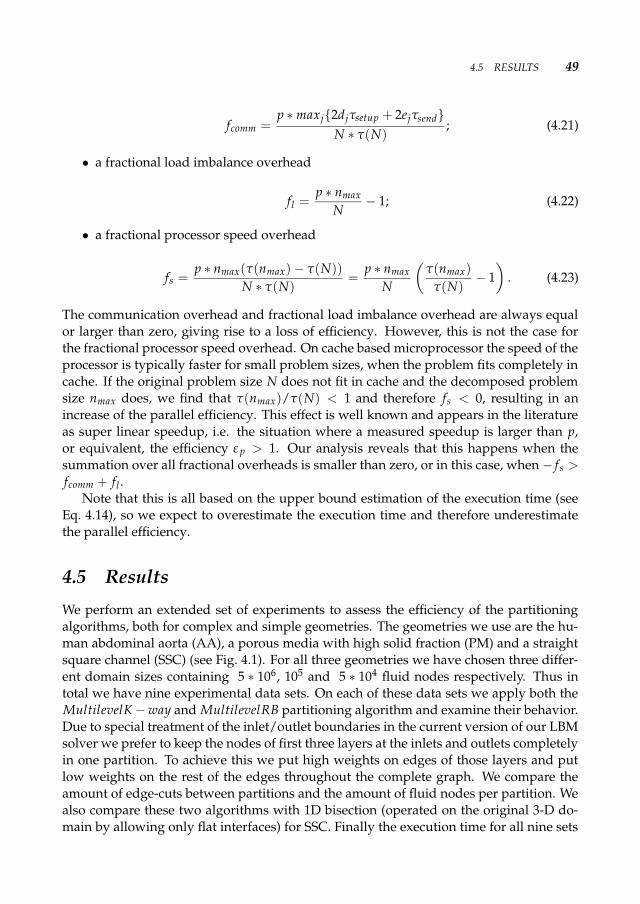
4.5 RESULTS 49
fcomm =p ∗ maxj{2djτsetup + 2ejτsend}
N ∗ τ(N); (4.21)
• a fractional load imbalance overhead
fl =p ∗ nmax
N − 1; (4.22)
• a fractional processor speed overhead
fs =p ∗ nmax(τ(nmax) − τ(N))
N ∗ τ(N)=
p ∗ nmaxN
(τ(nmax)
τ(N)− 1
). (4.23)
The communication overhead and fractional load imbalance overhead are always equalor larger than zero, giving rise to a loss of efficiency. However, this is not the case forthe fractional processor speed overhead. On cache based microprocessor the speed of theprocessor is typically faster for small problem sizes, when the problem fits completely incache. If the original problem size N does not fit in cache and the decomposed problemsize nmax does, we find that τ(nmax)/τ(N) < 1 and therefore fs < 0, resulting in anincrease of the parallel efficiency. This effect is well known and appears in the literatureas super linear speedup, i.e. the situation where a measured speedup is larger than p,or equivalent, the efficiency ε p > 1. Our analysis reveals that this happens when thesummation over all fractional overheads is smaller than zero, or in this case, when − f s >
fcomm + fl .Note that this is all based on the upper bound estimation of the execution time (see
Eq. 4.14), so we expect to overestimate the execution time and therefore underestimatethe parallel efficiency.
4.5 ResultsWe perform an extended set of experiments to assess the efficiency of the partitioningalgorithms, both for complex and simple geometries. The geometries we use are the hu-man abdominal aorta (AA), a porous media with high solid fraction (PM) and a straightsquare channel (SSC) (see Fig. 4.1). For all three geometries we have chosen three differ-ent domain sizes containing 5 ∗ 106, 105 and 5 ∗ 104 fluid nodes respectively. Thus intotal we have nine experimental data sets. On each of these data sets we apply both theMultilevelK − way and MultilevelRB partitioning algorithm and examine their behavior.Due to special treatment of the inlet/outlet boundaries in the current version of our LBMsolver we prefer to keep the nodes of first three layers at the inlets and outlets completelyin one partition. To achieve this we put high weights on edges of those layers and putlow weights on the rest of the edges throughout the complete graph. We compare theamount of edge-cuts between partitions and the amount of fluid nodes per partition. Wealso compare these two algorithms with 1D bisection (operated on the original 3-D do-main by allowing only flat interfaces) for SSC. Finally the execution time for all nine sets

50 HIGH PERFORMANCE LATTICE BOLTZMANN COMPUTING
of data is measured on two different platforms: a NEC SX-8 vector machine [1] (the char-acteristics are given in Table 4.1), and a PC cluster [2] (the characteristics are given in Ta-ble 4.2), using from 1 up to 128 processors. In order to be able to compare the results withthe performance prediction model and to find the sources of loss of parallel efficiency, weneed first to evaluate the basic parameters connected with the parallel architecture (singlenode performance, point-to-point communication) and with the parallel decomposition(load imbalance, edge-cuts, degree distribution).
Figure 4.1: (a)- Abdominal aorta, (b) - porous media, (c) - straight square channel.
Table 4.1: NEC SX-8 specifications (see: http://www.hpce.nec.com/).
Multi-Node Single-Node2-512 nodes 1 nodeSX-8R/M SX-8R/A SX-8R/BCentral Processing Unit
Number of CPUs 8 - 4096 4 - 8 1 - 4Logical Peak Perf. 299.2GF - 153.1TF 149.6GF - 299.2GF 37.4GF - 149.6GFVector Peak Perf. 281.6GF - 144TF 35.2GF - 140.8GF 35.2GF - 281.6GF
Main Memory UnitMemory Archit. Shared and Distr. SharedCapacity 64GB - 128TB 32GB - 256GB 32GB - 128GBPeak Data Transf. Rate 288TB/s 563.2 GB/s 281.6 GB/s
Internode Crossbar Switch (IXS)Pear Data Transf. Rate 16GB/s per node bi-directional -

4.5 RESULTS 51
Table 4.2: Specifications of the 2IntelXeonTM Lisa cluster (see:http://www.sara.nl/userinfo/lisa/description/index.html/).
Compute nodes 680Number Memory L2 cache InfiniBand
255 4GB 2MB Yes260 2GB 1MB Yes165 4GB 2MB No
Speed 3.4 GHzMemory Extended Memory 64 Technology (EM64T)Total Peak Performance 8.5 TF/sDisk Space 15 TB SGI Infinite Storage TP9300S disk array for home file system
Topspin’s InfiniBand NetworkBandwidth 800 MB/sLatency <6 µsec
4.5.1 Basic parameters1. Single processor speed - We first measure tcomp(N) by running multiple simula-
tions with a sufficient range of data sizes on a single processor and using Eq. 4.15to extract τcomp(N). Our experimental results (Fig. 4.2) show that on the PC clus-ter τcomp(N) is almost constant if N < 5 ∗ 103 and N > 105 and increases in be-tween. Thus we have divided the complete set of measurements into three regions.For small and large values of N, τcomp(N) is assumed to be constant, and in themiddle region we assume that τcomp(N) depends linearly on N. As mentioned insection 4.4, τcomp(N) depends on the cache size of a specific processor. For the PCcluster the cache size is 1Mbyte. From our computations we know that the memoryconsumption per lattice node is 2 ∗ 8 ∗ 19 = 304 bytes (for 19 distributions). Thus ifthe number of lattice nodes per processor is N < 3 ∗ 103, the data will completelyfit into cache.It is well-known that vector machines such as the NEC SX-8 perform best for largedata sizes. The experimental results show a rather smooth decrease of τcomp(N) asN increases. Assume that the execution time depends linearly on N (e.g. a constanttime to fill up the vector units, and then a time proportional to N to produce allresults), then the execution time can be written as a ∗ N + b. Using Eq. 4.15 we findτcomp(N) = a + b/N, and this function we use to fit the measurements.In Fig. 4.2 and 4.3 we have plotted τcomp(N) for the LBM solver on a single processoras a function of the number of fluid nodes for PC cluster and the NEC SX-8 machinerespectively. We see a good agreement between measurements, together with thefitting results. A clear discontinuity due to the cache size for the PC cluster at N =
3 ∗ 103 data size can be observed. In Fig. 4.3 we clearly see that the bigger theproblem size the better the performance. We have fitted the experimental results tothe models as described above, and the results are summarized in Table 4.3.In the figures, the seemingly misfit of measurements and fitting results betweenN = 3 ∗ 103 and N = 105 data sizes is due to the linear interpolations.
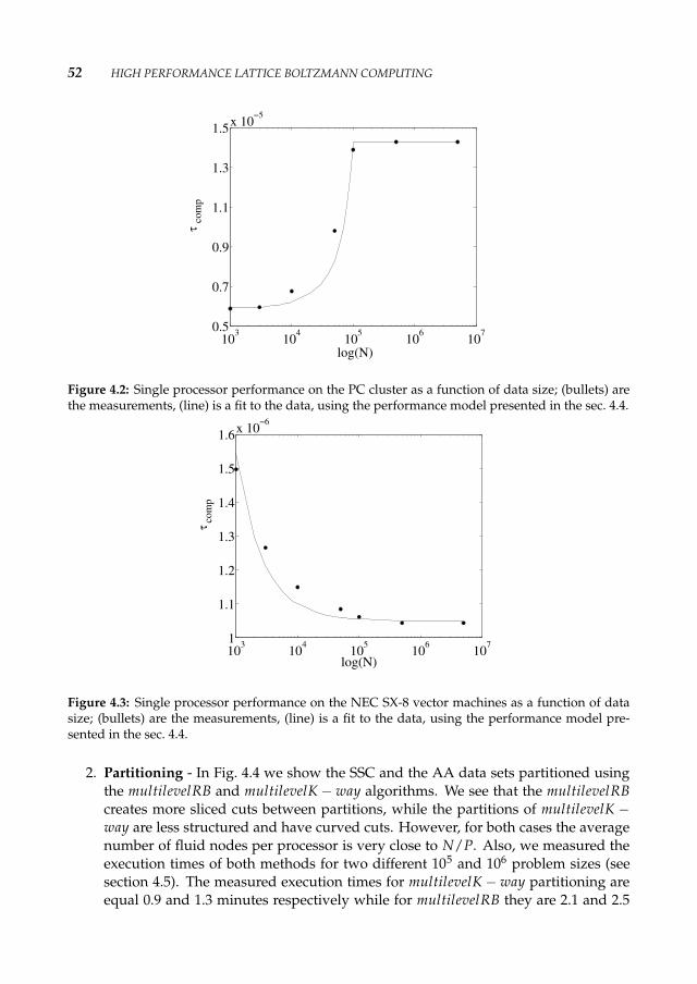
52 HIGH PERFORMANCE LATTICE BOLTZMANN COMPUTING
103 104 105 106 1070.5
0.7
0.9
1.1
1.3
1.5x 10⁻⁵
log(N)
τco
mp
Figure 4.2: Single processor performance on the PC cluster as a function of data size; (bullets) arethe measurements, (line) is a fit to the data, using the performance model presented in the sec. 4.4.
103 104 105 106 1071
1.1
1.2
1.3
1.4
1.5
1.6x 10⁻⁶
log(N)
τ com
p
Figure 4.3: Single processor performance on the NEC SX-8 vector machines as a function of datasize; (bullets) are the measurements, (line) is a fit to the data, using the performance model pre-sented in the sec. 4.4.
2. Partitioning - In Fig. 4.4 we show the SSC and the AA data sets partitioned usingthe multilevelRB and multilevelK − way algorithms. We see that the multilevelRBcreates more sliced cuts between partitions, while the partitions of multilevelK −way are less structured and have curved cuts. However, for both cases the averagenumber of fluid nodes per processor is very close to N/P. Also, we measured theexecution times of both methods for two different 105 and 106 problem sizes (seesection 4.5). The measured execution times for multilevelK − way partitioning areequal 0.9 and 1.3 minutes respectively while for multilevelRB they are 2.1 and 2.5

4.5 RESULTS 53
minutes (both executed on a single processor of a PC cluster).To get a better idea of the load imbalance, in Fig. 4.5 we have plotted the stan-dard deviation of the distribution of the number of fluid nodes on processors asa function of p. From the measurements of standard deviation we hardly observea difference between partitionings using multilevelRB and multilevelK − way onall geometries, except for SSC for a very large number of partitions. This is dueto the fact that multilevelRB performs bipartitioning along the shortest latitude ofthe geometry until it reaches the minimum possible number of layers per parti-tion and continues bipartitioning along the longitude which causes a high load im-balance for p = 128. For complex geometries we prefer to follow the advice ofKarypis et al. [62] and use multilevelRB for less than eight partitions while applymultilevelK − way for a larger number of partitions. Moreover, we have comparedthese algorithms with a 1D bisection and noted that both METIS algorithms per-formed better. That is, even though 1D bisectioning divides the domain into equalparts, after a certain number of partitions the deviation of number of fluid nodesper partition becomes quite high from the average number of fluid nodes per par-tition.
3. Point to point communication - This overhead depends on the specifics of the ma-chine architectures and the details of the edge-cut and degree of connectivity of thepartitions. Moreover, most modern machines have more than one processor pernode, and therefore we must also distinguish between on-board communication(with both processors on the same node) and off-board communication (betweenprocessors on different nodes). In our case this applies only to the NEC SX-8 whichhas eight processors per node.To measure the point-to-point communication we run a "pingpong"-type commu-nication with different data sizes between two processors. Next we fit the datato a linear function and obtain τsetup and τsend. The results are shown in Figs 4.6and 4.7. Moreover, in Fig. 4.7 we see a clear difference between communicationtimes for on-board and off-board measurements. Thus in our further predictionsfor the NEC SX-8 for p ≤ 8 we take the on-board values and for p > 8 the off-boardones. We also note that for N = 1Kbyte a discontinuity appears. This is a bufferingeffect in the MPI communication routines. From the fits we extract values of τsetupand τsend, which are shown in Table 4.4.Next we consider the edge-cuts per processor obtained from the partitioning algo-
Table 4.3: Single processor performance.Plat f orm N τcomp(N)(sec.)
< 3 ∗ 103 0.58 ∗ 10−5
PC cluster > 105 1.42 ∗ 10−5
Otherwise 0.58 ∗ 10−5 + 1.42∗10−5−0.58∗10−5
105−3∗103 ∗ (N − 3 ∗ 103)
NEC SX-8 For all data sizes 1.05 ∗ 10−6 + 4.95 ∗ 10−4/N
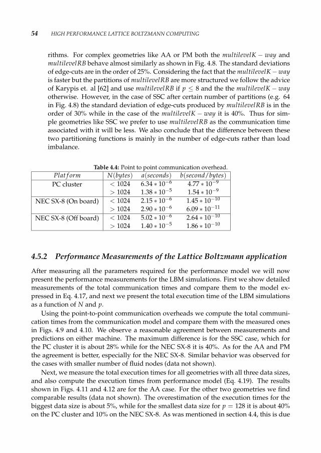
54 HIGH PERFORMANCE LATTICE BOLTZMANN COMPUTING
rithms. For complex geometries like AA or PM both the multilevelK − way andmultilevelRB behave almost similarly as shown in Fig. 4.8. The standard deviationsof edge-cuts are in the order of 25%. Considering the fact that the multilevelK −wayis faster but the partitions of multilevelRB are more structured we follow the adviceof Karypis et. al [62] and use multilevelRB if p ≤ 8 and the the multilevelK − wayotherwise. However, in the case of SSC after certain number of partitions (e.g. 64in Fig. 4.8) the standard deviation of edge-cuts produced by multilevelRB is in theorder of 30% while in the case of the multilevelK − way it is 40%. Thus for sim-ple geometries like SSC we prefer to use multilevelRB as the communication timeassociated with it will be less. We also conclude that the difference between thesetwo partitioning functions is mainly in the number of edge-cuts rather than loadimbalance.
Table 4.4: Point to point communication overhead.Plat f orm N(bytes) a(seconds) b(second/bytes)
< 1024 6.34 ∗ 10−6 4.77 ∗ 10−9PC cluster> 1024 1.38 ∗ 10−5 1.54 ∗ 10−9
< 1024 2.15 ∗ 10−6 1.45 ∗ 10−10NEC SX-8 (On board)> 1024 2.90 ∗ 10−6 6.09 ∗ 10−11
< 1024 5.02 ∗ 10−6 2.64 ∗ 10−10NEC SX-8 (Off board)> 1024 1.40 ∗ 10−5 1.86 ∗ 10−10
4.5.2 Performance Measurements of the Lattice Boltzmann applicationAfter measuring all the parameters required for the performance model we will nowpresent the performance measurements for the LBM simulations. First we show detailedmeasurements of the total communication times and compare them to the model ex-pressed in Eq. 4.17, and next we present the total execution time of the LBM simulationsas a function of N and p.
Using the point-to-point communication overheads we compute the total communi-cation times from the communication model and compare them with the measured onesin Figs. 4.9 and 4.10. We observe a reasonable agreement between measurements andpredictions on either machine. The maximum difference is for the SSC case, which forthe PC cluster it is about 28% while for the NEC SX-8 it is 40%. As for the AA and PMthe agreement is better, especially for the NEC SX-8. Similar behavior was observed forthe cases with smaller number of fluid nodes (data not shown).
Next, we measure the total execution times for all geometries with all three data sizes,and also compute the execution times from performance model (Eq. 4.19). The resultsshown in Figs. 4.11 and 4.12 are for the AA case. For the other two geometries we findcomparable results (data not shown). The overestimation of the execution times for thebiggest data size is about 5%, while for the smallest data size for p = 128 it is about 40%on the PC cluster and 10% on the NEC SX-8. As was mentioned in section 4.4, this is due
4.6 CONCLUSIONS 55
to the fact that all the computations of prediction model are based on the upper boundestimations.
We also plot in Figs. 4.13 and 4.14 the execution times in term of Lattice Updates persecond (LUP/s) for all data sizes on both architectures. In Fig. 4.13 we see the superlinear speed-up due to the "cache effect" on the PC cluster for the smallest geometrieswith 5 ∗ 104 fluid nodes. On NEC SX-8 (Fig. 4.14), as was expected, the best performancewe get for the largest data sizes, of almost 75% peak performance for 128 processors.
In Figs. 4.15 and 4.16 we show the efficiencies as a function of p. Here the under-estimation of the prediction model is approximately 4%. Thus the agreement betweenmeasurements and performance model is quite high. Also in Fig. 4.16 we see a steepdecline of efficiencies for the medium and small data sizes. This is due to the fact thaton vector machines for such small problem sizes we see more the single processor effect(as we partition the problem, the single processor performance goes down, see Fig. 4.3)and therefore a large positive fractional processor speed overhead (Eq. 4.23). For smallproblem sizes on the PC cluster the situation is reversed. Here the fractional processorspeed overhead is negative due to the caching effect, and we observe efficiencies muchlarger than one (see Fig. 4.15).
In Fig. 4.17 we have plotted fractional communication and fractional load imbalanceoverheads (Eqs. 4.21 and 4.22) as a function of p. From the plot it is clear that for large pthe loss of the efficiency due to the load imbalance can be as large as 18%, while the lossdue to communication is about 7% on the NEC SX-8 and 20% on the PC cluster. For asmall number of processors the fractional load imbalance overhead is negligible as com-pared to fractional communication overhead. Thus from Fig. 4.17 we conclude that for asmall number of processors the best way to improve the efficiency is the implementationof latency hiding [115] to decrease the communication overhead. For a large number ofprocessors we propose to use a better partitioning algorithm to improve the load balance.By comparing the fractional load imbalance overheads as a function of number of fluidnodes we also observed that the bigger the data size the easier it is to achieve good loadbalance (data not shown). Therefore we can try to extrapolate our results to much largerdata sizes. If we assume that the single processor speed overhead for large data sizes iszero, the point-to-point communication overhead decreases as 1/N2/3 and for a 108 datasize geometry we decrease the load imbalance by 10% we can achieve almost 95% peakperformance.
All these comparisons confirm that the performance model has a good accuracy andthat it is eligible for predicting the performance for any size/type of geometry, if oneknows the estimated fractional overheads.
4.6 ConclusionsIn this chapter we have developed a performance prediction model and tested it by com-paring the computed performance results with time complexity measurements of ourparallel sparse lattice Boltzmann solver. In order to interpret the results, we definedthree sources of parallel efficiency loss, i.e. fractional processor speed overhead, frac-
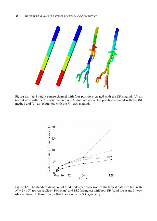
56 HIGH PERFORMANCE LATTICE BOLTZMANN COMPUTING
Figure 4.4: (a)- Straight square channel with four partitions created with the RB method, (b)- as(a) but now with the K − way method, (c)- Abdominal aorta, 128 partitions created with the RBmethod and (d)- as (c) but now with the K − way method.
048 16 32 64 1280
5
10
15
20
CPUs
Stan
dard
dev
iatio
n of
flui
d no
des (
%)
Figure 4.5: The standard deviation of fluid nodes per processor for the largest data size (i.e. withN = 5 ∗ 106) for AA (bullets), PM (stars) and SSC (triangles) with both RB (solid lines) and K-way(dashed lines). 1D bisection (dotted line) is only for SSC geometry.

4.6 CONCLUSIONS 57
100 102 104 106−6
−5
−4
−3
−2
log(N)
log(
t com
m)
Figure 4.6: Point-to-point communication time (seconds) as a function of data size (bytes) on thePC cluster. The bullets are the measured data and the solid line is a fit to the data.
100 102 104 106−6
−5.5
−5
−4.5
−4
−3.5
−3
log(N)
log(
t com
m)
Figure 4.7: Point-to-point communication time (seconds) as a function of data size (bytes) on theNEC SX-8 vector machines. Triangles are the measured off-board point-to-point communicationtimes, bullets are the measured on-board point-to-point communication times and the solid linesare the fit to the data.
tional communication overhead and fractional load imbalance overhead and measuredthem for all nine cases and two architecturally different supercomputers: a NEC SX-8vector machine and a PC cluster.
For the three different geometries with three different data sizes we have preformeda graph partitioning by using two different functions of the METIS graph partitioninglibrary. We compared the partitioning results and conclude that with simple geometries isit better to use the multilevelRB method rather than multilevelK −way, while for complexones the combination of both will give optimal solution [62].
The measurements show that for the largest data sizes we obtain almost 75% peak

58 HIGH PERFORMANCE LATTICE BOLTZMANN COMPUTING
048 16 32 64 1280
0.5
1
1.5
2
2.5x 10⁴
CPUs
Ave
rage
Edg
ecut
s
Figure 4.8: The average number of edge-cuts per processor for the largest data size(i.e. with N =5 ∗ 106) for AA(bullets), PM(stars)and SSC (triangles) with both RB (solid lines) and K-way (dashlines). 1D bisection (dotted line) is only for SSC geometry.
048 16 32 64 1281
1.5
2
2.5
3x 10⁻³
T com
m(s
ec)
CPUs
Figure 4.9: Total communication time as a function of p on the PC cluster for the largest geome-tries(i.e. with N = 5 ∗ 106). The solid lines are the measurements and the dashed lines are modelpredictions from Eq. 4.17. The bullets are for AA, the stars for PM and the triangles for SSC.
performance on NEC SX-8 vector machine. Moreover with the help of the performancemodel we estimate that the efficiency on the NEC SX-8 can be improved if one choosesmore robust partitioning algorithms as the efficiency loss for large p is mostly due to loadimbalance. The comparison of these measurements with prediction model gives us 5%error, which shows that the developed model can be used for scalability prediction ofparallel performance for any geometries.
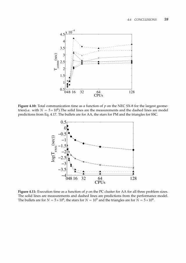
4.6 CONCLUSIONS 59
048 16 32 64 1280.5
1
1.5
2
2.5
3
3.5
4
4.5x 10⁻⁴
T com
m(s
ec)
CPUs
Figure 4.10: Total communication time as a function of p on the NEC SX-8 for the largest geome-tries(i.e. with N = 5 ∗ 106).The solid lines are the measurements and the dashed lines are modelpredictions from Eq. 4.17. The bullets are for AA, the stars for PM and the triangles for SSC.
048 16 32 64 128−4−3.5
−3−2.5
−2−1.5
−1−0.5
00.5
CPUs
log(
T exec
(sec
))
Figure 4.11: Execution time as a function of p on the PC cluster for AA for all three problem sizes.The solid lines are measurements and dashed lines are predictions from the performance model.The bullets are for N = 5 ∗ 106, the stars for N = 105 and the triangles are for N = 5 ∗ 104.

60 HIGH PERFORMANCE LATTICE BOLTZMANN COMPUTING
048 16 32 64 128−4−3.5
−3−2.5
−2−1.5
−1−0.5
00.5
CPUs
log(
T exec
)(sec
)
Figure 4.12: Execution time as a function of p on the NEC SX-8 vector machines for AA for allthree problem sizes. The solid lines are measurements and dashed lines are predictions from theperformance model. The bullets are for N = 5 ∗ 106, the stars for N = 105 and the triangles are forN = 5 ∗ 104.
048 16 32 64 1280
0.1
0.2
0.3
0.4
0.5
CPUs
GLU
P/s
Figure 4.13: Lattice Updates per second as a function of p on the PC cluster for N = 5 ∗ 106(solidlines), N = 105(dashed lines) and N = 5 ∗ 104(dotted lines). Bullets are AA, starts are PM andtriangles are SSC. The dotted line indicates the ideal peak performance.

4.6 CONCLUSIONS 61
048 16 32 64 1280
1
2
3
4
5
CPUs
GLU
P/s
Figure 4.14: Lattice Updates per second as a function of p on the NEC SX8 machines for N =5 ∗ 106(solid lines), N = 105(dashed lines) and N = 5 ∗ 104(dotted lines). The bullets are AA, thestarts are PM and the triangles are SSC. The dotted line indicates the ideal peak performance.
048 16 32 64 1280
0.5
1
1.5
2
2.5
CPUs
pε
Figure 4.15: Efficiencies as a function of p on the PC cluster. The solid lines are measurements anddashed lines are predictions from the performance model. The bullets are for N = 5 ∗ 106, the starsfor N = 105 and the triangles are for N = 5 ∗ 104.

62 HIGH PERFORMANCE LATTICE BOLTZMANN COMPUTING
048 16 32 64 1280
0.2
0.4
0.6
0.8
1
CPUs
ε p
Figure 4.16: Efficiencies as a function of p on the NEC SX-8 vector machines. The solid lines aremeasurements and dashed lines are predictions from the performance model. The bullets are forN = 5 ∗ 106, the stars for N = 105 and the triangles are for N = 5 ∗ 104.
2 4 8 16 32 64 128−3.5
−3
−2.5
−2
−1.5
−1
−0.5
log10(CPUs)
log1
0(Fr
actio
ns o
verh
eads
)
Figure 4.17: (a)- Fractional overheads for the largest data size (e.g. N = 5 ∗ 106). Bullets are AA,stars are PM and triangles are SSC. The solid lines are the load imbalance overheads, dashed linesand dotted-dashed lines are the communication overheads on the NEC SX-8 and the PC clusterrespectively.

Towards Decision Support in VascularSurgery through Computational
Hemodynamics∗
5.1 IntroductionNowadays, arterial diseases are a major cause of death [4, 101, 116]. Their consequencesare vascular system deformations and associated disorders of normal blood circulation inthe human vascular system. In order to understand the vascular mechanics and find ad-equate solutions to these problems the development of a well-established problem solv-ing environment is a major step. "A problem solving environment (PSE) is a computersystem that provides all the computational facilities necessary to solve a target class ofproblems" [39, 50].
In previous chapter 2 we introduced HemoSolve - a PSE for image-based compu-tational hemodynamics. The objective of HemoSolve is to provide an environment forsimulation of blood flow in patient specific arteries. Here further development of Hemo-Solve is presented. The new techniques integrated into its major components make it ahelpful and easy-applicable e-learning tool which also could be used as a decision sup-port system in pre-operational planing [65, 98, 99].
The human vascular system is a very complex structure and the treatments like by-pass and/or stent placement on its deformed parts is not always a straight forward pro-cedure for surgeons. An enhanced decision support system like HemoSolve can serve asa pre-operational planing tool for surgeons and a useful experimental system for medicalstudents for training purposes [93, 104].
As its ancestor, the new version of HemoSolve is also merged with Grid technol-ogy which allows an access to different and distant computational and instrumental re-sources [104]. This is one of the desirable features of PSEs in general [50].
We first describe the construction of HemoSolve and describe the new enhancementsof its major components. Next we provide an example of its applicability on a case studyof a carotid artery with a severe stenosis. We mimic a surgical procedure by adding a
∗This chapter is based on: L. Axner, H. A. Marquering, A. G. Hoekstra, R. J. van der Geest, J. H.C. Reiberand P. M.A. Sloot. Decision Support through Computational Hemodynamics in Vascular Surgery (submittedfor publication in Physics in Medicine and Biology)
63

64 TOWARDS DECISION SUPPORT IN VASCULAR SURGERY THROUGH COMPUTATIONALHEMODYNAMICS
bypass to the stenosed artery, and we simulate a time-harmonic blood flow before andafter the bypass placement and compare the obtained velocity profiles.
5.2 HemoSolve and the new enhancementsHemoSolve is a 3D image-based PSE that allows to simulate time-harmonic flow in thehuman vascular system. It consists of the following components:
1. Medical image segmentation to determine the morphology of the arteries of inter-est;
2. 3D editing and mesh generation, to prepare for the flow simulation;
3. Flow simulation, computing of blood flow during systole;
4. Analysis of the flow, pressure, and stress fields.
As pointed out in ref. [93] there is a high demand for well-defined and user-friendlytechniques that can turn a set of medical images into a computational fluid dynamics(CFD) input file in a matter of minutes. This is the goal we pursue in our further de-velopment of HemoSolve. The main changes, as compared to the previous version ofHemoSolve have been conducted on its 3D editing and mesh generation and flow simu-lation components (See Fig. 5.1).
Figure 5.1: Functional design of HemoSolve.
5.2.1 Medical Data Segmentation†The segmentation algorithm is similar to the one described in the section 2.2.1, exceptthe the middle stage which is modified according to Marquering et al. [71]and divided intwo parts: Longitudinal contour detection and Transversal contour detection. That is a
†Implemented at Department of Radiology, Leiden University Medical Center

5.2 HEMOSOLVE AND THE NEW ENHANCEMENTS 65
stretched Curved Multi Planar Reformatted (CMPR) image is constructed which consistsof a stack slices orthogonal to the detected centerline. On four longitudinal views of theCMPR image, the lumen contours along the running length of the vessel are automati-cally detected using a MinCost algorithm, which determines the minimal cost path on agradient image. The intersection points of the longitudinal contours with the transversalslices are subsequently used as attraction points in the third step which consists of thelumen contour detection on the transversal slices of the CMPR image.
Longitudinal contour detection:
The 3D volume is resampled to produce a CMPR image in which the centerline is stretchedto a straight line. By removing the curvature, the CMPR representation provides a goodoverview of the vessel in a single image by removing the its curvature. To make the con-tour detection insensitive to image noise we use information of the complete 3D shapeof the vessel. We produce four longitudinal cut planes of this CMPR volume that areperpendicular to the CMPR transversal planes and pass through the center of the CMPRimage, and thus through the centerline of the vessel. On these four views the longitudinalcontour detection is carried out. The vessel borders are detected using the model-guidedMinimum Cost Approach [91]. The contour is defined as the minimal cost path thattravels from top to bottom of a cost function of the intersection image that contains acombination of spatial first- and second- derivatives of the longitudinal cut planes. Thetwo vessel boundaries in a longitudinal plane are detected simultaneously such that awell-defined interface at one side can support the vessel border on the other side. Thelongitudinal contour detection of these four slices results in eight longitudinal contours.
To exclude calcified plaques from the lumen, an intensity based detection of calcifiedplaques is applied to exclude calcified plaques from the lumen. Dependent on the dis-tance between the calcified plaques and the lumen, the gradient-based penalty functionis adjusted.
Transversal contour detection:
The longitudinal contours are used to steer the contour detection on the transversal slicesof the CMPR slices: The longitudinal contours produce a series of intersection pointsfor each transversal slice. These points specify the region of interest for the transversalminimal cost contour detection and they function as attraction points with an adjustablestrength to attract the contour detection to areas close to these points. The contours in sin-gle transversal images can also be manually corrected by adjusting a part of the contouror by moving an attraction point.
5.2.2 3D Editor and Mesh GeneratorThe second component of HemoSolve is a user-friendly 3D editing tool where a 3Dstereoscopic image can easily be maintained. After loading of artery, the parts of in-terest can be selected and cropped from the original geometry with the help of a clipping

66 TOWARDS DECISION SUPPORT IN VASCULAR SURGERY THROUGH COMPUTATIONALHEMODYNAMICS
instrument. Then the remaining arterial geometry can be enhanced with structures likebypasses and/or stents, and inlet and outlet layers can be added on its end-points. Herethe geometrical measurements ( e.g. width, length, placement positions ) of these struc-tures are easy adjustable. Thus the 3D editing tool has all the necessary functionality tomimic a real surgical procedure.
The last stage is the 3D mesh generation from the prepared arterial geometry includ-ing bypasses and stents. The resolution of the mesh is also easy adjustable. The resultingmesh then serves as an input for the flow simulation.
In the previous version of HemoSolve, due to the limitations of the flow solver, onlystructured meshes were possible to create and use. Thus, during the generation of astructured mesh out of a very complex geometry, like the human abdominal aorta withits side brunches, the major part of the time, work and memory were consumed on thefilling-in of the complete structures hexagon. While in the current version due to theenhancement of the flow solver, HemoSolve is capable to treat also unstructured meshes.Thus the 3D editing tool is now capable to create unstructured meshes by saving 4/5 ofthe computational time and 80% of memory consumption.
5.2.3 Hemodynamic Solver - Sparse Lattice Boltzmann Method
The computational hemodynamic solver used in HemoSolve is the sparse lattice Boltz-mann method(LBM) based on the sparse matrix linear algebra [12, 85]. We have shownthat LBM is capable to cover a wide range of Reynolds (Re) and Womersley (α) num-bers [9, 13]. The model is described in detail in section 4.2
For the application described in the next section the sparse-LBM flow simulator usesbounce back on links as a wall boundary condition and pressure inlet and free-flow outletboundary conditions on the inlet/outlet layers. The flow solver receives as an input thegeometry mesh from 3D editing tool and after specification of patient-specific free inputparameters like the Re and α the flow is simulated.
5.2.4 Flow Analyses
There are several methods to examine the simulated blood flow. One of them is vi-sualization of its velocity, pressure and/or shear stress profiles. Different visualizationtechniques show different features of flow. In HemoSolve we use a technique based onsimulated pathline visualization [92]. The flow profiles are visualized during one periodat each time-step.
5.3 CAROTID ARTERY WITH SEVERE STENOSIS - WITH AND WITHOUT BYPASS 67
5.3 Carotid Artery with Severe Stenosis - with and withoutBypass
As a case study to demonstrate the applicability of the enhanced HemoSolve we havechosen to use a carotid artery with a severe stenosis obtained from a patient‡. The carotidartery (artery that supplies head and neck with blood) for this patient specific data hasa severe stenosis (narrowing) due to atherosclerosis. For clearness of the visualization ofresults we choose to use only its deformed branch in our simulations.
First the CT image of one branch of patient’s carotid artery with stenosis is segmentedby applying the segmentation algorithm ( Fig. 5.2 (a) ). Then the segmented part whichincludes the stenosis, is transfered into the 3D editing tool ( Fig. 5.2 (b) ) where the useradds a bypass ( Fig. 5.2 (b) and (c) ), crops the structurally interesting part ( Fig. 5.2(d) ) and defines inlet and outlet layers ( Fig. 5.2 (e) ). The placement of bypass is easyto control, by moving the top, middle and bottom manipulation points to change itsposition and length. The placement of inlet/outlet layers is also easy to control, that isto change the plane of position with simply moving the normal vector in the middle ofthe layer or to change the size just by movement of corner points of the rectangle. In thisexample there is one inlet at the top and one outlet at the bottom layer. The last step isthe unstructured mesh generation ( Fig. 5.2(f) ). The mesh is then used as input for theLBM flow simulator.
We assume that the blood flow characteristics in the stenosed artery with the bypassplacement are recovered to the same qualities as the flow in a healthy carotid artery. Themaximum Re of a healthy patient in the carotid artery is known to be 1100 [41], thus weapply the same Re in the simulation of blood flow in the geometry with bypass. Thesize of the generated mesh is 584x46x40 lattice points. Choosing the maximum Ma =
0.1, α = 7 and the rest of the parameters according the constraint optimization scheme(see sec. 3.3) we run the simulation with pressure boundary condition on the inlet layerand free flow on the outlet layer (see sec. 5.2.3). Next, after convergence, we obtain thevelocity profile at the inlet of this geometry and apply it as an inlet boundary conditionfor blood flow simulation in the carotid artery with severe stenosis (without bypass). Therest of the parameters are chosen the same way.
In Figs. 5.3 and 5.4 six frames during one period are captured for both cases.Our measurements show that the Re above stenosis part (region A in Fig. 5.3) is ex-
tremely low and about 36 for the geometry with bypass placement at the same place(region B in Fig. 5.4) the maximum Re = 1100. Thus, the bypass placement over thestenosis successfully recovers the expected flow profile through complete carotid artery.
Next, in Figs. 5.5 and 5.6 we plot the velocity profiles at the above stenosis (across Band A regions respectively as indicated in Figs. 5.3 and 5.4) part as a function of time anddiameter of geometry for both cases. We see that the peak velocity of the carotid arterywith bypass is about 16 times higher than the one without bypass.
‡The data is kindly provided to us by Dr Aad van der Lugt/Erasmus MC Rotterdam and Henk A. Marquer-ing, Laboratorium voor Klinische en Experimentele Beeldverwerking (LKEB)

68 TOWARDS DECISION SUPPORT IN VASCULAR SURGERY THROUGH COMPUTATIONALHEMODYNAMICS
Figure 5.2: Carotid artery with severe stenosis. Main stages of HemoSolve: Segmentation of theraw medical data (a), load of the segmented data into 3D editing tool (b) and bypass placement (c),cropping of the segmented data (d), adding inlet/outlet layers (e) and generation of an unstruc-tured mesh (f).
Figure 5.3: Velocity profile in lattice unites of carotid artery with severe stenosis every 100 time-steps during one period. Here A is the region where we look into velocity profiles in details inFigs. 5.5 and 5.6
5.4 ConclusionIn this chapter we have presented a new version of HemoSolve - a problem solving en-vironment for image based computational hemodynamics. We have described in detailthe new enhancements of its major components and explained their advantages. Forthe given example our measurements showed that we gained in the simulation speedabout 9 times. To confirm its usability we have mimicked a real surgical procedure of
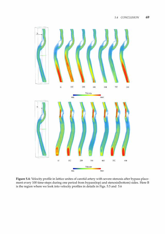
5.4 CONCLUSION 69
Figure 5.4: Velocity profile in lattice unites of carotid artery with severe stenosis after bypass place-ment every 100 time-steps during one period from bypass(top) and stenosis(bottom) sides. Here Bis the region where we look into velocity profiles in details in Figs. 5.5 and 5.6

70 TOWARDS DECISION SUPPORT IN VASCULAR SURGERY THROUGH COMPUTATIONALHEMODYNAMICS
0 10 20 30 400
0.02
0.04
0.06
0.08
Diameter
Vel
ocity
0 10 20 30 40−1
0
1
2
3x 10⁻³
Diameter
Vel
ocity
Figure 5.5: Velocity profiles as a function of diameter of carotid artery with (left) and without (right)bypass printed every 10th time-step.
0 200 400 6000
0.01
0.02
0.03
0.04
Time−steps
Vel
ocity
Figure 5.6: Velocity profiles as a function of time of carotid artery with (solid lines) and without(dashed lines) bypass during one period.
bypass placement on a patient specific carotid artery with severe stenosis. Next we haveexamined the obtained time-harmonic flow profiles. Thus from the raw medical dataof patients vascular system, after corresponding simple steps biomedical engineers andnovice surgeons can obtain a ready time-harmonic flow fields and analyze them withvisualization tools.
The new enhancements of HemoSolve make it not only highly sophisticated but alsofast and considerably less memory consumable PSE. Moreover, HemoSolve as a well-defined PSE satisfies its main requirements, e.g. it has a simple human-computer interac-tion graphical interface [126], it uses complete and accurate flow solver LBM for simula-tion of time-harmonic blood flow. It is integrated into parallel and distributed computing

5.4 CONCLUSION 71
environment [13] and also merged with Grid environment [104].As conclusion, HemoSolve is a well-established decision support and user-friendly
training system for novice surgeons and biomedical engineers for image-based hemody-namics research of time-harmonic blood flow in the human vascular system.

Conclusion
6.1 DiscussionHoustis and Rice [50] have mentioned that over the past 60 years there has been an enor-mous increase both in the speed of computer hardware and in algorithmic power. Withthe increase of the problem sizes, the demand for speeding up the simulation is alsoincreasing. There is also a need for high level and powerful problem solving environ-ments (PSE). The main idea behind a PSE is to combine powerful hardware and smartalgorithms to extract fast solutions for a target class of problems. As pointed out "Fu-ture PSEs will use essentially all the resources of future computing technologies, e.g.net-centric facilities, dynamic and collaborative computations, knowledge discovery andlearning, software reuse, human-machine interaction, etc.".
Our first step in this direction was to create a PSE (called HemoSolve) for image-based computational hemodynamic problems with the aim to transform medical datathrough information to knowledge. HemoSolve is user-friendly complete system, thatallows novice students to enlarge their practical skills by mimicking surgery. The rawmedical data of a patient’s vascular system can be obtained and after several steps, in ashort period of time, final results can be analyzed and visualized within the PSE. As CFDsolver in HemoSolve the lattice Boltzmann method is used.
Although HemoSolve is completely parallelized, optimizations were still needed. There-for our next goal was to speed-up the complete environment. For this reason we haveconcentrated on the improvement of each component separately. It is worthwhile to men-tion that HemoSolve is completely integrated into a Grid environment, thus supportingseamless integration of data (CT scan in the hospital), simulation (high performance com-puting center) and visualization (student desktop) tools.
The first and major component to improve was the hemodynamic solver. AlthoughLBM is a well-established method it is still hampered with slow convergence due to themethod specific constraints. We have developed a constraint optimization scheme that al-lows to choose the simulation parameters in a way to get a minimum execution time. Thenovel idea behind this scheme is that the simulation error is one of the constraints, andcan be defined a-priori. Good agreement between theoretical and experimental resultsproved the correctness of the scheme. In our simulations we have also managed to reachquite high Reynolds numbers for Womersley flow in a 3D straight tube. This is difficult toachieve for stability reasons due to the minimum relaxation parameter limit. Using this
73

74 CONCLUSION
scheme as an example for a real application we have simulated a time-harmonic bloodflow in a human abdominal aorta.
Also, as LBM is a relatively new method, we have decided to do another validationof this method by comparing it with FEM. As an application we have used the time-harmonic blood flow in the superior mesenteric artery with peak Reynolds number of3300. Although the Reynolds number is quite high, we have achieved a very good agree-ment between both solvers. When examining velocity profiles, we have observed all theflow characteristic similarities, such as vortex formation next to the bifurcation or thespiraling of the flow in the abdominal aorta.
Another improvement of time-harmonic LBM is the integration of the regularizedscheme into the collision term of LBM. Significant improvements of accuracy and stabilitywere obtained.
The next components of HemoSolve to improve were mesh generation and paral-lelization methods. The fact that LBM was applied on structured voxel meshes was con-sidered as one of the main disadvantages. Within the algorithm not only fluid but alsosolid nodes had to be saved and iterated, which consumed a major part of the executiontime and the memory. The new sparse-LBM scheme, where only fluid nodes are saved,appeared to be an enhanced scheme which increased the simulation speed enormouslyand allowed to treat data of over eight orders of magnitudes.
For the data distribution of parallel sparse-LBM we have used the METIS data par-titioning library. In contrast to other partitioning methods, the functions of the METISlibrary are able to partition large data sizes, e.g. 5 ∗ 106 fluid nodes in only 2 − 3 minutes.Our experiments showed that the efficiency loss due to the load imbalance between par-titions is about 18% for 5 ∗ 106 data size on 128 processors/partitions and less for smallernumber of partitions. Thus compared to the influence of e.g. fractional communicationoverhead, which is approximately 7% for any number of processors.
In order to evaluate the loss of efficiency of parallel sparse-LBM due to the differentfractional overheads, we have developed a performance prediction model. This modelallows us to preliminary estimate the efficiency, provided load imbalance, single proces-sor performance and point-to-point communication overheads.
All those improvements gave a significant speed-up of HemoSolve. For example,the time consumed for time-harmonic blood flow simulation in the carotid artery withbypass placement implemented with the latest version of HemoSolve was about ninetimes shorter than the time consumed by the previous version. Typically our experimentswith enhanced HemoSolve showed that the same experiment which used to take threehours of execution time now takes only about 20 minutes. Thus now we are able toanalyze the outputs much faster, even for very large problem sizes. The demonstratedfinal experiment of bypass placement on the carotid artery with severe stenosis usingHemoSolve is a clear example of mimicking a real surgery.
Thus, we have achieved the main goals posed at the beginning of this thesis: we havecreated a complete and enhanced computer-based simulation environment for image-based computational hemodynamics problems using the LBM, integrated it into highperformance computing environment, and applied it for visualization and understand-ing of biomechanical processes in complex vascular systems.

6.2 FUTURE WORK 75
We have presented LBM as a robust and accurate method for hemodynamic problems.In all our experiments we have shown a good agreement between LBM and analytical orother numerical solutions. We have managed to simulate time-harmonic blood flows ina large human arterial tree with very high Reynolds numbers, that are expected to causeinstabilities due to the low viscosity limitations of LBM. All the simulations were per-formed for incompressible, Newtonian flows. Therefore, the questions whether LBM iseligible to use for non-Newtonian flows and will it be robust enough to apply for sim-ulations of fluid-structure interactions to reconstruct the real flow physiology in humanvascular systems need still to be answered.
We have also developed an enhanced PSE that has all the necessary tools to mimic asurgical operation, such as bypass placement. Some experiments have been conductedto explore its usefulness for students as a learning tool. But whether PSE like HemoSolvewould be useful for the training of surgeons or whether it can serve as a decision supportsystem to use just before the operation of real patient is still an open issue.
And last but not the least, the main question "What is the role of computational hemo-dynamics for preoperational planing..." remains unanswered.
6.2 Future workThere are several possibilities to continue this research both from a numerical point ofview as well as from the application view point.
• Data distribution and load imbalance - Although in this research the obtained re-sults of using the METIS partitioning library are quite satisfactory, we have stillestimated that there is maximum of 18% impact of load imbalance on the efficiency.Thus there is a need of more sophisticated partitioning algorithms that will be com-parably fast but with better load balancing.
• Grid refinement - Our results of simulations of blood flow in the complete abdom-inal aortic tree have shown that in order to be able to analyze the flow profiles inthe narrow side-branches one needs to have a very fine mesh. The refinement ofthe complete geometry will increase the execution time of simulations enormously.Therefore the incorporation of partial refinement algorithm into HemoSolve is thenext logical step.
• Wall elasticity - Until now, for all the medical geometries in all the examples through-out this thesis the walls of arteries considered to be rigid. This is one of the majorgaps that separate us from reality. Implementation of the elasticity of the walls is amajor step. One of the possible algorithms to do this is the spring LBM [20].
The implementation of the above mentioned points may bring the LBM a step forwardtowards the simulation of non-Newtonian flows. It may also help to realize whetherwe need to use more advance numerical methods or will LBM be sufficient to use inimplementing the fluid-structure interactions for real flow simulations. Considerationof blood cells transportation and their possible deformation in the flow is also an open

76 CONCLUSION
issue. Another interesting question is: can we be satisfied with the results obtained fromsimulations of incompressible flows or do we need an immediate switch to compressibleones?
All those are the questions and discussions that still need substantial answers.

Summary
The aim of the work in this thesis was to create a complete and sophisticated computer-based simulation environment that may also serve as a decision support system for vas-cular reconstruction. We have defined a PSE for image-based computational hemody-namics, where as CFD solver we used LBM. We investigated optimization methods forthe LBM flow solver. We also merged the PSE into a high performance computing en-vironment. The intension was to improve its performance and scalability. We proposedoptimization models and analyzed the results on a wide range of experiments.
Chapter 1 is an introduction to the work. There we first have showed the relevanceof our research by introducing the main concepts. We have briefly described the actualformation, cause and influence of atherosclerosis and aneurysms in humans. Next wegave a short description of the high performance computing concept and discussed itsinfluence on optimized solutions of complex systems. Finally we have described the LBMas a fluid dynamics method, showing its ability to be parallelized and provide referencesto examples of earlier work where it has been applied on unstructured/nested grids ofcomplex geometries.
In Chapter 2 we have described a problem solving environment; HemoSolve for im-age based computational hemodynamics. We discussed its main components in detailshowing it as a robust image-based tools. Next we concentrated on the FEM and LBMhemodynamic solvers used in HemoSolve and compared them with each other. We haveproved the eligibility of LBM as an enhanced CFD solver for 3D time-harmonic fluidflows. This was confirmed by the experimental results of 3D time-harmonic blood flowsimulations in the abdominal aorta, superior mesenteric artery and an aortic part withlarge aneurysm. We have concluded by pointing out the advantages of HemoSolve as aneasy applicable, user-friendly and robust image-based problem solving environment.
After establishment of LBM as a well-defined hemodynamic solver we went one stepfurther and examined the possibilities of its optimization in Chapter 3. LBM has severalconstrains to fulfill the demand of stability and accuracy. Those constraints are causing aslow convergence, which in its turn decreases the performance of the complete PSE. Thuswe have defined a constraint optimization scheme which allows us to choose the simu-lation parameters in a way, that will speed-up the convergence of LBM. In this chapter
77
78 SUMMARY
we have described the theory of the scheme in detail and compared it with the experi-mental results. The good agreement between two of them allowed us to also examinethe stability of the system for very high Reynolds numbers. Also, using the constraintoptimization scheme we have simulated the time-harmonic blood flow in a human ab-dominal aorta. Next, we have tried to improve the accuracy of LBM by using a newregularized scheme, e.g. we introduced a small correction to the collision term of LBM.We have tested the scheme for time-harmonic flows by comparing it with usual LBMand by checking the numerical stability for high Reynold numbers. We conclude thatRL-LBGK is more accurate and stable than LBGK.
The fulfillment of optimizations of the LBM method itself led us to the optimizationof its parallelization schemes. In Chapter 4 we have described a sparse-LBM methodwhich allows us to work with only the fluid part of the complete data domain and ig-nore the solid fractions. Thus saving the memory consumption and also execution time.Here we used the graph partitioning library METIS for data decomposition. The func-tions we used from METIS are based on the combination of modified Kernighan-Lin andFiduccia-Mattheyses algorithms. Next, we have defined a performance prediction modelwhich allows us to determine the execution time of the system on the parallel machinesa-priori. This model takes into account such fractional overheads as the single processorperformance, load imbalance and communication overheads. The comparison of our ex-perimental measurements with theory sowed us very satisfactory results with only 5%prediction error.
Finally, in Chapter 5 we have combined all our improvements of LBM and the par-allelization scheme into our PSE, making it a complete decision support system. Wehave shown its enhancements and speed-up by simulating time-harmonic blood flow inhuman carotid artery with a severe stenosis. Next we have mimicked a real surgical op-eration by bypass placement over the stenosis and again simulating the blood flow. Ourresults were quite satisfactory as to comparison with blood flow characteristics in thecarotid artery of healthy patient.
Chapter 6 concluded our work by discussions of the thesis and discussing the futuredevelopments.
Nederlandse samenvatting
De belangrijkste doelstelling van het in dit proefschrift beschreven onderzoek washet ontwikkelen van een compleet, geavanceerd, computergebaseerd trainings- en be-slissingsondersteuningssysteem dat een verbinding legt tussen gegevens en kennis doormiddel van informatie. Daartoe hebben we een Problem Solving Environment (PSE) ge-definieerd voor beeldgebaseerde hemodynamica, gegeven een op een Lattice-BoltzmannMethode (LBM) gebaseerde techniek voor het oplossen van problemen in de vloeistofdy-namica (Computational Fluid Dynamics, of CFD). Ter verbetering van de efficiëntie en deschaalbaarheid hebben we ons bovendien intensief gericht op parallellisatie en optima-lisatie van de LBM. We hebben een aantal verschillende optimalisatiemodellen voorge-steld, en geanalyseerd op basis van een ruim scala aan experimenten. De optimalisatieshebben geleid tot een snelheidsverbetering die onze beeldgebaseerde PSE in staat steldechirurgische operaties op realistische wijze te simuleren.
Hoofdstuk 1 bevat een algemene introductie tot ons werk. Allereerst tonen we het be-lang aan van ons onderzoek door middel van een overzicht van de belangrijkste concep-ten die aan de basis liggen van het proefschrift. We geven een korte beschrijving van hetontstaan, de oorzaken, en de gevolgen van slagaderverkalking (atherosclerose) en vaat-verwijding (aneurysma). We definieren het probleem als een complex systeem, en stellenvoor een oplossing te vinden door middel van het modelleren en simuleren van bloed-stromen in het menselijke vaatstelsel. Verder geven we een korte beschrijving van hetgebied van parallel rekenen en bespreken haar invloed op geoptimaliseerde oplossingenvoor complexe systemen. Tot slot beschrijven we LBM als een model voor vloeistofdyna-mica, met inbegrip van haar geschiktheid voor parallellisatie, en geven voorbeelden vaneerder onderzoek dat LBM heeft toegepast op ongestructureerde en geneste grids vancomplexe geometrieën.
Hoofdstuk 2 geeft een gedetailleerde beschrijving van de belangrijkste componen-ten van de door ons ontwikkelde PSE, genaamd HemoSolve. Bovendien vergelijken wetwee verschillende, in HemoSolve gebruikte oplossingsmethoden voor problemen in devloeistofdynamica (LBM en FEM, of Finite Element Method), waarbij we de geschikt-heid van LBM aantonen als een oplossingtechniek voor 3-dimensionale tijdharmonischevloeistofstromen. We bevestigen onze theoretische discussie door middel van numerie-
79

80 NEDERLANDSE SAMENVATTING
ke experimenten met 3D tijdharmonische simulaties van bloedstromen in verschillendedelen van het vaatstelsel. Op basis van deze resultaten concluderen we dat HemoSolveeen eenvoudig te gebruiken en robuust beeldgebaseerd PSE systeem is.
Nadat we hebben aangetoond dat LBM een geschikte oplossingsmethode voor hemo-dynamicaproblemen is, hebben we in Hoofdstuk 3 de mogelijkheden ter optimalisatievan LBM onderzocht. LBM heeft een aantal randvoorwaarden die de eis van stabiliteitmoeten waarborgen. Deze randvoorwaarden zorgen voor een langzame convergentie,en derhalve voor een verminderde efficiëntie van onze gehele PSE. We hebben daaromeen methode ter optimalisatie van de randvoorwaarden ontwikkeld die ons in staat steltde simulatie parameters zodanig te kiezen dat de convergentie van de LBM wordt ver-sneld. In dit hoofdstuk hebben we de theorie van deze methode in detail beschreven,en vergeleken met experimentele resultaten. De hoge mate van overeenkomst tussen detheorie en de numerieke resultaten stelde ons in staat de stabiliteit van ons systeem tetesten voor zeer hoge Reynoldsgetallen. Op basis van onze optimalisatiemethode van derandvoorwaarden hebben we de tijdharmonische bloedstroom in een menselijke buik-slagader gesimuleerd. Daarnaast hebben we geprobeerd de nauwkeurigheid van LBMte vergroten door een kleine correctie van de LBM collisieparameter. We hebben dezeaanpassing getest voor tijdharmonische stromen, en - voor hoge Reynoldsgetallen - ver-geleken met de gebruikelijke LBM parameter instellingen. We hebben daarbij vastgestelddat onze aangepaste versie (RL-LBGK) nauwkeuriger en stabieler is dan de originele ver-sie (LBGK).
Om significante snelheidsverbeteringen van de LBM methode zelf te bereiken hebbenwe ons vooral gericht op het optimaliseren van de toegepaste parallelle rekenmethoden.In Hoofdstuk 4 beschrijven we een nieuwe sparse-LBM methode die ons in staat stelt hetsolide deel van het volledige data domein te negeren, en ons te beperken tot het fluïdedeel. Deze aanpak, gecombineerd met het gebruik van een nieuwe graafpartitionerings-bibliotheek voor data distributie (METIS), bespaart op het geheugengebruik, en resul-teert in een snellere executietijd. De METIS functionaliteit die we hebben toegepast isgebaseerd op aangepaste Kernighan-Lin en Fiduccia-Mattheyses algoritmen. Daarnaasthebben we een schattingsmodel ontwikkeld dat ons in staat stelt de executietijd van hetsysteem vooraf te bepalen. Dit model bevat kostenparameters voor de rekentijd op eenenkele processor, verschillen in de werkdruk tussen processoren onderling, en interpro-cescommunicatie. Experimentele resultaten tonen aan dat ons schattingsmodel resulteertin een maximale fout van slechts 5%.
Tot slot worden in Hoofdstuk 5 alle ontwikkelde verbeteringen van het LBM algorit-me geïntegreerd in ons PSE systeem. We tonen de verbeteringen in nauwkeurigheid eensnelheid aan door middel van een simulatie van een tijdharmonische bloedstroom in eenernstig vernauwde menselijke halsslagader. Verder hebben we een chirurgische bypassoperatie nagebootst, en achtereenvolgens de bloedstroom in de halsslagader opnieuwgesimuleerd. Het eindresultaat is zeer positief in vergelijking met de bloedstromen in dehalsslagader van een gezonde patiënt.
Hoofdstuk 6 besluit het proefschrift met een algemene discussie en een beschrijvingvan mogelijke richtingen voor toekomstige onderzoekingen in dit vakgebied.

Summary in Armenian
81

82 SUMMARY IN ARMENIAN
SUMMARY IN ARMENIAN 83

84 SUMMARY IN ARMENIAN

Acknowledgments
Ralph Fiennes: ‘The people I consider successful are so because of how they handle theirresponsibilities to other people, how they approach the future, people who have a full sense of the
value of their life and what they want to do with it.Success.. is all about being able to extend love to people... not in a big, capital letter sense but in
the everyday. Little by little, task by task, gesture by gesture, word by word.’
I would like to open my acknowledgment with the words of gratitude to my promoterProf. Peter M.A. Sloot. Peter, thank you very much, first of all for replying to my very firstmail from Sweden asking if there was any PhD position in your group. Your reply waswith challenge and since then I have tried my best to impress you with my knowledgeand scientific abilities. I hope I have managed :). I also want to thank you for all yourhelp, from the beginning until the end of my PhD. Knowing that in case of need of helpyou will always support me, helped me to succeed in many quests. Thank you!
Next, I want to thank my co-promoter Alfons G. Hoekstra. Alfons, it was a pleasure towork with you. You are a great teacher, scientist, you knew when I was stuck and neededa push and you were always ready to give me a hand. Thank you for your enormoushelp. I was happy to have a supervisor like you as I learned a lot from you and alsoknow how great to have a supervisor with high demands. Now I am ready to work withany tough boss ;).
My next special thanks are for my friend and great professor Bastien Chopard. BastienI will never forget our nice walks in Krakow and the visit to salt-mines, it was an honorto have you as a guest in Armenia, and I was truly amazed by the beauty of Chateaude Chillon and fairy nature around it, and the tasty Molokhov (if I remember the namecorrectly) of course. Also my special thanks to Jonas Latt.
I would also like to thank my coordinator in Sweden (KTH, Nada) Lennart Edsbergand the Swedish Institute organization that made my study in Sweden possible and thusnew horizons have opened to me.
I am vary grateful to Prof. Hans Reiber and Rob van der Geest for all the help duringcollaborations within DIME project. And thank you Jorrit and Henk for an easy and fastcollaboration.
85

86 ACKNOWLEDGMENTS
Another truly amazing experience was my collaboration with several German groupswithin the International lattice Boltzmann Consortium. I would like to thank Joerg for de-veloping this idea, for his hospitality during my visit to NEC Research Labs. Europe, formany many beer gardens and the Armenian dinner. Special thanks to Guntram (I wishI could work with you at least for a half year, I would learn so much from you), George(your father’s bike helped me to discover the wonderful nature around Bonn), Richardand Suzy (for entertaining weekends). Also I would like to thank Dr. Guy Lonsdale andDr. Achim Basermann for their hospitality.
My amazing experience continued in HLRS with Peter Lammers in Stuttgart. Peterwe worked three days, for more than 12 hours per day, around the same table, but Ithink those were the most productive days ever, that made even Joerg happy ;). And I’veappreciated a lot that at the end of the day you still have found energy to show me thebeautiful non-touristic Stuttgart.
Next thanks are for Thomas Zeiser. If there is any information in the world that onewants to know about supercomputers, ask Thomas. Thomas it was a great experience towork with you.
What impressed me a lot is the group of Prof. Manfred Krafczyk. It is like one com-plete family and I was happy to be their guest even for couple of days. For a great help Iwant to thank Sebastian, Jan and Soeren and of coarse Manfred and Jonas for making itpossible.
At the end of my research I had another nice collaboration with a group from SheffieldUniversity for which I would like to thank Dr. Rod Hose, Dr. Pat Lawford and AdamJeays. And of coarse my warm regards goes to Sara who was like me a visitor in Ger-many from Sheffield University. During these two visiting periods we managed to be-come friends, share thoughts and discussions both over lattice Boltzmann and over lifein general.
Even though I had a lot of collaboration during my research and multiple visits toother groups, the most of the time I have spent in my office at Science Park with my greatoffice-mates Qiu and Maxim. Although I have tried my best not to disturb them withmuch noise but I assume three people in a small room can cause problems (although wenever had one). Guys you have never complained but still I want to thank you for yourpatience. It seemed as if we were synchronized in work and in breaks for little chats.
I also would like to thank all the people in and outside of our SCS group: Bre-anndan (happy to be your next wall office neighbor), Alfredo (and Heidi of coarse),Drona, Evghenii, Derek, Alessia, Mike, Stefan, Nicolas, Alfonso, Yves, Jordi, Thomas,Jiangjun, Carlos, Paul, Michael(with Anya), Rob (for advice when I needed one), Simon,Thomasz(with Anja), Eric L., Gokhan, Syed, Dick, Marian, Jaap (was great to have a chatover a beer in Geneva), David, Dorien, Virginie, Amanda, Gohar, Zimming (always use-ful advice I got from you), Viktor, Wibi, Silvia(especially at the end ;)). Special thanksto Russians: Roman (hope you are managing the grapes-hunt by now with your forkand knife), Denis (for all the help with visualizations), Dmitri, Vladimir, Kostya, Lev andIlya. Guys my special thanks to you for always being ready to give me a hand when Iwas moving from house to house and that has happened 5 times. Also it was a pleasureto bicycle with you in Netherlands. Special thanks to Zeger for taking my huge suitcase
ACKNOWLEDGMENTS 87
into your slim sport-car :). Kamil, you started to help me from the first days, by translat-ing the dutch mails, until the last days, giving hints for the thesis writing format. Andof coarse, thank you Artoli, I don’t know how I would manage in Amsterdam if youwouldn’t teach me to cycle. Also, your advice, when I have just arrived to continue yourwork, helped me during all these four years. I am very grateful to you.
A big huge thank you is for Frederik Benjamin Hitipeuw well known as Erik ;). DearErik what we all were going to do without you? You are our problem solving personfrom bureaucratic questions until "no coffee" ones. In the mornings, making a couple ofjokes, while taking a cup of coffee, was enough to keep my and (I am sure others willagree with me) all poor PhD student’s mood up for the complete day.
One important component for comput(er or ational) scientist is probably the com-puter ;) and supercomputers in my case. When it has a problem the only ones that canhelp are network administrators. So I am very thankful to them especially Stephan, Ruudand Adri and also special thanks to Willem Vermine from SARA supercomputing center.
My dear Elena and Frank the first day I met you I realized that I have a family here. Iam very grateful to you for being my best friends that cared about me so much. You werethe ones sharing with me my happy and not so happy days. Thanks to you I became richwith two more amazing friends.
Valeriu, our friendship started at the first day in Sweden, where we studied in thesame group and continues until now and hopefully forever. It was a great coincidencethat you also found a PhD position in Amsterdam, CWI. I know that even in a verydifficult moment I can always count on you, thank you for that.
I met also amazing people out of work. Those people helped me to understand andpartially to get integrated into local society. Those people filled my days in Amsterdamwith joy and happiness. I would like to thank Stijn for all the fun days and bicycle ses-sion in Oosterpark. Another big thank you is for Erik for all the wonderful memories Igathered in and around Netherlands. My great regards to Erik’s family for giving me alltheir warmth.
I would like also to thank my friends and relatives from different parts of the worldthat were keeping my spirit up all the time with their attention: Aram Ohanyan, Aram Sa-hakyan, Arsen, Marianna, Goharik, Milena and Jorgen, Mohammad, Mika, Nora, Armenand Siranush(can you appear again in front of the Tropen museum out of nowhere whileyou suppose to be in Yerevan ;)), Zakar and Hasmik, Emma and Hakob with Stephanand Arpi, Keijo, Jari, Hans, Melanyan and Ruben (I am so proud that you are my friends)and many many more whom I didn’t mention but I always keep them in my heart. Mygreat thanks also to Avagyan family for everything and my great aunt Emma’s family.
My special and big thanks to Marko for his great support, encouragements and be-lieve in me during last year of my PhD.
This thesis wouldn’t have been finished or even started to be written without all thefaith, encouragement and support of my family. I will never be able to express my com-plete gratitude and love to my grandfather and grandmother. Unfortunately, I didn’tmanage to graduate before my grandfather’s death, only by several months. I hope heknew how much I loved him and that his dream to see me a doctor of science, as he washimself, came true. Both my beloved grandparents were my best support team ever dur-

88 ACKNOWLEDGMENTS
ing these years. One phone call with them gave me enough energy to proceed further.And I want to tell my grandmother how blessed I am that I have her.
This thesis is devoted to my mother, the best mother in the world :). A mother, whonot only gave a birth to me but also created step-by-step what I am now. With her wepassed through war, earthquake and hunger, fell from richness to poorness and recoveredagain. And during these four years she was the only one who knew all my worries andexcitements, my fails and successes, saw me devastated and happy.
Mama, you are the only one who truly understands me and always supports me, andto devote this thesis to you is the least I could do to express my love to you!

Publications
Journal Publications
[1] Lilit Axner, Adam Jeays, Alfons G. Hoekstra, Pat Lawford, Rod Hose and PeterM. A. Sloot. Simulations of Time Harmonic Blood Flow in the Mesenteric Artery:Comparing Finite Element and Lattice Boltzmann Methods (In preparation).
[2] Lilit Axner, Henk A. Marquering, Alfons G. Hoekstra, Rob J. van der Geest, JohanH.C. Reiber and Peter M. A. Sloot. Decision Support through Computational Hemo-dynamics in Vascular Surgery In Physics in Medicine and Biology (Submitted).
[3] Lilit Axner, Jörg Bernsdorf, Thomas Zeiser, Peter Lammers, Jan Linxweiler and Al-fons G. Hoekstra. Performance Evaluation of a Parallel Sparse Lattice BoltzmannSolver. In Journal of Computational Physics (Submitted).
[4] Lilit Axner, Jonas Latt, Alfons G. Hoekstra, Bastien Chopard and Peter M.A. Sloot.Simulating Time Harmonic Flows with the Regularized L-BGK Method. In Interna-tional Journal of Modern Physics C, 18, 4, p.661, 2007.
[5] Lilit Axner, Alfons G. Hoekstra and Peter M.A. Sloot. Simulating Time HarmonicFlows with the Lattice Boltzmann Method. In Physical Review E, 75, 3, p. 036709,2007.
Conference Proceedings
[6] Lilit Abrahamyan, Jörg Bernsdorf, Thomas Zeiser, Peter Lammers, Alfons G. Hoek-stra and Peter M.A. Sloot. MPI Parallelization and Performance Aspects of a GraphBased LB Flow Solver. In Discrete Simulation of Fluid Dynamics DSFD2006, Geneva,Switserland, 2006.
89

90 PUBLICATIONS
[7] Lilit Abrahamyan, Alfons G. Hoekstra and Peter M.A. Sloot. Choosing Optimal L-BGK Simulation Parameters for Time Harmonic Flows. In Discrete Simulation ofFluid Dynamics DSFD2006, Geneva, Switserland, 2006.
[8] Lilit Abrahamyan, Jorrit A. Schaap, Alfons G. Hoekstra, Denis Shamonin, FriekeM.A.Box, Rob J. van der Geest, Johan H.C. Reiber, Peter M.A. Sloot. A ProblemSolving Environment for Image-Based Computational Hemodynamics. In LNCS3514, p.287, April 2005.
[9] Abdel Monim Artoli, Lilit Abrahamyan, and Alfons G. Hoekstra. Accuracy versusPerformance in Lattice Boltzmann BGK Simulations of Systolic Flows. In LNCS 3039,p.548, June 2004.
Miscellaneous Publications
[10] Lilit Axner and Alfons G. Hoekstra. Virtuele bypassoperatie. In I/O InformaticaOn-derzoek Journal of Dutch National Foundation, 4, 3, July 2007.
[11] Lilit Axner. In Uitgelicht stellen ICT-onderzoekers zich aan u voor en vertellen overhun onderzoek en hun fascinatie hiervoor. In Informaticaonderzoek Platform Nederlandonline journal
Bibliography
[1] http://www.hpce.nec.com/.[2] http://www.sara.nl/userinfo/lisa/description/index.html/.[3] http://www.top500.org/list/2007/06/100.[4] World Health Organization, 2002, The World Health Report 2002,
http://www.who.int/whr/en/.[5] A. Abou-Rjeili and G. Karypis. Multilevel Algorithms for Partitioning Power-Law
Graphs. IEEE International Parallel & Distributed Processing Symposium (IPDPS),vol. 10, 2006.
[6] S. Ansumali and I. V. Karlin. Single Relaxation Time Model for Entropic LatticeBoltzmann Methods. Physical Review E, vol. 65, no. 5, pp. 056312 – 9, 2002.
[7] A. M. Artoli. Mesoscopic Computational Haemodynamics. PhD dissertation, Univer-sity of Amsterdam, Informatic Institute, 2003.
[8] A. M. Artoli, A. G. Hoekstra, and P. M. Sloot. 3D Pulsatile Flow with the LatticeBoltzmann BGK Method. International Journal of Modern Physics C, vol. 13, no. 8,pp. 1119–1134, 2002.
[9] A. M. Artoli, A. G. Hoekstra, and P. M. Sloot. Simulation of a Systolic Cycle in aRealistic Artery with the Lattice Boltzmann BGK Method. International Journal ofModern Physics B, vol. 17, no. 1-2, pp. 95 – 98, 2003.
[10] A. M. Artoli, A. G. Hoekstra, and P. M. Sloot. Mesoscopic Simulations of Sys-tolic Flow in the Human Abdominal Aorta. Journal of Biomechanics, vol. 39, no. 5,pp. 873–884, 2006.
[11] A. M. Artoli, A. G. Hoekstra, and P. M. Sloot. Optimizing Lattice Boltzmann Simu-lations for Unsteady Flows. Computers & Fluids, vol. 35, no. 2, pp. 227–240, 2006.
[12] L. Axner, J. Bernsdorf, T. Zeiser, P. Lammers, J. Linxweiler, and A. Hoekstra. Per-formance Evaluation of a Parallel Sparse Lattice Boltzmann Solver. Journal of Com-putational Physics, vol. (submitted), 2007.
91

92 BIBLIOGRAPHY
[13] L. Axner, A. Hoekstra, and P. Sloot. Simulating Time Harmonic Flows with theLattice Boltzmann Method. Physical Review E, vol. 75, no. 3, pp. 036709+7, 2007.
[14] L. Axner, J. Latt, A. G. Hoekstra, B. Chopard, and P. M. Sloot. Simulating Time Har-monic Flows with the Regularized L-BGK Method. International Journal of ModernPhysics C, vol. (accepted), 2007.
[15] A. Basermann, J. Clinckemaillie, T. Coupez, J. Fingberg, H. Digonnet, R. Ducloux,J.-M. Gratien, U. Hartmann, G. Lonsdale, B. Maerten, D. Roose, and C. Walshaw.Dynamic Load Balancing of Finite Element Applications with the DRAMA Library.Applied Mathematical Modelling, vol. 25, pp. 83 – 98, 2000.
[16] G. Bell, J. Gray, and A. Szalay. Petascale Computational Systems. IEEE Computer,vol. 39, no. 1, pp. 110 – 112, 2006.
[17] R. Benzi, S. Succi, and M. Vergassola. The Lattice Boltzmann Equation: Theory andApplications. Physics Reports, vol. 222, no. 3, pp. 145 – 197, 1992.
[18] J. Bernsdorf, S. E. Harrison, S. M. Smith, P. V. Lawford, and D. R. Hose. High Per-formance Computing on Vector Systems 2006. In Proceedings of the High PerformanceComputing Center Stuttgart, vol. March, 2006.
[19] M. Bouzidi, M. Firdaouss, and P. Lallemand. Finite Element Modeling of BloodFlow in Arteries. Physics of Fluids, vol. 13, no. 11, pp. 3452–3459, November 2001.
[20] G. A. Buxton, R. Verberg, D. Jasnow, and A. C. Balazs. Newtonian Fluid Meetsan Elastic Solid: Coupling Lattice Boltzmann and Lattice-Spring Models. PhysicalReview E, vol. 71, p. 056707, 2005.
[21] J. Cebral, R. Löhner, P. Choyke, and P. Yim. Parallel Patient-Specific ComputationalHaemodynamics. In Lecture Notes in Computer Science, vol. 2367, pp. 18 – 34, 2002.
[22] H. Chen. Volumetric Formulation of the Lattice Boltzmann Method for Fluid Dy-namics: Basic Concept. Physical Review E, vol. 58, no. 3, pp. 3955 – 3963, September1998.
[23] S. Chen and G. D. Doolen. Lattice Boltzmann Method for Fluid Flows. AnnualReview Fluid Mechanics, vol. 30, pp. 329 – 364, 1998.
[24] S. Chen, Z. Wang, X. Shan, and G. D. Doolen. Lattice Boltzmann ComputationalFluid Dynamics in Three Dimensions. Journal of Statistical Physics, vol. 68, no. 3/4,pp. 379 – 400, 1992.
[25] B. Chopard and M. Droz. Cellular Automata Modeling of Physical Systems. CambridgeUniversity Press, 1998.
[26] D. Clague, D. Kandhai, R. Zhang, and P. M. Sloot. On the Hydraulic Permeability of(Un)Bounded Fibrous Media Using the Lattice-Boltzmann Method. Physical ReviewE, vol. 61, no. 1, pp. 616–625, 2000.
[27] J. Cosgrove, J. Buick, S. Tonge, C. Munro, C. Greated, and D. Campbell. Applicationof the Lattice Boltzmann Method to Transition in Oscillatory Channel Flow. Journalof Physics A: Mathematical and General, vol. 36, pp. 2609 – 2620, 2003.
BIBLIOGRAPHY 93
[28] C.Pan, J. Prins, and C. T. Miller. A high-performance lattice boltzmann implemen-tation to model flow in porous media. Comp. Phys. Comm., vol. 158, no. 2, p. 89,2004.
[29] O. Cuisenaire. Distance Transformations: Fast Algorithms and Applications to MedicalImage Processing. PhD dissertation, Universite catholique de Louvain, Laboratoirede Telecommunications et Teledetection, 1999.
[30] R. R. A. Dampney. Functional Organization of Central Pathways Regulating theCardiovascular System. Physiological Reviews, vol. 74, no. 2, pp. 323 – 364, April1994.
[31] P. de Koning, J. Schaap, J. Janssen, J. Westenberg, R. van der Geest, and J. Reiber.Automated Segmentation and Analysis of Vascular Structures in Magnetic Reso-nance Angiographic Images. Magnetic Resonance in Medicine, vol. 50, no. 6, pp. 1189– 1198, 2003.
[32] J.-C. Desplat, I. Pagonabarraga, and P. Bladon. LUDWIG: A parallel Lattice-Boltzmann code for complex fluids. Computer Physics Communications, vol. 134,no. 3, p. 273, 2002.
[33] A. Dupuis and B. Chopard. An Object Oriented Approach to Lattice Gas Modeling.Future Generation Computer Systems, vol. 16, no. 5, pp. 523 – 532, 2000.
[34] H. Fang, Z. Wamg, Z. Lin, and M. Liu. Lattice Boltzmann Method for Simulatingthe Viscous Flow in Large Destensible Blood Vessels. Physical Review E, vol. 65,pp. 051925–11, 2002.
[35] O. Filippova and D. Heanel. Grid Refinement for Lattice-BGK Models. Journal ofComputational Physics, vol. 147, no. 1, pp. 219 – 228, 1998.
[36] A. Finkelstein, J. Hetherington, L. Li, O. Margoninski, P. Saffrey, R. Seymour, andA. Warner. Computational Challenges of Systems Biology. IEEE Computer, vol. 37,no. 5, pp. 26 – 33, 2004.
[37] I. Foster. Designing and Building Parallel Programs: Concepts and Tools for ParallelSoftware Engineering. Addison Wesley, 1995.
[38] G. Fox, M. Johnson, G. Lyzenga, S. Otto, J. Solman, and D. Walker. Solving Problemson Concurent Processors. Prentice-Hall Int. Inc., 1988.
[39] E. Gallopoulos, E. N. Houstis, and J. R. Rice. Computer as Thinker/Doer: Problem-Solving Environments for Computational Science. Computational Science and Engi-neering, IEEE, vol. 1, no. 2, pp. 11 – 23, 1994.
[40] S. Geller, M. Krafczyk, J. Toelke, S. Turek, and J. Hron. Benchmark ComputationsBased on Lattice-Boltzmann, Finite Element and Finite Volume Methods for Lami-nar Flows. Computers and Fluids, vol. 35, pp. 888–897, 2006.
[41] R. Gin, A. G. Straatman, and D. A. Steinman. Numerical Modelling of the CarotidArtery Bifurcation Using a Physiologically Relevant Geometric Model. 7th AnnualMeeting of the CFD Society of Canada,, vol. Halifax NS, 1999.

94 BIBLIOGRAPHY
[42] Z. Guo, T. S. Zhao, and Y. Shi. Preconditioned lattice-Boltzmann Method for SteadyFlows. Physical Review E, vol. 70, pp. 066706 – 066714, 2004.
[43] Z. Guo, C. Zheng, and T. Zhao. A Lattice BGK Scheme with General Propagation.Journal of Scientific Computing, vol. 16, no. 4, pp. 569–585, 2001.
[44] X. He and L.-S. Luo. Lattice Boltzmann Model for the Incompressible Navier-StokesEquation. Journal of Statistical Physics, vol. 88, no. 3-4, pp. 927 – 944, 1997.
[45] X. He and L.-S. Luo. A priori derivation of the lattice Boltzmann equation. PhysicalReview E, vol. 55, p. R6333, 1997.
[46] X. He, L.-S. Luo, and M. Dembo. Some Progress in Lattice Boltzmann Method.Part1: Nonuniform Mesh Grids. Journal of Computational Physics, vol. 129, pp. 357–363, July 1996.
[47] B. Hendrickson and K. Devine. Dynamic Load Balancing in Computational Me-chanics. Computer Methods in Applied Mechanics and Engineering, vol. 184, pp. 485 –500, 2000.
[48] F. J. Higuera. Lattice Gas Method Based on the Chapman-Enskog Expansion.Physics of Fluids A, vol. 2, no. 6, pp. 1049–1051, 1990.
[49] R. W. Hockney and C. R. Jesshope. Parallel Computers 2: Architecture, Programmingand Algorithms. IOP Publishing Ltd., Bristol, UK, 1988.
[50] E. N. Houstis and J. R. Rice. Future Problem Solving Environments for Computa-tional Science. Mathematics Computer Simulation, vol. 54, pp. 243–257, 2000.
[51] G. Házi. Accuracy of the Lattice Boltzmann Method based on Analytical Solutions.Physical Review E, vol. 67, no. 5, pp. 056705–5, 2003.
[52] J. Janssen, G. Koning, P. de Koning, J. Tuinenburg, and J. Reiber. A Novel Approachfor the Detection of Pathlines in X-Ray Angiograms: the Wavefront PropagationAlgorithm. International Journal of Cardiovascular Imaging, vol. 18, no. 5, pp. 317 –324, 2002.
[53] A. Jeays, P. Lawford, R. Gillott, P. Spencer, D. Barber, K. Bardhan, and D. Hose.Characterisation of the Haemodynamics of the Superior Mesenteric Artery. Journalof Biomechanics, vol. doi:10.1016/j.jbiomech.2006.09.009, 2006.
[54] B. Kandhai, D.-E. Vidal, A. Hoekstra, H. Hoefsloot, P. Iedema, and P. Sloot. Lattice-Boltzmann and Finite Element Simulations of Fluid Flow in a SMRX Mixer. Inter-national Journal of Numerical Methethods in Fluids, vol. 31, pp. 1019 – 1033, 1999.
[55] D. Kandhai, D. Dubbeldam, A. G. Hoekstra, J. Timonen, and P. M. A. Sloot. ParallelLattice-Boltzmann Simulation of Fluid Flow in Centrifugal Elutration Chambers. InLecture Notes in Computer Science, vol. 1401, pp. 173 – 182, 1998.
[56] D. Kandhai, D. Hlushkou, A. G. Hoekstra, P. M. Sloot, H. van As, and U. Tallarek.Influence of Stagnant Zones on Transient and Asymptotic Dispersion in Macro-scopically Homogeneous Porous Media. Physical Review letters, vol. 88, no. 23,pp. 234501:1–4, 2002.
BIBLIOGRAPHY 95
[57] D. Kandhai, A. Koponen, A. G. Hoekstra, M. Kataja, J. Timonen, and P. M. Sloot.Lattice Boltzmann Hydrodynamics on Parallel Systems. Computer Physics Commu-nications, vol. 111, pp. 14 – 26, 1998.
[58] D. Kandhai, A. Koponen, A. G. Hoekstra, M. Kataja, J. Timonen, and P. M. A. Sloot.Implementation aspects of 3D Lattice-BGK: Boundaries, Accuracy and a new FastRelaxation Method. J. Comp. Phys., vol. 150, pp. 482–501, 1999.
[59] D. Kandhai, A. Koponen, A. G. Hoekstra, J. Timonen, and P. M. A. Sloot. Implemen-tation Aspects of 3D Lattice-BGK: Boundaries Accuracy, and a New Fast RelaxationMethod. Journal of Computational Physics, vol. 150, pp. 482–501, 1999.
[60] D. Kandhai, W. Soll, S. Chen, A. G. Hoekstra, and P. M. Sloot. Finite-DifferenceLattice-BGK Methods on Nested Grids. Computer Physics Communication, vol. 129,pp. 100 – 109, 2000.
[61] G. Karypis and V. Kumar. Multilevel Graph Partitioning Schemes. In InternationalConference on Parallel Processing, vol. 3, pp. 113–122, 1995.
[62] G. Karypis and V. Kumar. Multilevel k-way Partitioning Scheme for IrregularGraphs. Journal of Parallel and Distributed Computing, vol. 481, no. 1, pp. 96 – 129,1998.
[63] A. Koponen, M. Kataja, J. Timonen, and D. Kandhai. Simulation of Single-FluidFlow in Porous Media. International Journal of Modern Physics C, vol. 9, pp. 1505–1522, 1998.
[64] D. N. Ku. Blood Flow in Arteries. Annual Review of Fluid Mechanics, vol. 29, pp. 399– 434, 1997.
[65] J. P. Ku, M. T. Draney, F. R. Arko, W. A. Lee, F. Chan, N. J. Pelc, C. K. Zarins, andC. A. Taylor. In Vivo Validation of Numerical Predictions of Blood Flow in ArterialBypass Grafts. Annals of Biomedical Engineering, vol. 30, no. 6, pp. 743 – 752, 2002.
[66] P. Lallemand and L.-S. Luo. Theory of the Lattice Boltzmann Method: Dispersion,Dissipation, Isotropy, Galilean Invariance, and Stability. Physical Review E, vol. 61,no. 6, pp. 6546 – 6562, 2000.
[67] P. Lammers, G. Wellein, T. Zeiser, and M. Breuer. Have the vectors the continuingability to parry the attack of the killer micros? In M. Resch, T. Bönisch, K. Benkert,T. Furui, Y. Seo, and W. Bez, editors, High Performance Computing on Vector Systems.Proceedings of the High Performance Computing Center Stuttgart, March 2005, pp. 25–39, Berlin, 2006. Springer.
[68] J. Latt and B. Chopard. Lattice Boltzmann Method with Regularized Nonequilib-rium Distribution Functions. Mathematics Comp. Sim., vol. 72, pp. 165 – 168, 2006.
[69] W. Li, X. Wei, and A. E. Kaufman. Implementing Lattice Boltzmann Computationon Graphics Hardware. The Visual Computer, vol. 19, no. 7-8, pp. 444–456, 2003.
[70] J.-M. Luursema, W. B. Verwey, P. A. Kommers, R. H. Geelkerken, and H. J. Vos.Optimizing conditions for computer-assisted anatomical learning. Interact. Comp.,vol. 18, pp. 1123 – 1138, 2006.

96 BIBLIOGRAPHY
[71] H. Marquering, J. Dijkstra, P. de Koning, B. Stoel, and J. Reiber. Towards Quanti-tative Analysis of Coronary. International Journal of Cardiovascular Imaging, vol. 21,pp. 73–84, 2005.
[72] D. Martinez, W. Matthaeus, and S. Chen. Comparison of Spectral Method andLattice Boltzmann Simulations of Two-Dimensional Hydrodynamics. Physics ofFluids, vol. 6, no. 3, pp. 1285 – 1298, 1993.
[73] F. Mazzocco, C. Arrighetti, G. Bella, L. Spagnoli, and S. Succi. Multiscale LatticeBoltzmann Schemes: A Preliminary Application to Axial Turbomachine Flow Sim-ulations. International Journal of Modern Physics C, vol. 11, no. 2, pp. 233 – 245, 2000.
[74] H. X. nad Gongwen Peng and S.-H. Chou. Finite-Volume Lattice BoltzmannMethod. Physical Review E, vol. 59, no. 5, pp. 6202–6205, 1998.
[75] F. Nannelli and S. Succi. The Lattice Boltzmann Equation on Irregular Lattices.Journal Statistical Physics, vol. 68, no. 3-4, pp. 401 – 407, 1992.
[76] X. Niu, C. Shu, Y. Chew, and T. Wang. Investigation of Stability and Hydrodynam-ics of Different Lattice Boltzmann Models. Journal of Statistical Physics, vol. 117,no. 3-4, pp. 665 – 680, 2004.
[77] G. Peng, H. Xi, C. Duncan, and S.-H. Chou. Lattice Boltzmann Method on IrregularMeshes. Physical Review E, vol. 58, no. 4, pp. R4124 – R4127, October 1998.
[78] T. Pohl, F. Deserno, N. Thurey, U. Rude, P. Lammers, G. Wellein, and T. Zeiser.Performance Evaluation of Parallel Large-Scale Lattice Boltzmann Applications onThree Supercomputing Architectures. In SC ’04: Proceedings of the 2004 ACM/IEEEconference on Supercomputing, p. 21, Washington, DC, USA, 2004. IEEE ComputerSociety.
[79] B. R. Rau and J. A. Fisher. Instruction-Level Parallel Processing: History, Overviewand Perspective. Journal of Supercomputing, vol. 7, pp. 9–50, May 1993.
[80] C. Redaelli, M. Schilling, and M. Buchler. Intraoperative laser Doppler Flowmetry:a Predictor of Ischemic Injury in Acute Mesenteric Infarction. Digestive Surgery,vol. 15, no. 1, pp. 55 – 9, 1998.
[81] J. Rivet and J. Boon. Lattice Gas Hydrodynamics. Cambridge University Press, 2001.[82] M. Rohde. Extending the Lattice Boltzmann Method: Novel Techniques for Local Grid
Refinement and Boundary Conditions. PhD dissertation, Technical University of Delft,2004.
[83] T. Saito and J. Toriwaki. New Algorithms for Euclidean Distance Transformation ofan N-dimensional Digitized Picture with Applications. Pattern Recognition, vol. 27,no. 11, pp. 1551 – 1565, 1994.
[84] N. Satofuka and T. Nishioka. Parallelization of lattice Boltzmann method for in-compressible flow computations. J. Comput. Mech., vol. 23, pp. 164–171, 1999.
[85] M. Schulz, M. Krafczyk, J. Toelke, and E. Rank. Parallelization Strategies and Ef-ficiency of CFD Computations in Complex Geometries using Lattice-Blotzmann
BIBLIOGRAPHY 97
Methods on High-Performance Computers. 3rd International FORTWIHR Confer-ence on HPSEC, Erlangen,, vol. March 12-14, 2001, p. 115, 2002.
[86] J. Sethian. A Fast Marching Level Set Method for Monotonically Advancing Fronts.National Academy of Science of USA, vol. 93, no. 4, pp. 1591 – 1595, 1996.
[87] L. A. Shemer. Laminar-Turbulent Transition in a Slowly Pulsating Pipe Flow.Physics of Fluids, vol. 28, no. 12, pp. 3506 – 3509, 1985.
[88] Y. Shi, T. Zhao, and Z. Guo. Lattice Boltzmann Method for Incompressible Flowswith Large Pressure Gradients. Physical Review E, vol. 73, no. 2, pp. 026704 – 11,2006.
[89] P. Sloot and A. Hoekstra. Handbook of Dynamic System Modeling, vol. Modeling Dy-namic Systems with Cellular Automata. Series: Cpaman & Hall/CRC Computer& Information Science Series, 2007.
[90] P. M. A. Sloot, J. A. Kaandorp, A. G. Hoekstra, and B. J. Overeinder. DistributedCellular Automata: Large-Scale Simulation of Natural Phenomena. Solutions toParallel and Distributed Computing Problems, vol. 1, pp. 1 – 46, 2001.
[91] M. Sonka, M. Winniford, and S.M.Collins. Robust Simultaneous Detection of Coro-nary Borders in Complex Images. IEEE Trans Medical Imaging, vol. 14, pp. 151–161,1995.
[92] D. Steinman. Simulated Pathline Visualization of Computed Periodic Blood FlowPatterns. Journal of Biomechanics, vol. 33, no. 5, pp. 623 – 628, 2000.
[93] D. Steinman. Image-Based Computational Fluid Dynamics Modeling in RealisticArterial Geometries. Annals of Biomedical Engineering, vol. 30, no. 4, pp. 483 – 482,2002.
[94] J. Sterling and S. Chen. Stability Analysis of Lattice Boltzmann Methods. Journal ofComputational Physics, vol. 123, no. 1, pp. 196–206, 1996.
[95] M. Stiebler, J. Tölke, and M. Krafczyk. An Upwind Discretization Scheme for the Fi-nite Volume Lattice Boltzmann Method. Computers & Fluids, vol. 35, no. 8-9, pp. 814– 819, 2006.
[96] E. Strohmaier, J. J. Dongarra, H. W. Meuer, and H. D. Simon. Recent Trends in theMarketplace of High Performance Computing. Parallel Computing, vol. 31, pp. 3–4,March/April 2005.
[97] S. Succi. The Lattice Boltzmann Equation for Fluid Dynamics and Beyond. NewYork:Oxford, 2001.
[98] C. A. Taylor and M. T. Draney. Experimental and Computational Methods in Car-diovascular Fluid Mechanics. Annual Review Fluid Mechanics, vol. 36, pp. 197–231,2004.
[99] C. A. Taylor, M. T. Draney, J. P. Ku, D. Parker, B. N. Steele, K. Wang, and C. K.Zarins. Predictive Medicine: Computational Techniques in Therapeutic Decision-Making. Computer Aided Surgery, vol. 30, pp. 231 – 247, 1999.
98 BIBLIOGRAPHY
[100] C. A. Taylor, T. J. Hughes, and C. K. Zarins. Finite Element Modeling of Blood Flowin Arteries. Computer Methods in Applies Mechanics and Engineering, vol. 158, pp. 155– 196, 1998.
[101] M. J. Thubrikar. Vascular Mechanics and Pathology. Spinger Science+Business Media,LLC, 2007.
[102] A. Tirado-Ramos, D. Groen, and P. Sloot. On-line Application Performance Moni-toring of Blood Flow Simulation in Computational Grid Architectures. In 18th IEEEInternational Symposium on Computer-Based Medical Systems, vol. CBMS’05, pp. 511–516, 2005.
[103] A. Tirado-Ramos and P. Sloot. A Conceptual Grid Architecture for InteractiveBiomedical Applications. In 19th IEEE International Symposium on Computer-BasedMedical Systems, vol. CBMS’06, pp. 762–767, 2006.
[104] A. Tirado-Ramos, P. M. Sloot, A. G. Hoekstra, and M. T. Bubak. An IntegrativeApproach to High-Performance Biomedical Problem Solving Environments on theGrid. Parallel Computing, vol. 30, no. 9-10, pp. 1037 – 1055, 2004.
[105] J. Tölke, S. Freudiger, and M. Krafczyk. An adaptive scheme for LBE MultiphaseFlow Simulations on Hierarchical Grids. Computers and Fluids, vol. 35, no. 8-9,p. 820, 2006.
[106] J. Tölke, M. Krafczyk, and E. Rank. A Multigrid Solver for the Discrete BoltzmannEquation. Journal of Statistical Physics, vol. 107, no. 1/2, pp. 573 – 591, 2002.
[107] J. Tölke, M. Krafczyk, M. Schulz, E. Rank, and R. Berrios. Implicit Discretizationand Non-uniform Mesh Refinement Approaches for FD Discretizations of LBGKModels. International Journal of Modern Physics C, vol. 9, no. 8, pp. 1143–1157, 1998.
[108] A. J. van der Steen. Overview of Recent Supercomputers. Netherlands NationalComputing Facilities Foundation, vol. The Haag, January 2004.
[109] N. J. Wald and M. R. Law. A Strategy to Reduce Cardiovascular Disease by morethan 80BMJ Publishing Group, vol. 326, pp. 1419 – 1423, June 2003.
[110] C. Walshaw and M. Everett. Parallel Dynamic Graph Partitioning for AdaptiveUnstructured Meshes. Journal of Parallel and Distributed Computing, vol. 47, pp. 102– 108, 1997.
[111] J. Wang, X. Zhang, A. G. Bengough, and J. W. Crawford. Domain-decompositionmethod for parallel lattice Boltzmann simulation of incompressible flow in porousmedia. Phys. Rev. E, vol. 72, pp. 016706+11, 2005.
[112] G. Wellein, G. H. T. Zeiser, and S. Donath. On the single processor performance ofsimple lattice Boltzmann kernels. Computers and Fluids, vol. 35, no. 8-9, pp. 910–919,2006.
[113] G. Wellein, T. Zeiser, P. Lammers, and U. Küster. Towards Optimal Performance forLattice Boltzmann Applications on Terascale Computers. In A. Deane, G. Brenner,A. Ecer, et al., editors, Parallel Computational Fluid Dynamics: Theory and Applica-tions, Proceedings of the 2005 International Conference on Parallel Computational FluidDynamics, May 24-27, College Park, MD, USA, pp. 31–40, Amsterdam, 2006. Elsevier.
BIBLIOGRAPHY 99
[114] N. Westerhof, F. Bosman, C. de Vries, and A. Noordergraaf. Analog Studies of theHuman Systemic Arterial Tree. Journal of Biomechanics, vol. 2, pp. 121 – 143, 1969.
[115] J. White, III, and S. Bova. Where’s the Overlap? - An Analysis of Popular MPI . . .,1999.
[116] N. Wilson, F.R.Arko, and C. Taylor. Predicting Changes in Blood Flow in Patient-Specific Operative Plans for Treating Aortoiliac Occlusive Disease. Computer AidedSurgery, vol. 10, no. 4, pp. 257–277, 2005.
[117] J. Womersley. Method for the Calculation of Velocity, Rate of Flow and ViscousDrag in Arteries when the Pressure Gradient is Known. Journal of Physiology,vol. 127, no. 3, pp. 553 – 563, 1955.
[118] N. Wood. Aspects of Fluid Dynamics Applied to the Large Arteries. J. Theor. Biol.,vol. 199, pp. 137 – 161, 1999.
[119] P. R. Woodward. Interactive Scientific Visualization of Fluid Flow. IEEE Computer,vol. 26, no. 10, pp. 13 – 25, 1993.
[120] R. A. Worthing, J. Mozer, and G. Seeley. Stability of Lattice Boltzmann Methods inHydrodynamic Regimes. Physical Review E, vol. 56, no. 2, pp. 2243 – 2253, 1997.
[121] X. Wu, V. Taylor, S. Garricka, D. Yu, and J. Richard. Performance Analysis, Mod-eling and Prediction of a Parallel Multiblock Lattice Boltzmann Application Us-ing Prophesy System. In IEEE International Conference on Cluster Computing, vol. 8,pp. 1–8, 2006.
[122] K. Xu and K. Prendergast. Numerical Navier-Stokes solutions from gas kinetictheory. J. Comput. Phys., vol. 114, pp. 9–17, 1994.
[123] Y.H.Qian, D. d’Humieres, and P. Lallemand. Lattice BGK Models for Navier-StokesEquation. Europhys Letters, vol. 17, pp. 479 – 484, 1992.
[124] D. Yu and S. Girimaji. Multi-Block Lattice Boltzmann Method: Extension to 3D andValidation in Turbulence. Physica A, vol. 362, pp. 118–124, 2006.
[125] D. Yua, R. Mei, and W. Shyy. A Multi-Block Lattice Boltzmann Method for FluidFlows. International Journal for Numerical Methods in Fluids, vol. 39, pp. 99 – 120,2002.
[126] E. V. Zudilova and P. M. Sloot. Multi-Modal Interaction in Biomedicine, in Y. Cai,editor, Ambient Intelligence for Scientific Discovery. Lecture Notes in Artificial Intel-ligence, vol. 3345, pp. 184 – 201, 2005.

Index
3D editing, 16, 18–20, 24, 64–67
abdominal aorta (AA), 1, 3, 20, 22–24,36, 40, 41, 49, 50, 52, 54, 56, 66
accuracy, 11, 12, 27–29, 38, 39, 41, 55analysis, 16, 27, 28, 30, 35, 40, 43, 49, 64analytical, 9, 27, 28, 30, 31, 33–35, 38, 41aneurysm, 2, 3, 17, 19, 23artery, 1–3, 15, 16, 19, 20, 23, 65, 67asymptotic error, 30, 35atherosclerosis, 1–3, 15, 67
Bessel function, 28Bhatnagar-Gross-Krook (BGK), 7bifurcation, 1, 19, 22, 24, 36, 37blood flow, 1, 3, 6, 15, 16, 19, 23–25, 36,
41, 63, 64, 66, 70, 71Bounce back on links (BBL), 28, 36, 38,
40, 66Bouzidi boundary condition (BBC), 28,
38, 40bypass, 15, 19, 24, 64, 67, 69
cardiovascular disease, 1, 13, 15carotid artery, 67–70Centerline extraction, 18CFD, 4, 7, 13, 16, 24, 43, 64Chapman-Enskog analysis, 7, 38collision, 7, 11, 27complex geometries, 11, 27, 53, 54compressibility error, 7, 30, 33–35, 41computational mesh, 11, 19
computer tomography angiography(CTA), 18
constraint optimization scheme, 13, 20,27, 28, 35, 36, 40, 41, 67
contour detection, 18, 64, 65convergence, 7, 13, 27, 28, 67Courant-Friedrich-Levy condition, 7, 27Curved Multi Planar Reformatted
(CMPR), 65
decision support, 63, 71decomposition, 9, 10, 43, 44, 50density distribution, 7, 8, 11, 44
edge-cuts, 43, 45, 49, 50, 53, 54efficiency, 11, 12, 25, 45, 46, 49, 50, 55, 58equilibrium, 8, 37execution time, 27–31, 39, 41, 46, 47, 49,
51, 52, 54, 55, 59, 60
Finite Element Method (FEM), 13, 19, 20FLOTRAN (ANSYS Inc.), 20flow behavior, 1, 20fluid dynamics, 1, 4, 15, 27, 64FV-LBM, 11
Galilean invariance, 7geometric schemes, 5graph partitioning library, 10, 44Grid, 15, 25, 63, 71
hemodynamics, 1, 4, 6, 15, 19, 25, 63, 68,71
101

102 INDEX
HemoSolve, 13, 15, 16, 19, 23–25, 63–66,68, 70, 71
high performance computing, 13, 43human vascular system, 11, 19, 23, 25,
63, 64, 71
inlet/outlet boundary conditions, 20,28, 38
interaction, 24, 70iso-error, 30, 31
L-BGK, 27, 37–40lattice gas automata (LGA), 7Lattice Updates per second, 55LBM, 7, 9–13, 19, 20, 24, 27, 28, 30, 34,
35, 40load balance, 9, 45, 55lumen contour detection, 65
Mach number (Ma), 7, 8, 27–31, 34, 39,67
Mach number(Ma), 29Medical data segmentation, 16, 64mesh generation, 16, 19, 20, 64, 66METIS, 10, 43, 45, 48, 53, 57modeling, 3, 7MRI, 20multi-block, 12multilevel graph partitioning, 5multilevel K-way, 45, 49, 52–54, 57multilevel RB, 45, 49, 52–54, 57multilevel schemes, 5
Navier-Stokes, 6, 7, 13, 20, 23, 27, 38NEC SX-8, 5, 50–55, 57–60, 62Newtonian flow, 7, 19non-equilibrium, 11, 12, 37, 38
ORB, 10overhead, 44, 46–49, 53–55, 57
partitioning, 5, 44, 45, 47–49, 52–55, 57,58
pathline, 16, 66PC cluster, 50, 51, 53–55, 57
performance prediction model, 13, 44,45, 50, 55
personal space station (PSS), 24Poisson equation, 7porous media (PM), 27, 49, 50, 54pre-operational planing, 15, 63problem solving environment (PSE), 12,
13, 15, 24, 25, 63, 64, 68, 70propagation, 7, 11, 12
quasi-incompressible, 28
regularization scheme, 27relaxation parameter, 8, 11, 28, 36Reynolds number (Re), 8, 24, 27–29, 35,
38, 41, 66, 67RL-BGK, 27, 38, 39, 41
scalability, 44, 45, 58segmentation, 19, 67SIMD architecture, 5simulation error, 28, 29, 40, 41single processor speed, 51, 55single-relaxation scheme, 12sparse-LBM, 43, 44, 66Spectral methods, 5SSE2, 5stability, 7, 27, 28, 30, 35, 39–41stenosis, 3, 67stent placement, 15straight square channel (SSC), 49, 52–54stress tensor, 38supercomputer, 4, 5, 57superior mesenteric artery (SMA),
20–22systole, 16, 20, 24
time-harmonic, 1, 6, 9, 13, 19, 23, 25, 27,28, 31, 36, 40, 41, 64, 70, 71
transversal contour, 18, 64
unstructured, 10, 11, 67user-friendly, 15, 19, 65, 71
vector machine, 4, 50, 51, 55, 57

INDEX 103
velocity profiles, 20, 64, 67vertices, 45viscosity, 8, 11, 30, 41visualization, 19, 23, 24, 66, 70
WaveProp, 18Westerhof model, 20Womersley number (α), 8, 28, 38, 66Womersley solution, 9, 20, 27, 28, 34, 38,
41

104 INDEX