Estimating the risk of driving under the influence of

psychoactive substances

Sjoerd Houwing

Estimating the risk of driving under the influence of psychoactive substances

Sjoerd Houw

ing

ISB

N: 978-90-73946-10-1

Estimating the risk of driving under the influence of

psychoactive substances

Sjoerd Houwing

SWOV-Dissertatiereeks, Leidschendam, Nederland. Dit proefschrift is mede tot stand gekomen met steun van de Stichting Wetenschappelijk Onderzoek Verkeersveiligheid SWOV en met steun van Europese Unie als onderdeel van het 6e Kaderprogramma van het Directoraat-Generaal voor Transport en Energie (DG TREN). Uitgever: Stichting Wetenschappelijk Onderzoek Verkeersveiligheid SWOV Postbus 1090 2260 BB Leidschendam E: info@swov.nl I: www.swov.nl ISBN: 978-90-73946-10-1 © 2013 Sjoerd Houwing Omslagfoto: Peter de Graaff Alle rechten zijn voorbehouden. Niets uit deze uitgave mag worden verveelvoudigd, opgeslagen of openbaar gemaakt op welke wijze dan ook zonder voorafgaande schriftelijke toestemming van de auteur.

RIJKSUNIVERSITEIT GRONINGEN

ESTIMATING THE RISK OF DRIVING UNDER THE INFLUENCE OF PSYCHOACTIVE SUBSTANCES

Proefschrift

ter verkrijging van het doctoraat in de Gedrags- en Maatschappijwetenschappen

aan de Rijksuniversiteit Groningen op gezag van de

Rector Magnificus, dr. E. Sterken, in het openbaar te verdedigen op

donderdag 2 mei 2013 om 14.30 uur

door

Sjoerd Houwing

geboren op 18 juli 1976

te Amersfoort

Promotor: Prof. dr. K.A. Brookhuis Copromotor: Dr. M.P. Hagenzieker, Technische Universiteit

Delft Beoordelingscommissie: Prof. dr. J.J. de Gier, Rijksuniversiteit Groningen

Prof. dr. J.G. Ramaekers, Universiteit Maastricht Prof. dr. A.G. Verstraete, Universiteit Gent

Preface

Writing a PhD thesis can make your life difficult. Just google for PhD pictures and you will find lots of cartoons in which a PhD student is being frustrated, puzzled, tired, nervous, angry, isolated, or sad. I probably repressed all these feelings, since to my mind I mainly felt positive while working on my thesis. This was most certainly not because there were no stressful moments, but probably because I was surrounded by nice colleagues, fellow researchers and friends during the past years. Therefore, I would like to thank all of them, although I am aware that I can only highlight a few names at this point. First of all I would like to thank my promotor Prof. Dr. Karel Brookhuis. Dear Karel, thank you for your pleasant guidance during the past years. I admire your patience, your intelligence and your ability to stay relaxed no matter what pressure comes your way. I always looked forward to meeting you, since each time you gave me a confidence boost and stimulated me in continuing with the process. I appreciated this very much. I would also like to express my gratitude to the members of the exam committee and especially to those who were also a member the reading committee: Prof. Dr. Han de Gier, Prof. Dr. Jan Ramaekers, and Prof. Dr. Alain Verstraete. I am very thankful that you agreed to read my thesis and decided to approve it. I enjoyed working with you in the European DRUID project (Driving Under the Influence of Drugs, Alcohol and Medicines) and the dissemination activities after the DRUID project had finished. Alain, you were a co-author of a number of my papers and I envy your knowledge and your dedication. No matter how busy you were, or whether you were in Belgium or near the North or South Pole, you always made time to help me with your comments on an article or on other issues. I can hardly express how much this meant to me. Aught for naught, and a penny change (voor niets komt de zon op). This thesis was possible thanks to the funding sources of my PhD project. A large share of the project was funded by the European Commission, under the DRUID Project 6th Framework Program. Furthermore, I would also like to thank the management team of SWOV, and especially the two department heads Rob Eenink and Henk Stipdonk, and managing director Fred Wegman, who gave me the opportunity to work on

my thesis. Furthermore, I would also like to thank the Ministry of Infrastructure and Environment, who agreed to fund my PhD project. During the work on my thesis I had two great colleagues at SWOV who supported me and who formed me professionally level over the past years: René Mathijssen and Marjan Hagenzieker. Dear René, you were the one who introduced me into the world of driving under the influence of psychoactive substances. You took me with you to Tilburg where we collected blood and urine samples from randomly selected drivers (mostly at times of the day when normal people were still asleep or just getting out of bed). I learned a lot from working with you in both the IMMORTAL and DRUID project. As the years went by I got more experienced and you gave me more and more responsibility. You have taught me many things and gave me room to make my own choices (and mistakes) to learn from. And in case of mistakes, you always patiently explained to me how to prevent these mistakes in future. I surely miss the discussions that we had at SWOV. Dear Marjan, initially you were only involved in your role as coordinator of all PhD students at SWOV. In this role you always gave very bright and constructive comments in a friendly way. When you took over René’s role in the DRUID project, out contact became much closer and I learned a lot from you. I admire your analytical abilities and your style of communication. These abilities enabled you to overcome all scientific and non-scientific difficulties that came on our path during the last years of the DRUID project. I believe that you and René both had your share in the success of the DRUID project. I met so many nice and bright colleagues during the DRUID project, both from the Netherlands and abroad. I would like to mention a few of them at this point. Cor Kuijten, thank you for the friendship that we started within the DRUID project. It was always both fun and educational to spend time with you during the DRUID meetings. The trip to the PhD defence of Sara-Ann is also memorable to me. I hope that you enjoy your after-police life together with your wife and hopefully we will run into each other once in a while. Sara-Ann Legrand: you are such a wonderful young woman with a kindness, spirit and perseverance that you should cherish. I hope the coming years will be totally without worries and that you will enjoy your new house this summer. All other members of WP 2 and WP3 of DRUID are thanked, among which the proud grandfather Laszlo, my Finnish friends from THL and ex-THL

such as Pirjo, Anna, Charlotta, Tom and Kaarina, and Hallvard Gjerde and Asborg Christoffersen from Norway. Furthermore, I would like to thank Ilona, Marija, Peter, Frau Lottner, Anja, Stephan, Javier, Juan Carlos, Monica, Kerstin, Michael, Martina, Raschid, Guido, Eva, Volker, Silvia, Susana, Simone, Elke, Kristof, Trudy, Kim, Tim, Annemiek, Wendy, Asa, Dick, Janet, Charles, Terje, Knut, Kirsten, Heike, Sofie, Liane, Tibor, Mario, Colette, Suzana, Anni, Cristina, Uta, and many, many others. Dimitri Margaritis, my Greek friend, it was nice seeing you again at the DRUID meetings. Horst: If you happen to see a nice coffin (), don’t hesitate to buy it for me. Jan: How do you say cheap in a French bar? Han: Thank you for the insights in the discussion on medicine use in traffic. I hope that I can continue to learn from you on the issue of medicinal drugs in traffic. Inger Marie and Tove: many thanks for working with you in WP2 of DRUID. I will miss the meetings with you and the discussions on guidelines, odds ratios and logistic regression. But I am also very happy that we have become friends and I look forward to seeing you again. Beitske Smink: thank you for the fun times we had at the meetings and the nice discussions on toxicological and non-toxicological issues. May there be many meetings to come. Many thanks as well to your colleagues at NFI: Bart, Peter, Albert, Veronique and Sandra. Thank you for your efforts and cooperation during all hours of the day and days of the week when we were collecting oral fluid and blood samples from drivers and visitors of ‘coffeeshops’. We survived broken down mobile homes, rain, wind, heat, cold, snowball fights and so on. Thanks also to all interviewers (about 30). Just to mention a few of them: Tiny, Vincent, Eric, Joyce, Yvonne, Linda, Tim, Philippe, Emma, Marjolein, Gerard, Ymte, Hans, Ellen, Marrit, and Marieke. I also wish to express my gratitude to the team leaders and team members of the regional traffic enforcement teams of Amsterdam-Amstelland, Groningen, Hollands Midden, Gelderland-Zuid, Twente, and the police of Tilburg. I am very happy that you were willing to cooperate with us, as without your help we couldn’t have conducted this research. Your work is very important for traffic safety in the Netherlands and it is my pleasure to have worked alongside you in the 70+ roadside survey sessions. Your work cannot be appreciated enough. I would also like to thank my colleagues at SWOV for working together with me in a setting that breathes research. I have worked at SWOV for more than 10 years now, and one of the major benefits of SWOV is working with such nice colleagues.

In addition to Marjan, René, and my management team, I have also benefited from the work of Ineke and Dennis who provided me with many articles and reports. Dennis, you are still continuing to do so and I want to thank you very much for your active search for publications that may fit my needs. Marijke and Hansje, many thanks for all the editing of my reports and helping me with the layout of this thesis. I am happy that you are always so patient with me. Patrick: thank you for the times we went on roadside surveys together and for guiding me through questions of the press. And of course, many thanks for teaching me some nice magic tricks. Niels, thank you for helping me in preparing tables and output during my thesis. To the closer friends among my colleagues: Thank you for your friendship, and for talking about other things than road safety once in a while. Jolieke, it is so nice to see you and Ramon as proud parents of Clarijn and I am already looking forward to your wedding. Maura and Saskia, good luck with the last weeks of your pregnancies. Thank you for the fun times we had, especially for the road trip to Germany. I hope that we can do this again. Saskia, thank you very much for agreeing to be my paranymph, although your belly will probably be nearly exploding by the beginning of May. I appreciate it very much; you are a very good friend/colleague. Frits, mon frère, thank you for the years that we were roommates at SWOV. It has always been very nice to work with you in our projects. Your advice, both work and non-work related, has always been very valuable to me. Marjan, thank you for our conversations and for supporting me along the way. I hope that we can continue like this in future. Dear friends from my childhood until the present time. My life in Raerd, at the football club, at high school, at university, in the city of Groningen and now in The Hague has always been so good. Thank you very much for being part of this: Harmen, Paul (Pol), André, Giacomo, Menze, Henri, Marcel, JJ, Merijn, all team members and old team members of HBS 9, Anno and Nathalie, my family-in-law, and many others. Saving the best for last, I would like to thank my parents and my sister for their support throughout the years and for giving me my nice childhood memories. Roel and Emi, you are the best parents that a child could wish. You have created a safe and warm environment and formed me into the person I am now (In case someone thinks of me as a terrible person, my parents shouldn’t be blamed of course). I look forward to spending some time together again. Saskia, little sister, thanks for everything. We have such

different characters and I have always envied your sense of adventure. I am happy that you agreed to be my paranymph. Sanneke, my dear wife and best friend, thank you for the wonderful years in which we have moved from a small student room to our own house in The Hague. Thank you for being there for me when I need you, and for just being you. Together, we make a great team. I love you. You gave birth to our two precious children: Lucas and Lisette. The three of you are the reason why I always want to rush back home when I am away.

Table of contents

1. General introduction 15 1.1. European road safety policy and the DRUID project 15 1.2. Injury risk 16 1.3. Case-control studies 17 1.4. Objectives of the thesis 31 1.5. Outline of the thesis 31

2. In search of a standard for assessing the crash risk of driving under the influence of drugs other than alcohol; Results of a questionnaire survey among researchers 33 2.1. Introduction 33 2.2. Materials and methods 37 2.3. Results 39 2.4. Discussion 51 2.5. Acknowledgements 57

3. Prevalence of psychoactive substances in Dutch and Belgian traffic 58 3.1. Introduction 58 3.2. Materials and methods 59 3.3. Results 64 3.4. Discussion 70 3.5. Conclusion 73 3.6. Disclaimer 73 3.7. Acknowledgements 73

4. Prevalence of alcohol and other psychoactive substances in injured drivers: comparison between Belgium and the Netherlands 75 4.1. Introduction 75 4.2. Materials and Methods 76 4.3. Results 79 4.4. Discussion 83 4.5. Conclusion 91 4.6. Disclaimer 93 4.7. Acknowledgements 93

5. Repeatability of oral fluid collection methods for THC measurement 94 5.1. Introduction 94 5.2. Materials and methods 95

5.3. Results 99 5.4. Discussion 106 5.5. Acknowledgements 109

6. Random and systematic errors in case-control studies estimating the injury risk of driving under the influence of psychoactive substances 110 6.1. Introduction 110 6.2. Method 115 6.3. Results 117 6.4. Discussion and conclusions 127 6.5. Disclaimer 132 6.6. Acknowledgements 132

7. General discussion and conclusions 133 7.1. Methods for estimating the risk of driving under the influence

of psychoactive substances 133 7.2. The most preferred case-control design in theory and the most

commonly used case-control design in practice 135 7.3. The prevalence of psychoactive substances in Dutch traffic 138 7.4. The prevalence of psychoactive substances in seriously injured

drivers in the Netherlands 140 7.5. The effect of the oral fluid collection device type on substance

concentrations 142 7.6. The effect of random and systematic errors on the odds ratios

of case-control studies 143 7.7. The best estimate of the relative risk of driving under the

influence of psychoactive substances 144 7.8. Drug driving legislation 150 7.9. Synthesis 152

References 157

Summary 167

Samenvatting 173

Curriculum Vitae 179

SWOV-Dissertatiereeks 181

15

1. General introduction1

1.1. European road safety policy and the DRUID project

In 2001, approximately 54,000 road users were killed in traffic accidents within the European Union. To decrease the number of traffic fatalities the European Commission formulated road safety targets (Commission of the European Communities, 2001). The target for 2010 was set at 27,000: a 50% decrease of the number of fatalities in European traffic as compared to 2001. By the end of 2010, the total number of road fatalities was nearly 31,000 which comes down to a 43% reduction (ETSC, 2011). Despite the fact that the decrease of road fatalities did not meet the 50% target reduction, a new ambitious road safety target was formulated for the period 2011-2020 which again included a 50% decrease of the number of traffic fatalities in a period of ten year. The aim of the 2020 road safety target was set at a maximum number of 15,500 traffic fatalities (European Commission, 2010). It is generally known that using psychoactive substances (such as alcohol and drugs) impairs driving skills resulting in higher relative risks of being involved in a road crash (Beirness et al., 2006; Brault et al., 2004; Compton et al., 2002; Drummer et al., 2004; Hels et al., 2011; Kelly et al., 2004; Krüger and Vollrath, 2004; Mathijssen and Houwing, 2005; Mura et al., 2003; Ramaekers et al., 2004; Walsh et al., 2004). The European Commission acknowledged the negative effect of substance use on traffic safety and granted a proposal of the DRUID consortium (DRiving Under the Influence of Drugs, alcohol and medicines) within the 6th EU Framework Programme (2002-2006) for conducting research into the prevalence and effects of driving under the influence and its countermeasures with the ultimate aim to decrease the number of traffic fatalities as a result of driving under the influence. The main target of DRUID was to provide scientific support to the EU transport policy to reach the road safety targets by establishing guidelines and measures to combat impaired driving (DRUID, 2012). The DRUID project covered different topics such as impairment, prevalence, risk, enforcement, classification of medicines, countermeasures, dissemination and guidelines. By combining the knowledge from different scientific fields a new approach

1 This chapter is partly based on Houwing, S., Mathijssen, R. and Brookhuis, K.A. (2009). Case-control studies. This is published as a chapter in Drugs, Driving and Traffic Safety edited by Verster, J.C., Pandi-Perumal, S.R., Ramaekers, J.G. and De Gier, J.J.

16

could be developed to help reduce the number of alcohol and drug impaired traffic fatalities. More information on the DRUID project is available at the DRUID website: www.druid-project.eu. The present PhD thesis is the result of prevalence and risk studies that were conducted within the DRUID project. Furthermore, it is part of the PhD program of the SWOV. In this program, researchers from SWOV are supported to write their PhD thesis.

1.2. Injury risk

A study on the concepts and applications of risk and exposure in traffic safety research (Hakkert and Braimaister, 2002) found that several definitions of risk are being used in the field of road safety research. They stated that “Popular perception associates risk with both the probability of a hazardous event for someone involved in a certain activity and with the severity of the outcome.” In traffic safety studies hazardous events are generally described in terms of accidents or injuries. Several factors are known to contribute to the risk of getting serious or fatally injured in a car crash. Commonly mentioned driver related factors are psychoactive substance use, drowsiness, seatbelt use, and vehicle speed (Dissanayake and Lu, 2002; Kim et al., 1995; Peden et al., 2004; Tefft, 2010). The focus of this thesis is solely on the injury risk related to the use of psychoactive substances in traffic. The use of psychoactive substances can influence injury risk in several ways. Firstly, psychoactive substances may influence the state of mind of drivers. XTC users for example, show more impulsive and reckless behavior, resulting in speeding and red light negation (Brookhuis et al., 2004; Morgan, 1998; Schifano, 1995). The effect of psychoactive substances on “the brain” can also cause a negative influence on driving performance tasks such as keeping the right track and reaction time which may result in a higher crash risk and therefore a higher injury risk (Hargutt et al., 2011; Ramaekers et al., 2004). Furthermore, drivers under the influence of drugs and alcohol seem to be using seatbelts less frequently than sober drivers causing injuries with relatively higher severity (Andersen et al., 1990; Desapriya et al., 2006; Isalberti et al., 2011; Li et al., 1999). And finally, it is assumed that the bad health condition of heavy drug and alcohol users could increase the overall likelihood of severe injury relatively to healthy car drivers (Shepherd and Brickley, 1996). Although many studies have found an increase of injury risk due to substance use (EMCDDA, 2008; Kelly et al., 2004; Krüger et al., 2008;

17

OECD, 2010; Walsh et al., 2004), the direct relationship between injury severity and substance use is under discussion as reported in earlier studies (Dissanayake and Lu, 2002; Smink et al., 2005). However, a recent study among injured persons who were hospitalized did find an effect of substance use on injury severity in general and also specifically among those who were injured after a car crash (Socie et al., 2012). Furthermore, in a recent European study the risk of fatal injury after use of psychoactive substances was generally higher than the risk of serious injury for the majority of the substances (Hels et al., 2011). The crash risk of driving under the influence of psychoactive substances is usually estimated by determining the relative risk (Houwing et al., 2012). Relative risk describes the crash or injury risk in relation to the use of psychoactive substances. In this PhD research, we specifically focused on the risk of serious injury of drivers of cars and small vans. Serious injury is defined as an injury with at an injury severity of 2 or higher on the Maximum Abbreviated Injury Scale (MAIS).

1.3. Case-control studies

Epidemiological case-control studies are regarded as the optimal methodological approach to determine crash and injury risks associated with driving under the influence of psychoactive substances, including alcohol, illegal drugs and medicines (Berghaus et al., 2007). However, most case-control studies have been conducted to determine the relative risk of driving under the influence of alcohol and no other substances. The most cited study in this field is the Grand Rapids study by Borkenstein (1974), conducted in 1964, that estimated drivers' crash risk at various Blood Alcohol Concentration (BAC)-levels. Only few case-control studies of drug driving have been conducted to date (see Section 1.3.3), since these studies tend to be very expensive and time (and labour) consuming. Furthermore, case-control studies are exposed to various sources of potential bias and to ethical issues.

1.3.1. The concept of case-control studies

In a case-control study the association between a risk factor (e.g. recent cannabis use) and an outcome measure (e.g. injury resulting from a road accident) can be determined for a defined population. Cases and controls are selected from the same source population with two subpopulations: exposed

18

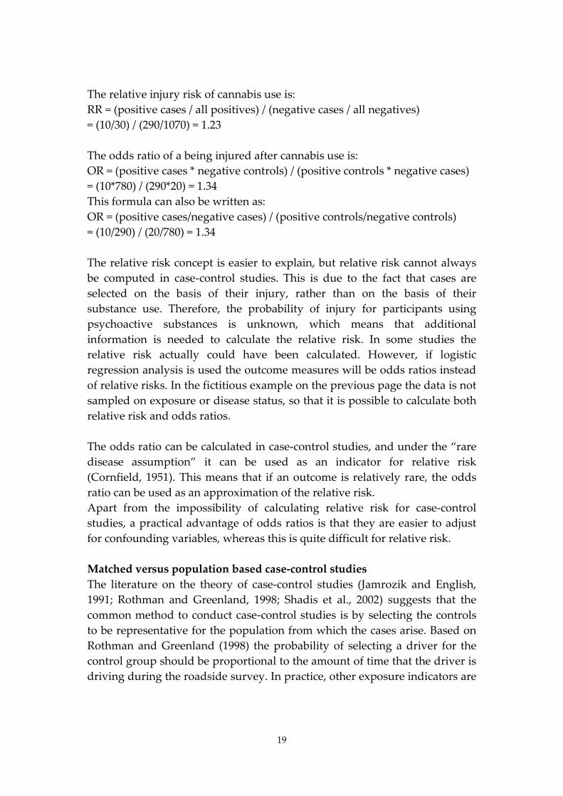
and unexposed to a risk factor. Based on this design, the odds ratio of an outcome can be computed. If the target population consists of car drivers, an odds ratio of 1 is assigned to drivers who are not exposed to the independent variable, i.e. who did not recently use cannabis. If the odds ratio of cannabis-exposed drivers is less than one, their risk is lower than the risk of unexposed drivers. If the odds ratio is more than one, the risk of exposed drivers is higher. Odds ratio versus relative risk The terms relative risk and odds ratio are often used as if they were synonyms. Technically this is not correct, since relative risk (or risk ratio) compares the probability of injury rather than the odds. Haworth et al. (1997) explained the difference between the odds and the probability of an event as follows: "The odds of an event occurring is equal to the probability of the event occurring divided by the probability of it not occurring. For example, the odds of drawing a diamond from a pack of cards is one-third (one quarter divided by three quarters), compared with the probability which is one quarter". (p. 18) Relative risk is a ratio of the probability of an event occurring in the exposed group versus the non-exposed group. It is frequently used in studies with low probabilities, where absolute risk measures will not provide significant differences between exposure and outcome variables. An odds ratio represents the ratio of the odds of an event occurring in one group to the odds of it occurring in another group. In Table 1.1, a fictitious example is given of the results of a study on the effects of cannabis use. Cases are injured car drivers and controls are randomly selected drivers from the same geographical area from which the cases arose. Both groups were tested for the presence of cannabis in blood, resulting in the following table:

Table 1.1. Example of fictive case-control study.

Cases Controls Total

Positive 10 20 30

Negative 290 780 1070

Total 300 800 1100

19

The relative injury risk of cannabis use is: RR = (positive cases / all positives) / (negative cases / all negatives) = (10/30) / (290/1070) = 1.23 The odds ratio of a being injured after cannabis use is: OR = (positive cases * negative controls) / (positive controls * negative cases) = (10*780) / (290*20) = 1.34 This formula can also be written as: OR = (positive cases/negative cases) / (positive controls/negative controls) = (10/290) / (20/780) = 1.34 The relative risk concept is easier to explain, but relative risk cannot always be computed in case-control studies. This is due to the fact that cases are selected on the basis of their injury, rather than on the basis of their substance use. Therefore, the probability of injury for participants using psychoactive substances is unknown, which means that additional information is needed to calculate the relative risk. In some studies the relative risk actually could have been calculated. However, if logistic regression analysis is used the outcome measures will be odds ratios instead of relative risks. In the fictitious example on the previous page the data is not sampled on exposure or disease status, so that it is possible to calculate both relative risk and odds ratios. The odds ratio can be calculated in case-control studies, and under the “rare disease assumption” it can be used as an indicator for relative risk (Cornfield, 1951). This means that if an outcome is relatively rare, the odds ratio can be used as an approximation of the relative risk. Apart from the impossibility of calculating relative risk for case-control studies, a practical advantage of odds ratios is that they are easier to adjust for confounding variables, whereas this is quite difficult for relative risk. Matched versus population based case-control studies The literature on the theory of case-control studies (Jamrozik and English, 1991; Rothman and Greenland, 1998; Shadis et al., 2002) suggests that the common method to conduct case-control studies is by selecting the controls to be representative for the population from which the cases arise. Based on Rothman and Greenland (1998) the probability of selecting a driver for the control group should be proportional to the amount of time that the driver is driving during the roadside survey. In practice, other exposure indicators are

20

used as well, e.g. traffic volume or trip distribution (Haworth et al., 1997; Mathijssen and Houwing, 2005). If random sampling is not feasible or if it is necessary to compensate for the effects of confounding factors (Jamrozik and English, 1991) it will be more efficient to match cases and controls. This is also the case if the outcome should include results for different subpopulations (Schlesselman, 1982). Matching is based on characteristics of the cases which are related to the outcome (confounding variables). The distribution of the confounding factors used for matching should be the same in both the control and the case groups. Common confounding factors that have been found in the literature on epidemiological studies to determine the risk of driving under the influence are: age, gender, time of day, day of week and road type. Matching all confounding variables is not efficient, though, and almost impossible in practice. Besides, it could lead to overmatching and thus to less precise estimates. Wacholder et al. (1992) state that "matching should be considered only for risk factors whose confounding effects need to be controlled for, but that are not of scientific interest as independent risk factors in the study". Matching for a subset of confounding factors is commonly applied in case-control studies. It implies that controls are selected to match a selection of confounding variables. Several case-control studies that have assessed the relative risk of driving under the influence of alcohol, have matched their controls regarding location, day of week and time of day (Borkenstein et al., 1974; Compton et al., 2002; Krüger and Vollrath, 2004). Matching for confounding factors like age and gender would lead to practical problems and less efficiency. Instead, in the studies mentioned above the adjustment for these confounding factors was performed afterwards in the statistical analysis.

1.3.2. Weaknesses of case-control studies

The main reason for conducting case-control studies is based on the methodological strength of this study type. The case-control design is very suitable when dealing with rare events such as substance use in traffic and when many factors for the psychoactive substances under study need to be evaluated. However, different practical and ethical issues regarding case-control studies have been mentioned in the literature as well. Berghaus et al. (2007) mention high cost and difficulties with the design. The results can be biased in many ways: by the selection of cases and controls, by the choice of confounding factors, and by non-response and missing cases.

21

The non-response rate will increase when the sample collection gets more invasive. This problem arises particularly when blood samples are required from control subjects (Beirness et al., 2006). If a study faces a large proportion of refusers, information on gender and age, self-reported drug use and clinical signs of impairment can be useful for determining whether, and to what extent, the non-response group would differ from the response group. These characteristics should therefore be available for both groups. The need for ethical approval can also lead to difficulties when conducting case-control studies. In Norway, a case-control study suffered difficulties due to requirements of the Ethical Committee (Assum, 2005) and in the United Kingdom a case-control study was cancelled because no approval was given by the Ethical committee and additional case-samples did not meet the requirements for comparison with the roadside (control) samples (Buttress et al., 2004). Alternatives for case-control studies are "culpability" or case-crossover studies, pharmaco-epidemiological studies and experimental studies. These alternative study types are in general less difficult and expensive to conduct than case-control studies. However, some particular methodological issues are associated with these study types when used for calculating relative risk. (Baldock, 2007; Berghaus et al., 2007).

1.3.3. Examples of case-control studies

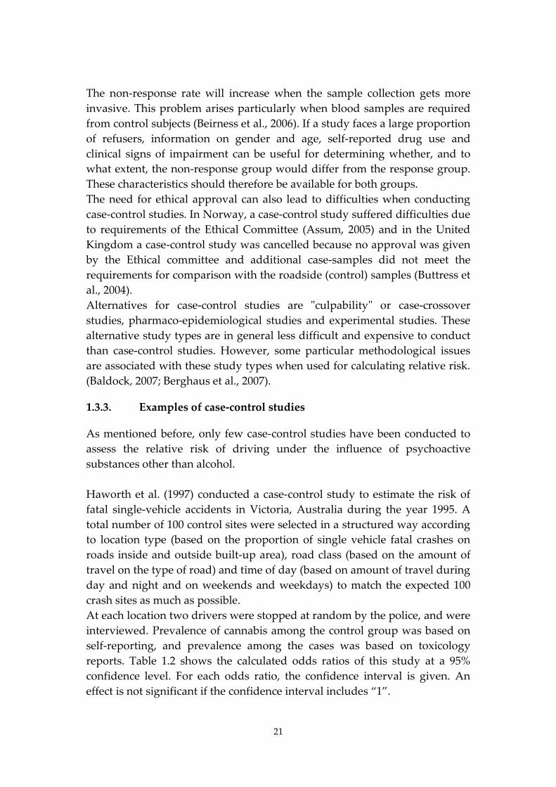
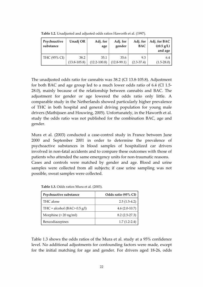
As mentioned before, only few case-control studies have been conducted to assess the relative risk of driving under the influence of psychoactive substances other than alcohol. Haworth et al. (1997) conducted a case-control study to estimate the risk of fatal single-vehicle accidents in Victoria, Australia during the year 1995. A total number of 100 control sites were selected in a structured way according to location type (based on the proportion of single vehicle fatal crashes on roads inside and outside built-up area), road class (based on the amount of travel on the type of road) and time of day (based on amount of travel during day and night and on weekends and weekdays) to match the expected 100 crash sites as much as possible. At each location two drivers were stopped at random by the police, and were interviewed. Prevalence of cannabis among the control group was based on self-reporting, and prevalence among the cases was based on toxicology reports. Table 1.2 shows the calculated odds ratios of this study at a 95% confidence level. For each odds ratio, the confidence interval is given. An effect is not significant if the confidence interval includes “1”.

22

Table 1.2. Unadjusted and adjusted odds ratios Haworth et al. (1997).

Psychoactive substance

Unadj OR Adj. for age

Adj. for gender

Adj. for BAC

Adj. for BAC (≥0.5 g/L)

and age

THC (95% CI) 38.2 (13.8-105.8)

35.1 (12.2-100.8)

35.6 (12.8-99.1)

9.3 (2.3-37.4)

6.4 (1.5-28.0)

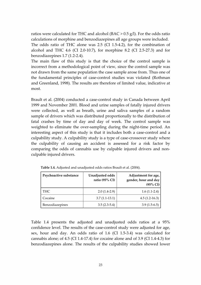
The unadjusted odds ratio for cannabis was 38.2 (CI 13.8-105.8). Adjustment for both BAC and age group led to a much lower odds ratio of 6.4 (CI 1.5-28.0), mainly because of the relationship between cannabis and BAC. The adjustment for gender or age lowered the odds ratio only little. A comparable study in the Netherlands showed particularly higher prevalence of THC in both hospital and general driving population for young male drivers (Mathijssen and Houwing, 2005). Unfortunately, in the Haworth et al. study the odds ratio was not published for the combination BAC, age and gender. Mura et al. (2003) conducted a case-control study in France between June 2000 and September 2001 in order to determine the prevalence of psychoactive substances in blood samples of hospitalized car drivers involved in non-fatal accidents and to compare these outcomes with those of patients who attended the same emergency units for non-traumatic reasons. Cases and controls were matched by gender and age. Blood and urine samples were collected from all subjects; if case urine sampling was not possible, sweat samples were collected.

Table 1.3. Odds ratios Mura et al. (2003).

Psychoactive substance Odds ratio (95% CI)

THC alone 2.5 (1.5-4.2)

THC + alcohol (BAC> 0.5 g/l) 4.6 (2.0-10.7)

Morphine (> 20 ng/ml) 8.2 (2.5-27.3)

Benzodiazepines 1.7 (1.2-2.4)

Table 1.3 shows the odds ratios of the Mura et al. study at a 95% confidence level. No additional adjustments for confounding factors were made, except for the initial matching for age and gender. For drivers aged 18-26, odds

23

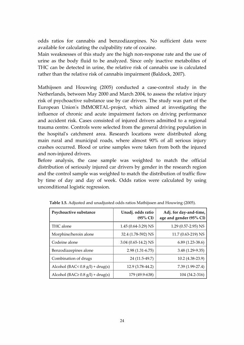
ratios were calculated for THC and alcohol (BAC > 0.5 g/l). For the odds ratio calculations of morphine and benzodiazepines all age groups were included. The odds ratio of THC alone was 2.5 (CI 1.5-4.2), for the combination of alcohol and THC 4.6 (CI 2.0-10.7), for morphine 8.2 (CI 2.5-27.3) and for benzodiazepines 1.7 (1.2-2.4). The main flaw of this study is that the choice of the control sample is incorrect from a methodological point of view, since the control sample was not drawn from the same population the case sample arose from. Thus one of the fundamental principles of case-control studies was violated (Rothman and Greenland, 1998). The results are therefore of limited value, indicative at most. Brault et al. (2004) conducted a case-control study in Canada between April 1999 and November 2001. Blood and urine samples of fatally injured drivers were collected, as well as breath, urine and saliva samples of a random sample of drivers which was distributed proportionally to the distribution of fatal crashes by time of day and day of week. The control sample was weighted to eliminate the over-sampling during the night-time period. An interesting aspect of this study is that it includes both a case-control and a culpability study. A culpability study is a type of case-crossover study where the culpability of causing an accident is assessed for a risk factor by comparing the odds of cannabis use by culpable injured drivers and non-culpable injured drivers.

Table 1.4. Adjusted and unadjusted odds ratios Brault et al. (2004).

Psychoactive substance Unadjusted odds ratio (95% CI)

Adjustment for age, gender, hour and day

(95% CI)

THC 2.0 (1.4-2.9) 1.6 (1.1-2.4)

Cocaine 3.7 (1.1-13.1) 4.5 (1.2-16.3)

Benzodiazepines 3.5 (2.3-5.4) 3.9 (1.5-6.5)

Table 1.4 presents the adjusted and unadjusted odds ratios at a 95% confidence level. The results of the case-control study were adjusted for age, sex, hour and day. An odds ratio of 1.6 (CI 1.5-3.4) was calculated for cannabis alone; of 4.5 (CI 1.4-17.4) for cocaine alone and of 3.9 (CI 1.4-4.3) for benzodiazepines alone. The results of the culpability studies showed lower

24

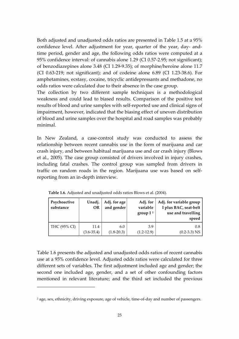
odds ratios for cannabis and benzodiazepines. No sufficient data were available for calculating the culpability rate of cocaine. Main weaknesses of this study are the high non-response rate and the use of urine as the body fluid to be analyzed. Since only inactive metabolites of THC can be detected in urine, the relative risk of cannabis use is calculated rather than the relative risk of cannabis impairment (Baldock, 2007). Mathijssen and Houwing (2005) conducted a case-control study in the Netherlands, between May 2000 and March 2004, to assess the relative injury risk of psychoactive substance use by car drivers. The study was part of the European Union's IMMORTAL-project, which aimed at investigating the influence of chronic and acute impairment factors on driving performance and accident risk. Cases consisted of injured drivers admitted to a regional trauma centre. Controls were selected from the general driving population in the hospital's catchment area. Research locations were distributed along main rural and municipal roads, where almost 90% of all serious injury crashes occurred. Blood or urine samples were taken from both the injured and non-injured drivers. Before analysis, the case sample was weighted to match the official distribution of seriously injured car drivers by gender in the research region and the control sample was weighted to match the distribution of traffic flow by time of day and day of week. Odds ratios were calculated by using unconditional logistic regression.

Table 1.5. Adjusted and unadjusted odds ratios Mathijssen and Houwing (2005).

Psychoactive substance Unadj. odds ratio (95% CI)

Adj. for day-and-time, age and gender (95% CI)

THC alone 1.45 (0.64-3.29) NS 1.29 (0.57-2.95) NS

Morphine/heroin alone 32.4 (1.78-592) NS 11.7 (0.63-219) NS

Codeine alone 3.04 (0.65-14.2) NS 6.89 (1.23-38.6)

Benzodiazepines alone 2.98 (1.31-6.75) 3.48 (1.29-9.35)

Combination of drugs 24 (11.5-49.7) 10.2 (4.38-23.9)

Alcohol (BAC< 0.8 g/l) + drug(s) 12.9 (3.78-44.2) 7.39 (1.99-27.4)

Alcohol (BAC≥ 0.8 g/l) + drug(s) 179 (49.9-638) 104 (34.2-316)

25

Both adjusted and unadjusted odds ratios are presented in Table 1.5 at a 95% confidence level. After adjustment for year, quarter of the year, day- and-time period, gender and age, the following odds ratios were computed at a 95% confidence interval: of cannabis alone 1.29 (CI 0.57-2.95; not significant); of benzodiazepines alone 3.48 (CI 1.29-9.35); of morphine/heroine alone 11.7 (CI 0.63-219; not significant); and of codeine alone 6.89 (CI 1.23-38.6). For amphetamines, ecstasy, cocaine, tricyclic antidepressants and methadone, no odds ratios were calculated due to their absence in the case group. The collection by two different sample techniques is a methodological weakness and could lead to biased results. Comparison of the positive test results of blood and urine samples with self-reported use and clinical signs of impairment, however, indicated that the biasing effect of uneven distribution of blood and urine samples over the hospital and road samples was probably minimal. In New Zealand, a case-control study was conducted to assess the relationship between recent cannabis use in the form of marijuana and car crash injury, and between habitual marijuana use and car crash injury (Blows et al., 2005). The case group consisted of drivers involved in injury crashes, including fatal crashes. The control group was sampled from drivers in traffic on random roads in the region. Marijuana use was based on self-reporting from an in-depth interview.

Table 1.6. Adjusted and unadjusted odds ratios Blows et al. (2004).

Psychoactive substance

Unadj. OR

Adj. for age and gender

Adj. for variable group I 2

Adj. for variable group I plus BAC, seat-belt

use and travelling speed

THC (95% CI) 11.4 (3.6-35.4)

6.0 (1.8-20.3)

3.9 (1.2-12.9)

0.8 (0.2-3.3) NS

Table 1.6 presents the adjusted and unadjusted odds ratios of recent cannabis use at a 95% confidence level. Adjusted odds ratios were calculated for three different sets of variables. The first adjustment included age and gender; the second one included age, gender, and a set of other confounding factors mentioned in relevant literature; and the third set included the previous 2 age, sex, ethnicity, driving exposure, age of vehicle, time-of-day and number of passengers.

26

variables plus a set of additional risky driving variables such as BAC level and seat-belt use. The authors reported adjusted odds ratios for these three sets of variables of respectively 6.0 (CI 1.8-20.3); 3.9 (1.2-12.9); and 0.8 (CI 0.2-3.3 not significant). The use of interviews, instead of samples of body fluids, is a major weakness of this study design. Furthermore, the choice of confounding factors could be questioned, since some of the variables, like sleepiness, may be associated with marijuana use. The authors have acknowledged this problem but indicated that it is difficult to estimate the size and direction of this potential bias. Finally, non-response among controls was 21.2%, which is quite a large proportion, especially since only 0.5% of the remaining drivers in the control group reported recent marijuana use. In comparison, 7.2% of the accident-involved drivers, refused to cooperate and 5.6% reported recent marijuana use. The comparison of the outcomes of the 5 case-control studies in this section shows that there is considerable variation between the results. This raises the question whether the designs of the studies were comparable or not.

1.3.4. Comparability of case-control studies

As stated earlier, the number of case-control studies that have been conducted to assess the risk of driving under the influence of psychoactive substances other than alcohol is very small. But even a limited number of studies can provide good estimates of the risk of drug driving. The outcomes are only comparable, however, when the selected studies both have comparable study designs, and no (or very limited) bias. The comparability of the study design and the presence of potential bias can be measured by several indicators. The effect of these indicators on the results may vary and some indicators might be related to each other. Therefore, it cannot be assumed that studies which differ on only one indicator are more comparable than studies with more variation between the indicators. To provide more insight in the comparability of the case-control studies that were discussed in the previous section, a list of nine indicators was used by Houwing et al. (2009): • Substances • Type of cases • Type of controls • Collection method cases • Collection method controls • Response rate cases

27

• Response rate controls • Lower limit of substance concentration • Confounding factors This list of indicators should be seen as a short-list to illustrate the differences and not as an exhaustive comparison between the studies. Table 1.7 provides an overview of main indicators for the five recently conducted case-control studies as summarized in the previous section. In this table only the results for THC have been used since, this was the only drug type that was analyzed in all five studies. The designs of four of these studies are quite comparable for the type of cases and controls. Only Mura et al. (2003), however, did not use randomly selected drivers as controls, but non-crash involved patients in possession of a driving license. The four remaining studies all vary in the way they collected data on cases and controls. Blows et al. (2004) used interviews for both cases and controls, Haworth et al. (1997) used toxicological reports for cases based on blood and urine samples and interviews for the subjects in the control group, Mathijssen and Houwing (2005) have used blood or urine for the cases and urine or blood for the controls, whereas Brault et al. (2004) used urine for both cases and controls. In order to estimate the relative risk of driving under the influence of psychoactive substances, urine is less useful than saliva and blood since the detection window is much larger which has definite consequences for its validity as body fluid sample. Furthermore, the response rate of the different studies varies between 63% and 96% for the cases and between 49.6% and 96% for the controls. This is mainly a validity issue: the higher the refusal rate, the higher the risk of bias. The cut-off levels of the analyzed body fluids differ from each other. A higher cut-off level will result in a smaller proportion of positive subjects. In the case of these five selected studies the differences between the cut-off levels were small and would probably hardly affect the comparability.

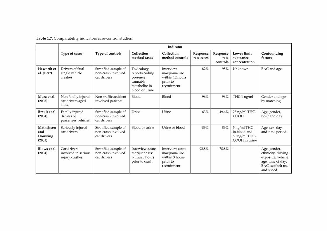
Table 1.7. Comparability indicators case-control studies.

Indicator

Type of cases Type of controls Collection method cases

Collection method controls

Response rate cases

Response rate

controls

Lower limit substance concentration

Confounding factors

Haworth et al. (1997)

Drivers of fatal single vehicle crashes

Stratified sample of non-crash involved car drivers

Toxicology reports coding presence cannabis metabolite in blood or urine

Interview marijuana use within 12 hours prior to recruitment

82% 95% Unknown BAC and age

Mura et al. (2003)

Non fatally injured car drivers aged 18-26

Non-traffic accident involved patients

Blood Blood 96% 96% THC 1 ng/ml Gender and age by matching

Brault et al. (2004)

Fatally injured drivers of passenger vehicles

Stratified sample of non-crash involved car drivers

Urine Urine 63% 49.6% 25 ng/ml THC-COOH

Age, gender, hour and day

Mathijssen and Houwing (2005)

Seriously injured car drivers

Stratified sample of non-crash involved car drivers

Blood or urine Urine or blood 89% 89% 5 ng/ml THC in blood and 50 ng/ml THC-COOH in urine

Age, sex, day-and-time period

Blows et al. (2004)

Car drivers involved in serious injury crashes

Stratified sample of non-crash involved car drivers

Interview acute marijuana use within 3 hours prior to crash

Interview acute marijuana use within 3 hours prior to recruitment

92.8% 78.8% - Age, gender, ethnicity, driving exposure, vehicle age, time of day, BAC, seatbelt use and speed

29

Finally, adjustment for confounding factors also differs from study to study. The impact of confounding factors on the odds ratio can be substantial. Haworth et al. (1997) found an unadjusted odds ratio for cannabis of 38.2, adjusting for age and gender resulting in lower odds ratios of respectively 35.1 and 35.6. Adjustment for alcohol use resulted in a much lower odds ratio of 9.3, and adjustment for both alcohol and age even to an odds ratio of 6.4. Most studies included at least age, gender and time of day as confounding variables or matched for these variables when selecting controls. Blows et al. (2004) included many more possible confounding factors in the analysis, which probably resulted in overmatching. Above that, not all factors that were used in this study can be regarded as confounding factors. In this PhD thesis a more elaborated study on the effect of random and systematic errors is presented in Chapter 6. In this chapter, six case-control studies with more or less uniform study designs were screened for the presence of potential sources of errors, which could cause bias in the results.

1.3.5. Discussion

Case-control studies have their strengths, but also their weaknesses. The methodology is hard to implement and there are many sources of potential bias that could affect the validity of the study results. On top of that, ethical issues may arise, especially in collecting samples of body fluids among controls. Case-control studies are therefore not commonly used as method for assessing the risk of driving under the influence of psychoactive substances other than alcohol. Another problem is the lack of comparability between the case-control studies that have been conducted. It is likely that this variation is at least partly caused by differences in the research design, causing incomparable results even if the odds ratios seem to be more or less the same. The lack of comparable case-control studies does not mean that there are no risk estimations for driving under the influence of psychoactive substances other than alcohol. Instead of difficult and expensive case-control studies, the risk of drug driving is also measured by culpability studies where no non-crash-involved drivers are selected in the control-group. These studies are also known as case-crossover studies. Furthermore, pharmaco-epidemiological studies are used to determine risk factors of medicines on therapeutic base. In these studies persons who are using prescriptive medicines or who are known to have a disease are compared crash involved drivers.

30

Finally, results of experimental studies are used as well to estimate risk. For this purpose the dose-related impairment of drugs or medicines is compared with the impairment by alcohol at different BAC levels. If the impairment factor is comparable, then the risk factor is regarded to be the same as that of the corresponding BAC level. These three alternative study designs are in general less difficult and expensive to conduct than case-control studies. However, some methodological issues are imbedded in these study types when using them for calculating the risk of drug driving (Baldock, 2007; Berghaus et al., 2007). Chapter 2 of this thesis provides a more detailed overview of the four study designs that are used to assess the risk of driving under the influence. The specific strengths and limitations of case-control studies and the three alternative study designs are discussed in this chapter. In 2006, a consensus meeting was organized by the International Council on Alcohol, Drugs and Traffic Safety (ICADTS) to develop standards for future research. These recommendations for standardized research included legal/ethical issues, subject and study design issues and core data parameters. At this meeting cut-off levels were recommended for blood, saliva and urine. These cut-off levels were applied in the prevalence and risk studies of the European DRUID project. Furthermore, guidelines were prepared for the design of the DRUID case-control studies (Assum et al., 2007). Six case-control studies were conducted in the DRUID project to assess the relative risk of serious injury due to driving under the influence. Although the design of the DRUID case-control studies was more or less comparable, differences were still present because of practical, ethical or legal limitations between these countries. In order to compare the outcome of these studies with each other and with previous studies, more insight is needed in the effects that study errors and differences in study design have on the study outcomes. With more knowledge on the effect of bias and survey errors it will be easier to interpret the odds ratios from formerly conducted case-control studies. Therefore we investigated the six DRUID case-control studies for the presence of potential sources of random and systematic errors. Researchers that are planning to conduct case-control studies to determine the risk of driving under the influence could use the results from this thesis to optimize their study design.

31

1.4. Objectives of the thesis

This thesis aims at contributing to the current knowledge on how to design case-control studies which are used to assess the relative risk of driving under the influence of psychoactive substances. The results of this thesis will give insight in how to provide the best estimate of the risk of driving under the influence of psychoactive substances (DUI). To accomplish this main objective, the following research questions are studied throughout the thesis: • Which are the possible methods to estimate the risk of driving under

the influence of psychoactive substances? (Chapter 2) • What is the most preferred case-control design and which design is

most commonly used in practice? (Chapter 2) • What is the prevalence of psychoactive substances in general traffic?

(Chapter 3) • What is the prevalence of psychoactive substances among seriously

injured drivers? (Chapter 4) • Is there any difference between substance concentrations collected by

means of spitting tubes and by a commercial oral fluid collection device? (Chapter 5)

• What is the effect of random and systematic errors on the odds ratios of case-control studies? (Chapter 6)

1.5. Outline of the thesis

Chapter 2 focuses on the differences in study design between studies that assess the crash risk of driving under the influence of psychoactive substances. To this end, four types of study designs were discussed. Furthermore, this chapter provides an overview of the differences between the preferred study designs and the studies that were actually conducted in practice. The epidemiological case-control studies that were conducted within the European research project DRUID study the relative risk of serious injury by comparing the prevalence of psychoactive substances among injured car drivers (cases) and among non-injured drivers from daily traffic (controls). Chapter 3 compares the results of the Dutch and Belgian roadside surveys in which data on substance use were collected from non-injured drivers. These non-injured drivers also formed the control population for the case-control studies in Belgium and the Netherlands in which the relative risk of driving under the influence of psychoactive substances is estimated. In Chapter 4 the

32

results of the hospital studies on substance use among seriously injured drivers (cases) in both countries were compared. These seriously injured drivers formed the case population of the Dutch and Belgian case-control study. The methods of sample collection were comparable in the Netherlands and Belgium, except that oral fluid samples in the Netherlands were collected by spit tubes, whereas in Belgium a commercial oral fluid collection device was used. Chapter 5 discusses the differences in variability between these two oral fluid collection methods in determining the presence of THC. The results also provide information on the correlation between THC concentrations that were collected by both methods. Chapter 6 presents an overview of the effect of random and systematic errors on the results of case-control studies. The results of the six DRUID case-control studies on the injury risk of driving under the influence of psychoactive substances were compared for eleven indicators of potential bias. In the final chapter the results of this thesis are discussed in the light of the research questions that were mentioned in Section 1.4.

33

2. In search of a standard for assessing the crash risk of driving under the influence of drugs other than alcohol; Results of a questionnaire survey among researchers3

2.1. Introduction

2.1.1. Relevance and previous research

While numerous studies have assessed the crash risk of driving under the influence of alcohol, and the outcomes of the different studies are generally comparable, only a limited number of studies have assessed the risk of driving under the influence of drugs and medicines, and with quite divergent outcomes (EMCDDA, 2008; Kelly et al., 2004; Krüger et al., 2008; OECD, 2010; Walsh et al., 2004). The theoretically most sound study design mentioned in literature to assess risk is the case-control study (Howe and Choi, 1983; Shadis et al., 2002). The case-control study is an epidemiological study design that compares drug use between crash involved drivers and non-crash involved drivers on the roads. However, case-control studies are expensive and time-consuming and therefore not commonly conducted. A less expensive epidemiological study design is the culpability study. Culpability studies are nested case-control studies, which are used to compare culpability rates of drug-positive accident-involved drivers with culpability rates of drug-negative accident-involved drivers. The classification of culpability is based on a structured culpability analysis that is assessed without previous knowledge on the use of psychoactive substances by the driver. A second alternative study design is the pharmaco-epidemiological study, which compares accident rates of medicine users with non-medicine users. For this purpose, information from pharmacy records or health insurance databases is linked with crash records. Other than epidemiological studies, experimental studies are used to determine the risk associated with driving under the influence of 3 This chapter is published as the following article: Houwing, S., Mathijssen, R. & Brookhuis, K.A. (2012). In search of a standard for assessing the crash risk of driving under the influence of drugs other than alcohol; Results of a questionnaire survey among researchers. This article is published in Traffic Injury Prevention (TIP) 2012; 13 (6) 554-565.

34

psychoactive substances. Experimental studies are applied to assess possible impairment of various skills and abilities that are related to driving (Brookhuis et al., 2003). At present, these experimental studies generally involve administering a drug to volunteer subjects and then measuring their performance in driving simulators, on closed courses, or in on-the-road situations in actual traffic (Ramaekers et al., 2004). For the additional assessment of the crash risk of licit and illicit drugs, the results are related to the results for alcohol at specific Blood Alcohol Concentration (Pelfrene et al.) levels, for which more or less standardized and accepted odds ratios have been derived from epidemiological research (Brookhuis et al., 2003; Krüger et al., 2008). Although in general the alternative study designs are less difficult and less expensive than case-control studies, they have some methodological limitations when they are used for calculating the risk of drug driving. An Australian literature review on cannabis and crash risk by Baldock (2007) states three limitations of culpability studies. The first limitation is that a non-culpable driver may still have contributed to the causation of the crash. Another limitation is the attribution of culpability. There may be a bias if the police are more likely to assign culpability to an impaired driver. The third problem of culpability studies is the (often small) sample size of the drug-positive group, which may result in low statistical power. However, this problem is not particularly restricted to culpability studies and may also occur in case-control studies. The disadvantages of pharmaco-epidemiology studies are mentioned in Berghaus et al. (2007). The authors question the compliance of the driver to his medication and they state that it may not be known whether the driver was impaired by additional psychoactive substances or other influencing factors. The validity of risk assessment by means of experimental studies is also questioned by some authors. One reason being that dose-related risk rates for THC resulting from case-control and culpability studies are lower than risk rates derived from experimental studies (Grotenhermen et al., 2007; Ramaekers et al., 2004). For other drugs, dose-related risk factors from epidemiological studies are hardly available, which makes it impossible to compare between experimental and epidemiological studies. Despite the previously mentioned potential limitations on determining the risk by other methods than case-control studies, it is clear that present knowledge on the crash risk of driving under the influence would have been very limited without the additional results of experimental, pharmaco-epidemiological and culpability studies.

35

The variety of study types on crash risk assessment with each different outcome measures makes it difficult though to compare the results for different substances. In addition to this, the comparison of results from studies within one and the same study type can also be difficult, since differences in study design may cause large differences in results as well. Design effects could directly influence the results, e.g. by differences in the applied adjustment for confounding factors. The relative risk of cannabis use for example varies in case-control studies from 0.8 to 35.6, depending on the confounding factors the odds ratio was adjusted for (Houwing et al., 2009). Differences in study design could also influence the results indirectly, e.g. by choosing a study design which could lead to a larger selective non-response bias, like gathering information by self-report. During the past 20 years, several meetings between researchers were organized to harmonize research designs. In 1991, a workshop was held in Padova, Italy, to address methodological issues of drug-driving research (Ferrara and Giorgetti, 1992). Guidelines and standards were proposed for both experimental and epidemiological studies. In the same year, a survey was conducted by Vermeeren et al. (1993) on expert opinions regarding the design and execution of experimental studies relevant to the effects of medicinal drugs and driving. One year later, in 1992, a follow-up meeting on the Padova workshop was organized during the ICADTS (International Council on Alcohol, Drugs and Traffic Safety) conference in Cologne. The results of Vermeeren’s survey were discussed and an agreement on six recommendations was reached. In 1994, a working group was established by ICADTS with the goal to "prepare a sound guide to an optimal methodology of experimental studies on drugs and driver fitness, publish these guidelines and attempt to get to acceptance by experts, institutions and authorities". Based on a review of the relevant literature this working group concluded in 1999 that the criteria of sound methodologies and comparable results are not met due to various differences in study design. Therefore, the guidelines on experimental research from the workshops in Padova and Cologne and the results of the expert survey by Vermeeren (1993) were compiled in a workshop report (ICADTS, 1999). Despite these efforts to harmonize results on drug driving, researchers still stated a lack of comparability at the beginning of the new millennium (Ramaekers et al., 2004; Walsh et al., 2004). In 2005, another ICADTS working group, the Working Group Illegal Drugs and Driving, identified the need for a set of standards and guidelines for drug-driving research and organized an expert meeting in September 2006,

36

in Talloires, France, to discuss the harmonisation of protocols for future drug-driving research. As a result, draft guidelines were developed for experimental research, epidemiological research and toxicological issues. Recommendations for standardized research include legal/ethical issues, subject selection issues, study design issues and core data parameters, such as demographic data and core drug groups. Furthermore, cut-off levels were recommended for blood, saliva and urine analysis. The draft "Talloires guidelines" were published on the ICADTS website during 45 days for comment and review by experts in the field of drug driving. The comments were integrated into a final document called "Guidelines for Drugged Driving Research” (Walsh et al., 2008). In the autumn of 2006, the European Research project DRUID (Driving Under the Influence of Drugs, Alcohol and Medicines) started. In this project several experimental and epidemiological studies on drug driving were conducted. In order to reach comparable results, a lot of effort was put into harmonization of study designs. For the case-control studies a working paper has been written containing guidelines for a uniform design and protocols for carrying out case-control and prevalence studies (Assum et al., 2007). This working paper was based on the Talloires guidelines and on past experience with case-control studies of the authors involved. It was agreed that any deviation from these guidelines should be reported by the partners. A similar protocol for study designs was prepared for the experimental studies within DRUID (Krüger et al., 2008).

2.1.2. Knowledge gap

A comparison of recent studies on the risk of driving under the influence of psychoactive substances including the case-control studies that were conducted within the DRUID project shows that design differences still exist (Houwing et al., 2009; Isalberti et al., 2011). Little is known about the reasons for these differences. Do they still occur because there is no consensus among researchers on standards to assess the risk of DUI, or is there actually a general consensus, but are researchers forced to deviate from their ’gold standard’ for more practical reasons? Furthermore, there is a knowledge gap with respect to the effect that design differences may have on the size and direction of differences between study results. Therefore, researchers have been requested to provide a rough indication of the size and direction of any bias that could arise from their deviations from the standard.

37

2.1.3. Study objective

The present study uses questionnaires to find out if DUI researchers agree on a ’gold standard’ for study designs. Furthermore, it wants to provide more insight in the extent to which researchers deviate from their own standard, and for which reasons.

2.2. Materials and methods

2.2.1. Participants

The questionnaire study was carried out among researchers who have conducted or are conducting studies to assess the crash risk of driving under the influence of psychoactive substances other than alcohol, and also among researchers who compiled reviews of these studies.

2.2.2. Procedure

First, an international literature search was conducted to generate a selection of authors of papers and studies involving the risk of driving under the influence of psychoactive substances. This search contained the combination of the keywords “driving” and “risk” plus one or more specified drugs or drug groups. From the resulting literature list, all corresponding authors were selected. If an author was mentioned more than once as a non-corresponding author, the author’s name was added to the study frame as well. In some cases no contact details were available, even after an internet search by name and institute. In these cases, one of the co-authors, if present, was added to the study frame. Next, five recent review studies (EMCDDA, 2008; Kelly et al., 2004; Penning et al., 2010; TIRF and Palmer, 2007; Walsh et al., 2004) on the risk of driving under the influence of psychoactive substances were screened for any additional references. Finally, any additional researchers from the roadside prevalence studies in the European DRUID project were included in the study frame. Based on this literature search, 88 researchers were included in the study frame: 26 were linked to case-control studies, 18 to experimental studies, 28 to review studies or DRUID roadside prevalence studies, 8 to pharmaco-epidemiological studies, and 6 to culpability studies. For two researchers the exact type of study could only be determined after completion of the questionnaire.

38

In the next step, an internet survey questionnaire was sent out to all authors included in the study frame. The initial questionnaire was pre-tested by four different researchers with experience in different study types. Based on their remarks, some questions were simplified and answer options stating "I don't know" were added. Furthermore, a question on the respondent’s experience with drink and drug driving research was included in the questionnaire. The responses were collected within a three month period, between June and August 2010. After one and a half month a reminder was sent to non-responders. The second and final reminder was sent one month after the first one. After completing the questionnaire, researchers who reported differences between their theoretical optimal study design and their design in practice, received a short follow-up questionnaire asking for the reasons why. The follow-up questionnaires were sent a week after the first responses arrived. A reminder was sent after two months and a second reminder was sent after three months. No incentives were used to encourage participation. When the questionnaire had been sent out, four e-mail addresses appeared to be invalid and no substitute e-mail address could be retrieved. Therefore, a total of 84 authors received an invitation to participate.

2.2.3. Questionnaire

The questionnaire consisted of several questions divided into three main categories. A general category contained a small number of questions on study types preference and research. This part contained questions such as whether the participant had conducted a study in the past or was conducting a study at present to assess the risk of driving under the influence of psychoactive substance. A second category contained questions on aspects of the theoretically optimal study design, such as which type of body fluid the participant would prefer to use to collect data on substance use among injured subjects if applicable. And a third category of questions regarded the study design in practice. This part contained questions such as which type of body fluid the participant used or was using in his study to collect data on substance use among injured subjects, if applicable. Researchers who had been conducting review studies and researchers who indicated that they had not been involved in the choice of study design, only needed to complete the general part of the questionnaire. The total number of questions depended both on the actually applied study design and on the answers that were given, since some answers would lead to additional questions.

39

Most questions throughout the questionnaire were closed questions. The majority of questions allowed only one answer option, but for a number of questions more than one answer could be given. In the part on the theoretically preferred design, these questions included a ranking of the answers, whereas the same questions on the design in practice included multiple choice questions. By using the ranking option, more detailed information became available regarding the preference of the respondent.

2.2.4. Data collection and analysis

All responses were collected through an online questionnaire application (LimeSurvey v1.85) and were exported into an Excel database for further analysis. Due to the small numbers and the explorative background of this survey, the results of the questionnaire were only analysed in a qualitative way, making use of SAS 9.2 statistical software (SAS Institute Inc., Cary, NC, USA). This study will discuss the extent to which researchers agree on the theoretical study design and the comparability of the different studies in practice. Comparability is defined in this study as the level of “similarity”. The similarity rate of the answers is calculated by dividing the largest number of identical answers by the total number of answers. The total number of answers equals the total number of respondents minus the 'no replies' and the number of 'I don't know' answers. Next, the average similarity rate of a study type is calculated by summing up all the similarity scores for a study type and dividing them by the number of questions. The similarity rate is regarded as 'good' if it is 75% or higher. The application of the 75% level is not based on a statistical ground rule, but we considered such a practical criterion very useful since it can be applied to make a statement on the similarity of study design items and different study designs.

2.3. Results

2.3.1. General results

The overall response rate was 68% (n=57). The majority, 89% (n=51), completed all questions and 11% (n=6) of the respondents did not respond to part of the questionnaire. This response rate was satisfying, since the expert questionnaire sent in 1993 (Vermeeren et al., 1993) had a response rate of 47% and a recent questionnaire (De Gier et al., 2009) among experts in the field of

40

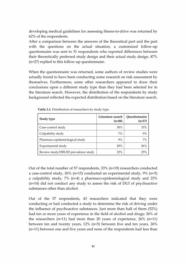
developing medical guidelines for assessing fitness-to-drive was returned by 62% of the respondents. After a comparison between the answers of the theoretical part and the part with the questions on the actual situation, a customized follow-up questionnaire was sent to 31 respondents who reported differences between their theoretically preferred study design and their actual study design. 87% (n=27) replied to this follow-up questionnaire. When the questionnaire was returned, some authors of review studies were actually found to have been conducting some research on risk assessment by themselves. Furthermore, some other researchers appeared to draw their conclusions upon a different study type than they had been selected for in the literature search. However, the distribution of the respondents by study background reflected the expected distribution based on the literature search.

Table 2.1. Distribution of researchers by study type.

Study type Literature search

(n=88) Questionnaire

(n=57)

Case-control study 30% 33%

Culpability study 7% 9%

Pharmaco-epidemiological study 9% 7%

Experimental study 20% 26%

Review study/DRUID prevalence study 32% 25%

Out of the total number of 57 respondents, 33% (n=19) researchers conducted a case-control study, 26% (n=15) conducted an experimental study, 9% (n=5) a culpability study, 7% (n=4) a pharmaco-epidemiological study and 25% (n=14) did not conduct any study to assess the risk of DUI of psychoactive substances other than alcohol. Out of the 57 respondents, 43 researchers indicated that they were conducting or had conducted a study to determine the risk of driving under the influence of psychoactive substances. Just more than half of them (52%) had ten or more years of experience in the field of alcohol and drugs: 26% of the researchers (n=11) had more than 20 years of experience, 26% (n=11) between ten and twenty years, 12% (n=5) between five and ten years, 26% (n=11) between one and five years and none of the respondents had less than

41

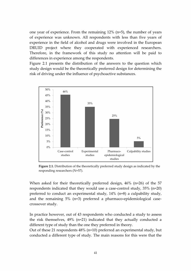
one year of experience. From the remaining 12% (n=5), the number of years of experience was unknown. All respondents with less than five years of experience in the field of alcohol and drugs were involved in the European DRUID project where they cooperated with experienced researchers. Therefore, in the framework of this study no attention will be paid to differences in experience among the respondents. Figure 2.1 presents the distribution of the answers to the question which study design would be the theoretically preferred design for determining the risk of driving under the influence of psychoactive substances.

46%

35%

25%

5%

0%

5%

10%

15%

20%

25%

30%

35%

40%

45%

50%

Case-controlstudies

Experimentalstudies

Pharmaco-epidemiological

studies

Culpability studies

Pref

eren

ce (%

)

Figure 2.1. Distribution of the theoretically preferred study design as indicated by the responding researchers (N=57).

When asked for their theoretically preferred design, 46% (n=26) of the 57 respondents indicated that they would use a case-control study, 35% (n=20) preferred to conduct an experimental study, 14% (n=8) a culpability study, and the remaining 5% (n=3) preferred a pharmaco-epidemiological case-crossover study. In practice however, out of 43 respondents who conducted a study to assess the risk themselves, 49% (n=21) indicated that they actually conducted a different type of study than the one they preferred in theory. Out of these 21 respondents 48% (n=10) preferred an experimental study, but conducted a different type of study. The main reasons for this were that the

42

research question was focused on epidemiological research and not on experimental research (n=4) or that they were not specialised in conducting experimental research (n=3).33% of the 21 (n=7) preferred a case-control study, but conducted a different study type. The main reason for this were practical problems in the design phase (n=4), such as lack of time and manpower, and inability to get cooperation from third parties like police and hospitals. Furthermore, some respondents indicated that they were specialised in other types of study (n=3) and not in matched or population based case-control studies and that the research question was focused on experimental research and not on epidemiological research (n=1). Out of the 21 respondents 14% (n=3) preferred a culpability study but did not conduct one. Two respondents answered the questions in the follow-up study. One of them gave as reason that it was too difficult to get the required data. The other respondent indicated that the research question required experimental instead of epidemiological research. Finally, one respondent preferred a pharmaco-epidemiological design, but conducted a case-control study. However, the preferred pharmaco-epidemiological design was in fact highly comparable to a standard case-control design.

2.3.2. Results per study type

The number of responses per study type varied between 4 and 19, although some researchers did not fully complete the questionnaire. For both culpability studies (5 questionnaires returned, 4 of which fully completed) and pharmaco-epidemiological studies (4 returned, 2 of which fully completed) the number of respondents was very low. Therefore, these results should be treated with special care and be seen as purely indicative. Case-control studies (n=19) Table 2.2 provides an overview of the comparability of case-control studies. Comparability rates are higher when more respondents give the same answer. For each question the most frequently given answer is presented in the table, as well as the total number of responses and the comparability score (total number of responses divided by the largest number of identical answers). Among researchers who indicated to conduct case-control studies, there seems to be considerable consensus on the theoretically preferred study design. The similarity of the answers was above the 75% criterion on eight out of twelve items. It was lower for the applied cut-off level (53%), the type of injury (35%), the type of roads (74%), and the reference group for drug

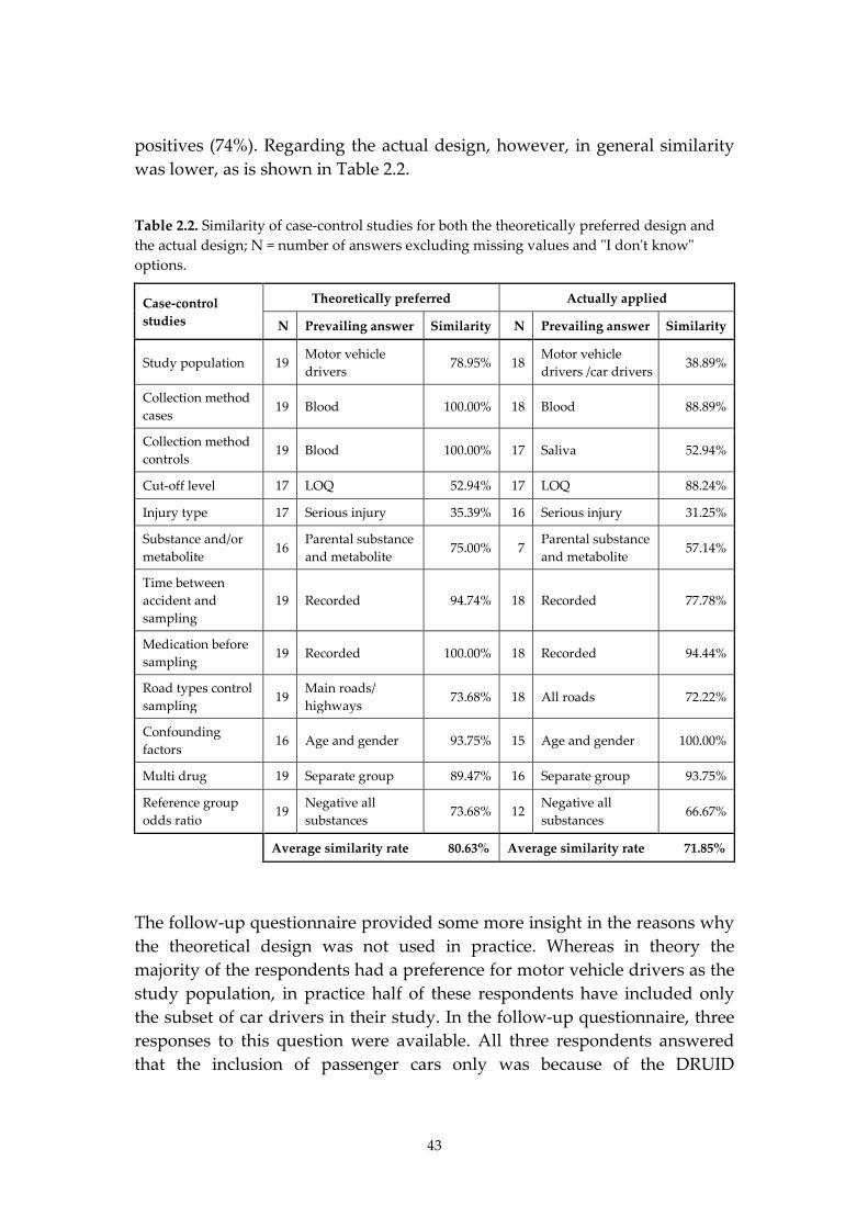
43

positives (74%). Regarding the actual design, however, in general similarity was lower, as is shown in Table 2.2.

Table 2.2. Similarity of case-control studies for both the theoretically preferred design and the actual design; N = number of answers excluding missing values and "I don't know" options.

Case-control studies

Theoretically preferred Actually applied

N Prevailing answer Similarity N Prevailing answer Similarity

Study population 19 Motor vehicle drivers 78.95% 18

Motor vehicle drivers /car drivers 38.89%

Collection method cases 19 Blood 100.00% 18 Blood 88.89%

Collection method controls

19 Blood 100.00% 17 Saliva 52.94%

Cut-off level 17 LOQ 52.94% 17 LOQ 88.24%

Injury type 17 Serious injury 35.39% 16 Serious injury 31.25%

Substance and/or metabolite 16

Parental substance and metabolite 75.00% 7

Parental substance and metabolite 57.14%

Time between accident and sampling

19 Recorded 94.74% 18 Recorded 77.78%

Medication before sampling 19 Recorded 100.00% 18 Recorded 94.44%

Road types control sampling 19

Main roads/ highways 73.68% 18 All roads 72.22%

Confounding factors

16 Age and gender 93.75% 15 Age and gender 100.00%

Multi drug 19 Separate group 89.47% 16 Separate group 93.75%

Reference group odds ratio

19 Negative all substances

73.68% 12 Negative all substances

66.67%

Average similarity rate 80.63% Average similarity rate 71.85%

The follow-up questionnaire provided some more insight in the reasons why the theoretical design was not used in practice. Whereas in theory the majority of the respondents had a preference for motor vehicle drivers as the study population, in practice half of these respondents have included only the subset of car drivers in their study. In the follow-up questionnaire, three responses to this question were available. All three respondents answered that the inclusion of passenger cars only was because of the DRUID

44

guidelines for case-control studies and one respondent added that the inclusion of truck drivers would have limited the number of possible research sites. All three respondents expected a bias from this deviation. One respondent reported that bias size and direction were unknown, another respondent expected a substantial underestimation of the risk, as did the third one, but without indicating the size of the underestimation. In practice saliva collection is the most commonly preferred collection method of samples from non-crash involved drivers at the roadside, although in theory the preference was for blood collection. Six respondents have used oral fluid in practice although they would have preferred blood in theory. Five of them replied to the follow-up questionnaire and stated that they did not collect blood in practice, since it would have increased the refusal rates, it took too much time, it was too costly, or since it was too difficult and not practical. Four of them stated that they did not know if the use of oral fluid instead of blood could have caused bias, and one stated that the use of saliva instead of blood did not induce bias. Neither in theory nor in practice, there was comparability concerning the preferred injury type of the cases. Some researchers preferred to include all drivers, whereas others preferred to include only seriously injured or fatally injured drivers. The most frequently mentioned reasons for selecting one group or the other were that fatally injured drivers are the most relevant group for road safety, that seriously injured drivers cover many of the accidents and are better reported than minor injuries, and, finally, that all accidents are important regardless of the injury severity. One respondent answered that he would have preferred to include fatally injured drivers but for practical and toxicological reasons he had chosen for injured drivers. He expected this deviation to result in a small underestimation of the risk. In theory, the majority of the respondents preferred the use of at least the parental substance for the detection of drug positives. In practice, however, some researchers only used an inactive metabolite for the detection of some drugs. Therefore, comparability for this item was only 57%. No information was provided on the reason for the deviation. However, one reason might be the choice of body fluid to be collected, since in urine only metabolites of psychoactive substances can be detected. As with the theoretical design, there was almost 75% similarity in practice regarding the choice of road types where samples were collected. Most researchers included all road types in their study, although in theory they would have skipped the residential roads. The inclusion of drivers from residential roads was not expected since fewer vehicles pass these roads,

45

especially during night-time hours. Since roadside survey sessions are often linked with police activities and locations at residential roads will probably be less cost-beneficial from a police perspective, resulting in an exclusion of this road type. This was indeed observed by one of the two respondents who included only main roads in their study whereas he would have preferred to include all road types. The other respondent indicated that the inclusion of all road types would have been too hard to manage by the researchers and the police. The respondent did not know whether this deviation could have induced bias. Both in theory and in practice there was less than 75% comparability regarding the choice of reference group. The majority opted for the use of subjects who were negative for all drugs as a reference group for drug positives. But there was also a group of researchers who preferred to use subjects who were negative for the specific substance under review. Six researchers stated that they did not know yet which method they would use in practice. One of the respondents indicated to prefer a reference group that was negative for all substances in theory, but that in practice this information was not known. However, no bias was expected by this researcher as a result of this deviation from his own theoretically preferred study design. The type of cut-off level that was used in practice was more uniform than the theoretical preference. This was mainly caused by the DRUID studies, where the lowest LOQ (Limit of Quantitation) was requested from all partners. One respondent stated that he would have chosen a level of impairment instead of the legal limit, but that this was asked for by his principals. He expected bias from this deviation from his preferred design, but stated that the size and direction would depend on the type of substance. Experimental studies (n=15) Table 2.3 gives an overview of the similarity of experimental studies aimed at assessing the risk of driving under the influence of psychoactive substances other than alcohol.

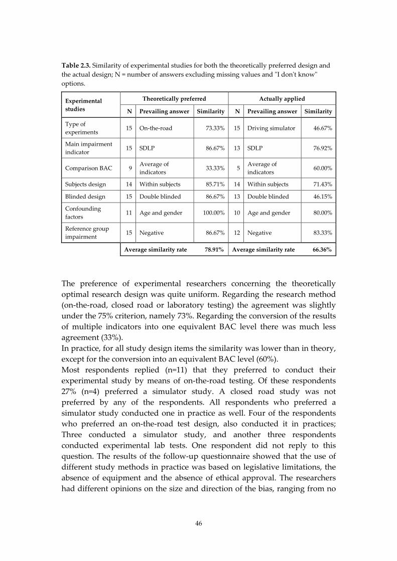
46

Table 2.3. Similarity of experimental studies for both the theoretically preferred design and the actual design; N = number of answers excluding missing values and "I don't know" options.

Experimental studies

Theoretically preferred Actually applied

N Prevailing answer Similarity N Prevailing answer Similarity

Type of experiments 15 On-the-road 73.33% 15 Driving simulator 46.67%

Main impairment indicator 15 SDLP 86.67% 13 SDLP 76.92%

Comparison BAC 9 Average of indicators 33.33% 5

Average of indicators 60.00%

Subjects design 14 Within subjects 85.71% 14 Within subjects 71.43%

Blinded design 15 Double blinded 86.67% 13 Double blinded 46.15%

Confounding factors

11 Age and gender 100.00% 10 Age and gender 80.00%

Reference group impairment 15 Negative 86.67% 12 Negative 83.33%

Average similarity rate 78.91% Average similarity rate 66.36%

The preference of experimental researchers concerning the theoretically optimal research design was quite uniform. Regarding the research method (on-the-road, closed road or laboratory testing) the agreement was slightly under the 75% criterion, namely 73%. Regarding the conversion of the results of multiple indicators into one equivalent BAC level there was much less agreement (33%). In practice, for all study design items the similarity was lower than in theory, except for the conversion into an equivalent BAC level (60%). Most respondents replied (n=11) that they preferred to conduct their experimental study by means of on-the-road testing. Of these respondents 27% (n=4) preferred a simulator study. A closed road study was not preferred by any of the respondents. All respondents who preferred a simulator study conducted one in practice as well. Four of the respondents who preferred an on-the-road test design, also conducted it in practices; Three conducted a simulator study, and another three respondents conducted experimental lab tests. One respondent did not reply to this question. The results of the follow-up questionnaire showed that the use of different study methods in practice was based on legislative limitations, the absence of equipment and the absence of ethical approval. The researchers had different opinions on the size and direction of the bias, ranging from no

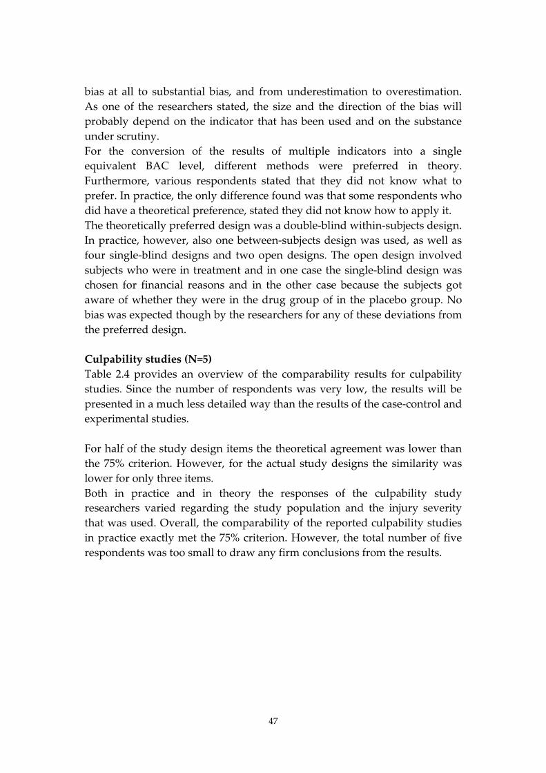
47

bias at all to substantial bias, and from underestimation to overestimation. As one of the researchers stated, the size and the direction of the bias will probably depend on the indicator that has been used and on the substance under scrutiny. For the conversion of the results of multiple indicators into a single equivalent BAC level, different methods were preferred in theory. Furthermore, various respondents stated that they did not know what to prefer. In practice, the only difference found was that some respondents who did have a theoretical preference, stated they did not know how to apply it. The theoretically preferred design was a double-blind within-subjects design. In practice, however, also one between-subjects design was used, as well as four single-blind designs and two open designs. The open design involved subjects who were in treatment and in one case the single-blind design was chosen for financial reasons and in the other case because the subjects got aware of whether they were in the drug group of in the placebo group. No bias was expected though by the researchers for any of these deviations from the preferred design. Culpability studies (N=5) Table 2.4 provides an overview of the comparability results for culpability studies. Since the number of respondents was very low, the results will be presented in a much less detailed way than the results of the case-control and experimental studies. For half of the study design items the theoretical agreement was lower than the 75% criterion. However, for the actual study designs the similarity was lower for only three items. Both in practice and in theory the responses of the culpability study researchers varied regarding the study population and the injury severity that was used. Overall, the comparability of the reported culpability studies in practice exactly met the 75% criterion. However, the total number of five respondents was too small to draw any firm conclusions from the results.

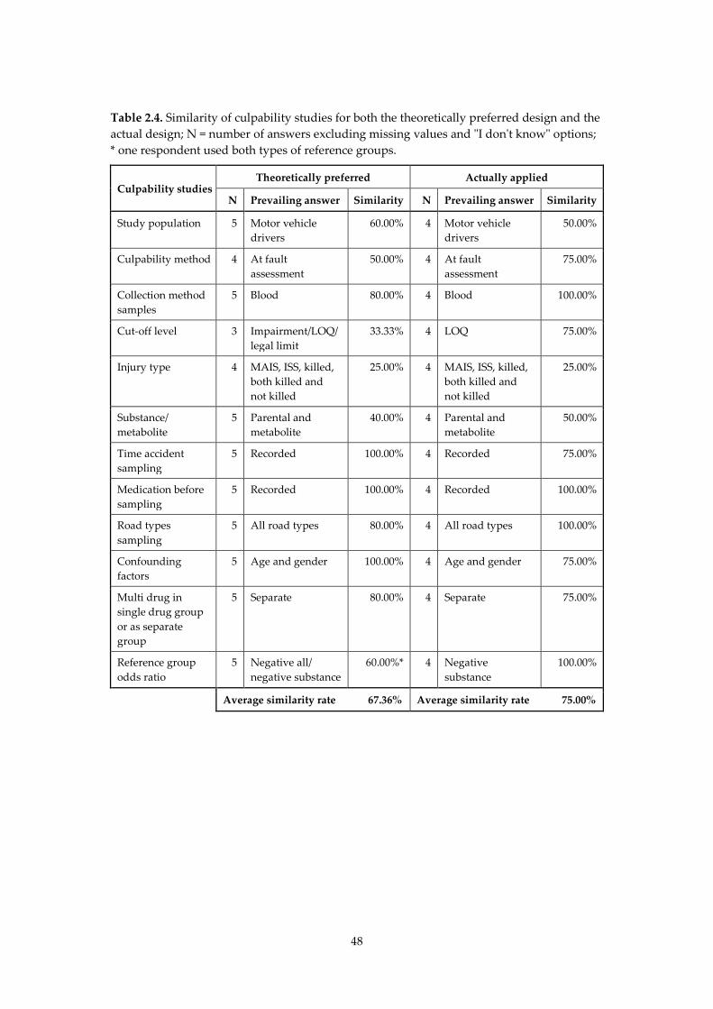
48

Table 2.4. Similarity of culpability studies for both the theoretically preferred design and the actual design; N = number of answers excluding missing values and "I don't know" options; * one respondent used both types of reference groups.

Culpability studies Theoretically preferred Actually applied

N Prevailing answer Similarity N Prevailing answer Similarity

Study population 5 Motor vehicle drivers

60.00% 4 Motor vehicle drivers

50.00%

Culpability method 4 At fault assessment

50.00% 4 At fault assessment

75.00%

Collection method samples

5 Blood 80.00% 4 Blood 100.00%

Cut-off level 3 Impairment/LOQ/ legal limit

33.33% 4 LOQ 75.00%

Injury type 4 MAIS, ISS, killed, both killed and not killed

25.00% 4 MAIS, ISS, killed, both killed and not killed

25.00%

Substance/ metabolite

5 Parental and metabolite

40.00% 4 Parental and metabolite

50.00%

Time accident sampling

5 Recorded 100.00% 4 Recorded 75.00%

Medication before sampling

5 Recorded 100.00% 4 Recorded 100.00%

Road types sampling

5 All road types 80.00% 4 All road types 100.00%

Confounding factors

5 Age and gender 100.00% 4 Age and gender 75.00%

Multi drug in single drug group or as separate group

5 Separate 80.00% 4 Separate 75.00%

Reference group odds ratio

5 Negative all/ negative substance

60.00%* 4 Negative substance

100.00%

Average similarity rate 67.36% Average similarity rate 75.00%

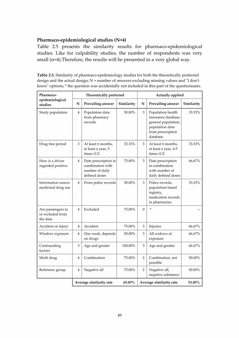
49

Pharmaco-epidemiological studies (N=4) Table 2.5 presents the similarity results for pharmaco-epidemiological studies. Like for culpability studies, the number of respondents was very small (n=4).Therefore, the results will be presented in a very global way.

Table 2.5. Similarity of pharmaco-epidemiology studies for both the theoretically preferred design and the actual design; N = number of answers excluding missing values and "I don't know" options; * the question was accidentally not included in this part of the questionnaire.

Pharmaco-epidemiological studies

Theoretically preferred Actually applied

N Prevailing answer Similarity N Prevailing answer Similarity

Study population 4 Population data from pharmacy records

50.00% 3 Population health insurance database, general population, population data from prescription database

33.33%

Drug free period 3 At least 6 months, at least a year, 5 times t1/2

33.33% 3 At least 6 months, at least a year, 4-5 times t1/2

33.33%

How is a driver regarded positive

4 Date prescription in combination with number of daily defined doses

75.00% 3 Date prescription in combination with number of daily defined doses

66.67%

Information source medicinal drug use

4 From police records 50.00% 3 Police records, population based registry, medication records in pharmacies

33.33%

Are passengers in or excluded from the data

4 Excluded 75.00% 0 * --

Accident or injury 4 Accident 75.00% 3 Injuries 66.67%

Window exposure 4 One week, depends on drugs

50.00% 3 All widows of exposure

66.67%

Confounding factors

3 Age and gender 100.00% 3 Age and gender 66.67%

Multi drug 4 Combination 75.00% 2 Combination, not possible

50.00%

Reference group 4 Negative all 75.00% 2 Negative all, negative substance

50.00%

Average similarity rate 65.83% Average similarity rate 51.85%

50

The similarity of the pharmaco-epidemiological studies that have been reported by the respondents is below the 75% criterion for both the theoretical design (five out of ten questions have a comparability score below 75%) and the design in practice (all questions have a similarity score below 75%). However, like for the culpability studies, the number of respondents was too small to draw conclusions from these results.

2.3.3. Overall results

Based on the literature (Howe and Choi, 1983; Shadis et al., 2002) it was expected that case-control studies would have been mentioned by the respondents as the theoretically most appropriate study type. However, the results from the questionnaire show that in theory only 44% of the respondents preferred to conduct a case-control study to determine the risk of driving under the influence of psychoactive substances. One could assume that this unexpected result might be due to the fact that researchers feel inclined to justify the choice of study design they have made in practice. However, the results of the questionnaire survey actually show that 49% of the respondents did not prefer the type of study they conducted in practice. Among the respondents who conducted case-control studies, the percentage was even higher (58%) than among the respondents who conducted other types of study (42%). This difference was not significant at a 95% confidence interval (p=0.42). Another possible reason for the lower share of researchers that preferred to conduct case-control studies in theory may have been the way that the question was phrased. The question referred to the risk of driving under the influence of psychoactive substances, and not specifically to the crash risk. The similarity varied both within and between the four most commonly used study designs. Table 2.6 provides an overview of the average similarity rates between the theoretically preferred and the study design applied in practice.

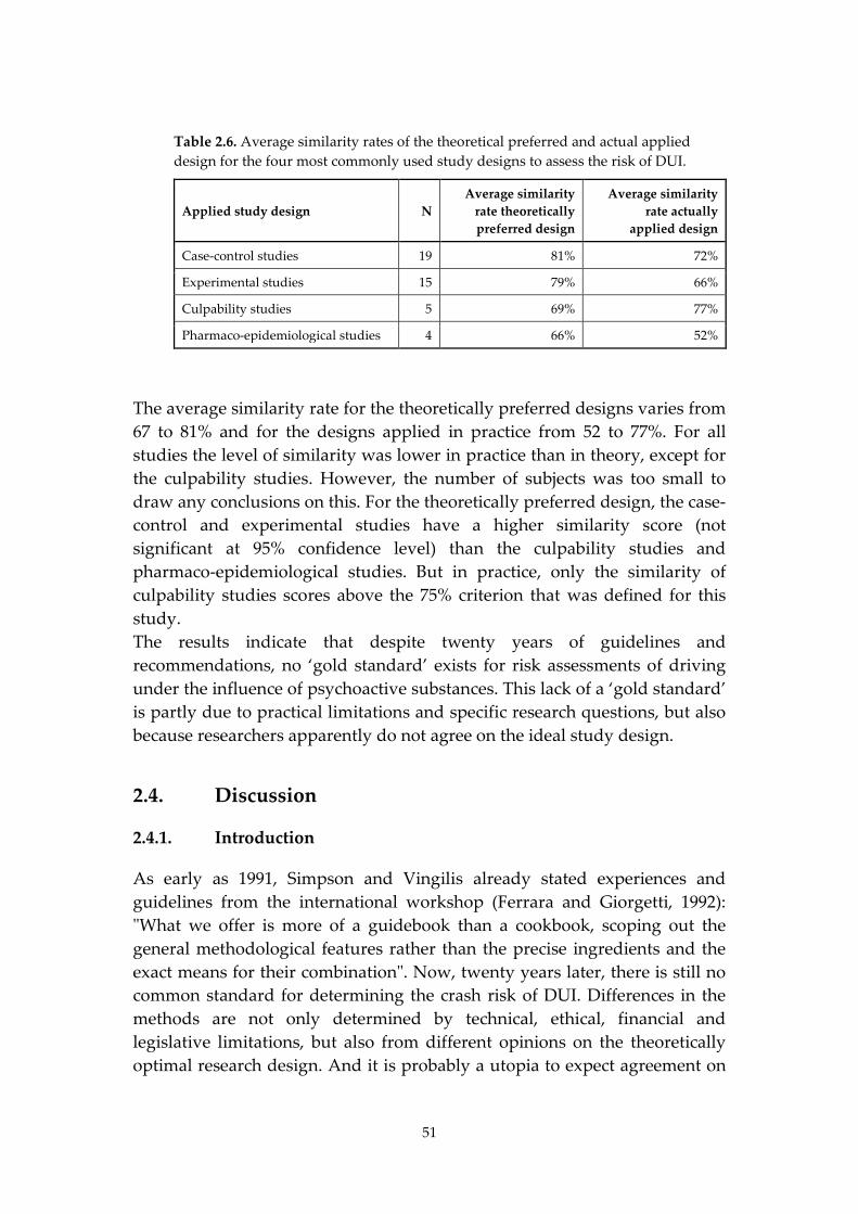
51

Table 2.6. Average similarity rates of the theoretical preferred and actual applied design for the four most commonly used study designs to assess the risk of DUI.

Applied study design N Average similarity

rate theoretically preferred design

Average similarity rate actually

applied design

Case-control studies 19 81% 72%

Experimental studies 15 79% 66%

Culpability studies 5 69% 77%

Pharmaco-epidemiological studies 4 66% 52%

The average similarity rate for the theoretically preferred designs varies from 67 to 81% and for the designs applied in practice from 52 to 77%. For all studies the level of similarity was lower in practice than in theory, except for the culpability studies. However, the number of subjects was too small to draw any conclusions on this. For the theoretically preferred design, the case-control and experimental studies have a higher similarity score (not significant at 95% confidence level) than the culpability studies and pharmaco-epidemiological studies. But in practice, only the similarity of culpability studies scores above the 75% criterion that was defined for this study. The results indicate that despite twenty years of guidelines and recommendations, no ‘gold standard’ exists for risk assessments of driving under the influence of psychoactive substances. This lack of a ‘gold standard’ is partly due to practical limitations and specific research questions, but also because researchers apparently do not agree on the ideal study design.

2.4. Discussion

2.4.1. Introduction

As early as 1991, Simpson and Vingilis already stated experiences and guidelines from the international workshop (Ferrara and Giorgetti, 1992): "What we offer is more of a guidebook than a cookbook, scoping out the general methodological features rather than the precise ingredients and the exact means for their combination". Now, twenty years later, there is still no common standard for determining the crash risk of DUI. Differences in the methods are not only determined by technical, ethical, financial and legislative limitations, but also from different opinions on the theoretically optimal research design. And it is probably a utopia to expect agreement on

52

a ‘cookbook’ for designing studies to assess the crash risk of driving under the influence in the near future. Nevertheless, it is advisable to focus on standardising at least some design aspects or ‘ingredients’ in order to improve comparability of results from different studies. Based on the results from this study on comparability and the expected bias as reported by the respondents of the follow-up questionnaire, certain design aspects could be considered as a starting point for further standardisation. This will, however, only be discussed for case-control and experimental studies, since the number of respondents for the culpability and the pharmaco-epidemiological studies was very low.

2.4.2. Case-control studies

For case control studies three design items are recommended for standardisation based on their low similarity rates: choice of body fluid sample for the control population of non-crash involved drivers at the roadside, injury severity type and the reference group. A fourth item is the choice of the parental substance and/or its metabolite. However, the dissimilarity of this item can probably to a large extent be solved by using the same body fluid sample in the control population. The collection of body fluids among non-crash involved drivers at the roadside has been an issue in case-control studies for a long time. The collection of blood is considered to be the theoretically most appropriate method, since the presence of a psychoactive substance in blood closely relates to the presence of an effect of the substance on the central nervous system. Furthermore, in most hospital studies blood is collected as a matrix. Using results from body fluids in the control population that are different from those in the case population would lead to less comparable data and therefore to loss of validity. The collection of blood also has several disadvantages, such as the high refusal rates and the relatively high cost of equipment and personnel (OECD, 2010). In the past decade, oral fluid has emerged as an alternative for blood as a body fluid matrix for detecting recent drug use. In the DRUID project blood was used at the roadside in only four out of thirteen roadside surveys (in three of these four surveys additional oral fluid samples were collected). In the other nine roadside surveys, only oral fluid was used to collect information of recent drug use by a random sample of car drivers. In order to be able to compare all results, cut-offs have been proposed for oral fluid that are equivalent to the cut-offs for blood. These equivalent cut-offs were obtained by calculating average oral fluid-blood ratios after excluding the outliers, as described in (Gjerde et al., 2010a). These ratios were based on collection by means of the Statsure

53

collection device, which was used in eleven of the twelve roadside surveys. The use of equivalent cut-offs allows comparison of blood results from injured or killed drivers with oral fluid results from drivers at the roadside. It has to be kept in mind, however, that for some substances the cut-off recommended by Gjerde was based on only a few positive cases and that these cut-offs are only usable when applying the same cut-offs based on the ones that were defined by the Talloires working group (Walsh et al., 2008) as was the case in the DRUID project. Furthermore, equivalent cut-offs may vary over the different oral fluid collection methods. For these reasons more research is needed to establish solid equivalent saliva cut-offs for all substances. Another option to get comparable outcomes from both hospital and traffic populations is mentioned in the DRUID report on the hospital studies (Isalberti et al., 2011). In this report the authors suggested collecting oral fluid samples both from hospitalised drivers and from drivers at the roadside. However, this method has two limitations as opposed to the equivalent cut-offs method: Firstly, the method is not applicable for all injured drivers since it is not always possible to collect an oral fluid sample from a person who is severely or fatally injured. Secondly, the one thing that researchers do agree on is that theoretically analyzing blood is the best method to gather information on recent drug use by injured drivers. Analyzing oral fluid samples from injured drivers is considered as a suboptimal method. A third solution is the collection and analysis of blood spots. Small drops of blood, collected on filter paper, are dried and analyzed in a laboratory. The benefit of this method is that it takes only a finger puncture to collect blood, which might, depending on national legislation and the permission of National Ethics Committees, reduce the necessity of a medical professional to collect the sample. The dried blood spot method has been evaluated for several substances (Jantos and Skopp, 2011; Skopp, 2007) and the results show equivalence to standard blood results for amphetamine, MDMA, risperidone, opioids, 6-acetylmorphine, morphine, and benzodiazepines. For Zopiclone the result was not equivalent due to degradation after storage (Nilsson et al., 2010), but after correction for degradation the blood spot method seems usable for Zopiclone as well. As yet, no results have been published on the equivalence for THC. If the results for the other substances are as promising as the ones for the evaluated substances, then the dried blood spot method can be regarded as a good alternative for saliva and intravenous blood collection. The second recommendation for improving the comparability of case-control studies regards the type of injury severity that is included in the study. Both

54

in the theoretically preferred and the actually applied method the level of similarity of the injury severity level was quite low. Although Smink et al. (2005) concluded that the relationship between relative risk per severity level and drug use was not clear, recent results from the DRUID project (Hels et al., 2011) indicate that the relative risk does increase with the increase of injury severity and therefore, that case-control studies with fatally injured drivers result in relatively high odds ratios that are not comparable to the odds ratios of studies including injured drivers. Therefore, it is recommended to separate reporting on killed drivers and on injured ones. For injured drivers it is recommended to use the MAIS coding system to scale injury severity since it is one of the most commonly applied injury scoring system for injured drivers (Gennarelli and Wodzin, 2006). A final recommendation for improving the comparability of case control studies is based on the choice of the reference group. This is important since it has a strong effect on the resulting odds ratio. It is recommended to use subjects who are negative for all substances as a reference group. Using a reference group that is only negative for the substance under review will result in underestimation of the relative risk associated with that particular substance. If the reference group consists of subjects who are negative for all included substances, the list of substances that are included is of major importance. If high risk substances are not included in the study, the relative risk of the included substances may either be underestimated or overestimated, depending on overrepresentation of the non-included substances in the case or control group. It is recommended to use the list of core substances composed by the Talloires working group (Walsh et al., 2008) as a starting point for the inclusion of substances and add any potentially high-risk substances that are expected to be prevalent in either the hospital (case) or the roadside (control) samples, e.g. GHB.

2.4.3. Experimental studies

For experimental studies the recommendations regard two design aspects: the study method and the comparison of outcomes for drugs with the BAC standard when two or more risk indicators are used. The study method used in experimental studies not only depends on methodological factors, but also on legislative and financial factors, and on the availability of the right equipment. Most respondents preferred to conduct on-the-road driving tests. In practice, however, driving simulator studies and experimental lab tests were conducted most frequently by the respondents. In experimental lab tests the internal validity is relatively high

55

since the experiment is conducted in a controlled setting. But the external validity- the possibility to generalize test results to the real driving population - is relatively low. The external validity of on-the-road driving tests is relatively high, but the internal validity is lower than that for experimental lab tests since driving circumstances may vary between the tests. For driving simulator studies the internal and external validity lie in between those of experimental lab tests and on-the-road driving tests. Most researchers who conducted a different study in practice than they preferred in theory, indicate that this may have induced bias. In order to gain more information on the potential bias that is induced by each of the three study methods, it would be interesting to conduct an experimental study comprising all three study types. Until results of such a study are available, it is recommended to only compare results from experimental studies with results from other experimental studies that have used the same study method. Finally, the conversion of various impairment indicators into a single BAC level and associated risk factor deserves attention. A high proportion of the respondents stated that they did not know which method they would prefer from a theoretical point of view. In practice, most respondents did not convert their results to a single BAC level. For the ones who included a conversion, the majority first calculated the equivalent BAC level for every single impairment indicator and subsequently used the average BAC level as the overall risk indicator. It remains questionable, however, how well a limited set of impairment indicators can predict the relative risk of a psychoactive substance.

2.4.4. Strengths and limitations of this study

The main strength of this study is the detailed insight it provides in the divergent designs of studies to assess the risk of driving under the influence of psychoactive substances. This seems to result for a large part from the different opinions of researchers regarding a ‘gold’ standard. Additionally, for a number of study design items this study gives some insight in the potential bias or lack of knowledge about it. The study also has some limitations. Firstly, participating researchers had different backgrounds and may therefore have interpreted some questions in a different way. An example is the different interpretation of the term ‘risk assessment’ that was used throughout the questionnaire. Some researchers may have interpreted risk as crash risk, where others might have interpreted it as risk of impairment. In experimental studies crash risk can be assessed by linking impairment of

56

other substances than alcohol with alcohol. However, a majority of the experimental researchers did not include a comparison with alcohol impairment in the study they referred to. This is mainly due to the fact that the main research question of experimental research is focused on risk of impairment rather than crash risk. In order to avoid misinterpretation of the term ‘risk assessment’, it should have been made clear to the respondents that the questionnaire was specifically on crash risk. Furthermore, the calculation of the overall scores for the various study types was based on simple rate calculations, while more sophisticated calculation methods might be required. A more appropriate method would probably include weighting, based on the impact of study design items on the outcome of risk assessment studies. But information to support the use of weighting factors is hard to obtain and it will be difficult to isolate the effect of single study design items. The follow-up questionnaire did ask for the expected size and direction of the bias resulting from a respondent’s deviation from the ‘gold standard’. The respondents expected no bias for most items. The effect of some design items may be calculated by simulating them in existing datasets. This is, however, on the condition that the study design item is included in the dataset in sufficient quantities to calculate the effect. Another limitation is the difficulty of some of the questions. By comparing the answers suspicion arose that some of the questions had not always been understood correctly. In these cases a clarification was asked in the follow-up questionnaire. However, it cannot be ruled out that some questions were interpreted incorrectly, but that this has not been noticed as the answer did not seem odd. The items included in the questionnaire were based on a literature review and on discussions with co-researchers. However, the list of items was not exhaustive. Some relevant items were not included in the questionnaire, but emerged during the analysis of the responses, e.g. measuring dose-related versus concentration-related impairment in experimental studies. Furthermore, the questionnaire was limited to the field of driving under the influence of psychoactive substances other than alcohol. The inclusion of methodological experts from outside this research field would have provided interesting and perhaps also more independent results on the preferred theoretical model. Finally, when interpreting the results of this study, it is important to bear in mind that the numbers of respondents per study type are quite small, and

57

that some of the respondents have worked together on the same studies or in the same institutes.

2.5. Acknowledgements

The authors wish to thank all respondents to the questionnaire and the follow-up questionnaire. Furthermore, this questionnaire could not have been prepared without the help of the dedicated test panel formed by the following co-researchers: Marjan Hagenzieker, Janet Veldstra, Tove Hels, Tom Blencowe and Silvia Ravera.

58

3. Prevalence of psychoactive substances in Dutch and Belgian traffic4

3.1. Introduction

Although the use of psychoactive substances by motor vehicle drivers is suspected as a major risk factor in traffic, valid information on psychoactive substance use by motorists is sparse (Behrensdorff and Steentoft, 2003; EMCDDA, 2008). Prevalence studies are, in general, complex and expensive to conduct, partly because of the relatively low incidence of psychoactive substances in traffic. For a study to have enough statistical power, many drivers need to be included. Review studies report a large variation of drivers in general traffic positive for one or more psychoactive substances other than alcohol. It is difficult to directly compare the results of these roadside surveys because of differences in study design, such as the number of substances included, the analytical cut-off levels applied and the biological matrix used (EMCDDA, 2008; Kelly et al., 2004; Walsh et al., 2004). In Norway 4.5% of the motor vehicle drivers were positive for psychoactive substances including illicit drugs, medicinal drugs or alcohol (Gjerde et al., 2008). In Thailand 5.5% of the drivers tested positive for alcohol and 9.7% of the drivers were positive for other psychoactive substances (Ingsathit et al., 2009). In the state of Victoria, Australia, 2.4% of the drivers were positive for methamphetamines, 3,4-methylenedioxy-metamphetamine (MDMA, or Ecstacy), or tetrahydro-cannabinol (THC, or cannabis). In the United States 11% of drivers were positive for illicit and medicinal drugs during daytime hours on Friday and 14.4% during night time hours on Friday and Saturday nights (Lacey et al., 2009). In British Columbia, 10.4% of the drivers tested positive for drug use on Wednesday and Saturday nights. In the European research-project DRUID (Driving Under the Influence of Drugs, Alcohol and Medicines) prevalence studies have been conducted from 2007 to 2009 in thirteen European countries (Houwing et al., 2011). Special attention was given to the comparability of these studies by using a

4 This chapter is published as the following article: Houwing, S., Legrand, S.-A., Mathijssen, R., Hagenzieker, M., Verstraete, A.G., Brookhuis, K.A. (2012). Prevalence of psychoactive substances in Dutch and Belgian traffic. This article is published in Journal of Studies on Alcohol and Drugs (JSAD) 2012; 73 (6) 951-960.

59

common study design (Assum et al., 2007), which included recommendations on the type of road users and substances to be included, as well as the cut-off levels of these substances. Despite recommendations for a common design, some differences could not be ruled out for practical, legislative or medical ethical reasons. The main difference in the design of these thirteen studies was that some countries used blood as the biological matrix, some used oral fluid and some used a combination of both. To be able to compare the results from countries that used blood with countries that used oral fluid, equivalent cut-offs were applied, as reported by Verstraete et al. (2011b) and Gjerde et al. (2010a). When using equivalent cut-off concentrations in blood and oral fluid, the prevalence of a drug will be equal in samples of blood and samples of oral fluid when studying a large cohort. Based on the outcomes of these thirteen studies and after application of weighing factors for the country size and the size of the represented European regions it was estimated that an average of 1.89% of the drivers in the European Union were positive for illicit drugs, 1.39% for medicinal drugs, 3.48% for alcohol, 0.39 % for poly-drug use, and 0.37% for the combined use of alcohol and drugs (Houwing et al., 2011). Belgium and the Netherlands are two neighbouring countries in Western Europe that shared a common history until 1830 when Belgium separated from the Netherlands. Comparisons between Belgium and the Netherlands are commonly made, because of their historical and cultural bonds. A comparison of the Dutch and Belgian results is also interesting because they were the only two Western European countries that were involved in the DRUID roadside surveys. This article reports and compares the use of psychoactive substances in traffic based on results of the Belgian and Dutch prevalence study that were conducted in the European DRUID project. Furthermore, the Dutch and Belgian results are compared with the estimated European mean and with previously conducted national studies in Belgium and the Netherlands on the use of psychoactive substances in traffic.

3.2. Materials and methods

3.2.1. General design

A cross-sectional roadside survey was conducted to determine the prevalence of psychoactive substances among the general driving population in Belgium and the Netherlands. A stratified multi-stage sampling design was used. In the first stage five study regions were selected in Belgium and

60

the Netherlands. These regions were meant to be representative for the whole country with regard to substance use and traffic. Within these regions smaller research areas (five Belgian and six Dutch police regions) were selected in the second stage, and within these areas, survey locations were selected, where car drivers and drivers from vans were randomly selected from actual traffic between January 2007 and August 2009. For each police region data were collected during several roadside survey sessions distributed over eight 6-hour time periods covering all hours of the day on both weekdays and weekend days. The time periods were distributed into type of day (weekday-weekend day) and time of the day (04.00-09.59, 10.00-15.59, 16.00-21.59, 22.00-03.59). Drivers were stopped by the police at the request of the research coordinator. As soon as an interviewer/nurse was ready for interviewing and blood sampling, a driver, (i.e. the next car approaching the research site) was stopped. Drivers who were stopped were asked to cooperate with the study on a voluntary basis. Drivers who agreed to cooperate were interviewed on their drug and medicine use. Apart from self-reported drug use and time of administration, data collection also comprised date and time of selection, gender and age of the subject, and signs of impairment. In Belgium all drivers were asked to provide both a blood and an oral fluid sample. If drivers refused to give a blood sample, a single oral fluid sample was requested. Participants received a reward of 20 euro in the Belgian study. All drivers in the Dutch study were asked to give a blood sample. If drivers refused to give a blood sample, an oral fluid sample was requested. Participants received a 5 euro reward for an oral fluid sample and 10 euro for a blood sample. In case drivers reported recent drug use an additional oral fluid sample was requested after collecting a blood sample. In the Netherlands as well as in Belgium the breath-test was compulsory for all drivers who were stopped. In the Netherlands participants were breath-tested for alcohol by a police officer after the interview and the blood or oral fluid sampling. Drivers who refused to participate were breath-tested for alcohol by a police officer and, if possible, additional information was collected including information on age, gender, clinical signs of impairment and reason for refusal. In Belgium all drivers who were stopped were breath-tested before the request regarding participation in the study.

3.2.2. Ethical approval

In Belgium, the protocol was approved by the ethics committee of Ghent University Hospital. Participants needed to sign an informed consent. No ethical approval was needed in the Netherlands. After having been informed

61

about the project, the ethics committee made clear that “the project is not encompassed by the law on ethics committees and consideration regarding bio-medical research projects. Therefore, the project does not have to be announced to the ethics committee”. Hence, no informed consent was requested. However, participants in the Netherlands were informed both in writing and by oral communication about the study and its voluntary nature.

3.2.3. Sample preparation and analysis

Venous blood samples were collected in glass tubes containing 20 mg sodium fluoride and 143 IU heparin sodium (BD Plymouth, Brest in the Netherlands and Terumo, Leuven in Belgium). In the Netherlands, oral fluid samples were taken by having the participant spit into a polypropylene container (Deltalab, Barcelona, Spain). In Belgium, oral fluid samples were collected by using the Statsure Saliva Sampler (Statsure Diagnostic Systems, Inc., Brooklyn, MA). In the Netherlands, estimated blood alcohol concentration (BAC) was measured with a handheld breath alcohol analyzer of the police teams using a Dräger Alcotest 7410 Plus com screening device (Dräger Safety Inc., Lübeck, Germany). In Belgium, BAC was estimated from both oral fluid and whole blood. For drivers from whom only oral fluid samples were collected results for ethanol (alcohol) in oral fluid were converted using the following formula:

Calculated blood ethanol (%) = measured ethanol in oral fluid (g/L) x 1.22 The applied factor of 1.22 was based on the average conversion factor between blood and oral fluid that was calculated from the Belgian DRUID results of those drivers from whom both blood and oral fluid samples were collected (Verstraete et al., unpublished observations). In Belgium, the following methods were used for the toxicological analysis of the whole blood samples: an enzymatic method for ethanol analysis, a solid phase extraction followed by ultra performance liquid chromatography-tandem mass spectrometry (UPLC-MS/MS) analysis for all substances except cannabinoids, enzyme-linked immunosorbent assay (ELISA) screening (qualitative) for cannabinoids and liquid-liquid extraction followed by gas chromatogaphy-mass spectrometry analysis for samples that gave positive result at the ELISA screening for cannabinoids. An enzymatic method for ethanol analysis and protein precipitation followed by UPLC-MS/MS for all other substances was used for the Dutch toxicological analysis of whole blood samples. Four rounds of proficiency testing were organized in the participating countries during the study.

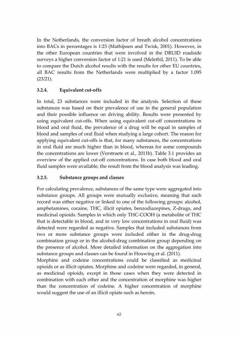
62

In the Netherlands, the conversion factor of breath alcohol concentrations into BACs in percentages is 1:23 (Mathijssen and Twisk, 2001). However, in the other European countries that were involved in the DRUID roadside surveys a higher conversion factor of 1:21 is used (Melethil, 2011). To be able to compare the Dutch alcohol results with the results for other EU countries, all BAC results from the Netherlands were multiplied by a factor 1.095 (23/21).

3.2.4. Equivalent cut-offs

In total, 23 substances were included in the analysis. Selection of these substances was based on their prevalence of use in the general population and their possible influence on driving ability. Results were presented by using equivalent cut-offs. When using equivalent cut-off concentrations in blood and oral fluid, the prevalence of a drug will be equal in samples of blood and samples of oral fluid when studying a large cohort. The reason for applying equivalent cut-offs is that, for many substances, the concentrations in oral fluid are much higher than in blood, whereas for some compounds the concentrations are lower (Verstraete et al., 2011b). Table 3.1 provides an overview of the applied cut-off concentrations. In case both blood and oral fluid samples were available, the result from the blood analysis was leading.

3.2.5. Substance groups and classes

For calculating prevalence, substances of the same type were aggregated into substance groups. All groups were mutually exclusive, meaning that each record was either negative or linked to one of the following groups: alcohol, amphetamines, cocaine, THC, illicit opiates, benzodiazepines, Z-drugs, and medicinal opioids. Samples in which only THC-COOH (a metabolite of THC that is detectable in blood, and in very low concentrations in oral fluid) was detected were regarded as negative. Samples that included substances from two or more substance groups were included either in the drug-drug combination group or in the alcohol-drug combination group depending on the presence of alcohol. More detailed information on the aggregation into substance groups and classes can be found in Houwing et al. (2011). Morphine and codeine concentrations could be classified as medicinal opioids or as illicit opiates. Morphine and codeine were regarded, in general, as medicinal opioids, except in those cases when they were detected in combination with each other and the concentration of morphine was higher than the concentration of codeine. A higher concentration of morphine would suggest the use of an illicit opiate such as heroin.

63

Table 3.1. Applied cut-offs for psychoactive substances other than alcohol; THC-COOH is not included in this table since THC-COOH was not analysed in oral fluid.

Substance Cut-off in oral fluid (ng/mL)

Cut-off in whole blood (ng/mL)

Substance group

Amphetamine 360 20

Amphetamines

Methamphetamine 410 20

MDA 220 20

MDEA 270 20

MDMA 270 20

Cocaine 170 10 Cocaine

Benzoylecgonine 95 50

THC 27 1.0 Cannabis

6-Acetylmorphine 16 10 Illicit opiates

Diazepam 5.0 140

Benzodiazepines

Flunitrazepam 1.0 5.3

Lorazepam 1.1 10

Alprazolam 3.5 10

Clonazepam 1.7 10

Nordiazepam 1.1 20

Oxazepam 13 50

Methadone 22 10 Medicinal opioids

Morphine 95 10 Medicinal opioids or illicit opiates Codeine 94 10

Zolpidem 10 37 Z-drugs

Zopiclone 25 10

3.2.6. Weighing factors

Because random sampling was applied, drivers were expected to be representative of gender and age during sampling sessions. However, because police preferences had to be considered, the selection of samples could not be distributed equally with traffic volumes over the different periods. To correct for the difference between distribution of roadside samples and distribution of traffic over eight different periods, weight factors were calculated by dividing the general distribution of traffic by period by

64

the distribution of sampled drivers in the same period. The weighing procedure in the Netherlands was based on 2007–2008 national trip distribution data from the National Travel Survey collected by the Dutch Central Bureau of Statistics (CBS, 2011), and the weighing procedure in Belgium was based on 2007 traffic counts from the Flemish Government’s Agency for Roads and Traffic (AWV, 2007).

3.2.7. Statistical analysis

Weighted prevalence was calculated by using descriptive statistics by means of the statistical software SAS Version 9.2 (SAS Institute, Cary, NC). Tables were created by using a FREQ procedure including a statement on the weight factors to be used. Weighted prevalence of the substance under scrutiny was calculated by dividing the weighted number of positives for this substance by the weighted total of samples. For calculating confidence intervals, the Wilson confidence interval formula (Wilson, 1927) was used because lower and upper confidence limits calculated using traditional approximations may result in limits outside the (0,1) interval. Possible differences in substance use between the two countries were investigated with binomial logistic regression in SPSS Version 16.0.1 (SPSS Inc., Chicago, IL). Type of country was used as a covariate (with two categories: 0 = Belgium, 1 = The Netherlands), and each substance was included as a dependent variable (also with two categories: 0 = negative, 1 = positive). In all statistical tests, the conventional critical 5% level was used to assess whether the obtained odds ratio (OR) significantly deviated from 1.

3.3. Results

3.3.1. Study population

In the Netherlands, 5,064 drivers were asked to participate in this study. Of these drivers, 242 (4.8%) declined and 4,822 (95.2%) agreed to participate. In Belgium, 6,155 drivers were asked to participate. Of these drivers, 3,206 (52.1%) refused and 2,949 (47.9%) agreed to participate. Of the 4,822 participating drivers in the Dutch study, 3,476 (72%) provided a blood sample, 1,068 (22%) provided an oral fluid sample, and 278 (6%) provided both a blood and an oral fluid sample. As stated previously, in case both blood and oral fluid samples were collected, the results of the blood analysis were leading. In the Belgian study, 2,750 (93%) of the 2,949 participating drivers provided both blood and oral fluid samples, and 199 (7%) provided an oral fluid sample only. Table 3.2 provides an overview of the distribution

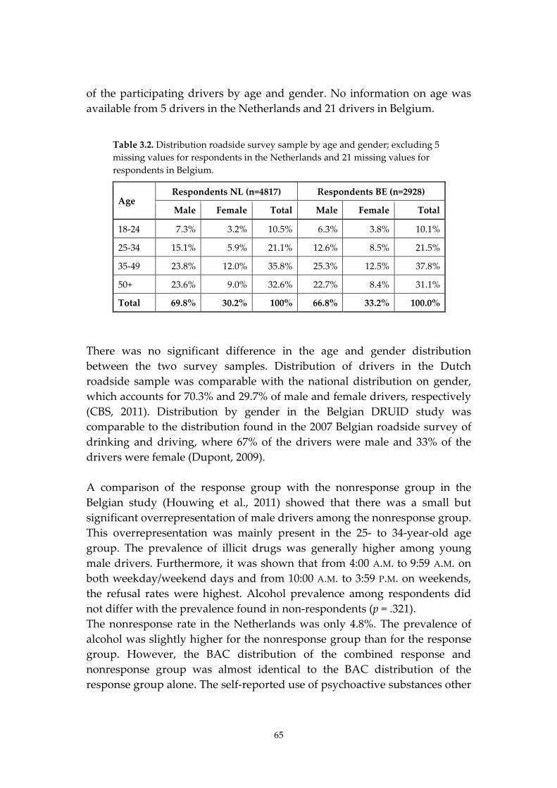
65

of the participating drivers by age and gender. No information on age was available from 5 drivers in the Netherlands and 21 drivers in Belgium.

Table 3.2. Distribution roadside survey sample by age and gender; excluding 5 missing values for respondents in the Netherlands and 21 missing values for respondents in Belgium.

Age Respondents NL (n=4817) Respondents BE (n=2928)

Male Female Total Male Female Total

18-24 7.3% 3.2% 10.5% 6.3% 3.8% 10.1%

25-34 15.1% 5.9% 21.1% 12.6% 8.5% 21.5%

35-49 23.8% 12.0% 35.8% 25.3% 12.5% 37.8%

50+ 23.6% 9.0% 32.6% 22.7% 8.4% 31.1%

Total 69.8% 30.2% 100% 66.8% 33.2% 100.0%

There was no significant difference in the age and gender distribution between the two survey samples. Distribution of drivers in the Dutch roadside sample was comparable with the national distribution on gender, which accounts for 70.3% and 29.7% of male and female drivers, respectively (CBS, 2011). Distribution by gender in the Belgian DRUID study was comparable to the distribution found in the 2007 Belgian roadside survey of drinking and driving, where 67% of the drivers were male and 33% of the drivers were female (Dupont, 2009). A comparison of the response group with the nonresponse group in the Belgian study (Houwing et al., 2011) showed that there was a small but significant overrepresentation of male drivers among the nonresponse group. This overrepresentation was mainly present in the 25- to 34-year-old age group. The prevalence of illicit drugs was generally higher among young male drivers. Furthermore, it was shown that from 4:00 A.M. to 9:59 A.M. on both weekday/weekend days and from 10:00 A.M. to 3:59 P.M. on weekends, the refusal rates were highest. Alcohol prevalence among respondents did not differ with the prevalence found in non-respondents (p = .321). The nonresponse rate in the Netherlands was only 4.8%. The prevalence of alcohol was slightly higher for the nonresponse group than for the response group. However, the BAC distribution of the combined response and nonresponse group was almost identical to the BAC distribution of the response group alone. The self-reported use of psychoactive substances other

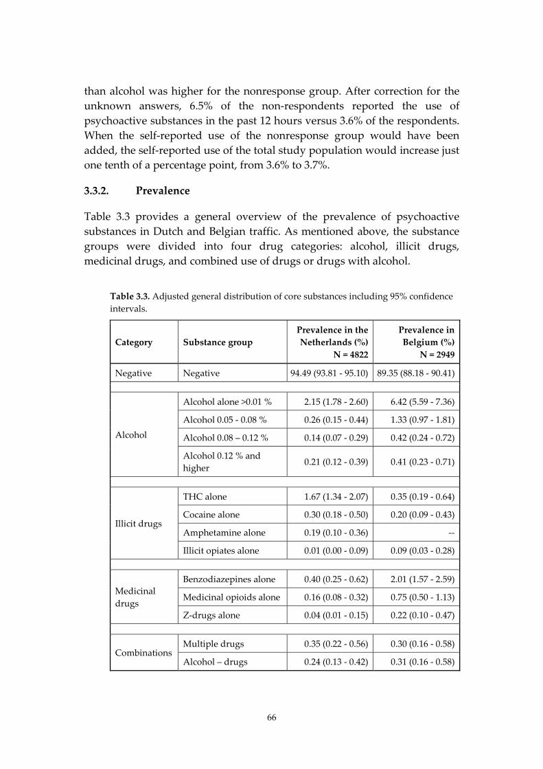
66

than alcohol was higher for the nonresponse group. After correction for the unknown answers, 6.5% of the non-respondents reported the use of psychoactive substances in the past 12 hours versus 3.6% of the respondents. When the self-reported use of the nonresponse group would have been added, the self-reported use of the total study population would increase just one tenth of a percentage point, from 3.6% to 3.7%.

3.3.2. Prevalence

Table 3.3 provides a general overview of the prevalence of psychoactive substances in Dutch and Belgian traffic. As mentioned above, the substance groups were divided into four drug categories: alcohol, illicit drugs, medicinal drugs, and combined use of drugs or drugs with alcohol.

Table 3.3. Adjusted general distribution of core substances including 95% confidence intervals.

Category Substance group Prevalence in the Netherlands (%)

N = 4822

Prevalence in Belgium (%)

N = 2949

Negative Negative 94.49 (93.81 - 95.10) 89.35 (88.18 - 90.41)

Alcohol

Alcohol alone >0.01 % 2.15 (1.78 - 2.60) 6.42 (5.59 - 7.36)

Alcohol 0.05 - 0.08 % 0.26 (0.15 - 0.44) 1.33 (0.97 - 1.81)

Alcohol 0.08 – 0.12 % 0.14 (0.07 - 0.29) 0.42 (0.24 - 0.72)

Alcohol 0.12 % and higher

0.21 (0.12 - 0.39) 0.41 (0.23 - 0.71)

Illicit drugs

THC alone 1.67 (1.34 - 2.07) 0.35 (0.19 - 0.64)

Cocaine alone 0.30 (0.18 - 0.50) 0.20 (0.09 - 0.43)

Amphetamine alone 0.19 (0.10 - 0.36) --

Illicit opiates alone 0.01 (0.00 - 0.09) 0.09 (0.03 - 0.28)

Medicinal drugs

Benzodiazepines alone 0.40 (0.25 - 0.62) 2.01 (1.57 - 2.59)

Medicinal opioids alone 0.16 (0.08 - 0.32) 0.75 (0.50 - 1.13)

Z-drugs alone 0.04 (0.01 - 0.15) 0.22 (0.10 - 0.47)

Combinations Multiple drugs 0.35 (0.22 - 0.56) 0.30 (0.16 - 0.58)

Alcohol – drugs 0.24 (0.13 - 0.42) 0.31 (0.16 - 0.58)

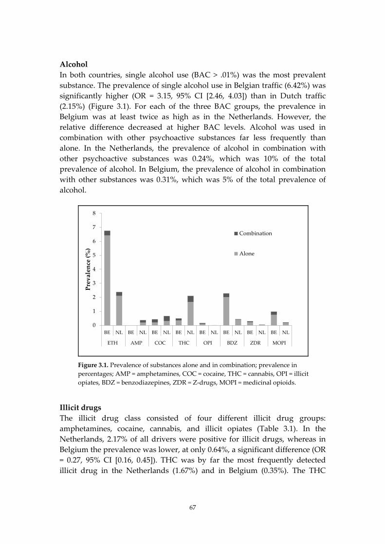
67

Alcohol In both countries, single alcohol use (BAC > .01%) was the most prevalent substance. The prevalence of single alcohol use in Belgian traffic (6.42%) was significantly higher (OR = 3.15, 95% CI [2.46, 4.03]) than in Dutch traffic (2.15%) (Figure 3.1). For each of the three BAC groups, the prevalence in Belgium was at least twice as high as in the Netherlands. However, the relative difference decreased at higher BAC levels. Alcohol was used in combination with other psychoactive substances far less frequently than alone. In the Netherlands, the prevalence of alcohol in combination with other psychoactive substances was 0.24%, which was 10% of the total prevalence of alcohol. In Belgium, the prevalence of alcohol in combination with other substances was 0.31%, which was 5% of the total prevalence of alcohol.

0

1

2

3

4

5

6

7

8

BE NL BE NL BE NL BE NL BE NL BE NL BE NL BE NL

ETH AMP COC THC OPI BDZ ZDR MOPI

Prev

alen

ce (%

)

Combination

Alone

Figure 3.1. Prevalence of substances alone and in combination; prevalence in percentages; AMP = amphetamines, COC = cocaine, THC = cannabis, OPI = illicit opiates, BDZ = benzodiazepines, ZDR = Z-drugs, MOPI = medicinal opioids.

Illicit drugs The illicit drug class consisted of four different illicit drug groups: amphetamines, cocaine, cannabis, and illicit opiates (Table 3.1). In the Netherlands, 2.17% of all drivers were positive for illicit drugs, whereas in Belgium the prevalence was lower, at only 0.64%, a significant difference (OR = 0.27, 95% CI [0.16, 0.45]). THC was by far the most frequently detected illicit drug in the Netherlands (1.67%) and in Belgium (0.35%). The THC

68

prevalence in Belgium was significantly lower than in the Netherlands (OR = 0.21, 95% CI [0.11, 0.40]). Cocaine was detected among 0.30% of the drivers in the Netherlands and among 0.20% of the drivers in Belgium (OR = 0.69, 95% CI [0.26, 1.88]). This difference was not significant. Amphetamines were detected among 0.19% of the Dutch drivers and were completely absent among the Belgian drivers. Because of the absence of amphetamines in the Belgian study sample, a value of 0.1 was added to each of the four cells (Agresti, 1996), which resulted in a non-significant difference (OR = 0.02, 95% CI [0.00, 8.97]) between the Dutch and Belgian prevalence. Illicit opiates were rarely present (0.01%) in the Netherlands and sparsely detected in Belgium (0.09%). This difference was not significant either (OR = 11.11, 95% CI [0.29, 432.54]). Medicinal drugs The medicinal drugs class consisted of three different drug groups: benzodiazepines, medicinal opioids, and Z drugs (see Table 3.1). Medicinal drugs were significantly more prevalent in general traffic in Belgium (2.98%) than in the Netherlands (0.60%) (OR = 6.40, 95% CI [4.00, 10.25]). The most frequently detected medicinal drugs were benzodiazepines. In the Netherlands, 0.40% of the drivers were screened positive for benzodiazepines, as did 2.01% in Belgium (OR = 5.16, 95% CI [3.08, 8.66]) (Figure 3.1). Medicinal opioids were detected relatively frequently in Belgium (0.75%) but significantly less in the Netherlands (0.16%) (OR = 4.60, 95% CI [2.04, 10.37]). Z drugs were significantly more prevalent in Belgium (0.22%) than in the Netherlands (0.04%) (OR = 5.12, 95% CI [1.08, 24.31]). Drug–drug and alcohol–drug combinations Patterns of the prevalence of combinations of psychoactive substances were more or less the same in the Netherlands (0.24% alcohol–drugs and 0.35% drug–drug combinations) and in Belgium (0.31% alcohol–drugs and 0.30% drug–drug combinations). The corresponding odds ratios were not significant (alcohol–drugs, OR = 1.37, 95% CI [0.62, 3.00]; drug–drug combinations, OR = 0.76, 95% CI [0.34, 1.71]). Both in Belgium and in the Netherlands, cocaine was detected with approximately the same frequency alone as it was in combination with other substances. For THC, Z drugs, and medicinal opiates and opioids, the share of combined use was approximately 25% of the total use, whereas for alcohol and benzodiazepines the proportion was about 10% in both countries. For amphetamines (0.00% in Belgium) and illicit opiates (0.01% in the Netherlands), the prevalence was too low to compare between countries.

69

3.3.3. Comparison with previous studies in the Netherlands and Belgium

In the Netherlands, only one previous prevalence study had been conducted in the past 10 years on the prevalence of drugs and medicines in traffic (Mathijssen and Houwing, 2005). For alcohol prevalence, data were available on a yearly basis since 1974, but this information is only gathered during weekend nights (DVS, 2011). For the prevalence of alcohol during other time periods, only data from the European research project IMMORTAL (Impaired Motorists, Methods of Roadside Testing and Assessment for Licensing) were available (Mathijssen and Houwing, 2005). Between 2000 and 2004, a roadside survey was conducted in the Dutch Tilburg police district as part of the European IMMORTAL study. The prevalence of single illicit drugs was higher in the IMMORTAL study (4.5%) than it was in the Dutch DRUID study (2.17%). However, the results of the IMMORTAL study were mainly based on urine samples in which drugs are detectable for a longer period than in blood and oral fluid (Verstraete, 2004). Therefore, a direct comparison between the prevalence rates of the IMMORTAL and the DRUID study was not possible. In Belgium, national data on the prevalence of alcohol in traffic were available for the years 2003, 2005 and 2007 (Dupont, 2009). No previous data were available on the prevalence of other psychoactive substances in traffic. The prevalence of alcohol in the DRUID study was somewhat higher than the results from the biannual roadside survey on alcohol use, which found an average prevalence of 2% during the whole week for a BAC of 0.5 g/L and higher. In the DRUID study, this prevalence was 2.33%. These results did not significantly differ from each other.

3.3.4. Comparison with DRUID mean

Within the DRUID project, a European mean was estimated based on the prevalence of psychoactive substances in 13 different European countries including the Netherlands and Belgium using a uniform study design (Houwing et al., 2011). Figure 3.2 presents the comparison of the Dutch and Belgian prevalence data (including 95% confidence intervals) with the estimated European mean.

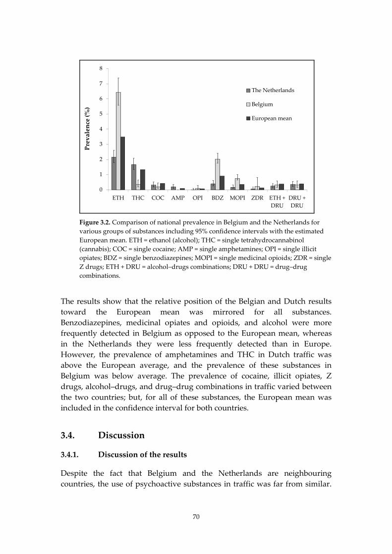
70

0

1

2

3

4

5

6

7

8

ETH THC COC AMP OPI BDZ MOPI ZDR ETH +DRU

DRU +DRU

Prev

alen

ce (%

)The Netherlands

Belgium

European mean

Figure 3.2. Comparison of national prevalence in Belgium and the Netherlands for various groups of substances including 95% confidence intervals with the estimated European mean. ETH = ethanol (alcohol); THC = single tetrahydrocannabinol (cannabis); COC = single cocaine; AMP = single amphetamines; OPI = single illicit opiates; BDZ = single benzodiazepines; MOPI = single medicinal opioids; ZDR = single Z drugs; ETH + DRU = alcohol–drugs combinations; DRU + DRU = drug–drug combinations.

The results show that the relative position of the Belgian and Dutch results toward the European mean was mirrored for all substances. Benzodiazepines, medicinal opiates and opioids, and alcohol were more frequently detected in Belgium as opposed to the European mean, whereas in the Netherlands they were less frequently detected than in Europe. However, the prevalence of amphetamines and THC in Dutch traffic was above the European average, and the prevalence of these substances in Belgium was below average. The prevalence of cocaine, illicit opiates, Z drugs, alcohol–drugs, and drug–drug combinations in traffic varied between the two countries; but, for all of these substances, the European mean was included in the confidence interval for both countries.

3.4. Discussion

3.4.1. Discussion of the results

Despite the fact that Belgium and the Netherlands are neighbouring countries, the use of psychoactive substances in traffic was far from similar.

71

In Belgium, the use of alcohol and medicinal drugs in traffic was higher than in the Netherlands, whereas the measured use of illicit substances in traffic was substantially higher in the Netherlands as compared with Belgium. The higher prevalence for alcohol in Belgium might be related to differences in the enforcement level. The enforcement level for alcohol (number of alcohol tests per 100,000 inhabitants) is estimated to be three to four times lower in Belgium than it is in the Netherlands (Veisten et al., 2011). Furthermore, cultural differences may be causing higher alcohol use in Belgian traffic. For example, in Belgium, people tend to go out eating and drinking more often. This is reflected in the number of restaurants per 10,000 inhabitants. In the Netherlands, the number of restaurants per 10,000 inhabitants is approximately 35 (BHC, 2011), whereas in the Flanders region—where about 60% of all Belgian inhabitants reside—the number of restaurants per 10,000 inhabitants is approximately 48 (GUIDEA, 2011). The higher use of medicinal drugs in Belgium might be explained by a higher consumption of medicines in the general population. The average expenditure per person on medicines has been approximately 15%–20% higher in Belgium than in the Netherlands (SFK, 2011). The low expenditure in the Netherlands could partly be explained by a reluctant prescription policy of general practitioners. The relatively low prevalence of illicit drugs that was found in Belgium may be related to the high nonresponse level. It can be expected that drivers who had recently used an illicit drug would be less likely to participate in the study because they might be afraid that the test results would be used for legal purposes (drug driving legislation of 1999). A lower participation rate of drug-positive drivers would result in nonresponse bias. Based on a comparison of the detected prevalence of illicit substances among injured drivers (Isalberti et al., 2011) and in the general population (Ravera and De Gier, 2008), a higher prevalence of illicit drugs in Belgian traffic would indeed be expected. The detected prevalence of illicit drugs in the general population was in fact comparable for the two countries, and the detected prevalence of illicit drugs among injured drivers was even higher for Belgium than it was for the Netherlands. Another indication of nonresponse bias can be derived from the odds ratios for illicit drugs that were calculated by Hels et al. (2011). Because of the low prevalence of illicit drugs in Belgium, only an adjusted odds ratio for getting seriously injured in a car crash could be calculated for cannabis. The Belgian odds ratio for cannabis (4.88) was approximately three times higher than the mean adjusted odds ratio (1.38) in Hels et al. (2011) which was based on the

72

combined data of four included countries (Belgium, Denmark, The Netherlands, and Lithuania). If the mean adjusted odds ratio would be applied to the Belgian hospital data, the estimated prevalence for THC in Belgian traffic is likely to be more comparable to the Dutch prevalence, although it is impossible to estimate the exact size of the potential nonresponse bias. Finally, keep in mind that, in this study, prevalence is based on predetermined limits of detection and not on limits of impairment.

3.4.2. Strengths and limitations

The main strength of the present study is the similar design of roadside surveys performed in both Belgium and the Netherlands, which makes it possible to compare the results between the two countries as well as with the estimated European mean. By using equivalent cutoffs for drugs in blood and oral fluid, the limitation of the comparability of the results when including two different body fluid samples (blood and oral fluid) was overcome. Another strength of this study is that blood and oral fluid samples were used, not urine samples. Blood and oral fluid can be used to detect recent drug use, whereas urine samples may reflect drug intake up to several days ago (Verstraete, 2004; Walsh et al., 2008). Furthermore, the study provides recent prevalence data of different psychoactive substances in the general driving population in Belgium and the Netherlands. For Belgium, this is the first large-scale study that includes information on the prevalence of illicit drugs in traffic. A limitation of this study is that the list of analyzed substances was not exhaustive. For example, there was no screening for gamma-hydroxybutyric acid (GHB), only seven benzodiazepines were screened for, and selective serotonin reuptake inhibitors were not included. The very high nonresponse rate (52.1%) in Belgium is another limitation of the study because it could lead to nonresponse bias, especially for illicit drugs. Based on the assessment on possible confounding effects of nonresponse by comparing age, gender, and alcohol data, we can conclude that the possibility of nonresponse bias cannot be totally ruled out. Despite that there was a significant difference (p < .001) in self-reported use of psychoactive substances other than alcohol between the response and the nonresponse group in the Netherlands, the actual bias seems to be very small because of the small size of the nonresponse group. Another limitation is that the studies in Belgium and the Netherlands did not collect oral fluid in the same way. The collection procedure may have influenced the concentrations of the samples, as described in previous literature (Crouch, 2005; Langel et al., 2008; O'Neal et al., 2000; Verstraete et

73

al., 2011a). Furthermore, the results from Chapter 5 show that THC concentrations in oral fluid samples collected by spit tubes were on average 5.9 times higher than THC concentrations collected by the StatSure collection device. These findings indicate that the applied equivalent cutoff concentrations might have been too high for the Dutch study. Finally, despite the large sample size of the Belgian and Dutch prevalence study, the cell counts for some substances were small or even zero, which resulted in less stable comparisons between the estimates of both countries.

3.5. Conclusion

The Netherlands and Belgium are neighboring countries. Nonetheless, statistical significant differences are present in the prevalence of psychoactive substances in traffic. In general, medicinal drug use and alcohol were more frequently detected in Belgian traffic, whereas illicit substances were more prevalent in the Netherlands. However, when comparing the results of roadside surveys with hospital data and data from illicit drug use in the general population, it is likely that the observed prevalence of illicit drugs at the Belgian roadside was underrepresented and that the prevalence of illicit drugs in Belgian traffic is probably higher than the current results show.

3.6. Disclaimer

This article has been produced under the project Driving Under Influence of Drugs, Alcohol and Medicines (DRUID) financed by the European Commission within the framework of the EU 6th Framework Program. This report reflects only the authors’ view. The European commission is not liable for any use that may be made of the information contained therein.

3.7. Acknowledgements

The Dutch roadside survey was conducted in close cooperation with one police district and five regional traffic enforcement teams of police, accounting for six different areas in the Netherlands (Amsterdam Amstelland, Hollands Midden, Tilburg, Twente, Groningen, and Gelderland-Zuid) and three in Belgium (Flanders, Brussels, and Wallonia). The authors are grateful for the dedication of the police staff and executive personnel. Many participated on a voluntary basis to make the survey a success. We also thank the Department of Toxicology of the Netherlands Forensic

74

Institute (The Hague, The Netherlands) for undertaking the analysis of blood and saliva samples. The researchers are grateful to all the students who helped to collect the prevalence data in Belgium. Special thanks go to Luc Claus and the emergency department of the Regional Hospital of Namur for help with blood sampling, as well as to Kristof Pil, Elke Raes, and the laboratory technicians involved in the DRUID project.

75

4. Prevalence of alcohol and other psychoactive substances in injured drivers: comparison between Belgium and the Netherlands5

4.1. Introduction

The prevalence of drugs, medicines and/or alcohol in injured drivers has been the object of research in different European countries but also in Australia, Canada, South Africa and the United States already for many years (Raes et al., 2008). These studies showed that alcohol and/or drugs are frequently detected in injured drivers, more frequently than in the general driving population. Alcohol was found in a higher percentage than any other substance. In most studies, cannabis and benzodiazepines were the most frequently detected illicit and medicinal drug respectively. Due to differences in methodology, study location or study design (different substances included, matrix or cut-offs applied) there is a large variation in the percentages of alcohol or drug-positive samples in the different studies. This variation in study design makes it difficult to compare the results from the different studies. Few prevalence studies have been performed in Belgium and the Netherlands. Only two studies on the prevalence of drugs and alcohol among injured drivers have been performed in Belgium (Meulemans et al., 1998; Schepens et al., 1998; Verstraete, 2000). Both studies are dated (1998). Schepens and colleagues performed the first study where blood and urine samples of drivers injured in weekend car crashes in Belgium were tested for different drugs and alcohol. Data on the prevalence of these psychoactive substances are available for injured drivers sampled between the first of July 1994 and the third of June 1995. The Belgian Toxicology and Trauma Study (BTTS) undertook a prospective study on the presence of alcohol and illicit and medicinal drugs in patients admitted to the emergency departments of five selected hospitals in Belgium. The study was performed between January 1995 and June 1996. More recent studies were performed in the 5 This chapter is published as the following article : Legrand, S.-A., Houwing, S., Hagenzieker, M., & Verstraete, A (2012). Prevalence of alcohol and other psychoactive substances in injured drivers: comparison between Belgium and the Netherlands. This article is published in Forensic Science International (FSI) 2012; 220 (1-3) 224-231.

76

Netherlands. One was part of the IMMORTAL (Impaired Motorists, Methods of Roadside Testing and Assessment for Licensing) project (Assum et al., 2005; Smink et al., 2005). In the study performed by Smink and colleagues blood samples of about 1000 injured drivers, collected from October 1998 to September 1999, were analysed for the presence of alcohol, illicit and medicinal drugs. From the IMMORTAL study, data on the prevalence of alcohol and drugs for about 200 injured drivers sampled during the 2000-2004 period are available. Within the European DRUID project (Driving Under the Influence of Drugs, alcohol and medicines) a study on the presence of alcohol and other drugs in injured drivers admitted to the emergency departments of five hospitals in Belgium and three hospitals in the Netherlands was undertaken. The study was performed between 2008 and 2010, using a uniform study design (Goessaert et al., 2010). This article presents the results of a comparison of the prevalence of psychoactive substances in seriously injured Belgian and Dutch drivers. These results will be compared to those from previous studies on prevalence of alcohol and drugs in injured drivers performed in Belgium (BE) and the Netherlands (NL).

4.2. Materials and Methods

4.2.1. Study population

In Belgium blood samples were collected from seriously injured drivers admitted between January 2008 and May 2010 to the emergency department of Ghent University Hospital, Regional Hospital of Namur, University Hospital Sart-Tilman (Liège), Leuven University Hospital and Brussels University Hospital. These 5 hospitals were selected because they participated in the ‘Belgium Toxicology and Trauma Study’ in 1995 (Meulemans et al., 1998; Verstraete, 2000). In the Netherlands blood samples were collected between March 2008 and April 2010 from injured drivers admitted to the emergency department of hospitals in the cities of Enschede, Nijmegen and Tilburg. Only drivers of personal cars or vans, aged more than 18 years and with a Maximum Abbreviated Injury Scale (MAIS) ≥2 were included (Association for the Advancement of Automotive Medicine (AAAM), 2008). In total 535 samples were collected (Belgium: 348; The Netherlands: 187). For the calculation of the alcohol prevalence in the Netherlands one subject was excluded as a consequence of incomplete toxicological analysis.

77

4.2.2. Ethical approval

The study protocol was approved by the ethics committees of the participating hospitals in the Belgian study and the three participating Dutch hospitals. The toxicological and patient data were separated from the clinical files and anonymised in order to guarantee the privacy of the participants. No reference was made to the study in the medical record. Informed consent was mandatory in Belgium but not in the Netherlands.

4.2.3. Data collected

The data collection took place in the emergency departments of the selected hospitals. A flow chart on the data collection procedure and a thesaurus for the medical personnel were prepared. Apart from a blood sample, patient information was gathered through a short questionnaire. The interview of the patient was preferably done face-to-face. If this was impossible (e.g. because the patient remained unconscious), partial information was gathered from other sources (e.g. medical record). Relatives of the patient who were present in the hospital were allowed to give certain information (such as age of the patient or which vehicle type the patient drove at the moment of the crash) if patients were unable to answer. It was stressed that the questionnaire was anonymous. When patients refused to participate in the study, the reason was recorded. The information gathered included patient information and information about the accident. The patient information registered included: age, gender, education, date and time of sampling, medication administered prior to blood sampling and severity of injuries. The following accident data were recorded: date and time of the accident, time of admission, name of hospital, vehicle type, type of accident (single/multi vehicle), speed limit at the location of the accident, safety belt use and weather and road conditions.

4.2.4. Toxicology

Blood samples were taken using a 5 mL glass collection tube containing potassium oxalate and sodium fluoride. In Belgium samples were stored frozen in the hospitals. Regular shipments (under cooled conditions) took place to the laboratory of the Department of clinical chemistry, microbiology and immunology of Ghent University where the toxicological analyses were performed using fully validated methods. In the Netherlands blood samples were stored in solid carbon dioxide in the hospitals. After transportation to

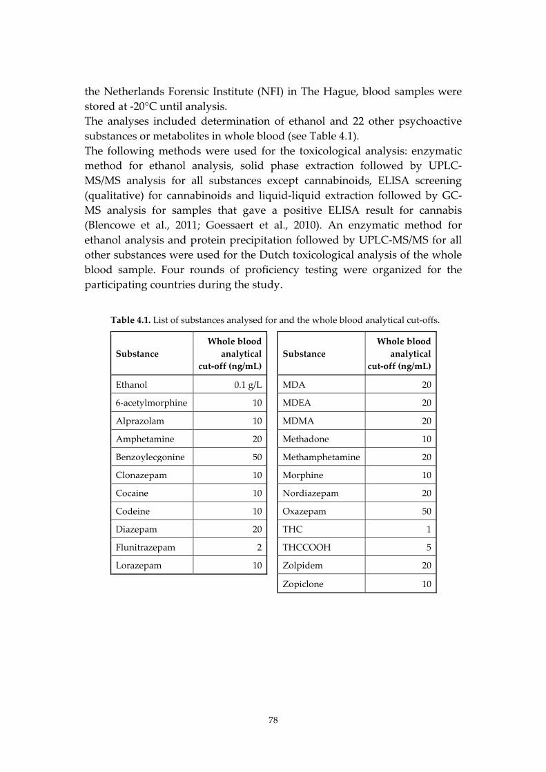
78

the Netherlands Forensic Institute (NFI) in The Hague, blood samples were stored at -20°C until analysis. The analyses included determination of ethanol and 22 other psychoactive substances or metabolites in whole blood (see Table 4.1). The following methods were used for the toxicological analysis: enzymatic method for ethanol analysis, solid phase extraction followed by UPLC-MS/MS analysis for all substances except cannabinoids, ELISA screening (qualitative) for cannabinoids and liquid-liquid extraction followed by GC-MS analysis for samples that gave a positive ELISA result for cannabis (Blencowe et al., 2011; Goessaert et al., 2010). An enzymatic method for ethanol analysis and protein precipitation followed by UPLC-MS/MS for all other substances were used for the Dutch toxicological analysis of the whole blood sample. Four rounds of proficiency testing were organized for the participating countries during the study.

Table 4.1. List of substances analysed for and the whole blood analytical cut-offs.

Substance Whole blood

analytical cut-off (ng/mL)

Substance

Whole blood analytical

cut-off (ng/mL)

Ethanol 0.1 g/L MDA 20

6-acetylmorphine 10 MDEA 20

Alprazolam 10 MDMA 20

Amphetamine 20 Methadone 10

Benzoylecgonine 50 Methamphetamine 20

Clonazepam 10 Morphine 10

Cocaine 10 Nordiazepam 20

Codeine 10 Oxazepam 50

Diazepam 20 THC 1

Flunitrazepam 2 THCCOOH 5

Lorazepam 10 Zolpidem 20

Zopiclone 10

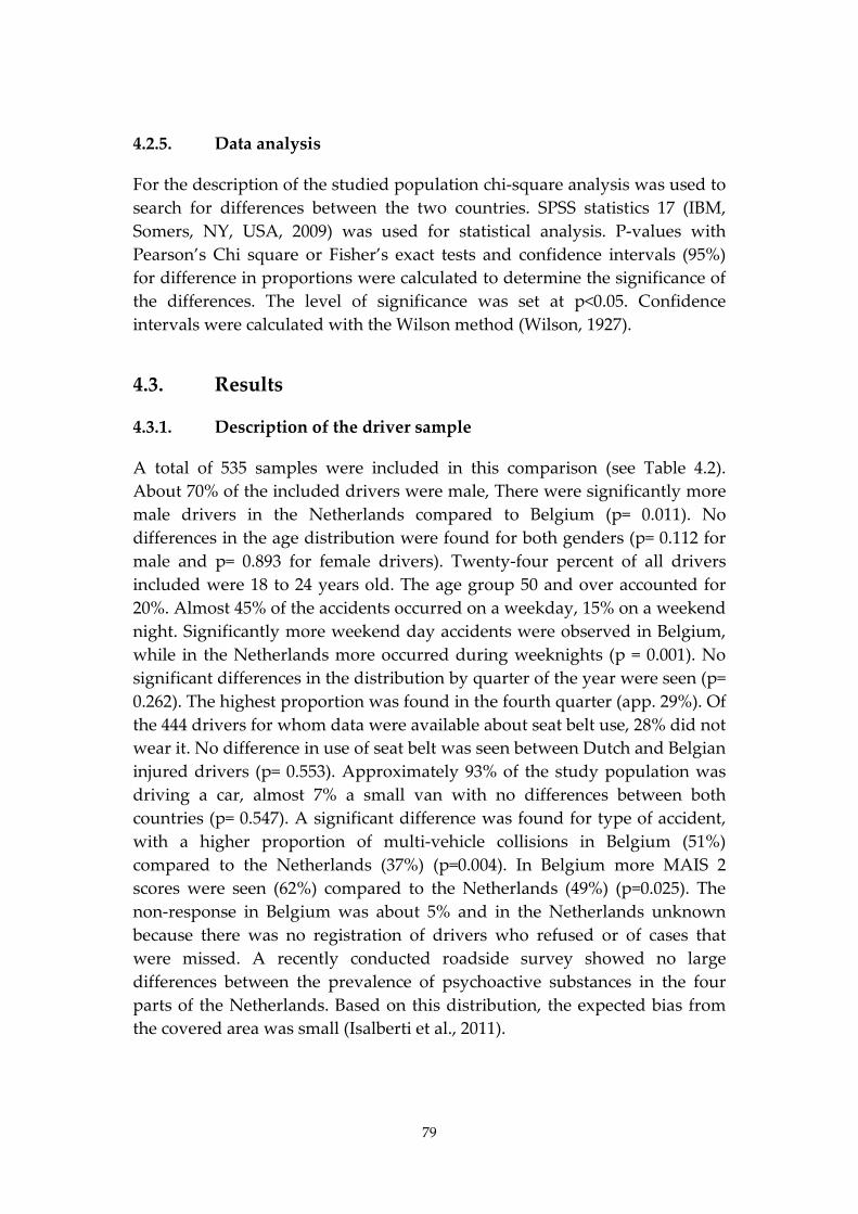
79

4.2.5. Data analysis

For the description of the studied population chi-square analysis was used to search for differences between the two countries. SPSS statistics 17 (IBM, Somers, NY, USA, 2009) was used for statistical analysis. P-values with Pearson’s Chi square or Fisher’s exact tests and confidence intervals (95%) for difference in proportions were calculated to determine the significance of the differences. The level of significance was set at p<0.05. Confidence intervals were calculated with the Wilson method (Wilson, 1927).

4.3. Results

4.3.1. Description of the driver sample

A total of 535 samples were included in this comparison (see Table 4.2). About 70% of the included drivers were male, There were significantly more male drivers in the Netherlands compared to Belgium (p= 0.011). No differences in the age distribution were found for both genders (p= 0.112 for male and p= 0.893 for female drivers). Twenty-four percent of all drivers included were 18 to 24 years old. The age group 50 and over accounted for 20%. Almost 45% of the accidents occurred on a weekday, 15% on a weekend night. Significantly more weekend day accidents were observed in Belgium, while in the Netherlands more occurred during weeknights (p = 0.001). No significant differences in the distribution by quarter of the year were seen (p= 0.262). The highest proportion was found in the fourth quarter (app. 29%). Of the 444 drivers for whom data were available about seat belt use, 28% did not wear it. No difference in use of seat belt was seen between Dutch and Belgian injured drivers (p= 0.553). Approximately 93% of the study population was driving a car, almost 7% a small van with no differences between both countries (p= 0.547). A significant difference was found for type of accident, with a higher proportion of multi-vehicle collisions in Belgium (51%) compared to the Netherlands (37%) (p=0.004). In Belgium more MAIS 2 scores were seen (62%) compared to the Netherlands (49%) (p=0.025). The non-response in Belgium was about 5% and in the Netherlands unknown because there was no registration of drivers who refused or of cases that were missed. A recently conducted roadside survey showed no large differences between the prevalence of psychoactive substances in the four parts of the Netherlands. Based on this distribution, the expected bias from the covered area was small (Isalberti et al., 2011).

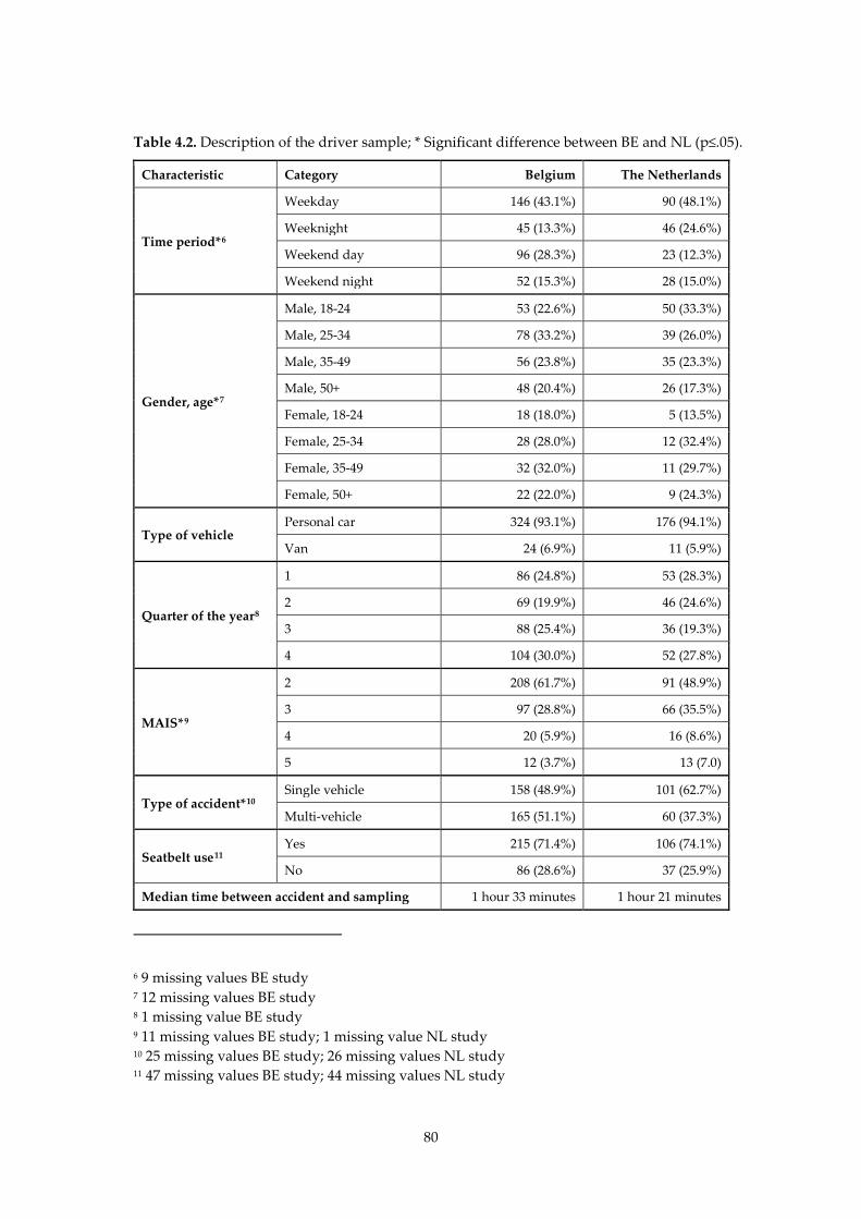
80

Table 4.2. Description of the driver sample; * Significant difference between BE and NL (p≤.05).

Characteristic Category Belgium The Netherlands

Time period*6

Weekday 146 (43.1%) 90 (48.1%)

Weeknight 45 (13.3%) 46 (24.6%)

Weekend day 96 (28.3%) 23 (12.3%)

Weekend night 52 (15.3%) 28 (15.0%)

Gender, age*7

Male, 18-24 53 (22.6%) 50 (33.3%)

Male, 25-34 78 (33.2%) 39 (26.0%)

Male, 35-49 56 (23.8%) 35 (23.3%)

Male, 50+ 48 (20.4%) 26 (17.3%)

Female, 18-24 18 (18.0%) 5 (13.5%)

Female, 25-34 28 (28.0%) 12 (32.4%)

Female, 35-49 32 (32.0%) 11 (29.7%)

Female, 50+ 22 (22.0%) 9 (24.3%)

Type of vehicle Personal car 324 (93.1%) 176 (94.1%)

Van 24 (6.9%) 11 (5.9%)

Quarter of the year8

1 86 (24.8%) 53 (28.3%)

2 69 (19.9%) 46 (24.6%)

3 88 (25.4%) 36 (19.3%)

4 104 (30.0%) 52 (27.8%)

MAIS*9

2 208 (61.7%) 91 (48.9%)

3 97 (28.8%) 66 (35.5%)

4 20 (5.9%) 16 (8.6%)

5 12 (3.7%) 13 (7.0)

Type of accident*10 Single vehicle 158 (48.9%) 101 (62.7%)

Multi-vehicle 165 (51.1%) 60 (37.3%)

Seatbelt use11 Yes 215 (71.4%) 106 (74.1%)

No 86 (28.6%) 37 (25.9%)

Median time between accident and sampling 1 hour 33 minutes 1 hour 21 minutes

6 9 missing values BE study 7 12 missing values BE study 8 1 missing value BE study 9 11 missing values BE study; 1 missing value NL study 10 25 missing values BE study; 26 missing values NL study 11 47 missing values BE study; 44 missing values NL study

81

4.3.2. Overview of the toxicological results

In Belgium more drivers were found positive for alcohol and drugs than in the Netherlands. In the Dutch driver population 66.1% was negative for all substance groups, compared to 47.4% in Belgium (see Table 4.2). Alcohol (≥0.1g/L) was the most prevalent substance among the injured drivers in Belgium (42.5%) and the Netherlands (29.6%). About 38% of the injured drivers in Belgium tested positive for alcohol above the legal limit (0.5g/L) compared to 28% in the Netherlands (p= 0.003). Although Belgium had a higher percentage of drivers positive for alcohol with a BAC > 1.3 g/l (29.0% compared to 17.2% ;(p= 0.010), the distribution of the BACs (>0.1 g/L) was similar, with approximately 65% of BACs higher than 1.3 g/L. In Belgium there were, besides more positive findings for alcohol, more positives for THC (BE: 8.0%; NL 0.5%, p < 0.001) and medicinal opiates (BE: 3.3%; NL: 0.5%, p= 0.005) than in the Netherlands. In the Netherlands no illicit opiates and benzodiazepines were found. In Belgium about 7% of the drivers was found positive for benzodiazepines and 0.6% for illicit opiates. For amphetamines (BE: 2.6%; NL: 2.2%), cocaine (BE: 2.3%; NL: 2.1%) and Z-drugs (BE: 1.8%; NL: 0.5%) the percentages were similar in Belgium and the Netherlands (Fisher exact test with p: 0.288, 1.00 and 0.430 respectively). A higher prevalence of single drug and combined drug use was found in Belgium. Around 13% of the Belgian drivers were found positive for an alcohol-drug combination (in NL: 4.3%, p<0.001) and 2.5% for a drug-drug combination (in NL: 0.5%, p<0.05). The median concentration was calculated for the two most prevalent substances: alcohol and THC. No large difference in the median alcohol concentration (≥0.1 g/L) in Belgium and the Netherlands was found (BE: 1.59 g/L; NL: 1.51g/L). In Belgium 30 drivers had a THC concentration at or above the cut-off (1 ng/ml), the median concentration of THC was 2.7 ng/ml. Only one case of THC was found in the Netherlands with a concentration of 19.7 ng/ml, which is much higher than the ones found in Belgium (maximum concentration was 14.2 ng/ml).

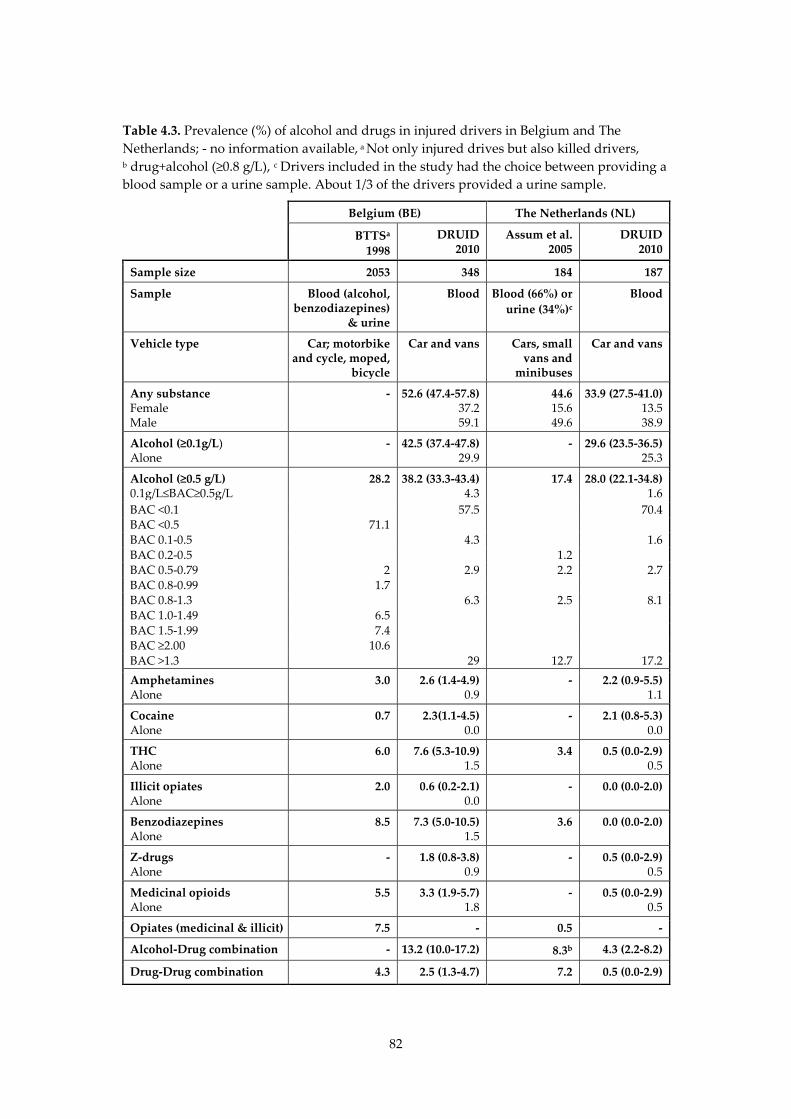
82

Table 4.3. Prevalence (%) of alcohol and drugs in injured drivers in Belgium and The Netherlands; - no information available, a Not only injured drives but also killed drivers, b drug+alcohol (≥0.8 g/L), c Drivers included in the study had the choice between providing a blood sample or a urine sample. About 1/3 of the drivers provided a urine sample.

Belgium (BE) The Netherlands (NL)

BTTSa 1998

DRUID 2010

Assum et al. 2005

DRUID 2010

Sample size 2053 348 184 187

Sample Blood (alcohol, benzodiazepines)

& urine

Blood Blood (66%) or urine (34%)c

Blood

Vehicle type Car; motorbike and cycle, moped,

bicycle

Car and vans Cars, small vans and

minibuses

Car and vans

Any substance Female Male

- 52.6 (47.4-57.8) 37.2 59.1

44.6 15.6 49.6

33.9 (27.5-41.0) 13.5 38.9

Alcohol (≥0.1g/L) Alone

- 42.5 (37.4-47.8) 29.9

- 29.6 (23.5-36.5) 25.3

Alcohol (≥0.5 g/L) 0.1g/L≤BAC≥0.5g/L

28.2 38.2 (33.3-43.4) 4.3

17.4 28.0 (22.1-34.8) 1.6

BAC <0.1 57.5 70.4 BAC <0.5 71.1 BAC 0.1-0.5 4.3 1.6 BAC 0.2-0.5 1.2 BAC 0.5-0.79 2 2.9 2.2 2.7 BAC 0.8-0.99 1.7 BAC 0.8-1.3 6.3 2.5 8.1 BAC 1.0-1.49 6.5 BAC 1.5-1.99 7.4 BAC ≥2.00 10.6 BAC >1.3 29 12.7 17.2 Amphetamines Alone

3.0 2.6 (1.4-4.9) 0.9

- 2.2 (0.9-5.5) 1.1

Cocaine Alone

0.7 2.3(1.1-4.5) 0.0

- 2.1 (0.8-5.3) 0.0

THC Alone

6.0 7.6 (5.3-10.9) 1.5

3.4 0.5 (0.0-2.9) 0.5

Illicit opiates Alone

2.0 0.6 (0.2-2.1) 0.0

- 0.0 (0.0-2.0)

Benzodiazepines Alone

8.5 7.3 (5.0-10.5) 1.5

3.6 0.0 (0.0-2.0)

Z-drugs Alone

- 1.8 (0.8-3.8) 0.9

- 0.5 (0.0-2.9) 0.5

Medicinal opioids Alone

5.5 3.3 (1.9-5.7) 1.8

- 0.5 (0.0-2.9) 0.5

Opiates (medicinal & illicit) 7.5 - 0.5 -

Alcohol-Drug combination - 13.2 (10.0-17.2) 8.3b 4.3 (2.2-8.2)

Drug-Drug combination 4.3 2.5 (1.3-4.7) 7.2 0.5 (0.0-2.9)

83

4.4. Discussion

4.4.1. Comparison with previous studies

Only two studies on the prevalence of alcohol and drugs in injured drivers could be identified in Belgium: the study of Schepens et al. and the Belgian Toxicology and Trauma study (BTTS), carried out in 1994-1995 & 1995-1996 respectively. In the Netherlands two studies were found that were carried out in 2005: the study that was part of the bigger IMMORTAL project (Assum et al., 2005) and a study by Smink and colleagues (Smink et al., 2005). When comparing the findings of present studies with the prevalence found in previous studies one should consider that there are differences with regard to the substances included in the different substance groups. For example in the DRUID project a division was made between the illicit (6-acetylmorphine) and the medicinal opiates (e.g. morphine, codeine, and methadone). In the IMMORTAL study the opiates group consisted of morphine, heroin and codeine and in the BTTS morphine, heroin and prescribed opiates. Secondly there are also differences with regard to the sample (blood, urine, serum) that was collected and analysed (see Table 4.3). Finally the inclusion criteria were not the same (e.g. type of vehicle, age of the drivers, MAIS and time period of data collection). Keeping in mind these limitations, a direct comparison of the results found in present study with those from previous research becomes difficult. In order to avoid misinterpretation of the findings, the limitations of every comparison are mentioned. For the Netherlands the highest prevalence of alcohol and drugs was found in the Smink study (Smink et al., 2005). We will not compare our findings with this study, because it studied only drivers who were suspected of drug or alcohol use. According to the Dutch legislation it is not allowed to take a blood sample without suspicion of alcohol or drug use (e.g. symptoms of drug use observed during medical examination), hence the high number of positives for alcohol >0.5 g/L found. The results from the DRUID study and the IMMORTAL study are more similar (see Table 4.3). A limitation of both the Dutch DRUID and the IMMORTAL study was the small sample size (184 and 186 respectively). Therefore, as the authors recognise, the small number of collected samples make more profound analyses impossible. While the sample size and the

84

driver characteristics (only car and vans; about 80% male drivers) are quite similar in these two studies, in IMMORTAL a third of the results were based on analysis of urine. A higher percentage of the IMMORTAL driver population tested positive for one or more substances (44.6%) compared to the DRUID study (33.9%). About 17% of the injured drivers in the IMMORTAL study tested positive for alcohol ≥0.5g/L (alone or combined with other substances) compared to 28% in the DRUID study. More than 10% of the drivers in both studies had a BAC≥1.3g/L (IMM: 12.7%; DRUID: 17.2%). Approximately 3% of the injured drivers in the IMMORTAL study tested positive for THC and benzodiazepines, while in the DRUID study no benzodiazepines and only 1 case of THC were found. In the IMMORTAL study the screening on THC and benzodiazepines was performed on urine in one third of the cases, and in DRUID screening of all samples was on whole blood. This may give also an overestimation of the prevalence of THC and benzodiazepines found in the IMMORTAL study. Secondly, the screening for benzodiazepines was wider in the IMMORTAL study (16 benzodiazepines) than in the DRUID study (8 benzodiazepines), which makes it more likely to find benzodiazepines in the blood of the injured drivers included in the IMMORTAL study. When calculating the prevalence of THC and/or THCCOOH in the present DRUID study for the Netherlands, 2.0% prevalence was found (in Belgium: 9.9%). Almost no drug-drug combinations were found among the injured drivers in the DRUID study, which was a bit surprising since these were detected more frequently than single drugs in the IMMORTAL study, but this could also be explained by the testing of urine samples. Also the prevalence of alcohol-drug combinations was higher in the IMMORTAL study (8.3%, alcohol > 0.2 g/L) compared to the DRUID study (4.3%). In general, the prevalence of drugs reported in the DRUID project was much lower than the prevalence reported in the IMMORTAL study. The differences could be explained by the difference in the biological matrix (IMMORTAL) (urine in one third of the IMMORTAL cases and whole blood in DRUID) or the (number of) substances screened for (e.g. differences in benzodiazepines /amphetamines). In Belgium, the BTTS study collected data about drivers of motor vehicles and bicycles, aged more than 14 years, involved in traffic accidents that led at least to 24-hour hospitalisation. In the BTTS toxicological analyses were performed on blood and urine samples taken from injured drivers admitted

85

to the same 5 hospitals selected in the present project. When comparing the DRUID and BTTS, one should keep in mind that in the BTTS urine was the matrix for drug testing (except for benzodiazepines) while blood was analysed in DRUID. No significant difference in gender distributions was found in both studies. Regarding time period distribution, there were fewer weekday accidents in DRUID. In the toxicological analyses, alcohol remains the most common finding. The percentage of BAC above 0.5 g/L was 28.2% in the BTTS and 38.2% in the present study. When taking into account only the prevalence among drivers of a car about 34.0% of the drivers in the BTTS was found positive for alcohol. This prevalence is similar to the one found in the DRUID study. The THC prevalence is lower in the BTTS (BTTS: 6.0%; DRUID: 7.6%). Cocaine prevalence appears also to be higher in the DRUID sample (2.3%) compared to the BTTS findings (0.7%), while the prevalence of amphetamines (BTTS: 3.0%; DRUID: 2.6%), benzodiazepines (BTTS: 8.5%; DRUID: 7.3%) and medicinal opioids (BTTS: 5.5%; DRUID: 3.3%) was lower. A small difference was found with regard to the drug-drug combinations. In the BTTS 4.3% of the drivers were found positive for two or more drugs (amphetamines, benzodiazepines, barbiturates, cannabis, cocaine, opiates, methadone or propoxyphene), compared to only 2.5 % in the DRUID study. Because urine was analysed, it is possible that a certain number of drivers were found positive in the BTTS because they had taken drugs several days before the accident. If the analysis in the BTTS would have been performed on blood the number of injured drivers positive for drugs would probably be even lower. The second study performed in Belgium included all injured weekend drivers (N= 211) admitted to the emergency units in Antwerp from July 1994-June 1995. Comparing our findings with those from the Schepens study is delicate due to great differences in study design (urine samples were tested for (il)legal drugs instead of blood; only weekend drivers). In general, about half of the injured drivers included in both studies were found positive and a similar prevalence of alcohol was found in the Schepens et al. study (BAC ≥0.5g/L: 35.5%) and the DRUID study (BAC≥0.5 g/L: 38.2%).

4.4.2. Comparison of Belgium and the Netherlands

The Netherlands is a larger country than Belgium (BE: 30500 km2; NL: 41500 km2 and with more inhabitants (NL: 16.485.787; BE: 10.750.000) but with fewer traffic accidents involving personal injury (in 2009 NL: 19.378 compared to BE: 40.700 and in 2010: BE: 729 killed drivers and 45369 injured

86

drivers; NL: 640 killed drivers; 17.000 injured drivers) and a lower prevalence of alcohol and drugs in the general driving population (Belgisch Instituut voor de Verkeersveiligheid, 2011; European Commission, 2011; Stichting Wetenschappelijk Onderzoek Verkeersveiligheid, 2010). It should be stated that in the past few years a decrease of the number of killed and injured drivers was observed in both countries. The higher alcohol enforcement in both countries (more alcohol tests and hours spent by the police on testing) could be one of the explanations. Secondly, in Belgium a per se legislation for illicit drugs is applied: in case a defined cut-off value of a substance concentration in the blood sample of the driver is exceeded s/he will be prosecuted. Fewer drivers were found positive in the Netherlands compared with Belgium. This is a remarkable finding since the sample of drivers in the Netherlands is younger (33% below 24 years compared to 23% in BE) and included more men (80%) than in Belgium (54%). Thirdly, more single-vehicle accidents were registered in the Dutch study (63%, versus 49% in BE). A higher prevalence is expected since studies showed that these groups (young males and single vehicle accidents) are more likely to test positive (Bogstrand et al., 2011; Longo et al., 2000; Palmentier et al., 2009; Ricci et al., 2008). Alcohol was the most common finding in both countries. In the present study about 10% more drivers tested positive for alcohol (≥0.1 and ≥0.5 g/L) in Belgium than in the Netherlands. In contrast to the difference in alcohol prevalence, the distribution of alcohol concentrations is similar in both studies. The drivers found positive for alcohol in both studies had high blood alcohol concentrations (35.3 % of the Belgian drivers had a BAC ≥0.8 g/L compared to 25.3% of the Dutch drivers). The median blood alcohol concentration in the Dutch and Belgian injured driver population was about 1.5 and 1.6 g/L respectively. The lower prevalence of alcohol found in the Dutch DRUID study could be the result of the higher enforcement of drink-driving legislation in the Netherlands. The enforcement level for alcohol (number of alcohol tests per 100.000 inhabitants) is estimated to be 3 to 4 times lower in Belgium than it is in the Netherlands . However the number of alcohol tests recently increased in Belgium (about 750.000 alcohol tests performed in 2010). Recently, the Belgian government announced an increase in the numbers of alcohol tests in the next two years. The level of alcohol enforcement expressed in hours that

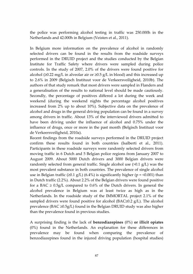
87

the police was performing alcohol testing in traffic was 250.000h in the Netherlands and 42.000h in Belgium (Veisten et al., 2011). In Belgium more information on the prevalence of alcohol in randomly selected drivers can be found in the results from the roadside surveys performed in the DRUID project and the studies conducted by the Belgian Institute for Traffic Safety where drivers were sampled during police controls. In the study of 2007, 2.0% of the drivers were found positive for alcohol (≥0.22 mg/L in alveolar air or ≥0.5 g/L in blood) and this increased up to 2.6% in 2009 (Belgisch Instituut voor de Verkeersveiligheid, 2010b). The authors of that study remark that most drivers were sampled in Flanders and a generalisation of the results to national level should be made cautiously. Secondly, the percentage of positives differed a lot during the week and weekend (during the weekend nights the percentage alcohol positives increased from 2% up to about 10%). Subjective data on the prevalence of alcohol and drugs in the general driving population can be found in a survey among drivers in traffic. About 13% of the interviewed drivers admitted to have been driving under the influence of alcohol and 0.75% under the influence of drugs, once or more in the past month (Belgisch Instituut voor de Verkeersveiligheid, 2010a). Recent findings from the roadside surveys performed in the DRUID project confirm these results found in both countries (Isalberti et al., 2011). Participants in these roadside surveys were randomly selected drivers from moving traffic in 6 Dutch and 5 Belgian police regions from January 2007 to August 2009. About 5000 Dutch drivers and 3000 Belgian drivers were randomly selected from general traffic. Single alcohol use (>0.1 g/L) was the most prevalent substance in both countries. The prevalence of single alcohol use in Belgian traffic (≥0.1 g/L) (6.4%) is significantly higher (p = <0.001) than in Dutch traffic (2.2%). About 2.2% of the Belgian drivers were found positive for a BAC ≥ 0.5g/L compared to 0.6% of the Dutch drivers. In general the alcohol prevalence in Belgium was at least twice as high as in the Netherlands. In the roadside study of the IMMORTAL project 2.1% of the sampled drivers were found positive for alcohol (BAC≥0.2 g/L). The alcohol prevalence (BAC ≥0.5g/L) found in the Belgian DRUID study was also higher than the prevalence found in previous studies. A surprising finding is the lack of benzodiazepines (0%) or illicit opiates (0%) found in the Netherlands. An explanation for these differences in prevalence may be found when comparing the prevalence of benzodiazepines found in the injured driving population (hospital studies)

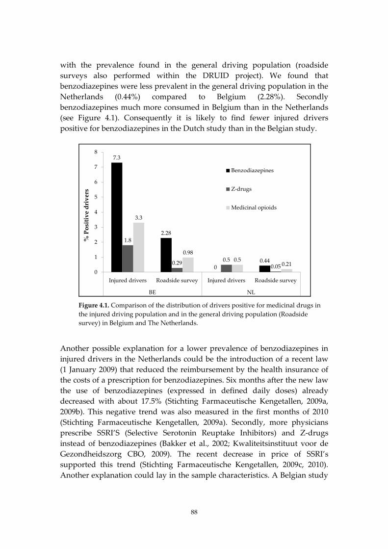
88

with the prevalence found in the general driving population (roadside surveys also performed within the DRUID project). We found that benzodiazepines were less prevalent in the general driving population in the Netherlands (0.44%) compared to Belgium (2.28%). Secondly benzodiazepines much more consumed in Belgium than in the Netherlands (see Figure 4.1). Consequently it is likely to find fewer injured drivers positive for benzodiazepines in the Dutch study than in the Belgian study.

7.3

2.28

00.44

1.8

0.29 0.50.05

3.3

0.980.5

0.210

1

2

3

4

5

6

7

8

Injured drivers Roadside survey Injured drivers Roadside survey

BE NL

% P

ositi

ve d

rive

rs

Benzodiazepines

Z-drugs

Medicinal opioids

Figure 4.1. Comparison of the distribution of drivers positive for medicinal drugs in the injured driving population and in the general driving population (Roadside survey) in Belgium and The Netherlands.

Another possible explanation for a lower prevalence of benzodiazepines in injured drivers in the Netherlands could be the introduction of a recent law (1 January 2009) that reduced the reimbursement by the health insurance of the costs of a prescription for benzodiazepines. Six months after the new law the use of benzodiazepines (expressed in defined daily doses) already decreased with about 17.5% (Stichting Farmaceutische Kengetallen, 2009a, 2009b). This negative trend was also measured in the first months of 2010 (Stichting Farmaceutische Kengetallen, 2009a). Secondly, more physicians prescribe SSRI’S (Selective Serotonin Reuptake Inhibitors) and Z-drugs instead of benzodiazepines (Bakker et al., 2002; Kwaliteitsinstituut voor de Gezondheidszorg CBO, 2009). The recent decrease in price of SSRI’s supported this trend (Stichting Farmaceutische Kengetallen, 2009c, 2010). Another explanation could lay in the sample characteristics. A Belgian study

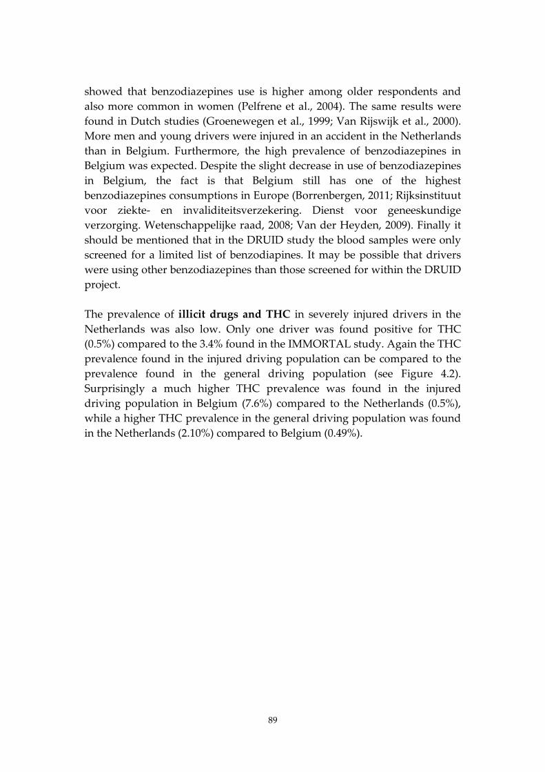
89

showed that benzodiazepines use is higher among older respondents and also more common in women (Pelfrene et al., 2004). The same results were found in Dutch studies (Groenewegen et al., 1999; Van Rijswijk et al., 2000). More men and young drivers were injured in an accident in the Netherlands than in Belgium. Furthermore, the high prevalence of benzodiazepines in Belgium was expected. Despite the slight decrease in use of benzodiazepines in Belgium, the fact is that Belgium still has one of the highest benzodiazepines consumptions in Europe (Borrenbergen, 2011; Rijksinstituut voor ziekte- en invaliditeitsverzekering. Dienst voor geneeskundige verzorging. Wetenschappelijke raad, 2008; Van der Heyden, 2009). Finally it should be mentioned that in the DRUID study the blood samples were only screened for a limited list of benzodiapines. It may be possible that drivers were using other benzodiazepines than those screened for within the DRUID project. The prevalence of illicit drugs and THC in severely injured drivers in the Netherlands was also low. Only one driver was found positive for THC (0.5%) compared to the 3.4% found in the IMMORTAL study. Again the THC prevalence found in the injured driving population can be compared to the prevalence found in the general driving population (see Figure 4.2). Surprisingly a much higher THC prevalence was found in the injured driving population in Belgium (7.6%) compared to the Netherlands (0.5%), while a higher THC prevalence in the general driving population was found in the Netherlands (2.10%) compared to Belgium (0.49%).

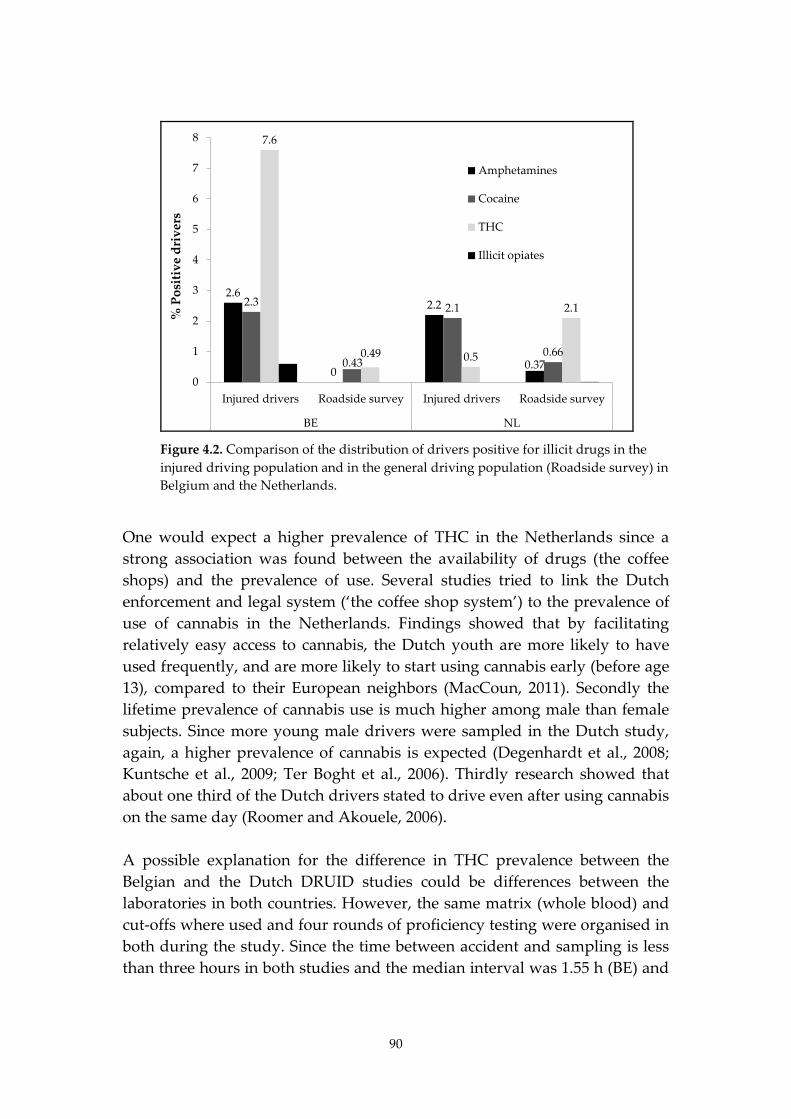
90

2.6

0

2.2

0.37

2.3

0.43

2.1

0.66

7.6

0.49 0.5

2.1

0

1

2

3

4

5

6

7

8

Injured drivers Roadside survey Injured drivers Roadside survey

BE NL

% P

ositi

ve d

rive

rsAmphetamines

Cocaine

THC

Illicit opiates

Figure 4.2. Comparison of the distribution of drivers positive for illicit drugs in the injured driving population and in the general driving population (Roadside survey) in Belgium and the Netherlands.

One would expect a higher prevalence of THC in the Netherlands since a strong association was found between the availability of drugs (the coffee shops) and the prevalence of use. Several studies tried to link the Dutch enforcement and legal system (‘the coffee shop system’) to the prevalence of use of cannabis in the Netherlands. Findings showed that by facilitating relatively easy access to cannabis, the Dutch youth are more likely to have used frequently, and are more likely to start using cannabis early (before age 13), compared to their European neighbors (MacCoun, 2011). Secondly the lifetime prevalence of cannabis use is much higher among male than female subjects. Since more young male drivers were sampled in the Dutch study, again, a higher prevalence of cannabis is expected (Degenhardt et al., 2008; Kuntsche et al., 2009; Ter Boght et al., 2006). Thirdly research showed that about one third of the Dutch drivers stated to drive even after using cannabis on the same day (Roomer and Akouele, 2006). A possible explanation for the difference in THC prevalence between the Belgian and the Dutch DRUID studies could be differences between the laboratories in both countries. However, the same matrix (whole blood) and cut-offs where used and four rounds of proficiency testing were organised in both during the study. Since the time between accident and sampling is less than three hours in both studies and the median interval was 1.55 h (BE) and

91

1.35 h (NL), no difference is expected. Furthermore it can be mentioned that some Dutch injured drivers were found positive for the metabolite THC-COOH. The presence of THC-COOH indicates past use of cannabis. When calculating the prevalence of THC and/or THC-COOH 1.6% of the Dutch drivers were found positive compared to the 0.5% drivers found positive for THC. Finally, given the low number of included subjects the confidence intervals give a more accurate prevalence (0.0-2.9%) A limitation of the DRUID study was that the Dutch data collected in three hospitals covered only the South and Eastern part of the Netherlands. However when comparing the prevalence of alcohol and drugs in the study population with those in general traffic, no differences were found. Consequently, no bias is expected. The Belgian data were grouped under the three Belgian regions (Brussels, Flanders and Wallonia) and collected in the same five hospitals as the data from the BTTS. About 81% of the drivers was sampled in Flanders compared to 60% in the BTTS. Despite a prolongation of the initial period of sample collection and an extra incentive when collecting more than 200 samples, the number of samples collected in Brussels (3%) and Wallonia (16%) stayed low. The BTTS reported the same problems with regard to sample collection in Brussels and Wallonia. Finally, it should also be kept in mind that in the DRUID study analyses were performed on only 23 target analytes, while in the BTTS a much broader screening (e.g. all benzodiazepines) was performed.

4.5. Conclusion

Only two studies on the prevalence of alcohol and drugs in injured drivers in Belgium and the Netherlands could be identified in each country. Comparing the prevalence of alcohol and drugs found in present and previous studies was difficult due to differences in matrix collected (blood/urine/serum), toxicological analyses (methods used and substances screened for), study design (e.g. time between accident and sampling), as well as inclusion criteria handled (age, time period, MAIS, type of vehicle). To overcome this comparability problem a uniform study design was used in the DRUID study. The DRUID study provides besides comparable data also recent data on the prevalence of alcohol, illicit and medicinal drugs in Belgium and the Netherlands. The prevalence of alcohol in DRUID was higher than in the comparable studies (BTTS and IMMORTAL) in the past. This does not necessarily mean a worsening of the problem of driving under

92

the influence of alcohol in the last 10 or 15 years, as it is possible that the absolute number of alcohol-related crashes has decreased. Keeping the differences in study design in mind some overall conclusion can be drawn regarding the prevalence of alcohol and drugs in Belgium and the Netherlands. In general some deviations in prevalence are found when comparing the DRUID results in the Netherlands with previous surveys (no benzodiazepines, low THC and drug-drug combinations). These differences could be explained by differences in (DRUID) enforcement level, drug driving legislation and enforcement, prescription policies (benzodiazepines), cultural differences and uncertainty of the data due to a small sample size. The results from the Belgian DRUID study are more similar to the results from previous studies, especially the prevalence of the illicit drugs where no increase of prevalence of illicit drugs or medical drugs is observed in the period between 1998 and 2010. However, in the same period an increase of the prevalence of alcohol was found (BTTS: 34.0% only car drivers; DRUID: 38.2%). In the present study a higher prevalence of alcohol and drugs in seriously injured drivers was found in Belgium compared to the Netherlands. Alcohol was the most prevalent finding in both studies. The distribution of blood alcohol concentrations in the Dutch and Belgian study was similar with very high blood alcohol concentrations in both and a similar median blood alcohol concentration (about 1.6 g/L). The lower prevalence of alcohol in the Netherlands is associated with a much lower number of crashes and killed and injured drivers (compared to the Netherlands, Belgium has 3.2 times more crashes involving injuries, 4.1 times more injured and 1.7 times more fatally injured people). One notable finding is the low prevalence of THC and benzodiazepines in the Dutch injured driver population. Despite the high prevalence of THC found in the general driving population surprisingly almost no THC was found in the Dutch injured driver population. The one Dutch driver found positive for THC had a very high THC concentration (about 19 ng/mL). In addition no benzodiazepines were found in the Dutch injured drivers. This could be expected since a low prevalence was found in the general driving population (Belgium had a prevalence of about five times higher than the Netherlands). For the other illicit drugs (amphetamines, cocaine and illicit opiates) and medicinal drugs (z-drugs and medicinal opioids) no larger differences were observed.

93

When looking for explanations for the differences in prevalence found above different aspects such as differences in alcohol enforcement between the countries, differences in sample collection and consumption patterns should be kept in mind.

4.6. Disclaimer

This article has been produced under the project Driving Under Influence of Drugs, Alcohol and Medicines (DRUID) financed by the European Commission within the framework of the EU 6th Framework Program. This report reflects only the authors’ view. The European Commission is not liable for any use that may be made of the information contained therein.

4.7. Acknowledgements

The authors would like to thank all hospital personnel involved in the study as well as to the laboratory technicians involved in the DRUID project: Ms. Charlotte Van Keirsbilck & Prof. Dr. Walter Buylaert - Ghent University Hospital Prof. Dr. Marc Sabbe & Dr. Agnes Meulemans - Leuven University Hospital Prof. Dr. Yves Hubloue & Mr. Peter Bruynseels - Brussel University Hospital Prof. Dr. Vincent D’Orio & Mr. Edmond Brasseur - University Hospital Sart Tilman (Liège) Dr. Albert Fox, Mr. Vincent Collet, Mr. Johan Silliard & Mr. Eric Lahaye - Regional Hospital of Namur Riny van der Ven, Miranda van Tits, Jan Verhagen & Gael Smits – UMC Nijmegen Kris Movig, Anja Stam, Paul Bertelink & Renate Kienhuis – Medisch Spectrum Twente, Enschede Paul Nagel, Robbert Groenewegen, Teun van Egmond & Ine van de Broek – Sint-Elizabeth, Tilburg Martine Reurings– SWOV Finally, this study was not realisable without the financial support of the European Commission.

94

5. Repeatability of oral fluid collection methods for THC measurement12

5.1. Introduction

Cannabis is the most frequently used illicit drug in traffic (Houwing et al., 2011; Lacey et al., 2009; Mallick et al., 2007). A recently conducted European study among injured and killed drivers in nine different European countries showed that THC, which is the active substance of cannabis, was detected in up to 7.6% of injured and 6.1% of killed drivers (Isalberti et al., 2011). In many countries, driving under the influence of THC is considered as illegal in the national Road Traffic Act (EMCDDA, 2007). The confirmation of cannabis use in traffic is mainly based on analysis of blood, although in some countries (e.g. Australia and Belgium) oral fluid is used as a standard (Lillsunde and Gunnar, 2005; Verstraete et al., 2011a). For screening purposes, however, oral fluid is used more often because blood sampling is invasive and expensive. Oral fluid sampling is regarded as a less invasive and cheaper alternative for blood sampling when screening drivers for drug use in traffic (Bosker and Huestis, 2009; Huestis and Cone, 2004; Niedbala et al., 2001; Toennes et al., 2005; Verstraete, 2004). The practical benefits of oral fluid collection compared to the collection of blood stimulate the discussion on the usability of oral fluid for confirmation analysis. However, the question can be raised how reliable oral fluid results are for determining specific ’per se’ concentrations of THC. The weak relationship between oral fluid and blood/serum concentrations for THC has been demonstrated in several studies (Gjerde et al., 2010a; Kauert et al., 2006; Kauert et al., 2007; Milman et al., 2011; Wille et al., 2009). The most commonly mentioned reason in literature is that oral fluid concentrations of THC are not necessarily based on the transfer from blood to oral fluid, but that they are merely the result of contamination of oral fluid by THC deposition on membranes and debris that are left in oral cavities (Bosker and Huestis, 2009; Drummer, 2008). Furthermore, it is well known in literature (Crouch, 2005; Drummer, 2008; O'Neal et al., 2000; Verstraete et al., 2011a)

12 This chapter is accepted for publication as the following article: Houwing, S., Smink, B.E., Legrand, S.-A., Mathijssen, M.P.M., Verstraete, A. G. & Brookhuis, K.A. Repeatability of oral fluid collection methods for THC measurement. This article is published in Forensic Science International (FSI) 2012; 223 (1-3) 266-272.

95

that the results of oral fluid drug testing can also be affected by the sampling method and the collection devices. O’Neal et al. (2000) found that on average codeine concentrations in specimens collected by spitting were 3.6 times higher than concentrations collected by acidic stimulation and 1.3 to 2.0 times higher than concentrations collected by nonacidic stimulation. These results are in line with a recently published study of Verstraete et al. (2011a) in which a factor of 1.5 was found for THC between nonacidic and acidic stimulation and a factor of 1.3 for codeine. Factors for five other substances ranged from 1.3 to 2.7. One issue that to our knowledge has only been reported once is the repeatability of THC concentrations in oral fluid in samples obtained by the same collection method. Repeatability tells something about the precision of a method. It means that under the same conditions, a second test by the same collection method should lead to the same results. If the repeatability of a method is low, the method could be regarded as not precise enough to be used. The study of Niedbala et al (2001) compared Intercept® oral fluid test results of simultaneously obtained samples from visitors of a coffee shop. In our present study we assessed the correlation between THC concentrations of two subsequently collected oral fluid samples for two different sampling methods. Furthermore, we compared THC concentrations collected by both methods. Additionally we evaluated the measurements of the sampling devices with respect to the Belgian legal limit for THC in traffic (10 ng/mL in oral fluid). In the Netherlands, confirmation analysis is based on blood samples. Therefore, no qualitative evaluation was possible for the Dutch legislation.

5.2. Materials and methods

5.2.1. Location and subjects

All oral fluid samples were collected in a so-called ‘coffee shop’ in Doetinchem (the Netherlands). In the Netherlands a coffee shop is a type of bar where selling and using soft drugs for personal consumption is tolerated. In the ‘coffee shop’ that participated in our study a special room was reserved for the collection of the samples. This room was separated from the area of the coffee shop in which the cannabis was actually smoked in order to decrease the possibility of contamination by air. Two adjacent windows were opened during the study to ventilate the room that was approximately 55m3. According to Niedbala et al. (2005), the risk of contamination of the collection

96

devices by polluted air would most likely be eliminated when using a separated room with open windows. Customers of the coffee shop were invited to participate by means of posters that were placed in the smoking area of the coffee shop. Each participant received an incentive of five euro.

5.2.2. Sample collection

Two methods were used to collect oral fluid samples. The first collection method was by using the Statsure Saliva samplerTM (Saliva Diagnostic Systems, Framingham, MA). This device was used in the European DRUID project (Driving Under the Influence of Drugs, Alcohol and Medicines) in Belgium and ten other countries for collecting oral fluid samples from the general driving population (Houwing et al., 2011). The Statsure sampling pad is made of cellulose and is not treated with chemicals stimulating the production of saliva. Oral fluid is gathered by placing the collection pad under the tongue. The indicator of the device turns completely blue when a sufficient amount of oral fluid is collected. The Statsure device contains 1.0 mL of buffer fluid which is added to the oral fluid. The second collection method was by spitting into a polypropylene tube (Deltalab, Spain). After collection, oral fluid samples were stored in solid carbon dioxide at about -80˚C (dry ice). After transportation to the Netherlands Forensic Institute (NFI) in The Hague, oral fluid samples were stored at -20˚C until analysis. The Statsure samples were transported on dry ice from the NFI to the toxicological laboratory in Ghent for analysis, while the spit tube samples remained for analysis at the NFI.

5.2.3. Sample preparation and analysis

The concentration of the oral fluid samples collected by the Statsure device needed to be corrected since the expected sample of oral fluid is approximately 1.0 mL, but in practice the volume varies considerably. Therefore, the collected volumes of oral fluid were determined for each sample by weighting using the following correction formula, under the assumption that the volume of buffer in the device is constant (1 mL), where w = weight of a sample, ŵ = average weight of an empty Statsure device:

)(2

)1(

ww

wwCC correctedcorrected −×

−+×=

97

The UPLC-MS/MS method for the analysis of the samples obtained with Statsure has been described by Goessaert et al. (2010). The first step in sample preparation of the spit tubes was defrosting the oral fluid samples. Next, the concentration of THC in oral fluid samples collected by spitting into a polypropylene tube was determined after protein precipitation followed by centrifugation, by LC-MS-MS on a Water Acquity UPLC®-system with a Waters Quattro premier XE triple quadrupole mass spectrometer. Chromatography employed a reversed-phase UPLC® column (BEH C-18, 100 x 2.1-mm i.d., 1.7 µm particle diameter) and a 17-min gradient elution (methanol / 10 mM ammonium bicarbonate pH 10.0, 5/95 to 95/5). Injection volume was 10 µL. The eluent was introduced to the electrospray source of the triple quadrupole MS instrument at a flow-rate of 500 µL/min. Molecular ions were fragmented using an optimized collision-induced dissociation voltages for each compound (positive ion mode). Parent ions (m/z 315.3 for THC and m/z 318.3 for Delta 9-THC-d3) and product ions (m/z 193.2 and 259.5 for THC and m/z 196.2 for Delta 9-THC-d3) were detected after collision.

5.2.4. Method validation

The linear range for the assay was 1 - 200 ng/mL for THC. The lowest concentration of the calibration curve was considered as the limit of quantification (LOQ). The limit of detection was 0.8 ng/mL for THC. No interfering compounds were present in blank oral fluid samples. The within-day precision was determined on two concentration levels by repeated analysis (n=10) and was < 15 %. The between-day reproducibility was determined at two concentration levels by analysis on different days (n=4) and was < 15%. However, calibration curves were included in each analytical run. The method validation results of the analytical method used for the quantification of THC in Statsure samples have been given in Goessaert et al. (2010). Briefly, the extraction recovery was 53%, LOQ was 1 ng/mL, the imprecision 8.8% and the inaccuracy – 3.9%.

5.2.5. Statistical analysis

The quantitative analysis procedure is based on visual inspection of data patterns using a Bland-Altman plot, as described in Bland and Altman (1986) and Hanneman (2008). The Bland-Altman plot consists of the average of the paired values on the x-axis and the difference between the paired values on the y-axis. Correlation measures cannot be used when comparing two

98

samples from one method since a correlation coefficient gives an analysis of the deviation from a line with any slope, but for this purpose we want to measure the deviation from a line with a slope of exactly 45 degrees. Mean value, bias from the mean, standard deviation of the difference, limits of agreement, and proportion error are reported together with the plot. The limits of agreements are drawn by using a 95% confidence interval. This confidence interval is calculated by the average difference plus or minus two times the standard deviation of the average difference. The proportional error can be established by dividing the limits of agreement by the mean value of the measurements obtained with the established method. In principle, simultaneous collection would be the best method to gather the oral fluid samples. However, this was not possible since the collection of two spit samples at once or a spit sample while collecting oral fluid by means of the Statsure device was very difficult. Therefore, all samples have been collected in sequence. Since the THC concentration in oral fluid was not likely to change a lot due to elimination between the collection of the first and second sample, this sequential method was regarded as acceptable by the authors. In those pairs with both a spitting sample and a Statsure sample, the order of the samples varied. In pairs that contained two samples from the same collection method, sample number one was always collected before sample number two. No error margin is determined at present for the Belgian legal limit. In this study we will regard a 30% margin as the acceptable error, based on the measurement uncertainty currently used in the Swiss legislation (Senna et al., 2010). For statistical analysis of qualitative results (positive or negative according to the Belgium legislation), Cohen’s Kappa was used to determine consistency between the two samples. The Kappa statistic is normally performed to determine consistency among raters. In this study for each pair the first bivariate result was compared with the second bivariate result. The Kappa score was interpreted by using a scoring list published by Landis and Koch (1977), in which 0-20% reflects a slight agreement, 21-40% a fair agreement, 41-60% a moderate agreement, 61-80% a substantial agreement and 81-100% an almost perfect agreement.

99

5.3. Results

5.3.1. Comparison of the sample concentrations

In total 117 sets of oral fluid samples were collected. The major part of the included sets consisted of two samples, but seven sets consisted of three samples and one set consisted of four samples. In order to analyze comparable pairs for the Statsure each set of three samples, e.g. a set with the samples X1, Y1, Y2, was divided into three sets of two samples: (X1, Y1), (X1, Y2), and (Y1, Y2). The remaining set of four samples was divided into 6 pairs based on the same principle. The conversion of the sets into unique pairs led to a total of 136 pairs, divided into three groups for analysis: 28 pairs of Statsure samples, 47 pairs of spit tube samples , and 61 pairs with one Statsure and one spit tube sample. Table 5.1 shows the distribution of THC concentrations for each collection method. THC concentrations varied from 0 to 12,063 ng/mL for the spit tube samples and from 0 to 5,446 ng/mL for the Statsure samples. Eight Statsure pairs, five spit tube pairs, and two combined pairs consisted of negative samples only. The inclusion of negative pairs in the sample could influence the results if one of the methods would have more negative samples, since an exact agreement in THC values is easier to achieve in negative samples than in positive samples. For this reason, all negative pairs and the pairs with outliers were removed from the dataset before analysis on repeatability, which led to an inclusion of twenty Statsure pairs, forty-two spit tube pairs and fifty-nine combined pairs. The median THC concentration for the first and second sample of the twenty Statsure pairs did not differ (p < 0.911) between the first sample and the second sample (50.4 and 69.3 ng/mL, respectively). Moreover, the highest concentration samples was almost evenly distributed over the first and second samples of the twenty pairs: eleven and nine, respectively. The median THC concentration of the forty-two spitting samples that were taken first did not differ (p < 0.48) from the median of the samples that were taken second (135.5 and 70.1 ng/mL, respectively). Furthermore, the highest samples were almost evenly divided between the first and second samples: twenty-two and twenty, respectively. Among the fifty-nine THC positive pairs consisting of both a Statsure and a spitting sample the median THC concentration of the Statsure samples (58.3 ng/mL) was lower (p < 0.001) than the median of the spitting samples (206.5 ng/mL).

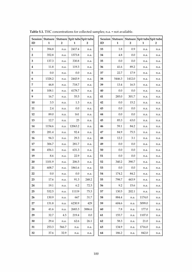
100

Table 5.1. THC concentrations for collected samples; n.a. = not available.

Session ID

Statsure 1

Statsure 2

Spit tube 1

Spit tube 2

Session ID

Statsure 1

Statsure 2

Spit tube 1

Spit tube 2

1 394.8 n.a. 2417.4 n.a. 33 1.8 0.9 n.a. n.a.

2 352.8 n.a. 1373.8 n.a. 34 4.8 0.0 n.a. n.a.

3 137.3 n.a. 330.8 n.a. 35 0.0 0.0 n.a. n.a.

4 11.8 n.a. 119.3 n.a. 36 41.6 89.2 n.a. n.a.

5 0.0 n.a. 0.0 n.a. 37 22.7 17.9 n.a. n.a.

6 1328.2 n.a. 2443.9 n.a. 38 5446.3 1412.0 n.a. n.a.

7 44.8 n.a. 718.7 n.a. 39 13.4 16.5 n.a. n.a.

8 108.1 n.a. 4178.7 n.a. 40 0.0 0.0 n.a. n.a.

9 16.7 n.a. 55.5 n.a. 41 285.0 301.7 n.a. n.a.

10 3.5 n.a. 1.3 n.a. 42 0.0 15.2 n.a. n.a.

11 2.4 n.a. 0.0 n.a. 43 0.0 0.0 n.a. n.a.

12 89.0 n.a. 161 n.a. 44 0.0 0.0 n.a. n.a.

13 12.7 n.a. 25 n.a. 45 85.3 63.0 n.a. n.a.

14 1154.6 n.a. 12063.2 n.a. 46 59.1 84.2 n.a. n.a.

15 281.4 n.a. 92.4 n.a. 47 84.9 75.5 n.a. n.a.

16 94.3 n.a. 29.3 n.a. 48 12.2 3.1 n.a. n.a.

17 306.7 n.a. 281.7 n.a. 49 0.0 0.0 n.a. n.a.

18 456.1 n.a. 631.3 n.a. 50 0.0 0.0 n.a. n.a.

19 8.6 n.a. 22.9 n.a. 51 0.0 0.0 n.a. n.a.

20 1101.9 n.a. 206.5 n.a. 52 340.2 390.7 n.a. n.a.

21 608.7 n.a. 1861.6 n.a. 53 0.0 0.0 n.a. n.a.

22 0.0 n.a. 0.0 n.a. 54 174.2 84.2 n.a. n.a.

23 17.6 n.a. 91.3 248.2 55 798.7 443.9 n.a. n.a.

24 19.1 n.a. 6.2 72.3 56 9.2 15.6 n.a. n.a.

25 532.5 n.a. 11119 75.3 57 130.5 202.1 n.a. n.a.

26 130.9 n.a. 667 31.7 58 884.4 n.a. 1174.0 n.a.

27 131.8 n.a. 6230.9 429 59 604.6 n.a. 3099.0 n.a.

28 41.6 n.a. 2683.3 3886.6 60 7.8 n.a. 177.0 n.a.

29 32.7 4.5 219.4 0.0 61 155.7 n.a. 1107.0 n.a.

30 29.4 n.a. 62.6 26.1 62 58.3 n.a. 21.0 n.a.

31 253.3 566.7 n.a. n.a. 63 134.9 n.a. 1716.0 n.a.

32 37.6 32.9 n.a. n.a. 64 186.2 n.a. 842.0 n.a.

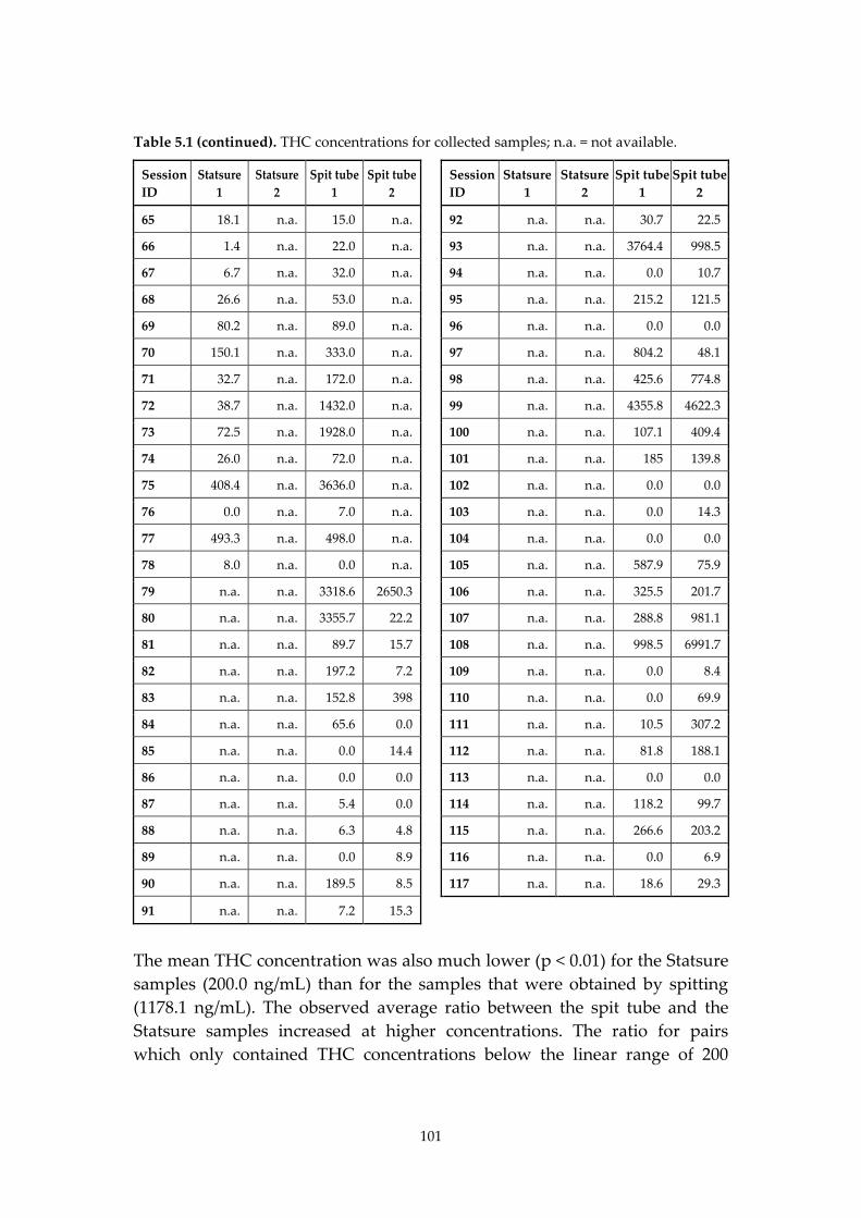
101

Table 5.1 (continued). THC concentrations for collected samples; n.a. = not available.

Session ID

Statsure 1

Statsure 2

Spit tube 1

Spit tube 2

Session ID

Statsure 1

Statsure 2

Spit tube 1

Spit tube 2

65 18.1 n.a. 15.0 n.a. 92 n.a. n.a. 30.7 22.5

66 1.4 n.a. 22.0 n.a. 93 n.a. n.a. 3764.4 998.5

67 6.7 n.a. 32.0 n.a. 94 n.a. n.a. 0.0 10.7

68 26.6 n.a. 53.0 n.a. 95 n.a. n.a. 215.2 121.5

69 80.2 n.a. 89.0 n.a. 96 n.a. n.a. 0.0 0.0

70 150.1 n.a. 333.0 n.a. 97 n.a. n.a. 804.2 48.1

71 32.7 n.a. 172.0 n.a. 98 n.a. n.a. 425.6 774.8

72 38.7 n.a. 1432.0 n.a. 99 n.a. n.a. 4355.8 4622.3

73 72.5 n.a. 1928.0 n.a. 100 n.a. n.a. 107.1 409.4

74 26.0 n.a. 72.0 n.a. 101 n.a. n.a. 185 139.8

75 408.4 n.a. 3636.0 n.a. 102 n.a. n.a. 0.0 0.0

76 0.0 n.a. 7.0 n.a. 103 n.a. n.a. 0.0 14.3

77 493.3 n.a. 498.0 n.a. 104 n.a. n.a. 0.0 0.0

78 8.0 n.a. 0.0 n.a. 105 n.a. n.a. 587.9 75.9

79 n.a. n.a. 3318.6 2650.3 106 n.a. n.a. 325.5 201.7

80 n.a. n.a. 3355.7 22.2 107 n.a. n.a. 288.8 981.1

81 n.a. n.a. 89.7 15.7 108 n.a. n.a. 998.5 6991.7

82 n.a. n.a. 197.2 7.2 109 n.a. n.a. 0.0 8.4

83 n.a. n.a. 152.8 398 110 n.a. n.a. 0.0 69.9

84 n.a. n.a. 65.6 0.0 111 n.a. n.a. 10.5 307.2

85 n.a. n.a. 0.0 14.4 112 n.a. n.a. 81.8 188.1

86 n.a. n.a. 0.0 0.0 113 n.a. n.a. 0.0 0.0

87 n.a. n.a. 5.4 0.0 114 n.a. n.a. 118.2 99.7

88 n.a. n.a. 6.3 4.8 115 n.a. n.a. 266.6 203.2

89 n.a. n.a. 0.0 8.9 116 n.a. n.a. 0.0 6.9

90 n.a. n.a. 189.5 8.5 117 n.a. n.a. 18.6 29.3

91 n.a. n.a. 7.2 15.3

The mean THC concentration was also much lower (p < 0.01) for the Statsure samples (200.0 ng/mL) than for the samples that were obtained by spitting (1178.1 ng/mL). The observed average ratio between the spit tube and the Statsure samples increased at higher concentrations. The ratio for pairs which only contained THC concentrations below the linear range of 200

102

ng/ml was 1.7, for pairs which contained only THC concentrations below 1000 ng/ml it was 1.9 and for all pairs the ratio was 5.9.

5.3.2. Repeatability

Figure 5.1 shows the Bland-Altman plot for both methods, together with the 30% acceptable error margin (open line) and the limits of agreement at the 95% confidence interval (closed line). The mean THC concentration of both samples in each pair is displayed on the X-axis, whereas the difference in THC concentrations between the first and second sample is displayed at the Y-axis. For both methods the results are presented using an original scale with back transformed limits of agreement. Due to the larger spread of the results at higher concentrations, a log scale was used. However, since the interpretation of results by log scaling is in general more difficult, the log scale has been transformed into a normal scale again. The average bias was -100.3 ng/mL (range -2017.1 to 156.7ng/mL) for the Statsure; for the spitting method it was almost the double at -200.2 ng/mL (range -5521.9 to 2296.6 ng/mL). The standard deviation from the mean was 454.7 ng/mL for the Statsure and 1056.6 ng/mL for the spitting method. The limit of agreement was -2.0 to 2.0 times the mean for both methods. The Bland-Altman plot shows that for the spitting method 86% of the results (n=36) were outside the area between the predefined acceptable error margin of 30%. The results for the Statsure were relatively better but still 70% of the results (n=14) were located outside the acceptable error margin.

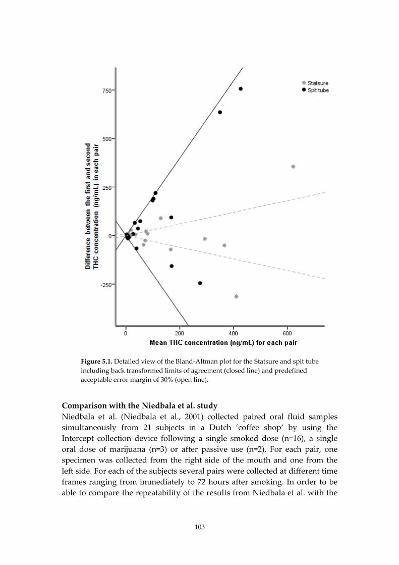
103

Figure 5.1. Detailed view of the Bland-Altman plot for the Statsure and spit tube including back transformed limits of agreement (closed line) and predefined acceptable error margin of 30% (open line).

Comparison with the Niedbala et al. study Niedbala et al. (Niedbala et al., 2001) collected paired oral fluid samples simultaneously from 21 subjects in a Dutch ’coffee shop‘ by using the Intercept collection device following a single smoked dose (n=16), a single oral dose of marijuana (n=3) or after passive use (n=2). For each pair, one specimen was collected from the right side of the mouth and one from the left side. For each of the subjects several pairs were collected at different time frames ranging from immediately to 72 hours after smoking. In order to be able to compare the repeatability of the results from Niedbala et al. with the

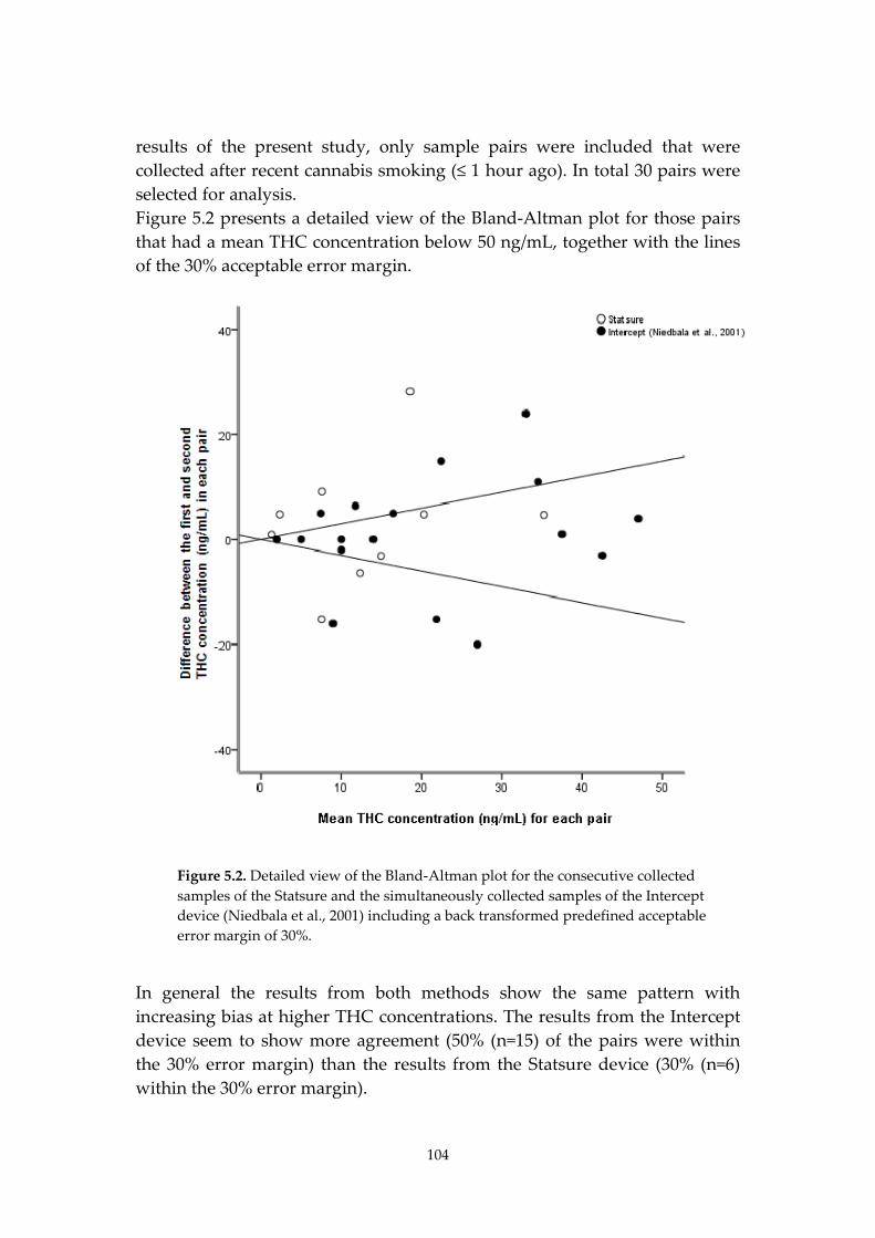
104

results of the present study, only sample pairs were included that were collected after recent cannabis smoking (≤ 1 hour ago). In total 30 pairs were selected for analysis. Figure 5.2 presents a detailed view of the Bland-Altman plot for those pairs that had a mean THC concentration below 50 ng/mL, together with the lines of the 30% acceptable error margin.

Figure 5.2. Detailed view of the Bland-Altman plot for the consecutive collected samples of the Statsure and the simultaneously collected samples of the Intercept device (Niedbala et al., 2001) including a back transformed predefined acceptable error margin of 30%.

In general the results from both methods show the same pattern with increasing bias at higher THC concentrations. The results from the Intercept device seem to show more agreement (50% (n=15) of the pairs were within the 30% error margin) than the results from the Statsure device (30% (n=6) within the 30% error margin).

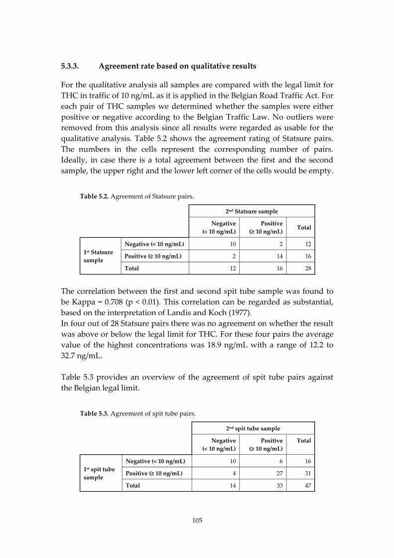
105

5.3.3. Agreement rate based on qualitative results

For the qualitative analysis all samples are compared with the legal limit for THC in traffic of 10 ng/mL as it is applied in the Belgian Road Traffic Act. For each pair of THC samples we determined whether the samples were either positive or negative according to the Belgian Traffic Law. No outliers were removed from this analysis since all results were regarded as usable for the qualitative analysis. Table 5.2 shows the agreement rating of Statsure pairs. The numbers in the cells represent the corresponding number of pairs. Ideally, in case there is a total agreement between the first and the second sample, the upper right and the lower left corner of the cells would be empty.

Table 5.2. Agreement of Statsure pairs.

2nd Statsure sample

Negative (< 10 ng/mL)

Positive (≥ 10 ng/mL)

Total

1st Statsure sample

Negative (< 10 ng/mL) 10 2 12

Positive (≥ 10 ng/mL) 2 14 16

Total 12 16 28

The correlation between the first and second spit tube sample was found to be Kappa = 0.708 (p < 0.01). This correlation can be regarded as substantial, based on the interpretation of Landis and Koch (1977). In four out of 28 Statsure pairs there was no agreement on whether the result was above or below the legal limit for THC. For these four pairs the average value of the highest concentrations was 18.9 ng/mL with a range of 12.2 to 32.7 ng/mL. Table 5.3 provides an overview of the agreement of spit tube pairs against the Belgian legal limit.

Table 5.3. Agreement of spit tube pairs.

2nd spit tube sample

Negative (< 10 ng/mL)

Positive (≥ 10 ng/mL)

Total

1st spit tube sample

Negative (< 10 ng/mL) 10 6 16

Positive (≥ 10 ng/mL) 4 27 31

Total 14 33 47

106

The correlation between the first and second spit tube sample was found to be Kappa = 0.511 (p < 0.01). This correlation can be regarded as moderate. Ten out of 47 spit tube pairs had no agreement on whether the subject would score above or below the legal THC limit. The average concentration of the highest sample from each of the ten deviant pairs was 86.9 ng/mL with a range of 10.7 to 219.4 ng/mL. The concentrations of the deviant pairs for the spitting method were considerably higher than the Belgian legal limit. The results show that the level of agreement between two consecutively collected oral fluid samples is relatively higher for the Statsure sampling method. The deviant pairs of the Statsure device were on average closer to the legal limit than the deviant pairs of the spit tubes. The highest THC concentration in the deviant sample was 22.7 ng/mL above the Belgian legal limit of 10 ng/mL, whereas the highest THC concentration for the deviant spit tube samples was 209.4 ng/mL above this legal limit.

5.4. Discussion

Results show that the sampling repeatability from two consecutively taken oral fluid samples is lower than the predefined 30% acceptable error margin, both for the Statsure and the spit tube collection method. However, this study was conducted among users who in general consumed cannabis very recently. Results from Niedbala et al. (9) showed higher agreement between two simultaneously collected samples when cannabis was consumed more than one hour before. For samples that were collected within one hour after smoking, THC results from Intercept samples seemed to be a little more in agreement with each other as compared to the Statsure samples. This difference might be explained by the simultaneous collection with the Intercept device versus the consecutive collection with the Statsure device. The variation in THC concentrations between consecutively collected spit tube samples was much higher than the variation between consecutively collected Statsure samples. The higher correlation between two Statsure samples might be explained by the fact that the absorption pad is put more or less at the same spot in the mouth (under the tongue) and that for spitting oral fluid could be collected from all parts of the mouth. Since mucosal cells and debris are collected over a larger area, more variation in THC concentrations could be expected. Compared to blood and urine sampling, where the sample is homogenous, this adds another important source of variability of the THC concentrations.

107

The results also show that in general the concentrations of the samples collected by spit tubes are almost six times higher than the corresponding concentrations collected by the Statsure in people who have very recently consumed cannabis. This was much higher than expected from the results from the O’Neal et al. (O'Neal et al., 2000) study. In this study it was reported that codeine concentrations were a factor 1.3 to 2.0 higher for spit tubes than for collection devices with nonacidic stimulation. Oral fluid containing higher THC concentrations will probably be contaminated more recently, which will result in a less homogenous spread over the oral cavity and the oral fluid. Therefore, these results could have shown more variability. Another potential reason for the difference is the higher lipophilicity of THC compared to codeine. If only sample pairs of samples within the linear range would have been taken into account though, the mean concentrations of the spit tubes would have been a factor 1.7 higher than the Statsure samples. This factor is in line with the O’Neal et al. study. THC adsorbed on cell debris of the mucosa might have contributed to the higher THC concentrations from spitting samples. The higher THC concentrations in spitting samples may potentially also be caused by the origin of the oral fluid. The Statsure samples were all placed in the vicinity of the orifice of the submandibular duct, whereas the oral fluid collected by spitting was collected from the whole oral cavity. More research is needed to investigate the influence of the sample preparation and the origin of the oral fluid on the THC concentration in oral fluid collected by spit tubes. The concentrations of the oral fluid samples collected by the Statsure device were corrected since the volume of the samples varies in practice. For the Statsure samples in this study the average volume was 0.34 mL, ranging between 0.15 and 1.51 mL. Both the large variation and the difference between the average volume (0.34 mL) and the expected volume (1.0 mL) showed that correction of the concentrations was indeed necessary. For the spitting samples no information was available on volumes. However, the effect of differences in sample volume was not expected to be large since no buffer fluid was used for diluting the spitting samples. The low repeatability of THC measurement in oral fluid leads to the question whether there are alternatives for THC collection in oral fluid. An alternative mentioned in literature (Day et al., 2006; Milman et al., 2010; Moore et al., 2011) is the analysis of THCCOOH in combination with THC analysis. According to these studies the presence of contamination could be defined by using the THCCOOH concentration. As THCCOOH may come from the blood or transport by some other mechanism, it is stated that enzymes necessary for conversion of THC to THCCOOH are not known to be present

108

in the oral mucosa. However, a limitation of this method is that concentrations for THCCOOH are very low (measured in ng/L, whereas THC is measured in ng/mL). Therefore, THCCOOH in oral fluid is at present not yet detectable by most laboratories. Blood spot collection might be a second alternative for the collection of oral fluid samples, since it is, like oral fluid sampling, less invasive than blood collection by venipuncture. Although, no correlation results are known for THC, for some other substances a high correlation was observed with blood obtained from venipuncture (Jantos and Skopp, 2011; Skopp, 2007). Strengths and limitations This was only the second study that has data on the repeatability of oral fluid collection methods available. The strength of this study is that it provides insight in the potential problems of using oral fluid as a matrix for detecting THC use and especially when oral fluid samples are used for quantitative measurements. A second strength of this study is that each of the Statsure samples was weighted to define the corrected concentration. A recent Norwegian study (Gjerde et al., 2010b) showed that lower volumes of oral fluid contained more frequently THC and that samples with low volumes should not be discarded from analysis. In this study all samples were included despite differences in volume. A limitation of the present study is that the samples had to be taken consecutively. This might have affected the results. Furthermore, the study was performed on people who in majority had consumed cannabis less than one hour before, while in the population of drivers the interval between smoking and collection might be longer. The results are therefore only applicable for very recent cannabis use and not for cannabis use in general. Results from Niedbala et al. (9) indicate that if the interval between smoking and collection had been longer, the agreement between the two samples would probably have been better. One can also conclude that it is not recommendable to use spit tubes for law enforcement purposes because of the low repeatability of the sampling process. A final limitation is that the spitting samples with THC concentrations above the linear range of the validated method of 1-200 ng/mL were not diluted. However, additional experiments showed that the bias for THC in spiked spitted oral fluid samples up to 20,000 ng/ml (calculated as the percent deviation of the observed concentration from the expected concentration, n=27) was less than 15%, three samples excepted, As a consequence, the

109

calibration curve for THC in spitted oral fluid is expected to be linear up to 20,000 ng/ml. Further research The results from this study may provide an interesting start for further research on the repeatability of oral fluid collection methods. If oral fluid is used as a matrix for legal purposes, it might be valuable to study the effect of the collection method on the results in more detail. Conclusions The repeatability of both the Statsure collection method and the ordinary spit tubes is low when applied among subjects who have consumed cannabis very recently. In comparison with the Belgian legal limit, results of the Statsure collection method are more in agreement with each other than results of the spit tubes. Furthermore, it was observed that samples obtained by spitting had 1.7-5.9 times higher THC concentrations than samples from the Statsure collection method, depending on the choice of the upper limit of THC concentrations that were included for analysis. The results of this study may have implications for confirmation analysis in oral fluid when applied for legal purposes.

5.5. Acknowledgements

This study was carried out as part of the project Driving under the Influence of Drugs, Alcohol and Medicines (DRUID), funded by the European Commission under the Sustainable Surface Transport RTD Programme of the 6th Framework Programme (contract n° TREN-05-FP6TR-S07.61320-518404-DRUID). We would like to thank the staff and the owner of coffee shop ‘t Rotterdammertje in Doetinchem for their hospitality and cooperation. Furthermore, we would like to thank Peter van Swinderen and Veronique Nelck for their participation in collecting the samples and transporting them to the laboratory of the Netherlands Forensic Institute. Finally, the staff of Ghent University Laboratory and the staff of the laboratory of the Netherlands Forensic Institute are thanked for analyzing the samples.

110

6. Random and systematic errors in case-control studies estimating the injury risk of driving under the influence of psychoactive substances13

6.1. Introduction

Between 2006 and 2010 six population based case-control studies were conducted during the European research-project DRUID (DRiving Under the Influence of Drugs, Alcohol and Medicines) in order to determine the risk of being seriously injured while driving with psychoactive substances (Hels et al., 2011). These case-control studies were performed in Belgium (BE), Denmark (DK), Finland (FI), Italy (IT), Lithuania (LT) and the Netherlands (NL). All six studies were screened for the same 23 substances applying uniform analytical cut-off levels. Cases were seriously injured drivers admitted to hospitals after a traffic crash and controls were randomly selected drivers from the general traffic. In epidemiological research, case-control studies are used to compare determinants (e.g. the presence of drugs) between injured and non-injured drivers. The main outcome measure of case-control studies is the odds ratio, which estimates relative risk, since relative risk calculations cannot always be used (Schmidt and Kohlmann, 2008). This is due to the fact that there is no denominator for the incidence rates, since the controls are only a sample of the underlying denominator (or study base). Some case-control studies may have the possibility to calculate relative risk. However, when choosing logistic regression as method for analysis, odds ratios will per definition be the outcome measure. An example of such a study is a case-control study from New Zealand by Connor et al. (2004)). Although an odds ratio and a relative risk calculation are not identical measures, the odds ratio can be used as an estimate of the relative risk, as long as the likelihood of a crash is small. In Figure 6.1 it can be observed that the odds ratio approximates the RR when the number of cases 13 This chapter is published as the following article: Houwing, S., Hagenzieker, M., Mathijssen, M.P.M., Legrand, S.-A., Verstraete, A. G., Hels, T., Bernhoft, I.M., Simonsen, K.W., Lillesunde, P., Favretto, D., Ferrara, D., Caplinskiene, M., Movig, K. & Brookhuis, K.A. Random and systematic errors in case-control studies calculating the injury risk of driving under the influence of psychoactive substances. This article is published online in Accident Analysis and Prevention (AAP) 2013; doi: 10.1016/j.aap.2012.12.034.

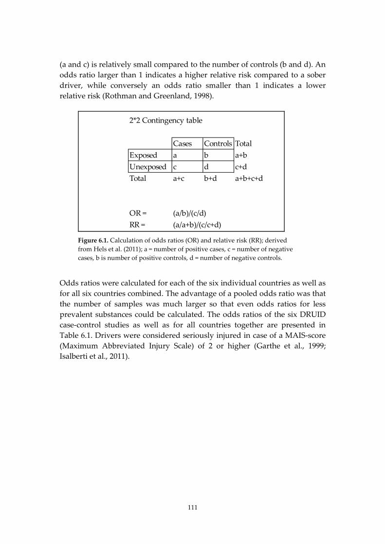
111

(a and c) is relatively small compared to the number of controls (b and d). An odds ratio larger than 1 indicates a higher relative risk compared to a sober driver, while conversely an odds ratio smaller than 1 indicates a lower relative risk (Rothman and Greenland, 1998).

2*2 Contingency table

Cases Controls TotalExposed a b a+bUnexposed c d c+dTotal a+c b+d a+b+c+d

OR = (a/b)/(c/d)RR = (a/a+b)/(c/c+d)

Figure 6.1. Calculation of odds ratios (OR) and relative risk (RR); derived from Hels et al. (2011); a = number of positive cases, c = number of negative cases, b is number of positive controls, d = number of negative controls.

Odds ratios were calculated for each of the six individual countries as well as for all six countries combined. The advantage of a pooled odds ratio was that the number of samples was much larger so that even odds ratios for less prevalent substances could be calculated. The odds ratios of the six DRUID case-control studies as well as for all countries together are presented in Table 6.1. Drivers were considered seriously injured in case of a MAIS-score (Maximum Abbreviated Injury Scale) of 2 or higher (Garthe et al., 1999; Isalberti et al., 2011).

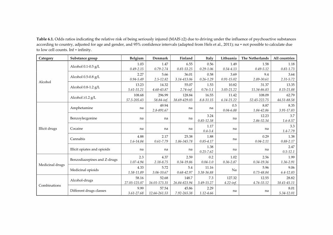
Table 6.1. Odds ratios indicating the relative risk of being seriously injured (MAIS ≥2) due to driving under the influence of psychoactive substances according to country, adjusted for age and gender, and 95% confidence intervals (adapted from Hels et al., 2011); na = not possible to calculate due to low cell counts. Inf = infinity.

Category Substance group Belgium Denmark Finland Italy Lithuania The Netherlands All countries

Alcohol

Alcohol 0.1-0.5 g/L 1.03

0.49-2.15 1.47

0.79-2.74 6.55

0.81-53.25 0.56

0.29-1.06 1.49

0.54-4.13 1.58

0.49-5.12 1.18

0.81-1.73

Alcohol 0.5-0.8 g/L 2.27 0.94-5.49

5.66 2.5-12.82

36.01 3.14-413.06

0.58 0.26-1.29

3.69 0.91-15.02

9.4 2.89-30.61

3.64 2.31-5.72

Alcohol 0.8-1.2 g/L 13.23 5.61-31.21

14.32 4.68-43.87

55.07 2.74-inf.

1.53 0.76-3.1

10.82 3.03-21.22

31.37 11.34-86.83

13.35 8.15-21.88

Alcohol ≥1.2 g/L 108.68

57.5-205.43 296.99

58.84-inf. 128.84

38.69-429.03 16.55

8.8-31.15 11.42

6.14-21.22 108.09

52.45-222.75 62.79

44.51-88.58

Illicit drugs

Amphetamine na 49.94

2.8-891.67 na na 0.5

0.04-6.88 8.87

1.84-42.86 8.35

3.91-17.83

Benzoylecgonine na na na 3.24

0.85-12.38 na

12.23 2.86-52.34

3.7 1.6-8.57

Cocaine na na na 1.17 0.4-3.4

na na 3.3 1.4-7.79

Cannabis 4.88 1.6-14.84

2.17 0.61-7.79

25.38 1.86-345.78

1.88 0.85-4.17

na 0.29 0.04-2.11

1.38 0.88-2.17

Illicit opiates and opioids na na na 1.38

0.25-7.62 na na 2.47

0.5-12.1

Medicinal drugs Benzodiazepines and Z-drugs

2.3 1.07-4.94

4.37 2.18-8.75

2.59 0.34-19.86

0.2 0.04-1.0

1.02 0.36-2.87

2.56 0.34-19.36

1.99 1.36-2.91

Medicinal opioids 4.33

1.58-11.89 5.72

3.06-10.67 5.4

0.68-42.97 11.16

3.38-36.88 Na

5.96 0.73-48.84

9.06 6.4-12.83

Combinations Alcohol-drugs 58.16

27.05-125.07 52.68

16.01-173.35 148.7

26.84-823.94 7.3

3.49-15.27 127.32

4.22-inf. 12.55

4.76-33.12 28.82

18.41-45.11

Different drugs classes 9.99 3.61-27.68

57.54 12.66-261.53

45.86 7.92-265.38

2.29 1.12-4.66

na na 8.01 5.34-12.01

113

In general, the highest odds ratios were calculated for drivers using alcohol-drug combinations, drug-drug combinations and for drivers with high blood alcohol concentration (BAC) levels (Hels et al., 2011). The risk posed by alcohol use increased at higher BAC levels, as has been found in previous case-control studies (Borkenstein et al., 1974; Compton et al., 2002; Krüger and Vollrath, 2004; Mathijssen and Houwing, 2005; Movig et al., 2004). However, the results of the DRUID case-control studies show that the calculated odds ratios for alcohol varied widely between countries. The odds ratios for illicit drug use showed large variations between countries as well, with odds ratios differing by up to a factor of 100. However, the confidence intervals were wide and for most countries the number of positive samples for illicit drugs was too small to calculate an odds ratio. The odds ratios for medicinal drugs varied less than those for illicit drugs and alcohol. Nonetheless, in Italy the calculated odds ratio of 0.2 for benzodiazepines and Z-drugs (including zolpidem and zopiclone) was much lower than the odds ratio of 4.37 found in Denmark. In sum, the results from these case-control studies showed large variations in the relative risks for driving under the influence of psychoactive substances. The differences between the odds ratios of the case-control studies could reflect actual differences in relative risk for driving under the influence in the different countries. However, it is hard to believe that drivers in different countries show such large differences for the relative risk of serious injury while driving under the influence of psychoactive substances. Therefore, the observed differences between the odds ratios could also be at least partially explained by different types of errors. Depending on the source of the error they can be divided into random errors and systematic errors (Rothman, 1986). A random error can be described as sampling variability. This variability is visualized in case-control studies by confidence intervals. An increase of the sample size leads to a decrease of the confidence interval, producing results with higher precision and power. A systematic error is often referred to as bias. Bias is generally described as the difference between the observed value and the true value. It is, unlike random error, not affected by sample size. In epidemiological literature different types categorisations of bias exist. In this study we used the classifications of Kleinbaum et al. (1982) and Rothman (1986) who distinguish three main types of bias: selection bias, information bias and confounding. Firstly, selection bias can be described as a deflection that results from the selection process of the study population. An example

114

of selection bias is detection bias, where there are differences in detecting exposed and non-exposed participants. For instance, detection bias may occur when drivers are not selected at random from moving traffic, but mainly based on suspicion. As a result the prevalence of psychoactive substances in traffic is overestimated and the odds ratio will consequently be underestimated. Selection bias is regarded as the most common type of bias in case-control studies (Schulz and Grimes, 2002). Secondly, information bias can be described as a deviation based on inaccuracy of the measurement, or classification, of study variables. An example of information bias is misclassification bias where a subject is assigned to a wrong group due to a measurement error of an instrument, or in case of an interview due to selective recall or misunderstanding the questions. Finally, confounding arises when a result is distorted by one or more variables that are associated both with exposure and with the outcome (Rothman, 1986). The most commonly included confounding factors in case-control studies that assess the risk of driving under the influence of psychoactive substances are gender and age (Blows et al., 2004; Brault et al., 2004; Haworth et al., 1997; Hels et al., 2011; Mathijssen and Houwing, 2005; Mura et al., 2003). Guidelines were formulated at the start of the DRUID surveys concerning several design issues to ensure that the results were representative and comparable (Assum et al., 2007). According to these guidelines a cross-sectional roadside survey had to be conducted to determine the prevalence of psychoactive substances among the general driving population. The method of this roadside survey was based on a stratified multi-stage sampling design. In the first stage of this design study regions were selected in the participating countries. These regions were meant to be representative for the whole country with regard to substance use and traffic. Within these regions smaller research areas were selected in the second stage, and within these areas, survey locations were selected, where car drivers and drivers from vans aged 18 and above were randomly selected from actual traffic. In each country, data were collected during several roadside survey sessions distributed over 8 six-hour time periods covering all hours of the day on both weekdays and weekend days. The time periods were distributed into type of day (weekday-weekend day) and time of the day (04.00-09.59, 10.00-15.59, 16.00-21.59, 22.00-03.59). Due to the preferences of the police that had to be taken into account, it turned out that the distribution of the samples over the different time periods in the six countries could not always be representative for the distribution of traffic volumes over the time periods. In order to adjust for these differences, weight factors were calculated for each country

115

by dividing the national traffic proportion per time period by the proportion of sampled drivers for these time periods. The case population consisted of seriously injured drivers (MAIS >= 2) of cars and small vans aged 18 and above. A list of 23 core substances was included together with analytical cut-off levels for whole blood and oral fluid. Oral fluid samples had to be collected by means of the Statsure Saliva Sampler device. However, for practical, financial and/or legal reasons not all studies were conducted according to these guidelines. Furthermore, some issues were not addressed in the guidelines, but could have caused variation in the odds ratios anyway (e.g. the minimum number of samples and the maximum proportion of non-response). Therefore, several sources of random and systematic errors could have led to differences in the results between the six DRUID case-control studies. The main objective of this study is to provide insight in the different types of errors that could explain the variance in the results of the six DRUID case-control studies. The results of this assessment may clarify the large inter-country variation that was observed between the odds ratios.

6.2. Method

The method that was applied to explore the source of errors in the DRUID case-control studies consisted of three steps: the first step was to prepare a list of potential indicators for errors based on the available data from the six case-control studies. Table 6.2 provides an overview of these indicators for potential errors categorized by type of error (random and systematic error) and by type of bias (selection bias, information bias and confounding) according to the categorization of Kleinbaum et al. (1982) and Rothman (1986). This categorization is supported by Wacholder et al. (1992) who wrote two companion papers on issues involved in selecting controls for case-control studies. They state that the selection of controls should be comparable to the selection of cases in three ways: the study base should be the same, confounding factors should be used to eliminate any distortion by other factors, and the measurement errors should be comparable. These principles should reduce the three previously mentioned types of bias in case-control studies: selection bias, information bias and confounding. However, they also state that the effectiveness of these principles is constrained by the availability of resources and time.

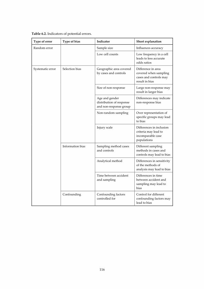
116

Table 6.2. Indicators of potential errors.

Type of error Type of bias Indicator Short explanation

Random error Sample size Influences accuracy

Low cell counts Low frequency in a cell leads to less accurate odds ratios

Systematic error Selection bias Geographic area covered by cases and controls

Difference in area covered when sampling cases and controls may result in bias

Size of non-response Large non-response may result in larger bias

Age and gender distribution of response and non-response group

Differences may indicate non-response bias

Non-random sampling Over representation of specific groups may lead to bias

Injury scale Differences in inclusion criteria may lead to incomparable case populations

Information bias Sampling method cases and controls

Different sampling methods in cases and controls may lead to bias

Analytical method Differences in sensitivity of the methods of analysis may lead to bias

Time between accident and sampling

Differences in time between accident and sampling may lead to bias

Confounding Confounding factors controlled for

Control for different confounding factors may lead to bias

117

In the second step, information was gathered for each of the potential indicators from the relevant DRUID reports on prevalence (Houwing et al., 2011; Isalberti et al., 2011) and risk estimates (Hels et al., 2011). These prevalence reports included the national reports for the six participating countries, which provided detailed information concerning the hospital studies and the roadside surveys. In the third and final step, the collected information from the DRUID reports was used to interpret the calculated odds ratios. A quantitative assessment of bias was not possible, since this would require a large amount of detailed data on e.g. the use of psychoactive substances in the general population for each study region, which were not available. Therefore, in this study bias is only discussed in qualitative terms based on the information derived from the reports on the prevalence and risk studies by searching for deviations between the six studies on each of the indicators. The likelihood of bias was divided into two categories: no indication of bias and indication of bias. In case of potential bias, an estimation of the size and direction of bias is provided when possible. Apart from the discussion on potential bias, random errors are discussed in terms of statistical power.

6.3. Results

Relevant information for each country was gathered from the individual DRUID reports and then categorised into the various indicators for potential errors. Table 6.3 presents an overview of the results of this analysis of potential errors.

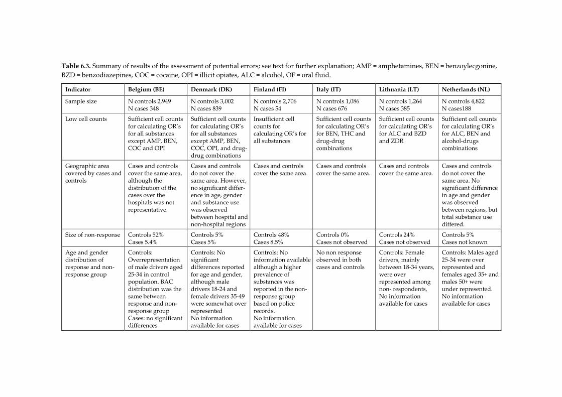
Table 6.3. Summary of results of the assessment of potential errors; see text for further explanation; AMP = amphetamines, BEN = benzoylecgonine, BZD = benzodiazepines, COC = cocaine, OPI = illicit opiates, ALC = alcohol, OF = oral fluid.

Indicator Belgium (BE) Denmark (DK) Finland (FI) Italy (IT) Lithuania (LT) Netherlands (NL)

Sample size N controls 2,949 N cases 348

N controls 3,002 N cases 839

N controls 2,706 N cases 54

N controls 1,086 N cases 676

N controls 1,264 N cases 385

N controls 4,822 N cases188

Low cell counts Sufficient cell counts for calculating OR’s for all substances except AMP, BEN, COC and OPI

Sufficient cell counts for calculating OR’s for all substances except AMP, BEN, COC, OPI, and drug-drug combinations

Insufficient cell counts for calculating OR’s for all substances

Sufficient cell counts for calculating OR’s for BEN, THC and drug-drug combinations

Sufficient cell counts for calculating OR’s for ALC and BZD and ZDR

Sufficient cell counts for calculating OR’s for ALC, BEN and alcohol-drugs combinations

Geographic area covered by cases and controls

Cases and controls cover the same area, although the distribution of the cases over the hospitals was not representative.

Cases and controls do not cover the same area. However, no significant differ-ence in age, gender and substance use was observed between hospital and non-hospital regions

Cases and controls cover the same area.

Cases and controls cover the same area.

Cases and controls cover the same area.

Cases and controls do not cover the same area. No significant difference in age and gender was observed between regions, but total substance use differed.

Size of non-response Controls 52% Cases 5.4%

Controls 5% Cases 5%

Controls 48% Cases 8.5%

Controls 0% Cases not observed

Controls 24% Cases not observed

Controls 5% Cases not known

Age and gender distribution of response and non-response group

Controls: Overrepresentation of male drivers aged 25-34 in control population. BAC distribution was the same between response and non-response group Cases: no significant differences

Controls: No significant differences reported for age and gender, although male drivers 18-24 and female drivers 35-49 were somewhat over represented No information available for cases

Controls: No information available although a higher prevalence of substances was reported in the non-response group based on police records. No information available for cases

No non response observed in both cases and controls

Controls: Female drivers, mainly between 18-34 years, were over represented among non- respondents, No information available for cases

Controls: Males aged 25-34 were over represented and females aged 35+ and males 50+ were under represented. No information available for cases

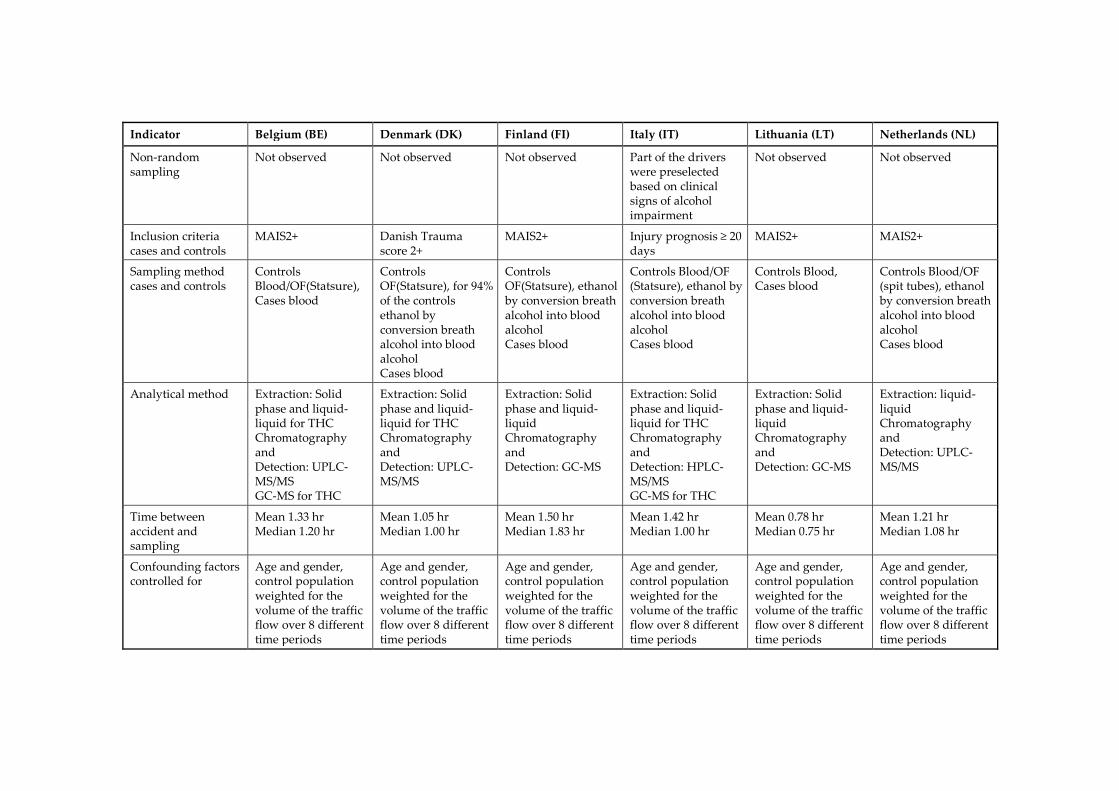
Indicator Belgium (BE) Denmark (DK) Finland (FI) Italy (IT) Lithuania (LT) Netherlands (NL)

Non-random sampling

Not observed Not observed Not observed Part of the drivers were preselected based on clinical signs of alcohol impairment

Not observed Not observed

Inclusion criteria cases and controls

MAIS2+ Danish Trauma score 2+

MAIS2+ Injury prognosis ≥ 20 days

MAIS2+ MAIS2+

Sampling method cases and controls

Controls Blood/OF(Statsure), Cases blood

Controls OF(Statsure), for 94% of the controls ethanol by conversion breath alcohol into blood alcohol Cases blood

Controls OF(Statsure), ethanol by conversion breath alcohol into blood alcohol Cases blood

Controls Blood/OF (Statsure), ethanol by conversion breath alcohol into blood alcohol Cases blood

Controls Blood, Cases blood

Controls Blood/OF (spit tubes), ethanol by conversion breath alcohol into blood alcohol Cases blood

Analytical method Extraction: Solid phase and liquid-liquid for THC Chromatography and Detection: UPLC-MS/MS GC-MS for THC

Extraction: Solid phase and liquid-liquid for THC Chromatography and Detection: UPLC-MS/MS

Extraction: Solid phase and liquid-liquid Chromatography and Detection: GC-MS

Extraction: Solid phase and liquid-liquid for THC Chromatography and Detection: HPLC-MS/MS GC-MS for THC

Extraction: Solid phase and liquid-liquid Chromatography and Detection: GC-MS

Extraction: liquid-liquid Chromatography and Detection: UPLC-MS/MS

Time between accident and sampling

Mean 1.33 hr Median 1.20 hr

Mean 1.05 hr Median 1.00 hr

Mean 1.50 hr Median 1.83 hr

Mean 1.42 hr Median 1.00 hr

Mean 0.78 hr Median 0.75 hr

Mean 1.21 hr Median 1.08 hr

Confounding factors controlled for

Age and gender, control population weighted for the volume of the traffic flow over 8 different time periods

Age and gender, control population weighted for the volume of the traffic flow over 8 different time periods

Age and gender, control population weighted for the volume of the traffic flow over 8 different time periods

Age and gender, control population weighted for the volume of the traffic flow over 8 different time periods

Age and gender, control population weighted for the volume of the traffic flow over 8 different time periods

Age and gender, control population weighted for the volume of the traffic flow over 8 different time periods

120

6.3.1. Random errors

Sample size The sample size is the number (n) of individual samples in a study. The precision and thus statistical power of a study increases with the sample size. Statistical power represents the probability that a test will find a significant difference if there is an actual difference. If the power is low, the confidence intervals will increase and may result in fewer significant outcomes (Cohen, 1988). However, odds ratios which are close to 1 are more sensitive to significance than odds ratios that differ more from 1. Therefore the number of cases and controls is used as an indicator for the power of the study, instead of the number of significant outcomes, which may be regarded as a more direct indicator. The results for the assessment on the sample sizes of the six DRUID case-control studies are presented in Table 6.3. The sample size for the hospital cases varied between 54 for the Finnish study and 839 for the Danish study. The sample size of the control samples which were collected at the roadside ranged between 1,086 for the Italian study and 4,822 for the Dutch study. Only the Belgian and the Danish study included relatively high number of samples in both the case (BE:348 and DK:839) and the control populations (BE: 2,949 and DK:3,002) (Houwing et al., 2011; Isalberti et al., 2011). Despite the relatively small numbers of samples in the control population, the Italian study has a greater precision than the studies from Finland, Lithuania and the Netherlands. This greater precision is a result of the relative large number of cases in the Italian case-control study (n=676). Low cell counts As described above, the sample size provides information concerning the study power. In addition, the distribution of the samples over the four cells in a case-control study (see Figure 6.1) provides valuable information on the accuracy of the outcomes as well. In the report on risk estimates (Hels et al., 2011) the issue of low cell counts was explored by an alternative method to calculate overall odds ratios. In this alternative method the lowest cell count for each odds ratio calculation was both decreased and increased by 1 to investigate the effect of a small change of the data. If the difference between the odds ratio of the decreased value and the increased value was larger than a factor 2, the study was regarded as too susceptible to bias due to low cell counts and therefore not sufficient to enable calculation of the overall odds ratios. The results of the analysis on low cell counts (Hels et al., 2011) showed low cell counts for all substances in the Finnish case-control study. The

121

Lithuanian, Italian and Dutch study each only had sufficient cell counts for three of the substance groups. In Denmark and Belgium the results of the case-control study seemed to have the highest accuracy with sufficient cell counts for five and six substance groups, respectively. Therefore, the Belgian and Danish studies were considered to have the highest study power. Both studies were also the only studies that were regarded as having a sufficiently large sample size of both cases and controls (see Section 3.1.1 on the sample size).

6.3.2. Systematic errors

Geographic area covered by cases and controls One of the basic principles of a population based case-control study is that both the case and control population should be drawn from the same study population (Rothman and Greenland, 1998). If the use of psychoactive substances varies according to region, and the cases are not collected from the same region as the controls, then the odds ratio calculations may not be valid. The results of the analysis on the area covered by the cases and controls showed that the only two countries in which the case-control study did not cover the same area for both cases and controls were Denmark and the Netherlands. Since there were no differences in the age and gender distributions between the hospital and non-hospital regions in both countries, a decision was made to include all the results from the Dutch and Danish roadside study in the odds ratio calculations (Hels et al., 2011). However, a significantly lower prevalence was found for the total substance use in the Dutch regions that did not include a hospital providing case samples. No significant differences were found for any of the separate substance groups though. In Denmark no differences were found for substance use in the additional calculations of the control samples. Therefore, we have concluded that the effect of selection bias related to the areas covered by the cases and controls is not likely to be of influence in Denmark and the Netherlands. In Belgium the inclusion of hospital samples seemed to vary over the study regions: the share of injured drivers in Flanders was over-represented (81% of the cases and 57% of the controls), and the share in Wallonia (16% of the cases and 39% of the controls) was under-represented (Houwing et al., 2011; Isalberti et al., 2011). However, additional analysis of the prevalence results in traffic by region did not show any significant differences between the substance use in Flanders and Wallonia. Therefore, the effect of bias due to

122

selection bias in the case samples in Belgium is expected to be very small. For all other studies no selection bias was observed in the case samples. Size of non-response A large share of non-response in a study increases the likelihood of a selection bias. This selection bias may lead to an underestimation of the share of illicit drug users, since drivers who were positive for illicit drugs can be assumed to be less likely to participate voluntarily because of the risk of being detected positive for drugs in the vicinity of the police who were present at the scene and took care of stopping the drivers. The share of non-response in the hospital studies, varied between 0 (not observed) and 8.5% (Isalberti et al., 2011), which can be considered as relatively low. Based on the information on the size of the non-response in the case population as shown in Table 6.3, it can be concluded that the presence of non-response bias in the case population is likely to be small. The non-response rates in the roadside surveys showed larger variations with a range of between 0 and 52%. In Italy, non-response was non-existent since participation was mandatory. In Lithuania, Belgium and Finland the proportion of non-respondents at the roadside was very high at 25%, 48% and 52%, respectively. Based on this information, we assess that there was likely to be an overestimation of the odds ratios for illicit drugs in these three countries. Age and gender distribution of response and non-response group Age and gender differences between the response and non-response groups may indicate selection bias, since both age and gender can be associated with different patterns in drug use by car drivers (Hels et al., 2011). Results from the roadside surveys in the DRUID project indicate that illicit drug use is more prevalent among young male drivers, whereas the use of medicinal drugs is relatively more frequently detected in female drivers aged 35 and older (Houwing, 2011). The only hospital study (cases) which collected data from the non-response group was the Belgian hospital study. No significant differences were found for age and gender distribution in this study. For the other hospital studies no information was available (DK and FI) or no non-response was observed (IT, LT and NL). The results from the roadside surveys (controls) showed that in Belgium and the Netherlands male drivers, aged 25-34, were over represented in the non-response group, in Denmark there was an over representation of young male drivers, aged 18-24, and female drivers aged 35-50 and in Lithuania female

123

drivers were generally over represented. In the Italian roadside survey no non-response group was observed at all, since refusal to participate led to a large penalty by the police. In Finland and Belgium drivers were first stopped and breath tested by the police, before they were asked to participate in the study. In these two countries a large share of drivers already declined to participate when the police asked them to drive to the researchers. In Finland, no information was recorded from these drivers on age, gender and reason for refusal. But from police records information was available on positive substance detections in those non-participating drivers whom the police suspected of driving under the influence of substances other than alcohol (Houwing et al., 2011). This information indicated that substance use was more frequently detected among non-respondents. In summary, it can be concluded that differences between the response and non-response group may have led to be an under representation of illicit drug use by car drivers in Belgium and Finland. Differences were detected in Denmark and the Netherlands as well, but since the total non-response rate was relatively low the effect is likely to be small. In Lithuania, it may be assumed that due to the over representation of female drivers in the non-response group the prevalence of illicit drugs in traffic is overestimated whereas the prevalence of medicinal drugs is underestimated. In Italy no non-response was observed in either the hospital study or the roadside survey. Non-random sampling One of the objectives of the hospital studies and roadside surveys was to gather information on substance use for a representative sample of drivers in order to calculate odds ratios. Therefore, sampling needed to be carried out on a random basis. The process of random sampling can be endangered by selection bias. Detection bias is a form of selection bias, which can occur due to oversampling of certain sub-populations. The presence of detection bias is hard to reveal. However, in the DRUID report on the case-control studies (Hels et al., 2011) it was noted, based on personal communication with the Italian researchers, that in the Italian roadside survey drivers who showed clinical signs of alcohol impairment had partially been preselected. Therefore, alcohol use in Italian traffic is expected to be overestimated, causing an underestimation of the odds ratios for alcohol use. This detection bias may also have been present for users of psychoactive substances other than alcohol, in the event that they showed signs of impairment as well. We assess that the Italian odds ratios for alcohol and other psychoactive

124

substances were likely to be underestimated. For all other countries no indication was found for bias due to non-random sampling. Inclusion criteria for cases and controls The inclusion criteria for the roadside surveys were the same for all countries: drivers of cars and small vans, during all times of the day and all days of the week (Houwing et al., 2011). For the hospital studies the inclusion criteria were seriously injured drivers, aged 18 years and older, driving a car or small van, with a MAIS score (Maximum Abbreviated Injury Scale) of 2 or higher (Isalberti et al., 2011). Furthermore, the time between the accident and sampling had to be less than three hours. In Denmark and Italy a national injury scale was applied instead of the MAIS-scale. In Denmark this scale was based on injury severity and in Italy injured drivers were included if the prognosis of recovery from injury was 20 days or longer (Isalberti et al., 2011). Based on the national study of Danish hospital results in the DRUID report on risk estimates (Hels et al., 2011), no large differences are expected for the Danish study due to the difference in the inclusion criteria for injured drivers. The potential effect of the divergent Italian inclusion criteria is hard to estimate since it is based on the number of days of care that is needed and not on the severity of the injury. Sampling method cases and controls The theoretically most appropriate method for comparison of cases and controls is by comparing blood samples from injured drivers with blood samples from non-injured drivers (Walsh et al., 2008). Blood samples were collected from all injured drivers in the hospital studies. However, for the roadside surveys blood samples were only collected in Lithuania (all samples), the Netherlands (78% of all samples), Belgium (93%) and Italy (73%). All other collected samples were oral fluid. Therefore, equivalent cut-offs between blood and oral fluid concentrations were developed in order to be able to compare blood and oral fluid concentrations (Verstraete et al., 2011b). Another issue concerning sampling of body fluids was the difference in collection method for oral fluid samples. In the Netherlands oral fluid samples were collected by using polyethylene spit tubes, whereas in all the other countries oral fluid samples were collected by using a Statsure© oral fluid collection device with non-acidic stimulation. The guidelines prescribed the use the Statsure© device for collecting oral fluid (Assum et al., 2007). However, the Dutch roadside survey had already started by the time this

125

decision was made and in order to keep the same oral fluid collection procedure during the whole study the Dutch researchers decided to continue working with the spit tubes. The equivalent cut-offs that were used in the DRUID studies were based on concentrations for the Statsure© collection device. A recent study (Houwing et al., 2012) shows that THC concentrations in oral fluid collected using spit tubes are in general almost six times higher than THC concentrations collected by a device without acidic stimulation. Results for codeine sampling by different oral fluid collection methods showed a factor ranging from 1.3- 2.0 (O'Neal et al., 2000). In the DRUID case-control studies, however, the same equivalent cut-offs were applied for samples collected with spit tubes as for those with the Statsure© device. It can be concluded that the potential bias by using blood-oral fluid comparisons instead of blood-blood comparisons is likely to be absent for all countries except for the Netherlands where 22% of the roadside samples were analyzed in oral fluid. Therefore, it can be assumed that the difference in the sampling method between the cases and controls has led to a (small) overestimation of the Dutch prevalence results in the controls. In four of the six roadside surveys (Denmark, Finland, Italy, the Netherlands), ethanol (alcohol) concentrations were measured by handheld breathalyzers of the police. In Belgium BAC was measured from both oral fluid and whole blood. The estimated blood ethanol concentration was a factor 1.22 higher than the measured ethanol concentration in oral fluid. This factor was based on the average conversion factor between blood and oral fluid that was calculated from the Belgian DRUID results of those drivers from whom both blood and oral fluid samples were collected (Verstraete et al., unpublished observations). In Denmark, due to missing data of the police, ethanol concentrations were measured in oral fluid in 6% of the drivers at the roadside by using the same factor of 1.22 as was used in the Belgian study. In the Netherlands the conversion factor of breath alcohol concentrations into blood alcohol concentrations in percentages is 1:23 (Mathijssen and Twisk, 2001). However, in the other European countries that were involved in the DRUID roadside surveys a higher conversion factor of 1:21 is used (Melethil, 2011). In order to be able to compare the Dutch alcohol results with the results for other EU countries, all blood alcohol concentrations (BAC) results from the Netherlands were multiplied by a factor 1.095 (23/21). In Lithuania, ethanol concentrations were directly measured in blood.

126

Based on the conversion factors that were applied, no substantial bias was expected for alcohol measurements. Method of toxicological analysis Differences in accuracy of the analytical methods may lead to biased results as well. Information on the methods was available for the extraction, separation and detection methods. Extraction of the samples was based either on liquid-liquid or solid phase extraction, chromatographic separation was performed by gas chromatography or liquid chromatography High Performance or Ultra Performance. Detection of substances was based on mass spectrometry or nitrogen/phosphorus detection. Four separate rounds of proficiency testing were performed. The results of the proficiency testing show that both qualitative and quantitative performance improved during the testing program (Pil et al., 2010). Therefore, bias due to differences in the analytical methods is not likely. Time between accident and sampling Based on the information in the databases from the six hospital studies it can be concluded that time between accident and blood sampling varied between zero minutes and three hours. The time span between accident and sampling could cause an underestimation of the number of case samples (and concentration of substances therein). This is due to the process of metabolisation, since psychoactive substances with a short half-life, such as heroin, could already be metabolised after only three hours. For all countries the mean and median times, shown in Table 6.3, were between one and two hours, except for Lithuania that shows a shorter time period. The recorded time between accident and sampling in Lithuania had a timeframe with both mean and median values of approximately 45 minutes. Since the differences between the countries are relatively small and the maximum time between accident and sampling was set at 3 hours, we assess that the presence of bias due to differences in time between accident and sampling is of the same order for all countries. Confounding factors Deconfounding is, like the presence of an identical study base for both cases and controls, one of the main principles of comparative case and control selections (Wacholder et al., 1992). Confounding factors are variables that co-vary both with substance use and crash risk. Taking into account different types of confounding factors can cause variation between the results of case-

127

control studies. In the DRUID project all the case-control studies’ results were calculated by the Technical University of Denmark (DTU), ensuring a uniform method of statistical analysis. The results of all countries were based on a similar set of variables (age and gender). Furthermore, the data from all six roadside surveys were weighted for the volume of traffic flow in the different time periods. There are probably other confounding factors that were not detected in these studies. Age and gender were included as confounding variables in all calculations and since the data were adjusted for differences in traffic volume between time periods, and therefore we assume that the potential effect of confounding has been reduced. However, since confounding has only been eliminated for those factors that we had data available for, any influence of confounding on the estimated odds ratios cannot be ruled out.

6.4. Discussion and conclusions

Based on the results of the assessment of potential bias due to random and systematic errors it can be concluded that each of the national case-control studies showed indications of potential bias. The assessment for the Belgian case-control indicated a potential overestimation of the odds ratio for cannabis due to the likelihood of non-response bias in the control sample, in combination with a large proportion of non-respondents. Relatively high odds ratios for illicit drugs were observed which supports the likelihood of the presence of at least some non-response bias in the roadside survey. For all other substances the odds ratios were relatively close to the overall odds ratio. In Denmark, a small overestimation of the odds ratio for illicit drugs was possible due to the likelihood of a non-response bias in the control sample. However, the effect of the potential non-response bias was probably small, because of the low non-response rate (5%). For the other substances the presence of bias was not likely. In Finland, the odds ratio for illicit drugs and alcohol was likely to be overestimated due to non-response bias in the control sample in combination with a large share of non-respondents. These expectations were supported by the results of the comparison with the overall odds ratios for alcohol and illicit drugs in Table 6.1, which shows relatively high odds ratios for Finland. The Finnish results were expected to be less precise because of the small number of cases (n=54). This has resulted in relatively large confidence intervals.

128

In Italy, the odds ratios for alcohol were likely to be underestimated due to a selection bias in the control population. There may have been an underestimation for the other substances as well, since the police tended to include drivers with clinical signs of impairment. These findings were supported by the results of Table 6.1 in which generally the odds ratios for the Italian study were considerably lower than those of the other countries. A very important principle of a case-control study is that selection of participants has to be independent of exposure. Since this principle was not (fully) met in the Italian study, a proper interpretation of the Italian results was not possible. In Lithuania, the odds ratios for alcohol and illicit drugs were likely to be underestimated due to the large under representation of female drivers in combination with the large (24%) non-response bias. Furthermore, the precision of the study was relatively low due to the small number of control samples. In the Netherlands, an overestimation of the odds ratio for illicit drugs was possible due to the likelihood of a non-response bias in the control sample and due to selection bias resulting from lower prevalence of substance use in traffic in regions that were not included in the case study. The non-response rate was very low though and therefore, the effect of the potential non-response bias was likely to be small. On the other hand, a potential underestimation of the odds ratios can be noted for all substances, except alcohol, due to the use of too low cut-offs in the control sample as a result of the different method of oral fluid sampling. Finally, the precision of the study was relatively low due to the small number of case samples. Taking the results of all countries together, we conclude that the most commonly found errors seem to be caused by selection bias (systematic errors) and were due to relatively small sample sizes and low cell counts for individual substances (random errors). The present analysis of potential bias due to random and systematic errors is qualitative. Therefore, it cannot be determined here to what extent these errors would have explained the differences in odds ratio between the countries. First of all, the confidence intervals of the odds ratios were very large which means that even large differences, such as the difference between the odds ratios for cannabis in the Netherlands (OR 0.29, CI 0.04-2.11) and Finland (OR 25.38, CI 1.86-345.78), might (theoretically) be considered a result arising from the different sample sizes. Furthermore, some differences between the odds ratios of the DRUID case-control studies

129

may arise from unknown confounding factors that are country related as was expressed by Hargutt et al. (2011) (e.g. climate, road conditions, and density of traffic). It is clear from the results of this study that the presence of uniform guidelines was not sufficient in excluding differences in the design and protocol of the six national DRUID case-control studies. Deviations from the guidelines such as those mentioned in the present study were caused by practical, financial and legal limitations. Such limitations are difficult to overcome for researchers. Therefore, it would be utopic to expect that future studies will be fully comparable with each other. Previous review studies on drug use in traffic that included case-control studies have discussed the issue of comparability between different study types. Only two studies were found in literature that have compared the calculated odds ratios from a case-control study with the odds ratios that were calculated by a case-crossover design (Brault et al., 2004; Ravera et al., 2011). The effects of errors on the outcomes of case-control studies are also discussed in literature. Connor et al. (2004) mentioned the effect of errors on the comparability of case-control studies that studied the effect of alcohol use among drivers, as was done more recently by Krueger et al. (2008). Houwing et al. (2009) formulated a list of comparability indicators for case-control studies assessing the risk of driving under the influence of psychoactive substances, including a list of study design items, which could lead to errors. Another review study on drugs and driving (OECD, 2010) listed methodological problems such as issues concerning body fluid samples, the elapsed time between accident and sampling, and the problem of determining the contribution of the substance to the accident as opposed to the possible contribution of confounding factors. The report concludes that the inconsistency of results of epidemiological studies on cannabis use is at least partially attributable to differences in study design and approach. Although these studies show that the presence of errors have been mentioned in literature, none of the previous studies was able to provide more insight into the degree that variation was caused by study errors. This is due to the fact that before the start of the European DRUID project there were no case-control studies conducted with comparable study designs that estimated the risk of driving under the influence of psychoactive substances other than alcohol. In the present study, the only major difference in study design between the six DRUID case-control studies was the use of two different types of body fluids for analyzing substance use in the control population. If we assume that the use of equivalent cut-offs adjusted for the larger part of differences in

130

substance concentrations between both matrices, we can conclude that the variation in odds ratios caused by errors is in particular large for alcohol at BACs of 0.5 g/L and above, and for illicit drugs. The results also show that standardization of case-control designs will probably not lead to comparable odds ratios and that further action is needed. The results of this study reflect the importance for future review studies or meta-analyses of epidemiological studies that estimate the risk of driving under the influence of psychoactive substances to include assessments of potential errors. These assessments are essential for better understanding the relationship between observed and actual risk estimations. Furthermore, we advise that future case-control studies in the field of driving under the influence include a pilot study with an assessment on potential bias. This would allow identification of the presence of potential limitations in the study design that could result in bias. The list of potential indicators that was used in this study could be used as a guidance, as long as it is kept in mind that this list is tailored to the DRUID case-control studies. Therefore, including additional variables in this list might be necessary. Finally, an a priori calculation of sample size could provide valuable information in how to maximize the precision of the study given certain limitations regarding resources and time.

6.4.1. Strengths and limitations

The main strength of this study within the DRUID project is that it provides insight in the source of errors in case-control studies to investigate the injury risk of driving under the influence of psychoactive substances. The results may also be valuable for future reviews of similar case-control studies. Another strength of this study is that it allowed the comparison of studies that included the same set of psychoactive substances at the same cut-off levels. This made it possible to examine the differences between the odds ratios. A limitation of this study was the lack of relevant information on the non-response group of the case populations. Therefore, it was not possible to detect non-response bias, although such a bias may well have been present. Another limitation is the qualitative nature of the method of assessment. The results provide at the very most information on the direction of the bias, but not on the exact bias between observed and real odds ratios. Furthermore, no information was available for the storage time of the samples before analysis. Degradation of analytes could well have influenced the results of the surveys

131

(Langel et al., 2008). Reporting information on the storage time of samples may be of added value as well when assessing studies for potential bias. Finally, the numbers of samples from seriously injured drivers were very small in some of the national case-control studies (e.g. Finland). A large number of cases is important for the precision of the study. However, in some countries the accident rates are lower than in other countries which could make it difficult to collect a sufficient number of cases. In order to increase the number of case samples it may be recommendable to enlarge the study base or the period of sample inclusion, or to include injured drivers with a MAIS score of 1 (light injury) in future as well in case of potential low cell counts, under the assumption that there is no clear relationship between injury severity and the presence of drugs (Smink et al., 2005). To what extent the number of samples needs to be increased depends on the purpose of the study. Odds ratios for cannabis use in traffic from two previously conducted case-control studies with more or less the same design (Brault et al., 2004; Mathijssen and Houwing, 2005) indicated only a minor increase of the relative risk (respectively an odds ratio of 1.6 and 1.29). Taking into account a power of 80% and a two-sided significance level of 95%, a very large sample size of thousands of cases and controls (Kelsey et al., 1996) is needed for calculating significant elevated risks for low odds ratios like the one for cannabis. However, if the main aim of a study is to determine which psychoactive substances have the highest risks, a smaller sample size will probably be sufficient. The number of samples from each of the national DRUID case-control studies was too small to calculate a significant odds ratio for cannabis. However, the combined number of samples from all six DRUID case-control studies would have been sufficient if all studies were conducted as originally planned. In practice, even the combined number of cases and controls appeared to be too small to result in a significant odds ratio for cannabis. This was due to the fact that most studies did not meet their target number of samples because of practical, financial, medical ethical and legal limitations.

6.4.2. Conclusions

The results provide clear indications that in spite of uniform guidelines differences between the odds ratios in the various national DRUID case-control studies may indeed be at least partially explained by random and systematic errors. In general, most errors in this study can be attributed to selection bias and to small sample sizes and cell counts. Therefore, the authors recommend that in epidemiological studies assessing the risk of psychoactive substances in traffic special attention should be given to avoid

132

these potential sources of bias. The list of potential indicators that was developed in this study may be useful both as guidance for review studies and for future epidemiological studies in the field of driving under the influence in order to minimize the effect of potential sources of errors.

6.5. Disclaimer

This article has been produced under the project Driving Under Influence of Drugs, Alcohol and Medicines (DRUID) financed by the European Community within the framework of the EU 6th Framework Program (contract no. TREN-05-FP6TR-S07.61320-518404-DRUID). This article reflects only the authors’ view. The European Commission is not liable for any use that may be made of the information contained therein.

6.6. Acknowledgements

The authors would like to thank all persons that were involved in the roadside surveys and hospital studies in the six countries. Furthermore, our thanks go to the staff of the toxicological laboratories who have analyzed the data. Special thanks go out for Tom Blencowe for editing the final text of the article. Finally we would like to thank the statisticians from the Danish Technical University for their role in the calculation of the odds ratios and Dr. Volker Hargutt for his valuable input in the discussions on the accuracy of the data.

133

7. General discussion and conclusions

The main objective of this thesis is to provide insight in how to provide the best estimate of the injury risk of driving under the influence of psychoactive substances. More specifically, this study intended to find answers to the following research questions that were formulated in Section 1.4. Each research question will be discussed in the following sections: 7.1 Which are the possible methods to estimate the risk of driving under

the influence of psychoactive substances? 7.2 What is the most preferred case-control design and which design is

most commonly used in practice? 7.3 What is the prevalence of psychoactive substances in general traffic? 7.4 What is the prevalence of psychoactive substances among seriously

injured drivers? 7.5 Is there any difference between substance concentrations collected by

means of spitting tubes and by a commercial oral fluid collection device 7.6 What is the effect of random and systematic errors on the odds ratios of

case-control studies? The main question of this thesis is what is the best estimate of the injury risk of driving under the influence of psychoactive substances? This question will be answered in Section 7.7. Next, it will be discussed how the results of thesis could be used in the light of drug driving legislation (Section 7.8). Finally, the main findings of this thesis will be highlighted in Section 7.9.

7.1. Methods for estimating the risk of driving under the influence of psychoactive substances

The injury risk of driving under the influence of psychoactive substances can be calculated by means of different study types. These study types can be classified into epidemiological studies and experimental studies. The epidemiological studies that estimate the injury risk can in general be subdivided in three types of study designs: case-control studies, culpability studies and pharmaco-epidemiological studies. A case-control study is an epidemiological study design in which psychoactive substance use is compared between crash involved drivers and non-crash involved drivers from traffic. For both groups of drivers the odds

134

of substance use is calculated. These odds are divided by each other to generate an odds ratio, which can be used as an estimate of relative risk. Case-control studies have been mentioned (Howe and Choi, 1983; Shadis et al., 2002) as the theoretically most appropriate study type to estimate risk. However, this is not shared by all researchers in the field of driving under the influence. A major disadvantage of case-control studies is that they are expensive and time-consuming. Therefore they have not been commonly conducted (Houwing et al., 2009; Ramaekers et al., 2004). A less expensive epidemiological study design is the culpability study. Culpability studies are nested case-control studies, which are used to compare culpability rates of drug-positive accident-involved drivers with culpability rates of drug-negative accident-involved drivers (Drummer, 2009). The classification of culpability is based on a structured culpability analysis that is assessed without previous knowledge on the use of psychoactive substances by the driver. The third epidemiological study design is the pharmaco-epidemiological study, which compares accident rates of medicine users with non-medicine users. For this purpose, information from pharmacy records or health insurance databases is linked with crash records (Ravera et al., 2011). As the name of this design already explains, this design can only be applied to calculate the relative accident or injury risk for licit drugs, and not for illicit drugs or alcohol. Besides epidemiological studies, experimental studies are used to determine the risk associated with driving under the influence of psychoactive substances. Experimental studies are applied to assess possible impairment of various skills and abilities that are related to driving (Brookhuis et al., 2003). At present, these experimental studies generally involve administering a drug to volunteer subjects and then measuring their performance in driving simulators, on closed courses, or in on-the-road situations in actual traffic (Ramaekers et al., 2004). For the additional assessment of the crash risk of licit and illicit drugs, the results are related to the results for alcohol at specific BACs, for which more or less standardized and accepted odds ratios have been derived from epidemiological research (Brookhuis et al., 2003; Krüger et al., 2008). Experimental studies can be used for all substances and substance combinations and are particularly valuable for substances that are not commonly used in traffic. Although in general the alternative study designs for case-control studies are less difficult to conduct and less expensive than case-control studies, they have some methodological limitations (as elaborated upon in Chapter 2) when used for calculating the risk of drug driving. Despite these limitations,

135

it is clear that present knowledge on the crash risk of driving under the influence would have been very limited without the additional results of experimental, pharmaco-epidemiological and culpability studies.

7.2. The most preferred case-control design in theory and the most commonly used case-control design in practice

In 2010, a questionnaire was sent to researchers in the field of driving under the influence of psychoactive substances. In this questionnaire experts in the field were asked for their preferred study design to determine the risk of driving under the influence. The results of this questionnaire are discussed in detail in Chapter 2. There appeared to be considerable consensus on their preferred study design in the hypothetical situation that no financial, legal or practical limitations were present. On eight of the twelve study design items that were included in the questionnaire the share of identical answers exceeded the predefined limit of 75%. The only items which showed a lower share of agreement was on the applied cut-off level (53%), the type of injury (35%), the type of roads (74%), and the reference group for drug positives (74%). Table 7.1 shows what the preferred case-control design would look like, based on the prevailing answers of the questionnaire.

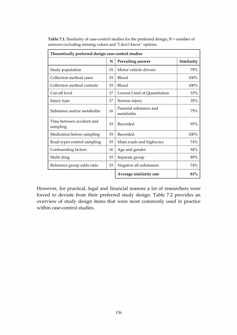
136

Table 7.1. Similarity of case-control studies for the preferred design; N = number of answers excluding missing values and "I don't know" options.

Theoretically preferred design case-control studies

N Prevailing answer Similarity

Study population 19 Motor vehicle drivers 79%

Collection method cases 19 Blood 100%

Collection method controls 19 Blood 100%

Cut-off level 17 Lowest Limit of Quantitation 53%

Injury type 17 Serious injury 35%

Substance and/or metabolite 16 Parental substance and metabolite

75%

Time between accident and sampling

19 Recorded 95%

Medication before sampling 19 Recorded 100%

Road types control sampling 19 Main roads and highways 74%

Confounding factors 16 Age and gender 94%

Multi drug 19 Separate group 89%

Reference group odds ratio 19 Negative all substances 74%

Average similarity rate 81%

However, for practical, legal and financial reasons a lot of researchers were forced to deviate from their preferred study design. Table 7.2 provides an overview of study design items that were most commonly used in practice within case-control studies.

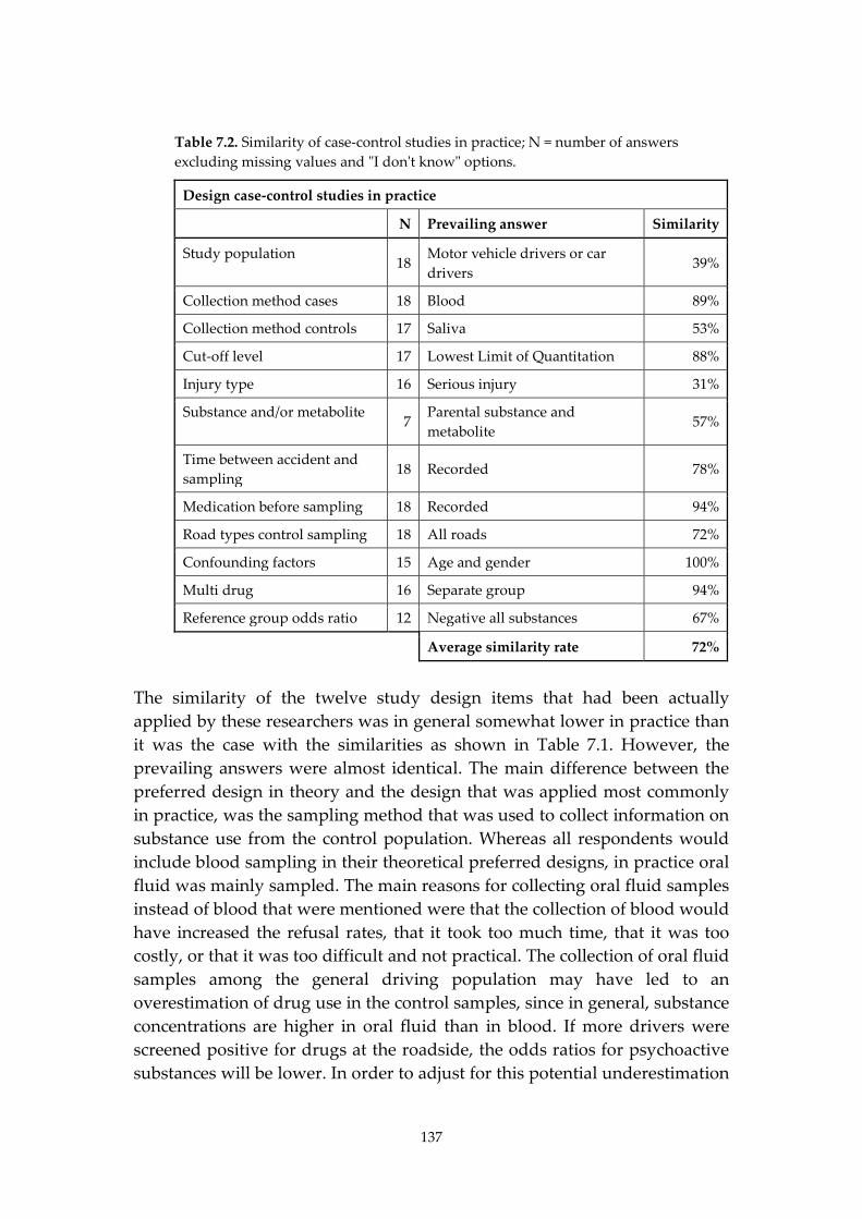
137

Table 7.2. Similarity of case-control studies in practice; N = number of answers excluding missing values and "I don't know" options.

Design case-control studies in practice

N Prevailing answer Similarity

Study population 18

Motor vehicle drivers or car drivers

39%

Collection method cases 18 Blood 89%

Collection method controls 17 Saliva 53%

Cut-off level 17 Lowest Limit of Quantitation 88%

Injury type 16 Serious injury 31%

Substance and/or metabolite 7

Parental substance and metabolite

57%

Time between accident and sampling

18 Recorded 78%

Medication before sampling 18 Recorded 94%

Road types control sampling 18 All roads 72%

Confounding factors 15 Age and gender 100%

Multi drug 16 Separate group 94%

Reference group odds ratio 12 Negative all substances 67%

Average similarity rate 72%

The similarity of the twelve study design items that had been actually applied by these researchers was in general somewhat lower in practice than it was the case with the similarities as shown in Table 7.1. However, the prevailing answers were almost identical. The main difference between the preferred design in theory and the design that was applied most commonly in practice, was the sampling method that was used to collect information on substance use from the control population. Whereas all respondents would include blood sampling in their theoretical preferred designs, in practice oral fluid was mainly sampled. The main reasons for collecting oral fluid samples instead of blood that were mentioned were that the collection of blood would have increased the refusal rates, that it took too much time, that it was too costly, or that it was too difficult and not practical. The collection of oral fluid samples among the general driving population may have led to an overestimation of drug use in the control samples, since in general, substance concentrations are higher in oral fluid than in blood. If more drivers were screened positive for drugs at the roadside, the odds ratios for psychoactive substances will be lower. In order to adjust for this potential underestimation

138

of the odds ratios, equivalent cut-offs were used in the analysis of the case-control studies within the DRUID project. However, the use of these equivalent cut-offs may not be usable for studies that use other cut-off levels for blood or other oral fluid collection devices. Furthermore, the present cut-offs should be seen as a practical cut-off to improve comparability rather than as exact cut-offs. In the future, the use of Dried Blood Spots (DBS) as described by Jantos and Skopp (2011) may solve the previously mentioned issues of collecting blood samples from the general driving population. However, the DBS-method is not yet accurate enough for all substances and when these issues would be overcome, additional time will still be needed for laboratories to have the necessary equipment available for analysis.

7.3. The prevalence of psychoactive substances in Dutch traffic

The prevalence of psychoactive substances among the general driving population in the Netherlands was studied in Chapter 3, in which the results of the Dutch roadside survey were compared with the results in Belgian traffic. More than 5,000 drivers from cars and small vans were randomly selected from Dutch traffic during all days of the week and all times of the day and asked to cooperate with the study on a voluntary base. Drivers who agreed to cooperate were interviewed on recent drug and medicine use. Additionally, the drivers were asked to give a blood sample. If drivers refused, an oral fluid sample was requested. The results of this study showed that 5.5% of all drivers were positive for one or more psychoactive substances. Alcohol was the most prevalent single substance in Dutch traffic. When corrected for time of the day and day of the week, single alcohol use was observed among 2.15% of the general driving population. Furthermore, 2.17% of all drivers were positive for illicit drugs. THC was by far the most frequently detected illicit drug (1.67%), followed by cocaine (0.30%), amphetamines (0.19%), and illicit opiates (0.01%). The most frequently detected medicinal drugs in Dutch traffic were benzodiazepines. On average, 0.40% of the drivers were positive for benzodiazepines. Medicinal opioids (0.16%) and Z-drugs (0.04%) were detected less frequent. With regard to combined use, cocaine was detected with approximately the same frequency alone as it was in combination with other substances. For THC, Z-drugs, and medicinal opiates and opioids, the share of combined use

139

was approximately 25% of the total use, whereas for alcohol and benzodiazepines the proportion was about 10%. The total use of alcohol in combination with other psychoactive substances was 0.24%, whereas the total use of drug-drug combinations was 0.35%. Although the Netherlands and Belgium are neighboring countries, statistical significant differences were present in the prevalence of psychoactive substances in traffic. In general, medicinal drug use and alcohol were more frequently detected in Belgian traffic, whereas illicit substances were more prevalent in The Netherlands. However, when comparing the results of roadside surveys with hospital data and data from illicit drug use in the general population, it is likely that the observed prevalence of illicit drugs at the Belgian roadside was underrepresented and that the prevalence of illicit drugs in Belgian traffic is probably higher than the current results show. Compared to the other European countries in which drivers were screened for these substances as part of the DRUID project, the results for the Netherlands were below the European average for benzodiazepines, medicinal opioids and alcohol, and above the European average for amphetamines and THC. The Dutch roadside survey had only 5% non-respondents, which is very low for this kind of study. However, since the non-respondents had higher BAC’s the results for alcohol were slightly underestimated. The list of DRUID substances did not contain screening for gamma-hydroxybutyric acid (GHB) and selective serotonin reuptake inhibitors (SSRIs), which means that the total prevalence of psychoactive substances may have been higher than 5.5%. On the other hand, the collection procedure of oral fluid may have influenced the concentrations of the samples. The results from Chapter 5 show that THC concentrations in oral fluid samples collected by spit tubes were on average 5.9 times higher than THC concentrations collected by the StatSure collection device. These findings imply that the applied equivalent cutoff concentrations, which is based on oral fluid results that were collected by the Statsure collection device, may have been too low for the Dutch study, in which spitting tubes were used for oral fluid collection. Consequently, some of the drug positive oral fluid samples in the Dutch study may have erroneously been regarded as positive.

140

7.4. The prevalence of psychoactive substances in seriously injured drivers in the Netherlands

Between March 2008 and April 2010 a study on the presence of alcohol and other drugs in injured drivers admitted to the emergency departments of three hospitals in the Netherlands was undertaken as part of the European DRUID project. Only drivers of personal cars or vans, aged more than 18 years and with a Maximum Abbreviated Injury Scale (MAIS) ≥2 were included (Association for the Advancement of Automotive Medicine (AAAM), 2008). In total 187 samples were collected. Blood samples were taken using a 5 mL glass collection tube containing potassium oxalate and sodium fluoride and stored in solid carbon dioxide in the hospitals. After transportation to the Netherlands Forensic Institute (NFI) in The Hague, blood samples were stored at -20°C until analysis. In Chapter 4 the results of the Dutch and Belgian DRUID study on psychoactive substance use among injured drivers were compared. The results showed that in the Netherlands almost 35% of the seriously injured drivers was positive for one or more psychoactive substances. Alcohol was the most prevalent substance. About 28% of the injured drivers in the Netherlands tested positive for alcohol above the legal limit (0.5g/L) and approximately 18% of BACs was higher than 1.3 g/L. Compared with the prevalence of alcohol, the prevalence of licit and illicit drugs was relatively low among injured drivers. Single use of psychoactive substances other than alcohol was barely detected in the Dutch hospital survey, ranging from 0 to 1.1% per substance. The prevalence of drug-drug combinations among injured drivers was also found to be low with 0.5%, whereas the prevalence of alcohol-drug combinations was relatively higher (4.3%). A higher prevalence of alcohol and drugs in seriously injured drivers was found in Belgium compared to the Netherlands. Alcohol was the most prevalent finding in both studies. The distribution of blood alcohol concentrations in the Dutch and Belgian study was similar with very high blood alcohol concentrations in both and a similar median blood alcohol concentration (about 1.6 g/L). One notable finding is the low prevalence of THC and benzodiazepines in the Dutch injured driver population. Despite the high prevalence of THC found in the general driving population surprisingly almost no THC was found in the Dutch injured driver population. In addition no benzodiazepines were found in the Dutch injured drivers. This could be

141

expected since a low prevalence was found in the general driving population (Belgium had a prevalence of about five times higher than the Netherlands). For the other illicit drugs (amphetamines, cocaine and illicit opiates) and medicinal drugs (z-drugs and medicinal opioids) no large differences were observed. When looking for explanations for the differences in prevalence found above different aspects such as differences in alcohol enforcement between the countries, differences in age and gender distribution of the samples and differences in consumption patterns should be kept in mind. In a previous study among seriously injured drivers in the Netherlands the prevalence of drugs was much higher (Mathijssen and Houwing, 2005). Several reasons can be given for the lower share of psychoactive substances other than alcohol. First, differences could be explained by the difference in the biological matrix. In one third of the IMMORTAL cases, urine was analysed. Since substance use can be detected more easily in urine, the prevalence of the hospital study in IMMORTAL could have been overestimated. The median interval between accident and sampling was 1.35 h. Some drugs with a short half-life, such as THC and cocaine, might have been used by more drivers than it was detected in the Dutch study. Some Dutch injured drivers were found positive for the metabolite THC-COOH. The presence of THC-COOH indicates past use of cannabis. When calculating the prevalence of THC and/or THC-COOH 1.6% of the Dutch drivers were found positive compared to the 0.5% drivers found positive for THC. These drivers would also have been detected when urine would have been used as a biological matrix. A second possible reason for the lower prevalence in the DRUID study is the smaller number of substances that was analysed. In the DRUID study the blood samples were only screened for a limited list of benzodiapines. It may be possible that drivers were using other benzodiazepines than those screened for within the DRUID project. Finally, given the small number of included subjects the 95% confidence intervals provide a more accurate prevalence. In the case of a prevalence of 0.5% e.g. for THC or Z-drugs the 95% confidence interval was 0.0-2.9%. For substances that were not detected, such as single cocaine use or single illicit opiate use, the 95% confidence interval was still 0.0-2.0%. The results of the prevalence of psychoactive substances in traffic (Section 7.3) and the prevalence among injured drivers (Section 7.4) can be used to estimate the relative risk of driving under the influence. By comparing the ratio of drug positive injured drivers with the ratio of drug positive drivers

142

among the general driving population odds ratio can be calculated. These odds ratios are discussed in Sections 7.6 and 7.7 of this thesis.

7.5. The effect of the oral fluid collection device type on substance concentrations

The repeatability of both the Statsure collection method and the ordinary spit tubes is low when applied among subjects who have consumed cannabis very recently. In comparison with the Belgian legal limit, results of the Statsure collection method are more in agreement with each other than results of the spit tubes. Furthermore, the results of Chapter 5 show that samples obtained by spitting had 1.7-5.9 times higher THC concentrations than samples from the Statsure collection method, depending on the choice of the upper limit of THC concentrations that were included for analysis. The results of this study have implications for the comparability of the results of the Dutch roadside survey with the other DRUID studies as was already mentioned in Section 7.3. Since the results of the roadside survey are also used as the control population in the Dutch case-control study that estimated the risk of driving under the influence of psychoactive substances, the Dutch odds ratios for psychoactive substances other than alcohol are probably underestimated. Unfortunately, the number of samples is too small to calculate an alternative equivalent cut-off, based on the same method that equivalent cut-offs have been calculated for the oral fluid samples that were gathered by the Statsure collection device. Therefore, no exact size of the effect of the oral fluid collection device on substance concentrations can be measured. The blood alcohol concentration (BAC) was not measured in oral fluid, but in breath. Therefore, this issue does not seem to concern the prevalence of alcohol directly. However, in theory it might be possible that due to the alternative higher cut-offs for drugs in the spitting samples, samples that were initially assigned to the group of drug-alcohol combinations might be reassigned to the single alcohol group. This would lead to a decrease of the share of drivers positive for drug-alcohol combination and an increase of the share of drivers positive for single-alcohol use. Therefore, higher cut-offs for drugs in spitting samples could indirectly affect the results for alcohol as well.

143

7.6. The effect of random and systematic errors on the odds ratios of case-control studies

As discussed in Section 1.3, the results of case-control studies on the risk of driving under the influence of psychoactive substances show large variations between the calculated odds ratios. This problem is acknowledged in review studies and is often related to differences in study design and to the effect of random and systematic errors. Separating the effect of differences in study design from the effect of errors is difficult though, and only possible if studies are compared that have been conducted by using the same design. Within the European DRUID project six case-control studies have been conducted to study the injury risk of driving under the influence of psychoactive substances. Guidelines were prepared to stimulate that the outcomes of these case-control studies were comparable. As a result, these studies were conducted based on a more or less similar design. The main design difference was the biological matrix that was used for sampling body fluids. In Lithuania, only blood samples were collected, in Denmark and Finland, only oral fluid samples were collected, whereas in Belgium, Italy and the Netherlands a mixture of both blood and oral fluid samples was available. To be able to compare the results from these studies, equivalent cut-offs were determined for all included samples. To study the potential effect of errors on the results of the six DRUID case-control studies on injury risk, a list of indicators for potential errors was needed. In this thesis the categorization of Kleinbaum et al. (1982) and Rothman (1986) is used, which is supported by Wacholder et al. (1992). Table 7.3 provides an overview of this list of indicators. Chapter 6 showed the results of the assessment of potential bias in the six DRUID case-control studies on injury risk. It can be concluded that none of these studies was perfect. The most commonly observed errors were due to selection bias and to relatively small sample sizes and low cell counts for individual substances. By introducing guidelines and a protocol for conducting case-control studies, and by using equivalent cut-offs, the effect of information bias (see Table 7.3) is probably relatively limited. The effect of confounding remains uncertain though. Age, gender and time period, which are commonly used confounding variables, have been included in the statistical model to calculate odds ratios. However, there may be other variables, such as road conditions and density of traffic, that influence the risk of injury when driving under the influence.

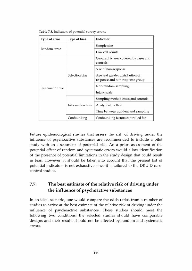
144

Table 7.3. Indicators of potential survey errors.

Type of error Type of bias Indicator

Random error Sample size

Low cell counts

Systematic error

Selection bias

Geographic area covered by cases and controls

Size of non-response

Age and gender distribution of response and non-response group

Non-random sampling

Injury scale

Information bias

Sampling method cases and controls

Analytical method

Time between accident and sampling

Confounding Confounding factors controlled for

Future epidemiological studies that assess the risk of driving under the influence of psychoactive substances are recommended to include a pilot study with an assessment of potential bias. An a priori assessment of the potential effect of random and systematic errors would allow identification of the presence of potential limitations in the study design that could result in bias. However, it should be taken into account that the present list of potential indicators is not exhaustive since it is tailored to the DRUID case-control studies.

7.7. The best estimate of the relative risk of driving under the influence of psychoactive substances

In an ideal scenario, one would compare the odds ratios from a number of studies to arrive at the best estimate of the relative risk of driving under the influence of psychoactive substances. These studies should meet the following two conditions: the selected studies should have comparable designs and their results should not be affected by random and systematic errors.

145

7.7.1. Comparable study designs

Several issues concerning study designs should be taken into account when comparing different studies that assess the risk of driving under the influence. First, the use of different study types should be considered. Case-control designs differ from the designs of culpability and pharmaco-epidemiological studies. Therefore, the results of pharmaco-epidemiological case-control studies and culpability studies, which can be seen as nested case-control studies, cannot be compared with those of regular case-control studies. Not much information is available on the effect of assessing the risk of driving under the influence of psychoactive substances by different types of studies. However, in the literature three studies were found that compared the estimated risk of driving under the influence, calculated by two different study types. Ravera et al. (2012) compared the results of their case-control study and their culpability study and found that the results differed. None of the results of the culpability study showed a significant increase of risk for psychotropic medication use, while their case-control study did. They concluded that their results were in line with Hebert et al. (2007) who also found an increased risk of benzodiazepine use in their case-control study which was not supported by their culpability study. Both Ravera et al. and Hebert and al. concluded that the differences among the findings of their studies could be the result of differences between the study types. A third example of a study in which both the results of a case-control and a culpability are compared is a study by Brault et al. (2004). In this study, odds ratios for fatal injury were calculated for alcohol, cannabis, benzodiazepines and cocaine. The results of the culpability studies showed lower odds ratios for alcohol, cannabis and benzodiazepines than the case-control results. No sufficient data were available for calculating the culpability rate of cocaine. The authors stated that the results of the responsibility analysis were deceiving. The lower odds ratios might be due to the high level of responsibility for fatal crashes of the included killed drivers. For this reason no large differences were found in the culpability study for sober and substance positive drivers, leading to relatively low odds ratios of being responsible for the fatal crash. Based on the results above it might be concluded that the differences between odds ratios for culpability studies and case-control studies are partly based on differences in methodology. The results of the studies that combine a regular case-control study with one of the other study designs indicate that odds ratios that were calculated by case-control studies might in general be

146

somewhat higher than odds ratios that were calculated by other epidemiological study designs. A second relevant issue when comparing the results of epidemiological studies that assess the risk of driving under the influence is the presence of differences within a specific type of study design. Examples of such differences are the type of injuries included, the cut-off levels of psychoactive substances, the biological matrix, and the list of substances included. The biological matrix is a design item that needs special attention. In theory, the ideal method would be to collect blood samples from both the case and the control population. However, in practice it is more common to collect oral fluid samples from the control population, since this leads to a lower share of non-response, is less expensive and easier to collect than blood. A disadvantage of oral fluid is that substance concentrations in oral fluid are not comparable to those in blood. In general, substance concentrations are higher in oral fluid than in blood which makes it easier to detect drug positive drivers. The selection of the biological matrix will therefore be of influence for the detected prevalence of psychoactive substances in the study population. Within the DRUID project a practical solution was found by using equivalent cut-offs. Another type of biological matrix is urine, which was used in the Dutch IMMORTAL study (Mathijssen and Houwing, 2005). However, the detection window of psychoactive substances is much larger in urine than it is in blood or oral fluid, which makes it difficult to regard the presence of substance concentrations in urine as a marker for recent substance use. By using urine to collect information on drug use among the control population in case-control studies, the prevalence of substances in general traffic could be overestimated. Subsequently, this would lead to an underestimation of the relative risk. In 2005, guidelines for epidemiological studies were prepared by a special ICADTS-committee (Walsh et al., 2008). These guidelines included several recommendations among which the use of specific cut-offs for substances and the use of blood or oral fluid as matrix. In 2007, the DRUID project adopted these guidelines for their case-control studies, and additionally included so-called equivalent cut-offs to correct for the differences in substance concentrations between blood and oral fluid. In six of the DRUID case-control studies research was conducted on the risk of serious injury, while four other studies assessed the risk of fatal injury. The focus of this PhD thesis is on the comparability of those six DRUID studies that estimated the risk of serious injury. By applying the ICADTS-guidelines in combination with the equivalent cut-offs, the first condition (having comparable study designs) for determining the best estimate for the risk of driving under the influence can be regarded as fulfilled.

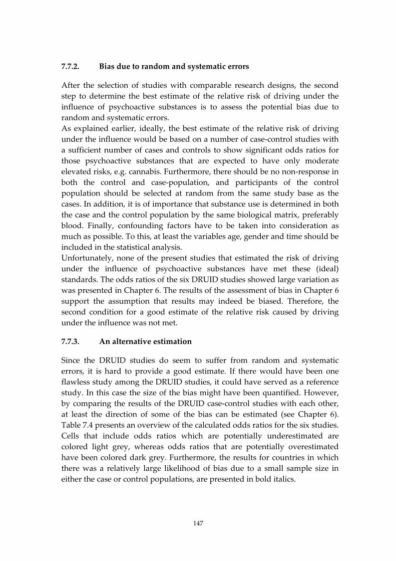
147

7.7.2. Bias due to random and systematic errors

After the selection of studies with comparable research designs, the second step to determine the best estimate of the relative risk of driving under the influence of psychoactive substances is to assess the potential bias due to random and systematic errors. As explained earlier, ideally, the best estimate of the relative risk of driving under the influence would be based on a number of case-control studies with a sufficient number of cases and controls to show significant odds ratios for those psychoactive substances that are expected to have only moderate elevated risks, e.g. cannabis. Furthermore, there should be no non-response in both the control and case-population, and participants of the control population should be selected at random from the same study base as the cases. In addition, it is of importance that substance use is determined in both the case and the control population by the same biological matrix, preferably blood. Finally, confounding factors have to be taken into consideration as much as possible. To this, at least the variables age, gender and time should be included in the statistical analysis. Unfortunately, none of the present studies that estimated the risk of driving under the influence of psychoactive substances have met these (ideal) standards. The odds ratios of the six DRUID studies showed large variation as was presented in Chapter 6. The results of the assessment of bias in Chapter 6 support the assumption that results may indeed be biased. Therefore, the second condition for a good estimate of the relative risk caused by driving under the influence was not met.

7.7.3. An alternative estimation

Since the DRUID studies do seem to suffer from random and systematic errors, it is hard to provide a good estimate. If there would have been one flawless study among the DRUID studies, it could have served as a reference study. In this case the size of the bias might have been quantified. However, by comparing the results of the DRUID case-control studies with each other, at least the direction of some of the bias can be estimated (see Chapter 6). Table 7.4 presents an overview of the calculated odds ratios for the six studies. Cells that include odds ratios which are potentially underestimated are colored light grey, whereas odds ratios that are potentially overestimated have been colored dark grey. Furthermore, the results for countries in which there was a relatively large likelihood of bias due to a small sample size in either the case or control populations, are presented in bold italics.

Table 7.4. Odds ratios indicating the relative risk of being seriously injured (MAIS ≥2) due to driving under the influence of psychoactive substances according to country, adjusted for age and gender, and 95% confidence intervals (adapted from Hels et al., 2011); cells with OR’s which are potentially underestimated are colored light grey and cells with OR’s which are potentially overestimated are colored dark grey; na = not possible to calculate due to low cell counts. Inf = infinity.

Psychoactive substance Belgium Denmark Finland Italy Lithuania Netherlands All countries

Alcohol Alcohol 0.1-0.5 g/L 1.03 0.49-2.15

1.47 0.79-2.74

6.55 0.81-53.25

0.56 0.29-1.06

1.49 0.54-4.13

1.58 0.49-5.12

1.18 0.81-1.73

Alcohol 0.5-0.8 g/L 2.27 0.94-5.49

5.66 2.5-12.82

36.01 3.14-413.06

0.58 0.26-1.29

3.69 0.91-15.02

9.4 2.89-30.61

3.64 2.31-5.72

Alcohol 0.8-1.2 g/L 13.23 5.61-31.21

14.32 4.68-43.87

55.07 2.74-inf.

1.53 0.76-3.1

10.82 3.03-21.22

31.37 11.34-86.83

13.35 8.15-21.88

Alcohol ≥1.2 g/L 108.68 57.5-205.43

296.99 58.84-inf.

128.84 38.69-429.03

16.55 8.8-31.15

11.42 6.14-21.22

108.09 52.45-222.75

62.79 44.51-88.58

Illicit drugs Amphetamine na 49.94 2.8-891.67

na na 0.5 0.04-6.88

8.87 1.84-42.86

8.35 3.91-17.83

Benzoylecgonine na na na 3.24 0.85-12.38

na 12.23 2.86-52.34

3.7 1.6-8.57

Cocaine na na na 1.17 0.4-3.4

na na 3.3 1.4-7.79

Cannabis 4.88 1.6-14.84

2.17 0.61-7.79

25.38 1.86-345.78

1.88 0.85-4.17

na 0.29 0.04-2.11

1.38 0.88-2.17

Illicit opiates and opioids na na na 1.38 0.25-7.62

na na 2.47 0.5-12.1

Medicinal drugs

Benzodiazepines and Z-drugs 2.3 1.07-4.94

4.37 2.18-8.75

2.59 0.34-19.86

0.2 0.04-1.0

1.02 0.36-2.87

2.56 0.34-19.36

1.99 1.36-2.91

Medicinal opioids 4.33 1.58-11.89

5.72 3.06-10.67

5.4 0.68-42.97

11.16 3.38-36.88

Na 5.96 0.73-48.84

9.06 6.4-12.83

Combinations Alcohol-drugs 58.16 27.05-125.07

52.68 16.01-173.35

148.7 26.84-823.94

7.3 3.49-15.27

127.32 4.22-inf.

12.55 4.76-33.12

28.82 18.41-45.11

Different drugs classes 9.99 3.61-27.68

57.54 12.66-261.53

45.86 7.92-265.38

2.29 1.12-4.66

na na 8.01 5.34-12.01

149

Although for most countries the estimations of the direction of the effect of potential bias look quite straightforward, not all effects seem to be fully explained by errors. Several reasons for this can be thought of: for example, the potential size of bias might not be the same for each country and even for each substance. Since qualitative measurements are not available, this issue has not been taken into account in the table. Furthermore, for some odds ratios two or more effects could have influenced the outcome. It is difficult to estimate which type of bias would have had the most dominant effect, let us take the case of the odds ratio for cannabis that was calculated in the Dutch study. This odds ratio is probably biased due to variation between the included regions and the non-included regions of the roadside survey, due to the use of spitting tubes as sample collection method at the roadside, and to the relatively small number of hospital samples which were sampled in the hospital study. It is impossible to disentangle the relative contribution of each of these biases. A third reason for variety that seems unexplainable by the assessment of bias as studied in this thesis, might be the presence of confounding by unidentified factors such as road conditions, and density of traffic. In general, the overall odds ratios for all countries in the last column of Table 7.4 seem to be as expected, taking into account the direction of bias in the national studies. The overall odds ratios for alcohol are in line with those in international literature (Hargutt et al., 2011), although it is always difficult to compare the results of the DRUID studies with other studies since these studies were in general based on other designs and suffer from random and systematic errors as well. For illicit and medicinal drugs the number of more or less comparable studies is small. The case-control studies from Haworth et al. (1997) and Blows (2004) that were reported in Chapter 1 have based the prevalence in the control population on self-reported use. The French case-control study by Mura et al. (2003) did not include non-injured car drivers as the control group, but patients from a hospital in possession of a driving license that were involved in a non-traffic accident. The Canadian case-control study from Brault et al. (2004) and the Dutch case-control study by Mathijssen and Houwing (2005) did use both urine and blood as biological matrix. Other design differences were present as well; but relative to the other case-control studies these two studies might be more comparable -or less incomparable- to the DRUID studies. A comparison of these latter two studies show that the overall odds ratios for illicit drugs are in line with each other. The Canadian case-control study by

150

Brault et al. (2004) found an odds ratio of 4.5 for cocaine and of 1.6 for THC after adjustment for gender, age and time period. The Dutch case-control study by Mathijssen and Houwing (2005) found an odds ratio of 1.29 for THC after adjustment for age, gender and time period and year and quarter of the year. For the other illicit substances the numbers were too small to calculate odds ratios. The designs from both the Dutch and the Canadian case-control study were not directly comparable to the ones of the DRUID study which makes it difficult to value the similarities between the odds ratios from these studies and the overall odds ratios from the DRUID studies. Therefore, similar results between these studies alone do not ensure that the studies were free of bias. The studies from Brault et al. and from Mathijssen and Houwing found odds ratios for benzodiazepines of respectively 3.9 and 3.48, whereas in the overall odds ratio of the DRUID studies was lower at 1.99. Of the six case-control studies on injury risk that were conducted in the DRUID project, most odds ratios for benzodiazepines were around 2. Only the Danish study had an odds ratio that was higher: 4.37, whereas the Italian and Lithuanian study were lower at 0.2 and 1.02, respectively. The results of the study from Mathijssen and Houwing showed an odds ratio of 6.89 for codeine. In the DRUID studies, the overall odds ratio for illicit opiates and opioids was 9.06. This overall odds ratio for medicinal opioids is considered to be high, since most of the results from the national studies showed odds ratios between 4 and 6. Only in Italy the odds ratio was higher, at 11.16, and in Lithuania the number of positive samples was too small to calculate the odds ratio for illicit opiates and opioids. Taken all together, we consider that apart from the odds ratio for medicinal opioids, the overall odds ratios for psychoactive substances provide a better estimate of the relative risk of having an injury when driving a car after recent use of psychoactive substances than the odds ratios of each of the six national case-control studies.

7.8. Drug driving legislation

Within Europe, new drug driving legislation has been introduced in February 2012 in Norway (Vindenes et al., 2012). In the Netherlands new drug driving legislation is foreseen for 2013. These are the first countries that have used the results of the DRUID project in their drug driving legislation. The proposed Dutch legislation covers the five different types of substances: amphetamines (amphetamine, methamphetamine, MDA, MDMA and MDEA), cocaine, THC (cannabis), and GHB (Adviescommissie

151

Grenswaarden, 2010). For these substances impairment related per se limits for concentrations have been determined by a group of experts. These concentration limits indicate that once they are exceeded, the driving skills are affected in such a way that the driver can no longer be expected to drive safely. Furthermore, the proposed drug driving legislation obliges drivers to cooperate with an oral fluid screening test and with a test on psycho-motor functions. If a driver is suspected for drug-driving a blood sample will be taken to determine whether or not the legal limits were exceeded. The results of the research as reported in this thesis could be used to support new drug driving legislation in several ways. Three relevant considerations in the process of new drug driving legislation can be distinguished. The first moment of consideration is in the design phase when the choice has to be made between per-se legislation and legislation on impairment. These per-se limits can be based on three different types of limits: the lowest limit of quantitation or the lowest limits of detection, the lowest limit of impairment or the lowest limit of risk (Verstraete et al., 2011b). When introducing per-se legislation with impairment or risk related legal limits, a meta-analysis of existing literature and/or an expert panel is needed to determine specific cut-offs for substance concentrations. Both in Norway and The Netherlands a panel of experts was established to determine a list of the psychoactive substances that should be included in legislation and their concentration limits. The panel of experts can discuss findings from different studies and come to an agreement on legal limits. The results from these studies are generally based on both experimental and epidemiological studies. Experimental studies provide information on the level of impairment that is caused by psychoactive substance use. Experimental studies can also compare impairment of licit and illicit drugs with impairment of alcohol at given BAC levels. Epidemiological studies can provide information on the share of drivers that are driving under the influence of psychoactive substances or that are seriously injured or even killed while driving under the influence. Furthermore, the relative injury or crash risk can be estimated by means of epidemiological studies. Although the information from epidemiological studies is at present insufficient to calculate risk-related legal limits, valuable information can be derived from epidemiological studies to support and interpret the results from experimental studies (Adviescommissie Grenswaarden, 2010). So even when legal limits are based on experimental studies, the results of epidemiological studies are still of value. This thesis provides some guidelines to review the outcomes of specific epidemiological studies. It offers a list of indicators of potential bias and a list

152

of items per specific study type that can be used to compare study designs and validate their results. The second relevant issue concerns the list of individual psychoactive substances to be included in the drug driving legislation. The present list of psychoactive substances and their legal limits are not fixed. From time to time it would be necessary to update the supporting literature to see whether the new substances could be included or the legal limits of listed substances need to be changed. If epidemiological studies are needed for supporting the introduction of new or altered legal limits, the results of the research presented here can provide background information on how to design or evaluate these studies. And finally, the results of this thesis can be used to design evaluation studies of new drug driving legislation. Within the European DRUID project a cost-benefit analysis was conducted to gain insight in the costs and benefits from increased drug driving enforcement by means of oral fluid screening devices (Veisten et al., 2011). The results of this study indicate that it is important to introduce drug-driving enforcement with special caution, due to the potential negative side effect on drink driving enforcement. Baring this in mind, it is recommended to monitor the effects of new drug driving legislation and its enforcement on traffic safety. This monitoring should preferably not only be focused on the use of illicit drugs in traffic but also on the use of alcohol in order to be able to detect potential negative side effects of drug driving enforcement on the use of alcohol in traffic.

7.9. Synthesis

The main objective of this thesis was to provide insight in how to arrive at the best estimate of the injury risk of driving under the influence of psychoactive substances. To this end, two conditions were formulated. First, studies are needed with a comparable study design, since variation in results can be caused by differences in study design. The second condition includes the absence of random and systematic errors in those studies that meet the first condition. Between 2007 and 2010, six case-control studies were conducted within the European research-project DRUID by means of similar study designs. Guidelines and study protocols were prepared for the DRUID case-control studies according to the ICADTS guidelines for epidemiological studies

153

(Walsh et al., 2008) to stimulate that the outcomes of these case-control studies were comparable. Furthermore, equivalent cut-offs were applied to adjust for differences between studies that used oral fluid as biological matrix and studies that used blood samples. Despite the high comparability of the study designs, the results still showed large variations between the calculated odds ratios. To get insight in the reason behind this variation, it was assessed in this thesis whether these differences could be caused by different kinds of random and systematic errors. The results showed that this variation in odds ratios could indeed be explained by the presence of random and systematic errors. Another finding was that the most common types of errors that were detected in the case-control studies under scrutiny were selection bias and lack of sufficient study power due to small sample size. Based on these results, it can be concluded that the presence of guidelines and protocols did not sufficiently solve the issue of incomparable odds ratios. The question is whether this issue is caused by flaws in the guidelines or by flaws in the compliance of researchers to the guidelines. The combination of the ICADTS guidelines and the equivalent cut-offs of the DRUID project may be seen as the state-of-the-art on attempts to conduct case-control studies that are comparable. However, it may be questioned whether it is possible for future studies to adapt this design. The compliance to these guidelines can be restricted by practical, legal, financial and ethical reasons. Furthermore, it also depends on the willingness of researchers to commit themselves to guidelines, that they might not always fully agree with. Finally, the need to answer specific research questions could cause deviation from the ICADTS and DRUID guidelines. For example, if a case-control study is designed to compare its results with that of a previous national case-control study the design should be comparable to that of the previous study in order to be able to monitor any differences. One of the largest problems in the design of case-control studies is the biological matrix that is used for collecting data on substance use from the control population. In theory, collecting blood samples would be the most appropriate method, since it matches with the collection of blood from injured drivers (the case population). However, one of the major disadvantages of blood sampling is that it may lead to relatively high non-response rates, since participants might not always be very eager to give blood. Therefore, in practice oral fluid samples are mainly collected. The substance concentrations in oral fluid differ from concentrations in blood and therefore equivalent cut-offs were used within the DRUID case-control

154

studies. The use of oral fluid sampling may be replaced in future studies by the Dried Blood Spot (DBS) method. This method could be a less expensive and more reliable method to calculate odds ratios, however, although the results for some psychoactive substances seem promising, no strong correlation exists at present between the THC concentrations in venous blood and in DBS. Researchers are still trying to find a solution for this and if the correlation for THC can be established, the DBS method might replace oral fluid sampling in future case-control studies. Until then, we recommend the use of equivalent cut-offs if oral fluid samples are collected from the control population. In order to avoid bias and confounding due to errors, future guidelines are recommended to more systematically include an overview of the sources of potential bias and instructions of how to avoid them. The ICADTS guidelines already contained some guidelines on how to avoid bias and increase the power and sensitivity of a study. However, they may not have been specific enough. One of the recommendations in the ICADTS guidelines was to conduct a power-study to estimate the number of samples that would be needed to reach a sufficient level of sensitivity. In the DRUID studies no a priori study was conducted to assess the number of cases and controls that would be necessary. It was expected that if all studies would include on average between 600-700 samples and 1,500-4,000 samples at the roadside, that this would be sufficient. The results of an a posteriori assessment of the necessary sample size to get sufficient power to get significant results for the odds ratios for THC, showed that at least 3,700 cases and 11,000 controls should have been included. These numbers are far too large for a single case-control study in the DRUID project, but by combining all case-control studies these numbers would have been feasible. Unfortunately, the average number of included cases in the six DRUID case-control studies was 415 (with only 54 cases in Finland and 188 in the Netherlands), adding up to a total of 2490 cases. It can be questioned whether it is necessary to calculate significant odds ratios for all substances. For policy purposes it might be sufficient to calculate significant odds ratios only for the most prevalent substances that cause high risks. On the other hand, if the results are used to calculate risk related legal concentration limits for psychoactive substances, far more cases and controls will be needed. It should therefore be noted that the required number of samples varies with the specific research question. It is also stated in the guidelines that the non-response level should be minimized and that specific information should be gathered to get more insight in the likelihood of non-response bias. However, guidelines do not

155

describe when a non-response percentage is regarded as too high, or when non-response bias is regarded as being so large that the results should be questioned. Since case-control studies are very costly and time-consuming to conduct it might be recommendable for future studies to a-priori assess the potential level of bias due to study errors by comparing the study design with one of the previous study designs. If the likelihood of bias is large and no or insufficient possibilities are available to avoid this potential bias, then it might be necessary to reconsider to conduct the study. Therefore, a pilot study with an a-priori assessment on potential bias, based on the one that was used in this thesis, could serve as a go-no go test for conducting future case-control studies that calculate the risk of driving under the influence of psychoactive substances. By increasing the comparability of study designs and by decreasing the potential errors of case-control studies a good estimate of the risk of driving under the influence of psychoactive substances might be available in future. However, since case-control studies are rarely conducted, it probably will take many years before a study is conducted and published that can serve as a theoretically sound landmark study for estimating the risk of driving under the influence of alcohol, drugs and medicines.

157

References

Adviescommissie Grenswaarden (2010). Advies grenswaarden drugs. In het kader van de voorgenomen wetswijziging van de Wegenverkeerswet 1994. Den Haag: Ministerie van Veiligheid en Justitie.

Agresti, A. (1996). An introduction to categorical data analysis. New York: John Wiley & Sons. Andersen, J.A., McLellan, B.A., Pagliarello, G. & Nelson, W.R. (1990). The relative influence

of alcohol and seatbelt usage on severity of injury from motor vehicle crashes. Journal of Trauma, 30(4), 415-417.

Association for the Advancement of Automotive Medicine (AAAM) (2008). International injury scaling (AIS) 2005; update 2008. Barrington: AAAM.

Assum, T. (2005). The prevalence and relative risk of drink and drug driving in Norway. Oslo: Institute of Transport Economics.

Assum, T., Frison, G., Hels, T., Houwing, S. & Mathijssen, R. (2007). Uniform design and protocols for carrying out case-control studies: DRUID DRiving Under the Influence of Drugs, Alcohol and Medicines. D2.1.2 Available from http://www.druid-project.eu/.

Assum, T., Mathijssen, M.P.M. & Houwing, S. (2005). The prevalence of drug driving and relative risk estimations. A study conducred in the Netherlands, Norway and United Kingdom. Vienna: Australian Road Safety Board.

AWV (2007). Verkeerstellingen 2007 in Vlaanderen. Brussel: Vlaamse Overheid Agentschap Wegen en Verkeer.

Bakker, A., Van Balkom , A. & Spinhoven, P. (2002). SSRIs vs TCAs in the treatment of panic disorder: a meta-analysis. Acta Psychiatrica Scandinavia, 106, 163-167.

Baldock, M.R.J. (2007). Review of the literature on cannabis and crash risk. Adelaide, Australia: The University of Adelaide.

Behrensdorff, I. & Steentoft, A. (2003). Medicinal and illegal drugs among Danish car drivers. Accident Analysis & Prevention, 35(6), 851-860.

Beirness, D.J., Simpson, H.M. & Williams, A.F. (2006). Role of cannabis and benzodiazepines in motor vehicle crashes. Transportation Research Circular E-C096: Drugs and Traffic.

Belgisch Instituut voor de Verkeersveiligheid (2010a). Attitudemeting verkeersveiligheid 2009. Evoluties sinds 2003-2006. Brussel: BIVV Belgisch Instituut voor de Verkeers-veiligheid.

Belgisch Instituut voor de Verkeersveiligheid (2010b). Rijden onder invloed van alcohol: resultaten van de gedragsmeting 2009. Brussel: BIVV Belgisch Instituut voor de Verkeersveiligheid.

Belgisch Instituut voor de Verkeersveiligheid (2011). Verkeersveiligheidsbarometer 2010. Brussel: BIVV Belgisch Instituut voor de Verkeersveiligheid.

Berghaus, G., Ramaekers, J.G. & Drummer, O.H. (2007). Demands on scientific studies in different fields of forensic medicine and forensic sciences: Traffic medicine-impaired driver: Alcohol, drugs, diseases. Forensic Science International, 165, 233-237.

BHC (2011). Kerncijfers Nederlandse Horeca from http://abf.kenniscentrumhoreca.nl/ quickstep/qsreportadvanced.aspx?report=horecava10t

Bland, M.J. & Altman, D.G. (1986). Statistical methods for assessing agreement between two methods of clinical measurement. The Lancet, 327(8476), 307-310.

Blencowe, T., Pehrsson, A., Lillsunde, P., Vimpari, K., Houwing, S., Smink, B., Mathijsen, R., Van der Linden, T., Legrand, S., Pil, K. & Verstraete, A. (2011). An analytical

158

evaluation of eight on-site oral fluid drug screening devices using laboratory confirmation results from oral fluid. Forensic Science International, 20(1-3), 173-179.

Blows, S., Ameratunga, S., Ivers, R.Q., Lo, S.K. & Norton, R. (2005). Risky driving habits and motor vehicle driver injury. Accident Analysis & Prevention, 37(4), 619-624.

Blows, S., Ivers, R.Q., Connor, J., Ameratunga, S., Woodward, M. & Norton, R. (2004). Marijuana use and car crash injury. Addiction 100, 605-611.

Bogstrand, S.T., Normann, P.T., Rossow, I., Larsen, M., Mørland, J. & Ekeberg, Ø. (2011). Prevalence of alcohol and other substances of abuse among injured patients in a Norwegian emergency department. Drug and Alcohol Dependence, 11(2-3), 132-138.

Borkenstein, R.F., Crowther, R.F., Shumate, W.B., Ziel, W.B. & Zylman, R. (1974). The role of the drinking driver in traffic accidents (the Grand Rapids study). Blutalkohol, 11 (2nd edition).

Borrenbergen, K. (2011). Campagne slaap- en kalmeermiddelen. Brussel: Federale Overheids-dienst Volksgezonheid, veiligheid van de voedselketen en leefmilieu.

Bosker, W.M. & Huestis, M.A. (2009). Oral fluid testing for drugs of abuse. Clinical Chemistry, 55(11), 1910-1931.

Brault, M., Dussault, C., Bouchard, J. & Lemire, A.M. (2004). The contribution of alcohol and other drugs among fatally injured drivers in Quebec: final results. In: 17th ICADTS conference. Glasgow.

Brookhuis, K.A., De Waard, D. & Fairclough, S.H. (2003). Criteria for driver impairment. Ergonomics, 46(5), 433-445.

Brookhuis, K.A., De Waard, D. & Samyn, N. (2004). Effects of MDMA (ecstacy), and multiple drug use on (simulated) driving performance and traffic safety. Psychopharmacology, 173, 440-445.

Buttress, S.C., Sexton, B., Tunbridge, R.J. & Oliver, J. (2004). Project IMMORTAL. Crowthorne, United Kingdom: Transport Research Laboratory.

CBS (2011). National Travel Survey. from http://www.swov.nl/uk/research/kennisbank/ inhoud/90_gegevensbronnen/inhoud/ovg.htm

Cohen, J. (1988). Statistical power analysis for the behavioral sciences (2nd ed.). Hillsdale, NJ: Lawrence Earlbaum Associates.

Commission of the European Communities (2001). White paper; European transport policy for 2010; Time to decide. Brussels: European Commission.

Compton, R.P., Blomberg, R.D., Moskowitz, H., Burns, M., Peck, R.C. & Fiorentino, D. (2002). Crash risk of alcohol impaired driving. In: 16th ICADTS conference. Montreal.

Connor, J., Norton, R., Ameratunga, S. & Jackson, R. (2004). The contribution of alcohol to serious car crash injuries. Epidemiology, 15(3), 337-344.

Cornfield, J. (1951). A method of estimating comparative rates from clinical data. Applications to cancer of the lung, breast and cervix. Journal National Cancer Institute, 11, 1269-1275.

Crouch, D.J. (2005). Oral fluid collection: The neglected variable in oral fluid testing. Forensic Science International, 150(2-3), 165-173.

Day, D., Kuntz, D.J., Feldman, M. & Presley, L. (2006). Detection of THCA in oral fluid by GC-MS/MS. Journal of Analytical Toxicology, 30(9), 645-650.

De Gier, J.J., Heissing, M., Alvarez, J. & Tant, M. (2009). Recommendations for improving medical guidelines for assessing fitness to drive in patients who use psychotropic medicines: DRUID Driving Under the Influence of Drugs, Alcohol and Medicines.

Degenhardt, L., Wai-Tat, C., Sampson, N., Kessler, R.C., Anthony, J.C., Angermeyer, M., Bruffaerts, R., De Girolamo, G., Gureje, O., Huang, Y., Karam, A., Kostyuchenko, S.,

159

Lepine, J.P., Mora, M.E.M., Neumark, Y., Ormel, J.H., Pinto-Meza, A., Posada-Villa, J., Stein, D.J., Takeshima, T. & Wells, J.E. (2008). Toward a global view of alcohol, tabacco, cannabis, and cocaine use: findings from the WHO World Mental Health Surveys. PLOS Medicine, 5(7), 1053-1066.

Desapriya, E., Pike, I. & Raina, P. (2006). Severity of alcohol-related motor vehicle crashes in British Columbia: case-control study. International Journal of Injury Control and Safety Promotion, 13(2), 89-94.

Dissanayake, S. & Lu, J.J. (2002). Factors influential in making an injury severity difference to older drivers involved in fixed object–passenger car crashes. Accident Analysis & Prevention, 34(5), 609-618.

DRUID (2012). Final report: DRUID Driving under the Influence of Drugs, Alcohol and Medicines. Available from http://www.druid-project.eu/.

Drummer, O.H. (2008). Introduction and review of collection techniques and applications of drug testing of oral fluid. Therapeutic Drug Monitoring, 30(2), 203-206.

Drummer, O.H. (2009). Epidemiology an traffic safety: culpability studies. In: Verster, J.C., Pandi-Perumal, S.R., Ramaekers, J.G. & De Gier, J.J. (Eds.), Drugs, Driving and Traffic Safety (pp. 107-120). Basel: Birkhäuser Verlag.

Drummer, O.H., Gerostamoulos, J., Batziris, H., Chu, M., Caplehorn, J., Robertson, M.D. & Swann, P. (2004). The involvement of drugs in drivers of motor vehicles killed in Australian road traffic crashes. Accident Analysis & Prevention, 36, 239-248.

Dupont, E. (2009). Nationale gedragsmeting "rijden onder invloed van alcohol" 2007. Brussel: BIVV, Observatorium voor de verkeersveiligheid.

DVS (2011). Rijden onder invloed in Nederland in 2002-2010; Ontwikkeling van het alcoholgebruik van automobilisten in weekendnachten. Rotterdam: Dienst Verkeer en Scheepvaart.

EMCDDA (2007). Drugs and Driving. Lisbon: European Monitoring Centre for Drugs and Drug Addiction.

EMCDDA (2008). Drug use, impaired driving and traffic accidents. Lisbon: European Monitoring Centre for Drugs and Drug Addiction.

European Commission (2010). Towards a European road safety area: policy orientations on road safety 2011-2020. Brussels: European Commission.

European Commission (2011). EU Transport in figures. Luxembourg. Garthe, E., States, J.D. & Mango, N.K. (1999). Abbreviated injury scale unification: the case

for a unified injury system for global use. Journal of Trauma, 47(2), 309-323. Gennarelli, T.A. & Wodzin, E. (2006). AIS 2005: A contemporary injury scale. Injury, 37(12),

1083-1091. Gjerde, H., Mordal, J., Christophersen, A.S., Bramness, J.G. & Mørland, J. (2010a).

Comparison of drug concentrations in blood and oral fluid collected with the Intercept sampling device. Journal of Analytical Toxicology, 34(4), 204-209.

Gjerde, H., Normann, P.T. & Christophersen, A.S. (2010b). The prevalence of alcohol and drugs in sampled oral fluid is related to sample volume. Journal of Analytical Toxicology, 34(7), 416-419.

Gjerde, H., Normann, P.T., Pettersen, B.S., Assum, T., Aldrin, M., Johansen, U., Kristoffersen, L., Øiestad, E.L., Christophersen, A.S. & Mørland, J. (2008). Prevalence of alcohol and drugs among Norwegian motor vehicle drivers: A roadside survey. Accident Analysis & Prevention, 40(5), 1765-1772.

Goessaert, A.S., Pil, K., Veramme, J. & Verstraete, A. (2010). Analytical evaluation of a rapid on-site oral fluid drug test. Analytical and Bioanalytical Chemistry, 396(7), 2461-2468.

160

Groenewegen, P.P., Leufkens, H.G., Spreeuwenberg, P.D. & Worm, W. (1999). Neighbourhood characteristics and use of benzodiazepines in the Netherlands. Social Science & Medicine, 48, 1701-1711.

Grotenhermen, F., Leson, G., Berghaus, G., Drummer, O.H., Krüger, H.-P., Longo, M., Moskowitz, H., Perrine, B., Ramaekers, J.G., Smiley, A. & Tunbridge, R. (2007). Developing limits for driving under cannabis. Addiction, 102(12), 1910-1917.

GUIDEA (2011). Aantal ondernemingen in alle sectoren in België in 2007. from http://www.guidea.be/sites/default/files/Ondernemingen%20Vlaanderen.pdf

Hakkert, A.S. & Braimaister, L. (2002). The uses of exposure and risk in road safety studies. Leidschendam: SWOV Institute for Road Safety Research.

Hanneman, S.K. (2008). Design, analysis, and interpretation of method-comparison studies. AACN Advanced Critical Care, 19(2), 223-234 210.1097/1001.AACN.0000318125. 0000341512.a0000318123.

Hargutt, V., Krüger, H.-P. & Knoche, A. (2011). Driving under the influence of alcohol, illicit drugs and medicines: Risk estimations from different methodological approaches: DRUID DRiving Under the Influence of Drugs, Alcohol and Medicines. D1.3.1 Available from http://www.druid-project.eu/.

Haworth, N., Vulcan, P., Bowland, L. & Pronk, N. (1997). Estimation of risk factors for fatal single vehicle crashes. Victoria: Monash University Accident Research Centre.

Hebert, C., Delaney, J.A.C., Hemmelgarn, B., Lévesque, L.E. & Suissa, S. (2007). Benzodiazepines and elderly drivers: a comparison of pharmacoepidemiological study designs. Pharmacoepidemiology and Drug Safety, 16(8), 845-849.

Hels, T., Bernhoft, I.M., Lyckegaard, A., Houwing, S., Hagenzieker, M., Legrand, S.-A., Isalberti, C., Van der Linden, T. & Verstraete, A. (2011). Risk of injury by driving with alcohol and other drugs DRUID Driving under the Influence of Drugs, Alcohol and Medicines, D2.3.5. Available from http://www.druid-project.eu/.

Houwing, S., Hagenzieker, M., Mathijssen, R., Bernhoft, I.M., Hels, T., Janstrup, K., Van der Linden, T., Legrand, S.-A. & Verstraete, A. (2011). Prevalence of alcohol and other psychoactive substances in drivers in general traffic. Part 1: General results and part 2: Country reports: DRUID Driving Under the Influence of Drugs, Alcohol and Medicines, D2.2.3. Available from http://www.druid-project.eu/.

Houwing, S., Mathijssen, R. & Brookhuis, K.A. (2009). Case-control studies. In: Verster, J.C., Pandi-Perumal, S.R., Ramaekers, J.G. & De Gier, J.J. (Eds.), Drugs, Driving and Traffic Safety (pp. 107-120). Basel: Birkhäuser Verlag.

Houwing, S., Smink, B.E., Legrand, S.-A., Mathijssen, M.P.M., Verstraete, A.G. & Brookhuis, K.A. (2012). Repeatability of THC measurements for oral fluid collection methods. Journal of Forensic Science, 223(1-3), 266-272.

Howe, G.R. & Choi, B.C.K. (1983). Methodological issues in case-control studies: Validity and power of various design/analysis strategies. International Journal of Epidemiology, 12, 238-245.

Huestis, M.A. & Cone, E.J. (2004). Relationship of 9-Tetrahydrocannabinol concentrations in oral fluid and plasma after controlled administration of smoked cannabis. Journal of Analytical Toxicology, 28(6), 394-399.

ICADTS (1999). Guidelines on experimental studies undertaken to determine a medicinal drug`s effect on driving or skills related to driving. Ann Arbor: International Council on Alcohol, Drugs, and Traffic Safety.

Ingsathit, A., Woratanarat, P., Anukarahanonta, T., Rattanasiri, S., Chatchaipun, P., Wattayakorn, K., Lim, S. & Suriyawongpaisal, P. (2009). Prevalence of psychoactive

161

drug use among drivers in Thailand: A roadside survey. Accident Analysis & Prevention, 41(3), 474-478.

Isalberti, C., Van der Linden, T., Legrand, S.-A., Verstraete, A., Bernhoft, I.M., Hels, T., Olesen, M.N., Houwing, S., Houtenbos, M. & Mathijssen, R. (2011). Prevalence of alcohol and other psychoactive substances in injured and killed drivers: DRUID Driving under the Influence of Drugs, Alcohol and Medicines, D2.2.5. Available from http://www.druid-project.eu/.

Jamrozik, K.D. & English, D.R. (1991). Case-control studies. The Medical Journal of Australia, 155, 167-172.

Jantos, R. & Skopp, G. (2011). Comparison of drug analysis in whole blood and dried blood spots. Toxichem Krimtech, 78 (Special Issue), 268-275.

Kauert, G.F., Iwersen-Bergmann, S. & Toennes, S.W. (2006). Assay of 9-Tetrahydro-cannabinol (THC) in oral fluid: evaluation of the OraSure oral specimen collection device. Journal of Analytical Toxicology, 30(4), 274-277.

Kauert, G.F., Ramaekers, J.G., Schneider, E., Moeller, M.R. & Toennes, S.W. (2007). Pharmacokinetic properties of Δ9-Tetrahydrocannabinol in serum and oral fluid. Journal of Analytical Toxicology, 31, 288-293.

Kelly, E., Darke, S. & Ross, J. (2004). A review of drug use and driving: epidemiology, impairment, risk factors and risk perceptions. Drug and Alcohol Review, 23(3), 319-344.

Kelsey, J.L., Whittemore, A.S., Evans, A.S. & Thompson, W.D. (1996). Methods in observational epidemiology (2nd ed.). New York: Oxford University Press.

Kim, K., Nitz, L., Richardson, J. & Li, L. (1995). Personal and behavioral predictors of automobile crash and injury severity. Accident Analysis & Prevention, 27(4), 469-481.

Kleinbaum, D.G., Kupper, L.L. & Morgenstern, H. (1982). Epidemiologic research. Principles and quantitative methods. Belmont.

Krüger, H.-P., Hargutt, V., Schnabel, E. & Brookhuis, K.A. (2008). Theoretical framework for substance effects on safe driving: DRUID Driving under the Influence of Drugs, Alcohol and Medicines.

Krüger, H.-P. & Vollrath, M. (2004). The alcohol-related accident risk in Germany: procedure, methods and results. Accident Analysis & Prevention, 36, 125-133.

Kuntsche, E., Simons-Morton, B., Fotiou, A., ter Boght, T. & Kokkevi, A. (2009). Decrease in adolescent cannabis use from 2002 to 2006 and links to evenings out with friends in 31 European and North America countries and regions. Archives of Pediatrics & Adolescent Medicine, 163(2), 119-125.

Kwaliteitsinstituut voor de Gezondheidszorg CBO (2009). Richtlijn voor de diagnostiek, behandeling en begeleiding van volwassen patiënten met een angststoornis. Alphen aan den Rijn.

Lacey, J.H., Kelley-Baker, T., Furr-Holden, D., Voas, R.B., Romano, E., Ramirez, A., Brainard, K., Moore, C., Torres, P. & Berning, A. (2009). 2007 National roadside survey of alcohol and drug use by drivers. Washington D. C.: National Highway Traffic Safety Administration.

Landis, J.R. & Koch, G.G. (1977). The measurement of observer agreement for categorical data. Biometrics, 33, 159-174.

Langel, K., Engblom, C., Pehrsson, A., Gunnar, T., Ariniemi, K. & Lillsunde, P. (2008). Drug testing in oral fluid; Evaluation of sample collection devices. Journal of Analytical Toxicology, 32(6), 397-401.

162

Li, L., Kim, K. & Nitz, L. (1999). Predictors of safety belt use among crash-involved drivers and front seat passengers: adjusting for over-reporting. Accident Analysis & Prevention, 31(6), 631-638.

Lillsunde, P. & Gunnar, P. (2005). Drugs and driving: the Finnish perspective. Bulletin on Narcotics, 57 213-229.

Longo, C.M., Hunter, C.E., Lokan, R.J., White, J.M. & Williamson, M. (2000). The prevalence of alcohol, cannabinoids, benzodiazepines and stimulants amongst injured drivers and their role in driver culpability. Part II: The relationship between drug prevalence and drug concentration, and driver culpability. Accident Analysis & Prevention 32, 623-632.

MacCoun, R.J. (2011). Paper: What can we learn from the Dutch cannabis coffeeshop system? available at http://papers.ssrn.com/sol3/papers.cfm?abstract_id=1862363

Mallick, J., Johnston, J., Goren, N. & Kennedy, V. (2007). Drugs and driving in Australia: A survey of community attitudes, experience and understanding. Melbourne: Australian Drug Foundation.

Mathijssen, M.P.M. & Houwing, S. (2005). The prevalence and relative risk of drink and drug driving in the Netherlands: a case-control study in the Tilburg police district. Leidschendam: SWOV Institute for Road Safety Research, R-2005-9.

Mathijssen, M.P.M. & Twisk, D.A.M. (2001). Opname en afbraak van alcohol in het menselijk lichaam. Leidschendam: Stichting Wetenschappelijk Onderzoek Verkeersveiligheid, R-2001-19.

Melethil, S.K. (2011). Breath Tests for Blood Alcohol Determination: Partition Ratio. 2011, from http://www.forensic-evidence.com/site/Biol_Evid/Breath_Tests.html

Meulemans, A., Hooft, P., Van Camp, L., De Vrieze, N., Buylaert, W., Verstraete, A. & Vansnick, M. (1998). Belgian Toxicology and Trauma Study (BTTS). A study on alcohol, medication and illicit drugs in drivers-victims of road traffic accidents. Leuven: Belgian Society of Emergency and Disaster Medicine, Toxicological Society of Belgium and Luxemburg, Belgian Road Safety Institute.

Milman, G., Barnes, A.J., Schwope, D.M., Schwilke, E.W., Darwin, W.D., Goodwin, R.S., Kelly, D.L., Gorelick, D.A. & Huestis, M.A. (2010). Disposition of cannabinoids in oral fluid after controlled around-the-clock oral THC administration. Clinical Chemistry, 56(8), 1261-1269.

Milman, G., Schwope, D.M., Schwilke, E.W., Darwin, W.D., Kelly, D.L., Goodwin, R.S., Gorelick, D.A. & Huestis, M.A. (2011). Oral fluid and plasma cannabinoid ratios after around-the-clock controlled oral Delta 9-Tetrahydrocannabinol administration. Clinical Chemistry, 57(11), 1597-1606.

Moore, C., Coulter, C., Uges, D., Tuyay, J., Van der Linde, S., Van Leeuwen, A., Garnier, M. & Orbita, J.J. (2011). Cannabinoids in oral fluid following passive exposure to marijuana smoke. Forensic Science International, 212(1-3), 227-230.

Morgan, M.J. (1998). Recreational use of "Ecstasy" (MDMA) is associated with elevated impulsivity. Neuropsychopharmacology 19(4), 252-264.

Movig, K.L.L., Mathijssen, M.P.M., Nagel, P.H.A., Van Egmond, T., De Gier, J.J., Leufkens, H.G.M. & Egberts, A.C.G. (2004). Psychoactive substance use and the risk of motor vehicle accidents. Accident Analysis & Prevention, 36(4), 631-636.

Mura, P., Kintz, P., Ludes, B., Gaulier, J.M. & Marquet, P. (2003). Comparison of the prevalence alcohol, cannabis and other drugs between 900 injured drivers and 900 control subjects: results of a French collaborative study. Forensic Science International, 133, 79-85.

163

Niedbala, R.S., Kardos, K.W., Fritch, D.F., Kardos, S., Fries, T., Waga, J., Robb, J. & Cone, E.J. (2001). Detection of marijuana use by oral fluid and urine analysis following single-dose administration of smoked and oral marijuana. Journal of Analytical Toxicology, 25(5), 289-303.

Niedbala, R.S., Kardos, K.W., Fritch, D.F., Kunsman, K.P., Blum, K.A., Newland, G.A., Waga, J., Kurtz, L., Bronsgeest, M. & Cone, E.J. (2005). Passive cannabis smoke exposure and oral fluid testing. II. Two studies of extreme cannabis smoke exposure in a motor vehicle. Journal of Analytical Toxicology, 29(7), 607-615.

Nilsson, G.H., Kugelberg, F.C., Kronstrand, R. & Ahlner, J. (2010). Stability tests of zopiclone in whole blood. Forensic Science International, 200(1-3), 130-135.

O'Neal, C.L., Crouch, D.J., Rollins, D.E. & Fatah, A.A. (2000). The effects of collection methods on oral fluid codeine concentrations. Journal of Analytical Toxicology, 24(7), 536-542.

OECD (2010). Drugs and driving: detection and deterrence: OECD Organisation for Economic Co-operation and Development.

Palmentier, J.P.F.P., Warren, R. & Gorczynski, L.Y. (2009). Alcohol and drugs in suspected impaired drivers in Ontario from 2001 to 2005. Journal of Forensic and Legal Medicine, 16(8), 444-448.

Peden, M., Scurfield, R., Sleet, D., Mohan, D., Hyder, A.A., Jarawan, E. & Mathers, C. (2004). World report on road traffic injury prevention. Geneva: WHO World Health Organization.

Pelfrene, E., Vlerick, P., Moreau, M., Mak, R.P., Kornitzer, M. & De Backer, G. (2004). Use of benzodiazepine drug and perceived job stress in a cohort of working men and women in Belgium. results from the BELSTRESS-study. Social Science & Medicine, 59, 433-442.

Penning, R., Veldstra, J.L., Daamen, A.P., Olivier, B. & Verster, J.C. (2010). Drugs of abuse, driving and traffic safety. Current Drug Abuse Reviews, 3(1), 23-32.

Pil, K., Esposito, F.M. & Verstraete, A. (2010). External quality assessment of multi-analyte chromatographic methods in oral fluid. Clinica Chimica Acta, 411(15–16), 1041-1045.

Raes, E., Van den Neste, T. & Verstraete, A.G. (2008). Drug use, impaired driving and traffic accidents Lisbon: European Monitoring Center for Drugs and Drug Addiction.

Ramaekers, J.G., Berghaus, G., Van Laar, M. & Drummer, O.H. (2004). Dose related risk of motor vehicle crashes after cannabis use. Drug and Alcohol Dependence, 73(2), 109-119.

Ravera, S. & De Gier, J.J. (2008). Prevalence of psychoactive substances in the general population: DRUID DRiving Under the Influence of Drugs, Alcohol and Medicines, D2.1.1.Available from http://www.druid-project.eu/.

Ravera, S., Van Rein, N., De Gier, J.J. & De Jong-van den Berg, L.T.W. (2011). Road traffic accidents and psychotropic medication use in the Netherlands: A case-control study. British Journal of Clinical Pharmacology, 72(3), 505-513.

Ravera, S., Van Rein, N., De Gier, J.J. & De Jong-van den Berg, L.T.W. (2012). A comparison of pharmacoepidemiological study designs in medication use and traffic safety research. European Journal of Epidemiology, 27(6), 473-481.

Ricci, G., Majori, S., Mantovani, W., Zappaterra, A., Rocca, G. & Buonocore, F. (2008). Prevalence of alcohol and drugs in urine of patients involved in road accidents. Journal of Preventive Medicine and Hygiene, 49(2), 89 - 95.

Rijksinstituut voor ziekte- en invaliditeitsverzekering. Dienst voor geneeskundige verzorging. Wetenschappelijke raad (2008). Farmaceutische kengetallen van de farmaceutische verstrekkingen in de ambulante praktijk. Brussel.

164

Roomer, A. & Akouele, T. (2006). Alcohol, Drugs & Verkeer. Een onderzoek onder bezoekers van coffeeshops en grootschalige discotheken in de regio Nijmegen (Nederland)-Kleve (Duitsland). Stadsregio Arnhem Nijmegen.

Rothman, K.J. (1986). Modern epidemiology. Boston: Little, Brown and Company. Rothman, K.J. & Greenland, S. (1998). Modern epidemiology (2nd Edition ed.). Philadelphia:

Lippincott-Raven. Schepens, P.J., Pauwels, A., Van Damme, P., Musuku, A., Beaucourt, L. & I Selala, M. (1998).

Drugs of abuse and alcohol in weekend drivers involved in car crashes in Belgium. Annals of Emergency Medicine, 31(5), 633-637.

Schifano, F. (1995). Dangerous driving and MDMA ('Ecstasy') abuse. Journal of Serotonin Research, 2(1), 53-57.

Schlesselman, J.J. (1982). Case-control studies. Monographs in epidemiology and biostatics. Oxford: Oxford University press.

Schmidt, C.A. & Kohlmann, T. (2008). When to use the odds ratio or the relative risk? International Journal of Public Health, 53(3), 165-167.

Schulz, K.F. & Grimes, D.A. (2002). Case-control studies: research in reverse. The Lancet, 359(9304), 431-434.

Senna, M.-C., Augsburger, M., Aebi, B., Briellmann, T.A., Donzé, N., Dubugnon, J.-L., Iten, P.X., Staub, C., Sturm, W. & Sutter, K. (2010). First nationwide study on driving under the influence of drugs in Switzerland. Forensic Science International, 198(1), 11-16.

SFK. (2011). Nederland stukken goedkoper dan buurlanden. Pharmaceutisch Weekblad, 146 (29/30).

Shadis, W.R., Cook, T.D. & Campbell, D.T. (2002). Experimental and quasi-experimental designs: for generalized causal inference. Boston: Houghton Mifflin Compagny.

Shepherd, J. & Brickley, M. (1996). The relationshop between alcohol intoxication, stressors and injury in urban violence. British Journal of Criminology, 36(4), 546-566.

Skopp, G. (2007). Blood spot analysis. Paper presented at the ICADTS International Council on Alcohol, Drugs, and Traffic Safety T2007, Seattle.

Smink, B.E., Ruiter, B., Lusthof, K.J., De Gier, J.J., Uges, D.R.A. & Egberts, A.C.G. (2005). Drug use and the severity of a traffic accident. Accident Analysis & Prevention, 37(3), 427-433.

Socie, E., Duffy, R.E. & Erskine, T. (2012). Substance use and type and severity of injury among hospitalized trauma cases: Ohio, 2004-2007. Journal of Studies on Alcohol and Drugs, 73(2), 260–267.

Stichting Farmaceutische Kengetallen. (2009a). Benzo's grotendeels voor eigen rekening. Pharmaceutisch Weekblad, 144, nr 9.

Stichting Farmaceutische Kengetallen. (2009b). Benzogebruik met een zesde teruggelopen. Pharmaceutisch Weekblad, 144, nr. 38.

Stichting Farmaceutische Kengetallen. (2009c). Kosten antidepressiva flink gedaald. Pharmaceutisch Weekblad, 144, nr. 13.

Stichting Farmaceutische Kengetallen. (2010). Kosten antidepressiva gehalveerd. Pharmaceutisch Weekblad, 145, nr. 5.

Stichting Wetenschappelijk Onderzoek Verkeersveiligheid (2010). SWOV-Factsheet: road crash casualties in the Netherlands. Leidschendam: SWOV Institute for Road Safety Research.

Tefft, B.C. (2010). The prevalence and impact of drowsy driving. Washington D.C.: AAA Foundation for Traffic Safety.

165

Ter Boght, T., Schmid, H., Gabhainn, S.N., Fotiou, A. & Vollebergh, W. (2006). Economic and cultural correlates of cannabis use among mid-adolescents in 31 countries. Addiction, 101(2), 242-251.

TIRF & Palmer, S.A. (2007). Drugs and driving: A compendium of research studies. Ottawa: TIRF Traffic Injury Research Foundation.

Toennes, S.W., Steinmeyer, S., Maurer, H.J., Moeller, M.R. & Kauert, G.F. (2005). Screening for drugs of abuse in oral fluid; correlation of analysis results with serum in forensic cases. Journal of Analytical Toxicology, 29(1), 22-27.

Van der Heyden, J. (2009). Gezondheidsenquête 2008. Gebruik van geneesmiddelen. Brussel: Wetenschappelijk Instituut Volksgezondheid.

Van Rijswijk, E., Van de Lisdonk, H.E. & Zitman, G.F. (2000). Who uses over-the-counter psychotropics? Characteristics, functioning and (mental)health profile. General Hospital Psychiatry, 22, 234-241.

Veisten, K., Houwing, S., Mathijssen, R. & Akhtar, J. (2011). Cost-benefit analysis of drug driving enforcement by the police: DRUID Driving under the Influence of Drugs, Alcohol and Medicines, D3.3.1. Available from http://www.druid-project.eu/.

Vermeeren, A., De Gier, J.J. & O'Hanlon, J.F. (1993). Methodological guidelines for experimental research aimed at the categorization of medicinal drugs affecting driving performance: An international survey. Maastricht: Institute for Human Psychopharmacology, University of Limburg.

Verstraete, A., Goessaert, A.-N. & Veramme, J. (2011a). Comparison of the drug concentrations in oral fluid collected by two sampling methods (Varian OraLab and Statsure Saliva Sampler). Annales de Toxicologie Analytique, 23(3), 133-138.

Verstraete, A., Knoche, A., Jantos, R., Skopp, G., Gjerde, H., Vindenes, V., Mørland, J., Langel, K. & Lillsunde, P. (2011b). Per se limits - Methods of defining cut-off values for zero tolerance: DRUID DRiving Under the Influence of Drugs, Alcohol and Medicines. Available from http://www.druid-project.eu/.

Verstraete, A.G. (2000). Results of the Belgian Toxicology and Trauma study (BTTS): prevalence of drugs in blood and urine of injured drivers. Blutalkohol, 37(2), 44-52.

Verstraete, A.G. (2004). Detection times of drugs of abuse in blood, urine, and oral fluid. Therapeutic Drug Monitoring, 26(2), 200-205.

Vindenes, V., Jordbru, D., Knapskog, A.B., Kvan, E., Mathisrud, G., Slørdal, L. & Mørland, J. (2012). Impairment based legislative limits for driving under the influence of non-alcohol drugs in Norway. Forensic Science International, 219(1-3), 1-11.

Wacholder, S., McLaughlin, J.K., Silverman, D.T. & Mandel, J.S. (1992). Selection of controls in case-control studies. American Journal of Epidemiology, 135(9), 1019-1050.

Walsh, J.M., De Gier, J.J., Christopherson, A.S. & Verstraete, A.G. (2004). Drugs and driving. Traffic Injury Prevention, 5(3), 241-253.

Walsh, J.M., Verstraete, A.G., Huestis, M.A. & Mørland, J. (2008). Guidelines for research on drugged driving. Addiction, 103(8), 1258-1268.

Wille, S.M., Raes, E., Lillsunde, P., Gunnar, T., Laloup, M., Samyn, N., Christophersen, A.S., Moeller, M.R., Hammer, K.P. & Verstraete, A.G. (2009). Relationship between oral fluid and blood concentrations of drugs of abuse in drivers suspected of driving under the influence of drugs. Therapeutic Drug Monitoring, 31(4), 511-519.

Wilson, E.B. (1927). Probable inference, the law of succession, and statistical inference. Journal of the American Statistical Association, 22, 209-212.

167

Summary

Driving under the influence is regarded to be one of the leading causes for fatal traffic crashes. In the past decades much research has been conducted to estimate the risk of driving under the influence of alcohol. However, studies that estimate the risk of driving under the influence of psychoactive substances other than alcohol are less common. Some researchers state that the optimal study design to study the risk of driving under the influence of psychoactive substances is by means of case-control studies. A case-control study is an epidemiological study design in which psychoactive substance use is compared between crash involved drivers and non-crash involved drivers from traffic. For both groups of drivers the odds of substance use is calculated. These odds are divided by each other to generate an odds ratio, which can be used as an estimate of relative risk. A major disadvantage of case-control studies is that they are expensive and time-consuming. Therefore they have not been commonly conducted. This thesis aims at contributing to the current knowledge on how to determine the best estimate of the injury risk of driving under the influence of psychoactive substances. Thereto, this thesis included the following research questions: • Which are the possible methods to estimate the risk of driving under

the influence of psychoactive substances? • What is the most preferred case-control design in theory and which

design is most commonly used in practice? • What is the prevalence of psychoactive substances in general traffic? • What is the prevalence of psychoactive substances among seriously

injured drivers? • Is there any difference between substance concentrations collected by

means of spitting tubes and by a commercial oral fluid collection device • What is the effect of random and systematic errors on the odds ratios of

case-control studies? In Chapter 1 an overview is given of the basic principles of case-control studies. Only few case-control studies have been conducted to estimate the risk of driving under the influence of psychoactive substances. This is mainly because case-control studies are expensive and difficult to conduct. Apart from the low number of case-control studies in the field of driving under the influence, the results of case-control studies seem to vary. Therefore, in 2006, a consensus meeting was organized by the International Council on Alcohol,

168

Drugs and Traffic Safety (ICADTS) to develop standards for future research. Their recommendations for standardized research included legal/ethical issues, subject and study design issues and core data parameters. Within the European research project DRUID (DRiving Under the Influence of Drugs, Alcohol and Medicines), six case-control studies were conducted according to these guidelines to assess the relative risk of serious injury due to driving under the influence. Although the design of the DRUID case-control studies was more or less comparable, differences were in practice still present because of practical, ethical or legal limitations. In order to compare the outcome of these studies with each other and with previous studies, more insight was needed in the effects that study errors and differences in study design have on the outcomes of case-control studies. Chapter 2 discusses the results of a questionnaire survey on methodological aspects concerning study designs that was sent to researchers in the field of driving under the influence of psychoactive substances. Four types of study designs could be distinguished among the studies of the researchers that actually conducted studies to estimate the risk of driving under the influence: case-control studies, culpability studies, pharmaco-epidemiological studies and experimental studies. The focus of this thesis is solely on case-control studies. The results of Chapter 2 showed considerable consensus among researchers that conducted case-control studies regarding their preferred study design in the hypothetical situation, that no financial, legal or practical limitations were present. However, in practice the previously mentioned types of limitations forced researchers to deviate from their preferred study design. The main difference between the preferred design in theory and the design that was most commonly applied in practice, was the biological matrix of body fluid sampling that was used to collect information on substance use from the control population. Whereas all respondents would include blood sampling in their theoretical preferred designs, in practice oral fluid was mainly sampled. Most commonly mentioned reasons for collecting oral fluid samples instead of blood were that the collection of blood would have increased the refusal rates, that it took too much time, that it was too costly, or that it was too difficult and not practical. The collection of oral fluid samples from the general driving population is relevant for the results of case-control studies, since it may have led to an overestimation of drug use in the control samples. In general, substance concentrations are higher in oral fluid than in blood, which makes it easier to

169

have drug positive screenings. Consequently, the odds ratios for psychoactive substances will be lower. As mentioned before, guidelines were prepared for the DRUID case-control studies to stimulate uniform study designs. Chapter 3 compares the results of the prevalence studies on psychoactive substance use among the general driving population both in the Netherlands and Belgium. The prevalence studies were used to provide the control samples for the Dutch and Belgian case-control studies. Blood and oral fluid samples were analysed for 23 substances including ethanol (alcohol) by means of UPLC-MS/MS or GC-MS analysis. The results show that the observed prevalence of psychoactive substances varies largely between the Netherlands and Belgium: the prevalence of single alcohol (6.4%) and single medicinal drugs (3.0%) was much higher in Belgium than in the Netherlands (respectively 2.2% and 0.6%), while the single illicit drugs were more common in Dutch traffic (2.2%) than in Belgian traffic (0.6%). Probable reasons for the differences are the higher level of alcohol enforcement in the Netherlands and non-response bias in the Belgian study (for illicit drugs in particular). Furthermore, cultural differences and differences in prescription policy could be of influence. In Chapter 4 the results of the Dutch and Belgian hospital study are compared. These hospital studies provided the cases for the Dutch and Belgian case-control studies. The results showed that in the Netherlands almost 35% of the seriously injured drivers was positive for one or more psychoactive substances. Alcohol was the most prevalent substance. About 28% of the injured drivers in the Netherlands tested positive for alcohol above the legal limit of 0.5 g/L. The use of licit and illicit drugs was detected among 10% of the seriously injured drivers in the Dutch hospital survey. The prevalence of single drug use was 3%, another 3% of the cases consisted of drug-drug combinations , and the prevalence of alcohol-drug combinations was 4%. A higher prevalence of alcohol and drugs in seriously injured drivers was found in Belgium compared to the Netherlands: 47% of the seriously injured drivers was positive for one of more psychoactive substances. A total of 38% was positive for alcohol above the legal limit of 0.5 g/L, around 6.5% was positive for single drug use, 2.5% was positive for drug-drug combinations, and 13% for the combination of alcohol and drugs. When looking for explanations for the differences in prevalence found above, different aspects such as differences in enforcement levels between the countries, differences in the age and gender distribution of the samples and differences in consumption patterns should be kept in mind. Furthermore,

170

the uncertainty of the data due to a small sample size in the Dutch hospital study could have been of influence. The results of the studies on the prevalence of psychoactive substances in traffic and the prevalence among injured drivers can be used to estimate the relative risk of driving under the influence. By comparing the ratio of drug positive injured drivers with the ratio of drug positive drivers among the general driving population odds ratios can be calculated. In five out of the six DRUID case-control studies on injury risk oral fluid samples were collected from the randomly selected drivers in general traffic. In the Netherlands oral fluid was collect by spitting tubes, whereas in the other four countries oral fluid was collected by means of a commercial non-acidic oral fluid collection device (Statsure Saliva samplerTM). Chapter 5 discusses the influence of both oral fluid sample collection methods on THC concentrations. The Statsure device had a better rate of agreement between two sequently collected oral fluid samples when compared to the spitting method. Above that, THC concentrations of samples collected by spit tubes were on average a factor 5.9 higher than the corresponding concentrations in samples collected by the Statsure device. In order to adjust for the use of oral fluid samples instead of blood samples in the roadside surveys, equivalent cut-offs were used in the DRUID case-control studies. These equivalent cut-offs were based on the concentrations of the Stature devices. Therefore, the outcomes of this chapter indicate that differences in oral fluid collection method could have biased the results of the Dutch case-control study. Chapter 6 deals with the potential effect of random and systematic errors on the calculated odds ratios for the six DRUID case-control studies that estimated the injury risk of driving under the influence of psychoactive substances. The odds ratios calculated in these studies showed large variations, despite the use of guidelines for uniform study designs. The results in Chapter 6 indicate that differences between the odds ratios in the DRUID case-control studies may indeed be (partially) explained by random and systematic errors. Selection bias and random errors due to small sample sizes and cell counts were the most frequently observed errors in the six DRUID case-control studies. Chapter 7 discusses how to determine the best estimate of the injury risk of driving under the influence of psychoactive substances. Two requirements were formulated: First, studies are needed with a comparable study design,

171

since variation in results can be caused by differences in study design. Second, studies that meet the first requirement should be free of random and systematic errors. The six DRUID case-control studies that estimated the injury risk of driving under the influence of psychoactive substances met the first condition. However, the results of this thesis show that all six case-control studies did seem to suffer from random and systematic errors. The guidelines of the DRUID case-control studies were based on the guidelines for epidemiological research as prepared by a special ICADTS-committee. These guidelines should ensure comparable study designs in future research on impaired driving. The guidelines seemed not capable though to prevent random and systematic errors. Possible reasons for this are the level of detail of the guidelines that leaves too much room for interpretation, but also the compliance of researchers to the guidelines may be questioned. Conducting pilot studies that include an assessment on potential indicators of random and systematic errors may improve the quality of future case-control studies, and consequently providing better estimates of the injury risk of driving under the influence of psychoactive substances. All in all, the best estimate of the injury risk of driving under the influence of psychoactive substances cannot yet be provided. As a result of the DRUID project and the ICADTS guidelines, studies with comparable study designs are available. These studies could be used to provide a solid estimate of the risk of driving under the influence. However, each of these studies suffer from random and systematic errors, causing large variation between the odds ratios. Based on the assessment of indicators of potential bias we regard, for the moment, the overall results of the DRUID case-control studies as the best possible estimate for the relative risk on serious injury, with the exception of the overall odds ratio for medicinal opioids which seems to be somewhat overestimated. However, the future should learn whether this best possible estimate was indeed a good estimate.

173

Samenvatting

Rijden onder invloed wordt beschouwd als een van de belangrijkste oorzaken van dodelijke verkeersongevallen. In de afgelopen decennia is er veel onderzoek uitgevoerd naar het risico van rijden onder invloed van alcohol. Onderzoeken naar het risico van rijden onder invloed van andere psychoactieve stoffen dan alcohol komen echter minder vaak voor. Sommige onderzoekers beschouwen case-controlstudies als de beste manier om het risico van rijden onder invloed van psychoactieve stoffen te onderzoeken. Een case-controlstudie is een epidemiologisch type studie waarin het gebruik van psychoactieve stoffen door automobilisten die betrokken zijn bij ongevallen, wordt vergeleken met het gebruik door automobilisten die niet bij ongevallen zijn betrokken. Voor beide groepen automobilisten wordt de relatieve kans op drugsgebruik berekend. Deze twee relatieve kansen worden vervolgens op elkaar gedeeld waardoor er een zogenaamd ‘odds ratio’ ontstaat. Deze kan gebruikt worden als schatting van het relatieve risico. Een belangrijk nadeel van case-controlstudies is dat de uitvoering kostbaar en moeilijk is. Daarom zijn er niet veel van deze studies uitgevoerd. Het doel van dit proefschrift is om een bijdrage te leveren aan de huidige kennis om tot de beste schatting te komen van het risico op letsel als gevolg van rijden onder invloed van psychoactieve stoffen. Het proefschrift behandelt daartoe de volgende onderzoeksvragen • Wat zijn de verschillende manieren om een schatting te geven van het

risico van rijden onder de invloed van psychoactieve stoffen? • Wat is in theorie de meest geprefereerde opzet van case-controlstudies

en welke opzet wordt het meest in de praktijk uitgevoerd? • Wat is de prevalentie van psychoactieve stoffen in het verkeer? • Wat is de prevalentie van psychoactieve stoffen onder ernstig gewonde

automobilisten? • Verschillen de concentraties van stoffen in speekselmonsters die

verzameld zijn met behulp van spuugpotjes, van de concentraties in speekselmonsters die verzameld zijn met behulp van een commerciële speekselafname set?

• Wat is het effect van willekeurige en systematische fouten op de odds ratio’s van case-controlstudies?

Hoofdstuk 1 geeft een overzicht van de basisprincipes van case-control-studies. Er zijn slechts weinig case-controlstudies uitgevoerd die een schatting geven van het risico van rijden onder invloed van psychoactieve

174

stoffen. De belangrijkste reden hiervoor is dat het uitvoeren van case-controlstudies duur en moeilijk is. Naast het kleine aantal case-controlstudies dat is uitgevoerd, lijken de resultaten ook nog eens te variëren. Daarom is in 2006 een bijeenkomst georganiseerd door de ‘International Council on Alcohol, Drugs and Traffic Safety (ICADTS) om wetenschappelijke standaarden te ontwikkelen voor toekomstig onderzoek. Hun aanbevelingen voor gestandaardiseerd onderzoek richtten zich op wettelijke en ethische aspecten, aspecten op het gebied van deelnemers en onderzoeksopzetten en op de basisgegevens die verzameld dienden te worden. Binnen het Europese onderzoeksproject DRUID (DRiving Under the Influence of Drugs, Alcohol and Medicines), zijn zes case-controlstudies volgens deze richtlijnen uitgevoerd om het risico op ernstig letsel te bepalen als gevolg van alcoholgebruik in het verkeer. Hoewel de onderzoeksopzet van de DRUID-case-controlstudies min of meer vergelijkbaar was, waren er toch nog verschillen in de uitvoering vanwege praktische en ethische beperkingen, en beperkingen gerelateerd aan wettelijke regels. Om de resultaten van deze studies met elkaar en met eerder uitgevoerde studies te kunnen vergelijken, is meer inzicht nodig in de effecten van fouten en verschillen in onderzoeksopzet op de resultaten van case-controlstudies. In Hoofdstuk 2 worden de resultaten van een vragenlijst besproken. Deze vragenlijst was gericht op methodologische aspecten van onderzoeks-opzetten en is naar personen gestuurd die onderzoek uitvoerden op het gebied van rijden onder invloed. De uitgevoerde studies konden verdeeld worden in vier verschillende typen: case-controlstudies, studies gericht op de schuldvraag, pharmaco-epidemiologische studies en experimentele studies. De focus van dit proefschrift ligt enkel op de case-controlstudies. De resultaten van Hoofdstuk 2 tonen aan dat er tussen onderzoekers die case-controlstudies hebben uitgevoerd, aanzienlijke overeenstemming bestaat over de in hun ogen optimale onderzoeksopzet in een theoretische situatie waarin geen financiële, wettelijke of praktische beperkingen bestonden. In de praktijk bestaan deze beperkingen echter wel en uit de enquête blijkt dat ze ervoor zorgen dat onderzoekers van hun optimale design moeten afwijken. Het belangrijkste verschil tussen de optimale onderzoeksopzet in theorie en de uitgevoerde versie in de praktijk was de biologische matrix die is gebruikt voor het verzamelen van lichaamsstoffen van de zogenaamde ‘control’-populatie. Waar in de theoretische situatie alle respondenten voor bloed-afname kozen, werd in de praktijk meestal speeksel afgenomen. De meest genoemde redenen voor deze afwijking waren dat de afname van bloed tot meer weigeraars zou leiden, dat het te veel tijd kostte, dat het te duur was, en

175

dat het te moeilijk en niet praktisch was. De verzameling van speeksel-monsters van verkeersdeelnemers is van belang voor de resultaten van case-controlstudies, omdat het zou kunnen leiden tot een overschatting van het gebruik van drugs en geneesmiddelen. Over het algemeen zijn de concentraties van stoffen namelijk hoger in speeksel dan in bloed, waardoor men sneller positief zal testen. Als gevolg hiervan zullen bij speekselafname van de ‘controls’ de odds ratio’s voor psychoactieve stoffen lager uitvallen. Zoals eerder vermeld zijn er richtlijnen opgesteld voor de case-controlstudies binnen DRUID om de uniformiteit van de onderzoeksopzetten te stimuleren. Hoofdstuk 3 bevat een overzicht van de resultaten van de studies naar het gebruik van psychoactieve stoffen in het Nederlandse en Belgische verkeer. Deze prevalentiestudies zijn ook gebruikt voor de verzameling van deelnemers voor de steekproefpopulatie van de ‘controls’ in de Nederlandse en Belgische case-controlstudies. Door middel van UPLC-MS/MS en GC-MS analyse werden bloed- en speekselmonsters geanalyseerd op 23 stoffen waaronder ethanol (alcohol). De resultaten tonen dat er grote verschillen bestaan tussen de geobserveerde prevalentie van psychoactieve stoffen in Nederland en België. De prevalentie van enkelvoudig alcoholgebruik (6,4%) en het enkelvoudige gebruik van geneesmiddelen (3,0%) was veel hoger in België dan in Nederland (respectievelijk 2,2% en 0,6%), terwijl het enkelvoudig gebruik van drugs meer in het Nederlandse verkeer (2,2%) is aangetroffen dan in het Belgische (0,6%). Deze verschillen worden waarschijnlijk veroorzaakt door het hogere handhavingsniveau op het gebied van alcohol in Nederland en non-response bias in de Belgische studie (met name voor drugs). Verder kunnen ook culturele verschillen en verschillen in het beleid om medicijnen voor te schrijven een rol spelen. In Hoofdstuk 4 worden de resultaten van de Nederlandse en Belgische ziekenhuisstudies met elkaar vergeleken. Deze ziekenhuisstudies voorzagen de Nederlandse en Belgische case-controlstudies van de ‘cases’. De resultaten toonden dat in Nederland bijna 35% van de ernstig gewonde automobilisten positief was voor een of meerdere psychoactieve stoffen. Alcohol kwam het vaakst voor. Ongeveer 28% van de gewonde automobilisten in Nederland was positief voor alcohol boven de wettelijke limiet van 0.5 g/L. Drugs en geneesmiddelen zijn bij ongeveer 10% van de ernstig gewonde automobi-listen aangetroffen. Hiervan was 3% enkelvoudig, 3% in combinatie met andere drugs of geneesmiddelen, en 4% in combinatie met alcohol.

176

In België was het aandeel psychoactieve stoffen onder gewonde automobi-listen hoger dan in Nederland: ongeveer 47% van de ernstig gewonde bestuurders was positief voor één of meerdere stoffen. Hiervan was 38% positief voor alcohol boven de wettelijke limiet van 0,5 g/L, ongeveer 6,5% positief voor enkelvoudig drugsgebruik, 2,5% voor de combinatie met andere drugs of geneesmiddelen, en 13% was positief voor de combinatie alcohol en drugs/geneesmiddelen. Mogelijke verklaringen voor deze verschillen tussen Nederland en België zijn de verschillen in handhavings-niveaus tussen de landen, verschillen in de leeftijdsopbouw van de steek-proeven en verschillen in de consumptiepatronen. Daarnaast speelt vanwege de kleine steekproef ook de onzekerheid van de resultaten in de Nederlandse ziekenhuisstudie een mogelijke rol. De resultaten van de studies naar het gebruik van psychoactieve stoffen in het verkeer en onder gewonde automobilisten kunnen gebruikt worden om het relatieve risico van rijden onder invloed te bepalen. Door de ratio van gewonde automobilisten die positief zijn voor drugs te vergelijken met het percentage automobilisten in de verkeerspopulatie dat positief test voor drugs, kunnen odds ratio’s berekend worden. In vijf van de zes DRUID-case-controlstudies zijn speekselmonsters verzameld van willekeurig geselec-teerde bestuurders in het verkeer. In Nederland is speeksel verzameld door middel van spuugpotjes, terwijl in de overige vier landen speeksel is verzameld met behulp van een commerciële speekselafnameset die geen gebruik maakte van zuur voor het stimuleren van de aanmaak van speeksel (Statsure Saliva samplerTM). Hoofdstuk 5 bediscussieert de invloed van beide speekselafnamemethoden op de concentraties van THC in speeksel. De afnameset van Statsure vertoon-de meer overeenkomsten tussen twee direct achter elkaar afgenomen speekselmonsters dan de monsters die door middel van spuugpotjes verzameld waren. Daarnaast waren de THC concentraties in monsters die afgenomen waren met de spuugpotjes gemiddeld een factor 5,9 hoger dan corresponderende monsterafnames met behulp van de Statsure. Om te corrigeren voor het gebruik van speekselmonsters in plaats van bloed-monsters in de metingen langs de kant van de weg, zijn equivalente ondergrenzen in de DRUID-case-controlstudies gebruikt. Deze equivalente ondergrenzen zijn gebaseerd op de concentraties van de Statsure-afnamesets. De resultaten van deze studie wijzen er dus op dat verschillen in de afnamemethode mogelijk geleid hebben tot een afwijking in de resultaten van de Nederlandse case-controlstudie.

177

Hoofdstuk 6 bespreekt het mogelijke effect van willekeurige en systema-tische fouten op de berekende odds ratio’s van de zes DRUID-case-controlstudies die een schatting geven van het risico op ernstig letsel als gevolg van rijden onder invloed van psychoactieve stoffen. Ondanks het gebruik van richtlijnen voor uniforme studieopzetten, variëren de berekende odds ratio’s enorm. De resultaten van Hoofdstuk 6 wijzen erop dat deze verschillen inderdaad mogelijk (gedeeltelijk) verklaard kunnen worden door willekeurige en systematische fouten. Afwijkingen door selectie en willekeurige fouten door kleine steekproeven en lage celaantallen waren de meest geobserveerde fouten in de zes DRUID-case-controlstudies. Hoofdstuk 7 bespreekt hoe men de beste schatting kan geven van het risico op ernstig letsel als gevolg van rijden onder invloed van psychoactieve stoffen. Er zijn twee criteria geformuleerd: ten eerste zijn studies nodig met een vergelijkbaar studieopzet omdat de variatie in resultaten veroorzaakt kan worden door verschillen in de opzet van studies. Ten tweede dienen studies die aan het eerste criterium voldoen vrij te zijn van willekeurige en systematische fouten. De zes DRUID-case-controlstudies die een schatting geven van het risico op ernstig letsel als gevolg van rijden onder invloed van psychoactieve stoffen voldoen aan het eerste criterium. De resultaten van dit proefschrift tonen echter aan dat alle zes case-controlstudies te lijden hebben gehad onder willekeurige en systematische fouten. De richtlijnen voor de DRUID-case-controlstudies waren gebaseerd op richtlijnen voor epidemiologisch onderzoek die opgesteld zijn door een special ICADTS-comité. Deze richtlijnen zouden vergelijkbare onderzoeks-opzetten moeten garanderen in toekomstig onderzoek naar rijden onder invloed. De richtlijnen lijken echter nog niet in staat om willekeurige en systematische fouten te voorkomen. Mogelijke redenen hiervoor zijn het detailniveau dat nog te veel ruimte voor interpretatie overlaat en de mate waarin onderzoekers zich aan deze richtlijnen houden. Het uitvoeren van voorstudies met daarin een analyse naar mogelijke indicatoren voor willekeurige en systematische fouten, zou de kwaliteit van toekomstige case-controlstudies mogelijk kunnen verbeteren en daardoor een betere schatting kunnen leveren van het risico op letsel als gevolg van rijden onder invloed van psychoactieve stoffen. Al met al kan de beste schatting van het risico op ernstig letsel als gevolg van rijden onder invloed van psychoactieve stoffen nog niet gegeven worden. Dankzij het DRUID-project en de richtlijnen van ICADTS zijn er studies met vergelijkbare onderzoeksopzetten beschikbaar. Deze studies kunnen

178

gebruikt worden om een goede schatting te geven van het risico van rijden onder invloed. Deze studies hebben echter te maken met willekeurige en systematische fouten, waardoor er een grote variatie bestaat tussen de odds ratio’s. Op basis van de analyse van indicatoren van mogelijke afwijkingen, kunnen we op dit moment, het totaal van de resultaten van de DRUID-case-controlstudies beschouwen als de best mogelijke schatting van het relatieve risico op ernstig letsel, met uitzondering van de odds ratio voor medicinale opioïden, die een beetje een overschatting lijkt te geven. De toekomst moet echter uitwijzen of deze best mogelijke schatting uiteindelijk ook daadwerkelijk een goede schatting is.

179

Curriculum Vitae

Sjoerd Houwing was born in Amersfoort on 18 July 1976. After obtaining his high school diploma at Stedelijk Gymnasium in Leeuwarden he began his study of Social Geography at Groningen University. In 2002 he received his master’s degree within the Department of Economical Geography after a study on factors determining the success of carpool areas. Since 2002, Sjoerd has worked as a researcher at SWOV Institute of Road Safety Research. He has worked on several traffic safety subjects, such as road infrastructure and the influence of weather on traffic safety. Since 2004 he has worked mainly in the field of driving under the influence of psychoactive substances. From Autumn 2006 to Autumn 2011 he was involved in the European Research Project DRUID (Driving Under the Influence of Drugs, Alcohol, and Medicines. It was within this project that he started this PhD study.

181

SWOV-Dissertatiereeks

In deze reeks zijn eerder verschenen: Jolieke Mesken (2006). Determinants and consequences of driversʹ emotions. Ragnhild Davidse (2007). Assisting the older driver: Intersection design and in-car devices to improve the safety of the older driver. Maura Houtenbos (2008). Expecting the unexpected: A study of interaction behaviour at intersections. Frits Bijleveld (2008). Time series analysis in road safety research using state space methods. Saskia de Craen (2010). The X-factor; A longitudinal study of calibration in young novice drivers. Atze Dijkstra (2011). En route to safer roads; How road structure and road classification can affect road safety. Charlotte Bax (2011). Processes and patterns; The utilisation of knowledge in Dutch road safety policy. Willem Vlakveld (2011). Hazard anticipation of young novice drivers; Assessing and enhancing the capabilities of young novice drivers to anticipate latent hazards in road and traffic situations.

Estimating the risk of driving under the influence of

psychoactive substances

Sjoerd Houwing

Estimating the risk of driving under the influence of psychoactive substances

Sjoerd Houw

ing

ISB

N: 978-90-73946-10-1