Dyn Sys Phase Portrait

8/17/2019 Dyn Sys Phase Portrait

http://slidepdf.com/reader/full/dyn-sys-phase-portrait 1/13

Phase Portraits for u = A u

• How to Construct a Phase Portrait

• Badly Threaded Solution Curves

•

Solution Curve Tangent Matching• Phase Portrait Illustration

• Phase plot by computer

• Revised Computer Phase plot

• Interactive Maple Computer Plot



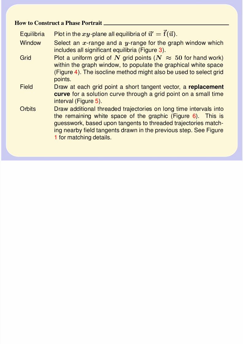
How to Construct a Phase Portrait

Equilibria Plot in the xy-plane all equilibria of u = f ( u).

Window Select an x-range and a y-range for the graph window whichincludes all significant equilibria (Figure 3).

Grid Plot a uniform grid of N grid points (N ≈ 50 for hand work)within the graph window, to populate the graphical white space

(Figure 4). The isocline method might also be used to select gridpoints.

Field Draw at each grid point a short tangent vector, a replacementcurve for a solution curve through a grid point on a small timeinterval (Figure 5).

Orbits Draw additional threaded trajectories on long time intervals intothe remaining white space of the graphic (Figure 6). This isguesswork, based upon tangents to threaded trajectories match-ing nearby field tangents drawn in the previous step. See Figure

1 for matching details.



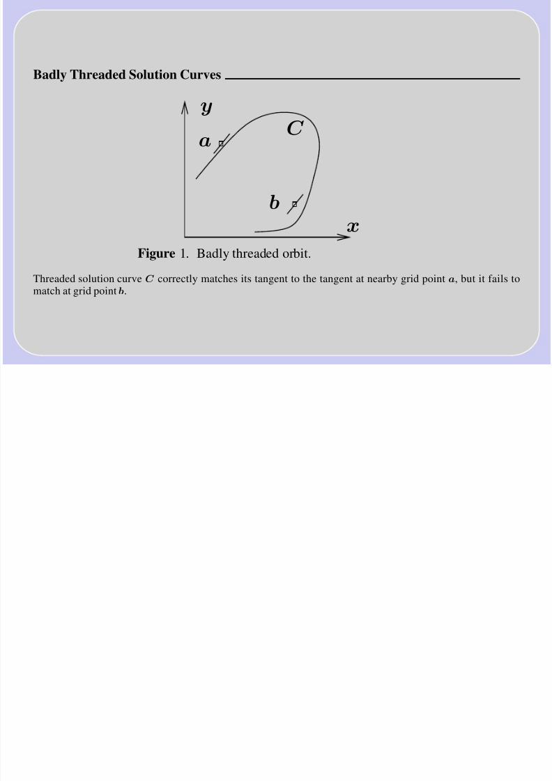
Badly Threaded Solution Curves

C y

xb

a

Figure 1. Badly threaded orbit.

Threaded solution curve C correctly matches its tangent to the tangent at nearby grid point a, but it fails to

match at grid point b.



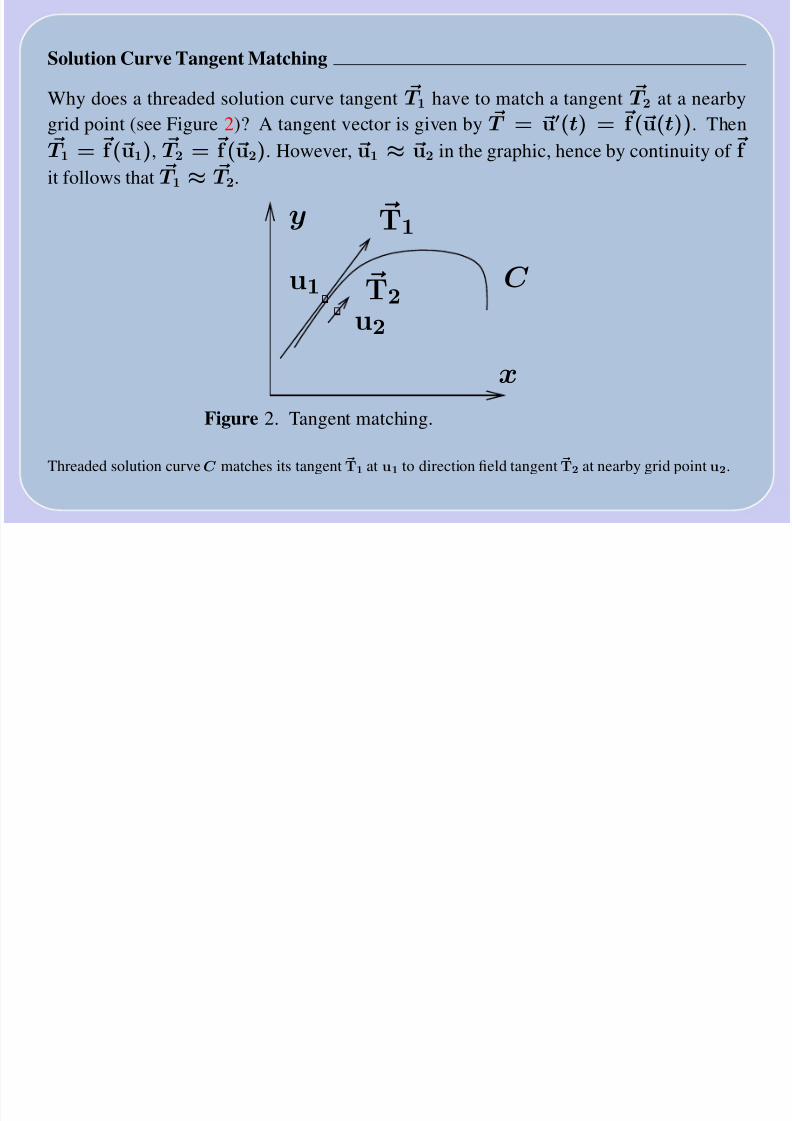
Solution Curve Tangent Matching

Why does a threaded solution curve tangent T 1 have to match a tangent T 2 at a nearby

grid point (see Figure 2)? A tangent vector is given by T = u(t) = f ( u(t)). Then

T 1 = f( u1), T 2 = f ( u2). However, u1 ≈ u2 in the graphic, hence by continuity of f

it follows that T 1 ≈ T 2.

u2

C

x

y T1

T2u1

Figure 2. Tangent matching.

Threaded solution curve C matches its tangent T1 at u1 to direction field tangent T2 at nearby grid point u2.



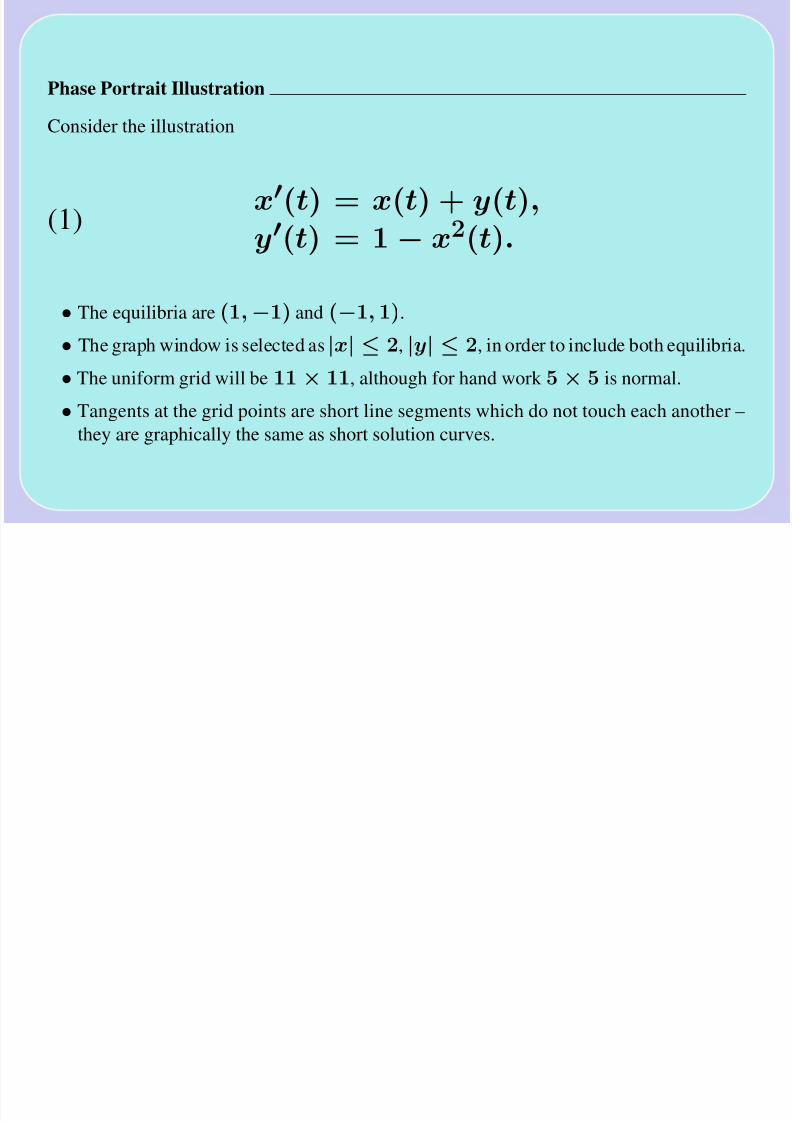
Phase Portrait Illustration

Consider the illustration

x(t) = x(t) + y(t),y(t) = 1 − x2(t).

(1)

• The equilibria are (1,−1) and (−1, 1).

• The graph window is selected as |x| ≤ 2, |y| ≤ 2, in order to include both equilibria.

• The uniform grid will be 11 × 11, although for hand work 5 × 5 is normal.

• Tangents at the grid points are short line segments which do not touch each another –they are graphically the same as short solution curves.



x

(−1, 1)

(1,−1)

−2 2−2

2 y

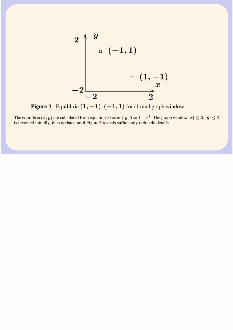
Figure 3. Equilibria (1,−1), (−1, 1) for (1) and graph window.

The equilibria (x, y) are calculated from equations 0 = x+y, 0 = 1−x2. The graph window |x| ≤ 2, |y| ≤ 2

is invented initially, then updated until Figure 5 reveals sufficiently rich field details.



−2 2x−2

2

y

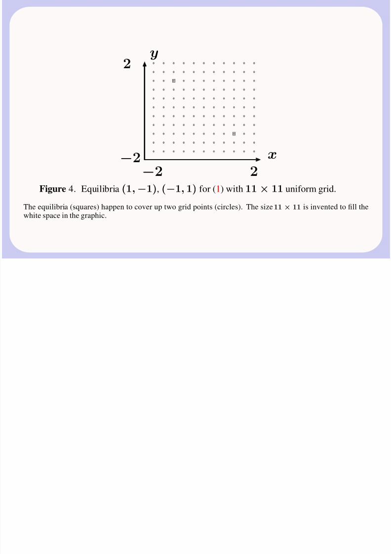
Figure 4. Equilibria (1,−1), (−1, 1) for (1) with 11 × 11 uniform grid.

The equilibria (squares) happen to cover up two grid points (circles). The size 11 × 11 is invented to fill thewhite space in the graphic.



y

x

1

−1

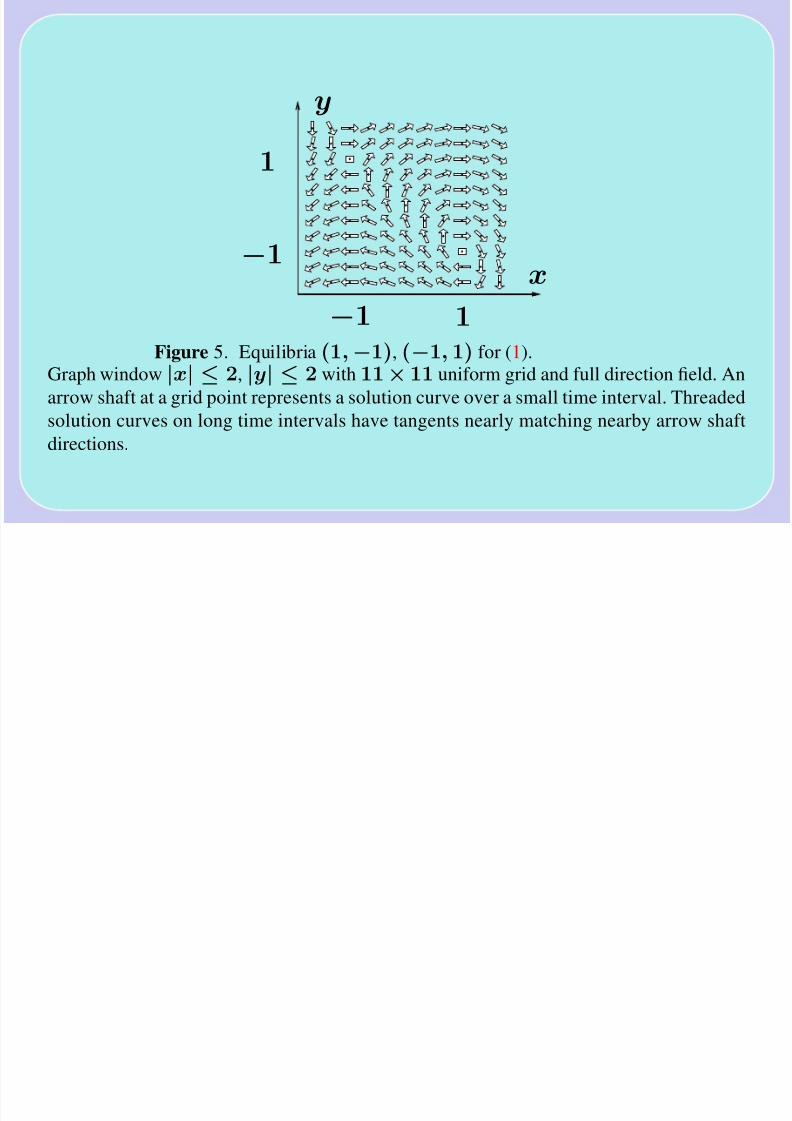
−1 1Figure 5. Equilibria (1,−1), (−1, 1) for (1).

Graph window |x| ≤ 2, |y| ≤ 2 with 11× 11 uniform grid and full direction field. An

arrow shaft at a grid point represents a solution curve over a small time interval. Threaded

solution curves on long time intervals have tangents nearly matching nearby arrow shaftdirections.



−1

1

1

y

x

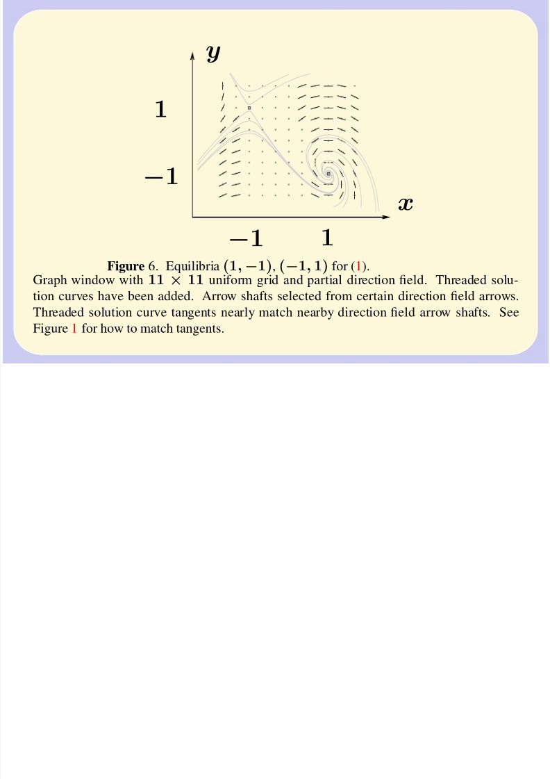
−1Figure 6. Equilibria (1,−1), (−1, 1) for (1).

Graph window with 11 × 11 uniform grid and partial direction field. Threaded solu-

tion curves have been added. Arrow shafts selected from certain direction field arrows.

Threaded solution curve tangents nearly match nearby direction field arrow shafts. See

Figure 1 for how to match tangents.



1

−1 1x

y

−1

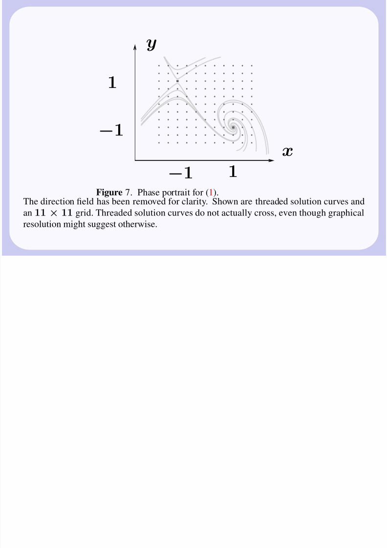
Figure 7. Phase portrait for (1).

The direction field has been removed for clarity. Shown are threaded solution curves andan 11 × 11 grid. Threaded solution curves do not actually cross, even though graphical

resolution might suggest otherwise.



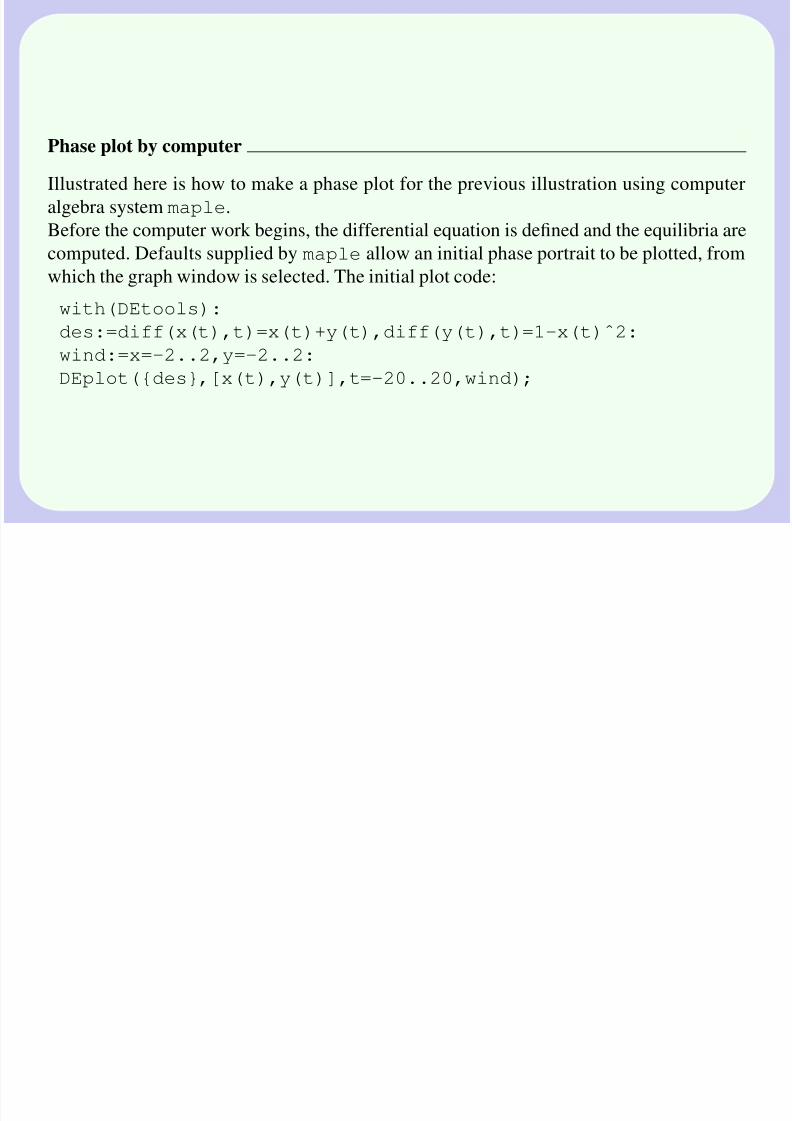
Phase plot by computer

Illustrated here is how to make a phase plot for the previous illustration using computer

algebra system maple.

Before the computer work begins, the differential equation is defined and the equilibria are

computed. Defaults supplied by maple allow an initial phase portrait to be plotted, from

which the graph window is selected. The initial plot code:with(DEtools):

des:=diff(x(t),t)=x(t)+y(t),diff(y(t),t)=1-x(t)ˆ2:

wind:=x=-2..2,y=-2..2:

DEplot({des},[x(t),y(t)],t=-20..20,wind);



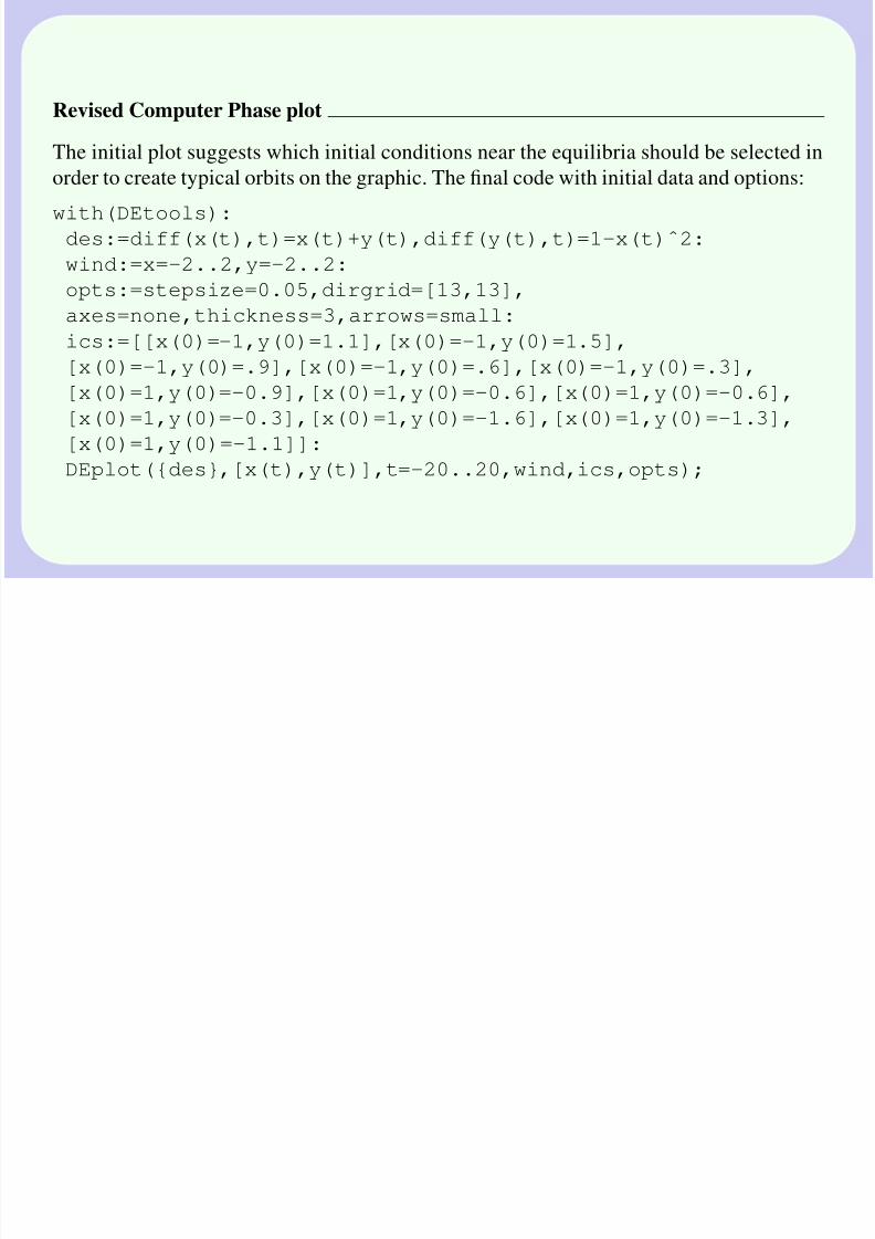
Revised Computer Phase plot

The initial plot suggests which initial conditions near the equilibria should be selected inorder to create typical orbits on the graphic. The final code with initial data and options:

with(DEtools):

des:=diff(x(t),t)=x(t)+y(t),diff(y(t),t)=1-x(t)ˆ2:

wind:=x=-2..2,y=-2..2:

opts:=stepsize=0.05,dirgrid=[13,13],

axes=none,thickness=3,arrows=small:

ics:=[[x(0)=-1,y(0)=1.1],[x(0)=-1,y(0)=1.5],

[x(0)=-1,y(0)=.9],[x(0)=-1,y(0)=.6],[x(0)=-1,y(0)=.3],

[x(0)=1,y(0)=-0.9],[x(0)=1,y(0)=-0.6],[x(0)=1,y(0)=-0.6],

[x(0)=1,y(0)=-0.3],[x(0)=1,y(0)=-1.6],[x(0)=1,y(0)=-1.3],

[x(0)=1,y(0)=-1.1]]:

DEplot({des},[x(t),y(t)],t=-20..20,wind,ics,opts);



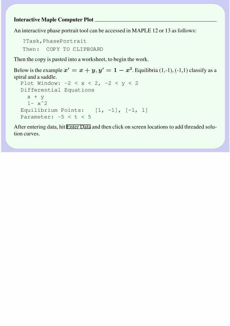
Interactive Maple Computer Plot

An interactive phase portrait tool can be accessed in MAPLE 12 or 13 as follows:

?Task,PhasePortrait

Then: COPY TO CLIPBOARD

Then the copy is pasted into a worksheet, to begin the work.

Below is the example x = x + y , y = 1 − x2. Equilibria (1,-1), (-1,1) classify as a

spiral and a saddle.Plot Window: -2 < x < 2, -2 < y < 2

Differential Equations

x + y

1- xˆ2

Equilibrium Points: [1, -1], [-1, 1]

Parameter: -5 < t < 5

After entering data, hit Enter Data and then click on screen locations to add threaded solu-

tion curves.

Dyn Sys Phase Portrait

Documents

Transcript of Dyn Sys Phase Portrait