
Dpfc Thesis
212
DISTRIBUTED POWER FLOW CONTROLLER Zhihui Yuan 苑 苑 苑 志 辉 辉 辉 Electrical Power Processing (EPP) Unit Electrical Sustainable Energy Department Delft University of Technology
-
Upload
rajapandiya -
Category
Documents
-
view
221 -
download
0
Transcript of Dpfc Thesis
7/25/2019 Dpfc Thesis
http://slidepdf.com/reader/full/dpfc-thesis 1/212
DISTRIBUTED POWER FLOW
CONTROLLER
Zhihui Yuan
苑苑苑苑
志志志志
辉辉辉辉
Electrical Power Processing (EPP) Unit
Electrical Sustainable Energy Department
Delft University of Technology

7/25/2019 Dpfc Thesis
http://slidepdf.com/reader/full/dpfc-thesis 2/212
7/25/2019 Dpfc Thesis
http://slidepdf.com/reader/full/dpfc-thesis 3/212
DISTRIBUTED POWER FLOW
CONTROLLER
Proefschrift
ter verkrijging van de graad van doctor
aan de Technische Universiteit Delft;op gezag van de Rector Magnificus prof. ir. K.C.A.M. Luyben;
voorzitter van het College voor Promoties
in het openbaar te verdedigen op maandag 18 oktober 2010 om 10.00 uur
door
Zhihui YUAN
Master of Science in Engineering, Charlmers University of Technology
geboren te Hei Long Jiang, China
7/25/2019 Dpfc Thesis
http://slidepdf.com/reader/full/dpfc-thesis 4/212
Dit proefschrift is goedgekeurd door de promotor:
Prof. dr. J.A. Ferreira
Samenstelling promotiecommissie:
Rector Magnificus, voorzitter
Prof. dr. J.A. Ferreira, Delft University of Technology, promotor
Ir. S.W.H. de Haan, Delft University of Technology, copromotor
Prof. ir. L. van der Sluis, Delft University of Technology
Prof. dr. ir. M. Verhaegen, Delft University of Technology
Prof. dr. ir. P. Lataire, Vrije Universiteit Brussel
Prof. ir. W.L. Kling, Eindhoven University of Technology
ISBN: 978-90-8570-612-0
Printed by WOHRMANN PRINT SERVICE, Zutphen, the Netherlands.
Proofread by Veronica Pisorn
Copyright c 2010 by Zhihui Yuan
All rights reserved.
7/25/2019 Dpfc Thesis
http://slidepdf.com/reader/full/dpfc-thesis 5/212
ACKNOWLEDGEMENT
The research presented in this thesis was carried out at the Delft University of Technology
in the Netherlands, in the research group of Electrical Power Processing (EPP), in where
I have spent unforgettable four years towards my Ph.D. During this period, many people
directly or indirectly involved in the research and this thesis would not complete without
them. I would like to take this opportunity to express my gratitude and appreciation to
these people.
First of all, I would like to thank to my promoter Professor Braham Ferreira for the
opportunity to do my Ph.D. in the Netherlands and for his guidance and brilliant ideas
that enlighten the research. I wish to express my sincere gratitude to my daily supervisor
Ir. Sjoerd W.H. de Haan, whose door was always open to me. Thanks for his guidance
and so many discussions on the research. I am also grateful for his patience on correcting
my papers and thesis. Without him, the thesis would not be possible.
I would also like to thank my doctoral examination committee, Prof. Philippe Lataire,
Prof. Lou van der Sluis, Prof. Michel Verhaegen and Prof. Wil Kling for spending a
large amount of time on reading on my draft thesis and giving valuable comments and
suggestions.
The research presented in this thesis was partially funded from the energy research
program ‘Energie Onderzoek Subsidie (EOS)’, supported by the Ministry of Economic
Affairs, the Netherlands. I wish to express my thanks for the support.
In addition, I would like to thank my colleagues and friends in the EPP group, espe-
cially Rob Schoevaars for his great help and assistance of my experiment, Bart Rooden-
burg for the translation of the summary into Dutch and Rick van Kessel for translating
the propositions into Dutch. Thanks to Aleksandar Borisavljevic, Anoop Jassal, Balazs
i

7/25/2019 Dpfc Thesis
http://slidepdf.com/reader/full/dpfc-thesis 6/212
ii
Czech, Dalibor Cvoric and J. Marcelo Gutierrez-Alcaraz for the enjoyable sports and fun
activities. It was super fun to play tennis, snowboard and to do gym with you. I wouldalso like to thank to Deok-Je Bang, Dongshen Zhao, Ghanshyam Shrestha, Ivan Josifovic,
Johan Wolmarans, Yi Wang and Yi Zhou for making the time of my Ph.D. enjoyable.
Last but not least, I would like to thank my family; my mother Gao Ling, my father
Yuan QingGuo and my lovely wife Zhao Bo, to whom this thesis is dedicated for, for their
love, support and understanding.

7/25/2019 Dpfc Thesis
http://slidepdf.com/reader/full/dpfc-thesis 7/212
To my family

7/25/2019 Dpfc Thesis
http://slidepdf.com/reader/full/dpfc-thesis 8/212
7/25/2019 Dpfc Thesis
http://slidepdf.com/reader/full/dpfc-thesis 9/212
SUMMARY
In modern power systems, there is a great demand to control the power flow actively.
Power flow controlling devices (PFCDs) are required for such purpose, because the power
flow over the lines is the nature result of the impedance of each line. Due to the control
capabilities of different types of PFCDs, the trend is that mechanical PFCDs are gradually
being replaced by Power Electronics (PE) PFCDs. Among all PE PFCDs, the Unified
Power Flow Controller (UPFC) is the most versatile device. However, the UPFC is not
widely applied in utility grids, because the cost of such device is much higher than the
rest of PFCDs and the reliability is relatively low due to its complexity.
The objective of this thesis is to develop a new PFCD that offers the same control
capability as the UPFC, at a reduced cost and with an increased reliability. The new
device, so-called Distributed Power Flow Controller (DPFC), is invented and presented
in this thesis. The DPFC is a further development of the UPFC. It has been shown that
the DPFC fulfills all three of the listed goals. This thesis starts with the review the state-
of-art of current PFCDs, followed by the research at the DPFC device level, including
the operation principle, the modeling and control, and experimental demonstrations. At
the end, the thesis presents the research at the system level, which includes the DPFC
applications to improve power system controllability and stability, and the feasibility of
the DPFC for real networks.
Device Level
The DPFC eliminates the common DC link within the UPFC, to enable the independent
operation of the shunt and the series converter. The D-FACTS concept is employed in
v
7/25/2019 Dpfc Thesis
http://slidepdf.com/reader/full/dpfc-thesis 10/212
vi
the design of the series converter. Multiple low-rating single-phase converters replace the
high-rating three-phase series converter, which greatly reduces the cost and increases thereliability. The active power that used to exchange through the common DC link in the
UPFC, is now transferred through the transmission line at the 3rd harmonic frequency.
The DPFC has been modeled in a rotating dq -frame. Based on this model, the basic
control of the DPFC is developed. The basic control stabilizes the level of the capacitor
DC voltage of each converter and ensures that the converters inject the voltages into the
network according to the command from the central control. The shunt converter injects
a constant current at the 3rd harmonic frequency, while its DC voltage is stabilized by the
fundamental frequency component. For the series converter, the reference of the output
voltage at the fundamental frequency is obtained from the central controller and the DC
voltage level is maintained by the 3rd harmonic component.
To verify the dynamic model and the basic control, a DPFC demonstration setup is
built. The setup consists of a scaled network, one shunt converter and six series converters.
All DPFC converters are independently controlled by their own DSP controllers. It shows
that the shunt and series converters can exchange active power through the 3rd harmonic
component and that the DC voltages of the series converter can be maintained at a
constant level during different situations.
The fault tolerance of the DPFC is also investigated. The protection method of the
DPFC for different types of failures is addressed. In addition, the use of supplementary
controls to ensure the continuously operation of the DPFC during converter failures is
presented.
Power System Level
Two applications of the DPFC at the system level are investigated, namely utilizing the
DPFC to damp low-frequency power oscillation and to compensate asymmetrical voltages.
A maximum of three Power Oscillation Damping (POD) controllers can be applied to one
DPFC, which indicates that the DPFC can shift three critical oscillatory modes at the
same time. Within the thesis, the POD controller is designed using the residue method and
a two-area network is used in the case study. For asymmetry compensation, the DPFC can
compensate both active and reactive asymmetry at the fundamental frequency, because
of the active power exchange between the shunt and the series converters. In addition,
7/25/2019 Dpfc Thesis
http://slidepdf.com/reader/full/dpfc-thesis 11/212
vii
since the series converter is single-phase converter, the DPFC can compensate for both
zero and negative sequence components. Accordingly, the DPFC currently is the mostversatile device for asymmetry compensation among all FACTS devices.
DPFC design procedures are introduced, which give the equations to determine the
major parameters of the DPFC. According to the procedure, a case study, which is to
use DPFC to replace the KEPCO UPFC in Korea, is investigated. It is found that in
order to achieve the same control capability as the UPFC, the DPFC requires much less
material and creates a smaller footprint. The application of the DPFC for power flow
control is discussed and a triangle network in the Netherlands is selected as the case. It
shows that the DPFC can dynamically control the power flow within the triangle network.In addition, the DPFC improves the voltage and angle stability of the network.

7/25/2019 Dpfc Thesis
http://slidepdf.com/reader/full/dpfc-thesis 12/212
7/25/2019 Dpfc Thesis
http://slidepdf.com/reader/full/dpfc-thesis 13/212
Samenvatting
Er is een grote vraag ontstaan om het energietransport in moderne elektriciteitsnetwerken
actief te kunnen regelen. Het energietransport over een lijn wordt bepaald door de aard
(impedantie) van elke lijn en voor actieve regeling zijn Power Flow Controlling Devices
(PFCDs) nodig. Door de beperkte mogelijkheden van de verschillende soorten PFCDs
is de trend dat mechanische PFCDs geleidelijk worden vervangen door varianten met
vermogenselektronica, zogenaamde PE PFCDs. Van alle PE PFCDs is de Unified PowerFlow Controller (UPFC) het meest veelzijdig. Deze worden echter niet op grote schaal
in elektriciteitsnetten toegepast omdat de kosten van dergelijke apparatuur veel hoger
ligt dan die van standaard PFCDs en tevens is door de complexiteit van de UPFC de
betrouwbaarheid relatief laag.
Het doel van dit proefschrift is om een nieuwe PFCD te ontwikkelen met dezelfde
controle mogelijkheden als de UPFC, maar dan tegen lagere kosten en met een hogere
betrouwbaarheid. Het ontwikkelde nieuwe apparaat, de zogenaamde Distributed PowerFlow Controller (DPFC) is beschreven in dit proefschrift. De DPFC is een verdere on-
twikkeling van de UPFC. Er wordt aangetoond dat de DPFC voldoet aan alle drie de
gestelde doelen. Dit proefschrift begint met een overzicht van de huidige PFCD tech-
nieken en vervolgens wordt het onderzoek aan de DPFC op apparaat niveau beschreven,
met inbegrip van het werkingsprincipe, de modellering, het regelgedrag, en experimentele
validatie. Als laatste presenteert het proefschrift het onderzoek op systeem niveau, in-
clusief de DPFC toepassingen voor het verbeteren van de stabiliteit en regelbaarheid van
netten en de haalbaarheid van de DPFC in het echte elektriciteitsnet.
ix
7/25/2019 Dpfc Thesis
http://slidepdf.com/reader/full/dpfc-thesis 14/212
x
Apparaat Niveau
De DPFC elimineert de gemeenschappelijke DC tussenkring in de UPFC, om een on-
afhankelijke werking van de shunt- en de series converter mogelijk te maken. Bij het on-
twerpen van de series converter is gebruik gemaakt van het D-FACTS concept. Meerdere
laag vermogen enkelfase omvormers vervangen de hoog vermogen driefasen serie converter.
Dit reduceert de kosten en verhoogt de betrouwbaarheid sterk. Het actieve vermogen
dat uitgewisseld werd via de gemeenschappelijke DC tussenkring in de UPFC, wordt nu
overgebracht via de transmissie lijn op de 3e harmonische frequentie.
De DPFC is gemodelleerd in een roterend dq stelsel en de ontwikkelde regeling van deDPFC is gebaseerd op dit model. De regeling stabiliseert het niveau van de condensator
gelijkspanning van elke converter en zorgt ervoor dat de te injecteren spanning in het
netwerk in overeenstemming is met het commando vanuit de centrale regelaar. De shunt
converter injecteert een constante 3e harmonische stroom, terwijl de DC spanning wordt
gestabiliseerd door de fundamentele frequentie. Het referentiesignaal aan serie converter
voor de fundamentele frequentie van de uitgangsspanning wordt verkregen vanuit de cen-
trale regelaar en het DC spanningsniveau wordt gehandhaafd door de 3e harmonische
component.Om het dynamische model en de fundamentele werking van de regelaar te verifiren
is een DPFC demonstrator gebouwd. De opstelling bestaat uit een geschaald netwerk,
een shunt converter en zes serie converters. Alle DPFC converters worden onafhankelijk
geregeld door hun eigen DSP regelaar. Hieruit blijkt dat de shunt- en series converters
actief vermogen kunnen uit te wisselen via de 3e harmonische component en dat de DC
spanning van de serie converter op een constant niveau kan worden gehouden gedurende
verschillende situaties.
Eveneens is de fouttolerantie van de DPFC onderzocht, inclusief de beveiliging ten
gevolge van verschillende fouten en het gebruik van aanvullende regelingen om de sys-
teemeigenschappen te verbeteren tijdens converter fouten.
System Niveau
Twee toepassingen van de DPFC zijn op systeemniveau onderzocht, te weten het gebruik
van de DPFC om laagfrequente vermogensoscillaties te dempen en de mogelijkheid om
7/25/2019 Dpfc Thesis
http://slidepdf.com/reader/full/dpfc-thesis 15/212
xi
asymmetrische spanningen te compenseren. Op een DPFC kunnen maximaal drie Power
Oscillatie Damping (POD) regelaars worden toegepast, waardoor de DPFC drie kritischeresonantie modes op hetzelfde moment kan verschuiven. De POD regelaar in dit proef-
schrift is ontworpen met behulp van de residue-method en in de case studie is een two-area
netwerk gebruikt. Tijdens asymmetrie compensatie kan de DPFC zowel actieve- als re-
actieve asymmetrie compenseren op de fundamentele frequentie. Dit is mogelijk omdat
actief vermogen uitgewisseld kan worden tussen de shunt- en de serie converters. Omdat
de serie converter een n fase converter is, kan de DPFC zowel de homopolaire component
als de negatieve component compenseren. Daardoor is de DPFC op dit moment het meest
veelzijdig van alle FACTS apparaten.Voor het bepalen van de systeemoverdracht en de belangrijkste parameters van de
DPFC is een ontwerp procedure ontwikkeld. Volgens deze procedure is een DPFC case
studie uitgevoerd, waarbij de KEPCO UPFC in Korea moest worden vervangen. Hieruit
kwam naar voren dat de DPFC bij gelijke regeleigenschappen veel minder materiaal en
ruimte nodig heeft. De toepassing om het energietransport te regelen met een DPFC
is besproken aan de hand van een driehoekig netwerk in Nederland. Hieruit blijkt dat
de DPFC in staat is het energietransport in dit netwerk dynamisch te kunnen regelen.
Bovendien verbetert de DPFC de spanning en de fase stabiliteit van het netwerk.

7/25/2019 Dpfc Thesis
http://slidepdf.com/reader/full/dpfc-thesis 16/212
7/25/2019 Dpfc Thesis
http://slidepdf.com/reader/full/dpfc-thesis 17/212
Contents
1 INTRODUCTION 1
1.1 Background . . . . . . . . . . . . . . . . . . . . . . . . . . . . . . . . . . . 1
1.2 Power Flow Controlling Devices . . . . . . . . . . . . . . . . . . . . . . . . 4
1.3 Problem Definition . . . . . . . . . . . . . . . . . . . . . . . . . . . . . . . 8
1.4 Objective and Approaches . . . . . . . . . . . . . . . . . . . . . . . . . . . 9
1.5 Thesis Layout . . . . . . . . . . . . . . . . . . . . . . . . . . . . . . . . . . 10
2 OVERVIEW OF POWER FLOW CONTROLLING DEVICES 13
2.1 Introduction . . . . . . . . . . . . . . . . . . . . . . . . . . . . . . . . . . . 13
2.2 Power Flow Control Theory . . . . . . . . . . . . . . . . . . . . . . . . . . 13
2.3 Categorization of PFCDs . . . . . . . . . . . . . . . . . . . . . . . . . . . . 16
2.4 Shunt Devices . . . . . . . . . . . . . . . . . . . . . . . . . . . . . . . . . . 16
2.4.1 SVC . . . . . . . . . . . . . . . . . . . . . . . . . . . . . . . . . . . 17
2.4.2 STATCOM . . . . . . . . . . . . . . . . . . . . . . . . . . . . . . . 19
2.5 Series Devices . . . . . . . . . . . . . . . . . . . . . . . . . . . . . . . . . . 212.5.1 TSSC . . . . . . . . . . . . . . . . . . . . . . . . . . . . . . . . . . 22
2.5.2 TCSC . . . . . . . . . . . . . . . . . . . . . . . . . . . . . . . . . . 22
2.5.3 SSSC . . . . . . . . . . . . . . . . . . . . . . . . . . . . . . . . . . . 23
2.5.4 DSSC . . . . . . . . . . . . . . . . . . . . . . . . . . . . . . . . . . 24
2.6 Combined Devices . . . . . . . . . . . . . . . . . . . . . . . . . . . . . . . 25
2.6.1 PST . . . . . . . . . . . . . . . . . . . . . . . . . . . . . . . . . . . 25
2.6.2 UPFC . . . . . . . . . . . . . . . . . . . . . . . . . . . . . . . . . . 26
2.7 IPFC . . . . . . . . . . . . . . . . . . . . . . . . . . . . . . . . . . . . . . . 27
xiii
7/25/2019 Dpfc Thesis
http://slidepdf.com/reader/full/dpfc-thesis 18/212
xiv CONTENTS
2.8 Conclusions . . . . . . . . . . . . . . . . . . . . . . . . . . . . . . . . . . . 28
3 DISTRIBUTED POWER FLOW CONTROLLER 29
3.1 Introduction . . . . . . . . . . . . . . . . . . . . . . . . . . . . . . . . . . . 29
3.2 Distributed Power Flow Controller (DPFC) . . . . . . . . . . . . . . . . . 30
3.2.1 DPFC Topology . . . . . . . . . . . . . . . . . . . . . . . . . . . . . 31
3.2.2 DPFC Operating Principle . . . . . . . . . . . . . . . . . . . . . . . 31
3.2.3 DPFC Control . . . . . . . . . . . . . . . . . . . . . . . . . . . . . 35
3.2.4 Variation of the Shunt Converter . . . . . . . . . . . . . . . . . . . 36
3.2.5 Advantages and Limitation of the DPFC . . . . . . . . . . . . . . . 373.3 DPFC Steady-State Analysis . . . . . . . . . . . . . . . . . . . . . . . . . . 38
3.3.1 DPPF Simplification and Equivalent Circuit . . . . . . . . . . . . . 38
3.3.2 Fundamental Frequency Circuit . . . . . . . . . . . . . . . . . . . . 40
3.3.3 Third Harmonic Frequency Circuit . . . . . . . . . . . . . . . . . . 44
3.3.4 Control Range of the DPFC . . . . . . . . . . . . . . . . . . . . . . 46
3.4 Distributed Interline Power Flow Controller . . . . . . . . . . . . . . . . . 47
3.4.1 DIPFC Topology . . . . . . . . . . . . . . . . . . . . . . . . . . . . 47
3.4.2 DIPFC Operating Principle . . . . . . . . . . . . . . . . . . . . . . 483.4.3 DIPFC Control . . . . . . . . . . . . . . . . . . . . . . . . . . . . . 50
3.5 DIPFC Steady-State Analysis . . . . . . . . . . . . . . . . . . . . . . . . . 51
3.5.1 DIPPF Simplification and Equivalent Circuit . . . . . . . . . . . . . 51
3.5.2 Fundamental Frequency Circuit . . . . . . . . . . . . . . . . . . . . 53
3.5.3 Third Harmonic Frequency Circuit . . . . . . . . . . . . . . . . . . 53
3.6 Conclusions . . . . . . . . . . . . . . . . . . . . . . . . . . . . . . . . . . . 54
4 DPFC MODELING AND BASIC CONTROL 574.1 Introduction . . . . . . . . . . . . . . . . . . . . . . . . . . . . . . . . . . . 57
4.2 DPFC Modeling . . . . . . . . . . . . . . . . . . . . . . . . . . . . . . . . . 58
4.2.1 DPFC Model Overview . . . . . . . . . . . . . . . . . . . . . . . . . 59
4.2.2 Connection of Separated Models . . . . . . . . . . . . . . . . . . . . 60
4.2.3 Network Modeling . . . . . . . . . . . . . . . . . . . . . . . . . . . 60
4.2.4 Series Converter Modeling . . . . . . . . . . . . . . . . . . . . . . . 64
4.2.5 Shunt Converter Modeling . . . . . . . . . . . . . . . . . . . . . . . 66
4.3 DPFC Basic Control . . . . . . . . . . . . . . . . . . . . . . . . . . . . . . 69
7/25/2019 Dpfc Thesis
http://slidepdf.com/reader/full/dpfc-thesis 19/212
CONTENTS xv
4.3.1 Series Converter Control . . . . . . . . . . . . . . . . . . . . . . . . 69
4.3.2 Shunt Converter Control . . . . . . . . . . . . . . . . . . . . . . . . 724.4 Simulation Results of the DPFC Modeling and Control . . . . . . . . . . . 78
4.5 Communication Between the Central Control and Series Converters . . . . 80
4.5.1 Principle of the Method . . . . . . . . . . . . . . . . . . . . . . . . 81
4.5.2 Simulation Results . . . . . . . . . . . . . . . . . . . . . . . . . . . 83
4.6 Conclusions . . . . . . . . . . . . . . . . . . . . . . . . . . . . . . . . . . . 84
5 DPFC EXPERIMENTAL DEMONSTRATOR 87
5.1 Introduction . . . . . . . . . . . . . . . . . . . . . . . . . . . . . . . . . . . 875.2 Specifications . . . . . . . . . . . . . . . . . . . . . . . . . . . . . . . . . . 87
5.2.1 Scaled Network Specifications . . . . . . . . . . . . . . . . . . . . . 88
5.2.2 DPFC Converter Specifications . . . . . . . . . . . . . . . . . . . . 89
5.3 DPFC Experimental Setup . . . . . . . . . . . . . . . . . . . . . . . . . . . 91
5.3.1 Scaled Network . . . . . . . . . . . . . . . . . . . . . . . . . . . . . 91
5.3.2 Series Converter . . . . . . . . . . . . . . . . . . . . . . . . . . . . . 92
5.3.3 Shunt Converter . . . . . . . . . . . . . . . . . . . . . . . . . . . . 92
5.3.4 Overall Experimental Setup . . . . . . . . . . . . . . . . . . . . . . 935.4 DPFC Control Realization . . . . . . . . . . . . . . . . . . . . . . . . . . . 94
5.5 Results of the Experimental Setup . . . . . . . . . . . . . . . . . . . . . . . 95
5.5.1 Steady-state Results . . . . . . . . . . . . . . . . . . . . . . . . . . 95
5.5.2 Step-response Results . . . . . . . . . . . . . . . . . . . . . . . . . . 97
5.6 Conclusions . . . . . . . . . . . . . . . . . . . . . . . . . . . . . . . . . . . 99
6 DPFC FAULT TOLERANCE 101
6.1 Introduction . . . . . . . . . . . . . . . . . . . . . . . . . . . . . . . . . . . 1016.2 Possible Faults in the DPFC . . . . . . . . . . . . . . . . . . . . . . . . . . 101
6.3 Shunt Converter Failure . . . . . . . . . . . . . . . . . . . . . . . . . . . . 103
6.3.1 Introduction . . . . . . . . . . . . . . . . . . . . . . . . . . . . . . . 103
6.3.2 Principle of the Control . . . . . . . . . . . . . . . . . . . . . . . . 103
6.3.3 Transient Analysis . . . . . . . . . . . . . . . . . . . . . . . . . . . 107
6.3.4 Simulation and Experiments Results . . . . . . . . . . . . . . . . . 109
6.4 Series Converter Failure . . . . . . . . . . . . . . . . . . . . . . . . . . . . 111
6.4.1 Introduction . . . . . . . . . . . . . . . . . . . . . . . . . . . . . . . 111
7/25/2019 Dpfc Thesis
http://slidepdf.com/reader/full/dpfc-thesis 20/212
xvi CONTENTS
6.4.2 Principle of the Control . . . . . . . . . . . . . . . . . . . . . . . . 111
6.4.3 Compensation Controller Design . . . . . . . . . . . . . . . . . . . . 1136.4.4 Simulation Results . . . . . . . . . . . . . . . . . . . . . . . . . . . 115
6.5 Conclusions . . . . . . . . . . . . . . . . . . . . . . . . . . . . . . . . . . . 117
7 DPFC AUXILIARY SERVICES 119
7.1 Introduction . . . . . . . . . . . . . . . . . . . . . . . . . . . . . . . . . . . 119
7.2 Power Oscillation Damping (POD) . . . . . . . . . . . . . . . . . . . . . . 120
7.2.1 Background . . . . . . . . . . . . . . . . . . . . . . . . . . . . . . . 120
7.2.2 POD Controller . . . . . . . . . . . . . . . . . . . . . . . . . . . . . 1217.2.3 DPFC Current Injection Model . . . . . . . . . . . . . . . . . . . . 121
7.2.4 DPFC POD Controller Design . . . . . . . . . . . . . . . . . . . . . 123
7.2.5 Case Study . . . . . . . . . . . . . . . . . . . . . . . . . . . . . . . 126
7.2.6 Summary . . . . . . . . . . . . . . . . . . . . . . . . . . . . . . . . 129
7.3 Asymmetrical Component Compensation . . . . . . . . . . . . . . . . . . . 129
7.3.1 Background . . . . . . . . . . . . . . . . . . . . . . . . . . . . . . . 129
7.3.2 Principle of Compensating the Asymmetrical Voltage . . . . . . . . 130
7.3.3 Analysis . . . . . . . . . . . . . . . . . . . . . . . . . . . . . . . . . 1327.3.4 Case Study . . . . . . . . . . . . . . . . . . . . . . . . . . . . . . . 134
7.3.5 Summary . . . . . . . . . . . . . . . . . . . . . . . . . . . . . . . . 135
7.4 Conclusions . . . . . . . . . . . . . . . . . . . . . . . . . . . . . . . . . . . 135
8 DPFC APPLICATION IN UTILITY GRIDS 137
8.1 Introduction . . . . . . . . . . . . . . . . . . . . . . . . . . . . . . . . . . . 137
8.2 DPFC Design Procedure . . . . . . . . . . . . . . . . . . . . . . . . . . . . 137
8.2.1 System Level . . . . . . . . . . . . . . . . . . . . . . . . . . . . . . 1388.2.2 DPFC Level . . . . . . . . . . . . . . . . . . . . . . . . . . . . . . . 138
8.2.3 Converter Level . . . . . . . . . . . . . . . . . . . . . . . . . . . . . 141
8.3 Case Study 1: Two-Port Network . . . . . . . . . . . . . . . . . . . . . . . 144
8.3.1 Case Specifications . . . . . . . . . . . . . . . . . . . . . . . . . . . 144
8.3.2 DPFC Design . . . . . . . . . . . . . . . . . . . . . . . . . . . . . . 146
8.3.3 Comparison . . . . . . . . . . . . . . . . . . . . . . . . . . . . . . . 147
8.4 Case Study 2: Triangle Network . . . . . . . . . . . . . . . . . . . . . . . . 149
8.4.1 Case Specifications . . . . . . . . . . . . . . . . . . . . . . . . . . . 149
7/25/2019 Dpfc Thesis
http://slidepdf.com/reader/full/dpfc-thesis 21/212
CONTENTS xvii
8.4.2 DPFC Solution . . . . . . . . . . . . . . . . . . . . . . . . . . . . . 150
8.4.3 Control Scheme . . . . . . . . . . . . . . . . . . . . . . . . . . . . . 1518.4.4 Advantages of the DPFC solution . . . . . . . . . . . . . . . . . . . 152
8.4.5 Simulation Results . . . . . . . . . . . . . . . . . . . . . . . . . . . 152
8.5 Conclusions . . . . . . . . . . . . . . . . . . . . . . . . . . . . . . . . . . . 155
9 CONCLUSIONS AND RECOMMENDATIONS 157
9.1 Conclusions . . . . . . . . . . . . . . . . . . . . . . . . . . . . . . . . . . . 157
9.2 Recommendations . . . . . . . . . . . . . . . . . . . . . . . . . . . . . . . . 160
A PARK’S TRANSFORMATION 163
A.1 3-Phase Park’s Transformation . . . . . . . . . . . . . . . . . . . . . . . . . 163
A.2 Single-phase Park’s Transformation . . . . . . . . . . . . . . . . . . . . . . 164
B SINGLE-PHASE PHASE LOCK LOOP 167
C NETWORK SIMPLFICATION 169
C.1 Network Specifications . . . . . . . . . . . . . . . . . . . . . . . . . . . . . 169
C.2 Network Simplification . . . . . . . . . . . . . . . . . . . . . . . . . . . . . 170
C.3 PU Values . . . . . . . . . . . . . . . . . . . . . . . . . . . . . . . . . . . . 171
C.4 Experimental Setup Specifications . . . . . . . . . . . . . . . . . . . . . . . 171
D LIST OF SYMBOLS 173
REFERENCES 185
LIST OF PUBLICATIONS 187
CURRICULUM VITAE 189

7/25/2019 Dpfc Thesis
http://slidepdf.com/reader/full/dpfc-thesis 22/212
7/25/2019 Dpfc Thesis
http://slidepdf.com/reader/full/dpfc-thesis 23/212
Chapter 1INTRODUCTION
1.1 Background
S INCE Thomas Edison and his company, the Edison Electric Light Company, devel-
oped the first steam-powered electric power station on Pearl Street in New York City,
electricity has played an increasingly important role in our daily lives, with a dramatic
increase in consumption as well as the generation of electricity over the past hundred
years. In the year 2008, the world’s electricity consumption reached 17.48 tera kWh1 and
this number continuously advances.
The electrical power system serves to deliver electrical energy to consumers. An elec-
trical power system deals with electrical generation, transmission, distribution and con-
sumption. In a traditional power system, the electrical energy is generated by centralized
power plants and flows to customers via the transmission and distribution network. The
rate of the transported electrical energy within the lines of the power system is referred
to as ‘Power Flow’ [Park 09], to be more specific, it is the active and reactive power that
flows in the transmission lines.
During the last twenty years, the operation of power systems has changed due to
growing consumption, the development of new technology, the behavior of the electricity
market and the development of renewable energies. In addition to existing changes, in
the future, new devices, such as electrical vehicles, distributed generation and smart grid
concepts, will be employed in the power system, making the system extremely complex.
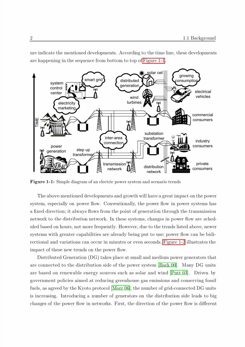
Figure 1-1 shows the representation of a future power system, where the clouds in the fig-
1
DATA SOURCE: CIA World Factbook
1
7/25/2019 Dpfc Thesis
http://slidepdf.com/reader/full/dpfc-thesis 24/212
2 1.1 Background
ure indicate the mentioned developments. According to the time line, these developments
are happening in the sequence from bottom to top of Figure 1-1.
transmission
network
substation
transformer
step up
transformer
power
generation
distribution
network
industry
consumers
private
consumers
inter-area
connection
commercial
consumers
distributed
generation
solar cell
wind
turbines
growing
consumption
electrical
vehicles
system
control
center
electricity
marketing
smart grid
T I M
E
Figure 1-1: Simple diagram of an electric power system and scenario trends
The above-mentioned developments and growth will have a great impact on the power
system, especially on power flow. Conventionally, the power flow in power systems has
a fixed direction; it always flows from the point of generation through the transmission
network to the distribution network. In these systems, changes in power flow are sched-
uled based on hours, not more frequently. However, due to the trends listed above, newer
systems with greater capabilities are already being put to use; power flow can be bidi-
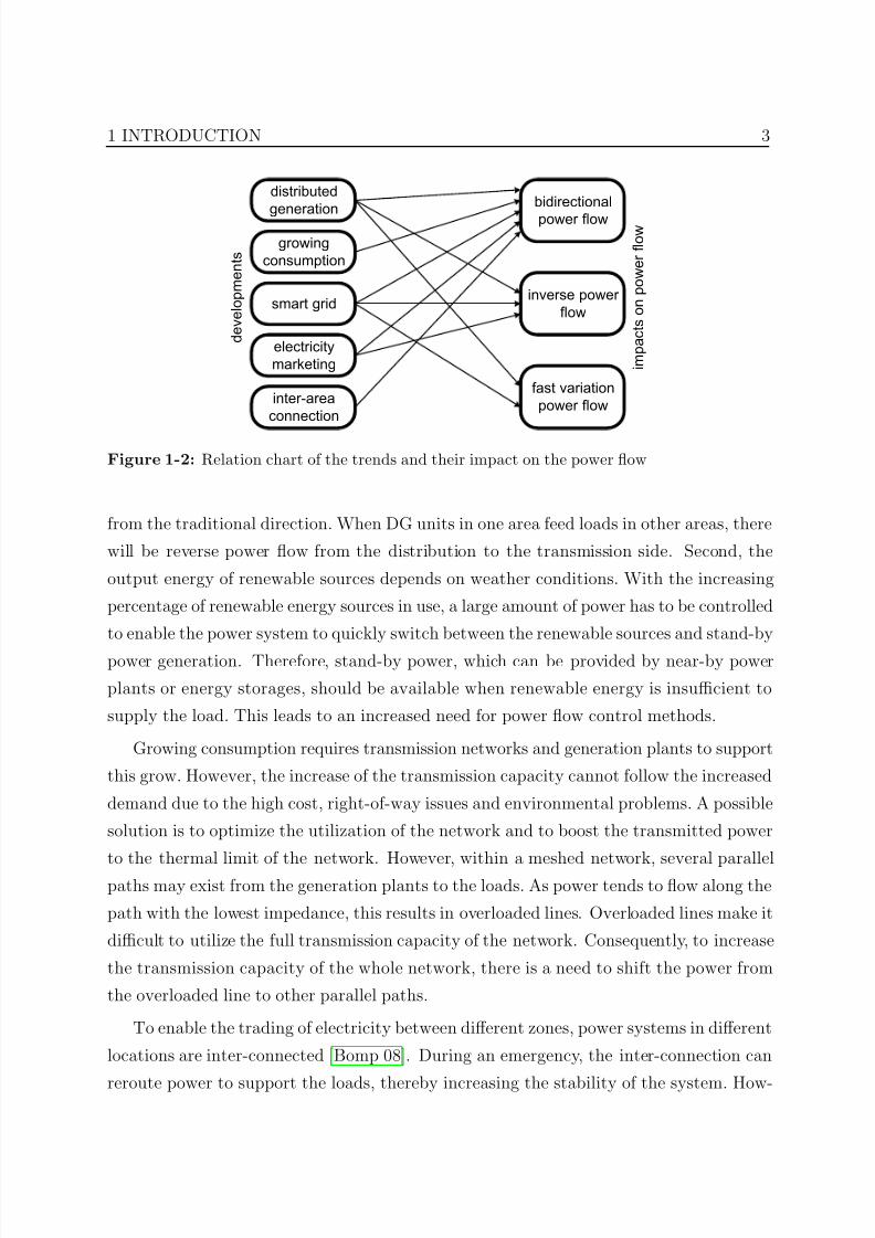
rectional and variations can occur in minutes or even seconds. Figure 1-2 illustrates theimpact of these new trends on the power flow.
Distributed Generation (DG) takes place at small and medium power generators that
are connected to the distribution side of the power system [Bark 00]. Many DG units
are based on renewable energy sources such as solar and wind [ Putt 03]. Driven by
government policies aimed at reducing greenhouse gas emissions and conserving fossil
fuels, as agreed by the Kyoto protocol [Morr 06], the number of grid-connected DG units
is increasing. Introducing a number of generators on the distribution side leads to big
changes of the power flow in networks. First, the direction of the power flow is different
7/25/2019 Dpfc Thesis
http://slidepdf.com/reader/full/dpfc-thesis 25/212
1 INTRODUCTION 3
distributed
generation
growing
consumption
smart grid
electricity
marketing
inter-area
connection
bidirectional
power flow
inverse power
flow
fast variation
power flow
d e v e l o p m e n t s
i m p a c t s o n p o w e r f l o w
Figure 1-2: Relation chart of the trends and their impact on the power flow
from the traditional direction. When DG units in one area feed loads in other areas, there
will be reverse power flow from the distribution to the transmission side. Second, the
output energy of renewable sources depends on weather conditions. With the increasing
percentage of renewable energy sources in use, a large amount of power has to be controlled
to enable the power system to quickly switch between the renewable sources and stand-by
power generation. Therefore, stand-by power, which can be provided by near-by power
plants or energy storages, should be available when renewable energy is insufficient to
supply the load. This leads to an increased need for power flow control methods.
Growing consumption requires transmission networks and generation plants to support
this grow. However, the increase of the transmission capacity cannot follow the increased
demand due to the high cost, right-of-way issues and environmental problems. A possible
solution is to optimize the utilization of the network and to boost the transmitted power
to the thermal limit of the network. However, within a meshed network, several parallelpaths may exist from the generation plants to the loads. As power tends to flow along the
path with the lowest impedance, this results in overloaded lines. Overloaded lines make it
difficult to utilize the full transmission capacity of the network. Consequently, to increase
the transmission capacity of the whole network, there is a need to shift the power from
the overloaded line to other parallel paths.
To enable the trading of electricity between different zones, power systems in different
locations are inter-connected [Bomp 08]. During an emergency, the inter-connection can
reroute power to support the loads, thereby increasing the stability of the system. How-
7/25/2019 Dpfc Thesis
http://slidepdf.com/reader/full/dpfc-thesis 26/212
4 1.2 Power Flow Controlling Devices
ever, inter-area connections result in multiple parallel paths between power plants and
consumers, which give rise to loop flow [Choo 06] and cause congestions. To reduce theloop flow, there is a need for bidirectional power flow control between zones [Wei 03].
The electricity market is a system for effecting the purchase and sale of electricity,
using supply and demand to set the price [Song 03]. With the emerging liberalization of
the electricity market, power prefers to flow ‘from the source with the lowest price in the
direction of the highest price’ [Grai 94]. To ensure that the power flows according to the
economic law, rather than Ohm’s law, the power should be controlled to flow within the
transmission network with the desired direction and quantity.
A smart grid is a concept that integrates IT technology into the electricity network to
control appliances at consumer locations to save energy, reduce cost and increase reliability
and transparency [Farh 09, Sloo 09]. The idea of a smart grid is to monitor conditions
anywhere in the power generation, transmission, distribution and demand chain. Any
change in conditions, in the environment, in the power supply market, locally in the
distribution grid or at home, will be reported to the system central controller to change
the power flows accordingly.
As a consequence of the above-mentioned developments, the future power system
will be a meshed network and the power flow within this network, both the direction and
quantity, will be controlled. To keep the system stable during faults or weather variations,
the response time of the power flow control should be within several cycles to minutes.
Without proper controls, the power cannot flow as required, because it follows the path
determined by the parameters of generation, consumption and transmission [Van 05]. To
fulfill the power flow requirements for the future network, power flow controlling devices
are needed.
1.2 Power Flow Controlling Devices
Power flow is controlled by adjusting the parameters of a system, such as voltage magni-
tude, line impedance and transmission angle. The device that attempts to vary system
parameters to control the power flow can be described as a Power Flow Controlling Device
(PFCD).
Depending on how devices are connected in systems, PFCDs can be divided into shunt
devices, series devices, and combined devices (both in shunt and series with the system),
7/25/2019 Dpfc Thesis
http://slidepdf.com/reader/full/dpfc-thesis 27/212
1 INTRODUCTION 5
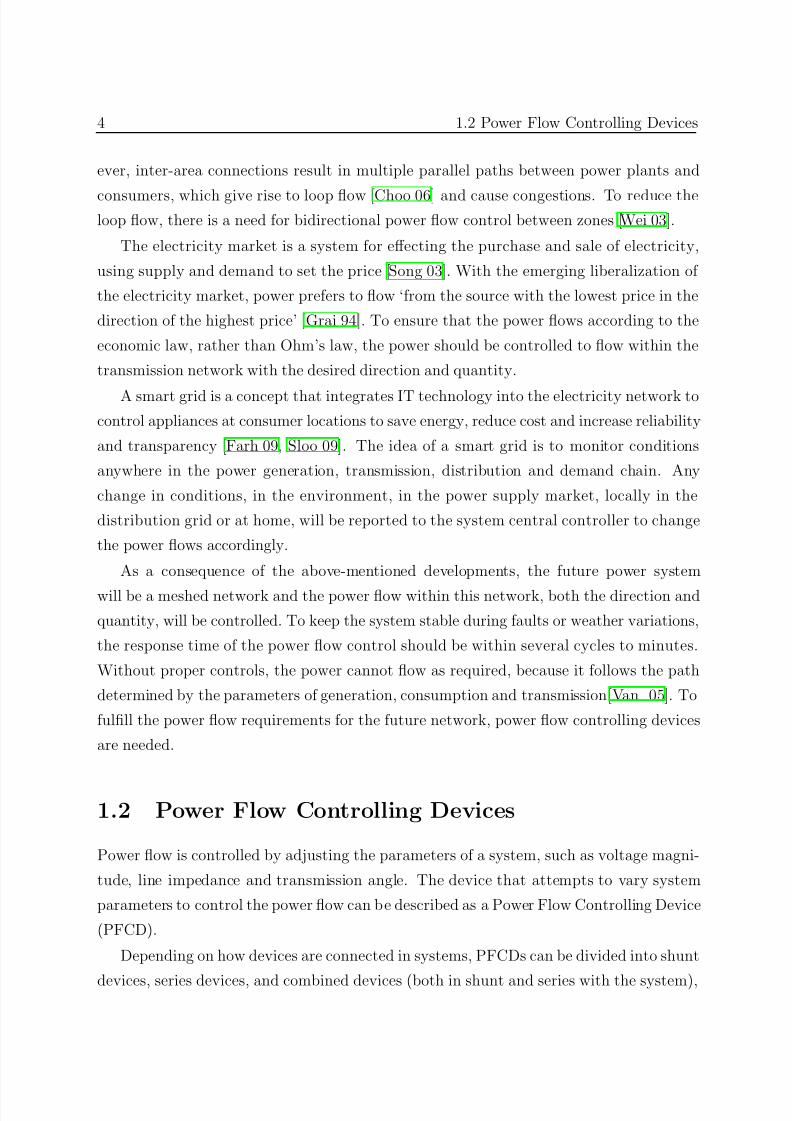
as shown in Figure 1-3.
PFC
PFC
PFC
grid grid grid
transmission
linetransmission
line
transmission
line
shunt PFC series PFC combined PFC
Figure 1-3: Simplified diagram of shunt, series and combined devices
A shunt device is a device that connects between the grid and the ground. Shunt
devices generate or absorb reactive power at the point of connection thereby controlling
the voltage magnitude. Because the bus voltage magnitude can only be varied within
certain limits, controlling the power flow in this way is limited and shunt devices mainly
serve other purposes. For example, the voltage support provided by a shunt device at the
midpoint of a long transmission line can boost the power transmission capacity [Hing 00].
Another application of shunt devices is to provide reactive power locally, thereby reduc-
ing unwanted reactive power flow through the line and reducing network losses. Also,
consumer-side shunt devices can improve power quality, especially during large demand
fluctuations [Zhan 06]. The operating principle of shunt devices can be found in chapter 2.
A device that is connected in series with the transmission line is referred to as a ‘series
device’. Series devices influence the impedance of transmission lines. The principle is to
change (reduce or increase) the line impedance by inserting a reactor or capacitor. To
compensate for the inductive voltage drop, a capacitor can be inserted in the line to reduce
the line impedance. By increasing the inductive impedance of the line, series devices are
also used to limit the current flowing through certain lines to prevent overheating. Theprinciple of series devices is explained in more detail in chapter 2.
A combined device is a two-port device that is connected to the grid, both as a
shunt and in a series, to enable active power exchange between the shunt and series parts.
Combined devices are suitable for power flow control because they can simultaneously vary
multiple system parameters, such as the transmission angle, the bus voltage magnitude
and the line impedance.
Based on the implemented technology, PFCDs can be categorized into mechanical-
based devices and power electronics (PE)-based devices.
7/25/2019 Dpfc Thesis
http://slidepdf.com/reader/full/dpfc-thesis 28/212
6 1.2 Power Flow Controlling Devices
Mechanical PFCDs consist of fixed or mechanical interchangeable passive components,
such as inductors or capacitors, together with transformers. Typically, mechanical PFCDshave relatively low cost and high reliability. However, because of their relatively low
switching speed (from several seconds to minutes) and step-wise adjustments of mechan-
ical PFCDs [Baum 65, Pill 03], they have relatively poor control capability and are not
suitable for complex networks of the future.
PE PFCDs also contain passive components, but include additional PE switches to
achieve smaller steps and faster adjustments [Song 99]. There is another term - Flexible
AC Transmission System (FACTS) - that overlaps with the PE PFCDs. According to
the IEEE, FACTS is defined as an ‘alternating current transmission system incorporating
power electronic based and other static controllers to enhance controllability and increase
power transfer capability’ [Edri 97]. Normally, the High Voltage DC transmission (HVDC)
and PE devices that are applied at the distribution network, such as a Dynamic Voltage
Restorer (DVR), are also considered as FACTS controllers [Moor 95]. Most of the FACTS
controllers can be used for power flow control. However, the HVDC and the DVR are out
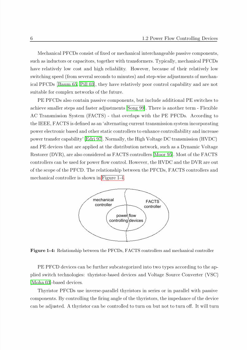
of the scope of the PFCD. The relationship between the PFCDs, FACTS controllers and
mechanical controller is shown in Figure 1-4.
power flow
controlling devices
FACTS
controller
mechanical
controller
Figure 1-4: Relationship between the PFCDs, FACTS controllers and mechanical controller
PE PFCD devices can be further subcategorized into two types according to the ap-
plied switch technologies: thyristor-based devices and Voltage Source Converter (VSC)
[Moha 03]-based devices.
Thyristor PFCDs use inverse-parallel thyristors in series or in parallel with passive
components. By controlling the firing angle of the thyristors, the impedance of the device
can be adjusted. A thyristor can be controlled to turn on but not to turn off. It will turn
7/25/2019 Dpfc Thesis
http://slidepdf.com/reader/full/dpfc-thesis 29/212
1 INTRODUCTION 7
off automatically when the current goes negative. Consequently, the thyristor can only be
turned on once within one cycle. The switching frequency of thyristor PFCDs is thereforelimited to the system frequency (50/60Hz), resulting in low switching losses. Because
thyristors can handle larger voltages and currents than other power semiconductors, the
power level of thyristor PFCDs are also higher. The thyristor PFCDs are simpler than
VSC PFCDs, allowing them higher reliability. However, the waveforms of voltages and
currents generated by thyristor PFCDs contain a large amount of harmonics, thereby
requiring large filters.
VSC PFCDs employ advanced switch technologies, such as Insulated Gate Bipolar
Transistors (IGBT), Insulated Gate Commutated Thyristors (IGCT), or Metal Oxide
Semiconductor Field Effect Transistors (MOSFET) to build converters. Because these
switches have turn-on and turn-off capability, the output voltage of a VSC is independent
from the current. Consequently, it is possible to turn the switches on and off within the
VSC multiple times within one cycle. Several types of VSCs have been developed, such
as multi-pulse converters, multi-level converters, square-wave converters, etc [Moha 03].
These VSCs proved a free controllable voltage in both magnitude and phase. Due to their
relatively high switching frequency, VSC PFCDs make practically instant control (less
than one cycle) possible. High switching frequencies also reduce low frequency harmon-
ics of the outputs and even enable PFCDs to compensate disturbances from networks.
Therefore, VSC PFCDs are the most suitable devices for future power systems.
On the other hand, there are some challenges facing VSC PFCDs. Firstly, because
large amounts of switches are connected in series or in parallel to allow the high voltage
and high current through, the VSC PFCDs are expensive. In addition, due to their
higher switching frequency and higher on-state voltage in comparison with thyristors,
VSC PFCD losses are higher as well. However, with developments in power electronics
(such as Silicon-carbide, Gallium-Nitride and synthetic diamond) [Davi 09], VSC PFCDs
can become more feasible and cost-effective in the future.
According to the above considerations of different types of PFCDs, it can be concluded
that PE combined PFCDs (also referred to as combined FACTS) have the best control
capability among all PFCDs. They inherit the advantages of PE PFCDs and combined
PFCDs, which is the fast adjustment of multiple system parameters. The Unified Power
Flow Controller (UPFC) and Interline Power Flow Controller (IPFC) [Gyug 92, Gyug 99]
are currently the most powerful PFCDs; they can adjust all system parameters: line
7/25/2019 Dpfc Thesis
http://slidepdf.com/reader/full/dpfc-thesis 30/212
8 1.3 Problem Definition
impedance, transmission angle, and bus voltage. The operating principle of the UPFC
and the IPFC will be introduced in chapter 2.
1.3 Problem Definition
Although the UPFC and the IPFC have superior capability to control power flow, there
is no commercial application currently. The main reasons are:
• The first concern with a combined FACTS is cost. Typically, a FACTS cost around
120-150 $ per kVA, compared to 15-20 $ per kVA for static capacitors [ Diva 07]. Oneof the reasons for the high cost is that the ratings of FACTS devices are normally
in 100 MVA, with the system voltage from 100 kV to 500 kV. This requires a large
number of power electronic switches in series and parallel connection. To provide
voltage isolation, 3-phase high-voltage transformers are essential; furthermore, the
series-connected transformers require an even higher rating to handle fault voltages
and currents. Secondly, as the FACTS devices are installed at different locations for
different purposes, each of them is unique. As a result, each FACTS device requires
custom design and manufacturing, which leads to a long building cycle and highcost. Lastly, a FACTS is a complex system, and requires a large area for installation
and also well-trained engineers for maintenance.
• The second concern is possible failures in the combined FACTS. Two issues are
considered: the reliability of the device itself and its influence on power system se-
curity. The combined FACTS is a complex system, which contains a large number of
active and passive components. The large component number results that, without
proper precautions, the combined FACTS have a bigger chance of failure than other
PFCDs. To gain the desired reliability, complex protections (bypass circuit) andredundant backups (backup transformers and capacitor banks) are always provided
for the combined FACTS device, further raising the cost, an already concerning
factor. Also, a failure in the combined FACTS is more critical to the power system
than in other devices. For a shunt FACTS, device failure results in a disconnection
of the device from the grid which prevents it from providing reactive compensation.
Because the series converter of the combined FACTS is directly inserted into trans-
mission lines, not only the device, but also the transmission lines will be disengaged
from the system during the failure [Verm 04].
7/25/2019 Dpfc Thesis
http://slidepdf.com/reader/full/dpfc-thesis 31/212
1 INTRODUCTION 9
Due to these two major drawbacks, the UPFC and IPFC are not widely applied in
practice. Even when there is a large demand of power flow control within the network, theUPFC and IPFC are not currently the industry’s first choice. Normally, a phase shifting
transformer, which has less control capability [Bres 04], is selected for economic reasons.
Accordingly, a low-cost, reliable combined FACTS device has great market potential.
1.4 Objective and Approaches
There is a great demand of power flow control in power systems of the future and combined
FACTS devices are the most suitable devices. However, due to the cost and the reliability
issues given above, there are many hurdles to the widespread application of combined
FACTS devices. Accordingly, the main objectives of this thesis can be summarized as:
To develop a new power flow controlling device that has the following characteristics:
• Comparable performance as the combined FACTS device - the UPFC or IPFC.
• Acceptable cost to electric utilities.
• Acceptable reliability for power systems.
The approach to develop such a device consists of the following steps:
• Review the fundamentals of power-flow-control theory and the state-of-art of PFCDs
with respect to operating principles, advantages and limitations.
• Analyze the UPFC and IPFC to determine their performance of power flow control.
• Find ways to reduce the cost and increase the reliability of combined FACTS devices.
• Generate a new concept of a power flow controlling device according to these points.
The new concept presented in this thesis is called ‘Distributed Power Flow Controller
(DPFC)’. It is a combined FACTS device, which has taken a UFPC as its starting point.The DPFC has the same control capability as the UPFC; independent adjustment of
the line impedance, the transmission angle and the bus voltage. The DPFC eliminates
the common DC link that is used to connect the shunt and series converter back-to-
back within the UPFC. By employing the Distributed FACTS concept [ Diva 07] as the
series converter of the DPFC, the cost is greatly reduced due to the small rating of the
components in the series converters. Also, the reliability of the DPFC is improved because
of the redundancy provided by the multiple series converters.
Once the DPFC concept is presented, the research follows the listed steps:
7/25/2019 Dpfc Thesis
http://slidepdf.com/reader/full/dpfc-thesis 32/212
10 1.5 Thesis Layout
• Analyze and evaluate the proposed concept with respects to the control capability
and the rating of the DPFC.• Find the mathematical model of the DPFC.
• According to the DPFC model, design the control schemes of the DPFC.
• Verify the DPFC concept, both in the simulation and in experimental setup.
• Investigate the reliability of the DPFC during the failure of a single converter.
The above research focuses on the level of the DPFC device, and the following studies
consider the DPFC application at the power system level:
• Investigate the capability of the DPFC to damp low-frequency power oscillation.
• Utilize the DPFC to balance asymmetrical components within the network.
• Study the feasibility of the DPFC in a real transmission network.
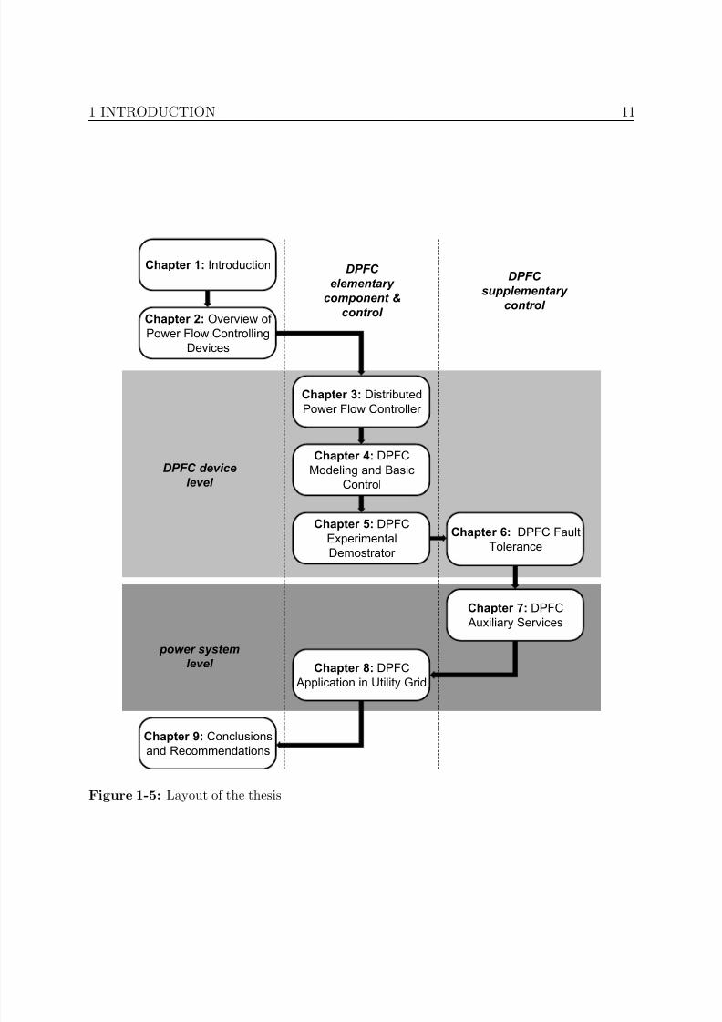
1.5 Thesis Layout
The layout of the thesis is illustrated in Figure 1-5.
Chapter 2 gives an overview of the status of PFCDs. This chapter begins with the
principle of power flow control. Various PFCDs are introduced, categorized and compared.A new FACTS device, called Distributed Power Flow Controller (DPFC), is presented
in chapter 3. The DPFC is developed based on the UPFC and employs the Distributed
FACTS concept [Diva 05] for the series converters. Once the principle of the DPFC is
presented, the steady-state of the DPFC is analyzed. In the last part of this chapter, a
concept that is derived from the DPFC, the so-called Distributed Interline Power Flow
Controller (DIPFC) is introduced.
Chapter 4 addresses the modeling and control of the DPFC. The chapter begins with
modeling the DPFC in the dq -frame. Once the modeling of the DPFC is examined, thedesign of the DPFC primary control is given. The primary control is the basic control
layer for the DPFC, responsible for maintaining DC voltages of converters and generating
the AC voltages required by the central control. Further, the communication between the
DPFC series converters and the central control is considered. A low-cost and high-reliable
synchronization method for series converters is presented.
Chapter 5 considers the DPFC verification in a scaled experimental setup. The chapter
begins by presenting the specification of the setup, and continues with the design of major
components and control implementation. The chapter is concluded with the experimental
7/25/2019 Dpfc Thesis
http://slidepdf.com/reader/full/dpfc-thesis 33/212
1 INTRODUCTION 11
Chapter 3: Distributed
Power Flow Controller
Chapter 4: DPFC
Modeling and Basic
Control
Chapter 6: DPFC FaultTolerance
Chapter 9: Conclusions
and Recommendations
Chapter 1: Introduction
Chapter 2: Overview of
Power Flow Controlling
Devices
Chapter 7: DPFC
Auxiliary Services
Chapter 8: DPFC
Application in Utility Grid
Chapter 5: DPFC
ExperimentalDemostrator
power system
level
DPFC device
level
DPFC
elementary
component &
control
DPFC
supplementary
control
Figure 1-5: Layout of the thesis
7/25/2019 Dpfc Thesis
http://slidepdf.com/reader/full/dpfc-thesis 34/212
12 1.5 Thesis Layout
results of the DPFC.
The reliability of the DPFC is considered in chapter 6. Two types of converter failuresin the DPFC, namely a shunt converter failure and a series converter failure, are discussed.
In this chapter, the supplementary controllers that deal with different converter failures are
separately introduced. The principle, analysis and design of the controller are presented,
and the results achieved in both simulation and experimental setups are shown.
Chapter 7 considers the DPFC application at the power system level and focuses
on the outer loop within the central control. Two issues are discussed in this chapter:
utilizing DPFC to damp low-frequency power oscillation and methods of compensating
asymmetrical components.In chapter 8, the realization of the DPFC in real networks is examined. First, DPFC
design procedures are introduced, which give the equations to determine the major pa-
rameters of the DPFC. Two cases are studied for different purposes. Case 1 aims to find
the feasibility of the DPFC in a real transmission line and a two-port network is taken
as an example. The physical and electrical sizing of the DPFC converters is considered.
In Case 2, the application of the DPFC for power flow control is discussed and a triangle
network in the Netherlands is selected as the case.
This thesis concludes with chapter 9, which summarizes the major contributions of
the research. Recommendations for future research on the subject are also given.
7/25/2019 Dpfc Thesis
http://slidepdf.com/reader/full/dpfc-thesis 35/212
Chapter 2OVERVIEW OF POWER FLOW
CONTROLLING DEVICES
2.1 Introduction
I
T is shown in the previous chapter that there is a growing demand for fast, reliable
and multi-directional power flow control. To achieve this, special devices are needed.
This chapter gives an overview of the state-of-art of PFCDs, considering the operating
principles and the advantages and limitations of each device.
First the theory of power flow control is discussed and the parameters that can be
used to control power flow are investigated. Later, several PFCDs are categorized and
introduced.
2.2 Power Flow Control Theory
To study the power flow through a transmission line, a mathematical representation of
a transmission line is required. A transmission line can be characterized by four param-
eters: resistance, inductance, capacitance and conductance. Conductance accounts for
the leakage current at the insulators of overhead lines. However, for a short and medium
length line (less than 240 km), the capacitance and conductance are so small that they
can be neglected with little loss of accuracy [Grai 94]. Accordingly, a transmission line
can be simplified as shown in Figure 2-1, where V s and V r are the sending and receiving
end line-to-ground phasor voltages, I is the phasor current through the line, and R and
13
7/25/2019 Dpfc Thesis
http://slidepdf.com/reader/full/dpfc-thesis 36/212
14 2.2 Power Flow Control Theory
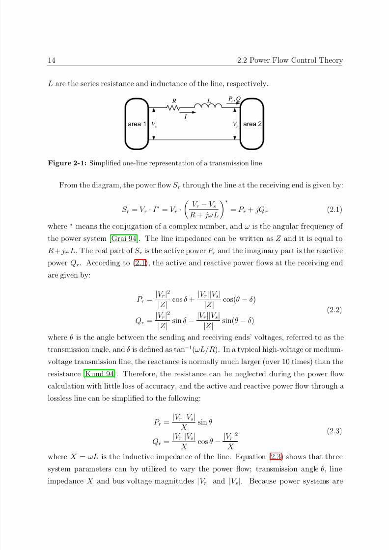
L are the series resistance and inductance of the line, respectively.
area 1 area 2
R L
sV
r V I
,r r P Q
Figure 2-1: Simplified one-line representation of a transmission line
From the diagram, the power flow S r through the line at the receiving end is given by:
S r = V r · I ∗ = V r ·
V r − V sR + jωL
∗
= P r + jQr (2.1)
where ∗ means the conjugation of a complex number, and ω is the angular frequency of
the power system [Grai 94]. The line impedance can be written as Z and it is equal to
R + jωL. The real part of S r is the active power P r and the imaginary part is the reactive
power Qr. According to (2.1), the active and reactive power flows at the receiving end
are given by:
P r = |V r|2|Z | cos δ +
|V r||V s||Z | cos(θ − δ )
Qr = |V r|2|Z | sin δ − |V r||V s|
|Z | sin(θ − δ )
(2.2)
where θ is the angle between the sending and receiving ends’ voltages, referred to as the
transmission angle, and δ is defined as tan−1(ωL/R). In a typical high-voltage or medium-
voltage transmission line, the reactance is normally much larger (over 10 times) than the
resistance [Kund 94]. Therefore, the resistance can be neglected during the power flow
calculation with little loss of accuracy, and the active and reactive power flow through alossless line can be simplified to the following:
P r = |V r||V s|
X sin θ
Qr = |V r||V s|
X cos θ − |V r|2
X
(2.3)
where X = ωL is the inductive impedance of the line. Equation (2.3) shows that three
system parameters can by utilized to vary the power flow; transmission angle θ, line
impedance X and bus voltage magnitudes |V r| and |V s|. Because power systems are
7/25/2019 Dpfc Thesis
http://slidepdf.com/reader/full/dpfc-thesis 37/212
2 OVERVIEW OF POWER FLOW CONTROLLING DEVICES 15
operated in a unified voltage mode (voltages are close to 1 per unit (pu)) [Grai 94],
power flows can only be adjusted in a small range by varying the bus voltage magnitude.Therefore, the bus voltage magnitude is not suitable for controlling the power flow over
a large range. By assuming that the bus voltages at the sending and receiving ends have
the same magnitude |V |, the power flow equations can be further simplified to:
P r = |V |2
X sin θ
Qr = |V |2
X (cos θ − 1)
(2.4)
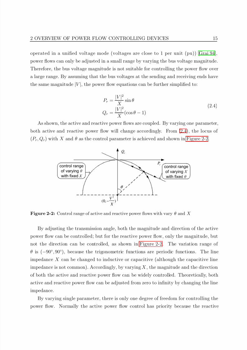
As shown, the active and reactive power flows are coupled. By varying one parameter,both active and reactive power flow will change accordingly. From (2.4), the locus of
(P r, Qr) with X and θ as the control parameter is achieved and shown in Figure 2-2.
r P
r Q
θ
2
(0, )V
X −
control range
of varying θ
with fixed X
control range
of varying X
with fixed θ
Figure 2-2: Control range of active and reactive power flows with vary θ and X
By adjusting the transmission angle, both the magnitude and direction of the active
power flow can be controlled; but for the reactive power flow, only the magnitude, but
not the direction can be controlled, as shown in Figure 2-2. The variation range of θ is (−90, 90), because the trigonometric functions are periodic functions. The line
impedance X can be changed to inductive or capacitive (although the capacitive line
impedance is not common). Accordingly, by varying X , the magnitude and the direction
of both the active and reactive power flow can be widely controlled. Theoretically, both
active and reactive power flow can be adjusted from zero to infinity by changing the line
impedance.
By varying single parameter, there is only one degree of freedom for controlling the
power flow. Normally the active power flow control has priority because the reactive
7/25/2019 Dpfc Thesis
http://slidepdf.com/reader/full/dpfc-thesis 38/212
16 2.3 Categorization of PFCDs
power can be generated at the load side though capacitor banks. If the active and reac-
tive power flows need to be controlled independently, two or more parameters should besimultaneously controlled by the PFCD.
2.3 Categorization of PFCDs
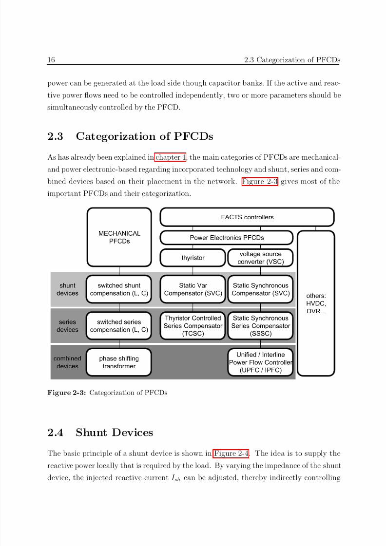
As has already been explained in chapter 1, the main categories of PFCDs are mechanical-
and power electronic-based regarding incorporated technology and shunt, series and com-
bined devices based on their placement in the network. Figure 2-3 gives most of the
important PFCDs and their categorization.
thyristor
MECHANICAL
PFCDs
voltage source
converter (VSC)
Static VarCompensator (SVC)
Static SynchronousCompensator (SVC)
Thyristor Controlled
Series Compensator
(TCSC)
Static Synchronous
Series Compensator
(SSSC)
Unified / Interline
Power Flow Controller
(UPFC / IPFC)
switched shuntcompensation (L, C)
switched series
compensation (L, C)
phase shifting
transformer
shuntdevices
series
devices
combined
devices
Power Electronics PFCDs
FACTS controllers
others:
HVDC,
DVR...
Figure 2-3: Categorization of PFCDs
2.4 Shunt Devices
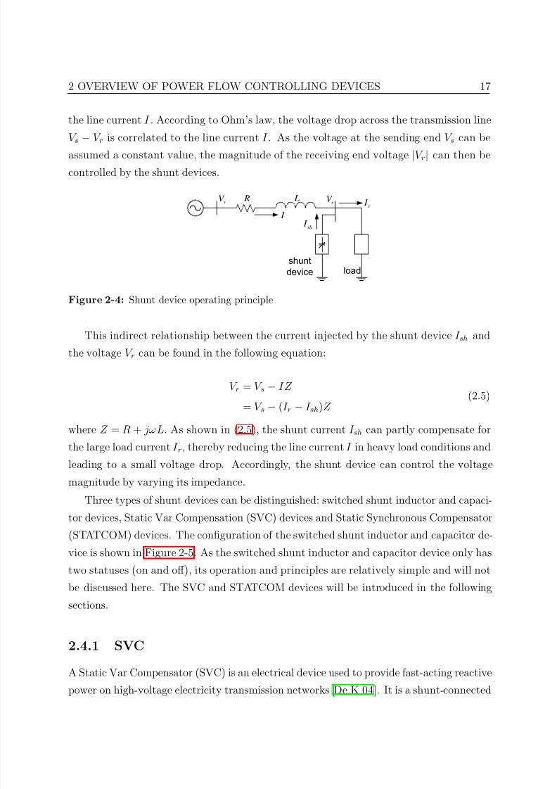
The basic principle of a shunt device is shown in Figure 2-4. The idea is to supply the
reactive power locally that is required by the load. By varying the impedance of the shunt
device, the injected reactive current I sh can be adjusted, thereby indirectly controlling
7/25/2019 Dpfc Thesis
http://slidepdf.com/reader/full/dpfc-thesis 39/212
2 OVERVIEW OF POWER FLOW CONTROLLING DEVICES 17
the line current I . According to Ohm’s law, the voltage drop across the transmission line
V s − V r is correlated to the line current I . As the voltage at the sending end V s can beassumed a constant value, the magnitude of the receiving end voltage |V r| can then be
controlled by the shunt devices.
R L
load
shunt
device
I
sh I
r I sV
r V
Figure 2-4: Shunt device operating principle
This indirect relationship between the current injected by the shunt device I sh and
the voltage V r can be found in the following equation:
V r = V s − IZ
= V s−
(I r−
I sh)Z (2.5)
where Z = R + jωL. As shown in (2.5), the shunt current I sh can partly compensate for
the large load current I r, thereby reducing the line current I in heavy load conditions and
leading to a small voltage drop. Accordingly, the shunt device can control the voltage
magnitude by varying its impedance.
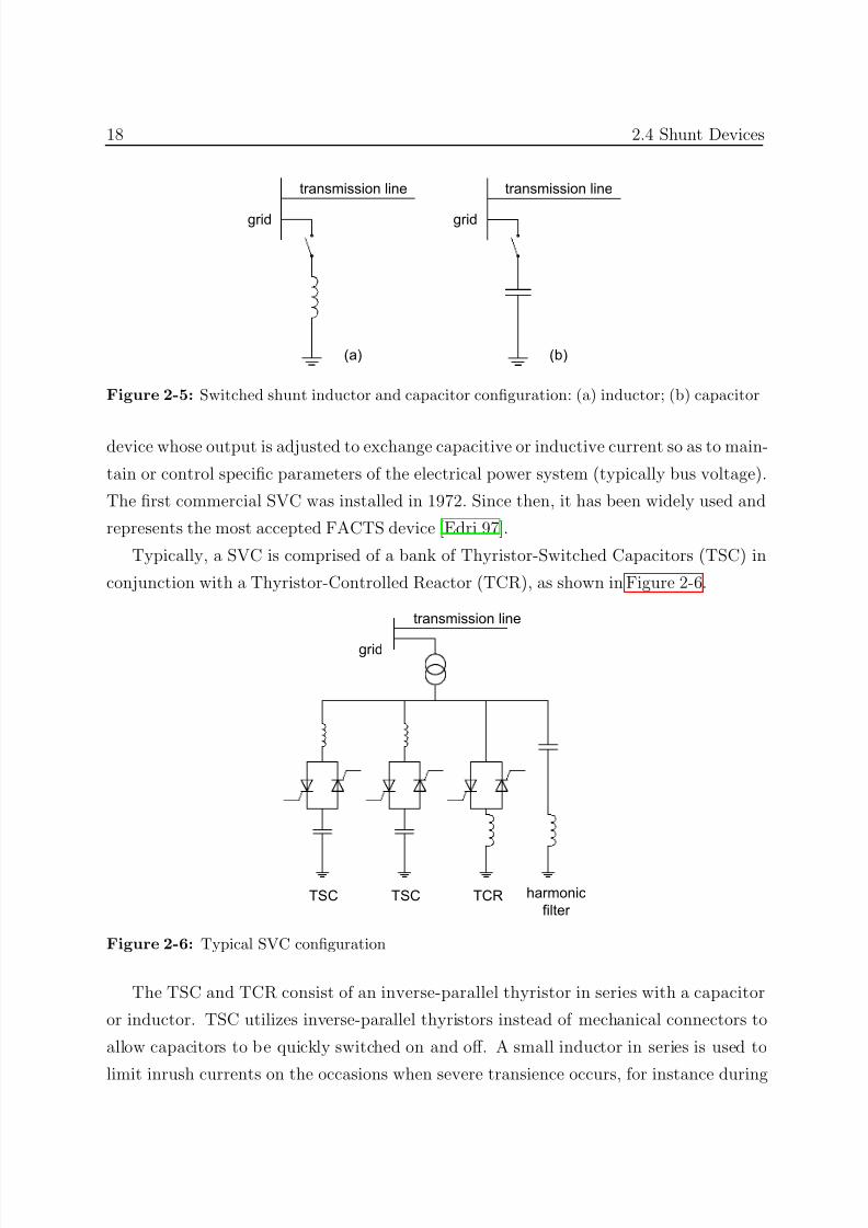
Three types of shunt devices can be distinguished: switched shunt inductor and capaci-
tor devices, Static Var Compensation (SVC) devices and Static Synchronous Compensator
(STATCOM) devices. The configuration of the switched shunt inductor and capacitor de-
vice is shown in Figure 2-5. As the switched shunt inductor and capacitor device only hastwo statuses (on and off), its operation and principles are relatively simple and will not
be discussed here. The SVC and STATCOM devices will be introduced in the following
sections.
2.4.1 SVC
A Static Var Compensator (SVC) is an electrical device used to provide fast-acting reactive
power on high-voltage electricity transmission networks [De K 04]. It is a shunt-connected
7/25/2019 Dpfc Thesis
http://slidepdf.com/reader/full/dpfc-thesis 40/212
18 2.4 Shunt Devices
grid
transmission line
grid
transmission line
(a) (b)
Figure 2-5: Switched shunt inductor and capacitor configuration: (a) inductor; (b) capacitor
device whose output is adjusted to exchange capacitive or inductive current so as to main-
tain or control specific parameters of the electrical power system (typically bus voltage).
The first commercial SVC was installed in 1972. Since then, it has been widely used and
represents the most accepted FACTS device [Edri 97].
Typically, a SVC is comprised of a bank of Thyristor-Switched Capacitors (TSC) in
conjunction with a Thyristor-Controlled Reactor (TCR), as shown in Figure 2-6.
TSC TSC TCR harmonic
filter
grid
transmission line
Figure 2-6: Typical SVC configuration
The TSC and TCR consist of an inverse-parallel thyristor in series with a capacitor
or inductor. TSC utilizes inverse-parallel thyristors instead of mechanical connectors to
allow capacitors to be quickly switched on and off. A small inductor in series is used to
limit inrush currents on the occasions when severe transience occurs, for instance during
7/25/2019 Dpfc Thesis
http://slidepdf.com/reader/full/dpfc-thesis 41/212
2 OVERVIEW OF POWER FLOW CONTROLLING DEVICES 19
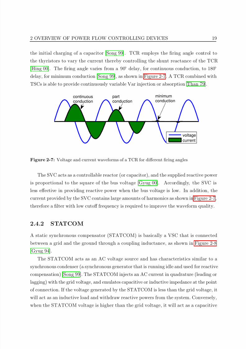
the initial charging of a capacitor [Song 99]. TCR employs the firing angle control to
the thyristors to vary the current thereby controlling the shunt reactance of the TCR[Hing 00]. The firing angle varies from a 90 delay, for continuous conduction, to 180
delay, for minimum conduction [Song 99], as shown in Figure 2-7. A TCR combined with
TSCs is able to provide continuously variable Var injection or absorption [Than 79].
voltage
current
partconduction
minimumconduction
continuousconduction
Figure 2-7: Voltage and current waveforms of a TCR for different firing angles
The SVC acts as a controllable reactor (or capacitor), and the supplied reactive power
is proportional to the square of the bus voltage [Gyug 00]. Accordingly, the SVC isless effective in providing reactive power when the bus voltage is low. In addition, the
current provided by the SVC contains large amounts of harmonics as shown in Figure 2-7,
therefore a filter with low cutoff frequency is required to improve the waveform quality.
2.4.2 STATCOM
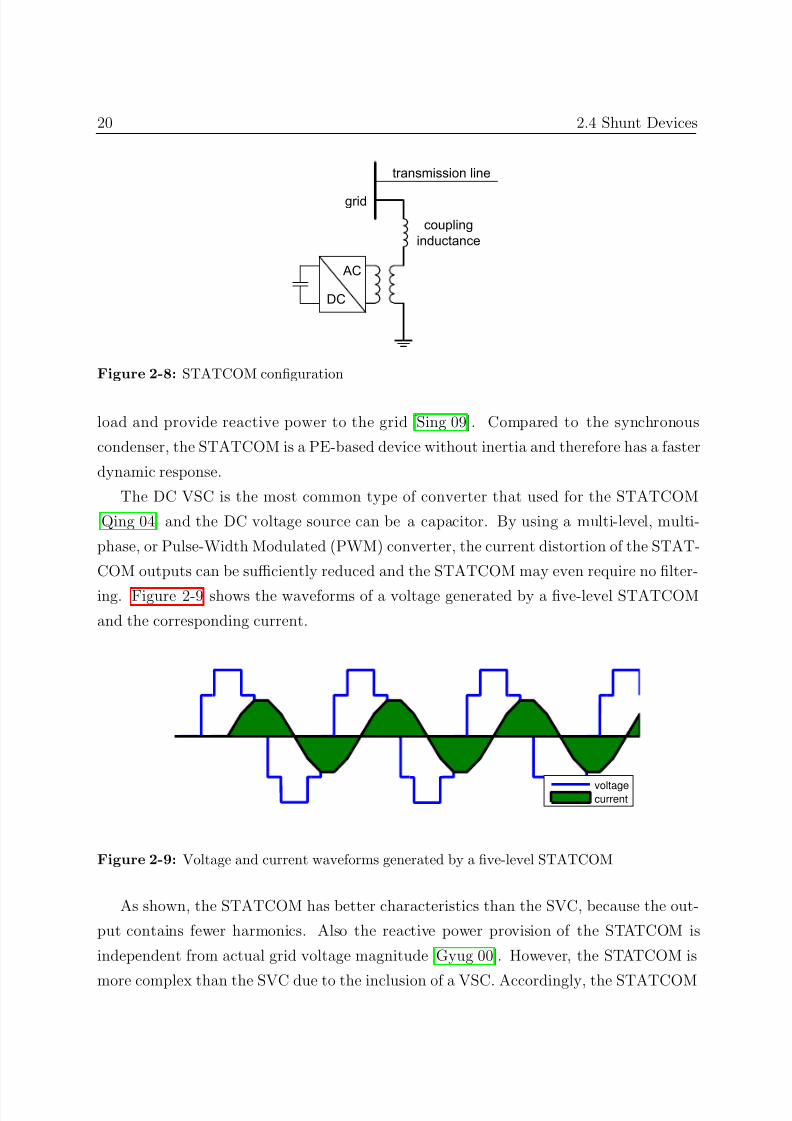
A static synchronous compensator (STATCOM) is basically a VSC that is connected
between a grid and the ground through a coupling inductance, as shown in Figure 2-8[Gyug 94].
The STATCOM acts as an AC voltage source and has characteristics similar to a
synchronous condenser (a synchronous generator that is running idle and used for reactive
compensation) [Song 99]. The STATCOM injects an AC current in quadrature (leading or
lagging) with the grid voltage, and emulates capacitive or inductive impedance at the point
of connection. If the voltage generated by the STATCOM is less than the grid voltage, it
will act as an inductive load and withdraw reactive powers from the system. Conversely,
when the STATCOM voltage is higher than the grid voltage, it will act as a capacitive
7/25/2019 Dpfc Thesis
http://slidepdf.com/reader/full/dpfc-thesis 42/212
20 2.4 Shunt Devices
grid
coupling
inductance
AC
DC
transmission line
Figure 2-8: STATCOM configuration
load and provide reactive power to the grid [Sing 09]. Compared to the synchronous
condenser, the STATCOM is a PE-based device without inertia and therefore has a faster
dynamic response.
The DC VSC is the most common type of converter that used for the STATCOM
[Qing 04] and the DC voltage source can be a capacitor. By using a multi-level, multi-
phase, or Pulse-Width Modulated (PWM) converter, the current distortion of the STAT-
COM outputs can be sufficiently reduced and the STATCOM may even require no filter-
ing. Figure 2-9 shows the waveforms of a voltage generated by a five-level STATCOM
and the corresponding current.
voltagecurrent
Figure 2-9: Voltage and current waveforms generated by a five-level STATCOM
As shown, the STATCOM has better characteristics than the SVC, because the out-
put contains fewer harmonics. Also the reactive power provision of the STATCOM is
independent from actual grid voltage magnitude [Gyug 00]. However, the STATCOM is
more complex than the SVC due to the inclusion of a VSC. Accordingly, the STATCOM
7/25/2019 Dpfc Thesis
http://slidepdf.com/reader/full/dpfc-thesis 43/212
2 OVERVIEW OF POWER FLOW CONTROLLING DEVICES 21
is more expensive than the SVC, especially for the high-voltage transmission lines.
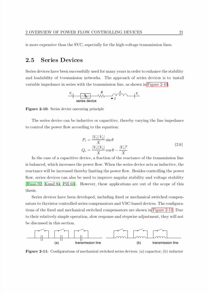
2.5 Series Devices
Series devices have been successfully used for many years in order to enhance the stability
and loadability of transmission networks. The approach of series devices is to install
variable impedance in series with the transmission line, as shown in Figure 2-10.
R L
I
sV
r V
series device
Figure 2-10: Series device operating principle
The series device can be inductive or capacitive, thereby varying the line impedance
to control the power flow according to the equation:
P r = |V r||V s|
X sin θ
Qr = |V r||V s|
X
cos θ
−
|V r|2
X
(2.6)
In the case of a capacitive device, a fraction of the reactance of the transmission line
is balanced, which increases the power flow. When the series device acts as inductive, the
reactance will be increased thereby limiting the power flow. Besides controlling the power
flow, series devices can also be used to improve angular stability and voltage stability
[Huan 02, Kund 94, Pill 03]. However, these applications are out of the scope of this
thesis.
Series devices have been developed, including fixed or mechanical switched compen-
sators to thyristor controlled series compensators and VSC-based devices. The configura-
tions of the fixed and mechanical switched compensators are shown in Figure 2-11. Due
to their relatively simple operation, slow response and stepwise adjustment, they will not
be discussed in this section.
(a) transmission line (b) transmission line
Figure 2-11: Configurations of mechanical switched series devices: (a) capacitor; (b) inductor
7/25/2019 Dpfc Thesis
http://slidepdf.com/reader/full/dpfc-thesis 44/212
22 2.5 Series Devices
2.5.1 TSSC
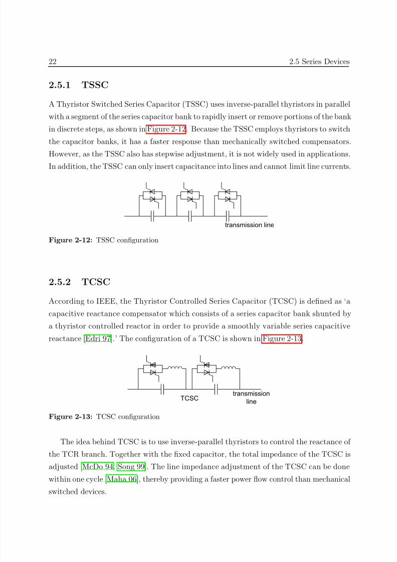
A Thyristor Switched Series Capacitor (TSSC) uses inverse-parallel thyristors in parallel
with a segment of the series capacitor bank to rapidly insert or remove portions of the bank
in discrete steps, as shown in Figure 2-12. Because the TSSC employs thyristors to switch
the capacitor banks, it has a faster response than mechanically switched compensators.
However, as the TSSC also has stepwise adjustment, it is not widely used in applications.
In addition, the TSSC can only insert capacitance into lines and cannot limit line currents.
transmission line
Figure 2-12: TSSC configuration
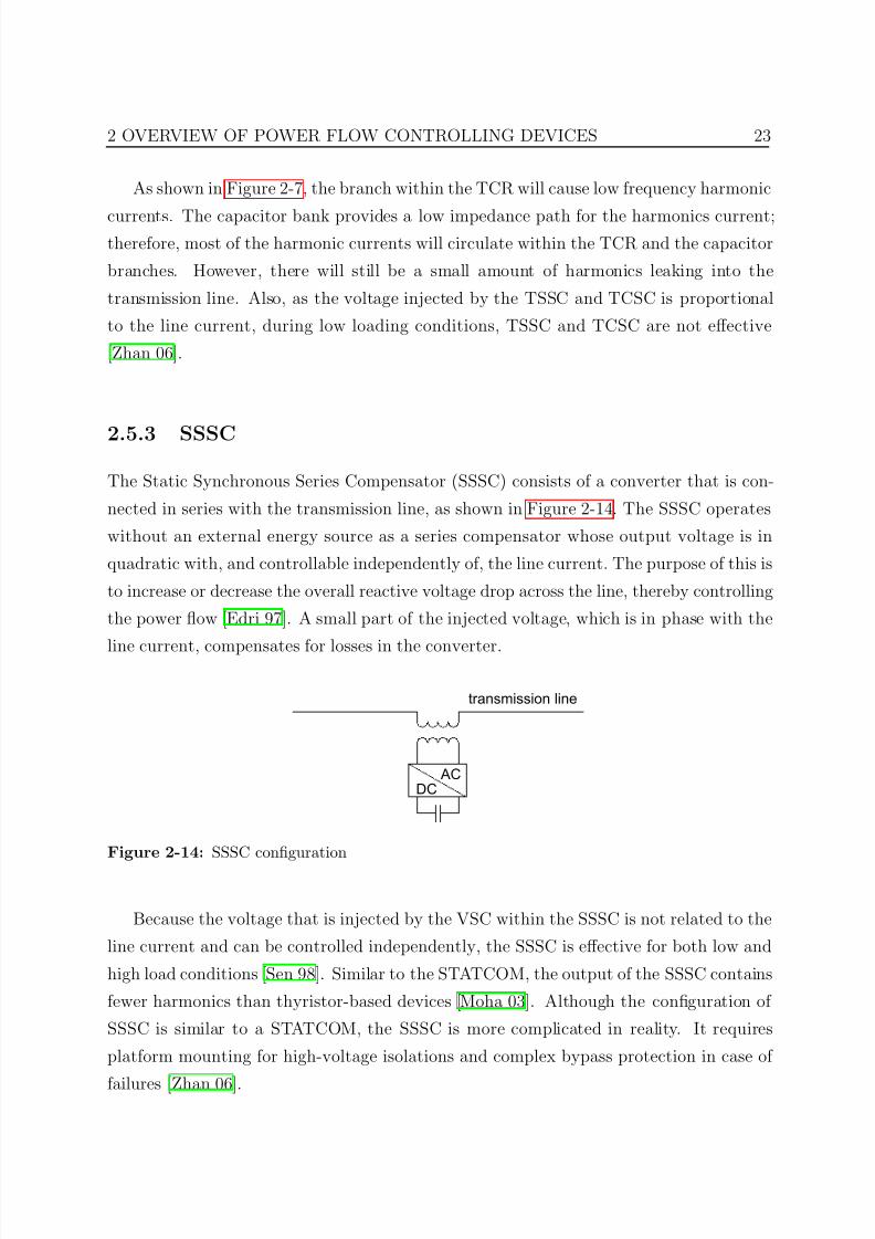
2.5.2 TCSC
According to IEEE, the Thyristor Controlled Series Capacitor (TCSC) is defined as ‘a
capacitive reactance compensator which consists of a series capacitor bank shunted by
a thyristor controlled reactor in order to provide a smoothly variable series capacitive
reactance [Edri 97].’ The configuration of a TCSC is shown in Figure 2-13.
TCSC transmissionline
Figure 2-13: TCSC configuration
The idea behind TCSC is to use inverse-parallel thyristors to control the reactance of
the TCR branch. Together with the fixed capacitor, the total impedance of the TCSC is
adjusted [McDo 94, Song 99]. The line impedance adjustment of the TCSC can be done
within one cycle [Maha 06], thereby providing a faster power flow control than mechanical
switched devices.
7/25/2019 Dpfc Thesis
http://slidepdf.com/reader/full/dpfc-thesis 45/212
2 OVERVIEW OF POWER FLOW CONTROLLING DEVICES 23
As shown in Figure 2-7, the branch within the TCR will cause low frequency harmonic
currents. The capacitor bank provides a low impedance path for the harmonics current;therefore, most of the harmonic currents will circulate within the TCR and the capacitor
branches. However, there will still be a small amount of harmonics leaking into the
transmission line. Also, as the voltage injected by the TSSC and TCSC is proportional
to the line current, during low loading conditions, TSSC and TCSC are not effective
[Zhan 06].
2.5.3 SSSC
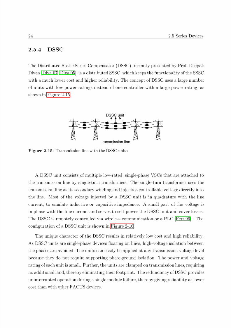
The Static Synchronous Series Compensator (SSSC) consists of a converter that is con-
nected in series with the transmission line, as shown in Figure 2-14. The SSSC operates
without an external energy source as a series compensator whose output voltage is in
quadratic with, and controllable independently of, the line current. The purpose of this is
to increase or decrease the overall reactive voltage drop across the line, thereby controlling
the power flow [Edri 97]. A small part of the injected voltage, which is in phase with the
line current, compensates for losses in the converter.
transmission line
AC
DC
Figure 2-14: SSSC configuration
Because the voltage that is injected by the VSC within the SSSC is not related to the
line current and can be controlled independently, the SSSC is effective for both low and
high load conditions [Sen 98]. Similar to the STATCOM, the output of the SSSC contains
fewer harmonics than thyristor-based devices [Moha 03]. Although the configuration of
SSSC is similar to a STATCOM, the SSSC is more complicated in reality. It requires
platform mounting for high-voltage isolations and complex bypass protection in case of
failures [Zhan 06].
7/25/2019 Dpfc Thesis
http://slidepdf.com/reader/full/dpfc-thesis 46/212
24 2.5 Series Devices
2.5.4 DSSC
The Distributed Static Series Compensator (DSSC), recently presented by Prof. Deepak
Divan [Diva 07, Diva 05], is a distributed SSSC, which keeps the functionality of the SSSC
with a much lower cost and higher reliability. The concept of DSSC uses a large number
of units with low power ratings instead of one controller with a large power rating, as
shown in Figure 2-15.
DSSC unit
transmission line
Figure 2-15: Transmission line with the DSSC units
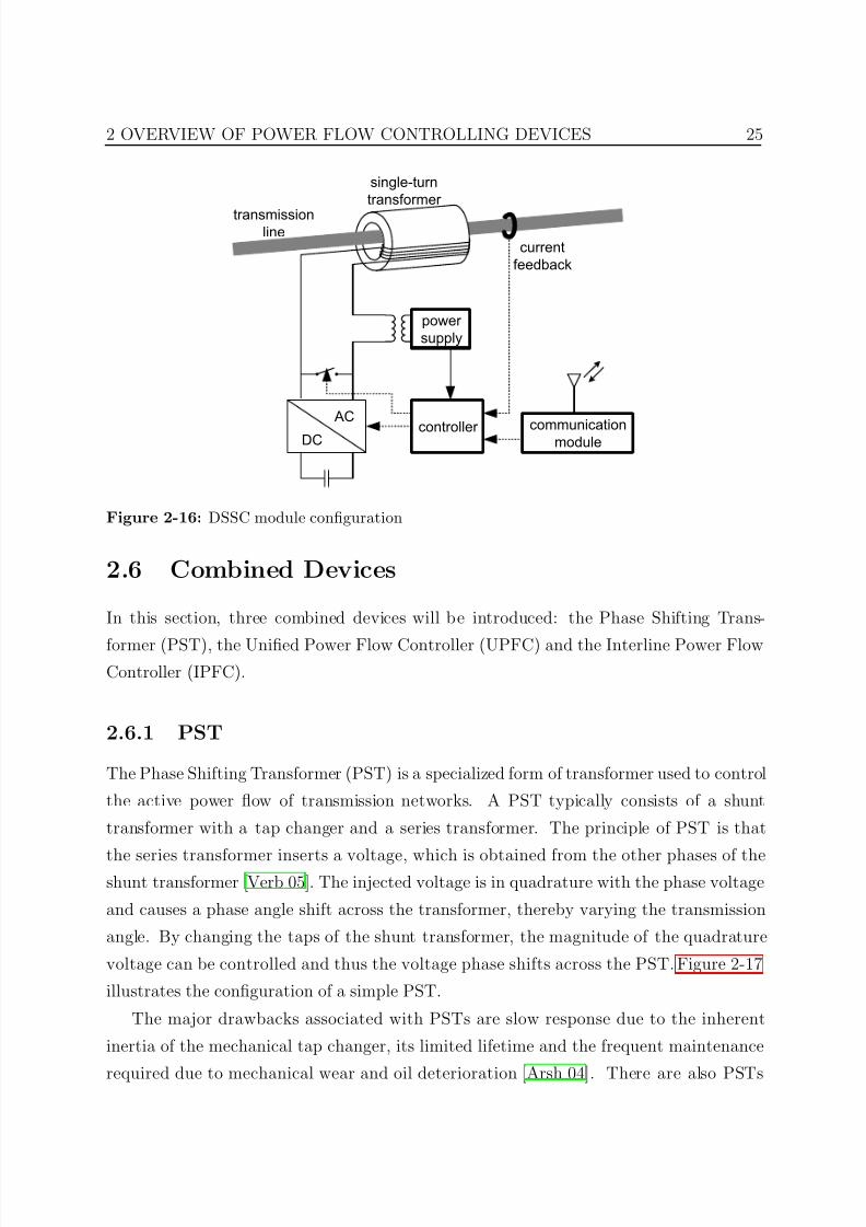
A DSSC unit consists of multiple low-rated, single-phase VSCs that are attached to
the transmission line by single-turn transformers. The single-turn transformer uses the
transmission line as its secondary winding and injects a controllable voltage directly into
the line. Most of the voltage injected by a DSSC unit is in quadrature with the line
current, to emulate inductive or capacitive impedance. A small part of the voltage is
in phase with the line current and serves to self-power the DSSC unit and cover losses.
The DSSC is remotely controlled via wireless communication or a PLC [ Ferr 96]. The
configuration of a DSSC unit is shown in Figure 2-16.
The unique character of the DSSC results in relatively low cost and high reliability.
As DSSC units are single-phase devices floating on lines, high-voltage isolation between
the phases are avoided. The units can easily be applied at any transmission voltage level
because they do not require supporting phase-ground isolation. The power and voltage
rating of each unit is small. Further, the units are clamped on transmission lines, requiring
no additional land, thereby eliminating their footprint. The redundancy of DSSC provides
uninterrupted operation during a single module failure, thereby giving reliability at lower
cost than with other FACTS devices.
7/25/2019 Dpfc Thesis
http://slidepdf.com/reader/full/dpfc-thesis 47/212
2 OVERVIEW OF POWER FLOW CONTROLLING DEVICES 25
AC
DC controller
power
supply
communicationmodule
current
feedback
single-turn
transformer
transmissionline
Figure 2-16: DSSC module configuration
2.6 Combined Devices
In this section, three combined devices will be introduced: the Phase Shifting Trans-
former (PST), the Unified Power Flow Controller (UPFC) and the Interline Power FlowController (IPFC).
2.6.1 PST
The Phase Shifting Transformer (PST) is a specialized form of transformer used to control
the active power flow of transmission networks. A PST typically consists of a shunt
transformer with a tap changer and a series transformer. The principle of PST is that
the series transformer inserts a voltage, which is obtained from the other phases of theshunt transformer [Verb 05]. The injected voltage is in quadrature with the phase voltage
and causes a phase angle shift across the transformer, thereby varying the transmission
angle. By changing the taps of the shunt transformer, the magnitude of the quadrature
voltage can be controlled and thus the voltage phase shifts across the PST. Figure 2-17
illustrates the configuration of a simple PST.
The major drawbacks associated with PSTs are slow response due to the inherent
inertia of the mechanical tap changer, its limited lifetime and the frequent maintenance
required due to mechanical wear and oil deterioration [Arsh 04]. There are also PSTs
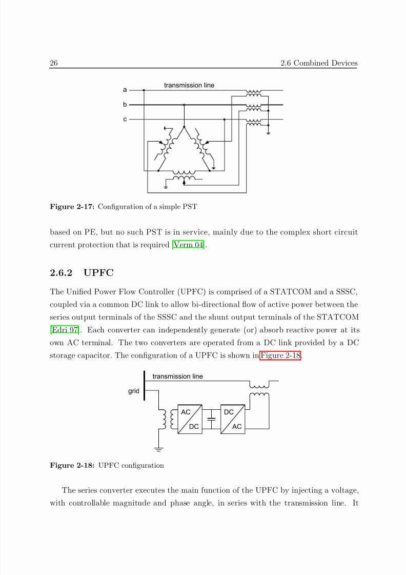
7/25/2019 Dpfc Thesis
http://slidepdf.com/reader/full/dpfc-thesis 48/212
26 2.6 Combined Devices
transmission linea
b
c
Figure 2-17: Configuration of a simple PST
based on PE, but no such PST is in service, mainly due to the complex short circuit
current protection that is required [Verm 04].
2.6.2 UPFC
The Unified Power Flow Controller (UPFC) is comprised of a STATCOM and a SSSC,
coupled via a common DC link to allow bi-directional flow of active power between the
series output terminals of the SSSC and the shunt output terminals of the STATCOM
[Edri 97]. Each converter can independently generate (or) absorb reactive power at its
own AC terminal. The two converters are operated from a DC link provided by a DC
storage capacitor. The configuration of a UPFC is shown in Figure 2-18.
grid
AC
DC
transmission line
DC
AC
Figure 2-18: UPFC configuration
The series converter executes the main function of the UPFC by injecting a voltage,
with controllable magnitude and phase angle, in series with the transmission line. It
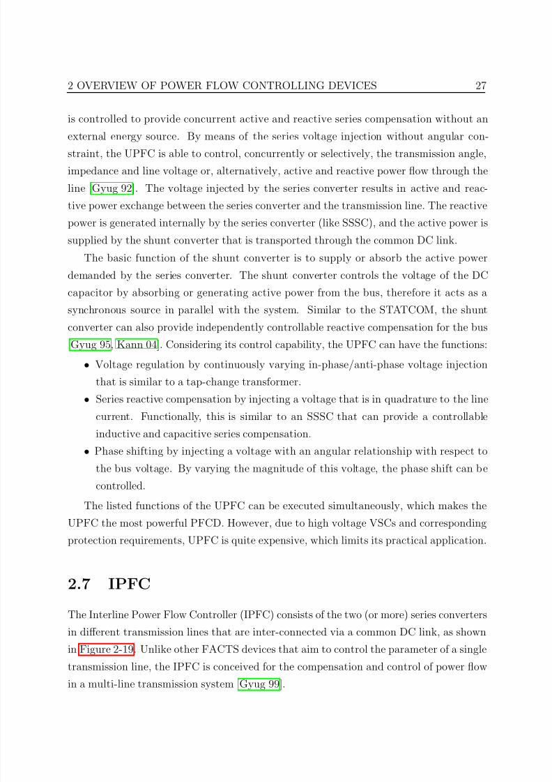
7/25/2019 Dpfc Thesis
http://slidepdf.com/reader/full/dpfc-thesis 49/212
2 OVERVIEW OF POWER FLOW CONTROLLING DEVICES 27
is controlled to provide concurrent active and reactive series compensation without an
external energy source. By means of the series voltage injection without angular con-straint, the UPFC is able to control, concurrently or selectively, the transmission angle,
impedance and line voltage or, alternatively, active and reactive power flow through the
line [Gyug 92]. The voltage injected by the series converter results in active and reac-
tive power exchange between the series converter and the transmission line. The reactive
power is generated internally by the series converter (like SSSC), and the active power is
supplied by the shunt converter that is transported through the common DC link.
The basic function of the shunt converter is to supply or absorb the active power
demanded by the series converter. The shunt converter controls the voltage of the DCcapacitor by absorbing or generating active power from the bus, therefore it acts as a
synchronous source in parallel with the system. Similar to the STATCOM, the shunt
converter can also provide independently controllable reactive compensation for the bus
[Gyug 95, Kann 04]. Considering its control capability, the UPFC can have the functions:
• Voltage regulation by continuously varying in-phase/anti-phase voltage injection
that is similar to a tap-change transformer.
• Series reactive compensation by injecting a voltage that is in quadrature to the line
current. Functionally, this is similar to an SSSC that can provide a controllable
inductive and capacitive series compensation.
• Phase shifting by injecting a voltage with an angular relationship with respect to
the bus voltage. By varying the magnitude of this voltage, the phase shift can be
controlled.
The listed functions of the UPFC can be executed simultaneously, which makes the
UPFC the most powerful PFCD. However, due to high voltage VSCs and corresponding
protection requirements, UPFC is quite expensive, which limits its practical application.
2.7 IPFC
The Interline Power Flow Controller (IPFC) consists of the two (or more) series converters
in different transmission lines that are inter-connected via a common DC link, as shown
in Figure 2-19. Unlike other FACTS devices that aim to control the parameter of a single
transmission line, the IPFC is conceived for the compensation and control of power flow
in a multi-line transmission system [Gyug 99].
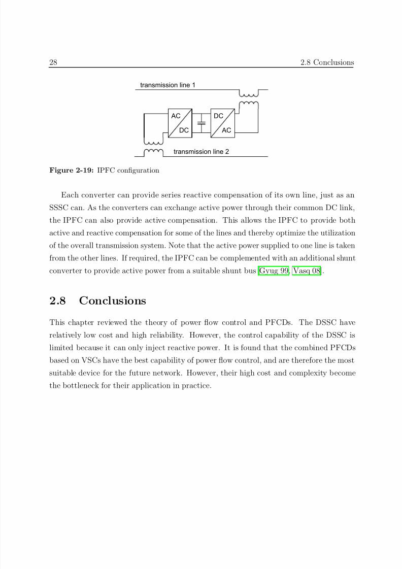
7/25/2019 Dpfc Thesis
http://slidepdf.com/reader/full/dpfc-thesis 50/212
28 2.8 Conclusions
AC
DC
transmission line 1
DC
AC
transmission line 2
Figure 2-19: IPFC configuration
Each converter can provide series reactive compensation of its own line, just as anSSSC can. As the converters can exchange active power through their common DC link,
the IPFC can also provide active compensation. This allows the IPFC to provide both
active and reactive compensation for some of the lines and thereby optimize the utilization
of the overall transmission system. Note that the active power supplied to one line is taken
from the other lines. If required, the IPFC can be complemented with an additional shunt
converter to provide active power from a suitable shunt bus [Gyug 99, Vasq 08].
2.8 Conclusions
This chapter reviewed the theory of power flow control and PFCDs. The DSSC have
relatively low cost and high reliability. However, the control capability of the DSSC is
limited because it can only inject reactive power. It is found that the combined PFCDs
based on VSCs have the best capability of power flow control, and are therefore the most
suitable device for the future network. However, their high cost and complexity become
the bottleneck for their application in practice.
7/25/2019 Dpfc Thesis
http://slidepdf.com/reader/full/dpfc-thesis 51/212
Chapter 3DISTRIBUTED POWER FLOW
CONTROLLER
3.1 Introduction
I
N the previous chapter, an overview was given of mechanical- and PE-based PFCDs.
Because of high control capability, the PE-based combined PFCs, specifically UPFCand IPFC are suitable for the future power system. However, the UPFC and IPFC are
not widely applied in practice, due to their high cost and the susceptibility to failures.
Generally, the reliability can be improved by reducing the number of components; however,
this is not possible due to the complex topology of the UPFC and IPFC. To reduce
the failure rate of the components by selecting components with higher ratings than
necessary or employing redundancy at the component or system levels are also options.
Unfortunately, these solutions increase the initial investment necessary, negating any cost-
related advantages. Accordingly, new approaches are needed in order to increase reliabilityand reduce cost of the UPFC and IPFC at the same time.
After studying the failure mode of the combined FACTS devices, it is found that a
common DC link between converters reduces the reliability of a device, because a failure
in one converter will pervade the whole device though the DC link. By eliminating this
DC link, the converters within the FACTS devices are operated independently, thereby
increasing their reliability.
The elimination of the common DC link also allows the DSSC concept to be applied
to series converters. In that case, the reliability of the new device is further improved
29
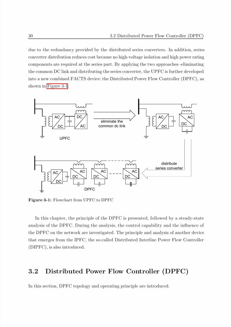
7/25/2019 Dpfc Thesis
http://slidepdf.com/reader/full/dpfc-thesis 52/212
30 3.2 Distributed Power Flow Controller (DPFC)
due to the redundancy provided by the distributed series converters. In addition, series
converter distribution reduces cost because no high-voltage isolation and high power ratingcomponents are required at the series part. By applying the two approaches -eliminating
the common DC link and distributing the series converter, the UPFC is further developed
into a new combined FACTS device: the Distributed Power Flow Controller (DPFC), as
shown in Figure 3-1.
AC
DC
DC
AC
AC
DC DC
AC
ACDC
ACDC
ACDC
AC
DC
UPFC
DPFC
eliminate the
common dc link
distribute
series converter
Figure 3-1: Flowchart from UPFC to DPFC
In this chapter, the principle of the DPFC is presented, followed by a steady-state
analysis of the DPFC. During the analysis, the control capability and the influence of
the DPFC on the network are investigated. The principle and analysis of another device
that emerges from the IPFC, the so-called Distributed Interline Power Flow Controller
(DIPFC), is also introduced.
3.2 Distributed Power Flow Controller (DPFC)
In this section, DPFC topology and operating principle are introduced.
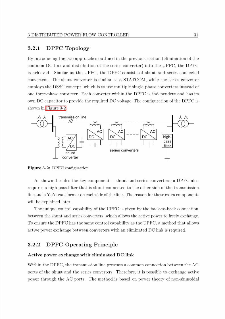
7/25/2019 Dpfc Thesis
http://slidepdf.com/reader/full/dpfc-thesis 53/212
3 DISTRIBUTED POWER FLOW CONTROLLER 31
3.2.1 DPFC Topology
By introducing the two approaches outlined in the previous section (elimination of the
common DC link and distribution of the series converter) into the UPFC, the DPFC
is achieved. Similar as the UPFC, the DPFC consists of shunt and series connected
converters. The shunt converter is similar as a STATCOM, while the series converter
employs the DSSC concept, which is to use multiple single-phase converters instead of
one three-phase converter. Each converter within the DPFC is independent and has its
own DC capacitor to provide the required DC voltage. The configuration of the DPFC is
shown in Figure 3-2.
AC
DC
transmission line
AC
DC
AC
DC
AC
DC high-
pass
filter
snt
onerter
seres onerters
Figure 3-2: DPFC configuration
As shown, besides the key components - shunt and series converters, a DPFC also
requires a high pass filter that is shunt connected to the other side of the transmission
line and a Y-∆ transformer on each side of the line. The reason for these extra components
will be explained later.
The unique control capability of the UPFC is given by the back-to-back connection
between the shunt and series converters, which allows the active power to freely exchange.
To ensure the DPFC has the same control capability as the UPFC, a method that allowsactive power exchange between converters with an eliminated DC link is required.
3.2.2 DPFC Operating Principle
Active power exchange with eliminated DC link
Within the DPFC, the transmission line presents a common connection between the AC
ports of the shunt and the series converters. Therefore, it is possible to exchange active
power through the AC ports. The method is based on power theory of non-sinusoidal
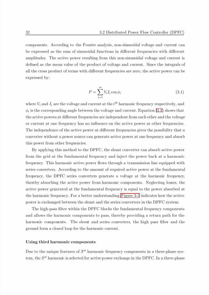
7/25/2019 Dpfc Thesis
http://slidepdf.com/reader/full/dpfc-thesis 54/212
32 3.2 Distributed Power Flow Controller (DPFC)
components. According to the Fourier analysis, non-sinusoidal voltage and current can
be expressed as the sum of sinusoidal functions in different frequencies with differentamplitudes. The active power resulting from this non-sinusoidal voltage and current is
defined as the mean value of the product of voltage and current. Since the integrals of
all the cross product of terms with different frequencies are zero, the active power can be
expressed by:
P =∞
i=1
V iI i cos φi (3.1)
where V i and I i are the voltage and current at the ith harmonic frequency respectively, and
φi is the corresponding angle between the voltage and current. Equation (3.1) shows that
the active powers at different frequencies are independent from each other and the voltage
or current at one frequency has no influence on the active power at other frequencies.
The independence of the active power at different frequencies gives the possibility that a
converter without a power source can generate active power at one frequency and absorb
this power from other frequencies.
By applying this method to the DPFC, the shunt converter can absorb active power
from the grid at the fundamental frequency and inject the power back at a harmonic
frequency. This harmonic active power flows through a transmission line equipped with
series converters. According to the amount of required active power at the fundamental
frequency, the DPFC series converters generate a voltage at the harmonic frequency,
thereby absorbing the active power from harmonic components. Neglecting losses, the
active power generated at the fundamental frequency is equal to the power absorbed at
the harmonic frequency. For a better understanding, Figure 3-3 indicates how the active
power is exchanged between the shunt and the series converters in the DPFC system.
The high-pass filter within the DPFC blocks the fundamental frequency components
and allows the harmonic components to pass, thereby providing a return path for the
harmonic components. The shunt and series converters, the high pass filter and the
ground form a closed loop for the harmonic current.
Using third harmonic components
Due to the unique features of 3rd harmonic frequency components in a three-phase sys-
tem, the 3rd harmonic is selected for active power exchange in the DPFC. In a three-phase
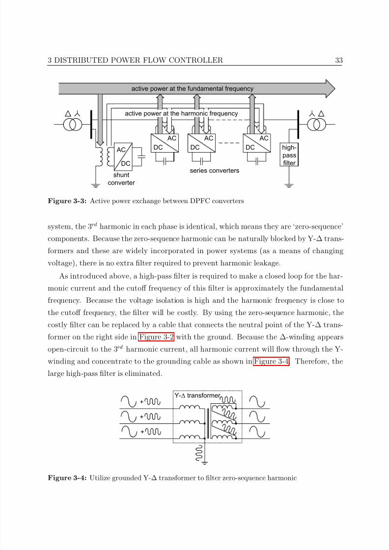
7/25/2019 Dpfc Thesis
http://slidepdf.com/reader/full/dpfc-thesis 55/212
3 DISTRIBUTED POWER FLOW CONTROLLER 33
AC
DC
AC
DC
AC
DC
AC
DC high
pass
filter
shunt
converter
series converters
active power at the fundamental frequency
active power at the harmonic frequency
Figure 3-3: Active power exchange between DPFC converters
system, the 3rd harmonic in each phase is identical, which means they are ‘zero-sequence’
components. Because the zero-sequence harmonic can be naturally blocked by Y-∆ trans-
formers and these are widely incorporated in power systems (as a means of changing
voltage), there is no extra filter required to prevent harmonic leakage.
As introduced above, a high-pass filter is required to make a closed loop for the har-
monic current and the cutoff frequency of this filter is approximately the fundamentalfrequency. Because the voltage isolation is high and the harmonic frequency is close to
the cutoff frequency, the filter will be costly. By using the zero-sequence harmonic, the
costly filter can be replaced by a cable that connects the neutral point of the Y-∆ trans-
former on the right side in Figure 3-2 with the ground. Because the ∆-winding appears
open-circuit to the 3rd harmonic current, all harmonic current will flow through the Y-
winding and concentrate to the grounding cable as shown in Figure 3-4. Therefore, the
large high-pass filter is eliminated.
+
+
+
Y-∆ transformer
Figure 3-4: Utilize grounded Y-∆ transformer to filter zero-sequence harmonic
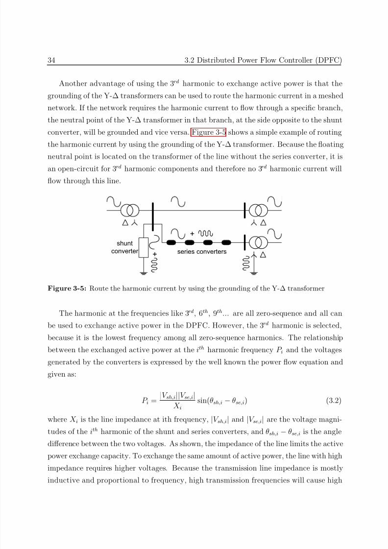
7/25/2019 Dpfc Thesis
http://slidepdf.com/reader/full/dpfc-thesis 56/212
34 3.2 Distributed Power Flow Controller (DPFC)
Another advantage of using the 3rd harmonic to exchange active power is that the
grounding of the Y-∆ transformers can be used to route the harmonic current in a meshednetwork. If the network requires the harmonic current to flow through a specific branch,
the neutral point of the Y-∆ transformer in that branch, at the side opposite to the shunt
converter, will be grounded and vice versa. Figure 3-5 shows a simple example of routing
the harmonic current by using the grounding of the Y-∆ transformer. Because the floating
neutral point is located on the transformer of the line without the series converter, it is
an open-circuit for 3rd harmonic components and therefore no 3rd harmonic current will
flow through this line.
shunt
converter +
+
series converters
Figure 3-5: Route the harmonic current by using the grounding of the Y-∆ transformer
The harmonic at the frequencies like 3rd, 6th, 9th... are all zero-sequence and all can
be used to exchange active power in the DPFC. However, the 3rd harmonic is selected,
because it is the lowest frequency among all zero-sequence harmonics. The relationship
between the exchanged active power at the ith harmonic frequency P i and the voltages
generated by the converters is expressed by the well known the power flow equation and
given as:
P i = |V sh,i||V se,i|
X isin(θsh,i − θse,i) (3.2)
where X i is the line impedance at ith frequency, |V sh,i| and |V se,i| are the voltage magni-
tudes of the ith harmonic of the shunt and series converters, and θsh,i − θse,i is the angle
difference between the two voltages. As shown, the impedance of the line limits the active
power exchange capacity. To exchange the same amount of active power, the line with high
impedance requires higher voltages. Because the transmission line impedance is mostly
inductive and proportional to frequency, high transmission frequencies will cause high
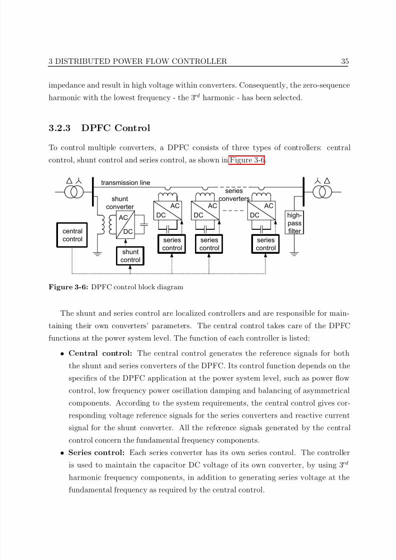
7/25/2019 Dpfc Thesis
http://slidepdf.com/reader/full/dpfc-thesis 57/212
3 DISTRIBUTED POWER FLOW CONTROLLER 35
impedance and result in high voltage within converters. Consequently, the zero-sequence
harmonic with the lowest frequency - the 3rd harmonic - has been selected.
3.2.3 DPFC Control
To control multiple converters, a DPFC consists of three types of controllers: central
control, shunt control and series control, as shown in Figure 3-6.
AC
DC
transmission line
AC
DC
AC
DC
AC
DC high-
pass
filter
snt
onerter
seres
onerters
snt
ontrol
seres
ontrol
seres
ontrol
seres
ontrol
entral
ontrol
Figure 3-6: DPFC control block diagram
The shunt and series control are localized controllers and are responsible for main-
taining their own converters’ parameters. The central control takes care of the DPFC
functions at the power system level. The function of each controller is listed:
• Central control: The central control generates the reference signals for both
the shunt and series converters of the DPFC. Its control function depends on the
specifics of the DPFC application at the power system level, such as power flow
control, low frequency power oscillation damping and balancing of asymmetricalcomponents. According to the system requirements, the central control gives cor-
responding voltage reference signals for the series converters and reactive current
signal for the shunt converter. All the reference signals generated by the central
control concern the fundamental frequency components.
• Series control: Each series converter has its own series control. The controller
is used to maintain the capacitor DC voltage of its own converter, by using 3 rd
harmonic frequency components, in addition to generating series voltage at the
fundamental frequency as required by the central control.
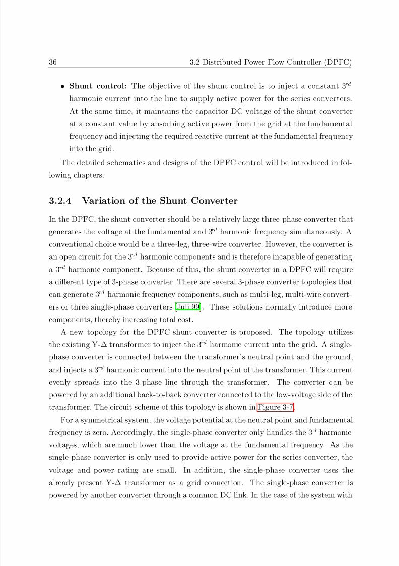
7/25/2019 Dpfc Thesis
http://slidepdf.com/reader/full/dpfc-thesis 58/212
36 3.2 Distributed Power Flow Controller (DPFC)
• Shunt control: The objective of the shunt control is to inject a constant 3 rd
harmonic current into the line to supply active power for the series converters.At the same time, it maintains the capacitor DC voltage of the shunt converter
at a constant value by absorbing active power from the grid at the fundamental
frequency and injecting the required reactive current at the fundamental frequency
into the grid.
The detailed schematics and designs of the DPFC control will be introduced in fol-
lowing chapters.
3.2.4 Variation of the Shunt Converter
In the DPFC, the shunt converter should be a relatively large three-phase converter that
generates the voltage at the fundamental and 3rd harmonic frequency simultaneously. A
conventional choice would be a three-leg, three-wire converter. However, the converter is
an open circuit for the 3rd harmonic components and is therefore incapable of generating
a 3rd harmonic component. Because of this, the shunt converter in a DPFC will require
a different type of 3-phase converter. There are several 3-phase converter topologies that
can generate 3rd
harmonic frequency components, such as multi-leg, multi-wire convert-ers or three single-phase converters [Juli 99]. These solutions normally introduce more
components, thereby increasing total cost.
A new topology for the DPFC shunt converter is proposed. The topology utilizes
the existing Y-∆ transformer to inject the 3rd harmonic current into the grid. A single-
phase converter is connected between the transformer’s neutral point and the ground,
and injects a 3rd harmonic current into the neutral point of the transformer. This current
evenly spreads into the 3-phase line through the transformer. The converter can be
powered by an additional back-to-back converter connected to the low-voltage side of thetransformer. The circuit scheme of this topology is shown in Figure 3-7.
For a symmetrical system, the voltage potential at the neutral point and fundamental
frequency is zero. Accordingly, the single-phase converter only handles the 3rd harmonic
voltages, which are much lower than the voltage at the fundamental frequency. As the
single-phase converter is only used to provide active power for the series converter, the
voltage and power rating are small. In addition, the single-phase converter uses the
already present Y-∆ transformer as a grid connection. The single-phase converter is
powered by another converter through a common DC link. In the case of the system with
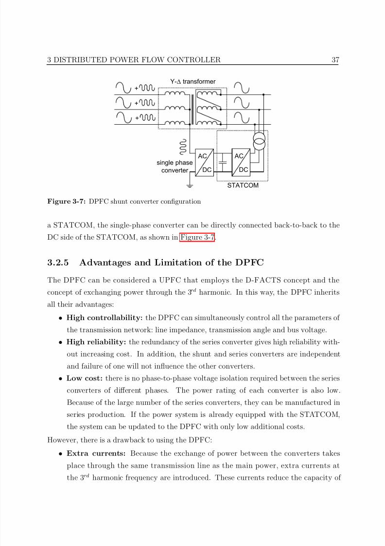
7/25/2019 Dpfc Thesis
http://slidepdf.com/reader/full/dpfc-thesis 59/212
3 DISTRIBUTED POWER FLOW CONTROLLER 37
+
+
+
Y-∆ transformer
AC
DC
AC
DCsingle phase
converter
STATCOM
Figure 3-7: DPFC shunt converter configuration
a STATCOM, the single-phase converter can be directly connected back-to-back to the
DC side of the STATCOM, as shown in Figure 3-7.
3.2.5 Advantages and Limitation of the DPFC
The DPFC can be considered a UPFC that employs the D-FACTS concept and the
concept of exchanging power through the 3rd harmonic. In this way, the DPFC inherits
all their advantages:
• High controllability: the DPFC can simultaneously control all the parameters of
the transmission network: line impedance, transmission angle and bus voltage.
• High reliability: the redundancy of the series converter gives high reliability with-
out increasing cost. In addition, the shunt and series converters are independent
and failure of one will not influence the other converters.
• Low cost: there is no phase-to-phase voltage isolation required between the series
converters of different phases. The power rating of each converter is also low.
Because of the large number of the series converters, they can be manufactured in
series production. If the power system is already equipped with the STATCOM,
the system can be updated to the DPFC with only low additional costs.
However, there is a drawback to using the DPFC:
• Extra currents: Because the exchange of power between the converters takes
place through the same transmission line as the main power, extra currents at
the 3rd harmonic frequency are introduced. These currents reduce the capacity of
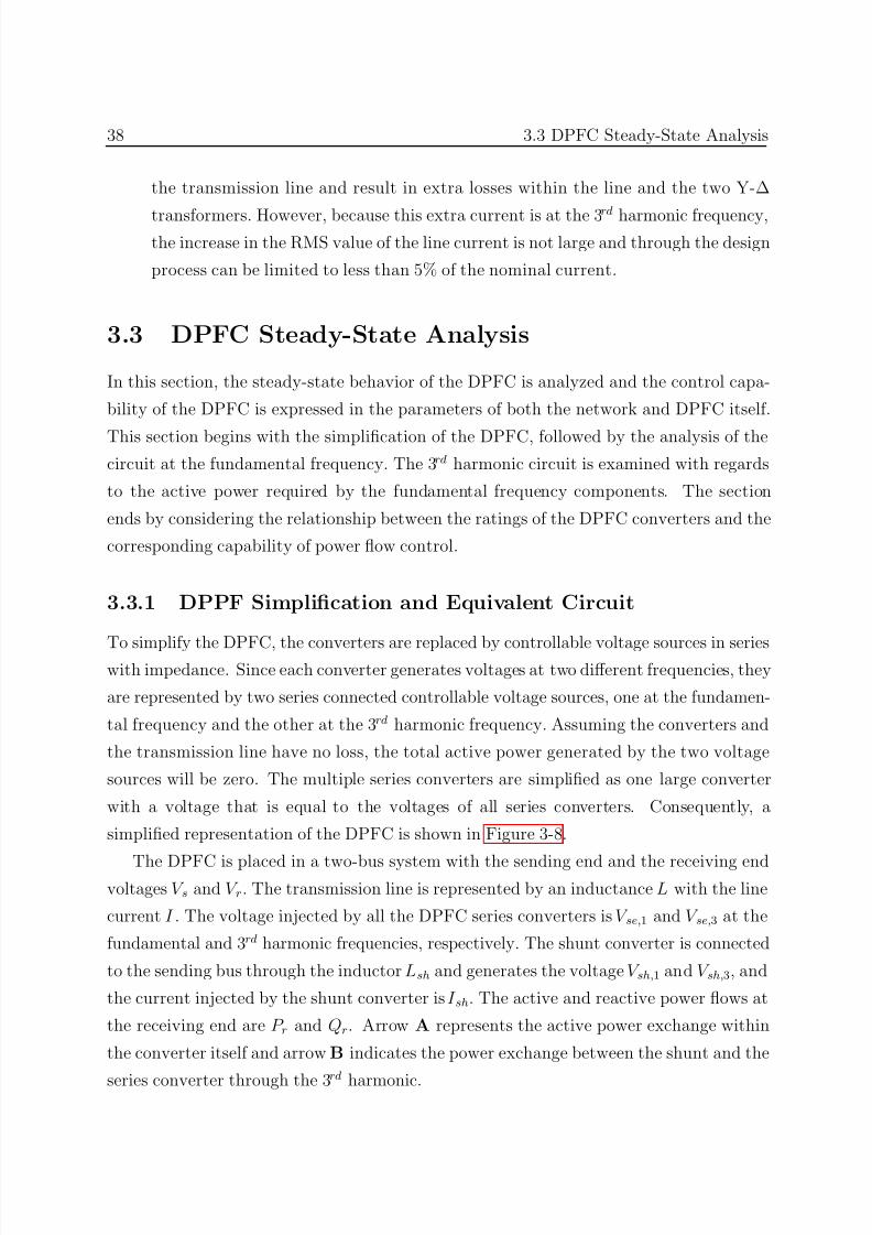
7/25/2019 Dpfc Thesis
http://slidepdf.com/reader/full/dpfc-thesis 60/212
38 3.3 DPFC Steady-State Analysis
the transmission line and result in extra losses within the line and the two Y-∆
transformers. However, because this extra current is at the 3rd harmonic frequency,the increase in the RMS value of the line current is not large and through the design
process can be limited to less than 5% of the nominal current.
3.3 DPFC Steady-State Analysis
In this section, the steady-state behavior of the DPFC is analyzed and the control capa-
bility of the DPFC is expressed in the parameters of both the network and DPFC itself.
This section begins with the simplification of the DPFC, followed by the analysis of the
circuit at the fundamental frequency. The 3rd harmonic circuit is examined with regards
to the active power required by the fundamental frequency components. The section
ends by considering the relationship between the ratings of the DPFC converters and the
corresponding capability of power flow control.
3.3.1 DPPF Simplification and Equivalent Circuit
To simplify the DPFC, the converters are replaced by controllable voltage sources in serieswith impedance. Since each converter generates voltages at two different frequencies, they
are represented by two series connected controllable voltage sources, one at the fundamen-
tal frequency and the other at the 3rd harmonic frequency. Assuming the converters and
the transmission line have no loss, the total active power generated by the two voltage
sources will be zero. The multiple series converters are simplified as one large converter
with a voltage that is equal to the voltages of all series converters. Consequently, a
simplified representation of the DPFC is shown in Figure 3-8.
The DPFC is placed in a two-bus system with the sending end and the receiving endvoltages V s and V r. The transmission line is represented by an inductance L with the line
current I . The voltage injected by all the DPFC series converters is V se,1 and V se,3 at the
fundamental and 3rd harmonic frequencies, respectively. The shunt converter is connected
to the sending bus through the inductor Lsh and generates the voltage V sh,1 and V sh,3, and
the current injected by the shunt converter is I sh. The active and reactive power flows at
the receiving end are P r and Qr. Arrow A represents the active power exchange within
the converter itself and arrow B indicates the power exchange between the shunt and the
series converter through the 3rd harmonic.
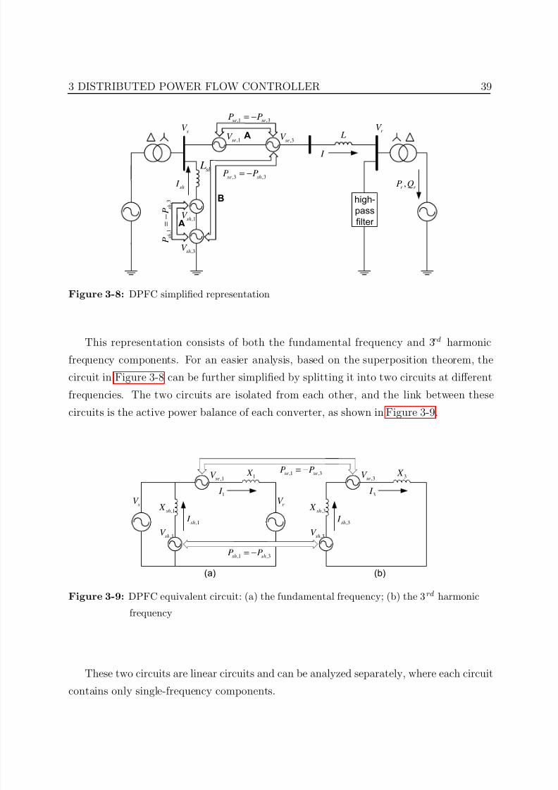
7/25/2019 Dpfc Thesis
http://slidepdf.com/reader/full/dpfc-thesis 61/212
3 DISTRIBUTED POWER FLOW CONTROLLER 39
,1seV ,3seV
,1shV
,3shV
sh L
L
r V s
V ,1 ,3se seP P= −
, 1
, 3
s h
s h
P
P
=
−
,3 ,3se shP P= −
,r r P Q
high-
pass
filter
I
sh I
A
A
B
Figure 3-8: DPFC simplified representation
This representation consists of both the fundamental frequency and 3rd harmonic
frequency components. For an easier analysis, based on the superposition theorem, the
circuit in Figure 3-8 can be further simplified by splitting it into two circuits at different
frequencies. The two circuits are isolated from each other, and the link between these
circuits is the active power balance of each converter, as shown in Figure 3-9.
,1seV
,1shV
,1sh X
1 X
r V sV
,1 ,3se seP P= −
,1 ,3sh shP P= −
1 I
,1sh I
,3seV
,3shV
,3sh X
3 X
3 I
,3sh I
(a) (b)
Figure 3-9: DPFC equivalent circuit: (a) the fundamental frequency; (b) the 3rd harmonic
frequency
These two circuits are linear circuits and can be analyzed separately, where each circuit
contains only single-frequency components.
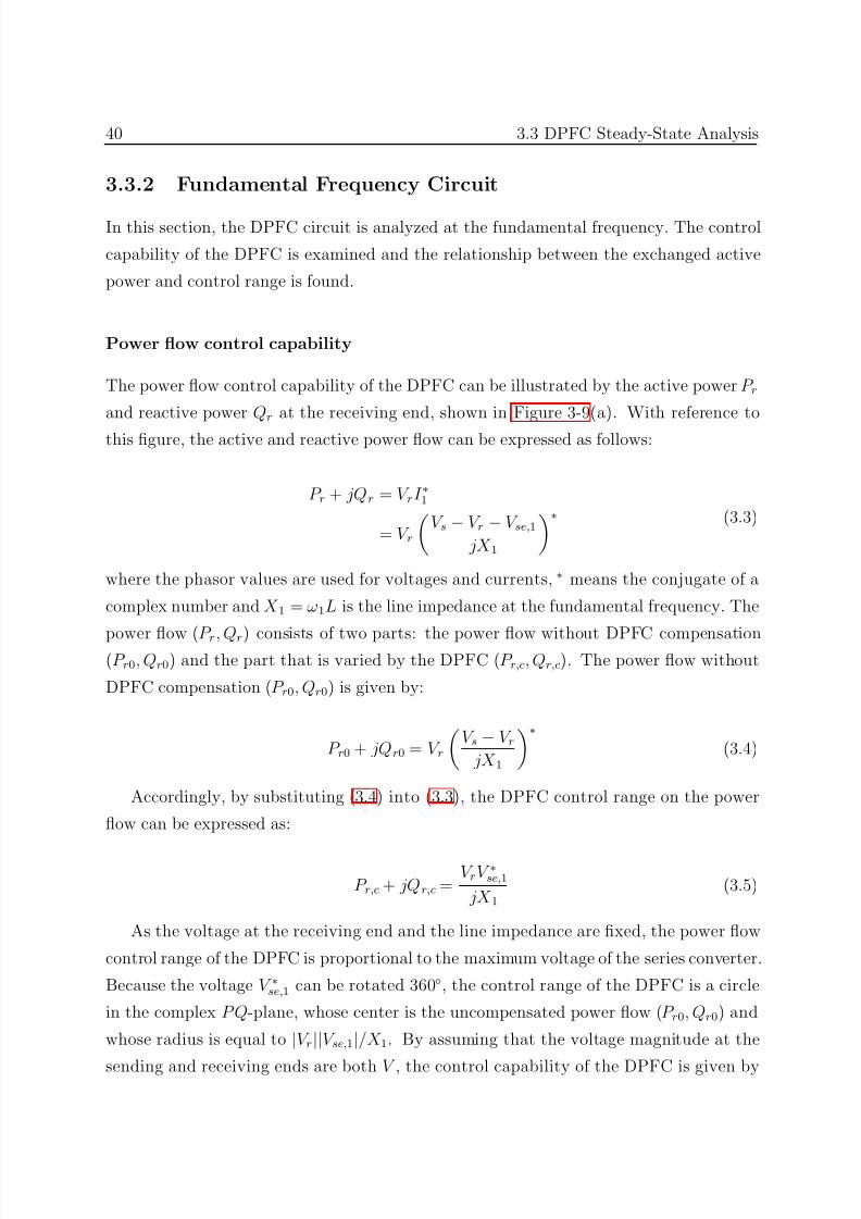
7/25/2019 Dpfc Thesis
http://slidepdf.com/reader/full/dpfc-thesis 62/212
40 3.3 DPFC Steady-State Analysis
3.3.2 Fundamental Frequency Circuit
In this section, the DPFC circuit is analyzed at the fundamental frequency. The control
capability of the DPFC is examined and the relationship between the exchanged active
power and control range is found.
Power flow control capability
The power flow control capability of the DPFC can be illustrated by the active power P r
and reactive power Qr at the receiving end, shown in Figure 3-9(a). With reference to
this figure, the active and reactive power flow can be expressed as follows:
P r + jQr = V rI ∗1
= V r
V s − V r − V se,1
jX 1
∗ (3.3)
where the phasor values are used for voltages and currents, ∗ means the conjugate of a
complex number and X 1 = ω1L is the line impedance at the fundamental frequency. The
power flow (P r, Qr) consists of two parts: the power flow without DPFC compensation(P r0, Qr0) and the part that is varied by the DPFC (P r,c, Qr,c). The power flow without
DPFC compensation (P r0, Qr0) is given by:
P r0 + jQr0 = V r
V s − V r
jX 1
∗
(3.4)
Accordingly, by substituting (3.4) into (3.3), the DPFC control range on the power
flow can be expressed as:
P r,c + jQr,c =V rV ∗se,1
jX 1(3.5)
As the voltage at the receiving end and the line impedance are fixed, the power flow
control range of the DPFC is proportional to the maximum voltage of the series converter.
Because the voltage V ∗se,1 can be rotated 360, the control range of the DPFC is a circle
in the complex P Q-plane, whose center is the uncompensated power flow (P r0, Qr0) and
whose radius is equal to |V r||V se,1|/X 1. By assuming that the voltage magnitude at the
sending and receiving ends are both V , the control capability of the DPFC is given by
7/25/2019 Dpfc Thesis
http://slidepdf.com/reader/full/dpfc-thesis 63/212
3 DISTRIBUTED POWER FLOW CONTROLLER 41
the following formula:
(P r − P r0)2 + (Qr −Qr0)2 =
V |V se,1|
X 1
2
(3.6)
In the complex P Q-plane, the locus of the power flow without the DPFC compensation
f (P r0, Qr0) is a circle with radius |V |2/|X 1| around its center (defined by coordinates
P = 0 and Q = |V |2/|X 1|). Each point of this circle gives P r0 and Qr0 values of the
uncompensated system at the corresponding transmission angle θ. The boundary of the
attainable control range for P r and Qr is obtained from a complete rotation of the voltage
V se,1 with its maximum magnitude. Figure 3-10 shows the power flow control range of theDPFC with the transmission angle θ.
r P
r Q
θ 2
1
(0, )V
X −
DPFC control
range with θ
,1
1
| |seV V
X
Figure 3-10: DPFC active and reactive power control range with the transmission angle θ
Active power required by the series converters
To inject a 360 rotatable voltage, an active and reactive power at the fundamental
frequency has to be supplied to the series converter, which is given as:
P se,1 + jQse,1 = V se,1I ∗1
= V se,1
S r
V r
(3.7)
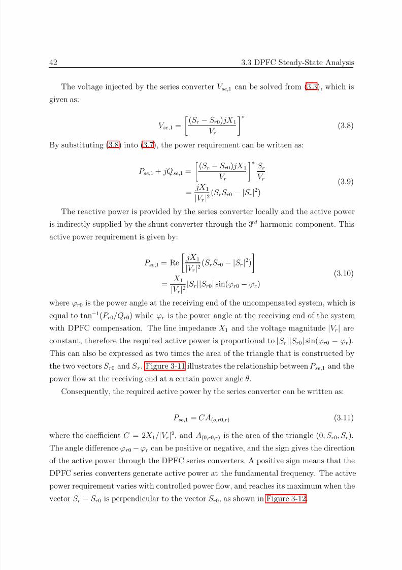
7/25/2019 Dpfc Thesis
http://slidepdf.com/reader/full/dpfc-thesis 64/212
42 3.3 DPFC Steady-State Analysis
The voltage injected by the series converter V se,1 can be solved from (3.3), which is
given as:
V se,1 =
(S r − S r0) jX 1
V r
∗
(3.8)
By substituting (3.8) into (3.7), the power requirement can be written as:
P se,1 + jQse,1 =
(S r − S r0) jX 1
V r
∗
S rV r
= jX 1
|V r|2
(S rS r0− |
S r|2)
(3.9)
The reactive power is provided by the series converter locally and the active power
is indirectly supplied by the shunt converter through the 3rd harmonic component. This
active power requirement is given by:
P se,1 = Re
jX 1|V r|2 (S rS r0 − |S r|2)
= X 1
|V r
|2|S r||S r0| sin(ϕr0 − ϕr)
(3.10)
where ϕr0 is the power angle at the receiving end of the uncompensated system, which is
equal to tan−1(P r0/Qr0) while ϕr is the power angle at the receiving end of the system
with DPFC compensation. The line impedance X 1 and the voltage magnitude |V r| are
constant, therefore the required active power is proportional to |S r||S r0| sin(ϕr0 − ϕr).
This can also be expressed as two times the area of the triangle that is constructed by
the two vectors S r0 and S r. Figure 3-11 illustrates the relationship between P se,1 and the
power flow at the receiving end at a certain power angle θ.
Consequently, the required active power by the series converter can be written as:
P se,1 = C A(o,r0,r) (3.11)
where the coefficient C = 2X 1/|V r|2, and A(0,r0,r) is the area of the triangle (0, S r0, S r).
The angle difference ϕr0−ϕr can be positive or negative, and the sign gives the direction
of the active power through the DPFC series converters. A positive sign means that the
DPFC series converters generate active power at the fundamental frequency. The active
power requirement varies with controlled power flow, and reaches its maximum when the
vector S r − S r0 is perpendicular to the vector S r0, as shown in Figure 3-12.
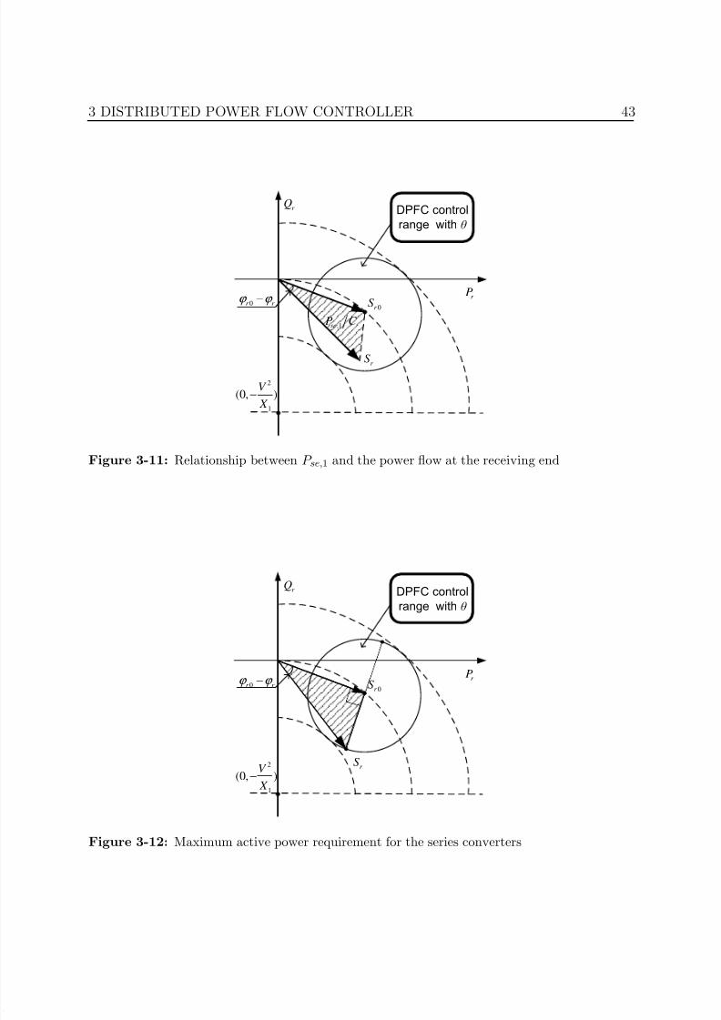
7/25/2019 Dpfc Thesis
http://slidepdf.com/reader/full/dpfc-thesis 65/212
3 DISTRIBUTED POWER FLOW CONTROLLER 43
r P
r Q
2
1
(0, )V
X −
DPFC control
range with θ
0r S
r S
0r r ϕ ϕ −
,1seP C
Figure 3-11: Relationship between P se,1 and the power flow at the receiving end
r P
r Q
2
1
(0, )V
X −
DPFC control
range with θ
0r S
r S
0r r ϕ ϕ −
Figure 3-12: Maximum active power requirement for the series converters
7/25/2019 Dpfc Thesis
http://slidepdf.com/reader/full/dpfc-thesis 66/212
44 3.3 DPFC Steady-State Analysis
The control range of the DPFC is limited by this maximum value. According to the
figure, the relationship between the power flow control range and the maximum activepower requirement can be represented with the following equation:
P se,1,max = |X 1||S r0||V r|2 |S r,c| (3.12)
where |S r,c| is the control range of the DPFC and given by:
|S r,c
|= max
|P r,c + jQr,c
| (3.13)
For a transmission line, the line impedance and the bus voltage can be assumed con-
stant values. Accordingly, the control range is proportional to the maximum of the ex-
changed active power. The line impedance |X 1| is normally around 0.05 pu. By assum-
ing that the bus voltage |V r| and uncompensated power flow |S r0| is 1 pu, the value of
exchanged active power can be determined as approximately 0.05 pu by using (3.12),
allowing the DPFC to control 1 pu power flow.
3.3.3 Third Harmonic Frequency Circuit
The 3rd harmonic component within the DPFC system is used to exchange active and
reactive power between the shunt and series converters. Therefore, the voltages and
currents at the 3rd harmonic frequency are related to the required active power at the
fundamental frequency. For the series converters, there is:
Re (V se,3I ∗3 ) = −P se,1 (3.14)
From Figure 3-9(b), the power that is absorbed by the series converters at the 3rd harmonic
frequency is given by:
P se,3 + jQse,3 = V se,3I ∗3
= V se,3
V sh,3
−V se,3
X ′3∗ (3.15)
7/25/2019 Dpfc Thesis
http://slidepdf.com/reader/full/dpfc-thesis 67/212
3 DISTRIBUTED POWER FLOW CONTROLLER 45
where X ′3 = X 3 + X sh,3. By separating the real and imaginary parts, the absorbed active
and reactive power at 3rd harmonic frequency can be expressed as:
P se,3 = |V se,3||V sh,3|
X ′3sin θ3
Qse,3 = |V se,3|
X ′3(|V sh,3| cos θ3 − |V se,3|)
(3.16)
where θ3 is the phase angle difference between the voltages V sh,3 and V se,3. For the series
converters, any reactive power at the 3rd harmonic frequency results in unnecessary extra
voltages and currents. Therefore, the reactive power flowing through the series converters
at the 3rd harmonic frequency is controlled to be zero, which is Qse,3 = 0. It follows that
the relationship between the voltages V sh,3 and V se,3 is:
|V se,3| = |V sh,3| cos θ3 (3.17)
By including (3.17) to (3.16),
P se,3 = |V sh,3|2
X ′3cos θ3 sin θ3 (3.18)
When the angle θ3 is 45, the maximum value of cos θ3 sin θ3 is equal to 1/2. Therefore,to efficiently supply the active power requirement P se,1,max, the voltage injected by the
shunt converter at the 3rd harmonic frequency should be:
|V sh,3,max| ≥
2|P se,1,max|X ′3 (3.19)
Equation (3.17) shows that the maximum voltage of the series converters at the 3rd
harmonic frequency should comply with:
|V se,3,max| ≤ |V sh,3,max| (3.20)
To transmit the same amount of active power, different combinations of voltage and
current can be selected for different cases. If the DPFC is employed to boost the power
flow through the transmission line, the DPFC can be designed to inject a small 3 rd har-
monic current, since the transmission line is likely to operate close to its thermal limits.
As compensation, more voltage at the 3rd harmonic frequency will be required, thereby
involving more series converters. In the case where the DPFC is used to limit the line cur-
rent, more losses at the 3rd harmonic frequency can be tolerated. Therefore, the DPFC
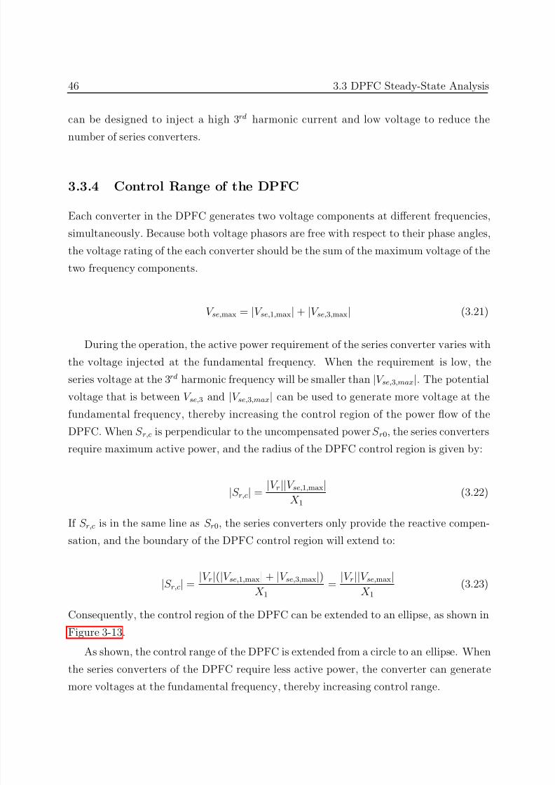
7/25/2019 Dpfc Thesis
http://slidepdf.com/reader/full/dpfc-thesis 68/212
46 3.3 DPFC Steady-State Analysis
can be designed to inject a high 3rd harmonic current and low voltage to reduce the
number of series converters.
3.3.4 Control Range of the DPFC
Each converter in the DPFC generates two voltage components at different frequencies,
simultaneously. Because both voltage phasors are free with respect to their phase angles,
the voltage rating of the each converter should be the sum of the maximum voltage of the
two frequency components.
V se,max = |V se,1,max|+ |V se,3,max| (3.21)
During the operation, the active power requirement of the series converter varies with
the voltage injected at the fundamental frequency. When the requirement is low, the
series voltage at the 3rd harmonic frequency will be smaller than |V se,3,max|. The potential
voltage that is between V se,3 and |V se,3,max| can be used to generate more voltage at the
fundamental frequency, thereby increasing the control region of the power flow of the
DPFC. When S r,c is perpendicular to the uncompensated power S r0, the series converters
require maximum active power, and the radius of the DPFC control region is given by:
|S r,c| = |V r||V se,1,max|
X 1(3.22)
If S r,c is in the same line as S r0, the series converters only provide the reactive compen-
sation, and the boundary of the DPFC control region will extend to:
|S r,c| = |V r|(|V se,1,max|+ |V se,3,max|)
X 1= |V r||V se,max|
X 1(3.23)
Consequently, the control region of the DPFC can be extended to an ellipse, as shown in
Figure 3-13.
As shown, the control range of the DPFC is extended from a circle to an ellipse. When
the series converters of the DPFC require less active power, the converter can generate
more voltages at the fundamental frequency, thereby increasing control range.
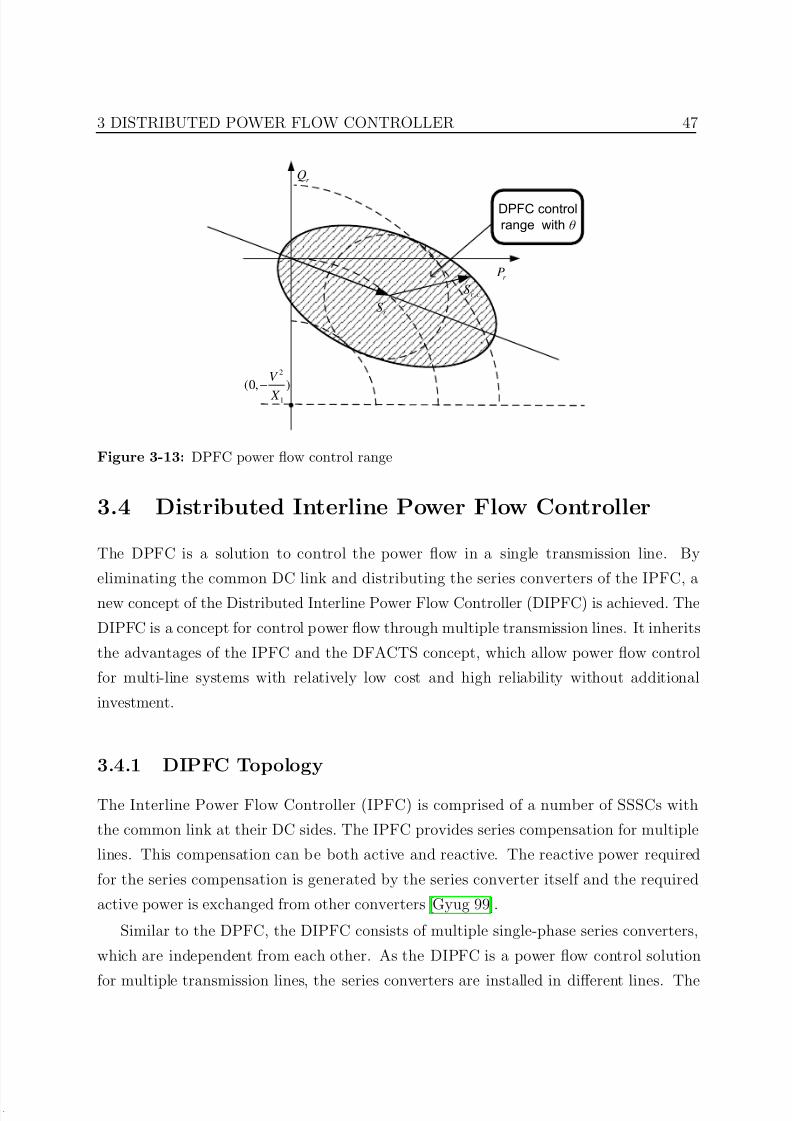
7/25/2019 Dpfc Thesis
http://slidepdf.com/reader/full/dpfc-thesis 69/212
3 DISTRIBUTED POWER FLOW CONTROLLER 47
r P
r Q
2
1
(0, )V
X −
DPFC control
range with θ
,r cS
r S
Figure 3-13: DPFC power flow control range
3.4 Distributed Interline Power Flow Controller
The DPFC is a solution to control the power flow in a single transmission line. By
eliminating the common DC link and distributing the series converters of the IPFC, a
new concept of the Distributed Interline Power Flow Controller (DIPFC) is achieved. The
DIPFC is a concept for control power flow through multiple transmission lines. It inherits
the advantages of the IPFC and the DFACTS concept, which allow power flow control
for multi-line systems with relatively low cost and high reliability without additional
investment.
3.4.1 DIPFC Topology
The Interline Power Flow Controller (IPFC) is comprised of a number of SSSCs with
the common link at their DC sides. The IPFC provides series compensation for multiple
lines. This compensation can be both active and reactive. The reactive power required
for the series compensation is generated by the series converter itself and the required
active power is exchanged from other converters [Gyug 99].
Similar to the DPFC, the DIPFC consists of multiple single-phase series converters,
which are independent from each other. As the DIPFC is a power flow control solution
for multiple transmission lines, the series converters are installed in different lines. The
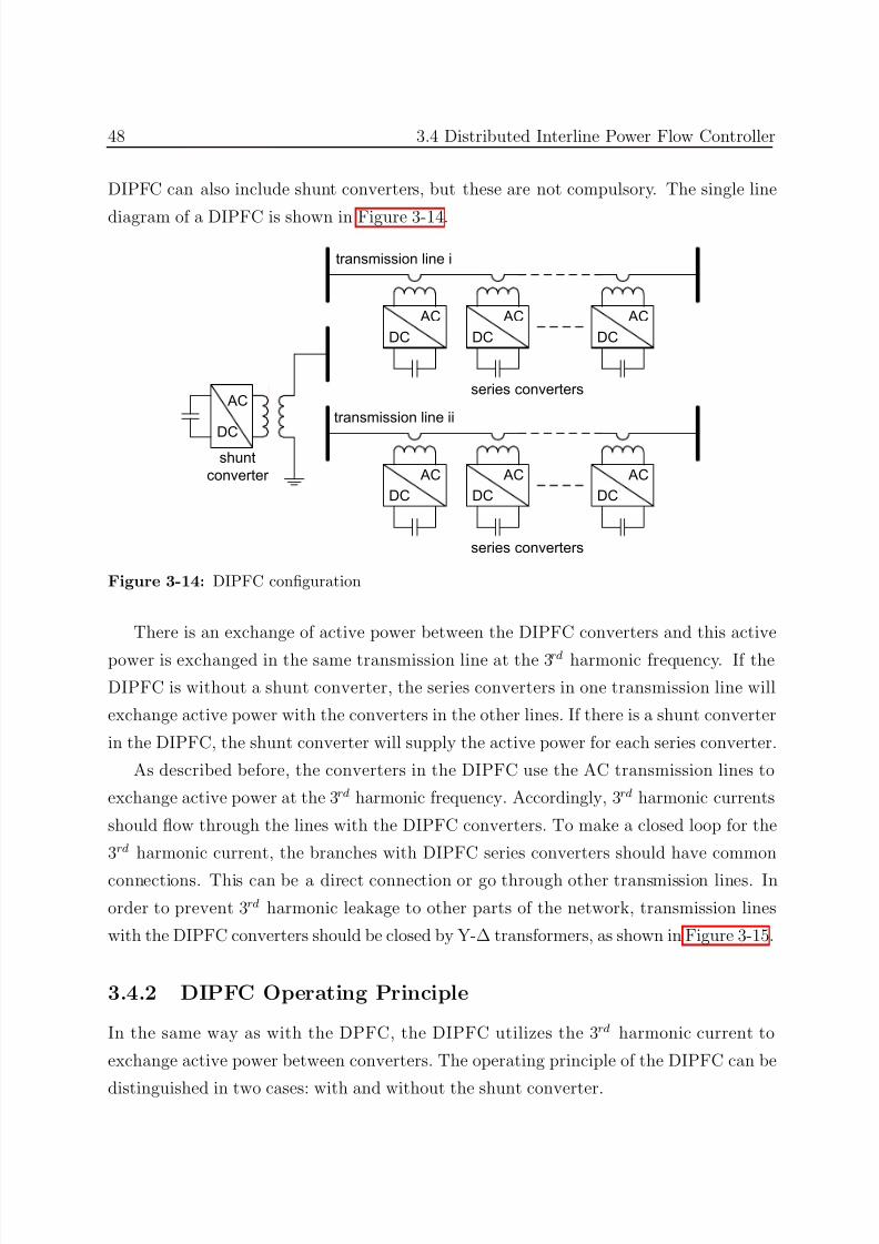
7/25/2019 Dpfc Thesis
http://slidepdf.com/reader/full/dpfc-thesis 70/212
48 3.4 Distributed Interline Power Flow Controller
DIPFC can also include shunt converters, but these are not compulsory. The single line
diagram of a DIPFC is shown in Figure 3-14.
AC
DC
transmission line i
AC
DC
AC
DC
AC
DC
sunt
converter
seres converters
transmsson lne
AC
DC
AC
DC
AC
DC
seres converters
Figure 3-14: DIPFC configuration
There is an exchange of active power between the DIPFC converters and this active
power is exchanged in the same transmission line at the 3rd harmonic frequency. If the
DIPFC is without a shunt converter, the series converters in one transmission line will
exchange active power with the converters in the other lines. If there is a shunt converter
in the DIPFC, the shunt converter will supply the active power for each series converter.
As described before, the converters in the DIPFC use the AC transmission lines to
exchange active power at the 3rd harmonic frequency. Accordingly, 3rd harmonic currents
should flow through the lines with the DIPFC converters. To make a closed loop for the
3rd harmonic current, the branches with DIPFC series converters should have common
connections. This can be a direct connection or go through other transmission lines. In
order to prevent 3rd harmonic leakage to other parts of the network, transmission lines
with the DIPFC converters should be closed by Y-∆ transformers, as shown in Figure 3-15.
3.4.2 DIPFC Operating Principle
In the same way as with the DPFC, the DIPFC utilizes the 3rd harmonic current to
exchange active power between converters. The operating principle of the DIPFC can be
distinguished in two cases: with and without the shunt converter.
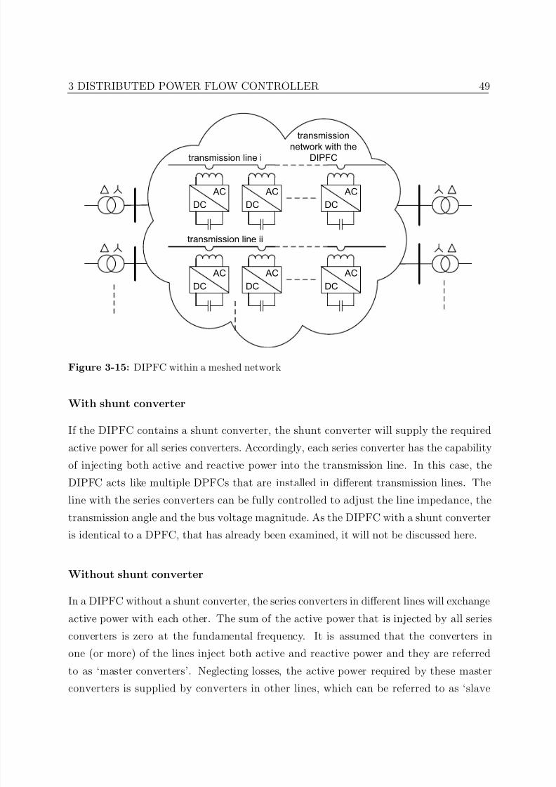
7/25/2019 Dpfc Thesis
http://slidepdf.com/reader/full/dpfc-thesis 71/212
3 DISTRIBUTED POWER FLOW CONTROLLER 49
transmission line i
AC
DC
AC
DC
AC
DC
transmission line ii
ACDC
ACDC
ACDC
transmissionnetwork with the
DIPFC
Figure 3-15: DIPFC within a meshed network
With shunt converter
If the DIPFC contains a shunt converter, the shunt converter will supply the required
active power for all series converters. Accordingly, each series converter has the capability
of injecting both active and reactive power into the transmission line. In this case, the
DIPFC acts like multiple DPFCs that are installed in different transmission lines. The
line with the series converters can be fully controlled to adjust the line impedance, the
transmission angle and the bus voltage magnitude. As the DIPFC with a shunt converter
is identical to a DPFC, that has already been examined, it will not be discussed here.
Without shunt converter
In a DIPFC without a shunt converter, the series converters in different lines will exchange
active power with each other. The sum of the active power that is injected by all series
converters is zero at the fundamental frequency. It is assumed that the converters in
one (or more) of the lines inject both active and reactive power and they are referred
to as ‘master converters’. Neglecting losses, the active power required by these master
converters is supplied by converters in other lines, which can be referred to as ‘slave
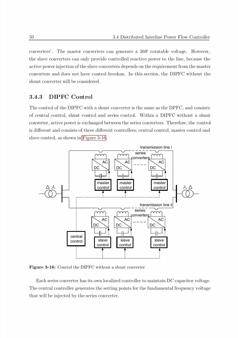
7/25/2019 Dpfc Thesis
http://slidepdf.com/reader/full/dpfc-thesis 72/212
50 3.4 Distributed Interline Power Flow Controller
converters’. The master converters can generate a 360 rotatable voltage. However,
the slave converters can only provide controlled reactive power to the line, because theactive power injection of the slave converters depends on the requirement from the master
converters and does not have control freedom. In this section, the DIPFC without the
shunt converter will be considered.
3.4.3 DIPFC Control
The control of the DIPFC with a shunt converter is the same as the DPFC, and consists
of central control, shunt control and series control. Within a DIPFC without a shunt
converter, active power is exchanged between the series converters. Therefore, the control
is different and consists of three different controllers; central control, master control and
slave control, as shown in Figure 3-16.
transmission line ii
AC
DC
AC
DC
AC
DC
series
converters
slave
control
slave
control
slave
control
centralcontrol
transmission line i
AC
DC
AC
DC
AC
DC
series
converters
master
control
master
control
master
control
Figure 3-16: Control the DIPFC without a shunt converter
Each series converter has its own localized controller to maintain DC capacitor voltage.
The central controller generates the setting points for the fundamental frequency voltage
that will be injected by the series converter.
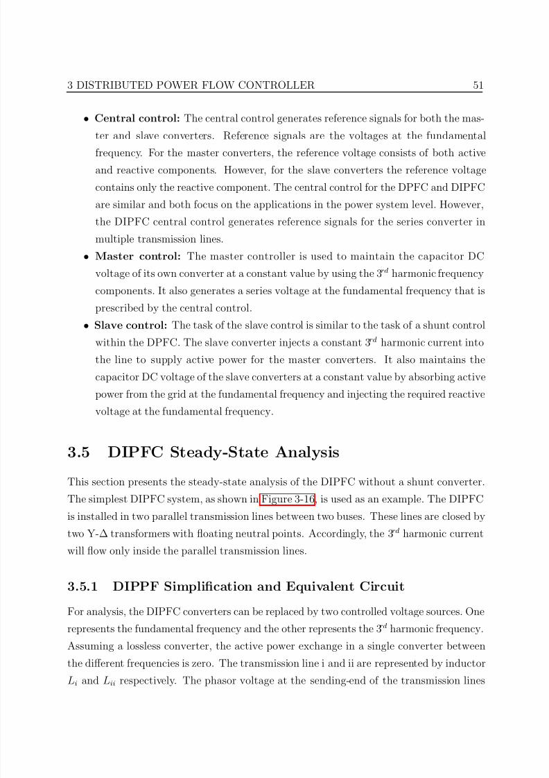
7/25/2019 Dpfc Thesis
http://slidepdf.com/reader/full/dpfc-thesis 73/212
3 DISTRIBUTED POWER FLOW CONTROLLER 51
• Central control: The central control generates reference signals for both the mas-
ter and slave converters. Reference signals are the voltages at the fundamentalfrequency. For the master converters, the reference voltage consists of both active
and reactive components. However, for the slave converters the reference voltage
contains only the reactive component. The central control for the DPFC and DIPFC
are similar and both focus on the applications in the power system level. However,
the DIPFC central control generates reference signals for the series converter in
multiple transmission lines.
• Master control: The master controller is used to maintain the capacitor DC
voltage of its own converter at a constant value by using the 3rd harmonic frequencycomponents. It also generates a series voltage at the fundamental frequency that is
prescribed by the central control.
• Slave control: The task of the slave control is similar to the task of a shunt control
within the DPFC. The slave converter injects a constant 3rd harmonic current into
the line to supply active power for the master converters. It also maintains the
capacitor DC voltage of the slave converters at a constant value by absorbing active
power from the grid at the fundamental frequency and injecting the required reactive
voltage at the fundamental frequency.
3.5 DIPFC Steady-State Analysis
This section presents the steady-state analysis of the DIPFC without a shunt converter.
The simplest DIPFC system, as shown in Figure 3-16, is used as an example. The DIPFC
is installed in two parallel transmission lines between two buses. These lines are closed by
two Y-∆ transformers with floating neutral points. Accordingly, the 3rd harmonic current
will flow only inside the parallel transmission lines.
3.5.1 DIPPF Simplification and Equivalent Circuit
For analysis, the DIPFC converters can be replaced by two controlled voltage sources. One
represents the fundamental frequency and the other represents the 3rd harmonic frequency.
Assuming a lossless converter, the active power exchange in a single converter between
the different frequencies is zero. The transmission line i and ii are represented by inductor
Li and Lii respectively. The phasor voltage at the sending-end of the transmission lines
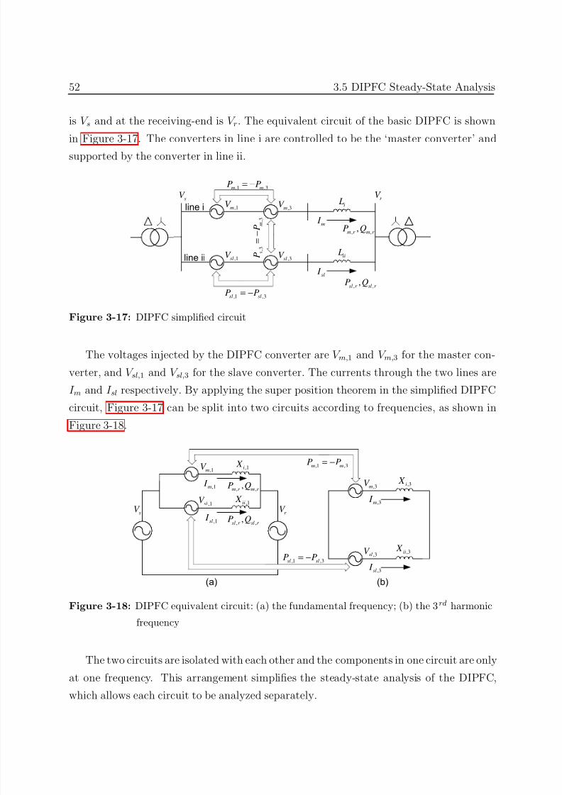
7/25/2019 Dpfc Thesis
http://slidepdf.com/reader/full/dpfc-thesis 74/212
52 3.5 DIPFC Steady-State Analysis
is V s and at the receiving-end is V r. The equivalent circuit of the basic DIPFC is shown
in Figure 3-17. The converters in line i are controlled to be the ‘master converter’ andsupported by the converter in line ii.
,1mV ,3m
V i L
r V s
V ,1 ,3m m
P P= −
, ,,
m r m r P Q
m I
,1slV ,3sl
V ii L
,1 ,3sl slP P= −
sl I
, 3
, 3
s
m
P
P
=
−
line i
line ii
, ,,
sl r sl r P Q
Figure 3-17: DIPFC simplified circuit
The voltages injected by the DIPFC converter are V m,1 and V m,3 for the master con-
verter, and V sl,1 and V sl,3 for the slave converter. The currents through the two lines are
I m and I sl respectively. By applying the super position theorem in the simplified DIPFC
circuit, Figure 3-17 can be split into two circuits according to frequencies, as shown in
Figure 3-18.
,1slV
,1i X
r V sV
,1 ,3m mP P= −
,1 ,3sl slP P= −
,1sl I
,3mV ,3i X
,3m I
(a) (b)
,1mV
,1ii X
,3slV ,3ii X
,3sl I
, ,,
m r m r P Q
, ,,
sl r sl r P Q
,1m I
Figure 3-18: DIPFC equivalent circuit: (a) the fundamental frequency; (b) the 3rd harmonic
frequency
The two circuits are isolated with each other and the components in one circuit are only
at one frequency. This arrangement simplifies the steady-state analysis of the DIPFC,
which allows each circuit to be analyzed separately.
7/25/2019 Dpfc Thesis
http://slidepdf.com/reader/full/dpfc-thesis 75/212
3 DISTRIBUTED POWER FLOW CONTROLLER 53
3.5.2 Fundamental Frequency Circuit
In the fundamental frequency circuit of the DIPFC, there are two transmission lines: the
line with the master converters and with the slave converters. The master converters
have the same capability as the series converters within the DPFC, which is to inject
a voltage with controllable active and reactive components. For a description of the
control capability of the DIPFC master converter refer to the analysis of the DPFC series
converter in previous section.
The slave converters can also inject a fundamental frequency voltage that contains both
active and reactive components. As the active power absorbed or generated by the slave
converters is related to the master converter, the slave converters can only independently
control the reactive voltage at the fundamental frequency. Accordingly, the control range
of the DIPFC slave converters depends on the active power requirement of the master
converters.
Assuming the active power required by master converters at the fundamental frequency
is Pm,1, the active power supplied by the slave converter is:
P sl,1 =−
P m,1 (3.24)
The active power injected by the converters is related to the triangle that is constructed
by the uncompensated and compensated power flow, as described above. Therefore, to
supply the active power P sl,1, the control range of the slave converters should have the
character that the area of triangle (0, S sl,r0, S sl,r) is P sl,1. Accordingly, the control range
of the slave converter is a straight line that is parallel with S sl,r0, as shown in Figure 3-19.
As shown, the control line of the slave converters is parallel with the vector S sl,r0 in
the complex P Q-plane. From (3.11), the distance S d,sl between the two parallel lines is
given by:
S d,sl = P sl,1
C |S sl,r0| (3.25)
where the coefficient C = 2X ii,1/|V r|2.
3.5.3 Third Harmonic Frequency Circuit
The structure of the 3rd harmonic frequency circuit of the DIPFC is similar as the one of
the DPFC. The slave converters correspond to the shunt converters of the DPFC and the
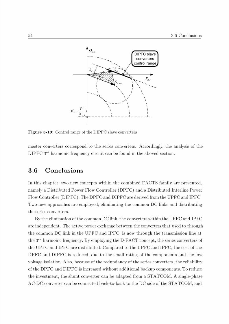
7/25/2019 Dpfc Thesis
http://slidepdf.com/reader/full/dpfc-thesis 76/212
54 3.6 Conclusions
,sl r P
,sl r Q
2
,1
(0, )sl
V
X −
DIPFC slave
converters
control range
, 0sl r S
,sl r S ,d sl
S
Figure 3-19: Control range of the DIPFC slave converters
master converters correspond to the series converters. Accordingly, the analysis of the
DIPFC 3rd harmonic frequency circuit can be found in the aboved section.
3.6 Conclusions
In this chapter, two new concepts within the combined FACTS family are presented,
namely a Distributed Power Flow Controller (DPFC) and a Distributed Interline Power
Flow Controller (DIPFC). The DPFC and DIPFC are derived from the UPFC and IPFC.
Two new approaches are employed; eliminating the common DC links and distributing
the series converters.
By the elimination of the common DC link, the converters within the UPFC and IPFC
are independent. The active power exchange between the converters that used to throughthe common DC link in the UPFC and IPFC, is now through the transmission line at
the 3rd harmonic frequency. By employing the D-FACT concept, the series converters of
the UPFC and IPFC are distributed. Compared to the UPFC and IPFC, the cost of the
DPFC and DIPFC is reduced, due to the small rating of the components and the low
voltage isolation. Also, because of the redundancy of the series converters, the reliability
of the DPFC and DIPFC is increased without additional backup components. To reduce
the investment, the shunt converter can be adapted from a STATCOM. A single-phase
AC-DC converter can be connected back-to-back to the DC side of the STATCOM, and
7/25/2019 Dpfc Thesis
http://slidepdf.com/reader/full/dpfc-thesis 77/212
3 DISTRIBUTED POWER FLOW CONTROLLER 55
its AC terminals are connected between the Y-∆ transformer’s neutral point and the
ground.A steady-state analysis is also presented in this chapter. It is found that the DPFC
and DIPFC have the same control capability as the DPFC and IPFC. The DPFC can
simultaneously adjust the line impedance, the transmission angle and the bus voltage.
The DIPFC is capable of controlling multiple transmission lines. If DIPFCs include a
shunt converter, it acts like multiple DPFCs. If made without a shunt converter, the
DIPFC will exchange active power between the converters in different lines. In this case,
the DIPFC converters can be distinguished: master and slave converters. The master
converter can inject a voltage that contains independent controllable active and reactivecomponents, while the slave converter supplies active power to the master converter and
provides reactive compensation for its own line.
To obtain the same control capability as the UPFC and IPFC, the rating of the DPFC
and DIPFC converters at the fundamental frequency should be the same as the one for
the UPFC. Because the voltages and currents at the 3rd harmonic frequency have to be
added, the rating of the DPFC converter is slightly larger than the UPFC and IPFC. The
increased rating is related with the active power exchanged at the 3 rd harmonic frequency
and can limited within 5% of the nominal rating.

7/25/2019 Dpfc Thesis
http://slidepdf.com/reader/full/dpfc-thesis 78/212
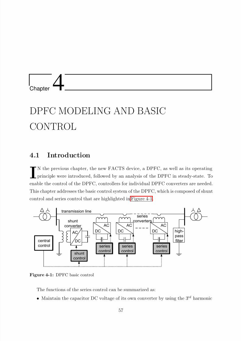
7/25/2019 Dpfc Thesis
http://slidepdf.com/reader/full/dpfc-thesis 79/212
Chapter 4DPFC MODELING AND BASIC
CONTROL
4.1 Introduction
I
N the previous chapter, the new FACTS device, a DPFC, as well as its operating
principle were introduced, followed by an analysis of the DPFC in steady-state. To
enable the control of the DPFC, controllers for individual DPFC converters are needed.
This chapter addresses the basic control system of the DPFC, which is composed of shunt
control and series control that are highlighted in Figure 4-1.
AC
DC
transmission line
AC
DC
AC
DC
AC
DC hgh-
pass
filter
snt
onerter
seres
onerters
snt
ontrol
seres
ontrol
seres
ontrol
seres
ontrol
entral
ontrol
Figure 4-1: DPFC basic control
The functions of the series control can be summarized as:
• Maintain the capacitor DC voltage of its own converter by using the 3 rd harmonic
57
7/25/2019 Dpfc Thesis
http://slidepdf.com/reader/full/dpfc-thesis 80/212
58 4.2 DPFC Modeling
frequency components.
• Generate the series voltage at the fundamental frequency that is prescribed by thecentral control.
The functions of the shunt control are:
• Inject a constant 3rd harmonic current into the line to supply active power for series
converters.
• Maintain the capacitor DC voltage of the shunt converter by absorbing active power
from the grid at the fundamental frequency.
• Inject reactive voltage at the fundamental frequency to the grid as prescribed bythe central control.
This chapter begins with the modeling of the DPFC in the dq -frame [Fitz 03]. The
AC components of the DPFC are transformed to DC components by using Park’s ( dq )
transformation. The transformed DC components of the DPFC can be controlled by
traditional PI controllers.
Once the modeling of the DPFC is introduced, the design of the DPFC basic control
is given in section 4.3. The basic control is responsible for maintaining the DC voltages of the DPFC converters and generating the AC voltages as prescribed by the central control.
Further, the communication between the DPFC series converters and the central con-
trol is considered in section 4.4. A relatively low cost and reliable synchronization method
for series converters is proposed. This method involves transmitting the control signals in
DC-quantity, thereby only requiring low-bandwidth communication. In addition, during
communication failure the series converters can continue synchronization.
4.2 DPFC Modeling
To design a DPFC control scheme, the DPFC must first be modeled. This section presents
such modeling of the DPFC. As the DPFC serves the power system, the model should
describe the behavior of the DPFC at the system level, which is at the fundamental and
the 3rd harmonic frequency. The modeling of the switching behavior of converters is not
required.
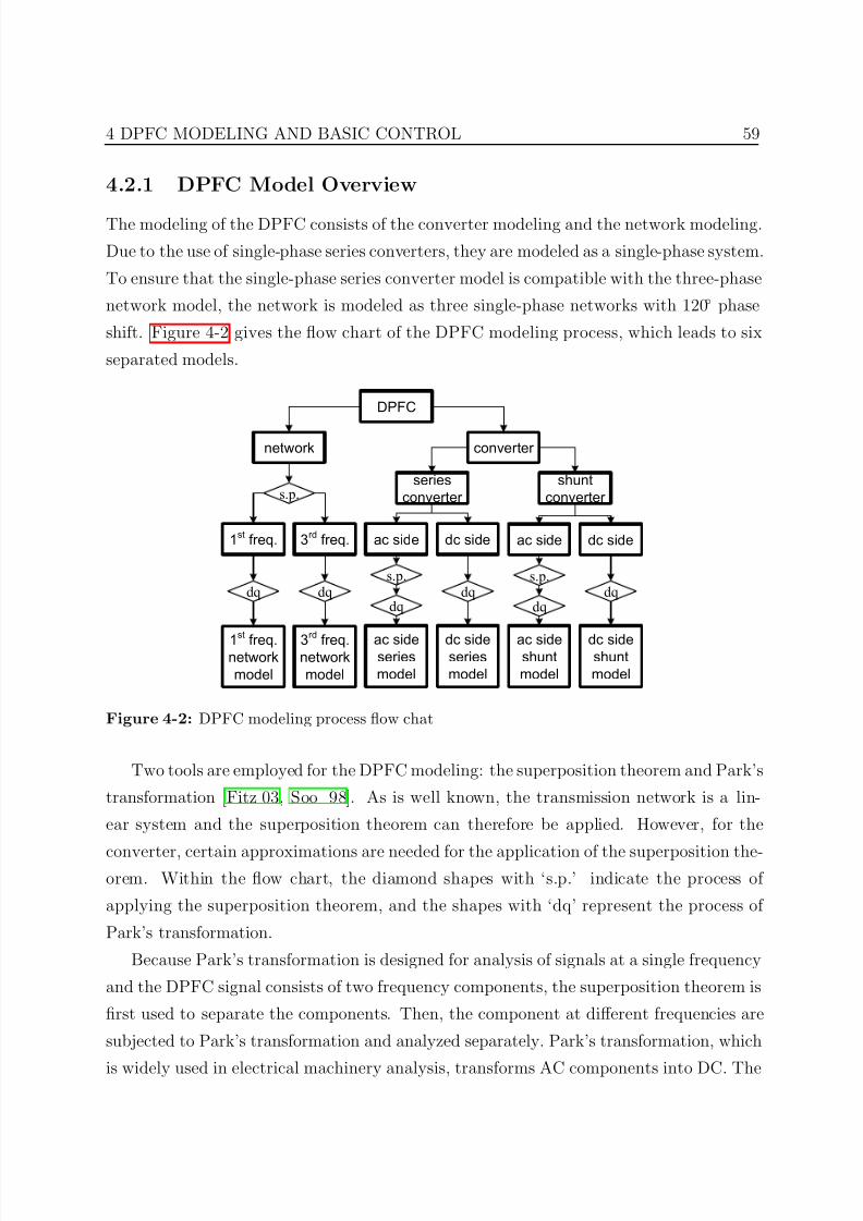
7/25/2019 Dpfc Thesis
http://slidepdf.com/reader/full/dpfc-thesis 81/212
4 DPFC MODELING AND BASIC CONTROL 59
4.2.1 DPFC Model Overview
The modeling of the DPFC consists of the converter modeling and the network modeling.
Due to the use of single-phase series converters, they are modeled as a single-phase system.
To ensure that the single-phase series converter model is compatible with the three-phase
network model, the network is modeled as three single-phase networks with 120 phase
shift. Figure 4-2 gives the flow chart of the DPFC modeling process, which leads to six
separated models.
DPFC
network converter
1st freq. 3
rd freq.
s.p.
dq dq
1st
freq.network
model
3rd
freq.network
model
shunt
converter
ac sideshunt
model
dc sideshunt
model
series
converter
ac side dc side
s.p.
dqdq
ac sideseries
model
dc sideseries
model
ac side dc side
s.p.
dqdq
Figure 4-2: DPFC modeling process flow chat
Two tools are employed for the DPFC modeling: the superposition theorem and Park’s
transformation [Fitz 03, Soo 98]. As is well known, the transmission network is a lin-
ear system and the superposition theorem can therefore be applied. However, for the
converter, certain approximations are needed for the application of the superposition the-orem. Within the flow chart, the diamond shapes with ‘s.p.’ indicate the process of
applying the superposition theorem, and the shapes with ‘dq’ represent the process of
Park’s transformation.
Because Park’s transformation is designed for analysis of signals at a single frequency
and the DPFC signal consists of two frequency components, the superposition theorem is
first used to separate the components. Then, the component at different frequencies are
subjected to Park’s transformation and analyzed separately. Park’s transformation, which
is widely used in electrical machinery analysis, transforms AC components into DC. The
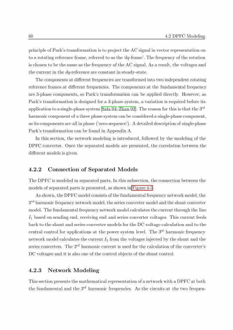
7/25/2019 Dpfc Thesis
http://slidepdf.com/reader/full/dpfc-thesis 82/212
60 4.2 DPFC Modeling
principle of Park’s transformation is to project the AC signal in vector representation on
to a rotating reference frame, referred to as the ‘dq -frame’. The frequency of the rotationis chosen to be the same as the frequency of the AC signal. As a result, the voltages and
the current in the dq -reference are constant in steady-state.
The components at different frequencies are transformed into two independent rotating
reference frames at different frequencies. The components at the fundamental frequency
are 3-phase components, so Park’s transformation can be applied directly. However, as
Park’s transformation is designed for a 3-phase system, a variation is required before its
application to a single-phase system [Sala 04, Zhan 02]. The reason for this is that the 3rd
harmonic component of a three phase system can be considered a single-phase component,
as its components are all in phase (‘zero-sequence’). A detailed description of single-phase
Park’s transformation can be found in Appendix A.
In this section, the network modeling is introduced, followed by the modeling of the
DPFC converter. Once the separated models are presented, the correlation between the
different models is given.
4.2.2 Connection of Separated Models
The DPFC is modeled in separated parts. In this subsection, the connection between the
models of separated parts is presented, as shown in Figure 4-3.
As shown, the DPFC model consists of the fundamental frequency network model, the
3rd harmonic frequency network model, the series converter model and the shunt converter
model. The fundamental frequency network model calculates the current through the line
I 1 based on sending end, receiving end and series converter voltages. This current feeds
back to the shunt and series converter models for the DC voltage calculation and to the
central control for applications at the power system level. The 3rd harmonic frequencynetwork model calculates the current I 3 from the voltages injected by the shunt and the
series converters. The 3rd harmonic current is used for the calculation of the converter’s
DC voltages and it is also one of the control objects of the shunt control.
4.2.3 Network Modeling
This section presents the mathematical representation of a network with a DPFC at both
the fundamental and the 3rd harmonic frequencies. As the circuits at the two frequen-
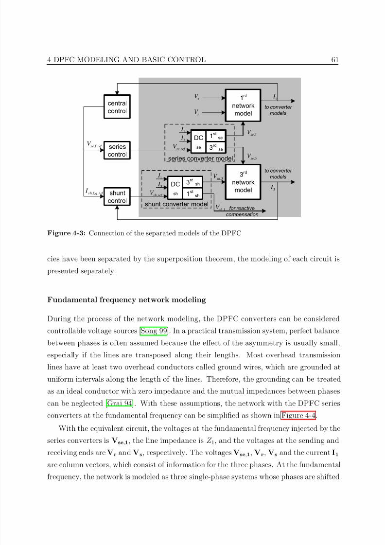
7/25/2019 Dpfc Thesis
http://slidepdf.com/reader/full/dpfc-thesis 83/212
4 DPFC MODELING AND BASIC CONTROL 61
DC
se
1st
se
3rd
se
1st
network
model
3rd
network
model
DC
sh 1stsh
3rd
sh
series
control
shunt
control
,se ref V
1 I
3 I
series converter model
,sh ref V
1 I
3 I
shunt converter model
1 I
3
I
central
control
,1seV
,3seV
,3shV
,1shV
sV
r V
to converter
models
to converter
models
,1,se ref V
,1, ,s h q r ef I
for reactive
compensation
Figure 4-3: Connection of the separated models of the DPFC
cies have been separated by the superposition theorem, the modeling of each circuit is
presented separately.
Fundamental frequency network modeling
During the process of the network modeling, the DPFC converters can be considered
controllable voltage sources [Song 99]. In a practical transmission system, perfect balance
between phases is often assumed because the effect of the asymmetry is usually small,
especially if the lines are transposed along their lengths. Most overhead transmission
lines have at least two overhead conductors called ground wires, which are grounded at
uniform intervals along the length of the lines. Therefore, the grounding can be treatedas an ideal conductor with zero impedance and the mutual impedances between phases
can be neglected [Grai 94]. With these assumptions, the network with the DPFC series
converters at the fundamental frequency can be simplified as shown in Figure 4-4.
With the equivalent circuit, the voltages at the fundamental frequency injected by the
series converters is Vse,1, the line impedance is Z 1, and the voltages at the sending and
receiving ends are Vr and Vs, respectively. The voltages Vse,1, Vr, Vs and the current I1
are column vectors, which consist of information for the three phases. At the fundamental
frequency, the network is modeled as three single-phase systems whose phases are shifted
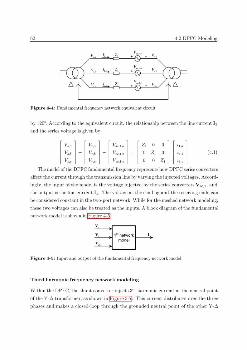
7/25/2019 Dpfc Thesis
http://slidepdf.com/reader/full/dpfc-thesis 84/212
62 4.2 DPFC Modeling
+ -1 Z ,1,se aV
,s aV ,r aV 1,a
I
+ -1 Z ,1,se b
V ,s bV ,r b
V 1,b I
+ -1 Z ,1,se c
V ,s cV ,r c
V 1,c I
Figure 4-4: Fundamental frequency network equivalent circuit
by 120. According to the equivalent circuit, the relationship between the line current I1
and the series voltage is given by:
V s,a
V s,b
V s,c
−
V r,a
V r,b
V r,c
−
V se,1,a
V se,1,b
V se,1,c
=
Z 1 0 0
0 Z 1 0
0 0 Z 1
i1,a
i1,b
i1,c
(4.1)
The model of the DPFC fundamental frequency represents how DPFC series converters
affect the current through the transmission line by varying the injected voltages. Accord-
ingly, the input of the model is the voltage injected by the series converters Vse,1, and
the output is the line current I1. The voltage at the sending and the receiving ends can
be considered constant in the two-port network. While for the meshed network modeling,
these two voltages can also be treated as the inputs. A block diagram of the fundamental
network model is shown in Figure 4-5.
1st network
model
1I
sV
rV
se,1V
Figure 4-5: Input and output of the fundamental frequency network model
Third harmonic frequency network modeling
Within the DPFC, the shunt converter injects 3rd harmonic current at the neutral point
of the Y-∆ transformer, as shown in Figure 3-7. This current distributes over the three
phases and makes a closed-loop through the grounded neutral point of the other Y-∆
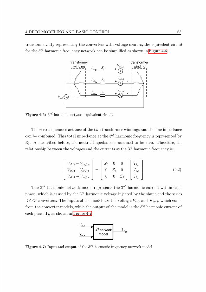
7/25/2019 Dpfc Thesis
http://slidepdf.com/reader/full/dpfc-thesis 85/212
4 DPFC MODELING AND BASIC CONTROL 63
transformer. By representing the converters with voltage sources, the equivalent circuit
for the 3rd harmonic frequency network can be simplified as shown in Figure 4-6.
+ -3 Z ,3,se aV
3,a I
+ -3 Z ,3,se bV
3,b I
+ -3 Z ,3,se cV
3,c I
,3shV
+
-
transformer
winding
transformer
winding
Figure 4-6: 3rd harmonic network equivalent circuit
The zero sequence reactance of the two transformer windings and the line impedance
can be combined. This total impedance at the 3rd harmonic frequency is represented by
Z 3. As described before, the neutral impedance is assumed to be zero. Therefore, the
relationship between the voltages and the currents at the 3rd harmonic frequency is:
V sh,3 − V se,3,a
V sh,3 − V se,3,b
V sh,3 − V se,3,c
=
Z 3 0 0
0 Z 3 0
0 0 Z 3
I 3,a
I 3,b
I 3,c
(4.2)
The 3rd harmonic network model represents the 3rd harmonic current within each
phase, which is caused by the 3rd harmonic voltage injected by the shunt and the series
DPFC converters. The inputs of the model are the voltages V sh3 and Vse,3, which come
from the converter models, while the output of the model is the 3rd harmonic current of
each phase I3, as shown in Figure 4-7.
3rd network
model
3I
,3shV
se,3V
Figure 4-7: Input and output of the 3rd harmonic frequency network model
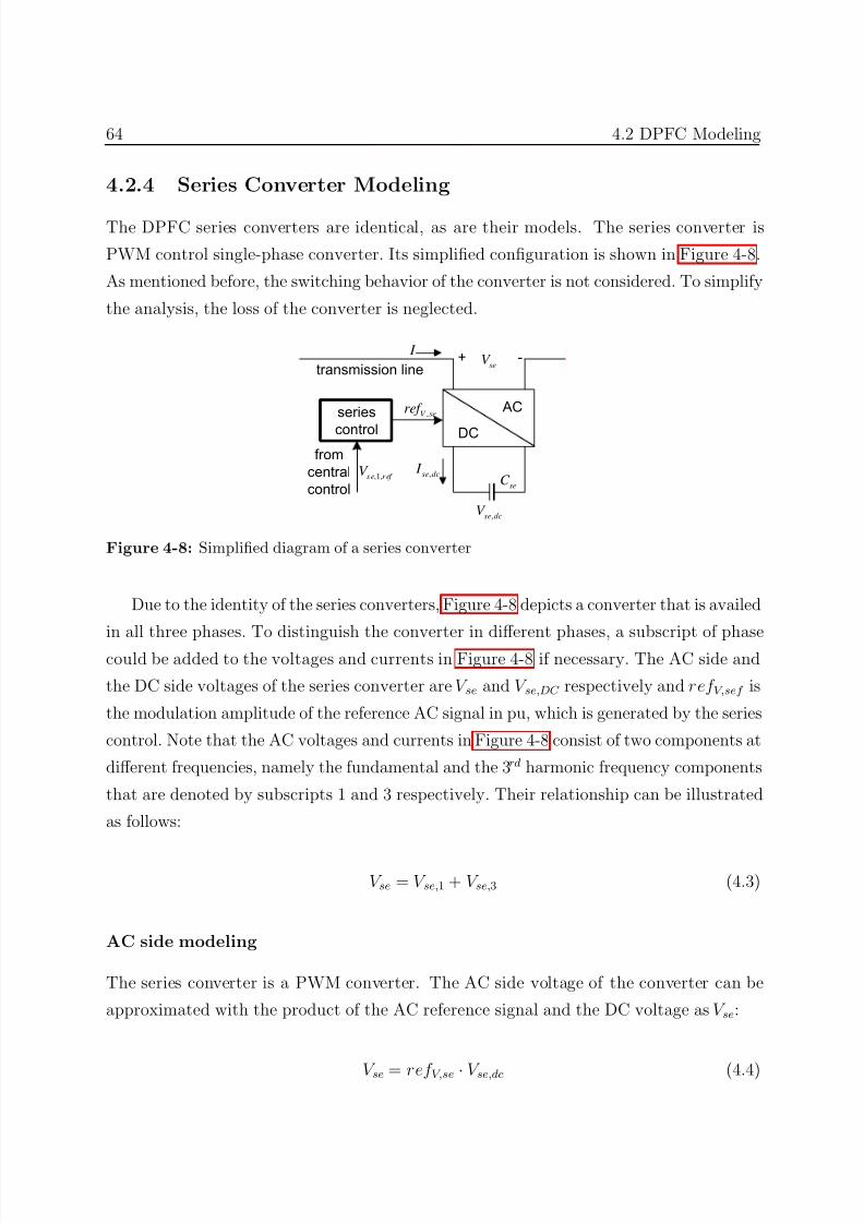
7/25/2019 Dpfc Thesis
http://slidepdf.com/reader/full/dpfc-thesis 86/212
64 4.2 DPFC Modeling
4.2.4 Series Converter Modeling
The DPFC series converters are identical, as are their models. The series converter is
PWM control single-phase converter. Its simplified configuration is shown in Figure 4-8.
As mentioned before, the switching behavior of the converter is not considered. To simplify
the analysis, the loss of the converter is neglected.
AC
DC
+ se
V I
,V seref
,se dc I
,se dcV
seC
transmission line
series
control
,1,s e r ef V from
central
control
Figure 4-8: Simplified diagram of a series converter
Due to the identity of the series converters, Figure 4-8 depicts a converter that is availed
in all three phases. To distinguish the converter in different phases, a subscript of phase
could be added to the voltages and currents in Figure 4-8 if necessary. The AC side and
the DC side voltages of the series converter are V se and V se,DC respectively and ref V,sef is
the modulation amplitude of the reference AC signal in pu, which is generated by the series
control. Note that the AC voltages and currents in Figure 4-8 consist of two components at
different frequencies, namely the fundamental and the 3rd harmonic frequency components
that are denoted by subscripts 1 and 3 respectively. Their relationship can be illustrated
as follows:
V se = V se,1 + V se,3 (4.3)
AC side modeling
The series converter is a PWM converter. The AC side voltage of the converter can be
approximated with the product of the AC reference signal and the DC voltage as V se:
V se = ref V,se · V se,dc (4.4)
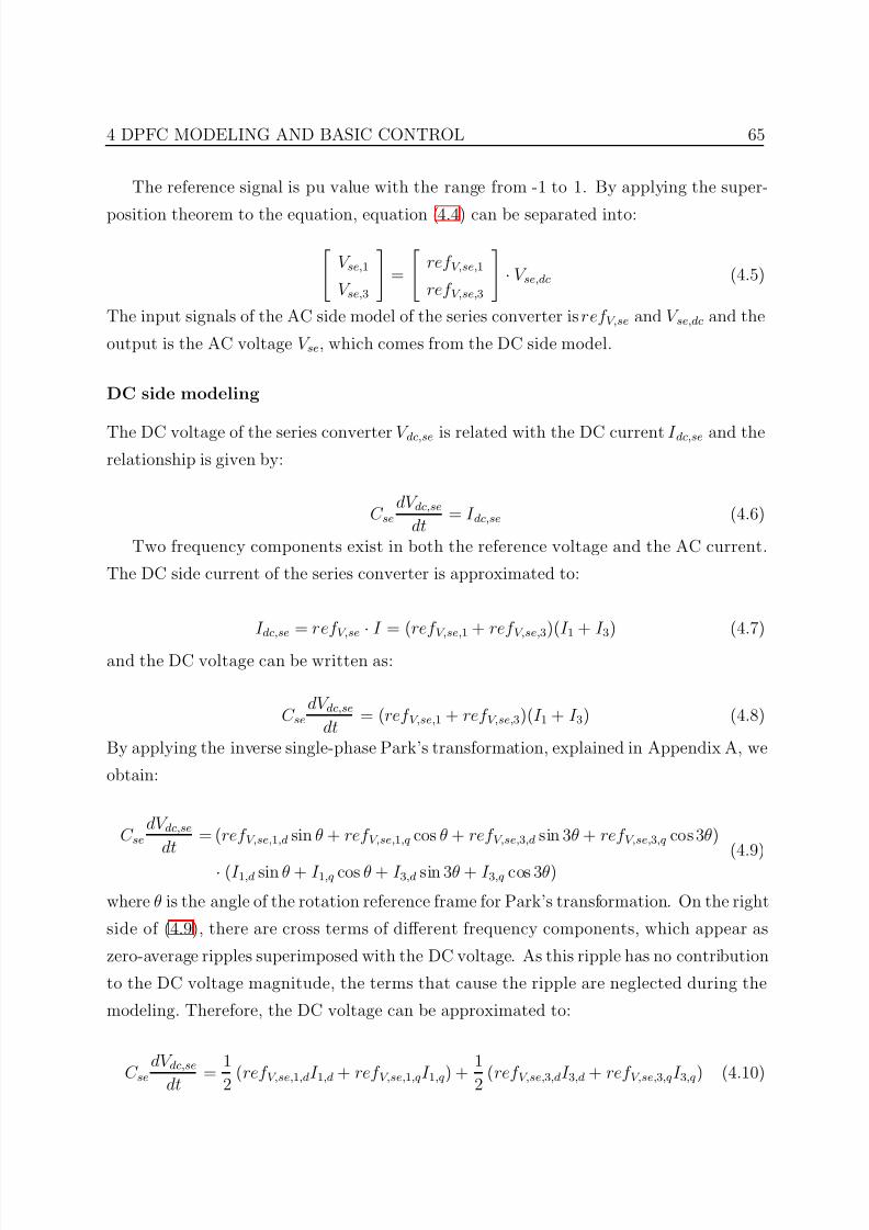
7/25/2019 Dpfc Thesis
http://slidepdf.com/reader/full/dpfc-thesis 87/212
4 DPFC MODELING AND BASIC CONTROL 65
The reference signal is pu value with the range from -1 to 1. By applying the super-
position theorem to the equation, equation (4.4) can be separated into: V se,1
V se,3
=
ref V,se,1
ref V,se,3
· V se,dc (4.5)
The input signals of the AC side model of the series converter is ref V,se and V se,dc and the
output is the AC voltage V se, which comes from the DC side model.
DC side modeling
The DC voltage of the series converter V dc,se is related with the DC current I dc,se and therelationship is given by:
C sedV dc,se
dt = I dc,se (4.6)
Two frequency components exist in both the reference voltage and the AC current.
The DC side current of the series converter is approximated to:
I dc,se = ref V,se
·I = (ref V,se,1 + ref V,se,3)(I 1 + I 3) (4.7)
and the DC voltage can be written as:
C sedV dc,se
dt = (ref V,se,1 + ref V,se,3)(I 1 + I 3) (4.8)
By applying the inverse single-phase Park’s transformation, explained in Appendix A, we
obtain:
C sedV dc,se
dt = (ref V,se,1,d sin θ + ref V,se,1,q cos θ + ref V,se,3,d sin 3θ + ref V,se,3,q cos 3θ)
· (I 1,d sin θ + I 1,q cos θ + I 3,d sin 3θ + I 3,q cos 3θ)
(4.9)
where θ is the angle of the rotation reference frame for Park’s transformation. On the right
side of (4.9), there are cross terms of different frequency components, which appear as
zero-average ripples superimposed with the DC voltage. As this ripple has no contribution
to the DC voltage magnitude, the terms that cause the ripple are neglected during the
modeling. Therefore, the DC voltage can be approximated to:
C se
dV dc,se
dt =
1
2 (ref V,se,1,dI 1,d + ref V,se,1,qI 1,q) +
1
2 (ref V,se,3,dI 3,d + ref V,se,3,qI 3,q) (4.10)
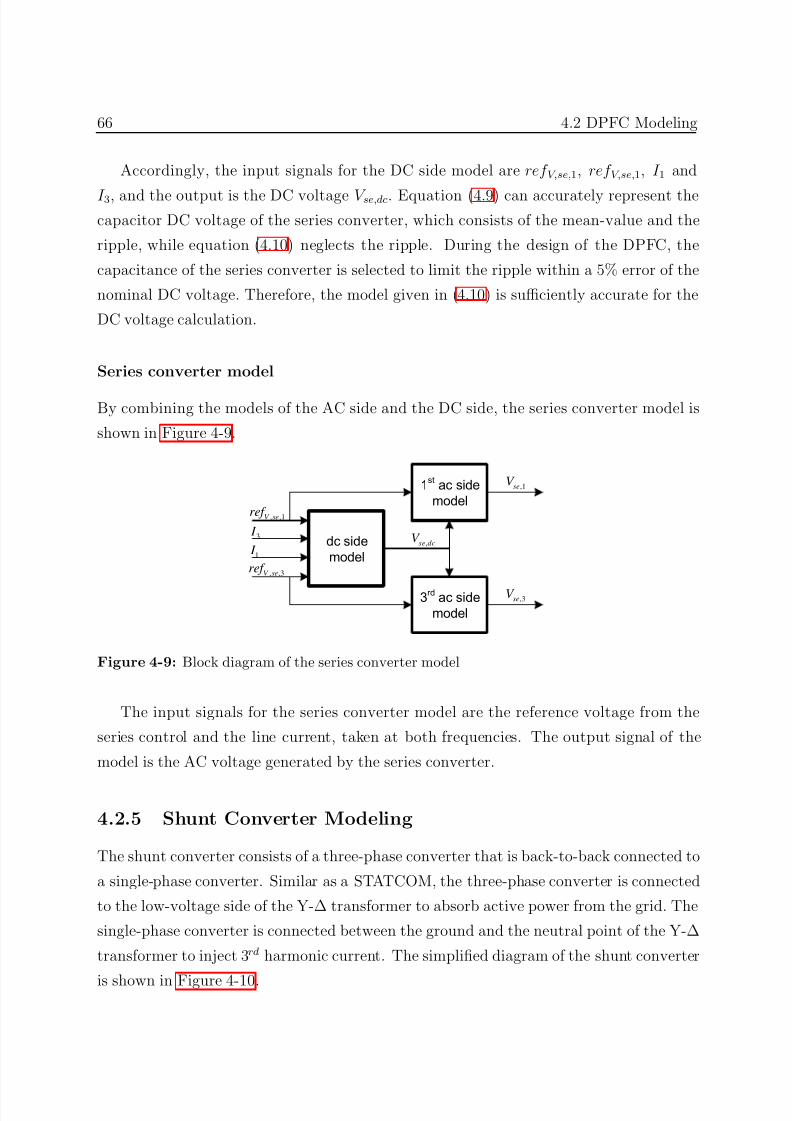
7/25/2019 Dpfc Thesis
http://slidepdf.com/reader/full/dpfc-thesis 88/212
66 4.2 DPFC Modeling
Accordingly, the input signals for the DC side model are ref V,se,1, ref V,se,1, I 1 and
I 3, and the output is the DC voltage V se,dc. Equation (4.9) can accurately represent thecapacitor DC voltage of the series converter, which consists of the mean-value and the
ripple, while equation (4.10) neglects the ripple. During the design of the DPFC, the
capacitance of the series converter is selected to limit the ripple within a 5% error of the
nominal DC voltage. Therefore, the model given in (4.10) is sufficiently accurate for the
DC voltage calculation.
Series converter model
By combining the models of the AC side and the DC side, the series converter model is
shown in Figure 4-9.
dc side
model
,se dcV
, ,1V seref
, ,3V seref
1st ac side
model
3rd
ac side
model
1 I
3 I
,1seV
,3seV
Figure 4-9: Block diagram of the series converter model
The input signals for the series converter model are the reference voltage from the
series control and the line current, taken at both frequencies. The output signal of the
model is the AC voltage generated by the series converter.
4.2.5 Shunt Converter Modeling
The shunt converter consists of a three-phase converter that is back-to-back connected to
a single-phase converter. Similar as a STATCOM, the three-phase converter is connected
to the low-voltage side of the Y-∆ transformer to absorb active power from the grid. The
single-phase converter is connected between the ground and the neutral point of the Y-∆
transformer to inject 3rd harmonic current. The simplified diagram of the shunt converter
is shown in Figure 4-10.
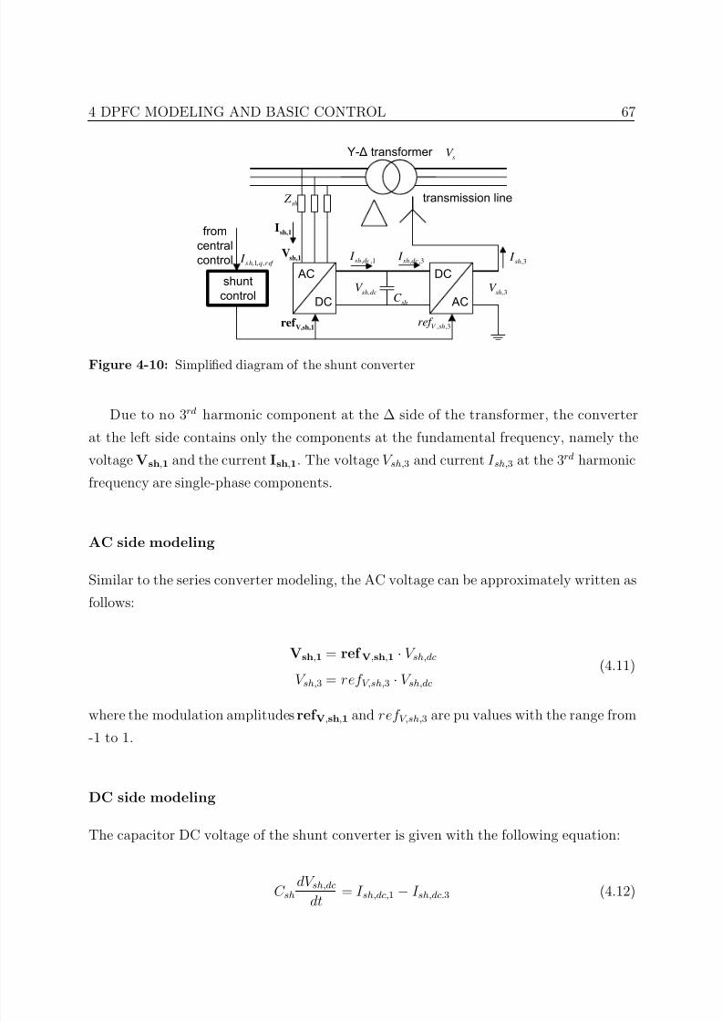
7/25/2019 Dpfc Thesis
http://slidepdf.com/reader/full/dpfc-thesis 89/212
4 DPFC MODELING AND BASIC CONTROL 67
AC
DC AC
DC
Y∆ tanfoms
V
sh,1V
sh,1I
sh Z
,sh dcV
shC
, ,1sh dc I , ,3sh dc I
V,sh,1ref , ,3V shref
,3shV
,3sh I
,1, ,s h q r ef I
hunt
contol
fom
cntal
contol
tanmon ln
Figure 4-10: Simplified diagram of the shunt converter
Due to no 3rd harmonic component at the ∆ side of the transformer, the converter
at the left side contains only the components at the fundamental frequency, namely the
voltage Vsh,1 and the current Ish,1. The voltage V sh,3 and current I sh,3 at the 3rd harmonic
frequency are single-phase components.
AC side modeling
Similar to the series converter modeling, the AC voltage can be approximately written as
follows:
Vsh,1 = ref V,sh,1 · V sh,dc
V sh,3 = ref V,sh,3 · V sh,dc
(4.11)
where the modulation amplitudes ref V,sh,1 and ref V,sh,3 are pu values with the range from-1 to 1.
DC side modeling
The capacitor DC voltage of the shunt converter is given with the following equation:
C sh
dV sh,dc
dt = I sh,dc,1 − I sh,dc.3 (4.12)
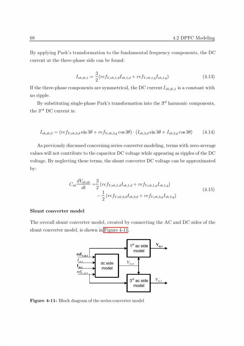
7/25/2019 Dpfc Thesis
http://slidepdf.com/reader/full/dpfc-thesis 90/212
68 4.2 DPFC Modeling
By applying Park’s transformation to the fundamental frequency components, the DC
current at the three-phase side can be found:
I sh,dc,1 = 3
2(ref V,sh,1,dI sh,1,d + ref V,sh,1,qI sh,1,q) (4.13)
If the three-phase components are symmetrical, the DC current I sh,dc,1 is a constant with
no ripple.
By substituting single-phase Park’s transformation into the 3rd harmonic components,
the 3rd DC current is:
I sh,dc,3 = (ref V,sh,3,d sin 3θ + ref V,sh,3,q cos 3θ) · (I sh,3,d sin 3θ + I sh,3,q cos 3θ) (4.14)
As previously discussed concerning series converter modeling, terms with zero-average
values will not contribute to the capacitor DC voltage while appearing as ripples of the DC
voltage. By neglecting these terms, the shunt converter DC voltage can be approximated
by:
C sh dV sh,dc
dt =3
2 (ref V,sh,1,dI sh,1,d + ref V,sh,1,qI sh,1,q)
− 1
2 (ref V,sh,3,dI sh,3,d + ref V,sh,3,qI sh,3,q)
(4.15)
Shunt converter model
The overall shunt converter model, created by connecting the AC and DC sides of the
shunt converter model, is shown in Figure 4-11.
dc side
model
,sh dcV
V,sh,1ref
, ,3V shref
1st ac side
model
3rd
ac side
model
sh,1I
,3sh I
sh,1V
,3shV
Figure 4-11: Block diagram of the series converter model

7/25/2019 Dpfc Thesis
http://slidepdf.com/reader/full/dpfc-thesis 91/212
4 DPFC MODELING AND BASIC CONTROL 69
The input signals for the model are reference voltage signals and current, at both
frequencies, while the outputs are the fundamental and 3rd harmonic frequency voltages,generated by the shunt converter.
4.3 DPFC Basic Control
Based on the DPFC model presented previously, the control can now be further developed.
The DPFC basic control consists of the series control and the shunt control. In this section,
the control schemes and their corresponding design are addressed. Because of its simple
implementation, the vector control method [Kann 04, Papi 97] is employed to control the
DPFC converter. The calculation of the controller parameter is based on the Internal
Model Control (IMC) method [Garc 82, Harn 98].
4.3.1 Series Converter Control
Each DPFC series converter is locally controlled by its own controller, and the scheme for
each series control is identical. To control the series converter, separate control loops are
employed for the two frequency components. The 3rd harmonic control loop is used for
DC voltage control. The block diagram of the DPFC series converter control is shown in
Figure 4-12.
1-ph PLL3rd passfilter
dc control
1-ph
inverse
dq
0
PWM
gen.
signal
process AC
DC
+ -seV
I
,V seref ,se dc
V
transmission line
, ,1V seref
3θ 3 I
, , 3,V se qref
, , 3,V se d ref , ,se dc ref
V
, ,3V seref
C
I
from central
control
+
+
,se dcV
series control
,1,s e r ef V
Figure 4-12: Control scheme of the series converter
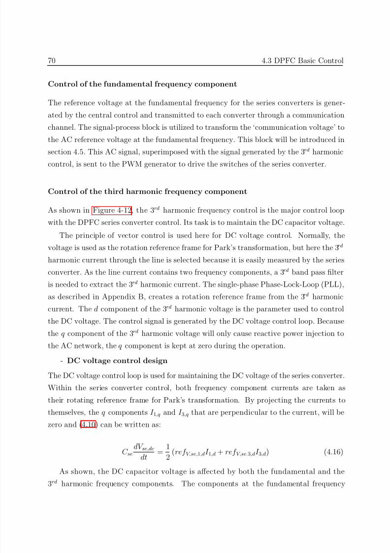
7/25/2019 Dpfc Thesis
http://slidepdf.com/reader/full/dpfc-thesis 92/212
70 4.3 DPFC Basic Control
Control of the fundamental frequency component
The reference voltage at the fundamental frequency for the series converters is gener-
ated by the central control and transmitted to each converter through a communication
channel. The signal-process block is utilized to transform the ‘communication voltage’ to
the AC reference voltage at the fundamental frequency. This block will be introduced in
section 4.5. This AC signal, superimposed with the signal generated by the 3rd harmonic
control, is sent to the PWM generator to drive the switches of the series converter.
Control of the third harmonic frequency component
As shown in Figure 4-12, the 3rd harmonic frequency control is the major control loop
with the DPFC series converter control. Its task is to maintain the DC capacitor voltage.
The principle of vector control is used here for DC voltage control. Normally, the
voltage is used as the rotation reference frame for Park’s transformation, but here the 3rd
harmonic current through the line is selected because it is easily measured by the series
converter. As the line current contains two frequency components, a 3rd band pass filter
is needed to extract the 3rd harmonic current. The single-phase Phase-Lock-Loop (PLL),
as described in Appendix B, creates a rotation reference frame from the 3rd harmonic
current. The d component of the 3rd harmonic voltage is the parameter used to control
the DC voltage. The control signal is generated by the DC voltage control loop. Because
the q component of the 3rd harmonic voltage will only cause reactive power injection to
the AC network, the q component is kept at zero during the operation.
- DC voltage control design
The DC voltage control loop is used for maintaining the DC voltage of the series converter.
Within the series converter control, both frequency component currents are taken astheir rotating reference frame for Park’s transformation. By projecting the currents to
themselves, the q components I 1,q and I 3,q that are perpendicular to the current, will be
zero and (4.10) can be written as:
C sedV se,dc
dt =
1
2 (ref V,se,1,dI 1,d + ref V,se,3,dI 3,d) (4.16)
As shown, the DC capacitor voltage is affected by both the fundamental and the
3rd harmonic frequency components. The components at the fundamental frequency
7/25/2019 Dpfc Thesis
http://slidepdf.com/reader/full/dpfc-thesis 93/212
4 DPFC MODELING AND BASIC CONTROL 71
ref V,se,1,dI 1,d can be treated as a disturbance. Because the 3rd harmonic current within
the line is a constant value, the current I 3,d is considered constant.To design the controller, (4.16) is transformed from the time-domain to the frequency
domain (s-domain) using the Laplace Transform. By selecting ref V,se,3,d as the control
parameter and V se,dc as the control object, the transfer function from ref V,se,3,d to V se,dc
is found:
G(s) = V se,dc(s)
ref V,se,3,d(s) =
I 3,d
2C ses (4.17)
As shown, the pole of the transfer function is at the origin. To improve disturbancerejection, an inner feedback loop is introduced for active damping [Pete 05] as a part of
the DC voltage control loop. The scheme of the DC voltage control is shown in Figure 4
13.
F ( s)
R
+
-
+
-
G( s), , 3,V se d
ref ,se dc
V , ,se dc ref
V
G’( s)
dc control
Figure 4-13: Scheme of the DC voltage control loop of the series converter
Within the DC control, F (s) is the control function and R is the active damping taken
as feedback in the controller. The active damping and G(s) results in a new virtual system
G′(s). The transfer function of G′(s) is given by:
G′(s) = G(s)1 + RG(s)
= I 3,d
2sC se + RI 3,d
(4.18)
The virtual system G′(s) is a first order system and according to the IMC method,
the control function for a first order system is given by:
F (s) = αd
s G′(s)−1 (4.19)
where αd is a design parameter, and means the desired bandwidth of the closed-loop
system here. The relationship between the bandwidth and the rise time trise (from 10%
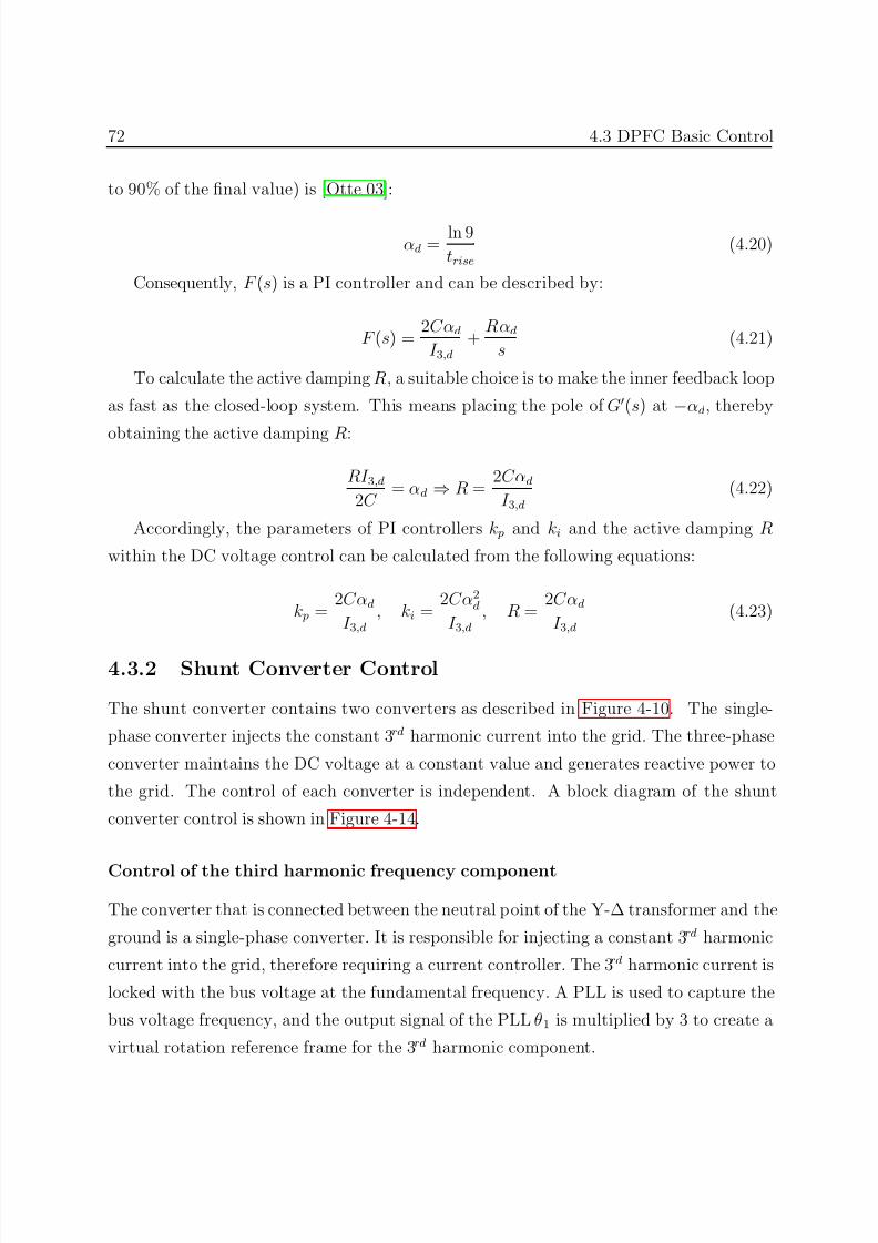
7/25/2019 Dpfc Thesis
http://slidepdf.com/reader/full/dpfc-thesis 94/212
72 4.3 DPFC Basic Control
to 90% of the final value) is [Otte 03]:
αd = ln 9
trise
(4.20)
Consequently, F (s) is a PI controller and can be described by:
F (s) = 2Cαd
I 3,d
+ Rαd
s (4.21)
To calculate the active damping R, a suitable choice is to make the inner feedback loop
as fast as the closed-loop system. This means placing the pole of G′(s) at −αd, thereby
obtaining the active damping R:
RI 3,d
2C = αd ⇒ R =
2Cαd
I 3,d
(4.22)
Accordingly, the parameters of PI controllers k p and ki and the active damping R
within the DC voltage control can be calculated from the following equations:
k p = 2Cαd
I 3,d, ki =
2Cα2d
I 3,d, R =
2Cαd
I 3,d(4.23)
4.3.2 Shunt Converter Control
The shunt converter contains two converters as described in Figure 4-10. The single-
phase converter injects the constant 3rd harmonic current into the grid. The three-phase
converter maintains the DC voltage at a constant value and generates reactive power to
the grid. The control of each converter is independent. A block diagram of the shunt
converter control is shown in Figure 4-14.
Control of the third harmonic frequency component
The converter that is connected between the neutral point of the Y-∆ transformer and the
ground is a single-phase converter. It is responsible for injecting a constant 3rd harmonic
current into the grid, therefore requiring a current controller. The 3rd harmonic current is
locked with the bus voltage at the fundamental frequency. A PLL is used to capture the
bus voltage frequency, and the output signal of the PLL θ1 is multiplied by 3 to create a
virtual rotation reference frame for the 3rd harmonic component.
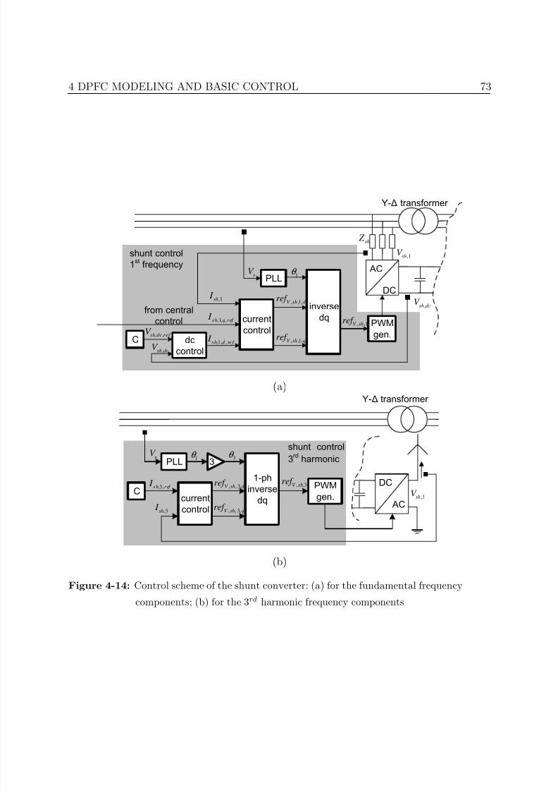
7/25/2019 Dpfc Thesis
http://slidepdf.com/reader/full/dpfc-thesis 95/212
4 DPFC MODELING AND BASIC CONTROL 73
, ,1V shref from central
control
PLL
dc
control
inverse
dqcurrent
control
, ,1,V sh d ref
, ,1,V sh qref
,1, ,s h d re f I
,1, ,s h q r ef I
AC
DC
Y-∆ transformer
s
V
,1shV
,1sh I
sh Z
,sh dcV
PWM
gen., ,sh dc ref V C
1
θ
,sh dcV
shunt control
1st frequency
(a)
AC
DC
Y∆ tanfom
sV
, ,3V shref
,3shV
1p
inverse
dqcurrent
control
P
, , 3,V sh d ref
, , 3,V sh qref
3
PWM
gen.
,3,s h r ef I C
,3sh I
1θ 3
θ shunt control
3rd
hrmonic
(b)
Figure 4-14: Control scheme of the shunt converter: (a) for the fundamental frequency
components; (b) for the 3rd harmonic frequency components
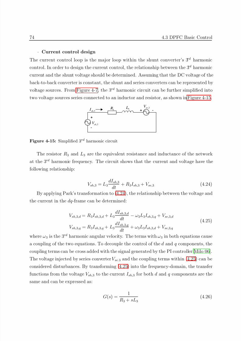
7/25/2019 Dpfc Thesis
http://slidepdf.com/reader/full/dpfc-thesis 96/212
74 4.3 DPFC Basic Control
- Current control design
The current control loop is the major loop within the shunt converter’s 3rd harmoniccontrol. In order to design the current control, the relationship between the 3rd harmonic
current and the shunt voltage should be determined. Assuming that the DC voltage of the
back-to-back converter is constant, the shunt and series converters can be represented by
voltage sources. From Figure 4-7, the 3rd harmonic circuit can be further simplified into
two voltage sources series connected to an inductor and resistor, as shown in Figure 4-15.
+ -
,3shV
,3sh I 3 R 3
L ,3seV
+
-
Figure 4-15: Simplified 3rd harmonic circuit
The resistor R3 and L3 are the equivalent resistance and inductance of the network
at the 3rd harmonic frequency. The circuit shows that the current and voltage have the
following relationship:
V sh,3 = L3dI sh,3
dt + R3I sh,3 + V se,3 (4.24)
By applying Park’s transformation to (4.24), the relationship between the voltage and
the current in the dq -frame can be determined:
V sh,3,d = R3I sh,3,d + L3dI sh,3,d
dt − ω3L3I sh,3,q + V se,3,d
V sh,3,q = R3I sh,3,q + L3dI sh,3,q
dt + ω3L3I sh,3,d + V se,3,q
(4.25)
where ω3
is the 3rd harmonic angular velocity. The terms with ω3
in both equations cause
a coupling of the two equations. To decouple the control of the d and q components, the
coupling terms can be cross added with the signal generated by the PI controller [Milo 06].
The voltage injected by series converter V se,3 and the coupling terms within (4.25) can be
considered disturbances. By transforming (4.25) into the frequency-domain, the transfer
functions from the voltage V sh,3 to the current I sh,3 for both d and q components are the
same and can be expressed as:
G(s) =
1
R3 + sL3 (4.26)
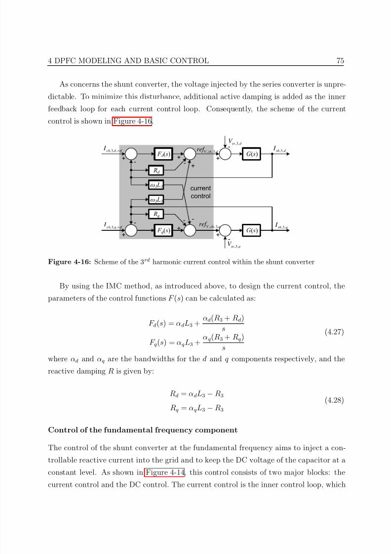
7/25/2019 Dpfc Thesis
http://slidepdf.com/reader/full/dpfc-thesis 97/212
4 DPFC MODELING AND BASIC CONTROL 75
As concerns the shunt converter, the voltage injected by the series converter is unpre-
dictable. To minimize this disturbance, additional active damping is added as the innerfeedback loop for each current control loop. Consequently, the scheme of the current
control is shown in Figure 4-16.
G( s) F d ( s)
+
-
+ +
-
+-
+
-
ω3 L3
+
-
Rd
-
-
,3,se d V
, , 3,V sh d ref
G( s)
ω3 L3
Rq
F q( s)+
,3,se qV
, , 3,V sh qref
,3,sh q I
,3,sh d I
, 3, ,s h d r ef I
, 3, ,s h q r ef I
current
control
Figure 4-16: Scheme of the 3rd harmonic current control within the shunt converter
By using the IMC method, as introduced above, to design the current control, the
parameters of the control functions F (s) can be calculated as:
F d(s) = αdL3 + αd(R3 + Rd)
s
F q(s) = αqL3 + αq(R3 + Rq)
s
(4.27)
where αd and αq are the bandwidths for the d and q components respectively, and the
reactive damping R is given by:
Rd = αdL3 −R3
Rq = αqL3 −R3
(4.28)
Control of the fundamental frequency component
The control of the shunt converter at the fundamental frequency aims to inject a con-
trollable reactive current into the grid and to keep the DC voltage of the capacitor at a
constant level. As shown in Figure 4-14, this control consists of two major blocks: the
current control and the DC control. The current control is the inner control loop, which
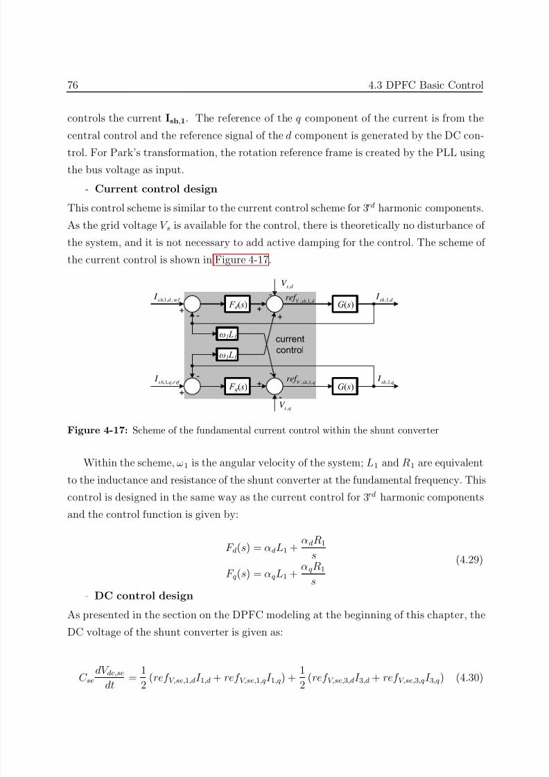
7/25/2019 Dpfc Thesis
http://slidepdf.com/reader/full/dpfc-thesis 98/212
76 4.3 DPFC Basic Control
controls the current Ish,1. The reference of the q component of the current is from the
central control and the reference signal of the d component is generated by the DC con-trol. For Park’s transformation, the rotation reference frame is created by the PLL using
the bus voltage as input.
- Current control design
This control scheme is similar to the current control scheme for 3rd harmonic components.
As the grid voltage V s is available for the control, there is theoretically no disturbance of
the system, and it is not necessary to add active damping for the control. The scheme of
the current control is shown in Figure 4-17.
G( s) F d ( s)
+
-
+
-
+-
+
-
ω1 L1
+
-
,s d V
, ,1,V sh d ref
G( s)
ω1 L1
F q( s)
,s qV
, ,1,V sh qref
,1,sh q I
,1,sh d I
,1, ,s h d re f I
,1, ,s h q r ef I
current
control
Figure 4-17: Scheme of the fundamental current control within the shunt converter
Within the scheme, ω1 is the angular velocity of the system; L1 and R1 are equivalent
to the inductance and resistance of the shunt converter at the fundamental frequency. This
control is designed in the same way as the current control for 3 rd harmonic components
and the control function is given by:
F d(s) = αdL1 + αdR1s
F q(s) = αqL1 + αqR1
s
(4.29)
- DC control design
As presented in the section on the DPFC modeling at the beginning of this chapter, the
DC voltage of the shunt converter is given as:
C se
dV dc,se
dt =
1
2 (ref V,se,1,dI 1,d + ref V,se,1,qI 1,q) +
1
2 (ref V,se,3,dI 3,d + ref V,se,3,qI 3,q) (4.30)
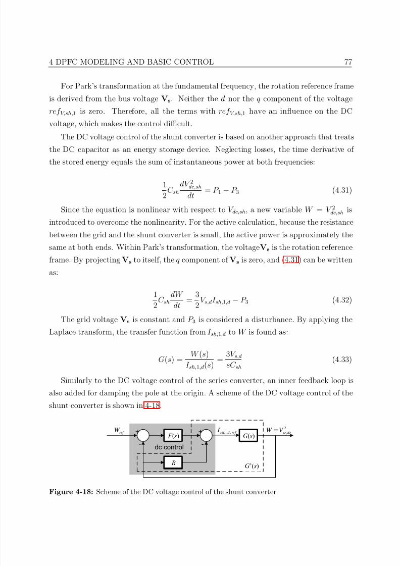
7/25/2019 Dpfc Thesis
http://slidepdf.com/reader/full/dpfc-thesis 99/212
4 DPFC MODELING AND BASIC CONTROL 77
For Park’s transformation at the fundamental frequency, the rotation reference frame
is derived from the bus voltage Vs. Neither the d nor the q component of the voltageref V,sh,1 is zero. Therefore, all the terms with ref V,sh,1 have an influence on the DC
voltage, which makes the control difficult.
The DC voltage control of the shunt converter is based on another approach that treats
the DC capacitor as an energy storage device. Neglecting losses, the time derivative of
the stored energy equals the sum of instantaneous power at both frequencies:
1
2
C sh
dV 2dc,sh
dt
= P 1
−P 3 (4.31)
Since the equation is nonlinear with respect to V dc,sh, a new variable W = V 2dc,sh is
introduced to overcome the nonlinearity. For the active calculation, because the resistance
between the grid and the shunt converter is small, the active power is approximately the
same at both ends. Within Park’s transformation, the voltage Vs is the rotation reference
frame. By projecting Vs to itself, the q component of Vs is zero, and (4.31) can be written
as:
12
C sh dW dt
= 32
V s,dI sh,1,d − P 3 (4.32)
The grid voltage Vs is constant and P 3 is considered a disturbance. By applying the
Laplace transform, the transfer function from I sh,1,d to W is found as:
G(s) = W (s)
I sh,1,d(s) =
3V s,d
sC sh
(4.33)
Similarly to the DC voltage control of the series converter, an inner feedback loop is
also added for damping the pole at the origin. A scheme of the DC voltage control of theshunt converter is shown in 4-18.
F ( s)
R
+
-
+
-
G( s),1, ,s h d re f I 2
,se dcW V =ref
W
G’( s)
dc control
Figure 4-18: Scheme of the DC voltage control of the shunt converter
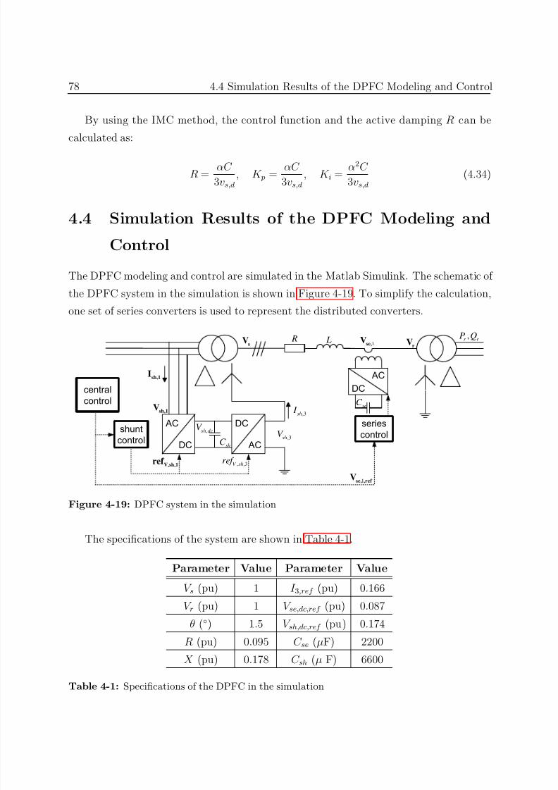
7/25/2019 Dpfc Thesis
http://slidepdf.com/reader/full/dpfc-thesis 100/212
78 4.4 Simulation Results of the DPFC Modeling and Control
By using the IMC method, the control function and the active damping R can be
calculated as:
R = αC
3vs,d
, K p = αC
3vs,d
, K i = α2C
3vs,d
(4.34)
4.4 Simulation Results of the DPFC Modeling and
Control
The DPFC modeling and control are simulated in the Matlab Simulink. The schematic of the DPFC system in the simulation is shown in Figure 4-19. To simplify the calculation,
one set of series converters is used to represent the distributed converters.
AC
DC
series
control
central
control
AC
DC AC
DC
sV
sh,1V
sh,1I
,sh dcV
shC
V,sh,1ref , ,3V shref
,3shV
,3sh
I
shunt
control
R L
seC
1se, ,ref V
rV1se,
V ,r r P Q
Figure 4-19: DPFC system in the simulation
The specifications of the system are shown in Table 4-1.
Parameter Value Parameter Value
V s (pu) 1 I 3,ref (pu) 0.166
V r (pu) 1 V se,dc,ref (pu) 0.087
θ () 1.5 V sh,dc,ref (pu) 0.174
R (pu) 0.095 C se (µF) 2200
X (pu) 0.178 C sh (µ F) 6600
Table 4-1: Specifications of the DPFC in the simulation
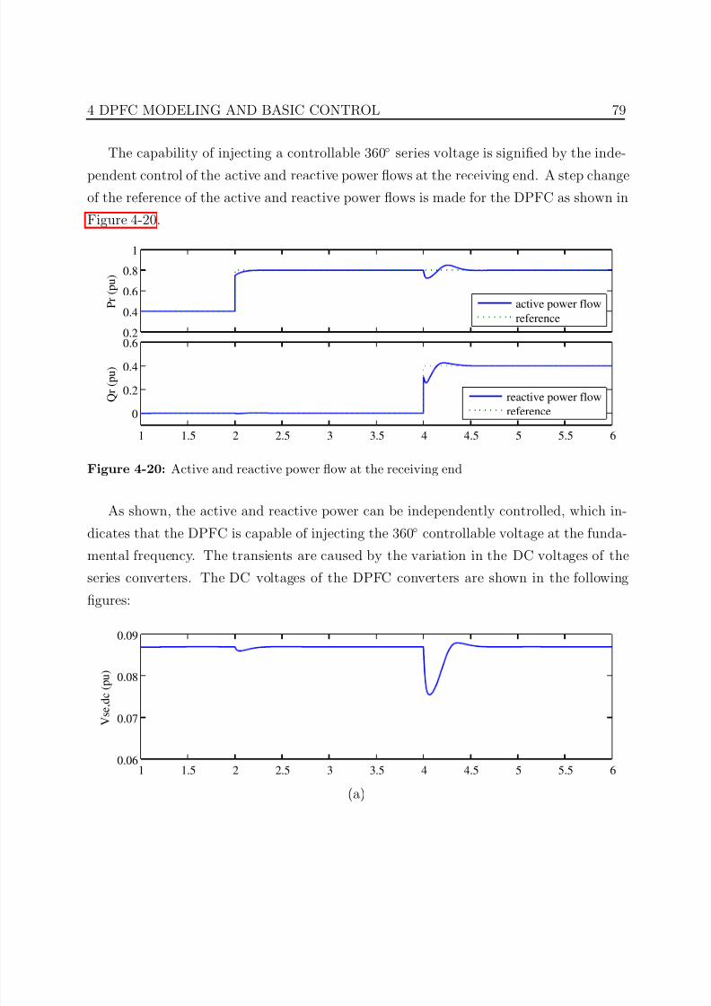
7/25/2019 Dpfc Thesis
http://slidepdf.com/reader/full/dpfc-thesis 101/212
4 DPFC MODELING AND BASIC CONTROL 79
The capability of injecting a controllable 360 series voltage is signified by the inde-
pendent control of the active and reactive power flows at the receiving end. A step changeof the reference of the active and reactive power flows is made for the DPFC as shown in
Figure 4-20.
0.2
0.4
0.6
0.8
1
P r ( p u )
1 1.5 2 2.5 3 3.5 4 4.5 5 5.5 6
0
0.2
0.4
0.6
Q r ( p u )
reactive power flow
reference
active power flow
reference
Figure 4-20: Active and reactive power flow at the receiving end
As shown, the active and reactive power can be independently controlled, which in-
dicates that the DPFC is capable of injecting the 360 controllable voltage at the funda-
mental frequency. The transients are caused by the variation in the DC voltages of the
series converters. The DC voltages of the DPFC converters are shown in the following
figures:
1 1.5 2 2.5 3 3.5 4 4.5 5 5.5 60.06
0.07
0.08
0.09
V s e , d c ( p u )
(a)
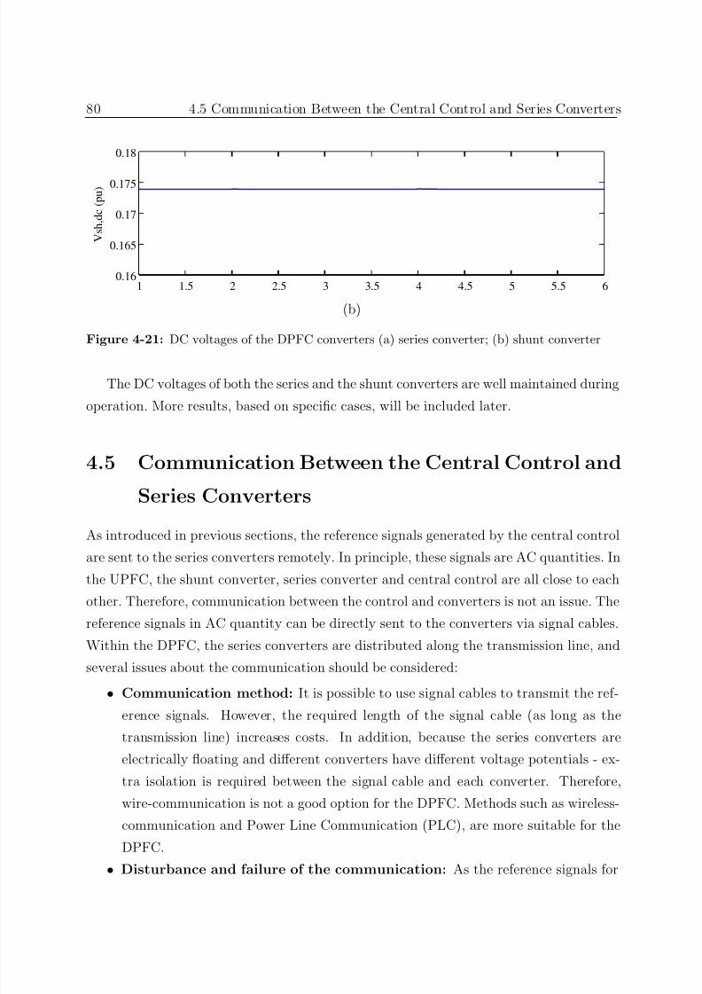
7/25/2019 Dpfc Thesis
http://slidepdf.com/reader/full/dpfc-thesis 102/212
80 4.5 Communication Between the Central Control and Series Converters
1 1.5 2 2.5 3 3.5 4 4.5 5 5.5 60.16
0.165
0.17
0.175
0.18
V s h , d c ( p u )
(b)
Figure 4-21: DC voltages of the DPFC converters (a) series converter; (b) shunt converter
The DC voltages of both the series and the shunt converters are well maintained during
operation. More results, based on specific cases, will be included later.
4.5 Communication Between the Central Control and
Series Converters
As introduced in previous sections, the reference signals generated by the central control
are sent to the series converters remotely. In principle, these signals are AC quantities. In
the UPFC, the shunt converter, series converter and central control are all close to each
other. Therefore, communication between the control and converters is not an issue. The
reference signals in AC quantity can be directly sent to the converters via signal cables.
Within the DPFC, the series converters are distributed along the transmission line, and
several issues about the communication should be considered:
• Communication method: It is possible to use signal cables to transmit the ref-erence signals. However, the required length of the signal cable (as long as the
transmission line) increases costs. In addition, because the series converters are
electrically floating and different converters have different voltage potentials - ex-
tra isolation is required between the signal cable and each converter. Therefore,
wire-communication is not a good option for the DPFC. Methods such as wireless-
communication and Power Line Communication (PLC), are more suitable for the
DPFC.
• Disturbance and failure of the communication: As the reference signals for
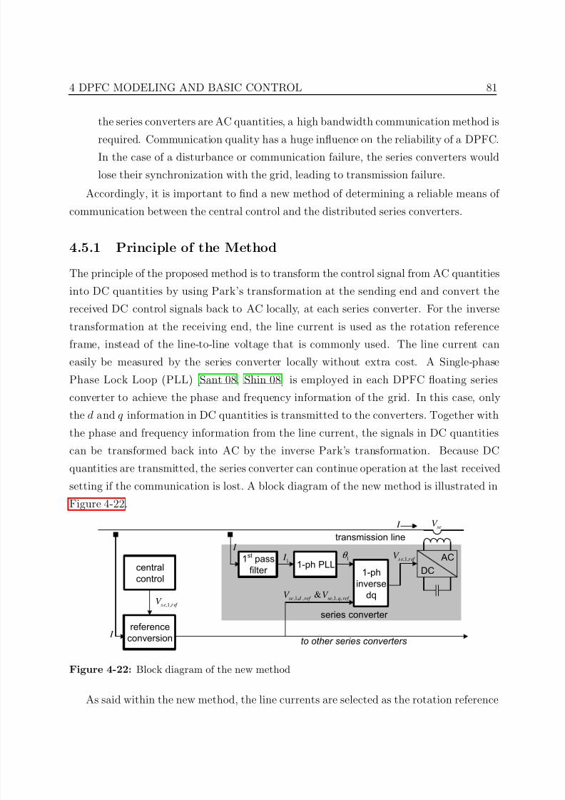
7/25/2019 Dpfc Thesis
http://slidepdf.com/reader/full/dpfc-thesis 103/212
4 DPFC MODELING AND BASIC CONTROL 81
the series converters are AC quantities, a high bandwidth communication method is
required. Communication quality has a huge influence on the reliability of a DPFC.In the case of a disturbance or communication failure, the series converters would
lose their synchronization with the grid, leading to transmission failure.
Accordingly, it is important to find a new method of determining a reliable means of
communication between the central control and the distributed series converters.
4.5.1 Principle of the Method
The principle of the proposed method is to transform the control signal from AC quantities
into DC quantities by using Park’s transformation at the sending end and convert the
received DC control signals back to AC locally, at each series converter. For the inverse
transformation at the receiving end, the line current is used as the rotation reference
frame, instead of the line-to-line voltage that is commonly used. The line current can
easily be measured by the series converter locally without extra cost. A Single-phase
Phase Lock Loop (PLL) [Sant 08, Shin 08] is employed in each DPFC floating series
converter to achieve the phase and frequency information of the grid. In this case, only
the d and q information in DC quantities is transmitted to the converters. Together withthe phase and frequency information from the line current, the signals in DC quantities
can be transformed back into AC by the inverse Park’s transformation. Because DC
quantities are transmitted, the series converter can continue operation at the last received
setting if the communication is lost. A block diagram of the new method is illustrated in
Figure 4-22.
1-ph PLL1st
passfilter 1-ph
inverse
q
seV I
transmission line
,1,s e r ef
V 1
θ 1 I
,1, , ,1, ,&se d ref se q ref V V
I
series onverter
ACDCentral
ontrol
referene
onversion
,1,s e r ef V
I to other series converters
Figure 4-22: Block diagram of the new method
As said within the new method, the line currents are selected as the rotation reference
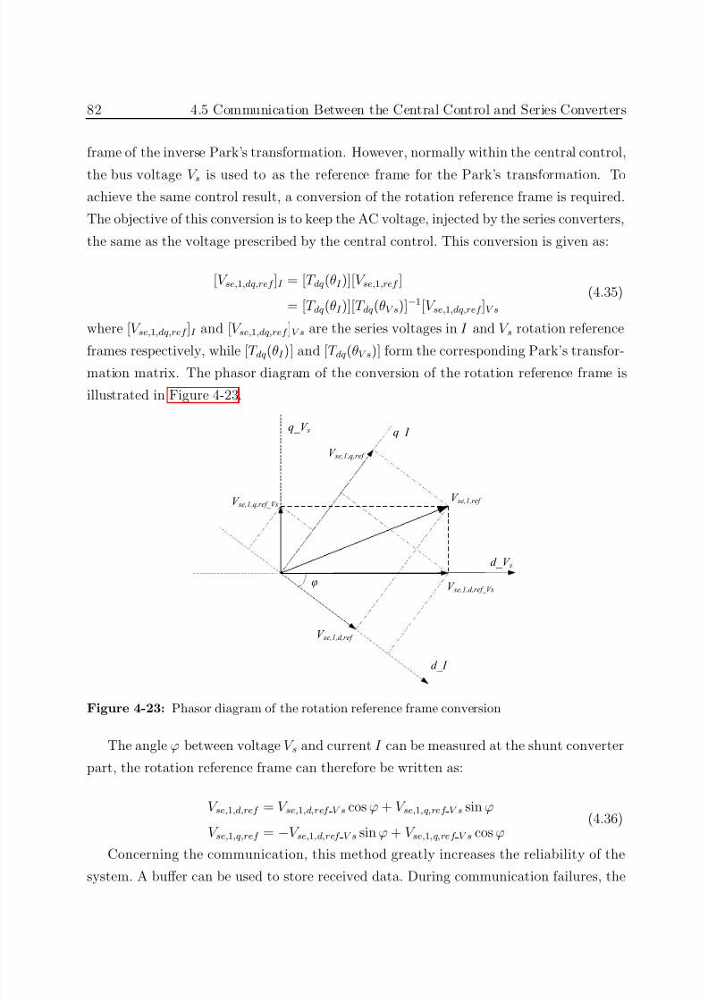
7/25/2019 Dpfc Thesis
http://slidepdf.com/reader/full/dpfc-thesis 104/212
82 4.5 Communication Between the Central Control and Series Converters
frame of the inverse Park’s transformation. However, normally within the central control,
the bus voltage V s is used to as the reference frame for the Park’s transformation. Toachieve the same control result, a conversion of the rotation reference frame is required.
The objective of this conversion is to keep the AC voltage, injected by the series converters,
the same as the voltage prescribed by the central control. This conversion is given as:
[V se,1,dq,ref ]I = [T dq(θI )][V se,1,ref ]
= [T dq(θI )][T dq(θV s)]−1[V se,1,dq,ref ]V s
(4.35)
where [V se,1,dq,ref ]I and [V se,1,dq,ref ]V s are the series voltages in I and V s rotation reference
frames respectively, while [T dq(θI )] and [T dq(θV s)] form the corresponding Park’s transfor-mation matrix. The phasor diagram of the conversion of the rotation reference frame is
illustrated in Figure 4-23.
d_V s
q_V s
V se,1,r ef
d_I
q_I
V se,1,q,ref
φ
V se,1,d,ref
V se,1,d ,ref_Vs
V se,1,q ,ref_Vs
Figure 4-23: Phasor diagram of the rotation reference frame conversion
The angle ϕ between voltage V s and current I can be measured at the shunt converter
part, the rotation reference frame can therefore be written as:
V se,1,d,ref = V se,1,d,ref V s cos ϕ + V se,1,q,ref V s sin ϕ
V se,1,q,ref = −V se,1,d,ref V s sin ϕ + V se,1,q,ref V s cos ϕ(4.36)
Concerning the communication, this method greatly increases the reliability of the
system. A buffer can be used to store received data. During communication failures, the
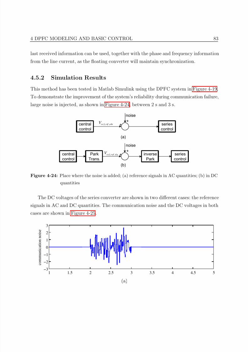
7/25/2019 Dpfc Thesis
http://slidepdf.com/reader/full/dpfc-thesis 105/212
4 DPFC MODELING AND BASIC CONTROL 83
last received information can be used, together with the phase and frequency information
from the line current, as the floating converter will maintain synchronization.
4.5.2 Simulation Results
This method has been tested in Matlab Simulink using the DPFC system in Figure 4-19.
To demonstrate the improvement of the system’s reliability during communication failure,
large noise is injected, as shown in Figure 4-24, between 2 s and 3 s.
centralcontrol
seriescontrol
,1, ,s e r ef a bcV
noise
++
central
control
series
control
,1, ,s e r ef d qV
noise
++
Park
Trans.
inverse
Park
(a)
(b)
Figure 4-24: Place where the noise is added; (a) reference signals in AC quantities; (b) in DC
quantities
The DC voltages of the series converter are shown in two different cases: the reference
signals in AC and DC quantities. The communication noise and the DC voltages in both
cases are shown in Figure 4-25.
1 1.5 2 2.5 3 3.5 4 4.5 5−3
−2
−1
0
1
2
3
c o m m u n i c a
t i o n n o i s e
(a)
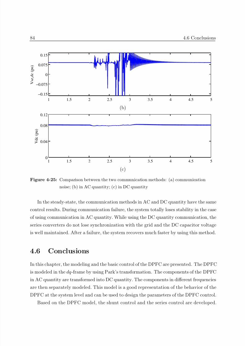
7/25/2019 Dpfc Thesis
http://slidepdf.com/reader/full/dpfc-thesis 106/212
84 4.6 Conclusions
1 1.5 2 2.5 3 3.5 4 4.5 5
−0.15
−0.075
0
0.075
0.15
V s e , d c ( p u )
(b)
1 1.5 2 2.5 3 3.5 4 4.5 50
0.04
0.08
0.12
V d c ( p u )
(c)
Figure 4-25: Comparison between the two communication methods: (a) communicationnoise; (b) in AC quantity; (c) in DC quantity
In the steady-state, the communication methods in AC and DC quantity have the same
control results. During communication failure, the system totally loses stability in the case
of using communication in AC quantity. While using the DC quantity communication, the
series converters do not lose synchronization with the grid and the DC capacitor voltage
is well maintained. After a failure, the system recovers much faster by using this method.
4.6 Conclusions
In this chapter, the modeling and the basic control of the DPFC are presented. The DPFC
is modeled in the dq -frame by using Park’s transformation. The components of the DPFC
in AC quantity are transformed into DC quantity. The components in different frequencies
are then separately modeled. This model is a good representation of the behavior of the
DPFC at the system level and can be used to design the parameters of the DPFC control.
Based on the DPFC model, the shunt control and the series control are developed.
7/25/2019 Dpfc Thesis
http://slidepdf.com/reader/full/dpfc-thesis 107/212
4 DPFC MODELING AND BASIC CONTROL 85
The functions of these controls are to maintain the DC capacitor voltages of the converters
and to ensure the required voltages and currents are injected from the central control.The IMC method is employed to calculate the control parameters. The DPFC basic
control and model are simulated in Matlab Simulink. The simulation results show that
the DPFC is able to control the active and reactive power flows independently and that
during operation, the DC voltages of the converters are well maintained.
Communication between the central control and the series converters is also consid-
ered. To increase the reliability of the DPFC during communication failure, the reference
signals in DC quantities are used instead of in AC quantities. The line current is selected
as the rotation reference frame because it can be easily measured by the series converterswithout extra cost. During communication failure, the series converter can use the last
received setting to continue operation, thereby increasing the system’s reliability. This
communication method is also tested in Matlab Simulink. It shows that in steady-state,
communication in DC quantities has the same result as in AC quantities. During com-
munication failure, the series converter of the DPFC can maintain synchronization with
the system.

7/25/2019 Dpfc Thesis
http://slidepdf.com/reader/full/dpfc-thesis 108/212
7/25/2019 Dpfc Thesis
http://slidepdf.com/reader/full/dpfc-thesis 109/212
Chapter 5DPFC EXPERIMENTAL
DEMONSTRATOR
5.1 Introduction
I
N the previous two chapters, a new concept of a DPFC and corresponding modeling
and control were presented. The DPFC has been simulated in Matlab, Simulink.
However, during the simulation, several issues were neglected, such as switching behaviors,
converter losses and measurement delays. Accordingly, to show the neglected effects and
to test the basic control whose design is based on the model, the DPFC is tested in
an experimental setup. The setup consists of two main parts: the network and DPFC
converters.
The chapter begins by presenting the specifications of the DPFC experimental setup.
Once the specifications are introduced, the design of the DPFC experimental setup is
given. The design concerns the electrical part of the experimental setup. The control
of the DPFC converters is done using the Texas Instrument DSP controller F2808. The
real-time programming of the converter is introduced after the electrical design. The last
section of this chapter presents the results of the DPFC experiments.
5.2 Specifications
As has been stated, the DPFC experimental setup consists of a scaled network part and
a converter part. In principle, the DPFC is used in transmission networks. However,
87
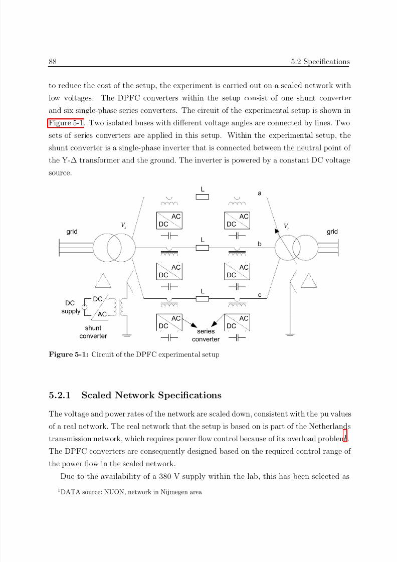
7/25/2019 Dpfc Thesis
http://slidepdf.com/reader/full/dpfc-thesis 110/212
88 5.2 Specifications
to reduce the cost of the setup, the experiment is carried out on a scaled network with
low voltages. The DPFC converters within the setup consist of one shunt converterand six single-phase series converters. The circuit of the experimental setup is shown in
Figure 5-1. Two isolated buses with different voltage angles are connected by lines. Two
sets of series converters are applied in this setup. Within the experimental setup, the
shunt converter is a single-phase inverter that is connected between the neutral point of
the Y-∆ transformer and the ground. The inverter is powered by a constant DC voltage
source.
AC
DC
AC
DC
AC
DC
L
ACDC
ACDC
L
ACDC
ACDC
L
a
b
cDC
supply
gi gi
seies
onvete
shunt
onvete
sV
r V
Figure 5-1: Circuit of the DPFC experimental setup
5.2.1 Scaled Network Specifications
The voltage and power rates of the network are scaled down, consistent with the pu values
of a real network. The real network that the setup is based on is part of the Netherlands
transmission network, which requires power flow control because of its overload problem1.
The DPFC converters are consequently designed based on the required control range of
the power flow in the scaled network.
Due to the availability of a 380 V supply within the lab, this has been selected as
1
DATA source: NUON, network in Nijmegen area
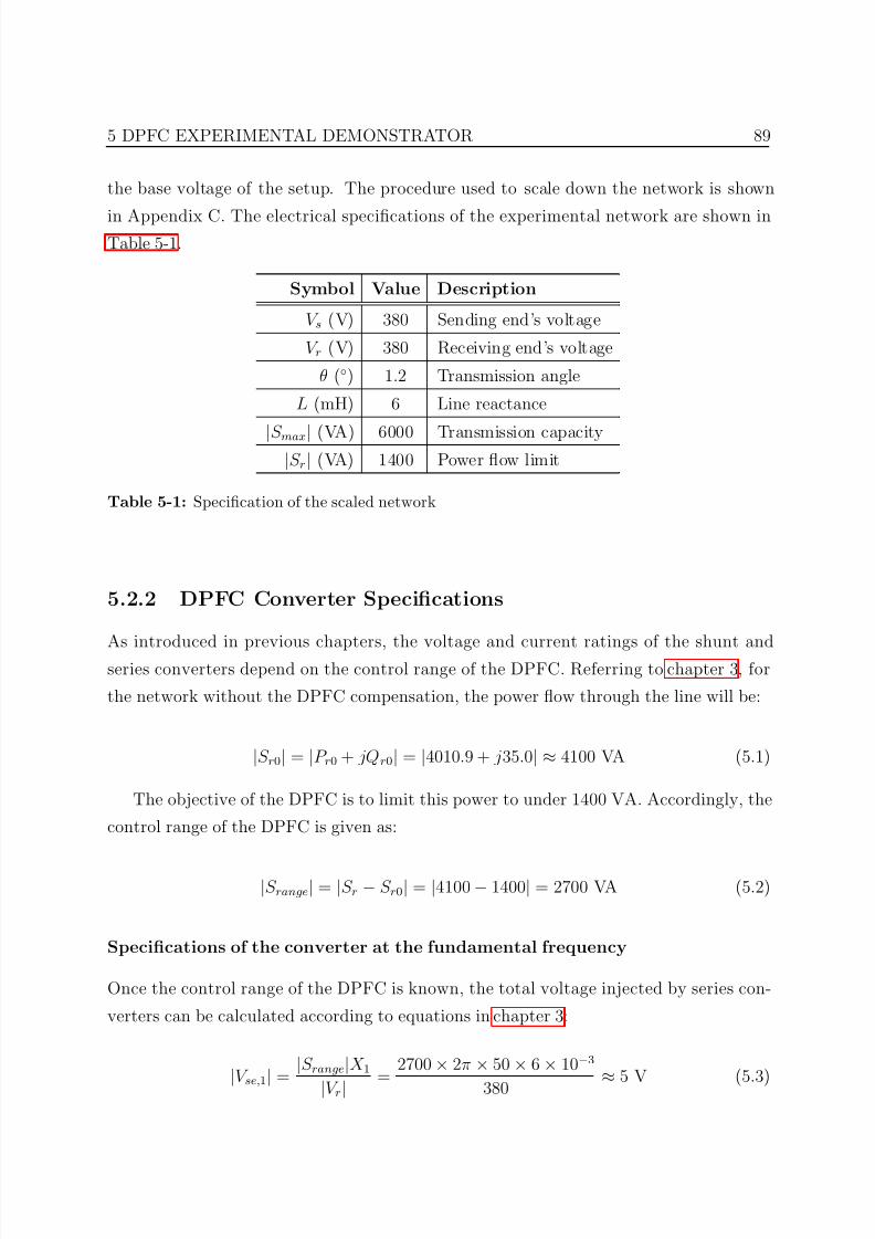
7/25/2019 Dpfc Thesis
http://slidepdf.com/reader/full/dpfc-thesis 111/212
5 DPFC EXPERIMENTAL DEMONSTRATOR 89
the base voltage of the setup. The procedure used to scale down the network is shown
in Appendix C. The electrical specifications of the experimental network are shown inTable 5-1.
Symbol Value Description
V s (V) 380 Sending end’s voltage
V r (V) 380 Receiving end’s voltage
θ () 1.2 Transmission angle
L (mH) 6 Line reactance
|S max| (VA) 6000 Transmission capacity|S r| (VA) 1400 Power flow limit
Table 5-1: Specification of the scaled network
5.2.2 DPFC Converter Specifications
As introduced in previous chapters, the voltage and current ratings of the shunt and
series converters depend on the control range of the DPFC. Referring to chapter 3, for
the network without the DPFC compensation, the power flow through the line will be:
|S r0| = |P r0 + jQr0| = |4010.9 + j35.0| ≈ 4100 VA (5.1)
The objective of the DPFC is to limit this power to under 1400 VA. Accordingly, the
control range of the DPFC is given as:
|S range| = |S r − S r0| = |4100− 1400| = 2700 VA (5.2)
Specifications of the converter at the fundamental frequency
Once the control range of the DPFC is known, the total voltage injected by series con-
verters can be calculated according to equations in chapter 3:
|V se,1| = |S range
|X 1
|V r| =
2700
×2π
×50
×6
×10−3
380 ≈ 5 V (5.3)
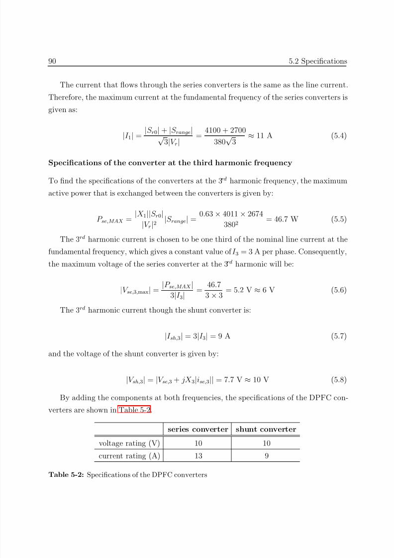
7/25/2019 Dpfc Thesis
http://slidepdf.com/reader/full/dpfc-thesis 112/212
90 5.2 Specifications
The current that flows through the series converters is the same as the line current.
Therefore, the maximum current at the fundamental frequency of the series converters isgiven as:
|I 1| = |S r0|+ |S range|√
3|V r|=
4100 + 2700
380√
3≈ 11 A (5.4)
Specifications of the converter at the third harmonic frequency
To find the specifications of the converters at the 3rd harmonic frequency, the maximum
active power that is exchanged between the converters is given by:
P se,MAX = |X 1||S r0||V r|2 |S range| =
0.63 × 4011 × 2674
3802 = 46.7 W (5.5)
The 3rd harmonic current is chosen to be one third of the nominal line current at the
fundamental frequency, which gives a constant value of I 3 = 3 A per phase. Consequently,
the maximum voltage of the series converter at the 3rd harmonic will be:
|V se,3,max| = |P se,MAX
|3|I 3| =
46.7
3 × 3 = 5.2 V ≈ 6 V (5.6)
The 3rd harmonic current though the shunt converter is:
|I sh,3| = 3|I 3| = 9 A (5.7)
and the voltage of the shunt converter is given by:
|V sh,3| = |V se,3 + jX 3|ise,3|| = 7.7 V ≈ 10 V (5.8)
By adding the components at both frequencies, the specifications of the DPFC con-
verters are shown in Table 5-2.
series converter shunt converter
voltage rating (V) 10 10
current rating (A) 13 9
Table 5-2: Specifications of the DPFC converters
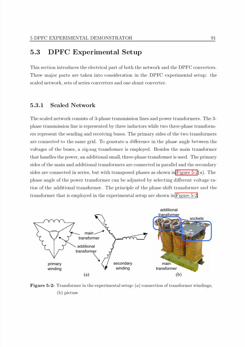
7/25/2019 Dpfc Thesis
http://slidepdf.com/reader/full/dpfc-thesis 113/212
5 DPFC EXPERIMENTAL DEMONSTRATOR 91
5.3 DPFC Experimental Setup
This section introduces the electrical part of both the network and the DPFC converters.
Three major parts are taken into consideration in the DPFC experimental setup: the
scaled network, sets of series converters and one shunt converter.
5.3.1 Scaled Network
The scaled network consists of 3-phase transmission lines and power transformers. The 3-
phase transmission line is represented by three inductors while two three-phase transform-
ers represent the sending and receiving buses. The primary sides of the two transformers
are connected to the same grid. To generate a difference in the phase angle between the
voltages of the buses, a zig-zag transformer is employed. Besides the main transformer
that handles the power, an additional small, three-phase transformer is used. The primary
sides of the main and additional transformers are connected in parallel and the secondary
sides are connected in series, but with transposed phases as shown in Figure 5-2(a). The
phase angle of the power transformer can be adjusted by selecting different voltage ra-tios of the additional transformer. The principle of the phase shift transformer and the
transformer that is employed in the experimental setup are shown in Figure 5-2.
primary
winding
secondary
winding
main
transformer
additional
transformer
main
transformer
additional
transformer sockets
(a) (b)
Figure 5-2: Transformer in the experimental setup: (a) connection of transformer windings;
(b) picture
7/25/2019 Dpfc Thesis
http://slidepdf.com/reader/full/dpfc-thesis 114/212
92 5.3 DPFC Experimental Setup
5.3.2 Series Converter
The series converter is the key component of the DPFC experimental setup. To verify the
concept of the distributed series converter, two sets of single-phase converters are required
with each set consisting of three converters for different phases. The series converter is
connected to the line by a transformer. To reduce the RMS currents on the converter
side, the ratio of the transformer winding is 5:25 V.
The series converter is a full-bridge single-phase converter with a capacitor acting as
short-term energy storage on the DC side. The technology used to control the series
converter is PWM with unipolar voltage switching with a 6 kHz switching frequency
[Moha 03]. The capacitors in the series converter are implemented with a combination of
an aluminum electrolytic capacitor in parallel with two ceramic capacitors. The aluminum
electrolytic capacitor is used to provide DC voltage as energy storage, while the ceramic
capacitors provide decoupling for the high-frequency switching components.
All inputs and outputs of the series converter are galvanically isolated from the outside.
The series device, consisting of the series converter, the control circuit (DSP board) and
auxiliaries, floats on the voltage potential of the transmission line. The central control
that gives a set point for voltage to be injected, operates at ground potential. Therefore,in practice the control signals have to be transmitted over a high voltage barrier, via
a wireless communication or through power line communication for instance. In the
experimental setup, communication between the central controller and series converters
takes place through USB cables to reduce its complexity. Therefore, voltage isolation is
required between the DSP board and the power circuit. This isolation is provided by the
gate drives and the measurement device that gives feedback signals for the DSP. Figure 5-3
shows a simplified diagram of the series converter and a photo of a series converter in the
experimental setup.
5.3.3 Shunt Converter
The basic structure of the shunt converter is similar to the series converter, which is a
single-phase full-bridge VSC with unipolar PWM control. To simplify the experimental
setup, the DC voltage is supplied by a DC voltage source instead of a back-to-back
connected AC/DC converter. The AC output terminals of the shunt converter are directly
connected to the neutral points of the Y-∆ transformers to inject 3rd harmonic current.
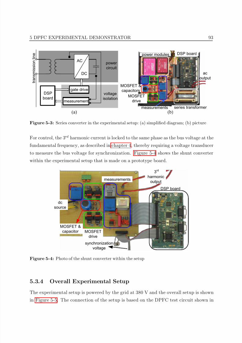
7/25/2019 Dpfc Thesis
http://slidepdf.com/reader/full/dpfc-thesis 115/212
5 DPFC EXPERIMENTAL DEMONSTRATOR 93
power modules DSP board
series transformer measurements
MOSFET
drive
MOSFET &
capacitors
ac
output
AC
DC
measurement
voltage
isolation
DSP
board
t r a n s m i s s i o n
l i n e
power
circuit
gate drive
(a) (b)
Figure 5-3: Series converter in the experimental setup: (a) simplified diagram; (b) picture
For control, the 3rd harmonic current is locked to the same phase as the bus voltage at the
fundamental frequency, as described in chapter 4, thereby requiring a voltage transducer
to measure the bus voltage for synchronization. Figure 5-4 shows the shunt converter
within the experimental setup that is made on a prototype board.
3rd
harmonic
output
DSP board
measurements
dc
source
MOSFET
drive
MOSFET &
capacitor
synchronization
voltage
Figure 5-4: Photo of the shunt converter within the setup
5.3.4 Overall Experimental Setup
The experimental setup is powered by the grid at 380 V and the overall setup is shown
in Figure 5-5. The connection of the setup is based on the DPFC test circuit shown in
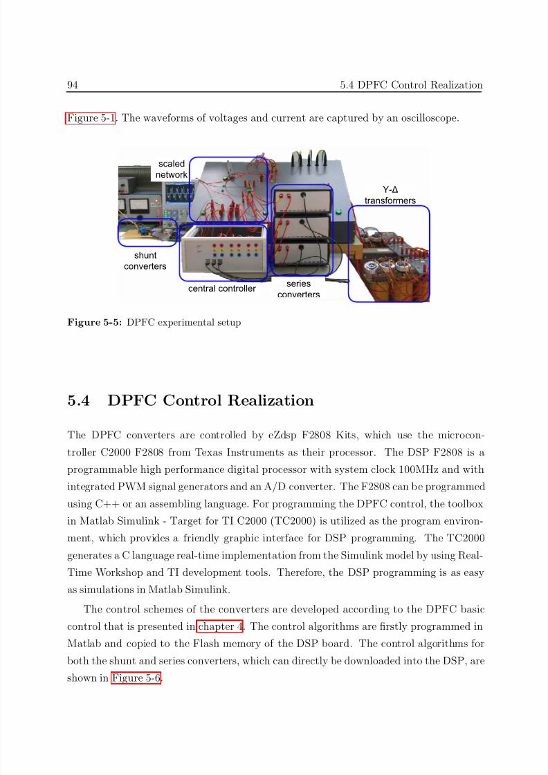
7/25/2019 Dpfc Thesis
http://slidepdf.com/reader/full/dpfc-thesis 116/212
94 5.4 DPFC Control Realization
Figure 5-1. The waveforms of voltages and current are captured by an oscilloscope.
series
converterscentral controller
shunt
converters
Y-∆
transformers
scaled
network
Figure 5-5: DPFC experimental setup
5.4 DPFC Control RealizationThe DPFC converters are controlled by eZdsp F2808 Kits, which use the microcon-
troller C2000 F2808 from Texas Instruments as their processor. The DSP F2808 is a
programmable high performance digital processor with system clock 100MHz and with
integrated PWM signal generators and an A/D converter. The F2808 can be programmed
using C++ or an assembling language. For programming the DPFC control, the toolbox
in Matlab Simulink - Target for TI C2000 (TC2000) is utilized as the program environ-
ment, which provides a friendly graphic interface for DSP programming. The TC2000generates a C language real-time implementation from the Simulink model by using Real-
Time Workshop and TI development tools. Therefore, the DSP programming is as easy
as simulations in Matlab Simulink.
The control schemes of the converters are developed according to the DPFC basic
control that is presented in chapter 4. The control algorithms are firstly programmed in
Matlab and copied to the Flash memory of the DSP board. The control algorithms for
both the shunt and series converters, which can directly be downloaded into the DSP, are
shown in Figure 5-6.
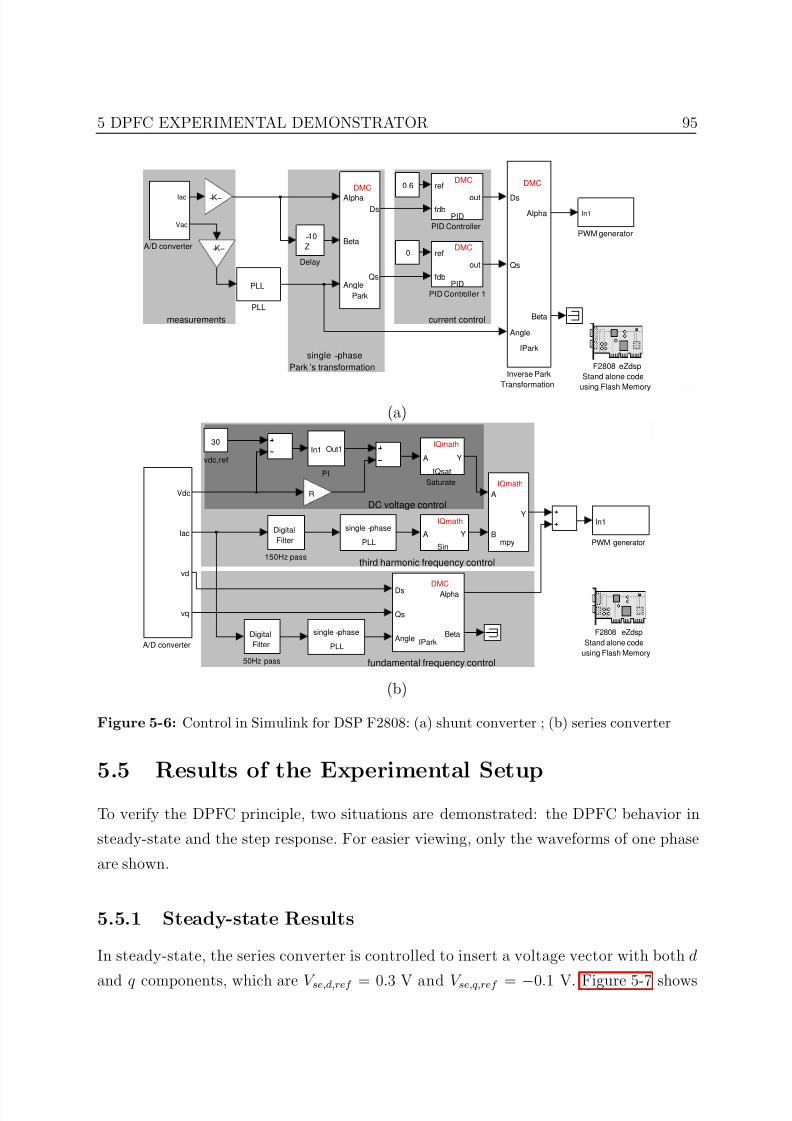
7/25/2019 Dpfc Thesis
http://slidepdf.com/reader/full/dpfc-thesis 117/212
5 DPFC EXPERIMENTAL DEMONSTRATOR 95
measurements
single −phase
Park ’s transformation
current control
Alpha
Beta
Angle
Ds
Qs
Park
DMC
PWM generator
In1
PLL
PLLPID Controller 1
ref
fdb
out
PID
DMC
PID Controller
ref
fdb
out
PID
DMC
Inverse Park
Transformation
Ds
Qs
Angle
Alpha
Beta
IPark
DMC
−K−
−K−
F2808 eZdsp
Stand alone code
using Flash Memory
Delay
−10
Z
0.6
0A/D converter
Iac
Vac
(a)
fundamental frequency control
third harmonic frequency control
DC voltage control
vdc,ref
30
single −phase
PLL
single −phase
PLLA Y
Sin
IQmath
Saturate
A Y
IQsat
IQmath
PWM generator
In1
PI
In1 Out1
Ds
Qs
Angle
Alpha
BetaIPark
DMC
A
B
Y
mpy
IQmath
R
F2808 eZdsp
Stand alone code
using Flash MemoryA/D converter
Vdc
Iac
vd
vq
50Hz pass
Digital
Filter
150Hz pass
Digital
Filter
(b)
Figure 5-6: Control in Simulink for DSP F2808: (a) shunt converter ; (b) series converter
5.5 Results of the Experimental Setup
To verify the DPFC principle, two situations are demonstrated: the DPFC behavior in
steady-state and the step response. For easier viewing, only the waveforms of one phase
are shown.
5.5.1 Steady-state Results
In steady-state, the series converter is controlled to insert a voltage vector with both d
and q components, which are V se,d,ref = 0.3 V and V se,q,ref = −0.1 V. Figure 5-7 shows
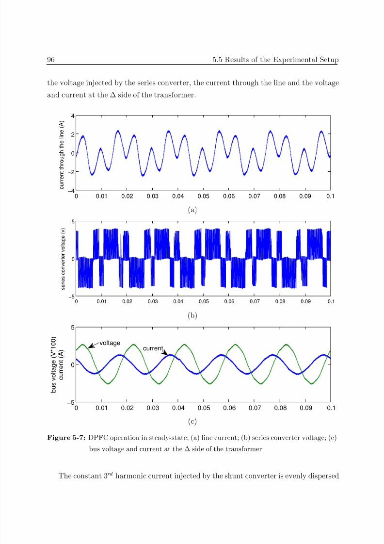
7/25/2019 Dpfc Thesis
http://slidepdf.com/reader/full/dpfc-thesis 118/212
96 5.5 Results of the Experimental Setup
the voltage injected by the series converter, the current through the line and the voltage
and current at the ∆ side of the transformer.
0 0.01 0.02 0.03 0.04 0.05 0.06 0.07 0.08 0.09 0.1−4
−2
0
2
4
c u r r e n t t h r o u g h t h e l i n e ( A )
(a)
0 0.01 0.02 0.03 0.04 0.05 0.06 0.07 0.08 0.09 0.1−5
0
5
s e
r i e s c o n v e r t e r v o l t a g e ( v )
(b)
0 0.01 0.02 0.03 0.04 0.05 0.06 0.07 0.08 0.09 0.1−5
0
5
b u s v o l t a g e ( V * 1 0 0 )
c u r r e n t ( A )
voltagecurrent
(c)
Figure 5-7: DPFC operation in steady-state; (a) line current; (b) series converter voltage; (c)
bus voltage and current at the ∆ side of the transformer
The constant 3rd harmonic current injected by the shunt converter is evenly dispersed
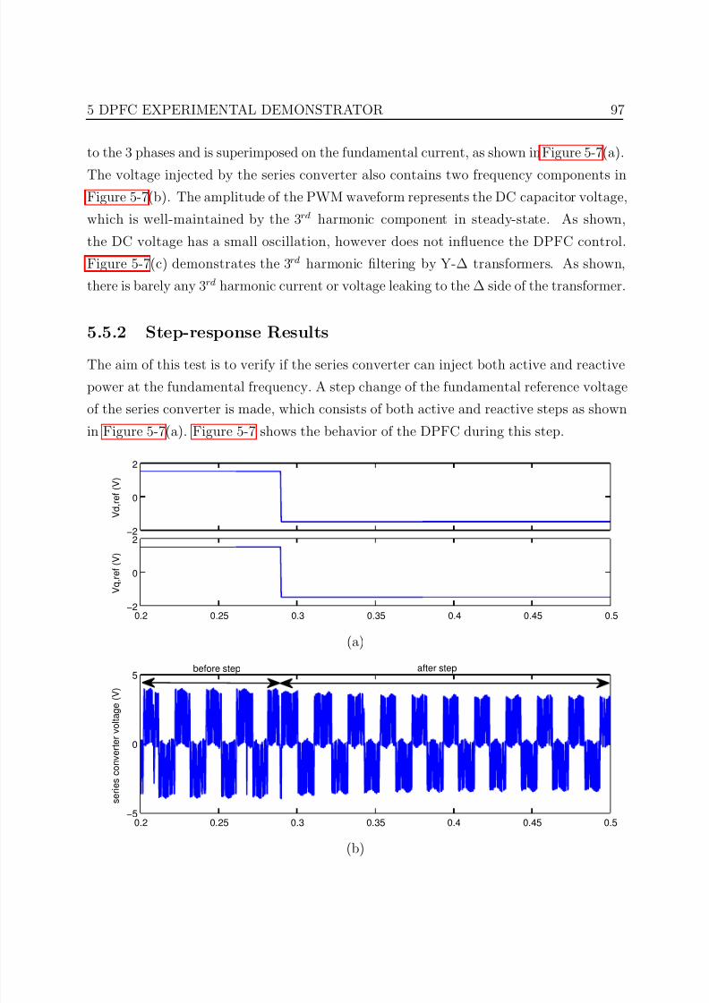
7/25/2019 Dpfc Thesis
http://slidepdf.com/reader/full/dpfc-thesis 119/212
5 DPFC EXPERIMENTAL DEMONSTRATOR 97
to the 3 phases and is superimposed on the fundamental current, as shown in Figure 5-7(a).
The voltage injected by the series converter also contains two frequency components inFigure 5-7(b). The amplitude of the PWM waveform represents the DC capacitor voltage,
which is well-maintained by the 3rd harmonic component in steady-state. As shown,
the DC voltage has a small oscillation, however does not influence the DPFC control.
Figure 5-7(c) demonstrates the 3rd harmonic filtering by Y-∆ transformers. As shown,
there is barely any 3rd harmonic current or voltage leaking to the ∆ side of the transformer.
5.5.2 Step-response Results
The aim of this test is to verify if the series converter can inject both active and reactive
power at the fundamental frequency. A step change of the fundamental reference voltage
of the series converter is made, which consists of both active and reactive steps as shown
in Figure 5-7(a). Figure 5-7 shows the behavior of the DPFC during this step.
0.2 0.25 0.3 0.35 0.4 0.45 0.5−2
0
2
V q , r e f ( V )
−2
0
2
V d , r e f ( V )
(a)
0.2 0.25 0.3 0.35 0.4 0.45 0.5−5
0
5
s e r i e s c o n v e r t e r v o l t a g e
( V )
before step after step
(b)
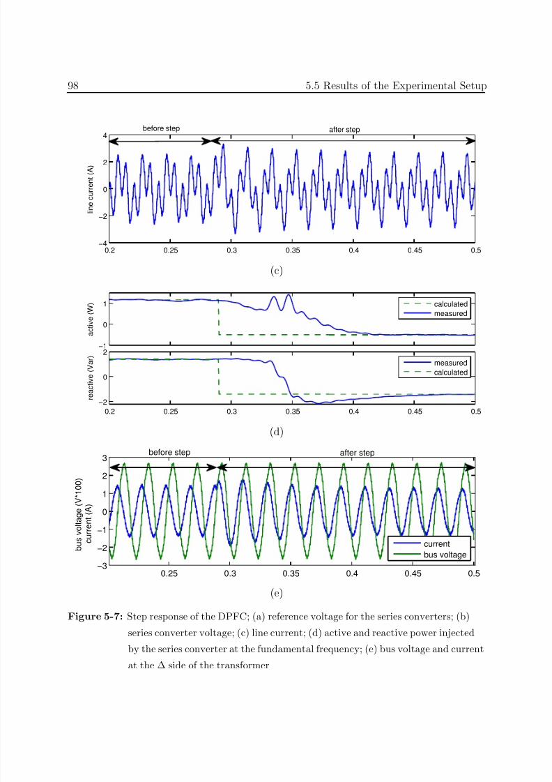
7/25/2019 Dpfc Thesis
http://slidepdf.com/reader/full/dpfc-thesis 120/212
98 5.5 Results of the Experimental Setup
0.2 0.25 0.3 0.35 0.4 0.45 0.5−4
−2
0
2
4
l i n e c u r r e n t ( A )
after stepbefore step
(c)
−1
0
1
a c t i v e ( W )
0.2 0.25 0.3 0.35 0.4 0.45 0.5
−2
0
2
r e a c t i v e ( V a r )
calculated
measured
measured
calculated
(d)
0.25 0.3 0.35 0.4 0.45 0.5−3
−2
−1
0
1
2
3
b u s v o l t a g e ( V * 1 0 0 )
c u r r e n t ( A )
currentbus voltage
after stepbefore step
(e)
Figure 5-7: Step response of the DPFC; (a) reference voltage for the series converters; (b)
series converter voltage; (c) line current; (d) active and reactive power injected
by the series converter at the fundamental frequency; (e) bus voltage and current
at the ∆ side of the transformer
7/25/2019 Dpfc Thesis
http://slidepdf.com/reader/full/dpfc-thesis 121/212
5 DPFC EXPERIMENTAL DEMONSTRATOR 99
As shown, the DC voltage of the series converter is stabilized before and after the step
change. To verify whether the series converter can inject or absorb active and reactivepower from the grid at the fundamental frequency, the power is calculated from the
measured voltage and current plotted in Figure 5-7(b&c). The measured data in one
phase is processed in the computer by using Matlab. To analyze the voltage and current
at the fundamental frequency, the measured data that contains harmonic distortion is
filtered by a low-pass digital filter with the 50Hz cut-off frequency. Because of this filter,
the calculated voltage and current at the fundamental frequency have a 1.5 cycle delay
compared to the actual values, thereby causing a delay of the measured active and reactive
power. Figure 5-7(d) illustrates the active and reactive power injected by the seriesconverter. A comparison is made between the measured power and the calculated power.
We can see that the series converters are able to absorb and inject both active and reactive
power to the grid at the fundamental frequency.
5.6 Conclusions
This chapter presents the experimental setup and test results of the DPFC. The electrical
design and the implementation of real-time control are considered and briefly introduced.
The DPFC is tested in a scaled two-bus network with fixed voltages at the sending and
receiving ends. Due to the phase shift between the voltages, there is a power flow between
the buses through the line. The DPFC series converters are in series with the line to
control the power flow. The DPFC converters employ the DSP board from TI for real-
time control. The control schemes were programmed in Matlab Simlink and downloaded
in the Flash memory of the DSP for the control. Two cases were tested: the steady-state
and the step response. During both tests, the shunt converter and the series converter
could exchange active power through the 3rd harmonic component and the DC voltages
of the series converters were-well maintained. The series converter can inject and absorb
both active and reactive power, which proves the DPFC principle and verifies the control
schemes that are presented in previous chapters.

7/25/2019 Dpfc Thesis
http://slidepdf.com/reader/full/dpfc-thesis 122/212
7/25/2019 Dpfc Thesis
http://slidepdf.com/reader/full/dpfc-thesis 123/212
Chapter 6DPFC FAULT TOLERANCE
6.1 Introduction
THE concept of the DPFC was presented and analyzed in previous chapters. The
basic control of the DPFC was designed and verified both in the simulation and
in the experimental setup. When the DPFC is applied to power systems, reliability is
one of the most important issues that should be taken into consideration. This chapter
addresses the fault tolerance of the DPFC.
The chapter begins by listing possible faults that can occur in the DPFC and their
corresponding effects on the network. Three types of faults are categorized: shunt con-
verter failure, series converter failure and control failure. In this chapter, the DPFC fault
tolerance of the shunt and series converter failures is examined. Several supplementary
controllers are added to ensure the continuously operation of the DPFC during converter
failure. The supplementary controllers that deal with the shunt and series converter fail-
ures are separately introduced. The principle, analysis, and design of the controller are
presented. The results of both the simulation and the experimental setup are shown.
6.2 Possible Faults in the DPFC
Several possible faults may occur in the DPFC, as shown in Figure 6-1. They are fault in
the central control 1, in communication 2, in the shunt control 3, in the shunt converter
4, in the series control 5 and in the series converter 6.
Faults in the central control and communication are categorized as ‘control failure’.
101
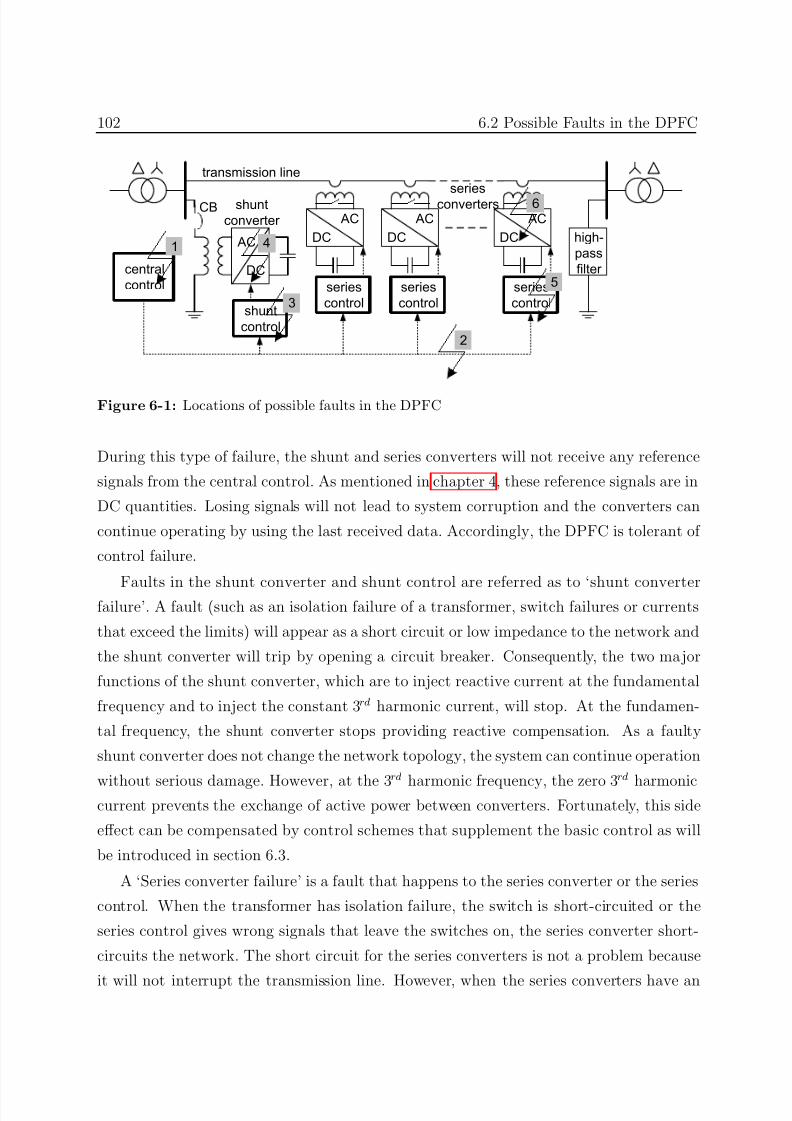
7/25/2019 Dpfc Thesis
http://slidepdf.com/reader/full/dpfc-thesis 124/212
102 6.2 Possible Faults in the DPFC
AC
DC
transmission line
AC
DC
AC
DC
AC
DC hgh-
pass
filter
snt
onerter
seres
onerters
snt
ontrol
seres
ontrol
seres
ontrol
seres
ontrol
entral
ontrol
1
2
3
4
5
6CB
Figure 6-1: Locations of possible faults in the DPFC
During this type of failure, the shunt and series converters will not receive any reference
signals from the central control. As mentioned in chapter 4, these reference signals are in
DC quantities. Losing signals will not lead to system corruption and the converters can
continue operating by using the last received data. Accordingly, the DPFC is tolerant of
control failure.
Faults in the shunt converter and shunt control are referred as to ‘shunt converterfailure’. A fault (such as an isolation failure of a transformer, switch failures or currents
that exceed the limits) will appear as a short circuit or low impedance to the network and
the shunt converter will trip by opening a circuit breaker. Consequently, the two major
functions of the shunt converter, which are to inject reactive current at the fundamental
frequency and to inject the constant 3rd harmonic current, will stop. At the fundamen-
tal frequency, the shunt converter stops providing reactive compensation. As a faulty
shunt converter does not change the network topology, the system can continue operation
without serious damage. However, at the 3rd
harmonic frequency, the zero 3rd
harmoniccurrent prevents the exchange of active power between converters. Fortunately, this side
effect can be compensated by control schemes that supplement the basic control as will
be introduced in section 6.3.
A ‘Series converter failure’ is a fault that happens to the series converter or the series
control. When the transformer has isolation failure, the switch is short-circuited or the
series control gives wrong signals that leave the switches on, the series converter short-
circuits the network. The short circuit for the series converters is not a problem because
it will not interrupt the transmission line. However, when the series converters have an
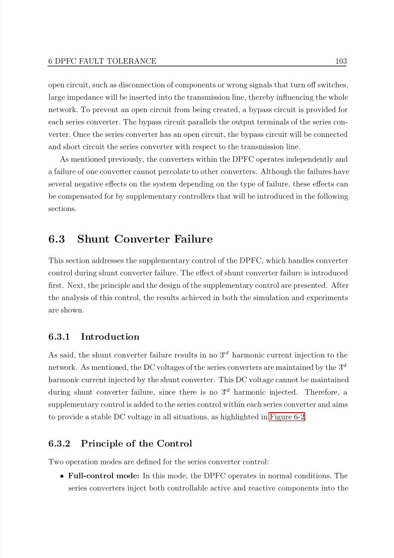
7/25/2019 Dpfc Thesis
http://slidepdf.com/reader/full/dpfc-thesis 125/212
6 DPFC FAULT TOLERANCE 103
open circuit, such as disconnection of components or wrong signals that turn off switches,
large impedance will be inserted into the transmission line, thereby influencing the wholenetwork. To prevent an open circuit from being created, a bypass circuit is provided for
each series converter. The bypass circuit parallels the output terminals of the series con-
verter. Once the series converter has an open circuit, the bypass circuit will be connected
and short circuit the series converter with respect to the transmission line.
As mentioned previously, the converters within the DPFC operates independently and
a failure of one converter cannot percolate to other converters. Although the failures have
several negative effects on the system depending on the type of failure, these effects can
be compensated for by supplementary controllers that will be introduced in the followingsections.
6.3 Shunt Converter Failure
This section addresses the supplementary control of the DPFC, which handles converter
control during shunt converter failure. The effect of shunt converter failure is introduced
first. Next, the principle and the design of the supplementary control are presented. After
the analysis of this control, the results achieved in both the simulation and experiments
are shown.
6.3.1 Introduction
As said, the shunt converter failure results in no 3rd harmonic current injection to the
network. As mentioned, the DC voltages of the series converters are maintained by the 3rd
harmonic current injected by the shunt converter. This DC voltage cannot be maintained
during shunt converter failure, since there is no 3rd harmonic injected. Therefore, asupplementary control is added to the series control within each series converter and aims
to provide a stable DC voltage in all situations, as highlighted in Figure 6-2.
6.3.2 Principle of the Control
Two operation modes are defined for the series converter control:
• Full-control mode: In this mode, the DPFC operates in normal conditions. The
series converters inject both controllable active and reactive components into the
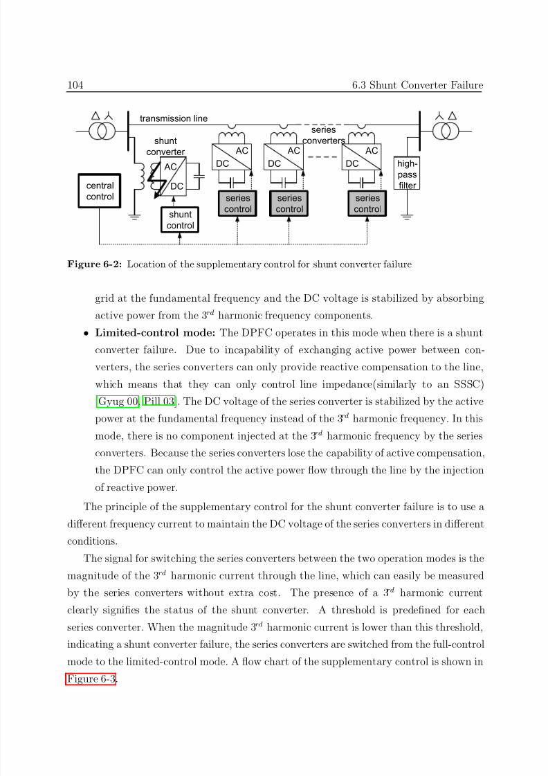
7/25/2019 Dpfc Thesis
http://slidepdf.com/reader/full/dpfc-thesis 126/212
104 6.3 Shunt Converter Failure
AC
DC
transmission line
AC
DC
AC
DC
AC
DC hgh-
pass
filter
snt
onerter
seres
onerters
snt
ontrol
seres
ontrol
seres
ontrol
seres
ontrol
entral
ontrol
Figure 6-2: Location of the supplementary control for shunt converter failure
grid at the fundamental frequency and the DC voltage is stabilized by absorbing
active power from the 3rd harmonic frequency components.
• Limited-control mode: The DPFC operates in this mode when there is a shunt
converter failure. Due to incapability of exchanging active power between con-
verters, the series converters can only provide reactive compensation to the line,
which means that they can only control line impedance(similarly to an SSSC)
[Gyug 00, Pill 03]. The DC voltage of the series converter is stabilized by the active
power at the fundamental frequency instead of the 3rd harmonic frequency. In this
mode, there is no component injected at the 3rd harmonic frequency by the series
converters. Because the series converters lose the capability of active compensation,
the DPFC can only control the active power flow through the line by the injection
of reactive power.
The principle of the supplementary control for the shunt converter failure is to use a
different frequency current to maintain the DC voltage of the series converters in different
conditions.The signal for switching the series converters between the two operation modes is the
magnitude of the 3rd harmonic current through the line, which can easily be measured
by the series converters without extra cost. The presence of a 3rd harmonic current
clearly signifies the status of the shunt converter. A threshold is predefined for each
series converter. When the magnitude 3rd harmonic current is lower than this threshold,
indicating a shunt converter failure, the series converters are switched from the full-control
mode to the limited-control mode. A flow chart of the supplementary control is shown in
Figure 6-3.
7/25/2019 Dpfc Thesis
http://slidepdf.com/reader/full/dpfc-thesis 127/212
6 DPFC FAULT TOLERANCE 105
measurement
3| | threshold I ≤
3| | I
full-control
mode
limited-
control mode
YESNO
Figure 6-3: Flow chart of the adapted shunt converter control
To enable the DPFC to switch between the two operation-modes, two controllers
should be adapted, namely the series control and the central control. For the series
control, the supplementary scheme should be able to use the components at different
frequencies to maintain the DC voltage of the series converter according to the operation
mode. For the central control, certain adaption is required due to the loss of the capability
of series active compensation.
Series control adaption
The supplementary scheme is implemented in the DSP control of each series converter.
In principle, two DC voltage control loops are required to enable the series converter to
operate in the two modes. In the full-control mode, the DC control loop that uses the 3rd
harmonic components is active and in the limited-control mode, the loop that uses the
fundamental frequency components is active. This solution increases the computational
effort required from the DSP because two loops need to be processed simultaneously
although only one loop is active. To reduce computation, a control scheme with only oneDC control loop is proposed and its structure is shown in Figure 6-4.
The control scheme for the series converter with the supplementary control is adapted
from the series control presented in chapter 4. As shown, there is only one DC control
within the series control at the left lower corner of Figure 6-4. Two signal selectors are
employed to route the output of the DC control to either the inverse Park’s transformation
block that generates V se,1,d,ref or the block that generates V se,3,d,ref .
In the full-control mode, the active component V se,1,d,ref is obtained from the signal
that is supplied by the central control. In the limited-control mode, this signal is obtained
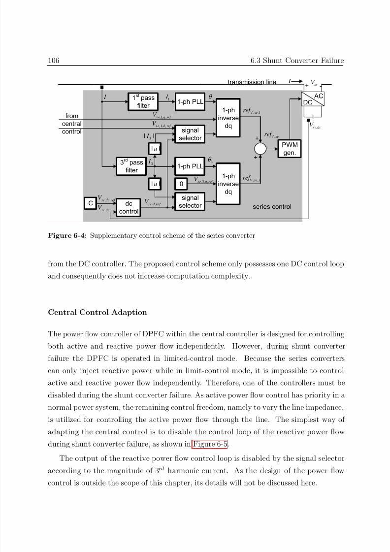
7/25/2019 Dpfc Thesis
http://slidepdf.com/reader/full/dpfc-thesis 128/212
106 6.3 Shunt Converter Failure
3rd
pass
filter
dc
control
1-ph
inverse
dq
0
PWM
gen.
ACDC
+ -seV
,V seref
,se dcV
transmission line
, ,1V seref
3θ
3 I
, 3, ,s e q r ef V
, ,se dc ref V
, ,3V seref
C
I
from
central
control+
+
,se dcV series control
, ,se d ref V
I
1-ph PLL1st passfilter
1-ph
inverse
dq
1θ 1 I
,1, ,s e q ref V
,1, ,s e d ref V signal
selector
| |u
signal
selector
1-ph PLL
3| | I
| |u
Figure 6-4: Supplementary control scheme of the series converter
from the DC controller. The proposed control scheme only possesses one DC control loop
and consequently does not increase computation complexity.
Central Control Adaption
The power flow controller of DPFC within the central controller is designed for controlling
both active and reactive power flow independently. However, during shunt converter
failure the DPFC is operated in limited-control mode. Because the series converters
can only inject reactive power while in limit-control mode, it is impossible to control
active and reactive power flow independently. Therefore, one of the controllers must bedisabled during the shunt converter failure. As active power flow control has priority in a
normal power system, the remaining control freedom, namely to vary the line impedance,
is utilized for controlling the active power flow through the line. The simplest way of
adapting the central control is to disable the control loop of the reactive power flow
during shunt converter failure, as shown in Figure 6-5.
The output of the reactive power flow control loop is disabled by the signal selector
according to the magnitude of 3rd harmonic current. As the design of the power flow
control is outside the scope of this chapter, its details will not be discussed here.
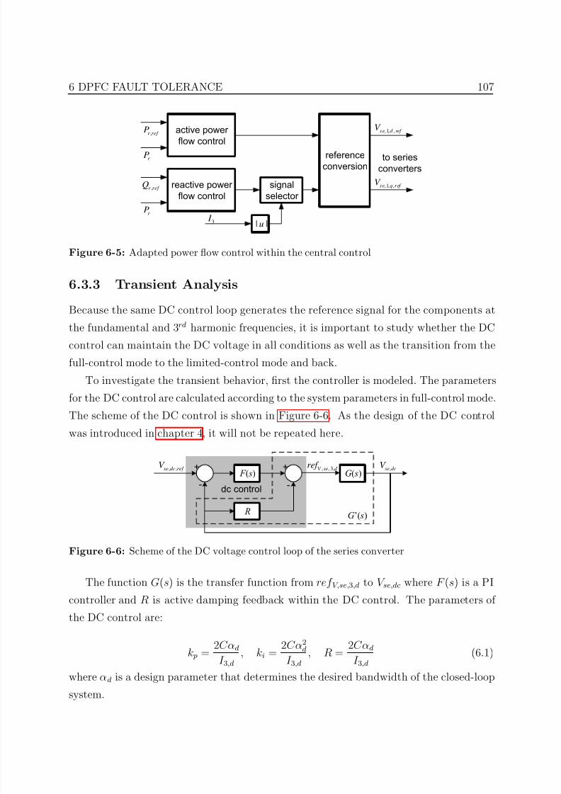
7/25/2019 Dpfc Thesis
http://slidepdf.com/reader/full/dpfc-thesis 129/212
6 DPFC FAULT TOLERANCE 107
active power
flow control
reactive power
flow control
signal
selector
reference
conversion
| |u
,r ref P
r P
,r ref Q
r P
3 I
,1, ,s e q r ef V
,1, ,s e d ref V
to series
converters
Figure 6-5: Adapted power flow control within the central control
6.3.3 Transient Analysis
Because the same DC control loop generates the reference signal for the components at
the fundamental and 3rd harmonic frequencies, it is important to study whether the DC
control can maintain the DC voltage in all conditions as well as the transition from the
full-control mode to the limited-control mode and back.
To investigate the transient behavior, first the controller is modeled. The parameters
for the DC control are calculated according to the system parameters in full-control mode.
The scheme of the DC control is shown in Figure 6-6. As the design of the DC controlwas introduced in chapter 4, it will not be repeated here.
F ( s)
R
+
-
+
-
G( s), , 3,V se d
ref ,se dcV
, ,se dc ref V
G’( s)
dc control
Figure 6-6: Scheme of the DC voltage control loop of the series converter
The function G(s) is the transfer function from ref V,se,3,d to V se,dc where F (s) is a PI
controller and R is active damping feedback within the DC control. The parameters of
the DC control are:
k p = 2Cαd
I 3,d
, ki = 2Cα2
d
I 3,d
, R = 2Cαd
I 3,d
(6.1)
where αd is a design parameter that determines the desired bandwidth of the closed-loop
system.
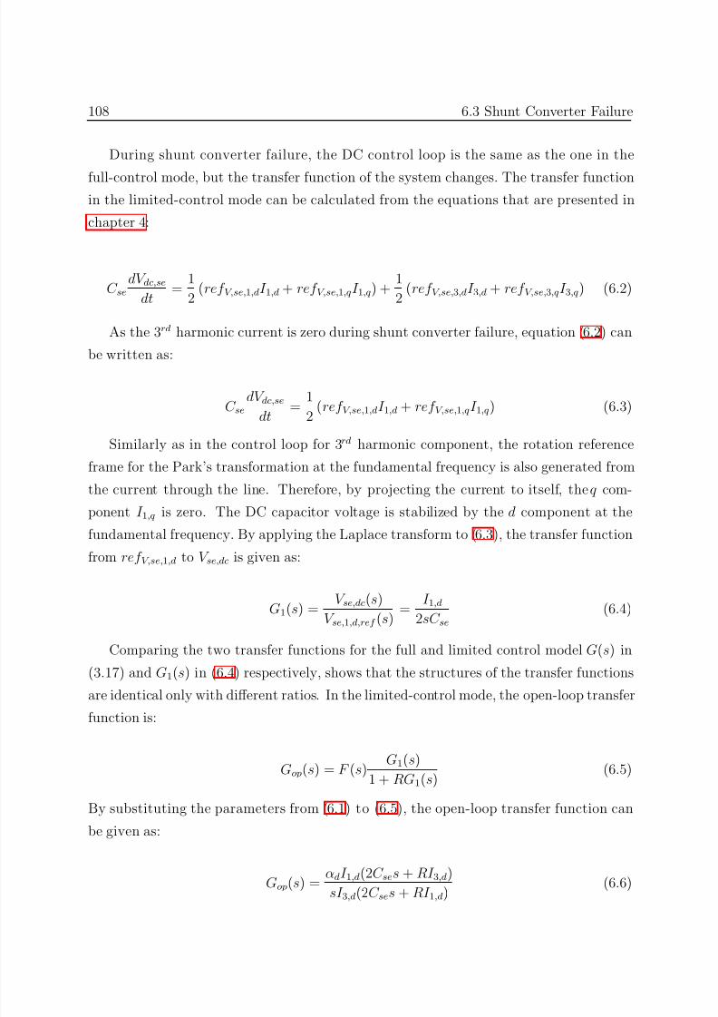
7/25/2019 Dpfc Thesis
http://slidepdf.com/reader/full/dpfc-thesis 130/212
108 6.3 Shunt Converter Failure
During shunt converter failure, the DC control loop is the same as the one in the
full-control mode, but the transfer function of the system changes. The transfer functionin the limited-control mode can be calculated from the equations that are presented in
chapter 4:
C sedV dc,se
dt =
1
2 (ref V,se,1,dI 1,d + ref V,se,1,qI 1,q) +
1
2 (ref V,se,3,dI 3,d + ref V,se,3,qI 3,q) (6.2)
As the 3rd harmonic current is zero during shunt converter failure, equation (6.2) can
be written as:
C sedV dc,se
dt =
1
2 (ref V,se,1,dI 1,d + ref V,se,1,qI 1,q) (6.3)
Similarly as in the control loop for 3rd harmonic component, the rotation reference
frame for the Park’s transformation at the fundamental frequency is also generated from
the current through the line. Therefore, by projecting the current to itself, the q com-
ponent I 1,q is zero. The DC capacitor voltage is stabilized by the d component at the
fundamental frequency. By applying the Laplace transform to (6.3), the transfer functionfrom ref V,se,1,d to V se,dc is given as:
G1(s) = V se,dc(s)
V se,1,d,ref (s) =
I 1,d
2sC se
(6.4)
Comparing the two transfer functions for the full and limited control model G(s) in
(3.17) and G1(s) in (6.4) respectively, shows that the structures of the transfer functions
are identical only with different ratios. In the limited-control mode, the open-loop transfer
function is:
Gop(s) = F (s) G1(s)
1 + RG1(s) (6.5)
By substituting the parameters from (6.1) to (6.5), the open-loop transfer function can
be given as:
Gop
(s) = αdI 1,d(2C ses + RI 3,d)
sI 3,d(2C ses + RI 1,d) (6.6)
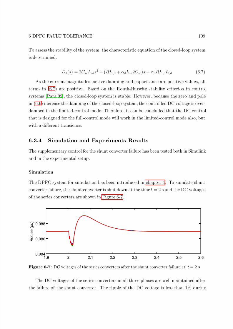
7/25/2019 Dpfc Thesis
http://slidepdf.com/reader/full/dpfc-thesis 131/212
6 DPFC FAULT TOLERANCE 109
To assess the stability of the system, the characteristic equation of the closed-loop system
is determined:
D1(s) = 2C seI 3,ds2 + (RI 1,d + αdI 1,d2C se)s + αdRI 1,dI 3,d (6.7)
As the current magnitudes, active damping and capacitance are positive values, all
terms in (6.7) are positive. Based on the Routh-Hurwitz stability criterion in control
systems [Para 02], the closed-loop system is stable. However, because the zero and pole
in (6.6) increase the damping of the closed-loop system, the controlled DC voltage is over-
damped in the limited-control mode. Therefore, it can be concluded that the DC control
that is designed for the full-control mode will work in the limited-control mode also, but
with a different transience.
6.3.4 Simulation and Experiments Results
The supplementary control for the shunt converter failure has been tested both in Simulink
and in the experimental setup.
Simulation
The DPFC system for simulation has been introduced in chapter 4. To simulate shunt
converter failure, the shunt converter is shut down at the time t = 2 s and the DC voltages
of the series converters are shown in Figure 6-7.
1.9 2 2.1 2.2 2.3 2.4 2.5 2.60.084
0.086
0.088
V d c , s e
( p u )
Figure 6-7: DC voltages of the series converters after the shunt converter failure at t = 2 s
The DC voltages of the series converters in all three phases are well maintained after
the failure of the shunt converter. The ripple of the DC voltage is less than 1% during
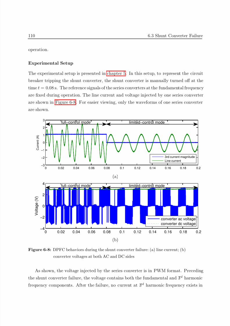
7/25/2019 Dpfc Thesis
http://slidepdf.com/reader/full/dpfc-thesis 132/212
110 6.3 Shunt Converter Failure
operation.
Experimental Setup
The experimental setup is presented in chapter 5. In this setup, to represent the circuit
breaker tripping the shunt converter, the shunt converter is manually turned off at the
time t = 0.08 s. The reference signals of the series converters at the fundamental frequency
are fixed during operation. The line current and voltage injected by one series converter
are shown in Figure 6-8. For easier viewing, only the waveforms of one series converter
are shown.
0 0.02 0.04 0.06 0.08 0.1 0.12 0.14 0.16 0.18 0.2−3
−2
−1
0
1
2
3
C u r r e n t ( A )
3rd current magnitude
Line current
full−control mode limited−control mode
(a)
0 0.02 0.04 0.06 0.08 0.1 0.12 0.14 0.16 0.18 0.2−4
−2
0
2
4
V o l t a g e ( V )
converter ac voltage
converter dc voltage
full−control mode limited−control mode
(b)
Figure 6-8: DPFC behaviors during the shunt converter failure: (a) line current; (b)
converter voltages at both AC and DC sides
As shown, the voltage injected by the series converter is in PWM format. Preceding
the shunt converter failure, the voltage contains both the fundamental and 3rd harmonic
frequency components. After the failure, no current at 3rd harmonic frequency exists in
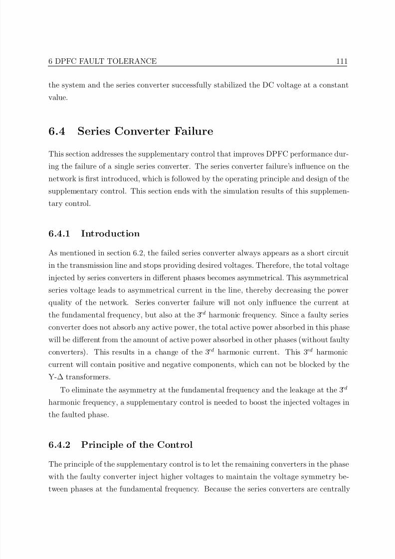
7/25/2019 Dpfc Thesis
http://slidepdf.com/reader/full/dpfc-thesis 133/212
6 DPFC FAULT TOLERANCE 111
the system and the series converter successfully stabilized the DC voltage at a constant
value.
6.4 Series Converter Failure
This section addresses the supplementary control that improves DPFC performance dur-
ing the failure of a single series converter. The series converter failure’s influence on the
network is first introduced, which is followed by the operating principle and design of the
supplementary control. This section ends with the simulation results of this supplemen-
tary control.
6.4.1 Introduction
As mentioned in section 6.2, the failed series converter always appears as a short circuit
in the transmission line and stops providing desired voltages. Therefore, the total voltage
injected by series converters in different phases becomes asymmetrical. This asymmetrical
series voltage leads to asymmetrical current in the line, thereby decreasing the powerquality of the network. Series converter failure will not only influence the current at
the fundamental frequency, but also at the 3rd harmonic frequency. Since a faulty series
converter does not absorb any active power, the total active power absorbed in this phase
will be different from the amount of active power absorbed in other phases (without faulty
converters). This results in a change of the 3rd harmonic current. This 3rd harmonic
current will contain positive and negative components, which can not be blocked by the
Y-∆ transformers.
To eliminate the asymmetry at the fundamental frequency and the leakage at the 3rd
harmonic frequency, a supplementary control is needed to boost the injected voltages in
the faulted phase.
6.4.2 Principle of the Control
The principle of the supplementary control is to let the remaining converters in the phase
with the faulty converter inject higher voltages to maintain the voltage symmetry be-
tween phases at the fundamental frequency. Because the series converters are centrally
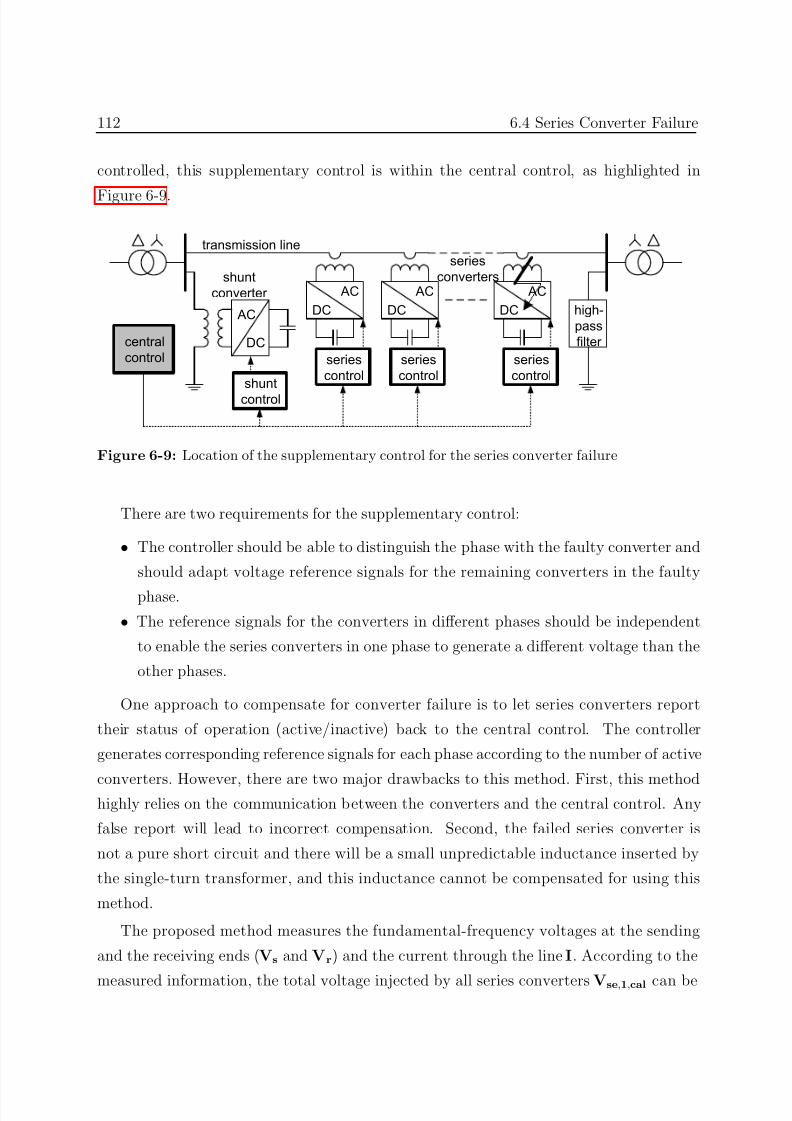
7/25/2019 Dpfc Thesis
http://slidepdf.com/reader/full/dpfc-thesis 134/212
112 6.4 Series Converter Failure
controlled, this supplementary control is within the central control, as highlighted in
Figure 6-9.
AC
DC
transmission line
AC
DC
AC
DC
AC
DC hgh-
pass
filter
snt
onerter
seres
onerters
snt
ontrol
seres
ontrol
seres
ontrol
seres
ontrol
entral
ontrol
Figure 6-9: Location of the supplementary control for the series converter failure
There are two requirements for the supplementary control:
• The controller should be able to distinguish the phase with the faulty converter and
should adapt voltage reference signals for the remaining converters in the faulty
phase.
• The reference signals for the converters in different phases should be independent
to enable the series converters in one phase to generate a different voltage than the
other phases.
One approach to compensate for converter failure is to let series converters report
their status of operation (active/inactive) back to the central control. The controller
generates corresponding reference signals for each phase according to the number of active
converters. However, there are two major drawbacks to this method. First, this methodhighly relies on the communication between the converters and the central control. Any
false report will lead to incorrect compensation. Second, the failed series converter is
not a pure short circuit and there will be a small unpredictable inductance inserted by
the single-turn transformer, and this inductance cannot be compensated for using this
method.
The proposed method measures the fundamental-frequency voltages at the sending
and the receiving ends (Vs and Vr) and the current through the line I. According to the
measured information, the total voltage injected by all series converters Vse,1,cal can be
7/25/2019 Dpfc Thesis
http://slidepdf.com/reader/full/dpfc-thesis 135/212
6 DPFC FAULT TOLERANCE 113
calculated by the following equation:
Vse,1,cal= Vs−Vr−I ·X (6.8)
where X is the line impedance at the fundamental frequency, the voltages and current
are column vectors that consist of the information of three phases. By comparing this
calculated voltage with the total reference voltage generated by the central control, the
operation status of the series converters is known. When the calculated voltage is lower
than the reference in one phase, it indicates one or more faulty converters in that phase.
To compensate for this missing voltage resulted by the faulty converter, a controller is
applied between the central control that gives the total reference voltage and the signal-
transmitting device that sending the reference to each series converter. This controller
generates a modified voltage reference for each series converter according to the calculated
operation status of the series converters. Because the series converters in different phases
are controlled independently, three supplementary controllers are needed, as shown in
Figure 6-10.
seriesvoltage
calculation
faulty converter
compensation
I
rV
sV
f r o m
m e a s u r e m e n t s
faulty converter
compensation
faulty converter
compensation f r o m c
e n t r a l
c o n t r o l
,1, ,s e a calV
,1, ,s e b c alV
,1, ,s e c c alV
,1, ,s e a r ef
V
,1, ,s e b r ef V
,1, ,s e c r ef V
signal
transmitting
to series
converters
,1, , ,s e a r ef a d pV
,1, , ,s e b r ef a d pV
,1, , ,s e c ref a dpV
Figure 6-10: Supplementary control scheme for compensating series converter failures
6.4.3 Compensation Controller Design
The objective of the compensation controller is to generate the adapted reference signal
according to the operation status of series converters. The input signals of the controller
are the reference voltage V se,1,ref and the calculated voltage V se,1,cal. The output signal is
the reference voltage of a single series converter V se,1,ref,adp. Because the reference voltages
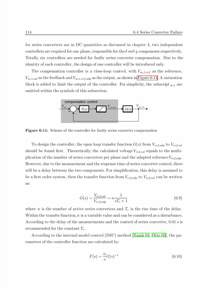
7/25/2019 Dpfc Thesis
http://slidepdf.com/reader/full/dpfc-thesis 136/212
114 6.4 Series Converter Failure
for series converters are in DC quantities as discussed in chapter 4, two independent
controllers are required for one phase, responsible for the d and q components respectively.Totally, six controllers are needed for faulty series converter compensation. Due to the
identity of each controller, the design of one controller will be introduced only.
The compensation controller is a close-loop control, with V se,1,ref as the reference,
V se,1,cal as the feedback and V se,1,ref,adp as the output, as shown in Figure 6-11. A saturation
block is added to limit the output of the controller. For simplicity, the subscript se,1 are
omitted within the symbols of this subsection.
G( s) F ( s)+
-
compensation controlref
V ,ref calV
,ref adpV
Figure 6-11: Scheme of the controller for faulty series converter compensation
To design the controller, the open loop transfer function G(s) from V ref,adp to V ref,cal
should be found first. Theoretically, the calculated voltage V ref,cal equals to the multi-
plication of the number of series converters per phase and the adapted reference V ref,adp.
However, due to the measurement and the response time of series converter control, there
will be a delay between the two components. For simplification, this delay is assumed to
be a first order system, then the transfer function from V ref,adp to V ref,cal can be written
as:
G(s) = V ref,cal
V ref,adp= n
1
sT r + 1 (6.9)
where n is the number of active series converters and T r is the rise time of the delay.
Within the transfer function, n is a variable value and can be considered as a disturbance.
According to the delay of the measurements and the control of series converter, 0.01 s is
recommended for the constant T r.
According to the internal model control (IMC) method [Namh 01, Otte 03], the pa-
rameters of the controller function are calculated by:
F (s) =
α
s G(s)−1
(6.10)
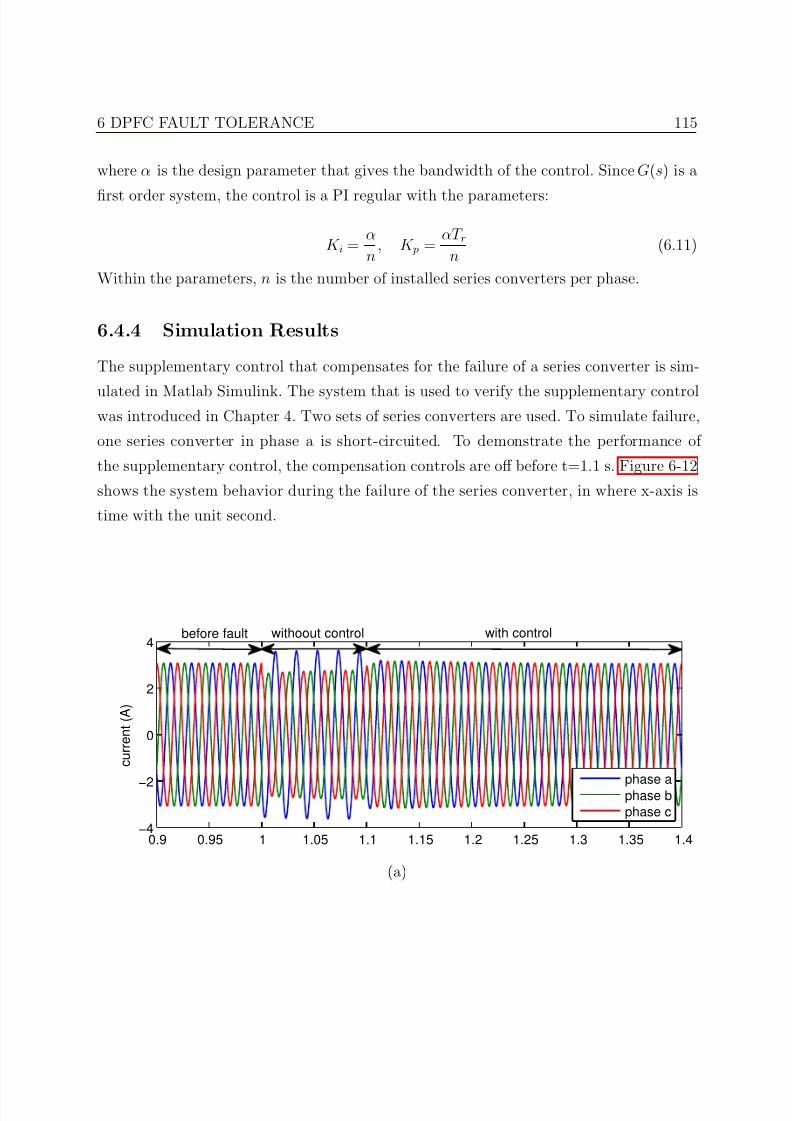
7/25/2019 Dpfc Thesis
http://slidepdf.com/reader/full/dpfc-thesis 137/212
6 DPFC FAULT TOLERANCE 115
where α is the design parameter that gives the bandwidth of the control. Since G(s) is a
first order system, the control is a PI regular with the parameters:
K i = α
n, K p =
αT rn
(6.11)
Within the parameters, n is the number of installed series converters per phase.
6.4.4 Simulation Results
The supplementary control that compensates for the failure of a series converter is sim-
ulated in Matlab Simulink. The system that is used to verify the supplementary controlwas introduced in Chapter 4. Two sets of series converters are used. To simulate failure,
one series converter in phase a is short-circuited. To demonstrate the performance of
the supplementary control, the compensation controls are off before t=1.1 s. Figure 6-12
shows the system behavior during the failure of the series converter, in where x-axis is
time with the unit second.
0.9 0.95 1 1.05 1.1 1.15 1.2 1.25 1.3 1.35 1.4−4
−2
0
2
4
c u r r e n t ( A )
phase aphase b
phase c
with controlwithoout controlbefore fault
(a)
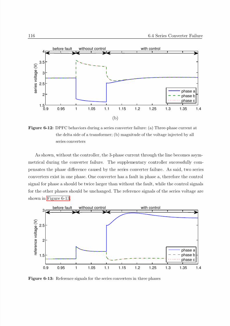
7/25/2019 Dpfc Thesis
http://slidepdf.com/reader/full/dpfc-thesis 138/212
116 6.4 Series Converter Failure
0.9 0.95 1 1.05 1.1 1.15 1.2 1.25 1.3 1.35 1.41.5
2
2.5
3
3.5
4
s e r i e s v o l t a g e ( V )
phase a
phase b
phase c
with controlwithoout controlbefore fault
(b)
Figure 6-12: DPFC behaviors during a series converter failure: (a) Three-phase current at
the delta side of a transformer; (b) magnitude of the voltage injected by all
series converters
As shown, without the controller, the 3-phase current through the line becomes asym-
metrical during the converter failure. The supplementary controller successfully com-
pensates the phase difference caused by the series converter failure. As said, two seriesconverters exist in one phase. One converter has a fault in phase a, therefore the control
signal for phase a should be twice larger than without the fault, while the control signals
for the other phases should be unchanged. The reference signals of the series voltage are
shown in Figure 6-13.
0.9 0.95 1 1.05 1.1 1.15 1.2 1.25 1.3 1.35 1.4
1.5
2
2.5
3
r e f e r e n c e v o l t a g e ( V )
phase a
phase b
phase c
with controlwithoout controlbefore fault
Figure 6-13: Reference signals for the series converters in three phases
7/25/2019 Dpfc Thesis
http://slidepdf.com/reader/full/dpfc-thesis 139/212
6 DPFC FAULT TOLERANCE 117
6.5 Conclusions
In this chapter, the DPFC’s operation during a failure is considered. It shows that the
DPFC is tolerant of control failure, shunt converter failure and series converter failure.
Two supplementary controllers are presented, used to compensate during shunt converter
and series converter failures.
For the shunt converter failure, the supplementary control is applied to each of the
series converters. This control automatically switches the series converters between the
full-control mode and the limited-control mode, according to the magnitude of the 3 rd
harmonic current. When the magnitude is lower than a threshold defined for this pur-pose, the series converters are switched to the limited-control mode that uses the active
component at the fundamental frequency to stabilize their DC voltages. Both a simulation
and practical experiment are done to verify the supplementary control and to prove that
the adapted control can successfully switch the DPFC between the two control modes,
thereby increasing the whole DPFC system reliability.
The series converters have over-voltage protection at the secondary side of the single-
turn transformer. When the series converter has a fault, the failed series converter appears
short-circuit to the transmission line and the voltage injected by all the series convertersbecomes asymmetrical. To improve the DPFC performance during the series converter
failure, a supplementary control scheme is added at the DPFC central control. The control
scheme has been simulated in Matlab and it proved that the asymmetry caused by the
failure could be compensated completely.

7/25/2019 Dpfc Thesis
http://slidepdf.com/reader/full/dpfc-thesis 140/212
7/25/2019 Dpfc Thesis
http://slidepdf.com/reader/full/dpfc-thesis 141/212
Chapter 7DPFC AUXILIARY SERVICES
7.1 Introduction
IN previous chapters, the control of the DPFC was presented. According to the control
objects, the DPFC control can be distinguished as the control at device level and
at system level. The control at the device level aims to maintain the capacitor DC
voltage of each converter. It also ensures that the DPFC generates the series voltages
and shunt reactive current, at the fundamental frequency, that is required by the system
operator. Consequently, the control at device level consists of the following controls that
were presented earlier:
• Shunt control (in chapter 4)
• Series control (in chapter 4)
• Supplementary controls that ensure the DPFC to keep operating during converter
failures (in chapter 6)
The control that is to use the DPFC for the network applications can be consideredthe control at system level. Such controls generate reference signals for the converters
of the DPFC and are normally on the central control side. The control at system level
discussed previously is:
• Power flow control
Because the DPFC can simultaneously adjust multiple network parameters, namely
the line impedance, the transmission angle and the bus voltage, it implies a great potential
of the DPFC for more auxiliary services at system level. In this chapter two auxiliary
services are discussed; they utilize the DPFC to damp low frequency power oscillation
119
7/25/2019 Dpfc Thesis
http://slidepdf.com/reader/full/dpfc-thesis 142/212
120 7.2 Power Oscillation Damping (POD)
and compensate for asymmetrical components.
7.2 Power Oscillation Damping (POD)
In this section, the DPFC application of low frequency power oscillation damping is
introduced. The section begins by describing the background of the power oscillation and
continues with the modeling of the DPFC that is used for POD controller design (based
on the so-called current injection model). Next, the parameters of the POD controller are
designed using the Residue method [Ghai 05] and finally a case study of using DPFC for
POD is presented.
7.2.1 Background
In the current power industry, networks tend to be interconnected to allow the use of a
market-oriented business model and improve system stability. However, the capability
of long, inter-regional power transmission is usually limited and one of its limitations is
caused by low-frequency power oscillations. Damping these oscillations is a prerequisite
for secure system operation because an undamped oscillation can lead to a blackout of the power network.
One type of oscillation, known as ‘local mode’, is associated with a single generator or
a very closely connected group of units at a generating plant. Local modes normally have
frequencies in the range of 0.7 to 2.0 Hz [Klei 91]. The characteristics of these oscillations
are well understood and can be damped by the use of Power System Stabilizers (PSSs)
in generator excitation control systems [Roge 00a]. The principle of PSS is to increase
the damping of the oscillation mode by regulating the voltage of the excitation system
of a synchronous generator, to generate an electrical damping torque that counters theoscillation [Pal 05].
Oscillations, which are observed when a group of generators in one region swings
against the group in another region [Kund 94], are known as ‘inter-area modes’. Inter-
area modes have frequencies in the range of 0.1 to 0.8 Hz. Because PSSs are usually
designed for local oscillation damping, they are not effective in damping inter-area modes.
However, recent research has proven FACTS devices can be used for inter-area power
oscillation damping (POD) [Cai 05, Mhas 06, Sadi 05]. Similar to PSSs, the principle
of using FACTS devices for POD is to vary one or multiple parameters of the network
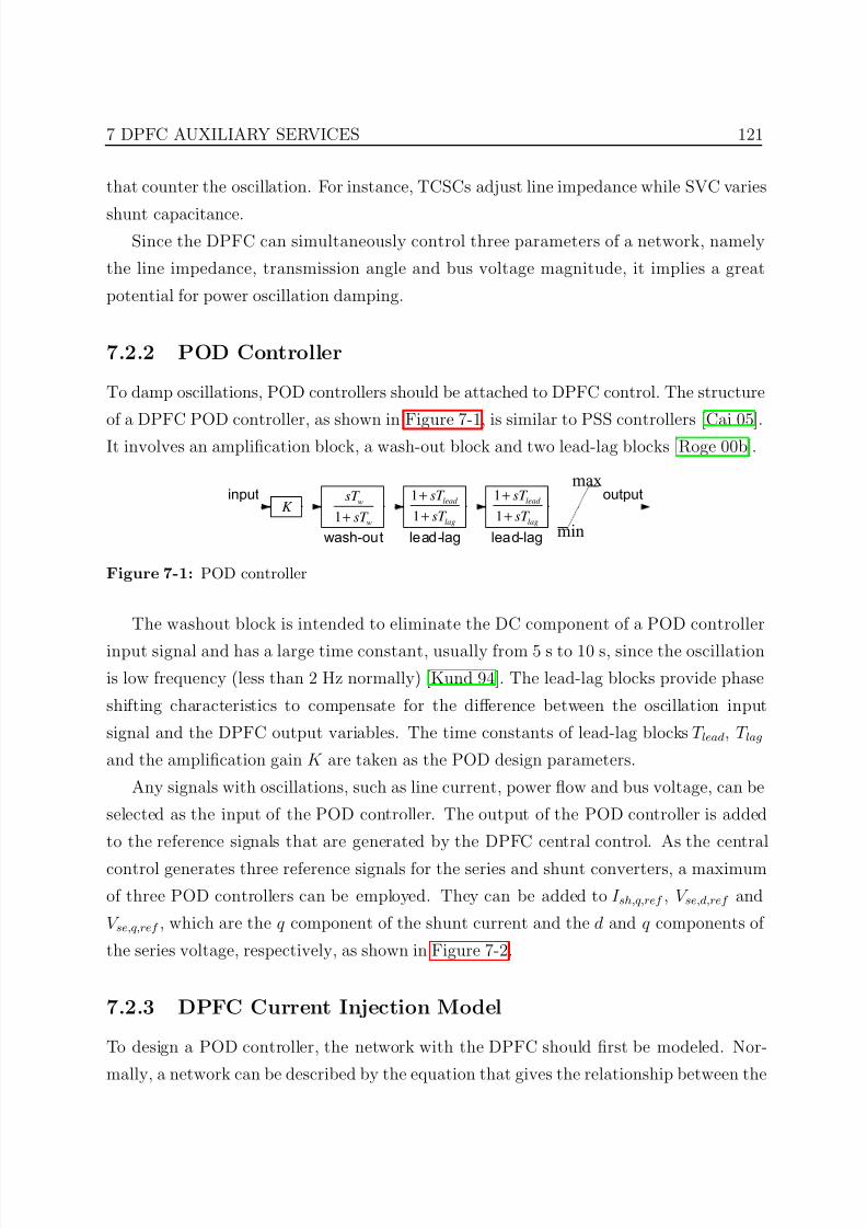
7/25/2019 Dpfc Thesis
http://slidepdf.com/reader/full/dpfc-thesis 143/212
7 DPFC AUXILIARY SERVICES 121
that counter the oscillation. For instance, TCSCs adjust line impedance while SVC varies
shunt capacitance.Since the DPFC can simultaneously control three parameters of a network, namely
the line impedance, transmission angle and bus voltage magnitude, it implies a great
potential for power oscillation damping.
7.2.2 POD Controller
To damp oscillations, POD controllers should be attached to DPFC control. The structure
of a DPFC POD controller, as shown in Figure 7-1, is similar to PSS controllers [Cai 05].
It involves an amplification block, a wash-out block and two lead-lag blocks [Roge 00b].
K 1
w
w
sT
sT +
1
1
lead
lag
sT
sT
+
+
1
1
lead
lag
sT
sT
+
+
max
min
input
wash-out lead-lag lead-lag
output
Figure 7-1: POD controller
The washout block is intended to eliminate the DC component of a POD controller
input signal and has a large time constant, usually from 5 s to 10 s, since the oscillation
is low frequency (less than 2 Hz normally) [Kund 94]. The lead-lag blocks provide phase
shifting characteristics to compensate for the difference between the oscillation input
signal and the DPFC output variables. The time constants of lead-lag blocks T lead, T lag
and the amplification gain K are taken as the POD design parameters.
Any signals with oscillations, such as line current, power flow and bus voltage, can be
selected as the input of the POD controller. The output of the POD controller is added
to the reference signals that are generated by the DPFC central control. As the central
control generates three reference signals for the series and shunt converters, a maximum
of three POD controllers can be employed. They can be added to I sh,q,ref , V se,d,ref and
V se,q,ref , which are the q component of the shunt current and the d and q components of
the series voltage, respectively, as shown in Figure 7-2.
7.2.3 DPFC Current Injection Model
To design a POD controller, the network with the DPFC should first be modeled. Nor-
mally, a network can be described by the equation that gives the relationship between the
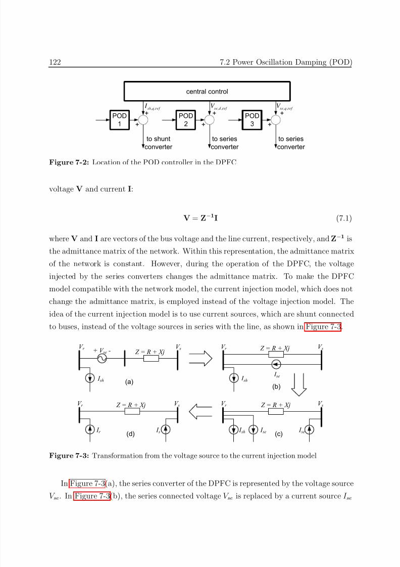
7/25/2019 Dpfc Thesis
http://slidepdf.com/reader/full/dpfc-thesis 144/212
122 7.2 Power Oscillation Damping (POD)
central control
POD
1
+POD
2
POD
3
, ,se q ref V
, ,se d ref V
, ,sh q ref I
+ +
++
+
to shunt
converter
to series
converter
to series
converter
Figure 7-2: Location of the POD controller in the DPFC
voltage V and current I:
V = Z−1I (7.1)
where V and I are vectors of the bus voltage and the line current, respectively, and Z−1 is
the admittance matrix of the network. Within this representation, the admittance matrix
of the network is constant. However, during the operation of the DPFC, the voltage
injected by the series converters changes the admittance matrix. To make the DPFC
model compatible with the network model, the current injection model, which does not
change the admittance matrix, is employed instead of the voltage injection model. The
idea of the current injection model is to use current sources, which are shunt connected
to buses, instead of the voltage sources in series with the line, as shown in Figure 7-3.
+ V se -
I sh
Z = R + XjV r V s
I sh
Z = R + XjV r V s
I se
I r
Z = R + XjV r V s
I s I sh
Z = R + XjV r V s
I se I se
(a)(b)
(c)(d)
Figure 7-3: Transformation from the voltage source to the current injection model
In Figure 7-3(a), the series converter of the DPFC is represented by the voltage source
V se. In Figure 7-3(b), the series connected voltage V se is replaced by a current source I se
7/25/2019 Dpfc Thesis
http://slidepdf.com/reader/full/dpfc-thesis 145/212
7 DPFC AUXILIARY SERVICES 123
in parallel with the transmission line. The current is given as:
I se = V se
Z (7.2)
By replacing the parallel current source I se by two shunt connected current sources
in Figure 7-3(c), the current injection model of the DPFC is achieved as shown in
Figure 7-3(d), where:
I r = −I sh − I se, I s = I se (7.3)
Since the currents injected into buses can be treated as loads, the DPFC current
injection model will not change the network admittance matrix.
7.2.4 DPFC POD Controller Design
The purpose of the POD controller design is to find the parameters K , T lead and T lag.
The process consists of the following steps.
Oscillatory modes
The first step in designing a POD controller is to identify the oscillatory modes. To do so,
the power system with the DPFC is represented in state-space format that is linearized
around the operation point [Kund 94]:
∆x = A∆x + B∆u
∆y = C∆x(7.4)
where A is the state matrix, ∆x is the state vector, ∆u is a single input, ∆y is a single
output, C is a row vector and B is a column vector. To find the oscillation mode, it
depends on the eigenvalues analysis of the system state matrix A. Let λi = σi + jωi be
the ith eigenvalue of the state matrix A. The real part of the eigenvalue gives the damping
and the imaginary part gives the angular velocity of the oscillation. The relative damping
ratio is given by:
ζ i = −σ√
σ2 + ω2(7.5)
The eigenvalues which have a damping ratio of less than 3% are considered the critical
oscillatory modes [Sadi 06].
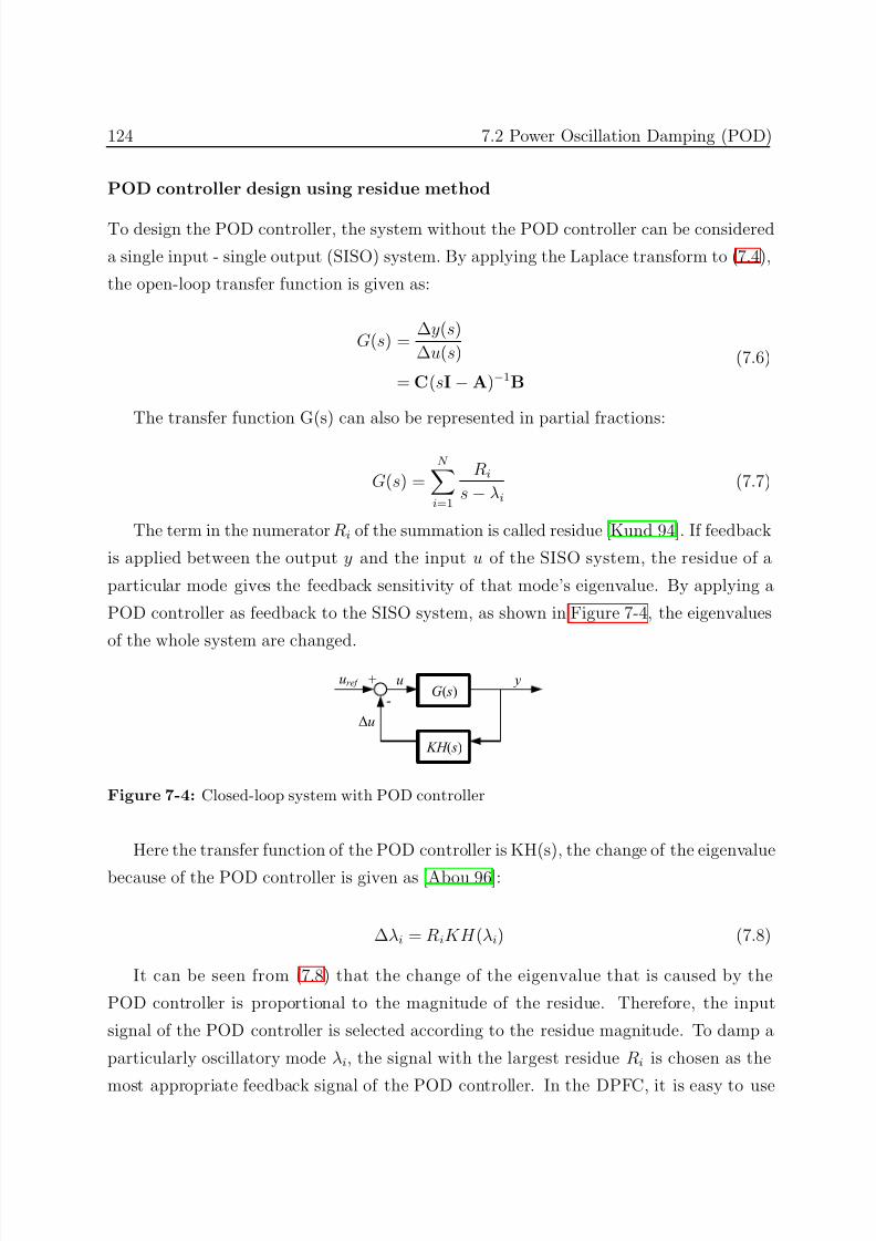
7/25/2019 Dpfc Thesis
http://slidepdf.com/reader/full/dpfc-thesis 146/212
124 7.2 Power Oscillation Damping (POD)
POD controller design using residue method
To design the POD controller, the system without the POD controller can be considered
a single input - single output (SISO) system. By applying the Laplace transform to ( 7.4),
the open-loop transfer function is given as:
G(s) = ∆y(s)
∆u(s)
= C(sI − A)−1B
(7.6)
The transfer function G(s) can also be represented in partial fractions:
G(s) =N
i=1
Ri
s − λi(7.7)
The term in the numerator Ri of the summation is called residue [Kund 94]. If feedback
is applied between the output y and the input u of the SISO system, the residue of a
particular mode gives the feedback sensitivity of that mode’s eigenvalue. By applying a
POD controller as feedback to the SISO system, as shown in Figure 7-4, the eigenvalues
of the whole system are changed.
G( s)
KH ( s)
+
-
uref y
∆u
u
Figure 7-4: Closed-loop system with POD controller
Here the transfer function of the POD controller is KH(s), the change of the eigenvalue
because of the POD controller is given as [Abou 96]:
∆λi = RiKH (λi) (7.8)
It can be seen from (7.8) that the change of the eigenvalue that is caused by the
POD controller is proportional to the magnitude of the residue. Therefore, the input
signal of the POD controller is selected according to the residue magnitude. To damp a
particularly oscillatory mode λi, the signal with the largest residue Ri is chosen as the
most appropriate feedback signal of the POD controller. In the DPFC, it is easy to use
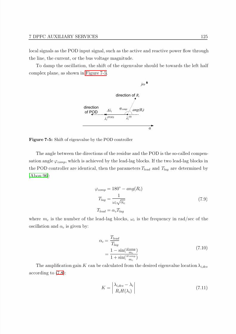
7/25/2019 Dpfc Thesis
http://slidepdf.com/reader/full/dpfc-thesis 147/212
7 DPFC AUXILIARY SERVICES 125
local signals as the POD input signal, such as the active and reactive power flow through
the line, the current, or the bus voltage magnitude.To damp the oscillation, the shift of the eigenvalue should be towards the left half
complex plane, as shown in Figure 7-5.
σ
jω
direction of Ri
ang(Ri )φcomp
λi(0) λi(POD)
direction
of POD ∆λi
Figure 7-5: Shift of eigenvalue by the POD controller
The angle between the directions of the residue and the POD is the so-called compen-
sation angle ϕcomp, which is achieved by the lead-lag blocks. If the two lead-lag blocks in
the POD controller are identical, then the parameters T lead and T lag are determined by
[Abou 96]:
ϕcomp = 180 − ang(Ri)
T lag = 1
ωi√
αc
T lead = αcT lag
(7.9)
where mc is the number of the lead-lag blocks, ωi is the frequency in rad/sec of the
oscillation and αc is given by:
αc = T lead
T lag
=1 − sin( ϕcomp
mc
)
1 + sin( ϕcompmc
)
(7.10)
The amplification gain K can be calculated from the desired eigenvalue location λi,des
according to (7.8):
K = λi,des − λi
RiH (λi) (7.11)
7/25/2019 Dpfc Thesis
http://slidepdf.com/reader/full/dpfc-thesis 148/212
126 7.2 Power Oscillation Damping (POD)
Design procedure of the DPFC POD controller
As described above, there are a maximum of three POD controllers that can be applied in
the DPFC. Since the POD controllers can influence each other, it is not easy to calculate
all three sets of POD parameters at one time by using the residue method. The process
for designing POD controller parameters for a DPFC is described in the following steps:
• Find the most critical eigenvalue of the system as the damping object of the first
POD controller.
• Calculate the residue for the possible POD locations and place the first POD con-
troller at the location with the biggest residue.• Compute the first POD controller parameters.
• Calculate the new eigenvalues of the system with the first POD controller, and find
the most critical one as the second POD controller damping objects.
• Repeat the procedures above to calculate the remaining POD controller parameters
in an iterative process.
7.2.5 Case Study
The POD capability of the DPFC is simulated in a simple two-area system [Kund 94]
shown in Figure 7-6. The system consists of two areas connected by a weak tie and each
area contains two coupled generators. The generators are self-excited by DC exciters and
without PSSs. After the linearization of the system without DPFC, a pair of eigenvalues
is found on a positive plane with an oscillation frequency of approximately 0.4 Hz. The
DPFC series converters are placed at the lines between bus 8 and 9 to control the power
flow through the tie and to damp the oscillation at the same time. Bus 8 is obviously a
suitable location for the shunt converter, because voltage swings are the greatest at bus8.
The placement of only a DPFC without a POD controller causes the unstable eigen-
values to be shifted slightly leftward; however, the eigenvalues are still on the right half of
the plane signifying that the system remains unstable. By increasing the DPFC control
dynamic, the eigenvalue can be further shifted to the left, however the shift is not large.
The critical oscillatory mode is characterized by eigenvalue λ1 = 0.034 + j3.004 with the
damping ratio ζ 1 = −1.12%. It is found that the DPFC control parameter V se,d,ref has
the largest residue R1 = 11.206 and therefore it would be most effective to apply the POD
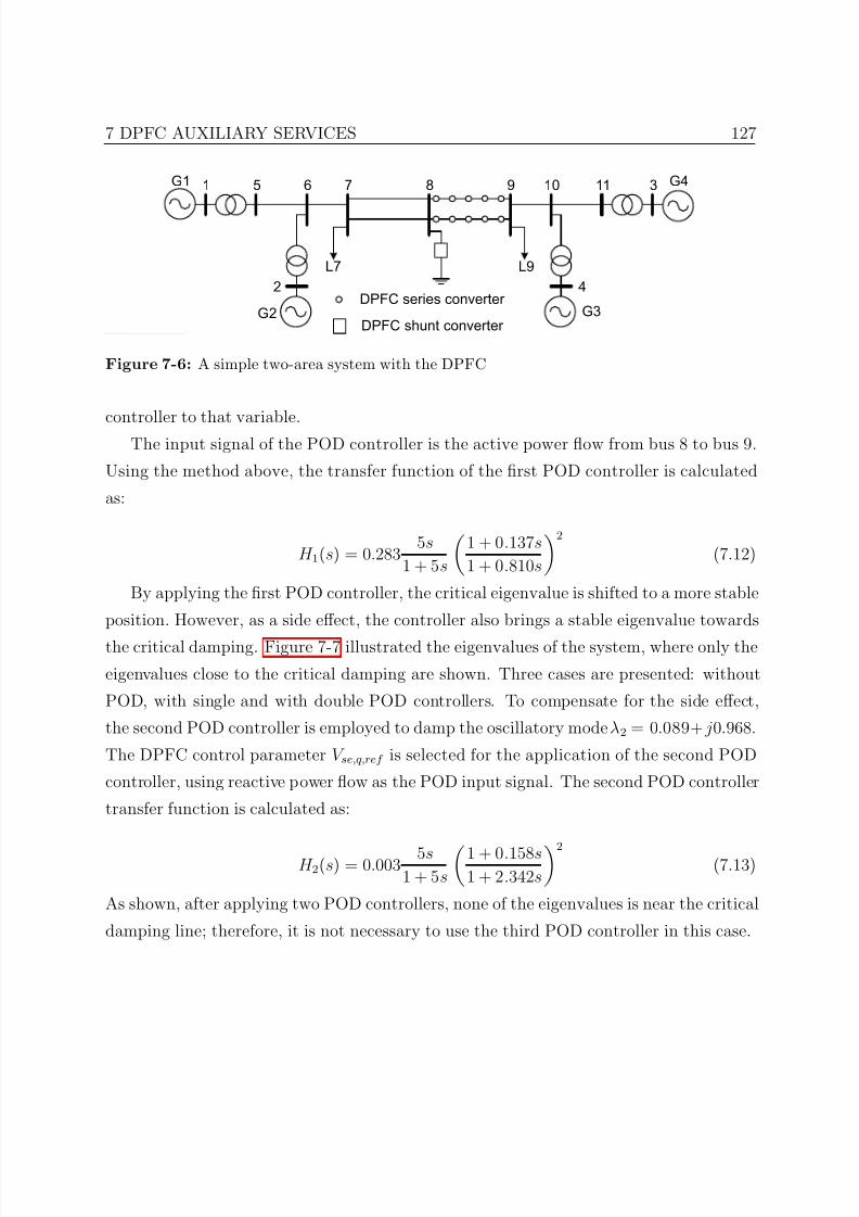
7/25/2019 Dpfc Thesis
http://slidepdf.com/reader/full/dpfc-thesis 149/212
7 DPFC AUXILIARY SERVICES 127
G1
G2 G3
G41
2
3
4
5 6 7 8 9 10 11
L7 L9
DPFC series converter
DPFC shunt converter
Figure 7-6: A simple two-area system with the DPFC
controller to that variable.The input signal of the POD controller is the active power flow from bus 8 to bus 9.
Using the method above, the transfer function of the first POD controller is calculated
as:
H 1(s) = 0.283 5s
1 + 5s
1 + 0.137s
1 + 0.810s
2
(7.12)
By applying the first POD controller, the critical eigenvalue is shifted to a more stable
position. However, as a side effect, the controller also brings a stable eigenvalue towards
the critical damping. Figure 7-7 illustrated the eigenvalues of the system, where only the
eigenvalues close to the critical damping are shown. Three cases are presented: without
POD, with single and with double POD controllers. To compensate for the side effect,
the second POD controller is employed to damp the oscillatory mode λ2 = 0.089+ j0.968.
The DPFC control parameter V se,q,ref is selected for the application of the second POD
controller, using reactive power flow as the POD input signal. The second POD controller
transfer function is calculated as:
H 2(s) = 0.003 5s1 + 5s
1 + 0.158s1 + 2.342s
2
(7.13)
As shown, after applying two POD controllers, none of the eigenvalues is near the critical
damping line; therefore, it is not necessary to use the third POD controller in this case.
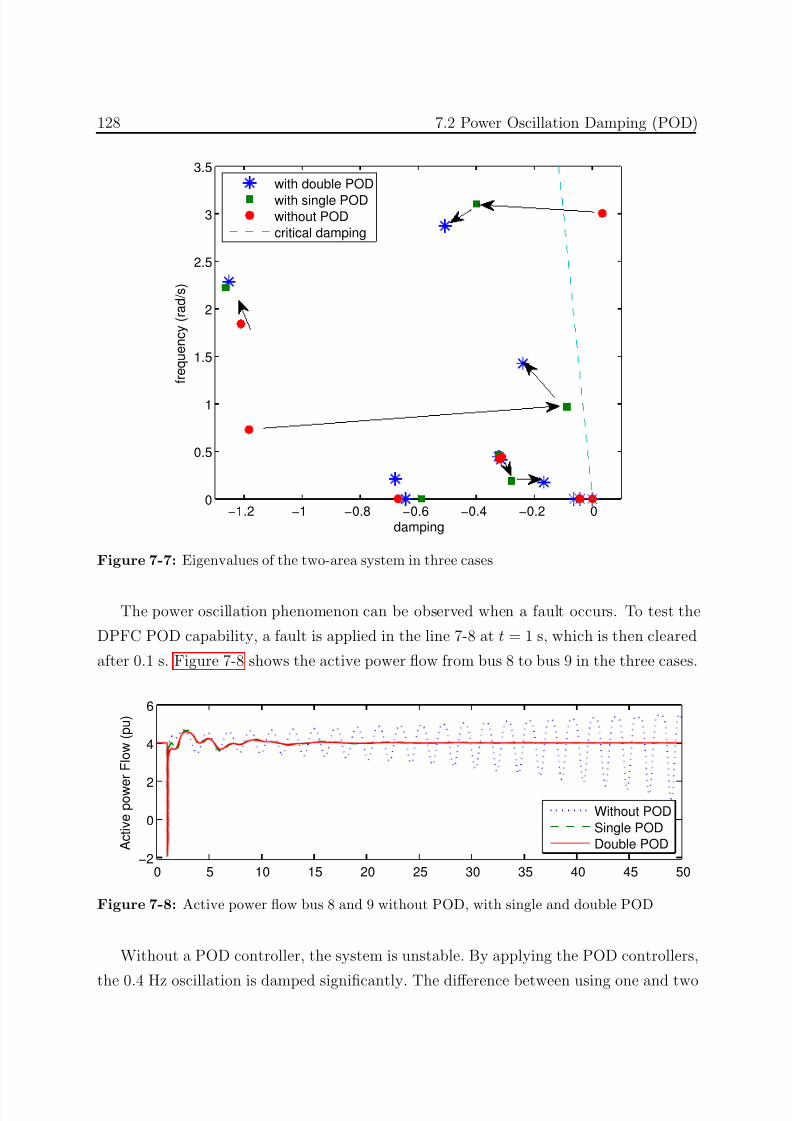
7/25/2019 Dpfc Thesis
http://slidepdf.com/reader/full/dpfc-thesis 150/212
128 7.2 Power Oscillation Damping (POD)
−1.2 −1 −0.8 −0.6 −0.4 −0.2 00
0.5
1
1.5
2
2.5
3
3.5
damping
f r e q u e n c y ( r a d / s )
with double POD
with single PODwithout POD
critical damping
Figure 7-7: Eigenvalues of the two-area system in three cases
The power oscillation phenomenon can be observed when a fault occurs. To test the
DPFC POD capability, a fault is applied in the line 7-8 at t = 1 s, which is then cleared
after 0.1 s. Figure 7-8 shows the active power flow from bus 8 to bus 9 in the three cases.
0 5 10 15 20 25 30 35 40 45 50−2
0
2
4
6
A c t i v e p o w e
r F l o w ( p u )
Without POD
Single POD
Double POD
Figure 7-8: Active power flow bus 8 and 9 without POD, with single and double POD
Without a POD controller, the system is unstable. By applying the POD controllers,
the 0.4 Hz oscillation is damped significantly. The difference between using one and two
7/25/2019 Dpfc Thesis
http://slidepdf.com/reader/full/dpfc-thesis 151/212
7 DPFC AUXILIARY SERVICES 129
POD controllers is not significant in this case because the damping object of the second
POD controller is still under the critical damping line. In this simple two-area system, onlytwo POD controllers are necessary to achieve the required stability. If all three possible
POD controllers are employed, the DPFC can further stabilize a complex system, which
has multiple critical eigenvalues.
7.2.6 Summary
This section studies the capability of the DPFC to damp low frequency power oscillation.
The POD controller parameters are calculated by using the residue method. It is shownthat the DPFC has the capability of damping multiple frequency oscillations at the same
time. Since the DPFC has three degrees of freedoms, the potential for the POD is larger
than other devices, like SVC, TCSC, or SSSC.
7.3 Asymmetrical Component Compensation
This section presents another DPFC auxiliary service at the system level, namely the
compensation of asymmetrical components.
7.3.1 Background
Power Quality is becoming an important issue for both electric utilities and end users
[Duga 03]. Asymmetrical voltages and currents in a network are one of the concerns un-
der the power quality issue. The asymmetry is mainly produced by single phase faults
within the network [Chin 07] or a large amount of single-phase loads. The asymmetrical
voltages can cause extra losses in components of the network, such as generators, motors,transmission lines and transformers [Pedr 05]. Active filters, dynamic voltage restorers
(DVR) and power factor correctors can be used to compensate the asymmetry at the load
side, however their contributions to the transmission system is not large because they are
focused on the load side [Noha 07, Soar 00]. FACTS devices can be employed to compen-
sate the asymmetrical currents and voltages in transmission systems. Unfortunately, it is
found that the capability of most FACTS devices to compensating asymmetry is limited.
Series and shunt FACTS device can only provide compensation of asymmetrical reactive
component [Kuan 07, Nune 01], and the most powerful device, i.e. the UPFC [Gyug 92],
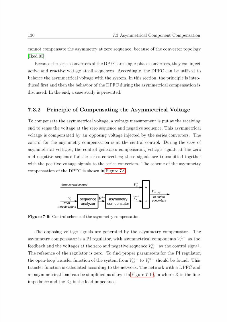
7/25/2019 Dpfc Thesis
http://slidepdf.com/reader/full/dpfc-thesis 152/212
130 7.3 Asymmetrical Component Compensation
cannot compensate the asymmetry at zero sequence, because of the converter topology
[Iked 05].Because the series converters of the DPFC are single-phase converters, they can inject
active and reactive voltage at all sequences. Accordingly, the DPFC can be utilized to
balance the asymmetrical voltage with the system. In this section, the principle is intro-
duced first and then the behavior of the DPFC during the asymmetrical compensation is
discussed. In the end, a case study is presented.
7.3.2 Principle of Compensating the Asymmetrical Voltage
To compensate the asymmetrical voltage, a voltage measurement is put at the receiving
end to sense the voltage at the zero sequence and negative sequence. This asymmetrical
voltage is compensated by an opposing voltage injected by the series converters. The
control for the asymmetry compensation is at the central control. During the case of
asymmetrical voltages, the control generates compensating voltage signals at the zero
and negative sequence for the series converters; these signals are transmitted together
with the positive voltage signals to the series converters. The scheme of the asymmetry
compensation of the DPFC is shown in Figure 7-9.
sequence
analyzer
+
+r
V 0,
r V −
seV +
,0
seV −
,1,s e r ef V
from central control
from
measurement
to series
convertersasymmetry
compensator
Figure 7-9: Control scheme of the asymmetry compensation
The opposing voltage signals are generated by the asymmetry compensator. The
asymmetry compensator is a PI regulator, with asymmetrical components V 0,−r as the
feedback and the voltages at the zero and negative sequence V 0,−se as the control signal.
The reference of the regulator is zero. To find proper parameters for the PI regulator,
the open-loop transfer function of the system from V 0,−se to V 0,−
r should be found. This
transfer function is calculated according to the network. The network with a DPFC and
an asymmetrical load can be simplified as shown in Figure 7-10, in where Z is the line
impedance and the Z L is the load impedance.
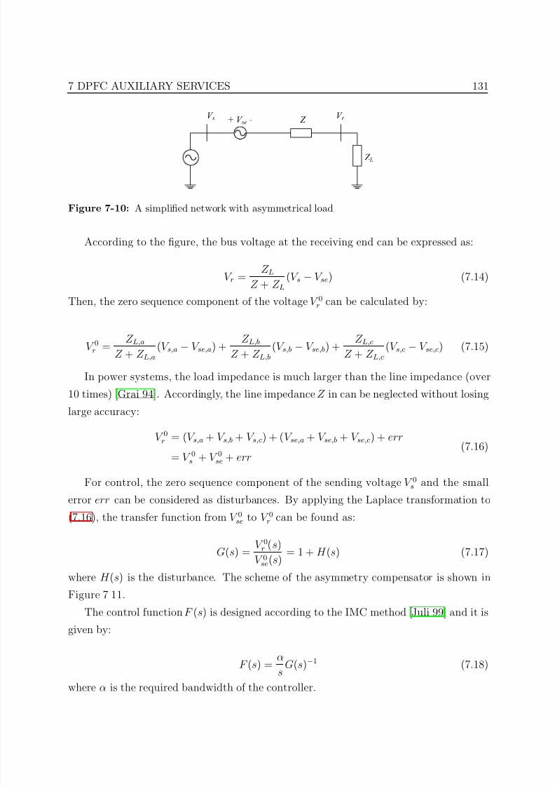
7/25/2019 Dpfc Thesis
http://slidepdf.com/reader/full/dpfc-thesis 153/212
7 DPFC AUXILIARY SERVICES 131
+ V se - Z V r V s
Z L
Figure 7-10: A simplified network with asymmetrical load
According to the figure, the bus voltage at the receiving end can be expressed as:
V r = Z LZ + Z L(V s − V se) (7.14)
Then, the zero sequence component of the voltage V 0r can be calculated by:
V 0r = Z L,a
Z + Z L,a
(V s,a − V se,a) + Z L,b
Z + Z L,b
(V s,b − V se,b) + Z L,c
Z + Z L,c
(V s,c − V se,c) (7.15)
In power systems, the load impedance is much larger than the line impedance (over
10 times) [Grai 94]. Accordingly, the line impedance Z in can be neglected without losing
large accuracy:
V 0r = (V s,a + V s,b + V s,c) + (V se,a + V se,b + V se,c) + err
= V 0s + V 0se + err(7.16)
For control, the zero sequence component of the sending voltage V 0s and the small
error err can be considered as disturbances. By applying the Laplace transformation to
(7.16), the transfer function from V 0se to V 0r can be found as:
G(s) = V 0
r (s)
V 0se(s) = 1 + H (s) (7.17)
where H (s) is the disturbance. The scheme of the asymmetry compensator is shown in
Figure 7 11.
The control function F (s) is designed according to the IMC method [Juli 99] and it is
given by:
F (s) = α
sG(s)−1 (7.18)
where α is the required bandwidth of the controller.
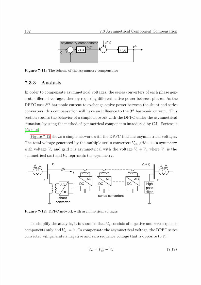
7/25/2019 Dpfc Thesis
http://slidepdf.com/reader/full/dpfc-thesis 154/212
132 7.3 Asymmetrical Component Compensation
G( s) F ( s)+-
asymmetry compensator
0
0,
r V −0,
seV −
H ( s)
+
+
Figure 7-11: The scheme of the asymmetry compensator
7.3.3 Analysis
In order to compensate asymmetrical voltages, the series converters of each phase gen-
erate different voltages, thereby requiring different active power between phases. As theDPFC uses 3rd harmonic current to exchange active power between the shunt and series
converters, this compensation will have an influence to the 3rd harmonic current. This
section studies the behavior of a simple network with the DPFC under the asymmetrical
situation, by using the method of symmetrical components introduced by C.L. Fortescue
[Grai 94].
Figure 7-12 shows a simple network with the DPFC that has asymmetrical voltages.
The total voltage generated by the multiple series converters V se, grid s is in symmetry
with voltage V s and grid r is asymmetrical with the voltage V r + V u where V r is thesymmetrical part and V u represents the asymmetry.
AC
DC
AC
DC
AC
DC
AC
DC high
pss
filter
shunt
converter
series converters
sV
r uV V +
I
s r
Figure 7-12: DPFC network with asymmetrical voltages
To simplify the analysis, it is assumed that V u consists of negative and zero sequence
components only and V +u = 0. To compensate the asymmetrical voltage, the DPFC series
converter will generate a negative and zero sequence voltage that is opposite to V u:
V se = V +
se − V u (7.19)
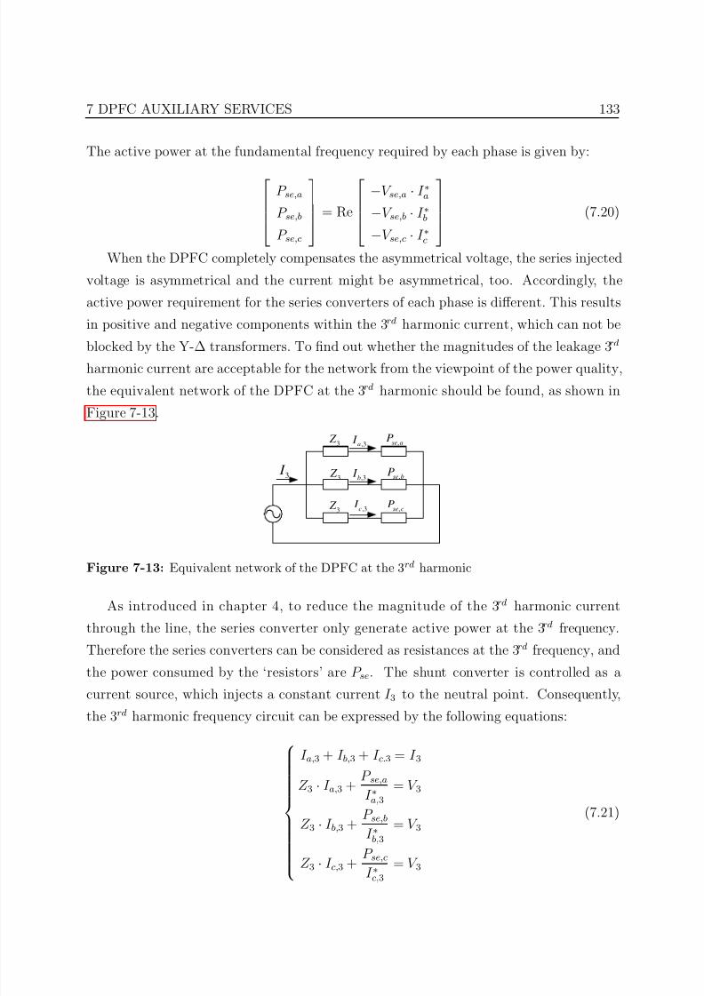
7/25/2019 Dpfc Thesis
http://slidepdf.com/reader/full/dpfc-thesis 155/212
7 DPFC AUXILIARY SERVICES 133
The active power at the fundamental frequency required by each phase is given by:
P se,a
P se,b
P se,c
= Re
−V se,a · I ∗a
−V se,b · I ∗b
−V se,c · I ∗c
(7.20)
When the DPFC completely compensates the asymmetrical voltage, the series injected
voltage is asymmetrical and the current might be asymmetrical, too. Accordingly, the
active power requirement for the series converters of each phase is different. This results
in positive and negative components within the 3rd harmonic current, which can not be
blocked by the Y-∆ transformers. To find out whether the magnitudes of the leakage 3rd
harmonic current are acceptable for the network from the viewpoint of the power quality,
the equivalent network of the DPFC at the 3rd harmonic should be found, as shown in
Figure 7-13.
3 Z
,3a I ,se aP
3 I
3 Z
3 Z
,3b I
,3c I
,se bP
,se cP
Figure 7-13: Equivalent network of the DPFC at the 3rd harmonic
As introduced in chapter 4, to reduce the magnitude of the 3rd harmonic current
through the line, the series converter only generate active power at the 3rd frequency.
Therefore the series converters can be considered as resistances at the 3 rd frequency, and
the power consumed by the ‘resistors’ are P se. The shunt converter is controlled as a
current source, which injects a constant current I 3 to the neutral point. Consequently,the 3rd harmonic frequency circuit can be expressed by the following equations:
I a,3 + I b,3 + I c.3 = I 3
Z 3 · I a,3 + P se,a
I ∗a,3
= V 3
Z 3 · I b,3 + P se,b
I ∗b,3
= V 3
Z 3·
I c,3 + P se,c
I ∗
c,3
= V 3
(7.21)
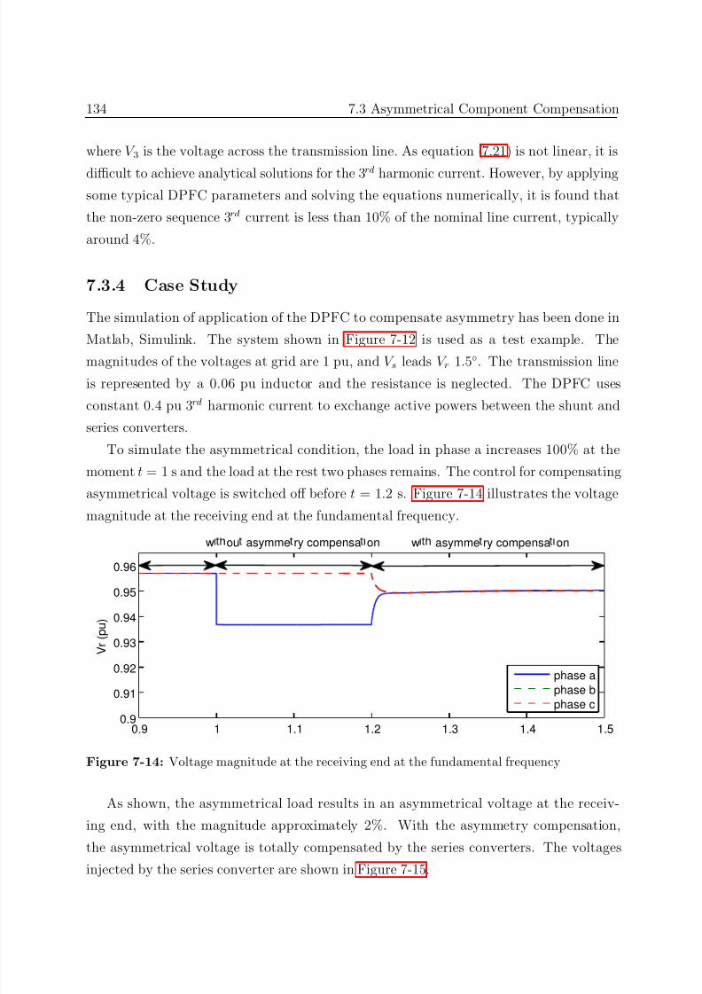
7/25/2019 Dpfc Thesis
http://slidepdf.com/reader/full/dpfc-thesis 156/212
134 7.3 Asymmetrical Component Compensation
where V 3 is the voltage across the transmission line. As equation (7.21) is not linear, it is
difficult to achieve analytical solutions for the 3rd harmonic current. However, by applyingsome typical DPFC parameters and solving the equations numerically, it is found that
the non-zero sequence 3rd current is less than 10% of the nominal line current, typically
around 4%.
7.3.4 Case Study
The simulation of application of the DPFC to compensate asymmetry has been done in
Matlab, Simulink. The system shown in Figure 7-12 is used as a test example. The
magnitudes of the voltages at grid are 1 pu, and V s leads V r 1.5. The transmission line
is represented by a 0.06 pu inductor and the resistance is neglected. The DPFC uses
constant 0.4 pu 3rd harmonic current to exchange active powers between the shunt and
series converters.
To simulate the asymmetrical condition, the load in phase a increases 100% at the
moment t = 1 s and the load at the rest two phases remains. The control for compensating
asymmetrical voltage is switched off before t = 1.2 s. Figure 7-14 illustrates the voltage
magnitude at the receiving end at the fundamental frequency.
0.9 1 1.1 1.2 1.3 1.4 1.50.9
0.91
0.92
0.93
0.94
0.95
0.96
V r ( p u )
phase a
phase b
phase c
w ou asymme ry compensa on w asymme ry compensa on
Figure 7-14: Voltage magnitude at the receiving end at the fundamental frequency
As shown, the asymmetrical load results in an asymmetrical voltage at the receiv-
ing end, with the magnitude approximately 2%. With the asymmetry compensation,
the asymmetrical voltage is totally compensated by the series converters. The voltages
injected by the series converter are shown in Figure 7-15.
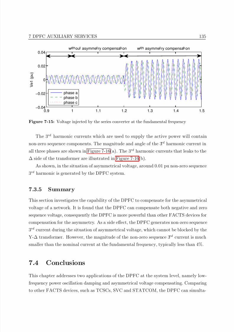
7/25/2019 Dpfc Thesis
http://slidepdf.com/reader/full/dpfc-thesis 157/212
7 DPFC AUXILIARY SERVICES 135
0.9 1 1.1 1.2 1.3 1.4 1.5−0.04
−0.02
0
0.02
0.04
V e 1 ( p u )
phase a
phase b
phase c
w ou asymme ry compensa on w asymme ry compensa on
Figure 7-15: Voltage injected by the series converter at the fundamental frequency
The 3rd harmonic currents which are used to supply the active power will contain
non-zero sequence components. The magnitude and angle of the 3rd harmonic current in
all three phases are shown in Figure 7-16(a). The 3rd harmonic currents that leaks to the
∆ side of the transformer are illustrated in Figure 7-16(b).
As shown, in the situation of asymmetrical voltage, around 0.01 pu non-zero sequence
3rd
harmonic is generated by the DPFC system.
7.3.5 Summary
This section investigates the capability of the DPFC to compensate for the asymmetrical
voltage of a network. It is found that the DPFC can compensate both negative and zero
sequence voltage, consequently the DPFC is more powerful than other FACTS devices for
compensation for the asymmetry. As a side effect, the DPFC generates non-zero sequence
3rd current during the situation of asymmetrical voltage, which cannot be blocked by the
Y-∆ transformer. However, the magnitude of the non-zero sequence 3rd current is much
smaller than the nominal current at the fundamental frequency, typically less than 4%.
7.4 Conclusions
This chapter addresses two applications of the DPFC at the system level, namely low-
frequency power oscillation damping and asymmetrical voltage compensating. Comparing
to other FACTS devices, such as TCSCs, SVC and STATCOM, the DPFC can simulta-
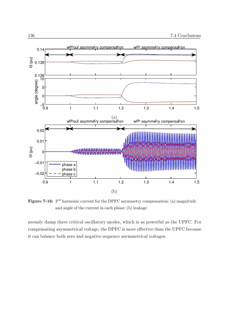
7/25/2019 Dpfc Thesis
http://slidepdf.com/reader/full/dpfc-thesis 158/212
136 7.4 Conclusions
0.136
0.138
0.14
I 3 ( p u )
0.9 1 1.1 1.2 1.3 1.4 1.5−5
0
5
10
a n g l e ( d e g r e e )
w ou asymme ry compensa on w asymme ry compensa on
(a)
0.9 1 1.1 1.2 1.3 1.4 1.5
−0.02
−0.01
0
0.01
0.02
I 3 ( p u )
phase a
phase bphase c
w ou asymme ry compensa on w asymme ry compensa on
(b)
Figure 7-16: 3rd harmonic current for the DPFC asymmetry compensation: (a) magnitude
and angle of the current in each phase; (b) leakage
neously damp three critical oscillatory modes, which is as powerful as the UPFC. For
compensating asymmetrical voltage, the DPFC is more effective than the UPFC because
it can balance both zero and negative sequence asymmetrical voltages.
7/25/2019 Dpfc Thesis
http://slidepdf.com/reader/full/dpfc-thesis 159/212
Chapter 8
DPFC APPLICATION IN UTILITY GRIDS
8.1 Introduction
THE concept of the DPFC is introduced previously. The presented issues, including
the modeling, control, fault tolerances and network applications, were focused on
the DPFC’s basic properties. As the DPFC intend to be applied in real power transmissionnetworks, it is important to study its feasibility.
In this chapter, the realization of the DPFC in real networks is examined. The DPFC
design procedures are introduced and the equations needed to determine the major pa-
rameters of the DPFC are given. Two case studies are presented. Case Study 1 aims to
analyze the feasibility of the DPFC on a real transmission line within a two-port network.
The DPFC will be considered from a physical, electrical and financial point of view. In
Case Study 2, the application of a DPFC for power flow control is discussed, in the case
of the Dodewaard triangle network in the Netherlands.
8.2 DPFC Design Procedure
The DPFC design can be divided into three major levels: system level, DPFC level and
converter level, as shown in Figure 8-1.
137
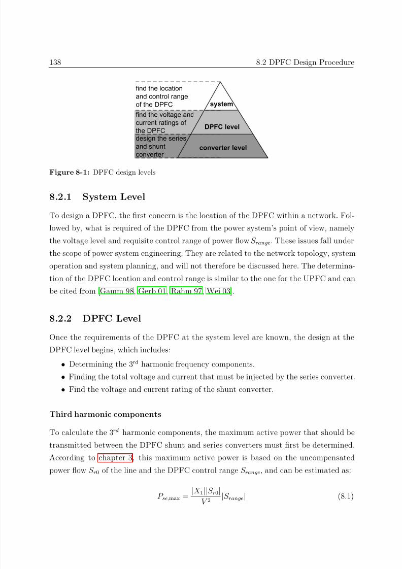
7/25/2019 Dpfc Thesis
http://slidepdf.com/reader/full/dpfc-thesis 160/212
138 8.2 DPFC Design Procedure
find the voltage and
current ratings of
the DPFC
system
DPFC level
converter level
find the location
and control rangeof the DPFC
design the series
and shunt
converter
Figure 8-1: DPFC design levels
8.2.1 System LevelTo design a DPFC, the first concern is the location of the DPFC within a network. Fol-
lowed by, what is required of the DPFC from the power system’s point of view, namely
the voltage level and requisite control range of power flow S range. These issues fall under
the scope of power system engineering. They are related to the network topology, system
operation and system planning, and will not therefore be discussed here. The determina-
tion of the DPFC location and control range is similar to the one for the UPFC and can
be cited from [Gamm 98, Gerb 01, Rahm 97, Wei 03].
8.2.2 DPFC Level
Once the requirements of the DPFC at the system level are known, the design at the
DPFC level begins, which includes:
• Determining the 3rd harmonic frequency components.
• Finding the total voltage and current that must be injected by the series converter.
• Find the voltage and current rating of the shunt converter.
Third harmonic components
To calculate the 3rd harmonic components, the maximum active power that should be
transmitted between the DPFC shunt and series converters must first be determined.
According to chapter 3, this maximum active power is based on the uncompensated
power flow S r0 of the line and the DPFC control range S range, and can be estimated as:
P se,max = |X 1
||S r0
|V 2 |S range| (8.1)
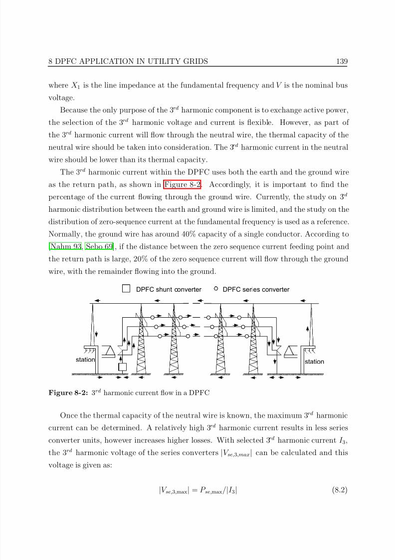
7/25/2019 Dpfc Thesis
http://slidepdf.com/reader/full/dpfc-thesis 161/212
8 DPFC APPLICATION IN UTILITY GRIDS 139
where X 1 is the line impedance at the fundamental frequency and V is the nominal bus
voltage.Because the only purpose of the 3rd harmonic component is to exchange active power,
the selection of the 3rd harmonic voltage and current is flexible. However, as part of
the 3rd harmonic current will flow through the neutral wire, the thermal capacity of the
neutral wire should be taken into consideration. The 3rd harmonic current in the neutral
wire should be lower than its thermal capacity.
The 3rd harmonic current within the DPFC uses both the earth and the ground wire
as the return path, as shown in Figure 8-2. Accordingly, it is important to find the
percentage of the current flowing through the ground wire. Currently, the study on 3rd
harmonic distribution between the earth and ground wire is limited, and the study on the
distribution of zero-sequence current at the fundamental frequency is used as a reference.
Normally, the ground wire has around 40% capacity of a single conductor. According to
[Nahm 93, Sebo 69], if the distance between the zero sequence current feeding point and
the return path is large, 20% of the zero sequence current will flow through the ground
wire, with the remainder flowing into the ground.
stationstation
DPFC shunt converter DPFC series converter
Figure 8-2: 3rd harmonic current flow in a DPFC
Once the thermal capacity of the neutral wire is known, the maximum 3 rd harmonic
current can be determined. A relatively high 3rd harmonic current results in less series
converter units, however increases higher losses. With selected 3rd harmonic current I 3,
the 3rd harmonic voltage of the series converters |V se,3,max| can be calculated and this
voltage is given as:
|V se,3,max| = P se,max/|I 3| (8.2)
7/25/2019 Dpfc Thesis
http://slidepdf.com/reader/full/dpfc-thesis 162/212
140 8.2 DPFC Design Procedure
The maximum voltage |V sh,3,max| and current |I sh,3,max| for the shunt converter at the
3rd harmonic frequency can be calculated from:
|I sh,3,max| = 3I 3
|V sh,3,max| =
(X 3I 3)2 + V 2se,3,max
(8.3)
Within the equation, X 3 is the total zero sequence impedance at the 3rd harmonic
frequency. This impedance includes the self-impedance of the lines and the mutual
impedance between the lines and the ground wire and the ground [Grai 94, Thap 90].
As the zero-sequence impedance is related with the ground, the ground wire and the
geometry of the line, it is difficult to calculate accurately. According to the data from
Kerite, the zero sequence impedance is normally 2 to 4 times larger than the positive
sequence impedance1.
Voltage and current rating of the series converters
The voltage and current of the series converter consist of a fundamental frequency compo-
nent and 3rd harmonic frequency component. The 3rd harmonic component of the series
converter has been given previously and the fundamental frequency component can becalculated from:
|V se,1,max| = |S range| · |V |
X 1(8.4)
The voltage and current rating of the DPFC converters is the sum of the components at
both the fundamental and 3rd harmonic frequencies:
V se,max = V se,1,max + V se,3,max
I se,max = I 1,max + I 3(8.5)
where I 1,max is the maximum line current at the fundamental frequency.
Voltage and current rating of the shunt converter
The shunt converter of the DPFC consists of a three-phase converter with a back-to-
back connected single-phase converter. The three-phase converter supports the capacitor
voltage and provides reactive power for the network. The voltage and power ratings of
1
Date Source: http://www.kerite.com/catalog/catalogfiles/impedance data power.htm
7/25/2019 Dpfc Thesis
http://slidepdf.com/reader/full/dpfc-thesis 163/212
8 DPFC APPLICATION IN UTILITY GRIDS 141
the three-phase converter can be calculated according to the reactive compensation range,
similarly to the calculations used in a STATCOM, which can be found in [Lee 03].The single-phase converter is connected between the neutral point of the Y-∆ trans-
former and the ground. Since the transformer blocks the voltage and current at the
fundamental frequency, the single-phase converter only needs to handle the component at
the 3rd harmonic frequency, which is shown in (8.3).
8.2.3 Converter Level
Due to the similarity between the shunt converter and a STATCOM, design of the shuntconverter will not be discussed here in detail. The converter level design within the thesis
is focused on the series converter design. Because the units of the DPFC series converter
are hung on the transmission line, their weight is a major design factor, to ensure that
the towers can hold the units. Accordingly, the DPFC series converter design consists of
the following steps:
• AC-DC converter design
• single-turn transformer design
• unit weight calculation
AC-DC converter design
The total voltage and power of all series converters has been given above. The selection
of the size and number of units is flexible. The units with small voltage and power ratings
result in lightweight per unit; however, in this case, more units are required.
Due to the relatively low rating of the series converter units, MOSFET or IGBT can
be selected as switching devices. It is possible to find, the maximum RMS voltage V s,
current I s and DC voltage V dc of the series converter unit based on the parameters of the
selected semiconductors. The capacitor is used to maintain the DC voltages, accordingly
its capacitance depends on the allowed DC ripple V dc,ripple and the capacitance is given
as:
C dc = I s
4πf V dc,ripple
(8.6)
where V dc,ripple is the maximum ripple that is allowed on the DC side, f is the network
fundamental frequency and I s is the maximum RMS current on the AC side of the unit.
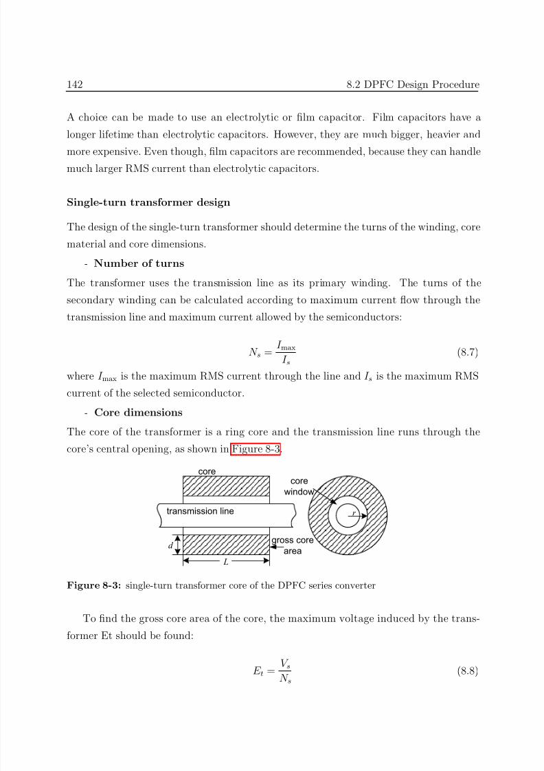
7/25/2019 Dpfc Thesis
http://slidepdf.com/reader/full/dpfc-thesis 164/212
142 8.2 DPFC Design Procedure
A choice can be made to use an electrolytic or film capacitor. Film capacitors have a
longer lifetime than electrolytic capacitors. However, they are much bigger, heavier andmore expensive. Even though, film capacitors are recommended, because they can handle
much larger RMS current than electrolytic capacitors.
Single-turn transformer design
The design of the single-turn transformer should determine the turns of the winding, core
material and core dimensions.
- Number of turns
The transformer uses the transmission line as its primary winding. The turns of the
secondary winding can be calculated according to maximum current flow through the
transmission line and maximum current allowed by the semiconductors:
N s = I max
I s(8.7)
where I max is the maximum RMS current through the line and I s is the maximum RMS
current of the selected semiconductor.
- Core dimensions
The core of the transformer is a ring core and the transmission line runs through the
core’s central opening, as shown in Figure 8-3.
core
transmission line
core
window
gross corearea
d
L
r
Figure 8-3: single-turn transformer core of the DPFC series converter
To find the gross core area of the core, the maximum voltage induced by the trans-
former Et should be found:
E t =
V s
N s (8.8)
7/25/2019 Dpfc Thesis
http://slidepdf.com/reader/full/dpfc-thesis 165/212
8 DPFC APPLICATION IN UTILITY GRIDS 143
According to the induced voltage per turn, maximum flux in the core is given as:
Φm = E t4.44f
(8.9)
To ensure the core not be saturated, the cross-section area of the core Agi should be:
Agi = Φm
0.9Bm(8.10)
where Bm is the saturation flux density of the core material. Normally, grain-oriented
silicon steel is used as the core material with maximum operation flux density 17000 gauss.
Once the cross-section is determined, the selection of the length L and the thickness d
of the core can be traded. A longer core requires less core material, but needs more
copper for the secondary winding. As most of the weight of the series converter unit is
contributed by the core, a longer core is recommended.
The transmission line and secondary winding run through the core window, which can
be calculated from:
Aw = 2Al
K w
(8.11)
where Al is the cross-section of the transmission line and K w is a design factor, so-called
window space factor, that gives extra space for voltage isolation. As the series converter
is electrically floated on the line, the single-turn transformer does not need high voltage
isolation. A window space factor of K w = 0.6 is recommended for a DPFC single-turn
transformer.
Weight calculation
The weight of the series converter unit is mainly contributed by the transformer and the
converter. According to the selected components, the converter weight can be roughly
calculated from data sheets. The weight of the transformer core is given as:
W c = ρcLπ[(d + r)2 + r2] (8.12)
where ρc is the density of the core. The weight of the secondary winding is given as:
W s = 2AsN s(L + d) (8.13)
7/25/2019 Dpfc Thesis
http://slidepdf.com/reader/full/dpfc-thesis 166/212
144 8.3 Case Study 1: Two-Port Network
where As is the cross-section of the secondary winding and N s is the number of turns.
Once the weight per unit is known, the total weight of the series converter can becalculated by multiplying it by the number of the units. The number of the series converter
units depends on the required series voltage and the maximum voltage of a single series
converter unit, which is given as:
N se =√
3V se,maxN s
V s(8.14)
Note that V se,max is line-to-line voltage. If the extra weight of the series converter cannot
be hold by towers, the converter level design should be repeated.
8.3 Case Study 1: Two-Port Network
This case study investigates the feasibility of the DPFC in a real network and focuses on
the electrical parameters, the physical parameters (including the size, weight of a single
unit) and the approximate cost.
In this section, the specifications of the studied case are introduced. The UPFC
that is applied in the KEPCO transmission system in Korea is used as the case. Oncethe specifications of the KEPCO UPFC are presented, the design of the DPFC, which
replaces the KEPCO UPFC, is discussed. This section ends with a comparison between
the two solutions.
8.3.1 Case Specifications
As mentioned before, because of reliability and economical issues, UPFC is not widely
applied and there have been two UPFC projects undertaken as of 2010, the AEP UPFCproject in the USA operating at 60 Hz and the KEPCO UPFC project in Korea operating
at 50 Hz [Chan 03, Kim 05, Rahm 97, Renz 99, Scha 98, Yoon 03]. As the studies of the
DPFC are based on a 50 Hz fundamental frequency in this thesis, the KEPCO UPFC is
selected.
The KEPCO UPFC is installed on the Kangjin - Jangheung transmission line at 154
kV. The shunt and series converters have 40 MVA capacity each and are connected to the
network through two main transformers. The converters of the UPFC have 3-level switch
technology and 24 pulses per period. GTOs are selected as the switches. The UPFC uses
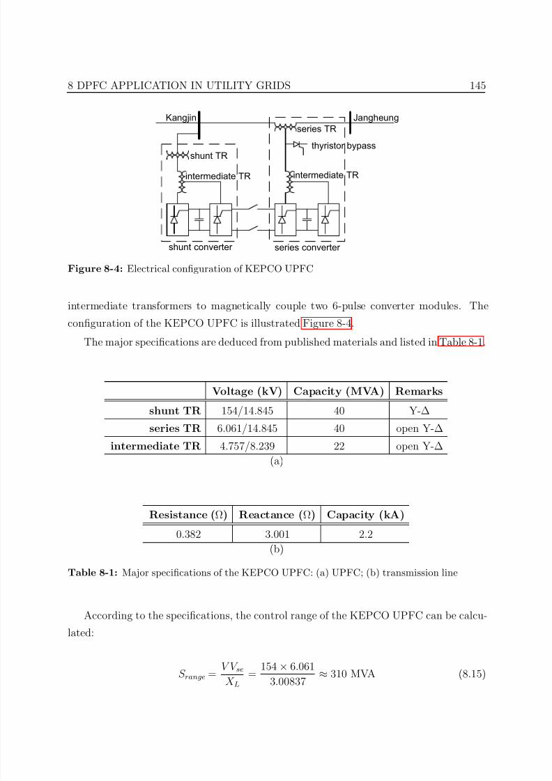
7/25/2019 Dpfc Thesis
http://slidepdf.com/reader/full/dpfc-thesis 167/212
8 DPFC APPLICATION IN UTILITY GRIDS 145
Kangjin Jangheung
shunt converter series converter
shunt TR
series TR
intermediate TRintermediate TR
thyristor bypass
Figure 8-4: Electrical configuration of KEPCO UPFC
intermediate transformers to magnetically couple two 6-pulse converter modules. The
configuration of the KEPCO UPFC is illustrated Figure 8-4.
The major specifications are deduced from published materials and listed in Table 8-1.
Voltage (kV) Capacity (MVA) Remarks
shunt TR 154/14.845 40 Y-∆series TR 6.061/14.845 40 open Y-∆
intermediate TR 4.757/8.239 22 open Y-∆
(a)
Resistance (Ω) Reactance (Ω) Capacity (kA)
0.382 3.001 2.2
(b)
Table 8-1: Major specifications of the KEPCO UPFC: (a) UPFC; (b) transmission line
According to the specifications, the control range of the KEPCO UPFC can be calcu-
lated:
S range = V V se
X L=
154 × 6.061
3.00837 ≈310 MVA (8.15)
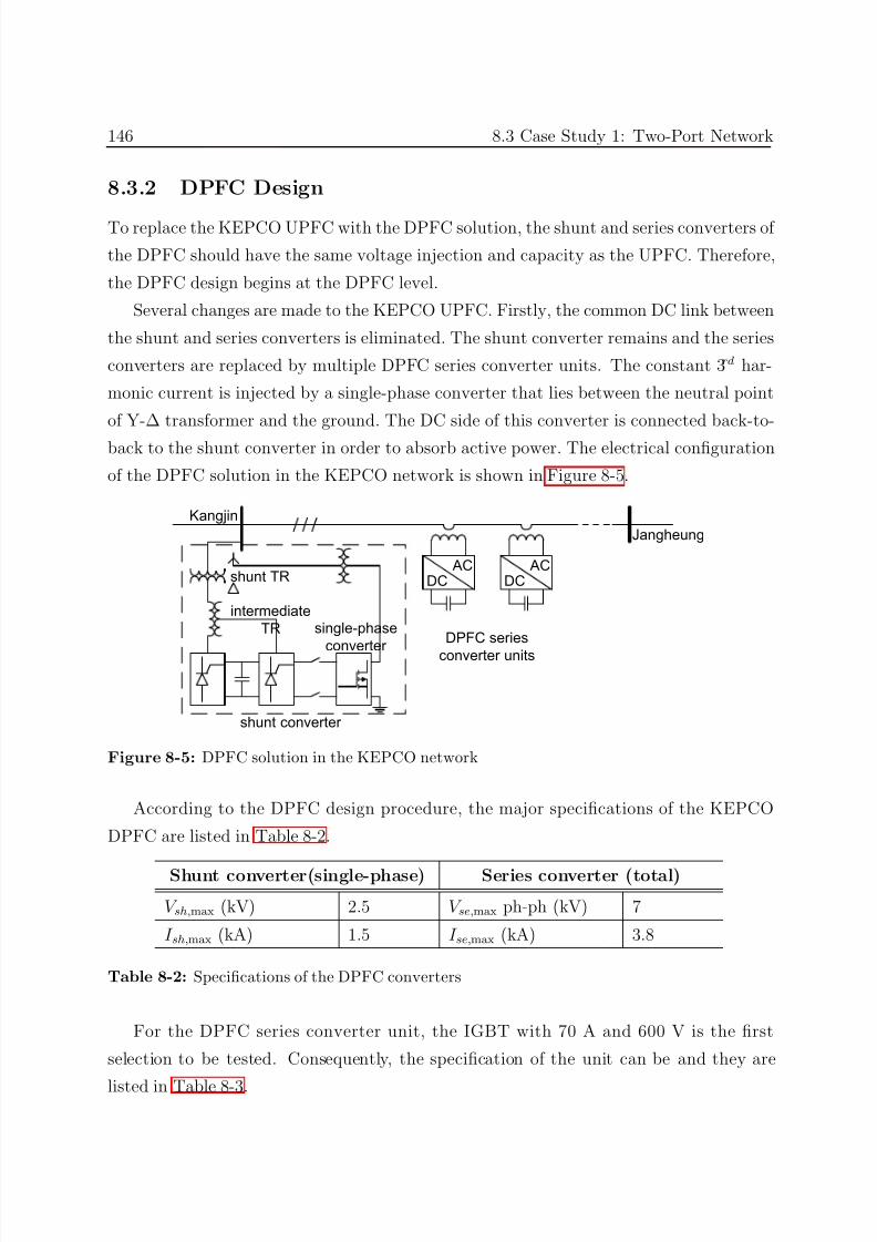
7/25/2019 Dpfc Thesis
http://slidepdf.com/reader/full/dpfc-thesis 168/212
146 8.3 Case Study 1: Two-Port Network
8.3.2 DPFC Design
To replace the KEPCO UPFC with the DPFC solution, the shunt and series converters of
the DPFC should have the same voltage injection and capacity as the UPFC. Therefore,
the DPFC design begins at the DPFC level.
Several changes are made to the KEPCO UPFC. Firstly, the common DC link between
the shunt and series converters is eliminated. The shunt converter remains and the series
converters are replaced by multiple DPFC series converter units. The constant 3rd har-
monic current is injected by a single-phase converter that lies between the neutral point
of Y-∆ transformer and the ground. The DC side of this converter is connected back-to-
back to the shunt converter in order to absorb active power. The electrical configuration
of the DPFC solution in the KEPCO network is shown in Figure 8-5.
Kangjin
Jangheung
shunt converter
shunt TR
intermediate
TR single-phase
converter
ACDC
ACDC
DPFC series
converter units
Figure 8-5: DPFC solution in the KEPCO network
According to the DPFC design procedure, the major specifications of the KEPCO
DPFC are listed in Table 8-2.
Shunt converter(single-phase) Series converter (total)
V sh,max (kV) 2.5 V se,max ph-ph (kV) 7
I sh,max (kA) 1.5 I se,max (kA) 3.8
Table 8-2: Specifications of the DPFC converters
For the DPFC series converter unit, the IGBT with 70 A and 600 V is the first
selection to be tested. Consequently, the specification of the unit can be and they are
listed in Table 8-3.
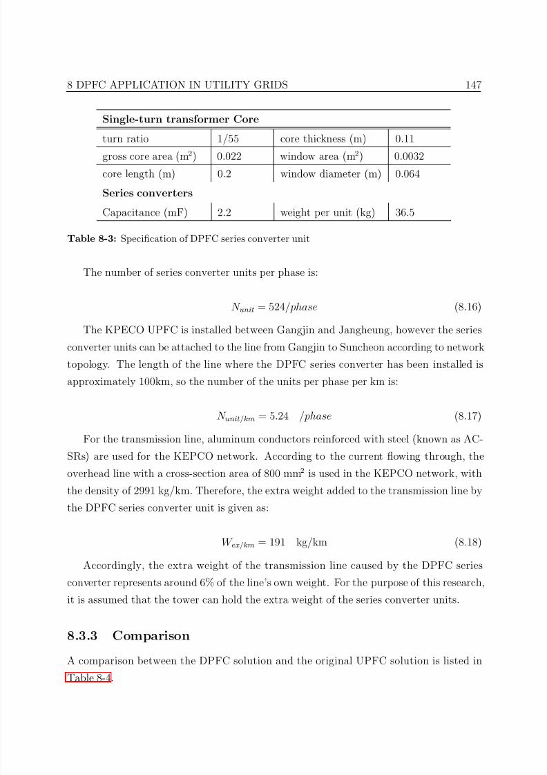
7/25/2019 Dpfc Thesis
http://slidepdf.com/reader/full/dpfc-thesis 169/212
8 DPFC APPLICATION IN UTILITY GRIDS 147
Single-turn transformer Core
turn ratio 1/55 core thickness (m) 0.11
gross core area (m2) 0.022 window area (m2) 0.0032
core length (m) 0.2 window diameter (m) 0.064
Series converters
Capacitance (mF) 2.2 weight per unit (kg) 36.5
Table 8-3: Specification of DPFC series converter unit
The number of series converter units per phase is:
N unit = 524/phase (8.16)
The KPECO UPFC is installed between Gangjin and Jangheung, however the series
converter units can be attached to the line from Gangjin to Suncheon according to network
topology. The length of the line where the DPFC series converter has been installed is
approximately 100km, so the number of the units per phase per km is:
N unit/km = 5.24 /phase (8.17)
For the transmission line, aluminum conductors reinforced with steel (known as AC-
SRs) are used for the KEPCO network. According to the current flowing through, the
overhead line with a cross-section area of 800 mm2 is used in the KEPCO network, with
the density of 2991 kg/km. Therefore, the extra weight added to the transmission line by
the DPFC series converter unit is given as:
W ex/km = 191 kg/km (8.18)
Accordingly, the extra weight of the transmission line caused by the DPFC series
converter represents around 6% of the line’s own weight. For the purpose of this research,
it is assumed that the tower can hold the extra weight of the series converter units.
8.3.3 Comparison
A comparison between the DPFC solution and the original UPFC solution is listed in
Table 8-4.
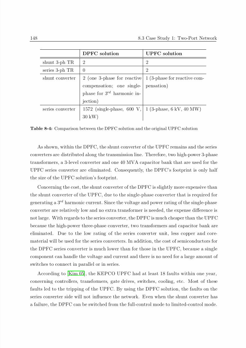
7/25/2019 Dpfc Thesis
http://slidepdf.com/reader/full/dpfc-thesis 170/212
148 8.3 Case Study 1: Two-Port Network
DPFC solution UPFC solution
shunt 3-ph TR 2 2
series 3-ph TR 0 2
shunt converter 2 (one 3-phase for reactive
compensation; one single-
phase for 3rd harmonic in-
jection)
1 (3-phase for reactive com-
pensation)
series converter 1572 (single-phase, 600 V,
30 kW)
1 (3-phase, 6 kV, 40 MW)
Table 8-4: Comparison between the DPFC solution and the original UPFC solution
As shown, within the DPFC, the shunt converter of the UPFC remains and the series
converters are distributed along the transmission line. Therefore, two high-power 3-phase
transformers, a 3-level converter and one 40 MVA capacitor bank that are used for the
UPFC series converter are eliminated. Consequently, the DPFC’s footprint is only half
the size of the UPFC solution’s footprint.
Concerning the cost, the shunt converter of the DPFC is slightly more expensive than
the shunt converter of the UPFC, due to the single-phase converter that is required for
generating a 3rd harmonic current. Since the voltage and power rating of the single-phase
converter are relatively low and no extra transformer is needed, the expense difference is
not large. With regards to the series converter, the DPFC is much cheaper than the UPFC
because the high-power three-phase converter, two transformers and capacitor bank are
eliminated. Due to the low rating of the series converter unit, less copper and core-
material will be used for the series converters. In addition, the cost of semiconductors for
the DPFC series converter is much lower than for those in the UPFC, because a single
component can handle the voltage and current and there is no need for a large amount of
switches to connect in parallel or in series.
According to [Kim 05], the KEPCO UPFC had at least 18 faults within one year,
concerning controllers, transformers, gate drives, switches, cooling, etc. Most of these
faults led to the tripping of the UPFC. By using the DPFC solution, the faults on the
series converter side will not influence the network. Even when the shunt converter has
a failure, the DPFC can be switched from the full-control mode to limited-control mode.
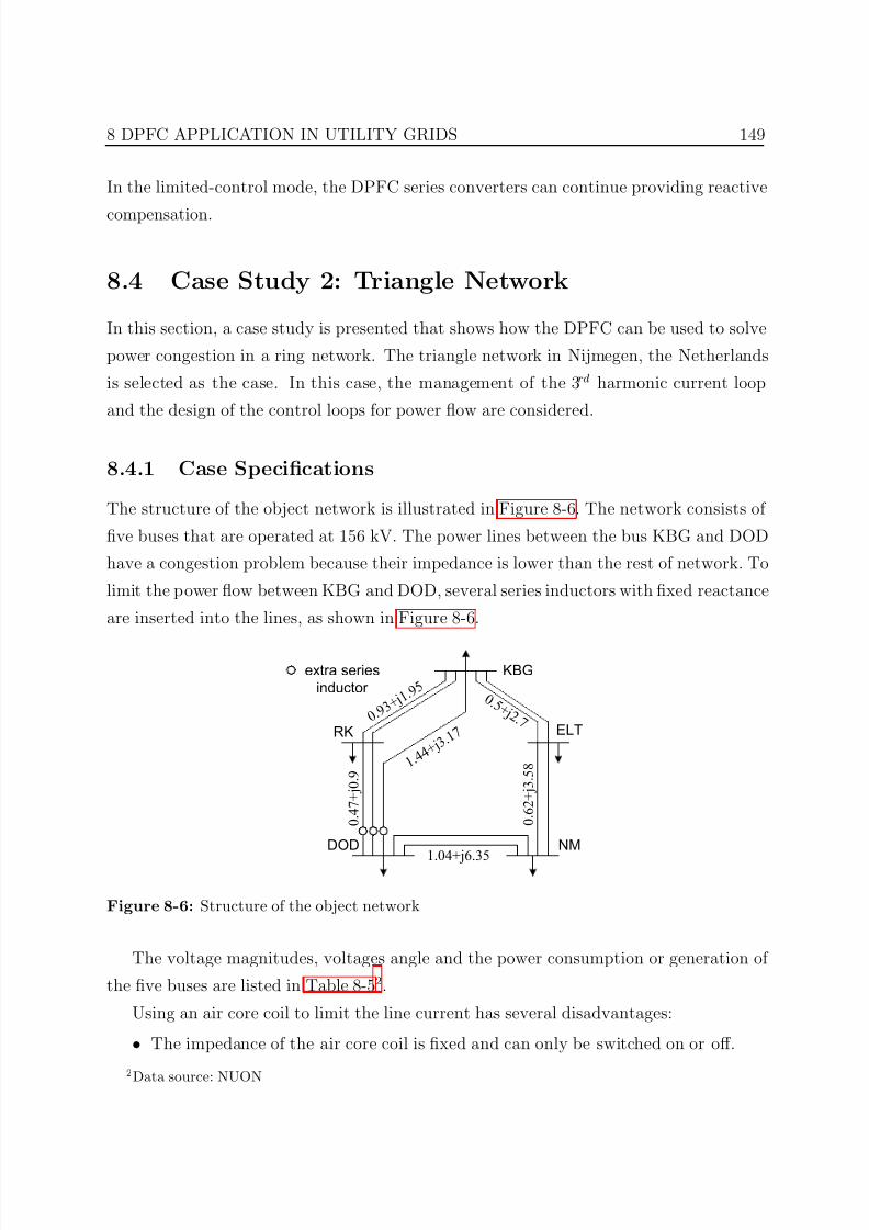
7/25/2019 Dpfc Thesis
http://slidepdf.com/reader/full/dpfc-thesis 171/212
8 DPFC APPLICATION IN UTILITY GRIDS 149
In the limited-control mode, the DPFC series converters can continue providing reactive
compensation.
8.4 Case Study 2: Triangle Network
In this section, a case study is presented that shows how the DPFC can be used to solve
power congestion in a ring network. The triangle network in Nijmegen, the Netherlands
is selected as the case. In this case, the management of the 3rd harmonic current loop
and the design of the control loops for power flow are considered.
8.4.1 Case Specifications
The structure of the object network is illustrated in Figure 8-6. The network consists of
five buses that are operated at 156 kV. The power lines between the bus KBG and DOD
have a congestion problem because their impedance is lower than the rest of network. To
limit the power flow between KBG and DOD, several series inductors with fixed reactance
are inserted into the lines, as shown in Figure 8-6.
KBG
ELT
NMDOD
RK
1. 4 4 + j 3.
1 7 0. 9
3 + j 1.
9 5 0 .5 + j 2 .7
1.04+j6.35
0 . 4
7 + j 0 . 9
0 . 6
2 + j 3 . 5
8
extra series
inductor
Figure 8-6: Structure of the object network
The voltage magnitudes, voltages angle and the power consumption or generation of
the five buses are listed in Table 8-52.
Using an air core coil to limit the line current has several disadvantages:
• The impedance of the air core coil is fixed and can only be switched on or off.
2
Data source: NUON
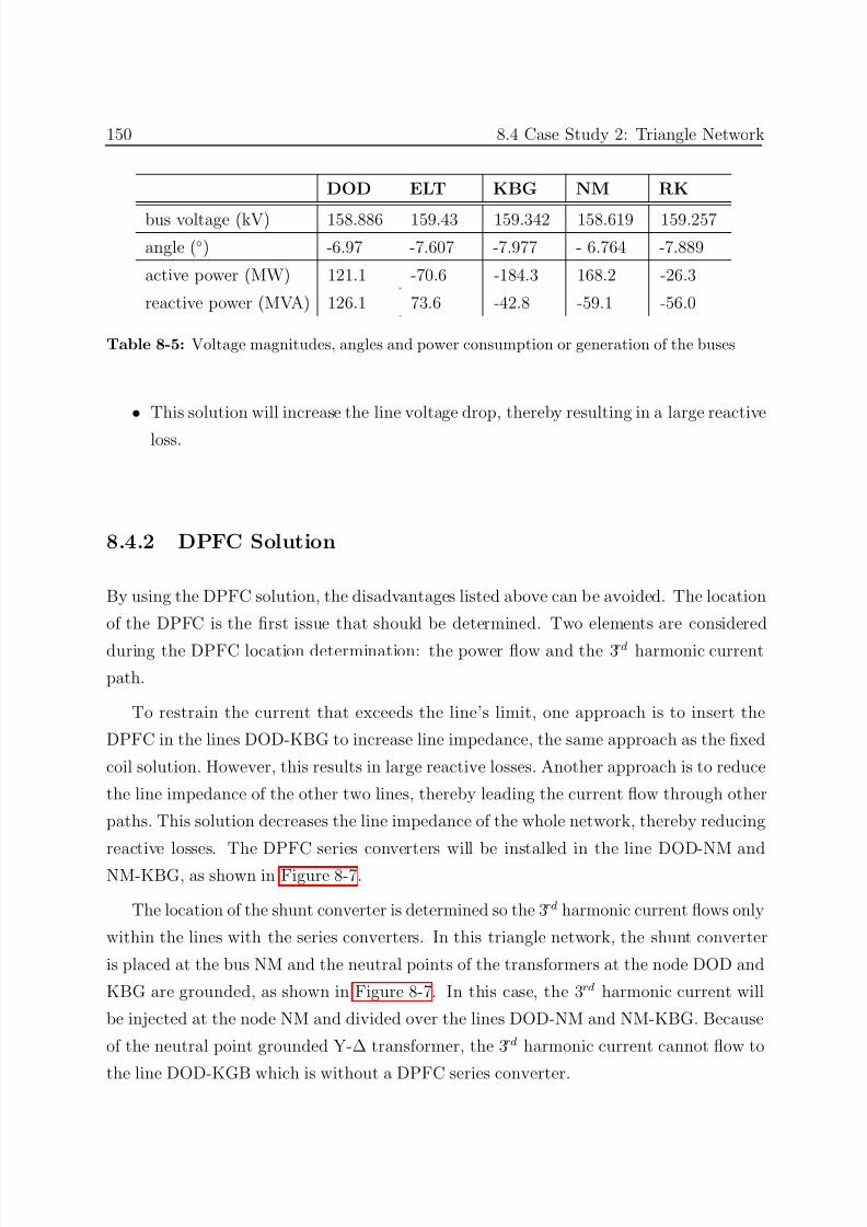
7/25/2019 Dpfc Thesis
http://slidepdf.com/reader/full/dpfc-thesis 172/212
150 8.4 Case Study 2: Triangle Network
DOD ELT KBG NM RK
bus voltage (kV) 158.886 159.43 159.342 158.619 159.257
angle () -6.97 -7.607 -7.977 - 6.764 -7.889
active power (MW) 121.1 -70.6 -184.3 168.2 -26.3
reactive power (MVA) 126.1 73.6 -42.8 -59.1 -56.0
Table 8-5: Voltage magnitudes, angles and power consumption or generation of the buses
• This solution will increase the line voltage drop, thereby resulting in a large reactive
loss.
8.4.2 DPFC Solution
By using the DPFC solution, the disadvantages listed above can be avoided. The location
of the DPFC is the first issue that should be determined. Two elements are considered
during the DPFC location determination: the power flow and the 3rd harmonic current
path.
To restrain the current that exceeds the line’s limit, one approach is to insert the
DPFC in the lines DOD-KBG to increase line impedance, the same approach as the fixed
coil solution. However, this results in large reactive losses. Another approach is to reduce
the line impedance of the other two lines, thereby leading the current flow through other
paths. This solution decreases the line impedance of the whole network, thereby reducing
reactive losses. The DPFC series converters will be installed in the line DOD-NM and
NM-KBG, as shown in Figure 8-7.
The location of the shunt converter is determined so the 3rd harmonic current flows only
within the lines with the series converters. In this triangle network, the shunt converter
is placed at the bus NM and the neutral points of the transformers at the node DOD and
KBG are grounded, as shown in Figure 8-7. In this case, the 3rd harmonic current will
be injected at the node NM and divided over the lines DOD-NM and NM-KBG. Because
of the neutral point grounded Y-∆ transformer, the 3rd harmonic current cannot flow to
the line DOD-KGB which is without a DPFC series converter.
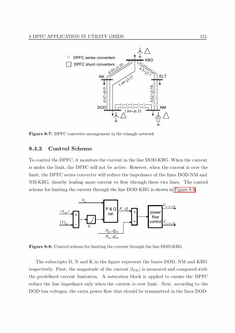
7/25/2019 Dpfc Thesis
http://slidepdf.com/reader/full/dpfc-thesis 173/212
8 DPFC APPLICATION IN UTILITY GRIDS 151
KBG
ELT
NMDOD
RK
1. 4 4 + j 3.
1 7 0. 9
3 + j 1.
9 50 .5 + j 2 .7
1.04+j6.35
0 . 4
7 + j 0 . 9
0 . 6
2 + j 3 . 5
8
DPFC ont
DPFC hunt ont
Figure 8-7: DPFC converter arrangement in the triangle network
8.4.3 Control Scheme
To control the DPFC, it monitors the current in the line DOD-KBG. When the current
is under the limit, the DPFC will not be active. However, when the current is over the
limit, the DPFC series converter will reduce the impedance of the lines DOD-NM andNM-KBG, thereby leading more current to flow through these two lines. The control
scheme for limiting the current through the line DOD-KBG is shown in Figure 8-8.
+
-lim| | I
| | DK I
0
P & Q
cal.
K V
power
flow
control
,ex exP Q+
+
, DN DN P Q
, NK NK P Q
, ,se ref DN V
, ,se ref NK V
Figure 8-8: Control scheme for limiting the current through the line DOD-KBG
The subscripts D, N and K in the figure represent the buses DOD, NM and KBG
respectively. First, the magnitude of the current |I DK | is measured and compared with
the predefined current limitation. A saturation block is applied to ensure the DPFC
reduce the line impedance only when the current is over limit. Next, according to the
DOD bus voltages, the extra power flow that should be transmitted in the lines DOD-
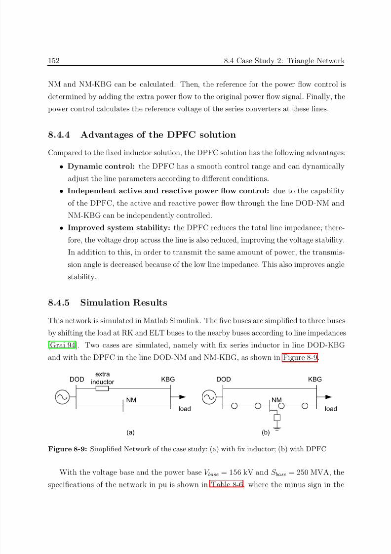
7/25/2019 Dpfc Thesis
http://slidepdf.com/reader/full/dpfc-thesis 174/212
152 8.4 Case Study 2: Triangle Network
NM and NM-KBG can be calculated. Then, the reference for the power flow control is
determined by adding the extra power flow to the original power flow signal. Finally, thepower control calculates the reference voltage of the series converters at these lines.
8.4.4 Advantages of the DPFC solution
Compared to the fixed inductor solution, the DPFC solution has the following advantages:
• Dynamic control: the DPFC has a smooth control range and can dynamically
adjust the line parameters according to different conditions.
• Independent active and reactive power flow control: due to the capabilityof the DPFC, the active and reactive power flow through the line DOD-NM and
NM-KBG can be independently controlled.
• Improved system stability: the DPFC reduces the total line impedance; there-
fore, the voltage drop across the line is also reduced, improving the voltage stability.
In addition to this, in order to transmit the same amount of power, the transmis-
sion angle is decreased because of the low line impedance. This also improves angle
stability.
8.4.5 Simulation Results
This network is simulated in Matlab Simulink. The five buses are simplified to three buses
by shifting the load at RK and ELT buses to the nearby buses according to line impedances
[Grai 94]. Two cases are simulated, namely with fix series inductor in line DOD-KBG
and with the DPFC in the line DOD-NM and NM-KBG, as shown in Figure 8-9.
DOD
NM
KBG
load
extra
inductor DOD
NM
KBG
load
(a) (b)
Figure 8-9: Simplified Network of the case study: (a) with fix inductor; (b) with DPFC
With the voltage base and the power base V base = 156 kV and S base = 250 MVA, the
specifications of the network in pu is shown in Table 8-6, where the minus sign in the
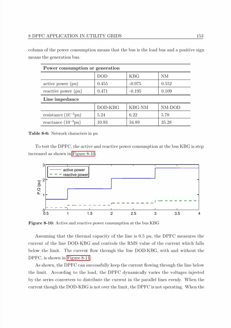
7/25/2019 Dpfc Thesis
http://slidepdf.com/reader/full/dpfc-thesis 175/212
8 DPFC APPLICATION IN UTILITY GRIDS 153
column of the power consumption means that the bus is the load bus and a positive sign
means the generation bus.
Power consumption or generation
DOD KBG NM
active power (pu) 0.455 -0.975 0.552
reactive power (pu) 0.471 -0.195 0.109
Line impedance
DOD-KBG KBG-NM NM-DOD
resistance (10−
3pu) 5.24 6.22 5.78reactance (10−3pu) 10.93 34.89 35.28
Table 8-6: Network characters in pu
To test the DPFC, the active and reactive power consumption at the bus KBG is step
increased as shown in Figure 8-10.
0.5 1 1.5 2 2.5 3 3.5 40
1
2
3
P , Q ( p u )
active power
reactive power
Figure 8-10: Active and reactive power consumption at the bus KBG
Assuming that the thermal capacity of the line is 0.5 pu, the DPFC measures the
current of the line DOD-KBG and controls the RMS value of the current which falls
below the limit. The current flow through the line DOD-KBG, with and without the
DPFC, is shown in Figure 8-11.
As shown, the DPFC can successfully keep the current flowing through the line below
the limit. According to the load, the DPFC dynamically varies the voltages injected
by the series converters to distribute the current in the parallel lines evenly. When the
current though the DOD-KBG is not over the limit, the DPFC is not operating. When the
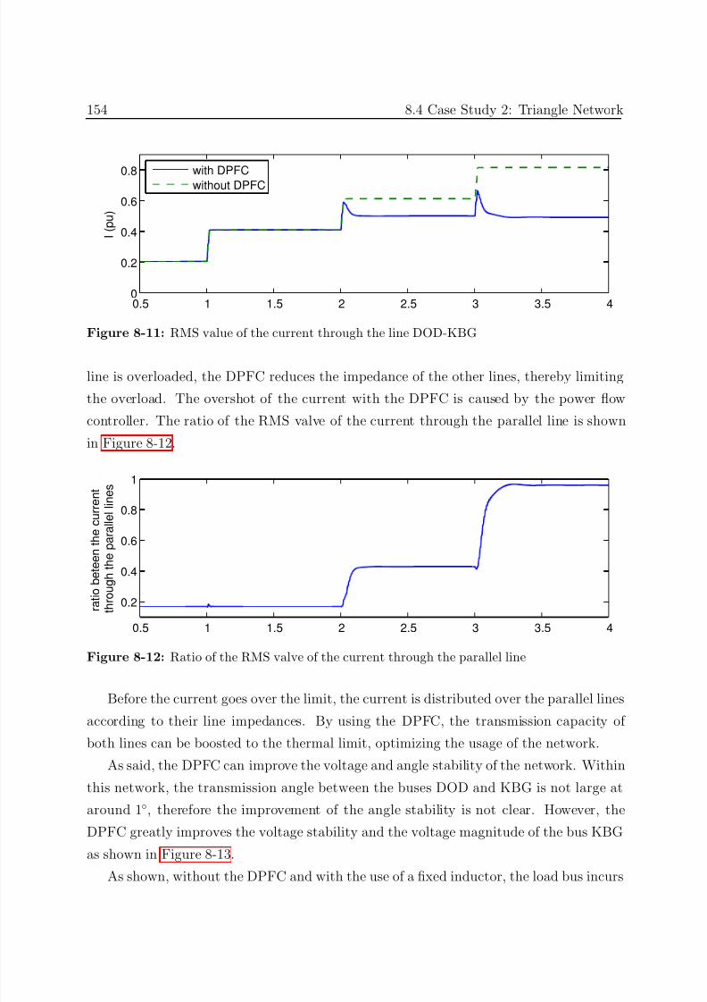
7/25/2019 Dpfc Thesis
http://slidepdf.com/reader/full/dpfc-thesis 176/212
154 8.4 Case Study 2: Triangle Network
0.5 1 1.5 2 2.5 3 3.5 40
0.2
0.4
0.6
0.8
I ( p u )
with DPFCwithout DPFC
Figure 8-11: RMS value of the current through the line DOD-KBG
line is overloaded, the DPFC reduces the impedance of the other lines, thereby limiting
the overload. The overshot of the current with the DPFC is caused by the power flow
controller. The ratio of the RMS valve of the current through the parallel line is shown
in Figure 8-12.
0.5 1 1.5 2 2.5 3 3.5 4
0.2
0.4
0.6
0.8
1
r a t i o b e t e e n t h e c u r r e n t
t h r o u g h t h e p a r a l l e l l i n e s
Figure 8-12: Ratio of the RMS valve of the current through the parallel line
Before the current goes over the limit, the current is distributed over the parallel linesaccording to their line impedances. By using the DPFC, the transmission capacity of
both lines can be boosted to the thermal limit, optimizing the usage of the network.
As said, the DPFC can improve the voltage and angle stability of the network. Within
this network, the transmission angle between the buses DOD and KBG is not large at
around 1, therefore the improvement of the angle stability is not clear. However, the
DPFC greatly improves the voltage stability and the voltage magnitude of the bus KBG
as shown in Figure 8-13.
As shown, without the DPFC and with the use of a fixed inductor, the load bus incurs
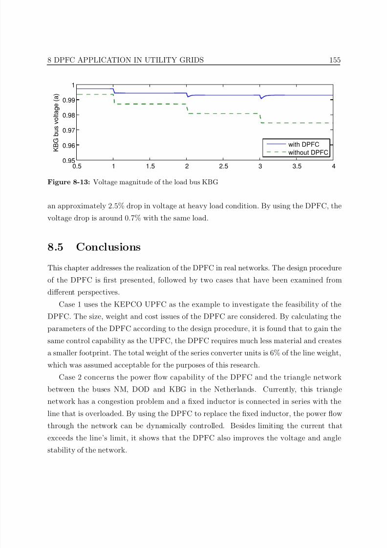
7/25/2019 Dpfc Thesis
http://slidepdf.com/reader/full/dpfc-thesis 177/212
8 DPFC APPLICATION IN UTILITY GRIDS 155
0.5 1 1.5 2 2.5 3 3.5 40.95
0.96
0.97
0.98
0.99
1
K B G b u s v o l t a g e ( a )
with DPFC
without DPFC
Figure 8-13: Voltage magnitude of the load bus KBG
an approximately 2.5% drop in voltage at heavy load condition. By using the DPFC, the
voltage drop is around 0.7% with the same load.
8.5 Conclusions
This chapter addresses the realization of the DPFC in real networks. The design procedure
of the DPFC is first presented, followed by two cases that have been examined from
different perspectives.
Case 1 uses the KEPCO UPFC as the example to investigate the feasibility of the
DPFC. The size, weight and cost issues of the DPFC are considered. By calculating the
parameters of the DPFC according to the design procedure, it is found that to gain the
same control capability as the UPFC, the DPFC requires much less material and creates
a smaller footprint. The total weight of the series converter units is 6% of the line weight,
which was assumed acceptable for the purposes of this research.
Case 2 concerns the power flow capability of the DPFC and the triangle network
between the buses NM, DOD and KBG in the Netherlands. Currently, this triangle
network has a congestion problem and a fixed inductor is connected in series with the
line that is overloaded. By using the DPFC to replace the fixed inductor, the power flow
through the network can be dynamically controlled. Besides limiting the current that
exceeds the line’s limit, it shows that the DPFC also improves the voltage and angle
stability of the network.

7/25/2019 Dpfc Thesis
http://slidepdf.com/reader/full/dpfc-thesis 178/212
7/25/2019 Dpfc Thesis
http://slidepdf.com/reader/full/dpfc-thesis 179/212
Chapter 9CONCLUSIONS AND
RECOMMENDATIONS
9.1 Conclusions
A
S mentioned in chapter 1, there is a large demand for power flow control in modern
power systems. The trend is that mechanical Power Flow Controlling Devices
(PFCDs) are gradually being replaced by Power Electronics (PE) PFCDs. Among all PE
PFCDs, the Unified Power Flow Controller (UPFC) is the most versatile device. However,
the UPFC is not widely applied in the utility grid due to its high cost and relatively low
reliability.
The aim of this thesis is to develop a new type of power flow controlling device that
offers the same control capability as the UPFC, at a reduced cost and with increased
reliability. The new device, the so-called Distributed Power Flow Controller (DPFC), is
a further development of the UPFC. It has been shown that the DPFC fulfills all three of
the listed goals. To ensure the feasibility of the DPFC, the detailed research in this thesis
addresses the following topics:
• Operating principle
The DPFC eliminates the common DC link within the UPFC to enable the independent
operation of the shunt and series converters. The D-FACTS concept is employed in
the design of the series converter. Multiple low-rating single-phase converters replace the
high-rating three-phase converter, which greatly reduces its cost, due to no requirement of
high-voltage isolation, and increases its reliability, due to redundancy. The active power
157
7/25/2019 Dpfc Thesis
http://slidepdf.com/reader/full/dpfc-thesis 180/212
158 9.1 Conclusions
that used to exchange through the common DC link in the UPFC, is now transferred
through the transmission line at the 3rd harmonic frequency. The reason to select the3rd harmonic is that it is a zero-sequence component and can be naturally blocked by
a Y-∆ transformer. The steady-state analysis shows that the DPFC can simultaneously
adjust the voltage magnitude, the line impedance and the transmission angle, thereby
independently controlling the active and reactive power flow through lines.
• Dynamic model
A dynamic model of the DPFC in the dq rotation reference is developed. This model is
used for the design of a DPFC control algorithm and can be used in computer simulations
of future research. Within the model, the DPFC operation at the system level, which is
at the fundamental and the 3rd harmonic frequency, is described. The switching behavior
of converters is neglected in the model.
• DPFC basic control
The DPFC basic control is developed based on the dynamic model. The basic control
stabilizes the level of the capacitor DC voltage of each converter and ensures that the
converters inject the voltages into the network according to the command from the central
control. The shunt converter injects a constant current at the 3rd harmonic frequency,
while its DC voltage is stabilized by the fundamental frequency component. For the series
converter, the reference of the output voltage at the fundamental frequency is obtained
from the central control and the DC voltage level is maintained by the 3rd harmonic
components. The control parameters of the basic control are determined. Both the model
and the basic control are verified in Matlab Simulink.
• DPFC laboratory demonstrator
To verify the dynamic model and the basic control, a DPFC demonstration setup is built.
The setup consists of a scaled network, one shunt converter and six series converters.The scaled network contains two buses with fixed voltage, where the buses are connected
through inductors. The voltages of two buses have a phase shift and the series converters
are meant to control the power that flows between the buses. All the DPFC converters
are independently controlled by their own DSP controllers that are preprogrammed in
Matlab Simulink. Two cases are tested: the steady state and the step response. It is
demonstrated that the shunt and series converters can exchange active power through
the 3rd harmonic component and that the DC voltages of the series converter can be
maintained at a constant level during both situations.
7/25/2019 Dpfc Thesis
http://slidepdf.com/reader/full/dpfc-thesis 181/212
9 CONCLUSIONS AND RECOMMENDATIONS 159
• Fault tolerance
When the DPFC is applied in power systems, the reliability issue is important. The fault
tolerance of the DPFC is investigated, including the protection method for different types
of failures and the use of supplementary controls, to improve system performance during
converter failures.
Two control modes are predefined for each series converter, namely full-control mode
and limited-control mode. In normal situations, the series converters operate in the full-
control mode, which uses the 3rd harmonic component to maintain the DC voltage. When
the shunt converter has a failure, the 3rd harmonic current cannot be injected and the
series converter will operate in the limited-control mode. In the limited-control mode, the
series converter uses the active power at the fundamental frequency to stabilize the DC
voltage. It is also capable of controlling the reactive power injection at the fundamental
frequency.
Due to the over-voltage protection, during a failure, the series converter appears as a
short-circuit to transmission lines. Accordingly, the network becomes asymmetric during
the failure of a series converter because of the asymmetrical voltage injection. To compen-
sate for this asymmetry, a supplementary control is applied to the central controller. The
controller monitors the voltages at the sending and receiving ends and the line current, to
calculate the total voltage injected by all series converters. By comparing this calculated
voltage and the reference voltage generated by the central control, the operation status
of the series converters is known. According to the operation status, the controller can
automatically adjust the reference for each series converter.
The two supplementary controls are verified both in Matlab Simulink and in the ex-
perimental setup. This proves that the supplementary controls can improve DPFC perfor-
mance during converter failures and therefore, the DPFC have relatively high reliability.
• Power oscillation damping
Utilizing the DPFC to damp low-frequency power oscillation is investigated. The DPFC
is used to damp the inter-area oscillatory modes. Because the DPFC can simultaneously
adjust three system parameters, namely the bus voltage, the line impedance and the
transmission angle, a maximum of three POD controllers can be applied to one DPFC.
Within the thesis, the POD controller is designed using the residue method and a two-area
network is used in the case study. From the simulation, it can be seen that the DPFC
can shift three critical oscillatory modes at the same time. Therefore, it can be concluded
7/25/2019 Dpfc Thesis
http://slidepdf.com/reader/full/dpfc-thesis 182/212
160 9.2 Recommendations
that the DPFC has the same capability as the UPFC for power oscillation damping.
• Asymmetrical components compensation
Employing the DPFC for asymmetry compensation is studied. Because of the active
power exchange between the shunt and the series converters, the DPFC can compensate
both active and reactive asymmetry at the fundamental frequency. In addition, since the
series converter is single-phase converter, the DPFC can compensate for both zero and
negative sequence components. Accordingly, the DPFC currently is the most versatile
device for asymmetry compensation among all FACTS devices.
• DPFC feasibility
To explore the feasibility of the DPFC, the design procedure of the DPFC is decided.
According to the procedure, a case study, which is to use DPFC to replace the KEPCO
UPFC in Korea, is investigated. It is found that in order to achieve the same control
capability as the UPFC, the DPFC requires much less material and creates a smaller
footprint. The total weight of the series converter units is approximately 6% of the
transmission line weight. In addition, the reliability of the DPFC is higher than that of
the UPFC.
• DPFC application in a triangle network
The application of the DPFC for power flow control in a real network is studied. The
triangle network between the buses NM, DOD and KBG in the Netherlands is selected.
Due to the existing congestion problem, fixed inductors are connected in series to the
transmission line to limit the current, which exceeds the line’s limit. By using the DPFC
instead of inductors, it is found that the DPFC can dynamically control the power flow
within the triangle network. In addition, the DPFC improves the voltage and angle
stability of the network.
9.2 Recommendations
The thesis shows that the DPFC has a lower cost and should be more reliable than the
UPFC. However, the DPFC also brings about some new problems. The issues that should
be addressed by future research are:
• Communications: Because the series converters operate outdoors, the communi-
cation (wireless or PLC) between the central control and series converters is sus-
ceptible to disturbances, such as lighting or a geomagnetic storm. Accordingly, the
7/25/2019 Dpfc Thesis
http://slidepdf.com/reader/full/dpfc-thesis 183/212
9 CONCLUSIONS AND RECOMMENDATIONS 161
communication should be reliable enough to continue operating in spite of these
disturbances.• Weight reduction of the series converter: Since the series converters are hung
on transmission lines, they result in extra pressure for towers. A lightweight series
converter unit is desirable.
The problem created by the DPFC, which cannot be avoided but can be minimized by
future research is:
• 3rd harmonic current management: The 3rd harmonic components within the
DPFC lead to extra losses in transmission lines and transformers. In this thesis, the
3rd harmonic current within the DPFC is set at a constant value. The magnitude
of the 3rd harmonic current can be managed in a way that it is adjusted according
to the requirement for active power. Consequently, the loss of the DPFC can be
reduced.
Besides the above concerns, additional DPFC applications for utility grid are also inter-
esting for future research:
• Centralized control for multiple DPFC: As the DPFC series converter can
be easily applied to multiple lines, the centralized control of multiple DPFCs is an
interesting potential application.
• Other applications: Besides the two presented applications to utilities, namely
power oscillation damping and asymmetry compensation, the DPFC can be used
for more applications, such as deicing, active filtering or voltage restoration.

7/25/2019 Dpfc Thesis
http://slidepdf.com/reader/full/dpfc-thesis 184/212
7/25/2019 Dpfc Thesis
http://slidepdf.com/reader/full/dpfc-thesis 185/212
7/25/2019 Dpfc Thesis
http://slidepdf.com/reader/full/dpfc-thesis 186/212
164 A.2 Single-phase Park’s Transformation
of [T dq0(θ)] is given by:
[T dq0]−1 =
cos θ − sin θ 1
cos(θ − 2π3
) − sin(θ − 2π3
) 1
cos(θ + 2π3
) − sin(θ + 2π3
) 1
(A.4)
In a symmetical power system, the zero-axis component is 0 and can be neglected.
The power in dq -frame can be calculated as:
S (t) = [vabc]T [iabc]
= [[T dq−abc][vdq]]T [T dq−abc][idq]
= [vdq]T [T dq−abc]T [T dq−abc][idq]
= 3
2[vdq]T [idq]
(A.5)
The factor 3/2 can simply be explained because the amplitude invariant Park’s trans-
formation converts 3-phase to 2-phase where vectors have the same amplitude in both
domains. Therefore, the power in one phase is missing after the transformation. The
factor 3/2 corrects this missing power.
A.2 Single-phase Park’s Transformation
The Park’s transformation is designed for 3-phase system. For single-phase system, vari-
ations are needed. Two single-phase Park’s transformation methods have been proposed
[Sala 04]. The method, which creates a αβ -frame by delaying the single-phase signal by
π/2, is employed here, because it is easy to be implemented [ Zhan 02].With this method, a virtual two-phase system (αβ system) is created from the single-
phase signal. The α signal is the original input signal x and the β signal is created by
applying a π/2 transport delay to x, as shown in Figure A-1. As the α-axis is leading
β -axis by π/2, the delayed signal is the minus of the β -axis.
The transformation from the stationary αβ -frame to rotating dq -frame is is given by:
xd
xq = sin θ cos θ
cos θ − sin θ xα
xβ (A.6)
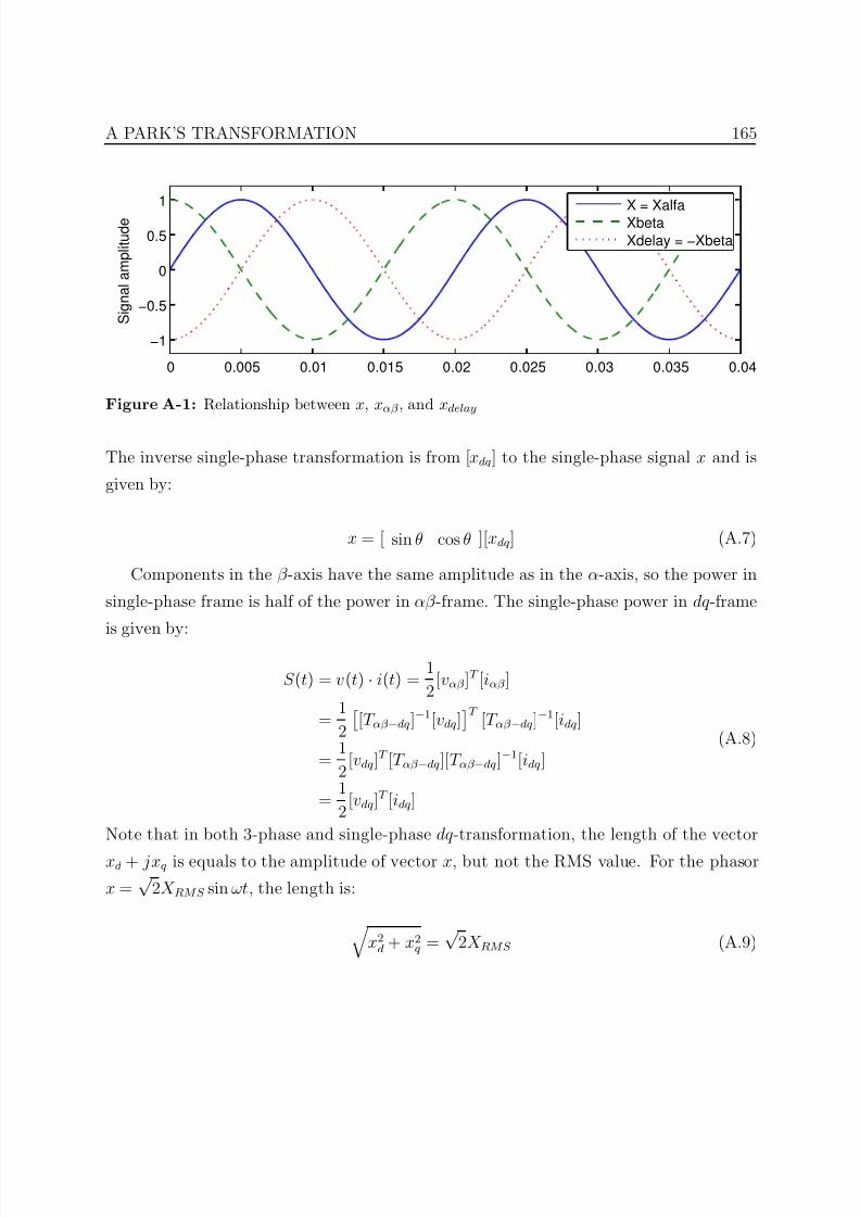
7/25/2019 Dpfc Thesis
http://slidepdf.com/reader/full/dpfc-thesis 187/212
A PARK’S TRANSFORMATION 165
0 0.005 0.01 0.015 0.02 0.025 0.03 0.035 0.04
−1
−0.5
0
0.5
1
S i g n a l a m p l i t u d e
X = Xalfa
Xbeta
Xdelay = −Xbeta
Figure A-1: Relationship between x, xαβ , and xdelay
The inverse single-phase transformation is from [xdq] to the single-phase signal x and is
given by:
x = [ sin θ cos θ ][xdq] (A.7)
Components in the β -axis have the same amplitude as in the α-axis, so the power in
single-phase frame is half of the power in αβ -frame. The single-phase power in dq -frame
is given by:
S (t) = v(t) · i(t) = 1
2[vαβ ]
T [iαβ ]
= 1
2
[T αβ −dq]−1[vdq]
T [T αβ −dq]−1[idq]
= 1
2[vdq]T [T αβ −dq][T αβ −dq]−1[idq]
= 1
2[vdq]T [idq]
(A.8)
Note that in both 3-phase and single-phase dq -transformation, the length of the vector
xd + jxq is equals to the amplitude of vector x, but not the RMS value. For the phasor
x =√
2X RMS sin ωt, the length is:
x2
d + x2q =
√ 2X RMS (A.9)

7/25/2019 Dpfc Thesis
http://slidepdf.com/reader/full/dpfc-thesis 188/212
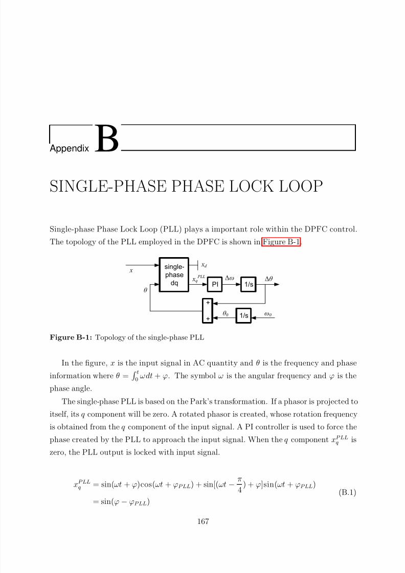
7/25/2019 Dpfc Thesis
http://slidepdf.com/reader/full/dpfc-thesis 189/212
Appendix BSINGLE-PHASE PHASE LOCK LOOP
Single-phase Phase Lock Loop (PLL) plays a important role within the DPFC control.
The topology of the PLL employed in the DPFC is shown in Figure B-1.
single-
phase
dq PI 1/s
x
xd
xq PLL ∆ω ∆θ
1/s
+
+ω0θ 0
θ
Figure B-1: Topology of the single-phase PLL
In the figure, x is the input signal in AC quantity and θ is the frequency and phase
information where θ = t0
ωdt + ϕ. The symbol ω is the angular frequency and ϕ is the
phase angle.
The single-phase PLL is based on the Park’s transformation. If a phasor is projected toitself, its q component will be zero. A rotated phasor is created, whose rotation frequency
is obtained from the q component of the input signal. A PI controller is used to force the
phase created by the PLL to approach the input signal. When the q component xP LLq is
zero, the PLL output is locked with input signal.
xP LLq = sin(ωt + ϕ)cos(ωt + ϕP LL) + sin[(ωt − π
4) + ϕ]sin(ωt + ϕP LL)
= sin(ϕ − ϕP LL)
(B.1)
167
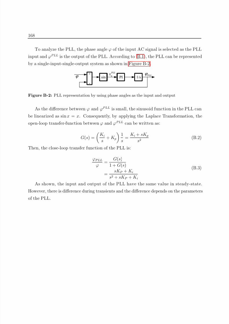
7/25/2019 Dpfc Thesis
http://slidepdf.com/reader/full/dpfc-thesis 190/212
168
To analyze the PLL, the phase angle ϕ of the input AC signal is selected as the PLL
input and ϕP LL is the output of the PLL. According to (B.1), the PLL can be representedby a single-input-single-output system as shown in Figure B-2.
PI 1/s+
-
sin PLLϕ
ϕ PLL
q x
Figure B-2: PLL representation by using phase angles as the input and output
As the difference between ϕ and ϕP LL is small, the sinusoid function in the PLL can
be linearized as sin x = x. Consequently, by applying the Laplace Transformation, the
open-loop transfer-function between ϕ and ϕP LL can be written as:
G(s) =
K is
+ K p
1
s =
K i + sK ps2
(B.2)
Then, the close-loop transfer function of the PLL is:
ϕP LL
ϕ =
G(s)
1 + G(s)
= sK P + K is2 + sK P + K i
(B.3)
As shown, the input and output of the PLL have the same value in steady-state.
However, there is difference during transients and the difference depends on the parameters
of the PLL.
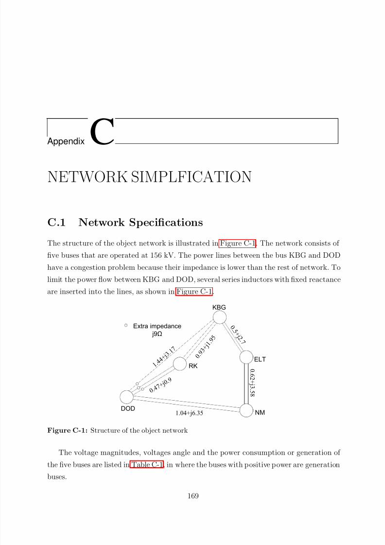
7/25/2019 Dpfc Thesis
http://slidepdf.com/reader/full/dpfc-thesis 191/212
Appendix CNETWORK SIMPLFICATION
C.1 Network Specifications
The structure of the object network is illustrated in Figure C-1. The network consists of
five buses that are operated at 156 kV. The power lines between the bus KBG and DOD
have a congestion problem because their impedance is lower than the rest of network. To
limit the power flow between KBG and DOD, several series inductors with fixed reactance
are inserted into the lines, as shown in Figure C-1.
KBG
RKELT
NMDOD
0 . 5 + j 2
. 7
0 . 6 2
+ j 3 . 5 8
1.04+j6.35
0 . 9 3
+ j 1 . 9 5
1. 4 4 + j 3.
1 7
0. 4 7 + j 0. 9
Extra impedance
j9Ω
Figure C-1: Structure of the object network
The voltage magnitudes, voltages angle and the power consumption or generation of
the five buses are listed in Table C-1, in where the buses with positive power are generation
buses.
169
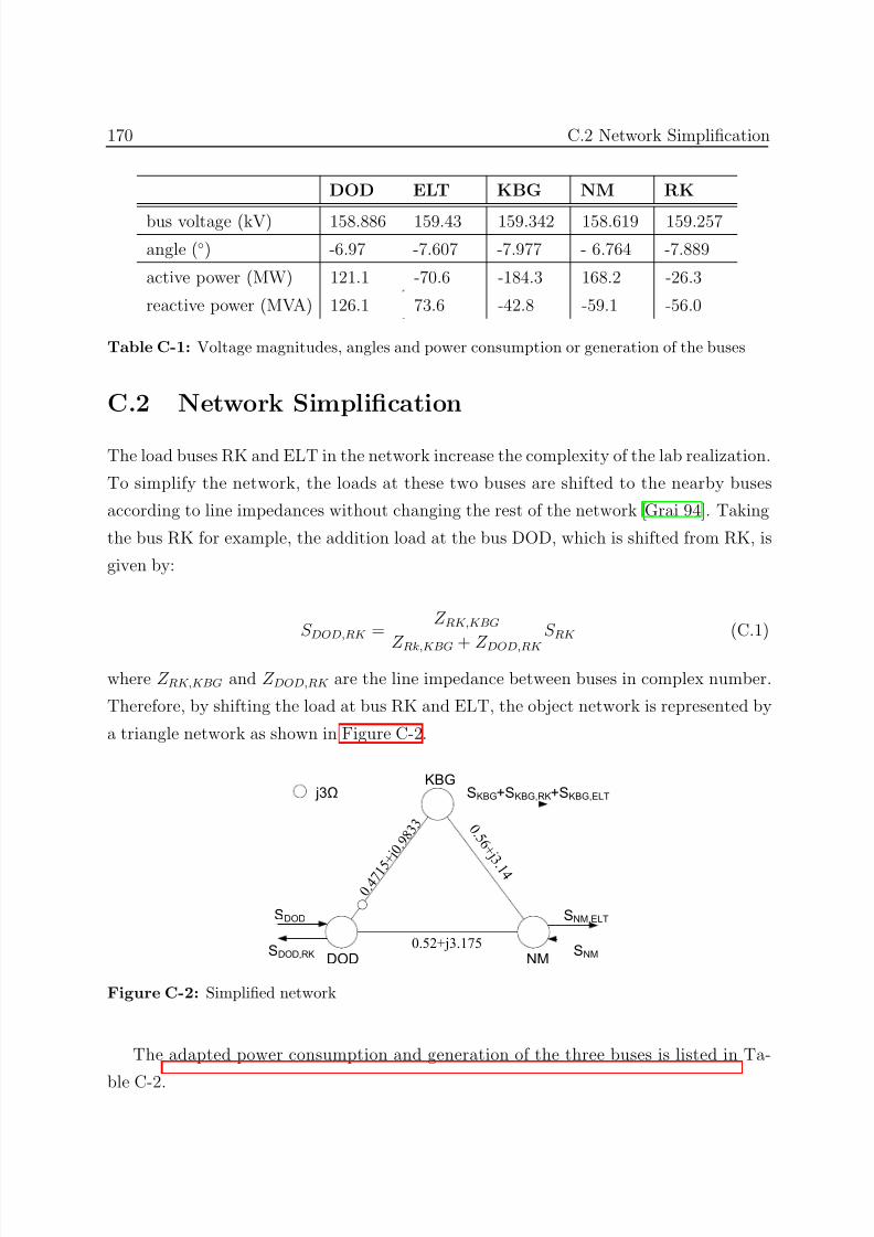
7/25/2019 Dpfc Thesis
http://slidepdf.com/reader/full/dpfc-thesis 192/212
170 C.2 Network Simplification
DOD ELT KBG NM RK
bus voltage (kV) 158.886 159.43 159.342 158.619 159.257
angle () -6.97 -7.607 -7.977 - 6.764 -7.889
active power (MW) 121.1 -70.6 -184.3 168.2 -26.3
reactive power (MVA) 126.1 73.6 -42.8 -59.1 -56.0
Table C-1: Voltage magnitudes, angles and power consumption or generation of the buses
C.2 Network Simplification
The load buses RK and ELT in the network increase the complexity of the lab realization.
To simplify the network, the loads at these two buses are shifted to the nearby buses
according to line impedances without changing the rest of the network [Grai 94]. Taking
the bus RK for example, the addition load at the bus DOD, which is shifted from RK, is
given by:
S DOD,RK = Z RK,KBG
Z Rk,KBG + Z DOD,RK
S RK (C.1)
where Z RK,KBG and Z DOD,RK are the line impedance between buses in complex number.
Therefore, by shifting the load at bus RK and ELT, the object network is represented by
a triangle network as shown in Figure C-2.
KBG
NMDOD0.52+j3.175
0 . 5 6 + j 3
. 1 4
0 . 4 7 1 5 +
j 0 . 9 8
3 3
j3Ω SKBG+SKBG,RK+SKBG,ELT
SDOD,RK
SDOD SNM,ELT
SNM
Figure C-2: Simplified network
The adapted power consumption and generation of the three buses is listed in Ta-
ble C-2.
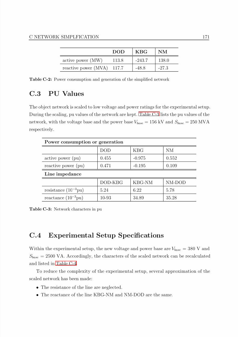
7/25/2019 Dpfc Thesis
http://slidepdf.com/reader/full/dpfc-thesis 193/212
C NETWORK SIMPLFICATION 171
DOD KBG NM
active power (MW) 113.8 -243.7 138.0
reactive power (MVA) 117.7 -48.8 -27.3
Table C-2: Power consumption and generation of the simplified network
C.3 PU Values
The object network is scaled to low voltage and power ratings for the experimental setup.
During the scaling, pu values of the network are kept. Table C-3 lists the pu values of the
network, with the voltage base and the power base V base = 156 kV and S base = 250 MVA
respectively.
Power consumption or generation
DOD KBG NM
active power (pu) 0.455 -0.975 0.552
reactive power (pu) 0.471 -0.195 0.109
Line impedance
DOD-KBG KBG-NM NM-DOD
resistance (10−3pu) 5.24 6.22 5.78
reactance (10−3pu) 10-93 34.89 35.28
Table C-3: Network characters in pu
C.4 Experimental Setup Specifications
Within the experimental setup, the new voltage and power base are V base = 380 V and
S base = 2500 VA. Accordingly, the characters of the scaled network can be recalculated
and listed in Table C-4.
To reduce the complexity of the experimental setup, several approximation of the
scaled network has been made:
• The resistance of the line are neglected.
• The reactance of the line KBG-NM and NM-DOD are the same.
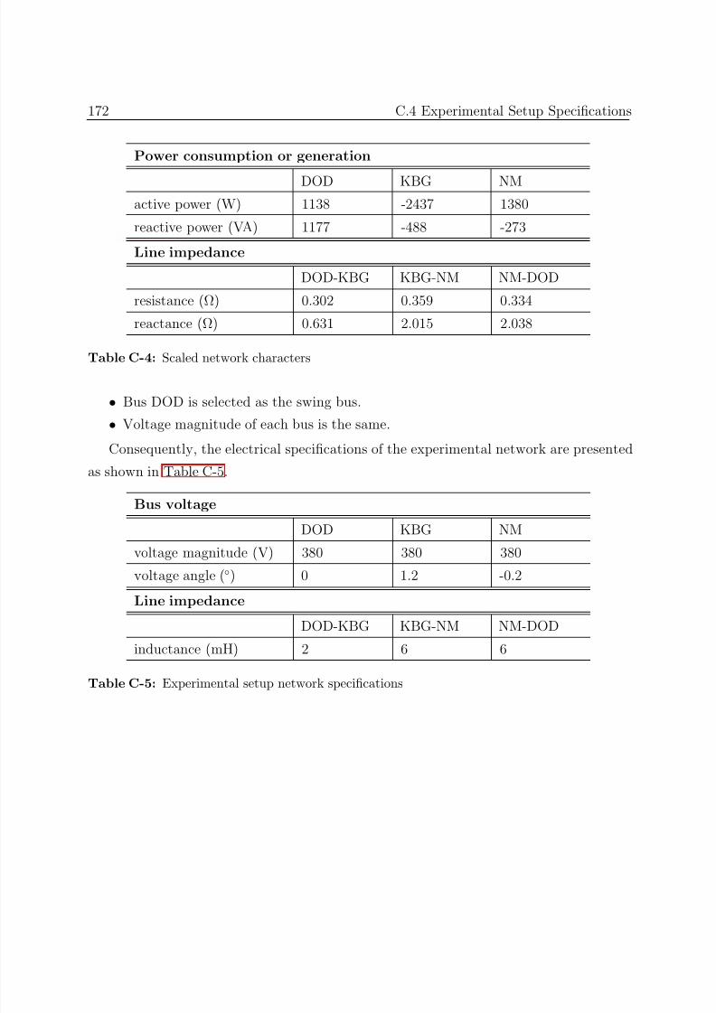
7/25/2019 Dpfc Thesis
http://slidepdf.com/reader/full/dpfc-thesis 194/212
172 C.4 Experimental Setup Specifications
Power consumption or generation
DOD KBG NM
active power (W) 1138 -2437 1380
reactive power (VA) 1177 -488 -273
Line impedance
DOD-KBG KBG-NM NM-DOD
resistance (Ω) 0.302 0.359 0.334
reactance (Ω) 0.631 2.015 2.038
Table C-4: Scaled network characters
• Bus DOD is selected as the swing bus.
• Voltage magnitude of each bus is the same.
Consequently, the electrical specifications of the experimental network are presented
as shown in Table C-5.
Bus voltage
DOD KBG NMvoltage magnitude (V) 380 380 380
voltage angle () 0 1.2 -0.2
Line impedance
DOD-KBG KBG-NM NM-DOD
inductance (mH) 2 6 6
Table C-5: Experimental setup network specifications
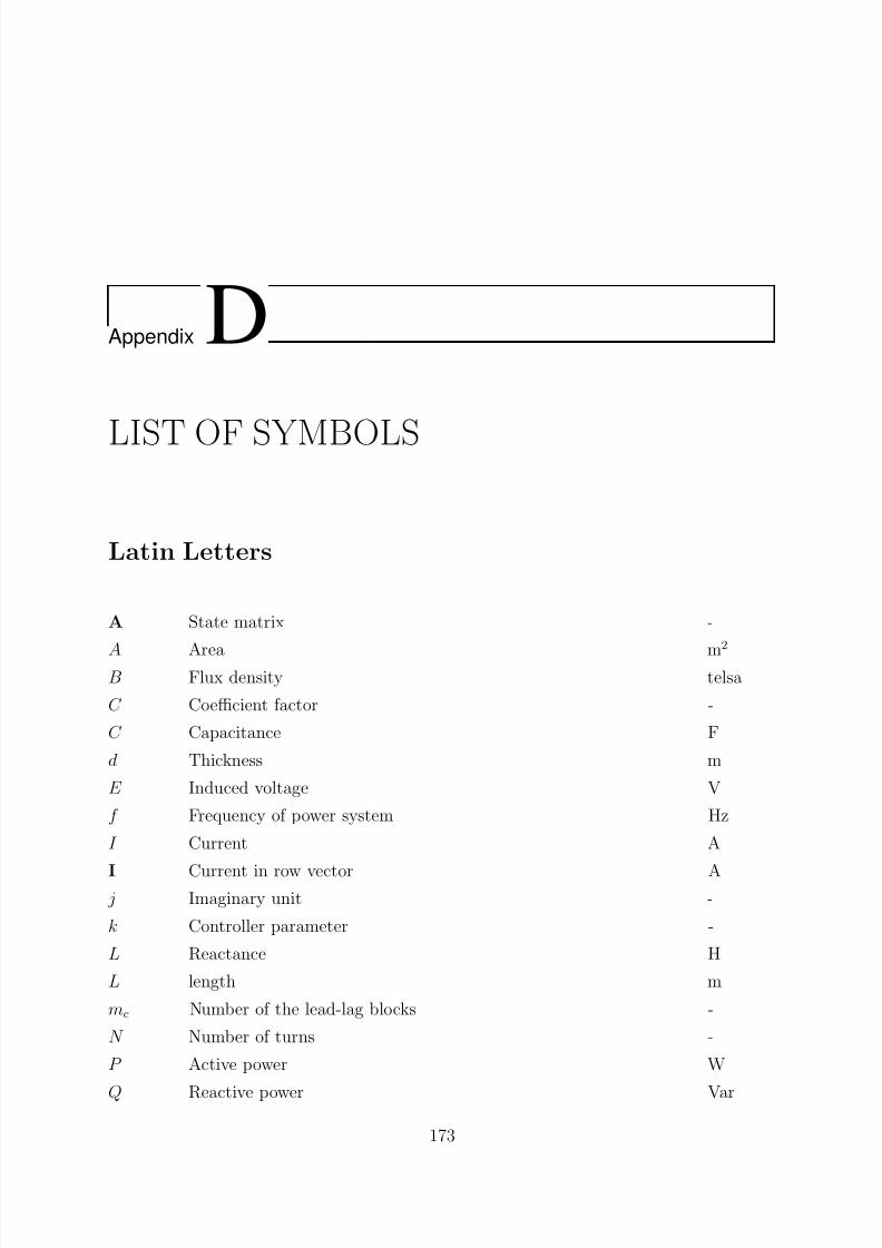
7/25/2019 Dpfc Thesis
http://slidepdf.com/reader/full/dpfc-thesis 195/212
Appendix D
LIST OF SYMBOLS
Latin Letters
A State matrix -
A Area m2
B Flux density telsa
C Coefficient factor -
C Capacitance F
d Thickness m
E Induced voltage V
f Frequency of power system Hz
I Current A
I Current in row vector A j Imaginary unit -
k Controller parameter -
L Reactance H
L length m
mc Number of the lead-lag blocks -
N Number of turns -
P Active power W
Q Reactive power Var
173
7/25/2019 Dpfc Thesis
http://slidepdf.com/reader/full/dpfc-thesis 196/212
174
R Resistance Ω
R Active damping in the IMC method -ref Reference signal -
ref Reference signal in row vector -
s Complex argument in Laplace transformation -
S Apparent power VA
t Time s
T dq Park’s transformation matrix -
∆u Single input -
V Voltage in phasor value V
V Voltage in row vector V
W Introduced variable in voltage control loop -
X Inductive impedance Ω
∆x State vector -
∆y Single output -
Z Impedance Ω
Greek Letters
α Desired bandwidth of the closed-loop -
θ Transmission angle
θ Angle of the rotation reference frame for Park’s transformation
ω Angular velocity rad/sϕ Power angle
ϕcomp Compensation angle of the POD controller
δ Phase angle of the impedance
λ Eigenvalue of the state matrix -
σ Damping of the oscillation mode -
ξ Relative damping ratio of the oscillation mode -
ρ Density kg/m3
Φ Flux weber
7/25/2019 Dpfc Thesis
http://slidepdf.com/reader/full/dpfc-thesis 197/212
D LIST OF SYMBOLS 175
Superscript
0 Zero sequence component
+ Positive sequence component
− Negative sequence component
P LL Phase lock loop component
Subscript
0 Initial value
1 The fundamental frequency component
3 The 3rd harmonic frequency component
a Phase a
abc abc domain
b Phase b
base Base for pu calculation
c Phase cc Magnetic core
c Control range
d d component in Park’s Transformation
D DOD bus
dc DC side
dq dq domain
gi Cross-section of a core
i ith harmonic frequency componenti Transmission line i
i Integral value for PID control
ii Transmission line ii
I Using current as rotation reference frame
K KBG bus
l Transmission line
lag Lagging time constant for POD controller
lead Leading time constant for POD controller
7/25/2019 Dpfc Thesis
http://slidepdf.com/reader/full/dpfc-thesis 198/212
7/25/2019 Dpfc Thesis
http://slidepdf.com/reader/full/dpfc-thesis 199/212
REFERENCES
[Abou 96] M. E. Aboul-Ela, A. A. Sallam, J. D. McCalley, and A. A. Fouad. “Damping
controller design for power system oscillations using global signals”. Power
Systems, IEEE Transactions on , 1996.
[Arsh 04] M. Arshad, S. M. Islam, and A. Khaliq. “Power transformer insulation re-
sponse and risk assessment”. In: Probabilistic Methods Applied to Power
Systems, International Conference on , 2004.
[Bark 00] P. P. Barker and R. W. De Mello. “Determining the impact of distributedgeneration on power systems. I. Radial distribution systems”. In: Power
Engineering Society Summer Meeting, IEEE , 2000.
[Baum 65] W. U. Baum and W. A. Frederick. “A method of applying switched and
fixed capacitors for voltage control”. Power Apparatus and Systems, IEEE
Transactions on , 1965.
[Bomp 08] E. Bompard and M. Yuchao. “Modeling bilateral electricity markets: a com-
plex network approach”. Power Systems, IEEE Transactions on , 2008.
[Bres 04] P. Bresesti, M. Sforna, V. Allegranza, D. Canever, and R. Vailati. “Applica-
tion of phase shifting transformers for a secure and efficient operation of the
interconnection corridors”. In: Power Engineering Society General Meeting,
IEEE , 2004.
[Cai 05] L. Cai and I. Erlich. “Simultaneous coordinated tuning of PSS and FACTS
damping controllers in large power systems”. Power Systems, IEEE Trans-
actions on , 2005.
177
7/25/2019 Dpfc Thesis
http://slidepdf.com/reader/full/dpfc-thesis 200/212
178 REFERENCES
[Chan 03] B. H. Chang, J. B. Choo, X. K. Xu, and B. P. Lam. “Steady-state Op-
erational Strategies of UPFC in the KEPCO Transmission System”. KIEE International Transactions on Power Engineering , 2003.
[Chin 07] M. Chindris, A. Cziker, A. Miron, H. Balan, A. Iacob, and A. Sudria. “Prop-
agation of unbalance in electric power systems”. In: Electrical Power Quality
and Utilisation, International Conference on , 2007.
[Choo 06] C. Y. Choo, N. K. C. Nair, and B. Chakrabarti. “Impacts of Loop Flow
on Electricity Market Design”. In: Power System Technology, International
Conference on , 2006.
[Davi 09] C. C. Davidson and G. de Preville. “The future of high power electronics in
Transmission and Distribution power systems”. In: Power Electronics and
Applications, European Conference on , 2009.
[De K 04] J. De Kock and C. Strauss. Practical power distribution for industry .
Newnes/Elsevier, 2004.
[Diva 05] D. Divan and H. Johal. “Distributed FACTS - A New Concept for RealizingGrid Power Flow Control”. In: Power Electronics Specialists Conference,
IEEE , 2005.
[Diva 07] D. Divan, E. B. William, S. S. Robert, K. Bill, W. G. Randal, T. B. Dale, R. I.
Michael, and S. G. Ian. “A distributed static series compensator system for
realizing active power flow control on existing power lines”. Power Delivery,
IEEE Transactions on , 2007.
[Duga 03] R. C. Dugan. Electrical power systems quality . McGraw-Hill, 2003.
[Edri 97] A. A. Edris. “Proposed terms and definitions for flexible AC transmission
system (FACTS)”. Power Delivery, IEEE Transactions on , 1997.
[Farh 09] H. Farhangi. “The path of the smart grid”. Power and Energy Magazine,
IEEE , 2009.
[Ferr 96] H. C. Ferreira, H. M. Grove, O. Hooijen, and A. J. Han Vinck. “Power line
communications: an overview”. In: AFRICON, IEEE , 1996.
7/25/2019 Dpfc Thesis
http://slidepdf.com/reader/full/dpfc-thesis 201/212
REFERENCES 179
[Fitz 03] A. E. Fitzgerald, C. Kingsley, and S. D. Umans. Electric machinery . McGraw-
Hill, 2003.
[Gamm 98] A. Z. Gamm and I. I. Golub. “Determination of locations for FACTS and
energy storage by the singular analysis”. In: Power System Technology, In-
ternational conference on , 1998.
[Garc 82] C. E. Garcia and M. Morari. “Internal model control. A unifying review and
some new results”. Industrial & Engineering Chemistry Process Design and
Development , 1982.
[Gerb 01] S. Gerbex, R. Cherkaoui, and A. J. Germond. “Optimal location of multi-type
FACTS devices in a power system by means of genetic algorithms”. IEEE
Power Engineering Review , 2001.
[Ghai 05] J. Ghaisari, A. Bakhshai, and P. K. Jain. “Power oscillations damping by
means of the SSSC: a multivariable control approach”. In: Electrical and
Computer Engineering, Canadian Conference on , 2005.
[Grai 94] J. J. Grainger and W. D. Stevenson. Power system analysis . McGraw-Hill,
1994.
[Gyug 00] L. Gyugyi. “Application characteristics of converter-based FACTS con-
trollers”. In: Power System Technology, International Conference on , 2000.
[Gyug 92] L. Gyugyi. “Unified power-flow control concept for flexible AC transmission
systems”. In: Generation, Transmission and Distribution, IEE Proceedings
Conference on , 1992.
[Gyug 94] L. Gyugyi. “Dynamic compensation of AC transmission lines by solid-statesynchronous voltage sources”. Power Delivery, IEEE Transactions on , 1994.
[Gyug 95] L. Gyugyi, C. D. Schauder, S. L. Williams, T. R. Rietman, D. R. Torgerson,
and A. Edris. “The unified power flow controller: a new approach to power
transmission control”. Power Delivery, IEEE Transactions on , 1995.
[Gyug 99] L. Gyugyi, K. K. Sen, and C. D. Schauder. “The interline power flow con-
troller concept: a new approach to power flow management in transmission
systems”. Power Delivery, IEEE Transactions on , 1999.
7/25/2019 Dpfc Thesis
http://slidepdf.com/reader/full/dpfc-thesis 202/212
180 REFERENCES
[Harn 98] L. Harnefors and H. P. Nee. “Model-based current control of AC machines us-
ing the internal model control method”. Industry Applications, IEEE Trans-actions on , 1998.
[Hing 00] N. G. Hingorani and L. Gyugyi. Understanding FACTS : concepts and tech-
nology of flexible AC transmission systems . IEEE Press, 2000.
[Huan 02] G. M. Huang and Y. Li. “Impact of thyristor controlled series capacitor
on bulk power system reliability”. In: Power Engineering Society Summer
Meeting, IEEE , 2002.
[Iked 05] Y. Ikeda and T. Kataoka. “A UPFC-based voltage compensator with current
and voltage balancing function”. In: Applied Power Electronics Conference
and Exposition, IEEE , 2005.
[Juli 99] A. L. Julian, G. Oriti, and T. A. Lipo. “Elimination of common-mode volt-
age in three-phase sinusoidal power converters”. Power Electronics, IEEE
Transactions on , 1999.
[Kann 04] S. Kannan, S. Jayaram, and M. M. A. Salama. “Real and reactive power co-
ordination for a unified power flow controller”. Power Systems, IEEE Trans-
actions on , 2004.
[Kim 05] S. Y. Kim, J. S. Yoon, B. H. Chang, and D. H. Baek. “The operation experi-
ence of KEPCO UPFC”. In: Electrical Machines and Systems, International
Conference on , 2005.
[Klei 91] M. Klein, G. J. Rogers, and P. Kundur. “A fundamental study of inter-area
oscillations in power systems”. Power Systems, IEEE Transactions on , 1991.
[Kuan 07] L. Kuang, L. Jinjun, W. Zhaoan, and W. Biao. “Strategies and Operating
Point Optimization of STATCOM Control for Voltage Unbalance Mitigation
in Three-Phase Three-Wire Systems”. Power Delivery, IEEE Transactions
on , 2007.
[Kund 94] P. Kundur, N. J. Balu, and M. G. Lauby. Power system stability and control .
McGraw-Hill, 1994.
7/25/2019 Dpfc Thesis
http://slidepdf.com/reader/full/dpfc-thesis 203/212
REFERENCES 181
[Lee 03] C. K. Lee, J. S. K. Leung, S. Y. R. Hui, and H. S. H. Chung. “Circuit-level
comparison of STATCOM technologies”. Power Electronics, IEEE Transac-tions on , 2003.
[Maha 06] V. Mahajan. “Thyristor Controlled Series Compensator”. In: Industrial
Technology, IEEE International Conference on , 2006.
[McDo 94] D. J. McDonald, J. Urbanek, and B. L. Damsky. “Modeling and testing
of a thyristor for thyristor controlled series compensation (TCSC)”. Power
Delivery, IEEE Transactions on , 1994.
[Mhas 06] U. P. Mhaskar and A. M. Kulkarni. “Power oscillation damping using FACTS
devices: modal controllability, observability in local signals, and location of
transfer function zeros”. Power Systems, IEEE Transactions on , 2006.
[Milo 06] M. Milosevic, G. Andersson, and S. Grabic. “Decoupling Current Control and
Maximum Power Point Control in Small Power Network with Photovoltaic
Source”. In: Power Systems Conference and Exposition, IEEE , 2006.
[Moha 03] N. Mohan, T. M. Undeland, and W. P. Robbins. Power electronics : con-
verters, applications, and design . John Wiley & Sons, 2003.
[Moor 95] P. Moore and P. Ashmole. “Flexible AC transmission systems”. Power En-
gineering Journal , 1995.
[Morr 06] J. Morren. Grid support by power electronic converters of distributed gener-
ation units . PhD thesis, TU Delft, 2006.
[Nahm 93] J. Nahman and V. Dordevic. “Distribution of zero sequence currents for earth
faults occurring along a transmission line and proximity effects”. Generation,Transmission and Distribution, IEE , 1993.
[Namh 01] H. Namho, J. Jinhwan, and N. Kwanghee. “A fast dynamic DC-link power-
balancing scheme for a PWM converter-inverter system”. Industrial Electron-
ics, IEEE Transactions on , 2001.
[Noha 07] K. Nohara, A. Ueda, A. Torii, and D. Kae. “Compensating Characteristics of
a Series-Shunt Active Power Filter Considering Unbalanced Source Voltage
and Unbalanced Load”. In: Power Conversion Conference , 2007.
7/25/2019 Dpfc Thesis
http://slidepdf.com/reader/full/dpfc-thesis 204/212
182 REFERENCES
[Nune 01] C. Nunez, V. Cardenas, G. Alarcon, and M. Oliver. “Voltage disturbances
and unbalance compensation by the use of a 3-phase series active filter”. In:Power Electronics Specialists Conference, IEEE , 2001.
[Otte 03] R. Ottersten. On control of back-to-back converters and sensorless induction
machine drives . PhD thesis, Chalmers University of Technology, 2003.
[Pal 05] B. Pal and B. Chaudhuri. Robust control in power systems . Springer, 2005.
[Papi 97] I. Papic, P. Zunko, D. Povh, and M. Weinhold. “Basic control of unified
power flow controller”. Power Systems, IEEE Transactions on , 1997.
[Para 02] P. N. Paraskevopoulos. Modern control engineering . Marcel Dekker, 2002.
[Park 09] S. P. Parker. Mcgraw-hill Dictionary of Scientific and Technical Terms .
McGraw-Hill, 2009.
[Pedr 05] J. Pedra, L. Sainz, F. Corcoles, and L. Guasch. “Symmetrical and unsym-
metrical voltage sag effects on three-phase transformers”. Power Delivery,IEEE Transactions on , 2005.
[Pete 05] A. Petersson. Analysis, modeling and control of doubly-fed induction gen-
erators for wind turbines . PhD thesis, Chalmers University of Technology,
2005.
[Pill 03] G. N. Pillai, A. Ghosh, and A. Joshi. “Torsional interaction studies on a
power system compensated by SSSC and fixed capacitor”. Power Delivery,
IEEE Transactions on , 2003.
[Putt 03] H. B. Puttgen, P. R. MacGregor, and F. C. Lambert. “Distributed generation:
Semantic hype or the dawn of a new era?”. Power and Energy Magazine,
IEEE , 2003.
[Qing 04] Y. Qingguang, L. Pei, L. Wenhua, and X. Xiaorong. “Overview of STATCOM
technologies”. In: Electric Utility Deregulation, Restructuring and Power
Technologies, IEEE Conference on , 2004.
7/25/2019 Dpfc Thesis
http://slidepdf.com/reader/full/dpfc-thesis 205/212
REFERENCES 183
[Rahm 97] M. Rahman, M. Ahmed, R. Gutman, R. J. O’Keefe, R. J. Nelson, and
B. Jianhua. “UPFC application on the AEP system: planning considera-tions”. Power Systems, IEEE Transactions on , 1997.
[Renz 99] B. A. Renz, A. Keri, A. S. Mehraban, C. Schauder, E. Stacey, L. Kovalsky,
L. Gyugyi, and A. Edris. “AEP unified power flow controller performance”.
Power Delivery, IEEE Transactions on , 1999.
[Roge 00a] G. J. Rogers. “The application of power system stabilizers to a multigenerator
plant”. Power Systems, IEEE Transactions on , 2000.
[Roge 00b] G. J. Rogers. Power system oscillations . Kluwer Academic, 2000.
[Sadi 05] R. Sadikovic, P. Korba, and G. Andersson. “Application of FACTS devices
for damping of power system oscillations”. In: Power Tech, IEEE , 2005.
[Sadi 06] R. Sadikovic. Use of FACTS devices for power flow control and damping of
oscillations in power systems . PhD thesis, ETH, Zrich, 2006.
[Sala 04] J. Salaet, S. Alepuz, A. Gilabert, and J. Bordonau. “Comparison between two
methods of DQ transformation for single phase converters control. Applica-
tion to a 3-level boost rectifier”. In: Power Electronics Specialists Conference,
IEEE , 2004.
[Sant 08] R. M. Santos Filho, P. F. Seixas, P. C. Cortizo, L. A. B. Torres, and A. F.
Souza. “Comparison of Three Single-Phase PLL Algorithms for UPS Appli-
cations”. Industrial Electronics, IEEE Transactions on , 2008.
[Scha 98] C. Schauder, E. Stacey, M. Lund, L. Gyugyi, L. Kovalsky, A. Keri, A. Mehra-ban, and A. Edris. “AEP UPFC project: installation, commissioning and
operation of the 160 MVA STATCOM (phase I)”. Power Delivery, IEEE
Transactions on , 1998.
[Sebo 69] S. A. Sebo. “Zero-Sequence Current Distribution Along Transmission Lines”.
Power Apparatus and Systems, IEEE Transactions on , 1969.
[Sen 98] K. K. Sen. “SSSC-static synchronous series compensator: theory, modeling,
and application”. Power Delivery, IEEE Transactions on , 1998.
7/25/2019 Dpfc Thesis
http://slidepdf.com/reader/full/dpfc-thesis 206/212
184 REFERENCES
[Shin 08] S. Shinji. “A Robust Single-Phase PLL System With Stable and Fast Track-
ing”. Industry Applications, IEEE Transactions on , 2008.
[Sing 09] B. Singh, R. Saha, A. Chandra, and K. Al-Haddad. “Static synchronous
compensators (STATCOM): a review”. Power Electronics, IET , 2009.
[Sloo 09] H. Slootweg. “Smart Grids - the future or fantasy?”. In: Smart Metering -
Making It Happen, IET , 2009.
[Soar 00] V. Soares, P. Verdelho, and G. D. Marques. “An instantaneous active and
reactive current component method for active filters”. Power Electronics,
IEEE Transactions on , 2000.
[Song 03] Y. H. Song and X. F. Wang. Operation of market-oriented power systems .
Springer, 2003.
[Song 99] Y. H. Song and A. Johns. Flexible ac transmission systems (FACTS). Insti-
tution of Electrical Engineers, 1999.
[Soo 98] H. Soo-Bin, C. Gyu-Hyeong, J. Bong-Man, and C. Soo-Hyun. “Vector-
transformed circuit theory and application to converter modeling/analysis”.In: Power Electronics Specialists Conference, IEEE , 1998.
[Than 79] H. L. Thanawala, W. P. Williams, and D. J. Young. “Static Reactive Com-
pensators for Ac Power Transmission - 10 Years Operational Experience with
Saturated Reactors”. Gec-Journal of Science & Technology , 1979.
[Thap 90] B. Thapar, V. Gerez, and A. Balakrishnan. “Zero-sequence impedance of
overhead transmission lines with discontinuous ground wire”. In: Power
Symposium, 1990. Proceedings of the Twenty-Second Annual North American ,pp. 190–192, 1990.
[Van 05] D. Van Hertem, J. Verboomen, R. Belmans, and W. L. Kling. “Power flow
controlling devices: an overview of their working principles and their applica-
tion range”. In: Future Power Systems, International Conference on , 2005.
[Vasq 08] R. L. Vasquez Arnez. “The Interline Power Flow Controller: Further as-
pects related to its operation and main limitations”. In: Transmission and
Distribution Conference and Exposition, IEEE/PES , 2008.
7/25/2019 Dpfc Thesis
http://slidepdf.com/reader/full/dpfc-thesis 207/212
REFERENCES 185
[Verb 05] J. Verboomen, D. Van Hertem, P. H. Schavemaker, W. L. Kling, and R. Bel-
mans. “Phase shifting transformers: principles and applications”. In: Future Power Systems, International Conference on , 2005.
[Verm 04] A. K. Verma, A. Srividya, and B. l. C. Deka. “Impact of a FACTS controller
on reliability of composite power generation and transmission system”. Elec-
tric Power Systems Research , 2004.
[Wei 03] W. Wei and W. Chikong. “FACTS applications in preventing loop flows in
interconnected systems”. In: Power Engineering Society General Meeting,
IEEE , 2003.
[Yoon 03] J. S. Yoon, S. Y. Kim, B. H. Chang, S. J. Lim, and J. Choo. “Modeling
and analysis of the KEPCO UPFC system by EMTDC/PSCAD”. KIEE
International Transactions on Power Engineering , 2003.
[Zhan 02] R. Zhang, M. Cardinal, P. Szczesny, and M. Dame. “A grid simulator with
control of single-phase power converters in D-Q rotating frame”. In: Power
Electronics Specialists Conference, IEEE , 2002.
[Zhan 06] X. P. Zhang, C. Rehtanz, and B. Pal. Flexible AC transmission systems
modelling and control . Springer, 2006.

7/25/2019 Dpfc Thesis
http://slidepdf.com/reader/full/dpfc-thesis 208/212
7/25/2019 Dpfc Thesis
http://slidepdf.com/reader/full/dpfc-thesis 209/212
LIST OF PUBLICATIONS
Patent
1. Yuan, Z.; de Haan, S.W.H.; Ferreira, B.: “Power Flow Controller”, Patent, WO
2008/153376 A1.
Journal Papers
1. Yuan, Z.; de Haan, S.W.H.; Ferreira, B.: “A FACTS Device - Distributed Power
Flow Controller (DPFC)”, Power Electronics, IEEE Transactions on, 2010.
2. Cvoric, D.; de Haan, S.W.H.; Ferreira, B.; Yuan, Z.; “New Three-Phase Inductive
FCL with Common Core and Trifilar Windings”, Power Delivery, IEEE Transac-
tions on, 2010.
Conference Papers
1. Yuan, Z.; de Haan, S.W.H.; Ferreira, B.: “UPFC with Eliminated Common DC
Link Connection between Shunt and Series Part”, IEEE Power Engineering SocietyGeneral Meeting (PESGM) 2007, Tampa, USA.
2. Yuan, Z.; de Haan, S.W.H.; Ferreira, B.: “A New FACTS Component - Distributed
Power Flow Controller (DPFC)”, European Conference on Power Electronics and
Applications (EPE) 2007, Aalborg, Denmark.
3. Yuan, Z.; de Haan, S.W.H.; Ferreira, B.: “A Method of Transmitting Active Power
Between Converters with Eliminated Common DC Link”, IEEE Benelux Young
Research Symposium in Electrical Power Engineering 2008, Eindhoven, the Nether-
lands.
187
7/25/2019 Dpfc Thesis
http://slidepdf.com/reader/full/dpfc-thesis 210/212
188
4. Yuan, Z.; de Haan, S.W.H.; Ferreira, B.: “A New Concept of Exchanging Active
Power without Common DC Link for Interline Power Flow Controller (S-IPFC)” ,IEEE Power and Energy Society General Meeting (PESGM) 2008, Pittsburgh,
USA.
5. Yuan, Z.; de Haan, S.W.H.; Ferreira, B.: “A Method to Synchronize Single-phase
Floating with Grid without High Voltage Measurement or High Bandwidth Commu-
nication”, IEEE Power and Energy Society PowerTech 2009, Bucharest, Romania.
6. Yuan, Z.; de Haan, S.W.H.; Ferreira, B.: “Utilizing Distributed Power Flow Con-
troller (DPFC) for Power Oscillation Damping”, IEEE Power and Energy Society
General Meeting (PESGM) 2009, Calgary, Canada.7. Yuan, Z.; de Haan, S.W.H.; Ferreira, B.: “Construction and First Result of a Scaled
Transmission System with the Distributed Power Flow Controller (DPFC)”, Euro-
pean Conference on Power Electronics and Applications (EPE) 2009, Barcelona,
Spain.
8. Yuan, Z.; de Haan, S.W.H.; Ferreira, B.: “DPFC Control during Shunt Converter
Failure”, IEEE Energy Conversion Congress and Exposition (ECCE) 2009, San
Jose, USA.
9. Yuan, Z.; de Haan, S.W.H.; Ferreira, B.; Cvoric, D.: “Utilize Distributed Power
Flow Controller (DPFC) to Compensate Unbalanced 3-phase Currents in Trans-
missions Systems”, Electric Power and Energy Conversion Systems (EPECS) 2009,
Sharjah, United Arab Emirates.
10. Yuan, Z.; de Haan, S.W.H.; Ferreira, B.: “DPFC design Procedure - a Case Study
Using the KEPCO UPFC as an Example”, International Power Electronics Con-
ference (IPEC) 2010, Sapporo, Japan.
11. Yuan, Z.; de Haan, S.W.H.; Ferreira, B.: “Control Scheme to Improve DPFC
Performance during Series Converter Failures”, IEEE Power and Energy Society
General Meeting (PESGM) 2010, Minneapolis, USA.
7/25/2019 Dpfc Thesis
http://slidepdf.com/reader/full/dpfc-thesis 211/212
CURRICULUM VITAE
ZHIHUI YUAN was born in Hei Long Jiang, China, on 24 Nov 1981. In 2004, he
got his Bachelor of Science degree from Harbin Institute of Technology, majored inElectrical Engineering and Automation.
At the same year, he went to Sweden for the master degree in Chalmers Technology
University. He did his master final thesis in the Power System Group, ETH, Zurich. In
2006, he received the Master of Science degree in Electrical Power Engineering.
Since 2006, he began to work toward his PhD degree in the Electrical Power Processing
(EPP) group, in Delft University of Technology, in the Netherlands. The title of his PhD
project is ‘Active power control in utility grid’, which aims at the development of new,
relatively low-cost methods for power flow control without sacrificing system reliability.This research has been granted a WO patent.
His research interests include Flexible AC Transmission Systems, power system oper-
ation and the grid integration of renewable energy.
189

7/25/2019 Dpfc Thesis
http://slidepdf.com/reader/full/dpfc-thesis 212/212