Development of a Wind Turbine

Rotor Flow Panel Method

A. van Garrel

ECN-E--11-071 DECEMBER 2011

2 ECN-E--11-071

AcknowledgementHet project is uitgevoerd met subsidie van het Ministerie van Economische Zaken, Landbouw en Innovatie, regeling EOS: Lange Termijn uitgevoerd door Agentschap NL. Project naam: ROTORFLOW-1Contract nummer: EOSLT02016

Abstract

The ongoing trend towards larger wind turbines intensifies the demand for more physically realistic wind turbine rotor aerodynamics models that can predict the detailed transient pressure loadings on the rotor blades better than current engineering models. In this report the mathematical, numerical, and practical aspects of a new wind turbine rotor flow simulation code is described. This wind turbine simulation code is designated ROTORFLOW. In this method the fluid dynamics problem is solved through a boundary integral equation which reduces the problem to the surface of the configuration. The derivation of the integral equations is described as well as the assumptions made to arrive at them starting with the full Navier-Stokes equations. The basic numerical aspects in the solution method are described and a verification study is performed to confirm the validity of the implementation. Example simulations with the code show the flow solutions for a stationary wing and for a rotating wing in yawed conditions.

With the ROTORFLOW code developed in this project it is possible to simulate the unsteady flow around wind turbine rotors in yawed conditions and obtain detailed pressure distributions, and thus blade loadings, at the surface of the blades. General rotor blade geometries can be handled, opening the way to the detailed flow analysis of winglets, partial span flaps, swept blade tips, etc. The ROTORFLOW solver only requires a description of the rotor surface which keeps simulation preparation time short, and makes it feasible to use the solver in the design iteration process.

Contents

Contents 3

Nomenclature 5

1 Introduction 7

2 Potential Flow Model 9

2.1 Introduction 9

2.2 Governing Equations 10

2.3 Boundary Integral Equation 11

2.4 Boundary Conditions 12

2.4.1 Body Surface 13

2.4.2 Wake Surface 14

2.5 Aerodynamic Forces 15

3 Numerical Approach 17

3.1 Geometry 17

3.2 Panel Method 17

3.2.1 Dipole Velocity Potential 18

3.2.2 Source Velocity Potential 19

3.2.3 Dipole Surface Gradient Velocity 20

4 Verification 21

4.1 Analytical Solution 21

4.2 Geometric Convergence 22

4.3 Velocity Potential Convergence 25

4.3.1 Single Patch Grid 25

4.3.2 Six Patch Grid 28

4.4 Presssure Coefficient Convergence 30

4.4.1 Single Patch Grid 30

4.4.2 Six Patch Grid 32

5 Application 35

5.1 Lifting wing in steady flow 35

5.2 Rotating wing in unsteady flow 35

References 38

A Mathematical Compendium 39

B Conservation Laws 42

B.1 Mass Conservation 42

B.2 Momentum Conservation 43

3

B.3 Energy Conservation 45

C Boundary Integral Equation 49

4 ECN-E--11-071

Nomenclature

Dimensions

[ l ] length[ m ] mass[ t ] time

Roman symbols

g [ l t−2 ] gravitational accelerationh [ l ] height, characteristic panel lengthp [ m l−1 t−2 ] pressureS [ l2 ] surfaceV [ l3 ] volume∂S [ l ] surface boundary∂V [ l2 ] volume boundary

Greek symbols

Φ [ l2 t−1 ] velocity potentialϕ [ l2 t−1 ] velocity perturbation potentialµ [ l2 t−1 ] dipole strengthρ [ m l−3 ] mass densityσ [ l t−1 ] source strength

Tensors, matrices and vectors

~g [ l t−2 ] gravitational acceleration vectorn [ – ] unit surface normal vector¯τ [ m l−1 t−2 ] viscous stress tensorτ [ – ] unit tangential vector~u [ l t−1 ] velocity vector~x [ l ] coordinate vector

5

Subscripts, superscripts and accents

( )∞ onset flow value( )n value in surface normal direction( )S value at the surface( )T transpose operator( )te value at the trailing edge( )W value at the wake surface( )µ value from dipole singularity( )σ value from source singularity( )+ value at fluid side( )− value at internal side~( ) vector( ) vector of unit length

6 ECN-E--11-071

1. Introduction

The ongoing trend in wind turbine design is towards larger turbines, leading to increasing in-vestment costs and related concerns regarding risk mitigation. The increase in size also leads torelatively more flexible structures that are more susceptible to unsteady load occurrences. An im-portant aspect of wind turbine rotor aerodynamics is the inherent unsteady character of the flowcaused by variations in wind speed and direction, irregularrotational speed, blade pitch actions,rotor yaw misalignment, blade deformations and the dynamiccharacter of the wake behind the ro-tor, to name a few. All this increases the need for wind turbine aerodynamics simulation tools thatcan predict the effects of unsteady flow on the pressure loading on the wind turbine rotor blades.The application of such a simulation tool in an engineering environment requires computationtimes and problem turnover times to be reasonable.

In current engineering practice the wind turbine blade loading is estimated using experimentallydetermined 2D airfoil characteristics for steady flow in combination with approximations for thelocal ’effective’ onset velocity field and approximating models to compensate for unaccountedunsteady and 3D effects. This 2D approach is computationally very fast but becomes more andmore questionable with increasing 3D flow and geometry characteristics. Example situations inwhich 3D modelling capabilities become indispensable include cases with blade rotation, bladepitch, blade sweep, rotor yaw misalignment, blade prebend,winglets, local aerodynamic controlsurfaces, etc.

One approach to account for the unsteady effects and the three-dimensional character of the flowproblem is the deployment of solvers for the 3D unsteady Navier-Stokes equations which can inprinciple generate solutions for general 3D unsteady viscous flows. A drawback of this approachhowever is the large effort that is required to setup a simulation and the excessive computationaltime to obtain a solution.

Inviscid flow

Viscous flow

~u

~u

Figure 1.1: Domain decomposition into an inviscid flow region and a viscous flow region.

The approach taken here is to combine the advantages of abovetwo approaches and developa solution method capable of providing detailed unsteady 3Dwind turbine rotor flow solutionswhile avoiding excessive computational costs. To this end the flow domain is decomposed intotwo subdomains: an outer region in which the flow is considered incompressible and inviscidand is formulated in terms of a potential flow solver, and an inner region where the effects ofviscosity will be taken into account by an integral boundarylayer solver (see Van Garrel [8]) assketched in Figure 1.1. The two domains will be coupled through a so-called viscous-inviscidinteraction procedure. Both the development of the boundary layer solver (Özdemir and Van denBoogaard [13]) and the viscous-inviscid interaction procedure (Bijleveld and Veldman [4]) are

7

currently underway at ECN.

In this report the development of the potential flow solver for incompressible, inviscid 3D flows isdiscussed. The code under development will be referred to asROTORFLOW.

The mathematical theory that forms the basis of flow field description for the incompressibleinviscid flow in the outer region of the ROTORFLOW code is described in Chapter 2.

In Chapter 3 some specific topics in the discretization of themathematical model will be discussed.

Some basic verification tests are reported in Chapter 4 for two grid types of a tri-axial ellipsoidand the order of convergence will be established for this geometry.

Finally, in Chapter 5 some applications of the ROTORFLOW code for lifting bodies are shown.

8 ECN-E--11-071

2. Potential Flow Model

The mathematical model for the three-dimensional unsteadyflow around wind turbine rotors isconsidered. The flow is assumed to be incompressible and the effects of viscosity are assumed tobe confined to thin boundary layer and wake regions due to the high operational Reynolds num-bers. Outside these regions the flow is assumed to be irrotational. The effects of heat conductionare considered negligible. The main area of interest lies inthe detailed prediction of the unsteadypressure loading on the wind turbine rotor blades as occurring during normal operation. An ac-curate representation of the wake behind the rotor is of interest for its influence on the flowfieldaround the upstream rotor blades.

Above observations and assumptions make it justifiable to model the flow around wind turbinerotors with the fluid dynamics equations for unsteady potential flow. These equations will be castin a boundary integral equation form.

2.1. Introduction

A continuously differentiable flowfield around an arbitrarybody in 3D space can be described interms of velocity vector~u(~x) or equivalently in terms of sourceσ(~x) and vorticity~ω(~x) distribu-tions throughout the volume plus an irrotational and solenoidal onset flow~u∞(~x) as depicted inFigure 2.1.

x

y

z

~ω

σ

~ω = ~∇× ~u

σ = ~∇ · ~u

~u ~u = ~u∞ + ~uσ + ~uω

~uσ = 14π

∫∫∫

σ~rr3dV

~uω = 14π

∫∫∫

~ω×~rr3 dV

Figure 2.1: Flowfield representation in terms of velocity vector field~u(~x) or in terms of sourcesσ(~x) and vorticesω(~x).

An approximation to the volumetric source and vorticity distributions is to restrict them to the bodyand wake surfaces as indicated in Figure 2.2 which will lead to divergence free and irrotationalflow everywhere except across these surfaces. The resultingboundary integral equations can besolved with a so called panel method in which the surface of the configuration is covered withpanels where boundary conditions are imposed in selected points.

9

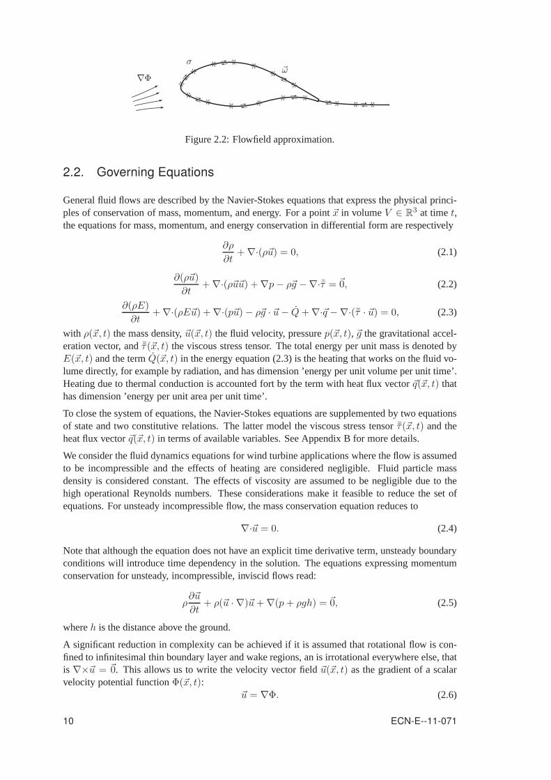
PSfragσ

~ω∇Φ

Figure 2.2: Flowfield approximation.

2.2. Governing Equations

General fluid flows are described by the Navier-Stokes equations that express the physical princi-ples of conservation of mass, momentum, and energy. For a point ~x in volumeV ∈ R

3 at timet,the equations for mass, momentum, and energy conservation in differential form are respectively

∂ρ

∂t+∇·(ρ~u) = 0, (2.1)

∂(ρ~u)

∂t+∇·(ρ~u~u) +∇p− ρ~g −∇·¯τ = ~0, (2.2)

∂(ρE)

∂t+∇·(ρE~u) +∇·(p~u)− ρ~g · ~u− Q+∇·~q −∇·(¯τ · ~u) = 0, (2.3)

with ρ(~x, t) the mass density,~u(~x, t) the fluid velocity, pressurep(~x, t), ~g the gravitational accel-eration vector, andτ(~x, t) the viscous stress tensor. The total energy per unit mass is denoted byE(~x, t) and the termQ(~x, t) in the energy equation (2.3) is the heating that works on the fluid vo-lume directly, for example by radiation, and has dimension ’energy per unit volume per unit time’.Heating due to thermal conduction is accounted fort by the term with heat flux vector~q(~x, t) thathas dimension ’energy per unit area per unit time’.

To close the system of equations, the Navier-Stokes equations are supplemented by two equationsof state and two constitutive relations. The latter model the viscous stress tensor¯τ(~x, t) and theheat flux vector~q(~x, t) in terms of available variables. See Appendix B for more details.

We consider the fluid dynamics equations for wind turbine applications where the flow is assumedto be incompressible and the effects of heating are considered negligible. Fluid particle massdensity is considered constant. The effects of viscosity are assumed to be negligible due to thehigh operational Reynolds numbers. These considerations make it feasible to reduce the set ofequations. For unsteady incompressible flow, the mass conservation equation reduces to

∇·~u = 0. (2.4)

Note that although the equation does not have an explicit time derivative term, unsteady boundaryconditions will introduce time dependency in the solution.The equations expressing momentumconservation for unsteady, incompressible, inviscid flowsread:

ρ∂~u

∂t+ ρ(~u · ∇)~u+∇(p+ ρgh) = ~0, (2.5)

whereh is the distance above the ground.

A significant reduction in complexity can be achieved if it isassumed that rotational flow is con-fined to infinitesimal thin boundary layer and wake regions, an is irrotational everywhere else, thatis ∇×~u = ~0. This allows us to write the velocity vector field~u(~x, t) as the gradient of a scalarvelocity potential functionΦ(~x, t):

~u = ∇Φ. (2.6)

10 ECN-E--11-071

Substitution of the velocity potential gradient (2.6) in the continuity equation (2.4) gives theLaplace equation for the velocity potential in domainV :

∇·∇Φ = 0. (2.7)

Substituting the gradient of the velocity potential (2.6) in the momentum conservation equa-tions (2.5) results in the Bernoulli equation for unsteady potential flow:

∂Φ

∂t+

1

2∇Φ · ∇Φ+

p

ρ+ gh = C(t). (2.8)

2.3. Boundary Integral Equation

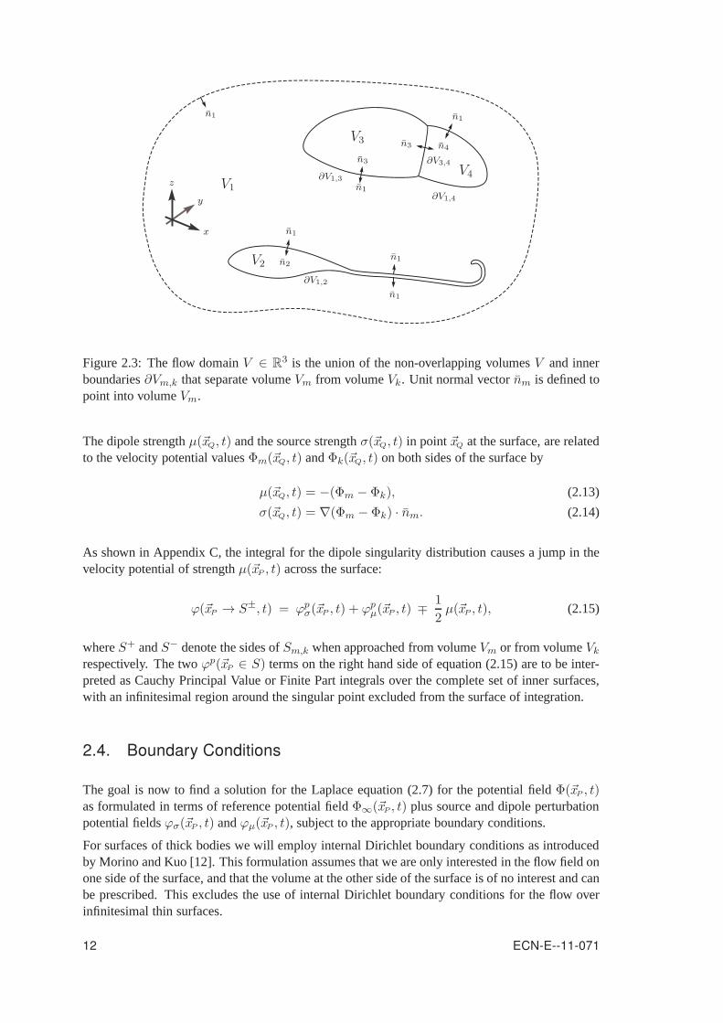
It is assumed that flow domain domainV can be decomposed into a set of non-overlapping vol-umesVm with boundaries∂Vm (see Figure 2.3). LetSm,k be the part of the boundary that the twovolumesVm andVk have in common:

Sm,k = ∂Vm ∩ ∂Vk, m 6= k.

The surfaceS of the configuration and its wake is now described by the complete set of innerboundaries:

S = ∪Sm,k.

It can be shown (Appendix C) that the solution of the Laplace equation (2.7) for the velocitypotentialΦ(~xP , t) in a point~xP in volumeV can be formulated in terms of a reference velocitypotentialΦ∞(~xP , t) and perturbation velocity potential contributionsϕµ(~xP , t) andϕσ(~xP , t) fromdipole singularity distributionsµ(~xQ, t) and source singularity distributionsσ(~xQ, t) on the innerboundaries repectively, that is

Φ = Φ∞ + ϕµ + ϕσ, (2.9)

whereΦ∞(~xP , t) is the unperturbed velocity potential in point~xP , the velocity potential if no innerboundaries were present. However, the unperturbed velocity potentialΦ∞ could also includecontributions from a designated set of source and dipole singularities in the nearby flow field.

The perturbation velocity potentials induced in point~xP by the dipole and source distributions onsurfaceS are defined by

ϕµ(~xP , t) =−1

4π

∫∫

S

µnm · ~r

r3dS, (2.10)

ϕσ(~xP , t) =−1

4π

∫∫

S

σ1

rdS, (2.11)

wherenm(~xQ, t) is the unit normal vector in~xQ ∈ ∂Vm,k that is pointing into volumeVm. Thevector~r is defined as the vector from a point~xQ on the surface to evaluation point~xP , whereas itslength is denoted byr, that is,

~r = ~xP − ~xQ, r = |~r |, for ~xQ ∈ Sm,k. (2.12)

For problems where the evaluation point~xP and the boundarySm,k are moving relative to eachother, we have~r = ~r(t).

ECN-E--11-071 11

V1

V2

V3

V4

x

y

z

∂V1,2

∂V1,3

∂V1,4

∂V3,4

n1

n1

n1

n1

n1

n1

n2

n3

n3

n4

Figure 2.3: The flow domainV ∈ R3 is the union of the non-overlapping volumesV and inner

boundaries∂Vm,k that separate volumeVm from volumeVk. Unit normal vectornm is defined topoint into volumeVm.

The dipole strengthµ(~xQ, t) and the source strengthσ(~xQ, t) in point~xQ at the surface, are relatedto the velocity potential valuesΦm(~xQ, t) andΦk(~xQ, t) on both sides of the surface by

µ(~xQ, t) = −(Φm − Φk), (2.13)

σ(~xQ, t) = ∇(Φm −Φk) · nm. (2.14)

As shown in Appendix C, the integral for the dipole singularity distribution causes a jump in thevelocity potential of strengthµ(~xP , t) across the surface:

ϕ(~xP → S±, t) = ϕpσ(~xP , t) + ϕp

µ(~xP , t) ∓1

2µ(~xP , t), (2.15)

whereS+ andS− denote the sides ofSm,k when approached from volumeVm or from volumeVkrespectively. The twoϕp(~xP ∈ S) terms on the right hand side of equation (2.15) are to be inter-preted as Cauchy Principal Value or Finite Part integrals over the complete set of inner surfaces,with an infinitesimal region around the singular point excluded from the surface of integration.

2.4. Boundary Conditions

The goal is now to find a solution for the Laplace equation (2.7) for the potential fieldΦ(~xP , t)as formulated in terms of reference potential fieldΦ∞(~xP , t) plus source and dipole perturbationpotential fieldsϕσ(~xP , t) andϕµ(~xP , t), subject to the appropriate boundary conditions.

For surfaces of thick bodies we will employ internal Dirichlet boundary conditions as introducedby Morino and Kuo [12]. This formulation assumes that we are only interested in the flow field onone side of the surface, and that the volume at the other side of the surface is of no interest and canbe prescribed. This excludes the use of internal Dirichlet boundary conditions for the flow overinfinitesimal thin surfaces.

12 ECN-E--11-071

2.4.1. Body Surface

For thick bodies, the internal Dirichlet formulation will be employed where it is assumed that onlythe solution in the volume on one side of the surface is of interest. LetS+ denote the side ofsurfaceSm,k in volumeVm where we want to obtain a solution of the flow problem, and letS−

denote the side of the surfaceSm,k in volumeVk that is considered non-physical and exhibits afictitious flow.

The boundary condition at surface sideS+ is such that the flow velocity at the surface in normaldirection, is equal to normal component of the surface velocity ~uS(~xP , t), plus a specified velocityvn(~xP , t) in normal direction:

∇Φm · nm = ~uS · nm + vn, ~xP → S+. (2.16)

The normal velocity distribution can be used for example to simulate boundary layer displacementthickness effects or for the simulation of inflow through a suction slot. The local surface velocity~uS(~xP , t) may be composed of solid body rotation, surface translation, surface rate of deformationand so on.

Suppose the velocity potential in the fictitious flow domainsVk is known in advance,

Φk = Φk(~xP , t), ~xP ∈ Vk, (2.17)

and let~uk(~xP , t) = ∇Φk, ~xP ∈ Vk. (2.18)

For point~xP in regionVk approaching the surfaceS−, the boundary integral equation (2.9) nowreads:

ϕµ(~xP , t) + ϕσ(~xP , t) = Φk(~xP , t)− Φ∞(~xP , t), ~xP → S−. (2.19)

Substitution of the boundary condition (2.16) atS+ and the known velocity potential in volumeVk (2.17) in the definition of the source strength (2.14), givesan expression for the source strengthin terms of known quantities:

σ(~xQ, t) = (~uS − ~uk) · nm + vn, ~xQ ∈ S. (2.20)

The boundary integral equation (2.19) at~xP → S− now gives an expression involving the unknowndipole strengthµ(~xQ, t) as a function of known quantities.

Taking the surface gradient of the dipole strength (2.13) gives us for the tangential component ofthe velocity at the surface side of interestS+

∇SΦm(~xP , t) = ∇SΦk − ∇Sµ, ~xP → S+. (2.21)

Combining the normal velocity from the boundary condition (2.16), the expression for the sourcestrength in equation (2.20), and the tangential velocity from equation (2.21) gives an expressionfor the velocity at the surface in the inertial coordinate system:

~u(~xP , t) = ~uk + σ nm − ∇Sµ, ~xP → S+. (2.22)

Equation (2.22) states that the velocity at the surface sideof interest is composed of a known baseflowfield ~uk and a perturbation flowfield due to the source and dipole singularity distributions.

Notice that the velocity potential fieldΦk, and consequently velocity field~uk, still has to be definedin the non-physical domains. This gives some freedom to basethis choice on the properties thatthe resulting set of equations will have. A choice that is expected to give small numerical errors is

ECN-E--11-071 13

one that results in smooth and weak source and dipole distributions. Here it is decided to set thefictitious flowfield equal to the onset flowfield as was introduced by Morino and Kuo [12], that isΦk = Φ∞, and~uk = ~u∞. Assuming a known surface velocity~uS and normal velocityvn, thisgives the following set of equations to determine the velocity distribution at the surface:

σ = (~uS − ~u∞) · n+ vnn,ϕµ = −ϕσ, ~xP → S−,~u(~xP , t) = ~u∞ + σ n − ∇Sµ, ~xP → S+.

(2.23)

2.4.2. Wake Surface

In the previous section we derived a set of equations to determine the dipole strength distributionthe solid body surface. In this section the conditions for the wake surface will be determined. Atthe trailing edge of a lifting body, the point where the vorticity leaves the surface (see Figures 2.1and 2.2), a linear Kutta condition will be imposed that results in a smooth flow with finite velocityat that point. This condition was used by Morino and Kuo [12] and equates the dipole strength atthe start of the wake equal to the jump in dipole strengths across the trailing edge:

µwte = JϕKte = JµKte. (2.24)

µ

µ

µw

µwte

Figure 2.4: Trailing edge Kutta condition.

For the evolution of the wake we will make use of the theorems of Helmholtz and Kelvin for vortic-ity dynamics (see Batchelor [3], Cottet and Koumoutsakos [5], Saffman [14]). In incompressibleflows the inviscid evolution of the vorticity field can be obtained by applying the curl operatorto the momentum conservation equation 2.2. After some manipulation, the resulting Lagrangiandescription is

D~ωDt

= ~ω · ∇~u. (2.25)

A similar relationship is valid for material line elementsδ~l and can be obtained by replacing~ω inabove equation withδ~l. We can thus conclude that in incompressible inviscid flows,vortex linesbehave as material line elements. Kelvin’s circulation theorem for incompressible inviscid flowsreads

DΓ

Dt= 0, (2.26)

where circulationΓ is defined by a surface integral of vorticity over a cross section of a vortextube or recast into a contour integral around the vortex tubewith the help of Stokes’ theorem (seeAppendix A)

Γ =

∫∫

S

~ω · n dS =

∫

∂S

~u · τ ds, (2.27)

with n the unit normal vector to the cross section surfaceS, and τ the unit vector tangential tothe contour∂S. From above equations it can be concluded that in incompressible inviscid flows

14 ECN-E--11-071

a tube of vorticity preserves its identity when moving with the fluid. In terms of the evolution ofwake element position~Xw and wake element dipole strengthµw the corresponding equations are

d ~Xw

dt= ~u, ~Xµ(t0) = ~xte(t0), (2.28)

andDµwDt

= 0, µw(t0) = µwte(t0), (2.29)

wheret0 is the time of wake element creation.

2.5. Aerodynamic Forces

The total force and moment with respect to the coordinate system origin are determined by inte-grating the pressure force over the surface of the configuration (see Figure 2.5):

~F (t) =

∫∫

S

p n dS, (2.30)

~M(t) = −

∫∫

S

p n× ~r dS, (2.31)

where~r is the position vector to the surface, andp the pressure that can be obtained from theBernoulli equation (2.8).

x

y

z

dS

S

~r

pn

Figure 2.5: Infinitesimal surface contribution to the totalforce and moment acting on the configu-ration.

ECN-E--11-071 15

16 ECN-E--11-071

3. Numerical Approach

The continuous mathematical description of the flow problemfor wind turbine applications willbe discretized such that it is possible to numerically determine the solution with apanel method.To this end we will introduce approximations and discretizations for the geometry, the singularsurface integral equations, and the boundary conditions. The geometry will be described in termsof bodies and wakes that consist of patches of structured grid cells, the so called ’panels’ in themethod. The quadrilateral panels will be described by a bilinear geometry where possible and bya planar surface elsewhere. Each panel on a body or wake patchis assigned a constant strengthdipole distribution and for body patches the panels are alsoassigned a constant strength sourcedistribution. Just below the surface of the body panel midpoints so calledcollocation pointsarelocated where the boundary conditions will be fulfilled.

3.1. Geometry

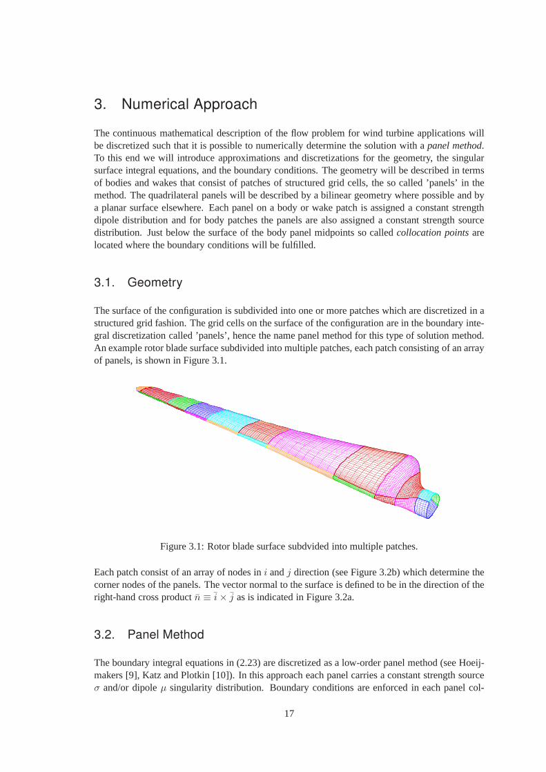
The surface of the configuration is subdivided into one or more patches which are discretized in astructured grid fashion. The grid cells on the surface of theconfiguration are in the boundary inte-gral discretization called ’panels’, hence the name panel method for this type of solution method.An example rotor blade surface subdivided into multiple patches, each patch consisting of an arrayof panels, is shown in Figure 3.1.

Figure 3.1: Rotor blade surface subdvided into multiple patches.

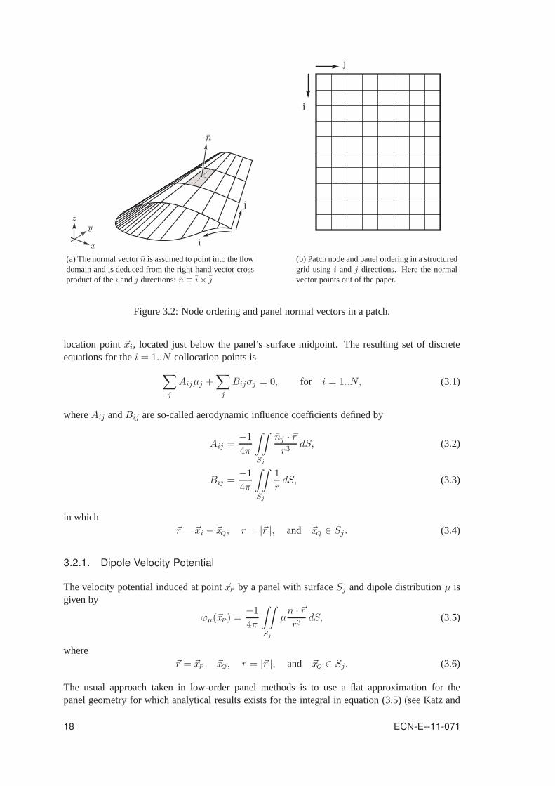
Each patch consist of an array of nodes ini andj direction (see Figure 3.2b) which determine thecorner nodes of the panels. The vector normal to the surface is defined to be in the direction of theright-hand cross productn ≡ i× j as is indicated in Figure 3.2a.

3.2. Panel Method

The boundary integral equations in (2.23) are discretized as a low-order panel method (see Hoeij-makers [9], Katz and Plotkin [10]). In this approach each panel carries a constant strength sourceσ and/or dipoleµ singularity distribution. Boundary conditions are enforced in each panel col-

17

x

yz

i

j

n

(a) The normal vectorn is assumed to point into the flowdomain and is deduced from the right-hand vector crossproduct of thei andj directions:n ≡ i× j

i

j

(b) Patch node and panel ordering in a structuredgrid usingi andj directions. Here the normalvector points out of the paper.

Figure 3.2: Node ordering and panel normal vectors in a patch.

location point~xi, located just below the panel’s surface midpoint. The resulting set of discreteequations for thei = 1..N collocation points is

∑

j

Aijµj +∑

j

Bijσj = 0, for i = 1..N, (3.1)

whereAij andBij are so-called aerodynamic influence coefficients defined by

Aij =−1

4π

∫∫

Sj

nj · ~r

r3dS, (3.2)

Bij =−1

4π

∫∫

Sj

1

rdS, (3.3)

in which~r = ~xi − ~xQ, r = |~r |, and ~xQ ∈ Sj . (3.4)

3.2.1. Dipole Velocity Potential

The velocity potential induced at point~xP by a panel with surfaceSj and dipole distributionµ isgiven by

ϕµ(~xP ) =−1

4π

∫∫

Sj

µn · ~r

r3dS, (3.5)

where~r = ~xP − ~xQ, r = |~r |, and ~xQ ∈ Sj. (3.6)

The usual approach taken in low-order panel methods is to usea flat approximation for thepanel geometry for which analytical results exists for the integral in equation (3.5) (see Katz and

18 ECN-E--11-071

Plotkin [10]). Flat panels, however, lead to gaps between the panels in the surface approximation,that grow larger with increasing surface twist. Especiallyfor panels in a highly deformed wakesurface this flat panel approximation is inadequate. The approach taken here is to use a bilinearrepresentation for the panel geometry (see Figure 3.3) which gives a better surface approximationand avoids gaps altogether.

x

y

z

Figure 3.3: A bilinear quadrilateral panel.

For a unit strength dipole distribution (µ = 1) the integral in equation (3.5) is equal to the solidangle and can be determined by the projection of the warped panel on a sphere with unit radiusand the evaluation point~xP as its center (see Figure 3.4). The solid angle is then the ratio betweenthe projected panel area and the surface area of the sphere. We use the fact that the area of aquadrilateral on a sphere with unit radius is equal to the sumof the included angles minus2π:

area = −2π +

4∑

i=1

βi. (3.7)

β1

β2

β3

β4

x

y

z

n

~xP

Figure 3.4: The solid angle is the ratio between the area of the projected panel and the surface areaof the sphere with the evaluation point as its center. The area of the projected quadrilateral can bedetermined from its included anglesβi.

3.2.2. Source Velocity Potential

The velocity potential induced by a panel with surfaceSj and source distributionσ in point ~xP isgiven by

ϕσ(~xP ) =−1

4π

∫∫

Sj

σ1

rdS. (3.8)

ECN-E--11-071 19

For the exact evaluation of this integral for constant source strengthσ on each panel the reader isreferred to the analytical formula in Katz and Plotkin [10].

3.2.3. Dipole Surface Gradient Velocity

To obtain the total velocity~u at the boundary of the configuration, one of the components inequation (2.22) that has to be determined is the surface gradient of the dipole strength∇Sµ. Thisis accomplished with the help of with Gauß’ Theorem (see Appendix A), giving an expression forthe average dipole surface gradient inside contour∂S (see Figure 3.5):

∇Sµ =1

S

∫

∂S

µ ν ds, (3.9)

where ν is the unit outward vector normal to the contour and tangential to the surface. Thecontour∂S is defined by the collocation points of four neighboring panel. As an approximation,the perturbation velocity in the grid node due to the dipole distribution is assigned this averagesurface gradient.

x

y

z

~τν

~u

Figure 3.5: Definitions used in the contour integral to determine the surface perturbation velocityin a grid node due to a dipole distribution.

20 ECN-E--11-071

4. Verification

In this chapter the results of the convergence tests on an ellipsoid with semi-axes4, 2, 1 are re-ported. For tri-axial ellipsoids analytical solutions exist. This makes it possible to verify theimplemented panel method for correctness of system of equation setup, the solution of the systemby a linear equation solver, and the application of postprocessing steps necessary to obtain the sur-face velocity distribution. The verification tests are performed for a single patch grid that exhibitstwo grid poles, and a six patch grid that does not possess collapsed edges. It is shown that for thetri-axial ellipsoid the rate of convergence for the perturbation potential and the pressure coefficientsurface distributions are up to orderO(h2), whereh is a characteristic panel length.

4.1. Analytical Solution

For ellipsoidal bodies in potential flow analytical solutions exist (see Durand [1], Lamb [11]). Ifwe define the functionψ(~x) as

ψ(~x) =(x

a

)2+(y

b

)2+(z

c

)2− 1, (4.1)

the surface of an ellipsoid with semi-axesa, b, c is described byψ(~xe) = 0. The perturbationpotential on the surface of this ellipsoid for a general onset flow ~u∞ = (u∞, v∞, w∞)T, is givenby

ϕ(~xe) = u∞xeα0

2− α0+ v∞ye

β02− β0

+w∞zeγ0

2− γ0, (4.2)

where

α0 =

∞∫

0

a b c

(a2 + λ)√

(a2 + λ)(b2 + λ)(c2 + λ)dλ, (4.3)

β0 =

∞∫

0

a b c

(b2 + λ)√

(a2 + λ)(b2 + λ)(c2 + λ)dλ, (4.4)

γ0 =

∞∫

0

a b c

(c2 + λ)√

(a2 + λ)(b2 + λ)(c2 + λ)dλ. (4.5)

Above integrals are regular and can be numerically evaluated given a specific choice for semi-axesa, b, c. In the current study, the integrals were integrated with anadaptive Simpson’s quadraturerule. For the total potential on the surface of the ellipsoidwe can write

Φ(~xe) = ~u∞ · ~xe + ϕ(~xe) =2u∞2− α0

xe +2v∞2− β0

ye +2w∞

2− γ0ze. (4.6)

The velocity vector on the surface of the ellipsoid can now bedetermined from the surface gradientof the total potential (4.6).

21

4.2. Geometric Convergence

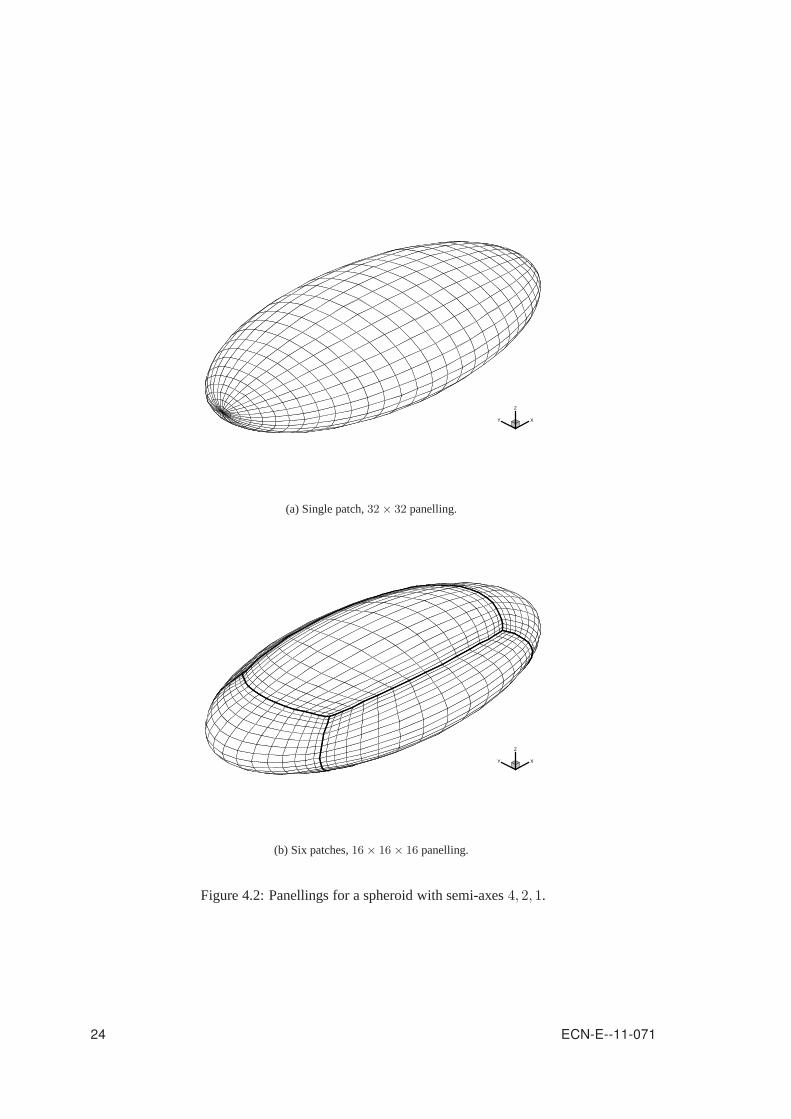
First the convergence of the discretised geometry towards the exact ellipsoidal surface is inves-tigated. The investigated geometric norm is based on the distance between the panel mid points~xc, and the points~xe on the surface of the ellipsoid. The surface is discretized as a single-domaingrid with poles along the x-axis as shown in Figure 4.2a. The vertex coordinates are obtainedby scaling a sphere with a cosine distribution in x-direction and an equidistant distribution in cir-cumferential direction. Anm×m panelling was used for the geometric convergence study, withm = 8, 16, 32, . . . , 1024. The points~xe are obtained by projecting the collocation points~xc alongthe normal vectornc onto the surface.

The discrete versions of the error norms are defined by

L1(x) =1

n

n∑

i=1

|xi|, (4.7)

L2(x) =

(

1

n

n∑

i=1

|xi|2

)1/2

, (4.8)

L∞(x) = maxi=1,n

|xi|, (4.9)

where|xi| is the absolute value of the difference between exact and approximated values in caseof scalar quantities, and the length of the vector differences in case of vectorial quantities.

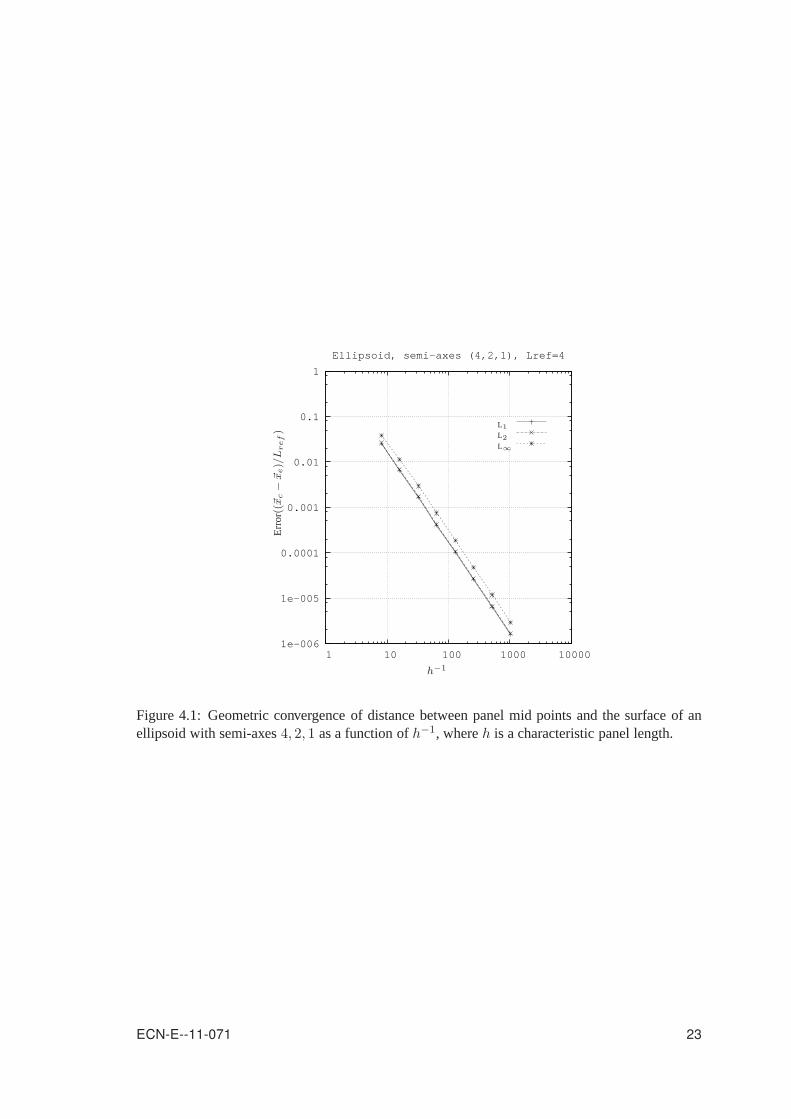
The variation of the error norms withh−1 is shown in Figure 4.1, whereh = N−12 is a charac-

teristic panel length andN the total number of panels. As can be seen, the error isO(h2) in thegeometric norms as expected. It should be noted that the largest errors were invariably for panelsnear the poles in the grid. This gives an indication that for practical purposes we would have torefine the mesh in these regions of large surface curvature toobtain a more evenly distributed error.

22 ECN-E--11-071

1e-006

1e-005

0.0001

0.001

0.01

0.1

1

1 10 100 1000 10000

Ellipsoid, semi-axes (4,2,1), Lref=4

L1

L2

L∞

h−1

Err

or((~xc−

~xe)/Lref)

Figure 4.1: Geometric convergence of distance between panel mid points and the surface of anellipsoid with semi-axes4, 2, 1 as a function ofh−1, whereh is a characteristic panel length.

ECN-E--11-071 23

XY

Z

(a) Single patch,32× 32 panelling.

XY

Z

(b) Six patches,16× 16× 16 panelling.

Figure 4.2: Panellings for a spheroid with semi-axes4, 2, 1.

24 ECN-E--11-071

4.3. Velocity Potential Convergence

In the panel method that is implemented, the perturbation potential in the collocation points of thepanels is obtained using a direct solver for the system of equations. The perturbation potentialthus obtained, is compared to the analytical solution in thepoints projected in normal direction atthe exact ellipsoid surface. For this study two panellings are used, a single patch panelling anda six patch panelling, of which example grids are shown in Figure 4.2. The six patch ellipsoidwas introduced to see if the behaviour in the grid poles of thesingle patch configuration could beavoided.

4.3.1. Single Patch Grid

In Figure 4.3, the error in the velocity potential is shown asa function of characteristic panel lengthh for the single patch grid. As can be seen, the error is ofO(h2) in the velocity potential for thispanelling. The largest errors appear near the poles of the grid, which in this case coincide with theareas of largest surface curvature, as is shown in Figures 4.4 and 4.5. In case the stagnation pointscoincide with the poles of the grid, the largest errors occurs elsewhere on the surface as can beseen in Figure 4.6.

0.0001

0.001

0.01

0.1

1 10 100

Err

or(ϕ

)

h−1

(1, 0, 0)(0, 1, 0)(0, 0, 1)

(a) L1-norms.

0.0001

0.001

0.01

0.1

1 10 100

Err

or(ϕ

)

h−1

(1, 0, 0)(0, 1, 0)(0, 0, 1)

(b) L2-norms.

0.0001

0.001

0.01

0.1

1 10 100

Err

or(ϕ

)

h−1

(1, 0, 0)(0, 1, 0)(0, 0, 1)

(c) L∞-norms.

Figure 4.3: Error norms in perturbation potential as a function of h−1, whereh is a characteristicpanel length, for onset flows along the three coordinate axesof a single patch grid.

ECN-E--11-071 25

XY

Z

dMU_001

0.00070.00060.00050.00040.00030.00020.00010

-0.0001-0.0002-0.0003-0.0004-0.0005-0.0006-0.0007

(a) Perturbation potential error.

XY

Z

dMU_001

0.00070.00060.00050.00040.00030.00020.00010

-0.0001-0.0002-0.0003-0.0004-0.0005-0.0006-0.0007

(b) Closeup of the pole region.

Figure 4.4: Perturbation potential error distribution fora single patch64 × 64 panel ellipsoid andan onset flow in z-direction. The largest errors appear near the poles of the grid.

26 ECN-E--11-071

XY

Z

dMU_001

0.00070.00060.00050.00040.00030.00020.00010

-0.0001-0.0002-0.0003-0.0004-0.0005-0.0006-0.0007

Figure 4.5: Perturbation potential error distribution fora single patch64× 64 panel ellipsoid andan onset flow in z-direction. A smooth potential error distribution across the patch edges is shown.

XY

Z

dMU_100

0-5E-05-0.0001-0.00015-0.0002-0.00025-0.0003-0.00035-0.0004

Figure 4.6: Perturbation potential error distribution fora single patch64× 64 panel ellipsoid andan onset flow in x-direction. The largest errors occur outside the poles of the grid.

ECN-E--11-071 27

4.3.2. Six Patch Grid

In Figure 4.7, the variation of the error in the velocity potential is shown as function of charac-teristic panel sizeh for the six patch grid. As can be seen, the error is ofO(h2) in the velocitypotential for this panelling. The largest errors appear near areas of large surface curvature, as isshown in Figures 4.8a and 4.8b.

0.0001

0.001

0.01

0.1

1 10 100

Err

or(ϕ

)

h−1

(1, 0, 0)(0, 1, 0)(0, 0, 1)

(a) L1-norms.

0.0001

0.001

0.01

0.1

1 10 100

Err

or(ϕ

)

h−1

(1, 0, 0)(0, 1, 0)(0, 0, 1)

(b) L2-norms.

0.0001

0.001

0.01

0.1

1 10 100

Err

or(ϕ

)

h−1

(1, 0, 0)(0, 1, 0)(0, 0, 1)

(c) L∞-norms.

Figure 4.7: Error norms in perturbation potential as a function of h−1, whereh is a characteristicpanel length, for onset flows along the three coordinate axesof a six patch grid.

28 ECN-E--11-071

XY

Z

dMU_001

0.00080.00070.00060.00050.00040.00030.00020.00010

-0.0001-0.0002-0.0003-0.0004-0.0005-0.0006-0.0007-0.0008

(a) Perturbation potential error.

XY

Z

dMU_001

0.00080.00070.00060.00050.00040.00030.00020.00010

-0.0001-0.0002-0.0003-0.0004-0.0005-0.0006-0.0007-0.0008

(b) Closeup of a region of large curvature.

Figure 4.8: Perturbation potential error distribution fora six patch32 × 32 × 32 panel ellipsoidand an onset flow in z-direction.

ECN-E--11-071 29

4.4. Presssure Coefficient Convergence

The pressure coefficients are obtained, via the Bernoulli equation (2.8), from the velocities at thesurface. In turn, these velocities are determined in the grid vertices involving a line integral of theperturbation potential through the surrounding collocation points as expressed in equation (3.2.3).At the edges of the grid the velocities are obtained using thepotential information of the abuttingpatch. Two types of panellings are used, one in which the geometry is described by a single patchand one in which six patches are used (see Figure 4.2).

4.4.1. Single Patch Grid

As can be seen in Figure 4.9 the L1-, L2- and L∞ error norms in the pressure coefficient for onsetflows along all three coordinate axes show a rate of error reduction of orderO(h2). It also showsthat the largest errors appear for an onset flow in z-direction.

0.0001

0.001

0.01

0.1

1

1 10 100

Err

or(C

p)

h−1

(1, 0, 0)(0, 1, 0)(0, 0, 1)

(a) L1-norm.

0.0001

0.001

0.01

0.1

1

10

1 10 100

Err

or(C

p)

h−1

(1, 0, 0)(0, 1, 0)(0, 0, 1)

(b) L2-norm.

0.001

0.01

0.1

1

10

1 10 100

Err

or(C

p)

h−1

(1, 0, 0)(0, 1, 0)(0, 0, 1)

(c) L∞-norm.

Figure 4.9: Error norms in pressure coefficient as a functionof h−1, whereh is a characteristicpanel length, for onset flows along the three coordinate axesof a single patch grid.

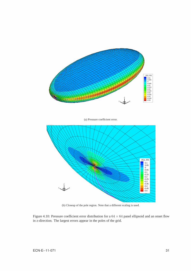
In Figure 4.10, the pressure coefficient error distributionis plotted for an onset flow in z-direction.Because the potential already showed the highest error gradient in the poles of the grid (see Fig-ure 4.4), it is of no surprise that the pressure coefficient error is highest in these poles also.

30 ECN-E--11-071

XY

Z

dCp_001

0.010.0050

-0.005-0.01-0.015-0.02-0.025-0.03-0.035-0.04-0.045-0.05

(a) Pressure coefficient error.

XY

Z

dCp_001

0.10.050

-0.05-0.1-0.15-0.2-0.25-0.3-0.35-0.4-0.45-0.5

(b) Closeup of the pole region. Note that a different scalingis used.

Figure 4.10: Pressure coefficient error distribution for a64× 64 panel ellipsoid and an onset flowin z-direction. The largest errors appear in the poles of thegrid.

ECN-E--11-071 31

4.4.2. Six Patch Grid

In Figure 4.11, the L1-, L2- and L∞ error norms in the pressure coefficient for onset flows alongall three coordinate axes are shown for an ellipsoid discretized with a six patch grid. The error isshown to be of orderO(h2). Notice that the error norms for the six patch grid show a smootherconvergence behavior than the single patch in Figure 4.9.

0.0001

0.001

0.01

0.1

1

1 10 100

Err

or(C

p)

h−1

(1, 0, 0)(0, 1, 0)(0, 0, 1)

(a) L1-norm.

0.0001

0.001

0.01

0.1

1

1 10 100

Err

or(C

p)

h−1

(1, 0, 0)(0, 1, 0)(0, 0, 1)

(b) L2-norm.

0.001

0.01

0.1

1

10

1 10 100

Err

or(C

p)

h−1

(1, 0, 0)(0, 1, 0)(0, 0, 1)

(c) L∞-norm.

Figure 4.11: Error norms in pressure coefficient as a function of characteristic panel lengthh, foronset flows along the three coordinate axes of an ellipsoid constructed from six patches.

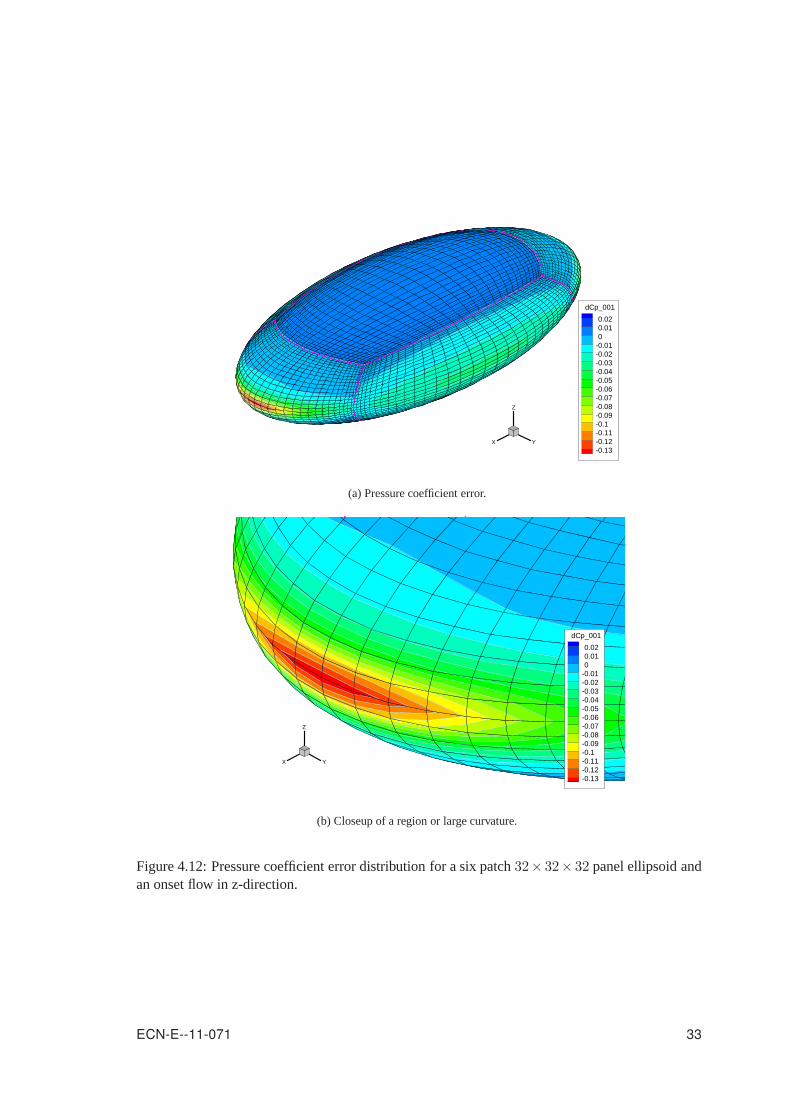
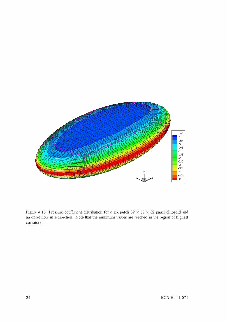
In Figure 4.12 the pressure coefficient error distribution is plotted for an onset flow in z-direction.The largest errors occur in regions of large curvature wherethe mesh is relatively coarse. Notethat the pressure coefficient distribution itself has highly negative values in the region of highestcurvature (see Figure 4.13) at this onset flow condition.

32 ECN-E--11-071

X Y

Z

dCp_001

0.020.010

-0.01-0.02-0.03-0.04-0.05-0.06-0.07-0.08-0.09-0.1-0.11-0.12-0.13

(a) Pressure coefficient error.

X Y

Z

dCp_001

0.020.010

-0.01-0.02-0.03-0.04-0.05-0.06-0.07-0.08-0.09-0.1-0.11-0.12-0.13

(b) Closeup of a region or large curvature.

Figure 4.12: Pressure coefficient error distribution for a six patch32× 32× 32 panel ellipsoid andan onset flow in z-direction.

ECN-E--11-071 33

XY

Z

Cp

10.50

-0.5-1-1.5-2-2.5-3-3.5-4-4.5-5

Figure 4.13: Pressure coefficient distribution for a six patch 32 × 32 × 32 panel ellipsoid andan onset flow in z-direction. Note that the minimum values arereached in the region of highestcurvature.

34 ECN-E--11-071

5. Application

The current code, designated ROTORFLOW, can be applied to compute inviscid, incompressibleflows around arbitrary 3D lifting and non-lifting bodies in rotating and translating motion. It isunfortunate that for lifting wings in 3D flow no exact analytical testcases exist like those reportedin Chapter 4 for the non-lifting tri-axial ellipsoid. The flow solution for a wing of large aspect ratiowith an elliptic planform however can be regarded quasi two-dimensional in its center section. Thisenables us to compare the pressure distribution at that position with a well established 2D airfoilanalysis code for steady flow.

5.1. Lifting wing in steady flow

From a modified NACA 0018 airfoil a wing with an elliptic planform was constructed. The span ofthe elliptic wing was 200 and the root chord was set to 1, giving an aspect ratio of over 254. For thiswing the flow at 5 degrees angle-of-attack was simulated and the sectional pressure distribution athalf span position was extracted. For the same airfoil section the inviscid pressure distribution atthe wing’s effective angle-of-attack of 4.961 degrees was computed with the 2D higher order panelcode XFOIL from Drela [6]. As shown in Figure 5.1 the XFOIL andthe ROTORFLOW pressuredistributions are comparable.

-2

-1.5

-1

-0.5

0

0.5

1 0 0.2 0.4 0.6 0.8 1

Cp

X/C

XFOILROTORFLOW

Figure 5.1: Inviscid flow pressure distributions for an airfoil at 5 degrees angle-of-attack.

5.2. Rotating wing in unsteady flow

As a demonstration of the capabilities of the current code the flow solution for a single blade rotorconfiguration under30 degrees of yaw was computed where an untwisted elliptic wingwas usedas blade. For the prescription of the motion of the blade a geometry manipulation approach likethe one in the AWSM code [7] was used.

35

X

Y

Z

MU

1050

-5-10-15-20-25-30-35-40-45-50-55

(a) Wake dipole strength development.

XY

Z

Cp

10.50

-0.5-1-1.5-2-2.5-3-3.5-4

(b) Surface pressure coefficient and velocity vector distibution.

-7

-6

-5

-4

-3

-2

-1

0

1 0 0.2 0.4 0.6 0.8 1

Cp

X/C

Y=25%Y=50%Y=75%

(c) Pressure distribution of sections at25%, 50%, and 75% bladelength.

Figure 5.2: Unsteady flow for a single blade rotor at 30 degrees yaw.

36 ECN-E--11-071

Notice that, due to the lack of blade twist in this blade, the inner airfoil sections experience a higherlocal angle-of-attack and consequently have a higher suction peak near the nose of the airfoil.

ECN-E--11-071 37

References

[1] W.F. Durand, editor,Aerodynamic Theory, Vol. 1, Dover Publications, 1934.

[2] J.D. Anderson,Fundamentals of Aerodynamics, McGraw-Hill, fourth ed., 2006.

[3] G.K. Batchelor,An Introduction to Fluid Dynamics, Cambridge University Press, 1967.

[4] H.A. Bijleveld, A.E.P. Veldman,RotorFlow: A quasi-simultaneous interaction for the pre-diction of aerodynamic flow over wind turbine blades, In “The Science of Making Torquefrom Wind”, 2010.

[5] G.H. Cottet, P.D. Koumoutsakos,Vortex Methods: Theory and Practice, Cambridge Univer-sity Press, 2000.

[6] M. Drela,XFOIL: An Analysis and Design System for Low Reynolds NumberAirfoils, In T.J.Mueller, editor, Low Reynolds Number Aerodynamics, Vol. 54of Lecture Notes in Engi-neering, pages 1–12. Springer-Verlag, New York, 1989.

[7] A. van Garrel,Development of a Wind Turbine Aerodynamics Simulation Module, ECN-C--03-079, Energy research Centre of the Netherlands, 2003.

[8] A. van Garrel,Integral Boundary Layer Methods for Wind Turbine Aerodynamics, ECN-C--04-004, Energy research Centre of the Netherlands, 2004.

[9] H.W.M. Hoeijmakers,Panel Methods for Aerodynamic Analysis and Design, In “SpecialCourse on Engineering Methods in Aerodynamic Analysis and Design of Aircraft”, AGARDReport R-783, 1991.

[10] J. Katz, A. Plotkin,Low-Speed Aerodynamics: From Wing Theory to Panel Methods, Cam-bridge University Press, second ed., 2001.

[11] H. Lamb,Hydrodynamics, Cambridge University Press, sixth ed., 1932.

[12] L. Morino, C.-C. Kuo,Subsonic Potential Aerodynamics for Complex Configurations: AGeneral Theory, AIAA J., 12(2):191–197, 1974.

[13] H. Özdemir, E.F. van den Boogaard,Solving the integral boundary layer equations with adiscontinuous Galerkin method, EWEA 2011, 2011.

[14] P.G. Saffman,Vortex Dynamics, Cambridge Monographs on Mechanics and Applied Mathe-matics, Cambridge University Press, 1992.

38

A. Mathematical Compendium

This chapter contains a collection of some useful mathematical formulas. In index notation for-mulas summation over repeated indices is assumed.

Divergence Theorem: The Divergence Theorem is Gauß’ theorem for a vector function ~b andrelates the volume and surface integrals of the vector field in a volumeV enclosed by thesurface∂V by:

∫∫∫

V

(∇·~b) dV =

∫∫

∂V

~b · n dS.

Gauß’ Theorem: Gauß’ theorem gives a relation between the volume and surface integrals of acontinuously differentiable (i.e.C1 functions with continuous derivative) arbitrary tensorfunction Tij over a volumeV enclosed by piecewise smooth boundary∂V with outwardunit normal vectorn. The tensorTjk may be a scalar, vector or tensor function of any rank.In index notation Gauß’ theorem reads:

∫∫∫

V

∂i(Tjk) dV =

∫∫

∂V

ni Tjk dS.

Some special forms of Gauß’ theorem are obtained when specific choices are substituted fortensorTjk. Substituting vector fieldbi for Tjk for example gives the Divergence Theoremand when scalar fieldφ is substituted forTjk we arrive at the Gradient Theorem.

Substitution ofǫkijbj for tensorTjk gives

∫∫∫

V

(∇×~b) dV =

∫∫

∂V

(n×~b) dS.

Gradient Theorem: The Gradient Theorem is Gauß’ theorem for a scalar functionφ and relatesthe volume and surface integrals of the scalar field over a volumeV enclosed by the surface∂V by:

∫∫∫

V

(∇φ) dV =

∫∫

∂V

φn dS

Green’s identities: One of Green’s identities is obtained whenǫkijbj is substituted forTjk inGauß’ theorem. Combined over all componentsk this leads to:

∫∫∫

V

(∇×~b) dV =

∫∫

∂V

(n×~b) dS.

Green’s first identity is obtained when(ψ ∂iφ) is substituted into Gauß’ theorem forTjk,whereψ andφ are once and twice continuously differentiable scalar functions respectively:

∫∫∫

V

ψ∇2φ dV =

∫∫

∂V

ψ∂φ

∂ndS −

∫∫∫

V

∇φ · ∇ψ dV,

39

where ∂φ/∂n = ∇φ · n denotes the derivative in the direction of the outward normal and∇2=∇·∇ is the Laplacian operator.

Green’s second identity is obtained from the first identity by interchanging the role ofψ andφ and subtract the resulting equations. Now bothψ andφ are assumed twice continuouslydifferentiable scalar functions. Green’s second identityreads:

∫∫∫

V

(

ψ∇2φ− φ∇2ψ)

dV =

∫∫

∂V

(

ψ∂φ

∂n− φ

∂ψ

∂n

)

dS.

Stokes’ Theorem: Stokes’ theorem relates the line integral of a smooth vectorfield ~b over aclosed curve∂S to the surface integral of~b over an open surfaceS bounded by curve∂S.The orientations of unit tangent vectorτ to curve∂S and the unit normal vectorn to surfaceS are related through the right hand rule.

x

y

z

S dS

∂S

n

τ

Stokes’ theorem reads:

∫∫

S

(∇×~b) · n dS =

∫

∂S

~b · τ ds.

Substantial derivative: The substantial derivative, also know as material derivative, is the timerate of change following a fluid element moving with velocity~u, and can be split into thelocal and the convective derivative:

DDt

=∂

∂t+ ~u · ∇.

40 ECN-E--11-071

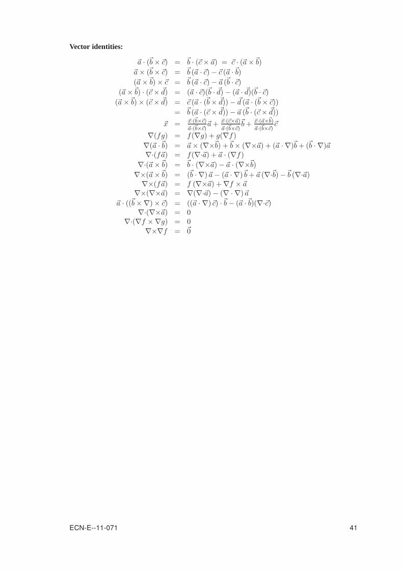
Vector identities:

~a · (~b× ~c) = ~b · (~c× ~a) = ~c · (~a×~b)

~a× (~b× ~c) = ~b (~a · ~c)− ~c (~a ·~b)

(~a×~b)× ~c = ~b (~a · ~c)− ~a (~b · ~c)

(~a×~b) · (~c× ~d) = (~a · ~c)(~b · ~d)− (~a · ~d)(~b · ~c)

(~a×~b)× (~c× ~d) = ~c (~a · (~b× ~d))− ~d (~a · (~b× ~c))

= ~b (~a · (~c× ~d))− ~a (~b · (~c× ~d))

~x = ~x·(~b×~c)

~a·(~b×~c)~a+ ~x·(~c×~a)

~a·(~b×~c)~b+ ~x·(~a×~b)

~a·(~b×~c)~c

∇(fg) = f(∇g) + g(∇f)

∇(~a ·~b) = ~a× (∇×~b) +~b× (∇×~a) + (~a · ∇)~b+ (~b · ∇)~a∇·(f~a) = f(∇·~a) + ~a · (∇f)

∇·(~a×~b) = ~b · (∇×~a)− ~a · (∇×~b)

∇×(~a×~b) = (~b · ∇)~a− (~a · ∇)~b+ ~a (∇·~b)−~b (∇·~a)∇×(f~a) = f (∇×~a) +∇f × ~a

∇×(∇×~a) = ∇(∇·~a)− (∇ · ∇)~a

~a · ((~b×∇)× ~c) = ((~a · ∇)~c) ·~b− (~a ·~b)(∇·~c)∇·(∇×~a) = 0

∇·(∇f ×∇g) = 0

∇×∇f = ~0

ECN-E--11-071 41

B. Conservation Laws

In this chapter the derivation of the conservation laws for mass and momentum is given for reasonsof completeness. It can be found in textbooks on fluid mechanics. A clear explanation is forexample given in reference [2].

B.1. Mass Conservation

Let us consider an arbitrary control volumeV fixed in space where fluid is freely flowing withvelocity~u(~x, t) through its bounding surface∂V with unit normal vectorn(~x) pointing outward asshown in Figure B.1. The equation for mass conservation, also known as the continuity equation,expresses that an increase in mass in volumeV can only come from a net mass flow through itsbounding surface∂V

ddt(Mass inV ) = Net mass inflow per unit time.

x

y

z

V

∂V

dS

n

~u

Figure B.1: A control volumeV fixed in space with fluid freely flowing through its boundingsurface∂V .

Considering that~u · n dS is the volume that flows out of areadS per unit time, we can write forthe net mass flowing through the surface into control volumeV per unit time:

Mass inflow= −

∫∫

∂V

ρ~u · n dS,

whereρ(~x, t) is the mass density of the fluid and the minus sign comes from the fact that wedefined the normal as positive when pointing outward. The integral form of the equation for massconservation can now be written as

ddt

∫∫∫

V

ρ dV +

∫∫

∂V

ρ~u · n dS = 0. (B.1)

42

We can use the Divergence Theorem to transform the surface integral into a volume integral,provided we have a continuously differentiable vector fieldρ~u:

ddt

∫∫∫

V

ρ dV +

∫∫∫

V

∇·(ρ~u) dV = 0,

which can be written as∫∫∫

V

(

∂ρ

∂t+∇·(ρ~u)

)

dV = 0,

where we used the fact that our control volume was fixed in space to shift the time derivative tothe integrand. Because this equation is valid for arbitrarycontrol volumes, the integrand has to bezero for any point withinV , and we arrive at the differential form of the continuity equation

∂ρ

∂t+∇·(ρ~u) = 0, (B.2)

which can also be written as

∇·~u = −1

ρ

DρDt. (B.3)

For incompressible flow the mass densityρ of fluid particles is constant and equation (B.2) reducesto a form without time derivative term

∇·~u = 0. (B.4)

If we now additionally assume irrotational flow∇×~u = ~0, we can write the velocity vector as thegradient of a scalar functionΦ(~x, t), that is

~u = ∇Φ. (B.5)

Substitution of this expression for the velocity vector into the continuity equation (B.4) results inthe Laplace equation for the unknown velocity potentialΦ:

∇·∇Φ =∂2Φ

∂x2+∂2Φ

∂y2+∂2Φ

∂z2= 0. (B.6)

B.2. Momentum Conservation

Momentum conservation is expressed by Newton’s second law of motion that states that, viewedfrom an inertial frame of reference, the time rate of change of the linear momentum of a particleis proportional to the net force excerted on it:

ddt(m~u) = ~F ,

wherem is the mass of the particle and~u its velocity.

Using our fixed control volume from Figure B.1, the equation for momentum conservation ex-presses that an increase in momentum in volumeV can only come from a net momentum flowthrough its surface or from a force excerted on the fluid. The equation for conservation of linearmomentum can be written symbolically as

ddt(Momentum inV ) = Net momentum inflow per unit time+ ~F

ECN-E--11-071 43

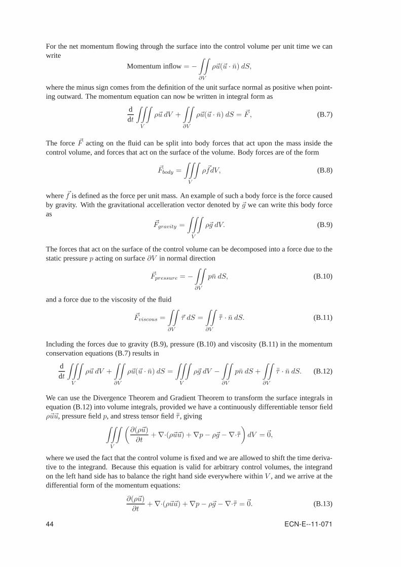
For the net momentum flowing through the surface into the control volume per unit time we canwrite

Momentum inflow= −

∫∫

∂V

ρ~u(~u · n) dS,

where the minus sign comes from the definition of the unit surface normal as positive when point-ing outward. The momentum equation can now be written in integral form as

ddt

∫∫∫

V

ρ~u dV +

∫∫

∂V

ρ~u(~u · n) dS = ~F , (B.7)

The force ~F acting on the fluid can be split into body forces that act upon the mass inside thecontrol volume, and forces that act on the surface of the volume. Body forces are of the form

~Fbody =

∫∫∫

V

ρ~fdV, (B.8)

where~f is defined as the force per unit mass. An example of such a body force is the force causedby gravity. With the gravitational accelleration vector denoted by~g we can write this body forceas

~Fgravity =

∫∫∫

V

ρ~g dV. (B.9)

The forces that act on the surface of the control volume can bedecomposed into a force due to thestatic pressurep acting on surface∂V in normal direction

~Fpressure = −

∫∫

∂V

pn dS, (B.10)

and a force due to the viscosity of the fluid

~Fviscous =

∫∫

∂V

~τ dS =

∫∫

∂V

¯τ · n dS. (B.11)

Including the forces due to gravity (B.9), pressure (B.10) and viscosity (B.11) in the momentumconservation equations (B.7) results in

ddt

∫∫∫

V

ρ~u dV +

∫∫

∂V

ρ~u(~u · n) dS =

∫∫∫

V

ρ~g dV −

∫∫

∂V

pn dS +

∫∫

∂V

¯τ · n dS. (B.12)

We can use the Divergence Theorem and Gradient Theorem to transform the surface integrals inequation (B.12) into volume integrals, provided we have a continuously differentiable tensor fieldρ~u~u, pressure fieldp, and stress tensor fieldτ , giving

∫∫∫

V

(

∂(ρ~u)

∂t+∇·(ρ~u~u) +∇p− ρ~g −∇·¯τ

)

dV = ~0,

where we used the fact that the control volume is fixed and we are allowed to shift the time deriva-tive to the integrand. Because this equation is valid for arbitrary control volumes, the integrandon the left hand side has to balance the right hand side everywhere withinV , and we arrive at thedifferential form of the momentum equations:

∂(ρ~u)

∂t+∇·(ρ~u~u) +∇p− ρ~g −∇·¯τ = ~0. (B.13)

44 ECN-E--11-071

For Newtonian fluids the viscous stresses are considered to be proportional to velocity gradientsthrough the constitutive relation

¯τ = µ

[

∇~u+ (∇~u)T −2

3(∇·~u) ¯I

]

, (B.14)

where the dynamic viscosity coefficientµ is in general a function of temperature.

This result can be simplified considerably if we assume the flow to be inviscid and incompressible.Additionally, we write the constant gravitational acceleration vector~g as the gradient of scalarfunctionh, the height above the ground,~g = −g∇h, where the minus sign comes from∇h havingthe opposite direction of~g. The constant mass density allows us then to combine the pressure andgravitational terms in equation (B.13) and, using the continuity equation (B.4) for incompressibleflows, we arrive at the differential form of the momentum equations for inviscid, incompressibleflows:

ρ∂~u

∂t+ ρ(~u · ∇)~u+∇(p+ ρgh) = ~0. (B.15)

Using one of the vector identities from appendix A, the second term in above equation can bewitten as

(~u · ∇)~u = ∇(1

2~u · ~u)− ~u× (∇×~u). (B.16)

Assuming steady flow, the substitution of the vector identity B.16 in the momentum equations B.15for inviscid, incompressible flow gives

∇

(

1

2~u · ~u+

p

ρ+ gh

)

= ~u× (∇×~u),

and taking the inner product with velocity vector~u results in

~u · ∇

(

1

2~u · ~u+

p

ρ+ gh

)

= 0,

which gives us the Bernoulli equation for steady, incompressible, inviscid, and rotational flow thatis valid in every point on a streamline through~x0:

1

2~u · ~u+

p

ρ+ gh = C(~x0). (B.17)

Let us start again with the momentum equations for unsteady,inviscid, incompressible flow B.15,and assume an irrotational velocity field∇×~u = ~0. We can now introduce~u = ∇Φ, and with theuse of vector identity B.16 arrive at

∇

(

ρ∂Φ

∂t+

1

2ρ∇Φ · ∇Φ+ p+ ρgh

)

= ~0,

which gives the Bernoulli equation for unsteady, incompressible, potential flow:

∂Φ

∂t+

1

2∇Φ · ∇Φ+

p

ρ+ gh = C(t). (B.18)

B.3. Energy Conservation

The equation for energy conservation is based on the first lawof thermodynamics that states that anincrease in total energy in a volumeV per unit time can only come from the energy added by heat

ECN-E--11-071 45

per unit time or from the work per unit time done by forces. Using the fixed control volume fromFigure B.1, the equation for energy conservation for fluid flows can be expressed symbolically by

ddt(Energy inV ) = Net energy inflow per unit time+ Heat + Work.

LetE(~x, t) be the total specific energy, that is the total energy per unitmass, and lete(~x, t) be theinternal specific energy that comes from molecular motion. The total specific energy is the sum ofthe internal specific energy and the kinetic specific energy that is associated with the bulk velocity~u(~x, t), that is

E = e+1

2~u · ~u. (B.19)

The total energy in volumeV is

Energy inV =

∫∫∫

V

ρE dV.

For the net energy flowing through the surface∂V into the control volume per unit time we canwrite

Energy inflow= −

∫∫

∂V

ρE(~u · n) dS,

where the minus sign comes from the definition of the unit surface normal as positive when point-ing outward. The expression for energy conservation can nowbe written as

ddt

∫∫∫

V

ρE dV +

∫∫

∂V

ρE(~u · n) dS = Heat + Work. (B.20)

The heat that is added to the volume can be split into body heating that acts on the fluid inside thevolume, and surface heating that acts through thermal conduction and is caused by gradients in theheat distribution. LetQ(~x, t) denote the body heat in Joule per unit volume per unit time, and let~q be the heat flux vector in Joule per unit area per unit time, then

Body heating =

∫∫∫

V

Q dV, (B.21)

Surface heating = −

∫∫

∂V

~q · n dS. (B.22)

In general, for the work done per unit time by applying a force~f(~x, t) to the fluid moving withvelocity~u(~x, t) we can write

Wforce = ~f · ~u

The forces can be split into body forces that act upon the massinside the volume, and forces thatact on the surface of the volume, see Appendix B.2.

An example of a body force is the gravitational force. With the gravitational accelleration vectordenoted by~g we can write the work done per unit time by this body force as

Wgravity =

∫∫∫

V

ρ~g · ~u dV. (B.23)

46 ECN-E--11-071

The forces that act on the surface of the control volume can bedecomposed into a force in normaldirection due to the static pressurep(~x, t) acting on surface∂V and a force due to the viscosity ofthe fluid. The work done by the static pressure per unit time is

Wpressure = −

∫∫

∂V

p~u · n dS, (B.24)

and for the work done by viscous forces per unit time we have

Wviscous =

∫∫

∂V

~τ · ~u dS =

∫∫

∂V

(¯τ · ~u) · n dS. (B.25)

Combining all heat and work contributions in the expressionfor energy conservation B.20 resultsin the energy equation in integral form:

ddt

∫∫∫

V

ρE dV +

∫∫

∂V

ρE(~u · n) dS = −

∫∫

∂V

p~u · n dS +

∫∫∫

V

ρ~g · ~u dV

+

∫∫∫

V

Q dV −

∫∫

∂V

~q · n dS

+

∫∫

∂V

(¯τ · ~u) · n dS. (B.26)

We can use the Divergence Theorem to convert the surface integrals to volume integrals, providedwe have continuously differentiable vector fieldsρE~u, p~u, ~q, and¯τ · ~u, and arrive at

∫∫∫

V

∂(ρE)

∂tdV +

∫∫∫

V

∇·(ρE~u) dV =

∫∫∫

V

∇·(p~u) dV +

∫∫∫

V

ρ~g · ~u dV

+

∫∫∫

V

Q dV −

∫∫∫

V

∇·~q dV

+

∫∫∫

V

∇·(¯τ · ~u) dV, (B.27)

where we used the fact that the control volume is fixed and we are allowed to shift the time deriva-tive to the integrand. Because this equation is valid for arbitrary control volumes, the integralshave to balance each other everywhere in volumeV and consequently the equation can be writtenin differential form:

∂(ρE)

∂t+∇·(ρE~u) +∇·(p~u)− ρ~g · ~u−Q+∇·~q −∇·(¯τ · ~u) = 0. (B.28)

We can rewrite above energy equation in terms of total specific enthalphyH(~x, t) which is definedas

H = E +p

ρ. (B.29)

The substitution of the definition for total specific enthalphy in energy equation B.28 gives asimpler enthalphy equation that does not explicitly contain the pressure work term:

∂(ρH)

∂t+∇·(ρH~u) =

∂p

∂t+ ρ~g · ~u+Q−∇·~q +∇·(¯τ · ~u). (B.30)

ECN-E--11-071 47

Expanding the term on the left hand side of the equation, and making use of the continuity equa-tion B.2, the non-conservative form of the equation for total enthalphyH is obtained

ρDHDt

=∂p

∂t+ ρ~g · ~u+Q−∇·~q +∇·(¯τ · ~u). (B.31)

The energy equation is supplemented with two equations of state and two constitutive relations,one for stress tensorτ(~x, t) and one for heat flux vector~q(~x, t). A model for the heat flux vectoris given by Fourier’s law

~q = −κ∇T,

whereκ is the heat conduction coefficient, andT (~x, t) the temperature field.

The constitutive relation for the stress tensor was introduced in the derivation of the momentumequations in Appendix B.2 and is

¯τ = µ

[

∇~u+ (∇~u)T −2

3(∇·~u) ¯I

]

,

with µ the dynamic viscosity coefficient that is in general a function of temperatureT .

Two equations of state complement the energy equation: one expressing the relation betweenpressurep, mass densityρ, and temperatureT , and one expression for the specific internal energye. For a calorically perfect gas the two equations of state are

p = ρRT,

with R the specific gas constant which for air is approximatelyR = 287 Joule per kilogram perKelvin, and

e = cvT,

with cv the specific heat at constant volume.

Related to these two expressions and the definition of specific enthalpyh = e+ pρ is the relation

h = cpT,

with cp the specific heat at constant pressure. The ratio between thetwo specific heats is denotedby γ =

cpcv

and is for airγ = 1.4.

48 ECN-E--11-071

C. Boundary Integral Equation

In an inertial Cartesian coordinate system in which coordinates are denoted by~x = (x, y, z)T, theLaplace equation for the velocity potential in unsteady, incompressible flow, in domainV ∈ R

3,can be written as

∇·∇Φ =∂2Φ

∂x2+∂2Φ

∂y2+∂2Φ

∂z2= 0 (C.1)

Although the Laplace equation has no time-dependent term, the velocity potentialΦ(~x, t) is afunction of space and time. Unsteady boundary conditions will introduce time-dependency in thesolution. In this section, this time-dependency is implicitly assumed. The problem in volumeVcan be reduced to a problem involving only surface integralsby the introduction of a special formof the Divergence Theorem that relates the volume and surface integrals of an arbitrary tensorfunction over a volumeV enclosed by surface∂V with unit normal vectorn pointing into thevolume:

∫∫

∂V

(Ψ2∇Ψ1 −Ψ1∇Ψ2) · n dS =

∫∫∫

V

(

Ψ1∇2Ψ2 −Ψ2∇

2Ψ1

)

dV. (C.2)

Equation (C.2) is known as Green’s second identity in which surface∂V is piecewise continuousand the scalar functionsΨ1 andΨ2 are assumed to be twice continuously differentiable.

Now, let us set for 3D flows

Ψ1 =1

r, Ψ2 = Φ, (C.3)

in whichΦ(~xP ) is the velocity potential function in point~xP (see Figure C.1) andr is the distancefrom point~xQ on the enclosing surface to an arbitrary fixed point~xP :

~r = ~xP − ~xQ, r = |~r |, where ~xQ ∈ ∂V. (C.4)

Notice that

∇1

r=

~r

r3, and ∇2 1

r= 0, for r 6= 0. (C.5)

x

y

z

2ǫVǫ

∂Vǫ

V

∂V

~xP

n

n

Figure C.1: Flow domain with region surrounding~xP ∈ V excluded from the domain of integra-tion.

49

For point ~xP outside flow domainV both Ψ1 andΨ2 satisfy the Laplace equation and equa-tion (C.2) becomes

∫∫

∂V

(

Φ∇1

r−

1

r∇Φ

)

· n dS = 0, ~xP /∈ V. (C.6)

In case point~xP is inside the domain of interestV , a small sphere with radiusǫ is introduced toexclude volumeVǫ around point~xP from the volume of integration (see Figure C.1). Again, bothΨ1 andΨ2 satisfy the Laplace equation and equation (C.2) now becomes

∫∫

∂V+∂Vǫ

(

Φ∇1

r−

1

r∇Φ

)

· n dS = 0, ~xP ∈ V. (C.7)

Now, let us evaluate the integral over the surface of the sphere∂Vǫ. With equation (C.5) we have∫∫

∂Vǫ

(

Φ∇1

r−

1

r∇Φ

)

· n dS =

∫∫

∂Vǫ

(

Φn · ~r

r3−

1

r∇Φ · n

)

dS. (C.8)

For a sphere with radiusǫ we have∫ dS=4πǫ2. Assuming a continuously differentiable velocitypotentialΦ and lettingǫ → 0, the second term in equation (C.8) vanishes:

∫∫

∂Vǫ

(

−1

r∇Φ · n

)

dS = −∂Φ

∂n

∫∫

∂Vǫ

(

1

r

)

dS = 0, (C.9)

while for the first term in equation (C.8) we find∫∫

∂Vǫ

(

Φn · ~r

r3

)

dS = − Φ(~xP )

∫∫

∂Vǫ

(

1

r2

)

dS = −4πΦ(~xP ), (C.10)

where we used for the normal vector on the sphere the expression

n =~xQ − ~xP|~xQ − ~xP |

= −~r

r. (C.11)

Substitution of this result in equation (C.7) gives an expression for the velocity potentialΦ in anarbitrary point~xP ∈ V in terms of an integral over the boundaries∂V :

Φ(~xP ) =1

4π

∫∫

∂V

(

Φ∇1

r−

1

r∇Φ

)

· n dS, ~xP ∈ V. (C.12)

The same procedure can be followed for point~xP located on∂V . Now only half a sphere is sur-rounding~xP , assuming that~xP is not located at a surface-slope discontinuity. In addition, the in-tersection of the hemisphere with∂V is excluded from the surface of integration (see Figure C.2).This results in the following integral:

Φ(~xP ) =1

2π

∫∫

∂V

(

Φ∇1

r−

1

r∇Φ

)

· n dS, ~xP ∈ ∂V. (C.13)

In summary, we have found that

1

4π

∫∫

∂V

(

Φ∇1

r−

1

r∇Φ

)

· n dS =

0 ~xP /∈ V,12Φ(~xP ) ~xP ∈ ∂V,Φ(~xP ) ~xP ∈ V.

(C.14)

50 ECN-E--11-071

x

y

z

2ǫ

∂Vǫ

V

∂V

~xP

n

n

Figure C.2: Flow domain with region surrounding~xP ∈ ∂V excluded from the domain of integra-tion.

Now, consider the situation in Figure C.3 in which we have a collection of non-overlapping sub-domainsVm, each with a velocity potential functionΦm. Some of the flow domains will havephysical significance, while others are introduced to allowfor certain boundary conditions, orfor their influence on external regions. The boundary separating volumeVm from volumeVk isdenoted bySm,k

Sm,k = ∂Vm ∩ ∂Vk, m 6= k, (C.15)

and normal vectornm is defined to point into subdomainVm. The surfaceS of the configurationand its wake (see Figure C.3) are described by the complete set of inner boundaries:

S = ∪Sm,k. (C.16)

The outer boundaryS0,1 is located either a finite or an infinite distance away from theinner bound-aries in case of internal or external flows respectively.

x

y

z

V0

V1

V2

V3

V4

V5

S0,1

S1,2

S1,3

S1,4

S3,4

S3,5

n1

n1

n1

n1

n1

n1

n2

n3

n3

n3

n4

n5

Figure C.3: Flow domain composed of non-overlapping volumes Vm and boundariesSm,k thatseparate volumeVm from volumeVk.

Summation of all surface integral contributions to the velocity potential in a point~xP ∈ V some-where in the domain gives:

ECN-E--11-071 51

Φ(~xP ) =1

4π

∫∫

S

(

(Φm − Φk)∇1

r−

1

r∇(Φm − Φk)

)

· nm dS +

1

4π

∫∫

S0,1

(

Φ1 ∇1

r−

1

r∇Φ1

)

· n1 dS, ~xP ∈ V. (C.17)

If outer boundaryS0,1 lies an infinite distance away from the other boundaries, thecontribution toΦ(~xP ) from the integral in equation (C.17) forS0,1 can be considered to represent the unperturbedvelocity potentialΦ∞(~xP ) in the entire domain, i.e. the velocity potential if no innerboundarieswere present. The integral contributions from the inner boundaries may thus be considered per-turbation velocity potentials. Of course this is only validif the velocity potential perturbation inequation (C.17) vanishes at infinity.

If we now define the dipole and source surface singularity strengths to be

µ = − (Φm − Φk, ) and σ = ∇(Φm −Φk) · nm, (C.18)

and, using the definition for~r in equation (C.4), introduce the dipole and source perturbationvelocity potentials

ϕµ(~xP ) =−1

4π

∫∫

S

µnm · ~r

r3dS, (C.19)

ϕσ(~xP ) =−1

4π

∫∫

S

σ1

rdS, (C.20)

we can reformulate boundary integral equation (C.17) as

Φ(~xP ) = Φ∞(~xP ) + ϕµ(~xP ) + ϕσ(~xP ), ~xP ∈ V. (C.21)

The perturbation velocity potential functions as defined inequation (C.19) and equation (C.20)vanish towards infinity and satisfy the far-field condition mentioned. The integrals have a singularintegrand which results in a jump in velocity potential acrossS± of size−µ:

ϕ(~xP → S±) = ϕpσ(~xP ∈ S) + ϕp

µ(~xP ∈ S) ∓1

2µ(~xP ∈ S), (C.22)

whereS+ andS− denote the sides ofSm,k when approached from volumeVm or from volumeVkrespectively. Theϕp(~xP ∈ S) terms are to be interpreted as Cauchy principal value or Hadamardfinite part integrals in which a small region around the singular point is excluded from the surfaceof integration.

52 ECN-E--11-071