DATA MINING ON AIRCRAFT COMPONENT FAILURES · 2018-12-14 · DATA MINING TECHNIQUES I only used two...

© 2017 InSpark, all rights reserved. Alle rechten voorbehouden. U ontvangt dit document onder de uitdrukkelijke voorwaarde dat u dit document vertrouwelijk zal behandelen en dat, indien u niet wenst in te gaan op dit document, van de inhoud geen gebruik zal maken zonder voorafgaande schriftelijke toestemming van InSpark. Tevens is het niet toegestaan dit document op enigerlei wijze aan derden ter beschikking te stellen zonder voorafgaande schriftelijke toestemming van InSpark. InSpark behoudt zich alle rechten voor ter zake auteursrecht rustende op dit document. Alle genoemde handelsmerken in dit document zijn eigendom van de rechthebbenden. Dit document is gebaseerd op informatie die is verstrekt door u en InSpark kan niet garanderen dat deze informatie correct en/of compleet is. Omdat InSpark de veranderingen in techniek en de wijzigingen in de computer- en netwerkomgevingen van klanten volgt, dient dit document niet te worden opgevat als een verbintenis of toezegging van InSpark. Prijswijzigingen onder voorbehoud.

Sensitivity: Regular

DATA MINING ON AIRCRAFT COMPONENT FAILURES

GANESH GEBHARD


1. Data mining on aircraft component failures ................................................... 1

1.1. What is data mining? ........................................................................... 1

1.2. data mining techniques ........................................................................ 2

1.2.1. Black box ...................................................................................... 2

1.2.2. features ........................................................................................ 2

1.3. performance of the techniques ............................................................... 4

1.3.1. hyper-parameter optimization ............................................................. 4

1.3.2. Area under curve (auc) ...................................................................... 6

2. Results ............................................................................................. 17

2.1. Verification ..................................................................................... 17

Design - (Title) Versie 0.1 Pagina 1 van 17


Big Data and Data Science in the aviation industry is something that is quite new.

Nowadays, more operators and manufacturers use data to predict certain patterns in order

to reduce time and costs.

There are many data science methods to perform data analysis. I explored one data

science method during my graduation internship at KLM Engineering & Maintenance: data

mining. This project is all about understanding how data mining works and if and how we

can use it for aircraft.

1.1. WHAT IS DATA MINING?

The term ‘data mining’ does not present every component that can be classified as data

mining. This can thus best be described using its other name Knowledge Discovery in Data

or KDD for short.

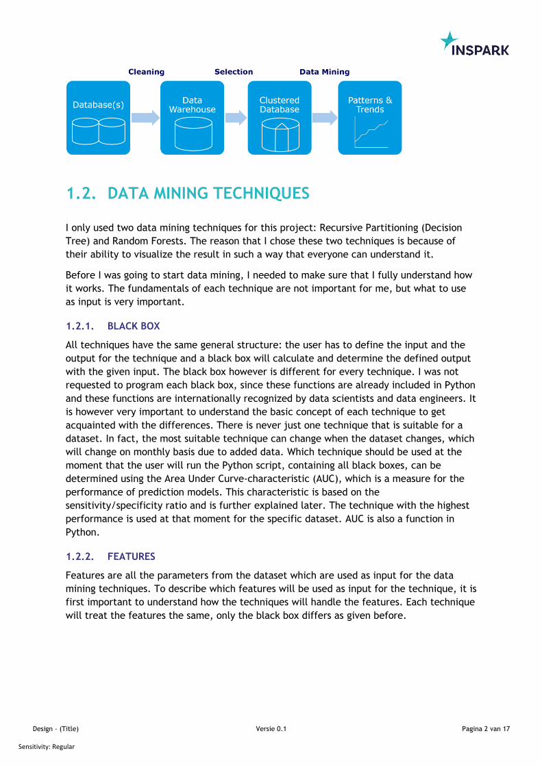
KDD is simply one step of a whole process, which consists of several steps and products.

The first product is/are the database(s), which is/are provided by the company.

The first step is cleaning. The data is often contaminated and therefore not reliable for

the analyses. Cleaning the data will be done to make the data more reliable for the

analyses. If there are more databases together, the databases can be combined first and

then be cleaned or each database can be cleaned separately first and then be combined.

How the data is cleaned and combined depends on the type of database(s) used. An Excel-

database can be cleaned by hand or a program has to be written for that. In case of an

SQL-database, a cleaning method is already available, and the users can use this to clean

the data of the database. The product that remains is a Data Warehouse, which is one

combined and cleaned big data set.

The next step is to make a selection of the data. This step will take some more time, since

I have to determine beforehand which types of data are important for the project and

thus needs to be analyzed. After the selection is made, the Clustered Database is created.

This database is reliable and precise enough for the last step.

The last step is Data Mining. As explained earlier, this part is used to create patterns in

the data, which then can be used for better insights and for better decision making. There

are different data mining techniques, which will be discussed later.

As explained above, data mining is more than just analyzing data. It is part of a process,

which has to be conducted in order to make the product, the patterns and trends, more

reliable. This product is very important for the decision making.



1.2. DATA MINING TECHNIQUES

I only used two data mining techniques for this project: Recursive Partitioning (Decision

Tree) and Random Forests. The reason that I chose these two techniques is because of

their ability to visualize the result in such a way that everyone can understand it.

Before I was going to start data mining, I needed to make sure that I fully understand how

it works. The fundamentals of each technique are not important for me, but what to use

as input is very important.

1.2.1. BLACK BOX

All techniques have the same general structure: the user has to define the input and the

output for the technique and a black box will calculate and determine the defined output

with the given input. The black box however is different for every technique. I was not

requested to program each black box, since these functions are already included in Python

and these functions are internationally recognized by data scientists and data engineers. It

is however very important to understand the basic concept of each technique to get

acquainted with the differences. There is never just one technique that is suitable for a

dataset. In fact, the most suitable technique can change when the dataset changes, which

will change on monthly basis due to added data. Which technique should be used at the

moment that the user will run the Python script, containing all black boxes, can be

determined using the Area Under Curve-characteristic (AUC), which is a measure for the

performance of prediction models. This characteristic is based on the

sensitivity/specificity ratio and is further explained later. The technique with the highest

performance is used at that moment for the specific dataset. AUC is also a function in

Python.

1.2.2. FEATURES

Features are all the parameters from the dataset which are used as input for the data

mining techniques. To describe which features will be used as input for the technique, it is

first important to understand how the techniques will handle the features. Each technique

will treat the features the same, only the black box differs as given before.



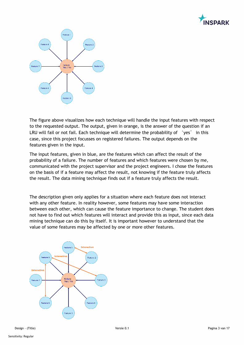
The figure above visualizes how each technique will handle the input features with respect

to the requested output. The output, given in orange, is the answer of the question if an

LRU will fail or not fail. Each technique will determine the probability of ‘yes’ in this

case, since this project focusses on registered failures. The output depends on the

features given in the input.

The input features, given in blue, are the features which can affect the result of the

probability of a failure. The number of features and which features were chosen by me,

communicated with the project supervisor and the project engineers. I chose the features

on the basis of if a feature may affect the result, not knowing if the feature truly affects

the result. The data mining technique finds out if a feature truly affects the result.

The description given only applies for a situation where each feature does not interact

with any other feature. In reality however, some features may have some interaction

between each other, which can cause the feature importance to change. The student does

not have to find out which features will interact and provide this as input, since each data

mining technique can do this by itself. It is important however to understand that the

value of some features may be affected by one or more other features.



1.3. PERFORMANCE OF THE TECHNIQUES

Before going into the process of the Python code for data mining, it is first important to

understand how to increase the performance of each data mining technique. There

multiple ways to do this, but I will use two of the most-used techniques.

1.3.1. HYPER-PARAMETER OPTIMIZATION

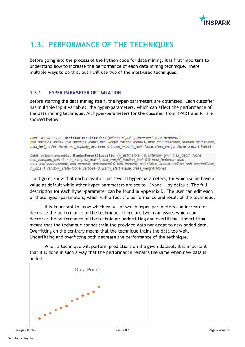
Before starting the data mining itself, the hyper-parameters are optimized. Each classifier

has multiple input variables, the hyper-parameters, which can affect the performance of

the data mining technique. All hyper-parameters for the classifier from RPART and RF are

showed below.

The figures show that each classifier has several hyper-parameters, for which some have a

value as default while other hyper-parameters are set to ‘None’ by default. The full

description for each hyper-parameter can be found in Appendix D. The user can edit each

of these hyper-parameters, which will affect the performance and result of the technique.

It is important to know which values of which hyper-parameters can increase or

decrease the performance of the technique. There are two main issues which can

decrease the performance of the technique: underfitting and overfitting. Underfitting

means that the technique cannot train the provided data nor adapt to new added data.

Overfitting on the contrary means that the technique trains the data too well.

Underfitting and overfitting both decrease the performance of the technique.

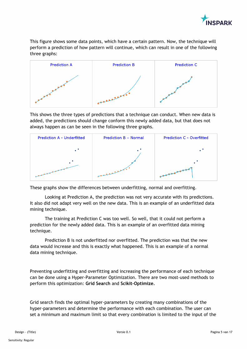
When a technique will perform predictions on the given dataset, it is important

that it is done in such a way that the performance remains the same when new data is

added.

Data Points



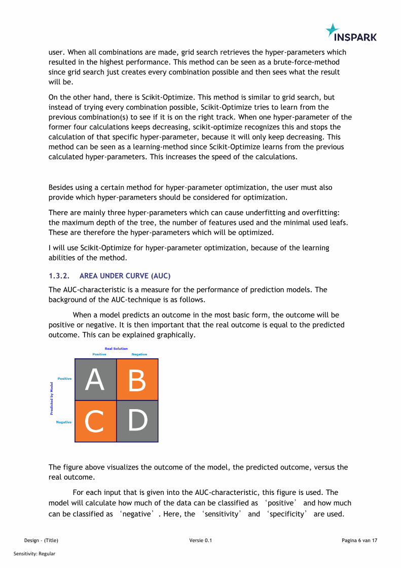
This figure shows some data points, which have a certain pattern. Now, the technique will

perform a prediction of how pattern will continue, which can result in one of the following

three graphs:

This shows the three types of predictions that a technique can conduct. When new data is

added, the predictions should change conform this newly added data, but that does not

always happen as can be seen in the following three graphs.

These graphs show the differences between underfitting, normal and overfitting.

Looking at Prediction A, the prediction was not very accurate with its predictions.

It also did not adapt very well on the new data. This is an example of an underfitted data

mining technique.

The training at Prediction C was too well. So well, that it could not perform a

prediction for the newly added data. This is an example of an overfitted data mining

technique.

Prediction B is not underfitted nor overfitted. The prediction was that the new

data would increase and this is exactly what happened. This is an example of a normal

data mining technique.

Preventing underfitting and overfitting and increasing the performance of each technique

can be done using a Hyper-Parameter Optimization. There are two most-used methods to

perform this optimization: Grid Search and Scikit-Optimize.

Grid search finds the optimal hyper-parameters by creating many combinations of the

hyper-parameters and determine the performance with each combination. The user can

set a minimum and maximum limit so that every combination is limited to the input of the



user. When all combinations are made, grid search retrieves the hyper-parameters which

resulted in the highest performance. This method can be seen as a brute-force-method

since grid search just creates every combination possible and then sees what the result

will be.

On the other hand, there is Scikit-Optimize. This method is similar to grid search, but

instead of trying every combination possible, Scikit-Optimize tries to learn from the

previous combination(s) to see if it is on the right track. When one hyper-parameter of the

former four calculations keeps decreasing, scikit-optimize recognizes this and stops the

calculation of that specific hyper-parameter, because it will only keep decreasing. This

method can be seen as a learning-method since Scikit-Optimize learns from the previous

calculated hyper-parameters. This increases the speed of the calculations.

Besides using a certain method for hyper-parameter optimization, the user must also

provide which hyper-parameters should be considered for optimization.

There are mainly three hyper-parameters which can cause underfitting and overfitting:

the maximum depth of the tree, the number of features used and the minimal used leafs.

These are therefore the hyper-parameters which will be optimized.

I will use Scikit-Optimize for hyper-parameter optimization, because of the learning

abilities of the method.

1.3.2. AREA UNDER CURVE (AUC)

The AUC-characteristic is a measure for the performance of prediction models. The

background of the AUC-technique is as follows.

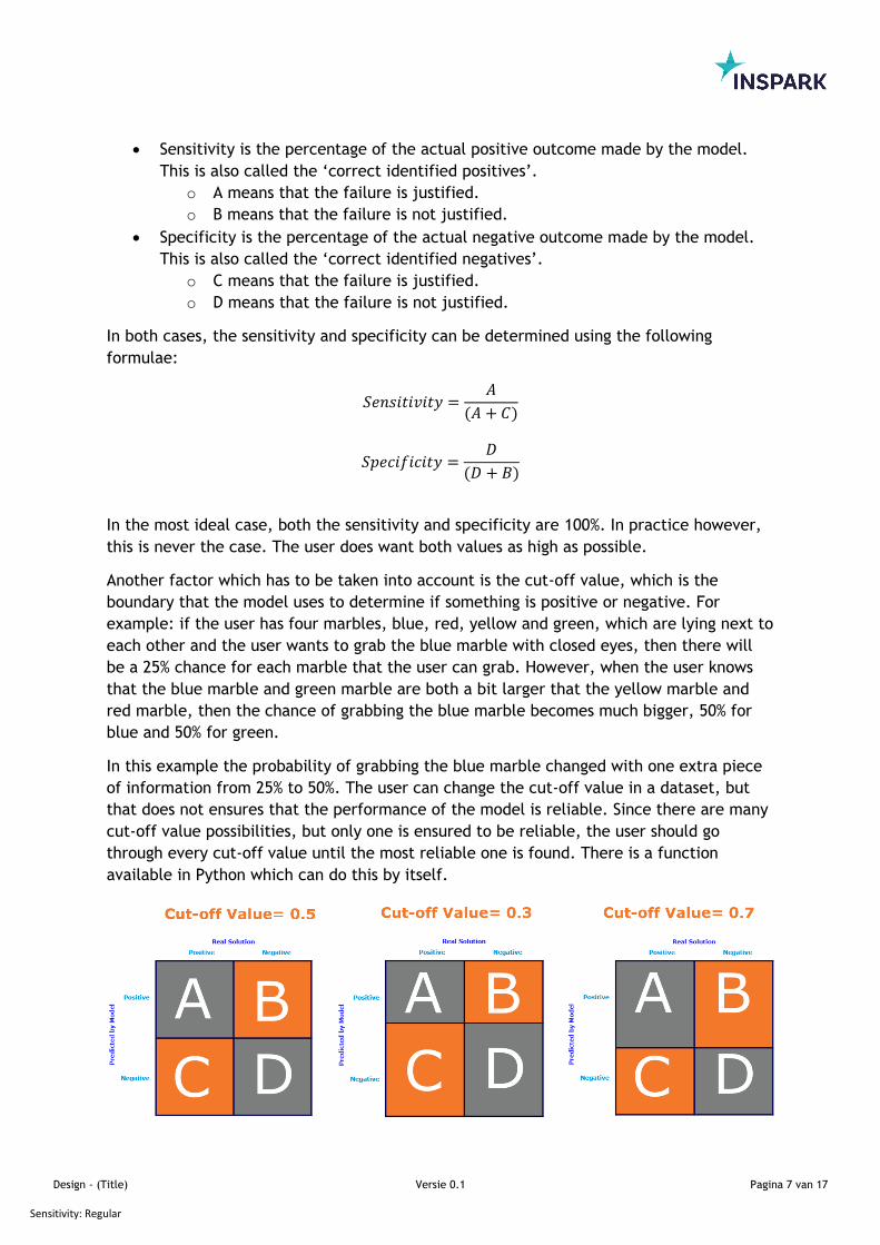
When a model predicts an outcome in the most basic form, the outcome will be

positive or negative. It is then important that the real outcome is equal to the predicted

outcome. This can be explained graphically.

The figure above visualizes the outcome of the model, the predicted outcome, versus the

real outcome.

For each input that is given into the AUC-characteristic, this figure is used. The

model will calculate how much of the data can be classified as ‘positive’ and how much

can be classified as ‘negative’. Here, the ‘sensitivity’ and ‘specificity’ are used.



• Sensitivity is the percentage of the actual positive outcome made by the model.

This is also called the ‘correct identified positives’.

o A means that the failure is justified.

o B means that the failure is not justified.

• Specificity is the percentage of the actual negative outcome made by the model.

This is also called the ‘correct identified negatives’.

o C means that the failure is justified.

o D means that the failure is not justified.

In both cases, the sensitivity and specificity can be determined using the following

formulae:

𝑆𝑒𝑛𝑠𝑖𝑡𝑖𝑣𝑖𝑡𝑦 =𝐴

(𝐴 + 𝐶)

𝑆𝑝𝑒𝑐𝑖𝑓𝑖𝑐𝑖𝑡𝑦 =𝐷

(𝐷 + 𝐵)

In the most ideal case, both the sensitivity and specificity are 100%. In practice however,

this is never the case. The user does want both values as high as possible.

Another factor which has to be taken into account is the cut-off value, which is the

boundary that the model uses to determine if something is positive or negative. For

example: if the user has four marbles, blue, red, yellow and green, which are lying next to

each other and the user wants to grab the blue marble with closed eyes, then there will

be a 25% chance for each marble that the user can grab. However, when the user knows

that the blue marble and green marble are both a bit larger that the yellow marble and

red marble, then the chance of grabbing the blue marble becomes much bigger, 50% for

blue and 50% for green.

In this example the probability of grabbing the blue marble changed with one extra piece

of information from 25% to 50%. The user can change the cut-off value in a dataset, but

that does not ensures that the performance of the model is reliable. Since there are many

cut-off value possibilities, but only one is ensured to be reliable, the user should go

through every cut-off value until the most reliable one is found. There is a function

available in Python which can do this by itself.



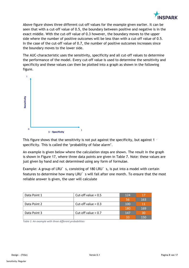
Above figure shows three different cut-off values for the example given earlier. It can be

seen that with a cut-off value of 0.5, the boundary between positive and negative is in the

exact middle. With the cut-off value of 0.3 however, the boundary moves to the upper

side where the number of positive outcomes will be less than with a cut-off value of 0.5.

In the case of the cut-off value of 0.7, the number of positive outcomes increases since

the boundary moves to the lower side.

The AUC-characteristic uses the sensitivity, specificity and all cut-off values to determine

the performance of the model. Every cut-off value is used to determine the sensitivity and

specificity and these values can then be plotted into a graph as shown in the following

figure.

This figure shows that the sensitivity is not put against the specificity, but against 1 –

specificity. This is called the ‘probability of false alarm’.

An example is given below where the calculation steps are shown. The result in the graph

is shown in Figure 17, where three data points are given in Table 7. Note: these values are

just given by hand and not determined using any form of formulae.

Example: A group of LRU’s, consisting of 180 LRU’s, is put into a model with certain

features to determine how many LRU’s will fail after one month. To ensure that the most

reliable answer is given, the user will calculate

Data Point 1 Cut-off value = 0.5 124 17

56 163


180 169


33 150 Table 1: An example with three different probabilities



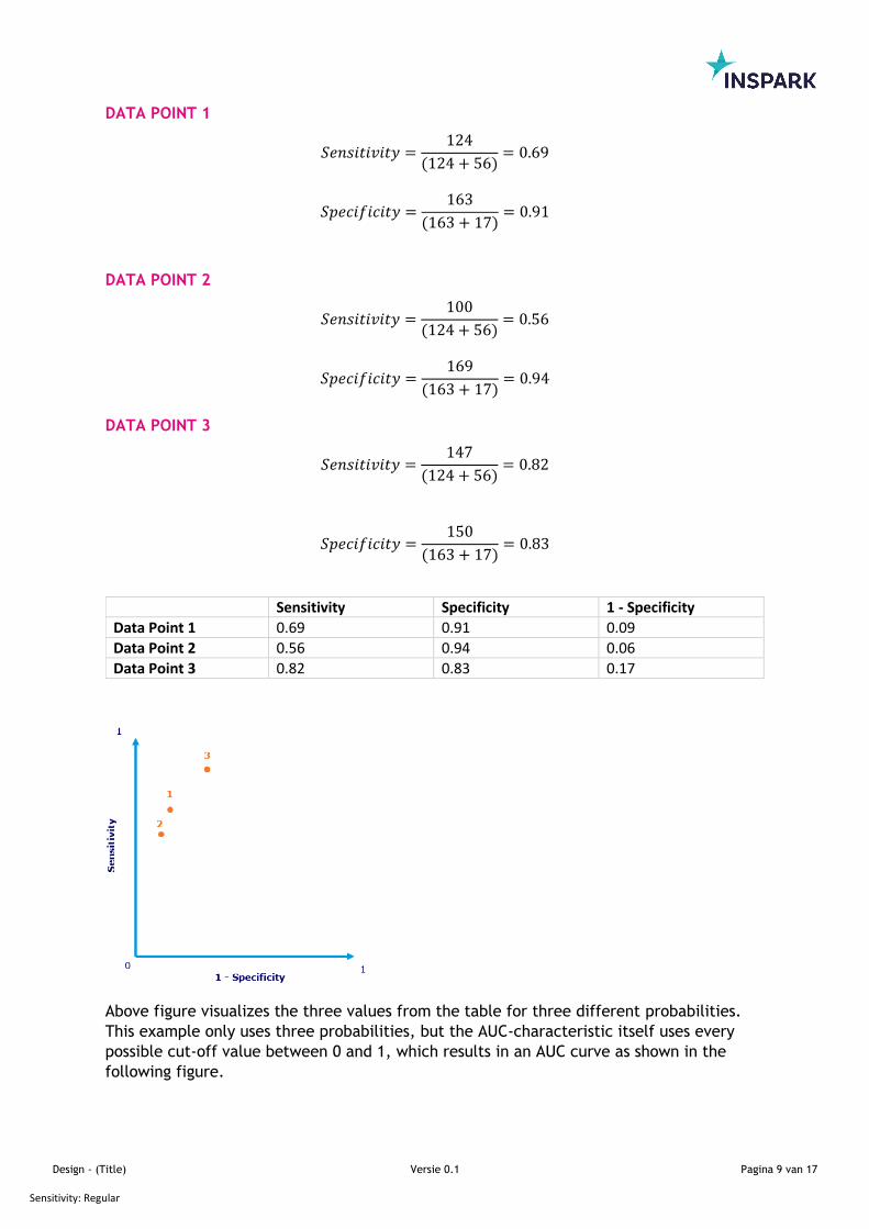
DATA POINT 1

𝑆𝑒𝑛𝑠𝑖𝑡𝑖𝑣𝑖𝑡𝑦 =124

(124 + 56)= 0.69

𝑆𝑝𝑒𝑐𝑖𝑓𝑖𝑐𝑖𝑡𝑦 =163

(163 + 17)= 0.91

DATA POINT 2


(124 + 56)= 0.56


(163 + 17)= 0.94

DATA POINT 3


(124 + 56)= 0.82


(163 + 17)= 0.83

Above figure visualizes the three values from the table for three different probabilities.

This example only uses three probabilities, but the AUC-characteristic itself uses every

possible cut-off value between 0 and 1, which results in an AUC curve as shown in the

following figure.

Sensitivity Specificity 1 - Specificity

Data Point 1 0.69 0.91 0.09

Data Point 2 0.56 0.94 0.06

Data Point 3 0.82 0.83 0.17



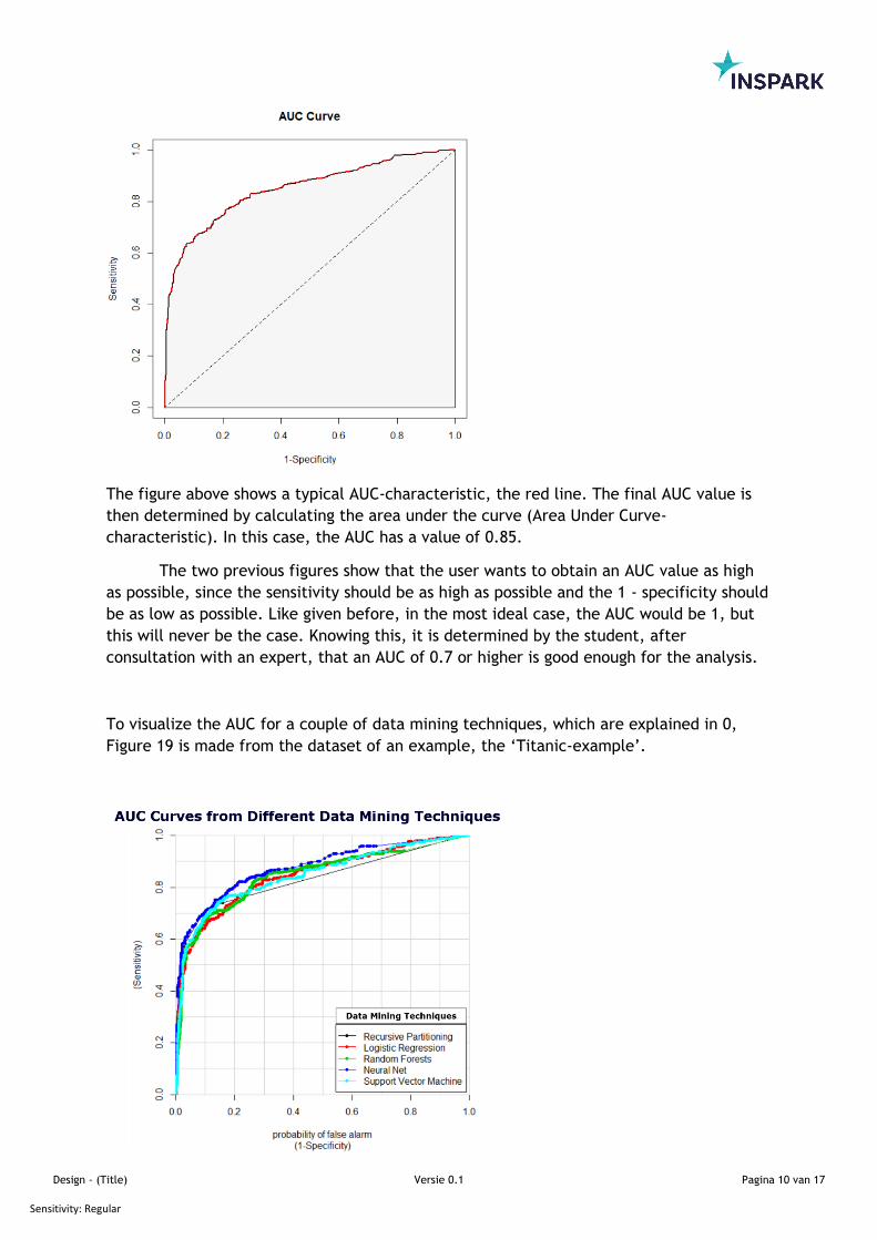
The figure above shows a typical AUC-characteristic, the red line. The final AUC value is

then determined by calculating the area under the curve (Area Under Curve-

characteristic). In this case, the AUC has a value of 0.85.

The two previous figures show that the user wants to obtain an AUC value as high

as possible, since the sensitivity should be as high as possible and the 1 - specificity should

be as low as possible. Like given before, in the most ideal case, the AUC would be 1, but

this will never be the case. Knowing this, it is determined by the student, after

consultation with an expert, that an AUC of 0.7 or higher is good enough for the analysis.

To visualize the AUC for a couple of data mining techniques, which are explained in 0,

Figure 19 is made from the dataset of an example, the ‘Titanic-example’.



Interpreting the above figure, it can be seen that the performance of each model is in this

case very close to each other. It seems that the technique Neural Net has the highest AUC

value, since the area under the curve seems to be the largest.

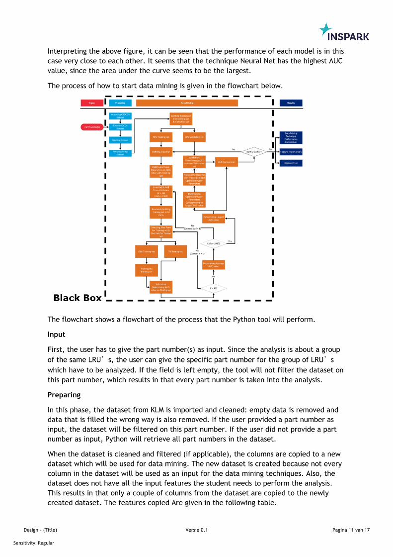
The process of how to start data mining is given in the flowchart below.

The flowchart shows a flowchart of the process that the Python tool will perform.

Input

First, the user has to give the part number(s) as input. Since the analysis is about a group

of the same LRU’s, the user can give the specific part number for the group of LRU’s

which have to be analyzed. If the field is left empty, the tool will not filter the dataset on

this part number, which results in that every part number is taken into the analysis.

Preparing

In this phase, the dataset from KLM is imported and cleaned: empty data is removed and

data that is filled the wrong way is also removed. If the user provided a part number as

input, the dataset will be filtered on this part number. If the user did not provide a part

number as input, Python will retrieve all part numbers in the dataset.

When the dataset is cleaned and filtered (if applicable), the columns are copied to a new

dataset which will be used for data mining. The new dataset is created because not every

column in the dataset will be used as an input for the data mining techniques. Also, the

dataset does not have all the input features the student needs to perform the analysis.

This results in that only a couple of columns from the dataset are copied to the newly

created dataset. The features copied Are given in the following table.



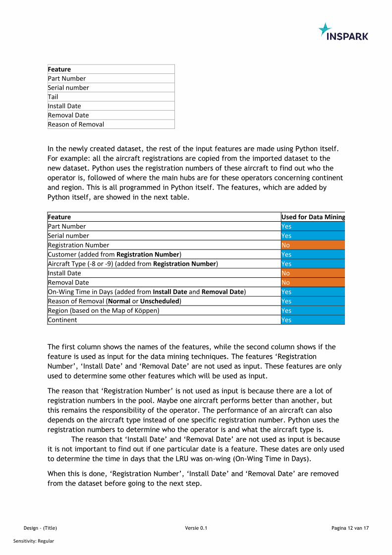
In the newly created dataset, the rest of the input features are made using Python itself.

For example: all the aircraft registrations are copied from the imported dataset to the

new dataset. Python uses the registration numbers of these aircraft to find out who the

operator is, followed of where the main hubs are for these operators concerning continent

and region. This is all programmed in Python itself. The features, which are added by

Python itself, are showed in the next table.

The first column shows the names of the features, while the second column shows if the

feature is used as input for the data mining techniques. The features ‘Registration

Number’, ‘Install Date’ and ‘Removal Date’ are not used as input. These features are only

used to determine some other features which will be used as input.

The reason that ‘Registration Number’ is not used as input is because there are a lot of

registration numbers in the pool. Maybe one aircraft performs better than another, but

this remains the responsibility of the operator. The performance of an aircraft can also

depends on the aircraft type instead of one specific registration number. Python uses the

registration numbers to determine who the operator is and what the aircraft type is.

The reason that ‘Install Date’ and ‘Removal Date’ are not used as input is because

it is not important to find out if one particular date is a feature. These dates are only used

to determine the time in days that the LRU was on-wing (On-Wing Time in Days).

When this is done, ‘Registration Number’, ‘Install Date’ and ‘Removal Date’ are removed

from the dataset before going to the next step.

Feature

Part Number

Serial number

Tail

Install Date

Removal Date

Reason of Removal

Feature Used for Data Mining

Part Number Yes

Serial number Yes

Registration Number No

Customer (added from Registration Number) Yes

Aircraft Type (-8 or -9) (added from Registration Number) Yes

Install Date No

Removal Date No

On-Wing Time in Days (added from Install Date and Removal Date) Yes

Reason of Removal (Normal or Unscheduled) Yes

Region (based on the Map of Köppen) Yes

Continent Yes



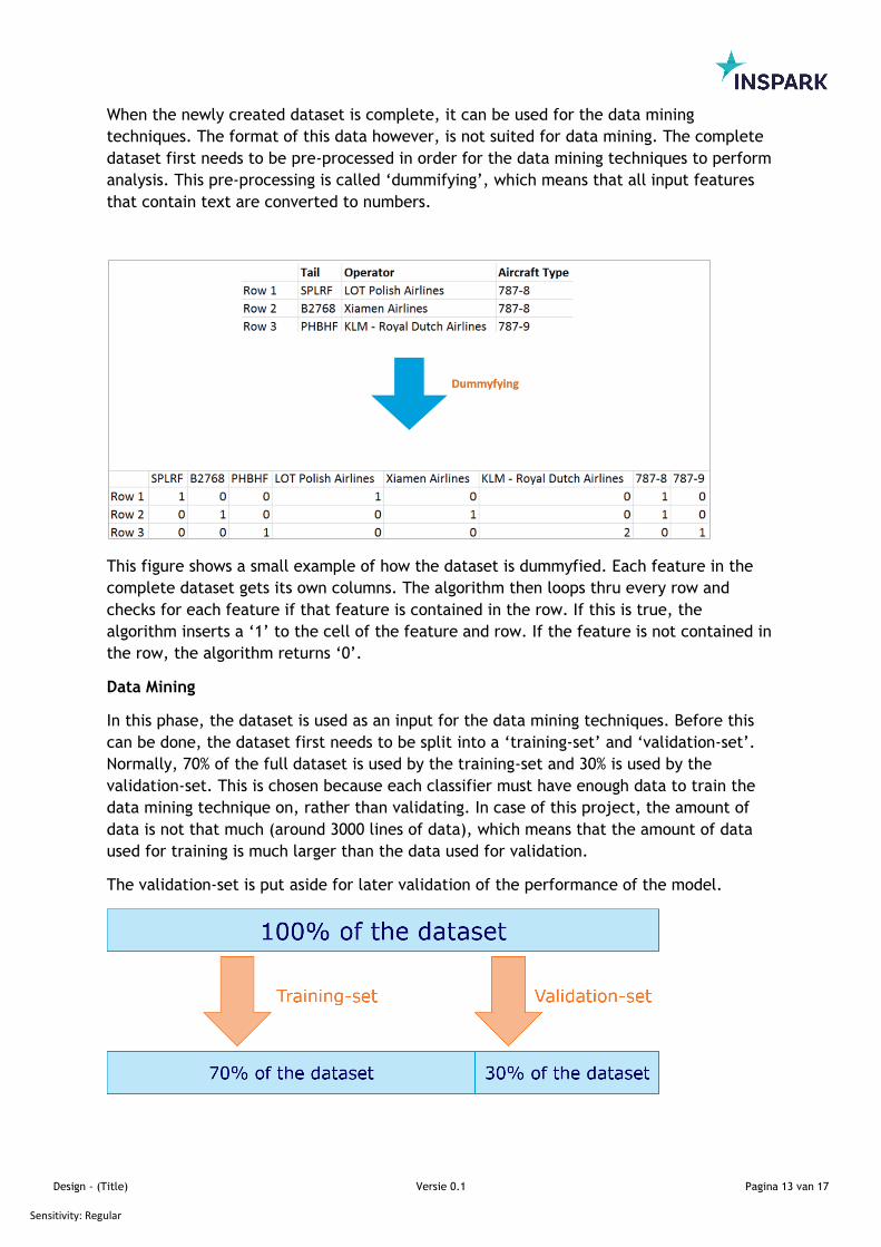
When the newly created dataset is complete, it can be used for the data mining

techniques. The format of this data however, is not suited for data mining. The complete

dataset first needs to be pre-processed in order for the data mining techniques to perform

analysis. This pre-processing is called ‘dummifying’, which means that all input features

that contain text are converted to numbers.

This figure shows a small example of how the dataset is dummyfied. Each feature in the

complete dataset gets its own columns. The algorithm then loops thru every row and

checks for each feature if that feature is contained in the row. If this is true, the

algorithm inserts a ‘1’ to the cell of the feature and row. If the feature is not contained in

the row, the algorithm returns ‘0’.

Data Mining

In this phase, the dataset is used as an input for the data mining techniques. Before this

can be done, the dataset first needs to be split into a ‘training-set’ and ‘validation-set’.

Normally, 70% of the full dataset is used by the training-set and 30% is used by the

validation-set. This is chosen because each classifier must have enough data to train the

data mining technique on, rather than validating. In case of this project, the amount of

data is not that much (around 3000 lines of data), which means that the amount of data

used for training is much larger than the data used for validation.

The validation-set is put aside for later validation of the performance of the model.



The training-set is used by each tool to train itself to make accurate predictions. First, the

hyper-parameters of the training-set are optimized. Each classifier has multiple input

variables, the hyper-parameters, which can affect the performance of the data mining

technique. Therefore, a hyper-parameter optimization will be done to optimize this

performance using the AUC-value, which was discussed earlier.

During this optimization process, the method called Stratified K-Fold Cross Validation

(SKCV) is used. SKCV first divides the training-set into a K number of batches, the ‘folds’

and then trains the model on K-1 batches, which results in that one batch remains

untrained. This last untrained batch is then used for validation of the trained K batches.

This process is then repeated K times.

The value of K is in default the number 3, but in the industry however, K is often the

number 10. This is done for two reasons:

1. If the number of folds get to high, the speed of the calculations and performance

of the model will be decreased. If the number of folds is too low, the reliability of

the model can become quite low.

2. The user wants to have relatively not so many conversions, while having enough

conversions per fold.

The reason for using Stratified K-Fold Cross Validation is because it also takes the relative

distribution of the data into account. This is very helpful if the data is unbalanced, which

can be the case if one feature appears more than once in the dataset for example.

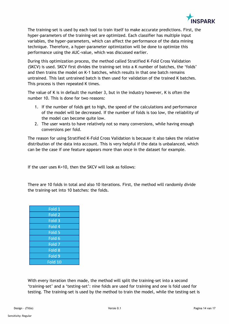
If the user uses K=10, then the SKCV will look as follows:

There are 10 folds in total and also 10 iterations. First, the method will randomly divide

the training-set into 10 batches: the folds.

With every iteration then made, the method will split the training-set into a second

‘training-set’ and a ‘testing-set’: nine folds are used for training and one is fold used for

testing. The training-set is used by the method to train the model, while the testing-set is



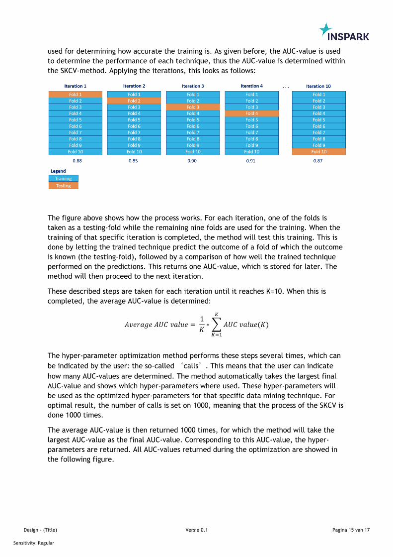
used for determining how accurate the training is. As given before, the AUC-value is used

to determine the performance of each technique, thus the AUC-value is determined within

the SKCV-method. Applying the iterations, this looks as follows:

The figure above shows how the process works. For each iteration, one of the folds is

taken as a testing-fold while the remaining nine folds are used for the training. When the

training of that specific iteration is completed, the method will test this training. This is

done by letting the trained technique predict the outcome of a fold of which the outcome

is known (the testing-fold), followed by a comparison of how well the trained technique

performed on the predictions. This returns one AUC-value, which is stored for later. The

method will then proceed to the next iteration.

These described steps are taken for each iteration until it reaches K=10. When this is

completed, the average AUC-value is determined:

𝐴𝑣𝑒𝑟𝑎𝑔𝑒 𝐴𝑈𝐶 𝑣𝑎𝑙𝑢𝑒 = 1

𝐾∗ ∑ 𝐴𝑈𝐶 𝑣𝑎𝑙𝑢𝑒(𝐾)

𝐾

𝐾=1

The hyper-parameter optimization method performs these steps several times, which can

be indicated by the user: the so-called ‘calls’. This means that the user can indicate

how many AUC-values are determined. The method automatically takes the largest final

AUC-value and shows which hyper-parameters where used. These hyper-parameters will

be used as the optimized hyper-parameters for that specific data mining technique. For

optimal result, the number of calls is set on 1000, meaning that the process of the SKCV is

done 1000 times.

The average AUC-value is then returned 1000 times, for which the method will take the

largest AUC-value as the final AUC-value. Corresponding to this AUC-value, the hyper-

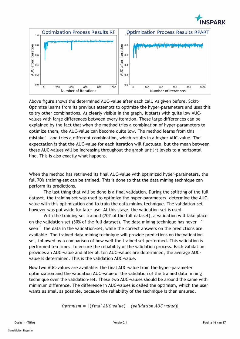
parameters are returned. All AUC-values returned during the optimization are showed in

the following figure.



Above figure shows the determined AUC-value after each call. As given before, Sckit-

Optimize learns from its previous attempts to optimize the hyper-parameters and uses this

to try other combinations. As clearly visible in the graph, it starts with quite low AUC-

values with large differences between every iteration. These large differences can be

explained by the fact that when the method tries a combination of hyper-parameters to

optimize them, the AUC-value can become quite low. The method learns from this ‘

mistake’ and tries a different combination, which results in a higher AUC-value. The

expectation is that the AUC-value for each iteration will fluctuate, but the mean between

these AUC-values will be increasing throughout the graph until it levels to a horizontal

line. This is also exactly what happens.

When the method has retrieved its final AUC-value with optimized hyper-parameters, the

full 70% training-set can be trained. This is done so that the data mining technique can

perform its predictions.

The last thing that will be done is a final validation. During the splitting of the full

dataset, the training-set was used to optimize the hyper-parameters, determine the AUC-

value with this optimization and to train the data mining technique. The validation-set

however was put aside for later use. At this stage, the validation-set is used.

With the training-set trained (70% of the full dataset), a validation will take place

on the validation-set (30% of the full dataset). The data mining technique has never ‘

seen’ the data in the validation-set, while the correct answers on the predictions are

available. The trained data mining technique will provide predictions on the validation-

set, followed by a comparison of how well the trained set performed. This validation is

performed ten times, to ensure the reliability of the validation process. Each validation

provides an AUC-value and after all ten AUC-values are determined, the average AUC-

value is determined. This is the validation AUC-value.

Now two AUC-values are available: the final AUC-value from the hyper-parameter

optimization and the validation AUC-value of the validation of the trained data mining

technique over the validation-set. These two AUC-values should be around the same with

minimum difference. The difference in AUC-values is called the optimism, which the user

wants as small as possible, because the reliability of the technique is then ensured.

𝑂𝑝𝑡𝑖𝑚𝑖𝑠𝑚 = |(𝑓𝑖𝑛𝑎𝑙 𝐴𝑈𝐶 𝑣𝑎𝑙𝑢𝑒) − (𝑣𝑎𝑙𝑖𝑑𝑎𝑡𝑖𝑜𝑛 𝐴𝑈𝐶 𝑣𝑎𝑙𝑢𝑒)|



The last step in the process are the results, where three types of results are given:

The first result is a comparison of the performances of both data mining

techniques. A graph containing the final AUC-value, validation AUC-value and optimism is

generated to visualize this comparison. Using this graph, the user can see which data

mining technique performs best and which data mining technique will be used to show the

results.

The second result are the feature importance’s. When the user has chosen a data

mining technique, the feature importance’s for that particular technique can be

retrieved visualized. Here, the user can easily see which features have the biggest

contribution in the predictions of the technique.

The last result is a decision tree. A decision tree is a very good way to see how

some features are related to each other. It consists of several nodes which each give a

prediction of what the chance would be that an LRU will fail under certain circumstances.

2.1. VERIFICATION

The last important procedure that has to be conducted is the verification of the script and

the validation of the techniques. Verification of the script means that the user and other

experts check the code in the Python script to see if the code that is put there is doing

exactly as the users expect it to do. One writing error can cause a wrong result.

The verification is done by three different data scientists, so that I’m sure of the

reliability of the code.

Another verification method is to look at the results. One employee already performed

some basic analysis concerning the operators. The results of the employee and my results

can now be compared.

DATA MINING ON AIRCRAFT COMPONENT FAILURES · 2018-12-14 · DATA MINING TECHNIQUES I only used two...

Documents

Transcript of DATA MINING ON AIRCRAFT COMPONENT FAILURES · 2018-12-14 · DATA MINING TECHNIQUES I only used two...