Conditional Optimization - Universiteit Utrecht · Conditional Optimization An N-particle formalism...
96
Conditional Optimization An N -particle formalism for protein structure refinement Conditionele Optimalisatie Een N -deeltjes formalisme voor eiwitstructuurverfijning (met een samenvatting in het Nederlands) PROEFSCHRIFT TER VERKRIJGING VAN DE GRAAD VAN DOCTOR AAN DE UNIVERSITEIT UTRECHT OP GEZAG VAN DE RECTOR MAGNIFICUS,PROF. DR. W.H. GISPEN, INGEVOLGE HET BESLUIT VAN HET COLLEGE VOOR PROMOTIES IN HET OPENBAAR TE VERDEDIGEN OP MAANDAG 16 JUNI 2003 DES OCHTENDS OM 10.30 UUR door SJORS HENDRIK WILLEM SCHERES geboren op 5 augustus 1975, te Roermond
Transcript of Conditional Optimization - Universiteit Utrecht · Conditional Optimization An N-particle formalism...
Conditional Optimization
An N-particle formalism for protein structure refinement
Conditionele Optimalisatie
Een N-deeltjes formalisme voor eiwitstructuurverfijning
(met een samenvatting in het Nederlands)
PROEFSCHRIFT
TER VERKRIJGING VAN DE GRAAD VAN DOCTOR AAN DEUNIVERSITEIT UTRECHT OP GEZAG VAN DE
RECTOR MAGNIFICUS, PROF. DR. W.H. GISPEN,INGEVOLGE HET BESLUIT VAN HET COLLEGE VOORPROMOTIES IN HET OPENBAAR TE VERDEDIGEN OP
MAANDAG 16 JUNI 2003 DES OCHTENDS OM 10.30 UUR
door
SJORS HENDRIK WILLEM SCHERES
geboren op 5 augustus 1975, te Roermond

Promotor: prof. dr. P. Grosverbonden aan het Bijvoet Centrum voor Biomoleculair Onderzoek,Faculteit Scheikunde der Universiteit Utrecht
Dit proefschrift werd mede mogelijk gemaakt door financiele steun van NWO(Jonge Chemici 99-564)
ISBN: 90-393-3352-1

Ter nagedachtenis aan Jan Kroon

Reproductie: Drukkerij Labor, Utrecht
Omslagvoorzijde: Hooiberg bij Huub vanne Waal in Stramproy, Limburg.achterzijde: Naaldvormig eiwitkristal, gegroeid in de ruimte (bron: NASA).
Contents
1 Introduction 71.1 Protein crystallography . . . . . . . . . . . . . . . . . . . . . . . . . . . . . 71.2 The phase problem . . . . . . . . . . . . . . . . . . . . . . . . . . . . . . . 81.3 Experimental phasing . . . . . . . . . . . . . . . . . . . . . . . . . . . . . 91.4 Ab initio phasing . . . . . . . . . . . . . . . . . . . . . . . . . . . . . . . . 10
1.4.1 Direct methods . . . . . . . . . . . . . . . . . . . . . . . . . . . . . 101.4.2 Molecular replacement . . . . . . . . . . . . . . . . . . . . . . . . . 101.4.3 Low-resolution phasing . . . . . . . . . . . . . . . . . . . . . . . . 10
1.5 Phase improvement . . . . . . . . . . . . . . . . . . . . . . . . . . . . . . . 111.5.1 Density modification . . . . . . . . . . . . . . . . . . . . . . . . . . 111.5.2 Model building . . . . . . . . . . . . . . . . . . . . . . . . . . . . . 121.5.3 Refinement . . . . . . . . . . . . . . . . . . . . . . . . . . . . . . . 12
1.6 Conditional Optimization . . . . . . . . . . . . . . . . . . . . . . . . . . . . 141.7 Scope and outline of this thesis . . . . . . . . . . . . . . . . . . . . . . . . . 15
2 Conditional Optimization: a new formalism for protein structure refinement 172.1 Introduction . . . . . . . . . . . . . . . . . . . . . . . . . . . . . . . . . . . 182.2 Conditional Formalism . . . . . . . . . . . . . . . . . . . . . . . . . . . . . 192.3 Experimental . . . . . . . . . . . . . . . . . . . . . . . . . . . . . . . . . . 23
2.3.1 Implementation . . . . . . . . . . . . . . . . . . . . . . . . . . . . . 232.3.2 Test case . . . . . . . . . . . . . . . . . . . . . . . . . . . . . . . . 242.3.3 Refinement protocols . . . . . . . . . . . . . . . . . . . . . . . . . . 24
2.4 Results . . . . . . . . . . . . . . . . . . . . . . . . . . . . . . . . . . . . . . 292.4.1 Refinement of scrambled models . . . . . . . . . . . . . . . . . . . . 292.4.2 Refinement of random atom distributions . . . . . . . . . . . . . . . 32
2.5 Discussion . . . . . . . . . . . . . . . . . . . . . . . . . . . . . . . . . . . . 34
3 Development of a force field for conditional optimization of protein structures 353.1 Introduction . . . . . . . . . . . . . . . . . . . . . . . . . . . . . . . . . . . 363.2 Mean-force potential for protein structures . . . . . . . . . . . . . . . . . . . 36
3.2.1 Brief review of the conditional formalism . . . . . . . . . . . . . . . 363.2.2 The general parameter set . . . . . . . . . . . . . . . . . . . . . . . 383.2.3 Protein-specific force fields . . . . . . . . . . . . . . . . . . . . . . . 40
6 CONTENTS
3.3 Experimental . . . . . . . . . . . . . . . . . . . . . . . . . . . . . . . . . . 413.4 Results & discussion . . . . . . . . . . . . . . . . . . . . . . . . . . . . . . 44
3.4.1 Stability of correct structures . . . . . . . . . . . . . . . . . . . . . . 443.4.2 Searching behaviour in optimization . . . . . . . . . . . . . . . . . . 45
3.5 Conclusions . . . . . . . . . . . . . . . . . . . . . . . . . . . . . . . . . . . 50
4 The potentials of conditional optimization in automated model building 534.1 Introduction . . . . . . . . . . . . . . . . . . . . . . . . . . . . . . . . . . . 544.2 Experimental . . . . . . . . . . . . . . . . . . . . . . . . . . . . . . . . . . 554.3 Results . . . . . . . . . . . . . . . . . . . . . . . . . . . . . . . . . . . . . . 594.4 Discussion & conclusions . . . . . . . . . . . . . . . . . . . . . . . . . . . . 64
5 Testing conditional optimization for application to ab initio phasing of proteinstructures 675.1 Introduction . . . . . . . . . . . . . . . . . . . . . . . . . . . . . . . . . . . 685.2 Experimental . . . . . . . . . . . . . . . . . . . . . . . . . . . . . . . . . . 69
5.2.1 Test case . . . . . . . . . . . . . . . . . . . . . . . . . . . . . . . . 695.2.2 Optimization protocol . . . . . . . . . . . . . . . . . . . . . . . . . 705.2.3 Phase probability estimation . . . . . . . . . . . . . . . . . . . . . . 72
5.3 Results . . . . . . . . . . . . . . . . . . . . . . . . . . . . . . . . . . . . . . 725.3.1 Condensation and the influence of low-resolution data . . . . . . . . 725.3.2 Quality of the phase probability estimates . . . . . . . . . . . . . . . 735.3.3 Convergence behaviour . . . . . . . . . . . . . . . . . . . . . . . . . 77
5.4 Discussion . . . . . . . . . . . . . . . . . . . . . . . . . . . . . . . . . . . . 795.4.1 The Alpha-1 test case . . . . . . . . . . . . . . . . . . . . . . . . . . 795.4.2 Implications for further development . . . . . . . . . . . . . . . . . 82
5.5 Conclusions . . . . . . . . . . . . . . . . . . . . . . . . . . . . . . . . . . . 84
6 Summary & general discussion 85
Bibliography 87
Samenvatting & algemene discussie 91
Curriculum Vitae 93
Dankwoord 94
Chapter 1
Introduction
1.1 Protein crystallography
X-ray crystallography plays a major role in the understanding of biological processes at amolecular level by providing atomic models of macro-molecular molecules. Typically, inprotein crystallography highly purified samples at high concentrations are crystallized usingvapour or liquid diffusion methods. Nowadays, large amounts of genome sequences are avail-able and due to well-defined expression systems and efficient purification protocols, samplescan be produced at scales large enough for crystallization trials for many target proteins.With the maturation of third-generation synchrotron beam lines providing high-intensity X-ray beams, cryogenic sample protection, robotic sample changing and charge-coupled-device(CCD) detectors, fast and highly automated diffraction experiments are becoming a routinematter. Crystals of only a few micrometer in size are now suitable for crystallographic anal-ysis (Cusack et al., 1998), and crystal structures of molecular assemblies as large as the 50Ssubunit of the ribosome have already been solved (Ban et al., 2000).
However, after fifty years of extensive research two bottle-necks remain in the processof protein crystal structure determination. Firstly, although automated setups require ever-decreasing amounts of sample material and efficient sparse-matrix screens of crystallizationconditions have been developed (reviewed by Stevens, 2000), obtaining suitable crystalsfor diffraction purposes remains a difficult process that is poorly understood (reviewed byGilliland & Ladner, 1996). Secondly, after obtaining diffracting crystals, phases need to bedetermined for the measured intensities in order to reconstruct the electron density of theunit cell. Since the early days of protein crystallography the most prominent answer to thisproblem has been based on the incorporation of heavy atoms in the crystal, but the search forappropiate soaking solutions is often a cumbersome one. The possibilities to incorporate co-valently bound heavy atoms in the protein, mainly by the incorporation of seleno-methionineusing bacterial expression systems, have contributed significantly to the successful appli-cation of experimental phasing techniques. However, with the increasing requirements ofpost-translational modifications for the more complex target structures of nowadays, equiva-lents for eukaryotic expression systems are awaited anxiously. In the favourable cases wherea homologous structure is available, molecular replacement can be applied to solve the phase
8 Introduction
problem. Despite large efforts throughout the field, other (ab initio) phasing techniques thatdo not depend on the incorporation of heavy atoms, have not yet provided a generally appli-cable answer to the phase problem in macro-molecular crystallography.
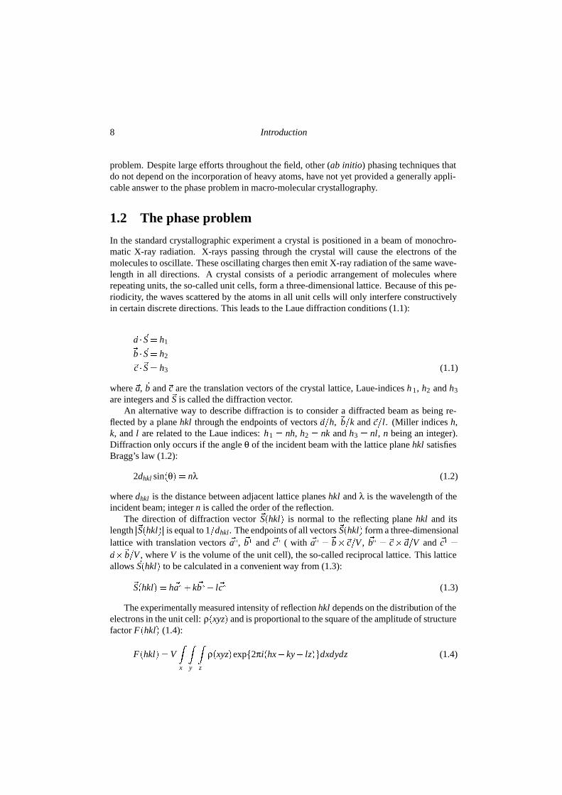
1.2 The phase problem
In the standard crystallographic experiment a crystal is positioned in a beam of monochro-matic X-ray radiation. X-rays passing through the crystal will cause the electrons of themolecules to oscillate. These oscillating charges then emit X-ray radiation of the same wave-length in all directions. A crystal consists of a periodic arrangement of molecules whererepeating units, the so-called unit cells, form a three-dimensional lattice. Because of this pe-riodicity, the waves scattered by the atoms in all unit cells will only interfere constructivelyin certain discrete directions. This leads to the Laue diffraction conditions (1.1):
�a ��S � h1
�b ��S � h2
�c ��S � h3 (1.1)
where �a,�b and�c are the translation vectors of the crystal lattice, Laue-indices h 1, h2 and h3
are integers and �S is called the diffraction vector.An alternative way to describe diffraction is to consider a diffracted beam as being re-
flected by a plane hkl through the endpoints of vectors �a�h, �b�k and �c�l. (Miller indices h,k, and l are related to the Laue indices: h1 � nh, h2 � nk and h3 � nl, n being an integer).Diffraction only occurs if the angle θ of the incident beam with the lattice plane hkl satisfiesBragg’s law (1.2):
2dhkl sin�θ� � nλ (1.2)
where dhkl is the distance between adjacent lattice planes hkl and λ is the wavelength of theincident beam; integer n is called the order of the reflection.
The direction of diffraction vector �S�hkl� is normal to the reflecting plane hkl and itslength ��S�hkl�� is equal to 1�dhkl. The endpoints of all vectors �S�hkl� form a three-dimensionallattice with translation vectors �a�, �b� and �c� ( with �a� ��b��c�V , �b� ��c��a�V and �c� �
�a��b�V , where V is the volume of the unit cell), the so-called reciprocal lattice. This latticeallows �S�hkl� to be calculated in a convenient way from (1.3):
�S�hkl� � h�a�� k�b�� l�c� (1.3)
The experimentally measured intensity of reflection hkl depends on the distribution of theelectrons in the unit cell: ρ�xyz� and is proportional to the square of the amplitude of structurefactor F�hkl� (1.4):
F�hkl� �V�
x
�
y
�
z
ρ�xyz�exp�2πi�hx� ky� lz��dxdydz (1.4)
Experimental phasing 9
with x, y and z being fractional coordinates.By inverse Fourier transform the electron density distribution in the unit cell is calculated
from structure factors F�hkl� (1.5):
ρ�xyz� � 1�V ∑h
∑k
∑l
F�hkl�exp��2πi�hx� ky� lz�� (1.5)
From the electron density distribution an atomic model of the molecules in the unit cellcan be constructed. However, structure factors F�hkl� in equation 1.5 are complex quantitieswith an amplitude and a phase (1.6):
F�hkl� � �F�hkl��exp�iϕ�hkl�� (1.6)
From the standard monochromatic experiment, amplitude �F�hkl�� can be derived fromthe measured intensity, but all information about phases ϕ�hkl� is lost. Therefore, the electrondensity distribution cannot be constructed directly using equation 1.5. This problem is knownas the crystallographic phase problem.
1.3 Experimental phasing
In macro-molecular crystallography it is common practice to solve the phase problem usingadditional experimental information (see classic texts like Drenth, 1999 for more details). Inthe isomorphous replacement method, protein crystals are soaked in one or more solutionscontaining ‘heavy’ atoms. In the optimal case this leads to specific binding of the heavyatoms to the protein molecules and the soaked crystals stay isomorphous to the native crystal.The resulting differences in intensity of the observed reflections are exploited to obtain phaseestimates. Many heavy atoms absorb X-ray radiation at wavelengths that are typically used inprotein crystallography (0.6-2.0 A). The absorbance of X-ray fotons gives rise to anomalousdiffraction. In anomalous scattering methods, the intensity differences between Friedel pairreflections hkl and �h� k� l (the so-called Bijvoet differences) are used to calculate phaseestimates. The continuous tunability of synchrotron radiation sources makes it convenient toexploit yet another signal: dispersive intensity differences between data collected at differentwavelenghts. In multiple-wavelength anomalous dispersion methods (MAD, Hendrickson &Ogata, 1997), combination of the anomalous and dispersive signals allows phase determina-tion from a single crystal. MAD-phasing has become increasingly popular due to the pos-sibility to bio-synthetically introduce anomalous scatterers into the protein itself (reviewedby Ogata, 1998). In particular the Eschericia coli bacterium is used to substitute methioninefor seleno-methionine. This yields anomalously scattering molecules with essentially equalstructural properties compared to the native protein. Recently, density modification methods(see also below) have been applied successfully to substitute the need for dispersive signals,allowing phasing by anomalous scattering using only a single wavelength (SAD, as advocatedby Wang, 1985).
10 Introduction
1.4 Ab initio phasing
In ab initio phasing phase estimates are obtained from a single set of structure factor am-plitudes, without using any of the experimentally determined intensity differences describedabove. In this case, the phase problem may be overcome by incorporation of additional, apriori available knowledge.
1.4.1 Direct methods
Even the simplest form of prior knowledge, the expectation that the electron density is non-negative and consists of separated atoms throughout the unit cell, leads to statistical relation-ships among the structure factors that can be used to solve the phase problem. In the 1950’sHauptman & Karle defined a functional form to express these relationships and therebyopened the field of direct methods. Ever since, this approach has increased its power andnowadays it is used to routinely solve thousands of structures with up to 250 non-hydrogenatoms every year. The ultimate potential of this method is still unknown; its only limitation isthat it requires diffraction data up to atomic, i.e. �1.2 A resolution. (reviewed by Hauptman,1997). For the direct phasing of macromolecules, up to now, direct methods have proven oflimited use. The reliability with which the phases can be estimated decreases rapidly with thenumber of atoms in the unit cell and in protein crystallography the requirement of diffractiondata up to atomic resolution is not often met. Recent advances, where reciprocal-space phaserefinement is combined with modifications in real-space, the so-called baked (Weeks et al.,1993) and half-baked (Sheldrick & Gould, 1995) methods have allowed the direct phasingof small protein structures of up to 1,000 non-hydrogen atoms. Provided that some initialphasing from a substructure is available, larger structures can be solved by a combination ofdirect methods and density modification (Foadi et al., 2002).
1.4.2 Molecular replacement
A much more common way of ‘ab initio’ phasing in protein crystallography is molecularreplacement. In molecular replacement (reviewed by Rossmann, 2001) the known structureof a homologous protein is used as prior information in the phasing process. Phases areobtained by correctly positioning the known model in the crystal lattice of the unkown struc-ture. Traditionally, this problem has been broken down into two three-dimensional searchproblems. Using Patterson methods, first the correct orientation is determined, followed by asearch for the correct translation vector. Recently also programs performing complete (Sher-iff S. et al., 1999) or directed (Kissinger et al., 1999 and Glykos et al., 2000) six-dimensionalsearches have been developed. Another recent development is the application of maximumlikelihood to molecular replacement, which may allow positioning molecules of significantlylower homology (Read, 2001).
1.4.3 Low-resolution phasing
Several attempts have been made to solve the phase problem by first finding the proteinmolecular envelope in the unit cell, which encompasses phasing of only the lowest resolution
Phase improvement 11
reflections. Urzhumtsev et al. (2000) applied various selection criteria based on histogramsand connectivity of the electron density map to select the better set of phases from a largenumber of random trial sets. None of their criteria proved capable of unambiguously dis-tinguising good from bad phase sets, but by making use of the statistical tendency of goodphase sets to have better criterion values than bad sets, enrichment of the phase quality couldbe obtained. For a test case of protein G these procedures resulted in moderate phase infor-mation for reflections up to 4-5 A resolution (Lunina et al., 2000). Additionally, instead ofgenerating random phases, these groups have tried to use large-sphere models that are placedrandomly in the unit cell to generate trial phases. This so-called few atom method uses thecorrelation coefficient between calculated and observed structure factors as selection criterionin the enrichment process (Lunin et al., 1995, 1998). A combination of the methods devel-oped by these groups allowed phasing up to 40 A resolution of the ribosomal 50S particlefrom Thermus thermophilus (Lunin et al., 2000).
A number of other methods to solve protein structures starting from the lowest resolu-tion reflections have been developed but none of them have come into common practice. Bysystematic translation of a large sphere filled with point scatterers at regular intervals andmonitoring the crystallographic R-factor, Harris (1995) could determine the correct molecu-lar envelope for some test cases. However, due to the limitation of a spherical search model,the method showed limited success for solvent regions with a significantly deviating shape.Subbiah (1991) used refinement of randomly distributed hard sphere point scatterers to phasethe lowest resolution reflections. Although initially this method yielded solutions with equallikelihood of the point scatterers ending up in the solvent or in the protein region, later suc-cessful methods were developed to distinguish these solutions (Subbiah, 1993). Guo et al.(2000) applied the probabilistic approach from conventional direct methods to low-resolutionphasing, avoiding the necessity of atomic resolution data by using globbic scattering factorsrepresenting multiple protein atoms. Complementation of the missing lowest-resolution re-flections with calculated data appeared critical for the successful application of this method.The dependance on complete low resolution data is a common feature for most low-resolutionphasing methods. Up to now, none of these methods have bridged the gap between phasesproviding a low-resolution molecular envelope and phases of sufficient quality to allow phaseextension to medium or high resolution with density modification methods (see next section).
1.5 Phase improvement
1.5.1 Density modification
The incorporation of prior information can be used to extend phase information as obtainedby the methods described above (reviewed by Abrahams & De Graaff, 1998). Protein crys-tals typically contain 30-70% solvent, organized in channels of unordered water molecules.In solvent flattening (Wang, 1985), the electron density is constrained towards a flat solventregion, and this real-space density modification is iterated with a phase-combination step inreciprocal space. A similar iterative procedure is used in histogram matching where prior in-formation in the form of expected density histograms is applied as constraints on the electrondensity map. Similarly, knowledge of non-crystallographic symmetry (NCS) can be used to
12 Introduction
modify the electron density by averaging over independent molecules. This NCS-averaginghas proven very powerful to extend the available phase information when multiple copies ofthe same molecule are present in the asymmetric unit. For some viruses for example, exten-sive NCS-averaging has allowed ab initio phasing starting from simple geometric models likea hollow sphere (reviewed by Rossmann, 1995). A new development in the field of densitymodification is the implementation of maximum-likelihood theory in the RESOLVE program(Terwilliger, 2000).
1.5.2 Model building
After an electron density map has been obtained from initial phasing and density modifica-tion techniques, interpretation of this map in terms of a protein model is required. In thisprocess prior knowledge of the amino-acid sequence as well as the known structural charac-teristics of protein molecules are of great importance. Therefore, visualization programs formanual model building like O (Jones et al., 1991), make extensive use of databases of com-monly observed main and side-chain conformations. Still, manual model building remainsnot only a time-consuming process but also a subjective one, shown to be prone to humanerror (Mowbray et al., 1999). Major advances have been achieved in more automated waysof map interpretation. Pattern recognition methods, exploiting similar knowledge as used inmanual building, have been implemented in semi-automated model-building programs likeTEXTAL (Holton et al., 2000), RESOLVE (Terwilliger, 2002) and QUANTA (Oldfield, 2000).Provided initial phases of sufficient quality, such methods have been shown to work at res-olution limits of �3A. With such limited amounts of diffraction data the generated modelsmay suffer a rather low accuracy. Iteration of model building steps with refinement cycles(see next section), as already implemented in the RESOLVE program, may provide a solutionto this problem.
Up till now the most widely used program for automated model building is ARP/wARP(Perrakis et al., 1999). In ARP/wARP, electron density maps are interpreted in terms of freeatoms, which are refined using the ARP procedure (Lamzin & Wilson, 1993), where (almost)unrestrained refinement is combined with atom repositioning based on various types of elec-tron density maps. Subsequently, the warpNtrace procedure (Perrakis et al., 1999) exploitsprior knowledge about oligo-peptide conformations to identify and trace possible main-chainfragments through the optimized distributions of free atoms. The resulting ’hybrid’ modelallows free-atom refinement to be combined with the application of standard geometric re-straints, reducing the danger of overfitting the data. The main limitation of the ARP/wARPprogram is that it requires data to relatively high resolution limits since the unrestrained re-finement cycles depend on a favourable observation-to-parameter ratio and the repositioningof separate atoms in the ARP procedure requires electron density maps of sufficient resolu-tion. Recently, major advances have been achieved for the warpNtrace algorithm (Morris etal., 2002), currently allowing automated main-chain tracing at resolution limits of 2.5 A.
1.5.3 Refinement
The building of a protein model is often hampered by a poor quality of the phase informationor limited resolution of the diffraction data. Therefore, the initial model generally contains
Phase improvement 13
errors and must be optimized. The goal of crystallographic refinement can be formulated asfinding the set of atomic coordinates that results in the best fit of the observed structure fac-tor amplitudes and the amplitudes calculated from this model. In conventional least-squaresrefinement (see for example Drenth, 1999), this goal has been formulated as finding the min-imum of target function (1.7):
EX�ray � ∑hkl
whkl��Fobshkl �� k�Fcalc
hkl ��2 (1.7)
Where whkl is a weighting factor, k is a scale factor and the calculated structure factoramplitude �F calc� is dependent on the parameter set of the model. Calculation of derivativesof �Fcalc� towards the model parameters allows application of gradient-driven optimizationtechniques to minimize this function.
Major advances in refinement have been made by the formulation of maximum likelihoodtarget functions (reviewed by Bricogne, 1997). In contrast to least-squares methods, maxi-mum likelihood provides a statistically valid way to deal with errors and incompleteness ofthe model. A general approach is to represent the resolution-dependent quality of the modelby the σA-distribution (1.8):
σA � �Eobs �Ecalc� (1.8)
where σA-values are calculated in resolution bins and E obs and Ecalc are observed and cal-culated normalized structure factors. Since the phases of E obs are unknown, σA-values needto be estimated. For this purpose Read (1986) developed a method called SIGMAA. Cross-validation, initially introduced to monitor over-fitting of the data by calculation of a freeR-factor (Brunger, 1993), plays an important role in the estimation of σ A-values (Adams etal., 1997). In cross-validation typically 5-10% of the data (the test set) is kept outside therefinement. Estimation of σA-values based on these test set reflections avoids serious over-estimation resulting from overfitting of the data. The probability to observe E obs, given Ecalc
of the model, can then be calculated by (1.9):
P�
Eobs;Ecalc��
1
π�1�σ2A�
exp
���Eobs�σAEcalc�2
1�σ2A
�(1.9)
Similar equations are derived to calculate the probability to observe structure factor am-plitude �Fobs�, given calculated structure factor F calc and the measurement error in �F obs�.Maximum likelihood refinement aims to maximize the likelihood of measuring the set ofobserved structure factor amplitudes, given the calculated structure factors of the model.
A key factor in crystallographic refinement is the ratio of observations to parameters.An atomic model is only justified when data to atomic resolution is available. In proteincrystallography typically resolution limits in the range of 1.5-3.5 A are observed. To avoidover-fitting of these limited amounts of experimental data, the number of observations is ef-fectively enlarged by the incorporation of prior geometrical knowledge. This knowledge canbe expressed as real-space restraints on expected bond distances, angles and torsion angles,defining a combined target function (1.10):
E � Egeom �waEX-ray (1.10)
14 Introduction
with (1.11):
Egeom � ∑bonds
wbond�ridealbond� rmodel
bond �2 � ∑angles
wangle�θidealangle�θmodel
angle �2 � ��� (1.11)
where bond distances rbond , angles θangle, and other geometric parameters of the proteinmodel like torsion angles, planarity of rings etc. are restrained towards their ideal valuesusing weights w. Weight wa for the crystallographic term is chosen such that approximatelyequal gradient contributions from both sides of the combined target function result. If onlydata to moderate resolution limits (dmin � 2�5 A) is available, constraints on bond distancesand angles are justified. This limits the degrees of freedom to torsion angles, thus resultingin a further improved observation-to-parameter ratio. A torsion-angle parameterization ofprotein molecules has been implemented in the CNS program (Brunger et al., 1998a, 1998b).Combined with a maximum likelihood crystallographic target function and a powerful simu-lated annealing optimization protocol, this makes CNS a preferred program for refinement ofprotein structures when the available data is not extending beyond 2.5 A resolution. Multipleannealing runs starting from different initial velocities have been shown to result in optimizedmodels that show largest spread in poorly fitted regions. Averaging over the individual solu-tions of this multi-start method gives a better structure factor set (Rice et al., 1998). A recentdevelopment in protein structure refinement is the possibility to model anisotropic motions ofcomplete domains by TLS-parameterization for the translation, libration and screw-rotationdisplacements of pseudo-rigid bodies (introduced by Schomaker & Trueblood, 1968), as im-plemented in the maximum likelihood refinement program REFMAC (Winn et al., 2001).
Despite the developments mentioned above, the radius of convergence of protein structurerefinement remains limited and in current practice refinement cycles still need to be iteratedwith time-consuming rebuilding steps where the model is improved manually by interpreta-tion of electron density maps.
1.6 Conditional Optimization
In the described steps to obtain phase information in protein crystallography, the incorpora-tion of prior knowledge plays a critical role to supplement the limited amounts of diffractiondata. The information that is used in these steps comes from a common source: in generalwe know how protein molecules look like and that they form crystals with disordered solventregions. This knowledge, embedded in the coordinates of many entries in the protein struc-ture data base (PDB: Berman et al., 2002), can be expressed in different ways. It typicallydepends on the quality of the available phases how much prior knowledge can be expressedin an efficient way. For example, in the absence of any phase information, limited knowledgeabout non-negativity and atomicity of electron density is expressed as probabilistic relation-ships among phases in direct methods. Given some initial phases, more specific knowledgeabout a flat solvent region is expressed as constraints on the electron density in density mod-ification techniques. At the final stages of the structure determination process, when enoughphase information is available for construction of a molecular model, extensive knowledgeabout the geometries of amino acids is expressed as restraints on bond distances and (torsion)angles in protein structure refinement.
Scope and outline of this thesis 15
In this thesis, a novel protein structure refinement method is presented, called condi-tional optimization. The conditional formalism allows expression of prior knowledge aboutthe geometry of protein structures without the requirement of a molecular model, and thuspotentially in the absence of phase information. Available knowledge about the geometriesof protein fragments up to several residues long and in many possible conformations is ex-pressed as real-space interaction functions acting on loose, unlabelled atoms. In an N-particleapproach, all topological and conformational possibilities are taken into account for all com-binations of loose atoms. Although other potential applications exist, this method wouldultimately allow ab initio phasing of protein structures at medium resolution limits. Based onthe assumption that combination of the defined interaction functions with a maximum likeli-hood crystallographic target function fully defines the system, the phase problem is rephrasedas a search problem. Hereby, starting refinement from random atom distributions solving thephase problem “merely” requires an efficient search strategy to reach the global minimumof these functions. For this purpose, gradient-driven optimization methods like energy mini-mization and dynamics calculations are applied. The N-particle approach of the conditionalformalism, combined with maximum likelihood crystallographic target functions and power-ful optimization protocols, may provide a protein structure refinement method with a largeradius of convergence.
1.7 Scope and outline of this thesis
In this thesis, the method of conditional optimization is presented and its potentials in crys-tallographic phasing are investigated. In chapter 2 the general principles of the method ofconditional optimization are presented, together with initial calculations using a simplifiedpolyalanine test structure. These tests show that, in principle, refinement starting from ran-dom atom distributions is possible and ab initio phasing can be achieved using only mediumresolution data. Chapter 3 describes the development of a potential of mean force suitablefor conditional optimization of protein molecules. This chapter includes test calculations withthe defined force field on three small protein structures against observed diffraction data, forwhich a large radius of convergence was observed. In chapter 4 the potentials of conditionaloptimization in automated map interpretation are explored. For three test cases at mediumresolution, automated model building by conditional optimization yielded results comparableto ARP/wARP and RESOLVE. Chapter 5 describes the application of conditional optimiza-tion to ab initio phasing of observed diffraction data to medium resolution. For the presentedtest case promising results were obtained, indicating that successful optimization of randomatom distributions may be possible, although further developments are currently limited byexcessive computational costs. The last chapter, chapter 6, gives a summary of the work de-scribed in this thesis and a short elaboration on the perspectives of conditional optimizationin protein crystallography.

16 Conditional Optimization
Chapter 2
Conditional Optimization: a newformalism for protein structurerefinement 1
Abstract
Conditional Optimization allows unlabelled, loose atom refinement to be combined with ex-tensive application of geometrical restraints. It offers an N-particle solution for the assign-ment of topology to loose atoms, with weighted gradients applied to all possibilities. For asimplified test structure, consisting of a polyalanine four-helical bundle, this method showsa large radius of convergence using calculated diffraction data to at least 3.5 A resolution. Itis shown that, with a new multiple-model protocol to estimate σA-values, this structure canbe successfully optimised against 2.0 A resolution diffraction data starting from a randomatom distribution. Conditional Optimization has potentials for map improvement and auto-mated model building at low or medium resolution limits. Future experiments will have tobe performed to explore the possibilities of this method for ab initio phasing of real proteindiffraction data.
1Sjors H.W. Scheres & Piet Gros (2001) Acta Cryst. D57, 1820-1828
18 Conditional Optimization
2.1 Introduction
A critical step in crystallographic protein-structure determination is deriving phase informa-tion for the measured amplitude data. Direct calculation of phases or phase improvementdepends on the use of prior information about the content of the unit cell. The simplest formof information, i.e. non-negativity and atomicity, is sufficient when diffraction data is avail-able to very high resolution (Bragg spacing d � 1�3 A). The methods of Shake-and-Bake(Weeks et al., 1993) and Half-baked (Sheldrick and Gould, 1995) solve protein structuresusing near-atomic resolution by combining phase refinement in reciprocal space and an ele-mentary form of density modification in real space, i.e. atom positioning by peak picking inthe electron density map. Alternatively, for approximate phasing of low-resolution diffractiondata, prior information about connectivity and globbicity of protein structures has been ap-plied using few-atom models (Lunin et al., 1998; Subbiah, 1991). More typically, in proteincrystallography structure determination uses initial phases that are derived by either experi-mental methods (reviewed by Ke, 1997; Hendrickson and Ogata, 1997) or through the use ofa known homologous structure (reviewed by Rossmann, 1990). Improvement of these initialphase estimates may be achieved by including prior knowledge of e.g. flatness of the elec-tron density in the bulk solvent region or non-crystallographic symmetry among independentmolecules by the technique of density modification (reviewed by Abrahams and De Graaff,1998). At the last stage, i.e. in protein-structure refinement, the prior knowledge of proteinstructures is used in the form of e.g. specific bond lengths, bond-angles and dihedral an-gles (reviewed by Brunger et al., 1998a). In these processes of phase improvement the priorknowledge is essential to supplement the limited amount of information available when theresolution of the diffraction data is insufficient.
Here, we focus on the application of the prior knowledge of protein structures, i.e. thearrangement of protein atoms in polypeptide chains with secondary structural elements. Thisinformation is most easily expressed in real space using atomic models. Optimization of thesemodels against the available X-ray data and the geometrical restraints is, however, compli-cated by the presence of many local minima. Therefore, the refinement procedures have lim-ited convergence radii and optimization depends on iterative model building and refinement.Probably, the search problem is greatly reduced when using loose atoms instead of polypep-tide chains with fixed topologies (see Isaacs and Agarwal, 1977, for an early use of looseatom refinement). However, in the absence of a topology the existing methods cannot applythe available geometrical information. As a compromise the ARP/wARP method (Perrakiset al., 1999) uses a hybrid model of restrained structural fragments and loose atoms. Thishas allowed structure building and refinement in an automated fashion, when data to �2.3 Aresolution and initial phase estimates are available. Critical in this process is the informationcontent that allows approximate positioning of loose atoms and subsequent identification ofstructural fragments. A procedure, in which more information can be applied to loose atoms,may depend less on the resolution of the diffraction data and the quality of the initial phaseset.
Here, we present a new formalism that allows conditional formulation of target functionsin structure optimization. Using this formalism, we can express the geometrical informationof protein structures in terms of loose atoms. Our approach overcomes the problem that, ingeneral, a chemical topology cannot be assigned unambiguously to loose atoms. We con-
Conditional Formalism 19
sider all possible interpretations, based on the structural similarity between the distribution ofloose atoms and that of given protein fragments. Weighted geometrical restraints are appliedin the optimization according to the extent by which the individual interpretations could bemade. In effect, the formalism presented here yields an N-particle solution to the problemof assigning a topology to a given atomic coordinate set. Thereby, the method of conditionaloptimization combines the search efficiency of loose atoms with the possibility of includinglarge amounts of geometrical information. The information expressed, using the conditionalformalism, includes structural fragments of protein structures from single bonds up to sec-ondary structural elements. We show that for a simple test case this method yields reliablephases when starting from random atom distributions.
2.2 Conditional Formalism
In the conditional formalism we describe a protein structure by linear elements, which arenon-branched sequences of atoms occurring in the protein structure. A protein structure con-tains various types of these linear elements with characteristic geometrical arrangements ofthe atoms (one example of such a type is the typical arrangement of the atoms CA-C-N-CA ina peptide plane). Using simple geometric criteria, we express the structural resemblance of aset of loose atoms to any of the expected structural elements in a protein structure. The aminoacid sequence and predicted secondary structure content determine the types of elements thatwe expect for a given protein. The geometrical arrangements of these types can be deducedfrom known protein structures. The best arrangement of loose atoms, corresponding to theminimum of the target function, is a distribution with exactly the expected number of struc-tural elements present as given by the protein sequence and expected secondary structure.
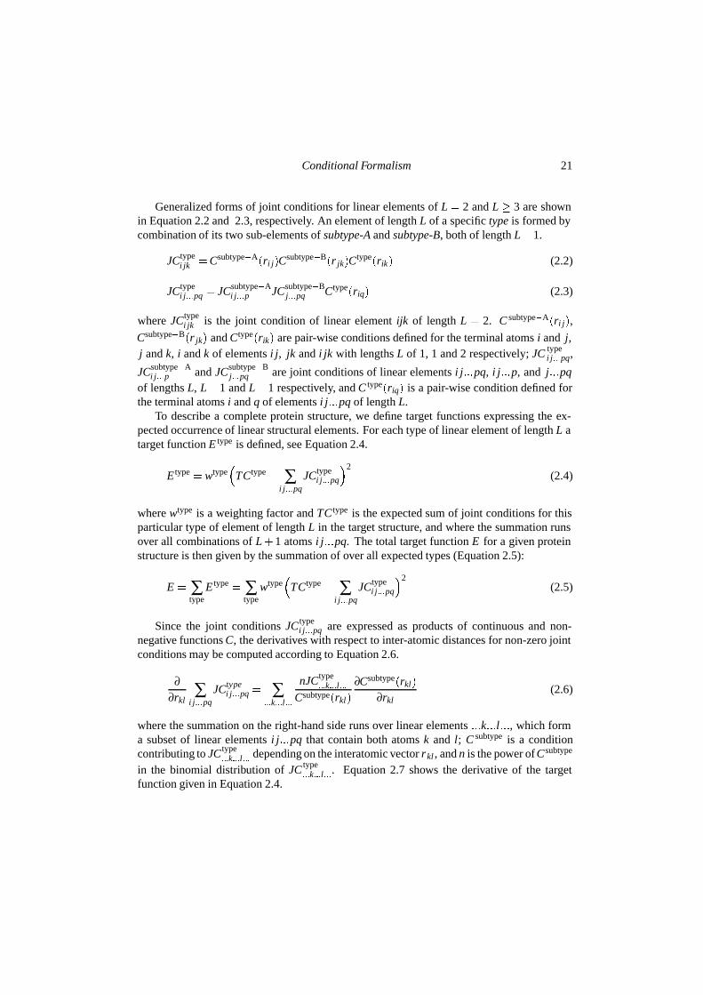
We define a linear structural element as a non-branched sequence of atoms i j���pq of Lbonds long, containing L�1 atoms. A linear structural element of atoms i j���pq of length L iscomposed of two linear sub-elements i j���p and j���pq, both of length L�1 (see Figure 2.1).We define conditions C, which are continuous functions with C � �0�1�, assigned to each ofthese elements. Conditions C reflect the degree to which a geometrical criterion is fulfilledassociated with forming a specific type of element from its two sub-elements. When consid-ering only distance criteria, the conditions C become pair-wise atomic interaction functions(see Figure 2.2).
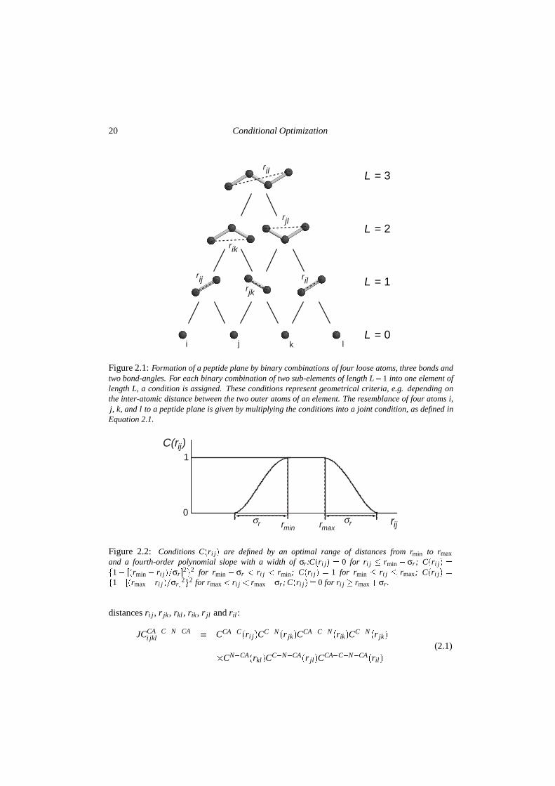
A linear element of length L is then described by a joint condition JC, which is a productof conditions C according to the binary decomposition of the linear element into its sub-elements. Thus, the (L�1)-particle function JCi���q for a linear structure consisting of atomsi � � �q forming L bonds is expressed in a (binomial) product of L�L�1��2 pair-wise functions.
Figure 2.1 shows an example of a binary combination of four atoms i, j, k and l resem-bling a peptide plane. A peptide plane is composed of six types of linear elements: bondsCA-C, C-N and N-CA, bond-angles CA-C-N and C-N-CA and peptide plane CA-C-N-CA. Foreach type of element a pair-wise interaction function C type is assigned. The resemblance ofthe four atoms to a peptide plane can then be expressed by the following multiplication offunctions Ctype yielding joint condition JCCA�C�N�CA
i jkl , which depends on all six inter-atomic
20 Conditional Optimization
i j lk
ril
rik
rjl
rijrjk
ril
L = 0
L = 1
L = 2
L = 3
Figure 2.1: Formation of a peptide plane by binary combinations of four loose atoms, three bonds andtwo bond-angles. For each binary combination of two sub-elements of length L�1 into one element oflength L, a condition is assigned. These conditions represent geometrical criteria, e.g. depending onthe inter-atomic distance between the two outer atoms of an element. The resemblance of four atoms i,j, k, and l to a peptide plane is given by multiplying the conditions into a joint condition, as defined inEquation 2.1.
rmin rmax
0
1
rij
C(rij)
σrσr
Figure 2.2: Conditions C�ri j� are defined by an optimal range of distances from rmin to rmaxand a fourth-order polynomial slope with a width of σr:C�ri j� � 0 for ri j � rmin � σr; C�ri j� ��1 � ��rmin � ri j��σr �
2�2 for rmin � σr � ri j � rmin; C�ri j� � 1 for rmin � ri j � rmax; C�ri j� ��1� ��rmax � ri j��σr�
2�2 for rmax � ri j � rmax �σr; C�ri j� � 0 for ri j � rmax �σr.
distances ri j, r jk, rkl , rik, r jl and ril :
JCCA�C�N�CAi jkl � CCA�C�ri j�CC�N�r jk�CCA�C�N�rik�CC�N�r jk�
�CN�CA�rkl�CC�N�CA�r jl�CCA�C�N�CA�ril�
(2.1)
Conditional Formalism 21
Generalized forms of joint conditions for linear elements of L � 2 and L 3 are shownin Equation 2.2 and 2.3, respectively. An element of length L of a specific type is formed bycombination of its two sub-elements of subtype-A and subtype-B, both of length L�1.
JCtypei jk �Csubtype�A�ri j�C
subtype�B�r jk�Ctype�rik� (2.2)
JCtypei j���pq � JCsubtype�A
i j���p JCsubtype�Bj���pq Ctype�riq� (2.3)
where JCtypei jk is the joint condition of linear element ijk of length L � 2. C subtype�A�ri j�,
Csubtype�B�r jk� and Ctype�rik� are pair-wise conditions defined for the terminal atoms i and j,j and k, i and k of elements i j, jk and i jk with lengths L of 1, 1 and 2 respectively; JC type
i j���pq,
JCsubtype�Ai j���p and JCsubtype�B
j���pq are joint conditions of linear elements i j���pq, i j���p, and j���pqof lengths L, L�1 and L�1 respectively, and C type�riq� is a pair-wise condition defined forthe terminal atoms i and q of elements i j���pq of length L.
To describe a complete protein structure, we define target functions expressing the ex-pected occurrence of linear structural elements. For each type of linear element of length L atarget function E type is defined, see Equation 2.4.
E type � wtype�
TCtype� ∑i j���pq
JCtypei j���pq
�2(2.4)
where wtype is a weighting factor and TC type is the expected sum of joint conditions for thisparticular type of element of length L in the target structure, and where the summation runsover all combinations of L� 1 atoms i j���pq. The total target function E for a given proteinstructure is then given by the summation of over all expected types (Equation 2.5):
E � ∑type
E type � ∑type
wtype�
TCtype� ∑i j���pq
JCtypei j���pq
�2(2.5)
Since the joint conditions JC typei j���pq are expressed as products of continuous and non-
negative functions C, the derivatives with respect to inter-atomic distances for non-zero jointconditions may be computed according to Equation 2.6.
∂∂rkl
∑i j���pq
JCtypei j���pq � ∑
���k���l���
nJCtype���k���l���
Csubtype�rkl�
∂Csubtype�rkl�
∂rkl(2.6)
where the summation on the right-hand side runs over linear elements ���k���l���, which forma subset of linear elements i j���pq that contain both atoms k and l; C subtype is a conditioncontributing to JC type
���k���l��� depending on the interatomic vector rkl , and n is the power of Csubtype
in the binomial distribution of JC type���k���l���. Equation 2.7 shows the derivative of the target
function given in Equation 2.4.
22 Conditional Optimization
d rijσd
1
n di
0
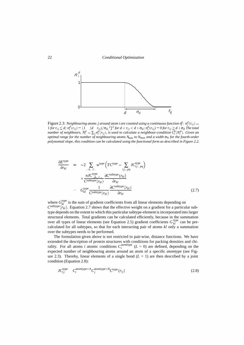
Figure 2.3: Neighbouring atoms j around atom i are counted using a continuous function ndi : nd
i �ri j��1 for ri j � d; nd
i �ri j� � �1� ��d�ri j��σd �2�2 for d � ri j � d�σd; nd
i �ri j� � 0 for ri j � d�σd The totalnumber of neighbours, Nd
i � ∑ j ndi �ri j�, is used to calculate a neighbour-condition C0
i �Ndi �. Given an
optimal range for the number of neighbouring atoms Nmin to Nmax and a width σN for the fourth-orderpolynomial slope, this condition can be calculated using the functional form as described in Figure 2.2.
∂E type
∂rkl� �2 ∑
���k���l���
wtype�
TCtype� ∑i j���pq
JCtypei j���pq
�
�nJCtype
���k���l���
Csubtype�rkl�
∂Csubtype�rkl�
∂rkl
� Gtypekl
1Csubtype�rkl�
∂Csubtype�rkl�
∂rkl(2.7)
where Gtypekl is the sum of gradient coefficients from all linear elements depending on
Csubtype�rkl�. Equation 2.7 shows that the effective weight on a gradient for a particular sub-type depends on the extent to which this particular subtype-element is incorporated into largerstructural elements. Total gradients can be calculated efficiently, because in the summationover all types of linear elements (see Equation 2.5) gradient coefficients G type
kl can be pre-calculated for all subtypes, so that for each interacting pair of atoms kl only a summationover the subtypes needs to be performed.
The formulation given above is not restricted to pair-wise, distance functions. We haveextended the description of protein structures with conditions for packing densities and chi-rality. For all atoms i atomic conditions Catomtype
i (L = 0) are defined, depending on theexpected number of neighbouring atoms around an atom of a specific atomtype (see Fig-ure 2.3). Thereby, linear elements of a single bond (L = 1) are then described by a jointcondition (Equation 2.8):
JCtypei j �Catomtype�A
i Catomtype�Bj Ctype�ri j� (2.8)
Experimental 23
ij
pqχijpq
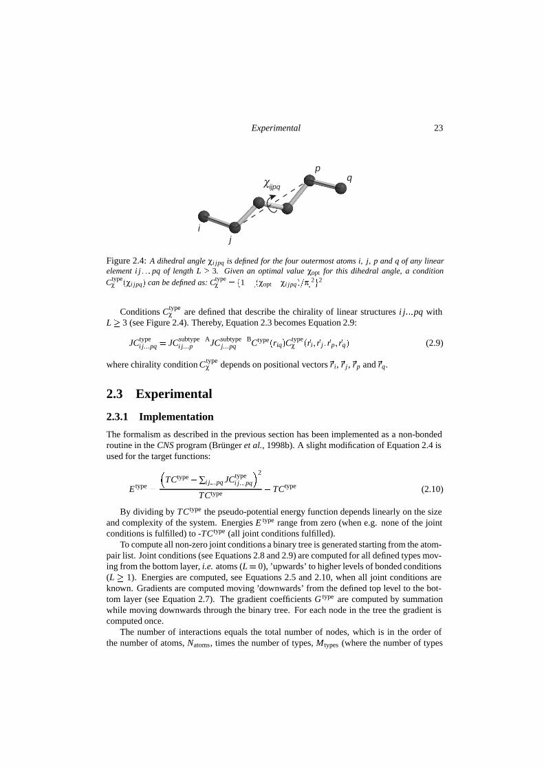
Figure 2.4: A dihedral angle χi jpq is defined for the four outermost atoms i, j, p and q of any linearelement i j � � � pq of length L � 3. Given an optimal value χopt for this dihedral angle, a condition
Ctypeχ �χi jpq� can be defined as: Ctype
χ � �1� ��χopt �χi jpq��π�2�2
Conditions Ctypeχ are defined that describe the chirality of linear structures i j���pq with
L 3 (see Figure 2.4). Thereby, Equation 2.3 becomes Equation 2.9:
JCtypei j���pq � JCsubtype�A
i j���p JCsubtype�Bj���pq Ctype�riq�C
typeχ ��ri��r j��rp��rq� (2.9)
where chirality condition C typeχ depends on positional vectors�ri,�r j,�rp and�rq.
2.3 Experimental
2.3.1 Implementation
The formalism as described in the previous section has been implemented as a non-bondedroutine in the CNS program (Brunger et al., 1998b). A slight modification of Equation 2.4 isused for the target functions:
E type �
�TCtype�∑i j���pq JCtype
i j���pq
�2
TCtype �TCtype (2.10)
By dividing by TCtype the pseudo-potential energy function depends linearly on the sizeand complexity of the system. Energies E type range from zero (when e.g. none of the jointconditions is fulfilled) to -TC type (all joint conditions fulfilled).
To compute all non-zero joint conditions a binary tree is generated starting from the atom-pair list. Joint conditions (see Equations 2.8 and 2.9) are computed for all defined types mov-ing from the bottom layer, i.e. atoms (L � 0), ’upwards’ to higher levels of bonded conditions(L 1). Energies are computed, see Equations 2.5 and 2.10, when all joint conditions areknown. Gradients are computed moving ’downwards’ from the defined top level to the bot-tom layer (see Equation 2.7). The gradient coefficients G type are computed by summationwhile moving downwards through the binary tree. For each node in the tree the gradient iscomputed once.
The number of interactions equals the total number of nodes, which is in the order ofthe number of atoms, Natoms, times the number of types, Mtypes (where the number of types
24 Conditional Optimization
are summed over all defined conditional layers L; for a simple all-helical poly-alanine modelMtypes � 71, when defining L � 9 conditional layers). The full binary tree with (non-zero)joint conditions is stored in memory at each pass. M types is a fixed number given the com-plexity and the number of conditional layers defined. Thus, the order of the algorithm isO�N� � N.
2.3.2 Test case
A target structure was built starting from the published coordinates of a four-helix bundleAlpha-1 crystallized in space group P1 with unit cell dimensions a � 20�846, b � 20�909,c � 27�057 A, α � 102�40o, β � 95�33o and γ � 119�62o (PDB-code: 1BYZ; Prive et al.,1999). All 48 amino acids of this peptide were replaced by alanines and all atomic B-factorswere set to 15 A2. The structure-factor amplitudes were taken from calculated X-ray data to2.0 A resolution.
Two types of starting models were generated for testing purposes. First, scrambled start-ing models with increasing coordinate errors were made by applying random coordinate shiftsof increasing magnitude to all atoms in the unit cell. For these starting structures a minimuminter-atomic distance of 1.4 A was enforced. Second, random atom distributions were madeby randomly placing 264 atoms in the unit cell, while enforcing a minimum inter-atomicdistance of 1.8 A. All atoms in the starting structures were given equal labels and carbonscattering factors were assigned to all of them.
2.3.3 Refinement protocols
The refinement protocols for optimization starting from the scrambled models and randommodels are given in Figures 2.5 a and b. These optimization protocols include standardprocedures: overall B-factor optimization and weight determination for the X-ray restraintfollowed by maximum likelihood optimization by either energy minimization or dynamicssimulation. Table 2.1 contains the set of parameters defining the conditional force field;target values for packing densities and inter-atomic distances were determined from theirdistributions in several high-resolution structures in the Protein Data Bank. Up to 9 layersof bonded conditions have been defined, corresponding to linear elements up to e.g. C α�i�to Cα�i� 3�. During the optimization, width σr of the conditional functions was adjustedaccording to the estimated coordinate error ( ε r) derived from the estimated σA-values: σ�
r �σr � εrL1�2. Atomic B-factors were assigned using an exponentially decreasing functiondepending on the number of neighbours N d
i within a shell d (+σd) of 4.3 (+0.7) A: Bi �150exp��0�1Nd
i �, with a minimum value of 15 A2. The time step in these calculations was0.2 fs and during the dynamics calculations the temperature was coupled to a temperaturebath (Tbath = 300 K).
Two aspects were tested for optimization starting from scrambled models: i. the effectof resolution by using data truncated at 3.5, 3.0, 2.5 and 2.0 A resolution and ii. the effectof the number of conditional layers L, three, six or nine. For each test condition three trialswere performed using different random starting velocities. A randomly selected 10% of thereflections were excluded from refinement and used for calculation of R free (Brunger, 1993)and cross-validated σA-estimates (Read, 1986; Pannu and Read, 1996).
Experimental 25
d+σ d
:1.
6+0.
5A
2.6+
0.7
A3.
6+0.
7A
4.3+
0.7
A5.
0+0.
7A
atom
type
Nm
inN
max
σ NN
min
Nm
axσ N
Nm
inN
max
σ NN
min
Nm
axσ N
Nm
inN
max
σ NN
1.0
2.0
4.0
6.5
9.5
8.0
10.0
16.0
8.0
10.0
25.0
8.0
10.0
32.0
8.0
CA
3.0
3.0
4.0
6.7
7.1
8.0
8.5
11.5
8.0
10.0
25.0
8.0
15.0
32.0
8.0
C3.
03.
04.
06.
08.
08.
09.
015
.08.
010
.025
.08.
017
.033
.08.
0O
1.0
1.0
2.5
3.5
6.5
8.0
7.0
19.0
8.0
10.0
25.0
8.0
15.0
33.0
8.0
CB
1.0
1.0
2.5
3.0
4.0
8.0
5.0
9.5
8.0
6.5
19.5
8.0
9.0
29.0
8.0
Tabl
e2.
1:C
ondi
tion
alfo
rce
field
for
alan
ines
ina
helic
alco
nfor
mat
ion.
�a
�
Para
met
ers
Nm
in,N
max
and
σ Nfo
rat
omty
pes
N,C
A,C
,Oan
dC
B,
defin
ing
the
atom
icco
ndit
ions
for
five
neig
hbou
rsh
ells
wit
hdi
ffere
ntd
+σ d
(see
Fig
ure
2.3)
.
26 Conditional Optimization
�b� Parameters rmin, rmax, σr and χopt see Figures 2.2 and 2.4, describing the bondedconditions for all types of linear elements with L � �1�9�.
Layer type subtype-A subtype-B rmin rmax σr χopt
(L) (L�1) (L�1) [A] [A] [A] [o]L=1 N-CA N CA 1.43 1.51 0.05
CA-C CA C 1.51 1.55 0.05C-O C O 1.21 1.27 0.05C-N C N 1.31 1.35 0.05
CA-CB CA CB 1.51 1.57 0.05L=2 N-C N-CA CA-C 2.41 2.53 0.08
CA-O CA-C C-O 2.35 2.45 0.08CA-N CA-C C-N 2.39 2.49 0.08C-CA C-N N-CA 2.39 2.49 0.08
O-N O-C* C-N 2.21 2.31 0.08O-O O-C* C-O 2.10 2.30 0.08
N-CB N-CA CA-CB 2.39 2.55 0.08CB-C CB-CA* CA-C 2.43 2.61 0.08
L=3 N-O N-C CA-O 3.43 3.61 0.15 138N-N N-C CA-N 2.71 2.93 0.15 -42
CA-CA CA-N C-CA 3.75 3.87 0.15 178C-C C-CA N-C 2.91 3.15 0.15 -62
O-CA O-N C-CA 2.69 2.85 0.15 -2CB-O CB-C CA-O 3.15 3.47 0.15 -98CB-N CB-C CA-N 3.01 3.37 0.15 82C-CB C-CA N-CB 3.63 3.79 0.15 174
L=4 N-CA N-N CA-CA 4.11 4.33 0.20 138CA-C CA-CA C-C 4.29 4.53 0.20 122
C-O C-C N-O 3.69 4.05 0.20 62O-C O-CA C-C 2.81 3.15 0.20 -58C-N C-C N-N 3.13 3.47 0.20 -90
CA-CB CA-CA C-CB 4.77 4.99 0.20 -10CB-CA CB-N CA-CA 4.31 4.71 0.20 -110
O-CB O-CA C-CB 4.17 4.35 0.20 174L=5 N-C N-CA CA-C 4.59 4.85 0.25 82
CA-O CA-C C-O 5.17 5.51 0.25 142O-O O-C C-O 3.17 3.71 0.25 14
CA-N CA-C C-N 4.19 4.59 0.25 14O-N O-C C-N 3.21 3.71 0.25 -114
C-CA C-N N-CA 4.31 4.67 0.25 -6N-CB N-CA CA-CB 4.81 5.19 0.25 -46
Experimental 27
CB-C CB-CA CA-C 5.31 5.61 0.25 -166CB-CB CB-CA CA-CB 5.13 5.67 0.25 66
L=6 N-O N-C CA-O 5.63 5.97 0.30 158CA-CA CA-N C-CA 5.27 5.69 0.30 78
N-N N-C CA-N 4.13 4.53 0.30 30C-C C-CA N-C 4.37 4.75 0.30 22
O-CA O-N C-CA 4.11 4.69 0.30 -50CB-O CB-C CA-O 6.11 6.51 0.30 -86CB-N CB-C CA-N 5.47 5.81 0.30 146C-CB C-CA N-CB 4.99 5.53 0.30 -94
L=7 CA-C CA-CA C-C 5.25 5.77 0.35 90C-N C-C N-N 3.63 4.07 0.35 -14
N-CA N-N CA-CA 5.13 5.61 0.35 86O-C O-CA C-C 3.83 4.39 0.35 -30C-O C-C N-O 5.43 5.85 0.35 98
CB-CA CB-N CA-CA 6.65 7.05 0.35 -166CA-CB CA-CA C-CB 5.57 6.27 0.35 -18
O-CB O-CA C-CB 5.05 5.81 0.35 -138L=8 N-C N-CA CA-C 5.43 5.85 0.40 130
O-O O-C C-O 4.73 5.26 0.40 22CA-O CA-C C-O 6.37 6.91 0.40 130CA-N CA-C C-N 4.27 4.85 0.40 42C-CA C-N N-CA 4.33 4.87 0.40 22
O-N O-C C-N 2.99 3.65 0.40 -70CB-CB CB-CA CA-CB 7.05 7.66 0.40 130
N-CB N-CA CA-CB 5.05 5.77 0.40 22CB-C CB-CA CA-C 6.71 7.15 0.40 -122
L=9 N-O N-C CA-O 6.65 7.09 0.45 166CA-CA CA-N C-CA 4.85 5.55 0.45 74
C-C C-CA N-C 4.67 5.17 0.45 90N-N N-C CA-N 4.61 5.07 0.45 110
O-CA O-N C-CA 3.47 4.09 0.45 -38CB-O CB-C CA-O 7.79 8.27 0.45 -58CB-N CB-C CA-N 5.71 6.31 0.45 -114C-CB C-CA N-CB 3.97 4.81 0.45 -22
* For types O-C and CB-CA the same parameters were used as for types C-O and CA-CB, respectively.
28 Conditional Optimization
(a) (b)
update B, std. σA & wa
200 steps min.
10,000 steps dyn.
200 steps min.
10x
update B, std. σA & wa
initial B, std. σA & wa
200 steps min.
200 steps min.
10,000 steps dyn.
2x
update B, std. σA & wa
update B, multiple-model σA & wa
10,000 steps dyn.
30x
update B, std. σA & wa
initial B, ccf. σA & wa
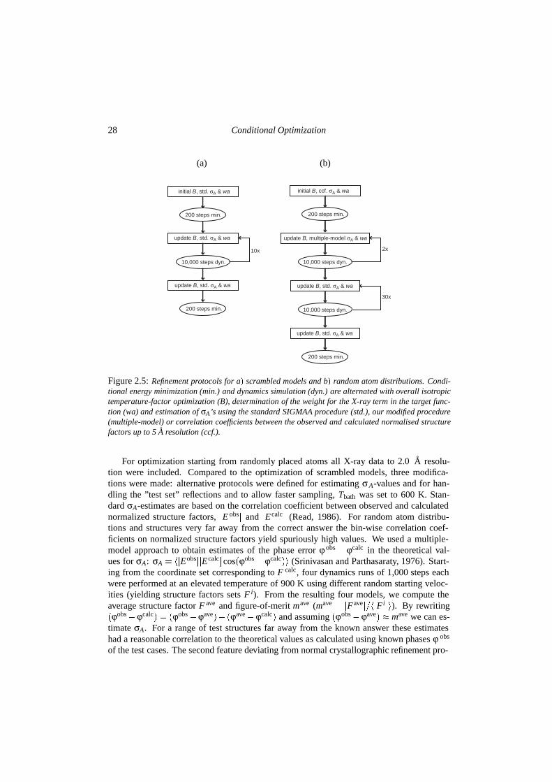
Figure 2.5: Refinement protocols for a� scrambled models and b� random atom distributions. Condi-tional energy minimization (min.) and dynamics simulation (dyn.) are alternated with overall isotropictemperature-factor optimization (B), determination of the weight for the X-ray term in the target func-tion (wa) and estimation of σA’s using the standard SIGMAA procedure (std.), our modified procedure(multiple-model) or correlation coefficients between the observed and calculated normalised structurefactors up to 5 A resolution (ccf.).
For optimization starting from randomly placed atoms all X-ray data to 2.0 A resolu-tion were included. Compared to the optimization of scrambled models, three modifica-tions were made: alternative protocols were defined for estimating σ A-values and for han-dling the ”test set” reflections and to allow faster sampling, Tbath was set to 600 K. Stan-dard σA-estimates are based on the correlation coefficient between observed and calculatednormalized structure factors, �E obs� and �Ecalc� (Read, 1986). For random atom distribu-tions and structures very far away from the correct answer the bin-wise correlation coef-ficients on normalized structure factors yield spuriously high values. We used a multiple-model approach to obtain estimates of the phase error ϕ obs �ϕcalc in the theoretical val-ues for σA: σA � ��Eobs��Ecalc�cos�ϕobs�ϕcalc�� (Srinivasan and Parthasaraty, 1976). Start-ing from the coordinate set corresponding to F calc, four dynamics runs of 1,000 steps eachwere performed at an elevated temperature of 900 K using different random starting veloc-ities (yielding structure factors sets F i). From the resulting four models, we compute theaverage structure factor F ave and figure-of-merit mave (mave � �Fave����Fi��). By rewriting�ϕobs�ϕcalc� � �ϕobs�ϕave���ϕave�ϕcalc� and assuming �ϕobs�ϕave� mave we can es-timate σA. For a range of test structures far away from the known answer these estimateshad a reasonable correlation to the theoretical values as calculated using known phases ϕ obs
of the test cases. The second feature deviating from normal crystallographic refinement pro-
Results 29
tocols was the handling of the test set reflections. A conventional test set comprising 7% ofall reflections was used to calculate Rfree and to estimate cross-validated σA-values accordingto Pannu and Read (1996) in the later stages of refinement. Additionally, another 7% of thereflections were taken out of the refinement. After every 1,000 steps, the selection of these7% was modified. As a result, the reflections used in the crystallographic target functionchanged every 1,000 steps, resulting in a ”tacking” behaviour during refinement minimizingthe chance of stalled progress due to local minima in the crystallographic target function.
Calculations were performed on a Compaq XP1000 workstation with 256 Mb of computermemory and a single 667 MHz processor. The CPU-time needed was about 4 hours for100,000 steps of optimization.
2.4 Results
2.4.1 Refinement of scrambled models
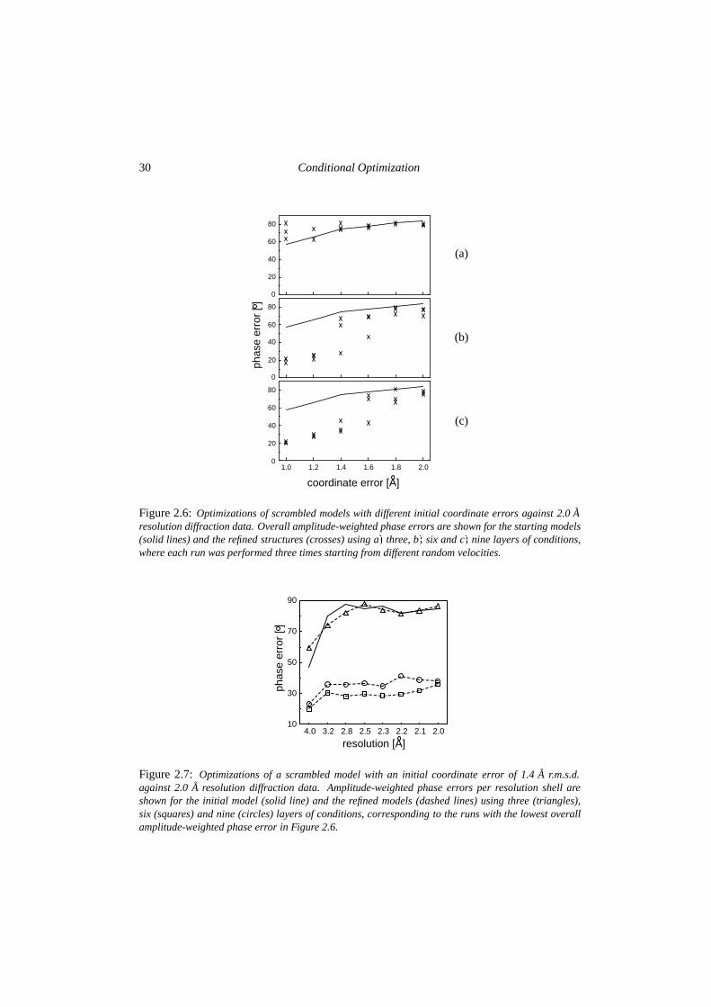
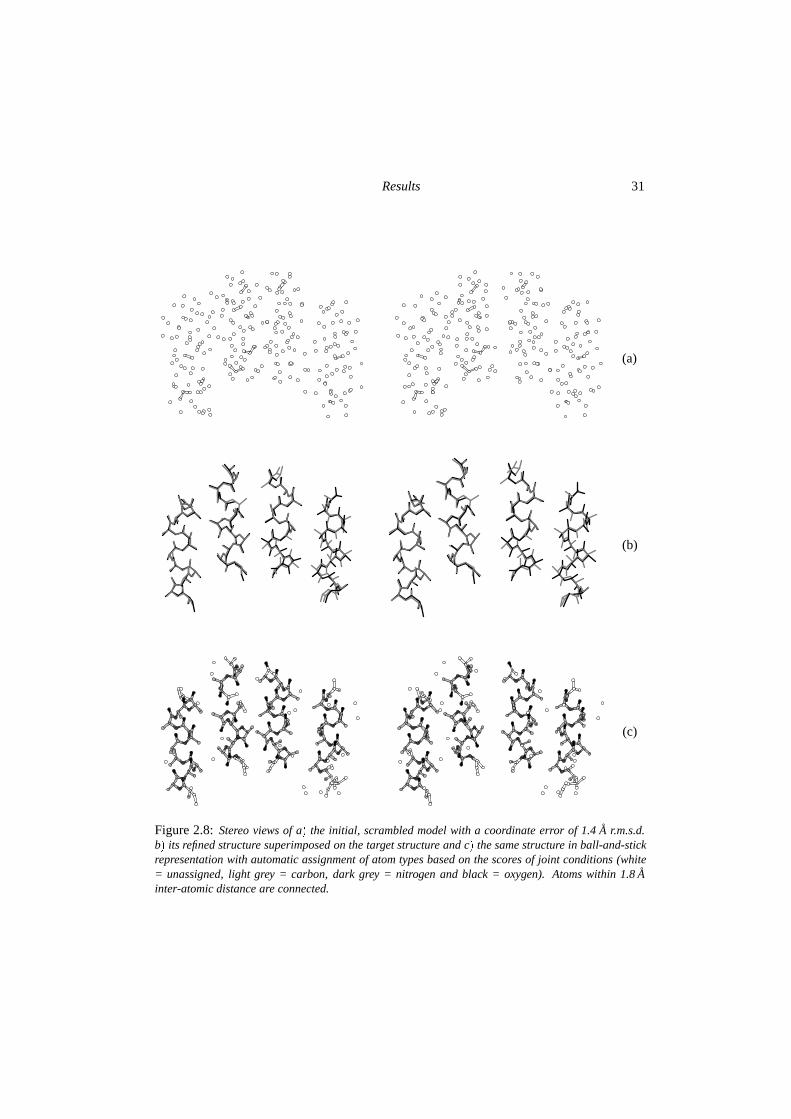
Six scrambled models with coordinate errors of 1.0, 1.2, 1.4, 1.6, 1.8 and 2.0 A root meansquare deviation (r.m.s.d.) respectively were generated. The dependence of the method on thenumber of conditional layers was tested performing a series of refinements using three, sixor nine layers. The resulting amplitude-weighted phase errors are shown in figure 2.6. Threelayers of conditions are not enough to give significant phase improvement. Using six layers,scrambled models with r.m.s.d.’s up to 1.4 A could be improved significantly. Adding anotherthree layers of conditions led to a small increase in the success rate. Figure 2.7 shows thephase improvement for the refined 1.4 A r.m.s.d. structure with the lowest free R-factor, usingthree, six or nine layers of conditions. Figure 2.8 shows an initial model with a coordinateerror of 1.4 A r.m.s.d and the refined structure with the lowest free R-factor using nine layersof conditions. This structure is representative for all successful runs: the four helices areclearly visible although some are not completed, contain breaks in the main chain or theN-C direction is reversed. For structures with a coordinate error larger than 1.4 A r.m.s.d.,refinement did not yield improvement of the phases. This coincides with the observation thatfor models with large errors, the SIGMAA procedure (Pannu and Read, 1996) gave spuriousestimates for the σA-values (results not shown).
The dependence on the high-resolution limit of the diffraction data was tested by refiningthe 1.0 A r.m.s.d. model using data truncated at various resolution limits. Calculations wereperformed using six or nine layers of conditions. The resulting phase improvements areshown in figure 2.9. All runs using data to a resolution of 3.0 A were successful. When usingonly 3.5 A data all three runs using six layers of conditions failed, while using nine layers ofconditions resulted in a success rate of two out of three.
30 Conditional Optimization
1.0 1.2 1.4 1.6 1.8 2.00
20
40
60
80
0
20
40
60
80
phas
e er
ror
[ ]
0
20
40
60
80
coordinate error [A]
(a)
(b)
(c)
Figure 2.6: Optimizations of scrambled models with different initial coordinate errors against 2.0 Aresolution diffraction data. Overall amplitude-weighted phase errors are shown for the starting models(solid lines) and the refined structures (crosses) using a� three, b� six and c� nine layers of conditions,where each run was performed three times starting from different random velocities.
4.0 3.2 2.8 2.5 2.3 2.2 2.1 2.0
resolution [A]
10
30
50
70
90
phas
e er
ror
[ ]
Figure 2.7: Optimizations of a scrambled model with an initial coordinate error of 1.4 A r.m.s.d.against 2.0 A resolution diffraction data. Amplitude-weighted phase errors per resolution shell areshown for the initial model (solid line) and the refined models (dashed lines) using three (triangles),six (squares) and nine (circles) layers of conditions, corresponding to the runs with the lowest overallamplitude-weighted phase error in Figure 2.6.
Results 31
(a)
(b)
(c)
Figure 2.8: Stereo views of a� the initial, scrambled model with a coordinate error of 1.4 A r.m.s.d.b� its refined structure superimposed on the target structure and c� the same structure in ball-and-stickrepresentation with automatic assignment of atom types based on the scores of joint conditions (white= unassigned, light grey = carbon, dark grey = nitrogen and black = oxygen). Atoms within 1.8 Ainter-atomic distance are connected.
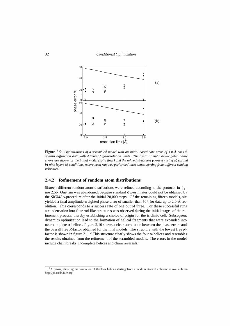
32 Conditional Optimization
2.0 2.5 3.0 3.50
20
40
600
20
40
60
phas
e er
ror
[ ]
resolution limit [A]
(a)
(b)
Figure 2.9: Optimizations of a scrambled model with an initial coordinate error of 1.0 A r.m.s.d.against diffraction data with different high-resolution limits. The overall amplitude-weighted phaseerrors are shown for the initial model (solid lines) and the refined structures (crosses) using a� six andb� nine layers of conditions, where each run was performed three times starting from different randomvelocities.
2.4.2 Refinement of random atom distributions
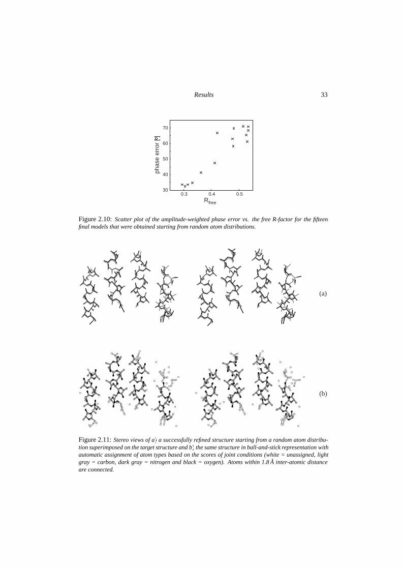
Sixteen different random atom distributions were refined according to the protocol in fig-ure 2.5b. One run was abandoned, because standard σ A-estimates could not be obtained bythe SIGMAA-procedure after the initial 20,000 steps. Of the remaining fifteen models, sixyielded a final amplitude-weighted phase error of smaller than 50 o for data up to 2.0 A res-olution. This corresponds to a success rate of one out of three. For these successful runsa condensation into four rod-like structures was observed during the initial stages of the re-finement process, thereby establishing a choice of origin for the triclinic cell. Subsequentdynamics optimization lead to the formation of helical fragments that were expanded intonear-complete α-helices. Figure 2.10 shows a clear correlation between the phase errors andthe overall free R-factor obtained for the final models. The structure with the lowest free R-factor is shown in figure 2.112.This structure clearly shows the four α-helices and resemblesthe results obtained from the refinement of the scrambled models. The errors in the modelinclude chain breaks, incomplete helices and chain reversals.
2A movie, showing the formation of the four helices starting from a random atom distribution is available on:http://journals.iucr.org
Results 33
0.3 0.4 0.5Rfree
30
40
50
60
70
phas
e er
ror
[ ]
Figure 2.10: Scatter plot of the amplitude-weighted phase error vs. the free R-factor for the fifteenfinal models that were obtained starting from random atom distributions.
(a)
(b)
Figure 2.11: Stereo views of a� a successfully refined structure starting from a random atom distribu-tion superimposed on the target structure and b� the same structure in ball-and-stick representation withautomatic assignment of atom types based on the scores of joint conditions (white = unassigned, lightgray = carbon, dark gray = nitrogen and black = oxygen). Atoms within 1.8 A inter-atomic distanceare connected.
34 Conditional Optimization
2.5 Discussion
We introduced a new method for optimization of protein structures that overcomes the neces-sity of a fixed topology for defining geometrical restraints. This N-particle approach offersa ‘restrained topology’, where weighted gradients over all possible assignments are appliedto loose atoms. We tested this method using calculated data and a very simple test case con-sisting of four poly-alanine helices with 244 non-hydrogen atoms in total. Optimizationsstarting from scrambled models show that the method works successfully with diffractiondata of at least 3.0 to 3.5 A resolution and with six or nine layers of conditions, correspond-ing to linear structural elements of the length of two and three peptide planes, respectively.Moreover, we have shown that our test structure can be optimized successfully starting fromrandomly distributed atoms when using 2.0 A resolution diffraction data. Important for suc-cessful optimization of random starting models was estimation of reasonable σ A-values forvery bad models using a multiple-model procedure. For trials with different random starts asuccess rate of one out of three was observed. The free R-factor readily distinguished correctsolutions from false ones. To our knowledge, we have presented the first method that in prin-ciple allows an ab initio optimization of atomic models under conditions relevant for proteincrystallography (i.e. at medium resolution).
In our experiments we used, however, calculated data without a bulk solvent contributionand a small and very simple test case. Calculations against real protein diffraction data willrequire a model for the bulk solvent and the conditional force field will have to be expandedto target functions that also include the structurally more variable β-sheets, loop regions andside chains. In analogy with the hybrid model of the ARP/wARP program, constrained as-signments of recognizable structural elements may be included in the optimization processin order to improve the rate of convergence by e.g. correcting errors like chain breaks andreversals. The efficiency of our approach for larger and more complex systems will have tobe demonstrated. Due to the possibility to use prior information extensively, conditional op-timization may offer a powerful alternative for phase improvement, both when initial phaseestimates are available and in ab initio structure determination.
Acknowledgements
We gratefully thank Drs. Bouke van Eijck, Jan Kroon (deceased, 3 May 2001), WijnandMooij and Titia Sixma for stimulating discussions. We also thank Drs. Alexandre Bonvinand Bouke van Eijck for carefully reading this manuscript. This work is supported by theNetherlands Organization for Scientific Research (NWO-CW: Jonge Chemici 99-564).
Chapter 3
Development of a force field forconditional optimization of proteinstructures 1
Abstract
Conditional optimization allows the incorporation of extensive geometrical information inprotein structure refinement, without the requirement of an explicit chemical assignment ofthe individual atoms. Here, a potential of mean force for the conditional optimization of pro-tein structures is presented that expresses knowledge about common protein conformationsin terms of inter-atomic distances, torsion angles and numbers of neighbouring atoms. Infor-mation is included for protein fragments up to several residues long in α-helical, β-strand andloop conformations, comprising the main chain and side chains up to the γ-position in threedistinct rotamers. Using this parameter set, conditional optimization of three small proteinstructures against 2.0 A observed diffraction data shows a large radius of convergence, vali-dating the presented force field and illustrating the feasibility of the approach. The generallyapplicable force field allows the development of novel phase improvement procedures usingthe conditional optimization technique.
1Sjors H.W. Scheres & Piet Gros (2003) Acta Cryst. D59, 438-446
36 Force field development
3.1 Introduction
During the standard crystallographic diffraction experiment, information about the phases ofthe observed reflections gets lost. In order to obtain a molecular model describing the crystalcontent, this information must be regained. In protein crystallography, this process typicallyhas been divided into well-separated steps: phase determination by experimental methodsor molecular replacement, phase extension by density modification and iterative cycles ofmodel building and refinement. Nowadays it is realized that these steps are coupled moretightly than thought before (Lamzin et al., 2000) and programs have been developed that linkthese steps in an automated way. For example, the (RE-)SOLVE package (Terwilliger, 1999)links structure solution, density modification and model building and the ARP/wARP program(Perrakis et al., 1999) links density modification, model building and refinement. Due to thetypically low observation-to-parameter ratio in protein crystallography, the incorporation ofadditional information in this process is critical. We have presented a method, called condi-tional optimization, in which extensive prior stereo-chemical information may be formulatedin terms of loose atoms (Scheres & Gros, 2001). With initial, simplified test calculationswe showed that a structure can be obtained using 2.0 A diffraction data without any priorphase information by this approach. Thus, in principle the entire process from phasing torefinement can be expressed in a single step. However, these tests were performed with cal-culated diffraction data of a highly simplified structure of four poly-alanine α-helices, whichcan be described by a very limited parameter set defining the expected geometries. Here, wepresent a parameter set for conditional optimization of the far more complex structures thatare protein molecules.
In the conditional formalism, we express geometrical knowledge by the definition ofinteraction functions, termed conditions. These conditions depend on expected numbersof neighbouring atoms, inter-atomic distances and torsion angles within protein molecules.Conditions are continuous functions ranging from zero to one, and show similarities withthe knowledge-based interaction functions as defined by Sippl (1995). Conformations ofprotein fragments up to several residues long are described by joint conditions, which areproducts of conditions describing a set of geometrical features of a protein fragment. In prin-ciple, (joint) conditions could be defined for all possible conformations in protein molecules,but this would require a vast amount of interaction functions exceeding available computingpower. Therefore, we have defined conditions describing the most common conformationsobserved in the protein structural database (PDB, Berman et al., 2002) for main-chain atomsand side-chain atoms up to the γ-position.
With the defined parameter set, we show that a large radius of convergence can be ob-tained for conditional optimization of three small protein structures against 2.0 A observeddiffraction data.
3.2 Mean-force potential for protein structures
3.2.1 Brief review of the conditional formalism
In conditional optimization, we express prior knowledge about protein structures withoutexplicitly assigning chemical identities to the atoms. Instead, we take all possible assign-
Mean-force potential for protein structures 37
ments into account by using an N-particle approach. We define conditions C � �0�1�, whichare continuous interaction functions based on optimal values for the inter-atomic distances,torsion angles and numbers of neighbouring atoms in protein structures. We describe pro-tein structures as a collection of linear elements (of length L), which are non-branched se-quences of L� 1 atoms. Figure 3.1 shows a common fragment present in protein structuresand a schematic representation of the conditions that describe a linear element N-CA-C-N-CA, which depend on the number of neighbouring atoms per atom, inter-atomic distances andtorsion angles.
As discussed in more detail before (Scheres & Gros 2001), a linear element of length L iscomposed of in total L�L� 1��2 linear (sub-)elements of length l � L. Multiplication of allconditions corresponding to these (sub-)elements, gives the so-called joint condition JC.
For a linear combination of L�1 atoms i, j, . . . , p and q, the joint condition JC typei j���pq de-
scribes to what extent the conformation of the atoms resembles a defined target conformationof a particular type of linear element. A minor change was made to the conditional formalismas presented before. Originally, joint conditions were defined as binomial multiplications ofthe individual conditions, according to the binary combination of all (sub-) elements. In thecurrent implementation, the resulting higher powers of individual conditions in the expressionof joint conditions have been removed, and joint conditions are defined as the multiplicationof all corresponding individual conditions. Consequently, the factor n in the calculation ofderivatives (see formulas 2.6 and 2.6 in chapter 2) reduces to one. In figure 3.1 the atoms i, j,k and l resemble a linear element of type N-CA-C-N. The corresponding joint condition forN-CA-C-N is determined by the individual conditions as given in (3.1):
JCN�CA�C�Ni jkl � CN
nb�ni�CCAnb �n j�CC
nb�nk�CNnb�nl�CN�CA�ri j�
�CCA�C�r jk�CC�N�rkl�CN�CA�C�rik�
�CCA�C�N�r jl�CN�CA�C�N�ril�CN�CA�C�Nχ �χi jkl�
(3.1)
The function JCN�CA�C�Ni jkl will take on the value one, when the configuration of atoms i,
j, k and l, with numbers of neighbouring atoms n, inter-atomic distances r and dihedral angleχ, matches all individual conditions. This implies that these atoms have adopted a N-CA-C-Nconformation.
A protein structure can be described by the sum of its linear elements. Therefore, wedefine a least-squares target function, as given in (3.2), that depends on the expected numberof conformations present in the target structure.
E � ∑type
E type � ∑type
wtype
�TCtype� ∑
i j���pq
JCtypei j���pq
�2
(3.2)
where, TCtype is the expected sum of joint conditions for the types of linear elements in thetarget structure, and wtype is a weighting factor. The first summation runs over all types oflinear elements (of various lengths L type� that have been defined. The second summationruns over all possible combinations of L type � 1 atoms i j���pq. The minimum of this targetfunction corresponds to a set of atoms with the expected number of linear elements in theirexpected types of conformations. Derivatives of this target function can be calculated with
38 Force field development
respect to all atomic coordinates. This allows the application of gradient-driven optimizationtechniques, which we termed conditional optimization.
3.2.2 The general parameter set
For the potential of mean force, we defined 18 atom types (L � 0) described by the expectednumbers of neighbouring atoms within four neighbour shells with increasing radii (corre-sponding to typical distances of respectively bonds, angles, torsion-angles and Lennard-Jonesinteractions). We did not take into account glycine C α and proline N, which have deviat-ing numbers of nearest neighbouring atoms. By combination of the atom types, we defined26 bond types (L � 1) and these combine to form 43 types of angles (L � 2). For longerfragments (L � 2) separate conformations observed in α-helices, β-strands and loops weredefined. For α-helices we defined conditions up to L � 12, for β-strands up to L � 9 andfor loops up to L � 7 taking into account the structural variability of the secondary structureelements. For loops, separate conditions were defined for conformations corresponding to theA and B-region of the Ramachandran plot, but conformations corresponding to the L-regionwere not taken into account. For linear elements comprising two subsequent loop residues,separate conditions were defined for the possible combinations of ϕ�ψ-angle rotations AA,AB, BA and BB. For side-chain atoms up to the γ-position we defined conditions according tothe three preferred χ1-rotamer conformations; in α-helices only the two commonly observedχ1-rotamers were defined. No distinction was made between the atoms at the γ-position ofdifferent amino acids except for the cysteine S γ-atom; consequently, Cγ or Oγ-atoms weretreated equally. Side chain atoms beyond the γ-position were only defined up to L � 2, omit-ting information with respect to their rotamer conformations, which drastically reduced thenumber of possible combinations of defined conformations.
To determine minimum and maximum values for the condition parameters, distributionsof observed numbers of neighbouring atoms, inter-atomic distances and torsion angles werecalculated for the high-resolution protein structures in the SCAN3D database of the WHATIFprogram (Vriend et al., 1994). The observed numbers of neighbouring atoms were calculatedfor twenty protein structures in this data base, comprising in total approximately 24,000 pro-tein atoms. Observed inter-atomic distances and torsion angles were calculated from oligo-peptides that were extracted using the SCAN3D structural annotation. Oligo-peptides in ahelical conformation were extracted as seven subsequent residues with an H (helix) assign-ment, β-strands were extracted as five subsequent residues with an S (strand) assignmentand loops as five subsequent residues, with a T (turn) or C (coil) assignment for the middlethree residues. Backbone conformations with annotated torsion angles �180 Æ � ϕ � 0Æ and�110Æ � ψ � 50Æ were termed A and conformations with �180Æ � ϕ � 0Æ and 50Æ � ψ �180Æ were termed B. Only β-strands with five subsequent residues in the B-conformationwere taken into account. For the middle residue of the extracted oligo-peptides a distinctionbetween the three χ1-rotamers g�, t and g� was made based on its value as annotated in thedatabase: respectively: �120Æ � χ1 � 0Æ, 120Æ � χ1 � 240Æ and 0Æ � χ1 � 120Æ. Table 3.1shows the total numbers of extracted oligo-peptides in the different conformations that wereused to determine the corresponding condition parameters.
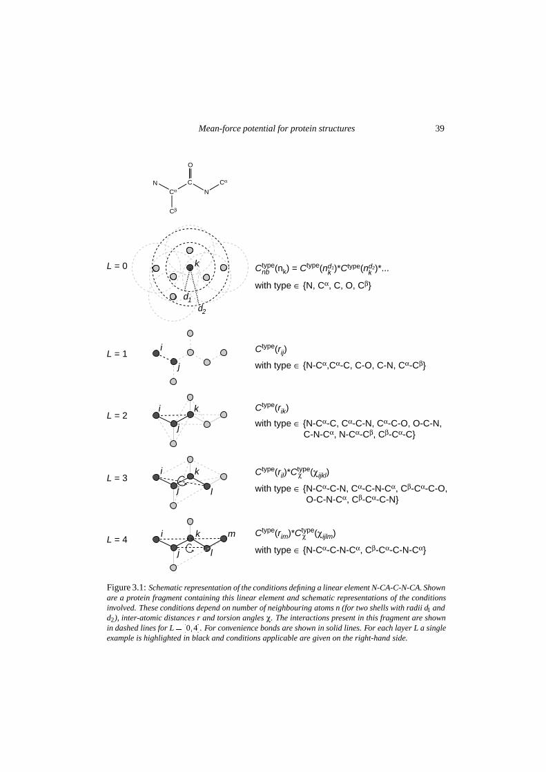
Mean-force potential for protein structures 39
Cα
Cβ
C
N
CαN
O
i
j
k
l
m
i
j
k
l
i
j
k
i
j
Ctype(rij)
Ctype(rik)
Ctype(rim)*Ctype(χijlm)χ
Ctype(ril)*Ctype(χijkl)χ
k
d1d2
with type ∈ {N, Cα, C, O, Cβ}
with type ∈ {N-Cα,Cα-C, C-O, C-N, Cα-Cβ}
with type ∈ {N-Cα-C, Cα-C-N, Cα-C-O, O-C-N, C-N-Cα, N-Cα-Cβ, Cβ-Cα-C}
with type ∈ {N-Cα-C-N, Cα-C-N-Cα, Cβ-Cα-C-O, O-C-N-Cα, Cβ-Cα-C-N}
with type ∈ {N-Cα-C-N-Cα, Cβ-Cα-C-N-Cα}
Ctype(nk) = Ctype(nd1)*Ctype(nd2)*...kkL = 0
L = 1
L = 2
L = 3
L = 4
nb
Figure 3.1: Schematic representation of the conditions defining a linear element N-CA-C-N-CA. Shownare a protein fragment containing this linear element and schematic representations of the conditionsinvolved. These conditions depend on number of neighbouring atoms n (for two shells with radii d1 andd2), inter-atomic distances r and torsion angles χ. The interactions present in this fragment are shownin dashed lines for L � �0�4�. For convenience bonds are shown in solid lines. For each layer L a singleexample is highlighted in black and conditions applicable are given on the right-hand side.
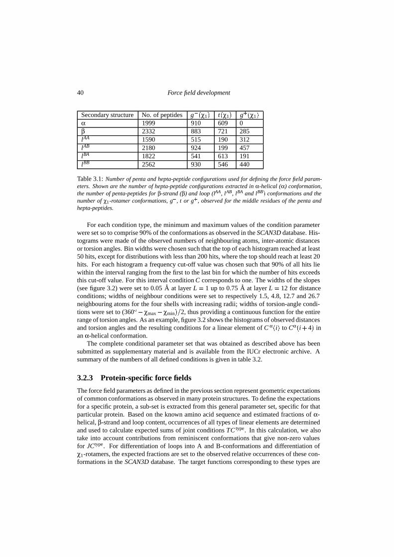
40 Force field development
Secondary structure No. of peptides g��χ1� t�χ1� g��χ1�α 1999 910 609 0β 2332 883 721 285lAA 1590 515 190 312lAB 2180 924 199 457lBA 1822 541 613 191lBB 2562 930 546 440
Table 3.1: Number of penta and hepta-peptide configurations used for defining the force field param-eters. Shown are the number of hepta-peptide configurations extracted in α-helical (α) conformation,the number of penta-peptides for β-strand (β) and loop (lAA, lAB, lBA and lBB� conformations and thenumber of χ1-rotamer conformations, g�, t or g�, observed for the middle residues of the penta andhepta-peptides.
For each condition type, the minimum and maximum values of the condition parameterwere set so to comprise 90% of the conformations as observed in the SCAN3D database. His-tograms were made of the observed numbers of neighbouring atoms, inter-atomic distancesor torsion angles. Bin widths were chosen such that the top of each histogram reached at least50 hits, except for distributions with less than 200 hits, where the top should reach at least 20hits. For each histogram a frequency cut-off value was chosen such that 90% of all hits liewithin the interval ranging from the first to the last bin for which the number of hits exceedsthis cut-off value. For this interval condition C corresponds to one. The widths of the slopes(see figure 3.2) were set to 0.05 A at layer L � 1 up to 0.75 A at layer L � 12 for distanceconditions; widths of neighbour conditions were set to respectively 1.5, 4.8, 12.7 and 26.7neighbouring atoms for the four shells with increasing radii; widths of torsion-angle condi-tions were set to (360Æ�χmax �χmin��2, thus providing a continuous function for the entirerange of torsion angles. As an example, figure 3.2 shows the histograms of observed distancesand torsion angles and the resulting conditions for a linear element of C α�i� to Cα�i� 4� inan α-helical conformation.
The complete conditional parameter set that was obtained as described above has beensubmitted as supplementary material and is available from the IUCr electronic archive. Asummary of the numbers of all defined conditions is given in table 3.2.
3.2.3 Protein-specific force fields
The force field parameters as defined in the previous section represent geometric expectationsof common conformations as observed in many protein structures. To define the expectationsfor a specific protein, a sub-set is extracted from this general parameter set, specific for thatparticular protein. Based on the known amino acid sequence and estimated fractions of α-helical, β-strand and loop content, occurrences of all types of linear elements are determinedand used to calculate expected sums of joint conditions TC type. In this calculation, we alsotake into account contributions from reminiscent conformations that give non-zero valuesfor JCtype. For differentiation of loops into A and B-conformations and differentiation ofχ1-rotamers, the expected fractions are set to the observed relative occurrences of these con-formations in the SCAN3D database. The target functions corresponding to these types are
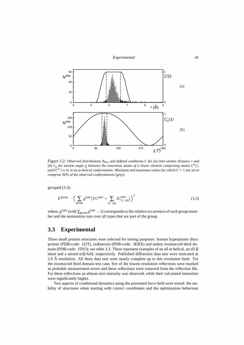
Experimental 41
0 90 180 270 3600
50
100
150
4 5 6 7 8 90
20
40
60
χ (o)
Nhits
Nhits
(A)
1
0
1
0
r
χ(χ)C
( )C r
(a)
(b)
Figure 3.2: Observed distributions Nhits and defined conditions C for (a) inter-atomic distance r and(b) Cχ for torsion angle χ between the outermost atoms of a linear element comprising atoms Cα�i�until Cα�i�4� in an α-helical conformation. Minimum and maximum values for which C � 1 are set tocomprise 90% of the observed conformations (grey).
grouped (3.3):
Egroup ��
∑group
gtype�TCtype� ∑i j���pq
JCtypei j���pq
��2(3.3)
where, gtype (with ∑group gtype � 1) corresponds to the relative occurrence of each group mem-ber and the summation runs over all types that are part of the group.
3.3 Experimental
Three small protein structures were selected for testing purposes: human hyperplastic discsprotein (PDB-code: 1I2T), erabutoxin (PDB-code: 3EBX) and turkey ovomucoid third do-main (PDB-code: 1DS3); see table 3.3. These represent examples of an all-α helical, an all-βsheet and a mixed α/β-fold, respectively. Published diffraction data sets were truncated at2.0 A resolution. All three data sets were nearly complete up to this resolution limit. Forthe ovomucoid third domain test case, five of the lowest resolution reflections were markedas probable measurement errors and these reflections were removed from the reflection file.For these reflections an almost-zero intensity was observed, while their calculated intensitieswere significantly higher.
Two aspects of conditional dynamics using the presented force field were tested: the sta-bility of structures when starting with correct coordinates and the optimization behaviour
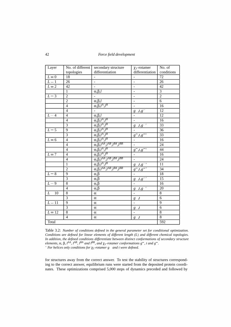
42 Force field development
Layer No. of differenttopologies
secondary structuredifferentiation
χ1-rotamerdifferentiation
No. ofconditions
L � 0 18 - - 72L � 1 26 - - 26L � 2 42 - - 42
1 α,β,l - 3L � 3 2 - - 2
2 α,β,l - 64 α,β,lA,lB - 164 - g�,t,g� 12
L � 4 4 α,β,l - 124 α,β,lA,lB - 163 α,β,lA,lB g�,t,g�� 33
L � 5 9 α,β,lA,lB - 363 α,β,lA,lB g�,t,g�� 33
L � 6 4 α,β,lA,lB - 164 α,β,lAA,lAB,lBA,lBB - 244 α,β,lA,lB g�,t,g�� 44
L � 7 4 α,β,lA,lB - 164 α,β,lAA,lAB,lBA,lBB - 241 α,β,lA,lB g�,t,g�� 112 α,β,lAA,lAB,lBA,lBB g�,t,g�� 34
L � 8 9 α,β - 183 α,β g�,t,g�� 15
L � 9 8 α,β - 164 α,β g�,t,g�� 20
L � 10 8 α - 83 α g�,t 6
L � 11 9 α - 93 α g�,t 6
L � 12 8 α - 84 α g�,t 8
Total 592
Table 3.2: Number of conditions defined in the general parameter set for conditional optimization.Conditions are defined for linear elements of different length (L� and different chemical topologies.In addition, the defined conditions differentiate between distinct conformations of secondary structureelements, α, β, lAA, lAB, lBA and lBB, and χ1-rotamer conformations g�, t and g�.� For helices only conditions for χ1-rotamer g� and t were defined.
for structures away from the correct answer. To test the stability of structures correspond-ing to the correct answer, equilibrium runs were started from the deposited protein coordi-nates. These optimizations comprised 5,000 steps of dynamics preceded and followed by
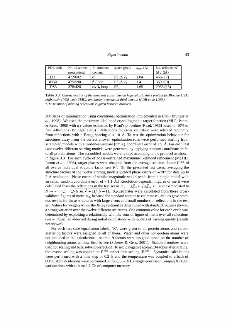
Experimental 43
PDB-code No. of atoms:protein/total
2Æ structurecontent
space group dmin (A) No. reflections�
(d � 2A)1I2T 472/602 α P212121 1.04 4662 (7)3EBX 475/590 β�loop P212121 1.4 3690 (0)1DS3 378/426 α�β�loop P21 1.65 2938 (13)
Table 3.3: Characteristics of the three test cases, human hyperplastic discs protein (PDB-code 1I2T),erabutoxin (PDB-code 3EBX) and turkey ovomucoid third domain (PDB-code 1DS3).�The number of missing reflections is given between brackets.
200 steps of minimization using conditional optimisation implemented in CNS (Brunger etal., 1998). We used the maximum-likelihood crystallographic target function (MLF; Pannu& Read, 1996) with σA-values estimated by Read’s procedure [Read, 1986] based on 10% offree reflections (Brunger, 1993). Reflections for cross validation were selected randomlyfrom reflections with a Bragg spacing d � 10 A. To test the optimization behaviour forstructures away from the correct answer, optimization runs were performed starting fromscrambled models with a root-mean-square (r.m.s.) coordinate error of 1.5 A. For each testcase twelve different starting models were generated by applying random coordinate shiftsto all protein atoms. The scrambled models were refined according to the protocol as shownin figure 3.3. For each cycle of phase-restrained maximum-likelihood refinement (MLHL;Pannu et al., 1998), target phases were obtained from the average structure factor F ave ofall twelve individual structure factor sets F i. (In the presented test cases, averaging thestructure factors of the twelve starting models yielded phase errors of �70 Æ for data up to2 A resolution. Phase errors of similar magnitude would result from a single model withan r.m.s. random coordinate error of �1.1 A.) Resolution-dependent figures of merit werecalculated from the reflections in the test set as m�
a � ∑Ni�1 Fi�∑N
i�1 �Fi� and extrapolated to
N � ∞ : ma ��
�N�m�
a�2�1���N�1�. σA-Estimates were calculated from these cross-
validated figures of merit ma, because the standard routine to estimate σA-values gave spuri-ous results for these structures with large errors and small numbers of reflections in the testset. Values for weights wa on the X-ray restraint as determined with standard routines showeda strong variation over the twelve different structures. One common value for each cycle wasdetermined by exploiting a relationship with the sum of figure of merit over all reflections(wa ∝ 1/Σm), as observed during initial calculations with models of varying quality (resultsnot shown).
For each test case equal atom labels, ‘X’, were given to all protein atoms and carbonscattering factors were assigned to all of them. Water and other non-protein atoms werenot included in the calculations. Atomic B-factors were assigned based on the number ofneighbouring atoms as described before (Scheres & Gros, 2001). Standard routines wereused for scaling and bulk solvent correction. To avoid negative atomic B-factors after scaling,the inverse scaling was applied to �F obs� rather than scaling �F calc�. Dynamics calculationswere performed with a time step of 0.2 fs and the temperature was coupled to a bath of600K. All calculations were performed on four, 667 MHz single-processor Compaq XP1000workstations with at least 1.2 Gb of computer memory.
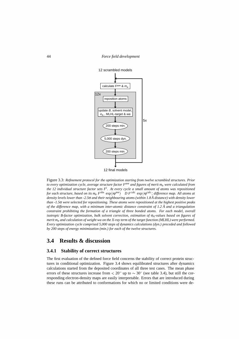
44 Force field development
update B, solvent model, σA , MLHL-target & wa
200 steps min.
5,000 steps dyn.
200 steps min.
5x
12 scrambled models
calculate Fave & ma
reposition atoms
12 final models
12x
Figure 3.3: Refinement protocol for the optimization starting from twelve scrambled structures. Priorto every optimization cycle, average structure factor Fave and figures of merit ma were calculated fromthe 12 individual structure factor sets Fi. At every cycle a small amount of atoms was repositionedfor each structure, based on its ma�Fobs�exp�iϕave��D�Fcalc�exp�iϕcalc� difference map. All atoms atdensity levels lower than -2.5σ and their neighbouring atoms (within 1.8 A distance) with density lowerthan -1.5σ were selected for repositioning. These atoms were repositioned at the highest positive peaksof the difference map, with a minimum inter-atomic distance constraint of 1.2 A and a triangulationconstraint prohibiting the formation of a triangle of three bonded atoms. For each model, overallisotropic B-factor optimization, bulk solvent correction, estimation of σA-values based on figures ofmerit ma and calculation of weight wa on the X-ray term of the target function (MLHL) were performed.Every optimization cycle comprised 5,000 steps of dynamics calculations (dyn.) preceded and followedby 200 steps of energy minimization (min.) for each of the twelve structures.
3.4 Results & discussion
3.4.1 Stability of correct structures
The first evaluation of the defined force field concerns the stability of correct protein struc-tures in conditional optimization. Figure 3.4 shows equilibrated structures after dynamicscalculations started from the deposited coordinates of all three test cases. The mean phaseerrors of these structures increase from � 20Æ up to � 30Æ (see table 3.4), but still the cor-responding electron-density maps are easily interpretable. Errors that are introduced duringthese runs can be attributed to conformations for which no or limited conditions were de-
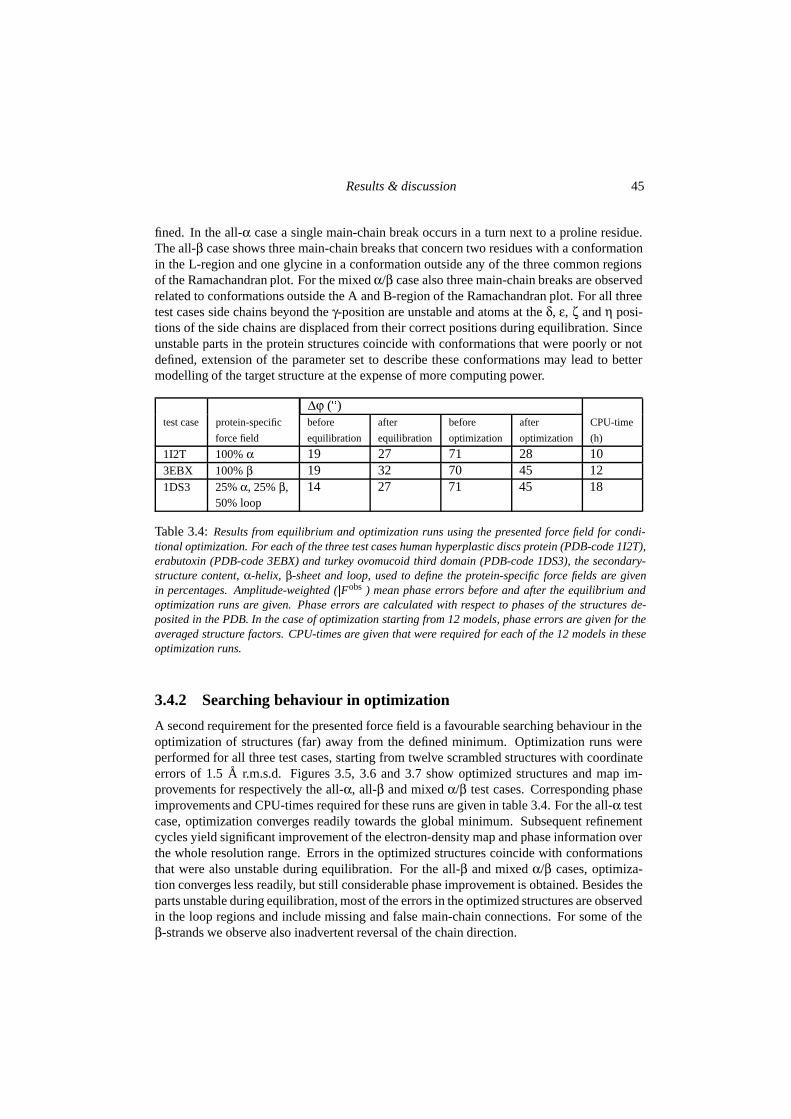
Results & discussion 45
fined. In the all-α case a single main-chain break occurs in a turn next to a proline residue.The all-β case shows three main-chain breaks that concern two residues with a conformationin the L-region and one glycine in a conformation outside any of the three common regionsof the Ramachandran plot. For the mixed α/β case also three main-chain breaks are observedrelated to conformations outside the A and B-region of the Ramachandran plot. For all threetest cases side chains beyond the γ-position are unstable and atoms at the δ, ε, ζ and η posi-tions of the side chains are displaced from their correct positions during equilibration. Sinceunstable parts in the protein structures coincide with conformations that were poorly or notdefined, extension of the parameter set to describe these conformations may lead to bettermodelling of the target structure at the expense of more computing power.
∆ϕ (Æ)test case protein-specific
force field
before
equilibration
after
equilibration
before
optimization
after
optimization
CPU-time
(h)
1I2T 100% α 19 27 71 28 103EBX 100% β 19 32 70 45 121DS3 25% α, 25% β,
50% loop14 27 71 45 18
Table 3.4: Results from equilibrium and optimization runs using the presented force field for condi-tional optimization. For each of the three test cases human hyperplastic discs protein (PDB-code 1I2T),erabutoxin (PDB-code 3EBX) and turkey ovomucoid third domain (PDB-code 1DS3), the secondary-structure content, α-helix, β-sheet and loop, used to define the protein-specific force fields are givenin percentages. Amplitude-weighted (�Fobs�) mean phase errors before and after the equilibrium andoptimization runs are given. Phase errors are calculated with respect to phases of the structures de-posited in the PDB. In the case of optimization starting from 12 models, phase errors are given for theaveraged structure factors. CPU-times are given that were required for each of the 12 models in theseoptimization runs.
3.4.2 Searching behaviour in optimization
A second requirement for the presented force field is a favourable searching behaviour in theoptimization of structures (far) away from the defined minimum. Optimization runs wereperformed for all three test cases, starting from twelve scrambled structures with coordinateerrors of 1.5 A r.m.s.d. Figures 3.5, 3.6 and 3.7 show optimized structures and map im-provements for respectively the all-α, all-β and mixed α/β test cases. Corresponding phaseimprovements and CPU-times required for these runs are given in table 3.4. For the all-α testcase, optimization converges readily towards the global minimum. Subsequent refinementcycles yield significant improvement of the electron-density map and phase information overthe whole resolution range. Errors in the optimized structures coincide with conformationsthat were also unstable during equilibration. For the all-β and mixed α/β cases, optimiza-tion converges less readily, but still considerable phase improvement is obtained. Besides theparts unstable during equilibration, most of the errors in the optimized structures are observedin the loop regions and include missing and false main-chain connections. For some of theβ-strands we observe also inadvertent reversal of the chain direction.
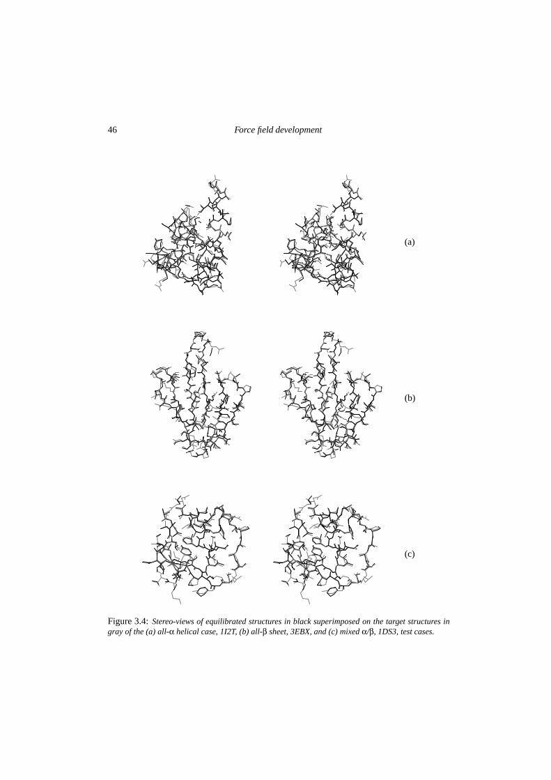
46 Force field development
(a)
(b)
(c)
Figure 3.4: Stereo-views of equilibrated structures in black superimposed on the target structures ingray of the (a) all-α helical case, 1I2T, (b) all-β sheet, 3EBX, and (c) mixed α/β, 1DS3, test cases.
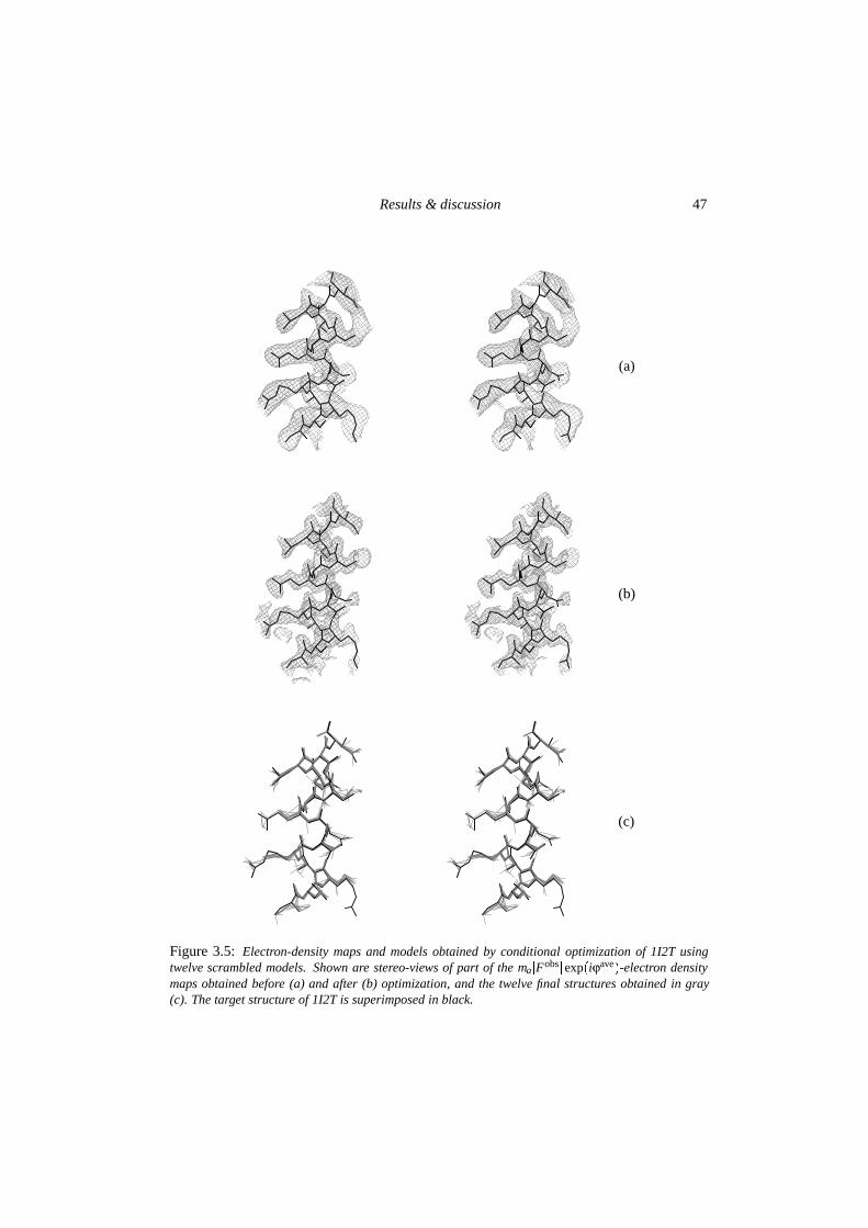
Results & discussion 47
(a)
(b)
(c)
Figure 3.5: Electron-density maps and models obtained by conditional optimization of 1I2T usingtwelve scrambled models. Shown are stereo-views of part of the ma�Fobs�exp�iϕave�-electron densitymaps obtained before (a) and after (b) optimization, and the twelve final structures obtained in gray(c). The target structure of 1I2T is superimposed in black.
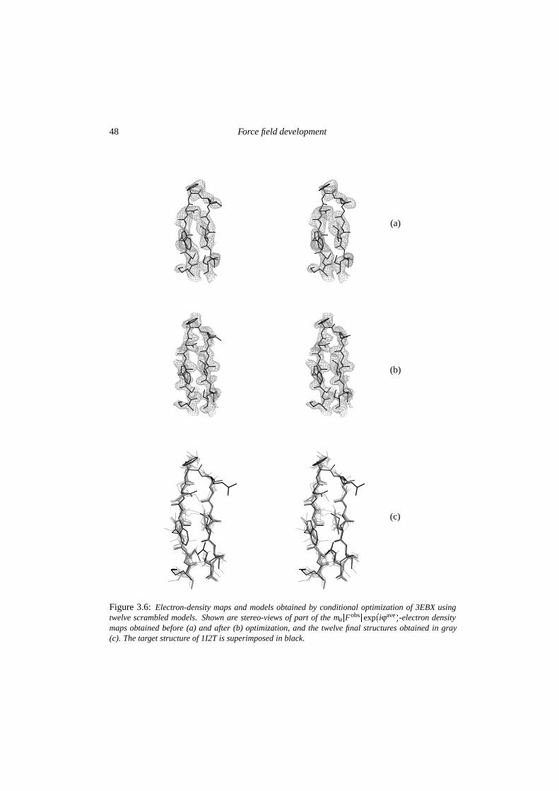
48 Force field development
(a)
(b)
(c)
Figure 3.6: Electron-density maps and models obtained by conditional optimization of 3EBX usingtwelve scrambled models. Shown are stereo-views of part of the ma�Fobs�exp�iϕave�-electron densitymaps obtained before (a) and after (b) optimization, and the twelve final structures obtained in gray(c). The target structure of 1I2T is superimposed in black.
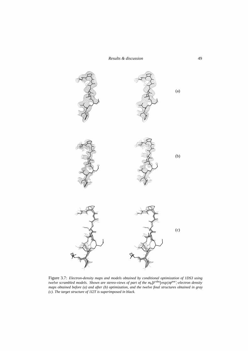
Results & discussion 49
(a)
(b)
(c)
Figure 3.7: Electron-density maps and models obtained by conditional optimization of 1DS3 usingtwelve scrambled models. Shown are stereo-views of part of the ma�Fobs�exp�iϕave�-electron densitymaps obtained before (a) and after (b) optimization, and the twelve final structures obtained in gray(c). The target structure of 1I2T is superimposed in black.
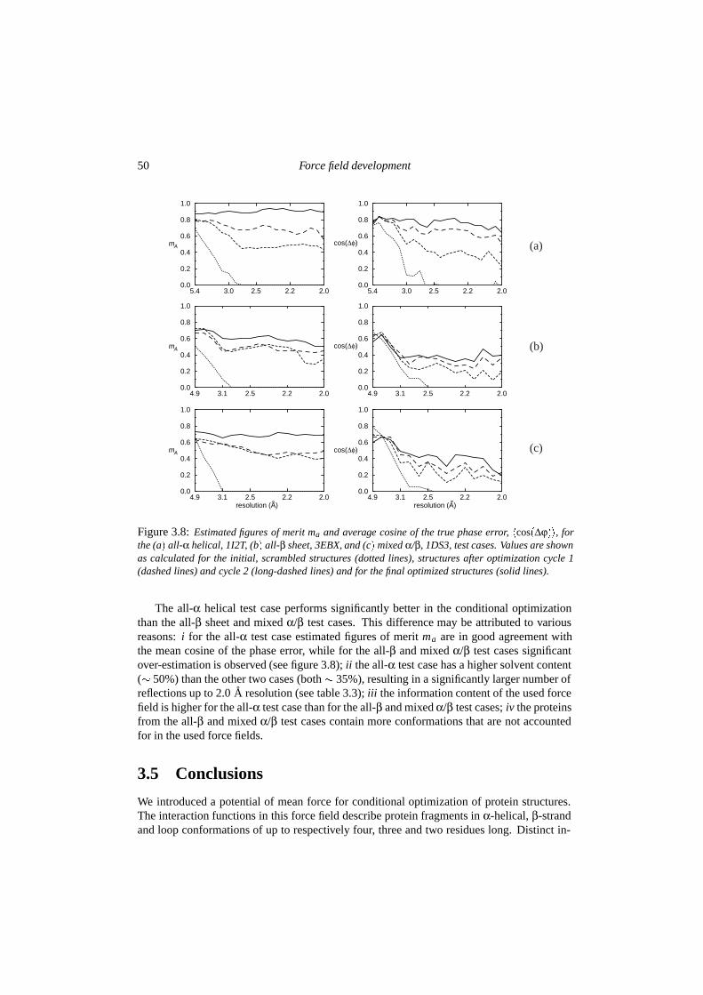
50 Force field development
5.4 3.0 2.5 2.2 2.00.0
0.2
0.4
0.6
0.8
1.0
5.4 3.0 2.5 2.2 2.00.0
0.2
0.4
0.6
0.8
1.0
4.9 3.1 2.5 2.2 2.00.0
0.2
0.4
0.6
0.8
1.0
4.9 3.1 2.5 2.2 2.00.0
0.2
0.4
0.6
0.8
1.0
4.9 3.1 2.5 2.2 2.00.0
0.2
0.4
0.6
0.8
1.0
4.9 3.1 2.5 2.2 2.00.0
0.2
0.4
0.6
0.8
1.0
mA cos(∆φ)
mA
mA cos(∆φ)
cos(∆φ)
(a)
(b)
(c)
resolution (A) resolution (A)
Figure 3.8: Estimated figures of merit ma and average cosine of the true phase error, �cos�∆ϕ��, forthe (a� all-α helical, 1I2T, (b� all-β sheet, 3EBX, and (c� mixed α/β, 1DS3, test cases. Values are shownas calculated for the initial, scrambled structures (dotted lines), structures after optimization cycle 1(dashed lines) and cycle 2 (long-dashed lines) and for the final optimized structures (solid lines).
The all-α helical test case performs significantly better in the conditional optimizationthan the all-β sheet and mixed α/β test cases. This difference may be attributed to variousreasons: i for the all-α test case estimated figures of merit ma are in good agreement withthe mean cosine of the phase error, while for the all-β and mixed α/β test cases significantover-estimation is observed (see figure 3.8); ii the all-α test case has a higher solvent content(� 50%) than the other two cases (both � 35%), resulting in a significantly larger number ofreflections up to 2.0 A resolution (see table 3.3); iii the information content of the used forcefield is higher for the all-α test case than for the all-β and mixed α/β test cases; iv the proteinsfrom the all-β and mixed α/β test cases contain more conformations that are not accountedfor in the used force fields.
3.5 Conclusions
We introduced a potential of mean force for conditional optimization of protein structures.The interaction functions in this force field describe protein fragments in α-helical, β-strandand loop conformations of up to respectively four, three and two residues long. Distinct in-
Conclusions 51
teraction functions for the three preferred χ 1-rotamers describe corresponding geometries forside chains up to the γ-position. Notably, we omitted glycine and proline residues, main-chain conformations involving the L-region of the Ramachandran plot and torsion angles(and higher order information) for side-chain atoms beyond the γ-position, due to increas-ing computational costs. We tested the parameter set in conditional optimization of threesmall protein structures using 2.0 A observed diffraction data. Dynamics runs starting fromthe deposited coordinates show that the definition of the global minimum is correct for thedefined main-chain conformations and for side chains up to the γ-position. Breaks are ob-served for main-chain conformations outside the A and B-region and for side chains beyondthe γ-position that were not or poorly defined. A more precise definition of these conforma-tions in the force field could improve the optimization behaviour. However, inclusion of theomitted elements would give rise to a large increase of the number of possible combinations,increasing the computational cost dramatically.
Optimization starting from twelve structures with 1.5 A r.m.s.d. random coordinateshifts showed excellent convergence for the α-helical hyperplastic discs protein. Consid-erable phase improvement was obtained as well for the β-sheet protein erabutoxin and theovomucoid third domain with mixed α/β fold, but the optimized structures contain more er-rors, typically chain reversals for β-strands and incorrect formation of loops. The appliedmultiple-model procedure proved crucial for these optimizations, since with the limited num-bers of available test set reflections standard procedures to estimate phase quality failed forstarting models with such large errors. In contrast to the all-α helical case, significant over-estimation of the phase quality was observed for the all-β sheet and mixed α/β test cases. Thisover-estimation coincides with the more difficult convergence in the optimization runs of theall-β and mixed α/β test cases, which may indicate the importance of further improvement ofthis procedure.
Our results illustrate that a large radius of convergence may be obtained by conditionaloptimization of protein molecules with observed diffraction data to medium resolution. Thecoordinate errors of our starting models were generated in a completely random way andsuch favourable error distributions are hard to obtain when starting from a single electron-density map. In addition, we used truncated data, which also may have contributed favourablyto the optimization behaviour. Still, the significant reduction in phase errors, from � 70 Æ
to 45Æ or better, is promising. The presented, generally applicable potential of mean forceallows development of phase improvement and automated model-building procedures usingconditional optimization, as well as investigation of the efficacy of this approach in ab initiophasing of protein structures.
Acknowledgements
This work is supported by the Netherlands Organization for Scientific Research (NWO-CW:Jonge Chemici 99-564).

52 Automated model building

Chapter 4
The potentials of conditionaloptimization in automated modelbuilding
Abstract
We have applied conditional optimization to automated model building for three test caseswith data to medium resolution and good experimental phases. Compared to ARP/wARPand RESOLVE, conditional optimization yielded models of comparable phase quality, forwhich most of the α-helical and β-strand segments were modelled. The main difference inthe results obtained was a poor modelling of loops and turns by conditional optimization.This might be improved by incorporation of more loop conformations in the conditionalforce field. Although iteration of conditional optimization with discrete model building stepsmay provide a more efficient procedure, here we only tested the potentials of conditionaloptimization alone. Further development of the procedures and the optimization of hybridmodels with explicit assignments of atom labels may provide a method suitable for automatedmodel building at lower resolutions and in maps of lower quality. This may then justify thelarge amounts of computer memory and CPU-time required for conditional optimization ofprotein structures.
54 Automated model building
4.1 Introduction
In protein crystallography, once the phase problem has been solved the electron density mapneeds to be interpreted in terms of a molecular model. This task is far from straightforwardand has been shown to be prone to human error (Mowbray et al., 1999). Even for a skilledcrystallographer manual model building can take up to weeks of time in front of a computergraphics. In the last few years, a number of programs have been developed that aim to auto-mate this process. By far the most widely used approach in automated model building up tillnow is the ARP/wARP program (Perrakis et al., 1999). In this program a powerful combina-tion of loose-atom refinement and recognition of protein fragments is implemented. Becauseof the coupling of refinement with the process of model building, the resulting models are typ-ically highly accurate and the program does not depend strongly on the quality of the initialphase information. The major limitation of this program lies in a strong dependence on theavailability of large amounts of diffraction data. Firstly, because in the automated refinementprocedure (ARP, Lamzin & Wilson, 1993) atoms are re-positioned in electron density maps,which should be of sufficiently high resolution. Secondly, because the (almost) unrestrainedloose-atom refinement in ARP depends intrinsically on a favourable observation-to-parameterratio. The ARP refinement cycles are iterated with discrete model building steps, where thewarpNtrace algorithm recognizes protein main-chain fragments in the refined distribution ofindividual atoms. Application of stereo-chemical restraints on the recognized protein frag-ments increases the observation-to-parameter ratio. Therefore, refinement of a hybrid modelconsisting of auto-built protein fragments and the remaining loose atoms is less dependenton the number of reflections available. Recently, major advances in the warpNtrace algo-rithm have been reported (Morris et al., 2002), currently allowing main-chain tracing at 2.5A resolution.
Several alternative approaches simulate the process of manual building, where fragmentsof secondary structure elements are positioned in the electron density map. For this task vari-ous pattern recognition techniques have been implemented in programs like TEXTAL (Holtonet el., 2000), QUANTA (Oldfield, 2000) and RESOLVE (Terwilliger, 2002). A major advan-tage of these methods is that, in principle, they can be applied to electron density maps ofmedium to low resolution. A disadvantage is a strong dependence on the quality of the initialphase information. For electron density maps of limited quality or resolution, the positionedfragments may suffer from a low accuracy. Iterative application of these model buildingtechniques with protein structure refinement may provide a solution to this problem. Suchan approach has been implemented in the latest version of RESOLVE (Terwilliger, 2002). Inthis program secondary structure elements are positioned in the electron density map usingphased translation functions (Cowtan, 1998). Subsequently, the positioned fragments are ex-tended into loop regions and the primary sequence is docked on the constructed models. Afinal model is obtained by iteration of these building steps with maximum-likelihood den-sity modification and restrained protein structure refinement in REFMAC (Murshudov et al.,1997).
With the method of conditional optimization (Scheres & Gros, 2001), we introduced atechnique that allows loose-atom refinement without the intrinsic need for high-resolutiondiffraction data. In conditional optimization, the number of observations from the diffractionexperiment is supplemented with extensive geometrical information, without the require-
Experimental 55
ment of an explicit chemical assignment of the unlabelled atoms. Initial test calculationswith this method showed a large radius of convergence, allowing successful refinement start-ing from random atom distributions for an artificial test case. The introduction of a forcefield describing commonly observed protein conformations (Scheres & Gros, 2003) allowedapplication to protein molecules, for which a large radius of convergence was observed us-ing observed diffraction data. The large radius of convergence and the limited dependenceon high-resolution data raised expectations for the application of conditional optimizationto automated model building in electron density maps of limited resolution. In analogy toARP/wARP and RESOLVE, the most powerful approach would probably be an iterated pro-cess of refinement cycles and discrete model-building steps. However, rather than providinga ready-to-use solution, we chose to first test the potentials of conditional optimization alonein the model building process. Therefore, in the calculations presented here, no other patternrecognition or model building techniques were applied than conditional optimization itself.Still, for the three test cases presented conditional optimization yielded models of compara-ble quality as ARP/wARP and RESOLVE, in which most of the α-helices and β-strands werebuilt.
4.2 Experimental
Three protein structures were selected for testing purposes: the A3-domain from human vonWillebrand Factor (vWF-A3, Huizinga et al., 1997), outer-membrane protein NspA fromNeisseria meningitidis (Vandeputte-Rutten et al., in preparation) and the C-terminal domainof leech anti-platelet protein (LAPP, Huizinga et al., 2001). All three structures were solvedin our laboratory and initial models were built manually using the graphics program O (Joneset al., 1991). Main characteristics of these test cases are given in table 4.1. The structureof vWF-A3 was solved at 2.35 A resolution in space group P212121 by multiple-wavelengthanomalous disperson methods (MAD) using the anomalous contribution from four seleno-methionine residues. An initial model built in the excellent experimental electron densitymap was transformed to space group P21 of the native crystals and subsequent refinementwas carried out using native data up to 1.8 A resolution. Here, automated model building wasperformed using only the MAD-data to 2.4 A resolution. The structure of NspA was solved bysingle-wavelength anomalous diffraction (SAD) at 4 A resolution using the strong anomaloussignal from two gold atoms, which were bound to the protein by soaking the crystal in asolution containing Au(CN)2. Subsequent density modification and phase extension of anative data set to 2.6 A resolution yielded an easily interpretable electron density map. Thismap was used for automated model building here. For LAPP, three heavy-atom sites wereidentified in a K2PtCl4 derivative and the structure was solved at 3.1 A resolution usingsingle isomorphous replacement with anomalous scattering (SIRAS). Density modificationby solvent flattening and three-fold non-crystallographic symmetry (NCS-) averaging wasused for phase extension of a low-resolution native data set to 3.0 A. The resulting electrondensity map was of high quality and allowed construction of an initial model. A final modelwas obtained by refinement against a high-resolution native data set to 2.2 A resolution. Here,the 3.0 A map after phase extension was used for automated model building.
Automated model building was performed in separate cycles of conditional optimiza-
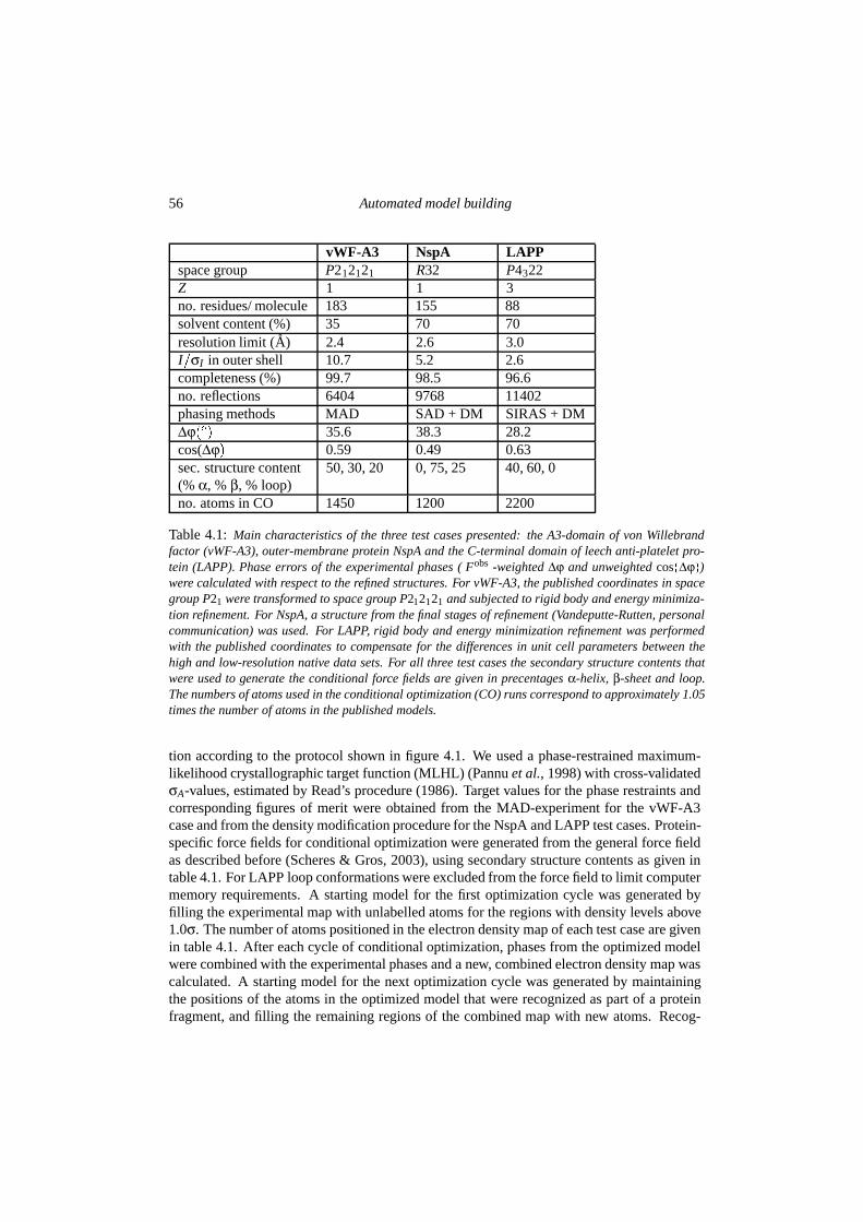
56 Automated model building
vWF-A3 NspA LAPPspace group P212121 R32 P4322Z 1 1 3no. residues/ molecule 183 155 88solvent content (%) 35 70 70resolution limit (A) 2.4 2.6 3.0I�σI in outer shell 10.7 5.2 2.6completeness (%) 99.7 98.5 96.6no. reflections 6404 9768 11402phasing methods MAD SAD + DM SIRAS + DM∆ϕ�Æ� 35.6 38.3 28.2cos(∆ϕ� 0.59 0.49 0.63sec. structure content(% α, % β, % loop)
50, 30, 20 0, 75, 25 40, 60, 0
no. atoms in CO 1450 1200 2200
Table 4.1: Main characteristics of the three test cases presented: the A3-domain of von Willebrandfactor (vWF-A3), outer-membrane protein NspA and the C-terminal domain of leech anti-platelet pro-tein (LAPP). Phase errors of the experimental phases (�Fobs�-weighted ∆ϕ and unweighted cos�∆ϕ�)were calculated with respect to the refined structures. For vWF-A3, the published coordinates in spacegroup P21 were transformed to space group P212121 and subjected to rigid body and energy minimiza-tion refinement. For NspA, a structure from the final stages of refinement (Vandeputte-Rutten, personalcommunication) was used. For LAPP, rigid body and energy minimization refinement was performedwith the published coordinates to compensate for the differences in unit cell parameters between thehigh and low-resolution native data sets. For all three test cases the secondary structure contents thatwere used to generate the conditional force fields are given in precentages α-helix, β-sheet and loop.The numbers of atoms used in the conditional optimization (CO) runs correspond to approximately 1.05times the number of atoms in the published models.
tion according to the protocol shown in figure 4.1. We used a phase-restrained maximum-likelihood crystallographic target function (MLHL) (Pannu et al., 1998) with cross-validatedσA-values, estimated by Read’s procedure (1986). Target values for the phase restraints andcorresponding figures of merit were obtained from the MAD-experiment for the vWF-A3case and from the density modification procedure for the NspA and LAPP test cases. Protein-specific force fields for conditional optimization were generated from the general force fieldas described before (Scheres & Gros, 2003), using secondary structure contents as given intable 4.1. For LAPP loop conformations were excluded from the force field to limit computermemory requirements. A starting model for the first optimization cycle was generated byfilling the experimental map with unlabelled atoms for the regions with density levels above1.0σ. The number of atoms positioned in the electron density map of each test case are givenin table 4.1. After each cycle of conditional optimization, phases from the optimized modelwere combined with the experimental phases and a new, combined electron density map wascalculated. A starting model for the next optimization cycle was generated by maintainingthe positions of the atoms in the optimized model that were recognized as part of a proteinfragment, and filling the remaining regions of the combined map with new atoms. Recog-
Experimental 57
nition of protein fragments was based on the gradient coefficients towards all possible atomassignments as calculated for every atom in the conditional optimization. Atoms were rec-ognized to be part of a protein fragment if the gradient contribution towards one of the atomtypes N, Cα, O, C, Cβ, Cγ or Sγ was at least two times as large as the second largest contri-bution. Only protein fragments consisting of at least two consecutive atoms were taken intoaccount. No attempts to model side chains extending beyond the γ-position were made. Afinal protein model was constructed from the protein fragments that were recognized in theoptimized model after the last optimization cycle. For the vWF-A3 and NspA test cases twocycles of conditional optimization were performed; for the LAPP test case four.
For comparison of the results obtained by conditional optimization, the electron densitymaps of all three test cases were also subjected to automated model building by ARP/wARP(version 6.0) and RESOLVE (version 2.03), using REFMAC version 5.1.24 for refinement.These calculations were performed using only default values for all parameters. In RESOLVEdocking of the primary sequence on the constructed fragments by side-chain modelling wasincluded in the model building process. Modelling of the side chains was not performed withARP/wARP, since this option of the program yielded significantly worse results (not shown).
All calculations were performed on a 667 MHz single-processor Compaq XP1000 workstation with 2 Gb of computer memory.
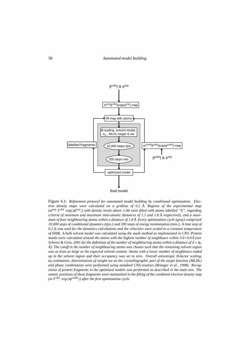
58 Automated model building
B-scaling, solvent model, σA , MLHL-target & wa
10,000 steps dyn.
200 steps min.
|Fobs| & φexp
mexp|Fobs|exp(iφexp) map
fill map with atoms
final model
optimized model
mcomb|Fobs|exp(iφcomb) maplabelled fragments
|Fobs| & φexp
Figure 4.1: Refinement protocol for automated model building by conditional optimization. Elec-tron density maps were calculated on a gridsize of 0.2 A. Regions of the experimental map(mexp�Fobs�exp�iϕexp�) with density levels above 1.0σ were filled with atoms labelled ”X”, regardingcriteria of minimum and maximum inter-atomic distances of 1.1 and 1.8 A respectively, and a maxi-mum of four neighbouring atoms within a distance of 1.8 A. Every optimization cycle (gray) comprised10,000 steps of conditional dynamics (dyn.) and 200 steps of energy minimization (min.). A time step of0.2 fs was used for the dynamics calculations and the velocities were scaled to a constant temperatureof 600K. A bulk solvent model was calculated using the mask method as implemented in CNS. Proteinmasks were calculated around the atoms with the highest number of neighbours within 3.6+0.9 A (seeScheres & Gros, 2001 for the definition of the number of neighbouring atoms within a distance of d�σdA). The cutoff in the number of neighbouring atoms was chosen such that the remaining solvent regionwas as least as large as the expected solvent content. Atoms with a lower number of neighbours endedup in the solvent region and their occupancy was set to zero. Overall anisotropic B-factor scaling,σA-estimation, determination of weight wa on the crystallographic part of the target function (MLHL)and phase combination were performed using standard CNS-routines (Brunger et al., 1998). Recog-nition of protein fragments in the optimized models was performed as described in the main text. Theatomic positions of these fragments were maintained in the filling of the combined electron density map(m�Fobs�exp�iϕcomb�) after the first optimization cycle.
Results 59
4.3 Results
For all three test cases, automated model building by conditional optimization yielded modelsof comparable phase quality as the models built by ARP/wARP and RESOLVE. Figures 4.2,4.3 and 4.4 display the models of respectively vWF-A3, NspA and LAPP, generated by thethree methods. Overall quality criteria for these models are shown in table 4.2. In gen-eral, conditional optimization generated models of a lower connectivity and with less loopsand turns, compared to the models built by ARP/wARP or RESOLVE. In none of the threetest cases conditional optimization yielded the most complete model, but the accuracy of thefragments positioned by conditional optimization was relatively good. For vWF-A3 bothconditional optimization and RESOLVE obtained a significant phase improvement with re-spect to the MAD-phases, while the phases resulting from ARP/wARP were not better thanthe experimental ones.
For vWF-A3, conditional optimization yielded a model consisting of almost all α-helicaland β-strand segments, except one small α-helix. Only one of the loops was modelled cor-rectly. Another loop was modelled with a reversed chain direction, and also a small strandflanking the central β-sheet was built in the wrong chain direction. Both ARP/wARP andRESOLVE built models of higher completeness for this case, mainly due to a better mod-elling of the loop regions. The most complete model was built by RESOLVE, including acorrect modelling of most of the side chains. In this model only one loop is missing, as wellas the same small α-helix that was not built by conditional optimization. In the model builtby ARP/wARP this α-helix is also missing, as well as one β-strand and two loops. No mainchain trace errors were observed for the models built by ARP/wARP and RESOLVE.
For NspA, conditional optimization built most of the strands in the β-barrel, but none ofthe turns. The main errors in the generated model are reversed chain directions for one entireβ-strand and for two smaller fragments. ARP/wARP built a model of higher completeness,including also two of the turns. Two of the β-strands in this model were built with a reversedchain direction. RESOLVE built the model with the lowest completeness, and this modelcontains a tracing error in the form of a crossing from one strand to a neighbouring one,resulting in a reversed chain direction for part of the neighbouring strand.
For LAPP, conditional optimization yielded a model consisting of partially modelled β-sheets and most of the α-helical segments for the three molecules in the asymmetric unit.Reversed chain directions were observed for some of the β-strands and for one α-helix. Oneof the loops was modelled incorrectly by an α-helical turn. ARP/wARP built a more completemodel with more β-strands and more loops. One incorrect main-chain trace from an α-helixto a neighbouring β-strand was observed in this model. As for NspA, RESOLVE obtainedthe model with the lowest completeness, and besides a low accuracy of the positioned frag-ments, more main-chain trace errors were observed for this model than for the models builtby conditional optimization and ARP/wARP.
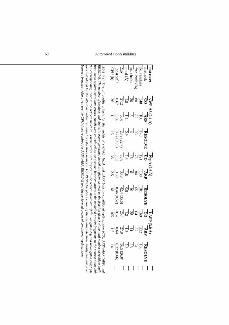
60 Automated model building
testcase:vW
F-A
3(2.4
A)
NspA
(2.6A
)L
AP
P(3.0
A)
method:
CO
AR
PR
ESO
LVE
CO
AR
PR
ESO
LVE
CO
AR
PR
ESO
LVE
no.residues148
160170
121130
101169
232136
frac.built(%)
8087
9378
8465
6487
51no.chains
208
416
610
3811
13rm
sd(A
)1.5
1.90.9
1.31.8
0.91.2
1.31.8
∆ϕ
��
27.236.0
23.9(22.7)
35.833.6
42.4(35.6)
25.427.9
56.5(26.0)
�cos�∆ϕ
��
0.670.56
0.72(0.69)
0.530.60
0.46(0.52)
0.670.64
0.32(0.66)
CPU
(h)36
115
382.5
18105
1.514
Table4.2:
Overall
qualitycriteria
forthe
models
ofvW
F-A
3,N
spAand
LA
PP
builtby
conditionaloptim
ization(C
O),
AR
P/w
AR
P(A
RP
)and
RE
SOLV
E.T
henum
berofresidues
andchains
inevery
generatedm
odelaregiven,as
wellas
thefraction
(frac.)ofthe
totalnumber
ofresiduesbuilt.
Root-m
ean-squarecoordinate
errors(rm
sd)w
erecalculated
asthe
distancebetw
eenatom
sin
them
odelledprotein
fragments
tothe
nearestatomw
iththe
correspondinglabel
inthe
refinedstructure.
Phase
errorsw
ithrespect
tothe
refinedstructures
( �Fobs�-w
eighted∆ϕ
andunw
eightedcos�∆ϕ
�)w
erecalculated
forthe
all-atomm
odelsresulting
fromthe
threem
ethods.For
RE
SOLV
Ephase
errorsofthe
resultingelectron
densitym
apare
givenbetw
eenbrackets.
Also
givenare
theC
PU
-times
requiredfor
AR
P/w
AR
P,R
ESO
LVE
andthe
performed
cyclesofconditional
optimization.
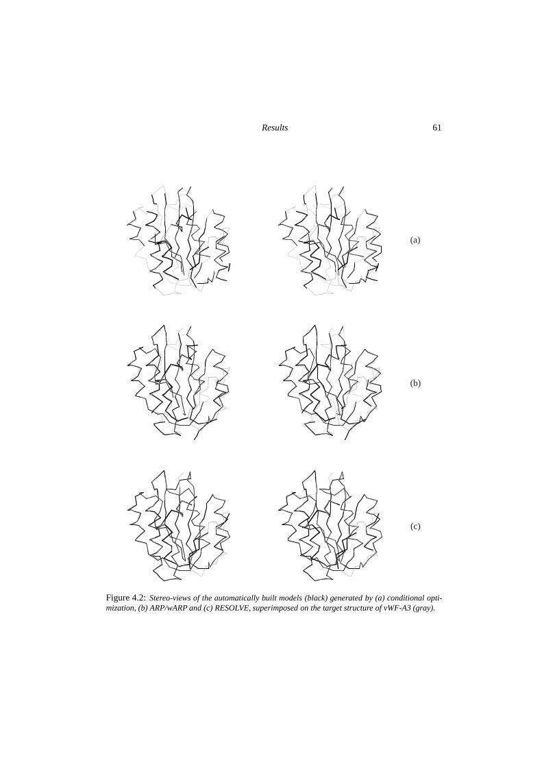
Results 61
(a)
(b)
(c)
Figure 4.2: Stereo-views of the automatically built models (black) generated by (a) conditional opti-mization, (b) ARP/wARP and (c) RESOLVE, superimposed on the target structure of vWF-A3 (gray).
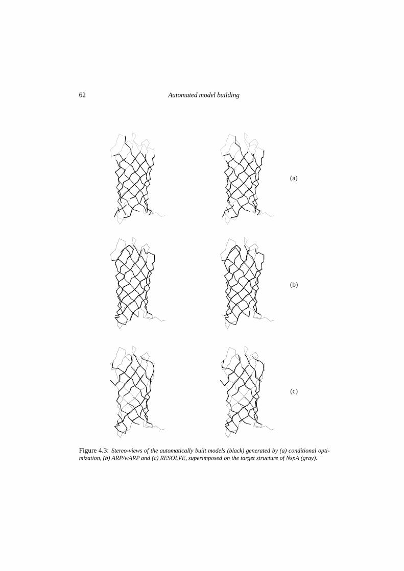
62 Automated model building
(a)
(b)
(c)
Figure 4.3: Stereo-views of the automatically built models (black) generated by (a) conditional opti-mization, (b) ARP/wARP and (c) RESOLVE, superimposed on the target structure of NspA (gray).
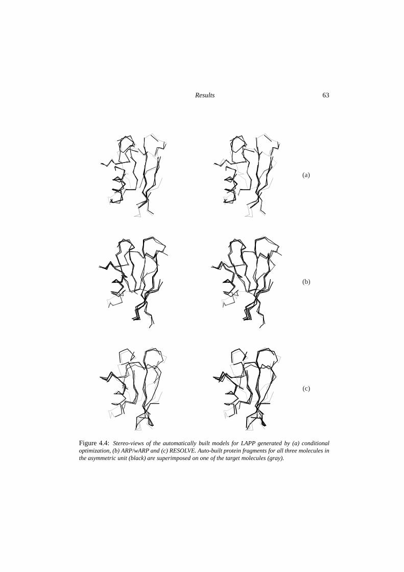
Results 63
(a)
(b)
(c)
Figure 4.4: Stereo-views of the automatically built models for LAPP generated by (a) conditionaloptimization, (b) ARP/wARP and (c) RESOLVE. Auto-built protein fragments for all three molecules inthe asymmetric unit (black) are superimposed on one of the target molecules (gray).
64 Automated model building
Conditional optimization required large amounts of CPU-time compared to ARP/wARPand RESOLVE (see table 4.2). With more than an order of magnitude difference with condi-tional optimization, ARP/wARP was the fastest program. Conditional optimization requiredalso much more computer memory than ARP/wARP or RESOLVE. Up to 1.5 and 1.4 Gbof memory was allocated for conditional optimization of the vWF-A3 and NspA test casesrespectively. To allow conditional optimization of LAPP on our work station with 2 Gbof memory, the program was re-compiled using single-precision instead of double-precisionnumbers for the storage of all condition values in computer memory. With the re-compiledprogram still up to 2.4 Gb of memory was allocated.
4.4 Discussion & conclusions
Conditional optimization yielded relatively accurate models for all three test cases, whichconsisted of most of the α-helical and β-strand segments. The models obtained were of com-parable phase quality as the models built by ARP/wARP or RESOLVE, but they consistedof less loops and turns and a higher number of separate chains. The most prominent errorsobserved in these models were reversed chain directions for β-strands. In the lowest reso-lution test case, i.e. LAPP, also one α-helix was built with a reversed chain direction andone loop was incorrectly modelled by a helical turn. The models generated by ARP/wARPand RESOLVE showed similar errors, which reflect the difficulties of model building at lowerresolutions.
Very few loops and turns were built by conditional optimization, and this forms the maindifference with the results from ARP/wARP and RESOLVE. The poor modelling of loops andturns may be ascribed to two factors. Firstly, loop conformations were poorly defined in theapplied conditional force fields. For LAPP, loop conformations were not taken into account atall, and for vWF-A3 and NspA only loop conformations corresponding to the A and B-regionof the Ramachandran plot were included (see Scheres & Gros, 2003). Most of the loops andturns in these proteins contain residues with conformations that were not defined by the forcefield and thus could not be modelled. This concerns residues with conformations in the L-region or residues (mainly glycines) with conformations outside any of the allowed regionsof the Ramachandran plot. For automated model building, extension of the force field withthese conformations may yield better results. Secondly, conditional optimization of loopsmay converge less readily than observed for α-helices and β-strands, because the informationcontent of the force field is lower for loop conformations. Similar problems may exist forside chain conformations extending beyond the γ-position. This is a consequence of thehigher structural variability of loops and side chains compared to main chain conformationsin α-helices and β-strands.
The models built by conditional optimization showed a lower connectivity than the mod-els generated by ARP/wARP or RESOLVE. This concerns not only the poor modelling ofloops and turns, but also the presence of additional breaks in β-strands and α-helices. Thesebreaks result in a larger number of separate chains, which would require more manual re-building. The occurrence of the breaks may be attributed to the absence of decision-basedmodel building steps as implemented in ARP/wARP and RESOLVE. In these programs, com-plete oligo-peptide fragments are positioned in discrete steps. In the applied conditional op-
Discussion & conclusions 65
timization protocol, protein fragments could be formed solely during the continuous processof refinement. The procedure to recognize protein fragments based on gradient contribu-tions did not alter any coordinates; only fragments with correct geometries were recognized.Therefore, minor topological errors in the optimized distributions of loose atoms resulted inbreaks in the recognized protein chains. Iteration of conditional optimization cycles with dis-crete model building steps, where optimized distributions of loose atoms would be replacedby atoms with the geometric arrangements of ideal protein fragments could lead to modelsof higher connectivity and completeness. A second option that might enhance the formationof longer protein fragments would be to explicitly assign corresponding atom labels to atomsthat are recognized as part of a protein fragment. For these atoms no longer all possible chem-ical assignments would be taken into account in the conditional optimization, which wouldreduce the degeneracy of the force field. Consequently, labelled protein fragments may growfaster into longer segments than in the current approach, where constantly all assignments areconsidered.
For the NspA and LAPP test cases, ARP/wARP yielded better results than RESOLVEand conditional optimization. For the vWF-A3 case however, RESOLVE yielded the mostcomplete model, and in contrast to conditional optimization and RESOLVE, ARP/wARP didnot achieve a phase improvement with respect to the MAD-phases. Despite the higher res-olution limit of this test case, the number of observations is relatively low due to a smallsolvent content. Possibly, the unrestrained ARP-refinement suffered from an unfavourableobservation-to-parameter ratio. The large amounts of geometric restraints in conditional op-timization and the restrained refinement as implemented in RESOLVE may have provided abetter defined refinement of the partially built models against the limited number of reflec-tions. The phase improvements obtained with these methods indicate that also with limitedamounts of diffraction data significant phase extension by automated model building may befeasible, as was already observed for model building at higher resolutions using ARP/wARP(for an extreme example see Tame, 2000).
The main drawback of the conditional optimization approach is formed by the extensivecomputational cost. Memory and CPU-time requirements are more than an order of magni-tude larger than for ARP/wARP, and conditional optimization is more than two times as slowas RESOLVE. Iteration of conditional optimization cycles with discrete model building stepsor explicit assignment of atom labels may provide a more efficient procedure, but the com-putational cost will remain high. For the vWF-A3 case, ARP/wARP may have suffered froma relatively low number of reflections. RESOLVE yielded a rather incomplete structure forLAPP, possibly due to the inaccuracy of the positioned fragments in the low-resolution map.Conditional optimization yielded relatively accurate models for all three test cases and doesnot depend on large numbers of reflections. Besides, a large radius of convergence has beenobserved for this method before (Scheres & Gros, 2003). Therefore, with the developmentsmentioned above, conditional optimization might eventually allow automated model buildingat lower resolutions and in electron density maps of lower quality. Dividing the computationalcost over multiple processors by parallelization of the program could then render conditionaloptimization suitable for common practice.

66 Automated model building
Acknowledgements
We are very grateful to Lucy Vandeputte-Rutten and Eric Huizinga for providing diffractiondata and coordinates and for useful comments and discussions. This work is supported by theNetherlands Organization for Scientific Research (NWO-CW: Jonge Chemici 99-564).
Chapter 5
Testing conditional optimizationfor application to ab initio phasingof protein structures
Abstract
At the resolution limits typically obtained in protein crystallography, the phase problem isunderdetermined and requires incorporation of additional prior knowledge. Conditional opti-mization allows expression of geometric knowledge about protein structures to be combinedwith refinement of loose, unlabelled atoms. We have tested the application of conditionaloptimization to ab initio structure determination of four-helix bundle Alpha-1. The resultsobtained with observed diffraction data to 2.0 A resolution and with calculated intensitiesfor four reflections illustrate the importance of low-resolution reflections and reliable phaseprobability estimates. Although convergence was very slow, a steady improvement in mapcorrelation coefficients and phase errors was observed, illustrating that for this case ab initiophasing by conditional optimization is possible. Further development is currently hinderedby excessive computational costs, but possibilities for advances are indicated that hopefullymay lead to a practical application of this approach in protein crystallography.
68 Ab initio phasing
5.1 Introduction
After obtaining diffracting crystals, the phase problem is a critical step in protein crystallo-graphy. When diffraction data to atomic resolution is available the problem is overdeterminedand therefore solvable in principle. Exploiting relationships among structure factors, directmethods nowadays allow routine ab initio phase calculation in small molecule crystallo-graphy (reviewed by Hauptman, 1997). Data to atomic resolution is usually not observedfor protein crystals and ab initio phasing by direct methods has not yet been commonly pos-sible in protein crystallography. To supplement the limited information from the observedintensities alone, other sources of information are critical to obtain phase information in pro-tein crystallography. Typically, isomorphous or anomalous intensity differences are used inexperimental phasing techniques (see for example Drenth, 1999). In the favourable casesthat the structure of a homologous protein is known, molecular replacement (reviewed byRossmann, 2001) can be used to obtain initial phases.
A wealthy source of prior information is formed by the available knowledge about thegeometry of protein structures. Protein structures consist of polypeptide chains arrangedin secondary structure elements with well-known geometries. Although the power of thisknowledge has been illustrated through the successful application of geometric restraints inprotein structure refinement, it has yet been scarcely used in ab initio phasing. The mainreason for this lies in the difficulty of expressing this knowledge in a way that allows efficientoptimization when no or limited crystallographic phase information is available. With con-ditional optimization we presented a method that allows expression of geometric knowledge,without the requirement of a topological assignment of the individual atoms (Scheres & Gros,2001). Given an estimate about the secondary structure content of the crystal, this knowledgecan be expressed in the absence of any phase information through geometric restraints actingon distributions of unlabelled atoms.
For a simple test case of four poly-alanine helices, we showed that in principle successfulrefinement of random atom distributions against medium-resolution diffraction data is possi-ble (Scheres & Gros, 2001). Standard routines to estimate phase probabilities fail for modelswith such large coordinate errors, and a novel procedure to estimate σ A-values from the dis-tribution of multiple models was necessary for successful optimization of random models.These calculations were performed with model diffraction data and protein structures aremore complex than the simplified model of this test case. Therefore, the feasibility of thisapproach remains to be shown for protein structures using observed diffraction data.
Here, we present conditional optimization of random atom distributions against 2.0 A ob-served diffraction data of four-helix bundle Alpha-1 (Prive et al., 1999). In the first instance,calculations were performed according to the protocols as developed for the ab initio phas-ing of the poly-alanine test structure (Scheres & Gros, 2001), and the optimization of threesmall protein structures against observed diffraction data (Scheres & Gros, 2003). Sinceoptimization according to these protocols did not result in convergence for this case, an al-ternative multiple-model procedure to estimate the phase quality of the optimized structureswas investigated. Also, the influence of four reflections at low resolution, which were likelymeasured incorrectly, was examined. Replacing the suspect intensities with calculated valuesand estimating the phase quality of each individual structure separately appeared critical forconvergence towards an interpretable electron density map in terms of helical elements.
Experimental 69
0 50 100 150 2000
100
200
300
400
500
0 10 20 30 400
10
20
|Fobs|
|Fcalc| hits
σobs
(1 0 0)
(0 2 0)
(0 -2 2) (0 0 2)
(1 0 0)
(0 -2 2) (0 2 0)
(0 0 2)
N
(a) (b)
Figure 5.1: (a) Calculated versus observed structure factor amplitudes for all observed reflections withBragg spacing d � 5 A. In the model structure factor calculation a bulk solvent contribution was takeninto account using the standard mask method as implemented in CNS. Four suspect reflections showa large difference between observed and calculated structure factor amplitudes. For these reflections(corresponding hkls are indicated with arrows), observed structure factor amplitudes were replaced bycalculated values. (b) Histogram of the measurement errors (σobs) of all observed reflections with Braggspacing d � 5 A. For three of the four suspect reflections a large measurement error was observed. Fora fourth reflection with a large measurement error (with hkl = 001) no large discrepancy betweenobserved and calculated structure factor amplitudes was observed.
5.2 Experimental
5.2.1 Test case
Four-helix bundle Alpha-1 was selected as a test case. This structure consists of 396 proteinatoms in space group P1 with unit-cell parameters a = 20.846, b = 20.909, c = 27.057 A, α= 102.40, β = 95.33, γ = 119.62o (PDB-code 1byz; Prive et al., 1999). The structure wasoriginally solved by direct metods using all observed diffraction data to 0.9 A resolution.Here, we truncated deposited structure-factor amplitudes to 2.0 A resolution. Analysis ofthis nearly complete data set (1 out of 2549 reflections is missing) showed that up to 5 Aresolution, four reflections were measured with much lower intensity than calculated fromthe deposited coordinates after scaling and bulk solvent correction (see figure 5.1a). For threeof these reflections also a significantly higher value for the measurement error was observed(figure 5.1b). The observed structure-factor amplitudes of these four suspect reflections werereplaced by their calculated values.
A force field for conditional optimization of this all-helical test structure was generatedusing the general parameter set as described by Scheres & Gros (2003). An expected sec-ondary structure content of 100% α-helix was used. The defined force field contained condi-
70 Ab initio phasing
tions describing linear protein fragments of up to twelve bonds long in an α-helical conforma-tion. Side chain conformations up to the γ-position were described in the two χ 1-rotamers thatare commonly observed in α-helices. Limited information was included about side chains ex-tending beyond the γ-position.
5.2.2 Optimization protocol
Figure 5.2 shows the refinement protocol, as implemented in the program CNS (Brunger etal., 1998a), for conditional optimization starting from multiple models consisting of ran-domly positioned atoms in the unit cell. In the absence of any prior phase information, amaximum likelihood crystallographic target function on amplitudes (MLF; Pannu & Read,1996) was set for the first optimization cycle, and σA-values were calculated according toan exponential decrease with the length of scattering vector �S: σA � exp��150���S�2�. Af-ter 1,000 steps of conditional dynamics, the N individual structures were positioned on acommon origin by iteratively shifting each structure using a phased translation function withphases from the average structure factor F ave. With all individual structures sharing a com-mon origin, the phases from F ave served as target values in the phase-restrained maximumlikelihood crystallographic target function (MLHL; Pannu et al., 1998) of subsequent con-ditional optimization cycles. These cycles comprised 10,000 steps of conditional dynamicsand phase probabilities were estimated as described in section 5.2.3. After each cycle theindividual structures were re-positioned on a common origin and F ave was updated.
Within each cycle of MLHL-refinement, atomic B-factors were assigned based on thenumbers of neighbouring atoms as described before (Scheres & Gros, 2001). To avoid neg-ative atomic B-factors after overall isotropic B-factor scaling, inverse scaling was applied to�Fobs� rather than scaling �F calc�. A bulk solvent contribution was calculated using the stan-dard mask routines implemented in CNS. Given an expected solvent content of 20%, a maskcovering 80% of the unit cell volume was calculated around the atoms with the highest num-bers of neighbours. The occupancy of all atoms inside the remaining solvent region was set tozero. Weights wa on the crystallographic part of the target function were calculated based ona relationship with the sum of D (as calculated from σA, see Read, 1986) over all reflections:wa ∝ 1�ΣD. A randomly selected 10% of all data with Bragg spacing d � 10 A were selectedfor cross-validation purposes (Brunger, 1993). As described before (Scheres & Gros, 2001),an additional 5% of the data were taken out of refinement and this selection was modified ev-ery 1,000 steps to avoid stalled progress owing to local minima in the crystallographic targetfunction.
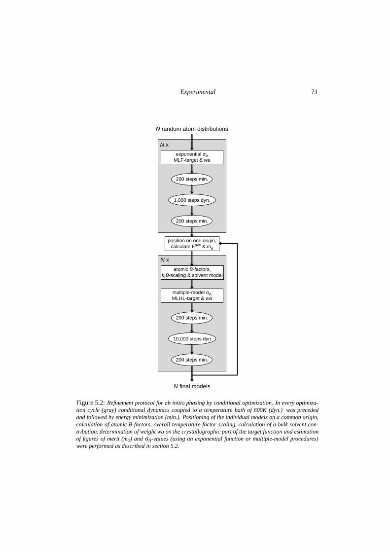
Experimental 71
exponential σA MLF-target & wa
200 steps min.
1,000 steps dyn.
200 steps min.
N random atom distributions
N final models
N x
200 steps min.
10,000 steps dyn.
200 steps min.
N x
position on one origin,calculate Fave & ma
multiple-model σA MLHL-target & wa
atomic B-factors,k,B-scaling & solvent model
Figure 5.2: Refinement protocol for ab initio phasing by conditional optimization. In every optimiza-tion cycle (gray) conditional dynamics coupled to a temperature bath of 600K (dyn.) was precededand followed by energy minimization (min.). Positioning of the individual models on a common origin,calculation of atomic B-factors, overall temperature-factor scaling, calculation of a bulk solvent con-tribution, determination of weight wa on the crystallographic part of the target function and estimationof figures of merit (ma) and σA-values (using an exponential function or multiple-model procedures)were performed as described in section 5.2.
72 Ab initio phasing
5.2.3 Phase probability estimation
Two types of phase probabilities need to be estimated for phase-restrained (MLHL) maximum-likelihood refinement: i� figures of merit for the average structure factors F ave of the phaserestraint and ii. σA-estimates for the individual models. Both must be estimated as a functionof resolution.
Shell-wise estimates ma for the figures of merit of the phase restraint were calculated by(5.1), using only test-set reflections:
ma �
N�m�
a�2�1
N�1(5.1)
where m�
a �N∑
i�1Fi�
N∑
i�1�Fi� and individual structure factor sets F i are calculated from the
corresponding N models (Scheres & Gros, 2003).Two ways to estimate σA-values for the individual models were tested.
i. As described before for conditional optimization of three small protein structures (Scheres& Gros, 2003), cross-validated figures of merit ma for the average structure factor were con-
verted to σa�i�A -estimates for every model i by (5.2):
σa�i�A �
��Eobs��Ei�ma����Eobs�2���Ei�2�
(5.2)
where �Eobs� and �Ei� are observed and calculated normalized structure factor amplitudes.These estimates will be referred to as σa
A because the differences between the different modelsare small due to the common figure of merit.ii. Different σA-estimates were calculated for each individual model, assuming that the truephase error of a model relates to the observed phase differences of that model with all othermodels. σi
A-Values for every model i were calculated by averaging shell-wise σ i jA -estimates
over all other models j (5.3):
σiA �
σi j
A
�j �
���Eobs��Ei�cos�ϕi�ϕ j���
��Eobs�2���Ei�2�
j
(5.3)
σiA-Values were calculated using all reflections because this calculation was unstable for the
low numbers of reflections in the test set alone.All calculations were performed on four, 667 MHz single-processor Compaq XP1000
workstations with at least 1.2 Gb of computer memory.
5.3 Results
5.3.1 Condensation and the influence of low-resolution data
Thirty-six random atom distributions were subjected to an initial optimization cycle compris-ing 1,000 steps of conditional dynamics using a MLF crystallographic target function. Fig-ure 5.3 shows a typical arrangement of the atoms resulting from these optimizations, where
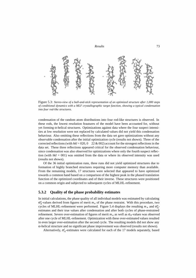
Results 73
Figure 5.3: Stereo-view of a ball-and-stick representation of an optimized structure after 1,000 stepsof conditional dynamics with a MLF crystallographic target function, showing a typical condensationinto four rod-like structures.
condensation of the random atom distributions into four rod-like structures is observed. Inthese rods, the lowest resolution feautures of the model have been accounted for, withoutyet forming α-helical structures. Optimizations against data where the four suspect intensi-ties at low resolution were not replaced by calculated values did not yield this condensationbehaviour. Also omitting these reflections from the data set gave optimizations without anyobservable condensation after the initial optimization cycle (results not shown). Three of thecorrected reflections (with hkl = 020, 0�22 & 002) account for the strongest reflections in thedata set. These three reflections appeared critical for the observed condensation behaviour,since condensation was also observed for optimizations where only the fourth suspect reflec-tion (with hkl = 001) was omitted from the data or where its observed intensity was used(results not shown).
Of the 36 initial optimization runs, three runs did not yield optimized structures due toformation of highly branched structures requiring more computer memory than available.From the remaining models, 17 structures were selected that appeared to have optimizedtowards a common hand based on a comparison of the highest peak in the phased translationfunction of the optimized coordinates and of their inverse. These structures were positionedon a common origin and subjected to subsequent cycles of MLHL-refinement.
5.3.2 Quality of the phase probability estimates
In initial calculations, the phase quality of all individual models was estimated by calculatingσa
A-values derived from figures of merit ma of the phase restraint. With this procedure, twocycles of MLHL-refinement were performed. Figure 5.4 displays the resulting m a and σa
A-estimates and their true values after condensation and after both cycles of phase-restrainedrefinement. Severe over-estimation of figures of merit m a as well as σA-values was observedafter one cycle of MLHL-refinement. Optimization with these over-estimated values resultedin even larger over-estimation after the second cycle. The resulting models did not show anyα-helical structure and no significant phase improvement was observed (results not shown).
Alternatively, σiA-estimates were calculated for each of the 17 models separately, based
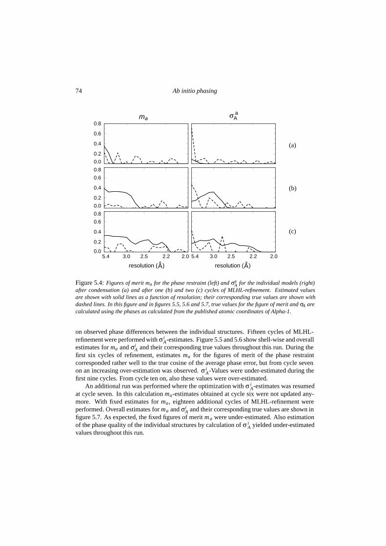
74 Ab initio phasing
5.4 3.0 2.5 2.2 2.00.0
0.2
0.4
0.6
0.8
0.0
0.2
0.4
0.6
0.8
0.0
0.2
0.4
0.6
0.8
5.4 3.0 2.5 2.2 2.0
(c)
σA
resolution ( ) resolution ( )
ma
(b)
(a)
a
A A
Figure 5.4: Figures of merit ma for the phase restraint (left) and σaA for the individual models (right)
after condensation (a) and after one (b) and two (c) cycles of MLHL-refinement. Estimated valuesare shown with solid lines as a function of resolution; their corresponding true values are shown withdashed lines. In this figure and in figures 5.5, 5.6 and 5.7, true values for the figure of merit and σA arecalculated using the phases as calculated from the published atomic coordinates of Alpha-1.
on observed phase differences between the individual structures. Fifteen cycles of MLHL-refinement were performed with σ i
A-estimates. Figure 5.5 and 5.6 show shell-wise and overallestimates for ma and σi
A and their corresponding true values throughout this run. During thefirst six cycles of refinement, estimates ma for the figures of merit of the phase restraintcorresponded rather well to the true cosine of the average phase error, but from cycle sevenon an increasing over-estimation was observed. σ i
A-Values were under-estimated during thefirst nine cycles. From cycle ten on, also these values were over-estimated.
An additional run was performed where the optimization with σ iA-estimates was resumed
at cycle seven. In this calculation ma-estimates obtained at cycle six were not updated any-more. With fixed estimates for ma, eighteen additional cycles of MLHL-refinement wereperformed. Overall estimates for ma and σi
A and their corresponding true values are shown infigure 5.7. As expected, the fixed figures of merit ma were under-estimated. Also estimationof the phase quality of the individual structures by calculation of σ i
A yielded under-estimatedvalues throughout this run.
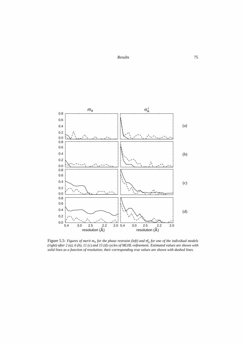
Results 75
5.4 3.0 2.5 2.2 2.0
0.0
0.2
0.4
0.6
0.8
0.0
0.2
0.4
0.6
0.8
0.0
0.2
0.4
0.6
0.8
0.0
0.2
0.4
0.6
0.8
5.4 3.0 2.5 2.2 2.0
(c)
(b)
(a)
(d)
σAma
resolution ( ) resolution ( )
i
A A
Figure 5.5: Figures of merit ma for the phase restraint (left) and σiA for one of the individual models
(right) after 2 (a), 6 (b), 11 (c) and 15 (d) cycles of MLHL-refinement. Estimated values are shown withsolid lines as a function of resolution; their corresponding true values are shown with dashed lines.
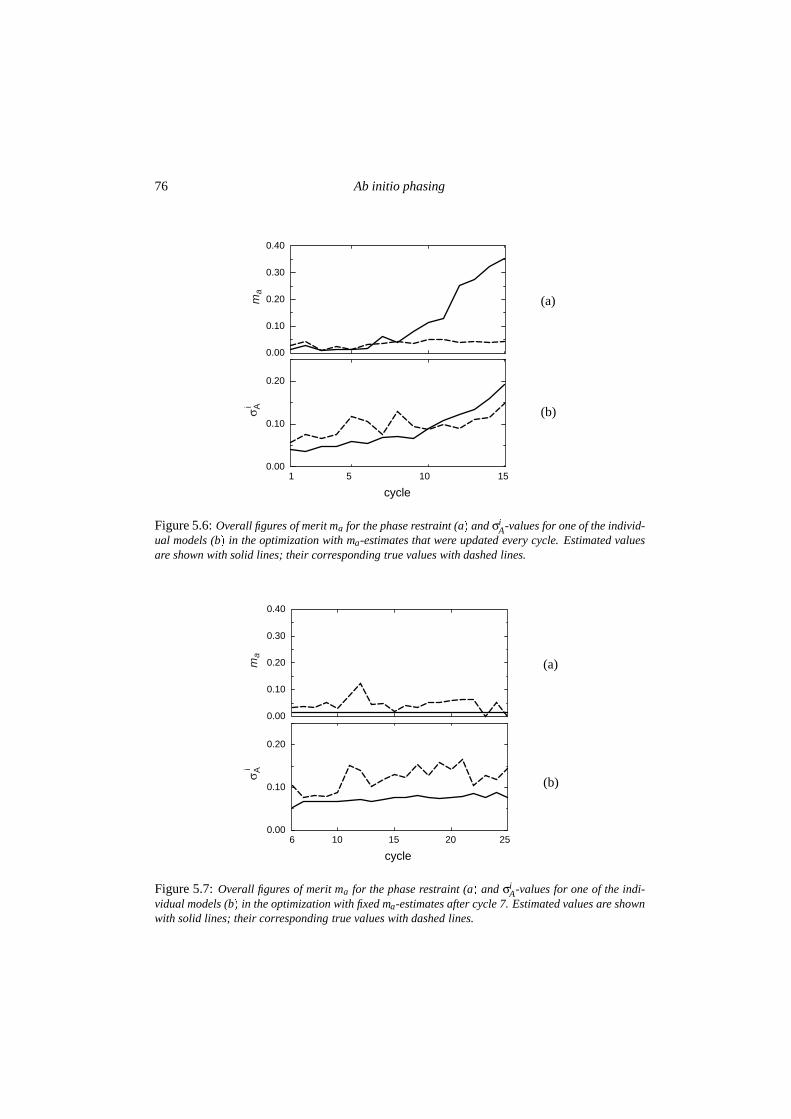
76 Ab initio phasing
1 5 10 150.00
0.10
0.20
0.00
0.10
0.20
0.30
0.40
cycle
(b)
(a)ma
σ Ai
Figure 5.6: Overall figures of merit ma for the phase restraint (a� and σiA-values for one of the individ-
ual models (b� in the optimization with ma-estimates that were updated every cycle. Estimated valuesare shown with solid lines; their corresponding true values with dashed lines.
6 10 15 20 250.00
0.10
0.20
0.00
0.10
0.20
0.30
0.40
cycle
(b)
(a)ma
σ Ai
Figure 5.7: Overall figures of merit ma for the phase restraint (a� and σiA-values for one of the indi-
vidual models (b� in the optimization with fixed ma-estimates after cycle 7. Estimated values are shownwith solid lines; their corresponding true values with dashed lines.
Results 77
best structure worst structure averagemap ccf. 0.36 0.18 0.37∆ϕ (Æ) 74.3 86.1 76.3cos�∆ϕ� 0.16 0.03 0.12rmsd (A) 1.54 1.74 -
Table 5.1: Overall quality criteria for the best and the worst structure and for the average over the17 individual structure factor sets after 25 optimization cycles. Map correlation coefficients (map ccf.)and phase errors (�Fobs�-weighted ∆ϕ and unweighted cos�∆ϕ�) were calculated using phases fromthe published coordinates. Root-mean-square coordinate errors (rmsd) were calculated as the nearestdistances from atoms in the optimized structures to any of the atoms in the published structure.
5.3.3 Convergence behaviour
An improvement in map correlation coefficients and phase errors was observed for both op-timization runs with σi
A-estimates (see figure 5.8). Fastest convergence was observed for therun with fixed, under-estimated values for figures of merit m a of the phase restraint. For thisrun a steady increase in average map correlation coefficient (of �0.005 per cycle) was ob-served throughout the optimization, as well as a decrease in the values of the overall phaseerrors. In the run where ma-estimates were updated every cycle, over-estimation of the phaseprobabilities coincided with a significantly slower improvement in map quality.
After cycle 25 of the run with fixed figures of merit m a, the individual structures with thebest and worst map correlation coefficients could be identified by their overall σ i
A-estimates(see figure 5.9). In the best structure (figure 5.10), three and a half α-helices have beenformed, of which two in the correct orientation and one and a half with a reversed chain di-rection. The worst structure (figure 5.11) shows multiple small α-helical fragments, of whichmost with incorrect orientations. Overall quality criteria for these two structures and for theaverage over all 17 individual structure factor sets are shown in table 5.1. Map correlationcoefficients for the average map m�F obs�exp�iϕave� tend to be better than for the best of themaps calculated with the phases of individual structure factor sets F i. The average electrondensity map at cycle 25 is shown in figure 5.12a. In this map, two right-handed helices areclearly visible and two helical-like rods with a less distinct choice of hand are observed. Mapcorrelation coefficients and phase errors for this map as a function of resolution are shownin figure 5.13. An average map calculated without the four suspect reflections (figure 5.12b)shows more electron density for the side chains.
The calculations presented here took in total approximately 115 CPU-days. Computermemory was allocated up to a maximum of 1.5 Gb.
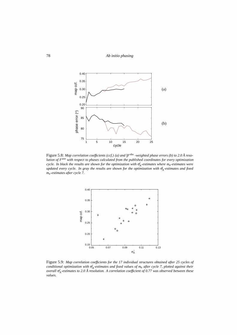
78 Ab initio phasing
1 5 10 15 20 2575
80
85
900.20
0.25
0.30
0.35
0.40m
ap c
cf.
cycle
phas
e er
ror
(0)
(b)
(a)
Figure 5.8: Map correlation coefficients (ccf.) (a) and �Fobs�-weighted phase errors (b) to 2.0 A reso-lution of Fave with respect to phases calculated from the published coordinates for every optimizationcycle. In black the results are shown for the optimization with σi
A-estimates where ma-estimates wereupdated every cycle. In gray the results are shown for the optimization with σi
A-estimates and fixedma-estimates after cycle 7.
0.05 0.07 0.09 0.11 0.130.15
0.20
0.25
0.30
0.35
0.40
σA
map
ccf
.
i
Figure 5.9: Map correlation coefficients for the 17 individual structures obtained after 25 cycles ofconditional optimization with σi
A-estimates and fixed values of ma after cycle 7, plotted against theiroverall σi
A-estimates to 2.0 A resolution. A correlation coefficient of 0.77 was observed between thesevalues.
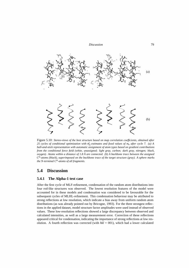
Discussion 79
(b)
(a)
Figure 5.10: Stereo-views of the best structure based on map correlation coefficients, obtained after25 cycles of conditional optimization with σi
A-estimates and fixed values of ma after cycle 7. (a) Aball-and-stick representation with automatic assignment of atom types based on gradient contributionsfrom the conditional force field (white, unassigned; light gray, carbon; dark gray, nitrogen; black,oxygen). Atoms within a distance of 1.8 A are connected. (b) A backbone trace between the assignedCα-atoms (black), superimposed on the backbone trace of the target structure (gray). A sphere marksthe N-terminal Cα-atoms of all fragments.
5.4 Discussion
5.4.1 The Alpha-1 test case
After the first cycle of MLF-refinement, condensation of the random atom distributions intofour rod-like structures was observed. The lowest resolution features of the model wereaccounted for in these models and condensation was considered to be favourable for thesubsequent cycles of MLHL-refinement. This condensation behaviour may be attributed tostrong reflections at low resolution, which indicate a bias away from uniform random atomdistributions (as was already pointed out by Bricogne, 1993). For the three strongest reflec-tions in the applied dataset, model structure factor amplitudes were used instead of observedvalues. These low-resolution reflections showed a large discrepancy between observed andcalculated intensities, as well as a large measurement error. Correction of these reflectionsappeared critical for condensation, indicating the importance of strong reflections at low res-olution. A fourth reflection was corrected (with hkl = 001), which had a lower calculated
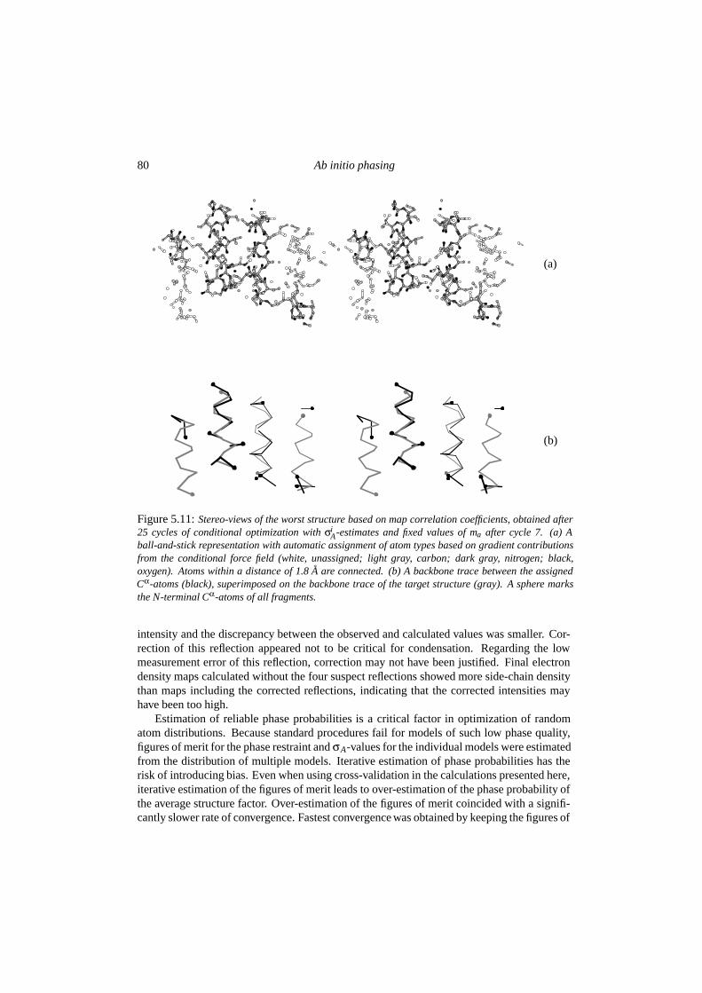
80 Ab initio phasing
(b)
(a)
Figure 5.11: Stereo-views of the worst structure based on map correlation coefficients, obtained after25 cycles of conditional optimization with σi
A-estimates and fixed values of ma after cycle 7. (a) Aball-and-stick representation with automatic assignment of atom types based on gradient contributionsfrom the conditional force field (white, unassigned; light gray, carbon; dark gray, nitrogen; black,oxygen). Atoms within a distance of 1.8 A are connected. (b) A backbone trace between the assignedCα-atoms (black), superimposed on the backbone trace of the target structure (gray). A sphere marksthe N-terminal Cα-atoms of all fragments.
intensity and the discrepancy between the observed and calculated values was smaller. Cor-rection of this reflection appeared not to be critical for condensation. Regarding the lowmeasurement error of this reflection, correction may not have been justified. Final electrondensity maps calculated without the four suspect reflections showed more side-chain densitythan maps including the corrected reflections, indicating that the corrected intensities mayhave been too high.
Estimation of reliable phase probabilities is a critical factor in optimization of randomatom distributions. Because standard procedures fail for models of such low phase quality,figures of merit for the phase restraint and σA-values for the individual models were estimatedfrom the distribution of multiple models. Iterative estimation of phase probabilities has therisk of introducing bias. Even when using cross-validation in the calculations presented here,iterative estimation of the figures of merit leads to over-estimation of the phase probability ofthe average structure factor. Over-estimation of the figures of merit coincided with a signifi-cantly slower rate of convergence. Fastest convergence was obtained by keeping the figures of
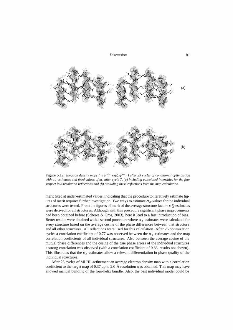
Discussion 81
(b)
(a)
Figure 5.12: Electron density maps ( m�Fobs�exp�iϕave� ) after 25 cycles of conditional optimizationwith σi
A-estimates and fixed values of ma after cycle 7, (a) including calculated intensities for the foursuspect low-resolution reflections and (b) excluding these reflections from the map calculation.
merit fixed at under-estimated values, indicating that the procedure to iteratively estimate fig-ures of merit requires further investigation. Two ways to estimate σ A-values for the individualstructures were tested. From the figures of merit of the average structure factors σ a
A-estimateswere derived for all structures. Although with this procedure significant phase improvementshad been obtained before (Scheres & Gros, 2003), here it lead to a fast introduction of bias.Better results were obtained with a second procedure where σ i
A-estimates were calculated forevery structure based on the average cosine of the phase differences between that structureand all other structures. All reflections were used for this calculation. After 25 optimizationcycles a correlation coefficient of 0.77 was observed between the σ i
A-estimates and the mapcorrelation coefficients of all individual structures. Also between the average cosine of themutual phase differences and the cosine of the true phase errors of the individual structuresa strong correlation was observed (with a correlation coefficient of 0.83, results not shown).This illustrates that the σi
A-estimates allow a relevant differentiation in phase quality of theindividual structures.
After 25 cycles of MLHL-refinement an average electron density map with a correlationcoefficient to the target map of 0.37 up to 2.0 A resolution was obtained. This map may haveallowed manual building of the four-helix bundle. Also, the best individual model could be
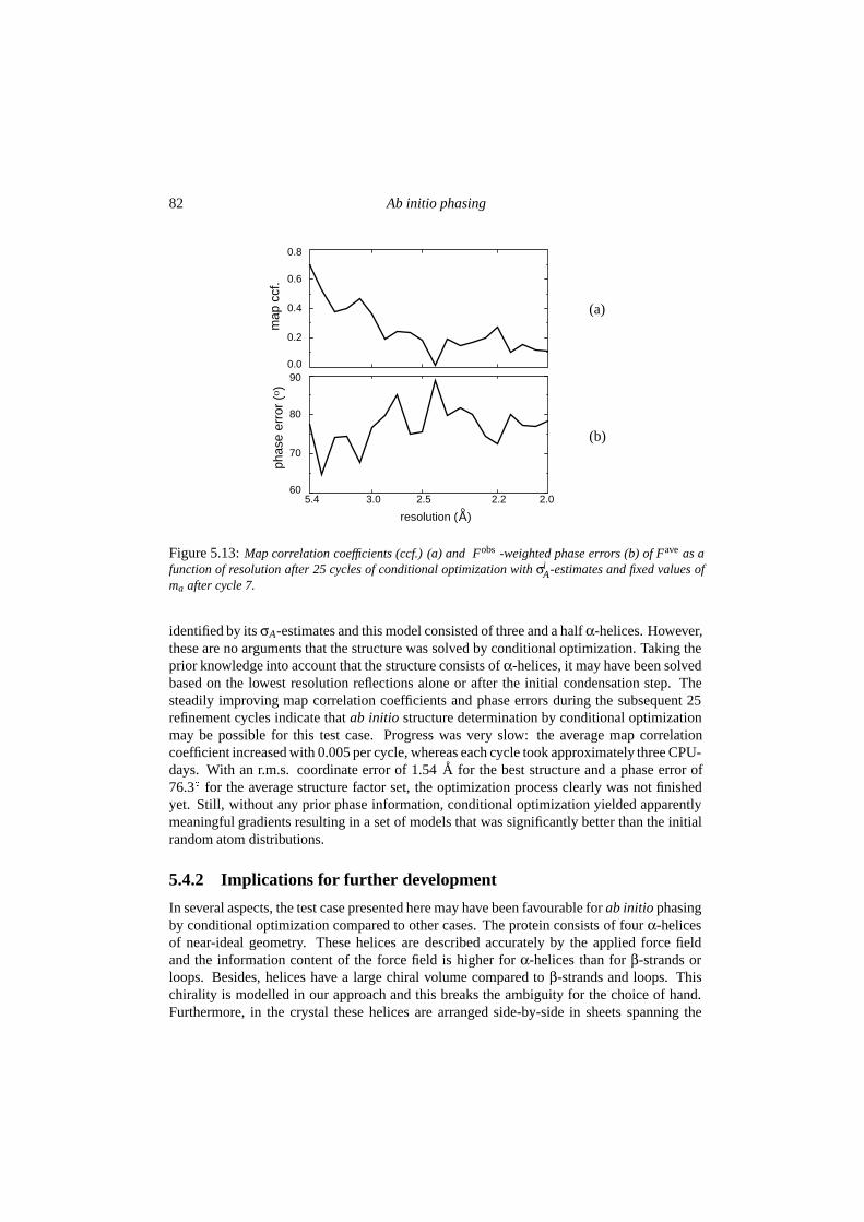
82 Ab initio phasing
5.4 3.0 2.5 2.2 2.060
70
80
900.0
0.2
0.4
0.6
0.8
map
ccf
.ph
ase
erro
r (0
)
(b)
(a)
resolution ( )A
Figure 5.13: Map correlation coefficients (ccf.) (a) and �Fobs�-weighted phase errors (b) of Fave as afunction of resolution after 25 cycles of conditional optimization with σi
A-estimates and fixed values ofma after cycle 7.
identified by its σA-estimates and this model consisted of three and a half α-helices. However,these are no arguments that the structure was solved by conditional optimization. Taking theprior knowledge into account that the structure consists of α-helices, it may have been solvedbased on the lowest resolution reflections alone or after the initial condensation step. Thesteadily improving map correlation coefficients and phase errors during the subsequent 25refinement cycles indicate that ab initio structure determination by conditional optimizationmay be possible for this test case. Progress was very slow: the average map correlationcoefficient increased with 0.005 per cycle, whereas each cycle took approximately three CPU-days. With an r.m.s. coordinate error of 1.54 A for the best structure and a phase error of76.3Æ for the average structure factor set, the optimization process clearly was not finishedyet. Still, without any prior phase information, conditional optimization yielded apparentlymeaningful gradients resulting in a set of models that was significantly better than the initialrandom atom distributions.
5.4.2 Implications for further development
In several aspects, the test case presented here may have been favourable for ab initio phasingby conditional optimization compared to other cases. The protein consists of four α-helicesof near-ideal geometry. These helices are described accurately by the applied force fieldand the information content of the force field is higher for α-helices than for β-strands orloops. Besides, helices have a large chiral volume compared to β-strands and loops. Thischirality is modelled in our approach and this breaks the ambiguity for the choice of hand.Furthermore, in the crystal these helices are arranged side-by-side in sheets spanning the
Discussion 83
width of the crystal. This packing results in a few relatively strong low-resolution reflections.As mentioned above, such reflections are favourable for the observed condensation behaviour.Replacing the observed intensities with possibly too large calculated values may have furtherenhanced the effect of condensation. For those protein crystals where the packing does notresult in such strong low-resolution reflections, initial condensation may be more difficult andsubsequent optimization more cumbersome. On the other hand, the relatively small solventregion in this test structure leads to an unfavourable, low number of reflections compared toother protein structures. The effect of these contributions will have to be adressed in futurecalculations with other test cases.
Currently, the main limitations for further development of this method are the excessiveCPU-time and the large amount of computer memory required for these calculations. Thissmall test case took in total four months of CPU-time, which severely limits the numberof variations that can be tested. Nevertheless, several possibilities for advances exist. Asmentioned before, the estimation of reliable phase probabilities is crucial. Iterative estimationof figures of merit for the phase restraint lead to over-estimation, and further development ofthis procedure is needed. Promising results were obtained with estimation of phase qualityfor each individual structure. In analogy to procedures developed by Lunin et al. (2000),the observed correlation between estimated σA-values and the true quality of the individualstructures may be exploited in procedures to enrich the average structure factors of the phaserestraints. Furthermore, the protocol applied in the calculations presented here consistedof continuous optimization steps alone. Possibly, the introduction of discrete steps in theoptimization process may allow a more readily escape from local minima, like for examplewrongly oriented α-helices. Possibilities include re-positioning of atoms based on variouselectron density maps or recognition of protein fragments among the distribution of looseatoms (as described in chapter 4). In this respect a challenge will probably lie in obtainingmultiple models that differ in a statistically valid way, yielding reliable phase probabilityestimates.
Faster convergence may also be obtained by adjusting some of the procedures that wereused in the presented calculations and which may not have been optimal. Calculated inten-sities were used for four suspect reflections at low resolution, and these values may havebeen too large. Preferably, complete and reliable data is used to test the full potentials of thismethod. In protein crystallographic data collection it is common practice to ignore the lowestresolution reflections, owing to experimental inconveniences. However, by a few modifica-tions to the standard experiment these problems can be overcome and reliable low-resolutiondata can be collected on a home source (Evans et al., 2000). Other points of interest arethe applied procedures for temperature-factor scaling and determination of the weight onthe crystallographic part of the target function. These procedures were transferred from cal-culations involving models with smaller coordinate errors than random atom distributions.Possibly, for models with such large errors other procedures may yield better results. Alsothe selection of structures with a common hand after condensation should be reconsidered,since in the early stages of optimization the hand appeared not to be fixed yet.
84 Ab initio phasing
5.5 Conclusions
The results for the single test case presented here indicate that ab initio phasing of observeddiffraction data by conditional optimization of random atom distributions may be possible.Although convergence was very slow, a steady improvement in map correlation coefficientsand phase errors was obtained. The importance of low-resolution reflections and estima-tion of reliable phase probabilities were illustrated. Correction of the three strongest, low-resolution reflections appeared crucial for condensation of the random starting models intorod-like structures. Under-estimation of phase probabilities yielded the best results in sub-sequent phase-restrained optimization cycles. Promising results were obtained with estimat-ing different σA-estimates for each individual structure, based on phase differences betweenthese structures. Iterative estimation of figures of merit for the average structure factors ofthe phase restraints gave over-estimated values, indicating that this procedure requires fur-ther examination. Further development of the applied procedures is currently limited by theexcessive computational cost, but there are several possibilities for potential improvement.Hopefully, these may lead to a practical application of conditional optimization in ab initioprotein structure determination.
Acknowledgements
This work is supported by the Netherlands Organization for Scientific Research (NWO-CW:Jonge Chemici 99-564).
Chapter 6
Summary & general discussion
In the standard crystallographic experiment, information about the phases of the reflections islost. From the observed intensities alone, the electron density of the unit cell cannot be recon-structed and this problem is known as the crystallographic phase problem. At the resolutionlimits typically obtained in protein crystallography the phase problem is underdetermined andrequires incorporation of additional information. Chapter 1 of this thesis describes existing,experimental and computational methods to determine and improve phases. The computa-tional methods exploit prior knowledge about the content of the unit cell to supplement thelimited experimental information. The quality of the available phase information typicallydetermines how much prior knowledge can be expressed. In chapter 2 a novel refinementmethod is presented, called conditional optimization. The conditional formalism offers anN-particle solution for the assignment of topology to loose, unlabelled atoms. Thereby, con-ditional optimization allows expression of large amounts of geometrical knowledge aboutprotein structures without the requirement of a molecular model, and thus potentially in theabsence of phase information. Initial tests with a simplified structure and calculated datashow that with this method, in principle, random atom distributions can be successfully opti-mized and ab initio phasing of medium-resolution data can be achieved. Conventional meth-ods for the estimation of phase probabilities fail for models of very low phase quality anda novel multiple-model procedure to estimate σA-values was necessary for these optimiza-tions. In chapter 3 a mean-force potential for conditional optimization of protein structures ispresented, which expresses knowledge about common protein conformations like α-helices,β-strands and loops. Using this generally applicable parameter set, conditional optimiza-tion of three small protein structures against 2.0 A observed diffraction data shows a largeradius of convergence, validating the presented force field and illustrating the feasibility ofthe approach. The application of conditional optimization to automated model building isexplored in chapter 4. For three test cases with data to medium resolution and good experi-mental phases, conditional optimization yields models of comparable quality as obtained bythe commonly used programs ARP/wARP and RESOLVE. Chapter 5 describes the applicationof conditional optimization to ab initio phasing of observed diffraction data. Low-resolutionreflections and reliable phase probability estimates appear to be important for convergence.For the presented test case promising results are obtained, indicating that also with observed
86 Summary & general discussion
diffraction data successful optimization of random atom distributions may be possible.Given the success of direct methods in small-molecule crystallography, a commonly ap-
plicable method for ab initio protein structure determination would be a valuable tool forstructural biology. The results described in this thesis indicate that conditional optimizationis a promising candidate for ab initio phasing of medium-resolution, protein diffraction data.On the other hand, major advances have been obtained with experimental approaches to solveprotein structures. The possibility to incorporate seleno-methionine in protein molecules us-ing bacterial expression systems has contributed significantly to the successful application ofanomalous dispersion methods, and eukaryotic expression systems for this purpose are beingdeveloped. Although these methods still require biochemical modifications to the native pro-tein molecule, techniques exploiting the anomalous signal of sulfur atoms in cysteines andmethionines require only a single diffraction experiment on a native protein crystal. Cur-rently, the weak anomalous signal of sulfur is still difficult to assess experimentally, but im-provements in data collection and processing techniques may also render these experimentalmethods a serious alternative for ab initio approaches. In addition, also molecular replace-ment may be expected to become more generally applicable given the rapidly increasingnumber of different folds in the protein structure database.
All the approaches mentioned here share the ultimate goal of providing a commonly ap-plicable solution to the phase problem in protein crystallography. Conditional optimizationmay benefit from advances in the other approaches and become suitable for common prac-tice before reaching this ultimate goal. Starting from initial phases as provided by the othermethods, the flexible searching behaviour with unlabelled atoms and the incorporation ofprior geometric knowledge by the conditional formalism may be exploited to extend phaseinformation in a commonly applicable way. As expressed in chapter 4 and 5, excessive com-putational costs form a stumble block for the applicability of conditional optimization. Paral-lelization of the program may be a way of dealing with this problem and such a developmentis underway. Common application of this method may then induce developments to furtherimprove the applied procedures. Improvements in the rate of convergence may be expectedfrom extension of the force field (especially concerning loops and side chains), optimizationof hybrid models with explicit topology assignments for recognizable protein fragments, anddevelopment of discrete modelling steps in the optimization protocols. Estimation of reli-able phase probabilities for models of low phase quality is also a point of interest. Variousmultiple-model procedures have been postulated in this thesis, but none of them proved gen-erally applicable and further investigation in this direction is needed. Eventually, also thegoal of ab initio phasing by conditional optimization would favour from these developments.From an optimistic point of view, and given the promising results described in chapter 2 and5, this method may then become, perhaps among others, a commonly applicable tool forprotein structure determination.

Bibliography
Abrahams, J.P. & de Graaff, R.A.G. (1998) Curr. Opin. Struct. Biol. 8, 601-605.
Adams, P.D., Pannu, N.S., Read, R.J. & Brunger, A.T. (1997) Proc. Natl. Acad. Sci. USA 94,5018-5023
Ban, N., Nissen, P., Hansen, J., Moore, P.B. & Steitz, T.A. (2000) Science 289, 905-920.
Berman, H.M., Battistuz, T., Bhat, T.N., Bluhm, W.F., Bourne, P.E., Burkhardt, K., Feng,Z., Gilliland, G.L., Iype, L., Jain, S., Fagan, P., Marvin, J., Padilla, D., Ravichandran, V.,Schneider, B., Thanki, N., Weissig, H., Westbrook, J.D. & Zardecki, C. (2002) Acta Cryst.D58, 899-907.
Bricogne, G. (1993) Acta Cryst. D49, 37-60.
Bricogne, G. (1997) Methods Enzymol. 276, 361-423.
Brunger, A.T. (1993) Acta Cryst. D49, 24-36.
Brunger, A.T., Adams, P.D., Clore, G.M., DeLano, W.L., Gros, P., Grosse-Kunstleve, R.W.,Jiang, J.S., Kuszewski, J., Nilges, M., Pannu, N.S., Read, R.J., Rice, L.M., Simonson, T.& Warren, G.L. (1998a) Acta Cryst. D54, 905-921.
Brunger, A.T., Adams, P.D. & Rice, L.M. (1998b) Curr. Opin. Struct. Biol. 8, 606-611.
Cowtan, K. (1998) Acta Cryst. D54, 750-756.
Cusack, S., Belrhali H., Bram, A., Burghammer, M., Perrakis, A. & Riekel, C. (1998) Nat.Struct. Biol. 5, 634 - 637.
Drenth, J. (1999) Principles of Protein X-ray Crystallography, 2 nd ed., Heidelberg: Springer.
Evans, G., Roversi, P. & Bricogne, G. (2000) Acta Cryst. D56, 1304-1311.
Foadi, J., Woolfson, M., Dodson, E. J., Wilson, K. S., Jia-xing, Y. & Chao-de, Z. (2000) ActaCryst. D56, 1137-1147.
Gilliland, G.L. & Ladner, J.E. (1996) Curr. Opin. Struc. Biol 6, 595-603.
Glykos, N.M. & Kokkindis, M. (2000) Acta Cryst. D56, 169-174.
88 BIBLIOGRAPHY
Guo, D.Y., Blessing, R.H. & Langs, D.A. (2000) Acta Cryst. D56, 1148-1155.
Harris, G.W. (1995) Acta Cryst. D51, 695-702.
Hauptman, H. (1997) Curr. Opin. Struc. Biol. 7, 672-680.
Hendrickson, W.A. & Ogata, C.M. (1997) Methods Enzymol. 276, 494-523.
Holton, T., Ioerger, T.R., Christopher, J.A. & Sacchettini, J.C. (2000) Acta Cryst. D56, 722-734.
Huizinga, E.G., Plas van der, R.M., Kroon, J., Sixma, J.J. & Gros, P. (1997) Structure 5,1147-1156.
Huizinga E.G., Schouten, A., Connolly, T.M., Kroon, J., Sixma, J.J. & Gros, P. (2001) ActaCryst. D57, 1071-1078.
Hauptman, H. (1997) Curr. Opin. Struc. Biol. 7, 672-680.
Isaacs, R.C. & Agarwal, N.W. (1977). Proc. Natl. Acad. Sci. USA 74, 2835-2839.
Jones, T.A., Zou, J.-Y., Cowan, S.W. & Kjeldgaard, M. (1991) Acta Cryst. A47, 110-119.
Ke, K. (1997). Methods Enzymol. 276, 448-461.
Kissinger, C.R., Gehlhaar, D.K. & Fogel, D.B. (1999) Acta Cryst. D55, 484-491.
Lamzin, V.S. & Wilson, K.S. (1993) Acta Cryst. D49, 129-147.
Lamzin, V.S., Perrakis, A., Bricogne, G., Jiang, J., Swaminathan, S. & Sussman, J.L. (2000)Acta Cryst. D56, 1510-1511.
Lunin, V.Y., Lunina, N.L., Petrova, T.E., Vernoslova, E.A., Urzhumtsev, A.G. & Podjarny,A.D. (1995) Acta Cryst. D51, 896-903.
Lunin, V.Y., Lunina, N.L., Petrova, T.E., Urzhumtsev, A.G., & Podjarny, A.D. (1998) ActaCryst. D51, 896-903.
Lunin, V.Y., Lunina, N.L., Petrova, T.E., Skovoroda, T.P., Urzhumtsev, A.G. & Podjarny,A.D. (2000) Acta Cryst. D56, 1223-1232.
Lunina, N.L., Lunin., V.Y. & Urzhumtsev, A.G. (2000) ECM-19 abstracts, XIXth EuropeanCrystallographic Meeting, 25-31 August 2000, Nancy, France
Morris, R.J., Perrakis, A. & Lamzin, V.S. (2002) Acta Cryst. D58, 968-975.
Mowbray, S.L., Helgstrand, C., Sigrell, J.A., Cameron, A.D. & Jones, T.A. (1999) Acta Cryst.D55, 1309-1319.
Murshudov, G.N., Vagin, A.A. & Dodson, E.J. (1997) Acta Cryst. D53, 240-255.
Navaza, J. & Saludjian P. (1997) Methods Enzym. 276, 581-595.
BIBLIOGRAPHY 89
Ogata, C.M. (1998) Nat. Struc. Biol. 5, 638-640.
Oldfield, T. (2000) Crystallographic Computing 7: Macromolecular Crystallographic Data.Edited by Bourne, P.E., Watenpaugh, K., Oxford: Oxford University Press.
Pannu, N.S. & Read, R.J. (1996). Acta Cryst. A52, 659-668.
Pannu, N.S., Murshudov, G.N., Dodson, E.J. & Read, R.J. (1998) Acta Cryst. D54, 1285-1294.
Perrakis, A., Morris, R. & Lamzin, V.S. (1999) Nat. Struc. Biol. 6, 458-463.
Prive, G.G., Anderson, D.H., Wesson, L., Cascio, D. & Eisenberg, D. (1999). Protein Sci. 8,1400-1409.
Read, R.J. (1986) Acta Cryst. A42, 140-149.
Read, R.J. (2001) Acta Cryst. D57, 1373-1382.
Rice, L.M., Shamoo, Y. & Brunger, A.T. (1998) J. Appl. Cryst. 31, 798-805.
Rossmann, M.G. (1990) Acta Cryst. A46, 73-82.
Rossmann, M.G. (1995) Curr. Opin. Struc. Biol. 5, 650-655.
Rossmann, M.G. (2001) Acta Cryst. D57, 1360-1366.
Schomaker, V. & Trueblood, K.N. (1968) Acta Cryst. B24, 63-76.
Scheres, S.H.W. & Gros, P. (2001), Chapter 2 of this thesis, Acta Cryst. D57, 1820-1828.
Scheres, S.H.W. & Gros, P. (2003), Chapter 3 of this thesis, Acta Cryst. D59, 438-446.
Sheldrick, G.M. & Gould, R.O. (1995) Acta Cryst. B51, 423-431.
Sheriff S., Klei H.E. & Davis, M.E. (1999) J. Appl. Cryst. 32, 98-101.
Sippl, M.J. (1995) Curr. Opin. Struct. Biol. 5, 229-235
Srinivasan, R. & Parthasaraty, S. (1976). Some Statistical Applications in X-ray Crystallog-raphy. Oxford: Pergamon Press.
Stevens, R.C. (2000) Curr. Opin. Struc. Biol. 10, 558-563.
Subbiah, S. (1991) Science 252, 128-133.
Subbiah, S. (1993) Acta Cryst. D49, 108-119.
Tame, J.R.H. (2000) Acta Cryst. D56, 1554-1559.
Terwilliger, T.C. & Berendzen, J. (1999) Acta Cryst. D55, 849-861.
Terwilliger, T.C. (2000) Acta Cryst. D56, 965-972.

90 BIBLIOGRAPHY
Terwilliger, T.C. (2001) Acta Cryst. D57, 1763-1775.
Terwilliger, T.C. (2002) Acta Cryst. D58, 1937-1940.
Urzhumtsev, A.G., Lunina, N.L., Skovoroda, T.P., Podjarny, A.D. & Lunin, V.Y. (2000) ActaCryst. D56, 1233-1244.
Vriend, G., Sander, C. & Stouten, P. F. (1994) Protein Eng. 7, 23-29.
Wang, B.C. (1985) Methods Enzymol. 115, 90-112.
Weeks, C.M., DeTitta, G.T., Miller, R. & Hauptman, H.A. (1993) Acta Cryst. D49, 179-181.
Winn, M.D., Isupov, M.N. & Murshudov, G.N. (2001) Acta Cryst. D57, 122-133.
Samenvatting & algemenediscussie
In het standaard kristallografisch experiment gaat alle informatie over de fasen van de re-flecties verloren. De electronendichtheid in de eenheidscel kan met enkel de gemeten inten-siteiten van de reflecties niet gereconstrueerd worden. Dit staat in de kristallografie bekendals het fasenprobleem. Bij de resolutielimieten die kenmerkend zijn voor de eiwitkristallo-grafie is het fasenprobleem onderbepaald. Het oplossen ervan is daarom afhankelijk van ad-ditionele informatie. Hoofdstuk 1 van dit proefschrift beschrijft bestaande, experimentele enrekenkundige methoden voor het bepalen en verbeteren van de fasen. De rekenkundige meth-oden maken gebruik van vooraf beschikbare kennis over de inhoud van de eenheidscel omde gebrekkige experimentele informatie aan te vullen. Kenmerkend hierbij is dat de kwaliteitvan de faseninformatie bepaalt hoeveel van die kennis gebruikt kan worden. In hoofdstuk 2wordt een nieuwe verfijningsmethode geıntroduceerd: conditionele optimalisatie. Het con-ditionele formalisme biedt een N-deeltjes oplossing voor het toekennen van een topologieaan losse, ongelabelde atomen. Daarmee kunnen grote hoeveelheden kennis over de geome-trie van eiwitstructuren tot uitdrukking worden gebracht zonder gebruik te maken van eenmoleculair model en dus mogelijk ook zonder enige faseninformatie. Aanvankelijke testsmet een vereenvoudigde structuur en berekende data toonden aan dat het in principe mo-gelijk is om met deze methode random verdelingen van atomen succesvol te verfijnen endaarmee data tot medium resolutie ab initio te faseren. Conventionele methoden om fasen-waarschijnlijkheden af te schatten werken niet met modellen die zo weinig faseninformatiebevatten. Daarom was het noodzakelijk een nieuwe procedure te ontwikkelen die gebruikmaakt van de spreiding in meerdere modellen. In hoofdstuk 3 wordt een krachtenveld voorconditionele optimalisatie van eiwitmoleculen gepresenteerd. Dit krachtenveld bevat kennisover veel voorkomende eiwitconformaties zoals α-helices, β-strands en loops. Met dit al-gemeen toepasbare krachtenveld werd een grote convergentiestraal bereikt voor conditioneleoptimalisatie van drie kleine eiwitmoleculen met experimentele diffractiedata. Hiermee werdhet krachtenveld gevalideerd en de haalbaarheid van de methode aangetoond. In hoofdstuk 4wordt de toepassing van deze methode op het geautomatiseerd bouwen van eiwitmoleculenonderzocht. Voor drie testgevallen met data tot medium resolutie en goede experimentelefasen leverde conditionele optimalisatie een model op van vergelijkbare kwaliteit als de veel-gebruikte programma’s ARP/wARP en RESOLVE. Hoofdstuk 5 beschrijft de toepassing vanconditionele optimalisatie op het ab initio faseren van experimentele diffractiedata. Lage
92 Samenvatting & algemene discussie
resolutie reflecties en betrouwbare fasenwaarschijnlijkheden blijken hiervoor van belang tezijn. Met het gepresenteerde testgeval werden veelbelovende resultaten behaald, wat aantoontdat succesvolle optimalisatie van random atoomverdelingen met experimentele data mogelijkis.
Gegeven het succes van directe methoden in de kleine-stofjes kristallografie zou een al-gemeen toepasbare methode voor ab initio structuurbepaling van eiwitten een waardevol in-strument zijn voor de structuurbiologie. De resultaten die in dit proefschrift staan beschreventonen aan dat conditionele optimalisatie een veelbelovende kandidaat is voor het ab initiofaseren van medium-resolutie, eiwitdiffractiedata. Van de andere kant is er ook grote vooruit-gang geboekt met experimentele methoden voor eiwitstructuurbepaling. De mogelijkheidom met bacteriele expressiesystemen seleniummethionine in eiwitmoleculen in te bouwenheeft significant bijgedragen aan de succesvolle toepassing van methoden die gebruik makenvan anomale dispersie. Momenteel worden er ook eukaryote expressiesystemen voor dezedoeleinden ontwikkeld. Deze methoden vereisen echter biochemische modificatie van hetnatieve eiwitmolecuul. Technieken die gebruik maken van het anomale signaal van zwavel-atomen in cysteine en methione vereisen daarentegen slechts een diffractieexperiment aaneen natief eiwitkristal. Momenteel is het nog moeizaam het kleine anomale signaal vanzwavel experimenteel te bepalen, maar door verbeteringen in data opname- en verwerkings-technieken kunnen dit soort experimentele methoden een serieus alternatief gaan vormenvoor ab initio technieken. Daarnaast kan ook van de molecular replacement techniek wordenverwacht dat ze algemener toepasbaar wordt, gezien het snel toenemend aantal verschillendeeiwitvouwingen in de databank van eiwitstructuren.
De bovenstaande technieken delen het ultieme doel om een algemeen toepasbare oplos-sing voor het fasenprobleem in de eiwitkristallografie te leveren. Conditionele optimalisatiekan haar voordeel doen met vorderingen die worden gemaakt met de overige benaderingen.Initiele faseninformatie die is verkregen met een van de andere technieken kan met condi-tionele optimalisatie uitgebreid worden, gebruik makende van het flexibele zoekgedrag metongelabelde atomen en de benutte kennis over de eiwitgeometrie. Daarmee kan deze methodeal algemeen toepasbaar worden voordat haar ultieme doel is bereikt. Zoals reeds vermeld inhoofdstuk 4 en 5 vormen excessieve rekentijden en geheugengebruik een struikelblok vooralgemene toepassing van conditionele optimalisatie. Parallellisatie van het programma zouhierbij kunnen helpen en momenteel wordt daaraan gewerkt. Versnelde convergentie zoubereikt kunnen worden door uitbreiding van het krachtenveld (met name wat betreft loops enzijketens), optimalisatie van hybride modellen met expliciete toekenning van topologie aanherkenbare eiwitfragmenten en de ontwikkeling van discrete modelbouwstappen in de opti-malisatieprotocollen. Het afschatten van betrouwbare fasenwaarschijnlijkheden voor model-len met weinig faseninformatie is hierbij ook van belang. In dit proefschrift zijn hiervoorverschillende procedures voorgesteld, maar geen enkele is algemeen toepasbaar gebleken.Daarom is verder onderzoek in deze richting noodzakelijk. Uiteindelijk zou ook het ultiemedoel van ab initio fasering kunnen profiteren van deze ontwikkelingen. Vanuit een opti-mistisch standpunt en gegeven de veelbelovende resultaten beschreven in hoofdstuk 2 en 5,zou deze methode dan, misschien naast andere methoden, een algemeen toepasbaar instru-ment voor eiwitstructuurbepaling kunnen worden.
Curriculum Vitae
De auteur van dit proefschrift werd op 5 augustus 1975 geboren in Roermond. In 1993voltooide hij zijn opleiding aan het Gymnasium van het Bisschoppelijk College in Weert enbegon aan de opleiding Scheikunde van de Universiteit Utrecht. Aldaar werd binnen een jaarhet propedeuse-diploma cum laude behaald. Het afstudeeronderzoek werd verricht onderbegeleiding van dr. Graafsma bij de Europese faciliteit voor synchrotronstraling (ESRF) inGrenoble, Frankrijk. Op 31 maart 1998 werd in Utrecht het doctoraal-examen cum laudeafgelegd. Een dag later trad hij als assistent-in-opleiding in dienst bij de vakgroep Kristal- enStructuurchemie van de Universiteit Utrecht onder begeleiding van prof. dr. Jan Kroon en dr.Piet Gros. Aanvankelijk werd getracht de kristalstructuur van het N-terminale domein vantranscriptiecofactor PC4 op te helderen. Later werd het onderzoek verricht dat beschrevenstaat in dit proefschrift. Vanaf juni zal hij waarschijnlijk werkzaam zijn als post-doc in hetlaboratorium van dr. Jose Marıa Carazo in Madrid, alwaar hij beeldverwerkingsmethodenvoor de electronenmicroscopie gaat ontwikkelen.
Publicaties
S.H.W. Scheres & P. Gros (2003) “Development of a force field for conditional opti-mization of protein structures”, Acta Cryst. D59, 438-446.
S.H.W. Scheres & P. Gros (2001) “Conditional Optimization: a new formalism forprotein structure refinement”, Acta Cryst. D57, 1820-1828.
R.B.G. Ravelli, M.L. Raves, S.H.W. Scheres, A. Schouten & J. Kroon (1999) “Abinitio structure determination of low-molecular-weight compounds using synchrotronradiation Laue diffraction”, J. Synchrotron Rad. 6, 19-28.
G.W.J.C. Heunen, A. Puig-Molina, S.H.W. Scheres, C. Schultze, D. Bourgeois & H.Graafsma (1998) “Broad energy band techniques for perturbation crystallography”,Proceedings of SPIE, 3448, 166-175.

94 Dankwoord
Dankwoord
Beste Jan, jij was het die mij strikte voor een hoofdvak in Grenoble en daarmee voor dekristallografie. Dank voor al je vertrouwen en steun en dat je mijn promoter wilde zijn.Helaas maak jij mijn promotie niet meer mee. Je was (ook als onze professor) een fantastischmens en aan jou draag ik dit boekje op. Piet, jij nam de stok van Jan over en ik bewonderde manier waarop je dat doet. Reeds daarvoor maakte je mij enthousiast voor jouw ideeenover ”conditional dynamics”. Bedankt voor al je begeleiding daarbij, al jouw enthousiasmeen je eindeloze stroom van ideeen, van ’s ochtends voor negenen tot laat in de middag. Ikheb veel van je geleerd en ik denk dat we een goed team vormden. Ik hoop dat dit boekjezal bijdragen aan het verwezenlijken van jouw wetenschappelijke droom. Loes, mijn innigmedeleven vanwege Jan gaat uit naar jou. Ook jou wil ik hartelijk danken, voor het samentennissen, het altijd open staan voor vragen en je exacte antwoorden daarop. Marjan, jij bentde spil van de vakGROEP, bedankt daarvoor en voor al je hulp van de afgelopen jaren.
Ik heb mezelf al die tijd zeer gelukkig geprezen met een vakgroep als Kristal & Structuur-chemie! Lucy en Clasien, met jullie ben ik daar samen aan een promotie-avontuur begonnen.Ik wil jullie hartelijk danken voor alle gezelligheid, steun en de vriendschap die wij al vijfjaar hebben mogen delen. Ik wens jullie veel succes met jullie laatste loodjes. Toen wijkwamen gingen Raimond en Jeroen net weg. Jeroen, ik nam aanvankelijk jouw PC4-projectover en hoewel ons gezamenlijk verblijf op de vakgroep kort was wil ik je danken voor jehulp bij mijn opstarten. Jouw ziekte en overlijden hebben ons allemaal erg geschokt. Rai-mond, jij wijdde me in in de geheimen van het dataverwerken. Bedankt daarvoor, ik heb eraltijd veel aan gehad. Ook de rest van de ’oude stempel’ wil ik hartelijk bedanken voor allegezelligheid en collegialiteit in de vakgroep. Martin W. en Roeland (o.a. voor een geweldigeWest-Highland ervaring; jammer dat jullie allebei weer roken...), Stephane (Martin’s spatzleswaren toch echt lekkerder), Wijnand (ook bedankt voor je gastvrijheid in Cambridge), Barend(spelletjes), Carien (blijven lachen), Ton L. (een biertje met een gulle lach), Diane (carnavalin Limburg), Anne (The Netherlands are so cold, but great fun), Jean (dank voor veel gezel-ligheid en je hulp met PC4), Ap (koffie-discussies) en Bouke (tennissen). Ik heb jullie alle-maal best gemist toen jullie vertrokken waren. Gelukkig is er ook weer een nieuwe lichtingenthousiaste mensen gekomen, waar ik steeds graag mee heb samengewerkt: Annika (dankvoor gezelligheid op onze kamer), Nicole & Jenny (brug naar de BOC), Mitja (nu eindelijkop de fiets naar Primus), Allison (koffietijd!), Hans, Fin & Bert (een aangename invasie uitWageningen) en Wiegert (van spinnen niet bang). En dan nog dank aan die mensen die eraltijd al waren en zonder wie de vakgroep de vakgroep niet zou zijn: Arie-laat-mij-hier-maar-achter (voor veel lol in Sheffield, Nancy en bij talloze andere gelegenheden), Martin L. (voor
96 Dankwoord
je grote behulpzaamheid bij vele computerproblemen),Eric (voor al je nuttige commentaren),Ton Spek (voor hulp bij kristallografische problemen), Huub (voor de lekkere koffie), Toine(voor al je steun met de workstations) en alle studenten. Jan, Ingrid en Aloys van de AV-dienstwil ik bedanken voor alle hulp bij de posters en de kaft van dit boekje. Janneke, bedankt voorje hulp bij mijn beursaanvragen. Van de NMR-groep wil ik verder Gert, Albert en Henribedanken voor onmisbare hulp met de bacterien, helaas kunnen jullie er in dit boekje niksover lezen. Ook andere leden van de BOC & NMR wil ik bedanken voor hun bijdragen aangezellige borrels en avondjes in Primus en De Vooghel. Speciale dank ook aan BOC Int. voorveel volleybalplezier.
Piet, gelukkig heb je ongelijk gekregen en kan ik ook na vijf jaar promoveren nog veelmensen van buiten het lab bedanken voor hun vriendschap en voor mooie tijden: al mijnscheikundevriendjes voor veel gezelligheid en alle huisgenootjes voor het (t)huisgevoel inHuize Rembrandt. Verder dank aan alle vrienden en familie in Limburg: ook daar kom ikgraag weer thuis. Bart & Cindy, dank voor jullie vriendschap en voor het aan Rosa laten zienhoe het in Limburg is. Alle minse van Scouting Tungelroy: hertstikke bedanktj veur hieelvul plezeer. Auch alle minse van de bouw in Utrecht wil ich hertstikke bedanke veur vul lolen veur os sjoeene huuske: wae woeene dur hieel gaer. Ook dank aan het Weert-clubje voorleuke VWO-etentjes (ik hoop binnenkort weer eens te kunnen!), Guido & Marie-Helene voorhun vriendschap-op-afstand, Heinz o.a. voor hulp bij aanbevelingen en de mensen van deKCV, speciaal het jongerenteam + helpers, voor alle verdieping en steun.
Paco, Rosa y Fran, gracias por toda vuestra ayuda y hospitalidad en Espana. Despuesde trabajar mucho siempre me he podido relajar con vosotros en San Lorenzo. Tambiengracias a todos nuestros amigos allı por esas noches de cachondeo. Mario, hartelijk dankvoor onze mooie vriendschap en dat jij deze keer mıjn paranimf wilt zijn. Waarvandaan jeook mag komen, onze deur blijft altijd voor je open. Marc, op zo’n broertje kun je rekenen.Bedankt dat je altijd klaar staat om te helpen, ook nu weer als paranimf. Succes met devoorbereidingen van jullie feest! Pa en ma, ook al vonden jullie het zelf moeilijk iets aanmijn proefschrift bij te dragen, jullie steun is altijd onmisbaar geweest! Bedankt voor alle(in)directe hulp bij mijn promotie en dat jullie altijd voor mij en Rosa klaar staan.
Rosita, tu me haces muy feliz. TQM. Juntos continuaremos por nuestro camino, dondesea. Ik ben blij dat we daarbij samen God mogen danken, voor elkaar en voor de dingen vaniedere dag, ook een promotiedag.