CONCEPT GENERAL MECHANICS Classical & Quantum Mechanics

CONCEPT

GENERAL MECHANICS

Classical & Quantum Mechanics

P.J. Mulders and H.G. Raven

Nikhef and Department of Physics and Astronomy,Faculty of Sciences, VU University,

1081 HV Amsterdam, the Netherlands

E-mail: [email protected] & [email protected]

November 2012 (version 0.0)

Introduction 1

Voorwoord

Het college Algemene Mechanica is een combinatie van Klassieke Mechanica en Quantummechanica enwordt verzorgd door Piet Mulders en Gerhard Raven geassisteerd door Maarten Buffing bij de werkcol-leges. Het college wordt getentamineerd in twee delen,Deel I: Van klassieke mechanica naar quantummechanica (6 ECTS),Deel II: Quantummechanica (6 ECTS).

Bij het college wordt gebruik gemaakt van de boeken ..... en Introduction to Quantum Mechanics,second edition van D.J. Griffiths (Pearson). Dit dictaat beschrijft de context van de colleges.

Het gehele vak beslaat 12 studiepunten en wordt gegeven in periodes 2 en 3. In totaal zullen er 28colleges van 2 uur elk en 28 werkcolleges van 3 uur gegeven worden. In blok 2 zijn er 14 colleges (2halve dagen per week gedurende 7 weken), afgerond met een tentamen (vaknaam: Van klassieke naarquantummechanica, 6 ECTS vakcode ....) In blok 3 zijn er 12 colleges (4 halve dagen per week gedurende3 weken), afgerond met een tentamen (vaknaam: Quantummechanica, 6 ECTS, vakcode ...). Bij deaansluitende werkcolleges worden problemen gemaakt, besproken, er worden daarnaast opgaven gegevendie moeten worden ingeleverd. De resultaten van deze opgaven vormen onderdeel van de toetsing.

Piet Mulders en Gerhard RavenNovember 2012

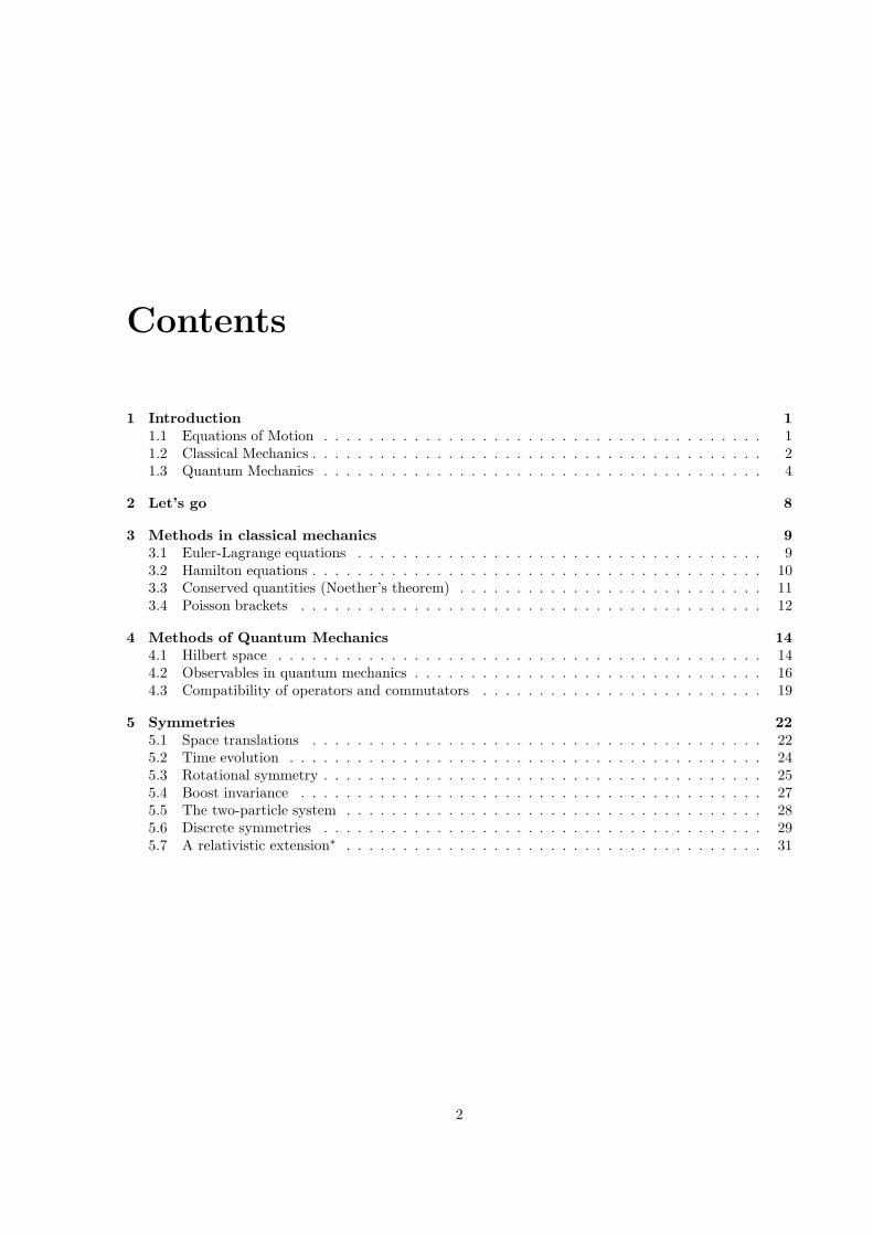
Contents

1 Introduction 1

1.1 Equations of Motion . . . . . . . . . . . . . . . . . . . . . . . . . . . . . . . . . . . . . . . 11.2 Classical Mechanics . . . . . . . . . . . . . . . . . . . . . . . . . . . . . . . . . . . . . . . . 21.3 Quantum Mechanics . . . . . . . . . . . . . . . . . . . . . . . . . . . . . . . . . . . . . . . 4

2 Let’s go 8

3 Methods in classical mechanics 9

3.1 Euler-Lagrange equations . . . . . . . . . . . . . . . . . . . . . . . . . . . . . . . . . . . . 93.2 Hamilton equations . . . . . . . . . . . . . . . . . . . . . . . . . . . . . . . . . . . . . . . . 103.3 Conserved quantities (Noether’s theorem) . . . . . . . . . . . . . . . . . . . . . . . . . . . 113.4 Poisson brackets . . . . . . . . . . . . . . . . . . . . . . . . . . . . . . . . . . . . . . . . . 12

4 Methods of Quantum Mechanics 14

4.1 Hilbert space . . . . . . . . . . . . . . . . . . . . . . . . . . . . . . . . . . . . . . . . . . . 144.2 Observables in quantum mechanics . . . . . . . . . . . . . . . . . . . . . . . . . . . . . . . 164.3 Compatibility of operators and commutators . . . . . . . . . . . . . . . . . . . . . . . . . 19

5 Symmetries 22

5.1 Space translations . . . . . . . . . . . . . . . . . . . . . . . . . . . . . . . . . . . . . . . . 225.2 Time evolution . . . . . . . . . . . . . . . . . . . . . . . . . . . . . . . . . . . . . . . . . . 245.3 Rotational symmetry . . . . . . . . . . . . . . . . . . . . . . . . . . . . . . . . . . . . . . . 255.4 Boost invariance . . . . . . . . . . . . . . . . . . . . . . . . . . . . . . . . . . . . . . . . . 275.5 The two-particle system . . . . . . . . . . . . . . . . . . . . . . . . . . . . . . . . . . . . . 285.6 Discrete symmetries . . . . . . . . . . . . . . . . . . . . . . . . . . . . . . . . . . . . . . . 295.7 A relativistic extension∗ . . . . . . . . . . . . . . . . . . . . . . . . . . . . . . . . . . . . . 31

2

Introduction 3

Chapter 1

Introduction

1.1 Equations of Motion

A classical system is determined by x(t) from which we get the velocity v(t) = x(t), etc. The motion isobtained from Newton’s equation,

md2x

dt2= −dV

dx. (1.1)

It determines how we get from x(0) −→ x(t) (given sufficient boundary conditions x(0) and x(0)).This can be extended to 3 dimensions by looking at three coordinates of an object/particle, r(t) =(x(t), y(t), z(t)). When there are more objects/particles one has many coordinates, r1(t), r2(t), . . . .

Quantum mechanically, one works with a complex wave function ψ(x, t), which by itself is not physicalbut contains all relevant information about the state (NL: toestand) referred to as |ψ〉. For example, theabsolute value squared |ψ(x, t)|2 represents a probability. The wave function satisfies the Schrodingerequation,

i~∂ψ

∂t= − ~2

2m

∂2ψ

∂x2+ V (x, t)ψ(x, t). (1.2)

This determines how the system evolves from ψ(x, 0) −→ ψ(x, t). The constant appearing in this equationis Planck’s constant,

h = 6.626× 10−34 J s. (1.3)

or more precise the reduced Planck’s constant ~ = h/2π = 1.055× 10−34 J s = 6.582× 10−16 eV s. Thisalso determines the domain where quantum mechanics is needed to get a good description of nature,namely the domain where appropriate quantities are of the order of this constant. In this respect, notethat energy × time and/or to momentum × distance or angular momentum have the same dimensionas ~. In 3 dimensions one works with wave functions ψ(r, t) and for many particles with wave functionsψ(r1, r2, . . . , t).

What do these equations have to do with each other. Are they the same. The answer is no. Theapproach in classical mechanics is deterministic. A position is known at a given time and at the sametime one can know its velocity or the momentum. From a quantum mechanical wave function, one alsocan get positions or momenta, but as it turns out not at the same time and in general the outcome of ameasurement of position or momenta is not unique. The probabilities of particular outcome for positionsor momenta, however, occur with well-determined probabilities.

The equations both do have the presence of a potential in common. This is where the dynamics is. Inits absence one has a free-moving system. It is interesting to see what this is in both cases, both of themhopefully familiar to you. In classical mechanics the solution with x(0) = x0 and x(0) = v0 is given by

x(t) = x0 + v0 t, (1.4)

1

Introduction 2

representing the trajectory of an object moving with constant velocity v0, constant momentum p = mv0and energy E = 1

2mv20 = p2/2m. The solution of the Schrodinger equation with V = 0 is probably also

familiar. The solution for a system moving with a fixed momentum is given by a wave with wave numberk and frequency ω,

ψk(x, t) =√ρ ei(k x−ω t). (1.5)

It has a constant probability ρ over space. The momentum is given by p = ~ k and the energy byE = ~ω. As for classical mechanics the energy is given by E = p2/2m, thus the frequeny is related tothe momentum through ω = ~k2/2m. It is known as a plane wave solution In contrast to the preciselydetermined momentum, the position is completely undetermined. We will compare both approachesin much more detail later. The examples are useful to keep in mind as reference examples in variousapplications.

==========================================================

Exercise: Check the solutions in Eqs 1.4 and 1.5.

==========================================================

1.2 Classical Mechanics

Let us first review some of the properties of classical mechanics. As should be clear from the way wewrote Newton’s equation in Eq. 1.1 we consider conservative forces of the type F (x) = −∂V/∂x orin 3-dimensional applications F = −∂V/∂r = −∇V . Note that we in principle could allow even atime-dependence in the potential, i.e. V = V (r, t). We see two interesting quantities popping up, themomentum p = m r and the kinetic energy K = 1

2m v2 satisfying

dp

dt= m r = F = −∂V

∂r, (1.6)

d

dt

(12mv2

)= F · v = −∂V

∂r· drdt, (1.7)

or introducing the energy E = K + V and using that dV/dt = (∂V/∂r) · (dr/dt) + ∂V/∂t, one sees that

dE

dt=∂V

∂t. (1.8)

It shows that in some cases energy and momentum are conserved. If the potential doesn’t depend onparticular coordinates, e.g. is independent of z, which means translation invariance in z-direction, thez-component of momentum is conserved. If the potential does not explicitly depend on time (invarianceunder time translations) one has conservation of energy.

There are many other quantities that play a role in classical mechanics, for instance the angularmomentum ℓ = r × p. For this quantity one has

dℓ

dt= r × dp

dt= −r × ∂V

∂r. (1.9)

For a central potentials V (r) one has ∇V (r) = ∂V/∂r = r ∂V/∂r, thus the right-hand side of the equa-tion vanishes and ℓ is conserved. It shows the link between rotational invariance and conservation ofangular momentum. Note that the notation ∂/∂r is somewhat sloppy. It refers to the gradient ∇ withcomponents ∇i = ∂/∂xi.

Introduction 3

==========================================================

Exercise: The link with rotational invariance can also be made more explicit by working in polarcoordinates. One has

x = r sin θ cosϕ, y = r sin θ sinϕ, z = r cos θ.

One can use this to calculate e.g.

∂V (r, θ, ϕ)

∂ϕ=∂V (x, y, z)

∂x

∂x

∂ϕ+∂V (x, y, z)

∂x

∂x

∂ϕ+∂V (x, y, z)

∂x

∂x

∂ϕ.

Use this to show that∂V

∂ϕ= x

∂V

∂y− y ∂V

∂x,

and using Eq. 1.9 one findsdℓzdt

= −∂V∂ϕ

.

This shows the link of conservation of ℓz with invariance under rotations around the z-axis.

==========================================================

Two interacting particles

We also recall the situation of two interacting particles with a potential that only depends on the relativedistance, i.e. V (r1, r2) = V (r1 − r2). The force on particle 1 and particle 2 are

F 1 = − ∂V∂r1

and F 2 = − ∂V∂r2

= −F 1,

thus action = −reaction and there is no net force on the combined system. The equations of motion(Newton) are two coupled equations

m1 r1 = F 1, and m2 r2 = F 2 = −F 1. (1.10)

It is convenient to introduce new coordinates, know as the center of mass and relative coordinates,

M R = m1 r1 +m2 r2

r = r1 − r2

⇐⇒

r1 = R+m2

Mr

r2 = R− m1

Mr

(1.11)

where M = m1 + m2 is the total mass. Furthermore it is convenient to introduce the reduced massm ≡ m1m2/(m1 +m2). (If there are more particles or confusion may arise, we can use subscripts R12,etc. for coordinates and masses.) In terms of these new coordinates, the equations of motion decouple,

M R = 0, and m r = F = −∂V/∂r. (1.12)

The momenta corresponding to the new coordinates are given by P = MV = MR and p = mv = mr

and they satisfy

MV =MR = P = p1 + p2

v = r =p1

m1− p2

m2

⇐⇒

p1 = m1 V +m v =m1

MP + p

p2 = m2 V −m v =m2

MP − p.

(1.13)

Introduction 4

Not only the equations of motion decouple, but it is now also straightforward to show that the kineticenergy K can be written as

K = 12 m1 v

21 +

12 m2 v

22 = 1

2 M V 2 + 12 m v2

=p21

2m1+

p22

2m2=

P 2

2M+

p2

2m. (1.14)

The potential energy only depends on the relative position, i.e. V (r1 − r2) = V (r).With the results of the first part of this section we see immediately that the total energy E =

K1 + K2 + V is conserved (the potential does not (explicitly) depend on time). It separates into twoparts,

E =P 2

2M︸︷︷︸

Ecm

+p2

2m+ V (r)

︸︷︷︸

Erel

, (1.15)

The center of mass (cm) part involves R through R and the relative (rel) part involves r and r. Fur-thermore the total momentum P = p1 + p2 is conserved (the potential energy does not depend on R).The energies of the particles 1 and 2 separately are not conserved, neither are their momenta p1 and p2

conserved.

1.3 Quantum Mechanics

To go any further with quantum mechanics, one needs to know what to do with ψ(x, t), or in 3 dimensionsψ(r, t). It turns out that its physical significance comes in by doing something with it. In particular|ψ(x, t)|2 dx is the probability to find the system at time t in an interval of size dx around the point x.Note that while the wave function may be complex, the probability

ρ(x, t) = |ψ(x, t)|2 = ψ∗(x, t)ψ(x, t) (1.16)

is real. For three dimensions |ψ(r, t)|2 d3r is the probability to find the system in a small volume d3raround the point r. The value ψ(x, t) of the function itself is referred to as probability amplitude (NL:waarschijnlijkheidsamplitudo) for the state ψ (or |ψ〉) to be at place r at time t. Where the system wasbefore time t cannot be answered, one would have to do a measurement for that at the earlier time. Butas soon as a measurement is done and the particle is found at a particular position, say the origin, thenthe state is no longer described by the wave function ψ but by ψ0, which would be a function peakingaround the origin. This sharp function will then evolve (spread) according to the Schrodinger equation.Pretty weird!

Operators and their expectation values

Suppose that we have a system described by by the wave function ψ. We measure the position. Werepeat the measurement with another system described by the same wave function. And so on. If thepossible outcome for the positions would be discrete, i.e. just a collection of possibilities xi we wouldmeasure how many times (ni) particles end up in each of the positions. That probability is Pi = ni/N ,where N =

∑

i ni is the total number of measurements. One has

1 =∑

i

Pi, (1.17)

〈x〉 =∑

i

xi Pi, (1.18)

〈x2〉 =∑

i

x2i Pi, (1.19)

Introduction 5

which states that the probabilities add up to one, and weighing with xi or x2i gives the average of x,

x2, etc., which can be extended to the average of any weight function w(x). The standard deviation(squared) is found by weighing with (xi − 〈x〉)2. Since 〈x〉 is a number, one finds

σ2 = ∆x2 =∑

i

(x2i − 〈x〉)2 Pi = 〈x2〉 − 〈x〉2. (1.20)

For the quantum mechanical outcome of an x-measurements one has the continuous version of the abovewith all (real) possibilities for x, with probabilities ρ(x, t) = |ψ(x, t)|2. This implies the normalizationand leads to specific expectation values (NL: verwachtingswaarden),

1 =

∫

dx ψ∗(x, t)ψ(x, t)︸︷︷︸

ρ(x,t)

, (1.21)

〈x〉 =

∫

dx x ρ(x, t) =

∫

dx ψ∗(x, t)xψ(x, t), (1.22)

〈x2〉 =

∫

dxx2 ρ(x, t) =

∫

dx ψ∗(x, t)x2 ψ(x, t), (1.23)

which can be extended to any weight function. For the position one has the standard deviation (NL:standaardafwijking) ∆x of which the square is

∆x2 =

∫

dx (x− 〈x〉)2 ρ(x, t) = 〈x2〉 − 〈x〉2. (1.24)

The notation on the right hand side with x between the functions ψ∗ and ψ can be generalized to anyproperty as well as to three dimensions. For this we first introduce the concept of operator and itsexpectation value,

〈O〉 =∫

d3r ψ∗(x, t) Oψ(x, t), (1.25)

where O is an operator acting on the function ψ and 〈O〉 is referred to as the expectation value of O.In the simple case above we were working with the position and one would have the position operatorx that acts like xψ(x, t) = xψ(x, t). But after generalizing this to an operator being something thatproduces a new function, ψ −→ Oψ, also the derivative d/dx is an example of an operator working on ψand producing a new function (the derivative function). Also the normalization of the wave function canbe considered as an expectation value of an operator. It is in fact just the expectation value of the unitoperator, 〈1〉 = 1. Usually the hat on the operators will be omitted. Finally we note that an expectationvalue does depend on the state ψ, so the better notation would have been 〈O〉ψ or 〈ψ|O|ψ〉 instead of

just 〈O〉. Just as one talks about the expectation value of x (in a state ψ), one now can talk about theexpectation value of O (in state ψ).

The momentum operator

If we look at the time dependence of 〈x〉, it is (in general) nonzero. We obtain after a few partialintegrations

d

dt〈x〉 = − i~

m

∫

dx ψ∗(x, t)∂ψ(x, t)

∂x=〈px〉m

, (1.26)

with the momentum operator (NL: impulsoperator) p given by

px = −i~ ∂

∂x. (1.27)

Introduction 6

The position and momentum are actually also in quantum mechanics the basic quantities, as they arein classical mechanics. E.g. classically the energy can be written as a function of p and x. That samefunction is actually the righthand-side of the Schrodinger equation in Eq. 1.2,

i~∂ψ(x, t)

∂t= Hψ(x, t), (1.28)

with

H =p2

2m+ V (x, t) = − ~2

2m

∂2

∂x2+ V (x, t). (1.29)

This is the energy operator or Hamiltonian, which is the most important operator because its role astime evolution operators.

In three dimensions, one has operators for each direction, denoted

r = r and p = −i~ ∂

∂r= −i~∇. (1.30)

Explicitly the momentum operators are

px = −i~ ∂

∂x, py = −i~ ∂

∂y, pz = −i~

∂

∂z. (1.31)

Other important operators in 3 dimensions are the angular momentum operators ℓ = r × p, which in 3dimensions play a key role. Explicitly, they are

ℓx = −i~(

y∂

∂z− z ∂

∂y

)

, ℓy = −i~(

z∂

∂x− x ∂

∂z

)

, ℓz = −i~(

x∂

∂y− y ∂

∂x

)

. (1.32)

==========================================================

Exercise: In the exercise on angular momentum in the section on classical mechanics we have used polarcoordinates. Show by acting with the operators on an arbitrary function ψ(x, y, z) that

ℓz = −i~∂

∂ϕ.

==========================================================

Two interacting particles

Let us also for quantum mechanics go to two interacting particles to illustrate some common features ofquantum mechanics and classical mechanics. Translating the Hamiltonian for two (interacting) particlesfrom classical mechanics we get the two-particle Hamiltonian,

H = − ~2

2m1∇

21 −

~2

2m2∇

22 + V (r1 − r2). (1.33)

An example of this is the interaction for a Hydrogen-like atom with electron and proton in which casethe potential is the electron-proton potential. Using total mass M = m1 +m2 and reduced mass m =m1m2/M , this Hamiltonian can be rewritten in terms of the center of mass and relative coordinates,although one should realize that these now are position operators,

MR = m1r1 +m2r2, (1.34)

r = r1 − r2. (1.35)

In classical mechanics we looked at R and r to get the momenta. For the momentum operators we nowof course have to rewrite the gradients.

Introduction 7

==========================================================

Exercise: Show for one dimension that

d

dX=

d

dx1+

d

dx2,

d

dx=m2

M

d

dx1− m1

M

d

dx2.

Start by rewriting d/dx1 and d/dx2 in terms of d/dX and d/dx and then invert the relations. Therelations can then trivially be generalized to relations for ∇R = (d/dX, d/dY, d/dZ) and ∇r.

==========================================================

The relations show that for the momenta one has

P = −i~∇R = p1 + p2, (1.36)

p

m= −i ~

m∇r =

p1

m1− p2

m2, (1.37)

which is idential to the classical relations (but now for quantum operators). One obtains

H = − ~2

2M∇

2R

︸︷︷︸

Hcm

− ~2

2m∇

2r − V (r)

︸︷︷︸

Hrel

. (1.38)

The Hamiltonian is separable into two parts (like the classical situation). The center of mass (cm) partinvolves R through ∇R and the relative (rel) part involves r and ∇r. The advantage of this will becomeclear.

Chapter 2

Let’s go

Following the starting points of classical mechanics and quantum mechanics in the previous chapter, oneneeds to get familar with the concepts of quantum mechanics and classical mechanics. These will betreated in two separate series of lectures. We suggest that you occasionally have a look at these notes,in particular the chapters three and four, which you may consider a summary of concepts.

Topics in classical mechanics

1. D’Alembert’s principle

2. Variational approach

3. Principle of least action; Euler-Lagrange equations

4. Symmetries and conserved quantities (Noether’s theorem)

5. Phase space

6. Hamilton equations

7. Canonical transformations

8. Poisson brackets

9. Non-inertial systems

Topics in quantum mechanics

1. Time dependence: stationary solutions, oscillations, probability density and probability current.

2. Schrodinger equation in one dimension: spectrum, bound states, scattering states.

3. Examples, a.o. square well, the harmonic oscillator, delta potential.

4. Exercises emphasizing probabilities, measurements, two/few level systems.

5. Momentum operator and plane waves. Wave packets.

6. Angular momentum operators and spherical harmonics.

7. Three dimensional Schrodinger equation and radial Schrodinger equation.

8. Hydrogen atom.

8

Chapter 3

Methods in classical mechanics

3.1 Euler-Lagrange equations

Starting with positions and velocities, Newton’s equations in the form of a force that gives a change ofmomentum, F = dp/dt = d(mr)/dt can be used to solve many problems. Here momentum including themass m shows up. One can extend it to several masses or mass distributions in which m =

∫d3x ρ(r),

where density and mass might itself be time-dependent. In several cases the problem is made easier byintroducing other coordinates, such as center of mass and relative coordinates, or using polar coordinates.Furthermore many forces are conservative, in which case they can be expressed as F = −∇V .

In a system with several degrees of freedom ri, the forces in F i−mri may contain internal constrainingforces that satisfy

∑

i Finti · δri = 0 (no work). This leads to D’alembert’s principle,

∑

i

(F exti −mri

)· δri = 0. (3.1)

This requires the sum, because the variations δri are not necessarily independent. Identifying the trulyindependent variables,

ri = ri(qα, t), (3.2)

with i being any of 3N coordinates of N particles and α running up to 3N − k where k is the number ofconstraints. The true path can be written as a variational principle,

∫ t2

t1

dt∑

i

(F exti −mri

)· δri = 0, (3.3)

or in terms of the independent variables as a variation of the action between fixed initial and final times,

δS(t1, t2) = δ

∫ t2

t1

dt L(qα, qα, t) = 0. (3.4)

The solution for variations in qα and qα between endpoints is

δS =

∫ t2

t1

dt∑

α

(∂L

∂qαδqα +

∂L

∂qαδqα

)

=

∫ t2

t1

dt∑

α

(∂L

∂qα− d

dt

∂L

∂qα

)

δqα +∑

α

∂L

∂qαδqα

∣∣∣∣∣

t2

t1

(3.5)

9

Methods in classical mechanics 10

which because of the independene of the δqα’s gives the Euler-Lagrange equations

d

dt

∂L

∂qα=

∂L

∂qα. (3.6)

For a simple unconstrained system of particles in an external potential, one has

L(ri, ri, t) =∑

i

12 mir

2i − V (ri, t), (3.7)

giving Newton’s equations.The Euler-Lagrange equations lead usually to second order differential equations. With the introduc-

tion of the canonical momentum for each degree of freedom,

pα ≡∂L

∂qα, (3.8)

one can rewrite the Euler-Lagrange equations as

pα =∂L

∂qα, (3.9)

which is a first order differential equation for pα.

3.2 Hamilton equations

The action principle also allows for the identification of quantities that are conserved in time, two examplesof which where already mentioned in our first chapter. Consider the effect of changes of coordinates andtime. Since the coordinates are themselves functions of time, we write

t −→ t′ = t+ δt, (3.10)

qα(t) −→ q′α(t) = qα(t) + δqα, (3.11)

and the full variationqα(t) −→ q′α(t

′) = qα(t) + δqα + qα(t) δt︸︷︷︸

∆qα(t)

. (3.12)

The Euler-Lagrange equations remain valid (obtained by considering any variation), but considering theeffect on the surface term, we get in terms of ∆qα and δt the surface term

δS = . . .+

(∑

α

pα∆qα −H δt

)∣∣∣∣

t2

t1

, (3.13)

where the quantity H is known as the Hamiltonian

H(qα, pα, t) =∑

α

pαqα − L(qα, qα, t). (3.14)

The full variation of this quantity is

δH =∑

α

qαδpα − pαδqα −∂L

∂tδt,


which shows that it is conserved if L does not explicitly depend on time, while one furthermore can workwith q and p as the independent variables (the dependence on δq drops out). One thus finds the Hamiltonequations,

qα =∂H

∂pαand pα = − ∂H

∂qαwith

dH

dt=∂H

∂t= −∂L

∂t. (3.15)

The (q, p) space defines the phase space for the classical problem.For the unconstrained system, we find pi = m ri and

H(pi, ri, t) =∑

i

p2i

2mi+ V (ri, t), (3.16)

and

ri =pimi

and pi = −∂V

∂riwith

dH

dt=∂V

∂t. (3.17)

3.3 Conserved quantities (Noether’s theorem)

Next we generalize the transformations to any continuous transformation. In general, one needs to realizethat a transformation may also imply a change of the Lagrangian,

L(qα, qα, t)→ L(qα, qα, t) +dΛ(qα, qα, t)

dt, (3.18)

that doesn’t affect the Euler-Lagrange equations, because it changes the action with a boundary term,

S(t1, t2)→ S(t1, t2) + Λ(qα, qα, t)∣∣∣

t2

t1. (3.19)

Let λ be the continuous parameter (e.g. time shift τ , translation ax, rotation angle φ, . . . ), then ∆qα =(dq′α/dλ)λ=0 δλ, δt = (dt′/dλ)λ=0 δλ, and ∆Λ = (dΛ/dλ)λ=0 δλ. This gives rise to a surface term of theform (Q(t2)−Q(t1))δλ, or a conserved quantity

Q(qα, pα, t) =∑

α

pα

(dq′αdλ

)

λ=0

+H

(dt′

dλ

)

λ=0

−(dΛ

dλ

)

λ=0

. (3.20)

==========================================================

Exercise: Get the conserved quantities for time translation (t′ = t + τ and r′ = r) for a one-particlesystem with V (r, t) = V (r).

==========================================================

Exercise: Get the conserved quantity for space translations (t′ = t and r′ = r + a) for a system of twoparticles with a potential of the form V (r1, r2, t) = V (r1 − r2).

==========================================================

Exercise: Show for a one-particle system with potential V (r, t) = V (|r|) that for rotations around thez-axis (coordinates that change are x′ = cos(α)x − sin(α) y and y′ = sin(α)x + cos(α) y) the conservedquantity is ℓz = xpy − ypz.

==========================================================


Exercise: Consider the special Galilean transformation or boosts in one dimension. The change ofcoordinates corresponds to looking at the system from a moving frame with velocity u. Thus t′ = t andx′ = x− ut. Get the conserved quantity for a one-particle system with V (x, t) = 0.

==========================================================

Exercise: Show that in the situation that the Lagrangian is not invariant but changes according to

L′ = L+dΛ

dt+∆LSB

(that means a change that is ’more’ than just a full time derivative, referred to as the symmetry breakingpart ∆LSB), one does not have a conserved quantity. One finds

dQ

dt=

(d∆LSBdλ

)

λ=0

.

Apply this to the previous exercises by relaxing the conditions on the potential.

==========================================================

3.4 Poisson brackets

If we have an quantity A(qi, pi, t) depending on (generalized) coordinates q and the canonical momentapi and possible explicit time-dependence, we can write

dA

dt=

∑

i

(∂A

∂qiqi +

∂A

∂pipi

)

+∂A

∂t

=∑

i

(∂A

∂qi

∂H

∂pi− ∂A

∂pi

∂H

∂qi

)

+∂A

∂t= {A,H}P +

∂A

∂t. (3.21)

The quantity

{A,B}P ≡∑

i

(∂A

∂qi

∂B

∂pi− ∂A

∂pi

∂B

∂qi

)

(3.22)

is the Poisson bracket of the quantities A and B. It is a bilinear product which has the following properties(omitting subscript P),

(1) {A,A} = 0 or {A,B} = −{B,A},(2) {A,BC} = {A,B}C +B{A,C} Leibniz identity,

(3) {A, {B,C}}+ {B, {C,A}}+ {C, {A,G}} (Jacobi identity).

You may remember these properties for commutators of two operators [A,B] in linear algebra or quantummechanics. One has the basic brackets,

{qi, qj}P = {pi, pj} = 0 and {qi, pj}P = δij . (3.23)

Many of our previous relations may now be written with the help of Poisson brackets, such as

qi = {qi, H}P and pi = {pi, H}P . (3.24)

Furthermore making a canonical transformation in phase space, going from (q, p) → (q, p) such that{q(q, p), p(q, p)} = 1, one finds that for A(p, q) = A(p, q) the Poisson brackets {A(p, q), B(p, q)}qp =

{A(p, q), B(p, q)}qp, i.e. they remain the same taken with respect to (q, p) or (q, p).


A particular set of canonical transformations, among them very important space-time transformationssuch as translations and rotations, are those of the type

q′i = qi + δqi = qi +∂G

∂piδλ, (3.25)

p′i = pi + δpi = pi −∂G

∂qiδλ. (3.26)

This implies that

δA(pi, qi) =∑

i

(∂A

∂qiδqi +

∂A

∂piδpi

)

=∑

i

(∂A

∂qi

∂G

∂pi+∂A

∂pi

∂G

∂qi

)

δλ = {A,G}P δλ (3.27)

Quantities G of this type are called generators of symmetries. For the Hamiltonian (omitting explicit timedependence) one has δH(pi, qi) = {H,G}P δλ. Looking at the constants of motion Q in Eq. 3.20 one seesthat those that do not have explicit time dependence leave the Hamiltonian invariant and have vanishingPoisson brackets {H,Q}P = 0. These constants of motion thus generate the symmetry transformationsof the Hamiltonian.

==========================================================

Exercise: Study the infinitesimal transformations for time and space translations, rotations and boosts.Show that they are generated by the conserved quantities that you have found in the previous exercises(that means, check the Poisson brackets of the quantities with coordinates and momenta).

==========================================================

Exercise: Show that the Poisson bracket of the components of the angular momentum vector ℓ = r× p

satisfy{ℓx, ℓy}P = ℓz.

==========================================================

Chapter 4

Methods of Quantum Mechanics

4.1 Hilbert space

In quantum mechanics the degrees of freedom of classical mechanics become operators acting in a Hilbertspace H , which is a linear space of quantum states, denoted as kets |u〉. These form a linear vector spaceover the complex numbers (C), thus a combination |u〉 = c1|u1〉 + c2|u2〉 also satisfies |u〉 ∈ H . Havinga linear space we can work with a complete basis of linearly independent kets, {|u1〉, . . . , |u1〉} for anN -dimensional Hilbert-space, although N in quantum mechanical applications certainly can be infinite!

An operator A acts as a mapping in the Hilbert-space H , i.e. |v〉 = A|u〉 = |Au〉 ∈H . Most operatorsare linear, if |u〉 = c1|u1〉 + c2|u2〉 then A|u〉 = c1A|u1〉 + c2A|u2〉. Depending on the nature of theoperators there is often a natural representation of the states. The most well-known is that in which thestates |ψ〉 are functions ψ(r, t) over space and time and the operators produce new functions, such as theposition operators xi or momentum operators pi, the latter acting as differential operator, pi = −i~ ∂/∂xi.It is important to realize that operators in general do not commute. One defines the commutator of twooperators as [A,B] ≡ AB −BA. The commutator of position and momentumoperators, satisfy

[xi, xj ] = [pi, pj] = 0 and [xi, pj] = i~ δij , (4.1)

resembling the Poisson brackets in Eq. 3.23, which is also reflected in its properties. It is bilinear and

• [A,B] = −[B,A]• [A,BC] = [A,B]C +B[A,C] (Leibniz law)

• [A, [B,C]] + [B, [C,A]] + [C, [A,B]] = 0 (Jacobi identity),

• [f(A), A] = 0.

The last property follows because a function of operators is defined via a Taylor expansion in terms ofpowers of A, f(A) = c0 1 + c1A+ c2A

2 + . . . and the fact that [An, A] = AnA−AAn = 0.

==========================================================

Exercise: Use the above relations to show some or all examples below of commutators

[ℓi, ℓj ] = i~ ǫijk ℓk and [ℓ2, ℓi] = 0,

[ℓi, rj ] = i~ ǫijk rk and [ℓi, pj] = i~ ǫijk pk,

[ℓi, r2] = 0, [ℓi,p

2] = 0 and [ℓi,p · r] = 0,

[pi, r2] = −2 i~ ri, [ri,p

2] = 2 i~ pi, and [pi, V (r)] = −i~∇iV.==========================================================

14

Methods of Quantum Mechanics 15

Quantum states

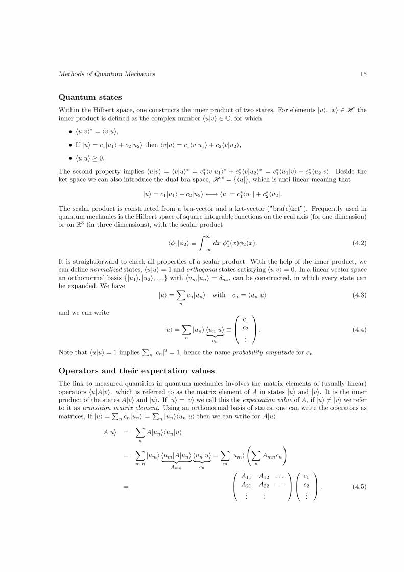
Within the Hilbert space, one constructs the inner product of two states. For elements |u〉, |v〉 ∈H theinner product is defined as the complex number 〈u|v〉 ∈ C, for which

• 〈u|v〉∗ = 〈v|u〉,

• If |u〉 = c1|u1〉+ c2|u2〉 then 〈v|u〉 = c1〈v|u1〉+ c2〈v|u2〉,

• 〈u|u〉 ≥ 0.

The second property implies 〈u|v〉 = 〈v|u〉∗ = c∗1〈v|u1〉∗ + c∗2〈v|u2〉∗ = c∗1〈u1|v〉 + c∗2〈u2|v〉. Beside theket-space we can also introduce the dual bra-space, H ∗ = {〈u|}, which is anti-linear meaning that

|u〉 = c1|u1〉+ c2|u2〉 ←→ 〈u| = c∗1〈u1|+ c∗2〈u2|.

The scalar product is constructed from a bra-vector and a ket-vector (”bra(c)ket”). Frequently used inquantum mechanics is the Hilbert space of square integrable functions on the real axis (for one dimension)or on R3 (in three dimensions), with the scalar product

〈φ1|φ2〉 ≡∫ ∞

−∞

dx φ∗1(x)φ2(x). (4.2)

It is straightforward to check all properties of a scalar product. With the help of the inner product, wecan define normalized states, 〈u|u〉 = 1 and orthogonal states satisfying 〈u|v〉 = 0. In a linear vector spacean orthonormal basis {|u1〉, |u2〉, . . .} with 〈um|un〉 = δmn can be constructed, in which every state canbe expanded, We have

|u〉 =∑

n

cn|un〉 with cn = 〈un|u〉 (4.3)

and we can write

|u〉 =∑

n

|un〉〈un|u〉︸︷︷︸

cn

≡

c1c2...

. (4.4)

Note that 〈u|u〉 = 1 implies∑

n |cn|2 = 1, hence the name probability amplitude for cn.

Operators and their expectation values

The link to measured quantities in quantum mechanics involves the matrix elements of (usually linear)operators 〈u|A|v〉. which is referred to as the matrix element of A in states |u〉 and |v〉. It is the innerproduct of the states A|v〉 and |u〉. If |u〉 = |v〉 we call this the expectation value of A, if |u〉 6= |v〉 we referto it as transition matrix element. Using an orthonormal basis of states, one can write the operators asmatrices, If |u〉 =∑n cn|un〉 =

∑

n |un〉〈un|u〉 then we can write for A|u〉

A|u〉 =∑

n

A|un〉〈un|u〉

=∑

m,n

|um〉〈um|A|un〉︸︷︷︸

Amn

〈un|u〉︸︷︷︸

cn

=∑

m

|um〉(∑

n

Amncn

)

=

A11 A12 . . .A21 A22 . . ....

...

c1c2...

. (4.5)


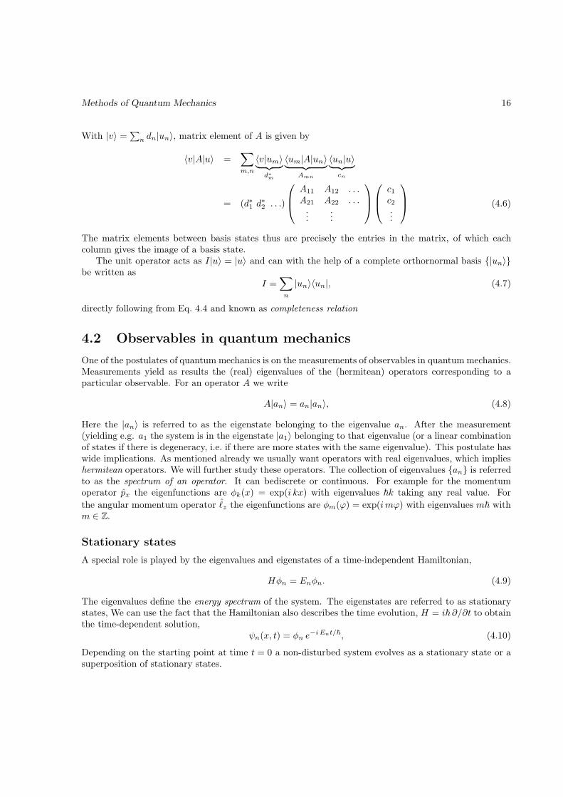
With |v〉 =∑n dn|un〉, matrix element of A is given by

〈v|A|u〉 =∑

m,n

〈v|um〉︸︷︷︸

d∗m

〈um|A|un〉︸︷︷︸

Amn

〈un|u〉︸︷︷︸

cn

= (d∗1 d∗2 . . .)

A11 A12 . . .A21 A22 . . ....

...

c1c2...

(4.6)

The matrix elements between basis states thus are precisely the entries in the matrix, of which eachcolumn gives the image of a basis state.

The unit operator acts as I|u〉 = |u〉 and can with the help of a complete orthornormal basis {|un〉}be written as

I =∑

n

|un〉〈un|, (4.7)

directly following from Eq. 4.4 and known as completeness relation

4.2 Observables in quantum mechanics

One of the postulates of quantum mechanics is on the measurements of observables in quantum mechanics.Measurements yield as results the (real) eigenvalues of the (hermitean) operators corresponding to aparticular observable. For an operator A we write

A|an〉 = an|an〉, (4.8)

Here the |an〉 is referred to as the eigenstate belonging to the eigenvalue an. After the measurement(yielding e.g. a1 the system is in the eigenstate |a1〉 belonging to that eigenvalue (or a linear combinationof states if there is degeneracy, i.e. if there are more states with the same eigenvalue). This postulate haswide implications. As mentioned already we usually want operators with real eigenvalues, which implieshermitean operators. We will further study these operators. The collection of eigenvalues {an} is referredto as the spectrum of an operator. It can bediscrete or continuous. For example for the momentumoperator px the eigenfunctions are φk(x) = exp(i kx) with eigenvalues ~k taking any real value. For

the angular momentum operator ℓz the eigenfunctions are φm(ϕ) = exp(imϕ) with eigenvalues m~ withm ∈ Z.

Stationary states

A special role is played by the eigenvalues and eigenstates of a time-independent Hamiltonian,

Hφn = Enφn. (4.9)

The eigenvalues define the energy spectrum of the system. The eigenstates are referred to as stationarystates, We can use the fact that the Hamiltonian also describes the time evolution, H = i~ ∂/∂t to obtainthe time-dependent solution,

ψn(x, t) = φn e−iEnt/~, (4.10)

Depending on the starting point at time t = 0 a non-disturbed system evolves as a stationary state or asuperposition of stationary states.


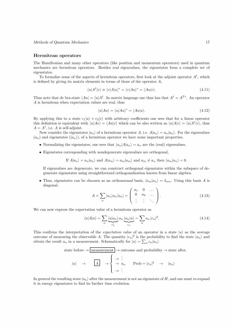
Hermitean operators

The Hamiltonian and many other operators (like position and momentum operators) used in quantummechanics are hermitean operators. Besides real eigenvalues, the eigenstates form a complete set ofeigenstates.

To formalize some of the aspects of hermitean operators, first look at the adjoint operator A†, whichis defined by giving its matrix elements in terms of those of the operator A,

〈u|A†|v〉 ≡ 〈v|A|u〉∗ = 〈v|Au〉∗ = 〈Au|v〉. (4.11)

Thus note that de bra-state 〈Au| = 〈u|A†. In matrix language one thus has that A† = AT∗. An operatorA is hermitean when expectation values are real, thus

〈u|Au〉 = 〈u|Au〉∗ = 〈Au|u〉. (4.12)

By applying this to a state c1|u〉 + c2|v〉 with arbitrary coefficients one sees that for a linear operatorthis definition is equivalent with 〈u|Av〉 = 〈Au|v〉 which can be also written as 〈u|A|v〉 = 〈u|A†|v〉, thusA = A†, i.e. A is self-adjoint.

Now consider the eigenstates |an〉 of a hermitean operator A, i.e. A|an〉 = an|an〉. For the eigenvalues(an) and eigenstates (|an〉), of a hermitean operator we have some important properties,

• Normalizing the eigenstates, one sees that 〈an|A|an〉 = an are the (real) eigenvalues.

• Eigenstates corresponding with nondegenerate eigenvalues are orthogonal,

If A|an〉 = an|an〉 and A|am〉 = am|am〉 and am 6= an then 〈am|an〉 = 0.

If eigenvalues are degenerate, we can construct orthogonal eigenstates within the subspace of de-generate eigenstates using straightforward orthogonalization known from linear algebra.

• Thus, eigenstates can be choosen as an orthonormal basis, 〈am|an〉 = δmn. Using this basis A isdiagonal,

A =∑

n

|an〉an〈an| =

a1 0 . . .0 a2 . . ....

.... . .

. (4.13)

We can now express the expectation value of a hermitean operator as

〈u|A|u〉 =∑

n

〈u|an〉︸︷︷︸

c∗n

an 〈an|u〉︸︷︷︸

cn

=∑

n

an |cn|2. (4.14)

This confirms the interpretation of the expectation value of an operator in a state |u〉 as the averageoutcome of measuring the observable A. The quantity |cn|2 is the probability to find the state |an〉 andobtain the result an in a measurement. Schematically for |u〉 =

∑

n cn|an〉

state before→ measurement → outcome and probability→ state after.

|u〉 → A →

→...

→ an Prob = |cn|2 → |an〉→

...

In general the resulting state |an〉 after the measurement is not an eigenstate ofH , and one must re-expandit in energy eigenstates to find its further time evolution.


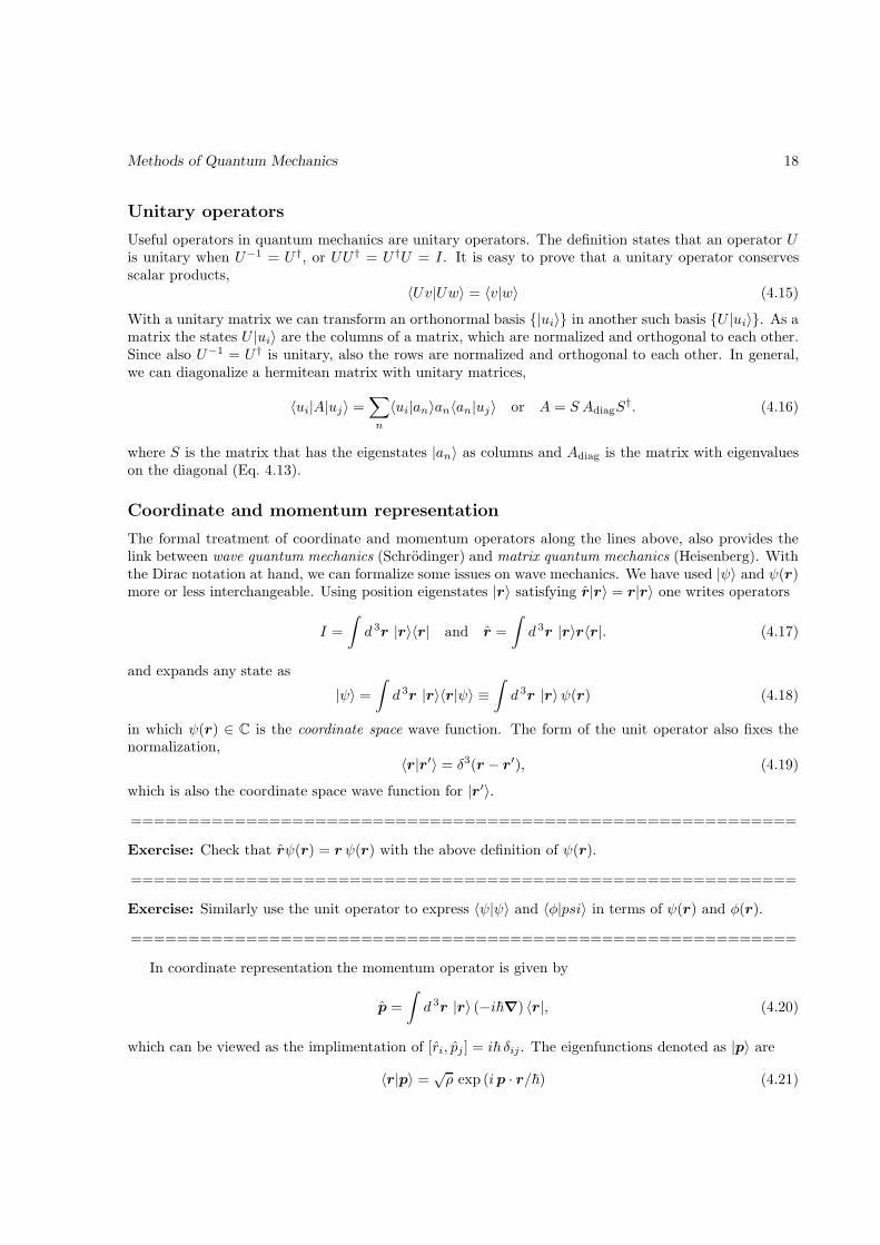
Unitary operators

Useful operators in quantum mechanics are unitary operators. The definition states that an operator Uis unitary when U−1 = U †, or UU † = U †U = I. It is easy to prove that a unitary operator conservesscalar products,

〈Uv|Uw〉 = 〈v|w〉 (4.15)

With a unitary matrix we can transform an orthonormal basis {|ui〉} in another such basis {U |ui〉}. As amatrix the states U |ui〉 are the columns of a matrix, which are normalized and orthogonal to each other.Since also U−1 = U † is unitary, also the rows are normalized and orthogonal to each other. In general,we can diagonalize a hermitean matrix with unitary matrices,

〈ui|A|uj〉 =∑

n

〈ui|an〉an〈an|uj〉 or A = S AdiagS†. (4.16)

where S is the matrix that has the eigenstates |an〉 as columns and Adiag is the matrix with eigenvalueson the diagonal (Eq. 4.13).

Coordinate and momentum representation

The formal treatment of coordinate and momentum operators along the lines above, also provides thelink between wave quantum mechanics (Schrodinger) and matrix quantum mechanics (Heisenberg). Withthe Dirac notation at hand, we can formalize some issues on wave mechanics. We have used |ψ〉 and ψ(r)more or less interchangeable. Using position eigenstates |r〉 satisfying r|r〉 = r|r〉 one writes operators

I =

∫

d 3r |r〉〈r| and r =

∫

d 3r |r〉r〈r|. (4.17)

and expands any state as

|ψ〉 =∫

d 3r |r〉〈r|ψ〉 ≡∫

d 3r |r〉ψ(r) (4.18)

in which ψ(r) ∈ C is the coordinate space wave function. The form of the unit operator also fixes thenormalization,

〈r|r′〉 = δ3(r − r′), (4.19)

which is also the coordinate space wave function for |r′〉.

==========================================================

Exercise: Check that rψ(r) = r ψ(r) with the above definition of ψ(r).

==========================================================

Exercise: Similarly use the unit operator to express 〈ψ|ψ〉 and 〈φ|psi〉 in terms of ψ(r) and φ(r).

==========================================================

In coordinate representation the momentum operator is given by

p =

∫

d 3r |r〉 (−i~∇) 〈r|, (4.20)

which can be viewed as the implimentation of [ri, pj ] = i~ δij . The eigenfunctions denoted as |p〉 are

〈r|p〉 = √ρ exp (ip · r/~) (4.21)


This defines ρ, e.g. in a box ρ = 1/L3, which is in principle arbitrary. Quite common choices for thenormalization of plane waves are ρ = 1 or ρ = (2π~)−3 (non-relativistic) or ρ = 2E (relativistic). Thequantity ρ also appears in the normalization of the momentum eigenstates,

〈p|p′〉 = ρ (2π~)3 δ3(p− p′). (4.22)

Using for momentum eigenstates p|p〉 = p|p〉 one has with the above normalization,

I =

∫d 3p

(2π~)3 ρ|p〉〈p| and p =

∫d 3p

(2π~)3 ρ|p〉p〈p|. (4.23)

The expansion of a state

|ψ〉 =∫

d 3p

(2π~)3 ρ|p〉〈p|ψ〉 ≡

∫d 3p

(2π~)3 ρ|p〉 ψ(p) (4.24)

defines the momentum space wave function, which is the Fourier transform of the coordinate space wavefunction.

4.3 Compatibility of operators and commutators

Two operators A and B are compatible if they have a common (complete) orthonormal set of eigenfunc-tions. For compatible operators we know after a measurement of A followed by a measurement of B botheigenvalues and we can confirm this by performing again a measurement of A. Suppose we have a com-plete common set ψabr, labeled by the eigenvalues of A, B and possibly an index r in case of degeneracy.Thus Aψabr = aψabr and B ψabr = b ψabr. Suppose we have an arbitrary state ψ =

∑

abr cabr ψabr, thenwe see that measurements of A and B or those in reverse order yield similar results,

ψ → A → a→∑

b,k

cabk ψabk → B → b→∑

k

cabk ψabk,

ψ → B → b→∑

a,k

cabk ψabk → A → a→∑

k

cabk ψabk.

Compatible operators can be readily identified using the following theorem:

A and B are compatible ⇐⇒ [A,B] = 0. (4.25)

Proof (⇒): There exists a complete common set ψn of eigenfunctions for which one thus has[A,B]ψn = (AB −BA)ψn = (anbn − bnan)ψn = 0.Proof (⇐): Suppose ψa eigenfunction of A. Then A(Bψa) = ABψa = BAψa = B aψa =aBψa. Thus Bψa is also an eigenfunction of A. Then one can distinguish(i) If a is nondegenerate, then Bψa ∝ ψa, say Bψa = bψa which implies that ψa is also aneigenfunction of B.(ii) If a is degenerate (degeneracy s), consider that part of the Hilbert space that is spannedby the functions ψar (r = 1, . . . , s). For a given ψap (eigenfunction of A) Bψap also can bewritten in terms of the ψar. Thus we have an hermitean operator B in the subspace of thefunctions ψar. In this subspace B can be diagonalized, and we can use the eigenvalues b1, . . . bsas second label, which leads to a common set of eigenfunctions.

We have seen the case of degeneracy for the spherical harmonics. The operators ℓ2 and ℓz commute andthe spherical harmonics Y ℓm(θ, ϕ) are the common set of eigenfunctions.


The uncertainty relations

For measurements of observables A and B (operators) we have

[A,B] = 0 ⇒ A and B have common set of eigenstates.For these common eigenstates one has ∆A = ∆B = 0 and hence ∆A∆B = 0.

[A,B] 6= 0 ⇒ A and B are not simultaneously measurable.The product of the standard deviations is bounded, depending on the commutator.

The precise bound on the product is given by

∆A∆B ≥ 1

2|〈 [A,B] 〉|, (4.26)

known as the uncertainty relation.

The proof of the uncertainty relation is in essence a triangle relation for inner products.Define for two hermitean operators A and B, the (also hermitean) operators α = A − 〈A〉and β = B − 〈B〉. We have [α, β] = [A,B]. Using positivity for any state, in particular|(α+ iλ β)ψ〉 with λ arbitrary, one has

0 ≤ 〈(α + iλ β)ψ|(α + iλ β)ψ〉 = 〈ψ|(α − iλ β)(α+ iλ β)|ψ〉 = 〈α2〉+ λ2 〈β2〉+ λ 〈 i[α, β] 〉︸︷︷︸

〈γ〉

.

Since i [α, β] is a hermitean operator (why), 〈γ〉 is real. Positivity of the quadratic equation〈α2〉+ λ2 〈β2〉+λ 〈γ〉 ≥ 0 for all λ gives 4 〈α2〉〈β2〉 ≥ 〈γ〉2. Taking the square root then givesthe desired result.

The most well-known example of the uncertainty relation is the one originating from the noncompatibilityof positionn and momentum operator, specifically from [x, px] = i~ one gets

∆x∆px ≥1

2~. (4.27)

Constants of motion

The time-dependence of an expectation value and the correspondence with classical mechanics has beenused to find the candidate momentum operator (see Eq. 1.26). We now take another look at this andwrite

d〈A〉dt

=d

dt

∫

d3r ψ∗(r, t)Aψ(r, t) =

∫

d3r

[∂ψ∗

∂tAψ + ψ∗A

∂ψ

∂t+ ψ∗ ∂A

∂tψ

]

=1

i~〈 [A,H ] 〉+ 〈 ∂

∂tA〉. (4.28)

Examples of this relation are the Ehrenfest relations

d

dt〈r〉 = 1

i~〈[r, H ]〉 = 1

i~

1

2m〈[r,p2]〉 = 〈p〉

m, (4.29)

d

dt〈p〉 = 1

i~〈[p, H ]〉 = 1

i~〈[p, V (r)]〉 = 〈−∇V (r)〉. (4.30)

An hermitean operator A that is compatible with the Hamiltonian, i.e. [A,H ] = 0 and that does not haveexplicit time dependence, i.e. ∂A∂t = 0 is referred to as a constant of motion. From Eq. 4.28 it is clear thatits expectation value is time-independent.


==========================================================

Exercise: Check the following examples of constants of motion, compatible with the Hamiltonian andthus providing eigenvalues that can be used to label eigenfunctions of the Hamiltonian.

(a) The hamiltonian for a free particle

H =p2

2MCompatible set: H,p

The plane waves φk(r) = exp(ik · r) form a common set of eigenfunctions.

(b) The hamiltonian with a central potential:

H =p2

2M+ V (|r|) Compatible set: H, ℓ2, ℓz

This allows writing the eigenfunctions of this hamiltonian as φnℓm(r) = (u(r)/r)Y ℓm(θ, ϕ).

==========================================================

Chapter 5

Symmetries

In this chapter, we want to complete the circle by discussing symmetries in all of their glory, in partic-ular the space-time symmetries, translations, rotations and boosts. They are important, because theychange time, coordinates and momenta, but in such a way that they leave basic quantities invariant (likeLagrangian and/or Hamiltonian) or at least they leave them in essence invariant (up to an irrelevantchange that can be expressed as a total time derivative). Furthermore, they modify coordinates andmomenta in such a way that these retain their significance as canonical variables. We first consider thefull set of (non-relativistic) space-time transformations known as the Galilean group. These include tentransformations, each of them governed by a (real) parameter. They are one time translation, threespace translations (one for each direction in space), three rotations (one for each plane in space) andthree boosts (one for each direction in space). They change the coordinates

t → t′ = t+ τ, one time translation, (5.1)

r → r′ = r + a three translations, (5.2)

r → r′ = R(n, α)r three rotations, (5.3)

r → r′ = r − ut three boosts. (5.4)

with parameters being (τ , a, αn, u). The Lagrangian and Hamiltonian that respect this symmetry arethe ones for a free particle or in the case of a many particle system, those for the center of mass system,

L =1

2mr2 and H =

p2

2m.

with p = mr.

5.1 Space translations

Let’s look at the translations T (a) in space. It is clear what is happening with positions and momenta,

r → r′ = r + a and p→ p′ = p. (5.5)

and infinitesimally,δr = δa and δp = 0. (5.6)

This is through Noether’s theorem consistent with ’conserved quantities’ Q·δa = p·δa, thus the momentap, which also generate the translations (see Eq. 3.27),

δxi = {xi,p}P ·δa = δai and δpi = −{pi,p}P ·δa = 0. (5.7)

22

Symmetries 23

Translations in Hilbert space

Let’s start with the Hilbert space of functions and look at ways to ’translate a function’ and then at waysto ’translate an operator’. Let us work in one dimension. For continuous transformations, it turns out tobe extremely useful to look at the infinitesimal problem (in general true for so-called Lie transformations).We get for small a a ’shifted’ function

φ′(x) = φ(x+ a) = φ(x) + adφ

dx+ . . . =

(

1 +i

~a px + . . .

)

︸︷︷︸

U(a)

φ(x), (5.8)

which defines the shift operator U(a) of which the momentum operator px = −i~ (d/dx) is referred to asthe generator. One can extend the above to higher orders,

φ′(x) = φ(x + a) = φ(x) + ad

dxφ+

1

2!a2

d

dx2φ+ . . . ,

Using the (operator) definition

eA ≡ 1 +A+1

2!A2 + . . . ,

one finds

U(a) = exp

(

+i

~a px

)

= I +i

~a px + . . . . (5.9)

In general, if G is a hermitean operator (G† = G), then eiλG is a unitary operator (U−1 = U †). Thusthe shift operator produces new wavefunctions, preserving orthonormality.

To see how a translation affects an operator, we look at Oφ, which is a function changing as

(Oφ)′(x) = Oφ(x + a) = U Oφ(x) = U OU−1︸︷︷︸

O′

Uφ︸︷︷︸

φ′

(x), (5.10)

thus for operators in Hilbert space

O −→ O′ = U OU−1 = eiλGO e−iλG. (5.11)

which expanded gives O′ = (1 + iλG+ . . .)O(1 − iλG+ . . .) = O + iλ[G,O] + . . ., thus

δO = −i[O,G]δλ. (5.12)

One has for the translation operator

O′ = ei apx/~O(0) e−i apx/~ and δO = −(i/~) [O, px] δa, (5.13)

which for position and momentum operator gives

δx = − i~[x, px] δa = δa and δpx = − i

~[px, px] δa = 0. (5.14)

Note that to show the full transformations for x and px one can use the exact relations

idO′

dλ= ei λG

[O,G

]e−i λG and i

dO′

dλ

∣∣∣∣λ=0

=[O,G

]. (5.15)

==========================================================

Exercise: Show that for the ket state one has U(a)|x〉 = |x − a〉. An active translation of a localizedstate with respect to a fixed frame, thus is given by |x+ a〉 = U−1(a)|x〉 = U †(a)|x〉 = e−i apx/~|x〉 .==========================================================

Symmetries 24

5.2 Time evolution

Time plays a special role, both in classical mechanics and quantum mechanics. We have seen the centralrole of the Hamiltonian in classical mechanics (conserved energy) and the dual role as time evolution andenergy operator in quantum mechanics. Actively describing time evolution,

ψ(t+ τ) = ψ(t) + τdψ

dt+ . . . =

(

1− i

~τ H + . . .

)

︸︷︷︸

U(τ)

ψ(t), (5.16)

we see that evolution is generated by the Hamiltonian H = i~ d/dt and given by the (unitary) operator

U(τ) = exp (−i τ H/~) . (5.17)

Since time evolution is usually our aim in solving problems, it is necessary to know the Hamiltonian,usually in terms of the positions, momenta (and spins) of the particles involved. If this Hamiltonian istime-independent, we can solve for its eigenfunctions, Hφn(x) = En φn(x) and use completeness to getthe general time-dependence (see Eq. 4.10).

Schrodinger and Heisenberg picture

The time evolution from t0 → t of a quantum mechanical system thus is generated by the Hamiltonian,

U(t, t0) = exp (−i(t− t0)H/~) , satisfying i~∂

∂tU(t, t0) = H U(t, t0). (5.18)

Two situations can be distinguished:

(i) Schrodinger picture, in which the operators are time-independent, AS(t) = AS and the states aretime dependent, |ψS(t)〉 = U(t, t0)|ψS(t0)〉,

i~∂

∂t|ψS〉 = H |ψS〉, (5.19)

i~∂

∂tAS ≡ 0. (5.20)

(ii) Heisenberg picture, in which the states are time-independent, |ψH(t)〉 = |ψH〉, and the operatorsare time-dependent, AH(t) = U−1(t, t0)AH(t0)U(t, t0),

i~∂

∂t|ψH〉 ≡ 0, (5.21)

i~∂

∂tAH = [AH , H ]. (5.22)

We note that in the Heisenberg picture one has the equivalence with classical mechanics, because thetime-dependent classical quantities are considered as time-dependent operators. In particular we have

i~d

dtr(t) = [r, H ] and i~

d

dtp(t) = [p, H ], (5.23)

to be compared with the classical Hamilton equations.

==========================================================

Exercise: Show that the time dependence of expectation values is the same in the two pictures, i.e.

〈ψ′S(t)|AS |ψS(t)〉 = 〈ψ′

H |AH(t)|ψH〉.This is important to get the Ehrenfest relations in Eqs 4.29 and 4.30 from the Eqs 5.23.

==========================================================

Symmetries 25

5.3 Rotational symmetry

Rotations are characterized by a rotation axis (n) and an angle (0 ≤ α ≤ 2π),

r −→ r′ = R(n, α) r or ϕ −→ ϕ′ = ϕ+ α, (5.24)

where the latter refers to the polar angle around the n-direction. The rotation R(z, α) around the z-axisis given by

xyz

−→

x′

y′

z′

=

cosα − sinα 0sinα cosα 00 0 1

xyz

. (5.25)

==========================================================

Exercise: Check that for polar coordinates (defined with respect to the z-axis),

x = r sin θ cosϕ, y = r sin θ sinϕ, z = r cos θ,

the rotations around the z-axis only change the azimuthal angle, ϕ′ = ϕ+ α.

==========================================================

Conserved quantities and generator in classical mechanics

Using Noether’s theorem, we construct the conserved quantity for a rotation around the z-axis. One hasthe infinitesimal changes δx = −y δα and δy = x δα, thus Qzδα = pxδx+ pyδy + pzδz = (xpy + ypz)δα,thus Qz = ℓz and in general for all rotations all components of the angular momentum ℓ are conserved,at least if {H, ℓ}P = 0. The angular momenta indeed generate the symmetry, leading to

δx = {x, ℓz}P δα = −yδα and δy = {y, ℓz}P δα = xδα, (5.26)

δpx = {px, ℓz}P δα = −pyδα and δpy = {py, ℓz}P δα = pxδα. (5.27)

with as general expressions for the Poisson brackets

{ℓi, xj}P = ǫijk xk and {ℓi, pj}P = ǫijk pk. (5.28)

The result found for the {ℓi, ℓj}P = ǫijk ℓk bracket indicates that angular momenta also change likevectors under rotations.

Rotation operators in Hilbert space

Rotations also gives rise to transformations in the Hilbert space of wave functions. Using polar coordinatesand a rotation around the z-axis, we find

φ(r, θ, ϕ + α) = φ(r, θ, ϕ) + α∂

∂ϕφ+ . . . =

(

1 +i

~α ℓz + . . .

)

︸︷︷︸

U(z,α)

φ, (5.29)

from which one concludes that ℓz = −i~(∂/∂ϕ) is the generator of rotations around the z-axis in Hilbertspace. As we have seen, in Cartesian coordinates this operator is ℓz = −i~(x∂/∂y−y ∂/∂x) = xpy−ypx,the z-component of the (orbital) angular momentum operator ℓ = r × p.

The full rotation operator in the Hilbert space is

U(z, α) = exp

(

+i

~α ℓz

)

= 1 +i

~α ℓz + . . . . (5.30)

Symmetries 26

The behavior of the various quantum operators under rotations is given by

O′ = eiαℓz/~O e−iαℓz/~ or δO = − i~[O, ℓz] δα. (5.31)

Using the various commutators calculated for quantum operators in Hilbert space (starting from the basic[xi, pj ] = i~ δij commutator,

[ℓi, rj ] = i~ ǫijk rk, [ℓi, pj ] = i~ ǫijk pk, and [ℓi, ℓj ] = i~ ǫijk ℓk, (5.32)

(note again their full equivalence with Poisson brackets) one sees that the behavior under rotations of thequantum operators r, p and ℓ is identical to that of the classical quantities. This is true infinitesimally,but also for finite rotations one has for operators r → r′ = R(n, α)r and p→ p′ = R(n, α)p. Finally therotational invariance of the Hamiltonian corresponds to [H, ℓ] = 0 and in that case it also implies timeindependence of the Heisenberg operator or the the expectation values 〈ℓ〉.

Generators of rotations in Euclidean space

A characteristic difference between rotations and translations is the importance of the order. The orderin which two consecutive translations are performed does not matter T (a)T (b) = T (b)T (a). This is alsotrue for the Hilbert space operators U(a)U(b) = U(b)U(a). The order does matter for rotations. Thisis so in coordinate space as well as Hilbert space, R(x, α)R(y, β) 6= R(y, β)R(x, α) and U(x, α)U(y, β) 6=U(y, β)U(x, α).

Going back to Euclidean space and looking at the infinitesimal form of rotations around the z-axis,

R(z, δα) = 1− i δα Jz (5.33)

one also can identify here the generator

Jz =1

−i∂R(α, z)

∂ϕ

∣∣∣∣α=0

=

0 −i 0i 0 00 0 0

. (5.34)

In the same way we can consider rotations around the x- and y-axes that are generated by

Jx =

0 0 00 0 −i0 i 0

, Jy =

0 0 i0 0 0−i 0 0

, (5.35)

The generators in Euclidean space do not commute. Rather they satisfy

[Ji, Jj ] = i ǫijk Jk. (5.36)

The same non-commutativity of generators is exhibited in Hilbert space by the commutator of the cor-responding quantum operators ℓ/~ and by the Poisson brackets for the conserved quantities in classical

mechanics. But realize an important point. Although identical, the commutation relations for ℓ are inHilbert space, found starting from the basic (canonical) commutation relations between r and p opera-tors! The consistence of commutation relations in Hilbert space with the requirements of symmetries isa prerequisite for achieving a consistent quantization of theories.

==========================================================

Symmetries 27

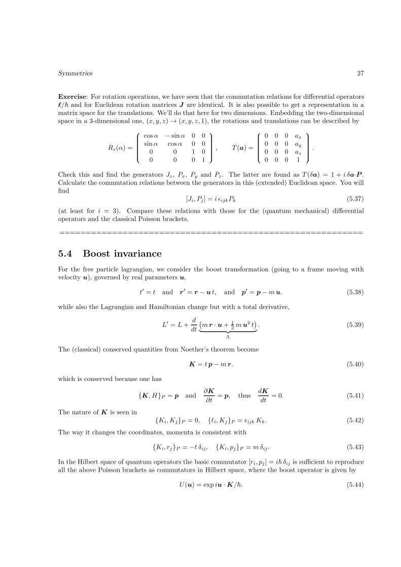
Exercise: For rotation operations, we have seen that the commutation relations for differential operatorsℓ/~ and for Euclidean rotation matrices J are identical. It is also possible to get a representation in amatrix space for the translations. We’ll do that here for two dimensions. Embedding the two-dimensionalspace in a 3-dimensional one, (x, y, z)→ (x, y, z, 1), the rotations and translations can be described by

Rz(α) =

cosα − sinα 0 0sinα cosα 0 00 0 1 00 0 0 1

, T (a) =

0 0 0 ax0 0 0 ay0 0 0 az0 0 0 1

.

Check this and find the generators Jz, Px, Py and Pz . The latter are found as T (δa) = 1 + i δa·P .Calculate the commutation relations between the generators in this (extended) Euclidean space. You willfind

[Ji, Pj ] = i ǫijkPk (5.37)

(at least for i = 3). Compare these relations with those for the (quantum mechanical) differentialoperators and the classical Poisson brackets.

==========================================================

5.4 Boost invariance

For the free particle lagrangian, we consider the boost transformation (going to a frame moving withvelocity u), governed by real parameters u,

t′ = t and r′ = r − u t, and p′ = p−mu. (5.38)

while also the Lagrangian and Hamiltonian change but with a total derivative,

L′ = L+d

dt

(m r · u+ 1

2 mu2 t)

︸︷︷︸

Λ

. (5.39)

The (classical) conserved quantities from Noether’s theorem become

K = tp−m r. (5.40)

which is conserved because one has

{K, H}P = p and∂K

∂t= p, thus

dK

dt= 0. (5.41)

The nature of K is seen in{Ki,Kj}P = 0, {ℓi,Kj}P = ǫijkKk. (5.42)

The way it changes the coordinates, momenta is consistent with

{Ki, rj}P = −t δij , {Ki, pj}P = mδij . (5.43)

In the Hilbert space of quantum operators the basic commutator [ri, pj ] = i~ δij is sufficient to reproduceall the above Poisson brackets as commutators in Hilbert space, where the boost operator is given by

U(u) = exp iu ·K/~. (5.44)

Symmetries 28

Explicitly we have for the quantum operators

]K, H ] = i~p and∂K

∂t= p, thus

d〈K〉dt

= 0, (5.45)

[Ki,Kj ] = 0, [ℓi,Kj] = i~ǫijkKk. (5.46)

[Ki, rj ] = −i~ t δij, [Ki, pj ] = i~mδij. (5.47)

Finally if one implements the transformations in space-time, e.g. writing them as matrices as done forrotations and translations, one gets a set of ten generators of the Gallilei transformations, which aredenoted as H (time translation generator), P (three generators of translations), J (three generators ofrotations) and K (three generators for boosts). They satisfy

[Pi, Pj ] = [Pi, H ] = [Ji, H ] = 0,

[Ji, Jj ] = i ǫijkJk, [Ji, Pj ] = i ǫijkPk, [Ji,Kj ] = i ǫijkKk,

[Ki, H ] = i Pi, [Ki,Kj] = 0, [Ki, Pj ] = im δij. (5.48)

This structure is indeed realized in the description of the quantum world, by implementing the abovecommutator structure of the symmetry group (Lie algebra of generators of the Gallilei group) by thecommutator structure in the Hilbert space or the Poisson bracket structure in the phase space of classicalmechanics. To be precise

i{u, v}P ⇐⇒[u, v]

~. (5.49)

are homomorphic to the commutation relations of the generators in the symmetry group, while thecorrespondence between Poisson brackets and quantum commutation relations is further extended tocoordinates and momenta.

5.5 The two-particle system

We ended the previous section with the commutation relations that should be valid for a free-movingsystem to which the invariance under Gallilei transformations applies. It is easy to check that for a single(free) particle the classically conserved quantities and the quantum mechanical set of operators

H = mc2 +p2

2m, (5.50)

P = p, (5.51)

J = ℓ+ s = r × p+ s (5.52)

K = mr − tp. (5.53)

satisfy the required Poisson brackets in classical phase space and the required commutation relationsin Hilbert space, in the latter case starting with the canonical commutation relations [ri, pj ] = i~ δij .This is true even if we allow for a set of spin operators [si, sj ] = i~ ǫijk sk as long as these satisfy[ri, sj ] = [pi, sj] = 0. The latter two commutators imply that spin decouples from the spatial partof the wave function. In classical language one would phrase this as that the spins do not depend onposition or velocity/momentum. A constant contribution to the energy doesn’t matter either. Uponadding a potential V (r) to the Hamiltonian, the symmetry requirements would fail and we do not haveGallilei invariance. A potential (e.g. centered around an origin) breaks translation invariance, the specificr-dependence might break rotational invariance, etc.

As we have seen, for two particles it is convenient to change to CM and relative coordinates R andr with dorresponding conjugate momenta P and p. and introduce the sum mass M and the reduced

Symmetries 29

mass m. The center of mass system should reflect again a free particle. On the other hand, the behaviorunder Gallilei transformations, implies applying the transformation to both coordinates. The sum of thegenerators is given by

H = H1 +H2 =P 2

2M+Hint,

P = p1 + p2,

J = J1 + J2 = ℓ1 + s1 + ℓ2 + s2 = R× P + S,

K = K1 +K2 =M R− tP , (5.54)

with

S = r × p+ s1 + s2, (5.55)

Hint =Mc2 +p2

2m+ V (r,p, s1, s2), (5.56)

only involving relative coordinates or spins (commuting with CM operators). These center of massgenerators then satisfy the classical Poisson brackets or quantum commutation relations for the Gallileigroup, starting simply from the canonical relations for each of the particles. The CM system behaves asa free (composite) system with constant energy and momentum and a spin determined by the ’relative’orbital angular momentum and the spins of the constituents. The example also shows that even withoutspins of the constituents (s1 = s2 = 0) a composite system has an intrinsic angular momentum showingup as its spin.

==========================================================

Exercise: Check that the canonical Poisson brackets or commutation relations for r1 and p1 and thosefor r2 and p2 imply the canonical commutation relations for R and P as well as for r and p. The explicitcheck of this for momenta expressed as time derivatives in classical mechanics or as derivative operatorswas what we did in Chapter 1, e.g. when proving Eqs 1.36 and 1.37.

==========================================================

5.6 Discrete symmetries

Three important discrete symmetries that we will be discuss are space inversion, time reversal and(complex) conjugation.

Space inversion and Parity

Starting with space inversion operation, we consider its implication for coordinates,

r −→ −r and t −→ t, (5.57)

implying for instance that classically for p = mr and ℓ = r × p one has

p −→ −p and ℓ −→ ℓ. (5.58)

The same is true for the explicit quantummechanical operators, e.g. p = −i~∇.In quantum mechanics the states |ψ〉 correspond (in coordinate representation) with functions ψ(r, t).

In the configuration space we know the result of inversion, r → −r and t → t, in the case of more

Symmetries 30

particles generalized to ri → −ri and t→ t. What is happening in the Hilbert space of wave functions.We can just define the action on functions, ψ → ψ′ ≡ Pψ in such a way that

Pφ(r) ≡ φ(−r). (5.59)

The function Pφ is a new wave function obtained by the action of the parity operator P . It is a hermitianoperator (convince yourself). The eigenvalues and eigenfunctions of the parity operator,

Pφπ(r) = π φπ(r), (5.60)

are π = ±1, both eigenvalues infinitely degenerate. The eigenfunctions corresponding to π = +1 are theeven functions, those corresponding to π = −1 are the odd functions.

==========================================================

Exercise: Proof that the eigenvalues of P are π = ±1. Although this looks evident, think carefullyabout the proof, which requires comparing P 2φ using Eqs 5.59 and 5.60.

==========================================================

The action of parity on the operators is as for any operator in the Hilbert space given by

Aφ −→ PAφ = PAP−1︸︷︷︸

A′

Pφ︸︷︷︸

φ′

, thus A −→ PAP−1. (5.61)

(Note that for the parity operator actually P−1 = P = P †). Examples are

r −→ PrP−1 = −r, (5.62)

p −→ PpP−1 = −p, (5.63)

ℓ −→ PℓP−1 = +ℓ, (5.64)

H(r,p) −→ PH(r,p)P−1 = H(−r,−p). (5.65)

If H is invariant under inversion, one has

PHP−1 = H ⇐⇒ [P,H ] = 0. (5.66)

This implies that eigenfunctions of H are also eigenfunctions of P , i.e. they are even or odd. Although Pdoes not commute with r or p (classical quantities are not invariant), the specific behavior POP−1 = −Ooften also is very useful, e.g. in discussing selection rules. The operators are referred to as P -odd operators.

==========================================================

Exercise: Show that the parity operation leaves ℓ invariant and show that the parity operator commuteswith ℓ2 and ℓz. The eigenfunctions of the latter operators (spherical harmonics) indeed are eigenfunctionsof P . What is the parity of the Y mℓ ’s.

==========================================================

Exercise: Show that for a P -even operator (satisfying POP−1 = +O or [P,O] = PO − OP = 0) thetransition probability

Probα→β = |〈β|O|α〉|2

for parity eigenstates is only nonzero if πα = πβ .What is the selection rule for a P -odd operator (satisfying POP−1 = −O or {P,O} = PO +OP = 0).

==========================================================

Symmetries 31

Time reversal

In classical mechanics with second order differential equations, one has for time-independent forces auto-matically time reversal invariance, i.e. invariance under t→ −t and r → r. There seems an inconsistencywith quantum mechanics for the momentum p and energy E. Classically it equals mr which changessign, while ∇ → ∇. Similarly one has classically E → E, while H = i~(∂/∂t) appears to change sign.The problem can be solved by requiring time reversal to be accompagnied by a complex conjugation, inwhich case one consistently has p = −i~∇ → i~∇ = −p and H → H . Furthermore a stationary stateψ(t) ∼ exp(−iEt) now nicely remains invariant, ψ∗(−t) = ψ(t).

Such a consistent description of the time reversal operator in Hilbert space is straightforward. Forunitary operators one has (mathematically) also the anti-linear option, where an anti-linear operatorsatisfies T (c1|φ1〉+ c2|φ2〉) = c∗1 T |φ1〉+ c∗2 T |φ2〉. It is easily implemented as

T |φ〉 = 〈Tφ|, (5.67)

which for matrix elements implies

〈φ|ψ〉 = 〈φ|T †T |ψ〉 = 〈Tψ|Tφ〉 = 〈Tφ|Tψ〉∗ (5.68)

〈φ|A|ψ〉 = 〈φ|T †T AT †T |ψ〉 = 〈Tφ|T AT †|Tψ〉∗. (5.69)

Operators satisfying TT † = T †T = 1, but swapping bra and ket space (being anti-linear) are known asanti-unitary operators.

Together with conjugation C, which for spinless systems is just complex conjugation, one can lookat CPT -invariance by combining the here discussed discrete symmetries. For all known interactions inthe world the combined CPT transformation appears to be a good symmetry. The separate discretesymmetries are violated, however, e.g. space inversion is broken by the weak force that causes decays ofelementary particles with clear left-right asymmetries. Also T and CP have been found to be broken.

5.7 A relativistic extension∗

The symmetry group for relativistic systems is the Poincare group, with as essential difference that boosts(with parameter u still representing a moving frame, are (for a boost in the x-direction given by

ct′ = γ ct− βγ x (5.70)

x′ = x− βγ ct, (5.71)

while y′ = y and z′ = z. The quantities β and γ are given by

β =u

cand γ =

1√

1− β2=

1√

1− u2/c2. (5.72)

These transformations guarantee that the velocity of light is constant in any frame, satisfying

c2t2 − r2 = c2t′ 2 − u′ 2 = c2τ2, (5.73)

where τ is referred to as eigentime (time in rest-frame of system). Mathematically one can look at thisstructure as we did for rotations and find the commutation relations of the Poincare group

[P i, P j ] = [P i, H ] = [J i, H ] = 0,

[J i, Jj ] = i ǫijkJk, [J i, P j ] = i ǫijkP k, [J i,Kj] = i ǫijkKk,

[Ki, H ] = i P i, [Ki,Kj ] = −i ǫijkJk/c2, [Ki, P j ] = i δijH/c2. (5.74)

Symmetries 32

The action of a relativistic free particle is actually extremely simple,

S = mc2∫

dτ = mc2∫

dt√

1− v2/c2. (5.75)

One can find the Lagrangian and Hamiltonian,

L = mc2√

1− v2/c2 and H =√

m2c4 + p2c2, (5.76)

where we have p = mv γ. Note that for E = mc2 dt/dτ and p = mcdr/dτ , so (E/c,p) transform amongthemselves exactly as (ct, r).

For a single free particle or for the CM coordinates, the classically conserved quantities or generatorsof the Poincare group can be found using Noether’s theorem. They are

H =√

p2 c2 +m2 c4,

P = p,

J = r × p+ s,

K =1

2c2(rH +Hr)− tp+

p× s

H +mc2. (5.77)

A consistent relativistic quantum mechanical treatment in terms of relative coordinates, however, requiresgreat care [See e.g. L.L. Foldy, Phys. Rev. 122 (1961) 275 and H. Osborn, Phys. Rev. 176 (1968) 1514]and is possible in an expansion in 1/c. Interaction terms, however, enter not only in the Hamiltonian,but also in the boost operators.

CONCEPT GENERAL MECHANICS Classical & Quantum Mechanics

Documents

Transcript of CONCEPT GENERAL MECHANICS Classical & Quantum Mechanics