Compiler Support for Sparse Matrix...
301
Compiler Support for Sparse Matrix Computations PROEFSCHRIFT TER VERKRIJGING VAN DE GRAAD VAN DOCTOR AAN DE RIJKSUNIVERSITEIT TE LEIDEN, OP GEZAG VAN DE RECTOR MAGNIFICUS DR. L. LEERTOUWER, HOOGLERAAR IN DE FACULTEIT DER GODGELEERDHEID, VOLGENS BESLUIT VAN HET COLLEGE VAN DEKANEN TE VERDEDIGEN OP WOENSDAG 29 MEI 1996 TE KLOKKE 15.15 UUR DOOR AART J OHANNES CASIMIR BIK GEBOREN TE GOUDA IN 1969
Transcript of Compiler Support for Sparse Matrix...
Compiler Support for Sparse Matrix Computations
PROEFSCHRIFT
TER VERKRIJGING VAN DE GRAAD VAN DOCTOR
AAN DE RIJKSUNIVERSITEIT TE LEIDEN,OP GEZAG VAN DE RECTOR MAGNIFICUS DR. L. LEERTOUWER,
HOOGLERAAR IN DE FACULTEIT DER GODGELEERDHEID,VOLGENS BESLUIT VAN HET COLLEGE VAN DEKANEN
TE VERDEDIGEN OP WOENSDAG 29 MEI 1996TE KLOKKE 15.15 UUR
DOOR
AART JOHANNES CASIMIR BIK
GEBOREN TE GOUDA IN 1969
Promotiecommissie
Promotor: Prof. dr. H.A.G. WijshoffReferenten: Prof. dr. M.J. Wolfe (Oregon Graduate Institute of
Science and Technology, USA)Prof. dr. C.D. Polychronopoulos (University of Illinois at
Urbana-Champaign, USA)Overige leden: Prof. dr. J.N. Kok
Prof. dr. J. van Leeuwen (Universiteit Utrecht)Prof. dr. ir. L.A. PeletierProf. dr. H.A. van der Vorst (Universiteit Utrecht)Dr. P.M.W. Knijnenburg
This research has been supported by the Netherlands Computer Science Research Foundation(SION) with funds from the Netherlands Organization for Scientific Research (NWO).
CIP-DATA KONINKLIJKE BIBLIOTHEEK, DEN HAAG
Bik, Aart Johannes Casimir
Compiler support for sparse matrix computations / AartJohannes Casimir Bik. - [S.l. : s.n.]. - Ill.Thesis Rijksuniversiteit Leiden. - With ref.ISBN 90-9009442-3NUGI 855Subject headings: compilers / sparse matrices / datastructure transformations.

He which soweth sparingly shall reap also sparingly...
2 CORINTHIANS 9 : 6

Preface
In this dissertation, consisting of two parts, I present the results of my research in compiler supportfor sparse matrix computations, which has been inspired by the research proposal [218].
In the first part, preliminaries are given to keep this dissertation as self-contained as possibleand to present some general purpose techniques that are useful in the second part of the disserta-tion. Some issues related to the implementation of loop transformations (chapter 2 and 3) haveappeared in publications [33, 36, 120].
The second part of this dissertation deals with the presentation of an automatic data struc-ture selection and transformation method. This method is used by a sparse compiler, which is acompiler capable of automatically converting a dense program into semantically equivalent sparsecode [27]. First, the organization of the sparse compiler is outlined, and a brief overview of thephases of the automatic data structure selection and transformation method is given (chapter 4).Thereafter, a discussion of automatically analyzing and pre-processing the original dense programand analyzing nonzero structures of sparse matrices is given (chapters 5 and 6). These methodsappeared in publications [28, 34, 38]. Moreover, the actual data structure selection and code gen-eration method are presented (chapters 7 and 8), which have been published in [25, 30, 32, 35, 39].Some initial experimentation indicating the potential of a sparse compiler has also been included(chapter 9). Finally, some more advanced transformations are explored (chapter 10), which havebeen presented in [26, 31], and conclusions and topics for future research are given (chapter 11).
Because notational conventions, definitions and methods have been altered during research,some small inconsistencies with previous publications may occur in this dissertation.
Many have contributed to this research, for which I am very grateful. In particular, I wouldlike to thank my parents for their constant love and support.
Aart J.C. Bik

Contents
I Preliminaries and Basic Results 1
1 Introduction 31.1 Exploiting Hardware Characteristics : : : : : : : : : : : : : : : : : : : : : : : 3
1.1.1 Architectural Advances : : : : : : : : : : : : : : : : : : : : : : : : : 31.1.2 Restructuring Compilers : : : : : : : : : : : : : : : : : : : : : : : : : 5
1.2 Exploiting Data Characteristics : : : : : : : : : : : : : : : : : : : : : : : : : 61.2.1 Sparse Matrix Computations : : : : : : : : : : : : : : : : : : : : : : : 61.2.2 Compiler Support for Sparse Matrix Computations : : : : : : : : : : : 7
2 Preliminaries 92.1 Preliminaries from Geometry and Linear Algebra : : : : : : : : : : : : : : : : 9
2.1.1 Cartesian Spaces : : : : : : : : : : : : : : : : : : : : : : : : : : : : : 92.1.2 Linear and Affine Subspaces : : : : : : : : : : : : : : : : : : : : : : : 102.1.3 Hyperplanes : : : : : : : : : : : : : : : : : : : : : : : : : : : : : : : 112.1.4 Half-Spaces : : : : : : : : : : : : : : : : : : : : : : : : : : : : : : : 122.1.5 Linear and Affine Transformations : : : : : : : : : : : : : : : : : : : : 14
2.2 Some Useful Methods : : : : : : : : : : : : : : : : : : : : : : : : : : : : : : 152.2.1 Extended Euclidean Algorithm : : : : : : : : : : : : : : : : : : : : : : 152.2.2 Completion Method for Unimodular Matrices : : : : : : : : : : : : : : 152.2.3 Solving a System of Linear Equations : : : : : : : : : : : : : : : : : : 192.2.4 Solving a System of Linear Inequalities : : : : : : : : : : : : : : : : : 21
3 Loop Transformations 293.1 Sequential Loops : : : : : : : : : : : : : : : : : : : : : : : : : : : : : : : : : 29
3.1.1 Loop Terminology : : : : : : : : : : : : : : : : : : : : : : : : : : : : 293.1.2 Loop Bounds : : : : : : : : : : : : : : : : : : : : : : : : : : : : : : : 303.1.3 Subscript Functions : : : : : : : : : : : : : : : : : : : : : : : : : : : 323.1.4 Execution Order : : : : : : : : : : : : : : : : : : : : : : : : : : : : : 333.1.5 Data Dependences : : : : : : : : : : : : : : : : : : : : : : : : : : : : 343.1.6 Data Dependence Analysis : : : : : : : : : : : : : : : : : : : : : : : : 36
3.2 Exploitation of Implicit Parallelism : : : : : : : : : : : : : : : : : : : : : : : 393.2.1 Loop Vectorization : : : : : : : : : : : : : : : : : : : : : : : : : : : : 393.2.2 Loop Concurrentization : : : : : : : : : : : : : : : : : : : : : : : : : 41
3.3 Unimodular Loop Transformations : : : : : : : : : : : : : : : : : : : : : : : : 423.3.1 Iteration-Level Loop Transformations : : : : : : : : : : : : : : : : : : 433.3.2 Validity of Application : : : : : : : : : : : : : : : : : : : : : : : : : : 433.3.3 Code Generation : : : : : : : : : : : : : : : : : : : : : : : : : : : : : 443.3.4 Construction of a Unimodular Loop Transformation : : : : : : : : : : : 473.3.5 Extensions to Unimodular Loop Transformations : : : : : : : : : : : : 51
3.4 Iteration Space Partitioning : : : : : : : : : : : : : : : : : : : : : : : : : : : 533.4.1 Execution Set Partitioning : : : : : : : : : : : : : : : : : : : : : : : : 533.4.2 Partitioning an Iteration Space : : : : : : : : : : : : : : : : : : : : : : 55
II A Sparse Compiler 59
4 A Sparse Compiler 614.1 Sparse Matrices : : : : : : : : : : : : : : : : : : : : : : : : : : : : : : : : : 62
4.1.1 Definitions : : : : : : : : : : : : : : : : : : : : : : : : : : : : : : : : 624.1.2 Nonzero Structures : : : : : : : : : : : : : : : : : : : : : : : : : : : : 644.1.3 Sparse Storage Schemes : : : : : : : : : : : : : : : : : : : : : : : : : 67
4.2 Organization of the Sparse Compiler : : : : : : : : : : : : : : : : : : : : : : : 744.2.1 Terminology of the Sparse Compiler : : : : : : : : : : : : : : : : : : : 744.2.2 The Sparse Compiler : : : : : : : : : : : : : : : : : : : : : : : : : : : 744.2.3 Incorporation of Sparse Methods : : : : : : : : : : : : : : : : : : : : : 76
4.3 Automatic Data Structure Selection and Transformation : : : : : : : : : : : : : 774.3.1 Intuition behind the Automatic Exploitation of Sparsity : : : : : : : : : 774.3.2 Phase 1: Program Analysis : : : : : : : : : : : : : : : : : : : : : : : : 794.3.3 Phase 2: Data Structure Selection : : : : : : : : : : : : : : : : : : : : 824.3.4 Phase 3: Sparse Code Generation : : : : : : : : : : : : : : : : : : : : 87
5 Phase 1: Program Analysis 895.1 Annotations : : : : : : : : : : : : : : : : : : : : : : : : : : : : : : : : : : : 89
5.1.1 Annotations in the Declarative Part : : : : : : : : : : : : : : : : : : : 895.1.2 Annotations in the Executable Part : : : : : : : : : : : : : : : : : : : : 93
5.2 Subroutines and Functions : : : : : : : : : : : : : : : : : : : : : : : : : : : : 955.2.1 Parameter Passing Mechanisms : : : : : : : : : : : : : : : : : : : : : 955.2.2 Procedure Cloning : : : : : : : : : : : : : : : : : : : : : : : : : : : : 99
5.3 Conditions : : : : : : : : : : : : : : : : : : : : : : : : : : : : : : : : : : : : 1045.3.1 Associating Conditions with Statements : : : : : : : : : : : : : : : : : 1045.3.2 Dominating Guards : : : : : : : : : : : : : : : : : : : : : : : : : : : 1115.3.3 Accounting for Side-Effects : : : : : : : : : : : : : : : : : : : : : : : 1125.3.4 Condition Improvement : : : : : : : : : : : : : : : : : : : : : : : : : 112
5.4 Access Patterns of Two-Dimensional Arrays : : : : : : : : : : : : : : : : : : : 1145.4.1 Preliminaries of Access Patterns : : : : : : : : : : : : : : : : : : : : : 1145.4.2 Two-Dimensional Simple Sections : : : : : : : : : : : : : : : : : : : : 1165.4.3 Access Summary Bag : : : : : : : : : : : : : : : : : : : : : : : : : : 124
6 Nonzero Structure Analysis 1316.1 Automatic Nonzero Structure Analysis : : : : : : : : : : : : : : : : : : : : : : 131
6.1.1 Preparatory Analysis : : : : : : : : : : : : : : : : : : : : : : : : : : : 1326.1.2 Some Nonzero Structures : : : : : : : : : : : : : : : : : : : : : : : : 1336.1.3 Selection of Best Form : : : : : : : : : : : : : : : : : : : : : : : : : : 1396.1.4 Dense Sub-Matrices : : : : : : : : : : : : : : : : : : : : : : : : : : : 142
6.2 Nonzero Structure Analyzer : : : : : : : : : : : : : : : : : : : : : : : : : : : 1426.2.1 Feedback to the Programmer : : : : : : : : : : : : : : : : : : : : : : : 1436.2.2 Performance : : : : : : : : : : : : : : : : : : : : : : : : : : : : : : : 143
6.3 Propagation of Nonzero Structure Information : : : : : : : : : : : : : : : : : : 1446.3.1 Property Summary Set : : : : : : : : : : : : : : : : : : : : : : : : : : 144
6.3.2 Nonzero Structure Annotations : : : : : : : : : : : : : : : : : : : : : 1456.3.3 Automatic Nonzero Structure Analysis : : : : : : : : : : : : : : : : : 146
7 Phase 2: Data Structure Selection 1477.1 Reshaping Access Patterns : : : : : : : : : : : : : : : : : : : : : : : : : : : : 148
7.1.1 Motivation : : : : : : : : : : : : : : : : : : : : : : : : : : : : : : : : 1487.1.2 Objective of Reshaping : : : : : : : : : : : : : : : : : : : : : : : : : 1507.1.3 Method of Reshaping : : : : : : : : : : : : : : : : : : : : : : : : : : 1517.1.4 Implementation of Reshaping in the Prototype Sparse Compiler : : : : : 161
7.2 Construction of Representatives : : : : : : : : : : : : : : : : : : : : : : : : : 1627.2.1 Simple Approach : : : : : : : : : : : : : : : : : : : : : : : : : : : : 1627.2.2 Improved Approach : : : : : : : : : : : : : : : : : : : : : : : : : : : 1637.2.3 Implementation of Representative Construction : : : : : : : : : : : : : 167
7.3 Data Structure Selection : : : : : : : : : : : : : : : : : : : : : : : : : : : : : 1727.3.1 Storage Summary Set : : : : : : : : : : : : : : : : : : : : : : : : : : 1727.3.2 Declaration of the Selected Storage Scheme : : : : : : : : : : : : : : : 173
8 Phase 3: Sparse Code Generation 1798.1 The Library : : : : : : : : : : : : : : : : : : : : : : : : : : : : : : : : : : : 179
8.1.1 Ceiling and Floor Functions : : : : : : : : : : : : : : : : : : : : : : : 1808.1.2 Sparse Primitives : : : : : : : : : : : : : : : : : : : : : : : : : : : : 181
8.2 Actual Sparse Code Generation : : : : : : : : : : : : : : : : : : : : : : : : : 1868.2.1 Zero and Dense Occurrences : : : : : : : : : : : : : : : : : : : : : : : 1878.2.2 Preparatory Pass over Sparse Occurrences : : : : : : : : : : : : : : : : 1888.2.3 Sparse Occurrences : : : : : : : : : : : : : : : : : : : : : : : : : : : 192
8.3 Initialization Code Generation : : : : : : : : : : : : : : : : : : : : : : : : : : 1988.3.1 Resetting Static Dense Storage and Switch Arrays : : : : : : : : : : : : 1988.3.2 File Input : : : : : : : : : : : : : : : : : : : : : : : : : : : : : : : : 199
9 Initial Experimentation 2039.1 Qualitative Experiments : : : : : : : : : : : : : : : : : : : : : : : : : : : : : 203
9.1.1 Constructs for General Sparse Matrices : : : : : : : : : : : : : : : : : 2039.1.2 Characteristic of Nonzero Structures : : : : : : : : : : : : : : : : : : : 2079.1.3 Subroutines and Functions : : : : : : : : : : : : : : : : : : : : : : : : 208
9.2 Quantitative Experiments : : : : : : : : : : : : : : : : : : : : : : : : : : : : 2109.2.1 Preliminary Discussion : : : : : : : : : : : : : : : : : : : : : : : : : 2109.2.2 Matrix times Vector : : : : : : : : : : : : : : : : : : : : : : : : : : : 2119.2.3 Matrix times Matrix : : : : : : : : : : : : : : : : : : : : : : : : : : : 2139.2.4 LU-Factorization : : : : : : : : : : : : : : : : : : : : : : : : : : : : : 2179.2.5 Forward and Back Substitution : : : : : : : : : : : : : : : : : : : : : 2239.2.6 A Non-Numerical Application : : : : : : : : : : : : : : : : : : : : : : 226
10 Advanced Transformations 22910.1 Exploiting Parallelism in the Generated Sparse Code : : : : : : : : : : : : : : 229
10.1.1 Direct Exploitation of Implicit Parallelism : : : : : : : : : : : : : : : : 23010.1.2 Exploitation of Parallelism Induced by Sparsity : : : : : : : : : : : : : 231
10.2 Towards Incorporating Reordering Methods : : : : : : : : : : : : : : : : : : : 23710.2.1 Recording a Permutation : : : : : : : : : : : : : : : : : : : : : : : : : 23810.2.2 Implementation of Induction Annotations : : : : : : : : : : : : : : : : 24010.2.3 Implementation of Interchange Annotations : : : : : : : : : : : : : : : 240
11 Conclusions 24511.1 Contributions of this Research : : : : : : : : : : : : : : : : : : : : : : : : : : 24511.2 Shortcomings of the Prototype Sparse Compiler : : : : : : : : : : : : : : : : : 24611.3 Related Work : : : : : : : : : : : : : : : : : : : : : : : : : : : : : : : : : : : 24811.4 Future Research : : : : : : : : : : : : : : : : : : : : : : : : : : : : : : : : : 249
A A Brief Overview of Direct Methods 251A.1 Direct Methods for Systems of Linear Equations : : : : : : : : : : : : : : : : : 251
A.1.1 Direct Methods for Dense Systems : : : : : : : : : : : : : : : : : : : : 251A.1.2 Direct Methods for Symmetric Systems : : : : : : : : : : : : : : : : : 255A.1.3 Direct Methods for Sparse Systems : : : : : : : : : : : : : : : : : : : 256
A.2 Sparsity Preserving Reordering Methods : : : : : : : : : : : : : : : : : : : : : 259A.2.1 Reordering Methods : : : : : : : : : : : : : : : : : : : : : : : : : : : 259A.2.2 Local Strategies : : : : : : : : : : : : : : : : : : : : : : : : : : : : : 260A.2.3 Unsymmetric A Priori Reordering Methods : : : : : : : : : : : : : : : 263A.2.4 Symmetric A Priori Reordering Methods : : : : : : : : : : : : : : : : 264

Part I
Preliminaries and Basic Results

Chapter 1
Introduction
In many fields of science and engineering, large problems are encountered that can only be solvedby executing an enormous amount of floating point operations. Solving these problems in a rea-sonable amount of time requires substantial computing power. Moreover, the lasting desire toobtain more accurate results in less time is responsible for the fact that there will always be a de-mand for even higher performance. The discipline that is concerned with making the solution ofthese large problems possible is referred to as high performance computing. Amongst manyinnovations, two approaches that are most notable with respect to this dissertation emerged fromthis discipline.
First, because many architectural advances have been made to keep up with the demands forhigher performance, exploiting the specific hardware characteristics of the target machine is ex-tremely important. Because effectively exploiting these characteristics is a complex and cumber-some task for the programmer, so-called restructuring compilers have been developed to providesome support in obtaining high performance. Another, less obvious approach to keep methods tosolve large problems feasible is to exploit characteristics of the data operated upon. In particular,many numerical applications in science and engineering operate on large sparse matrices, whichare matrices with many zero elements. The storage requirements and computational time of suchapplications may be reduced substantially if advantage of the zero elements is taken. Storage issaved if only the nonzero elements of a sparse matrix are stored explicitly, while less computationsare performed if redundant operations on zero elements are avoided. In fact, exploiting sparsitymay be the only way to keep solving a problem feasible. Although exploiting sparsity may alsobe a complex and cumbersome task for the programmer, only limited compiler support for sparsematrix computations has been developed in the past. In this dissertation, we try to make a steptowards resolving this omission by presenting a sparse compiler that completely supports thedevelopment of sparse matrix computations.
1.1 Exploiting Hardware Characteristics
Forced by demands for higher performance, computer designers have tried to keep up with thesedemands. In addition, restructuring compilers were developed to provide some support in effec-tively exploiting the architectural advances that have been made.
1.1.1 Architectural Advances
At the technological level, higher performance can be obtained by increasing the speed of circuitsand enhancing packaging densities. Due to physical limitations on the maximum speed of elec-tronic components, however, other means to obtain higher performance are required.
4 CHAPTER 1. INTRODUCTION
Most architectural advances are aimed either at reducing latency, i.e. the time between startand completion of an operation, or at increasing bandwidth, i.e. the width and rate of operations[103, 111][129, ch2][135][175, ch1][229][234, ch2]. A memory hierarchy, ranging from fastregisters and a small high-speed cache to slower but larger main memory, has been introduced toreduce the average memory latency, thereby relying on the spatial and temporal locality exhibitedby most programs. Memory bandwidth can be enhanced by using wider data paths (of which theswitch from bit-serial to bit-parallel data paths is the most obvious example), or by introducingmultiple memory paths. The memory bandwidth can be further increased by dividing memoryinto independent memory banks, called memory interleaving, where memory requests to differ-ent banks can be processed independently by these banks. Reducing execution latency usually in-volves technological advances that reduce the clock cycle time. The execution bandwidth (also re-ferred to as throughput), can be increased by instruction pipelining, a technique in which the exe-cution of instructions is divided in a number of stages and subsequent instructions are allowed to besimultaneously active in the different stages. In pipelined vector processors, a similar techniqueis applied to functional units, which is referred to as data pipelining. We can distinguish betweenmemory-to-memory pipelined vector processors, where vectors stream directly from memory topipelined functional units and back, and register-to-register pipelined vector processors, whereoperands and results must first be stored in vector registers. Finally, throughput can be improvedby the incorporation of multiple functional units or even the duplication of complete processorsto obtain a parallel computer. Although traditionally parallel computers were used to increase thethroughput of multiprogrammed operating systems [194], nowadays these architectures are usedmore often to reduce the execution time of a single application by means of parallel processing.
At control level, we can use the taxonomy of Flynn [89] to distinguish between SISD, SIMD,or MIMD architectures. The SISD class is formed by the conventional uni-processors. In a SIMDarchitecture, also referred to as a processor array, a single control unit dispatches one instructionto an ensemble of simple processing elements that execute this instruction synchronously on dif-ferent data items, where a mask must be used for conditionally executed instructions. A MIMDarchitecture consists of a number of asynchronously executing processors.
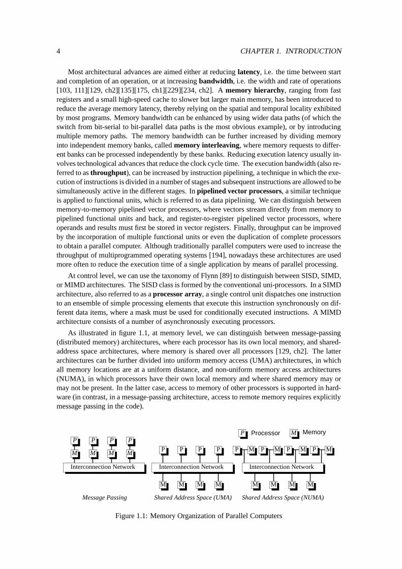
As illustrated in figure 1.1, at memory level, we can distinguish between message-passing(distributed memory) architectures, where each processor has its own local memory, and shared-address space architectures, where memory is shared over all processors [129, ch2]. The latterarchitectures can be further divided into uniform memory access (UMA) architectures, in whichall memory locations are at a uniform distance, and non-uniform memory access architectures(NUMA), in which processors have their own local memory and where shared memory may ormay not be present. In the latter case, access to memory of other processors is supported in hard-ware (in contrast, in a message-passing architecture, access to remote memory requires explicitlymessage passing in the code).
P
M MMM
P P P
Interconnection NetworkInterconnection Network
M MMM
P P P P
Interconnection Network
M MMM
P M P M P M P M
Shared Address Space (UMA) Shared Address Space (NUMA)Message Passing
MP Processor Memory
Figure 1.1: Memory Organization of Parallel Computers
1.1. EXPLOITING HARDWARE CHARACTERISTICS 5
Typically, interconnection networks like a bus, crossbar switch, or multistage interconnectionnetwork are used in shared-address space architectures, whereas interconnection networks like aring, tree, mesh or hypercube are used in message-passing architectures. Shared address spaceand message-passing MIMD architectures are often also referred to as multiprocessors and mul-ticomputers respectively.
1.1.2 Restructuring Compilers
Although some architectural advances remain reasonably invisible to the programmer, others mustbe dealt with explicitly to obtain high performance. For example, effectively exploiting the mem-ory hierarchy requires rewriting a program to operate on small data sets that fit in cache, whereasthe same program must be rewritten into a form that operates on long vectors to enhance the per-formance on a pipelined vector processor or processor array, where having stride-1 accesses be-comes important for machines with low-order memory interleaving. Efficiently executing differ-ent iterations of a loop on a multiprocessor requires yet other program transformations, whereasre-targeting a code for a message-passing architecture requires even more programming effort,because explicit message passing must be added to the program.
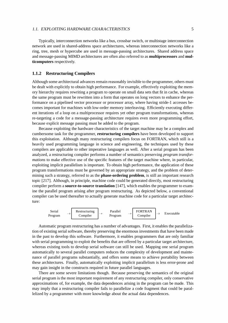
Because exploiting the hardware characteristics of the target machine may be a complex andcumbersome task for the programmer, restructuring compilers have been developed to supportthis exploitation. Although many restructuring compilers focus on FORTRAN, which still is aheavily used programming language in science and engineering, the techniques used by thesecompilers are applicable to other imperative languages as well. After a serial program has beenanalyzed, a restructuring compiler performs a number of semantics preserving program transfor-mations to make effective use of the specific features of the target machine where, in particular,exploiting implicit parallelism is important. To obtain high performance, the application of theseprogram transformations must be governed by an appropriate strategy, and the problem of deter-mining such a strategy, referred to as the phase-ordering problem, is still an important researchtopic [217]. Although, in principle, machine code could be generated directly, most restructuringcompiler perform a source-to-source translation [147], which enables the programmer to exam-ine the parallel program arising after program restructuring. As depicted below, a conventionalcompiler can be used thereafter to actually generate machine code for a particular target architec-ture:
SerialProgram
!
RestructuringCompiler
!
ParallelProgram
!
FORTRANCompiler
! Executable
Automatic program restructuring has a number of advantages. First, it enables the paralleliza-tion of existing serial software, thereby preserving the enormous investments that have been madein the past to develop this software. Furthermore, it enables programmers that are only familiarwith serial programming to exploit the benefits that are offered by a particular target architecture,whereas existing tools to develop serial software can still be used. Mapping one serial programautomatically to several parallel computers reduces the complexity of development and mainte-nance of parallel programs substantially, and offers some means to achieve portability betweenthese architectures. Finally, automatically exploiting implicit parallelism is less error-prone andmay gain insight in the constructs required in future parallel languages.
There are some severe limitations though. Because preserving the semantics of the originalserial program is the most important requirement of any restructuring compiler, only conservativeapproximations of, for example, the data dependences arising in the program can be made. Thismay imply that a restructuring compiler fails to parallelize a code fragment that could be paral-lelized by a programmer with more knowledge about the actual data dependences.
6 CHAPTER 1. INTRODUCTION
Moreover, some serial algorithms are just not amenable to parallelization, but must be rewrit-ten into a different semantically equivalent algorithm to allow for more parallelism. In an attemptto overcome these limitations, many restructuring compilers operate interactively, i.e. the com-piler cooperates with the programmer during program restructuring.
1.2 Exploiting Data Characteristics
Exploiting the occurrence of many zero elements in large sparse matrices may yield substantialsavings with respect to both the storage requirements and computational time of a numerical appli-cation. In the past, however, only limited compiler support has been developed for sparse matrixcomputations.
1.2.1 Sparse Matrix Computations
If many elements in a matrix are zero, then this matrix is called a sparse matrix. In contrast,a matrix containing many nonzero elements is referred to as a dense matrix. Both the storagerequirements and computational time of an application that operates on sparse matrices can bereduced substantially in comparison with an application that operates on dense matrices by onlystoring nonzero elements and avoiding redundant operations on zero elements [70, 72, 78, 97, 169,235].Example: Below, two FORTRAN fragments performing the operation~b ~
b+A~x are given. Inthe dense fragment, a two-dimensional array A is used to store all elements of the matrix, whereasa more complex sparse storage scheme (data structure) is used in the sparse fragment to avoidredundant operations on zero elements:
Dense Fragment:
REAL A(M,N)...DO I = 1, M
DO J = 1, NB(I) = B(I) + A(I,J) * X(J)
ENDDOENDDO
Sparse Fragment:
REAL VAL_A(SZ)INTEGER ROW_A(SZ), COL_A(SZ), NNZ_A...DO IJ = 1, NNZ_A
I = ROW_A(IJ)J = COL_A(IJ)B(I) = B(I) + VAL_A(IJ) * X(J)
ENDDO
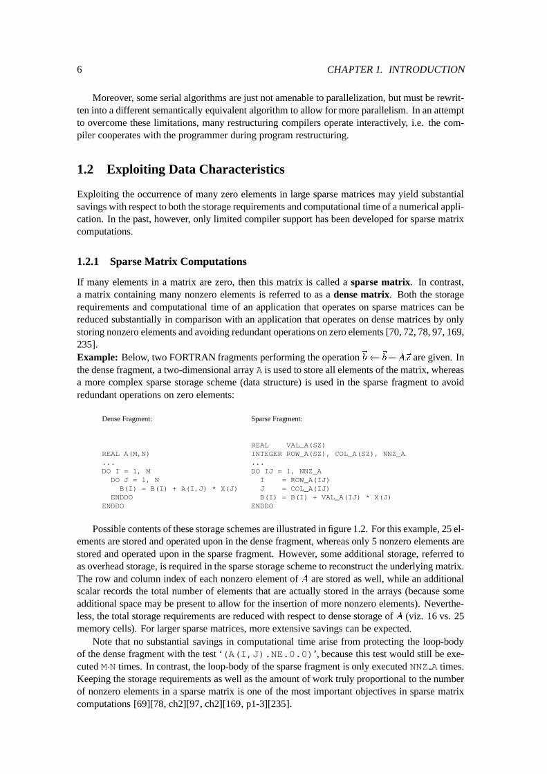
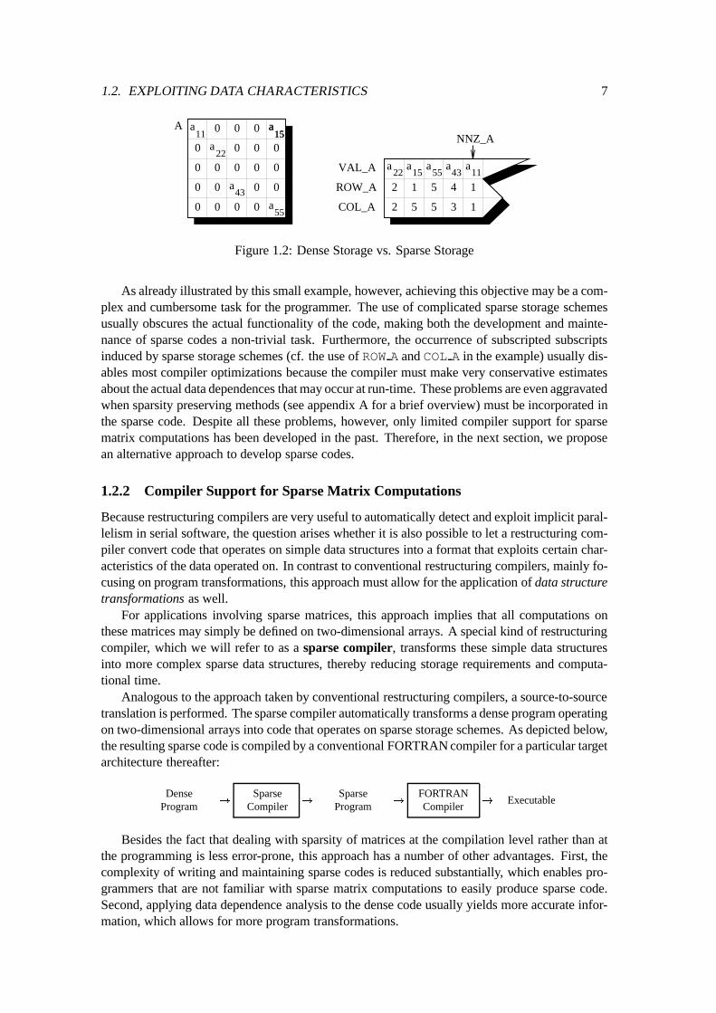
Possible contents of these storage schemes are illustrated in figure 1.2. For this example, 25 el-ements are stored and operated upon in the dense fragment, whereas only 5 nonzero elements arestored and operated upon in the sparse fragment. However, some additional storage, referred toas overhead storage, is required in the sparse storage scheme to reconstruct the underlying matrix.The row and column index of each nonzero element of A are stored as well, while an additionalscalar records the total number of elements that are actually stored in the arrays (because someadditional space may be present to allow for the insertion of more nonzero elements). Neverthe-less, the total storage requirements are reduced with respect to dense storage of A (viz. 16 vs. 25memory cells). For larger sparse matrices, more extensive savings can be expected.
Note that no substantial savings in computational time arise from protecting the loop-bodyof the dense fragment with the test ‘(A(I,J).NE.0.0) ’, because this test would still be exe-cuted M�N times. In contrast, the loop-body of the sparse fragment is only executed NNZA times.Keeping the storage requirements as well as the amount of work truly proportional to the numberof nonzero elements in a sparse matrix is one of the most important objectives in sparse matrixcomputations [69][78, ch2][97, ch2][169, p1-3][235].
1.2. EXPLOITING DATA CHARACTERISTICS 7
a55
a22
A a11
a15
a43
a150 00
0 0 0 0
0 0000
0 0 0 0
0 00 0
VAL_A
ROW_A
COL_A
NNZ_A
a15
a11
a22
a43
a55
2
2 15
5
5
4
3
11
Figure 1.2: Dense Storage vs. Sparse Storage
As already illustrated by this small example, however, achieving this objective may be a com-plex and cumbersome task for the programmer. The use of complicated sparse storage schemesusually obscures the actual functionality of the code, making both the development and mainte-nance of sparse codes a non-trivial task. Furthermore, the occurrence of subscripted subscriptsinduced by sparse storage schemes (cf. the use of ROWA and COLA in the example) usually dis-ables most compiler optimizations because the compiler must make very conservative estimatesabout the actual data dependences that may occur at run-time. These problems are even aggravatedwhen sparsity preserving methods (see appendix A for a brief overview) must be incorporated inthe sparse code. Despite all these problems, however, only limited compiler support for sparsematrix computations has been developed in the past. Therefore, in the next section, we proposean alternative approach to develop sparse codes.
1.2.2 Compiler Support for Sparse Matrix Computations
Because restructuring compilers are very useful to automatically detect and exploit implicit paral-lelism in serial software, the question arises whether it is also possible to let a restructuring com-piler convert code that operates on simple data structures into a format that exploits certain char-acteristics of the data operated on. In contrast to conventional restructuring compilers, mainly fo-cusing on program transformations, this approach must allow for the application of data structuretransformations as well.
For applications involving sparse matrices, this approach implies that all computations onthese matrices may simply be defined on two-dimensional arrays. A special kind of restructuringcompiler, which we will refer to as a sparse compiler, transforms these simple data structuresinto more complex sparse data structures, thereby reducing storage requirements and computa-tional time.
Analogous to the approach taken by conventional restructuring compilers, a source-to-sourcetranslation is performed. The sparse compiler automatically transforms a dense program operatingon two-dimensional arrays into code that operates on sparse storage schemes. As depicted below,the resulting sparse code is compiled by a conventional FORTRAN compiler for a particular targetarchitecture thereafter:
DenseProgram
!
SparseCompiler
!
SparseProgram
!
FORTRANCompiler
! Executable
Besides the fact that dealing with sparsity of matrices at the compilation level rather than atthe programming is less error-prone, this approach has a number of other advantages. First, thecomplexity of writing and maintaining sparse codes is reduced substantially, which enables pro-grammers that are not familiar with sparse matrix computations to easily produce sparse code.Second, applying data dependence analysis to the dense code usually yields more accurate infor-mation, which allows for more program transformations.
8 CHAPTER 1. INTRODUCTION
Because the sparse compiler can account for characteristics of both the nonzero structure andthe target machine (provided that these characteristics are made available in some manner), as wellas the actual operations performed while selecting a suitable sparse data structure, one dense pro-gram can be converted into a range of sparse versions, each of which is tailored for a particularinstance of the same problem. Program transformations may be applied to the dense program incase this data structure selection cannot be resolved efficiently. Finally, just as traditional restruc-turing compilers enable the re-use of existing serial software, a sparse compiler enables the re-useof parts of existing dense code.
Elaboration of these ideas have resulted in the development and implementation of a proto-type sparse compiler. In this dissertation, we present the automatic data structure selection andtransformation method used by this sparse compiler to automatically convert a dense program intosemantically equivalent code that exploits the sparsity of data operated upon.
Chapter 2
Preliminaries
In this chapter, a brief overview of some important concepts that are used throughout this disserta-tion is given. In particular, concepts that are useful for program analysis and program restructuringas well as for sparse matrix computations are presented.
Systems of linear equations or inequalities in integer-valued variables and affine transforma-tions are useful to represent many program constructs and transformations in a formal manner.In addition, many problems in science and engineering require the solution of a sparse system oflinear equations. Therefore, first some preliminaries from geometry and linear algebra are given.Thereafter, a number of useful methods that are used extensively in program analysis and programrestructuring are discussed.
2.1 Preliminaries from Geometry and Linear Algebra
In this section, some concepts of geometry and linear algebra are presented. For a detailed pre-sentation, the reader is referred to [40, 42, 61, 100, 104, 153, 172, 203].
2.1.1 Cartesian Spaces
Given a fixed natural number d 2 N , the d-dimensional Cartesian space consists of all d-tuples(x
1
; : : : ; x
d
) 2 R
d. This means that each coordinate xi
in a tuple is a real number. For d = 1,d = 2, and d = 3, the corresponding Cartesian spaces define the Euclidean straight line, Euclideanplane, and Euclidean space, respectively, for which direct graphical interpretations exist. How-ever, we do not restrict ourselves to these values of d, but allow for Cartesian spaces of arbitrarydimension.
Each tuple (x
1
; : : : ; x
d
) 2 R
d in such a d-dimensional Cartesian space can be thought of asa point X or as the components of the position vector OX = ~x representing this point X , wherepoint O = (0; : : : ; 0) is referred to as the origin. Usually we do not distinguish between pointsand position vectors and simply refer to point X by means of the (position) vector ~x 2 Rd.
The following operations are defined on two vectors ~x; ~y 2 Rd and a scalar � 2 R:(
~x+ ~y = ( x
1
+ y
1
; : : : ; x
d
+ y
d
)
� � ~x = ( � � x
1
; : : : ; � � x
d
)
In these operations, vectors are expressed as row vectors. A vector can also be expressed ascolumn vector, denoted as ~x = (x
1
; : : : ; x
d
)
T in the text for notational convenience:
~x =
0
B
@
x
1
...x
d
1
C
A
10 CHAPTER 2. PRELIMINARIES
The opposite vector of a vector ~x is defined as �~x = �1 � ~x. This vector has the propertythat �~x + ~x =
~
0, where ~0 = (0; : : : ; 0). The subtraction of two vectors ~x and ~y is defined as~x � ~y = ~x + (�~y). Furthermore, the scalar product of two vectors ~x; ~y 2 Rd is defined asfollows:
~x � ~y =
d
X
i=1
x
i
� y
i
(2.1)
The vectors are perpendicular or orthogonal, denoted by ~x ? ~y, if and only if these vectorshave a zero scalar product, i.e. ~x�~y = 0. In addition, this scalar product can be used to giveRd thestructure of a metric space by defining the following notion of distance between vectors, denotedby d(~x; ~y):
d(~x; ~y) =
q
(~x� ~y) � (~x� ~y) (2.2)
A set X � Rd is called bounded if for a particular � > 0 and ~x 2 X , we have d(~x; ~y) < �
for all ~y 2 X . This set X is called unbounded otherwise.
2.1.2 Linear and Affine Subspaces
We say that a vector ~x 2 Rd is a linear combination of a finite set X = f~x
1
; : : : ; ~x
k
g if thereexist scalars �
i
2 R such that:
~x =
k
X
i=1
�
i
� ~x
i
(2.3)
If, additionally, �1
+: : :+�
k
= 1, then ~x is called an affine combination of this set. A setX =
f~x
1
; : : : ; ~x
k
g is linearly independent if �1
�~x
1
+ : : :+�
k
�~x
k
=
~
0 implies that �i
= 0 for all 1 �i � k. All other sets are linearly dependent. A set X 0 = f~x
0
; : : : ; ~x
k
g is affinely independent,if the setX = f~x
1
�~x
0
; : : : ; ~x
k
�~x
0
g is linearly independent, and affinely dependent otherwise.In Rd, the sets X and X 0 can only be linearly and affinely independent respectively, if we havek � d.
Given a linearly independent set X = f~x
1
; : : : ; ~x
k
g, where each ~xi
2 R
d, the set S � Rd
consisting of all linear combinations of X forms a k-dimensional linear subspace ofRd:
S = f~x 2 R
d
j ~x =
k
X
i=1
�
i
� ~x
i
g
Given an affinely independent set X 0 = f~x0
; : : : ~x
k
g, where each ~xi
2 R
d, the set S � Rd
consisting of all affine combinations of X 0 forms a k-dimensional affine subspace of Rd (alsocalled a flat):
S = f~x 2 R
d
j ~x =
k
X
i=0
�
i
� ~x
i
and �0
+ : : :+ �
k
= 1g
Each linear subspace defined by a linearly independent set X = f~x
1
; : : : ; ~x
k
g is an affinesubspace through the origin defined by the affinely independent set X 0 = f~0; ~x
1
; : : : ~x
k
g. Hence,the dimension of linear and affine subspaces is defined consistently in this manner. Conversely,each affine subspace consists of the translate of a certain linear subspace of the same dimension.
A one-dimensional affine subspace, defined by an affinely independent set X 0 = f~x0
; ~x
1
g, iscalled a straight line. Since a linear combination �
0
� ~x
0
+ �
1
� ~x
1
is an affine combination if�
0
+ �
1
= 1, a line consists of all ~x satisfying the next equation, where � 2 R:
2.1. PRELIMINARIES FROM GEOMETRY AND LINEAR ALGEBRA 11
~x = (1� �) � ~x
0
+ � � ~x
1
(2.4)
Because X 0 is affine independent, the singleton set X = f ~x
1
� ~x
0
g is linearly independent.Since this is true for ~x
0
6= ~x
1
, we see that a line is defined by two different points. If we alsorequire that 0 � � � 1, then a straight line segment is defined. We can rewrite the previousequation into the following form, in which the line is defined by a position vector ~x
1
and a freevector ~d = ~x
1
� ~x
0
, denoting the direction of this line:
~x = ~x
0
+ � � (~x
1
� ~x
0
) = ~x
0
+ � �
~
d
An affinely independent set X 0 = f~x0
; ~x
1
; ~x
2
g defines a two-dimensional affine subspace,referred to as a plane, which can also be defined by a position vector and two linearly independentvectors.
2.1.3 Hyperplanes
A (d � 1)-dimensional affine subspace S � Rd defined by an affinely independent set X withcardinality d is called a hyperplane. Alternatively, a hyperplane S � Rd may be defined in Carte-sian form, since it consists of all ~x 2 Rd satisfying the linear equation ~a �~x = b for certain fixednonzero normal vector ~a 2 Rd and a scalar b 2 R:
S = f~x 2 R
d
j a
1
� x
1
+ : : : + a
d
� x
d
= bg
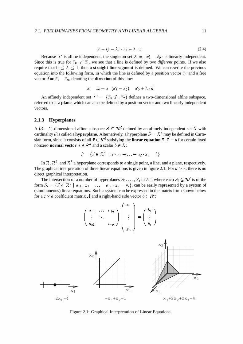
InR,R2, andR3 a hyperplane corresponds to a single point, a line, and a plane, respectively.The graphical interpretation of three linear equations is given in figure 2.1. For d > 3, there is nodirect graphical interpretation.
The intersection of a number of hyperplanes S1
; : : : ; S
c
inRd, where each Si
� R
d is of theform S
i
= f~x 2 R
d
j a
i1
� x
1
+ : : : + a
id
� x
d
= b
i
g, can be easily represented by a system of(simultaneous) linear equations. Such a system can be expressed in the matrix form shown belowfor a c� d coefficient matrix A and a right-hand side vector~b 2 Rc:
0
B
@
a
11
: : : a
1d
.... . .
a
c1
a
cd
1
C
A
0
B
B
B
B
B
B
@
x
1
...
x
d
1
C
C
C
C
C
C
A
=
0
B
@
b
1
...b
c
1
C
A
x 1
x2
x 1
x 2
x3
x 1
12x =4 1 2−x +x =1 2 31x +2x +2x =4
Figure 2.1: Graphical Interpretation of Linear Equations
12 CHAPTER 2. PRELIMINARIES
x2
x 1
x 2
x3
x 1x 10
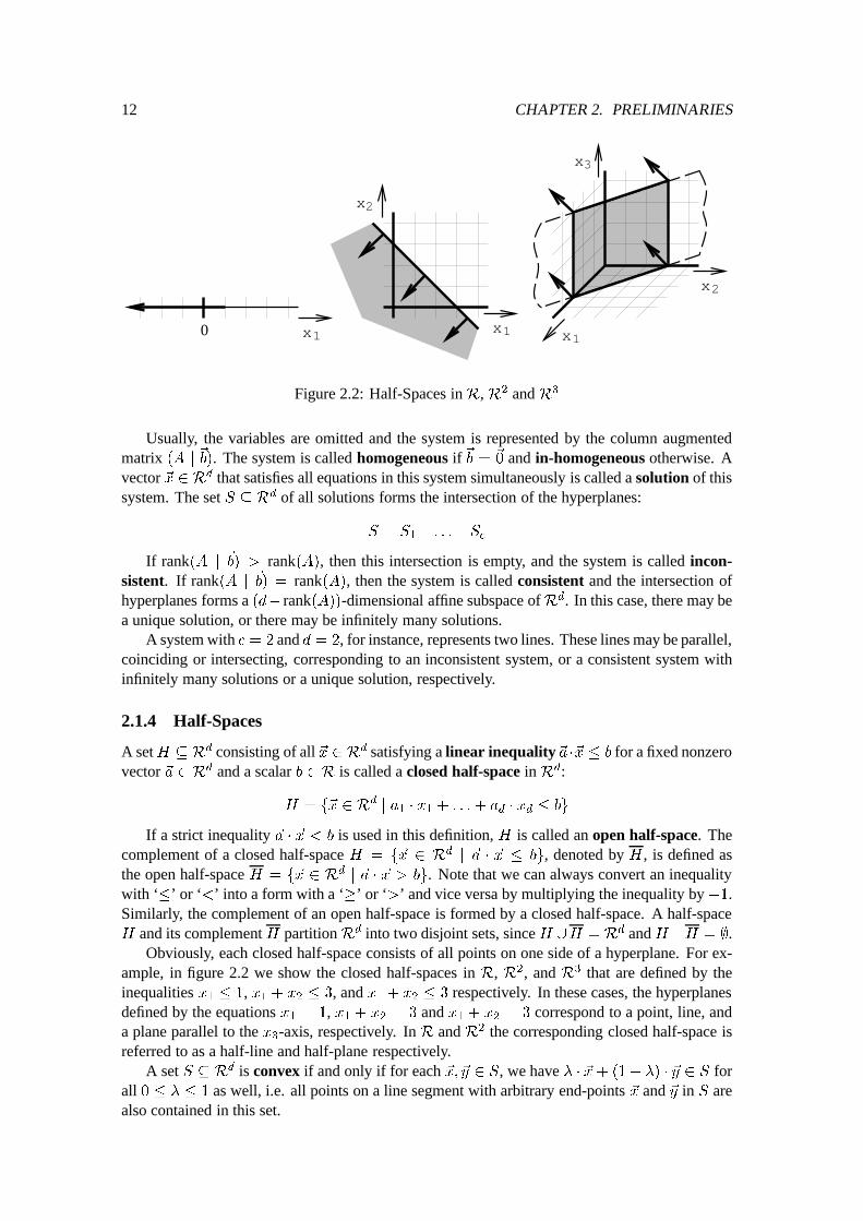
Figure 2.2: Half-Spaces inR, R2 and R3
Usually, the variables are omitted and the system is represented by the column augmentedmatrix (A j
~
b). The system is called homogeneous if ~b = ~
0 and in-homogeneous otherwise. Avector ~x 2 Rd that satisfies all equations in this system simultaneously is called a solution of thissystem. The set S � Rd of all solutions forms the intersection of the hyperplanes:
S = S
1
\ : : : \ S
c
If rank(A j ~b) > rank(A), then this intersection is empty, and the system is called incon-sistent. If rank(A j ~b) = rank(A), then the system is called consistent and the intersection ofhyperplanes forms a (d� rank(A))-dimensional affine subspace ofRd. In this case, there may bea unique solution, or there may be infinitely many solutions.
A system with c = 2 and d = 2, for instance, represents two lines. These lines may be parallel,coinciding or intersecting, corresponding to an inconsistent system, or a consistent system withinfinitely many solutions or a unique solution, respectively.
2.1.4 Half-Spaces
A setH � Rd consisting of all ~x 2 Rd satisfying a linear inequality~a �~x � b for a fixed nonzerovector ~a 2 Rd and a scalar b 2 R is called a closed half-space in Rd:
H = f~x 2 R
d
j a
1
� x
1
+ : : :+ a
d
� x
d
� bg
If a strict inequality ~a � ~x < b is used in this definition, H is called an open half-space. Thecomplement of a closed half-space H = f~x 2 R
d
j ~a � ~x � bg, denoted by H , is defined asthe open half-space H = f~x 2 R
d
j ~a � ~x > bg. Note that we can always convert an inequalitywith ‘�’ or ‘<’ into a form with a ‘�’ or ‘>’ and vice versa by multiplying the inequality by �1.Similarly, the complement of an open half-space is formed by a closed half-space. A half-spaceH and its complement H partitionRd into two disjoint sets, since H [H = R
d and H \H = ;.Obviously, each closed half-space consists of all points on one side of a hyperplane. For ex-
ample, in figure 2.2 we show the closed half-spaces in R, R2, and R3 that are defined by theinequalities x
1
� 1, x1
+ x
2
� 3, and x1
+ x
2
� 3 respectively. In these cases, the hyperplanesdefined by the equations x
1
= 1, x1
+ x
2
= 3 and x1
+ x
2
= 3 correspond to a point, line, anda plane parallel to the x
3
-axis, respectively. In R and R2 the corresponding closed half-space isreferred to as a half-line and half-plane respectively.
A set S � Rd is convex if and only if for each ~x; ~y 2 S, we have � � ~x+ (1� �) � ~y 2 S forall 0 � � � 1 as well, i.e. all points on a line segment with arbitrary end-points ~x and ~y in S arealso contained in this set.
2.1. PRELIMINARIES FROM GEOMETRY AND LINEAR ALGEBRA 13
Each half-space is convex. Because the intersection of a number of convex sets is also convex,the intersection of a number of half-spaces is a convex set.
Any set PS � Rd consisting of the intersection of a finite number of closed half-spacesH
1
; : : : ;H
c
in Rd is called a polyhedral set:
PS =
c
\
i=1
H
i
A bounded polyhedral set forms a convex polytope, called a line segment, convex polygon,and convex polyhedron in R,R2, and R3 respectively.
A half-space H � R
d for which the equality PS \ H = PS holds is called redundantwith respect to a polyhedral set PS � Rd. The following obvious property can be used to detectredundant half-spaces:
Proposition 2.1 A half-space H is redundant with respect to a polyhedral set PS if and only ifthe equation PS \H = ; holds.
Because a polyhedral set PS � Rd is defined by the intersection of a finite number of closedhalf-spaces, a convenient representation of PS consists of a system of linear inequalities. Assum-ing that PS is defined by the closed half-spaces H
1
; : : : ;H
c
in Rd, where each Hi
� R
d givesrise to a linear inequality a
i1
� x
1
+ : : :+ a
id
� x
d
� b
i
, the polyhedral set can be represented by asystem of linear inequalities A~x � ~b:
0
B
@
a
11
: : : a
1d
.... . .
a
c1
a
cd
1
C
A
0
B
B
B
B
B
B
@
x
1
...
x
d
1
C
C
C
C
C
C
A
�
0
B
@
b
1
...b
c
1
C
A
Analogous to the representation of a system of linear equations, we will frequently representthis system of linear inequalities by a column augmented matrix (A j
~
b).A vector ~x 2 Rd that satisfies all inequalities in A~x � ~b simultaneously is called a solution
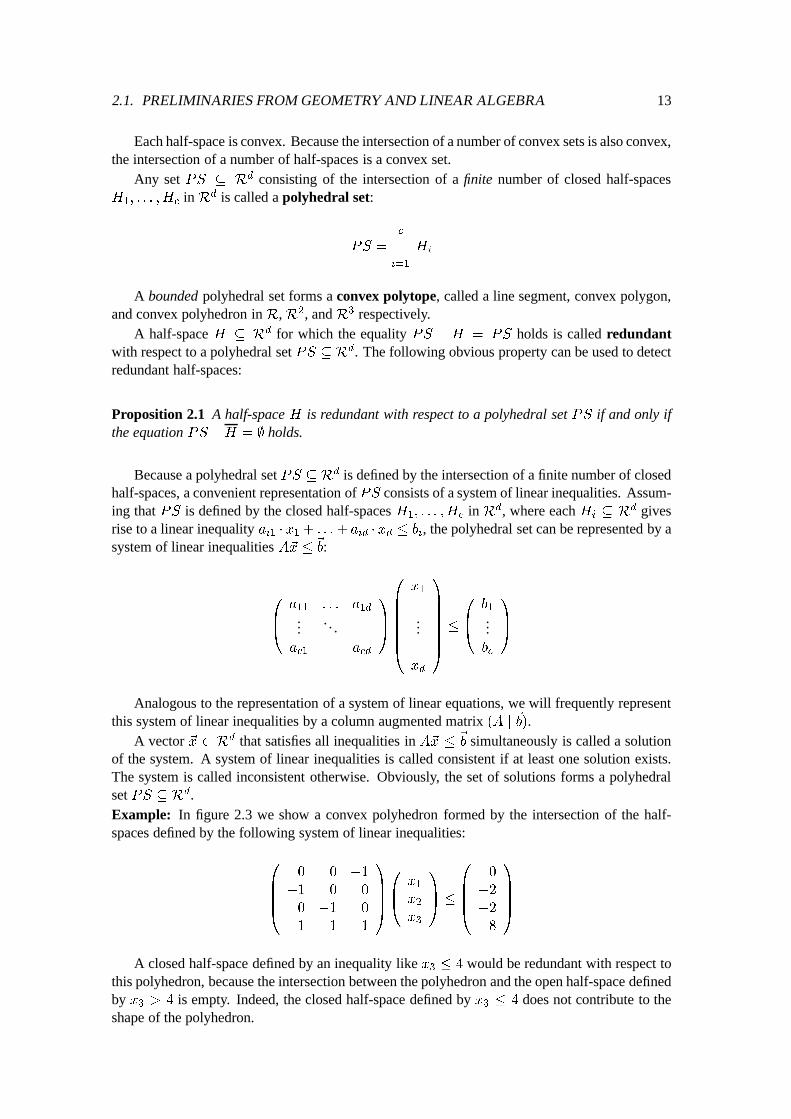
of the system. A system of linear inequalities is called consistent if at least one solution exists.The system is called inconsistent otherwise. Obviously, the set of solutions forms a polyhedralset PS � Rd.Example: In figure 2.3 we show a convex polyhedron formed by the intersection of the half-spaces defined by the following system of linear inequalities:
0
B
B
B
@
0 0 �1
�1 0 0
0 �1 0
1 1 1
1
C
C
C
A
0
B
@
x
1
x
2
x
3
1
C
A
�
0
B
B
B
@
0
�2
�2
8
1
C
C
C
A
A closed half-space defined by an inequality like x3
� 4 would be redundant with respect tothis polyhedron, because the intersection between the polyhedron and the open half-space definedby x
3
> 4 is empty. Indeed, the closed half-space defined by x3
� 4 does not contribute to theshape of the polyhedron.
14 CHAPTER 2. PRELIMINARIES
x 2
x3
x 1
5
5
5
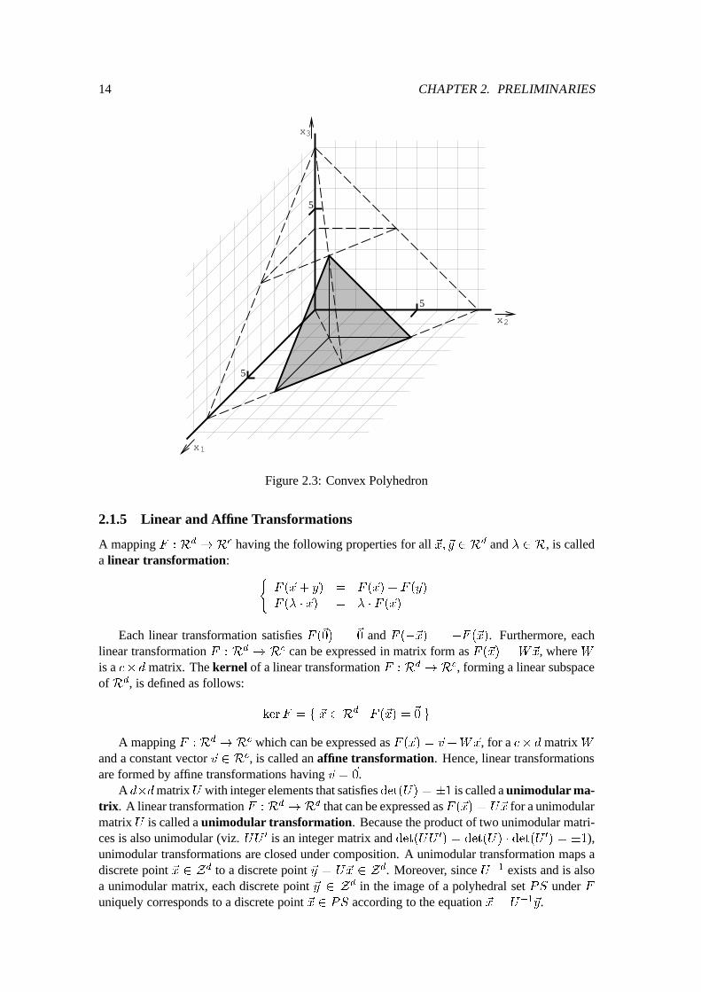
Figure 2.3: Convex Polyhedron
2.1.5 Linear and Affine Transformations
A mapping F : R
d
!R
c having the following properties for all ~x; ~y 2 Rd and � 2 R, is calleda linear transformation:
(
F (~x+ ~y) = F (~x) + F (~y)
F (� � ~x) = � � F (~x)
Each linear transformation satisfies F (~0) =
~
0 and F (�~x) = �F (~x). Furthermore, eachlinear transformation F : R
d
! R
c can be expressed in matrix form as F (~x) = W~x, where Wis a c� d matrix. The kernel of a linear transformation F : R
d
!R
c, forming a linear subspaceof Rd, is defined as follows:
kerF = f ~x 2 R
d
j F (~x) =
~
0 g
A mapping F : R
d
!R
c which can be expressed as F (~x) = ~v+W~x, for a c� d matrix Wand a constant vector ~v 2 Rc, is called an affine transformation. Hence, linear transformationsare formed by affine transformations having ~v =
~
0.A d�dmatrixU with integer elements that satisfies det(U) = �1 is called a unimodular ma-
trix. A linear transformation F : R
d
!R
d that can be expressed asF (~x) = U~x for a unimodularmatrix U is called a unimodular transformation. Because the product of two unimodular matri-ces is also unimodular (viz. UU 0 is an integer matrix and det(UU
0
) = det(U) � det(U
0
) = �1),unimodular transformations are closed under composition. A unimodular transformation maps adiscrete point ~x 2 Zd to a discrete point ~y = U~x 2 Z
d. Moreover, since U�1 exists and is alsoa unimodular matrix, each discrete point ~y 2 Zd in the image of a polyhedral set PS under Funiquely corresponds to a discrete point ~x 2 PS according to the equation ~x = U
�1
~y.
2.2. SOME USEFUL METHODS 15
2.2 Some Useful Methods
In this section, we discuss some methods that are used extensively in this dissertation.
2.2.1 Extended Euclidean Algorithm
The greatest common divisor of the integers �1
; : : : ; �
d
, denoted by g = gcd(�
1
; : : : ; �
d
), isthe greatest (positive) integer dividing all these integers (for all i, �
i
mod g = 0).Below, we present an implementation of the extended euclidean algorithm in pseudo-code
(cf. [18][100, p199-202][122, p14] [229, p93-96][234, p141]). Given the integers �1
and �2
, thisalgorithm computes the greatest common divisor g = gcd(�
1
; �
2
) and yields two other integersx and y satisfying �
1
� x+ �
2
� y = g as a side-effect:
integer function gcd(a1, a2, var x, var y)begin
c1 := abs(a1); c2 := abs(a2);x1 := 1; x2 := 0;while (c2 > 0) do
x1 := x1 - bc1 / c2c * x2;c1 := c1 - bc1 / c2c * c2;swap(x1, x2);swap(c1, c2);
enddogcd := c1;x := (a1 == 0) ? 0 : ( (a1 > 0) ? x1 : -x1);y := (a2 == 0) ? 0 : ( (c1 - a1 * x) / a2 );
end
This function can also be used to compute the greatest common divisor of a number of integersby repetitively using the following equation for d � 3:
gcd(�
1
; : : : ; �
d
) = gcd(�
1
; gcd(�
2
; : : : ; �
d
))
These integers are called relatively prime if gcd(�1
; : : : ; �
d
) = 1.
2.2.2 Completion Method for Unimodular Matrices
Unimodular transformations provide a convenient representation of some loop transformations, asis discussed further in chapter 3. The following completion method of a unimodular matrix U ofwhich only the first row is specified will be useful to construct a loop transformation that satisfiesa particular goal. In addition, because U�1 is required to implement this loop transformation, wealso present a method to construct this inverse simultaneously [29].
Conventional Completion Method
Given an arbitrary vector ~� 2 Zd of which the components are relatively prime, a unimodularmatrix of the following form exists [19, p55-59][159, p13-15]:
U =
0
B
B
B
B
@
�
1
: : : �
d
u
21
: : : u
2d
.... . .
u
d1
u
dd
1
C
C
C
C
A
The construction of the desired integer matrix is based on the fact that, given a k � k integermatrix U
k
with jdet(Uk
)j = g
k
, where gk
= gcd(�
1
; : : : ; �
k
), another (k+1)� (k+1) integermatrix U
k+1
with jdet(Uk+1
)j = g
k+1
can be constructed from U
k
in a relatively easy manner.
16 CHAPTER 2. PRELIMINARIES
Hence, if �1
6= 0, then the following sequence can be constructed, in which the final matrixis the desired matrix with jdet(U)j = g
d
= 1:
(�
1
) = U
1
! U
2
! : : :! U
d
= U
Unfortunately, the completion method cannot always be initiated for k = 1, since a prefix ofzeros may appear in ~�. However, for any ~� 2 Zd with gcd(�
1
; : : : ; �
d
) = 1, an m exists suchthat �
i
= 0 for all 1 � i < m and �m
6= 0. Hence, in general, the completion method can beinitiated for k = m with the following m�m matrix U
m
satisfying det(U
m
) = (�1)
m+1
� �
m
,which implies that jdet(U
m
)j = g
m
:
U
m
=
0
B
B
B
B
@
0 : : : 0 �
m
1 0
. . ....
1 0
1
C
C
C
C
A
(2.5)
Now, suppose that a k � k integer matrix Uk
has been constructed with (�
1
; : : : �
k
) as firstrow and jdet(U
k
)j = g
k
. First, two integers and � must be determined such that the followingequation holds:
g
k
� � �
k+1
� � = g
k+1
These integers are obtained as a side-effect of the extended euclidean algorithm, if we computeg
k+1
= gcd(g
k
; �
k+1
) as gcd(gk
;��
k+1
). The next (k + 1) � (k + 1) integer matrix Uk+1
inthe sequence with (�
1
; : : : ; �
k+1
) as first row can be easily obtained by extending the previousmatrix as follows, in which all divisions evaluate to integer values:
U
k+1
=
0
B
B
B
B
B
B
@
�
k+1
0
U
k
...0
�
1
��
g
k
: : :
�
k
��
g
k
1
C
C
C
C
C
C
A
(2.6)
Expansion of the determinant of this matrix by the last column reveals that the next equationholds, where the k�k matrixE
k
denotes the matrix that is obtained after eliminating the first rowand last column of U
k+1
:
det(U
k+1
) = (�1)
k+2
� �
k+1
� det(E
k
) + � det(U
k
)
Consequently, Ek
can be written as the following product:
E
k
=
0
B
B
B
B
@
0 1
.... . .
0 1
�
g
k
0 : : : 0
1
C
C
C
C
A
U
k
Because det(E
k
) =
�
(�1)
k+1
� �=g
k
�
� det(U
k
) and for k � 1 the expression (�1)
2k+3 isequal to �1, the following equations hold:
det(U
k+1
) =
det(U
k
)
g
k
� (g
k
� � �
k+1
� �) =
det(U
k
)
g
k
� g
k+1
2.2. SOME USEFUL METHODS 17
Since either det(Uk
) = g
k
or det(Uk
) = �g
k
holds, an integer matrix Uk+1
is constructedthat satisfies the following equation:
jdet(U
k+1
)j = g
k+1
Because the components of ~� 2 Zd are relatively prime, repetitive extending the matrix inthis manner eventually results in a unimodular matrix U = U
d
with jdet(U)j = 1.In [18, 159, 224], the case d = 2 is considered separately. In order to obtain a unimodular
2�2 matrixU with (�
1
; �
2
) as first row, the integers u21
and u22
are required such that det(U) =
�
1
� u
22
� �
2
� u
21
is either +1 or �1:
U =
�
1
�
2
u
21
u
22
!
The extended euclidean algorithm can be used to construct this matrix directly, since if thegreatest common divisor gcd(�
1
; �
2
) is computed as gcd(�1
;��
2
), then the integers u22
and u21
satisfying �1
� u
22
+(��
2
) � u
21
= gcd(�
1
; �
2
) = 1 are obtained as a side-effect. The inverse ofsuch a 2� 2 unimodular matrix can be easily obtained by using the following equation:
U
�1
=
1
det(U)
�
u
22
��
2
�u
21
�
1
!
Computation of U�1 is not so straightforward in general. However, because the inverse ofthe matrix is required to implement a loop transformation defined by U , we present an efficientmethod to construct U�1 simultaneously with the completion of U in the following section.
Extended Completion Method
If a matrixA is modified intoA+�A, where the modification can be expressed as�A = V SW
T ,then the inverse of the modified matrix A+�A can be obtained from the inverse of A using thematrix modification formula [78, p243-244]:
(A+ V SW
T
)
�1
= A
�1
�A
�1
V (S
�1
+W
T
A
�1
V )
�1
W
T
A
�1
| {z }
Correction Term
(2.7)
This formula provides a convenient method to derive the changes in the inverse of the originalmatrix that are required to obtain the inverse of the modified matrix. Hence, since form � k � d,we have det(U
k
) 6= 0, the question arises whether the matrix modification formula can be usedto construct U�1
m
! : : : ! U
�1
d
simultaneously with the construction of Um
! : : : ! U
d
during the completion method. In this manner, the completion method also yields the inverse ofthe desired matrix U = U
d
.A subtlety that must be dealt with is the fact that each modification changes the order of the
matrix. However, we can view each extension of Uk
into Uk+1
as a modification of a matrix Ainto A+�A, where A and, hence, A�1 are defined as follows:
A =
U
k
1
!
A
�1
=
U
�1
k
1
!
The modification �A = V SW
T can be expressed as follows (cf. formula (2.6)):
18 CHAPTER 2. PRELIMINARIES
V =
0
B
B
B
B
B
@
1 0
0
...... 0
0 1
1
C
C
C
C
C
A
S =
1 0
0 1
!
W
T
=
0 : : : 0 �
k+1
�
1
��
g
k
: : :
�
k
��
g
k
� 1
!
The expression W T
A
�1 in the correction term defined by (2.7) has the following form, inwhich we have used the fact that the product (�
1
; : : : ; �
k
)U
�1
k
yields the first row of the k � kidentity matrix:
W
T
A
�1
=
0 : : : 0 �
k+1
�
1
��
g
k
: : :
�
k
��
g
k
� 1
!
U
�1
k
1
!
=
0 0 : : : 0 �
k+1
�
g
k
0 : : : 0 � 1
!
Hence, expression (S
�1
+W
T
A
�1
V ) has the following form:
(S
�1
+W
T
A
�1
V ) =
1 0
0 1
!
+
0 �
k+1
�
g
k
� 1
!
=
1 �
k+1
�
g
k
!
Because the determinant of the resulting matrix is � (�
k+1
� �)=g
k
, which can be rewritteninto (g
k
� � �
k+1
� �)=g
k
= g
k+1
=g
k
, the inverse of this matrix is defined as follows:
(S
�1
+W
T
A
�1
V )
�1
=
g
k
g
k+1
�
��
k+1
�
�
g
k
1
!
Equation ��k+1
� � = g
k+1
� g
k
� implies that A�1V (S
�1
+W
T
A
�1
V )
�1
W
T
A
�1 hasthe following form, in which elements of U�1
k
are denoted as uij
:
g
k
g
k+1
�
0
B
B
B
B
@
u
11
0
......
u
k1
0
0 1
1
C
C
C
C
A
��
k+1
�
�
g
k
1
!
0 0 : : : 0 �
k+1
�
g
k
0 : : : 0 � 1
!
| {z }
g
k+1
g
k
� 0 : : : 0 �
k+1
�
g
k
0 : : : 0
g
k+1
g
k
� 1
!
Hence, the following correction term must be subtracted from the inverse of A to obtain theinverse of A+�A:
0
B
B
B
B
B
@
(1�
�g
k
g
k+1
) � u
11
0 : : : 0
�
k+1
�g
k
g
k+1
� u
11
......
. . ....
(1�
�g
k
g
k+1
) � u
k1
0 : : : 0
�
k+1
�g
k
g
k+1
� u
k1
�
g
k+1
0 : : : 0 1�
g
k
g
k
+1
1
C
C
C
C
C
A
(2.8)
Since most elements remain unaffected by the correction term, the matrix modification for-mula reveals a convenient method to construct U�1
m
! : : :! U
�1
d
simultaneously with the con-struction of the sequence U
m
! : : :! U
d
.One final difficulty that must be dealt with is that, since we have jdet(U
k
)j = g
k
, and gk
6= 1
may hold for m � k < d, matrices in this sequence are not necessarily unimodular. Hence,fractions may appear in some U�1
k
.
2.2. SOME USEFUL METHODS 19
As is shown below, each matrix U�1k
can be represented as (1=�m
) �
~
U
k
for a k � k integermatrix ~
U
k
. Therefore, even the sequence U�1m
! : : :! U
�1
d
can be constructed with only integerarithmetic.
The completion method is initiated with the matrix Um
defined in (2.5) and we can representthe inverse of this matrix as follows, where �
m
6= 0:
U
�1
m
=
1
�
m
�
~
U =
1
�
m
�
0
B
B
B
B
@
0 �
m
.... . .
0 �
m
1 0 : : : 0
1
C
C
C
C
A
Thereafter, as defined by the correction term (2.8), a representation (1=�
m
) �
~
U
k+1
of U�1k+1
isobtained from the representation (1=�
m
)�
~
U
k
ofU�1k
as follows, where elements of ~
U
k
are denotedas ~u
ij
and where p = � (g
k
=g
k+1
) and q = ��k+1
� (g
k
=g
k+1
):
U
�1
k+1
=
1
�
m
0
B
B
B
B
@
p � ~u
11
~u
12
: : : ~u
1k
q � ~u
11
......
. . ....
p � ~u
k1
~u
k2
~u
kk
q � ~u
k1
�
�
m
��
g
k+1
0 : : : 0
�
m
�g
k
g
k+1
1
C
C
C
C
A
Because gk+1
divides both gk
and �m
by construction, all divisions evaluate to integer values.Moreover, because jdet(U)j = 1 holds for the final matrix U = U
d
, dividing all elements of ~
U
d
by �m
yields an integer matrix that is equal to the inverse of this matrix.1
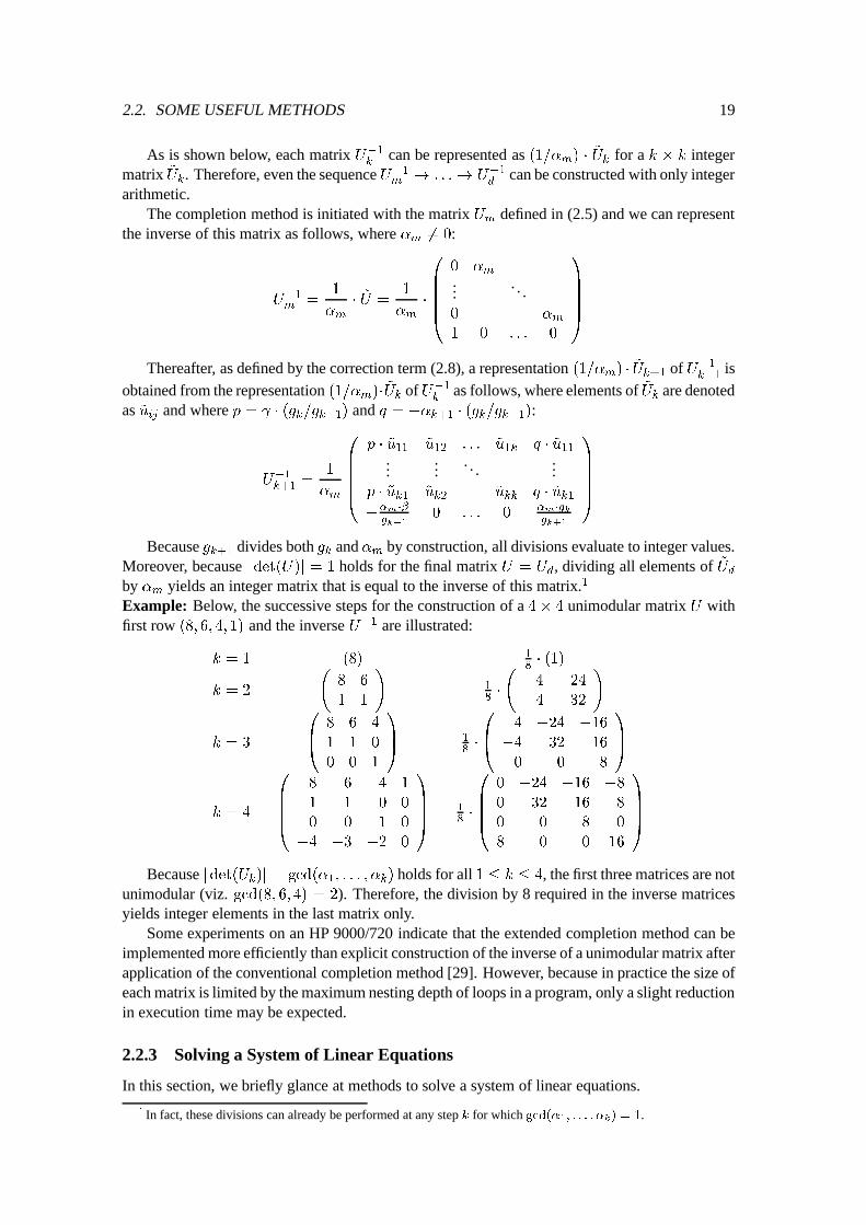
Example: Below, the successive steps for the construction of a 4� 4 unimodular matrix U withfirst row (8; 6; 4; 1) and the inverse U�1 are illustrated:
k = 1 (8)
1
8
� (1)
k = 2
8 6
1 1
!
1
8
�
4 �24
�4 32
!
k = 3
0
B
@
8 6 4
1 1 0
0 0 1
1
C
A
1
8
�
0
B
@
4 �24 �16
�4 32 16
0 0 8
1
C
A
k = 4
0
B
B
B
@
8 6 4 1
1 1 0 0
0 0 1 0
�4 �3 �2 0
1
C
C
C
A
1
8
�
0
B
B
B
@
0 �24 �16 �8
0 32 16 8
0 0 8 0
8 0 0 16
1
C
C
C
A
Because jdet(Uk
)j = gcd(�
1
; : : : ; �
k
) holds for all 1 � k � 4, the first three matrices are notunimodular (viz. gcd(8; 6; 4) = 2). Therefore, the division by 8 required in the inverse matricesyields integer elements in the last matrix only.
Some experiments on an HP 9000/720 indicate that the extended completion method can beimplemented more efficiently than explicit construction of the inverse of a unimodular matrix afterapplication of the conventional completion method [29]. However, because in practice the size ofeach matrix is limited by the maximum nesting depth of loops in a program, only a slight reductionin execution time may be expected.
2.2.3 Solving a System of Linear Equations
In this section, we briefly glance at methods to solve a system of linear equations.
1In fact, these divisions can already be performed at any step k for which gcd(�
1
; : : : ; �
k
) = 1.
20 CHAPTER 2. PRELIMINARIES
Elementary Row and Column Operations
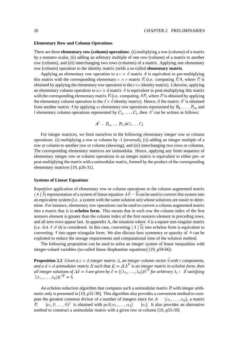
There are three elementary row (column) operations: (i) multiplying a row (column) of a matrixby a nonzero scalar, (ii) adding an arbitrary multiple of one row (column) of a matrix to anotherrow (column), and (iii) interchanging two rows (columns) of a matrix. Applying one elementaryrow (column) operation to the identity matrix yields a so-called elementary matrix.
Applying an elementary row operation to a c � d matrix A is equivalent to pre-multiplyingthis matrix with the corresponding elementary c � c matrix E (i.e. computing EA, where E isobtained by applying the elementary row operation to the c�c identity matrix). Likewise, applyingan elementary column operation to a c� d matrix A is equivalent to post-multiplying this matrixwith the corresponding elementary matrixE (i.e. computingAE, whereE is obtained by applyingthe elementary column operation to the d�d identity matrix). Hence, if the matrixA0 is obtainedfrom another matrixA by applying m elementary row operations represented byR
1
; : : : ; R
m
andl elementary column operations represented by C
1
; : : : ; C
l
, then A0 can be written as follows:
A
0
= R
m
: : : R
1
AC
1
: : : C
l
For integer matrices, we limit ourselves to the following elementary integer row or columnoperations: (i) multiplying a row or column by -1 (reversal), (ii) adding an integer multiple of arow or column to another row or column (skewing), and (iii) interchanging two rows or columns.The corresponding elementary matrices are unimodular. Hence, applying any finite sequence ofelementary integer row or column operations to an integer matrix is equivalent to either pre- orpost-multiplying the matrix with a unimodular matrix, formed by the product of the correspondingelementary matrices [19, p26-31].
Systems of Linear Equations
Repetitive application of elementary row or column operations to the column augmented matrix(A j
~
b) representation of a system of linear equationA~x =
~
b can be used to convert this system intoan equivalent system (i.e. a system with the same solution set) whose solutions are easier to deter-mine. For instance, elementary row operations can be used to convert a column augmented matrixinto a matrix that is in echelon form. This means that in each row the column index of the firstnonzero element is greater than the column index of the first nonzero element in preceding rows,and all zero rows appear last. In appendix A, the situation whereA is a square non-singular matrix(i.e. detA 6= 0) is considered. In this case, converting (A j
~
b) into echelon form is equivalent toconverting A into upper triangular form. We also discuss how symmetry or sparsity of A can beexploited to reduce the storage requirements and computational time of the solution method.
The following proposition can be used to solve an integer system of linear inequalities withinteger-valued variables (so-called linear diophantine equations) [19, p59-66]:
Proposition 2.2 Given a c� d integer matrix A, an integer column vector~b with c components,and a d� d unimodular matrix R such that E = RA
T is an integer matrix in echelon form, thenall integer solutions ofA~x =
~
b are given by ~x = [(�
1
; : : : ; �
d
)R]
T for arbitrary �i
2 Z satisfying[(�
1
; : : : ; �
d
)E]
T
=
~
b.
An echelon reduction algorithm that computes such a unimodular matrixR with integer arith-metic only is presented in [19, p32-39]. This algorithm also provides a convenient method to com-pute the greatest common divisor of a number of integers since for A = (�
1
; : : : ; �
d
), a matrixE = (e
1
; 0; : : : ; 0)
T is obtained with gcd(�
1
; : : : ; �
d
) = je
1
j. It also provides an alternativemethod to construct a unimodular matrix with a given row or column [19, p55-59].
2.2. SOME USEFUL METHODS 21
2.2.4 Solving a System of Linear Inequalities
The Fourier-Motzkin elimination method [10, 19] [61, p84-85][62][229, ch4] can be used to testthe consistency of a reasonably small system of linear inequalities A~x � ~b, or to convert this sys-tem into a form in which the lower and upper bounds of each variable x
i
are expressed in termsof the variables x
1
; : : : ; x
i�1
only. In particular, we focus on an implementation for integer sys-tems [33].
Intuition Behind the Elimination Method
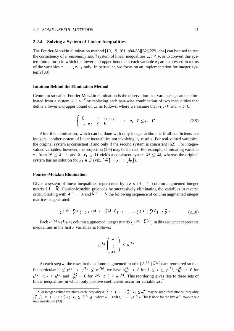
Central to so-called Fourier-Motzkin elimination is the observation that variable xk
can be elim-inated from a system A~x �
~
b by replacing each pair-wise combination of two inequalities thatdefine a lower and upper bound on x
k
as follows, where we assume that c1
> 0 and c2
> 0,
(
L � c
1
� x
k
c
2
� x
k
� U
! c
2
� L � c
1
� U (2.9)
After this elimination, which can be done with only integer arithmetic if all coefficients areintegers, another system of linear inequalities not involving x
k
results. For real-valued variables,the original system is consistent if and only if the second system is consistent [62]. For integer-valued variables, however, the projection (2.9) may be inexact. For example, eliminating variablex
1
from 16 � 3 � x
1
and 2 � x
1
� 11 yields a consistent system 32 � 33, whereas the originalsystem has no solution for x
1
2 Z (viz. d163
e � x
1
� b
11
2
c).
Fourier-Motzkin Elimination
Given a system of linear inequalities represented by a c � (d + 1) column augmented integermatrix (A j
~
b), Fourier-Motzkin proceeds by successively eliminating the variables in reverseorder. Starting withA(d)
= A and~b (d) = ~
b, the following sequence of column augmented integermatrices is generated:
(A
(d)
j
~
b
(d)
)! (A
(d�1)
j
~
b
(d�1)
)! : : :! (A
(1)
j
~
b
(1)
)!
~
b
(0) (2.10)
Eachm(k)
�(k+1) column augmented integer matrix (A(k)
j
~
b
(k)
) in this sequence representsinequalities in the first k variables as follows:
A
(k)
0
B
@
x
1
...x
k
1
C
A
�
~
b
(k)
At each step k, the rows in the column augmented matrix (A
(k)
j
~
b
(k)
) are reordered so that
for particular 1 � p
(k)
< q
(k)
� m
(k), we have a(k)ik
> 0 for 1 � i � p
(k), a(k)ik
< 0 for
p
(k)
< i � q
(k) and a(k)ik
= 0 for q(k) < i � m
(k). This reordering gives rise to three sets oflinear inequalities in which only positive coefficients occur for variable x
k
:2
2For integer-valued variables, each inequality a
(k)
i1
�x
1
+ : : :+a
(k)
ik
�x
k
� b
(k)
i
may be simplified into the inequality
a
(k)
i1
=g �x
1
+ : : :+a
(k)
ik
=g �x
k
� bb
(k)
i
=gc, where g = gcd(a
(k)
i1
; : : : ; a
(k)
ik
). This is done for the first q(k) rows in ourimplementation [33].
22 CHAPTER 2. PRELIMINARIES
8
>
>
>
>
>
>
>
>
<
>
>
>
>
>
>
>
>
:
a
(k)
ik
� x
k
� b
(k)
i
�
k�1
P
j=1
a
(k)
ij
� x
j
for 1 � i � p(k)
�b
(k)
i
+
k�1
P
j=1
a
(k)
ij
� x
j
� (�a
(k)
ik
) � x
k
for p(k) < i � q
(k)
k�1
P
j=1
a
(k)
ij
� x
j
� b
(k)
i
for q(k) < i � m
(k)
After the reordering, the first p(k) rows in (A
(k)
j
~
b
(k)
) define the upper bounds of variable xk
in terms of only the variables x1
; : : : ; x
k�1
. Moreover, the next q(k)� p(k) rows define the lowerbounds of x
k
in terms of only the variables x1
; : : : ; x
k�1
. For integer-valued variables, the lowerand upper bounds can be expressed as follows:
max
p
(k)
<i�q
(k)
2
6
6
6
6
6
6
b
(k)
i
�
k�1
P
j=1
a
(k)
ij
� x
j
a
(k)
ik
3
7
7
7
7
7
7
� x
k
� min
1�i�p
(k)
6
6
6
6
6
6
4
b
(k)
i
�
k�1
P
j=1
a
(k)
ij
� x
j
a
(k)
ik
7
7
7
7
7
7
5
(2.11)
The other rows represent inequalities in which xk
is not involved.Subsequently, the next column augmented matrix in the sequence (2.10) is obtained by elim-
inating variable xk
from the system according to (2.9). This implies that the first q(k) inequalitiesare replaced by p(k) � (q(k) � p(k)) new inequalities, which gives rise to the following system:
8
>
>
>
<
>
>
>
:
k�1
P
j=1
(a
(k)
ik
� a
(k)
i
0
j
� a
(k)
i
0
k
� a
(k)
ij
) � x
j
� a
(k)
ik
� b
(k)
i
0
� a
(k)
i
0
k
� b
(k)
i
1 � i � p
(k)
< i
0
� q
(k)
k�1
P
j=1
a
(k)
ij
� x
j
� b
(k)
i
q
(k)
< i � m
(k)
Form(k�1)
= p
(k)
�(q
(k)
�p
(k)
)+m
(k)
�q
(k), this system can be represented by anm(k�1)
�k
column augmented integer matrix (A
(k�1)
j
~
b
(k�1)
), which is the next matrix in the sequence.This process is repeated until all variables have been eliminated.
Eventually, a column integer vector~b(0) results. If any of the components of this vector is neg-ative, then the original system of inequalities is inconsistent (viz. an inequality 0 � b
(0)
i
results
where b(0)i
< 0). Otherwise, the system is consistent in the sense that at least one real solutionexists. Since projection (2.9) is inexact for integer-valued variables, however, this does not nec-essarily imply that there is also an integer solution. Still, this test provides a necessary (but notsufficient) condition for the existence of an integer solution.Example: Consider the following system of linear inequalities:
0
B
B
B
B
B
B
B
@
0 �1 �3
0 0 �1
�1 0 6
0 1 3
0 0 1
1 0 �6
1
C
C
C
C
C
C
C
A
0
B
@
x
1
x
2
x
3
1
C
A
�
0
B
B
B
B
B
B
B
@
�10
�1
�1
15
3
50
1
C
C
C
C
C
C
C
A
Applying Fourier-Motzkin to this system yields the following sequence of column augmentedinteger matrices (see also the footnote on the previous page):
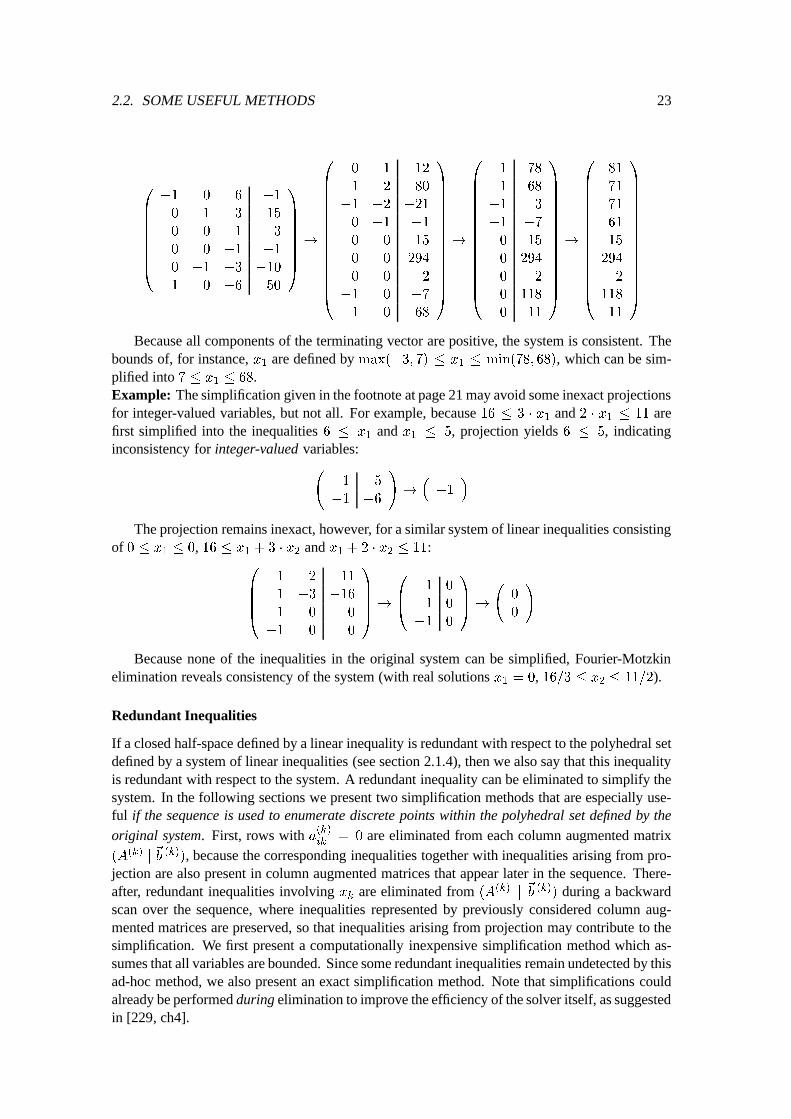
2.2. SOME USEFUL METHODS 23
0
B
B
B
B
B
B
B
@
�1 0 6 �1
0 1 3 15
0 0 1 3
0 0 �1 �1
0 �1 �3 �10
1 0 �6 50
1
C
C
C
C
C
C
C
A
!
0
B
B
B
B
B
B
B
B
B
B
B
B
B
B
@
0 1 12
1 2 80
�1 �2 �21
0 �1 �1
0 0 15
0 0 294
0 0 2
�1 0 �7
1 0 68
1
C
C
C
C
C
C
C
C
C
C
C
C
C
C
A
!
0
B
B
B
B
B
B
B
B
B
B
B
B
B
B
@
1 78
1 68
�1 3
�1 �7
0 15
0 294
0 2
0 118
0 11
1
C
C
C
C
C
C
C
C
C
C
C
C
C
C
A
!
0
B
B
B
B
B
B
B
B
B
B
B
B
B
B
@
81
71
71
61
15
294
2
118
11
1
C
C
C
C
C
C
C
C
C
C
C
C
C
C
A
Because all components of the terminating vector are positive, the system is consistent. Thebounds of, for instance, x
1
are defined by max(�3; 7) � x
1
� min(78; 68), which can be sim-plified into 7 � x
1
� 68.Example: The simplification given in the footnote at page 21 may avoid some inexact projectionsfor integer-valued variables, but not all. For example, because 16 � 3 � x
1
and 2 � x
1
� 11 arefirst simplified into the inequalities 6 � x
1
and x1
� 5, projection yields 6 � 5, indicatinginconsistency for integer-valued variables:
1 5
�1 �6
!
!
�
�1
�
The projection remains inexact, however, for a similar system of linear inequalities consistingof 0 � x
1
� 0, 16 � x1
+ 3 � x
2
and x1
+ 2 � x
2
� 11:0
B
B
B
@
1 2 11
1 �3 �16
1 0 0
�1 0 0
1
C
C
C
A
!
0
B
@
1 0
1 0
�1 0
1
C
A
!
0
0
!
Because none of the inequalities in the original system can be simplified, Fourier-Motzkinelimination reveals consistency of the system (with real solutions x
1
= 0, 16=3 � x2
� 11=2).
Redundant Inequalities
If a closed half-space defined by a linear inequality is redundant with respect to the polyhedral setdefined by a system of linear inequalities (see section 2.1.4), then we also say that this inequalityis redundant with respect to the system. A redundant inequality can be eliminated to simplify thesystem. In the following sections we present two simplification methods that are especially use-ful if the sequence is used to enumerate discrete points within the polyhedral set defined by the
original system. First, rows with a(k)ik
= 0 are eliminated from each column augmented matrix(A
(k)
j
~
b
(k)
), because the corresponding inequalities together with inequalities arising from pro-jection are also present in column augmented matrices that appear later in the sequence. There-after, redundant inequalities involving x
k
are eliminated from (A
(k)
j
~
b
(k)
) during a backwardscan over the sequence, where inequalities represented by previously considered column aug-mented matrices are preserved, so that inequalities arising from projection may contribute to thesimplification. We first present a computationally inexpensive simplification method which as-sumes that all variables are bounded. Since some redundant inequalities remain undetected by thisad-hoc method, we also present an exact simplification method. Note that simplifications couldalready be performed during elimination to improve the efficiency of the solver itself, as suggestedin [229, ch4].
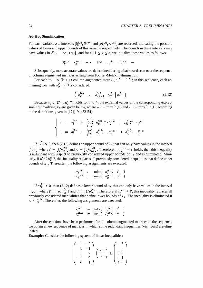
24 CHAPTER 2. PRELIMINARIES
Ad-Hoc Simplification
For each variable xk
, intervals [lmin
k
; l
max
k
] and [u
min
k
; u
max
k
] are recorded, indicating the possiblevalues of lower and upper bounds of this variable respectively. The bounds in these intervals mayhave values in Z [ f�1;+1g, and for all 1 � k � d, we initialize these values as follows:
l
min
k
= l
max
k
= �1 and u
min
k
= u
max
k
= +1
Subsequently, more accurate values are determined during a backward scan over the sequenceof column augmented matrices arising from Fourier-Motzkin elimination.
For each m(k)
� (k + 1) column augmented matrix (A
(k)
j
~
b
(k)
) in this sequence, each re-
maining row with a(k)ik
6= 0 is considered:
�
a
(k)
i1
: : : a
(k)
i;k�1
a
(k)
ik
b
(k)
i
�
(2.12)
Because xj
2 [l
min
j
; u
max
j
] holds for j < k, the extremal values of the corresponding expres-sion not involving x
k
are given below, where a+ = max(a; 0) and a� = max(�a; 0) accordingto the definitions given in [17][19, p52-54]:
8
>
>
>
<
>
>
>
:
l = b
(k)
i
+
k�1
P
j=1
(�a
(k)
ij
)
+
� l
min
j
� (�a
(k)
ij
)
�
� u
max
j
u = b
(k)
i
+
k�1
P
j=1
(�a
(k)
ij
)
+
� u
max
j
� (�a
(k)
ij
)
�
� l
min
j
If a(k)ik
> 0, then (2.12) defines an upper bound of xk
that can only have values in the interval
[l
0
; u
0
], where l0 = bl=a(k)ik
c and u0 = bu=a(k)ik
c. Therefore, if umax
k
� l
0 holds, then this inequalityis redundant with respect to previously considered upper bounds of x
k
and is eliminated. Simi-larly, if u0 � umin
k
, this inequality replaces all previously considered inequalities that define upperbounds of x
k
. Thereafter, the following assignments are executed:
u
min
k
:= min( u
min
k
; l
0
)
u
max
k
:= min( u
max
k
; u
0
)
If a(k)ik
< 0, then (2.12) defines a lower bound of xk
that can only have values in the interval
[l
0
; u
0
], where l0 = du=a(k)ik
e and u0 = dl=a(k)ik
e. Therefore, if lmax
k
� l
0, this inequality replaces allpreviously considered inequalities that define lower bounds of x
k
. The inequality is eliminated ifu
0
� l
min
k
. Thereafter, the following assignments are executed:
l
min
k
:= max( l
min
k
; l
0
)
l
max
k
:= max( l
max
k
; u
0
)
After these actions have been performed for all column augmented matrices in the sequence,we obtain a new sequence of matrices in which some redundant inequalities (viz. rows) are elim-inated.Example: Consider the following system of linear inequalities:
0
B
B
B
B
B
@
�1 �2
1 �1
1 2
�1 0
0 1
1
C
C
C
C
C
A
x
1
x
2
!
�
0
B
B
B
B
B
@
�3
0
300
�1
100
1
C
C
C
C
C
A
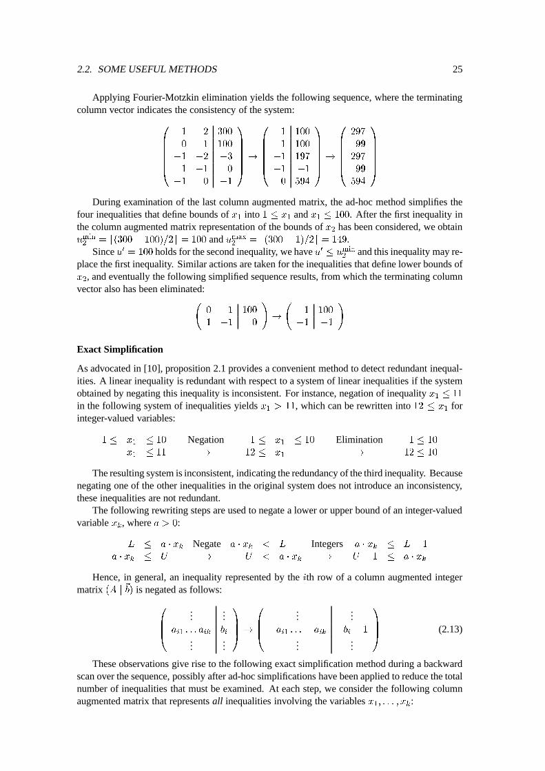
2.2. SOME USEFUL METHODS 25
Applying Fourier-Motzkin elimination yields the following sequence, where the terminatingcolumn vector indicates the consistency of the system:
0
B
B
B
B
B
@
1 2 300
0 1 100
�1 �2 �3
1 �1 0
�1 0 �1
1
C
C
C
C
C
A
!
0
B
B
B
B
B
@
1 100
1 100
�1 197
�1 �1
0 594
1
C
C
C
C
C
A
!
0
B
B
B
B
B
@
297
99
297
99
594
1
C
C
C
C
C
A
During examination of the last column augmented matrix, the ad-hoc method simplifies thefour inequalities that define bounds of x
1
into 1 � x
1
and x1
� 100. After the first inequality inthe column augmented matrix representation of the bounds of x
2
has been considered, we obtainu
min
2
= b(300 � 100)=2c = 100 and umax
2
= b(300 � 1)=2c = 149.Since u0 = 100 holds for the second inequality, we have u0 � umin
2
and this inequality may re-place the first inequality. Similar actions are taken for the inequalities that define lower bounds ofx
2
, and eventually the following simplified sequence results, from which the terminating columnvector also has been eliminated:
0 1 100
1 �1 0
!
!
1 100
�1 �1
!
Exact Simplification
As advocated in [10], proposition 2.1 provides a convenient method to detect redundant inequal-ities. A linear inequality is redundant with respect to a system of linear inequalities if the systemobtained by negating this inequality is inconsistent. For instance, negation of inequality x
1
� 11
in the following system of inequalities yields x1
> 11, which can be rewritten into 12 � x
1
forinteger-valued variables:
1 � x
1
� 10
x
1
� 11
Negation!
1 � x
1
� 10
12 � x
1
Elimination!
1 � 10
12 � 10
The resulting system is inconsistent, indicating the redundancy of the third inequality. Becausenegating one of the other inequalities in the original system does not introduce an inconsistency,these inequalities are not redundant.
The following rewriting steps are used to negate a lower or upper bound of an integer-valuedvariable x
k
, where a > 0:
L � a � x
k
a � x
k
� U
Negate!
a � x
k
< L
U < a � x
k
Integers!
a � x
k
� L� 1
U + 1 � a � x
k
Hence, in general, an inequality represented by the ith row of a column augmented integermatrix (A j
~
b) is negated as follows:
0
B
B
@
......
a
i1
: : : a
ik
b
i
......
1
C
C
A
!
0
B
B
@
......
�a
i1
: : :� a
ik
�b
i
� 1
......
1
C
C
A
(2.13)
These observations give rise to the following exact simplification method during a backwardscan over the sequence, possibly after ad-hoc simplifications have been applied to reduce the totalnumber of inequalities that must be examined. At each step, we consider the following columnaugmented matrix that represents all inequalities involving the variables x
1
; : : : ; x
k
:
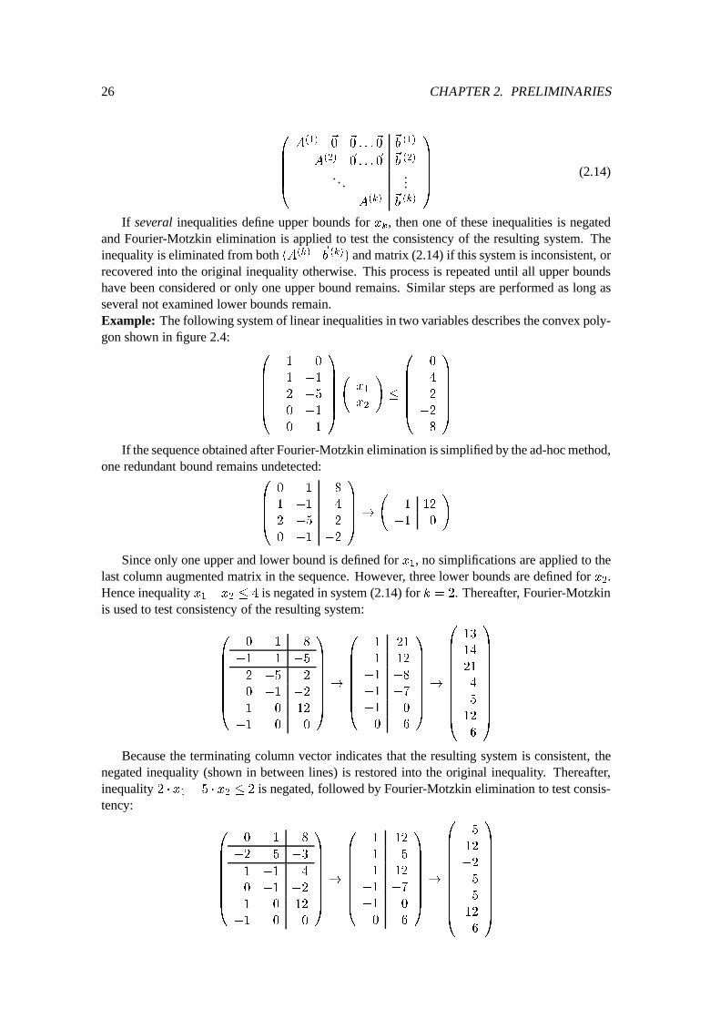
26 CHAPTER 2. PRELIMINARIES
0
B
B
B
B
@
A
(1)
~
0
~
0 : : :
~
0
~
b
(1)
A
(2)
~
0 : : :
~
0
~
b
(2)
. . ....
A
(k)
~
b
(k)
1
C
C
C
C
A
(2.14)
If several inequalities define upper bounds for xk
, then one of these inequalities is negatedand Fourier-Motzkin elimination is applied to test the consistency of the resulting system. Theinequality is eliminated from both (A
(k)
j
~
b
(k)
) and matrix (2.14) if this system is inconsistent, orrecovered into the original inequality otherwise. This process is repeated until all upper boundshave been considered or only one upper bound remains. Similar steps are performed as long asseveral not examined lower bounds remain.Example: The following system of linear inequalities in two variables describes the convex poly-gon shown in figure 2.4:
0
B
B
B
B
B
@
�1 0
1 �1
2 �5
0 �1
0 1
1
C
C
C
C
C
A
x
1
x
2
!
�
0
B
B
B
B
B
@
0
4
2
�2
8
1
C
C
C
C
C
A
If the sequence obtained after Fourier-Motzkin elimination is simplified by the ad-hoc method,one redundant bound remains undetected:
0
B
B
B
@
0 1 8
1 �1 4
2 �5 2
0 �1 �2
1
C
C
C
A
!
1 12
�1 0
!
Since only one upper and lower bound is defined for x1
, no simplifications are applied to thelast column augmented matrix in the sequence. However, three lower bounds are defined for x
2
.Hence inequality x
1
�x
2
� 4 is negated in system (2.14) for k = 2. Thereafter, Fourier-Motzkinis used to test consistency of the resulting system:
0
B
B
B
B
B
B
B
@
0 1 8
�1 1 �5
2 �5 2
0 �1 �2
1 0 12
�1 0 0
1
C
C
C
C
C
C
C
A
!
0
B
B
B
B
B
B
B
@
1 21
1 12
�1 �8
�1 �7
�1 0
0 6
1
C
C
C
C
C
C
C
A
!
0
B
B
B
B
B
B
B
B
B
B
@
13
14
21
4
5
12
6
1
C
C
C
C
C
C
C
C
C
C
A
Because the terminating column vector indicates that the resulting system is consistent, thenegated inequality (shown in between lines) is restored into the original inequality. Thereafter,inequality 2 � x
1
� 5 � x
2
� 2 is negated, followed by Fourier-Motzkin elimination to test consis-tency:
0
B
B
B
B
B
B
B
@
0 1 8
�2 5 �3
1 �1 4
0 �1 �2
1 0 12
�1 0 0
1
C
C
C
C
C
C
C
A
!
0
B
B
B
B
B
B
B
@
1 12
1 5
1 12
�1 �7
�1 0
0 6
1
C
C
C
C
C
C
C
A
!
0
B
B
B
B
B
B
B
B
B
B
@
5
12
�2
5
5
12
6
1
C
C
C
C
C
C
C
C
C
C
A
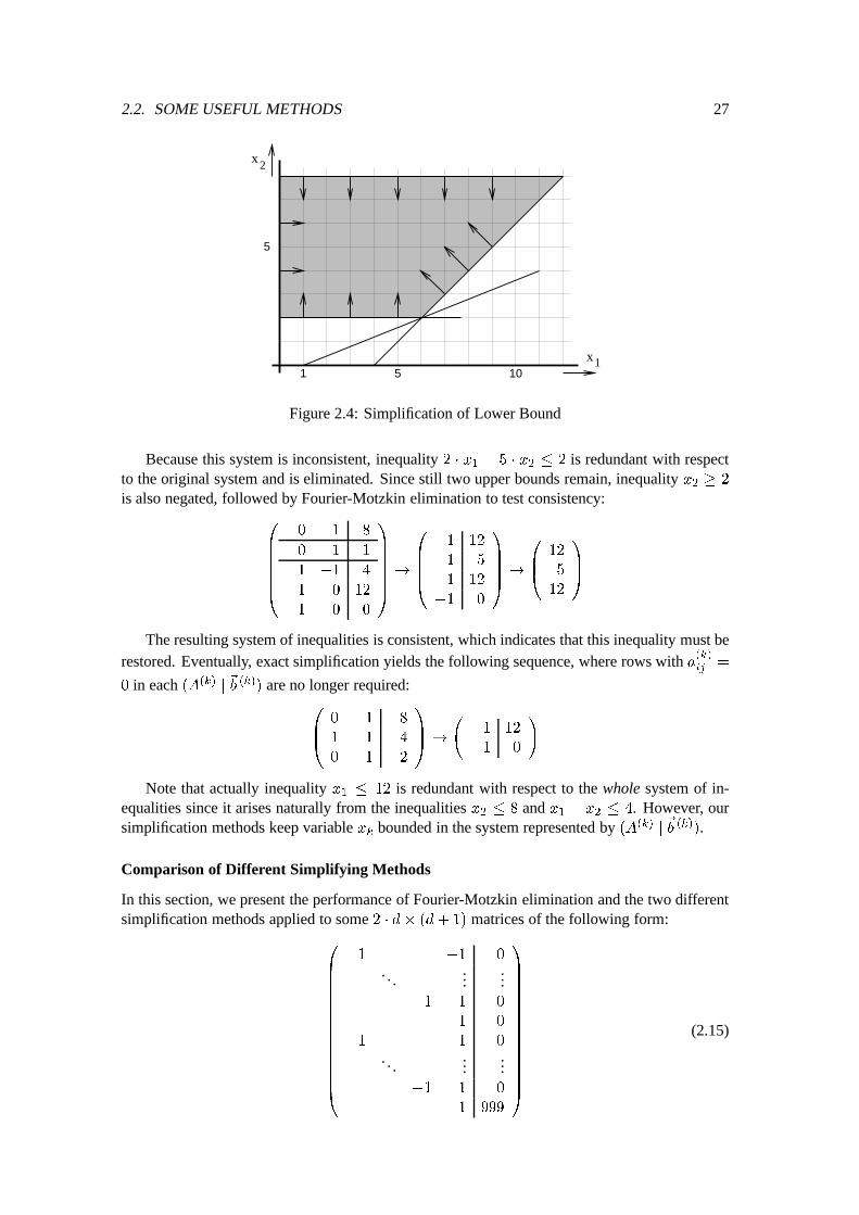
2.2. SOME USEFUL METHODS 27
5
1 5 101x
2x
Figure 2.4: Simplification of Lower Bound
Because this system is inconsistent, inequality 2 � x
1
� 5 � x
2
� 2 is redundant with respectto the original system and is eliminated. Since still two upper bounds remain, inequality x
2
� 2
is also negated, followed by Fourier-Motzkin elimination to test consistency:0
B
B
B
B
B
@
0 1 8
0 1 1
1 �1 4
1 0 12
�1 0 0
1
C
C
C
C
C
A
!
0
B
B
B
@
1 12
1 5
1 12
�1 0
1
C
C
C
A
!
0
B
@
12
5
12
1
C
A
The resulting system of inequalities is consistent, which indicates that this inequality must berestored. Eventually, exact simplification yields the following sequence, where rows with a(k)
ij
=
0 in each (A
(k)
j
~
b
(k)
) are no longer required:0
B
@
0 1 8
1 �1 4
0 �1 �2
1
C
A
!
1 12
�1 0
!
Note that actually inequality x1
� 12 is redundant with respect to the whole system of in-equalities since it arises naturally from the inequalities x
2
� 8 and x1
� x
2
� 4. However, oursimplification methods keep variable x
k
bounded in the system represented by (A
(k)
j
~
b
(k)
).
Comparison of Different Simplifying Methods
In this section, we present the performance of Fourier-Motzkin elimination and the two differentsimplification methods applied to some 2 � d� (d+ 1) matrices of the following form:
0
B
B
B
B
B
B
B
B
B
B
B
B
B
B
@
1 �1 0
. . ....
...1 �1 0
�1 0
�1 1 0
. . ....
...�1 1 0
1 999
1
C
C
C
C
C
C
C
C
C
C
C
C
C
C
A
(2.15)
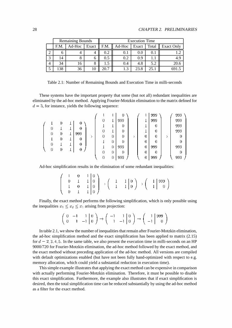
28 CHAPTER 2. PRELIMINARIES
Remaining Bounds Execution TimeF.M. Ad-Hoc Exact F.M. Ad-Hoc Exact Total Exact Only
2 6 4 4 0.2 0.1 0.0 0.1 1.23 14 8 6 0.5 0.2 0.9 1.1 4.94 34 16 8 1.5 0.4 4.8 5.2 20.65 138 36 10 20.7 1.3 23.8 25.1 691.5
Table 2.1: Number of Remaining Bounds and Execution Time in milli-seconds
These systems have the important property that some (but not all) redundant inequalities areeliminated by the ad-hoc method. Applying Fourier-Motzkin elimination to the matrix defined ford = 3, for instance, yields the following sequence:
0
B
B
B
B
B
B
B
@
�1 0 1 0
0 �1 1 0
0 0 1 999
1 0 �1 0
0 1 �1 0
0 0 �1 0
1
C
C
C
C
C
C
C
A
!
0
B
B
B
B
B
B
B
B
B
B
B
B
B
B
@
�1 1 0
0 1 999
1 �1 0
0 �1 0
0 0 0
�1 0 0
1 0 999
0 0 0
0 0 999
1
C
C
C
C
C
C
C
C
C
C
C
C
C
C
A
!
0
B
B
B
B
B
B
B
B
B
B
B
B
B
B
@
1 999
1 999
�1 0
�1 0
0 0
0 0
0 999
0 0
0 999
1
C
C
C
C
C
C
C
C
C
C
C
C
C
C
A
!
0
B
B
B
B
B
B
B
B
B
B
B
B
B
B
@
999
999
999
999
0
0
999
0
999
1
C
C
C
C
C
C
C
C
C
C
C
C
C
C
A
Ad-hoc simplification results in the elimination of some redundant inequalities:0
B
B
B
@
�1 0 1 0
0 �1 1 0
1 0 �1 0
0 1 �1 0
1
C
C
C
A
!
�1 1 0
1 �1 0
!
!
1 999
�1 0
!
Finally, the exact method performs the following simplification, which is only possible usingthe inequalities x
1
� x
2
� x
1
arising from projection:
0 �1 1 0
0 1 �1 0
!
!
�1 1 0
1 �1 0
!
!
1 999
�1 0
!
In table 2.1, we show the number of inequalities that remain after Fourier-Motzkin elimination,the ad-hoc simplification method and the exact simplification has been applied to matrix (2.15)for d = 2; 3; 4; 5. In the same table, we also present the execution time in milli-seconds on an HP9000/720 for Fourier-Motzkin elimination, the ad-hoc method followed by the exact method, andthe exact method without preceding application of the ad-hoc method. All versions are compiledwith default optimizations enabled (but have not been fully hand-optimized with respect to e.g.memory allocation, which could yield a substantial reduction in execution time).
This simple example illustrates that applying the exact method can be expensive in comparisonwith actually performing Fourier-Motzkin elimination. Therefore, it must be possible to disablethis exact simplification. Furthermore, the example also illustrates that if exact simplification isdesired, then the total simplification time can be reduced substantially by using the ad-hoc methodas a filter for the exact method.
Chapter 3
Loop Transformations
Many issues related to serial loops can be formalized using the concepts introduced in the previ-ous chapter. The iteration space of particular loops, for instance, can be represented by a systemof linear inequalities in the loop indices. Likewise, certain subscript functions may be expressedas affine transformations from an iteration space to the index space of an array. In this chapter,we first discuss these representations. In addition, we define two relations on statement instances.The execution order, arising from the sequential semantics of loops, induces a total order on state-ment instances. Data dependences, on the other hand, arise from the way in which data is usedby these statement instances. In general, data dependences (and control dependences) induce apartial order on statement instances.
An important observation for program restructuring is that changing the execution order onstatement instances does not affect the results of a program, if none of the dependences is vio-lated. Any program transformation that preserves all dependences, also preserves the semanticsof the program. In this chapter, we discuss how this observation can be used in the context of looptransformations. We briefly discuss the exploitation of implicit parallelism by relaxing the exe-cution order induced by individual DO-loops as far as dependences allow. Moreover, we discussthe framework of unimodular transformations that provides a mathematical foundation for someconventional loop transformations. Finally, we present a method that isolates the loop-body of anested loop for all iterations that satisfy a number of linear inequalities simultaneously.
3.1 Sequential Loops
In FORTRAN, the DO-loop is an important construct to define iteration. If individual DO-loopsare used within other DO-loops, a so-called nested loop results:
DO I1
= L1
, U1
: : :
DO I2
= L2
, U2
: : :
DO Id
= Ld
, Ud
B(I1
,...,Id
)ENDDO
: : :
ENDDO: : :
ENDDO
3.1.1 Loop Terminology
If no other statements appear in between the individual DO-loops, then the whole loop is called aperfectly nested loop. For d = 2 and d = 3, we speak of double and triple loops respectively.
30 CHAPTER 3. LOOP TRANSFORMATIONS
A loop in which arbitrary statements, or even complete other DO-loops appear in between theindividual DO-loops is referred to as a non-perfectly nested loop. We assume that each I
i
is aninteger-valued variable, called a loop index. We will refer to the DO-loop having I
i
as loop indexas the I
i
-loop. We call ~I = (I
1
; : : : ; I
d
)
T the index vector of the nested loop. The loop-bodyB of this loop consists of a sequence of indexed statements at nesting depth d. Each individualindexed statement in this loop-body is denoted by S
i
(
~
I) for some unique label Si
. These labelsreflect the relative position of a statement in a program in the sense that if S
i
textually appearsbefore S
j
, then i < j holds.If the loop-body is executed for the value ~I = ~{, where~{ 2 Zd, then we call this vector an
iteration (vector) of this loop. Substituting the value~{ 2 Zd for ~I in an indexed statement Si
(
~
I)
in this loop-body yields the statement instance Si
(~{) executed during this iteration. Statementsat nesting depth zero only have one instance and are usually referred to as scalar statements. Theset IS of all iterations for which the loop-body of a nested loop is executed is called the itera-tion space of the loop. Under the assumption that only integer-valued variables are used as loopindices, we have IS � Zd.Example: Consider the following double loop:
DO I1
= 1, 2DO I
2
= 1, 3S
1
: A(I1
,I2
) = 10.0S
2
: B(I1
,I2
) = B(I1
,I2
) - 1ENDDO
ENDDO
The index vector of this loop is ~I = (I
1
; I
2
)
T . The loop-body consists of the two assignmentstatements S
1
and S2
, appearing at nesting depth two. For this loop, S1
(
~
I) denotes the indexedstatement ‘A(I
1
,I2
)=10.0 ’ and S1
(1; 2) denotes the instance ‘A(1,2)=10.0 ’ of this state-ment executed in iteration~I = (1; 2)
T . The iteration space IS � Z2 of this loop is shown below:
IS = f(1; 1)
T
; (1; 2)
T
; (1; 3)
T
; (2; 1)
T
; (2; 2)
T
; (2; 3)
T
g
3.1.2 Loop Bounds
Because DO-loop normalization [234, p174–177] can be used to enforce unit strides, usually weassume that each DO-loop is stride one. For such a DO-loop, the loop index I
i
iterates over allintegers in the closed interval [L
i
; U
i
], called the execution set of the Ii
-loop. This execution setis defined by the loop bounds L
i
and U
i
, which may depend on the indices of outer DO-loops.
Admissible Loop Bounds
A single lower bound L
i
or upper bound U
i
is called an admissible loop bound if it can be ex-pressed as follows, where all l
ij
; u
ij
2 Z and lii
> 0 and uii
> 0:
L
i
=
2
6
6
6
6
6
6
l
i0
+
i�1
P
j=1
l
ij
� I
j
l
ii
3
7
7
7
7
7
7
and U
i
=
6
6
6
6
6
6
4
u
i0
+
i�1
P
j=1
u
ij
� I
j
u
ii
7
7
7
7
7
7
5
Because Ii
is an integer-valued variable and lii
> 0, the inequality L
i
� I
i
can be expressedin terms of the index vector ~I as follows:
(l
i1
: : : l
i;i�1
�l
ii
0 : : : 0
| {z }
d�i
) �
~
I � �l
i0 (3.1)
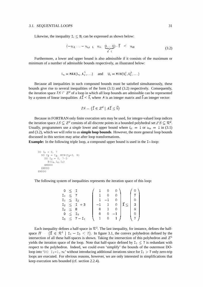
3.1. SEQUENTIAL LOOPS 31
Likewise, the inequality I
i
� U
i
can be expressed as shown below:
(�u
i1
: : :� u
i;i�1
u
ii
0 : : : 0
| {z }
d�i
) �
~
I � u
i0 (3.2)
Furthermore, a lower and upper bound is also admissible if it consists of the maximum orminimum of a number of admissible bounds respectively, as illustrated below:
L
i
= MAX(L
1
i
; L
2
i
; : : :) and U
i
= MIN(U
1
i
; U
2
i
; : : :)
Because all inequalities in such compound bounds must be satisfied simultaneously, thesebounds give rise to several inequalities of the form (3.1) and (3.2) respectively. Consequently,the iteration space IS � Zd of a loop in which all loop bounds are admissible can be representedby a system of linear inequalities A~I � ~b, where A is an integer matrix and~b an integer vector:
IS = f
~
I 2 Z
d
j A
~
I �
~
bg
Because in FORTRAN only finite execution sets may be used, for integer-valued loop indicesthe iteration space IS � Zd consists of all discrete points in a bounded polyhedral set PS � Rd.Usually, programmers use a single lower and upper bound where l
ii
= 1 or uii
= 1 in (3.1)and (3.2), which we will refer to as simple loop bounds. However, the more general loop boundsdiscussed in this section may arise after loop transformations.Example: In the following triple loop, a compound upper bound is used in the I
2
-loop:
DO I1
= 0, 7DO I
2
= I1
, MIN(I1
+3, 8)DO I
3
= 0, 7-I1
B(I1
,I2
,I3
)ENDDO
ENDDOENDDO
The following system of inequalities represents the iteration space of this loop:
0 � I
1
I
1
� 7
I
1
� I
2
I
2
� I
1
+ 3
I
2
� 8
0 � I
3
I
3
� 7� I
1
0
B
B
B
B
B
B
B
B
B
B
@
�1 0 0
1 0 0
1 �1 0
�1 1 0
0 1 0
0 0 �1
1 0 1
1
C
C
C
C
C
C
C
C
C
C
A
~
I �
0
B
B
B
B
B
B
B
B
B
B
@
0
7
0
3
8
0
7
1
C
C
C
C
C
C
C
C
C
C
A
Each inequality defines a half-space inR3. The last inequality, for instance, defines the half-space H = f
~
I 2 R
3
j I
1
+ I
3
� 7g. In figure 3.1, the convex polyhedron defined by theintersection of all these half-spaces is shown. Taking the intersection of this polyhedron and Z3
yields the iteration space of the loop. Note that half-space defined by I
1
� 7 is redundant withrespect to the polyhedron. Indeed, we could even ‘simplify’ the bounds of the outermost DO-loop into ‘DO I
1
=1, 1’ without introducing additional iterations since for I1
> 7 only zero-triploops are executed. For obvious reasons, however, we are only interested in simplifications thatkeep execution sets bounded (cf. section 2.2.4).
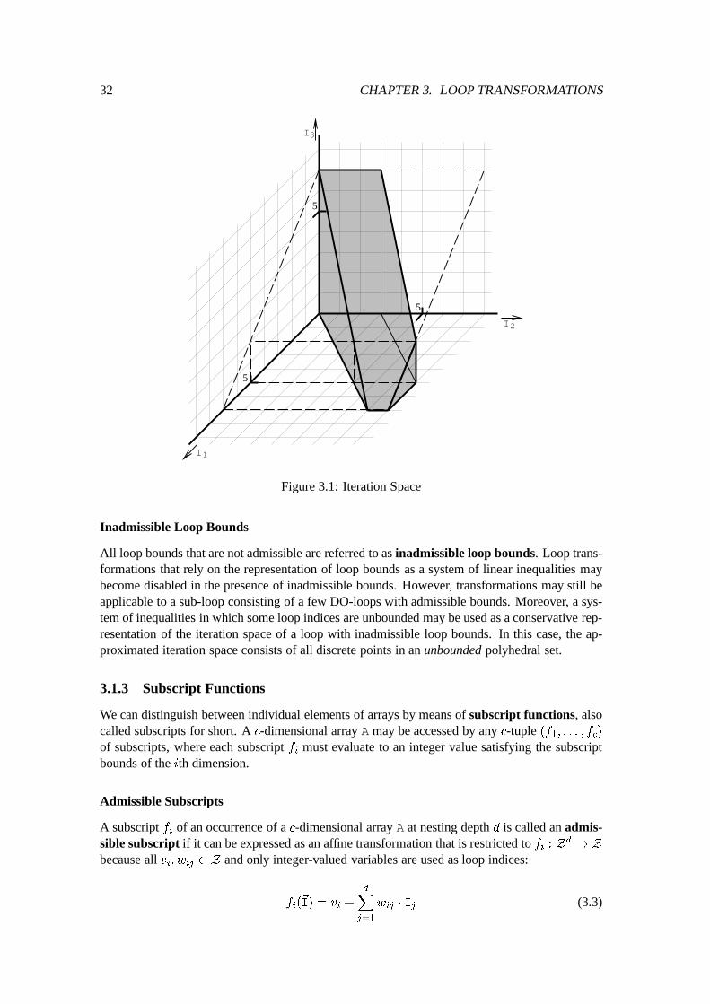
32 CHAPTER 3. LOOP TRANSFORMATIONS
2
3
1I
I
I
5
5
5
Figure 3.1: Iteration Space
Inadmissible Loop Bounds
All loop bounds that are not admissible are referred to as inadmissible loop bounds. Loop trans-formations that rely on the representation of loop bounds as a system of linear inequalities maybecome disabled in the presence of inadmissible bounds. However, transformations may still beapplicable to a sub-loop consisting of a few DO-loops with admissible bounds. Moreover, a sys-tem of inequalities in which some loop indices are unbounded may be used as a conservative rep-resentation of the iteration space of a loop with inadmissible loop bounds. In this case, the ap-proximated iteration space consists of all discrete points in an unbounded polyhedral set.
3.1.3 Subscript Functions
We can distinguish between individual elements of arrays by means of subscript functions, alsocalled subscripts for short. A c-dimensional array A may be accessed by any c-tuple (f
1
; : : : ; f
c
)
of subscripts, where each subscript fi
must evaluate to an integer value satisfying the subscriptbounds of the ith dimension.
Admissible Subscripts
A subscript fi
of an occurrence of a c-dimensional array A at nesting depth d is called an admis-sible subscript if it can be expressed as an affine transformation that is restricted to f
i
: Z
d
! Z
because all vi
; w
ij
2 Z and only integer-valued variables are used as loop indices:
f
i
(
~
I) = v
i
+
d
X
j=1
w
ij
� I
j
(3.3)
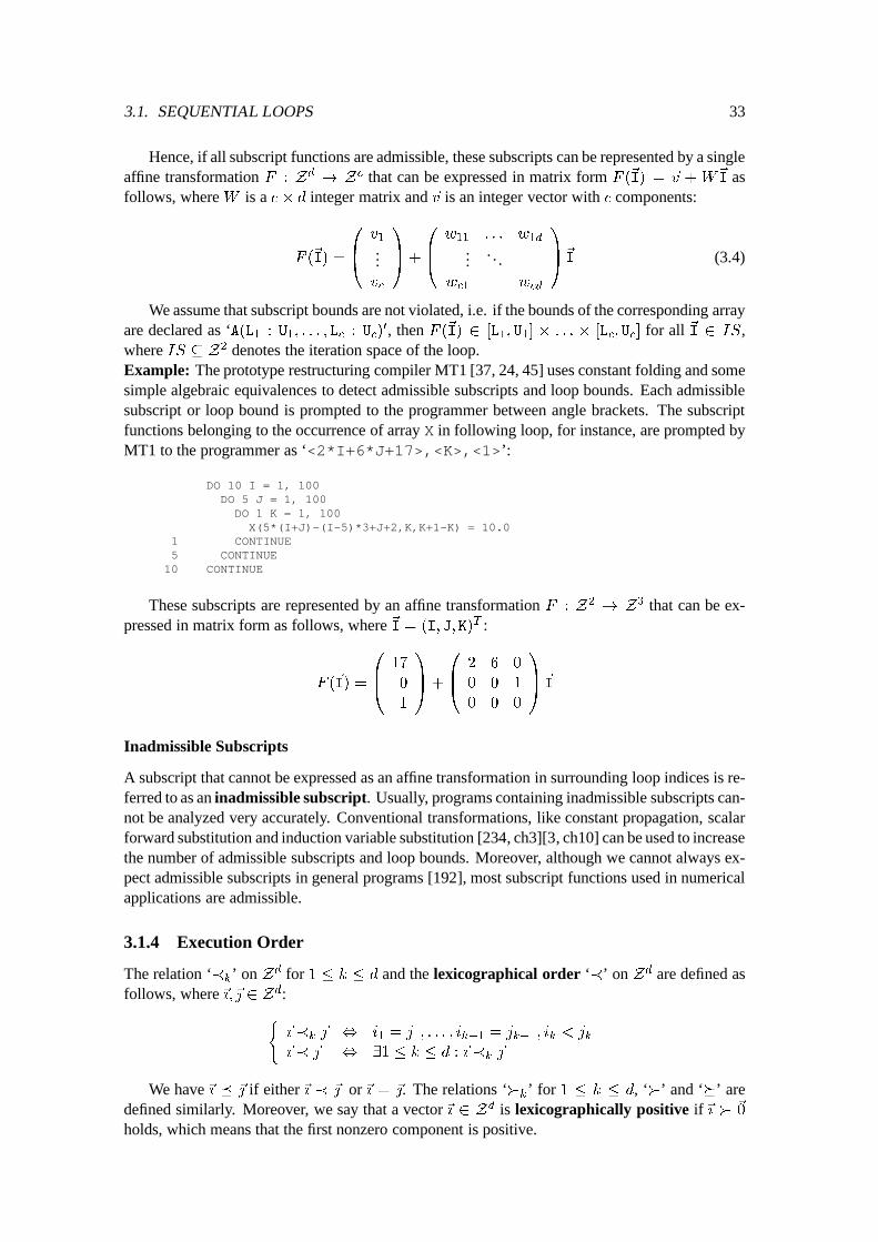
3.1. SEQUENTIAL LOOPS 33
Hence, if all subscript functions are admissible, these subscripts can be represented by a singleaffine transformation F : Z
d
! Z
c that can be expressed in matrix form F (
~
I) = ~v +W
~
I asfollows, where W is a c� d integer matrix and ~v is an integer vector with c components:
F (
~
I) =
0
B
@
v
1
...v
c
1
C
A
+
0
B
@
w
11
: : : w
1d
.... . .
w
c1
w
cd
1
C
A
~
I (3.4)
We assume that subscript bounds are not violated, i.e. if the bounds of the corresponding arrayare declared as ‘A(L
1
: U
1
; : : : ; L
c
: U
c
)
0, then F (~I) 2 [L
1
; U
1
] � : : : � [L
c
; U
c
] for all ~I 2 IS,where IS � Z2 denotes the iteration space of the loop.Example: The prototype restructuring compiler MT1 [37, 24, 45] uses constant folding and somesimple algebraic equivalences to detect admissible subscripts and loop bounds. Each admissiblesubscript or loop bound is prompted to the programmer between angle brackets. The subscriptfunctions belonging to the occurrence of array X in following loop, for instance, are prompted byMT1 to the programmer as ‘<2*I+6*J+17>,<K>,<1> ’:
DO 10 I = 1, 100DO 5 J = 1, 100
DO 1 K = 1, 100X(5*(I+J)-(I-5)*3+J+2,K,K+1-K) = 10.0
1 CONTINUE5 CONTINUE
10 CONTINUE
These subscripts are represented by an affine transformation F : Z
2
! Z
3 that can be ex-pressed in matrix form as follows, where ~I = (I; J; K)
T :
F (
~
I) =
0
B
@
17
0
1
1
C
A
+
0
B
@
2 6 0
0 0 1
0 0 0
1
C
A
~
I
Inadmissible Subscripts
A subscript that cannot be expressed as an affine transformation in surrounding loop indices is re-ferred to as an inadmissible subscript. Usually, programs containing inadmissible subscripts can-not be analyzed very accurately. Conventional transformations, like constant propagation, scalarforward substitution and induction variable substitution [234, ch3][3, ch10] can be used to increasethe number of admissible subscripts and loop bounds. Moreover, although we cannot always ex-pect admissible subscripts in general programs [192], most subscript functions used in numericalapplications are admissible.
3.1.4 Execution Order
The relation ‘�k
’ on Zd for 1 � k � d and the lexicographical order ‘�’ on Zd are defined asfollows, where~{;~| 2 Zd:
(
~{ �
k
~| , i
1
= j
1
; : : : ; i
k�1
= j
k�1
; i
k
< j
k
~{ � ~| , 91 � k � d :~{ �
k
~|
We have~{ � ~| if either~{ � ~| or~{ = ~|. The relations ‘�k
’ for 1 � k � d, ‘�’ and ‘�’ aredefined similarly. Moreover, we say that a vector~{ 2 Zd is lexicographically positive if~{ � ~0holds, which means that the first nonzero component is positive.
34 CHAPTER 3. LOOP TRANSFORMATIONS
The following notation is used to isolate some consecutive components of a vector~{ 2 Zd,where 1 � c
1
� c
2
� d:
~{ [c
1
: c
2
] = (i
c
1
; : : : ; i
c
2
)
T
Let IS � Zdi and JS � Zdj denote the iteration spaces of two loops in which respectivelythe statements S
i
and Sj
occur. We define the common nesting depth d � min(d
i
; d
j
) of Si
andS
j
as the nesting depth of the innermost DO-loop that is still shared by both statements. The exe-cution order ‘<
o
’ on instances of Si
and Sj
, induced by the sequential semantics of FORTRANDO-loops with positive strides, can be defined as follows, where~{ 2 IS and ~| 2 JS:
S
i
(~{ ) <
o
S
j
(~| ) ,
8
>
<
>
:
~{ [1 : d] � ~| [1 : d]
or~{ [1 : d] = ~| [1 : d] and i < j
If the stride of a particular DO-loop is negative, the value of the corresponding component ofthe iteration vector decreases in successive iterations of that DO-loop. Although it is straightfor-ward to deal with this subtlety in the definition of ‘<
o
’ [228], usually we assume that all stridesare positive. In fact, most DO-loops are stride-1 [123], whereas, as stated before, DO-loop nor-malization can be used to enforce unit strides.
3.1.5 Data Dependences
In this section, we define data dependences. This relation on statement instances arises from theflow of data in a program and, in contrast with the execution order, induces a partial order onstatement instances.
Input and Output Sets
The input set and the output set of a statement Si
, denoted by IN(S
i
) and OUT(Si
) respectively,consist of all variables that may be read or written to by this statement. Substituting an iteration~{ 2 IS for the index vector of the loop with iteration space IS � Zd in which S
i
appears yieldsthe sets IN(S
i
(~{ )) and OUT(Si
(~{ )) consisting of the actual elements that are read or written to bythe statement instance S
i
(~{ ).Example: Consider the following assignment statement:
S
1
: X(K+1) = A(I,J) * S - 4.0
The input and output set of this statement are shown below:
(
IN(S
1
) = f A(I; J); I; J; K; S g
OUT(S1
) = f X(K+ 1) g
If the variables I , J and Kare used as loop indices, then the input and output set of the instanceS
1
(1; 2; 3) have the following form (the loop indices vanish):
(
IN(S
1
(1; 2; 3)) = f A(1; 2); S g
OUT(S1
(1; 2; 3)) = f X(4) g
The input and output sets of statements enables us to define data dependences.
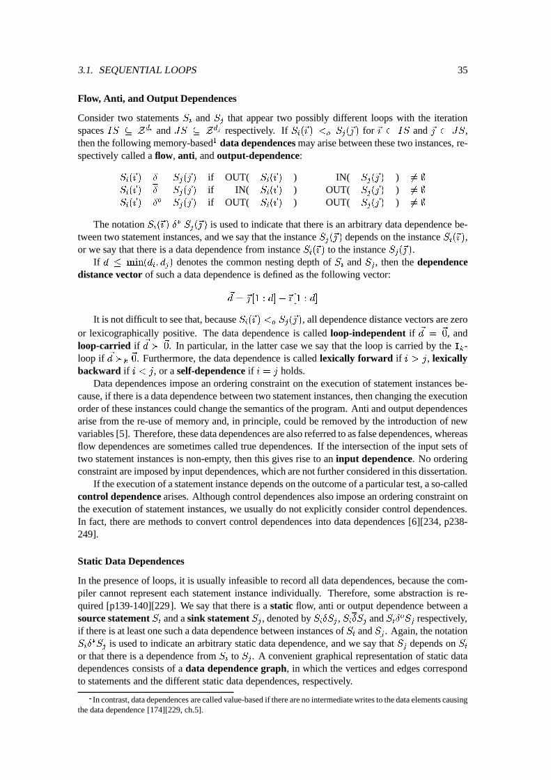
3.1. SEQUENTIAL LOOPS 35
Flow, Anti, and Output Dependences
Consider two statements Si
and Sj
that appear two possibly different loops with the iterationspaces IS � Zdi and JS � Zdj respectively. If S
i
(~{ ) <
o
S
j
(~| ) for ~{ 2 IS and ~| 2 JS,then the following memory-based1 data dependences may arise between these two instances, re-spectively called a flow, anti, and output-dependence:
S
i
(~{ ) � S
j
(~| ) if OUT( S
i
(~{ ) ) \ IN( S
j
(~| ) ) 6= ;
S
i
(~{ ) � S
j
(~| ) if IN( S
i
(~{ ) ) \ OUT( S
j
(~| ) ) 6= ;
S
i
(~{ ) �
o
S
j
(~| ) if OUT( S
i
(~{ ) ) \ OUT( S
j
(~| ) ) 6= ;
The notation Si
(~{ ) �
�
S
j
(~| ) is used to indicate that there is an arbitrary data dependence be-tween two statement instances, and we say that the instance S
j
(~| ) depends on the instance Si
(~{ ),or we say that there is a data dependence from instance S
i
(~{ ) to the instance Sj
(~| ).If d � min(d
i
; d
j
) denotes the common nesting depth of Si
and Sj
, then the dependencedistance vector of such a data dependence is defined as the following vector:
~
d = ~| [1 : d]�~{ [1 : d]
It is not difficult to see that, because Si
(~{ ) <
o
S
j
(~| ), all dependence distance vectors are zeroor lexicographically positive. The data dependence is called loop-independent if ~d =
~
0, andloop-carried if ~d � ~
0. In particular, in the latter case we say that the loop is carried by the I
k
-loop if ~d �
k
~
0. Furthermore, the data dependence is called lexically forward if i > j, lexicallybackward if i < j, or a self-dependence if i = j holds.
Data dependences impose an ordering constraint on the execution of statement instances be-cause, if there is a data dependence between two statement instances, then changing the executionorder of these instances could change the semantics of the program. Anti and output dependencesarise from the re-use of memory and, in principle, could be removed by the introduction of newvariables [5]. Therefore, these data dependences are also referred to as false dependences, whereasflow dependences are sometimes called true dependences. If the intersection of the input sets oftwo statement instances is non-empty, then this gives rise to an input dependence. No orderingconstraint are imposed by input dependences, which are not further considered in this dissertation.
If the execution of a statement instance depends on the outcome of a particular test, a so-calledcontrol dependence arises. Although control dependences also impose an ordering constraint onthe execution of statement instances, we usually do not explicitly consider control dependences.In fact, there are methods to convert control dependences into data dependences [6][234, p238-249].
Static Data Dependences
In the presence of loops, it is usually infeasible to record all data dependences, because the com-piler cannot represent each statement instance individually. Therefore, some abstraction is re-quired [p139-140][229]. We say that there is a static flow, anti or output dependence between asource statement S
i
and a sink statement Sj
, denoted by Si
�S
j
, Si
�S
j
and Si
�
o
S
j
respectively,if there is at least one such a data dependence between instances of S
i
and Sj
. Again, the notationS
i
�
�
S
j
is used to indicate an arbitrary static data dependence, and we say that Sj
depends on Si
or that there is a dependence from S
i
to Sj
. A convenient graphical representation of static datadependences consists of a data dependence graph, in which the vertices and edges correspondto statements and the different static data dependences, respectively.
1In contrast, data dependences are called value-based if there are no intermediate writes to the data elements causingthe data dependence [174][229, ch.5].
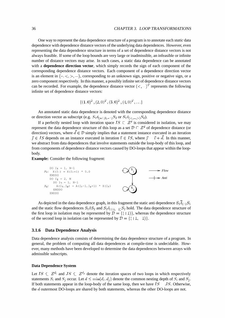
36 CHAPTER 3. LOOP TRANSFORMATIONS
One way to represent the data dependence structure of a program is to annotate each static datadependence with dependence distance vectors of the underlying data dependences. However, evenrepresenting the data dependence structure in terms of a set of dependence distance vectors is notalways feasible. If some of the loop bounds are very large or inadmissible, an infeasible or infinitenumber of distance vectors may arise. In such cases, a static data dependence can be annotatedwith a dependence direction vector, which simply records the sign of each component of thecorresponding dependence distance vectors. Each component of a dependence direction vectoris an element in f�; <;>;=g, corresponding to an unknown sign, positive or negative sign, or azero component respectively. In this manner, a possibly infinite set of dependence distance vectorscan be recorded. For example, the dependence distance vector (<;=)
T represents the followinginfinite set of dependence distance vectors:
f(1; 0)
T
; (2; 0)
T
; (3; 0)
T
; (4; 0)
T
; : : :g
An annotated static data dependence is denoted with the corresponding dependence distanceor direction vector as subscript (e.g. S
1
�
(+1;0;�4)
S
2
or S1
�
(<;=;>)
S
2
).If a perfectly nested loop with iteration space IS � Zd is considered in isolation, we may
represent the data dependence structure of this loop as a set D � Zd of dependence distance (ordirection) vectors, where ~d 2 D simply implies that a statement instance executed in an iteration~| 2 IS depends on an instance executed in iteration~{ 2 IS, where ~| = ~{ +
~
d. In this manner,we abstract from data dependences that involve statements outside the loop-body of this loop, andfrom components of dependence distance vectors caused by DO-loops that appear within the loop-body.Example: Consider the following fragment:
DO I1
= 1, N-1S
1
: X(I1
) = X(I1
+1) * 5.0ENDDODO I
1
= 2, NDO I
2
= 1, N-1S
2
: A(I1
,I2
) = A(I1
-1,I2
+1) * X(I1
)ENDDO
ENDDO2
S
1S Flow
Anti
As depicted in the data dependence graph, in this fragment the static anti dependence S1
�
(1)
S
1
and the static flow dependences S1
�S
2
and S2
�
(+1;�1)
S
2
hold. The data dependence structure ofthe first loop in isolation may be represented by D = f(+1)g, whereas the dependence structureof the second loop in isolation can be represented by D = f(+1;�1)g.
3.1.6 Data Dependence Analysis
Data dependence analysis consists of determining the data dependence structure of a program. Ingeneral, the problem of computing all data dependences at compile-time is undecidable. How-ever, many methods have been developed to determine the data dependences between arrays withadmissible subscripts.
Data Dependence System
Let IS � Zdi and JS � Zdj denote the iteration spaces of two loops in which respectivelystatements S
i
and Sj
occur. Let d � min(d
i
; d
j
) denote the common nesting depth of Si
and Sj
.If both statements appear in the loop-body of the same loop, then we have IS = JS. Otherwise,the d outermost DO-loops are shared by both statements, whereas the other DO-loops are not.
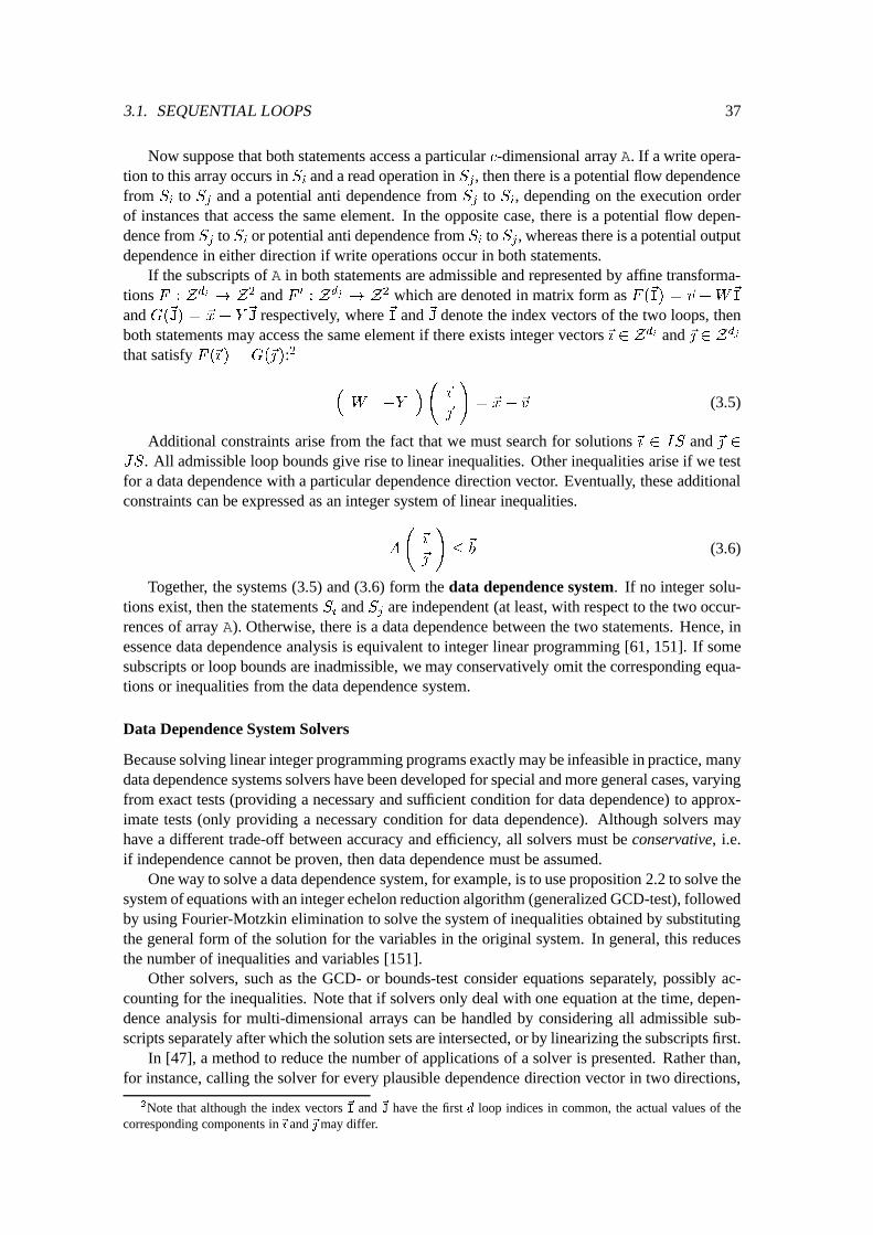
3.1. SEQUENTIAL LOOPS 37
Now suppose that both statements access a particular c-dimensional array A. If a write opera-tion to this array occurs in S
i
and a read operation in Sj
, then there is a potential flow dependencefrom S
i
to Sj
and a potential anti dependence from S
j
to Si
, depending on the execution orderof instances that access the same element. In the opposite case, there is a potential flow depen-dence from S
j
to Si
or potential anti dependence from S
i
to Sj
, whereas there is a potential outputdependence in either direction if write operations occur in both statements.
If the subscripts of A in both statements are admissible and represented by affine transforma-tions F : Z
d
i
! Z
2 and F 0 : Zdj ! Z2 which are denoted in matrix form as F (~I) = ~v +W
~
I
and G(
~
J) = ~x+ Y
~
J respectively, where ~I and ~J denote the index vectors of the two loops, thenboth statements may access the same element if there exists integer vectors~{ 2 Zdi and ~| 2 Zdj
that satisfy F (~{ ) = G(~| ):2
�
W �Y
�
~{
~|
!
= ~x� ~v (3.5)
Additional constraints arise from the fact that we must search for solutions ~{ 2 IS and ~| 2JS. All admissible loop bounds give rise to linear inequalities. Other inequalities arise if we testfor a data dependence with a particular dependence direction vector. Eventually, these additionalconstraints can be expressed as an integer system of linear inequalities.
A
~{
~|
!
�
~
b (3.6)
Together, the systems (3.5) and (3.6) form the data dependence system. If no integer solu-tions exist, then the statements S
i
and Sj
are independent (at least, with respect to the two occur-rences of array A). Otherwise, there is a data dependence between the two statements. Hence, inessence data dependence analysis is equivalent to integer linear programming [61, 151]. If somesubscripts or loop bounds are inadmissible, we may conservatively omit the corresponding equa-tions or inequalities from the data dependence system.
Data Dependence System Solvers
Because solving linear integer programming programs exactly may be infeasible in practice, manydata dependence systems solvers have been developed for special and more general cases, varyingfrom exact tests (providing a necessary and sufficient condition for data dependence) to approx-imate tests (only providing a necessary condition for data dependence). Although solvers mayhave a different trade-off between accuracy and efficiency, all solvers must be conservative, i.e.if independence cannot be proven, then data dependence must be assumed.
One way to solve a data dependence system, for example, is to use proposition 2.2 to solve thesystem of equations with an integer echelon reduction algorithm (generalized GCD-test), followedby using Fourier-Motzkin elimination to solve the system of inequalities obtained by substitutingthe general form of the solution for the variables in the original system. In general, this reducesthe number of inequalities and variables [151].
Other solvers, such as the GCD- or bounds-test consider equations separately, possibly ac-counting for the inequalities. Note that if solvers only deal with one equation at the time, depen-dence analysis for multi-dimensional arrays can be handled by considering all admissible sub-scripts separately after which the solution sets are intersected, or by linearizing the subscripts first.
In [47], a method to reduce the number of applications of a solver is presented. Rather than,for instance, calling the solver for every plausible dependence direction vector in two directions,
2Note that although the index vectors ~I and ~
J have the first d loop indices in common, the actual values of thecorresponding components in~{ and ~| may differ.
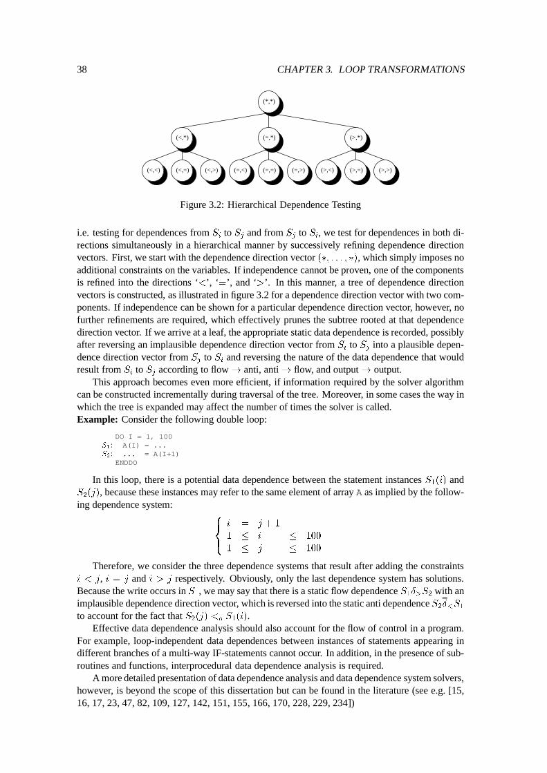
38 CHAPTER 3. LOOP TRANSFORMATIONS
(*,*)
(<,*) (=,*) (>,*)
(<,<) (<,=) (<,>) (=,<) (=,=) (=,>) (>,<) (>,=) (>,>)
Figure 3.2: Hierarchical Dependence Testing
i.e. testing for dependences from S
i
to Sj
and from S
j
to Si
, we test for dependences in both di-rections simultaneously in a hierarchical manner by successively refining dependence directionvectors. First, we start with the dependence direction vector (�; : : : ; �), which simply imposes noadditional constraints on the variables. If independence cannot be proven, one of the componentsis refined into the directions ‘<’, ‘=’, and ‘>’. In this manner, a tree of dependence directionvectors is constructed, as illustrated in figure 3.2 for a dependence direction vector with two com-ponents. If independence can be shown for a particular dependence direction vector, however, nofurther refinements are required, which effectively prunes the subtree rooted at that dependencedirection vector. If we arrive at a leaf, the appropriate static data dependence is recorded, possiblyafter reversing an implausible dependence direction vector from S
i
to Sj
into a plausible depen-dence direction vector from S
j
to Si
and reversing the nature of the data dependence that wouldresult from S
i
to Sj
according to flow! anti, anti! flow, and output! output.This approach becomes even more efficient, if information required by the solver algorithm
can be constructed incrementally during traversal of the tree. Moreover, in some cases the way inwhich the tree is expanded may affect the number of times the solver is called.Example: Consider the following double loop:
DO I = 1, 100S
1
: A(I) = ...S
2
: ... = A(I+1)ENDDO
In this loop, there is a potential data dependence between the statement instances S1
(i) andS
2
(j), because these instances may refer to the same element of array A as implied by the follow-ing dependence system:
8
>
<
>
:
i = j + 1
1 � i � 100
1 � j � 100
Therefore, we consider the three dependence systems that result after adding the constraintsi < j, i = j and i > j respectively. Obviously, only the last dependence system has solutions.Because the write occurs in S
1
, we may say that there is a static flow dependence S1
�
>
S
2
with animplausible dependence direction vector, which is reversed into the static anti dependence S
2
�
<
S
1
to account for the fact that S2
(j) <
o
S
1
(i).Effective data dependence analysis should also account for the flow of control in a program.
For example, loop-independent data dependences between instances of statements appearing indifferent branches of a multi-way IF-statements cannot occur. In addition, in the presence of sub-routines and functions, interprocedural data dependence analysis is required.
A more detailed presentation of data dependence analysis and data dependence system solvers,however, is beyond the scope of this dissertation but can be found in the literature (see e.g. [15,16, 17, 23, 47, 82, 109, 127, 142, 151, 155, 166, 170, 228, 229, 234])
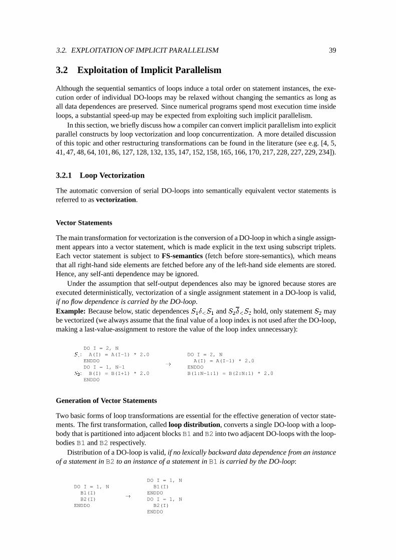
3.2. EXPLOITATION OF IMPLICIT PARALLELISM 39
3.2 Exploitation of Implicit Parallelism
Although the sequential semantics of loops induce a total order on statement instances, the exe-cution order of individual DO-loops may be relaxed without changing the semantics as long asall data dependences are preserved. Since numerical programs spend most execution time insideloops, a substantial speed-up may be expected from exploiting such implicit parallelism.
In this section, we briefly discuss how a compiler can convert implicit parallelism into explicitparallel constructs by loop vectorization and loop concurrentization. A more detailed discussionof this topic and other restructuring transformations can be found in the literature (see e.g. [4, 5,41, 47, 48, 64, 101, 86, 127, 128, 132, 135, 147, 152, 158, 165, 166, 170, 217, 228, 227, 229, 234]).
3.2.1 Loop Vectorization
The automatic conversion of serial DO-loops into semantically equivalent vector statements isreferred to as vectorization.
Vector Statements
The main transformation for vectorization is the conversion of a DO-loop in which a single assign-ment appears into a vector statement, which is made explicit in the text using subscript triplets.Each vector statement is subject to FS-semantics (fetch before store-semantics), which meansthat all right-hand side elements are fetched before any of the left-hand side elements are stored.Hence, any self-anti dependence may be ignored.
Under the assumption that self-output dependences also may be ignored because stores areexecuted deterministically, vectorization of a single assignment statement in a DO-loop is valid,if no flow dependence is carried by the DO-loop.Example: Because below, static dependences S
1
�
<
S
1
and S2
�
<
S
2
hold, only statement S2
maybe vectorized (we always assume that the final value of a loop index is not used after the DO-loop,making a last-value-assignment to restore the value of the loop index unnecessary):
DO I = 2, NS
1
: A(I) = A(I-1) * 2.0ENDDODO I = 1, N-1
S
2
: B(I) = B(I+1) * 2.0ENDDO
!
DO I = 2, NA(I) = A(I-1) * 2.0
ENDDOB(1:N-1:1) = B(2:N:1) * 2.0
Generation of Vector Statements
Two basic forms of loop transformations are essential for the effective generation of vector state-ments. The first transformation, called loop distribution, converts a single DO-loop with a loop-body that is partitioned into adjacent blocks B1 and B2 into two adjacent DO-loops with the loop-bodies B1 and B2 respectively.
Distribution of a DO-loop is valid, if no lexically backward data dependence from an instanceof a statement in B2 to an instance of a statement in B1 is carried by the DO-loop:
DO I = 1, NB1(I)B2(I)
ENDDO
!
DO I = 1, NB1(I)
ENDDODO I = 1, N
B2(I)ENDDO
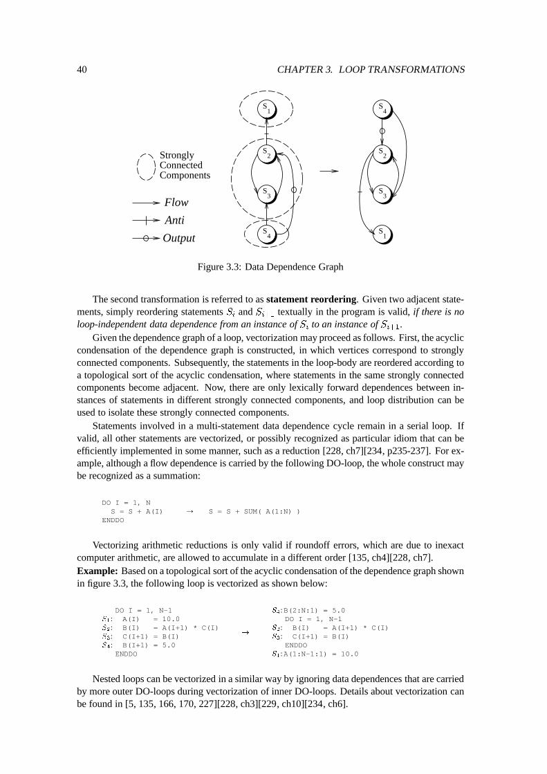
40 CHAPTER 3. LOOP TRANSFORMATIONS
S3
2S
1S
S4
Flow
Anti
Output
S3
2S
1S
S4
StronglyConnectedComponents
Figure 3.3: Data Dependence Graph
The second transformation is referred to as statement reordering. Given two adjacent state-ments, simply reordering statements S
i
and Si+1
textually in the program is valid, if there is noloop-independent data dependence from an instance of S
i
to an instance of Si+1
.Given the dependence graph of a loop, vectorization may proceed as follows. First, the acyclic
condensation of the dependence graph is constructed, in which vertices correspond to stronglyconnected components. Subsequently, the statements in the loop-body are reordered according toa topological sort of the acyclic condensation, where statements in the same strongly connectedcomponents become adjacent. Now, there are only lexically forward dependences between in-stances of statements in different strongly connected components, and loop distribution can beused to isolate these strongly connected components.
Statements involved in a multi-statement data dependence cycle remain in a serial loop. Ifvalid, all other statements are vectorized, or possibly recognized as particular idiom that can beefficiently implemented in some manner, such as a reduction [228, ch7][234, p235-237]. For ex-ample, although a flow dependence is carried by the following DO-loop, the whole construct maybe recognized as a summation:
DO I = 1, NS = S + A(I)
ENDDO! S = S + SUM( A(1:N) )
Vectorizing arithmetic reductions is only valid if roundoff errors, which are due to inexactcomputer arithmetic, are allowed to accumulate in a different order [135, ch4][228, ch7].Example: Based on a topological sort of the acyclic condensation of the dependence graph shownin figure 3.3, the following loop is vectorized as shown below:
DO I = 1, N-1S
1
: A(I) = 10.0S
2
: B(I) = A(I+1) * C(I)S
3
: C(I+1) = B(I)S
4
: B(I+1) = 5.0ENDDO
!
S
4
:B(2:N:1) = 5.0DO I = 1, N-1
S
2
: B(I) = A(I+1) * C(I)S
3
: C(I+1) = B(I)ENDDO
S
1
:A(1:N-1:1) = 10.0
Nested loops can be vectorized in a similar way by ignoring data dependences that are carriedby more outer DO-loops during vectorization of inner DO-loops. Details about vectorization canbe found in [5, 135, 166, 170, 227][228, ch3][229, ch10][234, ch6].
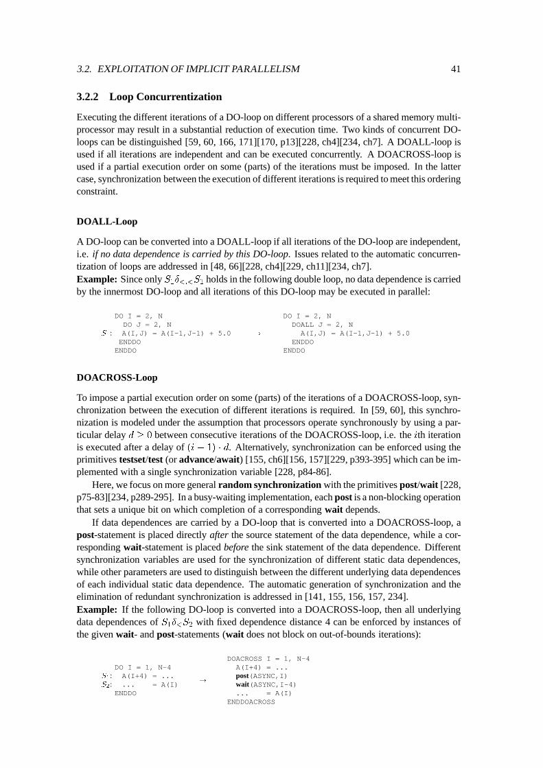
3.2. EXPLOITATION OF IMPLICIT PARALLELISM 41
3.2.2 Loop Concurrentization
Executing the different iterations of a DO-loop on different processors of a shared memory multi-processor may result in a substantial reduction of execution time. Two kinds of concurrent DO-loops can be distinguished [59, 60, 166, 171][170, p13][228, ch4][234, ch7]. A DOALL-loop isused if all iterations are independent and can be executed concurrently. A DOACROSS-loop isused if a partial execution order on some (parts) of the iterations must be imposed. In the lattercase, synchronization between the execution of different iterations is required to meet this orderingconstraint.
DOALL-Loop
A DO-loop can be converted into a DOALL-loop if all iterations of the DO-loop are independent,i.e. if no data dependence is carried by this DO-loop. Issues related to the automatic concurren-tization of loops are addressed in [48, 66][228, ch4][229, ch11][234, ch7].Example: Since only S
1
�
<;<
S
1
holds in the following double loop, no data dependence is carriedby the innermost DO-loop and all iterations of this DO-loop may be executed in parallel:
DO I = 2, NDO J = 2, N
S
1
: A(I,J) = A(I-1,J-1) + 5.0ENDDOENDDO
!
DO I = 2, NDOALL J = 2, N
A(I,J) = A(I-1,J-1) + 5.0ENDDO
ENDDO
DOACROSS-Loop
To impose a partial execution order on some (parts) of the iterations of a DOACROSS-loop, syn-chronization between the execution of different iterations is required. In [59, 60], this synchro-nization is modeled under the assumption that processors operate synchronously by using a par-ticular delay d � 0 between consecutive iterations of the DOACROSS-loop, i.e. the ith iterationis executed after a delay of (i � 1) � d. Alternatively, synchronization can be enforced using theprimitives testset/test (or advance/await) [155, ch6][156, 157][229, p393-395] which can be im-plemented with a single synchronization variable [228, p84-86].
Here, we focus on more general random synchronization with the primitives post/wait [228,p75-83][234, p289-295]. In a busy-waiting implementation, each post is a non-blocking operationthat sets a unique bit on which completion of a corresponding wait depends.
If data dependences are carried by a DO-loop that is converted into a DOACROSS-loop, apost-statement is placed directly after the source statement of the data dependence, while a cor-responding wait-statement is placed before the sink statement of the data dependence. Differentsynchronization variables are used for the synchronization of different static data dependences,while other parameters are used to distinguish between the different underlying data dependencesof each individual static data dependence. The automatic generation of synchronization and theelimination of redundant synchronization is addressed in [141, 155, 156, 157, 234].Example: If the following DO-loop is converted into a DOACROSS-loop, then all underlyingdata dependences of S
1
�
<
S
2
with fixed dependence distance 4 can be enforced by instances ofthe given wait- and post-statements (wait does not block on out-of-bounds iterations):
DO I = 1, N-4S
1
: A(I+4) = ...S
2
: ... = A(I)ENDDO
!
DOACROSS I = 1, N-4A(I+4) = ...post(ASYNC,I)wait(ASYNC,I-4)... = A(I)
ENDDOACROSS
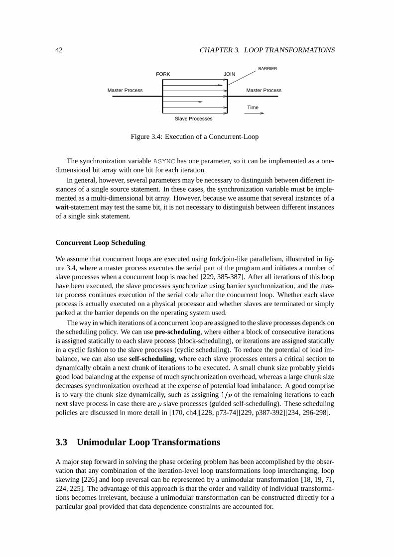
42 CHAPTER 3. LOOP TRANSFORMATIONS
FORK JOIN
Time
Master Process
Slave Processes
Master Process
BARRIER
Figure 3.4: Execution of a Concurrent-Loop
The synchronization variable ASYNChas one parameter, so it can be implemented as a one-dimensional bit array with one bit for each iteration.
In general, however, several parameters may be necessary to distinguish between different in-stances of a single source statement. In these cases, the synchronization variable must be imple-mented as a multi-dimensional bit array. However, because we assume that several instances of await-statement may test the same bit, it is not necessary to distinguish between different instancesof a single sink statement.
Concurrent Loop Scheduling
We assume that concurrent loops are executed using fork/join-like parallelism, illustrated in fig-ure 3.4, where a master process executes the serial part of the program and initiates a number ofslave processes when a concurrent loop is reached [229, 385-387]. After all iterations of this loophave been executed, the slave processes synchronize using barrier synchronization, and the mas-ter process continues execution of the serial code after the concurrent loop. Whether each slaveprocess is actually executed on a physical processor and whether slaves are terminated or simplyparked at the barrier depends on the operating system used.
The way in which iterations of a concurrent loop are assigned to the slave processes depends onthe scheduling policy. We can use pre-scheduling, where either a block of consecutive iterationsis assigned statically to each slave process (block-scheduling), or iterations are assigned staticallyin a cyclic fashion to the slave processes (cyclic scheduling). To reduce the potential of load im-balance, we can also use self-scheduling, where each slave processes enters a critical section todynamically obtain a next chunk of iterations to be executed. A small chunk size probably yieldsgood load balancing at the expense of much synchronization overhead, whereas a large chunk sizedecreases synchronization overhead at the expense of potential load imbalance. A good compriseis to vary the chunk size dynamically, such as assigning 1=p of the remaining iterations to eachnext slave process in case there are p slave processes (guided self-scheduling). These schedulingpolicies are discussed in more detail in [170, ch4][228, p73-74][229, p387-392][234, 296-298].
3.3 Unimodular Loop Transformations
A major step forward in solving the phase ordering problem has been accomplished by the obser-vation that any combination of the iteration-level loop transformations loop interchanging, loopskewing [226] and loop reversal can be represented by a unimodular transformation [18, 19, 71,224, 225]. The advantage of this approach is that the order and validity of individual transforma-tions becomes irrelevant, because a unimodular transformation can be constructed directly for aparticular goal provided that data dependence constraints are accounted for.
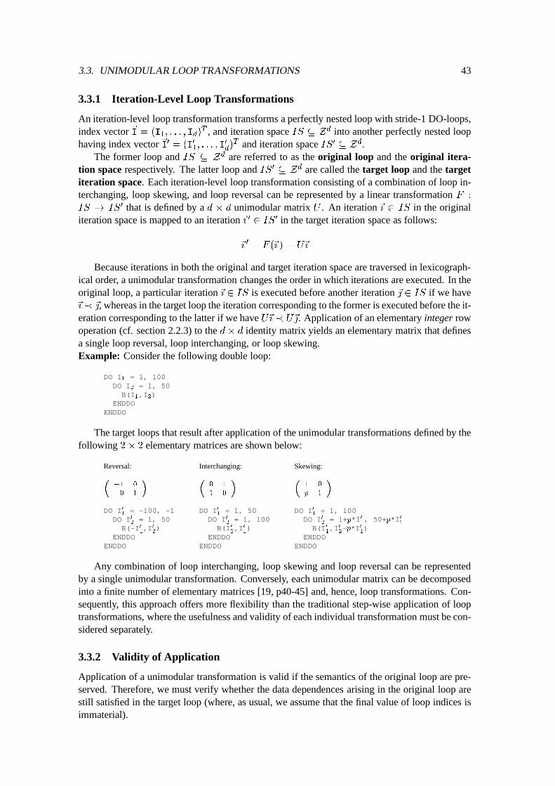
3.3. UNIMODULAR LOOP TRANSFORMATIONS 43
3.3.1 Iteration-Level Loop Transformations
An iteration-level loop transformation transforms a perfectly nested loop with stride-1 DO-loops,index vector ~I = (I
1
; : : : ; I
d
)
T , and iteration space IS � Zd into another perfectly nested loophaving index vector ~I0 = (I
0
1
; : : : ; I
0
d
)
T and iteration space IS0 � Zd.The former loop and IS � Zd are referred to as the original loop and the original itera-
tion space respectively. The latter loop and IS0 � Zd are called the target loop and the targetiteration space. Each iteration-level loop transformation consisting of a combination of loop in-terchanging, loop skewing, and loop reversal can be represented by a linear transformation F :
IS ! IS
0 that is defined by a d � d unimodular matrix U . An iteration~{ 2 IS in the originaliteration space is mapped to an iteration~{ 0 2 IS0 in the target iteration space as follows:
~{
0
= F (~{ ) = U~{
Because iterations in both the original and target iteration space are traversed in lexicograph-ical order, a unimodular transformation changes the order in which iterations are executed. In theoriginal loop, a particular iteration~{ 2 IS is executed before another iteration ~| 2 IS if we have~{ � ~|, whereas in the target loop the iteration corresponding to the former is executed before the it-eration corresponding to the latter if we have U~{ � U~|. Application of an elementary integer rowoperation (cf. section 2.2.3) to the d� d identity matrix yields an elementary matrix that definesa single loop reversal, loop interchanging, or loop skewing.Example: Consider the following double loop:
DO I1
= 1, 100DO I
2
= 1, 50B(I
1
,I2
)ENDDO
ENDDO
The target loops that result after application of the unimodular transformations defined by thefollowing 2� 2 elementary matrices are shown below:
Reversal: Interchanging: Skewing:
�
�1 0
0 1
� �
0 1
1 0
� �
1 0
p 1
�
DO I01
= -100, -1 DO I01
= 1, 50 DO I01
= 1, 100DO I0
2
= 1, 50 DO I02
= 1, 100 DO I02
= 1+p*I01
, 50+p*I01
B(-I01
,I02
) B(I02
,I01
) B(I01
,I02
-p*I01
)ENDDO ENDDO ENDDO
ENDDO ENDDO ENDDO
Any combination of loop interchanging, loop skewing and loop reversal can be representedby a single unimodular transformation. Conversely, each unimodular matrix can be decomposedinto a finite number of elementary matrices [19, p40-45] and, hence, loop transformations. Con-sequently, this approach offers more flexibility than the traditional step-wise application of looptransformations, where the usefulness and validity of each individual transformation must be con-sidered separately.
3.3.2 Validity of Application
Application of a unimodular transformation is valid if the semantics of the original loop are pre-served. Therefore, we must verify whether the data dependences arising in the original loop arestill satisfied in the target loop (where, as usual, we assume that the final value of loop indices isimmaterial).
44 CHAPTER 3. LOOP TRANSFORMATIONS
Dependence Distance Vectors
Let the set D � Zd of dependence distance vectors represent the data dependence structure ofthe original loop, i.e. if a statement instance executed in iteration ~| 2 IS depends on a statementinstance executed in iteration~{ 2 IS, then for ~d = ~|�~{, we have ~d 2 D.
Because U defines a linear transformation, applying a transformation defined by a unimodularmatrixU to this loop affects the dependence distance between the previous two iterations as shownbelow:
~
d
0
= U~{
0
� U~{ = U(~{
0
�~{ ) = U
~
d
Consequently, application of a unimodular transformation defined byU to a loop of which thedata dependence structure is represented by a set of dependence distance vectors D � Zd is validif and only if U ~d � ~0 holds for all ~d 2 D.
Dependence Direction Vectors
To deal with the general case, both dependence distance and direction vectors are represented bydependence vectors [224, 225]. Each component of a dependence vector ~d consists of a range[d
min
i
; d
max
i
] that is described by two bounds dmin
i
; d
max
i
2 Z [ f�1;+1g. Components of adependence direction vector are translated to components of a dependence vector as follows:
> � [�1;�1]
< � [+1;+1]
� � [�1;+1]
= � [0; 0]
A component of a dependence distance vector is represented by a degenerate interval [di
; d
i
].Given a dependence vector ~d with d components, then ~
d �
~
0 holds if there is a 1 � i � d
such that dmin
i
> 0 and dmin
j
= 0 for all 1 � j < i. Moreover, ~d � ~
0 holds if either ~d � ~
0 ord
min
i
� 0 for all 1 � i � d. Two ranges are added as follows, where1+s =1 for any s 6= �1and �1+ s = �1 for any s 6=1:
[l; u] + [l
0
; u
0
] = [l + l
0
; u+ u
0
]
Multiplication of a range by a scalar s 2 Z is defined below, where s � �1 = 0 if s = 0, ands � �1 = �1 has the appropriate sign for s 6= 0:
s � [l; u] =
(
[s � l; s � u] if s � 0
[s � u; s � l] otherwise
Applying a unimodular transformation defined by U to a loop of which the data dependencestructure is represented by a set D of dependence vectors with ~
d �
~
0 for all ~d 2 D is valid, ifU
~
d �
~
0 also holds for all ~d 2 D under the previous defined arithmetic. The converse implicationdoes not hold, because loop skewing may cause loss of data dependence information.
3.3.3 Code Generation
The application of a loop transformation defined by a unimodular matrix U to a loop nest withindex vector~I is implemented by replacing the original loop with the target loop. Effectively, thisreplacement is implemented by (i) rewriting the loop-body of the original loop, and (ii) generatingnew loops with index vector~I0 that induce a lexicographical traversal of the target iteration space.Here, we assume that all loop bounds of the original loop are admissible.
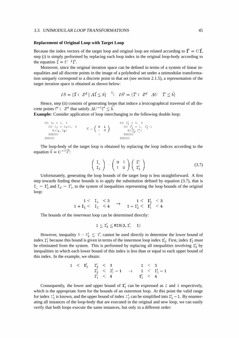
3.3. UNIMODULAR LOOP TRANSFORMATIONS 45
Replacement of Original Loop with Target Loop
Because the index vectors of the target loop and original loop are related according to ~I0 = U
~
I,step (i) is simply performed by replacing each loop index in the original loop-body according tothe equation ~I = U
�1
~
I
0.Moreover, since the original iteration space can be defined in terms of a system of linear in-
equalities and all discrete points in the image of a polyhedral set under a unimodular transforma-tion uniquely correspond to a discrete point in that set (see section 2.1.5), a representation of thetarget iteration space is obtained as shown below:
IS = f
~
I 2 Z
d
j A
~
I �
~
bg
U
! IS
0
= f
~
I
0
2 Z
d
j AU
�1
~
I
0
�
~
bg
Hence, step (ii) consists of generating loops that induce a lexicographical traversal of all dis-crete points~{ 0 2 Zd that satisfy AU�1~{ 0 � ~b.Example: Consider application of loop interchanging to the following double loop:
DO I1
= 1, 3DO I
2
= I1
+1, 4B(I
1
,I2
)ENDDO
ENDDO
U =
�
0 1
1 0
�
!
DO I01
= 2, 4DO I0
2
= 1, I01
-1B(I0
2
,I01
)ENDDO
ENDDO
The loop-body of the target loop is obtained by replacing the loop indices according to theequation ~I = U
�1
~
I
0:
I
1
I
2
!
=
0 1
1 0
!
I
0
1
I
0
2
!
(3.7)
Unfortunately, generating the loop bounds of the target loop is less straightforward. A firststep towards finding these bounds is to apply the substitution defined by equation (3.7), that isI
1
= I
0
2
and I
2
= I
0
1
, to the system of inequalities representing the loop bounds of the originalloop:
1 � I
1
� 3
1+ I
1
� I
2
� 4
!
1 � I
0
2
� 3
1+ I
0
2
� I
0
1
� 4
The bounds of the innermost loop can be determined directly:
1 � I
0
2
� MIN(3; I
0
1
� 1)
However, inequality 1+ I
0
2
� I
0
1
cannot be used directly to determine the lower bound ofindex I
0
1
because this bound is given in terms of the innermost loop index I
0
2
. First, index I
0
2
mustbe eliminated from the system. This is performed by replacing all inequalities involving I
0
2
byinequalities in which each lower bound of this index is less than or equal to each upper bound ofthis index. In the example, we obtain:
1 � I
0
2
I
0
2
� 3
I
0
2
� I
0
1
� 1
I
0
1
� 4
!
1 � 3
1 � I
0
1
� 1
I
0
1
� 4
Consequently, the lower and upper bound of I01
can be expressed as 2 and 4 respectively,which is the appropriate form for the bounds of an outermost loop. At this point the valid rangefor index I 0
1
is known, and the upper bound of index I 02
can be simplified into I01
�1. By enumer-ating all instances of the loop-body that are executed in the original and new loop, we can easilyverify that both loops execute the same instances, but only in a different order:
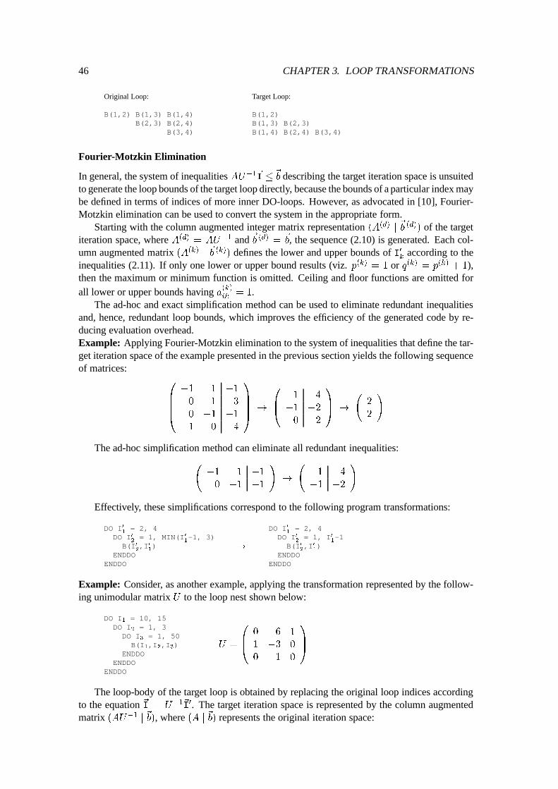
46 CHAPTER 3. LOOP TRANSFORMATIONS
Original Loop: Target Loop:
B(1,2) B(1,3) B(1,4) B(1,2)B(2,3) B(2,4) B(1,3) B(2,3)
B(3,4) B(1,4) B(2,4) B(3,4)
Fourier-Motzkin Elimination
In general, the system of inequalities AU�1~I � ~b describing the target iteration space is unsuitedto generate the loop bounds of the target loop directly, because the bounds of a particular index maybe defined in terms of indices of more inner DO-loops. However, as advocated in [10], Fourier-Motzkin elimination can be used to convert the system in the appropriate form.
Starting with the column augmented integer matrix representation (A
(d)
j
~
b
(d)
) of the targetiteration space, where A(d)
= AU
�1 and ~b (d) =
~
b, the sequence (2.10) is generated. Each col-umn augmented matrix (A
(k)
j
~
b
(k)
) defines the lower and upper bounds of I0k
according to theinequalities (2.11). If only one lower or upper bound results (viz. p(k) = 1 or q(k) = p
(k)
+ 1),then the maximum or minimum function is omitted. Ceiling and floor functions are omitted forall lower or upper bounds having a(k)
ik
= 1.The ad-hoc and exact simplification method can be used to eliminate redundant inequalities
and, hence, redundant loop bounds, which improves the efficiency of the generated code by re-ducing evaluation overhead.Example: Applying Fourier-Motzkin elimination to the system of inequalities that define the tar-get iteration space of the example presented in the previous section yields the following sequenceof matrices:
0
B
B
B
@
�1 1 �1
0 1 3
0 �1 �1
1 0 4
1
C
C
C
A
!
0
B
@
1 4
�1 �2
0 2
1
C
A
!
2
2
!
The ad-hoc simplification method can eliminate all redundant inequalities:
�1 1 �1
0 �1 �1
!
!
1 4
�1 �2
!
Effectively, these simplifications correspond to the following program transformations:
DO I01
= 2, 4DO I0
2
= 1, MIN(I01
-1, 3)B(I0
2
,I01
)ENDDO
ENDDO
!
DO I01
= 2, 4DO I0
2
= 1, I01
-1B(I0
2
,I01
)ENDDO
ENDDO
Example: Consider, as another example, applying the transformation represented by the follow-ing unimodular matrix U to the loop nest shown below:
DO I1
= 10, 15DO I
2
= 1, 3DO I
3
= 1, 50B(I
1
,I2
,I3
)ENDDO
ENDDOENDDO
U =
0
B
@
0 6 1
1 �3 0
0 1 0
1
C
A
The loop-body of the target loop is obtained by replacing the original loop indices accordingto the equation ~I = U
�1
~
I
0. The target iteration space is represented by the column augmentedmatrix (AU
�1
j
~
b), where (A j
~
b) represents the original iteration space:
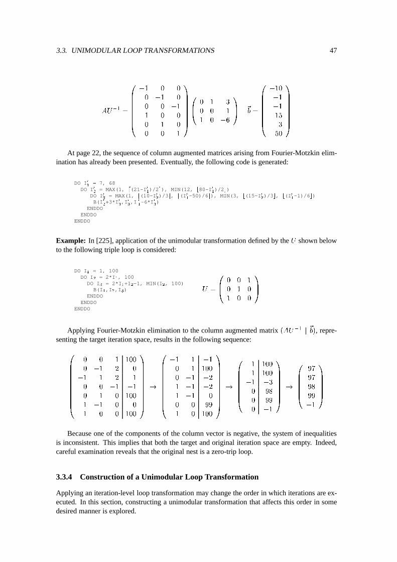
3.3. UNIMODULAR LOOP TRANSFORMATIONS 47
AU
�1
=
0
B
B
B
B
B
B
B
@
�1 0 0
0 �1 0
0 0 �1
1 0 0
0 1 0
0 0 1
1
C
C
C
C
C
C
C
A
0
B
@
0 1 3
0 0 1
1 0 �6
1
C
A
~
b =
0
B
B
B
B
B
B
B
@
�10
�1
�1
15
3
50
1
C
C
C
C
C
C
C
A
At page 22, the sequence of column augmented matrices arising from Fourier-Motzkin elim-ination has already been presented. Eventually, the following code is generated:
DO I01
= 7, 68DO I0
2
= MAX(1, d(21-I01
)/2e), MIN(12, b80-I01
)/2c)DO I0
3
= MAX(1, d(10-I02
)/3e, d(I01
-50)/6e), MIN(3, b(15-I02
)/3c, b(I01
-1)/6c)B(I0
2
+3*I03
,I03
,I 0
1
-6*I03
)ENDDO
ENDDOENDDO
Example: In [225], application of the unimodular transformation defined by the U shown belowto the following triple loop is considered:
DO I1
= 1, 100DO I
2
= 2*I1
, 100DO I
3
= 2*I1
+I2
-1, MIN(I2
, 100)B(I
1
,I2
,I3
)ENDDO
ENDDOENDDO
U =
0
B
@
0 0 1
0 1 0
1 0 0
1
C
A
Applying Fourier-Motzkin elimination to the column augmented matrix (AU
�1
j
~
b), repre-senting the target iteration space, results in the following sequence:
0
B
B
B
B
B
B
B
B
B
B
@
0 0 1 100
0 �1 2 0
�1 1 2 1
0 0 �1 �1
0 1 0 100
1 �1 0 0
1 0 0 100
1
C
C
C
C
C
C
C
C
C
C
A
!
0
B
B
B
B
B
B
B
B
B
B
@
�1 1 �1
0 1 100
0 �1 �2
1 �1 �2
1 �1 0
0 0 99
1 0 100
1
C
C
C
C
C
C
C
C
C
C
A
!
0
B
B
B
B
B
B
B
@
1 100
1 100
�1 �3
0 98
0 99
0 �1
1
C
C
C
C
C
C
C
A
!
0
B
B
B
B
B
@
97
97
98
99
�1
1
C
C
C
C
C
A
Because one of the components of the column vector is negative, the system of inequalitiesis inconsistent. This implies that both the target and original iteration space are empty. Indeed,careful examination reveals that the original nest is a zero-trip loop.
3.3.4 Construction of a Unimodular Loop Transformation
Applying an iteration-level loop transformation may change the order in which iterations are ex-ecuted. In this section, constructing a unimodular transformation that affects this order in somedesired manner is explored.
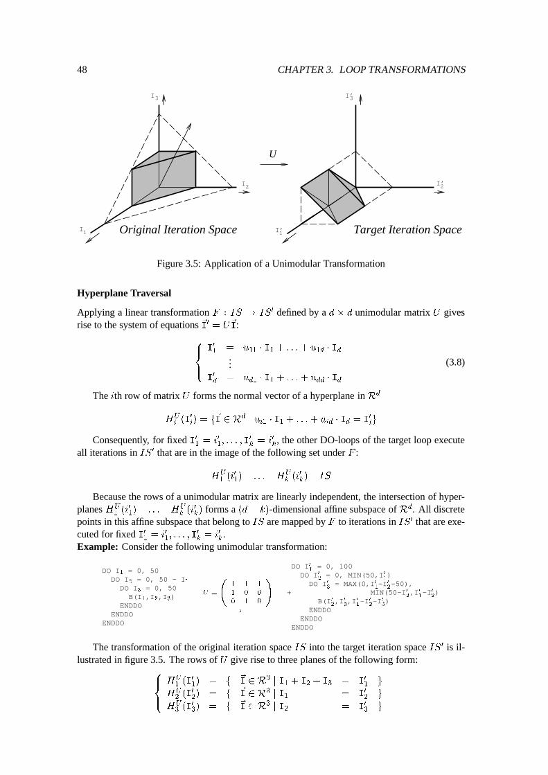
48 CHAPTER 3. LOOP TRANSFORMATIONS
I 3
I 1
I 2
U
Original Iteration Space Target Iteration Space
2I’
3I’
1I’
Figure 3.5: Application of a Unimodular Transformation
Hyperplane Traversal
Applying a linear transformation F : IS ! IS
0 defined by a d � d unimodular matrix U givesrise to the system of equations ~I0 = U
~
I:
8
>
<
>
:
I
0
1
= u
11
� I
1
+ : : :+ u
1d
� I
d
...I
0
d
= u
d1
� I
1
+ : : :+ u
dd
� I
d
(3.8)
The ith row of matrix U forms the normal vector of a hyperplane inRd
H
U
i
(I
0
i
) = f
~
I 2 R
d
j u
i1
� I
1
+ : : :+ u
id
� I
d
= I
0
i
g
Consequently, for fixed I
0
1
= i
0
1
; : : : ; I
0
k
= i
0
k
, the other DO-loops of the target loop executeall iterations in IS0 that are in the image of the following set under F :
H
U
1
(i
0
1
) \ : : : \H
U
k
(i
0
k
) \ IS
Because the rows of a unimodular matrix are linearly independent, the intersection of hyper-planes HU
1
(i
0
1
) \ : : : \H
U
k
(i
0
k
) forms a (d� k)-dimensional affine subspace of Rd. All discretepoints in this affine subspace that belong to IS are mapped by F to iterations in IS0 that are exe-cuted for fixed I
0
1
= i
0
1
; : : : ; I
0
k
= i
0
k
.Example: Consider the following unimodular transformation:
DO I1
= 0, 50DO I
2
= 0, 50 - I1
DO I3
= 0, 50B(I
1
,I2
,I3
)ENDDO
ENDDOENDDO
U =
1 1 1
1 0 0
0 1 0
!
!
DO I01
= 0, 100DO I0
2
= 0, MIN(50,I01
)DO I0
3
= MAX(0,I01
-I02
-50),+ MIN(50-I0
2
,I01
-I02
)B(I0
2
,I03
,I01
-I02
-I03
)ENDDO
ENDDOENDDO
The transformation of the original iteration space IS into the target iteration space IS0 is il-lustrated in figure 3.5. The rows of U give rise to three planes of the following form:
8
>
<
>
:
H
U
1
(I
0
1
) = f
~
I 2 R
3
j I
1
+ I
2
+ I
3
= I
0
1
g
H
U
2
(I
0
2
) = f
~
I 2 R
3
j I
1
= I
0
2
g
H
U
3
(I
0
3
) = f
~
I 2 R
3
j I
2
= I
0
3
g
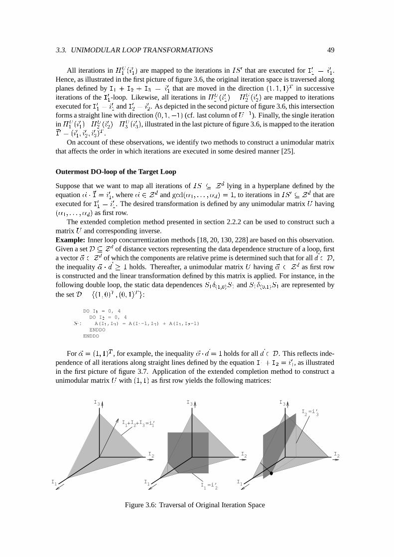
3.3. UNIMODULAR LOOP TRANSFORMATIONS 49
All iterations in HU
1
(i
0
1
) are mapped to the iterations in IS0 that are executed for I01
= i
0
1
.Hence, as illustrated in the first picture of figure 3.6, the original iteration space is traversed alongplanes defined by I
1
+ I
2
+ I
3
= i
0
1
that are moved in the direction (1; 1; 1)
T in successiveiterations of the I
0
1
-loop. Likewise, all iterations in HU
1
(i
0
1
) \ H
U
2
(i
0
2
) are mapped to iterationsexecuted for I0
1
= i
0
1
and I02
= i
0
2
. As depicted in the second picture of figure 3.6, this intersectionforms a straight line with direction (0; 1;�1) (cf. last column ofU�1). Finally, the single iterationinHU
1
(i
0
1
)\H
U
2
(i
0
2
)\H
U
3
(i
0
3
), illustrated in the last picture of figure 3.6, is mapped to the iteration~
I
0
= (i
0
1
; i
0
2
; i
0
3
)
T .On account of these observations, we identify two methods to construct a unimodular matrix
that affects the order in which iterations are executed in some desired manner [25].
Outermost DO-loop of the Target Loop
Suppose that we want to map all iterations of IS � Zd lying in a hyperplane defined by theequation ~� � ~I = i
0
1
, where ~� 2 Zd and gcd(�
1
; : : : ; �
d
) = 1, to iterations in IS0 � Zd that areexecuted for I0
1
= i
0
1
. The desired transformation is defined by any unimodular matrix U having(�
1
; : : : ; �
d
) as first row.The extended completion method presented in section 2.2.2 can be used to construct such a
matrix U and corresponding inverse.Example: Inner loop concurrentization methods [18, 20, 130, 228] are based on this observation.Given a setD � Zd of distance vectors representing the data dependence structure of a loop, firsta vector ~� 2 Zd of which the components are relative prime is determined such that for all ~d 2 D,the inequality ~� � ~d � 1 holds. Thereafter, a unimodular matrix U having ~� 2 Zd as first rowis constructed and the linear transformation defined by this matrix is applied. For instance, in thefollowing double loop, the static data dependences S
1
�
(1;0)
S
1
and S1
�
(0;1)
S
1
are represented bythe set D = f(1; 0)
T
; (0; 1)
T
g:
DO I1
= 0, 4DO I
2
= 0, 4S
1
: A(I1
,I2
) = A(I1
-1,I2
) + A(I1
,I2
-1)ENDDO
ENDDO
For ~� = (1; 1)
T , for example, the inequality ~� � ~d = 1 holds for all ~d 2 D. This reflects inde-pendence of all iterations along straight lines defined by the equation I
1
+ I
2
= i
0
1
, as illustratedin the first picture of figure 3.7. Application of the extended completion method to construct aunimodular matrix U with (1; 1) as first row yields the following matrices:
I 2
I 3
I 1
+I II1 32+ =i’1
2I =i’
3
1I =i’
2
I 1 I 1
I 2 I 2
I 3 I 3
Figure 3.6: Traversal of Original Iteration Space
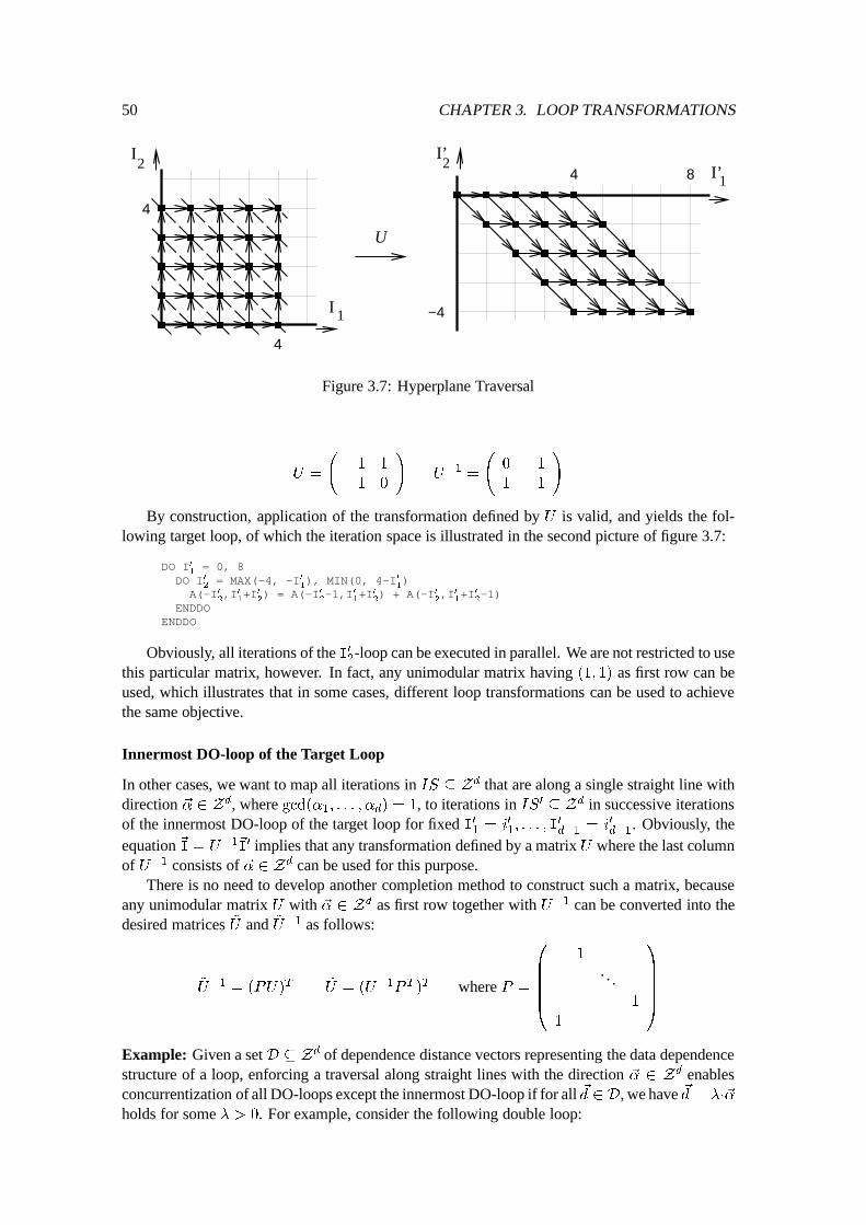
50 CHAPTER 3. LOOP TRANSFORMATIONS
U
I 1
I2
4
4
1I’
−4
4 82
I’
Figure 3.7: Hyperplane Traversal
U =
1 1
�1 0
!
U
�1
=
0 �1
1 1
!
By construction, application of the transformation defined by U is valid, and yields the fol-lowing target loop, of which the iteration space is illustrated in the second picture of figure 3.7:
DO I01
= 0, 8DO I0
2
= MAX(-4, -I01
), MIN(0, 4-I01
)A(-I0
2
,I01
+I02
) = A(-I02
-1,I01
+I02
) + A(-I02
,I01
+I02
-1)ENDDO
ENDDO
Obviously, all iterations of the I02
-loop can be executed in parallel. We are not restricted to usethis particular matrix, however. In fact, any unimodular matrix having (1; 1) as first row can beused, which illustrates that in some cases, different loop transformations can be used to achievethe same objective.
Innermost DO-loop of the Target Loop
In other cases, we want to map all iterations in IS � Zd that are along a single straight line withdirection ~� 2 Zd, where gcd(�
1
; : : : ; �
d
) = 1, to iterations in IS0 � Zd in successive iterationsof the innermost DO-loop of the target loop for fixed I
0
1
= i
0
1
; : : : ; I
0
d�1
= i
0
d�1
. Obviously, theequation~I = U
�1
~
I
0 implies that any transformation defined by a matrix U where the last columnof U�1 consists of ~� 2 Zd can be used for this purpose.
There is no need to develop another completion method to construct such a matrix, becauseany unimodular matrix U with ~� 2 Zd as first row together with U�1 can be converted into thedesired matrices ~
U and ~
U
�1 as follows:
~
U
�1
= (PU)
T
~
U = (U
�1
P
T
)
T where P =
0
B
B
B
B
@
1
. . .1
1
1
C
C
C
C
A
Example: Given a set D � Zd of dependence distance vectors representing the data dependencestructure of a loop, enforcing a traversal along straight lines with the direction ~� 2 Zd enablesconcurrentization of all DO-loops except the innermost DO-loop if for all ~d 2 D, we have ~d = ��~�
holds for some � > 0. For example, consider the following double loop:
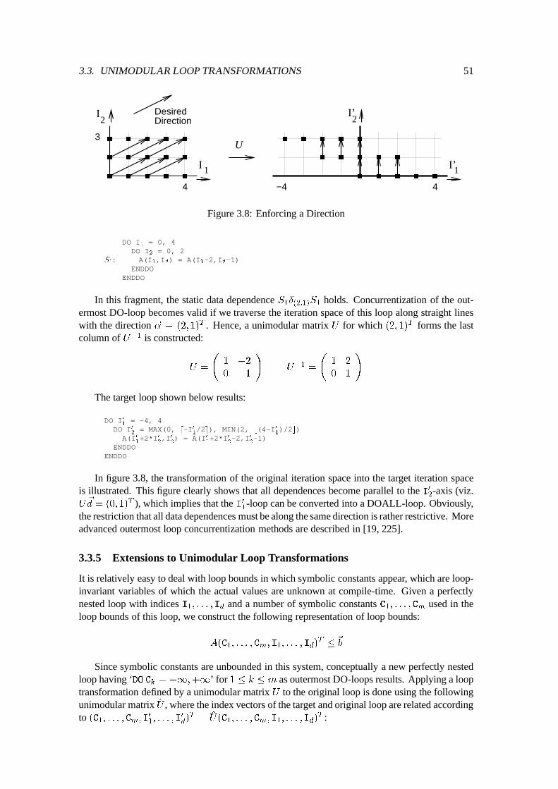
3.3. UNIMODULAR LOOP TRANSFORMATIONS 51
−4 4
1I’
2I’
4
2I
3
1I
DesiredDirection
U
Figure 3.8: Enforcing a Direction
DO I1
= 0, 4DO I
2
= 0, 2S
1
: A(I1
,I2
) = A(I1
-2,I2
-1)ENDDO
ENDDO
In this fragment, the static data dependence S1
�
(2;1)
S
1
holds. Concurrentization of the out-ermost DO-loop becomes valid if we traverse the iteration space of this loop along straight lineswith the direction ~� = (2; 1)
T . Hence, a unimodular matrix U for which (2; 1)
T forms the lastcolumn of U�1 is constructed:
U =
1 �2
0 1
!
U
�1
=
1 2
0 1
!
The target loop shown below results:
DO I01
= -4, 4DO I0
2
= MAX(0, d-I01
/2e), MIN(2, b(4-I01
)/2c)A(I0
1
+2*I02
,I02
) = A(I01
+2*I02
-2,I02
-1)ENDDO
ENDDO
In figure 3.8, the transformation of the original iteration space into the target iteration spaceis illustrated. This figure clearly shows that all dependences become parallel to the I
0
2
-axis (viz.U
~
d = (0; 1)
T ), which implies that the I 01
-loop can be converted into a DOALL-loop. Obviously,the restriction that all data dependences must be along the same direction is rather restrictive. Moreadvanced outermost loop concurrentization methods are described in [19, 225].
3.3.5 Extensions to Unimodular Loop Transformations
It is relatively easy to deal with loop bounds in which symbolic constants appear, which are loop-invariant variables of which the actual values are unknown at compile-time. Given a perfectlynested loop with indices I
1
; : : : ; I
d
and a number of symbolic constants C1
; : : : ; C
m
used in theloop bounds of this loop, we construct the following representation of loop bounds:
A(C
1
; : : : ; C
m
; I
1
; : : : ; I
d
)
T
�
~
b
Since symbolic constants are unbounded in this system, conceptually a new perfectly nestedloop having ‘DO C
k
= �1;+1’ for 1 � k � m as outermost DO-loops results. Applying a looptransformation defined by a unimodular matrix U to the original loop is done using the followingunimodular matrix ^
U , where the index vectors of the target and original loop are related accordingto (C
1
; : : : ; C
m
; I
0
1
; : : : ; I
0
d
)
T
=
^
U(C
1
; : : : ; C
m
; I
1
; : : : ; I
d
)
T :
52 CHAPTER 3. LOOP TRANSFORMATIONS
^
U =
I
U
!
^
U
�1
=
I
U
�1
!
The loop-body of the target loop is still obtained by replacing all original loop indices accord-ing to ~I = U
�1
~
I
0. The new loop bounds are obtained by applying Fourier-Motzkin eliminationto A ~
U
�1
�
~
b, where symbolic constants appear before loop indices (cf. [196]). During this elim-ination, unbounded variables may appear.Example: Consider, for example, application of loop interchanging to the following double loop:
DO I1
= 1, C1
+6DO I
2
= I1
-4,MIN(C2
-C1
+I1
,100)B(I
1
,I2
)ENDDO
ENDDO
!
DO I01
= -3, MIN(C2
+6,100)DO I0
2
= MAX(1,C1
-C2
+I01
),MIN(C1
+6,I01
+4)B(I0
2
,I01
)ENDDO
ENDDO
For appropriate ^
U , applying Fourier-Motzkin elimination to A ^
U
�1
(C
1
; C
2
; I
0
1
; I
0
2
)
T
�
~
b thatrepresents the loop bounds of the target loop, results in a sequence of column augmented matricesthat is initiated with the following two column augmented matrices from which the target loopbounds can be derived:
0
B
B
B
B
B
@
�1 0 0 1 6
0 0 �1 1 4
1 �1 1 �1 0
0 0 0 �1 �1
0 0 1 0 100
1
C
C
C
C
C
A
!
0
B
B
B
B
B
@
0 �1 1 6
0 0 1 100
0 0 �1 3
1 �1 0 4
�1 0 0 5
1
C
C
C
C
C
A
! : : :
The inequalities defined by the remaining column augmented matrices in this sequence defineconstraints under which execution sets are non-empty (e.g. �5 � C
1
or �9 � C
2
):
: : : !
0
B
B
B
@
0 �1 9
1 �1 4
0 0 103
�1 0 5
1
C
C
C
A
!
�1 5
0 103
!
!
�
103
�
A similar technique can be used to enable the application of a unimodular loop transformationto a perfectly nested sub-loop with admissible bounds appearing in a non-perfectly nested loopwith possibly inadmissible bounds. All loop indices of DO-loops that are not directly involvedin the loop transformation are also handled as symbolic constants. Note that in all these cases,an appropriate padding with zero components must be applied to the data dependence vectors toenable the validity test.
More advanced extensions can be found in the literature. For example, the framework can beextended to non-singular matrices [19, 22, 139, 140, 230], which allows for more freedom dur-ing construction of a suited loop transformation. However, some complications in code gener-ation arise because not all points within the convex polytope defined by the image of the origi-nal bounds belong to the target iteration space, whereas the use of conditionals in the loop-bodythat exclude such points must be avoided. The framework can also be extended to deal with thetransformation of non-perfectly nested loops [119]. Applying different loop transformations todifferent statements in a loop-body has been studied in [13, 14, 121]. In this case, it is useful toextend the framework to affine transformations (rather than just linear transformations) as well,to incorporate loop alignment [48].
3.4. ITERATION SPACE PARTITIONING 53
3.4 Iteration Space Partitioning
In this section, we present a method to isolate a loop-body for all iterations within a polyhedralset defined by a system of linear inequalities [36]. This method differs from directly generatingloop bounds from a given system of inequalities in the sense that loops iterating over the remain-ing iterations must also be generated. First, we present a simple loop transformation, referred toas execution set partitioning. Subsequently, we discuss how repetitive application of this basictransformation can be used to solve the problem.
Our iteration space partitioning method has as advantage that if the original iteration spaceconsists of all discrete points within a bounded polyhedral set, then all generated loops have thisproperty. In this manner, subsequent iteration space partitioning and other transformations rely-ing on the representation of an iteration space as a system of linear inequalities remain feasible.Moreover, the method avoids redundant code duplication.
Iteration space partitioning can be used for a number of purposes. First, it can be used to sim-plify programs [50, 120]. For instance, after we have isolated the part of an iteration space in whicha conditional is either true or false, a conditional statement that is controlled by that conditional canbe eliminated. Although such simplifications are not likely to be applicable to ordinary programs,in many cases the code resulting after compiler transformations provides many opportunities forsimplification. In other cases, isolating certain parts of the iteration space in which particular datadependences do not hold increases the opportunities for concurrentization and vectorization. Ob-viously, having a general method to isolate an iteration space in combination with an advanceddata dependence analysis tool provides the compiler with sufficient functionality to enhance theperformance of existing codes. Finally, the method can be very useful for a compiler that performsdata structure transformations, such as the prototype sparse compiler presented in the second partof this dissertation.
3.4.1 Execution Set Partitioning
Execution set partitioning transforms a single DO-loop into two DO-loops, thereby partitioningthe execution set into two disjoint sets.
Transformation
Given a stride-1 DO-loop with index I and an inequality I � T, application of execution setpartitioning transforms this DO-loop into two new DO-loops with the same loop-body, such thatall original iterations satisfying this inequality are executed in the first DO-loop, while all otheriterations for which T < I are executed in the second:
DO I = L, UB(I)
ENDDO!
DO I = L, MIN(U, T)B(I)
ENDDODO I = MAX(L, T+1), U
B(I)ENDDO
Likewise, given the inequality T � I, we partition the execution set of the DO-loop as follows,so that all iterations satisfying the inequality are executed in the second loop, while all remainingiterations for which I < T are executed in the first loop:
DO I = L, UB(I)
ENDDO!
DO I = L, MIN(U, T-1)B(I)
ENDDODO I = MAX(L, T), U
B(I)ENDDO
54 CHAPTER 3. LOOP TRANSFORMATIONS
Execution set partitioning resembles other loop transformations such as index set splitting,loop unrolling, and loop peeling [147, 166, 170, 228, 229, 234]. Obviously, the semantics of theoriginal DO-loop are preserved because the use of minimum and maximum functions preventsthe erroneous introduction of additional iterations. However, in many cases the efficiency of thegenerated code can be improved by eliminating redundant bounds. Furthermore, a zero-trip loopis eliminated and a one-trip loop is unrolled by replacing the complete DO-loop by the loop-bodyin which the appropriate value is substituted for I (recall that we always assume that the final valueof a loop index is not used after a DO-loop).
Implementation of Execution Set Partitioning
Execution set partitioning can be implemented as follows. Suppose that we want to isolate theloop-body appearing at nesting depth d of an arbitrary loop for all iterations of the iteration spaceIS � Z
d in the following half-space, where all ai
2 Z and b 2 Z:
H = f
~
I 2 R
d
j a
1
� I
1
+ : : : + a
d
� I
d
� bg
Let 1 � d
0
� d denote the index of the last nonzero coefficient in the equation (i.e. ad
0
6= 0
and ai
= 0 for d0 < i � d).Furthermore, let the system A(I
1
; : : : ; I
d
0
)
T
�
~
b, where A is a c � d
0 integer matrix and~
b 2 Z
c, form a (conservative) representation of the iteration space of the loop consisting of the d0
outermost DO-loops. We require that the Id
0-loop is a stride-1 DO-loop with admissible bounds.However, if some inadmissible bounds appear in the more outer DO-loops, then the correspondingindex is simply left unbounded. Furthermore, these DO-loops may have arbitrary strides, providedthat the role of the lower and upper bound is interchanged if the stride is negative.
The sets IS \ H and IS \ H restricted to the first d0 loop indices are represented by thesystems of linear inequalities of which the column augmented matrix representations are shownbelow (using the method (2.13) to negate an inequality for integer-valued variables):
M
1
=
A
~
b
a
1
: : : a
d
0
b
!
M
2
=
A
~
b
�a
1
: : :� a
d
0
�b� 1
!
(3.9)
Transforming the I
d
0-loop into two DO-loops, gives rise to two new nested loops, sharingsome outer DO-loops, where a copy of the loop-body of the original I
d
0-loop is used as loop-body:
DO I1
= L1
, U1
...DO I
d
0 = ..., ...... first loop
ENDDODO I
d
0 = ..., ...... second loop
ENDDO...
ENDDO
If ad
0
> 0, then the iteration space of the first and second loop are represented by M1
and M2
respectively. If ad
0
< 0, then these iteration spaces are represented by M2
and M1
respectivelyIn the former case, all iterations in IS \H are executed by the first loop, whereas these iterationsare executed by the second loop in the latter case.
Adding the bounds of indices of more outer DO-loops enables us to test the consistency ofeach system and to simplify the bounds of the resulting DO-loops. First, the consistency of bothsystems is tested using Fourier-Motzkin elimination. If a system M
i
is inconsistent, the corre-sponding DO-loop is a zero-trip loop and does not have to be generated. Otherwise, the systemmay be simplified as follows.
3.4. ITERATION SPACE PARTITIONING 55
While several non-examined upper bounds of index I
d
0 remain, the consistency of the systemobtained by negating one of the upper bounds in M
i
is tested using Fourier-Motzkin elimination.If the resulting system is inconsistent, the corresponding upper bound is eliminated (cf. proposi-tion 2.1), while the original upper bound is restored otherwise. Lower bounds are simplified in asimilar manner.
The bounds of the corresponding I
d
0-loop are generated according to the inequalities (2.11).If the lower bound is identical to the upper bound, the DO-loop may be unrolled.Example: Suppose that we want to isolate the loop-body of the following double loop for alliterations in the half-plane defined by the linear inequality �I+ J � 0:
DO I = 1, 100DO J = I, I+10B(I,J)
ENDDOENDDO
The column augmented matrix representation of the iteration space is shown below:
(A j
~
b) =
0
B
B
B
@
�1 1 10
1 �1 0
1 0 100
�1 0 �1
1
C
C
C
A
)
bounds ofthe J-loop
)
bounds ofthe I-loop
Adding the appropriate inequalities to this system and application of Fourier-Motzkin elimi-nation to these systems reveals that both systems are consistent. Because two lower bounds aredefined on J by the last system, consistency of this system where the second inequality is negatedis tested (i.e. I � J is replaced by J � I� 1). Since this system is inconsistent, this upper boundis eliminated.
Similar simplifications are applied to the first system:
A
~
b
�1 1 0
!
A
~
b
1 �1 �1
!
# #
�1 1 0
1 �1 0
!
�1 1 10
1 �1 �1
!
Consequently, the following code results, in which the first loop-body is isolated for iterationsin the polyhedral set. Loop overhead is reduced by unrolling the first J -loop:
DO I = 1, 100DO J = I, IB(I,J)
ENDDODO J = I+1, I+10B(I,J)
ENDDOENDDO
!
DO I = 1, 100B(I,I)DO J = I+1, I+10B(I,J)
ENDDOENDDO
3.4.2 Partitioning an Iteration Space
Repetitive application of execution set partitioning can be used to isolate a loop-body of a nestedloop with iteration space IS � Zd for all iterations in a polyhedral set PS � Rd defined byA
~
I �
~
b. For each inequality in the system, we partition the execution set of the appropriate DO-loop as explained in the previous section.
This gives rise to one of the following situations:
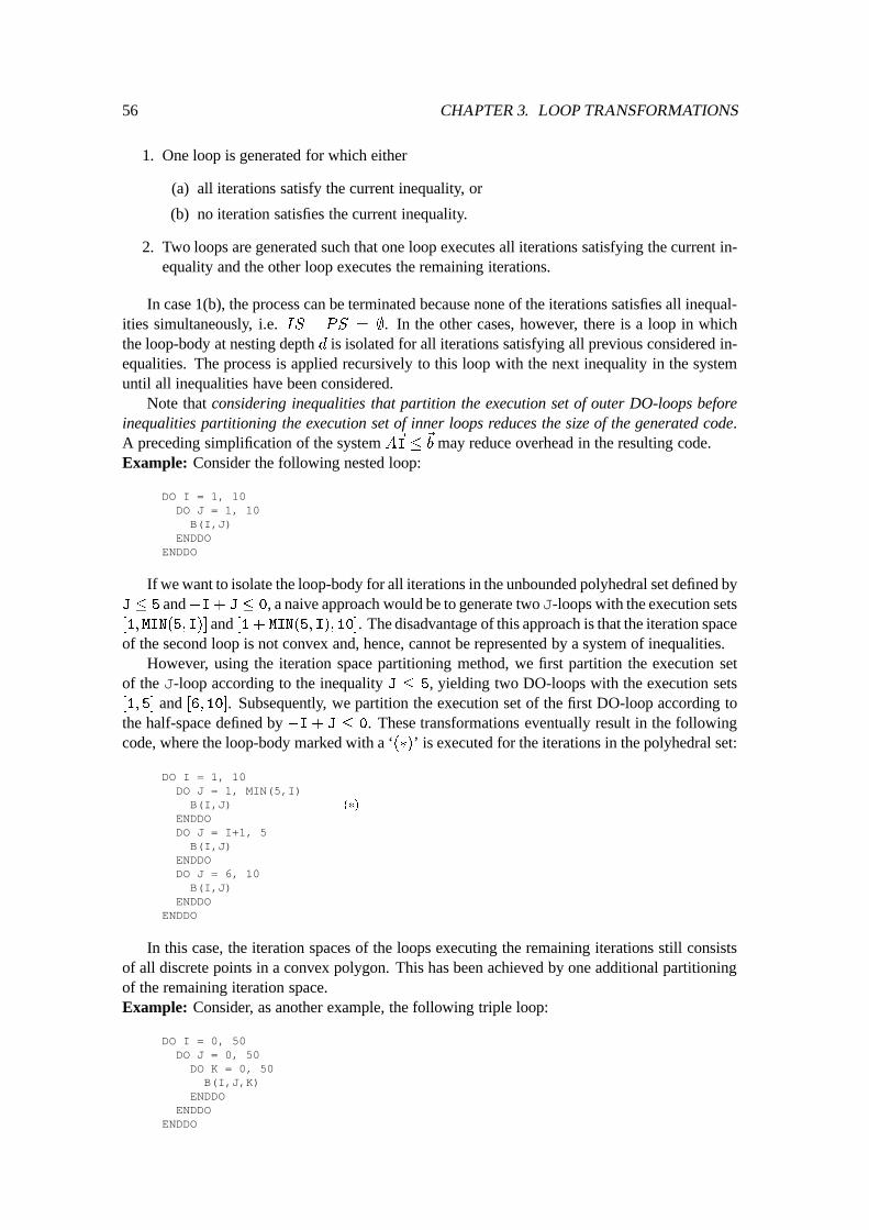
56 CHAPTER 3. LOOP TRANSFORMATIONS
1. One loop is generated for which either
(a) all iterations satisfy the current inequality, or
(b) no iteration satisfies the current inequality.
2. Two loops are generated such that one loop executes all iterations satisfying the current in-equality and the other loop executes the remaining iterations.
In case 1(b), the process can be terminated because none of the iterations satisfies all inequal-ities simultaneously, i.e. IS \ PS = ;. In the other cases, however, there is a loop in whichthe loop-body at nesting depth d is isolated for all iterations satisfying all previous considered in-equalities. The process is applied recursively to this loop with the next inequality in the systemuntil all inequalities have been considered.
Note that considering inequalities that partition the execution set of outer DO-loops beforeinequalities partitioning the execution set of inner loops reduces the size of the generated code.A preceding simplification of the system A
~
I �
~
b may reduce overhead in the resulting code.Example: Consider the following nested loop:
DO I = 1, 10DO J = 1, 10
B(I,J)ENDDO
ENDDO
If we want to isolate the loop-body for all iterations in the unbounded polyhedral set defined byJ � 5 and�I+ J � 0, a naive approach would be to generate two J -loops with the execution sets[1; MIN(5; I)] and [1+ MIN(5; I); 10]. The disadvantage of this approach is that the iteration spaceof the second loop is not convex and, hence, cannot be represented by a system of inequalities.
However, using the iteration space partitioning method, we first partition the execution setof the J -loop according to the inequality J � 5, yielding two DO-loops with the execution sets[1; 5] and [6; 10]. Subsequently, we partition the execution set of the first DO-loop according tothe half-space defined by �I+ J � 0. These transformations eventually result in the followingcode, where the loop-body marked with a ‘(�)’ is executed for the iterations in the polyhedral set:
DO I = 1, 10DO J = 1, MIN(5,I)B(I,J) (�)
ENDDODO J = I+1, 5B(I,J)
ENDDODO J = 6, 10B(I,J)
ENDDOENDDO
In this case, the iteration spaces of the loops executing the remaining iterations still consistsof all discrete points in a convex polygon. This has been achieved by one additional partitioningof the remaining iteration space.Example: Consider, as another example, the following triple loop:
DO I = 0, 50DO J = 0, 50
DO K = 0, 50B(I,J,K)
ENDDOENDDO
ENDDO
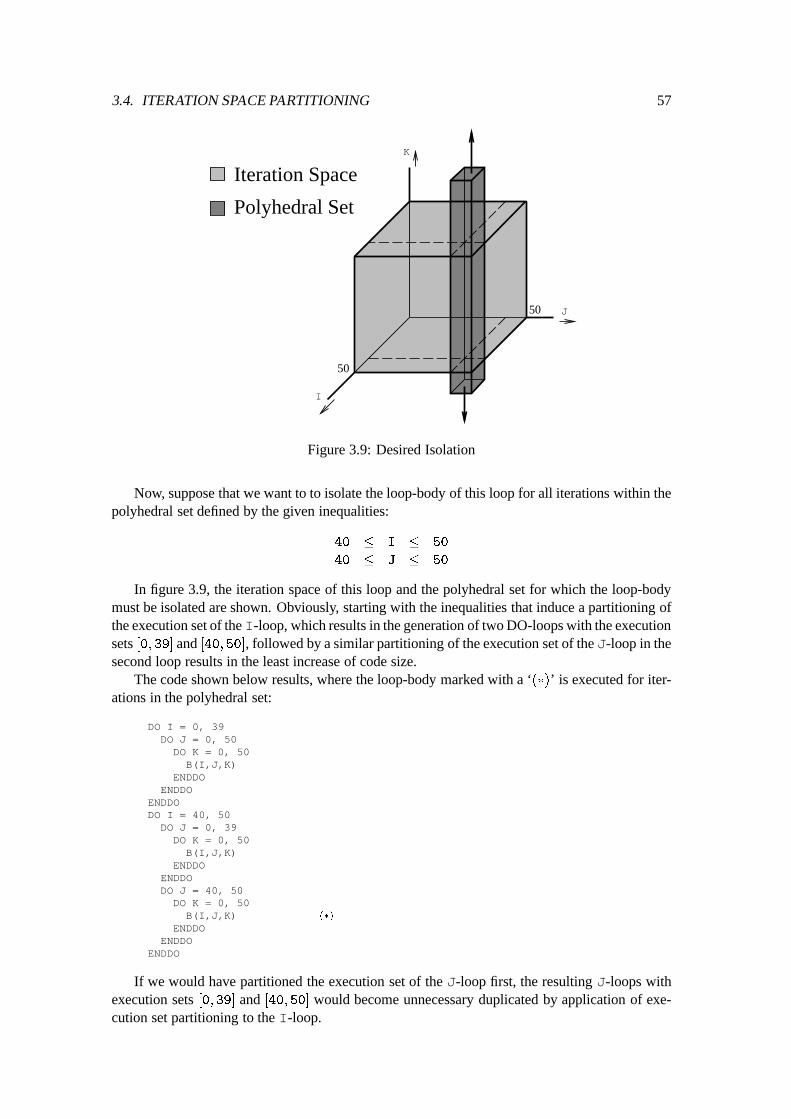
3.4. ITERATION SPACE PARTITIONING 57
J
K
I
50
50
Polyhedral Set
Iteration Space
Figure 3.9: Desired Isolation
Now, suppose that we want to to isolate the loop-body of this loop for all iterations within thepolyhedral set defined by the given inequalities:
40 � I � 50
40 � J � 50
In figure 3.9, the iteration space of this loop and the polyhedral set for which the loop-bodymust be isolated are shown. Obviously, starting with the inequalities that induce a partitioning ofthe execution set of the I -loop, which results in the generation of two DO-loops with the executionsets [0; 39] and [40; 50], followed by a similar partitioning of the execution set of the J -loop in thesecond loop results in the least increase of code size.
The code shown below results, where the loop-body marked with a ‘(�)’ is executed for iter-ations in the polyhedral set:
DO I = 0, 39DO J = 0, 50DO K = 0, 50
B(I,J,K)ENDDO
ENDDOENDDODO I = 40, 50DO J = 0, 39DO K = 0, 50
B(I,J,K)ENDDO
ENDDODO J = 40, 50DO K = 0, 50
B(I,J,K) (�)
ENDDOENDDO
ENDDO
If we would have partitioned the execution set of the J -loop first, the resulting J -loops withexecution sets [0; 39] and [40; 50] would become unnecessary duplicated by application of exe-cution set partitioning to the I -loop.
58 CHAPTER 3. LOOP TRANSFORMATIONS
Example: Below, we give an example in which iteration space partitioning can be used to elimi-nate an IF-statement from the loop-body to reduce run-time overhead:
DO I = 2, 50DO J = 1, I-1DO K = 1, 100IF ((2 * K - J) .EQ. 20) THEN
B1(I,J,K)ELSE
B2(I,J,K)ENDIF
ENDDOENDDO
ENDDO
!
DO I = 2, 50DO J = 1, I-1DO K = 1, b(J+19)/2cB2(I,J,K)
ENDDODO K = d(J+20)/2e, b(J+20)/2c
B1(I,J,K)ENDDODO K = d(J+21)/2e, 100
B2(I,J,K)ENDDO
ENDDOENDDO
Isolating the loop-body for all iterations lying within the hyperplane �J+ 2 � K = 20 can bedone by slicing the iteration space according to the inequalities 20 � �J+ 2 � K � 20.
Construction of the appropriate systems, followed by a test for consistency and elimination ofredundant bounds eventually results in the following three systems:
A
~
b
0 �1 2 19
!
0
B
@
A
~
b
0 �1 2 20
0 1 �2 �20
1
C
A
A
~
b
0 1 �2 �21
!
# # #
0 �1 2 19
0 0 �1 �1
!
0 �1 2 20
0 1 �2 �20
!
0 0 1 100
0 1 �2 �21
!
Although in the resulting fragment the lower bound of the second K-loop resembles the upperbound, unrolling is not allowed because this would erroneously introduce additional iterations incase the value of J is odd. The partitioned iteration space is shown in figure 3.10.
I
50
J
K
49
100
Figure 3.10: Partitioned Iteration Space
Part II
A Sparse Compiler

Chapter 4
A Sparse Compiler
A significant part of scientific codes consists of sparse matrix computations that are difficult todevelop and that show notoriously bad efficiency on today’s supercomputers (see e.g. [186]). Inmost cases, only a small fraction of the computing power of these computers can be utilized. Manyreasons can be given for these effects. First, the codes usually suffer from a lack of spatial localitycaused by irregular data accesses induced by sparse computations. This prohibits efficient cacheutilization and reduces memory bandwidth. Another reason is that temporal locality is not as highas in most dense codes, because the amount of possible reuse of data is limited due to the elim-ination of many operations. Not only does this prevent data locality optimizations, but the com-munication overhead in message-passing architectures can be substantial. Finally, problems arisebecause sparse matrices need to be represented in a compact way to keep the storage requirementsand computational time to reasonable levels. This causes the representation of a sparse code in ei-ther FORTRAN, with the occurrence of subscripted subscripts, or in another language with pointerstructures, to be complex. This is probably the most important problem, because it complicatesboth the development and maintenance of sparse codes which are more complex than dense appli-cations [73], and because it disables most compiler optimizations. In addition, because differentarchitectural features or properties of the nonzero structures may favor different sparse storageschemes, a sparse program that has been developed for a particular target architecture or class ofsparse matrices may perform poorly on another machine or for another class of sparse matrices.
To tackle the sparse data structure problem, examination of the following generic definition isuseful: sparse matrix computations are computations that compute on sparse data structures andsparse data structures are data structures that are logically contained in enveloping data struc-tures. The underlying problem for sparse matrix computations now is where to deal with the factthat only part of the enveloping data structure is computed on. The common approach is to dealwith sparsity at the programming level. However, it is also possible to deal with this issue at alower level, i.e. at the compilation level. This implies that all programming can be done as fordense computations, i.e. all sparse matrices are stored in simple two-dimensional arrays. Obvi-ously, this greatly reduces the complexity of developing and maintaining the original dense pro-gram. Thereafter, a sparse compiler selects an appropriate sparse storage scheme for each matrixthat is actually sparse and applies the corresponding data structure transformations to the originaldense program. Hence, the output of the sparse compiler consists of semantically equivalent codeoperating on sparse data structures to take advantage of sparse matrices to reduce both storage re-quirements and computational time of the original dense program. The resulting sparse programis supplied to a conventional compiler for a particular target machine.
An advantage of this approach is that the sparse compiler does not need to extract programknowledge from an obscured code, but is presented with a much cleaner program on which regulardata dependence checking and standard optimizations can be performed.
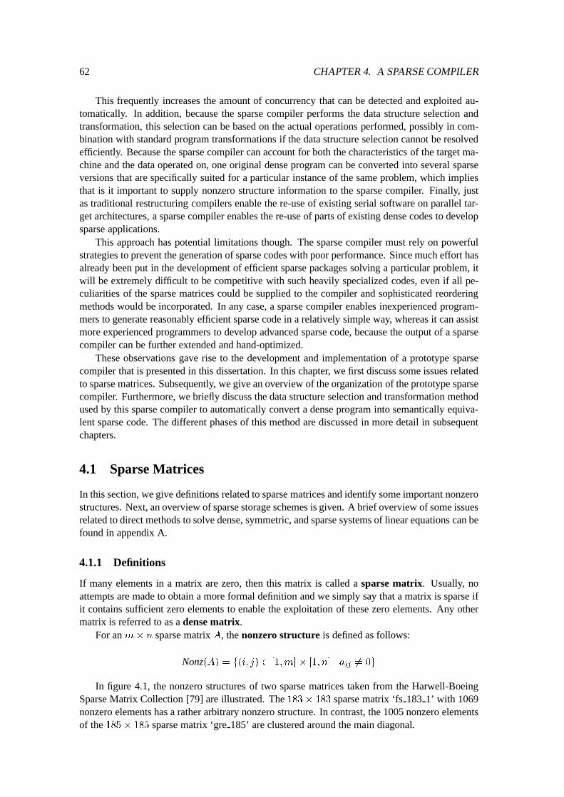
62 CHAPTER 4. A SPARSE COMPILER
This frequently increases the amount of concurrency that can be detected and exploited au-tomatically. In addition, because the sparse compiler performs the data structure selection andtransformation, this selection can be based on the actual operations performed, possibly in com-bination with standard program transformations if the data structure selection cannot be resolvedefficiently. Because the sparse compiler can account for both the characteristics of the target ma-chine and the data operated on, one original dense program can be converted into several sparseversions that are specifically suited for a particular instance of the same problem, which impliesthat is it important to supply nonzero structure information to the sparse compiler. Finally, justas traditional restructuring compilers enable the re-use of existing serial software on parallel tar-get architectures, a sparse compiler enables the re-use of parts of existing dense codes to developsparse applications.
This approach has potential limitations though. The sparse compiler must rely on powerfulstrategies to prevent the generation of sparse codes with poor performance. Since much effort hasalready been put in the development of efficient sparse packages solving a particular problem, itwill be extremely difficult to be competitive with such heavily specialized codes, even if all pe-culiarities of the sparse matrices could be supplied to the compiler and sophisticated reorderingmethods would be incorporated. In any case, a sparse compiler enables inexperienced program-mers to generate reasonably efficient sparse code in a relatively simple way, whereas it can assistmore experienced programmers to develop advanced sparse code, because the output of a sparsecompiler can be further extended and hand-optimized.
These observations gave rise to the development and implementation of a prototype sparsecompiler that is presented in this dissertation. In this chapter, we first discuss some issues relatedto sparse matrices. Subsequently, we give an overview of the organization of the prototype sparsecompiler. Furthermore, we briefly discuss the data structure selection and transformation methodused by this sparse compiler to automatically convert a dense program into semantically equiva-lent sparse code. The different phases of this method are discussed in more detail in subsequentchapters.
4.1 Sparse Matrices
In this section, we give definitions related to sparse matrices and identify some important nonzerostructures. Next, an overview of sparse storage schemes is given. A brief overview of some issuesrelated to direct methods to solve dense, symmetric, and sparse systems of linear equations can befound in appendix A.
4.1.1 Definitions
If many elements in a matrix are zero, then this matrix is called a sparse matrix. Usually, noattempts are made to obtain a more formal definition and we simply say that a matrix is sparse ifit contains sufficient zero elements to enable the exploitation of these zero elements. Any othermatrix is referred to as a dense matrix.
For an m� n sparse matrix A, the nonzero structure is defined as follows:
Nonz(A) = f(i; j) 2 [1;m] � [1; n] j a
ij
6= 0g
In figure 4.1, the nonzero structures of two sparse matrices taken from the Harwell-BoeingSparse Matrix Collection [79] are illustrated. The 183 � 183 sparse matrix ‘fs 183 1’ with 1069nonzero elements has a rather arbitrary nonzero structure. In contrast, the 1005 nonzero elementsof the 185� 185 sparse matrix ‘gre 185’ are clustered around the main diagonal.
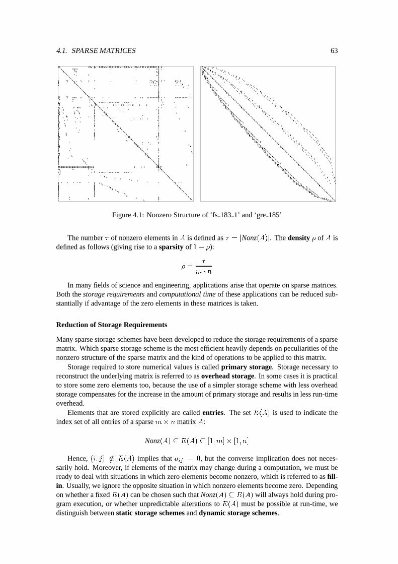
4.1. SPARSE MATRICES 63
Figure 4.1: Nonzero Structure of ‘fs 183 1’ and ‘gre 185’
The number � of nonzero elements in A is defined as � = jNonz(A)j. The density � of A isdefined as follows (giving rise to a sparsity of 1� �):
� =
�
m � n
In many fields of science and engineering, applications arise that operate on sparse matrices.Both the storage requirements and computational time of these applications can be reduced sub-stantially if advantage of the zero elements in these matrices is taken.
Reduction of Storage Requirements
Many sparse storage schemes have been developed to reduce the storage requirements of a sparsematrix. Which sparse storage scheme is the most efficient heavily depends on peculiarities of thenonzero structure of the sparse matrix and the kind of operations to be applied to this matrix.
Storage required to store numerical values is called primary storage. Storage necessary toreconstruct the underlying matrix is referred to as overhead storage. In some cases it is practicalto store some zero elements too, because the use of a simpler storage scheme with less overheadstorage compensates for the increase in the amount of primary storage and results in less run-timeoverhead.
Elements that are stored explicitly are called entries. The set E(A) is used to indicate theindex set of all entries of a sparse m� n matrix A:
Nonz(A) � E(A) � [1;m]� [1; n]
Hence, (i; j) =2 E(A) implies that aij
= 0, but the converse implication does not neces-sarily hold. Moreover, if elements of the matrix may change during a computation, we must beready to deal with situations in which zero elements become nonzero, which is referred to as fill-in. Usually, we ignore the opposite situation in which nonzero elements become zero. Dependingon whether a fixed E(A) can be chosen such that Nonz(A) � E(A) will always hold during pro-gram execution, or whether unpredictable alterations to E(A) must be possible at run-time, wedistinguish between static storage schemes and dynamic storage schemes.
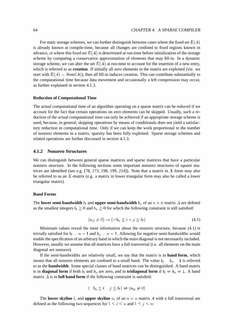
64 CHAPTER 4. A SPARSE COMPILER
For static storage schemes, we can further distinguish between cases where the fixed setE(A)
is already known at compile-time, because all changes are confined to fixed regions known inadvance, or where this fixed setE(A) is determined at run-time before initialization of the storagescheme by computing a conservative approximation of elements that may fill-in. In a dynamicstorage scheme, we can alter the set E(A) at run-time to account for the insertion of a new entry,which is referred to as creation. If initially all zero elements in the matrix are exploited (viz. westart withE(A) = Nonz(A)), then all fill-in induces creation. This can contribute substantially tothe computational time because data movement and occasionally a left compression may occur,as further explained in section 4.1.3.
Reduction of Computational Time
The actual computational time of an algorithm operating on a sparse matrix can be reduced if weaccount for the fact that certain operations on zero elements can be skipped. Usually, such a re-duction of the actual computational time can only be achieved if an appropriate storage scheme isused, because, in general, skipping operations by means of conditionals does not yield a satisfac-tory reduction in computational time. Only if we can keep the work proportional to the numberof nonzero elements in a matrix, sparsity has been fully exploited. Sparse storage schemes andrelated operations are further discussed in section 4.1.3.
4.1.2 Nonzero Structures
We can distinguish between general sparse matrices and sparse matrices that have a particularnonzero structure. In the following sections some important nonzero structures of square ma-trices are identified (see e.g. [78, 173, 198, 199, 214]). Note that a matrix in X-form may alsobe referred to as an X-matrix (e.g. a matrix in lower triangular form may also be called a lowertriangular matrix).
Band Forms
The lower semi-bandwidth bl
and upper semi-bandwidth bu
of an n� n matrix A are definedas the smallest integers b
l
� 0 and bu
� 0 for which the following constraint is still satisfied:
(a
ij
6= 0)) (�b
u
� i� j � b
l
) (4.1)
Minimum values reveal the most information about the nonzero structure, because (4.1) istrivially satisfied for b
l
= n� 1 and bu
= n� 1. Allowing for negative semi-bandwidths wouldenable the specification of an arbitrary band in which the main diagonal is not necessarily included.However, usually we assume that all matrices have a full transversal (i.e. all elements on the maindiagonal are nonzero).
If the semi-bandwidths are relatively small, we say that the matrix is in band form, whichmeans that all nonzero elements are confined to a small band. The value b
l
+ b
u
+ 1 is referredto as the bandwidth. Some special classes of band matrices can be distinguished. A band matrixis in diagonal form if both b
l
and bu
are zero, and in tridiagonal form if bl
= b
u
= 1. A bandmatrix A is in full band form if the following constraint is satisfied:
(�b
u
� i� j � b
l
), (a
ij
6= 0)
The lower skyline li
and upper skyline ui
of an n � n matrix A with a full transversal aredefined as the following two sequences for 1 � i � n and 1 � j � n:
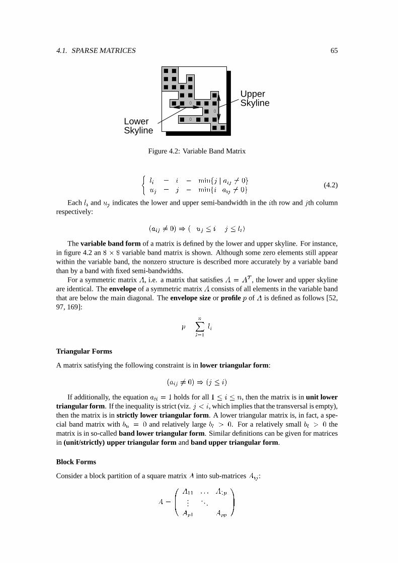
4.1. SPARSE MATRICES 65
0
0
0LowerSkyline
UpperSkyline
Figure 4.2: Variable Band Matrix
(
l
i
= i � minfj j a
ij
6= 0g
u
j
= j � minfi j a
ij
6= 0g
(4.2)
Each li
and uj
indicates the lower and upper semi-bandwidth in the ith row and jth columnrespectively:
(a
ij
6= 0)) (�u
j
� i� j � l
i
)
The variable band form of a matrix is defined by the lower and upper skyline. For instance,in figure 4.2 an 8 � 8 variable band matrix is shown. Although some zero elements still appearwithin the variable band, the nonzero structure is described more accurately by a variable bandthan by a band with fixed semi-bandwidths.
For a symmetric matrix A, i.e. a matrix that satisfies A = A
T , the lower and upper skylineare identical. The envelope of a symmetric matrix A consists of all elements in the variable bandthat are below the main diagonal. The envelope size or profile p of A is defined as follows [52,97, 169]:
p =
n
X
i=1
l
i
Triangular Forms
A matrix satisfying the following constraint is in lower triangular form:
(a
ij
6= 0)) (j � i)
If additionally, the equation aii
= 1 holds for all 1 � i � n, then the matrix is in unit lowertriangular form. If the inequality is strict (viz. j < i, which implies that the transversal is empty),then the matrix is in strictly lower triangular form. A lower triangular matrix is, in fact, a spe-cial band matrix with b
u
= 0 and relatively large bl
> 0. For a relatively small bl
> 0 thematrix is in so-called band lower triangular form. Similar definitions can be given for matricesin (unit/strictly) upper triangular form and band upper triangular form.
Block Forms
Consider a block partition of a square matrix A into sub-matrices Aij
:
A =
0
B
@
A
11
: : : A
1p
.... . .
A
p1
A
pp
1
C
A
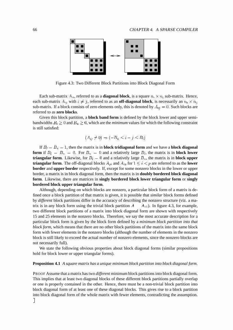
66 CHAPTER 4. A SPARSE COMPILER
Figure 4.3: Two Different Block Partitions into Block Diagonal Form
Each sub-matrix Aii
, referred to as a diagonal block, is a square ni
� n
i
sub-matrix. Hence,each sub-matrix A
ij
with i 6= j, referred to as an off-diagonal block, is necessarily an ni
� n
j
sub-matrix. If a block consists of zero elements only, this is denoted by Aij
= 0. Such blocks arereferred to as zero blocks.
Given this block partition, a block band form is defined by the block lower and upper semi-bandwidths B
l
� 0 andBu
� 0, which are the minimum values for which the following constraintis still satisfied:
(A
ij
6= 0)) (�B
u
� i� j � B
l
)
If Bl
= B
u
= 1, then the matrix is in block tridiagonal form and we have a block diagonalform if B
l
= B
u
= 0. For Bu
= 0 and a relatively large Bl
, the matrix is in block lowertriangular form. Likewise, for B
l
= 0 and a relatively large Bu
, the matrix is in block uppertriangular form. The off-diagonal blocks A
pi
and Aip
for 1 � i < p are referred to as the lowerborder and upper border respectively. If, except for some nonzero blocks in the lower or upperborder, a matrix is in block diagonal form, then the matrix is in doubly bordered block diagonalform. Likewise, there are matrices in singly bordered block lower triangular form or singlybordered block upper triangular form.
Although, depending on which blocks are nonzero, a particular block form of a matrix is de-fined once a block partition of that matrix is given, it is possible that similar block forms definedby different block partitions differ in the accuracy of describing the nonzero structure (viz. a ma-trix is in any block form using the trivial block partition A = A
11
). In figure 4.3, for example,two different block partitions of a matrix into block diagonal form are shown with respectively15 and 25 elements in the nonzero blocks. Therefore, we say the most accurate description for aparticular block form is given by the block form defined by a minimum block partition into thatblock form, which means that there are no other block partitions of the matrix into the same blockform with fewer elements in the nonzero blocks (although the number of elements in the nonzeroblock is still likely to exceed the actual number of nonzero elements, since the nonzero blocks arenot necessarily full).
We state the following obvious properties about block diagonal forms (similar propositionshold for block lower or upper triangular forms).
Proposition 4.1 A square matrix has a unique minimum block partition into block diagonal form.
PROOF Assume that a matrix has two different minimum block partitions into block diagonal form.This implies that at least two diagonal blocks of these different block partitions partially overlapor one is properly contained in the other. Hence, there must be a non-trivial block partition intoblock diagonal form of at least one of these diagonal blocks. This gives rise to a block partitioninto block diagonal form of the whole matrix with fewer elements, contradicting the assumption.[]
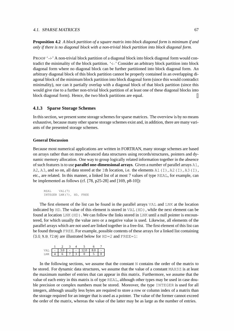
4.1. SPARSE MATRICES 67
Proposition 4.2 A block partition of a square matrix into block diagonal form is minimum if andonly if there is no diagonal block with a non-trivial block partition into block diagonal form.
PROOF ‘)’ A non-trivial block partition of a diagonal block into block diagonal form would con-tradict the minimality of the block partition. ‘(’ Consider an arbitrary block partition into blockdiagonal form where no diagonal block can be further partitioned into block diagonal form. Anarbitrary diagonal block of this block partition cannot be properly contained in an overlapping di-agonal block of the minimum block partition into block diagonal form (since this would contradictminimality), nor can it partially overlap with a diagonal block of that block partition (since thiswould give rise to a further non-trivial block partition of at least one of these diagonal blocks intoblock diagonal form). Hence, the two block partitions are equal. []
4.1.3 Sparse Storage Schemes
In this section, we present some storage schemes for sparse matrices. The overview is by no meansexhaustive, because many other sparse storage schemes exist and, in addition, there are many vari-ants of the presented storage schemes.
General Discussion
Because most numerical applications are written in FORTRAN, many storage schemes are basedon arrays rather than on more advanced data structures using records/structures, pointers and dy-namic memory allocation. One way to group logically related information together in the absenceof such features is to use parallel one-dimensional arrays. Given a number of parallel arrays A1,A2, A3, and so on, all data stored at the I th location, i.e. the elements A1(I) , A2(I) , A3(I) ,etc., are related. In this manner, a linked list of at most 7 values of type REAL, for example, canbe implemented as follows (cf. [78, p25-28] and [169, p8-10]):
REAL VAL(7)INTEGER LNK(7), HD, FREE
The first element of the list can be found in the parallel arrays VAL and LNKat the locationindicated by HD. The value of this element is stored in VAL(HD) , while the next element can befound at location LNK(HD) . We can follow the links stored in LNKuntil a null pointer is encoun-tered, for which usually the value zero or a negative value is used. Likewise, all elements of theparallel arrays which are not used are linked together in a free-list. The first element of this list canbe found through FREE. For example, possible contents of these arrays for a linked list containing(3:0; 8:0; 12:0) are illustrated below for HD=2and FREE=1:
1 2 3 4 5 6 7VAL - 3.0 - - 12.0 8.0 -LNK 4 6 7 3 0 5 0
In the following sections, we assume that the constant N contains the order of the matrix tobe stored. For dynamic data structures, we assume that the value of a constant MAXSZis at leastthe maximum number of entries that can appear in this matrix. Furthermore, we assume that thevalue of each entry in this matrix is of type REAL, although other types may be used in case dou-ble precision or complex numbers must be stored. Moreover, the type INTEGERis used for allintegers, although usually less bytes are required to store a row or column index of a matrix thanthe storage required for an integer that is used as a pointer. The value of the former cannot exceedthe order of the matrix, whereas the value of the latter may be as large as the number of entries.
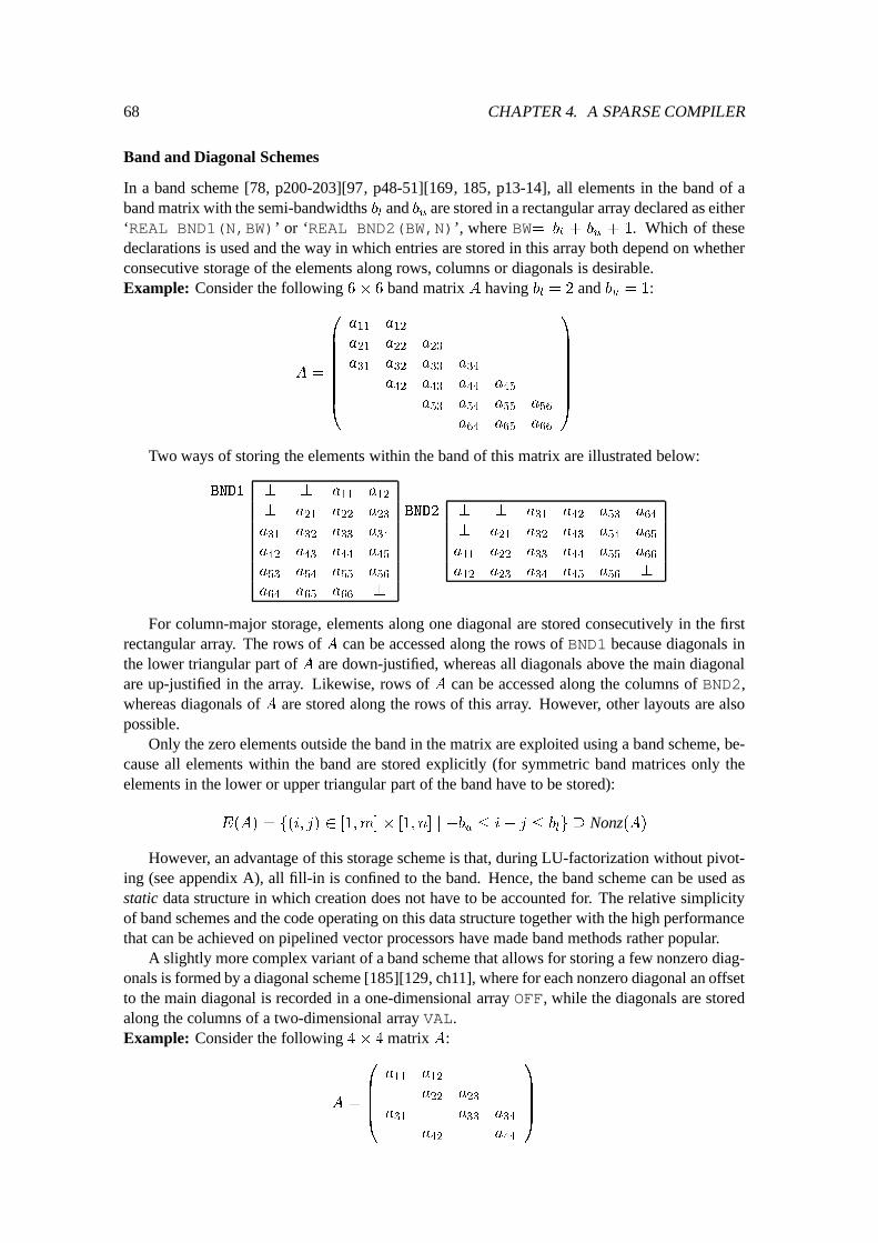
68 CHAPTER 4. A SPARSE COMPILER
Band and Diagonal Schemes
In a band scheme [78, p200-203][97, p48-51][169, 185, p13-14], all elements in the band of aband matrix with the semi-bandwidths b
l
and bu
are stored in a rectangular array declared as either‘REAL BND1(N,BW)’ or ‘REAL BND2(BW,N)’, where BW= b
l
+ b
u
+ 1. Which of thesedeclarations is used and the way in which entries are stored in this array both depend on whetherconsecutive storage of the elements along rows, columns or diagonals is desirable.Example: Consider the following 6� 6 band matrix A having b
l
= 2 and bu
= 1:
A =
0
B
B
B
B
B
B
B
@
a
11
a
12
a
21
a
22
a
23
a
31
a
32
a
33
a
34
a
42
a
43
a
44
a
45
a
53
a
54
a
55
a
56
a
64
a
65
a
66
1
C
C
C
C
C
C
C
A
Two ways of storing the elements within the band of this matrix are illustrated below:
BND1 ? ? a
11
a
12
? a
21
a
22
a
23
a
31
a
32
a
33
a
34
a
42
a
43
a
44
a
45
a
53
a
54
a
55
a
56
a
64
a
65
a
66
?
BND2 ? ? a
31
a
42
a
53
a
64
? a
21
a
32
a
43
a
54
a
65
a
11
a
22
a
33
a
44
a
55
a
66
a
12
a
23
a
34
a
45
a
56
?
For column-major storage, elements along one diagonal are stored consecutively in the firstrectangular array. The rows of A can be accessed along the rows of BND1because diagonals inthe lower triangular part of A are down-justified, whereas all diagonals above the main diagonalare up-justified in the array. Likewise, rows of A can be accessed along the columns of BND2,whereas diagonals of A are stored along the rows of this array. However, other layouts are alsopossible.
Only the zero elements outside the band in the matrix are exploited using a band scheme, be-cause all elements within the band are stored explicitly (for symmetric band matrices only theelements in the lower or upper triangular part of the band have to be stored):
E(A) = f(i; j) 2 [1;m]� [1; n] j �b
u
� i� j � b
l
g � Nonz(A)
However, an advantage of this storage scheme is that, during LU-factorization without pivot-ing (see appendix A), all fill-in is confined to the band. Hence, the band scheme can be used asstatic data structure in which creation does not have to be accounted for. The relative simplicityof band schemes and the code operating on this data structure together with the high performancethat can be achieved on pipelined vector processors have made band methods rather popular.
A slightly more complex variant of a band scheme that allows for storing a few nonzero diag-onals is formed by a diagonal scheme [185][129, ch11], where for each nonzero diagonal an offsetto the main diagonal is recorded in a one-dimensional array OFF, while the diagonals are storedalong the columns of a two-dimensional array VAL.Example: Consider the following 4� 4 matrix A:
A =
0
B
B
B
@
a
11
a
12
a
22
a
23
a
31
a
33
a
34
a
42
a
44
1
C
C
C
A
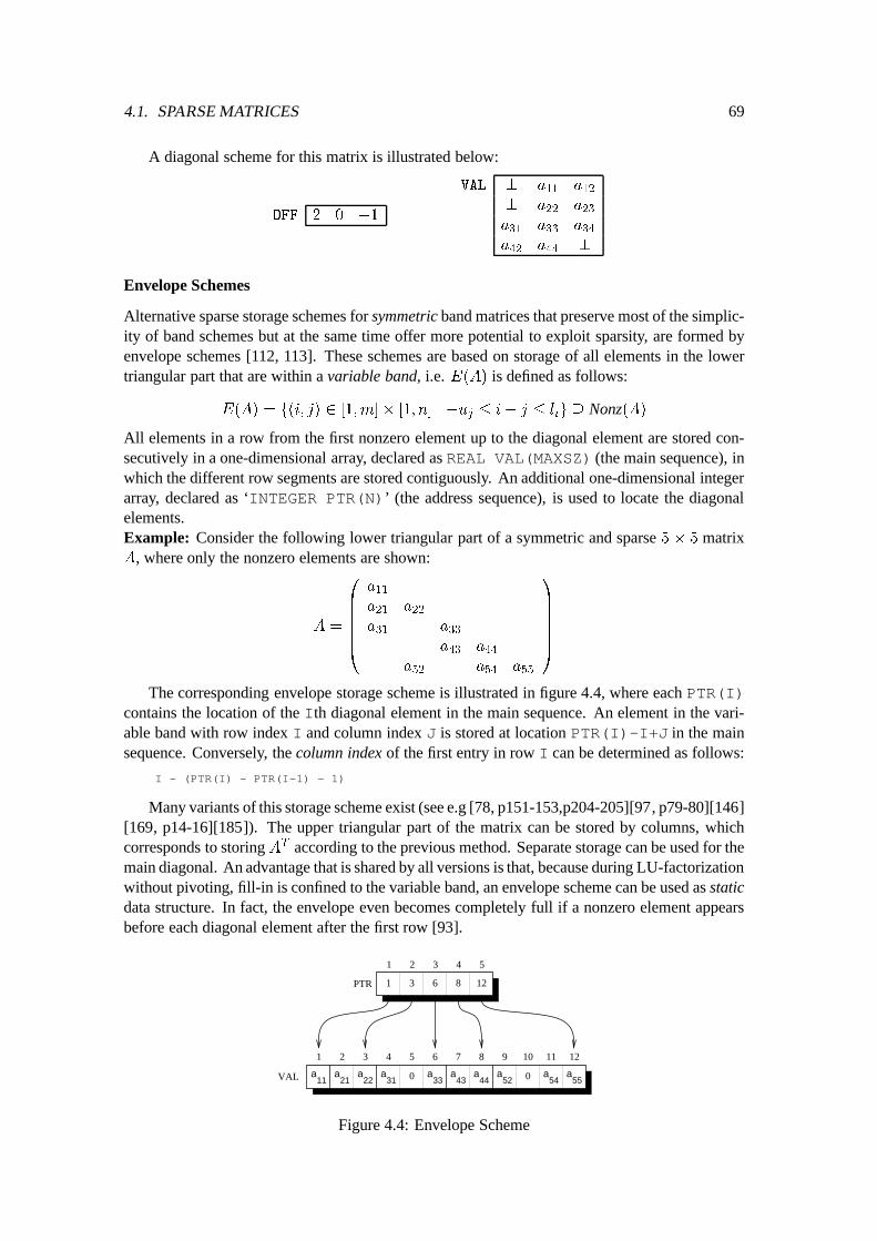
4.1. SPARSE MATRICES 69
A diagonal scheme for this matrix is illustrated below:
OFF 2 0 �1
VAL ? a
11
a
12
? a
22
a
23
a
31
a
33
a
34
a
42
a
44
?
Envelope Schemes
Alternative sparse storage schemes for symmetric band matrices that preserve most of the simplic-ity of band schemes but at the same time offer more potential to exploit sparsity, are formed byenvelope schemes [112, 113]. These schemes are based on storage of all elements in the lowertriangular part that are within a variable band, i.e. E(A) is defined as follows:
E(A) = f(i; j) 2 [1;m]� [1; n] j �u
j
� i� j � l
i
g � Nonz(A)
All elements in a row from the first nonzero element up to the diagonal element are stored con-secutively in a one-dimensional array, declared as REAL VAL(MAXSZ)(the main sequence), inwhich the different row segments are stored contiguously. An additional one-dimensional integerarray, declared as ‘INTEGER PTR(N)’ (the address sequence), is used to locate the diagonalelements.Example: Consider the following lower triangular part of a symmetric and sparse 5 � 5 matrixA, where only the nonzero elements are shown:
A =
0
B
B
B
B
B
@
a
11
a
21
a
22
a
31
a
33
a
43
a
44
a
52
a
54
a
55
1
C
C
C
C
C
A
The corresponding envelope storage scheme is illustrated in figure 4.4, where each PTR(I)contains the location of the I th diagonal element in the main sequence. An element in the vari-able band with row index I and column index J is stored at location PTR(I)-I+J in the mainsequence. Conversely, the column index of the first entry in row I can be determined as follows:
I - (PTR(I) - PTR(I-1) - 1)
Many variants of this storage scheme exist (see e.g [78, p151-153,p204-205][97, p79-80][146][169, p14-16][185]). The upper triangular part of the matrix can be stored by columns, whichcorresponds to storing AT according to the previous method. Separate storage can be used for themain diagonal. An advantage that is shared by all versions is that, because during LU-factorizationwithout pivoting, fill-in is confined to the variable band, an envelope scheme can be used as staticdata structure. In fact, the envelope even becomes completely full if a nonzero element appearsbefore each diagonal element after the first row [93].
VAL a11
a33
a22
a44
a21
a31 0 a 043
a52
a54
a55
1 2 3 4 5 6 7 8 9 10 11 12
12
1 2 3 4 5
1 3 6 8PTR
Figure 4.4: Envelope Scheme
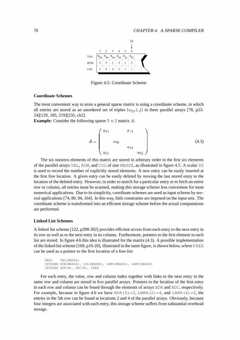
70 CHAPTER 4. A SPARSE COMPILER
VAL a11
1
1
a
4 2
a
4
4
a44 14
1
32
3
1
a51
5
1 2 3 4 5
5
5
a55
6
ROW
COL
SZ
Figure 4.5: Coordinate Scheme
Coordinate Schemes
The most convenient way to store a general sparse matrix is using a coordinate scheme, in whichall entries are stored as an unordered set of triples (a
ij
; i; j) in three parallel arrays [78, p23-24][129, 185, 219][235, ch2].Example: Consider the following sparse 5� 5 matrix A:
A =
0
B
B
B
B
B
@
a
11
a
14
a
32
a
44
a
51
a
55
1
C
C
C
C
C
A
(4.3)
The six nonzero elements of this matrix are stored in arbitrary order in the first six elementsof the parallel arrays VAL, ROW, and COL of size MAXSZ, as illustrated in figure 4.5. A scalar SZis used to record the number of explicitly stored elements. A new entry can be easily inserted atthe first free location. A given entry can be easily deleted by moving the last stored entry to thelocation of the deleted entry. However, in order to search for a particular entry or to fetch an entirerow or column, all entries must be scanned, making this storage scheme less convenient for mostnumerical applications. Due to its simplicity, coordinate schemes are used as input scheme by sev-eral applications [74, 80, 94, 164]. In this way, little constraints are imposed on the input sets. Thecoordinate scheme is transformed into an efficient storage scheme before the actual computationsare performed.
Linked List Schemes
A linked list scheme [122, p298-302] provides efficient access from each entry to the next entry inits row as well as to the next entry in its column. Furthermore, pointers to the first element in eachlist are stored. In figure 4.6 this idea is illustrated for the matrix (4.3). A possible implementationof the linked list scheme [169, p16-20], illustrated in the same figure, is shown below, where FREEcan be used as a pointer to the first location of a free-list:
REAL VAL(MAXSZ)INTEGER ROW(MAXSZ), COL(MAXSZ), LNKR(MAXSZ), LNKC(MAXSZ)INTEGER HDR(N), HDC(N), FREE
For each entry, the value, row and column index together with links to the next entry in thesame row and column are stored in five parallel arrays. Pointers to the location of the first entryin each row and column can be found through the elements of arrays HDR and HDC, respectively.For example, because in figure 4.6 we have HDR(5)=2, LNKR(2)=4, and LNKR(4)=0, theentries in the 5th row can be found at locations 2 and 4 of the parallel arrays. Obviously, becausefour integers are associated with each entry, this storage scheme suffers from substantial overheadstorage.
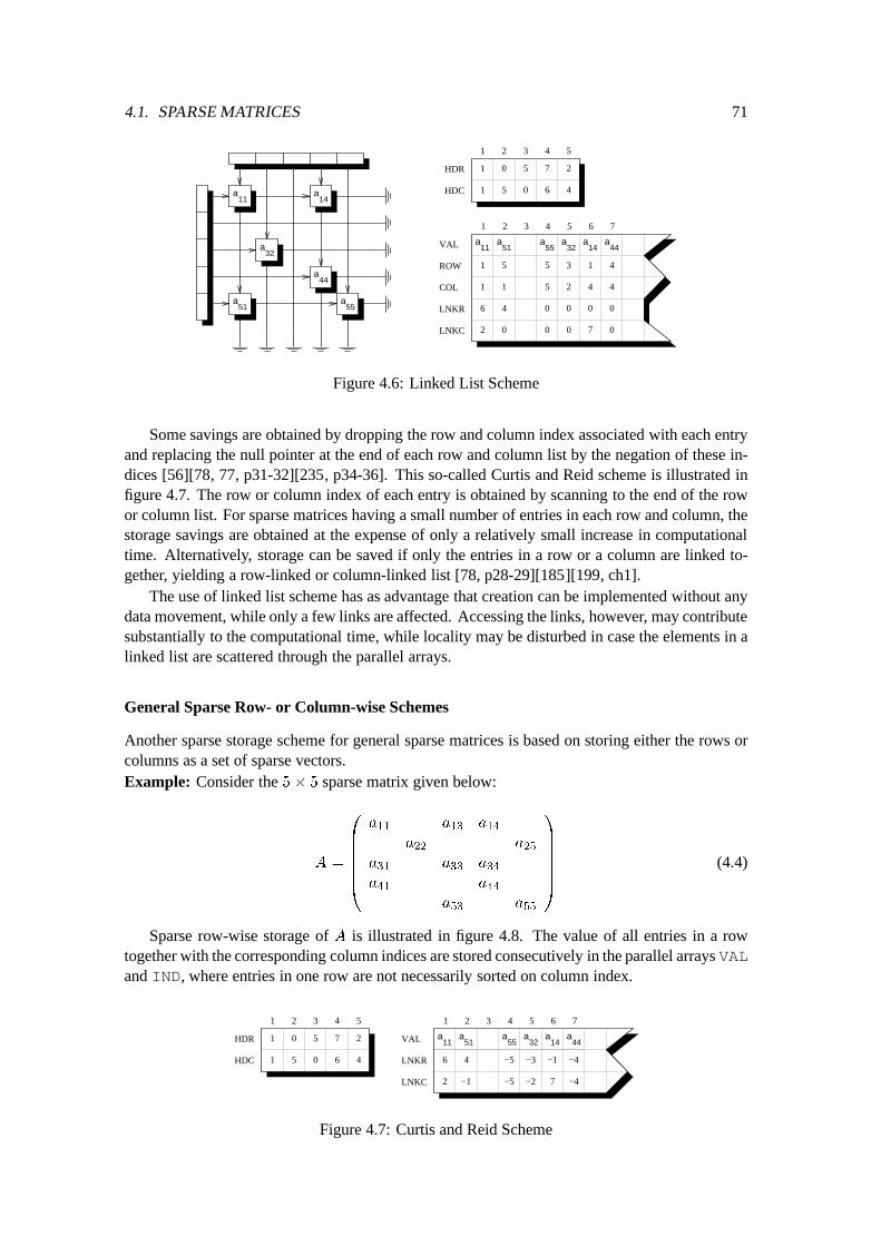
4.1. SPARSE MATRICES 71
a51
a55
VAL a55
a11
a14
a32
1
1
1
4
5
5
3
2
1 2 3 4 5 6
06 00
a51
1
5
4
0 0
a44
4
4
0
00
1 2 3 4 5
1 0 5
1 5 0 6 4
7
7
2
2
a11
a14
a32
a44
LNKR
LNKC
HDR
HDC
7
ROW
COL
Figure 4.6: Linked List Scheme
Some savings are obtained by dropping the row and column index associated with each entryand replacing the null pointer at the end of each row and column list by the negation of these in-dices [56][78, 77, p31-32][235, p34-36]. This so-called Curtis and Reid scheme is illustrated infigure 4.7. The row or column index of each entry is obtained by scanning to the end of the rowor column list. For sparse matrices having a small number of entries in each row and column, thestorage savings are obtained at the expense of only a relatively small increase in computationaltime. Alternatively, storage can be saved if only the entries in a row or a column are linked to-gether, yielding a row-linked or column-linked list [78, p28-29][185][199, ch1].
The use of linked list scheme has as advantage that creation can be implemented without anydata movement, while only a few links are affected. Accessing the links, however, may contributesubstantially to the computational time, while locality may be disturbed in case the elements in alinked list are scattered through the parallel arrays.
General Sparse Row- or Column-wise Schemes
Another sparse storage scheme for general sparse matrices is based on storing either the rows orcolumns as a set of sparse vectors.Example: Consider the 5� 5 sparse matrix given below:
A =
0
B
B
B
B
B
@
a
11
a
13
a
14
a
22
a
25
a
31
a
33
a
34
a
41
a
44
a
53
a
55
1
C
C
C
C
C
A
(4.4)
Sparse row-wise storage of A is illustrated in figure 4.8. The value of all entries in a rowtogether with the corresponding column indices are stored consecutively in the parallel arrays VALand IND, where entries in one row are not necessarily sorted on column index.
VAL a55
a11
a14
a32
1 2 3 4 5 6
a51
a44
6 4
72
LNKR
LNKC −1 −5 −2 −4
−5 −3 −1 −4
7 1 2 3 4 5
1 0 5
1 5 0 6 4
7 2HDR
HDC
Figure 4.7: Curtis and Reid Scheme
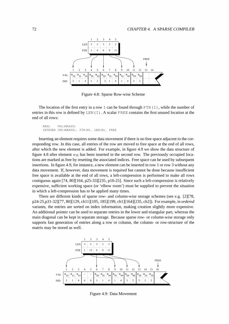
72 CHAPTER 4. A SPARSE COMPILER
VAL a11
a33
aa a a a a55
1 2 3 4 5 6 7 8 9 10 11 12
IND
a14
13
a22
a25 31 34 41
a44 5313
3 1 4 5 2 3 1 4 1 4 3 5
14
1 64 9 11
1 2 3 4 5
PTR
LEN 3 3 2 2
FREE
2
Figure 4.8: Sparse Row-wise Scheme
The location of the first entry in a row I can be found through PTR(I), while the number ofentries in this row is defined by LEN(I). A scalar FREE contains the first unused location at theend of all rows:
REAL VAL(MAXSZ)INTEGER IND(MAXSZ), PTR(N), LEN(N), FREE
Inserting an element requires some data movement if there is no free space adjacent to the cor-responding row. In this case, all entries of the row are moved to free space at the end of all rows,after which the new element is added. For example, in figure 4.9 we show the data structure offigure 4.8 after element a
23
has been inserted in the second row. The previously occupied loca-tions are marked as free by resetting the associated indices. Free space can be used by subsequentinsertions. In figure 4.9, for instance, a new element can be inserted in row 1 or row 3 without anydata movement. If, however, data movement is required but cannot be done because insufficientfree space is available at the end of all rows, a left-compression is performed to make all rowscontiguous again [74, 80][164, p25-33][235, p16-25]. Since such a left-compression is relativelyexpensive, sufficient working space (or ‘elbow room’) must be supplied to prevent the situationin which a left-compression has to be applied many times.
There are different kinds of sparse row- and column-wise storage schemes (see e.g. [2][78,p24-25,p31-32][77, 80][129, ch11][105, 185][199, ch1][164][235, ch2]). For example, in orderedvariants, the entries are sorted on index information, making creation slightly more expensive.An additional pointer can be used to separate entries in the lower and triangular part, whereas themain diagonal can be kept in separate storage. Because sparse row- or column-wise storage onlysupports fast generation of entries along a row or column, the column- or row-structure of thematrix may be stored as well.
VAL a11
a33
aa a a a a55
1 2 3 4 5 6 7 8 9 10 11 12
IND
a14
13
31 34 41a
44 53
1 6 9 11
1 2 3 4 5
PTR
13
3 1 4
a22
a25
5 23 1 4 1 4 3 5
LEN 3 3 2 2
14
3
0 0
− − a
3
23
15 16
FREE
13
Figure 4.9: Data Movement
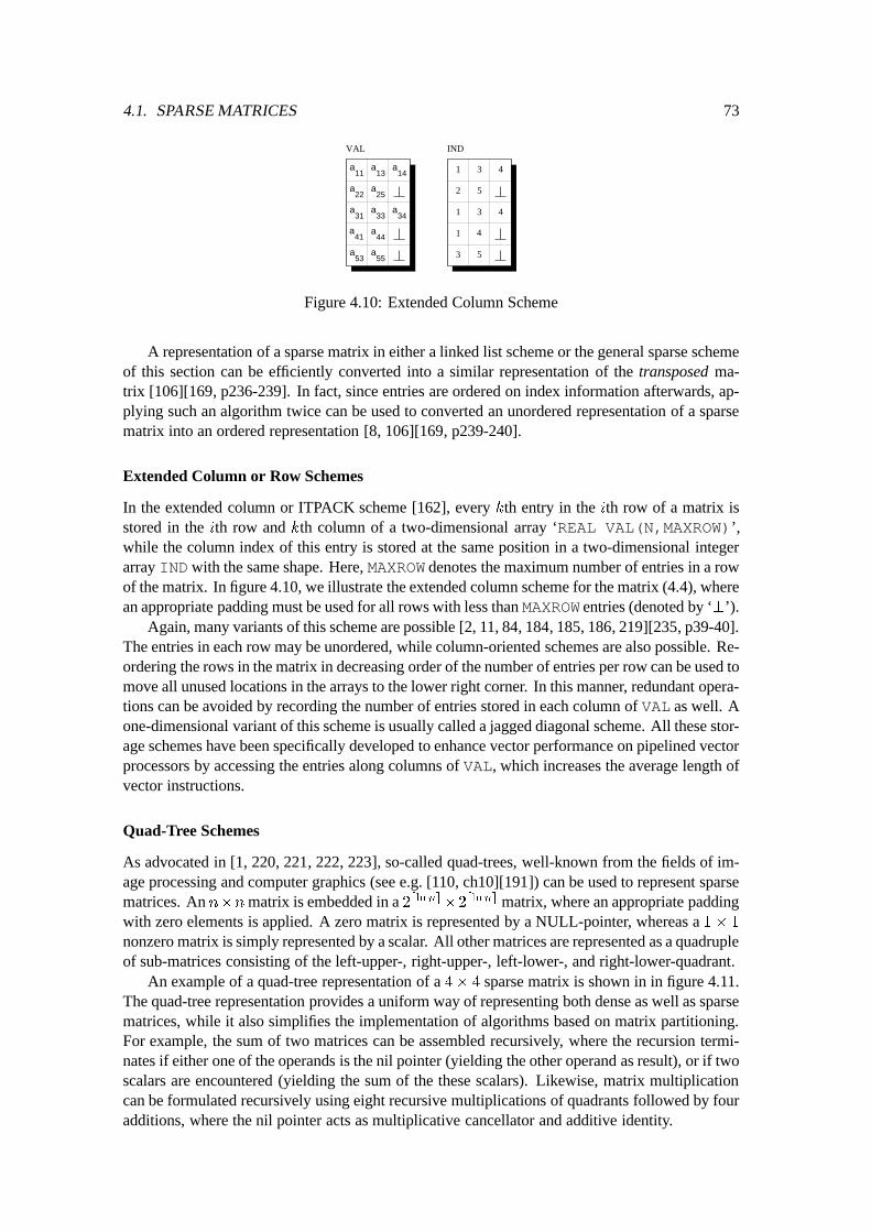
4.1. SPARSE MATRICES 73
VAL
a
a
a
a
IND
4
4
1
5
2
a
a
a
a
a a
a
a55
11 13 14
22 25
31 33 34
41 44
53 3
1
3 4
5
1 3
Figure 4.10: Extended Column Scheme
A representation of a sparse matrix in either a linked list scheme or the general sparse schemeof this section can be efficiently converted into a similar representation of the transposed ma-trix [106][169, p236-239]. In fact, since entries are ordered on index information afterwards, ap-plying such an algorithm twice can be used to converted an unordered representation of a sparsematrix into an ordered representation [8, 106][169, p239-240].
Extended Column or Row Schemes
In the extended column or ITPACK scheme [162], every kth entry in the ith row of a matrix isstored in the ith row and kth column of a two-dimensional array ‘REAL VAL(N,MAXROW)’,while the column index of this entry is stored at the same position in a two-dimensional integerarray INDwith the same shape. Here, MAXROW denotes the maximum number of entries in a rowof the matrix. In figure 4.10, we illustrate the extended column scheme for the matrix (4.4), wherean appropriate padding must be used for all rows with less than MAXROW entries (denoted by ‘?’).
Again, many variants of this scheme are possible [2, 11, 84, 184, 185, 186, 219][235, p39-40].The entries in each row may be unordered, while column-oriented schemes are also possible. Re-ordering the rows in the matrix in decreasing order of the number of entries per row can be used tomove all unused locations in the arrays to the lower right corner. In this manner, redundant opera-tions can be avoided by recording the number of entries stored in each column of VAL as well. Aone-dimensional variant of this scheme is usually called a jagged diagonal scheme. All these stor-age schemes have been specifically developed to enhance vector performance on pipelined vectorprocessors by accessing the entries along columns of VAL, which increases the average length ofvector instructions.
Quad-Tree Schemes
As advocated in [1, 220, 221, 222, 223], so-called quad-trees, well-known from the fields of im-age processing and computer graphics (see e.g. [110, ch10][191]) can be used to represent sparsematrices. An n�nmatrix is embedded in a 2dlnne�2
dln ne matrix, where an appropriate paddingwith zero elements is applied. A zero matrix is represented by a NULL-pointer, whereas a 1 � 1
nonzero matrix is simply represented by a scalar. All other matrices are represented as a quadrupleof sub-matrices consisting of the left-upper-, right-upper-, left-lower-, and right-lower-quadrant.
An example of a quad-tree representation of a 4� 4 sparse matrix is shown in in figure 4.11.The quad-tree representation provides a uniform way of representing both dense as well as sparsematrices, while it also simplifies the implementation of algorithms based on matrix partitioning.For example, the sum of two matrices can be assembled recursively, where the recursion termi-nates if either one of the operands is the nil pointer (yielding the other operand as result), or if twoscalars are encountered (yielding the sum of the these scalars). Likewise, matrix multiplicationcan be formulated recursively using eight recursive multiplications of quadrants followed by fouradditions, where the nil pointer acts as multiplicative cancellator and additive identity.
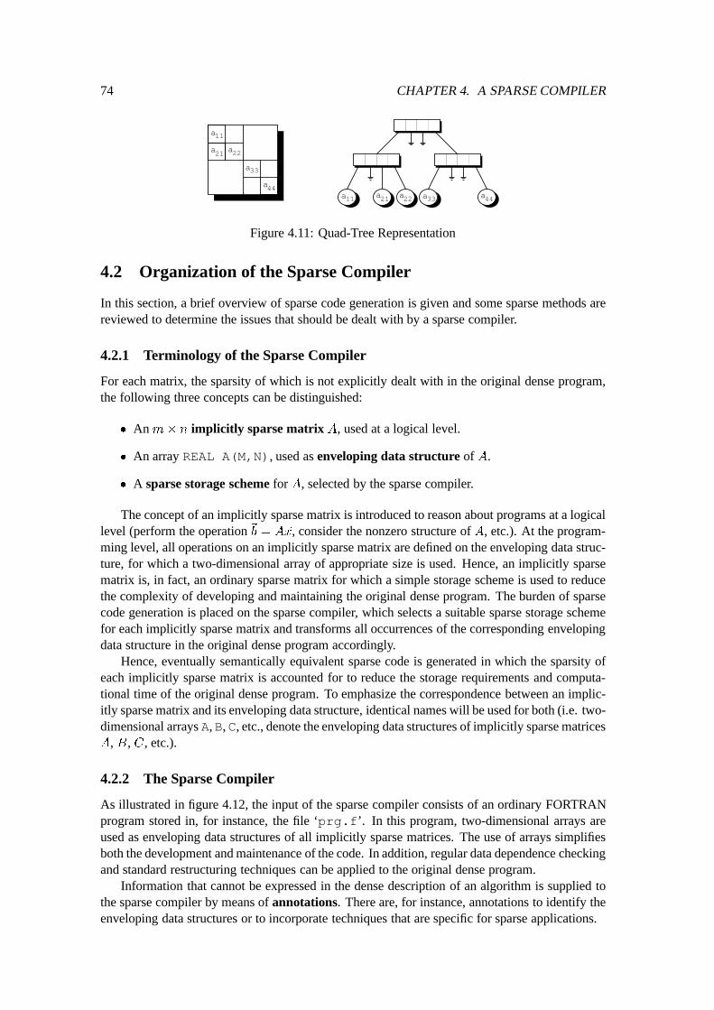
74 CHAPTER 4. A SPARSE COMPILER
a11
a22
a33
a44
a21
a21 a22 a33 a44a11
Figure 4.11: Quad-Tree Representation
4.2 Organization of the Sparse Compiler
In this section, a brief overview of sparse code generation is given and some sparse methods arereviewed to determine the issues that should be dealt with by a sparse compiler.
4.2.1 Terminology of the Sparse Compiler
For each matrix, the sparsity of which is not explicitly dealt with in the original dense program,the following three concepts can be distinguished:
� An m� n implicitly sparse matrix A, used at a logical level.
� An array REAL A(M,N), used as enveloping data structure of A.
� A sparse storage scheme for A, selected by the sparse compiler.
The concept of an implicitly sparse matrix is introduced to reason about programs at a logicallevel (perform the operation~b = A~x, consider the nonzero structure of A, etc.). At the program-ming level, all operations on an implicitly sparse matrix are defined on the enveloping data struc-ture, for which a two-dimensional array of appropriate size is used. Hence, an implicitly sparsematrix is, in fact, an ordinary sparse matrix for which a simple storage scheme is used to reducethe complexity of developing and maintaining the original dense program. The burden of sparsecode generation is placed on the sparse compiler, which selects a suitable sparse storage schemefor each implicitly sparse matrix and transforms all occurrences of the corresponding envelopingdata structure in the original dense program accordingly.
Hence, eventually semantically equivalent sparse code is generated in which the sparsity ofeach implicitly sparse matrix is accounted for to reduce the storage requirements and computa-tional time of the original dense program. To emphasize the correspondence between an implic-itly sparse matrix and its enveloping data structure, identical names will be used for both (i.e. two-dimensional arrays A,B,C, etc., denote the enveloping data structures of implicitly sparse matricesA, B, C , etc.).
4.2.2 The Sparse Compiler
As illustrated in figure 4.12, the input of the sparse compiler consists of an ordinary FORTRANprogram stored in, for instance, the file ‘prg.f’. In this program, two-dimensional arrays areused as enveloping data structures of all implicitly sparse matrices. The use of arrays simplifiesboth the development and maintenance of the code. In addition, regular data dependence checkingand standard restructuring techniques can be applied to the original dense program.
Information that cannot be expressed in the dense description of an algorithm is supplied tothe sparse compiler by means of annotations. There are, for instance, annotations to identify theenveloping data structures or to incorporate techniques that are specific for sparse applications.
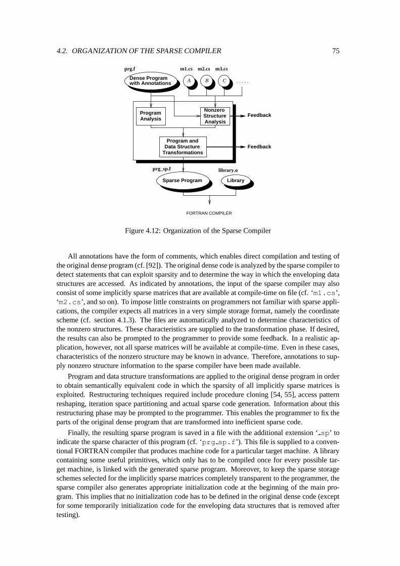
4.2. ORGANIZATION OF THE SPARSE COMPILER 75
Sparse Program
ProgramAnalysis
Nonzero StructureAnalysis
A CB
m1.cs m2.cs m3.cs
.....
Program andData Structure
Transformations
Dense Programwith Annotations
Library
FORTRAN COMPILER
Feedback
Feedback
prg.f
prg_sp.f library.o
Figure 4.12: Organization of the Sparse Compiler
All annotations have the form of comments, which enables direct compilation and testing ofthe original dense program (cf. [92]). The original dense code is analyzed by the sparse compiler todetect statements that can exploit sparsity and to determine the way in which the enveloping datastructures are accessed. As indicated by annotations, the input of the sparse compiler may alsoconsist of some implicitly sparse matrices that are available at compile-time on file (cf. ‘m1.cs’,‘m2.cs’, and so on). To impose little constraints on programmers not familiar with sparse appli-cations, the compiler expects all matrices in a very simple storage format, namely the coordinatescheme (cf. section 4.1.3). The files are automatically analyzed to determine characteristics ofthe nonzero structures. These characteristics are supplied to the transformation phase. If desired,the results can also be prompted to the programmer to provide some feedback. In a realistic ap-plication, however, not all sparse matrices will be available at compile-time. Even in these cases,characteristics of the nonzero structure may be known in advance. Therefore, annotations to sup-ply nonzero structure information to the sparse compiler have been made available.
Program and data structure transformations are applied to the original dense program in orderto obtain semantically equivalent code in which the sparsity of all implicitly sparse matrices isexploited. Restructuring techniques required include procedure cloning [54, 55], access patternreshaping, iteration space partitioning and actual sparse code generation. Information about thisrestructuring phase may be prompted to the programmer. This enables the programmer to fix theparts of the original dense program that are transformed into inefficient sparse code.
Finally, the resulting sparse program is saved in a file with the additional extension ‘ sp’ toindicate the sparse character of this program (cf. ‘prg sp.f’). This file is supplied to a conven-tional FORTRAN compiler that produces machine code for a particular target machine. A librarycontaining some useful primitives, which only has to be compiled once for every possible tar-get machine, is linked with the generated sparse program. Moreover, to keep the sparse storageschemes selected for the implicitly sparse matrices completely transparent to the programmer, thesparse compiler also generates appropriate initialization code at the beginning of the main pro-gram. This implies that no initialization code has to be defined in the original dense code (exceptfor some temporarily initialization code for the enveloping data structures that is removed aftertesting).
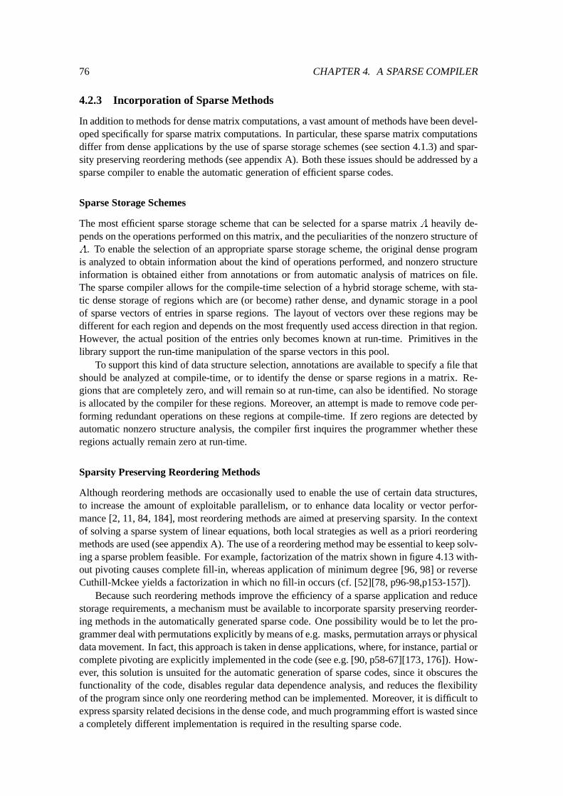
76 CHAPTER 4. A SPARSE COMPILER
4.2.3 Incorporation of Sparse Methods
In addition to methods for dense matrix computations, a vast amount of methods have been devel-oped specifically for sparse matrix computations. In particular, these sparse matrix computationsdiffer from dense applications by the use of sparse storage schemes (see section 4.1.3) and spar-sity preserving reordering methods (see appendix A). Both these issues should be addressed by asparse compiler to enable the automatic generation of efficient sparse codes.
Sparse Storage Schemes
The most efficient sparse storage scheme that can be selected for a sparse matrix A heavily de-pends on the operations performed on this matrix, and the peculiarities of the nonzero structure ofA. To enable the selection of an appropriate sparse storage scheme, the original dense programis analyzed to obtain information about the kind of operations performed, and nonzero structureinformation is obtained either from annotations or from automatic analysis of matrices on file.The sparse compiler allows for the compile-time selection of a hybrid storage scheme, with sta-tic dense storage of regions which are (or become) rather dense, and dynamic storage in a poolof sparse vectors of entries in sparse regions. The layout of vectors over these regions may bedifferent for each region and depends on the most frequently used access direction in that region.However, the actual position of the entries only becomes known at run-time. Primitives in thelibrary support the run-time manipulation of the sparse vectors in this pool.
To support this kind of data structure selection, annotations are available to specify a file thatshould be analyzed at compile-time, or to identify the dense or sparse regions in a matrix. Re-gions that are completely zero, and will remain so at run-time, can also be identified. No storageis allocated by the compiler for these regions. Moreover, an attempt is made to remove code per-forming redundant operations on these regions at compile-time. If zero regions are detected byautomatic nonzero structure analysis, the compiler first inquires the programmer whether theseregions actually remain zero at run-time.
Sparsity Preserving Reordering Methods
Although reordering methods are occasionally used to enable the use of certain data structures,to increase the amount of exploitable parallelism, or to enhance data locality or vector perfor-mance [2, 11, 84, 184], most reordering methods are aimed at preserving sparsity. In the contextof solving a sparse system of linear equations, both local strategies as well as a priori reorderingmethods are used (see appendix A). The use of a reordering method may be essential to keep solv-ing a sparse problem feasible. For example, factorization of the matrix shown in figure 4.13 with-out pivoting causes complete fill-in, whereas application of minimum degree [96, 98] or reverseCuthill-Mckee yields a factorization in which no fill-in occurs (cf. [52][78, p96-98,p153-157]).
Because such reordering methods improve the efficiency of a sparse application and reducestorage requirements, a mechanism must be available to incorporate sparsity preserving reorder-ing methods in the automatically generated sparse code. One possibility would be to let the pro-grammer deal with permutations explicitly by means of e.g. masks, permutation arrays or physicaldata movement. In fact, this approach is taken in dense applications, where, for instance, partial orcomplete pivoting are explicitly implemented in the code (see e.g. [90, p58-67][173, 176]). How-ever, this solution is unsuited for the automatic generation of sparse codes, since it obscures thefunctionality of the code, disables regular data dependence analysis, and reduces the flexibilityof the program since only one reordering method can be implemented. Moreover, it is difficult toexpress sparsity related decisions in the dense code, and much programming effort is wasted sincea completely different implementation is required in the resulting sparse code.
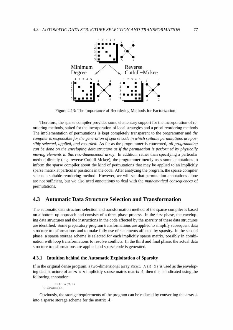
4.3. AUTOMATIC DATA STRUCTURE SELECTION AND TRANSFORMATION 77
1 2 3 4 512345
1
2 3
45
ReverseCuthill−Mckee
1 2 3 4 512345
5 1
4
23
1 2 3 4 512345
5
1 4
2 3
MinimumDegree
Figure 4.13: The Importance of Reordering Methods for Factorization
Therefore, the sparse compiler provides some elementary support for the incorporation of re-ordering methods, suited for the incorporation of local strategies and a priori reordering methodsThe implementation of permutations is kept completely transparent to the programmer and thecompiler is responsible for the generation of sparse code in which suitable permutations are pos-sibly selected, applied, and recorded. As far as the programmer is concerned, all programmingcan be done on the enveloping data structure as if the permutation is performed by physicallymoving elements in this two-dimensional array. In addition, rather than specifying a particularmethod directly (e.g. reverse Cuthill-Mckee), the programmer merely uses some annotations toinform the sparse compiler about the kind of permutations that may be applied to an implicitlysparse matrix at particular positions in the code. After analyzing the program, the sparse compilerselects a suitable reordering method. However, we will see that permutation annotations aloneare not sufficient, but we also need annotations to deal with the mathematical consequences ofpermutations.
4.3 Automatic Data Structure Selection and Transformation
The automatic data structure selection and transformation method of the sparse compiler is basedon a bottom-up approach and consists of a three phase process. In the first phase, the envelop-ing data structures and the instructions in the code affected by the sparsity of these data structuresare identified. Some preparatory program transformations are applied to simplify subsequent datastructure transformations and to make fully use of statements affected by sparsity. In the secondphase, a sparse storage scheme is selected for each implicitly sparse matrix, possibly in combi-nation with loop transformations to resolve conflicts. In the third and final phase, the actual datastructure transformations are applied and sparse code is generated.
4.3.1 Intuition behind the Automatic Exploitation of Sparsity
If in the original dense program, a two-dimensional array REAL A(M,N) is used as the envelop-ing data structure of an m� n implicitly sparse matrix matrix A, then this is indicated using thefollowing annotation:
REAL A(M,N)C_SPARSE(A)
Obviously, the storage requirements of the program can be reduced by converting the array Ainto a sparse storage scheme for the matrix A.
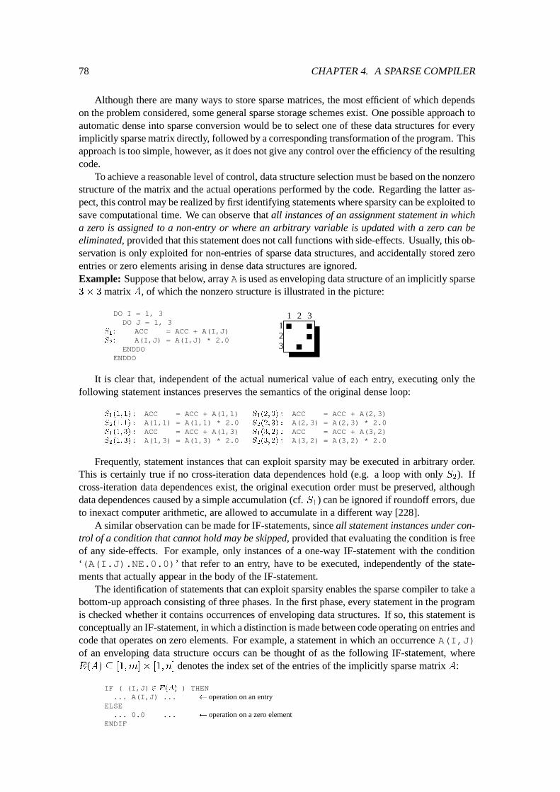
78 CHAPTER 4. A SPARSE COMPILER
Although there are many ways to store sparse matrices, the most efficient of which dependson the problem considered, some general sparse storage schemes exist. One possible approach toautomatic dense into sparse conversion would be to select one of these data structures for everyimplicitly sparse matrix directly, followed by a corresponding transformation of the program. Thisapproach is too simple, however, as it does not give any control over the efficiency of the resultingcode.
To achieve a reasonable level of control, data structure selection must be based on the nonzerostructure of the matrix and the actual operations performed by the code. Regarding the latter as-pect, this control may be realized by first identifying statements where sparsity can be exploited tosave computational time. We can observe that all instances of an assignment statement in whicha zero is assigned to a non-entry or where an arbitrary variable is updated with a zero can beeliminated, provided that this statement does not call functions with side-effects. Usually, this ob-servation is only exploited for non-entries of sparse data structures, and accidentally stored zeroentries or zero elements arising in dense data structures are ignored.Example: Suppose that below, array A is used as enveloping data structure of an implicitly sparse3� 3 matrix A, of which the nonzero structure is illustrated in the picture:
DO I = 1, 3DO J = 1, 3
S
1
: ACC = ACC + A(I,J)S
2
: A(I,J) = A(I,J) * 2.0ENDDO
ENDDO
1 2 3123
It is clear that, independent of the actual numerical value of each entry, executing only thefollowing statement instances preserves the semantics of the original dense loop:
S
1
(1; 1) : ACC = ACC + A(1,1)S
2
(1; 1) : A(1,1) = A(1,1) * 2.0S
1
(1; 3) : ACC = ACC + A(1,3)S
2
(1; 3) : A(1,3) = A(1,3) * 2.0
S
1
(2; 3) : ACC = ACC + A(2,3)S
2
(2; 3) : A(2,3) = A(2,3) * 2.0S
1
(3; 2) : ACC = ACC + A(3,2)S
2
(3; 2) : A(3,2) = A(3,2) * 2.0
Frequently, statement instances that can exploit sparsity may be executed in arbitrary order.This is certainly true if no cross-iteration data dependences hold (e.g. a loop with only S
2
). Ifcross-iteration data dependences exist, the original execution order must be preserved, althoughdata dependences caused by a simple accumulation (cf. S
1
) can be ignored if roundoff errors, dueto inexact computer arithmetic, are allowed to accumulate in a different way [228].
A similar observation can be made for IF-statements, since all statement instances under con-trol of a condition that cannot hold may be skipped, provided that evaluating the condition is freeof any side-effects. For example, only instances of a one-way IF-statement with the condition‘(A(I.J).NE.0.0)’ that refer to an entry, have to be executed, independently of the state-ments that actually appear in the body of the IF-statement.
The identification of statements that can exploit sparsity enables the sparse compiler to take abottom-up approach consisting of three phases. In the first phase, every statement in the programis checked whether it contains occurrences of enveloping data structures. If so, this statement isconceptually an IF-statement, in which a distinction is made between code operating on entries andcode that operates on zero elements. For example, a statement in which an occurrence A(I,J)of an enveloping data structure occurs can be thought of as the following IF-statement, whereE(A) � [1;m]� [1; n] denotes the index set of the entries of the implicitly sparse matrix A:
IF ( (I,J) 2 E(A) ) THEN... A(I,J) ... operation on an entry
ELSE... 0.0 ... operation on a zero element
ENDIF
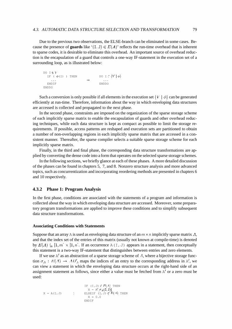
4.3. AUTOMATIC DATA STRUCTURE SELECTION AND TRANSFORMATION 79
Due to the previous two observations, the ELSE-branch can be eliminated in some cases. Be-cause the presence of guards like ‘(I; J) 2 E(A)’ reflects the run-time overhead that is inherentto sparse codes, it is desirable to eliminate this overhead. An important source of overhead reduc-tion is the encapsulation of a guard that controls a one-way IF-statement in the execution set of asurrounding loop, as is illustrated below:
DO I 2 VIF ( �(I) ) THEN...
ENDIFENDDO
!
DO I 2 fV j �g...
ENDDO
Such a conversion is only possible if all elements in the execution set fV j �g can be generatedefficiently at run-time. Therefore, information about the way in which enveloping data structuresare accessed is collected and propagated to the next phase.
In the second phase, constraints are imposed on the organization of the sparse storage schemeof each implicitly sparse matrix to enable the encapsulation of guards and other overhead reduc-ing techniques, while each data structure is kept as compact as possible to limit the storage re-quirements. If possible, access patterns are reshaped and execution sets are partitioned to obtaina number of non-overlapping regions in each implicitly sparse matrix that are accessed in a con-sistent manner. Thereafter, the sparse compiler selects a suitable sparse storage scheme for eachimplicitly sparse matrix.
Finally, in the third and final phase, the corresponding data structure transformations are ap-plied by converting the dense code into a form that operates on the selected sparse storage schemes.
In the following sections, we briefly glance at each of these phases. A more detailed discussionof the phases can be found in chapters 5, 7, and 8. Nonzero structure analysis and more advancedtopics, such as concurrentization and incorporating reordering methods are presented in chapters 6and 10 respectively.
4.3.2 Phase 1: Program Analysis
In the first phase, conditions are associated with the statements of a program and information iscollected about the way in which enveloping data structure are accessed. Moreover, some prepara-tory program transformations are applied to improve these conditions and to simplify subsequentdata structure transformations.
Associating Conditions with Statements
Suppose that an array A is used as enveloping data structure of anm�n implicitly sparse matrixA,and that the index set of the entries of this matrix (usually not known at compile-time) is denotedby E(A) � [1;m] � [1; n]. If an occurrence A(I,J) appears in a statement, then conceptuallythis statement is a two-way IF-statement that distinguishes between entries and zero elements.
If we use A0 as an abstraction of a sparse storage scheme of A, where a bijective storage func-tion �
A
: E(A) ! AD
0
A
maps the indices of an entry to the corresponding address in A0, wecan view a statement in which the enveloping data structure occurs at the right-hand side of anassignment statement as follows, since either a value must be fetched from A0 or a zero must beused:
X = A(I,J)!
IF (I,J) 2 E(A) THENX = A0[�
A
(I; J)]
ELSEIF (I,J) =2 E(A) THENX = 0.0
ENDIF
80 CHAPTER 4. A SPARSE COMPILER
Making the distinction seems useless in this case, and we rather use the convention that wehave �
A
(i; j) =? if (i; j) =2 E(A) holds, where A0[?] = 0, to avoid the distinction shown above.In other cases, however, branches may be eliminated due to the observations made in the previoussection. An example is shown below:
ACC = ACC + A(I,J)!
IF (I,J) 2 E(A) THENACC = ACC + A0[�
A
(I; J)]
ENDIF
Another, less obvious example where one branch can be eliminated if zero constants are han-dled as non-entries is shown below:1
A(I,J) = 0.0!
IF (I,J) 2 E(A) THENA0[�
A
(I; J)] = 0.0ENDIF
If an occurrence of an enveloping data structure appears at the left-hand side of an assignmentstatement in which an arbitrary expressions appears at the right-hand side, then the two branchesmust handle the change in value for an entry or creation respectively:
A(I,J) = X!
IF (I,J) 2 E(A) THENA0[�
A
(I; J)] = XELSEIF (I,J) =2 E(A) THEN
A0[newA
(I; J)] = XENDIF
We have used the function newA
to insert a new entry in A. This function returns the addressof a new entry a
ij
, and adapts the storage function �A
, the index set of the entries E(A) and theset of addresses AD0
A
accordingly as side-effects.The ‘2 E(A)’- and ‘=2 E(A)’-tests are referred to as positive and negative guards respec-
tively. Every different occurrence of an enveloping data structures gives rise to an additional posi-tive and negative guard. Hence, statements with k different occurrences of enveloping data struc-tures can be thought of as a multi-way IF-statements with 2
k branches for every possible conjunc-tion of the corresponding guards. An example is given below, where we assume that array B isalso used as enveloping data structure. The last branch has been eliminated to exploit sparsity:
X = X + A(I,J) + B(I,J)!
IF (I,J) 2 E(A) ^ (I,J) 2 E(B) THENX = X + A0[�
A
(I; J)] + B0[�B
(I; J)]
ELSEIF (I,J) 2 E(A) ^ (I,J) =2 E(B) THENX = X + A0[�
A
(I; J)]
ELSEIF (I,J) =2 E(A) ^ (I,J) 2 E(B) THENX = X + B0[�
B
(I,J)]ENDIF
We define the condition of a statement as the disjunction of all conditions (consisting of con-junctions of guards) that appear in the remaining branches of the multi-way IF-statement, i.e. thebranches that cannot exploit sparsity. For the previous example, for instance, the associated con-dition is:
( ((I; J) 2 E(A) ^ (I; J) 2 E(B)) _
((I; J) 2 E(A) ^ (I; J) =2 E(B)) _
((I; J) =2 E(A) ^ (I; J) 2 E(B)) ) � (I; J) 2 E(A) _ (I; J) 2 E(B)
This condition, which has been simplified into a single disjunction of guards, reflects the factthat all instances referring to at least one entry must be executed so that only the instances thataccess two non-entries can fully exploit sparsity (if we ignore the fact that some entries may acci-dentally be zero). In general, a condition of a statement defines the instances of the statement thatcannot exploit sparsity and, hence, must be executed. Another example is shown below:
1Note that in this case, the entry could be eliminated from the sparse storage scheme in the remaining branch. Usu-ally, however, the situation in which an entry becomes zero is simply ignored.
4.3. AUTOMATIC DATA STRUCTURE SELECTION AND TRANSFORMATION 81
X = X + A(I,K) * B(K,J)!
IF (I,K) 2 E(A) ^ (K,J) 2 E(B) THENX = X + A0[�
A
(I; J)] * B0[�B
(I; J)]
ENDIF
Condition ‘(I; K) 2 E(A) ^ (K; J) 2 E(B)’ is associated with this statement, which in-dicates that only the instances in which two entries are accessed have to be executed. In somecases, we can also associate conditions with IF-statements. Condition ‘(J; I) 2 E(A)’, for ex-ample, may be associated with the following one-way IF-statement, since the boolean expression‘(A(J,I).GT.ABS(X))’ necessarily evaluates to false for all non-entries:
IF (A(J,I) .GT. ABS(X)) THEN...
ENDIF!
IF (J,I) 2 E(A) THENIF (A0[�
A
(J; I)] .GT. ABS(X)) THEN...
ENDIFENDIF
Obviously, it would be extremely cumbersome to first generate multi-way-IF statements, fol-lowed by eliminating branches that can exploit sparsity and computing the condition for each state-ment according to the remaining branches. Fortunately, it is not necessary to explicitly constructmulti-way IF-statements to compute the condition of each statement. In chapter 5, we present asimple attributed grammar that directly computes the condition for each statement. The conditionscomputed by this attributed grammar only exploit zero constants and non-entries, i.e. the condi-tions conservatively assume that the contents of dense variables and entries are always nonzero.Although this implies that accidentally stored zeros are not exploited, it prevents the generationof additional tests on the value of such expressions which are likely to fail.
Dominating Guards
For some statements, the value of the associated condition is completely dependent on the valueof one particular positive guard. Such situations frequently occur in linear algebra operations thatare classified as static or simply dynamic [235, p10-12]. For example, implementing the opera-tion A � � A, which is called a simply dynamic operation, involves the following assignmentstatement:
A(I,J) = ALPHA * A(I,J)!
IF (I,J) 2 E(A) THENA0[�
A
(I; J)] = ALPHA * A0[�A
(I; J)]
ENDIF
We say that a positive guard dominates a condition �, if � ) holds. Informally speak-ing, if the guard does not hold, then the whole condition � does not hold. In this previous ex-ample, the guard ‘(I; J) 2 E(A)’ dominates the identical condition. As another example, boththe guards in the condition ‘(I; K) 2 E(A) ^ (K; J) 2 E(B)’ dominate this condition, whereasnone of these guards dominates the condition ‘(I; K) 2 E(A) _ (K; J) 2 E(B)’. Dominatingguards give rise to a convenient overhead reduction method, because sparse data structures usu-ally provide efficient generation of all entries, i.e. elements for which the guard holds, along anaccess pattern. Therefore, information about the way enveloping data structures are accessed iscollected and propagated to the second phase.
Preparatory Program Transformations
During the first phase, some preparatory program transformations are applied to simplify subse-quent data structure transformations and to improve the conditions that become associated withthe statements in the program. For example, because in the following fragment another data struc-ture will be selected for array A, the occurrences of the formal argument M in subroutine SUBmustbe converted accordingly to account for the fact that this subroutine may be called with A as actualargument:
82 CHAPTER 4. A SPARSE COMPILER
REAL A(10,10), X(100), D(10,10)C_SPARSE(A)
...CALL SUB(A)CALL SUB(X)CALL SUB(D)END
SUBROUTINE SUB(M)REAL M(10,10)...RETURNEND
However, since this subroutine is also called with X and D as actual arguments, we cannotbluntly apply program and data structure transformations to SUB. Instead, we first apply proce-dure cloning [54, 55] to construct a clone ‘SUB A’ of the subroutine, in which there is a uniqueassociation between the enveloping data structure A and the formal argument M. Thereafter, thefirst CALL-statements in the main program is converted accordingly and program and data struc-ture transformations can be applied to the clone without interfering with calls to SUB having denseactual arguments.
Some transformations that improve the conditions associated with statements may also be ap-plied. For example, using the attributed grammar that will be presented in chapter 5, condition‘true’ becomes associated with the following two assignment statements because it seems thatnone of the instances of these statements can exploit sparsity. However, after scalar forward sub-stitution [234, p178-179], the condition of the remaining statement changes into ‘(I; J) 2 E(A)’:
T = A(I,J)ACC = ACC + 3.0 * T
! ACC = ACC + 3.0 * A(I,J)
4.3.3 Phase 2: Data Structure Selection
Each occurrence of an enveloping data structure induces access patterns that form paths throughthe index set of the corresponding implicitly sparse matrix. The elements along every path can beviewed as a vector that, depending on the regions accessed, is either dense, sparse or zero. In thesecond phase, the sparse compiler selects a storage scheme for each implicitly sparse matrix. Sta-tic dense storage is used for the vectors through dense regions, whereas a pool of sparse vectors isselected as dynamic storage for the remaining regions. The layout of the vectors over these regionsis selected to enable overhead reducing techniques as much a possible. Loop transformations areused to obtain a number of non-overlapping regions that are accessed in a consistent manner.
Overhead Reducing Techniques
Although the multi-way IF-statements used during the presentation of the first phase are not ex-plicitly generated, the presence of guards, �
A
-lookups and newA
-functions reflect the overheadinherent to sparse storage schemes for scanning a compact data structure to determine if and wherean entry is stored or for inserting an entry. Because skipping operations by means of conditionalsdoes not reduce the execution time on most machines [78, 169], overhead reducing techniques arerequired. The prototype sparse compiler has the ability to apply one of the following overhead re-ducing techniques: (i) replacing accesses to zero regions by zero, (ii) avoiding overhead by usingstatic dense storage for particular regions, (iii) applying so-called guard encapsulation, where aconstruct that iterates over the entries along an access pattern is generated, or (iv) applying so-called access pattern expansion, where a sparse vector is scattered into a full-sized array beforeoperations are applied to this vector, and gathered back into sparse storage thereafter.
Zero Replacement
If we know that a particular region in an implicitly sparse matrix A is completely zero and willremain so at run-time, then all occurrences of the corresponding enveloping data structure that canonly induce accesses to this region can be replaced by the constant zero at compile-time.
4.3. AUTOMATIC DATA STRUCTURE SELECTION AND TRANSFORMATION 83
If, for example, we know that the whole main diagonal of an implicitly sparse matrixA havingA as enveloping data structure is completely zero and will remain so at run-time, then the followingreplacement becomes possible:
ACC = ACC + A(5,5) ! ACC = ACC + 0.0
Because the condition ‘false’ becomes associated with the resulting statement, the whole as-signment statement can be eliminated thereafter.
Using Static Dense Storage
If a particular region in an implicitly sparse matrix is rather dense, then we can use static densestorage for that region to avoid the overhead that is inherent to sparse storage schemes. For in-stance, using a one-dimensional array DIAG A to store all elements along the main diagonal of animplicitly sparse matrixA having the two-dimensional array A as enveloping data structure avoidsall lookup overhead in the following fragment (another storage organization may be used for theremaining regions):
REAL A(N,N)C_SPARSE(A)
...DO I = 1, N
X(I) = A(I,I)ENDDO
!
REAL DIAG_A(N), ......DO I = 1, NX(I) = DIAG_A(I)
ENDDO
If some zero elements along the main diagonal become nonzero, the use of static dense stor-age even avoids any overhead arising from the run-time insertion of entries. On the other hand,using static dense storage also disables any exploitation of sparsity to reduce either storage re-quirements or computational time. For example, although condition ‘(I; I) 2 E(A)’ is associ-ated with the following statement, sparsity cannot be exploited (viz. selecting static dense storageof the main diagonal implies that the inclusion f(1; 1); (2; 2); : : :g � E(A) is already known atcompile-time):
ACC = ACC + A(I,I) ! ACC = ACC + DIAG_A(I)
Only if the main diagonal is reasonably dense, the number of unnecessarily performed opera-tions and stored zero elements is small. Therefore, static dense storage should only be selected forregions that are or become rather dense, whereas sparse storage should be used for the remainingregions, using the overhead reducing techniques of the following sections where possible.
Guard Encapsulation
For an occurrence of an enveloping data structure that has admissible subscripts represented by theaffine transformation F (~I) = ~v +W
~
I appearing in a loop with index vector ~I = (I
1
; : : : ; I
d
)
T ,we define the access pattern P (I
1
; : : : ; I
d�1
) � Z
2 as the index set of all elements accessed insuccessive iterations of the innermost stride-1 I
d
-loop with bounds Ld
and Ud
:
P (I
1
; : : : ; I
d�1
) = fF (
~
I)
T
j I
d
2 [L
d
; U
d
]g
If guard ‘F (~I) 2 E(A)’ dominates the condition of all statements in the loop-body, we wouldlike to let index I
d
iterate over all values in the irregular execution set fId
2 [L
d
; U
d
] j F (
~
I) 2
E(A)g. This is obtained by guard encapsulation. In this manner, only iterations in which anentry is operated on, i.e. an element for which the dominating guard holds, are executed and testoverhead vanishes. Under certain conditions, guard encapsulation can be implemented by iterat-ing over the entries along each access pattern, as is illustrated below:
84 CHAPTER 4. A SPARSE COMPILER
DO I1
= L1
, U1
......DO I
d
= Ld
, Ud
IF F (
~
I) 2 E(A) THENACC = ACC + A0[�
A
(F (
~
I))]
ENDIFENDDO...
...ENDDO
!
DO I1
= L1
, U1
......DO ad 2 AD
0
A
(I
1
; : : : ; I
d�1
)
ACC = ACC + A0[ad]ENDDO...
...ENDDO
This conversion is feasible if the last column of matrix W is nonzero and the organization ofthe pool of sparse vectors satisfies the following constraints:
(a) For all possible values of the loop indices I1
; : : : ; I
d�1
, the addresses in the following setcan be generated efficiently:
AD
0
A
(I
1
; : : : ; I
d�1
) = f �
A
(f) j f 2 P (I
1
; : : : ; I
d�1
) \E(A) g
(b) To restore the value of loop index Id
, either the value �1
��
�1
A
(ad) if w1d
6= 0 holds, or thevalue �
2
� �
�1
A
(ad) if w2d
6= 0 holds, can be supplied efficiently together with each addressad 2 AD
0
A
(I
1
; : : : ; I
d�1
), where �i
� ~x = x
i
.
Furthermore, to prevent the requirement for ordered storage (not supported in the current pro-totype sparse compiler), this conversion is only done if iterations of this DO-loop may be executedin arbitrary order (although, as discussed in section 4.3.1, data dependences caused by accumula-tions may be ignored):
(c) No data dependence is carried by the Id
-loop and no exit branch [234, p238-241] or STOP-statement can be executed in the loop-body of this DO-loop.
Because, in general, it is very likely that some access patterns are subsets of other access pat-terns, we usually relax constraint (a) to the requirement that the addresses of entries along a lon-gitudinal enveloping access pattern of each true access pattern can be generated efficiently, wherea longitudinal enveloping access pattern of an access pattern simply consists of all discrete pointson an arbitrary line segment that is placed over the access pattern. However, in this case, we musttest if the restored value of the loop index I
d
is an integer value in the range [L
d
; U
d
] to deter-mine whether an entry actually corresponds to the true access pattern. Constraint (b) follows fromad = �
A
(~v +W
~
I) and the fact that the storage function �A
is invertible:(
�
1
� �
�1
A
(ad) = v
1
+ w
11
� I
1
+ : : :+ w
1d
� I
d
�
2
� �
�1
A
(ad) = v
2
+ w
21
� I
1
+ : : :+ w
2d
� I
d
(4.5)
Consequently, for column-wise access pattern (viz. w1d
6= 0), the value �1
� �
�1
A
(ad) is re-quired (in combination with the values of the indices of more outer DO-loops) to restore the valueof the loop index I
d
. This clearly illustrates that row index information is required in column-wise oriented data structures. Likewise, for row-wise access patterns (viz. w
2d
6= 0), the value�
2
� �
�1
A
(AD), i.e. the column index, is required, while for diagonal-wise access patterns (viz.w
1d
6= 0 orw2d
6= 0) either row or column index information suffices to solve an equation in (4.5).Example: Below, array A is used as enveloping data structure of a 100 � 100 implicitly sparsematrixA, and guard ‘(I; I+ J) 2 E(A)’, dominates the (identical) loop condition. Hence, guardencapsulation in the execution set of the J-loop is feasible if (a) the addresses of entries along theaccess patterns P (I) = f(I; I+ J) j 1 � J � 75g for 1 � I � 25 can be generated efficiently,(b) �
2
� �
�1
A
(ad)-values are available together with each address, and (c) the data dependencecaused by the accumulation may be ignored:
4.3. AUTOMATIC DATA STRUCTURE SELECTION AND TRANSFORMATION 85
DO I = 1, 25DO J = 1, 75X = X + A(I,I+J) * J
ENDDOENDDO
!
DO I = 1, 25DO ad 2 f�
A
(f) j f 2 P (I) \ E(A)g
J = �
2
� �
�1
A
(ad) - IX = X + A0[ad] * J
ENDDOENDDO
Relaxing constraint (a) enables the sparse compiler to select, for instance, general row-wisestorage of the entries but also requires the test ‘J 2 [1; 75]’ before the value of X is actually up-dated. Although, in general, test overhead remains in the loop-body, still fewer iterations are ex-ecuted, since the average number of entries along each longitudinal enveloping access pattern isprobably less than the size of the original execution set.
It is important to realize that the requirement for fast generation of entries along an accesspattern imposes constraints on the organization of the pool of sparse vectors. In general, the actualaddresses of the entries and their position in the matrix will only be known at run-time. Moreover,if creation may occur in A, this complicates the actual implementation of guard encapsulation,because this affects the value of guards, whereas addresses may change due to data movement or,for some data structures, due to an occasionally required left compression. For scalar-wise accesspatterns (viz. both w
1d
and w2d
are zero), it is possible that the guard can be hoisted out of someinnermost DO-loop, which enables guard encapsulation in the execution set of a more outer DO-loop. These issues are further elaborated in chapter 8.
Access Pattern Expansion
A related overhead reducing technique imposing similar constraints on the organization of the poolof sparse vectors is given by access pattern expansion. The compiler may decide to generate aconstruct that will expand the entries along an access pattern stored in dynamic sparse storage intoa temporary one-dimensional array using a scatter-operation, so that subsequent operations on thisvector do not suffer from the inherent sparse lookup overhead [69, 78, 169]. The actual numberof operations performed, however, is not reduced by this technique.
For example, if the addresses of entries along P = f(10; J) j 1 � J � Ng can be generatedefficiently for an implicitly sparse matrix A with enveloping data structure A, and the value �
2
�
�
�1
A
(ad) is available together with each address, then the following fragment, in which sparsitycannot be exploited to reduce computational time, can be implemented without repeated lookupoverhead as follows:
DO J = 1, ND(10,J) = D(10,J) * A(10,J)
ENDDO!
DO ad 2 f�
A
(f) j f 2 P \ E(A)g
AP(�2
� �
�1
A
(ad)) = A0[ad]ENDDO
)
scatter
DO J = 1, ND(10,J) = D(10,J) * AP(J)
ENDDO
If changes to the nonzero structure along the 10th row occur, then this can be easily accountedfor using the so-called switch technique [169], where a switch array records which elements areentries. Storage is obtained directly to account for creation if necessary and the actual valuesare stored back into sparse storage afterwards with a gather-operation. During this operation, theswitch array and the full-sized array are reset to support any subsequent access pattern expansion,as is further elaborated in chapter 8.
In any case, access pattern expansion is feasible if the organization of the pool of sparse vectorssatisfies constraints (a) and (b) of the previous section.
86 CHAPTER 4. A SPARSE COMPILER
Supporting Transformations
To enable guard encapsulation and access pattern expansion, the sparse compiler must select foreach implicitly sparse matrix an organization of the pool of sparse vectors that supports efficientgeneration of the addresses of entries along certain access patterns. Ideally, we would like to sup-port fast generation of addresses of entries along all access patterns through the correspondingenveloping data structures that are encountered in the program. However, this would demand forextensive overhead storage.
Consequently, it is desirable to have a number of non-overlapping regions in each implicitlysparse matrix that are accessed in a consistent way. Loop transformations can assist in achiev-ing this goal. Unimodular loop transformations can be used to reshape the access patterns of anoccurrence of an enveloping data structure. For example, simple loop interchanging changes therow-wise access patterns of the following occurrences into column-wise access patterns:
DO I = 1, MDO J = 1, NA(I,J) = A(I,J) * 3.0
ENDDOENDDO
!
DO J = 1, NDO I = 1, M
A(I,J) = A(I,J) * 3.0ENDDO
ENDDO
Likewise, iteration space partitioning can be used to obtain a number of non-overlapping re-gions as is illustrated below:
DO I = 1, MA(I,I) = 10.0DO J = 1, ID(I,J) = A(I,J) * X(J)
ENDDOENDDO
I � J � I
!
DO I = 1, MA(I,I) = 10.0DO J = 1, I - 1
D(I,J) = A(I,J) * X(J)ENDDOD(I,I) = A(I,I) * X(I)
ENDDO
After this loop transformation, a different storage organization can be selected for the maindiagonal and the strict lower triangular part of an implicitly sparse matrix A. In chapter 7, wediscuss methods to control these loop transformations and to update information that has beenobtained in the first phase incrementally to avoid re-analysis of the program.
Data Structure Selection
Eventually, the sparse compiler selects a sparse storage scheme for each implicitly sparse matrix.Static dense storage is used for dense regions, whereas a pool of sparse vectors is selected as dy-namic storage for the remaining regions. The layout of the vectors over these regions is selectedaccording to the way in which each region is accessed most frequently, in order to enable guardencapsulation and access pattern expansion as much as possible.
The pool of sparse vectors is stored using a variant of the sparse row- or column-wise schemespresented in section 4.1.3. The numerical values of entries in each sparse vector are stored consec-utively in an array VAL A, while the corresponding column or row indices are stored in a parallelinteger array IND A. The pointers LOW A(p) and HGH A(p) are used to locate the pth sparse vectorin the pool. In figure 4.14, possible contents of these arrays for a general sparse row-wise orga-nization of the pool are shown. In general, however, the layout of sparse vectors over the sparseregions may be selected arbitrarily by the sparse compiler, so that the number of sparse vectorsin the pool may exceed the number of rows or columns of the matrix. Row index information isavailable for column-wise sparse vectors and column index information for sparse vectors storedalong other directions.
Obviously, selecting different storage formats for different regions in an implicitly sparse ma-trix enables the sparse compiler to fully account for both the characteristics of the nonzero struc-ture of this matrix, as well as for the actual operations applied to the matrix.
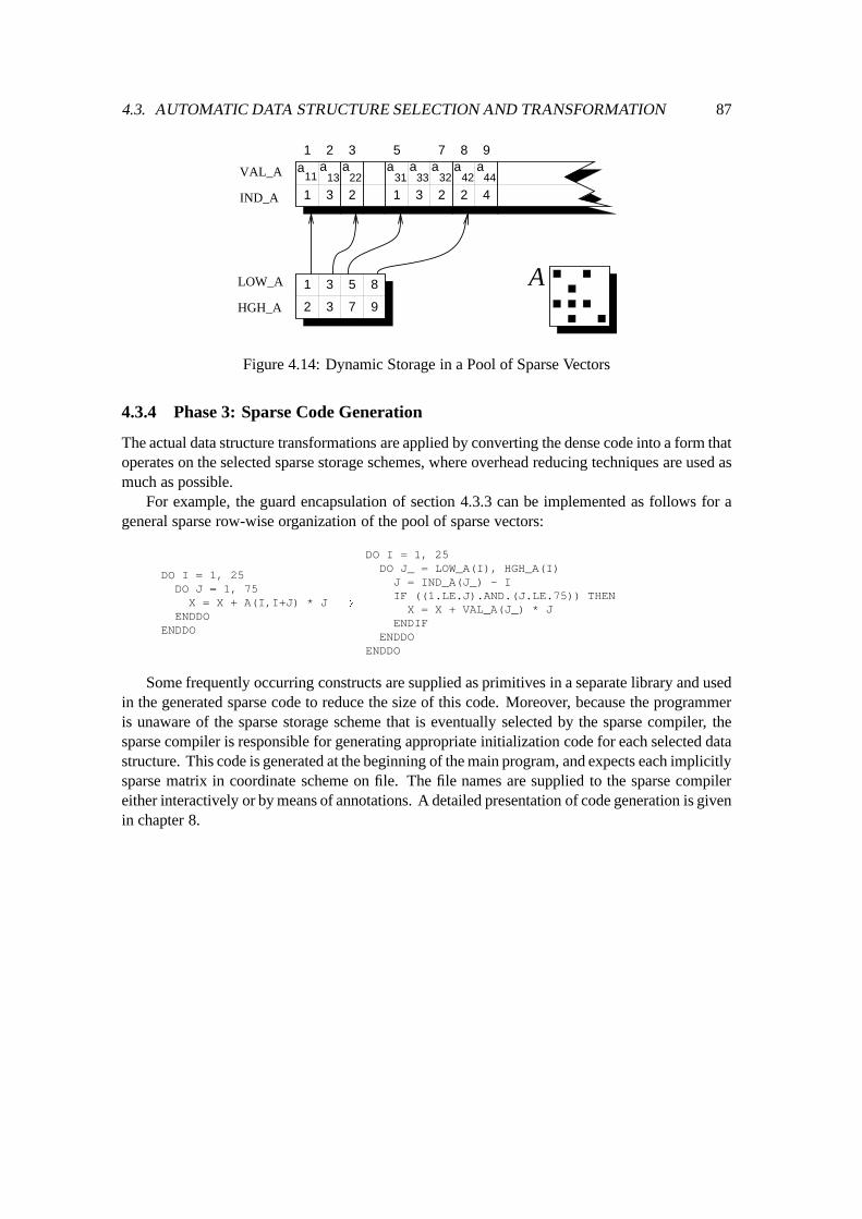
4.3. AUTOMATIC DATA STRUCTURE SELECTION AND TRANSFORMATION 87
A1
3
53
2 7
8
9
a11 13
a22
a a33
a31
a32
51 3 72
1 23 1 3 2
a44
a42
8 9
2 4
VAL_A
IND_A
LOW_A
HGH_A
Figure 4.14: Dynamic Storage in a Pool of Sparse Vectors
4.3.4 Phase 3: Sparse Code Generation
The actual data structure transformations are applied by converting the dense code into a form thatoperates on the selected sparse storage schemes, where overhead reducing techniques are used asmuch as possible.
For example, the guard encapsulation of section 4.3.3 can be implemented as follows for ageneral sparse row-wise organization of the pool of sparse vectors:
DO I = 1, 25DO J = 1, 75X = X + A(I,I+J) * J
ENDDOENDDO
!
DO I = 1, 25DO J_ = LOW_A(I), HGH_A(I)
J = IND_A(J_) - IIF ((1.LE.J).AND.(J.LE.75)) THEN
X = X + VAL_A(J_) * JENDIF
ENDDOENDDO
Some frequently occurring constructs are supplied as primitives in a separate library and usedin the generated sparse code to reduce the size of this code. Moreover, because the programmeris unaware of the sparse storage scheme that is eventually selected by the sparse compiler, thesparse compiler is responsible for generating appropriate initialization code for each selected datastructure. This code is generated at the beginning of the main program, and expects each implicitlysparse matrix in coordinate scheme on file. The file names are supplied to the sparse compilereither interactively or by means of annotations. A detailed presentation of code generation is givenin chapter 8.

88 CHAPTER 4. A SPARSE COMPILER
Chapter 5
Phase 1: Program Analysis
During the first phase, the original dense program is analyzed by the sparse compiler. First, theannotations appearing in the program are analyzed to identify the two-dimensional arrays usedas enveloping data structures of implicitly sparse matrices and to obtain information about thesematrices. Because, eventually, the data structures of implicitly sparse matrices will change, prob-lems arise if these matrices are passed as parameters to subroutines and functions. These problemsare solved by enforcing a unique association between enveloping data structures and formal ar-guments by means of procedure cloning [54, 55], which is a useful mechanism to differentiatebetween call-sites with different properties. Thereafter, conditions are associated with the state-ments in the resulting program and, possibly, improved by some simple transformations. Finally,information about the way in which enveloping data structures are accessed is collected.
5.1 Annotations
Information that cannot be expressed in the original dense program is supplied to the sparse com-piler by means of annotations. We distinguish between annotations that may appear in the declar-ative part, mainly used to identify the enveloping data structures, and annotations that may appearin the executable part.
5.1.1 Annotations in the Declarative Part
In the declarative part, annotations are used to identify the enveloping data structures in a programand to supply information about the corresponding implicitly sparse matrices.
Declaration Annotations
Because the compiler cannot distinguish between ordinary arrays and arrays that are used as en-veloping data structures of implicitly sparse matrices, a mechanism to provide the compiler withthis kind of information must be available. The identification of enveloping data structures is doneby means of annotations. All annotations in the declarative part start at the beginning of a line with‘C SPARSE’. In this manner, the annotations are simply handled as comments by other compilers,so that the original dense program can be compiled and tested without any modifications, providedthat the implicitly sparse matrices are not too large. In each declaration annotation, a parenthesizedlist of the identifiers of enveloping data structures is given, separated by semi-colons.
Declaration annotations are generated by the following context free grammar (unless statedotherwise, each token denotes the literal string in either lower or upper case):
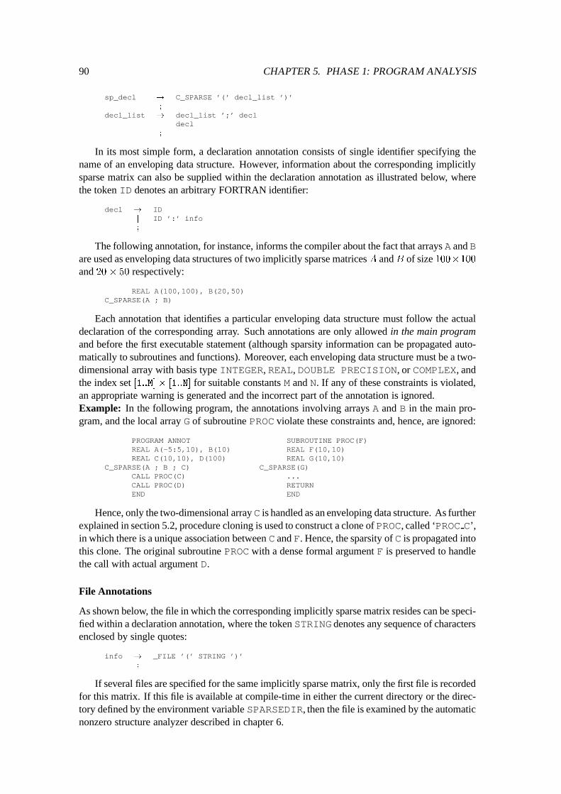
90 CHAPTER 5. PHASE 1: PROGRAM ANALYSIS
sp_decl ! C_SPARSE ’(’ decl_list ’)’;
decl_list ! decl_list ’;’ declj decl;
In its most simple form, a declaration annotation consists of single identifier specifying thename of an enveloping data structure. However, information about the corresponding implicitlysparse matrix can also be supplied within the declaration annotation as illustrated below, wherethe token ID denotes an arbitrary FORTRAN identifier:
decl ! IDj ID ’:’ info;
The following annotation, for instance, informs the compiler about the fact that arrays A and Bare used as enveloping data structures of two implicitly sparse matrices A andB of size 100�100
and 20� 50 respectively:
REAL A(100,100), B(20,50)C_SPARSE(A ; B)
Each annotation that identifies a particular enveloping data structure must follow the actualdeclaration of the corresponding array. Such annotations are only allowed in the main programand before the first executable statement (although sparsity information can be propagated auto-matically to subroutines and functions). Moreover, each enveloping data structure must be a two-dimensional array with basis type INTEGER, REAL, DOUBLE PRECISION, or COMPLEX, andthe index set [1::M]� [1::N] for suitable constants M and N. If any of these constraints is violated,an appropriate warning is generated and the incorrect part of the annotation is ignored.Example: In the following program, the annotations involving arrays A and B in the main pro-gram, and the local array G of subroutine PROC violate these constraints and, hence, are ignored:
PROGRAM ANNOTREAL A(-5:5,10), B(10)REAL C(10,10), D(100)
C_SPARSE(A ; B ; C)CALL PROC(C)CALL PROC(D)END
SUBROUTINE PROC(F)REAL F(10,10)REAL G(10,10)
C_SPARSE(G)...RETURNEND
Hence, only the two-dimensional arrayC is handled as an enveloping data structure. As furtherexplained in section 5.2, procedure cloning is used to construct a clone of PROC, called ‘PROC C’,in which there is a unique association between C and F. Hence, the sparsity of C is propagated intothis clone. The original subroutine PROC with a dense formal argument F is preserved to handlethe call with actual argument D.
File Annotations
As shown below, the file in which the corresponding implicitly sparse matrix resides can be speci-fied within a declaration annotation, where the token STRING denotes any sequence of charactersenclosed by single quotes:
info ! _FILE ’(’ STRING ’)’;
If several files are specified for the same implicitly sparse matrix, only the first file is recordedfor this matrix. If this file is available at compile-time in either the current directory or the direc-tory defined by the environment variable SPARSEDIR, then the file is examined by the automaticnonzero structure analyzer described in chapter 6.
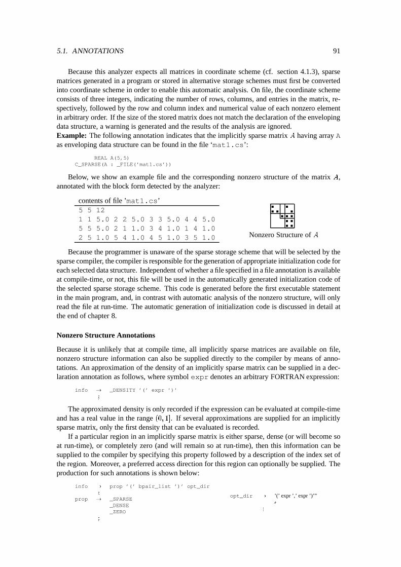
5.1. ANNOTATIONS 91
Because this analyzer expects all matrices in coordinate scheme (cf. section 4.1.3), sparsematrices generated in a program or stored in alternative storage schemes must first be convertedinto coordinate scheme in order to enable this automatic analysis. On file, the coordinate schemeconsists of three integers, indicating the number of rows, columns, and entries in the matrix, re-spectively, followed by the row and column index and numerical value of each nonzero elementin arbitrary order. If the size of the stored matrix does not match the declaration of the envelopingdata structure, a warning is generated and the results of the analysis are ignored.Example: The following annotation indicates that the implicitly sparse matrix A having array Aas enveloping data structure can be found in the file ‘mat1.cs’:
REAL A(5,5)C_SPARSE(A : _FILE(’mat1.cs’))
Below, we show an example file and the corresponding nonzero structure of the matrix A,annotated with the block form detected by the analyzer:
contents of file ’mat1.cs’5 5 121 1 5.0 2 2 5.0 3 3 5.0 4 4 5.05 5 5.0 2 1 1.0 3 4 1.0 1 4 1.02 5 1.0 5 4 1.0 4 5 1.0 3 5 1.0 Nonzero Structure of A
Because the programmer is unaware of the sparse storage scheme that will be selected by thesparse compiler, the compiler is responsible for the generation of appropriate initialization code foreach selected data structure. Independent of whether a file specified in a file annotation is availableat compile-time, or not, this file will be used in the automatically generated initialization code ofthe selected sparse storage scheme. This code is generated before the first executable statementin the main program, and, in contrast with automatic analysis of the nonzero structure, will onlyread the file at run-time. The automatic generation of initialization code is discussed in detail atthe end of chapter 8.
Nonzero Structure Annotations
Because it is unlikely that at compile time, all implicitly sparse matrices are available on file,nonzero structure information can also be supplied directly to the compiler by means of anno-tations. An approximation of the density of an implicitly sparse matrix can be supplied in a dec-laration annotation as follows, where symbol expr denotes an arbitrary FORTRAN expression:
info ! _DENSITY ’(’ expr ’)’;
The approximated density is only recorded if the expression can be evaluated at compile-timeand has a real value in the range (0; 1]. If several approximations are supplied for an implicitlysparse matrix, only the first density that can be evaluated is recorded.
If a particular region in an implicitly sparse matrix is either sparse, dense (or will become soat run-time), or completely zero (and will remain so at run-time), then this information can besupplied to the compiler by specifying this property followed by a description of the index set ofthe region. Moreover, a preferred access direction for this region can optionally be supplied. Theproduction for such annotations is shown below:
info ! prop ’(’ bpair_list ’)’ opt_dir;
prop ! _SPARSEj _DENSEj _ZERO;
opt_dir ! ’(’ expr ’,’ expr ’)’”j �
;
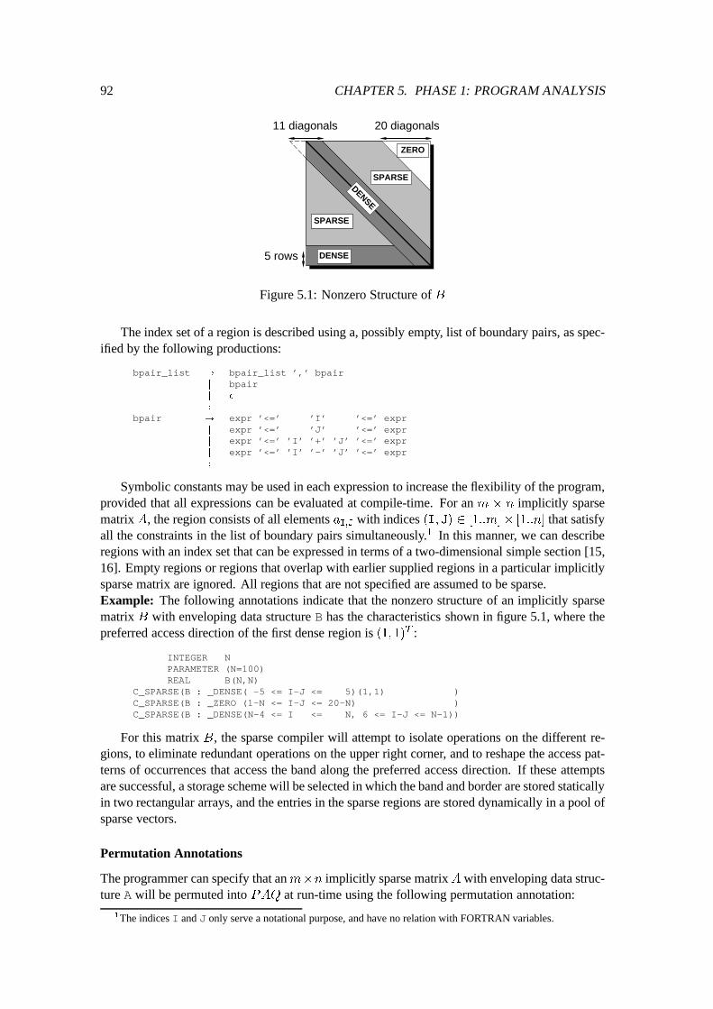
92 CHAPTER 5. PHASE 1: PROGRAM ANALYSIS
11 diagonals
5 rows
20 diagonals
SPARSE
ZERO
DENSE
DENSE
SPARSE
Figure 5.1: Nonzero Structure of B
The index set of a region is described using a, possibly empty, list of boundary pairs, as spec-ified by the following productions:
bpair_list ! bpair_list ’,’ bpairj bpairj �
;
bpair ! expr ’<=’ ’I’ ’<=’ exprj expr ’<=’ ’J’ ’<=’ exprj expr ’<=’ ’I’ ’+’ ’J’ ’<=’ exprj expr ’<=’ ’I’ ’-’ ’J’ ’<=’ expr;
Symbolic constants may be used in each expression to increase the flexibility of the program,provided that all expressions can be evaluated at compile-time. For an m � n implicitly sparsematrix A, the region consists of all elements a
I;J
with indices (I; J) 2 [1::m]� [1::n] that satisfyall the constraints in the list of boundary pairs simultaneously.1 In this manner, we can describeregions with an index set that can be expressed in terms of a two-dimensional simple section [15,16]. Empty regions or regions that overlap with earlier supplied regions in a particular implicitlysparse matrix are ignored. All regions that are not specified are assumed to be sparse.Example: The following annotations indicate that the nonzero structure of an implicitly sparsematrix B with enveloping data structure B has the characteristics shown in figure 5.1, where thepreferred access direction of the first dense region is (1; 1)T :
INTEGER NPARAMETER (N=100)REAL B(N,N)
C_SPARSE(B : _DENSE( -5 <= I-J <= 5)(1,1) )C_SPARSE(B : _ZERO (1-N <= I-J <= 20-N) )C_SPARSE(B : _DENSE(N-4 <= I <= N, 6 <= I-J <= N-1))
For this matrix B, the sparse compiler will attempt to isolate operations on the different re-gions, to eliminate redundant operations on the upper right corner, and to reshape the access pat-terns of occurrences that access the band along the preferred access direction. If these attemptsare successful, a storage scheme will be selected in which the band and border are stored staticallyin two rectangular arrays, and the entries in the sparse regions are stored dynamically in a pool ofsparse vectors.
Permutation Annotations
The programmer can specify that anm�n implicitly sparse matrixA with enveloping data struc-ture A will be permuted into PAQ at run-time using the following permutation annotation:
1The indices I and J only serve a notational purpose, and have no relation with FORTRAN variables.
5.1. ANNOTATIONS 93
REAL A(M,N)C_SPARSE(A : _PERM)
If the identifier specified in a permutation annotation does not correspond to an envelopingdata structure, the annotation is simply ignored because there is no support to reorder dense datastructures. Otherwise, the annotation indicates that any programmer-defined a priori reorderingmethod may be applied to A at run-time before this implicitly sparse matrix is initialized. More-over, the programmer can use interchange annotations (see next section) to indicate positions inthe code where certain row and column interchanges may be applied to A, thereby enabling thesparse compiler to select and implement a local strategy.
The actual implementation of permutations is kept transparent to the programmer. The sparsecompiler is responsible for generating code in which permutations are possibly selected, applied,and recorded. As far as the programmer is concerned, all programming can be done on the en-veloping data structure A as if elements are physically moved in this two-dimensional array, i.e. ifat a certain moment A is permuted into PAQ, then the programmer may assume that A containsthe elements of PAQ.
5.1.2 Annotations in the Executable Part
In this section, annotations that may appear in the executable part of the original dense programare discussed. Interchange annotations support the incorporation of local strategies. Inductionannotations deal with the mathematical consequences of permutations. Because the sparse com-piler enforces a unique association between enveloping data structures and formal arguments, incontrast with declaration annotations, the annotations discussed in this section may also appear insubroutines and functions.
Interchange Annotations
The following interchange annotation can be used to specify that at a particular position in thecode, at run-time an arbitrary row and column of an implicitly sparse matrix A with envelopingdata structure A that are in the range [LR; UR] and [LC; UC] respectively may be interchanged withthe Rth row and Cth column:
C_INTERCHANGE(A, LR:UR > R, LC:UC > C)
Rather than directly specifying the criteria for a local strategy that must be used to determine arow and column, the sparse compiler may select these criteria after analyzing the program. Aftera particular local strategy has been selected, the sparse compiler is also responsible for generat-ing code that implements the selected local strategy. In this code, desired row and column in-terchanges are selected at run-time, applied and recorded. The implementation issues are furtherexplored in chapter 10.
Induction Annotations
Permuting an implicitly sparse matrix A into PAQ may have mathematical consequences thathave to be dealt with in the original dense program. For example, if A is permuted into PAQbefore we compute~b A~x, then we must permute the original vector ~x into ~x 0 Q
T
~x beforethe product, and permute the computed vector~b 0 into the desired result~b P
T
~
b
0 after the producthas been computed. This is implied by the following formula, where the part (�) is computed by animplementation that assumes that elements are physically moved in the enveloping data structure:
P
~
b =
~
b
0
= PAQ~x
0
| {z }
(�)
= PAQ(Q
T
~x) = PA~x
94 CHAPTER 5. PHASE 1: PROGRAM ANALYSIS
Likewise, if before factorization or during LU-factorization to solve a system A~x =
~
b, theimplicitly sparse matrix A becomes permuted into PAQ using an a priori or local strategy, theneffectively the factorization PAQ = LU is computed. Hence, before forward substitution is ap-plied we must permute the right-hand side ~x into ~x 0 P~x. After back substitution, the computed~x
0 is permuted into the desired solution ~x Q~x
0. This is implied by the following formula,where (�) is solved by an implementation assuming physical data movement:
PA~x = PAQQ
T
~x = LU(Q
T
~x) = LU~x
0
=
~
b
0
| {z }
(�)
= P
~
b
Induction annotations are used to deal with such consequences. The implementation of record-ing and applying permutation matrices are kept transparent to the programmer, i.e. the compiler isresponsible for implementing induction annotations. However, it is the responsibility of the pro-grammer to correctly deal with all mathematical consequences of a permutation using inductionannotations, because it seems to be very hard to determine mathematical consequences automat-ically. Since incorrect use of induction annotations may affect the semantics of the original pro-gram, these annotations must be used with care.
In an induction annotation, the identifier of a one-dimensional array that must be permuted,2
an action, and a row or column permutation matrix currently associated with an implicitly sparsematrix are specified as shown below:
sp_exec ! C_INDUCE ID action matrix ’(’ ID ’)’;
action ! ’>’j ’<’;
matrix ! _ROWj _COLUMN;
The sparse compiler replaces each induction annotation with code that has the following im-pact on a column vector ~x = (x
1
; : : : ; x
m
)
T and a row vector ~y = (y
1
; : : : ; y
n
) stored in arraysX and Y respectively, where P and Q denote the row and column permutation matrices that at thetime of execution are associated with the implicitly sparse matrixAwith enveloping data structureA:
annotation: result: alternative result:C_INDUCE X < _ROW (A) ~x P~x ~x
T
~x
T
P
T
C_INDUCE Y < _COLUMN(A) ~y ~yQ ~y
T
Q
T
~y
T
C_INDUCE X > _ROW (A) ~x P
T
~x ~x
T
~x
T
P
C_INDUCE Y > _COLUMN(A) ~y ~yQ
T
~y
T
Q~y
T
The alternative result arises from the fact that transposition has no impact on FORTRAN arrayrepresentations (viz. X and Y interpreted as row and column vector). The method of recording per-mutation matrices and the actual implementation of the computations specified in induction anno-tations are kept transparent to the programmer. If the number of elements in the one-dimensionalarray and the order of the permutation matrix differ, a warning is generated and the annotation isignored. If a dense data structure is specified, then the one-dimensional array remains unaffected(viz. P = Q = I in this case).Example: Below, we present an implementation of~b A~x, where the 100�50 implicitly sparsematrix A may be permuted arbitrarily in advance:
2This restriction is imposed to simplify the implementation in the prototype sparse compiler.
5.2. SUBROUTINES AND FUNCTIONS 95
PROGRAM PERMINTEGER I, J, M, NPARAMETER (M=100, N=50)REAL A(M,N), B(M), X(N)
C_SPARSE(A : _PERM)...
C_INDUCE X < _COLUMN(A)DO I = 1, M
B(I) = 0.0DO J = 1, N
B(I) = B(I) + A(I,J) * X(J)ENDDO
ENDDOC_INDUCE B > _ROW(A)
...END
5.2 Subroutines and Functions
In the original dense program, two-dimensional arrays are used as enveloping data structures ofimplicitly sparse matrices. Because the sparse compiler eventually selects another data structurefor each implicitly sparse matrix, problems arise if enveloping data structures are used as actualarguments in subroutine or function calls. The way in which the array is passed to and handled inthe subroutine or function must be changed according to the selected data structure. In the follow-ing sections, we discuss which parameter passing mechanisms are allowed for implicitly sparsematrices. Furthermore, we discuss how these mechanisms are dealt with by the sparse compiler.
5.2.1 Parameter Passing Mechanisms
Assume that a subroutine P is called as follows:
CALL P(A1
; : : : ; A
n
)
The expressions A1
; : : : ; A
n
are referred to as the actual arguments. The header of the sub-routine definition introduces the formal arguments F
1
; : : : ; F
n
, which are further declared in thebody of the subroutine:
SUBROUTINE P(F1
; : : : ; F
n
)...END
For each CALL-statement, the number of actual arguments must be equal to the number of for-mal arguments of the called subroutine. Furthermore, the type of each actual and correspondingformal argument must be the same. During invocation of the subroutine, we say that each actualargument A
i
is associated with the formal argument Fi
. The same terminology is used for func-tion calls. Moreover, from now on, we use the generic term procedure to refer to a subroutine orfunction.
Single Element Arguments
A single element of an implicitly sparse matrix is passed to a procedure, if an arbitrary elementof the corresponding enveloping data structure is associated with a scalar formal argument. Forexample, in the following fragment, array A is used as enveloping data structure of a 10 � 10
implicitly sparse matrix A and element a27
is passed to the subroutine USE:
PROGRAM INREAL A(10,10)
C_SPARSE(A)CALL USE( A(2,7) )END
SUBROUTINE USE(X)REAL X... = XRETURNEND
96 CHAPTER 5. PHASE 1: PROGRAM ANALYSIS
In this fragment, A(2,7) is associated with an input-argument, because the formal argumentX cannot be modified in the subroutine. A similar situation is illustrated below:
X = ABS( A(I,J) )
In these situations, enveloping data structures used as actual arguments can simply be replacedby a lookup in the selected data structure, i.e. the value of the appropriate element is passed to thecalled procedure. In this manner, the subroutine or function remains unaware of the fact that el-ements of an enveloping data structure may be associated with its formal arguments. Althoughthis implies that sparsity cannot be exploited in body of the called procedure (a similar problemwas encountered at the end of section 4.3.2 for elements stored in temporary variables), the mainadvantage of this approach is that no further transformations are required in this body. The fol-lowing CALL-statement, for instance, would result for the first example shown above if generalsparse row-wise storage is selected for A (function ‘LKP ’ is presented in chapter 8):
CALL USE( VAL_A( LKP__(IND_A, LOW_A(2), HGH_A(2), 7) ) )
It is also possible that arbitrary elements of enveloping data structures become associated withoutput- or input/output-arguments, as is illustrated below:
PROGRAM OUTREAL A(10,10)
C_SPARSE(A)CALL DEF( A(3,4) )END
SUBROUTINE DEF(X)REAL XIF (....) X = ...RETURNEND
In this case, the subroutine must become aware of the sparsity of the formal argument, andthe whole data structure that will be selected for the implicitly sparse matrix must be accessible inthe subroutine to account for the possibility of creation. The best way to handle these situationsis to rewrite the CALL-statement into a form in which the whole implicitly sparse matrix and thesubscripts are passed separately to the subroutine, as is illustrated below:
PROGRAM OUTREAL A(10,10)
C_SPARSE(A)CALL DEF(A, 3, 4)END
SUBROUTINE DEF(M, I, J)REAL M(10,10)INTEGER I, JIF (...) M(I,J) = ...RETURNEND
As further explained in section 5.2.2, a clone ‘DEF A00’ will be generated having a uniqueassociation between the enveloping data structure A and the formal argument M. In this manner, alloccurrences of M can simply be handled as occurrences of A. The data structure that is selected forthe corresponding implicitly sparse matrixAwill be made available to the clone using COMMON-storage.
Implicitly Sparse Matrix Arguments
A whole implicitly sparse matrix is passed as a parameter to a procedure if the first element ofan enveloping data structure A becomes associated with a two-dimensional formal argument thathas the same index set as A. In FORTRAN, this first element can be defined in an actual argumentas either ‘A’ or ‘A(1,1)’. In the following program, for instance, the whole implicitly sparse10� 10 matrix A is passed to the subroutine GAUSS:
PROGRAM SOLVEREAL A(10,10), D(10,10)
C_SPARSE(A)CALL GAUSS(A)CALL GAUSS(D)END
SUBROUTINE GAUSS(M)REAL M(10,10)...RETURNEND
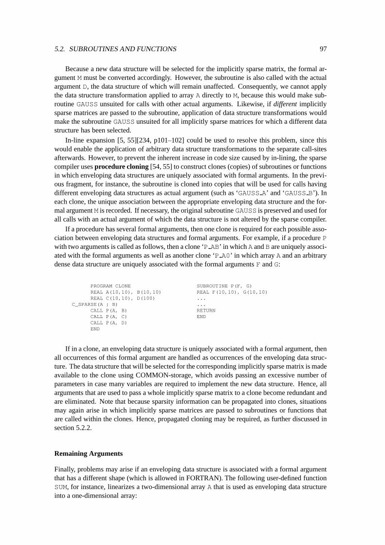
5.2. SUBROUTINES AND FUNCTIONS 97
Because a new data structure will be selected for the implicitly sparse matrix, the formal ar-gument M must be converted accordingly. However, the subroutine is also called with the actualargument D, the data structure of which will remain unaffected. Consequently, we cannot applythe data structure transformation applied to array A directly to M, because this would make sub-routine GAUSS unsuited for calls with other actual arguments. Likewise, if different implicitlysparse matrices are passed to the subroutine, application of data structure transformations wouldmake the subroutine GAUSS unsuited for all implicitly sparse matrices for which a different datastructure has been selected.
In-line expansion [5, 55][234, p101–102] could be used to resolve this problem, since thiswould enable the application of arbitrary data structure transformations to the separate call-sitesafterwards. However, to prevent the inherent increase in code size caused by in-lining, the sparsecompiler uses procedure cloning [54, 55] to construct clones (copies) of subroutines or functionsin which enveloping data structures are uniquely associated with formal arguments. In the previ-ous fragment, for instance, the subroutine is cloned into copies that will be used for calls havingdifferent enveloping data structures as actual argument (such as ‘GAUSS A’ and ‘GAUSS B’). Ineach clone, the unique association between the appropriate enveloping data structure and the for-mal argument M is recorded. If necessary, the original subroutine GAUSS is preserved and used forall calls with an actual argument of which the data structure is not altered by the sparse compiler.
If a procedure has several formal arguments, then one clone is required for each possible asso-ciation between enveloping data structures and formal arguments. For example, if a procedure Pwith two arguments is called as follows, then a clone ‘P AB’ in which A and B are uniquely associ-ated with the formal arguments as well as another clone ‘P A0’ in which array A and an arbitrarydense data structure are uniquely associated with the formal arguments F and G:
PROGRAM CLONEREAL A(10,10), B(10,10)REAL C(10,10), D(100)
C_SPARSE(A ; B)CALL P(A, B)CALL P(A, C)CALL P(A, D)END
SUBROUTINE P(F, G)REAL F(10,10), G(10,10)......RETURNEND
If in a clone, an enveloping data structure is uniquely associated with a formal argument, thenall occurrences of this formal argument are handled as occurrences of the enveloping data struc-ture. The data structure that will be selected for the corresponding implicitly sparse matrix is madeavailable to the clone using COMMON-storage, which avoids passing an excessive number ofparameters in case many variables are required to implement the new data structure. Hence, allarguments that are used to pass a whole implicitly sparse matrix to a clone become redundant andare eliminated. Note that because sparsity information can be propagated into clones, situationsmay again arise in which implicitly sparse matrices are passed to subroutines or functions thatare called within the clones. Hence, propagated cloning may be required, as further discussed insection 5.2.2.
Remaining Arguments
Finally, problems may arise if an enveloping data structure is associated with a formal argumentthat has a different shape (which is allowed in FORTRAN). The following user-defined functionSUM, for instance, linearizes a two-dimensional array A that is used as enveloping data structureinto a one-dimensional array:
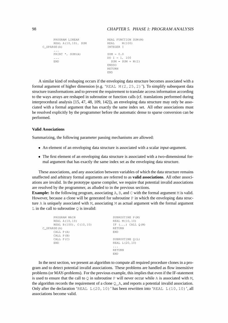
98 CHAPTER 5. PHASE 1: PROGRAM ANALYSIS
PROGRAM LINEARREAL A(10,10), SUM
C_SPARSE(A)...PRINT *, SUM(A)...END
REAL FUNCTION SUM(M)REAL M(100)INTEGER I
SUM = 0.0DO I = 1, 100
SUM = SUM + M(I)ENDDORETURNEND
A similar kind of reshaping occurs if the enveloping data structure becomes associated with aformal argument of higher dimension (e.g. ‘REAL M(2,25,2)’). To simplify subsequent datastructure transformations and to prevent the requirement to translate access information accordingto the ways arrays are reshaped in subroutine or function calls (cf. translations performed duringinterprocedural analysis [15, 47, 48, 109, 142]), an enveloping data structure may only be asso-ciated with a formal argument that has exactly the same index set. All other associations mustbe resolved explicitly by the programmer before the automatic dense to sparse conversion can beperformed.
Valid Associations
Summarizing, the following parameter passing mechanisms are allowed:
� An element of an enveloping data structure is associated with a scalar input-argument.
� The first element of an enveloping data structure is associated with a two-dimensional for-mal argument that has exactly the same index set as the enveloping data structure.
These associations, and any association between variables of which the data structure remainsunaffected and arbitrary formal arguments are referred to as valid associations. All other associ-ations are invalid. In the prototype sparse compiler, we require that potential invalid associationsare resolved by the programmer, as alluded to in the previous sections.Example: In the following program, associating A, B, and C with the formal argument M is valid.However, because a clone will be generated for subroutine P in which the enveloping data struc-ture A is uniquely associated with M, associating M as actual argument with the formal argumentL in the call to subroutine Q is invalid:
PROGRAM MAINREAL A(10,10)REAL B(100), C(10,10)
C_SPARSE(A)CALL P(A)CALL P(B)CALL P(C)END
SUBROUTINE P(M)REAL M(10,10)IF (...) CALL Q(M)RETURNEND
SUBROUTINE Q(L)REAL L(20,10)...RETURNEND
In the next section, we present an algorithm to compute all required procedure clones in a pro-gram and to detect potential invalid associations. These problems are handled as flow insensitiveproblems (or MAY-problems). For the previous example, this implies that even if the IF-statementis used to ensure that the call to Q in subroutine P will never occur while A is associated with M,the algorithm records the requirement of a clone Q_A, and reports a potential invalid association.Only after the declaration ‘REAL L(20,10)’ has been rewritten into ‘REAL L(10,10)’, allassociations become valid.

5.2. SUBROUTINES AND FUNCTIONS 99
5.2.2 Procedure Cloning
In the absence of procedure parameters, construction of a call graph is straightforward [183, 229,234]: a vertex labeled P is created for each procedure P in a program, and an edge from P to Qis added to the call graph if procedure P may call Q. Dynamic recursion, where at run-time sev-eral activations of the same procedure can exist simultaneously [3], is not allowed in FORTRAN.Moreover, we disallow static recursion, where two procedures can (in)directly call each other buttwo activations of the same procedure will never exist simultaneously. Consequently, the resultingcall graph is acyclic. Finally, because the prototype sparse compiler operates on whole programsrather than separate source files, we assume that the complete call graph is available.
Computing the Required Procedure Clones
All clones required to enforce a unique association between enveloping data structures and for-mal arguments can be determined during a visit of all procedures according to a topological sortof the call graph. Because this implies that for each edge from P to Q in the call graph, proce-dure P is visited before Q, all possible associations between enveloping data structures and formalarguments are known for all predecessors of a visited vertex. Below, we present a variant of thealgorithm given in [55] to compute the required clones, that also strongly resembles the call graphconstruction method accounting for procedure parameters in [183].
For each procedure P in a program, a table T
P
is created having a column for each formalargument. We can express the algorithm in a more regular manner, if the main program is alsohandled as a procedure. All local variables of the main program are viewed as formal arguments,denoted by L
1
; : : : ; L
n
. We also construct a table for the main program, having a column for eachlocal variable. Because declaration annotations are only allowed in the main program, this unit isthe only source of sparsity information. The table of the main program is initialized by insertinga single row [�
1
; : : : ; �
n
], where �i
= L
i
, if the ‘formal’ argument Li
is used as an enveloping datastructure of an implicitly sparse matrix and �
i
= 0, otherwise.Subsequently, rows are inserted in the other tables by executing the following procedure for
all vertices in the call graph according to a topological sort.
procedure visit(P)begin
for each procedure call ‘Q(A1
; : : :,An
)’ in P do
for each row r in TP
doinsert(T
Q
, [�1
(r); : : : ; �
n
(r)] )enddo
enddo
end
Each expression �i
(r), where 1 � i � n and n is the number of formal arguments of Q, isevaluated as follows:
�
i
(r) =
(
T
P
[r][j] if A
i
is jth formal argument of P0 otherwise
If the jth formal argument of P is equal to A
i
, then �i
(r) contains either the identifier of anenveloping data structure that may be associated with this variable, or the value ‘0’ if an unaffecteddata structure may be associated with this argument. We also have �
i
(r) = 0 in all other cases,i.e. if A
i
is a local variable or an arbitrary expression.
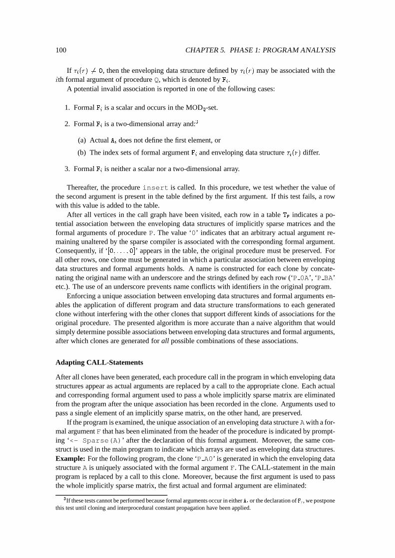
100 CHAPTER 5. PHASE 1: PROGRAM ANALYSIS
If �i
(r) 6= 0, then the enveloping data structure defined by �i
(r) may be associated with theith formal argument of procedure Q, which is denoted by F
i
.A potential invalid association is reported in one of the following cases:
1. Formal Fi
is a scalar and occurs in the MODQ
-set.
2. Formal Fi
is a two-dimensional array and:3
(a) Actual Ai
does not define the first element, or
(b) The index sets of formal argument Fi
and enveloping data structure �i
(r) differ.
3. Formal Fi
is neither a scalar nor a two-dimensional array.
Thereafter, the procedure insert is called. In this procedure, we test whether the value ofthe second argument is present in the table defined by the first argument. If this test fails, a rowwith this value is added to the table.
After all vertices in the call graph have been visited, each row in a table T
P
indicates a po-tential association between the enveloping data structures of implicitly sparse matrices and theformal arguments of procedure P. The value ‘0’ indicates that an arbitrary actual argument re-maining unaltered by the sparse compiler is associated with the corresponding formal argument.Consequently, if ‘[0; : : : ; 0]’ appears in the table, the original procedure must be preserved. Forall other rows, one clone must be generated in which a particular association between envelopingdata structures and formal arguments holds. A name is constructed for each clone by concate-nating the original name with an underscore and the strings defined by each row (‘P 0A’, ‘P BA’etc.). The use of an underscore prevents name conflicts with identifiers in the original program.
Enforcing a unique association between enveloping data structures and formal arguments en-ables the application of different program and data structure transformations to each generatedclone without interfering with the other clones that support different kinds of associations for theoriginal procedure. The presented algorithm is more accurate than a naive algorithm that wouldsimply determine possible associations between enveloping data structures and formal arguments,after which clones are generated for all possible combinations of these associations.
Adapting CALL-Statements
After all clones have been generated, each procedure call in the program in which enveloping datastructures appear as actual arguments are replaced by a call to the appropriate clone. Each actualand corresponding formal argument used to pass a whole implicitly sparse matrix are eliminatedfrom the program after the unique association has been recorded in the clone. Arguments used topass a single element of an implicitly sparse matrix, on the other hand, are preserved.
If the program is examined, the unique association of an enveloping data structure Awith a for-mal argument F that has been eliminated from the header of the procedure is indicated by prompt-ing ‘<- Sparse(A)’ after the declaration of this formal argument. Moreover, the same con-struct is used in the main program to indicate which arrays are used as enveloping data structures.Example: For the following program, the clone ‘P A0’ is generated in which the enveloping datastructure A is uniquely associated with the formal argument F. The CALL-statement in the mainprogram is replaced by a call to this clone. Moreover, because the first argument is used to passthe whole implicitly sparse matrix, the first actual and formal argument are eliminated:
3If these tests cannot be performed because formal arguments occur in either Ai
or the declaration of Fi
, we postponethis test until cloning and interprocedural constant propagation have been applied.
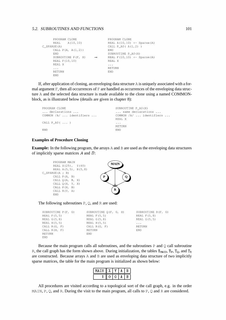
5.2. SUBROUTINES AND FUNCTIONS 101
PROGRAM CLONEREAL A(10,10)
C_SPARSE(A)CALL P(A, A(1,2))ENDSUBROUTINE P(F, X)REAL F(10,10)REAL X...RETURNEND
!
PROGRAM CLONEREAL A(10,10) <- Sparse(A)CALL P_A0( A(1,2) )ENDSUBROUTINE P_A0(X)REAL F(10,10) <- Sparse(A)REAL X...RETURNEND
If, after application of cloning, an enveloping data structure A is uniquely associated with a for-mal argument F, then all occurrences of F are handled as occurrences of the enveloping data struc-ture A and the selected data structure is made available to the clone using a named COMMON-block, as is illustrated below (details are given in chapter 8):
PROGRAM CLONE... declarations ...COMMON /A/ ... identifiers ...
CALL P_A0( ... )
END
SUBROUTINE P_A0(X)... same declarations ...COMMON /A/ ... identifiers ...REAL X...RETURNEND
Examples of Procedure Cloning
Example: In the following program, the arrays A and B are used as the enveloping data structuresof implicitly sparse matrices A and B:
PROGRAM MAINREAL X(25), Y(40)REAL A(5,5), B(5,8)
C_SPARSE(A ; B)CALL P(A, B)CALL Q(A, B, X)CALL Q(X, Y, X)CALL P(X, B)CALL R(Y, A)END
R
P Q
MAIN
The following subroutines P, Q, and R are used:
SUBROUTINE P(F, G)REAL F(5,5)REAL G(5,8)REAL H(5,5)CALL R(G, F)CALL R(H, F)RETURNEND
SUBROUTINE Q(F, G, H)REAL F(5,5)REAL G(5,8)REAL H(5,5)CALL R(G, F)RETURNEND
SUBROUTINE R(F, G)REAL F(5,8)REAL G(5,5)...RETURNEND
Because the main program calls all subroutines, and the subroutines P and Q call subroutineR, the call graph has the form shown above. During initialization, the tables T
MAIN
, TP
, TQ
, and T
R
are constructed. Because arrays A and B are used as enveloping data structure of two implicitlysparse matrices, the table for the main program is initialized as shown below:
MAIN X Y A B
1 0 0 A B
All procedures are visited according to a topological sort of the call graph, e.g. in the orderMAIN, P, Q, and R. During the visit to the main program, all calls to P, Q and R are considered.
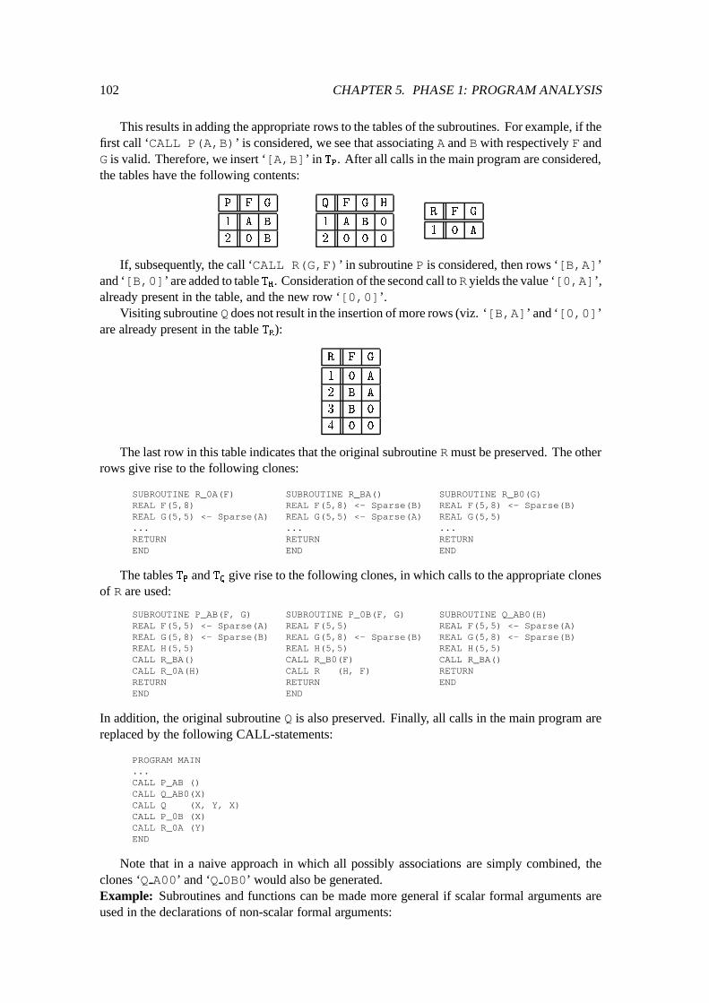
102 CHAPTER 5. PHASE 1: PROGRAM ANALYSIS
This results in adding the appropriate rows to the tables of the subroutines. For example, if thefirst call ‘CALL P(A,B)’ is considered, we see that associating A and B with respectively F andG is valid. Therefore, we insert ‘[A,B]’ in T
P
. After all calls in the main program are considered,the tables have the following contents:
P F G
1 A B
2 0 B
Q F G H
1 A B 0
2 0 0 0
R F G
1 0 A
If, subsequently, the call ‘CALL R(G,F)’ in subroutine P is considered, then rows ‘[B,A]’and ‘[B,0]’ are added to table T
R
. Consideration of the second call toR yields the value ‘[0,A]’,already present in the table, and the new row ‘[0,0]’.
Visiting subroutine Q does not result in the insertion of more rows (viz. ‘[B,A]’ and ‘[0,0]’are already present in the table T
R
):
R F G
1 0 A
2 B A
3 B 0
4 0 0
The last row in this table indicates that the original subroutine Rmust be preserved. The otherrows give rise to the following clones:
SUBROUTINE R_0A(F)REAL F(5,8)REAL G(5,5) <- Sparse(A)...RETURNEND
SUBROUTINE R_BA()REAL F(5,8) <- Sparse(B)REAL G(5,5) <- Sparse(A)...RETURNEND
SUBROUTINE R_B0(G)REAL F(5,8) <- Sparse(B)REAL G(5,5)...RETURNEND
The tables TP
and T
Q
give rise to the following clones, in which calls to the appropriate clonesof R are used:
SUBROUTINE P_AB(F, G)REAL F(5,5) <- Sparse(A)REAL G(5,8) <- Sparse(B)REAL H(5,5)CALL R_BA()CALL R_0A(H)RETURNEND
SUBROUTINE P_0B(F, G)REAL F(5,5)REAL G(5,8) <- Sparse(B)REAL H(5,5)CALL R_B0(F)CALL R (H, F)RETURNEND
SUBROUTINE Q_AB0(H)REAL F(5,5) <- Sparse(A)REAL G(5,8) <- Sparse(B)REAL H(5,5)CALL R_BA()RETURNEND
In addition, the original subroutine Q is also preserved. Finally, all calls in the main program arereplaced by the following CALL-statements:
PROGRAM MAIN...CALL P_AB ()CALL Q_AB0(X)CALL Q (X, Y, X)CALL P_0B (X)CALL R_0A (Y)END
Note that in a naive approach in which all possibly associations are simply combined, theclones ‘Q A00’ and ‘Q 0B0’ would also be generated.Example: Subroutines and functions can be made more general if scalar formal arguments areused in the declarations of non-scalar formal arguments:
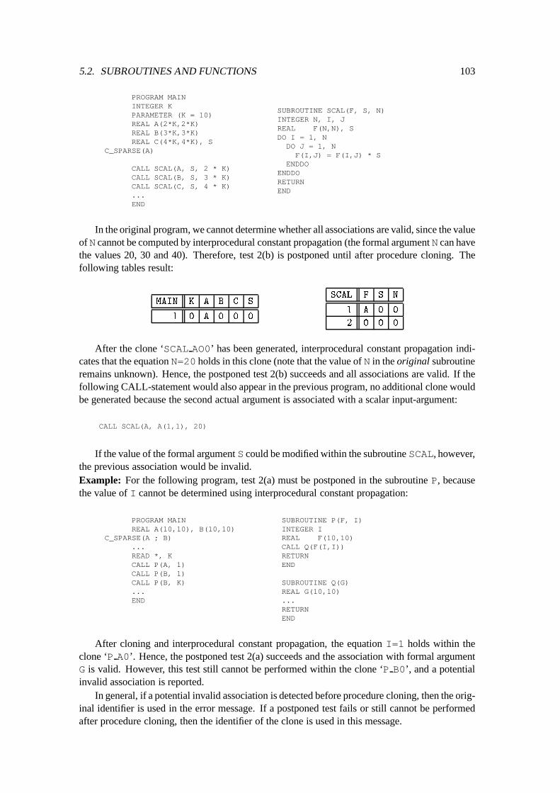
5.2. SUBROUTINES AND FUNCTIONS 103
PROGRAM MAININTEGER KPARAMETER (K = 10)REAL A(2*K,2*K)REAL B(3*K,3*K)REAL C(4*K,4*K), S
C_SPARSE(A)
CALL SCAL(A, S, 2 * K)CALL SCAL(B, S, 3 * K)CALL SCAL(C, S, 4 * K)...END
SUBROUTINE SCAL(F, S, N)INTEGER N, I, JREAL F(N,N), SDO I = 1, NDO J = 1, N
F(I,J) = F(I,J) * SENDDO
ENDDORETURNEND
In the original program, we cannot determine whether all associations are valid, since the valueof N cannot be computed by interprocedural constant propagation (the formal argument N can havethe values 20, 30 and 40). Therefore, test 2(b) is postponed until after procedure cloning. Thefollowing tables result:
MAIN K A B C S
1 0 A 0 0 0
SCAL F S N
1 A 0 0
2 0 0 0
After the clone ‘SCAL AO0’ has been generated, interprocedural constant propagation indi-cates that the equation N=20 holds in this clone (note that the value of N in the original subroutineremains unknown). Hence, the postponed test 2(b) succeeds and all associations are valid. If thefollowing CALL-statement would also appear in the previous program, no additional clone wouldbe generated because the second actual argument is associated with a scalar input-argument:
CALL SCAL(A, A(1,1), 20)
If the value of the formal argument S could be modified within the subroutine SCAL, however,the previous association would be invalid.Example: For the following program, test 2(a) must be postponed in the subroutine P, becausethe value of I cannot be determined using interprocedural constant propagation:
PROGRAM MAINREAL A(10,10), B(10,10)
C_SPARSE(A ; B)...READ *, KCALL P(A, 1)CALL P(B, 1)CALL P(B, K)...END
SUBROUTINE P(F, I)INTEGER IREAL F(10,10)CALL Q(F(I,I))RETURNEND
SUBROUTINE Q(G)REAL G(10,10)...RETURNEND
After cloning and interprocedural constant propagation, the equation I=1 holds within theclone ‘P A0’. Hence, the postponed test 2(a) succeeds and the association with formal argumentG is valid. However, this test still cannot be performed within the clone ‘P B0’, and a potentialinvalid association is reported.
In general, if a potential invalid association is detected before procedure cloning, then the orig-inal identifier is used in the error message. If a postponed test fails or still cannot be performedafter procedure cloning, then the identifier of the clone is used in this message.
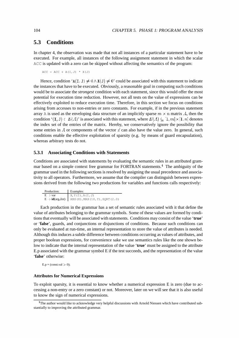
104 CHAPTER 5. PHASE 1: PROGRAM ANALYSIS
5.3 Conditions
In chapter 4, the observation was made that not all instances of a particular statement have to beexecuted. For example, all instances of the following assignment statement in which the scalarACC is updated with a zero can be skipped without affecting the semantics of the program:
ACC = ACC + A(I,J) * X(J)
Hence, condition ‘A(I; J) 6= 0^X(J) 6= 0’ could be associated with this statement to indicatethe instances that have to be executed. Obviously, a reasonable goal in computing such conditionswould be to associate the strongest condition with each statement, since this would offer the mostpotential for execution time reduction. However, not all tests on the value of expressions can beeffectively exploited to reduce execution time. Therefore, in this section we focus on conditionsarising from accesses to non-entries or zero constants. For example, if in the previous statementarray A is used as the enveloping data structure of an implicitly sparse m� n matrix A, then thecondition ‘(I; J) 2 E(A)’ is associated with this statement, whereE(A) � [1;m]�[1; n] denotesthe index set of the entries of the matrix. Hereby, we conservatively ignore the possibility thatsome entries in A or components of the vector ~x can also have the value zero. In general, suchconditions enable the effective exploitation of sparsity (e.g. by means of guard encapsulation),whereas arbitrary tests do not.
5.3.1 Associating Conditions with Statements
Conditions are associated with statements by evaluating the semantic rules in an attributed gram-mar based on a simple context free grammar for FORTRAN statements.4 The ambiguity of thegrammar used in the following sections is resolved by assigning the usual precedence and associa-tivity to all operators. Furthermore, we assume that the compiler can distinguish between expres-sions derived from the following two productions for variables and functions calls respectively:
Production: Examples:E! var X, Y(I), A(I,J)E! id(arg list) ABS(X), MAX(10,Y), SQRT(2.0)
Each production in the grammar has a set of semantic rules associated with it that define thevalue of attributes belonging to the grammar symbols. Some of these values are formed by condi-tions that eventually will be associated with statements. Conditions may consist of the value ‘true’or ‘false’, guards, and conjunctions or disjunctions of conditions. Because such conditions canonly be evaluated at run-time, an internal representation to store the value of attributes is needed.Although this induces a subtle difference between conditions occurring as values of attributes, andproper boolean expressions, for convenience sake we use semantics rules like the one shown be-low to indicate that the internal representation of the value ‘true’ must be assigned to the attributeE.p associated with the grammar symbol E if the test succeeds, and the representation of the value‘false’ otherwise:
E.p = (const.val > 0);
Attributes for Numerical Expressions
To exploit sparsity, it is essential to know whether a numerical expression E is zero (due to ac-cessing a non-entry or a zero constant) or not. Moreover, later on we will see that it is also usefulto know the sign of numerical expressions.
4The author would like to acknowledge very helpful discussions with Arnold Niessen which have contributed sub-stantially to improving the attributed grammar.

5.3. CONDITIONS 105
For this purpose, three synthesized attributes E.p, E.z, and E.n are associated with each nu-merical expression E, recording the condition under which the expression may be strictly positive,zero, and strictly negative, respectively.
Semantic rules for all numerical expressions formed using the arithmetic operators ‘+’ and‘�’ are derived by examination of the following tables in which, given particular assertions onthe value of the operands, similar assertions on the value of the resulting expression are shown:
E1
+ E2
E2
> 0 E2
= 0 E2
< 0
E1
> 0 > 0 > 0 ?
E1
= 0 > 0 = 0 < 0
E1
< 0 ? < 0 < 0
E1
� E2
E2
> 0 E2
= 0 E2
< 0
E1
> 0 ? > 0 > 0
E1
= 0 < 0 = 0 > 0
E1
< 0 < 0 < 0 ?
For example, because expression E=‘E1
+ E2
’ may be strictly positive if one of the operandsmay be strictly positive, we define E.p as ‘E
1
.p _ E2
.p’. Likewise, expression E=‘E1
� E2
’ maybe zero if both operands can be zero or if the operands have identical signs. Hence, in this case E.zis defined as ‘(E
1
.p ^ E2
.p) _ (E1
.z ^ E2
.z) _ (E1
.n ^ E2
.n)’. Continuing in this fashion yieldsthe following semantic rules:
Production Semantic Rule
E! E1
+ E2
E.p = E1
.p _ E2
.p;E.z = (E
1
.p ^ E2
.n) _ (E1
.z ^ E2
.z) _ (E1
.n ^ E2
.p);E.n = E
1
.n _ E2
.n;E! E
1
� E2
E.p = E1
.p _ E2
.n;E.z = (E
1
.p ^ E2
.p) _ (E1
.z ^ E2
.z) _ (E1
.n ^ E2
.n);E.n = E
1
.n _ E2
.p;
A similar table can be given for the unary minus, whereas the tables for the arithmetic opera-tors ‘�’, ‘=’, and ‘��’ are shown below:
E1
� E2
E2
> 0 E2
= 0 E2
< 0
E1
> 0 > 0 = 0 < 0
E1
= 0 = 0 = 0 = 0
E1
< 0 < 0 = 0 > 0
E1
= E2
E2
> 0 E2
= 0 E2
< 0
E1
> 0 > 0 ? < 0
E1
= 0 = 0 ? = 0
E1
< 0 < 0 ? > 0
E1
�� E2
E2
> 0 E2
= 0 E2
< 0
E1
> 0 > 0 > 0 > 0
E1
= 0 = 0 ? = 0
E1
< 0 6= 0 > 0 6= 0
A subtlety arises for the operators ‘=’ and ‘��’, because the values of 00 and an expressionin which a divisor occurs that is zero are undefined. However, under the assumption that suchsituations (and underflow) do not occur at run-time, ‘convenient’ assertions may be placed at thepositions of the ‘?’, which gives rise to the following semantic rules:
Production Semantic Rule
E! E1
� E2
E.p = (E1
.p ^ E2
.p) _ (E1
.n ^ E2
.n);E.z = E
1
.z _ E2
.z;E.n = (E
1
.p ^ E2
.n) _ (E1
.n ^ E2
.p);E! E
1
= E2
E.p = (E1
.p ^ E2
.p) _ (E1
.n ^ E2
.n);E.z = E
1
.z;E.n = (E
1
.p ^ E2
.n) _ (E1
.n ^ E2
.p);
Production Semantic Rule
E! E1
�� E2
E.p = E1
.p _ E1
.n;E.z = E
1
.z;E.n = (E
1
.n ^ E2
.p) _ (E1
.n ^ E2
.n);E!� E
1
E.p = E1
.n;E.z = E
1
.z;E.n = E
1
.p;
For variables, a guard is supplied in a synthesized attribute var.grd. For an occurrence of anenveloping data structure of an implicitly sparse matrix A with admissible subscripts F (~I), thisguard is ‘F (~I) 2 E(A)’ (where the unique association between enveloping data structures andformal arguments enforced by cloning is accounted for). For all other variables, the value ‘true’is supplied. Likewise, the value of each constant is supplied in an attribute E.val. This enables usto define the following semantic rules:
Production Semantic Rule
E! var E.p = var.grd;E.z = true;E.n = var.grd;
Production Semantic Rule
E! const E.p = (const.val > 0);E.z = (const.val = 0);E.n = (const.val < 0);
Production Semantic RuleE! ( E
1
) E.p = E1
.p;E.z = E
1
.z;E.n = E
1
.n;
Semantic rules for all remaining numerical expressions are given in the following table:
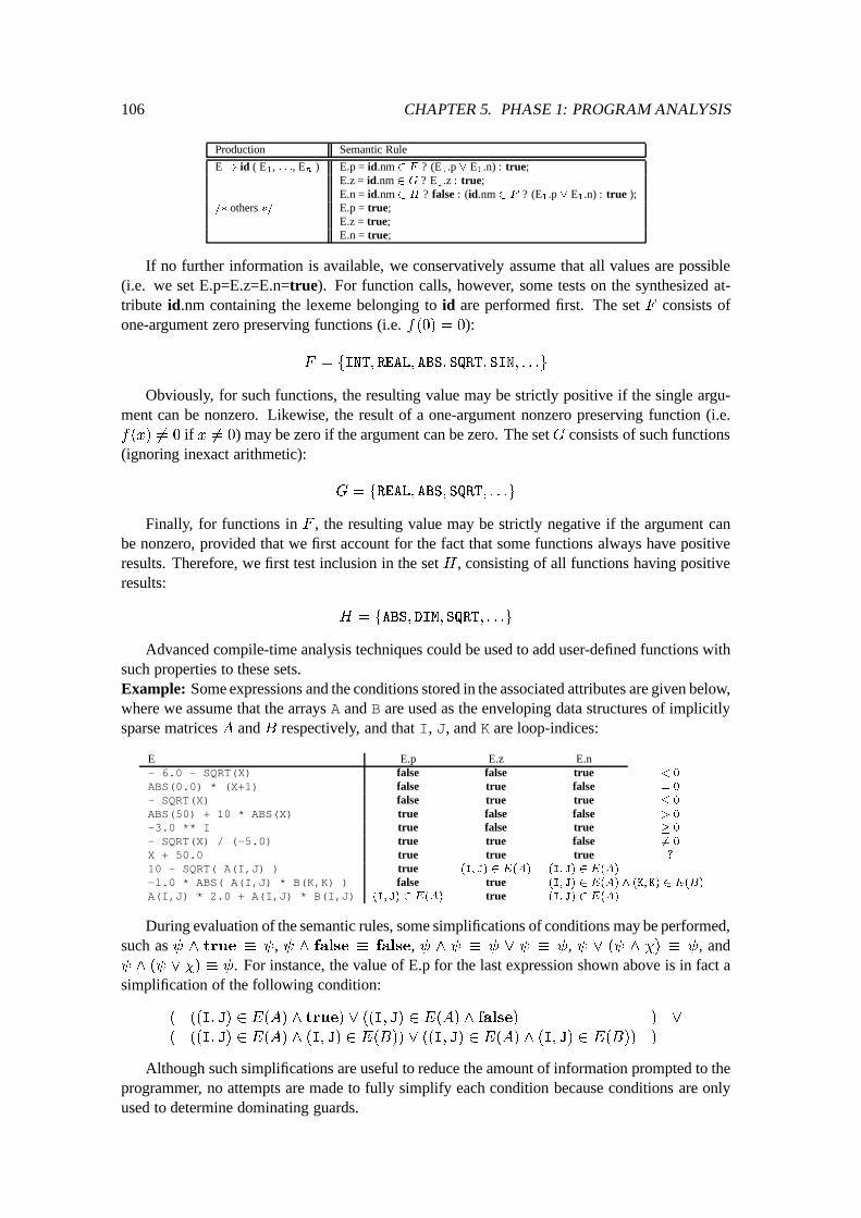
106 CHAPTER 5. PHASE 1: PROGRAM ANALYSIS
Production Semantic Rule
E! id ( E1
, : : :, En
) E.p = id.nm 2 F ? (E1
.p _ E1
.n) : true;E.z = id.nm 2 G ? E
1
.z : true;E.n = id.nm 2 H ? false : (id.nm 2 F ? (E
1
.p _ E1
.n) : true );=� others �= E.p = true;
E.z = true;E.n = true;
If no further information is available, we conservatively assume that all values are possible(i.e. we set E.p=E.z=E.n=true). For function calls, however, some tests on the synthesized at-tribute id.nm containing the lexeme belonging to id are performed first. The set F consists ofone-argument zero preserving functions (i.e. f(0) = 0):
F = fINT; REAL; ABS; SQRT; SIN; : : :g
Obviously, for such functions, the resulting value may be strictly positive if the single argu-ment can be nonzero. Likewise, the result of a one-argument nonzero preserving function (i.e.f(x) 6= 0 if x 6= 0) may be zero if the argument can be zero. The set G consists of such functions(ignoring inexact arithmetic):
G = fREAL; ABS; SQRT; : : :g
Finally, for functions in F , the resulting value may be strictly negative if the argument canbe nonzero, provided that we first account for the fact that some functions always have positiveresults. Therefore, we first test inclusion in the set H , consisting of all functions having positiveresults:
H = fABS; DIM; SQRT; : : :g
Advanced compile-time analysis techniques could be used to add user-defined functions withsuch properties to these sets.Example: Some expressions and the conditions stored in the associated attributes are given below,where we assume that the arrays A and B are used as the enveloping data structures of implicitlysparse matrices A and B respectively, and that I, J, and K are loop-indices:
E E.p E.z E.n- 6.0 - SQRT(X) false false true < 0
ABS(0.0) * (X+1) false true false = 0
- SQRT(X) false true true � 0
ABS(50) + 10 * ABS(X) true false false > 0
-3.0 ** I true false true � 0
- SQRT(X) / (-5.0) true true false 6= 0
X + 50.0 true true true ?
10 - SQRT( A(I,J) ) true (I; J) 2 E(A) (I; J) 2 E(A)
-1.0 * ABS( A(I,J) * B(K,K) ) false true (I; J) 2 E(A) ^ (K; K) 2 E(B)
A(I,J) * 2.0 + A(I,J) * B(I,J) (I; J) 2 E(A) true (I; J) 2 E(A)
During evaluation of the semantic rules, some simplifications of conditions may be performed,such as ^ true � , ^ false � false, ^ � _ � , _ ( ^ �) � , and ^ ( _ �) � . For instance, the value of E.p for the last expression shown above is in fact asimplification of the following condition:
( ((I; J) 2 E(A) ^ true) _ ((I; J) 2 E(A) ^ false) ) _
( ((I; J) 2 E(A) ^ (I; J) 2 E(B)) _ ((I; J) 2 E(A) ^ (I; J) 2 E(B)) )
Although such simplifications are useful to reduce the amount of information prompted to theprogrammer, no attempts are made to fully simplify each condition because conditions are onlyused to determine dominating guards.
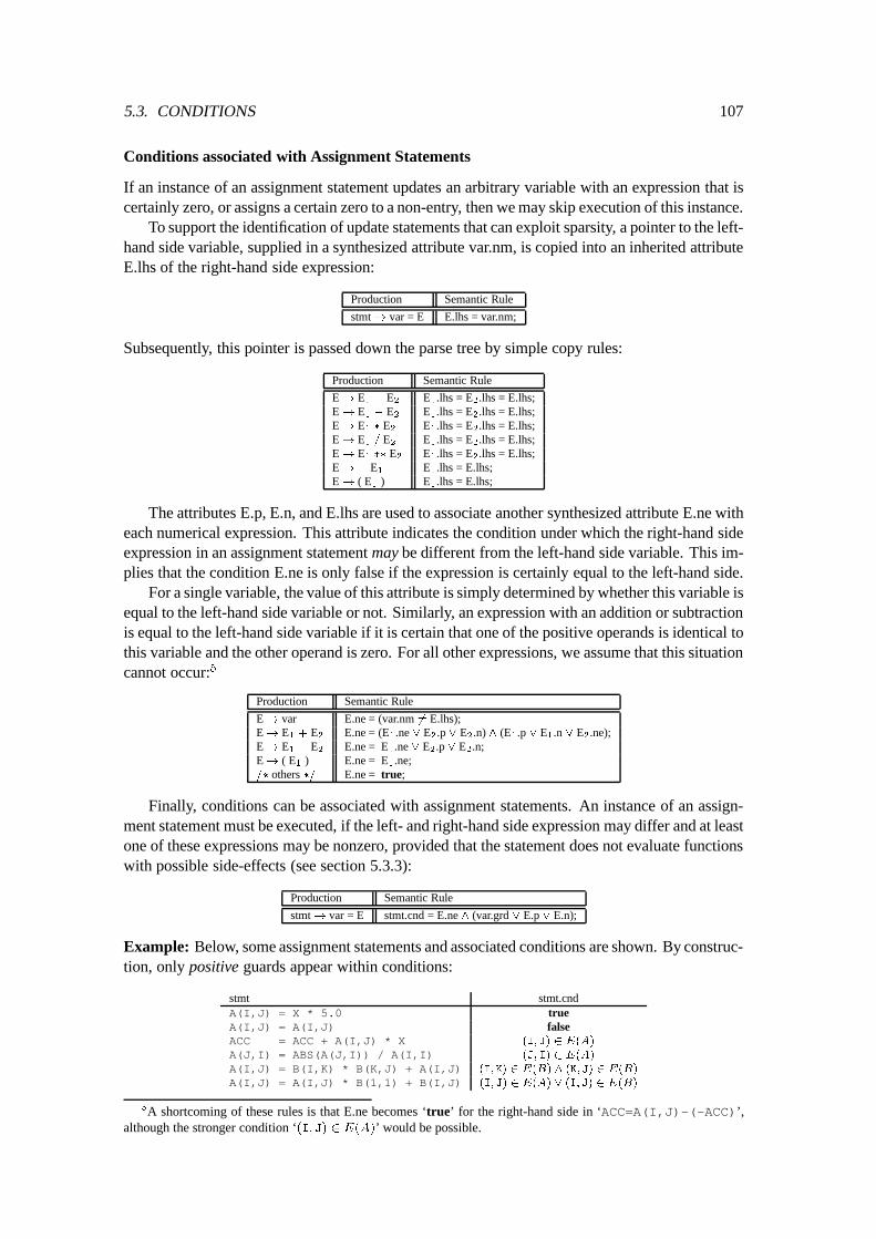
5.3. CONDITIONS 107
Conditions associated with Assignment Statements
If an instance of an assignment statement updates an arbitrary variable with an expression that iscertainly zero, or assigns a certain zero to a non-entry, then we may skip execution of this instance.
To support the identification of update statements that can exploit sparsity, a pointer to the left-hand side variable, supplied in a synthesized attribute var.nm, is copied into an inherited attributeE.lhs of the right-hand side expression:
Production Semantic Rule
stmt! var = E E.lhs = var.nm;
Subsequently, this pointer is passed down the parse tree by simple copy rules:
Production Semantic Rule
E! E1
+ E2
E1
.lhs = E2
.lhs = E.lhs;E! E
1
� E2
E1
.lhs = E2
.lhs = E.lhs;E! E
1
� E2
E1
.lhs = E2
.lhs = E.lhs;E! E
1
= E2
E1
.lhs = E2
.lhs = E.lhs;E! E
1
�� E2
E1
.lhs = E2
.lhs = E.lhs;E!� E
1
E1
.lhs = E.lhs;E! ( E
1
) E1
.lhs = E.lhs;
The attributes E.p, E.n, and E.lhs are used to associate another synthesized attribute E.ne witheach numerical expression. This attribute indicates the condition under which the right-hand sideexpression in an assignment statement may be different from the left-hand side variable. This im-plies that the condition E.ne is only false if the expression is certainly equal to the left-hand side.
For a single variable, the value of this attribute is simply determined by whether this variable isequal to the left-hand side variable or not. Similarly, an expression with an addition or subtractionis equal to the left-hand side variable if it is certain that one of the positive operands is identical tothis variable and the other operand is zero. For all other expressions, we assume that this situationcannot occur:5
Production Semantic Rule
E! var E.ne = (var.nm 6= E.lhs);E! E
1
+ E2
E.ne = (E1
.ne _ E2
.p _ E2
.n) ^ (E1
.p _ E1
.n _ E2
.ne);E! E
1
� E2
E.ne = E1
.ne _ E2
.p _ E2
.n;E! ( E
1
) E.ne = E1
.ne;=� others �= E.ne = true;
Finally, conditions can be associated with assignment statements. An instance of an assign-ment statement must be executed, if the left- and right-hand side expression may differ and at leastone of these expressions may be nonzero, provided that the statement does not evaluate functionswith possible side-effects (see section 5.3.3):
Production Semantic Rule
stmt! var = E stmt.cnd = E.ne ^ (var.grd _ E.p _ E.n);
Example: Below, some assignment statements and associated conditions are shown. By construc-tion, only positive guards appear within conditions:
stmt stmt.cndA(I,J) = X * 5.0 trueA(I,J) = A(I,J) falseACC = ACC + A(I,J) * X (I; J) 2 E(A)
A(J,I) = ABS(A(J,I)) / A(I,I) (J; I) 2 E(A)
A(I,J) = B(I,K) * B(K,J) + A(I,J) (I; K) 2 E(B) ^ (K; J) 2 E(B)
A(I,J) = A(I,J) * B(1,1) + B(I,J) (I; J) 2 E(A) _ (I; J) 2 E(B)
5A shortcoming of these rules is that E.ne becomes ‘true’ for the right-hand side in ‘ACC=A(I,J)-(-ACC)’,although the stronger condition ‘(I; J) 2 E(A)’ would be possible.
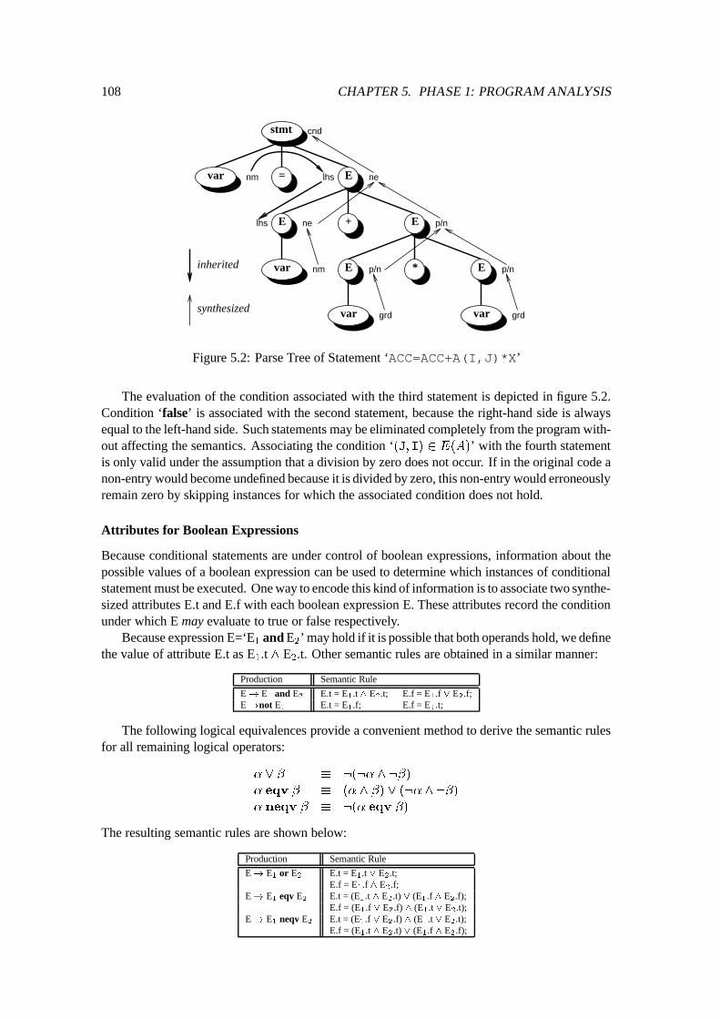
108 CHAPTER 5. PHASE 1: PROGRAM ANALYSIS
stmt
E=
+
*
EE
var E E
var vargrd grd
nm
ne
ne
lhs
lhsnmvar
cnd
inherited
synthesized
p/np/n
p/n
Figure 5.2: Parse Tree of Statement ‘ACC=ACC+A(I,J)*X’
The evaluation of the condition associated with the third statement is depicted in figure 5.2.Condition ‘false’ is associated with the second statement, because the right-hand side is alwaysequal to the left-hand side. Such statements may be eliminated completely from the program with-out affecting the semantics. Associating the condition ‘(J; I) 2 E(A)’ with the fourth statementis only valid under the assumption that a division by zero does not occur. If in the original code anon-entry would become undefined because it is divided by zero, this non-entry would erroneouslyremain zero by skipping instances for which the associated condition does not hold.
Attributes for Boolean Expressions
Because conditional statements are under control of boolean expressions, information about thepossible values of a boolean expression can be used to determine which instances of conditionalstatement must be executed. One way to encode this kind of information is to associate two synthe-sized attributes E.t and E.f with each boolean expression E. These attributes record the conditionunder which E may evaluate to true or false respectively.
Because expression E=‘E1
and E2
’ may hold if it is possible that both operands hold, we definethe value of attribute E.t as E
1
.t ^ E2
.t. Other semantic rules are obtained in a similar manner:
Production Semantic Rule
E! E1
and E2
E.t = E1
.t ^ E2
.t; E.f = E1
.f _ E2
.f;E!not E
1
E.t = E1
.f; E.f = E1
.t;
The following logical equivalences provide a convenient method to derive the semantic rulesfor all remaining logical operators:
� _ � � :(:� ^ :�)
� eqv � � (� ^ �) _ (:� ^ :�)
� neqv � � :(� eqv �)
The resulting semantic rules are shown below:
Production Semantic Rule
E! E1
or E2
E.t = E1
.t _ E2
.t;E.f = E
1
.f ^ E2
.f;E! E
1
eqv E2
E.t = (E1
.t ^ E2
.t) _ (E1
.f ^ E2
.f);E.f = (E
1
.f _ E2
.f) ^ (E1
.t _ E2
.t);E! E
1
neqv E2
E.t = (E1
.f _ E2
.f) ^ (E1
.t _ E2
.t);E.f = (E
1
.t ^ E2
.t) _ (E1
.f ^ E2
.f);
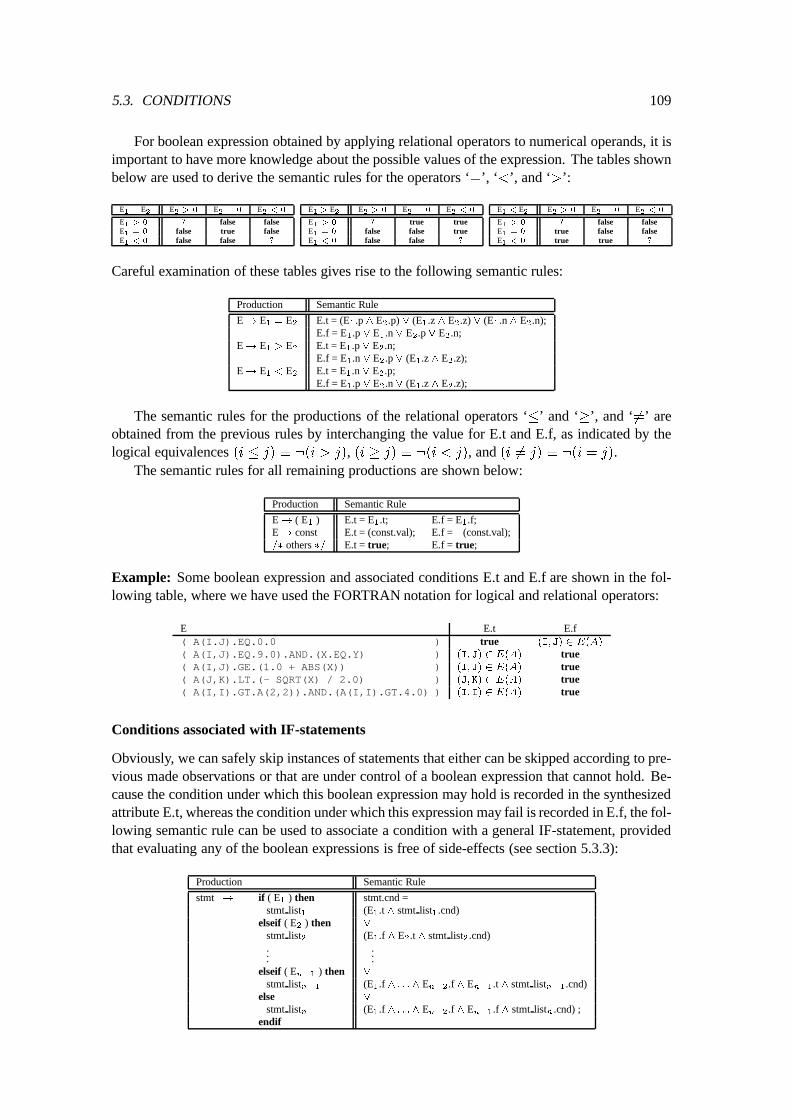
5.3. CONDITIONS 109
For boolean expression obtained by applying relational operators to numerical operands, it isimportant to have more knowledge about the possible values of the expression. The tables shownbelow are used to derive the semantic rules for the operators ‘=’, ‘<’, and ‘>’:
E1
= E2
E2
> 0 E2
= 0 E2
< 0
E1
> 0 ? false falseE1
= 0 false true falseE1
< 0 false false ?
E1
> E2
E2
> 0 E2
= 0 E2
< 0
E1
> 0 ? true trueE1
= 0 false false trueE1
< 0 false false ?
E1
< E2
E2
> 0 E2
= 0 E2
< 0
E1
> 0 ? false falseE1
= 0 true false falseE1
< 0 true true ?
Careful examination of these tables gives rise to the following semantic rules:
Production Semantic Rule
E! E1
= E2
E.t = (E1
.p ^ E2
.p) _ (E1
.z ^ E2
.z) _ (E1
.n ^ E2
.n);E.f = E
1
.p _ E1
.n _ E2
.p _ E2
.n;E! E
1
> E2
E.t = E1
.p _ E2
.n;E.f = E
1
.n _ E2
.p _ (E1
.z ^ E2
.z);E! E
1
< E2
E.t = E1
.n _ E2
.p;E.f = E
1
.p _ E2
.n _ (E1
.z ^ E2
.z);
The semantic rules for the productions of the relational operators ‘�’ and ‘�’, and ‘6=’ areobtained from the previous rules by interchanging the value for E.t and E.f, as indicated by thelogical equivalences (i � j) � :(i > j), (i � j) � :(i < j), and (i 6= j) � :(i = j).
The semantic rules for all remaining productions are shown below:
Production Semantic Rule
E! ( E1
) E.t = E1
.t; E.f = E1
.f;E! const E.t = (const.val); E.f = :(const.val);=� others �= E.t = true; E.f = true;
Example: Some boolean expression and associated conditions E.t and E.f are shown in the fol-lowing table, where we have used the FORTRAN notation for logical and relational operators:
E E.t E.f( A(I.J).EQ.0.0 ) true (I; J) 2 E(A)
( A(I,J).EQ.9.0).AND.(X.EQ.Y) ) (I; J) 2 E(A) true( A(I,J).GE.(1.0 + ABS(X)) ) (I; J) 2 E(A) true( A(J,K).LT.(- SQRT(X) / 2.0) ) (J; K) 2 E(A) true( A(I,I).GT.A(2,2)).AND.(A(I,I).GT.4.0) ) (I; I) 2 E(A) true
Conditions associated with IF-statements
Obviously, we can safely skip instances of statements that either can be skipped according to pre-vious made observations or that are under control of a boolean expression that cannot hold. Be-cause the condition under which this boolean expression may hold is recorded in the synthesizedattribute E.t, whereas the condition under which this expression may fail is recorded in E.f, the fol-lowing semantic rule can be used to associate a condition with a general IF-statement, providedthat evaluating any of the boolean expressions is free of side-effects (see section 5.3.3):
Production Semantic Rule
stmt ! if ( E1
) then stmt.cnd =stmt list
1
(E1
.t ^ stmt list1
.cnd)elseif ( E
2
) then _
stmt list2
(E1
.f ^ E2
.t ^ stmt list2
.cnd)...
...elseif ( E
n�1
) then _
stmt listn�1
(E1
.f ^ : : :^ En�2
.f ^ En�1
.t ^ stmt listn�1
.cnd)else _
stmt listn
(E1
.f ^ : : :^ En�2
.f ^ En�1
.f ^ stmt listn
.cnd) ;endif
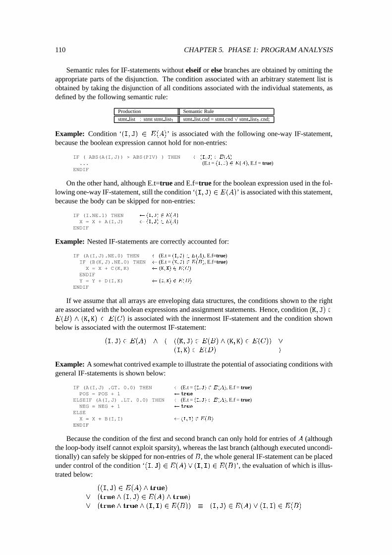
110 CHAPTER 5. PHASE 1: PROGRAM ANALYSIS
Semantic rules for IF-statements without elseif or else branches are obtained by omitting theappropriate parts of the disjunction. The condition associated with an arbitrary statement list isobtained by taking the disjunction of all conditions associated with the individual statements, asdefined by the following semantic rule:
Production Semantic Rule
stmt list! stmt stmt list1
stmt list.cnd = stmt.cnd _ stmt list1
.cnd;
Example: Condition ‘(I; J) 2 E(A)’ is associated with the following one-way IF-statement,because the boolean expression cannot hold for non-entries:
IF ( ABS(A(I,J)) > ABS(PIV) ) THEN (I; J) 2 E(A)
... (E.t = (I; J) 2 E(A), E.f = true)ENDIF
On the other hand, although E.t=true and E.f=true for the boolean expression used in the fol-lowing one-way IF-statement, still the condition ‘(I; J) 2 E(A)’ is associated with this statement,because the body can be skipped for non-entries:
IF (I.NE.1) THEN (I; J) 2 E(A)
X = X + A(I,J) (I; J) 2 E(A)
ENDIF
Example: Nested IF-statements are correctly accounted for:
IF (A(I,J).NE.0) THEN (E.t = (I; J) 2 E(A), E.f=true)IF (B(K,J).NE.0) THEN (E.t = (K; J) 2 E(B), E.f=true)
X = X + C(K,K) (K; K) 2 E(C)
ENDIFY = Y + D(I,K) (I; K) 2 E(D)
ENDIF
If we assume that all arrays are enveloping data structures, the conditions shown to the rightare associated with the boolean expressions and assignment statements. Hence, condition (K; J) 2
E(B) ^ (K; K) 2 E(C) is associated with the innermost IF-statement and the condition shownbelow is associated with the outermost IF-statement:
(I; J) 2 E(A) ^ ( ((K; J) 2 E(B) ^ (K; K) 2 E(C)) _
(I; K) 2 E(D) )
Example: A somewhat contrived example to illustrate the potential of associating conditions withgeneral IF-statements is shown below:
IF (A(I,J) .GT. 0.0) THEN (E.t = (I; J) 2 E(A), E.f = true)POS = POS + 1 true
ELSEIF (A(I,J) .LT. 0.0) THEN (E.t = (I; J) 2 E(A), E.f = true)NEG = NEG + 1 true
ELSEX = X + B(I,I) (I; I) 2 E(B)
ENDIF
Because the condition of the first and second branch can only hold for entries of A (althoughthe loop-body itself cannot exploit sparsity), whereas the last branch (although executed uncondi-tionally) can safely be skipped for non-entries ofB, the whole general IF-statement can be placedunder control of the condition ‘(I; J) 2 E(A)_ (I; I) 2 E(B)’, the evaluation of which is illus-trated below:
((I; J) 2 E(A) ^ true)
_ (true ^ (I; J) 2 E(A) ^ true)
_ (true ^ true ^ (I; I) 2 E(B)) � (I; J) 2 E(A) _ (I; I) 2 E(B)
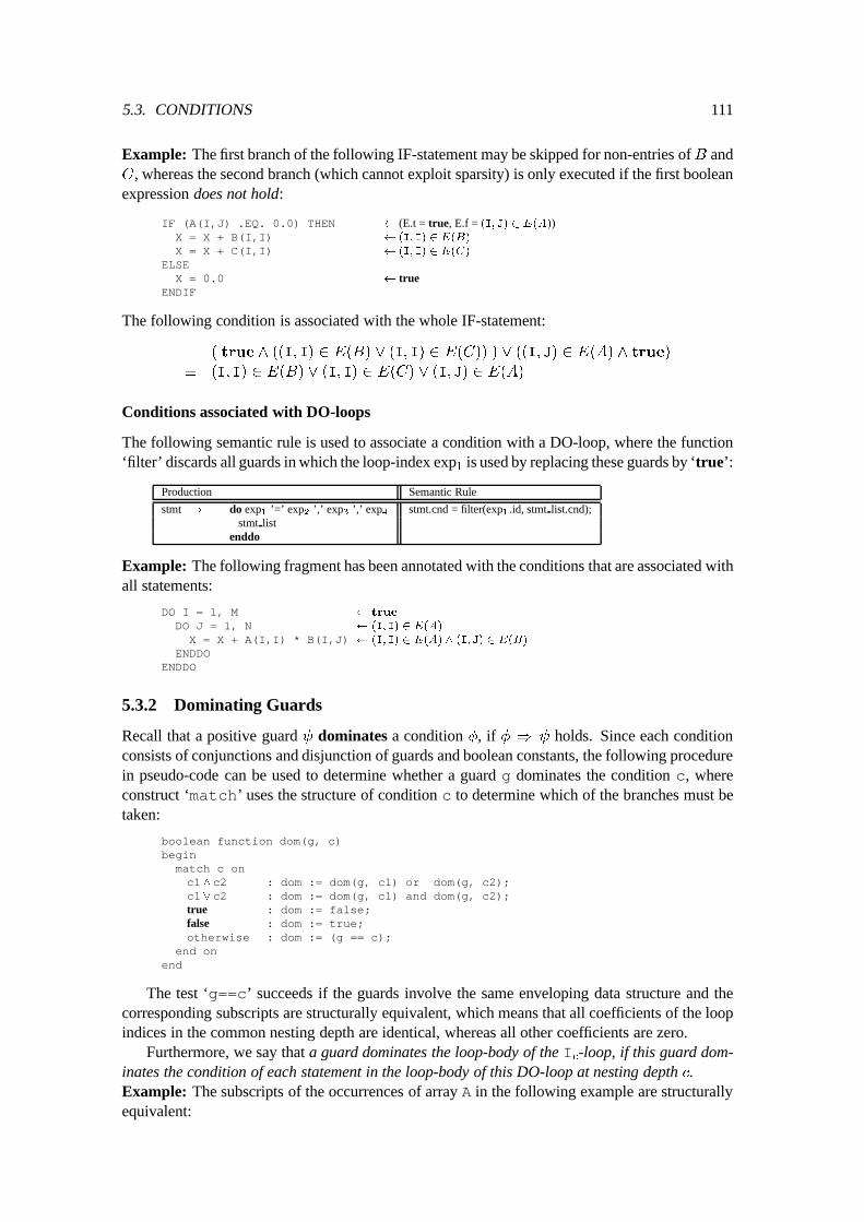
5.3. CONDITIONS 111
Example: The first branch of the following IF-statement may be skipped for non-entries ofB andC , whereas the second branch (which cannot exploit sparsity) is only executed if the first booleanexpression does not hold:
IF (A(I,J) .EQ. 0.0) THEN (E.t = true, E.f = (I; J) 2 E(A))X = X + B(I,I) (I; I) 2 E(B)
X = X + C(I,I) (I; I) 2 E(C)
ELSEX = 0.0 true
ENDIF
The following condition is associated with the whole IF-statement:
( true ^ ((I; I) 2 E(B) _ (I; I) 2 E(C)) ) _ ((I; J) 2 E(A) ^ true)
� (I; I) 2 E(B) _ (I; I) 2 E(C) _ (I; J) 2 E(A)
Conditions associated with DO-loops
The following semantic rule is used to associate a condition with a DO-loop, where the function‘filter’ discards all guards in which the loop-index exp
1
is used by replacing these guards by ‘true’:
Production Semantic Rule
stmt ! do exp1
’=’ exp2
’,’ exp3
’,’ exp4
stmt.cnd = filter(exp1
.id, stmt list.cnd);stmt list
enddo
Example: The following fragment has been annotated with the conditions that are associated withall statements:
DO I = 1, M true
DO J = 1, N (I; I) 2 E(A)
X = X + A(I,I) * B(I,J) (I; I) 2 E(A) ^ (I; J) 2 E(B)
ENDDOENDDO
5.3.2 Dominating Guards
Recall that a positive guard dominates a condition �, if � ) holds. Since each conditionconsists of conjunctions and disjunction of guards and boolean constants, the following procedurein pseudo-code can be used to determine whether a guard g dominates the condition c, whereconstruct ‘match’ uses the structure of condition c to determine which of the branches must betaken:
boolean function dom(g, c)beginmatch c onc1^c2 : dom := dom(g, c1) or dom(g, c2);c1_c2 : dom := dom(g, c1) and dom(g, c2);true : dom := false;false : dom := true;otherwise : dom := (g == c);
end onend
The test ‘g==c’ succeeds if the guards involve the same enveloping data structure and thecorresponding subscripts are structurally equivalent, which means that all coefficients of the loopindices in the common nesting depth are identical, whereas all other coefficients are zero.
Furthermore, we say that a guard dominates the loop-body of the Ic
-loop, if this guard dom-inates the condition of each statement in the loop-body of this DO-loop at nesting depth c.Example: The subscripts of the occurrences of array A in the following example are structurallyequivalent:
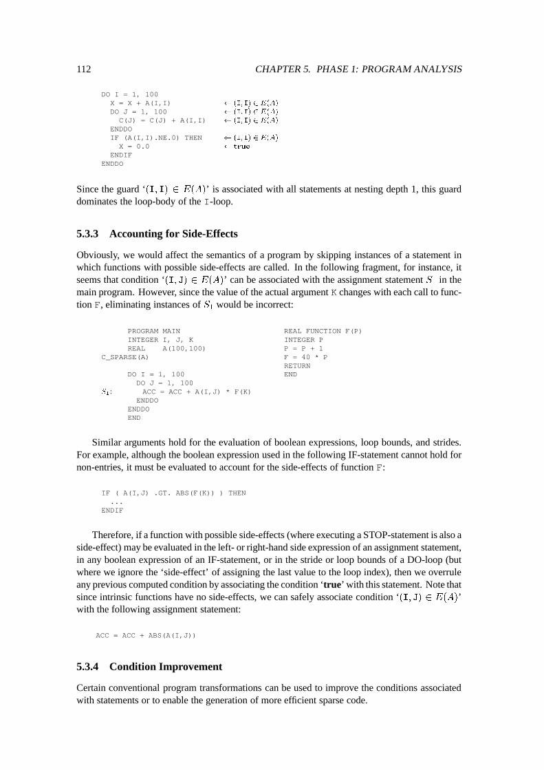
112 CHAPTER 5. PHASE 1: PROGRAM ANALYSIS
DO I = 1, 100X = X + A(I,I) (I; I) 2 E(A)
DO J = 1, 100 (I; I) 2 E(A)
C(J) = C(J) + A(I,I) (I; I) 2 E(A)
ENDDOIF (A(I,I).NE.0) THEN (I; I) 2 E(A)
X = 0.0 true
ENDIFENDDO
Since the guard ‘(I; I) 2 E(A)’ is associated with all statements at nesting depth 1, this guarddominates the loop-body of the I-loop.
5.3.3 Accounting for Side-Effects
Obviously, we would affect the semantics of a program by skipping instances of a statement inwhich functions with possible side-effects are called. In the following fragment, for instance, itseems that condition ‘(I; J) 2 E(A)’ can be associated with the assignment statement S
1
in themain program. However, since the value of the actual argument K changes with each call to func-tion F, eliminating instances of S
1
would be incorrect:
PROGRAM MAININTEGER I, J, KREAL A(100,100)
C_SPARSE(A)
DO I = 1, 100DO J = 1, 100
S
1
: ACC = ACC + A(I,J) * F(K)ENDDO
ENDDOEND
REAL FUNCTION F(P)INTEGER PP = P + 1F = 40 * PRETURNEND
Similar arguments hold for the evaluation of boolean expressions, loop bounds, and strides.For example, although the boolean expression used in the following IF-statement cannot hold fornon-entries, it must be evaluated to account for the side-effects of function F:
IF ( A(I,J) .GT. ABS(F(K)) ) THEN...
ENDIF
Therefore, if a function with possible side-effects (where executing a STOP-statement is also aside-effect) may be evaluated in the left- or right-hand side expression of an assignment statement,in any boolean expression of an IF-statement, or in the stride or loop bounds of a DO-loop (butwhere we ignore the ‘side-effect’ of assigning the last value to the loop index), then we overruleany previous computed condition by associating the condition ‘true’ with this statement. Note thatsince intrinsic functions have no side-effects, we can safely associate condition ‘(I; J) 2 E(A)’with the following assignment statement:
ACC = ACC + ABS(A(I,J))
5.3.4 Condition Improvement
Certain conventional program transformations can be used to improve the conditions associatedwith statements or to enable the generation of more efficient sparse code.
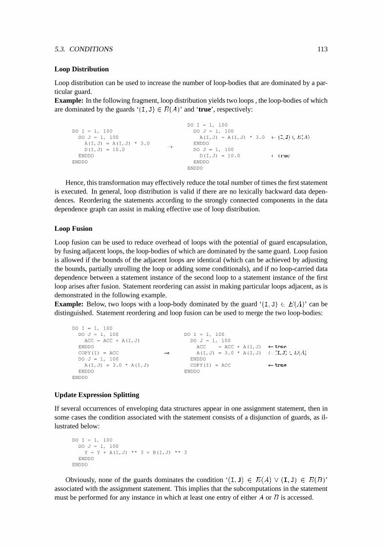
5.3. CONDITIONS 113
Loop Distribution
Loop distribution can be used to increase the number of loop-bodies that are dominated by a par-ticular guard.Example: In the following fragment, loop distribution yields two loops , the loop-bodies of whichare dominated by the guards ‘(I; J) 2 E(A)’ and ‘true’, respectively:
DO I = 1, 100DO J = 1, 100A(I,J) = A(I,J) * 3.0D(I,J) = 10.0
ENDDOENDDO
!
DO I = 1, 100DO J = 1, 100
A(I,J) = A(I,J) * 3.0 (I; J) 2 E(A)
ENDDODO J = 1, 100
D(I,J) = 10.0 true
ENDDOENDDO
Hence, this transformation may effectively reduce the total number of times the first statementis executed. In general, loop distribution is valid if there are no lexically backward data depen-dences. Reordering the statements according to the strongly connected components in the datadependence graph can assist in making effective use of loop distribution.
Loop Fusion
Loop fusion can be used to reduce overhead of loops with the potential of guard encapsulation,by fusing adjacent loops, the loop-bodies of which are dominated by the same guard. Loop fusionis allowed if the bounds of the adjacent loops are identical (which can be achieved by adjustingthe bounds, partially unrolling the loop or adding some conditionals), and if no loop-carried datadependence between a statement instance of the second loop to a statement instance of the firstloop arises after fusion. Statement reordering can assist in making particular loops adjacent, as isdemonstrated in the following example.Example: Below, two loops with a loop-body dominated by the guard ‘(I; J) 2 E(A)’ can bedistinguished. Statement reordering and loop fusion can be used to merge the two loop-bodies:
DO I = 1, 100DO J = 1, 100ACC = ACC + A(I,J)
ENDDOCOPY(I) = ACCDO J = 1, 100A(I,J) = 3.0 * A(I,J)
ENDDOENDDO
!
DO I = 1, 100DO J = 1, 100
ACC = ACC + A(I,J) true
A(I,J) = 3.0 * A(I,J) (I; J) 2 E(A)
ENDDOCOPY(I) = ACC true
ENDDO
Update Expression Splitting
If several occurrences of enveloping data structures appear in one assignment statement, then insome cases the condition associated with the statement consists of a disjunction of guards, as il-lustrated below:
DO I = 1, 100DO J = 1, 100Y = Y + A(I,J) ** 3 + B(I,J) ** 3
ENDDOENDDO
Obviously, none of the guards dominates the condition ‘(I; J) 2 E(A) _ (I; J) 2 E(B)’associated with the assignment statement. This implies that the subcomputations in the statementmust be performed for any instance in which at least one entry of either A or B is accessed.
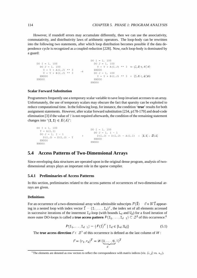
114 CHAPTER 5. PHASE 1: PROGRAM ANALYSIS
However, if roundoff errors may accumulate differently, then we can use the associativity,commutativity, and distributivity laws of arithmetic operators. The loop-body can be rewritteninto the following two statements, after which loop distribution becomes possible if the data de-pendence cycle is recognized as a coupled reduction [228]. Now, each loop-body is dominated bya guard:
DO I = 1, 100DO J = 1, 100Y = Y + A(I,J) ** 3Y = Y + B(I,J) ** 3
ENDDOENDDO
!
DO I = 1, 100DO J = 1, 100
Y = Y + A(I,J) ** 3 (I; J) 2 E(A)
ENDDODO J = 1, 100
Y = Y + B(I,J) ** 3 (I; J) 2 E(B)
ENDDOENDDO
Scalar Forward Substitution
Programmers frequently use a temporary scalar variable to save loop invariant accesses to an array.Unfortunately, the use of temporary scalars may obscure the fact that sparsity can be exploited toreduce computational time. In the following loop, for instance, the condition ‘true’ results for bothassignment statements. However, after scalar forward substitution [234, p178-179] and dead-codeelimination [3] if the value ofT is not required afterwards, the condition of the remaining statementchanges into ‘(I; I) 2 E(A)’:
DO I = 1, 100T = A(I,I)DO J = 1, I - 1D(I,J) = D(I,J) - T
ENDDOENDDO
!
DO I = 1, 100DO J = 1, I - 1
D(I,J) = D(I,J) - A(I,I) (I; I) 2 E(A)
ENDDOENDDO
5.4 Access Patterns of Two-Dimensional Arrays
Since enveloping data structures are operated upon in the original dense program, analysis of two-dimensional arrays plays an important role in the sparse compiler.
5.4.1 Preliminaries of Access Patterns
In this section, preliminaries related to the access patterns of occurrences of two-dimensional ar-rays are given.
Definitions
For an occurrence of a two-dimensional array with admissible subscripts F (~I) = ~v+W
~
I appear-ing in a nested loop with index vector ~I = (I
1
; : : : ; I
d
)
T , the index set of all elements accessedin successive iterations of the innermost I
d
-loop (with bounds Ld
and U
d
) for a fixed iteration ofmore outer DO-loops is called a true access pattern P (I
1
; : : : ; I
d�1
) � Z
2 of this occurrence:6
P (I
1
; : : : ; I
d�1
) = fF (
~
I)
T
j I
d
2 [L
d
; U
d
]g (5.1)
The true access direction ~r 2 Z2 of this occurrence is defined as the last column of W :
~r = (r
1
; r
2
)
T
=W (0; : : : ; 0;
| {z }
d�1
1)
T
6The elements are denoted as row vectors to reflect the correspondence with matrix indices (viz. (i; j) vs. aij
).
5.4. ACCESS PATTERNS OF TWO-DIMENSIONAL ARRAYS 115
If ~r =
~
0, then true access patterns are called scalar-wise. If ~r 6= ~
0, the true access patternsare called row-wise if r
1
= 0 and r2
6= 0, column-wise if r1
6= 0 and r2
= 0, or diagonal-wise otherwise. Likewise, if k � 1 denotes the index of the last nonzero column in matrix W ,then we define the effective access direction ~x 2 Z2 of the occurrence as the kth column of W .The index set of all elements accessed in successive iterations of the I
k
-loop for a fixed iterationof more outer DO-loops form is defined as an effective access pattern P (I
1
; : : : ; I
k�1
) � Z
2
of the occurrence (classified as row-, column-, or diagonal-wise in a similar manner). If such acolumn does not exist, the effective access direction is zero and we leave effective access patternsundefined.
Only for scalar-wise true access patterns, the true and effective access direction may differ,and we can speak of effective access patterns if the effective access direction is nonzero. For oc-currences in scalar-statements (viz. d = 0) or occurrences with inadmissible subscripts, we leaveboth the true as well as the effective access patterns undefined, and we set ~r = ~
0 and ~x =
~
0.Given the effective access direction ~x = (x
1
; x
2
)
T of an occurrence, we define the normal-ized direction ~x n
2 Z
2 of this occurrence as follows:
~x
n
=
(
( 0 ; 0 )
T
if ~x =
~
0
( s �
jx
1
j
g
;
jx
2
j
g
)
T
otherwise
(5.2)
In this formula, g denotes gcd(x
1
; x
2
) and we define s = (x
1
� x
2
> 0)? + 1 : �1. In thismanner, the components of normalized directions are relatively prime, whereas directions that arelinearly dependent become normalized into a uniform direction.Example: Consider the following occurrence of a two-dimensional array A:
DO I1
= 1, 3DO I
2
= I1
, 4... A(9-2*I
2
,I1
) ...ENDDO
ENDDO
F (
~
I) =
9
0
!
+
0 �2
1 0
!
~
I
Both the true and effective access direction of this occurrence are (�2; 0)
T , which gives riseto the normalized access direction ~x n
= (�1; 0)
T . The column-wise true (and effective) accesspatterns of this occurrence are defined as follows for 1 � I
1
� 3:
P (I
1
) = f(9� 2 � I
2
; I
1
) j I
1
� I
2
� 4g
Hence, the following access patterns are associated with this occurrence:
P (1) = f (7; 1); (5; 1); (3; 1); (1; 1) g
P (2) = f (5; 2); (3; 2); (1; 2) g
P (3) = f (3; 3); (1; 3) g
Example: Consider the following occurrence of a two-dimensional array A:
DO I1
= 1, 4DO I
2
= 1, 50... A(10,3 * I
1
) ...ENDDO
ENDDO
F (
~
I) =
10
0
!
+
0 0
3 0
!
~
I
The true access direction of this occurrence is ~r = ~
0, indicating that this occurrence has scalar-wise true access patterns. The four true access patterns that are associated with this occurrence areshown below:
P (1) = f (10; 3) g
P (2) = f (10; 6) g
P (3) = f (10; 9) g
P (4) = f (10; 12) g
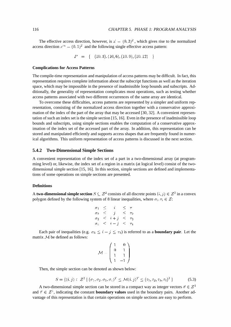
116 CHAPTER 5. PHASE 1: PROGRAM ANALYSIS
The effective access direction, however, is ~x = (0; 3)
T , which gives rise to the normalizedaccess direction ~x n
= (0; 1)
T and the following single effective access pattern:
P = f (10; 3); (10; 6); (10; 9); (10; 12) g
Complications for Access Patterns
The compile-time representation and manipulation of access patterns may be difficult. In fact, thisrepresentation requires complete information about the subscript functions as well as the iterationspace, which may be impossible in the presence of inadmissible loop bounds and subscripts. Ad-ditionally, the generality of representation complicates most operations, such as testing whetheraccess patterns associated with two different occurrences of the same array are identical.
To overcome these difficulties, access patterns are represented by a simpler and uniform rep-resentation, consisting of the normalized access direction together with a conservative approxi-mation of the index of the part of the array that may be accessed [30, 32]. A convenient represen-tation of such an index set is the simple section [15, 16]. Even in the presence of inadmissible loopbounds and subscripts, using simple sections enables the computation of a conservative approx-imation of the index set of the accessed part of the array. In addition, this representation can bestored and manipulated efficiently and supports access shapes that are frequently found in numer-ical algorithms. This uniform representation of access patterns is discussed in the next section.
5.4.2 Two-Dimensional Simple Sections
A convenient representation of the index set of a part in a two-dimensional array (at program-ming level) or, likewise, the index set of a region in a matrix (at logical level) consist of the two-dimensional simple section [15, 16]. In this section, simple sections are defined and implementa-tions of some operations on simple sections are presented.
Definitions
A two-dimensional simple section S � Z2 consists of all discrete points (i; j) 2 Z2 in a convexpolygon defined by the following system of 8 linear inequalities, where �
i
; �
i
2 Z:
�
1
� i � �
1
�
2
� j � �
2
�
3
� i+ j � �
3
�
4
� i� j � �
4
Each pair of inequalities (e.g. �3
� i + j � �
3
) is referred to as a boundary pair. Let thematrixM be defined as follows:
M =
0
B
B
B
@
1 0
0 1
1 1
1 �1
1
C
C
C
A
Then, the simple section can be denoted as shown below:
S = f(i; j) 2 Z
2
j (�
1
; �
2
; �
3
; �
4
)
T
�M(i; j)
T
� (�
1
; �
2
; �
3
; �
4
)
T
g (5.3)
A two-dimensional simple section can be stored in a compact way as integer vectors ~� 2 Z4
and ~� 2 Z4, indicating the constant boundary values used in the boundary pairs. Another ad-vantage of this representation is that certain operations on simple sections are easy to perform.
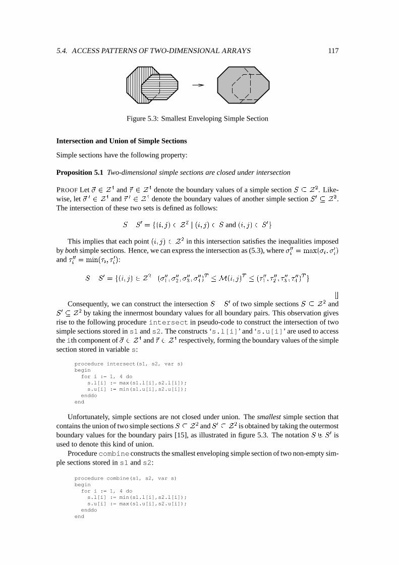
5.4. ACCESS PATTERNS OF TWO-DIMENSIONAL ARRAYS 117
Figure 5.3: Smallest Enveloping Simple Section
Intersection and Union of Simple Sections
Simple sections have the following property:
Proposition 5.1 Two-dimensional simple sections are closed under intersection
PROOF Let ~� 2 Z4 and ~� 2 Z4 denote the boundary values of a simple section S � Z2. Like-wise, let ~� 0 2 Z4 and ~� 0 2 Z4 denote the boundary values of another simple section S0 � Z2.The intersection of these two sets is defined as follows:
S \ S
0
= f(i; j) 2 Z
2
j (i; j) 2 S and (i; j) 2 S
0
g
This implies that each point (i; j) 2 Z2 in this intersection satisfies the inequalities imposedby both simple sections. Hence, we can express the intersection as (5.3), where �00
i
= max(�
i
; �
0
i
)
and � 00i
= min(�
i
; �
0
i
):
S \ S
0
= f(i; j) 2 Z
2
j (�
00
1
; �
00
2
; �
00
3
; �
00
4
)
T
�M(i; j)
T
� (�
00
1
; �
00
2
; �
00
3
; �
00
4
)
T
g
[]
Consequently, we can construct the intersection S \ S0 of two simple sections S � Z2 andS
0
� Z
2 by taking the innermost boundary values for all boundary pairs. This observation givesrise to the following procedure intersect in pseudo-code to construct the intersection of twosimple sections stored in s1 and s2. The constructs ‘s.l[i]’ and ‘s.u[i]’ are used to accessthe ith component of ~� 2 Z4 and ~� 2 Z4 respectively, forming the boundary values of the simplesection stored in variable s:
procedure intersect(s1, s2, var s)beginfor i := 1, 4 dos.l[i] := max(s1.l[i],s2.l[i]);s.u[i] := min(s1.u[i],s2.u[i]);
enddoend
Unfortunately, simple sections are not closed under union. The smallest simple section thatcontains the union of two simple sections S � Z2 andS0 � Z2 is obtained by taking the outermostboundary values for the boundary pairs [15], as illustrated in figure 5.3. The notation S ] S0 isused to denote this kind of union.
Procedure combine constructs the smallest enveloping simple section of two non-empty sim-ple sections stored in s1 and s2:
procedure combine(s1, s2, var s)beginfor i := 1, 4 dos.l[i] := min(s1.l[i],s2.l[i]);s.u[i] := max(s1.u[i],s2.u[i]);
enddoend
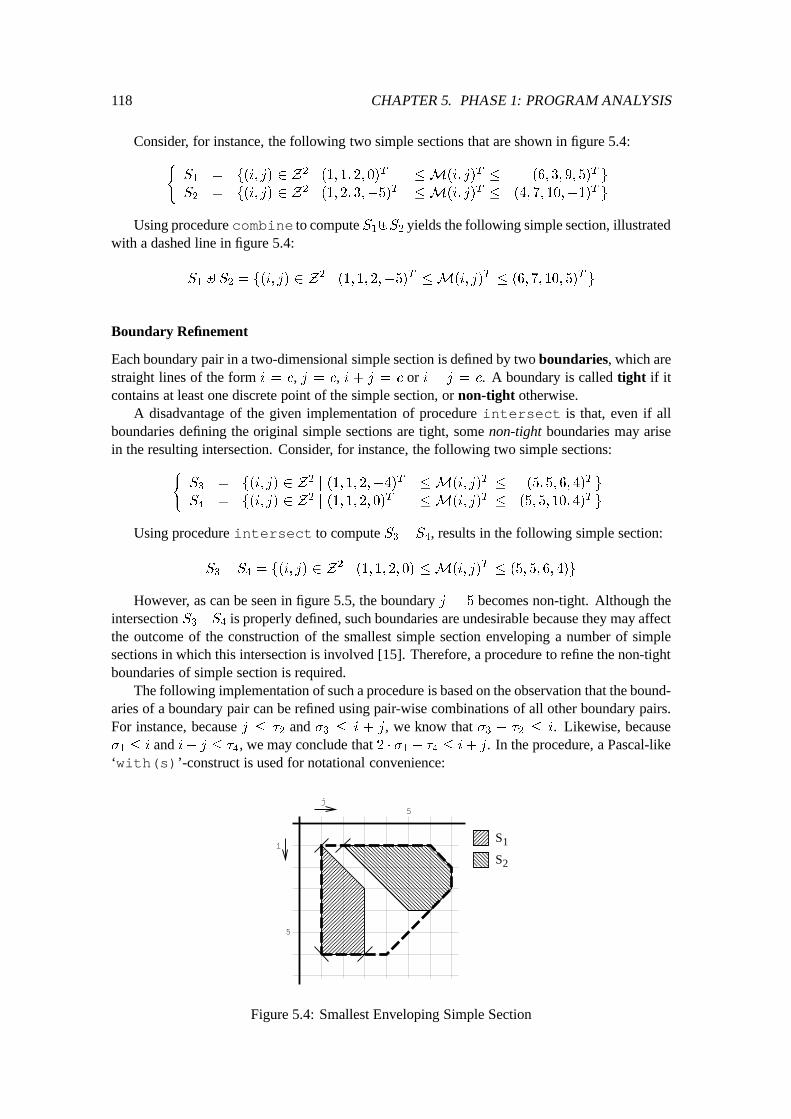
118 CHAPTER 5. PHASE 1: PROGRAM ANALYSIS
Consider, for instance, the following two simple sections that are shown in figure 5.4:(
S
1
= f(i; j) 2 Z
2
j (1; 1; 2; 0)
T
�M(i; j)
T
� (6; 3; 9; 5)
T
g
S
2
= f(i; j) 2 Z
2
j (1; 2; 3;�5)
T
�M(i; j)
T
� (4; 7; 10;�1)
T
g
Using procedure combine to compute S1
]S
2
yields the following simple section, illustratedwith a dashed line in figure 5.4:
S
1
] S
2
= f(i; j) 2 Z
2
j (1; 1; 2;�5)
T
�M(i; j)
T
� (6; 7; 10; 5)
T
g
Boundary Refinement
Each boundary pair in a two-dimensional simple section is defined by two boundaries, which arestraight lines of the form i = c, j = c, i + j = c or i � j = c. A boundary is called tight if itcontains at least one discrete point of the simple section, or non-tight otherwise.
A disadvantage of the given implementation of procedure intersect is that, even if allboundaries defining the original simple sections are tight, some non-tight boundaries may arisein the resulting intersection. Consider, for instance, the following two simple sections:
(
S
3
= f(i; j) 2 Z
2
j (1; 1; 2;�4)
T
�M(i; j)
T
� (5; 5; 6; 4)
T
g
S
4
= f(i; j) 2 Z
2
j (1; 1; 2; 0)
T
�M(i; j)
T
� (5; 5; 10; 4)
T
g
Using procedure intersect to compute S3
\ S
4
, results in the following simple section:
S
3
\ S
4
= f(i; j) 2 Z
2
j (1; 1; 2; 0) �M(i; j)
T
� (5; 5; 6; 4)g
However, as can be seen in figure 5.5, the boundary j = 5 becomes non-tight. Although theintersection S
3
\S
4
is properly defined, such boundaries are undesirable because they may affectthe outcome of the construction of the smallest simple section enveloping a number of simplesections in which this intersection is involved [15]. Therefore, a procedure to refine the non-tightboundaries of simple section is required.
The following implementation of such a procedure is based on the observation that the bound-aries of a boundary pair can be refined using pair-wise combinations of all other boundary pairs.For instance, because j � �
2
and �3
� i + j, we know that �3
� �
2
� i. Likewise, because�
1
� i and i� j � �4
, we may conclude that 2 � �1
� �
4
� i+ j. In the procedure, a Pascal-like‘with(s)’-construct is used for notational convenience:
5
5
S1
S2
i
j
Figure 5.4: Smallest Enveloping Simple Section
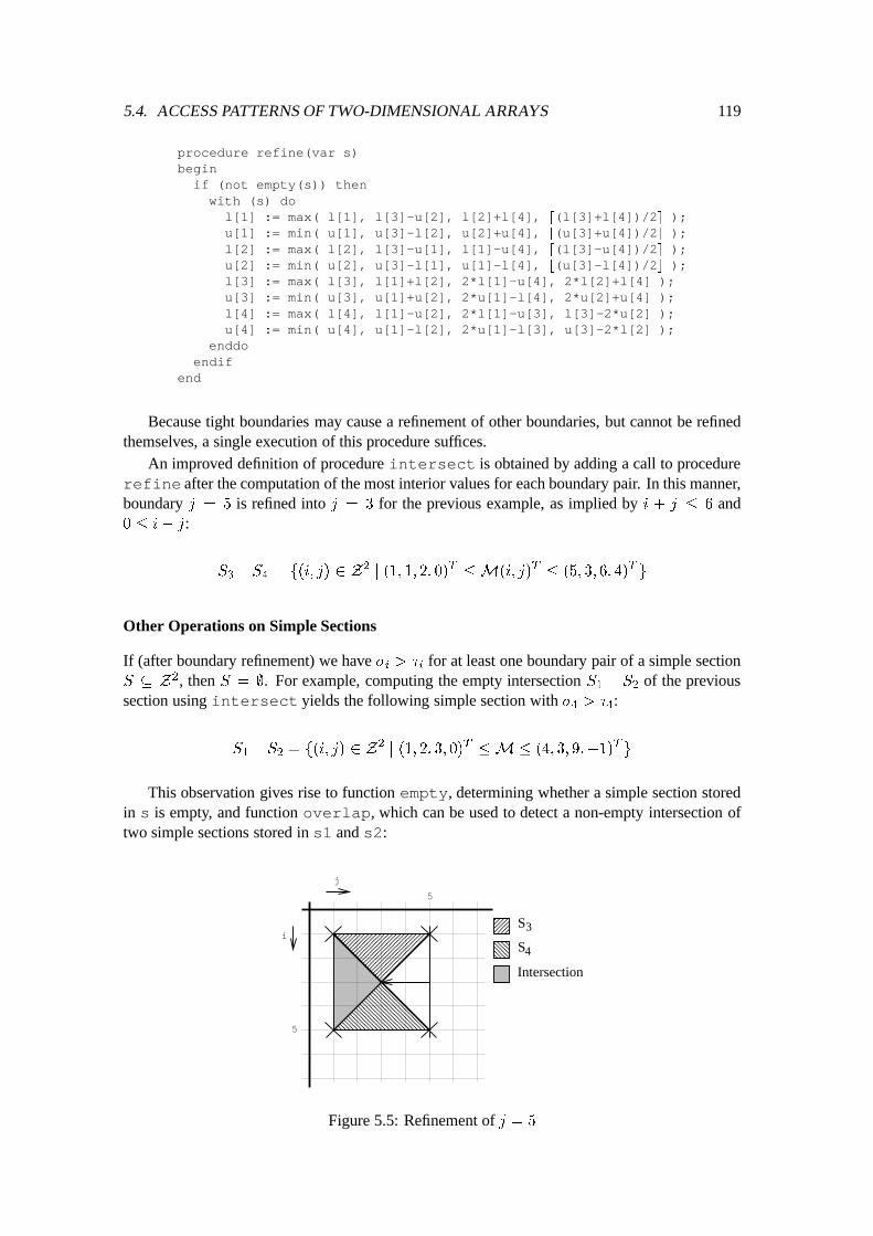
5.4. ACCESS PATTERNS OF TWO-DIMENSIONAL ARRAYS 119
procedure refine(var s)begin
if (not empty(s)) thenwith (s) do
l[1] := max( l[1], l[3]-u[2], l[2]+l[4], d(l[3]+l[4])/2e );u[1] := min( u[1], u[3]-l[2], u[2]+u[4], b(u[3]+u[4])/2c );l[2] := max( l[2], l[3]-u[1], l[1]-u[4], d(l[3]-u[4])/2e );u[2] := min( u[2], u[3]-l[1], u[1]-l[4], b(u[3]-l[4])/2c );l[3] := max( l[3], l[1]+l[2], 2*l[1]-u[4], 2*l[2]+l[4] );u[3] := min( u[3], u[1]+u[2], 2*u[1]-l[4], 2*u[2]+u[4] );l[4] := max( l[4], l[1]-u[2], 2*l[1]-u[3], l[3]-2*u[2] );u[4] := min( u[4], u[1]-l[2], 2*u[1]-l[3], u[3]-2*l[2] );
enddoendif
end
Because tight boundaries may cause a refinement of other boundaries, but cannot be refinedthemselves, a single execution of this procedure suffices.
An improved definition of procedure intersect is obtained by adding a call to procedurerefine after the computation of the most interior values for each boundary pair. In this manner,boundary j = 5 is refined into j = 3 for the previous example, as implied by i + j � 6 and0 � i� j:
S
3
\ S
4
= f(i; j) 2 Z
2
j (1; 1; 2; 0)
T
�M(i; j)
T
� (5; 3; 6; 4)
T
g
Other Operations on Simple Sections
If (after boundary refinement) we have �i
> �
i
for at least one boundary pair of a simple sectionS � Z
2, then S = ;. For example, computing the empty intersection S1
\ S
2
of the previoussection using intersect yields the following simple section with �
4
> �
4
:
S
1
\ S
2
= f(i; j) 2 Z
2
j (1; 2; 3; 0)
T
�M � (4; 3; 9;�1)
T
g
This observation gives rise to function empty, determining whether a simple section storedin s is empty, and function overlap, which can be used to detect a non-empty intersection oftwo simple sections stored in s1 and s2:
5
Intersection
5
S3
S4i
j
Figure 5.5: Refinement of j = 5
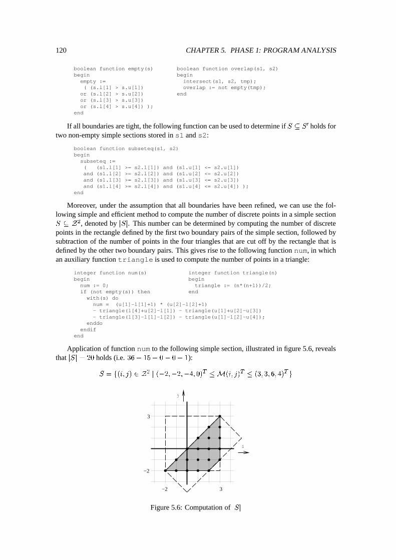
120 CHAPTER 5. PHASE 1: PROGRAM ANALYSIS
boolean function empty(s)beginempty :=( (s.l[1] > s.u[1])
or (s.l[2] > s.u[2])or (s.l[3] > s.u[3])or (s.l[4] > s.u[4]) );
end
boolean function overlap(s1, s2)beginintersect(s1, s2, tmp);overlap := not empty(tmp);
end
If all boundaries are tight, the following function can be used to determine if S � S0 holds fortwo non-empty simple sections stored in s1 and s2:
boolean function subseteq(s1, s2)beginsubseteq :=( (s1.l[1] >= s2.l[1]) and (s1.u[1] <= s2.u[1])and (s1.l[2] >= s2.l[2]) and (s1.u[2] <= s2.u[2])and (s1.l[3] >= s2.l[3]) and (s1.u[3] <= s2.u[3])and (s1.l[4] >= s2.l[4]) and (s1.u[4] <= s2.u[4]) );
end
Moreover, under the assumption that all boundaries have been refined, we can use the fol-lowing simple and efficient method to compute the number of discrete points in a simple sectionS � Z
2, denoted by jSj. This number can be determined by computing the number of discretepoints in the rectangle defined by the first two boundary pairs of the simple section, followed bysubtraction of the number of points in the four triangles that are cut off by the rectangle that isdefined by the other two boundary pairs. This gives rise to the following function num, in whichan auxiliary function triangle is used to compute the number of points in a triangle:
integer function num(s) integer function triangle(n)begin beginnum := 0; triangle := (n*(n+1))/2;if (not empty(s)) then end
with(s) donum = (u[1]-l[1]+1) * (u[2]-l[2]+1)- triangle(l[4]+u[2]-l[1]) - triangle(u[1]+u[2]-u[3])- triangle(l[3]-l[1]-l[2]) - triangle(u[1]-l[2]-u[4]);
enddoendif
end
Application of function num to the following simple section, illustrated in figure 5.6, revealsthat jSj = 20 holds (i.e. 36� 15� 0� 0� 1):
S = f(i; j) 2 Z
2
j (�2;�2;�4; 0)
T
�M(i; j)
T
� (3; 3; 6; 4)
T
g
−2 3
−2
3
i
j
Figure 5.6: Computation of jSj
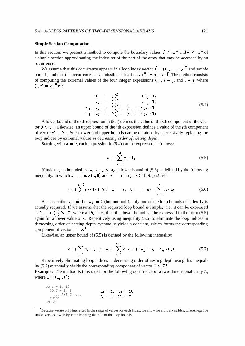
5.4. ACCESS PATTERNS OF TWO-DIMENSIONAL ARRAYS 121
Simple Section Computation
In this section, we present a method to compute the boundary values ~� 2 Z4 and ~� 2 Z4 ofa simple section approximating the index set of the part of the array that may be accessed by anoccurrence.
We assume that this occurrence appears in a loop index vector ~I = (I
1
; : : : ; I
d
)
T and simplebounds, and that the occurrence has admissible subscripts F (~I) = ~v+W
~
I. The method consistsof computing the extremal values of the four integer expressions i, j, i + j, and i � j, where(i; j) = F (
~
I)
T :
v
1
+
P
d
j=1
w
1j
� I
j
v
2
+
P
d
j=1
w
2j
� I
j
v
1
+ v
2
+
P
d
j=1
(w
1j
+ w
2j
) � I
j
v
1
� v
2
+
P
d
j=1
(w
1j
� w
2j
) � I
j
(5.4)
A lower bound of the ith expression in (5.4) defines the value of the ith component of the vec-tor ~� 2 Z4. Likewise, an upper bound of the ith expression defines a value of the ith componentof vector ~� 2 Z4. Such lower and upper bounds can be obtained by successively replacing theloop indices by extremal values in decreasing order of nesting depth.
Starting with k = d, each expression in (5.4) can be expressed as follows:
a
0
+
k
X
j=1
a
j
� I
j
(5.5)
If index I
k
is bounded as Lk
� I
k
� U
k
, a lower bound of (5.5) is defined by the followinginequality, in which a+ = max(a; 0) and a� = max(�a; 0) [19, p52-54]:
a
0
+
k�1
X
i=1
a
i
� I
i
+ (a
+
k
� L
k
� a
�
k
� U
k
) � a
0
+
k
X
i=1
a
i
� I
i
(5.6)
Because either a+k
6= 0 or a�k
6= 0 (but not both), only one of the loop bounds of index I
k
isactually required. If we assume that the required loop bound is simple,7 i.e. it can be expressedas b
0
+
P
k�1
j=1
b
j
� I
j
where all bi
2 Z , then this lower bound can be expressed in the form (5.5)again for a lower value of k. Repetitively using inequality (5.6) to eliminate the loop indices indecreasing order of nesting depth eventually yields a constant, which forms the correspondingcomponent of vector ~� 2 Z4.
Likewise, an upper bound of (5.5) is defined by the following inequality:
a
0
+
k
X
i=1
a
i
� I
i
� a
0
+
k�1
X
i=1
a
i
� I
i
+ (a
+
k
� U
k
� a
�
k
� L
k
) (5.7)
Repetitively eliminating loop indices in decreasing order of nesting depth using this inequal-ity (5.7) eventually yields the corresponding component of vector ~� 2 Z4.Example: The method is illustrated for the following occurrence of a two-dimensional array A,where ~I = (I; J)
T :
DO I = 1, 10DO J = 1, I... A(I,J) ...
ENDDOENDDO
L
1
= 1; U
1
= 10
L
2
= 1; U
2
= I
7Because we are only interested in the range of values for each index, we allow for arbitrary strides, where negativestrides are dealt with by interchanging the role of the loop bounds.
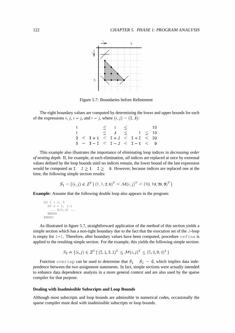
122 CHAPTER 5. PHASE 1: PROGRAM ANALYSIS
5
5
i
j
Figure 5.7: Boundaries before Refinement
The eight boundary values are computed by determining the lower and upper bounds for eachof the expressions i, j, i+ j, and i� j, where (i; j) = (I; J):
1 � I � 10
1 � J � I � 10
2 � I+ 1 � I+ J � I+ I � 20
0 = I� I � I� J � I� 1 � 9
This example also illustrates the importance of eliminating loop indices in decreasing orderof nesting depth. If, for example, at each elimination, all indices are replaced at once by extremalvalues defined by the loop bounds until no indices remain, the lower bound of the last expressionwould be computed as I� J � 1� I � �9. However, because indices are replaced one at thetime, the following simple section results:
S
1
= f(i; j) 2 Z
2
j (1; 1; 2; 0)
T
�M(i; j)
T
� (10; 10; 20; 9)
T
g
Example: Assume that the following double loop also appears in the program:
DO I = 1, 5DO J = 1, I-1: : : A(I,J) : : :
ENDDOENDDO
As illustrated in figure 5.7, straightforward application of the method of this section yields asimple section which has a non-tight boundary due to the fact that the execution set of the J-loopis empty for I=1. Therefore, after boundary values have been computed, procedure refine isapplied to the resulting simple section. For the example, this yields the following simple section:
S
2
= f(i; j) 2 Z
2
j (2; 1; 3; 1)
T
�M(i; j)
T
� (5; 4; 9; 4)
T
g
Function overlap can be used to determine that S1
\ S
2
= ;, which implies data inde-pendence between the two assignment statements. In fact, simple sections were actually intendedto enhance data dependence analysis in a more general context and are also used by the sparsecompiler for that purpose.
Dealing with Inadmissible Subscripts and Loop Bounds
Although most subscripts and loop bounds are admissible in numerical codes, occasionally thesparse compiler must deal with inadmissible subscripts or loop bounds.
5.4. ACCESS PATTERNS OF TWO-DIMENSIONAL ARRAYS 123
In this case, we can use the fact that the following simple section defines the index set of thewhole array that is used to store an m� n matrix:
S = f(i; j) 2 Z
2
j (1; 1; 2; 1 � n)
T
�M(i; j)
T
� (m;n;m+ n;m� 1)
T
g (5.8)
Hence, if we assume that subscript bounds are not violated,8 then we can use the boundaryvalue of this simple section in all cases where the method of the previous section fails.
If the first subscript of an occurrence of a two-dimensional array is inadmissible, the extremalvalues of the expressions i, i+ j, and i� j cannot be determined using the previous method, andthe corresponding boundary values are taken from (5.8) instead. Likewise, if the second subscriptis inadmissible, the method is not able to determine the extremal values of the expressions j, i+j,and i� j, but uses the corresponding boundary values of (5.8). However, the method is initiatedfor expression i, for expression j, or for all expressions if only the first, only the second, or allsubscripts are admissible respectively. If during computation of an extremal value for one of theseexpressions, a lower or upper loop bound is required (because the corresponding coefficient ineither (5.6) or (5.7) is nonzero) that is not simple, then the computation of the extremal value isabandoned, and the corresponding boundary value of (5.8) is used instead. After all boundaryvalues are determined in this manner, boundary refinement is applied.Example: The following occurrences of an enveloping data structure of a 100 � 100 implicitlysparse matrix have one inadmissible subscript:
DO I = 1, 10Z = ...... A
1
(I,Z) ...ENDDO
DO I = 1, 50DO J = 1, 90
... A2
(PV(I),J) ...ENDDO
ENDDO
For S1
, the inequalities 1 � i � 10 can be determined by examination of the admissiblesubscript i = I. The other boundary values arise naturally from (5.8) and boundary refinement.Simple section S
2
is computed similarly:(
S
1
= f(i; j) 2 Z
2
j (1; 1; 2;�99)
T
�M(i; j)
T
� (10; 100; 110; 9)
T
g
S
2
= f(i; j) 2 Z
2
j (1; 1; 2;�89)
T
�M(i; j)
T
� (100; 90; 190; 99)
T
g
Below, an example with an inadmissible loop bound is given:
Z = ...DO I = 10, ZDO J = 1, I.. A
3
(5+I,J) ..ENDDO
ENDDO
For instance, determining the lower bound of expression i � j for i = 5+ I and j = J canbe done without any knowledge of the loop bounds because 5+ I� J � 5+ I� I. However,computing an upper bound of this expression fails because the loop bound Z is inadmissible. Like-wise, the lower bound �
1
= 15 of i = 5+ I arises from the simple lower bound 10 of the I-loop,whereas determination of an upper bound of this expression fails.
Eventually, the simple section shown below results in which, rather surprisingly, inequalityJ � I � 95 arises from boundary refinement:
S
3
= f(i; j) 2 Z
2
j (15; 1; 16; 5)
T
�M(i; j)
T
� (100; 95; 195; 99)
T
g
8In fact, if one of the boundary values that can be computed is exterior to the corresponding boundary value of thissimple section, then a potential subscript violation is reported.
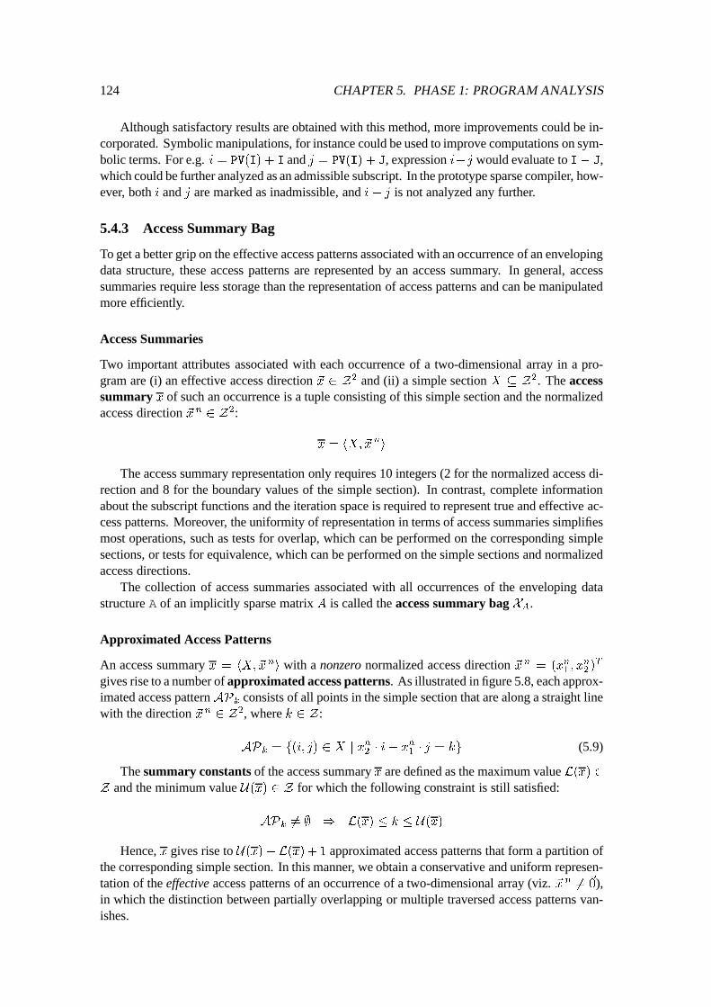
124 CHAPTER 5. PHASE 1: PROGRAM ANALYSIS
Although satisfactory results are obtained with this method, more improvements could be in-corporated. Symbolic manipulations, for instance could be used to improve computations on sym-bolic terms. For e.g. i = PV(I) + I and j = PV(I) + J, expression i�j would evaluate to I� J,which could be further analyzed as an admissible subscript. In the prototype sparse compiler, how-ever, both i and j are marked as inadmissible, and i� j is not analyzed any further.
5.4.3 Access Summary Bag
To get a better grip on the effective access patterns associated with an occurrence of an envelopingdata structure, these access patterns are represented by an access summary. In general, accesssummaries require less storage than the representation of access patterns and can be manipulatedmore efficiently.
Access Summaries
Two important attributes associated with each occurrence of a two-dimensional array in a pro-gram are (i) an effective access direction ~x 2 Z2 and (ii) a simple section X � Z2. The accesssummary x of such an occurrence is a tuple consisting of this simple section and the normalizedaccess direction ~x n
2 Z
2:
x = hX;~x
n
i
The access summary representation only requires 10 integers (2 for the normalized access di-rection and 8 for the boundary values of the simple section). In contrast, complete informationabout the subscript functions and the iteration space is required to represent true and effective ac-cess patterns. Moreover, the uniformity of representation in terms of access summaries simplifiesmost operations, such as tests for overlap, which can be performed on the corresponding simplesections, or tests for equivalence, which can be performed on the simple sections and normalizedaccess directions.
The collection of access summaries associated with all occurrences of the enveloping datastructure A of an implicitly sparse matrix A is called the access summary bag X
A
.
Approximated Access Patterns
An access summary x = hX;~x
n
i with a nonzero normalized access direction ~x n
= (x
n
1
; x
n
2
)
T
gives rise to a number of approximated access patterns. As illustrated in figure 5.8, each approx-imated access patternAP
k
consists of all points in the simple section that are along a straight linewith the direction ~x n
2 Z
2, where k 2 Z:
AP
k
= f(i; j) 2 X j x
n
2
� i� x
n
1
� j = kg (5.9)
The summary constants of the access summary x are defined as the maximum value L(x) 2Z and the minimum value U(x) 2 Z for which the following constraint is still satisfied:
AP
k
6= ; ) L(x) � k � U(
x)
Hence, x gives rise to U(x)�L(x) + 1 approximated access patterns that form a partition ofthe corresponding simple section. In this manner, we obtain a conservative and uniform represen-tation of the effective access patterns of an occurrence of a two-dimensional array (viz. ~x n
6=
~
0),in which the distinction between partially overlapping or multiple traversed access patterns van-ishes.
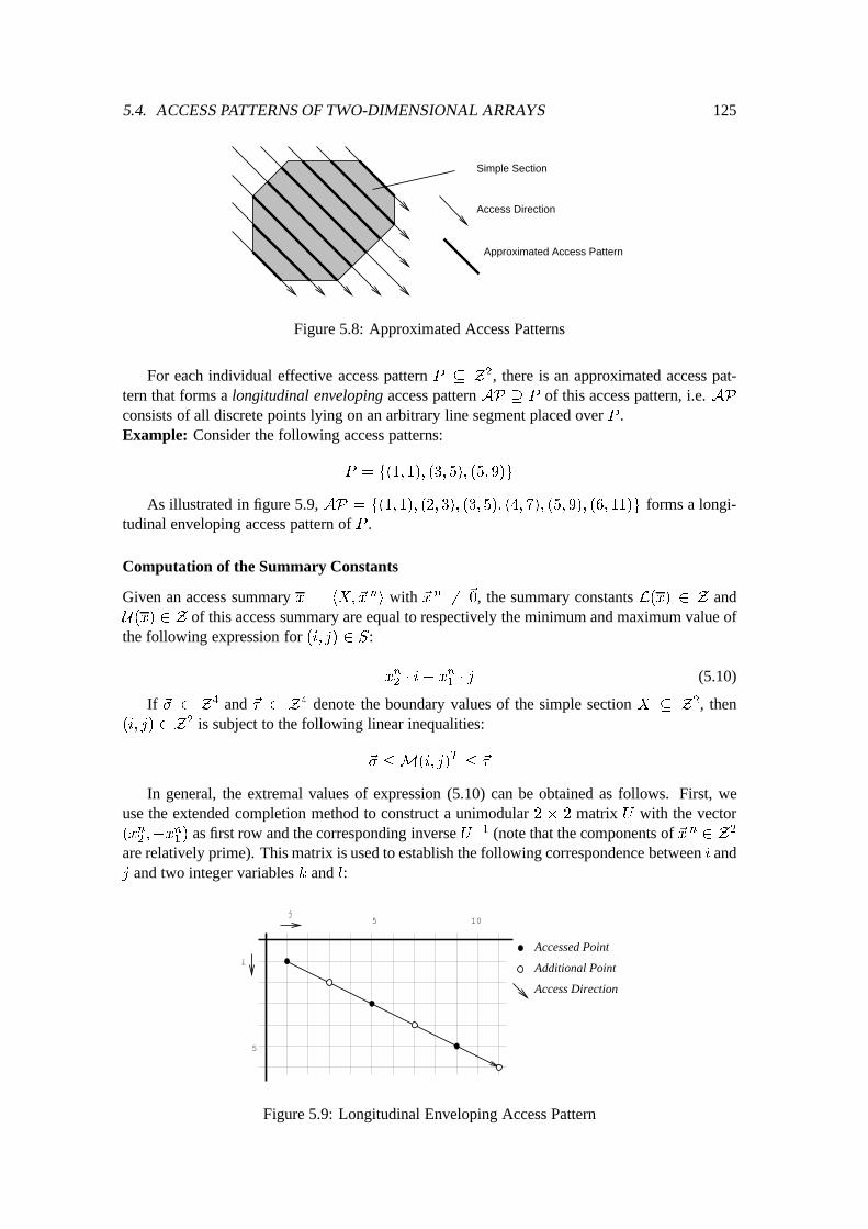
5.4. ACCESS PATTERNS OF TWO-DIMENSIONAL ARRAYS 125
Simple Section
Access Direction
Approximated Access Pattern
Figure 5.8: Approximated Access Patterns
For each individual effective access pattern P � Z2, there is an approximated access pat-tern that forms a longitudinal enveloping access pattern AP � P of this access pattern, i.e. APconsists of all discrete points lying on an arbitrary line segment placed over P .Example: Consider the following access patterns:
P = f(1; 1); (3; 5); (5; 9)g
As illustrated in figure 5.9, AP = f(1; 1); (2; 3); (3; 5); (4; 7); (5; 9); (6; 11)g forms a longi-tudinal enveloping access pattern of P .
Computation of the Summary Constants
Given an access summary x = hX;~x
n
i with ~x n
6=
~
0, the summary constants L(x) 2 Z andU(x) 2 Z of this access summary are equal to respectively the minimum and maximum value ofthe following expression for (i; j) 2 S:
x
n
2
� i� x
n
1
� j (5.10)
If ~� 2 Z4 and ~� 2 Z4 denote the boundary values of the simple section X � Z
2, then(i; j) 2 Z
2 is subject to the following linear inequalities:
~� �M(i; j)
T
� ~�
In general, the extremal values of expression (5.10) can be obtained as follows. First, weuse the extended completion method to construct a unimodular 2 � 2 matrix U with the vector(x
n
2
;�x
n
1
) as first row and the corresponding inverse U�1 (note that the components of ~x n
2 Z
2
are relatively prime). This matrix is used to establish the following correspondence between i andj and two integer variables k and l:
5
5
10
i
j
Accessed Point
Additional Point
Access Direction
Figure 5.9: Longitudinal Enveloping Access Pattern
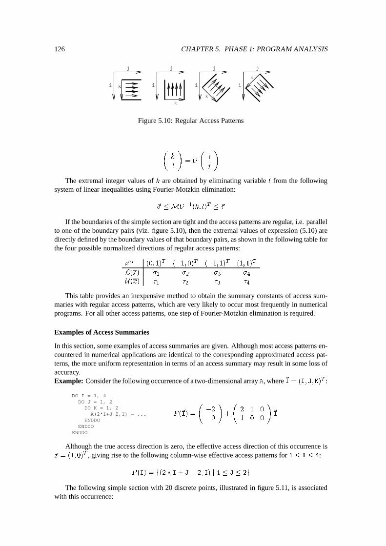
126 CHAPTER 5. PHASE 1: PROGRAM ANALYSIS
i
j
k
i
j
k
i
j
i
j
k
k
Figure 5.10: Regular Access Patterns
k
l
!
= U
i
j
!
The extremal integer values of k are obtained by eliminating variable l from the followingsystem of linear inequalities using Fourier-Motzkin elimination:
~� �MU
�1
(k; l)
T
� ~�
If the boundaries of the simple section are tight and the access patterns are regular, i.e. parallelto one of the boundary pairs (viz. figure 5.10), then the extremal values of expression (5.10) aredirectly defined by the boundary values of that boundary pairs, as shown in the following table forthe four possible normalized directions of regular access patterns:
~x
n
(0; 1)
T
(�1; 0)
T
(�1; 1)
T
(1; 1)
T
L(x) �
1
�
2
�
3
�
4
U(x) �
1
�
2
�
3
�
4
This table provides an inexpensive method to obtain the summary constants of access sum-maries with regular access patterns, which are very likely to occur most frequently in numericalprograms. For all other access patterns, one step of Fourier-Motzkin elimination is required.
Examples of Access Summaries
In this section, some examples of access summaries are given. Although most access patterns en-countered in numerical applications are identical to the corresponding approximated access pat-terns, the more uniform representation in terms of an access summary may result in some loss ofaccuracy.Example: Consider the following occurrence of a two-dimensional array A, where~I = (I; J; K)
T :
DO I = 1, 4DO J = 1, 2DO K = 1, 2A(2*I+J-2,I) = ...
ENDDOENDDO
ENDDO
F (
~
I) =
�2
0
!
+
2 1 0
1 0 0
!
~
I
Although the true access direction is zero, the effective access direction of this occurrence is~x = (1; 0)
T , giving rise to the following column-wise effective access patterns for 1 � I � 4:
P (I) = f(2 � I+ J� 2; I) j 1 � J � 2g
The following simple section with 20 discrete points, illustrated in figure 5.11, is associatedwith this occurrence:
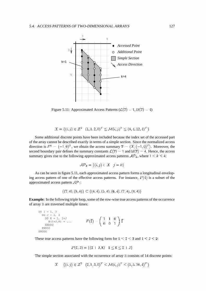
5.4. ACCESS PATTERNS OF TWO-DIMENSIONAL ARRAYS 127
5
5
Accessed Point
Simple Section
Additional Point
Access Direction
j
i
k=4
k=1
Figure 5.11: Approximated Access Patterns (L(x) = 1, U(x) = 4)
X = f(i; j) 2 Z
2
j (1; 1; 2; 0)
T
�M(i; j)
T
� (8; 4; 12; 4)
T
g
Some additional discrete points have been included because the index set of the accessed partof the array cannot be described exactly in terms of a simple section. Since the normalized accessdirection is ~x n
= (�1; 0)
T , we obtain the access summary x = hX; (�1; 0)
T
i. Moreover, thesecond boundary pair defines the summary constants L(x) = 1 and U(x) = 4. Hence, the accesssummary gives rise to the following approximated access patterns AP
k
, where 1 � k � 4:
AP
k
= f(i; j) 2 X j j = kg
As can be seen in figure 5.11, each approximated access pattern forms a longitudinal envelop-ing access pattern of one of the effective access patterns. For instance, P (4) is a subset of theapproximated access pattern AP
4
:
f(7; 4); (8; 4)g � f(4; 4); (5; 4); (6; 4); (7; 4); (8; 4)g
Example: In the following triple loop, some of the row-wise true access patterns of the occurrenceof array B are traversed multiple times:
DO I = 1, 3DO J = 1, 2DO K = 1, I+J
B(I+J,K) = ...ENDDO
ENDDOENDDO
F (
~
I) =
1 1 0
0 0 1
!
~
I
These true access patterns have the following form for 1 � I � 3 and 1 � J � 2:
P (I; J) = f(I+ J; K) j 1 � K � I+ Jg
The simple section associated with the occurrence of array B consists of 14 discrete points:
X = f(i; j) 2 Z
2
j (2; 1; 3; 0)
T
�M(i; j)
T
� (5; 5; 10; 4)
T
g
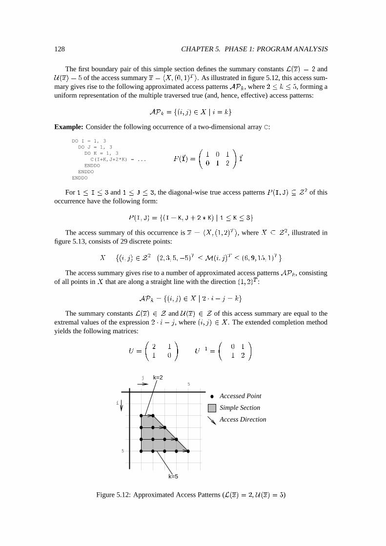
128 CHAPTER 5. PHASE 1: PROGRAM ANALYSIS
The first boundary pair of this simple section defines the summary constants L(x) = 2 andU(x) = 5 of the access summary x = hX; (0; 1)
T
i. As illustrated in figure 5.12, this access sum-mary gives rise to the following approximated access patterns AP
k
, where 2 � k � 5, forming auniform representation of the multiple traversed true (and, hence, effective) access patterns:
AP
k
= f(i; j) 2 X j i = kg
Example: Consider the following occurrence of a two-dimensional array C:
DO I = 1, 3DO J = 1, 3DO K = 1, 3C(I+K,J+2*K) = ...
ENDDOENDDO
ENDDO
F (
~
I) =
1 0 1
0 1 2
!
~
I
For 1 � I � 3 and 1 � J � 3, the diagonal-wise true access patterns P (I; J) � Z2 of thisoccurrence have the following form:
P (I; J) = f(I+ K; J+ 2 � K) j 1 � K � 3g
The access summary of this occurrence is x = hX; (1; 2)
T
i, where X � Z2, illustrated infigure 5.13, consists of 29 discrete points:
X = f(i; j) 2 Z
2
j (2; 3; 5;�5)
T
�M(i; j)
T
� (6; 9; 15; 1)
T
g
The access summary gives rise to a number of approximated access patterns APk
, consistingof all points in X that are along a straight line with the direction (1; 2)
T :
AP
k
= f(i; j) 2 X j 2 � i� j = kg
The summary constants L(x) 2 Z and U(x) 2 Z of this access summary are equal to theextremal values of the expression 2 � i � j, where (i; j) 2 X . The extended completion methodyields the following matrices:
U =
2 �1
1 0
!
U
�1
=
0 1
�1 2
!
5
i
j
Accessed Point
Simple Section
Access Direction
5k=2
k=5
Figure 5.12: Approximated Access Patterns (L(x) = 2, U(x) = 5)
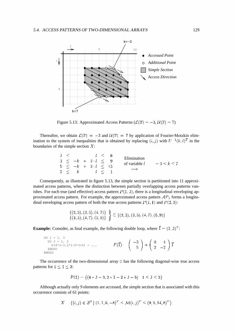
5.4. ACCESS PATTERNS OF TWO-DIMENSIONAL ARRAYS 129
5
5
10
i
j
Accessed Point
Simple Section
Additional Point
Access Direction
k=−3
k=7
Figure 5.13: Approximated Access Patterns (L(x) = �3, U(x) = 7)
Thereafter, we obtain L(x) = �3 and U(x) = 7 by application of Fourier-Motzkin elim-ination to the system of inequalities that is obtained by replacing (i; j) with U�1(k; l)T in theboundaries of the simple section X:
2 � l � 6
3 � �k + 2 � l � 9
5 � �k + 3 � l � 15
�5 � �k � l � 1
Eliminationof variable l�!
� 3 � k � 7
Consequently, as illustrated in figure 5.13, the simple section is partitioned into 11 approxi-mated access patterns, where the distinction between partially overlapping access patterns van-ishes. For each true (and effective) access pattern P (I; J), there is a longitudinal enveloping ap-proximated access pattern. For example, the approximated access pattern AP
1
forms a longitu-dinal enveloping access pattern of both the true access patterns P (1; 1) and P (2; 3):
f(2; 3); (3; 5); (4; 7)g
f(3; 5); (4; 7); (5; 9)g
)
� f(2; 3); (3; 5); (4; 7); (5; 9)g
Example: Consider, as final example, the following double loop, where ~I = (I; J)
T :
DO I = 1, 3DO J = 1, 3D(4*J-3,2*I-2*J+5) = ...
ENDDOENDDO
F (
~
I) =
�3
5
!
+
0 4
2 �2
!
~
I
The occurrence of the two-dimensional array D has the following diagonal-wise true accesspatterns for 1 � I � 3:
P (I) = f(4 � J� 3; 2 � I� 2 � J+ 5) j 1 � J � 3g
Although actually only 9 elements are accessed, the simple section that is associated with thisoccurrence consists of 61 points:
X = f(i; j) 2 Z
2
j (1; 1; 6;�8)
T
�M(i; j)
T
� (9; 9; 14; 8)
T
g
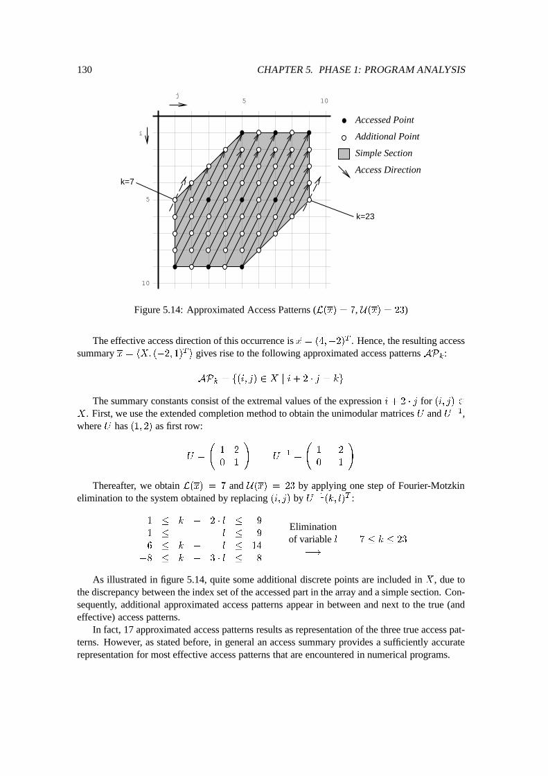
130 CHAPTER 5. PHASE 1: PROGRAM ANALYSIS
5
5
10
10
i
j
Accessed Point
Simple Section
Additional Point
Access Direction
k=23
k=7
Figure 5.14: Approximated Access Patterns (L(x) = 7, U(x) = 23)
The effective access direction of this occurrence is ~x = (4;�2)
T . Hence, the resulting accesssummary x = hX; (�2; 1)
T
i gives rise to the following approximated access patterns APk
:
AP
k
= f(i; j) 2 X j i+ 2 � j = kg
The summary constants consist of the extremal values of the expression i+ 2 � j for (i; j) 2X . First, we use the extended completion method to obtain the unimodular matrices U and U�1,where U has (1; 2) as first row:
U =
1 2
0 1
!
U
�1
=
1 �2
0 1
!
Thereafter, we obtain L(x) = 7 and U(x) = 23 by applying one step of Fourier-Motzkinelimination to the system obtained by replacing (i; j) by U�1(k; l)T :
1 � k � 2 � l � 9
1 � l � 9
6 � k � l � 14
�8 � k � 3 � l � 8
Eliminationof variable l�!
7 � k � 23
As illustrated in figure 5.14, quite some additional discrete points are included in X , due tothe discrepancy between the index set of the accessed part in the array and a simple section. Con-sequently, additional approximated access patterns appear in between and next to the true (andeffective) access patterns.
In fact, 17 approximated access patterns results as representation of the three true access pat-terns. However, as stated before, in general an access summary provides a sufficiently accuraterepresentation for most effective access patterns that are encountered in numerical programs.
Chapter 6
Nonzero Structure Analysis
Because the efficiency of sparse codes is very much dependent on the size and structure of theinput data, peculiarities of the nonzero structure of each sparse matrix must be accounted for inorder to avoid unsatisfactory performance. Therefore, an important part of the sparse compilerconsists of an analyzer that obtains some characteristics of the nonzero structure automatically.This information is used to control the data structure selection and sparse code generation. Sinceanalysis time contributes to compile-time, the efficiency of the analyzer is important.
A nonzero structure analyzer is also useful for other purposes. For example, if a representativeset of sparse matrices is available beforehand, an analyzer can provide a programmer with usefulinsights about the characteristics of the matrices for which an application must be developed. Al-though in this case the efficiency of the analyzer is less important, excessive long running timeswould disable the analysis of a large set of matrices. To deal with the more realistic situation inwhich the sparse matrices are not available beforehand, an analyzer can be used at run-time to se-lect between different versions of one algorithm (which are generated either by a sparse compileror by hand), each of which has been optimized for a particular class of nonzero structures. Atrun-time, the analyzer is invoked to determine which version is probably the most efficient. Thisapproach has as major advantage that nonzero structures do not have to be known at programming-or compile-time. However, the analyzer must be very efficient to avoid the situation in which thesavings in execution time using an optimized version are outweighed by analysis time. In general,it is desirable to keep analysis time proportional to the number of entries in the matrix [75].
The analyzer presented in this chapter examines each matrix as it is, i.e. no attempts are madeto permute the matrix into a particular form. If a permutation is applied before the analysis, theanalyzer can still be used to determine whether an unforeseen nonzero structure arises (since in-formation about the form for which the permutation is intended is usually obtained as side effectby the method that computes the permutation). First, some methods to automatically analyze thenonzero structure of a sparse matrix are discussed. Thereafter, we discuss how nonzero structureinformation is propagated to the sparse compiler.
6.1 Automatic Nonzero Structure Analysis
We assume that the nonzero structure of each m� n sparse matrix A to be analyzed is availableon file in coordinate scheme. In this scheme, the file consists of the integers m and n, an integer �that indicates the number of entries, followed by � unordered triples (i; j; a
ij
) to indicate row andcolumn indices and the value of each individual entry. Because there is no advantage in storingzero elements explicitly, we also assume that all entries are nonzero.
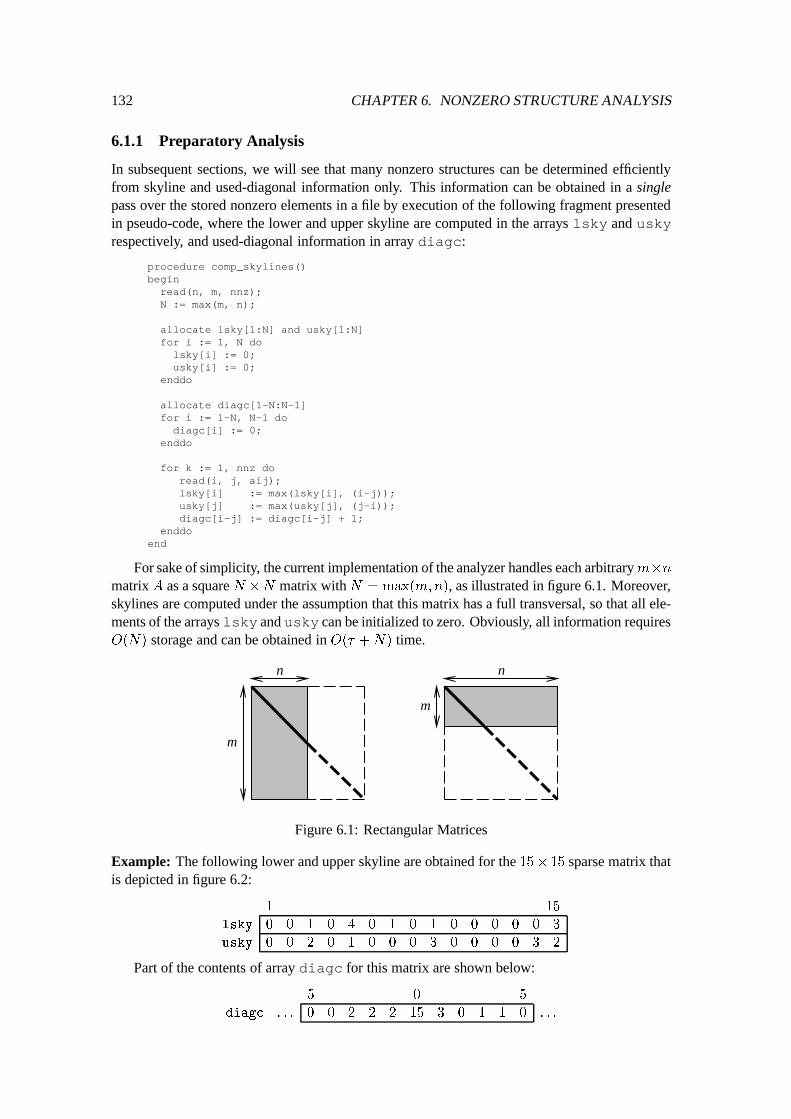
132 CHAPTER 6. NONZERO STRUCTURE ANALYSIS
6.1.1 Preparatory Analysis
In subsequent sections, we will see that many nonzero structures can be determined efficientlyfrom skyline and used-diagonal information only. This information can be obtained in a singlepass over the stored nonzero elements in a file by execution of the following fragment presentedin pseudo-code, where the lower and upper skyline are computed in the arrays lsky and uskyrespectively, and used-diagonal information in array diagc:
procedure comp_skylines()beginread(n, m, nnz);N := max(m, n);
allocate lsky[1:N] and usky[1:N]for i := 1, N dolsky[i] := 0;usky[i] := 0;
enddo
allocate diagc[1-N:N-1]for i := 1-N, N-1 dodiagc[i] := 0;
enddo
for k := 1, nnz doread(i, j, aij);lsky[i] := max(lsky[i], (i-j));usky[j] := max(usky[j], (j-i));diagc[i-j] := diagc[i-j] + 1;
enddoend
For sake of simplicity, the current implementation of the analyzer handles each arbitrarym�nmatrix A as a square N �N matrix withN = max(m;n), as illustrated in figure 6.1. Moreover,skylines are computed under the assumption that this matrix has a full transversal, so that all ele-ments of the arrays lsky and usky can be initialized to zero. Obviously, all information requiresO(N) storage and can be obtained in O(� +N) time.
m
n
m
n
Figure 6.1: Rectangular Matrices
Example: The following lower and upper skyline are obtained for the 15� 15 sparse matrix thatis depicted in figure 6.2:
1 15
lsky 0 0 1 0 4 0 1 0 1 0 0 0 0 0 3
usky 0 0 2 0 1 0 0 0 3 0 0 0 0 3 2
Part of the contents of array diagc for this matrix are shown below:
�5 0 5
diagc : : : 0 0 2 2 2 15 3 0 1 1 0 : : :
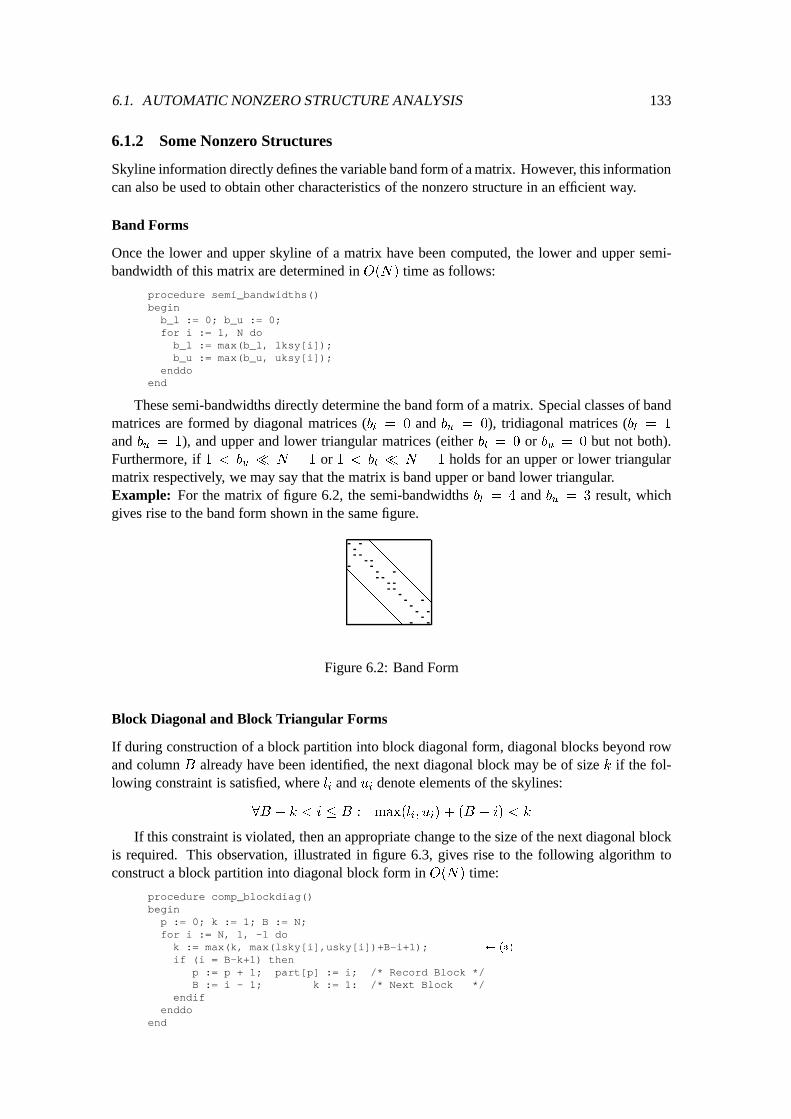
6.1. AUTOMATIC NONZERO STRUCTURE ANALYSIS 133
6.1.2 Some Nonzero Structures
Skyline information directly defines the variable band form of a matrix. However, this informationcan also be used to obtain other characteristics of the nonzero structure in an efficient way.
Band Forms
Once the lower and upper skyline of a matrix have been computed, the lower and upper semi-bandwidth of this matrix are determined in O(N) time as follows:
procedure semi_bandwidths()beginb_l := 0; b_u := 0;for i := 1, N dob_l := max(b_l, lksy[i]);b_u := max(b_u, uksy[i]);
enddoend
These semi-bandwidths directly determine the band form of a matrix. Special classes of bandmatrices are formed by diagonal matrices (b
l
= 0 and bu
= 0), tridiagonal matrices (bl
= 1
and bu
= 1), and upper and lower triangular matrices (either bl
= 0 or bu
= 0 but not both).Furthermore, if 1 < b
u
� N � 1 or 1 < b
l
� N � 1 holds for an upper or lower triangularmatrix respectively, we may say that the matrix is band upper or band lower triangular.Example: For the matrix of figure 6.2, the semi-bandwidths b
l
= 4 and bu
= 3 result, whichgives rise to the band form shown in the same figure.
@
@
@
@
@
@
@
@
@
@
Figure 6.2: Band Form
Block Diagonal and Block Triangular Forms
If during construction of a block partition into block diagonal form, diagonal blocks beyond rowand column B already have been identified, the next diagonal block may be of size k if the fol-lowing constraint is satisfied, where l
i
and ui
denote elements of the skylines:
8B � k < i � B : max(l
i
; u
i
) + (B � i) < k
If this constraint is violated, then an appropriate change to the size of the next diagonal blockis required. This observation, illustrated in figure 6.3, gives rise to the following algorithm toconstruct a block partition into diagonal block form in O(N) time:
procedure comp_blockdiag()beginp := 0; k := 1; B := N;for i := N, 1, -1 dok := max(k, max(lsky[i],usky[i])+B-i+1); (�)
if (i = B-k+1) thenp := p + 1; part[p] := i; /* Record Block */B := i - 1; k := 1: /* Next Block */
endifenddo
end
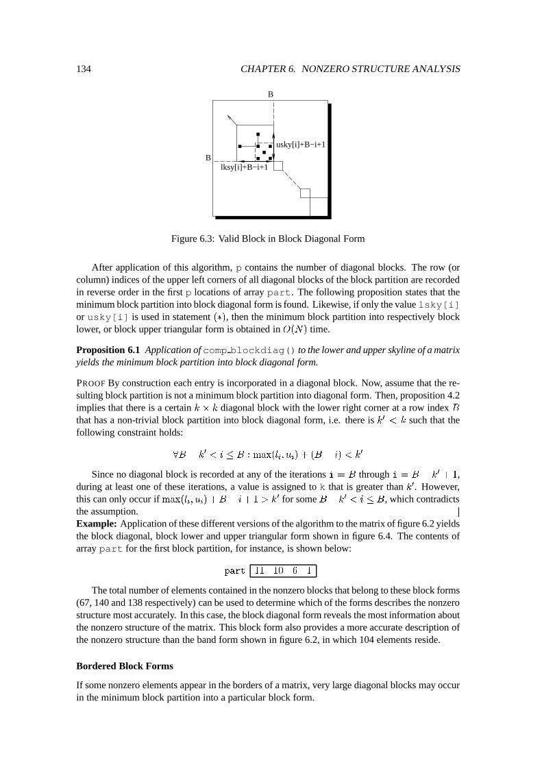
134 CHAPTER 6. NONZERO STRUCTURE ANALYSIS
usky[i]+B−i+1
lksy[i]+B−i+1
B
B
Figure 6.3: Valid Block in Block Diagonal Form
After application of this algorithm, p contains the number of diagonal blocks. The row (orcolumn) indices of the upper left corners of all diagonal blocks of the block partition are recordedin reverse order in the first p locations of array part. The following proposition states that theminimum block partition into block diagonal form is found. Likewise, if only the value lsky[i]or usky[i] is used in statement (�), then the minimum block partition into respectively blocklower, or block upper triangular form is obtained in O(N) time.
Proposition 6.1 Application of comp blockdiag() to the lower and upper skyline of a matrixyields the minimum block partition into block diagonal form.
PROOF By construction each entry is incorporated in a diagonal block. Now, assume that the re-sulting block partition is not a minimum block partition into diagonal form. Then, proposition 4.2implies that there is a certain k � k diagonal block with the lower right corner at a row index Bthat has a non-trivial block partition into block diagonal form, i.e. there is k0 < k such that thefollowing constraint holds:
8B � k
0
< i � B : max(l
i
; u
i
) + (B � i) < k
0
Since no diagonal block is recorded at any of the iterations i = B through i = B � k
0
+ 1,during at least one of these iterations, a value is assigned to k that is greater than k0. However,this can only occur if max(l
i
; u
i
) +B � i+1 > k
0 for some B � k0 < i � B, which contradictsthe assumption. []
Example: Application of these different versions of the algorithm to the matrix of figure 6.2 yieldsthe block diagonal, block lower and upper triangular form shown in figure 6.4. The contents ofarray part for the first block partition, for instance, is shown below:
part 11 10 6 1
The total number of elements contained in the nonzero blocks that belong to these block forms(67, 140 and 138 respectively) can be used to determine which of the forms describes the nonzerostructure most accurately. In this case, the block diagonal form reveals the most information aboutthe nonzero structure of the matrix. This block form also provides a more accurate description ofthe nonzero structure than the band form shown in figure 6.2, in which 104 elements reside.
Bordered Block Forms
If some nonzero elements appear in the borders of a matrix, very large diagonal blocks may occurin the minimum block partition into a particular block form.
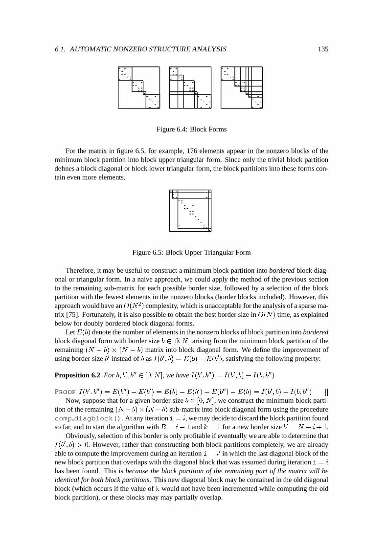
6.1. AUTOMATIC NONZERO STRUCTURE ANALYSIS 135
Figure 6.4: Block Forms
For the matrix in figure 6.5, for example, 176 elements appear in the nonzero blocks of theminimum block partition into block upper triangular form. Since only the trivial block partitiondefines a block diagonal or block lower triangular form, the block partitions into these forms con-tain even more elements.
Figure 6.5: Block Upper Triangular Form
Therefore, it may be useful to construct a minimum block partition into bordered block diag-onal or triangular form. In a naive approach, we could apply the method of the previous sectionto the remaining sub-matrix for each possible border size, followed by a selection of the blockpartition with the fewest elements in the nonzero blocks (border blocks included). However, thisapproach would have anO(N
2
) complexity, which is unacceptable for the analysis of a sparse ma-trix [75]. Fortunately, it is also possible to obtain the best border size in O(N) time, as explainedbelow for doubly bordered block diagonal forms.
LetE(b) denote the number of elements in the nonzero blocks of block partition into borderedblock diagonal form with border size b 2 [0; N ] arising from the minimum block partition of theremaining (N � b) � (N � b) matrix into block diagonal form. We define the improvement ofusing border size b0 instead of b as I(b0; b) = E(b)�E(b
0
), satisfying the following property:
Proposition 6.2 For b; b0; b00 2 [0; N ], we have I(b0; b00) = I(b
0
; b) + I(b; b
00
)
PROOF I(b
0
; b
00
) = E(b
00
)�E(b
0
) = E(b)�E(b
0
) +E(b
00
)�E(b) = I(b
0
; b) + I(b; b
00
) []
Now, suppose that for a given border size b 2 [0; N ], we construct the minimum block parti-tion of the remaining (N � b)� (N � b) sub-matrix into block diagonal form using the procedurecomp diagblock(). At any iteration i = i, we may decide to discard the block partition foundso far, and to start the algorithm with B = i� 1 and k = 1 for a new border size b0 = N � i+1.
Obviously, selection of this border is only profitable if eventually we are able to determine thatI(b
0
; b) > 0. However, rather than constructing both block partitions completely, we are alreadyable to compute the improvement during an iteration i = i
0 in which the last diagonal block of thenew block partition that overlaps with the diagonal block that was assumed during iteration i = i
has been found. This is because the block partition of the remaining part of the matrix will beidentical for both block partitions. This new diagonal block may be contained in the old diagonalblock (which occurs if the value of k would not have been incremented while computing the oldblock partition), or these blocks may may partially overlap.
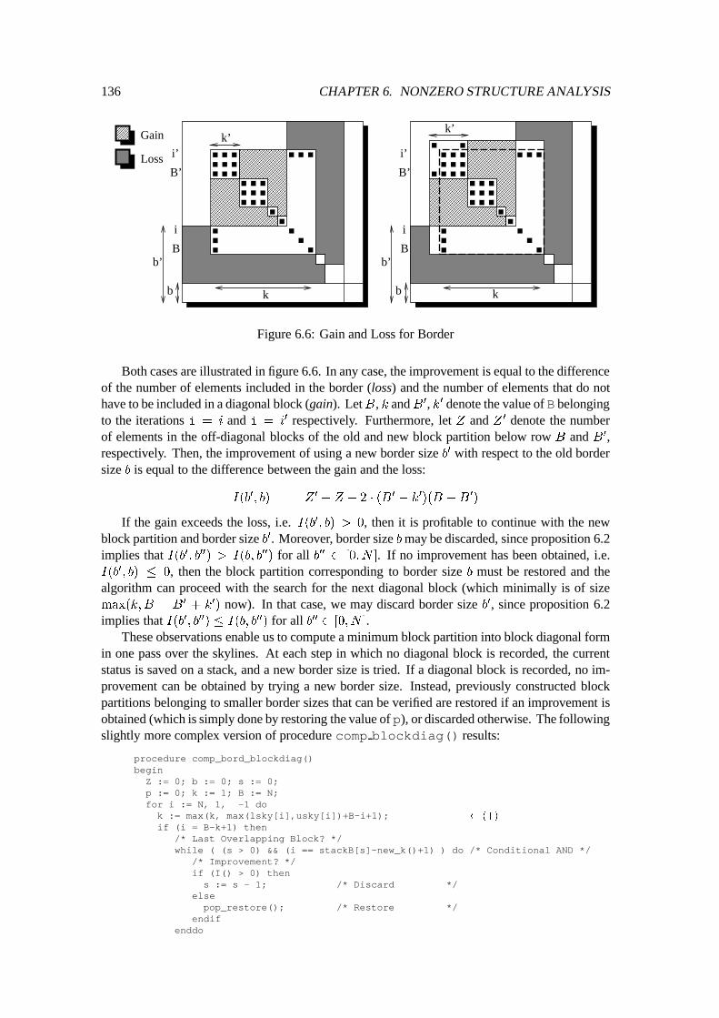
136 CHAPTER 6. NONZERO STRUCTURE ANALYSIS
Gain
Loss
b
k’
i
B
i’
B’
b
k’
i
B
i’
B’
kk
b’b’
Figure 6.6: Gain and Loss for Border
Both cases are illustrated in figure 6.6. In any case, the improvement is equal to the differenceof the number of elements included in the border (loss) and the number of elements that do nothave to be included in a diagonal block (gain). LetB, k andB0, k0 denote the value of B belongingto the iterations i = i and i = i
0 respectively. Furthermore, let Z and Z 0 denote the numberof elements in the off-diagonal blocks of the old and new block partition below row B and B0,respectively. Then, the improvement of using a new border size b0 with respect to the old bordersize b is equal to the difference between the gain and the loss:
I(b
0
; b) = Z
0
� Z � 2 � (B
0
� k
0
)(B �B
0
)
If the gain exceeds the loss, i.e. I(b0; b) > 0, then it is profitable to continue with the newblock partition and border size b0. Moreover, border size bmay be discarded, since proposition 6.2implies that I(b0; b00) > I(b; b
00
) for all b00 2 [0; N ]. If no improvement has been obtained, i.e.I(b
0
; b) � 0, then the block partition corresponding to border size b must be restored and thealgorithm can proceed with the search for the next diagonal block (which minimally is of sizemax(k;B � B
0
+ k
0
) now). In that case, we may discard border size b0, since proposition 6.2implies that I(b0; b00) � I(b; b00) for all b00 2 [0; N ].
These observations enable us to compute a minimum block partition into block diagonal formin one pass over the skylines. At each step in which no diagonal block is recorded, the currentstatus is saved on a stack, and a new border size is tried. If a diagonal block is recorded, no im-provement can be obtained by trying a new border size. Instead, previously constructed blockpartitions belonging to smaller border sizes that can be verified are restored if an improvement isobtained (which is simply done by restoring the value of p), or discarded otherwise. The followingslightly more complex version of procedure comp blockdiag() results:
procedure comp_bord_blockdiag()beginZ := 0; b := 0; s := 0;p := 0; k := 1; B := N;for i := N, 1, -1 dok := max(k, max(lsky[i],usky[i])+B-i+1); (+)
if (i = B-k+1) then/* Last Overlapping Block? */while ( (s > 0) && (i == stackB[s]-new_k()+1) ) do /* Conditional AND */
/* Improvement? */if (I() > 0) thens := s - 1; /* Discard */
elsepop_restore(); /* Restore */
endifenddo
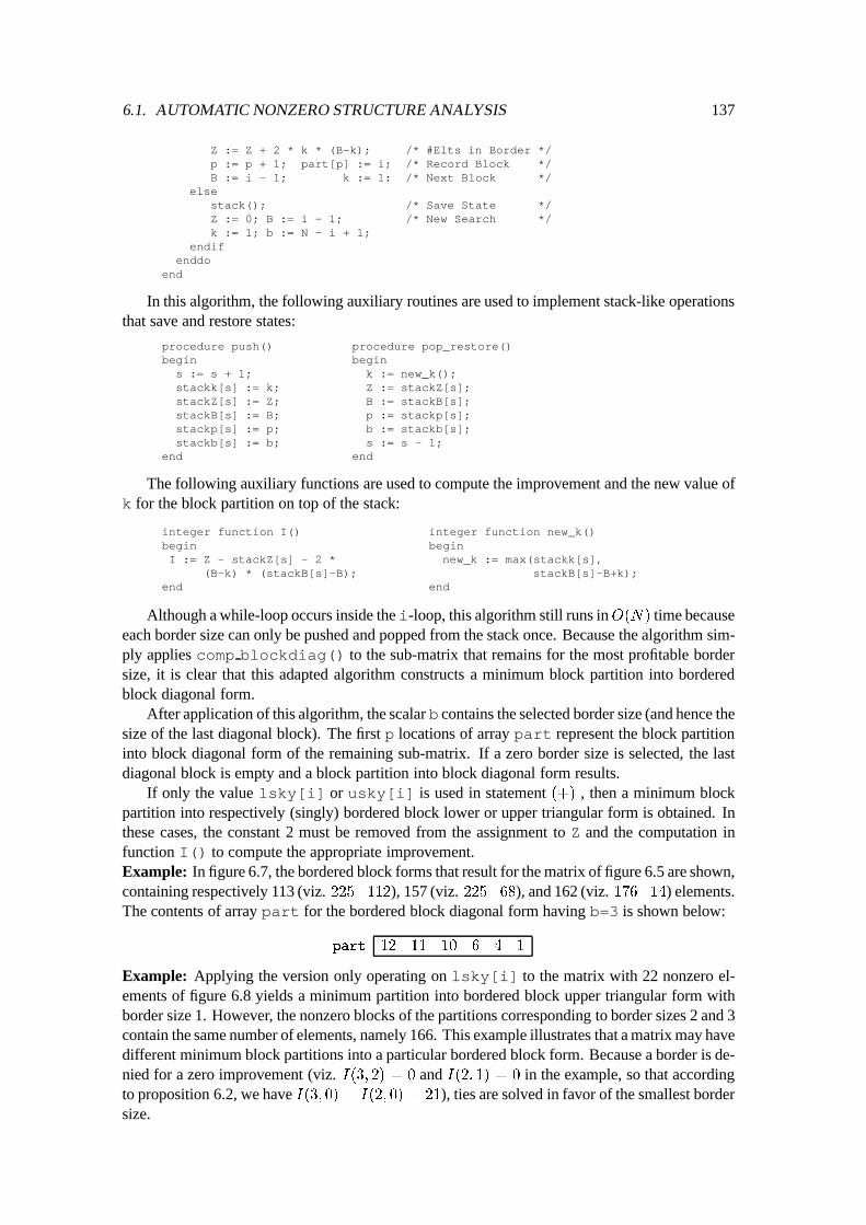
6.1. AUTOMATIC NONZERO STRUCTURE ANALYSIS 137
Z := Z + 2 * k * (B-k); /* #Elts in Border */p := p + 1; part[p] := i; /* Record Block */B := i - 1; k := 1: /* Next Block */
elsestack(); /* Save State */Z := 0; B := i - 1; /* New Search */k := 1; b := N - i + 1;
endifenddo
end
In this algorithm, the following auxiliary routines are used to implement stack-like operationsthat save and restore states:
procedure push()begins := s + 1;stackk[s] := k;stackZ[s] := Z;stackB[s] := B;stackp[s] := p;stackb[s] := b;
end
procedure pop_restore()begin
k := new_k();Z := stackZ[s];B := stackB[s];p := stackp[s];b := stackb[s];s := s - 1;
end
The following auxiliary functions are used to compute the improvement and the new value ofk for the block partition on top of the stack:
integer function I()beginI := Z - stackZ[s] - 2 *
(B-k) * (stackB[s]-B);end
integer function new_k()beginnew_k := max(stackk[s],
stackB[s]-B+k);end
Although a while-loop occurs inside the i-loop, this algorithm still runs inO(N) time becauseeach border size can only be pushed and popped from the stack once. Because the algorithm sim-ply applies comp blockdiag() to the sub-matrix that remains for the most profitable bordersize, it is clear that this adapted algorithm constructs a minimum block partition into borderedblock diagonal form.
After application of this algorithm, the scalar b contains the selected border size (and hence thesize of the last diagonal block). The first p locations of array part represent the block partitioninto block diagonal form of the remaining sub-matrix. If a zero border size is selected, the lastdiagonal block is empty and a block partition into block diagonal form results.
If only the value lsky[i] or usky[i] is used in statement (+) , then a minimum blockpartition into respectively (singly) bordered block lower or upper triangular form is obtained. Inthese cases, the constant 2 must be removed from the assignment to Z and the computation infunction I() to compute the appropriate improvement.Example: In figure 6.7, the bordered block forms that result for the matrix of figure 6.5 are shown,containing respectively 113 (viz. 225�112), 157 (viz. 225�68), and 162 (viz. 176�14) elements.The contents of array part for the bordered block diagonal form having b=3 is shown below:
part 12 11 10 6 4 1
Example: Applying the version only operating on lsky[i] to the matrix with 22 nonzero el-ements of figure 6.8 yields a minimum partition into bordered block upper triangular form withborder size 1. However, the nonzero blocks of the partitions corresponding to border sizes 2 and 3contain the same number of elements, namely 166. This example illustrates that a matrix may havedifferent minimum block partitions into a particular bordered block form. Because a border is de-nied for a zero improvement (viz. I(3; 2) = 0 and I(2; 1) = 0 in the example, so that accordingto proposition 6.2, we have I(3; 0) = I(2; 0) = 21), ties are solved in favor of the smallest bordersize.
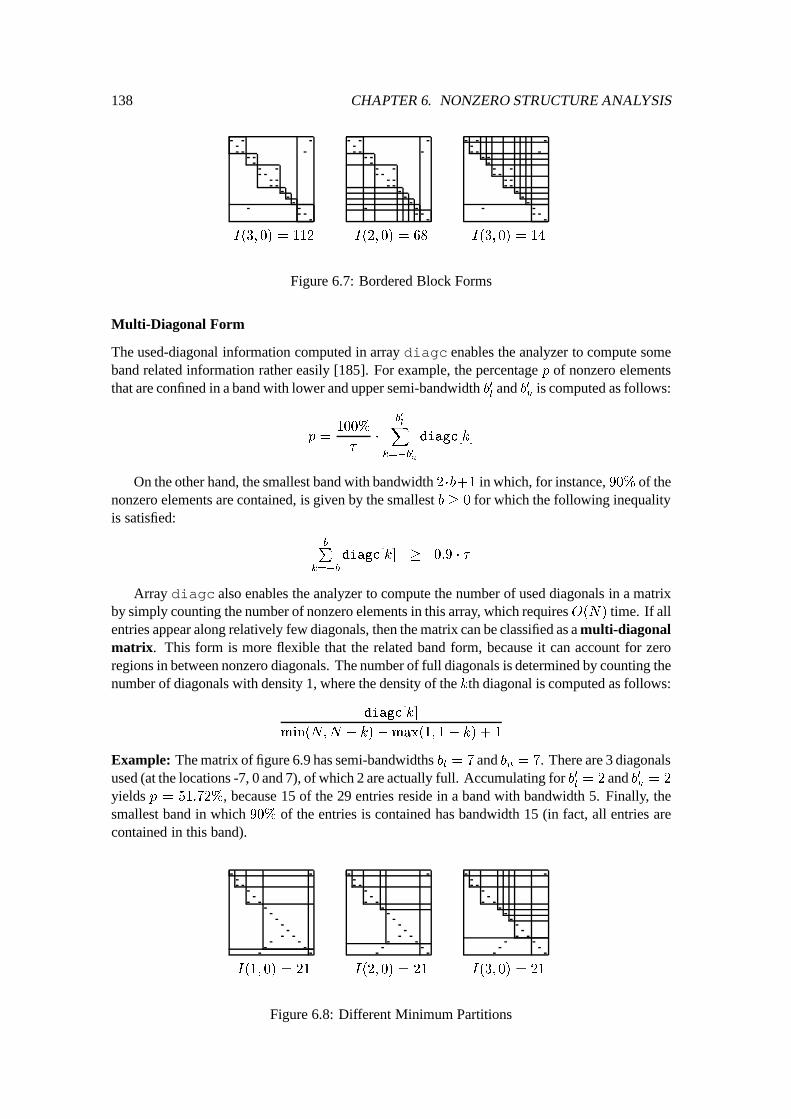
138 CHAPTER 6. NONZERO STRUCTURE ANALYSIS
I(3; 0) = 112 I(2; 0) = 68 I(3; 0) = 14
Figure 6.7: Bordered Block Forms
Multi-Diagonal Form
The used-diagonal information computed in array diagc enables the analyzer to compute someband related information rather easily [185]. For example, the percentage p of nonzero elementsthat are confined in a band with lower and upper semi-bandwidth b0
l
and b0u
is computed as follows:
p =
100%
�
�
b
0
l
X
k=�b
0
u
diagc[k]
On the other hand, the smallest band with bandwidth 2�b+1 in which, for instance, 90% of thenonzero elements are contained, is given by the smallest b � 0 for which the following inequalityis satisfied:
b
P
k=�b
diagc[k] � 0:9 � �
Array diagc also enables the analyzer to compute the number of used diagonals in a matrixby simply counting the number of nonzero elements in this array, which requiresO(N) time. If allentries appear along relatively few diagonals, then the matrix can be classified as a multi-diagonalmatrix. This form is more flexible that the related band form, because it can account for zeroregions in between nonzero diagonals. The number of full diagonals is determined by counting thenumber of diagonals with density 1, where the density of the kth diagonal is computed as follows:
diagc[k]
min(N;N � k)�max(1; 1 � k) + 1
Example: The matrix of figure 6.9 has semi-bandwidths bl
= 7 and bu
= 7. There are 3 diagonalsused (at the locations -7, 0 and 7), of which 2 are actually full. Accumulating for b0
l
= 2 and b0u
= 2
yields p = 51:72%, because 15 of the 29 entries reside in a band with bandwidth 5. Finally, thesmallest band in which 90% of the entries is contained has bandwidth 15 (in fact, all entries arecontained in this band).
I(1; 0) = 21 I(2; 0) = 21 I(3; 0) = 21
Figure 6.8: Different Minimum Partitions
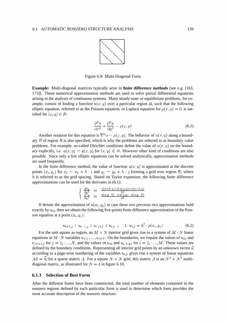
6.1. AUTOMATIC NONZERO STRUCTURE ANALYSIS 139
@
@
@
@
@
@
@
@
@
@
@
@
@
@
@
Figure 6.9: Multi-Diagonal Form
Example: Multi-diagonal matrices typically arise in finite difference methods (see e.g. [163,173]). These numerical approximation methods are used to solve partial differential equationsarising in the analysis of continuous systems. Many steady-state or equilibrium problems, for ex-ample, consist of finding a function u(x; y) over a particular region R, such that the followingelliptic equation, referred to as the Poisson equation, or Laplace equation for �(x; y) = 0, is sat-isfied for (x; y) 2 R:
@
2
u
@x
2
+
@
2
u
@y
2
= �(x; y) (6.1)
Another notation for this equation isr2
u = �(x; y). The behavior of u(x; y) along a bound-ary B of region R is also specified, which is why the problems are referred to as boundary valueproblems. For example, so-called Dirichlet conditions define the value of u(x; y) on the bound-ary explicitly, i.e. u(x; y) = g(x; y) for (x; y) 2 B. However other kind of conditions are alsopossible. Since only a few elliptic equations can be solved analytically, approximation methodsare used frequently.
In the finite difference method, the value of function u(x; y) is approximated at the discretepoints (x
i
; y
j
) for xi
= x
0
+ h � i and yj
= y
0
+ h � j forming a grid over region R, whereh is referred to as the grid spacing. Based on Taylor expansion, the following finite differenceapproximations can be used for the derivates in (6.1):
(
@
2
u
@x
2
�
u(x+h;y)�2�u(x;y)+u(x�h;y)
h
2
@
2
u
@y
2
�
u(x;y+h)�2�u(x;y)+u(x;y�h)
h
2
If denote the approximation of u(xi
; y
j
) in case these two previous two approximations holdexactly by u
ij
, then we obtain the following five-points finite difference approximation of the Pois-son equation at a point (x
i
; y
j
):
u
i+1;j
+ u
i�1;j
+ u
i;j+1
+ u
i;j�1
� 4 � u
i;j
= h
2
� �(x
i
; y
j
) (6.2)
For the unit square as region, an M �N interior grid gives rise to a system of M � N linearequations in M �N variables u
11
; : : : ; u
MN
. On the boundaries, we require the values of u0j
andu
M+1;j
for j = 1; : : : ; N , and the values of ui0
and ui;N+1
for i = 1; : : : ;M . These values aredefined by the boundary conditions. Representing all interior grid points by an unknown vector ~uaccording to a page-wise numbering of the variables u
ij
, gives rise a system of linear equationsA~u =
~
b, for a sparse matrix A. For a square N � N grid, this matrix A is an N2
� N
2 multi-diagonal matrix, as illustrated for N = 4 in figure 6.10.
6.1.3 Selection of Best Form
After the different forms have been constructed, the total number of elements contained in thenonzero regions defined by each particular form is used to determine which form provides themost accurate description of the nonzero structure.
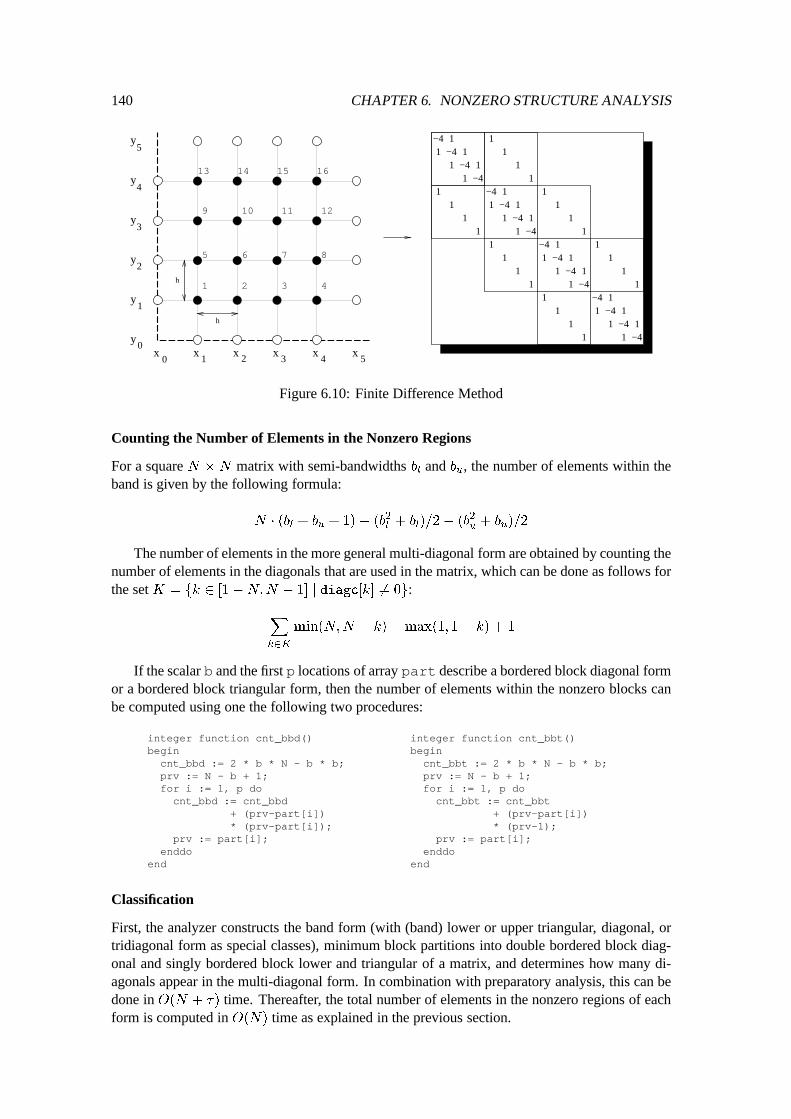
140 CHAPTER 6. NONZERO STRUCTURE ANALYSIS
1 2 3 4
5 6 7 8
9 10 11 12
13 14 15 16
11
11
11
11
−41 −4
−4−4
11
11
1
−41 −4
−4−4
11
11
1
−41 −4
−4−4
11
11
1
−41 −4
−4−4
11
11
1
11
11
11
11
11
11
11
11
x x xx x x1 2 30 4 5
y
y
y
y
y
y
h
h
0
1
2
3
4
5
Figure 6.10: Finite Difference Method
Counting the Number of Elements in the Nonzero Regions
For a square N � N matrix with semi-bandwidths bl
and bu
, the number of elements within theband is given by the following formula:
N � (b
l
+ b
u
+ 1)� (b
2
l
+ b
l
)=2� (b
2
u
+ b
u
)=2
The number of elements in the more general multi-diagonal form are obtained by counting thenumber of elements in the diagonals that are used in the matrix, which can be done as follows forthe set K = fk 2 [1�N;N � 1] j diagc[k] 6= 0g:
X
k2K
min(N;N � k)�max(1; 1� k) + 1
If the scalar b and the first p locations of array part describe a bordered block diagonal formor a bordered block triangular form, then the number of elements within the nonzero blocks canbe computed using one the following two procedures:
integer function cnt_bbd()begincnt_bbd := 2 * b * N - b * b;prv := N - b + 1;for i := 1, p docnt_bbd := cnt_bbd
+ (prv-part[i])* (prv-part[i]);
prv := part[i];enddo
end
integer function cnt_bbt()begin
cnt_bbt := 2 * b * N - b * b;prv := N - b + 1;for i := 1, p do
cnt_bbt := cnt_bbt+ (prv-part[i])* (prv-1);
prv := part[i];enddo
end
Classification
First, the analyzer constructs the band form (with (band) lower or upper triangular, diagonal, ortridiagonal form as special classes), minimum block partitions into double bordered block diag-onal and singly bordered block lower and triangular of a matrix, and determines how many di-agonals appear in the multi-diagonal form. In combination with preparatory analysis, this can bedone in O(N + �) time. Thereafter, the total number of elements in the nonzero regions of eachform is computed in O(N) time as explained in the previous section.
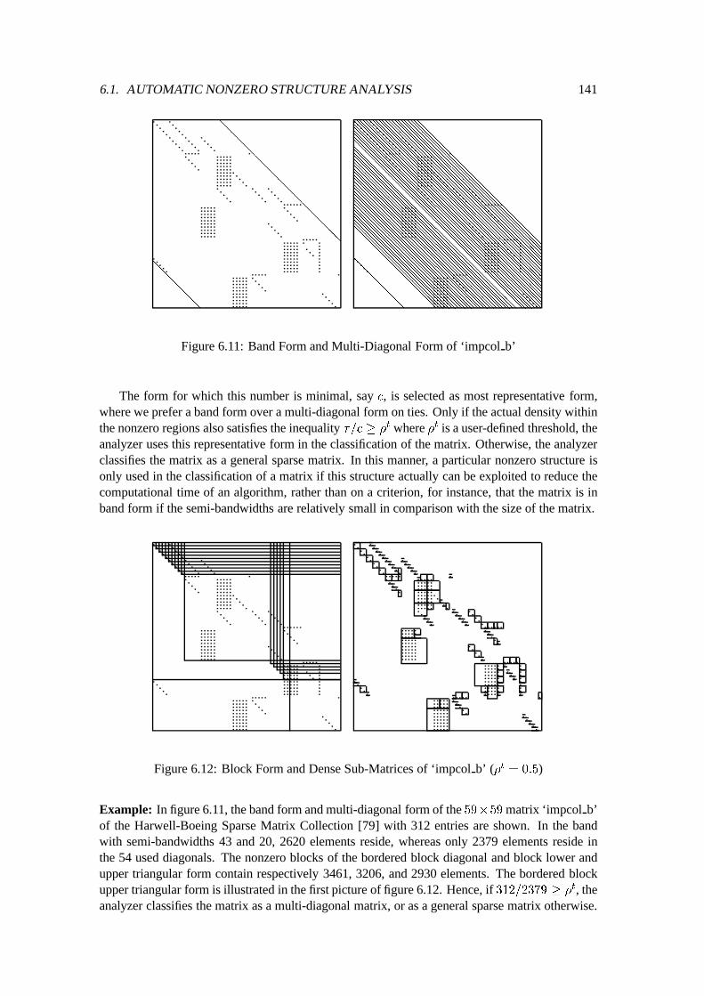
6.1. AUTOMATIC NONZERO STRUCTURE ANALYSIS 141
@
@
@
@
@
@
@
@
@
@
@
@
@
@
@
@
@
@
@
@
@
@
@
@
@
@
@
@
@
@
@
@
@
@
@
@
@
@
@
@
@
@
@
@
@
@
@
@
@
@
@
@
@
@
@
@
@
@
@
@
@
@
@
@
@
@
@
@
@
@
@
@
@
@
@
@
@
@
@
@
@
@
@
@
@
@
@
@
@
@
@
@
@
@
@
@
@
@
@
@
@
@
@
@
@
@
@
@
@
@
@
@
@
@
@
@
@
@
@
@
@
@
@
@
@
@
@
@
@
@
@
@
@
@
@
@
@
@
@
@
@
@
@
@
@
@
@
@
@
@
@
@
@
@
@
@
@
@
@
@
@
@
@
@
@
@
@
@
@
@
@
@
@
@
@
@
@
@
@
@
@
@
@
@
@
@
@
@
@
@
@
@
@
@
@
@
@
@
@
@
@
@
@
@
@
@
@
@
@
@
@
@
@
@
@
@
@
@
@
@
@
@
@
@
@
@
@
@
@
@
@
@
@
@
@
@
@
@
@
@
@
@
@
@
@
@
@
@
@
@
@
@
@
@
@
@
@
@
@
@
@
@
@
@
@
@
@
@
@
@
@
@
@
@
@
@
@
@
@
@
@
@
@
@
@
@
@
@
@
@
@
@
@
@
@
@
@
@
@
@
@
@
@
@
@
@
@
@
@
@
@
@
@
@
@
@
@
@
@
@
@
@
@
@
@
@
@
@
@
@
@
@
@
@
@
@
@
@
@
@
@
@
@
@
@
@
@
@
@
@
@
@
@
@
@
@
@
@
@
@
@
@
@
@
@
@
@
@
@
@
@
@
@
@
@
@
@
@
@
@
@
@
@
@
@
@
@
@
@
@
@
@
@
@
@
@
@
@
@
@
@
@
@
@
@
@
@
@
@
@
@
@
@
@
@
@
@
@
@
@
@
@
@
@
@
@
@
@
@
@
@
@
@
@
@
@
@
@
@
@
@
@
@
@
@
@
@
@
@
@
@
@
@
@
@
@
@
@
@
@
@
@
@
@
@
@
@
@
@
@
@
@
@
@
@
@
@
@
@
@
@
@
@
@
@
@
@
@
@
@
@
@
@
@
@
@
@
@
@
@
@
@
@
@
@
@
@
@
@
@
@
@
@
@
@
@
@
@
@
@
@
@
@
@
@
@
@
@
@
@
@
@
@
@
@
@
@
@
@
@
@
@
@
@
@
@
@
@
@
@
@
@
@
@
@
@
@
@
@
@
@
@
@
@
@
@
@
@
@
@
@
@
@
@
@
@
@
@
@
@
@
@@
@
@
@
@
@
@
@
@
@
@
@
@
@
@
@
@
@
@
@
@
@
@
@
@
@
@
@
@
@
@
@
@
@
@
@
@
@
@
@
@
@
@
@
@
@
@
@
@
@
@
@
@
@
@
@
@
@
@
@
@
@
@
@
@
@
@
@
@
@
@
@
@
@
@
@
@
@
@
@
@
@
@
@
@
@
@
@
@
@
@
@
@
@
@
@
@
@
@
@
@
@
@
@
Figure 6.11: Band Form and Multi-Diagonal Form of ‘impcol b’
The form for which this number is minimal, say c, is selected as most representative form,where we prefer a band form over a multi-diagonal form on ties. Only if the actual density withinthe nonzero regions also satisfies the inequality �=c � �t where �t is a user-defined threshold, theanalyzer uses this representative form in the classification of the matrix. Otherwise, the analyzerclassifies the matrix as a general sparse matrix. In this manner, a particular nonzero structure isonly used in the classification of a matrix if this structure actually can be exploited to reduce thecomputational time of an algorithm, rather than on a criterion, for instance, that the matrix is inband form if the semi-bandwidths are relatively small in comparison with the size of the matrix.
Figure 6.12: Block Form and Dense Sub-Matrices of ‘impcol b’ (�t = 0:5)
Example: In figure 6.11, the band form and multi-diagonal form of the 59�59 matrix ‘impcol b’of the Harwell-Boeing Sparse Matrix Collection [79] with 312 entries are shown. In the bandwith semi-bandwidths 43 and 20, 2620 elements reside, whereas only 2379 elements reside inthe 54 used diagonals. The nonzero blocks of the bordered block diagonal and block lower andupper triangular form contain respectively 3461, 3206, and 2930 elements. The bordered blockupper triangular form is illustrated in the first picture of figure 6.12. Hence, if 312=2379 � �t, theanalyzer classifies the matrix as a multi-diagonal matrix, or as a general sparse matrix otherwise.
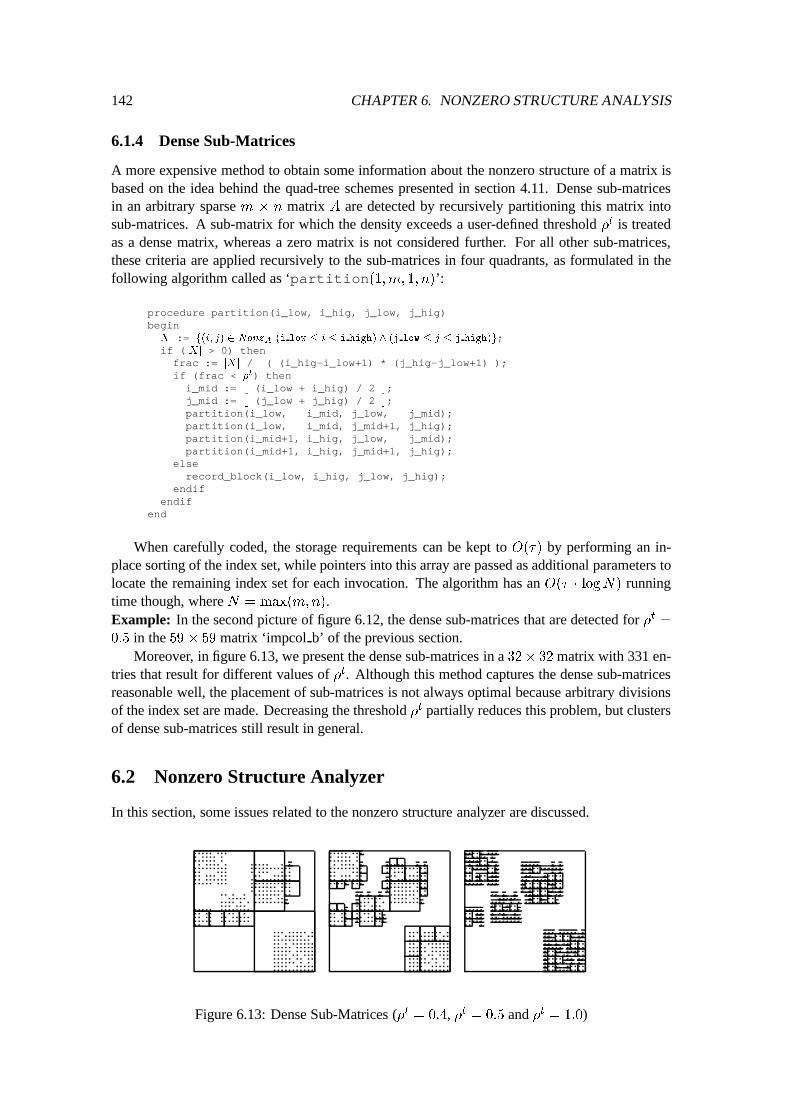
142 CHAPTER 6. NONZERO STRUCTURE ANALYSIS
6.1.4 Dense Sub-Matrices
A more expensive method to obtain some information about the nonzero structure of a matrix isbased on the idea behind the quad-tree schemes presented in section 4.11. Dense sub-matricesin an arbitrary sparse m � n matrix A are detected by recursively partitioning this matrix intosub-matrices. A sub-matrix for which the density exceeds a user-defined threshold �t is treatedas a dense matrix, whereas a zero matrix is not considered further. For all other sub-matrices,these criteria are applied recursively to the sub-matrices in four quadrants, as formulated in thefollowing algorithm called as ‘partition(1;m; 1; n)’:
procedure partition(i_low, i_hig, j_low, j_hig)beginX := f(i; j) 2 Nonz
A
j(i low � i � i high) ^ (j low � j � j high)g;if (jXj > 0) thenfrac := jXj / ( (i_hig-i_low+1) * (j_hig-j_low+1) );if (frac < �
t) theni_mid := b (i_low + i_hig) / 2 c;j_mid := b (j_low + j_hig) / 2 c;partition(i_low, i_mid, j_low, j_mid);partition(i_low, i_mid, j_mid+1, j_hig);partition(i_mid+1, i_hig, j_low, j_mid);partition(i_mid+1, i_hig, j_mid+1, j_hig);
elserecord_block(i_low, i_hig, j_low, j_hig);
endifendif
end
When carefully coded, the storage requirements can be kept to O(�) by performing an in-place sorting of the index set, while pointers into this array are passed as additional parameters tolocate the remaining index set for each invocation. The algorithm has an O(� � logN) runningtime though, where N = max(m;n).Example: In the second picture of figure 6.12, the dense sub-matrices that are detected for �t =0:5 in the 59 � 59 matrix ‘impcol b’ of the previous section.
Moreover, in figure 6.13, we present the dense sub-matrices in a 32� 32 matrix with 331 en-tries that result for different values of �t. Although this method captures the dense sub-matricesreasonable well, the placement of sub-matrices is not always optimal because arbitrary divisionsof the index set are made. Decreasing the threshold �t partially reduces this problem, but clustersof dense sub-matrices still result in general.
6.2 Nonzero Structure Analyzer
In this section, some issues related to the nonzero structure analyzer are discussed.
Figure 6.13: Dense Sub-Matrices (�t = 0:4, �t = 0:5 and �t = 1:0)
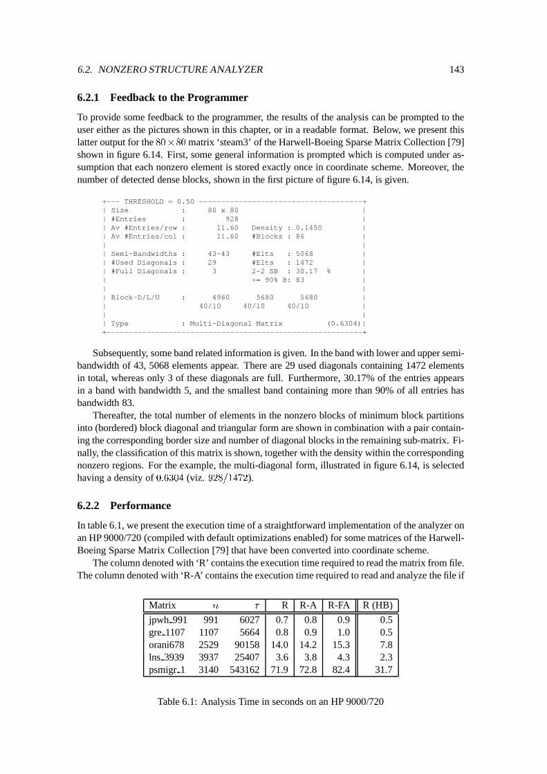
6.2. NONZERO STRUCTURE ANALYZER 143
6.2.1 Feedback to the Programmer
To provide some feedback to the programmer, the results of the analysis can be prompted to theuser either as the pictures shown in this chapter, or in a readable format. Below, we present thislatter output for the 80�80 matrix ‘steam3’ of the Harwell-Boeing Sparse Matrix Collection [79]shown in figure 6.14. First, some general information is prompted which is computed under as-sumption that each nonzero element is stored exactly once in coordinate scheme. Moreover, thenumber of detected dense blocks, shown in the first picture of figure 6.14, is given.
+--- THRESHOLD = 0.50 -------------------------------------+| Size : 80 x 80 || #Entries : 928 || Av #Entries/row : 11.60 Density : 0.1450 || Av #Entries/col : 11.60 #Blocks : 86 || || Semi-Bandwidths : 43-43 #Elts : 5068 || #Used Diagonals : 29 #Elts : 1472 || #Full Diagonals : 3 2-2 SB : 30.17 % || >= 90% B: 83 || || Block-D/L/U : 4960 5680 5680 || 40/10 40/10 40/10 || || Type : Multi-Diagonal Matrix (0.6304)|+----------------------------------------------------------+
Subsequently, some band related information is given. In the band with lower and upper semi-bandwidth of 43, 5068 elements appear. There are 29 used diagonals containing 1472 elementsin total, whereas only 3 of these diagonals are full. Furthermore, 30.17% of the entries appearsin a band with bandwidth 5, and the smallest band containing more than 90% of all entries hasbandwidth 83.
Thereafter, the total number of elements in the nonzero blocks of minimum block partitionsinto (bordered) block diagonal and triangular form are shown in combination with a pair contain-ing the corresponding border size and number of diagonal blocks in the remaining sub-matrix. Fi-nally, the classification of this matrix is shown, together with the density within the correspondingnonzero regions. For the example, the multi-diagonal form, illustrated in figure 6.14, is selectedhaving a density of 0:6304 (viz. 928=1472).
6.2.2 Performance
In table 6.1, we present the execution time of a straightforward implementation of the analyzer onan HP 9000/720 (compiled with default optimizations enabled) for some matrices of the Harwell-Boeing Sparse Matrix Collection [79] that have been converted into coordinate scheme.
The column denoted with ‘R’ contains the execution time required to read the matrix from file.The column denoted with ‘R-A’ contains the execution time required to read and analyze the file if
Matrix n � R R-A R-FA R (HB)
jpwh 991 991 6027 0.7 0.8 0.9 0.5gre 1107 1107 5664 0.8 0.9 1.0 0.5orani678 2529 90158 14.0 14.2 15.3 7.8lns 3939 3937 25407 3.6 3.8 4.3 2.3psmigr 1 3140 543162 71.9 72.8 82.4 31.7
Table 6.1: Analysis Time in seconds on an HP 9000/720
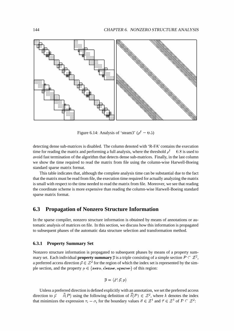
144 CHAPTER 6. NONZERO STRUCTURE ANALYSIS
@
@
@
@
@
@
@
@
@
@
@
@
@
@
@
@
@
@
@
@
@
@
@
@
@
@
@
@
@
@
@
@
@
@
@
@
@
@
@
@
@
@
@
@
@
@
@
@
@
@
@
@
@
@
@
@
@
@
@
@
@
@
@
@
@
@
@
@
@
@
@
@
@
@@
@
@
@
@
@
@
@
@
@
@
@
@
@
@
@
@
@
@
@
@
@
@
@
@
@
@
@
@
@
@
@
@
@
@
@
@
@
@
@
@
@
@
@
@
@
@
@
@
@
@
@
@
@
@
@
@
@
@
@
@
@
@
@
@
@
@
@
@
@
@
@
@
@
@
@
@
@
@
@
@
@
@
@
@
@
@
@
@
@
@
@
@
@
@
@
@
@
@
@
@
@
@
@
@
@
@
@
@
@
@
@
@
@
@
@
@
@
@
@
@
@
@
@
@
@
@
@
@
@
@
@
@
@
@
@
@
@
@
@
@
@
@
@
@
@
@
@
@
@
@
@
@
@
@
@
@
@
@
@
@
@
@
@
@
@
@
@
@
@
@
@
@
@
@
@
@
@
@
@
@
@
@
@
@
@
@
@
@
@
@
@
@
@
@
@
@
@
@
@
@
@
@
@
@
@
@
@
@
@
@
@
@
@
@
@
@
@
@
@
@
@
@
@
@
@
@
@
@
@
@
@
@
@
@
@
@
@
@
@
@
@
@
@
@
@
@
@
@
@
@
@
@@
@
@
@
@
@
@
@
@
@
@
@
@
@
@
@
@
@
@
@
@
@
@
@
@
@
@
@
@
@
@
@
@
@
@
@
@
@
@
@
@
@
@
@
@
@
@
@
@
@
@
@
@
@
@
@
@
@
@
@
@
@
@
@
Figure 6.14: Analysis of ‘steam3’ (�t = 0:5)
detecting dense sub-matrices is disabled. The column denoted with ‘R-FA’ contains the executiontime for reading the matrix and performing a full analysis, where the threshold �t = 0:8 is used toavoid fast termination of the algorithm that detects dense sub-matrices. Finally, in the last columnwe show the time required to read the matrix from file using the column-wise Harwell-Boeingstandard sparse matrix format.
This table indicates that, although the complete analysis time can be substantial due to the factthat the matrix must be read from file, the execution time required for actually analyzing the matrixis small with respect to the time needed to read the matrix from file. Moreover, we see that readingthe coordinate scheme is more expensive than reading the column-wise Harwell-Boeing standardsparse matrix format.
6.3 Propagation of Nonzero Structure Information
In the sparse compiler, nonzero structure information is obtained by means of annotations or au-tomatic analysis of matrices on file. In this section, we discuss how this information is propagatedto subsequent phases of the automatic data structure selection and transformation method.
6.3.1 Property Summary Set
Nonzero structure information is propagated to subsequent phases by means of a property sum-mary set. Each individual property summary p is a triple consisting of a simple section P � Z2,a preferred access direction ~p 2 Z2 for the region of which the index set is represented by the sim-ple section, and the property p 2 fzero;dense; sparseg of this region:
p = hP; ~p; pi
Unless a preferred direction is defined explicitly with an annotation, we set the preferred accessdirection to ~p =
~
�(P ) using the following definition of ~�(P ) 2 Z2, where k denotes the indexthat minimizes the expression �
i
� �
i
for the boundary values ~� 2 Z4 and ~� 2 Z4 of P � Z2:
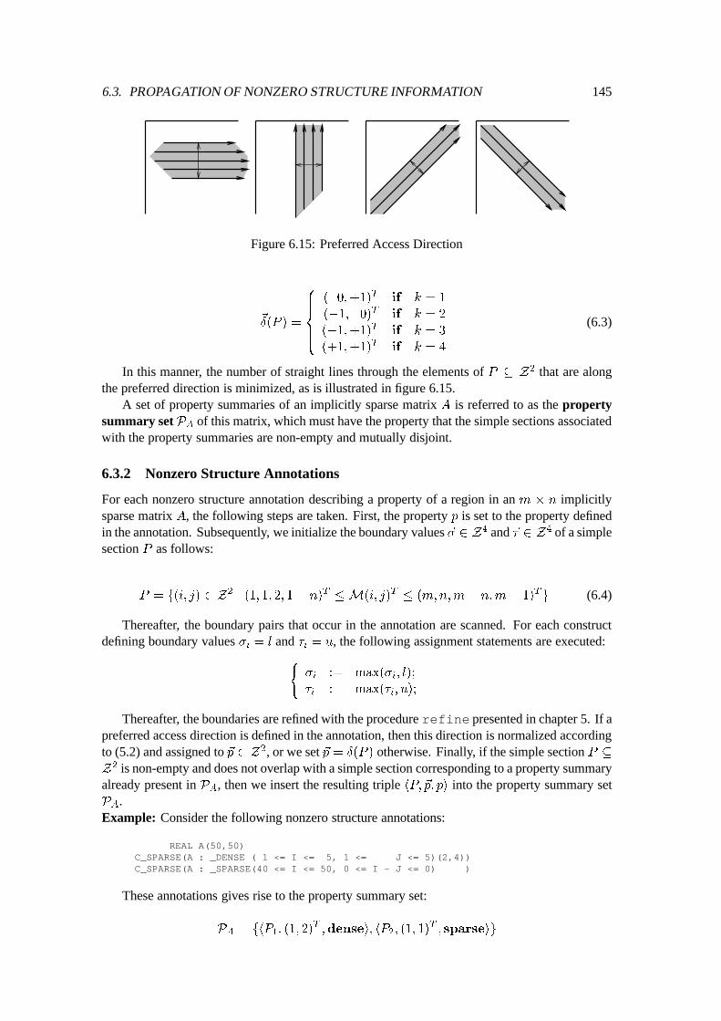
6.3. PROPAGATION OF NONZERO STRUCTURE INFORMATION 145
Figure 6.15: Preferred Access Direction
~
�(P ) =
8
>
>
>
<
>
>
>
:
( 0;+1)
T
if k = 1
(�1; 0)
T
if k = 2
(�1;+1)
T
if k = 3
(+1;+1)
T
if k = 4
(6.3)
In this manner, the number of straight lines through the elements of P � Z2 that are alongthe preferred direction is minimized, as is illustrated in figure 6.15.
A set of property summaries of an implicitly sparse matrix A is referred to as the propertysummary set P
A
of this matrix, which must have the property that the simple sections associatedwith the property summaries are non-empty and mutually disjoint.
6.3.2 Nonzero Structure Annotations
For each nonzero structure annotation describing a property of a region in an m � n implicitlysparse matrix A, the following steps are taken. First, the property p is set to the property definedin the annotation. Subsequently, we initialize the boundary values ~� 2 Z4 and ~� 2 Z4 of a simplesection P as follows:
P = f(i; j) 2 Z
2
j (1; 1; 2; 1 � n)
T
�M(i; j)
T
� (m;n;m+ n;m� 1)
T
g (6.4)
Thereafter, the boundary pairs that occur in the annotation are scanned. For each constructdefining boundary values �
i
= l and �i
= u, the following assignment statements are executed:(
�
i
:= max(�
i
; l);
�
i
:= max(�
i
; u);
Thereafter, the boundaries are refined with the procedure refine presented in chapter 5. If apreferred access direction is defined in the annotation, then this direction is normalized accordingto (5.2) and assigned to ~p 2 Z2, or we set ~p = �(P ) otherwise. Finally, if the simple section P �Z
2 is non-empty and does not overlap with a simple section corresponding to a property summaryalready present in P
A
, then we insert the resulting triple hP; ~p; pi into the property summary setP
A
.Example: Consider the following nonzero structure annotations:
REAL A(50,50)C_SPARSE(A : _DENSE ( 1 <= I <= 5, 1 <= J <= 5)(2,4))C_SPARSE(A : _SPARSE(40 <= I <= 50, 0 <= I - J <= 0) )
These annotations gives rise to the property summary set:
P
A
= fhP
1
; (1; 2)
T
;densei; hP
2
; (1; 1)
T
; sparseig
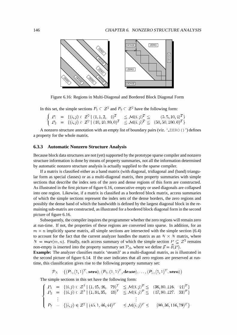
146 CHAPTER 6. NONZERO STRUCTURE ANALYSIS
ZERO
DENSE
DENSE
DENSE
ZERO
ZERO
ZERO
DENSE
ZERO
DENSE ZERO
DE
NS
E
Figure 6.16: Regions in Multi-Diagonal and Bordered Block Diagonal Form
In this set, the simple sections P1
� Z
2 and P2
� Z
2 have the following form:(
P
1
= f(i; j) 2 Z
2
j (1; 1; 2;�4)
T
�M(i; j)
T
� (5; 5; 10; 4)
T
g
P
2
= f(i; j) 2 Z
2
j (40; 40; 80; 0)
T
�M(i; j)
T
� (50; 50; 100; 0)
T
g
A nonzero structure annotation with an empty list of boundary pairs (viz. ‘ ZERO()’) definesa property for the whole matrix.
6.3.3 Automatic Nonzero Structure Analysis
Because block data structures are not (yet) supported by the prototype sparse compiler and nonzerostructure information is done by means of property summaries, not all the information determinedby automatic nonzero structure analysis is actually supplied to the sparse compiler.
If a matrix is classified either as a band matrix (with diagonal, tridiagonal and (band) triangu-lar form as special classes) or as a multi-diagonal matrix, then property summaries with simplesections that describe the index sets of the zero and dense regions of this form are constructed.As illustrated in the first picture of figure 6.16, consecutive empty or used diagonals are collapsedinto one region. Likewise, if a matrix is classified as a bordered block matrix, access summariesof which the simple sections represent the index sets of the dense borders, the zero regions andpossibly the dense band of which the bandwidth is defined by the largest diagonal block in the re-maining sub-matrix are constructed, as illustrated for a bordered block diagonal form in the secondpicture of figure 6.16.
Subsequently, the compiler inquires the programmer whether the zero regions will remain zeroat run-time. If not, the properties of these regions are converted into sparse. In addition, for anm � n implicitly sparse matrix, all simple sections are intersected with the simple section (6.4)to account for the fact that the current analyzer handles the matrix as an N � N matrix, whereN = max(m;n). Finally, each access summary of which the simple section P � Z2 remainsnon-empty is inserted into the property summary set P
A
, where we define ~p = ~
�(P ).Example: The analyzer classifies matrix ‘steam3’ as a multi-diagonal matrix, as is illustrated inthe second picture of figure 6.14. If the user indicates that all zero regions are preserved at run-time, this classification gives rise to the following property summary set:
P
A
= fhP
1
; (1; 1)
T
; zeroi; hP
2
; (1; 1)
T
;densei; : : : ; hP
7
; (1; 1)
T
; zeroig
The simple sections in this set have the following form:8
>
>
>
>
<
>
>
>
>
:
P
1
= f(i; j) 2 Z
2
j (1; 45; 46;�79)
T
�M(i; j)
T
� (36; 80; 116;�44)
T
g
P
2
= f(i; j) 2 Z
2
j (1; 34; 35;�43)
T
�M(i; j)
T
� (47; 80; 127;�33)
T
g
......
P
7
= f(i; j) 2 Z
2
j (45; 1; 46; 44)
T
�M(i; j)
T
� (80; 36; 116; 79)
T
g
Chapter 7
Phase 2: Data Structure Selection
After all enveloping data structures of implicitly sparse matrices have been identified, and the ac-cess summaries of all occurrences of these arrays have been computed, a sparse storage schememust be selected for each implicitly sparse matrix. Although there are dynamic sparse storageschemes that support the fast generation of entries along different directions, for instance, alongrows and columns (cf. the linked list schemes presented in section 4.1.3), the overhead storageand run-time maintenance overhead of such storage schemes is usually substantial. Therefore,we have limited the sparse storage scheme that may be selected to store the entries in the sparseregions of an implicitly sparse matrix to a dynamic data structure that consists of a pool of sparsevectors supporting only one direction for each individual sparse region. However, the layout ofsparse vectors may be different for different sparse regions.
This implies that it becomes very important that each sparse region is accessed in a consistentmanner, namely along the direction supported for that region. Only in this manner, the the sparseoverhead reducing techniques guard encapsulation and access pattern expansion may become en-abled. Even dense regions should be accessed in a consistent manner, because this enables theselection of a full-sized array over this region in which elements along the most frequently occur-ring access patterns are stored along the columns, which enhances spatial locality in FORTRAN.Because it is likely that the enveloping data structures are accessed along arbitrary directions inthe original dense program, a method to reshape the access patterns of two-dimensional arrays,based on the unimodular framework presented in chapter 3, has been incorporated in the sparsecompiler.
Another important step for the sparse compiler is the construction of a number of mutuallydisjoint regions in each implicitly sparse matrix A such that each part of the corresponding en-veloping data structure A that may be accessed by an arbitrary occurrence of A corresponds to aregion inA confined to one of these regions. Given these regions, the sparse compiler can select adifferent storage organization for each region and convert the code accordingly. Since each occur-rence can only access a part of the enveloping data structure corresponding to a region in A thatis confined to only one of these regions, the need for run-time tests to determine which of the se-lected storage organizations must be accessed is avoided. Because usually only a limited numberof such regions can be distinguished, we also discuss how iteration space partitioning, presentedin detail in chapter 3, can be used to increase the resulting amount of fragmentation.
In this chapter, we present a reshaping method as well as a method to construct a number ofnon-overlapping regions in an implicitly sparse matrix of which the index sets are described interms of simple sections. Where possible, unnecessary re-computation of information obtained inthe first phase is avoided. The chapter is concluded with a discussion of the actual data structureselection and generation of the corresponding declarations. Note that, in general, finding the bestdata structure is computationally infeasible [148].
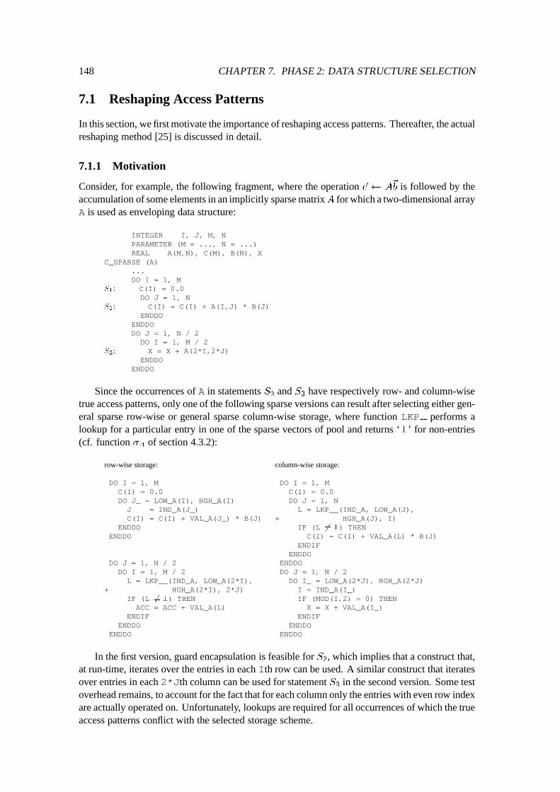
148 CHAPTER 7. PHASE 2: DATA STRUCTURE SELECTION
7.1 Reshaping Access Patterns
In this section, we first motivate the importance of reshaping access patterns. Thereafter, the actualreshaping method [25] is discussed in detail.
7.1.1 Motivation
Consider, for example, the following fragment, where the operation ~c A
~
b is followed by theaccumulation of some elements in an implicitly sparse matrixA for which a two-dimensional arrayA is used as enveloping data structure:
INTEGER I, J, M, NPARAMETER (M = ..., N = ...)REAL A(M,N), C(M), B(N), X
C_SPARSE (A)...DO I = 1, M
S
1
: C(I) = 0.0DO J = 1, N
S
2
: C(I) = C(I) + A(I,J) * B(J)ENDDO
ENDDODO J = 1, N / 2
DO I = 1, M / 2S
3
: X = X + A(2*I,2*J)ENDDO
ENDDO
Since the occurrences of A in statements S2
and S3
have respectively row- and column-wisetrue access patterns, only one of the following sparse versions can result after selecting either gen-eral sparse row-wise or general sparse column-wise storage, where function LKP performs alookup for a particular entry in one of the sparse vectors of pool and returns ‘?’ for non-entries(cf. function �
A
of section 4.3.2):
row-wise storage:
DO I = 1, MC(I) = 0.0DO J_ = LOW_A(I), HGH_A(I)J = IND_A(J_)C(I) = C(I) + VAL_A(J_) * B(J)
ENDDOENDDO
DO J = 1, N / 2DO I = 1, M / 2L = LKP__(IND_A, LOW_A(2*I),
+ HGH_A(2*I), 2*J)IF (L 6=?) THEN
ACC = ACC + VAL_A(L)ENDIF
ENDDOENDDO
column-wise storage:
DO I = 1, MC(I) = 0.0DO J = 1, NL = LKP__(IND_A, LOW_A(J),
+ HGH_A(J), I)IF (L 6=?) THEN
C(I) = C(I) + VAL_A(L) * B(J)ENDIF
ENDDOENDDODO J = 1, N / 2
DO I_ = LOW_A(2*J), HGH_A(2*J)I = IND_A(I_)IF (MOD(I,2) = 0) THEN
X = X + VAL_A(I_)ENDIF
ENDDOENDDO
In the first version, guard encapsulation is feasible for S2
, which implies that a construct that,at run-time, iterates over the entries in each Ith row can be used. A similar construct that iteratesover entries in each 2*Jth column can be used for statement S
3
in the second version. Some testoverhead remains, to account for the fact that for each column only the entries with even row indexare actually operated on. Unfortunately, lookups are required for all occurrences of which the trueaccess patterns conflict with the selected storage scheme.
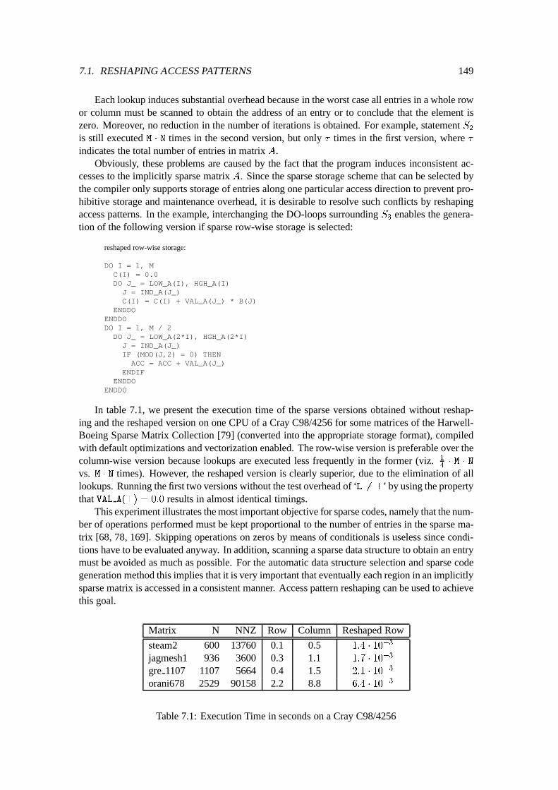
7.1. RESHAPING ACCESS PATTERNS 149
Each lookup induces substantial overhead because in the worst case all entries in a whole rowor column must be scanned to obtain the address of an entry or to conclude that the element iszero. Moreover, no reduction in the number of iterations is obtained. For example, statement S
2
is still executed M � N times in the second version, but only � times in the first version, where �indicates the total number of entries in matrix A.
Obviously, these problems are caused by the fact that the program induces inconsistent ac-cesses to the implicitly sparse matrix A. Since the sparse storage scheme that can be selected bythe compiler only supports storage of entries along one particular access direction to prevent pro-hibitive storage and maintenance overhead, it is desirable to resolve such conflicts by reshapingaccess patterns. In the example, interchanging the DO-loops surrounding S
3
enables the genera-tion of the following version if sparse row-wise storage is selected:
reshaped row-wise storage:
DO I = 1, MC(I) = 0.0DO J_ = LOW_A(I), HGH_A(I)J = IND_A(J_)C(I) = C(I) + VAL_A(J_) * B(J)
ENDDOENDDODO I = 1, M / 2DO J_ = LOW_A(2*I), HGH_A(2*I)J = IND_A(J_)IF (MOD(J,2) = 0) THEN
ACC = ACC + VAL_A(J_)ENDIF
ENDDOENDDO
In table 7.1, we present the execution time of the sparse versions obtained without reshap-ing and the reshaped version on one CPU of a Cray C98/4256 for some matrices of the Harwell-Boeing Sparse Matrix Collection [79] (converted into the appropriate storage format), compiledwith default optimizations and vectorization enabled. The row-wise version is preferable over thecolumn-wise version because lookups are executed less frequently in the former (viz. 1
4
� M � N
vs. M � N times). However, the reshaped version is clearly superior, due to the elimination of alllookups. Running the first two versions without the test overhead of ‘L 6=?’ by using the propertythat VAL A(?) = 0:0 results in almost identical timings.
This experiment illustrates the most important objective for sparse codes, namely that the num-ber of operations performed must be kept proportional to the number of entries in the sparse ma-trix [68, 78, 169]. Skipping operations on zeros by means of conditionals is useless since condi-tions have to be evaluated anyway. In addition, scanning a sparse data structure to obtain an entrymust be avoided as much as possible. For the automatic data structure selection and sparse codegeneration method this implies that it is very important that eventually each region in an implicitlysparse matrix is accessed in a consistent manner. Access pattern reshaping can be used to achievethis goal.
Matrix N NNZ Row Column Reshaped Row
steam2 600 13760 0.1 0.5 1:4 � 10
�3
jagmesh1 936 3600 0.3 1.1 1:7 � 10
�3
gre 1107 1107 5664 0.4 1.5 2:1 � 10
�3
orani678 2529 90158 2.2 8.8 6:4 � 10
�3
Table 7.1: Execution Time in seconds on a Cray C98/4256
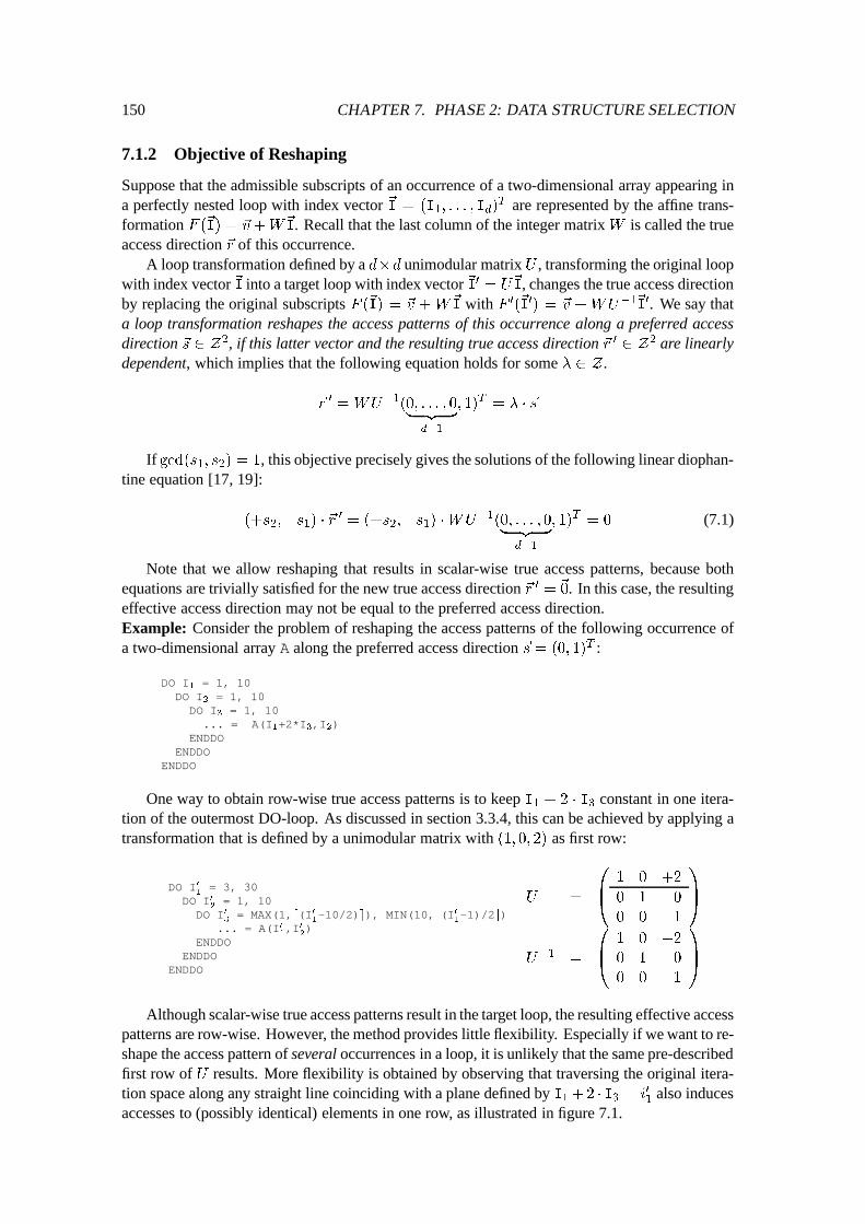
150 CHAPTER 7. PHASE 2: DATA STRUCTURE SELECTION
7.1.2 Objective of Reshaping
Suppose that the admissible subscripts of an occurrence of a two-dimensional array appearing ina perfectly nested loop with index vector ~I = (I
1
; : : : ; I
d
)
T are represented by the affine trans-formation F (~I) = ~v+W
~
I. Recall that the last column of the integer matrix W is called the trueaccess direction ~r of this occurrence.
A loop transformation defined by a d�d unimodular matrix U , transforming the original loopwith index vector~I into a target loop with index vector~I0 = U
~
I, changes the true access directionby replacing the original subscripts F (~I) = ~v +W
~
I with F 0(~I0) = ~v +WU
�1
~
I
0. We say thata loop transformation reshapes the access patterns of this occurrence along a preferred accessdirection ~s 2 Z2, if this latter vector and the resulting true access direction ~r 0 2 Z2 are linearlydependent, which implies that the following equation holds for some � 2 Z .
~r
0
=WU
�1
(0; : : : ; 0
| {z }
d�1
; 1)
T
= � � ~s
If gcd(s1
; s
2
) = 1, this objective precisely gives the solutions of the following linear diophan-tine equation [17, 19]:
(+s
2
;�s
1
) � ~r
0
= (+s
2
;�s
1
) �WU
�1
(0; : : : ; 0
| {z }
d�1
; 1)
T
= 0 (7.1)
Note that we allow reshaping that results in scalar-wise true access patterns, because bothequations are trivially satisfied for the new true access direction ~r 0 = ~
0. In this case, the resultingeffective access direction may not be equal to the preferred access direction.Example: Consider the problem of reshaping the access patterns of the following occurrence ofa two-dimensional array A along the preferred access direction ~s = (0; 1)
T :
DO I1
= 1, 10DO I
2
= 1, 10DO I
3
= 1, 10... = A(I
1
+2*I3
,I2
)ENDDO
ENDDOENDDO
One way to obtain row-wise true access patterns is to keep I
1
+ 2 � I
3
constant in one itera-tion of the outermost DO-loop. As discussed in section 3.3.4, this can be achieved by applying atransformation that is defined by a unimodular matrix with (1; 0; 2) as first row:
DO I01
= 3, 30DO I0
2
= 1, 10DO I0
3
= MAX(1,d(I01
-10/2)e), MIN(10,b(I01
-1)/2c)... = A(I0
1
,I02
)ENDDO
ENDDOENDDO
U =
0
B
@
1 0 +2
0 1 0
0 0 1
1
C
A
U
�1
=
0
B
@
1 0 �2
0 1 0
0 0 1
1
C
A
Although scalar-wise true access patterns result in the target loop, the resulting effective accesspatterns are row-wise. However, the method provides little flexibility. Especially if we want to re-shape the access pattern of several occurrences in a loop, it is unlikely that the same pre-describedfirst row of U results. More flexibility is obtained by observing that traversing the original itera-tion space along any straight line coinciding with a plane defined by I
1
+2 � I
3
= i
0
1
also inducesaccesses to (possibly identical) elements in one row, as illustrated in figure 7.1.
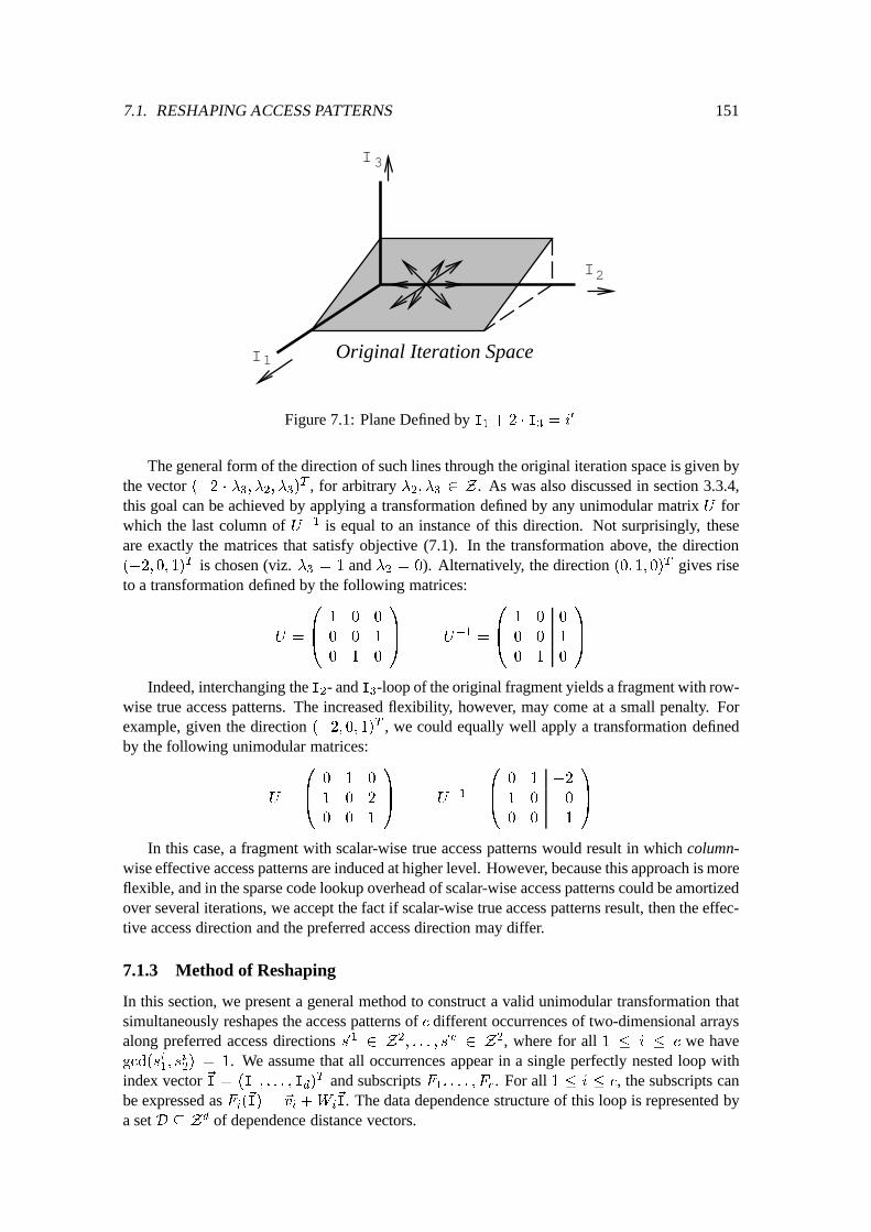
7.1. RESHAPING ACCESS PATTERNS 151
I 2
I 1
I 3
Original Iteration Space
Figure 7.1: Plane Defined by I
1
+ 2 � I
3
= i
0
1
The general form of the direction of such lines through the original iteration space is given bythe vector (�2 � �
3
; �
2
; �
3
)
T , for arbitrary �2
; �
3
2 Z . As was also discussed in section 3.3.4,this goal can be achieved by applying a transformation defined by any unimodular matrix U forwhich the last column of U�1 is equal to an instance of this direction. Not surprisingly, theseare exactly the matrices that satisfy objective (7.1). In the transformation above, the direction(�2; 0; 1)
T is chosen (viz. �3
= 1 and �2
= 0). Alternatively, the direction (0; 1; 0)
T gives riseto a transformation defined by the following matrices:
U =
0
B
@
1 0 0
0 0 1
0 1 0
1
C
A
U
�1
=
0
B
@
1 0 0
0 0 1
0 1 0
1
C
A
Indeed, interchanging the I2
- and I3
-loop of the original fragment yields a fragment with row-wise true access patterns. The increased flexibility, however, may come at a small penalty. Forexample, given the direction (�2; 0; 1)
T , we could equally well apply a transformation definedby the following unimodular matrices:
U =
0
B
@
0 1 0
1 0 2
0 0 1
1
C
A
U
�1
=
0
B
@
0 1 �2
1 0 0
0 0 1
1
C
A
In this case, a fragment with scalar-wise true access patterns would result in which column-wise effective access patterns are induced at higher level. However, because this approach is moreflexible, and in the sparse code lookup overhead of scalar-wise access patterns could be amortizedover several iterations, we accept the fact if scalar-wise true access patterns result, then the effec-tive access direction and the preferred access direction may differ.
7.1.3 Method of Reshaping
In this section, we present a general method to construct a valid unimodular transformation thatsimultaneously reshapes the access patterns of c different occurrences of two-dimensional arraysalong preferred access directions ~s 1
2 Z
2
; : : : ; ~s
c
2 Z
2, where for all 1 � i � c we havegcd(s
i
1
; s
i
2
) = 1. We assume that all occurrences appear in a single perfectly nested loop withindex vector ~I = (I
1
; : : : ; I
d
)
T and subscripts F1
; : : : ; F
c
. For all 1 � i � c, the subscripts canbe expressed as F
i
(
~
I) = ~v
i
+W
i
~
I. The data dependence structure of this loop is represented bya set D � Zd of dependence distance vectors.
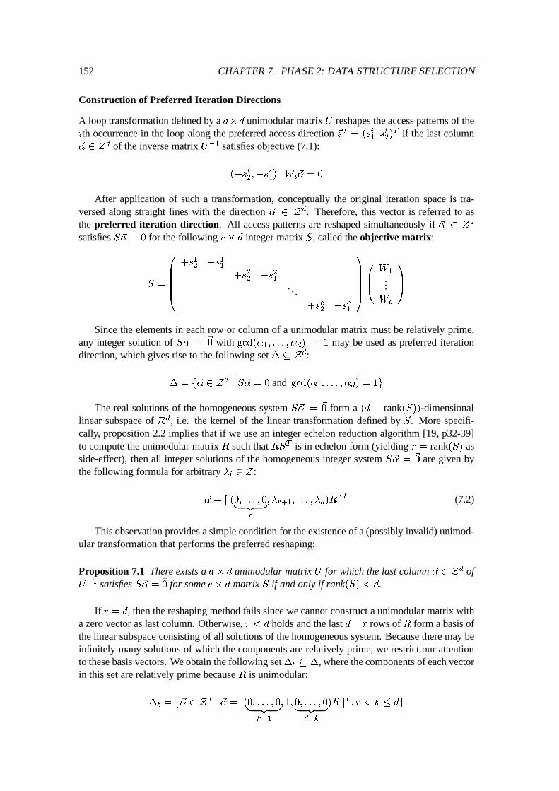
152 CHAPTER 7. PHASE 2: DATA STRUCTURE SELECTION
Construction of Preferred Iteration Directions
A loop transformation defined by a d�d unimodular matrix U reshapes the access patterns of theith occurrence in the loop along the preferred access direction ~s i = (s
i
1
; s
i
2
)
T if the last column~� 2 Z
d of the inverse matrix U�1 satisfies objective (7.1):
(+s
i
2
;�s
i
1
) �W
i
~� = 0
After application of such a transformation, conceptually the original iteration space is tra-versed along straight lines with the direction ~� 2 Z
d. Therefore, this vector is referred to asthe preferred iteration direction. All access patterns are reshaped simultaneously if ~� 2 Z
d
satisfies S~� =
~
0 for the following c� d integer matrix S, called the objective matrix:
S =
0
B
B
B
B
@
+s
1
2
�s
1
1
+s
2
2
�s
2
1
. . .+s
c
2
�s
c
1
1
C
C
C
C
A
0
B
@
W
1
...W
c
1
C
A
Since the elements in each row or column of a unimodular matrix must be relatively prime,any integer solution of S~� =
~
0 with gcd(�
1
; : : : ; �
d
) = 1 may be used as preferred iterationdirection, which gives rise to the following set � � Zd:
� = f~� 2 Z
d
j S~� = 0 and gcd(�
1
; : : : ; �
d
) = 1g
The real solutions of the homogeneous system S~� =
~
0 form a (d � rank(S))-dimensionallinear subspace of Rd, i.e. the kernel of the linear transformation defined by S. More specifi-cally, proposition 2.2 implies that if we use an integer echelon reduction algorithm [19, p32-39]to compute the unimodular matrix R such that RST is in echelon form (yielding r = rank(S) asside-effect), then all integer solutions of the homogeneous integer system S~� =
~
0 are given bythe following formula for arbitrary �
i
2 Z:
~� = [ (0; : : : ; 0
| {z }
r
; �
r+1
; : : : ; �
d
)R ]
T (7.2)
This observation provides a simple condition for the existence of a (possibly invalid) unimod-ular transformation that performs the preferred reshaping:
Proposition 7.1 There exists a d� d unimodular matrix U for which the last column ~� 2 Zd ofU
�1 satisfies S~� =
~
0 for some c� d matrix S if and only if rank(S) < d.
If r = d, then the reshaping method fails since we cannot construct a unimodular matrix witha zero vector as last column. Otherwise, r < d holds and the last d� r rows of R form a basis ofthe linear subspace consisting of all solutions of the homogeneous system. Because there may beinfinitely many solutions of which the components are relatively prime, we restrict our attentionto these basis vectors. We obtain the following set �
b
� �, where the components of each vectorin this set are relatively prime because R is unimodular:
�
b
= f~� 2 Z
d
j ~� = [(0; : : : ; 0
| {z }
k�1
; 1; 0; : : : ; 0
| {z }
d�k
)R ]
T
; r < k � dg
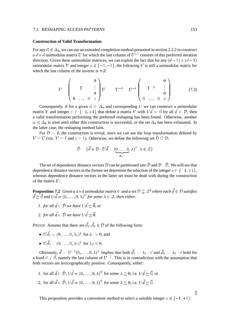
7.1. RESHAPING ACCESS PATTERNS 153
Construction of Valid Transformation
For any ~� 2 �
b
, we can use an extended completion method presented in section 2.2.2 to constructa d� d unimodular matrix U for which the last column of U�1 consists of this preferred iterationdirection. Given these unimodular matrices, we can exploit the fact that for any (d� 1)� (d� 1)
unimodular matrix Y and integer z 2 f�1;+1g, the following V is still a unimodular matrix forwhich the last column of the inverse is �~�:
V =
0
B
B
B
B
@
0
Y
...0
0 : : : 0 z
1
C
C
C
C
A
U V
�1
= U
�1
0
B
B
B
B
@
0
Y
�1
...0
0 : : : 0 z
1
C
C
C
C
A
(7.3)
Consequently, if for a given ~� 2 �
b
and corresponding U we can construct a unimodularmatrix Y and integer z 2 f�1;+1g that define a matrix V with V ~d � ~
0 for all ~d 2 D, thena valid transformation performing the preferred reshaping has been found. Otherwise, another~� 2 �
b
is tried until either this construction is successful, or the set �b
has been exhausted. Inthe latter case, the reshaping method fails.
For D = ;, the construction is trivial, since we can use the loop transformation defined byV = U (viz. Y = I and z = 1). Otherwise, we define the following set ~
D � D:
~
D = f
~
d 2 D j U
~
d = (0; : : : ; 0
| {z }
d�1
; �)
T
; � 2 Zg
The set of dependence distance vectorsD can be partitioned into ~
D andD� ~
D. We will see thatdependence distance vectors in the former set determine the selection of the integer z 2 f�1;+1g,whereas dependence distance vectors in the latter set must be dealt with during the constructionof the matrix Y :
Proposition 7.2 Given a d�d unimodular matrixU and a set ~
D � Z
d where each ~d 2 ~
D satisfies~
d �
~
0 and U ~d = (0; : : : ; 0; �)
T for some � 2 Z , then either:
1. for all ~d 2 ~
D we have U ~d � ~0, or
2. for all ~d 2 ~
D we have U ~d � ~0.
PROOF Assume that there are ~d1
;
~
d
2
2
~
D of the following form:
� U
~
d
1
= (0; : : : ; 0; �
1
)
T for �1
> 0, and
� U
~
d
2
= (0; : : : ; 0; �
2
)
T for �2
< 0.
Obviously, ~d = U
�1
(0; : : : ; 0; �)
T implies that both ~
d
1
= �
1
� ~v and ~
d
2
= �
2
� ~v hold fora fixed ~v 6= ~
0, namely the last column of U�1. This is in contradiction with the assumption thatboth vectors are lexicographically positive. Consequently, either:
1. for all ~d 2 ~
D, U ~d = (0; : : : ; 0; �)
T for some � � 0, i.e. U ~d � ~0, or
2. for all ~d 2 ~
D, U ~d = (0; : : : ; 0; �)
T for some � � 0, i.e. U ~d � ~0.
[]
This proposition provides a convenient method to select a suitable integer z 2 f�1;+1g:
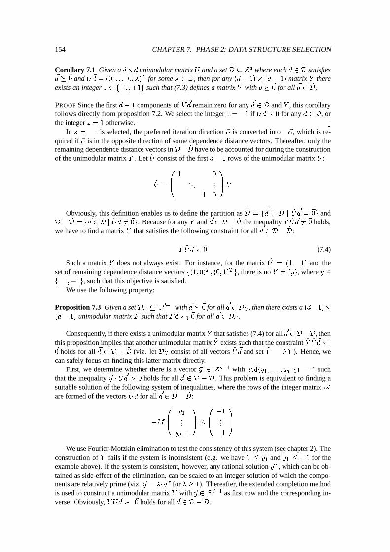
154 CHAPTER 7. PHASE 2: DATA STRUCTURE SELECTION
Corollary 7.1 Given a d�d unimodular matrix U and a set ~
D � Z
d where each ~d 2 ~
D satisfies~
d �
~
0 and U ~d = (0; : : : ; 0; �)
T for some � 2 Z , then for any (d � 1) � (d � 1) matrix Y thereexists an integer z 2 f�1;+1g such that (7.3) defines a matrix V with d � ~0 for all ~d 2 ~
D,
PROOF Since the first d� 1 components of V ~d remain zero for any ~d 2 ~
D and Y , this corollaryfollows directly from proposition 7.2. We select the integer z = �1 if U ~d � ~0 for any ~d 2 ~
D, orthe integer z = 1 otherwise. []
In z = �1 is selected, the preferred iteration direction ~� is converted into �~�, which is re-quired if ~� is in the opposite direction of some dependence distance vectors. Thereafter, only theremaining dependence distance vectors inD� ~
D have to be accounted for during the constructionof the unimodular matrix Y . Let ~
U consist of the first d� 1 rows of the unimodular matrix U :
~
U =
0
B
@
1 0
. . ....
1 0
1
C
A
U
Obviously, this definition enables us to define the partition as ~
D = f
~
d 2 D j
~
U
~
d =
~
0g andD�
~
D = f
~
d 2 D j
~
U
~
d 6=
~
0g. Because for any Y and ~d 2 D� ~
D the inequality Y ~
U
~
d 6=
~
0 holds,we have to find a matrix Y that satisfies the following constraint for all ~d 2 D � ~
D:
Y
~
U
~
d �
~
0 (7.4)
Such a matrix Y does not always exist. For instance, for the matrix ~
U = (1;�1) and theset of remaining dependence distance vectors f(1; 0)T ; (0; 1)T g, there is no Y = (y), where y 2f�1;+1g, such that this objective is satisfied.
We use the following property:
Proposition 7.3 Given a setDU
� Z
d�1 with ~d � ~0 for all ~d 2 DU
, then there exists a (d�1)�
(d� 1) unimodular matrix F such that F ~d �1
~
0 for all ~d 2 DU
.
Consequently, if there exists a unimodular matrix Y that satisfies (7.4) for all ~d 2 D� ~
D, thenthis proposition implies that another unimodular matrix ~
Y exists such that the constraint ~Y ~
U
~
d �
1
~
0 holds for all ~d 2 D � ~
D (viz. let DU
consist of all vectors ~
U
~
d and set ~
Y = FY ). Hence, wecan safely focus on finding this latter matrix directly.
First, we determine whether there is a vector ~y 2 Zd�1 with gcd(y
1
; : : : ; y
d�1
) = 1 suchthat the inequality ~y � ~U ~d > 0 holds for all ~d 2 D � ~
D. This problem is equivalent to finding asuitable solution of the following system of inequalities, where the rows of the integer matrix Mare formed of the vectors ~
U
~
d for all ~d 2 D � ~
D:
�M
0
B
@
y
1
...y
d�1
1
C
A
�
0
B
@
�1
...�1
1
C
A
We use Fourier-Motzkin elimination to test the consistency of this system (see chapter 2). Theconstruction of Y fails if the system is inconsistent (e.g. we have 1 � y
1
and y1
� �1 for theexample above). If the system is consistent, however, any rational solution ~y r, which can be ob-tained as side-effect of the elimination, can be scaled to an integer solution of which the compo-nents are relatively prime (viz. ~y = ��~y
r for � � 1). Thereafter, the extended completion methodis used to construct a unimodular matrix Y with ~y 2 Zd�1 as first row and the corresponding in-verse. Obviously, Y ~
U
~
d �
1
~
0 holds for all ~d 2 D � ~
D.
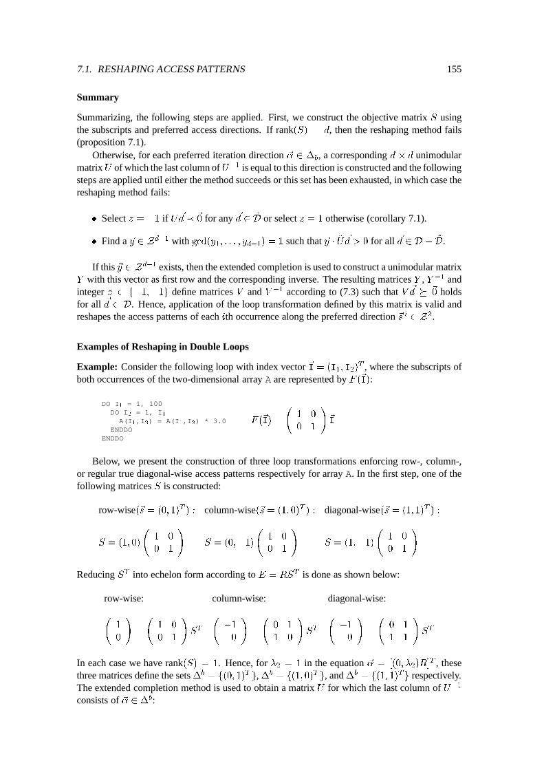
7.1. RESHAPING ACCESS PATTERNS 155
Summary
Summarizing, the following steps are applied. First, we construct the objective matrix S usingthe subscripts and preferred access directions. If rank(S) = d, then the reshaping method fails(proposition 7.1).
Otherwise, for each preferred iteration direction ~� 2 �
b
, a corresponding d � d unimodularmatrixU of which the last column ofU�1 is equal to this direction is constructed and the followingsteps are applied until either the method succeeds or this set has been exhausted, in which case thereshaping method fails:
� Select z = �1 if U ~d � ~0 for any ~d 2 ~
D or select z = 1 otherwise (corollary 7.1).
� Find a ~y 2 Zd�1 with gcd(y
1
; : : : ; y
d�1
) = 1 such that ~y � ~U ~d > 0 for all ~d 2 D � ~
D.
If this ~y 2 Zd�1 exists, then the extended completion is used to construct a unimodular matrixY with this vector as first row and the corresponding inverse. The resulting matrices Y , Y �1 andinteger z 2 f�1;+1g define matrices V and V �1 according to (7.3) such that V ~d � ~
0 holdsfor all ~d 2 D. Hence, application of the loop transformation defined by this matrix is valid andreshapes the access patterns of each ith occurrence along the preferred direction ~s i 2 Z2.
Examples of Reshaping in Double Loops
Example: Consider the following loop with index vector ~I = (I
1
; I
2
)
T , where the subscripts ofboth occurrences of the two-dimensional array A are represented by F (~I):
DO I1
= 1, 100DO I
2
= 1, I1
A(I1
,I2
) = A(I1
,I2
) * 3.0ENDDO
ENDDO
F (
~
I) =
1 0
0 1
!
~
I
Below, we present the construction of three loop transformations enforcing row-, column-,or regular true diagonal-wise access patterns respectively for array A. In the first step, one of thefollowing matrices S is constructed:
row-wise(~s = (0; 1)
T
) : column-wise(~s = (1; 0)
T
) : diagonal-wise(~s = (1; 1)
T
) :
S = (1; 0)
1 0
0 1
!
S = (0;�1)
1 0
0 1
!
S = (1;�1)
1 0
0 1
!
Reducing ST into echelon form according to E = RS
T is done as shown below:
row-wise: column-wise: diagonal-wise:
1
0
!
=
1 0
0 1
!
S
T
�1
0
!
=
0 1
1 0
!
S
T
�1
0
!
=
0 1
1 1
!
S
T
In each case we have rank(S) = 1. Hence, for �2
= 1 in the equation ~� = [(0; �
2
)R]
T , thesethree matrices define the sets �b
= f(0; 1)
T
g, �b
= f(1; 0)
T
g, and �
b
= f(1; 1)
T
g respectively.The extended completion method is used to obtain a matrix U for which the last column of U�1
consists of ~� 2 �
b:
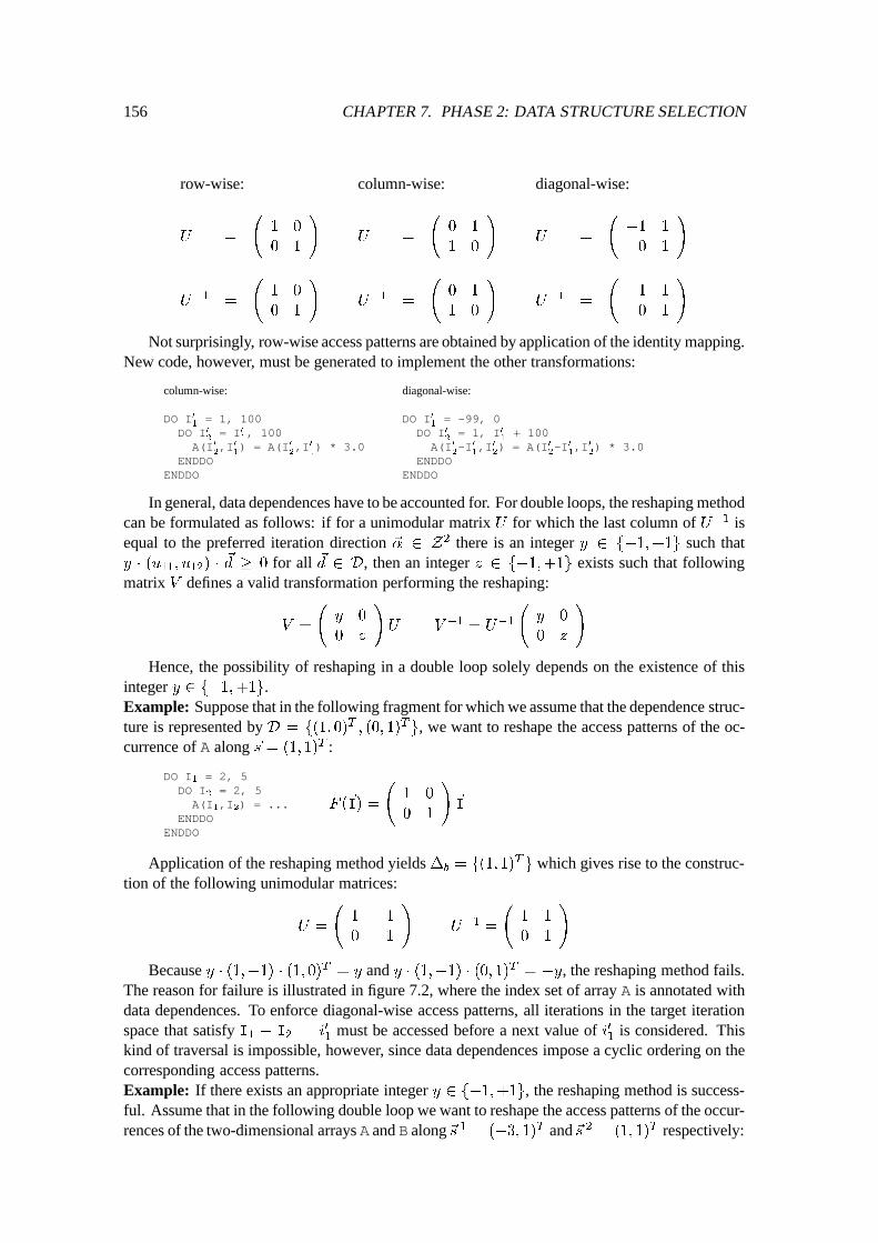
156 CHAPTER 7. PHASE 2: DATA STRUCTURE SELECTION
row-wise: column-wise: diagonal-wise:
U =
1 0
0 1
!
U =
0 1
1 0
!
U =
�1 1
0 1
!
U
�1
=
1 0
0 1
!
U
�1
=
0 1
1 0
!
U
�1
=
�1 1
0 1
!
Not surprisingly, row-wise access patterns are obtained by application of the identity mapping.New code, however, must be generated to implement the other transformations:
column-wise:
DO I01
= 1, 100DO I0
2
= I01
, 100A(I0
2
,I01
) = A(I02
,I01
) * 3.0ENDDO
ENDDO
diagonal-wise:
DO I01
= -99, 0DO I0
2
= 1, I01
+ 100A(I0
2
-I01
,I02
) = A(I02
-I01
,I02
) * 3.0ENDDO
ENDDO
In general, data dependences have to be accounted for. For double loops, the reshaping methodcan be formulated as follows: if for a unimodular matrix U for which the last column of U�1 isequal to the preferred iteration direction ~� 2 Z
2 there is an integer y 2 f�1;+1g such thaty � (u
11
; u
12
) �
~
d � 0 for all ~d 2 D, then an integer z 2 f�1;+1g exists such that followingmatrix V defines a valid transformation performing the reshaping:
V =
y 0
0 z
!
U V
�1
= U
�1
y 0
0 z
!
Hence, the possibility of reshaping in a double loop solely depends on the existence of thisinteger y 2 f�1;+1g.Example: Suppose that in the following fragment for which we assume that the dependence struc-ture is represented by D = f(1; 0)
T
; (0; 1)
T
g, we want to reshape the access patterns of the oc-currence of A along ~s = (1; 1)
T :
DO I1
= 2, 5DO I
2
= 2, 5A(I
1
,I2
) = ...ENDDO
ENDDO
F (
~
I) =
1 0
0 1
!
~
I
Application of the reshaping method yields �b
= f(1; 1)
T
g which gives rise to the construc-tion of the following unimodular matrices:
U =
1 �1
0 1
!
U
�1
=
1 1
0 1
!
Because y � (1;�1) � (1; 0)T = y and y � (1;�1) � (0; 1)T = �y, the reshaping method fails.The reason for failure is illustrated in figure 7.2, where the index set of array A is annotated withdata dependences. To enforce diagonal-wise access patterns, all iterations in the target iterationspace that satisfy I
1
� I
2
= i
0
1
must be accessed before a next value of i01
is considered. Thiskind of traversal is impossible, however, since data dependences impose a cyclic ordering on thecorresponding access patterns.Example: If there exists an appropriate integer y 2 f�1;+1g, the reshaping method is success-ful. Assume that in the following double loop we want to reshape the access patterns of the occur-rences of the two-dimensional arrays A and B along~s 1
= (�3; 1)
T and~s 2
= (1; 1)
T respectively:
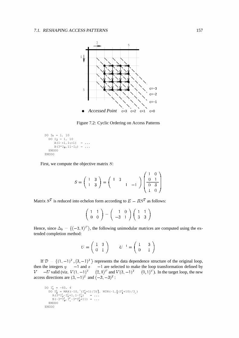
7.1. RESHAPING ACCESS PATTERNS 157
5
5
Accessed Point c=0
i
j
c=−3
c=−2
c=−1
c=1c=2c=3
Figure 7.2: Cyclic Ordering on Access Patterns
DO I1
= 1, 10DO I
2
= 1, 10A(I
1
+1,I2
+1) = ...B(3*I
2
,11-I1
) = ...ENDDO
ENDDO
First, we compute the objective matrix S:
S =
1 3
1 3
!
=
1 3
1 �1
!
0
B
B
B
@
1 0
0 1
0 3
1 0
1
C
C
C
A
Matrix ST is reduced into echelon form according to E = RS
T as follows:
1 1
0 0
!
=
1 0
�3 1
!
1 1
3 3
!
Hence, since �
b
= f(�3; 1)
T
g, the following unimodular matrices are computed using the ex-tended completion method:
U =
1 3
0 1
!
U
�1
=
1 �3
0 1
!
If D = f(1;�1)
T
; (3;�1)
T
g represents the data dependence structure of the original loop,then the integers y = �1 and z = �1 are selected to make the loop transformation defined byV = �U valid (viz. V (1;�1)
T
= (2; 1)
T and V (3;�1)
T
= (0; 1)
T ). In the target loop, the newaccess directions are (3;�1)
T and (�3;�3)
T :
DO I01
= -40, 4DO I0
2
= MAX(-10,d(I01
+1)/3)e, MIN(-1,b(I01
+10)/3c)A(3*I0
2
-I01
+1,1-I02
) = ...B(-3*I0
2
,I01
-3*I02
+11) = ...ENDDO
ENDDO
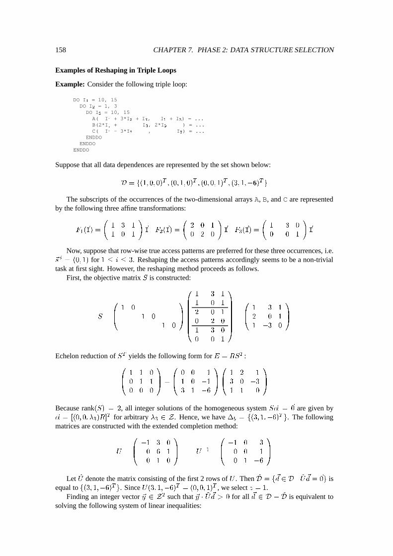
158 CHAPTER 7. PHASE 2: DATA STRUCTURE SELECTION
Examples of Reshaping in Triple Loops
Example: Consider the following triple loop:
DO I1
= 10, 15DO I
2
= 1, 3DO I
3
= 10, 15A( I
1
+ 3*I2
+ I3
, I1
+ I3
) = ...B(2*I
1
+ I3
, 2*I2
) = ...C( I
1
- 3*I2
, I3
) = ...ENDDO
ENDDOENDDO
Suppose that all data dependences are represented by the set shown below:
D = f(1; 0; 0)
T
; (0; 1; 0)
T
; (0; 0; 1)
T
; (3; 1;�6)
T
g
The subscripts of the occurrences of the two-dimensional arrays A, B, and C are representedby the following three affine transformations:
F
1
(
~
I) =
1 3 1
1 0 1
!
~
I F
2
(
~
I) =
2 0 1
0 2 0
!
~
I F
3
(
~
I) =
1 �3 0
0 0 1
!
~
I
Now, suppose that row-wise true access patterns are preferred for these three occurrences, i.e.~s
i
= (0; 1) for 1 � i � 3. Reshaping the access patterns accordingly seems to be a non-trivialtask at first sight. However, the reshaping method proceeds as follows.
First, the objective matrix S is constructed:
S =
0
B
@
1 0
1 0
1 0
1
C
A
0
B
B
B
B
B
B
B
@
1 3 1
1 0 1
2 0 1
0 2 0
1 �3 0
0 0 1
1
C
C
C
C
C
C
C
A
=
0
B
@
1 3 1
2 0 1
1 �3 0
1
C
A
Echelon reduction of ST yields the following form for E = RS
T :0
B
@
1 1 0
0 1 1
0 0 0
1
C
A
=
0
B
@
0 0 1
1 0 �1
3 1 �6
1
C
A
0
B
@
1 2 1
3 0 �3
1 1 0
1
C
A
Because rank(S) = 2, all integer solutions of the homogeneous system S~� =
~
0 are given by~� = [(0; 0; �
3
)R]
T for arbitrary �3
2 Z . Hence, we have �
b
= f(3; 1;�6)
T
g. The followingmatrices are constructed with the extended completion method:
U =
0
B
@
�1 3 0
0 6 1
0 1 0
1
C
A
U
�1
=
0
B
@
�1 0 3
0 0 1
0 1 �6
1
C
A
Let ~
U denote the matrix consisting of the first 2 rows of U . Then ~
D = f
~
d 2 D j
~
U
~
d =
~
0g isequal to f(3; 1;�6)T g. Since U(3; 1;�6)
T
= (0; 0; 1)
T , we select z = 1.Finding an integer vector ~y 2 Z2 such that ~y � ~U ~d > 0 for all ~d 2 D � ~
D is equivalent tosolving the following system of linear inequalities:
7.1. RESHAPING ACCESS PATTERNS 159
0
B
@
�1 0
3 �6
0 �1
1
C
A
y
1
y
2
!
�
0
B
@
�1
�1
�1
1
C
A
Obviously, this system is consistent, and a solution (1; 1)
T can be used directly for ~y. The follow-ing matrices results:
Y =
1 1
�1 0
!
Y
�1
=
0 �1
1 1
!
These matrices and z = 1 give rise to the following V and V �1:
V =
0
B
@
1 3 1
�1 3 0
0 1 0
1
C
A
V
�1
=
0
B
@
0 �1 3
0 0 1
1 1 �6
1
C
A
Application of the loop transformation defined by V yields the following target loop in whichrow-wise access patterns result for all occurrences:
DO I01
= 23, 39DO I0
2
= MAX(-12,I01
-45,16-I01
), MIN(-1,I01
-30,33-I01
)DO I0
3
= MAX(d(I01
+I02
-15)/6e,d(I02
+10)/3e),MIN(b(I0
1
+I02
-10)/6c,b(I02
+15)/3c)A(I0
1
, I01
- 3*I03
) = ...B(I0
1
- I02
, 2*I03
) = ...C( - I0
2
, I01
+ I02
- 6*I03
) = ...ENDDO
ENDDOENDDO
Example: Below, an example is given in which several possible preferred iteration directions re-sult:
DO I1
= 1, 4DO I
2
= 1, 4DO I
3
= 1, 4A(I
3
+ 5, I2
- I1
- 2*I3
+ 2) = ...B(I
3
, I1
+ 3*I3
- I2
) = ...ENDDO
ENDDOENDDO
Suppose that we want to reshape the access patterns of both occurrences, of which the sub-scripts are represented by the following affine transformation, along~s 1
= (1; 0) and~s 2
= (1; 1)
T
respectively:
F
1
(
~
I) =
5
2
!
+
0 0 1
�1 1 �2
!
~
I F
2
(
~
I) =
0 0 1
1 �1 3
!
~
I
First, the objective matrix S is constructed:
S =
0 �1
1 �1
!
0
B
B
B
@
0 0 1
�1 1 �2
0 0 1
1 �1 3
1
C
C
C
A
=
1 �1 2
�1 1 �2
!
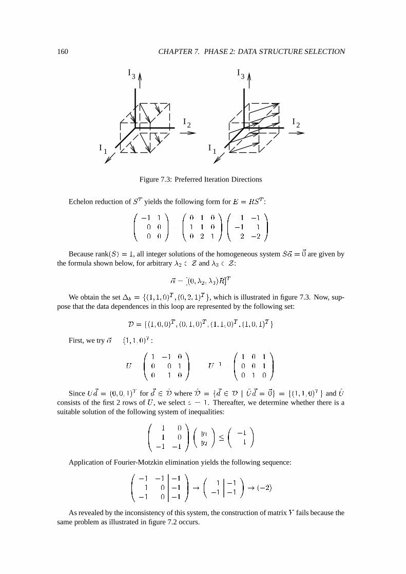
160 CHAPTER 7. PHASE 2: DATA STRUCTURE SELECTION
2I
I 1
3I
2I
I 1
3I
Figure 7.3: Preferred Iteration Directions
Echelon reduction of ST yields the following form for E = RS
T :0
B
@
�1 1
0 0
0 0
1
C
A
=
0
B
@
0 1 0
1 1 0
0 2 1
1
C
A
0
B
@
1 �1
�1 1
2 �2
1
C
A
Because rank(S) = 1, all integer solutions of the homogeneous system S~� =
~
0 are given bythe formula shown below, for arbitrary �
2
2 Z and �3
2 Z:
~� = [(0; �
2
; �
3
)R]
T
We obtain the set �b
= f(1; 1; 0)
T
; (0; 2; 1)
T
g, which is illustrated in figure 7.3. Now, sup-pose that the data dependences in this loop are represented by the following set:
D = f(1; 0; 0)
T
; (0; 1; 0)
T
; (1; 1; 0)
T
; (1; 0; 1)
T
g
First, we try ~� = (1; 1; 0)
T :
U =
0
B
@
1 �1 0
0 0 1
0 1 0
1
C
A
U
�1
=
0
B
@
1 0 1
0 0 1
0 1 0
1
C
A
Since U ~d = (0; 0; 1)
T for ~d 2 ~
D where ~
D = f
~
d 2 D j
~
U
~
d =
~
0g = f(1; 1; 0)
T
g and ~
U
consists of the first 2 rows of U , we select z = 1. Thereafter, we determine whether there is asuitable solution of the following system of inequalities:
0
B
@
�1 0
1 0
�1 �1
1
C
A
y
1
y
2
!
�
�1
�1
!
Application of Fourier-Motzkin elimination yields the following sequence:0
B
@
�1 �1 �1
1 0 �1
�1 0 �1
1
C
A
!
1 �1
�1 �1
!
! (�2)
As revealed by the inconsistency of this system, the construction of matrix Y fails because thesame problem as illustrated in figure 7.2 occurs.
7.1. RESHAPING ACCESS PATTERNS 161
Thereafter, we try ~� = (0; 2; 1)
T :
U =
0
B
@
1 0 0
0 �1 2
0 0 1
1
C
A
U
�1
=
0
B
@
1 0 0
0 �1 2
0 0 1
1
C
A
In this case, we have ~
D = ;. Hence, we try to find a vector ~y 2 Z2 that satisfies ~y � ~U ~d > 0
for all ~d 2 D, which is equivalent to solving the following system:0
B
B
B
@
�1 0
0 1
�1 1
�1 �2
1
C
C
C
A
y
1
y
2
!
�
0
B
B
B
@
�1
�1
�1
�1
1
C
C
C
A
Hence, we may use the solution ~y = (3;�1):
3 �1
1 0
!
3 �1
�1 3
!
These matrices together with z = 1 define the following matrices:
V =
0
B
@
3 1 �2
1 0 0
0 0 1
1
C
A
V
�1
=
0
B
@
0 1 0
1 �3 2
0 0 1
1
C
A
Application of the loop transformation defined by V yields the target loop shown below, inwhich the occurrences of A and B have the appropriate access direction:
DO I01
= -4, 14DO I0
2
= MAX(1,d(I01
-2)/3e), MIN(4,b(I01
+7)/3c)DO I0
3
= MAX(1,d(3*I02
-I01
+1)/2e), MIN(4,b(3*I02
-I01
+4)/2c)A(I0
3
+ 5, I01
- 4*I02
+ 2 ) = ...B(I0
3
, 4*I02
- I01
+ I03
) = ...ENDDO
ENDDOENDDO
7.1.4 Implementation of Reshaping in the Prototype Sparse Compiler
In the prototype sparse compiler, reshaping access patterns is implemented by scanning over allperfected nested sub-loops with admissible loop bounds in the dense program. Given such a per-fectly nested sub-loop, all occurrences of enveloping data structures with admissible subscriptsthat only depend on loop indices of the sub-loop are examined. If access summary hX;~x n
i 2 X
A
is associated with such an occurrence, then we choose a preferred access direction ~s 2 Z2 ofthis occurrence as any ~s = ~p for which there is a property summary hP; ~p; pi 2 P
A
such thatX \ P 6= ;, or we simply discard the occurrence from further consideration otherwise.
Subsequently, the reshaping method presented in previous sections is applied to the perfectlynested sub-loop and the remaining occurrences.1 On failure, some interaction with the program-mer is performed about whether some data dependences or occurrences may be ignored during thereshaping, after which another attempt is possibly taken. On success, the access summary hX;~x n
i
of each occurrence affected by the reshaping is replaced by a new access summary hX;~y niwhere~y
n
2 Z
2 denotes the new effective access direction. In this manner, re-computation of simplesections is avoided. Finally, all changes in subscripts of enveloping data structures are correctlyaccounted for by altering the conditions computed by the method of section 5.3.1 accordingly.
1Constructing a valid unimodular transformation is complicated by the fact that only dependence directions arecomputed by the prototype compiler, so that the way of testing validity presented at the end of section 3.3.2 must beused.
162 CHAPTER 7. PHASE 2: DATA STRUCTURE SELECTION
7.2 Construction of Representatives
Another important step in the automatic data structure selection and transformation method is theconstruction of a set �
A
= fS
1
; S
2
; : : :g of representative simple sections for each implicitlysparse matrix A. These simple sections, called representatives for short, should have the follow-ing properties:
(1) 8 S; S
0
2 �
A
: S 6= S
0
) S \ S
0
= ; (mutually disjoint)(2) 8 hX;~x
n
i 2 X
A
: 9 S 2 �
A
: X � S (representative)
Although these constraints are trivially satisfied for a single representative that contains thewhole index set of the matrixA, some of the simple sections in X
A
are fragmented using iterationspace partitioning to enable the construction of a set �
A
with a reasonable degree of fragmenta-tion. If possible, simple sections are fragmented according to the simple sections in the propertysummary set, since it is desirable to have the following property:
(3) 8 S 2 �
A
; hP; ~p; pi 2 P
A
: S \ P 6= ; ) S � P (property fragmented)
First, a simple approach is discussed that is based on repetitively combining overlapping sim-ple sections. Since usually only one representative results, we explore how iteration space parti-tioning, discussed in chapter 3, can be used to increase the resulting amount of fragmentation.
7.2.1 Simple Approach
A simple way to construct the representatives of an implicitly sparse matrix A is to use the union‘]’ to combine overlapping simple sections associated with the occurrences of the correspondingenveloping data structure A, until a set of mutually disjoint representatives remains. Starting with�
A
= ;, we scan over all access summaries in the set XA
. For each hX;~x n
i 2 X
A
, the followingtests and associated actions are performed:
1. If X \ S = ; for all S 2 �
A
, then X is added to the set �A
.
2. Otherwise, we have X \ S 6= ; for some S 2 �
A
.
(a) If X � S, then S is used directly as representative of X .
(b) If X 6� S, then X = X ] S is computed and S is deleted from �
A
. If X \ S 6= ;still holds for some (other) S 2 �
A
, then this step is repeated until X \ S = ; for allS 2 �
A
. The final X is inserted into the set �A
.
Example: Consider the following occurrences of a two-dimensional array A that is used as theenveloping data structure of an 100 � 100 implicitly sparse matrix A:
DO I = 1, 100DO J = 1, I-1A1
(I,J) = C(I,J)ENDDOB(I) = A
2
(I,I)DO J = I, 100
A3
(I,J) = D(I,J)ENDDO
ENDDO
This fragment gives rise to the following access summary bag:
X
A
= fhX
1
; (0; 1)
T
i; hX
2
; (1; 1)
T
i; hX
3
; (0; 1)
T
ig
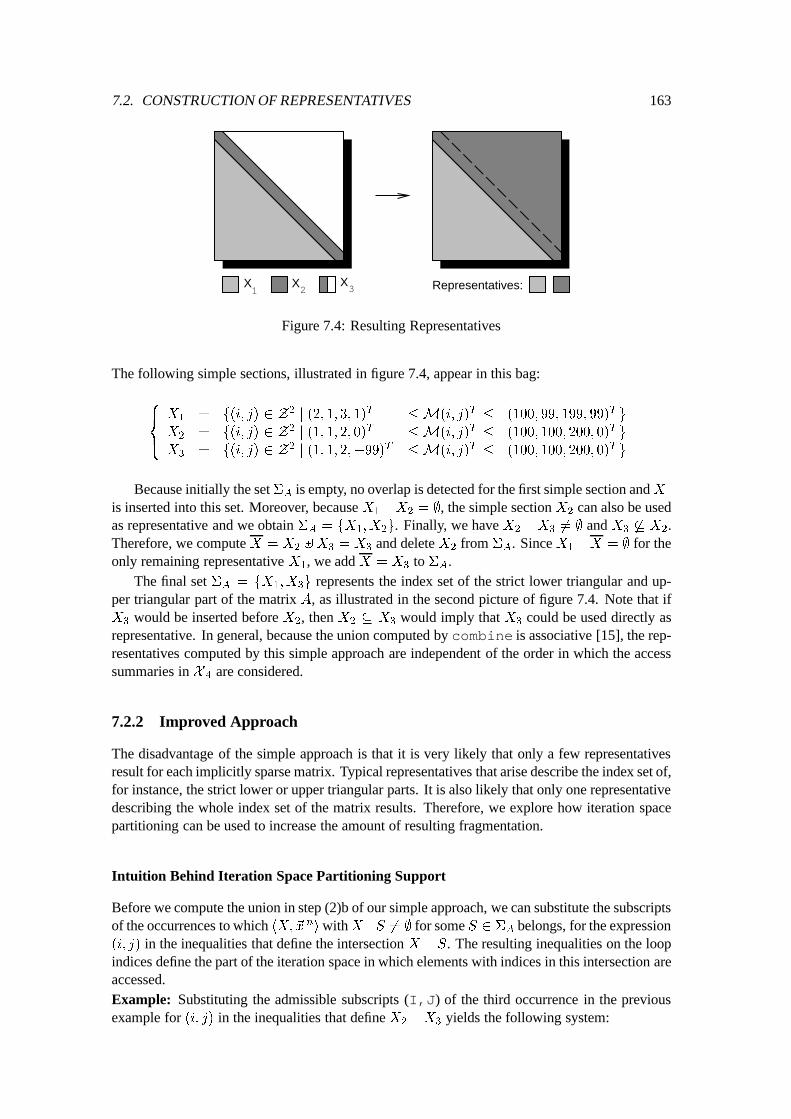
7.2. CONSTRUCTION OF REPRESENTATIVES 163
2 3 Representatives:1X X X
Figure 7.4: Resulting Representatives
The following simple sections, illustrated in figure 7.4, appear in this bag:
8
>
<
>
:
X
1
= f(i; j) 2 Z
2
j (2; 1; 3; 1)
T
�M(i; j)
T
� (100; 99; 199; 99)
T
g
X
2
= f(i; j) 2 Z
2
j (1; 1; 2; 0)
T
�M(i; j)
T
� (100; 100; 200; 0)
T
g
X
3
= f(i; j) 2 Z
2
j (1; 1; 2;�99)
T
�M(i; j)
T
� (100; 100; 200; 0)
T
g
Because initially the set �A
is empty, no overlap is detected for the first simple section andX1
is inserted into this set. Moreover, because X1
\X
2
= ;, the simple section X2
can also be usedas representative and we obtain �
A
= fX
1
;X
2
g. Finally, we have X2
\X
3
6= ; and X3
6� X
2
.Therefore, we compute X = X
2
]X
3
= X
3
and delete X2
from �
A
. Since X1
\X = ; for theonly remaining representative X
1
, we add X = X
3
to �
A
.The final set �
A
= fX
1
;X
3
g represents the index set of the strict lower triangular and up-per triangular part of the matrix A, as illustrated in the second picture of figure 7.4. Note that ifX
3
would be inserted before X2
, then X2
� X
3
would imply that X3
could be used directly asrepresentative. In general, because the union computed by combine is associative [15], the rep-resentatives computed by this simple approach are independent of the order in which the accesssummaries in X
A
are considered.
7.2.2 Improved Approach
The disadvantage of the simple approach is that it is very likely that only a few representativesresult for each implicitly sparse matrix. Typical representatives that arise describe the index set of,for instance, the strict lower or upper triangular parts. It is also likely that only one representativedescribing the whole index set of the matrix results. Therefore, we explore how iteration spacepartitioning can be used to increase the amount of resulting fragmentation.
Intuition Behind Iteration Space Partitioning Support
Before we compute the union in step (2)b of our simple approach, we can substitute the subscriptsof the occurrences to which hX;~x n
iwithX\S 6= ; for some S 2 �
A
belongs, for the expression(i; j) in the inequalities that define the intersection X \ S. The resulting inequalities on the loopindices define the part of the iteration space in which elements with indices in this intersection areaccessed.Example: Substituting the admissible subscripts (I,J) of the third occurrence in the previousexample for (i; j) in the inequalities that define X
2
\X
3
yields the following system:
164 CHAPTER 7. PHASE 2: DATA STRUCTURE SELECTION
8
>
>
>
<
>
>
>
:
1 � I � 100
1 � J � 100
2 � I+ J � 200
0 � I� J � 0
Simplification!
(
1 � I � 100
I � J � I
Confining overlap toX2
\X
3
can be done by isolating the loop-body in which the third occurrenceappears for all iterations satisfying 1 � I � 100 and I � J � I:
DO I = 1, 100DO J = 1, I-1A1
(I,J) = C(I,J)ENDDOB(I) = A
2
(I,I)DO J = I, 100
A3
(I,J) = D(I,J)ENDDO
ENDDO
I = J
!
DO I = 1, 100DO J = 1, I-1A1
(I,J) = C(I,J)ENDDOB(I) = A
2
(I,I)A3a
(I,I) = D(I,I)DO J = I+1, 100A3b
(I,J) = D(I,J)ENDDO
ENDDO
Obviously, after application of a relatively simple transformation, the index sets of the maindiagonal and the strict lower and upper triangular part of the matrix can be selected as represen-tatives, as illustrated with a dashed line in the second picture of figure 7.4.
Although iteration space partitioning can be used to increase the number of resulting represen-tatives, the code size may also increase. Another disadvantage arises if iteration space partitioninginduces redundant fragmentation of the simple sections that are associated with other occurrences.Although loop distribution can be used to limit this effect, in general, we must find a balance be-tween code duplication and this redundant fragmentation on one side, and the amount of usefulfragmentation on the other side.
Outline of the Improved Approach
Rather than starting the construction of representatives with�A
= ;, in the improved approach wefirst insert the simple sections arising in the property set P
A
into this set, i.e. for each hP; ~p; pi 2P
A
, the simple section P is added to �
A
. In this manner, the simple sections associated with theoccurrences of the corresponding enveloping data structure A may become fragmented accordingto the simple sections arising in P
A
.Subsequently, we scan over all the access summaries in the bag X
A
in increasing order of thesimple section size, because small simple sections tend to induce fragmentation of larger simplesections (note that once a representative has been added to the set �
A
, it cannot be further frag-mented because this representative may represent the simple sections of many occurrences). Foreach access summary inX
A
, the steps of the simple approach of section 7.2.1 are performed. How-ever, before we combine simple sections in step (2)b, we proceed as follows.
Let IS � Zd and ~I denote respectively the iteration space and the index vector of the loopin which this occurrence appears. Furthermore, suppose that the subscripts of the occurrence towhich the access summary hX;~x n
i with X \ S 6= ; for some S 2 �
A
belongs are admissible,and represented by F (~I) = ~v+W
~
I. Now, our goal is to isolate the loop-body of the loop for alliterations lying in the following set:
f
~
I 2 IS j F (
~
I) 2 X \ Sg (7.5)
If ~� 2 Z4 and ~� 2 Z4 denote the boundary values of the simple section X \ S, substitutingF (
~
I) for (i; j) in the corresponding set of inequalities yields the following system:2
2If only one subscript is admissible, still one of the first two pairs can be constructed.
7.2. CONSTRUCTION OF REPRESENTATIVES 165
�
1
� v
1
+
P
d
j=1
w
1j
� I
j
� �
1
�
2
� v
2
+
P
d
j=1
w
2j
� I
j
� �
2
�
3
� v
1
+ v
2
+
P
d
j=1
(w
1j
+ w
2j
) � I
j
� �
3
�
4
� v
1
� v
2
+
P
d
j=1
(w
1j
� w
2j
) � I
j
� �
4
(7.6)
For appropriate lk; akj
; u
k
2 Z , the kth pair of linear inequalities in this system gives rise tothe definition of a slice Ck
� Z
d that can be written in the following form:
C
k
= f
~
I 2 Z
d
j l
k
� a
k
1
� I
1
+ : : :+ a
k
d
� I
d
� u
k
g
Rather than using all linear inequalities simultaneously to isolate the loop-body for all iter-ations in (7.5), partitioning the iteration space according to only one of these slices enables theincremental construction of new simple sections into which the simple section X becomes frag-mented, which prevents re-computation of these simple sections by means of subscripts and loopbounds analysis. Moreover, using only one slice provides more control over the amount of re-sulting fragmentation, since it enables the compiler to determine whether further iteration spacepartitioning is useful. If this is not the case or if iteration space partitioning fails, then X is com-bined with representatives in �
A
as in the simple approach. Otherwise, X is replaced by the newsimple section, each of which is handled separately thereafter.
These issues are further elaborated upon in the following sections.
Incremental Construction of New Simple Sections
Central to incrementally constructing new simple sections is the procedure alter, in which asimple section stored innew is obtained from a simple section stored inold by refining all bound-aries after the boundary values of the kth boundary pair have been replaced by l and u:
procedure alter(old, k, l, u, var new)beginnew := old;new.l[k] := l;new.u[k] := u;refine(new)
end
If we partition the iteration space according to the kth slice Ck
� Z
d that is defined by sys-tem (7.6), then at most three duplicates of the occurrence are generated. Obviously, this iterationspace partitioning fragmentsX into three new simple sections that become associated with the du-plicates. These new simple section can be computed in s1, s2, and s3 by calling the followingprocedure incrementwith X , k, and X \ S as first three arguments:
procedure increment(s, t, k, swp, var s1, var s2, var s3)beginalter(s, k, s.l[k], t.l[k]-1, s1);alter(s, k, t.l[k], t.u[k], s2);alter(s, k, t.u[k]+1, s.u[k], s3);if (swp) thenswap(s1, s3);
endifend
If the last nonzero coefficient aki
2 Z defining Ck
� Z
d is negative, then we must swapthe first and last simple section to restore the association between the new simple sections and thethree duplicates of the original occurrence in the resulting DO-loops. In this case, the booleanvariable swp is set.
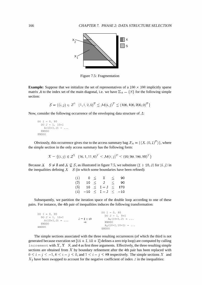
166 CHAPTER 7. PHASE 2: DATA STRUCTURE SELECTION
S
X
1
2X
X
Figure 7.5: Fragmentation
Example: Suppose that we initialize the set of representatives of a 100 � 100 implicitly sparsematrix A to the index set of the main diagonal, i.e. we have �
A
= fSg for the following simplesection:
S = f(i; j) 2 Z
2
j (1; 1; 2; 0)
T
�M(i; j)
T
� (100; 100; 200; 0)
T
g
Now, consider the following occurrence of the enveloping data structure of A:
DO I = 0, 80DO J = 1, 10+IA(10+I,J) = ...
ENDDOENDDO
Obviously, this occurrence gives rise to the access summary bag XA
= fhX; (0; 1)
T
ig, wherethe simple section in the only access summary has the following form:
X = f(i; j) 2 Z
2
j (10; 1; 11; 0)
T
�M(i; j)
T
� (90; 90; 180; 89)
T
g
Because X \S 6= ; and X 6� S, as illustrated in figure 7.5, we substitute (I+ 10; J) for (i; j) inthe inequalities defining X \ S (in which some boundaries have been refined):
(1) 0 � I � 90
(2) 10 � J � 90
(3) 10 � I+ J � 170
(4) �10 � I� J � �10
Subsequently, we partition the iteration space of the double loop according to one of thesepairs. For instance, the 4th pair of inequalities induces the following transformation:
DO I = 0, 80DO J = 1, 10+IA(10+I,J) = ...
ENDDOENDDO
J = I+ 10
!
DO I = 0, 80DO J = 1, 9+IA1
(10+I,J) = ...ENDDOA2
(10+I,10+I) = ...ENDDO
The simple sections associated with the three resulting occurrences (of which the third is notgenerated because execution set [11+ I; 10+ I] defines a zero trip loop) are computed by callingincrementwithX ,X\S, and 4 as first three arguments. Effectively, the three resulting simplesections are obtained from X by boundary refinement after the 4th pair has been replaced with0 � i � j � �1, 0 � i � j � 0, and 1 � i � j � 89 respectively. The simple sections X
1
andX
3
have been swapped to account for the negative coefficient of index J in the inequalities:
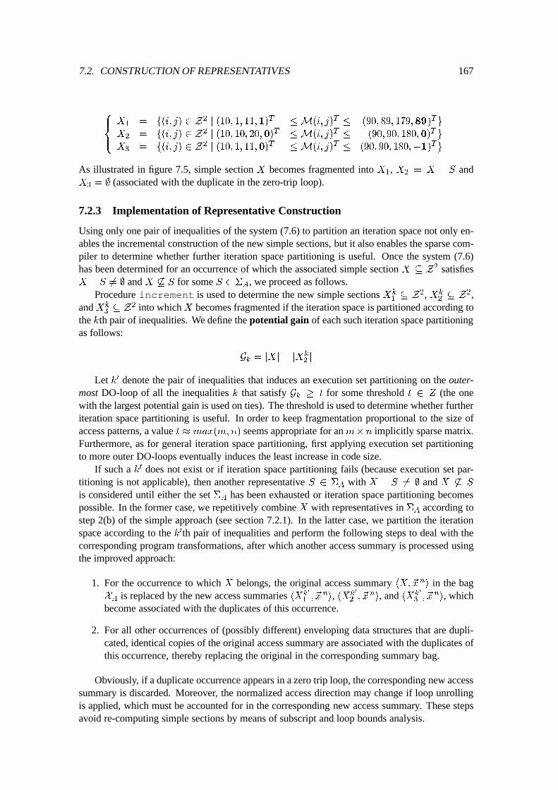
7.2. CONSTRUCTION OF REPRESENTATIVES 167
8
>
<
>
:
X
1
= f(i; j) 2 Z
2
j (10; 1; 11;1)
T
�M(i; j)
T
� (90; 89; 179;89)
T
g
X
2
= f(i; j) 2 Z
2
j (10; 10; 20;0)
T
�M(i; j)
T
� (90; 90; 180;0)
T
g
X
3
= f(i; j) 2 Z
2
j (10; 1; 11;0)
T
�M(i; j)
T
� (90; 90; 180;�1)
T
g
As illustrated in figure 7.5, simple section X becomes fragmented into X1
, X2
= X \ S andX
3
= ; (associated with the duplicate in the zero-trip loop).
7.2.3 Implementation of Representative Construction
Using only one pair of inequalities of the system (7.6) to partition an iteration space not only en-ables the incremental construction of the new simple sections, but it also enables the sparse com-piler to determine whether further iteration space partitioning is useful. Once the system (7.6)has been determined for an occurrence of which the associated simple section X � Z2 satisfiesX \ S 6= ; and X 6� S for some S 2 �
A
, we proceed as follows.Procedure increment is used to determine the new simple sections Xk
1
� Z
2, Xk
2
� Z
2,and Xk
3
� Z
2 into whichX becomes fragmented if the iteration space is partitioned according tothe kth pair of inequalities. We define the potential gain of each such iteration space partitioningas follows:
G
k
= jXj � jX
k
2
j
Let k0 denote the pair of inequalities that induces an execution set partitioning on the outer-most DO-loop of all the inequalities k that satisfy G
k
� t for some threshold t 2 Z (the onewith the largest potential gain is used on ties). The threshold is used to determine whether furtheriteration space partitioning is useful. In order to keep fragmentation proportional to the size ofaccess patterns, a value t � max(m;n) seems appropriate for anm�n implicitly sparse matrix.Furthermore, as for general iteration space partitioning, first applying execution set partitioningto more outer DO-loops eventually induces the least increase in code size.
If such a k0 does not exist or if iteration space partitioning fails (because execution set par-titioning is not applicable), then another representative S 2 �
A
with X \ S 6= ; and X 6� S
is considered until either the set �A
has been exhausted or iteration space partitioning becomespossible. In the former case, we repetitively combine X with representatives in �
A
according tostep 2(b) of the simple approach (see section 7.2.1). In the latter case, we partition the iterationspace according to the k0th pair of inequalities and perform the following steps to deal with thecorresponding program transformations, after which another access summary is processed usingthe improved approach:
1. For the occurrence to which X belongs, the original access summary hX;~x n
i in the bagX
A
is replaced by the new access summaries hXk
0
1
; ~x
n
i, hXk
0
2
; ~x
n
i, and hXk
0
3
; ~x
n
i, whichbecome associated with the duplicates of this occurrence.
2. For all other occurrences of (possibly different) enveloping data structures that are dupli-cated, identical copies of the original access summary are associated with the duplicates ofthis occurrence, thereby replacing the original in the corresponding summary bag.
Obviously, if a duplicate occurrence appears in a zero trip loop, the corresponding new accesssummary is discarded. Moreover, the normalized access direction may change if loop unrollingis applied, which must be accounted for in the corresponding new access summary. These stepsavoid re-computing simple sections by means of subscript and loop bounds analysis.
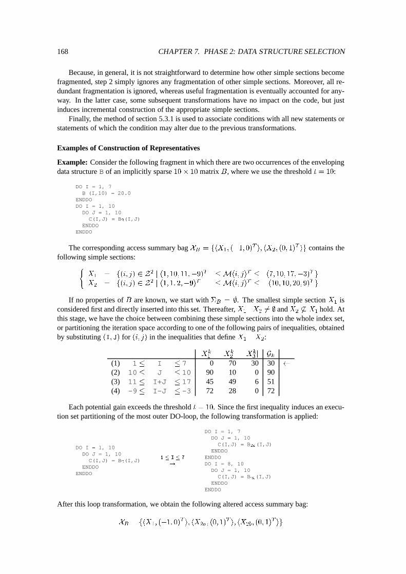
168 CHAPTER 7. PHASE 2: DATA STRUCTURE SELECTION
Because, in general, it is not straightforward to determine how other simple sections becomefragmented, step 2 simply ignores any fragmentation of other simple sections. Moreover, all re-dundant fragmentation is ignored, whereas useful fragmentation is eventually accounted for any-way. In the latter case, some subsequent transformations have no impact on the code, but justinduces incremental construction of the appropriate simple sections.
Finally, the method of section 5.3.1 is used to associate conditions with all new statements orstatements of which the condition may alter due to the previous transformations.
Examples of Construction of Representatives
Example: Consider the following fragment in which there are two occurrences of the envelopingdata structure B of an implicitly sparse 10� 10 matrix B, where we use the threshold t = 10:
DO I = 1, 7B1
(I,10) = 20.0ENDDODO I = 1, 10DO J = 1, 10C(I,J) = B
2
(I,J)ENDDO
ENDDO
The corresponding access summary bag XB
= fhX
1
; (�1; 0)
T
i; hX
2
; (0; 1)
T
ig contains thefollowing simple sections:
(
X
1
= f(i; j) 2 Z
2
j (1; 10; 11;�9)
T
�M(i; j)
T
� (7; 10; 17;�3)
T
g
X
2
= f(i; j) 2 Z
2
j (1; 1; 2;�9)
T
�M(i; j)
T
� (10; 10; 20; 9)
T
g
If no properties of B are known, we start with �
B
= ;. The smallest simple section X1
isconsidered first and directly inserted into this set. Thereafter, X
1
\X
2
6= ; andX2
6� X
1
hold. Atthis stage, we have the choice between combining these simple sections into the whole index set,or partitioning the iteration space according to one of the following pairs of inequalities, obtainedby substituting (I; J) for (i; j) in the inequalities that define X
1
\X
2
:
jX
k
1
j jX
k
2
j jX
k
3
j G
k
(1) 1 � I � 7 0 70 30 30
(2) 10 � J � 10 90 10 0 90(3) 11 � I+J � 17 45 49 6 51(4) -9 � I-J � -3 72 28 0 72
Each potential gain exceeds the threshold t = 10. Since the first inequality induces an execu-tion set partitioning of the most outer DO-loop, the following transformation is applied:
DO I = 1, 10DO J = 1, 10C(I,J) = B
2
(I,J)ENDDO
ENDDO
1 � I � 7
!
DO I = 1, 7DO J = 1, 10
C(I,J) = B2a
(I,J)ENDDO
ENDDODO I = 8, 10
DO J = 1, 10C(I,J) = B
2b
(I,J)ENDDO
ENDDO
After this loop transformation, we obtain the following altered access summary bag:
X
B
= fhX
1
; (�1; 0)
T
i; hX
2a
; (0; 1)
T
i; hX
2b
; (0; 1)
T
ig
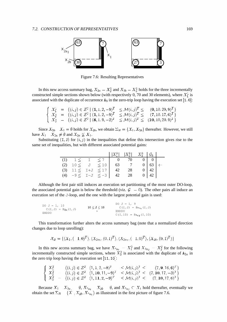
7.2. CONSTRUCTION OF REPRESENTATIVES 169
X1
3
63 7
2730X
2b
X2a1
63 7
Figure 7.6: Resulting Representatives
In this new access summary bag, X2a
= X
1
2
and X2b
= X
1
3
holds for the three incrementallyconstructed simple sections shown below (with respectively 0, 70 and 30 elements), where X1
1
isassociated with the duplicate of occurrence A
3
in the zero-trip loop having the execution set [1; 0]:8
>
<
>
:
X
1
1
= f(i; j) 2 Z
2
j (1; 1; 2;�9)
T
�M(i; j)
T
� (0; 10; 20; 9)
T
g
X
1
2
= f(i; j) 2 Z
2
j (1; 1; 2;�9)
T
�M(i; j)
T
� (7; 10; 17; 6)
T
g
X
1
3
= f(i; j) 2 Z
2
j (8; 1; 9;�2)
T
�M(i; j)
T
� (10; 10; 20; 9)
T
g
Since X2b
\X
1
= ; holds for X2b
, we obtain �
B
= fX
1
;X
2b
g thereafter. However, we stillhave X
1
\X
2a
6= ; and X2a
6� X
1
.Substituting (I; J) for (i; j) in the inequalities that define this intersection gives rise to the
same set of inequalities, but with different associated potential gains:
jX
k
1
j jX
k
2
j jX
k
3
j G
k
(1) 1 � I � 7 0 70 0 0(2) 10 � J � 10 63 7 0 63
(3) 11 � I+J � 17 42 28 0 42(4) -9 � I-J � -3 42 28 0 42
Although the first pair still induces an execution set partitioning of the most outer DO-loop,the associated potential gain is below the threshold (viz. G
1
= 0). The other pairs all induce anexecution set of the J-loop, and the one with the largest potential gain is used:
DO J = 1, 10C(I,J) = B
2a
(I,J)ENDDO
10 � J � 10
!
DO J = 1, 9C(I,J) = B
2a
1
(I,J)ENDDOC(I,10) = B
2a
2
(I,10)
This transformation further alters the access summary bag (note that a normalized directionchanges due to loop unrolling):
X
B
= fhX
1
; (�1; 0)
T
i; hX
2a
1
; (0; 1)
T
i; hX
2a
2
; (�1; 0)
T
i; hX
2b
; (0; 1)
T
ig
In this new access summary bag, we have X2a
1
= X
2
1
and X2a
2
= X
2
2
for the followingincrementally constructed simple sections, where X2
3
is associated with the duplicate of A2a
inthe zero trip loop having the execution set [11; 10]:
8
>
<
>
:
X
2
1
= f(i; j) 2 Z
2
j (1;1; 2;�8)
T
�M(i; j)
T
� (7;9; 16; 6)
T
g
X
2
2
= f(i; j) 2 Z
2
j (1;10; 11;�9)
T
�M(i; j)
T
� (7;10; 17;�3)
T
g
X
2
3
= f(i; j) 2 Z
2
j (1;11; 2;�9)
T
�M(i; j)
T
� (7;10; 17; 6)
T
g
Because X1
\ X
2a
1
= ;, X2a
1
\ X
2b
= ;, and X2a
2
� X
1
hold thereafter, eventually weobtain the set �
B
= fX
1
;X
2b
;X
2a
1
g as illustrated in the first picture of figure 7.6.
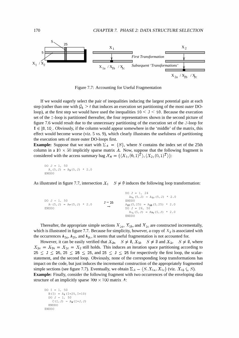
170 CHAPTER 7. PHASE 2: DATA STRUCTURE SELECTION
S
X / X1 2
55
25X 1
1a 1b 1cX / X / X
First Transformation
Subsequent ‘Transformations’
2aX / X / X2b 2c
X 2
Figure 7.7: Accounting for Useful Fragmentation
If we would eagerly select the pair of inequalities inducing the largest potential gain at eachstep (rather than one with G
k
� t that induces an execution set partitioning of the most outer DO-loop), at the first step we would have used the inequalities 10 � J � 10. Because the executionset of the I-loop is partitioned thereafter, the four representatives shown in the second picture offigure 7.6 would result due to the unnecessary partitioning of the execution set of the J-loop forI 2 [8; 10]. Obviously, if the column would appear somewhere in the ‘middle’ of the matrix, thiseffect would become worse (viz. 5 vs. 9), which clearly illustrates the usefulness of partitioningthe execution sets of more outer DO-loops first.Example: Suppose that we start with �
A
= fSg, where S contains the index set of the 25thcolumn in a 10 � 50 implicitly sparse matrix A. Now, suppose that the following fragment isconsidered with the access summary bag X
B
= fhX
1
; (0; 1)
T
i; hX
2
; (0; 1)
T
ig:
DO J = 1, 50A1
(5,J) = A2
(5,J) * 2.0ENDDO
As illustrated in figure 7.7, intersection X1
\ S 6= ; induces the following loop transformation:
DO J = 1, 50A1
(5,J) = A2
(5,J) * 2.0ENDDO
J = 25
!
DO J = 1, 24A1a
(5,J) = A2a
(5,J) * 2.0ENDDOA1b
(5,25) = A2b
(5,25) * 2.0DO J = 26, 50
A1c
(5,J) = A2c
(5,J) * 2.0ENDDO
Thereafter, the appropriate simple sections X1a
, X1b
, and X1c
are constructed incrementally,which is illustrated in figure 7.7. Because for simplicity, however, a copy ofX
2
is associated withthe occurrences A
2a
, A2b
, and A
2c
, it seems that useful fragmentation is not accounted for.However, it can be easily verified that X
2a
\ S 6= ;, X2b
\ S 6= ; and X2c
\ S 6= ;, whereX
2a
= X
2b
= X
2c
= X
2
still holds. This induces an iteration space partitioning according to25 � J � 25, 25 � 25 � 25, and 25 � J � 25 for respectively the first loop, the scalar-statement, and the second loop. Obviously, none of the corresponding loop transformations hasimpact on the code, but just induces the incremental construction of the appropriately fragmentedsimple sections (see figure 7.7). Eventually, we obtain �
A
= fS;X
1a
;X
1c
g (viz. X1b
� S).Example: Finally, consider the following fragment with two occurrences of the enveloping datastructure of an implicitly sparse 100 � 100 matrix A:
DO I = 1, 50B(I) = A
1
(I+25,I+10)DO J = 1, 50
C(I,J) = A2
(I+J,J)ENDDO
ENDDO
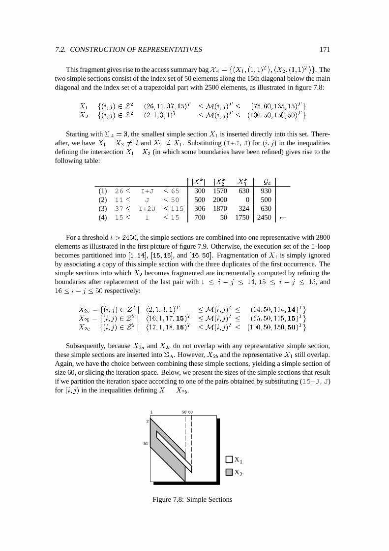
7.2. CONSTRUCTION OF REPRESENTATIVES 171
This fragment gives rise to the access summary bagXA
= fhX
1
; (1; 1)
T
i; hX
2
; (1; 1)
T
ig. Thetwo simple sections consist of the index set of 50 elements along the 15th diagonal below the maindiagonal and the index set of a trapezoidal part with 2500 elements, as illustrated in figure 7.8:
X
1
= f(i; j) 2 Z
2
j (26; 11; 37; 15)
T
�M(i; j)
T
� (75; 60; 135; 15)
T
g
X
2
= f(i; j) 2 Z
2
j (2; 1; 3; 1)
T
�M(i; j)
T
� (100; 50; 150; 50)
T
g
Starting with �
A
= ;, the smallest simple section X1
is inserted directly into this set. There-after, we have X
1
\ X
2
6= ; and X2
6� X
1
. Substituting (I+J,J) for (i; j) in the inequalitiesdefining the intersection X
1
\X
2
(in which some boundaries have been refined) gives rise to thefollowing table:
jX
k
1
j jX
k
2
j jX
k
3
j G
k
(1) 26� I+J � 65 300 1570 630 930(2) 11� J � 50 500 2000 0 500(3) 37� I+2J � 115 306 1870 324 630(4) 15� I � 15 700 50 1750 2450
For a threshold t > 2450, the simple sections are combined into one representative with 2800elements as illustrated in the first picture of figure 7.9. Otherwise, the execution set of the I-loopbecomes partitioned into [1; 14], [15; 15], and [16; 50]. Fragmentation of X
1
is simply ignoredby associating a copy of this simple section with the three duplicates of the first occurrence. Thesimple sections into which X
2
becomes fragmented are incrementally computed by refining theboundaries after replacement of the last pair with 1 � i � j � 14, 15 � i � j � 15, and16 � i� j � 50 respectively:
X
2a
= f(i; j) 2 Z
2
j (2; 1; 3;1)
T
�M(i; j)
T
� (64; 50; 114;14)
T
g
X
2b
= f(i; j) 2 Z
2
j (16; 1; 17;15)
T
�M(i; j)
T
� (65; 50; 115;15)
T
g
X
2c
= f(i; j) 2 Z
2
j (17; 1; 18;16)
T
�M(i; j)
T
� (100; 50; 150;50)
T
g
Subsequently, because X2a
and X2c
do not overlap with any representative simple section,these simple sections are inserted into �
A
. However, X2b
and the representative X1
still overlap.Again, we have the choice between combining these simple sections, yielding a simple section ofsize 60, or slicing the iteration space. Below, we present the sizes of the simple sections that resultif we partition the iteration space according to one of the pairs obtained by substituting (15+J,J)for (i; j) in the inequalities defining X
1
\X
2b
.
1 50
2
51
60
2
1X
X
Figure 7.8: Simple Sections
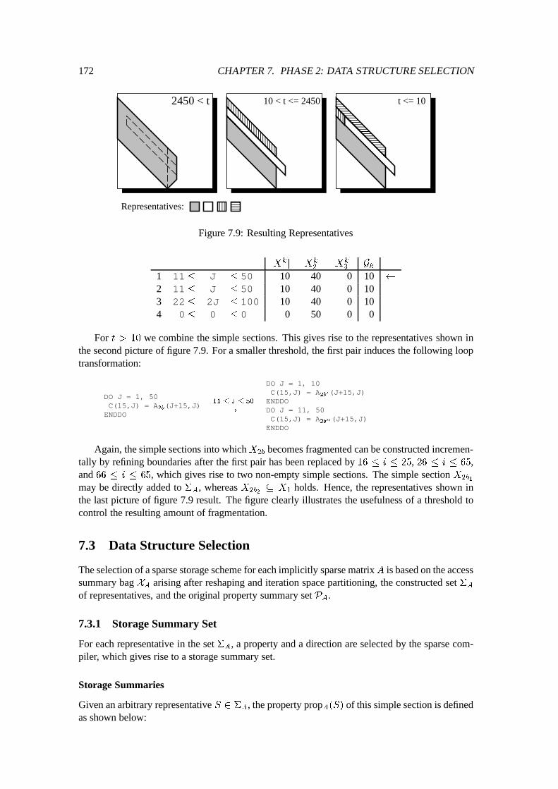
172 CHAPTER 7. PHASE 2: DATA STRUCTURE SELECTION
Representatives:
2450 < t 10 < t <= 2450 t <= 10
Figure 7.9: Resulting Representatives
jX
k
1
j jX
k
2
j jX
k
3
j G
k
1 11 � J � 50 10 40 0 10
2 11 � J � 50 10 40 0 103 22 � 2J � 100 10 40 0 104 0 � 0 � 0 0 50 0 0
For t > 10 we combine the simple sections. This gives rise to the representatives shown inthe second picture of figure 7.9. For a smaller threshold, the first pair induces the following looptransformation:
DO J = 1, 50C(15,J) = A
2b
(J+15,J)ENDDO
11 � J � 50
!
DO J = 1, 10C(15,J) = A
2b
0(J+15,J)ENDDODO J = 11, 50C(15,J) = A
2b
00(J+15,J)ENDDO
Again, the simple sections into whichX2b
becomes fragmented can be constructed incremen-tally by refining boundaries after the first pair has been replaced by 16 � i � 25, 26 � i � 65,and 66 � i � 65, which gives rise to two non-empty simple sections. The simple section X
2b
1
may be directly added to �
A
, whereas X2b
2
� X
1
holds. Hence, the representatives shown inthe last picture of figure 7.9 result. The figure clearly illustrates the usefulness of a threshold tocontrol the resulting amount of fragmentation.
7.3 Data Structure Selection
The selection of a sparse storage scheme for each implicitly sparse matrixA is based on the accesssummary bag X
A
arising after reshaping and iteration space partitioning, the constructed set �A
of representatives, and the original property summary set PA
.
7.3.1 Storage Summary Set
For each representative in the set �A
, a property and a direction are selected by the sparse com-piler, which gives rise to a storage summary set.
Storage Summaries
Given an arbitrary representative S 2 �
A
, the property propA
(S) of this simple section is definedas shown below:
7.3. DATA STRUCTURE SELECTION 173
propA
(S) =
8
>
<
>
:
zero if 9 hP; ~p; zero i 2 P
A
: S � P
dense if 9 hP; ~p;densei 2 P
A
: S � P
sparse otherwise
The direction dirA
(S) 2 Z
2 of each representative S 2 �
A
is defined as follows, where �(S) hasbeen defined in section 6.3.1:
dirA
(S) =
(
~p if 9 hP; ~p; pi 2 P
A
: S � P
~
�(S) otherwise
Given these definitions, each representative simple section S 2 �
A
defines the followingtriple s, called a storage summary:
s = hS; dirA
(S); propA
(S)i
The set of storage summaries defined by the simple sections in the set �A
is referred to as thestorage summary set S
A
.
Storage Patterns
Each storage summary hS; (s1
; s
2
)
T
; pi 2 S
A
gives rise to a number of storage patterns, whereeach storage pattern SP
k
is defined for a particular k 2 Z as follows:
SP
k
= f(i; j) 2 S j s
2
� i� s
1
� j = kg
The summary constants of a storage summary s = hS;~s; pi 2 S
A
with ~s 6= ~
0 are definedas the maximum value L(s) 2 Z and the minimum value U(s) 2 Z for which the followingconstraint is still satisfied:
SP
k
6= ; ) L(s) � k � U(
s)
As explained for access summaries, the summary constants of storage summary are either di-rectly defined by one of the boundary pairs for regular storage patterns, or obtained by one step ofFourier-Motzkin elimination to compute the extremal integer values of the expression s
2
�i�s
1
�j
for (i; j) 2 S. Moreover, the same terminology will be used for storage patterns. For instance, if~s = (0; 1)
T , then the storage patterns are called row-wise.
7.3.2 Declaration of the Selected Storage Scheme
The storage summary set SA
represents the storage scheme that has been selected for the implicitlysparse matrix A. Storage will be done according to the storage patterns arising from the storagesummaries in this set.
Zero Regions
A storage summary hS;~0; zeroi 2 SA
reflects the fact that aij
= 0 holds for all (i; j) 2 S.Hence, no explicit storage of the region represented by S � Z2 is required. Moreover, each oc-currence of the corresponding enveloping data structure A in the program having an access sum-mary hX;~x n
i 2 X
A
with X � S is replaced by a zero constant. Thereafter, the condition of thestatement in which this replacement occurs is re-computed, which may also affect the conditionsof surrounding DO-loops or IF-statements.
174 CHAPTER 7. PHASE 2: DATA STRUCTURE SELECTION
Example: In the following fragment, an annotation is used to inform the compiler that the maindiagonal of an implicitly sparse matrixAwith enveloping data structure A is zero, and will remainso at run-time:
REAL A(N,N), X(N)C_SPARSE(A : _ZERO(0 <= I-J <= 0))
...S
1
: DG = 0.0DO I = 1, N
S
2
: DG = DG + A(I,I) * X(I)ENDDO...
!
...DG = 0.0...
Under the assumption that the simple section representing the zero region results as a repre-sentative, occurrence A(I,I) is replaced by ‘0.0’. Thereafter, the condition ‘false’ becomesassociated with S
2
and, hence, with the I-loop (since we always ignore the ‘side-effect’ that setsthe final value of a loop index). This implies that both statements can be eliminated.
Dense Regions
A storage summary s = hS;~s;densei 2 S
A
indicates that dense storage must be used for theregion in A that is represented by the simple section S � Z2. Let ~� 2 Z4 and ~� 2 Z4 denote theboundary values of this simple section. First, an appropriate indexing method is selected:
�(s) =
8
>
<
>
:
row-indexed if ~s = (�1; 0)
T
_ ~s 6= (0;+1)
T
^ (�
1
� �
1
) < (�
2
� �
2
)
column-indexed otherwise
Dense storage of row- and column-wise storage patterns will be column- and row-indexedrespectively. For diagonal-wise storage patterns, the index inducing the smallest range will beused. A unique label lab(s), obtained by successively incrementing an integer-valued variable,is associated with each storage summary belonging to a dense region. Thereafter, the followingdeclaration is generated, where k = lab(s) and TYPE denotes the basis type of the envelopingdata structure A:
TYPE DNk_A(R,L(s) : U(s))
In this declaration, the range R is defined as follows:
R =
(
�
1
: �
1
if �(s) = row-indexed�
2
: �
2
otherwise
As is further discussed in chapter 8, appropriate initialization code for this array will be gen-erated at the beginning of the program, where each entry a
ij
with (i; j) 2 S is stored at either thelocation (i; s
2
� i� s
1
� j) or (j; s2
� i � s
1
� j) for row- or column-indexed storage respectively,where ~s = (s
1
; s
2
)
T . Moreover, the following replacement is performed for each occurrence ofthe enveloping data structure in the program with an access summary hX;~x n
i 2 X
A
that satisfiesX � S:
A(E1,E2) ! DNk_A(E,s2
* E1 - s
1
* E2)
In this replacement, k = lab(s) and subscript E is defined as follows:
E =
(
E1 if �(s) = row-indexedE2 otherwise
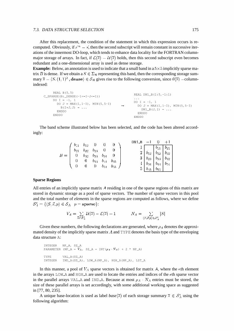
7.3. DATA STRUCTURE SELECTION 175
After this replacement, the condition of the statement in which this expression occurs is re-computed. Obviously, if ~x n
= ~s, then the second subscript will remain constant in successive iter-ations of the innermost DO-loop, which tends to enhance data locality for the FORTRAN column-major storage of arrays. In fact, if L(s) = U(s) holds, then this second subscript even becomesredundant and a one-dimensional array is used as dense storage.Example: Below, an annotation is used to indicate that a small band in a 5�5 implicitly sparse ma-trixB is dense. If we obtain aS 2 �
B
representing this band, then the corresponding storage sum-mary s = hS; (1; 1)T ;densei 2 S
B
gives rise to the following conversion, since �(s) =column-indexed:
REAL B(5,5)C_SPARSE(B:_DENSE(-1<=I-J<=1))
DO I = -1, 1DO J = MAX(1,1-I), MIN(5,5-I)
B(I+J,J) = ...ENDDO
ENDDO
!
REAL DN1_B(1:5,-1:1)...DO I = -1, 1
DO J = MAX(1,1-I), MIN(5,5-I)DN1_B(J,I) = ...
ENDDOENDDO
The band scheme illustrated below has been selected, and the code has been altered accord-ingly:
B =
0
B
B
B
B
B
@
b
11
b
12
0 0 0
b
21
b
22
b
23
0 0
0 b
32
b
33
b
34
0
0 0 b
43
b
44
b
45
0 0 0 b
54
b
55
1
C
C
C
C
C
A
DN1 B �1 0 +1
1 � b
11
b
21
2 b
12
b
22
b
32
3 b
23
b
33
b
42
4 b
34
b
44
b
54
5 b
45
b
55
�
Sparse Regions
All entries of an implicitly sparse matrix A residing in one of the sparse regions of this matrix arestored in dynamic storage as a pool of sparse vectors. The number of sparse vectors in this pooland the total number of elements in the sparse regions are computed as follows, where we defineS
s
A
= fhS;~s; pi 2 S
A
j p = sparseg:
V
A
=
P
s2S
s
A
U(s)�L(s) + 1 N
A
=
P
hS;~s;pi2S
s
A
jSj
Given these numbers, the following declarations are generated, where �A
denotes the approxi-mated density of the implicitly sparse matrixA and TYPE denotes the basis type of the envelopingdata structure A:
INTEGER NP_A, SZ_APARAMETER (NP_A = V
A
, SZ_A = INT(�A
�N
A
) + 2 * NP_A)
TYPE VAL_A(SZ_A)INTEGER IND_A(SZ_A), LOW_A(NP_A), HGH_A(NP_A), LST_A
In this manner, a pool of VA
sparse vectors is obtained for matrix A, where the eth elementin the arrays LOW A and HGH A are used to locate the entries and indices of the eth sparse vectorin the parallel arrays VAL A and IND A. Because at most �
A
� N
A
entries must be stored, thesize of these parallel arrays is set accordingly, with some additional working space as suggestedin [77, 80, 235].
A unique base-location is used as label base(s) of each storage summary s 2 SsA
using thefollowing algorithm:
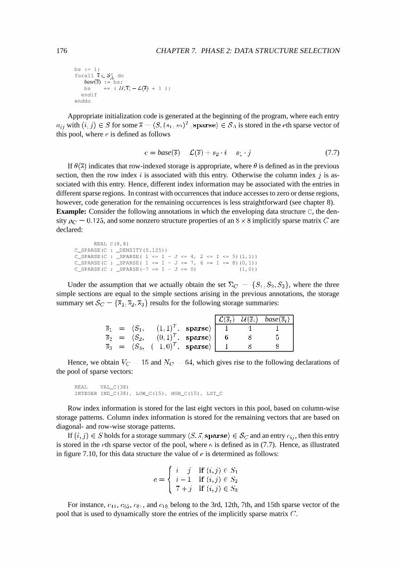
176 CHAPTER 7. PHASE 2: DATA STRUCTURE SELECTION
bs := 1;forall s 2 S
s
A
dobase(s) := bs;bs += ( U(s)� L(s) + 1 );
endifenddo
Appropriate initialization code is generated at the beginning of the program, where each entrya
ij
with (i; j) 2 S for some s = hS; (s1
; s
2
)
T
; sparsei 2 S
A
is stored in the eth sparse vector ofthis pool, where e is defined as follows
e = base(s)�L(s) + s
2
� i� s
1
� j (7.7)
If �(s) indicates that row-indexed storage is appropriate, where � is defined as in the previoussection, then the row index i is associated with this entry. Otherwise the column index j is as-sociated with this entry. Hence, different index information may be associated with the entries indifferent sparse regions. In contrast with occurrences that induce accesses to zero or dense regions,however, code generation for the remaining occurrences is less straightforward (see chapter 8).Example: Consider the following annotations in which the enveloping data structure C, the den-sity �
C
= 0:125, and some nonzero structure properties of an 8�8 implicitly sparse matrix C aredeclared:
REAL C(8,8)C_SPARSE(C : _DENSITY(0.125))C_SPARSE(C : _SPARSE( 1 <= I - J <= 4, 2 <= I <= 5)(1,1))C_SPARSE(C : _SPARSE( 1 <= I - J <= 7, 6 <= I <= 8)(0,1))C_SPARSE(C : _SPARSE(-7 <= I - J <= 0) (1,0))
Under the assumption that we actually obtain the set �C
= fS
1
; S
2
; S
3
g, where the threesimple sections are equal to the simple sections arising in the previous annotations, the storagesummary set S
C
= fs
1
; s
2
; s
3
g results for the following storage summaries:
L(s
i
) U(s
i
) base(si
)
s
1
= hS
1
; (1; 1)
T
; sparsei 1 4 1
s
2
= hS
2
; (0; 1)
T
; sparsei 6 8 5
s
3
= hS
3
; (�1; 0)
T
; sparsei 1 8 8
Hence, we obtain VC
= 15 and NC
= 64, which gives rise to the following declarations ofthe pool of sparse vectors:
REAL VAL_C(38)INTEGER IND_C(38), LOW_C(15), HGH_C(15), LST_C
Row index information is stored for the last eight vectors in this pool, based on column-wisestorage patterns. Column index information is stored for the remaining vectors that are based ondiagonal- and row-wise storage patterns.
If (i; j) 2 S holds for a storage summary hS;~s; sparsei 2 SC
and an entry cij
, then this entryis stored in the eth sparse vector of the pool, where e is defined as in (7.7). Hence, as illustratedin figure 7.10, for this data structure the value of e is determined as follows:
e =
8
>
<
>
:
i� j if (i; j) 2 S
1
i� 1 if (i; j) 2 S
2
7 + j if (i; j) 2 S
3
For instance, c41
, c55
, c81
, and c18
belong to the 3rd, 12th, 7th, and 15th sparse vector of thepool that is used to dynamically store the entries of the implicitly sparse matrix C .
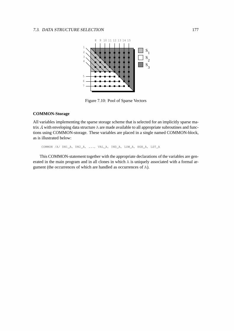
7.3. DATA STRUCTURE SELECTION 177
1
2
3
4
5
6
7
8 9 10 1211 13 14 15
S2
1S
3S
Figure 7.10: Pool of Sparse Vectors
COMMON-Storage
All variables implementing the sparse storage scheme that is selected for an implicitly sparse ma-trixAwith enveloping data structure A are made available to all appropriate subroutines and func-tions using COMMON-storage. These variables are placed in a single named COMMON-block,as is illustrated below:
COMMON /A/ DN1_A, DN2_A, ..., VAL_A, IND_A, LOW_A, HGH_A, LST_A
This COMMON-statement together with the appropriate declarations of the variables are gen-erated in the main program and in all clones in which A is uniquely associated with a formal ar-gument (the occurrences of which are handled as occurrences of A).
178 CHAPTER 7. PHASE 2: DATA STRUCTURE SELECTION
Chapter 8
Phase 3: Sparse Code Generation
In the third and final phase, the actual data structure transformations are applied by converting the(possibly adapted) dense code into a form that operates on the selected sparse storage schemes,thereby using overhead reducing techniques as much as possible. A small number of general prim-itives are supplied in a separate library, so that constructs that would otherwise appear frequentlyin the generated sparse code can be replaced by calls to the appropriate primitives. This approachtends to reduce the size of the generated sparse code whereas, on the other hand, the primitives arechosen general enough to leave the sparse compiler with enough flexibility in selecting data struc-tures. Identifiers of all subroutines and functions in this library, as well as all compiler generatedidentifiers contain underscores to prevent conflicts with identifiers in the original dense program.1
In this chapter, we first present the primitives that are supplied in the library. Thereafter, thegeneration of sparse code is presented in detail. Because the programmer remains unaware of theactual sparse storage scheme that is selected for each implicitly sparse matrix, the sparse compileris also responsible for generating appropriate initialization code, which is the final topic of thischapter.
8.1 The Library
The sparse compiler performs a source-to-source translation of a dense program into semanticallyequivalent sparse code. The resulting sparse program together with a library containing some use-ful primitives that may be used in this program are supplied to a conventional FORTRAN compilerfor the desired target architecture, as depicted below:
Library#
DenseProgram
!
SparseCompiler
!
SparseProgram
!
FORTRANCompiler
! Executable
To leave the sparse compiler with sufficient flexibility in the data structure selection, only asmall number of general primitives are supplied in this library. Supplying some primitives in alibrary, however, tends to reduce the size of the generated sparse program because constructs thatotherwise would appear frequently can be replaced by calls to the appropriate primitives. In addi-tion, several versions of the library that are fully hand-optimized for different target architecturescan be constructed in advance, which improves the efficiency of all sparse codes that are generatedfor one of these architectures.
1Here, we assume that identifiers in the original dense program adhere the ANSI FORTRAN 77-standard, whereasthe compiler used to compile the generated sparse code supports the use of underscores in identifiers.
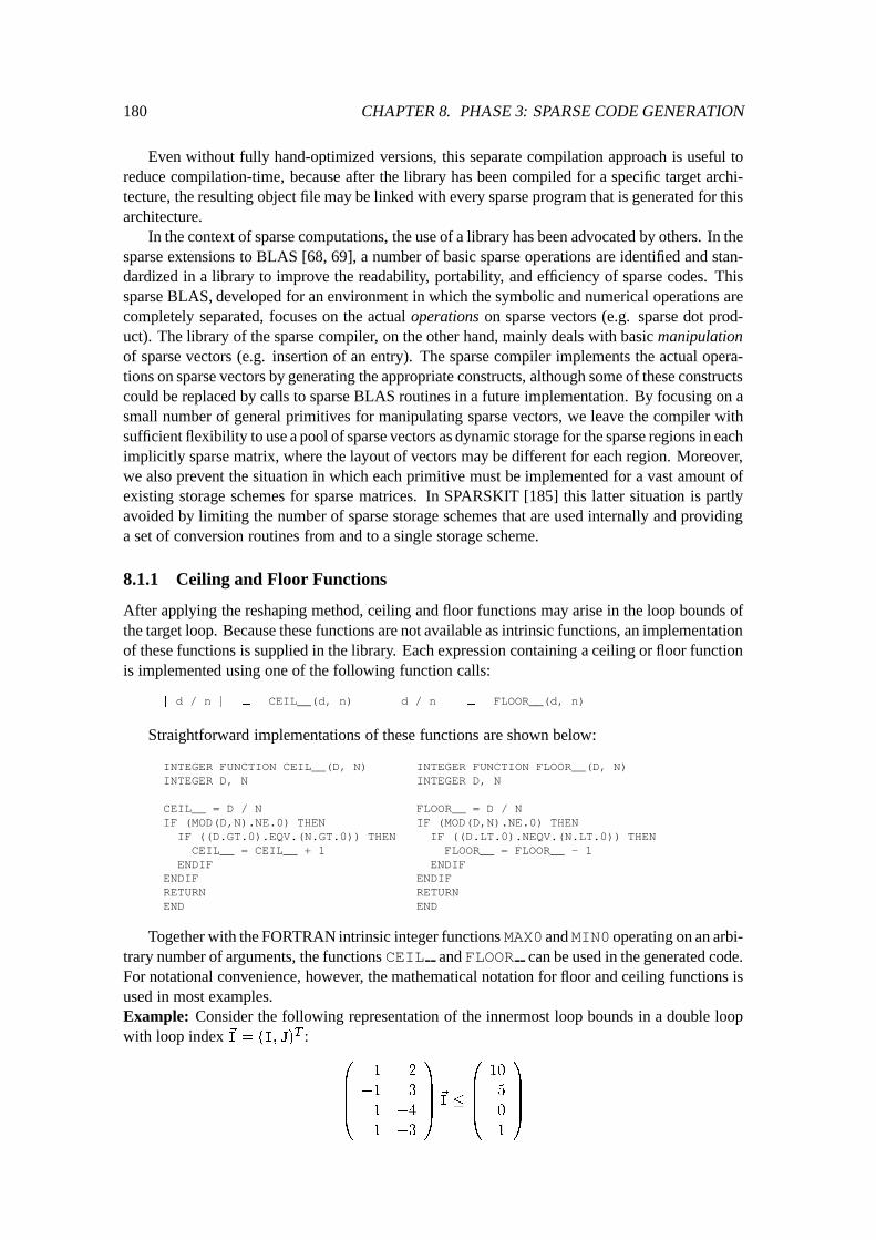
180 CHAPTER 8. PHASE 3: SPARSE CODE GENERATION
Even without fully hand-optimized versions, this separate compilation approach is useful toreduce compilation-time, because after the library has been compiled for a specific target archi-tecture, the resulting object file may be linked with every sparse program that is generated for thisarchitecture.
In the context of sparse computations, the use of a library has been advocated by others. In thesparse extensions to BLAS [68, 69], a number of basic sparse operations are identified and stan-dardized in a library to improve the readability, portability, and efficiency of sparse codes. Thissparse BLAS, developed for an environment in which the symbolic and numerical operations arecompletely separated, focuses on the actual operations on sparse vectors (e.g. sparse dot prod-uct). The library of the sparse compiler, on the other hand, mainly deals with basic manipulationof sparse vectors (e.g. insertion of an entry). The sparse compiler implements the actual opera-tions on sparse vectors by generating the appropriate constructs, although some of these constructscould be replaced by calls to sparse BLAS routines in a future implementation. By focusing on asmall number of general primitives for manipulating sparse vectors, we leave the compiler withsufficient flexibility to use a pool of sparse vectors as dynamic storage for the sparse regions in eachimplicitly sparse matrix, where the layout of vectors may be different for each region. Moreover,we also prevent the situation in which each primitive must be implemented for a vast amount ofexisting storage schemes for sparse matrices. In SPARSKIT [185] this latter situation is partlyavoided by limiting the number of sparse storage schemes that are used internally and providinga set of conversion routines from and to a single storage scheme.
8.1.1 Ceiling and Floor Functions
After applying the reshaping method, ceiling and floor functions may arise in the loop bounds ofthe target loop. Because these functions are not available as intrinsic functions, an implementationof these functions is supplied in the library. Each expression containing a ceiling or floor functionis implemented using one of the following function calls:
d d / n e � CEIL__(d, n) b d / n c � FLOOR__(d, n)
Straightforward implementations of these functions are shown below:
INTEGER FUNCTION CEIL__(D, N)INTEGER D, N
CEIL__ = D / NIF (MOD(D,N).NE.0) THENIF ((D.GT.0).EQV.(N.GT.0)) THENCEIL__ = CEIL__ + 1
ENDIFENDIFRETURNEND
INTEGER FUNCTION FLOOR__(D, N)INTEGER D, N
FLOOR__ = D / NIF (MOD(D,N).NE.0) THENIF ((D.LT.0).NEQV.(N.LT.0)) THEN
FLOOR__ = FLOOR__ - 1ENDIF
ENDIFRETURNEND
Together with the FORTRAN intrinsic integer functions MAX0 andMIN0 operating on an arbi-trary number of arguments, the functions CEIL and FLOOR can be used in the generated code.For notational convenience, however, the mathematical notation for floor and ceiling functions isused in most examples.Example: Consider the following representation of the innermost loop bounds in a double loopwith loop index ~I = (I; J)
T :0
B
B
B
@
1 2
�1 3
1 �4
1 �3
1
C
C
C
A
~
I �
0
B
B
B
@
10
5
0
1
1
C
C
C
A
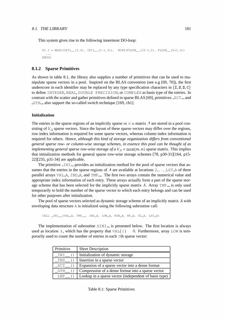
8.1. THE LIBRARY 181
This system gives rise to the following innermost DO-loop:
DO J = MAX0(CEIL__(I,4), CEIL__(I-1,3)), MIN0(FLOOR__(10-I,2), FLOOR__(5+I,3))...
ENDDO
8.1.2 Sparse Primitives
As shown in table 8.1, the library also supplies a number of primitives that can be used to ma-nipulate sparse vectors in a pool. Inspired on the BLAS convention (see e.g [69, 70]), the firstunderscore in each identifier may be replaced by any type specification characters in fI; S; D; Cgto define INTEGER, REAL, DOUBLE PRECISION, or COMPLEX as basis type of the entries. Incontrast with the scatter and gather primitives defined in sparse BLAS [69], primitives SCT andGTH also support the so-called switch technique [169, ch1].
Initialization
The entries in the sparse regions of an implicitly sparse m� n matrix A are stored in a pool con-sisting of V
A
sparse vectors. Since the layout of these sparse vectors may differ over the regions,row index information is required for some sparse vectors, whereas column index information isrequired for others. Hence, although this kind of storage organization differs from conventionalgeneral sparse row- or column-wise storage schemes, in essence this pool can be thought of asimplementing general sparse row-wise storage of a V
A
�max(m;n) sparse matrix. This impliesthat initialization methods for general sparse row-wise storage schemes [78, p30-31][164, p15-22][235, p31-34] are applicable.
The primitive INI provides an initialization method for the pool of sparse vectors that as-sumes that the entries in the sparse regions of A are available at locations 2; : : : ;LST A of threeparallel arrays VAL A, IND A, and TMP . The first two arrays contain the numerical value andappropriate index information of each entry. These arrays actually form a part of the sparse stor-age scheme that has been selected for the implicitly sparse matrix A. Array TMP is only usedtemporarily to hold the number of the sparse vector to which each entry belongs and can be usedfor other purposes after initialization.
The pool of sparse vectors selected as dynamic storage scheme of an implicitly matrix A withenveloping data structure A is initialized using the following subroutine call:
CALL _INI__(VAL_A, TMP__, IND_A, LOW_A, HGH_A, NP_A, SZ_A, LST_A)
The implementation of subroutine SINI is presented below. The first location is alwaysused as location ?, which has the property that VAL(?) = 0. Furthermore, array LOW is tem-porarily used to count the number of entries in each Ith sparse vector:
Primitive Short Description
_INI__() Initialization of dynamic storage_INS__() Insertion in a sparse vector_SCT__() Expansion of a sparse vector into a dense format_GTH__() Compression of a dense format into a sparse vectorLKP__() Lookup in a sparse vector (independent of basis type)
Table 8.1: Sparse Primitives
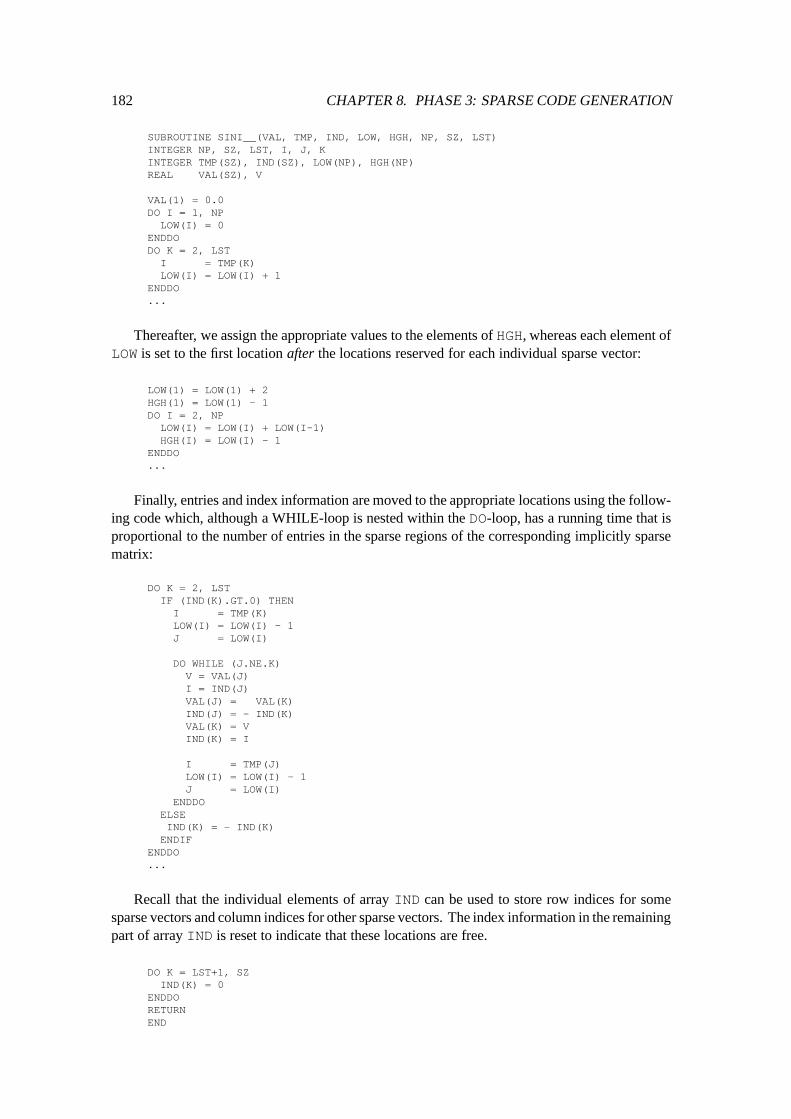
182 CHAPTER 8. PHASE 3: SPARSE CODE GENERATION
SUBROUTINE SINI__(VAL, TMP, IND, LOW, HGH, NP, SZ, LST)INTEGER NP, SZ, LST, I, J, KINTEGER TMP(SZ), IND(SZ), LOW(NP), HGH(NP)REAL VAL(SZ), V
VAL(1) = 0.0DO I = 1, NPLOW(I) = 0
ENDDODO K = 2, LSTI = TMP(K)LOW(I) = LOW(I) + 1
ENDDO...
Thereafter, we assign the appropriate values to the elements of HGH, whereas each element ofLOW is set to the first location after the locations reserved for each individual sparse vector:
LOW(1) = LOW(1) + 2HGH(1) = LOW(1) - 1DO I = 2, NPLOW(I) = LOW(I) + LOW(I-1)HGH(I) = LOW(I) - 1
ENDDO...
Finally, entries and index information are moved to the appropriate locations using the follow-ing code which, although a WHILE-loop is nested within the DO-loop, has a running time that isproportional to the number of entries in the sparse regions of the corresponding implicitly sparsematrix:
DO K = 2, LSTIF (IND(K).GT.0) THENI = TMP(K)LOW(I) = LOW(I) - 1J = LOW(I)
DO WHILE (J.NE.K)V = VAL(J)I = IND(J)VAL(J) = VAL(K)IND(J) = - IND(K)VAL(K) = VIND(K) = I
I = TMP(J)LOW(I) = LOW(I) - 1J = LOW(I)
ENDDOELSEIND(K) = - IND(K)
ENDIFENDDO...
Recall that the individual elements of array IND can be used to store row indices for somesparse vectors and column indices for other sparse vectors. The index information in the remainingpart of array IND is reset to indicate that these locations are free.
DO K = LST+1, SZIND(K) = 0
ENDDORETURNEND
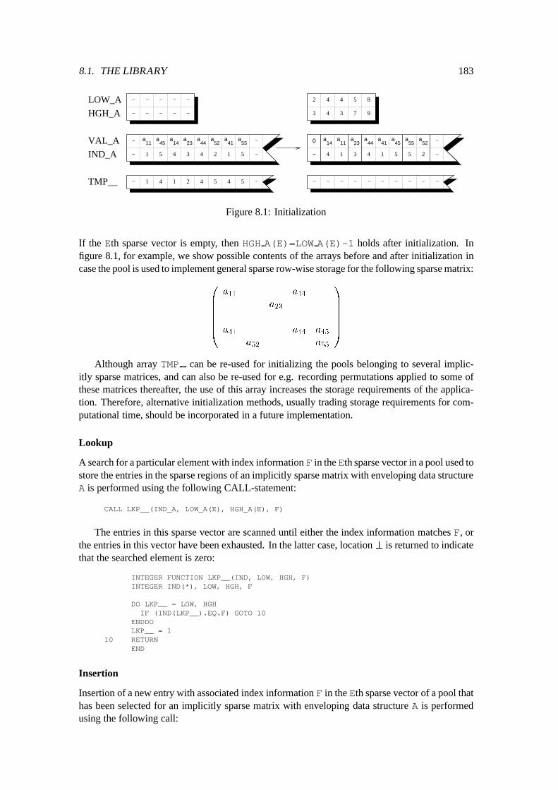
8.1. THE LIBRARY 183
aa a a a a a a
2
11
1
45 14 23 44 52 41 55
5 4 3 4 1 5−
VAL_A
IND_A
21 4 1 4 5 4 5
0
2
a11
1
a45
a14
a23
a44
a52
a41
a55
54 3 4 1 5−
4
4
LOW_A
HGH_A
−
−
−
−
−
−
−
−
−
−
−
−
−
− − − − − − − − − − −
−
−−
2
3
4
3
5
7
8
9
TMP__
Figure 8.1: Initialization
If the Eth sparse vector is empty, then HGH A(E)=LOW A(E)-1 holds after initialization. Infigure 8.1, for example, we show possible contents of the arrays before and after initialization incase the pool is used to implement general sparse row-wise storage for the following sparse matrix:
0
B
B
B
B
B
@
a
11
a
14
a
23
a
41
a
44
a
45
a
52
a
55
1
C
C
C
C
C
A
Although array TMP can be re-used for initializing the pools belonging to several implic-itly sparse matrices, and can also be re-used for e.g. recording permutations applied to some ofthese matrices thereafter, the use of this array increases the storage requirements of the applica-tion. Therefore, alternative initialization methods, usually trading storage requirements for com-putational time, should be incorporated in a future implementation.
Lookup
A search for a particular element with index information F in the Eth sparse vector in a pool used tostore the entries in the sparse regions of an implicitly sparse matrix with enveloping data structureA is performed using the following CALL-statement:
CALL LKP__(IND_A, LOW_A(E), HGH_A(E), F)
The entries in this sparse vector are scanned until either the index information matches F, orthe entries in this vector have been exhausted. In the latter case, location ? is returned to indicatethat the searched element is zero:
INTEGER FUNCTION LKP__(IND, LOW, HGH, F)INTEGER IND(*), LOW, HGH, F
DO LKP__ = LOW, HGHIF (IND(LKP__).EQ.F) GOTO 10
ENDDOLKP__ = 1
10 RETURNEND
Insertion
Insertion of a new entry with associated index information F in the Eth sparse vector of a pool thathas been selected for an implicitly sparse matrix with enveloping data structure A is performedusing the following call:
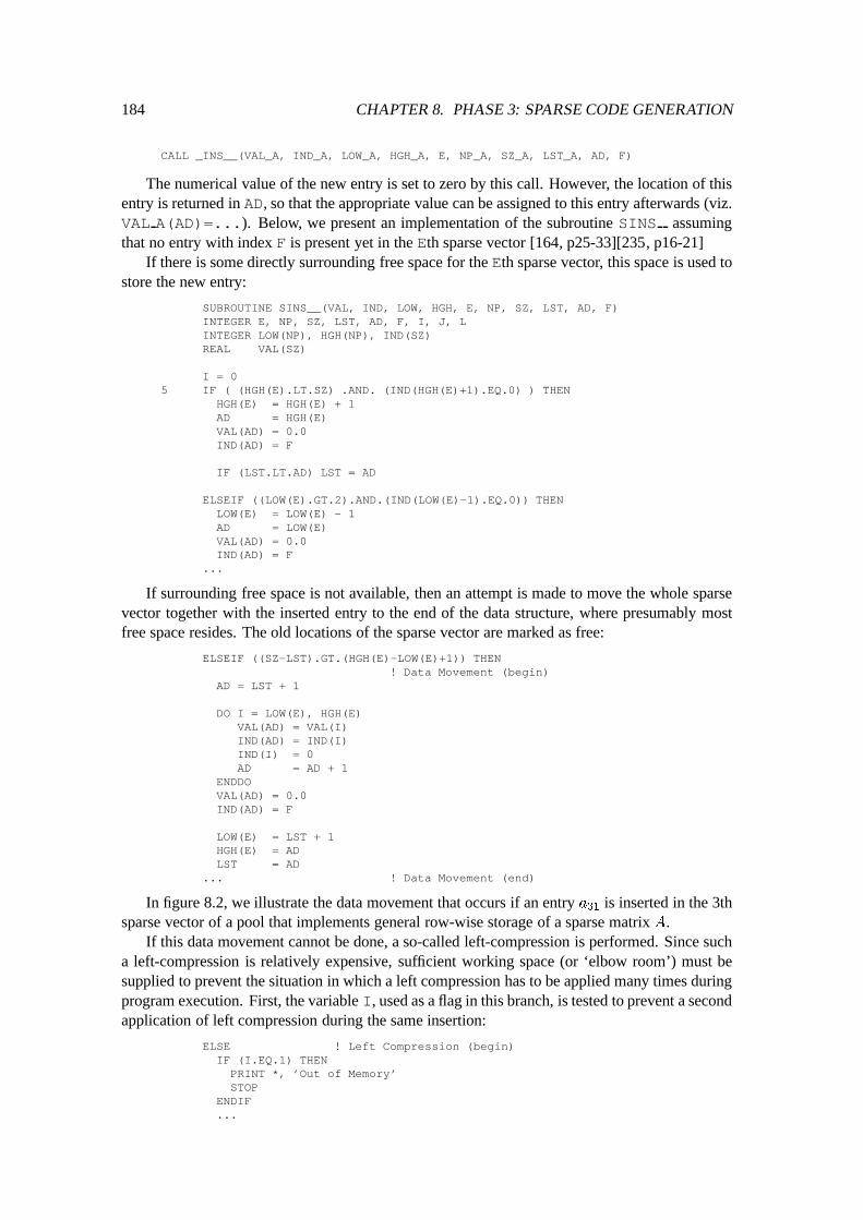
184 CHAPTER 8. PHASE 3: SPARSE CODE GENERATION
CALL _INS__(VAL_A, IND_A, LOW_A, HGH_A, E, NP_A, SZ_A, LST_A, AD, F)
The numerical value of the new entry is set to zero by this call. However, the location of thisentry is returned in AD, so that the appropriate value can be assigned to this entry afterwards (viz.VAL A(AD)=...). Below, we present an implementation of the subroutine SINS assumingthat no entry with index F is present yet in the Eth sparse vector [164, p25-33][235, p16-21]
If there is some directly surrounding free space for the Eth sparse vector, this space is used tostore the new entry:
SUBROUTINE SINS__(VAL, IND, LOW, HGH, E, NP, SZ, LST, AD, F)INTEGER E, NP, SZ, LST, AD, F, I, J, LINTEGER LOW(NP), HGH(NP), IND(SZ)REAL VAL(SZ)
I = 05 IF ( (HGH(E).LT.SZ) .AND. (IND(HGH(E)+1).EQ.0) ) THEN
HGH(E) = HGH(E) + 1AD = HGH(E)VAL(AD) = 0.0IND(AD) = F
IF (LST.LT.AD) LST = AD
ELSEIF ((LOW(E).GT.2).AND.(IND(LOW(E)-1).EQ.0)) THENLOW(E) = LOW(E) - 1AD = LOW(E)VAL(AD) = 0.0IND(AD) = F
...
If surrounding free space is not available, then an attempt is made to move the whole sparsevector together with the inserted entry to the end of the data structure, where presumably mostfree space resides. The old locations of the sparse vector are marked as free:
ELSEIF ((SZ-LST).GT.(HGH(E)-LOW(E)+1)) THEN! Data Movement (begin)
AD = LST + 1
DO I = LOW(E), HGH(E)VAL(AD) = VAL(I)IND(AD) = IND(I)IND(I) = 0AD = AD + 1
ENDDOVAL(AD) = 0.0IND(AD) = F
LOW(E) = LST + 1HGH(E) = ADLST = AD
... ! Data Movement (end)
In figure 8.2, we illustrate the data movement that occurs if an entry a31
is inserted in the 3thsparse vector of a pool that implements general row-wise storage of a sparse matrix A.
If this data movement cannot be done, a so-called left-compression is performed. Since sucha left-compression is relatively expensive, sufficient working space (or ‘elbow room’) must besupplied to prevent the situation in which a left compression has to be applied many times duringprogram execution. First, the variable I, used as a flag in this branch, is tested to prevent a secondapplication of left compression during the same insertion:
ELSE ! Left Compression (begin)IF (I.EQ.1) THEN
PRINT *, ’Out of Memory’STOP
ENDIF...
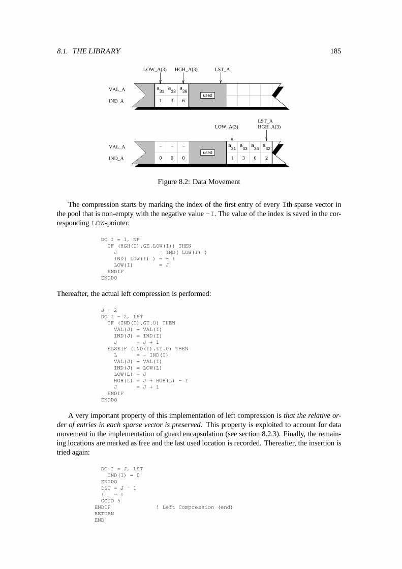
8.1. THE LIBRARY 185
a33
a31
31 6
a36
HGH_A(3)LOW_A(3)
VAL_A
IND_A
LST_A
used
a33
a31
31 6
a36
HGH_A(3)LOW_A(3)
VAL_A
IND_A
LST_A
used
a32
20 0 0
−−−
Figure 8.2: Data Movement
The compression starts by marking the index of the first entry of every Ith sparse vector inthe pool that is non-empty with the negative value -I. The value of the index is saved in the cor-responding LOW-pointer:
DO I = 1, NPIF (HGH(I).GE.LOW(I)) THENJ = IND( LOW(I) )IND( LOW(I) ) = - ILOW(I) = J
ENDIFENDDO
Thereafter, the actual left compression is performed:
J = 2DO I = 2, LST
IF (IND(I).GT.0) THENVAL(J) = VAL(I)IND(J) = IND(I)J = J + 1
ELSEIF (IND(I).LT.0) THENL = - IND(I)VAL(J) = VAL(I)IND(J) = LOW(L)LOW(L) = JHGH(L) = J + HGH(L) - IJ = J + 1
ENDIFENDDO
A very important property of this implementation of left compression is that the relative or-der of entries in each sparse vector is preserved. This property is exploited to account for datamovement in the implementation of guard encapsulation (see section 8.2.3). Finally, the remain-ing locations are marked as free and the last used location is recorded. Thereafter, the insertion istried again:
DO I = J, LSTIND(I) = 0
ENDDOLST = J - 1I = 1GOTO 5
ENDIF ! Left Compression (end)RETURNEND
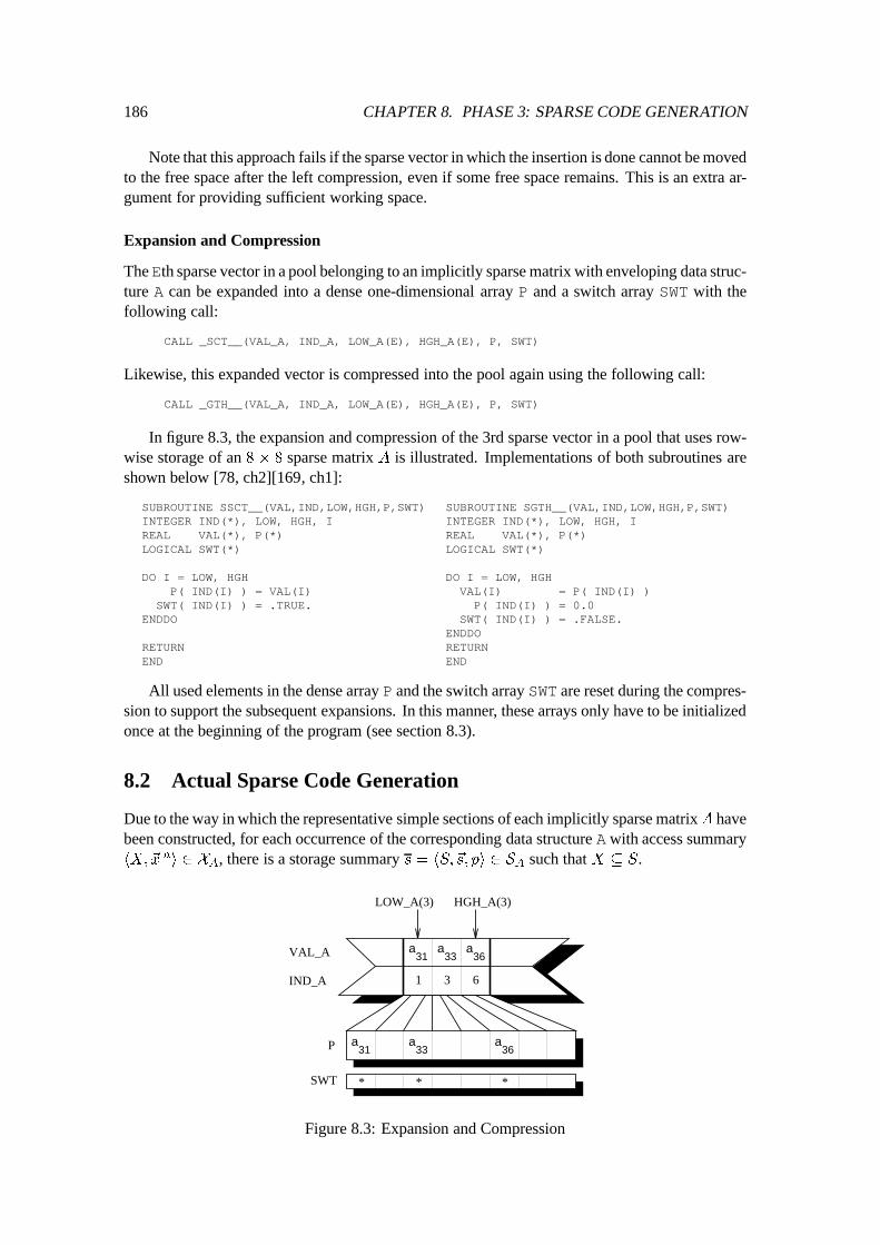
186 CHAPTER 8. PHASE 3: SPARSE CODE GENERATION
Note that this approach fails if the sparse vector in which the insertion is done cannot be movedto the free space after the left compression, even if some free space remains. This is an extra ar-gument for providing sufficient working space.
Expansion and Compression
TheEth sparse vector in a pool belonging to an implicitly sparse matrix with enveloping data struc-ture A can be expanded into a dense one-dimensional array P and a switch array SWT with thefollowing call:
CALL _SCT__(VAL_A, IND_A, LOW_A(E), HGH_A(E), P, SWT)
Likewise, this expanded vector is compressed into the pool again using the following call:
CALL _GTH__(VAL_A, IND_A, LOW_A(E), HGH_A(E), P, SWT)
In figure 8.3, the expansion and compression of the 3rd sparse vector in a pool that uses row-wise storage of an 8 � 8 sparse matrix A is illustrated. Implementations of both subroutines areshown below [78, ch2][169, ch1]:
SUBROUTINE SSCT__(VAL,IND,LOW,HGH,P,SWT)INTEGER IND(*), LOW, HGH, IREAL VAL(*), P(*)LOGICAL SWT(*)
DO I = LOW, HGHP( IND(I) ) = VAL(I)
SWT( IND(I) ) = .TRUE.ENDDO
RETURNEND
SUBROUTINE SGTH__(VAL,IND,LOW,HGH,P,SWT)INTEGER IND(*), LOW, HGH, IREAL VAL(*), P(*)LOGICAL SWT(*)
DO I = LOW, HGHVAL(I) = P( IND(I) )
P( IND(I) ) = 0.0SWT( IND(I) ) = .FALSE.
ENDDORETURNEND
All used elements in the dense array P and the switch array SWT are reset during the compres-sion to support the subsequent expansions. In this manner, these arrays only have to be initializedonce at the beginning of the program (see section 8.3).
8.2 Actual Sparse Code Generation
Due to the way in which the representative simple sections of each implicitly sparse matrixA havebeen constructed, for each occurrence of the corresponding data structure A with access summaryhX;~x
n
i 2 X
A
, there is a storage summary s = hS;~s; pi 2 SA
such that X � S.
a33
a31
31 6
a36
HGH_A(3)LOW_A(3)
VAL_A
IND_A
a33
a36
a31
* * *SWT
P
Figure 8.3: Expansion and Compression
8.2. ACTUAL SPARSE CODE GENERATION 187
In this case, we refer to the storage summary s as the storage summary that matches the oc-currence of A. Since p 2 fzero;dense; sparseg, we can distinguish between occurrences ofenveloping data structures accessing a part of the array corresponding to a zero, dense, or sparseregion in an implicitly sparse matrix. We refer to these occurrences as zero, dense, and sparseoccurrences, respectively.
In this section, we present a method to generate sparse code by applying the appropriate datastructure transformations to these occurrences. The method assumes that subscript bounds are notviolated in the original dense program, because otherwise subscripts of static dense storage or thepointers used to locate sparse vectors in the pool may also be violated in the generated sparse code.Since for some dense programs, out-of-bounds addressing is actually intended, the semantics ofthe program could be affected. Therefore, dense programs in which potential subscript violationsarise are not converted by the prototype sparse compiler.
8.2.1 Zero and Dense Occurrences
Suppose that the storage summary s = hS; (s1
; s
2
)
T
; pi 2 S
A
with p 2 fzero;denseg matchesan arbitrary occurrence A(E1,E2) in the program, where E1 and E2 denote the (possibly in-admissible) subscripts. If p = zero, then we replace the occurrence with a zero constant of theappropriate type, depending on the basis type of the enveloping data structure A:
basis type constantINTEGER 0REAL 0.0DOUBLE PRECISION 0.0DCOMPLEX CMPLX(0.0,0.0)
If p = dense, then we replace the occurrence with the following expression, where the secondsubscript is omitted if L(s) = U(s):
DNk_A(E, s
2
* E1 - s
1
* E2)
In this replacement, k = lab(s) and subscript E is defined as follows:
E =
(
E1 if �(s) = row-indexedE2 otherwise
After all such replacements are done in a statement, the conditions of this statement and sur-rounding IF-statements and DO-loops are re-computed. If the condition of a statement becomes‘false’ (which is only possible if this statement does not call any function with side-effects), thenthis statement is eliminated from the program (recall that we always assume that the final valueof a loop index is not used after a DO-loop).Example: As an extreme example, if we know that A = 0 holds for an implicitly sparse matrixwith enveloping data structure A, then the following fragment computing~b = A~x is converted asshown below:
REAL A(M,N), B(M), X(N)C_SPARSE(A : _ZERO() )
...DO I = 1, M
B(I) = 0.0DO J = 1, N
B(I) = B(I) + A(I,J) * X(J)ENDDO
ENDDO
!
REAL B(M), X(N)...DO I = 1, M
B(I) = 0.0ENDDO
188 CHAPTER 8. PHASE 3: SPARSE CODE GENERATION
The storage summary set SA
= fhS;
~
0; zeroig results, where S contains the whole indexset of A. Consequently, the occurrence of A is replaced by ‘0.0’, which converts the conditionsof the resulting assignment statement and surrounding J-loop into ‘false’. By cleaning up thecode accordingly, the fragment is automatically converted into code that performs the appropriateoperation~b = A~x =
~
0.Example: Replacement may also alter the condition of a statement in another manner. For ex-ample, if besides the implicitly sparse matrix of the previous example, we also have an implicitlysparse matrixB with enveloping data structure B, then the following conversion is done (the sparseoccurrence B(I,J) will be handled as explained in subsequent sections):
DO I = 1, MDO J = 1, NX = X + 3 * (A(I,J) + B(I,I))
ENDDOENDDO
!
DO I = 1, MDO J = 1, NX = X + 3 * (0.0 + B(I,I))
ENDDOENDDO
This affects the condition of the assignment statement as follows, which implies that guardencapsulation may become feasible because the guard ‘(I; I) 2 E(B)’ dominates the conditionafterwards:
(I; J) 2 E(A) _ (I; I) 2 E(B) ! (I; I) 2 E(B)
Example: A similar, but less trivial, example is shown below. The condition that has been asso-ciated with the original IF-statement is ‘(I; J) 2 E(A) _ (I; J) 2 E(B)_ (2; 2) 2 E(A)’. Afterreplacing both occurrences of A by zero, however, we have E.t=false for the boolean expression,while the condition of the last assignment statement becomes ‘false’. Hence, the condition of thewhole IF-statement changes into ‘ (I; J) 2 E(B)’:
IF (A(I,J).NE.0.0) THENNNZ = NNZ + 1
ELSEACC = ACC + B(I,J)A(2,2) = A(2,2) * 3.0
ENDDO
!
IF (0.0.NE.0.0) THEN (I; J) 2 E(B)
NNZ = NNZ + 1 true
ELSEACC = ACC + B(I,J) (I; J) 2 E(B)
ENDDO
In fact, the whole construct could be replaced by the ELSE-branch.
8.2.2 Preparatory Pass over Sparse Occurrences
Before any code is generated for the sparse occurrences of the enveloping data structure A of eachimplicitly sparse matrix A, a preparatory pass over the sparse occurrences with admissible sub-scripts is made to determine which occurrences may be involved in a guard encapsulation or accesspattern expansion. During examination of an occurrence of array A, we refer to this occurrence asthe candidate.
Suppose that s = hS; (s
1
; s
2
)
T
; sparsei 2 S
A
matches a candidate with access summaryhX;~x
n
i 2 X
A
and admissible subscripts F (~I) = ~v + W
~
I in a loop with index vector ~I anditeration space IS � Zd. Then, we define the e-tag of the candidate as follows, where base(s)contains the base-location of the access summary in the pool of sparse vectors:
e(
~
I) = base(s)�L(s) + (+s
2
;�s
1
) � F (
~
I)
The f-tag of the candidate is defined as shown below:
f(
~
I) =
(
(1; 0) � F (
~
I) if �(s) = row-indexed(0; 1) � F (
~
I) otherwise
8.2. ACTUAL SPARSE CODE GENERATION 189
During each iteration~I =~{, an element in the e(~{ )th sparse vector of the pool with associatedindex information f(~{ ) will be accessed. Obviously, we could generate lookup code directly, butthis would yield very inefficient sparse code and should only be used as a last resort.
If the effective access patterns of the candidate and the storage patterns are consistent, i.e.~x
n
= (s
1
; s
2
)
T , then either guard encapsulation or access pattern expansion may be feasible,because entries along each e(~I)th sparse vector can be generated efficiently together with the ap-propriate index information (cf. constraints (a) and (b) at page 84). It can be easily verified thatin this case there is a 1 � p � d such that both the e-tag and f-tag can be expressed as follows,where f
p
6= 0 :
(
e(
~
I) = e
0
+ e
1
� I
1
+ : : :+ e
p�1
� I
p�1
f(
~
I) = f
0
+ f
1
� I
1
+ : : : + f
p�1
� I
p�1
+ f
p
� I
p
(8.1)
Candidates for Guard Encapsulation
If guard ‘F (~I) 2 E(A)’ dominates the loop-body of the Ip
-loop (see section 5.3.2), and thisDO-loop is a stride-1 DO-loop with admissible loop bounds that has not been involved in a guardencapsulation before, then the candidate and the I
p
-loop can be involved in a guard encapsulationif the following two constraints are also satisfied.
To prevent the requirement for ordered storage , we require that the iterations of this DO-loopmay be executed in arbitrary order (cf. constraint (c) at page 84):
� No data dependence is carried by the Ip
-loop and no exit branch [234, p238-241] or STOP-statement can be executed in the loop-body of this DO-loop.
Additionally, to simplify code generation and, again, to prevent the need for ordered storage,we impose the following constraint:
� During each fixed iteration I
1
= i
1
; : : : ; I
p�1
= i
p�1
, insertions in the e(~I)th sparse vectorof the pool cannot occur.
If the first constraint is violated, the sparse compiler inquires the programmer whether the pro-hibitive loop-carried data dependences may be ignored (cf. section 4.3.1).
Verifying the second constraint requires more effort. All occurrences of the same envelop-ing data structure A appearing at the left-hand side of assignment statements in the loop-body ofthe I
p
-loop are examined. If the subscripts of such a left-hand side occurrence are structurallyequivalent to the subscripts F (~I) of the candidate, which means that coefficients of loop indicesin the common nesting depth of the two statements in which the occurrences appear are identicalwhereas all other coefficients are zero, then this left-hand side occurrence cannot induce insertion(viz. the corresponding guard dominates the loop-body). Likewise, if the storage summary thatmatches the left-hand side occurrence differs from s, the last constraint is still satisfied, althoughinsertions in other sparse vectors of the same pool may occur in this case.
Otherwise, a more expensive test is required. First, we construct the e-tag e0(~J) of the left-handside occurrence, where ~J denotes the index vector of the loop in which this occurrence appears,together with a (conservative) representation A~J � ~
b of the iteration space of this loop, whereinadmissible loop bounds are handled by leaving the corresponding loop indices unbounded. Be-cause the first p components of ~I and~J are equal and the e-tag e(~I) of the candidate only dependson indices I
1
; : : : ; I
p�1
, the last constraint may be violated if the following equation has an integersolution for A~J � ~b:2
2This test strongly resembles the test performed during data dependence analysis while testing for the data directionvector (=; : : : ;=; �; : : : ; �), although here the granularity is increased to sparse vectors rather than individual elements.
190 CHAPTER 8. PHASE 3: SPARSE CODE GENERATION
e(
~
I) = e
0
(
~
J)
Fourier-Motzkin elimination is used to test the consistency of the system of inequalities arisingfrom the representation of the iteration space and this equation (rewritten into e(~I) � e
0
(
~
J) ande
0
(
~
J) � e(
~
I)). If this system is consistent or if the e-tag of the left-hand side occurrence cannotbe constructed due to inadmissible subscripts, we conservatively assume that the last constraint isviolated and disable guard encapsulation. If Fourier-Motzkin elimination reveals that the systemis inconsistent, we may safely conclude that the last condition is not violated, although we stillassume that insertions in other sparse vectors of the same pool may occur.
If all constraints are satisfied, then we record that encapsulation of the dominating guard isfeasible for the I
p
-loop and the candidate (and all occurrences of enveloping data structure A inthe loop-body having structurally equivalent subscripts). If insertions in other sparse vectors ofthe same pool may occur, this is also recorded because eventually this must be dealt with in theactual implementation of guard encapsulation.Example: Consider the following example, in which an annotation is used to enforce the selectionof general sparse row-wise storage for an implicitly sparse matrix A:
REAL A(100,100)C_SPARSE(A: _SPARSE( )(0,1))
...DO I = 1, 50
DO J = I+1, 100X(J) = X(J) + A(I,J) (I; J) 2 E(A)
DO K = 1, 100 (I; J) 2 E(A)
A(J,K) = A(J,K) + A(I,J) (I; J) 2 E(A)
ENDDOA(I,J) = A(I,J) * 2.0 (I; J) 2 E(A)
ENDDOENDDO
The true and, hence effective access patterns of the first occurrence of A are consistent withthe storage patterns. When this occurrence becomes the candidate, the following e-tag and f-tagare constructed (viz. p = 2), where ~I = (I; J)
T :3
e(
~
I) = 1 � I
f(
~
I) = 0 � I+ 1 � J
Because guard ‘(I; J) 2 E(A)’ dominates the loop-body of the J-loop and no data depen-dences are carried by this DO-loop, we test whether insertion in the Ith sparse vector of the pool(i.e. the Ith row in this case) may occur during a fixed iteration I = i. Therefore, the occurrencesA(J,K) and A(I,J) appearing at the left-hand side of assignment statements in the J-loop areexamined. Because the subscripts of the latter are structurally equivalent to the subscripts of thecandidate, only the former is further examined. The following system of linear inequalities is con-structed, where ~J = (I; J; K)
T and e0(~J) = J:0
B
B
B
B
B
B
B
B
B
B
B
B
@
0 0 1 100
0 0 �1 �1
0 1 0 100
1 �1 0 �1
1 0 0 50
�1 0 0 �1
�1 1 0 0
1 �1 0 0
1
C
C
C
C
C
C
C
C
C
C
C
C
A
9
>
>
>
>
>
>
>
=
>
>
>
>
>
>
>
;
A
~
J �
~
b
)
e(
~
I) = e
0
(
~
J)
3Note that if the second occurrence A(I,J)would become the candidate, we would obtain a structurally equivalente-tag and f-tag for ~I = (I; J; K)
T .
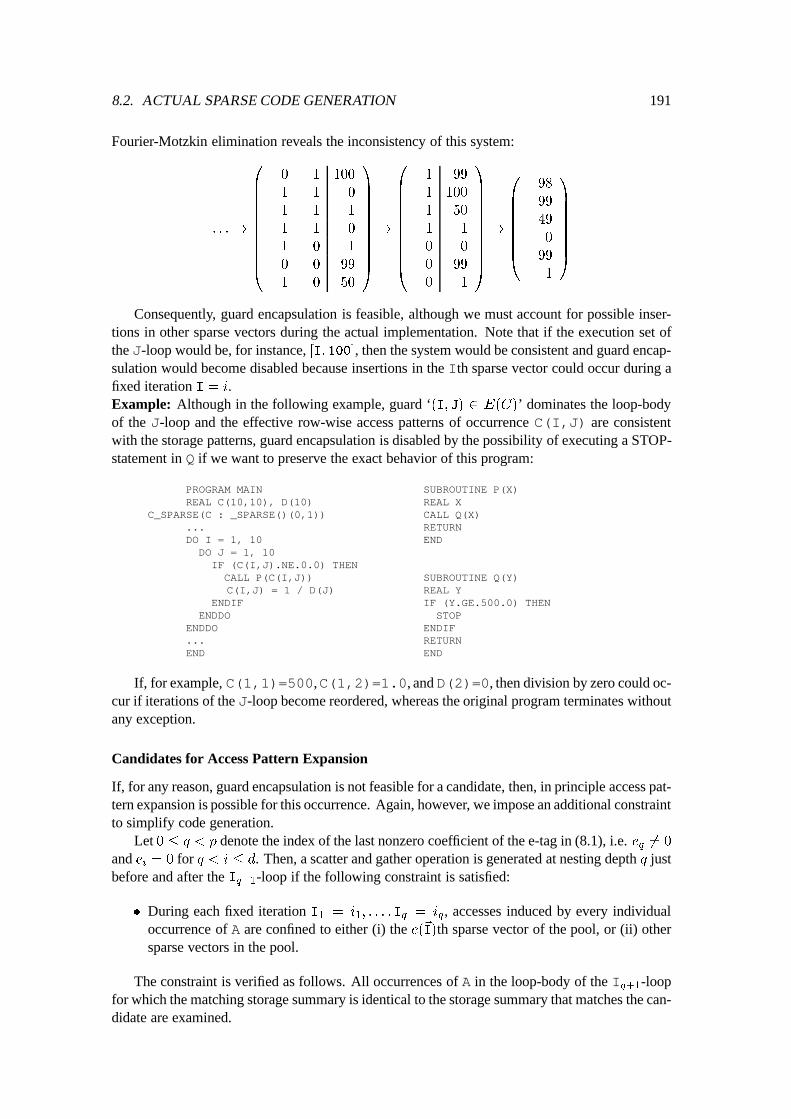
8.2. ACTUAL SPARSE CODE GENERATION 191
Fourier-Motzkin elimination reveals the inconsistency of this system:
: : :!
0
B
B
B
B
B
B
B
B
B
B
@
0 1 100
�1 1 0
1 �1 �1
1 �1 0
�1 0 �1
0 0 99
1 0 50
1
C
C
C
C
C
C
C
C
C
C
A
!
0
B
B
B
B
B
B
B
B
B
B
@
1 99
1 100
1 50
�1 �1
0 0
0 99
0 �1
1
C
C
C
C
C
C
C
C
C
C
A
!
0
B
B
B
B
B
B
B
@
98
99
49
0
�99
�1
1
C
C
C
C
C
C
C
A
Consequently, guard encapsulation is feasible, although we must account for possible inser-tions in other sparse vectors during the actual implementation. Note that if the execution set ofthe J-loop would be, for instance, [I; 100], then the system would be consistent and guard encap-sulation would become disabled because insertions in the Ith sparse vector could occur during afixed iteration I = i.Example: Although in the following example, guard ‘(I; J) 2 E(C)’ dominates the loop-bodyof the J-loop and the effective row-wise access patterns of occurrence C(I,J) are consistentwith the storage patterns, guard encapsulation is disabled by the possibility of executing a STOP-statement in Q if we want to preserve the exact behavior of this program:
PROGRAM MAINREAL C(10,10), D(10)
C_SPARSE(C : _SPARSE()(0,1))...DO I = 1, 10
DO J = 1, 10IF (C(I,J).NE.0.0) THENCALL P(C(I,J))C(I,J) = 1 / D(J)
ENDIFENDDO
ENDDO...END
SUBROUTINE P(X)REAL XCALL Q(X)RETURNEND
SUBROUTINE Q(Y)REAL YIF (Y.GE.500.0) THEN
STOPENDIFRETURNEND
If, for example, C(1,1)=500,C(1,2)=1.0, and D(2)=0, then division by zero could oc-cur if iterations of the J-loop become reordered, whereas the original program terminates withoutany exception.
Candidates for Access Pattern Expansion
If, for any reason, guard encapsulation is not feasible for a candidate, then, in principle access pat-tern expansion is possible for this occurrence. Again, however, we impose an additional constraintto simplify code generation.
Let 0 � q < p denote the index of the last nonzero coefficient of the e-tag in (8.1), i.e. eq
6= 0
and ei
= 0 for q < i � d. Then, a scatter and gather operation is generated at nesting depth q justbefore and after the I
q+1
-loop if the following constraint is satisfied:
� During each fixed iteration I
1
= i
1
; : : : ; I
q
= i
q
, accesses induced by every individualoccurrence of A are confined to either (i) the e(~I)th sparse vector of the pool, or (ii) othersparse vectors in the pool.
The constraint is verified as follows. All occurrences of A in the loop-body of the Iq+1
-loopfor which the matching storage summary is identical to the storage summary that matches the can-didate are examined.
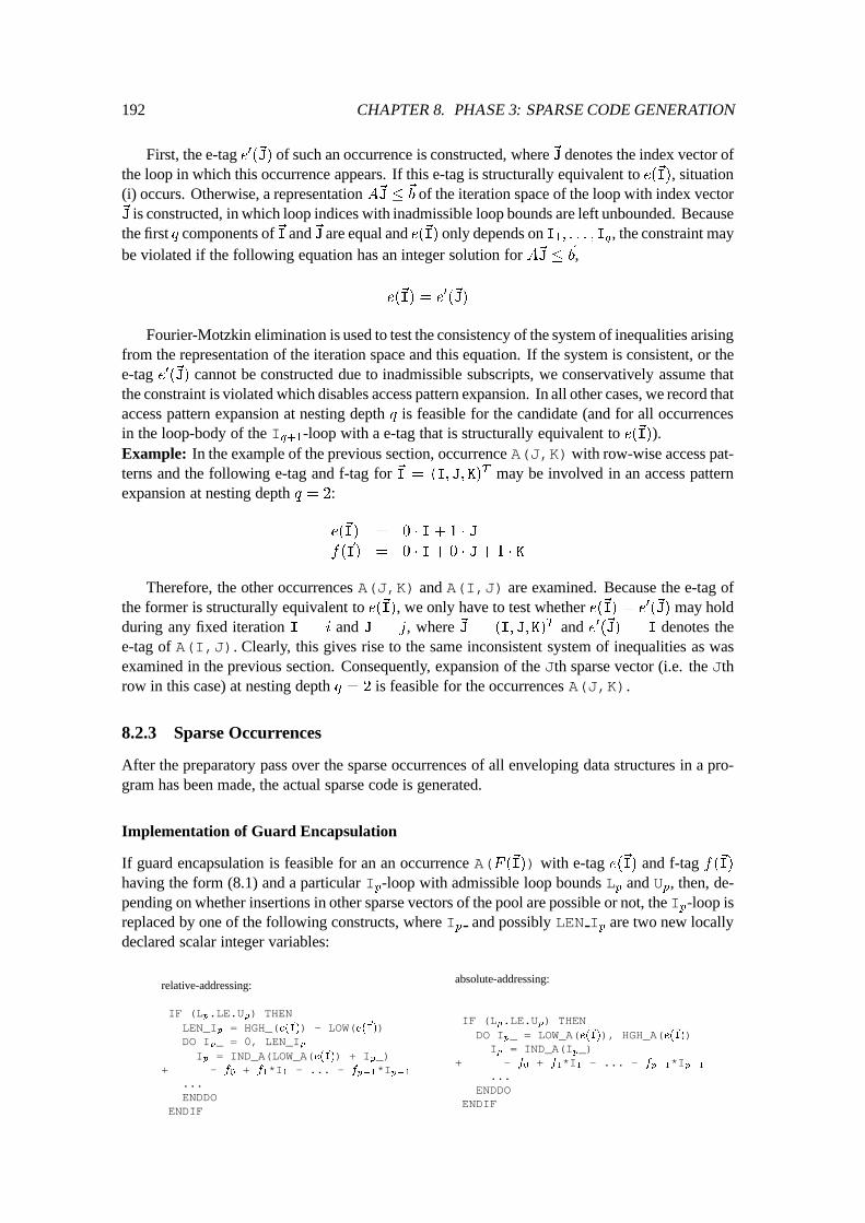
192 CHAPTER 8. PHASE 3: SPARSE CODE GENERATION
First, the e-tag e0(~J) of such an occurrence is constructed, where~J denotes the index vector ofthe loop in which this occurrence appears. If this e-tag is structurally equivalent to e(~I), situation(i) occurs. Otherwise, a representation A~J � ~b of the iteration space of the loop with index vector~
J is constructed, in which loop indices with inadmissible loop bounds are left unbounded. Becausethe first q components of~I and~J are equal and e(~I) only depends on I
1
; : : : ; I
q
, the constraint maybe violated if the following equation has an integer solution for A~J � ~b,
e(
~
I) = e
0
(
~
J)
Fourier-Motzkin elimination is used to test the consistency of the system of inequalities arisingfrom the representation of the iteration space and this equation. If the system is consistent, or thee-tag e0(~J) cannot be constructed due to inadmissible subscripts, we conservatively assume thatthe constraint is violated which disables access pattern expansion. In all other cases, we record thataccess pattern expansion at nesting depth q is feasible for the candidate (and for all occurrencesin the loop-body of the I
q+1
-loop with a e-tag that is structurally equivalent to e(~I)).Example: In the example of the previous section, occurrence A(J,K)with row-wise access pat-terns and the following e-tag and f-tag for ~I = (I; J; K)
T may be involved in an access patternexpansion at nesting depth q = 2:
e(
~
I) = 0 � I+ 1 � J
f(
~
I) = 0 � I+ 0 � J+ 1 � K
Therefore, the other occurrences A(J,K) and A(I,J) are examined. Because the e-tag ofthe former is structurally equivalent to e(~I), we only have to test whether e(~I) = e
0
(
~
J) may holdduring any fixed iteration I = i and J = j, where ~J = (I; J; K)
T and e0(~J) = I denotes thee-tag of A(I,J). Clearly, this gives rise to the same inconsistent system of inequalities as wasexamined in the previous section. Consequently, expansion of the Jth sparse vector (i.e. the Jthrow in this case) at nesting depth q = 2 is feasible for the occurrences A(J,K).
8.2.3 Sparse Occurrences
After the preparatory pass over the sparse occurrences of all enveloping data structures in a pro-gram has been made, the actual sparse code is generated.
Implementation of Guard Encapsulation
If guard encapsulation is feasible for an an occurrence A(F (~I)) with e-tag e(~I) and f-tag f(~I)having the form (8.1) and a particular I
p
-loop with admissible loop bounds Lp
and Up
, then, de-pending on whether insertions in other sparse vectors of the pool are possible or not, the I
p
-loop isreplaced by one of the following constructs, where I
p
and possibly LEN Ip
are two new locallydeclared scalar integer variables:
relative-addressing:
IF (Lp
.LE.Up
) THENLEN_I
p
= HGH_(e(~I)) - LOW(e(~I))DO I
p
_ = 0, LEN_Ip
Ip
= IND_A(LOW_A(e(~I)) + Ip
_)+ - f
0
+ f
1
*I1
- ... - f
p�1
*Ip�1
...ENDDO
ENDIF
absolute-addressing:
IF (Lp
.LE.Up
) THENDO I
p
_ = LOW_A(e(~I)), HGH_A(e(~I))Ip
= IND_A(Ip
_)+ - f
0
+ f
1
*I1
- ... - f
p�1
*Ip�1
...ENDDO
ENDIF
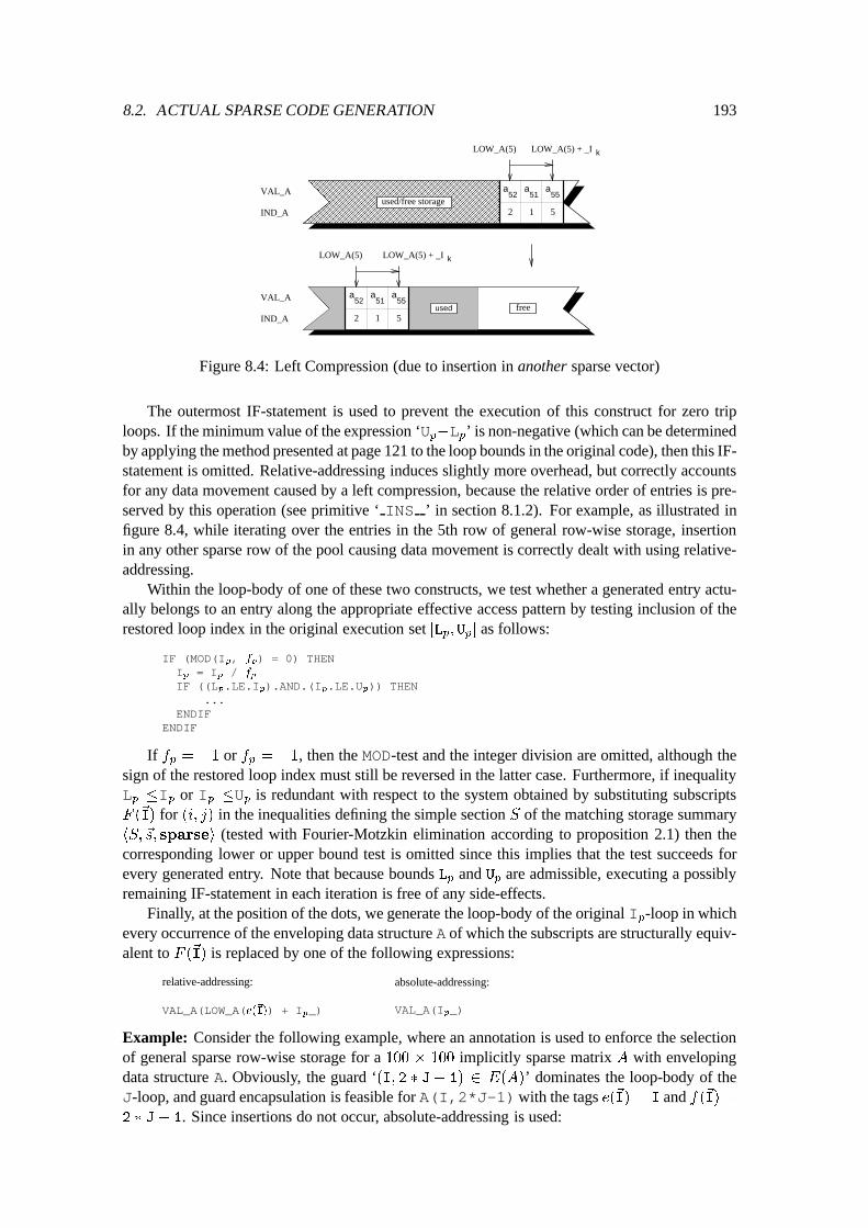
8.2. ACTUAL SPARSE CODE GENERATION 193
VAL_A
IND_A
VAL_A
IND_Aused
aa a52 5551
12 5
LOW_A(5)
used/free storage
aa a52 5551
12 5
LOW_A(5)
free
k
k
LOW_A(5) + _I
LOW_A(5) + _I
Figure 8.4: Left Compression (due to insertion in another sparse vector)
The outermost IF-statement is used to prevent the execution of this construct for zero triploops. If the minimum value of the expression ‘U
p
�Lp
’ is non-negative (which can be determinedby applying the method presented at page 121 to the loop bounds in the original code), then this IF-statement is omitted. Relative-addressing induces slightly more overhead, but correctly accountsfor any data movement caused by a left compression, because the relative order of entries is pre-served by this operation (see primitive ‘ INS ’ in section 8.1.2). For example, as illustrated infigure 8.4, while iterating over the entries in the 5th row of general row-wise storage, insertionin any other sparse row of the pool causing data movement is correctly dealt with using relative-addressing.
Within the loop-body of one of these two constructs, we test whether a generated entry actu-ally belongs to an entry along the appropriate effective access pattern by testing inclusion of therestored loop index in the original execution set [L
p
; U
p
] as follows:
IF (MOD(Ip
, f
p
) = 0) THENIp
= Ip
/ f
p
IF ((Lp
.LE.Ip
).AND.(Ip
.LE.Up
)) THEN...
ENDIFENDIF
If fp
= +1 or fp
= �1, then the MOD-test and the integer division are omitted, although thesign of the restored loop index must still be reversed in the latter case. Furthermore, if inequalityLp
�Ip
or Ip
�Up
is redundant with respect to the system obtained by substituting subscriptsF (
~
I) for (i; j) in the inequalities defining the simple section S of the matching storage summaryhS;~s; sparsei (tested with Fourier-Motzkin elimination according to proposition 2.1) then thecorresponding lower or upper bound test is omitted since this implies that the test succeeds forevery generated entry. Note that because bounds L
p
and U
p
are admissible, executing a possiblyremaining IF-statement in each iteration is free of any side-effects.
Finally, at the position of the dots, we generate the loop-body of the original Ip
-loop in whichevery occurrence of the enveloping data structure A of which the subscripts are structurally equiv-alent to F (~I) is replaced by one of the following expressions:
relative-addressing:
VAL_A(LOW_A(e(~I)) + Ip
_)
absolute-addressing:
VAL_A(Ip
_)
Example: Consider the following example, where an annotation is used to enforce the selectionof general sparse row-wise storage for a 100 � 100 implicitly sparse matrix A with envelopingdata structure A. Obviously, the guard ‘(I; 2 � J� 1) 2 E(A)’ dominates the loop-body of theJ-loop, and guard encapsulation is feasible for A(I,2*J-1)with the tags e(~I) = I and f(~I) =2 � J� 1. Since insertions do not occur, absolute-addressing is used:
194 CHAPTER 8. PHASE 3: SPARSE CODE GENERATION
REAL A(100,100)C_SPARSE(A: _SPARSE( )(0,1))
...DO I = 1, 45
DO J = I, I+5A(I,2*J-1) = A(I,2*J-1) * J
ENDDOENDDO
!
...DO I = 1, 45DO J_ = LOW_A(I), HIGH_A(I)
J = IND_A(J_) + 1IF (MOD(J, 2) .EQ. 0) THEN
J = J / 2IF ((I.LE.J).AND.(J.LE.I+5)) THENVAL_A(J_) = VAL_A(J_) * J
ENDIFENDIF
ENDDOENDDO
Example: Consider the following example in which the elements in the lower triangular part ofa 10� 10 implicitly sparse matrix B are accumulated in the scalar variable LW:
REAL B(10,10)C_SPARSE(B : ...)
DO I = 1, 10DO J = 1, I
LW = LW + B(I,J)ENDDO
ENDDO
The simple section X associated with the occurrence of B has the following form:
X = f(i; j) 2 Z
2
j (1; 1; 2; 0)
T
�M(i; j)
T
� (10; 10; 20; 9)
T
g
If the data dependences caused by the accumulation may be ignored, then one of the follow-ing fragments is generated, depending on whether we enforce the selection of, as illustrated infigure 8.5, general sparse row-wise or lower triangular sparse row-rise storage for B:
General Sparse Row-Wise:
DO I = 1, 10DO J_ = LOW_B(I), HGH_B(I)J = IND_B(J_)IF (J.LE.I) THENLW = LW + VAL_B(J_)
ENDIFENDDO
ENDDO
Lower Triangular Sparse Row-Wise:
DO I = 1, 10DO J_ = LOW_B(I), HGH_B(I)
J = IND_B(J_) ! could be omittedLW = LW + VAL_B(J_)
ENDDOENDDO
For general sparse row-wise storage, the test ‘((1.LE.J).AND.(J.LE.I))’ can be sim-plified into ‘(J.LE.I)’ with respect to the system obtained by substituting (I,J) for (i; j) inthe simple section of the matching storage summary hS;~s; sparsei, where S describes the wholeindex set of B (viz. X � S, but X 6= S):
S = f(i; j) 2 Z
2
j (1; 1; 2;�9)
T
�M(i; j)
T
� (10; 10; 20; 9)
T
g
On the other hand, for lower triangular sparse row-wise storage, the whole test may be omittedbecause both inequalities are redundant with respect to the system obtained by substituting (I,J)for (i; j) in the simple section of the matching storage summary hS;~s; sparsei, where S nowcontains the index set of the lower triangular part ofB (viz. X = S). For example, J � I may beomitted because Fourier-Motzkin elimination reveals the inconsistency of the following systemA(I; J)
T
�
~
b (viz. negating J � I for integer-valued variables yields I� J � �1):
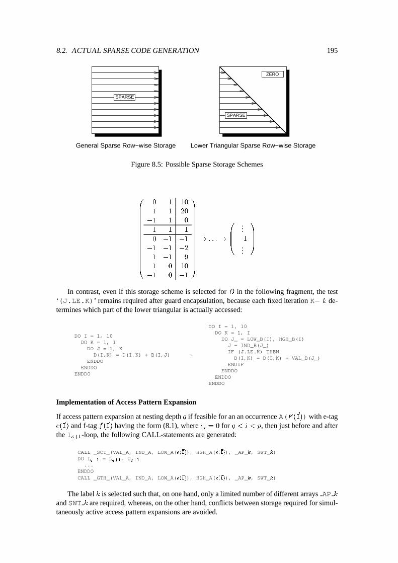
8.2. ACTUAL SPARSE CODE GENERATION 195
Lower Triangular Sparse Row−wise StorageGeneral Sparse Row−wise Storage
SPARSE
ZERO
SPARSE
Figure 8.5: Possible Sparse Storage Schemes
0
B
B
B
B
B
B
B
B
B
B
B
B
B
B
@
0 1 10
1 1 20
�1 1 0
1 �1 �1
0 �1 �1
�1 �1 �2
1 �1 9
1 0 10
�1 0 �1
1
C
C
C
C
C
C
C
C
C
C
C
C
C
C
A
! : : :!
0
B
B
@
...�1
...
1
C
C
A
In contrast, even if this storage scheme is selected for B in the following fragment, the test‘(J.LE.K)’ remains required after guard encapsulation, because each fixed iteration K= k de-termines which part of the lower triangular is actually accessed:
DO I = 1, 10DO K = 1, IDO J = 1, K
D(I,K) = D(I,K) + B(I,J)ENDDO
ENDDOENDDO
!
DO I = 1, 10DO K = 1, I
DO J_ = LOW_B(I), HGH_B(I)J = IND_B(J_)IF (J.LE.K) THEN
D(I,K) = D(I,K) + VAL_B(J_)ENDIF
ENDDOENDDO
ENDDO
Implementation of Access Pattern Expansion
If access pattern expansion at nesting depth q if feasible for an an occurrence A(F (~I))with e-tage(
~
I) and f-tag f(~I) having the form (8.1), where ei
= 0 for q < i < p, then just before and afterthe I
q+1
-loop, the following CALL-statements are generated:
CALL _SCT_(VAL_A, IND_A, LOW_A(e(~I)), HGH_A(e(~I)), _AP_k, SWT_k)DO I
q+1
= Lq+1
, Uq+1
...ENDDOCALL _GTH_(VAL_A, IND_A, LOW_A(e(~I)), HGH_A(e(~I)), _AP_k, SWT_k)
The label k is selected such that, on one hand, only a limited number of different arrays AP kand SWT k are required, whereas, on the other hand, conflicts between storage required for simul-taneously active access pattern expansions are avoided.
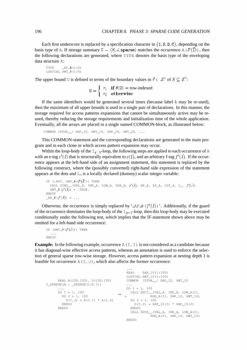
196 CHAPTER 8. PHASE 3: SPARSE CODE GENERATION
Each first underscore is replaced by a specification character in fI; S; D; Cg, depending on thebasis type of A. If storage summary s = hS;~s; sparsei matches the occurrence A(F (~I)), thenthe following declarations are generated, where TYPE denotes the basis type of the envelopingdata structure A:
TYPE _AP_k(1:U)LOGICAL SWT_k(1:U)
The upper bound U is defined in terms of the boundary values in ~� 2 Z4 of S � Z2:
U =
(
�
1
if �(s) = row-indexed�
2
otherwise
If the same identifiers would be generated several times (because label k may be re-used),then the maximum of all upper bounds is used in a single pair of declarations. In this manner, thestorage required for access patterns expansions that cannot be simultaneously active may be re-used, thereby reducing the storage requirements and initialization time of the whole application.Eventually, all the arrays are placed in a single named COMMON-block, as illustrated below:
COMMON /STOR__/ SAP_10, SWT_10, SAP_20, SWT_20, ...
This COMMON-statement and the corresponding declarations are generated in the main pro-gram and in each clone in which access pattern expansion may occur.
Within the loop-body of the Iq+1
-loop, the following steps are applied to each occurrence of Awith an e-tag e0(~J) that is structurally equivalent to e(~I), and an arbitrary f-tag f 0(~J). If the occur-rence appears at the left-hand side of an assignment statement, this statement is replaced by thefollowing construct, where the (possibly converted) right-hand side expression of the statementappears at the dots and L is a locally declared (dummy) scalar integer variable:
IF (.NOT. SWT_k(f 0(~J))) THENCALL SINS__(VAL_A, IND_A, LOW_A, HGH_A, e
0
(
~
J), NP_A, SZ_A, LST_A, L_, f
0
(
~
J))SWT_k(f 0(~J)) = .TRUE.
ENDIF_AP_k(f 0(~J)) = ...
Otherwise, the occurrence is simply replaced by ‘ AP k(f 0(~J))’. Additionally, if the guardof the occurrence dominates the loop-body of the I
q+1
-loop, then this loop-body may be executedconditionally under the following test, which implies that the IF-statement shown above may beomitted for a left-hand side occurrence:
IF (SWT_k(f 0(~J))) THEN...
ENDIF
Example: In the following example, occurrence A(I,I) is not considered as a candidate becauseit has diagonal-wise effective access patterns, whereas an annotation is used to enforce the selec-tion of general sparse row-wise storage. However, access pattern expansion at nesting depth 1 isfeasible for occurrence A(I,J), which also affects the former occurrence:
REAL A(100,100), D(100,100)C_SPARSE(A : _SPARSE()(0,1))
...DO I = 1, 100
DO J = 1, 100D(I,J) = A(I,I) * A(I,J)
ENDDOENDDO
!
...REAL SAP_10(1:100)LOGICAL SWT_10(1:100)COMMON /STOR__/ SAP_10, SWT_10...DO I = 1, 100
CALL SSCT__(VAL_A, IND_A, LOW_A(I),+ HGH_A(I), SAP_10, SWT_10)
DO J = 1, 100D(I,J) = SAP_10(I) * SAP_10(J)
ENDDOCALL SGTH__(VAL_A, IND_A, LOW_A(I),
HGH_A(I), SAP_10, SWT_10)ENDDO
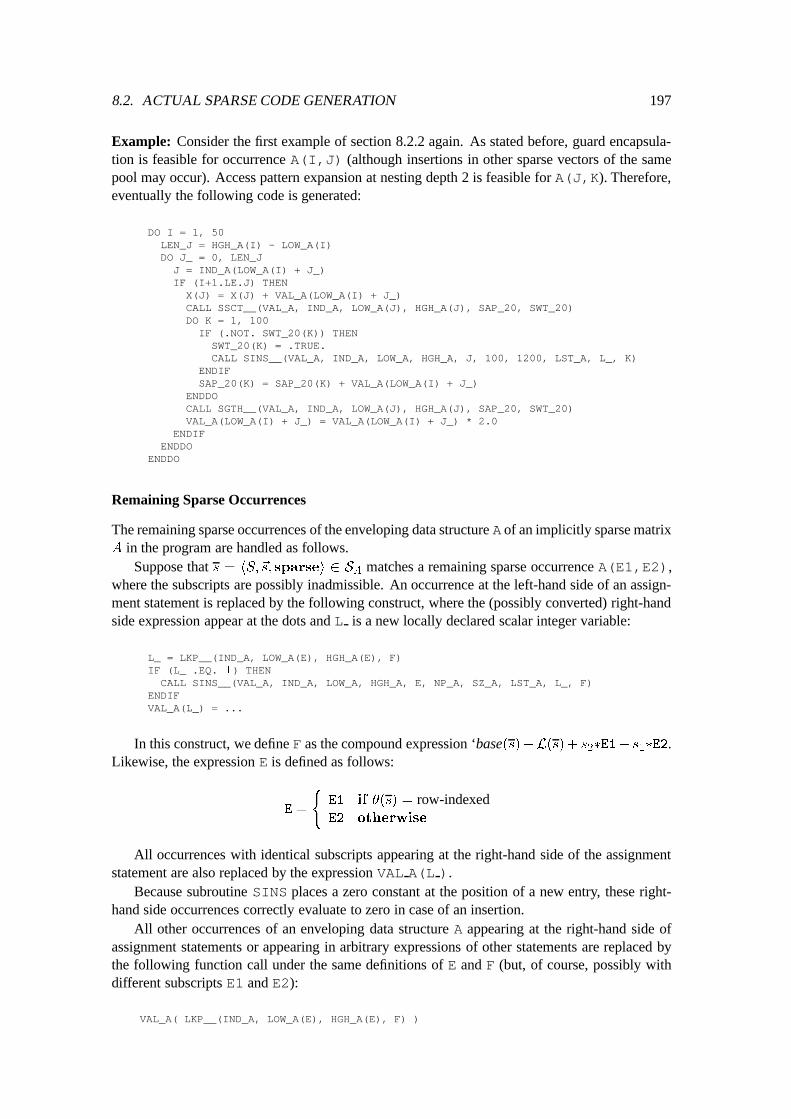
8.2. ACTUAL SPARSE CODE GENERATION 197
Example: Consider the first example of section 8.2.2 again. As stated before, guard encapsula-tion is feasible for occurrence A(I,J) (although insertions in other sparse vectors of the samepool may occur). Access pattern expansion at nesting depth 2 is feasible for A(J,K). Therefore,eventually the following code is generated:
DO I = 1, 50LEN_J = HGH_A(I) - LOW_A(I)DO J_ = 0, LEN_JJ = IND_A(LOW_A(I) + J_)IF (I+1.LE.J) THEN
X(J) = X(J) + VAL_A(LOW_A(I) + J_)CALL SSCT__(VAL_A, IND_A, LOW_A(J), HGH_A(J), SAP_20, SWT_20)DO K = 1, 100
IF (.NOT. SWT_20(K)) THENSWT_20(K) = .TRUE.CALL SINS__(VAL_A, IND_A, LOW_A, HGH_A, J, 100, 1200, LST_A, L_, K)
ENDIFSAP_20(K) = SAP_20(K) + VAL_A(LOW_A(I) + J_)
ENDDOCALL SGTH__(VAL_A, IND_A, LOW_A(J), HGH_A(J), SAP_20, SWT_20)VAL_A(LOW_A(I) + J_) = VAL_A(LOW_A(I) + J_) * 2.0
ENDIFENDDO
ENDDO
Remaining Sparse Occurrences
The remaining sparse occurrences of the enveloping data structure A of an implicitly sparse matrixA in the program are handled as follows.
Suppose that s = hS;~s; sparsei 2 S
A
matches a remaining sparse occurrence A(E1,E2),where the subscripts are possibly inadmissible. An occurrence at the left-hand side of an assign-ment statement is replaced by the following construct, where the (possibly converted) right-handside expression appear at the dots and L is a new locally declared scalar integer variable:
L_ = LKP__(IND_A, LOW_A(E), HGH_A(E), F)IF (L_ .EQ. ?) THENCALL SINS__(VAL_A, IND_A, LOW_A, HGH_A, E, NP_A, SZ_A, LST_A, L_, F)
ENDIFVAL_A(L_) = ...
In this construct, we define F as the compound expression ‘base(s)�L(s)+ s
2
�E1� s
1
�E2.Likewise, the expression E is defined as follows:
E =
(
E1 if �(s) = row-indexedE2 otherwise
All occurrences with identical subscripts appearing at the right-hand side of the assignmentstatement are also replaced by the expression VAL A(L ).
Because subroutine SINS places a zero constant at the position of a new entry, these right-hand side occurrences correctly evaluate to zero in case of an insertion.
All other occurrences of an enveloping data structure A appearing at the right-hand side ofassignment statements or appearing in arbitrary expressions of other statements are replaced bythe following function call under the same definitions of E and F (but, of course, possibly withdifferent subscripts E1 and E2):
VAL_A( LKP__(IND_A, LOW_A(E), HGH_A(E), F) )
198 CHAPTER 8. PHASE 3: SPARSE CODE GENERATION
Because VAL A(?) = 0, this construct correctly accounts for the fact that the value of a non-entry is zero. Obviously, these replacements should only be used as a last resort by the compiler(i.e. in case overhead reducing techniques are not applicable). No attempts are made to accountfor any remaining conditions, because the potential gains of skipping the actual statements areprobably small with respect to the incurred lookup overhead (although executing the first con-struct conditionally could reduce the amount of creation). In fact, frequent application of thesereplacements indicates that the conflicts in a program have not been resolved very well.Example: Consider the following fragment, in which annotations are used to enforce the selectionof general sparse row- and column-wise storage for the implicitly sparse matricesA andB havingarray A and B respectively as enveloping data structures:
REAL A(15,15), B(20,20)C_SPARSE(A : _SPARSE()(0,1))C_SPARSE(B : _SPARSE()(1,0))
...A(2,3) = 7.0 * B(15,4) + 1.0 - A(2,3)
Because occurrences at nesting depth 0 cannot be involved in any overhead reducing tech-nique, eventually the scalar statement is replaced by the following construct:
L_ = LKP__(IND_A, LOW_A(2), HGH_A(2), 3)IF (L_ .EQ. ?) THEN
CALL SINS__(VAL_A, IND_A, LOW_A, HGH_A, 2, NP_A, SZ_A, LST_A, L_, 3)ENDIFVAL_A(L_) = 7.0 * VAL_B(LKP__(IND_B, LOW_B(4), HGH_B(4), 15)) + 1.0 - VAL_A(L_)
8.3 Initialization Code Generation
While developing and testing the original dense program, the programmer can focus on the actualalgorithms and very simple initialization code can be used for all enveloping data structures to testthe program on some small dense matrices. Once the program has been debugged, all initializationcode involving enveloping data structures is eliminated. The remaining dense program is used asinput for the sparse compiler. After sparse storage schemes have been selected for all implicitlysparse matrices, the sparse compiler generates appropriate initialization code at the beginning ofthe main program, expecting all matrices in coordinate scheme. In this manner, the actual sparsestorage schemes that are used in the generated program are kept completely transparent to theprogrammer.
8.3.1 Resetting Static Dense Storage and Switch Arrays
For each storage summary s = hS;~s;densei 2 S
A
, the following code is used to reset all el-ements in the corresponding static dense storage, where k = lab(s) and the outermost DO-loopand second subscript are omitted if L(s) = U(s) holds:
DO J_ = L(s), U(s)DO I_ = L, UDNk_A(I_,J_) = 0.0
ENDDO " zero constant of appropriate typeENDDO
In this construct, the loop bounds L and U are defined as follows, where � 2 Z4 and � 2 Z4
denote the boundary values of the simple section S � Z2:
(L; U) =
(
(�
1
; �
1
) if �(s) = row-indexed(�
2
; �
2
) otherwise
8.3. INITIALIZATION CODE GENERATION 199
Likewise, for each pair AP k/SWT k in the named COMMON-block ‘STOR ’ (used to sup-port expansion and compression), the following code is generated, where U denotes the maximumupper bound recorded for each pair:
DO I_ = 1, USWT_k = .FALSE._AP_k = 0.0
ENDDO " zero constant of appropriate type
8.3.2 File Input
For each implicitly sparse matrixAwith enveloping data structure A in the program, the followingconstruct is generated:
LST_A = 1OPEN (UNIT=1, FILE=’file_name’, STATUS=’OLD’)READ (1,*) M_, N_, NNZ_DO K_ = 1, NNZ_
READ (1,*) I_, J_, V_C Insert A(I_,J_) = V_ in Selected Data Structure
...ENDDOCLOSE (UNIT = 1)
In case a pool of sparse vectors is used as dynamic storage for the entries in the sparse re-gions of A, the scalar ‘LST A’ is initialized to 1 because the first location in the parallel arraysimplementing this pool is used as location ?.
Thereafter, a construct that reads the matrix from file in coordinate scheme is generated, wherethe string ‘file name’ is the file name defined for A (a similar fragment with ‘A(I ,J )=V ’can be manually inserted in the original dense program for testing purposes). If no file has beenspecified, the sparse compiler inquires the programmer for a file name.
At the dots, a multi-way IF-statement appears that determines the action required for each en-try. Suppose we have the following set:
S
s;d
A
= fhS;~s; pi j p = sparse _ p = denseg = fS
1
; : : : ; S
k
g
Then, the following IF-statement is generated, in which the condition of the last branch is omitted,and the whole statement is omitted if jSs;d
A
j = 1:
IF (I_,J_) 2 S1
THEN...
ELSEIF (I_,J_) 2 S2
THEN...
ELSE IF (I_,J_) 2 Sk�1
THEN...
ELSE...
ENDIF
Testing inclusion in each individual simple section S � Z2 with boundary values � 2 Z4
and � 2 Z4 can be done as follows:IF ( (�
1
.LE.I_ ).AND.(I_ .LE.�1
).AND.(�2
.LE. J_).AND.( J_.LE.�2
).AND.+ (�
3
.LE.I_+J_).AND.(I_+J_.LE.�3
).AND.(�4
.LE.I_-J_).AND.(I_-J_.LE.�4
) ) THEN...
This inclusion test may induce substantial testing overhead. However, usually the conditioncan be simplified by omitting tests on lower or upper bounds that coincide with the minimumor maximum possible value of the expressions I , J , I +J and I -J under the equivalence(I ; J ) 2 [1;m] � [1; n] or that are implied by inequalities that have already been generated.Moreover, a non-redundant ith pair of tests can be replaced by a single test for equivalence if�
i
= �
i
(e.g. (I .EQ.�1
)).
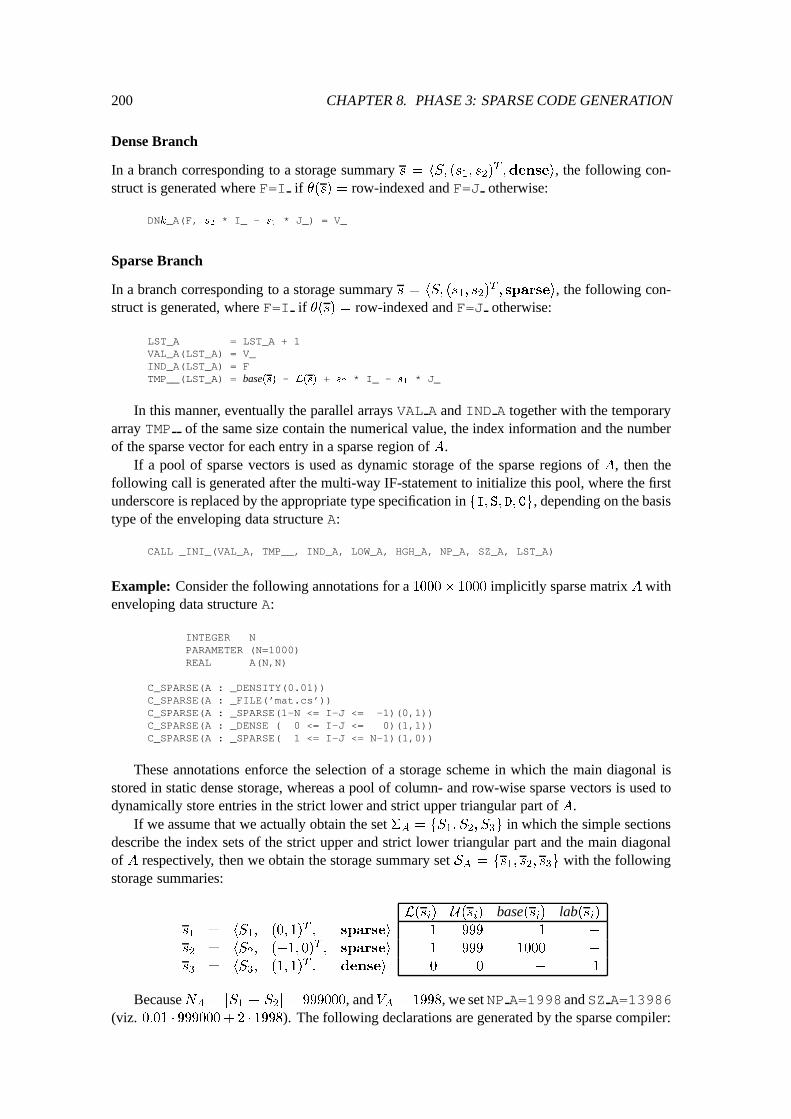
200 CHAPTER 8. PHASE 3: SPARSE CODE GENERATION
Dense Branch
In a branch corresponding to a storage summary s = hS; (s
1
; s
2
)
T
;densei, the following con-struct is generated where F=I if �(s) = row-indexed and F=J otherwise:
DNk_A(F, s
2
* I_ - s
1
* J_) = V_
Sparse Branch
In a branch corresponding to a storage summary s = hS; (s
1
; s
2
)
T
; sparsei, the following con-struct is generated, where F=I if �(s) = row-indexed and F=J otherwise:
LST_A = LST_A + 1VAL_A(LST_A) = V_IND_A(LST_A) = FTMP__(LST_A) = base(s) - L(s) + s
2
* I_ - s
1
* J_
In this manner, eventually the parallel arrays VAL A and IND A together with the temporaryarray TMP of the same size contain the numerical value, the index information and the numberof the sparse vector for each entry in a sparse region of A.
If a pool of sparse vectors is used as dynamic storage of the sparse regions of A, then thefollowing call is generated after the multi-way IF-statement to initialize this pool, where the firstunderscore is replaced by the appropriate type specification in fI; S; D; Cg, depending on the basistype of the enveloping data structure A:
CALL _INI_(VAL_A, TMP__, IND_A, LOW_A, HGH_A, NP_A, SZ_A, LST_A)
Example: Consider the following annotations for a 1000� 1000 implicitly sparse matrix A withenveloping data structure A:
INTEGER NPARAMETER (N=1000)REAL A(N,N)
C_SPARSE(A : _DENSITY(0.01))C_SPARSE(A : _FILE(’mat.cs’))C_SPARSE(A : _SPARSE(1-N <= I-J <= -1)(0,1))C_SPARSE(A : _DENSE ( 0 <= I-J <= 0)(1,1))C_SPARSE(A : _SPARSE( 1 <= I-J <= N-1)(1,0))
These annotations enforce the selection of a storage scheme in which the main diagonal isstored in static dense storage, whereas a pool of column- and row-wise sparse vectors is used todynamically store entries in the strict lower and strict upper triangular part of A.
If we assume that we actually obtain the set �A
= fS
1
; S
2
; S
3
g in which the simple sectionsdescribe the index sets of the strict upper and strict lower triangular part and the main diagonalof A respectively, then we obtain the storage summary set S
A
= fs
1
; s
2
; s
3
g with the followingstorage summaries:
L(s
i
) U(s
i
) base(si
) lab(si
)
s
1
= hS
1
; (0; 1)
T
; sparsei 1 999 1 �
s
2
= hS
2
; (�1; 0)
T
; sparsei 1 999 1000 �
s
3
= hS
3
; (1; 1)
T
; densei 0 0 � 1
BecauseNA
= jS
1
j+jS
2
j = 999000, and VA
= 1998, we set NP A=1998 andSZ A=13986(viz. 0:01 � 999000 + 2 � 1998). The following declarations are generated by the sparse compiler:
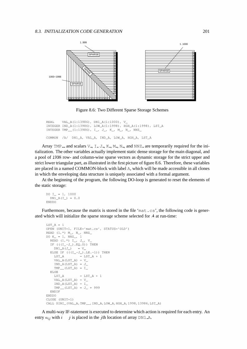
8.3. INITIALIZATION CODE GENERATION 201
1..1000
SPARSEDENSE
1..999
1000−1998
SPARSE
SPARSE
Figure 8.6: Two Different Sparse Storage Schemes
REAL VAL_A(1:13986), DN1_A(1:1000), V_INTEGER IND_A(1:13986), LOW_A(1:1998), HGH_A(1:1998), LST_AINTEGER TMP__(1:13986), I_, J_, K_, M_, N_, NNZ_
COMMON /A/ DN1_A, VAL_A, IND_A, LOW_A, HGH_A, LST_A
Array TMP and scalars V , I J , K , M , N , and NNZ are temporarily required for the ini-tialization. The other variables actually implement static dense storage for the main diagonal, anda pool of 1998 row- and column-wise sparse vectors as dynamic storage for the strict upper andstrict lower triangular part, as illustrated in the first picture of figure 8.6. Therefore, these variablesare placed in a named COMMON-block with label A, which will be made accessible in all clonesin which the enveloping data structure is uniquely associated with a formal argument.
At the beginning of the program, the following DO-loop is generated to reset the elements ofthe static storage:
DO I_ = 1, 1000DN1_A(I_) = 0.0
ENDDO
Furthermore, because the matrix is stored in the file ‘mat.cs’, the following code is gener-ated which will initialize the sparse storage scheme selected for A at run-time:
LST_A = 1OPEN (UNIT=1, FILE=’mat.cs’, STATUS=’OLD’)READ (1,*) M_, N_, NNZ_DO K_ = 1, NNZ_, 1READ (1,*) I_, J_, V_IF (((I_-J_).EQ.0)) THENDN1_A(J_) = V_
ELSE IF (((I_-J_).LE.-1)) THENLST_A = LST_A + 1VAL_A(LST_A) = V_IND_A(LST_A) = J_TMP__(LST_A) = I_
ELSELST_A = LST_A + 1VAL_A(LST_A) = V_IND_A(LST_A) = I_TMP__(LST_A) = J_ + 999
ENDIFENDDOCLOSE (UNIT=1)CALL SINI_(VAL_A,TMP__,IND_A,LOW_A,HGH_A,1998,13986,LST_A)
A multi-way IF-statement is executed to determine which action is required for each entry. Anentry a
ij
with i = j is placed in the jth location of array DN1 A.
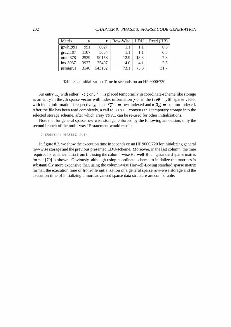
202 CHAPTER 8. PHASE 3: SPARSE CODE GENERATION
Matrix n � Row-Wise LDU Read (HB)
jpwh 991 991 6027 1.1 1.1 0.5gre 1107 1107 5664 1.1 1.1 0.5orani678 2529 90158 12.9 13.3 7.8lns 3937 3937 25407 4.0 4.1 2.3psmigr 1 3140 543162 73.1 73.8 31.7
Table 8.2: Initialization Time in seconds on an HP 9000/720
An entry aij
with either i < j or i > j is placed temporarily in coordinate-scheme like storageas an entry in the ith sparse vector with index information j or in the (999 + j)th sparse vectorwith index information i respectively, since �(s
1
) = row-indexed and �(s2
) = column-indexed.After the file has been read completely, a call to SINI converts this temporary storage into theselected storage scheme, after which array TMP can be re-used for other initializations.
Note that for general sparse row-wise storage, enforced by the following annotation, only thesecond branch of the multi-way IF-statement would result:
C_SPARSE(A: SPARSE()(0,1))
In figure 8.2, we show the execution time in seconds on an HP 9000/720 for initializing generalrow-wise storage and the previous presented LDU-scheme. Moreover, in the last column, the timerequired to read the matrix from file using the column-wise Harwell-Boeing standard sparse matrixformat [79] is shown. Obviously, although using coordinate scheme to initialize the matrices issubstantially more expensive than using the column-wise Harwell-Boeing standard sparse matrixformat, the execution time of from-file initialization of a general sparse row-wise storage and theexecution time of initializing a more advanced sparse data structure are comparable.
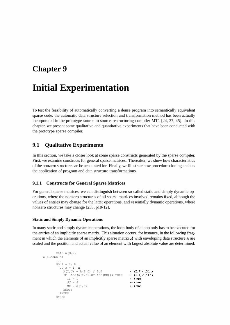
Chapter 9
Initial Experimentation
To test the feasibility of automatically converting a dense program into semantically equivalentsparse code, the automatic data structure selection and transformation method has been actuallyincorporated in the prototype source to source restructuring compiler MT1 [24, 37, 45]. In thischapter, we present some qualitative and quantitative experiments that have been conducted withthe prototype sparse compiler.
9.1 Qualitative Experiments
In this section, we take a closer look at some sparse constructs generated by the sparse compiler.First, we examine constructs for general sparse matrices. Thereafter, we show how characteristicsof the nonzero structure can be accounted for. Finally, we illustrate how procedure cloning enablesthe application of program and data structure transformations.
9.1.1 Constructs for General Sparse Matrices
For general sparse matrices, we can distinguish between so-called static and simply dynamic op-erations, where the nonzero structures of all sparse matrices involved remains fixed, although thevalues of entries may change for the latter operations, and essentially dynamic operations, wherenonzero structures may change [235, p10-12].
Static and Simply Dynamic Operations
In many static and simply dynamic operations, the loop-body of a loop only has to be executed forthe entries of an implicitly sparse matrix. This situation occurs, for instance, in the following frag-ment in which the elements of an implicitly sparse matrix A with enveloping data structure A arescaled and the position and actual value of an element with largest absolute value are determined:
REAL A(M,N)C_SPARSE(A)
...DO I = 1, M
DO J = 1, NA(I,J) = A(I,J) / 3.0 (I; J) 2 E(A)
IF (ABS(A(I,J).GT.ABS(MX))) THEN (I; J) 2 E(A)
II = I true
JJ = J true
MX = A(I,J) true
ENDIFENDDO
ENDDO
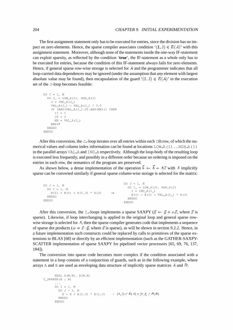
204 CHAPTER 9. INITIAL EXPERIMENTATION
The first assignment statement only has to be executed for entries, since the division has no im-pact on zero elements. Hence, the sparse compiler associates condition ‘(I; J) 2 E(A)’ with thisassignment statement. Moreover, although none of the statements inside the one-way IF-statementcan exploit sparsity, as reflected by the condition ‘true’, the IF-statement as a whole only has tobe executed for entries, because the condition of this IF-statement always fails for zero elements.Hence, if general sparse row-wise storage is selected for A and the programmer indicates that allloop-carried data dependences may be ignored (under the assumption that any element with largestabsolute value may be found), then encapsulation of the guard ‘(I; J) 2 E(A)’ in the executionset of the J-loop becomes feasible:
DO I = 1, MDO J_ = LOW_A(I), HGH_A(I)
J = IND_A(J_)VAL_A(J_) = VAL_A(J_) / 3.0IF (ABS(VAL_A(J_).GT.ABS(MX))) THENII = IJJ = JMX = VAL_A(J_)
ENDIFENDDO
ENDDO
After this conversion, the J -loop iterates over all entries within each Ith row, of which the nu-merical values and column index information can be found at locations LOW A(I)..HGH A(I)in the parallel arrays VAL A and IND A respectively. Although the loop-body of the resulting loopis executed less frequently, and possibly in a different order because no ordering is imposed on theentries in each row, the semantics of the program are preserved.
As shown below, a dense implementation of the operation ~b ~
b + A~x with A implicitlysparse can be converted similarly if general sparse column-wise storage is selected for the matrix:
DO J = 1, NDO I = 1, MB(I) = B(I) + A(I,J) * X(J)
ENDDOENDDO
!
DO J = 1, NDO I_ = LOW_A(J), HGH_A(J)
I = IND_A(I_)B(I) = B(I) + VAL_A(I_) * X(J)
ENDDOENDDO
After this conversion, the I -loops implements a sparse SAXPY (~y ~y + �~x, where ~x issparse). Likewise, if loop interchanging is applied to the original loop and general sparse row-wise storage is selected forA, then the sparse compiler generates code that implements a sequenceof sparse dot products (w = ~x � ~y, where ~x is sparse), as will be shown in section 9.2.2. Hence, ina future implementation such constructs could be replaced by calls to primitives of the sparse ex-tensions to BLAS [68] or directly by an efficient implementation (such as the GATHER-SAXPY-SCATTER implementation of sparse SAXPY for pipelined vector processors [65, 69, 76, 137,184]).
The conversion into sparse code becomes more complex if the condition associated with astatement in a loop consists of a conjunction of guards, such as in the following example, wherearrays A and B are used as enveloping data structure of implicitly sparse matrices A and B:
REAL A(M,N), B(M,N)C_SPARSE(A ; B)
...DO I = 1, M
DO J = 1, NX = X + A(I,J) * B(I,J) (I; J) 2 E(A) ^ (I; J) 2 E(B)
ENDDOENDDO
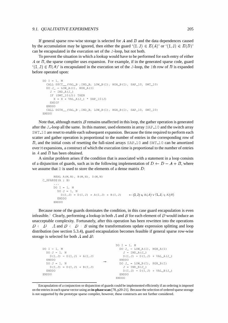
9.1. QUALITATIVE EXPERIMENTS 205
If general sparse row-wise storage is selected for A and B and the data dependences causedby the accumulation may be ignored, then either the guard ‘(I; J) 2 E(A)’ or ‘(I; J) 2 E(B)’can be encapsulated in the execution set of the J-loop, but not both.
To prevent the situation in which a lookup would have to be performed for each entry of eitherA or B, the sparse compiler uses expansion. For example, if in the generated sparse code, guard‘(I; J) 2 E(A)’ is encapsulated in the execution set of the J-loop, the Ith row of B is expandedbefore operated upon:
DO I = 1, MCALL SSCT__(VAL_B ,IND_B, LOW_B(I), HGH_B(I), SAP_10, SWT_10)DO J_ = LOW_A(I), HGH_A(I)J = IND_A(J_)IF (SWT_10(J)) THEN
X = X + VAL_A(J_) * SAP_10(J)ENDIF
ENDDOCALL SGTH__(VAL_B ,IND_B, LOW_B(I), HGH_B(I), SAP_10, SWT_10)
ENDDO
Note that, although matrixB remains unaffected in this loop, the gather operation is generatedafter the J -loop all the same. In this manner, used elements in array SAP 10 and the switch arraySWT 10 are reset to enable each subsequent expansion. Because the time required to perform eachscatter and gather operation is proportional to the number of entries in the corresponding row ofB, and the initial costs of resetting the full-sized arrays SAP 10 and SWT 10 can be amortizedover M expansions, a construct of which the execution time is proportional to the number of entriesin A and B has been obtained.
A similar problem arises if the condition that is associated with a statement in a loop consistsof a disjunction of guards, such as in the following implementation of D D + A+ B, wherewe assume that D is used to store the elements of a dense matrix D:
REAL A(M,N), B(M,N), D(M,N)C_SPARSE(A ; B)
...DO I = 1, M
DO J = 1, ND(I,J) = D(I,J) + A(I,J) + B(I,J) (I; J) 2 E(A) _ (I; J) 2 E(B)
ENDDOENDDO
Because none of the guards dominates the condition, in this case guard encapsulation is eveninfeasible.1 Clearly, performing a lookup in bothA andB for each element ofD would induce anunacceptable complexity. Fortunately, after this operation has been rewritten into the operationsD D + A and D D + B using the transformations update expression splitting and loopdistribution (see section 5.3.4), guard encapsulation becomes feasible if general sparse row-wisestorage is selected for both A and B:
DO I = 1, MDO J = 1, ND(I,J) = D(I,J) + A(I,J)
ENDDODO J = 1, ND(I,J) = D(I,J) + B(I,J)
ENDDOENDDO
!
DO I = 1, MDO J_ = LOW_A(I), HGH_A(I)
J = IND_A(J_)D(I,J) = D(I,J) + VAL_A(J_)
ENDDODO J_ = LOW_B(I), HGH_B(I)
J = IND_B(J_)D(I,J) = D(I,J) + VAL_B(J_)
ENDDOENDDO
1Encapsulation of a conjunction or disjunction of guards could be implemented efficiently if an ordering is imposedon the entries in each sparse vector using an in-phase scan [78, p20-21]. Because the selection of ordered sparse storageis not supported by the prototype sparse compiler, however, these constructs are not further considered.
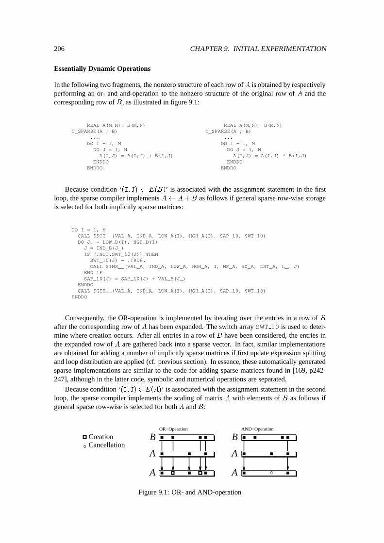
206 CHAPTER 9. INITIAL EXPERIMENTATION
Essentially Dynamic Operations
In the following two fragments, the nonzero structure of each row ofA is obtained by respectivelyperforming an or- and and-operation to the nonzero structure of the original row of A and thecorresponding row of B, as illustrated in figure 9.1:
REAL A(M,N), B(M,N)C_SPARSE(A ; B)
...DO I = 1, M
DO J = 1, NA(I,J) = A(I,J) + B(I,J)
ENDDOENDDO
REAL A(M,N), B(M,N)C_SPARSE(A ; B)
...DO I = 1, M
DO J = 1, NA(I,J) = A(I,J) * B(I,J)
ENDDOENDDO
Because condition ‘(I; J) 2 E(B)’ is associated with the assignment statement in the firstloop, the sparse compiler implements A A+B as follows if general sparse row-wise storageis selected for both implicitly sparse matrices:
DO I = 1, MCALL SSCT__(VAL_A, IND_A, LOW_A(I), HGH_A(I), SAP_10, SWT_10)DO J_ = LOW_B(I), HGH_B(I)J = IND_B(J_)IF (.NOT.SWT_10(J)) THENSWT_10(J) = .TRUE.CALL SINS__(VAL_A, IND_A, LOW_A, HGH_A, I, NP_A, SZ_A, LST_A, L_, J)
END IFSAP_10(J) = SAP_10(J) + VAL_B(J_)
ENDDOCALL SGTH__(VAL_A, IND_A, LOW_A(I), HGH_A(I), SAP_10, SWT_10)
ENDDO
Consequently, the OR-operation is implemented by iterating over the entries in a row of Bafter the corresponding row of A has been expanded. The switch array SWT 10 is used to deter-mine where creation occurs. After all entries in a row of B have been considered, the entries inthe expanded row of A are gathered back into a sparse vector. In fact, similar implementationsare obtained for adding a number of implicitly sparse matrices if first update expression splittingand loop distribution are applied (cf. previous section). In essence, these automatically generatedsparse implementations are similar to the code for adding sparse matrices found in [169, p242-247], although in the latter code, symbolic and numerical operations are separated.
Because condition ‘(I; J) 2 E(A)’ is associated with the assignment statement in the secondloop, the sparse compiler implements the scaling of matrix A with elements of B as follows ifgeneral sparse row-wise is selected for both A and B:
OR−Operation
A
B
A
AND−Operation
A
B
A 0
CreationCancellation0
Figure 9.1: OR- and AND-operation
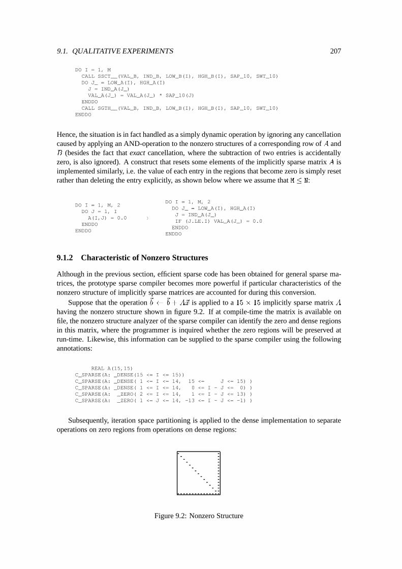
9.1. QUALITATIVE EXPERIMENTS 207
DO I = 1, MCALL SSCT__(VAL_B, IND_B, LOW_B(I), HGH_B(I), SAP_10, SWT_10)DO J_ = LOW_A(I), HGH_A(I)J = IND_A(J_)VAL_A(J_) = VAL_A(J_) * SAP_10(J)
ENDDOCALL SGTH__(VAL_B, IND_B, LOW_B(I), HGH_B(I), SAP_10, SWT_10)
ENDDO
Hence, the situation is in fact handled as a simply dynamic operation by ignoring any cancellationcaused by applying an AND-operation to the nonzero structures of a corresponding row of A andB (besides the fact that exact cancellation, where the subtraction of two entries is accidentallyzero, is also ignored). A construct that resets some elements of the implicitly sparse matrix A isimplemented similarly, i.e. the value of each entry in the regions that become zero is simply resetrather than deleting the entry explicitly, as shown below where we assume that M � N:
DO I = 1, M, 2DO J = 1, IA(I,J) = 0.0
ENDDOENDDO
!
DO I = 1, M, 2DO J_ = LOW_A(I), HGH_A(I)J = IND_A(J_)IF (J.LE.I) VAL_A(J_) = 0.0
ENDDOENDDO
9.1.2 Characteristic of Nonzero Structures
Although in the previous section, efficient sparse code has been obtained for general sparse ma-trices, the prototype sparse compiler becomes more powerful if particular characteristics of thenonzero structure of implicitly sparse matrices are accounted for during this conversion.
Suppose that the operation ~b ~
b + A~x is applied to a 15 � 15 implicitly sparse matrix Ahaving the nonzero structure shown in figure 9.2. If at compile-time the matrix is available onfile, the nonzero structure analyzer of the sparse compiler can identify the zero and dense regionsin this matrix, where the programmer is inquired whether the zero regions will be preserved atrun-time. Likewise, this information can be supplied to the sparse compiler using the followingannotations:
REAL A(15,15)C_SPARSE(A: _DENSE(15 <= I <= 15))C_SPARSE(A: _DENSE( 1 <= I <= 14, 15 <= J <= 15) )C_SPARSE(A: _DENSE( 1 <= I <= 14, 0 <= I - J <= 0) )C_SPARSE(A: _ZERO( 2 <= I <= 14, 1 <= I - J <= 13) )C_SPARSE(A: _ZERO( 1 <= J <= 14, -13 <= I - J <= -1) )
Subsequently, iteration space partitioning is applied to the dense implementation to separateoperations on zero regions from operations on dense regions:
Figure 9.2: Nonzero Structure
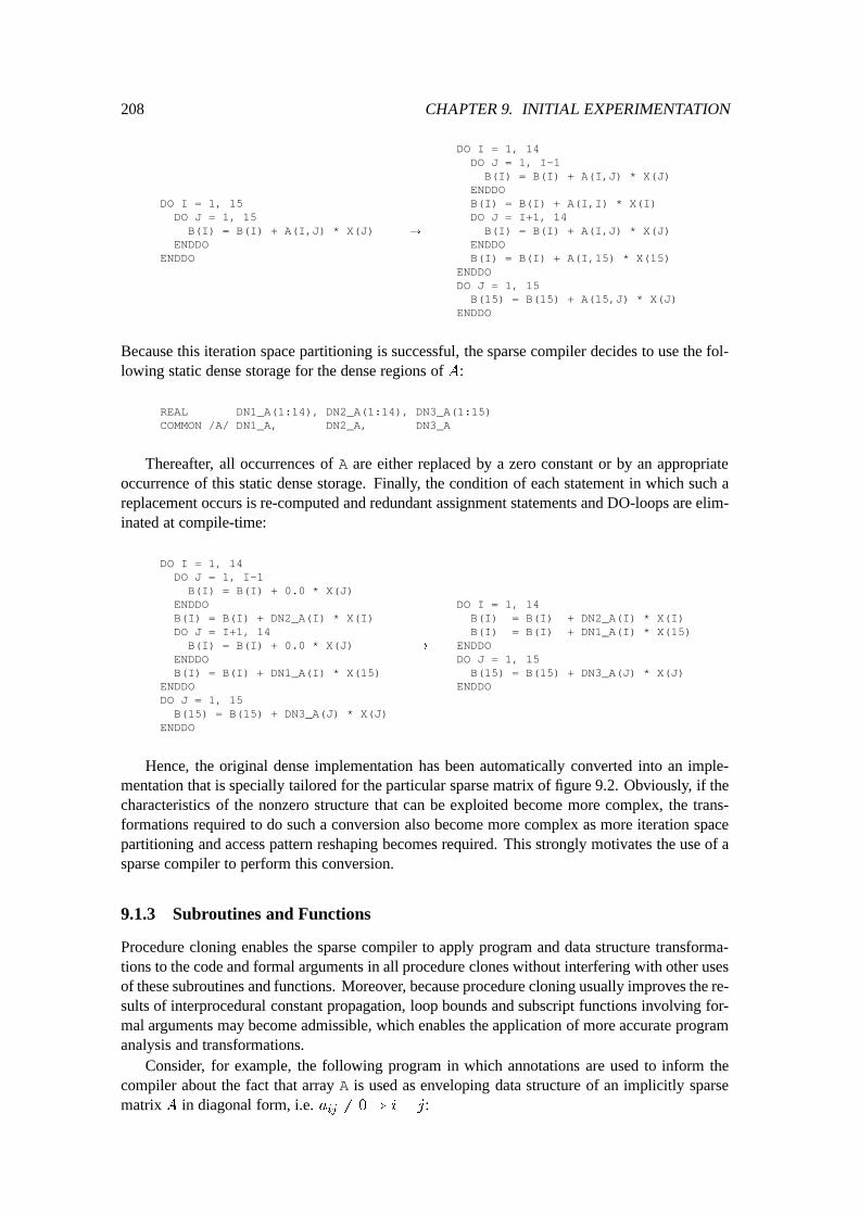
208 CHAPTER 9. INITIAL EXPERIMENTATION
DO I = 1, 15DO J = 1, 15
B(I) = B(I) + A(I,J) * X(J)ENDDO
ENDDO
!
DO I = 1, 14DO J = 1, I-1
B(I) = B(I) + A(I,J) * X(J)ENDDOB(I) = B(I) + A(I,I) * X(I)DO J = I+1, 14
B(I) = B(I) + A(I,J) * X(J)ENDDOB(I) = B(I) + A(I,15) * X(15)
ENDDODO J = 1, 15
B(15) = B(15) + A(15,J) * X(J)ENDDO
Because this iteration space partitioning is successful, the sparse compiler decides to use the fol-lowing static dense storage for the dense regions of A:
REAL DN1_A(1:14), DN2_A(1:14), DN3_A(1:15)COMMON /A/ DN1_A, DN2_A, DN3_A
Thereafter, all occurrences of A are either replaced by a zero constant or by an appropriateoccurrence of this static dense storage. Finally, the condition of each statement in which such areplacement occurs is re-computed and redundant assignment statements and DO-loops are elim-inated at compile-time:
DO I = 1, 14DO J = 1, I-1B(I) = B(I) + 0.0 * X(J)
ENDDOB(I) = B(I) + DN2_A(I) * X(I)DO J = I+1, 14B(I) = B(I) + 0.0 * X(J)
ENDDOB(I) = B(I) + DN1_A(I) * X(15)
ENDDODO J = 1, 15B(15) = B(15) + DN3_A(J) * X(J)
ENDDO
!
DO I = 1, 14B(I) = B(I) + DN2_A(I) * X(I)B(I) = B(I) + DN1_A(I) * X(15)
ENDDODO J = 1, 15
B(15) = B(15) + DN3_A(J) * X(J)ENDDO
Hence, the original dense implementation has been automatically converted into an imple-mentation that is specially tailored for the particular sparse matrix of figure 9.2. Obviously, if thecharacteristics of the nonzero structure that can be exploited become more complex, the trans-formations required to do such a conversion also become more complex as more iteration spacepartitioning and access pattern reshaping becomes required. This strongly motivates the use of asparse compiler to perform this conversion.
9.1.3 Subroutines and Functions
Procedure cloning enables the sparse compiler to apply program and data structure transforma-tions to the code and formal arguments in all procedure clones without interfering with other usesof these subroutines and functions. Moreover, because procedure cloning usually improves the re-sults of interprocedural constant propagation, loop bounds and subscript functions involving for-mal arguments may become admissible, which enables the application of more accurate programanalysis and transformations.
Consider, for example, the following program in which annotations are used to inform thecompiler about the fact that array A is used as enveloping data structure of an implicitly sparsematrix A in diagonal form, i.e. a
ij
6= 0) i = j:
9.1. QUALITATIVE EXPERIMENTS 209
MATRIX
MATMAT MATVEC
Figure 9.3: Call Graph of Program MATRIX
PROGRAM MATRIX
INTEGER M, NPARAMETER (M = 50, N = 100)
REAL A(M,M), B(M,M), C(M,M)REAL D(N,N), E(N,N)REAL X(N), Y(N)
C_SPARSE(A: _ZERO ( 1-M <= I - J <= -1))C_SPARSE(A: _DENSE( 0 <= I - J <= 0))C_SPARSE(A: _ZERO ( 1 <= I - J <= M-1))
...CALL MATMAT(A, B, C, M)CALL MATMAT(D, D, E, N)CALL MATVEC(E, X, Y, N)...
END
SUBROUTINE MATMAT(H, F, G, N)INTEGER N, IREAL H(N,N), F(N,N), G(N,N)DO I = 1, NCALL MATVEC(H, F(1,I), G(1,I), N)ENDDORETURNEND
SUBROUTINE MATVEC(H, R, S, N)INTEGER N, I, JREAL H(N,N), R(N), S(N)DO I = 1, N
DO J = 1, NS(I) = S(I) + H(I,J) * R(J)
ENDDOENDDORETURNEND
In this program, the call graph of which is shown in figure 9.3, the sparse compiler cannotbluntly apply data structure transformations to the formal arguments H in MATMAT and MATVEC,because these subroutines are also used to perform operations involving dense matrices. There-fore, the sparse compiler generates a clone MATMAT A000 of the subroutine MATMAT in which Ais uniquely associated with the formal argument H. Moreover, since the clone calls MATVECwithH as first actual argument, a clone MATVEC A000 of MATVEC is also generated. The original sub-routines are preserved to perform the operations E E + DD and ~y ~y + E~x, whereas theclones are used to compute C C +AB.
If static dense storage is selected for the main diagonal of A, this data structure is placed in anamed COMMON block, and the main program is converted as shown below, where the argumentused to pass the whole implicitly sparse matrix has been eliminated:
PROGRAM MATRIX...REAL DN1_A(1:50)COMMON /A/ DN1_A...CALL MATMAT_A000(B, C, M)CALL MATMAT (D, D, E, N)CALL MATVEC (E, X, Y, N)...END
After iteration space partitioning has been applied to the procedure clones, and redundant as-signment statements and DO-loops have been eliminated at compile-time, the sparse code shownbelow results. Interprocedural constant propagation has derived the value N=50 and the formal ar-gument H has been either eliminated or replaced by an occurrence of the selected storage scheme,made available to the subroutines using the named COMMON-block:
210 CHAPTER 9. INITIAL EXPERIMENTATION
SUBROUTINE MATMAT_A000(F, G, N)INTEGER N, IREAL F(50,50), G(50,50)REAL DN1_A(1: 50)COMMON /A/ DN1_A
DO I = 1, 50CALL MATVEC_A000(F(1,I), G(1,I), 50)
ENDDORETURNEND
SUBROUTINE MATVEC_A000(R, S, N)INTEGER N, I, JREAL R(50), S(50)REAL DN1_A(1:50)COMMON /A/ DN1_A
DO I = 1, 50S(I) = S(I) + DN1_A(I) * R(I)
ENDDORETURNEND
A subroutine computing the product of A with another matrix and a subroutine computingthe product of A with a vector tailored for the specific nonzero structure of A has been derivedautomatically.
9.2 Quantitative Experiments
In this section, quantitative experiments are conducted with some small sparse programs that havebeen generated automatically by the prototype sparse compiler.
9.2.1 Preliminary Discussion
The experiments have been conducted on an HP 9000/720 and on one CPU of a Cray C98/4256.On both machines, all programs are compiled with the native FORTRAN compiler, where defaultoptimizations and, for the latter, vectorization are enabled. Furthermore, experiments have beenconducted with sparse matrices of theE(n; c)-class of [164, p6-11][235, p57-62], which are n�nmatrices A having the following nonzero elements:
8
>
<
>
:
a
ii
= +4:0 i = 1; : : : ; n
a
i;i+1
= a
i+1;i
= �1:0 i = 1; : : : ; n� 1
a
i;i+c
= a
i+c;i
= �1:0 i = 1; : : : ; n� c
In fact, these matrices form simplifications of typical matrices arising in finite difference meth-ods (cf. figure 6.10). In figure 9.4, the nonzero structure of E(20; 5) is given. Although thesematrices have a very simple nonzero structure, using this class enables us to test the generatedsparse program for varying matrix sizes. Moreover, since for each n, at most 5 nonzero elementsappear in each row, the execution time of an algorithm that fully exploits the sparsity of the ma-trix is expected to depend linearly on the order of the matrix. For a number of dense programsand varying values of n, a version for a general sparse row-wise matrix and for the matrix hav-ing the specific nonzero structure of matrices of the E(n; 5)-class are generated. Subsequently,the execution time of each version is measured using the appropriate matrix of the E(n; 5)-class.Note that since sparse row-wise versions can also be used for sparse matrices having an arbitrarynonzero structure, probably some performance must be traded for generality.
We can enforce the sparse compiler to select general sparse row-wise storage for an implicitlyn � n sparse matrix A with enveloping data structure A by adding the following annotation tothe declaration of this array, which simply states that the region consisting of the whole matrix issparse and the preferred access direction of this region is ~p = (0; 1)
T :
REAL A(N,N)C_SPARSE(A : SPARSE()(0,1))
Likewise, we can supply the specific nonzero structure of a matrix of the E(n; 5)-class to thesparse compiler by replacing the previous annotation with the following annotations, in which theindex set of each region is described in terms of a simple section:
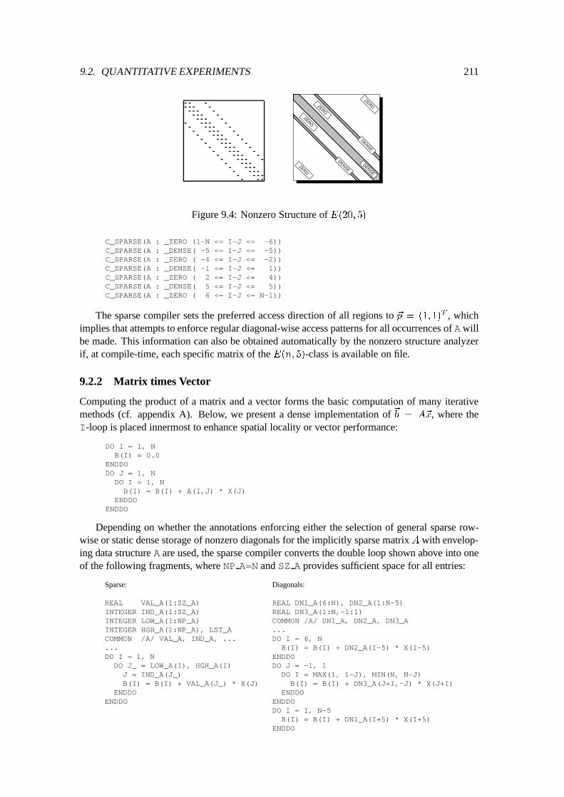
9.2. QUANTITATIVE EXPERIMENTS 211
ZERO
ZEROZEROZERO
DENSE
DENSE
DENSE
Figure 9.4: Nonzero Structure of E(20; 5)
C_SPARSE(A : _ZERO (1-N <= I-J <= -6))C_SPARSE(A : _DENSE( -5 <= I-J <= -5))C_SPARSE(A : _ZERO ( -4 <= I-J <= -2))C_SPARSE(A : _DENSE( -1 <= I-J <= 1))C_SPARSE(A : _ZERO ( 2 <= I-J <= 4))C_SPARSE(A : _DENSE( 5 <= I-J <= 5))C_SPARSE(A : _ZERO ( 6 <= I-J <= N-1))
The sparse compiler sets the preferred access direction of all regions to ~p = (1; 1)
T , whichimplies that attempts to enforce regular diagonal-wise access patterns for all occurrences of Awillbe made. This information can also be obtained automatically by the nonzero structure analyzerif, at compile-time, each specific matrix of the E(n; 5)-class is available on file.
9.2.2 Matrix times Vector
Computing the product of a matrix and a vector forms the basic computation of many iterativemethods (cf. appendix A). Below, we present a dense implementation of ~b = A~x, where theI-loop is placed innermost to enhance spatial locality or vector performance:
DO I = 1, NB(I) = 0.0
ENDDODO J = 1, NDO I = 1, NB(I) = B(I) + A(I,J) * X(J)
ENDDOENDDO
Depending on whether the annotations enforcing either the selection of general sparse row-wise or static dense storage of nonzero diagonals for the implicitly sparse matrix A with envelop-ing data structure A are used, the sparse compiler converts the double loop shown above into oneof the following fragments, where NP A=N and SZ A provides sufficient space for all entries:
Sparse:
REAL VAL_A(1:SZ_A)INTEGER IND_A(1:SZ_A)INTEGER LOW_A(1:NP_A)INTEGER HGH_A(1:NP_A), LST_ACOMMON /A/ VAL_A, IND_A, ......DO I = 1, NDO J_ = LOW_A(I), HGH_A(I)J = IND_A(J_)B(I) = B(I) + VAL_A(J_) * X(J)
ENDDOENDDO
Diagonals:
REAL DN1_A(6:N), DN2_A(1:N-5)REAL DN3_A(1:N,-1:1)COMMON /A/ DN1_A, DN2_A, DN3_A...DO I = 6, N
B(I) = B(I) + DN2_A(I-5) * X(I-5)ENDDODO J = -1, 1
DO I = MAX(1, 1-J), MIN(N, N-J)B(I) = B(I) + DN3_A(J+I,-J) * X(J+I)
ENDDOENDDODO I = 1, N-5
B(I) = B(I) + DN1_A(I+5) * X(I+5)ENDDO
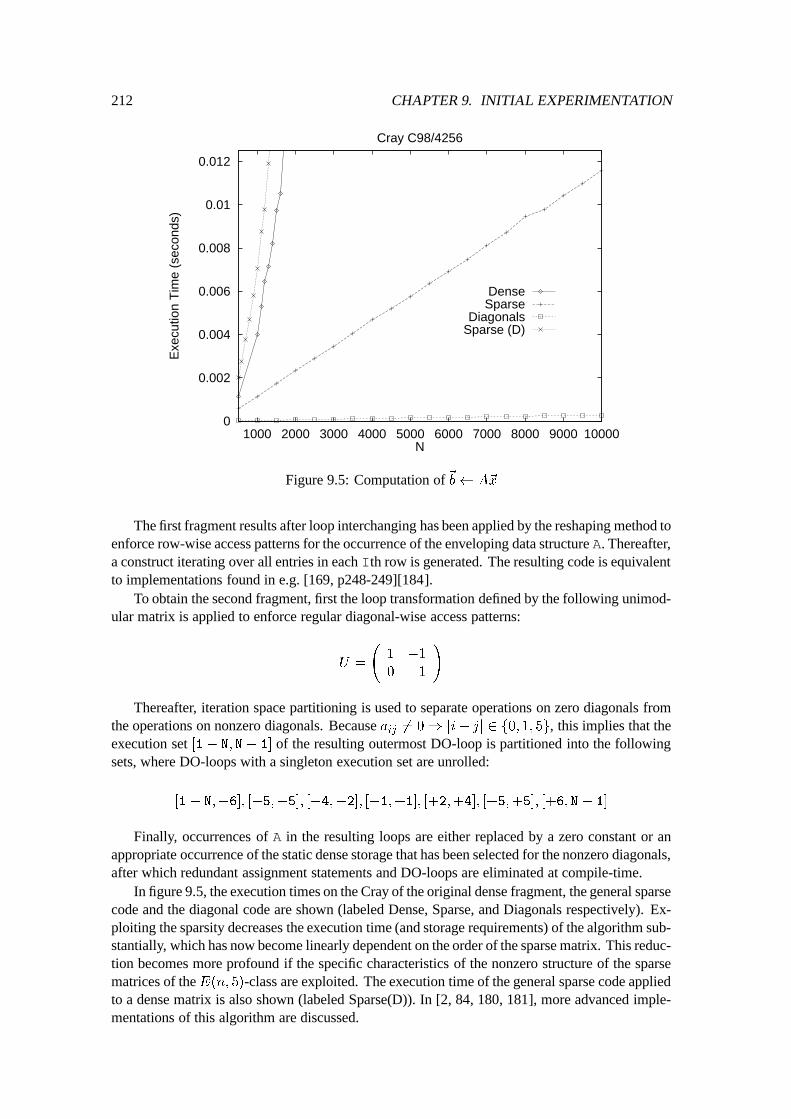
212 CHAPTER 9. INITIAL EXPERIMENTATION
0
0.002
0.004
0.006
0.008
0.01
0.012
1000 2000 3000 4000 5000 6000 7000 8000 9000 10000
Exe
cutio
n T
ime
(sec
onds
)
N
Cray C98/4256
DenseSparse
DiagonalsSparse (D)
Figure 9.5: Computation of~b A~x
The first fragment results after loop interchanging has been applied by the reshaping method toenforce row-wise access patterns for the occurrence of the enveloping data structure A. Thereafter,a construct iterating over all entries in each Ith row is generated. The resulting code is equivalentto implementations found in e.g. [169, p248-249][184].
To obtain the second fragment, first the loop transformation defined by the following unimod-ular matrix is applied to enforce regular diagonal-wise access patterns:
U =
1 �1
0 1
!
Thereafter, iteration space partitioning is used to separate operations on zero diagonals fromthe operations on nonzero diagonals. Because a
ij
6= 0) ji� jj 2 f0; 1; 5g, this implies that theexecution set [1� N; N� 1] of the resulting outermost DO-loop is partitioned into the followingsets, where DO-loops with a singleton execution set are unrolled:
[1� N;�6]; [�5;�5]; [�4;�2]; [�1;+1]; [+2;+4]; [+5;+5]; [+6; N� 1]
Finally, occurrences of A in the resulting loops are either replaced by a zero constant or anappropriate occurrence of the static dense storage that has been selected for the nonzero diagonals,after which redundant assignment statements and DO-loops are eliminated at compile-time.
In figure 9.5, the execution times on the Cray of the original dense fragment, the general sparsecode and the diagonal code are shown (labeled Dense, Sparse, and Diagonals respectively). Ex-ploiting the sparsity decreases the execution time (and storage requirements) of the algorithm sub-stantially, which has now become linearly dependent on the order of the sparse matrix. This reduc-tion becomes more profound if the specific characteristics of the nonzero structure of the sparsematrices of theE(n; 5)-class are exploited. The execution time of the general sparse code appliedto a dense matrix is also shown (labeled Sparse(D)). In [2, 84, 180, 181], more advanced imple-mentations of this algorithm are discussed.
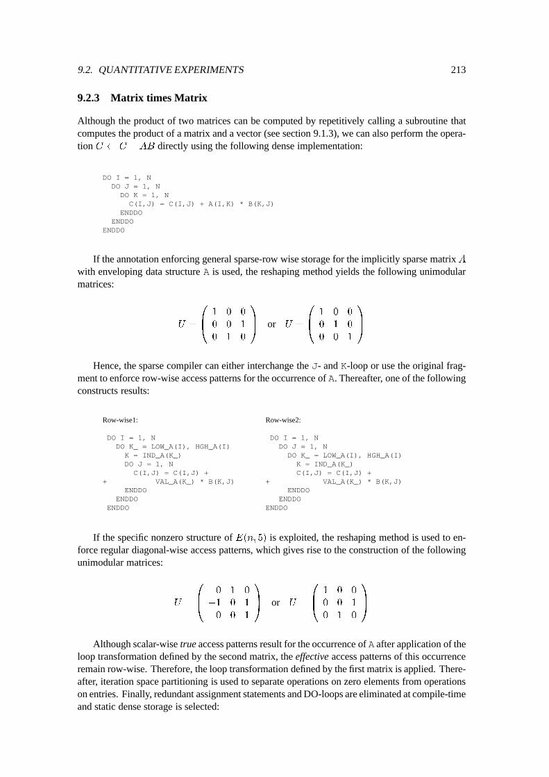
9.2. QUANTITATIVE EXPERIMENTS 213
9.2.3 Matrix times Matrix
Although the product of two matrices can be computed by repetitively calling a subroutine thatcomputes the product of a matrix and a vector (see section 9.1.3), we can also perform the opera-tion C C +AB directly using the following dense implementation:
DO I = 1, NDO J = 1, NDO K = 1, N
C(I,J) = C(I,J) + A(I,K) * B(K,J)ENDDO
ENDDOENDDO
If the annotation enforcing general sparse-row wise storage for the implicitly sparse matrixAwith enveloping data structure A is used, the reshaping method yields the following unimodularmatrices:
U =
0
B
@
1 0 0
0 0 1
0 1 0
1
C
A
or U =
0
B
@
1 0 0
0 1 0
0 0 1
1
C
A
Hence, the sparse compiler can either interchange the J- and K-loop or use the original frag-ment to enforce row-wise access patterns for the occurrence of A. Thereafter, one of the followingconstructs results:
Row-wise1:
DO I = 1, NDO K_ = LOW_A(I), HGH_A(I)K = IND_A(K_)DO J = 1, N
C(I,J) = C(I,J) ++ VAL_A(K_) * B(K,J)
ENDDOENDDO
ENDDO
Row-wise2:
DO I = 1, NDO J = 1, NDO K_ = LOW_A(I), HGH_A(I)
K = IND_A(K_)C(I,J) = C(I,J) +
+ VAL_A(K_) * B(K,J)ENDDO
ENDDOENDDO
If the specific nonzero structure of E(n; 5) is exploited, the reshaping method is used to en-force regular diagonal-wise access patterns, which gives rise to the construction of the followingunimodular matrices:
U =
0
B
@
0 1 0
�1 0 1
0 0 1
1
C
A
or U =
0
B
@
1 0 0
0 0 1
0 1 0
1
C
A
Although scalar-wise true access patterns result for the occurrence of A after application of theloop transformation defined by the second matrix, the effective access patterns of this occurrenceremain row-wise. Therefore, the loop transformation defined by the first matrix is applied. There-after, iteration space partitioning is used to separate operations on zero elements from operationson entries. Finally, redundant assignment statements and DO-loops are eliminated at compile-timeand static dense storage is selected:
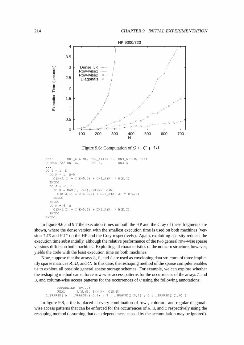
214 CHAPTER 9. INITIAL EXPERIMENTATION
0
0.5
1
1.5
2
2.5
3
3.5
4
100 200 300 400 500 600 700
Exe
cutio
n T
ime
(sec
onds
)
N
HP 9000/720
Dense IJKRow-wise1Row-wise2Diagonals
Figure 9.6: Computation of C C +AB
REAL DN1_A(6:N), DN2_A(1:N-5), DN3_A(1:N,-1:1)COMMON /A/ DN1_A, DN2_A, DN3_A...DO I = 1, NDO K = 1, N-5
C(K+5,I) = C(K+5,I) + DN2_A(K) * B(K,I)ENDDODO J = -1, 1DO K = MAX(1, J+1), MIN(N, J+N)C(K-J,I) = C(K-J,I) + DN3_A(K,-J) * B(K,I)
ENDDOENDDODO K = 6, NC(K-5,I) = C(K-5,I) + DN1_A(K) * B(K,I)
ENDDOENDDO
In figure 9.6 and 9.7 the execution times on both the HP and the Cray of these fragments areshown, where the dense version with the smallest execution time is used on both machines (ver-sion IJK and KJI on the HP and the Cray respectively). Again, exploiting sparsity reduces theexecution time substantially, although the relative performance of the two general row-wise sparseversions differs on both machines. Exploiting all characteristics of the nonzero structure, however,yields the code with the least execution time on both machines.
Now, suppose that the arrays A, B, and C are used as enveloping data structure of three implic-itly sparse matricesA,B, andC . In this case, the reshaping method of the sparse compiler enablesus to explore all possible general sparse storage schemes. For example, we can explore whetherthe reshaping method can enforce row-wise access patterns for the occurrences of the arrays A andB, and column-wise access patterns for the occurrences of C using the following annotations:
PARAMETER (N=...)REAL A(N,N), B(N,N), C(N,N)
C_SPARSE( A : _SPARSE()(0,1) ; B : _SPARSE()(0,1) ; C : _SPARSE()(1,0) )
In figure 9.8, a tile is placed at every combination of row-, column-, and regular diagonal-wise access patterns that can be enforced for the occurrences of A, B, and C respectively using thereshaping method (assuming that data dependences caused by the accumulation may be ignored).
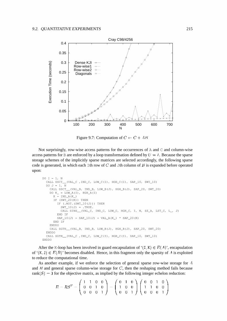
9.2. QUANTITATIVE EXPERIMENTS 215
0
0.05
0.1
0.15
0.2
0.25
0.3
0.35
0.4
100 200 300 400 500 600 700
Exe
cutio
n T
ime
(sec
onds
)
N
Cray C98/4256
Dense KJIRow-wise1Row-wise2Diagonals
Figure 9.7: Computation of C C +AB
Not surprisingly, row-wise access patterns for the occurrences of A and C and column-wiseaccess patterns for B are enforced by a loop transformation defined by U = I . Because the sparsestorage schemes of the implicitly sparse matrices are selected accordingly, the following sparsecode is generated, in which each Ith row of C and Jth column of B is expanded before operatedupon:
DO I = 1, NCALL SSCT__(VAL_C ,IND_C, LOW_C(I), HGH_C(I), SAP_10, SWT_10)DO J = 1, NCALL SSCT__(VAL_B, IND_B, LOW_B(J), HGH_B(J), SAP_20, SWT_20)DO K_ = LOW_A(I), HGH_A(I)
K = IND_A(K_)IF (SWT_20(K)) THEN
IF (.NOT.(SWT_10(J))) THENSWT_10(J) = .TRUE.CALL SINS__(VAL_C, IND_C, LOW_C, HGH_C, I, N, SZ_A, LST_C, L_, J)
END IFSAP_10(J) = SAP_10(J) + VAL_A(K_) * SAP_20(K)
END IFENDDOCALL SGTH__(VAL_B, IND_B, LOW_B(J), HGH_B(J), SAP_20, SWT_20)
ENDDOCALL SGTH__(VAL_C ,IND_C, LOW_C(I), HGH_C(I), SAP_10, SWT_10)
ENDDO
After the K-loop has been involved in guard encapsulation of ‘(I; K) 2 E(A)’, encapsulationof ‘(K; J) 2 E(B)’ becomes disabled. Hence, in this fragment only the sparsity of A is exploitedto reduce the computational time.
As another example, if we enforce the selection of general sparse row-wise storage for Aand B and general sparse column-wise storage for C , then the reshaping method fails becauserank(S) = 3 for the objective matrix, as implied by the following integer echelon reduction:
E = RS
T
=
0
B
@
1 1 0 0
0 0 1 0
0 0 0 1
1
C
A
=
0
B
@
0 1 0
1 0 0
0 0 1
1
C
A
0
B
@
0 0 1 0
1 1 0 0
0 0 0 1
1
C
A
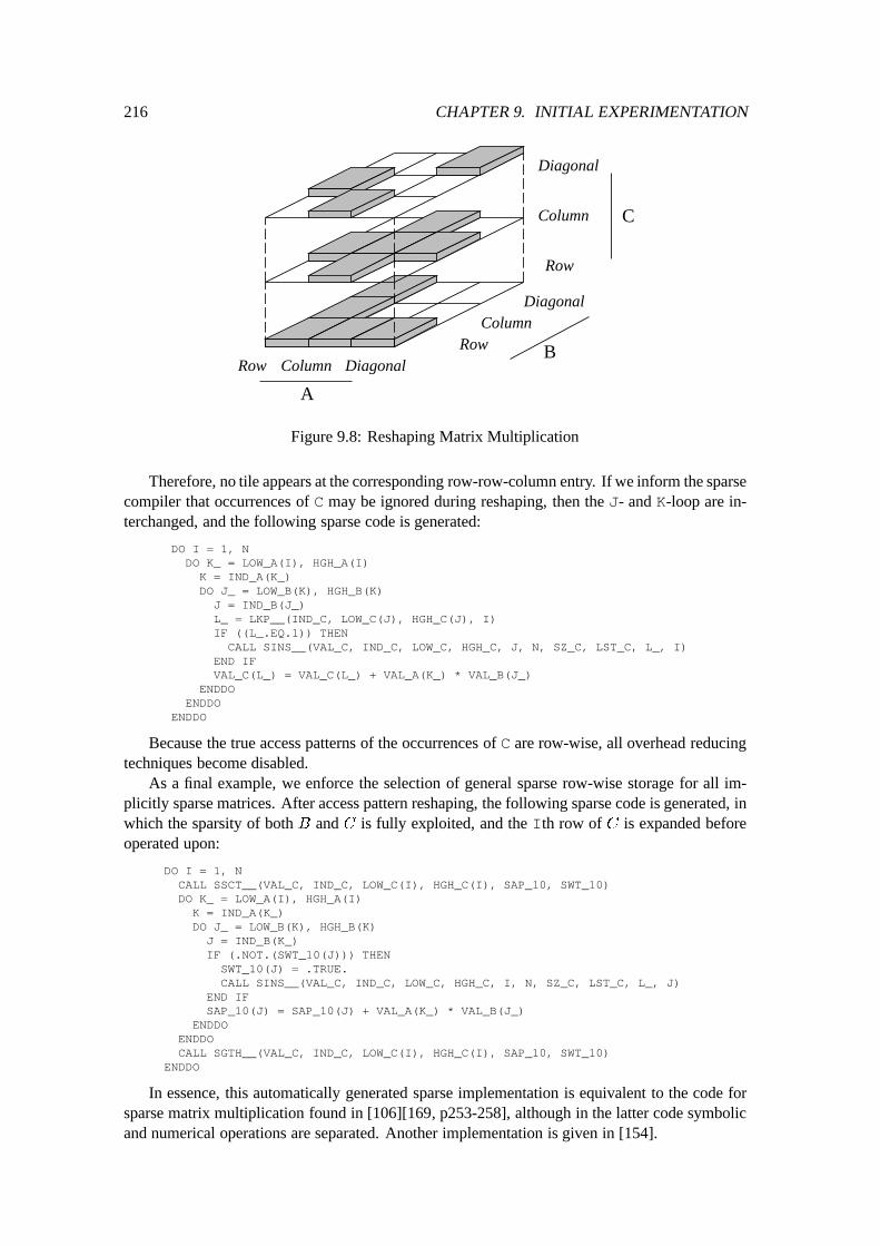
216 CHAPTER 9. INITIAL EXPERIMENTATION
Row Column DiagonalRow
ColumnDiagonal
Row
Column
Diagonal
A
B
C
Figure 9.8: Reshaping Matrix Multiplication
Therefore, no tile appears at the corresponding row-row-column entry. If we inform the sparsecompiler that occurrences of C may be ignored during reshaping, then the J- and K-loop are in-terchanged, and the following sparse code is generated:
DO I = 1, NDO K_ = LOW_A(I), HGH_A(I)K = IND_A(K_)DO J_ = LOW_B(K), HGH_B(K)
J = IND_B(J_)L_ = LKP__(IND_C, LOW_C(J), HGH_C(J), I)IF ((L_.EQ.1)) THEN
CALL SINS__(VAL_C, IND_C, LOW_C, HGH_C, J, N, SZ_C, LST_C, L_, I)END IFVAL_C(L_) = VAL_C(L_) + VAL_A(K_) * VAL_B(J_)
ENDDOENDDO
ENDDO
Because the true access patterns of the occurrences of C are row-wise, all overhead reducingtechniques become disabled.
As a final example, we enforce the selection of general sparse row-wise storage for all im-plicitly sparse matrices. After access pattern reshaping, the following sparse code is generated, inwhich the sparsity of both B and C is fully exploited, and the Ith row of C is expanded beforeoperated upon:
DO I = 1, NCALL SSCT__(VAL_C, IND_C, LOW_C(I), HGH_C(I), SAP_10, SWT_10)DO K_ = LOW_A(I), HGH_A(I)K = IND_A(K_)DO J_ = LOW_B(K), HGH_B(K)J = IND_B(K_)IF (.NOT.(SWT_10(J))) THEN
SWT_10(J) = .TRUE.CALL SINS__(VAL_C, IND_C, LOW_C, HGH_C, I, N, SZ_C, LST_C, L_, J)
END IFSAP_10(J) = SAP_10(J) + VAL_A(K_) * VAL_B(J_)
ENDDOENDDOCALL SGTH__(VAL_C, IND_C, LOW_C(I), HGH_C(I), SAP_10, SWT_10)
ENDDO
In essence, this automatically generated sparse implementation is equivalent to the code forsparse matrix multiplication found in [106][169, p253-258], although in the latter code symbolicand numerical operations are separated. Another implementation is given in [154].
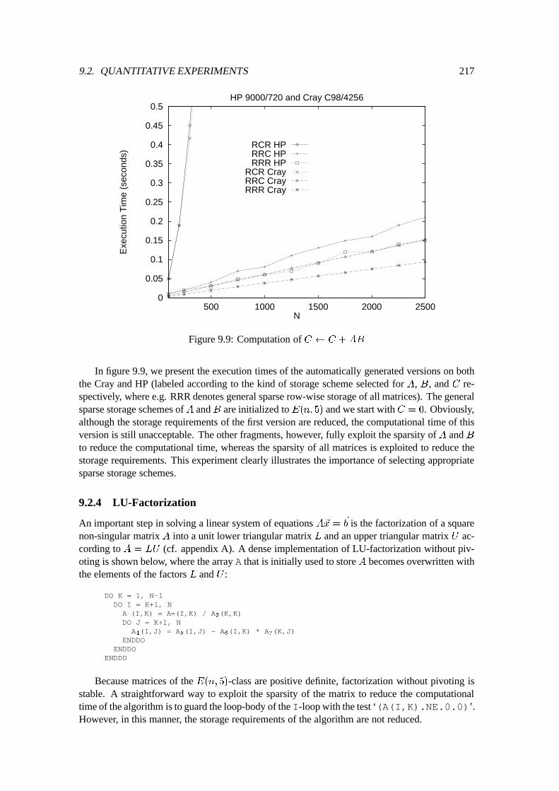
9.2. QUANTITATIVE EXPERIMENTS 217
0
0.05
0.1
0.15
0.2
0.25
0.3
0.35
0.4
0.45
0.5
500 1000 1500 2000 2500
Exe
cutio
n T
ime
(sec
onds
)
N
HP 9000/720 and Cray C98/4256
RCR HPRRC HPRRR HP
RCR CrayRRC CrayRRR Cray
Figure 9.9: Computation of C C +AB
In figure 9.9, we present the execution times of the automatically generated versions on boththe Cray and HP (labeled according to the kind of storage scheme selected for A, B, and C re-spectively, where e.g. RRR denotes general sparse row-wise storage of all matrices). The generalsparse storage schemes ofA andB are initialized to E(n; 5) and we start withC = 0. Obviously,although the storage requirements of the first version are reduced, the computational time of thisversion is still unacceptable. The other fragments, however, fully exploit the sparsity of A and Bto reduce the computational time, whereas the sparsity of all matrices is exploited to reduce thestorage requirements. This experiment clearly illustrates the importance of selecting appropriatesparse storage schemes.
9.2.4 LU-Factorization
An important step in solving a linear system of equations A~x =
~
b is the factorization of a squarenon-singular matrix A into a unit lower triangular matrix L and an upper triangular matrix U ac-cording to A = LU (cf. appendix A). A dense implementation of LU-factorization without piv-oting is shown below, where the array A that is initially used to store A becomes overwritten withthe elements of the factors L and U :
DO K = 1, N-1DO I = K+1, NA1
(I,K) = A2
(I,K) / A3
(K,K)DO J = K+1, N
A4
(I,J) = A5
(I,J) - A6
(I,K) * A7
(K,J)ENDDO
ENDDOENDDO
Because matrices of the E(n; 5)-class are positive definite, factorization without pivoting isstable. A straightforward way to exploit the sparsity of the matrix to reduce the computationaltime of the algorithm is to guard the loop-body of the I-loop with the test ‘(A(I,K).NE.0.0)’.However, in this manner, the storage requirements of the algorithm are not reduced.
218 CHAPTER 9. INITIAL EXPERIMENTATION
If we use an annotation to enforce the selection of general sparse row-wise storage for theimplicitly sparse matrix A with enveloping data structure A, then the reshaping method fails, andthe following sparse code is generated:2
DO K = 1, NDO I = K+1, N
CALL SSCT__(VAL_A, IND_A, LOW_A(I), HGH_A(I), SAP_20, SWT_20)IF (SWT_20(K)) THENSAP_20(K) = SAP_20(K) / VAL_A(LKP__(IND_A, LOW_A(K), HGH_A(K), K))LEN_J = HGH_A(K) - LOW_A(K)DO J_ = 0, LEN_J
J = IND_A(LOW_A(K) + J_)IF (K+1.LE.J) THEN
IF (.NOT.SWT_20(J)) THENSWT_20(J) = .TRUE.CALL SINS__(VAL_A, IND_A, LOW_A, HGH_A, I, NP_A, SZ_A, LST_A, L_, J)
END IFSAP_20(J) = SAP_20(J) - SAP_20(K) * VAL_A(LOW_A(K) + J_)
END IFENDDO
ENDIFCALL SGTH__(VAL_A, IND_A, LOW_A(I), HGH_A(I), SAP_20, SWT_20)
ENDDOENDDO
However, if the programmer indicates that the access patterns of occurrence A(K,K) maybe ignored during the reshaping, the I- and J-loop are interchanged to obtain row-wise accesspatterns for the three occurrences A(I,K). Thereafter, the following sparse code is generated:
DO I = 2, NCALL SSCT__(VAL_A1, IND_A, LOW_A(I), HGH_A(I), SAP_10, SWT_10)DO K = 1, I-1IF (SWT_10(K)) THENSAP_10(K) = SAP_10(K) / VAL_A(LKP__(IND_A, LOW_A(K), HGH_A(K), K))LEN_J = HGH_A(K) - LOW_A(K)DO J_ = 0, LEN_J
J = IND_A(LOW_A(K)+J_)IF (K+1.LE.J) THEN
IF (.NOT.SWT_10(J)) THENSWT_10(J) = .TRUE.CALL SINS__(VAL_A, IND_A, LOW_A, HGH_A, I, N, SZ_A, LST_A, L_, J)
END IFSAP_10(J) = SAP_10(J) - SAP_10(K) * VAL_A(LOW_A(K+J_))
END IFENDDO
END IFENDDOCALL SGTH__(VAL_A, IND_A, LOW_A(I), HGH_A(I), SAP_10, SWT_10)
ENDDO
Guard ‘(K; J) 2 E(A)’ has been encapsulated in the execution set of the J-loop because dur-ing each fixed iteration I = i and K = k, only insertions in the jth row, where i < k < j mayoccur. The entries are accessed relatively to the base location LOW A(K) to correctly account forany data movement that may occur during insertions in other rows. Moreover, since all entries ina row of the sparse matrix are stored in a single sparse vector, the test ‘(K+1.LE.J)’ is requiredto determine whether an entry must actually be operated upon. The possible insertions disable en-capsulation of guard ‘(I; K) 2 E(A)’ in the execution set of the K-loop, because we would liketo iterate over all entries in a row in which insertions are performed (which could only be imple-mented if some kind of ordering would be imposed on the entries in each row).
Because fill-in occurs, the nonzero structure of the sparse matrix changes into the nonzerostructure of the filled matrix, i.e. L+ U .
2Here, we have manually moved to the scatter operation before the first assignment statement to improve the per-formance. Such optimizations can be easily incorporated in a future implementation.
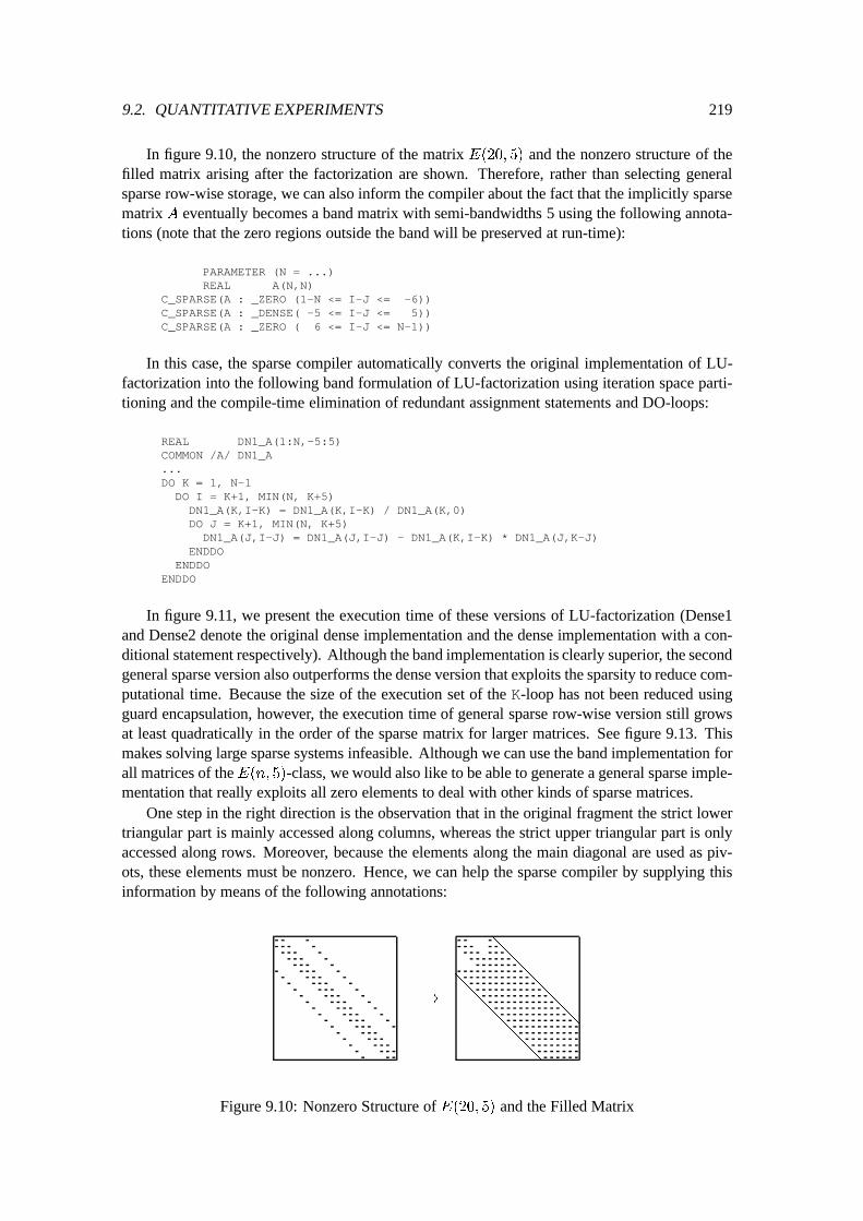
9.2. QUANTITATIVE EXPERIMENTS 219
In figure 9.10, the nonzero structure of the matrix E(20; 5) and the nonzero structure of thefilled matrix arising after the factorization are shown. Therefore, rather than selecting generalsparse row-wise storage, we can also inform the compiler about the fact that the implicitly sparsematrix A eventually becomes a band matrix with semi-bandwidths 5 using the following annota-tions (note that the zero regions outside the band will be preserved at run-time):
PARAMETER (N = ...)REAL A(N,N)
C_SPARSE(A : _ZERO (1-N <= I-J <= -6))C_SPARSE(A : _DENSE( -5 <= I-J <= 5))C_SPARSE(A : _ZERO ( 6 <= I-J <= N-1))
In this case, the sparse compiler automatically converts the original implementation of LU-factorization into the following band formulation of LU-factorization using iteration space parti-tioning and the compile-time elimination of redundant assignment statements and DO-loops:
REAL DN1_A(1:N,-5:5)COMMON /A/ DN1_A...DO K = 1, N-1DO I = K+1, MIN(N, K+5)DN1_A(K,I-K) = DN1_A(K,I-K) / DN1_A(K,0)DO J = K+1, MIN(N, K+5)
DN1_A(J,I-J) = DN1_A(J,I-J) - DN1_A(K,I-K) * DN1_A(J,K-J)ENDDO
ENDDOENDDO
In figure 9.11, we present the execution time of these versions of LU-factorization (Dense1and Dense2 denote the original dense implementation and the dense implementation with a con-ditional statement respectively). Although the band implementation is clearly superior, the secondgeneral sparse version also outperforms the dense version that exploits the sparsity to reduce com-putational time. Because the size of the execution set of the K-loop has not been reduced usingguard encapsulation, however, the execution time of general sparse row-wise version still growsat least quadratically in the order of the sparse matrix for larger matrices. See figure 9.13. Thismakes solving large sparse systems infeasible. Although we can use the band implementation forall matrices of theE(n; 5)-class, we would also like to be able to generate a general sparse imple-mentation that really exploits all zero elements to deal with other kinds of sparse matrices.
One step in the right direction is the observation that in the original fragment the strict lowertriangular part is mainly accessed along columns, whereas the strict upper triangular part is onlyaccessed along rows. Moreover, because the elements along the main diagonal are used as piv-ots, these elements must be nonzero. Hence, we can help the sparse compiler by supplying thisinformation by means of the following annotations:
!
@
@
@
@
@
@
@
@
@
@
@
@
Figure 9.10: Nonzero Structure of E(20; 5) and the Filled Matrix
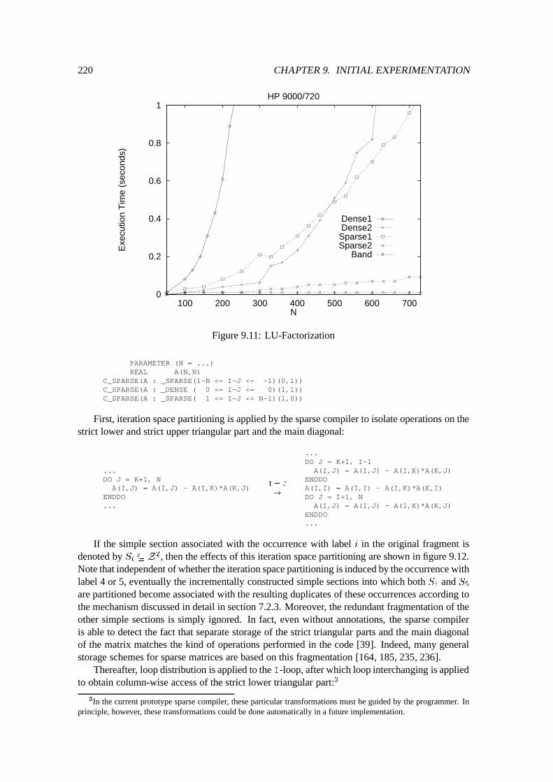
220 CHAPTER 9. INITIAL EXPERIMENTATION
0
0.2
0.4
0.6
0.8
1
100 200 300 400 500 600 700
Exe
cutio
n T
ime
(sec
onds
)
N
HP 9000/720
Dense1Dense2Sparse1Sparse2
Band
Figure 9.11: LU-Factorization
PARAMETER (N = ...)REAL A(N,N)
C_SPARSE(A : _SPARSE(1-N <= I-J <= -1)(0,1))C_SPARSE(A : _DENSE ( 0 <= I-J <= 0)(1,1))C_SPARSE(A : _SPARSE( 1 <= I-J <= N-1)(1,0))
First, iteration space partitioning is applied by the sparse compiler to isolate operations on thestrict lower and strict upper triangular part and the main diagonal:
...DO J = K+1, NA(I,J) = A(I,J) - A(I,K)*A(K,J)
ENDDO...
I = J
!
...DO J = K+1, I-1A(I,J) = A(I,J) - A(I,K)*A(K,J)
ENDDOA(I,I) = A(I,I) - A(I,K)*A(K,I)DO J = I+1, NA(I,J) = A(I,J) - A(I,K)*A(K,J)
ENDDO...
If the simple section associated with the occurrence with label i in the original fragment isdenoted by S
i
� Z
2, then the effects of this iteration space partitioning are shown in figure 9.12.Note that independent of whether the iteration space partitioning is induced by the occurrence withlabel 4 or 5, eventually the incrementally constructed simple sections into which both S
4
and S5
are partitioned become associated with the resulting duplicates of these occurrences according tothe mechanism discussed in detail in section 7.2.3. Moreover, the redundant fragmentation of theother simple sections is simply ignored. In fact, even without annotations, the sparse compileris able to detect the fact that separate storage of the strict triangular parts and the main diagonalof the matrix matches the kind of operations performed in the code [39]. Indeed, many generalstorage schemes for sparse matrices are based on this fragmentation [164, 185, 235, 236].
Thereafter, loop distribution is applied to the I-loop, after which loop interchanging is appliedto obtain column-wise access of the strict lower triangular part:3
3In the current prototype sparse compiler, these particular transformations must be guided by the programmer. Inprinciple, however, these transformations could be done automatically in a future implementation.
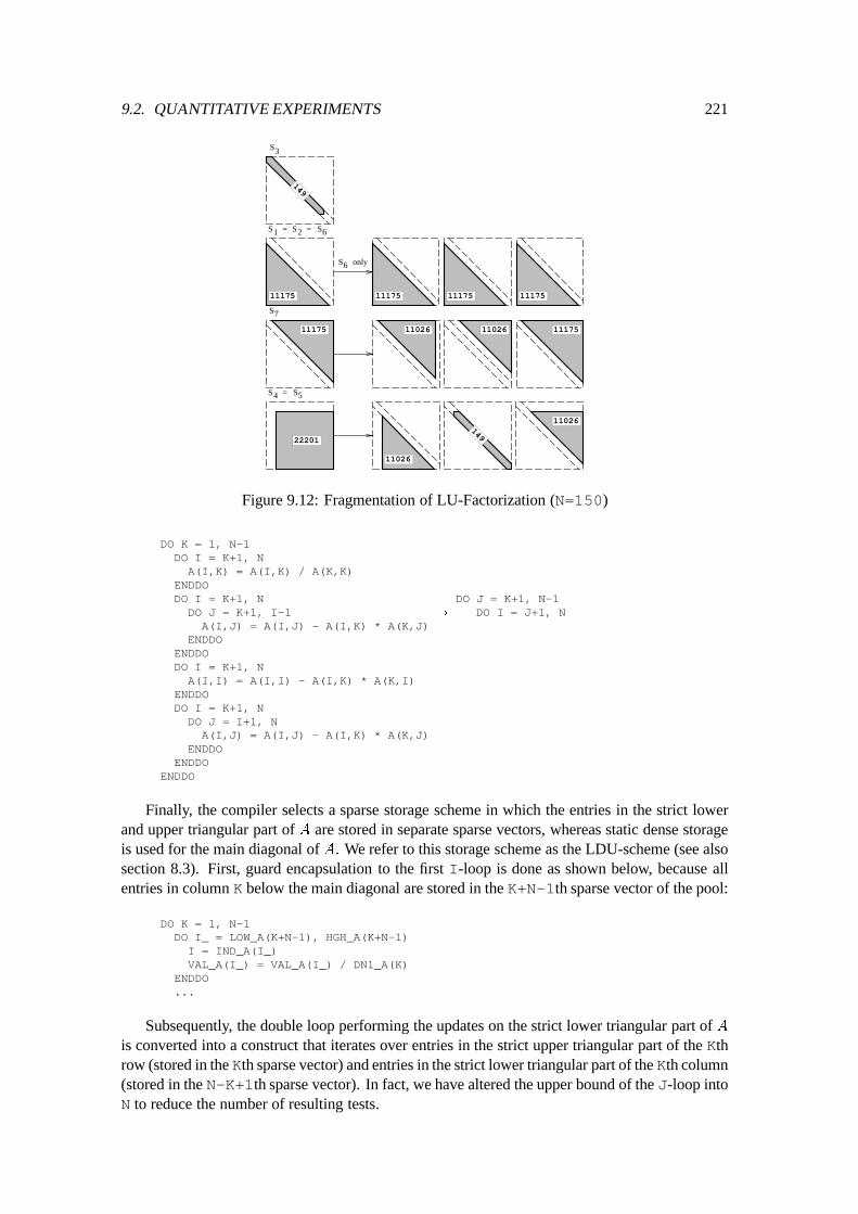
9.2. QUANTITATIVE EXPERIMENTS 221
149
S3
11175
S7
11175
S = S1 2 = S6
22201
S4 = S5
11026
11026149
11026 11026 11175
111751117511175
S6 only
Figure 9.12: Fragmentation of LU-Factorization (N=150)
DO K = 1, N-1DO I = K+1, NA(I,K) = A(I,K) / A(K,K)
ENDDODO I = K+1, N DO J = K+1, N-1DO J = K+1, I-1 ! DO I = J+1, N
A(I,J) = A(I,J) - A(I,K) * A(K,J)ENDDO
ENDDODO I = K+1, NA(I,I) = A(I,I) - A(I,K) * A(K,I)
ENDDODO I = K+1, NDO J = I+1, N
A(I,J) = A(I,J) - A(I,K) * A(K,J)ENDDO
ENDDOENDDO
Finally, the compiler selects a sparse storage scheme in which the entries in the strict lowerand upper triangular part of A are stored in separate sparse vectors, whereas static dense storageis used for the main diagonal of A. We refer to this storage scheme as the LDU-scheme (see alsosection 8.3). First, guard encapsulation to the first I-loop is done as shown below, because allentries in column K below the main diagonal are stored in the K+N-1th sparse vector of the pool:
DO K = 1, N-1DO I_ = LOW_A(K+N-1), HGH_A(K+N-1)I = IND_A(I_)VAL_A(I_) = VAL_A(I_) / DN1_A(K)
ENDDO...
Subsequently, the double loop performing the updates on the strict lower triangular part of Ais converted into a construct that iterates over entries in the strict upper triangular part of the Kthrow (stored in the Kth sparse vector) and entries in the strict lower triangular part of the Kth column(stored in the N-K+1th sparse vector). In fact, we have altered the upper bound of the J-loop intoN to reduce the number of resulting tests.
222 CHAPTER 9. INITIAL EXPERIMENTATION
The sparse compiler generates code in which relative addressing is used to account for possibledata movement. The Jth column below the main diagonal is expanded before operated upon:
LEN_J = HGH_A(K) - LOW_A(K)DO J_ = 0, LEN_J
J = IND_A(LOW_A(K)+J_)CALL SSCT__(VAL_A, IND_A, LOW_A(J+N-1), HGH_A(J+N-1), SAP_20, SWT_20)IF (J+1.LE.100) THENLEN_I = HGH_A(K+N-1) - LOW_A(K+N-1)DO I_ = 0, LEN_I, 1
I = IND_A((LOW_A(K+N-1)+I_))IF (J+1.LE.I) THEN
IF (.NOT.SWT_20(I)) THENSWT_20(I) = .TRUE.CALL SINS__(VAL_A, IND_A, LOW_A, HGH_A, J+N-1, N, SZ_A, LST_A, L_, I)
ENDIFSAP_20(I) = SAP_20(I) - VAL_A((LOW_A(K+N-1)+I_)) * VAL_A((LOW_A(K)+J_))
ENDIFENDDO
ENDIFCALL SGTH__(VAL_A, IND_A, LOW_A(J+N-1), HGH_A(J+N-1), SAP_20, SWT_20)
ENDDO
Updating the elements along the main diagonal is implemented as follows:
CALL SSCT__(VAL_A, IND_A, LOW_A(K), HGH_A(K), SAP_10, SWT_10)DO I_ = LOW_A(K+N-1), HGH_A(K+N-1)
I = IND_A(I_)IF (SWT_10(I)) THENDN1_A(I) = DN1_A(I) - VAL_A(I_) * SAP_10(I)
ENDIFENDDOCALL SGTH__(VAL_A, IND_A, LOW_A(K), HGH_A(K), SAP_10, SWT_10)
As partly illustrated below, the sparse code generated for the double loop that performs theupdating of elements in the strict upper triangular part is very similar to the code that updates thestrict lower triangular part:
LEN_I = HGH_A(K+N-1) - LOW_A(K+N-1)DO I_ = 0, LEN_I
I = IND_A(LOW_A(K)+N-1+I_)......
...ENDDO
ENDDO ! K-loop
In figure 9.13, the execution time of the implementation operating upon the LDU-schemeis compared with the execution time of the general sparse row-wise and band version of LU-factorization. Although the LDU sparse version is slightly more expensive than the band version,these experiments indicate that a general sparse implementation that fully exploits the sparsity ofA can be derived. In figure 9.14 and 9.15, the same experiments are done on the Cray (note thatthe dense versions run significantly faster than on the HP).
Another way to obtain an implementation of LU-factorization that fully exploits the sparsityof the matrix operated upon is to store the column nonzero structure of the matrix in combinationwith general sparse row-wise storage [105][235, ch2][236, 164]. Obviously, the LDU-scheme suf-fers from less overhead storage. Moreover, because matrices of the E(n; 5)-class are symmetricpositive definite, we would rather like to use the Choleski factorization to solve a correspondingsystem of linear equations. Experiments with the sparse compiler indicate that a row- or column-oriented formulation of Choleski factorization (see e.g. [129, p201]) is directly converted into aversion exploiting all zero elements. A symmetric implementation in which symbolic and numer-ical operations are separated can be found in [169, p258-268].
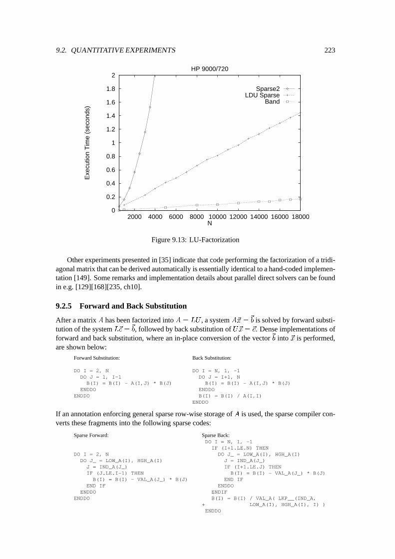
9.2. QUANTITATIVE EXPERIMENTS 223
0
0.2
0.4
0.6
0.8
1
1.2
1.4
1.6
1.8
2
2000 4000 6000 8000 10000 12000 14000 16000 18000
Exe
cutio
n T
ime
(sec
onds
)
N
HP 9000/720
Sparse2LDU Sparse
Band
Figure 9.13: LU-Factorization
Other experiments presented in [35] indicate that code performing the factorization of a tridi-agonal matrix that can be derived automatically is essentially identical to a hand-coded implemen-tation [149]. Some remarks and implementation details about parallel direct solvers can be foundin e.g. [129][168][235, ch10].
9.2.5 Forward and Back Substitution
After a matrix A has been factorized into A = LU , a system A~x =
~
b is solved by forward substi-tution of the system L~c =
~
b, followed by back substitution of U~x = ~c. Dense implementations offorward and back substitution, where an in-place conversion of the vector ~b into ~x is performed,are shown below:
Forward Substitution:
DO I = 2, NDO J = 1, I-1B(I) = B(I) - A(I,J) * B(J)
ENDDOENDDO
Back Substitution:
DO I = N, 1, -1DO J = I+1, N
B(I) = B(I) - A(I,J) * B(J)ENDDOB(I) = B(I) / A(I,I)
ENDDO
If an annotation enforcing general sparse row-wise storage of A is used, the sparse compiler con-verts these fragments into the following sparse codes:
Sparse Forward:
DO I = 2, NDO J_ = LOW_A(I), HGH_A(I)J = IND_A(J_)IF (J.LE.I-1) THEN
B(I) = B(I) - VAL_A(J_) * B(J)END IF
ENDDOENDDO
Sparse Back:DO I = N, 1, -1
IF (I+1.LE.N) THENDO J_ = LOW_A(I), HGH_A(I)J = IND_A(J_)IF (I+1.LE.J) THEN
B(I) = B(I) - VAL_A(J_) * B(J)END IF
ENDDOENDIFB(I) = B(I) / VAL_A( LKP__(IND_A,
+ LOW_A(I), HGH_A(I), I) )ENDDO
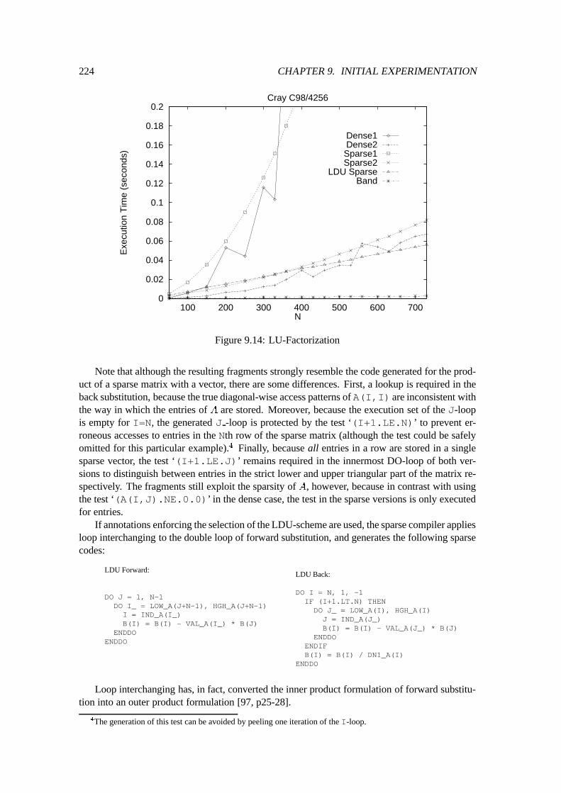
224 CHAPTER 9. INITIAL EXPERIMENTATION
0
0.02
0.04
0.06
0.08
0.1
0.12
0.14
0.16
0.18
0.2
100 200 300 400 500 600 700
Exe
cutio
n T
ime
(sec
onds
)
N
Cray C98/4256
Dense1Dense2Sparse1Sparse2
LDU SparseBand
Figure 9.14: LU-Factorization
Note that although the resulting fragments strongly resemble the code generated for the prod-uct of a sparse matrix with a vector, there are some differences. First, a lookup is required in theback substitution, because the true diagonal-wise access patterns of A(I,I) are inconsistent withthe way in which the entries of A are stored. Moreover, because the execution set of the J-loopis empty for I=N, the generated J -loop is protected by the test ‘(I+1.LE.N)’ to prevent er-roneous accesses to entries in the Nth row of the sparse matrix (although the test could be safelyomitted for this particular example).4 Finally, because all entries in a row are stored in a singlesparse vector, the test ‘(I+1.LE.J)’ remains required in the innermost DO-loop of both ver-sions to distinguish between entries in the strict lower and upper triangular part of the matrix re-spectively. The fragments still exploit the sparsity of A, however, because in contrast with usingthe test ‘(A(I,J).NE.0.0)’ in the dense case, the test in the sparse versions is only executedfor entries.
If annotations enforcing the selection of the LDU-scheme are used, the sparse compiler appliesloop interchanging to the double loop of forward substitution, and generates the following sparsecodes:
LDU Forward:
DO J = 1, N-1DO I_ = LOW_A(J+N-1), HGH_A(J+N-1)I = IND_A(I_)B(I) = B(I) - VAL_A(I_) * B(J)
ENDDOENDDO
LDU Back:
DO I = N, 1, -1IF (I+1.LT.N) THEN
DO J_ = LOW_A(I), HGH_A(I)J = IND_A(J_)B(I) = B(I) - VAL_A(J_) * B(J)
ENDDOENDIFB(I) = B(I) / DN1_A(I)
ENDDO
Loop interchanging has, in fact, converted the inner product formulation of forward substitu-tion into an outer product formulation [97, p25-28].
4The generation of this test can be avoided by peeling one iteration of the I-loop.
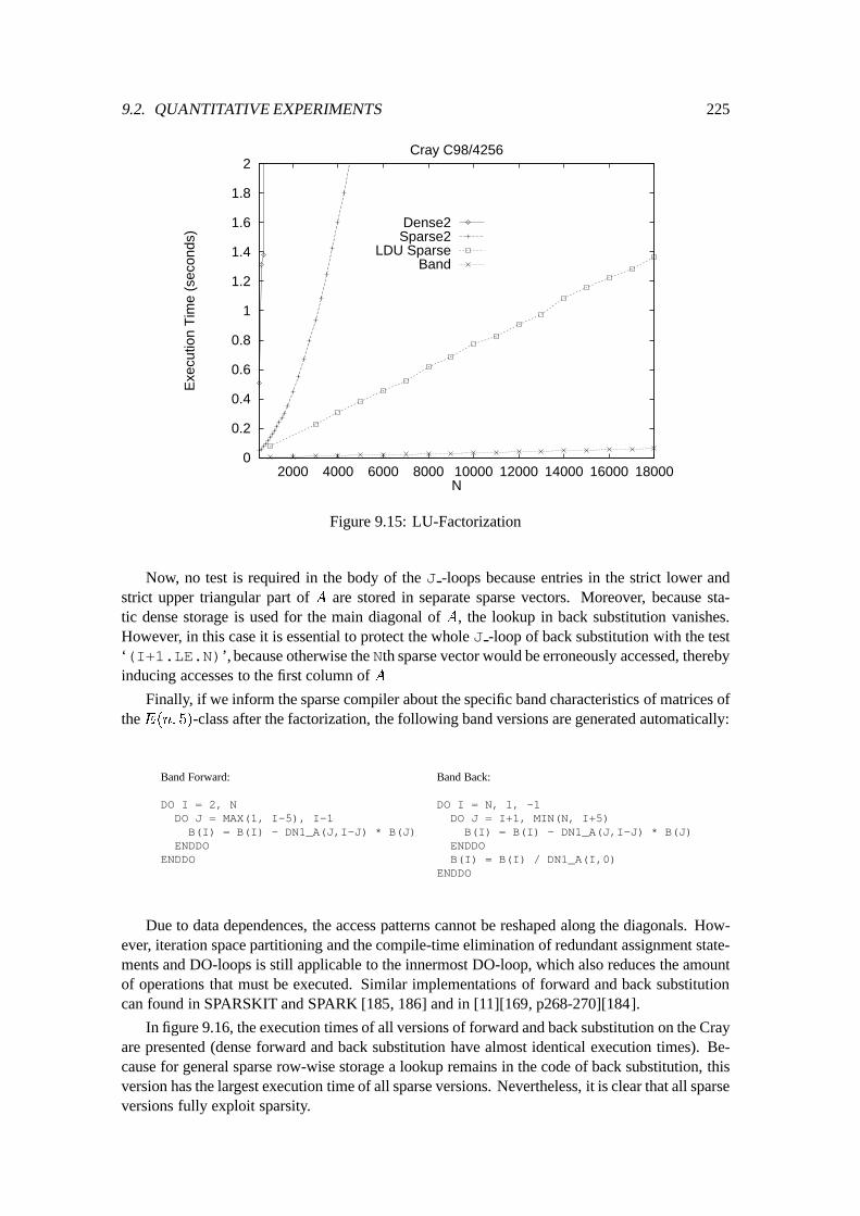
9.2. QUANTITATIVE EXPERIMENTS 225
0
0.2
0.4
0.6
0.8
1
1.2
1.4
1.6
1.8
2
2000 4000 6000 8000 10000 12000 14000 16000 18000
Exe
cutio
n T
ime
(sec
onds
)
N
Cray C98/4256
Dense2Sparse2
LDU SparseBand
Figure 9.15: LU-Factorization
Now, no test is required in the body of the J -loops because entries in the strict lower andstrict upper triangular part of A are stored in separate sparse vectors. Moreover, because sta-tic dense storage is used for the main diagonal of A, the lookup in back substitution vanishes.However, in this case it is essential to protect the whole J -loop of back substitution with the test‘(I+1.LE.N)’, because otherwise the Nth sparse vector would be erroneously accessed, therebyinducing accesses to the first column of A
Finally, if we inform the sparse compiler about the specific band characteristics of matrices ofthe E(n; 5)-class after the factorization, the following band versions are generated automatically:
Band Forward:
DO I = 2, NDO J = MAX(1, I-5), I-1B(I) = B(I) - DN1_A(J,I-J) * B(J)
ENDDOENDDO
Band Back:
DO I = N, 1, -1DO J = I+1, MIN(N, I+5)
B(I) = B(I) - DN1_A(J,I-J) * B(J)ENDDOB(I) = B(I) / DN1_A(I,0)
ENDDO
Due to data dependences, the access patterns cannot be reshaped along the diagonals. How-ever, iteration space partitioning and the compile-time elimination of redundant assignment state-ments and DO-loops is still applicable to the innermost DO-loop, which also reduces the amountof operations that must be executed. Similar implementations of forward and back substitutioncan found in SPARSKIT and SPARK [185, 186] and in [11][169, p268-270][184].
In figure 9.16, the execution times of all versions of forward and back substitution on the Crayare presented (dense forward and back substitution have almost identical execution times). Be-cause for general sparse row-wise storage a lookup remains in the code of back substitution, thisversion has the largest execution time of all sparse versions. Nevertheless, it is clear that all sparseversions fully exploit sparsity.
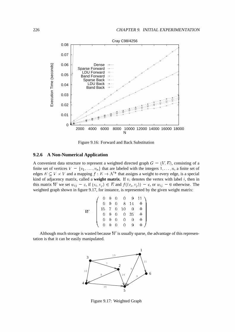
226 CHAPTER 9. INITIAL EXPERIMENTATION
0
0.01
0.02
0.03
0.04
0.05
0.06
0.07
0.08
2000 4000 6000 8000 10000 12000 14000 16000 18000
Exe
cutio
n T
ime
(sec
onds
)
N
Cray C98/4256
DenseSparse Forward
LDU ForwardBand Forward
Sparse BackLDU Back
Band Back
Figure 9.16: Forward and Back Substitution
9.2.6 A Non-Numerical Application
A convenient data structure to represent a weighted directed graph G = (V;E), consisting of afinite set of vertices V = fv
1
; : : : ; v
n
g that are labeled with the integers 1; : : : ; n, a finite set ofedges E � V � V and a mapping f : E ! N
+ that assigns a weight to every edge, is a specialkind of adjacency matrix, called a weight matrix. If v
i
denotes the vertex with label i, then inthis matrix W we set w
ij
= c, if (vi
; v
j
) 2 E and f((vi
; v
j
)) = c, or wij
= 0 otherwise. Theweighted graph shown in figure 9.17, for instance, is represented by the given weight matrix:
W =
0
B
B
B
B
B
B
B
@
0 0 0 0 9 11
0 0 0 8 14 0
15 7 0 10 0 0
0 0 0 0 35 0
0 0 0 0 0 0
0 0 0 0 9 0
1
C
C
C
C
C
C
C
A
Although much storage is wasted because W is usually sparse, the advantage of this represen-tation is that it can be easily manipulated.
1
2
5
6
4
8
35
14
9
9
11
315
7
10
Figure 9.17: Weighted Graph
9.2. QUANTITATIVE EXPERIMENTS 227
For example, below we present a straightforward implementation of finding a topological sortof a directed acyclic graph, which is a mapping t : V ! f1; : : : ; ng, such that 8(v
i
; v
j
) 2 E :
t(v
i
) < t(v
j
).In the implementation, first the in-degree of every vertex is determined in arrayINDEG. There-
after, the topological sort is computed in array TOP by using a stack to successively consider eachnext vertex with zero in-degree and adapting the in-degree of all neighbors:
PROGRAM TOPSORTINTEGER N, I, J, TOPPARAMETER (N = ...)INTEGER W(N,N), INDEG(N), TOP(N)INTEGER STACK(N), SP
DO J = 1, NINDEG(J) = 0DO I = 1, NIF (W(I,J).NE.0) THEN
INDEG(J) = INDEG(J) + 1ENDIF
ENDDOENDDOSP = 0DO I = 1, NIF (INDEG(I).EQ.0) THENCALL PUSH(STACK, SP, I)
ENDIFENDDOTP = 1CALL POP(STACK, SP, I)DO WHILE (I.GT.0)TOP(I) = TPTP = TP + 1DO J = 1, NIF (W(I,J).NE.0) THEN
INDEG(J) = INDEG(J) - 1IF (INDEG(J).EQ.0) THEN
CALL PUSH(STACK, SP, J)ENDIF
ENDIFENDDOCALL POP(STACK, SP, I)
ENDDO
END
SUBROUTINE PUSH(STACK, SP, I)INTEGER STACK(*), SP, I
SP = SP + 1STACK(SP) = IRETURNEND
SUBROUTINE POP(STACK, SP, I)INTEGER STACK(*), SP, I
IF (SP.GT.0) THENI = STACK(SP)SP = SP - 1
ELSEI = 0
ENDIFRETURNEND
For the previous graph, for instance, the mapping t(1) = 4, t(2) = 2, t(3) = 1, t(4) = 3,t(5) = 6, and t(6) = 5 is constructed.
Because matrix W is sparse and accessed along the rows within the WHILE-loop, an annota-tion that enforces the selection of general sparse row-wise storage for the implicitly sparse matrixW with enveloping data structure W is added to this program. Supported by loop distribution andloop interchanging, the following conversion is applied by the sparse compiler to the fragmentcomputing the indegree, because the condition of the IF-statement always fails for zero elements,where NP W=N and SZ W provides sufficient space to store the entries of W :
DO J = 1, NINDEG(J) = 0DO I = 1, N
IF (W(I,J).NE.0) THENINDEG(J) = INDEG(J) + 1
ENDIFENDDO
ENDDO...
!
DO J = 1, NINDEG(J) = 0
ENDDODO I = 1, N
DO J_ = LOW_W(I), HGH_W(I)J = IND_W(J_)IF (VAL_W(J_).NE.0) THEN
INDEG(J) = INDEG(J) + 1ENDIF
ENDDOENDDO...
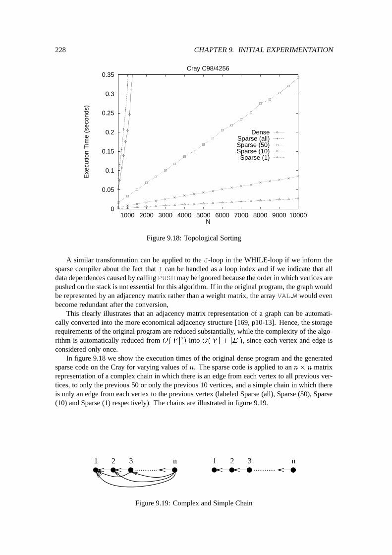
228 CHAPTER 9. INITIAL EXPERIMENTATION
0
0.05
0.1
0.15
0.2
0.25
0.3
0.35
1000 2000 3000 4000 5000 6000 7000 8000 9000 10000
Exe
cutio
n T
ime
(sec
onds
)
N
Cray C98/4256
DenseSparse (all)Sparse (50)Sparse (10)Sparse (1)
Figure 9.18: Topological Sorting
A similar transformation can be applied to the J-loop in the WHILE-loop if we inform thesparse compiler about the fact that I can be handled as a loop index and if we indicate that alldata dependences caused by calling PUSHmay be ignored because the order in which vertices arepushed on the stack is not essential for this algorithm. If in the original program, the graph wouldbe represented by an adjacency matrix rather than a weight matrix, the array VAL W would evenbecome redundant after the conversion,
This clearly illustrates that an adjacency matrix representation of a graph can be automati-cally converted into the more economical adjacency structure [169, p10-13]. Hence, the storagerequirements of the original program are reduced substantially, while the complexity of the algo-rithm is automatically reduced from O(jV j
2
) into O(jV j + jEj), since each vertex and edge isconsidered only once.
In figure 9.18 we show the execution times of the original dense program and the generatedsparse code on the Cray for varying values of n. The sparse code is applied to an n � n matrixrepresentation of a complex chain in which there is an edge from each vertex to all previous ver-tices, to only the previous 50 or only the previous 10 vertices, and a simple chain in which thereis only an edge from each vertex to the previous vertex (labeled Sparse (all), Sparse (50), Sparse(10) and Sparse (1) respectively). The chains are illustrated in figure 9.19.
1 2 3............
n1 2 3............
n
Figure 9.19: Complex and Simple Chain
Chapter 10
Advanced Transformations
In previous chapters, we have demonstrated the feasibility of automatically converting a denseprogram into semantically equivalent sparse code. Experiments indicate that in many cases thesparse compiler is capable of transforming a particular dense fragment into code that fully exploitsthe sparsity of all implicitly sparse matrices to reduce both the storage requirements as well ascomputational time of the original implementation. Although more experiments and probably thedevelopment of more advanced transformations and strategies are required to determine whether asuccessful conversion is also feasible for large programs, the fact that in principle the complexityof writing sparse codes can be reduced substantially by dealing with the sparsity of matrices at thecompilation level rather than at the programming level already seems to justify this new approach.So far, however, some other important issues have not been addressed.
First, because the sparse compiler is presented with the original dense program, the informa-tion obtained by data dependence analysis of this program is usually more accurate than the in-formation that can be obtained by a compiler to which only the resulting sparse code is presented.Although this advantage already has been exploited to a certain extend, since accurate data de-pendence information enables more program transformations to support the selection of a suitablesparse storage scheme, data dependence information obtained by analyzing the original dense pro-gram can also be used to exploit implicit parallelism in the corresponding sparse code, as furtherdiscussed in section 10.1 of this chapter.
Second, because on one hand a reordering method may be required to preserve sparsity and,possibly, stability as well (cf. appendix A), which can be essential to keep solving a sparse prob-lem feasible, whereas on the other hand it is difficult to express sparsity related decisions in theoriginal dense code, some elementary support for the incorporation of both local strategies and apriori reordering methods in the generated sparse code is provided by the sparse compiler. Theimplementation of this support is explored in section 10.2 of this chapter.
10.1 Exploiting Parallelism in the Generated Sparse Code
Because the sparse compiler is presented with the original dense program, accurate data depen-dence analysis can be performed. This provides the sparse compiler with all information requiredfor loop vectorization and concurrentization of the corresponding sparse code. However, becausethis information may be lost in an obscured sparse code, the information must be propagated tothe FORTRAN compiler that produces machine code for a particular target machine. Moreover,the sparsity of particular matrices may even provide opportunities for loop concurrentization thatare not present in the original dense code. In this section, we glance at both the direct exploitationof implicit parallelism and the exploitation of the kind of parallelism that is induced by sparsity.
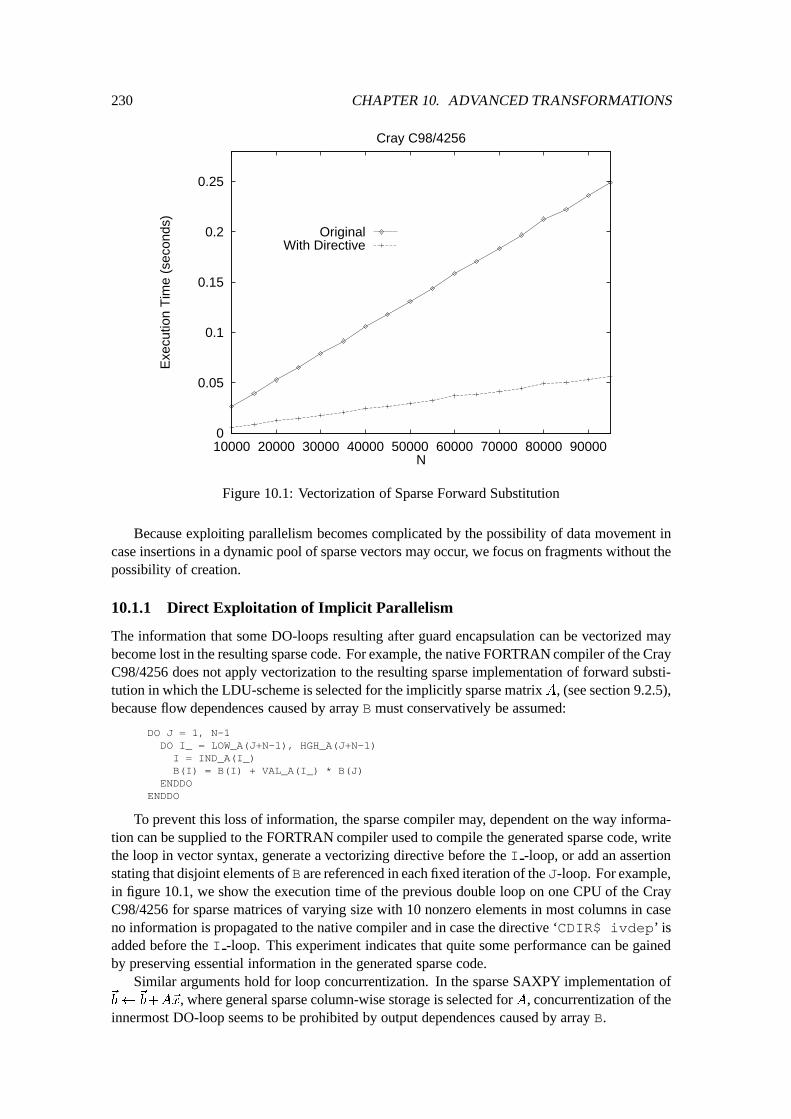
230 CHAPTER 10. ADVANCED TRANSFORMATIONS
0
0.05
0.1
0.15
0.2
0.25
10000 20000 30000 40000 50000 60000 70000 80000 90000
Exe
cutio
n T
ime
(sec
onds
)
N
Cray C98/4256
OriginalWith Directive
Figure 10.1: Vectorization of Sparse Forward Substitution
Because exploiting parallelism becomes complicated by the possibility of data movement incase insertions in a dynamic pool of sparse vectors may occur, we focus on fragments without thepossibility of creation.
10.1.1 Direct Exploitation of Implicit Parallelism
The information that some DO-loops resulting after guard encapsulation can be vectorized maybecome lost in the resulting sparse code. For example, the native FORTRAN compiler of the CrayC98/4256 does not apply vectorization to the resulting sparse implementation of forward substi-tution in which the LDU-scheme is selected for the implicitly sparse matrixA, (see section 9.2.5),because flow dependences caused by array B must conservatively be assumed:
DO J = 1, N-1DO I_ = LOW_A(J+N-1), HGH_A(J+N-1)I = IND_A(I_)B(I) = B(I) + VAL_A(I_) * B(J)
ENDDOENDDO
To prevent this loss of information, the sparse compiler may, dependent on the way informa-tion can be supplied to the FORTRAN compiler used to compile the generated sparse code, writethe loop in vector syntax, generate a vectorizing directive before the I -loop, or add an assertionstating that disjoint elements of B are referenced in each fixed iteration of the J-loop. For example,in figure 10.1, we show the execution time of the previous double loop on one CPU of the CrayC98/4256 for sparse matrices of varying size with 10 nonzero elements in most columns in caseno information is propagated to the native compiler and in case the directive ‘CDIR$ ivdep’ isadded before the I -loop. This experiment indicates that quite some performance can be gainedby preserving essential information in the generated sparse code.
Similar arguments hold for loop concurrentization. In the sparse SAXPY implementation of~
b
~
b+A~x, where general sparse column-wise storage is selected for A, concurrentization of theinnermost DO-loop seems to be prohibited by output dependences caused by array B.
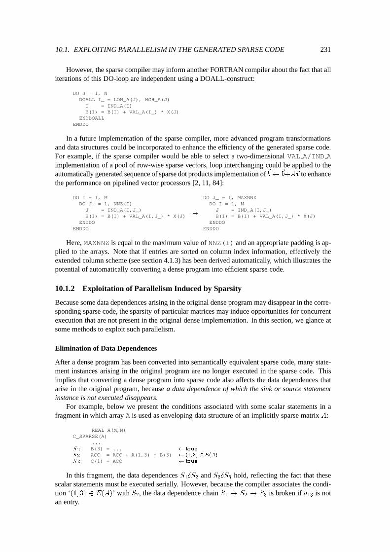
10.1. EXPLOITING PARALLELISM IN THE GENERATED SPARSE CODE 231
However, the sparse compiler may inform another FORTRAN compiler about the fact that alliterations of this DO-loop are independent using a DOALL-construct:
DO J = 1, NDOALL I_ = LOW_A(J), HGH_A(J)I = IND_A(I)B(I) = B(I) + VAL_A(I_) * X(J)
ENDDOALLENDDO
In a future implementation of the sparse compiler, more advanced program transformationsand data structures could be incorporated to enhance the efficiency of the generated sparse code.For example, if the sparse compiler would be able to select a two-dimensional VAL A/IND Aimplementation of a pool of row-wise sparse vectors, loop interchanging could be applied to theautomatically generated sequence of sparse dot products implementation of~b ~
b+A~x to enhancethe performance on pipelined vector processors [2, 11, 84]:
DO I = 1, MDO J_ = 1, NNZ(I)J = IND_A(I,J_)B(I) = B(I) + VAL_A(I,J_) * X(J)
ENDDOENDDO
!
DO J_ = 1, MAXNNZDO I = 1, M
J = IND_A(I,J_)B(I) = B(I) + VAL_A(I,J_) * X(J)
ENDDOENDDO
Here, MAXNNZ is equal to the maximum value of NNZ(I) and an appropriate padding is ap-plied to the arrays. Note that if entries are sorted on column index information, effectively theextended column scheme (see section 4.1.3) has been derived automatically, which illustrates thepotential of automatically converting a dense program into efficient sparse code.
10.1.2 Exploitation of Parallelism Induced by Sparsity
Because some data dependences arising in the original dense program may disappear in the corre-sponding sparse code, the sparsity of particular matrices may induce opportunities for concurrentexecution that are not present in the original dense implementation. In this section, we glance atsome methods to exploit such parallelism.
Elimination of Data Dependences
After a dense program has been converted into semantically equivalent sparse code, many state-ment instances arising in the original program are no longer executed in the sparse code. Thisimplies that converting a dense program into sparse code also affects the data dependences thatarise in the original program, because a data dependence of which the sink or source statementinstance is not executed disappears.
For example, below we present the conditions associated with some scalar statements in afragment in which array A is used as enveloping data structure of an implicitly sparse matrix A:
REAL A(M,N)C_SPARSE(A)
...S
1
: B(3) = ... true
S
2
: ACC = ACC + A(1,3) * B(3) (1; 3) 2 E(A)
S
3
: C(1) = ACC true
In this fragment, the data dependences S1
�S
2
and S2
�S
3
hold, reflecting the fact that thesescalar statements must be executed serially. However, because the compiler associates the condi-tion ‘(1; 3) 2 E(A)’ with S
2
, the data dependence chain S1
! S
2
! S
3
is broken if a13
is notan entry.
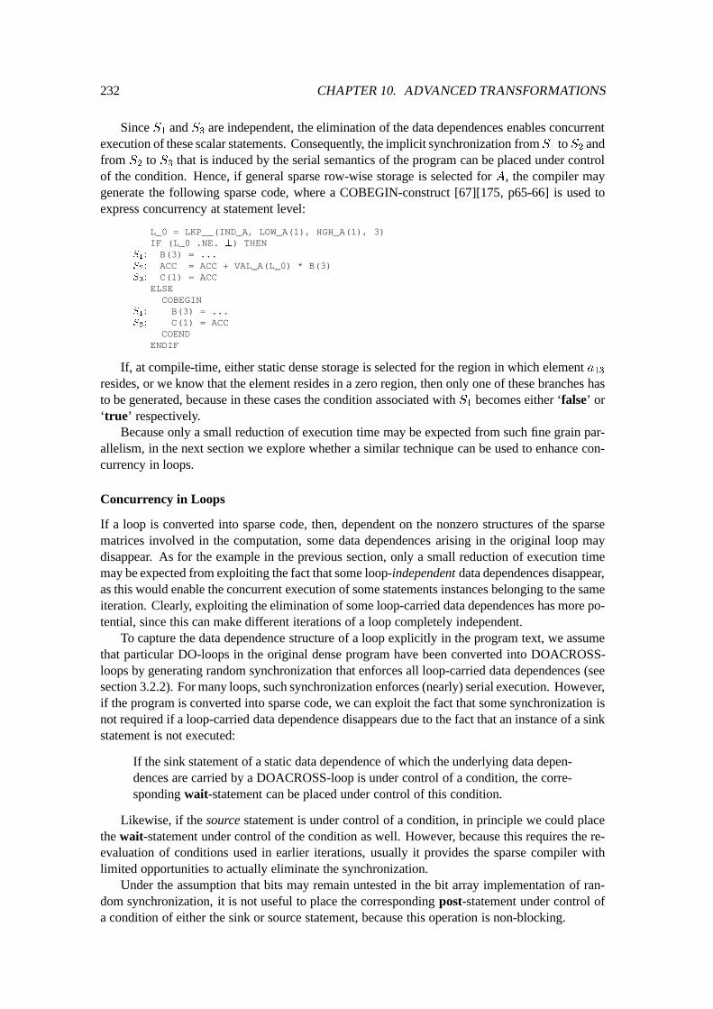
232 CHAPTER 10. ADVANCED TRANSFORMATIONS
Since S1
and S3
are independent, the elimination of the data dependences enables concurrentexecution of these scalar statements. Consequently, the implicit synchronization fromS
1
toS2
andfrom S
2
to S3
that is induced by the serial semantics of the program can be placed under controlof the condition. Hence, if general sparse row-wise storage is selected for A, the compiler maygenerate the following sparse code, where a COBEGIN-construct [67][175, p65-66] is used toexpress concurrency at statement level:
L_0 = LKP__(IND_A, LOW_A(1), HGH_A(1), 3)IF (L_0 .NE. ?) THEN
S
1
: B(3) = ...S
2
: ACC = ACC + VAL_A(L_0) * B(3)S
3
: C(1) = ACCELSECOBEGIN
S
1
: B(3) = ...S
3
: C(1) = ACCCOEND
ENDIF
If, at compile-time, either static dense storage is selected for the region in which element a13
resides, or we know that the element resides in a zero region, then only one of these branches hasto be generated, because in these cases the condition associated with S
1
becomes either ‘false’ or‘true’ respectively.
Because only a small reduction of execution time may be expected from such fine grain par-allelism, in the next section we explore whether a similar technique can be used to enhance con-currency in loops.
Concurrency in Loops
If a loop is converted into sparse code, then, dependent on the nonzero structures of the sparsematrices involved in the computation, some data dependences arising in the original loop maydisappear. As for the example in the previous section, only a small reduction of execution timemay be expected from exploiting the fact that some loop-independent data dependences disappear,as this would enable the concurrent execution of some statements instances belonging to the sameiteration. Clearly, exploiting the elimination of some loop-carried data dependences has more po-tential, since this can make different iterations of a loop completely independent.
To capture the data dependence structure of a loop explicitly in the program text, we assumethat particular DO-loops in the original dense program have been converted into DOACROSS-loops by generating random synchronization that enforces all loop-carried data dependences (seesection 3.2.2). For many loops, such synchronization enforces (nearly) serial execution. However,if the program is converted into sparse code, we can exploit the fact that some synchronization isnot required if a loop-carried data dependence disappears due to the fact that an instance of a sinkstatement is not executed:
If the sink statement of a static data dependence of which the underlying data depen-dences are carried by a DOACROSS-loop is under control of a condition, the corre-sponding wait-statement can be placed under control of this condition.
Likewise, if the source statement is under control of a condition, in principle we could placethe wait-statement under control of the condition as well. However, because this requires the re-evaluation of conditions used in earlier iterations, usually it provides the sparse compiler withlimited opportunities to actually eliminate the synchronization.
Under the assumption that bits may remain untested in the bit array implementation of ran-dom synchronization, it is not useful to place the corresponding post-statement under control ofa condition of either the sink or source statement, because this operation is non-blocking.
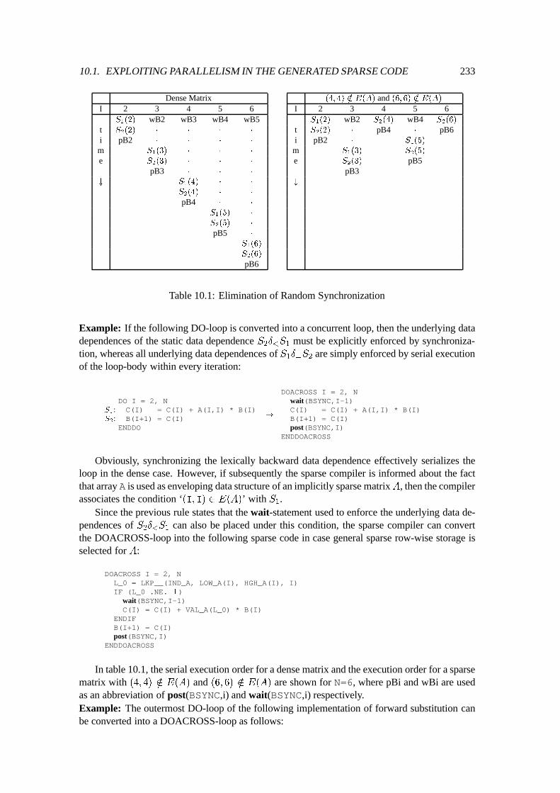
10.1. EXPLOITING PARALLELISM IN THE GENERATED SPARSE CODE 233
Dense MatrixI 2 3 4 5 6
S
1
(2) wB2 wB3 wB4 wB5t S
2
(2) � � � �
i pB2 � � � �
m S
1
(3) � � �
e S
2
(3) � � �
pB3 � � �
# S
1
(4) � �
S
2
(4) � �
pB4 � �
S
1
(5) �
S
2
(5) �
pB5 �
S
1
(6)
S
2
(6)
pB6
(4; 4) =2 E(A) and (6; 6) =2 E(A)
I 2 3 4 5 6S
1
(2) wB2 S
2
(4) wB4 S
2
(6)
t S
2
(2) � pB4 � pB6i pB2 � S
1
(5)
m S
1
(3) S
2
(5)
e S
2
(3) pB5pB3
#
Table 10.1: Elimination of Random Synchronization
Example: If the following DO-loop is converted into a concurrent loop, then the underlying datadependences of the static data dependence S
2
�
<
S
1
must be explicitly enforced by synchroniza-tion, whereas all underlying data dependences of S
1
�
=
S
2
are simply enforced by serial executionof the loop-body within every iteration:
DO I = 2, NS
1
: C(I) = C(I) + A(I,I) * B(I)S
2
: B(I+1) = C(I)ENDDO
!
DOACROSS I = 2, Nwait(BSYNC,I-1)C(I) = C(I) + A(I,I) * B(I)B(I+1) = C(I)post(BSYNC,I)
ENDDOACROSS
Obviously, synchronizing the lexically backward data dependence effectively serializes theloop in the dense case. However, if subsequently the sparse compiler is informed about the factthat array A is used as enveloping data structure of an implicitly sparse matrixA, then the compilerassociates the condition ‘(I; I) 2 E(A)’ with S
1
.Since the previous rule states that the wait-statement used to enforce the underlying data de-
pendences of S2
�
<
S
1
can also be placed under this condition, the sparse compiler can convertthe DOACROSS-loop into the following sparse code in case general sparse row-wise storage isselected for A:
DOACROSS I = 2, NL_0 = LKP__(IND_A, LOW_A(I), HGH_A(I), I)IF (L_0 .NE. ?)
wait(BSYNC,I-1)C(I) = C(I) + VAL_A(L_0) * B(I)
ENDIFB(I+1) = C(I)post(BSYNC,I)
ENDDOACROSS
In table 10.1, the serial execution order for a dense matrix and the execution order for a sparsematrix with (4; 4) =2 E(A) and (6; 6) =2 E(A) are shown for N=6, where pBi and wBi are usedas an abbreviation of post(BSYNC,i) and wait(BSYNC,i) respectively.Example: The outermost DO-loop of the following implementation of forward substitution canbe converted into a DOACROSS-loop as follows:
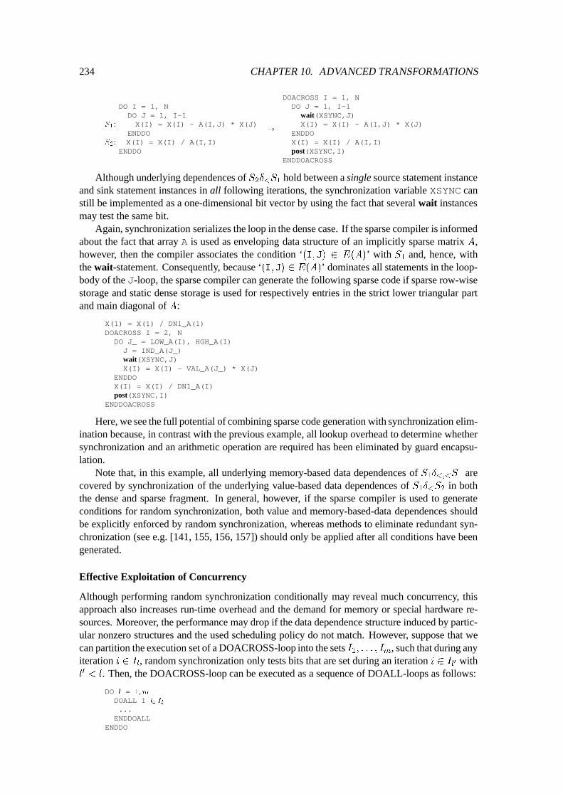
234 CHAPTER 10. ADVANCED TRANSFORMATIONS
DO I = 1, NDO J = 1, I-1
S
1
: X(I) = X(I) - A(I,J) * X(J)ENDDO
S
2
: X(I) = X(I) / A(I,I)ENDDO
!
DOACROSS I = 1, NDO J = 1, I-1
wait(XSYNC,J)X(I) = X(I) - A(I,J) * X(J)
ENDDOX(I) = X(I) / A(I,I)post(XSYNC,I)
ENDDOACROSS
Although underlying dependences of S2
�
<
S
1
hold between a single source statement instanceand sink statement instances in all following iterations, the synchronization variable XSYNC canstill be implemented as a one-dimensional bit vector by using the fact that several wait instancesmay test the same bit.
Again, synchronization serializes the loop in the dense case. If the sparse compiler is informedabout the fact that array A is used as enveloping data structure of an implicitly sparse matrix A,however, then the compiler associates the condition ‘(I; J) 2 E(A)’ with S
1
and, hence, withthe wait-statement. Consequently, because ‘(I; J) 2 E(A)’ dominates all statements in the loop-body of the J-loop, the sparse compiler can generate the following sparse code if sparse row-wisestorage and static dense storage is used for respectively entries in the strict lower triangular partand main diagonal of A:
X(1) = X(1) / DN1_A(1)DOACROSS I = 2, NDO J_ = LOW_A(I), HGH_A(I)
J = IND_A(J_)wait(XSYNC,J)X(I) = X(I) - VAL_A(J_) * X(J)
ENDDOX(I) = X(I) / DN1_A(I)post(XSYNC,I)
ENDDOACROSS
Here, we see the full potential of combining sparse code generation with synchronization elim-ination because, in contrast with the previous example, all lookup overhead to determine whethersynchronization and an arithmetic operation are required has been eliminated by guard encapsu-lation.
Note that, in this example, all underlying memory-based data dependences of S1
�
<;<
S
1
arecovered by synchronization of the underlying value-based data dependences of S
1
�
<
S
2
in boththe dense and sparse fragment. In general, however, if the sparse compiler is used to generateconditions for random synchronization, both value and memory-based-data dependences shouldbe explicitly enforced by random synchronization, whereas methods to eliminate redundant syn-chronization (see e.g. [141, 155, 156, 157]) should only be applied after all conditions have beengenerated.
Effective Exploitation of Concurrency
Although performing random synchronization conditionally may reveal much concurrency, thisapproach also increases run-time overhead and the demand for memory or special hardware re-sources. Moreover, the performance may drop if the data dependence structure induced by partic-ular nonzero structures and the used scheduling policy do not match. However, suppose that wecan partition the execution set of a DOACROSS-loop into the sets I
1
; : : : ; I
m
, such that during anyiteration i 2 I
l
, random synchronization only tests bits that are set during an iteration i 2 Il
0 withl
0
< l. Then, the DOACROSS-loop can be executed as a sequence of DOALL-loops as follows:
DO l = 1;m
DOALL I 2 Il
...ENDDOALL
ENDDO
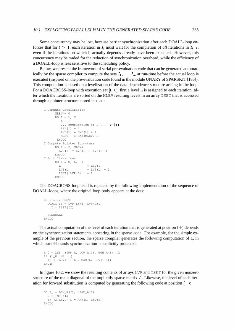
10.1. EXPLOITING PARALLELISM IN THE GENERATED SPARSE CODE 235
Some concurrency may be lost, because barrier synchronization after each DOALL-loop en-forces that for l > 1, each iteration in I
l
must wait for the completion of all iterations in Il�1
,even if the iterations on which it actually depends already have been executed. However, thisconcurrency may be traded for the reduction of synchronization overhead, while the efficiency ofa DOALL-loop is less sensitive to the scheduling policy.
Below, we present the framework of serial pre-evaluation code that can be generated automat-ically by the sparse compiler to compute the sets I
1
; : : : ; I
m
at run-time before the actual loop isexecuted (inspired on the pre-evaluation code found in the module UNARY of SPARSKIT [185]).This computation is based on a levelization of the data dependence structure arising in the loop.For a DOACROSS-loop with execution set [L; U], first a level L is assigned to each iteration, af-ter which the iterations are sorted on the MLEV resulting levels in an array ISET that is accessedthrough a pointer structure stored in LVP:
C Compute LevelizationMLEV = 0DO I = L, U
L = 1... computation of L ... (+)
LEV(I) = LLVP(L) = LVP(L) + 1MLEV = MAX(MLEV, L)
ENDDOC Compute Pointer Structure
DO I = 2, MLEV+1LVP(I) = LVP(I) + LVP(I-1)
ENDDOC Sort Iterations
DO I = U, L, -1L = LEV(I)LVP(L) = LVP(L) - 1ISET( LVP(L) ) = I
ENDDO
The DOACROSS-loop itself is replaced by the following implementation of the sequence ofDOALL-loops, where the original loop-body appears at the dots:
DO L = 1, MLEVDOALL II = LVP(L)+1, LVP(L+1)I = ISET(II)...
ENDDOALLENDDO
The actual computation of the level of each iteration that is generated at position (+) dependson the synchronization statements appearing in the sparse code. For example, for the simple ex-ample of the previous section, the sparse compiler generates the following computation of L, inwhich out-of-bounds synchronization is explicitly protected:
L_0 = LKP__(IND_A, LOW_A(I), HGH_A(I), I)IF (L_0 .NE. ?)IF (1.LE.I-1) L = MAX(L, LEV(I-1))
ENDIF
In figure 10.2, we show the resulting contents of arrays LVP and ISET for the given nonzerostructure of the main diagonal of the implicitly sparse matrix A. Likewise, the level of each iter-ation for forward substitution is computed by generating the following code at position (+):
DO J_ = LOW_A(I), HIGH_A(I)J = IND_A(J_)IF (2.LE.J) L = MAX(L, LEV(J))
ENDDO
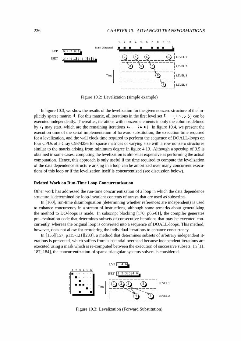
236 CHAPTER 10. ADVANCED TRANSFORMATIONS
21 3 4 5 6 7 8 9 10
Time
2 4
73 5
6
8
10
9
LEVEL 1
LEVEL 2
LEVEL 3
LEVEL 4
LVP
ISET 2 34 6 10 5 7 8 9
0 4 7 98Main Diagonal
Figure 10.2: Levelization (simple example)
In figure 10.3, we show the results of the levelization for the given nonzero structure of the im-plicitly sparse matrix A. For this matrix, all iterations in the first level set I
1
= f1; 2; 3; 5g can beexecuted independently. Thereafter, iterations with nonzero elements in only the columns definedby I
1
may start, which are the remaining iterations I2
= f4; 6g. In figure 10.4, we present theexecution time of the serial implementation of forward substitution, the execution time requiredfor a levelization, and the wall clock time required to perform the sequence of DOALL-loops onfour CPUs of a Cray C98/4256 for sparse matrices of varying size with arrow nonzero structuressimilar to the matrix arising from minimum degree in figure 4.13. Although a speedup of 3.5 isobtained in some cases, computing the levelization is almost as expensive as performing the actualcomputation. Hence, this approach is only useful if the time required to compute the levelizationof the data dependence structure arising in a loop can be amortized over many concurrent execu-tions of this loop or if the levelization itself is concurrentized (see discussion below).
Related Work on Run-Time Loop Concurrentization
Other work has addressed the run-time concurrentization of a loop in which the data dependencestructure is determined by loop-invariant contents of arrays that are used as subscripts.
In [160], run-time disambiguation (determining whether references are independent) is usedto enhance concurrency in a stream of instructions, although some remarks about generalizingthe method to DO-loops is made. In subscript blocking [170, p66-81], the compiler generatespre–evaluation code that determines subsets of consecutive iterations that may be executed con-currently, whereas the original loop is converted into a sequence of DOALL-loops. This method,however, does not allow for reordering the individual iterations to enhance concurrency.
In [155][157, p115-121][233], a method that determines subsets of arbitrary independent it-erations is presented, which suffers from substantial overhead because independent iterations areexecuted using a mask which is re-computed between the execution of successive subsets. In [11,187, 184], the concurrentization of sparse triangular systems solvers is considered.
1
32
4
65
51 2 3 4 6
4
1 2 3 5
6
LEVEL 1
LEVEL 2
Time
ISET 1 2 3 4 65
LVP 0 4 6
Figure 10.3: Levelization (Forward Substitution)
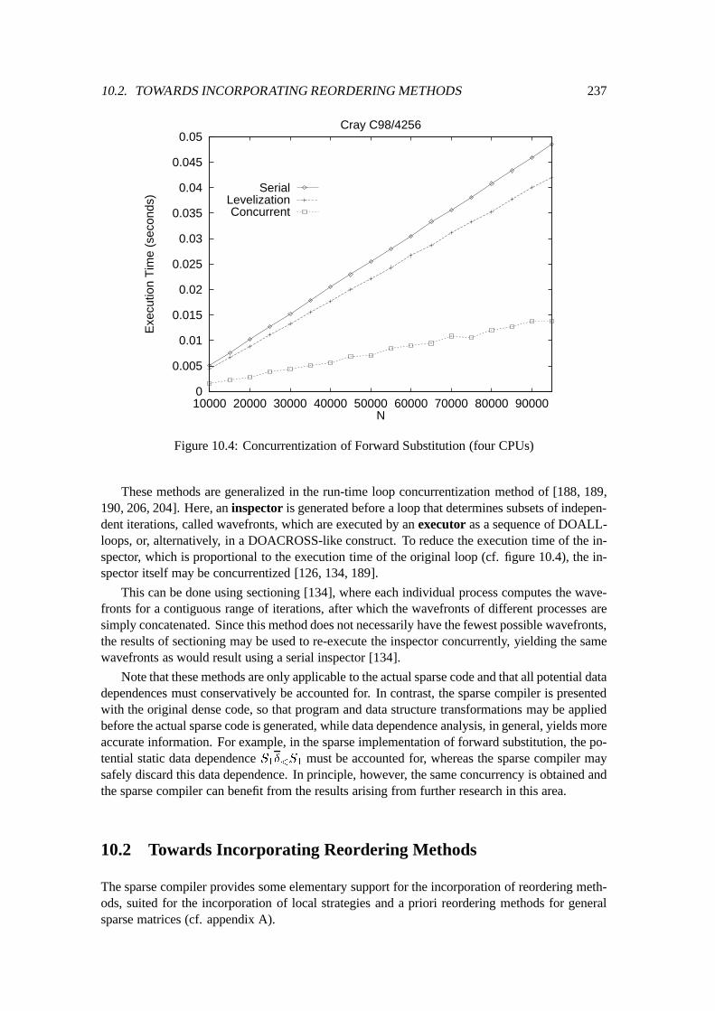
10.2. TOWARDS INCORPORATING REORDERING METHODS 237
0
0.005
0.01
0.015
0.02
0.025
0.03
0.035
0.04
0.045
0.05
10000 20000 30000 40000 50000 60000 70000 80000 90000
Exe
cutio
n T
ime
(sec
onds
)
N
Cray C98/4256
SerialLevelizationConcurrent
Figure 10.4: Concurrentization of Forward Substitution (four CPUs)
These methods are generalized in the run-time loop concurrentization method of [188, 189,190, 206, 204]. Here, an inspector is generated before a loop that determines subsets of indepen-dent iterations, called wavefronts, which are executed by an executor as a sequence of DOALL-loops, or, alternatively, in a DOACROSS-like construct. To reduce the execution time of the in-spector, which is proportional to the execution time of the original loop (cf. figure 10.4), the in-spector itself may be concurrentized [126, 134, 189].
This can be done using sectioning [134], where each individual process computes the wave-fronts for a contiguous range of iterations, after which the wavefronts of different processes aresimply concatenated. Since this method does not necessarily have the fewest possible wavefronts,the results of sectioning may be used to re-execute the inspector concurrently, yielding the samewavefronts as would result using a serial inspector [134].
Note that these methods are only applicable to the actual sparse code and that all potential datadependences must conservatively be accounted for. In contrast, the sparse compiler is presentedwith the original dense code, so that program and data structure transformations may be appliedbefore the actual sparse code is generated, while data dependence analysis, in general, yields moreaccurate information. For example, in the sparse implementation of forward substitution, the po-tential static data dependence S
1
�
<
S
1
must be accounted for, whereas the sparse compiler maysafely discard this data dependence. In principle, however, the same concurrency is obtained andthe sparse compiler can benefit from the results arising from further research in this area.
10.2 Towards Incorporating Reordering Methods
The sparse compiler provides some elementary support for the incorporation of reordering meth-ods, suited for the incorporation of local strategies and a priori reordering methods for generalsparse matrices (cf. appendix A).
238 CHAPTER 10. ADVANCED TRANSFORMATIONS
10.2.1 Recording a Permutation
The programmer can specify that anm�n implicitly sparse matrixA with enveloping data struc-ture A will be permuted into PAQ at run-time using the following annotation:
REAL A(M,N)C_SPARSE(A : _PERM)
This annotation indicates that any a priori reordering method may be applied to A before thisimplicitly sparse matrix is initialized, whereas particular row and column interchanges may be ap-plied toA at the position of an interchange annotation involving the array A. The actual implemen-tation of permutations is kept transparent to the programmer. The sparse compiler is responsiblefor generating code in which permutations are applied and recorded. As far as the programmeris concerned, all programming can be done on the enveloping data structure A as if elements arephysically moved in this two-dimensional array, i.e. if at a particular moment A is permuted intoPAQ, then the programmer may assume that A contains the elements of PAQ.
Because permutingAmay affect properties of the nonzero structure of this matrix in an unpre-dictable manner, exploiting peculiarities of the nonzero structure seems to be difficult. Therefore,in the current prototype sparse compiler, only general sparse storage schemes can be selected forA. If general sparse row-wise storage is selected, then the sparse compiler adds the followingpermutation arrays to the declarations of the sparse storage scheme (general sparse column-wisestorage is implemented analogously):
INTEGER ROW_A(1:M), COL_A(1:N), INVCOL_A(1:N)COMMON /A/ ..., ROW_A, COL_A, INVCOL_A
These permutation arrays are used to record the permutation matrices P , Q, and QT accord-ing to the method presented in [78, 169, p34-35], i.e. the arrays have the contents P (1; : : : ;m)
T ,(1; : : : ; n)Q, and (1; : : : ; n)Q
T respectively. The initial contents of the first two permutation ar-rays must be specified in the file that is used to initialize A at run-time. Given such an implicitlysparse matrixAwith enveloping data structure A, the sparse compiler adds the following fragmentto the initialization code:
OPEN (UNIT=1, FILE=’file_name’, STATUS=’OLD’)DO I_ = 1, MREAD (1,*) ROW_A(I_)
ENDDODO I_ = 1, NREAD (1,*) COL_A(I_)
ENDDO...CLOSE (UNIT = 1)
At the dots, the matrix is initialized as discussed earlier. However, after the whole matrix hasbeen initialized, the following code is executed to perform the row interchanges by simply apply-ing P to the row pointers, where the temporary integer array TMP is used:
Permute LOW A:
DO I_ = 1, MTMP__(I_) = LOW_A( ROW_A(I_) )
ENDDODO I_ = 1, MLOW_A(I_) = TMP__(I)
ENDDO
Permute HGH A:
DO I_ = 1, MTMP__(I_) = HGH_A( ROW_A(I_) )
ENDDODO I_ = 1, MHGH_A(I_) = TMP__(I)
ENDDO
However, in row-wise storage, permuting the columns is not so straightforward. Therefore,in addition to recording Q, permutation matrix QT is also recorded. The following fragment isgenerated to initialize the array INVCOL A:
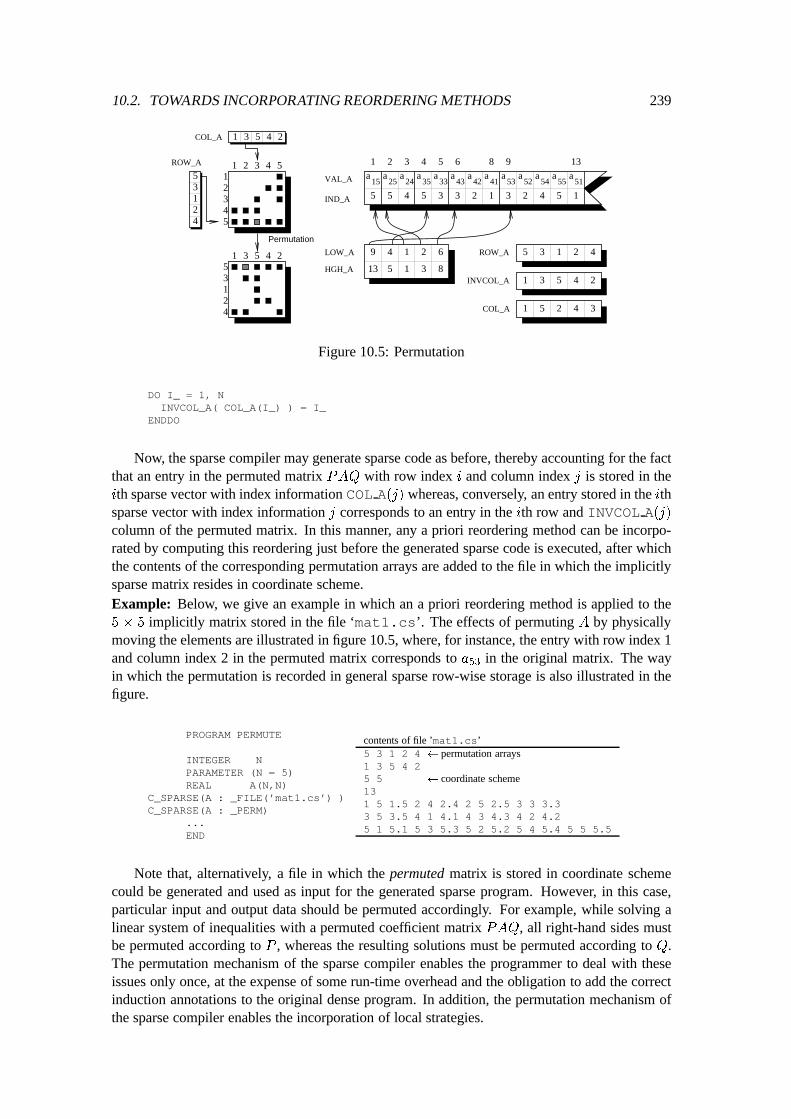
10.2. TOWARDS INCORPORATING REORDERING METHODS 239
a aa15
a24
a25
a33
a35
a4142
a43
a5152
a53
a54
a55VAL_A
IND_A 5 45 35 123 123 4 5
LOW_A
HGH_A 13
9 4
5 1
1 6
8
2
3
2 941 6
12345
1 2 3 4 5
1 55
2
3
3
124
4
12
3
4
5
Permutation
1 23 45COL_A
ROW_A
INVCOL_A
COL_A
ROW_A
1 2 3
4
5
1 23
3 21
4
4
5
5
3 5 8 13
Figure 10.5: Permutation
DO I_ = 1, NINVCOL_A( COL_A(I_) ) = I_
ENDDO
Now, the sparse compiler may generate sparse code as before, thereby accounting for the factthat an entry in the permuted matrix PAQ with row index i and column index j is stored in theith sparse vector with index information COL A(j) whereas, conversely, an entry stored in the ithsparse vector with index information j corresponds to an entry in the ith row and INVCOL A(j)column of the permuted matrix. In this manner, any a priori reordering method can be incorpo-rated by computing this reordering just before the generated sparse code is executed, after whichthe contents of the corresponding permutation arrays are added to the file in which the implicitlysparse matrix resides in coordinate scheme.Example: Below, we give an example in which an a priori reordering method is applied to the5 � 5 implicitly matrix stored in the file ‘mat1.cs’. The effects of permuting A by physicallymoving the elements are illustrated in figure 10.5, where, for instance, the entry with row index 1and column index 2 in the permuted matrix corresponds to a
53
in the original matrix. The wayin which the permutation is recorded in general sparse row-wise storage is also illustrated in thefigure.
PROGRAM PERMUTE
INTEGER NPARAMETER (N = 5)REAL A(N,N)
C_SPARSE(A : _FILE(’mat1.cs’) )C_SPARSE(A : _PERM)
...END
contents of file ’mat1.cs’5 3 1 2 4 permutation arrays1 3 5 4 25 5 coordinate scheme131 5 1.5 2 4 2.4 2 5 2.5 3 3 3.33 5 3.5 4 1 4.1 4 3 4.3 4 2 4.25 1 5.1 5 3 5.3 5 2 5.2 5 4 5.4 5 5 5.5
Note that, alternatively, a file in which the permuted matrix is stored in coordinate schemecould be generated and used as input for the generated sparse program. However, in this case,particular input and output data should be permuted accordingly. For example, while solving alinear system of inequalities with a permuted coefficient matrix PAQ, all right-hand sides mustbe permuted according to P , whereas the resulting solutions must be permuted according to Q.The permutation mechanism of the sparse compiler enables the programmer to deal with theseissues only once, at the expense of some run-time overhead and the obligation to add the correctinduction annotations to the original dense program. In addition, the permutation mechanism ofthe sparse compiler enables the incorporation of local strategies.
240 CHAPTER 10. ADVANCED TRANSFORMATIONS
10.2.2 Implementation of Induction Annotations
The implementation of induction annotation is rather straightforward. Because a row permuta-tion matrix P of an implicitly sparse matrix with enveloping data structure A is recorded with thecontents P (1; : : : ;m) in the permutation array ROW A, the induction annotations involving thisrow permutation matrix are implemented as follows, where array PERM A is a locally declaredtemporary array having the same basis type as A:1
action: X < _ROW(A)
DO I_ = 1, MPERM_A(I_) = X( ROW_A(I_) )
ENDDODO I_ = 1, MX(I_) = PERM_A(I_)
ENDDO
action: X > _ROW(A)
DO I_ = 1, MPERM_A(I_) = X(I_)
ENDDODO I_ = 1, M
X( ROW_A(I_) ) = PERM_A(I_)ENDDO
Likewise, because a column permutation matrixQ associated with an implicitly sparse matrixAwith enveloping data structure A is recorded with the contents (1; : : : ; n)Q in the permutation ar-ray COL A, the induction annotations involving this column permutation matrix are implementedas follows:
action: Y < _COLUMN(A)
DO I_ = 1, NPERM_A(I_) = Y( COL_A(I_) )
ENDDODO I_ = 1, NY(I_) = PERM_A(I_)
ENDDO
action: Y > _COLUMN(A)
DO I = 1, NPERM_A(I_) = Y(I_)
ENDDODO I_ = 1, N
Y( COL_A(I_) ) = PERM_A(I_)ENDDO
10.2.3 Implementation of Interchange Annotations
The programmer can specify that for an implicitly sparse matrix A with enveloping data structureA an arbitrary row and column in the range [LR; UR] and [LC; UC] respectively may be interchangedwith the Rth row and Cth column, using the following interchange annotation:
C_INTERCHANGE(A, LR:UR > R, LC:UC > C)
Rather than directly specifying the criteria for a local strategy that must be used to determine arow and column, the sparse compiler may select these criteria after analyzing the program. Aftera particular local strategy has been selected, the sparse compiler is also responsible for generatingcode that implements the selected local strategy. In this code, at run-time desired row and columninterchanges are determined and applied. In this manner, the sparse compiler is not restricted toselecting already existing local strategies, but may derive a local strategy that is suited for a par-ticular fragment.
Applying the actual interchanges is straightforward. Interchanging two rows is simply per-formed by interchanging the corresponding row pointers, while corresponding elements in arrayROW A are interchanged to record the new permutation matrix P . Interchanging two columns isperformed by altering the permutation arrays COL A and INVCOL A to record the new permuta-tion matrices Q and QT :
Interchanging Rows I1 and I2:
SWAP( ROW_A(I1), ROW_A(I2) )SWAP( LOW_A(I1), LOW_A(I2) )SWAP( HGH_A(I1), HGH_A(I2) )
Interchanging Columns J1 and J2:
SWAP( COL_A(J1), COL_A(J2) )INVCOL_A( COL_A(J1) ) = J1INVCOL_A( COL_A(J2) ) = J2
1Alternatively, array X could be permuted in-place if the permutation would be stored as a sequence of inter-changes [78, p34-35].
10.2. TOWARDS INCORPORATING REORDERING METHODS 241
Below, an example is given in which we explore the steps that could be taken by the sparsecompiler to incorporate a very simple local strategy. Obviously, as more advanced methods toselect criteria for a local method have been developed and incorporated in the sparse compiler,a dense program that has been used earlier to obtain sparse code can be re-translated into moreefficient sparse code without any modifications to the program.Example: Consider the following implementation of LU-factorization, where annotations areused to indicate that any a priori reordering may be applied to the implicitly sparse matrix A withenveloping data structure A. Moreover, interchanging annotations are used to indicate that an ar-bitrary element in the active sub-matrix may be used as pivot:
PROGRAM SOLVE
INTEGER NPARAMETER (N = ...)REAL A(N,N), B(N)
C_SPARSE(A : _PERM)...CALL FACT(A, N)CALL FORW(A, B, N)CALL BACK(A, B, N)...END
SUBROUTINE FACT(A, N)INTEGER I, J, K, NREAL A(N,N)
DO K = 1, N - 1C_INTERCHANGE(A, K:N > K, K:N > K)
DO I = K + 1, NA(I,K) = A(I,K) / A(K,K)DO J = K + 1, N
A(I,J) = A(I,J) - A(I,K)*A(K,J)ENDDO
ENDDOENDDORETURNEND
As far as the programmer is concerned, data in the enveloping data structure A is physicallymoved according to PAQ, so that eventually the enveloping data structure A is overwritten withelements of the factors L and U satisfying PAQ = LU for the original matrix A. Consequently,forward and back substitution can be implemented as follows. A right-hand side vector ~b is per-muted into P~b before forward substitution, whereas the in-place computed solution ~x is permutedinto Q~x to obtain the desired solution after back substitution. Note that a system AX = B can besolved by repetitively calling subroutines FORW and BACK with the columns of X and B after afactorization PAQ = LU has been computed, which effectively solves PAQQT
X = PB (seeappendix A for a detailed discussion of LU-factorization):
SUBROUTINE FORW(A, B, N)INTEGER I, J, NREAL A(N,N), B(N)
C_INDUCE B < _ROW(A)DO I = 1, N
DO J = 1, I - 1B(I) = B(I) - A(I,J) * B(J)
ENDDOENDDORETURNEND
SUBROUTINE BACK(A, B, N)INTEGER I, J, NREAL A(N,N), B(N)DO I = N, 1, -1
DO J = I + 1, NB(I) = B(I) - A(I,J) * B(J)
ENDDOB(I) = B(I) / A(I,I)
ENDDOC_INDUCE B > _COLUMN(A)
RETURNEND
Because the sparse compiler generates the clones FACT A0, FORW A00, and BACK A00 inwhich A is uniquely associated with the formal argument A, all permutation annotations uniquelydefine the permutation matrices associated with the implicitly sparse matrix A.
Straightforward conversion of the factorization code into sparse code yields a slightly differentversion of the code presented in chapter 9. Now, however, permutations are accounted for:
DO K = 1, N... interchanging code ...DO I = K+1, NCALL SSCT__(VAL_A, IND_A, LOW_A(I), HGH_A(I), SAP_20, SWT_20)IF (SWT_20(COL A(K))) THENSAP_20(COL A(K)) = SAP_20(COL A(K)) /
+ VAL_A(LKP__(IND_A, LOW_A(K), HGH_A_A(K), COL A(K)))...
242 CHAPTER 10. ADVANCED TRANSFORMATIONS
LEN_J = HGH_A(K) - LOW_A(K)DO J_ = 0, LEN_J
J = INVCOL A( IND_A(LOW_A(K)+J_) )IF (K+1.LE.J) THEN
IF (.NOT.SWT_20(COL A(J))) THENSWT_20(COL A(J)) = .TRUE.CALL SINS__(VAL_A,IND_A,LOW_A,HGH_A,I,NP_A,SZ_A,LST_A,L_,COL A(J))END IFSAP_20(COL A(J)) = SAP_20(COL A(J)) - SAP_20(COL A(K))*VAL_A(LOW_A(K)+J_)
END IFENDDO
ENDIFCALL SGTH__(VAL_A, IND_A, LOW_A(I), HGH_A(I), SAP_20, SWT_20)
ENDDOENDDO
As shown in boldface, permutation arrays are used to translate column indices of the storedsparse matrix into column indices of the permuted matrix. Because row interchanges are appliedby interchanging the row pointers accordingly, this translation is not required for rows. Likewise,straightforward conversion of the implementation of forward and back substitution yields the fol-lowing sparse fragments, in which the induction annotations are explicitly implemented:
DO I_ = 1, NPERM_A(I_) = B(ROW A(I_))
ENDDODO I_ = 1, NB(I_) = PERM_A(I_)
ENDDODO I = 2, NDO J_ = LOW_A(I), HGH_A(I)J = INVCOL A( IND_A(J_) )IF (J.LE.I-1) THENB(I) = B(I) - VAL_A(J_) * B(J)
ENDIFENDDO
ENDDO
DO I = N, 1, -1IF (I+1.LE.N) THENDO J_ = LOW_A(I), HGH_A(I)
J = INVCOL A( IND_A(J_) )IF (I+1.LE.J) THEN
B(I) = B(I) - VAL_A(J_) * B(J)ENDIF
ENDDOENDIFB(I) = B(I) / VAL_A(LKP__(IND_A,
+ LOW_A(I), HGH_A(I), COL A(I)))ENDDODO I = 1, N
PERM_A(I_) = B(I_)ENDDODO I_ = 1, N
B(COL A(I_)) = PERM_A(I_)ENDDO
Subsequently, the sparse compiler may select criteria to implement the interchange annotation.In fact, any local strategy varying from the minimum row in minimum column to the Markowitz orminimum deficiency strategy may arise, because the sparse compiler can determine the conditionsunder which creation occurs in the I- and J-loop.
For example, because any row in the range [K; N] may be interchanged with row K and becausethe expression ‘HGH A(K)-LOW A(K)’ provides a very rough measure of the amount of fill-inthat could occur at each step K, the sparse compiler may decide to generate the following inter-changing code in which a row that minimizes this expression is selected and interchanged withrow K:
C DETERMINE ROWLEN = 1DO I = K, N
IF ((HGH_A(I) - LOW_A(I)).LT.LEN) THENKK = ILEN = HGH_A(I) - LOW_A(I)
ENDIFENDDO
C INTERCHANGE ROWSSWAP( ROW_A(K), ROW_A(KK) )SWAP( LOW_A(K), LOW_A(KK) )SWAP( HGH_A(K), HGH_A(KK) )
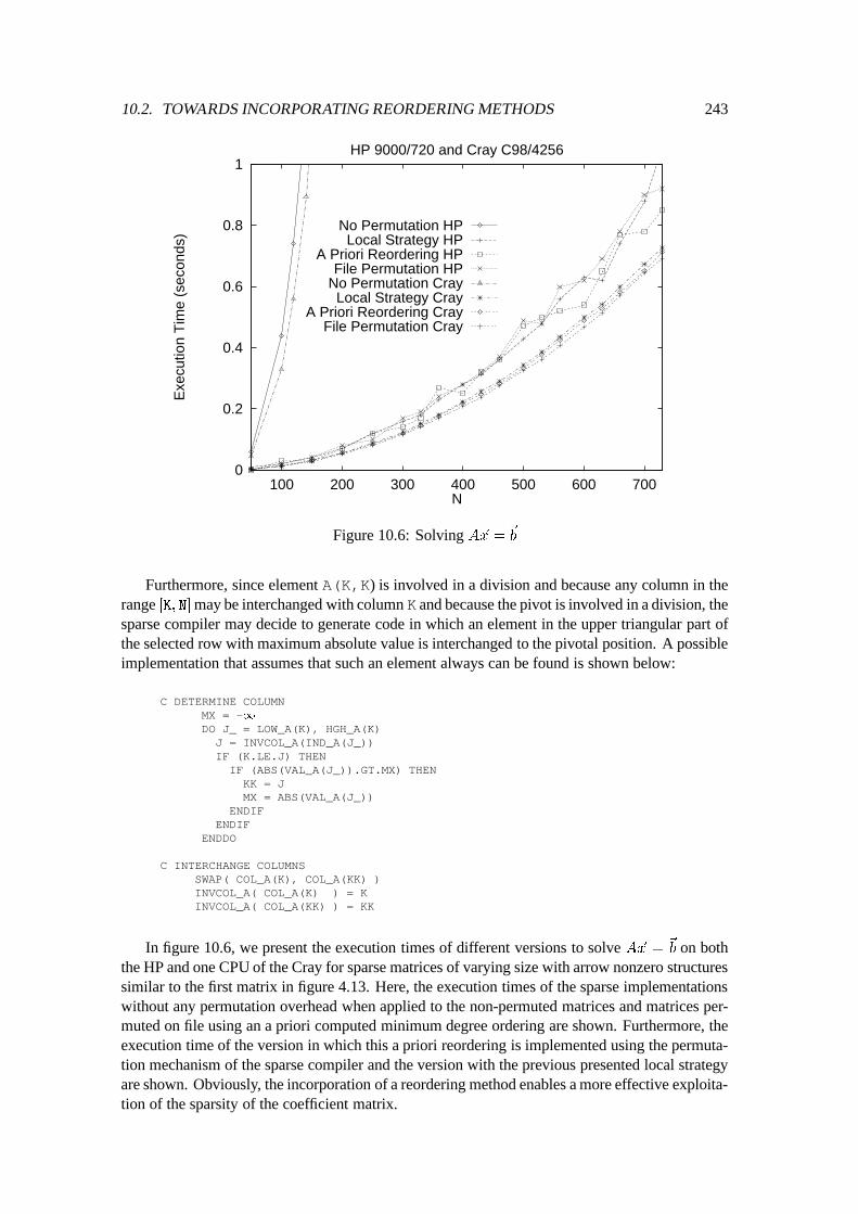
10.2. TOWARDS INCORPORATING REORDERING METHODS 243
0
0.2
0.4
0.6
0.8
1
100 200 300 400 500 600 700
Exe
cutio
n T
ime
(sec
onds
)
N
HP 9000/720 and Cray C98/4256
No Permutation HPLocal Strategy HP
A Priori Reordering HPFile Permutation HP
No Permutation CrayLocal Strategy Cray
A Priori Reordering CrayFile Permutation Cray
Figure 10.6: Solving A~x =
~
b
Furthermore, since element A(K,K) is involved in a division and because any column in therange [K; N]may be interchanged with column K and because the pivot is involved in a division, thesparse compiler may decide to generate code in which an element in the upper triangular part ofthe selected row with maximum absolute value is interchanged to the pivotal position. A possibleimplementation that assumes that such an element always can be found is shown below:
C DETERMINE COLUMNMX = -1DO J_ = LOW_A(K), HGH_A(K)
J = INVCOL_A(IND_A(J_))IF (K.LE.J) THEN
IF (ABS(VAL_A(J_)).GT.MX) THENKK = JMX = ABS(VAL_A(J_))
ENDIFENDIF
ENDDO
C INTERCHANGE COLUMNSSWAP( COL_A(K), COL_A(KK) )INVCOL_A( COL_A(K) ) = KINVCOL_A( COL_A(KK) ) = KK
In figure 10.6, we present the execution times of different versions to solve A~x =
~
b on boththe HP and one CPU of the Cray for sparse matrices of varying size with arrow nonzero structuressimilar to the first matrix in figure 4.13. Here, the execution times of the sparse implementationswithout any permutation overhead when applied to the non-permuted matrices and matrices per-muted on file using an a priori computed minimum degree ordering are shown. Furthermore, theexecution time of the version in which this a priori reordering is implemented using the permuta-tion mechanism of the sparse compiler and the version with the previous presented local strategyare shown. Obviously, the incorporation of a reordering method enables a more effective exploita-tion of the sparsity of the coefficient matrix.
244 CHAPTER 10. ADVANCED TRANSFORMATIONS
Unfortunately, however, due to the fact that in the current prototype only general sparse storagecan be selected for implicitly sparse matrices that may be permuted, still a sparse implementationof LU-factorization results of which the execution time grows at least quadratically in the orderof the coefficient matrix. Because this makes solving large sparse systems infeasible, in a futureimplementation, the incorporation of reordering methods should be combined with the selection ofmore advanced data structures in which, for example, the column structure of the matrix is storedas well [105, 235]. In addition, more advanced data structures may be required to support theselected local strategy in which, for example, linked lists sort rows and columns in increasing orderof row and column count [74, 81]. Note that, in contrast with the previous example, in which aninefficient pivot selection method could be used due to the fact that an inefficient implementationof LU-factorization itself was used, in efficient implementations of LU-factorization, it becomesextremely important to perform the selection of the next pivot very efficiently as well.
Chapter 11
Conclusions
Although developing and maintaining sparse codes is a complex and cumbersome task, only lim-ited compiler support for sparse matrix computations has been developed in the past. In this dis-sertation, we have tried to make a step towards solving this omission by proposing an alternativemethod to develop sparse codes. Rather than dealing with the sparsity at the programming level,as is done traditionally, the sparsity of implicitly sparse matrices is dealt with at the compilationlevel by a sparse compiler. In this approach, the programmer defines all operations on implicitlysparse matrices using simple two-dimensional arrays. The burden of sparse code generation iscompletely placed on the sparse compiler which selects a suitable sparse storage scheme for eachimplicitly sparse matrix and transforms the original dense code into sparse code that operates onthese selected storage schemes, thereby reducing the storage requirements and computational timeof the original dense program. In the introduction of chapter 4, several advantages of this approachhave been discussed. Elaboration of these ideas has resulted in the development and implemen-tation of a prototype sparse compiler. The automatic data structure selection and transformationmethod that is used by this sparse compiler has been presented in detail in this dissertation. In ad-dition, some initial experiments have been conducted that indicate that in many cases the sparsecompiler is capable of transforming a dense fragment into code that fully exploits the sparsity ofsome matrices to reduce both the storage requirements as well as computational time of the orig-inal implementation. Finally, we discussed the automatic exploitation of implicit parallelism inthe generated sparse code and explored incorporating sparsity preserving reordering methods.
In this final chapter, we discuss the contributions of our research and shortcomings of the cur-rent prototype. Moreover, we glance at related work, and we state topics for future research.
11.1 Contributions of this Research
Restricted by time constraints inherent to a four year research project on one hand, but driven bythe desire to actually implement the ideas proposed in the dissertation to demonstrate the feasibil-ity of these ideas on the other hand, we decided to implement a prototype sparse compiler by incor-porating the automatic data structure selection and transformation method in an existing prototyperestructuring compiler MT1 [24, 37, 45]. The resulting prototype sparse compiler, in which notall issues that should be dealt with in a commercially acceptable compiler are accounted for [212],provides sufficient functionality to make a first claim about the feasibility of automatically gener-ating sparse codes.
The experiments of chapter 9 indicate that in many cases the sparse compiler is able to converta particular dense fragment into semantically equivalent code that fully exploits the sparsity of allimplicitly sparse matrices to reduce both the storage requirements as well as computational timeof the original implementation.
246 CHAPTER 11. CONCLUSIONS
Although more experiments and probably the development of more advanced transformationsand strategies to control these transformations are required to determine whether a successful con-version is also feasible for large programs, these results already indicate that a sparse compiler canbe very useful during development of a sparse algorithm. The experiments also indicate that theselection of a sparse storage scheme for an implicitly sparse matrix can have a dramatic impacton the performance of the resulting sparse code. Very efficient sparse code can be obtained ifcharacteristics of the nonzero structure of each implicitly sparse matrix are already know and ac-counted for at compile-time. Although, in practice, these characteristics will not be known untilrun-time, this indicates that in principle the sparse compiler can be used to generate multi-versioncode for an algorithm, in which each version is suited for a particular class of sparse matrices. Atrun-time, the characteristics of the nonzero structure of each implicitly sparse matrix are deter-mined by means of efficient automatic nonzero structure analysis, after which the outcome of thisanalysis determines which version is most appropriate.
We also have shown that this approach provides the sparse compiler with more opportunitiesto exploit implicit parallelism and we have made a cautious step towards incorporating sparsitypreserving reordering methods in the generated sparse code. Although definitely more researchis required to make effective use of all these ideas, the fact that the complexity of writing sparsecodes can be reduced substantially by dealing with the sparsity of matrices at the compilation levelrather than at the programming level seems to justify this new approach. Moreover, the fact thatthe sparse compiler can be used to transform an adjacency matrix representation into the moreeconomical adjacency structure representation, thereby reducing the complexity of the algorithmaccordingly (see section 9.2.6), reveals the potential of going beyond numerical applications andto provide compiler support for other kinds of data structure transformations as well.
11.2 Shortcomings of the Prototype Sparse Compiler
While experimenting with the current prototype sparse compiler, some severe shortcomings wereencountered that should be fixed before this sparse compiler can provide a serious full alterna-tive to explicitly dealing with sparsity at the programming level. In this section, we discuss theseshortcomings.
A first shortcoming of the prototype sparse compiler is that, although for many operations thatoccur frequently in numerical programs, at least one obvious dense implementation exists that ishandled appropriately by the sparse compiler, there are also some operations for which any ob-vious dense implementation becomes translated into extremely inefficient sparse code. Consider,for example, the following dense implementation of matrix transposition (found in any textbookon programming, see e.g. [12]), in which annotations are used to enforce selection of the LDU-scheme for the implicitly sparse matrix A with enveloping data structure A:
INTEGER I, JREAL A(N,N), TMP
C_SPARSE(A : _SPARSE( 1 - N <= I - J <= - 1)(0,1)))C_SPARSE(A : _DENSE ( 0 <= I - J <= 0)(1,1)))C_SPARSE(A : _SPARSE( 1 <= I - J <= N - 1)(1,0))
...DO I = 1, N-1
DO J = I+1, NTMP = A(I,J) true
A(I,J) = A(J,I) (I; J) 2 E(A) _ (J; I) 2 E(A)
A(J,I) = TMP true
ENDDOENDDO
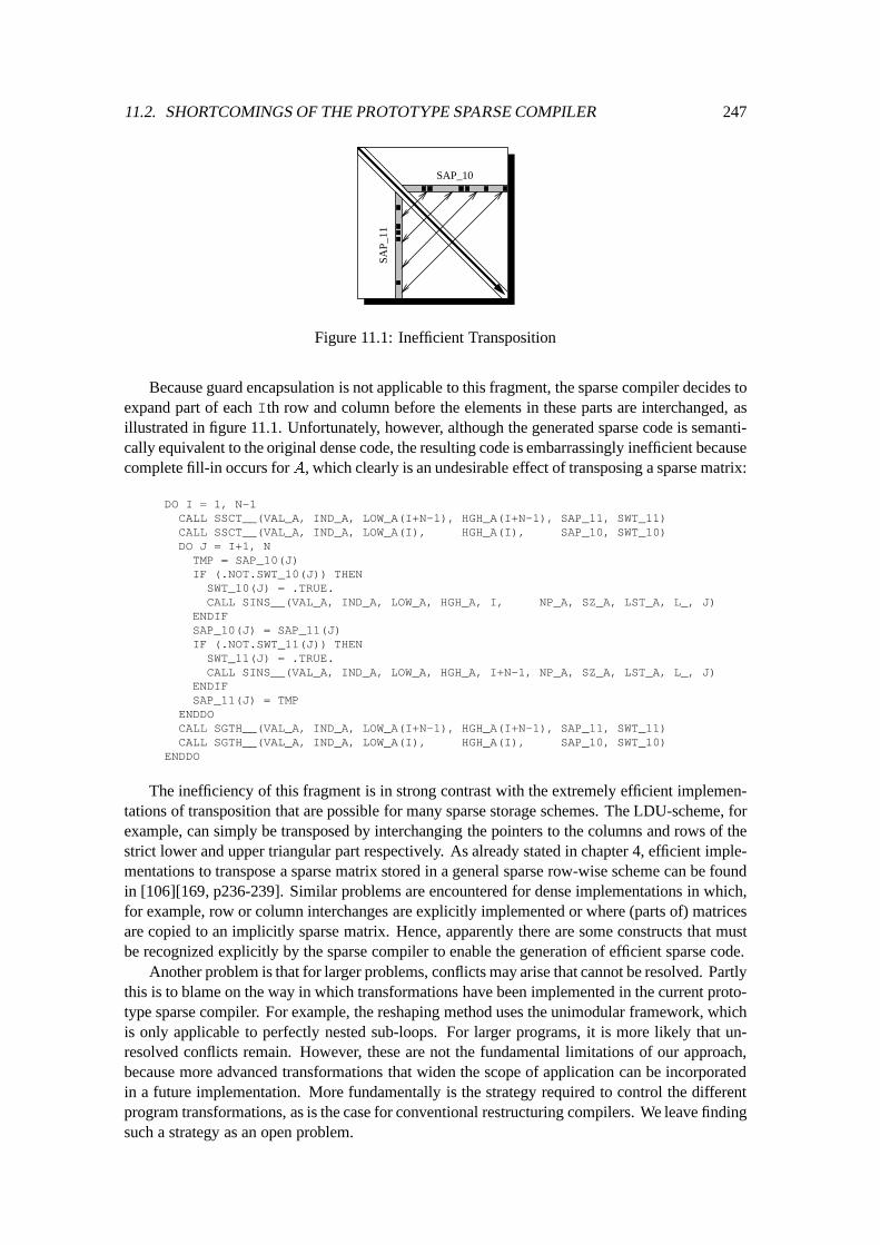
11.2. SHORTCOMINGS OF THE PROTOTYPE SPARSE COMPILER 247
SAP_10
SA
P_1
1
Figure 11.1: Inefficient Transposition
Because guard encapsulation is not applicable to this fragment, the sparse compiler decides toexpand part of each Ith row and column before the elements in these parts are interchanged, asillustrated in figure 11.1. Unfortunately, however, although the generated sparse code is semanti-cally equivalent to the original dense code, the resulting code is embarrassingly inefficient becausecomplete fill-in occurs forA, which clearly is an undesirable effect of transposing a sparse matrix:
DO I = 1, N-1CALL SSCT__(VAL_A, IND_A, LOW_A(I+N-1), HGH_A(I+N-1), SAP_11, SWT_11)CALL SSCT__(VAL_A, IND_A, LOW_A(I), HGH_A(I), SAP_10, SWT_10)DO J = I+1, NTMP = SAP_10(J)IF (.NOT.SWT_10(J)) THEN
SWT_10(J) = .TRUE.CALL SINS__(VAL_A, IND_A, LOW_A, HGH_A, I, NP_A, SZ_A, LST_A, L_, J)
ENDIFSAP_10(J) = SAP_11(J)IF (.NOT.SWT_11(J)) THEN
SWT_11(J) = .TRUE.CALL SINS__(VAL_A, IND_A, LOW_A, HGH_A, I+N-1, NP_A, SZ_A, LST_A, L_, J)
ENDIFSAP_11(J) = TMP
ENDDOCALL SGTH__(VAL_A, IND_A, LOW_A(I+N-1), HGH_A(I+N-1), SAP_11, SWT_11)CALL SGTH__(VAL_A, IND_A, LOW_A(I), HGH_A(I), SAP_10, SWT_10)
ENDDO
The inefficiency of this fragment is in strong contrast with the extremely efficient implemen-tations of transposition that are possible for many sparse storage schemes. The LDU-scheme, forexample, can simply be transposed by interchanging the pointers to the columns and rows of thestrict lower and upper triangular part respectively. As already stated in chapter 4, efficient imple-mentations to transpose a sparse matrix stored in a general sparse row-wise scheme can be foundin [106][169, p236-239]. Similar problems are encountered for dense implementations in which,for example, row or column interchanges are explicitly implemented or where (parts of) matricesare copied to an implicitly sparse matrix. Hence, apparently there are some constructs that mustbe recognized explicitly by the sparse compiler to enable the generation of efficient sparse code.
Another problem is that for larger problems, conflicts may arise that cannot be resolved. Partlythis is to blame on the way in which transformations have been implemented in the current proto-type sparse compiler. For example, the reshaping method uses the unimodular framework, whichis only applicable to perfectly nested sub-loops. For larger programs, it is more likely that un-resolved conflicts remain. However, these are not the fundamental limitations of our approach,because more advanced transformations that widen the scope of application can be incorporatedin a future implementation. More fundamentally is the strategy required to control the differentprogram transformations, as is the case for conventional restructuring compilers. We leave findingsuch a strategy as an open problem.
248 CHAPTER 11. CONCLUSIONS
Another drawback is that the prototype sparse compiler cannot handle existing sparse codes.Obviously, it would be very useful if a sparse compiler could provide some support to alter sparsestorage schemes in such codes. Now, each algorithm must written as a dense algorithm first. Al-though this is much simpler than coding a sparse algorithm, this approach does not allow forreusing existing sparse codes.
Finally, the limited support to incorporate sparsity reordering methods currently provided bythe prototype sparse compiler forms a fundamental shortcoming. This should be fixed in a futureimplementation, probably in combination with the ability to select more advanced data structures.
Despite all these shortcomings, we would like to stress that for many small fragments, thesparse compiler enabled us to rapidly obtain reasonably efficient sparse code which, if desired,could be further improved by hand. Consequently, even if not all shortcomings are solved in afuture implementation, using a sparse compiler as a programming tool to develop new sparse al-gorithms seems to have some potential.
11.3 Related Work
As already discussed at the end of section 10.1, part of the compiler support for sparse matrixcomputations has been focused on the run-time concurrentization of loops in which the data de-pendence structure is determined by loop-invariant contents of arrays that are used as subscripts[126, 134][155][157, p115-121][160][170, p66-81][188, 189, 190, 204, 206]. Compiler supportfor cache optimization for band matrices is presented in [138].
Techniques required to make languages that facilitate data parallel programming also suitablefor irregular and sparse computations have been studied in [205, 207, 208, 209]. In this approach,the compiler can automatically generate efficient code for distributed memory architectures. Sincethis issue has been left unexplored in this dissertation, no comparison can be given about the effec-tiveness of this approach in relationship with our approach. In contrast with our sparse compiler,however, the actual sparse storage schemes are not transparent to the programmer, but must beexplicitly operated upon in original code, which complicates the development of the sparse appli-cation. Future efforts could be aimed at combining the advancements made in both areas.
In general, much effort has already been put in the development of sparse primitives. In chap-ter 9, some references to papers focusing on efficiently implementing particular sparse primitiveshave already been given. Some basic sparse operations are provided in the sparse extensions toBLAS [68, 69]. Other primitives are supplied in the basic tool-kit SPARSKIT [185]. Completegeneral-purpose packages to solve systems of linear equations are also available (e.g. MA18,MA27, MA28, SPARSPAK, Y12M [56, 78, 80, 81, 74, 94, 97, 169, 236, 164, 235]). The ex-tremely good performance obtained in such packages for specific problems will make it very hardto automatically produce sparse code that is competitive with these applications. In case a pack-age for a problem one wants to solve is already available, using a sparse compiler seems to beless attractive, although tailoring an application for one specific instance of a problem may offsetperformance disadvantages. In general, the main potential for sparse compilers here is to assistthe development of new sparse primitives or complete packages.
The automatic conversion of a high level functional specification to an efficient implemen-tation for sparse matrices also has been addressed. In [49], it is shown that a general realizationof Gaussian elimination can be automatically converted into a tridiagonal solver by a number ofdevelopment steps, where each step goes towards a lower level of abstraction. In [43, 88, 87], theobservation has been made that programmers will attempt to exploit characteristics of both thetarget architecture as well as the data being operated upon (cf. chapter 1). Usually this impliesthat one particular algorithm is converted into several implementations, each of which is tailoredfor particular characteristics of the data and target architecture.
11.4. FUTURE RESEARCH 249
Hence, here the same question as explored in this dissertation arises, namely whether this con-version can be done automatically. The automatic conversion of a high level functional specifica-tion of a dense algorithm into an efficient implementation for several target architectures in whichthe sparsity of matrices is exploited, is presented in [88, 87]. Unlike our method, the program-mer is still responsible for selecting a sparse storage scheme. On the other hand, in this approachadvantage of the symmetry of matrices can also be taken. Moreover, high-level functional speci-fications do not suffer from the semantic gap between imperative programming and linear algebrathat is inherent to our approach. Functional specifications allow for more freedom in code gen-eration, making the transformations easier in general. Furthermore, being close to the underlyinglinear algebra makes it probably easier to incorporate reordering methods that permute the sparsematrices, an issue that has only been partly dealt with using awkward annotations in our sparsecompiler. However, in [88] it is still reported that automatically incorporating reordering meth-ods may be difficult.
Finally, others [125] have started to follow our approach of automatically converting a denseimperative program into sparse code by showing how a sequential implementation of ConjugateGradient can be automatically converted into a sparse implementation of this algorithm that issuited for a distributed memory architecture.
11.4 Future Research
Future research should be focusing on improving the techniques presented in this dissertation andthe development of strategies that control the different transformations of the automatic data struc-ture selection and transformation method. Moreover, the ability to select more advanced datastructures, possibly in combination with other representations of access patterns, supporting morecomplex access shapes and striding information should be incorporated. In particular, the sparsecompiler must also be able to select sparse storage schemes for block forms, which enables theautomatic generation of block algorithms.
To improve the efficiency of the generated sparse code in case some conflicts cannot be re-solved, the compiler should be able to generate code that changes the storage scheme of an im-plicitly sparse matrix at run-time in between particular algorithms having inherently different ac-cess patterns through an implicitly sparse matrix. Generating multi-version code should also beaddressed since, in practice, characteristics of the nonzero structure of implicitly sparse matri-ces will only be available at run-time. This may require the ability to parameterize the generatedsparse code, however, since we must be ready to deal with, for example, band matrices with vary-ing bandwidths.
Finally, separating symbolic and numerical processing, an approach frequently taken in sparsematrix computations, or automatically exploiting other properties like symmetry or the occurrenceof many ones could be studied and incorporated in future implementations of sparse compilers.

250 CHAPTER 11. CONCLUSIONS
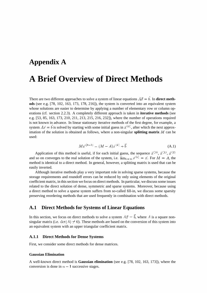
Appendix A
A Brief Overview of Direct Methods
There are two different approaches to solve a system of linear equations A~x =
~
b. In direct meth-ods (see e.g. [78, 102, 163, 173, 178, 216]), the system is converted into an equivalent systemwhose solutions are easier to determine by applying a number of elementary row or column op-erations (cf. section 2.2.3). A completely different approach is taken in iterative methods (seee.g. [53, 85, 163, 173, 210, 211, 213, 215, 216, 232]), where the number of operations requiredis not known in advance. In linear stationary iterative methods of the first degree, for example, asystem A~x =
~
b is solved by starting with some initial guess in ~x (0), after which the next approx-imation of the solution is obtained as follows, where a non-singular splitting matrix M can beused:
M~x
(k+1)
= (M �A)~x
(k)
+
~
b (A.1)
Application of this method is useful, if for each initial guess, the sequence ~x (0), ~x (1), ~x (2)
and so on converges to the real solution of the system, i.e. limi!1
~x
(i)
= ~x. For M = A, themethod is identical to a direct method. In general, however, a splitting matrix is used that can beeasily inverted.
Although iterative methods play a very important role in solving sparse systems, because thestorage requirements and roundoff errors can be reduced by only using elements of the originalcoefficient matrix, in this section we focus on direct methods. In particular, we discuss some issuesrelated to the direct solution of dense, symmetric and sparse systems. Moreover, because usinga direct method to solve a sparse system suffers from so-called fill-in, we discuss some sparsitypreserving reordering methods that are used frequently in combination with direct methods.
A.1 Direct Methods for Systems of Linear Equations
In this section, we focus on direct methods to solve a system A~x =
~
b, where A is a square non-singular matrix (i.e. det(A) 6= 0). These methods are based on the conversion of this system intoan equivalent system with an upper triangular coefficient matrix.
A.1.1 Direct Methods for Dense Systems
First, we consider some direct methods for dense matrices.
Gaussian Elimination
A well-known direct method is Gaussian elimination (see e.g. [78, 102, 163, 173]), where theconversion is done in n� 1 successive stages.
252 APPENDIX A. A BRIEF OVERVIEW OF DIRECT METHODS
At each stage 1 � k < n, an equivalent system A
(k+1)
~x =
~
b
(k+1) is obtained from theprevious system according to the following formulae, where A(1)
= A and ~b(1) =
~
b. All otherelements remain unaffected:
8
>
<
>
:
a
(k+1)
ij
= a
(k)
ij
� (a
(k)
ik
=a
(k)
kk
) � a
(k)
kj
for k < i � n; k � j � n
b
(k+1)
i
= b
(k)
i
� (a
(k)
ik
=a
(k)
kk
) � b
(k)
k
for k < i � n
(A.2)
Here, we assume that at each stage, the pivot a(k)kk
is nonzero. The variable xk
is eliminatedfrom the equations k + 1; : : : ; n by application of elementary row operations nullifying all ele-ments below the diagonal in the kth column. All elements involved in these computations consti-tute the so-called (n� k + 1)� (n� k + 1) active sub-matrix at stage k.
In the final system A
(n)
~x =
~
b
(n), matrix A(n) is an upper triangular matrix U and the systemU~x =
~
b
(n) can be solved easily by back substitution, explained below in more detail. Back substi-tution is not required if A is converted into diagonal form by Gauss-Jordan elimination. In thiscase, each component of the solution vector can be computed directly. Gauss-Jordan eliminationcan also be used to compute A�1 in-place [173].
LU-Factorization
A variant is formed by LU-factorization (see e.g. [78, 97, 169, 173, 175, 235]). This method con-sists of computing a triangular factorization A = LU , in which U is the upper triangular matrixarising from Gaussian elimination, and L is a unit lower triangular matrix that represents all el-ementary row operations. In particular, each stage of Gaussian elimination can be expressed asA
(k+1)
= L
(k)
A
(k), for 1 � k < n, where L(k) represents the elimination at that stage as followsusing the multipliers l
ik
= a
(k)
ik
=a
(k)
kk
:
L
(k)
=
0
B
B
B
B
B
B
B
B
B
@
1
. . .1
�l
k+1;k
.... . .
�l
n;k
1
1
C
C
C
C
C
C
C
C
C
A
(A.3)
Since U = L
(n�1)
: : : L
(1)
A, the following factorization of A is obtained:
A = (L
(1)
)
�1
: : : (L
(n�1)
)
�1
U = LU
The inverse of each lower column matrix L(k) is simply obtained by negation of all the off-diagonal elements. Moreover, the product (L(1)
)
�1
: : : (L
(n�1)
)
�1 is a lower triangular matrix inwhich the off-diagonal elements in the kth column are the multipliers in (L
(k)
)
�1. Consequently,the matrix L is in unit lower triangular form. The storage that is originally used to store A canbe used to store both the matrices L and U , i.e. the factorization can be computed in-place, if theunit diagonal of L is stored implicitly. Each eliminated element a(k+1)
ik
in A(k+1) for k < i � n
is simply replaced by the multiplier lik
.An alternative formulation of LU-factorization arises from the following factorization of a
partitioned matrix A, where H1
= H �
1
d
� ~v ~u
T and we assume that d 6= 0:
A.1. DIRECT METHODS FOR SYSTEMS OF LINEAR EQUATIONS 253
A =
d ~u
T
~v H
!
=
0
B
B
B
@
1 0 � � � 0
1
d
� ~v I
1
C
C
C
A
0
B
B
B
B
@
d 0 � � � 0
0
...0
H
1
1
C
C
C
C
A
0
B
B
B
B
@
1
1
d
� ~u
T
0
...0
I
1
C
C
C
C
A
(A.4)
A recursively obtained factorization H1
= L
1
D
1
U
1
gives rise to the factorization A = LDU
in which both factors L and U are unit triangular and D is in diagonal form:
A =
0
B
B
B
@
1 0 � � � 0
1
d
� ~v L
1
1
C
C
C
A
0
B
B
B
B
@
d 0 � � � 0
0
...0
D
1
1
C
C
C
C
A
0
B
B
B
B
@
1
1
d
� ~u
T
0
...0
U
1
1
C
C
C
C
A
= LDU
This defines either the factorization A = (LD)U or A = L(DU), in which only one fac-tor is unit triangular. The latter factorization corresponds to the factorization presented above,whereas the former factorization results if before each stage an elementary row operation is ap-plied to obtain a unit pivot. In this case, each stage can be expressed as A(k+1)
= L
(k)
D
(k)
A
(k),for 1 � k � n, where each n � n matrix D(k) represents the previous described normalization.Since L(k) represents the elimination at stage k, we have L(n)
= I .
Forward and Back Substitution
After the factorization A = LU has been computed (where L is in lower unit triangular form), thesystem LU~x =
~
b is solved in two steps. First, L~c = ~
b is solved by forward substitution, wherethe components of ~c are computed for i = 1; : : : ; n:
c
i
= b
i
�
i�1
X
k=1
l
ik
� c
k
(A.5)
The remaining system U~x = ~c is solved by back substitution, where the components of thesolution ~x are computed for decreasing values i = n; : : : ; 1:
x
i
= (c
i
�
n
X
k=i+1
u
ik
� x
k
) = u
ii
(A.6)
The advantage of LU-factorization over other direct methods is that if we want to solve thesystem for multiple right-hand side vectors (i.e. solving AX = B), these right-hand sides do nothave to be known in advance [78, 200]. All forward operations are simply recorded in the factor Lduring the factorization, so that these operations can be delayed until a new right-hand side vectorbecomes available. LU-factorization can also be used to compute A�1 by solving AY = I , or todetermine the determinant of A. Moreover, LU-factorization has a lower operation count thanGauss-Jordan elimination for solving a system of linear equations, and performs equally well forinverting a matrix if the special form of the right-hand side in AY = I is accounted for [173].
Pivoting for Stability
Row or column interchanges with a later row or column may be required during each stage ofLU-factorization for two reasons. First, in some cases a row interchange is necessary to obtain anonzero pivot (if such a pivot cannot be obtained, the matrix is singular).
254 APPENDIX A. A BRIEF OVERVIEW OF DIRECT METHODS
The second reason for interchanging is due to the fact that representation errors for real num-bers and inexact computer arithmetic may cause a loss of accuracy. Consequently, effectively afactorization LU = A+H is obtained for some perturbation matrix H . Only if H is relativelysmall in comparison with A, the algorithm used to obtain the factorization is considered stable.
Stability can be controlled by limiting the growth of elements in the matrix during factoriza-tion. Based on the bounds of elements of H derived in [21, 177], we can limit this growth byenforcing the inequalities jl
ik
j � 1 for all k � i � n at each stage k. This can be achieved byapplication of partial pivoting, where at each stage a row interchange is performed if necessaryto enforce the following inequality:
ja
(k)
kk
j � max
k�i�n
ja
(k)
ik
j
Alternatively, a column interchange can be used to obtain a pivot with the largest absolutevalue in the kth row of the upper triangular part, enforcing the inequality ja(k)
kj
=a
(k)
kk
j � 1 for allk � j � n. Although partial pivoting yields stable factorizations in practice, the growth of ele-ments can be further limited by the use of complete pivoting, where row and column interchangesmay be applied to obtain a pivot with the maximum absolute value in the whole active sub-matrix.
Mathematically, there is no difference between applying all row and column interchanges tothe whole compact storage containing elements of both factors during factorization, or permutingA into PAQ before the factorization, where the permutation matrices P and Q represent the ac-cumulated effects of all row and column interchanges respectively [78, p299]. This permutationis called a symmetric permutation if P = Q
T holds. However, because row and column inter-changes correspond to rearranging the equations and relabeling the components of ~x respectively,these changes must be accounted for in the solution. We write the original system A~x =
~
b asfollows:
(PAQ)Q
T
~x = (LU)Q
T
~x = P
~
b
This permuted system is solved by forward substitution of L~c = P
~
b, followed by back sub-stitution of U~y = ~c and permuting the resulting vector according to ~x = Q~y.
Iterative Improvement
Even if pivoting is used by a direct method to preserve stability, inexact computer arithmetic isresponsible for the fact that, in general, we still may obtain the factorization PAQ + H = LU
for some perturbation matrix H . Consequently, if this inaccurate factorization is used to solve asystem of linear equations A~x =
~
b as (LU)Q
T
~x = P
~
b, then usually the computed vector ~x differsfrom the real solution. We can improve the accuracy of the computed solution by a method callediterative improvement or iterative refinement (see e.g. [78, 102, 173, 235]).
Starting with the computed solution in a column vector ~x (0), at each step k the residual vector~r
(k)
=
~
b�A~x
(k) is determined. If the current solution differs from the real solution ~x, then thisresidual vector is nonzero. In this case, we can write the real solution as ~x = ~x
(k)
+
~
�
(k) for someunknown correction vector. Moreover, because A~x = A(~x
(k)
+
~
�
(k)
) is equal to~b, the followingequation holds:
A
~
�
(k)
=
~
b�A~x
(k)
= ~r
(k)
Because a factorization of A is available, the correction vector can be computed by solvingthis system as (LU)Q
T
~
�
(k)
= P~r
(k). Subsequently, we can improve the solution as follows:
~x
(k+1)
= ~x
(k)
+
~
�
(k)
A.1. DIRECT METHODS FOR SYSTEMS OF LINEAR EQUATIONS 255
This method can be repeated if desired until some criterion has been satisfied. During thisprocess, it is essential to use more precision for the residual vector. Because both the originalmatrixA and the factorsL andU must be kept in memory, the use of iterative refinement increasesthe storage requirements of the solution method while additional computational time is requiredto perform the iterations.
A.1.2 Direct Methods for Symmetric Systems
While solving a system A~x =
~
b with a symmetric coefficient matrix, i.e. A = A
T , symmetry ispreserved in the factorization if at any stage a suitable pivot can be chosen from the diagonal inthe active sub-matrix. This form of pivoting, referred to diagonal pivoting, yields the factoriza-tion of a symmetric permutation PAP T
= LDL
T . In this manner, the storage requirements andoperation count of the factorization method are reduced by only computing L and D.
Choleski Factorization
A symmetric matrix A is called positive definite if ~x T
A~x > 0 holds for all ~x 6= 0, negativedefinite if ~x T
A~x < 0 holds for all ~x 6= 0, and indefinite otherwise. For a symmetric positivedefinite matrix A, each diagonal element of D in the factorization A = LDL
T is positive andthe factorization can be written as (LD
1
2
)(D
1
2
L
T
) =
~
L
~
L
T . This Choleski factorization can beobtained as shown below:
A =
d ~v
T
~v H
!
=
0
B
B
B
@
p
d 0 � � � 0
1
p
d
� ~v
I
1
C
C
C
A
0
B
B
B
B
@
1 0 � � � 0
0
...0
H
1
1
C
C
C
C
A
0
B
B
B
B
@
p
d
1
p
d
� ~v
T
0
...0
I
1
C
C
C
C
A
In this factorization, H1
= H �
1
d
(~v � ~v
T
) is again a symmetric positive definite matrix [97,169]. After the factorizationH
1
= L
1
L
T
1
has been obtained recursively, the Choleski factorizationof A is defined as follows:
A =
0
B
B
B
@
p
d 0 � � � 0
1
p
d
� ~v
L
1
1
C
C
C
A
0
B
B
B
B
@
p
d
1
p
d
� ~v
T
0
...0
L
T
1
1
C
C
C
C
A
=
~
L
~
L
T
Given the Choleski factorization A =
~
L
~
L
T , the solution of a system A~x =
~
b is determinedby subsequently solving the systems ~
L~c =
~
b and ~
L
T
~x = ~c.Note that a symmetric positive definite matrix can be factorized without any pivoting. Another
important class of matrices for which pivoting is not required to control the stability consists ofdiagonally dominant matrices, which are matrices for which the following condition holds forall diagonal elements and at least one of the inequalities is strict:
ja
ii
j �
X
j 6=i
ja
ij
j
Hence, if a diagonal dominant matrix is also symmetric, the symmetry can be easily preservedin the factorization. Furthermore, because symmetric permutations preserve both properties de-scribed above (i.e. if A is a symmetric positive definite matrix or diagonal dominant matrix, thenPAP
T is also a symmetric positive definite or diagonal dominant matrix), diagonal pivoting isstable.
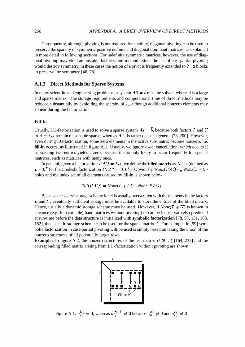
256 APPENDIX A. A BRIEF OVERVIEW OF DIRECT METHODS
Consequently, although pivoting is not required for stability, diagonal pivoting can be used topreserve the sparsity of symmetric positive definite and diagonal dominant matrices, as explainedin more detail in following sections. For indefinite symmetric matrices, however, the use of diag-onal pivoting may yield an unstable factorization method. Since the use of e.g. partial pivotingwould destroy symmetry, in these cases the notion of a pivot is frequently extended to 2�2 blocksto preserve the symmetry [46, 78].
A.1.3 Direct Methods for Sparse Systems
In many scientific and engineering problems, a system A~x =
~
bmust be solved, where A is a largeand sparse matrix. The storage requirements and computational time of direct methods may bereduced substantially by exploiting the sparsity of A, although additional nonzero elements mayappear during the factorization.
Fill-In
Usually, LU-factorization is used to solve a sparse system A~x =
~
b, because both factors L and UinA = LU remain reasonable sparse, whereasA�1 is rather dense in general [78, 200]. However,even during LU-factorization, some zero elements in the active sub-matrix become nonzero, i.e.fill-in occurs, as illustrated in figure A.1. Usually, we ignore exact cancellation, which occurs ifsubtracting two entries yields a zero, because this is only likely to occur frequently for specialmatrices, such as matrices with many ones.
In general, given a factorization PAQ = LU , we define the filled matrix asL+U (defined asL+L
T for the Choleski factorization PAP T
= LL
T ). Obviously, Nonz(PAQ) � Nonz(L+U)
holds and the index set of all elements caused by fill-in is shown below:
Fill(PAQ) = Nonz(L+ U)� Nonz(PAQ)
Because the sparse storage scheme forA is usually overwritten with the elements in the factorsL and U , eventually sufficient storage must be available to store the entries of the filled matrix.Hence, usually a dynamic storage scheme must be used. However, if Nonz(L + U) is known inadvance (e.g. for (variable) band matrices without pivoting) or can be (conservatively) predictedat run-time before the data structure is initialized with symbolic factorization [78, 97, 131, 169,182], then a static storage scheme can be used for the sparse matrix A. For example, in [99] sym-bolic factorization in case partial pivoting will be used is simply based on taking the union of thenonzero structures of all potentially target rows.Example: In figure A.2, the nonzero structures of the test matrix D(20; 5) [164, 235] and thecorresponding filled matrix arising from LU-factorization without pivoting are shown.
k
k
Fill−In
Figure A.1: a(k)ij
= 0, whereas a(k+1)
ij
6= 0 because a(k)ik
6= 0 and a(k)kj
6= 0
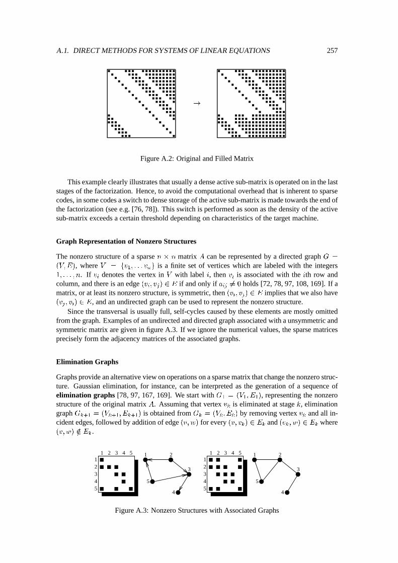
A.1. DIRECT METHODS FOR SYSTEMS OF LINEAR EQUATIONS 257
!
Figure A.2: Original and Filled Matrix
This example clearly illustrates that usually a dense active sub-matrix is operated on in the laststages of the factorization. Hence, to avoid the computational overhead that is inherent to sparsecodes, in some codes a switch to dense storage of the active sub-matrix is made towards the end ofthe factorization (see e.g. [76, 78]). This switch is performed as soon as the density of the activesub-matrix exceeds a certain threshold depending on characteristics of the target machine.
Graph Representation of Nonzero Structures
The nonzero structure of a sparse n � n matrix A can be represented by a directed graph G =
(V;E), where V = fv
1
; : : : v
n
g is a finite set of vertices which are labeled with the integers1; : : : ; n. If v
i
denotes the vertex in V with label i, then vi
is associated with the ith row andcolumn, and there is an edge (v
i
; v
j
) 2 E if and only if aij
6= 0 holds [72, 78, 97, 108, 169]. If amatrix, or at least its nonzero structure, is symmetric, then (v
i
; v
j
) 2 E implies that we also have(v
j
; v
i
) 2 E, and an undirected graph can be used to represent the nonzero structure.Since the transversal is usually full, self-cycles caused by these elements are mostly omitted
from the graph. Examples of an undirected and directed graph associated with a unsymmetric andsymmetric matrix are given in figure A.3. If we ignore the numerical values, the sparse matricesprecisely form the adjacency matrices of the associated graphs.
Elimination Graphs
Graphs provide an alternative view on operations on a sparse matrix that change the nonzero struc-ture. Gaussian elimination, for instance, can be interpreted as the generation of a sequence ofelimination graphs [78, 97, 167, 169]. We start with G
1
= (V
1
; E
1
), representing the nonzerostructure of the original matrix A. Assuming that vertex v
k
is eliminated at stage k, eliminationgraph G
k+1
= (V
k+1
; E
k+1
) is obtained from G
k
= (V
k
; E
k
) by removing vertex vk
and all in-cident edges, followed by addition of edge (v; w) for every (v; v
k
) 2 E
k
and (v
k
; w) 2 E
k
where(v; w) =2 E
k
.
12345
1 2 3 4 5 1 2
3
4
5
12345
1 2 3 4 5 1 2
3
4
5
Figure A.3: Nonzero Structures with Associated Graphs
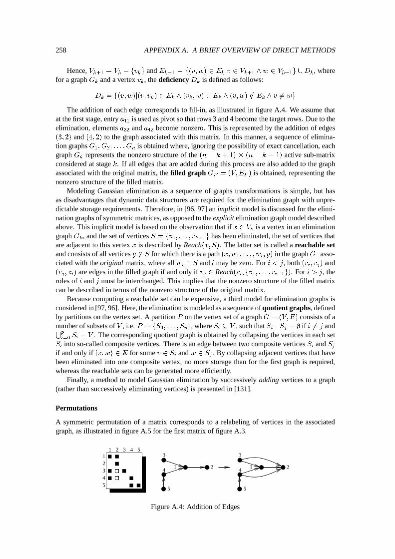
258 APPENDIX A. A BRIEF OVERVIEW OF DIRECT METHODS
Hence, Vk+1
= V
k
� fv
k
g and Ek+1
= f(v; w) 2 E
k
jv 2 V
k+1
^ w 2 V
k+1
g [D
k
, wherefor a graph G
k
and a vertex vk
, the deficiency Dk
is defined as follows:
D
k
= f(v; w)j(v; v
k
) 2 E
k
^ (v
k
; w) 2 E
k
^ (v; w) =2 E
k
^ v 6= wg
The addition of each edge corresponds to fill-in, as illustrated in figure A.4. We assume thatat the first stage, entry a
11
is used as pivot so that rows 3 and 4 become the target rows. Due to theelimination, elements a
32
and a42
become nonzero. This is represented by the addition of edges(3; 2) and (4; 2) to the graph associated with this matrix. In this manner, a sequence of elimina-tion graphs G
1
; G
2
; : : : ; G
n
is obtained where, ignoring the possibility of exact cancellation, eachgraph G
k
represents the nonzero structure of the (n � k + 1) � (n � k + 1) active sub-matrixconsidered at stage k. If all edges that are added during this process are also added to the graphassociated with the original matrix, the filled graph G
F
= (V;E
F
) is obtained, representing thenonzero structure of the filled matrix.
Modeling Gaussian elimination as a sequence of graphs transformations is simple, but hasas disadvantages that dynamic data structures are required for the elimination graph with unpre-dictable storage requirements. Therefore, in [96, 97] an implicit model is discussed for the elimi-nation graphs of symmetric matrices, as opposed to the explicit elimination graph model describedabove. This implicit model is based on the observation that if x 2 V
k
is a vertex in an eliminationgraph G
k
, and the set of vertices S = fv
1
; : : : ; v
k�1
g has been eliminated, the set of vertices thatare adjacent to this vertex x is described by Reach(x; S). The latter set is called a reachable setand consists of all vertices y 62 S for which there is a path (x;w
1
; : : : ; w
l
; y) in the graphG1
asso-ciated with the original matrix, where all w
i
2 S and l may be zero. For i < j, both (v
i
; v
j
) and(v
j
; v
i
) are edges in the filled graph if and only if vj
2 Reach(vi
; fv
1
; : : : ; v
i�1
g). For i > j, theroles of i and j must be interchanged. This implies that the nonzero structure of the filled matrixcan be described in terms of the nonzero structure of the original matrix.
Because computing a reachable set can be expensive, a third model for elimination graphs isconsidered in [97, 96]. Here, the elimination is modeled as a sequence of quotient graphs, definedby partitions on the vertex set. A partition P on the vertex set of a graph G = (V;E) consists of anumber of subsets of V , i.e. P = fS
0
; : : : ; S
p
g, where Si
� V , such that Si
\S
j
= ; if i 6= j andS
p
i=0
S
i
= V . The corresponding quotient graph is obtained by collapsing the vertices in each setS
i
into so-called composite vertices. There is an edge between two composite vertices Si
and Sj
if and only if (v; w) 2 E for some v 2 Si
and w 2 Sj
. By collapsing adjacent vertices that havebeen eliminated into one composite vertex, no more storage than for the first graph is required,whereas the reachable sets can be generated more efficiently.
Finally, a method to model Gaussian elimination by successively adding vertices to a graph(rather than successively eliminating vertices) is presented in [131].
Permutations
A symmetric permutation of a matrix corresponds to a relabeling of vertices in the associatedgraph, as illustrated in figure A.5 for the first matrix of figure A.3.
12345
1 2 3 4 5
1 2
3
4
5
1 2
3
4
5
Figure A.4: Addition of Edges
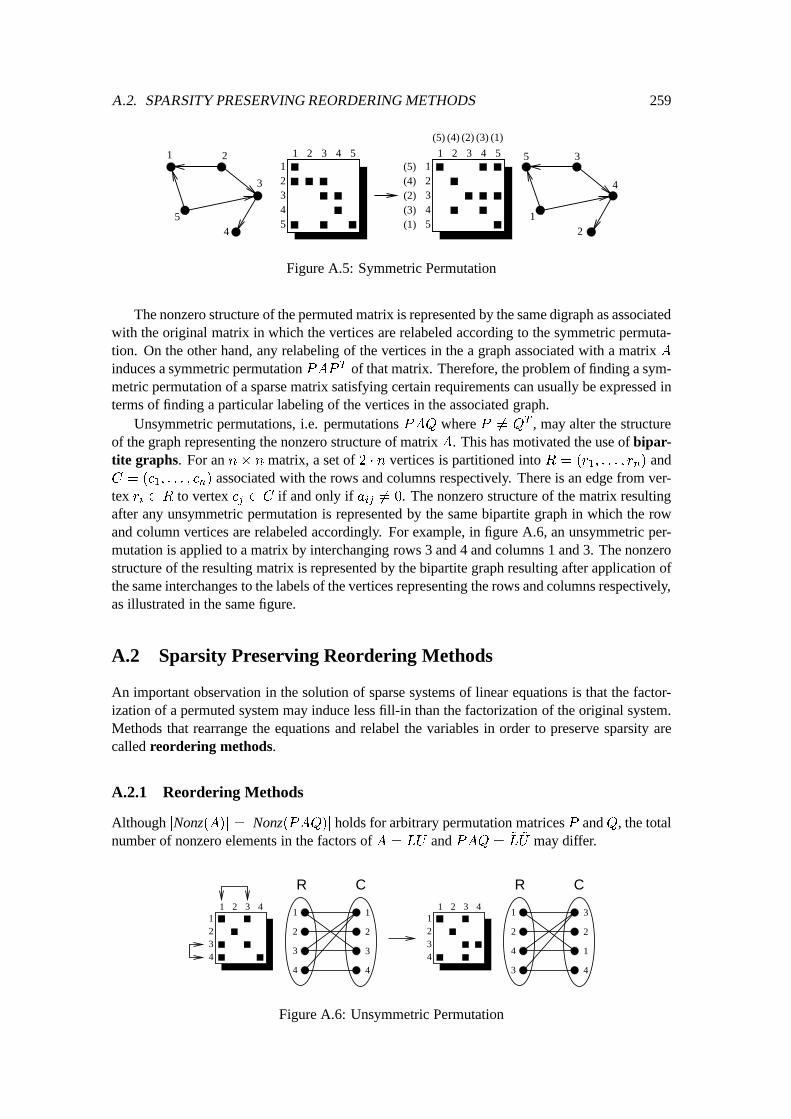
A.2. SPARSITY PRESERVING REORDERING METHODS 259
12345
1 2 3 4 5
12
3
4
512345
1 2 3 4 51 2
3
45
(1)(2) (3)(4)(5)
(1)
(2)(4)(5)
(3)
Figure A.5: Symmetric Permutation
The nonzero structure of the permuted matrix is represented by the same digraph as associatedwith the original matrix in which the vertices are relabeled according to the symmetric permuta-tion. On the other hand, any relabeling of the vertices in the a graph associated with a matrix Ainduces a symmetric permutation PAP T of that matrix. Therefore, the problem of finding a sym-metric permutation of a sparse matrix satisfying certain requirements can usually be expressed interms of finding a particular labeling of the vertices in the associated graph.
Unsymmetric permutations, i.e. permutations PAQ where P 6= Q
T , may alter the structureof the graph representing the nonzero structure of matrix A. This has motivated the use of bipar-tite graphs. For an n� n matrix, a set of 2 � n vertices is partitioned into R = (r
1
; : : : ; r
n
) andC = (c
1
; : : : ; c
n
) associated with the rows and columns respectively. There is an edge from ver-tex r
i
2 R to vertex cj
2 C if and only if aij
6= 0. The nonzero structure of the matrix resultingafter any unsymmetric permutation is represented by the same bipartite graph in which the rowand column vertices are relabeled accordingly. For example, in figure A.6, an unsymmetric per-mutation is applied to a matrix by interchanging rows 3 and 4 and columns 1 and 3. The nonzerostructure of the resulting matrix is represented by the bipartite graph resulting after application ofthe same interchanges to the labels of the vertices representing the rows and columns respectively,as illustrated in the same figure.
A.2 Sparsity Preserving Reordering Methods
An important observation in the solution of sparse systems of linear equations is that the factor-ization of a permuted system may induce less fill-in than the factorization of the original system.Methods that rearrange the equations and relabel the variables in order to preserve sparsity arecalled reordering methods.
A.2.1 Reordering Methods
Although jNonz(A)j = jNonz(PAQ)j holds for arbitrary permutation matrices P andQ, the totalnumber of nonzero elements in the factors of A = LU and PAQ =
~
L
~
U may differ.
1
2
3
4
1
2
3
4
1234
1 2 3 4
R C
1234
1 2 3 41
2
3
4 1
2
3
4
R C
Figure A.6: Unsymmetric Permutation
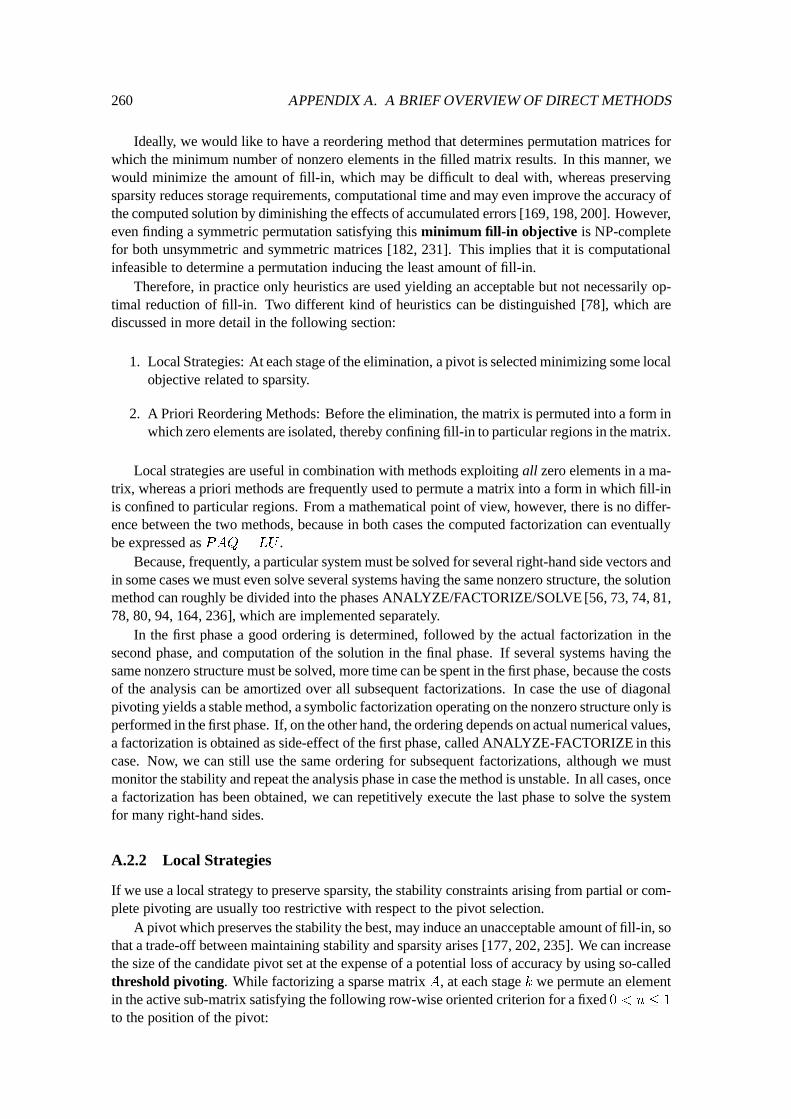
260 APPENDIX A. A BRIEF OVERVIEW OF DIRECT METHODS
Ideally, we would like to have a reordering method that determines permutation matrices forwhich the minimum number of nonzero elements in the filled matrix results. In this manner, wewould minimize the amount of fill-in, which may be difficult to deal with, whereas preservingsparsity reduces storage requirements, computational time and may even improve the accuracy ofthe computed solution by diminishing the effects of accumulated errors [169, 198, 200]. However,even finding a symmetric permutation satisfying this minimum fill-in objective is NP-completefor both unsymmetric and symmetric matrices [182, 231]. This implies that it is computationalinfeasible to determine a permutation inducing the least amount of fill-in.
Therefore, in practice only heuristics are used yielding an acceptable but not necessarily op-timal reduction of fill-in. Two different kind of heuristics can be distinguished [78], which arediscussed in more detail in the following section:
1. Local Strategies: At each stage of the elimination, a pivot is selected minimizing some localobjective related to sparsity.
2. A Priori Reordering Methods: Before the elimination, the matrix is permuted into a form inwhich zero elements are isolated, thereby confining fill-in to particular regions in the matrix.
Local strategies are useful in combination with methods exploiting all zero elements in a ma-trix, whereas a priori methods are frequently used to permute a matrix into a form in which fill-inis confined to particular regions. From a mathematical point of view, however, there is no differ-ence between the two methods, because in both cases the computed factorization can eventuallybe expressed as PAQ = LU .
Because, frequently, a particular system must be solved for several right-hand side vectors andin some cases we must even solve several systems having the same nonzero structure, the solutionmethod can roughly be divided into the phases ANALYZE/FACTORIZE/SOLVE [56, 73, 74, 81,78, 80, 94, 164, 236], which are implemented separately.
In the first phase a good ordering is determined, followed by the actual factorization in thesecond phase, and computation of the solution in the final phase. If several systems having thesame nonzero structure must be solved, more time can be spent in the first phase, because the costsof the analysis can be amortized over all subsequent factorizations. In case the use of diagonalpivoting yields a stable method, a symbolic factorization operating on the nonzero structure only isperformed in the first phase. If, on the other hand, the ordering depends on actual numerical values,a factorization is obtained as side-effect of the first phase, called ANALYZE-FACTORIZE in thiscase. Now, we can still use the same ordering for subsequent factorizations, although we mustmonitor the stability and repeat the analysis phase in case the method is unstable. In all cases, oncea factorization has been obtained, we can repetitively execute the last phase to solve the systemfor many right-hand sides.
A.2.2 Local Strategies
If we use a local strategy to preserve sparsity, the stability constraints arising from partial or com-plete pivoting are usually too restrictive with respect to the pivot selection.
A pivot which preserves the stability the best, may induce an unacceptable amount of fill-in, sothat a trade-off between maintaining stability and sparsity arises [177, 202, 235]. We can increasethe size of the candidate pivot set at the expense of a potential loss of accuracy by using so-calledthreshold pivoting. While factorizing a sparse matrix A, at each stage k we permute an elementin the active sub-matrix satisfying the following row-wise oriented criterion for a fixed 0 < u � 1
to the position of the pivot:
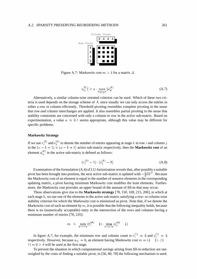
A.2. SPARSITY PRESERVING REORDERING METHODS 261
4443
3 4 4 4Row Count
Column Count
Figure A.7: Markowitz cost m > 4 for a matrix A
ja
(k)
ij
j � u � max
k�l�n
ja
(k)
il
j (A.7)
Alternatively, a similar column-wise oriented criterion can be used. Which of these two cri-teria is used depends on the storage scheme of A, since usually we can only access the entries ineither a row or column efficiently. Threshold pivoting resembles complete pivoting in the sensethat row and column interchanges are applied. It also resembles partial pivoting in the sense thatstability constraints are concerned with only a column or row in the active sub-matrix. Based onexperimentation, a value u � 0:1 seems appropriate, although this value may be different forspecific problems.
Markowitz Strategy
If we use r(k)i
and c(k)j
to denote the number of entries appearing at stage k in row i and column jin the (n� k + 1)� (n� k + 1) active sub-matrix respectively, then the Markowitz cost of an
element a(k)ij
in the active sub-matrix is defined as follows:
(r
(k)
i
� 1) � (c
(k)
j
� 1) (A.8)
Examination of the formulation (A.4) of LU-factorization reveals that, after possibly a suitablepivot has been brought into position, the next active sub-matrix is updated with�1
d
~v~u
T . Becausethe Markowitz cost of an element is equal to the number of nonzero elements in the correspondingupdating matrix, a pivot having minimum Markowitz cost modifies the least elements. Further-more, the Markowitz cost provides an upper bound of the amount of fill-in that may occur.
These observations give rise to the Markowitz strategy [78, 150, 169, 215, 200], in which ateach stage k, we use one of the elements in the active sub-matrix satisfying a row- or column-wisestability criterion for which the Markowitz cost is minimized as pivot. Note that, if we denote theMarkowitz cost of such an element bym, it is possible that the following inequality holds, becausethere is no (numerically acceptable) entry in the intersection of the rows and columns having aminimum number of entries [78, 235]:
m > min
k�i�n
(r
(k)
i
� 1) � min
k�j�n
(c
(k)
j
� 1)
In figure A.7, for example, the minimum row and column count is r(1)4
= 3 and c(1)1
= 3
respectively. However, because a41
= 0, an element having Markowitz cost m = (4 � 1) � (4 �
1) = 9 > 4 will be used at the first stage.To prevent the situation in which computational savings arising from fill-in reduction are out-
weighed by the costs of finding a suitable pivot, in [56, 80, 78] the following mechanism is used.
262 APPENDIX A. A BRIEF OVERVIEW OF DIRECT METHODS
Rows and columns are ordered in increasing entry count in a data structure allowing for anefficient update at each stage. Rows and columns are scanned in increasing order of entry count,taking rows before columns. The search can be terminated as soon as a stable element is encoun-tered with a Markowitz cost that does not exceed (r
i
� 1)
2 while scanning a row with count ri
, orthat does not exceed (c
j
� 1) � c
j
while scanning a column with count cj
. This mechanism may
fail to find a suitable pivot quickly. In case c(k)j
> r
(k)
i
holds for many elements satisfying thestability constraints, it is possible that a lot of these elements are searched before the terminationcriterion described above holds [235]. Furthermore, there may be many elements with minimumMarkowitz costs that do not satisfy the stability constraints.
Therefore, the mechanism proposed in [164, 235, 236] only performs a search of a few rows inincreasing number of nonzero elements. Furthermore, all elements in these rows are consideredand the element which is the largest in absolute value of all suitable elements is used as pivot.Limiting the search for a suitable pivot yields an unacceptable increase of the amount of additionalfill-in in practice, reduces the pivotal search time substantially, and even may yield more accuratesolutions [235].
Minimum Degree Method
A symmetric version of the Markowitz strategy, useful for symmetric positive definite matrices forwhich pivoting is not required for stability and diagonal pivoting may be used to preserve sparsity(see section A.1.2), is called the minimum degree method [52, 78, 97, 200]. At each stage k, asymmetric permutation is applied, enforcing the following condition for the pivot a(k)
kk
:
r
(k)
k
� max
k�i�n
r
(k)
i
Because, effectively, at each stage we use a pivot corresponding to a vertex in the eliminationgraph with minimum degree, the minimum degree strategy is independent of any numerical val-ues. Therefore, the ordering can be computed symbolically beforehand once the nonzero structureof the matrix is known. The ordering can be used for several systems with the same nonzero struc-ture. In [96, 97, 98, 144], various implementations of the minimum degree method are discussed(yielding a symbolic factorization as side-effect).
No fill-in occurs with this strategy in case the original graph is a tree, since only the leaf ver-tices and possibly the root vertex have minimum degree and elimination of one of these verticesyields a new tree without the introduction of additional edges. In general, if we apply a symmet-ric permutation to such a matrix according to a monotone labeling of the associated graph, whereeach child appears before its parent in the labeling, then Gaussian elimination proceeds withoutany fill-in [78, 167, 169].
Other Local Strategies
Simplifications of the Markowitz strategy, such as the min.row in min.column strategy [78, 169],where a pivot with minimum row count in the column with minimum column count is selected,usually induce too much fill-in to be practical. On the other hand, gains arising from the reductionof fill-in in the more complex strategies are usually diminished by the increase in search time. Sucha complex strategy is formed by the the minimum deficiency strategy [57, 78, 200, 215], where apivot is used at each stage with a minimum size of the deficiency, locally minimizing the amountof fill-in. However, even this strategy does not necessarily minimize the total amount of fill-in.Hence, because the Markowitz strategy is relatively simple to implement and yields a satisfactoryreduction of fill-in, this strategy has been most successful in practice.
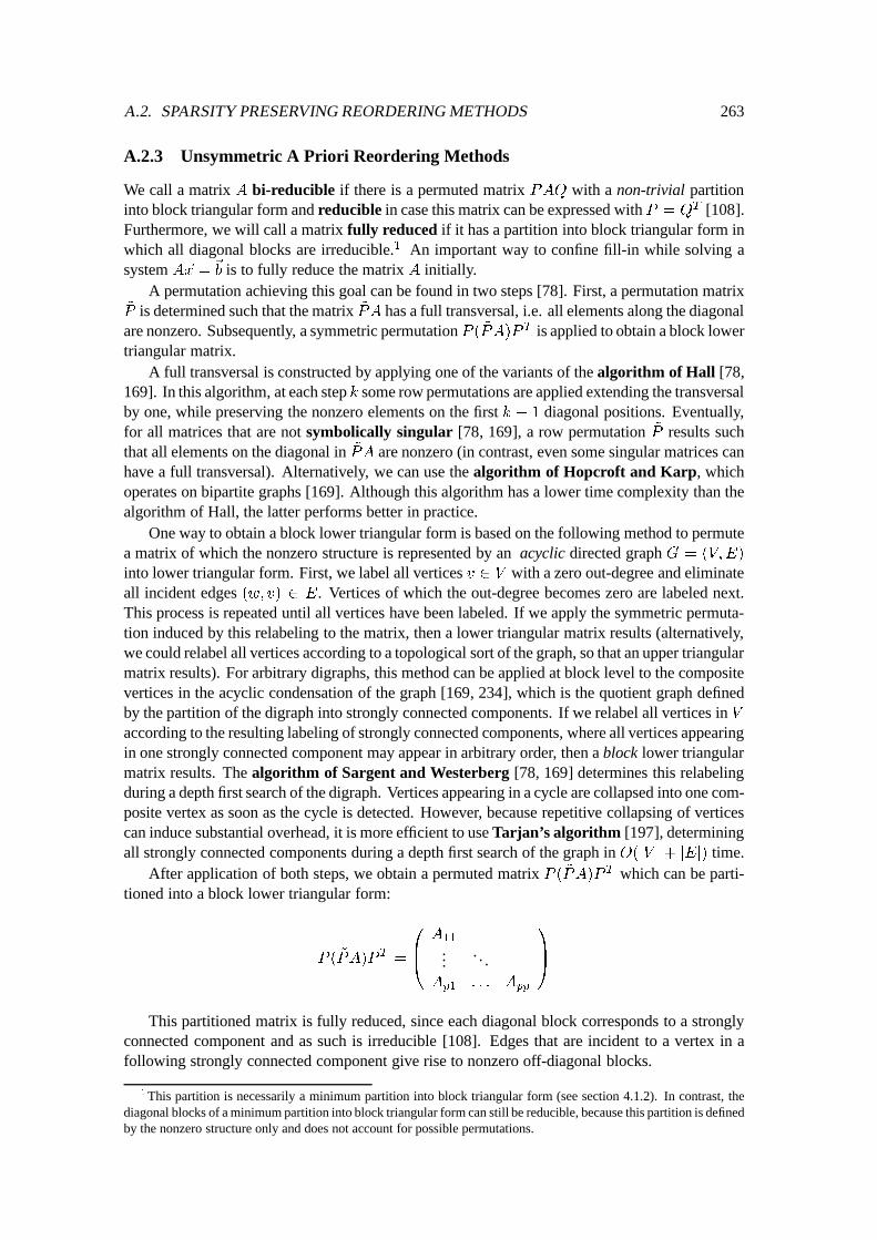
A.2. SPARSITY PRESERVING REORDERING METHODS 263
A.2.3 Unsymmetric A Priori Reordering Methods
We call a matrix A bi-reducible if there is a permuted matrix PAQ with a non-trivial partitioninto block triangular form and reducible in case this matrix can be expressed with P = Q
T [108].Furthermore, we will call a matrix fully reduced if it has a partition into block triangular form inwhich all diagonal blocks are irreducible.1 An important way to confine fill-in while solving asystem A~x =
~
b is to fully reduce the matrix A initially.A permutation achieving this goal can be found in two steps [78]. First, a permutation matrix
~
P is determined such that the matrix ~
PA has a full transversal, i.e. all elements along the diagonalare nonzero. Subsequently, a symmetric permutation P ( ~PA)P T is applied to obtain a block lowertriangular matrix.
A full transversal is constructed by applying one of the variants of the algorithm of Hall [78,169]. In this algorithm, at each step k some row permutations are applied extending the transversalby one, while preserving the nonzero elements on the first k � 1 diagonal positions. Eventually,for all matrices that are not symbolically singular [78, 169], a row permutation ~
P results suchthat all elements on the diagonal in ~
PA are nonzero (in contrast, even some singular matrices canhave a full transversal). Alternatively, we can use the algorithm of Hopcroft and Karp, whichoperates on bipartite graphs [169]. Although this algorithm has a lower time complexity than thealgorithm of Hall, the latter performs better in practice.
One way to obtain a block lower triangular form is based on the following method to permutea matrix of which the nonzero structure is represented by an acyclic directed graph G = (V;E)
into lower triangular form. First, we label all vertices v 2 V with a zero out-degree and eliminateall incident edges (w; v) 2 E. Vertices of which the out-degree becomes zero are labeled next.This process is repeated until all vertices have been labeled. If we apply the symmetric permuta-tion induced by this relabeling to the matrix, then a lower triangular matrix results (alternatively,we could relabel all vertices according to a topological sort of the graph, so that an upper triangularmatrix results). For arbitrary digraphs, this method can be applied at block level to the compositevertices in the acyclic condensation of the graph [169, 234], which is the quotient graph definedby the partition of the digraph into strongly connected components. If we relabel all vertices in Vaccording to the resulting labeling of strongly connected components, where all vertices appearingin one strongly connected component may appear in arbitrary order, then a block lower triangularmatrix results. The algorithm of Sargent and Westerberg [78, 169] determines this relabelingduring a depth first search of the digraph. Vertices appearing in a cycle are collapsed into one com-posite vertex as soon as the cycle is detected. However, because repetitive collapsing of verticescan induce substantial overhead, it is more efficient to use Tarjan’s algorithm [197], determiningall strongly connected components during a depth first search of the graph in O(jV j+ jEj) time.
After application of both steps, we obtain a permuted matrix P ( ~PA)P T which can be parti-tioned into a block lower triangular form:
P (
~
PA)P
T
=
0
B
@
A
11
.... . .
A
p1
: : : A
pp
1
C
A
This partitioned matrix is fully reduced, since each diagonal block corresponds to a stronglyconnected component and as such is irreducible [108]. Edges that are incident to a vertex in afollowing strongly connected component give rise to nonzero off-diagonal blocks.
1This partition is necessarily a minimum partition into block triangular form (see section 4.1.2). In contrast, thediagonal blocks of a minimum partition into block triangular form can still be reducible, because this partition is definedby the nonzero structure only and does not account for possible permutations.
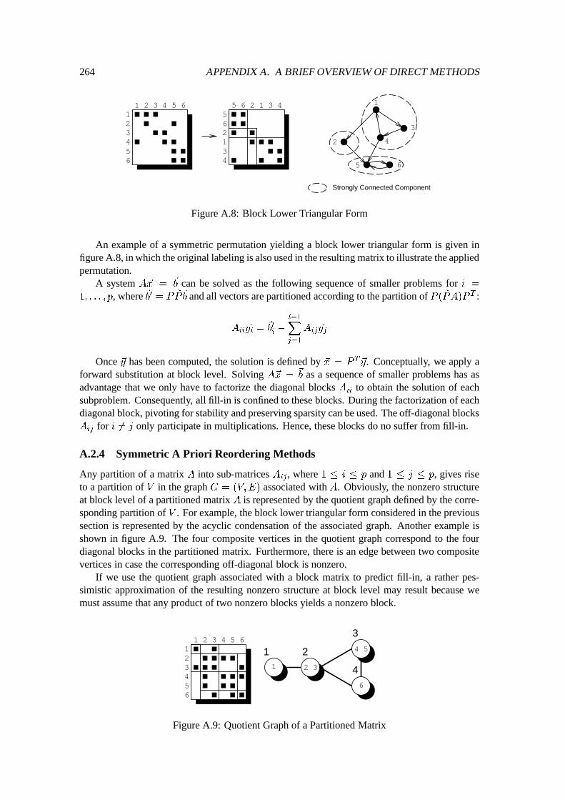
264 APPENDIX A. A BRIEF OVERVIEW OF DIRECT METHODS
1
2
3
4
5 6
12
3
45 6
12
3
4
56
31 2
3
4 5 612
456
3
Strongly Connected Component
Figure A.8: Block Lower Triangular Form
An example of a symmetric permutation yielding a block lower triangular form is given infigure A.8, in which the original labeling is also used in the resulting matrix to illustrate the appliedpermutation.
A system A~x =
~
b can be solved as the following sequence of smaller problems for i =
1; : : : ; p, where~b0 = P
~
P
~
b and all vectors are partitioned according to the partition of P ( ~PA)P T :
A
ii
~y
i
=
~
b
0
i
�
i�1
X
j=1
A
ij
~y
j
Once ~y has been computed, the solution is defined by ~x = P
T
~y. Conceptually, we apply aforward substitution at block level. Solving A~x =
~
b as a sequence of smaller problems has asadvantage that we only have to factorize the diagonal blocks A
ii
to obtain the solution of eachsubproblem. Consequently, all fill-in is confined to these blocks. During the factorization of eachdiagonal block, pivoting for stability and preserving sparsity can be used. The off-diagonal blocksA
ij
for i 6= j only participate in multiplications. Hence, these blocks do no suffer from fill-in.
A.2.4 Symmetric A Priori Reordering Methods
Any partition of a matrix A into sub-matrices Aij
, where 1 � i � p and 1 � j � p, gives riseto a partition of V in the graph G = (V;E) associated with A. Obviously, the nonzero structureat block level of a partitioned matrix A is represented by the quotient graph defined by the corre-sponding partition of V . For example, the block lower triangular form considered in the previoussection is represented by the acyclic condensation of the associated graph. Another example isshown in figure A.9. The four composite vertices in the quotient graph correspond to the fourdiagonal blocks in the partitioned matrix. Furthermore, there is an edge between two compositevertices in case the corresponding off-diagonal block is nonzero.
If we use the quotient graph associated with a block matrix to predict fill-in, a rather pes-simistic approximation of the resulting nonzero structure at block level may result because wemust assume that any product of two nonzero blocks yields a nonzero block.
1 2
3
4 5 612
3
456
3
6
1
54
2 3
1 2
3
4
Figure A.9: Quotient Graph of a Partitioned Matrix
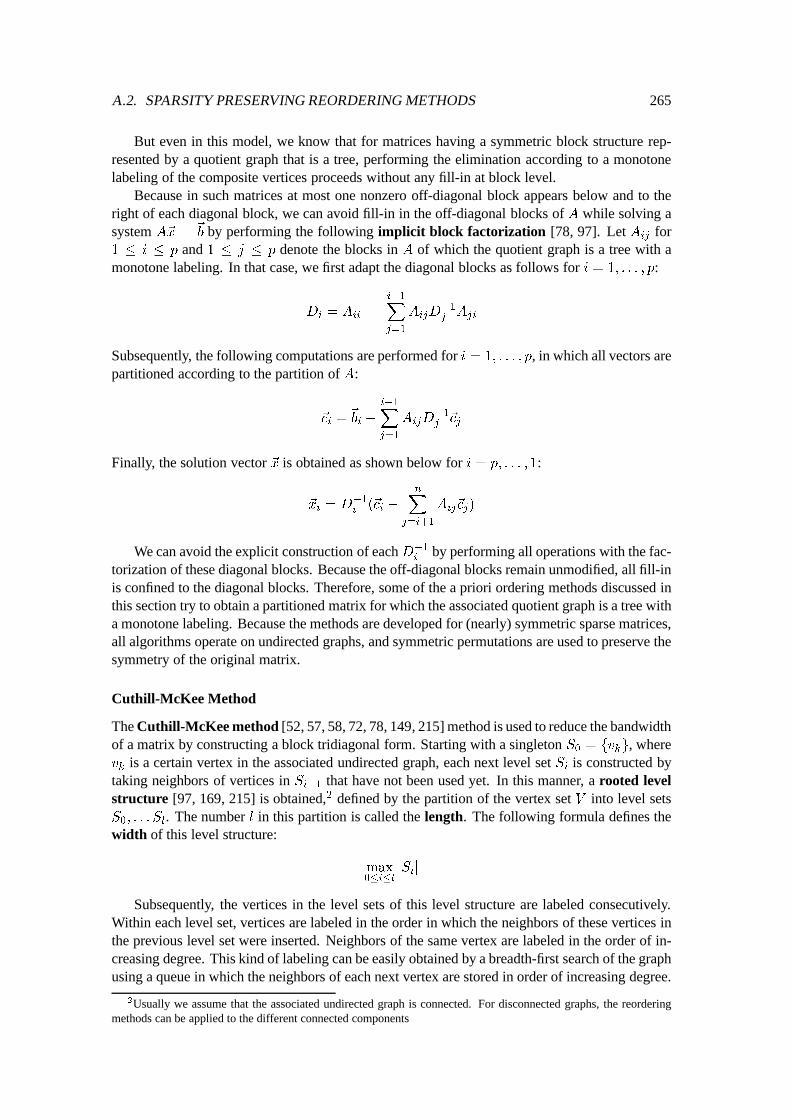
A.2. SPARSITY PRESERVING REORDERING METHODS 265
But even in this model, we know that for matrices having a symmetric block structure rep-resented by a quotient graph that is a tree, performing the elimination according to a monotonelabeling of the composite vertices proceeds without any fill-in at block level.
Because in such matrices at most one nonzero off-diagonal block appears below and to theright of each diagonal block, we can avoid fill-in in the off-diagonal blocks of A while solving asystem A~x =
~
b by performing the following implicit block factorization [78, 97]. Let Aij
for1 � i � p and 1 � j � p denote the blocks in A of which the quotient graph is a tree with amonotone labeling. In that case, we first adapt the diagonal blocks as follows for i = 1; : : : ; p:
D
i
= A
ii
�
i�1
X
j=1
A
ij
D
�1
j
A
ji
Subsequently, the following computations are performed for i = 1; : : : ; p, in which all vectors arepartitioned according to the partition of A:
~c
i
=
~
b
i
�
i�1
X
j=1
A
ij
D
�1
j
~c
j
Finally, the solution vector ~x is obtained as shown below for i = p; : : : ; 1:
~x
i
= D
�1
i
(~c
i
�
n
X
j=i+1
A
ij
~c
j
)
We can avoid the explicit construction of eachD�1i
by performing all operations with the fac-torization of these diagonal blocks. Because the off-diagonal blocks remain unmodified, all fill-inis confined to the diagonal blocks. Therefore, some of the a priori ordering methods discussed inthis section try to obtain a partitioned matrix for which the associated quotient graph is a tree witha monotone labeling. Because the methods are developed for (nearly) symmetric sparse matrices,all algorithms operate on undirected graphs, and symmetric permutations are used to preserve thesymmetry of the original matrix.
Cuthill-McKee Method
The Cuthill-McKee method [52, 57, 58, 72, 78, 149, 215] method is used to reduce the bandwidthof a matrix by constructing a block tridiagonal form. Starting with a singleton S
0
= fv
k
g, wherev
k
is a certain vertex in the associated undirected graph, each next level set Si
is constructed bytaking neighbors of vertices in S
i�1
that have not been used yet. In this manner, a rooted levelstructure [97, 169, 215] is obtained,2 defined by the partition of the vertex set V into level setsS
0
; : : : S
l
. The number l in this partition is called the length. The following formula defines thewidth of this level structure:
max
0�i�l
jS
i
j
Subsequently, the vertices in the level sets of this level structure are labeled consecutively.Within each level set, vertices are labeled in the order in which the neighbors of these vertices inthe previous level set were inserted. Neighbors of the same vertex are labeled in the order of in-creasing degree. This kind of labeling can be easily obtained by a breadth-first search of the graphusing a queue in which the neighbors of each next vertex are stored in order of increasing degree.
2Usually we assume that the associated undirected graph is connected. For disconnected graphs, the reorderingmethods can be applied to the different connected components
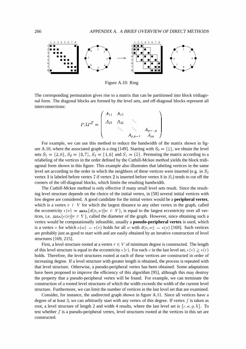
266 APPENDIX A. A BRIEF OVERVIEW OF DIRECT METHODS
12345678
1 2 3 4 5 6 7 8
12
3
45
6
7
81
23
45
678
12345678
1 2 3 4 5 6 7 8
Figure A.10: Ring
The corresponding permutation gives rise to a matrix that can be partitioned into block tridiago-nal form. The diagonal blocks are formed by the level sets, and off-diagonal blocks represent allinterconnections:
PAP
T
=
0
B
B
B
B
B
@
A
11
A
12
A
21
A
22
. . .. . . . . .
A
p�1;p
A
p;p�1
A
pp
1
C
C
C
C
C
A
For example, we can use this method to reduce the bandwidth of the matrix shown in fig-ure A.10, where the associated graph is a ring [149]. Starting with S
0
= f1g, we obtain the levelsets S
1
= f2; 8g, S2
= f3; 7g, S3
= f4; 6g and S4
= f5g. Permuting the matrix according to arelabeling of the vertices in the order defined by the Cuthill-Mckee method yields the block tridi-agonal form shown in this figure. This example also illustrates that labeling vertices in the samelevel set according to the order in which the neighbors of these vertices were inserted (e.g. in S
2
vertex 3 is labeled before vertex 7 if vertex 2 is inserted before vertex 8 in S1
) tends to cut off thecorners of the off-diagonal blocks, which limits the resulting bandwidth.
The Cuthill-Mckee method is only effective if many small level sets result. Since the result-ing level structure depends on the choice of the initial vertex, in [58] several initial vertices withlow degree are considered. A good candidate for the initial vertex would be a peripheral vertex,which is a vertex v 2 V for which the largest distance to any other vertex in the graph, calledthe eccentricity e(v) = maxfd(v; w)jw 2 V g, is equal to the largest eccentricity over all ver-tices, i.e. maxfe(v)jv 2 V g, called the diameter of the graph. However, since obtaining such avertex would be computationally infeasible, usually a pseudo-peripheral vertex is used, whichis a vertex v for which e(w) = e(v) holds for all w with d(v; w) = e(v) [169]. Such verticesare probably just as good to start with and are easily obtained by an iterative construction of levelstructures [169, 215].
First, a level structure rooted at a vertex r 2 V of minimum degree is constructed. The lengthof this level structure is equal to the eccentricity e(r). For each v in the last level set, e(v) � e(r)holds. Therefore, the level structures rooted at each of these vertices are constructed in order ofincreasing degree. If a level structure with greater length is obtained, the process is repeated withthat level structure. Otherwise, a pseudo-peripheral vertex has been obtained. Some adaptationshave been proposed to improve the efficiency of this algorithm [95], although this may destroythe property that a pseudo-peripheral vertex will be found. For example, we can terminate theconstruction of a rooted level structures of which the width exceeds the width of the current levelstructure. Furthermore, we can limit the number of vertices in the last level set that are examined.
Consider, for instance, the undirected graph shown in figure A.11. Since all vertices have adegree of at least 3, we can arbitrarily start with any vertex of this degree. If vertex f is taken asroot, a level structure of length 2 and width 4 results, where the last level set is fc; e; g; hg. Totest whether f is a pseudo-peripheral vertex, level structures rooted at the vertices in this set areconstructed.
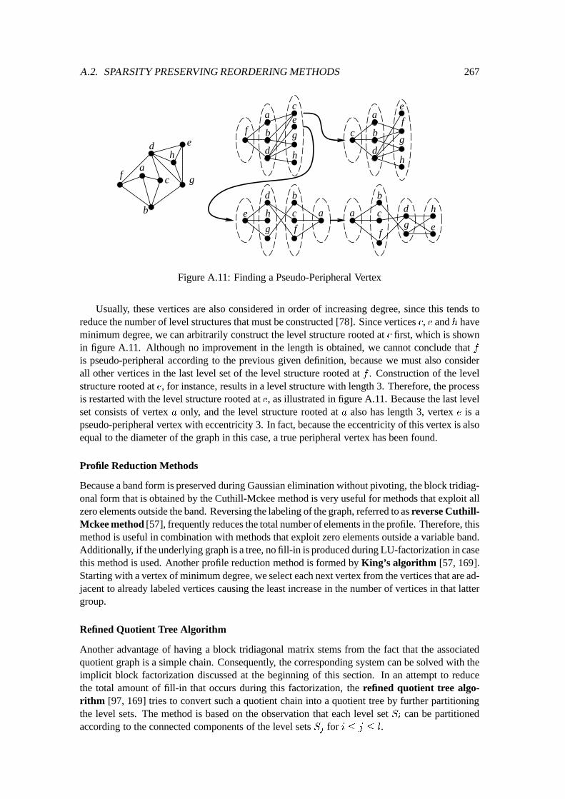
A.2. SPARSITY PRESERVING REORDERING METHODS 267
a
b
c
ed
gf
h
c b
d
af
g
e
h
c
bda
fg e
h
f
c
g
e
h
b
d
a
c
bd
a
fg
e h
Figure A.11: Finding a Pseudo-Peripheral Vertex
Usually, these vertices are also considered in order of increasing degree, since this tends toreduce the number of level structures that must be constructed [78]. Since vertices c, e and h haveminimum degree, we can arbitrarily construct the level structure rooted at c first, which is shownin figure A.11. Although no improvement in the length is obtained, we cannot conclude that fis pseudo-peripheral according to the previous given definition, because we must also considerall other vertices in the last level set of the level structure rooted at f . Construction of the levelstructure rooted at e, for instance, results in a level structure with length 3. Therefore, the processis restarted with the level structure rooted at e, as illustrated in figure A.11. Because the last levelset consists of vertex a only, and the level structure rooted at a also has length 3, vertex e is apseudo-peripheral vertex with eccentricity 3. In fact, because the eccentricity of this vertex is alsoequal to the diameter of the graph in this case, a true peripheral vertex has been found.
Profile Reduction Methods
Because a band form is preserved during Gaussian elimination without pivoting, the block tridiag-onal form that is obtained by the Cuthill-Mckee method is very useful for methods that exploit allzero elements outside the band. Reversing the labeling of the graph, referred to as reverse Cuthill-Mckee method [57], frequently reduces the total number of elements in the profile. Therefore, thismethod is useful in combination with methods that exploit zero elements outside a variable band.Additionally, if the underlying graph is a tree, no fill-in is produced during LU-factorization in casethis method is used. Another profile reduction method is formed by King’s algorithm [57, 169].Starting with a vertex of minimum degree, we select each next vertex from the vertices that are ad-jacent to already labeled vertices causing the least increase in the number of vertices in that lattergroup.
Refined Quotient Tree Algorithm
Another advantage of having a block tridiagonal matrix stems from the fact that the associatedquotient graph is a simple chain. Consequently, the corresponding system can be solved with theimplicit block factorization discussed at the beginning of this section. In an attempt to reducethe total amount of fill-in that occurs during this factorization, the refined quotient tree algo-rithm [97, 169] tries to convert such a quotient chain into a quotient tree by further partitioningthe level sets. The method is based on the observation that each level set S
i
can be partitionedaccording to the connected components of the level sets S
j
for i � j � l.
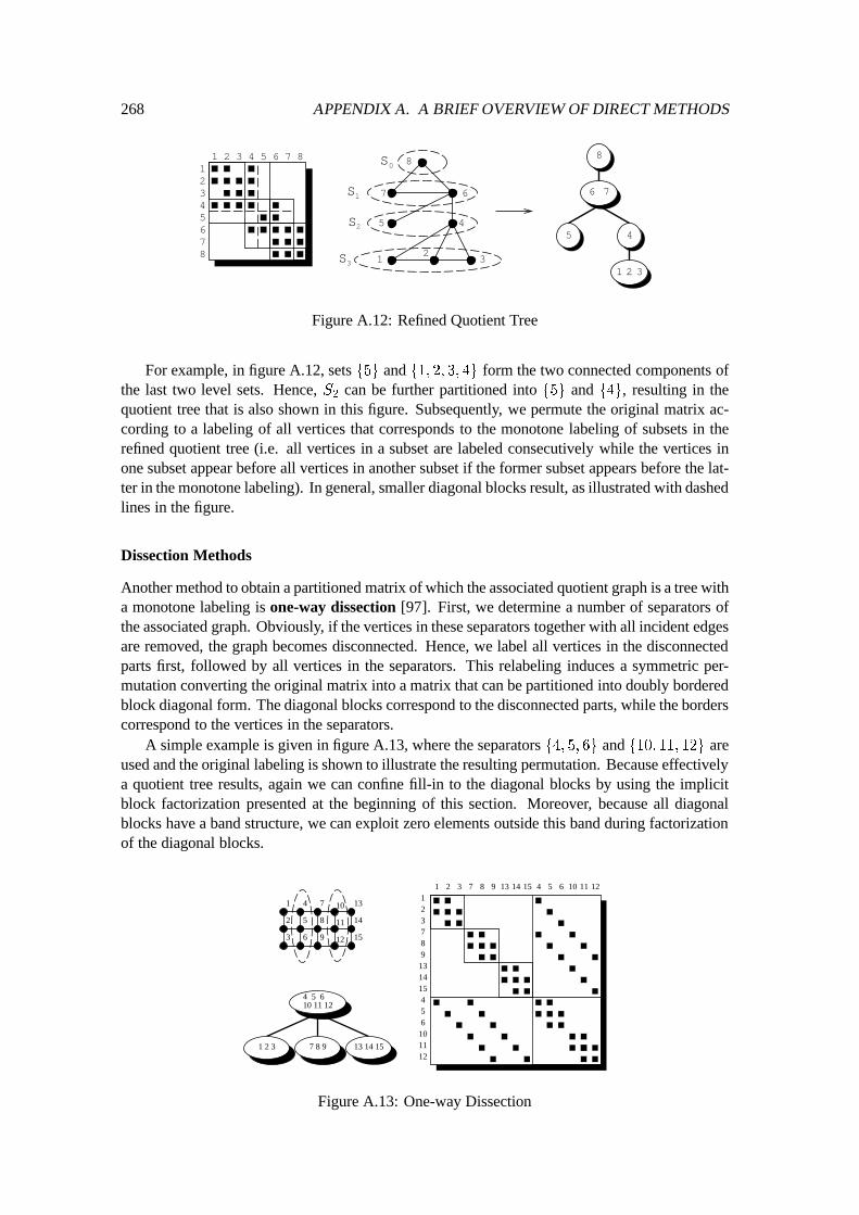
268 APPENDIX A. A BRIEF OVERVIEW OF DIRECT METHODS
1 2
3
4 5 612
456
3 7 8
78 1
23
45
67
8S0
1S
2S
3S
6 7
8
5 4
1 2 3
Figure A.12: Refined Quotient Tree
For example, in figure A.12, sets f5g and f1; 2; 3; 4g form the two connected components ofthe last two level sets. Hence, S
2
can be further partitioned into f5g and f4g, resulting in thequotient tree that is also shown in this figure. Subsequently, we permute the original matrix ac-cording to a labeling of all vertices that corresponds to the monotone labeling of subsets in therefined quotient tree (i.e. all vertices in a subset are labeled consecutively while the vertices inone subset appear before all vertices in another subset if the former subset appears before the lat-ter in the monotone labeling). In general, smaller diagonal blocks result, as illustrated with dashedlines in the figure.
Dissection Methods
Another method to obtain a partitioned matrix of which the associated quotient graph is a tree witha monotone labeling is one-way dissection [97]. First, we determine a number of separators ofthe associated graph. Obviously, if the vertices in these separators together with all incident edgesare removed, the graph becomes disconnected. Hence, we label all vertices in the disconnectedparts first, followed by all vertices in the separators. This relabeling induces a symmetric per-mutation converting the original matrix into a matrix that can be partitioned into doubly borderedblock diagonal form. The diagonal blocks correspond to the disconnected parts, while the borderscorrespond to the vertices in the separators.
A simple example is given in figure A.13, where the separators f4; 5; 6g and f10; 11; 12g areused and the original labeling is shown to illustrate the resulting permutation. Because effectivelya quotient tree results, again we can confine fill-in to the diagonal blocks by using the implicitblock factorization presented at the beginning of this section. Moreover, because all diagonalblocks have a band structure, we can exploit zero elements outside this band during factorizationof the diagonal blocks.
2
3
1 4
5
6
7
8
9
10
11
12
13
14
15
123
456
789
101112
131415
7
1 2 3 4 5 613 14 158 97 11 1210
13 14 15
4 5 610 11 12
1 2 3 7 8 9
Figure A.13: One-way Dissection
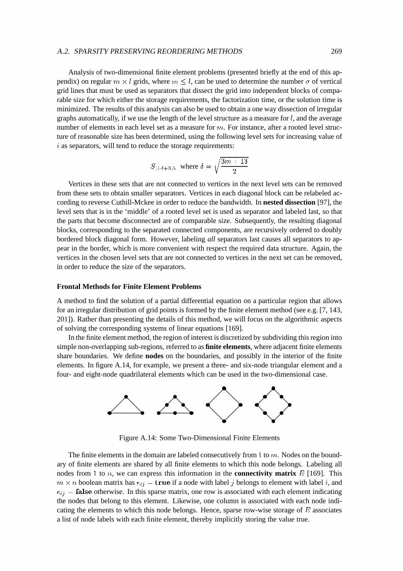
A.2. SPARSITY PRESERVING REORDERING METHODS 269
Analysis of two-dimensional finite element problems (presented briefly at the end of this ap-pendix) on regular m� l grids, where m � l, can be used to determine the number � of verticalgrid lines that must be used as separators that dissect the grid into independent blocks of compa-rable size for which either the storage requirements, the factorization time, or the solution time isminimized. The results of this analysis can also be used to obtain a one way dissection of irregulargraphs automatically, if we use the length of the level structure as a measure for l, and the averagenumber of elements in each level set as a measure for m. For instance, after a rooted level struc-ture of reasonable size has been determined, using the following level sets for increasing value ofi as separators, will tend to reduce the storage requirements:
S
bi��+0:5c
where � =
r
3m+ 13
2
Vertices in these sets that are not connected to vertices in the next level sets can be removedfrom these sets to obtain smaller separators. Vertices in each diagonal block can be relabeled ac-cording to reverse Cuthill-Mckee in order to reduce the bandwidth. In nested dissection [97], thelevel sets that is in the ‘middle’ of a rooted level set is used as separator and labeled last, so thatthe parts that become disconnected are of comparable size. Subsequently, the resulting diagonalblocks, corresponding to the separated connected components, are recursively ordered to doublybordered block diagonal form. However, labeling all separators last causes all separators to ap-pear in the border, which is more convenient with respect the required data structure. Again, thevertices in the chosen level sets that are not connected to vertices in the next set can be removed,in order to reduce the size of the separators.
Frontal Methods for Finite Element Problems
A method to find the solution of a partial differential equation on a particular region that allowsfor an irregular distribution of grid points is formed by the finite element method (see e.g. [7, 143,201]). Rather than presenting the details of this method, we will focus on the algorithmic aspectsof solving the corresponding systems of linear equations [169].
In the finite element method, the region of interest is discretized by subdividing this region intosimple non-overlapping sub-regions, referred to as finite elements, where adjacent finite elementsshare boundaries. We define nodes on the boundaries, and possibly in the interior of the finiteelements. In figure A.14, for example, we present a three- and six-node triangular element and afour- and eight-node quadrilateral elements which can be used in the two-dimensional case.
Figure A.14: Some Two-Dimensional Finite Elements
The finite elements in the domain are labeled consecutively from 1 tom. Nodes on the bound-ary of finite elements are shared by all finite elements to which this node belongs. Labeling allnodes from 1 to n, we can express this information in the connectivity matrix E [169]. Thism� n boolean matrix has e
ij
= true if a node with label j belongs to element with label i, ande
ij
= false otherwise. In this sparse matrix, one row is associated with each element indicatingthe nodes that belong to this element. Likewise, one column is associated with each node indi-cating the elements to which this node belongs. Hence, sparse row-wise storage of E associatesa list of node labels with each finite element, thereby implicitly storing the value true.
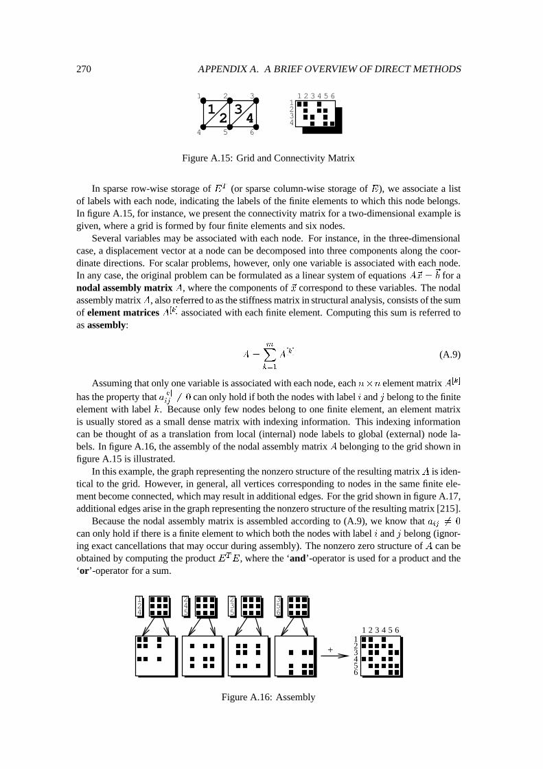
270 APPENDIX A. A BRIEF OVERVIEW OF DIRECT METHODS
1 2 3
4 5 6
1234
1234
1 2 3 4 5 6
Figure A.15: Grid and Connectivity Matrix
In sparse row-wise storage of ET (or sparse column-wise storage of E), we associate a listof labels with each node, indicating the labels of the finite elements to which this node belongs.In figure A.15, for instance, we present the connectivity matrix for a two-dimensional example isgiven, where a grid is formed by four finite elements and six nodes.
Several variables may be associated with each node. For instance, in the three-dimensionalcase, a displacement vector at a node can be decomposed into three components along the coor-dinate directions. For scalar problems, however, only one variable is associated with each node.In any case, the original problem can be formulated as a linear system of equations A~x =
~
b for anodal assembly matrix A, where the components of ~x correspond to these variables. The nodalassembly matrixA, also referred to as the stiffness matrix in structural analysis, consists of the sumof element matrices A[k] associated with each finite element. Computing this sum is referred toas assembly:
A =
m
X
k=1
A
[k] (A.9)
Assuming that only one variable is associated with each node, each n�n element matrixA[k]
has the property that a[e]ij
6= 0 can only hold if both the nodes with label i and j belong to the finiteelement with label k. Because only few nodes belong to one finite element, an element matrixis usually stored as a small dense matrix with indexing information. This indexing informationcan be thought of as a translation from local (internal) node labels to global (external) node la-bels. In figure A.16, the assembly of the nodal assembly matrix A belonging to the grid shown infigure A.15 is illustrated.
In this example, the graph representing the nonzero structure of the resulting matrixA is iden-tical to the grid. However, in general, all vertices corresponding to nodes in the same finite ele-ment become connected, which may result in additional edges. For the grid shown in figure A.17,additional edges arise in the graph representing the nonzero structure of the resulting matrix [215].
Because the nodal assembly matrix is assembled according to (A.9), we know that aij
6= 0
can only hold if there is a finite element to which both the nodes with label i and j belong (ignor-ing exact cancellations that may occur during assembly). The nonzero zero structure of A can beobtained by computing the product ET
E, where the ‘and’-operator is used for a product and the‘or’-operator for a sum.
124 5
24
2
53 5
6
3
123
56
4
1 2 3 4 5 6
+
Figure A.16: Assembly
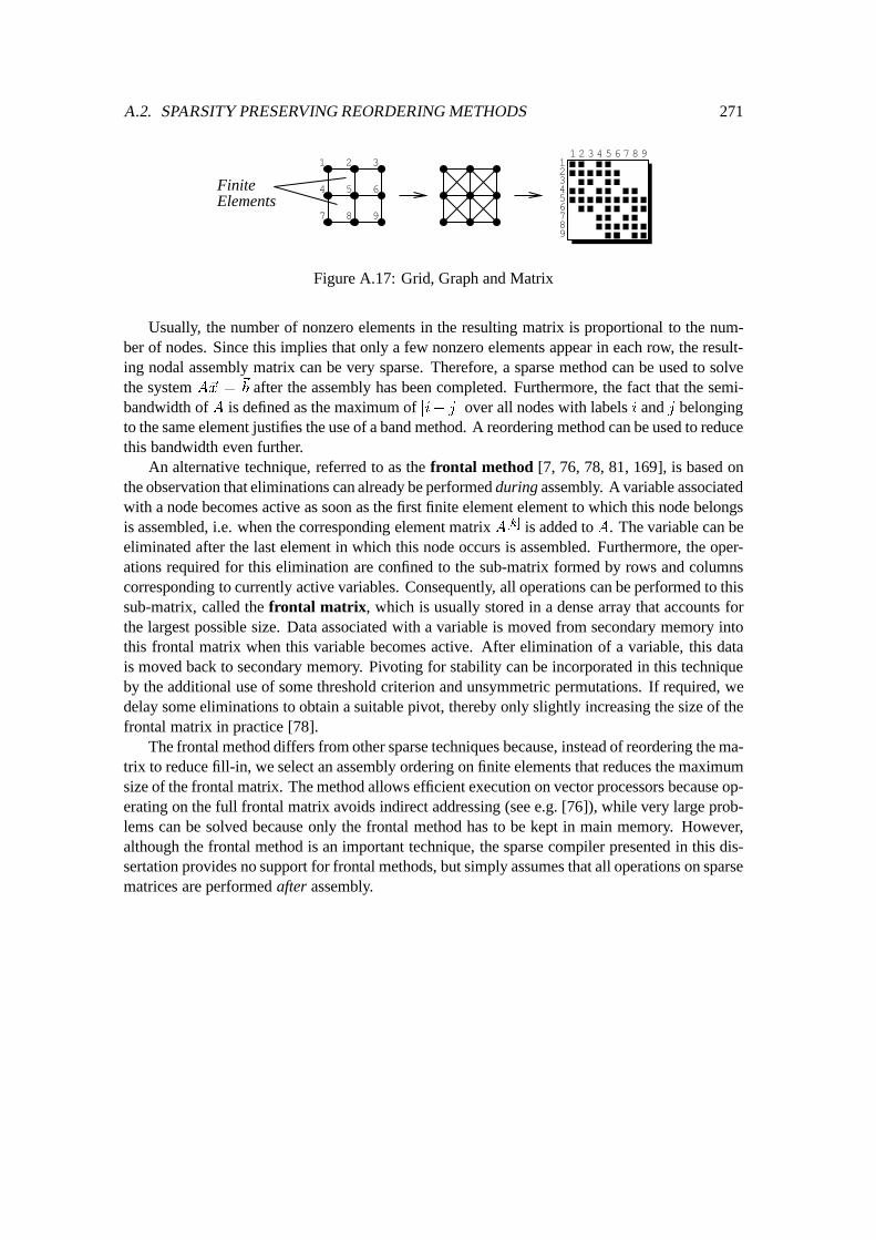
A.2. SPARSITY PRESERVING REORDERING METHODS 271
FiniteElements
1 2 3
4 5 6
7 8 9
1 2 3 4 5 6 7 8 9123456789
Figure A.17: Grid, Graph and Matrix
Usually, the number of nonzero elements in the resulting matrix is proportional to the num-ber of nodes. Since this implies that only a few nonzero elements appear in each row, the result-ing nodal assembly matrix can be very sparse. Therefore, a sparse method can be used to solvethe system A~x =
~
b after the assembly has been completed. Furthermore, the fact that the semi-bandwidth of A is defined as the maximum of ji� jj over all nodes with labels i and j belongingto the same element justifies the use of a band method. A reordering method can be used to reducethis bandwidth even further.
An alternative technique, referred to as the frontal method [7, 76, 78, 81, 169], is based onthe observation that eliminations can already be performed during assembly. A variable associatedwith a node becomes active as soon as the first finite element element to which this node belongsis assembled, i.e. when the corresponding element matrix A[k] is added toA. The variable can beeliminated after the last element in which this node occurs is assembled. Furthermore, the oper-ations required for this elimination are confined to the sub-matrix formed by rows and columnscorresponding to currently active variables. Consequently, all operations can be performed to thissub-matrix, called the frontal matrix, which is usually stored in a dense array that accounts forthe largest possible size. Data associated with a variable is moved from secondary memory intothis frontal matrix when this variable becomes active. After elimination of a variable, this datais moved back to secondary memory. Pivoting for stability can be incorporated in this techniqueby the additional use of some threshold criterion and unsymmetric permutations. If required, wedelay some eliminations to obtain a suitable pivot, thereby only slightly increasing the size of thefrontal matrix in practice [78].
The frontal method differs from other sparse techniques because, instead of reordering the ma-trix to reduce fill-in, we select an assembly ordering on finite elements that reduces the maximumsize of the frontal matrix. The method allows efficient execution on vector processors because op-erating on the full frontal matrix avoids indirect addressing (see e.g. [76]), while very large prob-lems can be solved because only the frontal method has to be kept in main memory. However,although the frontal method is an important technique, the sparse compiler presented in this dis-sertation provides no support for frontal methods, but simply assumes that all operations on sparsematrices are performed after assembly.

272 APPENDIX A. A BRIEF OVERVIEW OF DIRECT METHODS
Bibliography
[1] S. Kamal Abdali and David S. Wise. Experiments with quadtree representation of matrices.In P. Gianni, editor, Lecture Notes in Computer Science, No. 358, pages 96–108. Springer-Verlag, 1988.
[2] R.C. Agarwal, F.G. Gustavson, and M. Zubair. A high performance algorithm using pre-processing for the sparse matrix-vector multiplication. In Proceedings of the InternationalConference on Supercomputing, pages 32–41, 1992.
[3] Alfred V. Aho, Ravi Sethi, and Jeffrey D. Ullman. Compilers Principles, Techniques andTools. Addison-Wesley, 1986.
[4] Frances E. Allen and John Cocke. A catalogue of optimizing transformations. In RandallRustin, editor, Design and Optimization of Compilers, pages 1–30. Prentice-Hall, 1971.
[5] J.R. Allen and K. Kennedy. Automatic translation of Fortran programs to vector form. ACMTransactions on Programming Languages and Systems, 9:491–542, 1987.
[6] J.R. Allen, K. Kennedy, C. Porterfield, and J. Warren. Conversion of control dependence todata dependence. In Conf. Rec. ACM Sym. Principles of Programming Languages, pages177–189, 1983.
[7] R.J. Allwood. Matrix methods of structural analysis. In J.K. Reid, editor, Large SparseSets of Linear Equations, pages 17–24. Academic Press, 1971.
[8] F.L. Alvarado. A note on sorting sparse matrices. In Proceedings of the IEEE, volume 67,pages 1362–1363, 1979.
[9] F.L. Alvarado. The Sparse Matrix Manipulation System: User and Reference Manual. TheUniversity of Wisconsin, Madison, Wisconsin 53706, USA, 1993. SMMS93 software anddocumentation available from ftp://eceserv0.ece.wisc.edu/pub/smms93.
[10] Corinne Ancourt and Francois Irigoin. Scanning polyhedra with DO loops. In Proceedingsof Third ACM SIGPLAN Symposium on Principles and Practice of Parallel Programming,pages 39–50, 1991.
[11] Edward Anderson and Youcef Saad. Solving sparse triangular linear systems on parallelcomputers. International Journal of High Speed Computing, 1(6):73–95, 1989.
[12] Laurence V. Atkinson. Pascal Programming. John Wiley and Sons, Chichester, 1980.
[13] E. Ayguade, P.M.W. Knijnenburg, and J. Torres. Multi-transformations: Definition andusefulness. In 15th International Conference of the Chilean Computer Science Society,Arica, Chile, 1995.
274 BIBLIOGRAPHY
[14] Eduard Ayguade and Jordi Torres. Partitioning the statement per iteration space using non-singular matrices. In Proceedings of the International Conference on Supercomputing,pages 407–415, 1993.
[15] Vasanth Balasundaram. Interactive Parallelization of Numerical Scientific Programs. PhDthesis, Department of Computer Science, Rice University, 1989.
[16] Vasanth Balasundaram. A mechanism for keeping useful internal information in parallelprogramming tools: The data access descriptor. Journal of Parallel and Distributed Com-puting, 9:154–170, 1990.
[17] Utpal Banerjee. Dependence Analysis for Supercomputing. Kluwer, Boston, 1988.
[18] Utpal Banerjee. Unimodular transformations of double loops. In Proceedings of ThirdWorkshop on Languages and Compilers for Parallel Computing, 1990.
[19] Utpal Banerjee. Loop Transformations for Restructuring Compilers: The Foundations.Kluwer, Boston, 1993.
[20] Utpal Banerjee. Loop Parallelization. Kluwer, Boston, 1994.
[21] J.L. Barlow. A note on monitoring the stability of triangular decomposition of sparse ma-trices. SIAM J. Sci. Stat. Comput., 7:166–168, 1986.
[22] Michael Barnett and Christian Lengauer. Unimodularity considered non-essential. In Pro-ceedings of the Second Joint International Conference on Vector and Parallel Processing,1992.
[23] A.J. Bernstein. Analysis of programs for parallel processing. IEEE Transactions on Elec-tronic Computers, 15(5):757–763, 1966.
[24] Aart J.C. Bik. A prototype restructuring compiler. Master’s thesis, Utrecht University,1992. INF/SCR-92-11.
[25] Aart J.C. Bik, Peter M.W. Knijnenburg, and Harry A.G. Wijshoff. Reshaping access pat-terns for generating sparse codes. In K. Pingali, U. Banerjee, D. Gelernter, A. Nicolau, andD. Padua, editors, Lecture Notes in Computer Science, No. 892, pages 406–422. Springer-Verlag, Berlin/New York, 1995.
[26] Aart J.C. Bik and Harry A.G. Wijshoff. Advanced compiler optimizations for sparse com-putations. In Proceedings of Supercomputing, pages 430–439, 1993.
[27] Aart J.C. Bik and Harry A.G. Wijshoff. Compilation techniques for sparse matrix computa-tions. In Proceedings of the International Conference on Supercomputing, pages 416–424,1993.
[28] Aart J.C. Bik and Harry A.G. Wijshoff. Nonzero structure analysis. In Proceedings of theInternational Conference on Supercomputing, pages 226–235, 1994.
[29] Aart J.C. Bik and Harry A.G. Wijshoff. On a completion method for unimodular matrices.Technical Report no. 94-14, Department of Computer Science, Leiden University, 1994.
[30] Aart J.C. Bik and Harry A.G. Wijshoff. On automatic data structure selection and codegeneration for sparse computations. In Utpal Banerjee, David Gelernter, Alex Nicolau, andDavid Padua, editors, Lecture Notes in Computer Science, No. 768, pages 57–75. Springer-Verlag, Berlin/New York, 1994.

BIBLIOGRAPHY 275
[31] Aart J.C. Bik and Harry A.G. Wijshoff. Advanced compiler optimizations for sparse com-putations. Journal of Parallel and Distributed Computing, 31:14–24, 1995.
[32] Aart J.C. Bik and Harry A.G. Wijshoff. Construction of representative simple sections.In Proceedings of the International Conference on Parallel Processing, pages 9–18, 1995.Volume 2: Software.
[33] Aart J.C. Bik and Harry A.G. Wijshoff. Implementation of Fourier-Motzkin elimination.In Proceedings of the first annual conference of the Advanced School for Computing andImaging (ASCI), pages 377–386, 1995. Heijen, The Netherlands.
[34] Aart J.C. Bik and Harry A.G. Wijshoff. Annotations for a sparse compiler. In C.-H. Huang,P. Sadayappan, U. Banerjee, D. Gelernter, A. Nicolau, and D. Padua, editors, Lecture Notesin Computer Science, No. 1033, pages 500–514. Springer-Verlag, 1996.
[35] Aart J.C. Bik and Harry A.G. Wijshoff. Automatic data structure selection and transfor-mation for sparse matrix computations. IEEE Transactions on Parallel and DistributedSystems, 7(2):109–126, 1996.
[36] Aart J.C. Bik and Harry A.G. Wijshoff. Iteration space partitioning. In H. Liddell, A. Col-brook, B. Hertzberger, and P. Sloot, editors, Lecture Notes in Computer Science, No. 1067,pages 475–484. Springer-Verlag, 1996.
[37] Aart J.C. Bik and Harry A.G. Wijshoff. MT1: A prototype restructuring compiler. In Pro-ceedings of the second annual conference of the Advanced School for Computing and Imag-ing (ASCI), pages 78–83, 1996. Lommel, Belgium.
[38] Aart J.C. Bik and Harry A.G. Wijshoff. A note on dealing with subroutines and functions inthe automatic generation of sparse codes. In Proceedings of the second annual conferenceof the Advanced School for Computing and Imaging (ASCI), pages 96–101, 1996. Lommel,Belgium.
[39] Aart J.C. Bik and Harry A.G. Wijshoff. The use of iteration space partitioning to constructrepresentative simple sections. Journal of Parallel and Distributed Computing, 34:95–110,1996.
[40] David M. Bloom. Linear Algebra and Geometry. Cambridge University Press, Cambridge,1979.
[41] William Blume, Rudolf Eigenmann, Jay Hoeflinger, David Padua, Paul Petersen, LawrenceRauchwerger, and Peng Tu. Automatic detection of parallelism: A grand challenge forhigh-performance computing. Technical Report no. 1348, Center for Supercomputing Re-search and Development, University of Illinios, 1994.
[42] K. Borsuk. Multidimensional Analytic Geometry. Polish Scientific Publishers, Warszawa,1969.
[43] James M. Boyle, Maurice Clint, Stephen Fitzpatrick, and Terence J. Harmer. The construc-tion of numerical mathematical software for the AMT DAP by program transformation. InL. Bouge, M. Cosnard, Y. Robert, and D.Trystram, editors, Lecture Notes in Computer Sci-ence, No. 634, pages 761–767. Springer-Verlag, 1992.
[44] W.S. Brainerd, Ch.H Goldberg, and J.C. Adams. Fortran 90. Academic Service, 1990.
276 BIBLIOGRAPHY
[45] Peter J.H. Brinkhaus. Compiler analysis of procedure calls. Master’s thesis, Utrecht Uni-versity, 1993. INF/SCR-93-13.
[46] James R. Bunch. Partial pivoting strategies for symmetric matrices. SIAM J. Numer. Anal.,11:521–528, 1974.
[47] Michael Burke and Ron Cytron. Interprocedural dependence analysis and parallelization.In Proceedings of the Symposium on Compiler Construction, pages 162–175, 1986.
[48] David Callahan. A Global Approach to Detection of Parallelism. PhD thesis, Departmentof Computer Science, Rice University, 1987.
[49] H.H. ten Cate. Applying abstraction and formal specification in numerical software design.Computers Math. Applic., 29(12):81–102, 1995.
[50] Z. Chamski. Nested loop sequences: Towards efficient loop structures in automatic par-allelization. In Proceedings of the Twenty-Seventh Hawaii International Conference onSystem Sciences, pages 14–22, 1994.
[51] Alex L. Cheung and Anthony P. Reeves. Sparse data representation for dense data-parallelcomputation. In Proceedings of the International Conference on Parallel Processing, pages106–113, 1992.
[52] Thomas F. Coleman. Large sparse numerical optimization. In G. Goos and J. Hartmanis,editors, Lecture Notes in Computer Science, No. 165. Springer-Verlag, 1984.
[53] L.H. Colgan. Iterative methods for solving large sparse linear systems. In J. Noye, edi-tor, Numerical Solutions of Partial Differential Equations, pages 367–396. North-HollandPublishing Company, Amsterdam, 1982.
[54] Keith D. Cooper, Mary W. Hall, and Ken Kennedy. Procedure cloning. In Proceedings ofthe IEEE International Conference on Computer Languages, pages 96–105, 1992.
[55] Keith D. Cooper, Ken Kennedy, and Linda Torczon. The impact of interprocedural analysisand optimization in the Rn programming environment. ACM Transactions on Program-ming Languages and Systems, 8:491–523, 1986.
[56] A.R. Curtis and J.K. Reid. The solution of large sparse unsymmetric systems of linear equa-tions. Journal Inst. Maths. Applics., 8:344–353, 1971.
[57] Elizabeth Cuthill. Several strategies for reducing the bandwidth of matrices. In Donald J.Rose and Ralph A. Willoughby, editors, Sparse Matrices and Their Applications, pages157–166. Plenum Press, New York, 1972.
[58] Elizabeth Cuthill and J. Mckee. Reducing the bandwidth of sparse symmetric matrices. InProceedings of 24th National Conference of the ACM, pages 157–172, 1969.
[59] Ron G. Cytron. Doacross, beyond vectorization for multiprocessors. In Proceedings of theInternational Conference on Parallel Processing, pages 836–844, 1986.
[60] Ron G. Cytron. Limited processor scheduling of doacross loops. In Proceedings of theInternational Conference on Parallel Processing, pages 226–234, 1987.
[61] George B. Dantzig. Linear Programming and Extensions. Princeton University Press,Princeton, New Jersey, 1963.
BIBLIOGRAPHY 277
[62] George B. Dantzig and B. Curtis Eaves. Fourier-Motzkin elimination and its dual. Journalof Combinatorial Theory, 14:288–297, 1973.
[63] Ervan Darnell, John M. Mellor-Crummey, and Ken Kennedy. Automatic software cachecoherence through vectorization. In Proceedings of the International Conference on Su-percomputing, pages 129–138, 1992.
[64] P.F.G. Dechering, J.A. Trescher, J.P.M. de Vreught, and H.J. Sips. V-cal: a Calculus forthe Compilation of Data Parallel Languages. In Languages and Compilers for ParallelComputing, Columbus, Ohio, August 1995.
[65] B. Dembart and K.W. Neves. Sparse triangular factorization on vector computers. In Ex-ploring Applications of Parallel Processing, pages 22–25, 1977.
[66] Erik H. D’Hollander. Partitioning and labeling of index sets in DO loops with constant de-pendence vectors. In Proceedings of the International Conference on Parallel Processing,pages 139–144, 1989. Volume 2: Software.
[67] E.W. Dijkstra. Cooperating sequential processes. In F. Genuys, editor, Programming Lan-guages. Academic Press, New York, 1968.
[68] David S. Dodson, Roger G. Grimes, and John G. Lewis. Algorithm 692: Model implemen-tation and test package for the sparse linear algebra subprograms. ACM Transactions onMathematical Software, 17:264–272, 1991.
[69] David S. Dodson, Roger G. Grimes, and John G. Lewis. Sparse extensions to the Fortranbasic linear algebra subprograms. ACM Transactions on Mathematical Software, 17:253–263, 1991.
[70] Jack J. Dongarra, Iain S. Duff, Danny C. Sorensen, and Henk A. van der Vorst. Solving Lin-ear Systems on Vector and Shared Memory Computers. Society for Industrial and AppliedMathematics, 1991.
[71] Michael L. Dowling. Optimal code parallelization using unimodular transformations. Par-allel Computing, 16:157–171, 1990.
[72] Iain S. Duff. A survey of sparse matrix research. In Proceedings of the IEEE, pages 500–535, 1977.
[73] Iain S. Duff. Practical comparisons of codes for the solution of sparse linear systems. InIain S. Duff and G.W. Stewart, editors, Sparse Matrix Proceedings 1978, pages 107–134.SIAM, Philadelphia, 1979.
[74] Iain S. Duff. MA28 – a set of Fortran subroutines for sparse unsymmetric linear equations.Technical Report AERE R-8730 (1980 revision), Computer Science and Systems Division,AERE Harwell, 1980.
[75] Iain S. Duff. A sparse future. In Iain S. Duff, editor, Sparse Matrices and their Uses, pages1–29. Academic Press, London, 1981.
[76] Iain S. Duff. The solution of sparse linear equations on the CRAY-1. In J.S. Kowalik,editor, High-Speed Computing, pages 293–309. Springer-Verlag, Berlin, Heidelberg, NewYork, Tokyo, 1984. NATO ASI Series, Volume F7.
278 BIBLIOGRAPHY
[77] Iain S. Duff. Data structures, algorithms and software for sparse matrices. In David J.Evans, editor, Sparsity and Its Applications, pages 1–29. Cambridge University Press,1985.
[78] Iain S. Duff, A.M. Erisman, and J.K. Reid. Direct Methods for Sparse Matrices. OxfordScience Publications, Oxford, 1990.
[79] Iain S. Duff, Roger G. Grimes, and John G. Lewis. Sparse matrix test problems. ACMTransactions on Mathematical Software, 15:1–14, 1989.
[80] Iain S. Duff and J.K. Reid. Some design features of a sparse matrix code. ACM Transactionson Mathematical Software, pages 18–35, 1979.
[81] Iain S. Duff and J.K. Reid. MA27 – a set of Fortran subroutines for solving sparse sym-metric sets of linear equations. Technical Report AERE R-10533, Computer Science andSystems Division, AERE Harwell, 1982.
[82] C. Eisenbeis, O. Temam, and H. Wijshoff. On efficiently characterizing solutions of lineardiophantine equations and its application to data dependence analysis. In Proceedings ofthe Seventh International Symposium on Computer and Information Sciences, 1992.
[83] J. Engelfriet. Attribute grammars: Attribute evaluation methods. In B. Lorho, editor, Meth-ods and Tools for Compiler Construction, pages 103–138. Cambridge University Press,1984.
[84] Jocelyne Erhel and Bernard Philippe. Multiplication of a vector by a sparse matrix on super-computers. In M. Cosnard, M.H. Barton, and M. Vanneschi, editors, Parallel Processing,pages 181–187. Elsevier Science Publishers B.V., North-Holland, 1988.
[85] D.J. Evans. Iterative sparse matrix algorithms. In D.J. Evans, editor, Software for Numer-ical Mathematics, pages 49–83. Academic Press, London and New York, 1974.
[86] Thomas Fahringer, Roman Blasko, and Hans P. Zima. Automatic performance prediction tosupport parallelization of Fortran programs for massively parallel systems. In Proceedingsof the International Conference on Supercomputing, pages 347–356, 1992.
[87] Stephen Fitzpatrick, M. Clint, and P. Kilpatrick. The automatated derivation of sparse im-plementations of numerical algorithms through program transformation. Technical ReportApr-SF.MC.PLK, The Queen’s University of Belfast, Department of Computer Science,1995.
[88] Stephen Fitzpatrick, T.J. Harmer, and J.M. Boyle. Deriving efficient parallel implementa-tions of algorithms operating on general sparse matrices using automatic program transfor-mation. In Bruno Buchberger and Jens Volkert, editors, Lecture Notes in Computer Science,No. 854, pages 148–159. Springer-Verlag, 1994.
[89] M.J. Flynn. Very high-speed computing systems. Proceedings of the IEEE, 54(12):1901–1909, 1966.
[90] George E. Forsythe and Cleve B. Moler. Computer Solution of Linear Algebraic Equations.Prentice-Hall Inc., Englewood Cliffs, New Jersey, 1967.
[91] Kyle Gallivan, William Jalby, and Dennis Gannon. On the problem of optimizing datatransfers for complex memory systems. In Proceedings of the International Conference onSupercomputing, pages 238–253, 1988.
BIBLIOGRAPHY 279
[92] Dennis Gannon et al. SIGMA II: A tool kit for building parallelizing compilers and perfor-mance analysis systems. Department of Computer Science, Indiana University, 1992.
[93] Alan George and Joseph W.H. Liu. A note on fill for sparse matrices. SIAM J. Numer. Anal.,12:452–455, 1975.
[94] Alan George and Joseph W.H. Liu. The design of a user interface for a sparse matrix pack-age. ACM Transactions on Mathematical Software, 5:139–162, 1979.
[95] Alan George and Joseph W.H. Liu. An implementation of a pseudoperipheral node finder.ACM Transactions on Mathematical Software, 5:284–295, 1979.
[96] Alan George and Joseph W.H. Liu. A fast implementation of the minimum degree algorithmusing quotient graphs. ACM Transactions on Mathematical Software, 6:337–358, 1980.
[97] Alan George and Joseph W.H. Liu. Computer Solution of Large Sparse Positive DefiniteSystems. Prentice-Hall, Englewood Cliffs, New York, 1981.
[98] Alan George and Joseph W.H. Liu. The evolution of the minimum degree ordering algo-rithm. SIAM Review, 31:1–19, 1989.
[99] Alan George and Esmond Ng. Symbolic factorization for sparse gaussian elimination withpartial pivoting. SIAM J. Sci. Stat. Comput., 8:877–898, 1987.
[100] Gilbert. Modern Algebra with Applications. Kluwer, Boston, 1994.
[101] Patricia C. Goldberg. A comparison of certain optimization techniques. In Randall Rustin,editor, Design and Optimization of Compilers, pages 31–50. Prentice-Hall, 1971.
[102] Gene H. Golub and Charles F. van Loan. Matrix Computations. The Johns Hopkins Uni-versity Press, Baltimore, Maryland, 1983.
[103] A.J. van de Goor. Computer Architecture. Delftse Uitgevers Maatschappij, Delft, 1989.
[104] Branko Grunbaum. Convex Polytopes. Interscience Publishers, London, 1967.
[105] Fred G. Gustavson. Some basic techniques for solving sparse systems of linear equations.In Donald J. Rose and Ralph A. Willoughby, editors, Sparse Matrices and Their Applica-tions, pages 41–52. Plenum Press, New York, 1972.
[106] Fred G. Gustavson. Two fast algorithms for sparse matrices: Multiplication and permutedtransposition. ACM Transactions on Mathematical Software, 4:250–269, 1978.
[107] G. Hadley. Linear Programming. Addison-Wesley, Reading, Massachusetts, U.S.A., 1962.University of Chicago.
[108] Frank Harary. Sparse matrices and graph theory. In J.K. Reid, editor, Large Sparse Sets ofLinear Equations, pages 139–150. Academic Press, 1971.
[109] Paul Havlak and Ken Kennedy. Experience with interprocedural analysis of array side ef-fects. Supercomputing, pages 952–961, 1990.
[110] Donald Hearn and M. Pauline Baker. Computer Graphics. Prentice-Hall International,1986.
280 BIBLIOGRAPHY
[111] John L. Hennessy and David A. Patterson. Computer Architecture: A Quantitative Ap-proach. Morgan Kaufmann Publishers, Inc., San Mateo, California, 1990.
[112] A. Jennings. A compact storage scheme for the solution of symmetric linear simultaneousequations. The Computer Journal, 9:281–285, 1966.
[113] A. Jennings and A.D. Tuff. A direct method for the solution of large sparse symmetricsimultaneous equations. In J.K. Reid, editor, Large Sparse Sets of Linear Equations, pages97–104. Academic Press, 1971.
[114] Stephen C. Johnson. Yacc: Yet another compiler-compiler. Technical Report 32, Bell Lab-oratories, Murray Hill, New Jersey 07974, 1975.
[115] Geraint Jones and Michael Goldsmith. Programming in OCCAM 2. Prentice Hall, NewYork, 1988. C.A.R. Hoare, series editor.
[116] Uwe Kastens. Lifetime analysis for attributes. Acta Informatica, pages 633–652, 1987.
[117] Brian W. Kernighan. The UNIX Programming Environment. Prentice Hall, EnglewoodCliffs, New Jersey, 1984.
[118] Brian W. Kernighan and Dennis M. Ritchie. The C Programming Language. Prentice Hall,Englewood Cliffs, New Jersey, 1988.
[119] Peter M.W. Knijnenburg. Towards unimodular transformations for non-perfectly nestedloops. Technical Report no. 94-41, Department of Computer Science, Leiden University,1994.
[120] Peter M.W. Knijnenburg and Aart J.C. Bik. On reducing overhead in loops. In Proceedingsof the Fifth International Workshop on Compilers for Parallel Computers, pages 200–211,1995.
[121] P.M.W. Knijnenburg, E. Ayguade, and J. Torres. Multi-transformations: Code generationand validity. Technical Report 95-12, Department of Computer Science, Leiden University,1995.
[122] Donald E. Knuth. The Art of Computer Programming. Addison Wesley, Reading, Massa-chusetts, 1968. Volume 1: Fundamental Algorithms.
[123] Donald E. Knuth. An Empirical Study of Fortran Programs. U.S. Department of Com-merce, Stanford University, 1971.
[124] Donald E. Knuth. The Art of Computer Programming. Addison Wesley, Reading, Massa-chusetts, 1973. Volume 3: Sorting and Searching.
[125] Vladimir Kotlyar, Keshav Pingali, and Paul Stodghill. Automatic parallelization of theconjugate gradient algorithm. In C.-H. Huang, P. Sadayappan, U. Banerjee, D. Gelernter,A. Nicolau, and D. Padua, editors, Lecture Notes in Computer Science, No. 1033, pages480–499. Springer-Verlag, 1996.
[126] V. Prasad Krothapalli, Thulasiraman Jeyaraman, and Mark Giesbrecht. Run-time paral-lelization of irregular doacross-loops. In Afonso Ferreira and Jose Rolim, editors, LectureNotes in Computer Science, No. 980, pages 75–80. Springer-Verlag, 1995.
BIBLIOGRAPHY 281
[127] David J. Kuck. The Structure of Computers and Computations. John Wiley and Sons, NewYork, 1978. Volume 1.
[128] David J. Kuck et al. The effects of program restructuring, algorithm change, and architec-ture choice on program performance. In Proceedings of the International Conference onParallel Processing, pages 129–138, 1984.
[129] Vipin Kumar, Ananth Grama, Anshul Gupta, and George Karypis. Introduction to ParallelProgramming. The Benjamin/Cummings Publishing Company, Redwood City, CA, 1994.
[130] Leslie Lamport. The parallel execution of DO loops. Communications of the ACM, pages83–93, 1974.
[131] Kincho H. Law and Steven J. Fenves. A node-addition model for symbolic factorization.ACM Transactions on Mathematical Software, 12:37–50, 1986.
[132] Gyungho Lee, Clyde P. Kruskal, and David J. Kuck. An empirical study of automatic re-structuring of nonnumerical programs for parallel processors. IEEE Transactions on Com-puters, pages 927–933, 1985.
[133] M.E. Lesk and E. Schmidt. Lex: A lexical analyzer generator. Technical Report 39, BellLaboratories, Murray Hill, New Jersey 07974, 1975.
[134] Shun-Tak Leung and John Zahorjan. Improving the performance of run-time paralleliza-tion. In ACM SIGPLAN Symposium on Principles and Practice of Parallel Programming,pages 83–91, 1993.
[135] John M. Levesque and Joel W. Williamson. A Guidebook to Fortran on Supercomputers.Academic Press, Inc., San Diego, 1991.
[136] John R. Levine, Tony Mason, and Doug Brown. Lex and Yacc. O’Reilly and Associates,Sebastopol, CA, 1992.
[137] John G. Lewis and Horst D. Simon. The impact of hardware gather/scatter on sparseGaussian elimination. SIAM J. Sci. Stat. Comput., Volume 9:304–311, 1988.
[138] Wei Li. Compiler cache optimizations for banded matrix problems. In Proceedings of theInternational Conference on Supercomputing, pages 21–30, 1995.
[139] Wei Li and Keshav Pingali. Access normalization: Loop restructuring for numa compil-ers. In Proceedings of the Fifth International Conference on Architectural Support for Pro-gramming Languages and Operating Systems, pages 285–295, 1992.
[140] Wei Li and Keshav Pingali. A singular loop transformation framework based on non-singular matrices. In Proceedings of the Fifth Workshop on Languages and Compilers forParallel Computing, 1992.
[141] Zhiyuan Li and Walid Abu-Sufah. On reducing data synchronization in multiprocessedloops. IEEE Transactions on Computers, C-36:105–109, 1987.
[142] Zhiyuan Li and Pen-Chung Yew. Interprocedural analysis for parallel computing. In Pro-ceedings of the International Conference on Parallel Processing, pages 221–228, 1988.Volume 2: Software.
282 BIBLIOGRAPHY
[143] H.X. Lin. A Methodology for the Parallel Direct Solution of Finite Element Systems. PhDthesis, Delft University of Technology, 1993.
[144] Joseph W.H. Liu. Modification of the minimum degree algorithm by multiple elimination.ACM Transactions on Mathematical Software, 11:141–153, 1985.
[145] Joseph W.H. Liu. A compact row storage scheme for cholesky factors using eliminationtrees. ACM Transactions on Mathematical Software, pages 127–148, 1986.
[146] Joseph W.H. Liu. A generalized envelope method for sparse factorization by rows. ACMTransactions on Mathematical Software, 17:112–129, 1991.
[147] David B. Loveman. Program improvement by source-to-source transformations. Journalof the ACM, 24:121–145, 1977.
[148] Mary E. Mace. Memory Storage Patterns in Parallel Processing. Kluwer, Boston, 1987.
[149] Ken J. Mann. Inversion of large sparse matrices: Direct methods. In J. Noye, editor, Numer-ical Solutions of Partial Differential Equations, pages 313–366. North-Holland PublishingCompany, Amsterdam, 1982.
[150] H.M. Markowitz. The elimination form of the inverse and its applications. ManagementScience, 3:255–269, 1957.
[151] Dror E. Maydan, John L. Hennessy, and Monica S. Lam. Efficient and exact data depen-dence analysis. In Proceedings ACM SIGPLAN Conference on Programming LanguagesDesign and Implementation, pages 1–14, 1991.
[152] Kathryn S. McKinley. Automatic and Interactive Parallelization. PhD thesis, Rice Uni-versity, 1992.
[153] P. McMullen and G.C. Shephard. Convex Polytopes and the Upper Bound Conjecture.Cambridge University Press, 1971.
[154] John Michael McNamee. Algorithm 408: A sparse matrix package. Communications ofthe ACM, pages 265–273, 1971.
[155] Samuel P. Midkiff. The Dependence Analysis and Synchronization of Parallel Programs.PhD thesis, C.S.R.D., 1993.
[156] Samuel P. Midkiff and David A. Padua. Compiler generated synchronization for DO loops.In Proceedings of the International Conference on Parallel Processing, pages 544–551,1986.
[157] Samuel P. Midkiff and David A. Padua. Compiler algorithms for synchronization. IEEETransactions on Computers, C-36:1485–1495, 1987.
[158] Kenneth W. Neves. Vectorization of scientific software. In J.S. Kowalik, editor, High-SpeedComputing, pages 277–291. Springer-Verlag, Berlin, Heidelberg, New York, Tokyo, 1984.NATO ASI Series, Volume F7.
[159] Morris Newman. Integral Matrices. Academic Press, New York, 1972. Pure and AppliedMathematics, Volume 45.
[160] Alexandru Nicolau. Run-time disambiguation: Coping with statically unpredictable de-pendences. IEEE Transactions on Computers, 38(5):663–678, 1989.
BIBLIOGRAPHY 283
[161] U.S. Department of Commerce/National Bureau of Standards. Using ANS Fortran. U.S.Government Printing Office, Washington, 1980. Edited by Gordon Lyon.
[162] Thomas C. Oppe and David R. Kincaid. The performance of ITPACK on vector computersfor solving large sparse linear systems arising in sample oil reservoir simulation problems.Communications in Applied Numerical Methods, 3(1):23–29, 1987.
[163] James M. Ortega and Jr. William G. Poole. Numerical Methods for Differential Equations.Pitman Publishing, Marshfield, Massachusetts, 1981.
[164] Ole Østerby and Zahari Zlatev. Direct methods for sparse matrices. In G. Goos and J. Hart-manis, editors, Lecture Notes in Computer Science, No. 157. Springer-Verlag, Berlin, 1983.
[165] David A. Padua, David J. Kuck, and Duncan H. Lawrie. High speed multiprocessors andcompilation techniques. IEEE Transactions on Computers, C-29:763–776, 1980.
[166] David A. Padua and Michael J. Wolfe. Advanced compiler optimizations for supercomput-ers. Communications of the ACM, 29:1184–1201, 1986.
[167] S. Parter. The use of linear graphs in Gauss elimination. SIAM Review, 3:119–130, 1961.
[168] Frans J. Peters. Parallelism and sparse linear equations. In David J. Evans, editor, Sparsityand Its Applications, pages 285–301. Cambridge University Press, 1985.
[169] Sergio Pissanetsky. Sparse Matrix Technology. Academic Press, London, 1984.
[170] Constantine D. Polychronopoulos. Parallel Programming and Compilers. Kluwer, Boston,1988.
[171] Constantine D. Polychronopoulos, David J. Kuck, and David A. Padua. Execution of par-allel loops on parallel processor systems. In Proceedings of the International Conferenceon Parallel Processing, pages 519–527, 1986.
[172] Franco P. Preparata and Michael Ian Shamos. Computational Geometry. Springer-Verlag,New York, 1985.
[173] William H. Press, Brian P. Flannery, Saul A. Teukolsky, and William T. Vetterling. Numer-ical Recipes. Cambridge University Press, Cambridge, 1986.
[174] William Pugh and David Wonnacott. An evaluation of exact methods for analysis of value-based array data dependences. In Proceedings of the Sixth Annual Workshop on Languagesand Compilers for Parallel Computing, 1993.
[175] Michael J. Quinn. Designing Efficient Algorithms for Parallel Computers. McGraw-Hill,New York, 1987.
[176] Michael J. Quinn. Parallel Computing: Theory and Practice. McGraw-Hill, New York,1994.
[177] J.K. Reid. A note on the stability of Gaussian elimination. Journal Inst. Maths. Applics,8:374–375, 1971.
[178] J.K. Reid. Direct methods for sparse matrices. In D.J. Evans, editor, Software for NumericalMathematics, pages 29–47. Academic Press, London and New York, 1974.
284 BIBLIOGRAPHY
[179] Thomas W. Reps and Tim Teitelbaum. The Synthesizer Generator. Springer-Verlag, NewYork, 1988.
[180] L.F. Romero and E.L. Zapata. Data distributions for sparse matrix vector multiplication. InProceedings of the Fourth International Workshop on Compilers for Parallel Computers,pages 154–167, 1993.
[181] L.F. Romero and E.L. Zapata. Data distributions for sparse matrix vector multiplication.Journal of Parallel Computing, 21(4):583–605, 1995.
[182] Donald J. Rose and Robert Endre Tarjan. Algorithmic aspects of vertex elimination ondirected graphs. SIAM J. Appl. Math., 34:176–197, 1978.
[183] Barbara G. Ryder. Constructing the call graph of a program. IEEE Transactions on SoftwareEngineering, SE-5:216–226, 1979.
[184] Youcef Saad. Krylov subspace methods on supercomputers. SIAM J. Sci. Stat. Comput.,10:1200–1232, 1989.
[185] Youcef Saad. SPARSKIT: a basic tool kit for sparse matrix computations. CSRD/RIACS,1990.
[186] Youcef Saad and Harry A.G. Wijshoff. Spark: A benchmark package for sparse computa-tions. In Proceedings of the International Conference on Supercomputing, pages 239–253,1990.
[187] Joel H. Saltz. Aggregation methods for solving sparse triangular systems on multiproces-sors. SIAM J. Sci. Stat. Comput., 11:123–144, 1990.
[188] Joel H. Saltz, Kathleen Crowley, Ravi Mirchandaney, and Harry Berryman. Run-timescheduling and execution of loops on message passing machines. Journal of Parallel andDistributed Computing, 8:303–312, 1990.
[189] Joel H. Saltz, Ravi Mirchandaney, and Kathleen Crowley. The DOConsider loop. In Pro-ceedings of the International Conference on Supercomputing, pages 29–40, 1989.
[190] Joel H. Saltz, Ravi Mirchandaney, and Kathleen Crowley. Run-time parallelization andscheduling of loops. IEEE Transactions on Computers, 40:603–612, 1991.
[191] Hanan Samet. Connected component labeling using quadtrees. Journal of the ACM,28:487–501, 1981.
[192] Zhiyu Shen, Zhiyuan Li, and Pen-Chung Yew. An empirical study on array subscripts anddata dependencies. In Proceedings of the International Conference on Parallel Processing,pages 145–152, 1989. Volume 2: Software.
[193] Andrew H. Sherman. ALGORITHM 533 NSPIV, a Fortran subroutine for sparse gaussianelimination with partial pivoting. ACM Transactions on Mathematical Software, 4:391–398, 1978.
[194] Abraham Siberschatz, James L. Peterson, and Peter B. Galvin. Operating System Concepts.Addison-Wesley Publishing Company, Reading, Massachusetts, 1991.
[195] Per Stenstrom and Lund University. A survey of cache coherence schemes for multiproces-sor. Computer, pages 12–24, 1990.
BIBLIOGRAPHY 285
[196] E. Su et al. Advanced compilation techniques in the PARADIGM compiler for distributed-memory multicomputers. In Proceedings of the International Conference on Supercomput-ing, pages 424–433, 1995.
[197] R. Tarjan. Depth-first search and linear graph algorithms. SIAM J. Computing, pages 146–160, 1972.
[198] Reginal P. Tewarson. Sorting and ordering sparse linear systems. In J.K. Reid, editor, LargeSparse Sets of Linear Equations, pages 151–167. Academic Press, 1971.
[199] Reginal P. Tewarson. Sparse Matrices. Academic Press, New York, 1973.
[200] William F. Tinney and John W. Walker. Direct solutions of sparse network equations byoptimally ordered triangular factorization. In Proceedings of the IEEE, pages 1801–1809,1967.
[201] Josef A. Tomas. The finite element method in engineering practice and education. InJ. Noye, editor, Numerical Solutions of Partial Differential Equations, pages 227–288.North-Holland Publishing Company, Amsterdam, 1982.
[202] Ljubomir B. Tosovic. Some experiments on sparse sets of linear equations. SIAM J. Appl.Math., 25:142–148, 1973.
[203] David A. Towers. Guide To Linear Algebra. Macmillan, 1988.
[204] M. Ujaldon, S. Sharma, J. Saltz, and E.L. Zapata. Run-time techniques for parallelizingsparse matrix problems. In Afonso Ferreira and Jose Rolim, editors, Lecture Notes in Com-puter Science, No. 980, pages 43–57. Springer-Verlag, Berlin, 1996.
[205] M. Ujaldon and E.L. Zapata. Development and implementation of data-parallel compila-tion techniques for sparse codes. In Proceedings of the Fifth International Workshop onCompilers for Parallel Computers, pages 78–97, 1995.
[206] M. Ujaldon and E.L. Zapata. Efficient resolution of sparse indirections in data-parallel com-pilers. In Proceedings of the International Conference on Supercomputing, pages 117–126,1995.
[207] M. Ujaldon, E.L. Zapata, B.M. Chapman, and H.P. Zima. Data-parallel computations forsparse codes: A survey and contributions. In B.K. Szymanski and B. Sinharoy, editors,Languages, Compilers and Run-Time Systems for Scalable Computers, pages 253–264.Kluwer, 1995.
[208] M. Ujaldon, E.L. Zapata, B.M. Chapman, and H.P. Zima. New data-parallel language fea-tures for sparse matrix computations. In 9th IEEE International Parallel Processing Sym-posium, pages 742–749, 1995.
[209] M. Ujaldon, E.L. Zapata, B.M. Chapman, and H.P. Zima. Vienna–Fortran/HPF extensionsfor sparse and irregular problems and their compilation. Technical Report TR 95-5, Institutefor Software Technology and Parallel Systems, University of Vienna, 1995.
[210] H.A. van der Vorst. Iterative solution methods for certain sparse linear systems with a non-symmetric matrix arising from pde-problems. J. Comp. Phys., 44:1–19, 1981.
[211] H.A. van der Vorst. High performance preconditioning. SIAM J. Sci. Stat. Comput.,10(6):1174–1185, November 1989.
286 BIBLIOGRAPHY
[212] J.C. van Vliet. Software Engineering. H.E. Stenfert Kroese B.V., Leiden, 1988.
[213] Richard S. Varga. Matrix Iterative Analysis. Prentice-Hall Inc., Englewood Cliffs, NewJersey, 1962.
[214] M. Veldhorst. An Analysis of Sparse Matrix Storage Schemes. PhD thesis, MathematischCentrum, Amsterdam, 1982.
[215] R. Wait. The Numerical Solution of Algebraic Equations. John Wiley and Sons, Chichester,1979.
[216] Joan Walsh. Direct and indirect methods. In J.K. Reid, editor, Large Sparse Sets of LinearEquations, pages 41–56. Academic Press, 1971.
[217] Debbie Whitfield and Mary Lou Soffa. An approach to ordering optimizing transforma-tions. In Proceedings of the second ACM SIGPLAN Symposium on Principles and Practiceof Parallel Programming, pages 137–146, 1990.
[218] Harry A.G. Wijshoff. Sparse supercomputing. Research Proposal.
[219] Harry A.G. Wijshoff. Implementing sparse BLAS primitives on concurrent/vector proces-sors: a case study. Technical Report no. 843, Center for Supercomputing Research andDevelopment, University of Illinios, 1989.
[220] David S. Wise. Representing matrices as quadtrees for parallel processing. InformationProcessing Letters, 20:195–199, 1985.
[221] David S. Wise. Parallel decomposition of matrix inversion using quadtrees. In Proceedingsof the International Conference on Parallel Processing, pages 92–99, 1986.
[222] David S. Wise. Undulant block elimination and integer-preserving matrix inversion. Tech-nical Report 418, Computer Science Department, Indiana University, 1995.
[223] David S. Wise and John Franco. Costs of quadtree representation of nondense matrices.Journal of Parallel and Distributed Computing, 9:282–296, 1990.
[224] Michael E. Wolf and Monica S. Lam. A data locality optimizing algorithm. In Proceed-ings ACM SIGPLAN Conference on Programming Languages Design and Implementation,pages 30–44, 1991.
[225] Michael E. Wolf and Monica S. Lam. A loop transformation theory and an algorithm tomaximize parallelism. IEEE Transactions on Parallel and Distributed Algorithms, pages452–471, 1991.
[226] Michael J. Wolfe. Loop skewing: The wavefront method revisited. International Journalof Parallel Programming, 15:279–293, 1986.
[227] Michael J. Wolfe. Vector optimization vs. vectorization. Journal of Parallel and Distrib-uted Computing, 5:551–567, 1988.
[228] Michael J. Wolfe. Optimizing Supercompilers for Supercomputers. Pitman, London, 1989.
[229] Michael J. Wolfe. High Performance Compilers for Parallel Computers. Addison-Wesley,Redwood City, California, 1996.
BIBLIOGRAPHY 287
[230] Jingling Xue. Automating non-unimodular loop transformations for massive parallelism.Parallel Computing, 20:711–728, 1994.
[231] Mihalis Yannakakis. Computing the minimum fill-in is NP-complete. SIAM J. Alg. DiscMeth., pages 77–79, 1981.
[232] David M. Young. Iterative Solution of Large Linear Systems. Academic Press, New Yorkand London, 1971.
[233] Chuan-Qi Zhu and Pen-Chung Yew. A scheme to enforce data dependence on large multi-processor systems. IEEE Transactions on Software Engineering, SE-13:726–739, 1987.
[234] H. Zima and B. Chapman. Supercompilers for Parallel and Vector Computers. ACM Press,New York, 1990.
[235] Zahari Zlatev. Computational Methods for General Sparse Matrices. Kluwer, Dordrecht,1991.
[236] Zahari Zlatev, Jerzy Wasniewski, and Kjeld Schaumburg. Y12M - solution of large andsparse systems of linear algebraic equations. In G. Goos and J. Hartmanis, editors, LectureNotes in Computer Science, No. 121. Springer-Verlag, Berlin, 1981.

288 BIBLIOGRAPHY
Samenvatting
Veel problemen binnen de natuurwetenschappen kunnen met behulp van matrices geformuleerdworden. Het oplossen van dergelijke problemen kan gedaan worden door bepaalde operaties opde matrices toe te passen. Als een computer gebruikt wordt voor het toepassen van deze operaties,is een representatie voor matrices nodig. De meeste imperatieve programmeertalen ondersteunenzogenaamde twee-dimensionale arrays, hetgeen de programmeur de beschikking geeft over eendatastructuur die nauw verwant is aan een matrix en tevens abstraheert van het feit dat de echterepresentatie in het geheugen een-dimensionaal is.
In veel van bovengenoemde problemen komen echter zogenaamde ijle matrices voor, het-geen matrices zijn die erg veel nul-elementen bevatten. Het moge duidelijk zijn dat, ook al ishet mogelijk om een twee-dimensionale array te gebruiken als representatie voor een ijle matrix,het gebruik van een compacte representatie waarin alleen de niet-nul-elementen expliciet opge-slagen zijn het geheugengebruik van een programma drastisch kan reduceren. Bovendien kan eendergelijke representatie gebruikt worden om de totale tijd die nodig is om een programma uit tevoeren aanzienlijk te reduceren door onnodige operaties op nullen niet uit te voeren. Voor groteijle matrices kan het gebruik van een compacte representatie de enige mogelijkheid zijn om eenprobleem binnen redelijke tijd op te lossen.
Omdat dergelijke compacte representaties niet direct ondersteund worden in imperatieve pro-grammeertalen, moet de programmeur datastructuren die wel ondersteund worden gebruiken omeen compacte representatie expliciet te implementeren. Programma’s waarin dit gebeurt zijn bij-zonder moeilijk te ontwerpen en te onderhouden. Vertalers hebben tevens moeite om dergelijkeprogramma’s te optimaliseren. Omdat huidige herstructurerende vertalers in staat zijn bepaaldekarakteristieken van een computer zeer succesvol te benutten, ligt het voor de hand te onderzoekenof een herstructurerende vertaler ook karakteristieken van de invoergegevens kan benutten om hetgeheugengebruik en executietijd van een programma te reduceren. In tegenstelling tot conven-tionele herstructurerende vertalers, die voornamelijk gericht zijn op het toepassen van programma-transformaties, moeten in deze aanpak ook datastructuur-transformaties toegepast worden.
In dit proefschrift wordt specifiek gekeken naar de mogelijkheid om een programma waarinsimpelweg een twee-dimensionale array gebruikt wordt als representatie voor elke ijle matrix (eenniet-ijl programma) automatisch te converteren naar een programma waarin compacte represen-taties gebruikt worden (een ijl programma). Om een efficient programma te verkrijgen, moet deijle vertaler tijdens deze conversie rekening houden met de operaties die uitgevoerd worden op deijle matrices, patronen waarin niet-nul-elementen in elke ijle matrix voorkomen en de karakter-istieken van de computer waarop uiteindelijk het programma uitgevoerd zal worden. Een herstruc-turerende vertaler die een dergelijke conversie uit kan voeren wordt een ijle vertaler genoemd.Het automatisch gegenereerde ijle programma wordt vervolgens door een conventionele vertalervertaald naar machine code voor een bepaalde computer, zoals hieronder is geıllustreerd:
niet-ijlprogramma
!
ijlevertaler
!
ijlprogramma
!
conventionelevertaler
!
machinecode

Het automatisch genereren van een ijl programma geeft minder aanleiding tot het maken vanprogrammafouten dan het expliciet ontwerpen van een ijl programma. Bovendien verlicht een ijlevertaler de taak van de programmeur. De ijle vertaler kan aan de hand van karakteristieken van decomputer, de patronen waarin de niet-nul-elementen voorkomen in de ijle matrices en de operatiesdie op die matrices uitgevoerd worden, geschikte datastructuren kiezen en een efficient ijl pro-gramma genereren. Tenslotte, omdat een ijle vertaler de functionaliteit van een niet-ijl programmagemakkelijker kan doorzien dan de functionaliteit van een ijl programma, is het gegenereerde pro-gramma ook beter te optimaliseren.
De technieken die besproken worden in dit proefschrift zijn daadwerkelijk geımplementeerdin een prototype ijle vertaler. Diverse simpele experimenten met deze prototype ijle vertaler zijntevens opgenomen in dit proefschrift.

Curriculum Vitae
Aart J.C. Bik is geboren op 31 mei 1969 te Gouda. Op 2 juni 1987 behaalde hij het gymnasium �
diploma, waarna hij informatica ging studeren aan de Rijksuniversiteit Utrecht. Op 29 augustus1988 behaalde hij het propaedeutisch examen (cum-laude) en op 25 mei 1992 slaagde hij voor hetdoctoraal examen (cum-laude). Zijn afstudeerproject bestond uit het implementeren van een her-structurerende vertaler die ook gebruikt is tijdens zijn promotie onderzoek. Op 16 mei 1992 tradhij in dienst van de Nederlandse Organisatie voor Wetenschappelijk Onderzoek (NWO) als onder-zoeker in opleiding (OIO) met als tijdelijke standplaats de Rijksuniversiteit Utrecht. Kort daaropwerd zijn definitieve standplaats de Rijksuniversiteit Leiden. Gedurende vier jaar verrichtte hijpromotie onderzoek op het gebied van herstructurerende vertalers en berekeningen op ijle matri-ces onder begeleiding van zijn promotor prof. dr. H.A.G. Wijshoff, hetgeen afgerond werd metdit proefschrift in mei 1996.