Berk-Breizman and diocotron instability testcasesmehrenbe/AMVV2012_mehrenberger.pdf ·...
36
Berk-Breizman and diocotron instability testcases M. Mehrenberger, N. Crouseilles, V. Grandgirard, S. Hirstoaga, E. Madaule, J. Petri, E. Sonnendrücker Université de Strasbourg, IRMA (France); INRIA Grand Est, CALVI project; ANR GYPSI AMVV, East Lansing (Michigan), 13 November 2012 www.egr.msu.edu/amvv2012 M. Mehrenberger et al. (Strasbourg, France) Berk-Breizman and diocotron AMVV, 13 November 2012 1 / 36
Transcript of Berk-Breizman and diocotron instability testcasesmehrenbe/AMVV2012_mehrenberger.pdf ·...
Berk-Breizman and diocotron instability testcases
M. Mehrenberger, N. Crouseilles, V. Grandgirard, S. Hirstoaga, E.Madaule, J. Petri, E. Sonnendrücker
Université de Strasbourg, IRMA (France); INRIA Grand Est, CALVI project; ANR GYPSI
AMVV, East Lansing (Michigan), 13 November 2012www.egr.msu.edu/amvv2012
M. Mehrenberger et al. (Strasbourg, France) Berk-Breizman and diocotron AMVV, 13 November 2012 1 / 36
INTRODUCTION
Outline
Berk-Breizman testcaseDiocotron instability testcase
M. Mehrenberger et al. (Strasbourg, France) Berk-Breizman and diocotron AMVV, 13 November 2012 2 / 36
BERK-BREIZMAN TESTCASE
The equation
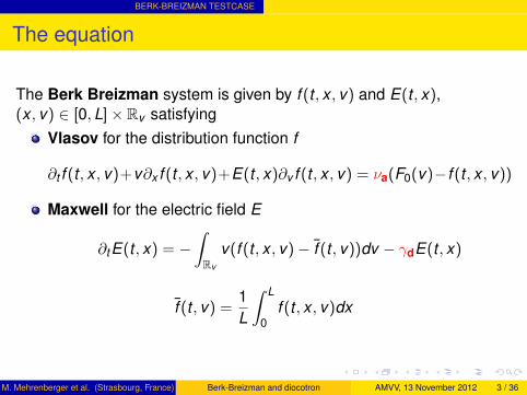
The Berk Breizman system is given by f (t , x , v) and E(t , x),(x , v) ∈ [0,L]× Rv satisfying
Vlasov for the distribution function f
∂t f (t , x , v)+v∂x f (t , x , v)+E(t , x)∂v f (t , x , v) = νa(F0(v)−f (t , x , v))
Maxwell for the electric field E
∂tE(t , x) = −∫Rv
v(f (t , x , v)− f̄ (t , v))dv − γdE(t , x)
f̄ (t , v) =1L
∫ L
0f (t , x , v)dx
M. Mehrenberger et al. (Strasbourg, France) Berk-Breizman and diocotron AMVV, 13 November 2012 3 / 36
BERK-BREIZMAN TESTCASE
Reference and physical context
R. G. L. Vann, Characterization of a fully nonlinear Berk-Breizmanphenomonology, PhD thesis, University of Warwick, 2002.
Classical Vlasov-Poisson system for νa = γd = 0distribution function : addition of source Q(v) and loss (friction)
Q(v)− νaf , Q(v) = νaF0(v)
electric field : addition of dissipative term
−γdE(t , x)
M. Mehrenberger et al. (Strasbourg, France) Berk-Breizman and diocotron AMVV, 13 November 2012 4 / 36
BERK-BREIZMAN TESTCASE
Bump on tail
Initial data :f (0, x , v) = (1 + α cos(kx))F0(v),
with equilibrium distribution function : beam-bulk interaction
F0(v) = Fbulk + Fbeam,
Fbulk =η
vc√
2πexp
(−1
2
(vvc
)2),
Fbeam =1− ηvt√
2πexp
(−1
2
(v − vb
vt
)2),
Physical parameters :vb = 4.5, vc = 1, vt = 0.5, η = 0.9, α = 0.01, L = 4π, k = 2π
L .
M. Mehrenberger et al. (Strasbourg, France) Berk-Breizman and diocotron AMVV, 13 November 2012 5 / 36
BERK-BREIZMAN TESTCASE
Bump on tail : source and loss term
RHS of Vlasov rewrites
νaFbeam − νa(f − Fbulk)
first term : injected beamsecond term : similar to a Krook collision operator
M. Mehrenberger et al. (Strasbourg, France) Berk-Breizman and diocotron AMVV, 13 November 2012 6 / 36
BERK-BREIZMAN TESTCASE
Numerical difficulties
use of Maxwell instead of Poisson
basic schemes can lead to cumulative error in electric fieldsimple framework for testing well-adapted solversvalidity of the schemes can be assessed by comparing withPoisson (case νa = γd = 0)
bump on tail distribution with several vortices (k = 32πL , L = 20π)
already difficult for Vlasov-Poisson (νa = γd = 0)empirical observation of the numerical schemes :
either too diffusive behavioureither bad transition, when the vortices merge
M. Mehrenberger et al. (Strasbourg, France) Berk-Breizman and diocotron AMVV, 13 November 2012 7 / 36
BERK-BREIZMAN TESTCASE
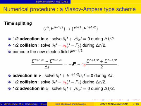
Numerical procedure : a Vlasov-Ampere type scheme
Time splitting(f n,En−1/2)→ (f n+1,En+1/2)
1/2 advection in x : solve ∂t f + v∂x f = 0 during ∆t/2.1/2 collision : solve ∂t f = νa(f − F0) during ∆t/2.compute the new electric field En+1/2
En+1/2 − En−1/2
∆t= −Jn − γd
En+1/2 + En−1/2
2.
advection in v : solve ∂t f + En+1/2∂v f = 0 during ∆t .1/2 collision : solve ∂t f = νa(f − F0) during ∆t/2.1/2 advection in x : solve ∂t f + v∂x f = 0 during ∆t/2.
M. Mehrenberger et al. (Strasbourg, France) Berk-Breizman and diocotron AMVV, 13 November 2012 8 / 36

BERK-BREIZMAN TESTCASE
Reconstruction of the current Jn
Basic reconstruction J0=J_basicVanner (reformulated) reconstruction J2=J_vannerNew reconstruction J1=J_new
The different schemes can be evaluated by comparing withP=Poisson, in the case νa = γd = 0.
M. Mehrenberger et al. (Strasbourg, France) Berk-Breizman and diocotron AMVV, 13 November 2012 9 / 36
BERK-BREIZMAN TESTCASE
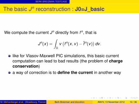
The basic Jn reconstruction : J0=J_basic
We compute the current Jn directly from f n, that is
Jn(x) =
∫R
v(f n(x , v)− f̄ n(v)
)dv .
like for Vlasov-Maxwell PIC simulations, this basic currentcomputation can lead to bad results (the problem of chargeconservation)a way of correction is to define the current in another way
M. Mehrenberger et al. (Strasbourg, France) Berk-Breizman and diocotron AMVV, 13 November 2012 10 / 36
BERK-BREIZMAN TESTCASE
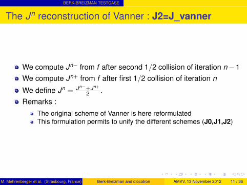
The Jn reconstruction of Vanner : J2=J_vanner
We compute Jn− from f after second 1/2 collision of iteration n−1We compute Jn+ from f after first 1/2 collision of iteration n
We define Jn = Jn−+Jn+
2 .Remarks :
The original scheme of Vanner is here reformulatedThis formulation permits to unify the different schemes (J0,J1,J2)
M. Mehrenberger et al. (Strasbourg, France) Berk-Breizman and diocotron AMVV, 13 November 2012 11 / 36

BERK-BREIZMAN TESTCASE
A new reconstruction J1=J_new
The charge density ρ(t , x) is defined by ρ(t , x) =∫R f (t , x , v)dv .
We compute ρn−1/2 after first 1/2 collision at iteration n − 1We compute ρn+1/2 after first 1/2 collision at iteration n + 1∂xJn is obtained from charge conservation equation
ρn+1/2 − ρn−1/2
∆t+ ∂xJn = νa(1− ρn+1/2 + ρn−1/2
2)
Jn is obtained from ∂xJn and∫ L
0 Jn(x)dx = 0.
M. Mehrenberger et al. (Strasbourg, France) Berk-Breizman and diocotron AMVV, 13 November 2012 12 / 36
BERK-BREIZMAN TESTCASE
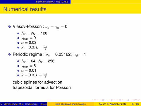
Numerical results
Vlasov-Poisson : νa = γd = 0
Nx = Nv = 128vmax = 9α = 0.03k = 0.3,L = 2π
k
Periodic regime : νa = 0.03162, γd = 1
Nx = 64, Nv = 256vmax = 8α = 0.01k = 0.3,L = 2π
k
cubic splines for advectiontrapezoidal formula for Poisson
M. Mehrenberger et al. (Strasbourg, France) Berk-Breizman and diocotron AMVV, 13 November 2012 13 / 36
BERK-BREIZMAN TESTCASE
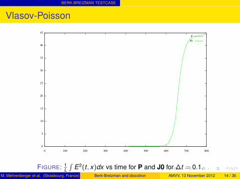
Vlasov-Poisson
FIGURE: 1L
∫E2(t , x)dx vs time for P and J0 for ∆t = 0.1.
M. Mehrenberger et al. (Strasbourg, France) Berk-Breizman and diocotron AMVV, 13 November 2012 14 / 36
BERK-BREIZMAN TESTCASE
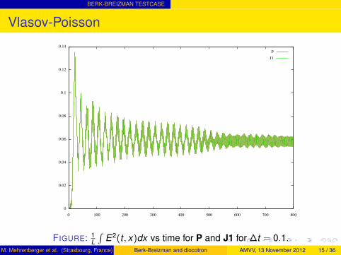
Vlasov-Poisson
FIGURE: 1L
∫E2(t , x)dx vs time for P and J1 for ∆t = 0.1.
M. Mehrenberger et al. (Strasbourg, France) Berk-Breizman and diocotron AMVV, 13 November 2012 15 / 36

BERK-BREIZMAN TESTCASE
Vlasov-Poisson
FIGURE: 1L
∫E2(t , x)dx vs time for P and J2 for ∆t = 0.1.
M. Mehrenberger et al. (Strasbourg, France) Berk-Breizman and diocotron AMVV, 13 November 2012 16 / 36
BERK-BREIZMAN TESTCASE
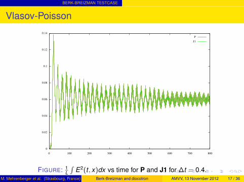
Vlasov-Poisson
FIGURE: 1L
∫E2(t , x)dx vs time for P and J1 for ∆t = 0.4.
M. Mehrenberger et al. (Strasbourg, France) Berk-Breizman and diocotron AMVV, 13 November 2012 17 / 36
BERK-BREIZMAN TESTCASE
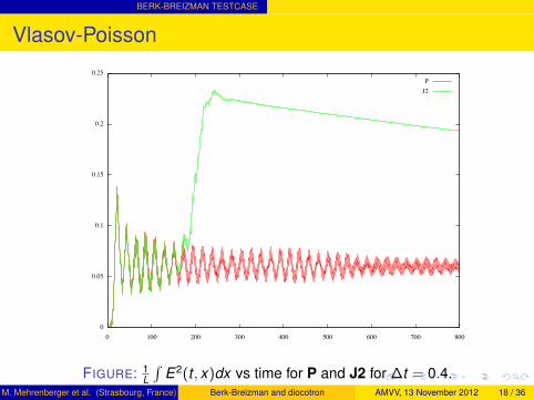
Vlasov-Poisson
FIGURE: 1L
∫E2(t , x)dx vs time for P and J2 for ∆t = 0.4.
M. Mehrenberger et al. (Strasbourg, France) Berk-Breizman and diocotron AMVV, 13 November 2012 18 / 36
BERK-BREIZMAN TESTCASE
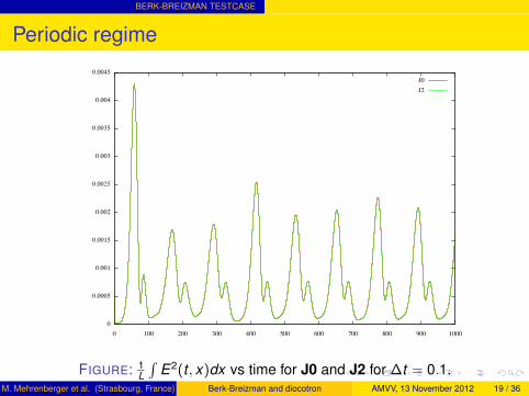
Periodic regime
FIGURE: 1L
∫E2(t , x)dx vs time for J0 and J2 for ∆t = 0.1.
M. Mehrenberger et al. (Strasbourg, France) Berk-Breizman and diocotron AMVV, 13 November 2012 19 / 36

BERK-BREIZMAN TESTCASE
Periodic regime
FIGURE: 1L
∫E2(t , x)dx vs time for J1 and J2 for ∆t = 0.1.
M. Mehrenberger et al. (Strasbourg, France) Berk-Breizman and diocotron AMVV, 13 November 2012 20 / 36
BERK-BREIZMAN TESTCASE
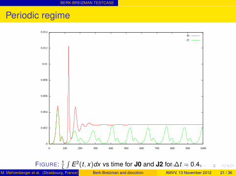
Periodic regime
FIGURE: 1L
∫E2(t , x)dx vs time for J0 and J2 for ∆t = 0.4.
M. Mehrenberger et al. (Strasbourg, France) Berk-Breizman and diocotron AMVV, 13 November 2012 21 / 36
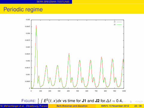
BERK-BREIZMAN TESTCASE
Periodic regime
FIGURE: 1L
∫E2(t , x)dx vs time for J1 and J2 for ∆t = 0.4.
M. Mehrenberger et al. (Strasbourg, France) Berk-Breizman and diocotron AMVV, 13 November 2012 22 / 36
BERK-BREIZMAN TESTCASE
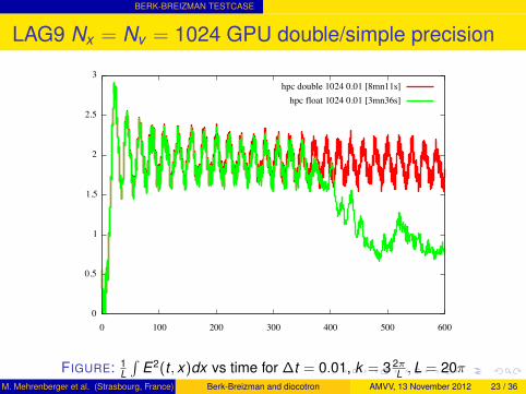
LAG9 Nx = Nv = 1024 GPU double/simple precision
FIGURE: 1L
∫E2(t , x)dx vs time for ∆t = 0.01, k = 3 2π
L ,L = 20πM. Mehrenberger et al. (Strasbourg, France) Berk-Breizman and diocotron AMVV, 13 November 2012 23 / 36

BERK-BREIZMAN TESTCASE
Conclusion/Perspectives
Simple problem for charge conservation issueSimulation of different regimesDesign of a new scheme adapted to this contextDifficulties with several vortices
what can we hope numerically ?
How to extend to higher dimension ?
M. Mehrenberger et al. (Strasbourg, France) Berk-Breizman and diocotron AMVV, 13 November 2012 24 / 36
DIOCOTRON INSTABILITY
Guiding center model in polar coordinates
The transport equation reads
∂tρ−∂θΦ
r∂rρ+
∂r Φ
r∂θρ = 0,
and is coupled with the Poisson equation for the potential Φ = Φ(t , r , θ)
∂2r Φ +
1r∂r Φ +
1r2∂
2θΦ = ρ.
M. Mehrenberger et al. (Strasbourg, France) Berk-Breizman and diocotron AMVV, 13 November 2012 25 / 36
DIOCOTRON INSTABILITY
Features
center guide model generally studied in cartesian geometrysame geometry as in toric gyrokinetic equations for tokamakmodelling, for a poloidal section
⇒ such intermediate testcase was missing, for testing numericalmethods, which include geometrical effects (cf FSL)
astrophysical testcase : diocotron instability (see Petri, Davidson)PIC method done by Petrireferences :
R. C. DAVIDSON, Physics of non neutral plasmas, 1990J. PÉTRI, Non-linear evolution of the diocotron instability in apulsar electrosphere : 2D PIC simulations, Astronomy &Astrophysics, May 7, 2009.
M. Mehrenberger et al. (Strasbourg, France) Berk-Breizman and diocotron AMVV, 13 November 2012 26 / 36
DIOCOTRON INSTABILITY
Work
development of Vlasov semi-Lagrangian method for this testcasestudy of boundary conditions
conservation of electrostatic energy issuelinear stability issues
M. Mehrenberger et al. (Strasbourg, France) Berk-Breizman and diocotron AMVV, 13 November 2012 27 / 36
DIOCOTRON INSTABILITY
Electric energy
Proposition
We define the electric energy
E(t) =
∫ rmax
rmin
∫ 2π
0r |∂r Φ|2 +
1r|∂θΦ|2drdθ.
We have(i)
E(t) =
∫ 2π
0[rΦ∂r Φ]r=rmax
r=rmindθ −
∫ rmax
rmin
∫ 2π
0ρΦrdrdθ.
(ii)
∂tE(t) = 2∫ 2π
0[rΦ∂t∂r Φ]r=rmax
r=rmindθ − 2
∫ 2π
0[Φρ∂θΦ]r=rmax
r=rmindθ.
M. Mehrenberger et al. (Strasbourg, France) Berk-Breizman and diocotron AMVV, 13 November 2012 28 / 36
DIOCOTRON INSTABILITY
BC1 boundary conditions
Proposition
We suppose Dirichlet boundary conditions at rmin and at rmax :
Φ(t , rmin, θ) = Φ(t , rmax, θ) = 0.
Then the electric energy is constant in time :
∂tE(t) = 0.
M. Mehrenberger et al. (Strasbourg, France) Berk-Breizman and diocotron AMVV, 13 November 2012 29 / 36
DIOCOTRON INSTABILITY
BC2 boundary conditions
Proposition
The electric energy is also constant in time if we suppose(i) Dirichlet boundary condition at rmax : Φ(t , rmax, θ) = 0(ii) Inhomogeneous Neumann boundary condition at rmin for the
Fourier mode 0 in θ :∫ 2π
0∂r Φ(t , rmin, θ)dθ = Q,
where Q is a given constant.(iii) Dirichlet boundary condition at rmin for the other modes, which
reads
Φ(t , rmin, θ) =1
2π
∫ 2π
0Φ(t , rmin, θ
′)dθ′
M. Mehrenberger et al. (Strasbourg, France) Berk-Breizman and diocotron AMVV, 13 November 2012 30 / 36
DIOCOTRON INSTABILITY
BC3 boundary conditions
Remark
We do not know whether the electric energy remains in constant intime when we consider the following boundary conditions :
(i) Dirichlet at rmax : Φ(t , rmax, θ) = 0.(ii) Neumann at rmin : Φ(t , rmin, θ) = 0.
M. Mehrenberger et al. (Strasbourg, France) Berk-Breizman and diocotron AMVV, 13 November 2012 31 / 36
DIOCOTRON INSTABILITY
We consider the following initial data
ρ(0, r , θ) =
0, rmin ≤ r < r−,1 + ε cos(`θ), r− ≤ r ≤ r+,0, r+ < r ≤ rmax,
where ε is a small parameter.The linear analysis is performed in Davidson, 1990
BC2 are consideredFormulae for instability growth rate are explicitFormulae for BC1 can be derived from BC2 with good choice of QFormulae can be adapted for BC3Values between BC2 and BC3 are very closenumerical treatment of dispersion relation also studied withapproximate growth rate
M. Mehrenberger et al. (Strasbourg, France) Berk-Breizman and diocotron AMVV, 13 November 2012 32 / 36

DIOCOTRON INSTABILITY
Numerical results
Linear growth rate observed for corresponding Fourier modeModes visible on distribution function plots, as in PIC simulationEh(t)− Eh(0) can increase or decrease with same growth rate
For PIC (Petri), Eh(t)− Eh(0) increase with same growth rateContinous model conserves the electric energy for BC1 and BC2
BC2 and BC3 simulations are near, particularly in the linear phasestructures can merge in the non linear phase
M. Mehrenberger et al. (Strasbourg, France) Berk-Breizman and diocotron AMVV, 13 November 2012 33 / 36
DIOCOTRON INSTABILITY
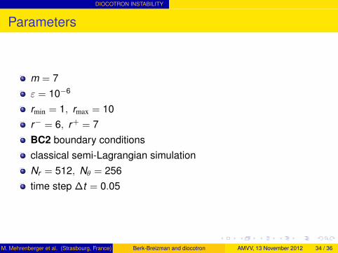
Parameters
m = 7ε = 10−6
rmin = 1, rmax = 10r− = 6, r+ = 7BC2 boundary conditionsclassical semi-Lagrangian simulationNr = 512, Nθ = 256time step ∆t = 0.05
M. Mehrenberger et al. (Strasbourg, France) Berk-Breizman and diocotron AMVV, 13 November 2012 34 / 36
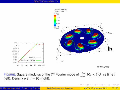
DIOCOTRON INSTABILITY
FIGURE: Square modulus of the 7th Fourier mode of∫ rmax
rminΦ(t , r , θ)dr vs time t
(left). Density ρ at t = 95 (right).
M. Mehrenberger et al. (Strasbourg, France) Berk-Breizman and diocotron AMVV, 13 November 2012 35 / 36
DIOCOTRON INSTABILITY
Conclusion/Perspectives
validation of testcase for a grid based solverspecial boundary conditions treatment ; highlighting of BC2future use of this testcase, for testing numerical methods
2D conservative remapping (P. Glanc)curvilinear grids (A. Hamiaz)gyroaverage operator (C. Steiner)
M. Mehrenberger et al. (Strasbourg, France) Berk-Breizman and diocotron AMVV, 13 November 2012 36 / 36