
Bara Kominkova Master Thesis
90
University of Pardubice Faculty of Chemical Technology Department of Graphic Arts and Photophysics Gjøvik University College Faculty of Computer Science and Media Technology COMPARISON OF TWO EYE TRACKING DEVICES USED ON PRINTED IMAGES Master Thesis Author: Bc. Barbora Komínková Supervisor: prof. Jon Yngve Hardeberg, prof. RNDr. Marie Kaplanová, CSc. 2008
Transcript of Bara Kominkova Master Thesis
8/12/2019 Bara Kominkova Master Thesis
http://slidepdf.com/reader/full/bara-kominkova-master-thesis 1/90
University of PardubiceFaculty of Chemical Technology
Department of Graphic Arts and Photophysics
Gjøvik University CollegeFaculty of Computer Science and Media Technology
COMPARISON OF TWO EYE TRACKINGDEVICES USED ON PRINTED IMAGES
Master Thesis
Author: Bc. Barbora Komínková
Supervisor: prof. Jon Yngve Hardeberg,prof. RNDr. Marie Kaplanová, CSc.
2008
8/12/2019 Bara Kominkova Master Thesis
http://slidepdf.com/reader/full/bara-kominkova-master-thesis 2/90
Univerzita PardubiceFakulta Chemicko-technologická
Katedra polygrafie a fotofyziky
Vysoká škola v GjøvikuFakulta informatiky a mediálních technologií
POROVNÁNÍ „EYE TRACKING“ ZAŘ ÍZENÍPOUŽITÉ NA TIŠTĚNÉ OBRAZY
Diplomová práce
Autor: Bc. Barbora Komínková
Vedoucí práce: prof. Jon Yngve Hardeberg,prof. RNDr. Marie Kaplanová, CSc.
2008

8/12/2019 Bara Kominkova Master Thesis
http://slidepdf.com/reader/full/bara-kominkova-master-thesis 3/90
Original Submission (Zadání)

8/12/2019 Bara Kominkova Master Thesis
http://slidepdf.com/reader/full/bara-kominkova-master-thesis 4/90

8/12/2019 Bara Kominkova Master Thesis
http://slidepdf.com/reader/full/bara-kominkova-master-thesis 5/90
Acknowledgments
I would like to thank to my supervisor Marie Kaplanova, who informed me
about the exchange program in abroad and accepted this project made in Norway.
Then I would like to thank the Socrates/Erasmus Exchange Program and Financial
Mechanism EHP/Norway for the opportunity to study at the Gjøvik University
College and the financial support I was provided while studying there.
Thanks belong to my supervisor Jon Yngve Hardeberg and to colleague
Marius Pedersen in procreative discussions, recommendations and constructive
criticism, to Faouzi Alaya Cheikh for the help with stabilization of the video, to
Damien Lefloch for the processing of the algorithm in the transformation of theimages.
Big thanks to Jon Yngve Hardeberg and HiG for allowing me to present
parts of this work at Electronic Imaging 2008, San Jose, CA, USA.
8/12/2019 Bara Kominkova Master Thesis
http://slidepdf.com/reader/full/bara-kominkova-master-thesis 6/90
Summary
Eye tracking as a quantitative method for collecting eye movement data,
requires the accurate knowledge of the eye position, where eye movements can
provide indirect evidence about what the subject see. In this study two eye tracking
devices have been compared, a Head-mounted Eye Tracking Device (HED) and a
Remote Eye Tracking Device (RED). The precision of both devices has been
evaluated, in terms of gaze position accuracy and stability of the calibration. For
the HED it has been investigated how to register data to real-world coordinates.
This is needed since coordinates collected by the HED eye tracker are relative to
the position of the subject’s head and not relative to the actual stimuli as it is thecase for the RED device. Results show that the precision gets worse with time for
both eye tracking devices. The precision of RED is better than the HED and the
difference between them is around 7 – 14 px, it is approximately 2.44 – 4.89 mm.
The distribution of gaze positions for HED and RED devices was expressed by a
percentage distribution of the points of regard in areas defined by the viewing
angle. For the HED the gaze position accuracy has been 95 – 99% at 2.5 – 3°
viewing angle and for the RED it has been 95 – 99% at 2 – 3° viewing angle. The
stability of the calibration was investigated at the end of the experiment and the
obtained result was not statistically significant. But the distribution of the gaze
position is larger at the end of the experiment than at the beginning.
Keywords: Eye tracking, precision, gaze position, stability of calibration.
8/12/2019 Bara Kominkova Master Thesis
http://slidepdf.com/reader/full/bara-kominkova-master-thesis 7/90
Souhrn
„Eye tracking“, jako kvantitativní metoda pro shromáždění dat očního
pohybu, požaduje př esné znalosti o pozici oka, kde oční pohyby mohou
poskytnout nepř ímý důkaz o tom, jak pozorovatel vidí. V této studii byly
porovnány dvě „eye tracking“ zař ízení, Head-mounted Eye tracking Device (HED)
a Remote Eye tracking Device (RED). Pro obě zař ízení byla vyhodnocena jejich
př esnost z hlediska př esné pozice pohledu a stability kalibrace. Jelikož souř adnice
shromážděné HED zař ízením jsou vztažené k pozici hlavě pozorovatele a ne
k aktuálnímu podmětu jak je v př ípadě RED zař ízení, muselo být vyšetř eno jak
zaznamenat skutečná data pro HED zař ízení. Výsledky ukázali, že př esnosts odstupem času byla horší pro obě zař ízení. Kdežto př esnost RED zař ízení je lepší
než HED zař ízení a rozdíl mezi nimi je v rozmezí 7 – 14 px (2.44 – 4.89 mm).
Distribuce pozic pohledů pro HED a RED zař ízení byla vyjádř ena procentuální
reprezentací bodů pohledů (tzv. point of regard) v oblasti definované pozorovacím
úhlem. Pro HED př esnost upř eného pohledu je 95 – 99% v pozorovacím úhlu
2.5 – 3° a pro RED je př esnost upř eného pohledu je 95 – 99% v pozorovacím úhlu
2 – 3°. Na konci experimentu byla vyšetř ena stabilita kalibrace, ale výsledek nebyl
statisticky významný. Distribuce pohledové pozice je větší na konci experimentu
než na jeho začátku.
Klí čová slova: Eye tracking, př esnost, pozice upř eného pohledu, stabilitakalibrace.
8/12/2019 Bara Kominkova Master Thesis
http://slidepdf.com/reader/full/bara-kominkova-master-thesis 8/90
Content
1. Introduction ..................................................................................................... 10
1.1 Background ................................................................................................ 101.2 Aim ............................................................................................................. 12
2. Theoretical part ............................................................................................... 142.1 Visual perception ........................................................................................ 14
2.2 Eye movements .......................................................................................... 15
2.3 Eye tracking ................................................................................................ 16
2.4 Eye tracking technology ............................................................................. 16
2.4.1 Pupil eye tracking system ............................................................... 17
2.4.2 Corneal reflection ........................................................................... 19
2.5 Head movements ........................................................................................ 192.6 Principle of operation of eye tracking devices ........................................... 20
2.7 Output and visualization of data ................................................................. 21
3. Experimental part ........................................................................................... 233.1 Experimental equipment ......................................................................... 23
3.1.1 iView X system .............................................................................. 23
3.1.1.1 User interface ................................................................... 23
3.1.1.2 External interface ............................................................. 25
3.1.1.3 Analysis software ............................................................. 25
3.1.1.4 BeGaze analysis software ................................................. 253.1.2 iView X hardware equipment ......................................................... 27
3.1.2.1 Remote Eye tracking Device (RED) ................................ 28
3.1.2.2 Head-mounted Eye tracking Device (HED) ..................... 29
3.2 Experiment setup and methodology ....................................................... 303.2.1 Experiment setup ............................................................................ 30
3.2.2 Viewing and light conditions.......................................................... 30
3.2.3 Implementation of images .............................................................. 32
3.2.4 Sequence and signification of images ............................................ 33
3.2.5 Placement of images ....................................................................... 343.2.6 Direction of watching track on the image ...................................... 34
3.2.7 Dominant eye.................................................................................. 35
3.2.8 Calibration ...................................................................................... 36
3.2.8.1 RED calibration ................................................................ 36
3.2.8.2 HED calibration ................................................................ 38
3.2.9 Instructions ..................................................................................... 38
3.2.9.1 Instructions before the experiment ................................... 38
3.2.9.2 Instructions during the experiment ................................... 39
8/12/2019 Bara Kominkova Master Thesis
http://slidepdf.com/reader/full/bara-kominkova-master-thesis 9/90
3.2.9.3 Questionnaire ................................................................... 39
3.2.10 Data processing .............................................................................. 40
3.2.11 Real-world coordinate .................................................................... 403.3 Experiment results ................................................................................... 443.3.1 Evaluation and statistical analysis the three images A ................... 45
3.3.2 Evaluation and statistical analysis of second image B ................... 51
3.3.3 Evaluation and statistical analysis of third image C ....................... 59
3.3.4 Evaluation and statistical analysis of fourth image D .................... 61
3.3.5 Questionnaires ................................................................................ 68
3.3.6 Disturbing elements ........................................................................ 69
4. Conclusion ........................................................................................................ 71
References ........................................................................................................ 73List of Figures .................................................................................................. 76List of Tables .................................................................................................... 78
Appendix A: Questionnaire
Appendix B: M edian distances for image A; RED and HED
Appendix C: Distance between median and center point of the cross for
image B; RED and HED
Appendix D: M edian distances for image C; RED and HED
Appendix E: Median distances for image D; RED and HED
8/12/2019 Bara Kominkova Master Thesis
http://slidepdf.com/reader/full/bara-kominkova-master-thesis 10/90
10
1 Introduction
1.1 BackgroundEye tracking is a technique used in different field such as vision,
cognitive science, psychology, human-computer interaction, marketing
research and medical research to provide useful information. Specific areas
include web usability [1, 2, 3], advertising [4], reading studies [5], and
evaluation of image quality [6, 7, 8, 9] and this all could be include to the
initiatory questions how do we look at image [10, 8].
Eye tracking as a quantitative method for collecting eye movement data,requires the accurate knowledge of the eye position, where eye movements can
provide indirect evidence about what the subject look at. To perform these kind
of studies with valid data a precise eye tracker is needed.
In the printing industry it is very important to know how look soft
proofs and hard proof designed for customers, as the control before the print in
order to get the highest possible quality of the print. Therefore it is very
important to have image quality on a such level, which can be invariable
throughout whole processing of print and customers will be still satisfied.
Image quality evaluation plays an important role in the design of many
products, including imaging peripherals such as digital cameras, scanners,
printers and displays. Joyce E. Farrell [12] describes some engineering tools
such as device simulation, subjective evaluation and distortion metrics that help
to evaluate how customers perceive the image quality of different products.
For understanding of devices, predict their output and optimize their designwere used software simulators for image capture devices (scanners, digital
cameras), and rendering devices (displays, printers, to determine how
adjustments in device parameters affect subject impressions of image quality.
Since customers are the final arbiter of image quality, we consider their
subjective image quality judgements to be the key to the success of imaging
products.
8/12/2019 Bara Kominkova Master Thesis
http://slidepdf.com/reader/full/bara-kominkova-master-thesis 11/90
11
Many methods to reproduce images are made, and the need to quantify
how reproduced images have been changed by the reproduction process and
how much of these change are perceived by the human eye become more
important.
Image difference metrics try to predict the perceived image difference,
but they do not work very well[8]. For predicting perceived image quality
psychological experiments are mostly used. Recently studies of eye movements
get more importance and its application to evaluation of image quality in
several studies by using an eye tracker device[8, 11].
Accurate knowledge of the eye position is often desired, not only in
research on the oculomotor system itself but also in many experiments
concerning visual perception, where eye movements can provide indirect
evidence about what the subject sees [13]. Research works are focused on the
accuracy of the image of the eye pupil, because the accuracy of gaze tracking
greatly depends upon the resolution of the eye images. The detection of pupil
center in the image of the eye is the most important step for video-based eye
tracking method [14]. If good accuracy is required, there is a method that uses
edges and local patterns to obtain detection of eye features with subpixel
precision. This algorithm can robustly detect the inner eye corner and the
center of an iris with subpixel accuracy [15].
Different light conditions are also considerably influencing the eye
tracking methods. The high contrast between the pupils and the rest of the face
can significantly improve the eye tracking robustness and accuracy [16]. Very
small pupil sizes make it difficult for the eye tracking system to model thepupil center. It depends on the brightness and size of the pupils; therefore light
conditions are required to be relatively stable and the subjects close to the
camera.
8/12/2019 Bara Kominkova Master Thesis
http://slidepdf.com/reader/full/bara-kominkova-master-thesis 12/90
12
1.2 Aim
The main question was, if the Head-mounted Eye Tracking Device
(HED) can be used on printed images as the Remote Eye Tracking Device
(RED) is used in some cases.
The aim of the work presented in this thesis is to compare eye tracking
devices used on printed images. From the literature review we have identified
prior work that compares three different eye tracking devices in psychology of
programming experiment. Nevalainen and Sajaniemi [17] studied the ease of
use and accuracy of the three devices by having observers examine shortcomputer programs using a program animator. The results showed that there
were significant differences in accuracy and ease of use between the devices.
As it is known, the head-mounted systems (HED) are effective for
studies which require the head to move freely. On the other hand, with RED
systems the observer has to keep the same position and avoid large movements
most of the time. Head-mounted systems, within traditional usability testing, is
useful for paper prototype studies or out-of-the-box studies, and also typically
used in studies, where head or body movement is required of users (automobile
drivers, airplane pilots or even athletes practicing). This project investigates if
the HED can be used on printed images as the RED is used in some cases. One
of the advantages is that the observer has larger possibility of freedom than the
RED.
In case of HED, data analysis is performed on data collected by a video
camera. The problem is how to register data from HED to real-world
coordinates. The system creates a superimposed image of a dot representing the
participant’s point of regard (exactly where they are looking), laid over the top
of the image of their field of vision [18]. The coordinates collected by the eye
tracker are thus relative to the position of the subject’s head and not relative to
the actual stimuli as in the remote eye tracking case [19]. Hence, this method
requires not only analysis of the coordinates generated by the eye tracker but
also analysis of the recorded video.

8/12/2019 Bara Kominkova Master Thesis
http://slidepdf.com/reader/full/bara-kominkova-master-thesis 13/90
13
In order to investigate advantages and disadvantages of both eye
tracking devices, an experiment has been designed and carried out mainly for
determining the precision of both devices in different directions (precision in
the time aspect, precision on the edges of the image, etc.). Other data obtained
from the experiment were a percentage representation of the fixation point of
the eye in certain areas (circles), which matches different viewing angles and
data indicate a stability of the calibration.
8/12/2019 Bara Kominkova Master Thesis
http://slidepdf.com/reader/full/bara-kominkova-master-thesis 14/90
14
2 Theoretical part
2.1 Visual perception
Eye tracking studies have been performed for many years, with many
different purposes. Once of the main goals of such studies has been understanding
the human visual system and the visual process itself.
Visual perception is the ability to interpret information from visible light
and the result perception is known as vision. Visual system is a part of the nervous
system which allows organisms to see.
The eye as a biological device can be comparable with a camera device,
that are similarly working. Light entering the eye is reflected when it passes
through the corneas, subsequently through the pupil and further refracted by the
lens. The cornea and lens together project an inverted image onto the retina. The
retina is composed of two types of sensors called rods and cones. The cones occur
where the visual axis intersects the retina. This place is called a fovea. The rods
are mainly in the periphery of the retina where outnumber the cones. The sensors
are differently sensitive on the different level of the luminance. The observationwhile low luminance level is mediated by the rods and while high luminance level
by the cones. The high luminance level effectively saturates the rods so that only
the cone photoreceptors are functioning and conversely [10,20]. The retina is
actually a part of the brain and each cone photoreceptor in the fovea (whereon the
light is focused by the lens) reports information to the visual cortex of the brain.
The detailed spatial information from the scene is gained through the high-
resolution fovea.
Oculomotor system as the study about eyes in motion allows us to orient
our eye to areas of interest very rapidly with little effort. But most of us are
unaware that spatial acuity is not uniform across the visual field [20].
8/12/2019 Bara Kominkova Master Thesis
http://slidepdf.com/reader/full/bara-kominkova-master-thesis 15/90
15
2.2 Eye movements
Common types of eye movements (at a macro-level) which can be describe
during static scene perception are in the form of saccades and fixation. On
average, humans execute well over 100 000 eye movements each day [21].
To re-orient the fovea to other locations, the eyes make angular rotations.
These angular rotation called saccades are rapid eye movements where the eye
makes a series of sudden jumping from point to point between fixations in the
stimulus. The saccade is the fastest movement with high acceleration and
deceleration rates. In general the eye movements make approximately 3-4 saccadic
eye movements per second [22].More typically a saccade is followed by a fixation. A fixation is when the
eye is looking at the same spot for a longer period of time and may consist of a
number of view positions. If there are more than 5 view positions in a circle with a
radius of 7 mm we count them as 1 fixation [23]. Even during fixation, the eyes
are not completely still, but are making continual small movements, generally
within a one-degree radius [24]. These micro-fixation movements are composed of
three components: slow drift, rapid, small-amplitude tremor, and micro-saccades.
The micro-saccade can be described as a tiny saccade jump, brings the gaze back
when the drift has moved it too far from the particular point in the image [25].
The saccades can cover a range from about 2-10 degrees of visual angle,
and the duration of the saccades are completed in about 25-100 ms [26]. Fixation
time is dependent on the amount and quality of the visual information in the scene
[27]. The fixation must have a minimum duration of 200 ms (a typical fixation
range is 200-600 ms). The velocity of saccadic eye movements show two
distributions of rotational velocities: low velocities for fixations (i.e., < 100
deg/sec), and high velocities for saccades (i.e., > 300 deg/sec) [28].
When the observer and/or the scene is in motion, other mechanisms are
necessary to stabilize the retinal image. Eye movement which can be tracked in
this case is smooth pursuit. These eye movements are much slower than a saccade
(1-30 deg/sec).
8/12/2019 Bara Kominkova Master Thesis
http://slidepdf.com/reader/full/bara-kominkova-master-thesis 16/90
16
Simply, eye movements are traditionally divided into a number of
subcategories. These include fixation eye movements, gaze-holding eye
movements such as vestibular and optokinetic eye movements, and gaze-shifting
movements such as saccades, pursuits, and vergence eye movements. Gaze is the
combination of head and eye movements to position the fovea [22].
2.3 Eye tracking
Eye tracking is the process of measuring either the point of gaze or the
motion of an eye relative to the head. Collected data such as eye positions and eye
movement can be statistically analyzed to determine the pattern and duration ofeye fixations and the sequence of scan paths as an user visually moves through a
page or screen.
2.4 Eye tracking technology
There are many different ways of determining eye fixation durations and
frequencies for various point of regard requires both periodically sensing and
recording the direction of gaze, and processing the gaze data to compute fixationstatistic. Video based eye tracking systems which use a video camera to track the
eye movement by measuring the movement of an infrared light reflecting off the
eye, can be divided into two categories: head-mounted eye tracking technology
and remote eye tracking technology.
“Pupil-centre/corneal-reflection” eye tracking systems are probably the
most effective and the most commonly used method. Others variants of eye
tracking systems that make use of equipment are for instance, skin electrode or
marked contact lenses [24, 29], electro-oculography (EOG), limbus tracking,
direct vision, mirror-based systems.
In direct vision system a fixed video camera is mounted on the hood of the
car facing the driver and the image of the driver´s face is recorded on videotape.
Electro-Oculography (EOG) method, for instance, involves measuring electric
8/12/2019 Bara Kominkova Master Thesis
http://slidepdf.com/reader/full/bara-kominkova-master-thesis 17/90
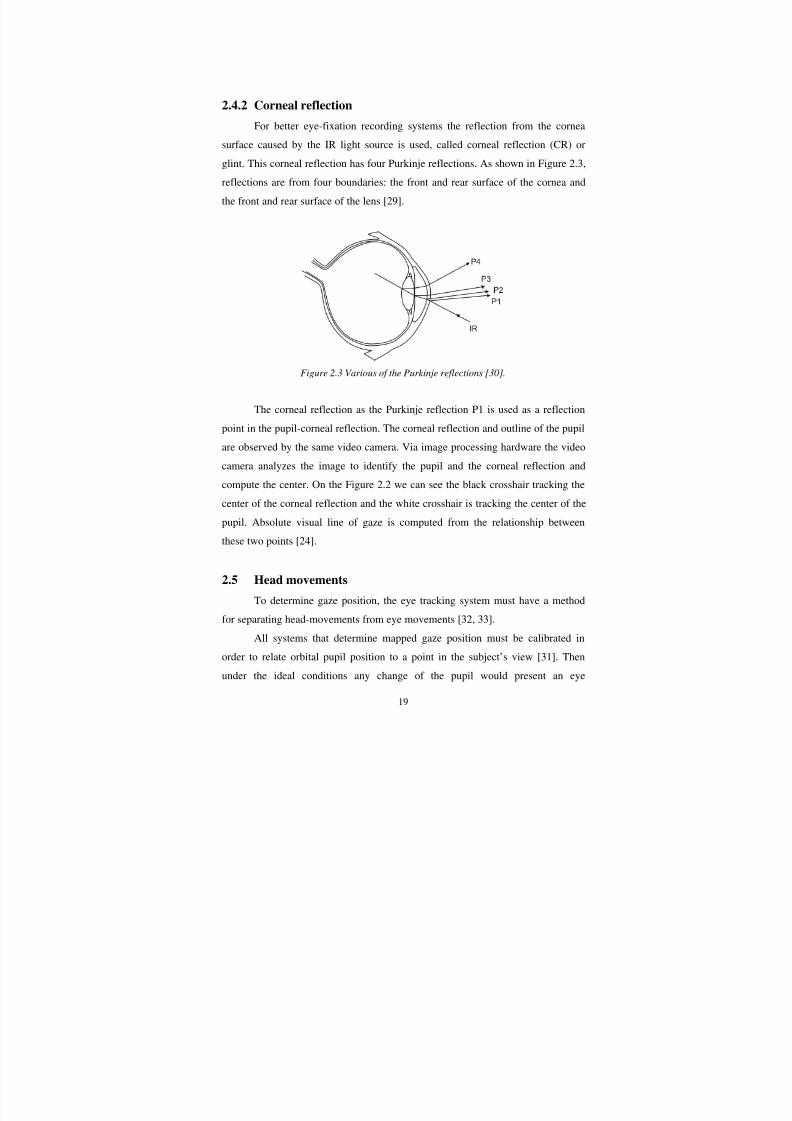
17
potential differences between locations on different side of the eye. Brief
description of this method, Paul Green describes in his work [30].
Practical eye tracking methods are based on a non-contacting camera that
observes the eyeball plus image processing techniques to interpret the picture. The
limbus and pupil tracking systems are one of these methods [30, 24, 29]. The
limbus or boundary between the iris and sclera is due to the contrast of these two
regions easily tracked horizontally. In vertical direction it has low accuracy,
because the eyelids are covering part of the iris.
2.4.1 Pupil tracking systemsPupil tracking techniques have better accuracy than limbus tracking
system, but pupils are harder to detect and track [29]. The retina is highly
reflective and not sensitive in the near infrared wavelengths around 880 nm, which
is invisible for the human eye and can be detected by most commercial cameras.
Hence the IR light is used as the light source with IR sensitive camera. There are
two ways of imaging the pupil: bright pupil and dark pupil system.
Bright pupil
In case of the bright pupil system, the IR light source should be placed near
to the subject’s line of sight (optical axis of the camera) and by including a beam
splitter in the optics, the pupil will appear bright. The camera now is able to see
the movement of the light reflected from the back of the eye and using a calibrated
algorithm, the systems can translate these movements to gaze position. For this
system some external head-tracking method is needed or the head must be
immobilized [31]. For example Jason Babcock is using the bright pupil system
with head-mounted technology [20].
Dark pupil
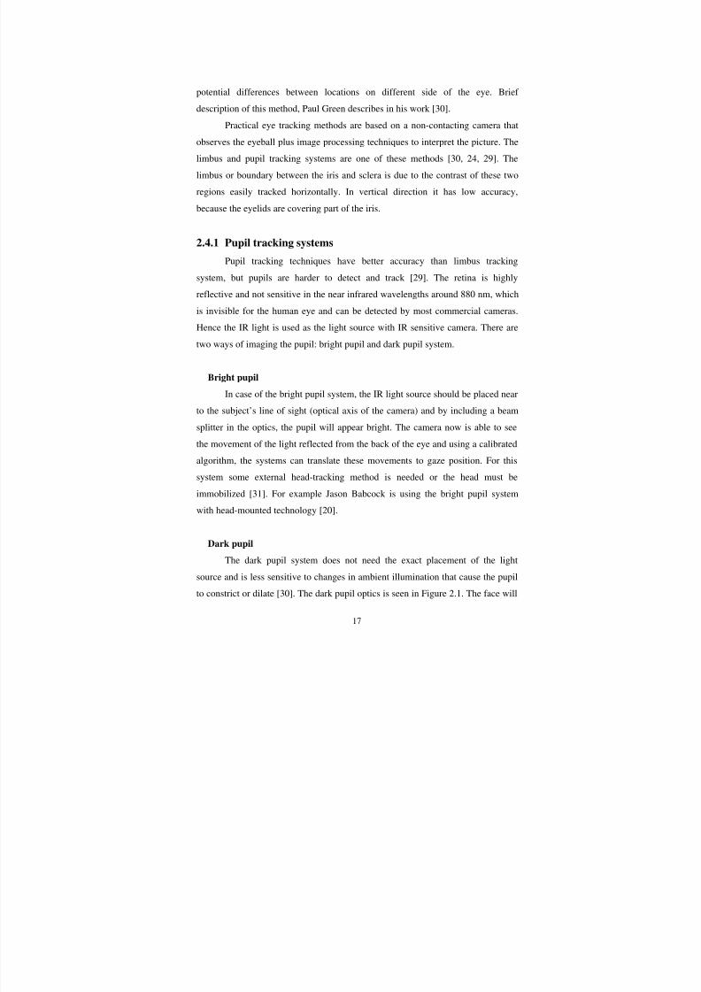
The dark pupil system does not need the exact placement of the light
source and is less sensitive to changes in ambient illumination that cause the pupil
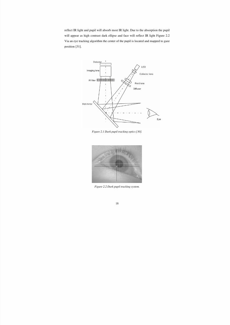
to constrict or dilate [30]. The dark pupil optics is seen in Figure 2.1. The face will
8/12/2019 Bara Kominkova Master Thesis
http://slidepdf.com/reader/full/bara-kominkova-master-thesis 18/90
18
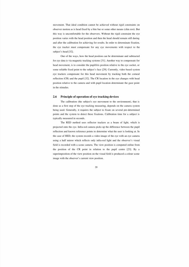
reflect IR light and pupil will absorb most IR light. Due to the absorption the pupil
will appear as high contrast dark ellipse and face will reflect IR light Figure 2.2
Via an eye tracking algorithm the center of the pupil is located and mapped to gaze
position [31].
Figure 2.1 Dark pupil tracking optics [30].
Figure 2.2 Dark pupil tracking system.
8/12/2019 Bara Kominkova Master Thesis
http://slidepdf.com/reader/full/bara-kominkova-master-thesis 19/90
8/12/2019 Bara Kominkova Master Thesis
http://slidepdf.com/reader/full/bara-kominkova-master-thesis 20/90
20
movement. That ideal condition cannot be achieved without rigid constraints on
observer motion as is head fixed by a bite bar or some other means (chin rest). But
this way is uncomfortable for the observers. Without the rigid constraint the eye
position varies with the head position and then the head should remain still during
and after the calibration for achieving for results. In order to determinate fixation,
the eye tracker must compensate for any eye movements with respect to the
subject’s head [32].
One of the ways, how the head position can be determinate and subtracted
for eye data is via magnetic tracking systems [31]. Another way to compensate for
head movement, is to consider the pupil/iris position relative to the eye socket, orsome reliable fixed point to the subject’s face [29]. Currently, video based system
eye trackers compensate for this head movement by tracking both the corneal
reflection (CR) and the pupil [32]. The CR location in the eye changes with head
position relative to the camera and with pupil location determinate the gaze point
in the stimulus.
2.6 Principle of operation of eye tracking devices
The calibration (the subject's eye movement to the environment), that is
done as a first step of the eye tracking measuring, depends on the camera system
being used. Generally, it requires the subject to fixate on several pre-determined
points and the system to detect these fixations. Calibration time for a subject is
typically measured in seconds.
The RED method uses reflector trackers as a beam of light, which is
projected onto the eye. Infra-red camera picks up the difference between the pupil
reflection and known reference points to determine what the user is looking at. Inthe case of HED, the system records a video image of the eye with an eye camera
using a half mirror which reflects only infra-red light and the observer’s visual
field is recorded with a scene camera. The view position is computed online from
the position of the CR point in relation to the pupil centre [23]. By a
superimposition of the view position on the visual field is produced a colour scene
image with the observer’s current view position.
8/12/2019 Bara Kominkova Master Thesis
http://slidepdf.com/reader/full/bara-kominkova-master-thesis 21/90

8/12/2019 Bara Kominkova Master Thesis
http://slidepdf.com/reader/full/bara-kominkova-master-thesis 22/90
8/12/2019 Bara Kominkova Master Thesis
http://slidepdf.com/reader/full/bara-kominkova-master-thesis 23/90
23
3. Experimental part
3.1 Experimental equipment
3.1.1 iView X system
The iView X system is an advanced video-based eye tracking system that
combines flexibility design with easy setup and operation, reliable data recording,
and efficient analysis for eye tracking research. All required components for
efficient high-quality eye movement and scene video recordings are combined into
a high-performance PC Workstation. Real-time image processing, calibration,
auxiliary device I/O, stimulus-software interface, as well as data and video
recording are all combined into one easy-to-use application.
The iView X system is designed for eye tracking studies in a number of
fields ranging from psychology/neuroscience to human factors, to usability and
marketing. Interfaces are available for remote and head-mounted eye tracking as
well as more complex application like fMRI (functional Magnetic Resonance
Imaging). [34]
3.1.1.1 User interface
The user interface includes parallel, live video displays of the eye and
scene video with online data plots and all required user controls [34].
The workspace in the software is similar for both eye tracking devices with
only small alternations. The workspace presents several windows (tools) of
functions which are necessary for eye tracking recording Figure 3.4.
8/12/2019 Bara Kominkova Master Thesis
http://slidepdf.com/reader/full/bara-kominkova-master-thesis 24/90
24
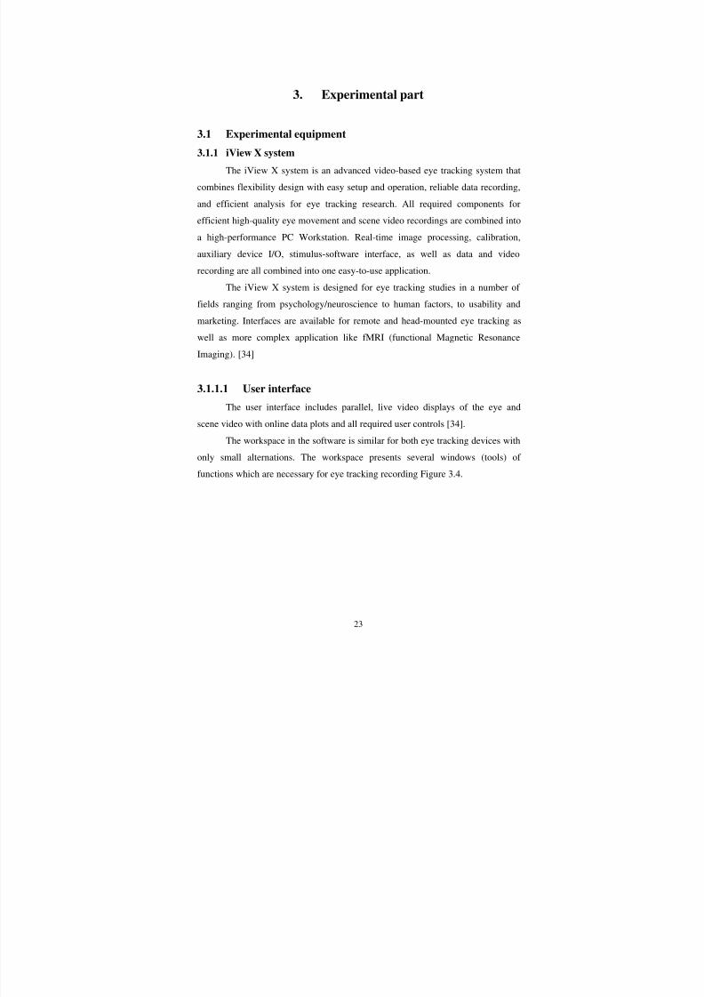
Figure 3.4 Workspace of the iView X system.
In the window bitmap view or scene video we can open different
calibration planes, predefined or created by the researcher. After the calibration,
this plane can be change for bitmap image, where the observer is looking, orchange for the scene video used usually in case of the HED. The bitmap or the
scene video is overlaid by targets, gaze cursors or other informations (i.e. time,
logo).
The window eye camera video represents eye image with two crosshairs.
One crosshair is for the pupil and one for the corneal reflex as was mentioned
above. In this window we can easily see the detection of the eye. Eye tracking
parameters are helpful for the detection of the eye. After the detection of a “good”
eye ,it is saved and the camera position will be a default. If the eye image is lost,
the camera will return to this default position in order to find it.
Recording, dividing data to several different sets and saving of the data or
video is done easy in the panel recording control. Actual date seen during the
recording we can see in the window online data.
Toolbar
Eye camera video
Recording control
Bitmap view or scene video
Eye tracker parameters
System log Online data
8/12/2019 Bara Kominkova Master Thesis
http://slidepdf.com/reader/full/bara-kominkova-master-thesis 25/90
25
3.1.1.2 External Interfaces
iView X offers communication interfaces for
- Visual stimuli (direct or via 3rd party software).
- Ingoing or outgoing external synchronization.
- 16 digital input channels, which can be assigned to system functions or
synchronization events.
- 16 digital output lines which can be used to output fixation in areas or system
status information.
- Online eye movement data access via high speed serial interface during the
experiment.- External control the recording process via serial interface.[34]
3.1.1.3 Analysis Software
The standard iView X package provides interactive analysis functions for
image-based stimuli. All analysis options are based on user-adjustable parameters
that allow individual adaptation to the application. Objects (i.e. areas of interest)
can either be defined with the integrated object editor or can be detached from aloaded bitmap file. Recorded data and results are available for further post
processing (ASCII data export). Analysis graphics can be saved, printed in high
quality, or exported for documentation purposes.
iView X analysis software provides support for area of interest analysis
(overlapping objects and non-overlapping objects defined by a 256 color bitmap
file), fixation analysis (shows a viewing path or linked fixations over visual
stimulus and displays location and length of fixations over live video or still
image) and statistical analysis (absolute and relative duration of fixations). [34]
3.1.1.4 BeGaze analysis software
SMI (Sensomotoric Instruments) presents the BeGaze analysis software
which allows complete data processing from loading of data to print diagrams or
export results as text tables for further processing. BeGaze is working with
8/12/2019 Bara Kominkova Master Thesis
http://slidepdf.com/reader/full/bara-kominkova-master-thesis 26/90
8/12/2019 Bara Kominkova Master Thesis
http://slidepdf.com/reader/full/bara-kominkova-master-thesis 27/90
27
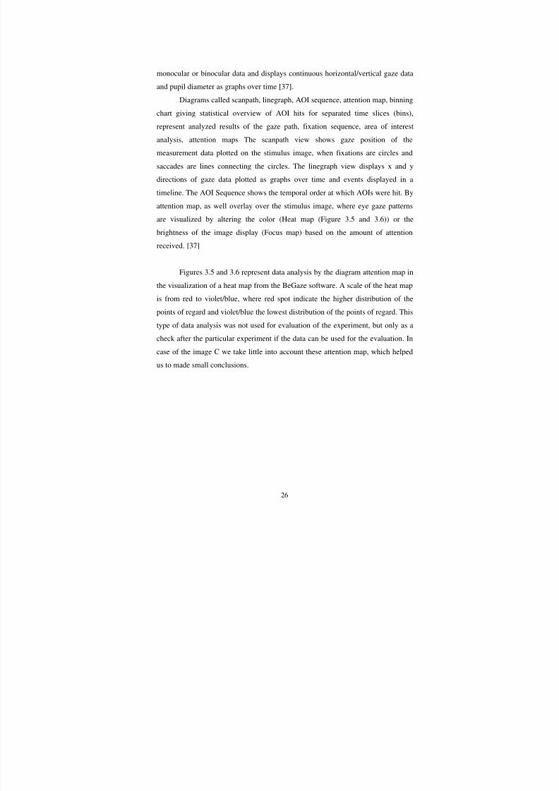
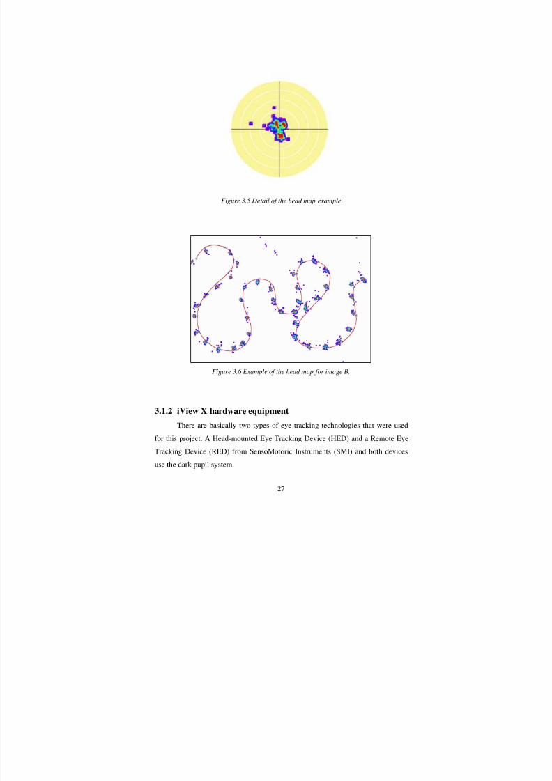
Figure 3.5 Detail of the head map example
Figure 3.6 Example of the head map for image B.
3.1.2 iView X hardware equipment
There are basically two types of eye-tracking technologies that were used
for this project. A Head-mounted Eye Tracking Device (HED) and a Remote Eye
Tracking Device (RED) from SensoMotoric Instruments (SMI) and both devices
use the dark pupil system.
8/12/2019 Bara Kominkova Master Thesis
http://slidepdf.com/reader/full/bara-kominkova-master-thesis 28/90
28
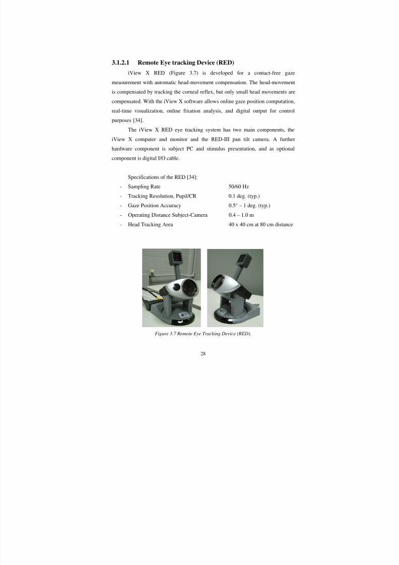
3.1.2.1 Remote Eye tracking Device (RED)
iView X RED (Figure 3.7) is developed for a contact-free gaze
measurement with automatic head-movement compensation. The head-movement
is compensated by tracking the corneal reflex, but only small head movements are
compensated. With the iView X software allows online gaze position computation,
real-time visualization, online fixation analysis, and digital output for control
purposes [34].
The iView X RED eye tracking system has two main components, the
iView X computer and monitor and the RED-III pan tilt camera. A furtherhardware component is subject PC and stimulus presentation, and as optional
component is digital I/O cable.
Specifications of the RED [34]:
- Sampling Rate 50/60 Hz
- Tracking Resolution, Pupil/CR 0.1 deg. (typ.)
- Gaze Position Accuracy 0.5° – 1 deg. (typ.)
- Operating Distance Subject-Camera 0.4 – 1.0 m
- Head Tracking Area 40 x 40 cm at 80 cm distance
Figure 3.7 Remote Eye Tracking Device (RED).
8/12/2019 Bara Kominkova Master Thesis
http://slidepdf.com/reader/full/bara-kominkova-master-thesis 29/90
29
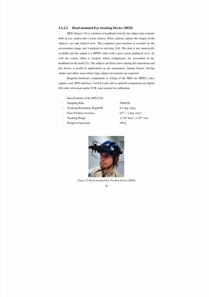
3.1.2.2 Head mounted Eye tracking Device (HED)
HED (Figure 3.8) is a helmet or headband worn by the subject that contains
both an eye camera and a scene camera. These cameras capture the images of the
subject's eye and field-of-view. The computed gaze position is overlaid on the
environment image and visualized in real-time [34]. The data is not numerically
available and the output is a MPEG video with a gaze cursor displayed on it. As
well the cornea reflex is tracked, which compensates for movement of the
headband on the head [31]. The subject can freely move during the experiment and
this device is useful in applications as are ergonomics, human factors, driving
studies and others areas where large subject movements are expected.Required hardware components to wiring of the HED are MPEG video
capture card, HED interface, CurVid Card, and as optional components are digital
I/O cable, television and/or VCR, laser pointer for calibration.
Specifications of the HED [34]:
- Sampling Rate 50/60 Hz
- Tracking Resolution, Pupil/CR 0.1 deg. (typ.)
- Gaze Position Accuracy 0.5° – 1 deg. (typ.)
- Tracking Range +/-30° horz., +/-25° vert.
- Weight of head unit 450 g
Figure 3.8 Head-mounted Eye Tracking Device (HED)
8/12/2019 Bara Kominkova Master Thesis
http://slidepdf.com/reader/full/bara-kominkova-master-thesis 30/90
30
3.2 Experimental setup and methodology
3.2.1 Experiment setup
The experiment was modeled in the same way for both eye tracking
devices, and divided into two parts. One part was done with one of the eye
tracking devices on one day and the second part was done with the second eye
tracking device on the second day.
The experiment was carried out with 20 observers. Observers included a
mix of students and no observers provided any evidence of color blindness. None
of the participating observers used glasses, in order to achieve precise data. The
dominant eye was found before the experiment, and this eye was tracked. How tofind and why to use the dominant eye is explained in paragraph below. Observers
were randomly divided into groups, the first group used RED first then HED, and
the second group used the devices in the reverse order. Six images were shown to
the observers in a given sequence in the both case with RED and HED. In case of
RED it was important to keep the same position of the images, and the same
distance between the image, observer and RED. Instructions for observers were
presented before and also during the experiment and after the experiment
observers were asked to fill out a questionnaire.
The quality of the experiment is dependent on the calibration of the device.
Not all the time the calibration was successful or sufficiently precise to get
satisfactory data. Hence, in order to get sufficiency of data each observer was
asked to make the experiment twice (20 observers resulted in 40 measurements).
Then the not suitable data were possible to omit from this amount of data.
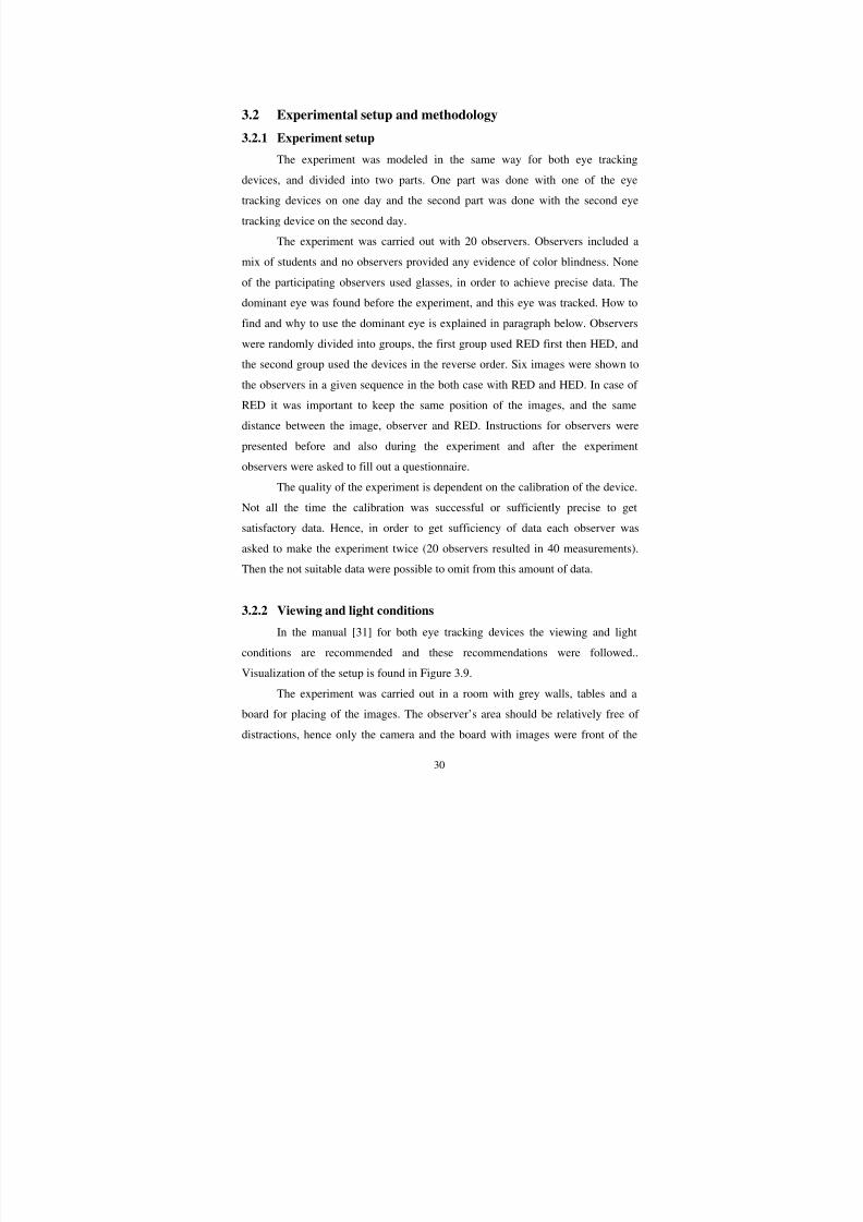
3.2.2 Viewing and light conditions
In the manual [31] for both eye tracking devices the viewing and light
conditions are recommended and these recommendations were followed..
Visualization of the setup is found in Figure 3.9.
The experiment was carried out in a room with grey walls, tables and a
board for placing of the images. The observer’s area should be relatively free of
distractions, hence only the camera and the board with images were front of the
8/12/2019 Bara Kominkova Master Thesis
http://slidepdf.com/reader/full/bara-kominkova-master-thesis 31/90
31
observer. Operator PC was near to the observer, but was not visible for the
observer [31].
The distance from the observers to the board with the images was
approximately 80 cm for all the observers and the viewing angle for the whole
image was about 32×24 degrees. The remote eye tracking camera had placement
below the eye and the location of the camera depended on the dominant eye of the
observer. A chair was selected that minimized the amount of upper body
movements made by the observer. This decreased the possibility that the observer
will change position in a way that causes gaze inaccuracies and prevented the
observer from changing the distance from the eye to the image during theexperiment.
The auto-iris and threshold options on the iView X system will adjust for
many different light conditions. In an experiment for maximum accuracy is good
to avoid to presence of another IR light, light changes and complete darkness [31].
For this experiment the images had to be highly visible and the eye could not have
a lot of reflections. Hence the experiment was carried out in standard D50 and the
light was kept constant during the experiment.
Figure 3.9 Arrangement in the experimental room.
8/12/2019 Bara Kominkova Master Thesis
http://slidepdf.com/reader/full/bara-kominkova-master-thesis 32/90
32
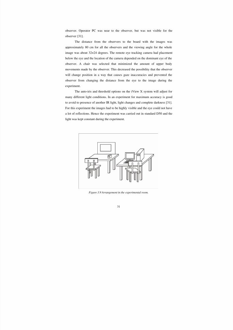
3.2.3 Implementation of images
Six images, of format A3 were created in a Adobe Illustrator, represented
very simple test fields with different symbols. The symbols were predominantly in
a shape of a cross (Figure 3.10). In order to better distinguish crosses in evaluation
part each cross was numbered. To make a simple understanding and survey, we
can say that four different images were made and one of them was created three
times. From now we can call them as image A, B, C and D.
A B
C DFigure 3.10 Images used in the experiment (Image A, Image B, Image C, Image D).
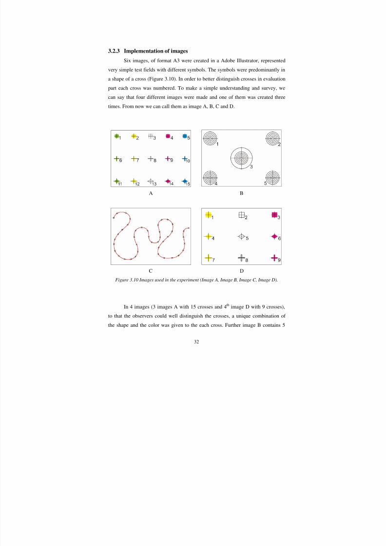
In 4 images (3 images A with 15 crosses and 4th image D with 9 crosses),
to that the observers could well distinguish the crosses, a unique combination of
the shape and the color was given to the each cross. Further image B contains 5
8/12/2019 Bara Kominkova Master Thesis
http://slidepdf.com/reader/full/bara-kominkova-master-thesis 33/90
8/12/2019 Bara Kominkova Master Thesis
http://slidepdf.com/reader/full/bara-kominkova-master-thesis 34/90
34
leaves his or her position in front of the device, and returns to sit in the same
position. In the case of the HED, the observer took off the helmet and after a while
the helmet was refitted on the observer’s head. This experiment will show whether
the devices are able to correctly calculate point of regard even though the observer
has moved or changed positions. Image D contains 9 crosses, which are distributed
in the same way as the image A, but only with less number of crosses.
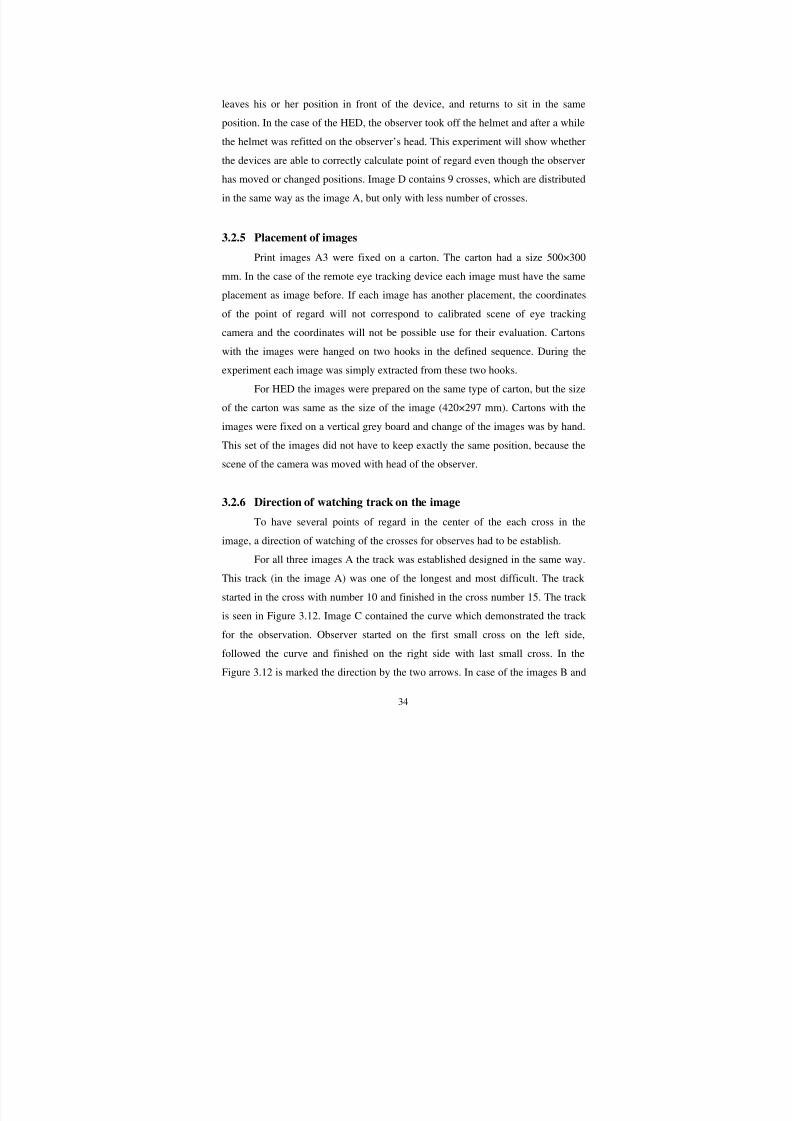
3.2.5 Placement of images
Print images A3 were fixed on a carton. The carton had a size 500×300
mm. In the case of the remote eye tracking device each image must have the sameplacement as image before. If each image has another placement, the coordinates
of the point of regard will not correspond to calibrated scene of eye tracking
camera and the coordinates will not be possible use for their evaluation. Cartons
with the images were hanged on two hooks in the defined sequence. During the
experiment each image was simply extracted from these two hooks.
For HED the images were prepared on the same type of carton, but the size
of the carton was same as the size of the image (420×297 mm). Cartons with the
images were fixed on a vertical grey board and change of the images was by hand.
This set of the images did not have to keep exactly the same position, because the
scene of the camera was moved with head of the observer.
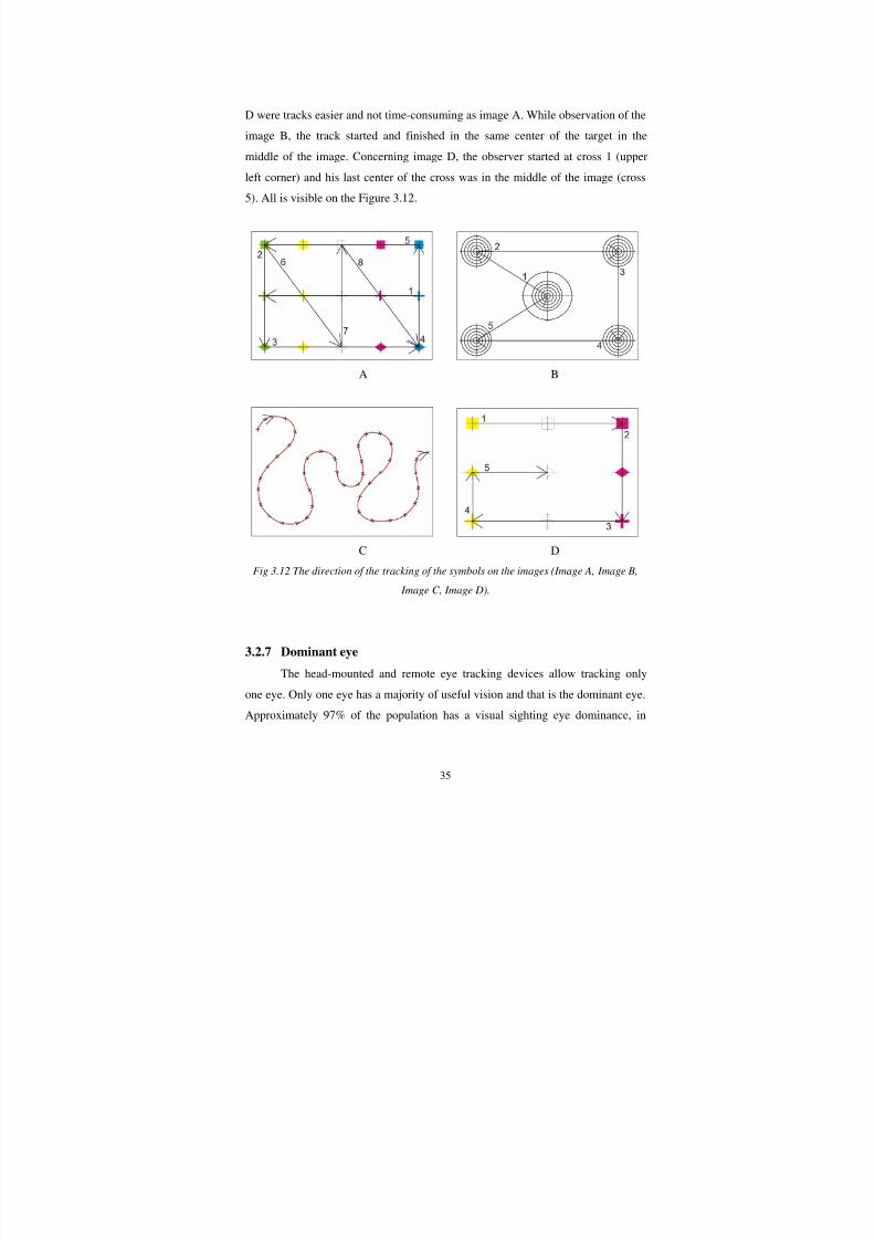
3.2.6 Direction of watching track on the image
To have several points of regard in the center of the each cross in the
image, a direction of watching of the crosses for observes had to be establish.
For all three images A the track was established designed in the same way.
This track (in the image A) was one of the longest and most difficult. The track
started in the cross with number 10 and finished in the cross number 15. The track
is seen in Figure 3.12. Image C contained the curve which demonstrated the track
for the observation. Observer started on the first small cross on the left side,
followed the curve and finished on the right side with last small cross. In the
Figure 3.12 is marked the direction by the two arrows. In case of the images B and
8/12/2019 Bara Kominkova Master Thesis
http://slidepdf.com/reader/full/bara-kominkova-master-thesis 35/90
35
D were tracks easier and not time-consuming as image A. While observation of the
image B, the track started and finished in the same center of the target in the
middle of the image. Concerning image D, the observer started at cross 1 (upper
left corner) and his last center of the cross was in the middle of the image (cross
5). All is visible on the Figure 3.12.
A B
C D
Fig 3.12 The direction of the tracking of the symbols on the images (Image A, Image B,
Image C, Image D).
3.2.7 Dominant eye
The head-mounted and remote eye tracking devices allow tracking only
one eye. Only one eye has a majority of useful vision and that is the dominant eye.
Approximately 97% of the population has a visual sighting eye dominance, in
8/12/2019 Bara Kominkova Master Thesis
http://slidepdf.com/reader/full/bara-kominkova-master-thesis 36/90
36
which observers consistently use the same eye for primary vision. 65% of all
observers are right-eye dominant, and 32% are left-eye dominant.
In this experiment the dominant eye of the observers has been tested
according to the “Porta test”.
- The participant is asked to point to a far object with an outstretched arm
using both eyes.
- While still pointing, the participants were asked to close one eye at a
time.
- The eye that sees the finger pointing directly at the target is dominant.
[26]
3.2.8 Calibration
The calibration of the equipment is a very necessary and a critical part of
the experiment. The calibration establishes the relationship between the position of
the eye in the camera view and a gaze point in space, the so-called point of regard.
At the same time the calibration establishes the plane in space where eyes
movements are rendered. Poor calibration can invalidate an entire eye tracking
experiment, because there will be a mismatch between the participant’s point of
regard, and the corresponding location on a display [26].
There are many calibration methods which are possible to use, these
usually differ in the number of points calibrated The calibration method named “9
Point with Corner Correction” was used in this experiment for both eye tracking
devices [31]. Calibration of the system was done for each observer before
commencing the experiment.
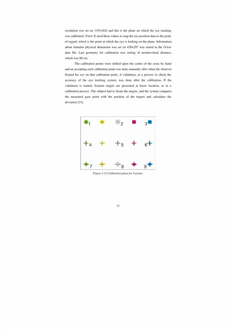
3.2.8.1 RED calibration
For the calibration plane was used the image A_1. Only few symbols were
used in a defined sequence to make the calibration, as is seen on the Figure 3.13.
The calibration plane (image A_1) was loaded to the computer with the iView X
system thus the resolution of the printed image and the calibration plane was
matched. The calibration geometry was adjusted manually. Stimulus screen
8/12/2019 Bara Kominkova Master Thesis
http://slidepdf.com/reader/full/bara-kominkova-master-thesis 37/90

8/12/2019 Bara Kominkova Master Thesis
http://slidepdf.com/reader/full/bara-kominkova-master-thesis 38/90
38
3.2.8.2 HED calibration
There a few methods of calibrating the HED. An easy way to calibrate the
HED system is to use a laser pointer, where the observer stands facing a wall or
flat surface. In this experiment the laser point was not used. The calibration does
not have to be as large as in case for laser point.
The process of the calibration was practically similar to the calibration of
the RED. For the calibration plane was used also the image A_1 Figure 3.13. In
case of the HED, we worked with a scene video and therefore we had just two
possibilities in choose of the resolution. For the experiment the resolution
768×568 PAL (Europe) was chosen. After the setting of the resolution and otherparameters we could started with the calibration. As in the case of the RED
calibration, the calibration points were shift upon the centre of the cross by hand,
accepting each calibration point was made manually after the observer fixated his
eye on that calibration point and last process of the calibration was the validation.
3.2.9 Instructions
This experiment could not be without instructions from the operator not
just on the beginning of the experiment, but also during the experiment. Therefore
we can divide the instruction on the instruction before the experiment and
instructions during the experiment.
3.2.9.1 Instructions before the experiment
Although the experiment had two parts in different days (one with RED
camera and second with HED camera or vice-versa), the observer got these
instructions only while the first part on the beginning of the experiment.
The instructions are:
- First what you will do is a calibration of the eye tracking camera. The
calibration is main important thing in the experiment and therefore has to be
accurate as is possible. Please try to keep the same position of your head and
move minimally.

8/12/2019 Bara Kominkova Master Thesis
http://slidepdf.com/reader/full/bara-kominkova-master-thesis 39/90
39
- For correct results I would like to ask you if you can minimalize movements of
the head and body all the time of the experiment.
- You will see six images with various symbols. Each symbol will have a cross
which mark centre of the symbol. Please, important is to look still to the
middle of this cross.
- Others instructions you will get during the experiment.
After these instructions the observer was asked if he/she understands all and if
he/she has some question. Then the observer was familiarized with the first image.
3.2.9.2 Instructions during the experimentBecause observers saw images without numbering and marking of the
observation track (Figure 3.10), the operator navigated them where they had to
look and eventually what they had to do.
Before when observers started to look at the image C, the instruction from
the operator sounds: You will keep track of the red line from the first cross in the
left corner and on the each cross stay a minute. When you will be on the end (on
the last cross) say that you are there.
The last image D was created to find calibration constancy when the
observer change position. In order to find out calibration constancy for the RED,
the observer was asked if he could stand up from the chair, make a few steps and
return back and sit down. In case of the HED, observer was asked to take off the
helmet and after a while set the helmet back.
3.2.9.3 Questionnaire
After the experiment observers were asked to fill out a questionnaire
(Appendix A). The most important questions were:
- Age and gender.
- Have you participated in eye tracking experiment before?
- Which picture was most problematic for you: Image A, Image B, Image
C, Image D
- Which camera was more comfortable for you? And why?
8/12/2019 Bara Kominkova Master Thesis
http://slidepdf.com/reader/full/bara-kominkova-master-thesis 40/90
8/12/2019 Bara Kominkova Master Thesis
http://slidepdf.com/reader/full/bara-kominkova-master-thesis 41/90
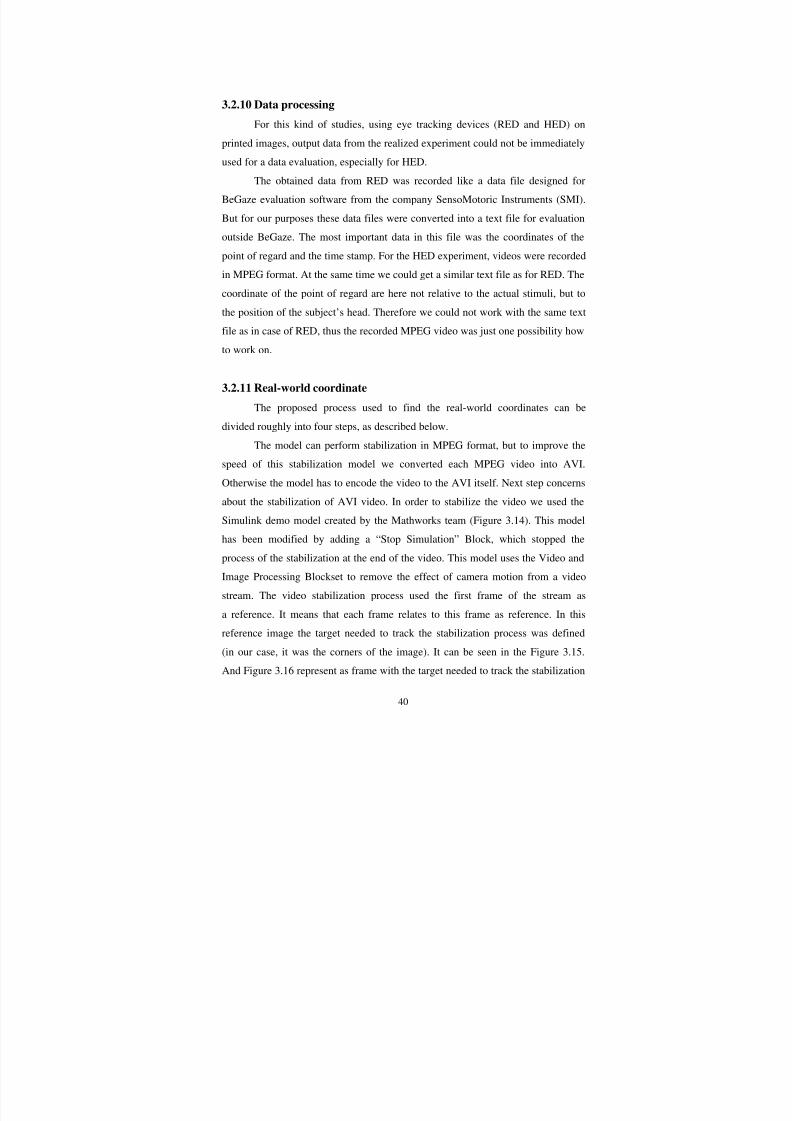
41
process as the stabilized image. Simply, the model searched for the target and in
each frame determines how much the target has moved relative to the reference
frame. It uses this information to remove unwanted shaky motions from video and
generate a stabilized video.
Figure 3.14 Simulink demo model.
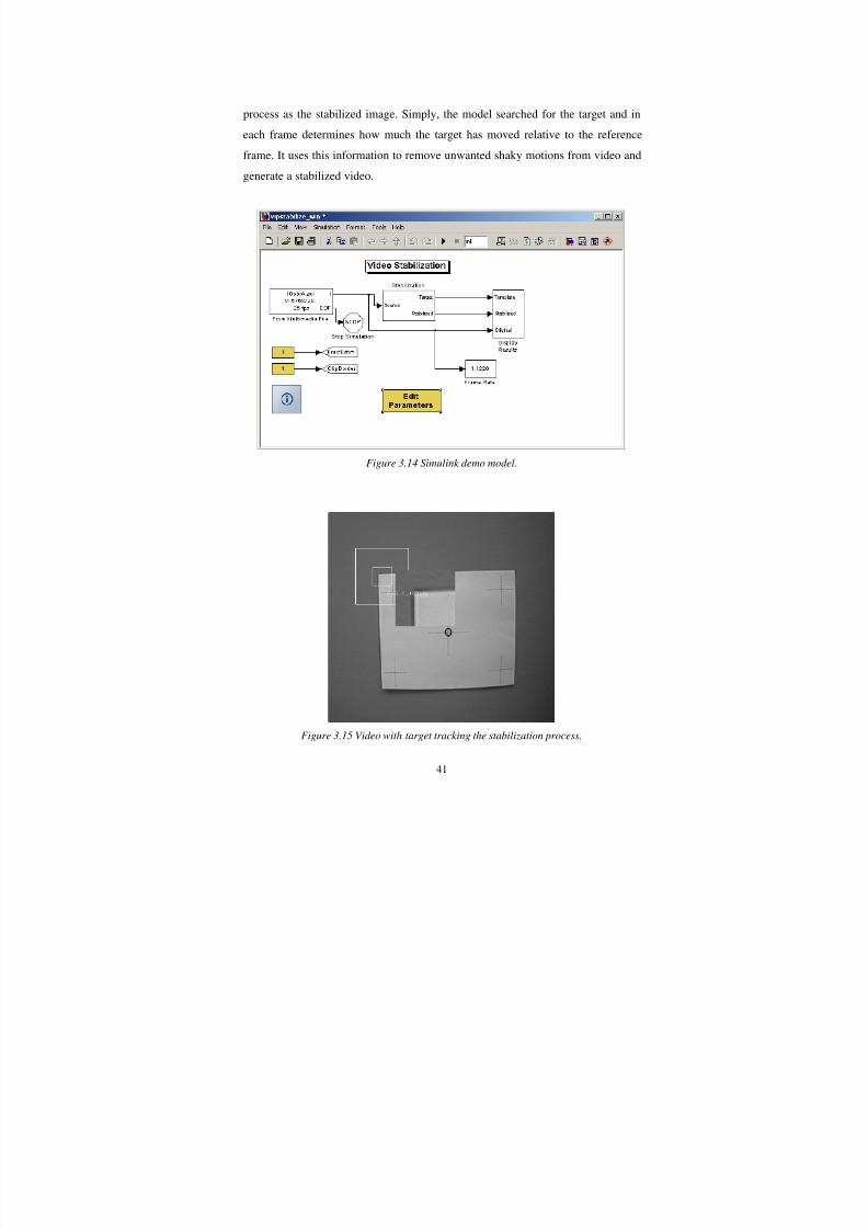
Figure 3.15 Video with target tracking the stabilization process.
8/12/2019 Bara Kominkova Master Thesis
http://slidepdf.com/reader/full/bara-kominkova-master-thesis 42/90
42
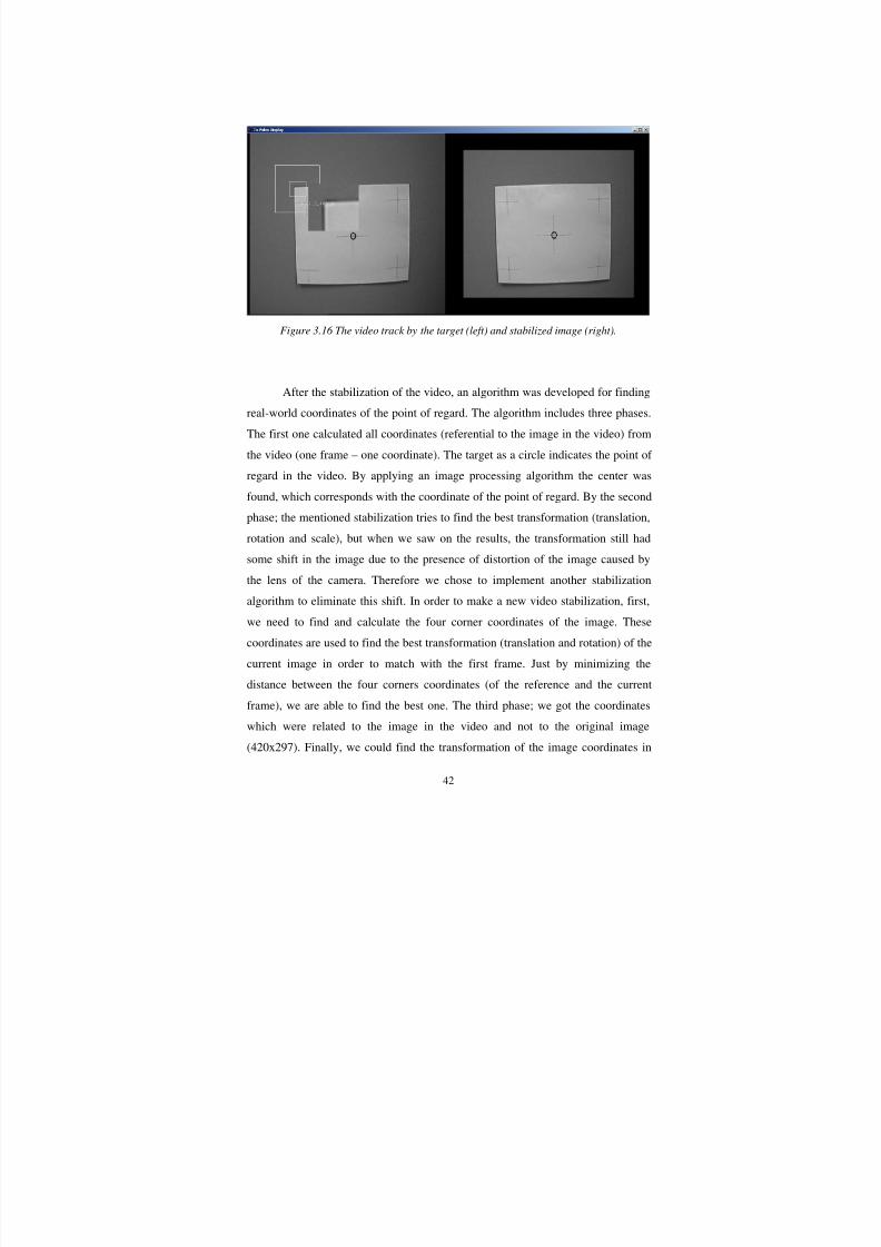
Figure 3.16 The video track by the target (left) and stabilized image (right).
After the stabilization of the video, an algorithm was developed for finding
real-world coordinates of the point of regard. The algorithm includes three phases.
The first one calculated all coordinates (referential to the image in the video) from
the video (one frame – one coordinate). The target as a circle indicates the point of
regard in the video. By applying an image processing algorithm the center was
found, which corresponds with the coordinate of the point of regard. By the second
phase; the mentioned stabilization tries to find the best transformation (translation,
rotation and scale), but when we saw on the results, the transformation still had
some shift in the image due to the presence of distortion of the image caused by
the lens of the camera. Therefore we chose to implement another stabilization
algorithm to eliminate this shift. In order to make a new video stabilization, first,
we need to find and calculate the four corner coordinates of the image. These
coordinates are used to find the best transformation (translation and rotation) of the
current image in order to match with the first frame. Just by minimizing the
distance between the four corners coordinates (of the reference and the current
frame), we are able to find the best one. The third phase; we got the coordinates
which were related to the image in the video and not to the original image
(420x297). Finally, we could find the transformation of the image coordinates in

8/12/2019 Bara Kominkova Master Thesis
http://slidepdf.com/reader/full/bara-kominkova-master-thesis 43/90
43
the video into the original image (the width and length of the image are compute
thanks to the four corners) and the result was the real-world coordinates of the
points of regard, which are relative to the actual stimuli. With these coordinates we
could work on evaluation of the data.
8/12/2019 Bara Kominkova Master Thesis
http://slidepdf.com/reader/full/bara-kominkova-master-thesis 44/90
44
3.3 Experimental results
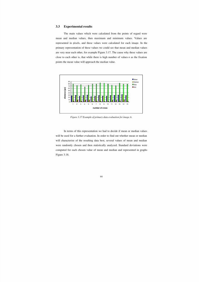
The main values which were calculated from the points of regard weremean and median values, then maximum and minimum values. Values are
represented in pixels, and these values were calculated for each image. In the
primary representation of these values we could see that mean and median values
are very near each other, for example Figure 3.17. The cause why these values are
close to each other is, that while there is high number of values n as the fixation
points the mean value will approach the median value.
0
10
20
30
40
50
60
70
80
90
1 2 3 4 5 6 7 8 9 10 11 12 13 14 15
number of cross
d i s t a n c e [ p x ]
Mean
Median
Max
Min
Figure 3.17 Example of primary data evaluation for image A.
In terms of this representation we had to decide if mean or median values
will be used for a further evaluation. In order to find out whether mean or median
will characterize of the resulting data best, several values of mean and median
were randomly chosen and then statistically analyzed. Standard deviations were
computed for each chosen value of mean and median and represented in graphs
Figure 3.18.
8/12/2019 Bara Kominkova Master Thesis
http://slidepdf.com/reader/full/bara-kominkova-master-thesis 45/90
45
6
8
10
12
14
16
18
20
0 2 4 6 8 10 12 14 16 18 20 22 24 26 28
random values
s t a n d a r d d e v i s t i o n [ p x ]
mean
median
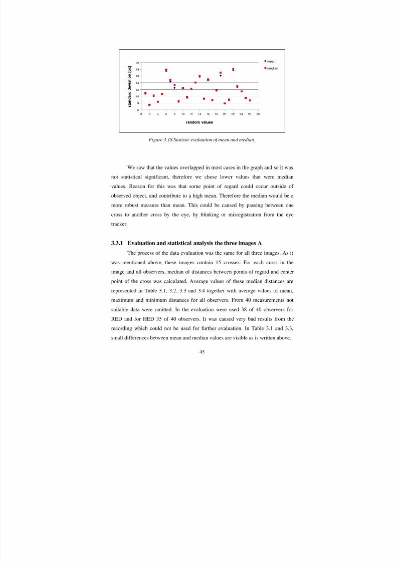
Figure 3.18 Statistic evaluation of mean and median.
We saw that the values overlapped in most cases in the graph and so it was
not statistical significant, therefore we chose lower values that were median
values. Reason for this was that some point of regard could occur outside of
observed object, and contribute to a high mean. Therefore the median would be a
more robust measure than mean. This could be caused by passing between one
cross to another cross by the eye, by blinking or misregistration from the eye
tracker.
3.3.1 Evaluation and statistical analysis the three images A
The process of the data evaluation was the same for all three images. As it
was mentioned above, these images contain 15 crosses. For each cross in the
image and all observers, median of distances between points of regard and center
point of the cross was calculated. Average values of these median distances are
represented in Table 3.1, 3.2, 3.3 and 3.4 together with average values of mean,
maximum and minimum distances for all observers. From 40 measurements not
suitable data were omitted. In the evaluation were used 38 of 40 observers for
RED and for HED 35 of 40 observers. It was caused very bad results from the
recording which could not be used for further evaluation. In Table 3.1 and 3.3,
small differences between mean and median values are visible as is written above.
8/12/2019 Bara Kominkova Master Thesis
http://slidepdf.com/reader/full/bara-kominkova-master-thesis 46/90
46
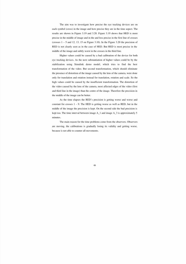
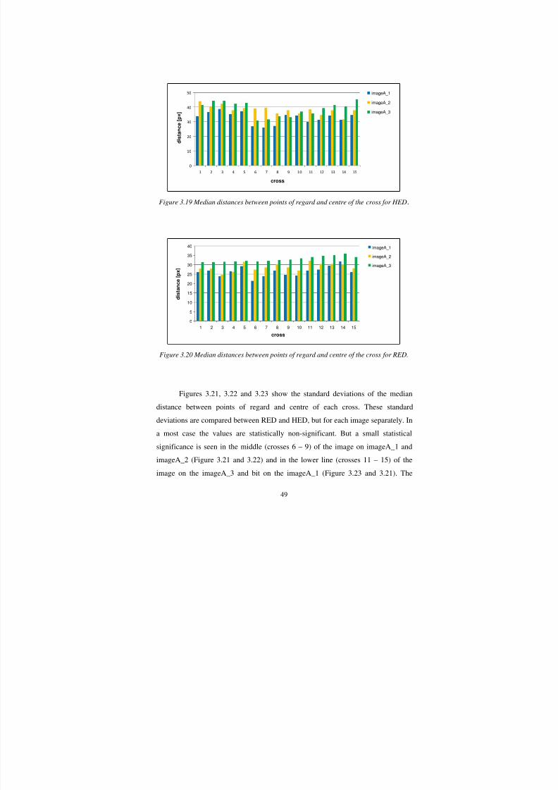
The aim was to investigate how precise the eye tracking devices are on
each symbol (cross) in the image and how precise they are in the time aspect. The
results are shown in Figure 3.19 and 3.20. Figure 3.19 shows that HED is more
precise in the middle of image and in the and less precise in the first line of crosses
(crosses 1 – 5 and 12, 13, 15 on Figure 3.10). In the Figure 3.20 the precision of
RED is not clearly seen as in the case of HED. But RED is most precise in the
middle of the image and subtly worst in the crosses in the third line.
Higher values could be caused by a bad calibration of the device for both
eye tracking devices. As the next substantiation of higher values could be by the
stabilization using Simulink demo model, which tries to find the besttransformation of the video. But second transformation, which should eliminate
the presence of distortion of the image caused by the lens of the camera, were done
only for translation and rotation instead for translation, rotation and scale. So the
high values could be caused by the insufficient transformation. The distortion of
the video caused by the lens of the camera, most affected edges of the video (first
and third line in the image) than the centre of the image. Therefore the precision in
the middle of the image can be better.
As the time elapses the RED’s precision is getting worse and worse and
constant for crosses 1 – 9. The HED is getting worse as well as RED, but in the
middle of the image the precision is kept. On the second side the bad precision is
kept too. The time interval between image A_1 and image A_3 is approximately 5
minutes.
The main reason for the time problems come from the observers. Observers
are moving, the calibrations is gradually losing its validity and getting worse,
because is not able to counter all movements.

8/12/2019 Bara Kominkova Master Thesis
http://slidepdf.com/reader/full/bara-kominkova-master-thesis 47/90
47
Table 3.1 HED average mean and median distances between points of regard and center
point of the cross for all observes.
CrossnumberMEAN [px] MEDIAN [px]
ImageA_1 ImageA_2 ImageA_3 ImageA_1 ImageA_2 ImageA_31 34,11 41,66 43,13 33,68 41,51 43,92
2 37,40 44,60 40,93 36,58 44,43 40,40
3 38,42 44,49 43,03 38,76 44,28 42,14
4 35,49 42,90 38,11 35,22 42,29 37,88
5 37,25 43,58 39,56 37,30 42,92 39,44
6 27,39 31,86 39,13 26,90 30,71 38,89
7 27,92 33,92 41,17 25,91 31,73 39,51
8 28,94 35,45 37,01 27,23 33,55 35,77
9 35,15 35,13 37,92 34,47 33,21 37,77
10 33,83 38,22 35,57 34,22 36,92 35,7211 30,42 36,75 38,80 29,90 35,88 38,40
12 31,84 39,29 34,94 31,37 39,27 34,56
13 35,33 41,70 38,03 34,34 41,32 37,82
14 31,42 40,59 32,14 31,27 40,51 31,60
15 33,94 45,27 38,57 34,43 45,31 37,85
Mean 33,25 39,69 38,54 32,77 38,92 38,11
Table 3.2 HED average maximum and minimum distances between points of regard and
center point of the cross for all observes.
Crossnumber
MAX [px] MIN [px]ImageA_1 ImageA_2 ImageA_3 ImageA_1 ImageA_2 ImageA_3
1 64,20 71,81 68,45 11,98 15,56 15,33
2 58,27 63,06 61,73 20,87 27,87 24,33
3 57,75 70,69 68,32 20,18 23,09 22,47
4 52,41 65,25 58,87 17,91 22,73 20,68
5 53,92 64,99 56,71 23,67 24,68 24,46
6 55,45 65,81 68,52 7,05 10,08 18,18
7 60,01 72,77 70,39 7,62 9,78 18,08
8 62,52 75,03 72,20 8,49 10,49 10,919 65,71 69,51 68,59 13,14 8,55 11,06
10 62,86 70,37 66,04 12,03 14,45 10,45
11 54,14 61,58 59,90 16,20 17,91 24,53
12 50,72 60,31 52,60 18,76 20,55 20,61
13 61,31 68,20 61,53 16,40 15,01 16,40
14 53,03 60,92 49,51 16,04 22,48 19,27
15 56,73 70,30 61,31 13,69 23,85 20,55
Mean 57,94 67,38 62,98 14,94 17,81 18,49

8/12/2019 Bara Kominkova Master Thesis
http://slidepdf.com/reader/full/bara-kominkova-master-thesis 48/90
8/12/2019 Bara Kominkova Master Thesis
http://slidepdf.com/reader/full/bara-kominkova-master-thesis 49/90
8/12/2019 Bara Kominkova Master Thesis
http://slidepdf.com/reader/full/bara-kominkova-master-thesis 50/90
50
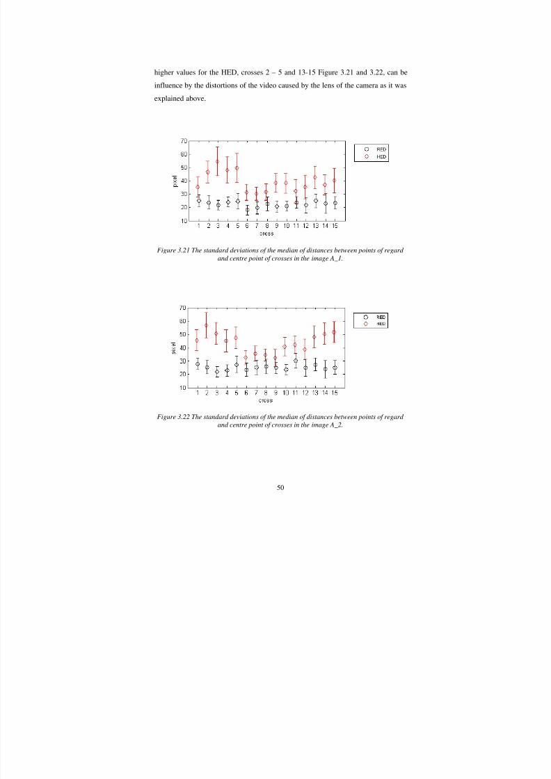
higher values for the HED, crosses 2 – 5 and 13-15 Figure 3.21 and 3.22, can be
influence by the distortions of the video caused by the lens of the camera as it was
explained above.
Figure 3.21 The standard deviations of the median of distances between points of regard
and centre point of crosses in the image A_1.
Figure 3.22 The standard deviations of the median of distances between points of regard
and centre point of crosses in the image A_2.
8/12/2019 Bara Kominkova Master Thesis
http://slidepdf.com/reader/full/bara-kominkova-master-thesis 51/90
51
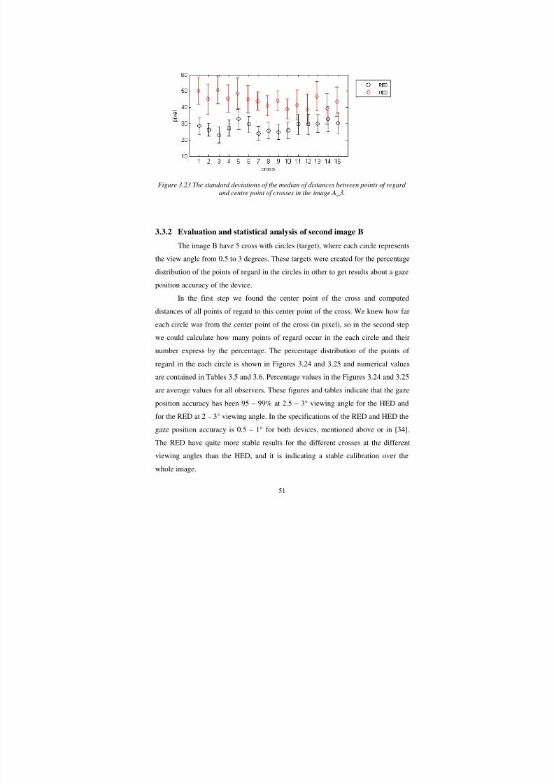
Figure 3.23 The standard deviations of the median of distances between points of regard
and centre point of crosses in the image A_3.
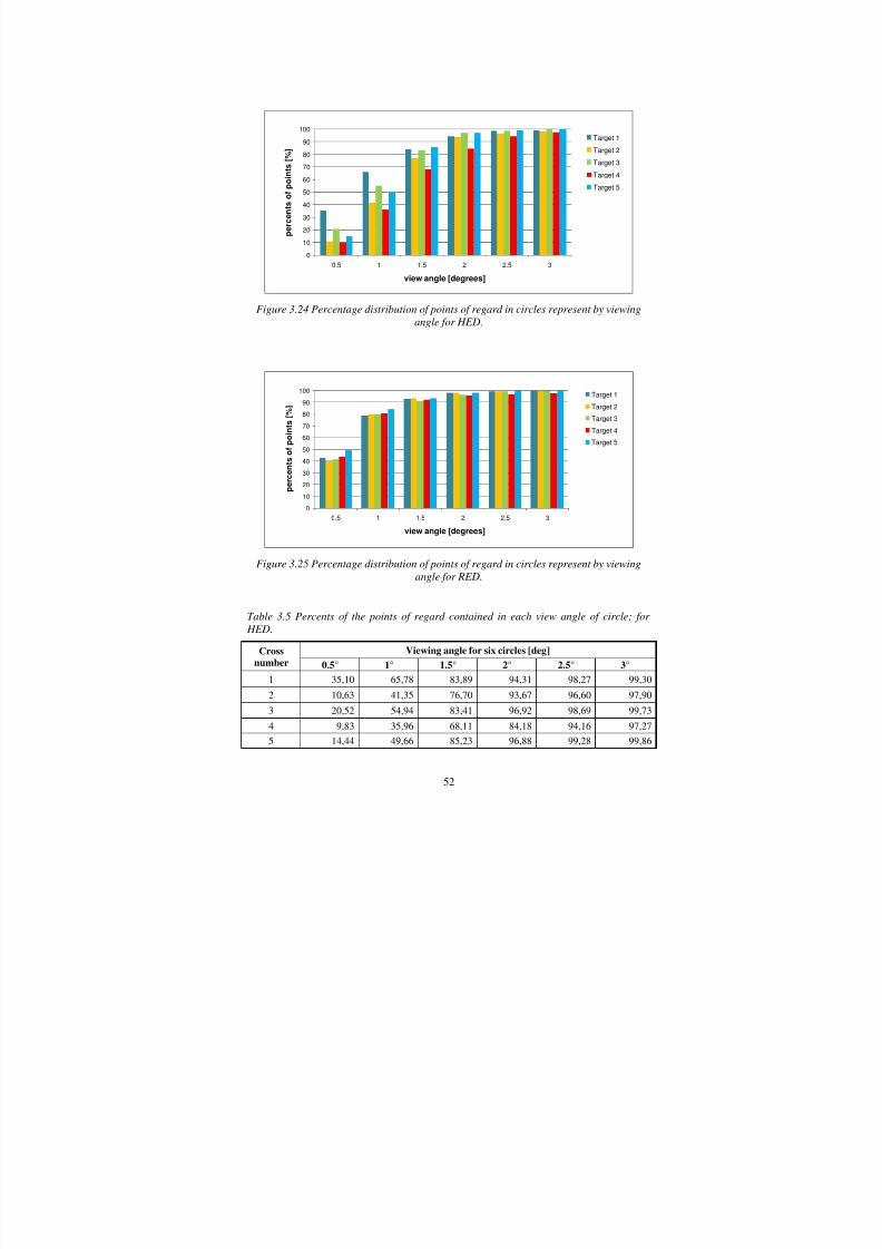
3.3.2 Evaluation and statistical analysis of second image B
The image B have 5 cross with circles (target), where each circle represents
the view angle from 0.5 to 3 degrees. These targets were created for the percentage
distribution of the points of regard in the circles in other to get results about a gaze
position accuracy of the device.
In the first step we found the center point of the cross and computed
distances of all points of regard to this center point of the cross. We knew how far
each circle was from the center point of the cross (in pixel), so in the second step
we could calculate how many points of regard occur in the each circle and their
number express by the percentage. The percentage distribution of the points of
regard in the each circle is shown in Figures 3.24 and 3.25 and numerical values
are contained in Tables 3.5 and 3.6. Percentage values in the Figures 3.24 and 3.25
are average values for all observers. These figures and tables indicate that the gaze
position accuracy has been 95 – 99% at 2.5 – 3° viewing angle for the HED and
for the RED at 2 – 3° viewing angle. In the specifications of the RED and HED the
gaze position accuracy is 0.5 – 1° for both devices, mentioned above or in [34].
The RED have quite more stable results for the different crosses at the different
viewing angles than the HED, and it is indicating a stable calibration over the
whole image.
8/12/2019 Bara Kominkova Master Thesis
http://slidepdf.com/reader/full/bara-kominkova-master-thesis 52/90
8/12/2019 Bara Kominkova Master Thesis
http://slidepdf.com/reader/full/bara-kominkova-master-thesis 53/90
53
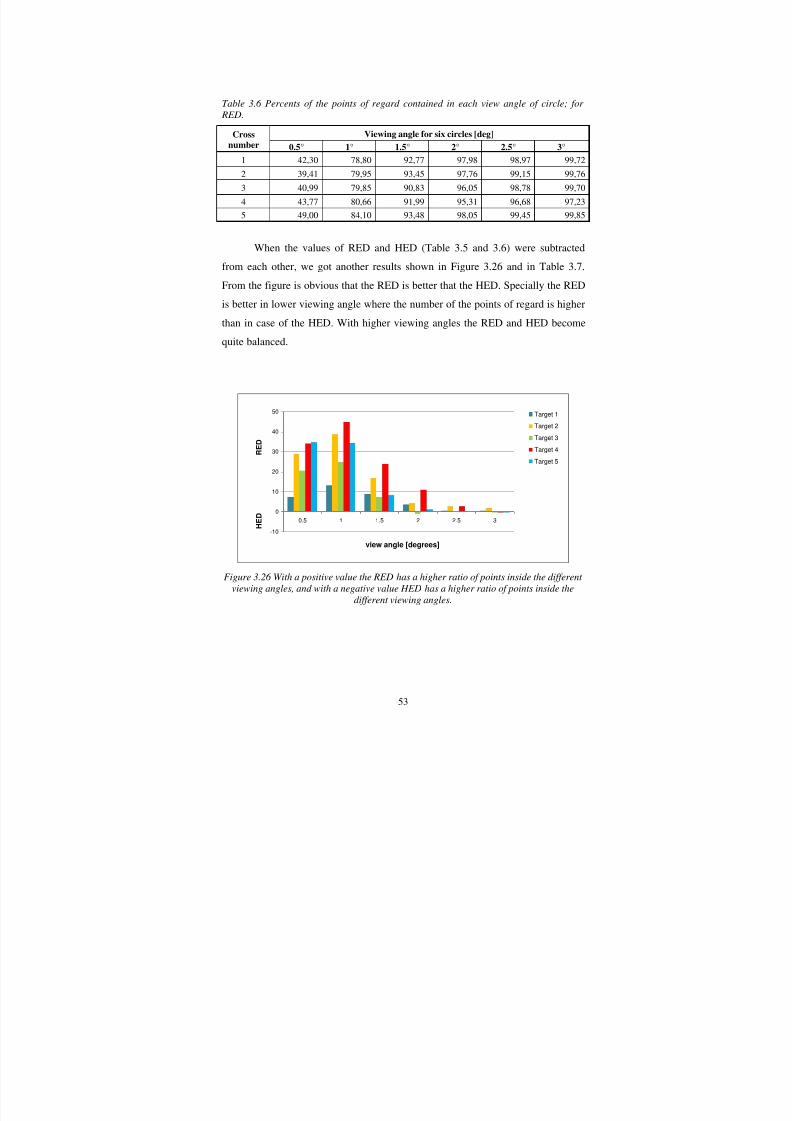
Table 3.6 Percents of the points of regard contained in each view angle of circle; for
RED.
Crossnumber Viewing angle for six circles [deg]0.5° 1° 1.5° 2° 2.5° 3°
1 42,30 78,80 92,77 97,98 98,97 99,72
2 39,41 79,95 93,45 97,76 99,15 99,76
3 40,99 79,85 90,83 96,05 98,78 99,70
4 43,77 80,66 91,99 95,31 96,68 97,23
5 49,00 84,10 93,48 98,05 99,45 99,85
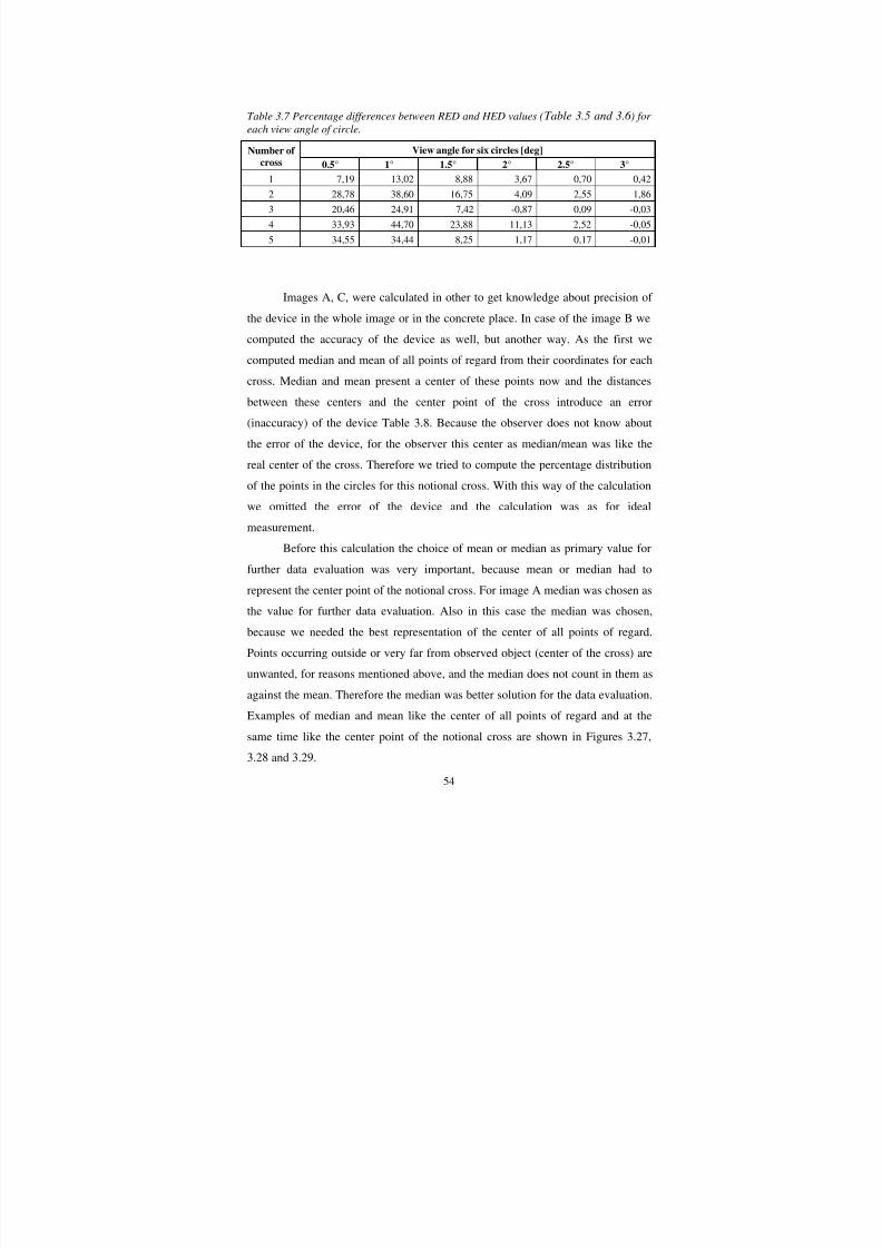
When the values of RED and HED (Table 3.5 and 3.6) were subtracted
from each other, we got another results shown in Figure 3.26 and in Table 3.7.
From the figure is obvious that the RED is better that the HED. Specially the RED
is better in lower viewing angle where the number of the points of regard is higher
than in case of the HED. With higher viewing angles the RED and HED become
quite balanced.
-10
0
10
20
30
40
50
0.5 1 1.5 2 2.5 3
view angle [degrees]
H E D
R E D
Target 1
Target 2
Target 3
Target 4
Target 5
Figure 3.26 With a positive value the RED has a higher ratio of points inside the different
viewing angles, and with a negative value HED has a higher ratio of points inside the
different viewing angles.
8/12/2019 Bara Kominkova Master Thesis
http://slidepdf.com/reader/full/bara-kominkova-master-thesis 54/90
8/12/2019 Bara Kominkova Master Thesis
http://slidepdf.com/reader/full/bara-kominkova-master-thesis 55/90
55
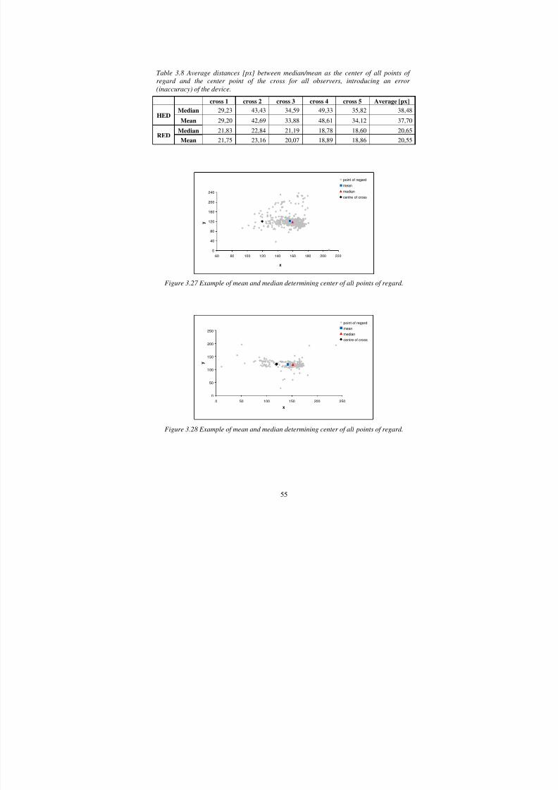
Table 3.8 Average distances [px] between median/mean as the center of all points of
regard and the center point of the cross for all observers, introducing an error
(inaccuracy) of the device.
cross 1 cross 2 cross 3 cross 4 cross 5 Average [px]
HEDMedian 29,23 43,43 34,59 49,33 35,82 38,48
Mean 29,20 42,69 33,88 48,61 34,12 37,70
REDMedian 21,83 22,84 21,19 18,78 18,60 20,65
Mean 21,75 23,16 20,07 18,89 18,86 20,55
0
40
80
120
160
200
240
60 80 100 120 140 160 180 200 220
x
y
point of regard
mean
median
centre of cross
Figure 3.27 Example of mean and median determining center of all points of regard.
0
50
100
150
200
250
0 50 100 150 200 250
x
y
point of regard
mean
median
centre of cross
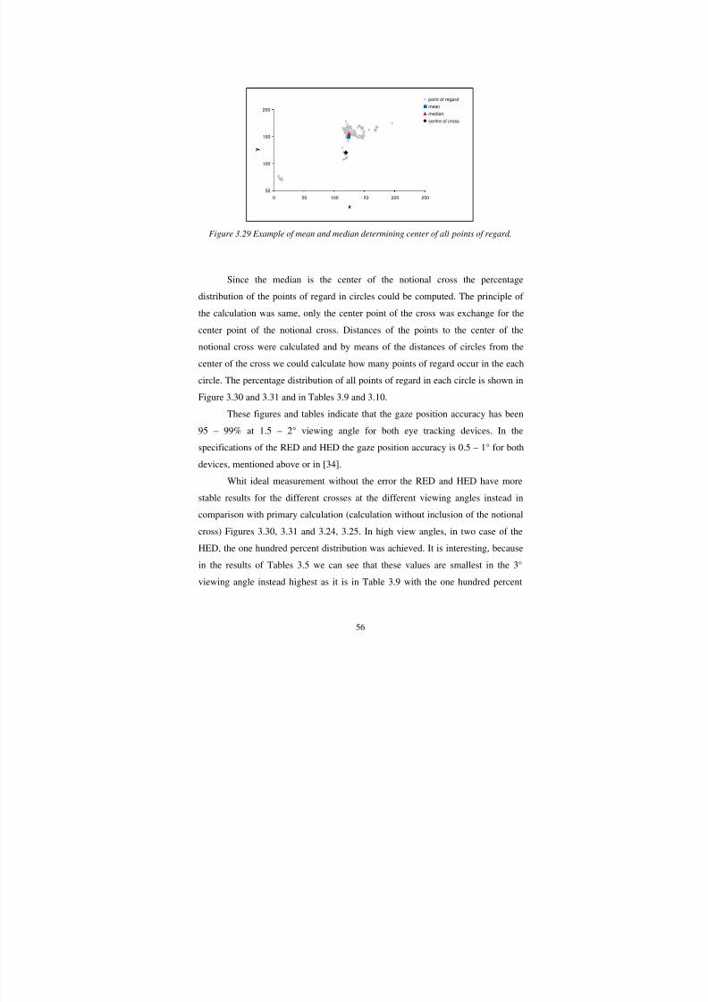
Figure 3.28 Example of mean and median determining center of all points of regard.
8/12/2019 Bara Kominkova Master Thesis
http://slidepdf.com/reader/full/bara-kominkova-master-thesis 56/90
56
50
100
150
200
0 50 100 150 200 250
x
y
point of regard
mean
median
centre of cross
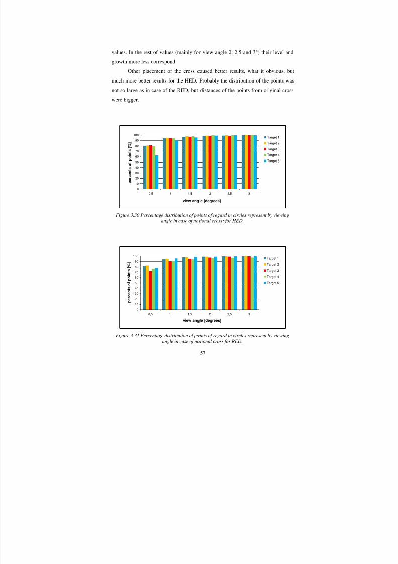
Figure 3.29 Example of mean and median determining center of all points of regard.
Since the median is the center of the notional cross the percentage
distribution of the points of regard in circles could be computed. The principle of
the calculation was same, only the center point of the cross was exchange for the
center point of the notional cross. Distances of the points to the center of the
notional cross were calculated and by means of the distances of circles from the
center of the cross we could calculate how many points of regard occur in the each
circle. The percentage distribution of all points of regard in each circle is shown in
Figure 3.30 and 3.31 and in Tables 3.9 and 3.10.
These figures and tables indicate that the gaze position accuracy has been
95 – 99% at 1.5 – 2° viewing angle for both eye tracking devices. In the
specifications of the RED and HED the gaze position accuracy is 0.5 – 1° for both
devices, mentioned above or in [34].
Whit ideal measurement without the error the RED and HED have more
stable results for the different crosses at the different viewing angles instead in
comparison with primary calculation (calculation without inclusion of the notional
cross) Figures 3.30, 3.31 and 3.24, 3.25. In high view angles, in two case of the
HED, the one hundred percent distribution was achieved. It is interesting, because
in the results of Tables 3.5 we can see that these values are smallest in the 3°
viewing angle instead highest as it is in Table 3.9 with the one hundred percent
8/12/2019 Bara Kominkova Master Thesis
http://slidepdf.com/reader/full/bara-kominkova-master-thesis 57/90
57
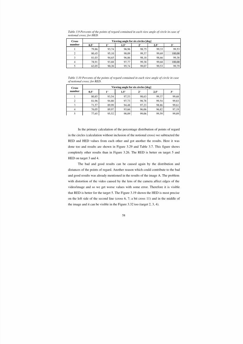
values. In the rest of values (mainly for view angle 2, 2.5 and 3°) their level and
growth more less correspond.
Other placement of the cross caused better results, what it obvious, but
much more better results for the HED. Probably the distribution of the points was
not so large as in case of the RED, but distances of the points from original cross
were bigger.
0
10
20
30
40
50
60
70
80
90
100
0,5 1 1,5 2 2,5 3
view angle [degrees]
p e r c e n t s o f p o i n t s [ % ]
Target 1
Target 2
Target 3
Target 4
Target 5
Figure 3.30 Percentage distribution of points of regard in circles represent by viewing
angle in case of notional cross; for HED.
0
10
20
30
40
5060
70
80
90
100
0,5 1 1,5 2 2,5 3
view angle [degrees]
p e r c e n t s o f p o i n t s [ % ]
Target 1
Target 2
Target 3
Target 4
Target 5
Figure 3.31 Percentage distribution of points of regard in circles represent by viewing
angle in case of notional cross for RED.
8/12/2019 Bara Kominkova Master Thesis
http://slidepdf.com/reader/full/bara-kominkova-master-thesis 58/90
8/12/2019 Bara Kominkova Master Thesis
http://slidepdf.com/reader/full/bara-kominkova-master-thesis 59/90
59
-10
-6
-2
2
6
10
14
0.5 1 1.5 2 2.5 3
view angle [degrees]
H E D
R E D
target 1
target 2target 3
target 4
target 5
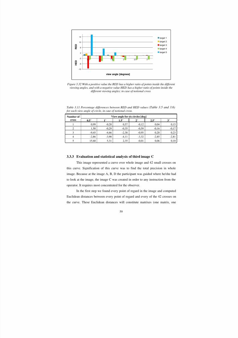
Figure 3.32 With a positive value the RED has a higher ratio of points inside the differentviewing angles, and with a negative value HED has a higher ratio of points inside the
different viewing angles; in case of notional cross.
Table 3.11 Percentage differences between RED and HED values (Table 3.5 and 3.6 ) for each view angle of circle, in case of notional cross.
Number ofcross
View angle for six circles [deg]
0.5° 1° 1.5° 2° 2.5° 3°
1 0,99 -0,20 0,57 -0,12 0,04 0,152 1,50 -0,29 -0,35 -0,59 -0,16 -0,17
3 -9,45 -4,66 -2,38 -0,95 0,20 0,23
4 -2,86 -3,90 -4,11 -3,32 -2,85 -2,81
5 15,60 5,31 2,35 -0,01 0,06 0,10
3.3.3 Evaluation and statistical analysis of third image C
This image represented a curve over whole image and 42 small crosses on
this curve. Signification of this curve was to find the total precision in whole
image. Because at the image A, B, D the participant was guided where he/she had
to look at the image, the image C was created in order to any instruction from the
operator. It requires most concentrated for the observer.
In the first step we found every point of regard in the image and computed
Euclidean distances between every point of regard and every of the 42 crosses on
the curve. These Euclidean distances will constitute matrixes (one matrix, one
8/12/2019 Bara Kominkova Master Thesis
http://slidepdf.com/reader/full/bara-kominkova-master-thesis 60/90
60
observer) about 42 lines (42 crosses) and columns corresponding to a number ∆E
of points of regard. In the second step, a local minimum is found corresponding to
the minimum of each line of this matrix and is kept for further evaluation. By the
evaluation as third step, mean, median, maximum and minimum distances were
computed for every observer. Median values of the distance and their average for
all observers are displayed in Figures 3.33 and 3.34 and all average distances of
mean, median, maximum and minimum are seen in the Table 3.12.
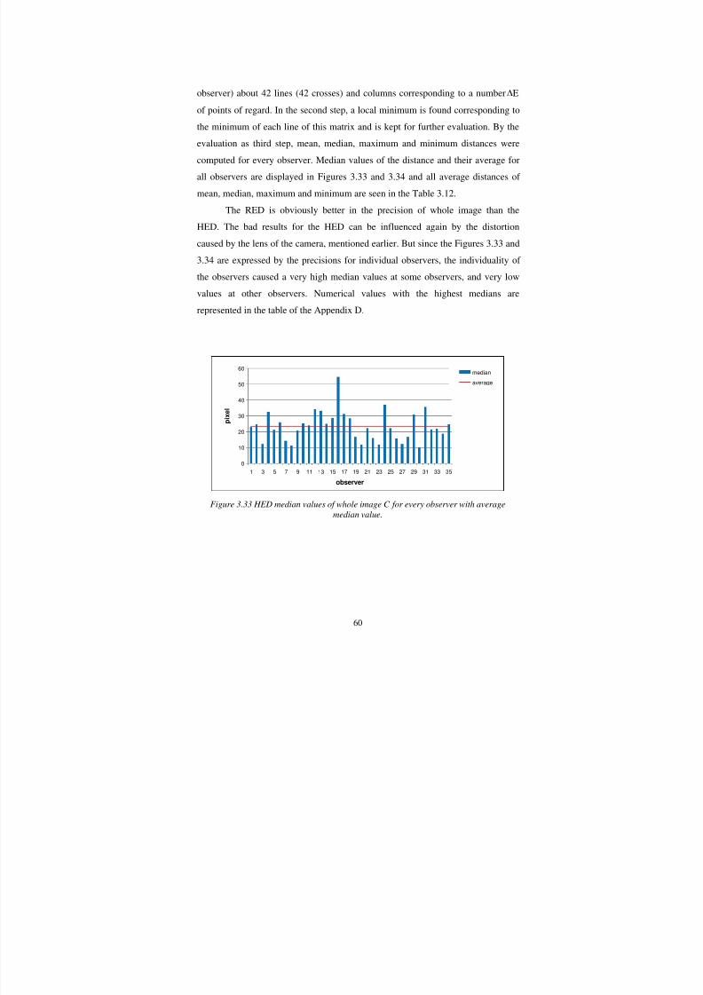
The RED is obviously better in the precision of whole image than the
HED. The bad results for the HED can be influenced again by the distortion
caused by the lens of the camera, mentioned earlier. But since the Figures 3.33 and3.34 are expressed by the precisions for individual observers, the individuality of
the observers caused a very high median values at some observers, and very low
values at other observers. Numerical values with the highest medians are
represented in the table of the Appendix D.
0
10
20
30
40
50
60
1 3 5 7 9 11 13 15 17 19 21 23 25 27 29 31 33 35
observer
p i x e l
median
average
Figure 3.33 HED median values of whole image C for every observer with average
median value.
8/12/2019 Bara Kominkova Master Thesis
http://slidepdf.com/reader/full/bara-kominkova-master-thesis 61/90
61
0
5
10
15
20
25
30
1 3 5 7 9 11 13 15 17 19 21 23 25 27 29 31 33 35 37
observer
p i x e l
median
average
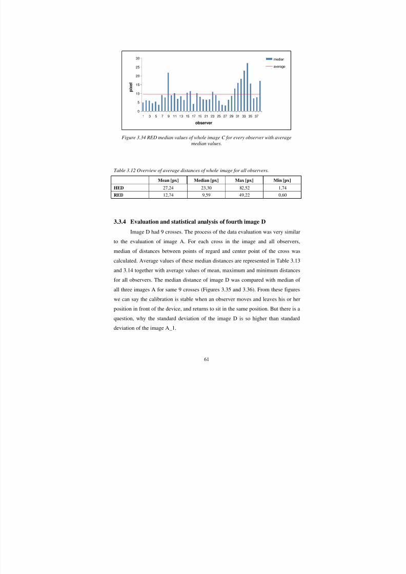
Figure 3.34 RED median values of whole image C for every observer with average
median values.
Table 3.12 Overview of average distances of whole image for all observers.
Mean [px] Median [px] Max [px] Min [px]
HED 27,24 23,30 82,52 1,74
RED 12,74 9,59 49,22 0,60
3.3.4 Evaluation and statistical analysis of fourth image D
Image D had 9 crosses. The process of the data evaluation was very similar
to the evaluation of image A. For each cross in the image and all observers,
median of distances between points of regard and center point of the cross was
calculated. Average values of these median distances are represented in Table 3.13
and 3.14 together with average values of mean, maximum and minimum distances
for all observers. The median distance of image D was compared with median of
all three images A for same 9 crosses (Figures 3.35 and 3.36). From these figures
we can say the calibration is stable when an observer moves and leaves his or her
position in front of the device, and returns to sit in the same position. But there is a
question, why the standard deviation of the image D is so higher than standard
deviation of the image A_1.

8/12/2019 Bara Kominkova Master Thesis
http://slidepdf.com/reader/full/bara-kominkova-master-thesis 62/90
62
Table 3.13 RED average mean, median, maximum and minimum distances between pointsof regard and center point of the cross for all observes.
Crossnumber
RED
Mean [px] Median [px] Max [px] Min [px]
1 43,11 41,93 91,58 17,37
2 41,86 40,56 91,48 15,90
3 41,28 39,96 91,01 15,30
4 42,01 40,69 91,80 16,01
5 40,80 39,44 91,35 14,94
6 40,70 39,26 91,94 15,15
7 41,88 40,66 93,98 15,32
8 37,88 36,32 92,24 12,92
9 35,82 34,19 91,64 11,99
Mean 40,59 39,22 91,89 14,99
Table 3.14 HED average mean, median, maximum and minimum distances between points
of regard and center point of the cross for all observes.
Crossnumber
HEDMean [px] Median [px] Max [px] Min [px]
1 48,09 48,09 70,71 29,85
2 44,08 43,43 69,31 28,05
3 47,56 47,66 69,80 27,99
4 48,21 48,97 70,60 26,89
5 38,09 38,10 57,80 21,83
6 53,72 52,94 78,30 38,92
7 47,54 47,28 68,92 32,12
8 51,93 51,86 75,46 36,02
9 49,08 49,13 70,43 32,14
Mean 47,59 47,49 70,15 30,42
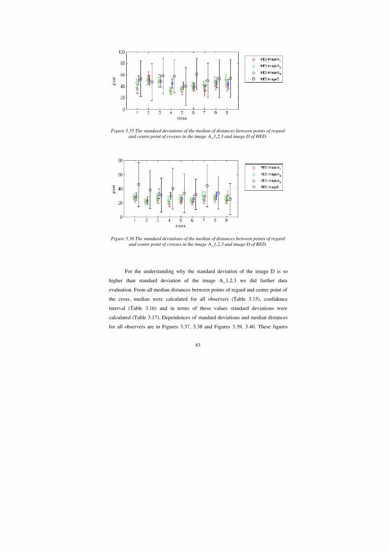
8/12/2019 Bara Kominkova Master Thesis
http://slidepdf.com/reader/full/bara-kominkova-master-thesis 63/90
63
Figure 3.35 The standard deviations of the median of distances between points of regard
and centre point of crosses in the image A_1,2,3 and image D of HED.
Figure 3.36 The standard deviations of the median of distances between points of regard
and centre point of crosses in the image A_1,2,3 and image D of RED.
For the understanding why the standard deviation of the image D is sohigher than standard deviation of the image A_1,2,3 we did further data
evaluation. From all median distances between points of regard and center point of
the cross, median were calculated for all observers (Table 3.15), confidence
interval (Table 3.16) and in terms of these values standard deviations were
calculated (Table 3.17). Dependences of standard deviations and median distances
for all observers are in Figures 3.37, 3.38 and Figures 3.39, 3.40. These figures

8/12/2019 Bara Kominkova Master Thesis
http://slidepdf.com/reader/full/bara-kominkova-master-thesis 64/90
64
show that when the median is increasing the standard deviation is increasing as
well, indicating a larger spread of points not only a moved cluster of points. With
time aspect the median of RED is continuously increased as the standard
deviation, but the median of HED is increased continuously with standard
deviation as well except image A_2.
Table 3.15 Average median distances for all observers of image A_1,2,3 and D; for RED
and HED. The image D contains only 9 crosses, which are identical with some crosses of
the image A. Their identity is visible in this table.
Crossnumber
RED – Median [px] HED – Median [px]ImageA
ImageDImageA
ImageD1 2 3 1 2 3
1 24,99 28,01 28,49 45,79 35,52 45,60 50,09 53,08
2 23,81 25,32 26,24 46,64 56,68 45,13
3 21,85 22,00 23,01 38,66 54,74 50,78 50,73 47,64
4 24,14 22,89 27,38 48,04 45,05 45,38
5 24,79 27,44 32,95 30,85 49,58 47,33 48,37 58,26
6 18,17 23,48 29,73 40,08 31,38 32,51 44,85 57,34
7 19,68 25,17 24,04 30,45 35,49 43,88
8 22,66 25,86 25,64 33,45 31,67 34,57 41,09 39,73
9 20,82 25,03 24,71 38,37 32,40 44,0810 20,95 23,67 25,78 31,98 38,28 40,70 39,02 61,31
11 23,80 30,40 29,61 44,11 32,28 42,12 41,51 50,18
12 21,62 24,92 29,61 35,35 38,70 38,76
13 25,07 27,38 30,02 34,01 42,69 48,23 46,86 53,19
14 22,93 23,87 32,91 37,05 50,51 39,08
15 23,43 25,03 30,27 25,29 40,19 51,81 43,47 53,31
Mean 22,58 25,36 28,03 36,02 39,48 43,50 44,15 52,67

8/12/2019 Bara Kominkova Master Thesis
http://slidepdf.com/reader/full/bara-kominkova-master-thesis 65/90
65
Table 3.16 Average confident intervals for all observers of image A_1,2,3 and D; for RED
and HED.
Crossnumber
RED – Confident interval [px] HED – Confident interval [px]ImageA
ImageDImageA
ImageD1 2 3 1 2 3
1 4,34 4,00 5,30 10,22 7,64 7,90 8,10 11,57
2 5,10 4,90 3,92 8,27 9,42 9,22
3 3,66 4,05 5,08 8,83 10,68 8,20 8,41 12,05
4 3,70 4,48 5,12 9,80 8,28 8,60
5 5,52 6,10 6,38 7,81 11,04 7,84 9,71 11,55
6 3,58 5,22 4,95 9,40 6,02 5,22 8,39 10,60
7 4,62 5,31 4,43 4,88 5,53 5,78
8 5,07 5,42 5,03 9,06 6,16 4,64 6,11 12,35
9 4,20 4,42 4,65 7,13 6,35 5,8710 3,92 3,96 5,10 7,05 7,50 6,90 6,06 10,35
11 4,26 5,56 6,13 9,67 8,80 6,71 9,27 11,26
12 5,70 6,47 6,31 9,11 7,62 9,37
13 5,15 4,80 5,55 7,47 8,28 8,13 9,02 12,20
14 7,44 6,54 7,74 7,74 8,05 9,38
15 4,58 5,09 6,30 7,16 9,24 7,90 8,98 12,30
Mean 4,72 5,09 5,47 8,52 8,15 7,25 8,15 11,58
Table 3.17 Average standard deviations for all observers of image A_1,2,3 and D; for
RED and HED.
Crossnumber
RED – Standard deviation [px] HED – Standard deviation [px]ImageA
ImageDImageA
ImageD1 2 3 1 2 3
1 13,23 12,21 16,15 31,16 19,73 21,89 21,71 31,04
2 15,55 14,96 11,95 21,35 26,09 24,73
3 11,17 12,36 15,48 26,94 27,60 22,70 22,55 32,32
4 11,27 13,66 15,61 25,32 22,93 23,07
5 16,83 18,61 19,46 23,83 28,53 21,71 26,03 30,98
6 10,93 15,92 15,11 28,67 15,55 14,46 22,49 28,42
7 14,08 16,19 13,53 12,61 15,33 15,51
8 15,47 16,52 15,34 27,64 15,92 12,86 16,39 33,129 12,80 13,48 14,18 18,42 17,58 15,74
10 11,95 12,08 15,57 21,49 19,38 19,12 16,26 27,77
11 13,00 16,96 18,70 29,49 22,72 18,59 24,85 30,19
12 17,38 19,72 19,25 23,53 21,12 25,14
13 15,69 14,64 16,94 22,79 21,39 22,52 24,20 32,72
14 22,68 19,94 23,60 20,00 22,29 25,15
15 13,96 15,52 19,21 21,85 23,86 21,87 24,08 32,98
Mean 14,40 15,52 16,67 25,99 21,06 20,07 21,86 31,06
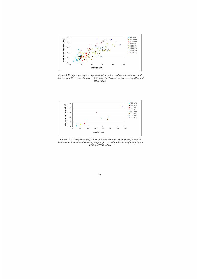
8/12/2019 Bara Kominkova Master Thesis
http://slidepdf.com/reader/full/bara-kominkova-master-thesis 66/90
66
10
15
20
25
30
35
15 25 35 45 55 65
median [px]
s t a n d a r d d e v i a t i o n [ p x ]
RED imA1
RED imA2
RED imA3
RED imD
HED imA1
HED imA2
HED imA3
HED imD
Figure 3.37 Dependence of average standard deviations and median distances of all
observers for 15 crosses of image A_1, 2, 3 and for 9 crosses of image D; for RED and
HED values.
14
18
22
26
30
34
20 25 30 35 40 45 50 55
median [px]
s t a n d a r d d e v i a t i o n [ p x ] RED imA1
RED imA2
RED imA3
RED imD
HED imA1
HED imA2
HED imA3
HED imD
Figure 3.38 Average values of values from Figure 9a) in dependence of standard
deviation on the median distance of image A_1, 2, 3 and for 9 crosses of image D; for
RED and HED values.
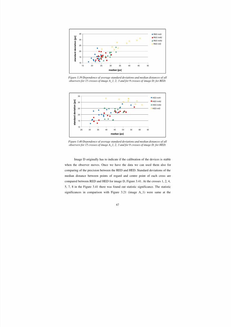
8/12/2019 Bara Kominkova Master Thesis
http://slidepdf.com/reader/full/bara-kominkova-master-thesis 67/90
67
10
15
20
25
30
35
15 20 25 30 35 40 45 50
median [px]
s t a n d a r d d e v i a t i o n [ p x ]
RED imA1
RED imA2
RED imA3
RED imD
Figure 3.39 Dependence of average standard deviations and median distances of all
observers for 15 crosses of image A_1, 2, 3 and for 9 crosses of image D; for RED.
10
15
20
25
30
35
25 30 35 40 45 50 55 60 65
median [px]
s t a n
d a r d d e v i a t i o n [ p x ]
HED imA1
HED imA2
HED imA3
HED imD
Figure 3.40 Dependence of average standard deviations and median distances of all
observers for 15 crosses of image A_1, 2, 3 and for 9 crosses of image D; for HED.
Image D originally has to indicate if the calibration of the devices is stable
when the observer moves. Once we have the data we can used them also for
comparing of the precision between the RED and HED. Standard deviations of the
median distance between points of regard and centre point of each cross are
compared between RED and HED for image D, Figure 3.41. At the crosses 1, 2, 4,
5, 7, 8 in the Figure 3.41 there was found out statistic significance. The statistic
significances in comparison with Figure 3.21 (image A_1) were same at the
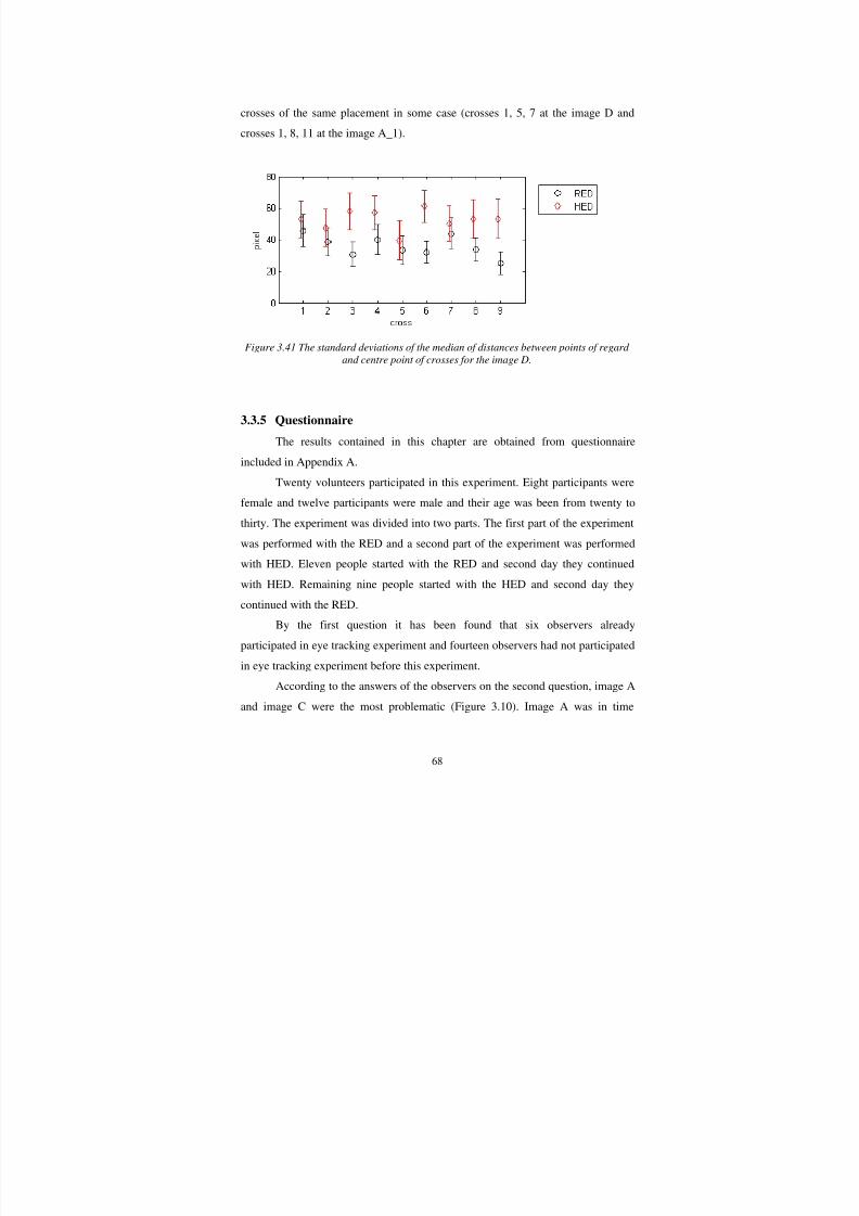
8/12/2019 Bara Kominkova Master Thesis
http://slidepdf.com/reader/full/bara-kominkova-master-thesis 68/90
68
crosses of the same placement in some case (crosses 1, 5, 7 at the image D and
crosses 1, 8, 11 at the image A_1).
Figure 3.41 The standard deviations of the median of distances between points of regard
and centre point of crosses for the image D.
3.3.5 Questionnaire
The results contained in this chapter are obtained from questionnaire
included in Appendix A.
Twenty volunteers participated in this experiment. Eight participants were
female and twelve participants were male and their age was been from twenty to
thirty. The experiment was divided into two parts. The first part of the experiment
was performed with the RED and a second part of the experiment was performed
with HED. Eleven people started with the RED and second day they continued
with HED. Remaining nine people started with the HED and second day they
continued with the RED.
By the first question it has been found that six observers already
participated in eye tracking experiment and fourteen observers had not participated
in eye tracking experiment before this experiment.
According to the answers of the observers on the second question, image A
and image C were the most problematic (Figure 3.10). Image A was in time

8/12/2019 Bara Kominkova Master Thesis
http://slidepdf.com/reader/full/bara-kominkova-master-thesis 69/90
69
longest task and has many symbols. The image C was the most difficult because it
required a lot of concentration of the observers.
Last question has been built in a psychological way. The observer should
answer which eye tracking device was more comfortable for realization of the
experiment. Most observers (16 observers) felt more comfortable with RED than
HED.
Causes why the observers felt worse with HED than RED were:
- Size of the helmet. The helmet was too small or too big. Observer worried
about helmet movement instead of concentrating on the experiment.
- Observer did not feel free; the weight of the helmet was noticeable by theobservers and after a while it became uncomfortable to wear and to heavy. In
case of RED observer did not have to wear anything and did not realize that the
camera was present.
- Observer felt uncomfortable when he/she had camera from of the face.
Causes why the observers felt better with HED than RED were:
- Observers had more possibility to move by the head, because the helmet was asa part of the observer and therefore they could concentrate better.
- The position of sitting was better to look at the image and observers had a
feeling that did not have to focus so much with the helmet.
In this experiment non observer wore glasses. Just four observers had
lenses which participated in the experiment. With the lenses no problems were
encountered, but for some participants they felt dry in their eye after concentrating
for a long time.
3.3.6 Disturbing elements
Many attributes of the observers could influence the calibration and all
processes of the experiment.
The greatest common disturbing element has been big movements of the
observers at the calibration process and in the experiment. This problem was major
for the RED. In the case of the HED was problem with size of the helmet.

8/12/2019 Bara Kominkova Master Thesis
http://slidepdf.com/reader/full/bara-kominkova-master-thesis 70/90
70
Especially the helmet was very big for girls, even if all bands have been adjusted
to a smallest possibility. Then the movement of the helmet was influencing whole
the experiment. For boys the size of the helmet was not a big problem.
The next attributes which influenced the experiment were small eyes and
make-up (eye shadow) on the eyes. While the small eyes, the eye tracking camera
could not localize the pupil center very well, what caused a recording coordinates
of the gaze eye in a zero position. While the make-up on the eyes, the coordinates
of the gaze did not match with the real gaze of the eye. The make-up caused other
reflections instead of the reflections from the pupil and cornea. The points of
regard occurred then outside of the observed object.
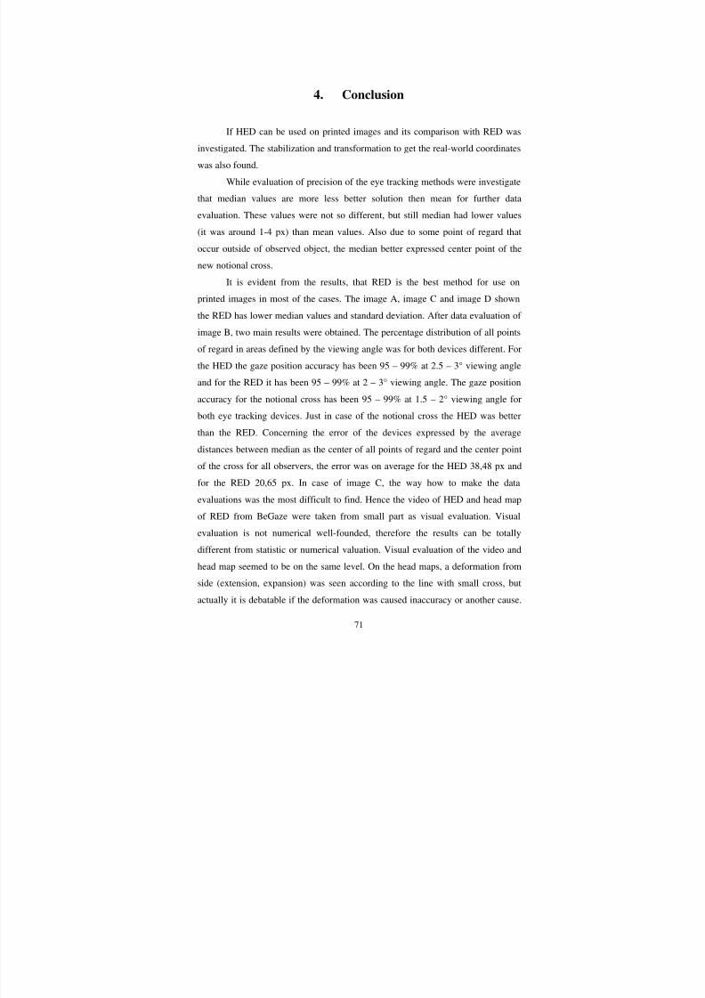
8/12/2019 Bara Kominkova Master Thesis
http://slidepdf.com/reader/full/bara-kominkova-master-thesis 71/90
71
4. Conclusion
If HED can be used on printed images and its comparison with RED was
investigated. The stabilization and transformation to get the real-world coordinates
was also found.
While evaluation of precision of the eye tracking methods were investigate
that median values are more less better solution then mean for further data
evaluation. These values were not so different, but still median had lower values
(it was around 1-4 px) than mean values. Also due to some point of regard that
occur outside of observed object, the median better expressed center point of thenew notional cross.
It is evident from the results, that RED is the best method for use on
printed images in most of the cases. The image A, image C and image D shown
the RED has lower median values and standard deviation. After data evaluation of
image B, two main results were obtained. The percentage distribution of all points
of regard in areas defined by the viewing angle was for both devices different. For
the HED the gaze position accuracy has been 95 – 99% at 2.5 – 3° viewing angleand for the RED it has been 95 – 99% at 2 – 3° viewing angle. The gaze position
accuracy for the notional cross has been 95 – 99% at 1.5 – 2° viewing angle for
both eye tracking devices. Just in case of the notional cross the HED was better
than the RED. Concerning the error of the devices expressed by the average
distances between median as the center of all points of regard and the center point
of the cross for all observers, the error was on average for the HED 38,48 px and
for the RED 20,65 px. In case of image C, the way how to make the data
evaluations was the most difficult to find. Hence the video of HED and head map
of RED from BeGaze were taken from small part as visual evaluation. Visual
evaluation is not numerical well-founded, therefore the results can be totally
different from statistic or numerical valuation. Visual evaluation of the video and
head map seemed to be on the same level. On the head maps, a deformation from
side (extension, expansion) was seen according to the line with small cross, but
actually it is debatable if the deformation was caused inaccuracy or another cause.
8/12/2019 Bara Kominkova Master Thesis
http://slidepdf.com/reader/full/bara-kominkova-master-thesis 72/90
72
Globally the visual evaluation on the scale: excellent, good, bad, could be
evaluated good. With the image D, questions were opened concerning the
calibration. The results said that when the observer leaves the chair and come back
the accuracy of the eye tracking device will be worst. That result we expected.
This accuracy concerning median distance of all points of regard was different in
average values 6.41 px for RED and 8.61 px for HED between image A_3 and
image D. For both devices, when observers get longer into the experiment, the
median values and standard deviation increases. Then the median and standard
deviation were from image D highest. The total precision of the RED is better than
the HED and the difference between HED and RED is around 7 – 14 px, it isapproximately 2.44 – 4.89 mm.
On the end of the experiment the observers filled out a questionnaire. The
questionnaires shown that the most problematic image as a task for observer was
image A and C, for in term of the time and difficultness concentration. Next results
from the questionnaires said the RED was most comfortable for observer.
In this paper there was said, that the calibration of the eye tracking
equipment is very necessary and critical part of the experiment. If an eye was
difficult to track, the calibration was very difficult to manage as well, it took too
long and observer became tired. It could be a cause of bad results in the
experiment, but we have tried to minimize this by removing the worst results.
Attempt at a better stabilization and transformation, which was done just
for directions (translation and rotation) instead of three directions (translation,
rotation and scale), can acquire better results in the HED case. The change of the
lens could be the next cause of getting better results. But in the first step, how to
get the real-world coordinates, the results are not so different. Majority of theobservers said that the RED was more comfortable than HED, but it is also
observer dependent.
8/12/2019 Bara Kominkova Master Thesis
http://slidepdf.com/reader/full/bara-kominkova-master-thesis 73/90
73
References
[1] Goldberg, J. H., Stimson, M. J., Lewenstein, M., Scott, N. and Wichansky, A. M.,
“Eye Tracking in Web Search Tasks: Design Implications,” ETRA ’02. NewOrleans, Louisiana USA, (2002).
[2] Cowen, L., Ball, L. J. and Delin, J., “An eye movement analysis of webpageusability,” In Proceedings of the annual HCI 2002, 317-335 (2002).
[3] McCarthy, J., Sasse, A., and Riegelsberger, J., “Could i have a menu please? an eyetracking study of design conventions,” In Proceedings of HCI2003, 401-414 (2003).
[4] In Hyönä, J. R. and Deubel, H. (Eds.), [The mind's eye: cognitive and appliedaspects of eye movement research], Radach, R., Lemmer, S.,Vorstius, Ch., Heller,D. and Radach, K., “Eye movement in the processing of print advertisements,”
Elsevier Science Ltd., 609-632 (2003).[5] In Hyönä, J. R. and Deubel, H. (Eds.), [The mind's eye: cognitive and applied
aspects of eye movement research], Holmqvist, K., Holsanova, J., Barthelson, M.and Lundqvist, D., “Reading or scanning? A study of newspaper and net paperreading,” Elsevier Science Ltd., 657-670 (2003).
[6] Babcock, J. S., Pelz, J. B. and Fairchild, M. D., “Eye tracking observers during rankorder, paired comparison, and graphical rating tasks,” IS&T PICS Conference,Rochester, 10-15 (2003).
[7] Ninassi, A., Le Meur, O., Le Callet, P., Barba, D. and Tirel, A., “Task Impact onthe Visual Attention in Subjective Image Quality Assessment,” In The 14thEuropean Signal Processing Conference, (2006).
[8] Pedersen, M., Hardeberg, J. Y. and Nussbaum, P., “Using gaze information toimprove image difference metrics,” Human Vision and Electronic Imaging XIII, Proceedings of SPIE Vol. 6806-35 (2008).
[9] Miyata, K., Saito, N., Tsumura, N., Haneishi, H. and Miyake, Y., “Eye MovementAnalysis and its Application to Evaluation of Image Quality,” IS&T/SID's 5thColor Imaging Conference, Color Science, Systems and Appl, Scottsdale, Arizona,116-119 (1997).
[10] Babcock, J., S., Lipps, M., and Pelz. J., B., “How people look at picture before,during, and after scene capture: Buswell revisited,” Proc. SPIE Human Vision andElectronic Imaging VII, 4662, 34-47 (2002).
[11] Bai, J., Nakaguchi, T., Tsumura, N., and Miyake, Y., “Evaluation of imagecorrected by retinex method based on S-CIELAB and gazing information,” IEICETransactions 89-A(11), 2955-2961 (2006).
[12] Farrell, J., E., “Image quality evaluation,” In Color Imaging: Vision andTechnology, eds. L.W. Macdonald and M. R. Luo, Wiley Press, 285-313 (1999).
[13] Mulligan, J. B., “Image processing for improved eye-tracking accuracy,” BehavRes Methods Instrum Comput., 54-65 (1997).
[14] Gintautas, D. and Ramanauskas, N., “The accuracy of eye tracking using imageprocessing,” Proceedings of the Third Nordic Conference on Human-ComputerInteraction, October 23-27, 2004, Tampere, Finland, 377-380 (2004).

8/12/2019 Bara Kominkova Master Thesis
http://slidepdf.com/reader/full/bara-kominkova-master-thesis 74/90
74
[15] Zhu, J. and Yang, J., “Subpixel Eye-Gaze Tracking,” Proceedings of the Fifth IEEEInternational Conference on Automatic Face and Gesture Recognition, May 20-21,131 (2002).
[16] Zhu, Z., Fujimura, K., and Ji, Q., “Real-Time Eye Detection and Tracking UnderVarious Light Conditions,” Proc. ETRA 2002, ACM Press, 139-144 (2002).
[17] Nevalainen, S. and Sajaniemi, J., “Comparison of Three Eye Tracking Devices inPsychology of Programming Research,” Proceedings of the 16th Annual Workshopof the Psychology of Programming Interest Group, Carlow, Ireland, 151-158(2004).
[18] DeSantis, R., Zhou, Q. and Ramey, J., “A Comparison of Eye Tracking Tools inUsability Testing,” STC Proceedings, Usability and Information Design, (2005).
[19] Lessing, S., and Linge., L., “IICap - A New Environment for Eye Tracking DataAnalysis,” Master/4th term thesis, Lunds University, (2002).
[20] Babcock, J., S., “Eye Tracking Observers During Color Image Evaluation Tasks,”Master's Thesis: New York: Rochester Institute of Technology, (2002).
[21] Babcock, J., S., “Eye Tracking Observers During Color Image Evaluation Tasks,”Master's Thesis: New York: Rochester Institute of Technology, (2002).
[22] Jaimes, A., Pelz, J., B., Grabowski, T., Babcock, J., and Chang, S.-F., “UsingHuman Observers' Eye Movements in Automatic Image Classifiers,” in proceedingsof SPIE Human Vision and Electronic Imaging VI, San Jose, CA, (2001).
[23] In Hyönä, J. R. and Deubel, H. (Eds.), [The mind's eye: cognitive and appliedaspects of eye movement research], Zülch, G., and Stowasser, S., “Eye tracking forevaluation human-computer interface,” Elsevier Science, Amterdam, 531-553
(2003).[24] Jacob, R., J., K., “Eye Tracking in Advanced Interface Design,” in Virtual
Environments and Advanced Interface Design, ed. by W. Barfield and T.A.Furness, Oxford University Press, New York , 258-288 (1995).
[25] Carpenter, R., “Eye movements,” http://www.cai.cam.ac.uk/people/rhsc/oculo.html,02/08/07
[26] In Hyönä, J. R. and Deubel, H. (Eds.), [The mind's eye: cognitive and appliedaspects of eye movement research], Goldberg, J. H. and Wichansky, A. M., “Eyetracking in Usability Evaluation: A Practitioner’s Guide,” North-Holland, 493–517(2003).
[27] Hedberg, B., “Areas of Interest in Eye Movement Data,” Master's graduate papers(2000).
[28] Salvucci, D., D., and Goldberg, J., H., “Identifying fixations and saccades in eye-tracking protocol,” Proceedings of the Eye Tracking Research and ApplicationsSymposium, New York: ACM Press, 71-78 (2000).
[29] Morimoto, C., H., Mimica, M., R., M., “Eye gaze tracking techniques forinteractive applications,” Computer Vision and Image Understanding 98 (1), 4-24(2005).
[30] Green, P. “Review of Eye Fixation Recording Methods and Equipment, ” TechnicalReport UMTRI9228, IVHS Technical Report 92-20, Ann Arbor, MI: TheUniversity of Michigan Transportation Research Institute, (1992).

8/12/2019 Bara Kominkova Master Thesis
http://slidepdf.com/reader/full/bara-kominkova-master-thesis 75/90
75
[31] SMI (SensoMotoric Instruments). iViewX system manual, version 1.07.19,document version IVX-1.7-0605.
[32] Kolakowski, S. M. and Pelz, J. B., “Compensating for Eye Tracer CameraMovement,” Proceedings of the 2006 Symposium on Eye Tracking Research &Applications, San Diego, California USA, (2006).
[33] Li, F., Kolakowski, S. and Pelz, J. B., “A model-based approach to video-based eyetracking, ” Journal of Modern Optics (2007).
[34] SMI(SensoMotoric Instruments). http://www.smi.de, 02/08/07
[35] Špako,v O., Miniotas, D., “Visualization of Eye Gaze Data using Heat Maps,”Electronics and eletrical engineering, No. 2 (74), (2007).
[36] Lessing, S., and Linge., L., “IICap - A New Environment for Eye Tracking DataAnalysis,” Master/4th term thesis, Lunds University, (2002).
[37] SMI (SensoMotoric Instruments). BeGazeTM
software manual, version 1.2,document version 1.06.03.
8/12/2019 Bara Kominkova Master Thesis
http://slidepdf.com/reader/full/bara-kominkova-master-thesis 76/90
76
List of Figures
Figure 2.1 Dark pupil tracking optics [29]. ..................................................................... 18
Figure 2.2 Dark pupil tracking system. ............................................................................ 18
Figure 2.3 Various of the Purkinje reflections [29]. ........................................................ 19
Figure 3.4 Workspace of the iView X system. ................................................................... 24
Figure 3.5 Detail of the head map example. ..................................................................... 27
Figure 3.6 Example of the head map for image B. ........................................................... 27
Figure 3.7 Remote Eye Tracking Device (RED). .............................................................. 28
Figure 3.8 Head-mounted Eye Tracking Device (HED). .................................................. 28
Figure 3.9 Arrangement in the experimental room. ......................................................... 31
Figure 3.10 Images used in the experiment (Image A, Image B, Image C, Image D). ..... 32
Figure 3.11 One of the targets of image B represent distances between circles
create by 0.5 viewing angles. ............................................................................................ 33
Fig 3.12 The direction of the tracking of the symbols on the images (Image A,
Image B, Image C, Image D). ........................................................................................... 35
Figure 3.13 Calibration plane for 9 points. ...................................................................... 37
Figure 3.14 Simulink demo model .................................................................................... 41
Figure 3.15 Video with target tracking the stabilization process. .................................... 41
Figure 3.16 The video track by the target (left) and stabilized image (right). .................. 42
Figure 3.17 Example of primary data evaluation for image A. ........................................ 44
Figure 3.18 Statistic evaluation of mean and median....................................................... 45
Figure 3.19 Median distances between points of regard and centre of the cross for
HED. ....................................................................................................................... 49
Figure 3.20 Median distances between points of regard and centre of the cross for
RED. .................................................................................................................................. 49
Figure 3.21 The standard deviations of the median of distances between points of
regard and centre point of crosses in the image A_1. ....................................................... 50
Figure 3.22 The standard deviations of the median of distances between points of
regard and centre point of crosses in the image A_2. ....................................................... 50Figure 3.23 The standard deviations of the median of distances between points of
regard and centre point of crosses in the image A_3. ....................................................... 51
Figure 3.24 Percentage distribution of points of regard in circles represent by
viewing angle for HED. .................................................................................................... 52
Figure 3.25 Percentage distribution of points of regard in circles represent by
viewing angle for RED. ..................................................................................................... 52
Figure 3.26 With a positive value the RED has a higher ratio of points inside the
different viewing angles, and with a negative value HED has a higher ratio of
points inside the different viewing angles. ........................................................................ 53
8/12/2019 Bara Kominkova Master Thesis
http://slidepdf.com/reader/full/bara-kominkova-master-thesis 77/90
77
Figure 3.27 Example of mean and median determining center of all points of
regard. ............................................................................................................................... 55
Figure 3.28 Example of mean and median determining center of all points of
regard. ............................................................................................................................... 55
Figure 3.29 Example of mean and median determining center of all points of
regard. ............................................................................................................................... 56
Figure 3.30 Percentage distribution of points of regard in circles represent by
viewing angle in case of notional cross; for HED. ........................................................... 57
Figure 3.31 Percentage distribution of points of regard in circles represent by
viewing angle in case of notional cross for RED. ............................................................. 57
Figure 3.32 With a positive value the RED has a higher ratio of points inside the
different viewing angles, and with a negative value HED has a higher ratio of
points inside the different viewing angles; in case of notional cross. ............................... 59
Figure 3.33 HED median values of whole image C for every observer with average
median value. .................................................................................................................... 60
Figure 3.34 RED median values of whole image C for every observer with average
median values.................................................................................................................... 61
Figure 3.35 The standard deviations of the median of distances between points of
regard and centre point of crosses in the image A_1,2,3 and image D of HED. .............. 63
Figure 3.36 The standard deviations of the median of distances between points of
regard and centre point of crosses in the image A_1,2,3 and image D of RED. .............. 63
Figure 3.37 Dependence of average standard deviations and median distances of
all observers for 15 crosses of image A_1, 2, 3 and for 9 crosses of image D; for
RED and HED values. ...................................................................................................... 66
Figure 3.38 Average values of values from Figure 9a) in dependence of standard
deviation on the median distance of image A_1, 2, 3 and for 9 crosses of image D;
for RED and HED values. ................................................................................................. 66
Figure 3.39 Dependence of average standard deviations and median distances of
all observers for 15 crosses of image A_1, 2, 3 and for 9 crosses of image D; for
RED. .................................................................................................................................. 67
Figure 3.40 Dependence of average standard deviations and median distances of
all observers for 15 crosses of image A_1, 2, 3 and for 9 crosses of image D; for
HED. ................................................................................................................................. 67
Figure 3.41 The standard deviations of the median of distances between points of
regard and centre point of crosses for the image D.......................................................... 68
8/12/2019 Bara Kominkova Master Thesis
http://slidepdf.com/reader/full/bara-kominkova-master-thesis 78/90
78
List of Tables
Table 3.1 HED average mean and median distances between points of regard and
center point of the cross for all observes.. ........................................................................ 47
Table 3.2 HED average maximum and minimum distances between points of
regard and center point of the cross for all observes.. ..................................................... 47
Table 3.3 RED Average mean and median distances between points of regard and
center point of the cross for all observes.. ........................................................................ 48
Table 3.4 RED average maximum and minimum distances between points of
regard and center point of the cross for all observes.. ..................................................... 48
Table 3.5 Percents of the points of regard contained in each view angle of circle;
for HED. ............................................................................................................................ 52
Table 3.6 Percents of the points of regard contained in each view angle of circle;
for RED. ............................................................................................................................ 53
Table 3.7 Percentage differences between RED and HED values (Table 3.5 and
3.6 ) for each view angle of circle. .................................................................................... 54
Table 3.8 Average distances [px] between median/mean as the center of all points
of regard and the center point of the cross for all observers, introducing an error
(inaccuracy) of the device. ................................................................................................ 55
Table 3.9 Percents of the points of regard contained in each view angle of circle in
case of notional cross; for HED. ...................................................................................... 58
Table 3.10 Percents of the points of regard contained in each view angle of circle
in case of notional cross; for RED. ................................................................................... 58
Table 3.11 Percentage differences between RED and HED values (Table 3.5 and
3.6 ) for each view angle of circle, in case of notional cross. ........................................... 59
Table 3.12 Overview of average distances of whole image for all observers. .................. 61
Table 3.13 RED average mean, median, maximum and minimum distances between
points of regard and center point of the cross for all observes. ....................................... 62
Table 3.14 HED average mean, median, maximum and minimum distances
between points of regard and center point of the cross for all observes. ......................... 62
Table 3.15 Average median distances for all observers of image A_1,2,3 and D; for
RED and HED. The image D contains only 9 crosses, which are identical with
some crosses of the image A. Their identity is visible in this table. .................................. 64Table 3.16 Average confident intervals for all observers of image A_1,2,3 and D;
for RED and HED. ............................................................................................................ 65
Table 3.17 Average standard deviations for all observers of image A_1,2,3 and D;
for RED and HED. ............................................................................................................ 65
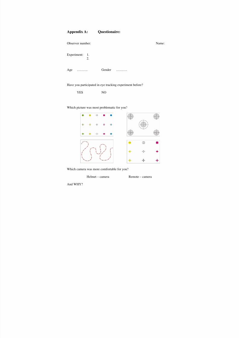
8/12/2019 Bara Kominkova Master Thesis
http://slidepdf.com/reader/full/bara-kominkova-master-thesis 79/90
Appendix A: Questionaire:
Observer number: Name:
Experiment: 1.2.
Age ………. Gender ……….
Have you participated in eye tracking experiment before?
YES NO
Which picture was most problematic for you?
Which camera was more comfortable for you?
Helmet – camera Remote – camera
And WHY?

8/12/2019 Bara Kominkova Master Thesis
http://slidepdf.com/reader/full/bara-kominkova-master-thesis 80/90
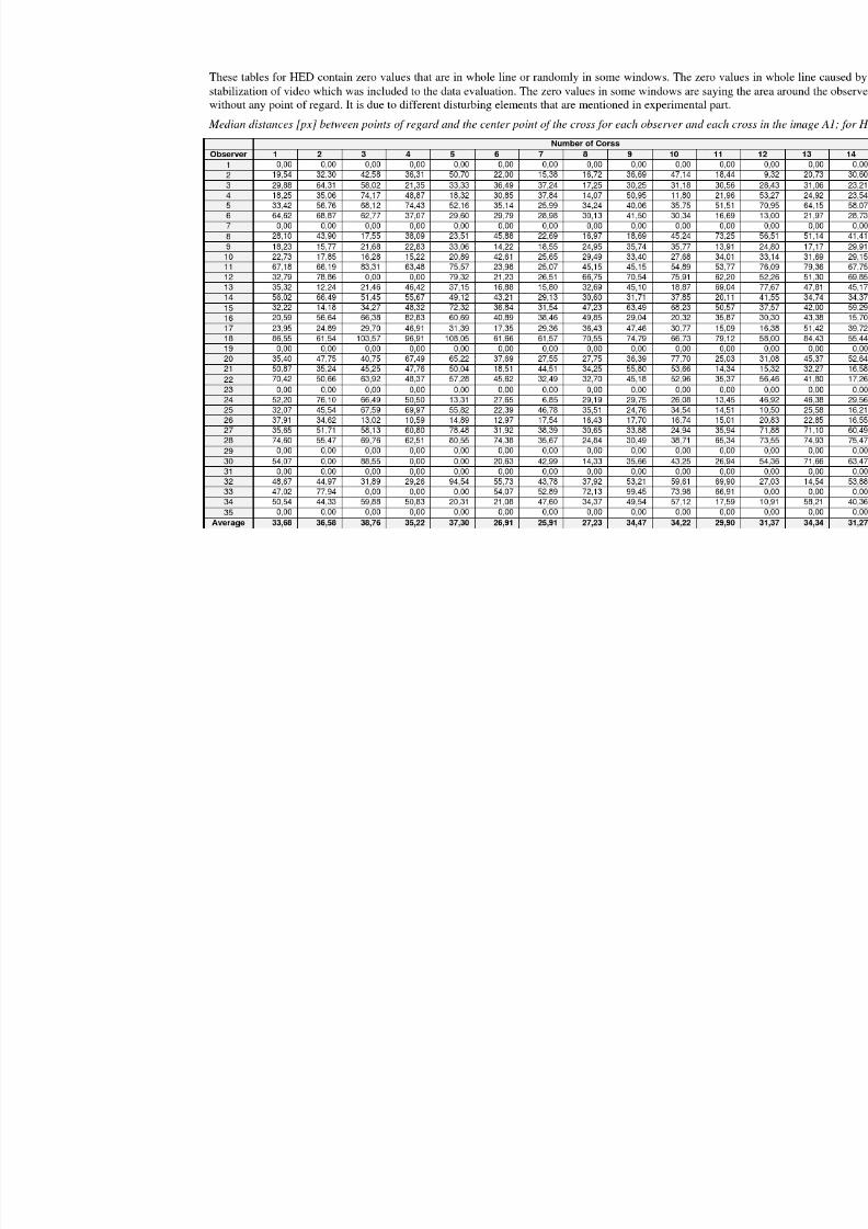
8/12/2019 Bara Kominkova Master Thesis
http://slidepdf.com/reader/full/bara-kominkova-master-thesis 81/90

8/12/2019 Bara Kominkova Master Thesis
http://slidepdf.com/reader/full/bara-kominkova-master-thesis 82/90
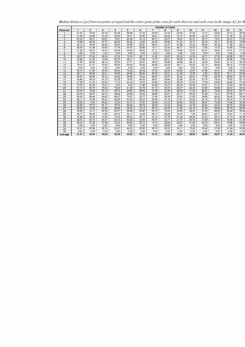
8/12/2019 Bara Kominkova Master Thesis
http://slidepdf.com/reader/full/bara-kominkova-master-thesis 83/90
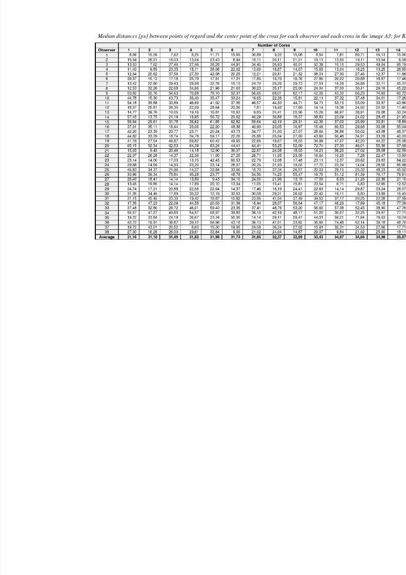
8/12/2019 Bara Kominkova Master Thesis
http://slidepdf.com/reader/full/bara-kominkova-master-thesis 84/90
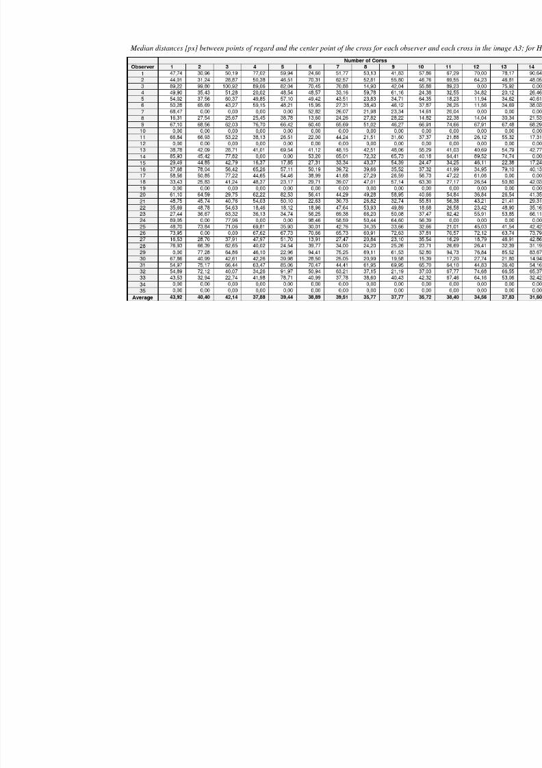
8/12/2019 Bara Kominkova Master Thesis
http://slidepdf.com/reader/full/bara-kominkova-master-thesis 85/90

8/12/2019 Bara Kominkova Master Thesis
http://slidepdf.com/reader/full/bara-kominkova-master-thesis 86/90
Appendix C: Distance between median and center point of the cross for
image B; RED and HED
Distances [px] between median as the center of all points of regard (new center point of the notionalcross) and the center point of the cross for each observer and each cross in the image B, introducing
an error (inaccuracy) of the device; for RED.
Observer 1cross 2cross 3cross 4cross 5cross
1 16,40 9,00 13,46 7,00 10,63
2 8,94 19,42 27,20 11,40 17,03
3 8,94 5,10 5,00 28,79 8,60
4 17,80 40,61 21,02 20,62 12,65
5 44,01 21,40 30,48 9,85 5,00
6 7,81 10,05 16,28 5,00 3,61
7 2,83 16,00 9,49 26,93 30,61
8 9,43 30,81 24,70 29,68 23,60
9 37,62 43,05 18,38 26,93 53,45
10 9,00 18,03 10,00 10,77 5,39
11 34,95 33,24 29,41 10,05 27,46
12 30,00 16,12 9,85 20,00 5,83
13 61,15 5,10 20,25 17,09 0,00
14 11,31 17,00 20,25 40,03 18,44
15 9,00 25,00 7,21 25,94 20,59
16 11,40 5,39 42,95 5,39 2,83
17 13,65 10,77 9,90 8,06 6,71
18 23,58 31,02 20,16 32,56 22,32
19 25,50 38,48 13,42 11,18 40,11
20 54,45 19,03 8,06 20,25 21,10
21 15,31 14,87 15,03 6,08 25,55
22 4,47 36,77 20,62 28,46 13,46
23 36,24 29,83 32,28 0,00 14,21
24 32,02 16,55 20,22 18,44 17,00
2516,16 40,22 23,26 12,65 15,81
26 26,63 18,60 61,07 36,01 65,51
27 12,81 17,56 9,00 5,39 7,28
28 6,40 13,04 5,10 2,83 2,24
29 18,87 18,11 15,00 8,06 0,00
30 22,36 22,20 13,45 14,42 26,02
31 35,36 8,38 16,32 21,10 17,03
32 19,10 16,55 22,50 40,16 14,32
33 30,86 69,35 65,22 58,62 53,85
34 20,59 45,00 26,23 5,32 28,32
35 38,40 29,07 30,59 29,07 11,18
36 34,93 26,48 37,85 25,32 18,00
37 14,87 10,06 18,03 17,09 26,48
38 6,32 20,62 15,81 17,00 14,42
Average 21,83 22,84 21,19 18,78 18,60
Average distances [px] between median as the center of all points of regard (new center point of the
notional cross) and the center point of the cross; and the distance (difference) [pixel] between mean
and median for the image B; for RED.
Cross Mean Median Difference
1 21,75 21,83 0,0733
2 23,16 22,84 0,3230
3 20,07 21,19 1,1193
4 18,89 18,78 0,1160
5 18,86 18,60 0,2649

8/12/2019 Bara Kominkova Master Thesis
http://slidepdf.com/reader/full/bara-kominkova-master-thesis 87/90
Distances [px] between median as the center of all points of regard(new center point of the notional
cross) and the center point of the cross for each observer and each cross in the image B, introducing
an error (inaccuracy) of the device; for HED.
Observer 1 cross 2 cross 3 cross 4 cross 5 cross
1 58,97 58,89 34,67 24,85 31,21
2 13,64 35,91 60,61 33,61 43,66
3 25,40 14,87 45,66 36,02 13,66
4 52,12 51,81 30,92 58,17 58,26
5 26,85 49,10 24,86 73,61 35,23
6 26,99 43,65 7,27 37,78 40,01
7 23,54 52,41 47,49 51,08 37,51
8 13,73 51,81 28,78 42,02 32,55
9 18,76 34,63 27,32 39,47 14,77
10 0,53 38,16 40,60 31,98 38,13
11 6,03 34,63 45,68 47,12 40,92
12 26,42 58,79 39,69 87,30 51,44
13 51,80 39,30 74,08 61,96 41,76
14 29,24 53,44 66,72 38,01 44,03
15 33,70 30,72 44,25 79,99 40,6216 10,90 42,43 53,03 59,72 41,38
17 8,82 12,84 16,88 21,69 22,35
18 4,37 49,92 14,92 54,29 34,40
19 58,10 65,63 44,94 74,48 43,33
20 28,27 17,98 53,42 3,14 36,12
21 34,64 46,93 30,52 25,61 17,57
22 16,40 29,20 6,22 30,75 22,04
23 53,38 40,39 13,88 64,96 19,27
24 13,66 34,14 51,68 58,69 4,13
25 19,51 3,43 17,92 44,02 34,66
26 10,40 26,33 3,01 31,72 16,81
27 14,32 32,84 12,45 22,48 14,69
28 26,15 12,18 24,29 13,17 25,72
29 61,76 64,46 34,67 73,35 64,92
30 76,32 39,51 22,34 23,88 45,6431 76,08 125,31 42,85 136,55 60,36
32 57,35 64,80 52,01 45,83 43,52
33 23,99 56,67 15,03 49,98 37,70
34 11,12 30,09 57,39 51,25 56,84
35 9,76 76,86 24,65 98,18 48,42
Average 29,23 43,43 34,59 49,33 35,82
Average distances [px] between median as the center of all points of regard (new center point of the
notional cross) and the center point of the cross; and the distance (difference) [pixel] between mean
and median for the image B; for HED.
Cross Mean Median Difference1 29,20 29,22 0,0269
2 42,69 43,43 0,7385
3 33,88 34,59 0,71024 48,61 49,33 0,7197
5 34,12 35,82 1,6925

8/12/2019 Bara Kominkova Master Thesis
http://slidepdf.com/reader/full/bara-kominkova-master-thesis 88/90
Appendix D: Median distances for image C; RED and HED
Median distances [px] between points of regard and the center point of the cross for each observer in whole
image C; for RED and HED.
RED HEDObserver Mean Median Max Min Mean Median Max Min
1 12,19 4,79 78,34 0,00 21,31 22,96 41,61 1,32
2 7,46 6,08 21,40 0,00 24,46 24,57 42,09 4,96
3 7,08 5,83 31,32 0,00 17,95 12,09 70,23 0,59
4 6,30 4,36 26,63 1,00 37,45 32,67 106,08 2,20
5 7,07 5,33 26,00 0,00 25,93 21,05 78,40 1,56
6 5,33 3,61 21,95 0,00 24,91 25,97 56,30 0,46
7 9,90 9,03 28,86 0,00 17,26 14,35 54,88 0,70
8 10,43 7,67 46,14 0,00 13,49 11,10 36,72 2,81
9 26,79 21,70 85,21 1,00 23,58 20,86 54,67 2,92
10 10,45 8,94 37,64 1,00 31,44 25,33 103,65 0,49
11 13,46 10,20 39,82 1,00 25,13 23,99 65,56 0,85
12 8,57 6,99 39,70 0,00 32,95 34,32 94,80 1,27
13 11,90 8,42 66,71 0,00 42,63 33,15 178,89 0,80
14 8,53 6,27 33,12 1,00 47,87 25,09 285,30 0,64
15 14,21 10,25 51,87 1,00 32,73 28,81 109,89 4,25
16 24,49 11,28 135,07 0,00 49,69 54,57 79,51 3,77
17 5,53 4,12 25,18 0,00 36,57 31,13 92,24 1,97
18 11,30 10,22 30,89 0,00 38,43 28,26 108,48 1,63
19 9,40 8,06 30,61 1,00 19,76 16,56 70,36 1,18
20 11,03 6,66 42,05 1,00 14,85 11,85 44,03 1,57
21 11,61 6,32 50,99 1,00 23,52 22,26 70,58 3,51
22 9,51 6,56 30,02 0,00 17,95 16,16 47,23 0,47
23 17,88 10,91 166,24 1,00 13,07 11,73 30,83 0,76
24 14,31 9,08 72,42 1,00 38,26 37,11 82,91 2,03
25 12,63 5,90 64,85 1,00 24,74 22,22 70,49 2,14
26 5,45 3,61 22,47 0,00 19,29 15,54 49,26 0,88
27 4,99 3,16 17,26 0,00 12,80 12,19 34,57 0,99
28 7,51 6,40 19,21 1,00 17,64 16,80 35,65 0,81
29 18,41 8,60 69,63 2,00 34,39 30,72 70,71 3,24
30 16,21 12,73 51,87 1,00 16,01 10,02 90,99 1,92
31 18,21 15,82 44,18 1,00 43,38 35,46 130,18 5,04
32 20,80 18,19 54,67 1,41 37,65 21,43 196,92 1,50
33 25,55 22,81 65,95 0,00 22,36 21,81 44,91 0,56
34 28,44 27,05 71,03 1,00 20,44 18,82 66,70 0,75
35 14,60 15,50 38,00 1,41 33,38 24,67 92,76 0,40
36 7,95 7,07 21,26 1,00 0,00 0,00 0,00 0,00
37 10,41 7,81 48,83 1,00 0,00 0,00 0,00 0,00
38 18,11 17,06 62,80 0,00 0,00 0,00 0,00 0,00
Average 12,74 9,59 49,22 0,60 27,24 23,30 82,52 1,74

8/12/2019 Bara Kominkova Master Thesis
http://slidepdf.com/reader/full/bara-kominkova-master-thesis 89/90
Appendix E: Median distances for image D; RED and HED
Median distances [px] between points of regard and the center point of the cross for each observer and each
cross in the image D; for RED.
Number of CorssObserver 1 2 3 4 5 6 7 8 9
1 29,72 20,32 12,04 33,62 18,79 6,40 22,06 15,73 10,05
2 60,21 39,83 25,18 57,04 28,84 15,03 49,21 28,60 24,41
3 15,52 18,52 14,23 33,96 27,31 35,51 13,45 38,94 49,96
4 91,69 74,89 41,23 74,33 33,52 48,41 82,87 38,12 29,55
5 34,68 53,94 21,61 61,22 12,35 7,62 39,70 30,00 22,09
6 11,66 14,14 22,85 23,77 21,02 39,36 24,04 16,00 26,17
7 97,59 58,82 54,23 66,19 20,94 37,34 79,08 34,02 17,12
8 35,61 31,06 37,27 17,46 21,98 28,28 18,44 15,00 18,97
9 46,62 31,47 25,00 29,02 54,64 39,13 21,21 64,76 60,21
10 0,00 108,72 93,49 0,00 86,49 62,65 84,01 79,71 48,04
11 59,17 40,36 48,87 71,55 74,69 47,95 61,77 32,45 30,81
12 96,18 35,36 20,13 75,04 38,37 30,07 71,81 54,92 13,04
13 73,82 48,83 27,80 60,21 26,17 32,65 66,48 32,99 21,84
14 15,02 29,97 41,19 17,07 29,41 48,66 24,00 26,91 51,97
15 45,61 35,74 35,03 48,83 34,57 54,57 43,57 29,83 20,10
16 46,10 27,46 33,90 47,01 39,05 27,51 115,07 44,55 50,23
17 110,35 105,98 102,36 107,75 124,02 71,17 65,05 94,88 56,86
18 45,97 42,31 26,25 27,38 18,23 25,50 69,96 18,39 27,02
19 120,25 118,34 0,00 116,68 0,00 0,00 76,94 92,01 0,00
20 32,06 28,16 26,93 21,96 25,63 17,46 44,66 19,85 20,52
21 69,03 21,20 43,17 29,67 10,00 10,63 38,90 34,02 20,00
22 40,03 24,52 26,93 38,28 37,36 13,42 37,40 22,76 23,77
23 104,20 76,32 80,91 64,07 68,10 87,79 64,42 77,37 77,67
24 39,21 22,09 35,23 24,84 44,28 21,02 25,30 35,93 20,22
25 74,03 29,72 41,82 94,92 72,73 42,06 73,79 38,11 30,59
26 45,53 61,54 57,17 54,20 105,95 48,10 76,20 84,27 66,66
27 58,31 81,14 0,00 82,28 83,68 0,00 0,00 0,00 67,36
28 22,36 39,46 19,21 41,88 33,96 20,56 26,00 39,70 19,17
29 67,12 62,77 61,52 33,14 50,59 68,94 33,96 41,32 50,45
30 15,23 7,71 10,61 18,44 32,55 9,85 10,53 19,96 18,49
31 86,31 40,72 39,46 61,84 20,03 29,92 47,40 20,62 12,37
32 31,25 23,54 11,22 12,65 39,40 31,31 30,87 26,76 19,17
33 29,07 25,24 26,02 25,63 29,00 27,02 68,47 34,79 21,02
34 83,24 39,85 17,87 28,06 41,23 70,22 34,54 17,15 57,07
35 41,00 37,86 11,18 69,12 47,78 21,37 108,25 46,07 64,63
36 72,86 63,60 66,61 76,06 33,38 42,64 95,28 49,09 43,85
37 40,91 36,42 41,55 24,17 23,26 53,85 11,31 38,63 22,56
38 19,70 43,42 52,84 15,13 16,02 58,52 18,25 27,46 65,03
Average 41,93 40,56 39,96 40,69 39,44 39,26 40,66 36,33 34,19

8/12/2019 Bara Kominkova Master Thesis
http://slidepdf.com/reader/full/bara-kominkova-master-thesis 90/90
Median distances [px] between points of regard and the center point of the cross for each observer and each
cross in the image D; for HED.
Number of CorssObserver 1 2 3 4 5 6 7 8 9
1 105,08 34,93 16,86 74,29 13,49 11,31 39,86 10,11 17,052 80,77 71,27 81,41 85,02 71,56 84,56 91,16 79,51 75,55
3 11,74 26,40 31,59 39,17 14,19 26,84 21,68 23,88 18,90
4 96,81 104,87 49,95 46,51 83,12 47,52 39,00 53,26 38,76
5 37,63 45,71 56,45 28,25 22,48 33,80 40,66 42,26 34,67
6 22,13 18,16 57,16 59,26 33,96 48,47 36,92 27,97 48,92
7 63,21 71,80 61,08 90,22 102,03 77,16 0,00 94,87 95,78
8 69,99 76,78 92,17 91,01 95,18 88,84 89,18 94,52 104,82
9 48,98 68,17 70,68 19,74 30,76 88,05 30,48 51,76 95,00
10 50,45 49,11 80,80 67,97 88,64 83,66 96,04 94,39 80,06
11 0,00 0,00 0,00 88,24 0,00 88,83 90,79 95,11 93,98
12 65,71 44,18 20,52 61,21 40,13 21,75 43,68 50,83 29,96
13 92,96 0,00 80,68 123,75 0,00 78,91 117,73 127,66 0,00
14 41,79 17,63 73,44 60,02 21,45 60,45 60,38 56,34 12,59
15 0,00 0,00 0,00 105,39 0,00 51,21 0,00 0,00 0,00
16 60,11 30,10 88,28 33,61 65,81 76,52 31,91 53,12 52,3317 35,89 61,69 88,23 68,71 101,04 95,00 80,30 53,38 90,41
18 78,60 55,65 22,82 46,31 21,79 22,04 63,68 49,76 32,22
19 24,39 71,23 49,72 57,60 30,54 60,20 77,30 65,19 52,55
20 49,37 20,93 59,37 57,08 40,75 33,76 66,93 30,04 35,84
21 0,00 0,00 0,00 0,00 0,00 0,00 0,00 0,00 0,00
22 0,00 0,00 0,00 0,00 0,00 0,00 0,00 0,00 0,00
23 0,00 0,00 0,00 0,00 0,00 0,00 0,00 0,00 0,00
24 48,85 41,26 52,34 49,73 80,79 64,38 46,73 53,69 64,44
25 99,58 103,00 91,10 0,00 0,00 52,15 39,52 83,93 98,43
26 66,36 72,07 48,30 67,84 57,66 43,81 15,03 23,46 26,37
27 77,47 93,97 92,30 84,96 0,00 104,81 76,67 82,78 107,45
28 0,00 0,00 0,00 0,00 0,00 0,00 0,00 0,00 0,00
29 49,42 46,18 24,50 37,29 31,95 38,14 53,15 44,26 40,61
30 0,00 0,00 0,00 0,00 0,00 0,00 0,00 0,00 0,00
31 32,49 17,61 65,50 44,11 59,78 62,18 50,45 45,17 75,6632 17,66 71,72 86,65 42,88 55,61 75,67 35,65 49,09 54,07
33 79,22 86,55 0,00 37,34 47,23 116,65 63,87 48,84 86,98
34 120,66 106,64 102,43 0,00 84,12 91,82 106,06 128,42 94,60
35 55,70 12,53 23,85 46,32 39,33 24,34 49,92 101,70 61,43
Average 48,09 43,43 47,66 48,97 38,10 52,94 47,28 51,87 49,13