atlas.physics.arizona.eduatlas.physics.arizona.edu/~shupe/ATLAS/BumpHunting/... ·...

Model-independent and quasi-model-independent search for new physics at CDF

T. Aaltonen,22 A. Abulencia,23 J. Adelman,12 T. Akimoto,53 M.G. Albrow,16 B. Alvarez Gonzalez,10 S. Amerio,41

D. Amidei,33 A. Anastassov,50 A. Annovi,18 J. Antos,13 G. Apollinari,16 A. Apresyan,46 T. Arisawa,55 A. Artikov,14

W. Ashmanskas,16 A. Aurisano,51 F. Azfar,40 P. Azzi-Bacchetta,41 P. Azzurri,44 N. Bacchetta,41 W. Badgett,16

V. E. Barnes,46 B. A. Barnett,24 S. Baroiant,6 V. Bartsch,29 G. Bauer,31 P.-H. Beauchemin,32 F. Bedeschi,44 P. Bednar,13

S. Behari,24 G. Bellettini,44 J. Bellinger,57 A. Belloni,31 D. Benjamin,15 A. Beretvas,16 T. Berry,28 A. Bhatti,48

M. Binkley,16 D. Bisello,41 I. Bizjak,29 R. E. Blair,2 C. Blocker,5 B. Blumenfeld,24 A. Bocci,15 A. Bodek,47 V. Boisvert,47

G. Bolla,46 A. Bolshov,31 D. Bortoletto,46 J. Boudreau,45 A. Boveia,9 B. Brau,9 L. Brigliadori,4 C. Bromberg,34

E. Brubaker,12 J. Budagov,14 H. S. Budd,47 S. Budd,23 K. Burkett,16 G. Busetto,41 P. Bussey,20 A. Buzatu,32 K. L. Byrum,2

S. Cabrera,15,s M. Campanelli,34 M. Campbell,33 F. Canelli,16 A. Canepa,43 D. Carlsmith,57 R. Carosi,44 S. Carrillo,17,m

S. Carron,32 B. Casal,10 M. Casarsa,16 A. Castro,4 P. Catastini,44 D. Cauz,52 A. Cerri,27 L. Cerrito,29,q S. H. Chang,26

Y. C. Chen,1 M. Chertok,6 G. Chiarelli,44 G. Chlachidze,16 F. Chlebana,16 K. Cho,26 D. Chokheli,14 J. P. Chou,21

G. Choudalakis,31 S. H. Chuang,50 K. Chung,11 W.H. Chung,57 Y. S. Chung,47 C. I. Ciobanu,23 M.A. Ciocci,44 A. Clark,19

D. Clark,5 G. Compostella,41 M. E. Convery,16 J. Conway,6 B. Cooper,29 K. Copic,33 M. Cordelli,18 G. Cortiana,41

F. Crescioli,44 C. Cuenca Almenar,6,s J. Cuevas,10,p R. Culbertson,16 J. C. Cully,33 D. Dagenhart,16 M. Datta,16 T. Davies,20

P. de Barbaro,47 S. De Cecco,49 A. Deisher,27 G. De Lentdecker,47,e M. Dell’Orso,44 L. Demortier,48 J. Deng,15

M. Deninno,4 D. De Pedis,49 P. F. Derwent,16 G. P. Di Giovanni,42 C. Dionisi,49 B. Di Ruzza,52 J. R. Dittmann,3 S. Donati,44

P. Dong,7 J. Donini,41 T. Dorigo,41 S. Dube,50 J. Efron,37 R. Erbacher,6 D. Errede,23 S. Errede,23 R. Eusebi,16 H. C. Fang,27

S. Farrington,28 W. T. Fedorko,12 R. G. Feild,58 M. Feindt,25 J. P. Fernandez,30 C. Ferrazza,44 R. Field,17 G. Flanagan,46

R. Forrest,6 S. Forrester,6 M. Franklin,21 J. C. Freeman,27 I. Furic,17 M. Gallinaro,48 J. Galyardt,11 F. Garberson,9

J. E. Garcia,44 A. F. Garfinkel,46 H. Gerberich,23 D. Gerdes,33 S. Giagu,49 P. Giannetti,44 K. Gibson,45 J. L. Gimmell,47

C. Ginsburg,16 N. Giokaris,14,b M. Giordani,52 P. Giromini,18 M. Giunta,44 V. Glagolev,14 D. Glenzinski,16 M. Gold,35

N. Goldschmidt,17 J. Goldstein,40,d A. Golossanov,16 G. Gomez,10 G. Gomez-Ceballos,31 M. Goncharov,51 O. Gonzalez,30

I. Gorelov,35 A. T. Goshaw,15 K. Goulianos,48 A. Gresele,41 S. Grinstein,21 C. Grosso-Pilcher,12 R. C. Group,16

U. Grundler,23 J. Guimaraes da Costa,21 Z. Gunay-Unalan,34 K. Hahn,31 S. R. Hahn,16 E. Halkiadakis,50 A. Hamilton,19

B.-Y. Han,47 J. Y. Han,47 R. Handler,57 F. Happacher,18 K. Hara,53 D. Hare,50 M. Hare,54 S. Harper,40 R. F. Harr,56

R.M. Harris,16 M. Hartz,45 K. Hatakeyama,48 J. Hauser,7 C. Hays,40 M. Heck,25 A. Heijboer,43 J. Heinrich,43

C. Henderson,31 M. Herndon,57 J. Heuser,25 S. Hewamanage,3 D. Hidas,15 C. S. Hill,9,d D. Hirschbuehl,25 A. Hocker,16

S. Hou,1 M. Houlden,28 S.-C. Hsu,8 B. T. Huffman,40 R. E. Hughes,37 U. Husemann,58 J. Huston,34 J. Incandela,9

G. Introzzi,44 M. Iori,49 A. Ivanov,6 B. Iyutin,31 E. James,16 B. Jayatilaka,15 D. Jeans,49 E. J. Jeon,26 S. Jindariani,17

W. Johnson,6 M. Jones,46 K.K. Joo,26 S. Y. Jun,11 J. E. Jung,26 T. R. Junk,23 T. Kamon,51 D. Kar,17 P. E. Karchin,56

Y. Kato,39 R. Kephart,16 U. Kerzel,25 V. Khotilovich,51 B. Kilminster,37 D.H. Kim,26 H. S. Kim,26 J. E. Kim,26 M. J. Kim,16

S. B. Kim,26 S. H. Kim,53 Y.K. Kim,12 N. Kimura,53 L. Kirsch,5 S. Klimenko,17 M. Klute,31 B. Knuteson,31 B. R. Ko,15

S. A. Koay,9 K. Kondo,55 D. J. Kong,26 J. Konigsberg,17 A. Korytov,17 A.V. Kotwal,15 J. Kraus,23 M. Kreps,25 J. Kroll,43

N. Krumnack,3 M. Kruse,15 V. Krutelyov,9 T. Kubo,53 S. E. Kuhlmann,2 T. Kuhr,25 N. P. Kulkarni,56 Y. Kusakabe,55

S. Kwang,12 A. T. Laasanen,46 S. Lai,32 S. Lami,44 M. Lancaster,29 R. L. Lander,6 K. Lannon,37 A. Lath,50 G. Latino,44

I. Lazzizzera,41 T. LeCompte,2 J. Lee,47 J. Lee,26 Y. J. Lee,26 S.W. Lee,51,r R. Lefevre,19 N. Leonardo,31 S. Leone,44

S. Levy,12 J. D. Lewis,16 C. Lin,58 M. Lindgren,16 E. Lipeles,8 A. Lister,6 D.O. Litvintsev,16 T. Liu,16 N. S. Lockyer,43

A. Loginov,58 M. Loreti,41 L. Lovas,13 R.-S. Lu,1 D. Lucchesi,41 J. Lueck,25 C. Luci,49 P. Lujan,27 P. Lukens,16 G. Lungu,17

L. Lyons,40 R. Lysak,13 E. Lytken,46 P. Mack,25 D. MacQueen,32 R. Madrak,16 K. Maeshima,16 K. Makhoul,31 T. Maki,22

P. Maksimovic,24 S. Malde,40 S. Malik,29 A. Manousakis,14,b F. Margaroli,46 C. Marino,25 C. P. Marino,23 A. Martin,58

M. Martin,24 V. Martin,20,k R. Martınez-Balların,30 T. Maruyama,53 P. Mastrandrea,49 T. Masubuchi,53 M. E. Mattson,56

P. Mazzanti,4 K. S. McFarland,47 P. McIntyre,51 R. McNulty,28,j A. Mehta,28 P. Mehtala,22 S. Menzemer,10,l A. Menzione,44

P. Merkel,46 C. Mesropian,48 A. Messina,34 T. Miao,16 N. Miladinovic,5 J. Miles,31 R. Miller,34 C. Mills,21 M. Milnik,25

A. Mitra,1 G. Mitselmakher,17 H. Miyake,53 S. Moed,19 N. Moggi,4 C. S. Moon,26 R. Moore,16 M. Morello,44

P. Movilla Fernandez,27 S. Mrenna,16 J. Mulmenstadt,27 A. Mukherjee,16 Th. Muller,25 R. Mumford,24 P. Murat,16

M. Mussini,4 J. Nachtman,16 Y. Nagai,53 A. Nagano,53 J. Naganoma,55 K. Nakamura,53 I. Nakano,38 A. Napier,54

V. Necula,15 C. Neu,43 M. S. Neubauer,23 L. Nodulman,2 M. Norman,8 O. Norniella,23 E. Nurse,29 S. H. Oh,15 Y.D. Oh,26

I. Oksuzian,17 T. Okusawa,39 R. Orava,22 K. Osterberg,22 S. Pagan Griso,41 C. Pagliarone,44 E. Palencia,16

V. Papadimitriou,16 A. Papaikonomou,25 A.A. Paramonov,12 B. Parks,37 S. Pashapour,32 J. Patrick,16 G. Pauletta,52

PHYSICAL REVIEW D 78, 012002 (2008)

1550-7998=2008=78(1)=012002(42) 012002-1 � 2008 The American Physical Society

M. Paulini,11 C. Paus,31 D. E. Pellett,6 A. Penzo,52 T. J. Phillips,15 G. Piacentino,44 J. Piedra,42 L. Pinera,17 K. Pitts,23

C. Plager,7 L. Pondrom,57 O. Poukhov,14 N. Pounder,40 F. Prakoshyn,14 A. Pronko,16 J. Proudfoot,2 F. Ptohos,16,i

G. Punzi,44 J. Pursley,57 J. Rademacker,40,d A. Rahaman,45 V. Ramakrishnan,57 N. Ranjan,46 I. Redondo,30 B. Reisert,16

V. Rekovic,35 P. Renton,40 M. Rescigno,49 S. Richter,25 F. Rimondi,4 L. Ristori,44 A. Robson,20 T. Rodrigo,10 E. Rogers,23

R. Roser,16 M. Rossi,52 R. Rossin,9 P. Roy,32 A. Ruiz,10 J. Russ,11 V. Rusu,16 H. Saarikko,22 A. Safonov,51

W.K. Sakumoto,47 G. Salamanna,49 L. Santi,52 S. Sarkar,49 L. Sartori,44 K. Sato,16 A. Savoy-Navarro,42 T. Scheidle,25

P. Schlabach,16 E. E. Schmidt,16 M. P. Schmidt,58 M. Schmitt,36 T. Schwarz,6 L. Scodellaro,10 A. L. Scott,9 A. Scribano,44

F. Scuri,44 A. Sedov,46 S. Seidel,35 Y. Seiya,39 A. Semenov,14 L. Sexton-Kennedy,16 A. Sfyrla,19 S. Z. Shalhout,56

T. Shears,28 P. F. Shepard,45 D. Sherman,21 M. Shimojima,53,o M. Shochet,12 Y. Shon,57 I. Shreyber,19 A. Sidoti,44

A. Sisakyan,14 A. J. Slaughter,16 J. Slaunwhite,37 K. Sliwa,54 J. R. Smith,6 F. D. Snider,16 R. Snihur,32 M. Soderberg,33

A. Soha,6 S. Somalwar,50 V. Sorin,34 J. Spalding,16 F. Spinella,44 T. Spreitzer,32 P. Squillacioti,44 M. Stanitzki,58

R. St. Denis,20 B. Stelzer,7 O. Stelzer-Chilton,40 D. Stentz,36 J. Strologas,35 D. Stuart,9 J. S. Suh,26 A. Sukhanov,17

H. Sun,54 I. Suslov,14 T. Suzuki,53 A. Taffard,23,f R. Takashima,38 Y. Takeuchi,53 R. Tanaka,38 M. Tecchio,33 P. K. Teng,1

K. Terashi,48 J. Thom,16,h A. S. Thompson,20 G.A. Thompson,23 E. Thomson,43 P. Tipton,58 V. Tiwari,11 S. Tkaczyk,16

D. Toback,51 S. Tokar,13 K. Tollefson,34 T. Tomura,53 D. Tonelli,16 S. Torre,18 D. Torretta,16 S. Tourneur,42 Y. Tu,43

N. Turini,44 F. Ukegawa,53 S. Uozumi,53 S. Vallecorsa,19 N. van Remortel,22 A. Varganov,33 E. Vataga,35 F. Vazquez,17,m

G. Velev,16 C. Vellidis,44,b V. Veszpremi,46 M. Vidal,30 R. Vidal,16 I. Vila,10 R. Vilar,10 T. Vine,29 M. Vogel,35 G. Volpi,44

F. Wurthwein,8 P. Wagner,43 R.G. Wagner,2 R. L. Wagner,16 J. Wagner,25 W. Wagner,25 R. Wallny,7 S.M. Wang,1

A. Warburton,32 D. Waters,29 M. Weinberger,51 W.C. Wester III,16 B. Whitehouse,54 D. Whiteson,43,f A. B. Wicklund,2

E. Wicklund,16 G. Williams,32 H.H. Williams,43 P. Wilson,16 B. L. Winer,37 P. Wittich,16,h S. Wolbers,16 C. Wolfe,12

T. Wright,33 X. Wu,19 S.M. Wynne,28 S. Xie,31 A. Yagil,8 K. Yamamoto,39 J. Yamaoka,50 T. Yamashita,38 C. Yang,58

U. K. Yang,12,o Y. C. Yang,26 W.M. Yao,27 G. P. Yeh,16 J. Yoh,16 K. Yorita,12 T. Yoshida,39 G. B. Yu,47 I. Yu,26 S. S. Yu,16

J. C. Yun,16 L. Zanello,49 A. Zanetti,52 I. Zaw,21 X. Zhang,23 Y. Zheng,7,c and S. Zucchelli4

(CDF Collaboration)a

1Institute of Physics, Academia Sinica, Taipei, Taiwan 11529, Republic of China2Argonne National Laboratory, Argonne, Illinois 60439, USA

3Baylor University, Waco, Texas 76798, USA4Istituto Nazionale di Fisica Nucleare, University of Bologna, I-40127 Bologna, Italy

5Brandeis University, Waltham, Massachusetts 02254, USA6University of California, Davis, Davis, California 95616, USA

7University of California, Los Angeles, Los Angeles, California 90024, USA8University of California, San Diego, La Jolla, California 92093, USA

9University of California, Santa Barbara, Santa Barbara, California 93106, USA10Instituto de Fisica de Cantabria, CSIC-University of Cantabria, 39005 Santander, Spain

11Carnegie Mellon University, Pittsburgh, Pennsylvania 15213, USA12Enrico Fermi Institute, University of Chicago, Chicago, Illinois 60637, USA

13Comenius University, 842 48 Bratislava, Slovakia; Institute of Experimental Physics, 040 01 Kosice, Slovakia14Joint Institute for Nuclear Research, RU-141980 Dubna, Russia

15Duke University, Durham, North Carolina 27708, USA16Fermi National Accelerator Laboratory, Batavia, Illinois 60510, USA

17University of Florida, Gainesville, Florida 32611, USA18Laboratori Nazionali di Frascati, Istituto Nazionale di Fisica Nucleare, I-00044 Frascati, Italy

19University of Geneva, CH-1211 Geneva 4, Switzerland20Glasgow University, Glasgow G12 8QQ, United Kingdom

21Harvard University, Cambridge, Massachusetts 02138, USA22Division of High Energy Physics, Department of Physics, University of Helsinki and Helsinki Institute of Physics,

FIN-00014, Helsinki, Finland23University of Illinois, Urbana, Illinois 61801, USA

24The Johns Hopkins University, Baltimore, Maryland 21218, USA25Institut fur Experimentelle Kernphysik, Universitat Karlsruhe, 76128 Karlsruhe, Germany

26Center for High Energy Physics, Kyungpook National University, Taegu 702-701, Korea; Seoul National University, Seoul 151-742,

Korea; SungKyunKwan University, Suwon 440-746, Korea; Korea Institute of Science and Technology Information, Daejeon, 305-806,

Korea; Chonnam National University, Gwangju, 500-757, Korea27Ernest Orlando Lawrence Berkeley National Laboratory, Berkeley, California 94720, USA

T. AALTONEN et al. PHYSICAL REVIEW D 78, 012002 (2008)

012002-2

28University of Liverpool, Liverpool L69 7ZE, United Kingdom29University College London, London WC1E 6BT, United Kingdom

30Centro de Investigaciones Energeticas Medioambientales y Tecnologicas, E-28040 Madrid, Spain31Massachusetts Institute of Technology, Cambridge, Massachusetts 02139, USA

32Institute of Particle Physics, McGill University, Montreal, Canada H3A 2T8; and University of Toronto, Toronto, Canada M5S 1A733University of Michigan, Ann Arbor, Michigan 48109, USA

34Michigan State University, East Lansing, Michigan 48824, USA35University of New Mexico, Albuquerque, New Mexico 87131, USA

36Northwestern University, Evanston, Illinois 60208, USA37The Ohio State University, Columbus, Ohio 43210, USA

38Okayama University, Okayama 700-8530, Japan39Osaka City University, Osaka 588, Japan

40University of Oxford, Oxford OX1 3RH, United Kingdom41University of Padova, Istituto Nazionale di Fisica Nucleare, Sezione di Padova-Trento, I-35131 Padova, Italy

42LPNHE, Universite Pierre et Marie Curie/IN2P3-CNRS, UMR7585, Paris, F-75252 France43University of Pennsylvania, Philadelphia, Pennsylvania 19104, USA

44Istituto Nazionale di Fisica Nucleare Pisa, Universities of Pisa, Siena and Scuola Normale Superiore, I-56127 Pisa, Italy45University of Pittsburgh, Pittsburgh, Pennsylvania 15260, USA

46Purdue University, West Lafayette, Indiana 47907, USA47University of Rochester, Rochester, New York 14627, USA

48The Rockefeller University, New York, New York 10021, USA49Istituto Nazionale di Fisica Nucleare, Sezione di Roma 1, University of Rome ‘‘La Sapienza,’’ I-00185 Roma, Italy

50Rutgers University, Piscataway, New Jersey 08855, USA51Texas A&M University, College Station, Texas 77843, USA

52Istituto Nazionale di Fisica Nucleare, University of Trieste/Udine, Italy53University of Tsukuba, Tsukuba, Ibaraki 305, Japan54Tufts University, Medford, Massachusetts 02155, USA

55Waseda University, Tokyo 169, Japan56Wayne State University, Detroit, Michigan 48201, USA

57University of Wisconsin, Madison, Wisconsin 53706, USA58Yale University, New Haven, Connecticut 06520, USA(Received 13 December 2007; published 11 July 2008)

Data collected in run II of the Fermilab Tevatron are searched for indications of new electroweak scale

physics. Rather than focusing on particular new physics scenarios, CDF data are analyzed for discrep-

ancies with respect to the standard model prediction. A model-independent approach (VISTA) considers the

gross features of the data and is sensitive to new large cross section physics. A quasi-model-independent

approach (SLEUTH) searches for a significant excess of events with large summed transverse momentum

and is particularly sensitive to new electroweak scale physics that appears predominantly in one final state.

This global search for new physics in over 300 exclusive final states in 927 pb�1 of p �p collisions atffiffiffis

p ¼ 1:96 TeV reveals no such significant indication of physics beyond the standard model.

rTexas Tech University, Lubbock, TX 79409, USA;

qQueen Mary’s College, University of London, London, E1 4NS, England;

pUniversity de Oviedo, E-33007 Oviedo, Spain;

oNagasaki Institute of Applied Science, Nagasaki, Japan;

nUniversity of Manchester, Manchester M13 9PL, England;

mUniversidad Iberoamericana, Mexico D.F., Mexico;

lUniversity of Heidelberg, D-69120 Heidelberg, Germany;

kUniversity of Edinburgh, Edinburgh EH9 3JZ, United Kingdom;

jUniversity College Dublin, Dublin 4, Ireland;

iUniversity of Cyprus, Nicosia CY-1678, Cyprus;

gUniversity of California Santa Cruz, Santa Cruz, CA 95064, USA;

sIFIC (CSIC-Universitat de Valencia), 46071 Valencia, Spain.

fUniversity of California, Irvine, Irvine, CA 92697, USA;

eUniversity Libre de Bruxelles, B-1050 Brussels, Belgium;

dUniversity of Bristol, Bristol BS8 1TL, United Kingdom;

cChinese Academy of Sciences, Beijing 100864, China;

bUniversity of Athens, 15784 Athens, Greece;

hCornell University, Ithaca, NY 14853, USA;

aWith visitors from

MODEL-INDEPENDENT AND QUASI-MODEL-INDEPENDENT . . . PHYSICAL REVIEW D 78, 012002 (2008)

012002-3

DOI: 10.1103/PhysRevD.78.012002 PACS numbers: 13.90.+i

I. INTRODUCTION

In the past 30 years of frontier energy collider physics,the only objects discovered were those for which thepredictions were definite. TheW and Z bosons (discoveredat CERN in 1983 [1–4]) and the top quark (discovered atFermilab in 1995 [5,6]) were well-known objects longbefore their discoveries, with all quantum numbers butmass uniquely specified. The present situation is qualita-tively different, with plausible predictions for physics lyingbeyond the standard model running the gamut of possibleexperimental signatures.

Searches for physics beyond the standard model typi-cally begin with a particular model. A region is selected inthe data where the model’s expected contribution is en-hanced, and the extent to which the data (dis)favor themodel is determined by comparing the prediction to data.

The state of the theoretical landscape and the vastness ofmost model spaces suggests the utility of searching in adifferent space altogether. The experimental space, definedby the isolated and energetic objects observed in frontierenergy collisions, forms a natural space to consider.

This article describes a systematic and model-independent look (VISTA) at gross features of the data,and a quasi-model-independent search (SLEUTH) for newphysics at high transverse momentum. These global algo-rithms provide a complementary approach to searchesoptimized for more specific new physics scenarios.

II. STRATEGY

The search for new physics described in this article isdesigned with the intention of maximizing the chance fordiscovery, and not excluding model parameter space if nodiscrepancy is found. Discrepancies between data and acomplete standard model background estimate are identi-fied in a global sample of high transverse momentum(high-pT) collision events. Three statistics are employedto identify and quantify disagreement: populations of ex-clusive final states defined by the objects the events con-tain, shapes of kinematic distributions, and excesses on thetail of summed scalar transverse momentum distributions.

The VISTA [7] algorithm provides a global study of thestandard model prediction and CDF detector response inthe bulk of the high-pT data; an algorithm called SLEUTH

complements this with a search for possibly small cross-section physics in the high-pT tails. The purpose of thesealgorithms is to identify discrepancies worthy of furtherconsideration.

A claim of discovery requires convincing arguments thatthe observed discrepancy between data and standard modelprediction

(1) is not a statistical fluctuation,

(2) is not due to a mismodeling of the detector response,and

(3) is not due to an inadequate implementation of thestandard model prediction,

and therefore must be due to new underlying physics. Anyobserved discrepancy is subject to scrutiny, and explana-tions are sought in terms of the above points.The VISTA and SLEUTH algorithms provide a means for

making the above three arguments, with a high thresholdplaced on the statistical significance of a discrepancy inorder to minimize the chance of a false discovery claim. Asdescribed later, this threshold is the requirement that thefalse discovery rate is less than 0.001, after taking intoaccount the total number of final states, distributions, orregions being examined.This analysis employs a correction model implementing

specific hypotheses to account for mismodeling of detectorresponse and imperfect implementation of standard modelprediction. Achieving this on the entire high-pT data setrequires a framework for quickly implementing and testingmodifications to the correction model. The specific detailsof the correction model are intentionally kept as simpleas possible in the interest of transparency in the event ofa possible new physics claim. VISTA’s toolkit includes aglobal comparison of data to the standard model predic-tion, with a check of thousands of kinematic distributionsand an easily adjusted correction model allowing a quick fitfor values of associated correction factors.The traditional notions of signal and control regions are

modified. Without prejudice as to where new physics mayappear, all regions of the data are treated as both signal andcontrol. This analysis is not blind, but rather seeks toidentify and understand discrepancies between data andthe standard model prediction. With the goal of discovery,emphasis is placed on examining discrepancies, focusingon outliers rather than global goodness of fit. Individualdiscrepancies that are not statistically significant are gen-erally not pursued.

VISTA and SLEUTH are employed simultaneously, rather

than sequentially. An effect highlighted by SLEUTH

prompts additional investigation of the discrepancy, usu-ally resulting in a specific hypothesis explaining the dis-crepancy in terms of a detector effect or adjustment to thestandard model prediction that is then fed back and testedfor global consistency using VISTA.Forming hypotheses for the cause of specific discrep-

ancies, implementing those hypotheses to assess theirwider consequences, and testing global agreement afterthe implementation are emphasized as the crucial activitiesfor the investigator throughout the process of data analysis.This process is constrained by the requirement that alladjustments be physically motivated. The investigationand resolution of discrepancies highlighted by the algo-


012002-4

http://dx.doi.org/10.1103/PhysRevD.78.012002

rithms is the defining characteristic of this global analy-sis [8].

This search for new physics terminates when one of twoconditions are satisfied: either a compelling case for newphysics is made, or there remain no statistically significantdiscrepancies on which a new physics case can be made. Inthe former case, to quantitatively assess the significance ofthe potential discovery, a full treatment of systematic un-certainties must be implemented. In the latter case, it issufficient to demonstrate that all observed effects are not insignificant disagreement with an appropriate global stan-dard model description.

III. VISTA

This section describes VISTA: object identification, eventselection, estimation of standard model backgrounds,simulation of the CDF detector response, development ofa correction model, and results.

A. CDF II detector

CDF II is a general purpose detector [9,10] designed todetect particles produced in p �p collisions. The detector hasa cylindrical layout centered on the accelerator beam line.

CDF uses a cylindrical coordinate system with the z-axisalong the axis of the colliding beams. The variable � is thepolar angle relative to the incoming proton beam, and thevariable � is the azimuthal angle about the beam axis. Thepseudorapidity of a particle trajectory is defined as � ¼� lnðtanð�=2ÞÞ. It is also useful to define detector pseudor-apidity �det, denoting a particle’s pseudorapidity in a co-ordinate system in which the origin lies at the center of theCDF detector rather than at the event vertex. The trans-verse momentum pT is the component of the momentumprojected on a plane perpendicular to the beam axis.

Charged particle tracks are reconstructed in a 3.1-m-long open cell drift chamber that performs up to 96 mea-surements of the track position in the radial region from0.4 m to 1.4 m. Between the beam pipe and this trackingchamber are multiple layers of silicon microstrip detectors,enabling high precision determination of the impact pa-rameter of a track relative to the primary event vertex. Thetracking detectors are immersed in a uniform 1.4 T sole-noidal magnetic field.

Outside the solenoid, calorimeter modules are arrangedin a projective tower geometry to provide energy measure-ments for both charged and neutral particles. Proportionalchambers are embedded in the electromagnetic calorime-ters to measure the transverse profile of electromagneticshowers at a depth corresponding to the shower maximumfor electrons. The outermost part of the detector consistsof a series of drift chambers used to detect and identifymuons, minimum ionizing particles that typically passthrough the calorimeter.

A set of forward gas Cerenkov detectors is used tomeasure the average number of inelastic p �p collisions per

Tevatron bunch crossing, and hence determine the lumi-nosity acquired. A three level trigger and data acquisitionsystem selects the most interesting collisions for offlineanalysis.Here and below the word ‘‘central’’ is used to describe

objects with j�detj< 1:0; ‘‘plug’’ is used to describe ob-jects with 1:0< j�detj< 2:5.

B. Object identification

Energetic and isolated electrons, muons, taus, photons,jets, and b-tagged jets with j�detj< 2:5 and pT > 17 GeVare identified according to standard criteria. The samecriteria are used for all events. The isolation criteriaemployed vary according to object, but roughly requireless than 2 GeV of extra energy flow within a cone of�R ¼ ffiffiffiffiffiffiffiffiffiffiffiffiffiffiffiffiffiffiffiffiffiffiffiffiffiffi

��2 þ ��2p ¼ 0:4 in �� space around each

object.Standard CDF criteria [11] are used to identify electrons

(e�) in the central and plug regions of the CDF detector.Electrons are characterized by a narrow shower in thecentral or plug electromagnetic calorimeter and a matchingisolated track in the central gas tracking chamber or amatching plug track in the silicon detector.Standard CDF muons (��) are identified using three

separate subdetectors in the regions j�detj< 0:6, 0:6<j�detj< 1:0, and 1:0< j�detj< 1:5 [11]. Muons are char-acterized by a track in the central tracking chambermatched to a track segment in the central muon detectors,with energy consistent with minimum ionizing depositionin the electromagnetic and hadronic calorimeters along themuon trajectory.Narrow central jets with a single charged track are iden-

tified as tau leptons (��) that have decayed hadronically[12]. Taus are distinguished from electrons by requiring asubstantial fraction of their energy to be deposited in thehadron calorimeter; taus are distinguished from muons byrequiring no track segment in the muon detector coincidingwith the extrapolated track of the tau. Track and calorime-ter isolation requirements are imposed.Standard CDF criteria requiring the presence of a narrow

electromagnetic cluster with no associated tracks are usedto identify photons (�) in the central and plug regions ofthe CDF detector [13].Jets (j) are reconstructed using the JetClu [14] clustering

algorithm with a cone of size �R ¼ 0:4, unless the eventcontains one or more jets with pT > 200 GeV and noleptons or photons, in which case cones of �R ¼ 0:7 areused. Jet energies are appropriately corrected to the partonlevel [15]. Since uncertainties in the standard model pre-diction grow with increasing jet multiplicity, up to the fourlargest pT jets are used to characterize the event; any re-constructed jets with pT-ordered ranking of five or greaterare neglected, except in final states with small summedscalar transverse momentum containing only jets.


012002-5

A secondary vertex b-tagging algorithm is used to iden-tify jets likely resulting from the fragmentation of a bottomquark (b) produced in the hard scattering [16].

Momentum visible in the detector but not clustered intoan electron, muon, tau, photon, jet, or b-tagged jet is re-ferred to as unclustered momentum (uncl).

Missing momentum (p6 ) is calculated as the negativevector sum of the 4-vectors of all identified objects andunclustered momentum. An event is said to contain a p6object if the transverse momentum of this object exceeds17 GeV, and if additional quality criteria discriminatingagainst fake missing momentum due to jet mismeasure-ment are satisfied [17].

C. Event selection

Events containing an energetic and isolated electron,muon, tau, photon, or jet are selected. A set of three levelonline triggers requires:

(i) a central electron candidate with pT > 18 GeVpassing level 3, with an associated track havingpT > 8 GeV and an electromagnetic energy clus-ter with pT > 16 GeV at levels 1 and 2; or

(ii) a central muon candidate with pT > 18 GeV pass-ing level 3, with an associated track having pT >15 GeV and muon chamber track segments atlevels 1 and 2; or

(iii) a central or plug photon candidate with pT >25 GeV passing level 3, with hadronic to electro-magnetic energy less than 1:8 and with energysurrounding the photon to the photon’s energyless than 1:7 at levels 1 and 2; or

(iv) a central or plug jet with pT > 20 GeV passinglevel 3, with 15 GeV of transverse momentumrequired at levels 1 and 2, with correspondingprescales of 50 and 25, respectively; or

(v) a central or plug jet with pT > 100 GeV passinglevel 3, with energy clusters of 20 GeV and90 GeV required at levels 1 and 2; or

(vi) a central electron candidate with pT > 4 GeV anda central muon candidate with pT > 4 GeV pass-ing level 3, with a muon segment, electromag-netic cluster, and two tracks with pT > 4 GeVrequired at levels 1 and 2; or

(vii) a central electron or muon candidate with pT >4 GeV and a plug electron candidate with pT >8 GeV, requiring a central muon segment andtrack or central electromagnetic energy clusterand track at levels 1 and 2, together with anisolated plug electromagnetic energy cluster; or

(viii) two central or plug electromagnetic clusters withpT > 18 GeV passing level 3, with hadronic toelectromagnetic energy less than 1:8 at levels 1and 2; or

(ix) two central tau candidates with pT > 10 GeVpassing level 3, each with an associated track

having pT > 10 GeV and a calorimeter clusterwith pT > 5 GeV at levels 1 and 2.

Events satisfying one or more of these online triggers arerecorded for further study. Offline event selection for thisanalysis uses a variety of further filters. Single objectrequirements keep events containing:

(i) a central electron with pT > 25 GeV, or(ii) a plug electron with pT > 40 GeV, or(iii) a central muon with pT > 25 GeV, or(iv) a central photon with pT > 60 GeV, or(v) a central jet or b-tagged jet with pT > 200 GeV, or(vi) a central jet or b-tagged jet with pT > 40 GeV

(prescaled by a factor of roughly 104),possibly with other objects present. Multiple object criteriaselect events containing:

(i) two electromagnetic objects (electron or photon)with j�j< 2:5 and pT > 25 GeV, or

(ii) two taus with j�j< 1:0 and pT > 17 GeV, or(iii) a central electron or muon with pT > 17 GeV and

a central or plug electron, central muon, or centraltau with pT > 17 GeV, or

(iv) a central photon with pT > 40 GeV and a centralelectron or muon with pT > 17 GeV, or

(v) a central or plug photon with pT > 40 GeV and acentral tau with pT > 40 GeV, or

(vi) a central photon with pT > 40 GeV and a centralb-jet with pT > 25 GeV, or

(vii) a central jet or b-tagged jet with pT > 40 GeVand a central tau with pT > 17 GeV (prescaled bya factor of roughly 103), or

(viii) a central or plug photon with pT > 40 GeV andtwo central taus with pT > 17 GeV, or

(ix) a central or plug photon with pT > 40 GeVand two central b-tagged jets with pT > 25 GeV,or

(x) a central or plug photon with pT > 40 GeV, acentral tau with pT > 25 GeV, and a centralb-tagged jet with pT > 25 GeV,

possibly with other objects present. Explicit online triggersfeeding this offline selection are required. The pT thresh-olds for these criteria are chosen to be sufficiently abovethe online trigger turn-on curves that trigger efficienciescan be treated as roughly independent of object pT .Good run criteria are imposed, requiring the operation of

all major subdetectors. To reduce contributions from cos-mic rays and events from beam halo, standard CDF cosmicray and beam halo filters are applied [18].These selections result in a sample of roughly 2� 106

high-pT data events in an integrated luminosity of927 pb�1.

D. Event generation

Standard model backgrounds are estimated by generat-ing a large sample of Monte Carlo events, using the PYTHIA

[19], MADEVENT [20], and HERWIG [21] generators.


012002-6

MADEVENT performs an exact leading order matrix element

calculation and provides 4-vector information correspond-ing to the outgoing legs of the underlying Feynman dia-grams, together with color flow information. PYTHIA 6.218is used to handle showering and fragmentation. TheCTEQ5L [22] parton distribution functions are used.

QCD jets.—QCD dijet and multijet production are esti-mated using PYTHIA. Samples are generated with Tune A[23] with lower cuts on pT , the transverse momentum ofthe scattered partons in the center of momentum frame ofthe incoming partons, of 0, 10, 18, 40, 60, 90, 120, 150,200, 300, and 400 GeV. These samples are combined toprovide a complete estimation of QCD jet production,using the sample with greatest statistics in each rangeof pT .

�þ jets.—The estimation of QCD single prompt pho-ton production comes from PYTHIA. Five samples are gen-erated with Tune A corresponding to lower cuts on pT of 8,12, 22, 45, and 80 GeV. These samples are combined toprovide a complete estimation of single prompt photonproduction in association with one or more jets, placingcuts on pT to avoid double counting.

��þ jets.—QCD diphoton production is estimated us-ing PYTHIA.

V þ jets.—The estimation of V þ jets processes (withV denoting W or Z), where the W or Z decays to first orsecond generation leptons, comes from MADEVENT, withPYTHIA employed for showering. Tune AW [23] is used

within PYTHIA for these samples. The CKKW matchingprescription [24] with a matching scale of 15 GeV is usedto combine these samples and avoid double counting.Additional statistics are generated on the high-pT tailsusing the MLM matching prescription [25]. The factoriza-tion scale is set to the vector boson mass; the renormaliza-tion scale for each vertex is set to the pT of the jet. W þ 4jets are generated inclusively in the number of jets; Zþ 3jets are generated inclusively in the number of jets.

VV þ jets.—The estimation of WW, WZ, and ZZ pro-duction with zero or more jets comes from PYTHIA.

V�þ jets.—The estimation of W� and Z� productioncomes from MADEVENT, with showering provided byPYTHIA. These samples are inclusive in the number of jets.

Wð! ��Þ þ jets.—Estimation of W ! �� with zero ormore jets comes from PYTHIA.

Zð! ��Þ þ jets.—Estimation of Z ! �� with zero ormore jets comes from PYTHIA.

t�t.—Top quark pair production is estimated usingHERWIG assuming a top quark mass of 175 GeV and

next-to-next-to-leading order (NNLO) cross section of6:77� 0:42 pb [26].

Remaining processes, including for example Zð! � ��Þ�and Zð! ‘þ‘�Þb �b, are generated by systematically loop-ing over possible final state partons, using MADGRAPH [27]to determine all relevant diagrams and using MADEVENT toperform a Monte Carlo integration over the final state

phase space and to generate events. The MLM matchingprescription is employed to combine samples with differ-ent numbers of final state jets.A higher statistics estimate of the high-pT tails is ob-

tained by computing the thresholds inP

pT correspond-ing to the top 10% and 1% of each process, where

PpT

denotes the scalar summed transverse momentum of allidentified objects in an event. Roughly 10 times as manyevents are generated for the top 10%, and roughly 100times as many events are generated for the top 1%.Cosmic rays.—Backgrounds from cosmic ray or beam

halo muons that interact with the hadronic or electro-magnetic calorimeters, producing objects that look like aphoton or jet, are estimated using a sample of data eventscontaining fewer than three reconstructed tracks. Thisprocedure is described in more detail in Appendix A 2 a.Minimum bias.—Minimum bias events are overlaid

according to run-dependent instantaneous luminosity insome of the Monte Carlo samples, including those usedfor inclusive W and Z production. In all samples notcontaining overlaid minimum bias events, including thoseused to estimate QCD dijet production, additional unclus-tered momentum is added to events to mimic the effect ofthe majority of multiple interactions, in which a soft dijetevent accompanies the rare hard scattering of interest. Arandom number is drawn from a Gaussian centered at 0with width 1.5 GeV for each of the x and y components ofthe added unclustered momentum. Backgrounds due to tworare hard scatterings occurring in the same bunch crossingare estimated by forming overlaps of events, as describedin Appendix A 2 b.Each generated standard model event is assigned a

weight, calculated as the cross section for the process (inunits of picobarns) divided by the number of events gen-erated for that process, representing the number of suchevents expected in a data sample corresponding to anintegrated luminosity of 1 pb�1. When multiplied by theintegrated luminosity of the data sample used in this analy-sis, the weight gives the predicted number of such events inthis analysis.

E. Detector simulation

The response of the CDF detector is simulated usinga GEANT-based detector simulation (CDFSIM) [28], withGFLASH [29] used to simulate shower development in the

calorimeter.In p �p collisions there is an ordering of frequency with

which objects of different types are produced: many morejets (j) are produced than b-jets (b) or photons (�), andmany more of these are produced than charged leptons (e,�, �). The CDF detectors and reconstruction algorithmshave been designed such that the probability of misrecon-structing a frequently produced object as an infrequentlyproduced object is small. The fraction of central jets thatCDFSIM misreconstructs as photons, electrons, and muons


012002-7

is �10�3, �10�4, and �10�5, respectively. Because ofthese small numbers, the use of CDFSIM to model these fakeprocesses would require generating samples with prohibi-tively large statistics. Instead, the modeling of a frequentlyproduced object faking a less frequently produced object(specifically: j faking b, �, e, �, or �; or b or � faking e,�, or �) is obtained by the application of a misidenti-

fication probability, a particular type of correction factorin the VISTA correction model, described in the nextsection.

In Monte Carlo samples passed through CDFSIM, recon-structed leptons and photons are required to match to acorresponding generator level object. This procedure re-moves reconstructed leptons or photons that arise from amisreconstructed quark or gluon jet.

F. Correction model

Unfortunately some numbers that cannot be determinedfrom first principles enter the comparison between data andthe standard model prediction. These numbers are referredto as ‘‘correction factors’’ in the VISTA correction model.This correction model is applied to generated Monte Carloevents to obtain the standard model prediction across allfinal states.

Correction factors must be obtained from the datathemselves. These factors may be thought of as Bayesiannuisance parameters. The actual values of the correctionfactors are not directly of interest. Of interest is the com-parison of data to standard model prediction, with correc-tion factors adjusted to whatever they need to be, consistentwith external constraints, to bring the standard model intoclosest agreement with the data.

The traditional prescription for determining these cor-rection factors is to measure them in a control region inwhich no signal is expected. This procedure encountersdifficulty when the entire high-pT data sample is consid-ered to be a signal region. The approach adopted instead isto ask whether a consistent set of correction factors can bechosen so that the standard model prediction is in agree-ment with the CDF high-pT data.

The correction model is obtained by an iterative proce-

dure informed by observed inadequacies in modeling. Theprocess of correction model improvement, motivated by

observed discrepancies, may allow a real signal to be ar-

tificially suppressed. If adjusting correction factor values

within allowed bounds removes a signal, then the case for

the signal disappears, since it can be explained in terms of

known physics. This is true in any analysis. The stronger

the constraints on the correction model, the more difficult itis to artificially suppress a real signal. By requiring aconsistent interpretation of hundreds of final states, VISTAis less likely to mistakenly explain away new physics than

if it had more limited scope.

The 44 correction factors currently included in the VISTA

correction model are shown in Table I. These factors can be

classified into two categories: theoretical and experimen-

tal. A more detailed description of each individual correc-

tion factor is provided in Appendix A 4.Theoretical correction factors reflect the practical diffi-

culty of calculating accurately within the framework of thestandard model. These factors take the form of k-factors,so-called ‘‘knowledge factors,’’ representing the ratio ofthe unavailable all order cross section to the calculableleading order cross section. Twenty-three k-factors areused for standard model processes including QCD multi-jet production, W þ jets, Zþ jets, and ðdiÞphotonþ jetsproduction.Experimental correction factors include the integrated

luminosity of the data, efficiencies associated with trigger-ing on electrons and muons, efficiencies associated withthe correct identification of physics objects, and fake ratesassociated with the mistaken identification of physics ob-jects. Obtaining an adequate description of object misiden-

tification has required an understanding of the underlyingphysical mechanisms by which objects are misrecon-structed, as described in Appendix A 1.In the interest of simplicity, correction factors represent-

ing k-factors, efficiencies, and fake rates are generallytaken to be constants, independent of kinematic quantitiessuch as object pT , with only five exceptions. The pT

dependence of three fake rates is too large to be treatedas approximately constant: the jet faking electron ratepðj ! eÞ in the plug region of the CDF detector; the jet

faking b-tagged jet rate pðj ! bÞ, which increases steadilywith increasing pT; and the jet faking tau rate pðj ! �Þ,which decreases steadily with increasing pT . Two otherfake rates possess geometrical features in �� due to theconstruction of the CDF detector: the jet faking electronrate pðj ! eÞ in the central region, because of the fiducialtower geometry of the electromagnetic calorimeter; and the

jet faking muon rate pðj ! �Þ, due to the nontrivial fidu-cial geometry of the muon chambers. After determiningappropriate functional forms, a single overall multiplica-tive correction factor is used.Correction factor values are obtained from a global fit to

the data. The procedure is outlined here, with further de-tails relegated to Appendix A 3.Events are first partitioned into final states according to

the number and types of objects present. Each final state isthen subdivided into bins according to each object’s detec-tor pseudorapidity (�det) and transverse momentum (pT),as described in Appendix A 3 a.Generated Monte Carlo events, adjusted by the correc-

tion model, provide the standard model prediction for eachbin. The standard model prediction in each bin is thereforea function of the correction factor values. A figure of meritis defined to quantify global agreement between the dataand the standard model prediction, and correction factorvalues are chosen to maximize this agreement, consistentwith external experimental constraints.


012002-8

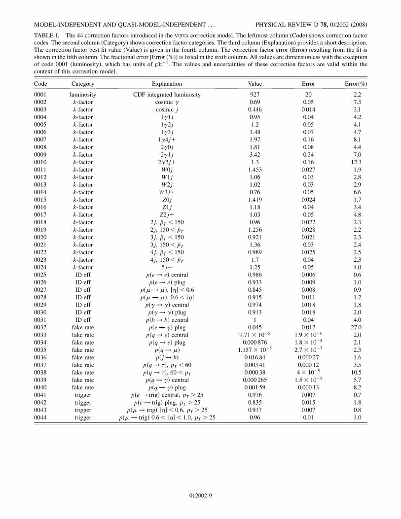
TABLE I. The 44 correction factors introduced in the VISTA correction model. The leftmost column (Code) shows correction factorcodes. The second column (Category) shows correction factor categories. The third column (Explanation) provides a short description.The correction factor best fit value (Value) is given in the fourth column. The correction factor error (Error) resulting from the fit isshown in the fifth column. The fractional error [Error (%)] is listed in the sixth column. All values are dimensionless with the exceptionof code 0001 (luminosity), which has units of pb�1. The values and uncertainties of these correction factors are valid within thecontext of this correction model.

Code Category Explanation Value Error Error(%)

0001 luminosity CDF integrated luminosity 927 20 2.2

0002 k-factor cosmic � 0.69 0.05 7.3

0003 k-factor cosmic j 0.446 0.014 3.1

0004 k-factor 1�1j 0.95 0.04 4.2

0005 k-factor 1�2j 1.2 0.05 4.1

0006 k-factor 1�3j 1.48 0.07 4.7

0007 k-factor 1�4jþ 1.97 0.16 8.1

0008 k-factor 2�0j 1.81 0.08 4.4

0009 k-factor 2�1j 3.42 0.24 7.0

0010 k-factor 2�2jþ 1.3 0.16 12.3

0011 k-factor W0j 1.453 0.027 1.9

0012 k-factor W1j 1.06 0.03 2.8

0013 k-factor W2j 1.02 0.03 2.9

0014 k-factor W3jþ 0.76 0.05 6.6

0015 k-factor Z0j 1.419 0.024 1.7

0016 k-factor Z1j 1.18 0.04 3.4

0017 k-factor Z2jþ 1.03 0.05 4.8

0018 k-factor 2j, pT < 150 0.96 0.022 2.3

0019 k-factor 2j, 150< pT 1.256 0.028 2.2

0020 k-factor 3j, pT < 150 0.921 0.021 2.3

0021 k-factor 3j, 150< pT 1.36 0.03 2.4

0022 k-factor 4j, pT < 150 0.989 0.025 2.5

0023 k-factor 4j, 150< pT 1.7 0.04 2.3

0024 k-factor 5jþ 1.25 0.05 4.0

0025 ID eff pðe ! eÞ central 0.986 0.006 0.6

0026 ID eff pðe ! eÞ plug 0.933 0.009 1.0

0027 ID eff pð� ! �Þ, j�j< 0:6 0.845 0.008 0.9

0028 ID eff pð� ! �Þ, 0:6< j�j 0.915 0.011 1.2

0029 ID eff pð� ! �Þ central 0.974 0.018 1.8

0030 ID eff pð� ! �Þ plug 0.913 0.018 2.0

0031 ID eff pðb ! bÞ central 1 0.04 4.0

0032 fake rate pðe ! �Þ plug 0.045 0.012 27.0

0033 fake rate pðq ! eÞ central 9:71� 10�5 1:9� 10�6 2.0

0034 fake rate pðq ! eÞ plug 0.000 876 1:8� 10�5 2.1

0035 fake rate pðq ! �Þ 1:157� 10�5 2:7� 10�7 2.3

0036 fake rate pðj ! bÞ 0.016 84 0.000 27 1.6

0037 fake rate pðq ! �Þ, pT < 60 0.003 41 0.000 12 3.5

0038 fake rate pðq ! �Þ, 60< pT 0.000 38 4� 10�5 10.5

0039 fake rate pðq ! �Þ central 0.000 265 1:5� 10�5 5.7

0040 fake rate pðq ! �Þ plug 0.001 59 0.000 13 8.2

0041 trigger pðe ! trigÞ central, pT > 25 0.976 0.007 0.7

0042 trigger pðe ! trigÞ plug, pT > 25 0.835 0.015 1.8

0043 trigger pð� ! trigÞ j�j< 0:6, pT > 25 0.917 0.007 0.8

0044 trigger pð� ! trigÞ 0:6< j�j< 1:0, pT > 25 0.96 0.01 1.0


012002-9

Letting ~s represent a vector of correction factors, for thekth bin

�2kð ~sÞ ¼

ðData½k� � SM½k�Þ2ffiffiffiffiffiffiffiffiffiffiffiffiffiffiSM½k�p 2 þ SM½k�2

; (1)

where Data½k� is the number of data events observed in thekth bin, SM½k� is the number of events predicted by thestandard model in the kth bin, SM½k� is the Monte Carlostatistical uncertainty on the standard model prediction in

the kth bin [30], andffiffiffiffiffiffiffiffiffiffiffiffiffiffiSM½k�p

is the statistical uncertaintyon the expected data in the kth bin. The standard modelprediction SM½k� in the kth bin is a function of ~s.

Relevant information external to the VISTA high-pT datasample provides additional constraints in this global fit.The CDF luminosity counters measure the integrated lu-minosity of the sample described in this article to be902 pb�1 � 6% by measuring the fraction of bunch cross-ings in which zero inelastic collisions occur [31]. Theintegrated luminosity of the sample measured by the lumi-nosity counters enters in the form of a Gaussian constrainton the luminosity correction factor. Higher order theoreti-cal calculations exist for some standard model processes,providing constraints on corresponding k-factors, andsome CDF experimental correction factors are also con-strained from external information. In total, 26 of the44 correction factors are constrained. The specific con-straints employed are provided in Appendix A 3 b.

The overall function to be minimized takes the form

�2ð ~sÞ ¼� Xk2bins

�2kð~sÞ

�þ �2

constraintsð ~sÞ; (2)

where the sum in the first term is over bins in the CDFhigh-pT data sample with �2

kð ~sÞ defined in Eq. (1), and the

second term is the contribution from explicit constraints.Minimization of �2ð ~sÞ in Eq. (2) as a function of the

vector of correction factors ~s results in a set of correctionfactor values ~s0 providing the best global agreement be-tween the data and the standard model prediction. The bestfit correction factor values are shown in Table I, togetherwith absolute and fractional uncertainties. The determineduncertainties are not used explicitly in the subsequentanalysis, but rather provide information used implicitly toassist in appropriate adjustment to the correction model inlight of observed discrepancies. The uncertainties are veri-fied by subdividing the data into thirds, performing sepa-rate fits on each third, and noting that the correction factorvalues obtained with each subset are consistent withinquoted uncertainties. Further details on the correlationmatrix and other technical aspects of this global fit canbe found in Appendix A 3 c.

Although the correction factors are determined from aglobal fit, in practice the determination of many correctionfactors’ values are dominated by one recognizable subsam-

ple. The rate pðj ! eÞ for a jet to fake an electron isdetermined largely by the number of events in the ej finalstate, since the largest contribution to this final state is fromdijet events with one jet misreconstructed as an electron.Similarly, the rates pðj ! bÞ and pðj ! �Þ for a jet to fakea b-tagged jet and tau lepton are determined largely by thenumber of events in the bj and �j final states, respectively.The determination of the fake rate pðj ! �Þ, photon effi-ciency pð� ! �Þ, and k-factors for prompt photon produc-tion and prompt diphoton production are dominated by the�j, �jj, and �� final states. Additional knowledge incor-porated in the determination of fake rates is described inAppendix A 1.The global fit �2 per number of bins is 288:1=133þ

27:9, where the last term is the contribution to the �2 fromthe imposed constraints. A �2 per degree of freedom largerthan unity is expected, since the limited set of correctionfactors in this correction model is not expected to provide acomplete description of all features of the data. Emphasisis placed on individual outlying discrepancies that maymotivate a new physics claim, rather than overall goodnessof fit.Corrections to object identification efficiencies are typi-

cally less than 10%; fake rates are consistent with anunderstanding of the underlying physical mechanisms re-sponsible; k-factors range from slightly less than unity togreater than two for some processes with multiple jets. Allvalues obtained are physically reasonable. Further analysisis provided in Appendix A 4.With the details of the correction model in place, the

complete standard model prediction can be obtained. Foreach Monte Carlo event after detector simulation, the eventweight is multiplied by the value of the luminosity correc-tion factor and the k-factor for the relevant standard modelprocess. The single Monte Carlo event can be misrecon-structed in a number of ways, producing a set of MonteCarlo events derived from the original, with weights multi-plied by the probability of each misreconstruction. Theweight of each resulting event is multiplied by the proba-bility the event satisfies trigger criteria. The resulting stan-dard model prediction, corrected as just described, isreferred to as ‘‘the standard model prediction’’ throughoutthe rest of this paper, with ‘‘corrected’’ implied in all cases.

G. Results

Data and standard model events are partitioned intoexclusive final states. This partitioning is orthogonal,with each event ending up in one and only one final state.Data are compared to standard model prediction in eachfinal state, considering the total number of events observedand predicted, and the shapes of relevant kinematicdistributions.In a data driven search, it is crucial to explicitly account

for the trials factor, quantifying the number of places aninteresting signal could appear. Fluctuations at the level of


012002-10

three or more standard deviations are expected to appearsimply because a large number of regions are considered.A reasonably rigorous accounting of this trials factor ispossible as long as the measures of interest and the regionsto which these measures are applied are specified a priori,as is done here. In this analysis a discrepancy at the level of3 or greater after accounting for the trials factor (typicallycorresponding to a discrepancy at the level of 5 or greaterbefore accounting for the trials factor) is considered‘‘significant.’’

Discrepancy in the total number of events in a final state(fs) is measured by the Poisson probability pfs that thenumber of predicted events would fluctuate up to or above(or down to or below) the number of events observed. Toaccount for the trials factor due to the 344 VISTA final statesexamined, the quantity p ¼ 1� ð1� pfsÞ344 is calculatedfor each final state. The result is the probability p ofobserving a discrepancy corresponding to a probabilityless than pfs in the total sample studied. This probabilityp can then be converted into units of standard deviations by

solving for such thatR1

1ffiffiffiffiffi2�

p e�ðx2=2Þdx ¼ p [32]. A final

state exhibiting a population discrepancy greater than 3after the trials factor is thus accounted for is consideredsignificant.

Many kinematic distributions are considered in eachfinal state, including the transverse momentum, pseudor-apidity, detector pseudorapidity, and azimuthal angle of allobjects, masses of individual jets and b-jets, invariantmasses of all object combinations, transverse masses ofobject combinations including p6 , angular separation ��and �R of all object pairs, and several other more speci-alized variables. A Kolmogorov-Smirnov (KS) test is usedto quantify the difference in shape of each kinematicdistribution between data and standard model prediction.As with populations, a trials factor is assessed to accountfor the 16 486 distributions examined, and the resultingprobability is converted into units of standard deviations. Adistribution with KS statistic greater than 0.02 and proba-bility corresponding to greater than 3 after assessing thetrials factor is considered significant.

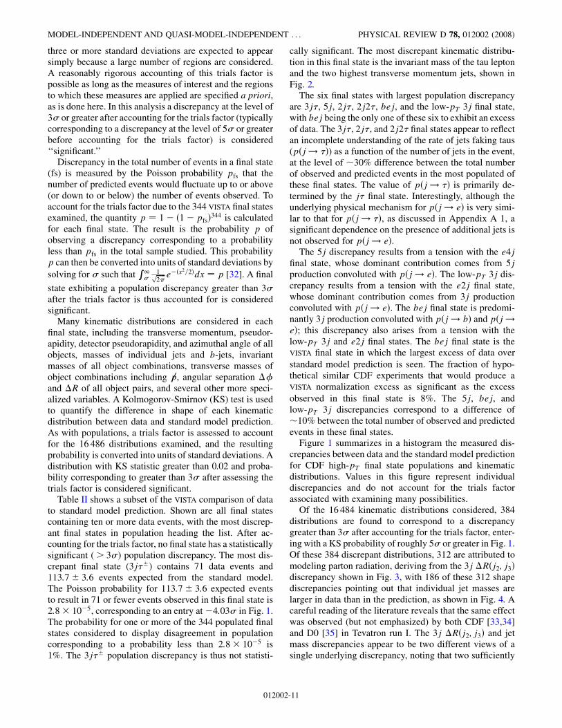
Table II shows a subset of the VISTA comparison of datato standard model prediction. Shown are all final statescontaining ten or more data events, with the most discrep-ant final states in population heading the list. After ac-counting for the trials factor, no final state has a statisticallysignificant (> 3) population discrepancy. The most dis-crepant final state (3j��) contains 71 data events and113:7� 3:6 events expected from the standard model.The Poisson probability for 113:7� 3:6 expected eventsto result in 71 or fewer events observed in this final state is2:8� 10�5, corresponding to an entry at�4:03 in Fig. 1.The probability for one or more of the 344 populated finalstates considered to display disagreement in populationcorresponding to a probability less than 2:8� 10�5 is1%. The 3j�� population discrepancy is thus not statisti-

cally significant. The most discrepant kinematic distribu-tion in this final state is the invariant mass of the tau leptonand the two highest transverse momentum jets, shown inFig. 2.The six final states with largest population discrepancy

are 3j�, 5j, 2j�, 2j2�, bej, and the low-pT 3j final state,with bej being the only one of these six to exhibit an excessof data. The 3j�, 2j�, and 2j2� final states appear to reflectan incomplete understanding of the rate of jets faking taus(pðj ! �Þ) as a function of the number of jets in the event,at the level of �30% difference between the total numberof observed and predicted events in the most populated ofthese final states. The value of pðj ! �Þ is primarily de-termined by the j� final state. Interestingly, although theunderlying physical mechanism for pðj ! eÞ is very simi-lar to that for pðj ! �Þ, as discussed in Appendix A 1, asignificant dependence on the presence of additional jets isnot observed for pðj ! eÞ.The 5j discrepancy results from a tension with the e4j

final state, whose dominant contribution comes from 5jproduction convoluted with pðj ! eÞ. The low-pT 3j dis-crepancy results from a tension with the e2j final state,whose dominant contribution comes from 3j productionconvoluted with pðj ! eÞ. The bej final state is predomi-nantly 3j production convoluted with pðj ! bÞ and pðj !eÞ; this discrepancy also arises from a tension with thelow-pT 3j and e2j final states. The bej final state is theVISTA final state in which the largest excess of data over

standard model prediction is seen. The fraction of hypo-thetical similar CDF experiments that would produce aVISTA normalization excess as significant as the excess

observed in this final state is 8%. The 5j, bej, andlow-pT 3j discrepancies correspond to a difference of�10% between the total number of observed and predictedevents in these final states.Figure 1 summarizes in a histogram the measured dis-

crepancies between data and the standard model predictionfor CDF high-pT final state populations and kinematicdistributions. Values in this figure represent individualdiscrepancies and do not account for the trials factorassociated with examining many possibilities.Of the 16 484 kinematic distributions considered, 384

distributions are found to correspond to a discrepancygreater than 3 after accounting for the trials factor, enter-ing with a KS probability of roughly 5 or greater in Fig. 1.Of these 384 discrepant distributions, 312 are attributed tomodeling parton radiation, deriving from the 3j �Rðj2; j3Þdiscrepancy shown in Fig. 3, with 186 of these 312 shapediscrepancies pointing out that individual jet masses arelarger in data than in the prediction, as shown in Fig. 4. Acareful reading of the literature reveals that the same effectwas observed (but not emphasized) by both CDF [33,34]and D0 [35] in Tevatron run I. The 3j �Rðj2; j3Þ and jetmass discrepancies appear to be two different views of asingle underlying discrepancy, noting that two sufficiently


012002-11

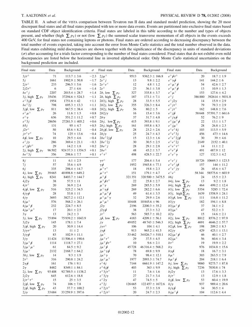
TABLE II. A subset of the VISTA comparison between Tevatron run II data and standard model prediction, showing the 20 mostdiscrepant final states and all final states populated with ten or more data events. Events are partitioned into exclusive final states basedon standard CDF object identification criteria. Final states are labeled in this table according to the number and types of objectspresent, and whether (high

PpT) or not (low

PpT) the summed scalar transverse momentum of all objects in the events exceeds

400 GeV, for final states not containing leptons or photons. Final states are ordered according to decreasing discrepancy between thetotal number of events expected, taking into account the error from Monte Carlo statistics and the total number observed in the data.Final states exhibiting mild discrepancies are shown together with the significance of the discrepancy in units of standard deviations() after accounting for a trials factor corresponding to the number of final states considered. Final states that do not exhibit even milddiscrepancies are listed below the horizontal line in inverted alphabetical order. Only Monte Carlo statistical uncertainties on thebackground prediction are included.

Final state Data Background Final state Data Background Final state Data Background

3j�� 71 113:7� 3:6 �2:3 2j�� 9513 9362:3� 166:8 e�p6 �� 20 18:7� 1:9

5j 1661 1902:9� 50:8 �1:7 2e�j 13 9:8� 2:2 e��p6 141 144:2� 6

2j�� 233 296:5� 5:6 �1:6 2e�e� 12 4:8� 1:2 e��p6 54 42:6� 2:7

2j2�� 6 27� 4:6 �1:4 2e� 23 36:1� 3:8 e��p6 13 10:9� 1:3

be�j 2207 2015:4� 28:7 þ1:4 2b, lowP

pT 327 335:8� 3:7 e�� 153 127:6� 4:2

3j, highP

pT 35436 37294:6� 524:3 �1:1 2b, highP

pT 187 173:1� 7:1 e�j 386 880 392614� 5031:8

e�3jp6 1954 1751:6� 42 þ1:1 2b3j, highP

pT 28 33:5� 5:5 e�j2� 14 15:9� 2:9

be�2j 798 695:3� 13:3 þ1:1 2b2j, lowP

pT 355 326:3� 8:4 e�j�� 79 79:3� 2:9

3jp6 , low PpT 811 967:5� 38:4 �0:8 2b2j, high

PpT 56 80:2� 5 e�j�� 162 148:8� 7:6

e�� 26 11:6� 1:5 þ0:8 2b2j� 16 15:4� 3:6 e�jp6 58 648 57391:7� 661:6

e�� 636 551:2� 11:2 þ0:7 2b� 37 31:7� 4:8 e�j�p6 52 76:2� 9

e�3j 28656 27281:5� 405:2 þ0:6 2bj, lowP

pT 415 393:8� 9:1 e�j��p6 22 13:1� 1:7

b5j 131 95� 4:7 þ0:5 2bj, highP

pT 161 195:8� 8:3 e�j�� 28 26:8� 2:3

j2�� 50 85:6� 8:2 �0:4 2bjp6 , low PpT 28 23:2� 2:6 e�e�4j 103 113:5� 5:9

j�� 74 125� 13:6 �0:4 2bj� 25 24:7� 4:3 e�e�3j 456 473� 14:6

bp6 , low PpT 10 29:5� 4:6 �0:4 2be�2jp6 15 12:3� 1:6 e�e�2jp6 30 39� 4:6

e�j� 286 369:4� 21:1 �0:3 2be�2j 30 30:5� 2:5 e�e�2j 2149 2152� 40:1

e�jp6 �� 29 14:2� 1:8 þ0:2 2be�j 28 29:1� 2:8 e�e�� 14 11:1� 2

2j, highP

pT 96 502 924 37:3� 1354:5 þ0:1 2be� 48 45:2� 3:7 e�e�p6 491 487:9� 12

be�3j 356 298:6� 7:7 þ0:1 �� 498 428:5� 22:7 e�e�� 127 132:3� 4:2

8j 11 6:1� 2:5 �� 177 204:4� 5:4 e�e�j 10 726 10669:3� 123:5

7j 57 35:6� 4:9 �p6 1952 1945:8� 77:1 e�e�jp6 157 144� 11:2

6j 335 298:4� 14:7 �� 18 19:8� 2:3 e�e�j� 26 45:6� 4:7

4j, lowP

pT 39 665 40 898:8� 649:2 �� 151 179:1� 4:7 e�e� 58 344 58575:6� 603:9

4j, highP

pT 8241 8403:7� 144:7 ��p6 321 351 320 500� 3475:5 b6j 24 15:5� 2:3

4j2� 38 57:5� 11 ��p6 �� 22 25:8� 2:7 b4j, lowP

pT 13 9:2� 1:8

4j�� 20 36:9� 2:4 �� 269 285:5� 5:9 b4j, highP

pT 464 499:2� 12:4

4jp6 , low PpT 516 525:2� 34:5 ��p6 269 282:2� 6:6 b3j, low

PpT 5354 5285� 72:4

4j�p6 28 53:8� 11 ��p6 49 61:4� 3:5 b3j, highP

pT 1639 1558:9� 24:1

4j� 3693 3827:2� 112:1 �� 32 29:9� 2:6 b3jp6 , low PpT 111 116:8� 11:2

4j�� 576 568:2� 26:1 �� 10 648 10 845:6� 96 b3j� 182 194:1� 8:8

4j��p6 232 224:7� 8:5 j2� 2196 2200:3� 35:2 b3j��p6 37 34:1� 2

4j�� 17 20:1� 2:5 j2�p6 38 27:3� 3:2 b3j�� 47 52:2� 3

3� 13 24:2� 3 j�� 563 585:7� 10:2 b2� 15 14:6� 2:1

3j, lowP

pT 75 894 75 939:2� 1043:9 jp6 , low PpT 4183 4209:1� 56:1 b2j, low

PpT 8812 8576:2� 97:9

3j2� 145 178:1� 7:4 j� 49 052 48 743� 546:3 b2j, highP

pT 4691 4646:2� 57:7

3jp6 , high PpT 20 30:9� 14:4 j�� 106 104� 4:1 b2jp6 , low P

pT 198 209:2� 8:3

3j�� 13 11� 2 j�p6 913 965:2� 41:5 b2j� 429 425:1� 13:1

3j�p6 83 102:9� 11:1 j�� 33 462 34 026:7� 510:1 b2j��p6 46 40:1� 2:7

3j� 11 424 11 506:4� 190:6 j�� 29 37:5� 4:5 b2j�� 56 60:6� 3:4

3j��p6 1114 1118:7� 27:1 j��p6 �� 10 9:6� 2:1 b�� 19 19:9� 2:2

3j�� 61 84:5� 9:2 j��p6 45 728 46 316:4� 568:2 b� 976 1034:8� 15:6

3j�� 2132 2168:7� 64:2 j��p6 78 69:8� 9:9 b�p6 18 16:7� 3:1

3bj, lowP

pT 14 9:3� 1:9 j�� 70 98:4� 12:1 b�� 303 263:5� 7:9

2�� 316 290:8� 24:2 j�� 1977 2093:3� 74:7 b��p6 204 218:1� 6:4

2�p6 161 176� 9:1 e�4j 7144 6661:9� 147:2 bj, lowP

pT 9060 9275:7� 87:8

2� 8482 8349:1� 84:1 e�4jp6 403 363� 9:9 bj, highP

pT 7236 7030:8� 74

2j, lowP

pT 93 408 92 789:5� 1138:2 e�3j�� 11 7:6� 1:6 bj2� 13 17:6� 3:3

2j2� 645 612:6� 18:8 e�3j� 27 21:7� 3:4 bj�� 13 12:9� 1:8

2j�� 15 25� 3:5 e�2� 47 74:5� 5 bjp6 , low PpT 53 60:4� 19:9

2jp6 , low PpT 74 106� 7:8 e�2j 126 665 122 457� 1672:6 bj� 937 989:4� 20:6

2jp6 , high PpT 43 37:7� 100:2 e�2j�� 53 37:3� 3:9 bj�p6 34 30:5� 4

2j� 33 684 33 259:9� 397:6 e�2j�� 20 24:7� 2:3 bj��p6 104 112:6� 4:4


012002-12

nearby distinct jets correspond to a pattern of calorimetricenergy deposits similar to a single massive jet. The under-lying 3j �Rðj2; j3Þ discrepancy is manifest in many otherfinal states. The final state bej, arising primarily from QCDproduction of three jets with one misreconstructed as anelectron, shows a similar discrepancy in �Rðj; bÞ in Fig. 5.While these discrepancies are clearly statistically sig-

nificant, basing a new physics claim around them is diffi-cult. In the kinematic regime of the discrepancy, differentalgorithms to match exact leading order calculations with aparton shower lead to different predictions [36]. Newerpredictions have not been systematically compared toLEP 1 data, which provide constraints on parton showeringreflected in PYTHIA’s tuning. Further investigation intoobtaining an adequate QCD-based description of this dis-crepancy continues.An additional 59 discrepant distributions reflect an in-

adequate modeling of the overall transverse boost of thesystem. The overall transverse boost of the primary physicsobjects in the event is attributed to two sources: the intrin-

Final state Data Background Final state Data Background Final state Data Background

2j�� 48 41:4� 3:4 e�2jp6 12 451 12 130:1� 159:4 bj�� 173 141:4� 4:8

2j�p6 403 425:2� 29:7 e�2j� 101 88:9� 6:1 be�3jp6 68 52:2� 2:2

2j��p6 7287 7320:5� 118:9 e�� 609 555:9� 10:2 be�2jp6 87 65� 3:3

2j��p6 13 12:6� 2:7 e�� 225 211:2� 4:7 be�p6 330 347:2� 6:9

2j�� 41 35:7� 6:1 e�p6 476 424 479 572� 5361:2 be�jp6 211 176:6� 5

2j�� 374 394:2� 24:8 e�p6 �� 48 35� 2:7 be�e�j 22 34:6� 2:6

TABLE II. (Continued)

σ-6 -4 -2 0 2 4 6

Vis

ta F

inal

Sta

tes

0

10

20

30

40

50

60

70

80

90Entries 344Underflow 0Overflow 0

Entries 344Underflow 0Overflow 0

Entries 16486

Underflow 0

Overflow 0

σ-10 -8 -6 -4 -2 0 2 4 6 8 10

Vis

ta D

istr

ibu

tio

ns

0

500

1000

1500

2000

2500

Entries 16486

ove

rflo

w

FIG. 1 (color online). Distribution of observed discrepancybetween data and the standard model prediction, measured inunits of standard deviation (), shown as the solid (green) histo-gram, before accounting for the trials factor. The upper paneshows the distribution of discrepancies between the total numberof events observed and predicted in the 344 populated final statesconsidered. Negative values on the horizontal axis correspond toa deficit of data compared to standard model prediction; positivevalues indicate an excess of data compared to standard modelprediction. The lower pane shows the distribution of discrepan-cies between the observed and predicted shapes in 16 486 kine-matic distributions. Distributions in which the shapes of data andstandard model prediction are in relative disagreement corre-spond to large positive . The solid (black) curves indicate ex-pected distributions, if the data were truly drawn from the stan-dard model background. Interest is focused on the entries in thetails of the upper distribution and the high tail of the lower dis-tribution. The final state entering the upper histogram at �4:03is the VISTA 3j� final state, which heads Table II. Most of thedistributions entering the lower histogram with >4 derivefrom the 3j �Rðj2; j3Þ discrepancy, discussed in the text.

FIG. 2 (color online). The invariant mass of the tau lepton andtwo leading jets in the final state consisting of three jets and onepositively or negatively charged tau. (The VISTA final state nam-ing convention gives the tau lepton a positive charge.) Data areshown as filled (black) circles, with the standard model pre-diction shown as the shaded (red) histogram. This is the mostdiscrepant kinematic distribution in the final state exhibiting thelargest population discrepancy.


012002-13

sic Fermi motion of the colliding partons within the proton,and soft or collinear radiation of the colliding partons asthey approach collision. Together these effects are herereferred to as ‘‘intrinsic kT ,’’ representing an overall mo-mentum kick to the hard scattering. Further discussionappears in Appendix A 2 c.

The remaining 13 discrepant distributions are seen to bedue to the coarseness of the VISTA correction model. Mostof these discrepancies, which are at the level of 10% orless when expressed as ðdata� theoryÞ=theory, arise frommodeling most fake rates as independent of transversemomentum.

In summary, this global analysis of the bulk features ofthe high-pT data has not yielded a discrepancy motivatinga new physics claim. There are no statistically significantpopulation discrepancies in the 344 populated final statesconsidered, and although there are several statisticallysignificant discrepancies among the 16 486 kinematic dis-tributions investigated, the nature of these discrepanciesmakes it difficult to use them to support a new physicsclaim.

This global analysis of course cannot conclude withcertainty that there is no new physics hiding in the CDFdata. The VISTA population and shape statistics may beinsensitive to a small excess of events appearing at large

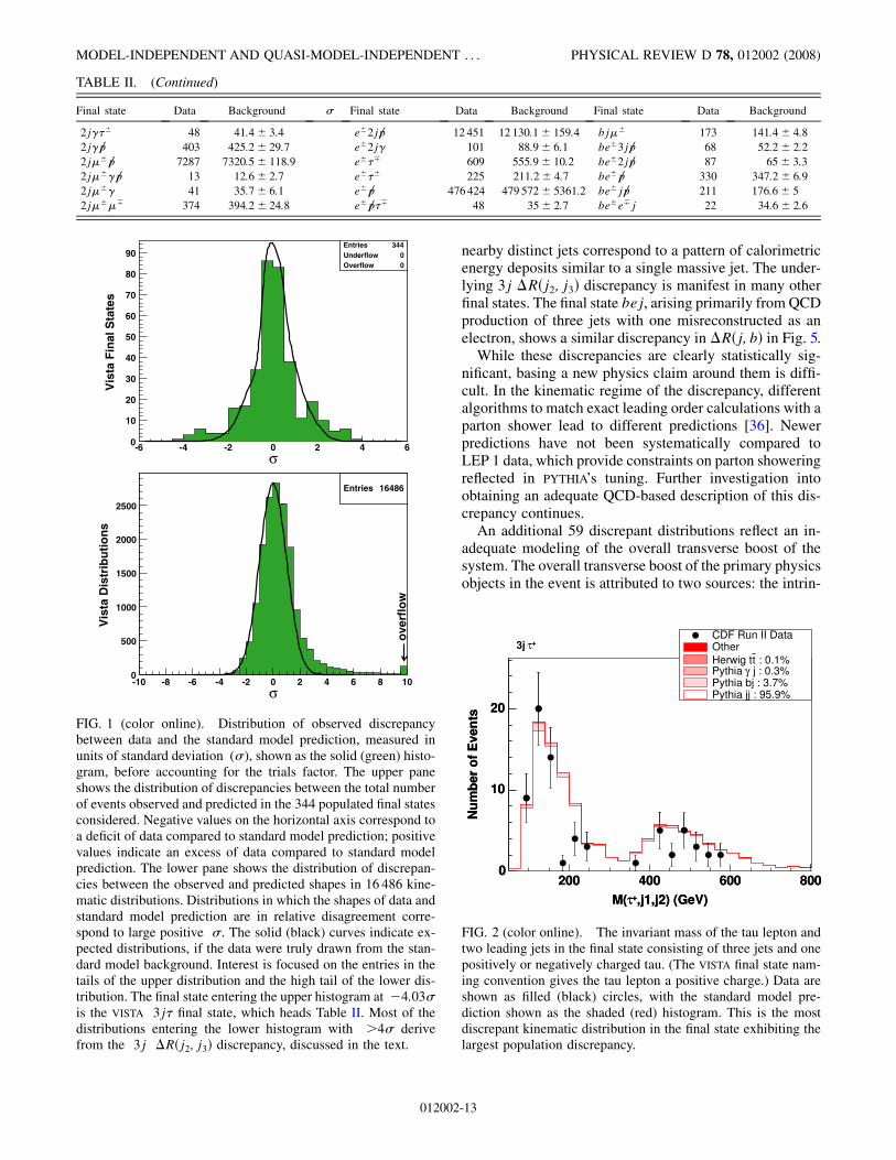
FIG. 3 (color online). A shape discrepancy highlighted byVISTA in the final state consisting of exactly three reconstructed

jets with j�j< 2:5 and pT > 17 GeV, and with one of the jetssatisfying j�j< 1 and pT > 40 GeV. This distribution illus-trates the effect underlying most of the VISTA shape discrep-ancies. Filled (black) circles show CDF data, with the shaded(red) histogram showing the prediction of PYTHIA. The discrep-ancy is clearly statistically significant, with statistical error barssmaller than the size of the data points. The vertical axis showsthe number of events per bin, with the horizontal axis showingthe angular separation (�R ¼ ffiffiffiffiffiffiffiffiffiffiffiffiffiffiffiffiffiffiffiffiffiffiffiffiffi

��2 þ �2p

) between the sec-ond and third jets, where the jets are ordered according todecreasing transverse momentum. In the region �Rðj2; j3Þ *2, populated primarily by initial state radiation, the standardmodel prediction can to some extent be adjusted. The region�Rðj2; j3Þ & 2 is dominated by final state radiation, the descrip-tion of which is constrained by data from LEP 1.

M(j) (GeV)

Nu

mb

er o

f E

ven

ts

> 400 GeVTp∑b j CDF Run II DataOther

) jj : 0%νe→MadEvent W( j : 0.2%γPythia

Pythia bj : 15.8%Pythia jj : 83.9%

50 1000

500

1000

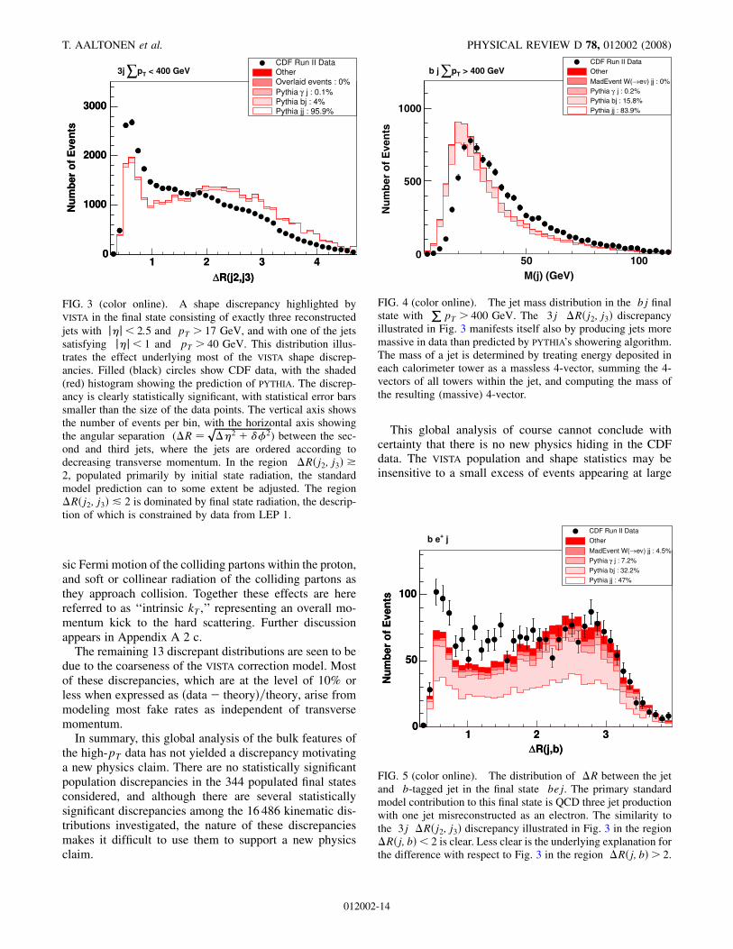
FIG. 4 (color online). The jet mass distribution in the bj finalstate with

PpT > 400 GeV. The 3j �Rðj2; j3Þ discrepancy

illustrated in Fig. 3 manifests itself also by producing jets moremassive in data than predicted by PYTHIA’s showering algorithm.The mass of a jet is determined by treating energy deposited ineach calorimeter tower as a massless 4-vector, summing the 4-vectors of all towers within the jet, and computing the mass ofthe resulting (massive) 4-vector.

FIG. 5 (color online). The distribution of �R between the jetand b-tagged jet in the final state bej. The primary standardmodel contribution to this final state is QCD three jet productionwith one jet misreconstructed as an electron. The similarity tothe 3j �Rðj2; j3Þ discrepancy illustrated in Fig. 3 in the region�Rðj; bÞ< 2 is clear. Less clear is the underlying explanation forthe difference with respect to Fig. 3 in the region �Rðj; bÞ> 2.


012002-14

PpT in a highly populated final state. For such signals

another algorithm is required.

IV. SLEUTH

Taking a broad view of all proposed models that mightextend the standard model, a profound commonality isnoted: nearly all predict an excess of events at high pT ,concentrated in a particular final state. The second stage ofthis research program involves the systematic search forsuch physics using an algorithm called SLEUTH [37].SLEUTH is quasi-model-independent, where ‘‘quasi’’ refers

to the assumption that the first sign of new physics willappear as an excess of events in some final state at largesummed scalar transverse momentum (

PpT).

The SLEUTH algorithm used by CDF in Tevatron run II isessentially that developed by D0 in Tevatron run I [38–40],and subsequently improved by H1 in HERA run I [41],with small modifications.

SLEUTH’s definition of interest relies on the following

assumptions:(1) The data can be categorized into exclusive final

states in such a way that any signature of newphysics is apt to appear predominantly in one ofthese final states.

(2) New physics will appear with objects at highsummed transverse momentum (

PpT) relative to

standard model and instrumental background.(3) New physics will appear as an excess of data over

standard model and instrumental background.

A. Algorithm

The SLEUTH algorithm consists of three steps, followingthe above three assumptions.

1. Final states

In the first step of the algorithm, all events are placedinto exclusive final states as in VISTA, with the followingmodifications.

(i) Jets are identified as pairs, rather than individually,to reduce the total number of final states and to keepsignal events with one additional radiated gluonwithin the same final state. Final state names in-clude ‘‘ n jj’’ if n jet pairs are identified, withpossibly one unpaired jet assumed to have origi-nated from a radiated gluon.

(ii) The present understanding of quark flavor suggeststhat b quarks should be produced in pairs. Bottomquarks are identified as pairs, rather than individu-ally, to increase the robustness of identification andto reduce the total number of final states. Final statenames include ‘‘ n bb’’ if n b pairs are identified.

(iii) Final states related through global charge conjuga-tion are considered to be equivalent. Thus eþe��

is a different final state than eþeþ�, but eþeþ�and e�e�� together make up a single SLEUTH fi-nal state.

(iv) Final states related through global interchange ofthe first and second generation are considered to beequivalent. Thus eþp6 � and �þp6 � together makeup a single SLEUTH final state. The decision toconsider third generation objects (b quarks and �leptons) differently from first and second genera-tion objects reflects theoretical prejudice that thethird generation may be special, and the experimen-tal ability (in the case of b quarks) and experimentalchallenge (in the case of � leptons) in the identi-fication of third generation objects.

The symbol ‘ is used to denote electron or muon. Thesymbol W is used in naming final states containing oneelectron or muon, significant missing momentum, andperhaps other nonleptonic objects. Thus the final stateseþp6 �, e�p6 �, �þp6 �, and ��p6 � are combined into theSLEUTH final state W�. A table showing the relationship

between VISTA and SLEUTH final states is provided inAppendix B 1.

2. Variable

The second step of the algorithm considers a singlevariable in each exclusive final state: the summed scalartransverse momentum of all objects in the event (

PpT).

Assuming momentum conservation in the plane transverseto the axis of the colliding beams,

Xi

~pi þ uncl! þ ~p6 ¼ ~0; (3)

where the sum over i represents a sum over all identified

objects in the event, the ith object has momentum ~pi, uncl!

denotes the vector sum of all momentum visible in the

detector but not clustered into an identified object, ~p6denotes the missing momentum, and the equation is a two-component vector equality for the components of the mo-mentum along the two spatial directions transverse to theaxis of the colliding beams. The SLEUTH variable

PpT is

then defined by

XpT � X

i

j ~pij þ juncl! j þ j ~p6 j; (4)

where only the momentum components transverse to theaxis of the colliding beams are considered when computingmagnitudes.

3. Regions

The algorithm’s third step involves searching for regionsin which more events are seen in the data than expectedfrom standard model and instrumental background. This


012002-15

search is performed in the variable space defined in thesecond step of the algorithm, for each of the exclusive finalstates defined in the first step.

The steps of the search can be sketched as follows.(i) In each final state, the regions considered are the

one-dimensional intervals inP

pT extending fromeach data point up to infinity. A region is requiredto contain at least three data events, as described inAppendix B.

(ii) In a particular final state, the data point with the dthlargest value of

PpT defines an interval in the

variableP

pT extending from this data point upto infinity. This semi-infinite interval containsd data events. The standard model prediction inthis interval, estimated from the VISTA compari-son described above, integrates to b predictedevents. In this final state, the interest of the dth

region is defined as the Poisson probability pd ¼P1i¼d

bi

i! e�b that the standard model background b

would fluctuate up to or above the observed numberof data events d in this region. The most interestingregion in this final state is the one with smallestPoisson probability.

(iii) For this final state, pseudo experiments are gener-ated, with pseudo data pulled from the standardmodel background. For each pseudo experiment,the interest of the most interesting region is calcu-lated. An ensemble of pseudo experiments deter-mines the fraction P of pseudo experiments in thisfinal state in which the most interesting region ismore interesting than the most interesting region inthis final state observed in the data. If there is nonew physics in this final state, P is expected to be arandom number pulled from a uniform distributionin the unit interval. If there is new physics in thisfinal state, P is expected to be small.

(iv) Looping over all final states, P is computed foreach final state. The minimum of these values isdenoted Pmin. The most interesting region in thefinal state with smallest P is denoted R.

(v) The interest of the most interesting regionR in the

most interesting final state is defined by ~P ¼ 1�Qað1� paÞ, where the product is over all SLEUTH

final states a, and pa is the lesser of Pmin and theprobability for the total number of events predictedby the standard model in the final state a to fluc-tuate up to or above three data events. The quantity~P represents the fraction of hypothetical similarCDF experiments that would produce a final state

with P < Pmin. The range of~P is the unit interval.

If the data are distributed according to standard

model prediction, ~P is expected to be a randomnumber pulled from a uniform distribution in the

unit interval. If new physics is present, ~P is ex-pected to be small.

4. Output

The output of the algorithm is the most interesting

region R observed in the data, and a number ~P quantify-ing the interest ofR. A reasonable threshold for discovery

is ~P & 0:001, which corresponds loosely to a local 5effect after the trials factor is accounted for.Although no integration over systematic errors is per-

formed in computing ~P , systematic uncertainties do affectthe final SLEUTH result. If SLEUTH highlights a discrepancyin a particular final state, explanations in terms of a cor-rection to the background estimate are considered. Thisprocess necessarily requires physics judgement. A reason-able explanation of a SLEUTH discrepancy in terms of aninadequacy in the modeling of the detector response orstandard model prediction that is consistent with externalinformation is fed back into the VISTA correction modeland tested for global consistency. In this way, plausibleexplanations for discrepancies observed by SLEUTH areincorporated into the VISTA correction model. This itera-tion continues until either all reasonable explanations for asignificant SLEUTH discrepancy are exhausted, resulting ina possible new physics claim, or no significant SLEUTH

discrepancy remains.

B. Sensitivity

Two important questions must be asked:(i) Will SLEUTH find nothing if there is nothing to be

found?(ii) Will SLEUTH find something if there is something to

be found?If there is nothing to be found, SLEUTH will find nothing

999 times out of 1000, given a uniform distribution of~P and a discovery threshold of ~P & 0:001. The uniformdistribution of ~P in the absence of new physics is illus-trated in Fig. 6, using values of ~P obtained in pseudoexperiments with pseudo data generated from the standardmodel prediction. SLEUTH will of course return spurioussignals if provided improperly modeled backgrounds. Thealgorithm directly addresses the issue of whether an ob-served hint is due to a statistical fluctuation. SLEUTH it-self is unable to address systematic mismeasurement orincorrect modeling, but is quite useful in bringing these toattention.The answer to the second question depends to what

degree the new physics satisfies the three assumptions onwhich SLEUTH is based: new physics will appear predomi-nantly in one final state, at high summed scalar transversemomentum, and as an excess of data over standard modelprediction. SLEUTH’s sensitivity to any particular new phe-nomenon depends on the extent to which this new phe-nomenon satisfies these assumptions.

1. Known standard model processes

Consideration of specific standard model processes canprovide intuition for SLEUTH’s sensitivity to new physics.


012002-16

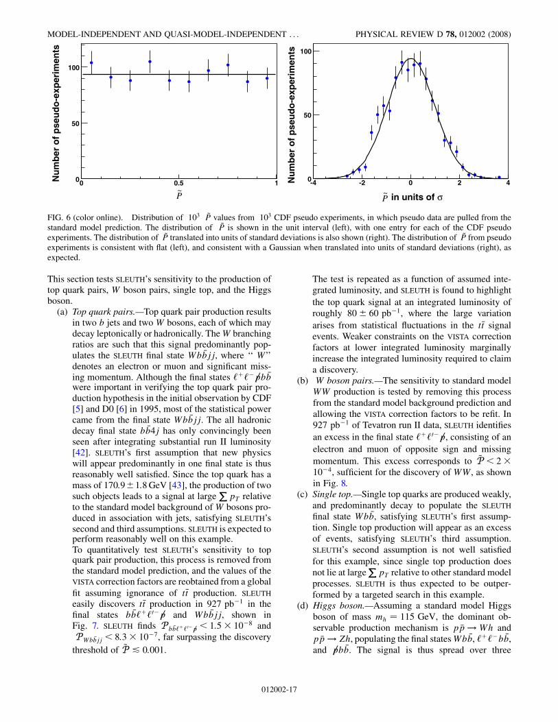
This section tests SLEUTH’s sensitivity to the production oftop quark pairs, W boson pairs, single top, and the Higgsboson.

(a) Top quark pairs.—Top quark pair production resultsin two b jets and two W bosons, each of which maydecay leptonically or hadronically. TheW branchingratios are such that this signal predominantly pop-ulates the SLEUTH final state Wb �bjj, where ‘‘ W’’denotes an electron or muon and significant miss-ing momentum. Although the final states ‘þ‘�p6 b �bwere important in verifying the top quark pair pro-duction hypothesis in the initial observation by CDF[5] and D0 [6] in 1995, most of the statistical powercame from the final state Wb �bjj. The all hadronicdecay final state b �b4j has only convincingly beenseen after integrating substantial run II luminosity[42]. SLEUTH’s first assumption that new physicswill appear predominantly in one final state is thusreasonably well satisfied. Since the top quark has amass of 170:9�1:8GeV [43], the production of twosuch objects leads to a signal at large

PpT relative

to the standard model background of W bosons pro-duced in association with jets, satisfying SLEUTH’ssecond and third assumptions. SLEUTH is expected toperform reasonably well on this example.To quantitatively test SLEUTH’s sensitivity to topquark pair production, this process is removed fromthe standard model prediction, and the values of theVISTA correction factors are reobtained from a global

fit assuming ignorance of t�t production. SLEUTH

easily discovers t�t production in 927 pb�1 in thefinal states b �b‘þ‘0�p6 and Wb �bjj, shown inFig. 7. SLEUTH finds P b �b‘þ‘0�p6 < 1:5� 10�8 and

PWb �bjj < 8:3� 10�7, far surpassing the discovery

threshold of ~P & 0:001.

The test is repeated as a function of assumed inte-grated luminosity, and SLEUTH is found to highlight

the top quark signal at an integrated luminosity ofroughly 80� 60 pb�1, where the large variation

arises from statistical fluctuations in the t�t signalevents. Weaker constraints on the VISTA correctionfactors at lower integrated luminosity marginallyincrease the integrated luminosity required to claima discovery.

(b) W boson pairs.—The sensitivity to standard modelWW production is tested by removing this processfrom the standard model background prediction andallowing the VISTA correction factors to be refit. In927 pb�1 of Tevatron run II data, SLEUTH identifies

an excess in the final state ‘þ‘0�p6 , consisting of an

electron and muon of opposite sign and missing

momentum. This excess corresponds to ~P < 2�10�4, sufficient for the discovery of WW, as shownin Fig. 8.

(c) Single top.—Single top quarks are produced weakly,and predominantly decay to populate the SLEUTH

final state Wb �b, satisfying SLEUTH’s first assump-tion. Single top production will appear as an excessof events, satisfying SLEUTH’s third assumption.SLEUTH’s second assumption is not well satisfied

for this example, since single top production doesnot lie at large

PpT relative to other standard model

processes. SLEUTH is thus expected to be outper-formed by a targeted search in this example.

(d) Higgs boson.—Assuming a standard model Higgsboson of mass mh ¼ 115 GeV, the dominant ob-servable production mechanism is p �p ! Wh andp �p ! Zh, populating the final statesWb �b, ‘þ‘�b �b,and p6 b �b. The signal is thus spread over three

P~

15.00Nu

mb

er o

f p

seu

do

-exp

erim

ents

0

50

100

σ in units of P~

-4 -2 0 2 4Nu

mb

er o

f p

seu

do

-exp

erim

ents

0

50

100

FIG. 6 (color online). Distribution of 103 ~P values from 103 CDF pseudo experiments, in which pseudo data are pulled from thestandard model prediction. The distribution of ~P is shown in the unit interval (left), with one entry for each of the CDF pseudoexperiments. The distribution of ~P translated into units of standard deviations is also shown (right). The distribution of ~P from pseudoexperiments is consistent with flat (left), and consistent with a Gaussian when translated into units of standard deviations (right), asexpected.


012002-17

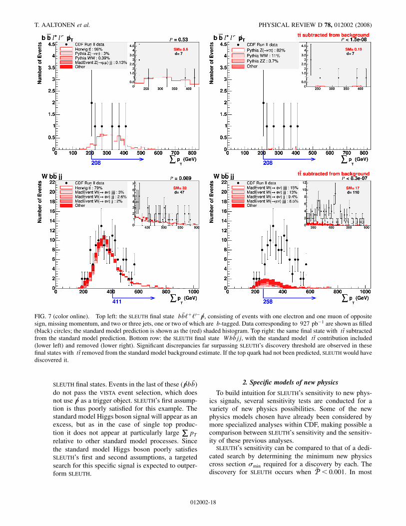
SLEUTH final states. Events in the last of these (p6 b �b)do not pass the VISTA event selection, which doesnot use p6 as a trigger object. SLEUTH’s first assump-tion is thus poorly satisfied for this example. Thestandard model Higgs boson signal will appear as anexcess, but as in the case of single top produc-

tion it does not appear at particularly largeP

pT

relative to other standard model processes. Since

the standard model Higgs boson poorly satisfiesSLEUTH’s first and second assumptions, a targeted

search for this specific signal is expected to outper-form SLEUTH.

2. Specific models of new physics

To build intuition for SLEUTH’s sensitivity to new phys-ics signals, several sensitivity tests are conducted for avariety of new physics possibilities. Some of the newphysics models chosen have already been considered bymore specialized analyses within CDF, making possible acomparison between SLEUTH’s sensitivity and the sensitiv-ity of these previous analyses.

SLEUTH’s sensitivity can be compared to that of a dedi-

cated search by determining the minimum new physicscross section min required for a discovery by each. Thediscovery for SLEUTH occurs when ~P < 0:001. In most

FIG. 7 (color online). Top left: the SLEUTH final state b �b‘þ‘0�p6 , consisting of events with one electron and one muon of oppositesign, missing momentum, and two or three jets, one or two of which are b-tagged. Data corresponding to 927 pb�1 are shown as filled(black) circles; the standard model prediction is shown as the (red) shaded histogram. Top right: the same final state with t�t subtractedfrom the standard model prediction. Bottom row: the SLEUTH final state Wb �bjj, with the standard model t�t contribution included(lower left) and removed (lower right). Significant discrepancies far surpassing SLEUTH’s discovery threshold are observed in thesefinal states with t�t removed from the standard model background estimate. If the top quark had not been predicted, SLEUTH would havediscovered it.


012002-18

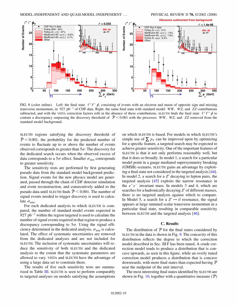
SLEUTH regions satisfying the discovery threshold of~P < 0:001, the probability for the predicted number ofevents to fluctuate up to or above the number of eventsobserved corresponds to greater than 5. The discovery forthe dedicated search occurs when the observed excess ofdata corresponds to a 5 effect. Smaller min correspondsto greater sensitivity.

The sensitivity tests are performed by first generatingpseudo data from the standard model background predic-tion. Signal events for the new physics model are gener-ated, passed through the chain of CDF detector simulationand event reconstruction, and consecutively added to the

pseudo data until SLEUTH finds ~P < 0:001. The number ofsignal events needed to trigger discovery is used to calcu-late min.

For each dedicated analysis to which SLEUTH is com-pared, the number of standard model events expected in927 pb�1 within the region targeted is used to calculate thenumber of signal events required in that region to produce adiscrepancy corresponding to 5. Using the signal effi-ciency determined in the dedicated analysis, min is calcu-lated. The effect of systematic uncertainties are removedfrom the dedicated analyses and are not included forSLEUTH. The inclusion of systematic uncertainties will re-

duce the sensitivity of both SLEUTH and the dedicatedanalysis to the extent that the systematic parameters areallowed to vary. VISTA and SLEUTH have the advantage ofusing a large data set to constrain them.

The results of five such sensitivity tests are summa-rized in Table III. SLEUTH is seen to perform comparablyto targeted analyses on models satisfying the assumptions

on which SLEUTH is based. For models in which SLEUTH’ssimple use of

PpT can be improved upon by optimizing

for a specific feature, a targeted search may be expected toachieve greater sensitivity. One of the important features ofSLEUTH is that it not only performs reasonably well, but

that it does so broadly. In model 1, a search for a particularmodel point in a gauge mediated supersymmetry breaking(GMSB) scenario, SLEUTH gains an advantage by exploit-ing a final state not considered in the targeted analysis [44].In model 2, a search for a Z0 decaying to lepton pairs, thetargeted analysis [45] exploits the narrow resonance inthe eþe� invariant mass. In models 3 and 4, which aresearches for a hadronically decaying Z0 of different masses,there is no targeted analysis against which to compare.In Model 5, a search for a Z0 ! t�t resonance, the signalappears at large summed scalar transverse momentum in aparticular final state, resulting in comparable sensitivitybetween SLEUTH and the targeted analysis [46].

C. Results

The distribution of P for the final states considered bySLEUTH in the data is shown in Fig. 9. The concavity of this

distribution reflects the degree to which the correctionmodel described in Sec. III F has been tuned. A crude cor-rection model tends to produce a distribution that is con-cave upwards, as seen in this figure, while an overly tunedcorrection model produces a distribution that is concavedownwards, with more final states than expected having Pnear the midpoint of the unit interval.The most interesting final states identified by SLEUTH are

shown in Fig. 10, together with a quantitative measure (P )

0 50 100 150 200 250 300 350

Nu

mb

er o

f E

ven

ts

0

5

10

15

20

25

Tp-l’+l = 0.035P

(GeV)T

p∑71

CDF Run II dataPythia WW : 45%

) : 27%ττ→Pythia Z( : 6.6%γ)νµ→MadEvent W(

) j : 4.1%νµ→MadEvent W(Other

100 200 3000

2

4

6

8

10

SM= 56 d= 77

0 50 100 150 200 250 300 350

Nu

mb

er o

f E

ven

ts

0

5

10

15

20

25

Dibosons subtracted from background

Tp-l’+l < 1.4e-06P

(GeV)T

p∑71

CDF Run II data) : 51%ττ→Pythia Z(

: 13%γ)νµ→MadEvent W() j : 7.6%νµ→MadEvent W(

) : 6.2%µµ→Pythia Z(Other

100 200 3000

2

4

6

8

10

SM= 30 d= 77

FIG. 8 (color online). Left: the final state ‘þ‘0�p6 , consisting of events with an electron and muon of opposite sign and missingtransverse momentum, in 927 pb�1 of CDF data. Right: the same final state with standard model WW, WZ, and ZZ contributionssubtracted, and with the VISTA correction factors refit in the absence of these contributions. SLEUTH finds the final state ‘þ‘0�p6 tocontain a discrepancy surpassing the discovery threshold of ~P < 0:001 with the processes WW, WZ, and ZZ removed from thestandard model background.


012002-19

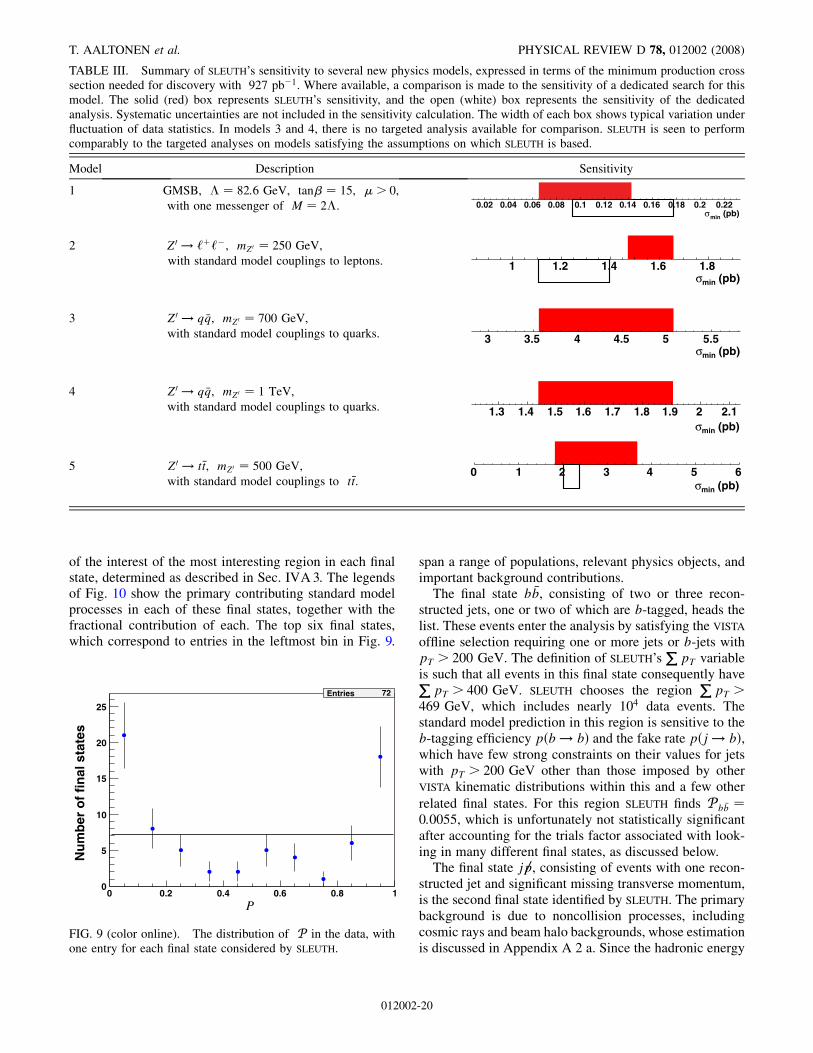
of the interest of the most interesting region in each finalstate, determined as described in Sec. IVA3. The legendsof Fig. 10 show the primary contributing standard modelprocesses in each of these final states, together with thefractional contribution of each. The top six final states,which correspond to entries in the leftmost bin in Fig. 9.

span a range of populations, relevant physics objects, andimportant background contributions.The final state b �b, consisting of two or three recon-

structed jets, one or two of which are b-tagged, heads thelist. These events enter the analysis by satisfying the VISTA

offline selection requiring one or more jets or b-jets withpT > 200 GeV. The definition of SLEUTH’s

PpT variable

is such that all events in this final state consequently havePpT > 400 GeV. SLEUTH chooses the region

PpT >

469 GeV, which includes nearly 104 data events. Thestandard model prediction in this region is sensitive to theb-tagging efficiency pðb ! bÞ and the fake rate pðj ! bÞ,which have few strong constraints on their values for jetswith pT > 200 GeV other than those imposed by otherVISTA kinematic distributions within this and a few other

related final states. For this region SLEUTH finds P b �b ¼0:0055, which is unfortunately not statistically significantafter accounting for the trials factor associated with look-ing in many different final states, as discussed below.The final state jp6 , consisting of events with one recon-

structed jet and significant missing transverse momentum,is the second final state identified by SLEUTH. The primarybackground is due to noncollision processes, includingcosmic rays and beam halo backgrounds, whose estimationis discussed in Appendix A 2 a. Since the hadronic energy

P0 0.2 0.4 0.6 0.8 1

Nu

mb

er o

f fi

nal

sta

tes

0

5

10

15

20

25

Entries 72

FIG. 9 (color online). The distribution of P in the data, withone entry for each final state considered by SLEUTH.

TABLE III. Summary of SLEUTH’s sensitivity to several new physics models, expressed in terms of the minimum production crosssection needed for discovery with 927 pb�1. Where available, a comparison is made to the sensitivity of a dedicated search for thismodel. The solid (red) box represents SLEUTH’s sensitivity, and the open (white) box represents the sensitivity of the dedicatedanalysis. Systematic uncertainties are not included in the sensitivity calculation. The width of each box shows typical variation underfluctuation of data statistics. In models 3 and 4, there is no targeted analysis available for comparison. SLEUTH is seen to performcomparably to the targeted analyses on models satisfying the assumptions on which SLEUTH is based.

Model Description Sensitivity

1 GMSB, � ¼ 82:6 GeV, tan� ¼ 15, �> 0,with one messenger of M ¼ 2�.

(pb)minσ0.02 0.04 0.06 0.08 0.1 0.12 0.14 0.16 0.18 0.2 0.22

2 Z0 ! ‘þ‘�, mZ0 ¼ 250 GeV,with standard model couplings to leptons.

(pb)minσ1 1.2 1.4 1.6 1.8

3 Z0 ! q �q, mZ0 ¼ 700 GeV,with standard model couplings to quarks.

(pb)minσ3 3.5 4 4.5 5 5.5

4 Z0 ! q �q, mZ0 ¼ 1 TeV,with standard model couplings to quarks.

(pb)minσ1.3 1.4 1.5 1.6 1.7 1.8 1.9 2 2.1

5 Z0 ! t�t, mZ0 ¼ 500 GeV,with standard model couplings to t�t. (pb)minσ

0 1 2 3 4 5 6


012002-20

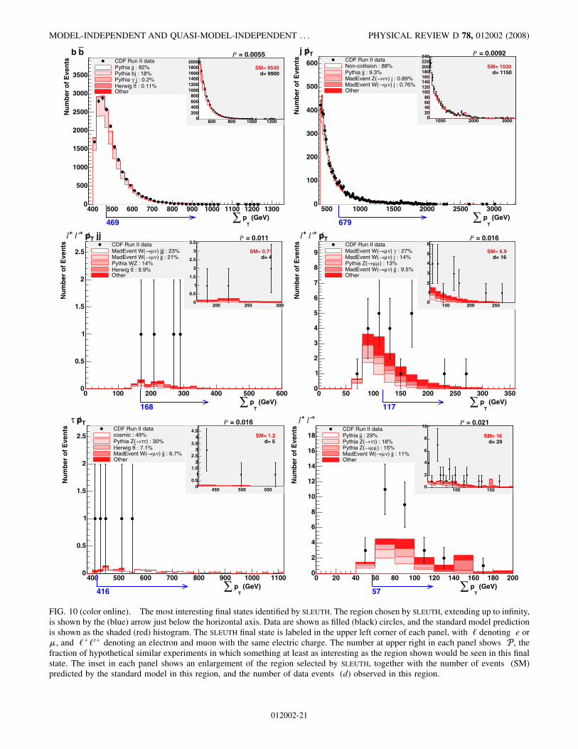
400 500 600 700 800 900 1000 1100 1200 1300

Nu

mb

er o

f E

ven

ts

0

500

1000

1500

2000

2500

3000

3500

bb = 0.0055P

(GeV)T

p∑469

CDF Run II dataPythia jj : 82%Pythia bj : 18%

j : 0.2%γPythia : 0.11%tHerwig t

Other

600 800 1000 12000

200400600800

100012001400160018002000

SM= 9540 d= 9900

500 1000 1500 2000 2500 3000

Nu

mb

er o

f E

ven

ts

0

100

200

300

400

500

600Tpj = 0.0092P

(GeV)T

p∑679

CDF Run II dataNon-collision : 88%Pythia jj : 9.3%

) j : 0.89%νν→MadEvent Z() j : 0.76%νµ→MadEvent W(

Other

1000 2000 30000

20406080

100120140160180200220240

SM= 1030 d= 1150

0 100 200 300 400 500 600

Nu

mb

er o

f E

ven

ts

0

0.5

1

1.5

2

2.5

jjTp+l’+l = 0.011P

(GeV)T

p∑168

CDF Run II data) jjj : 23%νµ→MadEvent W() jj : 21%νµ→MadEvent W(

Pythia WZ : 14% : 9.9%tHerwig t

Other

200 250 3000

0.5

1

1.5

2

2.5

3

3.5

SM= 0.71 d= 4

0 50 100 150 200 250 300 350

Nu

mb

er o

f E

ven

ts

0

1

2

3

4

5

6

7

8

9

Tp+l’+l = 0.016P

(GeV)T

p∑117

CDF Run II data : 27%γ)νµ→MadEvent W(

) j : 14%νµ→MadEvent W() : 13%µµ→Pythia Z(

) jj : 9.5%νµ→MadEvent W(Other

150 200 2500

1

2

3

4

5

6

SM= 6.9 d= 16

400 500 600 700 800 900 1000 1100

Nu

mb

er o

f E

ven

ts

0

0.5

1

1.5

2

2.5

Tpτ = 0.016P

(GeV)T

p∑416

CDF Run II datacosmic : 49%

) : 30%ττ→Pythia Z( : 7.1%tHerwig t

) jj : 6.7%νµ→MadEvent W(Other

450 500 5500

0.51

1.52

2.53

3.54

4.5SM= 1.2

d= 5

0 20 40 60 80 100 120 140 160 180 200

Nu

mb

er o

f E

ven

ts

0

2

4

6

8

10

12

14

16

18

+l’+l = 0.021P

(GeV)T

p∑57

CDF Run II dataPythia jj : 29%

) : 18%ττ→Pythia Z() : 15%µµ→Pythia Z(

) jj : 11%νµ→MadEvent W(Other

100 1500

2

4

6

8

10

SM= 16 d= 29

FIG. 10 (color online). The most interesting final states identified by SLEUTH. The region chosen by SLEUTH, extending up to infinity,is shown by the (blue) arrow just below the horizontal axis. Data are shown as filled (black) circles, and the standard model predictionis shown as the shaded (red) histogram. The SLEUTH final state is labeled in the upper left corner of each panel, with ‘ denoting e or�, and ‘þ‘0þ denoting an electron and muon with the same electric charge. The number at upper right in each panel shows P , thefraction of hypothetical similar experiments in which something at least as interesting as the region shown would be seen in this finalstate. The inset in each panel shows an enlargement of the region selected by SLEUTH, together with the number of events (SM)predicted by the standard model in this region, and the number of data events (d) observed in this region.


012002-21

is not required to be deposited in time with the beamcrossing, SLEUTH’s analysis of this final state is sensitiveto particles with a lifetime between 1 ns and 1 �s thatlodge temporarily in the hadronic calorimeter, comple-menting Ref. [47].

The final states ‘þ‘0þp6 jj, ‘þ‘0þp6 , and ‘þ‘0þ all con-tain an electron (‘) and muon (‘0) with identical recon-structed charge (either both positive or both negative). Thefinal states with and without missing transverse momentumare qualitatively different in terms of the standard modelprocesses contributing to the background estimate, with thefinal state ‘þ‘0� composed mostly of dijets where one jet ismisreconstructed as an electron and a second jet is mis-reconstructed as a muon; Z ! �þ��, where one tau decaysto a muon and the other to a leading �0, one of the twophotons from which converts while traveling through thesilicon support structure to result in an electron recon-structed with the same sign as the muon, as described inAppendix A 1; and Z ! �þ��, in which a photon isproduced, converts, and is misreconstructed as an electron.The final states containing missing transverse momentumare dominated by the production of Wð! ��Þ in associa-tion with one or more jets, with one of the jets misrecon-structed as an electron. The muon is significantly morelikely than the electron to have been produced in the hardinteraction, since the fake rate pðj ! �Þ is roughly anorder of magnitude smaller than the fake rate pðj ! eÞ,as observed in Table I. The final state ‘þ‘0�p6 jj, whichcontains two or three reconstructed jets in addition tothe electron, muon, and missing transverse momentum,also has some contribution from WZ and top quark pairproduction.

The final state �p6 contains one reconstructed tau,significant missing transverse momentum, and one re-constructed jet with pT > 200 GeV. This final state inprinciple also contains events with one reconstructed tau,significant missing transverse momentum, and zero recon-structed jets, but such events do not satisfy the offlineselection criteria described in Sec. III C. Roughly halfof the background is noncollision, in which two differentcosmic ray muons (presumably from the same cosmic rayshower) leave two distinct energy deposits in the CDFhadronic calorimeter, one with pT > 200 GeV, and onewith a single associated track from a p �p collision occur-ring during the same bunch crossing. Less than a singleevent is predicted from this noncollision source (usingtechniques described in Appendix A 2 a) over the pastfive years of Tevatron running.

In these CDF data, SLEUTH finds ~P ¼ 0:46. The fractionof hypothetical similar CDF experiments (assuming a fixedstandard model prediction, detector simulation, and cor-rection model) that would exhibit a final state with Psmaller than the smallest P observed in the CDF run IIdata is approximately 46%. The actual value obtained for~P is not of particular interest, except to note that this valueis significantly greater than the threshold of & 0:001 re-

quired to claim an effect of statistical significance. SLEUTHhas not revealed a discrepancy of sufficient statisticalsignificance to justify a new physics claim.Systematics are incorporated into SLEUTH in the form of

the flexibility in the VISTA correction model, as describedpreviously. This flexibility is significantly more importantin practice than the uncertainties on particular correctionfactor values obtained from the fit, although the latter areeasier to discuss. The relative importance of correctionfactor value uncertainties on SLEUTH’s result depends onthe number of predicted standard model events (b) inSLEUTH’s high

PpT tail. The uncertainties on the correc-

tion factors of Table I are such that the appropriate additionin quadrature gives a typical uncertainty of � 10% onthe total background prediction in each final state. Usingsys � 10%� b and stat �

ffiffiffib

p, the relative importance

of systematic uncertainty and statistical uncertainty is esti-mated to be sys=stat ¼ 10%� b=

ffiffiffib

p. The importance of

systematic and statistical uncertainties are thus comparablefor high

PpT tails containing b� 100 predicted events.

The effect of systematic uncertainties is provided in thisapproximation rather than through a rigorous integrationover these uncertainties as nuisance parameters due to thehigh computational cost of performing the integration.This estimate of systematic uncertainty is valid only withinthe particular correction model resulting in the list ofcorrection factors shown in Table I; additional changes tothe correction model may result in larger variation. Theinclusion of additional systematic uncertainties does notqualitatively change the conclusion that SLEUTH has notrevealed a discrepancy of sufficient statistical significanceto justify a new physics claim.Because of the large number of final states considered,

there are regions (such as those shown in Fig. 10) in whichthe probability for the standard model prediction to fluc-tuate up to or above the number of events observed in thedata corresponds to a significance exceeding 3 if theappropriate trials factor is not accounted for. A doublingof data may therefore result in discovery. In particular,although the excesses in Fig. 10 are currently consistentwith simple statistical fluctuations, if any of them aregenuinely due to new physics, SLEUTH will find they pass

the discovery threshold of ~P < 0:001 with roughly a dou-bling of data.

V. CONCLUSIONS

A broad search for new physics (VISTA) has been per-formed in 927 pb�1 of CDF run II data. A completestandard model background estimate has been obtainedand compared with data in 344 populated exclusive finalstates and 16 486 relevant kinematic distributions, most ofwhich have not been previously considered. Considerationof exclusive final state populations yields no statisticallysignificant (> 3) discrepancy after the trials factor isaccounted for. Quantifying the difference in shape of kine-


012002-22

matic distributions using the Kolmogorov-Smirnov statis-tic, significant discrepancies are observed between dataand standard model prediction. These discrepancies arebelieved to arise from mismodeling of the parton showerand intrinsic kT , and represent observables for which aQCD-based understanding is highly motivated. None ofthe shape discrepancies highlighted motivates a new phys-ics claim.

A further systematic search (SLEUTH) for regions of ex-cess on the high-

PpT tails of exclusive final states has

been performed, representing a quasi-model-independentsearch for new electroweak scale physics. Most of the ex-clusive final states searched with SLEUTH have not beenconsidered by previous Tevatron analyses. A measure ofinterest rigorously accounting for the trials factor associ-ated with looking in many regions with few events isdefined and used to quantify the most interesting regionobserved in the CDF run II data. No region of excess on thehigh-

PpT tail of any of the SLEUTH exclusive final states

surpasses the discovery threshold.Although this global analysis of course cannot prove that

no new physics is hiding in these data, this broad search ofthe Tevatron run II data represents one of the single mostencompassing tests of the particle physics standard modelat the energy frontier.

ACKNOWLEDGMENTS

Tim Stelzer and Fabio Maltoni have provided particu-larly valuable assistance in the estimation of standardmodel backgrounds. Sergey Alekhin provided helpful cor-respondence in understanding the theoretical uncertaintiesonW and Z production imposed as constraints on the VISTA

correction factor fit. Sascha Caron provided insight gainedfrom the general search at H1. Torbjorn Sjostrand assistedin the understanding of PYTHIA’s treatment of parton show-ering applied to the VISTA 3j �Rðj2; j3Þ discrepancy. Wethank the Fermilab staff and the technical staffs of theparticipating institutions for their vital contributions. Thiswork was supported by the U.S. Department of Energy andNational Science Foundation; the Italian Istituto Nazionaledi Fisica Nucleare; the Ministry of Education, Culture,Sports, Science and Technology of Japan; the NaturalSciences and Engineering Research Council of Canada;the National Science Council of the Republic of China; theSwiss National Science Foundation; the A. P. Sloan Foun-dation; the Bundesministerium fur Bildung und Forschung,Germany; the Korean Science and Engineering Foundationand the Korean Research Foundation; the Science andTechnology Facilities Council and the Royal Society, UK;the Institut National de Physique Nucleaire et Physique desParticules/CNRS; the Russian Foundation for BasicResearch; the Comision Interministerial de Ciencia yTecnologıa, Spain; the European Community’s HumanPotential Programme; the Slovak R&D Agency; and theAcademy of Finland.

APPENDIX A: VISTA CORRECTIONMODEL DETAILS

This appendix contains details of the VISTA correctionmodel. Appendix A 1 covers the physical mechanismsunderlying fake rates. Appendix A 2 contains informationabout additional background sources, including back-grounds from cosmic rays and beam halo, multiple inter-actions, and the effects of intrinsic kT . Appendix A 3contains details of the VISTA correction factor fit, includingthe construction of the �2 function that is minimized andthe resulting covariance matrix. Appendix A 4 discussesthe values of the correction factors that are obtained.

1. Fake rate physics

The following facts begin to build a unified understand-ing of fake rates for electrons, muons, taus, and photons.This understanding is woven throughout the VISTA correc-tion model and significantly informs and constrains theVISTA correction process. Explicit constraints derived from

these studies are provided in Appendix A 3. The underlyingphysical mechanisms for these fakes lead to simple andwell-justified relations among them.Table IV shows the response of the CDF detector simu-

lation, reconstruction, and object identification algorithmsto single particles. Using a single particle gun, 105 particlesof each type shown at the left of the table are shot withpT ¼ 25 GeV into the CDF detector, uniformly distributedin � and in �. The resulting reconstructed object types areshown at the top of the table, labeling the columns. Thefirst four entries on the diagonal at upper left show the ef-ficiency for reconstructing electrons and muons [48]. Thefraction of electrons misidentified as photons, shown inthe top row, seventh column, is seen to be roughly equal tothe fraction of photons identified as electrons or positrons,shown in the fifth row, first and second columns, andmeasures the number of radiation lengths in the innermostregions of the CDF tracker. The fraction of B mesonsidentified as electrons or muons, primarily through semi-leptonic decay, are shown in the four left columns, elevenththrough fourteenth rows. Other entries provide similarlyuseful information, most easily comprehensible from sim-ple physics.The transverse momenta of the objects reconstructed

from single particles are displayed in Fig. 11. The relativeresolutions for the measurement of electron and muonmomenta are shown in the first four histograms on thediagonal at upper left. The histograms in the left column,sixth through eighth rows, show that single neutral pionsmisreconstructed as electrons have their momenta wellmeasured, while single charged pions misreconstructed aselectrons have their momenta systematically undermeas-ured, as discussed below. The histogram in the top row,second column from the right, shows that electrons mis-reconstructed as jets have their energies systematicallyovermeasured. Other histograms in Fig. 11 contain simi-


012002-23

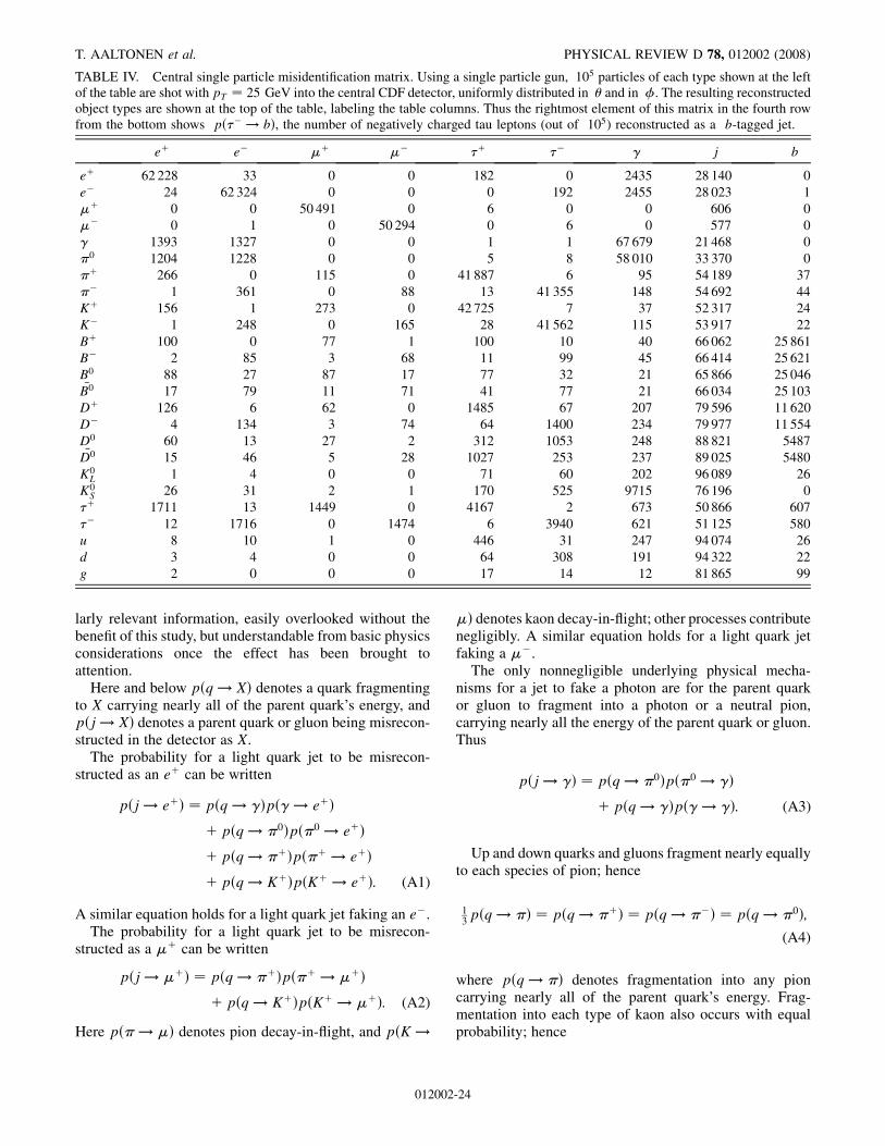
larly relevant information, easily overlooked without thebenefit of this study, but understandable from basic physicsconsiderations once the effect has been brought toattention.

Here and below pðq ! XÞ denotes a quark fragmentingto X carrying nearly all of the parent quark’s energy, andpðj ! XÞ denotes a parent quark or gluon being misrecon-structed in the detector as X.

The probability for a light quark jet to be misrecon-structed as an eþ can be written

pðj ! eþÞ ¼ pðq ! �Þpð� ! eþÞþ pðq ! �0Þpð�0 ! eþÞþ pðq ! �þÞpð�þ ! eþÞþ pðq ! KþÞpðKþ ! eþÞ: (A1)

A similar equation holds for a light quark jet faking an e�.The probability for a light quark jet to be misrecon-

structed as a �þ can be written

pðj ! �þÞ ¼ pðq ! �þÞpð�þ ! �þÞþ pðq ! KþÞpðKþ ! �þÞ: (A2)

Here pð� ! �Þ denotes pion decay-in-flight, and pðK !

�Þ denotes kaon decay-in-flight; other processes contributenegligibly. A similar equation holds for a light quark jetfaking a ��.The only nonnegligible underlying physical mecha-

nisms for a jet to fake a photon are for the parent quarkor gluon to fragment into a photon or a neutral pion,carrying nearly all the energy of the parent quark or gluon.Thus

pðj ! �Þ ¼ pðq ! �0Þpð�0 ! �Þþ pðq ! �Þpð� ! �Þ: (A3)

Up and down quarks and gluons fragment nearly equallyto each species of pion; hence

13pðq ! �Þ ¼ pðq ! �þÞ ¼ pðq ! ��Þ ¼ pðq ! �0Þ;

(A4)

where pðq ! �Þ denotes fragmentation into any pioncarrying nearly all of the parent quark’s energy. Frag-mentation into each type of kaon also occurs with equalprobability; hence

TABLE IV. Central single particle misidentification matrix. Using a single particle gun, 105 particles of each type shown at the leftof the table are shot with pT ¼ 25 GeV into the central CDF detector, uniformly distributed in � and in �. The resulting reconstructedobject types are shown at the top of the table, labeling the table columns. Thus the rightmost element of this matrix in the fourth rowfrom the bottom shows pð�� ! bÞ, the number of negatively charged tau leptons (out of 105) reconstructed as a b-tagged jet.

eþ e� �þ �� þ �� j b

eþ 62 228 33 0 0 182 0 2435 28 140 0

e� 24 62 324 0 0 0 192 2455 28 023 1

�þ 0 0 50 491 0 6 0 0 606 0

�� 0 1 0 50 294 0 6 0 577 0

� 1393 1327 0 0 1 1 67 679 21 468 0

�0 1204 1228 0 0 5 8 58 010 33 370 0

�þ 266 0 115 0 41 887 6 95 54 189 37

�� 1 361 0 88 13 41 355 148 54 692 44

Kþ 156 1 273 0 42 725 7 37 52 317 24

K� 1 248 0 165 28 41 562 115 53 917 22

Bþ 100 0 77 1 100 10 40 66 062 25 861

B� 2 85 3 68 11 99 45 66 414 25 621

B0 88 27 87 17 77 32 21 65 866 25 046�B0 17 79 11 71 41 77 21 66 034 25 103

Dþ 126 6 62 0 1485 67 207 79 596 11 620

D� 4 134 3 74 64 1400 234 79 977 11 554

D0 60 13 27 2 312 1053 248 88 821 5487�D0 15 46 5 28 1027 253 237 89 025 5480

K0L 1 4 0 0 71 60 202 96 089 26

K0S 26 31 2 1 170 525 9715 76 196 0

�þ 1711 13 1449 0 4167 2 673 50 866 607

�� 12 1716 0 1474 6 3940 621 51 125 580

u 8 10 1 0 446 31 247 94 074 26

d 3 4 0 0 64 308 191 94 322 22

g 2 0 0 0 17 14 12 81 865 99


012002-24

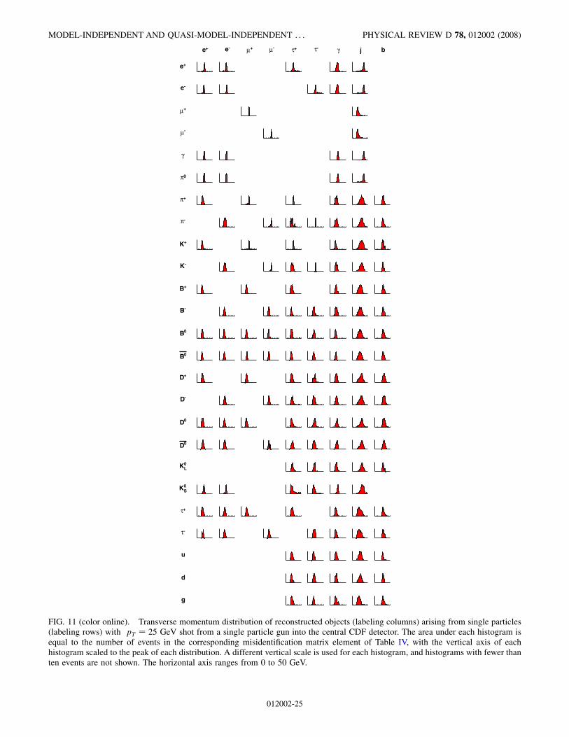
+e -e +µ -µ +τ -τ γ j b

+e

-e

+µ

-µ

γ

0π

+π

-π

+K

-K

+B

-B

0B

0B

+D

-D

0D

0D

L0K

S0K

+τ

-τ

u

d

g

FIG. 11 (color online). Transverse momentum distribution of reconstructed objects (labeling columns) arising from single particles(labeling rows) with pT ¼ 25 GeV shot from a single particle gun into the central CDF detector. The area under each histogram isequal to the number of events in the corresponding misidentification matrix element of Table IV, with the vertical axis of eachhistogram scaled to the peak of each distribution. A different vertical scale is used for each histogram, and histograms with fewer thanten events are not shown. The horizontal axis ranges from 0 to 50 GeV.


012002-25

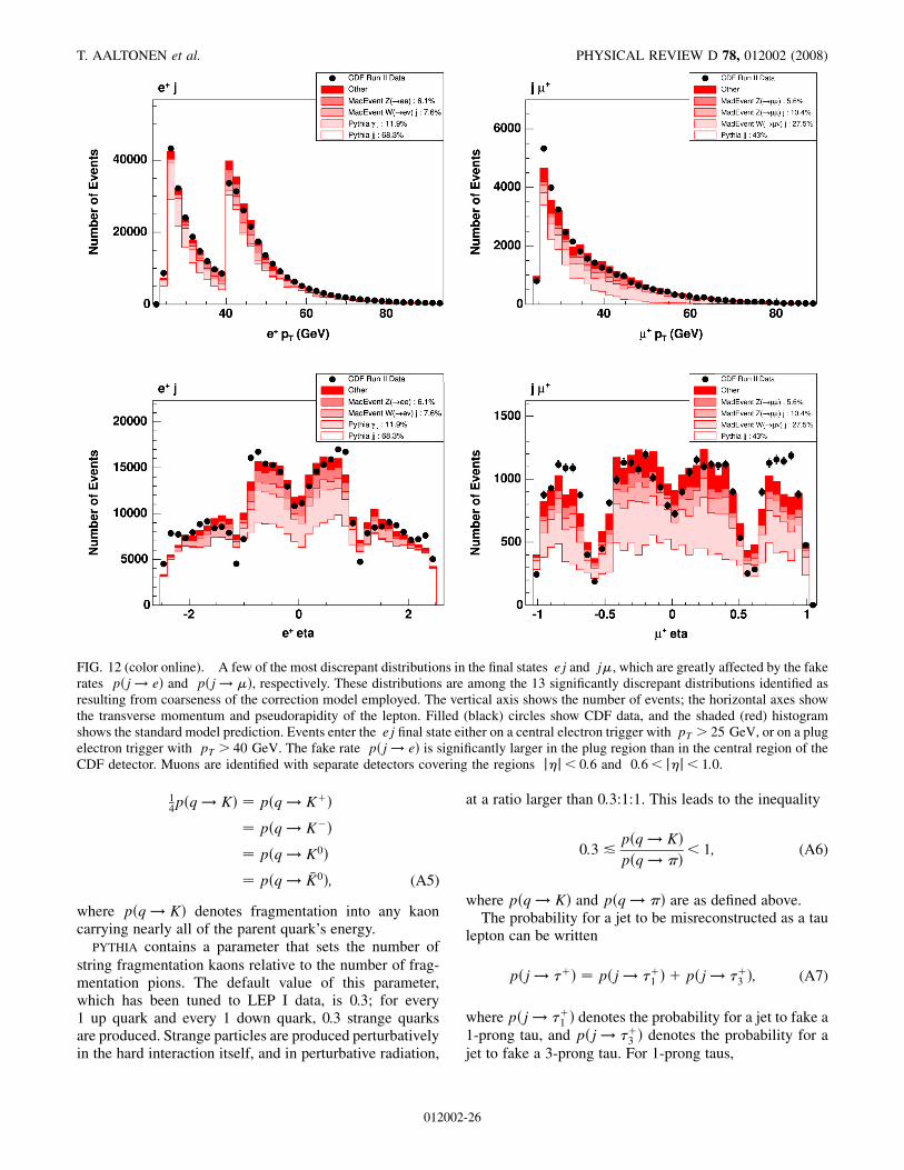
14pðq ! KÞ ¼ pðq ! KþÞ

¼ pðq ! K�Þ¼ pðq ! K0Þ¼ pðq ! �K0Þ; (A5)

where pðq ! KÞ denotes fragmentation into any kaoncarrying nearly all of the parent quark’s energy.

PYTHIA contains a parameter that sets the number of

string fragmentation kaons relative to the number of frag-mentation pions. The default value of this parameter,which has been tuned to LEP I data, is 0.3; for every1 up quark and every 1 down quark, 0.3 strange quarksare produced. Strange particles are produced perturbativelyin the hard interaction itself, and in perturbative radiation,

at a ratio larger than 0:3:1:1. This leads to the inequality

0:3 &pðq ! KÞpðq ! �Þ< 1; (A6)

where pðq ! KÞ and pðq ! �Þ are as defined above.The probability for a jet to be misreconstructed as a tau

lepton can be written

pðj ! �þÞ ¼ pðj ! �þ1 Þ þ pðj ! �þ3 Þ; (A7)

where pðj ! �þ1 Þ denotes the probability for a jet to fake a1-prong tau, and pðj ! �þ3 Þ denotes the probability for a

jet to fake a 3-prong tau. For 1-prong taus,

FIG. 12 (color online). A few of the most discrepant distributions in the final states ej and j�, which are greatly affected by the fakerates pðj ! eÞ and pðj ! �Þ, respectively. These distributions are among the 13 significantly discrepant distributions identified asresulting from coarseness of the correction model employed. The vertical axis shows the number of events; the horizontal axes showthe transverse momentum and pseudorapidity of the lepton. Filled (black) circles show CDF data, and the shaded (red) histogramshows the standard model prediction. Events enter the ej final state either on a central electron trigger with pT > 25 GeV, or on a plugelectron trigger with pT > 40 GeV. The fake rate pðj ! eÞ is significantly larger in the plug region than in the central region of theCDF detector. Muons are identified with separate detectors covering the regions j�j< 0:6 and 0:6< j�j< 1:0.


012002-26

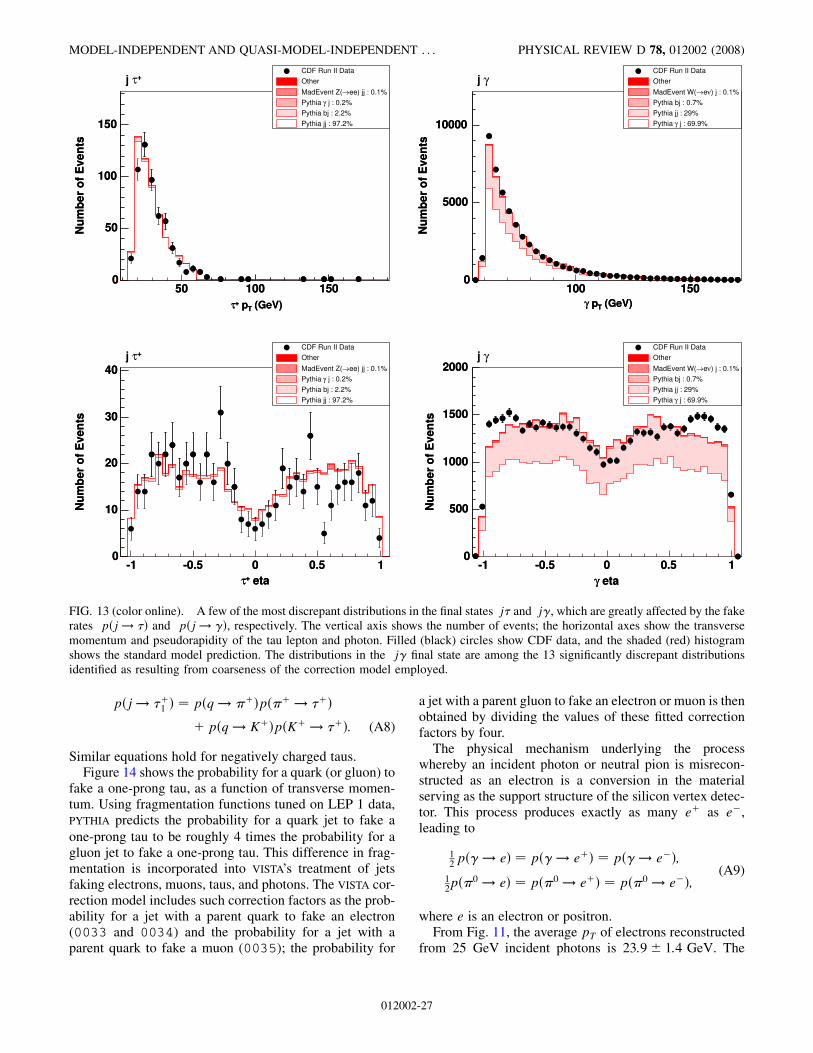
pðj ! �þ1 Þ ¼ pðq ! �þÞpð�þ ! �þÞþ pðq ! KþÞpðKþ ! �þÞ: (A8)

Similar equations hold for negatively charged taus.Figure 14 shows the probability for a quark (or gluon) to

fake a one-prong tau, as a function of transverse momen-tum. Using fragmentation functions tuned on LEP 1 data,PYTHIA predicts the probability for a quark jet to fake a

one-prong tau to be roughly 4 times the probability for agluon jet to fake a one-prong tau. This difference in frag-mentation is incorporated into VISTA’s treatment of jetsfaking electrons, muons, taus, and photons. The VISTA cor-rection model includes such correction factors as the prob-ability for a jet with a parent quark to fake an electron(0033 and 0034) and the probability for a jet with aparent quark to fake a muon (0035); the probability for

a jet with a parent gluon to fake an electron or muon is thenobtained by dividing the values of these fitted correctionfactors by four.The physical mechanism underlying the process

whereby an incident photon or neutral pion is misrecon-structed as an electron is a conversion in the materialserving as the support structure of the silicon vertex detec-tor. This process produces exactly as many eþ as e�,leading to

12pð� ! eÞ ¼ pð� ! eþÞ ¼ pð� ! e�Þ;12pð�0 ! eÞ ¼ pð�0 ! eþÞ ¼ pð�0 ! e�Þ; (A9)

where e is an electron or positron.From Fig. 11, the average pT of electrons reconstructed

from 25 GeV incident photons is 23:9� 1:4 GeV. The

FIG. 13 (color online). A few of the most discrepant distributions in the final states j� and j�, which are greatly affected by the fakerates pðj ! �Þ and pðj ! �Þ, respectively. The vertical axis shows the number of events; the horizontal axes show the transversemomentum and pseudorapidity of the tau lepton and photon. Filled (black) circles show CDF data, and the shaded (red) histogramshows the standard model prediction. The distributions in the j� final state are among the 13 significantly discrepant distributionsidentified as resulting from coarseness of the correction model employed.


012002-27

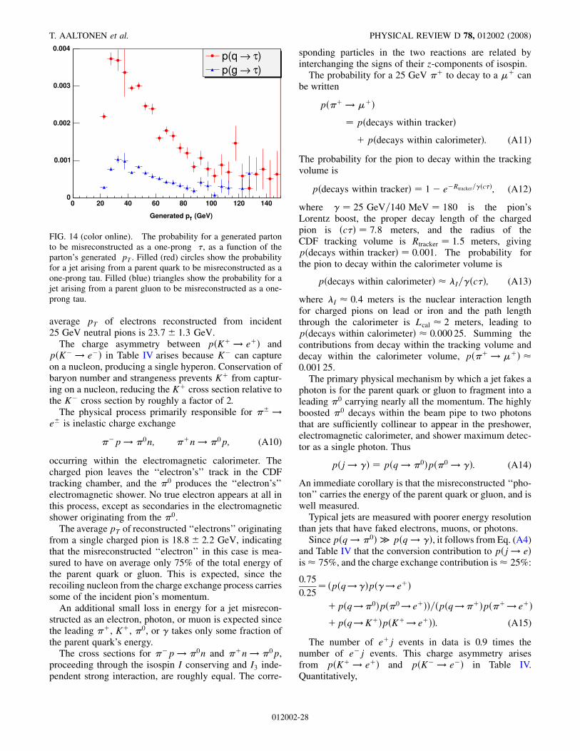
average pT of electrons reconstructed from incident25 GeV neutral pions is 23:7� 1:3 GeV.

The charge asymmetry between pðKþ ! eþÞ andpðK� ! e�Þ in Table IV arises because K� can captureon a nucleon, producing a single hyperon. Conservation ofbaryon number and strangeness prevents Kþ from captur-ing on a nucleon, reducing the Kþ cross section relative tothe K� cross section by roughly a factor of 2.

The physical process primarily responsible for �� !e� is inelastic charge exchange

��p ! �0n; �þn ! �0p; (A10)

occurring within the electromagnetic calorimeter. Thecharged pion leaves the ‘‘electron’s’’ track in the CDFtracking chamber, and the �0 produces the ‘‘electron’s’’electromagnetic shower. No true electron appears at all inthis process, except as secondaries in the electromagneticshower originating from the �0.

The average pT of reconstructed ‘‘electrons’’ originatingfrom a single charged pion is 18:8� 2:2 GeV, indicatingthat the misreconstructed ‘‘electron’’ in this case is mea-sured to have on average only 75% of the total energy ofthe parent quark or gluon. This is expected, since therecoiling nucleon from the charge exchange process carriessome of the incident pion’s momentum.

An additional small loss in energy for a jet misrecon-structed as an electron, photon, or muon is expected sincethe leading �þ, Kþ, �0, or � takes only some fraction ofthe parent quark’s energy.

The cross sections for ��p ! �0n and �þn ! �0p,proceeding through the isospin I conserving and I3 inde-pendent strong interaction, are roughly equal. The corre-

sponding particles in the two reactions are related byinterchanging the signs of their z-components of isospin.The probability for a 25 GeV �þ to decay to a �þ can

be written

pð�þ ! �þÞ¼ pðdecays within trackerÞ

þ pðdecays within calorimeterÞ: (A11)

The probability for the pion to decay within the trackingvolume is

pðdecays within trackerÞ ¼ 1� e�Rtracker=�ðc�Þ; (A12)

where � ¼ 25 GeV=140 MeV ¼ 180 is the pion’sLorentz boost, the proper decay length of the chargedpion is ðc�Þ ¼ 7:8 meters, and the radius of theCDF tracking volume is Rtracker ¼ 1:5 meters, givingpðdecays within trackerÞ ¼ 0:001. The probability forthe pion to decay within the calorimeter volume is

pðdecays within calorimeterÞ � I=�ðc�Þ; (A13)

where I � 0:4 meters is the nuclear interaction lengthfor charged pions on lead or iron and the path lengththrough the calorimeter is Lcal � 2 meters, leading topðdecays within calorimeterÞ � 0:000 25. Summing thecontributions from decay within the tracking volume anddecay within the calorimeter volume, pð�þ ! �þÞ �0:001 25.The primary physical mechanism by which a jet fakes a

photon is for the parent quark or gluon to fragment into aleading �0 carrying nearly all the momentum. The highlyboosted �0 decays within the beam pipe to two photonsthat are sufficiently collinear to appear in the preshower,electromagnetic calorimeter, and shower maximum detec-tor as a single photon. Thus

pðj ! �Þ ¼ pðq ! �0Þpð�0 ! �Þ: (A14)

An immediate corollary is that the misreconstructed ‘‘pho-ton’’ carries the energy of the parent quark or gluon, and iswell measured.Typical jets are measured with poorer energy resolution

than jets that have faked electrons, muons, or photons.Since pðq ! �0Þ pðq ! �Þ, it follows from Eq. (A4)

and Table IV that the conversion contribution to pðj ! eÞis� 75%, and the charge exchange contribution is� 25%:

0:75

0:25¼ðpðq!�Þpð�! eþÞþpðq!�0Þpð�0! eþÞÞ=ðpðq!�þÞpð�þ! eþÞþpðq!KþÞpðKþ! eþÞÞ: (A15)

The number of eþj events in data is 0.9 times thenumber of e�j events. This charge asymmetry arisesfrom pðKþ ! eþÞ and pðK� ! e�Þ in Table IV.Quantitatively,

FIG. 14 (color online). The probability for a generated partonto be misreconstructed as a one-prong �, as a function of theparton’s generated pT . Filled (red) circles show the probabilityfor a jet arising from a parent quark to be misreconstructed as aone-prong tau. Filled (blue) triangles show the probability for ajet arising from a parent gluon to be misreconstructed as a one-prong tau.


012002-28

pðj ! eþÞpðj ! e�Þ ¼ 0:9þ 0:2pðKþ ! eþÞ=pðK ! eÞ

0:9þ 0:2pðK� ! e�Þ=pðK ! eÞ ;(A16)

where 0.9 is the sum of 0.75 from Eq. (A15) and 0:15 �0:25� 0:6 from Eq. (A6), and 0.2 is twice 1� 0:9. FrompðKþ ! eþÞ and pðK� ! e�Þ in Table IV, pðKþ !eþÞ=pðK ! eÞ ¼ 1=3 and pðK� ! e�Þ=pðK ! eÞ ¼2=3, predicting pðj ! eþÞ=pðj ! e�Þ ¼ 0:935, in reason-able agreement with the ratio of the observed number ofevents in the eþj and e�j final states.

The number of j�þ events observed in CDF run II is 1.1times the number of j�� events observed. This chargeasymmetry arises from pðKþ ! �þÞ and pðK� ! ��Þ inTable IV.

The physical mechanism by which a prompt photonfakes a tau lepton is for the photon to convert, producingan electron or positron carrying most of the photon’senergy, which is then misreconstructed as a tau. Theprobability for this to occur is equal for positively andnegatively charged taus,

12pð� ! �Þ ¼ pð� ! �þÞ ¼ pð� ! ��Þ; (A17)

and is related to previously defined quantities by

pð� ! �Þ ¼ pð� ! eÞ 1

pðe ! eÞpðe ! �Þ; (A18)

where pð� ! eÞ denotes the fraction of produced photonsthat are reconstructed as electrons, pðe ! eÞ denotes thefraction of produced electrons that are reconstructed aselectrons, and hence pð� ! eÞ=pðe ! eÞ is the fractionof produced photons that pair produce a single leadingelectron.

Note pðe ! �Þ � pð� ! eÞ from Table IV, as expected,with a value of� 0:03 determined by the amount of 5 ma-terial in the inner detectors and the tightness of isolationcriteria. A hard bremsstrahlung followed by a conversion isresponsible for electrons to be reconstructed with oppositesign; hence

pðe� ! e�Þ ¼ pðeþ ! e�Þ¼ pðe� ! eþÞ� 1

2pðe� ! �Þpð� ! e�Þ; (A19)

where the factor of 1=2 comes because the material alreadytraversed by the e� will not be traversed again by the �. Inparticular, track curvature mismeasurement is not respon-sible for erroneous sign determination in the central regionof the CDF detector.

From knowledge of the underlying physical mechanismsby which jets fake electrons, muons, taus, and photons, thesimple use of a reconstructed jet as a lepton or photon withan appropriate fake rate applied to the weight of the eventneeds slight modification to correctly handle the fact that ajet that has faked a lepton or photon generally is measured

more accurately than a hadronic jet. Rather than using themomentum of the reconstructed jet, the momentum of theparent quark or gluon is determined by adding up allMonte Carlo particle level objects within a cone of �R ¼0:4 about the reconstructed jet. In misreconstructing a jetin an event, the momentum of the corresponding parentquark or gluon is used rather than the momentum of the re-constructed jet. A jet that fakes a photon then has momen-tum equal to the momentum of the parent quark or gluonplus a fractional correction equal to 0:01� ðparent pT �25 GeVÞ=ð25 GeVÞ to account for leakage out of the coneof �R ¼ 0:4, and a further smearing of 0:2

ffiffiffiffiffiffiffiffiffiffiGeV

p �ffiffiffiffiffiffiffiffiffiffiffiffiffiffiffiffiffiffiffiffiffiparent pT

p, reflecting the electromagnetic resolution of

the CDF detector. The momenta of jets that fake photonsare multiplied by an overall factor of 1.12, and jets thatfake electrons, muons, or taus are multiplied by an overallfactor of 0.95. These numbers are determined by the ‘p6 , ‘j,and �j final states. The distributions most sensitive to thesenumbers are the missing energy and the jet pT .A b quark fragmenting into a leading b hadron that then

decays leptonically or semileptonically results in an elec-tron or muon that shares the pT of the parent b quark withthe associated neutrino. If all hadronic decay products aresoft, the distribution of the momentum fraction carried bythe charged lepton can be obtained by considering thedecay of a scalar to two massless fermions. Isolated andenergetic electrons and muons arising from parent b quarksin this way are modeled as having pT equal to the parentb quark pT , multiplied by a random number uniformlydistributed between 0 and 1.

2. Additional background sources

This appendix provides additional details on the estima-tion of the standard model prediction.

a. Cosmic ray and beam halo muons

There are four dominant categories of events caused bycosmic ray muons penetrating the detector: �p6 , �þ��,�p6 , and jp6 . There is negligible contribution from cosmicray secondaries of any particle type other than muons.A cosmic ray muon penetrating the CDF detector whose

trajectory passes within 1 mm of the beam line and within�60< z < 60 cm of the origin may be reconstructed astwo outgoing muons. In this case the cosmic ray event ispartitioned into the final state�þ��. If one of the tracks ismissed, the cosmic ray event is partitioned into the finalstate�p6 . The standard CDF cosmic ray filter, which makesuse of drift time information in the central tracking cham-ber, is used to reduce these two categories of cosmic rayevents.CDF data events with exactly one track (corresponding

to one muon) and events with exactly two tracks (corre-sponding to two muons) are used to estimate the cosmicray muon contribution to the final states �p6 and �þ��after the cosmic ray filter. This sample of events is used as


012002-29

the standard model background process cosmic �. Thecosmic � sample does not contribute to the events pass-ing the analysis offline trigger, whose cleanup cuts requirethe presence of three or more tracks. Roughly 100 eventsare expected from cosmic ray muons in the categories�þp6and �þ��. The sample cosmic � is neglected from thebackground estimate, since there is no discrepancy thatdemands its inclusion.

The remaining two categories are �p6 and jp6 , resultingfrom a cosmic ray muon that penetrates the CDF electro-magnetic or hadronic calorimeter and undergoes a hardbremsstrahlung in one calorimeter cell. Such an interactioncan mimic a single photon or a single jet, respectively. Thereconstruction algorithm infers the presence of signifi-cant missing energy balancing the ‘‘photon’’ or ‘‘jet.’’ Ifthis cosmic ray interaction occurs during a bunch crossingin which there is a p �p interaction producing three or moretracks, the event will be partitioned into the final state �p6or jp6 .

CDF data events with fewer than three tracks are usedto estimate the cosmic ray muon contribution to the fi-nal states �p6 and jp6 . These samples of events are usedas standard model background processes cosmic � andcosmic j for the modeling of this background, corre-sponding to offline triggers requiring a photon with pT >60 GeV, or a jet with pT > 40 GeV (prescaled) or pT >200 GeV (unprescaled), respectively. These samples donot contribute to the events passing the analysis offlinetrigger, whose cleanup cuts require three or more tracks.The contribution of these events is adjusted with correc-tion factors that are listed as cosmic � and cosmic j‘‘ k-factors’’ in Table I, but which are more properlyunderstood as reflecting the number of bunch crossingswith zero p �p interactions (resulting in zero reconstructedtracks) relative to the number of bunch crossings with oneor more interactions (resulting in three or more recon-structed tracks). Since the number of bunch crossingswith no inelastic p �p interactions is used to determine theCDF instantaneous luminosity, these cosmic correctionfactors can be viewed as containing direct informationabout the luminosity-averaged instantaneous luminosity.

The cosmic ray muon contribution to the final states �p6and jp6 is uniform as a function of the CDF azimuthal angle�. Consider the CDF detector to be a thick cylindricalshell, and consider two arbitrary infinitesimal volume ele-ments at different locations in the material of the shell.Since the two volume elements have similar overburdens,the number of cosmic ray muons with E * 20 GeV pene-trating the first volume element is very nearly the same asthe number of cosmic ray muons with E * 20 GeV pene-trating the second volume element. Since the material ofthe CDF calorimeters is uniform as a function of CDFazimuthal angle �, it follows that the cosmic ray muoncontribution to the final states �p6 and jp6 should also beuniform as a function of�. In particular, it is noted that the

� dependence of this contribution depends solely on thematerial distribution of the CDF calorimeter, which is uni-form in�, and has no dependence on the distribution of thehorizon angle of the muons from cosmic rays streakingthrough the atmosphere.The final states �p6 and jp6 are also populated by beam

halo muons, traveling horizontally through the CDF detec-tor in time with a bunch. A beam halo muon can undergoa hard bremsstrahlung in the electromagnetic or hadroniccalorimeters, producing an energy deposit that can bereconstructed as a photon or jet, respectively. These beamhalo muons tend to lie in the plane and outside of theTevatron ring, thus horizontally penetrating the CDF de-tector along z at y ¼ 0, x > 0, and hence � ¼ 0.Figure 15 shows the �p6 and jp6 final states, in which

events come primarily from cosmic ray and beam halomuons.

b. Multiple interactions

In order to estimate event overlaps, consider an interest-ing event observed in final state C, which looks like anoverlap of two events in the final states A and B. Anexample is C ¼ eþ e�4j, A ¼ eþ e�, and B ¼ 4j.It is desired to estimate how many C events are expectedfrom the overlap of A and B events, given the observedfrequencies of A and B.LetLðtÞ be the instantaneous luminosity as a function of

time t; let

L ¼ZRunII

LðtÞdt ¼ 927 pb�1 (A20)

denote the total integrated luminosity; and let

�L ¼RRunII LðtÞLðtÞdtR

RunII LðtÞdt � 1032 cm�2 s�1 (A21)

be the luminosity-averaged instantaneous luminosity. De-note by t0 the time interval of 396 ns between successivebunch crossings. The total number of effective bunchcrossings X is then

X ¼ L�Lt0

� 2:3� 1013: (22)

Letting A and B denote the number of observed events infinal states A and B, it follows that the number of events inthe final state C expected from overlap of A and B is

C ¼ AB

X: (A23)

Overlap events are included in the VISTA background esti-mate, although their contribution is generally negligible.

c. Intrinsic kT

Significant discrepancy is observed in many final statescontaining two objects o1 and o2 in the variables


012002-30

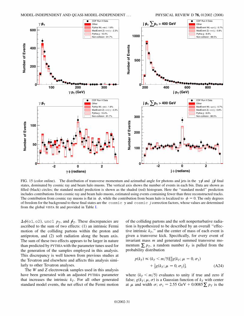
��ðo1;o2Þ, uncl pT , and p6 T . These discrepancies areascribed to the sum of two effects: (1) an intrinsic Fermimotion of the colliding partons within the proton andantiproton, and (2) soft radiation along the beam axis.The sum of these two effects appears to be larger in naturethan predicted by PYTHIAwith the parameter tunes used forthe generation of the samples employed in this analysis.This discrepancy is well known from previous studies atthe Tevatron and elsewhere and affects this analysis simi-larly to other Tevatron analyses.

The W and Z electroweak samples used in this analysishave been generated with an adjusted PYTHIA parameterthat increases the intrinsic kT . For all other generatedstandard model events, the net effect of the Fermi motion

of the colliding partons and the soft nonperturbative radia-tion is hypothesized to be described by an overall ‘‘effec-tive intrinsic kT ,’’ and the center of mass of each event isgiven a transverse kick. Specifically, for every event ofinvariant mass m and generated summed transverse mo-mentum

PpT , a random number kT is pulled from the

probability distribution

pðkTÞ / ðkT < m=5Þ½45gðkT;� ¼ 0; 1Þþ 1

5gðkT ;� ¼ 0; 2Þ�; (A24)

where ðkT < m=5Þ evaluates to unity if true and zero iffalse; gðkT;�;Þ is a Gaussian function of kT with centerat � and width ; 1 ¼ 2:55 GeVþ 0:0085

PpT is the

(GeV)T pγ100 200 300

Nu

mb

er o

f E

ven

ts

0

200

400

600

TpγCDF Run II Data

Other

) : 1.8%νe→Pythia W(

: 2.3%γ)νν→MadEvent Z(

Pythia jj : 10.4%Non-collision : 81.7%

γ (GeV)Tj p200 400 600 800

Nu

mb

er o

f E

ven

ts

0

500

1000

> 400 GeVTp∑TpjCDF Run II Data

Other

) j : 0.7%νµ→MadEvent W(

) j : 0.8%νν→MadEvent Z(


T

(radians)φγ-2 0 2

Nu

mb

er o

f E

ven

ts

0

50

100

TpγCDF Run II Data

Other

) : 1.8%νe→Pythia W(

: 2.3%γ)νν→MadEvent Z(


φγ (radians)φj-2 0 2

Nu

mb

er o

f E

ven

ts

0

100

200

300

> 400 GeVTp∑TpjCDF Run II Data

Other

) j : 0.7%νµ→MadEvent W(

) j : 0.8%νν→MadEvent Z(


-

FIG. 15 (color online). The distribution of transverse momentum and azimuthal angle for photons and jets in the �p6 and jp6 finalstates, dominated by cosmic ray and beam halo muons. The vertical axis shows the number of events in each bin. Data are shown asfilled (black) circles; the standard model prediction is shown as the shaded (red) histogram. Here the ‘‘standard model’’ predictionincludes contributions from cosmic ray and beam halo muons, estimated using events containing fewer than three reconstructed tracks.The contribution from cosmic ray muons is flat in �, while the contribution from beam halo is localized to � ¼ 0. The only degreesof freedom for the background to these final states are the cosmic � and cosmic j correction factors, whose values are determinedfrom the global VISTA fit and provided in Table I.


012002-31

width of the core of the double Gaussian; and 2 ¼5:25 GeVþ 0:0175

PpT is the width of the second, wider

Gaussian. The event is then boosted to an inertial frametraveling with speed j ~�j ¼ kT=m with respect to the labframe, in a direction transverse to the beam axis, where mis the invariant mass of all reconstructed objects in theevent, along an azimuthal angle pulled randomly from auniform distribution between 0 and 2�. The momenta ofidentified objects are recalculated in the lab frame. Sixtypercent of the recoil kick is assigned to unclustered mo-mentum in the event. The remaining 40% of the recoil kickis assumed to disappear down the beam pipe, and contrib-utes to the missing transverse momentum in the event. Thispicture, and the particular parameter values that accom-pany this story, are determined primarily by the uncl pT

and p6 T distributions in highly populated two-object finalstates, including the low-pT 2j final state, the high-pT 2jfinal state, and the final states j�, eþe�, and �þ��.

Under the hypothesis described, reasonable althoughimperfect agreement with observation is obtained. The re-sult of this analysis supports the conclusions of previousstudies indicating that the effective intrinsic kT needed tomatch observation is quite large relative to naive expecta-tion. That the data appear to require such a large effectiveintrinsic kT may be pointing out the need for some basicimprovement to our understanding of this physics.

3. Global fit

This section describes the construction of the global �2

used in the VISTA global fit.

a. �2k

The bins in the CDF high-pT data sample are labeled bythe index k ¼ ðk1; k2Þ, where each value of k1 represents aphrase such as ‘‘this bin contains events with three objects:one with 17< pT < 25 GeV and j�j< 0:6, one with 40<pT < 60 GeV and 0:6< j�j< 1:0, and one with 25<pT < 40 GeV and 1:0< j�j,’’ and each value of k2 repre-sents a phrase such as ‘‘this bin contains events with threeobjects: an electron, muon, and jet, respectively.’’ The rea-son for splitting k into k1 and k2 is that a jet can fake anelectron (mixing the contents of k2), but an object withj�j< 0:6 cannot fake an object with 0:6< j�j< 1:0 (nomixing of k1). The term corresponding to the kth bin takesthe form of Eq. (1), where Data½k� is the number of dataevents observed in the kth bin, SM½k� is the number ofevents predicted by the standard model in the kth bin,SM½k� is the Monte Carlo statistical uncertainty on the

standard model prediction in the kth bin, andffiffiffiffiffiffiffiffiffiffiffiffiffiffiSM½k�p

is thestatistical uncertainty on the prediction in the kth bin. Tolegitimize the use of Gaussian errors, only bins containingeight or more data events are considered. The standardmodel prediction SM½k� for the kth bin can be written interms of the introduced correction factors as

SM½k� ¼ SM½ðk1; k2Þ�¼ X

k202object lists

Xl2processes

�ZLdt

�

ðkFactor½l�Þ ðSM0½ðk1; k02Þ�½l�Þ ðp½ðk1; k02Þ�½k2�Þ ðt½ðk1; k2Þ�Þ; (A25)

where SM½k� is the standard model prediction for the kthbin; the index k is the Cartesian product of the two indicesk1 and k2 introduced above, labeling the regions of thedetector in which there are energy clusters and the identi-fied objects corresponding to those clusters, respectively;the index k02 is a dummy summation index; the index llabels standard model background processes, such as dijetproduction orW þ 1 jet production; SM0½ðk1; k02Þ�½l� is theinitial number of standard model events predicted in binðk1; k02Þ from the process labeled by the index l;p½ðk1; k02Þ�½k2� is the probability that an event producedwith energy clusters in the detector regions labeled by k1that are identified as objects labeled by k02 would be mis-taken as having objects labeled by k2; and t½ðk1; k2Þ� rep-resents the probability that an event produced with energyclusters in the detector regions labeled by k1 that areidentified as objects labeled by k2 would pass the trigger.The quantity SM0½ðk1; k02Þ�½l� is obtained by generating

some number nl (say 104) of Monte Carlo events corre-sponding to the process l. The event generator provides across section l for this process l. The weight of each ofthese Monte Carlo events is equal to l=nl. Passing theseevents through the CDF simulation and reconstruction, thesum of the weights of these events falling into the binðk1; k02Þ is SM0½ðk1; k02Þ�½l�.

b. �2constraints

The term �2constraintsð ~sÞ in Eq. (2) reflects constraints on

the values of the correction factors determined by dataother than those in the global high-pT sample. Theseconstraints include k-factors taken from theoretical calcu-lations and numbers from the CDF literature when use ismade of CDF data external to the VISTA high-pT sample.The constraints imposed are

(i) The luminosity (0001) is constrained to be within6% of the value measured by the CDF Cerenkovluminosity counters.

(ii) The fake rate pðq ! �Þ (0039) is constrained tobe 2:6� 10�4 � 1:5� 10�5, from the single par-ticle gun study of Appendix A 1.

(iii) The fake rate pðe ! �Þ (0032) plus the effi-ciency pðe ! eÞ (0026) for electrons in theplug is constrained to be within 1% of unity.

(iv) Noting pðq ! �Þ corresponds to correctionfactor 0039, pðq ! ��Þ ¼ 2pðq ! �0Þ, andpðq ! �0Þ ¼ pðq ! �Þ=pð�0 ! �Þ, and takingpð�0 ! �Þ ¼ 0:6 and pð�� ! �Þ ¼ 0:415 fromthe single particle gun study of Appendix A 1, the


012002-32

fake rate pðq ! �Þ (0038) is constrained topðq ! �Þ ¼ pðq ! ��Þpð�� ! �Þ � 10%.

(v) The k-factors for dijet production (0018 and0019) are constrained to 1:10� 0:05 and 1:33�0:05 in the kinematic regions pT < 150 GeVand pT > 150 GeV, respectively, where pT isthe transverse momentum of the scattered partonsin the 2 ! 2 process in the colliding parton centerof momentum frame.

(vi) The inclusive k-factor for �þ N jets (0004–0007) is constrained to 1:25� 0:15 [49,50].

(vii) The inclusive k-factor for ��þ N jets (0008–0010) is constrained to 2:0� 0:15 [51].

(viii) The inclusive k-factors for W and Z production(0011–0014 and 0015–0017) are subject to a2-dimensional Gaussian constraint, with mean atthe NNLO/LO theoretical values [52], and a co-variance matrix that encapsulates the highly cor-related theoretical uncertainties, as discussed inAppendix A 4.

(ix) Trigger efficiency correction factors are con-strained to be less than unity.

(x) All correction factors are constrained to bepositive.

c. Covariance matrix

This section describes the correction factor covari-ance matrix �. The inverse of the covariance matrix isobtained from

��1ij ¼ 1

2

@2�2ð ~sÞ@si@sj

��~s0

; (A26)

where �2ð~sÞ is defined by Eq. (2) as a function of thecorrection factor vector ~s, vector elements si and sj arethe ith and jth correction factors, and ~s0 is the vector ofcorrection factors that minimizes �2ð ~sÞ. Numerical estima-tion of the right-hand side of Eq. (A26) is achieved bycalculating �2 at ~s0 and at positions slightly displaced from~s0 in the direction of the ith and jth correction factors,denoted by the unit vectors i and j. Approximating thesecond partial derivative

@2�2

@sj@si

��~s0

¼ �2ð ~s0 þ isi þ jsjÞ � �2ð~s0 þ jsjÞsjsi

� �2ð ~s0 þ isiÞ � �2ð ~s0Þsjsi

leads to

��1ij ¼ ½�2ð~s0 þ siiþ sjjÞ � �2ð~s0 þ siiÞ

� �2ð~s0 þ sjjÞ þ �2ð ~s0Þ�=ð2sisjÞ; (A27)

for appropriately small steps si and sj away from the

minimum. The covariance matrix � is calculated by in-verting��1. The diagonal element�ii is the variance

2i of

the ith correction factor, and the correlation �ij between

the ith and jth correction factors is �ij ¼ �ij=ij. The

variances of each correction factor, corresponding to thediagonal elements of the covariance matrix, are shown inTable I. The correlation matrix obtained is shown inTable V.

4. Correction factor values

This section provides notes on the values of the VISTA

correction factors obtained from a global fit of standardmodel prediction to data. The correction factors consideredare numbers that can in principle be calculated a priori, butwhose calculation is in practice not feasible. These correc-tion factors divide naturally into two classes, the first ofwhich reflects the difficulty of calculating the standardmodel prediction to all orders, and the second of whichreflects the difficulty of understanding from first principlesthe response of the experimental apparatus.The theoretical correction factors considered are of two

types. The difficulty of calculating the standard modelprediction for many processes to all orders in perturbationtheory is handled through the introduction of k-factors,representing the ratio of the true all orders prediction tothe prediction at lowest order in perturbation theory.Uncertainties in the distribution of partons inside the col-liding proton and antiproton as a function of parton mo-mentum are in principle handled through the introductionof correction factors associated with parton distributionfunctions, but there are currently no discrepancies to mo-tivate this.Experimental correction factors correspond to numbers

describing the response of the CDF detector that are pre-cisely calculable in principle, but that are in practice bestconstrained by the high-pT data themselves. These correc-tion factors take the form of the integrated luminosity,object identification efficiencies, object misidentificationprobabilities, trigger efficiencies, and energy scales.

a. k-factors

For nearly all standard model processes, k-factors areused as an overall multiplicative constant, rather than beingconsidered to be a function of one or more kinematicvariables. The spirit of the approach is to introduce asfew correction factors as possible, and to only introducecorrection factors motivated by specific discrepancies.0001.—The integrated luminosity of the analysis sam-

ple has a close relationship with the theoretically deter-mined values of inclusive W and Z production at theTevatron. Figure 16 shows the variation in calculated in-clusive W and Z k-factors under changes in the assumedparton distribution functions. Each point represents a dif-ferent W and Z inclusive cross section determined usingmodified parton distribution functions. The use of 16 basesto reflect systematic uncertainties results in 32 black dots inFig. 16. The uncertainties in theW and Z cross sections dueto variations in the renormalization and factorization scales


012002-33

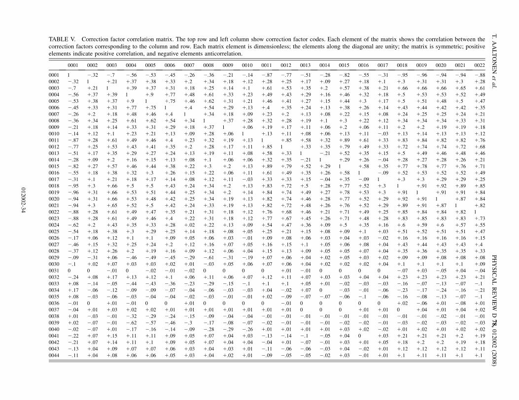
TABLE V. Correction factor correlation matrix. The top row and left column show correction factor codes. Each element of the matrix shows the correlation between thecorrection factors corresponding to the column and row. Each matrix element is dimensionless; the elements along the diagonal are unity; the matrix is symmetric; positiveelements indicate positive correlation, and negative elements anticorrelation.

0001 0002 0003 0004 0005 0006 0007 0008 0009 0010 0011 0012 0013 0014 0015 0016 0017 0018 0019 0020 0021 0022

0001 1 �:32 �:7 �:56 �:53 �:45 �:26 �:36 �:21 �:14 �:87 �:77 �:51 �:28 �:82 �:55 �:31 �:95 �:96 �:94 �:94 �:88

0002 �:32 1 þ:21 þ:37 þ:38 þ:33 þ:2 þ:34 þ:18 þ:12 þ:28 þ:25 þ:17 þ:09 þ:27 þ:18 þ:1 þ:3 þ:31 þ:31 þ:3 þ:28

0003 �:7 þ:21 1 þ:39 þ:37 þ:31 þ:18 þ:25 þ:14 þ:1 þ:61 þ:53 þ:35 þ:2 þ:57 þ:38 þ:21 þ:66 þ:66 þ:66 þ:65 þ:61

0004 �:56 þ:37 þ:39 1 þ:9 þ:77 þ:48 þ:61 þ:33 þ:23 þ:49 þ:43 þ:29 þ:16 þ:46 þ:32 þ:18 þ:5 þ:53 þ:53 þ:52 þ:49

0005 �:53 þ:38 þ:37 þ:9 1 þ:75 þ:46 þ:62 þ:31 þ:21 þ:46 þ:41 þ:27 þ:15 þ:44 þ:3 þ:17 þ:5 þ:51 þ:48 þ:5 þ:47

0006 �:45 þ:33 þ:31 þ:77 þ:75 1 þ:4 þ:54 þ:29 þ:13 þ:4 þ:35 þ:24 þ:13 þ:38 þ:26 þ:14 þ:43 þ:44 þ:42 þ:42 þ:35

0007 �:26 þ:2 þ:18 þ:48 þ:46 þ:4 1 þ:34 þ:18 þ:09 þ:23 þ:2 þ:13 þ:08 þ:22 þ:15 þ:08 þ:24 þ:25 þ:25 þ:24 þ:21

0008 �:36 þ:34 þ:25 þ:61 þ:62 þ:54 þ:34 1 þ:37 þ:28 þ:32 þ:28 þ:19 þ:1 þ:3 þ:22 þ:12 þ:34 þ:34 þ:34 þ:33 þ:31

0009 �:21 þ:18 þ:14 þ:33 þ:31 þ:29 þ:18 þ:37 1 þ:06 þ:19 þ:17 þ:11 þ:06 þ:2 þ:06 þ:11 þ:2 þ:2 þ:19 þ:19 þ:18

0010 �:14 þ:12 þ:1 þ:23 þ:21 þ:13 þ:09 þ:28 þ:06 1 þ:13 þ:11 þ:08 þ:06 þ:13 þ:11 �:03 þ:13 þ:14 þ:13 þ:13 þ:12

0011 �:87 þ:28 þ:61 þ:49 þ:46 þ:4 þ:23 þ:32 þ:19 þ:13 1 þ:85 þ:58 þ:32 þ:89 þ:61 þ:33 þ:83 þ:84 þ:82 þ:82 þ:76

0012 �:77 þ:25 þ:53 þ:43 þ:41 þ:35 þ:2 þ:28 þ:17 þ:11 þ:85 1 þ:33 þ:35 þ:79 þ:49 þ:33 þ:72 þ:74 þ:74 þ:72 þ:68

0013 �:51 þ:17 þ:35 þ:29 þ:27 þ:24 þ:13 þ:19 þ:11 þ:08 þ:58 þ:33 1 �:21 þ:52 þ:35 þ:15 þ:5 þ:49 þ:46 þ:48 þ:46

0014 �:28 þ:09 þ:2 þ:16 þ:15 þ:13 þ:08 þ:1 þ:06 þ:06 þ:32 þ:35 �:21 1 þ:29 þ:26 �:04 þ:28 þ:27 þ:28 þ:26 þ:21

0015 �:82 þ:27 þ:57 þ:46 þ:44 þ:38 þ:22 þ:3 þ:2 þ:13 þ:89 þ:79 þ:52 þ:29 1 þ:58 þ:35 þ:77 þ:78 þ:77 þ:76 þ:71

0016 �:55 þ:18 þ:38 þ:32 þ:3 þ:26 þ:15 þ:22 þ:06 þ:11 þ:61 þ:49 þ:35 þ:26 þ:58 1 �:09 þ:52 þ:53 þ:52 þ:52 þ:49

0017 �:31 þ:1 þ:21 þ:18 þ:17 þ:14 þ:08 þ:12 þ:11 �:03 þ:33 þ:33 þ:15 �:04 þ:35 �:09 1 þ:3 þ:3 þ:29 þ:29 þ:25

0018 �:95 þ:3 þ:66 þ:5 þ:5 þ:43 þ:24 þ:34 þ:2 þ:13 þ:83 þ:72 þ:5 þ:28 þ:77 þ:52 þ:3 1 þ:91 þ:92 þ:89 þ:85

0019 �:96 þ:31 þ:66 þ:53 þ:51 þ:44 þ:25 þ:34 þ:2 þ:14 þ:84 þ:74 þ:49 þ:27 þ:78 þ:53 þ:3 þ:91 1 þ:91 þ:91 þ:84

0020 �:94 þ:31 þ:66 þ:53 þ:48 þ:42 þ:25 þ:34 þ:19 þ:13 þ:82 þ:74 þ:46 þ:28 þ:77 þ:52 þ:29 þ:92 þ:91 1 þ:87 þ:84

0021 �:94 þ:3 þ:65 þ:52 þ:5 þ:42 þ:24 þ:33 þ:19 þ:13 þ:82 þ:72 þ:48 þ:26 þ:76 þ:52 þ:29 þ:89 þ:91 þ:87 1 þ:82

0022 �:88 þ:28 þ:61 þ:49 þ:47 þ:35 þ:21 þ:31 þ:18 þ:12 þ:76 þ:68 þ:46 þ:21 þ:71 þ:49 þ:25 þ:85 þ:84 þ:84 þ:82 1

0023 �:88 þ:28 þ:61 þ:49 þ:46 þ:4 þ:22 þ:31 þ:18 þ:12 þ:77 þ:67 þ:45 þ:26 þ:71 þ:48 þ:28 þ:83 þ:85 þ:83 þ:83 þ:73



0026 �:17 þ:06 þ:12 þ:1 þ:1 þ:09 þ:05 þ:06 þ:03 �:01 þ:09 þ:08 þ:06 þ:03 þ:04 þ:03 �:02 þ:16 þ:16 þ:16 þ:16 þ:15



0029 �:09 �:31 þ:06 �:46 �:49 �:45 �:29 �:61 �:31 �:19 þ:07 þ:06 þ:04 þ:02 þ:05 þ:03 þ:02 þ:09 þ:09 þ:08 þ:08 þ:08

0030 �:1 þ:02 þ:07 þ:03 þ:03 þ:02 þ:01 �:03 þ:05 þ:06 þ:07 þ:06 þ:04 þ:02 þ:02 þ:02 þ:04 þ:1 þ:1 þ:1 þ:1 þ:09

0031 0 0 �:01 0 �:02 �:01 �:02 0 0 0 0 þ:01 �:01 0 0 0 0 �:07 þ:03 �:05 þ:04 �:04


0033 þ:08 �:14 �:05 �:44 �:43 �:36 �:23 �:29 �:15 �:1 þ:1 þ:1 þ:05 þ:01 �:02 �:03 �:03 �:16 �:07 �:13 �:07 �:1

0034 þ:17 �:06 �:12 �:09 �:09 �:07 �:04 �:06 �:03 �:03 þ:04 �:02 þ:07 0 �:03 �:01 �:06 �:23 �:17 �:24 �:16 �:21

0035 þ:08 �:03 �:06 �:03 �:04 �:04 �:02 �:03 �:01 �:01 þ:02 �:09 �:07 �:07 �:06 �:1 �:06 �:16 �:08 �:13 �:07 �:1

0036 �:01 0 þ:01 �:01 0 0 þ:01 0 0 0 0 �:01 0 0 0 0 0 þ:02 �:06 þ:01 �:08 þ:01

0037 �:04 þ:01 þ:03 þ:02 þ:02 þ:01 þ:01 þ:01 þ:01 þ:01 þ:01 þ:01 0 0 0 þ:01 þ:01 0 þ:04 þ:01 þ:04 þ:02

0038 þ:01 �:03 �:01 �:32 �:29 �:24 �:15 �:09 �:04 �:04 �:01 �:01 �:01 �:01 �:01 �:01 �:01 �:01 �:01 �:02 �:01 �:01

0039 þ:02 �:07 �:01 �:62 �:57 �:46 �:3 �:17 �:08 �:07 �:02 �:01 �:01 �:01 �:02 �:02 �:01 �:03 �:02 �:03 �:02 �:03

0040 �:02 �:07 þ:01 �:17 �:16 �:14 �:09 �:28 �:29 �:26 þ:01 þ:01 þ:01 þ:01 þ:03 þ:02 �:02 þ:01 þ:02 þ:01 þ:02 þ:02

0041 �:22 þ:07 þ:15 þ:11 þ:11 þ:09 þ:05 þ:07 þ:04 þ:03 �:13 �:14 �:1 �:05 þ:04 0 þ:03 þ:21 þ:21 þ:21 þ:2 þ:19

0042 �:21 þ:07 þ:14 þ:11 þ:1 þ:09 þ:05 þ:07 þ:04 þ:04 �:04 þ:01 �:07 �:01 þ:03 þ:01 þ:05 þ:18 þ:2 þ:2 þ:19 þ:18

0043 �:13 þ:04 þ:09 þ:07 þ:07 þ:06 þ:03 þ:04 þ:03 þ:01 �:11 �:06 �:06 �:03 þ:04 �:02 þ:01 þ:12 þ:12 þ:12 þ:12 þ:11

0044 �:11 þ:04 þ:08 þ:06 þ:06 þ:05 þ:03 þ:04 þ:02 þ:01 �:09 �:05 �:05 �:02 þ:03 �:01 þ:01 þ:1 þ:11 þ:11 þ:1 þ:1

T.AALTONEN

etal.

PHYSICALREVIEW

D78,012002(2008)

012002-34

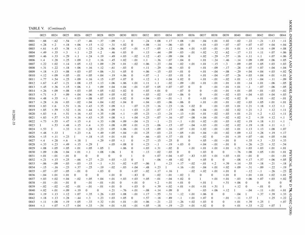
0023 0024 0025 0026 0027 0028 0029 0030 0031 0032 0033 0034 0035 0036 0037 0038 0039 0040 0041 0042 0043 0044

0001 �:88 �:62 �:54 �:17 �:46 �:37 �:09 �:1 0 �:24 þ:08 þ:17 þ:08 �:01 �:04 þ:01 þ:02 �:02 �:22 �:21 �:13 �:11

0002 þ:28 þ:2 þ:18 þ:06 þ:15 þ:12 �:31 þ:02 0 þ:08 �:14 �:06 �:03 0 þ:01 �:03 �:07 �:07 þ:07 þ:07 þ:04 þ:04

0003 þ:61 þ:43 þ:38 þ:12 þ:32 þ:26 þ:06 þ:07 �:01 þ:17 �:05 �:12 �:06 þ:01 þ:03 �:01 �:01 þ:01 þ:15 þ:14 þ:09 þ:08

0004 þ:49 þ:35 þ:3 þ:1 þ:25 þ:2 �:46 þ:03 0 þ:13 �:44 �:09 �:03 �:01 þ:02 �:32 �:62 �:17 þ:11 þ:11 þ:07 þ:06

0005 þ:46 þ:33 þ:29 þ:1 þ:24 þ:19 �:49 þ:03 �:02 þ:12 �:43 �:09 �:04 0 þ:02 �:29 �:57 �:16 þ:11 þ:1 þ:07 þ:06

0006 þ:4 þ:28 þ:25 þ:09 þ:2 þ:16 �:45 þ:02 �:01 þ:1 �:36 �:07 �:04 0 þ:01 �:24 �:46 �:14 þ:09 þ:09 þ:06 þ:05

0007 þ:22 þ:02 þ:14 þ:05 þ:12 þ:09 �:29 þ:01 �:02 þ:06 �:23 �:04 �:02 þ:01 þ:01 �:15 �:3 �:09 þ:05 þ:05 þ:03 þ:03

0008 þ:31 þ:22 þ:18 þ:06 þ:16 þ:12 �:61 �:03 0 þ:11 �:29 �:06 �:03 0 þ:01 �:09 �:17 �:28 þ:07 þ:07 þ:04 þ:04

0009 þ:18 þ:13 þ:08 þ:03 þ:07 þ:06 �:31 þ:05 0 þ:06 �:15 �:03 �:01 0 þ:01 �:04 �:08 �:29 þ:04 þ:04 þ:03 þ:02

0010 þ:12 þ:09 þ:05 �:01 þ:05 þ:04 �:19 þ:06 0 þ:07 �:1 �:03 �:01 0 þ:01 �:04 �:07 �:26 þ:03 þ:04 þ:01 þ:01

0011 þ:77 þ:54 þ:25 þ:09 þ:16 þ:15 þ:07 þ:07 0 þ:12 þ:1 þ:04 þ:02 0 þ:01 �:01 �:02 þ:01 �:13 �:04 �:11 �:09

0012 þ:67 þ:47 þ:21 þ:08 þ:15 þ:13 þ:06 þ:06 þ:01 þ:11 þ:1 �:02 �:09 �:01 þ:01 �:01 �:01 þ:01 �:14 þ:01 �:06 �:05

0013 þ:45 þ:36 þ:15 þ:06 þ:1 þ:09 þ:04 þ:04 �:01 þ:07 þ:05 þ:07 �:07 0 0 �:01 �:01 þ:01 �:1 �:07 �:06 �:05

0014 þ:26 þ:09 þ:08 þ:03 þ:05 þ:05 þ:02 þ:02 0 þ:03 þ:01 0 �:07 0 0 �:01 �:01 þ:01 �:05 �:01 �:03 �:02

0015 þ:71 þ:5 þ:09 þ:04 þ:06 þ:05 þ:05 þ:02 0 þ:03 �:02 �:03 �:06 0 0 �:01 �:02 þ:03 þ:04 þ:03 þ:04 þ:03

0016 þ:48 þ:35 þ:1 þ:03 þ:08 þ:07 þ:03 þ:02 0 þ:04 �:03 �:01 �:1 0 þ:01 �:01 �:02 þ:02 0 þ:01 �:02 �:01

0017 þ:28 þ:16 þ:03 �:02 þ:04 þ:04 þ:02 þ:04 0 þ:04 �:03 �:06 �:06 0 þ:01 �:01 �:01 �:02 þ:03 þ:05 þ:01 þ:01

0018 þ:83 þ:6 þ:51 þ:16 þ:43 þ:35 þ:09 þ:1 �:07 þ:23 �:16 �:23 �:16 þ:02 0 �:01 �:03 þ:01 þ:21 þ:18 þ:12 þ:1

0019 þ:85 þ:59 þ:52 þ:16 þ:44 þ:36 þ:09 þ:1 þ:03 þ:23 �:07 �:17 �:08 �:06 þ:04 �:01 �:02 þ:02 þ:21 þ:2 þ:12 þ:11


0021 þ:83 þ:57 þ:51 þ:16 þ:43 þ:35 þ:08 þ:1 þ:04 þ:23 �:07 �:16 �:07 �:08 þ:04 �:01 �:02 þ:02 þ:2 þ:19 þ:12 þ:1


0023 1 þ:53 þ:48 þ:15 þ:4 þ:33 þ:08 þ:09 þ:01 þ:21 �:06 �:15 �:07 �:04 þ:03 �:01 �:02 þ:02 þ:19 þ:18 þ:11 þ:1

0024 þ:53 1 þ:33 þ:11 þ:28 þ:23 þ:05 þ:06 �:01 þ:15 �:09 �:16 �:07 þ:01 þ:02 �:01 �:02 þ:01 þ:13 þ:13 þ:08 þ:07

0025 þ:48 þ:33 1 þ:23 þ:6 þ:49 þ:05 þ:04 �:01 þ:25 �:03 �:23 �:05 þ:01 þ:04 �:01 �:02 þ:09 þ:12 þ:28 þ:19 þ:17

0026 þ:15 þ:11 þ:23 1 þ:18 þ:15 þ:01 þ:01 0 �:66 �:03 þ:37 �:01 0 �:02 0 �:01 þ:19 þ:07 �:44 þ:05 þ:04

0027 þ:4 þ:28 þ:6 þ:18 1 þ:29 þ:05 þ:1 0 þ:27 �:15 �:25 0 0 þ:05 �:01 �:01 0 þ:35 þ:3 �:33 þ:33

0028 þ:33 þ:23 þ:49 þ:15 þ:29 1 þ:05 þ:08 0 þ:23 �:1 �:19 þ:03 0 þ:04 �:01 �:01 0 þ:26 þ:23 þ:32 �:54

0029 þ:08 þ:05 þ:05 þ:01 þ:05 þ:05 1 þ:06 0 þ:03 þ:31 �:02 0 þ:01 þ:01 þ:01 þ:01 þ:21 þ:03 þ:03 þ:01 þ:01

0030 þ:09 þ:06 þ:04 þ:01 þ:1 þ:08 þ:06 1 0 �:13 �:02 �:03 0 0 þ:03 0 0 �:76 þ:08 þ:05 þ:01 þ:01

0031 þ:01 �:01 �:01 0 0 0 0 0 1 0 þ:07 þ:04 þ:07 �:83 þ:03 þ:01 þ:03 þ:01 �:01 0 �:01 �:01

0032 þ:21 þ:15 þ:25 �:66 þ:27 þ:23 þ:03 �:13 0 1 �:06 �:48 �:02 0 þ:05 0 0 �:08 þ:17 þ:57 þ:06 þ:05

0033 �:06 �:09 �:03 �:03 �:15 �:1 þ:31 �:02 þ:07 �:06 1 þ:23 þ:17 �:02 �:01 þ:2 þ:39 þ:14 �:55 �:18 �:21 �:18

0034 �:15 �:16 �:23 þ:37 �:25 �:19 �:02 �:03 þ:04 �:48 þ:23 1 þ:16 �:01 �:04 þ:01 þ:02 þ:09 �:31 �:89 �:22 �:19

0035 �:07 �:07 �:05 �:01 0 þ:03 0 0 þ:07 �:02 þ:17 þ:16 1 �:02 þ:02 þ:01 þ:01 0 �:12 �:1 �:26 �:23

0036 �:04 þ:01 þ:01 0 0 0 þ:01 0 �:83 0 �:02 �:01 �:02 1 0 0 þ:01 0 þ:01 þ:01 þ:02 þ:01

0037 þ:03 þ:02 þ:04 �:02 þ:05 þ:04 þ:01 þ:03 þ:03 þ:05 �:01 �:04 þ:02 0 1 þ:01 þ:01 �:03 þ:06 þ:07 þ:03 þ:02

0038 �:01 �:01 �:01 0 �:01 �:01 þ:01 0 þ:01 0 þ:2 þ:01 þ:01 0 þ:01 1 þ:51 þ:06 0 0 0 0

0039 �:02 �:02 �:02 �:01 �:01 �:01 þ:01 0 þ:03 0 þ:39 þ:02 þ:01 þ:01 þ:01 þ:51 1 þ:12 0 �:01 0 0

0040 þ:02 þ:01 þ:09 þ:19 0 0 þ:21 �:76 þ:01 �:08 þ:14 þ:09 0 0 �:03 þ:06 þ:12 1 �:04 �:11 þ:01 þ:01

0041 þ:19 þ:13 þ:12 þ:07 þ:35 þ:26 þ:03 þ:08 �:01 þ:17 �:55 �:31 �:12 þ:01 þ:06 0 0 �:04 1 þ:37 þ:39 þ:33

0042 þ:18 þ:13 þ:28 �:44 þ:3 þ:23 þ:03 þ:05 0 þ:57 �:18 �:89 �:1 þ:01 þ:07 0 �:01 �:11 þ:37 1 þ:25 þ:22

0043 þ:11 þ:08 þ:19 þ:05 �:33 þ:32 þ:01 þ:01 �:01 þ:06 �:21 �:22 �:26 þ:02 þ:03 0 0 þ:01 þ:39 þ:25 1 þ:07

0044 þ:1 þ:07 þ:17 þ:04 þ:33 �:54 þ:01 þ:01 �:01 þ:05 �:18 �:19 �:23 þ:01 þ:02 0 0 þ:01 þ:33 þ:22 þ:07 1

TABLE V. (Continued)

MODEL-IN

DEPENDENTAND

QUASI-M

ODEL-IN

DEPENDENT...

PHYSICALREVIEW

D78,012002(2008)

012002-35

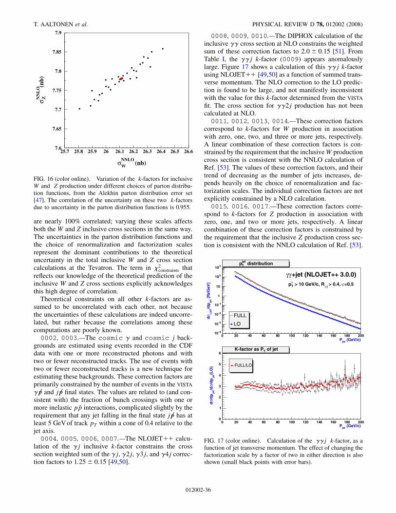
are nearly 100% correlated; varying these scales affectsboth theW and Z inclusive cross sections in the same way.The uncertainties in the parton distribution functions andthe choice of renormalization and factorization scalesrepresent the dominant contributions to the theoreticaluncertainty in the total inclusive W and Z cross sectioncalculations at the Tevatron. The term in �2

constraints that

reflects our knowledge of the theoretical prediction of theinclusive W and Z cross sections explicitly acknowledgesthis high degree of correlation.

Theoretical constraints on all other k-factors are as-sumed to be uncorrelated with each other, not becausethe uncertainties of these calculations are indeed uncorre-lated, but rather because the correlations among thesecomputations are poorly known.

0002, 0003.—The cosmic � and cosmic j back-grounds are estimated using events recorded in the CDFdata with one or more reconstructed photons and withtwo or fewer reconstructed tracks. The use of events withtwo or fewer reconstructed tracks is a new technique forestimating these backgrounds. These correction factors areprimarily constrained by the number of events in the VISTA

�p6 and jp6 final states. The values are related to (and con-sistent with) the fraction of bunch crossings with one ormore inelastic p �p interactions, complicated slightly by therequirement that any jet falling in the final state jp6 has atleast 5 GeVof track pT within a cone of 0.4 relative to thejet axis.

0004, 0005, 0006, 0007.—The NLOJETþþ calcu-lation of the �j inclusive k-factor constrains the crosssection weighted sum of the �j, �2j, �3j, and �4j correc-tion factors to 1:25� 0:15 [49,50].

0008, 0009, 0010.—The DIPHOX calculation of theinclusive �� cross section at NLO constrains the weightedsum of these correction factors to 2:0� 0:15 [51]. FromTable I, the ��j k-factor (0009) appears anomalouslylarge. Figure 17 shows a calculation of this ��j k-factorusing NLOJETþþ [49,50] as a function of summed trans-verse momentum. The NLO correction to the LO predic-tion is found to be large, and not manifestly inconsistentwith the value for this k-factor determined from the VISTA

fit. The cross section for ��2j production has not beencalculated at NLO.0011, 0012, 0013, 0014.—These correction factors

correspond to k-factors for W production in associationwith zero, one, two, and three or more jets, respectively.A linear combination of these correction factors is con-strained by the requirement that the inclusiveW productioncross section is consistent with the NNLO calculation ofRef. [53]. The values of these correction factors, and theirtrend of decreasing as the number of jets increases, de-pends heavily on the choice of renormalization and fac-torization scales. The individual correction factors are notexplicitly constrained by a NLO calculation.0015, 0016, 0017.—These correction factors corre-

spond to k-factors for Z production in association withzero, one, and two or more jets, respectively. A linearcombination of these correction factors is constrained bythe requirement that the inclusive Z production cross sec-tion is consistent with the NNLO calculation of Ref. [53].

(GeV/c)jetP0 20 40 60 80 100 120 140 160 180 200

0 20 40 60 80 100 120 140 160 180 200

[fb

/GeV

]je

t/d

pje

tγγσd

-410

-310

-210

-110

1

10

210

310 distributionjet

T p

FULL

LO

+jet (NLOJET++ 3.0.0)γγ=0.5∈ > 0.4, jγ > 10 GeV/c, Rγ

Tp

distributionjetT p

(GeV/c)jetP

(LO

)je

t/d

pσ

/dje

t/d

pσd

0

1

2

3

4

5

6 of jetT K-factor as P

FULL/LO

of jetT K-factor as P

FIG. 17 (color online). Calculation of the ��j k-factor, as afunction of jet transverse momentum. The effect of changing thefactorization scale by a factor of two in either direction is alsoshown (small black points with error bars).

NNLOW

NN

LO

Z

FIG. 16 (color online). Variation of the k-factors for inclusiveW and Z production under different choices of parton distribu-tion functions, from the Alekhin parton distribution error set[47]. The correlation of the uncertainty on these two k-factorsdue to uncertainty in the parton distribution functions is 0.955.


012002-36

0018, 0019.—The two k-factors for dijet productioncorrespond to two bins in pT , the pT of the hard two to twoscattering in the parton center of mass frame. These cor-rection factors are constrained by a NLO calculation [54]and show expected behavior as a function of pT .

0020, 0021.—The two k-factors for 3-jet production,corresponding to two bins in pT , are unconstrained by anyNLO calculation but show reasonable behavior as a func-tion of pT .

0022, 0023.—The k-factors for 4-jet production, cor-responding to two bins in pT , are unconstrained by anyNLO calculation, but show reasonable behavior as a func-tion of pT .

0024.—The k-factor for the production of five or morejets, constrained primarily by the VISTA low-pT 5j finalstate, is found to be close to unity.

b. Identification efficiencies

The correction factors in this section, although billed as‘‘identification efficiencies,’’ are truly ratios of the identi-fication efficiency in the data relative to the identificationefficiency in CDFSIM. A correction factor value of unityindicates a proper modeling of the overall identificationefficiency by CDFSIM; a correction factor value of 0.5 in-dicates that CDFSIM overestimates the overall identificationefficiency by a factor of 2.

0025.—The central electron identification efficiencyscale factor is close to unity, indicating the central electronefficiency measured in data is similar (to within 1%) to thecentral electron efficiency in the CDF detector simulation.This reflects an emphasis within CDF on tuning the detec-tor simulation for central electrons. The determination ofthis correction factor is dominated by the VISTA final statesep6 and eþe�, where one of the electrons has j�j< 1.

0026.—The plug electron identification efficiency scalefactor is several percent less than unity, indicating that theCDF detector simulation slightly overestimates the elec-tron identification efficiency in the plug region of theCDF detector. The determination of this correction factoris dominated by the VISTA final states ep6 and eþe�, whereone of the electrons has j�j> 1.

0027, 0028.—To reduce backgrounds hypothesized toarise from pion and kaon decays in flight with a substan-tially mismeasured track, a very good track fit in theCDF tracker is required. Partially due to this tight trackfit requirement, CDFmuon identification efficiencies in theregions j�j< 0:6 and 0:6< j�j< 1:5 are overestimated inthe CDF detector simulation by over 10%. The determi-nation of the identification efficiencies pð� ! �Þ is domi-nated by the VISTA final states �p6 and �þ��.

0029.—The central photon identification efficiencyscale factor is determined primarily by the number ofevents in the VISTA final states j� and ��. The uncertaintyon this correction factor is highly correlated with the un-

certainties on the �j k-factor, the pðj ! �Þ fake rate, andthe �� k-factor.0030.—The plug photon identification efficiency scale

factor is determined primarily by the number of events inthe VISTA final state ��. The uncertainty on this correctionfactor is highly correlated with the uncertainty on the plugpðj ! �Þ fake rate.0031.—The b-jet identification efficiency is determined

to be consistent with the prediction from CDFSIM.

c. Fake rates

0032.—The fake rate pðe ! �Þ for electrons to bemisreconstructed as photons in the plug region of thedetector is added on top of the significant number ofelectrons misreconstructed as photons by CDFSIM.0033.—In VISTA, the contribution of jets faking elec-

trons is modeled by applying a fake rate pðj ! eÞ toMonte Carlo jets. VISTA represents the first large scaleTevatron analysis in which a completely Monte Carlobased modeling of jets faking electrons is employed.Significant understanding of the physical mechanisms con-tributing to this fake rate has been achieved, as summarizedin Appendix A 1. Consistency with this understanding isrequired; for example, pðj ! eÞ � pðj ! �Þpð� ! eÞ.The value of this correction factor is determined primarilyby the number of events in the VISTA final state ej, wherethe electron is identified in the central region of the CDFdetector. It is notable that this fake rate is independent ofglobal event properties, and that a consistent simultaneousunderstanding of the ej, e2j, e3j, and e4j final states isobtained.0034.—The value of the fake rate pðj ! eÞ in the plug

region of the CDF detector is roughly 1 order of magnitudelarger than the corresponding fake rate pðj ! eÞ in thecentral region of the detector, consistent with an under-standing of the relative performance of the detector in thecentral and plug regions for the identification of electrons.This correction factor is determined primarily by the num-ber of events in the VISTA final state ej, where the electronis identified in the plug region of the CDF detector.0035.—In VISTA, the contribution of jets faking muons

is modeled by applying a fake rate pðj ! �Þ to MonteCarlo jets. VISTA represents the first large scale Tevatronanalysis in which a completely Monte Carlo based model-ing of jets faking muons is employed. The value obtainedfrom the VISTA fit is seen to be roughly 1 order of magni-tude smaller than the fake rate pðj ! eÞ in the centralregion of the detector, consistent with our understandingof the physical mechanisms underlying these fake rates, asdescribed in Appendix A 1. The value of this correctionfactor is determined primarily by the number of events inthe VISTA final state j�.0036.—The fake rate pðj ! bÞ has pT dependence

explicitly imposed. The number of tracks inside a typicaljet, and hence the probability that a secondary vertex is


012002-37

(mis)reconstructed, increases with jet pT . The values ofthese correction factors are consistent with the mistag ratedetermined using secondary vertices reconstructed on theother side of the beam axis with respect to the direction ofthe tagged jet [55]. The value of this correction factor isdetermined primarily by the number of events in the VISTA

final states bj and bb.0037, 0038.—The fake rate pðj ! �Þ decreases with

jet pT , since the number of tracks inside a typical jetincreases with jet pT . The values of these correction factorsare determined primarily by the number of events in theVISTA final state j�.

0039, 0040.—The fake rate pðj ! �Þ is deter-mined separately in the central and plug regions of theCDF detector. The values of these correction factors aredetermined primarily by the number of events in the VISTA

final states j� and ��. The value obtained for 0039 isconsistent with the value obtained from a study using de-tailed information from the central preshower detector. Thefake rate determined in the plug region is noticeably higherthan the fake rate determined in the central region, asexpected.

d. Trigger efficiencies

0041.—The central electron trigger inefficiency isdominated by not correctly reconstructing the electron’strack at the first online trigger level.

0042.—The plug electron trigger inefficiency is due toinefficiencies in clustering at the second online triggerlevel.

0043, 0044.—The muon trigger inefficiencies in theregions j�j< 0:6 and 0:6< j�j< 1:0 derive partly fromtracking inefficiency and partly from an inefficiency inreconstructing muon stubs in the CDF muon chambers.The value of these corrections factors are consistent withother trigger efficiency measurements made using addi-tional information [56].

e. Energy scales

The VISTA infrastructure also allows the jet energy scaleto be treated as a correction factor. At present this cor-rection factor is not used, since there is no discrepancyrequiring it.

To understand the effect of introducing such a correctionfactor, a jet energy scale correction factor is added andconstrained to 1� 0:03, reflecting the jet energy scaledetermination at CDF [15]. The fit returns a value with avery small error, since this correction factor is highly con-strained by the low-pT 2j, 3j, ej, and e2j final states.Assuming perfectly correct modeling of jets faking elec-trons, as described in Appendix A 1, this is a correct energyscale error. The inclusion of additional correction factordegrees of freedom to reflect possible imperfections in thismodeling of jets faking electrons increases the energy scaleerror. The interesting conclusion is that the jet energy scale

(considered as a lone free parameter) is very well con-strained by the large number of dijet events; adjustment tothe jet energy scale must be accompanied by simultaneousadjustment of other correction factors (such as the dijetk-factor) in order to retain agreement with data.

APPENDIX B: SLEUTH DETAILS

This appendix elaborates on the SLEUTH partitioning ruleand on the minimum number of events required for a finalstate to be considered by SLEUTH.

1. Partitioning

Table VI lists the VISTA final states associated with eachSLEUTH final state.

2. Minimum number of events

This section expands on a subtle point in the definition ofthe SLEUTH algorithm: for purely practical considerations,only final states in which three or more events are observedin the data are considered.

Suppose P eþe�b �b ¼ 10�6; then in computing ~P all finalstates with b > 10�6 must be considered and accountedfor. (A final state with b ¼ 10�7, on the other hand, countsas only� 0:1 final states, since the fraction of hypotheticalsimilar experiments in which P < 10�6 in this final state isequal to the fraction of hypothetical similar experiments inwhich one or more events is seen in this final state, which is10�7.) This is a large practical problem, since it requiresthat all final states with b > 10�6 be enumerated andestimated, and it is difficult to do this believably.To solve this problem, let SLEUTH consider only final

states with at least dmin events observed in the data. Thegoal is to be able to find ~P < 10�3. There will be somenumber NfsðbminÞ of final states with expected number ofevents b > bmin, writing Nfs explicitly as a function ofbmin; thus bmin must be chosen to be sufficiently largethat all of these NfsðbminÞ final states can be enumeratedand estimated. The time cost of simulating events is suchthat the integrated luminosity of Monte Carlo events is atmost 100 times the integrated luminosity of the data; thispractical constraint restricts bmin > 0:01. The number ofSLEUTH Tevatron run II final states with b > 0:01 isNfsðbmin ¼ 0:01Þ � 103.For small Pmin, keeping the first term in a binomial

expansion yields ~P ¼ PminNfsðbminÞ, where Pmin is the

smallest P found in any final state. From the discussion

above, the computation of ~P from Pmin can only be

justified if Pmin > ðbmindminÞ; if otherwise, final states with

b < bmin will need to be accounted for. Thus ~P can be

confidently computed only if ~P > ðbmindminÞNfsðbminÞ.

Solving this inequality for dmin and inserting valuesfrom above,


012002-38

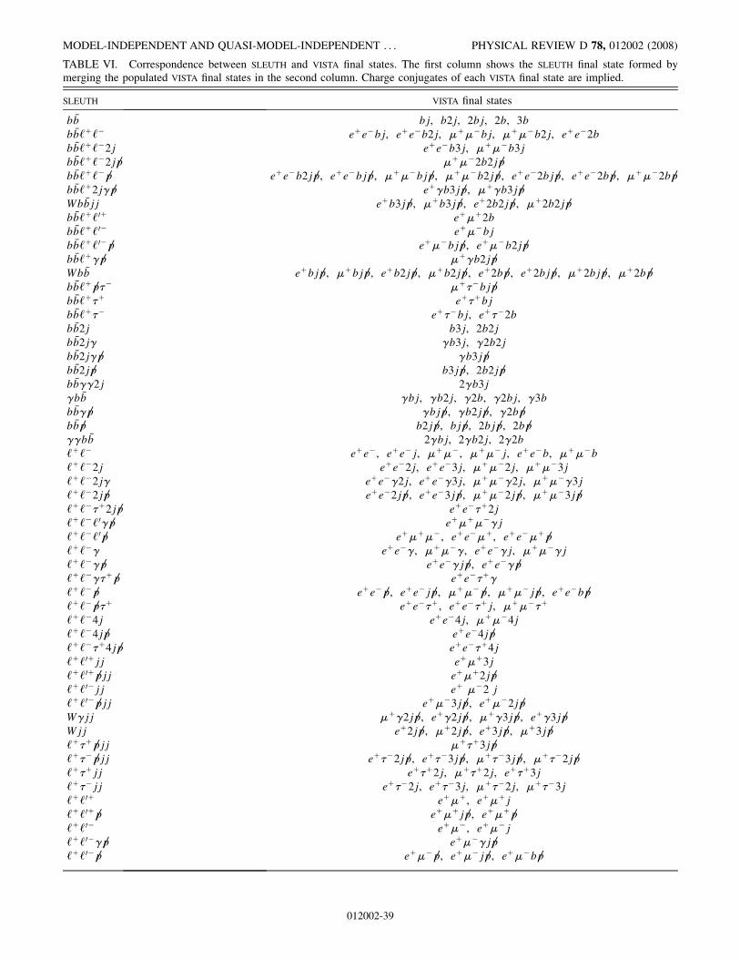
TABLE VI. Correspondence between SLEUTH and VISTA final states. The first column shows the SLEUTH final state formed bymerging the populated VISTA final states in the second column. Charge conjugates of each VISTA final state are implied.

SLEUTH VISTA final states

b �b bj, b2j, 2bj, 2b, 3bb �b‘þ‘� eþe�bj, eþe�b2j, �þ��bj, �þ��b2j, eþe�2bb �b‘þ‘�2j eþe�b3j, �þ��b3jb �b‘þ‘�2jp6 �þ��2b2jp6b �b‘þ‘�p6 eþe�b2jp6 , eþe�bjp6 , �þ��bjp6 , �þ��b2jp6 , eþe�2bjp6 , eþe�2bp6 , �þ��2bp6b �b‘þ2j�p6 eþ�b3jp6 , �þ�b3jp6Wb �bjj eþb3jp6 , �þb3jp6 , eþ2b2jp6 , �þ2b2jp6b �b‘þ‘0þ eþ�þ2bb �b‘þ‘0� eþ��bjb �b‘þ‘0�p6 eþ��bjp6 , eþ��b2jp6b �b‘þ�p6 �þ�b2jp6Wb �b eþbjp6 , �þbjp6 , eþb2jp6 , �þb2jp6 , eþ2bp6 , eþ2bjp6 , �þ2bjp6 , �þ2bp6b �b‘þp6 �� þ��bjp6b �b‘þ�þ eþ�þbjb �b‘þ�� eþ��bj, eþ��2bb �b2j b3j, 2b2jb �b2j� �b3j, �2b2jb �b2j�p6 �b3jp6b �b2jp6 b3jp6 , 2b2jp6b �b��2j 2�b3j�b �b �bj, �b2j, �2b, �2bj, �3bb �b�p6 �bjp6 , �b2jp6 , �2bp6b �bp6 b2jp6 , bjp6 , 2bjp6 , 2bp6��b �b 2�bj, 2�b2j, 2�2b‘þ‘� eþe�, eþe�j, �þ��, �þ��j, eþe�b, �þ��b‘þ‘�2j eþe�2j, eþe�3j, �þ��2j, �þ��3j‘þ‘�2j� eþe��2j, eþe��3j, �þ��2j, �þ��3j‘þ‘�2jp6 eþe�2jp6 , eþe�3jp6 , �þ��2jp6 , �þ��3jp6‘þ‘��þ2jp6 eþe��þ2j‘þ‘�‘0�p6 eþ�þ��j‘þ‘�‘0p6 eþ�þ��, eþe��þ, eþe��þp6‘þ‘�� eþe��, �þ��, eþe��j, �þ��j‘þ‘��p6 eþe��jp6 , eþe��p6‘þ‘��þp6 eþe��þ�‘þ‘�p6 eþe�p6 , eþe�jp6 , �þ��p6 , �þ��jp6 , eþe�bp6‘þ‘�p6 �þ eþe��þ, eþe��þj, �þ��þ‘þ‘�4j eþe�4j, �þ��4j‘þ‘�4jp6 eþe�4jp6‘þ‘��þ4jp6 eþe��þ4j‘þ‘0þjj eþ�þ3j‘þ‘0þp6 jj eþ�þ2jp6‘þ‘0�jj eþ ��2 j‘þ‘0�p6 jj eþ��3jp6 , eþ��2jp6W�jj �þ�2jp6 , eþ�2jp6 , �þ�3jp6 , eþ�3jp6Wjj eþ2jp6 , �þ2jp6 , eþ3jp6 , �þ3jp6‘þ�þp6 jj �þ�þ3jp6‘þ��p6 jj eþ��2jp6 , eþ��3jp6 , �þ��3jp6 , �þ��2jp6‘þ�þjj eþ�þ2j, �þ�þ2j, eþ�þ3j‘þ��jj eþ��2j, eþ��3j, �þ��2j, �þ��3j‘þ‘0þ eþ�þ, eþ�þj‘þ‘0þp6 eþ�þjp6 , eþ�þp6‘þ‘0� eþ��, eþ��j‘þ‘0��p6 eþ��jp6‘þ‘0�p6 eþ��p6 , eþ��jp6 , eþ��bp6


012002-39

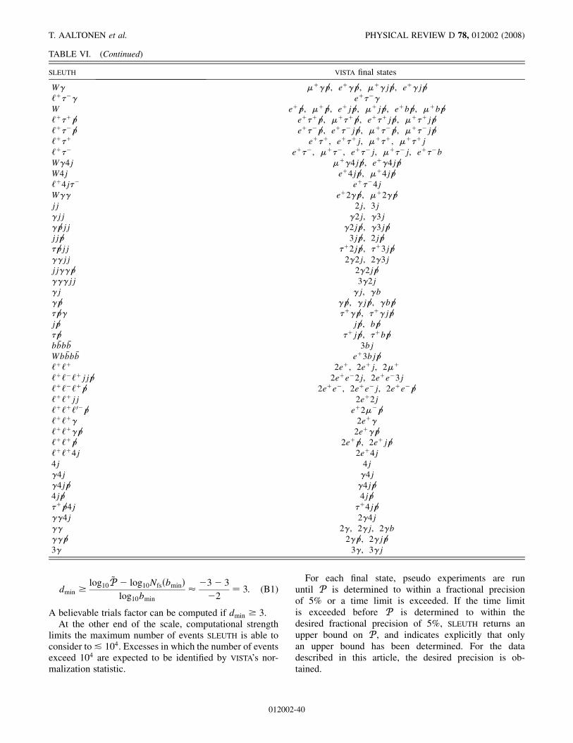
dmin � log10~P � log10NfsðbminÞlog10bmin

� �3� 3

�2¼ 3: (B1)

A believable trials factor can be computed if dmin � 3.At the other end of the scale, computational strength

limits the maximum number of events SLEUTH is able toconsider to& 104. Excesses in which the number of eventsexceed 104 are expected to be identified by VISTA’s nor-malization statistic.

For each final state, pseudo experiments are rununtil P is determined to within a fractional precisionof 5% or a time limit is exceeded. If the time limitis exceeded before P is determined to within thedesired fractional precision of 5%, SLEUTH returns anupper bound on P , and indicates explicitly that onlyan upper bound has been determined. For the datadescribed in this article, the desired precision is ob-tained.

SLEUTH VISTA final states

W� �þ�p6 , eþ�p6 , �þ�jp6 , eþ�jp6‘þ�� eþ��W eþp6 , �þp6 , eþjp6 , �þjp6 , eþbp6 , �þbp6‘þ�þp6 eþ�þp6 , �þ�þp6 , eþ�þjp6 , �þ�þjp6‘þ��p6 eþ��p6 , eþ��jp6 , �þ��p6 , �þ��jp6‘þ�þ eþ�þ, eþ�þj, �þ�þ, �þ�þj‘þ�� eþ��, �þ��, eþ��j, �þ��j, eþ��bW�4j �þ�4jp6 , eþ�4jp6W4j eþ4jp6 , �þ4jp6‘þ4j�� eþ��4jW�� eþ2�p6 , �þ2�p6jj 2j, 3j�jj �2j, �3j�p6 jj �2jp6 , �3jp6jjp6 3jp6 , 2jp6�p6 jj �þ2jp6 , �þ3jp6��jj 2�2j, 2�3jjj��p6 2�2jp6��jj 3�2j�j �j, �b�p6 �p6 , �jp6 , �bp6�p6 � �þ�p6 , �þ�jp6jp6 jp6 , bp6�p6 �þjp6 , �þbp6b �bb �b 3bjWb �bb �b eþ3bjp6‘þ‘þ 2eþ, 2eþj, 2�þ‘þ‘�‘þjjp6 2eþe�2j, 2eþe�3j‘þ‘�‘þp6 2eþe�, 2eþe�j, 2eþe�p6‘þ‘þjj 2eþ2j‘þ‘þ‘0�p6 eþ2��p6‘þ‘þ� 2eþ�‘þ‘þ�p6 2eþ�p6‘þ‘þp6 2eþp6 , 2eþjp6‘þ‘þ4j 2eþ4j4j 4j�4j �4j�4jp6 �4jp64jp6 4jp6�þp6 4j �þ4jp6��4j 2�4j�� 2�, 2�j, 2�b��p6 2�p6 , 2�jp63� 3�, 3�j

TABLE VI. (Continued)


012002-40

[1] G. Arnison et al. (UA1 Collaboration), Phys. Lett. 122B,103 (1983).

[2] M. Banner et al. (UA2 Collaboration), Phys. Lett. 122B,476 (1983).

[3] G. Arnison et al. (UA1 Collaboration), Phys. Lett. 126B,398 (1983).

[4] P. Bagnaia et al. (UA2 Collaboration), Phys. Lett. 129B,130 (1983).

[5] F. Abe et al. (CDF Collaboration), Phys. Rev. Lett. 74,2626 (1995).

[6] S. Abachi et al. (D0 Collaboration), Phys. Rev. Lett. 74,2632 (1995).

[7] The name ‘‘VISTA’’ (Spanish or Italian for ‘‘view’’ or‘‘sight’’) reflects the goal of obtaining a global, panoramicview of data collected at the energy frontier.

[8] It is not possible to systematically simulate the process ofconstructing, implementing, and testing hypotheses moti-vated by particular discrepancies, since this process iscarried out by individuals. The statistical interpretationof this analysis is made bearing this process in mind.

[9] R. Blair et al., FERMILAB Report No. FERMILAB-PUB-96-390-E, 1996.

[10] D. Acosta et al. (CDF Collaboration), Phys. Rev. D 71,032001 (2005).

[11] A. Abulencia et al. (CDF Collaboration), J. Phys. G 34,2457 (2007).

[12] A. Abulencia et al. (CDF Collaboration), Phys. Rev. D 75,092004 (2007).

[13] D. Acosta et al. (CDF Collaboration), Phys. Rev. Lett. 95,022003 (2005).

[14] F. Abe et al. (CDF Collaboration), Phys. Rev. D 45, 1448(1992).

[15] A. Bhatti et al., Nucl. Instrum. Methods Phys. Res., Sect.A 566, 375 (2006).

[16] C. Neu (CDF Collaboration), presented at TOP 2006:International Workshop on Top Quark Physics, Coimbra,Portugal.

[17] An additional quality criterion is applied to the signifi-

cance of the missing transverse momentum ~6pT in an event,

requiring that the energies of hadronic objects cannot be

adjusted within resolution to reduce the missing transverse

momentum to less than 10 GeV. The transverse compo-

nents of all hadronic energy clusters ~pTi in the event are

projected onto the unit missing transverse momentum

vector ^6pT ¼ ~6pT=j ~6pT j, and a ‘‘conservative’’ missing

transverse momentum p6 T0 ¼ p6 T � 2:5

ffiffiffiffiffiffiffiffiffiffiffiffiffiffiffiffiffiffiffiffiffiffiffiffiffiffiPij ~pTi ^6pTj

qis

defined, where the sum is over hadronic energy clusters

in the event, and the hadronic energy resolution of the

CDF detector has been approximated as 100%ffiffiffiffiffiffiffipTi

p, ex-

pressed in GeV. An event is said to contain missing

transverse momentum if p6 T > 17 GeV and p6 T0 >

10 GeV.[18] A. Kotwal, H. Gerberich, and C. Hays, Nucl. Instrum.

Methods Phys. Res., Sect. A 506, 110 (2003).[19] T. Sjostrand et al., Comput. Phys. Commun. 135, 238

(2001).[20] F. Maltoni and T. Stelzer J. High Energy Phys. 02 (2003)

027, http://madgraph.physics.uiuc.edu/.[21] G. Corcella et al., arXiv:hep-ph/0210213.[22] H. L. Lai et al. (CTEQ Collaboration), Eur. Phys. J. C 12,

375 (2000).[23] R. Field, Proceedings of TeV4LHC Workshop, Fermilab,

Batavia, Illinois, Fermilab Report No. FERMILAB-CONF-06-408-E, http://www.phys.ufl.edu/rfield/cdf/tunes/rdf_tunes.html.

[24] F. Krauss, J. High Energy Phys. 08 (2002) 015.[25] S. Mrenna and P. Richardson, J. High Energy Phys. 05

(2004) 040.[26] N. Kidonakis and R. Vogt, Phys. Rev. D 68, 114014

(2003).[27] T. Stelzer and W. F. Long, Comput. Phys. Commun. 81,

357 (1994).[28] E. Gerchtein and M. Paulini, arXiv:physics/0306031.[29] G. Grindhammer, M. Rudowicz, and S. Peters, Nucl.

Instrum. Methods Phys. Res., Sect. A 290, 469 (1990).[30] Given a set of Monte Carlo events with individual weights

wj, so that the total standard model prediction from theseMonte Carlo events is SM ¼ P

jwj events, the ‘‘effectiveweight’’ weff of these events can be taken to be the

weighted average of the weights: weff ¼P

jwjwjPjwj

. The

‘‘effective number of Monte Carlo events’’ is Neff ¼SM=weff , and the error on the standard model predictionis SM ¼ SM=

ffiffiffiffiffiffiffiffiffiNeff

p.

[31] D. Acosta et al., Nucl. Instrum. Methods Phys. Res., Sect.A 494, 57 (2002).

[32] Final states for which p > 0:5 after accounting for thetrials factor are not even mildly interesting, and thecorresponding after accounting for the trials factor isnot quoted. For the mildly interesting final states with p <0:5 after accounting for the trials factor, is quoted asposi-tive if the number of observed data events exceeds thestandard model prediction, and negative if the number ofobserved data events is less than the standard modelprediction.



[35] S. Abachi et al. (D0 Collaboration), Phys. Lett. B 357, 500(1995).

[36] J. Alwall et al., Eur. Phys. J. C 53, 473 (2008).[37] B. Knuteson, Ph.D. thesis, University of California,

Berkeley (2000).[38] B. Abbott et al. (D0 Collaboration), Phys. Rev. D 62,

092004 (2000).[39] V.M. Abazov et al. (D0 Collaboration), Phys. Rev. D 64,

012004 (2001).[40] B. Abbott et al. (D0 Collaboration), Phys. Rev. Lett. 86,

3712 (2001).[41] A. Aktas et al. (H1 Collaboration), Phys. Lett. B 602, 14

(2004).[42] T. Aaltonen et al. (CDF Collaboration), Phys. Rev. Lett.

98, 142001 (2007).[43] Tevatron Electroweak Working Group (CDF Collabo-

ration and D0 Collaboration), arXiv:hep-ex/0703034.[44] D. Acosta et al. (CDF Collaboration), Phys. Rev. D 71,

031104 (2005).[45] A. Abulencia et al. (CDF Collaboration), Phys. Rev. Lett.

96, 211801 (2006).


012002-41

[46] T. Aaltonen et al. (CDF Collaboration), arXiv:0709.0705.[47] A. Abulencia et al. (CDF Collaboration), Phys. Rev. Lett.

97, 171802 (2006).[48] The electron and muon efficiencies shown in this table

are different from the correction factors 0025 and 0027in Table I, which show the ratio of the object efficien-cies in the data to the object identification efficienciesin CDFSIM.

[49] Z. Nagy, Phys. Rev. D 68, 094002 (2003).[50] Z. Nagy and Z. Trocsanyi, Phys. Rev. Lett. 87, 082001

(2001).

[51] T. Binoth, J. P. Guillet, E. Pilon, and M. Werlen, Eur. Phys.J. C 16, 311 (2000).

[52] P. J. Sutton, A.D. Martin, R.G. Roberts, and W. J. Stirling,Phys. Rev. D 45, 2349 (1992).

[53] S. Alekhin, JETP Lett. 82, 628 (2005).[54] D. Stump et al., J. High Energy Phys. 10 (2003) 046.[55] D. Acosta et al. (CDF Collaboration), Phys. Rev. D 71,

052003 (2005).[56] A. Messina (CDF Collaboration), Braz. J. Phys. 37, 840

(2007).


012002-42

atlas.physics.arizona.eduatlas.physics.arizona.edu/~shupe/ATLAS/BumpHunting/... ·...

Documents

Transcript of atlas.physics.arizona.eduatlas.physics.arizona.edu/~shupe/ATLAS/BumpHunting/... ·...