Analysis, Design and Management of Multimedia Multiprocessor
191
Analysis, Design and Management of Multimedia Multiprocessor Systems. PROEFSCHRIFT ter verkrijging van de graad van doctor aan de Technische Universiteit Eindhoven, op gezag van de Rector Magnificus, prof.dr.ir. C.J. van Duijn, voor een commissie aangewezen door het College voor Promoties in het openbaar te verdedigen op dinsdag 28 april 2009 om 10.00 uur door Akash Kumar geboren te Bijnor, India
Transcript of Analysis, Design and Management of Multimedia Multiprocessor
Analysis, Design and Management ofMultimedia Multiprocessor Systems.
PROEFSCHRIFT
ter verkrijging van de graad van doctoraan de Technische Universiteit Eindhoven, op gezag van de
Rector Magnificus, prof.dr.ir. C.J. van Duijn, voor eencommissie aangewezen door het College voor
Promoties in het openbaar te verdedigenop dinsdag 28 april 2009 om 10.00 uur
door
Akash Kumar
geboren te Bijnor, India
Dit proefschrift is goedgekeurd door de promotor:
prof.dr. H. Corporaal
Copromotoren:dr.ir. B. Mesmanendr. Y. Ha
Analysis, Design and Management of Multimedia Multiprocessor Systems./ by Akash Kumar. - Eindhoven : Eindhoven University of Technology, 2009.A catalogue record is available from the Eindhoven University of Technology LibraryISBN 978-90-386-1642-1NUR 959Trefw.: multiprogrammeren / elektronica ; ontwerpen / multiprocessoren /ingebedde systemen.Subject headings: data flow graphs / electronic design automation /multiprocessing systems / embedded systems.
Analysis, Design and Management ofMultimedia Multiprocessor Systems.
Committee:
prof.dr. H. Corporaal (promotor, TU Eindhoven)dr.ir. B. Mesman (co-promotor, TU Eindhoven)dr. Y. Ha (co-promotor, National University of Singapore)prof.dr.ir. R.H.J.M. Otten (TU Eindhoven)dr. V. Bharadwaj (National University of Singapore)dr. W.W. Fai (National University of Singapore)prof.dr.ing. M. Berekovic (Technische Universitt Braunschweig)
The work in this thesis is supported by STW (Stichting TechnischeWetenschappen) within the PreMADoNA project.
Advanced School for Computing and Imaging
This work was carried out in the ASCI graduate school.ASCI dissertation series number 175.
PlayStation3 is a registered trademark of Sony Computer Entertainment Inc.
c© Akash Kumar 2009. All rights are reserved. Reproduction in whole or in partis prohibited without the written consent of the copyright owner.
Printing: Printservice Eindhoven University of Technology
Abstract
Analysis, Design and Management of Multimedia MultiprocessorSystems.
The design of multimedia platforms is becoming increasingly more complex. Mod-ern multimedia systems need to support a large number of applications or func-tions in a single device. To achieve high performance in such systems, more andmore processors are being integrated into a single chip to build Multi-ProcessorSystems-on-Chip (MPSoCs). The heterogeneity of such systems is also increasingwith the use of specialized digital hardware, application domain processors andother IP (intellectual property) blocks on a single chip, since various standardsand algorithms are to be supported. These embedded systems also need to meettiming and other non-functional constraints like low power and design area. Fur-ther, processors designed for multimedia applications (also known as streamingprocessors) often do not support preemption to keep costs low, making traditionalanalysis techniques unusable.
To achieve high performance in such systems, the limited computational re-sources must be shared. The concurrent execution of dynamic applications onshared resources causes interference. The fact that these applications do not al-ways run concurrently only adds a new dimension to the design problem. Wedefine each such combination of applications executing concurrently as a use-case. Currently, companies often spend 60-70% of the product development costin verifying all feasible use-cases. Having an analysis technique can significantlyreduce this development cost. Since applications are often added to the systemat run-time (for example, a mobile-phone user may download a Java applicationat run-time), a complete analysis at design-time is also not feasible. Existingtechniques are unable to handle this dynamism, and the only solution left to thedesigner is to over-dimension the hardware by a large factor leading to increasedarea, cost and power.
In this thesis, a run-time performance prediction methodology is presentedthat can accurately and quickly predict the performance of multiple applications
i
ii
before they execute in the system. Synchronous data flow (SDF) graphs are usedto model applications, since they fit well with characteristics of multimedia appli-cations, and at the same time allow analysis of application performance. Further,their atomic execution requirement matches well with the non-preemptive natureof many streaming processors. While a lot of techniques are available to ana-lyze performance of single applications, for multiple applications this task is a lotharder and little work has been done in this direction. This thesis presents one ofthe first attempts to analyze performance of multiple applications executing onheterogeneous non-preemptive multiprocessor platforms.
Our technique uses performance expressions computed off-line from the appli-cation specifications. A run-time iterative probabilistic analysis is used to estimatethe time spent by tasks during the contention phase, and thereby predict the per-formance of applications. An admission controller is presented using this analysistechnique. The controller admits incoming applications only if their performanceis expected to meet their desired requirements.
Further, we present a design-flow for designing systems with multiple appli-cations. A hybrid approach is presented where the time-consuming application-specific computations are done at design-time, and in isolation with other appli-cations, and the use-case-specific computations are performed at run-time. Thisallows easy addition of applications at run-time. A run-time mechanism is pre-sented to manage resources in a system. This ensures that once an application isadmitted in the system, it can meet its performance constraints. This mechanismenforces budgets and suspends applications if they achieve a higher performancethan desired. A resource manager (RM) is presented to manage computation andcommunication resources, and to achieve the above goals of performance predic-tion, admission control and budget enforcement.
With high consumer demand the time-to-market has become significantlylower. To cope with the complexity in designing such systems, a largely automateddesign-flow is needed that can generate systems from a high-level architectural de-scription such that they are not error-prone and consume less time. This thesispresents a highly automated flow – MAMPS (Multi-Application Multi-ProcessorSynthesis), that synthesizes multi-processor platforms for multiple applicationsspecified in the form of SDF graph models.
Another key design automation challenge is fast exploration of software andhardware implementation alternatives with accurate performance evaluation, alsoknown as design space exploration (DSE). This thesis presents a design methodol-ogy to generate multiprocessor systems in a systematic and fully automated wayfor multiple use-cases. Techniques are presented to merge multiple use-cases intoone hardware design to minimize cost and design time, making it well-suited forfast DSE of MPSoC systems. Heuristics to partition use-cases are also presentedsuch that each partition can fit in an FPGA, and all use-cases can be catered for.The above tools are made available on-line for use by the research community.The tools allow anyone to upload their application descriptions and generate theFPGA multi-processor platform in seconds.
Acknowledgments
I have always regarded the journey as being more important than the destinationitself. While for PhD the destination is surely desired, the importance of thejourney can not be underestimated. At the end of this long road, I would like toexpress my sincere gratitude to all those who supported me all through the lastfour years and made this journey enjoyable. Without their help and support, thisthesis would not have reached its current form.
First of all I would like to thank Henk Corporaal, my promoter and super-visor all through the last four years. All through my research he has been verymotivating. He constantly made me think of how I can improve my ideas andapply them in a more practical way. His eye for details helped me maintain a highquality of my research. Despite being a very busy person, he always ensured thatwe had enough time for regular discussions. Whenever I needed something doneurgently, whether it was feedback on a draft or filling some form, he always gaveit utmost priority. He often worked in holidays and weekends to give me feedbackon my work in time.
I would especially like to thank Bart Mesman, in whom I have found both amentor and a friend over the last four years. I think the most valuable ideas duringthe course of my Phd were generated during detailed discussions with him. Inthe beginning phase of my Phd, when I was still trying to understand the domainof my research, we would often meet daily and go on talking for 2-3 hours at ago pondering on the topic. He has been very supportive of my ideas and alwayspushed me to do better.
Further, I would like to thank Yajun Ha for supervising me not only duringmy stay in the National University of Singapore, but also during my stay at TUe.He gave me useful insight into research methodology, and critical comments onmy publications throughout my PhD project. He also helped me a lot to arrange
iii
iv
the administrative things at the NUS side, especially during the last phase ofmy PhD. I was very fortunate to have three supervisors who were all very hardworking and motivating.
My thanks also extend to Jef van Meerbergen who offered me this PhD positionas part of the PreMaDoNA project. I would like to thank all members of thePreMaDoNA project for the nice discussions and constructive feedback that I gotfrom them.
The last few years I had the pleasure to work in the Electronic Systems groupat TUe. I would like to thank all my group members, especially our group leaderRalph Otten, for making my stay memorable. I really enjoyed the friendly at-mosphere and discussions that we had over the coffee breaks and lunches. Inparticular, I would like to thank Sander for providing all kinds of help from fillingDutch tax forms to installing printers in Ubuntu. I would also like to thank oursecretaries Rian and Marja, who were always optimistic and maintained a friendlysmile on their face.
I would like to thank my family and friends for their interest in my projectand the much needed relaxation. I would especially like to thank my parents andsister without whom I would not have been able to achieve this result. My specialthanks goes to Arijit who was a great friend and cooking companion during thefirst two years of my PhD. Last but not least, I would like to thank Maartje whoI met during my PhD, and who is now my companion for this journey of life.
Akash Kumar
Contents
Abstract i
Acknowledgments iii
1 Trends and Challenges in Multimedia Systems 1
1.1 Trends in Multimedia Systems Applications . . . . . . . . . . . . . 31.2 Trends in Multimedia Systems Design . . . . . . . . . . . . . . . . 51.3 Key Challenges in Multimedia Systems Design . . . . . . . . . . . 11
1.3.1 Analysis . . . . . . . . . . . . . . . . . . . . . . . . . . . . . 111.3.2 Design . . . . . . . . . . . . . . . . . . . . . . . . . . . . . . 14
1.3.3 Management . . . . . . . . . . . . . . . . . . . . . . . . . . 151.4 Design Flow . . . . . . . . . . . . . . . . . . . . . . . . . . . . . . . 161.5 Key Contributions and Thesis Overview . . . . . . . . . . . . . . . 18
2 Application Modeling and Scheduling 21
2.1 Application Model and Specification . . . . . . . . . . . . . . . . . 222.2 Introduction to SDF Graphs . . . . . . . . . . . . . . . . . . . . . . 24
2.2.1 Modeling Auto-concurrency . . . . . . . . . . . . . . . . . . 26
2.2.2 Modeling Buffer Sizes . . . . . . . . . . . . . . . . . . . . . 272.3 Comparison of Dataflow Models . . . . . . . . . . . . . . . . . . . . 272.4 Performance Modeling . . . . . . . . . . . . . . . . . . . . . . . . . 31
2.4.1 Steady-state vs Transient . . . . . . . . . . . . . . . . . . . 322.4.2 Throughput Analysis of (H)SDF Graphs . . . . . . . . . . . 33
2.5 Scheduling Techniques for Dataflow Graphs . . . . . . . . . . . . . 342.6 Analyzing Application Performance on Hardware . . . . . . . . . . 37
v
vi
2.6.1 Static Order Analysis . . . . . . . . . . . . . . . . . . . . . 37
2.6.2 Dynamic Order Analysis . . . . . . . . . . . . . . . . . . . . 42
2.7 Composability . . . . . . . . . . . . . . . . . . . . . . . . . . . . . 44
2.7.1 Performance Estimation . . . . . . . . . . . . . . . . . . . . 45
2.8 Static vs Dynamic Ordering . . . . . . . . . . . . . . . . . . . . . . 49
2.9 Conclusions . . . . . . . . . . . . . . . . . . . . . . . . . . . . . . . 50
3 Probabilistic Performance Prediction 51
3.1 Basic Probabilistic Analysis . . . . . . . . . . . . . . . . . . . . . . 53
3.1.1 Generalizing the Analysis . . . . . . . . . . . . . . . . . . . 54
3.1.2 Extending to N Actors . . . . . . . . . . . . . . . . . . . . 57
3.1.3 Reducing Complexity . . . . . . . . . . . . . . . . . . . . . 60
3.2 Iterative Analysis . . . . . . . . . . . . . . . . . . . . . . . . . . . . 63
3.2.1 Terminating Condition . . . . . . . . . . . . . . . . . . . . . 66
3.2.2 Conservative Iterative Analysis . . . . . . . . . . . . . . . . 68
3.2.3 Parametric Throughput Analysis . . . . . . . . . . . . . . . 69
3.2.4 Handling Other Arbiters . . . . . . . . . . . . . . . . . . . . 69
3.3 Experiments . . . . . . . . . . . . . . . . . . . . . . . . . . . . . . . 70
3.3.1 Setup . . . . . . . . . . . . . . . . . . . . . . . . . . . . . . 70
3.3.2 Results and Discussion – Basic Analysis . . . . . . . . . . . 71
3.3.3 Results and Discussion – Iterative Analysis . . . . . . . . . 73
3.3.4 Varying Execution Times . . . . . . . . . . . . . . . . . . . 80
3.3.5 Mapping Multiple Actors . . . . . . . . . . . . . . . . . . . 81
3.3.6 Mobile Phone Case Study . . . . . . . . . . . . . . . . . . . 82
3.3.7 Implementation Results on an Embedded Processor . . . . 84
3.4 Related Work . . . . . . . . . . . . . . . . . . . . . . . . . . . . . . 85
3.5 Conclusions . . . . . . . . . . . . . . . . . . . . . . . . . . . . . . . 87
4 Resource Management 89
4.1 Off-line Derivation of Properties . . . . . . . . . . . . . . . . . . . 90
4.2 On-line Resource Manager . . . . . . . . . . . . . . . . . . . . . . . 94
4.2.1 Admission Control . . . . . . . . . . . . . . . . . . . . . . . 95
4.2.2 Resource Budget Enforcement . . . . . . . . . . . . . . . . 97
4.3 Achieving Predictability through Suspension . . . . . . . . . . . . . 102
4.3.1 Reducing Complexity . . . . . . . . . . . . . . . . . . . . . 104
4.3.2 Dynamism vs Predictability . . . . . . . . . . . . . . . . . . 105
4.4 Experiments . . . . . . . . . . . . . . . . . . . . . . . . . . . . . . . 105
4.4.1 DSE Case Study . . . . . . . . . . . . . . . . . . . . . . . . 105
4.4.2 Predictability through Suspension . . . . . . . . . . . . . . 109
4.5 Related Work . . . . . . . . . . . . . . . . . . . . . . . . . . . . . . 112
4.6 Conclusions . . . . . . . . . . . . . . . . . . . . . . . . . . . . . . . 114
vii
5 Multiprocessor System Design and Synthesis 115
5.1 Performance Evaluation Framework . . . . . . . . . . . . . . . . . 1175.2 MAMPS Flow Overview . . . . . . . . . . . . . . . . . . . . . . . . 118
5.2.1 Application Specification . . . . . . . . . . . . . . . . . . . 1195.2.2 Functional Specification . . . . . . . . . . . . . . . . . . . . 1205.2.3 Platform Generation . . . . . . . . . . . . . . . . . . . . . . 121
5.3 Tool Implementation . . . . . . . . . . . . . . . . . . . . . . . . . . 1225.4 Experiments and Results . . . . . . . . . . . . . . . . . . . . . . . . 124
5.4.1 Reducing the Implementation Gap . . . . . . . . . . . . . . 1245.4.2 DSE Case Study . . . . . . . . . . . . . . . . . . . . . . . . 127
5.5 Related Work . . . . . . . . . . . . . . . . . . . . . . . . . . . . . . 1305.6 Conclusions . . . . . . . . . . . . . . . . . . . . . . . . . . . . . . . 131
6 Multiple Use-cases System Design 133
6.1 Merging Multiple Use-cases . . . . . . . . . . . . . . . . . . . . . . 1356.1.1 Generating Hardware for Multiple Use-cases . . . . . . . . . 1356.1.2 Generating Software for Multiple Use-cases . . . . . . . . . 1366.1.3 Combining the Two Flows . . . . . . . . . . . . . . . . . . . 137
6.2 Use-case Partitioning . . . . . . . . . . . . . . . . . . . . . . . . . . 1396.2.1 Hitting the Complexity Wall . . . . . . . . . . . . . . . . . 1406.2.2 Reducing the Execution time . . . . . . . . . . . . . . . . . 1416.2.3 Reducing Complexity . . . . . . . . . . . . . . . . . . . . . 141
6.3 Estimating Area: Does it Fit? . . . . . . . . . . . . . . . . . . . . . 1436.4 Experiments and Results . . . . . . . . . . . . . . . . . . . . . . . . 146
6.4.1 Use-case Partitioning . . . . . . . . . . . . . . . . . . . . . . 1466.4.2 Mobile-phone Case Study . . . . . . . . . . . . . . . . . . . 147
6.5 Related Work . . . . . . . . . . . . . . . . . . . . . . . . . . . . . . 1486.6 Conclusions . . . . . . . . . . . . . . . . . . . . . . . . . . . . . . . 149
7 Conclusions and Future Work 151
7.1 Conclusions . . . . . . . . . . . . . . . . . . . . . . . . . . . . . . . 1517.2 Future Work . . . . . . . . . . . . . . . . . . . . . . . . . . . . . . 153
Bibliography 157
Glossary 169
Curriculum Vitae 173
List of Publications 175

viii
CHAPTER 1
Trends and Challenges in Multimedia Systems
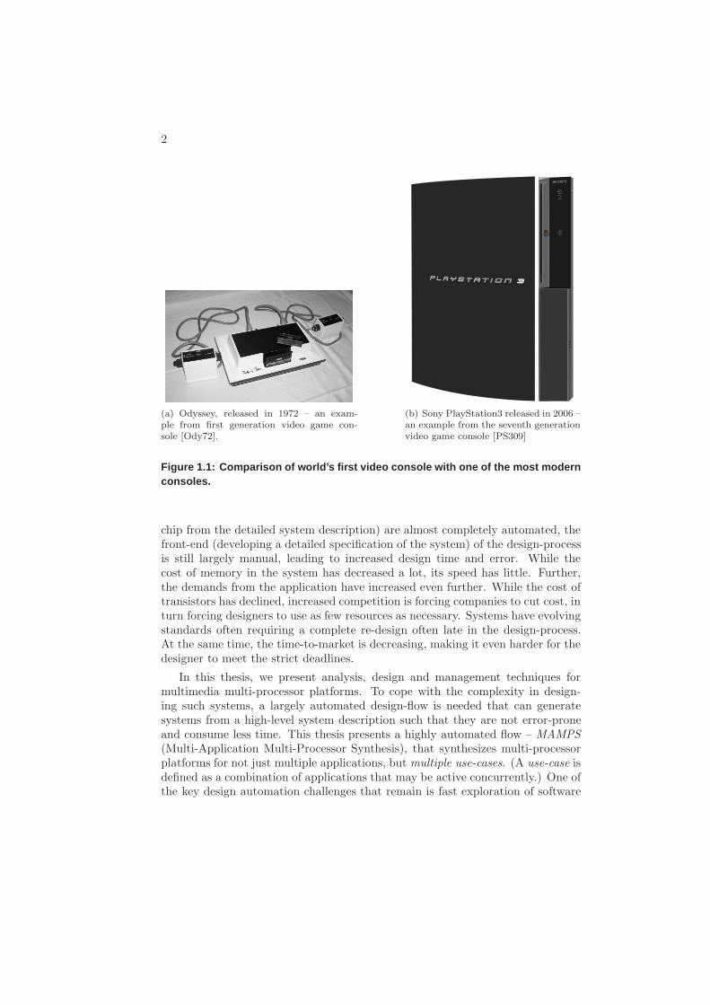
Odyssey, released by Magnavox in 1972, was the world’s first video game con-sole [Ody72]. This supported a variety of games from tennis to baseball. Re-movable circuit cards consisting of a series of jumpers were used to interconnectdifferent logic and signal generators to produce the desired game logic and screenoutput components respectively. It did not support sound, but it did come withtranslucent plastic overlays that one could put on the TV screen to generatecolour images. This was what is called as the first generation video game console.Figure 1.1(a) shows a picture of this console, that sold about 330,000 units. Letus now forward to the present day, where the video game consoles have movedinto the seventh generation. An example of one such console is the PlayStation3from Sony [PS309] shown in Figure 1.1(b), that sold over 21 million units in thefirst two years of its launch. It not only supports sounds and colours, but is acomplete media centre which can play photographs, video games, movies in highdefinitions in the most advanced formats, and has a large hard-disk to store gamesand movies. Further, it can connect to one’s home network, and the entire world,both wireless and wired. Surely, we have come a long way in the development ofmultimedia systems.
A lot of progress has been made from both applications and system-designperspective. The designers have a lot more resources at their disposal – moretransistors to play with, better and almost completely automated tools to placeand route these transistors, and much more memory in the system. However, anumber of key challenges remains. With increasing number of transistors has comeincreased power to worry about. While the tools for the back-end (synthesizing a
1
2
(a) Odyssey, released in 1972 – an exam-ple from first generation video game con-sole [Ody72].
(b) Sony PlayStation3 released in 2006 –an example from the seventh generationvideo game console [PS309]
Figure 1.1: Comparison of world’s first video console with on e of the most modernconsoles.
chip from the detailed system description) are almost completely automated, thefront-end (developing a detailed specification of the system) of the design-processis still largely manual, leading to increased design time and error. While thecost of memory in the system has decreased a lot, its speed has little. Further,the demands from the application have increased even further. While the cost oftransistors has declined, increased competition is forcing companies to cut cost, inturn forcing designers to use as few resources as necessary. Systems have evolvingstandards often requiring a complete re-design often late in the design-process.At the same time, the time-to-market is decreasing, making it even harder for thedesigner to meet the strict deadlines.
In this thesis, we present analysis, design and management techniques formultimedia multi-processor platforms. To cope with the complexity in design-ing such systems, a largely automated design-flow is needed that can generatesystems from a high-level system description such that they are not error-proneand consume less time. This thesis presents a highly automated flow – MAMPS(Multi-Application Multi-Processor Synthesis), that synthesizes multi-processorplatforms for not just multiple applications, but multiple use-cases. (A use-case isdefined as a combination of applications that may be active concurrently.) One ofthe key design automation challenges that remain is fast exploration of software
1. TRENDS AND CHALLENGES IN MULTIMEDIA SYSTEMS 3
and hardware implementation alternatives with accurate performance evaluation.Techniques are presented to merge multiple use-cases into one hardware designto minimize cost and design time, making it well-suited for fast design spaceexploration in MPSoC systems.
In order to contain the design-cost it is important to have a system that isneither hugely over-dimensioned, nor too limited to support the modern appli-cations. While there are techniques to estimate application performance, theyoften end-up providing a high-upper bound such that the hardware is grosslyover-dimensioned. We present a performance prediction methodology that canaccurately and quickly predict the performance of multiple applications beforethey execute in the system. The technique is fast enough to be used at run-timeas well. This allows run-time addition of applications in the system. An admissioncontroller is presented using the analysis technique that admits incoming appli-cations only if their performance is expected to meet their desired requirements.Further, a mechanism is presented to manage resources in a system. This ensuresthat once an application is admitted in the system, it can meet its performanceconstraints. The entire set-up is integrated in the MAMPS flow and availableon-line for the benefit of research community.
This chapter is organized as follows. In Section 1.1 we take a closer look at thetrends in multimedia systems from the applications perspective. In Section 1.2we look at the trends in multimedia system design. Section 1.3 summarizes thekey challenges that remain to be solved as seen from the two trends. Section 1.4explains the overall design flow that is used in this thesis. Section 1.5 lists the keycontributions that have led to this thesis, and their organization in this thesis.
1.1 Trends in Multimedia Systems Applications
Multimedia systems are systems that use a combination of content forms like text,audio, video, pictures and animation to provide information or entertainment tothe user. The video game console is just one example of the many multimedia sys-tems that abound around us. Televisions, mobile phones, home theatre systems,mp3 players, laptops, personal digital assistants, are all examples of multimediasystems. Modern multimedia systems have changed the way in which users re-ceive information and expect to be entertained. Users now expect information tobe available instantly whether they are traveling in the airplane, or sitting in thecomfort of their houses. In line with users’ demand, a large number of multimediaproducts are available. To satisfy this huge demand, the semiconductor compa-nies are busy releasing newer embedded, and multimedia systems in particular,every few months.
The number of features in a multimedia system is constantly increasing. Forexample, a mobile phone that was traditionally meant to support voice calls, nowprovides video-conferencing features and streaming of television programs using3G networks [HM03]. An mp3 player, traditionally meant for simply playing
4 1.1. TRENDS IN MULTIMEDIA SYSTEMS APPLICATIONS
music, now stores contacts and appointments, plays photos and video clips, andalso doubles up as a video game. Some people refer to it as the convergenceof information, communication and entertainment [BMS96]. Devices that weretraditionally meant for only one of the three things, now support all of them. Thedevices have also shrunk, and they are often seen as fashion accessories. A mobilephone that was not very mobile until about 15 years ago, is now barely thickenough to support its own structure, and small enough to hide in the smallest ofladies-purses.
Further, many of these applications execute concurrently on the platform indifferent combinations. We define each such combination of simultaneously activeapplications as a use-case. (It is also known as scenario in literature [PTB06].)For example, a mobile phone in one instant may be used to talk on the phonewhile surfing the web and downloading some Java application in the background.In another instant it may be used to listen to MP3 music while browsing JPEGpictures stored in the phone, and at the same time allow a remote device to accessthe files in the phone over a bluetooth connection. Modern devices are built tosupport different use-cases, making it possible for users to choose and use thedesired functions concurrently.
Another trend we see is increasing and evolving standards. A number of stan-dards for radio communication, audio and video encoding/decoding and interfacesare available. The multimedia systems often support a number of these. Whilea high-end TV supports a variety of video interfaces like HDMI, DVI, VGA,coaxial cable; a mobile phone supports multiple bands like GSM 850, GSM 900,GSM 180 and GSM 1900, besides other wireless protocols like Infrared and Blue-tooth [MMZ+02, KB97, Blu04]. As standards evolve, allowing faster and moreefficient communication, newer devices are released in the market to match thosespecifications. The time to market is also reducing since a number of companiesare in the market [JW04], and the consumers expect quick releases. A late launchin the market directly hurts the revenue of the company.
Power consumption has become a major design issue since many multimediasystems are hand-held. According to a survey by TNS research, two-thirds ofmobile phone and PDA users rate two-days of battery life during active use asthe most important feature of the ideal converged device of the future [TNS06].While the battery life of portable devices has generally been increasing, the activeuse is still limited to a few hours, and in some extreme cases to a day. Even forother plugged multimedia systems, power has become a global concern with risingoil prices, and a growing awareness in people to reduce energy consumption.
To summarize, we see the following trends and requirements in the applicationof multimedia devices.
• An increasing number of multimedia devices are being brought to market.
• The number of applications in multimedia systems is increasing.
• The diversity of applications is increasing with convergence and multiple
1. TRENDS AND CHALLENGES IN MULTIMEDIA SYSTEMS 5
standards.
• The applications execute concurrently in varied combinations known as use-cases, and the number of these use-cases is increasing.
• The time-to-market is reducing due to increased competition, and evolvingstandards and interfaces.
• Power consumption is becoming an increasingly important concern for fu-ture multimedia devices.
1.2 Trends in Multimedia Systems Design
A number of factors are involved in bringing the progress outlined above in mul-timedia systems. Most of them can be directly or indirectly attributed to thefamous Moore’s law [Moo65], that predicted the exponential increase in transis-tor density as early as 1965. Since then, almost every measure of the capabilitiesof digital electronic devices – processing speed, transistor count per chip, memorycapacity, even the number and size of pixels in digital cameras – are improvingat roughly exponential rates. This has had two-fold impact. While on one hand,the hardware designers have been able to provide bigger, better and faster meansof processing, on the other hand, the application developers have been workinghard to utilize this processing power to its maximum. This has led them to de-liver better and increasingly complex applications in all dimensions of life – be itmedical care systems, airplanes, or multimedia systems.
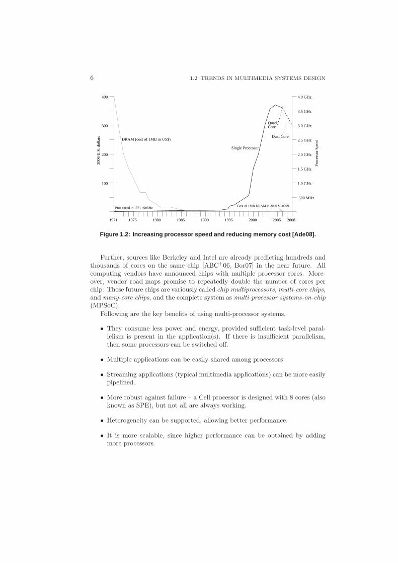
When the first Intel processor was released in 1971, it had 2,300 transistorsand operated at a speed of 400 kHz. In contrast, a modern chip has more thana billion transistors operating at more than 3 GHz [Int09]. Figure 1.2 shows thetrend in processor speed and the cost of memory [Ade08]. The cost of memory hascome down from close to 400 U.S. dollars in 1971, to less than a cent for 1 MB ofdynamic memory (RAM). The processor speed has risen to over 3.5 GHz. Anotherinteresting observation from this figure is the introduction of dual and quad corechips since 2005 onwards. This indicates the beginning of multi-processor era. Asthe transistor size shrinks, they can be clocked faster. However, this also leads toan increase in power consumption, in turn making chips hotter. Heat dissipationhas become a serious problem forcing chip manufacturers to limit the maximumfrequency of the processor. Chip manufacturers are therefore, shifting towardsdesigning multiprocessor chips operating at a lower frequency. Intel reports thatunder-clocking a single core by 20 percent saves half the power while sacrificingjust 13 percent of the performance [Ros08]. This implies that if the work is dividedbetween two processors running at 80 percent clock rate, we get 74 percent betterperformance for the same power. Further, the heat is dissipated at two pointsrather than one.
6 1.2. TRENDS IN MULTIMEDIA SYSTEMS DESIGN
1971 1975 200520001995199019851980 2008
500 MHz
1.0 GHz
1.5 GHz
2.0 GHz
2.5 GHz
3.0 GHz
3.5 GHz
4.0 GHz
100
200
300
400
DRAM (cost of 1MB in US$)Dual Core
QuadCore
Single Processor
Pro
cess
or S
peed
2006
U.S
. dol
lars
Proc speed in 1971 400kHzCost of 1MB DRAM in 2006 $0.0009
Figure 1.2: Increasing processor speed and reducing memory cost [Ade08].
Further, sources like Berkeley and Intel are already predicting hundreds andthousands of cores on the same chip [ABC+06, Bor07] in the near future. Allcomputing vendors have announced chips with multiple processor cores. More-over, vendor road-maps promise to repeatedly double the number of cores perchip. These future chips are variously called chip multiprocessors, multi-core chips,and many-core chips, and the complete system as multi-processor systems-on-chip(MPSoC).
Following are the key benefits of using multi-processor systems.
• They consume less power and energy, provided sufficient task-level paral-lelism is present in the application(s). If there is insufficient parallelism,then some processors can be switched off.
• Multiple applications can be easily shared among processors.
• Streaming applications (typical multimedia applications) can be more easilypipelined.
• More robust against failure – a Cell processor is designed with 8 cores (alsoknown as SPE), but not all are always working.
• Heterogeneity can be supported, allowing better performance.
• It is more scalable, since higher performance can be obtained by addingmore processors.
1. TRENDS AND CHALLENGES IN MULTIMEDIA SYSTEMS 7
(a) Homogeneous systems (b) Heterogeneous systems
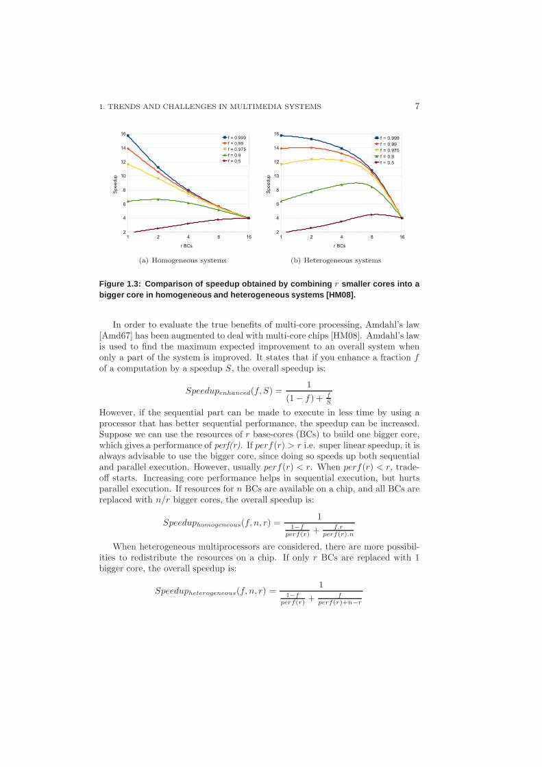
Figure 1.3: Comparison of speedup obtained by combining r smaller cores into abigger core in homogeneous and heterogeneous systems [HM08 ].
In order to evaluate the true benefits of multi-core processing, Amdahl’s law[Amd67] has been augmented to deal with multi-core chips [HM08]. Amdahl’s lawis used to find the maximum expected improvement to an overall system whenonly a part of the system is improved. It states that if you enhance a fraction fof a computation by a speedup S, the overall speedup is:
Speedupenhanced(f, S) =1
(1 − f) + fS
However, if the sequential part can be made to execute in less time by using aprocessor that has better sequential performance, the speedup can be increased.Suppose we can use the resources of r base-cores (BCs) to build one bigger core,which gives a performance of perf(r). If perf(r) > r i.e. super linear speedup, it isalways advisable to use the bigger core, since doing so speeds up both sequentialand parallel execution. However, usually perf(r) < r. When perf(r) < r, trade-off starts. Increasing core performance helps in sequential execution, but hurtsparallel execution. If resources for n BCs are available on a chip, and all BCs arereplaced with n/r bigger cores, the overall speedup is:
Speeduphomogeneous(f, n, r) =1
1−fperf(r) + f.r
perf(r).n
When heterogeneous multiprocessors are considered, there are more possibil-ities to redistribute the resources on a chip. If only r BCs are replaced with 1bigger core, the overall speedup is:
Speedupheterogeneous(f, n, r) =1
1−fperf(r) + f
perf(r)+n−r
8 1.2. TRENDS IN MULTIMEDIA SYSTEMS DESIGN
intrinsic computationalefficiency of silicon
0.070.130.250.52 1
com
puta
tiona
l effi
cien
cy, M
OP
S/W
microprocessors
1
10
10
10
10
10
10
2
3
4
5
6
200620021998199419901986 2010
0.045feature size (um)
year
Figure 1.4: The intrinsic computational efficiency of silic on as compared to theefficiency of microprocessors.
Figure 1.3 shows the speedup obtained for both homogeneous and heteroge-neous systems, for different fractions of parallelizable software. The x-axis showsthe number of base processors that are combined into one larger core. In totalthere are resources for 16 BCs. The origin shows the point when we have a homo-geneous system with only base-cores. As we move along the x-axis, the number ofbase-core resources used to make a bigger core are increased. In a homogeneoussystem, all the cores are replaced by a bigger core, while for heterogeneous, onlyone bigger core is built. The end-point for the x-axis is when all available resourcesare replaced with one big core. For this figure, it is assumed that perf(r) =
√r.
As can be seen, the corresponding speedup when using a heterogeneous system ismuch greater than homogeneous system. While these graphs are shown for only16 base-cores, similar performance speedups are obtained for other bigger chipsas well. This shows that using a heterogeneous system with several large cores ona chip can offer better speedup than a homogeneous system.
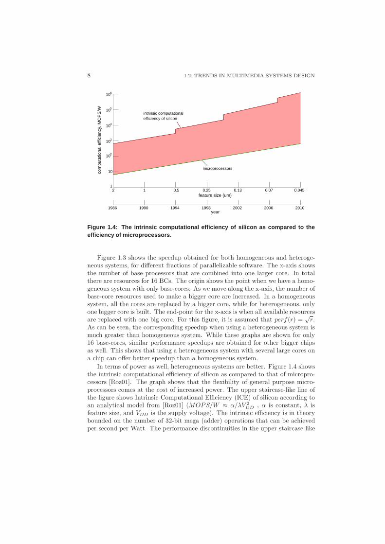
In terms of power as well, heterogeneous systems are better. Figure 1.4 showsthe intrinsic computational efficiency of silicon as compared to that of micropro-cessors [Roz01]. The graph shows that the flexibility of general purpose micro-processors comes at the cost of increased power. The upper staircase-like line ofthe figure shows Intrinsic Computational Efficiency (ICE) of silicon according toan analytical model from [Roz01] (MOPS/W ≈ α/λV 2
DD , α is constant, λ isfeature size, and VDD is the supply voltage). The intrinsic efficiency is in theorybounded on the number of 32-bit mega (adder) operations that can be achievedper second per Watt. The performance discontinuities in the upper staircase-like
1. TRENDS AND CHALLENGES IN MULTIMEDIA SYSTEMS 9
line are caused by changes in the supply voltage from 5V to 3.3V, 3.3V to 1.5V,1.5V to 1.2V and 1.2 to 1.0V. We observe that there is a gap of 2-to-3 orders ofmagnitude between the intrinsic efficiency of silicon and general purpose micro-processors. The accelerators – custom hardware modules designed for a specifictask – come close to the maximum efficiency. Clearly, it may not always be de-sirable to actually design a hypothetically maximum efficiency processor. A fullmatch between the application and architecture can bring the efficiency close tothe hypothetical maximum. A heterogeneous platform may combine the flexibilityof using a general purpose microprocessor and custom accelerators for computeintensive tasks, thereby minimizing the power consumed in the system.
Most modern multiprocessor systems are heterogeneous, and contain one ormore application-specific processing elements (PEs). The CELL processor [KDH+05],jointly developed by Sony, Toshiba and IBM, contains up to nine-PEs – one gen-eral purpose PowerPC [WS94] and eight Synergistic Processor Elements (SPEs).The PowerPC runs the operating system and the control tasks, while the SPEsperform the compute-intensive tasks. This Cell processor is used in PlaySta-tion3 described above. STMicroelectronics Nomadik contains an ARM processorand several Very Long Instruction Word (VLIW) DSP cores [AAC+03]. TexasInstruments OMAP processor [Cum03] and Philips Nexperia [OA03] are other ex-amples. Recently, many companies have begun providing configurable cores thatare targeted towards an application domain. These are known as ApplicationSpecific Instruction-set Processors (ASIPs). These provide a good compromisebetween general-purpose cores and ASICs. Tensilica [Ten09, Gon00] and SiliconHive [Hiv09, Hal05] are two such examples, which provide the complete toolset togenerate multiprocessor systems where each processor can be customized towardsa particular task or domain, and the corresponding software programming toolsetis automatically generated for them. This also allows the re-use of IP (IntellectualProperty) modules designed for a particular domain or task.
Another trend that we see in multimedia systems design is the use of Platform-Based Design paradigm [SVCBS04, KMN+00]. This is becoming increasinglypopular due to three main factors: (1) the dramatic increase in non-recurringengineering cost due to mask making at the circuit implementation level, (2) thereducing time to market, and (3) streamlining of industry – chip fabrication andsystem design, for example, are done in different companies and places. Thisparadigm is based on segregation between the system design process, and thesystem implementation process. The basic tenets of platform-based design areidentification of design as meeting-in-the-middle process, where successive refine-ments of specifications meet with abstractions of potential implementations, andthe identification of precisely defined abstraction layers where the refinement tothe subsequent layer and abstraction processes take place [SVCBS04]. Each layersupports a design stage providing an opaque abstraction of lower layers that allowsaccurate performance estimations. This information is incorporated in appropri-ate parameters that annotate design choices at the present layer of abstraction.These layers of abstraction are called platforms. For MPSoC system design, this

10 1.2. TRENDS IN MULTIMEDIA SYSTEMS DESIGN
MappingPlatform
DesignPlatform
Exploration
Architectural Space
PlatformSystem
Application instance
Platform instance
Application Space
Figure 1.5: Platform-based design approach – system platfo rm stack.
translates into abstraction between the application space and architectural spacethat is provided by the system-platform. Figure 1.5 captures this system-platformthat provides an abstraction between the application and architecture space. Thisdecouples the application development process from the architecture implemen-tation process.
We further observe that for high-performance multimedia systems (like cell-processing engine and graphics processor), non-preemptive systems are preferredover preemptive ones for a number of reasons [JSM91]. In many practical systems,properties of device hardware and software either make the preemption impos-sible or prohibitively expensive due to extra hardware and (potential) executiontime needed. Further, non-preemptive scheduling algorithms are easier to imple-ment than preemptive algorithms and have dramatically lower overhead at run-time [JSM91]. Further, even in multi-processor systems with preemptive proces-sors, some processors (or co-processors/ accelerators) are usually non-preemptive;for such processors non-preemptive analysis is still needed. It is therefore impor-tant to investigate non-preemptive multi-processor systems.
To summarize, the following trends can be seen in the design of multimediasystems.
• Increase in system resources: The resources available for disposal in termsof processing and memory are increasing exponentially.
• Use of multiprocessor systems: Multi-processor systems are being developedfor reasons of power, efficiency, robustness, and scalability.
• Increasing heterogeneity: With the re-use of IP modules and design of cus-
1. TRENDS AND CHALLENGES IN MULTIMEDIA SYSTEMS 11
tom (co-) processors (ASIPs), heterogeneity in MPSoCs is increasing.
• Platform-based design: Platform-based design methodology is being em-ployed to improve the re-use of components and shorten the developmentcycle.
• Non-preemptive processors: Non-preemptive processors are preferred overpreemptive to reduce cost.
1.3 Key Challenges in Multimedia Systems Design
The trends outlined in the previous two sections indicate the increasing complexityof modern multimedia systems. They have to support a number of concurrentlyexecuting applications with diverse resource and performance requirements. Thedesigners face the challenge of designing such systems at low cost and in short time.In order to keep the costs low, a number of design options have to be exploredto find the optimal or near-optimal solution. The performance of applicationsexecuting on the system have to be carefully evaluated to satisfy user-experience.Run-time mechanisms are needed to deal with run-time addition of applications.In short, following are the major challenges that remain in the design of modernmultimedia systems, and are addressed in this thesis.
• Multiple use-cases: Analyzing performance of multiple applications execut-ing concurrently on heterogeneous multi-processor platforms. Further, thisnumber of use-cases and their combinations is exponential in the number ofapplications present in the system. (Analysis and Design)
• Design and Program: Systematic way to design and program multi-processorplatforms. (Design)
• Design space exploration: Fast design space exploration technique. (Analy-sis and Design)
• Run-time addition of applications: Deal with run-time addition of applica-tions – keep the analysis fast and composable, adapt the design (-process),manage the resources at run-time (e.g. admission controller). (Analysis,Design and Management)
• Meeting performance constraints: A good mechanism for keeping perfor-mance of all applications executing above the desired level. (Design andManagement)
1.3.1 Analysis
We present a novel probabilistic performance prediction (P 3) algorithm for pre-dicting performance of multiple applications executing on multi-processor plat-
12 1.3. KEY CHALLENGES IN MULTIMEDIA SYSTEMS DESIGN
forms. The algorithm predicts the time that tasks have to spend during con-tention phase for a resource. The computation of accurate waiting time is thekey to performance analysis. When applications are modeled as synchronousdataflow (SDF) graphs, their performance on a (multi-processor) system can beeasily computed when they are executing in isolation (provided we have a goodmodel). When they execute concurrently, depending on whether the used sched-uler is static or dynamic, the arbitration on a resource is either fixed at design-timeor chosen at run-time respectively (explained in more detail in Chapter 2). In theformer case, the execution order can be modeled in the graph, and the perfor-mance of the entire application can be determined. The contention is thereforemodeled as dependency edges in the SDF graph. However, this is more suitedfor static applications. For dynamic applications such as multimedia, dynamicscheduler is more suitable. For dynamic scheduling approaches, the contentionhas to be modeled as waiting time for a task, which is added to the executiontime to give the total response time. The performance can be determined by com-puting the performance (throughput) of this resulting SDF graph. With lack ofgood techniques for accurately predicting the time spent in contention, designershave to resort to worst-case waiting time estimates, that lead to over-designingthe system and loss of performance. Further, those approaches are not scalableand the over-estimate increases with the number of applications.
In this thesis, we present a solution to performance prediction, with easy anal-ysis. We highlight the issue of composability i.e. mapping and analysis of perfor-mance of multiple applications on a multiprocessor platform in isolation, as far aspossible. This limits computational complexity and allows high dynamism in thesystem. While in this thesis, we only show examples with processor contention,memory and network contention can also be easily modeled in SDF graph asshown in [Stu07]. The technique presented here can therefore be easily extendedto other system components as well. The analysis technique can be used both atdesign-time and run-time.
We would ideally want to analyze each application in isolation, thereby re-ducing the analysis time to a linear function, and still reason about the overallbehaviour of the system. One of the ways to achieve this, would be complete vir-tualization. This essentially implies dividing the available resources by the totalnumber of applications in the system. The application would then have exclusiveaccess to its share of resources. For example, if we have 100 MHz processorsand a total of 10 applications in the system, each application would get 10 MHzof processing resource. The same can be done for communication bandwidthand memory requirements. However this gives two main problems. When fewerthan 10 tasks are active, the tasks will not be able to exploit the extra avail-able processing power, leading to wastage. Secondly, the system would be grosslyover-dimensioned when the peak requirements of each application are taken intoaccount, even though these peak requirements of applications may rarely occurand never be at the same time.
Figure 1.6 shows this disparity in more detail. The graph shows the period of
1. TRENDS AND CHALLENGES IN MULTIMEDIA SYSTEMS 13
0
2
4
6
8
10
12
14
A B C D E F G H I J
Per
iod
of A
pplic
atio
ns (
Nor
mal
ized
)
Applications
Comparison of Period: Virtualization vs Simulation
Estimated Full VirtualizationAverage Case in Simulation
Worst Case in SimulationOriginal (Individual)
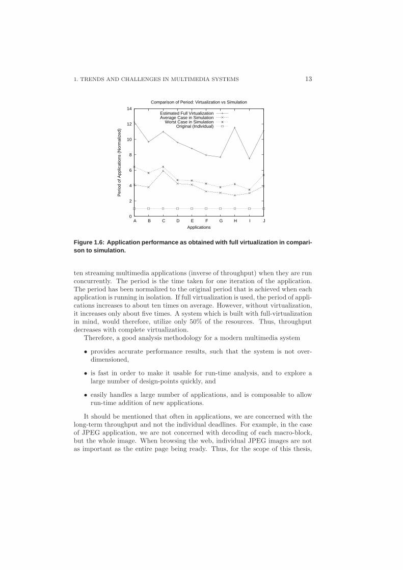
Figure 1.6: Application performance as obtained with full v irtualization in compari-son to simulation.
ten streaming multimedia applications (inverse of throughput) when they are runconcurrently. The period is the time taken for one iteration of the application.The period has been normalized to the original period that is achieved when eachapplication is running in isolation. If full virtualization is used, the period of appli-cations increases to about ten times on average. However, without virtualization,it increases only about five times. A system which is built with full-virtualizationin mind, would therefore, utilize only 50% of the resources. Thus, throughputdecreases with complete virtualization.
Therefore, a good analysis methodology for a modern multimedia system
• provides accurate performance results, such that the system is not over-dimensioned,
• is fast in order to make it usable for run-time analysis, and to explore alarge number of design-points quickly, and
• easily handles a large number of applications, and is composable to allowrun-time addition of new applications.
It should be mentioned that often in applications, we are concerned with thelong-term throughput and not the individual deadlines. For example, in the caseof JPEG application, we are not concerned with decoding of each macro-block,but the whole image. When browsing the web, individual JPEG images are notas important as the entire page being ready. Thus, for the scope of this thesis,
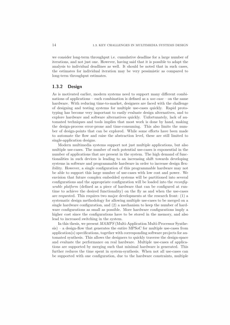
14 1.3. KEY CHALLENGES IN MULTIMEDIA SYSTEMS DESIGN
we consider long-term throughput i.e. cumulative deadline for a large number ofiterations, and not just one. However, having said that it is possible to adapt theanalysis to individual deadlines as well. It should be noted that in such cases,the estimates for individual iteration may be very pessimistic as compared tolong-term throughput estimates.
1.3.2 Design
As is motivated earlier, modern systems need to support many different combi-nations of applications – each combination is defined as a use-case – on the samehardware. With reducing time-to-market, designers are faced with the challengeof designing and testing systems for multiple use-cases quickly. Rapid proto-typing has become very important to easily evaluate design alternatives, and toexplore hardware and software alternatives quickly. Unfortunately, lack of au-tomated techniques and tools implies that most work is done by hand, makingthe design-process error-prone and time-consuming. This also limits the num-ber of design-points that can be explored. While some efforts have been madeto automate the flow and raise the abstraction level, these are still limited tosingle-application designs.
Modern multimedia systems support not just multiple applications, but alsomultiple use-cases. The number of such potential use-cases is exponential in thenumber of applications that are present in the system. The high demand of func-tionalities in such devices is leading to an increasing shift towards developingsystems in software and programmable hardware in order to increase design flex-ibility. However, a single configuration of this programmable hardware may notbe able to support this large number of use-cases with low cost and power. Weenvision that future complex embedded systems will be partitioned into severalconfigurations and the appropriate configuration will be loaded into the reconfig-urable platform (defined as a piece of hardware that can be configured at run-time to achieve the desired functionality) on the fly as and when the use-casesare requested. This requires two major developments at the research front: (1) asystematic design methodology for allowing multiple use-cases to be merged on asingle hardware configuration, and (2) a mechanism to keep the number of hard-ware configurations as small as possible. More hardware configurations imply ahigher cost since the configurations have to be stored in the memory, and alsolead to increased switching in the system.
In this thesis, we present MAMPS (Multi-Application Multi-Processor Synthe-sis) – a design-flow that generates the entire MPSoC for multiple use-cases fromapplication(s) specifications, together with corresponding software projects for au-tomated synthesis. This allows the designers to quickly traverse the design-spaceand evaluate the performance on real hardware. Multiple use-cases of applica-tions are supported by merging such that minimal hardware is generated. Thisfurther reduces the time spent in system-synthesis. When not all use-cases canbe supported with one configuration, due to the hardware constraints, multiple
1. TRENDS AND CHALLENGES IN MULTIMEDIA SYSTEMS 15
configurations of hardware are automatically generated, while keeping the num-ber of partitions low. Further, an area estimation technique is provided that canaccurately predict the area of a design and decide whether a given system-designis feasible within the hardware constraints or not. This helps in quick evaluationof designs, thereby making the DSE faster.
Thus, the design-flow presented in this thesis is unique in a number of ways:(1) it supports multiple use-cases on one hardware platform, (2) estimates thearea of design before the actual synthesis, allowing the designer to choose theright device, (3) merges and partitions the use-cases to minimize the number ofhardware configurations, and (4) it allows fast DSE by automating the designgeneration and exploration process.
The work in this thesis is targeted towards heterogeneous multi-processor sys-tems. In such systems, the mapping is largely determined by the capabilities ofprocessors and the requirements of different tasks. Thus, the freedom in terms ofmapping is rather limited. For homogeneous systems, task mapping and schedul-ing are coupled by performance requirements of applications. If for a particularscheduling policy, the performance of a given application is not met, mapping mayneed to be altered to ensure that the performance improves. As for the schedul-ing policy, it is not always possible to steer them at run-time. For example, ifa system uses first-come-first-serve scheduling policy, it is infeasible to change itto a fixed priority schedule for a short time, since it requires extra hardware andsoftware. Further, identifying the ideal mapping given a particular schedulingpolicy already takes exponential time in the total number of tasks. When thescheduling policy is also allowed to vary independently on processors, the timetaken increases even more.
1.3.3 Management
Resource management, i.e. managing all the resources present in the multipro-cessor system, is similar to the task of an operating system on a general purposecomputer. This includes starting up of applications, and allocating resources tothem appropriately. In the case of a multimedia system (or embedded systems, ingeneral), a key difference from a general purpose computer is that the applications(or application domain) is generally known, and the system can be optimized forthem. Further, most decisions can be already taken at design-time to save thecost at run-time. Still, a complete design-time analysis is becoming increasinglyharder due to three major reasons: 1) little may be known at design-time aboutthe applications that need to be used in future, e.g. a navigation application likeTom-Tom may be installed on the phone after-wards, 2) the precise platform mayalso not be known at design time, e.g. some cores may fail at run-time, and 3)the number of design-points that need to be evaluated is prohibitively large. Arun-time approach can benefit from the fact that the exact application mix isknown, but the analysis has to be fast enough to make it feasible.
In this thesis, we present a hybrid approach for designing systems with
16 1.4. DESIGN FLOW
multiple applications. This splits the management tasks into off-line and on-line.The time-consuming application specific computations are done at design-timeand for each application independent from other applications, and the use-casespecific computations are performed at run-time. The off-line computation in-cludes tasks like application-partitioning, application-modeling, determining thetask execution times, determining their maximum throughput, etc. Further, para-metric equations are derived that allow throughput computation of tasks withvarying execution times. All this analysis is time-consuming and best carried outat design-time. Further, in this part no information is needed from the otherapplications and it can be performed in isolation. This information is sufficientenough to let a run-time manager determine the performance of an applicationwhen executing concurrently on the platform with other applications. This al-lows easy addition of applications at run-time. As long as all the propertiesneeded by the run-time resource manager are derived for the new application, theapplication can be treated as all the other applications that are present in thesystem.
At run-time, when the resource manager needs to decide, for example, whichresources to allocate to an incoming application, it can evaluate the performanceof applications with different allocations and determine the best option. In somecases, multiple quality levels of an application may be specified, and at run-timethe resource manager can choose from one of those levels. This functionality ofthe resource manager is referred to as admission control. The manager alsoneeds to ensure that applications that are admitted do not take more resourcesthan allocated, and starve the other applications executing in the system. Thisfunctionality is referred to as budget enforcement. The manager periodicallychecks the performance of all applications, and when an application does betterthan the required level, it is suspended to ensure that it does not take moreresources than needed. For the scope of this thesis, the effect of task migration isnot considered since it is orthogonal to our approach.
1.4 Design Flow
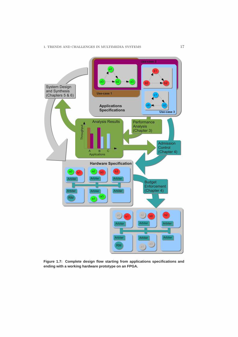
Figure 1.7 shows the design-flow that is used in this thesis. Specifications ofapplications are provided to the designer in the form of Synchronous Dataflow(SDF) graphs [SB00, LM87]. These are often used for modeling multimedia ap-plications. This is further explained in Chapter 2. As motivated earlier in thechapter, modern multimedia systems support a number of applications in variedcombinations defined as use-case. Figure 1.7 shows three example applications– A, B and C, and three use-cases with their combinations. For example, in Use-case 2 applications A and B execute concurrently. For each of these use-cases,the performance of all active applications is analyzed. When a suitable mappingto hardware is to be explored, this step is often repeated with different mappings,until the desired performance is obtained. A probabilistic mechanism is used to
1. TRENDS AND CHALLENGES IN MULTIMEDIA SYSTEMS 17
Figure 1.7: Complete design flow starting from applications specifications andending with a working hardware prototype on an FPGA.
18 1.5. KEY CONTRIBUTIONS AND THESIS OVERVIEW
estimate the average performance of applications. This performance analysis
technique is presented in Chapter 3.
When a satisfactory mapping is obtained, the system can be designed andsynthesized automatically using the system-design approach presented in Chap-ter 5. Multiple use-cases need to be merged on to one hardware design such thata new hardware configuration is not needed for every use-case. This is explainedin Chapter 6. When it is not possible to merge all use-cases due to resourceconstraints (slices in an FPGA, for example), use-cases need to be partitionedsuch that the number of hardware partitions are kept to a minimum. Further, afast area estimation method is needed that can quickly identify whether a set ofuse-cases can be merged due to hardware constraints. Trying synthesis for everyuse-case combination is too time-consuming. A novel area-estimation techniqueis needed that can save precious time during design space exploration. This isexplained in Chapter 6.
Once the system is designed, a run-time mechanism is needed to ensure thatall applications can meet their performance requirements. This is accomplishedby using a resource manager (RM). Whenever a new application is to be started,the manager checks whether sufficient resources are available. This is definedas admission-control. The probabilistic analysis is used to predict the perfor-mance of applications when the new application is admitted in the system. If theexpected performance of all applications is above the minimum desired perfor-mance then the application is started, else a lower quality of incoming applicationis tried. The resource manager also takes care of budget-enforcement i.e. en-suring applications use only as much resources as assigned. If an application usesmore resources than needed and starves other applications, it is suspended. Fig-ure 1.7 shows an example where application A is suspended. Chapter 4 providesdetails of two main tasks of the RM – admission control and budget-enforcement.
The above flow also allows for run-time addition of applications. Since theperformance analysis presented is fast, it is done at run-time. Therefore, anyapplication whose properties have been derived off-line can be used, if there areenough resources present in the system. This is explained in more detail in Chap-ter 4.
1.5 Key Contributions and Thesis Overview
Following are some of the major contributions that have been achieved during thecourse of this research and have led to this thesis.
• A detailed analysis of why estimating performance of multiple applicationsexecuting on a heterogeneous platform is so difficult. This work was pub-lished in [KMC+06], and an extended version is published in a special issueof the Journal of Systems Architecture containing the best papers of theDigital System Design conference [KMT+08].
1. TRENDS AND CHALLENGES IN MULTIMEDIA SYSTEMS 19
• A probabilistic performance prediction (P 3) mechanism for multiple applica-tions. The prediction is within 2% of real performance for experiments done.The basic version of the P 3 mechanism was first published in [KMC+07],and later improved and published in [KMCH08].
• An admission controller based on P 3 mechanism to admit applications onlyif they are expected to meet their performance requirements. This work ispublished in [KMCH08].
• A budget enforcement mechanism to ensure that applications can all meettheir desired performance if they are admitted. This work is publishedin [KMT+06].
• A Resource Manager (RM) to manage computation and communicationresources, and achieve the above goals. This work is published in [KMCH08].
• A design flow for multiple applications, such that composability is main-tained and applications can be added at run-time with ease.
• A platform synthesis design technique that generates multiprocessors plat-forms with ease automatically and also programs them with relevant pro-gram codes, for multiple applications. This work is published in [KFH+07].
• A design flow explaining how systems that support multiple use-cases shouldbe designed. This work is published in [KFH+08].
A tool-flow based on the above for Xilinx FPGAs that is also made availablefor use on-line for the benefit of research community. This tool is available on-lineat www.es.ele.tue.nl/mamps/ [MAM09].
This thesis is organized as follows. Chapter 2 explains the concepts involvedin modeling and scheduling of applications. It explores the problems encounteredwhen analyzing multiple applications executing on a multi-processor platform.The challenge of Composability, i.e. being able to analyze applications in isola-tion with other applications, is presented in this chapter. Chapter 3 presents aperformance prediction methodology that can accurately predict the performanceof applications at run-time before they execute in the system. A run-time it-erative probabilistic analysis is used to estimate the time spent by tasks duringcontention phase, and thereby predict the performance of applications. Chapter 4explains the concepts of resource management and enforcing budgets to meet theperformance requirements. The performance prediction is used for admission con-trol – one of the main functions of the resource manager. Chapter 5 proposes anautomated design methodology to generate program MPSoC hardware designs ina systematic and automated way for multiple applications named MAMPS. Chap-ter 6 explains how systems should be designed when multiple use-cases have tobe supported. Algorithms for merging and partitioning use-cases are presented inthis chapter as well. Finally, Chapter 7 concludes this thesis and gives directionsfor future work.

20 1.5. KEY CONTRIBUTIONS AND THESIS OVERVIEW
CHAPTER 2
Application Modeling and Scheduling
Multimedia applications are becoming increasingly more complex and computa-tion hungry to match consumer demands. If we take video, for example, televisionsfrom leading companies are already available with high-definition (HD) video res-olution of 1080x1920 i.e. more than 2 million pixels [Son09, Sam09, Phi09] forconsumers and even higher resolutions are showcased in electronic shows [CES09].Producing images for such a high resolution is already taxing for even high-endMPSoC platforms. The problem is compounded by the extra dimension of mul-tiple applications sharing the same resources. Good modeling is essential for twomain reasons: 1) to predict the behaviour of applications on a given hardwarewithout actually synthesizing the system, and 2) to synthesize the system after afeasible solution has been identified from the analysis. In this chapter we will seein detail the model requirements we have for designing and analyzing multimediasystems. We see the various models of computation, and choose one that meetsour design-requirements.
Another factor that plays an important role in multi-application analysis isdetermining when and where a part of application is to be executed, also knownas scheduling. Heuristics and algorithms for scheduling are called schedulers.Studying schedulers is essential for good system design and analysis. In thischapter, we discuss the various types of schedulers for dataflow models. Whenconsidering multiple applications executing on multi-processor platforms, threemain things need to be taken care of: 1) assignment – deciding which task ofapplication has to be executed on which processor, 2) ordering – determining theorder of task-execution, and 3) timing – determining the precise time of task-
21
22 2.1. APPLICATION MODEL AND SPECIFICATION
execution1. Each of these three tasks can be done at either compile-time orrun-time. In this chapter, we classify the schedulers on this criteria and highlighttwo of them most suited for use in multiprocessor multimedia platforms. Wehighlight the issue of composability i.e. mapping and analysis of performance ofmultiple applications on a multiprocessor platform in isolation, as far as possible.This limits computational complexity and allows high dynamism in the system.
This chapter is organized as follows. The next section motivates the need ofmodeling applications and the requirements for such a model. Section 2.2 gives anintroduction to the synchronous dataflow (SDF) graphs that we use in our analy-sis. Some properties that are relevant for this thesis are also explained in the samesection. Section 2.3 discusses the models of computation (MoCs) that are avail-able, and motivates the choice of SDF graphs as the MoC for our applications.Section 2.4 gives state-of-the-art techniques used for estimating performance ofapplications modeled as SDF graphs. Section 2.5 provides background on thescheduling techniques used for dataflow graphs in general. Section 2.6 extendsthe performance analysis techniques to include hardware constraints as well. Sec-tion 2.8 provides a comparison between static and dynamic ordering schedulers,and Section 2.9 concludes the chapter.
2.1 Application Model and Specification
Multimedia applications are often also referred to as streaming applications
owing to their repetitive nature of execution. Most applications execute for a verylong time in a fixed execution pattern. When watching television for example,the video decoding process potentially goes on decoding for hours – an hour isequivalent to 180,000 video frames at a modest rate of 50 frames per second (fps).High-end televisions often provide a refresh rate of even 100 fps, and the trendindicates further increase in this rate. The same goes for an audio stream thatusually accompanies the video. The platform has to work continuously to get thisoutput to the user.
In order to ensure that this high performance can be met by the platform, thedesigner has to be able to model the application requirements. In the absenceof a good model, it is very difficult to know in advance whether the applicationperformance can be met at all times, and extensive simulation and testing isneeded. Even now, companies report a large effort being spent on verifying thetiming requirements of the applications. With multiple applications executing onmultiple processors, the potential number of use-cases increases rapidly, and sodoes the cost of verification.
We start by defining a use-case.
1Some people also define only ordering and timing as scheduling, and assignment as binding
or mapping.
2. APPLICATION MODELING AND SCHEDULING 23
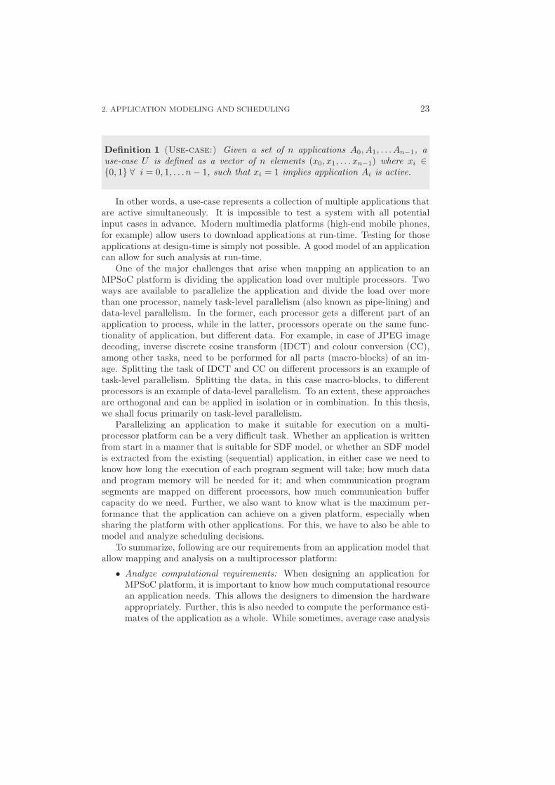
Definition 1 (Use-case:) Given a set of n applications A0, A1, . . . An−1, ause-case U is defined as a vector of n elements (x0, x1, . . . xn−1) where xi ∈{0, 1} ∀ i = 0, 1, . . . n − 1, such that xi = 1 implies application Ai is active.
In other words, a use-case represents a collection of multiple applications thatare active simultaneously. It is impossible to test a system with all potentialinput cases in advance. Modern multimedia platforms (high-end mobile phones,for example) allow users to download applications at run-time. Testing for thoseapplications at design-time is simply not possible. A good model of an applicationcan allow for such analysis at run-time.
One of the major challenges that arise when mapping an application to anMPSoC platform is dividing the application load over multiple processors. Twoways are available to parallelize the application and divide the load over morethan one processor, namely task-level parallelism (also known as pipe-lining) anddata-level parallelism. In the former, each processor gets a different part of anapplication to process, while in the latter, processors operate on the same func-tionality of application, but different data. For example, in case of JPEG imagedecoding, inverse discrete cosine transform (IDCT) and colour conversion (CC),among other tasks, need to be performed for all parts (macro-blocks) of an im-age. Splitting the task of IDCT and CC on different processors is an example oftask-level parallelism. Splitting the data, in this case macro-blocks, to differentprocessors is an example of data-level parallelism. To an extent, these approachesare orthogonal and can be applied in isolation or in combination. In this thesis,we shall focus primarily on task-level parallelism.
Parallelizing an application to make it suitable for execution on a multi-processor platform can be a very difficult task. Whether an application is writtenfrom start in a manner that is suitable for SDF model, or whether an SDF modelis extracted from the existing (sequential) application, in either case we need toknow how long the execution of each program segment will take; how much dataand program memory will be needed for it; and when communication programsegments are mapped on different processors, how much communication buffercapacity do we need. Further, we also want to know what is the maximum per-formance that the application can achieve on a given platform, especially whensharing the platform with other applications. For this, we have to also be able tomodel and analyze scheduling decisions.
To summarize, following are our requirements from an application model thatallow mapping and analysis on a multiprocessor platform:
• Analyze computational requirements: When designing an application forMPSoC platform, it is important to know how much computational resourcean application needs. This allows the designers to dimension the hardwareappropriately. Further, this is also needed to compute the performance esti-mates of the application as a whole. While sometimes, average case analysis
24 2.2. INTRODUCTION TO SDF GRAPHS
of requirements may suffice, often we also need the worst case estimates, forexample in case of real-time embedded systems.
• Analyze memory requirements: This constraint becomes increasingly moreimportant as the memory cost on a chip goes high. A model that allowsaccurate analysis of memory needed for the program execution can allow adesigner to distribute the memory across processors appropriately and alsodetermine proper mapping on the hardware.
• Analyze communication requirements: The buffer capacity between the com-municating tasks (potentially) affects the overall application performance. Amodel that allows computing these buffer-throughput trade-offs can let thedesigner allocate appropriate memory for the channel and predict through-put.
• Model and analyze scheduling: When we have multiple applications sharingprocessors, scheduling becomes one of the major challenges. A model thatallows us to analyze the effect of scheduling on applications performance isneeded.
• Design the system: Once the performance of system is considered satisfac-tory, the system has to be synthesized such that the properties analyzed arestill valid.
Dataflow models of computation fit rather well with the above requirements. Theyprovide a model for describing signal processing systems where infinite streams ofdata are incrementally transformed by processes executing in sequence or paral-lel. In a dataflow model, processes communicate via unbounded FIFO channels.Processes read and write atomic data elements or tokens from and to channels.Writing to a channel is non-blocking, i.e. it always succeeds and does not stall theprocess, while reading from a channel is blocking, i.e. a process that reads froman empty channel will stall and can only continue when the channel contains suf-ficient tokens. In this thesis, we use synchronous dataflow (SDF) graph to modelapplications and the next section explains them in more detail.
2.2 Introduction to SDF Graphs
Synchronous Data Flow Graphs (SDFGs, see [LM87]) are often used for modelingmodern DSP applications [SB00] and for designing concurrent multimedia applica-tions implemented on multi-processor systems-on-chip. Both pipelined streamingand cyclic dependencies between tasks can be easily modeled in SDFGs. Tasksare modeled by the vertices of an SDFG, which are called actors. The commu-nication between actors is represented by edges through which it is connected toother actors. Edges represent channels for communication in a real system.
2. APPLICATION MODELING AND SCHEDULING 25
1 1
1
1
22
100
50
100
A
a0
a1
a2
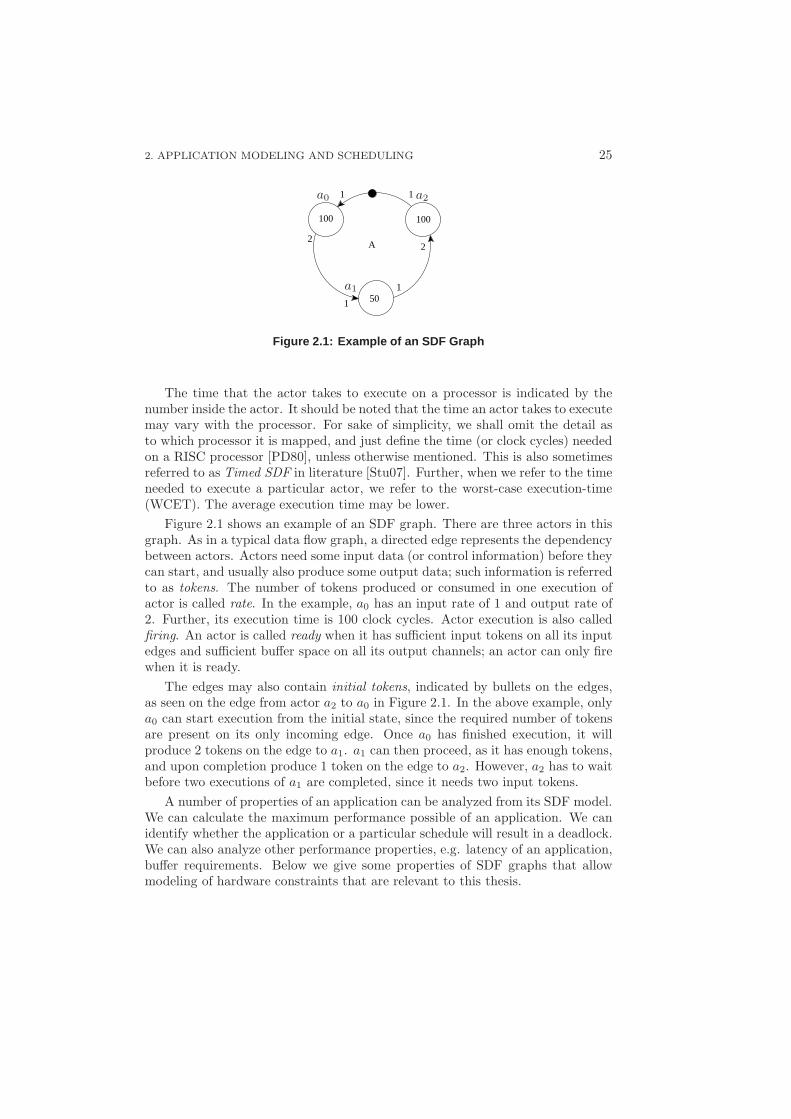
Figure 2.1: Example of an SDF Graph
The time that the actor takes to execute on a processor is indicated by thenumber inside the actor. It should be noted that the time an actor takes to executemay vary with the processor. For sake of simplicity, we shall omit the detail asto which processor it is mapped, and just define the time (or clock cycles) neededon a RISC processor [PD80], unless otherwise mentioned. This is also sometimesreferred to as Timed SDF in literature [Stu07]. Further, when we refer to the timeneeded to execute a particular actor, we refer to the worst-case execution-time(WCET). The average execution time may be lower.
Figure 2.1 shows an example of an SDF graph. There are three actors in thisgraph. As in a typical data flow graph, a directed edge represents the dependencybetween actors. Actors need some input data (or control information) before theycan start, and usually also produce some output data; such information is referredto as tokens. The number of tokens produced or consumed in one execution ofactor is called rate. In the example, a0 has an input rate of 1 and output rate of2. Further, its execution time is 100 clock cycles. Actor execution is also calledfiring. An actor is called ready when it has sufficient input tokens on all its inputedges and sufficient buffer space on all its output channels; an actor can only firewhen it is ready.
The edges may also contain initial tokens, indicated by bullets on the edges,as seen on the edge from actor a2 to a0 in Figure 2.1. In the above example, onlya0 can start execution from the initial state, since the required number of tokensare present on its only incoming edge. Once a0 has finished execution, it willproduce 2 tokens on the edge to a1. a1 can then proceed, as it has enough tokens,and upon completion produce 1 token on the edge to a2. However, a2 has to waitbefore two executions of a1 are completed, since it needs two input tokens.
A number of properties of an application can be analyzed from its SDF model.We can calculate the maximum performance possible of an application. We canidentify whether the application or a particular schedule will result in a deadlock.We can also analyze other performance properties, e.g. latency of an application,buffer requirements. Below we give some properties of SDF graphs that allowmodeling of hardware constraints that are relevant to this thesis.
26 2.2. INTRODUCTION TO SDF GRAPHS
2.2.1 Modeling Auto-concurrency
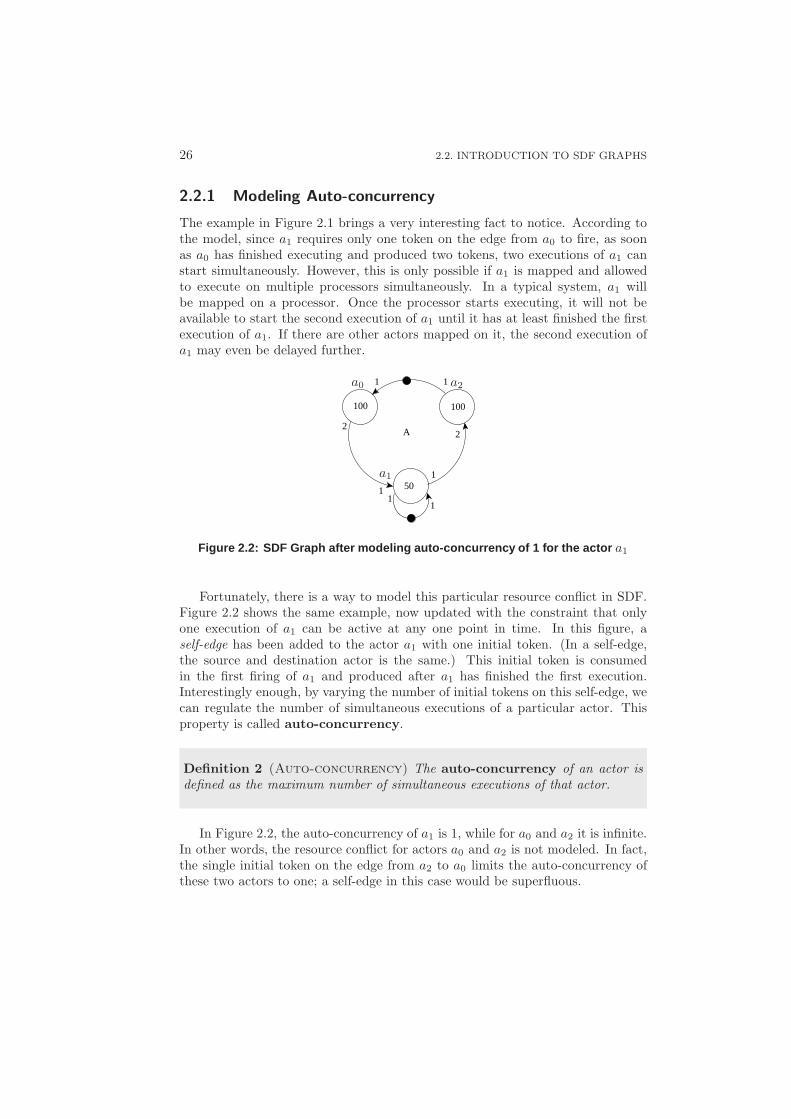
The example in Figure 2.1 brings a very interesting fact to notice. According tothe model, since a1 requires only one token on the edge from a0 to fire, as soonas a0 has finished executing and produced two tokens, two executions of a1 canstart simultaneously. However, this is only possible if a1 is mapped and allowedto execute on multiple processors simultaneously. In a typical system, a1 willbe mapped on a processor. Once the processor starts executing, it will not beavailable to start the second execution of a1 until it has at least finished the firstexecution of a1. If there are other actors mapped on it, the second execution ofa1 may even be delayed further.
1 1
1
1
22
100
50
100
A
11
a0
a1
a2
Figure 2.2: SDF Graph after modeling auto-concurrency of 1 f or the actor a1
Fortunately, there is a way to model this particular resource conflict in SDF.Figure 2.2 shows the same example, now updated with the constraint that onlyone execution of a1 can be active at any one point in time. In this figure, aself-edge has been added to the actor a1 with one initial token. (In a self-edge,the source and destination actor is the same.) This initial token is consumedin the first firing of a1 and produced after a1 has finished the first execution.Interestingly enough, by varying the number of initial tokens on this self-edge, wecan regulate the number of simultaneous executions of a particular actor. Thisproperty is called auto-concurrency.
Definition 2 (Auto-concurrency) The auto-concurrency of an actor isdefined as the maximum number of simultaneous executions of that actor.
In Figure 2.2, the auto-concurrency of a1 is 1, while for a0 and a2 it is infinite.In other words, the resource conflict for actors a0 and a2 is not modeled. In fact,the single initial token on the edge from a2 to a0 limits the auto-concurrency ofthese two actors to one; a self-edge in this case would be superfluous.
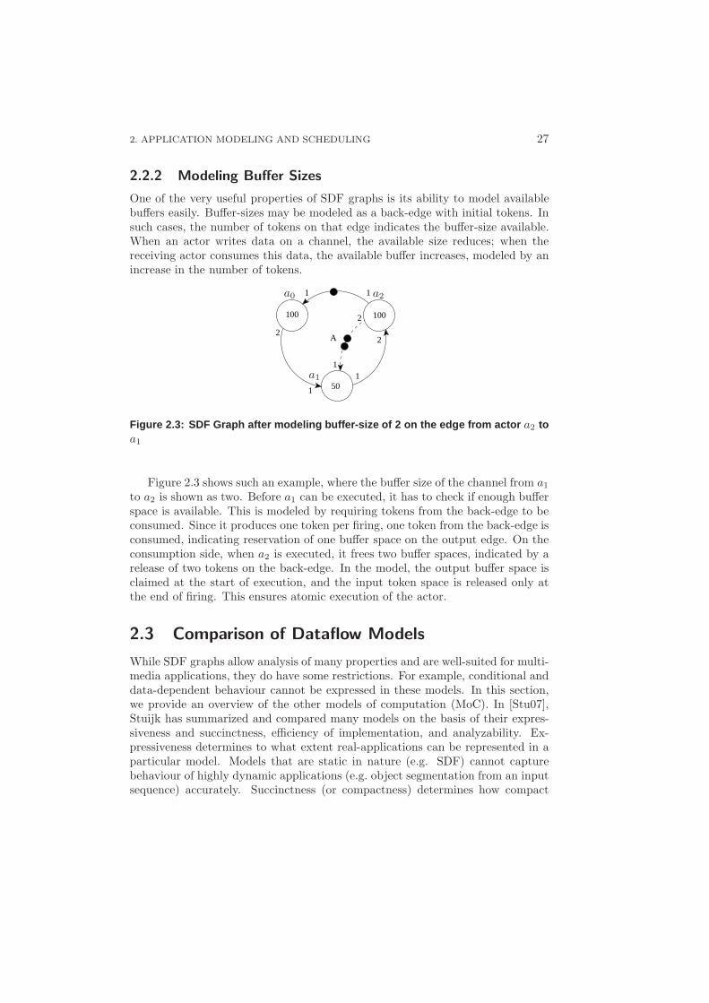
2. APPLICATION MODELING AND SCHEDULING 27
2.2.2 Modeling Buffer Sizes
One of the very useful properties of SDF graphs is its ability to model availablebuffers easily. Buffer-sizes may be modeled as a back-edge with initial tokens. Insuch cases, the number of tokens on that edge indicates the buffer-size available.When an actor writes data on a channel, the available size reduces; when thereceiving actor consumes this data, the available buffer increases, modeled by anincrease in the number of tokens.
1 1
1
1
22
100
50
100
A
2
1
a0
a1
a2
Figure 2.3: SDF Graph after modeling buffer-size of 2 on the e dge from actor a2 toa1
Figure 2.3 shows such an example, where the buffer size of the channel from a1
to a2 is shown as two. Before a1 can be executed, it has to check if enough bufferspace is available. This is modeled by requiring tokens from the back-edge to beconsumed. Since it produces one token per firing, one token from the back-edge isconsumed, indicating reservation of one buffer space on the output edge. On theconsumption side, when a2 is executed, it frees two buffer spaces, indicated by arelease of two tokens on the back-edge. In the model, the output buffer space isclaimed at the start of execution, and the input token space is released only atthe end of firing. This ensures atomic execution of the actor.
2.3 Comparison of Dataflow Models
While SDF graphs allow analysis of many properties and are well-suited for multi-media applications, they do have some restrictions. For example, conditional anddata-dependent behaviour cannot be expressed in these models. In this section,we provide an overview of the other models of computation (MoC). In [Stu07],Stuijk has summarized and compared many models on the basis of their expres-siveness and succinctness, efficiency of implementation, and analyzability. Ex-pressiveness determines to what extent real-applications can be represented in aparticular model. Models that are static in nature (e.g. SDF) cannot capturebehaviour of highly dynamic applications (e.g. object segmentation from an inputsequence) accurately. Succinctness (or compactness) determines how compact
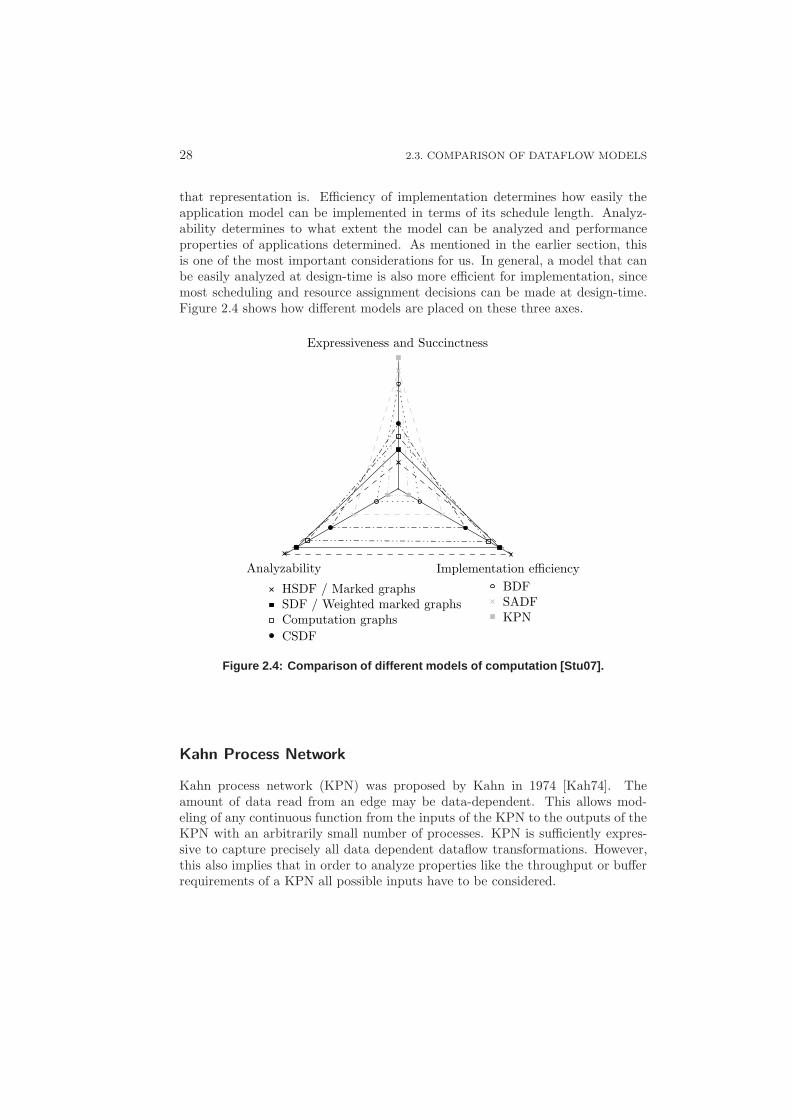
28 2.3. COMPARISON OF DATAFLOW MODELS
that representation is. Efficiency of implementation determines how easily theapplication model can be implemented in terms of its schedule length. Analyz-ability determines to what extent the model can be analyzed and performanceproperties of applications determined. As mentioned in the earlier section, thisis one of the most important considerations for us. In general, a model that canbe easily analyzed at design-time is also more efficient for implementation, sincemost scheduling and resource assignment decisions can be made at design-time.Figure 2.4 shows how different models are placed on these three axes.
Expressiveness and Succinctness
Analyzability Implementation efficiency
KPNSADFBDF
CSDF
Computation graphsSDF / Weighted marked graphsHSDF / Marked graphs
Figure 2.4: Comparison of different models of computation [ Stu07].
Kahn Process Network
Kahn process network (KPN) was proposed by Kahn in 1974 [Kah74]. Theamount of data read from an edge may be data-dependent. This allows mod-eling of any continuous function from the inputs of the KPN to the outputs of theKPN with an arbitrarily small number of processes. KPN is sufficiently expres-sive to capture precisely all data dependent dataflow transformations. However,this also implies that in order to analyze properties like the throughput or bufferrequirements of a KPN all possible inputs have to be considered.
2. APPLICATION MODELING AND SCHEDULING 29
Scenario Aware Dataflow
Scenario aware dataflow (SADF) was first introduced by Theelen in 2006 [TGB+06].This is also a model for design-time analysis of dynamic streaming and signalprocessing applications.This model also allows for data-dependent behaviour inprocesses. Each different execution pattern is defined as a scenario. Such scenar-ios denote different modes of operations in which resource requirements can differconsiderably. The scenario concept enables to coherently capture the variationsin behaviour of different processes in a streaming application. A key novelty ofSADF is the use of a stochastic approach to capture the scenario occurrences aswell as the occurrence of different execution times within a scenario in an abstractway. While some properties of these graphs like deadlock and throughput are pos-sible to analyze at design time, in practice this analysis can be quite slow. Thismodel is less compact than KPN, since all scenarios have to be explicitly specifiedin the model, and known at design time. This also makes it less expressive sincenot all kinds of systems can be expressed accurately in SADF.
Boolean Dataflow
The last model of computation that we discuss having data-dependent behaviouris boolean dataflow (BDF) model [Lee91, BL93]. In this model, each processhas a number of inputs and outputs to choose from. Depending on the value ofcontrol tokens data is read from one of the input channels, and written to one ofthe output channels. This model is less expressive than the earlier two modelsdiscussed, since the control freedom in modeling processes is limited to either trueor false. Similar to the earlier two models discussed, the analyzability is limited.
Cyclo Static Dataflow
Now we move on to the class of more deterministic data flow models of computa-tion. In a cyclo-static dataflow (CSDF) model [LWAP94, BELP96], the rates ofdata consumed and produced may change between subsequent firings. However,the pattern of this change is pre-determined and that makes it more analyzableat design time. These graphs may be converted to SDF graphs, and are thereforeas expressive as SDF graphs. However, the freedom to change the rates of datamakes them more compact than SDF in representing some applications. Theyare also as analyzable, but slower if we consider the same number of actors, sincethe resulting schedule is generally a little more complex.
Recently, special channels have been introduced for CSDF graphs [DBC+07].Often applications share buffers between multiple consumers. This cannot bedirectly described in CSDF. The authors show how such implementation spe-cific aspects can be modeled in CSDF without the need of extensions. Thus,the analyzability of the graph is maintained, and appropriate buffer-sizes can becomputed from the application model.
30 2.3. COMPARISON OF DATAFLOW MODELS
Computation Graphs
Computation graphs were first introduced by Karp and Miller in 1966 [KM66]. Inthese graphs there is a threshold set for each edge specifying the minimum numberof tokens that should be present on that edge before an actor can fire. However,the number of tokens produced and consumed for each edge is still fixed. Thesemodels are less expressive than CSDF, but more analyzable. A synchronous dataflow graph is a subset of these computation graphs.
Synchronous Dataflow
Synchronous dataflow (SDF) graphs were first proposed by Lee and Messerschmittin 1987 [LM87]. However, as has been earlier claimed [Stu07], these correspondto subclass weighted marked graph [TCWCS92] of Petri nets, which is a generalpurpose model of computation with a number of applications [Pet62, Mur89]. SDFgraphs have a constant input and output rate that does not change with input oracross different firings. They also don’t support execution in different scenarios asmay be specified by data. Therefore, their expressivity is rather limited. However,this also makes them a lot easier to analyze. Many performance parameters canbe analyzed as explained in Section 2.4.
Homogeneous Synchronous Data Flow
Homogeneous Synchronous Data Flow (HSDF) graphs are a subset of SDF graphs.In HSDF graph model, the rates of all input and output edges is one. This impliesthat only one token is read and written in any firing of an actor. This limits theexpressiveness even more, but makes the analysis somewhat easier. HSDF graphscan be converted into SDF and vice-versa. However, in practice the size of anHSDF for an equivalent SDFG may be very large as shown by examples in [Stu07].Lately, analysis techniques have been developed that work almost as fast directlyon an SDF graph as on an HSDF graph (for the same number of nodes) [Gha08].Therefore, the added advantage of using an HSDF graph is lost.
After considering all the alternatives, we decided in favour of SDF graphs sincetheir ability to analyze applications in terms of other performance requirements,such as throughput and buffer, was one of our key requirements. Further, anumber of analysis tools for SDF graph were available (and more in development)when this research was started [SDF09]. However, since SDF graphs are not ableto express some real applications accurately, we do have to pay a little overheadin estimating performance. For example, the execution time is assumed to be theworst-case execution-time. Thus, in some cases, the performance estimates maybe pessimistic.
2. APPLICATION MODELING AND SCHEDULING 31
2.4 Performance Modeling
In this section, we define the major terminology that is relevant for this thesis.
Definition 3 (Actor Execution Time) Actor execution time, τ(a) is definedas the time needed to complete execution of actor a on a specified node. In caseswhere the required time is not constant but varying, this indicates the maximumtime for actor execution.
τ(a0) = 100, for example, in Figure 2.3.
Definition 4 (Iteration) An iteration of a graph is defined as the minimumnon-zero execution (i.e. at least one actor has executed) such that the initialstate of the graph is obtained.
In Figure 2.3, one iteration of graph A is completed when a0, a1 and a2 havecompleted one, two and one execution(s) each respectively.
Definition 5 (Repetition Vector) Repetition Vector q of an SDF graph Ais defined as the vector specifying the number of times an actor in A is executedfor one iteration of A.
For example, in Figure 2.3, q[a0 a1 a2] = [1 2 1]. It should be mentioned thatany integer multiple of repetition vector defined above is also a repetition vector.The above definition gives a minimal repetition vector in which all entries areintegers.
Definition 6 (Application Period) Application Period Per(A) is defined asthe time SDFG A takes to complete one iteration on average.
Per(A) = 300 in Figure 2.3, assuming it has sufficient resources and no con-tention, and all the actors fire as soon as they are ready. (Note that actor a1 hasto execute twice.)
Definition 7 (Application Throughput) Application Throughput, ThrA isdefined as the number of iterations of an SDF graph A in one second.
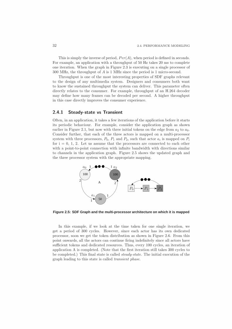
32 2.4. PERFORMANCE MODELING
This is simply the inverse of period, Per(A), when period is defined in seconds.For example, an application with a throughput of 50 Hz takes 20 ms to completeone iteration. When the graph in Figure 2.3 is executing on a single processor of300 MHz, the throughput of A is 1 MHz since the period is 1 micro-second.
Throughput is one of the most interesting properties of SDF graphs relevantto the design of any multimedia system. Designers and consumers both wantto know the sustained throughput the system can deliver. This parameter oftendirectly relates to the consumer. For example, throughput of an H.264 decodermay define how many frames can be decoded per second. A higher throughputin this case directly improves the consumer experience.
2.4.1 Steady-state vs Transient
Often, in an application, it takes a few iterations of the application before it startsits periodic behaviour. For example, consider the application graph as shownearlier in Figure 2.1, but now with three initial tokens on the edge from a2 to a0.Consider further, that each of the three actors is mapped on a multi-processorsystem with three processors, P0, P1 and P2, such that actor ai is mapped on Pi
for i = 0, 1, 2. Let us assume that the processors are connected to each otherwith a point-to-point connection with infinite bandwidth with directions similarto channels in the application graph. Figure 2.5 shows the updated graph andthe three processor system with the appropriate mapping.
1 1
1
1
22
100
50
100
A
a0
a1
a2
P0 P1 P2
Figure 2.5: SDF Graph and the multi-processor architecture on which it is mapped
In this example, if we look at the time taken for one single iteration, weget a period of 300 cycles. However, since each actor has its own dedicatedprocessor, soon we get the token distribution as shown in Figure 2.6. From thispoint onwards, all the actors can continue firing indefinitely since all actors havesufficient tokens and dedicated resources. Thus, every 100 cycles, an iteration ofapplication A is completed. (Note that the first iteration still takes 300 cycles tobe completed.) This final state is called steady-state. The initial execution of thegraph leading to this state is called transient phase.
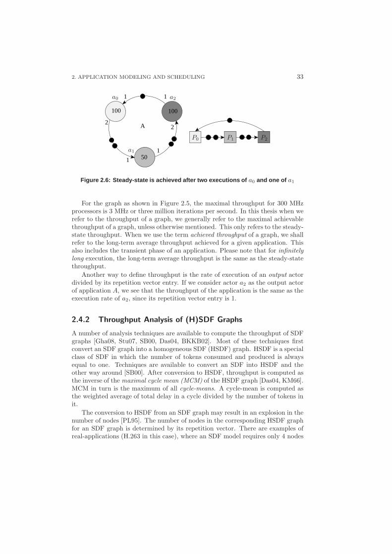
2. APPLICATION MODELING AND SCHEDULING 33
1 1
1
1
22
100
50
100
A
a0
a1
a2
P0 P1 P2
Figure 2.6: Steady-state is achieved after two executions o f a0 and one of a1
For the graph as shown in Figure 2.5, the maximal throughput for 300 MHzprocessors is 3 MHz or three million iterations per second. In this thesis when werefer to the throughput of a graph, we generally refer to the maximal achievablethroughput of a graph, unless otherwise mentioned. This only refers to the steady-state throughput. When we use the term achieved throughput of a graph, we shallrefer to the long-term average throughput achieved for a given application. Thisalso includes the transient phase of an application. Please note that for infinitelylong execution, the long-term average throughput is the same as the steady-statethroughput.
Another way to define throughput is the rate of execution of an output actordivided by its repetition vector entry. If we consider actor a2 as the output actorof application A, we see that the throughput of the application is the same as theexecution rate of a2, since its repetition vector entry is 1.
2.4.2 Throughput Analysis of (H)SDF Graphs
A number of analysis techniques are available to compute the throughput of SDFgraphs [Gha08, Stu07, SB00, Das04, BKKB02]. Most of these techniques firstconvert an SDF graph into a homogeneous SDF (HSDF) graph. HSDF is a specialclass of SDF in which the number of tokens consumed and produced is alwaysequal to one. Techniques are available to convert an SDF into HSDF and theother way around [SB00]. After conversion to HSDF, throughput is computed asthe inverse of the maximal cycle mean (MCM) of the HSDF graph [Das04, KM66].MCM in turn is the maximum of all cycle-means. A cycle-mean is computed asthe weighted average of total delay in a cycle divided by the number of tokens init.
The conversion to HSDF from an SDF graph may result in an explosion in thenumber of nodes [PL95]. The number of nodes in the corresponding HSDF graphfor an SDF graph is determined by its repetition vector. There are examples ofreal-applications (H.263 in this case), where an SDF model requires only 4 nodes
34 2.5. SCHEDULING TECHNIQUES FOR DATAFLOW GRAPHS
and an HSDF model of the same application has 4754 nodes [Stu07]. This makesthe above approach very infeasible for many multimedia applications. Lately,techniques have been presented that operate on SDF graphs directly [GGS+06,Gha08]. These techniques essentially simulate the SDF execution and identifywhen a steady-state is reached by comparing previous states with current state.Even though the theoretical bound is high, the experimental results show thatthese techniques can compute the throughput of many multimedia applicationswithin milliseconds.
A tool called SDF 3 has been written and is available on-line for use by theresearch community [SGB06a, SDF09]. Beside being able to generate randomSDF graphs with specified properties, it can also compute throughput of SDFgraphs easily. It allows to visualize these graphs as well, and compute otherperformance properties. The same tool was used for throughput computationand graph generation in many experiments conducted in this thesis.
However, the above techniques only work on a particular execution time ofactors. If there is any change in the actor execution time, the entire analysishas to be repeated. Recently, a technique has been proposed in [GGBS08] thatallows variable execution time. This technique computes equations that limit theapplication period, for a given range of actor execution times. When the exactactor execution time is known, these equations can be evaluated to compute theactual period of the application. This idea is used in Chapter 3 to computethroughput of applications.
It should be mentioned that the techniques mentioned here do not take intoaccount resource contention and essentially assume that infinite resources areavailable, except SDF 3. SDF 3 also takes resource contention into account but islimited to preemptive systems. Before we see how throughput can be computedwhen considering limited computation resources, we review the basic techniquesused for scheduling dataflow graphs.
2.5 Scheduling Techniques for Dataflow Graphs
One of the key aspects in designing multiprocessor systems from any MoC isscheduling. Compile-time scheduling promises near-optimal performance at lowcost for final system, but is only suitable for static applications. Run-time schedul-ing can address a wider variety of applications, at greater system cost. Schedulingtechniques can be classified in a number of categories based on which decisionsare made at compile time (also known as design-time) and which decisions aremade at run-time. [LH89, SB00]. There are three main decisions when schedulingtasks (or actors) on a processor:2 1) which tasks to assign to a given processor,2) what is the order of these tasks on it and 3) what is the timing of these tasks.We consider four different types of schedulers.
2When considering mapping of channels on the network, there are many more categories.
2. APPLICATION MODELING AND SCHEDULING 35
1. The first one is fully static where everything is decided at compile timeand the processor has to simply execute the tasks. This approach has tradi-tionally been used extensively for DSP applications due to their repetitiveand constant resource requirement. This is also good for systems whereguarantees are more important and (potential) speed-up from earlier exe-cution is not desired. Further, the run-time scheduler becomes very simplesince it does not need to check for availability of data and simply executesthe scheduled actors at respective times. However, this mechanism is com-pletely static, and cannot handle any dynamism in the system like run-timeaddition of applications, or any unexpectedly higher execution time for aparticular iteration.
2. The second type is self-timed, where the assignment and ordering isalready done at compile time. However, the exact time for firing of actorsis determined at run-time, depending on the availability of data. Self-timedscheduling is more suitable for cases when the execution time of tasks maybe data-dependent, but the variation is not very large. This can oftenresult in speed-up of applications as compared to analysis at design-time,provided the worst-case execution time estimates are used for analyzing theapplication performance. Since earlier arrival of data cannot result in laterproduction of data, the performance bounds computed at compile-time arepreserved. However, this also implies that the schedule may become non-work-conserving, i.e. that a task may be waiting on a processor, while theprocessor is sitting idle waiting for the task in order.
3. The third type is static assignment, where the mapping is already fixedat compile time, but the ordering and timing is done at run-time by thescheduler. This allows the schedule to become work-conserving and perhapsachieve a higher overall throughput in the system. However, it might alsoresult in a lower overall throughput since the bounds cannot be computedat compile-time (or are not preserved in this scheduler). This schedulingis most applicable for systems where applications have a large variation inexecution time. While for a single application, the order is still imposed bythe data-dependency among tasks and makes self-timed more suitable, formultiple applications the high variation in execution time, makes it infeasibleto enforce the static-order.
4. The last one is called fully dynamic where mapping, ordering and tim-ing are all done at run-time. This gives full freedom to the scheduler, andthe tasks are assigned to an idle processor as soon as they are ready. Thisscheduler also allows for task migration. This may result in a yet higherthroughput, since this tries to maximize the resource utilization and mini-mize the idle time, albeit at the cost of performance guarantee. It shouldbe noted that run-time assignment also involves a (potentially) higher over-head in data movement. When the assignment is fixed at compile time, the
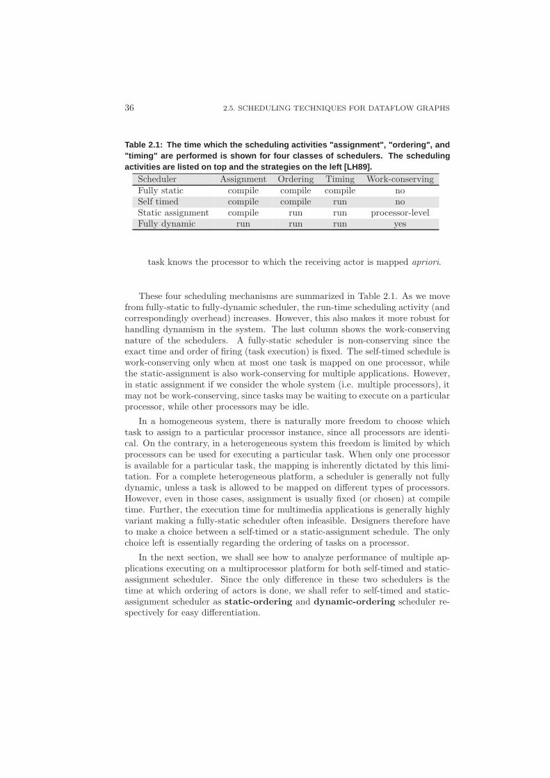
36 2.5. SCHEDULING TECHNIQUES FOR DATAFLOW GRAPHS
Table 2.1: The time which the scheduling activities "assign ment", "ordering", and"timing" are performed is shown for four classes of schedule rs. The schedulingactivities are listed on top and the strategies on the left [L H89].
Scheduler Assignment Ordering Timing Work-conservingFully static compile compile compile noSelf timed compile compile run noStatic assignment compile run run processor-levelFully dynamic run run run yes
task knows the processor to which the receiving actor is mapped apriori.
These four scheduling mechanisms are summarized in Table 2.1. As we movefrom fully-static to fully-dynamic scheduler, the run-time scheduling activity (andcorrespondingly overhead) increases. However, this also makes it more robust forhandling dynamism in the system. The last column shows the work-conservingnature of the schedulers. A fully-static scheduler is non-conserving since theexact time and order of firing (task execution) is fixed. The self-timed schedule iswork-conserving only when at most one task is mapped on one processor, whilethe static-assignment is also work-conserving for multiple applications. However,in static assignment if we consider the whole system (i.e. multiple processors), itmay not be work-conserving, since tasks may be waiting to execute on a particularprocessor, while other processors may be idle.
In a homogeneous system, there is naturally more freedom to choose whichtask to assign to a particular processor instance, since all processors are identi-cal. On the contrary, in a heterogeneous system this freedom is limited by whichprocessors can be used for executing a particular task. When only one processoris available for a particular task, the mapping is inherently dictated by this limi-tation. For a complete heterogeneous platform, a scheduler is generally not fullydynamic, unless a task is allowed to be mapped on different types of processors.However, even in those cases, assignment is usually fixed (or chosen) at compiletime. Further, the execution time for multimedia applications is generally highlyvariant making a fully-static scheduler often infeasible. Designers therefore haveto make a choice between a self-timed or a static-assignment schedule. The onlychoice left is essentially regarding the ordering of tasks on a processor.
In the next section, we shall see how to analyze performance of multiple ap-plications executing on a multiprocessor platform for both self-timed and static-assignment scheduler. Since the only difference in these two schedulers is thetime at which ordering of actors is done, we shall refer to self-timed and static-assignment scheduler as static-ordering and dynamic-ordering scheduler re-spectively for easy differentiation.
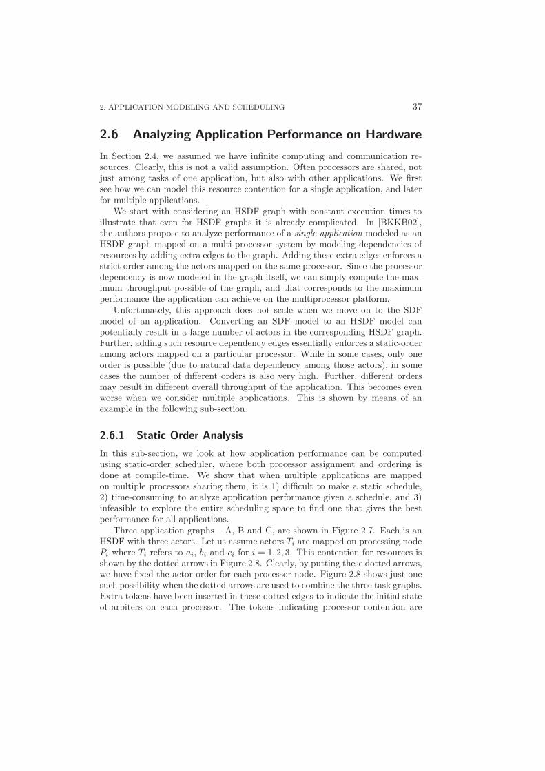
2. APPLICATION MODELING AND SCHEDULING 37
2.6 Analyzing Application Performance on Hardware
In Section 2.4, we assumed we have infinite computing and communication re-sources. Clearly, this is not a valid assumption. Often processors are shared, notjust among tasks of one application, but also with other applications. We firstsee how we can model this resource contention for a single application, and laterfor multiple applications.
We start with considering an HSDF graph with constant execution times toillustrate that even for HSDF graphs it is already complicated. In [BKKB02],the authors propose to analyze performance of a single application modeled as anHSDF graph mapped on a multi-processor system by modeling dependencies ofresources by adding extra edges to the graph. Adding these extra edges enforces astrict order among the actors mapped on the same processor. Since the processordependency is now modeled in the graph itself, we can simply compute the max-imum throughput possible of the graph, and that corresponds to the maximumperformance the application can achieve on the multiprocessor platform.
Unfortunately, this approach does not scale when we move on to the SDFmodel of an application. Converting an SDF model to an HSDF model canpotentially result in a large number of actors in the corresponding HSDF graph.Further, adding such resource dependency edges essentially enforces a static-orderamong actors mapped on a particular processor. While in some cases, only oneorder is possible (due to natural data dependency among those actors), in somecases the number of different orders is also very high. Further, different ordersmay result in different overall throughput of the application. This becomes evenworse when we consider multiple applications. This is shown by means of anexample in the following sub-section.
2.6.1 Static Order Analysis
In this sub-section, we look at how application performance can be computedusing static-order scheduler, where both processor assignment and ordering isdone at compile-time. We show that when multiple applications are mappedon multiple processors sharing them, it is 1) difficult to make a static schedule,2) time-consuming to analyze application performance given a schedule, and 3)infeasible to explore the entire scheduling space to find one that gives the bestperformance for all applications.
Three application graphs – A, B and C, are shown in Figure 2.7. Each is anHSDF with three actors. Let us assume actors Ti are mapped on processing nodePi where Ti refers to ai, bi and ci for i = 1, 2, 3. This contention for resources isshown by the dotted arrows in Figure 2.8. Clearly, by putting these dotted arrows,we have fixed the actor-order for each processor node. Figure 2.8 shows just onesuch possibility when the dotted arrows are used to combine the three task graphs.Extra tokens have been inserted in these dotted edges to indicate the initial stateof arbiters on each processor. The tokens indicating processor contention are
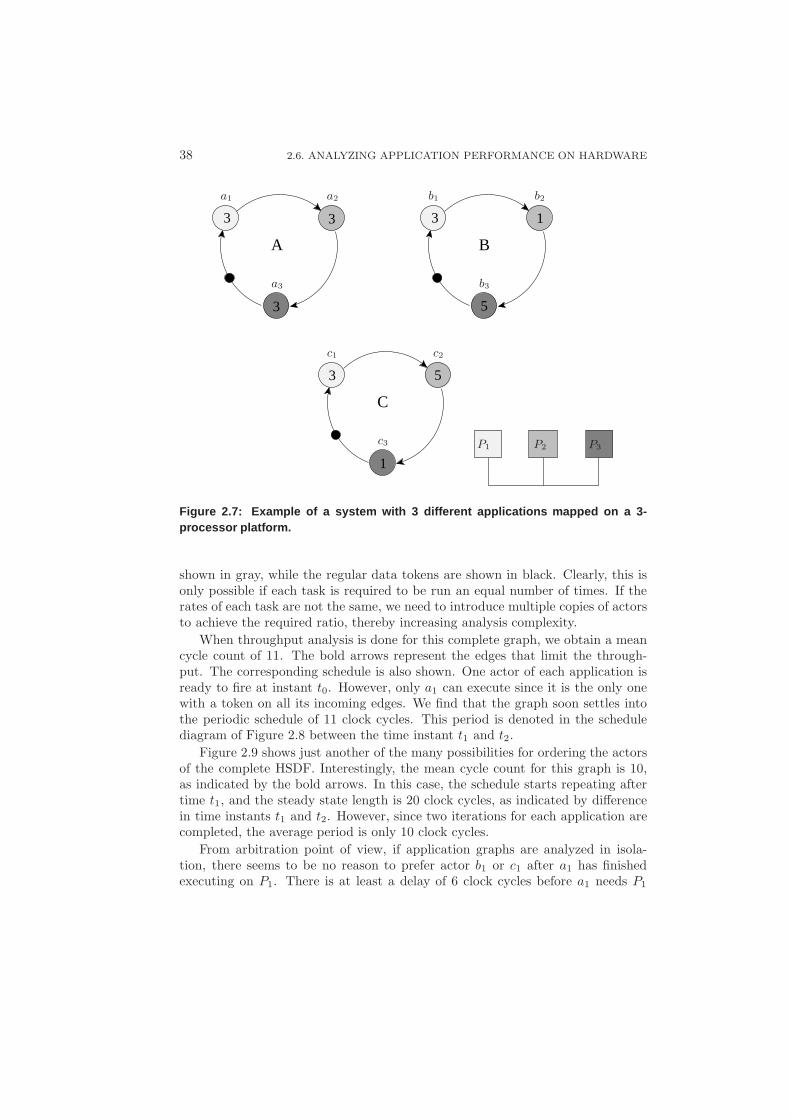
38 2.6. ANALYZING APPLICATION PERFORMANCE ON HARDWARE
C
A B
3
3
3
1
5
3 1
5
3
a1 a2
a3
b1 b2
b3
c1 c2
c3 P1 P2 P3
Figure 2.7: Example of a system with 3 different application s mapped on a 3-processor platform.
shown in gray, while the regular data tokens are shown in black. Clearly, this isonly possible if each task is required to be run an equal number of times. If therates of each task are not the same, we need to introduce multiple copies of actorsto achieve the required ratio, thereby increasing analysis complexity.
When throughput analysis is done for this complete graph, we obtain a meancycle count of 11. The bold arrows represent the edges that limit the through-put. The corresponding schedule is also shown. One actor of each application isready to fire at instant t0. However, only a1 can execute since it is the only onewith a token on all its incoming edges. We find that the graph soon settles intothe periodic schedule of 11 clock cycles. This period is denoted in the schedulediagram of Figure 2.8 between the time instant t1 and t2.
Figure 2.9 shows just another of the many possibilities for ordering the actorsof the complete HSDF. Interestingly, the mean cycle count for this graph is 10,as indicated by the bold arrows. In this case, the schedule starts repeating aftertime t1, and the steady state length is 20 clock cycles, as indicated by differencein time instants t1 and t2. However, since two iterations for each application arecompleted, the average period is only 10 clock cycles.
From arbitration point of view, if application graphs are analyzed in isola-tion, there seems to be no reason to prefer actor b1 or c1 after a1 has finishedexecuting on P1. There is at least a delay of 6 clock cycles before a1 needs P1
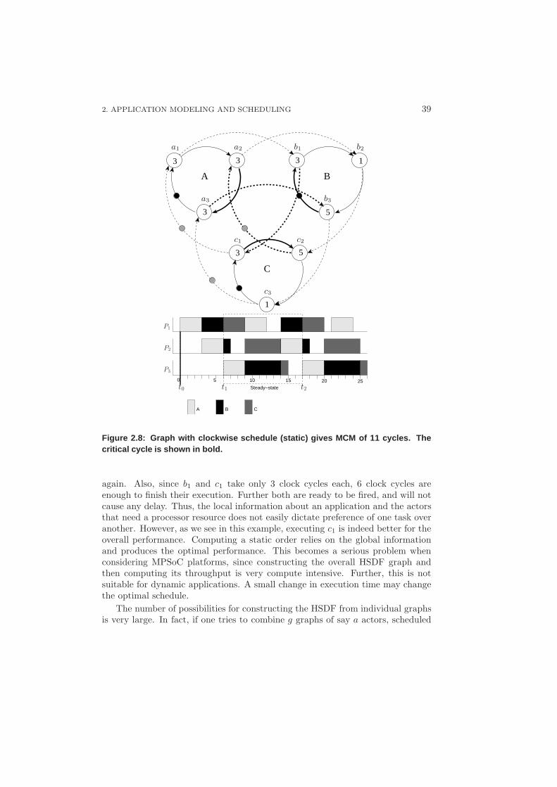
2. APPLICATION MODELING AND SCHEDULING 39
A B
C
3
3 3 3 1
5
53
1
a1 a2
a3
b1 b2
b3
c1 c2
c3
0 5 10 15 20 25
A B C
Steady−statet0 t1 t2
P1
P2
P3
Figure 2.8: Graph with clockwise schedule (static) gives MC M of 11 cycles. Thecritical cycle is shown in bold.
again. Also, since b1 and c1 take only 3 clock cycles each, 6 clock cycles areenough to finish their execution. Further both are ready to be fired, and will notcause any delay. Thus, the local information about an application and the actorsthat need a processor resource does not easily dictate preference of one task overanother. However, as we see in this example, executing c1 is indeed better for theoverall performance. Computing a static order relies on the global informationand produces the optimal performance. This becomes a serious problem whenconsidering MPSoC platforms, since constructing the overall HSDF graph andthen computing its throughput is very compute intensive. Further, this is notsuitable for dynamic applications. A small change in execution time may changethe optimal schedule.
The number of possibilities for constructing the HSDF from individual graphsis very large. In fact, if one tries to combine g graphs of say a actors, scheduled
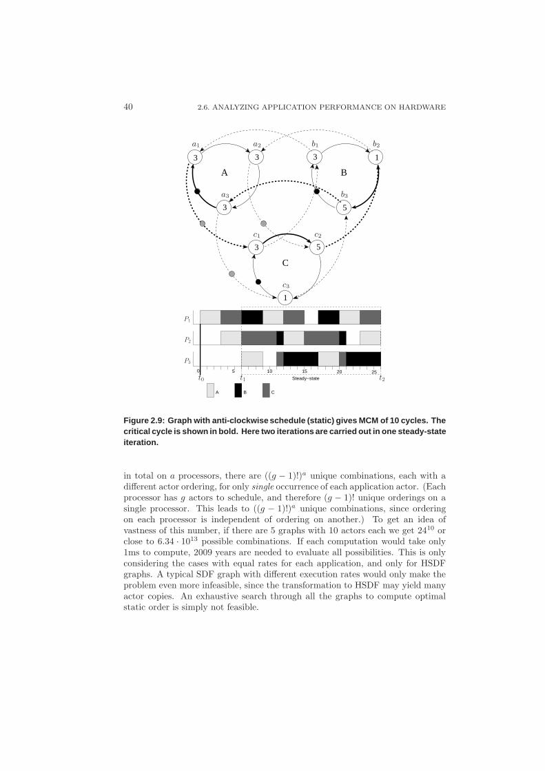
40 2.6. ANALYZING APPLICATION PERFORMANCE ON HARDWARE
A B
C
3
3 3 3 1
5
53
1
a1 a2
a3
b1 b2
b3
c1 c2
c3
0 5 10 15 20 25
A B C
Steady−statet0 t1 t2
P1
P2
P3
Figure 2.9: Graph with anti-clockwise schedule (static) gi ves MCM of 10 cycles. Thecritical cycle is shown in bold. Here two iterations are carr ied out in one steady-stateiteration.
in total on a processors, there are ((g − 1)!)a unique combinations, each with adifferent actor ordering, for only single occurrence of each application actor. (Eachprocessor has g actors to schedule, and therefore (g − 1)! unique orderings on asingle processor. This leads to ((g − 1)!)a unique combinations, since orderingon each processor is independent of ordering on another.) To get an idea ofvastness of this number, if there are 5 graphs with 10 actors each we get 2410 orclose to 6.34 · 1013 possible combinations. If each computation would take only1ms to compute, 2009 years are needed to evaluate all possibilities. This is onlyconsidering the cases with equal rates for each application, and only for HSDFgraphs. A typical SDF graph with different execution rates would only make theproblem even more infeasible, since the transformation to HSDF may yield manyactor copies. An exhaustive search through all the graphs to compute optimalstatic order is simply not feasible.
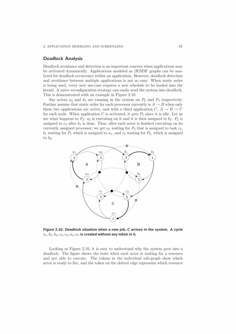
2. APPLICATION MODELING AND SCHEDULING 41
Deadlock Analysis
Deadlock avoidance and detection is an important concern when applications maybe activated dynamically. Applications modeled as (H)SDF graphs can be ana-lyzed for deadlock occurrence within an application. However, deadlock detectionand avoidance between multiple applications is not so easy. When static orderis being used, every new use-case requires a new schedule to be loaded into thekernel. A naive reconfiguration strategy can easily send the system into deadlock.This is demonstrated with an example in Figure 2.10.
Say actors a2 and b3 are running in the system on P2 and P3 respectively.Further assume that static order for each processor currently is A → B when onlythese two applications are active, and with a third application C, A → B → Cfor each node. When application C is activated, it gets P1 since it is idle. Let ussee what happens to P2: a2 is executing on it and it is then assigned to b2. P3 isassigned to c3 after b3 is done. Thus, after each actor is finished executing on itscurrently assigned processor, we get a3 waiting for P3 that is assigned to task c3,b1 waiting for P1 which is assigned to a1, and c2 waiting for P2, which is assignedto b2.
A B
C
3
3 3 3
5
3
1
5
1
a1 a2
a3
b1 b2
b3
c1 c2
c3
Figure 2.10: Deadlock situation when a new job, C arrives in t he system. A cyclea1, b1, b2, c2, c3, a3, a1 is created without any token in it.
Looking at Figure 2.10, it is easy to understand why the system goes into adeadlock. The figure shows the state when each actor is waiting for a resourceand not able to execute. The tokens in the individual sub-graph show whichactor is ready to fire, and the token on the dotted edge represents which resource
42 2.6. ANALYZING APPLICATION PERFORMANCE ON HARDWARE
is available to the application. In order for an actor to fire, the token should bepresent on all its incoming edges – in this case both on the incoming dotted edgeand the solid edge. It can be further noted that a cycle is formed without anytoken in it. This is clearly a situation of deadlock [KM66] since the actors on thiscycle will never be enabled. This cycle is shown in Figure 2.10 in bold edges. It ispossible to take special measure to check and prevent the system from going intosuch deadlock. This, however, implies extra overhead at both compile-time andrun-time. The application may also have to be delayed before it can be admittedinto the system.
We can therefore conclude that computing a static order for multiple appli-cations is very compute intensive and infeasible. Further, the performance weobtain may not be optimal. However, the advantage of this approach is that weare guaranteed to achieve the performance that is analyzed for any static orderat design-time provided the worst-case execution time estimates are correct.
2.6.2 Dynamic Order Analysis
In this sub-section, we look at static-assignment scheduler, where only proces-sor assignment is done at compile-time and the ordering is done at run-time.First-come-first-serve (FCFS) falls under this category. Another arbiter that wepropose here in this category is round-robin-with-skipping (RRWS). In RRWS, arecommended order is specified, but the actors can be skipped over if they arenot ready when the processor becomes idle. This is similar to the fairness arbiterproposed by Gao in 1983 [Gao83]. However, in that scheduler, all actors haveequal weight. In RRWS, multiple instances of an actor can be scheduled in onecycle to provide an easy rate control mechanism.
The price a system-designer has to pay when using dynamic scheduling isthe difficulty in determining application performance. Analyzing application per-formance when multiple applications are sharing multiprocessor platform is noteasy. An approach that models resource contention by computing worst-case-
response-time for TDMA scheduling (requires preemption) has been analyzedin [BHM+05]. This analysis also requires limited information from the otherSDFGs, but gives a very conservative bound that may be too pessimistic. Asthe number of applications increases, the minimum performance bound decreasesmuch more than the average case performance. Further, this approach assumesa preemptive system. A similar worst-case analysis approach for round-robin ispresented in [Hoe04], which also works on non-preemptive systems, but suffersfrom the same problem of lack of scalability.
Let us revisit the example in Figure 2.7. Since 3 actors are mapped on eachprocessor, an actor may need to wait when it is ready to be executed at a processor.The maximum waiting time for a particular actor can be computed by consideringthe critical instant as defined by Liu and Layland [LL73]. The critical instant
for an actor is defined as an instant at which a request for that actor has thelargest response time. The response time is defined as the sum of an actor’s
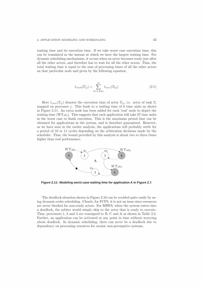
2. APPLICATION MODELING AND SCHEDULING 43
waiting time and its execution time. If we take worst case execution time, thiscan be translated as the instant at which we have the largest waiting time. Fordynamic scheduling mechanisms, it occurs when an actor becomes ready just afterall the other actors, and therefore has to wait for all the other actors. Thus, thetotal waiting time is equal to the sum of processing times of all the other actorson that particular node and given by the following equation.
twait(Tij) =m
∑
k=1,k 6=i
texec(Tkj) (2.1)
Here texec(Tij) denotes the execution time of actor Tij , i.e. actor of task Ti
mapped on processor j. This leads to a waiting time of 6 time units as shownin Figure 2.11. An extra node has been added for each ‘real’ node to depict thewaiting time (WT ai). This suggests that each application will take 27 time unitsin the worst case to finish execution. This is the maximum period that can beobtained for applications in the system, and is therefore guaranteed. However,as we have seen in the earlier analysis, the applications will probably settle fora period of 10 or 11 cycles depending on the arbitration decisions made by thescheduler. Thus, the bound provided by this analysis is about two to three timeshigher than real performance.
3 6
336 6
A
a1 a2
a3
WT a1 WT a2
WT a3
Figure 2.11: Modeling worst case waiting time for applicati on A in Figure 2.7.
The deadlock situation shown in Figure 2.10 can be avoided quite easily by us-ing dynamic-order scheduling. Clearly, for FCFS, it is not an issue since resourcesare never blocked for non-ready actors. For RRWS, when the system enters intoa deadlock, the arbiter would simply skip to the actor that is ready to execute.Thus, processors 1, 2 and 3 are reassigned to B, C and A as shown in Table 2.2.Further, an application can be activated at any point in time without worryingabout deadlock. In dynamic scheduling, there can never be a deadlock due todependency on processing resources for atomic non-preemptive systems.
44 2.7. COMPOSABILITY
Table 2.2: Table showing the deadlock condition in Figure 2. 10.Node Assigned to Task waiting Reassigned in RRWS
P1 A B BP2 B C CP3 C A A
2.7 Composability
As highlighted in Chapter 1, one of the key challenges when designing multime-dia systems is dealing with multiple applications. For example, a mobile phonesupports various applications that can be active at the same time, such as lis-tening to mp3 music, typing an sms and downloading some java application inthe background. Evaluating resource requirements for each of these cases can bequite a challenge even at design time, let alone at run time. When designing asystem, it is quite useful to be able to estimate resource requirements early in thedesign phase. Design managers often have to negotiate with the product divisionsfor the overall resources needed for the system. These estimates are mostly on ahigher level, and the managers usually like to adopt a spread-sheet approach forcomputing it. As we see in this section, it is often not possible to use this view.
We define composability as mapping and analysis of performance of multipleapplications on a multiprocessor platform in isolation, as far as possible. Notethat this is different from what has been defined in literature by Kopetz [KO02,KS03]. Composability as defined by Kopetz is integration of a whole system fromwell-specified and pre-tested sub-systems without unintended side-effects. The keydifference in this definition and our definition is that composability as definedby Kopetz is a property of a system such that the performance of applicationsin isolation and running concurrently with other applications is the same. Forexample, say we have a system with 10 applications, each with only one task andall mapped on the same processor. Let us further assume that all tasks take 100time units to execute in isolation. According to the definition of Kopetz, it willalso take 100 time units when running with the other tasks. This can only beachieved in two ways.
1. We can assume complete virtualization of resources, and that each applica-tion gets one-tenth of processor resources. This implies that we only useone-tenth of the resources when only one application is active. Further, toachieve complete virtualization, the processor has to be preempted and itscontext has to be switched every single cycle3.
2. We consider a worst-case schedule in which all applications are scheduled,and the total execution time of all applications is 100 time units. Thus, ifa particular application is not active, the processor simply waits for that
3This could be relaxed a bit, depending on the observability of the system.
2. APPLICATION MODELING AND SCHEDULING 45
many time units as it is scheduled for. This again leads to under-utilizationof the processor resources. Besides, if any application takes more time, thenthe system may collapse.
Clearly, this implies that we cannot harness the full processing capability. Ina typical system, we would want to use this compute power to deliver a betterquality-of-service for an application when possible. We want to let the systemexecute as many applications as possible with the current resource availability,and let applications achieve their best behaviour possible in the given use-case.Thus, in the example with 10 applications, if each application can run in 10 timeunits in isolation, it might take 100 time units when running concurrently withall the other applications. We would like to predict the application propertiesgiven the application mix of the system, with as little information from otherapplications as possible.
Some of the things we would like to analyze are for example, deadlock oc-currence, and application performance. Clearly, since there is more than oneapplication mapped on a multi-processor system, there will be contention for theresources. Due to this contention, the throughput analyzed for an application inisolation is not always achievable when the application runs together with otherapplications. We see how different levels of information from other applicationsaffect analysis results in the next sub-section.
2.7.1 Performance Estimation
Let us consider a scenario of video-conferencing in a hand-held device. Figure 2.12shows SDF graphs for both H263 encoding and decoding applications. The en-coder model is based on the SDF graph presented in [OH04], and the decodermodel is based on [Stu07]4. The video-stream assumed for the example is ofQCIF resolution that has 99 macro-blocks to process, as indicated by the rateson the edges. Both encoding and decoding have an actor that works on variablelength (VLC and VLD respectively), quantization (Quant and IQ respectively),and discrete cosine transform (DCT and IDCT respectively). Since we are consid-ering a heterogeneous system, the processor responsible for an actor in encodingprocess is usually responsible for the corresponding decoding actor. When the en-coding and decoding are done concurrently, the DCT and IDCT are likely to beexecuted on the same processor, since that processor is probably more suited forcosine transforms. This resource dependency in the encoder and decoder modelsis shown by shading in Figure 2.12. Thus, the resource dependency in encodingand decoding is exactly reversed. A similar situation happens during decodingand encoding of an audio stream as well.
A simple example is shown in Figure 2.13 to illustrate the same behaviour aspresented above. The figure shows an example of two application graphs A andB with three actors each, mapped on a 3-processor system. Actors a1 and b1 are
4The self-edges are removed for simplicity.
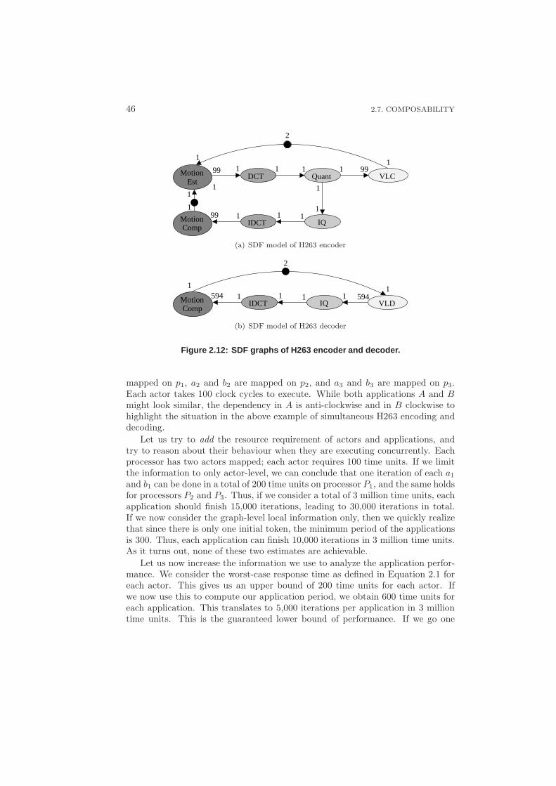
46 2.7. COMPOSABILITY
MotionEst
MotionComp
IDCT
DCT Quant VLC
IQ
1
99 99
99
1 1 1 1
1
111 1
1
1
11
2
(a) SDF model of H263 encoder
MotionComp
IDCT IQ VLD594 11 1 1
1 1594
2
(b) SDF model of H263 decoder
Figure 2.12: SDF graphs of H263 encoder and decoder.
mapped on p1, a2 and b2 are mapped on p2, and a3 and b3 are mapped on p3.Each actor takes 100 clock cycles to execute. While both applications A and Bmight look similar, the dependency in A is anti-clockwise and in B clockwise tohighlight the situation in the above example of simultaneous H263 encoding anddecoding.
Let us try to add the resource requirement of actors and applications, andtry to reason about their behaviour when they are executing concurrently. Eachprocessor has two actors mapped; each actor requires 100 time units. If we limitthe information to only actor-level, we can conclude that one iteration of each a1
and b1 can be done in a total of 200 time units on processor P1, and the same holdsfor processors P2 and P3. Thus, if we consider a total of 3 million time units, eachapplication should finish 15,000 iterations, leading to 30,000 iterations in total.If we now consider the graph-level local information only, then we quickly realizethat since there is only one initial token, the minimum period of the applicationsis 300. Thus, each application can finish 10,000 iterations in 3 million time units.As it turns out, none of these two estimates are achievable.
Let us now increase the information we use to analyze the application perfor-mance. We consider the worst-case response time as defined in Equation 2.1 foreach actor. This gives us an upper bound of 200 time units for each actor. Ifwe now use this to compute our application period, we obtain 600 time units foreach application. This translates to 5,000 iterations per application in 3 milliontime units. This is the guaranteed lower bound of performance. If we go one
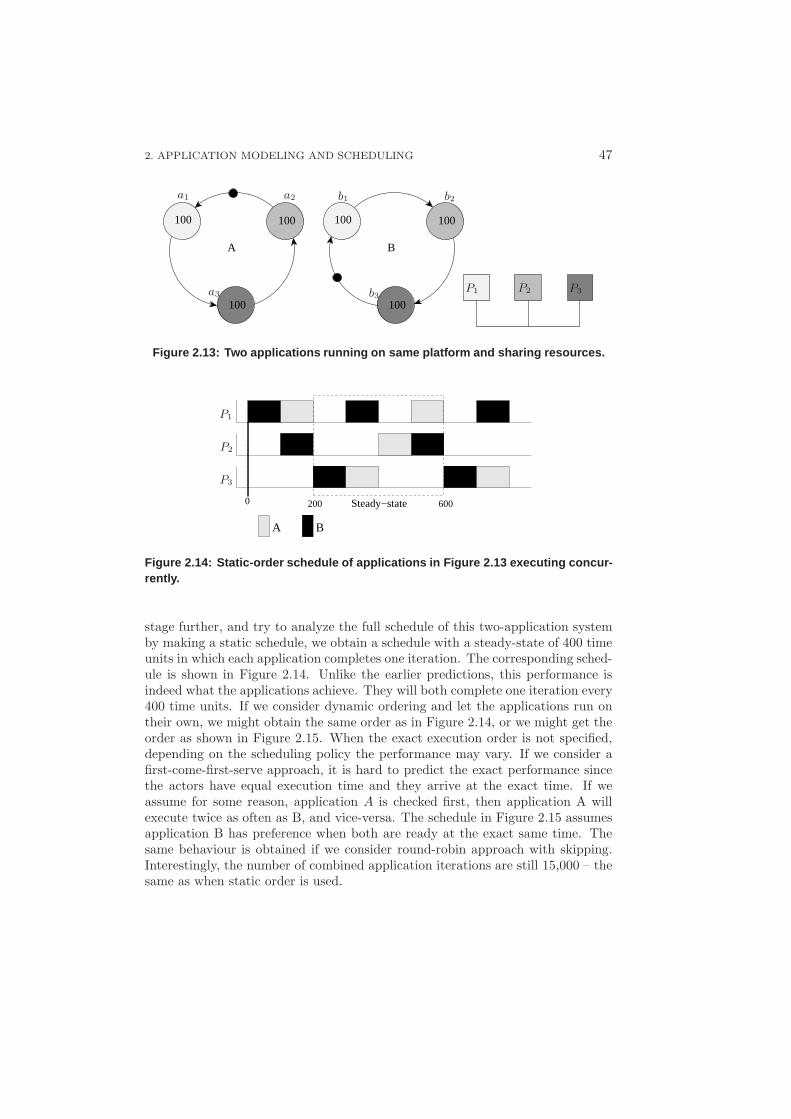
2. APPLICATION MODELING AND SCHEDULING 47
100
100
100
A
100
100
100
B
a1 a2
a3
b1 b2
b3P1 P2 P3
Figure 2.13: Two applications running on same platform and s haring resources.
A B
0 Steady−state 600200
P1
P2
P3
Figure 2.14: Static-order schedule of applications in Figu re 2.13 executing concur-rently.
stage further, and try to analyze the full schedule of this two-application systemby making a static schedule, we obtain a schedule with a steady-state of 400 timeunits in which each application completes one iteration. The corresponding sched-ule is shown in Figure 2.14. Unlike the earlier predictions, this performance isindeed what the applications achieve. They will both complete one iteration every400 time units. If we consider dynamic ordering and let the applications run ontheir own, we might obtain the same order as in Figure 2.14, or we might get theorder as shown in Figure 2.15. When the exact execution order is not specified,depending on the scheduling policy the performance may vary. If we consider afirst-come-first-serve approach, it is hard to predict the exact performance sincethe actors have equal execution time and they arrive at the exact time. If weassume for some reason, application A is checked first, then application A willexecute twice as often as B, and vice-versa. The schedule in Figure 2.15 assumesapplication B has preference when both are ready at the exact same time. Thesame behaviour is obtained if we consider round-robin approach with skipping.Interestingly, the number of combined application iterations are still 15,000 – thesame as when static order is used.
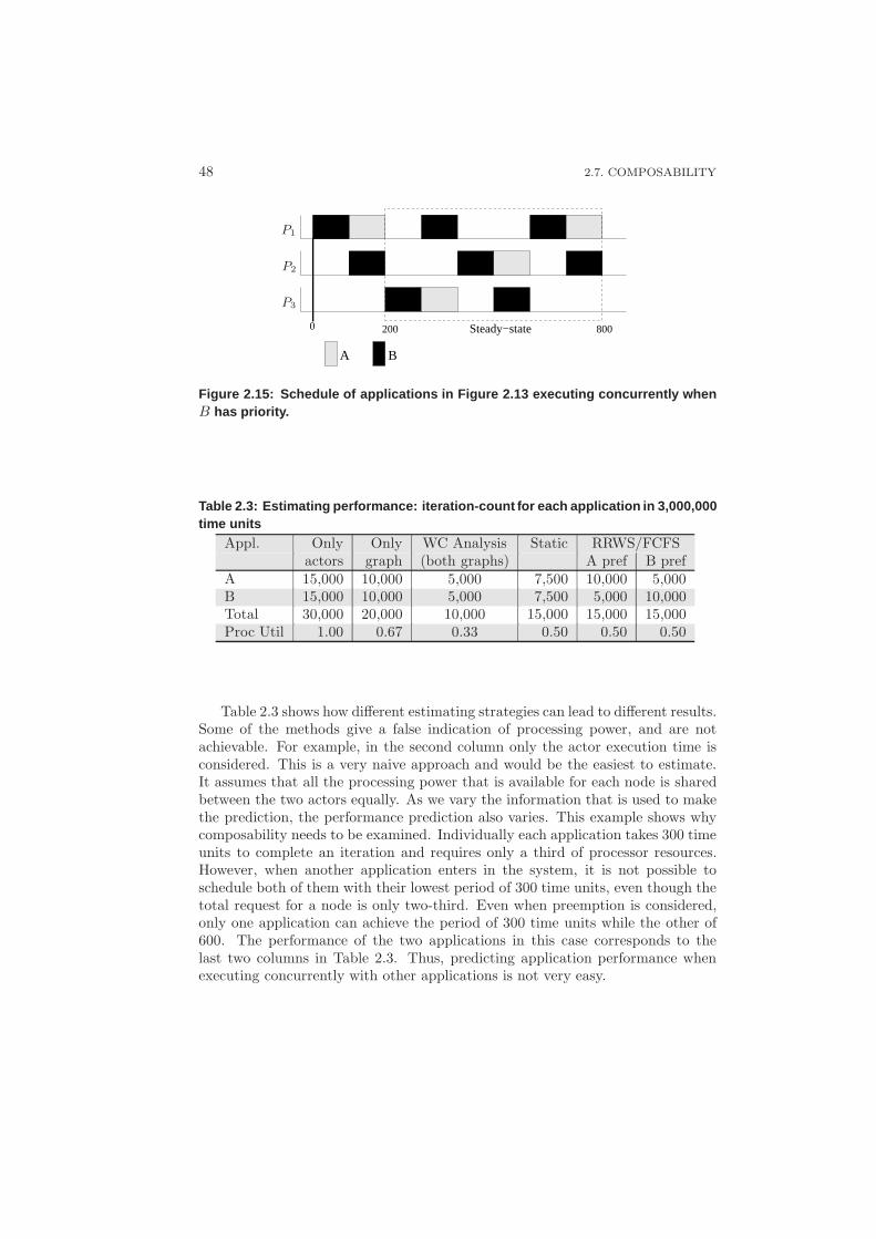
48 2.7. COMPOSABILITY
Steady−state
A B
0 200 800
P1
P2
P3
Figure 2.15: Schedule of applications in Figure 2.13 execut ing concurrently whenB has priority.
Table 2.3: Estimating performance: iteration-count for ea ch application in 3,000,000time units
Appl. Only Only WC Analysis Static RRWS/FCFSactors graph (both graphs) A pref B pref
A 15,000 10,000 5,000 7,500 10,000 5,000B 15,000 10,000 5,000 7,500 5,000 10,000Total 30,000 20,000 10,000 15,000 15,000 15,000Proc Util 1.00 0.67 0.33 0.50 0.50 0.50
Table 2.3 shows how different estimating strategies can lead to different results.Some of the methods give a false indication of processing power, and are notachievable. For example, in the second column only the actor execution time isconsidered. This is a very naive approach and would be the easiest to estimate.It assumes that all the processing power that is available for each node is sharedbetween the two actors equally. As we vary the information that is used to makethe prediction, the performance prediction also varies. This example shows whycomposability needs to be examined. Individually each application takes 300 timeunits to complete an iteration and requires only a third of processor resources.However, when another application enters in the system, it is not possible toschedule both of them with their lowest period of 300 time units, even though thetotal request for a node is only two-third. Even when preemption is considered,only one application can achieve the period of 300 time units while the other of600. The performance of the two applications in this case corresponds to thelast two columns in Table 2.3. Thus, predicting application performance whenexecuting concurrently with other applications is not very easy.
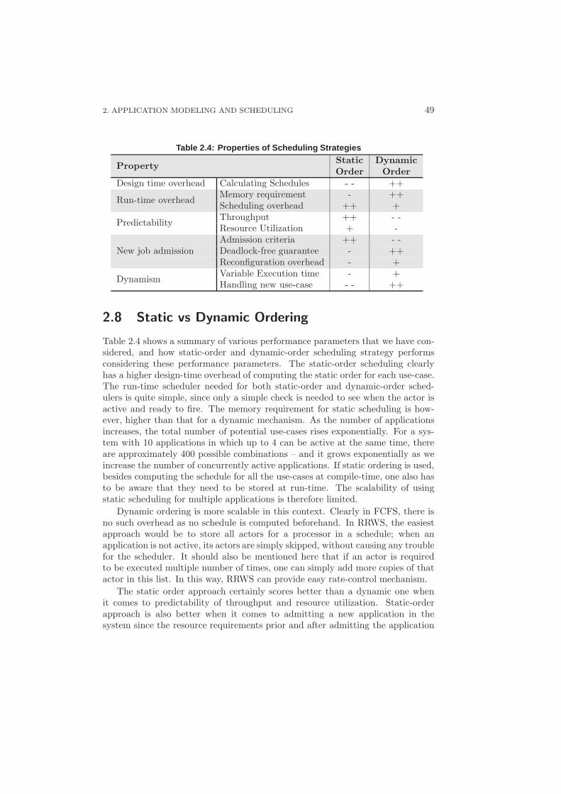
2. APPLICATION MODELING AND SCHEDULING 49
Table 2.4: Properties of Scheduling StrategiesStatic Dynamic
PropertyOrder Order
Design time overhead Calculating Schedules - - ++Memory requirement - ++
Run-time overheadScheduling overhead ++ +Throughput ++ - -
PredictabilityResource Utilization + -Admission criteria ++ - -Deadlock-free guarantee - ++New job admissionReconfiguration overhead - +Variable Execution time - +
DynamismHandling new use-case - - ++
2.8 Static vs Dynamic Ordering
Table 2.4 shows a summary of various performance parameters that we have con-sidered, and how static-order and dynamic-order scheduling strategy performsconsidering these performance parameters. The static-order scheduling clearlyhas a higher design-time overhead of computing the static order for each use-case.The run-time scheduler needed for both static-order and dynamic-order sched-ulers is quite simple, since only a simple check is needed to see when the actor isactive and ready to fire. The memory requirement for static scheduling is how-ever, higher than that for a dynamic mechanism. As the number of applicationsincreases, the total number of potential use-cases rises exponentially. For a sys-tem with 10 applications in which up to 4 can be active at the same time, thereare approximately 400 possible combinations – and it grows exponentially as weincrease the number of concurrently active applications. If static ordering is used,besides computing the schedule for all the use-cases at compile-time, one also hasto be aware that they need to be stored at run-time. The scalability of usingstatic scheduling for multiple applications is therefore limited.
Dynamic ordering is more scalable in this context. Clearly in FCFS, there isno such overhead as no schedule is computed beforehand. In RRWS, the easiestapproach would be to store all actors for a processor in a schedule; when anapplication is not active, its actors are simply skipped, without causing any troublefor the scheduler. It should also be mentioned here that if an actor is requiredto be executed multiple number of times, one can simply add more copies of thatactor in this list. In this way, RRWS can provide easy rate-control mechanism.
The static order approach certainly scores better than a dynamic one whenit comes to predictability of throughput and resource utilization. Static-orderapproach is also better when it comes to admitting a new application in thesystem since the resource requirements prior and after admitting the application
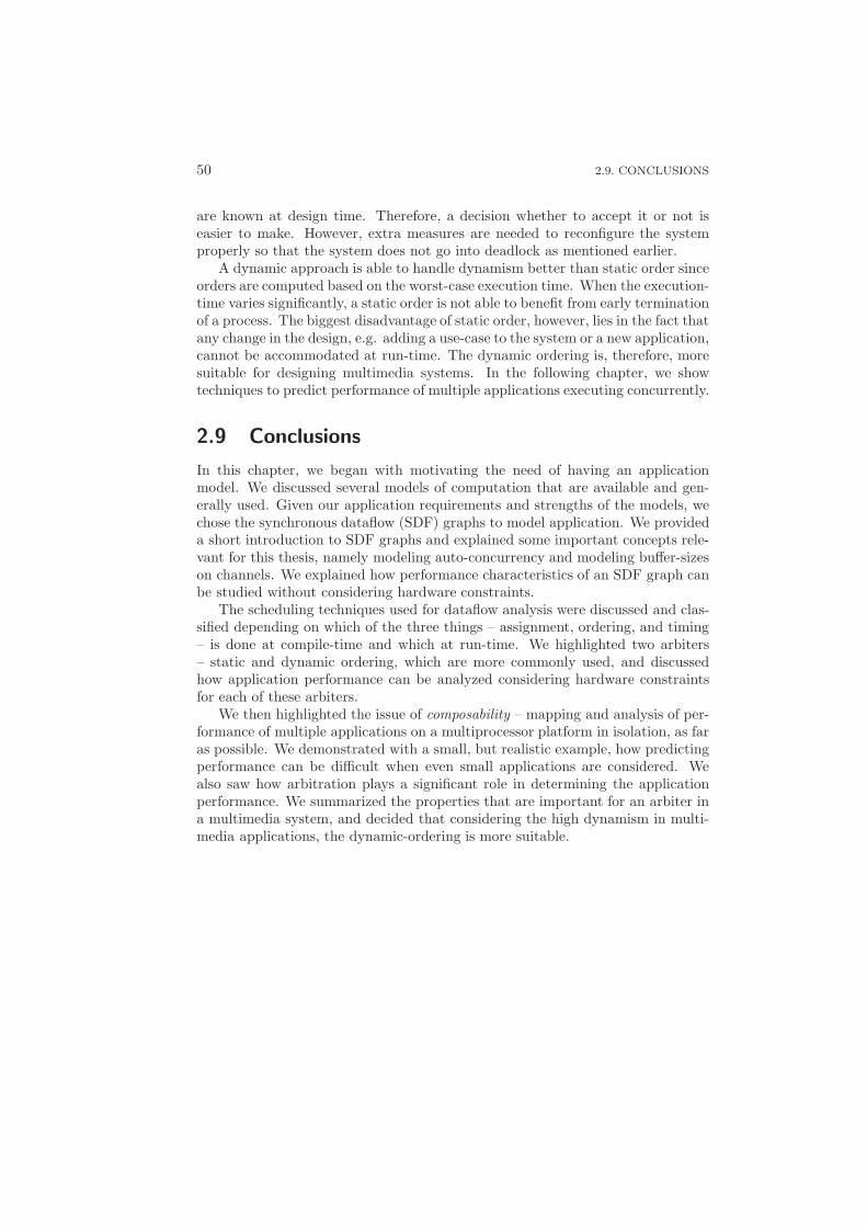
50 2.9. CONCLUSIONS
are known at design time. Therefore, a decision whether to accept it or not iseasier to make. However, extra measures are needed to reconfigure the systemproperly so that the system does not go into deadlock as mentioned earlier.
A dynamic approach is able to handle dynamism better than static order sinceorders are computed based on the worst-case execution time. When the execution-time varies significantly, a static order is not able to benefit from early terminationof a process. The biggest disadvantage of static order, however, lies in the fact thatany change in the design, e.g. adding a use-case to the system or a new application,cannot be accommodated at run-time. The dynamic ordering is, therefore, moresuitable for designing multimedia systems. In the following chapter, we showtechniques to predict performance of multiple applications executing concurrently.
2.9 Conclusions
In this chapter, we began with motivating the need of having an applicationmodel. We discussed several models of computation that are available and gen-erally used. Given our application requirements and strengths of the models, wechose the synchronous dataflow (SDF) graphs to model application. We provideda short introduction to SDF graphs and explained some important concepts rele-vant for this thesis, namely modeling auto-concurrency and modeling buffer-sizeson channels. We explained how performance characteristics of an SDF graph canbe studied without considering hardware constraints.
The scheduling techniques used for dataflow analysis were discussed and clas-sified depending on which of the three things – assignment, ordering, and timing– is done at compile-time and which at run-time. We highlighted two arbiters– static and dynamic ordering, which are more commonly used, and discussedhow application performance can be analyzed considering hardware constraintsfor each of these arbiters.
We then highlighted the issue of composability – mapping and analysis of per-formance of multiple applications on a multiprocessor platform in isolation, as faras possible. We demonstrated with a small, but realistic example, how predictingperformance can be difficult when even small applications are considered. Wealso saw how arbitration plays a significant role in determining the applicationperformance. We summarized the properties that are important for an arbiter ina multimedia system, and decided that considering the high dynamism in multi-media applications, the dynamic-ordering is more suitable.
CHAPTER 3
Probabilistic Performance Prediction
As mentioned earlier in Chapter 1, in modern multimedia systems, multiple ap-plications are executing concurrently. While traditionally a mobile phone had tosupport only a handful of applications like communicating with the base station,sending and receiving short messages, and encoding and decoding voice; modernhigh-end mobile devices also act as a music and video player, camera, gps, mobileTV and a complete personal digital assistant. Due to a huge number of possi-ble combinations of these multiple applications, it becomes a challenge to predicttheir performance in advance. One of the key design automation challenges aredesigning systems for these use-cases and fast exploration of software and hard-ware implementation alternatives with accurate performance evaluation of theseuse-cases. The number of use-cases are already exponential. When we considerthe possibilities of mapping application actors on processors and other resources,the total number of design points that need to be evaluated becomes even larger.A quick but accurate performance analysis technique is therefore very important.
This becomes even more important when applications may be dynamicallystarted and stopped in the system. Mis-prediction may result in reduced qualityof applications and lower the user-experience. To further complicate matters, theuser also expects to be able to download applications at run-time that may becompletely unknown to the system designer, for example, a security applicationrunning in the background to protect the mobile phone against theft. While someof these applications may not be so critical for the user-experience (e.g. browsinga web), others like playing video and audio are some functions where a reducedperformance is easily noticed. Accurate performance prediction is therefore es-
51
52
sential to be performed at run-time before starting a new application, and notalways feasible at design-time.
While this analysis is well understood (and relatively easier) for preemptivesystems [LL73][DD86][BCPV96], non-preemptive scheduling has received consid-erably less attention. However, for high-performance embedded systems (likecell-processing engine (SPE) [KDH+05] and graphics processors), non-preemptivesystems are preferred over preemptive scheduling for a number of reasons [JSM91].In many practical systems, properties of device hardware and software either makethe preemption impossible or prohibitively expensive. Further, non-preemptivescheduling algorithms are easier to implement than preemptive algorithms andhave dramatically lower overhead at run-time [JSM91]. Further, even in multi-processor systems with preemptive processors, some processors (or coprocessors/accelerators) are usually non-preemptive; for such processors, non-preemptiveanalysis is still needed. It is therefore important to investigate non-preemptivemulti-processor systems.
When applications are modeled as synchronous dataflow (SDF) graphs, theirperformance on a (multi-processor) system can be easily computed when theyare executing in isolation (provided we have a good model). When they executeconcurrently, depending on whether the used scheduler is static or dynamic, thearbitration on a resource is either fixed at design-time or chosen at run-timerespectively (as we have seen in Chapter 2). In the former case, the execution ordercan be modeled in the graph, and the performance of the entire use-case can bedetermined. The contention is therefore modeled as dependency edges in the SDFgraph. An example of such model is presented in Figure 2.8. However, this is moresuited for static applications. For dynamic applications such as multimedia, adynamic scheduler is more suitable, as has already been motivated in the previouschapter. A static scheduler is not able to deal with varying execution times andactor execution rates; something that is quite typical of dynamic applications. Fordynamic scheduling approaches, the contention can be modeled as waiting time fora task, which is added to the execution time to give the total response time. Theperformance can be determined by computing the performance (throughput) ofthis resulting SDF graph. With lack of good techniques for accurately predictingthe time spent in contention, designers have to resort to worst-case waiting timeestimates, that lead to over-designing the system. An example of this is shown inFigure 2.11, where the waiting time of each actor is equal to the sum of worst-caseexecution time of other actors. Further, those approaches are not scalable andthe over-estimate increases with the number of applications.
In this chapter, a novel probabilistic performance prediction (P 3) algorithm ispresented for predicting performance of multiple applications executing concur-rently on multi-processor platforms. The algorithm predicts the time that taskshave to spend during the contention phase for a resource. Each application con-tains a number of tasks that have a worst-case execution time. Two approaches arepresented – basic and iterative probabilistic techniques. The basic P 3 approachlooks at all the possible combinations of actors blocking a particular actor. Since
3. PROBABILISTIC PERFORMANCE PREDICTION 53
the number of combinations is exponential in the number of actors mapped ona resource, the analysis has a high complexity. The iterative P 3 approach com-putes how much a particular actor contributes to the waiting time of the otheractors. This is therefore linear in the number of actors, but needs to be iteratedto improve the waiting time estimate. Both techniques compute the expectedwaiting time when multiple tasks share a processing resource (The approach canbe adapted for other types of resource like communication and memory as well).These waiting time estimates, together with the execution time are used to esti-mate the performance of applications. The approach is very fast and can be usedboth at design-time and run-time owing to its low implementation complexity.
Following are the key features of the proposed P 3 algorithm.
• Accurate: The performance values predicted vary from the measured valuesby 2% on average and 3% at maximum, as observed.
• Fast: The algorithm has the complexity of O(n), where n is the number ofactors on each processor.
• Scalable: The algorithm is scalable in the number of actors per application,the number of processing nodes, and the number of applications in thesystem. This implies that when the number of actors or processing nodesare doubled, the execution time for the algorithm is also doubled.
• Composable: The above algorithm uses limited information from the otherapplications, thereby keeping the entire analysis composable.
The above features make the algorithm very suitable for implementation in em-bedded multimedia systems.
The remainder of the chapter is organized as follows. Section 3.1 explains theprobabilistic approach that is used to predict performance of multiple applicationsaccurately. Section 3.2 explains the iterative probabilistic technique that buildsupon the probability technique to improve the accuracy of the technique further.Section 3.3 describes the experimental setup and results obtained. Section 3.4discusses related work about how performance analysis is done using SDF graphstraditionally – for single and multiple applications. Section 3.5 presents majorconclusions and gives directions for future work.
3.1 Basic Probabilistic Analysis
When multiple applications execute in parallel, they often cause contention forthe shared resources. The probabilistic mechanism predicts this contention. Thetime spent by an actor in contention is added to its execution time, and the totalgives its response time. The equation below puts it more clearly.
tresp = texec + twait (3.1)
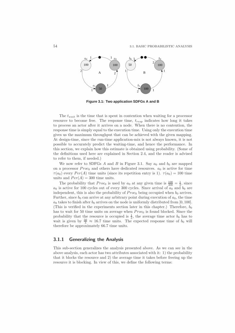
54 3.1. BASIC PROBABILISTIC ANALYSIS
1 1
1
1
1
1
1
1
22
2
2100
50
100
A
100
100
50
B
a0
a1
a2 b0
b1
b2
Figure 3.1: Two application SDFGs A and B
The twait is the time that is spent in contention when waiting for a processorresource to become free. The response time, tresp indicates how long it takesto process an actor after it arrives on a node. When there is no contention, theresponse time is simply equal to the execution time. Using only the execution timegives us the maximum throughput that can be achieved with the given mapping.At design-time, since the run-time application-mix is not always known, it is notpossible to accurately predict the waiting-time, and hence the performance. Inthis section, we explain how this estimate is obtained using probability. (Some ofthe definitions used here are explained in Section 2.4, and the reader is advisedto refer to them, if needed.)
We now refer to SDFGs A and B in Figure 3.1. Say a0 and b0 are mappedon a processor Proc0 and others have dedicated resources. a0 is active for timeτ(a0) every Per(A) time units (since its repetition entry is 1). τ(a0) = 100 timeunits and Per(A) = 300 time units.
The probability that Proc0 is used by a0 at any given time is 100300 = 1
3 , sincea0 is active for 100 cycles out of every 300 cycles. Since arrival of a0 and b0 areindependent, this is also the probability of Proc0 being occupied when b0 arrives.Further, since b0 can arrive at any arbitrary point during execution of a0, the timea0 takes to finish after b0 arrives on the node is uniformly distributed from [0, 100].(This is verified in the experiments section later in this chapter.) Therefore, b0
has to wait for 50 time units on average when Proc0 is found blocked. Since theprobability that the resource is occupied is 1
3 , the average time actor b0 has towait is given by 50
3 ≈ 16.7 time units. The expected response time of b0 willtherefore be approximately 66.7 time units.
3.1.1 Generalizing the Analysis
This sub-section generalizes the analysis presented above. As we can see in theabove analysis, each actor has two attributes associated with it: 1) the probabilitythat it blocks the resource and 2) the average time it takes before freeing up theresource it is blocking. In view of this, we define the following terms:
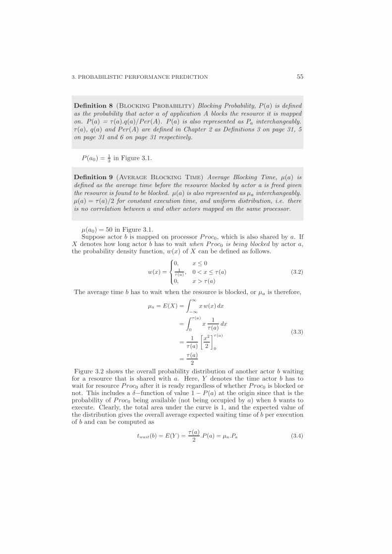
3. PROBABILISTIC PERFORMANCE PREDICTION 55
Definition 8 (Blocking Probability) Blocking Probability, P (a) is definedas the probability that actor a of application A blocks the resource it is mappedon. P (a) = τ(a).q(a)/Per(A). P (a) is also represented as Pa interchangeably.τ(a), q(a) and Per(A) are defined in Chapter 2 as Definitions 3 on page 31, 5on page 31 and 6 on page 31 respectively.
P (a0) = 13 in Figure 3.1.
Definition 9 (Average Blocking Time) Average Blocking Time, µ(a) isdefined as the average time before the resource blocked by actor a is freed giventhe resource is found to be blocked. µ(a) is also represented as µa interchangeably.µ(a) = τ(a)/2 for constant execution time, and uniform distribution, i.e. thereis no correlation between a and other actors mapped on the same processor.
µ(a0) = 50 in Figure 3.1.Suppose actor b is mapped on processor Proc0, which is also shared by a. If
X denotes how long actor b has to wait when Proc0 is being blocked by actor a,the probability density function, w(x) of X can be defined as follows.
w(x) =
0, x ≤ 01
τ(a), 0 < x ≤ τ (a)
0, x > τ (a)
(3.2)
The average time b has to wait when the resource is blocked, or µa is therefore,
µa = E(X) =
∫ ∞
−∞
x w(x) dx
=
∫ τ(a)
0
x1
τ (a)dx
=1
τ (a)
[
x2
2
]τ(a)
0
=τ (a)
2
(3.3)
Figure 3.2 shows the overall probability distribution of another actor b waitingfor a resource that is shared with a. Here, Y denotes the time actor b has towait for resource Proc0 after it is ready regardless of whether Proc0 is blocked ornot. This includes a δ−function of value 1 − P (a) at the origin since that is theprobability of Proc0 being available (not being occupied by a) when b wants toexecute. Clearly, the total area under the curve is 1, and the expected value ofthe distribution gives the overall average expected waiting time of b per executionof b and can be computed as
twait(b) = E(Y ) =τ (a)
2.P (a) = µa.Pa (3.4)
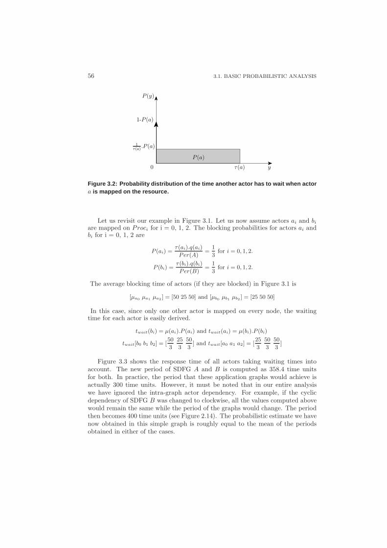
56 3.1. BASIC PROBABILISTIC ANALYSIS
0
1τ(a)
.P (a)
yτ(a)
P (a)
1-P (a)
P (y)
Figure 3.2: Probability distribution of the time another ac tor has to wait when actora is mapped on the resource.
Let us revisit our example in Figure 3.1. Let us now assume actors ai and bi
are mapped on Proci for i = 0, 1, 2. The blocking probabilities for actors ai andbi for i = 0, 1, 2 are
P (ai) =τ (ai).q(ai)
Per(A)=
1
3for i = 0, 1, 2.
P (bi) =τ (bi).q(bi)
Per(B)=
1
3for i = 0, 1, 2.
The average blocking time of actors (if they are blocked) in Figure 3.1 is
[µa0µa1
µa2] = [50 25 50] and [µb0 µb1 µb2 ] = [25 50 50]
In this case, since only one other actor is mapped on every node, the waitingtime for each actor is easily derived.
twait(bi) = µ(ai).P (ai) and twait(ai) = µ(bi).P (bi)
twait[b0 b1 b2] = [50
3
25
3
50
3] and twait[a0 a1 a2] = [
25
3
50
3
50
3]
Figure 3.3 shows the response time of all actors taking waiting times intoaccount. The new period of SDFG A and B is computed as 358.4 time unitsfor both. In practice, the period that these application graphs would achieve isactually 300 time units. However, it must be noted that in our entire analysiswe have ignored the intra-graph actor dependency. For example, if the cyclicdependency of SDFG B was changed to clockwise, all the values computed abovewould remain the same while the period of the graphs would change. The periodthen becomes 400 time units (see Figure 2.14). The probabilistic estimate we havenow obtained in this simple graph is roughly equal to the mean of the periodsobtained in either of the cases.
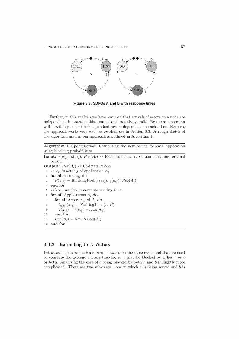
3. PROBABILISTIC PERFORMANCE PREDICTION 57
1 1
1
1
1
1
1
1
22
2
2
A B
108.3
66.7
116.7 66.7 116.7
108.3
a0
a1
a2 b0
b1
b2
Figure 3.3: SDFGs A and B with response times
Further, in this analysis we have assumed that arrivals of actors on a node areindependent. In practice, this assumption is not always valid. Resource contentionwill inevitably make the independent actors dependent on each other. Even so,the approach works very well, as we shall see in Section 3.3. A rough sketch ofthe algorithm used in our approach is outlined in Algorithm 1.
Algorithm 1 UpdatePeriod: Computing the new period for each applicationusing blocking probabilities
Input: τ(aij), q(aij), Per(Ai) // Execution time, repetition entry, and originalperiod.
Output: Per(Ai) // Updated Period1: // aij is actor j of application Ai
2: for all actors aij do
3: P (aij) = BlockingProb(τ(aij), q(aij), Per(Ai))4: end for
5: //Now use this to compute waiting time.6: for all Applications Ai do
7: for all Actors aij of Ai do
8: twait(aij) = WaitingTime(τ , P )9: τ(aij) = τ(aij) + twait(aij)
10: end for
11: Per(Ai) = NewPeriod(Ai)12: end for
3.1.2 Extending to N Actors
Let us assume actors a, b and c are mapped on the same node, and that we needto compute the average waiting time for c. c may be blocked by either a or bor both. Analyzing the case of c being blocked by both a and b is slightly morecomplicated. There are two sub-cases – one in which a is being served and b is
58 3.1. BASIC PROBABILISTIC ANALYSIS
queued, and another in which b is being served and a is queued. We thereforehave four possible cases outlined below, including the waiting time for each case.
Blocking only by a
twait(c1) = µa.Pa.(1 − Pb)
Blocking only by b
twait(c2) = µb.Pb.(1 − Pa)
a being served, b queued
The average time spent by b in each execution of b waiting behind a is given byµa.Pa. Therefore, the total probability of b behind a is,
Pwait(c3) = µa.Pa.q[b]
Per(b)= Pa.Pb.
µa
2.µb
, (3.5)
and the corresponding waiting time is,
twait(c3) = Pa.Pb.µa
2.µb
.(µa + 2µb)
b being served, a queued
This can be derived similar to above as follows:
twait(c4) = Pb.Pa.µb
2.µa
.(µb + 2µa)
The time that c needs to wait when two actors are in the queue varies dependingon which actor is being served. For example, when a is ahead in the queue, c hasto wait for µa due to a, since a is being served. However, since the whole actorb remains to be served after a is finished, c needs to wait 2.µb for b. One canalso observe that the waiting time due to actor a is µa.Pa when it is in front, and2.µa.Pa when behind. Adding the contributions from each of the four cases aboveto the waiting time, we get
twait(c) = µab.Pab =1
2.Pa.Pb.(
µ2a
µb
+µ2
b
µa
) + µa.Pa + µb.Pb
= µa.Pa.(1 +µa
2µb
Pb) + µb.Pb.(1 +µb
2µa
Pa)
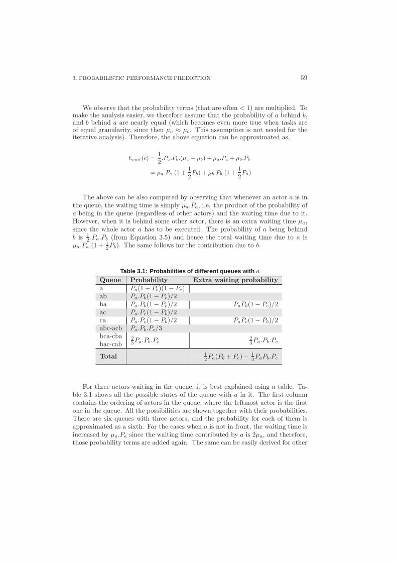
3. PROBABILISTIC PERFORMANCE PREDICTION 59
We observe that the probability terms (that are often < 1) are multiplied. Tomake the analysis easier, we therefore assume that the probability of a behind b,and b behind a are nearly equal (which becomes even more true when tasks areof equal granularity, since then µa ≈ µb. This assumption is not needed for theiterative analysis). Therefore, the above equation can be approximated as,
twait(c) =1
2.Pa.Pb.(µa + µb) + µa.Pa + µb.Pb
= µa.Pa.(1 +1
2Pb) + µb.Pb.(1 +
1
2Pa)
The above can be also computed by observing that whenever an actor a is inthe queue, the waiting time is simply µa.Pa, i.e. the product of the probability ofa being in the queue (regardless of other actors) and the waiting time due to it.However, when it is behind some other actor, there is an extra waiting time µa,since the whole actor a has to be executed. The probability of a being behindb is 1
2 .Pa.Pb (from Equation 3.5) and hence the total waiting time due to a isµa.Pa.(1 + 1
2Pb). The same follows for the contribution due to b.
Table 3.1: Probabilities of different queues with a
Queue Probability Extra waiting probability
a Pa(1 − Pb)(1 − Pc)ab Pa.Pb(1 − Pc)/2ba Pa.Pb(1 − Pc)/2 PaPb(1 − Pc)/2ac Pa.Pc(1 − Pb)/2ca Pa.Pc(1 − Pb)/2 PaPc(1 − Pb)/2abc-acb Pa.Pb.Pc/3bca-cba 2
3Pa.Pb.Pc23Pa.Pb.Pcbac-cab
Total 12Pa(Pb + Pc) − 1
3PaPb.Pc
For three actors waiting in the queue, it is best explained using a table. Ta-ble 3.1 shows all the possible states of the queue with a in it. The first columncontains the ordering of actors in the queue, where the leftmost actor is the firstone in the queue. All the possibilities are shown together with their probabilities.There are six queues with three actors, and the probability for each of them isapproximated as a sixth. For the cases when a is not in front, the waiting time isincreased by µa.Pa since the waiting time contributed by a is 2µa, and therefore,those probability terms are added again. The same can be easily derived for other
60 3.1. BASIC PROBABILISTIC ANALYSIS
actors too. We therefore obtain the following equation.
µabc.Pabc =µa.Pa.(
1 +1
2(Pb + Pc) −
1
3Pb.Pc
)
+ µb.Pb.(
1 +1
2(Pa + Pc) −
1
3Pa.Pc
)
+ µc.Pc.(
1 +1
2(Pa + Pb) −
1
3Pa.Pb
)
(3.6)
We can also understand intuitively, to some extent, how the terms in theequation derived above contribute to the delay (extra waiting time) in the analysis.The first term of each of the three lines (for instance µa.Pa in first line) denotesthe delay due to the respective actors. The terms that follow are the probabilitiesof the actor being in front of the queue; being there with at least one more actorbut behind; and then with at least two more actors and so on and so forth. Sincethe third probability term (≥ 2 actors) is included in the second probability term(≥ 1 actor), the last term is subtracted. Similar analysis and reasoning gives usthe following equation for waiting time when n actors a1, a2, . . . an are mappedon a particular resource
µa1...anPa1...an =
n∑
i=1
µaiPai
(
1 +
n−1∑
j=1
(−1)j+1
j + 1
∏
j(Pa1
. . . Pai−1Pai+1
. . . Pan))
(3.7)
where∏
j(x1, ..., xn) =
∑
1≤k1<k2...<kj≤n
(xk1xk2
...xkj)
∏
j(x1, ..., xn) is an elementary symmetric polynomial defined in [TW08]. In
simple terms, it is the summation of all the products of j unique terms in the set(x1, ..., xn). The number of terms clearly increases exponentially with increasingn. The total number of terms in Equation 3.7 in the symmetric polynomial is given
by(
n−1j
)
i.e. (n−1)!j!(n−1−j)! . As the number of actors mapped on a node increases,
the complexity of analysis also becomes high. To be exact, the complexity of theabove formula is O(nn+1), where n is the number of actors mapped on a node.Since this is done for each actor, the overall complexity becomes O(nn+2). In thenext sub-section we see how this complexity can be reduced.
3.1.3 Reducing Complexity
The complexity of the analysis plays an important role when putting an idea topractice. In this section we shall look at how the complexity can be reduced. Firstwe shall see how the formula can be rewritten in order to improve the complexitywithout changing the accuracy. Later we observe that higher order probability
3. PROBABILISTIC PERFORMANCE PREDICTION 61
products start appearing in the equation as the number of actors mapped on aprocessor is increased. Thus, we provide two approximations to second and fourth-order respectively. One of the main advantages of the probabilistic approach is therun-time implementation as is explained in Chapter 4. The composability-basedapproach can make the approach even more usable for run-time when applicationsenter and leave the system.
The total analysis complexity in Equation 3.7 is O(nn+2). Using some clevertechniques for implementation the complexity can be reduced to O(n2 + nn) i.e.O(nn). This can be achieved by modifying the equation such that we first compute∏
j(Pa1
, Pa2. . . Pan
) including Pai. The extra component is then subtracted from
the total for each ai separately.However, this is still infeasible and not scalable. An important observation
that can be made is that higher order terms start to appear in our analysis. Thenumber of these terms in Πj in Equation 3.7 increases exponentially. Since theseterms are products of probabilities (being smaller than one), higher order termscan likely be neglected. To limit the computational complexity, we provide asecond order approximation of the formula.
µa1...anPa1...an ≈
n∑
i=1
µaiPai
(
1 +1
2
n∑
j=1,j 6=i
(Paj))
The complexity of the above formula is O(n3), since we have to do it for nactors. For the above equation, we can modify the summation inside the loopsuch that the complexity is reduced. The new formula is re-written as
µa1...anPa1...an ≈
n∑
i=1
µaiPai
(
1 +1
2(Tot Summ − Pai
))
(3.8)
where
Tot Summ =n
∑
j=1
Paj
This makes the overall complexity O(n2). In general, the complexity can bereduced to O(nm) for m ≥ 2 by using m-th order approximation. In Section 3.3we present results of second and fourth order approximations.
Composability-based Approach
In a system often applications are added at run-time. In the earlier approach if wealready have a prediction for a particular combination of applications executing,and another application wants to start, the entire analysis has to be repeated.Here we present an alternative approach, in which when the prediction of a par-ticular combination is already known, the effect of the new application can be
62 3.1. BASIC PROBABILISTIC ANALYSIS
simply added to the overall effect of the previous combination. This approach isdefined as composability-based approach. In this approach the effect of multipleactors together is treated as if it were one actor. If there are two actors, theyare composed into one actor such that the properties of this new actor can beapproximated by the sum of their individual properties. In particular, if we havetwo actors a and b, we would like to know their combined blocking probabilityPab, and combined waiting time due to them, µab.Pab. Thus, when new applica-tions are started, the analysis can be incremental instead of repeating the wholeanalysis. We further define this composability operation for probability by ⊕ andfor waiting time by ⊗. We therefore get,
Pab = Pa ⊕ Pb = Pa + Pb − Pa.Pb (3.9)
µab.Pab = µa.Pa ⊗ µb.Pb = µa.Pa.(1 +Pb
2) + µb.Pb.(1 +
Pa
2) (3.10)
(Strictly speaking ⊗ operation also requires individual probabilities of theactors as inputs, but this has been omitted in the notation for simplicity.) Asso-ciativity of ⊕ is easily proven by showing Pabc = Pab ⊕ Pc = Pa ⊕ Pbc. Operation⊗ is associative only to the second order approximation. This can be proven in asimilar way by showing µabcPabc = µabPab ⊗ µcPc = µaPa ⊗ µbcPbc.
The associative property of these operations reduces the complexity even fur-ther. Complexity of Equation 3.9 and 3.10 is clearly O(1). If the waiting timeof a particular actor is to be computed, all the other actors have to be com-bined giving a total complexity of O(n2), which is equivalent to the complexity ofthe second-order approximation approach. However, in this approach the effectof actors is incrementally added. Therefore, when a new application has to beadded to the analysis and new actors are added to the nodes, the complexity ofthe computation is O(n) as compared to O(n2) in the case of the second-orderapproximation, for which the entire analysis has to be repeated.
Computing inverse of Formulae
The complexity of this composability-based approach can be further reduced whenwe can compute the inverse of the formulae in Equation 3.9 and Equation 3.10.When the inverse function is known, all the actors can be composed into one actorby deriving their total blocking probability and total average blocking time. Tocompute the individual waiting time, only the inverse operation with their ownparameters has to be performed. The total complexity of this approach is O(n)+n.O(1) = O(n). The inverse is also useful when applications enter and leave theanalysis, since only an incremental add or subtract has to be done to update thewaiting time instead of computing all the values. For example, if 10 applicationsare concurrently executing in the system, and one of them leaves. Normally, wewould need to recompute the effect of the remaining 9 applications all over again.However, with the inverse, this can be directly computed. In Equation 3.9, a then
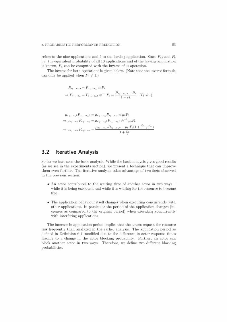
3. PROBABILISTIC PERFORMANCE PREDICTION 63
refers to the nine applications and b to the leaving application. Since Pab and Pb
i.e. the equivalent probability of all 10 applications and of the leaving applicationis known, Pa can be computed with the inverse of ⊕ operation.
The inverse for both operations is given below. (Note that the inverse formulacan only be applied when Pb 6= 1.)
Pa1...anb = Pa1...an ⊕ Pb
⇒ Pa1...an = Pa1...anb ⊕−1
Pb =Pa1...anb − Pb
1 − Pb
(Pb 6= 1)
µa1...anbPa1...anb = µa1...anPa1...an ⊗ µbPb
⇒ µa1...anPa1...an = µa1...anbPa1...anb ⊗−1
µbPb
⇒ µa1...anPa1...an =µa1...anbPa1...anb − µb.Pb(1 +
Pa1...an
2)
1 + Pb
2
3.2 Iterative Analysis
So far we have seen the basic analysis. While the basic analysis gives good results(as we see in the experiments section), we present a technique that can improvethem even further. The iterative analysis takes advantage of two facts observedin the previous section.
• An actor contributes to the waiting time of another actor in two ways –while it is being executed, and while it is waiting for the resource to becomefree.
• The application behaviour itself changes when executing concurrently withother applications. In particular the period of the application changes (in-creases as compared to the original period) when executing concurrentlywith interfering applications.
The increase in application period implies that the actors request the resourceless frequently than analyzed in the earlier analysis. The application period asdefined in Definition 6 is modified due to the difference in actor response timesleading to a change in the actor blocking probability. Further, an actor canblock another actor in two ways. Therefore, we define two different blockingprobabilities.
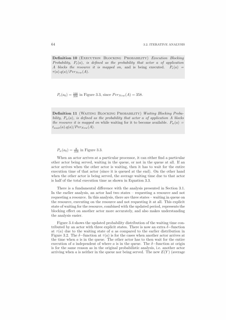
64 3.2. ITERATIVE ANALYSIS
Definition 10 (Execution Blocking Probability) Execution BlockingProbability, Pe(a), is defined as the probability that actor a of applicationA blocks the resource it is mapped on, and is being executed. Pe(a) =τ(a).q(a)/PerNew(A).
Pe(a0) = 100358 in Figure 3.3, since PerNew(A) = 358.
Definition 11 (Waiting Blocking Probability) Waiting Blocking Proba-bility, Pw(a), is defined as the probability that actor a of application A blocksthe resource it is mapped on while waiting for it to become available. Pw(a) =twait(a).q(a)/PerNew(A).
Pw(a0) = 8358 in Figure 3.3.
When an actor arrives at a particular processor, it can either find a particularother actor being served, waiting in the queue, or not in the queue at all. If anactor arrives when the other actor is waiting, then it has to wait for the entireexecution time of that actor (since it is queued at the end). On the other handwhen the other actor is being served, the average waiting time due to that actoris half of the total execution time as shown in Equation 3.3.
There is a fundamental difference with the analysis presented in Section 3.1.In the earlier analysis, an actor had two states – requesting a resource and notrequesting a resource. In this analysis, there are three states – waiting in queue onthe resource, executing on the resource and not requesting it at all. This explicitstate of waiting for the resource, combined with the updated period, represents theblocking effect on another actor more accurately, and also makes understandingthe analysis easier.
Figure 3.4 shows the updated probability distribution of the waiting time con-tributed by an actor with three explicit states. There is now an extra δ−functionat τ(a) due to the waiting state of a as compared to the earlier distribution inFigure 3.2. The δ−function at τ(a) is for the cases when another actor arrives atthe time when a is in the queue. The other actor has to then wait for the entireexecution of a independent of where a is in the queue. The δ−function at originis for the same reason as in the original probabilistic analysis, i.e. another actorarriving when a is neither in the queue nor being served. The new E(Y ) (average
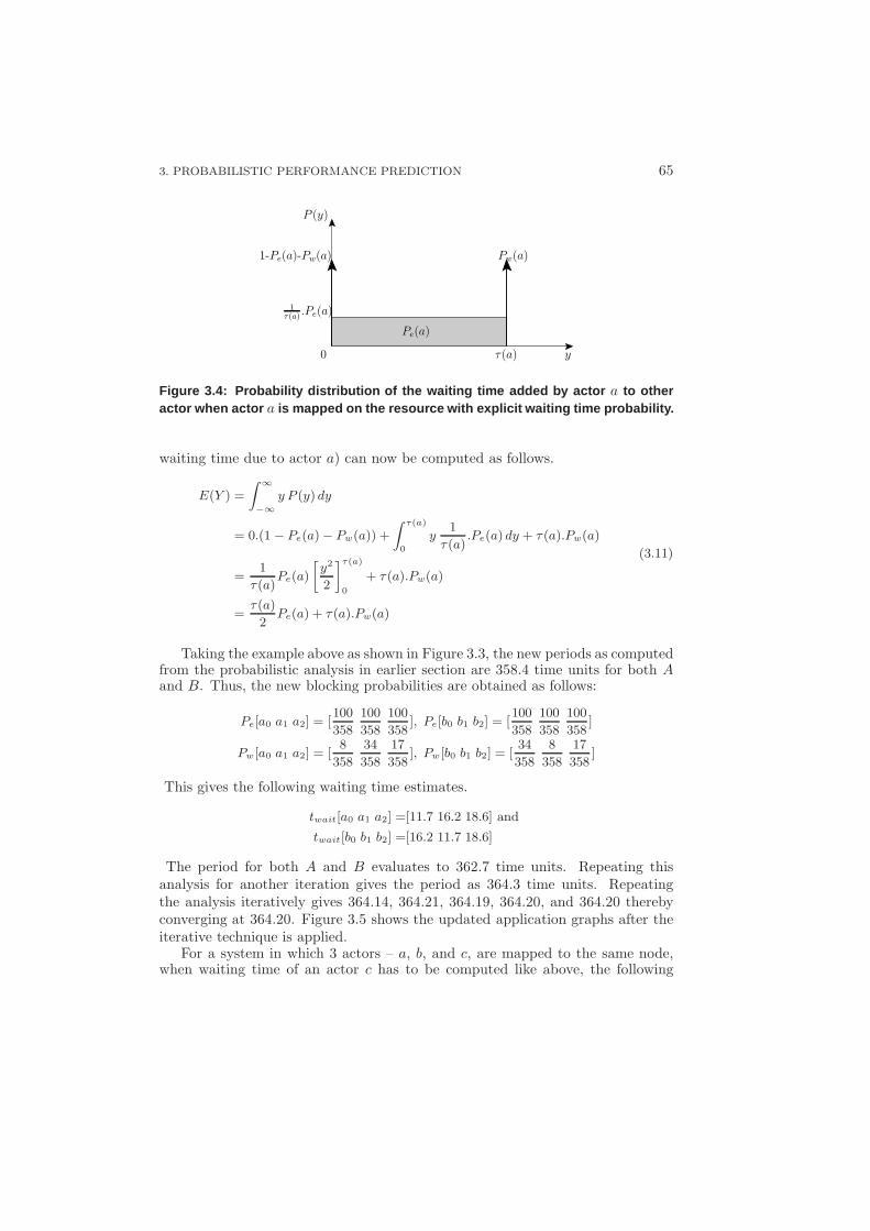
3. PROBABILISTIC PERFORMANCE PREDICTION 65
0
1τ(a)
.Pe(a)
yτ(a)
Pe(a)
Pw(a)1-Pe(a)-Pw(a)
P (y)
Figure 3.4: Probability distribution of the waiting time ad ded by actor a to otheractor when actor a is mapped on the resource with explicit waiting time probabi lity.
waiting time due to actor a) can now be computed as follows.
E(Y ) =
∫ ∞
−∞
y P (y) dy
= 0.(1 − Pe(a) − Pw(a)) +
∫ τ(a)
0
y1
τ (a).Pe(a) dy + τ (a).Pw(a)
=1
τ (a)Pe(a)
[
y2
2
]τ(a)
0
+ τ (a).Pw(a)
=τ (a)
2Pe(a) + τ (a).Pw(a)
(3.11)
Taking the example above as shown in Figure 3.3, the new periods as computedfrom the probabilistic analysis in earlier section are 358.4 time units for both Aand B. Thus, the new blocking probabilities are obtained as follows:
Pe[a0 a1 a2] = [100
358
100
358
100
358], Pe[b0 b1 b2] = [
100
358
100
358
100
358]
Pw[a0 a1 a2] = [8
358
34
358
17
358], Pw[b0 b1 b2] = [
34
358
8
358
17
358]
This gives the following waiting time estimates.
twait[a0 a1 a2] =[11.7 16.2 18.6] and
twait[b0 b1 b2] =[16.2 11.7 18.6]
The period for both A and B evaluates to 362.7 time units. Repeating thisanalysis for another iteration gives the period as 364.3 time units. Repeatingthe analysis iteratively gives 364.14, 364.21, 364.19, 364.20, and 364.20 therebyconverging at 364.20. Figure 3.5 shows the updated application graphs after theiterative technique is applied.
For a system in which 3 actors – a, b, and c, are mapped to the same node,when waiting time of an actor c has to be computed like above, the following
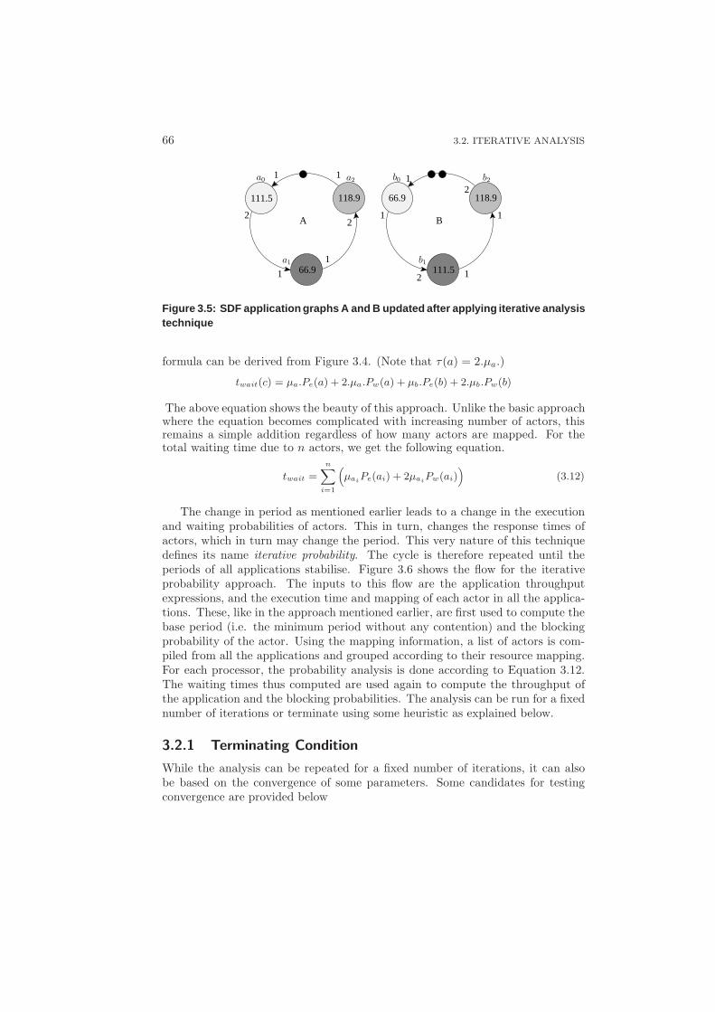
66 3.2. ITERATIVE ANALYSIS
1 1
1
1
1
1
1
1
22
2
2
A B
111.5 118.9
66.9 111.5
66.9 118.9
a0
a1
a2 b0
b1
b2
Figure 3.5: SDF application graphs A and B updated after appl ying iterative analysistechnique
formula can be derived from Figure 3.4. (Note that τ(a) = 2.µa.)
twait(c) = µa.Pe(a) + 2.µa.Pw(a) + µb.Pe(b) + 2.µb.Pw(b)
The above equation shows the beauty of this approach. Unlike the basic approachwhere the equation becomes complicated with increasing number of actors, thisremains a simple addition regardless of how many actors are mapped. For thetotal waiting time due to n actors, we get the following equation.
twait =n
∑
i=1
(
µaiPe(ai) + 2µai
Pw(ai))
(3.12)
The change in period as mentioned earlier leads to a change in the executionand waiting probabilities of actors. This in turn, changes the response times ofactors, which in turn may change the period. This very nature of this techniquedefines its name iterative probability. The cycle is therefore repeated until theperiods of all applications stabilise. Figure 3.6 shows the flow for the iterativeprobability approach. The inputs to this flow are the application throughputexpressions, and the execution time and mapping of each actor in all the applica-tions. These, like in the approach mentioned earlier, are first used to compute thebase period (i.e. the minimum period without any contention) and the blockingprobability of the actor. Using the mapping information, a list of actors is com-piled from all the applications and grouped according to their resource mapping.For each processor, the probability analysis is done according to Equation 3.12.The waiting times thus computed are used again to compute the throughput ofthe application and the blocking probabilities. The analysis can be run for a fixednumber of iterations or terminate using some heuristic as explained below.
3.2.1 Terminating Condition
While the analysis can be repeated for a fixed number of iterations, it can alsobe based on the convergence of some parameters. Some candidates for testingconvergence are provided below
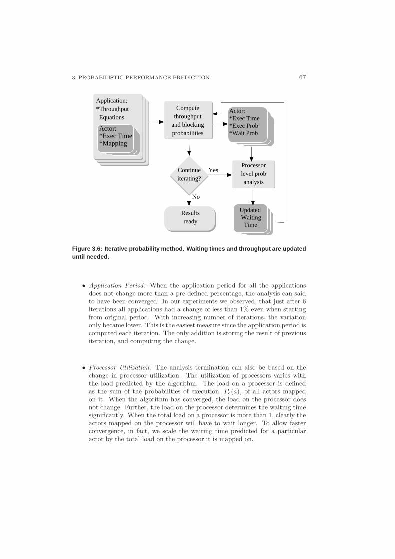
3. PROBABILISTIC PERFORMANCE PREDICTION 67
Yes
No
Actor:*Exec Time*Exec Prob*Wait Prob
Processorlevel probanalysis
Time
UpdatedWaiting
Actor:*Exec Time*Mapping
Application:*Throughput Equations
Continueiterating?
Resultsready
throughputand blockingprobabilities
Compute
Figure 3.6: Iterative probability method. Waiting times an d throughput are updateduntil needed.
• Application Period: When the application period for all the applicationsdoes not change more than a pre-defined percentage, the analysis can saidto have been converged. In our experiments we observed, that just after 6iterations all applications had a change of less than 1% even when startingfrom original period. With increasing number of iterations, the variationonly became lower. This is the easiest measure since the application period iscomputed each iteration. The only addition is storing the result of previousiteration, and computing the change.
• Processor Utilization: The analysis termination can also be based on thechange in processor utilization. The utilization of processors varies withthe load predicted by the algorithm. The load on a processor is definedas the sum of the probabilities of execution, Pe(a), of all actors mappedon it. When the algorithm has converged, the load on the processor doesnot change. Further, the load on the processor determines the waiting timesignificantly. When the total load on a processor is more than 1, clearly theactors mapped on the processor will have to wait longer. To allow fasterconvergence, in fact, we scale the waiting time predicted for a particularactor by the total load on the processor it is mapped on.
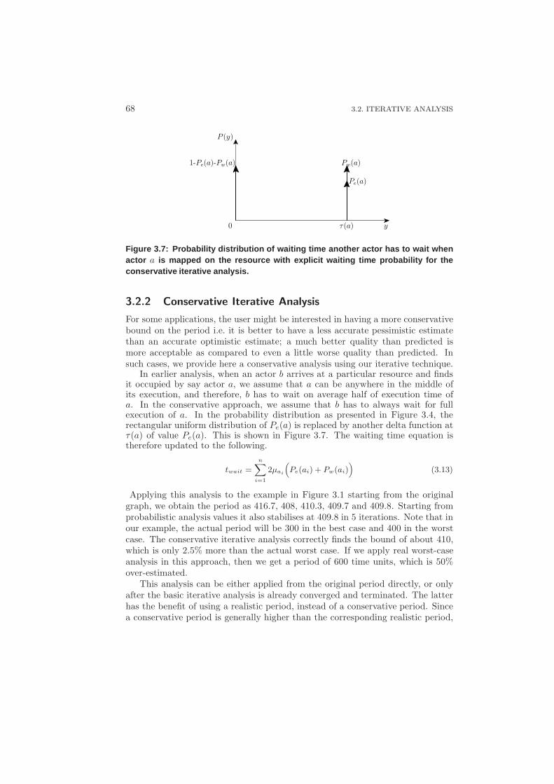
68 3.2. ITERATIVE ANALYSIS
0 yτ(a)
Pw(a)1-Pe(a)-Pw(a)
P (y)
Pe(a)
Figure 3.7: Probability distribution of waiting time anoth er actor has to wait whenactor a is mapped on the resource with explicit waiting time probabi lity for theconservative iterative analysis.
3.2.2 Conservative Iterative Analysis
For some applications, the user might be interested in having a more conservativebound on the period i.e. it is better to have a less accurate pessimistic estimatethan an accurate optimistic estimate; a much better quality than predicted ismore acceptable as compared to even a little worse quality than predicted. Insuch cases, we provide here a conservative analysis using our iterative technique.
In earlier analysis, when an actor b arrives at a particular resource and findsit occupied by say actor a, we assume that a can be anywhere in the middle ofits execution, and therefore, b has to wait on average half of execution time ofa. In the conservative approach, we assume that b has to always wait for fullexecution of a. In the probability distribution as presented in Figure 3.4, therectangular uniform distribution of Pe(a) is replaced by another delta function atτ(a) of value Pe(a). This is shown in Figure 3.7. The waiting time equation istherefore updated to the following.
twait =n
∑
i=1
2µai
(
Pe(ai) + Pw(ai))
(3.13)
Applying this analysis to the example in Figure 3.1 starting from the originalgraph, we obtain the period as 416.7, 408, 410.3, 409.7 and 409.8. Starting fromprobabilistic analysis values it also stabilises at 409.8 in 5 iterations. Note that inour example, the actual period will be 300 in the best case and 400 in the worstcase. The conservative iterative analysis correctly finds the bound of about 410,which is only 2.5% more than the actual worst case. If we apply real worst-caseanalysis in this approach, then we get a period of 600 time units, which is 50%over-estimated.
This analysis can be either applied from the original period directly, or onlyafter the basic iterative analysis is already converged and terminated. The latterhas the benefit of using a realistic period, instead of a conservative period. Sincea conservative period is generally higher than the corresponding realistic period,
3. PROBABILISTIC PERFORMANCE PREDICTION 69
the execution and waiting probability is correspondingly lower when using theconservative period. Thus, using a realistic period with a conservative analysisfor the last iteration gives the most conservative results. In experiments below,we present results of both approaches.
3.2.3 Parametric Throughput Analysis
Throughput computation of an SDF graph is generally very time consuming asexplained in Chapter 2. Lately, techniques have been presented in [GGS+06] thatcan compute throughput of many multimedia applications within milliseconds.However, those results have been taken on a high-end computer while assumingfixed actor execution times. Therefore, throughput computation of an SDF graphis generally done off-line or at design-time for a particular graph. However, if theexecution time of an actor changes, the entire analysis has to be repeated. Re-cently, a technique has been proposed to derive throughput equations for a rangeof execution times (defined as parameters) at design-time and these equationscan be easily evaluated at run-time to compute the critical cycle, and hence theperiod [GGBS08]. This technique greatly enhances the usability of the iterativeanalysis. With this the iterative analysis can be applied at both design-time andrun-time.
For example, for application A shown in Figure 3.1, there is only one crit-ical cycle. If the execution times of all actors of A are variable, the followingparametric equation is obtained (assuming auto-concurrency of 1):
Per(A) = τ(a0) + 2 × τ(a1) + τ(a2) (3.14)
Thus, whenever the period of application A is needed, the above equation canbe computed with the updated response times of actors a0, a1 and a2. Whilein this case there is only one equation for application A, in general the numberof equations depends on the graph structure and the range of execution times.When there are multiple equations, all of them need to be evaluated to find thelimiting period. This technique makes the iterative analysis suitable for run-timeimplementation.
3.2.4 Handling Other Arbiters
The above analysis has been presented for first-come-first-serve (FCFS) arbitra-tion. For static-order schedulers like round-robin or another arbitrary order de-rived from SDF 3 [SDF09], the schedule can be directly modeled in the graphitself. Other dynamic-order schedulers like a priority-based scheduler can be eas-ily modeled in the probability approach. One key difference in a priority-basedscheduler as compared to FCFS is that in FCFS once the actor arrives, it has toalways wait for actors ahead of it in the queue. In a priority-based system, if it ispreemptive, a higher priority actor can immediately preempt a lower priority ac-tor, and if it is non-preemptive, it has only to wait for lower priority actors if they
70 3.3. EXPERIMENTS
are executing. Let us define the priority of an actor a by Pr(a), such that a highervalue of Pr(a) implies a higher priority. Equation 3.12 that is presented for FCFS,can be rewritten as Equation 3.15. It shows the waiting time for an actor a whensharing a resource with actors a1 to an. Note that the waiting time contributedby the arrival of actor a during the queuing phase of an actor with a prioritylower than that of a, is not added in the equation. Similarly, Equation 3.16 showsthe adapted version of Equation 3.13 for handling priority-based schedulers. Itcan be seen that these equations are a generalized form of earlier versions, sincein FCFS the priorities of all actors are equal, i.e. Pr(a) = Pr(ai)∀i = 1, 2, ...n.It should be further noted, that since the priorities are only considered for localanalysis on a processor (or any resource), different processors (or resources) canhave different arbiters.
twait =n
∑
i=1
(
τai
2Pe(ai)
)
+n
∑
i=1,Pr(ai)≥Pr(a)
(
τaiPw(ai)
)
(3.15)
twait =n
∑
i=1
(
τaiPe(ai)
)
+n
∑
i=1,Pr(ai)≥Pr(a)
(
τaiPw(ai)
)
(3.16)
3.3 Experiments
In this section, we describe our experimental setup and some results obtainedfor the basic probability, explained in Section 3.1. The iterative technique asexplained in Section 3.2 improves upon this. First, we only show results of thebasic probability analysis since iterative analysis results are very close to the mea-sured results. Superimposing iterative analysis results on the same scale makesthe graph difficult to understand. In the basic analysis results, the graph is scaledto the original period, while in the iterative analysis it is scaled to the measuredperiod. The results of the software implementation of the probability approacheson an embedded processor, Microblaze are also provided.
3.3.1 Setup
In this section we present the results of above analysis obtained as compared tosimulation results for a number of use-cases. For this purpose, ten random SD-FGs were generated with eight to ten actors each using the SDF 3 tool [SGB06a],mimicking DSP and multimedia applications. Each graph is a strongly connectedcomponent i.e. every actor in the graph can be reached from every actor. Theexecution time and the rates of actors were also set randomly. The SDF 3 toolwas also used to analytically compute the periods of the graphs. Using theseten SDFGs, over a thousand use-cases (210) were generated. Simulations wereperformed using POOSL [TFG+07] to measure the actual performance for eachuse-case. Two different probabilistic approaches were used – the second order and
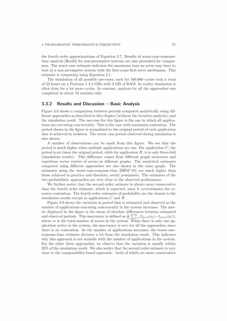
3. PROBABILISTIC PERFORMANCE PREDICTION 71
the fourth order approximations of Equation 3.7. Results of worst-case-response-time analysis [Hoe04] for non-preemptive systems are also presented for compar-ison. The worst-case estimate indicates the maximum time an actor may have towait in a non-preemptive system with the first-come-first-serve mechanism. Thisestimate is computing using Equation 2.1.
The simulation of all possible use-cases, each for 500,000 cycles took a totalof 23 hours on a Pentium 4 3.4 GHz with 3 GB of RAM. In reality simulation isoften done for a lot more cycles. In contrast, analysis for all the approaches wascompleted in about 10 minutes only.
3.3.2 Results and Discussion – Basic Analysis
Figure 3.8 shows a comparison between periods computed analytically using dif-ferent approaches as described in this chapter (without the iterative analysis), andthe simulation result. The use-case for this figure is the one in which all applica-tions are executing concurrently. This is the case with maximum contention. Theperiod shown in the figure is normalized to the original period of each applicationthat is achieved in isolation. The worst case period observed during simulation isalso shown.
A number of observations can be made from this figure. We see that theperiod is much higher when multiple applications are run. For application C, theperiod is six times the original period, while for application H , it is only three-fold(simulation results). This difference comes from different graph structures andrepetition vector entries of actors in different graphs. The analytical estimatescomputed using different approaches are also shown in the same graph. Theestimates using the worst-case-response-time [BHM+05] are much higher thanthose achieved in practice and therefore, overly pessimistic. The estimates of thetwo probabilistic approaches are very close to the observed performance.
We further notice that the second order estimate is always more conservativethan the fourth order estimate, which is expected, since it overestimates the re-source contention. The fourth order estimates of probability are the closest to thesimulation results except in applications C and H .
Figure 3.9 shows the variation in period that is estimated and observed as thenumber of applications executing concurrently in the system increases. The met-ric displayed in the figure is the mean of absolute differences between estimatedand observed periods. This inaccuracy is defined as 1
m
∑m
i=1 |tpred(ai)−tmeas(ai)|,where m is the total number of actors in the system. When there is only one ap-plication active in the system, the inaccuracy is zero for all the approaches, sincethere is no contention. As the number of applications increases, the worst-case-response-time estimate deviates a lot from the simulation result. This indicateswhy this approach is not scalable with the number of applications in the system.For the other three approaches, we observe that the variation is usually within20% of the simulation result. We also notice that the second order estimate is veryclose to the composability-based approach – both of which are more conservative
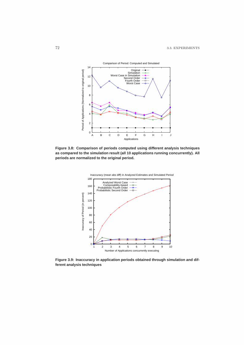
72 3.3. EXPERIMENTS
0
2
4
6
8
10
12
14
A B C D E F G H I J
Per
iod
of A
pplic
atio
ns (
Nor
mal
ized
to o
rigin
al p
erio
d)
Applications
Comparison of Period: Computed and Simulated
OriginalSimulation
Worst Case in SimulationSecond OrderFourth OrderWorst Case
Figure 3.8: Comparison of periods computed using different analysis techniquesas compared to the simulation result (all 10 applications ru nning concurrently). Allperiods are normalized to the original period.
0
20
40
60
80
100
120
140
160
180
1 2 3 4 5 6 7 8 9 10
Inac
cura
cy o
f Per
iod
(in p
erce
nt)
Number of Applications concurrently executing
Inaccuracy (mean abs diff) in Analyzed Estimates and Simulated Period
Analyzed Worst CaseComposability-based
Probabilistic Fourth OrderProbabilistic Second Order
Figure 3.9: Inaccuracy in application periods obtained thr ough simulation and dif-ferent analysis techniques
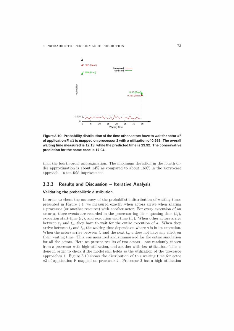
3. PROBABILISTIC PERFORMANCE PREDICTION 73
0
0.005
0 5 10 15 20 25 30 35
Pro
babi
lity
Waiting Time
0.287 (Meas)0.30 (Pred)
0.582 (Meas)
0.505 (Pred)
MeasuredPredicted
Figure 3.10: Probability distribution of the time other act ors have to wait for actor a2of application F. a2 is mapped on processor 2 with a utilization of 0.988. The over allwaiting time measured is 12.13, while the predicted time is 1 3.92. The conservativeprediction for the same case is 17.94.
than the fourth-order approximation. The maximum deviation in the fourth or-der approximation is about 14% as compared to about 160% in the worst-caseapproach – a ten-fold improvement.
3.3.3 Results and Discussion – Iterative Analysis
Validating the probabilistic distribution
In order to check the accuracy of the probabilistic distribution of waiting timespresented in Figure 3.4, we measured exactly when actors arrive when sharinga processor (or another resource) with another actor. For every execution of anactor a, three events are recorded in the processor log file – queuing time (tq),execution start-time (ts), and execution end-time (te). When other actors arrivebetween tq and ts, they have to wait for the entire execution of a. When theyarrive between ts and te, the waiting time depends on where a is in its execution.When the actors arrive between te and the next tq, a does not have any effect ontheir waiting time. This was measured and summarized for the entire simulationfor all the actors. Here we present results of two actors – one randomly chosenfrom a processor with high utilization, and another with low utilization. This isdone in order to check if the model still holds as the utilization of the processorapproaches 1. Figure 3.10 shows the distribution of this waiting time for actora2 of application F mapped on processor 2. Processor 2 has a high utilization
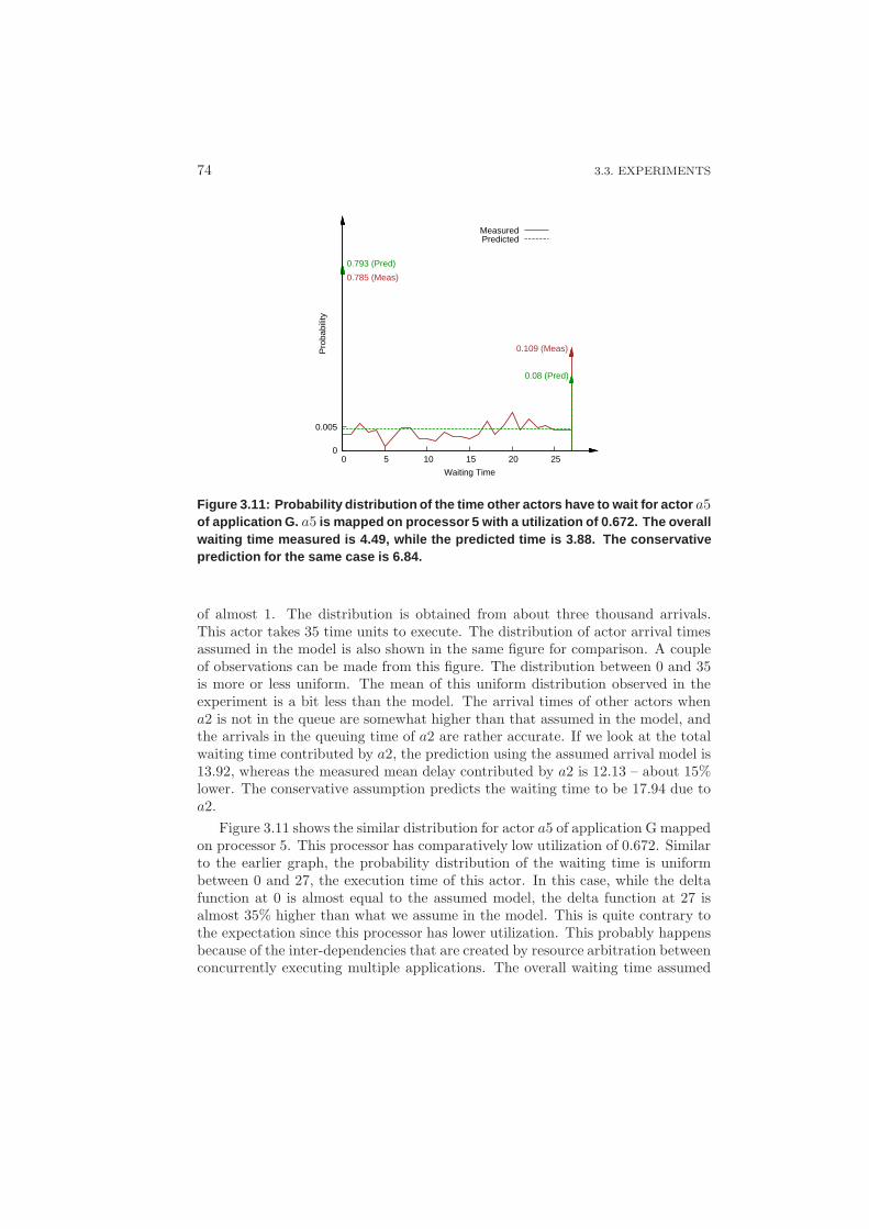
74 3.3. EXPERIMENTS
0
0.005
0 5 10 15 20 25
Pro
babi
lity
Waiting Time
0.109 (Meas)
0.08 (Pred)
0.785 (Meas)
0.793 (Pred)
MeasuredPredicted
Figure 3.11: Probability distribution of the time other act ors have to wait for actor a5of application G. a5 is mapped on processor 5 with a utilization of 0.672. The over allwaiting time measured is 4.49, while the predicted time is 3. 88. The conservativeprediction for the same case is 6.84.
of almost 1. The distribution is obtained from about three thousand arrivals.This actor takes 35 time units to execute. The distribution of actor arrival timesassumed in the model is also shown in the same figure for comparison. A coupleof observations can be made from this figure. The distribution between 0 and 35is more or less uniform. The mean of this uniform distribution observed in theexperiment is a bit less than the model. The arrival times of other actors whena2 is not in the queue are somewhat higher than that assumed in the model, andthe arrivals in the queuing time of a2 are rather accurate. If we look at the totalwaiting time contributed by a2, the prediction using the assumed arrival model is13.92, whereas the measured mean delay contributed by a2 is 12.13 – about 15%lower. The conservative assumption predicts the waiting time to be 17.94 due toa2.
Figure 3.11 shows the similar distribution for actor a5 of application G mappedon processor 5. This processor has comparatively low utilization of 0.672. Similarto the earlier graph, the probability distribution of the waiting time is uniformbetween 0 and 27, the execution time of this actor. In this case, while the deltafunction at 0 is almost equal to the assumed model, the delta function at 27 isalmost 35% higher than what we assume in the model. This is quite contrary tothe expectation since this processor has lower utilization. This probably happensbecause of the inter-dependencies that are created by resource arbitration betweenconcurrently executing multiple applications. The overall waiting time assumed
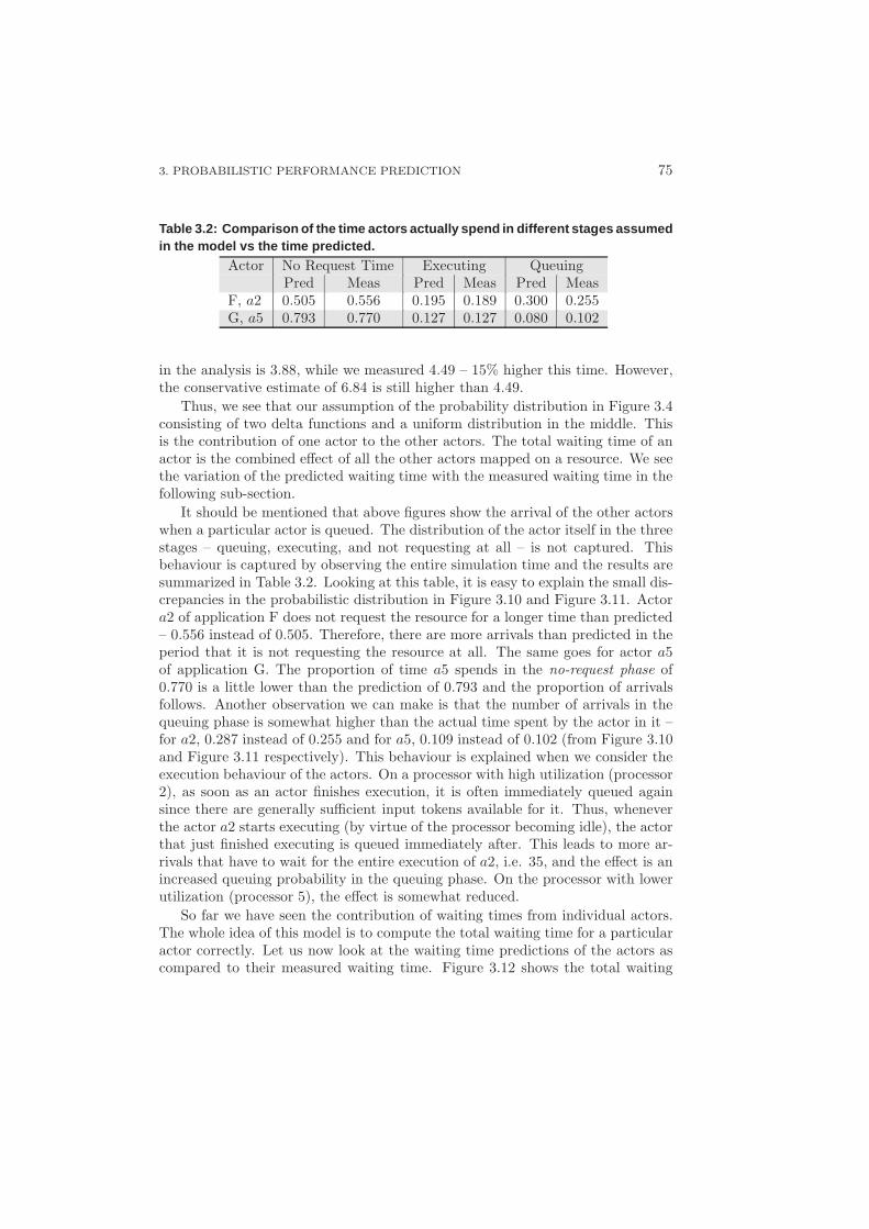
3. PROBABILISTIC PERFORMANCE PREDICTION 75
Table 3.2: Comparison of the time actors actually spend in di fferent stages assumedin the model vs the time predicted.
Actor No Request Time Executing QueuingPred Meas Pred Meas Pred Meas
F, a2 0.505 0.556 0.195 0.189 0.300 0.255G, a5 0.793 0.770 0.127 0.127 0.080 0.102
in the analysis is 3.88, while we measured 4.49 – 15% higher this time. However,the conservative estimate of 6.84 is still higher than 4.49.
Thus, we see that our assumption of the probability distribution in Figure 3.4consisting of two delta functions and a uniform distribution in the middle. Thisis the contribution of one actor to the other actors. The total waiting time of anactor is the combined effect of all the other actors mapped on a resource. We seethe variation of the predicted waiting time with the measured waiting time in thefollowing sub-section.
It should be mentioned that above figures show the arrival of the other actorswhen a particular actor is queued. The distribution of the actor itself in the threestages – queuing, executing, and not requesting at all – is not captured. Thisbehaviour is captured by observing the entire simulation time and the results aresummarized in Table 3.2. Looking at this table, it is easy to explain the small dis-crepancies in the probabilistic distribution in Figure 3.10 and Figure 3.11. Actora2 of application F does not request the resource for a longer time than predicted– 0.556 instead of 0.505. Therefore, there are more arrivals than predicted in theperiod that it is not requesting the resource at all. The same goes for actor a5of application G. The proportion of time a5 spends in the no-request phase of0.770 is a little lower than the prediction of 0.793 and the proportion of arrivalsfollows. Another observation we can make is that the number of arrivals in thequeuing phase is somewhat higher than the actual time spent by the actor in it –for a2, 0.287 instead of 0.255 and for a5, 0.109 instead of 0.102 (from Figure 3.10and Figure 3.11 respectively). This behaviour is explained when we consider theexecution behaviour of the actors. On a processor with high utilization (processor2), as soon as an actor finishes execution, it is often immediately queued againsince there are generally sufficient input tokens available for it. Thus, wheneverthe actor a2 starts executing (by virtue of the processor becoming idle), the actorthat just finished executing is queued immediately after. This leads to more ar-rivals that have to wait for the entire execution of a2, i.e. 35, and the effect is anincreased queuing probability in the queuing phase. On the processor with lowerutilization (processor 5), the effect is somewhat reduced.
So far we have seen the contribution of waiting times from individual actors.The whole idea of this model is to compute the total waiting time for a particularactor correctly. Let us now look at the waiting time predictions of the actors ascompared to their measured waiting time. Figure 3.12 shows the total waiting
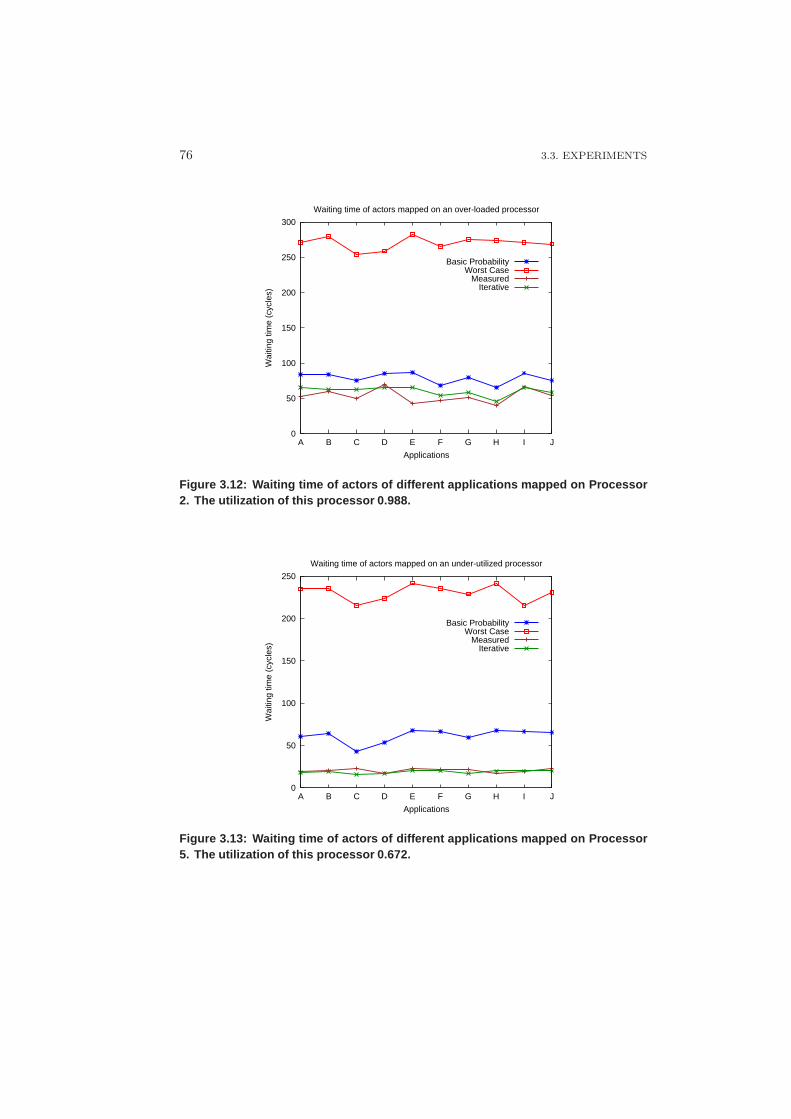
76 3.3. EXPERIMENTS
0
50
100
150
200
250
300
A B C D E F G H I J
Wai
ting
time
(cyc
les)
Applications
Waiting time of actors mapped on an over-loaded processor
Basic ProbabilityWorst Case
MeasuredIterative
Figure 3.12: Waiting time of actors of different applicatio ns mapped on Processor2. The utilization of this processor 0.988.
0
50
100
150
200
250
A B C D E F G H I J
Wai
ting
time
(cyc
les)
Applications
Waiting time of actors mapped on an under-utilized processor
Basic ProbabilityWorst Case
MeasuredIterative
Figure 3.13: Waiting time of actors of different applicatio ns mapped on Processor5. The utilization of this processor 0.672.
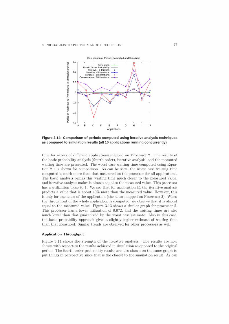
3. PROBABILISTIC PERFORMANCE PREDICTION 77
0.7
0.8
0.9
1
1.1
1.2
1.3
A B C D E F G H I J
Per
iod
of A
pplic
atio
ns (
Nor
mal
ized
to s
imul
atio
n pe
riod)
Applications
Comparison of Period: Computed and Simulated
SimulationFourth Order Probability
Iterative - 1 iterationIterative - 5 iterations
Iterative - 10 iterationsConservative - 10 iterations
Figure 3.14: Comparison of periods computed using iterativ e analysis techniquesas compared to simulation results (all 10 applications runn ing concurrently)
time for actors of different applications mapped on Processor 2. The results ofthe basic probability analysis (fourth order), iterative analysis, and the measuredwaiting time are presented. The worst case waiting time computed using Equa-tion 2.1 is shown for comparison. As can be seen, the worst case waiting timecomputed is much more than that measured on the processor for all applications.The basic analysis brings this waiting time much closer to the measured value,and iterative analysis makes it almost equal to the measured value. This processorhas a utilization close to 1. We see that for application E, the iterative analysispredicts a value that is about 40% more than the measured value. However, thisis only for one actor of the application (the actor mapped on Processor 2). Whenthe throughput of the whole application is computed, we observe that it is almostequal to the measured value. Figure 3.13 shows a similar graph for processor 5.This processor has a lower utilization of 0.672, and the waiting times are alsomuch lower than that guaranteed by the worst case estimate. Also in this case,the basic probability approach gives a slightly higher estimate of waiting timethan that measured. Similar trends are observed for other processors as well.
Application Throughput
Figure 3.14 shows the strength of the iterative analysis. The results are nowshown with respect to the results achieved in simulation as opposed to the originalperiod. The fourth-order probability results are also shown on the same graph toput things in perspective since that is the closest to the simulation result. As can
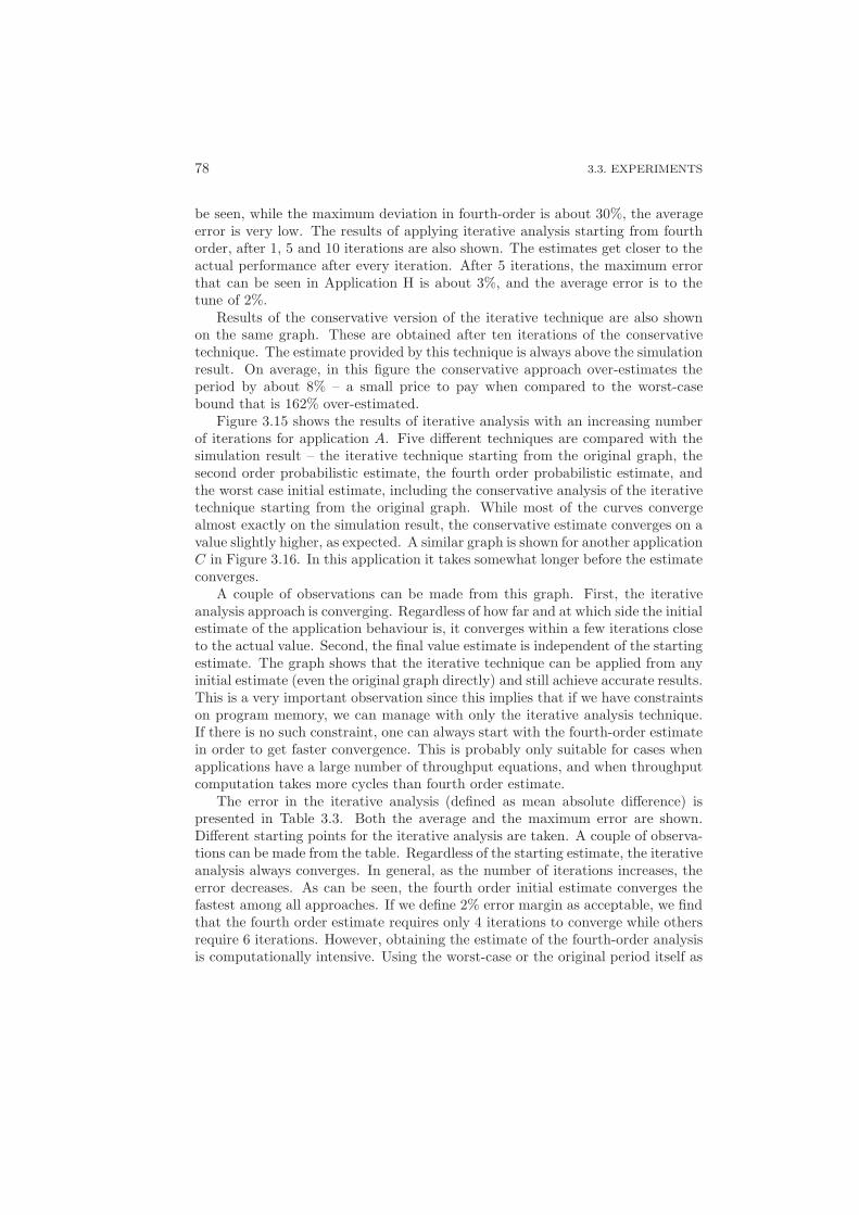
78 3.3. EXPERIMENTS
be seen, while the maximum deviation in fourth-order is about 30%, the averageerror is very low. The results of applying iterative analysis starting from fourthorder, after 1, 5 and 10 iterations are also shown. The estimates get closer to theactual performance after every iteration. After 5 iterations, the maximum errorthat can be seen in Application H is about 3%, and the average error is to thetune of 2%.
Results of the conservative version of the iterative technique are also shownon the same graph. These are obtained after ten iterations of the conservativetechnique. The estimate provided by this technique is always above the simulationresult. On average, in this figure the conservative approach over-estimates theperiod by about 8% – a small price to pay when compared to the worst-casebound that is 162% over-estimated.
Figure 3.15 shows the results of iterative analysis with an increasing numberof iterations for application A. Five different techniques are compared with thesimulation result – the iterative technique starting from the original graph, thesecond order probabilistic estimate, the fourth order probabilistic estimate, andthe worst case initial estimate, including the conservative analysis of the iterativetechnique starting from the original graph. While most of the curves convergealmost exactly on the simulation result, the conservative estimate converges on avalue slightly higher, as expected. A similar graph is shown for another applicationC in Figure 3.16. In this application it takes somewhat longer before the estimateconverges.
A couple of observations can be made from this graph. First, the iterativeanalysis approach is converging. Regardless of how far and at which side the initialestimate of the application behaviour is, it converges within a few iterations closeto the actual value. Second, the final value estimate is independent of the startingestimate. The graph shows that the iterative technique can be applied from anyinitial estimate (even the original graph directly) and still achieve accurate results.This is a very important observation since this implies that if we have constraintson program memory, we can manage with only the iterative analysis technique.If there is no such constraint, one can always start with the fourth-order estimatein order to get faster convergence. This is probably only suitable for cases whenapplications have a large number of throughput equations, and when throughputcomputation takes more cycles than fourth order estimate.
The error in the iterative analysis (defined as mean absolute difference) ispresented in Table 3.3. Both the average and the maximum error are shown.Different starting points for the iterative analysis are taken. A couple of observa-tions can be made from the table. Regardless of the starting estimate, the iterativeanalysis always converges. In general, as the number of iterations increases, theerror decreases. As can be seen, the fourth order initial estimate converges thefastest among all approaches. If we define 2% error margin as acceptable, we findthat the fourth order estimate requires only 4 iterations to converge while othersrequire 6 iterations. However, obtaining the estimate of the fourth-order analysisis computationally intensive. Using the worst-case or the original period itself as
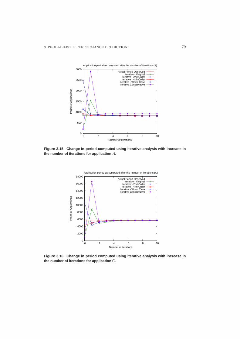
3. PROBABILISTIC PERFORMANCE PREDICTION 79
0
500
1000
1500
2000
2500
3000
0 2 4 6 8 10
Per
iod
of A
pplic
atio
ns
Number of iterations
Application period as computed after the number of iterations (A)
Actual Period ObservedIterative - Original
Iterative - 2nd OrderIterative - 4rth Order
Iterative - Worst CaseIterative Conservative
Figure 3.15: Change in period computed using iterative anal ysis with increase inthe number of iterations for application A.
0
2000
4000
6000
8000
10000
12000
14000
16000
18000
0 2 4 6 8 10
Per
iod
of A
pplic
atio
ns
Number of iterations
Application period as computed after the number of iterations (C)
Actual Period ObservedIterative - Original
Iterative - 2nd OrderIterative - 4rth Order
Iterative - Worst CaseIterative Conservative
Figure 3.16: Change in period computed using iterative anal ysis with increase inthe number of iterations for application C.
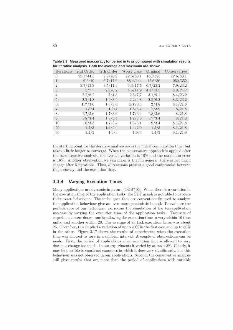
80 3.3. EXPERIMENTS
Table 3.3: Measured inaccuracy for period in % as compared wi th simulation resultsfor iterative analysis. Both the average and maximum are sho wn.
Iterations 2nd Order 4rth Order Worst Case Original Conservative0 22.3/44.5 9.9/28.9 72.6/83.1 163/325 72.6/83.11 6.2/19 6.7/17.6 88.4/144 12.6/36 252/3522 3.7/13.3 3.5/11.9 6.3/17.6 6.7/23.2 7.9/23.23 3/7.7 2.9/6.2 4.5/11.9 4.3/13.3 8.8/24.74 2.2/6.2 2/4.8 2.5/7.7 3.1/9.1 8.4/23.25 2.2/4.8 1.9/3.9 2.2/4.8 2.5/6.2 8.3/23.26 1.7/3.6 1.6/3.6 1.7/3.4 2/4.8 8.1/21.87 1.8/4 1.9/4 1.8/3.4 1.7/3.9 8/21.88 1.7/3.6 1.7/3.6 1.7/3.4 1.8/3.6 8/21.89 1.8/3.4 1.9/3.4 1.7/3.6 1.7/3.4 8/21.810 1.6/3.3 1.7/3.4 1.3/3.1 1.9/3.4 8.1/21.820 1.7/3 1.4/2.9 1.4/2.9 1.5/3 8.1/21.830 1.4/3 1.6/3 1.6/3 1.4/3 8.1/21.8
the starting point for the iterative analysis saves the initial computation time, buttakes a little longer to converge. When the conservative approach is applied afterthe base iterative analysis, the average variation is 10% and the maximum erroris 16%. Another observation we can make is that in general, there is not muchchange after 5 iterations. Thus, 5 iterations present a good compromise betweenthe accuracy and the execution time.
3.3.4 Varying Execution Times
Many applications are dynamic in nature [TGB+06]. When there is a variation inthe execution time of the application tasks, the SDF graph is not able to capturetheir exact behaviour. The techniques that are conventionally used to analyzethe application behaviour give an even more pessimistic bound. To evaluate theperformance of our technique, we re-ran the simulation of the ten-applicationuse-case by varying the execution time of the application tasks. Two sets ofexperiments were done – one by allowing the execution time to vary within 10 timeunits, and another within 20. The average of all task execution times was about25. Therefore, this implied a variation of up to 40% in the first case and up to 80%in the other. Figure 3.17 shows the results of experiments when the executiontime was allowed to vary in a uniform interval. A couple of observations can bemade. First, the period of applications when execution time is allowed to varydoes not change too much. In our experiments it varied by at most 2%. Clearly, itmay be possible to construct examples in which it does vary significantly, but thisbehaviour was not observed in our applications. Second, the conservative analysisstill gives results that are more than the period of applications with variable
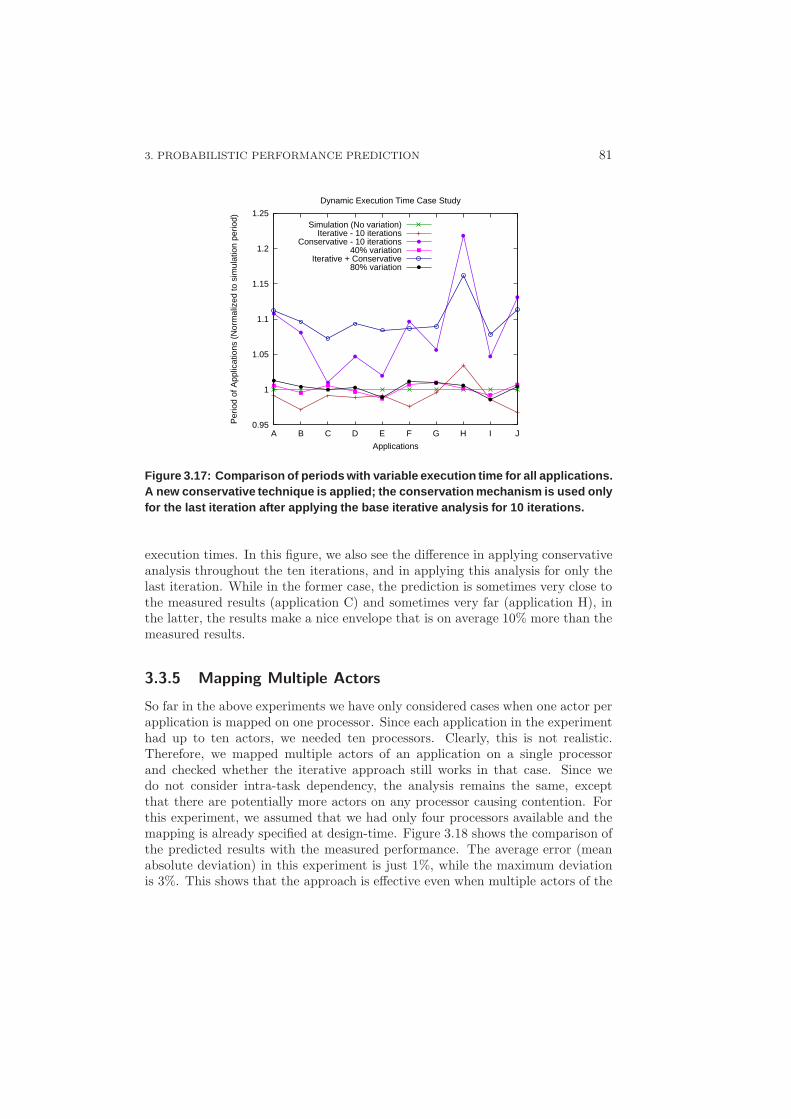
3. PROBABILISTIC PERFORMANCE PREDICTION 81
0.95
1
1.05
1.1
1.15
1.2
1.25
A B C D E F G H I J
Per
iod
of A
pplic
atio
ns (
Nor
mal
ized
to s
imul
atio
n pe
riod)
Applications
Dynamic Execution Time Case Study
Simulation (No variation)Iterative - 10 iterations
Conservative - 10 iterations40% variation
Iterative + Conservative80% variation
Figure 3.17: Comparison of periods with variable execution time for all applications.A new conservative technique is applied; the conservation m echanism is used onlyfor the last iteration after applying the base iterative ana lysis for 10 iterations.
execution times. In this figure, we also see the difference in applying conservativeanalysis throughout the ten iterations, and in applying this analysis for only thelast iteration. While in the former case, the prediction is sometimes very close tothe measured results (application C) and sometimes very far (application H), inthe latter, the results make a nice envelope that is on average 10% more than themeasured results.
3.3.5 Mapping Multiple Actors
So far in the above experiments we have only considered cases when one actor perapplication is mapped on one processor. Since each application in the experimenthad up to ten actors, we needed ten processors. Clearly, this is not realistic.Therefore, we mapped multiple actors of an application on a single processorand checked whether the iterative approach still works in that case. Since wedo not consider intra-task dependency, the analysis remains the same, exceptthat there are potentially more actors on any processor causing contention. Forthis experiment, we assumed that we had only four processors available and themapping is already specified at design-time. Figure 3.18 shows the comparison ofthe predicted results with the measured performance. The average error (meanabsolute deviation) in this experiment is just 1%, while the maximum deviationis 3%. This shows that the approach is effective even when multiple actors of the
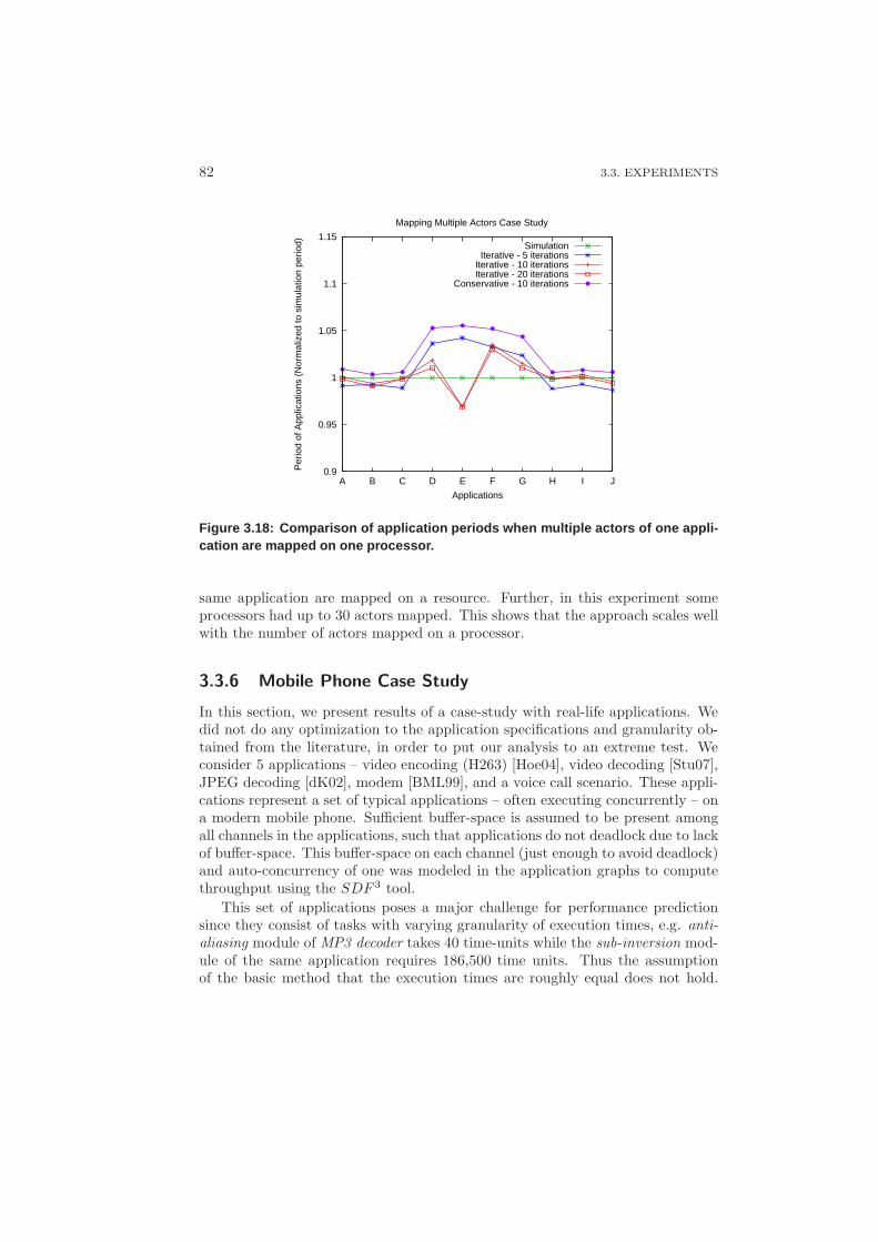
82 3.3. EXPERIMENTS
0.9
0.95
1
1.05
1.1
1.15
A B C D E F G H I J
Per
iod
of A
pplic
atio
ns (
Nor
mal
ized
to s
imul
atio
n pe
riod)
Applications
Mapping Multiple Actors Case Study
SimulationIterative - 5 iterations
Iterative - 10 iterationsIterative - 20 iterations
Conservative - 10 iterations
Figure 3.18: Comparison of application periods when multip le actors of one appli-cation are mapped on one processor.
same application are mapped on a resource. Further, in this experiment someprocessors had up to 30 actors mapped. This shows that the approach scales wellwith the number of actors mapped on a processor.
3.3.6 Mobile Phone Case Study
In this section, we present results of a case-study with real-life applications. Wedid not do any optimization to the application specifications and granularity ob-tained from the literature, in order to put our analysis to an extreme test. Weconsider 5 applications – video encoding (H263) [Hoe04], video decoding [Stu07],JPEG decoding [dK02], modem [BML99], and a voice call scenario. These appli-cations represent a set of typical applications – often executing concurrently – ona modern mobile phone. Sufficient buffer-space is assumed to be present amongall channels in the applications, such that applications do not deadlock due to lackof buffer-space. This buffer-space on each channel (just enough to avoid deadlock)and auto-concurrency of one was modeled in the application graphs to computethroughput using the SDF 3 tool.
This set of applications poses a major challenge for performance predictionsince they consist of tasks with varying granularity of execution times, e.g. anti-aliasing module of MP3 decoder takes 40 time-units while the sub-inversion mod-ule of the same application requires 186,500 time units. Thus the assumptionof the basic method that the execution times are roughly equal does not hold.
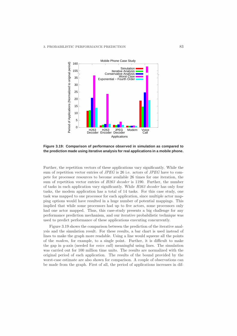
3. PROBABILISTIC PERFORMANCE PREDICTION 83
0
5
10
15
20
25
30
35
155
160
H263Decoder
H263Encoder
JPEGDecoder
Modem VoiceCallP
erio
d of
App
licat
ions
(N
orm
aliz
ed to
orig
inal
per
iod)
Applications
Mobile Phone Case Study
SimulationIterative Analysis
Conservative AnalysisWorst Case
Exponential − Fourth Order
Figure 3.19: Comparison of performance observed in simulat ion as compared tothe prediction made using iterative analysis for real appli cations in a mobile phone.
Further, the repetition vectors of these applications vary significantly. While thesum of repetition vector entries of JPEG is 26 i.e. actors of JPEG have to com-pete for processor resources to become available 26 times for one iteration, thesum of repetition vector entries of H263 decoder is 1190. Further, the numberof tasks in each application vary significantly. While H263 decoder has only fourtasks, the modem application has a total of 14 tasks. For this case study, onetask was mapped to one processor for each application, since multiple actor map-ping options would have resulted in a huge number of potential mappings. Thisimplied that while some processors had up to five actors, some processors onlyhad one actor mapped. Thus, this case-study presents a big challenge for anyperformance prediction mechanism, and our iterative probabilistic technique wasused to predict performance of these applications executing concurrently.
Figure 3.19 shows the comparison between the prediction of the iterative anal-ysis and the simulation result. For these results, a bar chart is used instead oflines to make the graph more readable. Using a line would squeeze all the pointsof the modem, for example, to a single point. Further, it is difficult to makethe gap in y-axis (needed for voice call) meaningful using lines. The simulationwas carried out for 100 million time units. The results are normalized with theoriginal period of each application. The results of the bound provided by theworst-case estimate are also shown for comparison. A couple of observations canbe made from the graph. First of all, the period of applications increases in dif-
84 3.3. EXPERIMENTS
ferent proportions. While the period of modem application increases by only 1.1times, the period of H263 decoder increases by almost 12 times, and that of a voicecall by almost 18 times. This depends on the granularity of tasks, the numberof tasks a particular application is divided into, and the mapping of tasks on themultiprocessor platform. The modem application consists of about 14 tasks, butonly 6 of them experience contention. The remaining 8 tasks have a dedicatedprocessor, and therefore have no waiting time. Further, the 6 tasks that do sharea processor, are only executed once per application iteration. In contrast theinverse-quantization module of the H263 decoder executes 594 times per iterationof the decoder, and has to wait for the processor to become available each time.This causes significant degradation in its performance. The second observationwe can make is that the iterative analysis is still very accurate. The average devi-ation in throughput estimate is about 15%, and the maximum deviation is in thevoice call application of 29%. The basic approach to fourth-order approximationalso performs quite well for this case-study, and the average deviation is the sameas the iterative approach, but the maximum deviation is 47%. The worst-caseestimate in contrast is almost 18 times overly pessimistic. The prediction in thevoice call application is actually 158 times of the original period. Another inter-esting observation is that the worst-case bound of the modem application is only15% pessimistic. This is because most actors of this application do not have anycontention. It should be mentioned that in this experiment first-come-first-servearbitration was used. A different arbitration mechanism and a better mappingcan distribute the resources more evenly.
3.3.7 Implementation Results on an Embedded Processor
The proposed algorithms were ported to an embedded processor – Microblaze; thisrequired some rewriting to optimize the implementation for timing and reducedmemory use. The default time taken for second and fourth order, for example,was 72M and 11M cycles respectively. Table 3.4 shows the time taken duringvarious stages and algorithms after rewriting. The algorithmic complexity of eachstage and the error as compared to the simulation result is also shown.
The error in various techniques as compared to the performance achieved isalso shown in Table 3.4. As can be seen, the basic probability analysis with fourthorder gives an average error of about 10% and a maximum error of 29%. Theiterative technique after just five iterations predicts a performance that is within2% of the measured performance on average and has only 3% maximum deviationin the entire set of applications.
This system consists of the same 10 applications as used in the previous sub-section. The loading of application properties from the CF card took the mostamount of time. However, this is only done once at the start of the system, andhence does not cause any bottleneck. On our system operating at 50 MHz, ittakes about 40ms to load the applications-specification. Parametric throughputcomputation is quite fast, and takes about 12K cycles for all 10 applications.
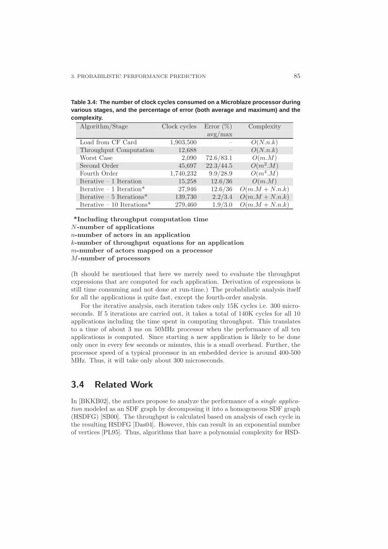
3. PROBABILISTIC PERFORMANCE PREDICTION 85
Table 3.4: The number of clock cycles consumed on a Microblaz e processor duringvarious stages, and the percentage of error (both average an d maximum) and thecomplexity.
Algorithm/Stage Clock cycles Error (%) Complexityavg/max
Load from CF Card 1,903,500 – O(N.n.k)Throughput Computation 12,688 – O(N.n.k)Worst Case 2,090 72.6/83.1 O(m.M)Second Order 45,697 22.3/44.5 O(m2.M)Fourth Order 1,740,232 9.9/28.9 O(m4.M)Iterative – 1 Iteration 15,258 12.6/36 O(m.M)Iterative – 1 Iteration* 27,946 12.6/36 O(m.M + N.n.k)Iterative – 5 Iterations* 139,730 2.2/3.4 O(m.M + N.n.k)Iterative – 10 Iterations* 279,460 1.9/3.0 O(m.M + N.n.k)
*Including throughput computation time
N-number of applications
n-number of actors in an application
k-number of throughput equations for an application
m-number of actors mapped on a processor
M-number of processors
(It should be mentioned that here we merely need to evaluate the throughputexpressions that are computed for each application. Derivation of expressions isstill time consuming and not done at run-time.) The probabilistic analysis itselffor all the applications is quite fast, except the fourth-order analysis.
For the iterative analysis, each iteration takes only 15K cycles i.e. 300 micro-seconds. If 5 iterations are carried out, it takes a total of 140K cycles for all 10applications including the time spent in computing throughput. This translatesto a time of about 3 ms on 50MHz processor when the performance of all tenapplications is computed. Since starting a new application is likely to be doneonly once in every few seconds or minutes, this is a small overhead. Further, theprocessor speed of a typical processor in an embedded device is around 400-500MHz. Thus, it will take only about 300 microseconds.
3.4 Related Work
In [BKKB02], the authors propose to analyze the performance of a single applica-tion modeled as an SDF graph by decomposing it into a homogeneous SDF graph(HSDFG) [SB00]. The throughput is calculated based on analysis of each cycle inthe resulting HSDFG [Das04]. However, this can result in an exponential numberof vertices [PL95]. Thus, algorithms that have a polynomial complexity for HSD-
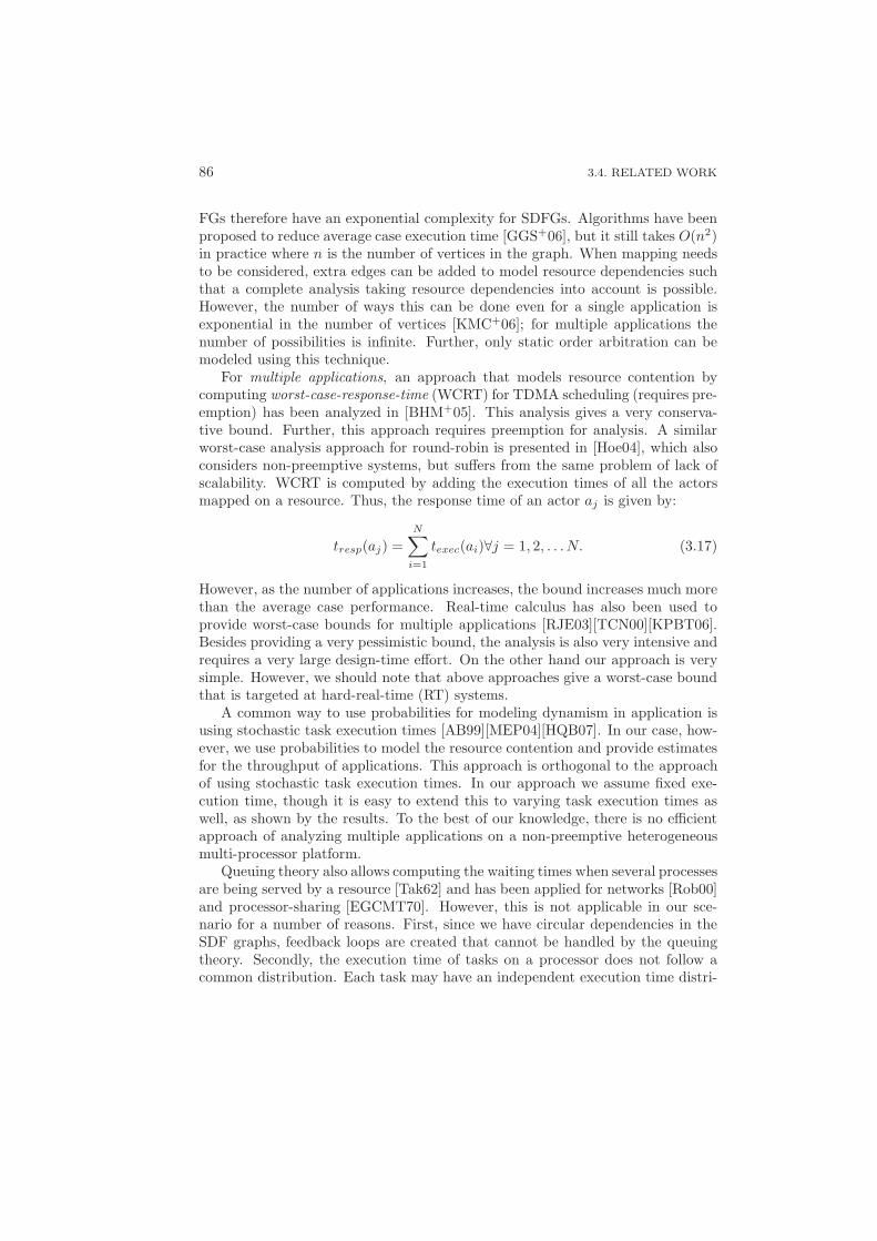
86 3.4. RELATED WORK
FGs therefore have an exponential complexity for SDFGs. Algorithms have beenproposed to reduce average case execution time [GGS+06], but it still takes O(n2)in practice where n is the number of vertices in the graph. When mapping needsto be considered, extra edges can be added to model resource dependencies suchthat a complete analysis taking resource dependencies into account is possible.However, the number of ways this can be done even for a single application isexponential in the number of vertices [KMC+06]; for multiple applications thenumber of possibilities is infinite. Further, only static order arbitration can bemodeled using this technique.
For multiple applications, an approach that models resource contention bycomputing worst-case-response-time (WCRT) for TDMA scheduling (requires pre-emption) has been analyzed in [BHM+05]. This analysis gives a very conserva-tive bound. Further, this approach requires preemption for analysis. A similarworst-case analysis approach for round-robin is presented in [Hoe04], which alsoconsiders non-preemptive systems, but suffers from the same problem of lack ofscalability. WCRT is computed by adding the execution times of all the actorsmapped on a resource. Thus, the response time of an actor aj is given by:
tresp(aj) =
N∑
i=1
texec(ai)∀j = 1, 2, . . .N. (3.17)
However, as the number of applications increases, the bound increases much morethan the average case performance. Real-time calculus has also been used toprovide worst-case bounds for multiple applications [RJE03][TCN00][KPBT06].Besides providing a very pessimistic bound, the analysis is also very intensive andrequires a very large design-time effort. On the other hand our approach is verysimple. However, we should note that above approaches give a worst-case boundthat is targeted at hard-real-time (RT) systems.
A common way to use probabilities for modeling dynamism in application isusing stochastic task execution times [AB99][MEP04][HQB07]. In our case, how-ever, we use probabilities to model the resource contention and provide estimatesfor the throughput of applications. This approach is orthogonal to the approachof using stochastic task execution times. In our approach we assume fixed exe-cution time, though it is easy to extend this to varying task execution times aswell, as shown by the results. To the best of our knowledge, there is no efficientapproach of analyzing multiple applications on a non-preemptive heterogeneousmulti-processor platform.
Queuing theory also allows computing the waiting times when several processesare being served by a resource [Tak62] and has been applied for networks [Rob00]and processor-sharing [EGCMT70]. However, this is not applicable in our sce-nario for a number of reasons. First, since we have circular dependencies in theSDF graphs, feedback loops are created that cannot be handled by the queuingtheory. Secondly, the execution time of tasks on a processor does not follow acommon distribution. Each task may have an independent execution time distri-
3. PROBABILISTIC PERFORMANCE PREDICTION 87
bution. Therefore, a general expression for the service time for tasks mapped ona processor cannot be determined.
3.5 Conclusions
In this chapter, we saw a probabilistic technique to estimate the performance ofapplications when sharing resources. An iterative analysis is presented that canpredict the performance of applications very accurately. Besides, a conservativeflavour of the iterative analysis is presented that can also provide conservativeprediction for applications for which the mis-prediction penalty may be high.
The basic probability analysis gives results with an average error of 10%, and amaximum error is 29%. In contrast, the average error in prediction using iterativeprobability is only 2% and the maximum error of 3%. Further, it takes about fourto six iterations for the prediction to converge. The complexity and execution timeof the algorithm is very low – it takes only 3ms to evaluate the performance often applications on a 50MHz embedded processor.
Further, we presented results of a case-study of applications commonly usedin a mobile phone. The models of these applications vary in the number of tasks,granularity of tasks, and also the repetition vectors of the applications. Thesimulation result of executing all applications concurrently is compared with theiterative analysis. Even in this particular use-case, the prediction by iterativeanalysis is close to the simulation result. This proves the robustness of the tech-nique. We also see that applications with coarser task granularity perform betterin the first-come-first-serve arbitration as compared to applications that have afiner granularity. This occurs since the tasks with finer granularity have to com-pete for resources more often. Different arbitration mechanisms can potentiallyalleviate this problem, and more research should be done into that.

88 3.5. CONCLUSIONS
CHAPTER 4
Resource Management
Modern multimedia systems consist of a number of resources. This includes notjust computational resources, but also others, for example, memory, communica-tion bandwidth, energy. Resources have to be allocated to applications executingon the system such that all applications can produce the expected result. Whendealing with multimedia embedded systems, ensuring that all applications canmeet their non-functional requirements, e.g. throughput, also becomes impor-tant. As has been emphasized in the earlier chapters, this poses a significantchallenge when multiple applications are executing. Further, when run-time ad-mission and addition of applications is supported, e.g. in modern mobile phones,this challenge takes yet another dimension. A complete analysis is infeasible atdesign-time due to two major reasons: 1) little may be known at design-timeabout the applications that need to be used in future, and 2) the number ofdesign-points that need to be evaluated is prohibitively large. A run-time ap-proach can benefit from the fact that the exact application mix is known, butthe analysis has to be fast enough to make it feasible. Resource management –simply said – is managing the resources available on the multiprocessor platform.
In this chapter, we present a design-flow for designing systems with mul-tiple applications. We present a hybrid approach where the time-consumingapplication-specific computations are done at design-time, and isolated from otherapplications – to maintain composability, and the use-case-specific computationsare performed at run-time. Further, we present a resource manager (RM) for therun-time aspects of resource management. The need for a middle-ware or OS-likecomponent for the MPSoC has already been highlighted in literature [Wol04]. We
89
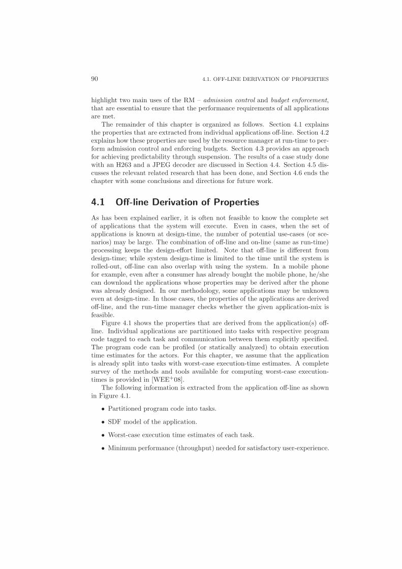
90 4.1. OFF-LINE DERIVATION OF PROPERTIES
highlight two main uses of the RM – admission control and budget enforcement,that are essential to ensure that the performance requirements of all applicationsare met.
The remainder of this chapter is organized as follows. Section 4.1 explainsthe properties that are extracted from individual applications off-line. Section 4.2explains how these properties are used by the resource manager at run-time to per-form admission control and enforcing budgets. Section 4.3 provides an approachfor achieving predictability through suspension. The results of a case study donewith an H263 and a JPEG decoder are discussed in Section 4.4. Section 4.5 dis-cusses the relevant related research that has been done, and Section 4.6 ends thechapter with some conclusions and directions for future work.
4.1 Off-line Derivation of Properties
As has been explained earlier, it is often not feasible to know the complete setof applications that the system will execute. Even in cases, when the set ofapplications is known at design-time, the number of potential use-cases (or sce-narios) may be large. The combination of off-line and on-line (same as run-time)processing keeps the design-effort limited. Note that off-line is different fromdesign-time; while system design-time is limited to the time until the system isrolled-out, off-line can also overlap with using the system. In a mobile phonefor example, even after a consumer has already bought the mobile phone, he/shecan download the applications whose properties may be derived after the phonewas already designed. In our methodology, some applications may be unknowneven at design-time. In those cases, the properties of the applications are derivedoff-line, and the run-time manager checks whether the given application-mix isfeasible.
Figure 4.1 shows the properties that are derived from the application(s) off-line. Individual applications are partitioned into tasks with respective programcode tagged to each task and communication between them explicitly specified.The program code can be profiled (or statically analyzed) to obtain executiontime estimates for the actors. For this chapter, we assume that the applicationis already split into tasks with worst-case execution-time estimates. A completesurvey of the methods and tools available for computing worst-case execution-times is provided in [WEE+08].
The following information is extracted from the application off-line as shownin Figure 4.1.
• Partitioned program code into tasks.
• SDF model of the application.
• Worst-case execution time estimates of each task.
• Minimum performance (throughput) needed for satisfactory user-experience.
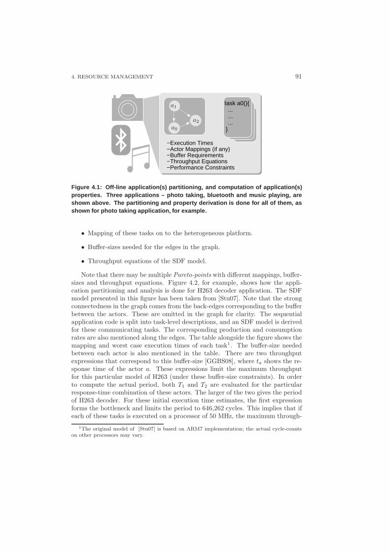
4. RESOURCE MANAGEMENT 91
...
...
...}
−Execution Times−Actor Mappings (if any)−Buffer Requirements−Throughput Equations−Performance Constraints
task a0(){
a0
a1
a2
Figure 4.1: Off-line application(s) partitioning, and com putation of application(s)properties. Three applications – photo taking, bluetooth a nd music playing, areshown above. The partitioning and property derivation is do ne for all of them, asshown for photo taking application, for example.
• Mapping of these tasks on to the heterogeneous platform.
• Buffer-sizes needed for the edges in the graph.
• Throughput equations of the SDF model.
Note that there may be multiple Pareto-points with different mappings, buffer-sizes and throughput equations. Figure 4.2, for example, shows how the appli-cation partitioning and analysis is done for H263 decoder application. The SDFmodel presented in this figure has been taken from [Stu07]. Note that the strongconnectedness in the graph comes from the back-edges corresponding to the bufferbetween the actors. These are omitted in the graph for clarity. The sequentialapplication code is split into task-level descriptions, and an SDF model is derivedfor these communicating tasks. The corresponding production and consumptionrates are also mentioned along the edges. The table alongside the figure shows themapping and worst case execution times of each task1. The buffer-size neededbetween each actor is also mentioned in the table. There are two throughputexpressions that correspond to this buffer-size [GGBS08], where ta shows the re-sponse time of the actor a. These expressions limit the maximum throughputfor this particular model of H263 (under these buffer-size constraints). In orderto compute the actual period, both T1 and T2 are evaluated for the particularresponse-time combination of these actors. The larger of the two gives the periodof H263 decoder. For these initial execution time estimates, the first expressionforms the bottleneck and limits the period to 646,262 cycles. This implies that ifeach of these tasks is executed on a processor of 50 MHz, the maximum through-
1The original model of [Stu07] is based on ARM7 implementation; the actual cycle-countson other processors may vary.
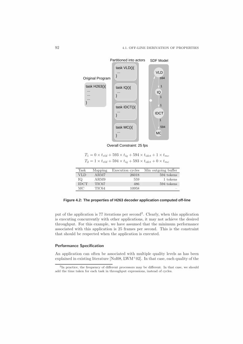
92 4.1. OFF-LINE DERIVATION OF PROPERTIES
594
594
1
1
1
1
Original Program
Partitioned into actors SDF Model
Overall Constraint: 25 fps
task H263(){.........
}
IQ
IDCT
MC
task VLD(){...
}
task IQ(){...
}
task MC(){...
}
task IDCT(){...
}
VLD
T1 = 0 × tvld + 593 × tiq + 594 × tidct + 1 × tmc
T2 = 1 × tvld + 594 × tiq + 593 × tidct + 0 × tmc
Task Mapping Execution cycles Min outgoing buffer
VLD ARM7 26018 594 tokensIQ ARM9 559 1 tokensIDCT TIC67 486 594 tokensMC TIC64 10958 –
Figure 4.2: The properties of H263 decoder application comp uted off-line
put of the application is 77 iterations per second2. Clearly, when this applicationis executing concurrently with other applications, it may not achieve the desiredthroughput. For this example, we have assumed that the minimum performanceassociated with this application is 25 frames per second. This is the constraintthat should be respected when the application is executed.
Performance Specification
An application can often be associated with multiple quality levels as has beenexplained in existing literature [Nol08, LWM+02]. In that case, each quality of the
2In practice, the frequency of different processors may be different. In that case, we shouldadd the time taken for each task in throughput expressions, instead of cycles.
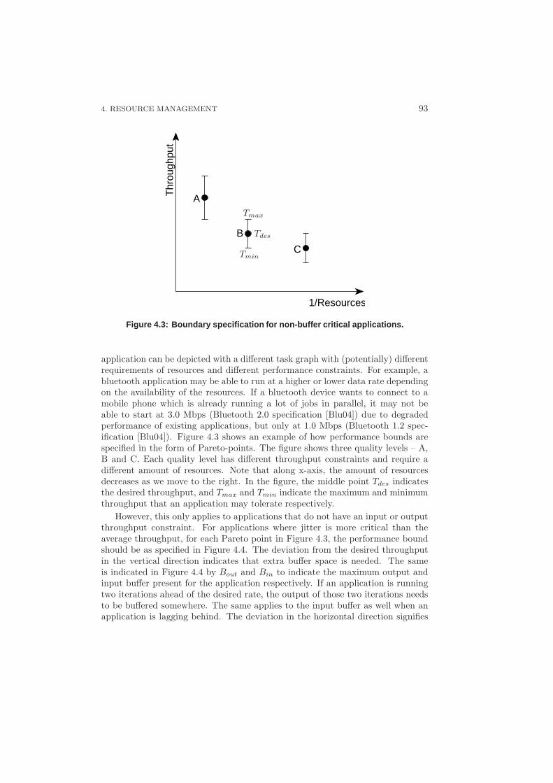
4. RESOURCE MANAGEMENT 93
1/Resources
Thr
ough
put
A
B
CTmin
Tmax
Tdes
Figure 4.3: Boundary specification for non-buffer critical applications.
application can be depicted with a different task graph with (potentially) differentrequirements of resources and different performance constraints. For example, abluetooth application may be able to run at a higher or lower data rate dependingon the availability of the resources. If a bluetooth device wants to connect to amobile phone which is already running a lot of jobs in parallel, it may not beable to start at 3.0 Mbps (Bluetooth 2.0 specification [Blu04]) due to degradedperformance of existing applications, but only at 1.0 Mbps (Bluetooth 1.2 spec-ification [Blu04]). Figure 4.3 shows an example of how performance bounds arespecified in the form of Pareto-points. The figure shows three quality levels – A,B and C. Each quality level has different throughput constraints and require adifferent amount of resources. Note that along x-axis, the amount of resourcesdecreases as we move to the right. In the figure, the middle point Tdes indicatesthe desired throughput, and Tmax and Tmin indicate the maximum and minimumthroughput that an application may tolerate respectively.
However, this only applies to applications that do not have an input or outputthroughput constraint. For applications where jitter is more critical than theaverage throughput, for each Pareto point in Figure 4.3, the performance boundshould be as specified in Figure 4.4. The deviation from the desired throughputin the vertical direction indicates that extra buffer space is needed. The sameis indicated in Figure 4.4 by Bout and Bin to indicate the maximum output andinput buffer present for the application respectively. If an application is runningtwo iterations ahead of the desired rate, the output of those two iterations needsto be buffered somewhere. The same applies to the input buffer as well when anapplication is lagging behind. The deviation in the horizontal direction signifies
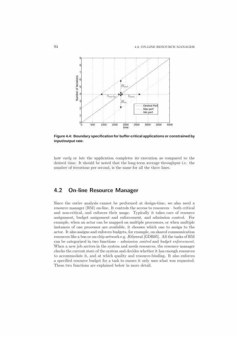
94 4.2. ON-LINE RESOURCE MANAGER
0 500 1000 1500 2000 2500 3000 3500 40000
1
2
3
4
5
6
7
8
9
time
Num
ber
of It
erat
ions
Desired Perf.Max perf.Min perf.
tearly tlate
Bout
Bin
Figure 4.4: Boundary specification for buffer-critical app lications or constrained byinput/output rate.
how early or late the application completes its execution as compared to thedesired time. It should be noted that the long-term average throughput i.e. thenumber of iterations per second, is the same for all the three lines.
4.2 On-line Resource Manager
Since the entire analysis cannot be performed at design-time, we also need aresource manager (RM) on-line. It controls the access to resources – both criticaland non-critical, and enforces their usage. Typically it takes care of resourceassignment, budget assignment and enforcement, and admission control. Forexample, when an actor can be mapped on multiple processors, or when multipleinstances of one processor are available, it chooses which one to assign to theactor. It also assigns and enforces budgets, for example, on shared communicationresources like a bus or on-chip network e.g. Æthereal [GDR05]. All the tasks of RMcan be categorized in two functions – admission control and budget enforcement.When a new job arrives in the system and needs resources, the resource managerchecks the current state of the system and decides whether it has enough resourcesto accommodate it, and at which quality and resource-binding. It also enforcesa specified resource budget for a task to ensure it only uses what was requested.These two functions are explained below in more detail.
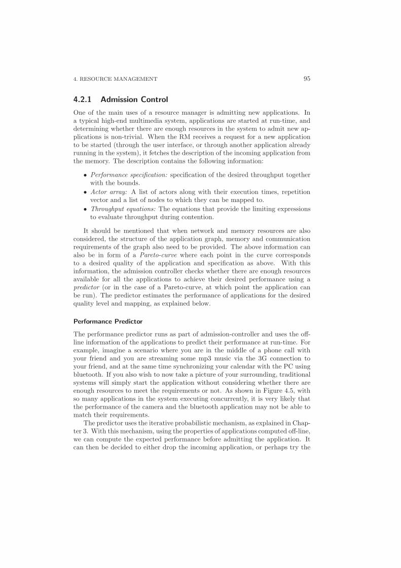
4. RESOURCE MANAGEMENT 95
4.2.1 Admission Control
One of the main uses of a resource manager is admitting new applications. Ina typical high-end multimedia system, applications are started at run-time, anddetermining whether there are enough resources in the system to admit new ap-plications is non-trivial. When the RM receives a request for a new applicationto be started (through the user interface, or through another application alreadyrunning in the system), it fetches the description of the incoming application fromthe memory. The description contains the following information:
• Performance specification: specification of the desired throughput togetherwith the bounds.
• Actor array: A list of actors along with their execution times, repetitionvector and a list of nodes to which they can be mapped to.
• Throughput equations: The equations that provide the limiting expressionsto evaluate throughput during contention.
It should be mentioned that when network and memory resources are alsoconsidered, the structure of the application graph, memory and communicationrequirements of the graph also need to be provided. The above information canalso be in form of a Pareto-curve where each point in the curve correspondsto a desired quality of the application and specification as above. With thisinformation, the admission controller checks whether there are enough resourcesavailable for all the applications to achieve their desired performance using apredictor (or in the case of a Pareto-curve, at which point the application canbe run). The predictor estimates the performance of applications for the desiredquality level and mapping, as explained below.
Performance Predictor
The performance predictor runs as part of admission-controller and uses the off-line information of the applications to predict their performance at run-time. Forexample, imagine a scenario where you are in the middle of a phone call withyour friend and you are streaming some mp3 music via the 3G connection toyour friend, and at the same time synchronizing your calendar with the PC usingbluetooth. If you also wish to now take a picture of your surrounding, traditionalsystems will simply start the application without considering whether there areenough resources to meet the requirements or not. As shown in Figure 4.5, withso many applications in the system executing concurrently, it is very likely thatthe performance of the camera and the bluetooth application may not be able tomatch their requirements.
The predictor uses the iterative probabilistic mechanism, as explained in Chap-ter 3. With this mechanism, using the properties of applications computed off-line,we can compute the expected performance before admitting the application. Itcan then be decided to either drop the incoming application, or perhaps try the
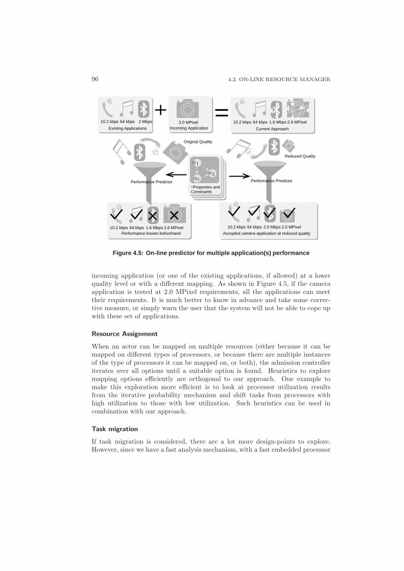
96 4.2. ON-LINE RESOURCE MANAGER
Original Quality
Reduced Quality
Performance Predictor
Accepted camera application at reduced quality
10.2 kbps 64 kbps 1.6 Mbps 2.6 MPixel
10.2 kbps 64 kbps 1.6 Mbps 2.6 MPixel 10.2 kbps 64 kbps 2.0 Mbps 2.0 MPixel
Performance Predictor
10.2 kbps 64 kbps 2 Mbps
Existing Applications
3.0 MPixelIncoming Application Current Approach
−Properties andConstraints
Performance known beforehand
a0
a1
a2
Figure 4.5: On-line predictor for multiple application(s) performance
incoming application (or one of the existing applications, if allowed) at a lowerquality level or with a different mapping. As shown in Figure 4.5, if the cameraapplication is tested at 2.0 MPixel requirements, all the applications can meettheir requirements. It is much better to know in advance and take some correc-tive measure, or simply warn the user that the system will not be able to cope upwith these set of applications.
Resource Assignment
When an actor can be mapped on multiple resources (either because it can bemapped on different types of processors, or because there are multiple instancesof the type of processors it can be mapped on, or both), the admission controlleriterates over all options until a suitable option is found. Heuristics to exploremapping options efficiently are orthogonal to our approach. One example tomake this exploration more efficient is to look at processor utilization resultsfrom the iterative probability mechanism and shift tasks from processors withhigh utilization to those with low utilization. Such heuristics can be used incombination with our approach.
Task migration
If task migration is considered, there are a lot more design-points to explore.However, since we have a fast analysis mechanism, with a fast embedded processor
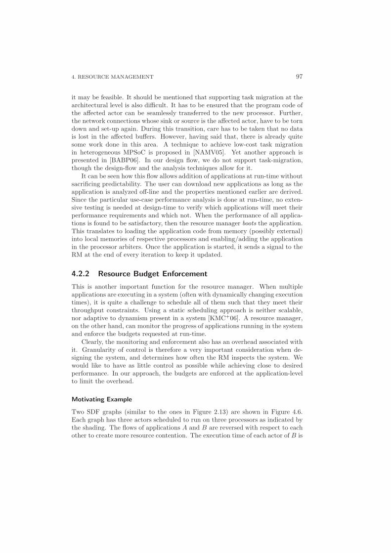
4. RESOURCE MANAGEMENT 97
it may be feasible. It should be mentioned that supporting task migration at thearchitectural level is also difficult. It has to be ensured that the program code ofthe affected actor can be seamlessly transferred to the new processor. Further,the network connections whose sink or source is the affected actor, have to be torndown and set-up again. During this transition, care has to be taken that no datais lost in the affected buffers. However, having said that, there is already quitesome work done in this area. A technique to achieve low-cost task migrationin heterogeneous MPSoC is proposed in [NAMV05]. Yet another approach ispresented in [BABP06]. In our design flow, we do not support task-migration,though the design-flow and the analysis techniques allow for it.
It can be seen how this flow allows addition of applications at run-time withoutsacrificing predictability. The user can download new applications as long as theapplication is analyzed off-line and the properties mentioned earlier are derived.Since the particular use-case performance analysis is done at run-time, no exten-sive testing is needed at design-time to verify which applications will meet theirperformance requirements and which not. When the performance of all applica-tions is found to be satisfactory, then the resource manager boots the application.This translates to loading the application code from memory (possibly external)into local memories of respective processors and enabling/adding the applicationin the processor arbiters. Once the application is started, it sends a signal to theRM at the end of every iteration to keep it updated.
4.2.2 Resource Budget Enforcement
This is another important function for the resource manager. When multipleapplications are executing in a system (often with dynamically changing executiontimes), it is quite a challenge to schedule all of them such that they meet theirthroughput constraints. Using a static scheduling approach is neither scalable,nor adaptive to dynamism present in a system [KMC+06]. A resource manager,on the other hand, can monitor the progress of applications running in the systemand enforce the budgets requested at run-time.
Clearly, the monitoring and enforcement also has an overhead associated withit. Granularity of control is therefore a very important consideration when de-signing the system, and determines how often the RM inspects the system. Wewould like to have as little control as possible while achieving close to desiredperformance. In our approach, the budgets are enforced at the application-levelto limit the overhead.
Motivating Example
Two SDF graphs (similar to the ones in Figure 2.13) are shown in Figure 4.6.Each graph has three actors scheduled to run on three processors as indicated bythe shading. The flows of applications A and B are reversed with respect to eachother to create more resource contention. The execution time of each actor of B is
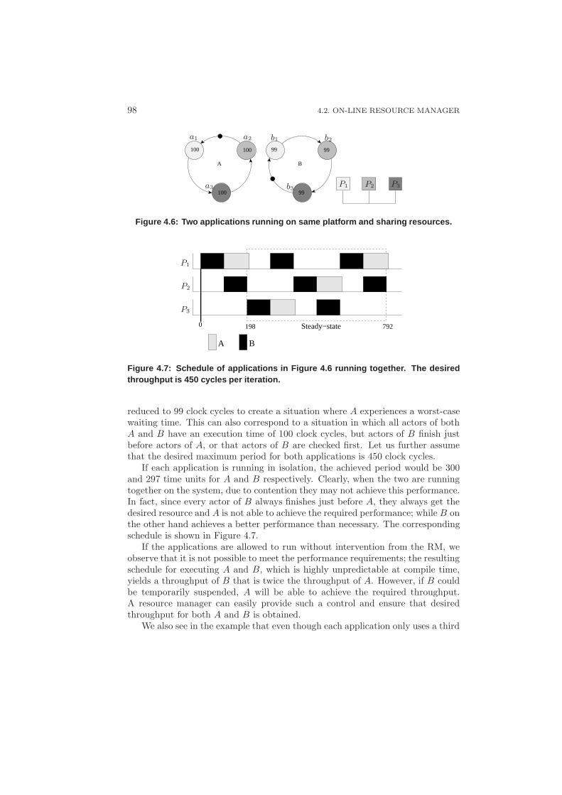
98 4.2. ON-LINE RESOURCE MANAGER
100
100
100
A
99
99
99
B
a1 a2
a3
b1 b2
b3P1 P2 P3
Figure 4.6: Two applications running on same platform and sh aring resources.
Steady−state
A B
0 198 792
P1
P2
P3
Figure 4.7: Schedule of applications in Figure 4.6 running t ogether. The desiredthroughput is 450 cycles per iteration.
reduced to 99 clock cycles to create a situation where A experiences a worst-casewaiting time. This can also correspond to a situation in which all actors of bothA and B have an execution time of 100 clock cycles, but actors of B finish justbefore actors of A, or that actors of B are checked first. Let us further assumethat the desired maximum period for both applications is 450 clock cycles.
If each application is running in isolation, the achieved period would be 300and 297 time units for A and B respectively. Clearly, when the two are runningtogether on the system, due to contention they may not achieve this performance.In fact, since every actor of B always finishes just before A, they always get thedesired resource and A is not able to achieve the required performance; while B onthe other hand achieves a better performance than necessary. The correspondingschedule is shown in Figure 4.7.
If the applications are allowed to run without intervention from the RM, weobserve that it is not possible to meet the performance requirements; the resultingschedule for executing A and B, which is highly unpredictable at compile time,yields a throughput of B that is twice the throughput of A. However, if B couldbe temporarily suspended, A will be able to achieve the required throughput.A resource manager can easily provide such a control and ensure that desiredthroughput for both A and B is obtained.
We also see in the example that even though each application only uses a third
4. RESOURCE MANAGEMENT 99
of each processing node, thereby placing a total demand of two-third on each pro-cessing node, the applications are not able to achieve their required performance.A compile-time analysis of all possible use-cases can alleviate this problem byderiving how applications would affect each other at run-time. However, thepotentially large number of use-cases in a real system makes such analysis infeasi-ble. A resource manager can shift the burden of compile-time analysis to run-timemonitoring and intervention when necessary.
Suspending Applications
We now discuss how this suspension is implemented. Each application sends asignal to the RM upon completion of each iteration. This is achieved by appendinga small message at the end of the output actor of the application graph3, i.e. thelast task in the execution of an application after whose execution an iterationof the application can be said to have been completed. This allows the RMto monitor the progress of each application at little cost. After every sampleperiod – defined as sample points, the RM checks whether all applications areprogressing at their desired level. If any application is found to be running belowthe desired throughput, the application which has the most slack (i.e. the highestratio of achieved to desired throughput) is suspended. The suspended applicationis re-activated when all applications are running above the desired throughput.Suspension and re-activation occur only at sample points.
Each arbiter maintains two lists – an actor ready queue, and an applicationenable list. Once the processor is available, the arbiter checks the actor at thehead of the queue, and if its corresponding application is enabled, it is executed.Otherwise, the next available actor (with enabled application) is executed. Sus-pension of an application is achieved by sending a temporary disable signal to thearbiters running the application. Say, for example, if application A has actorsmapped on 3 processors P1, P2 and P3, then the three processor-arbiters will besignalled to disable application A. Thus, even when actors of application A areready, they will not be executed.
Suspension of an application is not to be confused with preemption. In ourapproach, we do not allow actors to be preempted in the middle of their execu-tion; actors execute atomically. However, an application can be suspended aftercompleting the execution of any actor. This limits the context that needs to besaved when an actor is in the middle of its execution.
Suspension Example
Figure 4.8 shows an example interaction diagram between various modules in thedesign. The user-interface module sends a request to start application X (1).The resource manager checks if there are enough resources for it, and then admitsit in the system (2). Applications Y and Z are also started respectively soon
3In the event of multiple output actors, any output actor may be chosen for this.

100 4.2. ON-LINE RESOURCE MANAGER
X suffers when it is restarted
Y starts to sufferwhen Z starts
ApplicationsZ Y X
1. Start Appl X
3. Start Appl Y
5. Start Appl Z
2. Queue/Enable X
4. Queue/Enable Y
6. Queue/Enable Z
7. Suspend X8. Start Appl A
11. Z Done
13. Suspend Y
15. X Done
17. Y Done
Tim
e
10. Resume X
14. Resume Y
I/O In
terf
ace
Res
ourc
e m
anag
er9. Appl A Reject
12. Z Finished
16. X Finished
18. Y Finished
Figure 4.8: Interaction diagram between user interface, re source manager, andapplications in the system-setup.
after as indicated on the figure (3-6). However, when Z is admitted, Y starts todeteriorate in performance. The resource manager then sends a signal to suspendX (7) to the platform because it has slack and Y is then able to meet its desiredperformance. When X resumes (10), it is not able to meet its performance and Yis suspended (13) because now Y has slack. When the applications are finished,the result is transmitted back to the user-interface (12, 16 and 18). We also seean example of application A being rejected (9) since the system is possibly toobusy, and A is of lower priority than applications X , Y and Z.
Communication Overhead
The overhead of monitoring and suspension is easy to compute. Consider tenapplications running concurrently on a ten-processor system. Each applicationsignals the RM every time it completes an iteration. Let us assume the period ofeach application is 100,000 clock cycles. Therefore, on average only one messageis sent to the resource manager every 10,000 cycles. Let us consider the case withsampling period being 500,000 cycles. The RM sends messages at most every pro-cessing node every sampling interval. This is on average, one message every 50,000cycles, giving in total 6 messages every 50,000 cycles – 5 from the application tothe resource manager and 1 from the resource manager to the processor. If thelength of each message is around 10 bytes, we get a bandwidth requirement of 60
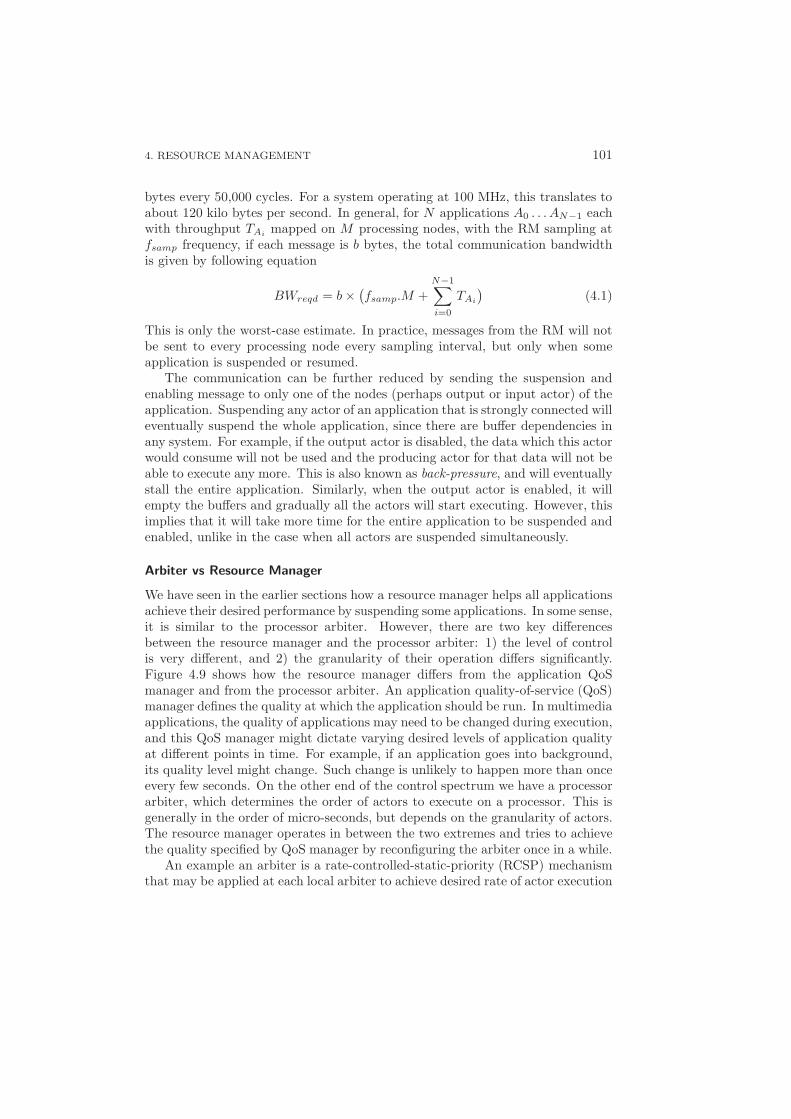
4. RESOURCE MANAGEMENT 101
bytes every 50,000 cycles. For a system operating at 100 MHz, this translates toabout 120 kilo bytes per second. In general, for N applications A0 . . . AN−1 eachwith throughput TAi
mapped on M processing nodes, with the RM sampling atfsamp frequency, if each message is b bytes, the total communication bandwidthis given by following equation
BWreqd = b ×(
fsamp.M +N−1∑
i=0
TAi
)
(4.1)
This is only the worst-case estimate. In practice, messages from the RM will notbe sent to every processing node every sampling interval, but only when someapplication is suspended or resumed.
The communication can be further reduced by sending the suspension andenabling message to only one of the nodes (perhaps output or input actor) of theapplication. Suspending any actor of an application that is strongly connected willeventually suspend the whole application, since there are buffer dependencies inany system. For example, if the output actor is disabled, the data which this actorwould consume will not be used and the producing actor for that data will not beable to execute any more. This is also known as back-pressure, and will eventuallystall the entire application. Similarly, when the output actor is enabled, it willempty the buffers and gradually all the actors will start executing. However, thisimplies that it will take more time for the entire application to be suspended andenabled, unlike in the case when all actors are suspended simultaneously.
Arbiter vs Resource Manager
We have seen in the earlier sections how a resource manager helps all applicationsachieve their desired performance by suspending some applications. In some sense,it is similar to the processor arbiter. However, there are two key differencesbetween the resource manager and the processor arbiter: 1) the level of controlis very different, and 2) the granularity of their operation differs significantly.Figure 4.9 shows how the resource manager differs from the application QoSmanager and from the processor arbiter. An application quality-of-service (QoS)manager defines the quality at which the application should be run. In multimediaapplications, the quality of applications may need to be changed during execution,and this QoS manager might dictate varying desired levels of application qualityat different points in time. For example, if an application goes into background,its quality level might change. Such change is unlikely to happen more than onceevery few seconds. On the other end of the control spectrum we have a processorarbiter, which determines the order of actors to execute on a processor. This isgenerally in the order of micro-seconds, but depends on the granularity of actors.The resource manager operates in between the two extremes and tries to achievethe quality specified by QoS manager by reconfiguring the arbiter once in a while.
An example an arbiter is a rate-controlled-static-priority (RCSP) mechanismthat may be applied at each local arbiter to achieve desired rate of actor execution
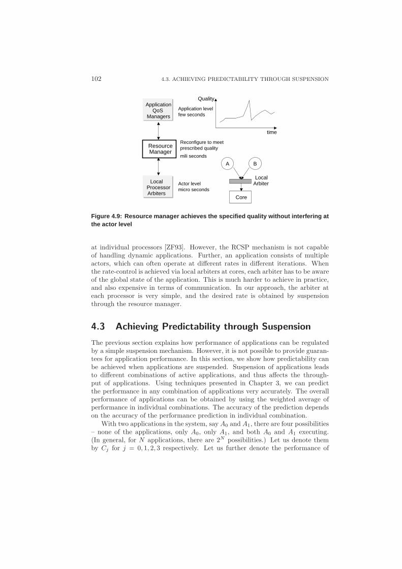
102 4.3. ACHIEVING PREDICTABILITY THROUGH SUSPENSION
ManagerResource
Actor levelmicro seconds
Reconfigure to meet prescribed quality
Application levelfew seconds
ApplicationQoS
Managers
mili seconds
Core
BA
Quality
time
ArbiterLocal
ProcessorLocal
Arbiters
Figure 4.9: Resource manager achieves the specified quality without interfering atthe actor level
at individual processors [ZF93]. However, the RCSP mechanism is not capableof handling dynamic applications. Further, an application consists of multipleactors, which can often operate at different rates in different iterations. Whenthe rate-control is achieved via local arbiters at cores, each arbiter has to be awareof the global state of the application. This is much harder to achieve in practice,and also expensive in terms of communication. In our approach, the arbiter ateach processor is very simple, and the desired rate is obtained by suspensionthrough the resource manager.
4.3 Achieving Predictability through Suspension
The previous section explains how performance of applications can be regulatedby a simple suspension mechanism. However, it is not possible to provide guaran-tees for application performance. In this section, we show how predictability canbe achieved when applications are suspended. Suspension of applications leadsto different combinations of active applications, and thus affects the through-put of applications. Using techniques presented in Chapter 3, we can predictthe performance in any combination of applications very accurately. The overallperformance of applications can be obtained by using the weighted average ofperformance in individual combinations. The accuracy of the prediction dependson the accuracy of the performance prediction in individual combination.
With two applications in the system, say A0 and A1, there are four possibilities– none of the applications, only A0, only A1, and both A0 and A1 executing.(In general, for N applications, there are 2N possibilities.) Let us denote themby Cj for j = 0, 1, 2, 3 respectively. Let us further denote the performance of
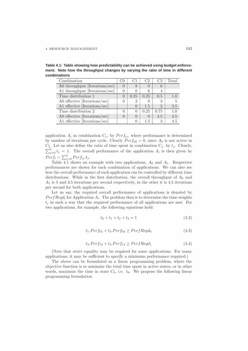
4. RESOURCE MANAGEMENT 103
Table 4.1: Table showing how predictability can be achieved using budget enforce-ment. Note how the throughput changes by varying the ratio of time in differentcombinations
Combination C0 C1 C2 C3 TotalA0 throughput [Iterations/sec] 0 8 0 6A1 throughput [Iterations/sec] 0 0 6 4Time distribution 1 0 0.25 0.25 0.5 1.0A0 effective [Iterations/sec] 0 2 0 3 5A1 effective [Iterations/sec] 0 1.5 2 3.5Time distribution 2 0 0 0.25 0.75 1.0A0 effective [Iterations/sec] 0 0 0 4.5 4.5A1 effective [Iterations/sec] 0 1.5 3 4.5
application Ai in combination Cj , by Perfij , where performance is determinedby number of iterations per cycle. Clearly Perf02 = 0, since A0 is not active inC2. Let us also define the ratio of time spent in combination Cj , by tj . Clearly,∑3
j=0 tj = 1. The overall performance of the application Ai is then given by
Perfi =∑3
j=0 Perfij .tj .Table 4.1 shows an example with two applications, A0 and A1. Respective
performances are shown for each combination of applications. We can also seehow the overall performance of each application can be controlled by different timedistributions. While in the first distribution, the overall throughput of A0 andA1 is 5 and 3.5 iterations per second respectively, in the other it is 4.5 iterationsper second for both applications.
Let us say, the required overall performance of applications is denoted byPerfReqdi for Application Ai. The problem then is to determine the time-weightstj in such a way that the required performance of all applications are met. Fortwo applications, for example, the following equations hold:
t0 + t1 + t2 + t3 = 1 (4.2)
t1.P erf01 + t3.P erf03 ≥ PerfReqd0 (4.3)
t2.P erf12 + t3.P erf13 ≥ PerfReqd1 (4.4)
(Note that strict equality may be required for some applications. For manyapplications, it may be sufficient to specify a minimum performance required.)
The above can be formulated as a linear programming problem, where theobjective function is to minimize the total time spent in active states; or in otherwords, maximize the time in state C0, i.e. t0. We propose the following linearprogramming formulation
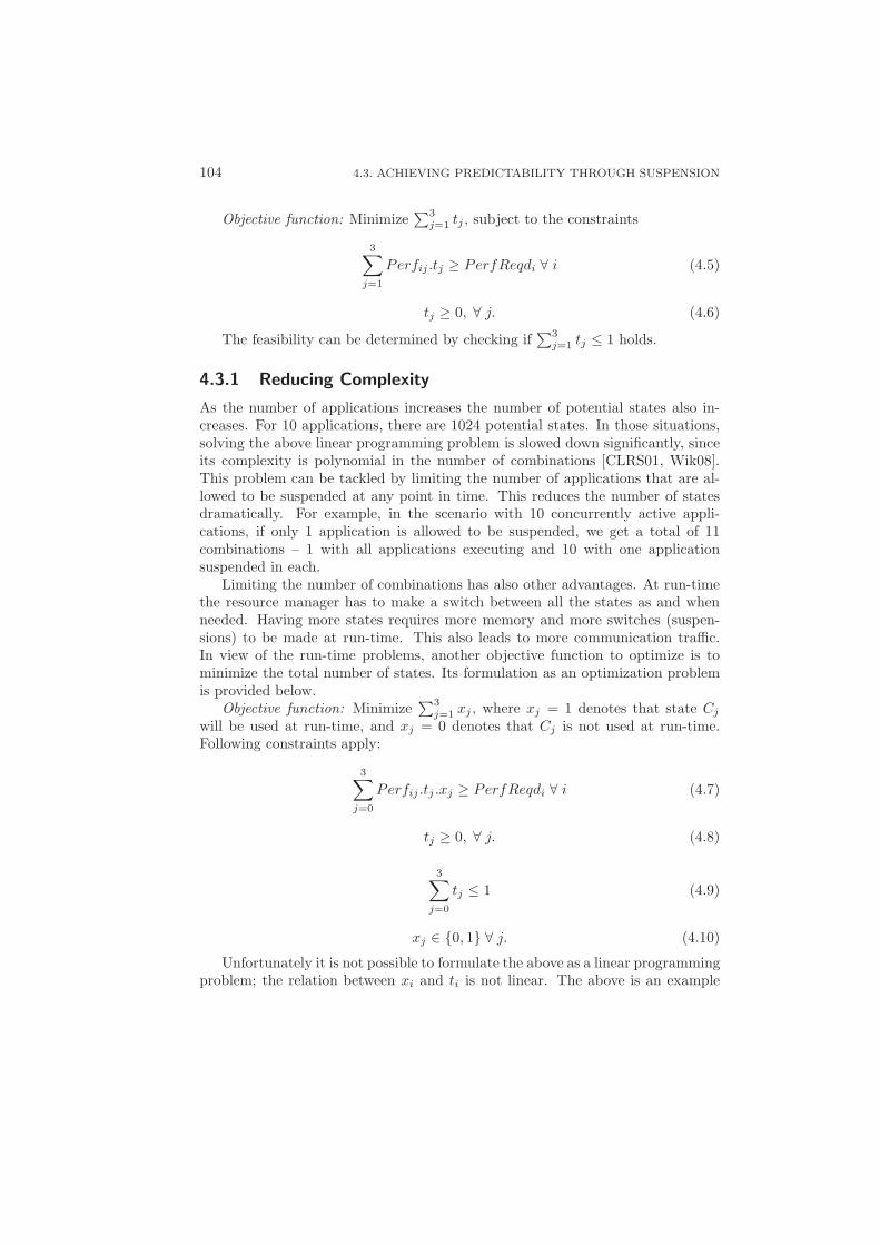
104 4.3. ACHIEVING PREDICTABILITY THROUGH SUSPENSION
Objective function: Minimize∑3
j=1 tj , subject to the constraints
3∑
j=1
Perfij .tj ≥ PerfReqdi ∀ i (4.5)
tj ≥ 0, ∀ j. (4.6)
The feasibility can be determined by checking if∑3
j=1 tj ≤ 1 holds.
4.3.1 Reducing Complexity
As the number of applications increases the number of potential states also in-creases. For 10 applications, there are 1024 potential states. In those situations,solving the above linear programming problem is slowed down significantly, sinceits complexity is polynomial in the number of combinations [CLRS01, Wik08].This problem can be tackled by limiting the number of applications that are al-lowed to be suspended at any point in time. This reduces the number of statesdramatically. For example, in the scenario with 10 concurrently active appli-cations, if only 1 application is allowed to be suspended, we get a total of 11combinations – 1 with all applications executing and 10 with one applicationsuspended in each.
Limiting the number of combinations has also other advantages. At run-timethe resource manager has to make a switch between all the states as and whenneeded. Having more states requires more memory and more switches (suspen-sions) to be made at run-time. This also leads to more communication traffic.In view of the run-time problems, another objective function to optimize is tominimize the total number of states. Its formulation as an optimization problemis provided below.
Objective function: Minimize∑3
j=1 xj , where xj = 1 denotes that state Cj
will be used at run-time, and xj = 0 denotes that Cj is not used at run-time.Following constraints apply:
3∑
j=0
Perfij .tj .xj ≥ PerfReqdi ∀ i (4.7)
tj ≥ 0, ∀ j. (4.8)
3∑
j=0
tj ≤ 1 (4.9)
xj ∈ {0, 1} ∀ j. (4.10)
Unfortunately it is not possible to formulate the above as a linear programmingproblem; the relation between xi and ti is not linear. The above is an example
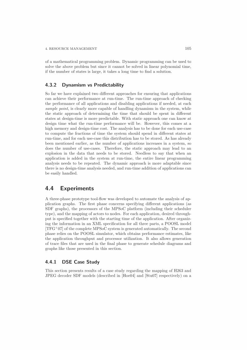
4. RESOURCE MANAGEMENT 105
of a mathematical programming problem. Dynamic programming can be used tosolve the above problem but since it cannot be solved in linear polynomial time,if the number of states is large, it takes a long time to find a solution.
4.3.2 Dynamism vs Predictability
So far we have explained two different approaches for ensuring that applicationscan achieve their performance at run-time. The run-time approach of checkingthe performance of all applications and disabling applications if needed, at eachsample point, is clearly more capable of handling dynamism in the system, whilethe static approach of determining the time that should be spent in differentstates at design-time is more predictable. With static approach one can know atdesign time what the run-time performance will be. However, this comes at ahigh memory and design-time cost. The analysis has to be done for each use-caseto compute the fractions of time the system should spend in different states atrun-time, and for each use-case this distribution has to be stored. As has alreadybeen mentioned earlier, as the number of applications increases in a system, sodoes the number of use-cases. Therefore, the static approach may lead to anexplosion in the data that needs to be stored. Needless to say that when anapplication is added in the system at run-time, the entire linear programminganalysis needs to be repeated. The dynamic approach is more adaptable sincethere is no design-time analysis needed, and run-time addition of applications canbe easily handled.
4.4 Experiments
A three-phase prototype tool-flow was developed to automate the analysis of ap-plication graphs. The first phase concerns specifying different applications (asSDF graphs), the processors of the MPSoC platform (including their schedulertype), and the mapping of actors to nodes. For each application, desired through-put is specified together with the starting time of the application. After organiz-ing the information in an XML specification for all three parts, a POOSL model[TFG+07] of the complete MPSoC system is generated automatically. The secondphase relies on the POOSL simulator, which obtains performance estimates, likethe application throughput and processor utilization. It also allows generationof trace files that are used in the final phase to generate schedule diagrams andgraphs like those presented in this section.
4.4.1 DSE Case Study
This section presents results of a case study regarding the mapping of H263 andJPEG decoder SDF models (described in [Hoe04] and [Stu07] respectively) on a
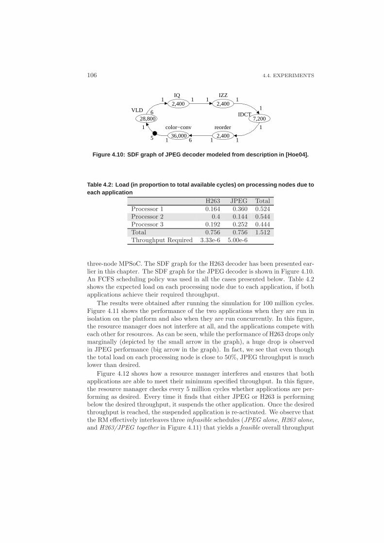
106 4.4. EXPERIMENTS
28,800
2,400 2,400
2,400
7,200
VLD
IQ
reorder
6
1 1 1 1
1
1
111
1
5
IZZ
IDCT
6
color−conv
36,000
Figure 4.10: SDF graph of JPEG decoder modeled from descript ion in [Hoe04].
Table 4.2: Load (in proportion to total available cycles) on processing nodes due toeach application
H263 JPEG TotalProcessor 1 0.164 0.360 0.524Processor 2 0.4 0.144 0.544Processor 3 0.192 0.252 0.444Total 0.756 0.756 1.512Throughput Required 3.33e-6 5.00e-6
three-node MPSoC. The SDF graph for the H263 decoder has been presented ear-lier in this chapter. The SDF graph for the JPEG decoder is shown in Figure 4.10.An FCFS scheduling policy was used in all the cases presented below. Table 4.2shows the expected load on each processing node due to each application, if bothapplications achieve their required throughput.
The results were obtained after running the simulation for 100 million cycles.Figure 4.11 shows the performance of the two applications when they are run inisolation on the platform and also when they are run concurrently. In this figure,the resource manager does not interfere at all, and the applications compete witheach other for resources. As can be seen, while the performance of H263 drops onlymarginally (depicted by the small arrow in the graph), a huge drop is observedin JPEG performance (big arrow in the graph). In fact, we see that even thoughthe total load on each processing node is close to 50%, JPEG throughput is muchlower than desired.
Figure 4.12 shows how a resource manager interferes and ensures that bothapplications are able to meet their minimum specified throughput. In this figure,the resource manager checks every 5 million cycles whether applications are per-forming as desired. Every time it finds that either JPEG or H263 is performingbelow the desired throughput, it suspends the other application. Once the desiredthroughput is reached, the suspended application is re-activated. We observe thatthe RM effectively interleaves three infeasible schedules (JPEG alone, H263 alone,and H263/JPEG together in Figure 4.11) that yields a feasible overall throughput
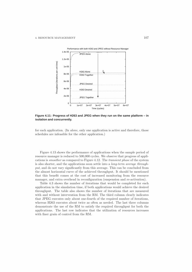
4. RESOURCE MANAGEMENT 107
0
2e-06
4e-06
6e-06
8e-06
1e-05
1.2e-05
1.4e-05
0 1e+07 2e+07 3e+07 4e+07 5e+07 6e+07
Thr
ough
put (
itera
tions
per
uni
t tim
e)
Time (cycles)
Performance with both H263 and JPEG without Resource Manager
H263 Alone
H263 Together
JPEG Alone
JPEG Together
H263 Desired
JPEG Desired
Figure 4.11: Progress of H263 and JPEG when they run on the sam e platform – inisolation and concurrently.
for each application. (In alone, only one application is active and therefore, thoseschedules are infeasible for the other application.)
Figure 4.13 shows the performance of applications when the sample period ofresource manager is reduced to 500,000 cycles. We observe that progress of appli-cations is smoother as compared to Figure 4.12. The transient phase of the systemis also shorter, and the applications soon settle into a long-term average through-put, and do not vary significantly from this average. This can be concluded fromthe almost horizontal curve of the achieved throughput. It should be mentionedthat this benefit comes at the cost of increased monitoring from the resourcemanager, and extra overhead in reconfiguration (suspension and re-activation).
Table 4.3 shows the number of iterations that would be completed for eachapplication in the simulation time, if both applications would achieve the desiredthroughput. The table also shows the number of iterations that are measuredwith and without intervention from the RM. The third column clearly indicatesthat JPEG executes only about one-fourth of the required number of iterations,whereas H263 executes about twice as often as needed. The last three columnsdemonstrate the use of the RM to satisfy the required throughput for both theapplications. The last row indicates that the utilization of resources increaseswith finer grain of control from the RM.
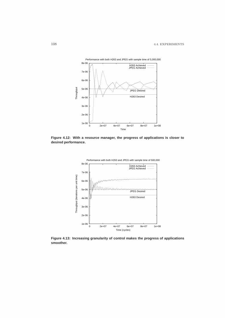
108 4.4. EXPERIMENTS
1e-06
2e-06
3e-06
4e-06
5e-06
6e-06
7e-06
8e-06
0 2e+07 4e+07 6e+07 8e+07 1e+08
Thr
ough
put
Time
Performance with both H263 and JPEG with sample time of 5,000,000
H263 Desired
JPEG Desired
H263 AchievedJPEG Achieved
Figure 4.12: With a resource manager, the progress of applic ations is closer todesired performance.
1e-06
2e-06
3e-06
4e-06
5e-06
6e-06
7e-06
8e-06
0 2e+07 4e+07 6e+07 8e+07 1e+08
Thr
ough
put (
itera
tions
per
uni
t tim
e)
Time (cycles)
Performance with both H263 and JPEG with sample time of 500,000
H263 Desired
JPEG Desired
H263 AchievedJPEG Achieved
Figure 4.13: Increasing granularity of control makes the pr ogress of applicationssmoother.
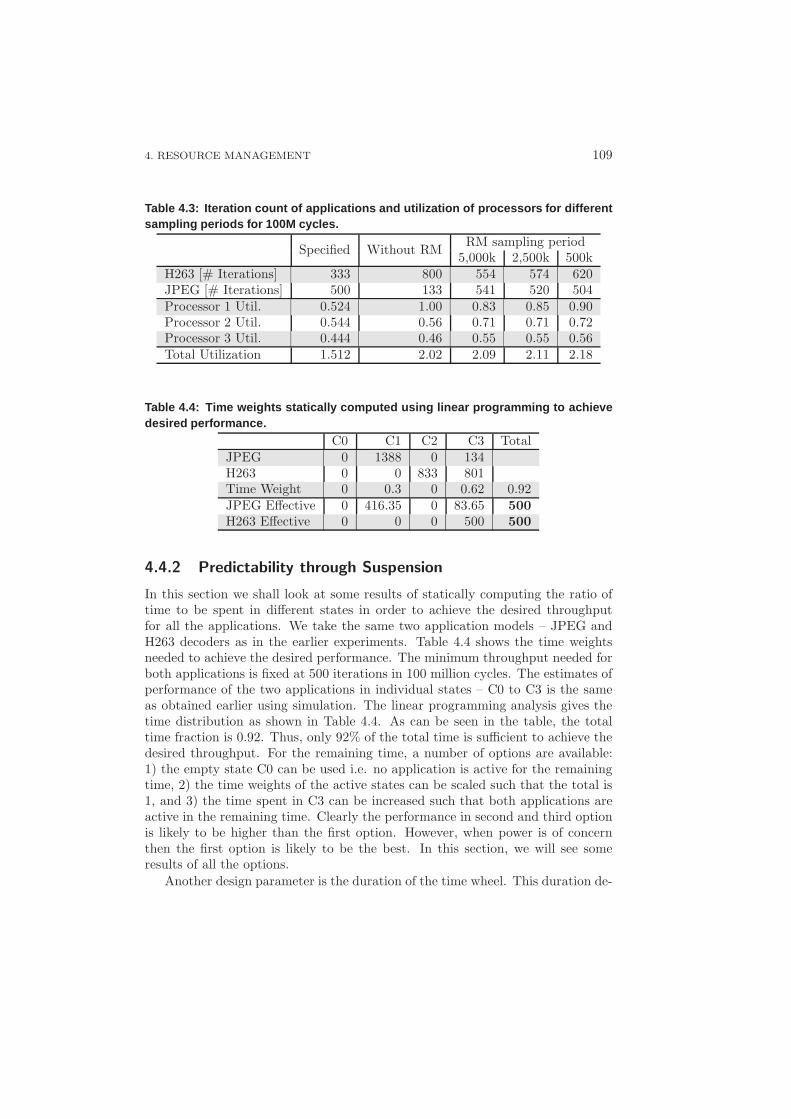
4. RESOURCE MANAGEMENT 109
Table 4.3: Iteration count of applications and utilization of processors for differentsampling periods for 100M cycles.
RM sampling periodSpecified Without RM
5,000k 2,500k 500kH263 [# Iterations] 333 800 554 574 620JPEG [# Iterations] 500 133 541 520 504Processor 1 Util. 0.524 1.00 0.83 0.85 0.90Processor 2 Util. 0.544 0.56 0.71 0.71 0.72Processor 3 Util. 0.444 0.46 0.55 0.55 0.56Total Utilization 1.512 2.02 2.09 2.11 2.18
Table 4.4: Time weights statically computed using linear pr ogramming to achievedesired performance.
C0 C1 C2 C3 TotalJPEG 0 1388 0 134H263 0 0 833 801Time Weight 0 0.3 0 0.62 0.92JPEG Effective 0 416.35 0 83.65 500
H263 Effective 0 0 0 500 500
4.4.2 Predictability through Suspension
In this section we shall look at some results of statically computing the ratio oftime to be spent in different states in order to achieve the desired throughputfor all the applications. We take the same two application models – JPEG andH263 decoders as in the earlier experiments. Table 4.4 shows the time weightsneeded to achieve the desired performance. The minimum throughput needed forboth applications is fixed at 500 iterations in 100 million cycles. The estimates ofperformance of the two applications in individual states – C0 to C3 is the sameas obtained earlier using simulation. The linear programming analysis gives thetime distribution as shown in Table 4.4. As can be seen in the table, the totaltime fraction is 0.92. Thus, only 92% of the total time is sufficient to achieve thedesired throughput. For the remaining time, a number of options are available:1) the empty state C0 can be used i.e. no application is active for the remainingtime, 2) the time weights of the active states can be scaled such that the total is1, and 3) the time spent in C3 can be increased such that both applications areactive in the remaining time. Clearly the performance in second and third optionis likely to be higher than the first option. However, when power is of concernthen the first option is likely to be the best. In this section, we will see someresults of all the options.
Another design parameter is the duration of the time wheel. This duration de-
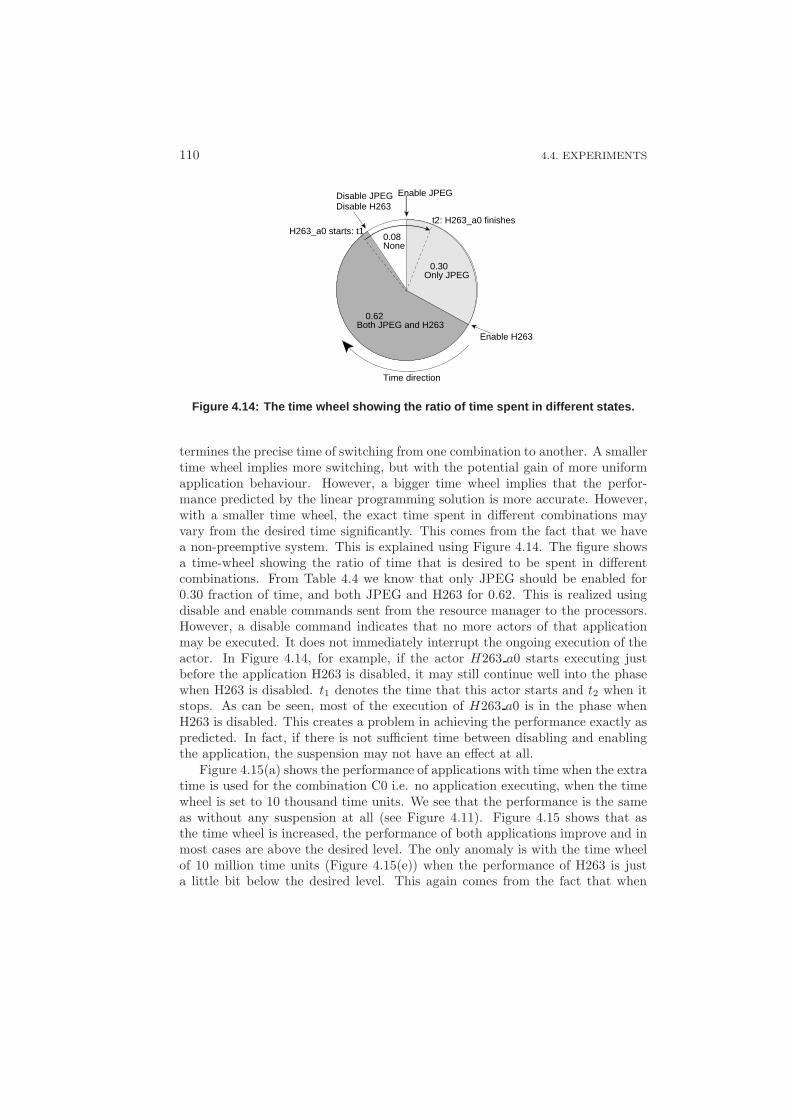
110 4.4. EXPERIMENTS
0.30
None
Disable H263
Enable JPEG
Enable H263
Time direction
t2: H263_a0 finishes
0.08
Both JPEG and H263 0.62
Disable JPEG
Only JPEG
H263_a0 starts: t1
Figure 4.14: The time wheel showing the ratio of time spent in different states.
termines the precise time of switching from one combination to another. A smallertime wheel implies more switching, but with the potential gain of more uniformapplication behaviour. However, a bigger time wheel implies that the perfor-mance predicted by the linear programming solution is more accurate. However,with a smaller time wheel, the exact time spent in different combinations mayvary from the desired time significantly. This comes from the fact that we havea non-preemptive system. This is explained using Figure 4.14. The figure showsa time-wheel showing the ratio of time that is desired to be spent in differentcombinations. From Table 4.4 we know that only JPEG should be enabled for0.30 fraction of time, and both JPEG and H263 for 0.62. This is realized usingdisable and enable commands sent from the resource manager to the processors.However, a disable command indicates that no more actors of that applicationmay be executed. It does not immediately interrupt the ongoing execution of theactor. In Figure 4.14, for example, if the actor H263 a0 starts executing justbefore the application H263 is disabled, it may still continue well into the phasewhen H263 is disabled. t1 denotes the time that this actor starts and t2 when itstops. As can be seen, most of the execution of H263 a0 is in the phase whenH263 is disabled. This creates a problem in achieving the performance exactly aspredicted. In fact, if there is not sufficient time between disabling and enablingthe application, the suspension may not have an effect at all.
Figure 4.15(a) shows the performance of applications with time when the extratime is used for the combination C0 i.e. no application executing, when the timewheel is set to 10 thousand time units. We see that the performance is the sameas without any suspension at all (see Figure 4.11). Figure 4.15 shows that asthe time wheel is increased, the performance of both applications improve and inmost cases are above the desired level. The only anomaly is with the time wheelof 10 million time units (Figure 4.15(e)) when the performance of H263 is justa little bit below the desired level. This again comes from the fact that when
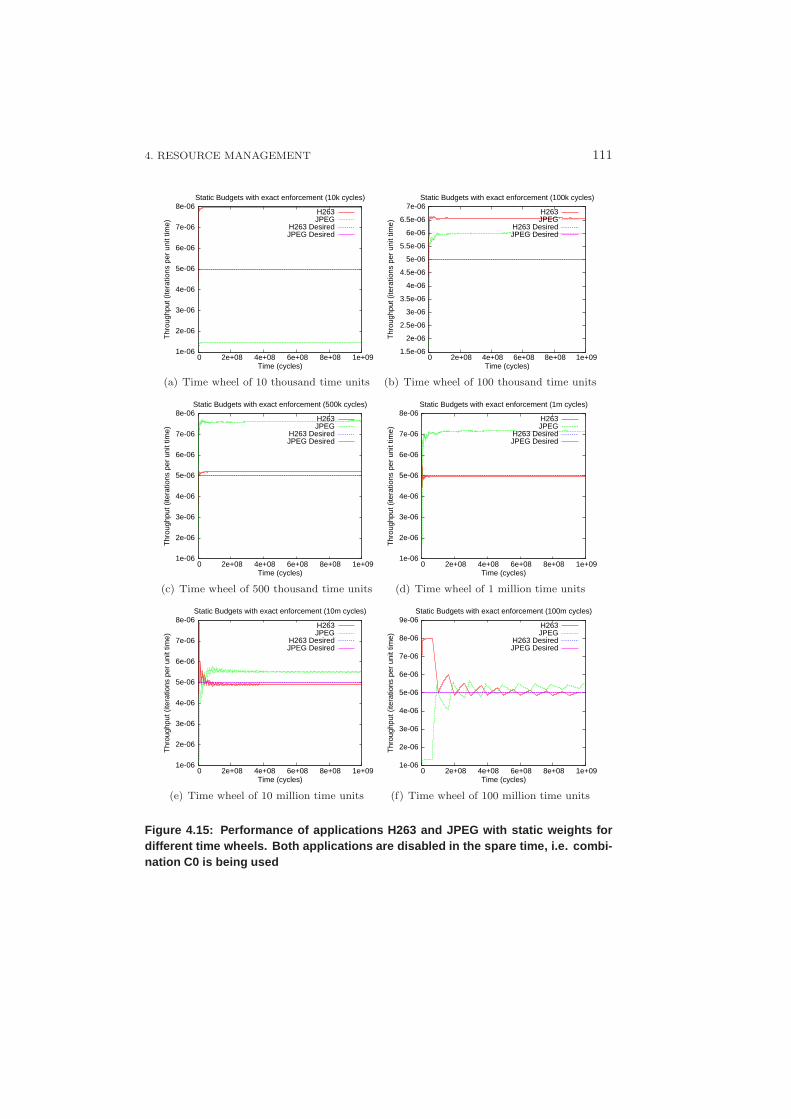
4. RESOURCE MANAGEMENT 111
1e-06
2e-06
3e-06
4e-06
5e-06
6e-06
7e-06
8e-06
0 2e+08 4e+08 6e+08 8e+08 1e+09
Thr
ough
put (
itera
tions
per
uni
t tim
e)
Time (cycles)
Static Budgets with exact enforcement (10k cycles)
H263JPEG
H263 DesiredJPEG Desired
(a) Time wheel of 10 thousand time units
1.5e-06
2e-06
2.5e-06
3e-06
3.5e-06
4e-06
4.5e-06
5e-06
5.5e-06
6e-06
6.5e-06
7e-06
0 2e+08 4e+08 6e+08 8e+08 1e+09
Thr
ough
put (
itera
tions
per
uni
t tim
e)
Time (cycles)
Static Budgets with exact enforcement (100k cycles)
H263JPEG
H263 DesiredJPEG Desired
(b) Time wheel of 100 thousand time units
1e-06
2e-06
3e-06
4e-06
5e-06
6e-06
7e-06
8e-06
0 2e+08 4e+08 6e+08 8e+08 1e+09
Thr
ough
put (
itera
tions
per
uni
t tim
e)
Time (cycles)
Static Budgets with exact enforcement (500k cycles)
H263JPEG
H263 DesiredJPEG Desired
(c) Time wheel of 500 thousand time units
1e-06
2e-06
3e-06
4e-06
5e-06
6e-06
7e-06
8e-06
0 2e+08 4e+08 6e+08 8e+08 1e+09
Thr
ough
put (
itera
tions
per
uni
t tim
e)
Time (cycles)
Static Budgets with exact enforcement (1m cycles)
H263JPEG
H263 DesiredJPEG Desired
(d) Time wheel of 1 million time units
1e-06
2e-06
3e-06
4e-06
5e-06
6e-06
7e-06
8e-06
0 2e+08 4e+08 6e+08 8e+08 1e+09
Thr
ough
put (
itera
tions
per
uni
t tim
e)
Time (cycles)
Static Budgets with exact enforcement (10m cycles)
H263JPEG
H263 DesiredJPEG Desired
(e) Time wheel of 10 million time units
1e-06
2e-06
3e-06
4e-06
5e-06
6e-06
7e-06
8e-06
9e-06
0 2e+08 4e+08 6e+08 8e+08 1e+09
Thr
ough
put (
itera
tions
per
uni
t tim
e)
Time (cycles)
Static Budgets with exact enforcement (100m cycles)
H263JPEG
H263 DesiredJPEG Desired
(f) Time wheel of 100 million time units
Figure 4.15: Performance of applications H263 and JPEG with static weights fordifferent time wheels. Both applications are disabled in th e spare time, i.e. combi-nation C0 is being used
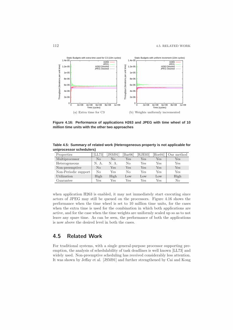
112 4.5. RELATED WORK
0
2e-06
4e-06
6e-06
8e-06
1e-05
1.2e-05
1.4e-05
0 2e+08 4e+08 6e+08 8e+08 1e+09
Thr
ough
put (
itera
tions
per
uni
t tim
e)
Time (cycles)
Static Budgets with extra time used for C3 (10m cycles)
H263JPEG
H263 DesiredJPEG Desired
(a) Extra time for C3
0
2e-06
4e-06
6e-06
8e-06
1e-05
1.2e-05
1.4e-05
0 2e+08 4e+08 6e+08 8e+08 1e+09
Thr
ough
put (
itera
tions
per
uni
t tim
e)
Time (cycles)
Static Budgets with uniform increment (10m cycles)
H263JPEG
H263 DesiredJPEG Desired
(b) Weights uniformly incremented
Figure 4.16: Performance of applications H263 and JPEG with time wheel of 10million time units with the other two approaches
Table 4.5: Summary of related work (Heterogeneous property is not applicable foruniprocessor schedulers)
Properties [LL73] [JSM91] [Bar06] [RJE03] [Hoe04] Our method
Multiprocessor No No Yes Yes Yes YesHeterogeneous N. A. N. A. No Yes Yes YesNon-preemptive No Yes Yes Yes Yes YesNon-Periodic support No Yes No Yes Yes YesUtilization High High Low Low Low HighGuarantee Yes Yes Yes Yes Yes No
when application H263 is enabled, it may not immediately start executing sinceactors of JPEG may still be queued on the processors. Figure 4.16 shows theperformance when the time wheel is set to 10 million time units, for the caseswhen the extra time is used for the combination in which both applications areactive, and for the case when the time weights are uniformly scaled up so as to notleave any spare time. As can be seen, the performance of both the applicationsis now above the desired level in both the cases.
4.5 Related Work
For traditional systems, with a single general-purpose processor supporting pre-emption, the analysis of schedulability of task deadlines is well known [LL73] andwidely used. Non-preemptive scheduling has received considerably less attention.It was shown by Jeffay et al. [JSM91] and further strengthened by Cai and Kong
4. RESOURCE MANAGEMENT 113
[CK96] that the problem of determining whether a given periodic task systemis non-preemptively feasible even upon a single processor is already intractable.Also, research on multiprocessor real-time scheduling has mainly focused on pre-emptive systems [DD86, BCPV96].
Recently, more work has been done on non-preemptive scheduling for multi-processor systems [Bar06]. Alternative methods have been proposed for analyzingtask performance and resource sharing. A formal approach to verification of MP-SoC performance has been proposed in [RJE03]. Use of real-time calculus forschedulability analysis was proposed in [TCN00]. Computing worst-case wait-ing time, taking resource contention into account, for round-robin and TDMAscheduling (requires preemption) has also been analyzed [Hoe04]. However, po-tential disadvantages of these approaches are that the analysis can be very pes-simistic as has been explained in Chapter 2.
A lot of work has been done in the context of resource management for multi-processor systems [MMB07, NAE+08, KMT+06]. The work in [MMB07] only con-siders preemptive systems, while our work is targeted at non-preemptive systems.Non-preemptive systems are harder to analyze since the interference of other ap-plications has to be taken into account. The work in [NAE+08] presents a run-timemanager for MPSoC platforms, but they only consider one task mapped on oneprocessor in the system; they do not allow sharing of processors. In [KMT+06]the authors deal with non-preemptive heterogeneous platforms where processorsare shared, but only discuss the issue of budget enforcement and not of admissioncontrol.
The authors in [PTB06] motivate the use of a scenario-oriented (or use-casein this thesis) design flow for heterogeneous MPSoC platforms. They propose toanalyze the scenarios at design-time. However, with the need to add applicationsat run-time, a design-flow is needed that can accommodate this dynamic additionof applications. We presented such a flow in this chapter.
A number of techniques are present in literature to do the partitioning of pro-gram code into tasks. Compaan is one such example that converts sequentialdescription of an application into concurrent tasks by doing static code anal-ysis and transformation [SZT+04]. Sprint also allows code partitioning by al-lowing the users to tag the functions that need to be split across different ac-tors [CDVS07]. Yet another technique has been presented that is based on exe-cution profile [RVB07].
Table 4.5 shows a comparison of various analysis techniques that have beenpresented so far in literature, and where our approach is different. As can beseen, all of the research done in multiprocessor domain provides low utilizationguarantees. Our approach on the other hand aims at achieving high utilizationby sacrificing hard guarantees.
114 4.6. CONCLUSIONS
4.6 Conclusions
In this chapter, we presented a novel flow for designing systems with multipleapplications, such that the entire analysis remains composable. This allows easyand quick analysis of an application-mix while properties of individual applicationsare derived in isolation. Our flow also allows addition of applications at run-time,even when they are not known at design-time. We present a hybrid approachwhere the time-consuming application-specific computations are done at design-time, and in isolation to other applications – to maintain composability, and theuse-case-specific computations are performed at run-time. Further, we present aresource manager (RM) for run-time aspects of resource management.
We propose a resource manager (RM) for non-preemptive heterogeneous MP-SoCs. Although the scheduling of these systems has been considered in the liter-ature, the actual resource management in the context of concurrently executingapplications is still unexplored area. Theoretically, design-time analysis of allpossible use-cases can provide performance guarantees, but the potentially largenumber of use-cases in a real system and dynamic properties of applications makesuch analysis infeasible. Our resource manager shifts the burden of design-timeanalysis to run-time monitoring and intervention when necessary.
A high-level simulation model of the resource manger has been developedusing POOSL methodology. A case study with an H263 and a JPEG decoderdemonstrates that RM intervention is essential to ensure that both applicationsare able to meet their throughput requirements. Further, a finer grain of controlincreases the utilization of processor resources, and leads to a more stable system.Results of statically computing the time weights for suspension are also presented,although more research needs to be done to evaluate the size of time-wheel.
CHAPTER 5
Multiprocessor System Design and Synthesis
In the earlier chapters, we saw how to analyze performance of multiple applica-tions executing concurrently on a multiprocessor platform. We saw how we canmanage the resources available on a multiprocessor platform by splitting the man-agement into design-time and run-time. We also saw how to use the performanceanalysis technique for run-time admission control of applications, and the budgetenforcement technique to ensure all applications can achieve their desired perfor-mance. While analysis and management of a multiprocessor system is important,designing and programming the system is no easy task either. With reducingtime-to-market, designers are faced with the challenge of designing and testingsystems quickly. Rapid prototyping has become very important to easily evaluatedesign alternatives, and to explore hardware and software alternatives quickly.Unfortunately, lack of automated techniques and tools implies that most work isdone by hand, making the design-process error-prone and time-consuming. Thisalso limits the number of design-points that can be explored. While some effortshave been made to automate the flow and raise the abstraction level, these arestill limited to single-application designs.
Figure 5.1 shows the ideal design flow to overcome this challenge. It is ev-ery designer’s dream to directly input the application specification in the formof C-code (or whichever language it is given in) – be it sequential or parallel,and generate and synthesize the best multiprocessor system that meets all theconstraints of applications performance, and at the same time achieve the design-objectives of low silicon area and power. Current state-of-the-art tools only allowfor single application designs, as shown by the shaded area in Figure 5.1.
115
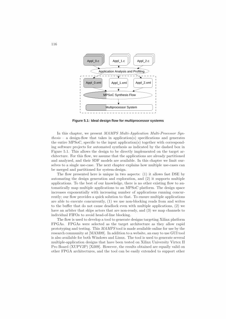
116
Multiprocessor System
Application Analysis and Profiling
Appl_0.c Appl_1.c Appl_2.c
Appl_2.xmlAppl_1.xmlAppl_0.xml
MPSoC Synthesis Flow
Figure 5.1: Ideal design flow for multiprocessor systems
In this chapter, we present MAMPS Multi-Application Multi-Processor Syn-thesis – a design-flow that takes in application(s) specifications and generatesthe entire MPSoC, specific to the input application(s) together with correspond-ing software projects for automated synthesis as indicated by the dashed box inFigure 5.1. This allows the design to be directly implemented on the target ar-chitecture. For this flow, we assume that the applications are already partitionedand analyzed, and their SDF models are available. In this chapter we limit our-selves to a single use-case. The next chapter explains how multiple use-cases canbe merged and partitioned for system-design.
The flow presented here is unique in two aspects: (1) it allows fast DSE byautomating the design generation and exploration, and (2) it supports multipleapplications. To the best of our knowledge, there is no other existing flow to au-tomatically map multiple applications to an MPSoC platform. The design spaceincreases exponentially with increasing number of applications running concur-rently; our flow provides a quick solution to that. To ensure multiple applicationsare able to execute concurrently, (1) we use non-blocking reads from and writesto the buffer that do not cause deadlock even with multiple applications, (2) wehave an arbiter that skips actors that are non-ready, and (3) we map channels toindividual FIFOs to avoid head-of-line blocking.
The flow is used to develop a tool to generate designs targeting Xilinx platformFPGAs. FPGAs were selected as the target architecture as they allow rapidprototyping and testing. This MAMPS tool is made available online for use by theresearch community at [MAM09]. In addition to a website, an easy to use GUI toolis also available for both Windows and Linux. The tool is used to generate severalmultiple-application designs that have been tested on Xilinx University Virtex IIPro Board (XUPV2P) [Xil09]. However, the results obtained are equally valid onother FPGA architectures, and the tool can be easily extended to support other
5. MULTIPROCESSOR SYSTEM DESIGN AND SYNTHESIS 117
FPGA boards and architectures. We present a case study on how our methodologycan be used for design space exploration using JPEG and H263 decoders. Wewere able to explore 24 design points that trade-off memory requirements andperformance achieved with both applications running concurrently on an FPGAin a total of 45 minutes, including synthesis time.
This chapter is organized as follows. Section 5.2 gives an overview of our flow,MAMPS, while Section 5.3 describes the tool implementation. Section 5.4 presentsresults of experiments done to evaluate our methodology. Section 5.5 reviews therelated work for architecture-generation and synthesis flows for multiprocessorsystems. Section 5.6 concludes this chapter and gives directions for future work.
5.1 Performance Evaluation Framework
Performance evaluation forms an integral part of system design. In MPSoC de-signs, the design space exploration and the parameter optimization can quicklybecome intractable [JB06]. Performance evaluation approaches can broadly be di-vided in two main categories – statistical and deterministic. Statistical approachesrely on developing a high-level system-performance model, calibrating the modelparameters, and using them to predict the behaviour of new applications. Theexact application is not taken into account. Deterministic approaches on the otherhand, take the application into account. System simulation is one of the mostcommon ways for deterministic performance evaluation. It relies on the execu-tion of the complete system using input use-cases. Accuracy of this approachdepends on the parameters covered in the simulation model. Unfortunately, theaccuracy is generally inversely proportional to the speed. The greater the numberof parameters modeled, the slower it is.
Analytical approach, also deterministic, is often used to investigate systemcapabilities. The sub-system is abstracted away using algebraic equations. Math-ematical theories allow full analysis of the system performance at an early designstage. The probabilistic analysis provided in Chapter 3 is an example of such anapproach. Another deterministic approach is measurement on the actual plat-form, but this is generally harder since the actual system is available much laterin the design. This is exactly where our approach helps.
Our method allows mapping of applications on real hardware and measuringtheir performance accurately. This can be done for either individual or multi-ple applications, as desired. Application(s)-specific architecture is generated, andreal performance can be measured way before the actual system is available with-out losing accuracy. The design runs on an FPGA platform and the interactionbetween multiple applications can be observed.
Table 5.1 shows a comparison of using different techniques for deterministicevaluation. Analytical approaches are fast but generally lack accuracy. Simulationcan improve on the accuracy part with enough parameters being modeled, buttakes a long time before giving meaningful results. In order to speed up the
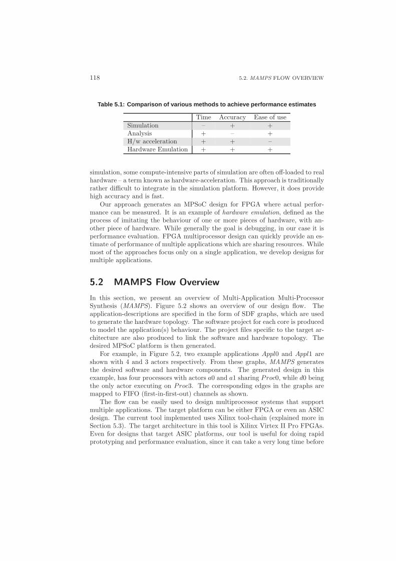
118 5.2. MAMPS FLOW OVERVIEW
Table 5.1: Comparison of various methods to achieve perform ance estimates
Time Accuracy Ease of useSimulation – + +Analysis + – +H/w acceleration + + –Hardware Emulation + + +
simulation, some compute-intensive parts of simulation are often off-loaded to realhardware – a term known as hardware-acceleration. This approach is traditionallyrather difficult to integrate in the simulation platform. However, it does providehigh accuracy and is fast.
Our approach generates an MPSoC design for FPGA where actual perfor-mance can be measured. It is an example of hardware emulation, defined as theprocess of imitating the behaviour of one or more pieces of hardware, with an-other piece of hardware. While generally the goal is debugging, in our case it isperformance evaluation. FPGA multiprocessor design can quickly provide an es-timate of performance of multiple applications which are sharing resources. Whilemost of the approaches focus only on a single application, we develop designs formultiple applications.
5.2 MAMPS Flow Overview
In this section, we present an overview of Multi-Application Multi-ProcessorSynthesis (MAMPS). Figure 5.2 shows an overview of our design flow. Theapplication-descriptions are specified in the form of SDF graphs, which are usedto generate the hardware topology. The software project for each core is producedto model the application(s) behaviour. The project files specific to the target ar-chitecture are also produced to link the software and hardware topology. Thedesired MPSoC platform is then generated.
For example, in Figure 5.2, two example applications Appl0 and Appl1 areshown with 4 and 3 actors respectively. From these graphs, MAMPS generatesthe desired software and hardware components. The generated design in thisexample, has four processors with actors a0 and a1 sharing Proc0, while d0 beingthe only actor executing on Proc3. The corresponding edges in the graphs aremapped to FIFO (first-in-first-out) channels as shown.
The flow can be easily used to design multiprocessor systems that supportmultiple applications. The target platform can be either FPGA or even an ASICdesign. The current tool implemented uses Xilinx tool-chain (explained more inSection 5.3). The target architecture in this tool is Xilinx Virtex II Pro FPGAs.Even for designs that target ASIC platforms, our tool is useful for doing rapidprototyping and performance evaluation, since it can take a very long time before
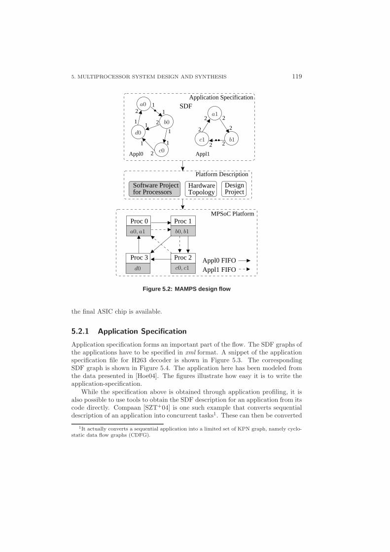
5. MULTIPROCESSOR SYSTEM DESIGN AND SYNTHESIS 119
Software Project for Processors
DesignProject
HardwareTopology
Proc 0 Proc 1
Proc 2Proc 3 Appl0 FIFOAppl1 FIFO
MPSoC Platform
SDF1
12
1 211
11
2
2
2
22
2
2
Application Specification
Platform Description
Appl1Appl0
a0
b0
c0
d0
d0
a1
b1c1
a0, a1 b0, b1
c0, c1
Figure 5.2: MAMPS design flow
the final ASIC chip is available.
5.2.1 Application Specification
Application specification forms an important part of the flow. The SDF graphs ofthe applications have to be specified in xml format. A snippet of the applicationspecification file for H263 decoder is shown in Figure 5.3. The correspondingSDF graph is shown in Figure 5.4. The application here has been modeled fromthe data presented in [Hoe04]. The figures illustrate how easy it is to write theapplication-specification.
While the specification above is obtained through application profiling, it isalso possible to use tools to obtain the SDF description for an application from itscode directly. Compaan [SZT+04] is one such example that converts sequentialdescription of an application into concurrent tasks1. These can then be converted
1It actually converts a sequential application into a limited set of KPN graph, namely cyclo-static data flow graphs (CDFG).
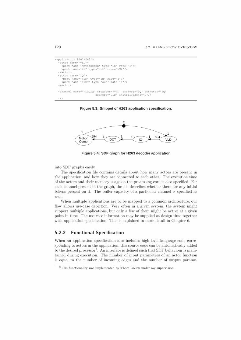
120 5.2. MAMPS FLOW OVERVIEW
<application id="H263"><actor name="VLD">
<port name="MotionComp" type="in" rate="1"/><port name="IQ" type="out" rate="594"/>
</actor><actor name="IQ">
<port name="VLD" type="in" rate="1"/><port name="IDCT" type="out" rate="1"/>
</actor>...<channel name="VLD_IQ" srcActor="VLD" srcPort="IQ" dstActor="IQ"
dstPort="VLD" initialTokens="0"/>...
Figure 5.3: Snippet of H263 application specification.
5941
1 1 1 1 5941
2
MotionComp
IDCT IQ VLD
Figure 5.4: SDF graph for H263 decoder application
into SDF graphs easily.The specification file contains details about how many actors are present in
the application, and how they are connected to each other. The execution timeof the actors and their memory usage on the processing core is also specified. Foreach channel present in the graph, the file describes whether there are any initialtokens present on it. The buffer capacity of a particular channel is specified aswell.
When multiple applications are to be mapped to a common architecture, ourflow allows use-case depiction. Very often in a given system, the system mightsupport multiple applications, but only a few of them might be active at a givenpoint in time. The use-case information may be supplied at design time togetherwith application specification. This is explained in more detail in Chapter 6.
5.2.2 Functional Specification
When an application specification also includes high-level language code corre-sponding to actors in the application, this source code can be automatically addedto the desired processor2. An interface is defined such that SDF behaviour is main-tained during execution. The number of input parameters of an actor functionis equal to the number of incoming edges and the number of output parame-
2This functionality was implemented by Thom Gielen under my supervision.
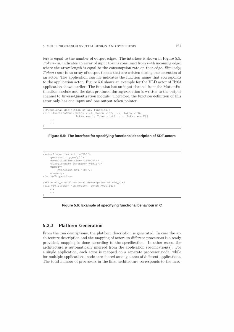
5. MULTIPROCESSOR SYSTEM DESIGN AND SYNTHESIS 121
ters is equal to the number of output edges. The interface is shown in Figure 5.5.Token∗ini indicates an array of input tokens consumed from i−th incoming edge,where the array length is equal to the consumption rate on that edge. Similarly,Token∗outi is an array of output tokens that are written during one execution ofan actor. The application xml file indicates the function name that correspondsto the application actor. Figure 5.6 shows an example for the VLD actor of H263application shown earlier. The function has an input channel from the MotionEs-timation module and the data produced during execution is written to the outputchannel to InverseQuantization module. Therefore, the function definition of thisactor only has one input and one output token pointer.
/*Functional definition of any function*/void <functionName>(Token *in1, Token *in2, ..., Token *inN,
Token *out1, Token *out2, ..., Token *outM){......
}
Figure 5.5: The interface for specifying functional descri ption of SDF-actors
<actorProperties actor="VLD"><processor type="p1"><executionTime time="120000"/><functionName funcname="vld_c"/><memory>
<statesize max="100"/></memory>
</actorProperties>
/*File vld_c.c: Functional description of vld_c */void vld_c(Token *in_motion, Token *out_iq){
...
...}
Figure 5.6: Example of specifying functional behaviour in C
5.2.3 Platform Generation
From the xml descriptions, the platform description is generated. In case the ar-chitecture description and the mapping of actors to different processors is alreadyprovided, mapping is done according to the specification. In other cases, thearchitecture is automatically inferred from the application specification(s). Fora single application, each actor is mapped on a separate processor node, whilefor multiple applications, nodes are shared among actors of different applications.The total number of processors in the final architecture corresponds to the max-
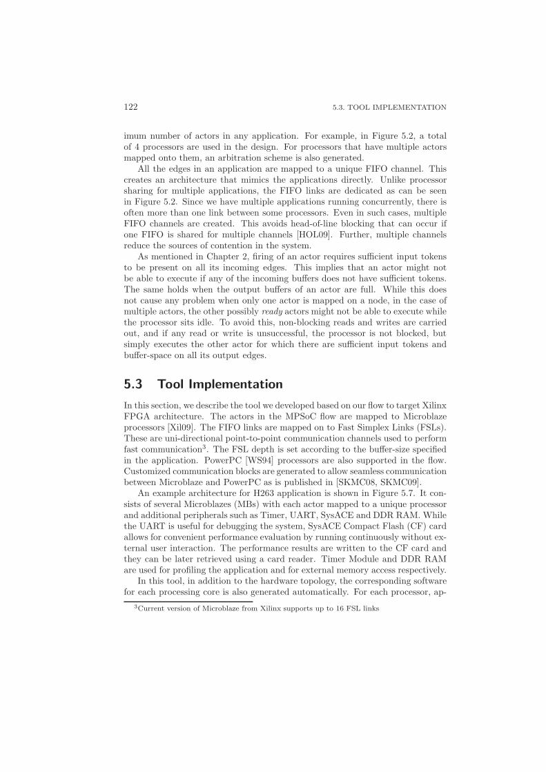
122 5.3. TOOL IMPLEMENTATION
imum number of actors in any application. For example, in Figure 5.2, a totalof 4 processors are used in the design. For processors that have multiple actorsmapped onto them, an arbitration scheme is also generated.
All the edges in an application are mapped to a unique FIFO channel. Thiscreates an architecture that mimics the applications directly. Unlike processorsharing for multiple applications, the FIFO links are dedicated as can be seenin Figure 5.2. Since we have multiple applications running concurrently, there isoften more than one link between some processors. Even in such cases, multipleFIFO channels are created. This avoids head-of-line blocking that can occur ifone FIFO is shared for multiple channels [HOL09]. Further, multiple channelsreduce the sources of contention in the system.
As mentioned in Chapter 2, firing of an actor requires sufficient input tokensto be present on all its incoming edges. This implies that an actor might notbe able to execute if any of the incoming buffers does not have sufficient tokens.The same holds when the output buffers of an actor are full. While this doesnot cause any problem when only one actor is mapped on a node, in the case ofmultiple actors, the other possibly ready actors might not be able to execute whilethe processor sits idle. To avoid this, non-blocking reads and writes are carriedout, and if any read or write is unsuccessful, the processor is not blocked, butsimply executes the other actor for which there are sufficient input tokens andbuffer-space on all its output edges.
5.3 Tool Implementation
In this section, we describe the tool we developed based on our flow to target XilinxFPGA architecture. The actors in the MPSoC flow are mapped to Microblazeprocessors [Xil09]. The FIFO links are mapped on to Fast Simplex Links (FSLs).These are uni-directional point-to-point communication channels used to performfast communication3. The FSL depth is set according to the buffer-size specifiedin the application. PowerPC [WS94] processors are also supported in the flow.Customized communication blocks are generated to allow seamless communicationbetween Microblaze and PowerPC as is published in [SKMC08, SKMC09].
An example architecture for H263 application is shown in Figure 5.7. It con-sists of several Microblazes (MBs) with each actor mapped to a unique processorand additional peripherals such as Timer, UART, SysACE and DDR RAM. Whilethe UART is useful for debugging the system, SysACE Compact Flash (CF) cardallows for convenient performance evaluation by running continuously without ex-ternal user interaction. The performance results are written to the CF card andthey can be later retrieved using a card reader. Timer Module and DDR RAMare used for profiling the application and for external memory access respectively.
In this tool, in addition to the hardware topology, the corresponding softwarefor each processing core is also generated automatically. For each processor, ap-
3Current version of Microblaze from Xilinx supports up to 16 FSL links
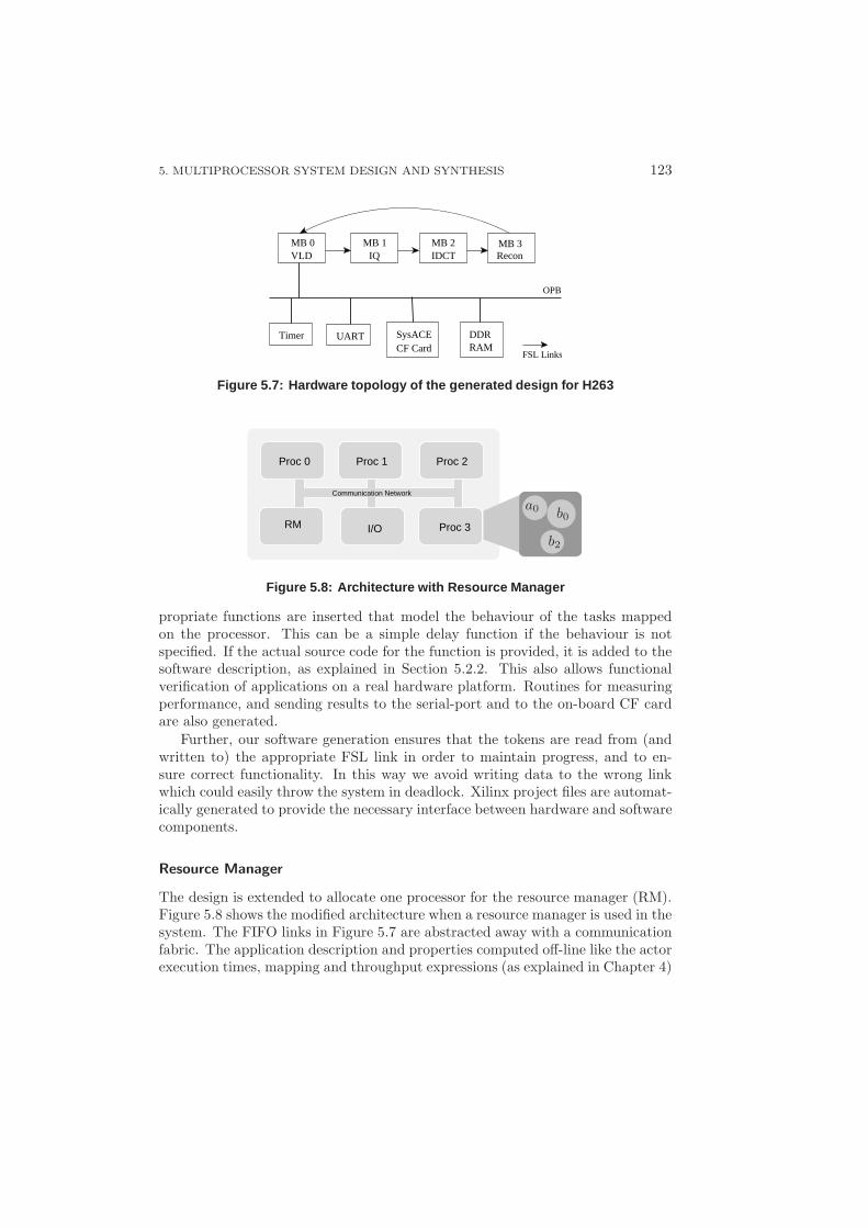
5. MULTIPROCESSOR SYSTEM DESIGN AND SYNTHESIS 123
MB 1
Timer UART DDRRAM
SysACECF Card
OPB
FSL Links
ReconMB 0VLD IDCT
MB 2 MB 3IQ
Figure 5.7: Hardware topology of the generated design for H2 63
Proc 0 Proc 1
RM
Proc 2
Proc 3
Communication Network
I/O
a0 b0
b2
Figure 5.8: Architecture with Resource Manager
propriate functions are inserted that model the behaviour of the tasks mappedon the processor. This can be a simple delay function if the behaviour is notspecified. If the actual source code for the function is provided, it is added to thesoftware description, as explained in Section 5.2.2. This also allows functionalverification of applications on a real hardware platform. Routines for measuringperformance, and sending results to the serial-port and to the on-board CF cardare also generated.
Further, our software generation ensures that the tokens are read from (andwritten to) the appropriate FSL link in order to maintain progress, and to en-sure correct functionality. In this way we avoid writing data to the wrong linkwhich could easily throw the system in deadlock. Xilinx project files are automat-ically generated to provide the necessary interface between hardware and softwarecomponents.
Resource Manager
The design is extended to allocate one processor for the resource manager (RM).Figure 5.8 shows the modified architecture when a resource manager is used in thesystem. The FIFO links in Figure 5.7 are abstracted away with a communicationfabric. The application description and properties computed off-line like the actorexecution times, mapping and throughput expressions (as explained in Chapter 4)
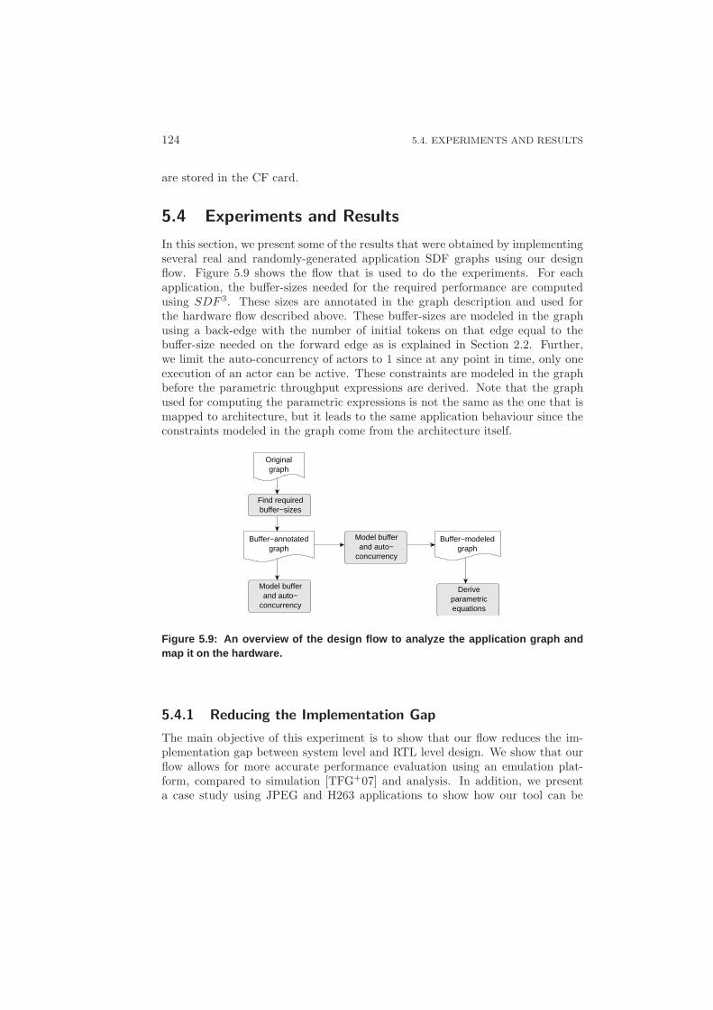
124 5.4. EXPERIMENTS AND RESULTS
are stored in the CF card.
5.4 Experiments and Results
In this section, we present some of the results that were obtained by implementingseveral real and randomly-generated application SDF graphs using our designflow. Figure 5.9 shows the flow that is used to do the experiments. For eachapplication, the buffer-sizes needed for the required performance are computedusing SDF 3. These sizes are annotated in the graph description and used forthe hardware flow described above. These buffer-sizes are modeled in the graphusing a back-edge with the number of initial tokens on that edge equal to thebuffer-size needed on the forward edge as is explained in Section 2.2. Further,we limit the auto-concurrency of actors to 1 since at any point in time, only oneexecution of an actor can be active. These constraints are modeled in the graphbefore the parametric throughput expressions are derived. Note that the graphused for computing the parametric expressions is not the same as the one that ismapped to architecture, but it leads to the same application behaviour since theconstraints modeled in the graph come from the architecture itself.
graphOriginal
Buffer−modeledgraphgraph
Buffer−annotated Model bufferand auto−
concurrency
Find requiredbuffer−sizes
Model bufferand auto−
concurrency
Deriveparametricequations
Figure 5.9: An overview of the design flow to analyze the appli cation graph andmap it on the hardware.
5.4.1 Reducing the Implementation Gap
The main objective of this experiment is to show that our flow reduces the im-plementation gap between system level and RTL level design. We show that ourflow allows for more accurate performance evaluation using an emulation plat-form, compared to simulation [TFG+07] and analysis. In addition, we presenta case study using JPEG and H263 applications to show how our tool can be
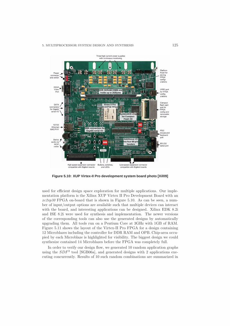
5. MULTIPROCESSOR SYSTEM DESIGN AND SYNTHESIS 125
Figure 5.10: XUP Virtex-II Pro development system board pho to [Xil09]
used for efficient design space exploration for multiple applications. Our imple-mentation platform is the Xilinx XUP Virtex II Pro Development Board with anxc2vp30 FPGA on-board that is shown in Figure 5.10. As can be seen, a num-ber of input/output options are available such that multiple devices can interactwith the board, and interesting applications can be designed. Xilinx EDK 8.2iand ISE 8.2i were used for synthesis and implementation. The newer versionsof the corresponding tools can also use the generated designs by automaticallyupgrading them. All tools run on a Pentium Core at 3GHz with 1GB of RAM.Figure 5.11 shows the layout of the Virtex-II Pro FPGA for a design containing12 Microblazes including the controller for DDR RAM and OPB. Chip-area occu-pied by each Microblaze is highlighted for visibility. The biggest design we couldsynthesize contained 14 Microblazes before the FPGA was completely full.
In order to verify our design flow, we generated 10 random application graphsusing the SDF 3 tool [SGB06a], and generated designs with 2 applications exe-cuting concurrently. Results of 10 such random combinations are summarized in
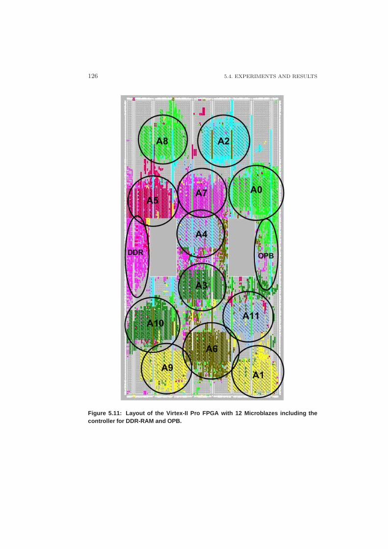
126 5.4. EXPERIMENTS AND RESULTS
Figure 5.11: Layout of the Virtex-II Pro FPGA with 12 Microbl azes including thecontroller for DDR-RAM and OPB.
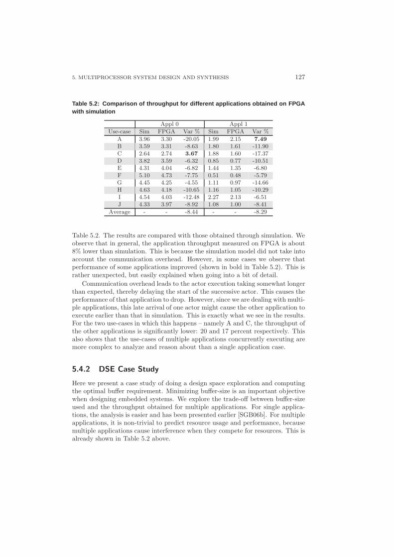
5. MULTIPROCESSOR SYSTEM DESIGN AND SYNTHESIS 127
Table 5.2: Comparison of throughput for different applicat ions obtained on FPGAwith simulation
Appl 0 Appl 1
Use-case Sim FPGA Var % Sim FPGA Var %
A 3.96 3.30 -20.05 1.99 2.15 7.49
B 3.59 3.31 -8.63 1.80 1.61 -11.90C 2.64 2.74 3.67 1.88 1.60 -17.37D 3.82 3.59 -6.32 0.85 0.77 -10.51E 4.31 4.04 -6.82 1.44 1.35 -6.80F 5.10 4.73 -7.75 0.51 0.48 -5.79G 4.45 4.25 -4.55 1.11 0.97 -14.66H 4.63 4.18 -10.65 1.16 1.05 -10.29I 4.54 4.03 -12.48 2.27 2.13 -6.51J 4.33 3.97 -8.92 1.08 1.00 -8.41
Average - - -8.44 - - -8.29
Table 5.2. The results are compared with those obtained through simulation. Weobserve that in general, the application throughput measured on FPGA is about8% lower than simulation. This is because the simulation model did not take intoaccount the communication overhead. However, in some cases we observe thatperformance of some applications improved (shown in bold in Table 5.2). This israther unexpected, but easily explained when going into a bit of detail.
Communication overhead leads to the actor execution taking somewhat longerthan expected, thereby delaying the start of the successive actor. This causes theperformance of that application to drop. However, since we are dealing with multi-ple applications, this late arrival of one actor might cause the other application toexecute earlier than that in simulation. This is exactly what we see in the results.For the two use-cases in which this happens – namely A and C, the throughput ofthe other applications is significantly lower: 20 and 17 percent respectively. Thisalso shows that the use-cases of multiple applications concurrently executing aremore complex to analyze and reason about than a single application case.
5.4.2 DSE Case Study
Here we present a case study of doing a design space exploration and computingthe optimal buffer requirement. Minimizing buffer-size is an important objectivewhen designing embedded systems. We explore the trade-off between buffer-sizeused and the throughput obtained for multiple applications. For single applica-tions, the analysis is easier and has been presented earlier [SGB06b]. For multipleapplications, it is non-trivial to predict resource usage and performance, becausemultiple applications cause interference when they compete for resources. This isalready shown in Table 5.2 above.
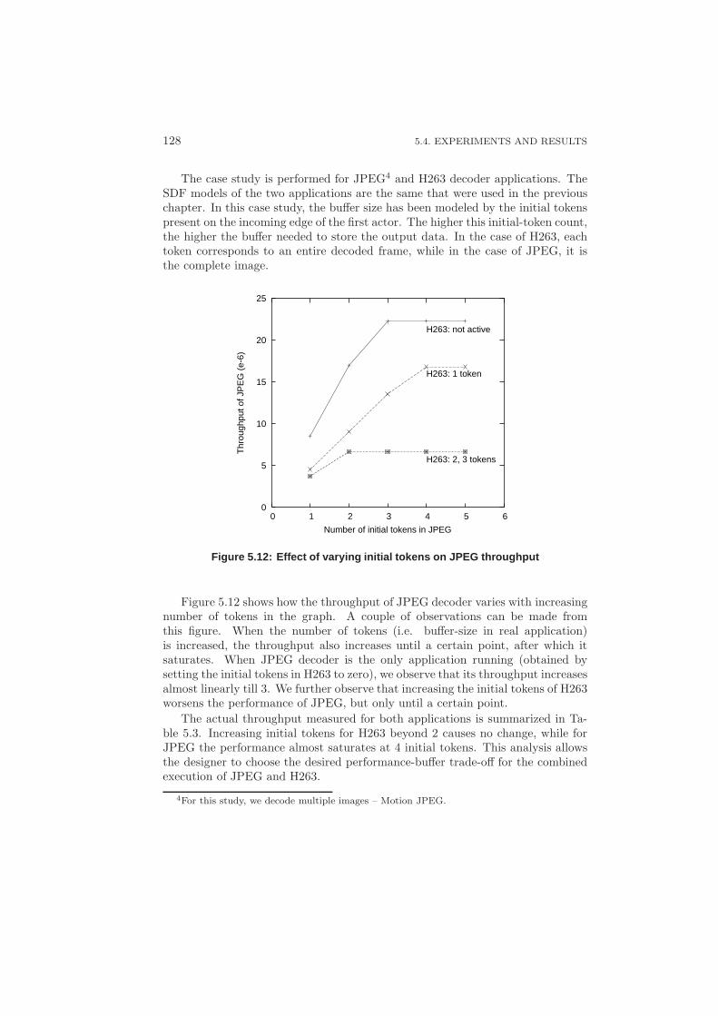
128 5.4. EXPERIMENTS AND RESULTS
The case study is performed for JPEG4 and H263 decoder applications. TheSDF models of the two applications are the same that were used in the previouschapter. In this case study, the buffer size has been modeled by the initial tokenspresent on the incoming edge of the first actor. The higher this initial-token count,the higher the buffer needed to store the output data. In the case of H263, eachtoken corresponds to an entire decoded frame, while in the case of JPEG, it isthe complete image.
0
5
10
15
20
25
0 1 2 3 4 5 6
Thr
ough
put o
f JP
EG
(e-
6)
Number of initial tokens in JPEG
H263: not active
H263: 1 token
H263: 2, 3 tokens
Figure 5.12: Effect of varying initial tokens on JPEG throug hput
Figure 5.12 shows how the throughput of JPEG decoder varies with increasingnumber of tokens in the graph. A couple of observations can be made fromthis figure. When the number of tokens (i.e. buffer-size in real application)is increased, the throughput also increases until a certain point, after which itsaturates. When JPEG decoder is the only application running (obtained bysetting the initial tokens in H263 to zero), we observe that its throughput increasesalmost linearly till 3. We further observe that increasing the initial tokens of H263worsens the performance of JPEG, but only until a certain point.
The actual throughput measured for both applications is summarized in Ta-ble 5.3. Increasing initial tokens for H263 beyond 2 causes no change, while forJPEG the performance almost saturates at 4 initial tokens. This analysis allowsthe designer to choose the desired performance-buffer trade-off for the combinedexecution of JPEG and H263.
4For this study, we decode multiple images – Motion JPEG.
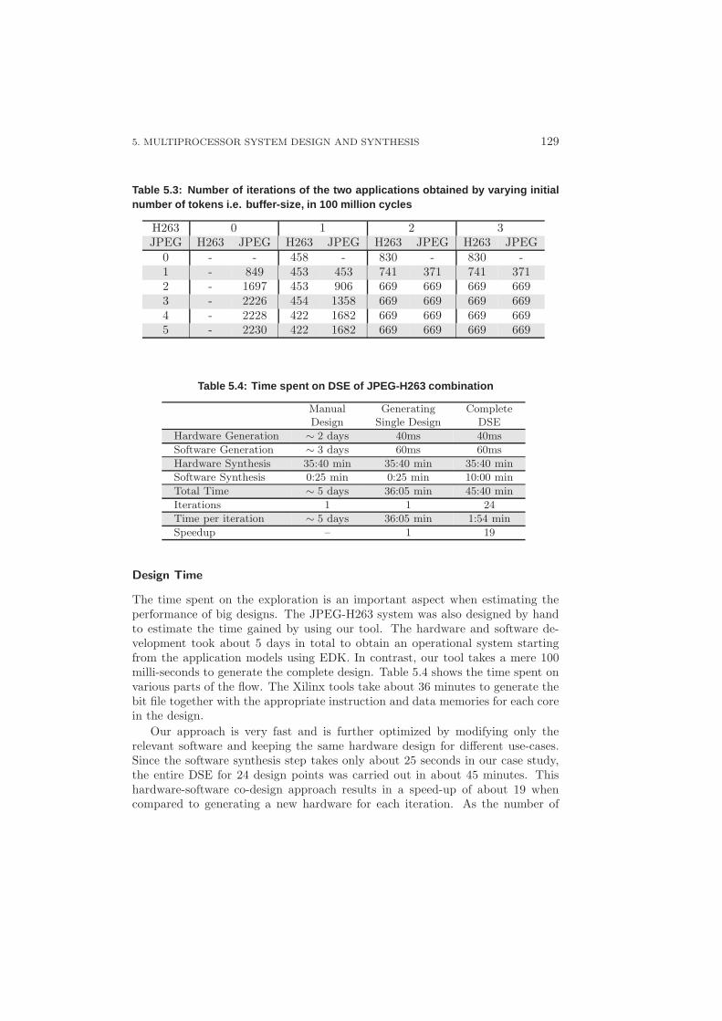
5. MULTIPROCESSOR SYSTEM DESIGN AND SYNTHESIS 129
Table 5.3: Number of iterations of the two applications obta ined by varying initialnumber of tokens i.e. buffer-size, in 100 million cycles
H263 0 1 2 3JPEG H263 JPEG H263 JPEG H263 JPEG H263 JPEG
0 - - 458 - 830 - 830 -1 - 849 453 453 741 371 741 3712 - 1697 453 906 669 669 669 6693 - 2226 454 1358 669 669 669 6694 - 2228 422 1682 669 669 669 6695 - 2230 422 1682 669 669 669 669
Table 5.4: Time spent on DSE of JPEG-H263 combination
Manual Generating CompleteDesign Single Design DSE
Hardware Generation ∼ 2 days 40ms 40ms
Software Generation ∼ 3 days 60ms 60ms
Hardware Synthesis 35:40 min 35:40 min 35:40 min
Software Synthesis 0:25 min 0:25 min 10:00 min
Total Time ∼ 5 days 36:05 min 45:40 min
Iterations 1 1 24
Time per iteration ∼ 5 days 36:05 min 1:54 min
Speedup – 1 19
Design Time
The time spent on the exploration is an important aspect when estimating theperformance of big designs. The JPEG-H263 system was also designed by handto estimate the time gained by using our tool. The hardware and software de-velopment took about 5 days in total to obtain an operational system startingfrom the application models using EDK. In contrast, our tool takes a mere 100milli-seconds to generate the complete design. Table 5.4 shows the time spent onvarious parts of the flow. The Xilinx tools take about 36 minutes to generate thebit file together with the appropriate instruction and data memories for each corein the design.
Our approach is very fast and is further optimized by modifying only therelevant software and keeping the same hardware design for different use-cases.Since the software synthesis step takes only about 25 seconds in our case study,the entire DSE for 24 design points was carried out in about 45 minutes. Thishardware-software co-design approach results in a speed-up of about 19 whencompared to generating a new hardware for each iteration. As the number of
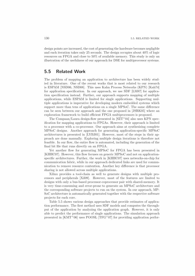
130 5.5. RELATED WORK
design points are increased, the cost of generating the hardware becomes negligibleand each iteration takes only 25 seconds. The design occupies about 40% of logicresources on FPGA and close to 50% of available memory. This study is only anillustration of the usefulness of our approach for DSE for multiprocessor systems.
5.5 Related Work
The problem of mapping an application to architecture has been widely stud-ied in literature. One of the recent works that is most related to our researchis ESPAM [NSD06, NSD08]. This uses Kahn Process Networks (KPN) [Kah74]for application specification. In our approach, we use SDF [LM87] for applica-tion specification instead. Further, our approach supports mapping of multipleapplications, while ESPAM is limited for single applications. Supporting mul-tiple applications is imperative for developing modern embedded systems whichsupport more than tens of applications on a single MPSoC. The same differencecan be seen between our approach and the one proposed in [JSRK05] where anexploration framework to build efficient FPGA multiprocessors is proposed.
The Compaan/Laura design-flow presented in [SZT+04] also uses KPN spec-ification for mapping applications to FPGAs. However, their approach is limitedto a processor with a co-processor. Our approach aims at synthesizing completeMPSoC designs. Another approach for generating application-specific MPSoCarchitectures is presented in [LYBJ01]. However, most of the steps in their ap-proach are done manually. Exploring multiple design iterations is therefore notfeasible. In our flow, the entire flow is automated, including the generation of thefinal bit file that runs directly on an FPGA.
Yet another flow for generating MPSoC for FPGA has been presented in[KHHC07]. However, this flow focuses on generic MPSoC and not on application-specific architectures. Further, the work in [KHHC07] uses networks-on-chip forcommunication fabric, while in our approach dedicated links are used for commu-nication to remove resource contention. Another key difference is that processorsharing is not allowed across multiple applications.
Xilinx provides a tool-chain as well to generate designs with multiple pro-cessors and peripherals [Xil09]. However, most of the features are limited todesigns with only a bus-based processor-coprocessor pair with shared-memory. Itis very time-consuming and error-prone to generate an MPSoC architecture andthe corresponding software projects to run on the system. In our approach, MP-SoC architecture is automatically generated together with the respective softwareprojects for each core.
Table 5.5 shows various design approaches that provide estimates of applica-tion performance. The first method uses SDF models and computes the through-put of the application by analyzing the application graph. However, it is onlyable to predict the performance of single applications. The simulation approachpresented in [KMT+06] uses POOSL [TFG+07] for providing application perfor-
5. MULTIPROCESSOR SYSTEM DESIGN AND SYNTHESIS 131
Table 5.5: Comparison of various approaches for providing p erformance estimates
SDF 3 [SGB06a] POOSL [KMT+06] ESPAM [NSD06] MAMPS
Approach Used Analysis Simulation FPGA FPGAModel Used SDF SDF KPN SDFSingle Appl Yes Yes Yes YesMultiple Appl No Yes No YesSpeed Fastest Slow Fast FastAccuracy Less High Highest HighestHard RT Guarantee Yes No No NoDedicated FIFO N. A. No No YesArbiter Support N. A. Yes N. A. YesC-support No No Yes Yes
mance estimates. This is more accurate than high level formal analysis since moredetails can be modeled and their effects are measured using simulations. ESPAMis closest to our approach as it also uses FPGA and supports functional descrip-tion(s) of application(s) in C. However, it does not support multiple applications.MAMPS supports multiple applications, and provides fast and accurate results.
5.6 Conclusions
In this chapter, a design-flow is presented to generate multiprocessor designs formultiple applications. The approach takes application(s) description(s) and pro-duces the corresponding MPSoC system. This is the first flow that allows mappingof multiple applications on a single platform. The tool developed using this flow ismade available online [MAM09]. The flow allows the designers to traverse the de-sign space quickly, thus making DSE of even concurrently executing applicationsfeasible. A case study is presented to find the trade-offs between the buffer-sizeand performance when JPEG and H263 execute concurrently on a platform.
However, the number of applications that can be concurrently mapped on theFPGA is limited by the hardware resources present. When synthesizing designswith applications of 8-10 actors and 12-15 channels, we found that it was difficultto map more than four applications simultaneously due to resource constraints,namely block RAMs. A bigger FPGA would certainly allow bigger designs to betested.

132 5.6. CONCLUSIONS
CHAPTER 6
Multiple Use-cases System Design
In the previous chapter, we have seen how to design and synthesize multiprocessorsystems for multiple applications. As has been motivated in the earlier chapters,not all applications are always active at the same time. Each combination ofsimultaneously active applications is defined as a use-case. For example, a mobilephone in one instant may be used to talk on the phone while surfing the web anddownloading some Java application in the background, and in another instant beused to listen to MP3 music while browsing JPEG pictures stored in the phone,and at the same time allow a remote device to access the files in the phone overa bluetooth connection.
The number of such potential use-cases is exponential in the number of appli-cations that are present in the system. The high demand of functionalities in suchdevices is leading to an increasing shift towards developing systems in softwareand programmable hardware in order to increase design flexibility. However, asingle configuration of this programmable hardware may not be able to supportthis large number of use-cases with low cost and power. We envision that futurecomplex embedded systems will be partitioned into several configurations and theappropriate configuration will be loaded into the reconfigurable platform on thefly as and when the use-cases are requested. This requires two major develop-ments at the research front: (1) a systematic design methodology for allowingmultiple use-cases to be merged on a single hardware configuration, and (2) amechanism to keep the number of hardware configurations as small as possible.More hardware configurations imply a higher cost since the configurations haveto be stored in the memory, and also lead to increased switching in the system.
133

134
In this chapter, we present a solution to the above-mentioned objectives. Fol-lowing are the key contributions of this chapter:
• Support for Multiple Use-cases: An algorithm for merging use-cases onto asingle (FPGA) hardware configuration such that multiple use-cases may besupported in a single configuration, while minimizing hardware resources.
• Partitioning Use-cases: When (FPGA) area constraints do not allow map-ping of all use-cases on one configuration, a methodology to partition use-cases in a way that the number of partitions (or configurations of FPGA)is minimized.
• Reducing Complexity: Use-case partitioning is an instance of the set-coveringproblem [CLRS01], which is known to be NP-hard. We propose efficientheuristics to solve this problem and compare their performance and com-plexity.
• Area Estimation: A technique that accurately predicts the resource require-ments on the target FPGA without going through the entire synthesis pro-cess, thereby saving DSE time.
• MPSoC Design Tool for FPGA: All of the above methods and algorithms areimplemented, such that the entire multi-processor system can be generatedfor the given application and use-case descriptions in a fully automated wayfor Xilinx FPGAs. Besides the hardware, the required software for each pro-cessor is also generated. The tool is available at www.es.ele.tue.nl/mamps/.
The above contributions are essential to further research in design automationcommunity since the embedded devices are increasingly becoming multi-featured.Our flow allows designers to generate MPSoC designs quickly for multiple use-cases and keep the number of hardware configurations to a minimum. Thoughthe flow is aimed at minimizing the number of partitions, it also generates allthe partitions and allows the designer to study the performance of all use-casesin an automated way. The designer can then tailor the partitions (e.g. changeprocessor-arbiters) to achieve better performance of all applications in a use-case.
While the flow is suitable for both design and evaluation, in this thesis wefocus on the suitability of our flow for evaluating whether all the applications canmeet their functional requirements in all the use-cases on FPGA. We present anumber of techniques to minimize the time spent in evaluation and design spaceexploration of the system. As before, we assume that applications are specifiedin the form of Synchronous Data Flow (SDF) graphs [LM87, SB00].
This chapter is organized as follows. Section 6.1 describes our approach ofmerging use-cases in a single hardware description, while Section 6.2 explainshow our partitioning approach splits the use-cases when not all of them can fitin one design. Section 6.3 explains how resource utilization is estimated with-out synthesis. Section 6.4 presents results of experiments done to evaluate our
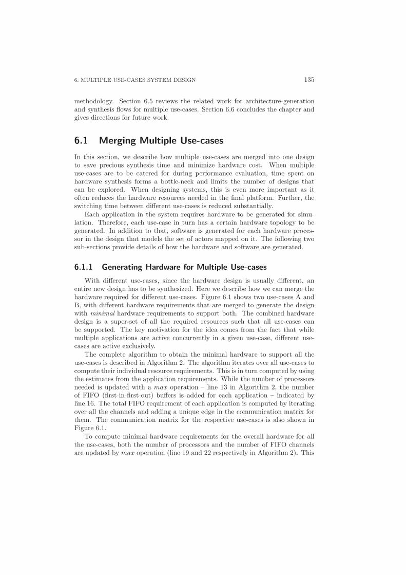
6. MULTIPLE USE-CASES SYSTEM DESIGN 135
methodology. Section 6.5 reviews the related work for architecture-generationand synthesis flows for multiple use-cases. Section 6.6 concludes the chapter andgives directions for future work.
6.1 Merging Multiple Use-cases
In this section, we describe how multiple use-cases are merged into one designto save precious synthesis time and minimize hardware cost. When multipleuse-cases are to be catered for during performance evaluation, time spent onhardware synthesis forms a bottle-neck and limits the number of designs thatcan be explored. When designing systems, this is even more important as itoften reduces the hardware resources needed in the final platform. Further, theswitching time between different use-cases is reduced substantially.
Each application in the system requires hardware to be generated for simu-lation. Therefore, each use-case in turn has a certain hardware topology to begenerated. In addition to that, software is generated for each hardware proces-sor in the design that models the set of actors mapped on it. The following twosub-sections provide details of how the hardware and software are generated.
6.1.1 Generating Hardware for Multiple Use-cases
With different use-cases, since the hardware design is usually different, anentire new design has to be synthesized. Here we describe how we can merge thehardware required for different use-cases. Figure 6.1 shows two use-cases A andB, with different hardware requirements that are merged to generate the designwith minimal hardware requirements to support both. The combined hardwaredesign is a super-set of all the required resources such that all use-cases canbe supported. The key motivation for the idea comes from the fact that whilemultiple applications are active concurrently in a given use-case, different use-cases are active exclusively.
The complete algorithm to obtain the minimal hardware to support all theuse-cases is described in Algorithm 2. The algorithm iterates over all use-cases tocompute their individual resource requirements. This is in turn computed by usingthe estimates from the application requirements. While the number of processorsneeded is updated with a max operation – line 13 in Algorithm 2, the numberof FIFO (first-in-first-out) buffers is added for each application – indicated byline 16. The total FIFO requirement of each application is computed by iteratingover all the channels and adding a unique edge in the communication matrix forthem. The communication matrix for the respective use-cases is also shown inFigure 6.1.
To compute minimal hardware requirements for the overall hardware for allthe use-cases, both the number of processors and the number of FIFO channelsare updated by max operation (line 19 and 22 respectively in Algorithm 2). This
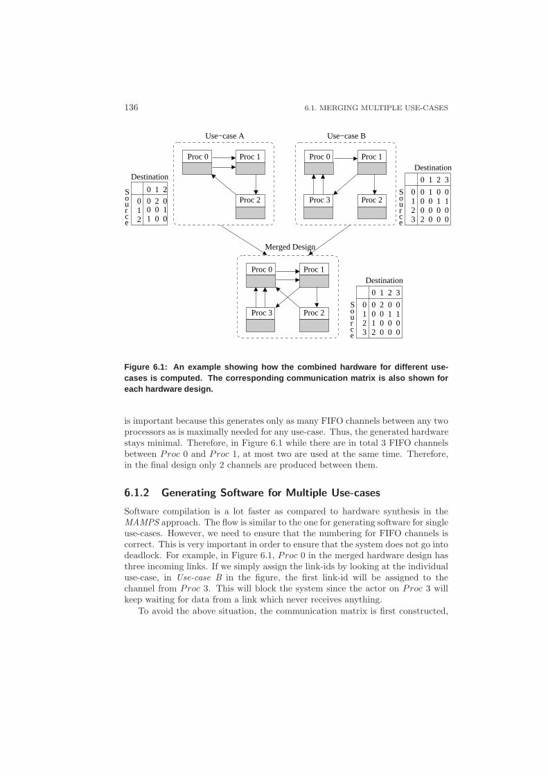
136 6.1. MERGING MULTIPLE USE-CASES
0 2 00 0 1
0 1 2
012 1 0 0
0 1 2 3
0 2 0 0
2 0 0 01 0 0 00 0 1 1
0123
Source
Source
Source
0 1 2 3
0 1 0 0
2 0 0 00 0 0 00 0 1 1
0123
Proc 0 Proc 1
Proc 2Proc 3
Proc 0 Proc 1
Proc 2
Proc 0 Proc 1
Proc 2Proc 3
Use−case BUse−case A
Merged Design
Destination
DestinationDestination
Figure 6.1: An example showing how the combined hardware for different use-cases is computed. The corresponding communication matrix is also shown foreach hardware design.
is important because this generates only as many FIFO channels between any twoprocessors as is maximally needed for any use-case. Thus, the generated hardwarestays minimal. Therefore, in Figure 6.1 while there are in total 3 FIFO channelsbetween Proc 0 and Proc 1, at most two are used at the same time. Therefore,in the final design only 2 channels are produced between them.
6.1.2 Generating Software for Multiple Use-cases
Software compilation is a lot faster as compared to hardware synthesis in theMAMPS approach. The flow is similar to the one for generating software for singleuse-cases. However, we need to ensure that the numbering for FIFO channels iscorrect. This is very important in order to ensure that the system does not go intodeadlock. For example, in Figure 6.1, Proc 0 in the merged hardware design hasthree incoming links. If we simply assign the link-ids by looking at the individualuse-case, in Use-case B in the figure, the first link-id will be assigned to thechannel from Proc 3. This will block the system since the actor on Proc 3 willkeep waiting for data from a link which never receives anything.
To avoid the above situation, the communication matrix is first constructed,
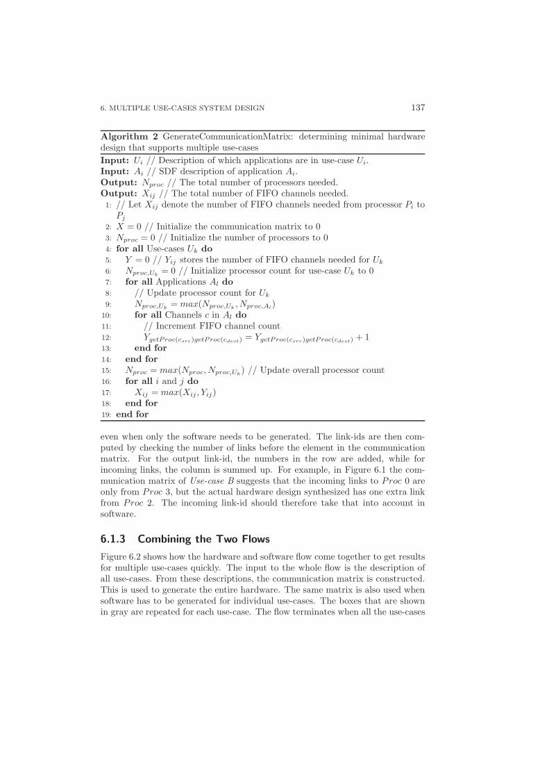
6. MULTIPLE USE-CASES SYSTEM DESIGN 137
Algorithm 2 GenerateCommunicationMatrix: determining minimal hardwaredesign that supports multiple use-cases
Input: Ui // Description of which applications are in use-case Ui.Input: Ai // SDF description of application Ai.Output: Nproc // The total number of processors needed.Output: Xij // The total number of FIFO channels needed.1: // Let Xij denote the number of FIFO channels needed from processor Pi to
Pj
2: X = 0 // Initialize the communication matrix to 03: Nproc = 0 // Initialize the number of processors to 04: for all Use-cases Uk do
5: Y = 0 // Yij stores the number of FIFO channels needed for Uk
6: Nproc,Uk= 0 // Initialize processor count for use-case Uk to 0
7: for all Applications Al do
8: // Update processor count for Uk
9: Nproc,Uk= max(Nproc,Uk
, Nproc,Al)
10: for all Channels c in Al do
11: // Increment FIFO channel count12: YgetProc(csrc)getProc(cdest) = YgetProc(csrc)getProc(cdest) + 113: end for
14: end for
15: Nproc = max(Nproc, Nproc,Uk) // Update overall processor count
16: for all i and j do
17: Xij = max(Xij , Yij)18: end for
19: end for
even when only the software needs to be generated. The link-ids are then com-puted by checking the number of links before the element in the communicationmatrix. For the output link-id, the numbers in the row are added, while forincoming links, the column is summed up. For example, in Figure 6.1 the com-munication matrix of Use-case B suggests that the incoming links to Proc 0 areonly from Proc 3, but the actual hardware design synthesized has one extra linkfrom Proc 2. The incoming link-id should therefore take that into account insoftware.
6.1.3 Combining the Two Flows
Figure 6.2 shows how the hardware and software flow come together to get resultsfor multiple use-cases quickly. The input to the whole flow is the description ofall use-cases. From these descriptions, the communication matrix is constructed.This is used to generate the entire hardware. The same matrix is also used whensoftware has to be generated for individual use-cases. The boxes that are shownin gray are repeated for each use-case. The flow terminates when all the use-cases
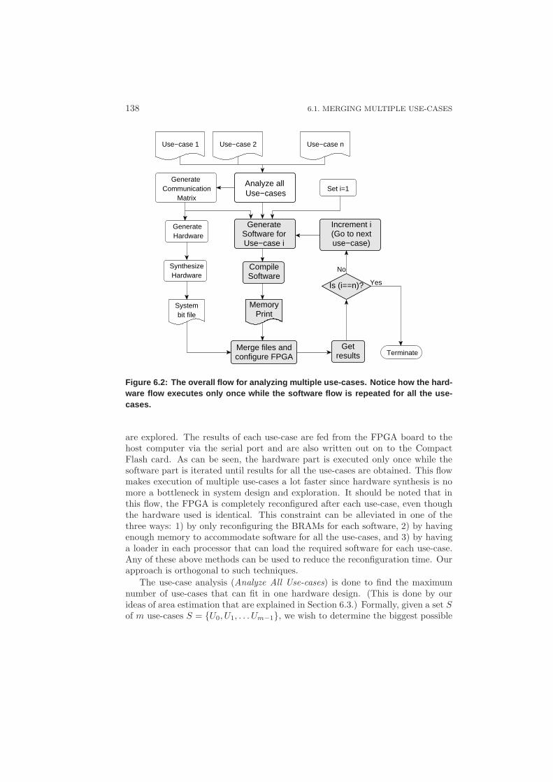
138 6.1. MERGING MULTIPLE USE-CASES
Is (i==n)?
configure FPGAMerge files and
Increment i(Go to nextuse−case)
Generate
Use−case iSoftware for
SoftwareCompile
Getresults
Systembit file
SynthesizeHardware
Generate Hardware
Generate Communication
Matrix
Analyze all Use−cases
PrintMemory
Use−case n
No
Yes
Use−case 1 Use−case 2
Set i=1
Terminate
Figure 6.2: The overall flow for analyzing multiple use-case s. Notice how the hard-ware flow executes only once while the software flow is repeate d for all the use-cases.
are explored. The results of each use-case are fed from the FPGA board to thehost computer via the serial port and are also written out on to the CompactFlash card. As can be seen, the hardware part is executed only once while thesoftware part is iterated until results for all the use-cases are obtained. This flowmakes execution of multiple use-cases a lot faster since hardware synthesis is nomore a bottleneck in system design and exploration. It should be noted that inthis flow, the FPGA is completely reconfigured after each use-case, even thoughthe hardware used is identical. This constraint can be alleviated in one of thethree ways: 1) by only reconfiguring the BRAMs for each software, 2) by havingenough memory to accommodate software for all the use-cases, and 3) by havinga loader in each processor that can load the required software for each use-case.Any of these above methods can be used to reduce the reconfiguration time. Ourapproach is orthogonal to such techniques.
The use-case analysis (Analyze All Use-cases) is done to find the maximumnumber of use-cases that can fit in one hardware design. (This is done by ourideas of area estimation that are explained in Section 6.3.) Formally, given a set Sof m use-cases S = {U0, U1, . . . Um−1}, we wish to determine the biggest possible
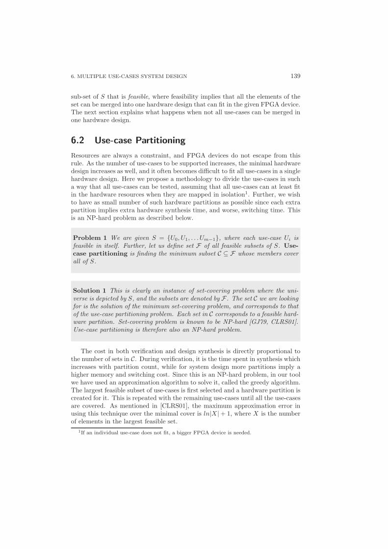
6. MULTIPLE USE-CASES SYSTEM DESIGN 139
sub-set of S that is feasible, where feasibility implies that all the elements of theset can be merged into one hardware design that can fit in the given FPGA device.The next section explains what happens when not all use-cases can be merged inone hardware design.
6.2 Use-case Partitioning
Resources are always a constraint, and FPGA devices do not escape from thisrule. As the number of use-cases to be supported increases, the minimal hardwaredesign increases as well, and it often becomes difficult to fit all use-cases in a singlehardware design. Here we propose a methodology to divide the use-cases in sucha way that all use-cases can be tested, assuming that all use-cases can at least fitin the hardware resources when they are mapped in isolation1. Further, we wishto have as small number of such hardware partitions as possible since each extrapartition implies extra hardware synthesis time, and worse, switching time. Thisis an NP-hard problem as described below.
Problem 1 We are given S = {U0, U1, . . . Um−1}, where each use-case Ui isfeasible in itself. Further, let us define set F of all feasible subsets of S. Use-
case partitioning is finding the minimum subset C ⊆ F whose members coverall of S.
Solution 1 This is clearly an instance of set-covering problem where the uni-verse is depicted by S, and the subsets are denoted by F . The set C we are lookingfor is the solution of the minimum set-covering problem, and corresponds to thatof the use-case partitioning problem. Each set in C corresponds to a feasible hard-ware partition. Set-covering problem is known to be NP-hard [GJ79, CLRS01].Use-case partitioning is therefore also an NP-hard problem.
The cost in both verification and design synthesis is directly proportional tothe number of sets in C. During verification, it is the time spent in synthesis whichincreases with partition count, while for system design more partitions imply ahigher memory and switching cost. Since this is an NP-hard problem, in our toolwe have used an approximation algorithm to solve it, called the greedy algorithm.The largest feasible subset of use-cases is first selected and a hardware partition iscreated for it. This is repeated with the remaining use-cases until all the use-casesare covered. As mentioned in [CLRS01], the maximum approximation error inusing this technique over the minimal cover is ln|X |+ 1, where X is the numberof elements in the largest feasible set.
1If an individual use-case does not fit, a bigger FPGA device is needed.
140 6.2. USE-CASE PARTITIONING
Applications Set of Use-cases S Feasible subsets F Potential Partitions
A0: H263 EncA1: H263 DecA2: JPEG DecA3: MP3 DecA4: ModemA5: Voice Call
U0 = {A0, A1, A4}U1 = {A0, A1, A5}U2 = {A2, A3, A4}U3 = {A0, A4}U4 = {A2, A4, A5}
f0 = {U0, U1}f1 = {U0, U2}f2 = {U1, U2}f3 = {U1, U3, U4}f4 = {U2, U3}f5 = {U2, U4}
{f0, f1, f4, f5}{f0, f3, f4}{f1, f2, f3}{f1, f3}
Figure 6.3: Putting applications, use-cases and feasible p artitions in perspective.
Figure 6.3 helps in understanding the partitioning problem better and providesa good perspective of the hierarchy of sets. The first box shows the applicationsthat need to run on the platform. These are some of the applications that runon a mobile phone. The next box shows some of the use-cases that are typical,e.g. U1 represents a video-call that requires video encoding, video decoding andregular voice call. As mentioned earlier, a use-case is a set of applications thatrun concurrently. The next box shows the family of sets F , each of which isfeasible. For simplicity only a part of F is shown in the figure. Clearly, thesubsets of elements of F are also feasible e.g. when f3 is feasible, so is {U3, U4}.Therefore, we should only include maximal subsets; F − i is maximal if we cannotadd any other use-case. As often the case, no feasible-set exists which containsall the use-cases. Therefore, a subset C ⊆ F needs to be chosen such that all theuse-cases are covered in this subset. A few of such possible subsets are shown inthe last box. The last option is preferred over the rest since it provides only twopartitions.
6.2.1 Hitting the Complexity Wall
In order to be able to implement the greedy algorithm, we still need to be able todetermine the largest feasible set. This poses a big problem in terms of implemen-tation. The total number of possible sets grows exponentially with the number ofuse-cases. Suppose, we have 8 applications in the system, and every combinationof them is possible, we have 255 use-cases overall. Since each use-case can eitherbe in the set or not, we obtain a total of 2255 sets. Each set then needs to be ex-amined whether it is feasible or not – this takes linear time in size of the set, whichcan in the worst case be the number of applications in the system. Thus, a systemwith N applications and M possible use-cases, has a complexity of O(N.2M ) tofind the largest feasible set. In the worst-case, the number of use-cases is alsoexponential, i.e. M = 2N − 1. We see how the design-space becomes infeasible toexplore. In Section 6.4 we see some results of actual execution times.
6. MULTIPLE USE-CASES SYSTEM DESIGN 141
6.2.2 Reducing the Execution time
Here we present some measures to reduce the execution time. The followingapproaches do not reduce the complexity of the algorithm, but may provide sig-nificant reduction in execution time.
1. Identify infeasible use-cases: Our intention is to be able to analyze all theuse-cases that we can with our given hardware resources. Identifying theinfeasible use-cases reduces the potential set of use-cases.
2. Reduce feasible use-cases: This method identifies all the use-cases that areproper subsets of feasible use-cases – such use-cases are defined as trivial,while the ones that are not included in any other feasible use-case are de-fined as non-trivial. When a use-case is feasible, all its sub-sets are alsofeasible. Formally, if a use-case Ui is a subset of Uj , the minimal hardwareneeded for Uj is sufficient for Ui. (A proper subset here implies that all theapplications executing concurrently in Ui are also executing in Uj , thoughthe inverse is not true.) In other words, any partition that supports use-caseUj will also support Ui. It should be noted however that the performanceof applications in these two use-cases may not be the same due to differentset of applications active, and therefore it might be required to evaluateperformance of both use-cases.
These approaches are very effective and may significantly reduce the numberof feasible use-cases left for analysis. With a scenario of 10 randomly generatedapplications and 1023 use-cases (considering all the possibilities), we found thatonly 853 were feasible2. The reduction technique further reduced the number ofnon-trivial use-cases to 178. The above approaches reduce the execution time butdo not help in dealing with complexity. However, the optimality of the solution(in generation of feasible sets, not in the set-cover) is maintained.
6.2.3 Reducing Complexity
In this section, we propose a simple heuristic to compute the partitions. Thisheuristic reduces the complexity significantly albeit at the cost of optimality. Asmentioned earlier, the greedy approach of partitioning requires to compute thelargest feasible set. Since computing the largest set has a high complexity, wehave an alternative implementation which simply gives the first partition thatincludes the first non-included use-case, and scans the whole list to check whichuse-cases can be added such that the set remains feasible. The algorithm isshown in Algorithm 3. An array is maintained to check which use-cases are notyet included in any partition (UseCaseDone). Infeasible use-cases are indicatedin line 6 in the algorithm. Use-cases are then reduced by considering only the
2This depends on the available hardware resources. On our FPGA platform only 853 werefeasible.
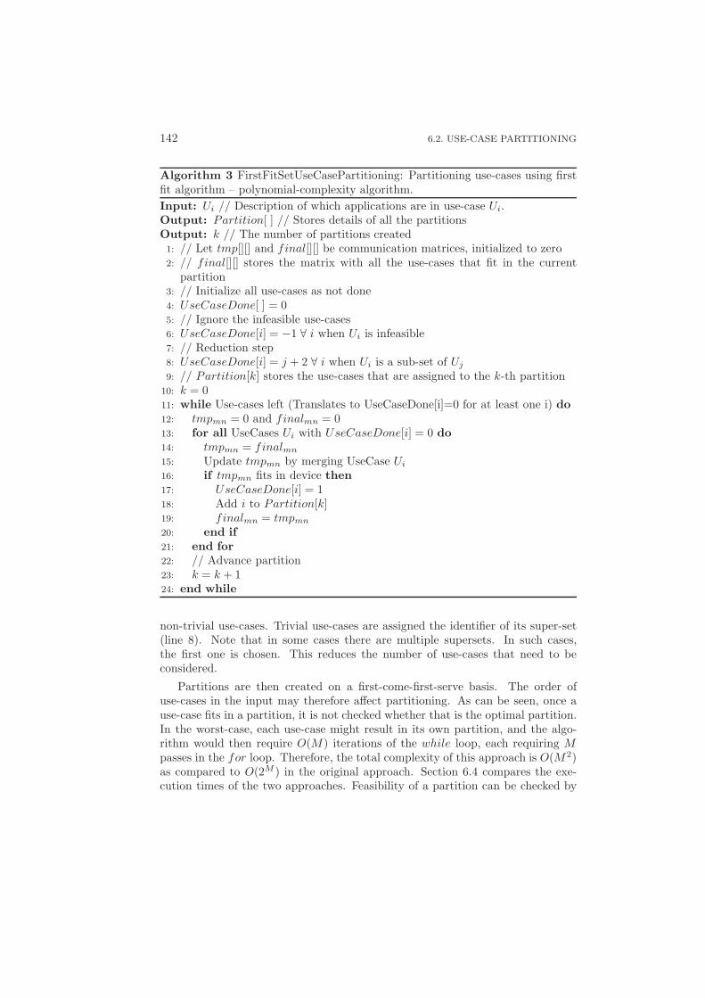
142 6.2. USE-CASE PARTITIONING
Algorithm 3 FirstFitSetUseCasePartitioning: Partitioning use-cases using firstfit algorithm – polynomial-complexity algorithm.
Input: Ui // Description of which applications are in use-case Ui.Output: Partition[ ] // Stores details of all the partitionsOutput: k // The number of partitions created1: // Let tmp[][] and final[][] be communication matrices, initialized to zero2: // final[][] stores the matrix with all the use-cases that fit in the current
partition3: // Initialize all use-cases as not done4: UseCaseDone[ ] = 05: // Ignore the infeasible use-cases6: UseCaseDone[i] = −1 ∀ i when Ui is infeasible7: // Reduction step8: UseCaseDone[i] = j + 2 ∀ i when Ui is a sub-set of Uj
9: // Partition[k] stores the use-cases that are assigned to the k-th partition10: k = 011: while Use-cases left (Translates to UseCaseDone[i]=0 for at least one i) do
12: tmpmn = 0 and finalmn = 013: for all UseCases Ui with UseCaseDone[i] = 0 do
14: tmpmn = finalmn
15: Update tmpmn by merging UseCase Ui
16: if tmpmn fits in device then
17: UseCaseDone[i] = 118: Add i to Partition[k]19: finalmn = tmpmn
20: end if
21: end for
22: // Advance partition23: k = k + 124: end while
non-trivial use-cases. Trivial use-cases are assigned the identifier of its super-set(line 8). Note that in some cases there are multiple supersets. In such cases,the first one is chosen. This reduces the number of use-cases that need to beconsidered.
Partitions are then created on a first-come-first-serve basis. The order ofuse-cases in the input may therefore affect partitioning. As can be seen, once ause-case fits in a partition, it is not checked whether that is the optimal partition.In the worst-case, each use-case might result in its own partition, and the algo-rithm would then require O(M) iterations of the while loop, each requiring Mpasses in the for loop. Therefore, the total complexity of this approach is O(M2)as compared to O(2M ) in the original approach. Section 6.4 compares the exe-cution times of the two approaches. Feasibility of a partition can be checked by
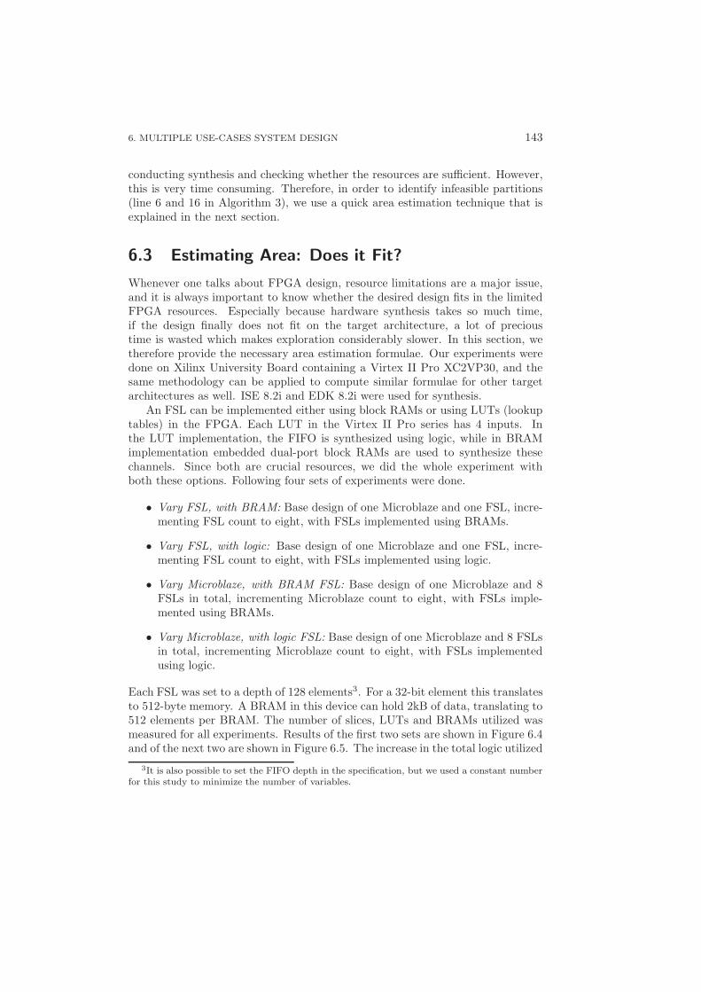
6. MULTIPLE USE-CASES SYSTEM DESIGN 143
conducting synthesis and checking whether the resources are sufficient. However,this is very time consuming. Therefore, in order to identify infeasible partitions(line 6 and 16 in Algorithm 3), we use a quick area estimation technique that isexplained in the next section.
6.3 Estimating Area: Does it Fit?
Whenever one talks about FPGA design, resource limitations are a major issue,and it is always important to know whether the desired design fits in the limitedFPGA resources. Especially because hardware synthesis takes so much time,if the design finally does not fit on the target architecture, a lot of precioustime is wasted which makes exploration considerably slower. In this section, wetherefore provide the necessary area estimation formulae. Our experiments weredone on Xilinx University Board containing a Virtex II Pro XC2VP30, and thesame methodology can be applied to compute similar formulae for other targetarchitectures as well. ISE 8.2i and EDK 8.2i were used for synthesis.
An FSL can be implemented either using block RAMs or using LUTs (lookuptables) in the FPGA. Each LUT in the Virtex II Pro series has 4 inputs. Inthe LUT implementation, the FIFO is synthesized using logic, while in BRAMimplementation embedded dual-port block RAMs are used to synthesize thesechannels. Since both are crucial resources, we did the whole experiment withboth these options. Following four sets of experiments were done.
• Vary FSL, with BRAM: Base design of one Microblaze and one FSL, incre-menting FSL count to eight, with FSLs implemented using BRAMs.
• Vary FSL, with logic: Base design of one Microblaze and one FSL, incre-menting FSL count to eight, with FSLs implemented using logic.
• Vary Microblaze, with BRAM FSL: Base design of one Microblaze and 8FSLs in total, incrementing Microblaze count to eight, with FSLs imple-mented using BRAMs.
• Vary Microblaze, with logic FSL: Base design of one Microblaze and 8 FSLsin total, incrementing Microblaze count to eight, with FSLs implementedusing logic.
Each FSL was set to a depth of 128 elements3. For a 32-bit element this translatesto 512-byte memory. A BRAM in this device can hold 2kB of data, translating to512 elements per BRAM. The number of slices, LUTs and BRAMs utilized wasmeasured for all experiments. Results of the first two sets are shown in Figure 6.4and of the next two are shown in Figure 6.5. The increase in the total logic utilized
3It is also possible to set the FIFO depth in the specification, but we used a constant numberfor this study to minimize the number of variables.
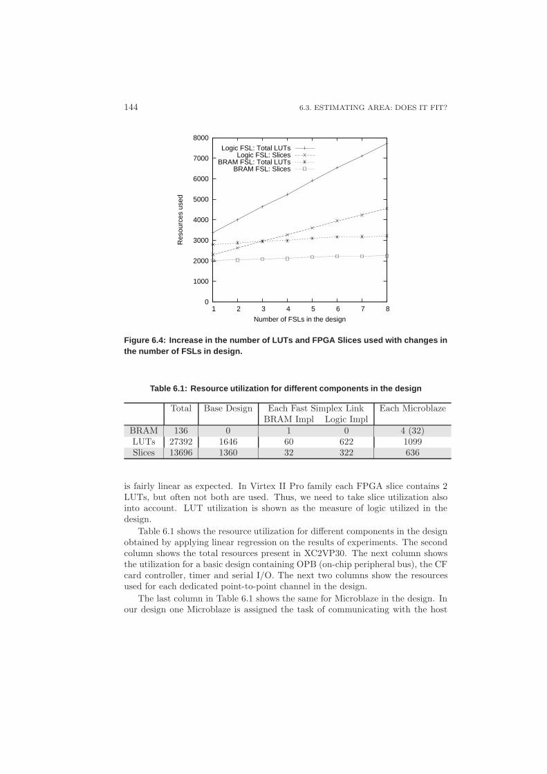
144 6.3. ESTIMATING AREA: DOES IT FIT?
0
1000
2000
3000
4000
5000
6000
7000
8000
1 2 3 4 5 6 7 8
Res
ourc
es u
sed
Number of FSLs in the design
Logic FSL: Total LUTsLogic FSL: Slices
BRAM FSL: Total LUTsBRAM FSL: Slices
Figure 6.4: Increase in the number of LUTs and FPGA Slices use d with changes inthe number of FSLs in design.
Table 6.1: Resource utilization for different components i n the design
Total Base Design Each Fast Simplex Link Each MicroblazeBRAM Impl Logic Impl
BRAM 136 0 1 0 4 (32)LUTs 27392 1646 60 622 1099Slices 13696 1360 32 322 636
is fairly linear as expected. In Virtex II Pro family each FPGA slice contains 2LUTs, but often not both are used. Thus, we need to take slice utilization alsointo account. LUT utilization is shown as the measure of logic utilized in thedesign.
Table 6.1 shows the resource utilization for different components in the designobtained by applying linear regression on the results of experiments. The secondcolumn shows the total resources present in XC2VP30. The next column showsthe utilization for a basic design containing OPB (on-chip peripheral bus), the CFcard controller, timer and serial I/O. The next two columns show the resourcesused for each dedicated point-to-point channel in the design.
The last column in Table 6.1 shows the same for Microblaze in the design. Inour design one Microblaze is assigned the task of communicating with the host
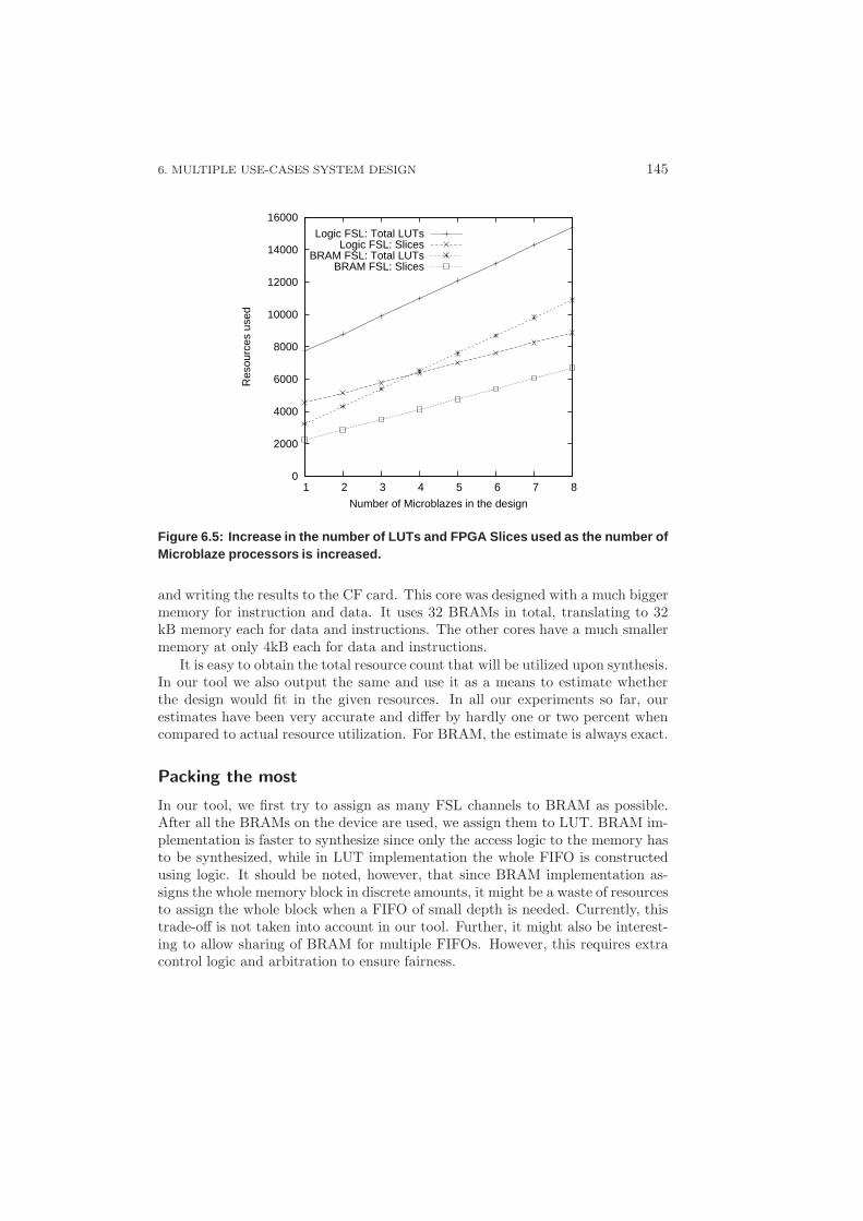
6. MULTIPLE USE-CASES SYSTEM DESIGN 145
0
2000
4000
6000
8000
10000
12000
14000
16000
1 2 3 4 5 6 7 8
Res
ourc
es u
sed
Number of Microblazes in the design
Logic FSL: Total LUTsLogic FSL: Slices
BRAM FSL: Total LUTsBRAM FSL: Slices
Figure 6.5: Increase in the number of LUTs and FPGA Slices use d as the number ofMicroblaze processors is increased.
and writing the results to the CF card. This core was designed with a much biggermemory for instruction and data. It uses 32 BRAMs in total, translating to 32kB memory each for data and instructions. The other cores have a much smallermemory at only 4kB each for data and instructions.
It is easy to obtain the total resource count that will be utilized upon synthesis.In our tool we also output the same and use it as a means to estimate whetherthe design would fit in the given resources. In all our experiments so far, ourestimates have been very accurate and differ by hardly one or two percent whencompared to actual resource utilization. For BRAM, the estimate is always exact.
Packing the most
In our tool, we first try to assign as many FSL channels to BRAM as possible.After all the BRAMs on the device are used, we assign them to LUT. BRAM im-plementation is faster to synthesize since only the access logic to the memory hasto be synthesized, while in LUT implementation the whole FIFO is constructedusing logic. It should be noted, however, that since BRAM implementation as-signs the whole memory block in discrete amounts, it might be a waste of resourcesto assign the whole block when a FIFO of small depth is needed. Currently, thistrade-off is not taken into account in our tool. Further, it might also be interest-ing to allow sharing of BRAM for multiple FIFOs. However, this requires extracontrol logic and arbitration to ensure fairness.
146 6.4. EXPERIMENTS AND RESULTS
6.4 Experiments and Results
In this section, we present some of the results that were obtained by implementingseveral real and randomly-generated application SDF graphs. Here we show thatour flow reduces the implementation gap between system level and RTL leveldesign, and allows for more accurate performance evaluation using an emulationplatform compared to simulation [TFG+07] and analysis. Further, we see howour use-case partitioning approach minimizes the number of hardware designs bystudying an example of applications running in a high-end mobile phone.
Our implementation platform is the Xilinx XUP Virtex II Pro DevelopmentBoard with an xc2vp30 FPGA on-board. Xilinx EDK 8.2i and ISE 8.2i were usedfor synthesis and implementation. All tools run on a Pentium 4 Core at 3GHzwith 1GB of RAM.
6.4.1 Use-case Partitioning
In this section, we show the effectiveness of our approach to partition use-cases,and the heuristics to optimize on the execution time. This is demonstrated firstusing some random test cases and then with a case study involving applicationsin a mobile phone.
Using 10 random application SDF models, we generated all possible combi-nations giving a total of 1023 use-cases. We found that only 853 of these werefeasible; the rest required more resources than were present on our FPGA device.In general, most use-cases of up to 6 applications could fit on the FPGA, whileonly a couple of use-cases with 7 applications were feasible.
When trying to compute partitions using the greedy method directly on these853 use-cases, the algorithm terminated after 30 minutes without any result sincethere were too many sets to consider. When using the first-fit heuristic on theseuse-cases we obtained a total of 145 partitions in 500 milli-seconds. However,since this approach is dependent on the order of use-cases, another order gave usa partition count of 126 in about 400 milli-seconds. After applying our reductiontechnique on feasible use-cases, 178 non-trivial use-cases were obtained. Thegreedy approach on these use-cases terminated in 3.3 seconds and resulted in 112partitions. The first-fit heuristic on the non-trivial cases took 300 milli-secondsand gave 125 partitions, while another order of use-cases gave 116 partitions inabout the same time.
A couple of observations can be made from this. Our techniques of use-casereduction are very effective in pruning the search space. Up to 80% of the use-cases are pruned away as trivial. This is essential in this case for example, whenotherwise no results are obtained for greedy. We observe that while the first-fitheuristic is a lot faster, the results depend heavily on the order of input use-cases. However, if the search space is large, first-fit may be the only heuristic forobtaining results.
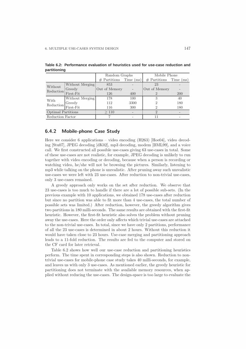
6. MULTIPLE USE-CASES SYSTEM DESIGN 147
Table 6.2: Performance evaluation of heuristics used for us e-case reduction andpartitioning
Random Graphs Mobile Phone# Partitions Time (ms) # Partitions Time (ms)
Without Merging 853 - 23 -Without
Greedy Out of Memory - Out of Memory -Reduction
First-Fit 126 400 2 200
Without Merging 178 100 3 40With
Greedy 112 3300 2 180Reduction
First-Fit 116 300 2 180
Optimal Partitions ≥ 110 - 2 -
Reduction Factor 7 - 11 -
6.4.2 Mobile-phone Case Study
Here we consider 6 applications – video encoding (H263) [Hoe04], video decod-ing [Stu07], JPEG decoding [dK02], mp3 decoding, modem [BML99], and a voicecall. We first constructed all possible use-cases giving 63 use-cases in total. Someof these use-cases are not realistic, for example, JPEG decoding is unlikely to runtogether with video encoding or decoding, because when a person is recording orwatching video, he/she will not be browsing the pictures. Similarly, listening tomp3 while talking on the phone is unrealistic. After pruning away such unrealisticuse-cases we were left with 23 use-cases. After reduction to non-trivial use-cases,only 3 use-cases remained.
A greedy approach only works on the set after reduction. We observe that23 use-cases is too much to handle if there are a lot of possible sub-sets. (In theprevious example with 10 applications, we obtained 178 use-cases after reductionbut since no partition was able to fit more than 4 use-cases, the total number ofpossible sets was limited.) After reduction, however, the greedy algorithm givestwo partitions in 180 milli-seconds. The same results are obtained with the first-fitheuristic. However, the first-fit heuristic also solves the problem without pruningaway the use-cases. Here the order only affects which trivial use-cases are attachedto the non-trivial use-cases. In total, since we have only 2 partitions, performanceof all the 23 use-cases is determined in about 2 hours. Without this reduction itwould have taken close to 23 hours. Use-case merging and partitioning approachleads to a 11-fold reduction. The results are fed to the computer and stored onthe CF card for later retrieval.
Table 6.2 shows how well our use-case reduction and partitioning heuristicsperform. The time spent in corresponding steps is also shown. Reduction to non-trivial use-cases for mobile-phone case study takes 40 milli-seconds, for example,and leaves us with only 3 use-cases. As mentioned earlier, the greedy heuristic forpartitioning does not terminate with the available memory resources, when ap-plied without reducing the use-cases. The design-space is too large to evaluate the
148 6.5. RELATED WORK
largest feasible set. After reducing to non-feasible use-cases for random-graphs,we obtain 178 use-cases and at most 4 use-cases fit in any partition. Since themaximum error in using the greedy approach is given by ln|X |+1, where X is thenumber of elements in the largest partition, we get a maximum error of ln|4|+ 1i.e. 2.38. We can therefore be sure that the minimum number of partitions is atleast 110. We see a 7-fold reduction in the number of hardware configurations inthe random-graphs use-case and about 11-fold in the mobile phone case study.Therefore, we can conclude that our heuristics of use-case reduction and parti-tion are very effective in reducing the design time and in reducing the number ofpartitions.
Reconfiguration Time
The time to reconfigure an FPGA varies with the size of configuration file andthe mode of reconfiguration. For Virtex II Pro 30, the configuration file is about11 Mbits. The used CF card controller provides configuration bandwidth of 30Mbit/s, translating to about 370 milli-seconds for reconfiguration. Configuringthrough the on-board programmable memory is a lot faster since it provides band-width of up to 800 Mbit/s. Thus, for the above FPGA device it takes only about13 milli-seconds. The USB connection is a lot slower, and often takes about 8seconds. However, for the end-design, we expect the configurations to be storedin a programmable memory on board that are retrieved as and when use-casesare enabled. A typical mobile-phone user is unlikely to start a new use-casemore than once every few minutes. Therefore, the reconfiguration overhead of 13milli-seconds is not significantly large, and is amortized over the duration of theuse-case.
6.5 Related Work
The multiple use-case concept is relatively new to the MPSoC, and one of therelated research done is presented in [MCR+06]. However, this focuses on sup-porting multiple use-cases for the communication infrastructure, in particularnetwork-on-chip. Our flow is mainly targeted towards supporting multiple use-cases from computation perspective. In addition, we generate dedicated point-to-point connections for all the use-cases that are to be supported. It should bementioned that links are shared across use-cases but not within the use-case.
Our definition of a use-case is similar to what is defined as a scenario in [PTB06].The authors in [PTB06] motivate the use of a scenario-oriented (or use-case in ourpaper) design flow for heterogeneous MPSoC platforms. Our approach providesone such design flow where designers can study the performance of all use-casesin an automated way and tune the architecture to achieve better performanceof all applications in a use-case. The biggest advantage of our approach is thatwe provide a real synthesized MPSoC platform for designers to play with and
6. MULTIPLE USE-CASES SYSTEM DESIGN 149
measure performance. Further, in [PTB06] the architecture is provided as an in-put and is static, while we generate platforms given the application and use-casedescriptions and the architecture is changed (reconfigured) dynamically for thedifferent use-cases.
6.6 Conclusions
In this chapter, we propose a design-flow to generate architecture designs formultiple use-cases. Our approach takes the description of multiple use-cases andproduces the corresponding MPSoC platform. A use-case is defined as a set ofapplications active concurrently. This is the first flow that allows mapping ofmultiple use-cases on a single platform. We propose techniques to merge and par-tition use-cases in order to minimize hardware requirements. The tool developedusing this flow is made available online, and a stand-alone GUI tool is developedfor both Windows and Linux. The flow allows the designers to traverse the de-sign space quickly, thus making DSE of even concurrently executing applicationsfeasible. The heuristics used for use-case merging and partitioning reduce thedesign-exploration time 11-fold in a case study with mobile phone applications.
Further, we provide techniques to estimate resource utilization in an FPGAwithout carrying out the actual synthesis. This saves precious time during DSEand is very accurate as verified by the results. Our approach is also capable ofminimizing the number of reconfigurations in the system. The use-case partition-ing algorithm can be adapted to consider the relative frequency of the use of eachuse-case. The use-cases should be first sorted in the decreasing order of their use,and then the first-fit algorithm proposed in an earlier section should be applied.The algorithm will therefore first pack all the most frequently used use-cases to-gether in one hardware partition, thereby reducing the reconfiguration from onefrequently used use-case into another. However, for an optimal solution of thepartition problem, many other parameters need to be taken into account, for ex-ample, reconfiguration time and average duration for each use-case. We wouldlike to extend the use-case partitioning algorithm to take the exact reconfigurationoverhead into account.
We would also like to develop and automate more ways of design space explo-ration, for example trying different mappings of applications. We would also liketo try different kinds of arbiters in the design to improve fairness and allow forload-balancing between multiple applications.

150 6.6. CONCLUSIONS
CHAPTER 7
Conclusions and Future Work
In this chapter, the major conclusions from this thesis are presented, togetherwith several issues that remain to be solved.
7.1 Conclusions
The design of multimedia platforms is becoming increasingly more complex. Mod-ern multimedia systems need to support a large number of applications or func-tions in a single device. To achieve high performance in such systems, more andmore processors are being integrated into a single chip to build Multi-ProcessorSystems-on-Chip (MPSoCs). The heterogeneity of such systems is also increasingwith the use of specialized digital hardware, application domain processors andother IP (intellectual property) blocks on a single chip, since various standardsand algorithms are to be supported. These embedded systems also need to meettiming and other non-functional constraints like low power and design area. Fur-ther, processors designed for multimedia applications (also known as streamingprocessors) often do not support preemption to keep costs low, making traditionalanalysis techniques unusable.
To achieve high performance in such systems, the limited computational re-sources must be shared. The concurrent execution of dynamic applications onshared resources causes interference. The fact that these applications do not al-ways run concurrently only adds a new dimension to the design problem. Wedefined each such combination of applications executing concurrently as a use-case. Currently, companies often spend 60-70% of the product development cost
151
152 7.1. CONCLUSIONS
in verifying all feasible use-cases. Having an efficient, but accurate analysis tech-nique can significantly reduce this development cost. Since applications are oftenadded to the system at run-time (for example, a mobile-phone user may down-load a Java application at run-time), a complete analysis at design-time is alsonot feasible. Existing techniques are unable to handle this dynamism, and theonly solution left to the designer is to over-dimension the hardware by a largefactor leading to increased area, cost and power.
In Chapter 3 of this thesis, a run-time performance prediction methodologyis presented that can accurately and quickly predict the performance of multipleapplications before they execute in the system. Synchronous data flow (SDF)graphs are used to model applications, since they fit well with characteristics ofmultimedia applications, and at the same time allow analysis of application per-formance. Further, their atomic execution requirement matches well with thenon-preemptive nature of many streaming processors. While a lot of techniquesare available to analyze performance of single applications, for multiple applica-tions this task is a lot harder and little work has been done in this direction. Thisthesis presents one of the first attempts to analyze performance of multiple ap-plications executing on heterogeneous non-preemptive multiprocessor platforms.
Our technique uses performance expressions computed off-line from the appli-cation specifications. A run-time iterative probabilistic analysis is used to esti-mate the time spent by tasks during the contention phase, and thereby predictthe performance of applications. The average error in prediction using iterativeprobability is only 2% and the maximum error is 3%. Further, it takes about fourto six iterations for the prediction to converge. The complexity and executiontime of the algorithm is very low – it takes only 3ms to evaluate the performanceof ten applications on a 50MHz embedded processor. This also proves the suit-ability of the technique for design space exploration on a regular desktop runningat about 3GHz where the same analysis takes just 50 microseconds.
Further, we presented a design-flow for designing systems with multiple appli-cations in Chapter 4. A hybrid approach is presented where the time-consumingapplication-specific computations are done at design-time, and in isolation fromother applications, and the use-case-specific computations are performed at run-time. This allows easy addition of applications at run-time. Further, a run-timemechanism is presented to manage resources in a system. This ensures that noapplication starves due to another application. This mechanism enforces bud-gets and suspends applications if they achieve a higher performance than desired.This allows other applications to also achieve their desired performance. A re-source manager (RM) is presented to manage computation and communicationresources, and to achieve the above goals of performance prediction, admissioncontrol and budget enforcement. A case-study done with two application models– H263 and JPEG, shows the effectiveness of budget enforcement in achieving thedesired performance of both applications.
With high consumer demands the time-to-market has become significantlylower. To cope with the complexity in designing such systems, a largely automated
7. CONCLUSIONS AND FUTURE WORK 153
design-flow is needed that can generate systems from a high-level architecturaldescription such that they are not error-prone and their design consumes lesstime. A highly automated flow – MAMPS (Multi-Application Multi-ProcessorSynthesis) is presented in Chapter 5, that synthesizes multi-processor platformsfor multiple applications specified in the form of SDF graph models. The flow hasbeen used to implement a tool that directly generates multi-processor designs forXilinx FPGAs, complete with hardware and software descriptions. A case studydone with the tool shows the effectiveness of the tool in which 24 design pointswere explored to compute the optimal buffer requirements of multiple applicationsin about 45 minutes including FPGA synthesis time.
One of the key design automation challenges that remain is fast explorationof software and hardware implementation alternatives with accurate performanceevaluation, also known as design space exploration (DSE). A design methodologyis presented in Chapter 6 to generate multiprocessor systems in a systematic andfully automated way for multiple use-cases. Techniques are presented to mergemultiple use-cases into one hardware design to minimize cost and design time,making it well-suited for fast DSE of MPSoC systems. Heuristics to partitionuse-cases are also presented such that each partition can fit in an FPGA, and alluse-cases can be catered for. A case study with mobile-phone applications showsan 11-fold reduction in DSE time.
7.2 Future Work
While this thesis presents solutions to various problems in analysis, design andmanagement of multimedia multiprocessor systems, a number of issues remain tobe solved. Some of these are listed below.
1. Hard-real time support: While the analysis techniques presented inthis thesis are aimed towards multimedia systems that do not require ahard-bound on performance, they can easily be extended to support hard-real time applications as well. However, as has been mentioned earlier,that generally translates to a poor resource utilization. Techniques thatcan achieve high utilization and provide hard-bounds on performance stillneed to be developed. One option is to consider joining multiple applicationgraphs with very few edges – only the minimum number needed to achieverate-control – and then derive a static-order for that graph. This wouldachieve high-utilization and provide hard-bounds on performance. However,a potential drawback of this scheme is that for every possible use-case, astatic order has to be stored, and care has to be taken that the system doesnot go into deadlock while switching between use-cases.
2. Soft-real time guarantee: The analysis technique presented in Chap-ter 3 is very accurate and fast. However, it does not provide any guaranteeon the accuracy of the results. Even for soft-real time applications like video
154 7.2. FUTURE WORK
and audio processing, some sort of measure of accuracy of results is desir-able. Extending the probabilistic analysis to support this would increasethe potential of this analysis technique. The designer wants to know howthe applications would perform with the given resources, and accordinglyincrease or decrease the resources needed for system design.
3. Model network and memory: In this thesis, we have often ignoredthe contention for memory and network resources. Even though, in theory,this contention can be naturally modeled in SDF graph as well, it remainsto be seen how well the technique applies, and how does it affect the per-formance of multiple applications. With a complete design-flow where thememory and network contention are also modeled, a designer will be ableto make choices about the distribution of memory and network resources inthe system, and about the allocation to different applications.
4. SDF derivation: Throughout this thesis, we have assumed that an SDFmodel of application has already been derived. In practice, this task can bevery time consuming, and mostly manual. Automated extraction of parallelmodels from a sequential specification of an application is still an openproblem. While a lot of tools are available to help in this derivation, mostof them require extensive human interaction. This makes the design spaceexploration very time-consuming. The extraction of worst-case execution-times needed for each task is also very difficult. While static code analysiscan provide very high estimates for task execution-time, profiling is only asaccurate as the input sequence. This makes the compromise between anaccurate and reasonable model rather difficult.
5. Other models: In this thesis, we have used synchronous dataflow formodeling applications. While these models are very good in expressingstreaming behaviour, they are not always the best for expressing the dy-namism in the applications. A number of other models are available thatallow for dynamic behaviour in the model, e.g. CSDF, SADF and KPN.While CSDF is still static, it allows for different channel rates during dif-ferent iterations of the actors. Developing analysis techniques for thosemodels would help provide predictability to dynamic applications as well,and satisfy both the designers and the consumers.
6. Achieving predictability in suspension: In Section 4.3, a techniquehas been suggested to achieve predictability by using suspension. This tech-nique is very powerful as it allows the designer to specify the desired applica-tion performance. By varying the time the system spends in each state, theperformance of applications can be changed. While the basic idea has beenoutlined, the size of the time-wheel affects the performance significantly.The technique can also be adapted to support hard-real time tasks by usinga conservative analysis, such as worst-case waiting-time analysis.
7. CONCLUSIONS AND FUTURE WORK 155
7. Design space exploration heuristics: In this thesis, we have concen-trated on enabling design space exploration. Various techniques are pro-vided for performance analysis of multiple applications to give feedback tothe designer. Further, hardware design flow for rapid prototyping and per-formance evaluation is provided. However, we have not focused on heuristicsto explore mapping options for optimizing performance and generating de-signs that satisfy the constraints of area and power.
8. Optimizing the use-case partitions: The use-case partitioning algo-rithm can be adapted to consider the relative frequency of the use of eachuse-case. The use-cases can first be sorted in the decreasing order of theiruse, and then the first-fit algorithm can be applied. The algorithm can there-fore first pack all the most frequently used use-cases together in one hard-ware partition, thereby reducing the reconfiguration from one frequentlyused use-case into another. However, for an optimal solution of the par-tition problem, many other parameters need to be taken into account, forexample reconfiguration time and average duration for each use-case. Moreresearch needs to be done in this to verify the suitability and effectivenessof this approach.
The above are some of the issues that need to be solved to take the analysis,design and management of multimedia multiprocessor systems into the next era.

156 7.2. FUTURE WORK
Bibliography
[AAC+03] A. Artieri, VD Alto, R. Chesson, M. Hopkins, and M.C. Rossi. No-madik Open Multimedia Platform for Next-generation Mobile De-vices. Technical Article TA305, ST Microelectronics, 2003.
[AB99] L. Abeni and G. Buttazzo. QoS guarantee using probabilistic dead-lines. In Proceedings of the 11th Euromicro Conference on Real-TimeSystems, 1999., pages 242–249, York, UK, 1999. IEEE.
[ABC+06] K. Asanovic, R. Bodik, B.C. Catanzaro, J.J. Gebis, P. Husbands,K. Keutzer, D.A. Patterson, W.L. Plishker, J. Shalf, S.W. Williams,et al. The Landscape of Parallel Computing Research: A Viewfrom Berkeley. Technical Report 2006-183, Electrical Engineeringand Computer Sciences, University of California Berkeley, December2006.
[Ade08] S. Adee. the data: 37 years of moore’s law. Spectrum, IEEE,45(5):56–56, May 2008.
[Amd67] Gene M. Amdahl. Validity of the single processor approach toachieving large scale computing capabilities. In AFIPS ’67 (Spring):Proceedings of the April 18-20, 1967, spring joint computer confer-ence, pages 483–485, New York, NY, USA, 1967. ACM.
[BABP06] Stefano Bertozzi, Andrea Acquaviva, Davide Bertozzi, and AntonioPoggiali. Supporting task migration in multi-processor systems-on-chip: a feasibility study. In DATE ’06: Proceedings of the confer-ence on Design, automation and test in Europe, pages 15–20, 3001
157
158 BIBLIOGRAPHY
Leuven, Belgium, Belgium, 2006. European Design and AutomationAssociation.
[Bar06] S. Baruah. The non-preemptive scheduling of periodic tasks uponmultiprocessors. Real-Time Systems, 32(1):9–20, 2006.
[BCPV96] S. K. Baruah, N. K. Cohen, C. G. Plaxton, and D. A. Varvel. Pro-portionate progress: A notion of fairness in resource allocation. Al-gorithmica, 15:600–625, 1996.
[BELP96] G. Bilsen, M. Engels, R. Lauwereins, and J. Peperstraete.Cycle-static dataflow. Signal Processing, IEEE Transactions on,44(2):397–408, Feb 1996.
[BHM+05] Marco Bekooij, Rob Hoes, Orlando Moreira, Peter Poplavko, MilanPastrnak, Bart Mesman, Jan David Mol, Sander Stuijk, ValentinGheorghita, and Jef van Meerbergen. Dataflow analysis for real-timeembedded multiprocessor system design. In Dynamic and RobustStreaming in and between Connected Consumer-Electronic Devices,pages 81–108. Springer, 2005.
[BKKB02] Neal Bambha, Vida Kianzad, Mukul Khandelia, and Shuvra S.Bhattacharyya. Intermediate representations for design automationof multiprocessor DSP systems. Design Automation for EmbeddedSystems, 7(4):307–323, 2002.
[BL93] J.T. Buck and E.A. Lee. Scheduling dynamic dataflow graphs withbounded memory using the token flow model. Acoustics, Speech,and Signal Processing, 1993. ICASSP-93., 1993 IEEE InternationalConference on, 1:429–432 vol.1, Apr 1993.
[Blu04] SIG Bluetooth. Bluetooth Specification Version 2.0+ EDR. Blue-tooth SIG Standard, 2004.
[BML99] S.S. Bhattacharyya, P.K. Murthy, and E.A. Lee. Synthesis of Em-bedded Software from Synchronous Dataflow Specifications. TheJournal of VLSI Signal Processing, 21(2):151–166, 1999.
[BMS96] T.F. Baldwin, D.S. McVoy, and C. Steinfield. Convergence: Inte-grating Media, Information & Communication. Sage Publications,1996.
[Bor07] Shekhar Borkar. Thousand core chips: a technology perspective.In DAC ’07: Proceedings of the 44th annual conference on Designautomation, pages 746–749, New York, NY, USA, 2007. ACM.
BIBLIOGRAPHY 159
[CDVS07] Johan Cockx, Kristof Denolf, Bart Vanhoof, and Richard Stahl.Sprint: a tool to generate concurrent transaction-level models fromsequential code. EURASIP Journal on Applied Signal Processing,2007(1):213–213, 2007.
[CES09] CES. Consumer electronics show. Available from:http://www.cesweb.org/, 2009.
[CK96] Y. Cai and M. C. Kong. Nonpreemptive scheduling of periodic tasksin uni- and multiprocessor systems. Algorithmica, 15(6):572–599,1996.
[CLRS01] T.H. Cormen, C.E. Leiserson, R.L. Rivest, and C. Stein. Introduc-tion to Algorithms, Second Edition. MIT Press, Cambridge, MA,USA, 2001.
[Cum03] Peter Cumming. Winning the SoC Revolution, chapter THE TIOMAP PLATFORM APPROACH TO SOC. Kluwer AcademicPublishers, 2003.
[Das04] Ali Dasdan. Experimental analysis of the fastest optimum cycleratio and mean algorithms. ACM Trans. Des. Autom. Electron.Syst., 9(4):385–418, 2004.
[DBC+07] Kristof Denolf, Marco Bekooij, Johan Cockx, Diederik Verkest, ,and Henk Corporaal. Exploiting the expressiveness of cyclo-staticdataflow to model multimedia implementations. EURASIP Journalon Advances in Signal Processing, 2007, 2007.
[DD86] S. Davari and S. K. Dhall. An on line algorithm for real-time tasksallocation. IEEE Real-time Systems Symposium, pages 194–200,1986.
[dK02] E.A. de Kock. Multiprocessor mapping of process networks: a JPEGdecoding case study. In Proceedings of 15th ISSS, pages 68–73, LosAlamitos, CA, USA, 2002. IEEE Computer Society.
[EGCMT70] Jr. E. G. Coffman, R. R. Muntz, and H. Trotter. Waiting timedistributions for processor-sharing systems. J. ACM, 17(1):123–130,1970.
[Gao83] G.R. Gao. A pipelined code mapping scheme for static data flowcomputers. PhD thesis, Massachusetts Institute of Technology, 1983.
[GDR05] K. Goossens, J. Dielissen, and A. Radulescu. Æthereal network onchip: concepts, architectures, and implementations. IEEE Designand Test of Computers, 22(5):414–421, 2005.
160 BIBLIOGRAPHY
[GGBS08] A.H. Ghamarian, M.C.W. Geilen, T. Basten, and S. Stuijk. Para-metric throughput analysis of synchronous data flow graphs. In De-sign Automation and Test in Europe, pages 116–121, Los Alamitos,CA, USA, 10-14 March 2008. IEEE Computer Society.
[GGS+06] A.H. Ghamarian, M.C.W. Geilen, S. Stuijk, T. Basten, B.D. Thee-len, M.R. Mousavi, A.J.M. Moonen, and M.J.G. Bekooij. Through-put Analysis of Synchronous Data Flow Graphs. In Sixth Interna-tional Conference on Application of Concurrency to System Design,(ACSD), pages 25–36, Los Alamitos, CA, USA, 2006. IEEE Com-puter Society.
[Gha08] A.H. Ghamarian. Timing Analysis of Synchronous Data FlowGraphs. PhD thesis, Eindhoven University of Technology, 2008.
[GJ79] M.R. Garey and D.S. Johnson. Computers and Intractability: AGuide to the Theory of NP-Completeness. WH Freeman & Co.,New York, NY, USA, 1979.
[Gon00] R.E. Gonzalez. Xtensa: a configurable and extensible processor.Micro, IEEE, 20(2):60–70, Mar/Apr 2000.
[Hal05] TR Halfhill. Busy Bees at Silicon Hive. Microprocessor Report, June2005.
[Hiv09] Silicon Hive. Silicon hive. Available from:http://www.siliconhive.com, 2009.
[HM03] T. Halonen and J. Melero. GSM, GPRS and EDGE Performance:Evolution Towards 3G/UMTS. Wiley, 2003.
[HM08] M.D. Hill and M.R. Marty. Amdahl’s law in the multicore era.Computer, 41(7):33–38, July 2008.
[Hoe04] R. Hoes. Predictable Dynamic Behavior in NoC-based MPSoC.Available from: www.es.ele.tue.nl/epicurus/, 2004.
[HOL09] HOL. Head-of-line blocking [Online].Available from: http://en.wikipedia.org/wiki/Head-of-line_blocking, 2009.
[HQB07] Shaoxiong Hua, Gang Qu, and Shuvra S. Bhattacharyya. Probabilis-tic design of multimedia embedded systems. Trans. on EmbeddedComputing Sys., 6(3):15, 2007.
[Int09] Intel. Intel press kit. Available from:http://www.intel.com/pressroom/kits/45nm/index.htm, 2009.
BIBLIOGRAPHY 161
[JB06] Ahmed Jerraya and Iuliana Bacivarov. Performance EvaluationMethods for Multiprocessor System-on-Chip Design. In EDA forIC System Design, Verification and Testing, pages 6.1–6.14. Taylorand Francis, 2006.
[JSM91] K. Jeffay, D. F. Stanat, and C. U. Martel. On non-preemptivescheduling of periodic and sporadic tasks. In Proceedings of 12thIEEE Real-Time Systems Symposium, pages 129–139, 1991.
[JSRK05] Yujia Jin, Nadathur Satish, Kaushik Ravindran, and Kurt Keutzer.An automated exploration framework for FPGA-based soft multi-processor systems. In 3rd CODES+ISSS, pages 273–278, Los Alami-tos, CA, USA, 2005. IEEE Computer Society.
[JW04] Ahmed Jerraya and Wayne Wolf. Multiprocessor Systems-on-Chips.Morgan Kaufmann, San Francisco, CA, 2004.
[Kah74] G. Kahn. The semantics of a simple language for parallel program-ming. Information Processing, 74:471–475, 1974.
[KB97] JM Kahn and JR Barry. Wireless infrared communications. Pro-ceedings of the IEEE, 85(2):265–298, 1997.
[KDH+05] J.A. Kahle, M.N. Day, H.P. Hofstee, C.R. Johns, T.R. Maeurer, andD. Shippy. Introduction to the Cell multiprocessor, 2005.
[KFH+07] Akash Kumar, Shakith Fernando, Yajun Ha, Bart Mesman, andHenk Corporaal. Multi-processor System-level Synthesis for Multi-ple Applications on Platform FPGA. In Proceedings of 17th Inter-national Conference on Field Programmable Logic and Applications,pages 92–97, New York, NY, USA, 2007. IEEE Circuits and SystemsSociety.
[KFH+08] Akash Kumar, Shakith Fernando, Yajun Ha, Bart Mesman, andHenk Corporaal. Multiprocessor systems synthesis for multiple use-cases of multiple applications on fpga. ACM Trans. Des. Autom.Electron. Syst., 13(3):1–27, 2008.
[KHHC07] Akash Kumar, Andreas Hansson, Jos Huisken, and Henk Corporaal.An FPGA Design Flow For Reconfigurable Network-Based Multi-Processor Systems On Chip. In Design, Automation and Test inEurope, pages 117–122, Los Alamitos, CA, USA, 2007. IEEE Com-puter Society.
[KM66] Richard M Karp and Raymond E Miller. Properties of a model forparallel computations: Determinancy, termination, queueing. SIAMJournal on Applied Mathematics, 14(6):1390–1411, nov 1966.
162 BIBLIOGRAPHY
[KMC+06] Akash Kumar, Bart Mesman, Henk Corporaal, Jef van Meerbergen,and Ha Yajun. Global Analysis of Resource Arbitration for MPSoC.In DSD ’06: Proceedings of the 9th EUROMICRO Conference onDigital System Design, pages 71–78, Washington, DC, USA, 2006.IEEE Computer Society.
[KMC+07] Akash Kumar, Bart Mesman, Henk Corporaal, Bart Theelen, andYajun Ha. A probabilistic approach to model resource contention forperformance estimation of multi-featured media devices. In DesignAutomation Conference, pages 726–731, New York, NY, USA, 2007.ACM.
[KMCH08] Akash Kumar, Bart Mesma, Henk Corporaal, and Yajun Ha.Accurate Run-Time Performance Prediction for Multi-ApplicationMulti-Processor Systems. Technical report, Tech. Univ. Eindhoven,http://www.es.ele.tue.nl/esreports/, 2008.
[KMN+00] K. Keutzer, S. Malik, A.R. Newton, J.M. Rabaey, andA. Sangiovanni-Vincentelli. System-level design: Orthogonaliza-tion of concerns and platform-based design. IEEE Transactionson Computer-Aided Design of Integrated Circuits and Systems,19(12):1523–1543, December 2000.
[KMT+06] A. Kumar, B. Mesman, B. Theelen, H. Corporaal, and H. Ya-jun. Resource manager for non-preemptive heterogeneous multi-processor system-on-chip. In ESTMED ’06: Proceedings of the 2006IEEE/ACM/IFIP Workshop on Embedded Systems for Real TimeMultimedia, pages 33–38, Washington, DC, USA, 2006. IEEE Com-puter Society.
[KMT+08] Akash Kumar, Bart Mesman, Bart Theelen, Henk Corporaal, andYajun Ha. Analyzing composability of applications on mpsoc plat-forms. J. Syst. Archit., 54(3-4):369–383, 2008.
[KO02] H. Kopetz and R. Obermaisser. Temporal composability [real-timeembedded systems]. Computing & Control Engineering Journal,13(4):156–162, Aug 2002.
[KPBT06] S. Kunzli, F. Poletti, L. Benini, and L. Thiele. Combining Simu-lation and Formal Methods for System-level Performance Analysis.In Design, Automation and Test in Europe, volume 1, pages 1–6.IEEE, 2006.
[KS03] Hermann Kopetz and Neeraj Suri. Compositional design of rt sys-tems: A conceptual basis for specification of linking interfaces. InISORC ’03: Proceedings of the Sixth IEEE International Symposium
BIBLIOGRAPHY 163
on Object-Oriented Real-Time Distributed Computing (ISORC’03),page 51, Washington, DC, USA, 2003. IEEE Computer Society.
[Lee91] E.A. Lee. Consistency in dataflow graphs. Parallel and DistributedSystems, IEEE Transactions on, 2(2):223–235, Apr 1991.
[LH89] E.A. Lee and S. Ha. Scheduling strategies for multiprocessor real-time dsp. In Global Telecommunications Conference, 1989, andExhibition. Communications Technology for the 1990s and Beyond.GLOBECOM ’89., IEEE, volume 2, pages 1279–1283, 1989.
[LL73] C. L. Liu and J. W. Layland. Scheduling algorithms for multipro-gramming in a hard-real-time environment. J. ACM, 20(1):46–61,1973.
[LM87] E. A. Lee and D. G. Messerschmitt. Static scheduling of synchronousdataflow programs for digital signal processing. IEEE Transactionson Computers, 36(1):24–35, Feb 1987.
[LWAP94] R. Lauwereins, P. Wauters, M. Ade, and J.A. Peperstraete. Geomet-ric parallelism and cyclo-static data flow in grape-ii. Rapid SystemPrototyping, 1994. Shortening the Path from Specification to Proto-type. Proceedings., Fifth International Workshop on, pages 90–107,Jun 1994.
[LWM+02] Rudy Lauwereins, Chun Wong, Paul Marchal, Johan Vounckx,Patrick David, Stefaan Himpe, Francky Catthoor, and Peng Yang.Managing dynamic concurrent tasks in embedded real-time multi-media systems. In Proceedings of the 15th international symposiumon System Synthesis, pages 112–119, Los Alamitos, CA, USA, 2002.IEEE Computer Society.
[LYBJ01] D. Lyonnard, S. Yoo, A. Baghdadi, and A.A. Jerraya. Automaticgeneration of application-specific architectures for heterogeneousmultiprocessor system-on-chip. In Design Automation Conference,pages 518–523, New York, NY, USA, 2001. ACM Press.
[MAM09] MAMPS. Multi-Application Multi-Processor Synthesis [On-line]. Username: todaes, Password: guest. Available at:http://www.es.ele.tue.nl/mamps/, 2009.
[MCR+06] S. Murali, M. Coenen, A. Radulescu, K. Goossens, andG. De Micheli. A methodology for mapping multiple use-cases ontonetworks on chips. In Design, Automation and Test in Europe, pages118–123, Los Alamitos, CA, USA, 2006. IEEE Computer Society.
164 BIBLIOGRAPHY
[MEP04] Sorin Manolache, Petru Eles, and Zebo Peng. Schedulability anal-ysis of applications with stochastic task execution times. Trans. onEmbedded Computing Sys., 3(4):706–735, 2004.
[MMB07] Orlando Moreira, Jacob Jan-David Mol, and Marco Bekooij. Onlineresource management in a multiprocessor with a network-on-chip.In SAC ’07: Proceedings of the 2007 ACM symposium on Appliedcomputing, pages 1557–1564, New York, NY, USA, 2007. ACM.
[MMZ+02] R. Magoon, A. Molnar, J. Zachan, G. Hatcher, W. Rhee, S.S. Inc,and N. Beach. A single-chip quad-band (850/900/1800/1900 MHz)direct conversion GSM/GPRS RF transceiver with integrated VCOsand fractional-n synthesizer. Solid-State Circuits, IEEE Journal of,37(12):1710–1720, 2002.
[Moo65] Gordon E. Moore. Cramming more components onto integratedcircuits. Electronics Magazine, 38(8):114–117, 1965.
[Mur89] T. Murata. Petri nets: Properties, analysis and applications. Pro-ceedings of the IEEE, 77(4):541–580, Apr 1989.
[NAE+08] V. Nollet, P. Avasare, H. Eeckhaut, D. Verkest, and H. Corpo-raal. Run-time management of a mpsoc containing fpga fabric tiles.Very Large Scale Integration (VLSI) Systems, IEEE Transactionson, 16(1):24–33, jan 2008.
[NAMV05] V. Nollet, P. Avasare, J-Y. Mignolet, and D. Verkest. Low costtask migration initiation in a heterogeneous mp-soc. In Design,Automation and Test in Europe, pages 252–253, Los Alamitos, CA,USA, 2005. IEEE Computer Society.
[Nol08] Vincent Nollet. Run-time management for Future MPSoC Plat-forms. PhD thesis, Eindhoven University of Technology, 2008.
[NSD06] H. Nikolov, T. Stefanov, and E. Deprettere. Multi-processor systemdesign with ESPAM. In Proceedings of the 4th CODES+ISSS, pages211–216, New York, NY, USA, 2006. ACM Press.
[NSD08] H. Nikolov, T. Stefanov, and E. Deprettere. Systematic and auto-mated multiprocessor system design, programming, and implemen-tation. Computer-Aided Design of Integrated Circuits and Systems,IEEE Transactions on, 27(3):542–555, March 2008.
[OA03] J.A. De Oliveira and H. Van Antwerpen. Winning the SoC Revolu-tion, chapter The Philips Nexperia digial video platforms. KluwerAcademic Publishers, 2003.
BIBLIOGRAPHY 165
[Ody72] Magnavox Odyssey. World’s first video game console. Availablefrom: http://en.wikipedia.org/wiki/Magnavox Odyssey, 1972.
[OH04] H. Oh and S. Ha. Fractional rate dataflow model for efficient codesynthesis. Journal of VLSI Signal Processing, 37(1):41–51, May2004.
[PD80] David A. Patterson and David R. Ditzel. The case for the reduced in-struction set computer. SIGARCH Comput. Archit. News, 8(6):25–33, 1980.
[Pet62] C.A. Petri. Kommunikation mit Automaten. PhD thesis, Rheinisch-Westfalisches Institut f. instrumentelle Mathematik an d. Univ.,1962.
[Phi09] Philips. Royal philips. Available from: www.philips.com, 2009.
[PL95] J.L. Pino and E.A. Lee. Hierarchical static scheduling of dataflowgraphs onto multipleprocessors. In Acoustics, Speech, and SignalProcessing, 1995. ICASSP-95., 1995 International Conference on,volume 4, pages 2643–2646, Detroit, MI, USA, 1995. IEEE.
[PS309] PS3. Sony playstation 3. Available from:http://www.playstation.com/, 2009.
[PTB06] J. M. Paul, D. E. Thomas, and A. Bobrek. Scenario-oriented designfor single-chip heterogeneous multiprocessors. IEEE Transactionson Very Large Scale Integration (VLSI) Systems, 14(8):868–880, Au-gust 2006.
[RJE03] K. Richter, M. Jersak, and R. Ernst. A formal approach to MPSoCperformance verification. Computer, 36(4):60–67, 2003.
[Rob00] T.G. Robertazzi. Computer Networks and Systems: Queueing The-ory and Performance Evaluation. Springer, 2000.
[Ros08] P.E. Ross. Why cpu frequency stalled. Spectrum, IEEE, 45(4):72–72, April 2008.
[Roz01] E. Roza. Systems-on-chip: what are the limits? ELECTRONICSAND COMMUNICATION ENGINEERING JOURNAL, 13(6):249–255, 2001.
[RVB07] Sean Rul, Hans Vandierendonck, and Koen De Bosschere. Func-tion level parallelism driven by data dependencies. ACM SIGARCHComputer Architecture News, 35(1):55–62, 2007.
[Sam09] Samsung. Samsung. Available from: http://www.samsung.com,2009.
166 BIBLIOGRAPHY
[SB00] S. Sriram and S.S. Bhattacharyya. Embedded Multiprocessors;Scheduling and Synchronization. Marcel Dekker, New York, NY,USA, 2000.
[SDF09] SDF3. SDF3: SDF For Free [Online]. Available at:http://www.es.ele.tue.nl/sdf3/, 2009.
[SGB06a] S. Stuijk, M. Geilen, and T. Basten. SDF3: SDF For Free. In SixthInternational Conference on Application of Concurrency to SystemDesign (ACSD)., pages 276–278, Los Alamitos, CA, USA, 2006.IEEE Computer Society.
[SGB06b] S. Stuijk, M.C.W. Geilen, and T. Basten. Exploring trade-offsin buffer requirements and throughput constraints for synchronousdataflow graphs. In Design Automation Conference, pages 899–904,New York, NY, USA, 2006. ACM Press.
[SKMC08] Ahsan Shabbir, Akash Kumar, Bart Mesman, and Henk Corporaal.Enabling mpsoc design space exploration on fpgas. In Proceedingsof International Multi Topic Conference (IMTIC), New York, NY,USA, 2008. Springer.
[SKMC09] Ahsan Shabbir, Akash Kumar, Bart Mesman, and Henk Corporaal.Enabling MPSoC Design Space Exploration on FPGAs, volume 20 ofCommunications in Computer and Information Science, chapter 44,pages 412–421. Springer Berlin Heidelberg, 2009.
[Son09] Sony. World of sony. Available from: http://www.sony.com, 2009.
[Stu07] S. Stuijk. Predictable mapping of streaming applications on multi-processors. PhD thesis, Eindhoven University of Technology, 2007.
[SVCBS04] Alberto Sangiovanni-Vincentelli, Luca Carloni, Fernando DeBernardinis, and Marco Sgroi. Benefits and challenges for platform-based design. In DAC ’04: Proceedings of the 41st annual conferenceon Design automation, pages 409–414, New York, NY, USA, 2004.ACM.
[SZT+04] T. Stefanov, C. Zissulescu, A. Turjan, B. Kienhuis, and E. Deprette.System design using Kahn process networks: the Compaan/Lauraapproach. In Design, Automation and Test in Europe, pages 340–345, Los Alamitos, CA, USA, 2004. IEEE Computer Society.
[Tak62] L. Takacs. Introduction to the Theory of Queues. Greenwood Press,1962.
BIBLIOGRAPHY 167
[TCN00] L. Thiele, S. Chakraborty, and M. Naedele. Real-time calculusfor scheduling hard real-time systems. In Proceedings of ISCAS2000 Geneva., volume 4, pages 101–104, Geneva, Switzerland, 2000.IEEE.
[TCWCS92] E. Teruel, P. Chrzastowski-Wachtel, J. Colom, and M. Silva. Onweighted t-systems. Application and Theory of Petri Nets 1992,pages 348–367, 1992.
[Ten09] Tensilica. Tensilica - the dataplane processor company. Availablefrom: http://www.tensilica.com, 2009.
[TFG+07] B.D. Theelen, O. Florescu, M.C.W. Geilen, J. Huang, P.H.A. van derPutten, and J.P.M. Voeten. Software/Hardware Engineering withthe Parallel Object-Oriented Specification Langauge. In Proceedingsof the Fifth ACM-IEEE International Conference on Formal Meth-ods and Models for Codesign, pages 139–148, Los Alamitos, CA,USA, 2007. IEEE Computer Society.
[TGB+06] B.D. Theelen, M.C.W. Geilen, T. Basten, J.P.M. Voeten, S.V. Ghe-orghita, and S. Stuijk. A Scenario-Aware Data Flow Model for Com-bined Long-Run Average and Worst-Case Performance Analysis. InProceedings of the International Conference on Formal Methods andModels for Co-Design. IEEE Computer Society Press, 2006.
[TNS06] TNS. Tns research [Online].Available from: http://www.tns.lv/?lang=en&fullarticle=true&category=showuid&id=2288, 2006.
[TW08] David Terr and Eric W. Weisstein. Symmetric polynomial. Availablefrom: mathworld.wolfram.com/SymmetricPolynomial.html, 2008.
[WEE+08] Reinhard Wilhelm, Jakob Engblom, Andreas Ermedahl, Niklas Hol-sti, Stephan Thesing, David Whalley, Guillem Bernat, ChristianFerdinand, Reinhold Heckmann, Tulika Mitra, Frank Mueller, Is-abelle Puaut, Peter Puschner, Jan Staschulat, and Per Stenstrom.The worst-case execution-time problem—overview of methods andsurvey of tools. Trans. on Embedded Computing Sys., 7(3):1–53,2008.
[Wik08] Wikipedia. Linear programming [Online].Available from: http://en.wikipedia.org/wiki/Linear_programming, 2008.
[Wol04] W. Wolf. The future of multiprocessor systems-on-chips. In Pro-ceedings of the 41st DAC ’04, pages 681–685, 2004.
168 BIBLIOGRAPHY
[WS94] Shlomo Weiss and James E. Smith. IBM Power and PowerPC.Morgan Kaufmann Publishers Inc., San Francisco, CA, USA, 1994.
[Xil09] Xilinx. Xilinx Resource page [Online]. Available from: http://www.xilinx.com, 2009.
[ZF93] H. Zhang and D. Ferrari. Rate-controlled static-priority queueing. InINFOCOM ’93. Proceedings.Twelfth Annual Joint Conference of theIEEE Computer and Communications Societies. Networking: Foun-dation for the Future. IEEE, pages 227–236, San Francisco, CA,USA, 1993.
Glossary
Acronyms and abbreviations
ASIC Application specific integrated circuitASIP Application specific instruction-set processorBDF Boolean dataflowCF Compact flashCSDF Cyclo static dataflowDCT Discrete cosine transformDSE Design space explorationDSP Digital signal processingFCFS First-come-first-serveFIFO First-in-first-outFPGA Field-programmable gate arrayFSL Fast simplex linkHSDFG Homogeneous synchronous dataflow graphIDCT Inverse discrete cosine transformIP Intellectual propertyJPEG Joint Photographers Expert GroupKPN Kahn process networkLUT Lookup tableMAMPS Multi-Application Multi-Processor Synthesis.MB MicroblazeMoC Models of ComputationMCM Maximum cycle meanMPSoC Multi-processor system-on-chip
169
170 Glossary
POOSL Parallel object oriented specification languageQoS Quality-of-serviceRAM Random access memoryRCSP Rate controlled static priorityRISC Reduced instruction set computingRM Resource managerRR Round-robinRRWS Round-robin with skippingRTL Register transfer levelSADF Scenario aware dataflowSDF Synchronous dataflowSDFG Synchronous dataflow graphSMS short messaging serviceTDMA Time-division multiple accessVLC Variable length codingVLD Variable length decodingVLIW Very long instruction wordWCET Worst case execution timeWCRT Worst case response timeXML Extensible markup language
Terminology and definitions
Actor A program segment of an application modeled as a vertexof a graph that should be executed atomically.
Composability Mapping and analysis of performance of multiple applica-tions on a multiprocessor platform in isolation, as far aspossible.
Control token Some information that controls the behaviour of actor. Itcan determine the rate of different ports in some MoC (saySADF and BDF), and the execution time in some otherMoC (say SADF and KPN).
Critical Instant The critical instant for an actor is defined as an instant atwhich a request for that actor has the largest response time.
Multimedia sys-tems
Systems that use a combination of content forms like text,audio, video, pictures and animation to provide informationor entertainment to the user.
Output actor The last task in the execution of an application after whoseexecution one iteration of the application can be said tohave been completed.
Rate The number of tokens that need to be consumed (for inputrate) or produced (for output rate) during an execution ofan actor.
Glossary 171
Reconfigurableplatform
A piece of hardware that can be programmed or reconfig-ured at run-time to achieve the desired functionality.
Response time The time an actor takes to respond once it is ready i.e. thesum of its waiting and its execution time.
Scenario A mode of operation of a particular application. For exam-ple, an MPEG video stream may be decoding an I-frame ora B-frame or a P-frame. The resource requirement in eachscenario may be very different.
Scheduling Process of determining when and where a part of applica-tion is to be executed.
Task A program segment of an application that is executed atom-ically.
Token A data element that is consumed or produced during anactor-execution.
Use-case This refers to a combination of applications that may beactive concurrently. Each such combination is a new use-case.
Work-conservingschedule
This implies if there is work to be done (or task to be ex-ecuted) on a processor, it will execute it and not wait forsome other work (or task). A schedule is work-conservingwhen the processor is not idle as long as there is any taskwaiting to execute on the processor.

172 Glossary
Curriculum Vitae
Akash Kumar was born in Bijnor, India on November 12, 1980. After finishingthe middle high-school at the Dayawati Modi Academy in Rampur, India in 1996,he proceeded to Raffles Junior College, Singapore for his pre-university education.In 2002, he completed Bachelors in Computer Engineering (First Class Honours)from the National University of Singapore (NUS), and in 2004 he completed jointMasters in Technological Design (Embedded Systems) from Eindhoven Universityof Technology (TUe) and NUS.
In 2005, he began working towards his joint Ph.D. degree from TUe and NUS inthe Electronic Systems group and Electical and Computer Engineering depart-ment respectively. His research was funded by STW within the PreMaDoNAproject. It has led, among others, to several publications and this thesis.
173

174 Curriculum Vitae
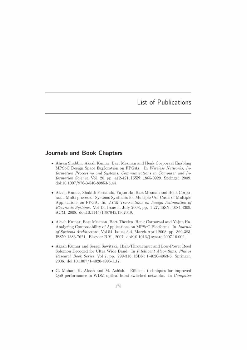
List of Publications
Journals and Book Chapters
• Ahsan Shabbir, Akash Kumar, Bart Mesman and Henk Corporaal EnablingMPSoC Design Space Exploration on FPGAs. In Wireless Networks, In-formation Processing and Systems, Communications in Computer and In-formation Science, Vol. 20, pp. 412-421, ISSN: 1865-0929. Springer, 2009.doi:10.1007/978-3-540-89853-5 44.
• Akash Kumar, Shakith Fernando, Yajun Ha, Bart Mesman and Henk Corpo-raal. Multi-processor Systems Synthesis for Multiple Use-Cases of MultipleApplications on FPGA. In: ACM Transactions on Design Automation ofElectronic Systems. Vol 13, Issue 3, July 2008, pp. 1-27, ISSN: 1084-4309.ACM, 2008. doi:10.1145/1367045.1367049.
• Akash Kumar, Bart Mesman, Bart Theelen, Henk Corporaal and Yajun Ha.Analyzing Composability of Applications on MPSoC Platforms. In Journalof Systems Architecture. Vol 54, Issues 3-4, March-April 2008, pp. 369-383.ISSN: 1383-7621. Elsevier B.V., 2007. doi:10.1016/j.sysarc.2007.10.002.
• Akash Kumar and Sergei Sawitzki. High-Throughput and Low-Power ReedSolomon Decoded for Ultra Wide Band. In Intelligent Algorithms, PhilipsResearch Book Series, Vol 7, pp. 299-316, ISBN: 1-4020-4953-6. Springer,2006. doi:10.1007/1-4020-4995-1 17.
• G. Mohan, K. Akash and M. Ashish. Efficient techniques for improvedQoS performance in WDM optical burst switched networks. In Computer
175
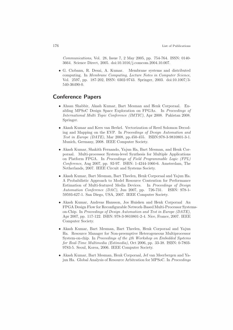
176 List of Publications
Communications, Vol. 28, Issue 7, 2 May 2005, pp. 754-764. ISSN: 0140-3664. Science Direct, 2005. doi:10.1016/j.comcom.2004.10.007.
• G. Ciobanu, R. Desai, A. Kumar. Membrane systems and distributedcomputing. In Membrane Computing, Lecture Notes in Computer Science,Vol. 2597, pp. 187-202, ISSN: 0302-9743. Springer, 2003. doi:10.1007/3-540-36490-0.
Conference Papers
• Ahsan Shabbir, Akash Kumar, Bart Mesman and Henk Corporaal. En-abling MPSoC Design Space Exploration on FPGAs. In Proceedings ofInternational Multi Topic Conference (IMTIC), Apr 2008. Pakistan 2008.Springer.
• Akash Kumar and Kees van Berkel. Vectorization of Reed Solomon Decod-ing and Mapping on the EVP. In Proceedings of Design Automation andTest in Europe (DATE), Mar 2008, pp.450-455. ISBN:978-3-9810801-3-1.Munich, Germany, 2008. IEEE Computer Society.
• Akash Kumar, Shakith Fernando, Yajun Ha, Bart Mesman, and Henk Cor-poraal. Multi-processor System-level Synthesis for Multiple Applicationson Platform FPGA. In Proceedings of Field Programmable Logic (FPL)Conference, Aug 2007, pp. 92-97. ISBN: 1-4244-1060-6. Amsterdam, TheNetherlands, 2007. IEEE Circuit and Systems Society.
• Akash Kumar, Bart Mesman, Bart Theelen, Henk Corporaal and Yajun Ha.A Probabilistic Approach to Model Resource Contention for PerformanceEstimation of Multi-featured Media Devices. In Proceedings of DesignAutomation Conference (DAC), Jun 2007, pp. 726-731. ISBN: 978-1-59593-627-1. San Diego, USA, 2007. IEEE Computer Society.
• Akash Kumar, Andreas Hansson, Jos Huisken and Henk Corporaal AnFPGA Design Flow for Reconfigurable Network-Based Multi-Processor Systems-on-Chip. In Proceedings of Design Automation and Test in Europe (DATE),Apr 2007, pp. 117-122. ISBN: 978-3-9810801-2-4. Nice, France, 2007. IEEEComputer Society.
• Akash Kumar, Bart Mesman, Bart Theelen, Henk Corporaal and YajunHa. Resource Manager for Non-preemptive Heterogeneous MultiprocessorSystem-on-chip. In Proceedings of the 4th Workshop on Embedded Systemsfor Real-Time Multimedia (Estimedia), Oct 2006, pp. 33-38. ISBN: 0-7803-9783-5. Seoul, Korea, 2006. IEEE Computer Society.
• Akash Kumar, Bart Mesman, Henk Corporaal, Jef van Meerbergen and Ya-jun Ha. Global Analysis of Resource Arbitration for MPSoC. In Proceedings
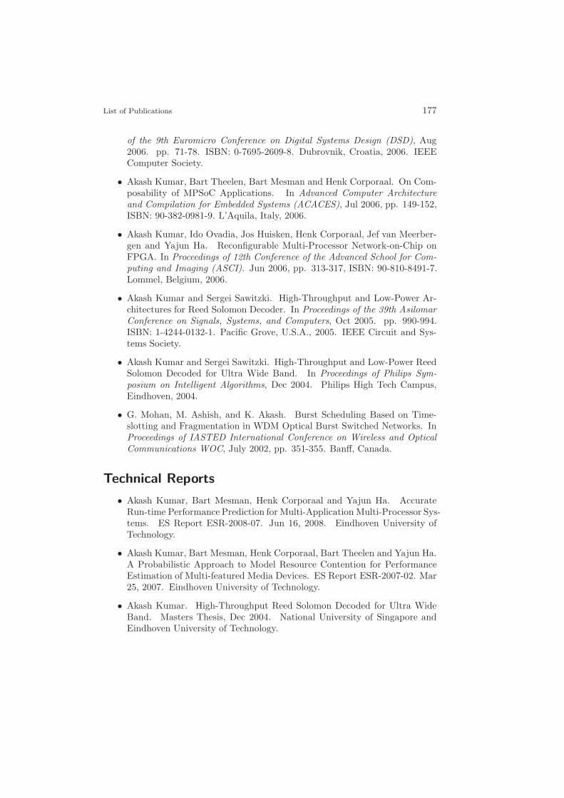
List of Publications 177
of the 9th Euromicro Conference on Digital Systems Design (DSD), Aug2006. pp. 71-78. ISBN: 0-7695-2609-8. Dubrovnik, Croatia, 2006. IEEEComputer Society.
• Akash Kumar, Bart Theelen, Bart Mesman and Henk Corporaal. On Com-posability of MPSoC Applications. In Advanced Computer Architectureand Compilation for Embedded Systems (ACACES), Jul 2006, pp. 149-152,ISBN: 90-382-0981-9. L’Aquila, Italy, 2006.
• Akash Kumar, Ido Ovadia, Jos Huisken, Henk Corporaal, Jef van Meerber-gen and Yajun Ha. Reconfigurable Multi-Processor Network-on-Chip onFPGA. In Proceedings of 12th Conference of the Advanced School for Com-puting and Imaging (ASCI). Jun 2006, pp. 313-317, ISBN: 90-810-8491-7.Lommel, Belgium, 2006.
• Akash Kumar and Sergei Sawitzki. High-Throughput and Low-Power Ar-chitectures for Reed Solomon Decoder. In Proceedings of the 39th AsilomarConference on Signals, Systems, and Computers, Oct 2005. pp. 990-994.ISBN: 1-4244-0132-1. Pacific Grove, U.S.A., 2005. IEEE Circuit and Sys-tems Society.
• Akash Kumar and Sergei Sawitzki. High-Throughput and Low-Power ReedSolomon Decoded for Ultra Wide Band. In Proceedings of Philips Sym-posium on Intelligent Algorithms, Dec 2004. Philips High Tech Campus,Eindhoven, 2004.
• G. Mohan, M. Ashish, and K. Akash. Burst Scheduling Based on Time-slotting and Fragmentation in WDM Optical Burst Switched Networks. InProceedings of IASTED International Conference on Wireless and OpticalCommunications WOC, July 2002, pp. 351-355. Banff, Canada.
Technical Reports
• Akash Kumar, Bart Mesman, Henk Corporaal and Yajun Ha. AccurateRun-time Performance Prediction for Multi-Application Multi-Processor Sys-tems. ES Report ESR-2008-07. Jun 16, 2008. Eindhoven University ofTechnology.
• Akash Kumar, Bart Mesman, Henk Corporaal, Bart Theelen and Yajun Ha.A Probabilistic Approach to Model Resource Contention for PerformanceEstimation of Multi-featured Media Devices. ES Report ESR-2007-02. Mar25, 2007. Eindhoven University of Technology.
• Akash Kumar. High-Throughput Reed Solomon Decoded for Ultra WideBand. Masters Thesis, Dec 2004. National University of Singapore andEindhoven University of Technology.

178 List of Publications
• Akash Kumar. Wavelength Channel Scheduling Using Fragmentation Ap-proach in Optical Burst Switching Networks. Bachelors Thesis, June 2002.National University of Singapore.

Reader’s Notes
179


![[invloed van de media op het wereldbeeld van jongvolwassenen] · 2012. 7. 17. · wereldbeeld van jongvolwassenen] Scriptie, Communication & Multimedia design Babette van Saarloos](https://static.fdocuments.nl/doc/165x107/5feb10f992a4087a666ed10a/invloed-van-de-media-op-het-wereldbeeld-van-jongvolwassenen-2012-7-17-wereldbeeld.jpg)