
ACTUARIAL AND FINANCIAL MATHEMATICS CONFERENCE · 2014-06-06 · KONINKLIJKE VLAAMSE ACADEMIE VAN...
112
KONINKLIJKE VLAAMSE ACADEMIE VAN BELGIE VOOR WETENSCHAPPEN EN KUNSTEN ACTUARIAL AND FINANCIAL MATHEMATICS CONFERENCE Interplay between Finance and Insurance February 6-7, 2014 Michèle Vanmaele, Griselda Deelstra, Ann De Schepper, Jan Dhaene, Wim Schoutens, Steven Vanduffel & David Vyncke (Eds.) CONTACTFORUM
Transcript of ACTUARIAL AND FINANCIAL MATHEMATICS CONFERENCE · 2014-06-06 · KONINKLIJKE VLAAMSE ACADEMIE VAN...

KONINKLIJKE VLAAMSE ACADEMIE VAN BELGIE
VOOR WETENSCHAPPEN EN KUNSTEN
ACTUARIAL AND FINANCIAL
MATHEMATICS CONFERENCE Interplay between Finance and Insurance
February 6-7, 2014
Michèle Vanmaele, Griselda Deelstra, Ann De Schepper,
Jan Dhaene, Wim Schoutens, Steven Vanduffel & David Vyncke (Eds.)
CONTACTFORUM

Handelingen van het contactforum "Actuarial and Financial Mathematics Conference. Interplay between Finance and Insurance" (6-7 februari 2014, hoofdaanvrager: Prof. M. Vanmaele, UGent) gesteund door de Koninklijke Vlaamse Academie van België voor Wetenschappen en Kunsten. Afgezien van het afstemmen van het lettertype en de alinea’s op de richtlijnen voor de publicatie van de handelingen heeft de Academie geen andere wijzigingen in de tekst aangebracht. De inhoud, de volgorde en de opbouw van de teksten zijn de verantwoordelijkheid van de hoofdaanvrager (of editors) van het contactforum.
KONINKLIJKE VLAAMSE ACADEMIE VAN BELGIE VOOR WETENSCHAPPEN EN KUNSTEN Paleis der Academiën Hertogsstraat 1 1000 Brussel
© Copyright 2014 KVAB D/2014/0455/05
ISBN 978 90 6569 135 4
Niets uit deze uitgave mag worden verveelvoudigd en/of openbaar gemaakt door middel van druk, fotokopie, microfilm of op welke andere wijze ook zonder voorafgaande schriftelijke toestemming van de uitgever. No part of this book may be reproduced in any form, by print, photo print, microfilm or any other means without written permission from the publisher.
KONINKLIJKE VLAAMSE ACADEMIE VAN BELGIE
VOOR WETENSCHAPPEN EN KUNSTEN
Actuarial and Financial Mathematics Conference Interplay between finance and insurance
CONTENTS
Invited talk Minimization of hedging error on Orlicz space...................................................................... 3
T. Arai, T. Choulli Contributed talks Greeks without resimulation in spatially homogeneous Markov Chain Models.................... 17 S. Crépey, T.M. Nguyen Worst-case optimization for an investment consumption problem........................................ 29 T. Engler First-passage time problems under regime switching: application in finance and insurance. 41 P. Hieber Construction of cost-efficient self-quanto calls and puts in exponential Lévy models.......... 49 E.A. von Hammerstein, E. Lütkebohmert, L. Rüschendorf, V. Wolf Extended abstracts Pricing participating products under regime-switching generalized gamma process............. 65 F. Alavi Fard Risk classification for claim counts using finite mixture models........................................... 71 L. Bermúdez, D. Karlis Two efficient valuation methods of the exposure of Bermudan options under Heston model......................................................................................................................................
77
Q. Feng, C.S.L. de Graaf, D. Kandhai, C.W.Oosterlee

Evolution of copulas and its applications............................................................................... 85 N. Ishimura Valuation of employee stock options in the Heston model.................................................... 91 T. Sayer Markov switching affine processes and applications to pricing............................................. 97 M. van Beek, M. Mandjes, P. Spreij, E. Winands

KONINKLIJKE VLAAMSE ACADEMIE VAN BELGIE
VOOR WETENSCHAPPEN EN KUNSTEN
Actuarial and Financial Mathematics Conference Interplay between finance and insurance
PREFACE In 2014, our two-day international “Actuarial and Financial Mathematics Conference” was organized in Brussels for the seventh time. As for the previous editions, we could use the facilities of the Royal Flemish Academy of Belgium for Science and Arts. The organizing committee consisted of colleagues from 6 Belgian universities, i.e. the University of Antwerp, Ghent University, the KU Leuven and the Vrije Universiteit Brussel on the one hand, and the Université Libre de Bruxelles and the Université catholique de Louvain on the other hand. The conference included 8 invited lectures, 9 selected contributions and a poster session with 10 posters. As for the scientific committee, we were happy that we could rely on leading international researchers, and just as in the previous years, we could welcome renowned international speakers for the invited lectures. There were 130 registrations in total, with 75 participants from Belgium, and 55 participants from 17 other countries from all continents. The population was mixed, with 70% of the participants associated with a university (PhD students, post doc researchers and professors), and with 30% working in the banking and insurance industry, from home and abroad. On the first day, February 6, we had 9 speakers, with 4 international and eminent invited speakers, alternated with 5 interesting contributions selected by the scientific committee. In de morning, the first speaker was Prof.dr. Martijn Pistorius, from Imperial College London (U.K.), with a lecture entitled “Distance to default, inverse first-passage time problems & counterparty credit risk”; afterwards Prof.dr. Tahir Choulli, University of Alberta (Canada) gave a well-received talk about “Viability Structures under Additional Information & Uncertainty”. These two lectures were followed by 2 presentations by researchers from Germany and France. In the afternoon, we heard Prof.dr. Christian Gouriéroux, University of Toronto (Canada) & CREST (France), who presented new research results about “Pricing default events: surprise, exogeneity and contagion”, and Prof.dr. Matthias Scherer, TU München (Germany), with his paper on “Consistent iterated simulation of multi-variate default times: a Markovian indicators characterization”. As in the morning, these two lectures were alternated now by 3 presentations, with one speaker from France, one from Germany and one from Japan. During the lunch break, we organized a poster session, preceded by a poster storm session, where the 10 different posters were introduced very briefly by the researchers. The posters remained in the main meeting room during the whole conference, so that they could be

consulted and discussed during the lunches and coffee breaks. We were pleased with the lively interaction between the participants and the posters’ authors, with very useful suggestions to the younger researchers. Also on the second day, February 7, we had 8 lectures, again with 4 keynote speakers and 4 selected contributions. The first speaker was Prof.dr. Pierre Devolder, Université Catholique de Louvain (Belgium), with a lecture on “Some actuarial questions around a possible reform of the Belgian pension system”. Afterwards, Prof.dr. Enrico Biffis, Imperial College London (U.K.) presented his research on “Optimal collateralization with bilateral default risk”. In the afternoon, we could listen to Prof.dr. Marcus Christiansen, Universität Ulm (Germany), about “Deterministic optimal consumption and investment in a stochastic model with applications in insurance”. Prof.dr. Ralf Korn, TU Kaiserslautern (Germany) was the last invited speaker, with a nice lecture entitled “Save for the bad times or consume as long as you have? Worst-case optimal lifetime consumption!”. The other 4 presentations were again selected from a substantial number of submissions by the scientific committee; the speakers came from France, the Netherlands, Canada and Germany. In these proceedings, you can find one paper of an invited speaker co-authored with a contributed speaker, four articles related to contributed talks, and six extended abstracts written by the poster presenters of the poster sessions, giving an overview of the topics and activities at the conference. We are much indebted to the members of the scientific committee, H. Albrecher (University of Lausanne, Switzerland), C. Bernard (University of Waterloo, Canada), J. Dhaene (Katholieke Universiteit Leuven, Belgium), E. Eberlein (University of Freiburg, Germany), M. Jeanblanc (Université d'Evry Val d'Essonne, France), R. Norberg (SAF, Université Lyon 1, France), Ludger Rüschendorf (University of Freiburg, Germany), S. Vanduffel (Vrije Universiteit Brussel, Belgium), M. Vellekoop (University of Amsterdam, the Netherlands) and the chair G. Deelstra (Université Libre de Bruxelles, Belgium). We appreciate their excellent scientific support, their presence at the meeting and their chairing of sessions. We also thank Wouter Dewolf (Ghent University, Belgium), for the administrative work. We are very grateful to our sponsors, namely the Royal Flemish Academy of Belgium for Science and Arts, the Research Foundation Flanders (FWO), the Scientific Research Network (WOG) “Stochastic modelling with applications in finance”, le Fonds de la Recherche Scientifique (FNRS), KBC Bank en Verzekeringen, the BNP Paribas Fortis Chair in Banking at the Vrije Universiteit Brussel and Université Libre de Bruxelles, and exhibitors Cambridge, Springer and NAG. Without them it would not have been possible to organize this event in this very enjoyable and inspiring environment. We are also grateful for the support by the ESF Research Networking Programme Advanced Mathematical Methods for Finance (AMAMEF). The continuing success of the meeting encourages us to go on with the organization of this contact-forum, in order to create future opportunities for exchanging ideas and results in this fascinating research field of actuarial and financial mathematics. The editors: Griselda Deelstra, Ann De Schepper, Jan Dhaene, Wim Schoutens, Steven Vanduffel, Michèle Vanmaele, David Vyncke
The other members of the organising committee: Michel Denuit, Karel In ‘t Hout

INVITED TALK

MINIMIZATION OF HEDGING ERROR ON ORLICZ SPACE
Takuji Arai† and Tahir Choulli§
†Department of Economics, Keio University, 2-15-45 Mita, Minato-ku, Tokyo, 108-8345, Japan§Mathematical and Statistical Sciences Department, University of Alberta, Edmonton, Alberta,T6G 2G1, CanadaEmail: [email protected], [email protected]
Abstract
Minimization problems on hedging error in the Orlicz space framework are discussed. In thispaper, we deal with general forms of such problems as follows:
infv∈V
E[Φ(|H − v|)], infv∈V
NΦ(H − v), infv∈V‖H − v‖Φ,
where Φ is a Young function, NΦ and ‖ · ‖Φ are norms on the Orlicz space LΦ, H is a randomvariable, V is a convex subset of LΦ. We aim to investigate relationships among the threeproblems. We focus on, firstly, properties of the first problem, and study its relationships tothe others. Moreover, we prove that there exist solutions to the three when LΦ is reflexive.
1. INTRODUCTION
In mathematical finance, it is very important to study pricing and hedging problem for contingentclaims. If the underlying market is complete, any contingent claim H , given by a random variable,is represented as a stochastic integral with respect to underlying asset price process S, which is asemimartingale, that is, there exist a constant c and an Rd-valued S-integrable predictable processϑ such that
H = c+
∫ T
0
ϑtdSt, (1)
where T is the maturity of our market. Under the no-arbitrage condition, the fair price of H mustbe given by the initial cost to replicate H , that is, the constant c in (1), and ϑ is regarded as a self-financing replicating strategy. On the other hand, in the case of incomplete markets, there is nopair (c, ϑ) satisfying (1), unfortunately. Instead of the replicating strategy, we should look for anoptimal pair (c, ϑ) in an appropriate sense. There are, in fact, many ways to define optimality, say,mean-variance hedging (Schweizer (2001), Schweizer (2010)), risk minimizing hedging (Follmer
3
4 T. Arai and T. Choulli
and Schweizer (2010), Schweizer (2001),), utility indifference valuation (Becherer (2010), Hen-derson and Hobson (2008)), and so forth. In this paper, we focus on problems finding a pair (c, ϑ)
so that c +∫ T
0ϑtdSt is as near to H as possible, that is, optimization problems on hedging er-
ror∣∣∣c+
∫ T0ϑtdSt −H
∣∣∣. For example, mean-variance hedging is defined as the optimal strategy
minimizing its hedging error in the L2-sense, that is, a solution to the following:
minc∈R,ϑ∈Θ
E
[(c+
∫ T
0
ϑtdSt −H)2], (2)
where Θ is a set of Rd-valued S-integrable predictable processes. In order to discuss varioustypes of minimization problem on hedging error in a unified way, we try to extend mean-variancehedging to general Orlicz space setting, that is, we consider
minc∈R,ϑ∈Θ
E
[Φ
(∣∣∣∣H − c− ∫ T
0
ϑtdSt
∣∣∣∣)] , (3)
where Φ is a Young function, that is, a continuous increasing convex function defined on [0,∞)with starting at 0. Incidentally, we can rewrite (2) as
minc∈R,ϑ∈Θ
∥∥∥∥c+
∫ T
0
ϑtdSt −H∥∥∥∥L2
.
Now, a question arises; we wonder if we can rewrite (3) similarly as follows:
minc∈R,ϑ∈Θ
NΦ
(H − c−
∫ T
0
ϑtdSt
), (4)
and
minc∈R,ϑ∈Θ
∥∥∥∥H − c− ∫ T
0
ϑtdSt
∥∥∥∥Φ
, (5)
where NΦ(·) and ‖ · ‖Φ are norms on the Orlicz space induced by Φ, whose definitions will beintroduced in the sequel.
Remark 1.1 We can regard the three problems (3), (4) and (5) as purely mathematical problems.More precisely, these are projections of a random variable on a space of stochastic integrations.Thus, we can say that results obtained in this paper would be important not only for mathematicalfinance, but also for both stochastic analysis and functional analysis.
The aim of this paper is to investigate relationships among the three problems (3), (4) and (5),and to give sufficient conditions under which all the three admit solutions. Note that we rewrite thethree problems into general forms, and treat them throughout this paper. Model description andmathematical preliminaries are given in section 2. In section 3, we study the relationship amongthe three problems. In particular, we investigate properties of solutions to (3), and its relations tothe two other problems. In section 4, we prove that, if the based Orlicz space is reflexive, then theexistence of solutions to the three are guaranteed.

Minimization of hedging error on Orlicz space 5
2. PRELIMINARIES
Let (Ω,F , P ;F = Ftt∈[0,T ]) be a filtered probability space with a right-continuous filtrationF such that F0 is trivial and contains all null sets of F , and FT = F . Consider an incompletefinancial market composed of one riskless asset and d risky assets. Suppose that the price of theriskless asset is 1 at all times, that is, the interest rate of our market is assumed to be 0. Note thatT > 0 is the maturity. Let Φ be a continuous nondecreasing convex function defined on [0,∞)with starting at 0, which is called a Young function. Remark that Φ is differentiable a.e. andits left-derivative φ satisfies Φ(x) =
∫ x0φ(u)du. Note that φ is left continuous, and may have at
most countably many jumps. Define ψ(y) := infx ∈ (0,∞)|φ(x) ≥ y, which is called thegeneralized left-continuous inverse of φ. We define Ψ(y) :=
∫ y0ψ(v)dv for y ≥ 0, which is a
Young function and called the conjugate function of Φ. Now, we define the Orlicz space and theOrlicz heart for Φ, and norms on them as follows:
Definition 2.1 We define two spaces of random variables for a Young function Φ:(Orlicz space) LΦ := X ∈ L0|E[Φ(c|X|)] <∞ for some c > 0,(Orlicz heart) MΦ := X ∈ L0|E[Φ(c|X|)] <∞ for any c > 0,where L0 is the set of all FT -measurable random variables. In addition, we define two norms:(Luxemburg norm) ‖X‖Φ := inf
λ > 0|E
[Φ(∣∣X
λ
∣∣)] ≤ 1
,(Orlicz norm) NΦ(X) := supE[XY ]| ‖Y ‖Ψ ≤ 1.
Remark that MΦ ⊂ LΦ and both spaces LΦ and MΦ are linear. Moreover, the norm dual of(MΦ, ‖ · ‖Φ) is given by (LΨ, NΦ(·)), since Φ is finite. For more details on Orlicz space, see Edgarand Sucheston (1992) and Rao and Ren (1991). Henceforth, we fix arbitrarily a Young function Φsatisfying the following assumptions:
Assumption 2.1 (1) Φ(x) > 0 for any x > 0,(2) limx→∞Φ(x)/x = +∞.
Example 2.1 Typical examples of Φs satisfying all conditions mentioned are Φ(x) = ex − 1,ex − x − 1, (x + 1) log(x + 1) − x and xp/p for p > 1. On the other hand, Φ(x) = 0 if x < 1;= (x− 1)2 if x ≥ 1 and Φ(x) = ax for a > 0 are excluded in this paper.
Letting S be an Rd-valued semimartingale describing the fluctuation of risky assets, problems(3), (4) and (5) can be regarded as minimization problems on the space
c+
∫ T
0
ϑtdSt|c ∈ R, ϑ ∈ Θ
or∫ T
0
ϑtdSt|ϑ ∈ Θ
, (6)
where Θ is a set of Rd-valued S-integrable predictable processes. Although we do not specify thedefinition of Θ, we assume the convexity of Θ, that is, the space (6) forms a convex set. Thus, wecan rewrite problems (3), (4) and (5) as the following general forms:
Problem 2.2 minv∈V E[Φ(|H − v|)] or infv∈V E[Φ(|H − v|)],
Problem 2.3 minv∈V NΦ(H − v) or infv∈V NΦ(H − v),

6 T. Arai and T. Choulli
Problem 2.4 minv∈V ‖H − v‖Φ or infv∈V ‖H − v‖Φ,
where V is a convex subset of LΦ. As mentioned in section 1, we can regard these problems asthe LΦ-projections of a random variable H on a convex set V . We shall investigate relationshipsamong Problems 2.2–2.4, and the existence of solutions. We suppose, throughout the paper, thatH ∈ LΦ. Since we are not interested in the case where H ∈ V , we assume H /∈ V . For allunexplained notation, we refer to Dellacherie and Meyer (1982).
3. RELATIONSHIPS AMONG THE THREE PROBLEMS
3.1. Relationships on finiteness
First of all, we can see the following proposition:
Proposition 3.1 (1) infv∈V ‖H − v‖Φ = +∞⇔ infv∈V NΦ(H − v) = +∞.(2) infv∈V ‖H − v‖Φ = +∞⇒ infv∈V E[Φ(|H − v|)] = +∞.
Proof. These are clear by Theorem 2.2.9 of Edgar and Sucheston (1992). 2
Actually, the relationship between Problems 2.2 and 2.4 (as well as 2.2 and 2.3) is not simple asthe case of between Problems 2.3 and 2.4. The reverse assertion of (2) does not hold in general.We introduce a counterexample.
Example 3.1 We consider a one period model. LetX and Y be two independent random variablesfollowing the exponential distribution with parameter 1 and 1/2, respectively. The asset priceprocess S is given by S0 = 0 and S1 = X − 1. Let Φ be Φ(x) = ex− 1 and H given by X + Y . Vis assumed to be given by ϑS1|ϑ ∈ R. Then, we have, for any ϑ ≥ 1,
E[Φ(|H − ϑS1|)] =
∫ ∞0
∫ ∞0
e|x+y−ϑx+ϑ|e−xe−y/2
2dydx− 1
≥∫ ϑ
ϑ−1
0
∫ ∞0
ex+y−ϑx+ϑe−xe−y/2
2dydx− 1
≥ eϑ∫ ϑ
ϑ−1
0
∫ ∞0
ey/2
2dye−ϑxdx− 1
= +∞.
Moreover, for any ϑ < 1,
E[Φ(|H − ϑS1|)] =
∫ ∞0
∫ ∞0
e|x+y−ϑx+ϑ|e−xe−y/2
2dydx− 1
≥∫ ∞
ϑϑ−1∨0
∫ ∞0
ex+y−ϑx+ϑe−xe−y/2
2dydx− 1
≥ eϑ∫ ∞
ϑϑ−1∨0
∫ ∞0
ey/2
2dye−ϑxdx− 1
= +∞.

Minimization of hedging error on Orlicz space 7
Thus, we obtain infv∈V E[Φ(|H − v|)] = +∞. On the other hand, letting ϑ = 0 and λ > 2, wehave
E
[Φ
(|H − ϑS1|
λ
)]=
∫ ∞0
∫ ∞0
e|x+y−ϑx+ϑ|
λ e−xe−y/2
2dydx− 1
=
∫ ∞0
∫ ∞0
ex+yλ e−x
e−y/2
2dydx− 1
=1(
1− 2λ
) 1(1− 1
λ
) − 1.
Substituting λ = 6, E[Φ(|H−0S1|
6
)]= 4/5 ≤ 1. Hence, we have at least ‖H − 0S1‖Φ ≤ 6, that
is, infv∈V ‖H − v‖Φ < +∞. 2
3.2. Properties of solutions to Problem 2.2
Even though Problems 2.2–2.4 all have solutions, they do not necessarily coincide. Roughly speak-ing, if V is cone, and v3 ∈ V is a solution to Problem 2.4, v3/c is a solution to Problem 2.4 withrespect to H/c for any c > 0, that is, we can say that Problem 2.4 has the conicality. On the otherhand, when v1 is a solution to Problem 2.2 with respect to H , v1/c is not necessarily a solution tothe problem with respect to H/c. We introduce such a counterexample.
Example 3.2 We consider a simple one-period model with Ω = ω1, ω2, ω3, andP (ωi) = 1/3 for i = 1, 2, 3. Moreover, S0 = 0, S1 is given by
S1(ωi) =
2, i = 1,0, i = 2,−1, i = 3.
Supposing that H = 1ω1 and Φ(x) = ex − 1, and V = ϑS1|ϑ ∈ R, we have
E[Φ(|H − ϑS1|)] =1
3
e|1−2ϑ| + 1 + e|ϑ|
− 1
=1
3
e|1−2ϑ| + e|ϑ|
− 2
3.
Thus, the optimizer is given by 1/2.Next, letting H = 21ω1, we have
E[Φ(|H − ϑS1|)] =1
3
e|2−2ϑ| + 1 + e|ϑ|
− 1
=1
3
e|2−2ϑ| + e|ϑ|
− 2
3.
Thus, the optimizer is given by log 2+23
. Hence, Problem 2.2 does not have the conicality. 2

8 T. Arai and T. Choulli
Before stating relationships among solutions to the three problems, we study properties ofsolutions to Problem 2.2. In the rest of this section, we assume that
Φ is differentiable,
for simplicity.
Proposition 3.2 Assuming that there exists a v∗ ∈ V such that
minv∈V
E[Φ(|H − v|)] = E[Φ(|H − v∗|)], (7)
and there exists a c > 1 such that E[Φ(c|H − v∗|)] < +∞. We have the following two conditions:
1. For any v ∈ V , E[φ(|H − v∗|)|H − v∗|] ≤ E[φ(|H − v∗|)|H − v|].
2. For any v ∈ V , E[φ(|H − v∗|) sgn(H − v∗)(v∗ − v)] ≥ 0.
Moreover, if v∗ ∈ V satisfies E[φ(|H − v∗|)|H − v∗|] < +∞ and either the above condition, thenv∗ satisfies (7).
To prove Proposition 3.2, we need some preparations. We define the Gateaux derivative DF as
DF (u1, u) := limt→0
1
tE[Φ(|u1 + tu|)− Φ(|u1|)], for any u, u1 ∈ LΦ.
Proposition 3.3 Let v1 ∈ V and u ∈ LΦ such that E[Φ(c|H − v1|)] < +∞ and E[Φ(
2cc−1|u|)]<
+∞ for some c > 1. Then, we have
DF (H − v1, u) = E[φ(|H − v1|) sgn(H − v1)u].
Proof. For any t ∈ (0, 1), we have
1
tΦ(|H − v1|+ t|u|)− Φ(|H − v1|)
=Φ(|H − v1|+ t|u|)− Φ(|H − v1|)
t|u||u|
≤ φ(|H − v1|+ t|u|)|u|≤ Φ(|H − v1|+ (1 + t)|u|)− Φ(|H − v1|+ t|u|)≤ Φ(|H − v1|+ (1 + t)|u|)
≤ 1
cΦ(c|H − v1|) +
(1− 1
c
)Φ
(1 + t
1− 1c
|u|)
≤ 1
cΦ(c|H − v1|) +
(1− 1
c
)Φ
(2c
c− 1|u|)∈ L1
The dominated convergence theorem then implies that
DF (H − v1, u) = limt→0
1
tE[Φ(|H − v1 + tu|)− Φ(|H − v1|)]
= E
[limt→0
Φ(|H − v1 + tu|)− Φ(|H − v1|)t
]= E[φ(|H − v1|) sgn(H − v1)u].

Minimization of hedging error on Orlicz space 9
This completes the proof of Proposition 3.3. 2
Proof of Proposition 3.2. Condition 1: Let v ∈ V be fixed arbitrarily. Denoting X = |H − v|and X∗ = |H − v∗|, we define f(α) := E[Φ(αX∗ + (1− α)X)] for any α ∈ [0, 1]. Under (7), wehave
f(α) ≥ E[Φ(|H − αv∗ − (1− α)v|)] ≥ f(1)
for any α ∈ [0, 1], which implies that, for any α ∈ [0, 1)
0 ≥ f(α)− f(1)
α− 1=
1
α− 1E [Φ(αX∗ + (1− α)X)− Φ(X∗)] .
In fact, we can prove that the right hand side converges to E[φ(X∗)(X∗ − X)] as α tends to 1,which from Condition 1 follows.
Now, we shall prove the above convergence. To see it, we have only to prove the existenceof α0 ∈ [0, 1) such that, for any α ∈ [α0, 1), there exists a random variable Z, independent of α,satisfying ∣∣∣∣ 1
α− 1(Φ(αX∗ + (1− α)X)− Φ(X∗))
∣∣∣∣ ≤ Z ∈ L1,
since the rest is proved by the dominated convergence theorem. Note that α0 depends on X . Wehave ∣∣∣∣ 1
α− 1(Φ(αX∗ + (1− α)X)− Φ(X∗))
∣∣∣∣=
1
1− α(Φ(X∗)− Φ(αX∗ + (1− α)X))1X∗>X
+1
1− α(Φ(αX∗ + (1− α)X)− Φ(X∗))1X>X∗
=: I1 + I2.
Now, we remark that there exists a c > 1 such that Φ(cX∗) ∈ L1 by the assumption. We have then,for any α ∈ (0, 1),
I1 =Φ(X∗)− Φ(X∗ − (1− α)(X∗ −X))
(1− α)(X∗ −X)(X∗ −X)1X∗>X
≤ φ(X∗)(X∗ −X)1X∗>X ≤ φ(X∗)X∗
≤ 1
c− 1(Φ(cX∗)− Φ(X∗)) ∈ L1.
Next, we prove that there exists a random variable Z2, which is independent of α, such that I2 ≤Z2 ∈ L1. Since X ∈ LΦ, there exists an ε > 0 such that Φ(εX) ∈ L1. We may assume that ε < 1.We take a sufficient small β ∈ (0, 1) to satisfy 1−βε
1−β < c. Set α0 := 1 − βε. For any α ∈ [α0, 1),

10 T. Arai and T. Choulli
denoting α = 1− γε, which means γ ≤ β, the convexity of Φ implies that
I2 =Φ(αX∗ + (1− α)X)− Φ(X∗)
1− α1X>X∗
=Φ((1− γε)X∗ + γεX)− Φ(X∗)
γε1X>X∗
≤(1− γ)Φ
(1−γε1−γ X
∗)
+ γΦ(εX)− Φ(X∗)
γε1X>X∗
≤ (1− γ)(δΦ(cX∗) + (1− δ)Φ(X∗)) + γΦ(εX)− Φ(X∗)
γε1X>X∗
=
γ(1−ε)c−1
Φ(cX∗) + (1− δ)(1− γ)− 1Φ(X∗) + γΦ(εX)
γε1X>X∗
≤1−εc−1
Φ(cX∗) + Φ(εX)
ε∈ L1,
where δ = γ(1−ε)(c−1)(1−γ)
. Note that, since c−1 > β(1−ε)1−β , we have δ = γ(1−ε)
(c−1)(1−γ)< γ(1−β)
β(1−γ)≤ γ(1−γ)
γ(1−γ)=
1, δc + (1 − δ) = 1 + (c − 1)δ = 1 + γ(1−ε)1−γ = 1−γε
1−γ , and (1 − γ)δ = γ(1−ε)c−1
. Thus, Condition 1follows.
Condition 2: Suppose that there exists a v ∈ V such that E[φ(|H − v∗|) sgn(H − v∗)(v∗ −v)] < 0. Now, we take a sufficient small constant ε > 0 satisfying E
[Φ(
2cεc−1|v∗ − v|
)]< +∞.
Proposition 3.3 yieldsDF (H−v∗, ε(v∗−v)) < 0. On the other hand, we haveDF (H−v∗, ε(v∗−v)) ≥ 0 for any v ∈ V by the definition of the Gateaux derivative and the optimality of v∗. This isa contradiction! Hence, Condition 2 holds.
The second assertion: First, we suppose Condition 1. By Young’s inequality (Theorem 2.1.4of Edgar and Sucheston (1992)) and Condition 1, we have
E[Φ(|H − v∗|)] = E[φ(|H − v∗|)|H − v∗|]− E[Ψ(φ(|H − v∗|))]≤ E[φ(|H − v∗|)|H − v|]− E[Ψ(φ(|H − v∗|))]≤ E[Φ(|H − v|)]
for any v ∈ V , from which v∗ satisfies (7). Note that Ψ is R+-valued.Next, we suppose Condition 2. We can rewrite Condition 2 as follows:
E[φ(|H − v∗|) sgn(H − v∗)(H − v∗)] ≤ E[φ(|H − v∗|) sgn(H − v∗)(H − v)]
for any v ∈ V . Theorem 2.1.4 of Edgar and Sucheston (1992) implies that
E[φ(|H − v∗|) sgn(H − v∗)(H − v∗)] = E[Ψ(φ(|H − v∗|))] + E[Φ(|H − v∗|)].
andE[φ(|H − v∗|) sgn(H − v∗)(H − v)] ≤ E[Ψ(φ(|H − v∗|))] + E[Φ(|H − v|)]
for any v ∈ V . Hence, v∗ satisfies (7). 2
Remark 3.1 If V ⊂ MΦ and H ∈ MΦ, then we have E[Φ(c|H − v|)] < +∞ for any c > 0 andany v ∈ V . Thus, in such a case, we can get rid of any condition on the existence of c > 1 from thestatements in Propositions 3.2 and 3.3.

Minimization of hedging error on Orlicz space 11
3.3. Relationship on solutions
We investigate in this subsection relationships among Problems 2.2–2.4. The first is relationshipsbetween Problems 2.2 and 2.4.
Proposition 3.4 We consider the following two conditions:
1. There exists a v1 ∈ V such that
minv∈V
E[Φ(|H − v|)] = E[Φ(|H − v1|)] = 1. (8)
2. There exists a v2 ∈ V such that
minv∈V‖H − v‖Φ = ‖H − v2‖Φ = 1. (9)
Then, we have 1⇒2, and (9) holds for v1. Moreover, if V ⊂ MΦ and H ∈ MΦ, then the reversedirection also holds and (8) holds for v2.
Proof. We prove the first assertion. Under condition 1, two assertions (2) and (3) in Proposition2.1.10 of Edgar and Sucheston (1992) provide ‖H−v1‖Φ = 1. Again, Proposition 2.1.10 of Edgarand Sucheston (1992) implies that ‖H − v‖Φ > 1 whenever E[Φ(|H − v|)] > 1. Thus, we haveminv∈V ‖H − v‖Φ = ‖H − v1‖Φ = 1.
Next, we prove the second assertion. By Proposition 2.1.10 (4) of Edgar and Sucheston (1992),we have E[Φ(|H − v2|)] = 1. Moreover, we have ‖H − v‖Φ > 1 ⇒ E[Φ(|H − v|)] > 1 byProposition 2.1.10 (3) of Edgar and Sucheston (1992). This completes the proof. 2
In the above proposition, the inclusion 2⇒1 does not hold in general. We exemplify it as follows:
Example 3.3 We consider a one-period model. Only one risky asset is tradable. Its price process(St)t=0,1 is given as follows: S0 = 0 and S1 is expressed by X − 2, where X is a random variablewhose probability density function fX is given by:
fX(x) =
e−x
Dx2, x ≥ 1,
0, x < 1,
whereD :=∫∞
1e−x
x2dx. The underlying contingent claimH follows the same distribution asX , but
is independent ofX . Suppose that V = ϑS1|ϑ ∈ R. Let Φ(x) := a(ex−1), where 0 < a < D1−D .
For any ϑ ∈ R, we have
E[Φ(|H − ϑS1|)] = a
∫ ∞1
∫ ∞1
e|y−ϑ(x−2)| e−y
Dy2
e−x
Dx2dydx− 1
.
In particular, when ϑ = 0, we have
E[Φ(|H − ϑS1|)] = E[Φ(|H|)] = a
∫ ∞1
e|y|e−y
Dy2dy − 1
= a
∫ ∞1
dy
Dy2− 1
= a
1−DD
.

12 T. Arai and T. Choulli
Thus, infϑ∈RE[Φ(|H − ϑS1|)] ≤ a1−DD
. Noting that a < D1−D , infϑ∈RE[Φ(|H − ϑS1|)] < 1.
Next, we consider, for any λ > 0, E[Φ(|H−ϑS1|
λ
)]. Note that
E
[Φ
(|H − ϑS1|
λ
)]= a
∫ ∞1
∫ ∞1
e|y−ϑ(x−2)|
λe−y
Dy2
e−x
Dx2dydx− 1
.
When λ < 1 and ϑ ≤ 0, we have∫ ∞1
∫ ∞1
e|y−ϑ(x−2)|
λe−y
Dy2
e−x
Dx2dxdy
≥ e2ϑλ
∫ ∞1
e(1λ−1)y
Dy2dy
∫ ∞2
e−(ϑλ+1)x
Dx2dx = +∞.
Besides, when λ < 1 and ϑ > 0, we have∫ ∞1
∫ ∞1
e|y−ϑ(x−2)|
λe−y
Dy2
e−x
Dx2dydx
≥∫ ∞
1
∫ ∞ϑ(x−2)∨1
ey−ϑ(x−2)
λe−y
Dy2
e−x
Dx2dydx = +∞.
Thus, for any ϑ ∈ R, ‖H − ϑS1‖Φ ≥ 1. On the other hand, if ϑ = 0, E[Φ(|H − ϑS1|)] < 1. Wecan conclude that minϑ∈R ‖H − ϑS1‖Φ = ‖H − 0S1‖Φ = 1. 2
We state a result with respect to relationships between Problems 2.2 and 2.3.
Proposition 3.5 Assume that there exists an element v∗ ∈ V satisfying E[Ψ(φ(|H − v∗|))] = 1and E[Φ(c|H − v∗|)] < +∞ for some c > 1. The following are then equivalent:
1. E[Φ(|H − v∗|)] = minv∈V E[Φ(|H − v|)].
2. NΦ(H − v∗) = minv∈V NΦ(H − v).
Proof. 1⇒2: By the definition of NΦ(·), Young’s inequality and the assumption of this propo-sition, we have NΦ(H − v∗) ≥ E[φ(|H − v∗|)|H − v∗|] = E[Φ(|H − v∗|)] + 1. Moreover,Theorem 2.2.9 of Edgar and Sucheston (1992) yields NΦ(H − v∗) ≤ E[Φ(|H − v∗|)] + 1. Thus,NΦ(H− v∗) = E[φ(|H− v∗|)|H− v∗|] = E[Φ(|H− v∗|)] + 1. By Proposition 3.2, for any v ∈ V ,we have
NΦ(H − v∗) = E[φ(|H − v∗|)|H − v∗|]≤ E[φ(|H − v∗|)|H − v|] ≤ NΦ(H − v).
Thus, v∗ is also a solution to minv∈V NΦ(H − v).2⇒1: Note that Ψ is finite by Assumption 2.1 (2). Thus, Proposition 2.2.8 (3) of Edgar and
Sucheston (1992) implies that, for any v ∈ V and any ε > 0, there exists a u ∈MΨ with ‖u‖Ψ ≤ 1

Minimization of hedging error on Orlicz space 13
such thatNΦ(H−v) ≤ E[|H−v||u|]+ε. In addition, we have E[Φ(|H−v∗|)]+1 = NΦ(H−v∗)by the aforementioned argument. Hence, we obtain that
E[Φ(|H − v∗|)] + 1 = NΦ(H − v∗) ≤ NΦ(H − v)
≤ E[|H − v||u|] + ε
≤ E[Φ(|H − v|)] + E[Ψ(|u|)] + ε
≤ E[Φ(|H − v|)] + 1 + ε,
from which E[Φ(|H − v∗|)] ≤ E[Φ(|H − v|)] follows for any v ∈ V , since ε > 0 is arbitrary. 2
4. EXISTENCE OF SOLUTIONS TO MINIMIZATION PROBLEMS
Our aim of this section lies in obtaining sufficient conditions under which solutions to Problems2.2–2.4 exist. Throughout this section, we assume
V is a closed convex subset of LΦ.
Although the closedness of V is essential, we need some additional conditions to ensure the exis-tence of solutions. We consider the case where LΦ is reflexive.
Remark 4.1 Supposing that Φ(x) = xp/p for p > 1, the space LΦ is reflexive. More generally,the space LΦ is reflexive, if both Φ and Ψ satisfy the following ∆2-condition: there exist an x0 ∈(0,∞) and a K > 0 such that Φ(2x) < KΦ(x) for any x ≥ x0. Thus, ex − 1, ex − x − 1 and(x + 1) log(x + 1) − x are not the case. For more details, see Corollary 2.2.12 of Edgar andSucheston (1992) and Theorem IV.1.10 of Rao and Ren (1991).
Proposition 4.1 Let LΦ be reflexive. Then, Problems 2.2–2.4 all have solutions.
Proof. As for Problems 2.3 and 2.4, we can prove them easily by consulting with PropositionII.1.2 of Ekeland and Temam (1999). For example, as regards Problem 2.4, letting F (v) :=‖H − v‖Φ, F is a lower semi-continuous convex function. Moreover, since F (v) ≥ ‖v‖Φ−‖H‖Φ
for any v ∈ V , F is coercive. Thus, there exists a solution to Problem 2.4.It remains to show the assertion with respect to Problem 2.2. Before proving it, we should
remark that LΦ = MΦ whenever LΦ is reflexive. See Theorem IV.2.10 of Rao and Ren (1991). Wedenote F (v) := E[Φ(|H − v|)] and d∗ := infv∈V F (v). Remark that we are interested in only thecase where d∗ < +∞; otherwise every v ∈ V becomes a solution. Let (vn)n≥1 be a minimizingsequence, that is, F (vn)→ d∗ as n→∞.
For any v ∈ V satisfying (d∗ ≤)F (v) ≤ d∗ + 1, we have, by Theorem 2.2.9 of Edgar andSucheston (1992),
‖v‖Φ ≤ NΦ(v) ≤ NΦ(H) +NΦ(H − v) ≤ NΦ(H) + F (v) + 1
≤ NΦ(H) + d∗ + 2.
Consequently, we have infv∈V F (v) = infv∈A F (v), whereA := v ∈ V|‖v‖Φ ≤ NΦ(H)+d∗+2.We can then extract a minimizing sequence (vn) within A. Since LΦ is reflexive, (vn) convergesto some v∗ ∈ A in the weak topology σ(MΦ, LΨ) by extracting a subsequence if need be.

14 T. Arai and T. Choulli
Letting w∗ := sgn(H − v∗)φ(|H − v∗|), we have
E[Ψ(|w∗|)] = E[Ψ(φ(|H − v∗|))]= E[|H − v∗|φ(|H − v∗|)]− E[Φ(|H − v∗|)]≤ E[Φ(2|H − v∗|)]− 2E[Φ(|H − v∗|)] < +∞,
since H − v∗ ∈MΦ. Thus, w∗ ∈ LΨ follows. Moreover, we have
F (v∗) = E[Φ(|H − v∗|)] = E[(H − v∗)w∗]− E[Ψ(|w∗|)]= lim
n→∞E[(H − vn)w∗]− E[Ψ(|w∗|)]
≤ lim infn→∞
E[Φ(|H − vn|)] + E[Ψ(|w∗|)]− E[Ψ(|w∗|)]
= lim infn→∞
F (vn).
Consequently, v∗ is a solution to Problem 2.2. 2
ACKNOWLEDGEMENTSThe research of Tahir Choulli is supported financially by the Natural Sciences and EngineeringResearch Council of Canada, through Grant G121210818.
References
B. Becherer. Utility indifference valuation. In R. Cont, editor, Encyclopedia of QuantitativeFinance, pages 1854–1860. Wiley, 2010.
C. Dellacherie and P.A. Meyer. Probabilities and Potential B. North-Holland, Amsterdam, 1982.
G.A. Edgar and L. Sucheston. Stopping times and directed processes. Cambridge University Press,1992.
I. Ekeland and R. Temam. Convex analysis and variational problems. Society for Industrial &Applied Mathematics, Philadelphia, 1999.
H. Follmer and M. Schweizer. The minimal martingale measure. In R. Cont, editor, Encyclopediaof Quantitative Finance, pages 1200–1204. Wiley, 2010.
V. Henderson and D. Hobson. Utility indifference pricing – an overview. In R. Carmona, editor,Indifference pricing, pages 44–74. Princeton University Press, 2008.
M.M. Rao and Z.D. Ren. Theory of Orlicz spaces. Marcel Dekker, New York, 1991.
M. Schweizer. A guided tour through quadratic hedging approaches. In E. Jouini et al., editor,Option Pricing, pages 538–574. Cambridge Univ. Press, 2001.
M. Schweizer. Mean-variance hedging. In R. Cont, editor, Encyclopedia of Quantitative Finance,pages 1177–1181. Wiley, 2010.

CONTRIBUTED TALKS

GREEKS WITHOUT RESIMULATION IN SPATIALLY HOMOGENEOUSMARKOV CHAIN MODELS 1
Stephane Crepey‡ and Tuyet Mai Nguyen‡
‡Universite d’Evry, Laboratoire de Mathematiques et Modelisation d’Evry, FranceEmail: [email protected], [email protected]
Abstract
In this paper, we model credit portfolios by continuous-time Markov chainswith some form ofspatial homogeneity, so that direct Monte Carlo Greeks estimates, without resimulation, can bederived. We implement our results in two specific credit models: the shock model of Bieleckiet al. (2012), where the spatial homogeneity is straightforward, and the group model of section11.2 in Crepey (2013), where spatial homogeneity can be recovered by a change of measureand tools of Malliavin calculus. The direct Monte Carlo Greek estimates are competitive withpreviously developed simulation/regression estimates, but they are also unbiased, and there issome evidence that they would be less impacted by the curse of dimensionality.
Keywords: Markov chains, portfolio credit risk, Greeks, Monte Carlo simulation, Malliavin calcu-lus, Clark-Ocone formula.
1. INTRODUCTION
Though CDO issuances have become quite rare since the crisis,there is still a huge amount ofoutstanding CDO contracts which need to be marked to market and hedged up to their maturitydates. Moreover, the issue of valuation and hedging of counterparty risk on credit portfolios isvery topical since the crisis. With these motivations in mind, we develop in this paper MonteCarlo Greeking schemes without resimulation for continuous-time models of portfolio credit risk.Without resimulation means that all the Greeks (and there are many of them in the case of large
1This research benefited from the support of the “Chaire Marches en Mutation”, Federation Bancaire Francaise.
17
18 S. Crepey and T.M. Nguyen
portfolios) are estimated based on a single set of model trajectories. Simulation/regression es-timates were proposed in the section 11.2 of Crepey (2013) (cf. also Crepey and Rahal (2013)for a short version in article form focusing on CVA applications), but these are biased by con-struction. Here we propose unbiased estimates under a suitable spatial homogeneity condition onthe Markov chain. As in Crepey (2013) (for comparison purposes), we illustrate our approach inthe shock model of Bielecki et al. (2012), where spatial homogeneity is straightforward, and ina group model where spatial homogeneity does not hold in the first place but can be recoveredunder a changed probability measure, using tools of Malliavin calculus for jump processes. Thepractical performances of our estimates are competitive with those of Crepey (2013) (but, again,our estimates are unbiased, as opposed to those of Crepey (2013)). Moreover, in the shock model,where exact formulas can be used for benchmarking our results, the performance of our estimatesdoesn’t deteriorate with the dimension. This yields one more example of the abilities of simulationschemes to deal with high-dimensional problems , by exploiting the degeneracies of the underlyingfactor processes, when deterministic schemes are banned bythe curse of dimensionality (see also,e.g., Crepey and Rahal (2012)).
Sect. 2 presents the approach in general. Sect. 3 and 4 study its applicability in the shock andin the group model, respectively.
2. GENERAL SETUP
We consider a risk neutral pricing model(Ω,F ,P, (Ft)t∈[0,T ]) whereT ≥ 0 is a fixed time hori-zon and(Ft)t∈[0,T ] is the natural filtration of a continuous-timed-variate Markov chainN =(N1, · · · , Nd) with components inNν = 0, 1, · · · , ν − 1, for some fixed integerν. So Nlives in the state spaceI = N
dν . The cumulative default processNt on a credit risk portfolio
is modeled asNt = ϕ(Nt), for some integer valued loss functionϕ, e.g. ϕ(ı) =∑d
k=1 ik, forı = (i1, · · · , id) ∈ I. Given a credit derivative payoffξ = π(NT ) = π(ϕ(NT )) = φ(NT ), whereφ = π ϕ, we have the corresponding price process, by the Markov property ofN assuming zerorisk-free rate for simplicity:
Πt = E[ξ|Ft] = E[φ(NT )|Ft] = E[φ(NT )|Nt] = u(t,Nt), for t ∈ [0, T ], (1)
for some pricing functionu(t, ı), t ∈ [0, T ], ı ∈ I. We are interested in the sensitivity of the pricingfunction with respect to eventsY (specified in later sections), which can be represented as
δuY (t, ı) = u(t, ıY )− u(t, ı),
whereı andıY represent the state of the chain right before and after the eventY . Since
u(t, ı) = E[φ(NT )|Nt = ı] andu(t, ıY ) = E[φ(NT )|Nt = ıY ],
in general, computingδuY (t, ı) by Monte Carlo implies resimulation (conditionally givenNt = ı
and then givenNt = ıY , and this for eachY ). However, this is unnecessary under the followingspatial homogeneity condition onN (since thenE[φ(NT )|Nt = ıY ] = E[φ(ϕY (NT ))|Nt = ı]above).

Greeks without Resimulation in Spatially Homogeneous Markov Chain Models 19
Definition 2.1 The Markov chainN is said to be spatially homogeneous if for every eventY , thereexists a deterministic functionϕY such that
(NT |Nt = ıY )L= (ϕY (NT )|Nt = ı).
Example: If Nt = Nt is a Poisson process capped atn andY represents a Poisson jump, thenNis spatially homogeneous withϕY (i) = min(i+ 1, n).
In the following sections we use the above results to greek CDOcontracts in two specificMarkov chain models of credit portfolio. For the prerequisites of the CDO pricing problem, seee.g. Crepey and Rahal (2013). The nominal on each credit name is set to100 and all the recoveryrates are set to40%.
3. SHOCK MODEL
First we describe briefly the shock model of Bielecki et al. (2012) (or, in extended book form,Chapter 8 in Crepey et al. (2014)). We considern reference credit names, indexed from1 to n.With respect to the general setup, this corresponds to a casewhered = n andN l, l = 1, · · · , nstands for the default indicator process of namel. The state spaceI is equal to0, 1n. First, wedefine a familyY of “shocks”, i.e. subsetsY of obligors, typically the singletons (or “idiosyn-cratic shocks”)1, . . . , n and a small number of “common (or systemic) shocks”I1, . . . , Imrepresenting simultaneous defaults. For everyY ∈ Y , we define
τY =EYλY
,
where theEY are i.i.d. standard exponential random variables and theλY > 0 are constant shockintensities. At last, we define for each obligorl
τl =∧
Y ∈Y;l∈Y τY , N
lt = It≥τl .
The idea is that the advent of the shockIj at timet triggers the default of all the surviving names inIj att, which corresponds to a kind of “instantaneous” credit contagion in the form of simultaneousdefaults. As shown in Chapter 8 of Crepey et al. (2014),N = (N l)1≤l≤n is a Markov process andthe greeks needed for hedging are theδuY (t, ı) = u(t, ıY ) − u(t, ı), where, forı ∈ I andY ∈ Y ,
ıY representsı with coordinates inY replaced by one (when not already so).
Proposition 3.1 (Spatial homogeneity in the shock model) For everyı ∈ I andY ∈ Y ,
(NT |Nt = ıY )L= (N Y
T |Nt = ı). (2)
Proof. This can be verified on the explicit formula that is availablefor the conditional joint sur-vival probability in the shock model (see Proposition 2.1 inBielecki et al. (2012)).
As a consequence,δuY (t, ı) = E
[
φ(N YT )− φ(NT )
∣
∣Nt = ı]
and, in particular,δuY (0, 0) = E[φ(N Y
T )]− E[φ(NT )].
20 S. Crepey and T.M. Nguyen
3.1. Numerical Results
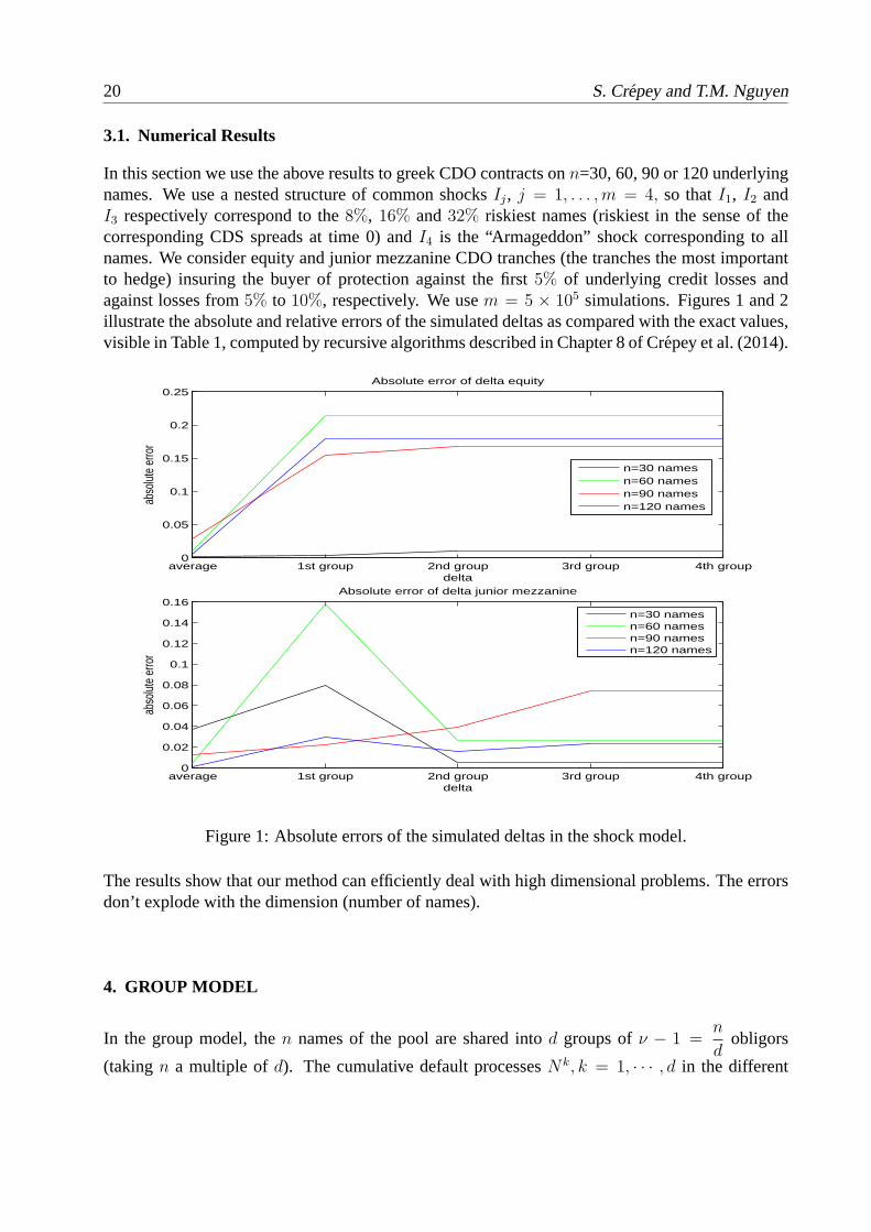
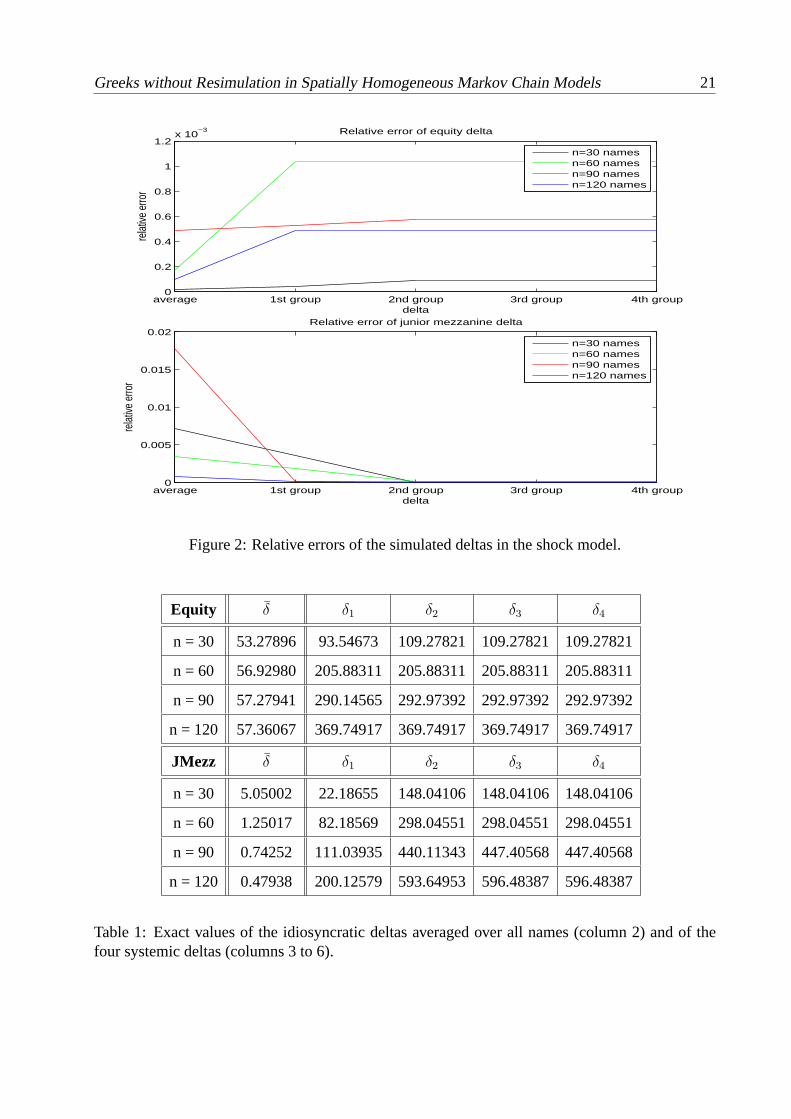
In this section we use the above results to greek CDO contractsonn=30, 60, 90 or 120 underlyingnames. We use a nested structure of common shocksIj, j = 1, . . . ,m = 4, so thatI1, I2 andI3 respectively correspond to the8%, 16% and32% riskiest names (riskiest in the sense of thecorresponding CDS spreads at time 0) andI4 is the “Armageddon” shock corresponding to allnames. We consider equity and junior mezzanine CDO tranches (the tranches the most importantto hedge) insuring the buyer of protection against the first5% of underlying credit losses andagainst losses from5% to 10%, respectively. We usem = 5 × 10⁵ simulations. Figures 1 and 2illustrate the absolute and relative errors of the simulated deltas as compared with the exact values,visible in Table 1, computed by recursive algorithms described in Chapter 8 of Crepey et al. (2014).
average 1st group 2nd group 3rd group 4th group0
0.05
0.1
0.15
0.2
0.25
delta
abso
lute
erro
r
Absolute error of delta equity
n=30 namesn=60 namesn=90 namesn=120 names
average 1st group 2nd group 3rd group 4th group0
0.02
0.04
0.06
0.08
0.1
0.12
0.14
0.16
delta
abso
lute
erro
r
Absolute error of delta junior mezzanine
n=30 namesn=60 namesn=90 namesn=120 names
Figure 1: Absolute errors of the simulated deltas in the shock model.
The results show that our method can efficiently deal with high dimensional problems. The errorsdon’t explode with the dimension (number of names).
4. GROUP MODEL
In the group model, then names of the pool are shared intod groups ofν − 1 =n
dobligors
(takingn a multiple ofd). The cumulative default processesNk, k = 1, · · · , d in the different
Greeks without Resimulation in Spatially Homogeneous Markov Chain Models 21
average 1st group 2nd group 3rd group 4th group0
0.2
0.4
0.6
0.8
1
1.2x 10
−3
delta
relat
ive e
rror
Relative error of equity delta
n=30 namesn=60 namesn=90 namesn=120 names
average 1st group 2nd group 3rd group 4th group0
0.005
0.01
0.015
0.02
delta
relat
ive e
rror
Relative error of junior mezzanine delta
n=30 namesn=60 namesn=90 namesn=120 names
Figure 2: Relative errors of the simulated deltas in the shockmodel.
Equity δ δ1 δ2 δ3 δ4
n = 30 53.27896 93.54673 109.27821 109.27821 109.27821
n = 60 56.92980 205.88311 205.88311 205.88311 205.88311
n = 90 57.27941 290.14565 292.97392 292.97392 292.97392
n = 120 57.36067 369.74917 369.74917 369.74917 369.74917
JMezz δ δ1 δ2 δ3 δ4
n = 30 5.05002 22.18655 148.04106 148.04106 148.04106
n = 60 1.25017 82.18569 298.04551 298.04551 298.04551
n = 90 0.74252 111.03935 440.11343 447.40568 447.40568
n = 120 0.47938 200.12579 593.64953 596.48387 596.48387
Table 1: Exact values of the idiosyncratic deltas averaged over all names (column 2) and of thefour systemic deltas (columns 3 to 6).
22 S. Crepey and T.M. Nguyen
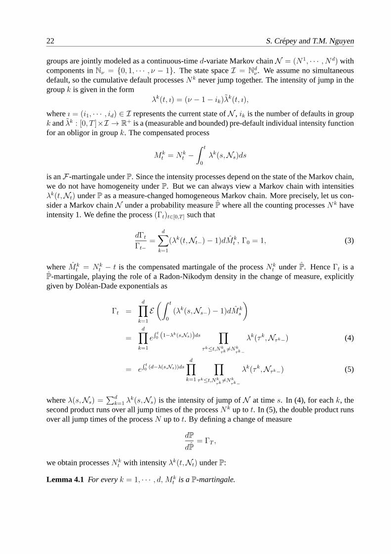
groups are jointly modeled as a continuous-timed-variate Markov chainN = (N1, · · · , Nd) withcomponents inNν = 0, 1, · · · , ν − 1. The state spaceI = N
dν . We assume no simultaneous
default, so the cumulative default processesNk never jump together. The intensity of jump in thegroupk is given in the form
λk(t, ı) = (ν − 1− ik)λk(t, ı),
whereı = (i1, · · · , id) ∈ I represents the current state ofN , ik is the number of defaults in groupk andλk : [0, T ]×I → R
+ is a (measurable and bounded) pre-default individual intensity functionfor an obligor in groupk. The compensated process
Mkt = Nk
t −
∫ t
0
λk(s,Ns)ds
is anF-martingale underP. Since the intensity processes depend on the state of the Markov chain,we do not have homogeneity underP. But we can always view a Markov chain with intensitiesλk(t,Nt) underP as a measure-changed homogeneous Markov chain. More precisely, let us con-sider a Markov chainN under a probability measureP where all the counting processesNk haveintensity 1. We define the process(Γt)t∈[0,T ] such that
dΓt
Γt−=
d∑
k=1
(λk(t,Nt−)− 1)dMkt , Γ0 = 1, (3)
whereMkt = Nk
t − t is the compensated martingale of the processNkt underP. HenceΓt is a
P-martingale, playing the role of a Radon-Nikodym density in the change of measure, explicitlygiven by Dolean-Dade exponentials as
Γt =d∏
k=1
E
(∫ t
0
(λk(s,Ns−)− 1)dMks
)
=d∏
k=1
e∫t
0 (1−λk(s,Ns))ds∏
τk≤t,Nk
τk6=Nk
τk−
λk(τ k,Nτk−) (4)
= e∫t
0(d−λ(s,Ns))ds
d∏
k=1
∏
τk≤t,Nk
τk6=Nk
τk−
λk(τ k,Nτk−) (5)
whereλ(s,Ns) =∑d
k=1 λk(s,Ns) is the intensity of jump ofN at times. In (4), for eachk, the
second product runs over all jump times of the processNk up tot. In (5), the double product runsover all jump times of the processN up tot. By defining a change of measure
dP
dP= ΓT ,
we obtain processesNkt with intensityλk(t,Nt) underP:
Lemma 4.1 For everyk = 1, · · · , d, Mkt is aP-martingale.

Greeks without Resimulation in Spatially Homogeneous Markov Chain Models 23
Proof. We have
d(Mkt Γt) = Mk
t−dΓt + Γt−dMkt + d[Mk,Γ]t
= Mkt−dΓt + Γt−(dN
kt − λk(t,Nt)dt) + Γt−(λ
k(t,Nt−)− 1)dNkt
= Mkt−dΓt + Γt−λ
k(t,Nt−)dMkt ,
whereMk andΓ are bounded, soMkΓ is aP-martingale, henceMk is aP-martingale.
In the group model, the martingale representation has the form
Πt = Π0 +d
∑
k=1
∫ t
0
δuk(s,Ns−)dMks , (6)
whereδuk(t, ı) = u(t, ık) − u(t, ı), in which ık represents the stateı with componentk increasedby one.
Proposition 4.2 For everyt ∈ [0, T ] such thatΓt− 6= 0 andλk(t,Nt−) 6= 0,
δuk(t,Nt−) =1
λk(t,Nt−)E
[
ǫ+t,0k
(ΓT ξ)
ΓT
|Ft
]
− E[ξ|Ft], (7)
whereǫ+t,z, so-called creation operator (see lemma III.3 of Bouleau and Denis (2013)), adds a jumpof sizez at t in the processN . In particular,
δuk(0,N0) =1
λk(0,N0)E
[
ǫ+0,0k
(ΓT ξ)
ΓT
]
− E[ξ]. (8)
Proof. The group modelN can be represented as
Nt =Nt∑
i=1
Zi, (9)
whereNt =∑d
k=1Nkt is the cumulative default process and theZi are the successive jump sizes
of N in
Z = 01 := (1, 0, · · · , 0), 02 := (0, 1, 0, · · · , 0), · · · , 0d := (0, · · · , 0, 1) ⊂ Nd.
Under the probabilityP, N has the form (9), whereNt is a homogeneous Poisson process ofintensityd and (Zi)i≥0 are i.i.d. with uniform distributionU on Z. Hence,N is a compoundPoisson process underP. The jump counting measureν of N is a Poisson random measure onR+ × Z with intensity measureµ(dt, dz) = ddt⊗ U(dz) and with compensated random measureν(dt, dz) = ν(dt, dz)− µ(dt, dz). The Clark-Ocone formula for the random variableΓT ξ underPyields (see Di Nunno et al. (2008)):
ΓT ξ = E[ΓT ξ] +
∫ T
0
∫
ZE[Ds,z(ΓT ξ)|Fs]ν(ds, dz),

24 S. Crepey and T.M. Nguyen
whereDs,z(ΓT ξ) is the Malliavin derivative ofΓT ξ at (s, z) (and for a predictable version of theconditional expectation processE[Ds,z(ΓT ξ)|Fs], s ≥ 0). Hence,
ΓtΠt = ΓtE[ξ|Ft] = E[ΓT ξ|Ft] = E[ΓT ξ] +
∫ t
0
∫
ZE[Ds,z(ΓT ξ)|Fs]ν(ds, dz)
and
d(ΓtΠt) = E[Dt,z(ΓT ξ)|Ft]ν(dt, dz) =d
∑
k=1
E[Dt,0k(ΓT ξ)|Ft]dMkt . (10)
Moreover, from (3) and (6), we obtain
d(ΓtΠt) = Γt−dΠt +Πt−dΓt + d[Π,Γ]t
= Γt−
d∑
k=1
δuk(t,Nt−)dMkt +Πt−Γt−
d∑
k=1
(λk(t,Nt−)− 1)dMkt
+Γt−
d∑
k=1
δuk(t,Nt−)(λk(t,Nt−)− 1)dNk
t
= Γt−
d∑
k=1
[δuk(t,Nt−)λk(t,Nt−) + Πt−(λ
k(t,Nt−)− 1)]dMkt . (11)
By identifying (10) and (11) we get
Γt−[δuk(t,Nt−)λ
k(t,Nt−) + Πt−(λk(t,Nt−)− 1)] = E[Dt,0k(ΓT ξ)|Ft].
But by properties of the Malliavin derivative and of the creation operatorǫ+ (see lemma III.3 ofBouleau and Denis (2013)), we haveDt,0k(ΓT ξ) = ǫ+
t,0k(ΓT ξ)− ΓT ξ, and
E[Dt,0k(ΓT ξ)|Ft] = E[ǫ+t,0k
(ΓT ξ)− ΓT ξ|Ft] = E[ǫ+t,0k
(ΓT ξ)|Ft]− Γt−Πt−
(for a predictable version of the conditional expectationE[ǫ+t,0k
(ΓT ξ)|Ft]). Therefore,
Γt−λk(t,Nt−)[δu
k(t,Nt−) + Πt−] = E[ǫ+t,0k
(ΓT ξ)|Ft] = Γt−E
[
ǫ+t,0k
(ΓT ξ)
ΓT
|Ft
]
, (12)
with the convention that the ratio equals to0 whenΓT = 0, hence alsoǫ+t,0k
(ΓT ξ) = 0, in the righthand side. In the case whereΓt− 6= 0 andλk(t,Nt−) 6= 0, we deduce
δuk(t,Nt−) + Πt− =1
λk(t,Nt−)E
[
ǫ+t,0k
(ΓT ξ)
ΓT
|Ft
]
.
Now we consider the problem of min-variance hedging an equity or senior CDO tranche by theunderlying credit index. LetΠ andP (resp. u andv) denote the price processes (resp. pricing

Greeks without Resimulation in Spatially Homogeneous Markov Chain Models 25
functions) of a tranche and of the index. By application of theformula (11.14) in Crepey (2013),we can min-variance hedge a tranche by the index and the riskless (constant) asset by using thestrategyζ in the index defined by
ζt =
∑d
l=1 λl(δul)(δvl)
∑d
l=1 λl(δvl)2
(t,Nt−) =d
∑
l=1
wl
(
δul
δvl
)
with wl =(δvl)2
∑d
j=1 λj(δvj)2
, for t ∈ [0, T ],
(13)whereδul andδvl can be represented in the form (7) (or, at time 0, (8)). In caseof a local intensitymodel (d = 1), the martingale representation (6) yields
dΠt = δu(t,Nt−)dMt, dPt = δv(t,Nt−)dMt.
Therefore,
dΠt = δtdPt, whereδt = δ(t,Nt−) =u(t,Nt)− u(t,Nt−)
v(t,Nt)− v(t,Nt−). (14)
In this case, it is thus possible to replicate the tranche by the index using the strategyδt defined by(14), which coincides with the min-variance hedging strategy ζt in (13).
4.1. Numerical Results
We estimate, by Monte Carlo based on (8) usingm = 104 or m = 106 simulations, the deltas ofthe equity tranche and of the senior tranche with maturityT = 5 and “strike”k = 45% (equitytranche[0, 45%] and senior tranche[45%, 100%] with pricing functions denoted byu+ andu−,respectively). The nominal is set to1. The results are compared with the exact values computedby matrix exponentiation and with the simulation/regression estimates of section 11.2 in Crepey(2013) (note that these are based onm = 4× 10⁴ simulations).
One group This is the special case whered = 1. For tractability of the matrix exponentiationmethod that is used for validating our simulation results, we consider a small portfolio ofn = 8obligors. The pre-default individual intensity function is taken as
λ(i) =1 + i
n.
The results are displayed in Table 2.
k = 45% val δ err δ11 err δ1s err δ2s
Eq 0.41513 0.29196 -7.97263 -0.08968
Sen 0.58487 -0.20723 5.65883 0.06365
Table 2: One group: Exact values (column 2) and percentage relative errors forδ =δu±
0(0)
δv0(0)es-
timated by simulation/regression withm = 104 (column 3) or by simulation based on spatialhomogeneity withm = 104 (column 4) orm = 106 (column 5).
26 S. Crepey and T.M. Nguyen
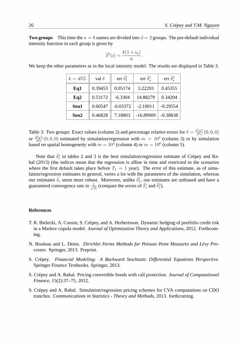
Two groups This time then = 8 names are divided intod = 2 groups. The pre-default individualintensity function in each group is given by
λk(ı) =k(1 + ik)
n.
We keep the other parameters as in the local intensity model.The results are displayed in Table 3.
k = 45% val δ err δ11 err δ1s err δ2s
Eq1 0.39453 0.05174 3.22293 0.45355
Eq2 0.53172 -6.3304 14.88279 0.34204
Sen1 0.60547 -0.03372 -2.10011 -0.29554
Sen2 0.46828 7.18803 -16.89909 -0.38838
Table 3: Two groups: Exact values (column 2) and percentage relative errors forδ = δ1u±
δ1v(0, 0, 0)
or δ2u±
δ2v(0, 0, 0) estimated by simulation/regression withm = 104 (column 3) or by simulation
based on spatial homogeneity withm = 104 (column 4) orm = 106 (column 5).
Note thatδ11 in tables 2 and 3 is the best simulation/regression estimateof Crepey and Ra-hal (2013) (the indices mean that the regression is affine in time and restricted to the scenarioswhere the first default takes place beforeT1 = 1 year). The error of this estimate, as of simu-lation/regression estimates in general, varies a lot with the parameters of the simulation, whereasour estimatesδs seem more robust. Moreover, unlikeδ11, our estimates are unbiased and have aguaranteed convergence rate in1√
m(compare the errors ofδ1s andδ2s ).
References
T. R. Bielecki, A. Cousin, S. Crepey, and A. Herbertsson. Dynamic hedging of portfolio credit riskin a Markov copula model.Journal of Optimization Theory and Applications, 2012. Forthcom-ing.
N. Bouleau and L. Denis.Dirichlet Forms Methods for Poisson Point Measures and Levy Pro-cesses. Springer, 2013. Preprint.
S. Crepey. Financial Modeling: A Backward Stochastic Differential Equations Perspective.Springer Finance Textbooks. Springer, 2013.
S. Crepey and A. Rahal. Pricing convertible bonds with call protection. Journal of ComputationalFinance, 15(2):37–75, 2012.
S. Crepey and A. Rahal. Simulation/regression pricing schemes for CVA computations on CDOtranches.Communications in Statistics - Theory and Methods, 2013. forthcoming.

Greeks without Resimulation in Spatially Homogeneous Markov Chain Models 27
S. Crepey, T. R. Bielecki, and D. Brigo.Counterparty Risk and Funding–A Tale of Two Puzzles.Taylor & Francis, 2014. Forthcoming Spring 2014.
G. Di Nunno, B.K. Øksendal, and F. Proske.Malliavin Calculus for Levy Processes with Appli-cations to Finance. Universitext (En ligne). Springer-Verlag Berlin Heidelberg, 2008. ISBN9783540785729. URLhttp://books.google.fr/books?id=G9EvB\_HZCVwC.

WORST-CASE OPTIMIZATION FOR AN INVESTMENT CONSUMPTION PROBLEM
Tina Engler
Department of Mathematics, Martin Luther University Halle-WittenbergTheodor-Lieser-Str. 5, 06120 Halle (Saale), GermanyEmail: [email protected]
Abstract
We investigate a Merton-type investment-consumption problem under the threat of a marketcrash, where the interest rate of the savings account is stochastic. Inspired by the recent workof Desmettre et al. (2013), we model the market crash as an uncertain event (τ, l). While thestock price is driven by a geometric Brownian motion at times t ∈ [0, τ) ∪ (τ,∞], it loses afraction l of its value at the crash time τ . We maximize the expected discounted logarithmicutility of consumption over an infinite time horizon in the worst-case scenario, and solve theproblem by separating it into a post- and a pre-crash problem. We determine the optimalpost-crash strategy by means of classical stochastic optimal control theory. Finally, based onthe martingale approach, developed by Seifried (2010), we characterize the optimal pre-crashstrategy.
1. INTRODUCTION AND MOTIVATION
The classical Merton-type model for determining optimal rules for investment and consumption ona complete market with constant market parameters was solved by Merton (1969) using DynamicProgramming. Since then, several generalizations, such as stochastic volatilities of the stock price,transaction costs or acting on an incomplete market were considered in a wide-ranging body ofliterature. Moreover, in contrast to the classical work of Merton, for example, Fleming and Pang(2004) and Pang (2006) considered a model where the market parameter r, which represents theinterest rate, is an ergodic Markov diffusion process. The authors motivated this by the fact thateven for money in the bank, the interest rate may fluctuate over time. On the other hand, the fluc-tuations of the stock price were generalized to model market crashes. The standard approach oftenused in the literature is to replace the geometric Brownian motion by a jump diffusion process,which requires distributional assumptions on the jumps. However, Korn and Wilmott (2002) pro-posed modeling a market crash as an uncertain event and optimized the expected discounted utilityof consumption in the worst-case scenario.
29

30 T. Engler
This paper combines both of these aspects in a model with a stochastic interest rate and the threatof a market crash modeled as an uncertain event. We are interested in finding the infinite horizonoptimal investment and consumption behavior of an investor with a logarithmic utility function inthe worst-case scenario with respect to a market crash. As in Desmettre et al. (2013), we model themarket crash as an uncertain once-in-a-lifetime event (τ, l), where τ denotes the random crash timeand l indicates the crash size. The advantage of this method is that no distributional assumptionsabout price jumps are needed.After explaining the investment-consumption model in Section 2, we apply the worst-case opti-mization theory to our model with a stochastic interest rate. In Section 3 we solve the worst-caseoptimization problem for two different models of interest rates. Therein, we proceed in threesteps. First, we can solve the post-crash problem by standard stochastic optimal control theory(Section 3.1) for both a Vasicek interest rate model and a Cox-Ingersoll-Ross (CIR) model. Then,in Section 3.2, we reformulate the worst-case problem into a pre-crash problem that we reduce to acontroller-vs-stopper game. Finally, we can determine the optimal pre-crash strategy by applyinga martingale approach by Seifried (2010).
2. THE WORST-CASE OPTIMIZATION PROBLEM
Let us consider a financial market with one risky asset and a savings account with a stochastic inter-est rate. Throughout the paper, we consider a complete probability space (Ω,F ,P) with filtrationF = (Ft)t≥0. As in Desmettre et al. (2013), we are interested in finding the optimal investmentand consumption behavior of an investor under the threat of a market crash (τ, l), which is definedas follows. The event (τ, l) consists of the crash time τ and the crash size l. The crash time τ isa [0,∞]-valued stopping time. At time τ , the risky asset loses a fraction l of its value, where l isan Fτ -adapted random variable with 0 ≤ l ≤ l∗ and l∗ < 1 denotes the maximal crash size. Weabbreviate the set of all crash scenarios briefly by
C := (τ, l) : τ ∈ [0,∞], stopping time, l ∈ [0, l∗]Fτ - measurable random variable.
Moreover, we assume at normal times t ∈ [0, τ)∪(τ,∞] that the asset price Pt follows a geometricBrownian motion
dPt = Pt[µ dt+ σ1 dw1,t], P0 = p0,
where µ, σ1 > 0 are constant, and w1 = (w1,t)t≥0 is a standard Wiener process. At the crash timeτ , we have
Pτ = (1− l)Pτ− .
Our model and the model considered in Desmettre et al. (2013) differ in the interest rate modeling.Here, we assume that the interest rate, denoted by r = (rt)t≥0, follows a stochastic process. Weconsider two different interest rate models in this paper. On the one hand, we consider an interestrate r = rV that follows a Vasicek process after the market crash
rVt =
rc : t ≤ τ
rce−a(t−τ) + rM
(1− e−a(t−τ)
)+ σ2e
−at ∫ tτeasdws : t > τ
, (1)

Worst-Case Optimization for an Investment-Consumption Problem 31
and on the other hand, we consider an interest rate r = rC that follows a CIR process after time τ
rCt =
rc : t ≤ τ
rce−a(t−τ) + rM
(1− e−a(t−τ)
)+ σ2e
−at ∫ tτ
√rCs e
asdws : t > τ, (2)
where a, rM , σ2 > 0 and w = (wt)t≥0 denotes a Wiener process, correlated withw1 by a correlationcoefficient ρ ∈ [−1, 1]. Assuming model (1) or (2), the interest rate before the market crash is givenby a positive constant rc with µ− rc > 0. After the market crash, the interest rate follows an affinelinear stochastic process, of either Vasicek- or CIR-type, with a speed of reversion a to the long-term mean level rM . If we require 2arM > σ2
2 , then we have rCt > 0 for all t ≥ 0. This propertyis an advantage of the CIR model over the Vasicek interest rate. In the text below, we use theuniversal notation rt for the interest rate if it makes no difference which model is considered.We denote the ratio of investor’s wealth invested in the risky asset by kt, while ct is the ratio ofwealth consumed at time t. Below, we separate the problem into a pre- and a post-crash problem.Thus, we denote the pre-crash strategy, valid for t ≤ τ , by (kt, ct), and the post-crash strategy,valid for t > τ , by (kt, ct).Now, the investor’s wealth at time t ≥ 0 is denoted by Xt and it is defined by the followingstochastic differential equations:
X0 = x0 > 0,
dXt = Xt [rc + (µ− rc)kt − ct] dt+Xtσ1kt dw1,t, on [0, τ),
Xτ = (1− lkτ )Xτ− ,
dXt = Xt
[rt + (µ− rt)kt − ct
]dt+Xtσ1kt dw1,t, on (τ,∞],
where, as mentioned above, we can write the post-crash interest rate for model (1), denoted by rt,in the form
drt = a(rM − rt) + σ2(ρ dw1,t +√
1− ρ2 dw2,t), on (τ,∞], (3)rτ = rc.
If we consider (2), we find that:
drt = a(rM − rt) + σ2
√rt(ρ dw1,t +
√1− ρ2 dw2,t), on (τ,∞], (4)
rτ = rc.
Given these assumptions, the investor aims to maximize the expected discounted logarithmic utilityof consumption over an infinite time horizon in the worst-case crash scenario. Thus, we formulatethe following worst-case optimization problem:
sup(k,c)∈Π
inf(τ,l)∈C
E(∫ ∞
0
e−εt ln(ctXt) dt
), (5)
where ε > 0 denotes the discount factor and Π is the admissible control space defined below.
Definition 2.1 (Admissible control space Π) An investment and consumption portfolio (k, c) :=(k, c, k, c) belongs to the admissible control space Π, if the following conditions hold:

32 T. Engler
1. (kt, ct) and (kt, ct) are Ft-adapted for all t ≥ 0,
2. E(∫ t
0k2sds)<∞, ∀ t ≥ 0,
3. 0 ≤ ct ≤ C <∞ for all t ≥ 0, where C > 0 is a sufficiently large constant,
4. limT→∞ e−εTE
∫ T0k
2
t dt = 0,
5. kt <1l∗
for all t ≥ 0 and k is right continuous.
Remark 2.1 Condition 2 in Definition 2.1 has to be fulfilled for both the pre-crash strategy (k, c)and the post-crash strategy (k, c), respectively. Conditions 3 and 4 are assumed in order to applya verification theorem when identifying the optimal post-crash strategy (see Section 3.1 below).Note that the admissible control space contains strategies k with values in (−∞,∞). Negativevalues of k correspond to short-selling. Condition 5 ensures that the wealth at the crash time τstays positive.
The aim of the next section is to determine the optimal worst-case strategy (k∗, c∗) for problem(5). It turns out that we can apply the same main steps as in Desmettre et al. (2013) to solve theworst-case optimization problem under a stochastic interest rate.
3. THE SOLUTION BY A MARTINGALE APPROACH
First, in Section 3.1 we can find an optimal post-crash strategy (k∗, c∗) by solving a classical
stochastic optimal control problem. Using the special structure of the resulting post-crash valuefunction, we can reformulate problem (5) into a pre-crash problem. This will be done in Sec-tion 3.2. Finally, in Section 3.3 we identify the optimal pre-crash strategy (k∗, c∗) by solving aconstrained stochastic optimal control problem.
3.1. The optimal post-crash strategy
In this section we consider the optimization problem that the investor faces at the crash time τ .In fact, the investor is faced with a classical stochastic optimal control problem over an infinitetime horizon because, at the crash time, he knows that no further crash can occur. Equipped with awealth x and an observed interest rate r at the crash time, the investor has to maximize the expecteddiscounted utility of consumption. Because the interest rate after the crash is stochastic, we haveto consider a two-dimensional state process (X t, rt). Let us define the post-crash value function:
V (x, r) = sup(k,c)∈Π
Ex,r(∫ ∞
0
e−εt ln(ctX t) dt
)(6)
with respect to the post-crash dynamics:
dX t = X t
[rt + (µ− rt)kt − ct
]dt+X tσ1kt dw1,t, X0 = x, (7)

Worst-Case Optimization for an Investment-Consumption Problem 33
where the post-crash interest rate rt in the Vasicek and the CIR model is given by (3) and (4),respectively.
Remark 3.1 The post-crash value function V (x, r) depends on the initial values of the post-crashdynamics, given by arbitrary x ∈ R+ and r ∈ R, that will represent the wealth and the interestrate at the crash time, respectively. Note that the starting point 0 takes the role of the crash time τ .
Vasicek model. We can use the result in (Pang 2006, Chp.5) to obtain the optimal post-crashstrategy for (6) with the post-crash interest rate of Vasicek-type (see (3)). Pang solved this infinitehorizon stochastic control problem by Dynamic Programming Principle. Thus, we obtain theoptimal post-crash strategy
k∗t = k
∗(rt) =
µ− rtσ2
1
, c∗t ≡ ε
and an explicit form of the post-crash value function:
V (x, r) =1
εln(x) + f(r), f(r) = α2r
2 + α1r + α0 (8)
where αi (i = 1, 2, 3) are given by
α2 =1
2εσ21(ε+ 2a)
,
α1 =1
ε(ε+ a)
[arM + (ε+ 2a)(σ2
1 − µ)
σ21(ε+ 2a)
],
α0 =1
ε
[σ2
2
2σ21ε(ε+ 2a)
+arM
ε(ε+ a)
[arM + (ε+ 2a)(σ2
1 − µ)
σ21(ε+ 2a)
]+
µ2
2σ21ε
+ ln(ε)− 1
].
Moreover, by reducing the Hamilton-Jacobi-Bellman (HJB) equation, we know that f ∈ C2(R)solves the differential equation
σ22
2frr + a(rM − r)fr − εf + ln(ε)− 1 +
1
ε
[(µ− r)2
2σ21
+ r
]= 0, ∀ r ∈ R. (9)
In order to prove that the solution of the HJB equation V (x, r) is indeed equal to the post-crashvalue function, Pang also required conditions 1-4 in Definition 2.1. Hence, we also included theserequirements. The same requirements are needed for the solution of problem (6) under the post-crash interest of CIR-type (see (4)).
CIR model. In contrast to the Vasicek model, as far as we know, no previous work exists thatsolves problem (6). Here, we can also determine the optimal post-crash strategy by applying theDynamic Programming Principle. In this case, the HJB equation for the value function V (x, r) isgiven by
εV = supk
[(µ− r)kxV x +
1
2σ2
1k2x2V xx + ρσ1σ2k
√rxV xr
]+ rxV x
+a(rM − r)V r +1
2σ2
2rV rr + supc≥0
[−cxV x + ln(cx)
].

34 T. Engler
Using the standard approach V (x, r) = A ln(x) + g(r) with A = 1ε
and g ∈ C2(R), we can reducethe HJB equation to
εg =1
εsupk∈Π
[(µ− r)k − 1
2σ2
1k2]
+r
ε+ a(rM − r)gr +
1
2σ2
2rgrr + supc∈Π
[−cε
+ ln(c)
].
The optimal post-crash strategy is then given by
k∗t = k
∗(rt) =
µ− rtσ2
1
, c∗ = ε, (10)
where rt is given by (4). We verify this result in the verification theorem below. Inserting theseoptimal candidates, we obtain the differential equation for g ∈ C2(R)
σ22
2r grr + a(rM − r)gr − εg + ln(ε)− 1 +
1
ε
[(µ− r)2
2σ21
+ r
]= 0, ∀ r ∈ R. (11)
In contrast to equation (9), the coefficient of grr is linear in r. Nevertheless, since the last term isquadratic in r, we suppose that g(r) = β2r
2 + β1r + β0. Comparing the coefficients, we obtain
β2 =1
2εσ21(ε+ 2a)
,
β1 =1
ε(ε+ a)
[arM + (ε+ 2a)(σ2
1 − µ) +σ22
2
σ21(ε+ 2a)
],
β0 =1
ε
[arM
ε(ε+ a)
[arM + (ε+ 2a)(σ2
1 − µ) +σ22
2
σ21(ε+ 2a)
]+
µ2
2σ21ε
+ ln(ε)− 1
].
In order to show that the candidates in (10) are in fact optimal for the stochastic control problem(6), we can prove the following verification theorem.
Theorem 3.1 (Verification theorem) Suppose g(r) = β2r2 + β1r + β0 is a classical solution of
(11) and define
V (x, r) :=1
εln(x) + g(r). (12)
If
k∗(rt) =
µ− rtσ2
1
, c∗(rt) ≡ ε,
where rt is given by (4), then (k∗, c∗) ∈ Π and
V (x, r) = Ex,r(∫ ∞
0
e−εt ln(c∗tX∗t ) dt
),
where X∗t denotes the process that solves (7) corresponding to (k∗, c∗). That means, V (x, r) =
V (x, r), where V (x, r) is defined by (6) under the CIR interest rate.

Worst-Case Optimization for an Investment-Consumption Problem 35
Proof. We prove the result by rather standard arguments. By the definition of V and by apply-ing Ito’s formula, we obtain for arbitrary (k, c) ∈ Π that V (x, r) ≥ Ex,r
(∫∞0e−εt ln(ctX t) dt
).
Afterwards, we get (k∗, c∗) ∈ Π, and by the above calculation we have
k∗ ∈ arg max
k
[(µ− r)kxVx +
1
2σ2
1k2x2Vxx + ρσ1σ2kx
√rVxr
],
c∗ ∈ arg maxc≥0
[−cxVx + ln(cx)
].
Using Ito’s formula and the explicit form of the first and second moment of rt, we are able to showthat
V (x, r) ≤ E(∫ ∞
0
e−εt ln(c∗tX∗t ) dt
)= V (x, r).
Thus, the assertion holds.
Remark 3.2 Due to the stochastic interest rate rt after the market crash, the optimal post-crashstrategy is a feedback control depending on the stochastic interest rate rt, given by a Vasicekprocess and a CIR process, respectively.
At the crash time, the investor has an amount of wealth of x = (1− lkτ )Xτ and the interest rate atthe crash time is r = rτ . These values are the initial values of the post-crash problem and can beinserted in the post-crash value function V (x, r). From now on, we write for the post-crash valuefunction:
V (x, r) =1
εln(x) +W (r),
where W (r) stands for f(r) in the Vasicek case and for g(r) in the CIR case. Thus, we canreformulate the worst-case optimization problem into a pre-crash problem.
3.2. Reformulation of the worst-case optimization problem
From the post-crash analysis in the previous section we know that the performance of the optimalpost-crash strategy at time τ is given by the post-crash value function at x = (1 − lkτ )Xτ andr = rτ , namely V ((1− lkτ )Xτ , rτ ). Since V (x, r), given by (8) and (12), is monotone increasingin x, we obtain
V ((1− lkτ )Xτ , rτ ) ≥ V ((1− l∗k+τ )Xτ , rτ ),
where k+ := max0, k. Thus, we can conclude that the worst-case crash size is realized forl = l∗. Because we assumed a constant interest rate rc before and including the crash time, wehave rτ = rc. Now, we discount V ((1 − l∗k+
τ )Xτ , rc) to the starting time 0 by e−ετ and wereformulate the worst-case problem (5) into the following pre-crash problem:
sup(k,c)∈Π
infτ∈C
E(∫ τ
0
e−εt ln(ctXt) dt+ e−ετV ((1− l∗k+τ )Xτ , rc)
)(13)
with respect to the pre-crash dynamics
dXt = Xt [rc + (µ− rc)kt − ct] dt+Xtσ1kt dw1,t, X0 = x0 > 0.

36 T. Engler
Note that the pre-crash problem is considered with respect to the pre-crash dynamics. Because ofconstant interest rates before the crash, we have to consider only the state equation for the pre-crashwealth. In the pre-crash problem (13) the infimum is only taken over the crash time τ , because wealready identified the worst-case crash size by l∗. From now on, we write (k, c) instead of (k, c)for the pre-crash strategy and therefore, by (13), the worst-case problem (5) reduces to a controllervs. stopper game of the form
sup(k,c)∈Π
infτE(Mk,c
τ
), (14)
where
Mk,ct :=
∫ t
0
e−εs ln(csXs) ds+ e−εtV ((1− l∗k+t )Xt, rc), t ≥ 0.
Such a controller vs. stopper game is also explained in Seifried (2010). Here, we also try to solvethis kind of a stochastic game, where the investor controls Mk,c by choosing (k, c) and the stopper,namely the market, decides on the duration of the game τ ∈ C. In the text below, we see that wecan apply the concept of Indifference and Indifference Optimality Principle, developed in Seifried(2010) and Desmettre et al. (2013) to identify the optimal pre-crash strategy for the stochasticgame (14). Analogously, we define an indifference strategy as follows.
Definition 3.1 (Indifference Strategy, cf. (Seifried 2010, p.566)) A pre-crash strategy (k, c) iscalled indifference strategy if
E(M k,cτ1
) = E(M k,cτ2
) (15)
for stopping times τ1 6= τ2.
The idea here is that the investor chooses an indifference strategy before the crash, such that theperformance of this choice does not depend on the crash time τ . After formulating a sufficient con-dition for a strategy to be an indifference strategy, we can use the notion of an Indifference Frontierand an Indifference Optimality Principle to identify the worst-case optimal pre-crash strategy.
Proposition 3.2 (Indifference Condition) Let (k, c) be a constant pre-crash strategy such thatH(k, c) = 0, where
H(k, c) := ln(c)− ln(1− l∗k+) +1
ε[rc + (µ− rc)k − c]−
σ21
2εk2 − εW (rc). (16)
Then (k, c) ∈ Π is an indifference strategy, which means E(M k,cτ1
) = E(M k,cτ2
).
Proof. The proof is similar to that in Desmettre et al. (2013) and it is divided into two steps.First, we show that M k,c is a uniformly integrable martingale. In the second step we apply Doob’sOptional Sampling theorem and the assertion follows.By the definition of Mk,c and for arbitrary (k, c), we have
dMk,ct = e−εt ln(ctXt) dt+ d
[e−εtV ((1− l∗k+
t )Xt, rc)].
Worst-Case Optimization for an Investment-Consumption Problem 37
Now, we restrict ourselves to constant pre-crash strategies. With V (x, r) = 1ε
ln(x) + W (r) (seesection 3.1) and by applying Ito’s formula, we obtain
dMk,ct = e−εt
ln(c)− ln(1− l∗k+) +
1
ε[rc + (µ− rc)k − c]−
σ21
2εk2 − εW (rc)
dt (17)
+e−εt1
εσ1k dw1,t.
Let (k, c) be a constant pre-crash strategy such that H(k, c) = 0, then
dM k,ct = e−εt
1
εσ1k dw1,t.
Since k is assumed to be constant, it is easy to check that M k,ct =
∫ t0e−εs 1
εσ1k dw1,s is a uniformly
integrable martingale. By (Protter 1990, Thm. 12), we find that the uniformly integrable martingaleM k,c is closed by the random variable M k,c
∞ := limt→∞Mk,ct . Then, by applying Doob’s Optional
Sampling Theorem (for example, see (Protter 1990, Thm.16)), we obtain (15). By Definition 3.1,it follows that (k, c) is an indifference strategy. Finally, it follows that a constant (k, c) with c ≥ 0is an admissible strategy.
Remark 3.3 In our model it is essential that the interest rate before the crash is constant. Thisleads to the fact that the dt-coefficient in (17) does not depend on ω ∈ Ω. Moreover, due to theinfinite time horizon, the indifference strategy does not depend on time t. By these arguments it issufficient to consider constant pre-crash strategies.
Now, having a sufficient condition for a pre-crash strategy to be an indifference strategy, we canapply the Indifference Optimality Principle stated in Seifried (2010) and Desmettre et al. (2013).Let (k, c) be an indifference strategy and (k, c) ∈ Π be an arbitrary admissible pre-crash strategy.Then, by (Desmettre et al. 2013, Lemma 4.3), we can improve the worst-case performance for(k, c) by cutting off at the strategy (k, c). In detail, they showed that
infτE(M k,c
τ ) ≥ infτE(Mk,c
τ ), (18)
where
kt =
kt : t < η
k : t ≥ ηct =
ct : t < η
c : t ≥ η,
and η := inft ≥ 0 : kt > k. The application of (Desmettre et al. 2013, Lemma 4.3) is possiblefor our model, because of the required right continuity of the pre-crash strategy kt and the fact thatthe post-crash value function V (x, r) is also monotone increasing in x for the log-utility function.Thus, for details of the proof of (18) we refer to the literature.
By (18), we can restrict our considerations on strategies that are dominated by an indifferencestrategy because all other strategies would provide worse performances. In order to do this, weabbreviate the set of such strategies by
A(k) :=
(k, c) ∈ Π : kt ≤ k, ∀t ≥ 0.

38 T. Engler
Next, we apply the Indifference Optimality Principle (see (Desmettre et al. 2013, Proposition 5.1))to identify a worst-case optimal pre-crash strategy for our model with a stochastic interest rate.This principle provides us a sufficient condition for a pre-crash strategy (k∗, c∗) to be optimalin the worst-case scenario: An indifference strategy (k, c) = (k∗, c∗) is the worst-case optimalinvestment consumption strategy for (5), if it is optimal in the no-crash scenario τ = ∞ in theclass of all strategies respecting the associated indifference frontier. Thus, our task in the nextSection is to identify an indifference strategy (k∗, c∗), which fulfills the condition:
E(Mk,c∞ ) ≤ E(Mk∗,c∗
∞ ) ∀ (k, c) ∈ A(k∗). (M)
3.3. Identification of the optimal pre-crash strategy
The aim of this Section is to identify the optimal pre-crash strategy by applying the IndifferenceOptimality Principle. We are done if we can find (k∗, c∗) ∈ Π which fulfills the IndifferenceCondition of Proposition 3.2 and the Indifference Optimality Condition (M).
Theorem 3.3 Let k∗ < m := min
1l∗, µ−rc
σ21
be the unique root of the function H(k, ε), where H
is defined in (16). Then, the optimal pre-crash strategy for the worst-case problem (5) is given by
k∗t ≡ k∗, c∗t ≡ ε.
Proof. We divide the proof into two steps. First, we show that there exists a uniquely determinedk∗, such thatH(k∗, ε) = 0. In a second step we show that (k∗, ε) is optimal in the no-crash scenarioin the class of strategies that respect the Indifference Frontier (k∗, ε). Finally, we can conclude that(k∗, ε) is the optimal pre-crash strategy.
Step 1.By definition of H in (16), we have
∂
∂kH(k, ε) =
− 1
(1−l∗k+)· (−l∗) + 1
ε((µ− rc)− σ2
1k) : 0 ≤ k < m1ε
((µ− rc)− σ21k) : k < 0
.
It follows that H(k, ε) is strictly monotone increasing for k < m. If m = 1l∗
, it holds
limk1/l∗
H(k, ε) = ln(ε)− limk1/l∗
ln(1− l∗k+) +1
ε[rc + (µ− rc)
1
l∗− ε]− σ2
1
2ε
1
l∗2− εW (rc) = +∞
and if m = µ−rcσ21
we obtain
H
(µ− rcσ2
1
, ε
)= ln(ε)− ln
(1− l∗ · µ− rc
σ21
)+rcε− 1 +
1
2ε
(µ− rc)2
σ21
− εW (rc) > 0
because W (rc) is given in Section 3.1 and we can choose ε > 0 large enough such that the lastinequality holds.
Worst-Case Optimization for an Investment-Consumption Problem 39
Moreover, we get
limk→−∞
H(k, ε)
= ln(ε)− limk→−∞
ln(1− l∗k+
)+rcε
+1
εlim
k→−∞
((µ− rc)k −
σ21
2k2
)− 1− εW (rc) = −∞.
Because of the fact that H(k, ε) is strictly monotone increasing for k < m, H(m, ε) > 0 andlimk→−∞H(k, ε) < 0, we know that there exists a uniquely determined k∗ such that H(k∗, ε) = 0.Thus (k∗, ε) is an indifference strategy, and the first step of the proof is complete. Now, it remainsto show the second step.
Step 2.Here, we consider the constrained optimization problem
sup(k,c):k≤k∗
E(∫ ∞
0
e−εt ln(ctXt) dt
)with respect to the pre-crash dynamics
dXt = Xt [rc + (µ− rc)kt − ct] dt+Xtσ1kt dw1,t, X0 = x0 > 0. (19)
We solve this problem by separating the investment and consumption decisions. This separationis possible due to the logarithmic utility function (see Korn and Seifried (2013) for more details).This separation leads, on the one hand, to an optimal consumption strategy c∗ = ε, and on theother hand to the remaining problem for determining k∗
supk≤k∗
E(∫ ∞
0
e−εt ln(εXεt ) dt
), (20)
where Xεt denotes the solution of (19) controlled by ct = ε. By Ito’s formula, we have
E (ln(Xεt )) = ln(x0) + E
∫ t
0
φ(ks) ds− εt, φ(ks) := (µ− rc)ks −σ2
1
2k2s + rc.
Thus, the maximization of (20) is reduced to the maximization of φ over k ≤ k∗. Obviously, φ isstrictly monotone increasing for k < µ−rc
σ21
. Since k∗ < m, the maximum is attained for k = k∗.Thus, (k∗, ε) fulfills (M). Finally, the application the Infifference Optimality Principle proves theassertion.
4. CONCLUSIONS
The optimal investment and consumption behavior consists of determining a constant investmentcontrol k∗ such that H(k∗, ε) = 0 and c∗ = ε. It is important to note that determining k∗ de-pends on the interest rate model being considered. In contrast to the pre-crash strategy, the optimal

40 T. Engler
post-crash investment depends on the stochastic interest rate, whereas the optimal post-crash con-sumption strategy is again equal to the discount factor ε. The latter point is not surprising for thecase of a logarithmic utility function because the investment and consumption decisions can beseparated. This will certainly not be the case if we consider, for example, a power utility function.Thus, the case of more general utility functions is left for future research.
References
S. Desmettre, R. Korn, and F.T. Seifried. Worst-case consumption-portfolio optimization. Tech-nical Report 227, Fraunhofer ITWM, Kaiserslautern, 2013. URL http://publica.fraunhofer.de/documents/N-241439.html.
W. H. Fleming and T. Pang. An application of stochastic control theory to financial economics.SIAM Journal on Control and Optimization, 43(2):502–531, 2004.
R. Korn and F.T. Seifried. A concise characterization of optimal consumption with logarithmicpreferences. International Journal of Theoretical and Applied Finance, 16(06):1–7, 2013.
R. Korn and Paul Wilmott. Optimal portfolios under the threat of a crash. International Journal ofTheoretical and Applied Finance, 5(2):171–187, 2002.
R. C. Merton. Lifetime portfolio selection under uncertainty: The continuous-time case. TheReview of Economics and Statistics, 51(3):247–257, 1969.
T. Pang. Stochastic portfolio optimization with log utility. International Journal of Theoreticaland Applied Finance, 9(6):869–887, 2006.
P. Protter. Stochastic integration and differential equations, volume 21 of Applications of Mathe-matics (New York). Springer-Verlag, Berlin, 1990.
F.T. Seifried. Optimal investment for worst-case crash scenarios: a martingale approach. Mathe-matics of Operations Research, 35(3):559–579, 2010.
FIRST-PASSAGE TIME PROBLEMS UNDER REGIME SWITCHING:
APPLICATIONS IN FINANCE AND INSURANCE
Peter Hieber†
†Lehrstuhl fur Finanzmathematik, Technische Universitat Munchen, Parkring 11, 85748 Garching-Hochbruck, GermanyEmail: [email protected]
AbstractOne common approach in stochastic modeling of (rare) events (for example company de-
faults or natural catastrophes) is to assume that those events are triggered as soon as a stochasticrisk process falls below a constant barrier. In this paper, we model this risk process as a regimeswitching Brownian motion, a process that allows to incorporate many of the cyclical patternsthat either naturally arise (i.e. seasons, rainfall) or result from peoples’ interactions (i.e. busi-ness cycles). Two numerical examples demonstrate the flexibility of a regime switching riskprocess: Stress testing option prices on exchange rates and the pricing of CAT bonds.
1. INTRODUCTION
Recently, first-passage time problems for regime switching models have earned considerable at-tention. One reason for this increased interest is that first-passage time problems occur in manydifferent areas of science, for example:
• In Biology, they can be used as a tool in population modeling to, for example, estimateextinction probabilities for species. Food-supply is usually regime-dependent.
• In Insurance, companies have to provide enough capital to pay any claim that results out oftheir insurance policies. The claim arrival intensity is often regime-dependent; it might – forexample – be coupled to weather (sunny, rain) or season.
• In Finance, economic cycles (boom, recession) influence many financial time series. Regimeswitching models reflect the tendency of financial markets to often change their behaviorabruptly and persistently. First-passage time problems have to be solved if one wants toprice certain exotic options, i.e. American, barrier, lookback, or digital options (see, e.g.,Guo (2001b), Buffington and Elliott (2002), Elliott et al. (2005), Jobert and Rogers (2006),Boyle and Draviam (2007), Jiang and Pistorius (2008), Hieber and Scherer (2010), and manyothers).
41
42 P. Hieber
Another reason for the popularity of regime switching models is the fact that – conceptionally –they are rather simple (conditional on the regimes, the distribution is normal) and thus analyticallytractable. Nevertheless, they can generate many non-linear effects like heavy tails or volatilityclusters.
In this paper, we want to focus on applications of first-passage time problems under regimeswitching. In two numerical examples on the pricing of first-touch options and of CAT bonds, wedemonstrate that this rather simple (but very tractable) model has several nice features that cannotbe captured by a Levy process.
The paper is organized as follows: In Section 2, we introduce notation and regime switchingBrownian motion. Section 3 recalls some of the results on the first-passage time of regime switch-ing models (see also Guo (2001a), Jiang and Pistorius (2008), Hieber (2013a)). Then – the mainpart of this paper – is the application of those results to Finance and Insurance (see Section 4).
2. MODEL DESCRIPTION
On the filtered probability space (Ω,F,F ,P), we consider the process B = Btt≥0 described bythe stochastic differential equation (sde)
dBt = µZtdt+ σZtdWt, B0 = x, (1)
where µZt ∈ R, σZt > 0, Z = Ztt≥0 ∈ 1, 2, . . . ,M is a time-homogeneous Markov chainwith intensity matrix1 Q0, and W = Wtt≥0 an independent Brownian motion. The initial valueis B0 = x ∈ R. The filtration F = Ftt≥0 is generated by the pair (W,Z), i.e. Ft = σWs, Zs :0 ≤ s ≤ t. The time to a state change from the current state i is an exponential random variablewith intensity parameter Q0(i, i). The probability of moving to state j 6= i is −Q0(i, j)/Q0(i, i).The model is fully determined if an initial state (or, more generally, an initial distribution π0 :=(P(Z0 = 1),P(Z0 = 2), . . . ,P(Z0 = M)
)on the states) is defined.
The first-passage time on a lower barrier b < B0 = x is defined as
Tb :=
inf t ≥ 0 : Bt ≤ b , if such a t exists,∞, else.
(2)
The one-sided Fourier transform of the first-passage time is given by
Ψb(u) :=1
π
∫ ∞0
exp(iuTb
)dTb . (3)
3. FIRST-PASSAGE TIME RESULTS
This section recalls some of the results on the first-passage time of regime switching models. Forproofs and a more detailed review, we refer to Hieber (2013a). First, Theorem 3.1 presents theFourier transform of the first-passage time contingent on the solution of a matrix equation.
1An intensity matrix has negative diagonal and non-negative off-diagonal entries. Each row sums up to zero.

First-passage time problems under regime switching: Applications in Finance and Insurance 43
Theorem 3.1 (First-passage times) We denote the class of irreducibleM×M generator matrices(non-negative off-diagonal entries and non-positive row sums) by QM . The Fourier transform ofthe first-passage time on a lower barrier b < B0 = x is given by
Ψb(u, x) = π0 exp(Q−(x− b)
)1, (4)
where exp( · ) denotes the matrix exponential, π0 ∈ R1×M is the initial distribution on the states,and 1 a vector of ones of appropriate size. The tuple (Q+, Q−), Q+, Q− ∈ QM , is for u > 0defined via the two unique solutions Ξ(−Q+) = Ξ(Q−) = 0 of
Ξ(Q) :=
σ21 0 . . .
0 . . . 0. . . 0 σ2
M
Q2
2+
µ1 0 . . .0 . . . 0. . . 0 µM
Q+Q0 +
iu 0 . . .. . . iu 0. . . 0 iu
. (5)
Proof. For a proof, we refer to Rogers (1994), Jiang and Pistorius (2008), and the referencestherein.
Similar results have been derived in the more general case of regime switching exponentialjump-diffusion models and in the case of two barriers, see, e.g., Jiang and Pistorius (2008). Thefirst-passage time problems then rest on solving matrix equations similar to Equation (5).
For 2 and 3 regimes and in the case where µZt/σ2Zt
is constant over time, closed-form solutionsfor Equation (5) are available, see, e.g., Hieber (2013a). Theorem 3.2 recalls the 2-regime case.
Theorem 3.2 (2-state model: Matrix Wiener–Hopf factorization) Consider the regime switch-ing model as defined in Equation (1) with M = 2 states and q11q22 6= 0. The tuple (Q+, Q−) thatsolves Equation (5) is given by
Q+ =
−β3,uβ4,u+ 2(q11−u)
σ21
β3,u+β4,u+2µ1σ21
− 2q11σ21
β3,u+β4,u+2µ1σ21
− 2q22σ22
β3,u+β4,u+2µ2σ22
−β3,uβ4,u+ 2(q22−u)σ22
β3,u+β4,u+2µ2σ22
, Q− =
β1,uβ2,u− 2(q11−u)
σ21
β1,u+β2,u+2µ1σ21
2q11σ21
β1,u+β2,u+2µ1σ21
2q22σ22
β1,u+β2,u+2µ2σ22
β1,uβ2,u− 2(q22−u)σ22
β1,u+β2,u+2µ2σ22
,
where q11 := Q0(1, 1), q22 := Q0(2, 2), and β1,u, β2,u, β3,u, and β4,u are the unique roots of theCramer–Lundberg equation given by(1
2σ21β
2 + µ1β + q11 + iu)(1
2σ22β
2 + µ2β + q22 + iu)− q11q22 = 0 , (6)
where −∞ < <(β1,u) < <(β2,u) < 0 < <(β3,u) < <(β4,u) <∞.
Proof. For a detailed proof, see Hieber (2013a).
The Fourier transform of the first-passage times is then a straightforward implication of Theorem3.1. Exploiting the fact that the matrix exponential for 2× 2 matrices can be derived explicitly, theone-sided first-passage time result can be further simplified, see Theorem 3.3.
44 P. Hieber
Theorem 3.3 (2-state model: First-passage time) Consider the regime switching model as de-fined in Equation (1) with M = 2 states and q11q22 6= 0. The Fourier transform of the first passagetime on a lower barrier b < B0 = x, is given by
Ψb(u) =β1,ue
β2,u(x−b) − β2,ueβ1,u(x−b)
β1,u − β2,u
+eβ1,u(x−b) − eβ2,u(x−b)
β1,u − β2,u
(π
β1,uβ2,u + 2uσ21
β1,u + β2,u + 2µ1σ21
+ (1− π)β1,uβ2,u + 2u
σ22
β1,u + β2,u + 2µ2σ22
),
where −∞ < <(β1,u) < <(β2,u) < 0 < <(β3,u) < <(β4,u) < ∞ are the roots of Equation (6)and π0 = (π, 1− π) := (P(Z0 = 1),P(Z0 = 2)) is the initial distribution on the states.
Proof. See, e.g., Guo (2001a), Hieber (2013a), Hieber (2013b).
Similarly, one can treat M = 3 regimes and the case of two barriers. In both cases there are stillclosed-form expressions for the Fourier transform of the first-passage time, see Hieber (2013a).For more than three states one has to rely on numerical schemes, see Rogers and Shi (1994) for acomparison of several approaches.
However, as discussed above, more than three states translate into a large number of param-eters. That is why, sometimes a reduction in the number of parameters might be useful. In thefollowing, we assume that the quotient µZt/σ2
Ztis constant over all states (see, e.g., Eloe et al.
(2009)). One can then easily solve Equation (5), see Theorem 3.4.
Theorem 3.4 (µZt/σ2Zt
constant: Matrix Wiener–Hopf factorization) Consider the regime switch-ing model (1) with µ1/σ
21 = µ2/σ
22 = . . . = µM/σ
2M =: c ∈ R. Equation (5) can then be solved
to
Q± =
±c . . . . . .0 . . . . . .. . . 0 ±c
−√√√√√√ c2 . . . . . .
0 c2 . . .. . . 0 c2
−
2σ21
0 . . .
0 . . . 0. . . 0 2
σ2M
Q0 −
u 0 . . .0 . . . 0. . . 0 u
.
Proof. See Hieber (2013a).
In this special case, one can represent model (1) as a time-changed Brownian motion. In the caseof two barriers this allows one to avoid Fourier inversion and to compute the first-passage timeprobability by a rapidly converging infinite series, see, e.g., Hieber and Scherer (2012), Hieber(2013a).
4. APPLICATIONS IN FINANCE AND INSURANCE
The main goal of this paper is to apply the theoretical results on the first-passage time probabilitiesto demonstrate the flexibility of regime switching models. First, we deal with the pricing of CAT
First-passage time problems under regime switching: Applications in Finance and Insurance 45
bonds whose payoff depends on whether a risk index (for example coupled to temperatures orrainfall) falls below a threshold. We observe that a state change has a similar effect as a jump inthe risk index: It leads to a sudden jump in the first-passage time probabilities. Secondly, we usethe first-passage time results to price first-touch options. Here, we exploit another advantage ofregime switching models: The inclusion of additional (probably distressed) regimes allows us tostress test our option prices.
For an implementation of the first-passage time probabilities, the Fourier transforms in Theo-rem 3.1 have to be inverted to yield the first-passage time probability P(Tb ≤ T ). One possibilityto implement this inversion is to numerically evaluate
P(Tb ≤ T
)=
Ψb(0)
2− 1
π
∫ ∞0
e−iuTΨb(u)
iudu . (7)
4.1. PRICING CAT BONDS
Pricing CAT bonds is similar to pricing corporate bonds; the difference being that instead of defaultrisk, we now deal with insurance risk (see, e.g., Vaugirard (2003)). The bondholders accept to losepart of their investment if a risk index It – for example coupled to temperatures or the accumulatedrainfall – falls below a constant threshold b. More specifically – at a fixed maturity T – the CATbondholders receive the face value F if this threshold is not hit, and (1 − R)F , for 0 ≤ R ≤ 1,otherwise. The risk index is modeled as a regime switching Brownian motion, i.e. – under therisk-neutral measure Q
dIt = κZtdt+ σZtdWt, I0 = x , (8)
where κZt ∈ R and σZt > 0. Independent of Itt≥0, we assume that the risk-free interest ratefollows an Ornstein-Uhlenbeck process, i.e.
drt = ξ(κ − rt)dt+ k dWt, r0 > 0, (9)
where ξ, κ, and k are positive constants; Wtt≥0 a one-dimensional Brownian motion. We cannow price CAT bonds as
B(0) = EQ
[exp
(−∫ T
0
rtdt)(1Tb≤T (1−R)F + 1Tb>T F
)]= DT
(F −RF Q(Tb ≤ T )
), (10)
where the bond can be priced as
DT :=EQ
[exp
(−∫ T
0
rtdt)]
= exp(AT −BT r0
), (11)
with
BT :=1
ξ
(1− exp(−ξT )
),
AT :=(κ − k2
2ξ2
)(BT − T )− k2
4ξB2T .

46 P. Hieber
Table 1 gives a numerical example of a 2-state regime switching risk process. The parametersof the risk process are chosen as
I0 = 0,
(κ1κ2
)=
(10%−10%
),
(σ1σ2
)=
(10%20%
), Q0 =
(−1.0 1.00.5 −0.5
). (12)
Z0 = 1 Z0 = 2b = −0.05 0.7204 0.5597b = −0.10 0.8225 0.6373b = −0.20 0.9131 0.7766b = −0.25 0.9370 0.8329
Table 1: Prices B(0) of CAT bonds in a 2-state regime switching model for several thresholds b.The remaining parameters are set as follows: F = 1,R = 0.5, ξ = 2, κ = 3%, k = 0.02, r0 = 2%,T = 1 (year).
We observe large price differences if the current state is Z0 = 1, respectively Z0 = 2. Thus, ifthere is a state change in the risk process, we observe a sudden jump in CAT bond prices, a veryconvenient feature in stochastic modeling.
4.2. OPTION PRICING
We now turn to financial mathematics and work on the pricing of options on exchange rates. Em-pirically, the existence of regimes in exchange rates is strongly confirmed (see, e.g., Bollen et al.(2000), Cheung and Erlandsson (2005)). We model the Canadian Dollar (CAD) – Euro (EUR)exchange rate as a regime switching geometric Brownian motion Stt≥0
dStSt
= σZt dWt, S0 > 0. (13)
A 2-state model is chosen using the following set of parameters2(σ1σ2
)=
(9.5%6.3%
), Q0 =
(−1.34 1.340.56 −0.56
). (14)
The steady state of this parameter set is 30% (state 1) and 70% (state 2). Regime-switching modelscan easily be used for stress-testing by adding additional regimes. To demonstrate this capability,a third regime σ3 = 16.0% is included in the ongoing analysis to assess the effect of a (possiblyappearing) volatility increase that cannot be observed historically. Therefore, a second parameterset is introduced: σ1σ2
σ3
=
9.5%6.3%16.0%
, Q0 =
−1.34 1.20 0.140.50 −0.56 0.061.45 1.24 −2.69
. (15)
2It is not the goal of this paper to discuss calibration, we therefore refer to the literature (e.g. Henriksen (2011) andthe references therein). The given parameter set fits to the annualized historical volatility of the CAD-EUR exchangerate in the period 2000-2012.

First-passage time problems under regime switching: Applications in Finance and Insurance 47
The steady state of this parameter set is (29%, 68%, 3%). The first two states are the same as inparameter set (14).
In the following, we price digital first-touch options on the CAD-EUR exchange rate. Accord-ing to Carr and Crosby (2010), those kind of options are the “most liquid and actively traded”exotic options on foreign exchange markets. We price a first-touch option that pays 1 at maturity Tif the exchange rate stays above a barrier B < S0. Under the risk-neutral measure Q with risk-lessinterest rate r, this contract can be priced as
FT (0) = exp(−rT )(1− P(Tb ≤ T )
), (16)
where we set b = log(B/S0), S0 = 1, and µZt = −σ2Zt/2.
no third state σ3 = 12.0% σ3 = 16.0% σ3 = 20.0%B = 0.6 0.9913 0.9892 0.9861 0.9813B = 0.7 0.9353 0.9262 0.9177 0.9074B = 0.8 0.7455 0.7336 0.7218 0.7091B = 0.9 0.4022 0.3932 0.3851 0.3767
Table 2: Prices FT (0) of digital first-touch options for different magnitudes of risk in the third state(crisis state). The left column shows the result if there are only two states (parameter set (14)); theother three columns add a third state with different volatilities σ3 (parameter set (15)). Severalthresholds B are chosen. The remaining parameters are set as follows: S0 = 1, b = log(S0/B),r = 0%, x = log(S0) = 0, T = 6 (years), and P(Z0 = 1) = 1.
Table 2 examines the effect of the turbulent third regime to first-touch option prices. Althoughthis regime is very unlikely (on average 3% of the time is spent in this third regime), there is anapparent effect on option prices. Being aware of unforeseeable turbulent periods thus seems to beimportant for the pricing and risk management of digital options.
5. CONCLUSION
In this paper, we discussed applications of first-passage time problems under regime switching.The possibility of changing the state space is a possibility to stress test option prices by addingpossibly distressed economic regimes. Similar to jump models, state changes can lead to suddenand significant changes in, for example, bond prices.
References
N.P.D. Bollen, S.F. Gray, and R.E. Whaley. Regime switching in foreign exchange rates. Journalof Econometrics, 84:239–276, 2000.
P. Boyle and T. Draviam. Pricing exotic options under regime switching. Insurance: Mathematicsand Economics, 40:267–282, 2007.

48 P. Hieber
J. Buffington and R. J. Elliott. American options with regime switching. International Journal ofTheoretical and Applied Finance, 5:497–514, 2002.
P. Carr and J. Crosby. A class of Levy process models with almost exact calibration to both barrierand vanilla FX options. Journal of Quantitative Finance, 10(10):1115–1136, 2010.
J.-W. Cheung and U.G. Erlandsson. Exchange rates and Markov switching dynamics. Journal ofBusiness & Econcomic Statistics, 23(3):314–320, 2005.
R. J. Elliott, L. Chan, and T. K. Siu. Option pricing and Esscher transform under regime switching.Annals of Finance, 1(4):423–432, 2005.
P. Eloe, R.H. Liu, and J.Y. Sun. Double barrier option under regime-switching exponential mean-reverting process. International Journal of Computer Mathematics, 86(6):964–981, 2009.
X. Guo. When the “Bull” meets the “Bear” – A first passage time problem for a hidden Markovprocess. Methodology and Computing in Applied Probability, 3(2):135–143, 2001a.
X. Guo. An explicit solution to an optimal stopping problem with regime switching. Journal ofApplied Probability, 38:464–481, 2001b.
P. N. Henriksen. Pricing barrier options by a regime switching model. Journal of QuantitativeFinance, 11(8):1221–1231, 2011.
P. Hieber. First-passage times of regime switching models. working paper, 2013a.
P. Hieber. A correction note on: When the “Bull” meets the “Bear” – A first passage time problemfor a hidden Markov process. Methodology and Computing in Applied Probability, in press,2013b.
P. Hieber and M. Scherer. Efficiently pricing barrier options in a Markov-switching framework.Journal of Computational and Applied Mathematics, 235:679–685, 2010.
P. Hieber and M. Scherer. A note on first-passage times of continuously time-changed Brownianmotion. Statistics & Probability Letters, 82(1):165–172, 2012.
Z. Jiang and M.R. Pistorius. On perpetual American put valuation and first-passage in a regime-switching model with jumps. Finance and Stochastics, 12(3):331–355, 2008.
A. Jobert and L.C.G. Rogers. Option pricing with Markov modulated dynamics. SIAM Journal onControl and Optimization, 44:2063–2078, 2006.
L.C.G. Rogers. Fluid models in queueing theory and Wiener-Hopf factorization of Markov chains.Annals of Applied Probability, 4(2):390–413, 1994.
L.C.G. Rogers and Z. Shi. Computing the invariant law of a fluid model. Journal of AppliedProbability, 31(4):885–896, 1994.
V. E. Vaugirard. Pricing catastrophe bonds by an arbitrage approach. The Quarterly Review ofEconomics and Finance, 43:119–132, 2003.
CONSTRUCTION OF COST-EFFICIENT SELF-QUANTO CALLS AND PUTS INEXPONENTIAL LEVY MODELS
Ernst August v. Hammerstein†, Eva Lutkebohmert†, Ludger Ruschendorf§ and Viktor Wolf§
†Department of Financial Mathematics, University of Freiburg, Platz der Alten Synagoge, D-79098Freiburg, Germany§Department of Mathematical Stochastics, University of Freiburg, Eckerstrasse 1, D-79104 Freiburg,GermanyEmail: [email protected],
[email protected],[email protected], [email protected]
AbstractIn this paper we derive explicit representations for cost-efficient puts and calls in financialmarkets which are driven by a Levy process and where the pricing of derivatives is based onthe Esscher martingale measure. Whereas the construction and evaluation of the efficient self-quanto call is a straightforward application of the general theory, the pricing of an efficient self-quanto put is more involved due to the lack of monotonicity of the standard payoff function.We show how to circumvent these difficulties and arrive at numerically tractable expressions.The potential savings of the cost-efficient strategies are illustrated in market models driven byNIG- and VG-processes using estimated parameters from German stock market data.
1. INTRODUCTION
The task of determining cost-efficient strategies is to construct resp. derive a payoff function whichprovides a predetermined payoff distribution at minimal costs. In other words, a cost-efficientstrategy should provide the same chances of gaining or losing money as a given asset or derivative,but has a lower price than the latter one. This problem was first introduced by Dybvig (1988a,b) inthe case of a discrete and arbitrage-free binomial model. Bernard and Boyle (2010), Bernard et al.(2014) give a solution of the efficient claim problem in a fairly general setting. They calculate inexplicit form efficient strategies for several options in Black–Scholes markets.
In v. Hammerstein et al. (2014), their results are applied to certain classes of exponential Levymodels driven by Variance Gamma and Normal inverse Gaussian distributions. Under the assump-tion that the Esscher martingale measure is used for risk-neutral pricing, they investigate the im-pact of the risk-neutral Esscher parameter on the cost-efficient strategies and associated efficiency
49

50 E. A. v. Hammerstein et al.
losses and derive concrete formulas for a variety of efficient options such as puts, calls, forwards,and spreads. Moreover, they consider the problem of hedging and provide explicit formulas for thedeltas of cost-efficient calls and puts. Built on these results, we show in this paper how to obtainand price cost-efficient versions of self-quanto calls and puts and illustrate the theoretical resultswith a practical example using German stock market data.
The paper is structured as follows: Section 2 summarizes some basic definitions and resultson cost-efficient payoffs in Levy models. The self-quanto call and its efficient counterpart arediscussed in Section 3, and formulas for the efficient self-quanto put are derived in Section 4.Explicit results based on real data from the German stock market are presented in Section 5, andSection 6 concludes.
2. GENERAL SETUP, BASIC NOTATION AND RESULTS
We assume to be given a filtered probability space (Ω,F , (Ft)t∈[0,T ], P ) satisfying the usual con-ditions with finite trading horizon [0, T ], T ∈ R+, on which the risky asset price process (St)0≤t≤Tis defined and adapted to the filtration. Further, we suppose that there exists a constant risk-free in-terest rate r and a risk-neutral measure Q with dQ
dP
∣∣Ft
= Zt. A European style option with terminalpayoff XT = h(ST ) for some payoff function h then has the initial price (or cost)
c(XT ) = e−rTE[ZTXT
]where we denote here and in the following with E[·] = EP [·] the expectation w.r.t. P .
Definition 2.1 (Cost-efficient and most-expensive strategies)
a) A strategy (or payoff) XT ∼ G is called cost-efficient w.r.t. the payoff-distribution G if anyother strategy XT that generates the same payoff-distribution G costs at least as much, i.e.
c(XT ) = e−rTE[ZTXT ] = minXT∼G
e−rTE[ZTXT ]. (1)
b) A strategy (or payoff) XT ∼ G is called most-expensive w.r.t. the payoff-distribution G ifany other strategy XT that generates the same payoff-distribution G costs at most as much:
c(XT ) = e−rTE[ZTXT ] = maxXT∼G
e−rTE[ZTXT ]. (2)
c) The efficiency loss of a strategy with payoff XT ∼ G at maturity T is defined as
c(XT )− c(XT ).
Since the distribution FZT of ZT and the payoff distribution G have to be kept fixed, it can easilybe seen that the problem of minimizing the cost is equivalent to finding a strategy XT ∼ G suchthat the covariance Cov(XT , ZT ) is minimized which can be achieved by constructing XT in sucha way that it is countermonotonic to ZT . Analogously, the most-expensive payoff XT has to bechosen comonotonic to ZT . This general result was first obtained in Bernard and Boyle (2010).
Construction of cost-efficient self-quanto calls and puts 51
To obtain a more explicit representation of cost-efficient resp. most-expensive payoffs, we fur-ther suppose that the asset price process (St)0≤t≤T = (S0e
Lt)0≤t≤T is of exponential Levy type andthat the risk-neutral measure Q is the Esscher martingale measure. This approach is widespreadand has been well established since the last two decades. Further information on the use of expo-nential Levy processes in financial modeling can be found in the books of Schoutens (2003), Contand Tankov (2004), and Rachev et al. (2011). For a more detailed description of Levy processesthemselves, we refer the reader to the book of Barndorff-Nielsen et al. (2001) and the monographsof Sato (1999), and Applebaum (2009). The Esscher transform of a probability measure has orig-inally been introduced in actuarial sciences by Esscher (1932) and was first suggested as a usefultool for option pricing in the seminal paper of Gerber and Shiu (1994). A more precise analysisof the Esscher transform for exponential Levy models is given in (Raible 2000, Chapter 1) andHubalek and Sgarra (2006). For the Esscher martingale measure to be well-defined in our setting,the Levy process (Lt)t≥0 has to fulfill the
Assumption 2.1 The random variable L1 is nondegenerate and possesses a moment generatingfunction (mgf) ML1(u) = E[euL1 ] on some open interval (a, b) with a < 0 < b and b− a > 1.
This condition is necessary (but not always sufficient) for the existence of the risk-neutral Esschermeasure. Sufficient conditions were first given in (Raible 2000, Proposition 2.8).
Definition 2.2 We call an Esscher transform any change of P to a locally equivalent measure Qθ
with a density process Zθt = dQθ
dP|Ft of the form
Zθt =
eθLt
MLt(θ), (3)
where MLt is the mgf of Lt as before, and θ ∈ (a, b).
It can easily be shown that (Zθt )t≥0 indeed is a density process for all θ ∈ (a, b), and (Lt)t≥0 also is a
Levy process under Qθ for all these θ (see, for example, (Raible 2000, Proposition 1.8)). However,there will be at most one parameter θ for which the discounted asset price process (e−rtSt)t≥0 isa martingale under the so-called risk-neutral Esscher measure or Esscher martingale measure Qθ.This θ has to solve the equation
er =ML1(θ + 1)
ML1(θ). (4)
With these preliminaries, the general results of (Bernard et al. 2014, Proposition 3) can be refor-mulated in the present framework as follows (see (v. Hammerstein et al. 2014, Proposition 2.1)):
Proposition 2.1 Let (Lt)t≥0 be a Levy process with continuous distribution function FLT at matu-rity T > 0, and assume that a solution θ of (4) exists.
a) If θ < 0, then the cost-efficient payoff XT and the most-expensive payoff XT with distribu-tion function G are a.s. unique and are given by
XT = G−1(FLT (LT )) and XT = G−1(1− FLT (LT )). (5)

52 E. A. v. Hammerstein et al.
Further, the following bounds for the cost of any strategy with terminal payoffXT ∼ G hold:
c(XT ) ≥ E[e−rTZ θ
TXT
]=
1
MLT (θ)
∫ 1
0
eθF−1LT
(1−y)−rTG−1(1− y) dy,
c(XT ) ≤ E[e−rTZ θ
TXT
]=
1
MLT (θ)
∫ 1
0
eθF−1LT
(1−y)−rTG−1(y) dy.
b) If θ > 0, then the cost-efficient and the most-expensive payoffs are a.s. unique and given by
XT = G−1(1− FLT (LT )) and XT = G−1(FLT (LT )). (6)
The bounds in a) hold true with F−1LT
(1− y) replaced by F−1LT
(y).
From the previous proposition one can easily deduce the following characterization of cost-efficien-cy in exponential Levy models where the notions increasing and decreasing have to be understoodin the weak sense.
Corollary 2.2 Let (Lt)t≥0 be a Levy process with continuous distribution FLT at maturity T > 0,and assume that a solution θ of (4) exists.
a) If θ < 0, a payoff XT ∼ G is cost-efficient if and only if it is increasing in LT .
b) If θ > 0, a payoff XT ∼ G is cost-efficient if and only if it is decreasing in LT .
For the most-expensive strategy, the reverse holds true.
Let us remark that the sign of the risk-neutral Esscher parameter θ not only plays an essential rolefor the construction of cost-efficient strategies, but also characterizes the current market scenario.More specifically, a negative θ < 0 corresponds to a bullish market, and in case of θ > 0 we havea bearish market behaviour. A more detailed formulation and proof of this fact can be found in(v. Hammerstein et al. 2014, Proposition 2.2).
For the practical applications in Section 5 we shall consider two specific exponential Levy mod-els which we shortly describe in the following. Both are based on special sub- resp. limiting classesof the more general family of generalized hyperbolic (GH) distributions which was introduced inBarndorff-Nielsen (1977). A detailed description of uni- and multivariate GH distributions as wellas their weak limits is provided in (v. Hammerstein 2011, Chapters 1 and 2).
Normal inverse Gaussian model. The Normal inverse Gaussian distribution (NIG) has beenintroduced to finance in Barndorff-Nielsen (1998). It can be obtained as a normal mean-variancemixture with an inverse Gaussian mixing distribution. This in particular entails that the infinitedivisibility of the mixing inverse Gaussian distribution transfers to the NIG mixture distribution,thus there exists a Levy process (Lt)t≥0 with L(L1) = NIG(α, β, δ, µ). The density and mgf of anNIG distribution are given by
dNIG(x) =αδeδ√α2−β2
π
K1
(α√δ2 + (x− µ)2
)√δ2 + (x− µ)2
eβ(x−µ), MNIG(u) =euµ+δ
√α2−β2
eδ√α2−(β+u)2
. (7)

Construction of cost-efficient self-quanto calls and puts 53
The parameter θ of the risk-neutral Esscher martingale measure Qθ, i.e., the solution of (4) (if itexists) is given by
θNIG = −1
2− β +
r − µδ
√α2
1 + ( r−µδ
)2− 1
4. (8)
We have
dθLt(x) =eθx
MNIG(α,β,δt,µt)(θ)dNIG(α,β,δt,µt)(x) = dNIG(α,β+θ,δt,µt)(x) (9)
which implies that (Lt)t≥0 remains a NIG Levy process under the risk-neutral Esscher measureQθ, but with skewness parameter β replaced by β + θ.
Variance Gamma model. Similar to the NIG distributions, a Variance Gamma distribution (VG)can be represented as a normal mean-variance mixture with a mixing Gamma distribution. Sym-metric VG distributions were first defined (with a different parametrization) in Madan and Seneta(1990), the general case with skewness was considered in Madan et al. (1998). Again, the infinitedivisibility of the Gamma distribution transfers to the Variance Gamma distribution V G(λ, α, β, µ)whose density and mgf are given by
dV G(x) =(α2 − β2)λ|x− µ|λ− 1
2
√π(2α)λ−
12 Γ(λ)
Kλ(α|x−µ|)eβ(x−µ), MV G(u) = euµ(
α2 − β2
α2 − (β + u)2
)λ. (10)
Here the condition 2α > 1 is sufficient to guarantee a unique solution θ of equation (4) which isgiven by
θV G =
−1
2− β, r = µ,
− 1
1−e−r−µλ
− β + sign(r − µ)
√e−
r−µλ(
1−e−r−µλ
)2 + α2, r 6= µ.(11)
Similar as above, we have
dθLt(x) =eθx
MV G(λt,α,β,µt)(θ)dV G(λt,α,β,µt)(x) = dV G(λt,α,β+θ,µt)(x), (12)
hence under Qθ (Lt)t≥0 again is a VG process, but with skewness parameter β + θ instead of β.
3. STANDARD AND EFFICIENT SELF-QUANTO CALLS
A quanto option is a (typically European) option whose payoff is converted into a different currencyor numeraire at maturity at a pre-specified rate, called the quanto-factor. In the special case of aself-quanto option the numeraire is the underlying asset price at maturity itself. The payoff of along self-quanto call with maturity T and strike price K therefore is
XsqCT = ST · (ST −K)+ = S0e
LT (S0eLT −K)+
54 E. A. v. Hammerstein et al.
Applying the risk-neutral pricing rule, together with equation (4), we obtain the following formulafor the time-0-price of a self-quanto call:
c(XsqCT ) = e−rTE
[Z θTST · (ST −K)+
]=
MLT (θ)
MLT (θ + 1)E
[eθLT
MLT (θ)S0e
LT(S0e
LT −K)1(ln(K/S0),∞)(LT )
]
= S20
MLT (θ + 2)
MLT (θ + 1)E[Z θ+2T 1(ln(K/S0),∞)(LT )
]−KS0E
[Z θ+1T 1(ln(K/S0),∞)(LT )
]From equations (7) and (9) resp. (10) and (12) we can derive more explicit formulas for the NIGand VG models:
c(XsqCT )
=
S20eµT+δT
√α2−(β+θ+1)2
eδT√α2−(β+θ+2)2
FNIG(α,β+θ+2,δT,µT )
(ln(K/S0)
)−KS0FNIG(α,β+θ+1,δT,µT )
(ln(K/S0)
)S2
0eµT(α2−(β+θ+1)2
α2−(β+θ+2)2
)λTFV G(λT,α,β+θ+2,µT )
(ln(K/S0)
)−KS0FV G(λT,α,β+θ+1,µT )
(ln(K/S0)
)where F (x) = 1 − F (x) denotes the survival function of the corresponding distribution. For0 ≤ t ≤ T , the time-t-price c(XsqC
T,t ) of the self-quanto call is obtained from the preceding formulasby replacing S0 by St and T by T − t.
The payoff XsqCT of a self-quanto call obviously is increasing in LT and therefore not cost-
efficient if θ > 0 by Corollary 2.2. According to Proposition 2.1 b), its efficient counterpart XsqCT
is given by G−1sqC (1− FLT (LT )). To derive the corresponding distribution function GsqC = FXsqC
T,
observe that the positive solution S∗T of the quadratic equation S2T −KST = x, x > 0, is given by
S∗T = K2
+√
K2
4+ x, hence
GsqC (x) = P(XsqCT ≤ x
)=
0 , if x < 0,
FLT
(ln
(K2
+
√K2
4+x
S0
)), if x ≥ 0.
The inverse then can easily be shown to equal
G−1sqC (y) = S0e
F−1LT
(y)(S0e
F−1LT
(y) −K)
+, y ∈ (0, 1),
consequently the cost-efficient strategy for a long self-quanto call in the case θ > 0 is
XsqCT = G−1
sqC (1− FLT (LT )) = S0eF−1LT
(1−FLT (LT ))(S0e
F−1LT
(1−FLT (LT )) −K)
+. (13)
A comparison of the payoff functions XsqCT and XsqC
T of a standard resp. efficient self-quanto callon ThyssenKrupp with strike K = 16 and maturity T = 22 days can be found in Figure 1 below.The estimated NIG parameters for ThyssenKrupp used to calculate the efficient payoff profile canbe found in Table 1 in Section 5.
Observe that in contrast to the standard payoff XsqCT = hsqC (ST ) = hsqC (LT ), the payoff
function hsqC (LT ) of the efficient self-quanto call depends on the time to maturity because so do

Construction of cost-efficient self-quanto calls and puts 55
0 5 10 15 20 25
050
100
150
200
Self-quanto call payoffs for ThyssenKrupp (T = 22, K = 16)
ST
payo
ff
standard sq-callefficient sq-call
Figure 1: Payoff functions of a standard and efficient self-quanto call on ThyssenKrupp. The initialstock price is S0 = 15.25, the closing price of ThyssenKrupp at July 1, 2013.
the distribution and quantile functions FLT resp. F−1LT
. However, if an investor buys an efficient self-quanto call, its payoff profile is fixed at the purchase date and will not be altered afterwards. Oncebought or sold, the payoff distribution of a cost-efficient contract only equals that of its classicalcounterpart at the (initial) trading date, but no longer in the remaining time to maturity. To calculatethe price c(XsqC
T,t ) of an efficient self-quanto call with a payoff function fixed at time 0 at some later
point in time t > 0, one has to resort to the fact that ST = S0eLT d
= S0eLt+LT−t = Ste
LT−t andthus replace LT = ln(ST/S0) in (13) by ln(Ste
LT−t/S0), that is,
XsqCT,t = S0e
F−1LT
(1−FLT (ln(SteLT−t/S0)))(
S0eF−1LT
(1−FLT (ln(SteLT−t/S0))) −K
)+.
The time-t-price of an efficient self-quanto call initiated at time 0 then can be calculated by
c(XsqCT,t ) = e−r(T−t)S0
∫ a
−∞eF−1LT
(1−FLT (y+ln(St/S0)))(S0e
F−1LT
(1−FLT (y+ln(St/S0))) −K)dθLT−t
(y) dy
(14)where a = F−1
LT(1− FLT (ln(K/S0)))− ln(St/S0). If t = 0, one can alternatively use the general
formula of Proposition 2.1, together with the representation of G−1sqC given above.
4. STANDARD AND EFFICIENT SELF-QUANTO PUTS
The payoff of a long self-quanto put with maturity T and strike price K is
XsqPT = ST · (K − ST )+ = S0e
LT (K − S0eLT )+
and similar as in the call case, we find the time-0-price of a self-quanto put to equal
c(XsqPT ) = KS0E
[Z θ+1T 1(−∞,ln(K/S0))(LT )
]− S2
0
MLT (θ + 2)
MLT (θ + 1)E[Z θ+2T 1(−∞,ln(K/S0))(LT )
]
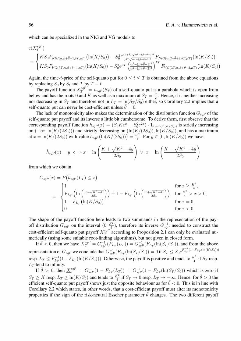
56 E. A. v. Hammerstein et al.
which can be specialized in the NIG and VG models to
c(XsqPT )
=
KS0FNIG(α,β+θ+1,δT,µT )
(ln(K/S0)
)− S2
0eµT+δT
√α2−(β+θ+1)2
eδT√α2−(β+θ+2)2
FNIG(α,β+θ+2,δT,µT )
(ln(K/S0)
)KS0FV G(λT,α,β+θ+1,µT )
(ln(K/S0)
)− S2
0eµT(α2−(β+θ+1)2
α2−(β+θ+2)2
)λTFV G(λT,α,β+θ+2,µT )
(ln(K/S0)
)Again, the time-t-price of the self-quanto put for 0 ≤ t ≤ T is obtained from the above equationsby replacing S0 by St and T by T − t.
The payoff function XsqPT = hsqP(ST ) of a self-quanto put is a parabola which is open from
below and has the roots 0 and K as well as a maximum at ST = K2
. Hence, it is neither increasingnor decreasing in ST and therefore not in LT = ln(ST/S0) either, so Corollary 2.2 implies that aself-quanto put can never be cost-efficient unless θ = 0.
The lack of monotonicity also makes the determination of the distribution function GsqP of theself-quanto put payoff and its inverse a little bit cumbersome. To derive them, first observe that thecorresponding payoff function hsqP(x) = (S0Ke
x − S20e
2x) · 1(−∞,ln(K/S0)) is strictly increasingon (−∞, ln(K/(2S0))) and strictly decreasing on (ln(K/(2S0)), ln(K/S0)), and has a maximumat x = ln(K/(2S0)) with value hsqP
(ln(K/(2S0))
)= K2
4. For y ∈ (0, ln(K/S0)) we have
hsqP(x) = y ⇐⇒ x = ln
(K +
√K2 − 4y
2S0
)∨ x = ln
(K −
√K2 − 4y
2S0
)
from which we obtain
GsqP(x) = P(hsqP(LT ) ≤ x
)
=
1 for x ≥ K2
4,
FLT
(ln(K−√K2−4x
2S0
))+ 1− FLT
(ln(K+√K2−4x
2S0
))for K2
4> x > 0,
1− FLT(ln(K/S0)
)for x = 0,
0 for x < 0.
The shape of the payoff function here leads to two summands in the representation of the pay-off distribution GsqP on the interval (0, K
2
4), therefore its inverse G−1
sqP needed to construct thecost-efficient self-quanto put payoff XsqP
T according to Proposition 2.1 can only be evaluated nu-merically (using some suitable root-finding algorithms), but not given in closed form.
If θ < 0, then we have XsqPT = G−1
sqP(FLT (LT )) = G−1sqP(FLT (ln(ST/S0)), and from the above
representation ofGsqP we conclude thatG−1sqP(FLT (ln(ST/S0)) = 0 if ST ≤ S0e
F−1LT
(1−FLT (ln(K/S0)))
resp. LT ≤ F−1LT
(1−FLT (ln(K/S0))). Otherwise, the payoff is positive and tends to K2
4if ST resp.
LT tend to infinity.If θ > 0, then XsqP
T = G−1sqP(1 − FLT (LT )) = G−1
sqP(1 − FLT (ln(ST/S0)) which is zero ifST ≥ K resp. LT ≥ ln(K/S0) and tends to K2
4if ST → 0 resp. LT → −∞. Hence, for θ > 0 the
efficient self-quanto put payoff shows just the opposite behaviour as for θ < 0. This is in line withCorollary 2.2 which states, in other words, that a cost-efficient payoff must alter its monotonicityproperties if the sign of the risk-neutral Esscher parameter θ changes. The two different payoff

Construction of cost-efficient self-quanto calls and puts 57
0 5 10 15 20
010
2030
4050
60
Self-quanto put payoffs for ThyssenKrupp (T = 22, K = 16)
ST
payo
ff
K2
standard sq-putefficient sq-put
0 5 10 15 20 25 30
020
4060
8010
0
Self-quanto put payoffs for Deutsche Post (T = 22, K = 20)
ST
payo
ff
K2
standard sq-putefficient sq-put
Figure 2: Left: Payoff functions of a standard and efficient self-quanto put on ThyssenKrupp(θ > 0). The initial stock price is S0 = 15.25, the closing price of ThyssenKrupp at July 1, 2013.Right: Payoff functions of a standard and efficient self-quanto put on Deutsche Post (θ < 0). Theinitial stock price is S0 = 19.31, the closing price of Deutsche Post at July 1, 2013.
profiles that can occur for an efficient self-quanto put are visualized in Figure 2 above. The esti-mated VG parameters for ThyssenKrupp and Deutsche Post that are used to calculate the efficientpayoffs can be found in Table 1 in Section 5. As can be seen from the latter, the efficient payofffor ThyssenKrupp corresponds to the case θ > 0, whereas the efficient payoff for Deutsche Posthas the typical shape for θ < 0.
For the time-t-price of an efficient self-quanto put that is issued at time 0, one obtains, with thesame reasoning as in Section 3,
c(XsqPT,t ) = e−r(T−t)E
[Z θT−tX
sqPT,t
]=
e−r(T−t)
∫ ∞a−
G−1sqP
(FLT (y + ln(St/S0))
)dθLT−t
(y) dy =: c−t (St) if θ < 0,
e−r(T−t)∫ a+
−∞G−1
sqP
(1− FLT (y + ln(St/S0))
)dθLT−t
(y) dy =: c+t (St) if θ > 0,
(15)
where a− = F−1LT
(1 − FLT (ln(K/S0))) − ln(St/S0) and a+ = ln(K/St). Due to the necessarynumerical determination of G−1
sqP(x), the integrals in (15) have to be truncated in practical applica-tions to obtain sensible and stable results from a numerical evaluation. The inequalities
e−r(T−t)∫ z−
a−
G−1sqP
(FLT (y + ln(St/S0))
)dθLT−t
(y) dy ≤ c−t (St)
≤ e−r(T−t)∫ z−
a−
G−1sqP
(FLT (y + ln(St/S0))
)dθLT−t
(y) dy + e−r(T−t)K2
4F θLT−t
(z−),
e−r(T−t)∫ a+
z+
G−1sqP
(1− FLT (y + ln(St/S0))
)dθLT−t
(y) dy ≤ c+t (St)
≤ e−r(T−t)∫ a+
z+
G−1sqP
(1− FLT (y + ln(St/S0))
)dθLT−t
(y) dy + e−r(T−t)K2
4F θLT−t
(z+),
which hold for all z− > a− resp. z+ < a+ allow to well control the error caused by the truncation.
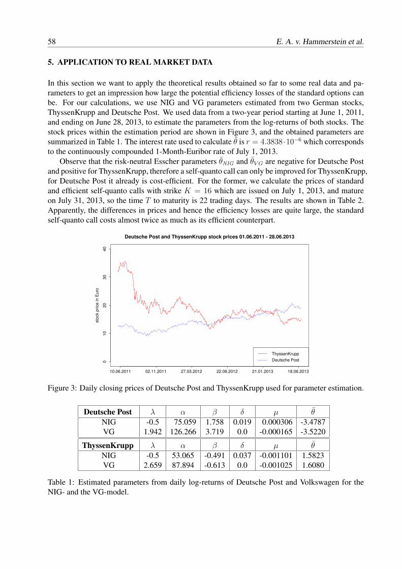
58 E. A. v. Hammerstein et al.
5. APPLICATION TO REAL MARKET DATA
In this section we want to apply the theoretical results obtained so far to some real data and pa-rameters to get an impression how large the potential efficiency losses of the standard options canbe. For our calculations, we use NIG and VG parameters estimated from two German stocks,ThyssenKrupp and Deutsche Post. We used data from a two-year period starting at June 1, 2011,and ending on June 28, 2013, to estimate the parameters from the log-returns of both stocks. Thestock prices within the estimation period are shown in Figure 3, and the obtained parameters aresummarized in Table 1. The interest rate used to calculate θ is r = 4.3838·10−6 which correspondsto the continuously compounded 1-Month-Euribor rate of July 1, 2013.
Observe that the risk-neutral Esscher parameters θNIG and θV G are negative for Deutsche Postand positive for ThyssenKrupp, therefore a self-quanto call can only be improved for ThyssenKrupp,for Deutsche Post it already is cost-efficient. For the former, we calculate the prices of standardand efficient self-quanto calls with strike K = 16 which are issued on July 1, 2013, and matureon July 31, 2013, so the time T to maturity is 22 trading days. The results are shown in Table 2.Apparently, the differences in prices and hence the efficiency losses are quite large, the standardself-quanto call costs almost twice as much as its efficient counterpart.
010
2030
40
Deutsche Post and ThyssenKrupp stock prices 01.06.2011 - 28.06.2013
stoc
k pr
ice
in E
uro
10.06.2011 02.11.2011 27.03.2012 22.08.2012 21.01.2013 18.06.2013
ThyssenKruppDeutsche Post
Figure 3: Daily closing prices of Deutsche Post and ThyssenKrupp used for parameter estimation.
Deutsche Post λ α β δ µ θNIG -0.5 75.059 1.758 0.019 0.000306 -3.4787VG 1.942 126.266 3.719 0.0 -0.000165 -3.5220
ThyssenKrupp λ α β δ µ θNIG -0.5 53.065 -0.491 0.037 -0.001101 1.5823VG 2.659 87.894 -0.613 0.0 -0.001025 1.6080
Table 1: Estimated parameters from daily log-returns of Deutsche Post and Volkswagen for theNIG- and the VG-model.

Construction of cost-efficient self-quanto calls and puts 59
ThyssenKrupp c(XsqCT ) c(XsqC
T ) Efficiency loss in %NIG 8.3288 4.2251 49.27VG 8.2629 4.1609 49.64
Table 2: Comparison of the prices of a self-quanto call on ThyssenKrupp with strike K = 16 andT = 22, and its cost-efficient counterpart in the NIG and VG models. The initial stock price isS0 = 15.25, the closing price of ThyssenKrupp on July 1, 2013.
In contrast to the self-quanto call, the standard self-quanto put is—at least theoretically—inefficient for both stocks since the risk-neutral Esscher parameter θ is different from zero in allcases. In our example we assume that the standard and efficient self-quanto puts on ThyssenKruppand Deutsche Post have the same issuance day and maturity date as the self-quanto calls above,and the strikes are again K = 16 for ThyssenKrupp and K = 20 for Deutsche Post. The obtainedresults are listed in Table 3. Whereas the efficiency losses for Deutsche Post are of compara-ble magnitude as in the call example, one surprisingly does not save anything by investing in theefficient self-quanto put on ThyssenKrupp.
This becomes clearer if we take a look back on the corresponding payoff functionXsqPT . Recall
that the risk-neutral Esscher parameters for ThyssenKrupp are always positive, therefore the leftplot of Figure 2 applies here. If θ > 0, then obviously XsqP
T and XsqPT are almost identical for
ST ∈ (K2,∞) and only differ significantly if ST ∈ (0, K
2). But if the risk-neutral probability
Qθ(0 < ST <K2
) is very small, then it is intuitively evident that the prices c(XsqPT ) and c(XsqP
T )should nearly coincide. This is the case here. The strike K is very close to the initial stock priceS0, and the risk-neutral measureQθ is more right-skewed than the real-word one P (under the risk-neutral Esscher measure, only the skewness parameter β of the NIG and VG distributions changesto β + θ), so under Qθ it becomes even more unlikely that ST < K
2.
The evolution of the prices c(XsqCT,t ), c(XsqC
T,t ) of the standard and efficient self-quanto call onThyssenKrupp as well as that of the prices c(XsqP
T,t ), c(XsqPT,t ) of the self-quanto puts on Deutsche
Post in the NIG models during the lifetime of the options is shown in Figure 4. The prices ofthe efficient options always roughly move in the opposite direction of that of the standard optionswhich reflects the reversed resp. altered monotonicity properties of the underlying payoff profiles.
ThyssenKrupp c(XsqPT ) c(XsqP
T ) Efficiency loss in %NIG 16.1541 16.1541 0.0VG 16.1226 16.1226 0.0
Deutsche Post c(XsqPT ) c(XsqP
T ) Efficiency loss in %NIG 17.6912 10.2613 42.00VG 17.6593 10.2152 42.15
Table 3: Comparison of the prices of standard and efficient self-quanto puts on ThyssenKrupp andDeutsche Post with strikes K = 16 resp. K = 20, and T = 22, in the NIG and VG models. Theinitial stock prices are S0 = 15.25 for ThyssenKrupp and S0 = 19.31 for Deutsche Post, which arethe closing prices on July 1, 2013.
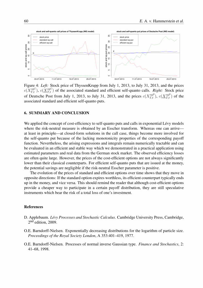
60 E. A. v. Hammerstein et al.
05
1015
2025
30
stock and self-quanto call prices of ThyssenKrupp (NIG model)
stoc
k an
d sq
-cal
l pric
es
03.07.2013 11.07.2013 19.07.2013 29.07.2013
K
stock pricestandard sq-callefficient sq-call
05
1015
2025
3035
stock and self-quanto put prices of Deutsche Post (NIG model)
stoc
k an
d sq
-put
pric
es
03.07.2013 11.07.2013 19.07.2013 29.07.2013
K
stock pricestandard sq-putefficient sq-put
Figure 4: Left: Stock price of ThyssenKrupp from July 1, 2013, to July 31, 2013, and the pricesc(XsqC
T,t ), c(XsqCT,t ) of the associated standard and efficient self-quanto calls. Right: Stock price
of Deutsche Post from July 1, 2013, to July 31, 2013, and the prices c(XsqPT,t ), c(XsqP
T,t ) of theassociated standard and efficient self-quanto puts.
6. SUMMARY AND CONCLUSION
We applied the concept of cost-efficiency to self-quanto puts and calls in exponential Levy modelswhere the risk-neutral measure is obtained by an Esscher transform. Whereas one can arrive—at least in principle—at closed-form solutions in the call case, things become more involved forthe self-quanto put because of the lacking monotonicity properties of the corresponding payofffunction. Nevertheless, the arising expressions and integrals remain numerically tractable and canbe evaluated in an efficient and stable way which we demonstrated in a practical application usingestimated parameters and real data from the German stock market. The observed efficiency lossesare often quite large. However, the prices of the cost-efficient options are not always significantlylower than their classical counterparts. For efficient self-quanto puts that are issued at the money,the potential savings are negligible if the risk-neutral Esscher parameter is positive.
The evolution of the prices of standard and efficient options over time shows that they move inopposite directions: If the standard option expires worthless, its efficient counterpart typically endsup in the money, and vice versa. This should remind the reader that although cost-efficient optionsprovide a cheaper way to participate in a certain payoff distribution, they are still speculativeinstruments which bear the risk of a total loss of one’s investment.
References
D. Applebaum. Levy Processes and Stochastic Calculus. Cambridge University Press, Cambridge,2nd edition, 2009.
O.E. Barndorff-Nielsen. Exponentially decreasing distributions for the logarithm of particle size.Proceedings of the Royal Society London, A 353:401–419, 1977.
O.E. Barndorff-Nielsen. Processes of normal inverse Gaussian type. Finance and Stochastics, 2:41–68, 1998.
Construction of cost-efficient self-quanto calls and puts 61
O.E. Barndorff-Nielsen, T. Mikosch, and S. Resnick, editors. Levy Processes: Theory and Appli-cations. Birkhauser, Boston, 2001.
C. Bernard and P.P. Boyle. Explicit representation of cost-efficient strategies. working paper,available at http://ssrn.com/abstract=1695543, 2010.
C. Bernard, P.P. Boyle, and S. Vanduffel. Explicit representation of cost-efficient strategies. Fi-nance, 2014. forthcoming.
R. Cont and P. Tankov. Financial Modelling with Jump Processes. Chapman & Hall / CRC Press,Boca Raton, 2004.
P. Dybvig. Distributional analysis of portfolio choice. Journal of Business, 61(3):369–393, 1988a.
P. Dybvig. Inefficient dynamic portfolio strategies or how to throw away a million dollars in thestock market. Review of Financial Studies, 1(1):67–88, 1988b.
F. Esscher. On the probability function in the collective theory of risk. Scandinavian ActuarialJournal, 15(3):175–195, 1932.
H.U. Gerber and E.S.W. Shiu. Option pricing by esscher transforms. Transactions of the Societyof Actuaries, 46:99–191, 1994.
F. Hubalek and C. Sgarra. Esscher transforms and the minimal entropy martingale measure forexponential Levy models. Quantitative Finance, 6(2):125–145, 2006.
D.B. Madan and E. Seneta. The variance gamma (V.G.) model for share market returns. Journalof Business, 63:511–524, 1990.
D.B. Madan, P.P. Carr, and E.C. Chang. The variance gamma process and option pricing. EuropeanFinance Review, 2:79–105, 1998.
S.T. Rachev, Y.S. Kim, M.L. Bianchi, and F.J. Fabozzi. Financial Models with Levy Processes andVolatility Clustering. Wiley, Hoboken, 2011.
S. Raible. Levy processes in finance: theory, numerics, and empirical facts. PhD thesis, Uni-versity of Freiburg, 2000. Available at http://www.freidok.uni-freiburg.de/volltexte/51/.
K.-I. Sato. Levy Processes and Infinitely Divisible Distributions. Cambridge University Press,Cambridge, 1999.
W. Schoutens. Levy Processes in Finance: Pricing Financial Derivatives. Wiley, Chichester, 2003.
E.A. v. Hammerstein. Generalized hyperbolic distributions: Theory and applications to CDO pric-ing. PhD thesis, University of Freiburg, 2011. Available at http://www.freidok.uni-freiburg.de/volltexte/7974/.
E.A. v. Hammerstein, E. Lutkebohmert, L. Ruschendorf, and V. Wolf. Optimality of payoffs inLevy models. International Journal of Theoretical and Applied Finance, forthcoming, 2014.


POSTER SESSION

PRICING PARTICIPATING PRODUCTS UNDER REGIME-SWITCHINGGENERALIZED GAMMA PROCESS
Farzad Alavi Fard
School of Economics, Finance and Marketing, RMIT, VIC 3001, AustraliaEmail: [email protected]
We propose a model for valuing participating life insurance products under a regime-switchinggeneralized gamma process. The Esscher transform is employed to determine an equivalent mar-tingale measure in the incomplete market. The results are further manipulated through the utiliza-tion of the change of numeraire technique to reduce the dimensions of the pricing formulation. Dueto the path dependency of the payoff of the insurance product and the non-existence of a closed-form solution for the PIDE, the finite difference method is utilized to numerically calculate thevalue of the product. To highlight some practical features of the product, we present a numericalexample.
1. INTRODUCTION
Participating life insurance products are a popular class of equity linked insurance products aroundthe world. In these policies the insured not only receives the guaranteed annual minimum benefit,but also receives proceeds from an investment portfolio. Grosen and Jorgensen (2000) provided acomprehensive discussion on different contractual features of participating policies.
In this article, we propose a model for valuing participating life insurance products under aregime-switching generalized gamma process, which is an extension of Fard and Siu (2013). Read-ers, may refer to this article for extended discussions for similar models and calculations.
2. MODELING FRAMEWORK
Consider a financial market, where an agent can either invest in a risk-free money market accountor choose from a range of risky assets. All the parameters of the risk-free asset, as well as the riskyassets, vary as the economy switches regimes, a process governed by a Markov-chain. We fix acomplete probability space (Γ,F ,P), where P is the real-world probability measure. Let T denote
65
66 F. Alavi Fard
the time index set [0, T ] of the economy. Let Xtt∈T on (Γ,F ,P) be a continuous-time Markovchain with a finite state space S := (s1, s2, · · · , sN). The state space of the process Xtt∈T is afinite set of unit vectors e1, e2, · · · , eN, where ei = (0, · · · , 1, · · · , 0) ∈ RN .
Let Q(t) = [qij(t)]i,j=1,2,...,N , t ∈ T , denote a family of generators, or rate matrices, of thechain Xtt∈T under P. Then, as in Elliott et al. (1995):
Xt = X0 +
∫ t
0
QXsds+Mt, (1)
where Mt is a RN -valued martingale with respect to the filtration generated by Xtt∈T . In thisarticle, any parameter Υ modulated by the Markov chain Xt is denoted by Υt, and defined asfollows
Υt := Υ(t,Xt) := 〈Υ, Xt〉 =N∑i=1
Υi〈Xt, ej〉, t ∈ T , (2)
where Υ := (Υ1,Υ2, · · · ,ΥN) with Υj > 0 for each j = 1, 2, · · · , N and 〈., .〉 denotes the innerproduct in the spaceRN .
Let (T ,B(T )) denote a measurable space, where B(T ) is the Borel σ-field generated by theopen subsets of T . Let X denote T × R+, then (X ,B(X )) is a measurable space. Let NXt(., U)denote a Markov-switching Poisson random measure on the space X . Write NXt(dt, dz) for thedifferential form of measure NXt(t, U). Let ρXt(dz|t) denote a Markov-switching Levy measureon the space X depending on t and the state Xt; η is a σ-finite (nonatomic) measure on T . First,as in James (2005), consider the following Markov-modulated completely random measure
µXt(dt) :=
∫R+
h(z)NXt(dt, dz),
which is a kernel-biased. The generalized gamma (GG) process is a special case of the kernel-biased completely random measure and can be obtained by setting the kernel function h(z) = z.In this paper we are seeking a specific class of the GG processes that assist us in describing theimpact of the states of an economy on the jump component. Hence, we use a MGG process, whosecompensator switches over time, according to the states of the economy. Following, we presenthow to derive the intensity process for different classes of the MGG process.
Let α ≥ 0 and bt denote the shape parameter and the scale parameter of the MGG process,defined according to (2). Then,
ρXt(dz|t)η(dt) =1
Γ(1− α)z(1+α)
N∑i=1
e−biz〈b, Xt〉dzη(dt). (3)
When α = 0, the MGG process reduces to a Markov modulated weighted gamma(MWG)process. When α = 0.5 the MGG process becomes the Markov modulated inverse Gaussian(MIG) process.
Let Wtt∈T denote a standard Brownian motion, and NXt(dt, dz) denote the compensatedPoisson random measure. Further, let rt be the instantaneous market interest rate, and µt and σt
Pricing Participating Products under Regime-Switching Generalized Gamma Process 67
denote the drift and volatility of the market value of the reference asset, respectively, all defined asper (2). Then, consider a generalized jump-diffusion process A := A(t)|t ∈ T , such that
dAt = At−
[µtdt+ σtdWt +
∫R+
zNXt(dt, dz)
], (4)
where A0 = 0. We assume under P the price process Stt∈T is defined as St := exp(At).For each time t ∈ T , let Rt and Dt denote the book value of the policy reserve and the bonus
buffer, respectively. Rt is considered as the policyholder’s account balance. Let St denote themarket value of the asset backing the policy, so that St = Rt + Dt, t ∈ T . The funds aredistributed between two components of liability over time according to the bonus policy describedby the continuously compounded interest rate credited to the policy reserve cR,
dRt = cR(S,R)Rtdt.
Definition 2.1 Let g(S,R,X, T ) denote the terminal payoff of the policy. Then the fair value
V (ST , RT , XT ) = RT + γP1T − P2T , (5)
where γ is the terminal bonus distribution rate, P1T := max(αpST −RT , 0) is the terminal bonusoption, P2T := max(RT − ST , 0) is the terminal default option, and RT is the guaranteed benefit.
FAIR VALUATION OF THE PARTICIPATING POLICY
Define Gt for the σ-algebra FXt ∨ FAt for each t ∈ T . For each θt defined as in (2) write(θ.A)t :=
∫ t0θ(u)dA(u) such that θ is integrable with respect to the return process. LetM(θ)t :=
E[e(θ.A)t |FXt ] be a Laplace cumulant process. Denote also in the following η′(t)dt := η(dt). Then,let Λtt∈T denote a G-adapted stochastic process
Λt := e(θ.A)t .M(θ)−1t , (6)
= e∫ t0 θsσsdWs− 1
2
∫ t0 θ
2sσ
2sds+
∫ t0
∫R+ θszNXs (dz,ds)−
∫ t0
∫R+ (eθsz−1+θsz)ρXs (dz|s)η(ds).
Proposition 2.1 Λt is P martingale w.r.t. Gt.
Definition 2.2 For each θ ∈ L(A) define Pθ ∼ P on G(T ) by the Radon-Nikodym derivativedPθdP
∣∣G(T ) := ΛT .
Proposition 2.2 For each t ∈ T , let the discounted price of the risky asset at time t be S(t) :=
e−rtS(t). Then, S := S(t)|t ∈ T is a Pθ-local-martingale if and only if θt satisfies :
θtσ2t +
∫R+
eθtz(ez − 1)− z
ρXt(dz|t)η′(t) = rt − µt. (7)
68 F. Alavi Fard
Proposition 2.3 Suppose Wt = Wt−∫ t0σsθsds is a Pθ-Browning motion, ρθXt(dz|t) := eθszρXt(dz|t)
is the Pθ compensator of N θXt
(dz, dt) then
dAt =(µt + 2θtσ
2t −
1
2σ2t
)dt+ σtdWt +
∫R+
z(1− e−θtz
)ρθXt(dz|t)η(dt) +
∫R+
zN θXt(dz, dt).
As in Hansen and Jorgensen (2000), we choose an alternative numeraire to reduce the numberof state variables. Define a new state variable Z := ln( S
R), so that CZ(Z) = CR(S,R,X, t). Then,
under Pθ we define
E(t) := exp
(−∫ t
0
(rs −1
2σ2s)ds
)StS0
(8)
We notice that E(t) is martingale w.r.t. Gt (Oksendal and Sulem (2005), chapter 1).
Definition 2.3 Define Q ∼ Pθ on G(T ) by the Radon-Nikodym derivative dQdPθ∣∣G(T ) := E(T ).
Also, defineWQt := Wt−
∫ t0σsds, andNQ
Xt(dz, dt) := N θ
Xt(dz, dt)−f(z, θ)ρθXt(dz|t)η(dt),where
f(z, θt) := eθtz(ez − 1) − z for convenience in presentation. Then by a version of the Girsanovtheorem
dSt = (rt + 12σ2t )dt+ σtdW
Qt +
∫R+
(eθtz(ez − 1)− z
)NQXt
(dz, dt).
Consequently, by Ito’s lemma, the dynamic of Z under Q is
dZt =(rt − CZ(Zt)
)dt+ σtdW
Qt +
∫R+
ln(1 + f(z, θt))NQXt
(dt, dz),
+
∫R+
(ln(1 + f(z, θt))− f(z, θt)
)ρQXt(dz|t)η(dt). (9)
Where, ρQXt(dz|t)η(dt) is defined under Q for NQ(dt, dz).
Proposition 2.4 The valuation of Vt using the process Z under Q, is equivalent to that from pro-cess S under Pθ.
Proof. Let EQ and Eθ be the expectation operator under Q and Pθ, respectively. Then, by Bayes’rule
Vt = Eθ
[exp
(−∫ T
t
rsds)V (S,R,X, T )
∣∣∣Gt]= StE
Q[e−ZTVZ(Z,X, t)
∣∣∣(Zt, Xt) = (Z,X)].
We call VZ(Z,X, t), S-denominated value of the contract; that is
VZ(Z,X, t) = EQ[e−ZTVZ(Z,X, T )
∣∣∣(Zt, Xt) = (Z,X)].
Pricing Participating Products under Regime-Switching Generalized Gamma Process 69
Corollary 2.5 (Zt, Xt) is a two-dimensional Markov process with respect to the filtration Gt.
Corollary 2.6 The S-denominated value of the participating product VZ(Z,X, t) is Q martingale.
Further, write Vi for V (Z, ei, t), where i = 1, 2, ..., N and V := V1, V2, ..., VN. Then, as inBuffington and Elliot (2002), V satisfies the following N PIDEs:
LZ,ei(Vi) + 〈V,Qei〉 = 0, i = 1, 2, ..., N, (10)
where LZ,ei(Vi) is the differential operator. Further, as a result of the Corollary2.6, we have
dVZ(Z,X, t) =
∫R+
VZ
(Zt− + ln(1 + f(z, θt))
)− VZ(Zt−)
NQXt
(dt, dz)
+∂VZ∂Z
(Z,X, t)σdWQt + 〈V,QXt〉dt.
With the auxiliary condition VZ(Z,X, T ) = e−ZT + γmax(α− e−ZT , 0) + max(e−ZT − 1, 0).
3. NUMERICAL ANALYSIS
There is no known analytical solution to (10). We employ the explicit finite difference methodto approximate the solution numerically. Let [0, Zmax] × [0, T ] denote the finite computationaldomain, where the width of the spatial interval is chosen to be sufficiently large. The derivativesof the value function V (Z,X, t) in equations (10) can be replaced by the finite differences and theintegral terms are approximated by using the trapezoidal rule at first. The computational domainis discretized into a finite difference mesh, where ∆Z and ∆t are the step-width and time step,respectively. In order to approximate the integral term, we adopt the trapezoidal rule with the samespatial grids. By the explicit finite difference scheme, we start from the terminal values, and movebackwards in time so that we can calculate the value function.
Assume an economy with two states, namely, where Xt = 1 and Xt = 2 represent ’Good’and ’Bad’ economies, respectively. Let P(t) = [pij] be the transition probability matrix for time t.Note that in Section 2, we characterize the Markov chain using the matrix of transition rates,Q, soP(t) must be calculated by solving (1), first. To illustrate our model, we assume p11 = p22 = 0.40,r1 = 0.035, r2 = 0.015, b1 = 200.00, b2 = 500.00, β = 0.5, σ1 = 0.2, σ2 = 0.2, µ1 = 0.10,µ2 = 0.05, S0 = 100 and γ = 0.7. The term to maturity of the contract is T = 20 years, ∆t isassumed to be one trading day (∆t = 1/252). For the Merton jump diffusion model, we considerthe drift and the dispersion of the reference portfolio as well as the risk-free rate to be equal to thecorresponding parameters in the no-regime-switching version of the model. In addition, we assumethe intensity parameter of the model to be 60%, and the jump size of the compound Poisson processfollows a normal distribution of N(−0.05, 0.49).
Figure 1 presents the impact of α on the fair values of the participating policy, calculatedwith the above model specifications. The graph shows a meaningful difference between the fairvalues of the policy, with and without switching regimes. For example, when α = 0.2, the fair

70 F. Alavi Fard
0.0 0.1 0.2 0.3 0.4 0.5 0.6 0.7 0.8 0.9 1.0
20
40
60
80
100
α
Fai
r va
lue
of th
e po
licy
Merton Jump ModelWith Markov SwitchingWithout Markov Switching
(M)IG processes
(M)WG processes
Figure 1: The fair value of the participating policy, with general (M)GG processes.
value calculated without regime-switching is 16.01% lower than the fair value of the contract withregime-switching. This difference is as high as 73.33% for the fair values under the two scenarioswith α = 0.9. We also document the significant effect of α on the values of the contracts for bothcases.
References
J. Buffington and R.J. Elliot. American options with regime switching. International Journal ofTheoretical and Applied Finance, 5:497–514, 2002.
R. J. Elliott, L. Aggoun, and J. B. Moore. Hidden Markov Models: Estimation and Control, vol.29 of Applications of Mathematics. Springer, 1995.
F.A. Fard and T.K. Siu. Pricing participating products with markov-modulated jumpdiffusionprocess: An efficient numerical pide approach. Insurance: Mathematics and Economics, 53(3):712 – 721, 2013. ISSN 0167-6687. doi: http://dx.doi.org/10.1016/j.insmatheco.2013.09.011.
A. Grosen and P.L. Jorgensen. Fair valuation of life insurance liabilities: the impact of interest rateguarantees, surrender options, and bonus policies. Insurance, Mathmatics and Economics, 26:37–57, 2000.
M. Hansen and P.L. Jorgensen. Analytical valuation of American-style Asian options. Manage-ment Science, 46:1116–1136, 2000.
L.F. James. Bayesian Poisson process partition calculus with an application to Bayesian Levymoving averages. The Annals of Statistics, 33:1771–1799, 2005.
B. Oksendal and A. Sulem. Applied Stochastic Control of Jump Difussion. Springer, 2005.
RISK CLASSIFICATION FOR CLAIM COUNTS USING FINITE MIXTURE MODELS
Lluıs Bermudez† and Dimitris Karlis§
†Riskcenter, University of Barcelona§Athens University of Economics and BusinessEmail: [email protected], [email protected]
When modelling insurance claim counts data, the actuary often observes overdispersion and excessof zeros that may be caused by the unobserved heterogeneity. A common approach for account-ing for overdispersion is to consider models with some overdispersed distribution as opposed toPoisson models. Zero-inflated, hurdle and compound frequency models are usually applied to in-surance data to account for such features of the data. A natural way to allow for overdispersion isto consider mixtures of a simpler model. In this paper, we consider a K-finite mixture of Poissonand Negative Binomial regressions. This approach has interesting features: first, the zero-inflatedmodel represents a special case; and second, it allows for an elegant interpretation based on thetypical clustering application of finite mixture models. These models are applied to an automobileinsurance claims data set in order to analyse the consequences for risk classification.
1. INTRODUCTION AND MOTIVATION
Risk classification based on generalized linear models is usually accepted. A regression componentis included in the claim count distribution to take the individual characteristics into account.
In insurance data sets, for claim count modelling purposes, the Poisson regression model isusually rejected because of the presence of overdispersion. This rejection may be interpreted asthe sign that the portfolio is heterogeneous.
In automobile insurance, the problem of unobserved heterogeneity is caused by the differencesin driving behaviour among policyholders that cannot be observed or measured by the actuary (i.e.driving ability, driving aggressiveness, obedience of traffic regulations). The omission of theseimportant classification variables may be the reason for the overdispersion detected. Meanwhile,the presence of excess of zeros can be also seen as a consequence of unobserved heterogeneity.
Many attempts have been made in the actuarial literature to account for such features of thedata. Compound frequency models, zero-inflated models and hurdle models are usually appliedto insurance claim count data. Boucher et al. (2007) present and compare different risk classifica-tion models for the annual number of claims reported to the insurer: Poisson-Gamma (or Nega-tive Binomial) model, Poisson-Inverse Gaussian model, Poisson-Log Normal model, Zero-inflatedmodels and Hurdle models.
71

72 L. Bermudez and D. Karlis
In the bivariate setting, in a recent paper, Bermudez (2009) used bivariate Poisson regressionmodels for ratemaking in car insurance to account for the dependence between two different typesof claims, including zero-inflated models to account for the excess of zeros and the overdispersionin the data set. In Bermudez and Karlis (2012), these models were revisited in order to consideralternatives, proposing a 2-finite mixture of bivariate Poisson regression models to demonstratethat the overdispersion in the data requires more structure if it is to be taken into account and thata simple zero-inflated bivariate Poisson model does not suffice.
In this paper, to account for overdispersion and excess of zeros in the univariate setting, weconsider a K-finite mixture of Poisson and Negative Binomial (NB) regressions. The finite mix-tures of Poisson or NB regression models are especially useful where count data were drawn fromheterogeneous populations as Park and Lord (2009) show for vehicle crash data analysis.
2. K-FINITE MIXTURE OF REGRESSION MODELS
Let Y be the number of claims for automobile insurance, we consider the K-finite mixture ofPoisson or NB regressions as
P (Yi = yi) =K∑j=1
pjP (yi;µij) or P (Yi = yi) =K∑j=1
pjNB(yi;µij, θj)
respectively, where pj > 0 (j = 1, . . . , K) are the mixing proportions with∑pj = 1.
For the NB regression model, we assume
NB(y;µ, θ) =Γ(θ + y)
Γ(θ)y!
(µ
θ + µ
)y (θ
θ + µ
)θ, µ, θ > 0, y = 0, 1, . . .
i.e. the probability function of a NB with mean µ and variance µ+ µ2
θ.
Furthermore, in both cases, we assume for the mean of the j-th components that it relates tosome covariate vector, namely we assume that
log(µij) = xiβj
where xi is the vector of covariates related to the i-th individual and βj is the vector of regressioncoefficients for the j-th component.
This modelling has some interesting features: first of all, the zero inflated model is a specialcase; secondly, it allows for overdispersion; and thirdly, it allows for a neat interpretation based onthe typical clustering usage of finite mixture models.
We fitted the model by a using standard EM algorithm. For the NB mixture, at the E-step weestimated the weights wij as
wij = pjNB(yi;µij, θj) /K∑j=1
pjNB(yi;µij, θj)

Risk classification for claim counts using finite mixture models 73
and during the M-step we update βj by fitting a standard NB regression model with response y,covariates x and weights wj = (w1j, . . . , wnj).
Initial values for K = 2 were selected by perturbing a simple NB regression model. Namelywe fitted a single NB regression and keeping the fitted values, we split them in two componentswith mixing probabilities 0.5 each one and means equal to 1.2 and 0.8 of the fitted values. Thenin order to fit a model with K + 1 components we used the solution with K components and anew component at the center (that of a single NB regression), with mixing probability 0.05. Therest mixing probabilities were rescaled to sum to 1. Extensive simulation have shown that thisapproach works well to locate the maximum.
3. APPLICATION
The data contains information for 80,994 policyholders from a major insurance company operat-ing in Spain. Twelve exogenous variables were considered plus the annual number of accidentsrecorded. The description of the explanatory variables is presented in table 1.
We have fitted models of added complexity to this data set, starting from a simple Poissonregression model. We have used AIC to select the best among a series of candidate models. Allmodels were run in R. In table 2 we have compared the fitted models, resulting that the best fitwas obtained with the 2-Finite NB mixture model. Finite mixture models with K > 2 were alsofitted, but no improvement in terms of AIC were achieved. In table 3 the results for the 2-FiniteNB mixture model are summarized.
Variable DefinitionV1 equals 1 for women and 0 for menV2 equals 1 when driving in urban area, 0 otherwiseV3 equals 1 when zone is medium risk (Madrid and Catalonia)V4 equals 1 when zone is high risk (Northern Spain)V5 equals 1 if the driving license is between 4 and 14 years oldV6 equals 1 if the driving license is 15 or more years oldV8 equals 1 if the client is in the company for more than 5 yearsV9 equals 1 of the insured is 30 years old or youngerV10 equals 1 if includes comprehensive coverage (except fire)V11 equals 1 if includes comprehensive and collision coverageV12 equals 1 if horsepower is greater than or equal to 5500cc
Table 1: Explanatory variables used in the models
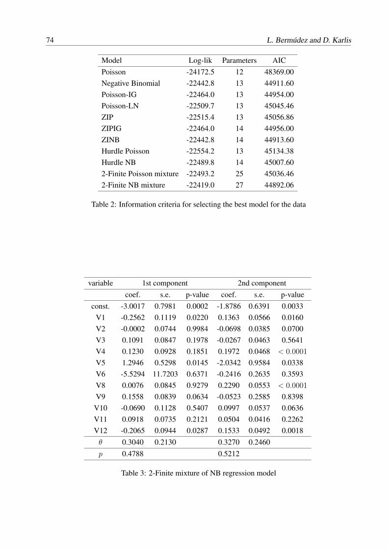
74 L. Bermudez and D. Karlis
Model Log-lik Parameters AICPoisson -24172.5 12 48369.00Negative Binomial -22442.8 13 44911.60Poisson-IG -22464.0 13 44954.00Poisson-LN -22509.7 13 45045.46ZIP -22515.4 13 45056.86ZIPIG -22464.0 14 44956.00ZINB -22442.8 14 44913.60Hurdle Poisson -22554.2 13 45134.38Hurdle NB -22489.8 14 45007.602-Finite Poisson mixture -22493.2 25 45036.462-Finite NB mixture -22419.0 27 44892.06
Table 2: Information criteria for selecting the best model for the data
variable 1st component 2nd componentcoef. s.e. p-value coef. s.e. p-value
const. -3.0017 0.7981 0.0002 -1.8786 0.6391 0.0033V1 -0.2562 0.1119 0.0220 0.1363 0.0566 0.0160V2 -0.0002 0.0744 0.9984 -0.0698 0.0385 0.0700V3 0.1091 0.0847 0.1978 -0.0267 0.0463 0.5641V4 0.1230 0.0928 0.1851 0.1972 0.0468 < 0.0001
V5 1.2946 0.5298 0.0145 -2.0342 0.9584 0.0338V6 -5.5294 11.7203 0.6371 -0.2416 0.2635 0.3593V8 0.0076 0.0845 0.9279 0.2290 0.0553 < 0.0001
V9 0.1558 0.0839 0.0634 -0.0523 0.2585 0.8398V10 -0.0690 0.1128 0.5407 0.0997 0.0537 0.0636V11 0.0918 0.0735 0.2121 0.0504 0.0416 0.2262V12 -0.2065 0.0944 0.0287 0.1533 0.0492 0.0018θ 0.3040 0.2130 0.3270 0.2460p 0.4788 0.5212
Table 3: 2-Finite mixture of NB regression model

Risk classification for claim counts using finite mixture models 75
4. CONCLUSIONS
In this paper, we have proposed the use of a 2-finite mixture of Poisson and Negative Binomialregressions to allow for the overdispersion and the excess of zeros usually detected in automobileinsurance dataset. Assuming the existence of two type of clients described separately by eachcomponent of the mixture improves the modelling of the dataset. The idea is that the data consistof subpopulations for which the regression structure is different. The model corrects for zeroinflation and overdispersion.
The existence of “true” zeros assumed by zero-inflated or Hurdle models may be a too strongassumption in some cases. However, the 2-finite mixture of Poisson or Negative Binomial regres-sion does not make this somewhat strict assumption and allows mixing with respect to both zerosand positives. This idea is more flexible than zero-inflated and Hurdle models and it holds betterin our case. As it can be seen in figure 1, the group separation is characterized by low mean for thefirst component (“good” drivers) and high mean with higher variance for the second one (“bad”drivers).
Figure 1: Boxplots of the fitted means for each of the two components
Finally, as it seems that the data set may have been generated from two distinct subpopulations,the model allows for a net interpretation of each cluster separately. Note that different regressioncoefficients can be used to account for the “observed” heterogeneity within each population.
References
L. Bermudez. A priori ratemaking using bivariate Poisson regression models. Insurance: Mathe-matics and Economics, 44(1):135–141, 2009.
L. Bermudez and D. Karlis. A finite mixture of bivariate poisson regression models with an ap-plication to insurance ratemaking. Computational Statistics & Data Analysis, 56:3988–3999,2012.

76 L. Bermudez and D. Karlis
J.P. Boucher, M. Denuit, and M. Guillen. Risk classification for claim counts: a comparativeanalysis of various zero-inflated mixed poisson and hurdle models. North American ActuarialJournal, 11(4):110–131, 2007.
B.J. Park and D. Lord. Application of finite mixture models for vehicle crash data analysis. Acci-dent Analysis and Prevention, 41(4):683–691, 2009.
TWO EFFICIENT VALUATION METHODS OF THE EXPOSURE OF BERMUDANOPTIONS UNDER THE HESTON MODEL
Q. Feng1, C.S.L. de Graaf 2, D. Kandhai2,3 and C.W. Oosterlee1,4
1Center for Mathematics and Computer Science (CWI), Science Park 123, 1098 XG Amsterdam,The Netherlands2University of Amsterdam, Kruislaan 403, 1098 SJ Amsterdam, The Netherlands3ING BANK, Amsterdamse Poort Bijlmerplein 888, 1102 MG Amsterdam, The Netherlands4Delft University of Technology, Mekelweg 4, 2628 CD Delft, The NetherlandsEmail: [email protected]
1. INTRODUCTION
Expected Exposure (EE) is one of the key elements in Credit Value Adjustment (CVA) (Gregory2012). In credit risk management, the Potential Future Exposure (PFE) is another important indi-cator. It indicates the maximum expected exposure at some level of confidence. Valuation of eitherEE or PFE of path-dependent derivatives has the additional difficulty that some event may happenat any time over the entire path, either earlier or later than the valuation time.
A Bermudan option is an option where the buyer has the right to exercise at a set of times,which we may call watch times. If the option is exercised, the exposure disappears as the holderhas realized the value of the option; otherwise, the holder will lose the current value of the optionif the counterparty defaults. With simulated scenarios, the option value at each exercise time canbe calculated; when a large number of scenarios is available, we can get an empirical distributionof the option value at each time point. It is easy to get the EE and PFE when the distribution of theexposure is known.
In de Graaf et al. (2014), three computational techniques for approximation of counterpartyexposure for financial derivatives are presented. This abstract focuses on the introduction on oneof them: the Stochastic Grid Bundling method (SGBM). We will show that the EE and PFE arenatural by-products when pricing a Bermudan option applying SGBM. The Greeks of the exposurecan be calculated at the same time without additional computational costs.
The COS method in Fang (2010) also offers an efficient way for pricing a Bermudan optionunder the Heston model. We extend it for pricing the exposure values of the Bermudan options.We use the results of the COS method as the reference value.
COS and SGBM are fundamentally different: one is aimed to recover the conditional densityfrom the characteristic function based on Fourier-cosine expansion while the other employs regres-sion to approximate the conditional distribution based on bundling and simulation. Monte Carlo
77

78 Q. Feng et al.
simulation is needed for generating the scenarios/the stochastic grid. We apply the QE scheme(Andersen 2007) with a martingale correction for generating the paths under the Heston model.
2. BERMUDAN OPTIONS AND THE HESTON MODEL
A Bermudan option is defined as an option where the buyer has the right to exercise at a set numberof (discretely spaced) times. The exercise time set is denoted by
T = t1, t2, . . . , tM, (1)
where M denotes the number of exercise times, and the time difference is ∆t. At initial time t0exercising is not allowed.
The dynamics of the Heston stochastic volatility model (Heston 1993) are given bydSt = rStdt+
√vtStdW
1t ,
dvt = κ(η − vt)dt+ σ√vtdW
2t ,
dW 1t dW
2t = ρdt,
(2)
where
• W 1t and W 2
t are two Wiener processes correlated by ρ;
• κ is the mean-reversion speed;
• η the mean reversion level;
• σ the so-called volatility of volatility;
• r the risk-free interest rate.
Knowing the market condition (Sm, vm) at time tm, the immediate exercise and the continuationvalue for the Bermudan option at time tm are, respectively, defined as:
g(Sm) = max(γ(Sm −K), 0) with γ =
1, for a call−1, for a put
, (3)
c(Sm, vm, tm) = e−r∆tE[U(Sm+1, vm+1, tm+1)
∣∣∣∣(Sm, vm)
], (4)
where U(Sm+1, vm+1, tm+1) is the option value at time tm+1.The holder of the option will exercise when the exercise value is higher than the continuation
value, and then the contract terminates. At maturity tM , the option value is equal to the exercisevalue. The following recursive scheme based on dynamic programming can be set up to price aBermudan option:
U(Sm, vm, tm) =
g(SM), for m = M ;
max [c(Sm, vm, tm), g(Sm)] , for m = 1, 2, · · · ,M − 1;
c(S0, v0, t0), for m = 0.
(5)
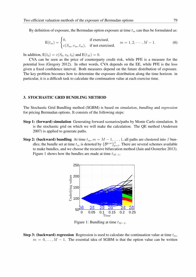
Two efficient valuation methods of the exposure of Bermudan options 79
By definition of exposure, the Bermudan option exposure at time tm can thus be formulated as:
E(tm) =
0, if exercised,c(Sm, vm, tm), if not exercised,
m = 1, 2, · · · ,M − 1. (6)
In addition, E(t0) = c(S0, v0, t0) and E(tM) = 0.CVA can be seen as the price of counterparty credit risk, while PFE is a measure for the
potential loss (Gregory 2012). In other words, CVA depends on the EE, while PFE is the lossgiven a fixed confidence interval. Both measures depend on the future distribution of exposure.The key problem becomes how to determine the exposure distribution along the time horizon. inparticular, it is a difficult task to calculate the continuation value at each exercise time.
3. STOCHASTIC GRID BUNDLING METHOD
The Stochastic Grid Bundling method (SGBM) is based on simulation, bundling and regressionfor pricing Bermudan options. It consists of the following steps:
Step 1: (forward) simulation Generating forward scenarios/paths by Monte Carlo simulation. Itis the stochastic grid on which we will make the calculation. The QE method (Andersen2007) is applied to generate paths.
Step 2: (backward) bundling At time tm, m = M − 1, . . . , 1, all paths are clustered into β bun-dles; the bundle set at time tm is denoted by Bp,mβp=1. There are several schemes availableto make bundles, and we choose the recursive bifurcation method (Jain and Oosterlee 2013).Figure 1 shows how the bundles are made at time tM−1.
0 0.05 0.1 0.15 0.2 0.2550
100
150
200
250
Underlyingvalues
Time
t0 t1 t2 t3 t4 t5
Figure 1: Bundling at time tM−1.
Step 3: (backward) regression Regression is used to calculate the continuation value at time tm,m = 0, . . . ,M − 1. The essential idea of SGBM is that the option value can be written

80 Q. Feng et al.
as a linear combination of a set of basis functions. We choose the set of the basis func-tions gk(S, v)Bk=0 in such a way that analytic formulas of their conditional expectationsare available. The basic idea is the same as the Longstaff-Schwarz method (Longstaff andSchwartz 2001).
However, there is an important difference between SGBM and the Longstaff-Schwartz method.In SGBM, the coefficients are different among each bundle. We assume that, for paths inthe p-th bundle Bp,m at time tm, a set of coefficients αp,mk Bk=0 exists, so that for the optionvalues of these paths at time tm+1, the following relationship holds
U (Sm+1, vm+1, tm+1) ≈B∑k=0
αp,mk gk(Sm+1, vm+1), (7)
where the coefficient set αp,mk Bk=0 can be approximated by regression when the optionvalues U (Sm+1, vm+1, tm+1) at the stochastic paths have been determined.
Equation (7) can be substituted into (4), which gives us:
c(Sm, vm, tm) = e−r∆tE[U(Sm+1, vm+1, tm+1)
∣∣∣∣(Sm, vm)
]≈ e−r∆tE
[B∑k=0
αp,mk gk(Sm+1, vm+1)
∣∣∣∣(Sm, vm)
]
= e−r∆tB∑k=0
αp,mk fk(Sm, vm), (8)
where fk(Sm, vm) represents the conditional expectations of the basis functions gk(Sm+1, vm+1).Consequently, we can approximate the option and exposure value of each path at time tm.
We repeat Steps 2 and 3 backwards in time, until the initial time t0.Moreover, the sensitivity of EE w.r.t. S0 can be obtained directly from (8), as:
∆(Sm, vm, tm) =
0, if exercised,e−r∆t
∑Bk=0 α
p,mk
∂fk(Sm,vm)∂Sm
· ∂Sm∂S0
, if not exercised,(9)
where m = 1, 2, · · · ,M − 1, and for calculation of the ∂Sm∂S0
term, we note that at time τ
Sτ = S0e(r− 1
2vτ )τ+
√vτW 1
τ , (10)
as the variance follows CIR dynamics, we can write the derivative of Sτ w.r.t S0 as
∂Sτ∂S0
= e(r− 12vτ )τ+
√vτW 1
τ =SτS0
. (11)
At time t0, the sensitivity of EE w.r.t. S0 is then given by
∆(S0, v0, t0) = e−r∆tB∑k=0
α0k
∂fk(S0, v0)
∂S0
. (12)
Notice that there is no need for bundling at time t0.
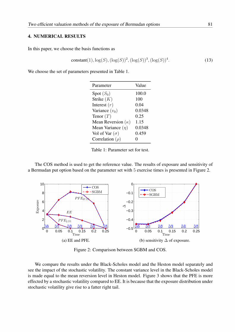
Two efficient valuation methods of the exposure of Bermudan options 81
4. NUMERICAL RESULTS
In this paper, we choose the basis functions as
constant(1), log(S), (log(S))2, (log(S))3, (log(S))4. (13)
We choose the set of parameters presented in Table 1.
Parameter Value
Spot (S0) 100.0Strike (K) 100Interest (r) 0.04Variance (v0) 0.0348Tenor (T ) 0.25Mean Reversion (κ) 1.15Mean Variance (η) 0.0348Vol of Var (σ) 0.459Correlation (ρ) 0
Table 1: Parameter set for test.
The COS method is used to get the reference value. The results of exposure and sensitivity ofa Bermudan put option based on the parameter set with 5 exercise times is presented in Figure 2.
0 0.05 0.1 0.15 0.2 0.250
2
4
6
8
10
Time
Exposure
COS
SGBM
PFE97.5%
EE
PFE2.5%
t0 t1 t2 t3 t4 t5
(a) EE and PFE.
0 0.05 0.1 0.15 0.2 0.25−0.5
−0.4
−0.3
−0.2
−0.1
0
Time
∆
COS
SGBM
t0 t1 t2 t3 t4 t5
(b) sensitivity ∆ of exposure.
Figure 2: Comparison between SGBM and COS.
We compare the results under the Black-Scholes model and the Heston model separately andsee the impact of the stochastic volatility. The constant variance level in the Black-Scholes modelis made equal to the mean reversion level in Heston model. Figure 3 shows that the PFE is moreeffected by a stochastic volatility compared to EE. It is because that the exposure distribution understochastic volatility give rise to a fatter right tail.
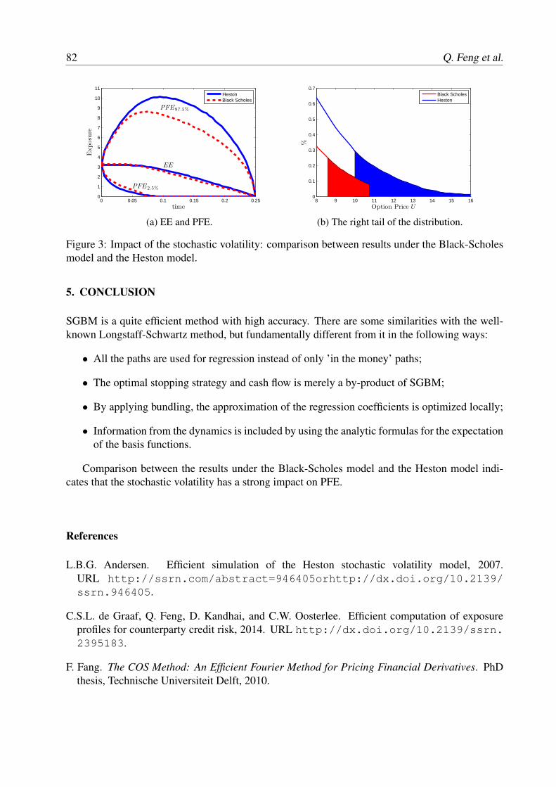
82 Q. Feng et al.
0 0.05 0.1 0.15 0.2 0.250
1
2
3
4
5
6
7
8
9
10
11
time
Exposure
PFE97.5%
EE
PFE 2.5%
HestonBlack Scholes
(a) EE and PFE.
8 9 10 11 12 13 14 15 160
0.1
0.2
0.3
0.4
0.5
0.6
0.7
Option Price U
%
Black ScholesHeston
(b) The right tail of the distribution.
Figure 3: Impact of the stochastic volatility: comparison between results under the Black-Scholesmodel and the Heston model.
5. CONCLUSION
SGBM is a quite efficient method with high accuracy. There are some similarities with the well-known Longstaff-Schwartz method, but fundamentally different from it in the following ways:
• All the paths are used for regression instead of only ’in the money’ paths;
• The optimal stopping strategy and cash flow is merely a by-product of SGBM;
• By applying bundling, the approximation of the regression coefficients is optimized locally;
• Information from the dynamics is included by using the analytic formulas for the expectationof the basis functions.
Comparison between the results under the Black-Scholes model and the Heston model indi-cates that the stochastic volatility has a strong impact on PFE.
References
L.B.G. Andersen. Efficient simulation of the Heston stochastic volatility model, 2007.URL http://ssrn.com/abstract=946405orhttp://dx.doi.org/10.2139/ssrn.946405.
C.S.L. de Graaf, Q. Feng, D. Kandhai, and C.W. Oosterlee. Efficient computation of exposureprofiles for counterparty credit risk, 2014. URL http://dx.doi.org/10.2139/ssrn.2395183.
F. Fang. The COS Method: An Efficient Fourier Method for Pricing Financial Derivatives. PhDthesis, Technische Universiteit Delft, 2010.

Two efficient valuation methods of the exposure of Bermudan options 83
J. Gregory. Counterparty credit risk and credit value adjustment: A continuing challenge forglobal financial markets - Second Edition. John Wiley & Sons, The Atrium, Southern Gate,Chichester, West Sussex, PO19 8Q, United Kingdom, 2012.
S.L. Heston. A closed-form solution for options with stochastic volatility with applications to bondand currency options. Review of Financial Studies, 6(2):327–343, 1993.
S. Jain and C.W. Oosterlee. The stochastic grid bundling method: Efficient pricing of bermudanoptions and their greeks, 2013. URL http://dx.doi.org/10.2139/ssrn.2293942.
F.A. Longstaff and E.S. Schwartz. Valuing american options by simulation: a simple least-squaresapproach. Review of Financial Studies, 14(1):113–147, 2001.


EVOLUTION OF COPULAS AND ITS APPLICATIONS
Naoyuki Ishimura
Graduate School of Economics, Hitotsubashi University, Kunitachi, Tokyo 186-8601, JapanEmail: [email protected]
Copulas are known to provide a flexible tool for describing possible nonlinear relations among riskfactors. Except for several examples, however, copulas are mainly concerned with the static prob-lems, not with the time-dependent processes. Here, we review our recent studies on the evolutionof copulas, which assumes that a copula itself evolves according to the time variable, and considerits slight generalization in discrete processes. Possible applications of our evolution of copulas arealso discussed.
1. INTRODUCTION
A copula is a well-employed tool for investigating the dependence structure among risk factors.Copulas make a link between multivariate joint distributions and univariate marginal distributions.Because of their flexibility, copulas have been extensively studied and applied in a wide range ofareas concerning the problem of dependence relations, which include, to name a few, actuarial andinsurance mathematics, financial mathematics, hydrology, seismology, and so on. For a generalreference on the theory of copulas, we refer to the book by Nelsen (2006).
Copulas, however, are concerned mainly with the stationary situation and not with the time-dependent circumstance. There exist of course a few attempts which deal with the time variable inthe copula theory. We recall the study on copulas with Markov processes by Darsow et al. (1992),and also on dynamic copulas by Patton (2006).
In our research, we introduce the concept of the evolution of copulas both in continuous anddiscrete time, which proclaims that a copula itself evolves according to the time variable. Tostart with the continuous processes, let C(u, v, t)t≥0 be a time parameterized family of bivariatecopulas, which satisfy the heat equation:
∂C
∂t(u, v, t) =
( ∂2∂u2
+∂2
∂v2
)C(u, v, t). (1)
By the definition of a copula, C(·, ·, t) verifies the following conditions:
(i) C(u, 0, t) = C(0, v, t) = 0, C(u, 1, t) = u and C(1, v, t) = v;
85

86 N. Ishimura
(ii) For every (ui, vi, t) ∈ I2 × (0,∞) (i = 1, 2) with u1 ≤ u2 and v1 ≤ v2, it follows thatC(u1, v1, t)− C(u1, v2, t)− C(u2, v1, t) + C(u2, v2, t) ≥ 0. Here, we write I := [0, 1].
It is proved in Ishimura and Yoshizawa (2011) that for any given bivariate copula C0 asthe initial condition, there exists a family of copulas C(u, v, t)t≥0, which satisfy (1), withC(u, v, 0) = C0(u, v). Moreover, we have
C(u, v, t) −→ Π(u, v) := uv as t→∞.
Remark that the product copula Π is also a steady solution of (1) and thus it is customarily calleda harmonic copula.
From a practical point of view, however, the discrete version of the above evolution may bemuch more useful. In this short note, we deal with the evolution of multivariate copulas in discreteprocesses and discuss the possibility of applications. First, we clarify the notion of evolution ofcopulas in discrete time.
Definition 1.1 A discretely parameterized family of functions Cnn∈N defined on Id := [0, 1]d
and valued in I is called the evolution of copulas in a discrete process if the following threeconditions are satisfied:
(i) For every n ∈ N, Cn(u1, u2, . . . , ud) is increasing in each component ui.
(ii) For every n ∈ N and i ∈ 1, 2, . . . , d with ui ∈ I ,
Cn(u1, . . . , ui−1, 0, ui+1, . . . , ud) = 0 and Cn(1, . . . , 1, ui, 1, . . . , 1) = ui.
(iii) (d-increasing condition) For every n ∈ N and (u1i, u2i, . . . , udi) ∈ Id with u1i ≤ u2i (i =1, 2),
2∑i1=1
· · ·2∑
id=1
(−1)i1+i2+···+idCn(u1i1 , u2i2 , . . . , udid) ≥ 0.
In the next section, we exhibit the construction of such a family of copulas.
2. EVOLUTION OF COPULAS IN DISCRETE PROCESSES
We now turn our attention to the investigation of the evolution of copulas in discrete processes,with the intention to undertake a slight generalization of Ishimura and Yoshizawa (2012).
Let d ≥ 2 and assume that N 1 and 0 < h 1. We define
∆u1 = ∆u2 = · · · = ∆ud :=1
Nand ∆t := h,
such that
λ :=∆t
(∆ui)2= hN2 (i = 1, 2, . . . , d),

Evolution of copulas 87
and for i = 1, 2, . . . , d, we have
ui,ki := ki∆ui =kiN, (ki = 0, 1, . . . , N).
A family of copulas Cn(u1, u2, . . . , ud)n∈N is now defined as follows.The initial condition is defined by
C0(u1, u2, . . . , ud) := C0(u1, u2, . . . , ud),
where C0 denotes a given initial copula.Let Cn
k1,k2,...,kd:= Cn(u1,k1 , u2,k2 , . . . , ud,kd), where (u1,k1 , u2,k2 , . . . , ud,kd)k1,k2,...,kd=0,1,...,N
denote the lattice points. Its values for k1, k2, . . . , kd = 1, 2, . . . , N −1 are governed by the systemof difference equations
Cn+1k1,k2,...,kd
= αnCnk1,k2,...,kd
+ βni
d∑i=1
(Cnk1,...,ki−1,ki+1,ki+1,...,kd
+ Cnk1,...,ki−1,ki−1,ki+1,...,kd
). (2)
Here, we postulate that
αn > 0, βni > 0 (i = 1, 2, . . . , d) and αn + 2d∑
i=1
βni = 1.
If for some j, kj = N , then the j-th term in the sum of the right hand side of (2) should be replacedby
Cnk1,...,kj−1,N+1,kj+1,...,kd
+ Cnk1,...,kj−1,N−1,kj+1,...,kd
−→ 2Cnk1,...,kj−1,N,kj+1,...,kd
.
If for some j, kj = 0, then
Cnk1,...,kj−1,1,kj+1,...,kd
+ Cnk1,...,kj−1,−1,kj+1,...,kd
−→ 2Cnk1,...,kj−1,0,kj+1,...,kd
= 0.
Given these adjustments, we see that the boundary conditionCn
k1,...,ki−1,0,ki+1,...,kd= 0
CnN,...,N,ki,N,...,N = ui,ki ,
for ki = 0, 1, . . . , N (i = 1, 2, . . . , N)
is properly imposed.For a point (u1, u2, . . . , ud) ∈ Id other than (u1,k1 , u2,k2 , . . . , ud,kd)k1,k2,...,kd=0,1,...,N , the
value Cn(u1, u2, . . . , ud) is provided by interpolation; that is, if
u1,k1 ≤ u1 ≤ u1,k1+1, u2,k2 ≤ u2 ≤ u2,k2+1, . . . , ud,kd ≤ ud ≤ ud,kd+1,
then we define
Cn(u1, u2, . . . , ud) =1∑
j1=0
· · ·1∑
jd=0
S(k1 + j1, k2 + j2, . . . , kd + jd)(u1 − u1,k1)j1(u2 − u2,k2)j2 · · · (ud − ud,kd)jd ,(3)

88 N. Ishimura
where we have
S(k1 + j1, k2 + j2, . . . , kd + jd) =
j1∑l1=0
· · ·jd∑
ld=0
(−1)j1+···+jd+l1+···+ldCnk1+l1,k2+l2,...,kd+ld
.
We remark that the values S(k1 + j1, k2 + j2, . . . , kd + jd) are all non-negative by virtue of thed-increasing condition above, which makes Cn(u1, u2, . . . , ud) indeed a copula. We also notethat if Cn
k1+l1,k2+l2,...,kd+ld=∏d
i=1 ui,ki+li for all values, which means that the product copula isconcerned, then Cn(u1, u2, . . . , ud) reduces to
∏di=1 ui for u1,k1 ≤ u1 ≤ u1,k1+1, u2,k2 ≤ u2 ≤
u2,k2+1, . . ., ud,kd ≤ ud ≤ ud,kd+1.It is easy to check that a sequence of copulas Cn(u1, u2, . . . , ud)n∈N is well defined and gives
the evolution of copulas in discrete time. Furthermore, the difference scheme is stable and we inferthat
max(u1,u2,··· ,ud)∈Id
∣∣∣∣∣Cn(u1, u2, . . . , ud)−d∏
i=1
ui
∣∣∣∣∣ ≤ Kθn,
for some constants K and θ with 0 < θ < 1. In summary, we can state the next theorem.
Theorem 2.1 Let d ≥ 2. For any initial copula C0 of dimension d, there exists an evolution ofcopulas Cn(u1, u2, . . . , ud)n∈N in discrete time, which satisfies the system of difference equations(2) at every (u1,k1 , u2,k2 , . . . , ud,kd)k1,k2,...,kd=0,1,...,N and are bridged by the interpolation (3).Additionally, we have
Cn(u1, u2, . . . , ud)→d∏
i=1
ui uniformly on Id as n→∞.
We may omit the details of the proof and other properties.
Remark 2.1 The difference scheme (2) originally comes from the discretization of the heat equa-tion; e.g. Ishimura and Yoshizawa (2012) deals with
Cn+1k1,k2,...,kd
− Cnk1,k2,...,kd
∆t
=d∑
i=1
Cnk1,...,ki−1,ki+1,ki+1,...,kd
− 2Cnk1,...,ki−1,ki,ki+1,...,kd
+ Cnk1,...,ki−1,ki−1,ki+1,...,kd
(∆ui)2.
Our current scheme (2) is thus regarded as a slightly generalized version.
3. DISCUSSIONS
We have developed the concept of time-dependent copulas, and in particular, the evolution ofcopulas in discrete processes. Compared to other time-related copulas, in our notion, a copula
Evolution of copulas 89
evolves according to the time variable. It may be employed in certain inference on the time-varying deformation of structures among random events. Since the dependence between randomfactors usually changes in time, one can expect that a mathematical modeling with some evolutionsystem has a place to be involved. We hope that such a description is realized with the use of ourtheory.
A major drawback of our evolution, however, is that every copula converges to the simplestcopula, the product copula. The relation between random variables, which is described by oursystem, is gradually becoming simple in a sense. It may be challenging to bypass this difficulty.A possible way would be to presume that it is rather suitable to invoke the backward type of thescheme (2); we assign the maturity state and consider the backward evolution which starts from thismaturity. We believe that other good applications of the evolution of copulas are still unexploredand we continue to make an effort on finding a relevant example.
References
W.F. Darsow, B. Nguyen, and E.T. Olsen. Copulas and Markov Processes. Illinois J. Math., 36:600–642, 1992.
N. Ishimura and Y. Yoshizawa. On time-dependent bivariate copulas. Theor. Appl. Mech. Japan,59:303–307, 2011.
N. Ishimura and Y. Yoshizawa. Evolution of multivariate copulas in discrete processes. ProcediaEconomics and Finance, 1:186–192, 2012.
R.B. Nelsen. An Introduction to Copulas. Springer, New York, 2006.
A.J. Patton. Modelling asymmetric exchange rate dependence. International Econ. Review, 47:527–556, 2006.

VALUATION OF EMPLOYEE STOCK OPTIONS IN THE HESTON MODEL
Tilman Sayer
Department of Financial Mathematics, Fraunhofer Institute for Industrial Mathematics,Fraunhofer-Platz 1, 67663 Kaiserslautern, GermanyEmail: [email protected]
The paper deals with the valuation of employee stock optionswithin the stochastic volatility modelof Heston (1993). We introduce personal market perspectives into the model and apply a two-dimensional tree algorithm to value the options for both subjective and objective beliefs. Pseudocode that illustrates the valuation principle is presented.
1. INTRODUCTION AND MOTIVATION
Employee stock options (ESOs) are a popular part of employeeremuneration. Typically theseoptions are non-tradable calls on the company’s stock and are given to an employee as part ofher compensation. Often they last as long as ten or fifteen years, are issued at-the-money and areinaccessible during the vesting period, an interval of variable length after grant. After vesting, theoptions can be exercised at any time, however, when the employee quits the job during the vestingperiod, the ESOs forfeit worthless.
In the literature, three values arise when pricing employeestock options. The first one is thesubjective value, which is the price the employee assigns tothe option. Due to her trading restric-tions, she tends to exercise the ESO sub-optimally from market perspectives. Mathematically thisis incorporated into the model through subjective market beliefs and risk aversion. The secondvalue is the objective price, that equals the costs for setting up a hedging portfolio of the stock andthe riskless asset that exactly mimics the subjective exercise policy. Since the company can act asan unconstrained market player, the portfolio follows the risk-neutral processes. The third optionprice equals the value an unrestricted market participant is willing to pay, i.e. it is determined underrisk neutrality and optimal exercise.
The structure of the paper is as follows. Section 2 introduces the model framework in thecontext of the stochastic volatility model of Heston (1993)and sets up the refined tree model.Pseudo code as well as implementation details are given in Section 3. Section 4 shows numericalresults, Section 5 concludes and gives an outlook.
Parts of this work are included in the PhD thesis of Tilman Sayer, see Sayer (2012).
91
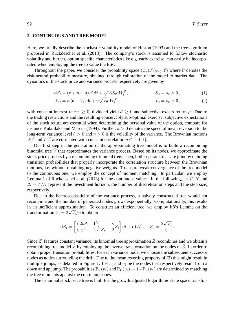
92 T. Sayer
2. CONTINUOUS AND TREE MODEL
Here, we briefly describe the stochastic volatility model ofHeston (1993) and the tree algorithmproposed in Ruckdeschel et al. (2013). The company’s stock isassumed to follow stochasticvolatility and further, option specific characteristics like e.g. early exercise, can easily be incorpo-rated when employing the tree to value the ESO.
Throughout the paper, we consider the probability space(Ω, (Ft)t≥0,P) whereP denotes therisk-neutral probability measure, obtained through calibration of the model to market data. Thedynamics of the stock price and variance process respectively are given by
dSt = (r + µ− d)Stdt+√
VtStdWSt , S0 = s0 > 0 , (1)
dVt = κ (θ − Vt) dt+ η√
VtdWVt , V0 = v0 > 0 , (2)
with constant interest rater ≥ 0, dividend yieldd ≥ 0 and subjective excess returnµ. Due tothe trading restrictions and the resulting conceivably sub-optimal exercise, subjective expectationsof the stock return are essential when determining the personal value of the option, compare forinstance Kulatilaka and Marcus (1994). Further,κ > 0 denotes the speed of mean reversion to thelong-term variance levelθ > 0 andη > 0 is the volatility of the variance. The Brownian motionsW S
t andW Vt are correlated with constant correlationρ ∈ [−1, 1].
Our first step in the generation of the approximating tree model is to build a recombiningbinomial treeV that approximates the variance process. Based on its nodes, we approximate thestock price process by a recombining trinomial tree. Then, both separate trees are joint by definingtransition probabilities that properly incorporate the correlation structure between the Brownianmotions, i.e. without obtaining negative weights. To ensure weak convergence of the tree modelto the continuous one, we employ the concept of moment matching. In particular, we employLemma 1 of Ruckdeschel et al. (2013) for the continuous values. In the following, letT , N and∆ = T/N represent the investment horizon, the number of discretisation steps and the step size,respectively.
Due to the heteroscedasticity of the variance process, a naively constructed tree would notrecombine and the number of generated nodes grows exponentially. Computationally, this resultsin an inefficient approximation. To construct an efficient tree, we employ Ito’s Lemma on thetransformationZt = 2
√Vt/η to obtain
dZt =
[(
2κθ
η2−
1
2
)
1
Zt
−κ
2Zt
]
dt+ dW Vt , Z0 =
2√V0
η.
SinceZt features constant variance, its binomial tree approximation Z recombines and we obtain arecombining tree modelV by employing the inverse transformation on the nodes ofZ. In order toobtain proper transition probabilities, for each variancenode, we choose the subsequent successornodes as nodes surrounding the drift. Due to the mean reverting property of (2) this might result inmultiple jumps, as detailed in Figure 1. Letv1 andv2 be the nodes that respectively result from adown and up jump. The probabilitiesPV (v1) andPV (v2) = 1−PV (v1) are determined by matchingthe tree moments against the continuous ones.
The trinomial stock price tree is built for the growth adjusted logarithmic state space transfor-
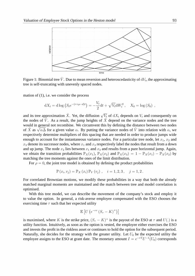
Valuation of Employee Stock Options in the Heston model 93
time
varia
nce
Figure 1: Binomial treeV . Due to mean reversion and heteroscedasticity ofdVt, the approximatingtree is self-truncating with unevenly spaced nodes.
mation of (1), i.e. we consider the process
dXt = d log(
Ste−(r+µ−d)t
)
= −Vt
2dt+
√
VtdWSt , X0 = log (S0) ,
and its tree approximationX. Yet, the diffusion√Vt of dXt depends onVt and consequently on
the nodes ofV . As a result, the jump heights ofX depend on the variance nodes and the treewould in general not recombine. We circumvent this by defining the distance between two nodesof X as
√α∆ for a given valueα. By putting the variance nodes ofV into relation withα, we
respectively determine multipliers of this spacing that are needed in order to produce jumps wideenough to account for the instantaneous variance nodes. Fora particular tree node, letx1, x2 andx3 denote its successor nodes, wherex1 andx3 respectively label the nodes that result from a downand up jump. The nodex2 lies betweenx1 andx3 and results from a pure horizontal jump. Again,we obtain the transition probabilitiesPX(x1), PX(x2) andPX(x3) = 1 − PX(x1) − PX(x2) bymatching the tree moments against the ones of the limit distribution.
Forρ = 0, the joint tree model is obtained by defining the product probabilities
P (xi, vj) = PX (xi)PV (vj) , i = 1, 2, 3 , j = 1, 2 .
For correlated Brownian motions, we modify these probabilities in a way that both the alreadymatched marginal moments are maintained and the match between tree and model correlation isoptimised.
With this tree model, we can describe the movement of the company’s stock and employ itto value the option. In general, a risk-averse employee compensated with the ESO chooses theexercising timeτ such that her expected utility
E[
U(
e−rτ (Sτ −K)+)]
is maximised, whereK is the strike price,(Sτ −K)+ is the payout of the ESO atτ andU(.) is autility function. Intuitively, as soon as the option is vested, the employee either exercises the ESOand invests the profit in the riskless asset or continues to hold the option for the subsequent period.Naturally, she decides for the strategy with the greater utility. Let U0 be the expected utility theemployee assigns to the ESO at grant date. The monetary amount I = e−rTU−1(U0) corresponds

94 T. Sayer
to the subjective price of the ESO and is typically interpreted as an indifferent payment, i.e. as theparticular value for which the employee is neutral betweenI and the ESO. Given the exercise pol-icy of the employee, the value of the hedging portfolio is calculated respectively, even if exercisingthe option is sub-optimal from market perspectives. Its value at grant date defines the objectivevalue of the ESO.
3. IMPLEMENTATION DETAILS
The tree model is implemented using Matlab programming language. Pseudo code that illustratesthe option pricing by backward induction is given in Figure 2, where we consider the subjectiveand objective value. Letn denote a node in the joint tree. In the code,n.Ssub andn.Sobj
Input: parameters % relevant market, option & tree parameters
Output: sub, obj % subjective & objective value
( 1) for t = T, T - ∆, ..., 0 do
( 2) N = getRelevantNodes(t); % obtain active tree nodes
( 3) sub_e = 0;
( 4) obj_e = 0;
( 5) for each n in N do
( 6) if (isESOVested) % exercise values from subjective & market perspectives
( 7) sub_e = U(exp(r * (T - t)) * max(0, n.Ssub - K));
( 8) obj_e = max(0, n.Sobj - K);
( 9) end
(10) if (t == T)
(11) n.sub = sub_e;
(12) n.obj = obj_e;
(13) else
(14) (n1, ..., n6, P1, ..., P6) = getNodesAndWeights(n);
(15) sub_h = P1 * n1.sub + ... + P6 * n6.sub;
(16) obj_h = P1 * n1.obj + ... + P6 * n6.obj;
(17) n.sub = max(sub_h, sub_e);
(18) if (n.sub == sub_h) n.obj = exp(-r * ∆) * obj_h;
(19) else n.obj = obj_e;
(20) end
(21) end
(22) end
(23) end
(24) sub = exp(-r * T) * InvU(n.sub); % subjective value
(25) obj = n.obj; % objective value
(26) return sub, obj;
Figure 2: Pseudo code illustrating the backward induction and the calculation of the subjective andobjective value. The functionsU(.), InvU(.) andgetNodesAndWeights(.) respectivelyreturn utility, inverse utility and the successor nodes as well as the corresponding transition proba-bilities. At each time step, the active nodes are obtained throughgetRelevantNodes(.).
label the stock price from subjective and market perspectives. Furthermore,n.sub andn.obj
Valuation of Employee Stock Options in the Heston model 95
denote the subjective and objective option value at noden. Since the marginal treesV andX aswell as the correlated transition probabilitiesP(xi, vj) for i = 1, 2, 3 andj = 1, 2 do not dependon the current time step, these values can be determined before running the backward induction,i.e. before valuing the tree from its leafs to the root. Lines(7) and (8) determine the exercise valuesfor subjective and market beliefs. The values for holding the ESO are obtained between lines (14)and (16). Depending on the subjective policy of the employee, i.e. the maximum value ofsub handsub e, the hedging portfolio mimics her decision in the lines (18)to (20), where the objectivevalue of noden is set. Finally, line (24) determines the indifferent payment.
4. NUMERICAL RESULTS
The relation betweenI and the price of the hedging portfolio is illustrated in Figure 3 for differentvalues ofµ and for a spot price range from20 to 300. The remaining parameters arer = 5%,
50 100 150 200 250 3000
0.2
0.4
0.6
0.8
1
spot
ratio
µ = −3%µ = 0%µ = 3%
Figure 3: Relation between the subjective and objective option value for varying subjective excessreturnµ and spot value.
d = 0%, v0 = θ = 4%, κ = 2, η = 20% andρ = −0.85. We further assume power utilityU(x) = x1−γ/(1 − γ) with γ = 0.25. The option lives for two years and vests after six months.The strike is set to100, N = 200 andα = 2%. Forµ = 0%, the subjective and market beliefscoincide. Since the employee acts risk-averse, she exercises sub-optimally, hence waives optionvalue. As the spot increases, this reduction becomes irrelevant, i.e. the particular ratio tends toone. Forµ = −3%, the effect of waiving option value is further stressed due to the pessimisticsubjective beliefs. In the case ofµ = 3%, the optimistic personal perceptions cause the employeeto delay her exercise decision. Further, the indifferent paymentI even exceeds the value of theportfolio, despite risk aversion.
5. CONCLUSION AND OUTLOOK
In this paper, we have introduced subjective excess returnsin the stochastic volatility model ofHeston (1993) and modified a recombining tree model to value employee stock options accord-
96 T. Sayer
ingly. Due to the structure of the tree, many specific characteristics of ESOs can easily be incor-porated. We determined price ratios between subjective andobjective option values, where wefocused on the excess returns. Future work could for instance cover further ESO specifications oremploy the tree to value similar sophisticated derivative types.
References
S. L. Heston. A Closed-Form Solution for Options with Stochastic Volatility with Applications toBond and Currency Options.Review of Financial Studies, 6(2):327–343, 1993.
N. Kulatilaka and A. J. Marcus. Valuing Employee Stock Options. Financial Analysts Journal, 50(6):46–56, 1994.
P. Ruckdeschel, T. Sayer, and A. Szimayer. Pricing American Options in the Heston Model: AClose Look at Incorporating Correlation.Journal of Derivatives, 20(3):9–29, 2013.
T. Sayer.Valuation of American-style derivatives within the stochastic volatility model of Heston.PhD Dissertation, Dr. Hut, Munchen, Germany, 2012.
MARKOV SWITCHING AFFINE PROCESSES AND APPLICATIONS TO PRICING
Misha van Beek†, Michel Mandjes†,‡,§, Peter Spreij† and Erik Winands†
†Korteweg-de Vries Institute for Mathematics, University of Amsterdam,1090 GE Amsterdam, The Netherlands‡EURANDOM, 5600 MB Eindhoven, The Netherlands§CWI, 1090 GB Amsterdam, The NetherlandsEmail: [email protected], [email protected], [email protected],
1. INTRODUCTION
This paper extends derivative pricing based on multivariate affine processes to affine models withMarkov switching drift and diffusion coefficients. In the economic and finance literature, modelswith Markov switching parameters are often said to be regime switching.
In many economic and finance applications, processes fall prey to changes in regime. Regimesare time periods between which the dynamics of these processes are substantially different (Hamil-ton 1989). E.g. the mean returns, correlations and volatilities of stock prices are different in bulland bear markets, and the mean reversion level of interest rates may be lower in crisis scenarios.Based on this observation, the pricing of derivatives should account for the existence of differentregimes.
Furthermore, many financial products benefit from multidimensional analysis. The price ofa European call option is better modeled by allowing for stochastic interest rates and stochasticvolatility. Also other products require multidimensional analysis directly through their structure.The price of a credit default swap (CDS) is derived from the dynamics of the interest rate and thehazard rate of default of the underlying. When we want to adjust to a price of a derivative for thecreditworthiness of its seller, an additional process for the hazard rate of the seller enters into thegame. This is known as a credit valuation adjustment (CVA), and together with a similar adjust-ment for the buyer’s creditworthiness, the debit valuation adjustment (DVA), these are commonand increasingly important drivers of multivariate analysis (Hull and White 2013).
In this paper, we consider the popular and broad class of multivariate affine processes that isoften used to jointly model time series such as interest rates, stochastic volatility, hazard rates andlog-asset prices (Duffie et al. 2003). Affine processes include the Vasicek and Cox-Ingersoll-Ross
97
98 M. van Beek et al.
short rate models as special univariate cases. The primary advantage of affine processes over gen-eral multivariate processes in general is that the price of many derivatives has a closed form oris implicit in a system of ordinary differential equations (ODEs). ODE solutions are markedlymore tractable than the partial differential equations (PDEs) that multivariate processes produce.We generalize multivariate affine processes to include Markov switching drift and diffusion co-efficients. Our resulting Markov switching- (MS-)affine process maintains the property of ODEpricing solutions.
There is a rather restraint body of literature on this problem. Elliott and Mamon (2002) considerpricing a bond based on a short rate that follows a univariate Vasicek model with Markov switchingmean reversion level. Elliott and Siu (2009) extend this result to bond prices based on a short ratethat follows a univariate affine process with Markov switching mean reversion level and (in theVasicek case) diffusion.
We take a more formal approach and follow the line of argumentation of Filipovic (2009,Chapter 10). We derive the characteristic function of the MS-affine process and show that it canbe expressed using the solutions of two systems of ODEs. We also prove that these solutions existand are unique, provided that the parameters of the process are admissible in some sense. Thecharacteristic function is the basis to price a wide variety of payoffs.
Effectively, our main theorem extends all pricing ODEs for affine processes to MS-affine pro-cesses. These include CVA and DVA adjustments, CDSs, exchange options, and many more.Moreover, for all these derivatives we may have regime dependent payoffs. The regime dependentpayouts are used, for example, when the payoff of a derivative relies on the rating of a counterparty,and for this counterparty we have a rating migration matrix. Each rating (e.g. AAA, AA, etc.) canbe seen as a regime in which the dynamics of the processes are different. Another example iswhen the dynamics of the affine process are different after some policy is introduced, but we areunsure when this policy takes effect. The different regimes would be the different states that thedevelopment and implementation of this policy can be in.
This remainder of this paper is outlined as follows. First we define the MS-affine process andthe admissibility of its parameters. Then we provide two theorems that can be used for derivativepricing. We conclude with a simple example on how to apply these theorems to a bond price.
2. MODEL AND ANALYSIS
Let Wt be a d-dimensional Brownian motion with filtration Gt. Let St be a continuous timeMarkov chain with state space S = 1, . . . , h, filtration Ht and generator Q that switchesbetween the regimes in S. Wt and St are independent and defined on a filtered probability space〈Ω,F , Ft,P〉, where Ft = Gt ∨Ht.
Definition 2.1 We call the process X on the canonical state space X = Rm+ ×Rn, m ≥ 0, n ≥ 0,
m+ n = d ≥ 1, MS-affine if
dXt = µSt(Xt)dt+ σSt(Xt)dWt, (1)

Markov Switching Affine Processes and applications to pricing 99
where
σs(x)σ>s (x) = as +d∑i=1
xiαi, µs(x) = bs +d∑i=1
xiβi = bs + Bx (2)
for some d× d-matrices as and αi, and d-vectors bs and βi, with B =[β1 · · · βd
].
Hence only as and bs are regime dependent, not αi and βi.1
Xt may stack all sorts of financial variables. For example, if rt is the short rate, At someasset price, Vt the stochastic volatility of the stock price, and ht the hazard rate of default of thecounterparty, thenXt = (rt, lnAt, Vt, ht) models these processes jointly. For financial applicationsthis model is usually under the risk neutral measure. This implies (among other things) that thedrift of lnAt is rt − 1
2Vt.
For ease of notation, we write Zt = eSt ∈ 0, 1h, a vector of zeros with St-th entry one. Z isthe state space of Zt. Then by Elliott (1993),
dZt = QZtdt+ dMt, (3)
where Mt is a martingale. Without proof we assume throughout this text that for every x ∈ X ,z ∈ Z there exists a unique solution (X,Z) = (Xx, Zz) of (1) with X0 = x and Z0 = z.
To ensure that the process does not escape X we need some admissibility conditions on theparameters in (2). In what follows, we denote I = 1, . . . ,m and J = m+ 1, . . . , d. Also, forany sets of indices M and N , and vector v and matrix w, vM = [vi]i∈M and wMN = [wij]i∈M,j∈Nare the corresponding sub-vector and sub-matrix.
Definition 2.2 We call X an MS-affine process with admissible parameters if X is MS-affine and
as, αi are symmetric positive semi-definite,asII = 0 for all s ∈ S (and thus asIJ = a>sJI = 0),αj = 0 for all j ∈ J,
αi,kl = αi,lk = 0 for k ∈ I\i, for all i, l ∈ 1, . . . , d,bs ∈ X for all s ∈ S,BIJ = 0,
BII has nonnegative off-diagonal elements.
We now state our main contribution. diag(Fs) refers to the (block) diagonal matrix from theregime specific matrices F1, . . . , Fh.
Theorem 2.1 Let X be an MS-affine process with admissible parameters. Let u ∈ iRd, t ≤ T ,x ∈ X and z ∈ Z . Then there exists unique solutions A(t, u) : R+ × iRd → Cd×d and B(t, u) :
1Taking αi and βi regime dependent complicates further analysis and we are not sure whether ODE solutions tothe characteristic function are possible in that case.

100 M. van Beek et al.
R+ × iRd → Cd to
∂tA(t, u) = A(t, u)(diag
(12BJ(t, u)>asJJBJ(t, u) + b>s B(t, u)
)+Q
), (4)
A(0, u) = Ih,
∂tBi(t, u) = 12B(t, u)>αiB(t, u) + β>i B(t, u), i ∈ I,
∂tBJ(t, u) = B>JJBJ(t, u),
B(0, u) = u,
such that the Ft-conditional regime specific characteristic function satisfies
E[eu
>XTZT
∣∣∣Ft] = A(T − t, u)eB>(T−t,u)XtZt. (5)
Before proving the above theorem, we state (without proof) the following lemma, which is usefulin an MS setting. ⊗ denotes the Kronecker product.
Lemma 2.2 Let FSt ∈ Rp×q be a set of d matrices with Markov switching index, then (Zt ⊗Ip)FSt = diag(FSt)(Zt ⊗ Iq).
Also, we use the following lemma adapted from Filipovic (2009, Lemma 10.1).
Lemma 2.3 Consider the system of ODEs
∂ty(t, y0) = f(y(t, y0)), y(0, y0) = y0, (6)
where f : Cd → Cd is a locally Lipschitz continuous function. Then:
1. For every y0 ∈ Cd there exists a lifetime t+(y0) ∈ (0,∞] such that there exists a uniquesolution y(·, y0) : [0, t+(y0))→ Cd of (6).
2. The domain D =
(t, y0) ∈ R+ × Cd∣∣t ≤ t+(y0)
is open in R+ × Cd and maximal in the
sense that either t+(y0) =∞ or limt↑t+(y0) ‖y(t, y0)‖ =∞, respectively, for all y0 ∈ Cd.
Proof of Theorem 2.1. Define Φt = A(T − t, u)eB(T−t,u)>Xt . We prove that ΦtZt is martingalebecause this implies that E
[eu
>XTZT∣∣Ft] = E [ΦTZT |Ft] = ΦtZt, and then (5) is true. The
dynamics of ΦtZt follow from Ito’s lemma and Lemma 2.2,
d(ΦtZt) = dΦtZt + ΦtdZt =(
(∂tA(T − t, u)) eB(T−t,u)>Xt
+ Φt (∂tB(T − t, u))>Xt + ΦtB(T − t, u)>µSt(Xt)
+ 12ΦtB(T − t, u)>σSt(Xt)σSt(Xt)
>B(T − t, u))Ztdt+ ΦtQZt
+ ΦtB(T − t, u)>σSt(Xt)dWtZt + ΦtdMt
= Φt
(B(T − t, u)>σSt(Xt)dWtZt + dMt
).
Therefore, ΦtZt is a local martingale. The remaining part of the proof is showing that this localmartingale is uniformly bounded, so it is also a martingale.
Markov Switching Affine Processes and applications to pricing 101
We know from Filipovic (2009, proof of Theorem 10.2) that by admissibility, for any u ∈Cm− × iRn, t ∈ R+ a unique solution B(t, u) : R+ × Cm
− × iRn → Cm− × iRn exists with infinite
lifetime, so <(B(t, u)>x
)≤ 0 for all x ∈ X .
Apply Lemma 2.3 to the vectorization of the ODE of A(t, u) (4), so y = vec(A), y0 = vec(Ih)and f the vectorization of the RHS of (4). f is differentiable by differentiability ofB(t, u) and thuslocally Lipschitz continuous. Therefore a unique solution for A exists with lifetime t+(vec(Ih)) ∈(0,∞]. We prove by contradiction that t+(vec(Ih)) = ∞. Suppose t+(vec(Ih)) < ∞, thenlimt↑t+(vec(Ih)) ‖ vec(A(t, u))‖ =∞. Note that
‖ vec(A(t, u))‖2 = vec(A(t, u))∗ vec(A(t, u)) = tr(A(t, u)∗A(t, u)).
Define λ = maxi=1,...,h−λi, 0, with λi the eigenvalues of Q+Q>, then
∂t‖ vec(A(t, u))‖2 = tr(∂tA(t, u)∗A(t, u) + A(t, u)∗∂tA(t, u))
= tr((Q+Q>
)A(t, u)∗A(t, u)
)+ 2 tr
(<(diag
(12BJ(t, u)>asJJBJ(t, u) + b>s B(t, u)
))A(t, u)∗A(t, u)
)≤ tr
((Q+Q>
)A(t, u)∗A(t, u)
)+ λ tr (A(t, u)∗A(t, u))
≤ tr(Q+Q> + λIh
)tr(A(t, u)∗A(t, u))
= tr(Q+Q> + λIh
)‖ vec(A(t, u))‖2.
For the second equality we have substituted ∂tA(t, u) with (4). The first inequality follows fromλ ≥ 0 and the fact that for all s ∈ S,
<(12BJ(t, u)>asJJBJ(t, u) + b>s B(t, u)
)= 1
2<(BJ(t, u))>asJJ<(BJ(t, u))− 1
2=(BJ(t, u))>asJJ=(BJ(t, u)) + b>s <(B(t, u)) ≤ 0
by the admissibility restrictions on asJJ and bs and the codomain of B(t, u). The second inequal-ity holds because Q + Q> + λIh is positive semi-definite by construction and for any positivedefinite matrices C and D of the same size it holds that tr(CD) ≤ tr(C) tr(D). Applying Gron-wall’s inequality gives ‖ vec(A(t, u))‖2 ≤ hetr(Q+Q>+λIh)t, for all t < t+(vec(Ih)). This yieldslimt↑t+(vec(Ih)) ‖ vec(A(t, u))‖ < ∞, so by contradiction it follows that t+(vec(Ih)) = ∞; A(t, u)has infinite lifetime for all u ∈ Cm
− × iRn.Combining these results we have that Φt and B(t, u) are uniformly bounded for all t ≤ T , so
ΦtZt is a martingale.Theorem 2.1 is pivotal to derivatives pricing, but cannot be applied directly. Additionally, we
need that (5) holds when u ∈ Rd. Filipovic (2009, Theorem 10.3 and Corollary 10.1) proves thisfor affine processes, and we conjecture that this result extends to MS-affine processes.
3. SIMPLE EXAMPLE
As an example on how to apply the above theorems to derivative pricing, we consider the bondprice in a MS-Vasicek short rate model. Take the short rate model drt = γ (µSt − rt) dt+σStdWt,
102 M. van Beek et al.
where St is the continuous time Markov chain that switches between regimes and has generator Q.Introduce the integrator dRt = rtdt, R0 = 0, then Xt = (rt, Rt) is a MS-affine process, and foru = (0,−1) we have
1> E[eu
>XTZT∣∣F0
]= E
[e−RT
∣∣F0
]= E
[exp
(−∫ T
0
rtdt
)∣∣∣∣F0
].
Using Theorem 2.1 we can solve the LHS and thus obtain the price of the bond (the RHS, if it isfinite). More examples can be found in Filipovic (2009, Chapter 10.3).
References
D. Duffie, D. Filipovic, and W. Schachermayer. Affine processes and applications in finance. TheAnnals of Applied Probability, 13(3):984–1053, 2003.
Robert J. Elliott. New finite-dimensional filters and smoothers for noisily observed Markov chains.IEEE Transactions on Information Theory, 39(1):265–271, 1993.
Robert J. Elliott and Rogemar S. Mamon. An interest rate model with a Markovian mean revertinglevel. Quantitative Finance, 2(6):454–458, 2002.
Robert J. Elliott and Tak Kuen Siu. On Markov-modulated exponential-affine bond price formulae.Applied Mathematical Finance, 16(1):1–15, 2009.
Damir Filipovic. Term-Structure Models: A Graduate Course. Springer Finance. Springer, 2009.
James D. Hamilton. A new approach to the economic analysis of nonstationary time series and thebusiness cycle. Econometrica, 57(2):357–384, 1989.
John C. Hull and Alan White. Collateral and credit issues in derivatives pricing. Rotman Schoolof Management Working Paper, 2013.


De Koninklijke Vlaamse Academie van België voor Wetenschappen en Kunsten coördineert jaarlijks tot 25 wetenschappelijke bijeenkomsten, ook contactfora genoemd, in de domeinen van de natuurwetenschappen (inclusief de biomedische wetenschappen), menswetenschappen en kunsten. De contactfora hebben tot doel Vlaamse wetenschappers of kunstenaars te verenigen rond specifieke thema’s. De handelingen van deze contactfora vormen een aparte publicatiereeks van de Academie. Contactforum “Actuarial and Financial Mathematics Conference” (6-7 February 2014, Prof. M. Vanmaele) Deze handelingen van de “Actuarial and Financial Mathematics Conference 2014” geven een inkijk in een aantal onderwerpen die in de editie van 2014 van dit contactforum aan bod kwamen. Zoals de vorige jaren handelden de voordrachten over zowel actuariële als financiële onderwerpen en technieken met speciale aandacht voor de wisselwerking tussen beide. Deze internationale conferentie biedt een forum aan zowel experten als jonge onderzoekers om hun onderzoeksresultaten ofwel in een voordracht ofwel via een poster aan een ruim publiek voor te stellen bestaande uit academici uit binnen- en buitenland alsook collega's uit de bank- en verzekeringswereld.