Abstract Ivo Sousa -Ferreira 016 survsim survivalAna Maria ...

A review of Cox's model extensions for multiple events

Ivo Sousa-Ferreira1, Ana Maria Abreu2, 3, *

1Centro de Estatística e Aplicações, Faculdade de Ciências, Universidade de Lisboa, 1749-016

Lisboa, Portugal 2Departamento de Matemática, Faculdade de Ciências Exatas e da Engenharia, Universidade da

Madeira, 9020-105 Funchal, Portugal 3Centro de Investigação em Matemática e Aplicações, Portugal

*Correspondence to: Ana Maria Abreu. Campus Universitário da Penteada, 9020-105 Funchal,

Portugal. Email: [email protected]

Abstract

In longitudinal studies, it is usual that a given subject can experience several failures. To

analyse multiple failure-time data, we reviewed some extensions of Cox's regression model,

which were proposed by: Prentice, Williams and Peterson (PWP); Andersen and Gill (AG);

Wei, Lin e Weissfeld (WLW); and Lee, Wei and Amato (LWA). Our main goal is to underline

the differences between these extensions, through a brief but careful description, providing also

some guidance on how to choose the proper model for each situation. The guidelines presented

in this work revealed to be a useful pointer to easily choose the most suitable model.

Secondarily, we used the survsim and the survival R packages to illustrate the practical

implementation of these models.

Key words: extensions of Cox's model, multiple events, Survival Analysis

1. Introduction

In many research fields, the focus is in studying the time until the occurrence of one or of

multiple events. In clinical trials, Cox's regression model [1, 2] is the most popularly applied

model, because is suitable for analysing the time until the occurrence of a single event.

Nevertheless, it can also be used to analyse only the first event even in a multiple failure-time

framework. Over the past four decades there has been an increasing interest in developing new

extensions of the Cox model to accommodate the characteristics and the peculiarities of

situations involving multiple events [3, 4]. Some of these models, that have been commonly

used, were proposed by: Prentice, Williams and Peterson (PWP) [5]; Andersen and Gill (AG)

[6]; Wei, Lin e Weissfeld (WLW) [7]; and Lee, Wei and Amato (LWA) [8].

An important aspect on the multiple events analysis is the strong possibility of within-

subject correlation (due to the existence of more than one observation per subject). However,

the regression parameters estimation is made ignoring the potential existence of correlation. In

order to offset this fact, a robust estimator for the covariance matrix was developed [7, 9]. This

estimator allows to check whether or not the observations are truly correlated. In general, when

the robust estimate is much greater than the usual estimate it is said that there is within-subject

correlation. Otherwise there is between-subject correlation.

In the current literature, there is only a small number of scientific works describing the

implementation of this type of models through a statistical software [10, 11, 12, 13].

Furthermore, as far as we know, there is no available guide explaining, and comparing, how

these four models are, in practice, implemented through R statistical software [14]. This is a

major obstacle for practitioners, since R is an open access software.

Although there are several approaches to analyse multiple failure-time data [7, 10, 15,

16, 17], this paper focus only on models resulting from the Cox model. Therefore, the aim is to

bring those extensions to a wider audience, by giving an overview, outline some guidelines, and

IJRDO - Journal of Applied Science ISSN: 2455-6653

Volume-5 | Issue-2 | Feb,2019 47

mailto:[email protected]

present the software commands for easy and flexible fitting. With this intention, we provide

some guidance on how to choose the most appropriate model for each situation. In this point,

we also make some considerations about the care that must be taken in the construction of the

database, because its formatting has to be adequate to the characteristics of each model.

In this work there are four additional sections. In Section 2, we introduce some

characteristics of each model, along with its formulation. Already in Section 3, we briefly

describe how the data set was obtained and subsequently illustrate the computational

implementation of the models. Also, in these last two sections, we provide a tutorial in R1 for

the analysis of multiple failure-time data, in furtherance to create some guidelines for future

practitioners. Sections 4 contains the results of the fitted models and section 5 comprises some

remarks. In Section 6, we conclude the paper summing up the general contributions of this

review and presenting some further work.

2. The models

2.1. Formulation and characteristics

All the models considered in this work are extensions of the Cox model and are formulated in

terms of the hazard function. Suppose that there are 𝑛 subjects and that each of them can

experience a maximum of 𝑆 failures. The hazard function of the 𝑖th subject, 𝑖 = 1, … , 𝑛,

corresponding to the 𝑠th failure, 𝑠 = 1, … , 𝑆, is assumed to take, in general, one of the two

following expressions

ℎ(𝑡; 𝒛𝑖𝑠(𝑡)) = ℎ0𝑠(𝑡) exp(𝜷′𝒛𝑖𝑠(𝑡)) , 𝑡 ≥ 0, (1)

or

ℎ(𝑡; 𝒛𝑖𝑠(𝑡)) = ℎ0(𝑡) exp(𝜷′𝒛𝑖𝑠(𝑡)) , 𝑡 ≥ 0, (2)

where ℎ0𝑠(⋅) ≥ 0 represents an event-specific baseline hazard function for the 𝑠th failure,

ℎ0(⋅) ≥ 0 is the common baseline hazard function for all failures, 𝜷 = (𝛽1, … , 𝛽𝑝)′ denotes a

𝑝 × 1 overall vector of unknown regression parameters and 𝒛𝑖𝑠(𝑡) = (𝑧𝑖𝑠1(𝑡), … , 𝑧𝑖𝑠𝑝(𝑡))′

is

the 𝑝-vector of covariates (possibly time dependent) for the 𝑖th subject with respect to the 𝑠th

event. Despite we take 𝛽 to be the same among both models, this entails no loss of generality

considering that it can be always estimated by adjusting the appropriate overall covariate vector,

𝒛𝑖(𝑡) = (𝑧𝑖1′ (𝑡), … , 𝑧𝑖𝑆

′ (𝑡)), to the model. Notice that under the first formulation, (1), there is a

stratification by event in order to obtain the event-specific baseline hazard functions

ℎ01(⋅), ℎ02(⋅), … , ℎ0𝑆(⋅). Moreover, with this formulation it is also possible to estimate an

event-specific vector of unknown regression parameters 𝜷𝑠 = (𝛽𝑠1, … , 𝛽𝑠𝑝)′ because it is a

stratified model.

These models differ according to the time formulation used – counting process (CP),

gap time (GT) or total time (TT) – to record the risk intervals, as we will see throughout this

section.

2.1.1. Prentice, Williams and Peterson (PWP) model

One of the first extensions of the Cox model to analyse multiple-failure time data was proposed

by Prentice, Williams and Peterson [5]. This model emerged to analyse (recurrent) events that

occur in an orderly way, wherein the risk of occurrence of the following event is affected by

the previous ones. Thereby it is necessary to consider an event-specific baseline hazard

1 The practical implementation of the models was performed through R version 3.5.2.



function, ℎ0𝑠(𝑡) (𝑠 = 1, … , 𝑆), for each event, which means that this model is formulated by

the hazard function (1).

The PWP model allows two possible time scales for recording the risk intervals:

counting process or gap time formulations. Counting process formulation is the time from the

beginning of the study, where the initial time of each risk interval matches with the instant

wherein the previous event ends. This gives rise to the PWP-CP model, where the risk set

indicator associated with the CP formulation is defined as 𝑌𝑖𝑠(𝑡) = 𝐼(𝑡𝑖(𝑠−1) < 𝑡 < 𝑡𝑖𝑠). Gap

time formulation is the time from the previous event, which means that the clock restarts after

the occurrence of each event. Then, the risk set indicator associated with this formulation is

defined as 𝑌𝑖𝑠(𝑡) = 𝐼(𝑔𝑖𝑠 ≥ 𝑡), where 𝑔𝑖𝑠 = 𝑡𝑖𝑠 − 𝑡𝑖(𝑠−1) represents the observed gap time

among two consecutive events. However, to accommodate the implicit time scale, it is also

necessary to make a slight change in equation (1): ℎ0𝑠(𝑡) has to be replaced by

ℎ0𝑠(𝑡 − 𝑡𝑖(𝑠−1)), which is an event-specific baseline hazard function related to the time since

the last occurrence. This case in turn gives rise to the PWP-GT model.

In both formulations of PWP models, it is assumed that events have different risks of

occurrence, which involves stratifying subjects according to the occurrence order, i.e., by event

number. Besides that, it is also admitted that the risk of occurrence of each event is conditioned

by the observation of the preceding event. Therefore, only the subjects who have experienced

exactly 𝑠 − 1 failures can contribute with their 𝑠th risk intervals to the constitution of the 𝑠th

risk set. This is also another relevant assumption in the application of this model. In fact, it

should be borne in mind that the greater the order of the event, the smaller the size of the

corresponding risk set, which may give rise to unreliable estimates in the latter strata [16]. To

avoid such situation, the choice of the maximum number of events to be included in the analysis

should be done carefully.

2.1.2. Andersen and Gill (AG) model

Another extension of the Cox model was proposed by Andersen and Gill [6], appearing in the

same line of reasoning of the previous model. This one equally emerged to analyse ordered

events of a single-type, but where it is assumed that events have the same risk of occurrence.

Therefore, unlike the PWP model, it is no longer necessary to consider an event-specific

baseline hazard function, i.e., this model is characterized by the hazard function (2).

The AG model enables the recording of risk intervals through counting process

formulation, allowing to view this model as a PWP-CP model without stratification, so the risk

set indicator is defined as 𝑌𝑖𝑠(𝑡) = 𝐼(𝑡𝑖(𝑠−1) < 𝑡 < 𝑡𝑖𝑠). However, in addition to assuming a

common baseline hazard function for all events, it is considered that all subjects and their risk

intervals may contribute to the risk set of any event.

Several authors consider that the AG model is the simplest model, but the one that has

stronger assumptions [12, 16]. This model was developed for situations in which events do not

depend on the observed time from last occurrence, neither on the number of events previously

observed. Although counting process formulation implies a conditional dependence structure

among events, it is assumed that times among them are independent.

2.1.3. Wei, Lin and Weissfeld (WLW) model

Wei, Lin and Weissfeld [7] developed an extension of the Cox model that allows modelling

separately the time until the occurrence of each failure, thus solving the lack of robustness

revealed in the two previous models when there is a misspecification of the dependence

structure among events. In fact, the application of the PWP and AG models is unwise in

situations where events are not conditionally dependent [18]. Nevertheless, regardless of event

type, it is assumed that they have different risk of occurrence. Accordingly, this model is

assembled by the hazard function (1).



In WLW model, risk intervals are recorded based on total time formulation, which

refers to the time from the beginning of the study but where (for each subject) the initial time

of all risk intervals start at the same time, unlike the counting process formulation. Then, the

risk set indicator associated with the TT formulation is defined as 𝑌𝑖𝑠(𝑡) = 𝐼(𝑡𝑖𝑠 ≥ 𝑡). It should

be noted that, although the PWP and WLW models are characterized by the same hazard

function, they differ in the definition of the risk intervals.

Unlike PWP and AG models, the application of WLW model does not require any

dependence structure among events and may even be said that the risk of occurrence of each

one is patterned in a marginal way. For this model it is assumed that the risk set of the 𝑠th event

is composed by any subject who has not yet experienced the 𝑠th failure, i.e., any subject who

has experienced a maximum of 𝑠 − 1 failures. Since this is a stratified model, the overall

estimates and/or the event-specific estimates of regression parameters can be obtained, but in

this case the decreasing on the amount of subjects at risk throughout the study is not so steep

and, therefore, not so worrisome than in PWP model. Furthermore, events do not have to occur

in an orderly way, but for the construction of the database it is necessary to assign an order for

subsequently carry out the right stratification (as we will describe in section 3).

2.1.4. Lee, Wei and Amato (LWA) model

The last extension of the Cox model discussed in this paper arose after WLW model and was

proposed by Lee, Wei and Amato [8]. Comparing with the other three models, LWA model

emerged from a slightly different perspective since it aims to study clustered data. Thereby,

this model was suggested to analyse events of a single-type, which are organized in a large

number of small independent groups. Thus, its formulation is based on hazard function (2) and

the risk intervals are recorded using total time formulation, so the risk set indicator is defined

as 𝑌𝑖𝑠(𝑡) = 𝐼(𝑡𝑖𝑠 ≥ 𝑡).

The LWA model is applied to situations where events are observed within the same

group, wherein clustering may happen for two reasons: i) subjects have similar characteristics;

or ii) each subject can be seen as a group. The last one is a special case that was detailed and

explained by these authors, where they reanalysed the sorbinil drug effect in diabetic

rhinopathy. In this study, each subject can be seen as a group since all of them have two eyes.

In general, it can be said that the LWA model considers a WLW model per group, but

where events have the same risk of occurrence. Furthermore, there is no imposition on the

dependence structure between events considering that total time formulation is used to record

the risk intervals, which means that subjects are simultaneously at risk for the occurrence of

any event from the beginning of study.

2.2. Guidelines for choosing a model

One of the major challenges in statistics and data analysis is deciding the most appropriate

model to be applied. This is also true in choosing an extension of the Cox model in a multiple

events setting. In order to overcome this situation, we have developed a practical guide that

supports practitioners in this difficult decision and, in addition, highlighted the differences

between these extensions.

Given the features of each model, the choice of the most appropriate model can be

achieved by answering two practical questions, as shown in Figure 1. According with this

flowchart, firstly we have to discuss the possibility of dependence between events. This issue

is, usually, influenced by the practitioner's interpretation of the case study. When there is any

suspicion of dependence between events, CP or GT formulations has to be used in order to

capture such dependence structure. Otherwise, TT formulation is applied to record the risk

intervals. Thereafter, with regard to the second question, it is necessary to examine the risk of

occurrence of each event. For this issue, we recommend to plot the Kaplan-Meier [19]

estimates of the survival function or the cumulative hazard function of each event. When events



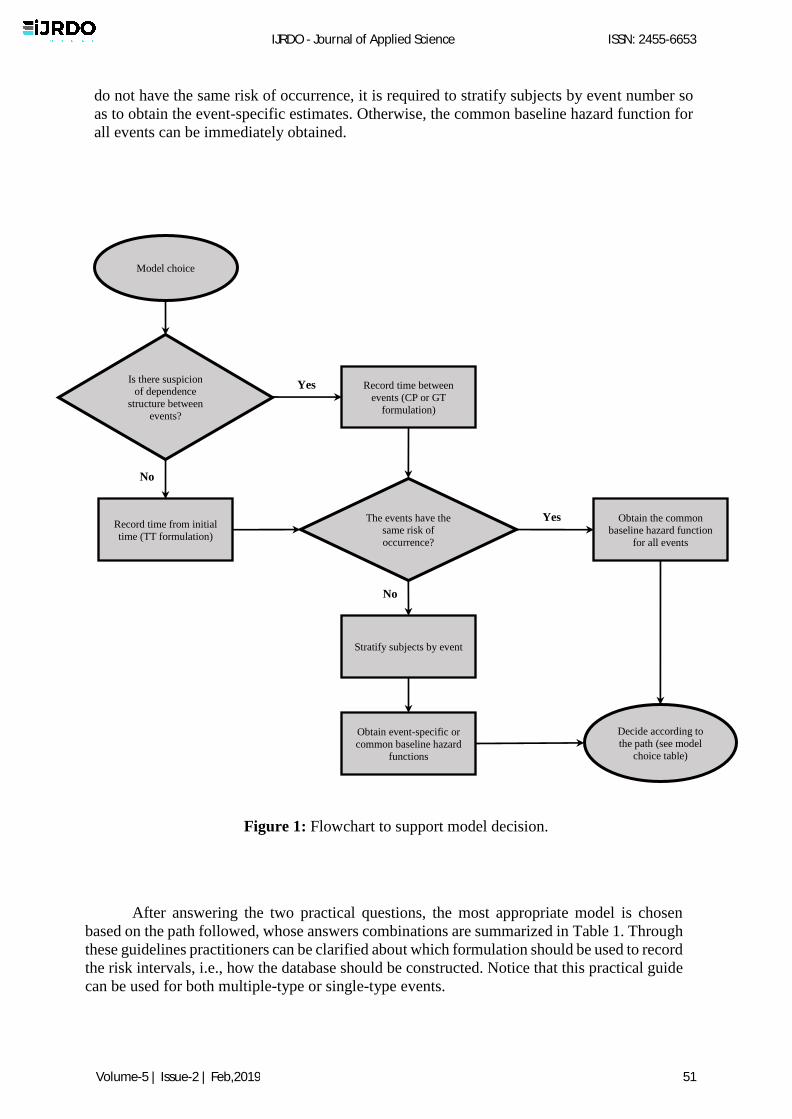
do not have the same risk of occurrence, it is required to stratify subjects by event number so

as to obtain the event-specific estimates. Otherwise, the common baseline hazard function for

all events can be immediately obtained.

After answering the two practical questions, the most appropriate model is chosen

based on the path followed, whose answers combinations are summarized in Table 1. Through

these guidelines practitioners can be clarified about which formulation should be used to record

the risk intervals, i.e., how the database should be constructed. Notice that this practical guide

can be used for both multiple-type or single-type events.

Model choice

The events have the same risk of

occurrence?

Obtain the common

baseline hazard function

for all events

Stratify subjects by event

Obtain event-specific or

common baseline hazard

functions

Is there suspicion of dependence

structure between

events?

Record time between

events (CP or GT

formulation)

Yes

No

Record time from initial

time (TT formulation)

Decide according to

the path (see model

choice table)

Yes

No

Figure 1: Flowchart to support model decision.



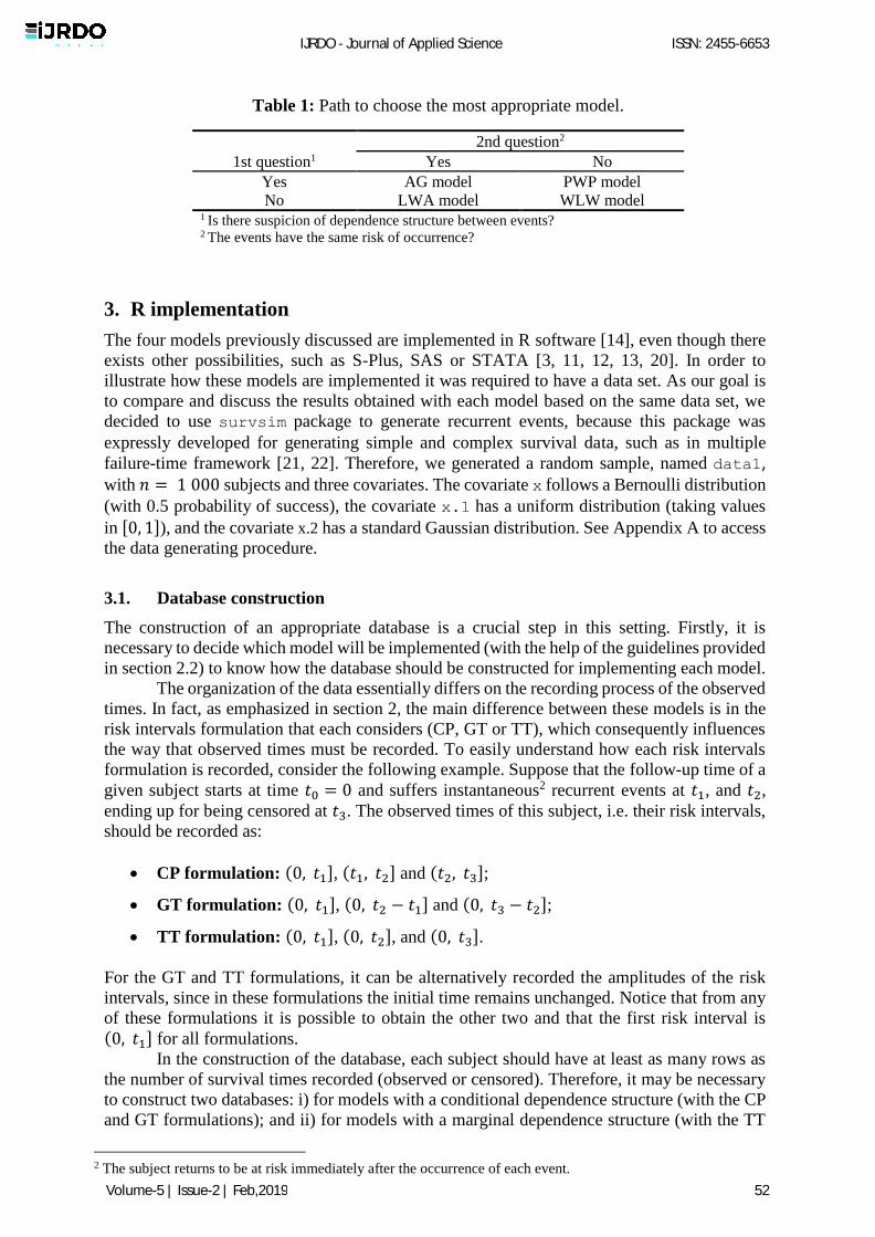
Table 1: Path to choose the most appropriate model.

2nd question2

1st question1 Yes No

Yes AG model PWP model

No LWA model WLW model 1 Is there suspicion of dependence structure between events? 2 The events have the same risk of occurrence?

3. R implementation

The four models previously discussed are implemented in R software [14], even though there

exists other possibilities, such as S-Plus, SAS or STATA [3, 11, 12, 13, 20]. In order to

illustrate how these models are implemented it was required to have a data set. As our goal is

to compare and discuss the results obtained with each model based on the same data set, we

decided to use survsim package to generate recurrent events, because this package was

expressly developed for generating simple and complex survival data, such as in multiple

failure-time framework [21, 22]. Therefore, we generated a random sample, named data1, with 𝑛 = 1 000 subjects and three covariates. The covariate x follows a Bernoulli distribution

(with 0.5 probability of success), the covariate x.1 has a uniform distribution (taking values

in [0, 1]), and the covariate x.2 has a standard Gaussian distribution. See Appendix A to access

the data generating procedure.

3.1. Database construction

The construction of an appropriate database is a crucial step in this setting. Firstly, it is

necessary to decide which model will be implemented (with the help of the guidelines provided

in section 2.2) to know how the database should be constructed for implementing each model.

The organization of the data essentially differs on the recording process of the observed

times. In fact, as emphasized in section 2, the main difference between these models is in the

risk intervals formulation that each considers (CP, GT or TT), which consequently influences

the way that observed times must be recorded. To easily understand how each risk intervals

formulation is recorded, consider the following example. Suppose that the follow-up time of a

given subject starts at time 𝑡0 = 0 and suffers instantaneous2 recurrent events at 𝑡1, and 𝑡2,

ending up for being censored at 𝑡3. The observed times of this subject, i.e. their risk intervals,

should be recorded as:

• CP formulation: (0, 𝑡1], (𝑡1, 𝑡2] and (𝑡2, 𝑡3];

• GT formulation: (0, 𝑡1], (0, 𝑡2 − 𝑡1] and (0, 𝑡3 − 𝑡2];

• TT formulation: (0, 𝑡1], (0, 𝑡2], and (0, 𝑡3].

For the GT and TT formulations, it can be alternatively recorded the amplitudes of the risk

intervals, since in these formulations the initial time remains unchanged. Notice that from any

of these formulations it is possible to obtain the other two and that the first risk interval is (0, 𝑡1] for all formulations.

In the construction of the database, each subject should have at least as many rows as

the number of survival times recorded (observed or censored). Therefore, it may be necessary

to construct two databases: i) for models with a conditional dependence structure (with the CP

and GT formulations); and ii) for models with a marginal dependence structure (with the TT

2 The subject returns to be at risk immediately after the occurrence of each event.



formulation). Furthermore, as will be seen below, one important difference is in the marginal

dependence structure, where each subject should have the same number of entries, which is

equal to the maximum number of events that could be observed.

3.1.1. Conditional dependence structure

As usual, it is necessary to indicate whether or not the observed times are censored, and in this

setting also the corresponding order for each subject. The order of the observed times must be

recorded with particular care, since this variable will be used as a stratification variable in the

models that consider an event-specific baseline hazard function.

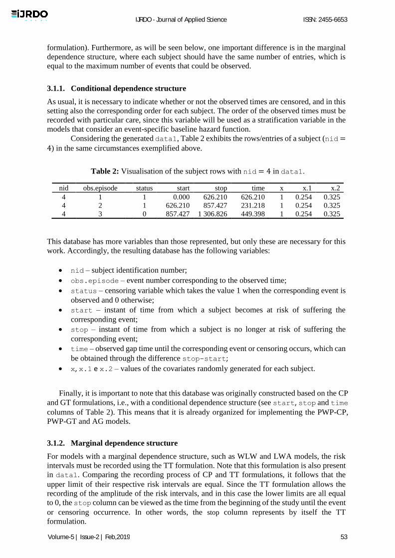
Considering the generated data1, Table 2 exhibits the rows/entries of a subject (nid =4) in the same circumstances exemplified above.

Table 2: Visualisation of the subject rows with nid = 4 in data1.

nid obs.episode status start stop time x x.1 x.2

4 1 1 0.000 626.210 626.210 1 0.254 0.325

4 2 1 626.210 857.427 231.218 1 0.254 0.325

4 3 0 857.427 1 306.826 449.398 1 0.254 0.325

This database has more variables than those represented, but only these are necessary for this

work. Accordingly, the resulting database has the following variables:

• nid – subject identification number;

• obs.episode – event number corresponding to the observed time;

• status – censoring variable which takes the value 1 when the corresponding event is

observed and 0 otherwise;

• start – instant of time from which a subject becomes at risk of suffering the

corresponding event;

• stop – instant of time from which a subject is no longer at risk of suffering the

corresponding event;

• time – observed gap time until the corresponding event or censoring occurs, which can

be obtained through the difference stop-start;

• x, x.1 e x.2 – values of the covariates randomly generated for each subject.

Finally, it is important to note that this database was originally constructed based on the CP

and GT formulations, i.e., with a conditional dependence structure (see start, stop and time columns of Table 2). This means that it is already organized for implementing the PWP-CP,

PWP-GT and AG models.

3.1.2. Marginal dependence structure

For models with a marginal dependence structure, such as WLW and LWA models, the risk

intervals must be recorded using the TT formulation. Note that this formulation is also present

in data1. Comparing the recording process of CP and TT formulations, it follows that the

upper limit of their respective risk intervals are equal. Since the TT formulation allows the

recording of the amplitude of the risk intervals, and in this case the lower limits are all equal

to 0, the stop column can be viewed as the time from the beginning of the study until the event

or censoring occurrence. In other words, the stop column represents by itself the TT

formulation.



Nevertheless, for WLW and LWA models there is still another aspect that influences

the construction of its database. In these models, it is assumed that the subject is simultaneously

at risk for the occurrence of any event from the beginning of the study. Therefore, it is essential

that the database reflects this aspect, because only then it is possible to differentiate a model

with a marginal dependence structure (WLW and LWA models) from another with a

conditional dependence structure (PWP and AG models). To capture this aspect, it is necessary

to construct a new database.

When 𝑆 is the maximum number of events that can be observed for each subject, then

all subjects under study must have 𝑆 observed times. Consequently, each event will have 𝑛

observations associated, so the database must contain 𝑛 × 𝑆 rows. Executing the R command

max(data1$obs.episode), it was determined that in the new database each subject must

have 𝑆 = 10 rows. Hence, the new database has 𝑛 × 𝑆 = 1 000 × 10 = 10 000 rows.

The construction of the new database, which is called data2, is done by repeating the

values of the last row of each subject until reaches 10 rows. Thus, the variable obs.episode takes, for all subjects, the consecutive values 1,2, … , 10. Only the variable stop is included to

define the observed time, but it is suggested to change its label to fulltime, in order to avoid

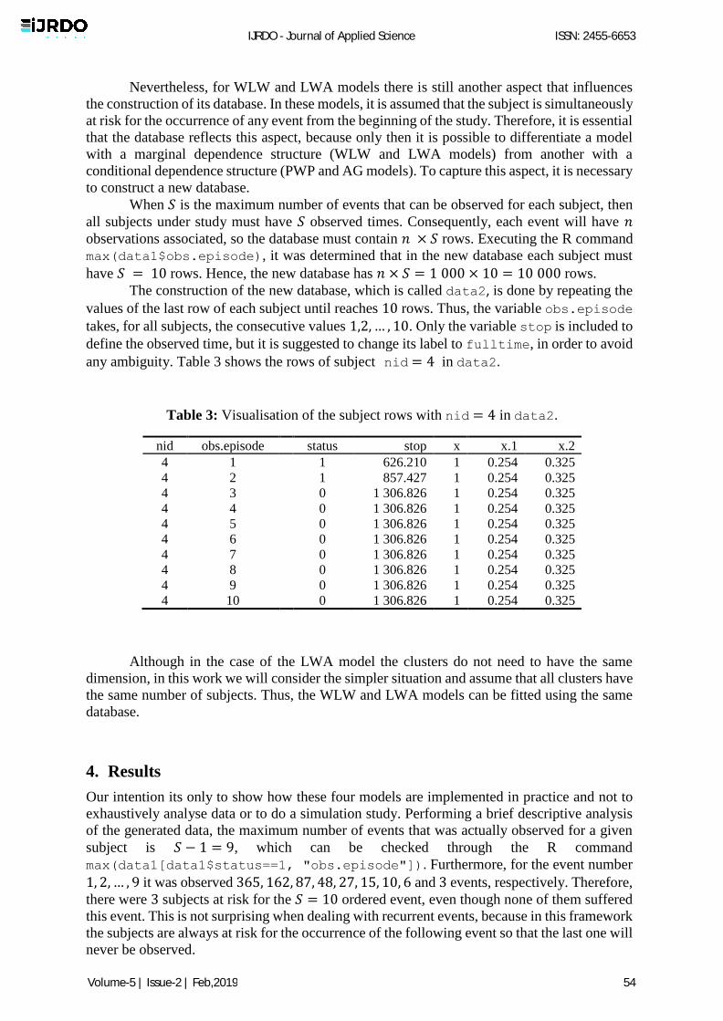
any ambiguity. Table 3 shows the rows of subject nid = 4 in data2.

Table 3: Visualisation of the subject rows with nid = 4 in data2.

nid obs.episode status stop x x.1 x.2

4 1 1 626.210 1 0.254 0.325

4 2 1 857.427 1 0.254 0.325

4 3 0 1 306.826 1 0.254 0.325

4 4 0 1 306.826 1 0.254 0.325

4 5 0 1 306.826 1 0.254 0.325

4 6 0 1 306.826 1 0.254 0.325

4 7 0 1 306.826 1 0.254 0.325

4 8 0 1 306.826 1 0.254 0.325

4 9 0 1 306.826 1 0.254 0.325

4 10 0 1 306.826 1 0.254 0.325

Although in the case of the LWA model the clusters do not need to have the same

dimension, in this work we will consider the simpler situation and assume that all clusters have

the same number of subjects. Thus, the WLW and LWA models can be fitted using the same

database.

4. Results

Our intention its only to show how these four models are implemented in practice and not to

exhaustively analyse data or to do a simulation study. Performing a brief descriptive analysis

of the generated data, the maximum number of events that was actually observed for a given

subject is 𝑆 − 1 = 9, which can be checked through the R command

max(data1[data1$status==1, "obs.episode"]). Furthermore, for the event number

1, 2, … , 9 it was observed 365, 162, 87, 48, 27, 15, 10, 6 and 3 events, respectively. Therefore,

there were 3 subjects at risk for the 𝑆 = 10 ordered event, even though none of them suffered

this event. This is not surprising when dealing with recurrent events, because in this framework

the subjects are always at risk for the occurrence of the following event so that the last one will

never be observed.



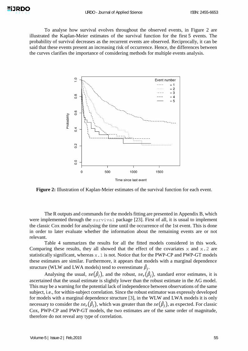
To analyse how survival evolves throughout the observed events, in Figure 2 are

illustrated the Kaplan-Meier estimates of the survival function for the first 5 events. The

probability of survival decreases as the recurrent events are observed. Reciprocally, it can be

said that these events present an increasing risk of occurrence. Hence, the differences between

the curves clarifies the importance of considering methods for multiple events analysis.

Figure 2: Illustration of Kaplan-Meier estimates of the survival function for each event.

The R outputs and commands for the models fitting are presented in Appendix B, which

were implemented through the survival package [23]. First of all, it is usual to implement

the classic Cox model for analysing the time until the occurrence of the 1st event. This is done

in order to later evaluate whether the information about the remaining events are or not

relevant.

Table 4 summarizes the results for all the fitted models considered in this work.

Comparing these results, they all showed that the effect of the covariates x and x.2 are

statistically significant, whereas x.1 is not. Notice that for the PWP-CP and PWP-GT models

these estimates are similar. Furthermore, it appears that models with a marginal dependence

structure (WLW and LWA models) tend to overestimate �̂�𝑗.

Analysing the usual, 𝑠𝑒(�̂�𝑗), and the robust, 𝑠𝑒𝑟(�̂�𝑗), standard error estimates, it is

ascertained that the usual estimate is slightly lower than the robust estimate in the AG model.

This may be a warning for the potential lack of independence between observations of the same

subject, i.e., for within-subject correlation. Since the robust estimator was expressly developed

for models with a marginal dependence structure [3], in the WLW and LWA models it is only

necessary to consider the 𝑠𝑒𝑟(�̂�𝑗), which was greater than the 𝑠𝑒(�̂�𝑗), as expected. For classic

Cox, PWP-CP and PWP-GT models, the two estimates are of the same order of magnitude,

therefore do not reveal any type of correlation.



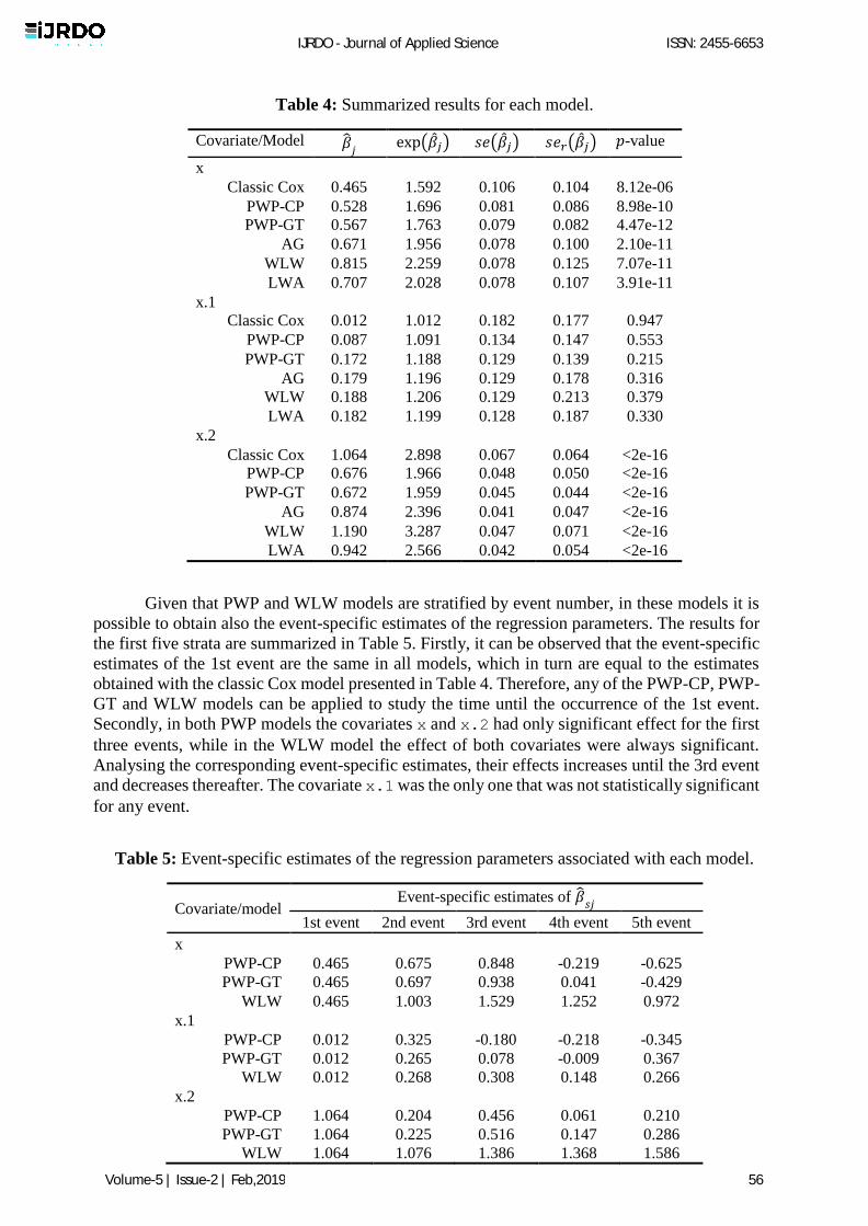
Table 4: Summarized results for each model.

Covariate/Model �̂�𝑗 exp(�̂�𝑗) 𝑠𝑒(�̂�𝑗) 𝑠𝑒𝑟(�̂�𝑗) 𝑝-value

x

Classic Cox 0.465 1.592 0.106 0.104 8.12e-06

PWP-CP 0.528 1.696 0.081 0.086 8.98e-10

PWP-GT 0.567 1.763 0.079 0.082 4.47e-12

AG 0.671 1.956 0.078 0.100 2.10e-11

WLW 0.815 2.259 0.078 0.125 7.07e-11

LWA 0.707 2.028 0.078 0.107 3.91e-11

x.1

Classic Cox 0.012 1.012 0.182 0.177 0.947

PWP-CP 0.087 1.091 0.134 0.147 0.553

PWP-GT 0.172 1.188 0.129 0.139 0.215

AG 0.179 1.196 0.129 0.178 0.316

WLW 0.188 1.206 0.129 0.213 0.379

LWA 0.182 1.199 0.128 0.187 0.330

x.2

Classic Cox 1.064 2.898 0.067 0.064 <2e-16

PWP-CP 0.676 1.966 0.048 0.050 <2e-16

PWP-GT 0.672 1.959 0.045 0.044 <2e-16

AG 0.874 2.396 0.041 0.047 <2e-16

WLW 1.190 3.287 0.047 0.071 <2e-16

LWA 0.942 2.566 0.042 0.054 <2e-16

Given that PWP and WLW models are stratified by event number, in these models it is

possible to obtain also the event-specific estimates of the regression parameters. The results for

the first five strata are summarized in Table 5. Firstly, it can be observed that the event-specific

estimates of the 1st event are the same in all models, which in turn are equal to the estimates

obtained with the classic Cox model presented in Table 4. Therefore, any of the PWP-CP, PWP-

GT and WLW models can be applied to study the time until the occurrence of the 1st event.

Secondly, in both PWP models the covariates x and x.2 had only significant effect for the first

three events, while in the WLW model the effect of both covariates were always significant.

Analysing the corresponding event-specific estimates, their effects increases until the 3rd event

and decreases thereafter. The covariate x.1 was the only one that was not statistically significant

for any event.

Table 5: Event-specific estimates of the regression parameters associated with each model.

Covariate/model Event-specific estimates of �̂�

𝑠𝑗

1st event 2nd event 3rd event 4th event 5th event

x

PWP-CP 0.465 0.675 0.848 -0.219 -0.625

PWP-GT 0.465 0.697 0.938 0.041 -0.429

WLW 0.465 1.003 1.529 1.252 0.972

x.1

PWP-CP 0.012 0.325 -0.180 -0.218 -0.345

PWP-GT 0.012 0.265 0.078 -0.009 0.367

WLW 0.012 0.268 0.308 0.148 0.266

x.2

PWP-CP 1.064 0.204 0.456 0.061 0.210

PWP-GT 1.064 0.225 0.516 0.147 0.286

WLW 1.064 1.076 1.386 1.368 1.586



As mentioned before, the survival curves for the several events (see Figure 2) look

different and tend to decrease, so there is suspicion of dependence between events and also of

different risk of occurrence. Therefore, we have the answer for the two question of the flowchart

in Figure 1. Consequently, it seems that the best choice lies in the PWP model. Notice that in a

real case study, the interpretation of the relationship between events becomes a little easier. To

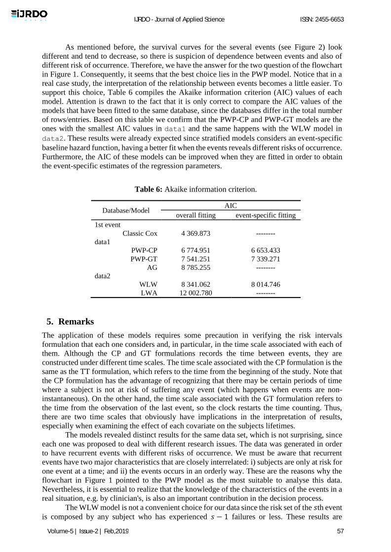
support this choice, Table 6 compiles the Akaike information criterion (AIC) values of each

model. Attention is drawn to the fact that it is only correct to compare the AIC values of the

models that have been fitted to the same database, since the databases differ in the total number

of rows/entries. Based on this table we confirm that the PWP-CP and PWP-GT models are the

ones with the smallest AIC values in data1 and the same happens with the WLW model in data2. These results were already expected since stratified models considers an event-specific

baseline hazard function, having a better fit when the events reveals different risks of occurrence.

Furthermore, the AIC of these models can be improved when they are fitted in order to obtain

the event-specific estimates of the regression parameters.

Table 6: Akaike information criterion.

Database/Model AIC

overall fitting event-specific fitting

1st event

Classic Cox 4 369.873 --------

data1

PWP-CP 6 774.951 6 653.433

PWP-GT 7 541.251 7 339.271

AG 8 785.255 --------

data2

WLW 8 341.062 8 014.746

LWA 12 002.780 --------

5. Remarks

The application of these models requires some precaution in verifying the risk intervals

formulation that each one considers and, in particular, in the time scale associated with each of

them. Although the CP and GT formulations records the time between events, they are

constructed under different time scales. The time scale associated with the CP formulation is the

same as the TT formulation, which refers to the time from the beginning of the study. Note that

the CP formulation has the advantage of recognizing that there may be certain periods of time

where a subject is not at risk of suffering any event (which happens when events are non-

instantaneous). On the other hand, the time scale associated with the GT formulation refers to

the time from the observation of the last event, so the clock restarts the time counting. Thus,

there are two time scales that obviously have implications in the interpretation of results,

especially when examining the effect of each covariate on the subjects lifetimes.

The models revealed distinct results for the same data set, which is not surprising, since

each one was proposed to deal with different research issues. The data was generated in order

to have recurrent events with different risks of occurrence. We must be aware that recurrent

events have two major characteristics that are closely interrelated: i) subjects are only at risk for

one event at a time; and ii) the events occurs in an orderly way. These are the reasons why the

flowchart in Figure 1 pointed to the PWP model as the most suitable to analyse this data.

Nevertheless, it is essential to realize that the knowledge of the characteristics of the events in a

real situation, e.g. by clinician's, is also an important contribution in the decision process.

The WLW model is not a convenient choice for our data since the risk set of the 𝑠th event

is composed by any subject who has experienced 𝑠 − 1 failures or less. These results are



consistent with those obtained by other researchers who studied recurrent events [16, 24]. In

fact, this model does not grant to accommodate the ordered nature of this type of data. Moreover,

it can not clearly explain the relationship between the observed events of the same subject, since

it has a marginal dependence structure. Besides that, Lin [25] argues that when we are interested

in studying the effect of a given covariate (e.g., the effect of a treatment) we must apply both

the PWP and WLW models and analyse them separately in order to obtain a global picture.

6. Conclusions and further work

In this paper we made an overview of some extensions of the Cox regression model for

modelling multiple events (PWP, AG, WLW and LWA models). We also contributed with a

tutorial for the application of these models and provided a practical guide to support future

practitioners in choosing the proper model. It was shown that the application of this class of

models can be achieved through R statistical software.

We encourage that the choice of the most appropriate model to handle with the

peculiarities of multiple events analysis be based on the practical guide suggested in this work.

However, before making any decision in the application of these guidelines it is imperative to

conduct an exploratory data analysis, so as to have the correct answer for each question.

In future research, we intend to continue to study the application of the proposed practical

guide, namely to analyse events of multiple-type. Another challenging work would be to develop

a statistical test to validate the choice of the proper model on multiple failure-time framework.

7. Acknowledgements

This work was supported by Fundação para a Ciência e a Tecnologia (FCT) with funds from the

Portuguese Government, through the projects UID/MAT/00006/2019 (Centro de Estatística e

Aplicações) and UID/MAT/04674/2013 (Centro de Investigação em Matemática e Aplicações).

Appendix A. Data generating procedure

The data used in this contribution was obtained through the survsim package. After installing, install.packages("survsim"), and loading, library(survsim), the referred package

the data was generated using the following code:

> set.seed(500)

> dist.ev <- c("weibull", "weibull", "weibull", "weibull", "weibull")

> anc.ev <- c(1.5, 1.2, 0.8, 0.5, 0.4)

> beta0.ev <- c(7.2, 6.5, 6.7, 6.4, 6.4)

> dist.cens <- c("weibull", "weibull", "weibull", "weibull", "weibull")

> anc.cens <- c(1.5, 1.1, 0.9, 0.5, 0.5)

> beta0.cens <- c(7.2, 6.6, 6.7, 6.4, 6.4)

> data1 <- rec.ev.sim(n=1000, foltime=1825, dist.ev, anc.ev, beta0.ev,

dist.cens, anc.cens, beta0.cens, x=list(c("bern", 0.5), c("unif", 0, 1),

c("normal", 0, 1)), beta=list(c(-0.4, -0.5, -0.6, -0.7, -0.8), c(-0.07, -

0.02, -0.06, -0.06, -0.06), c(-0.7, -0.2, -0.6, -0.6, -0.6)))

In this data, we were concerned to control only some of the arguments that can be defined

in the rec.ev.sim function, returning this procedure as simple as possible. Essentially, a

random sample of 𝑛 = 1 000 subjects was generated, where a maximum follow-up time of

1 825 days (equivalent to 5 years) was established. The time until the occurrence of each event,

and the time until the occurrence of right censoring, was defined that follows a Weibull



distribution. As the covariates can be generated through three distinct distributions, we generated

a categorical variable x with a Bernoulli distribution with probability of success equal to 0.5,

and two continuous variables, one denoted by x.1 with a uniform distribution that take values

in the range [0, 1], and another one denoted by x.2 with a standard Gaussian distribution. After

completing this procedure, the resulting data set was named data1. Although it is possible to obtain data with the desired characteristics, it must be borne in

mind that these are randomly generated, which means that for the same characteristics it can be

obtained a variety of different data sets. Thus, it was necessary to fix a seed to enable the

replication of data1, which is the reason we used the set.seed function.

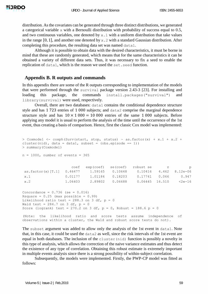
Appendix B. R outputs and commands

In this appendix there are some of the R outputs corresponding to implementation of the models

that were performed through the survival package version 2.43-3 [23]. For installing and

loading this package, the commands install.packages("survival") and library(survival) were used, respectively. Overall, there are two databases: data1 contains the conditional dependence structure

style and has 1 723 entries of 1 000 subjects; and data2 comprise the marginal dependence

structure style and has 10 × 1 000 = 10 000 entries of the same 1 000 subjects. Before

applying any model it is usual to perform the analysis of the time until the occurrence of the 1st

event, thus creating a basis of comparison. Hence, first the classic Cox model was implemented:

> Coxmodel <- coxph(Surv(start, stop, status) ~ as.factor(x) + x.1 + x.2 +

cluster(nid), data = data1, subset = (obs.episode == 1))

> summary(Coxmodel)

n = 1000, number of events = 365

coef exp(coef) se(coef) robust se z p

as.factor(x)[T.1] 0.46477 1.59165 0.10648 0.10416 4.462 8.12e-06

x.1 0.01177 1.01184 0.18203 0.17741 0.066 0.947

x.2 1.06403 2.89802 0.06688 0.06445 16.510 <2e-16

Concordance = 0.736 (se = 0.016)

Rsquare = 0.25 (max possible = 0.99)

Likelihood ratio test = 288.3 on 3 df, p = 0

Wald test = 284.7 on 3 df, p = 0

Score (logrank) test = 270.2 on 3 df, p = 0, Robust = 188.6 p = 0

(Note: the likelihood ratio and score tests assume independence of

observations within a cluster, the Wald and robust score tests do not).

The subset argument was added to allow only the analysis of the 1st event in data1. Note

that, in this case, it could be used the data2 as well, since the risk intervals of the 1st event are

equal in both databases. The inclusion of the cluster(nid) function is possibly a novelty in

this type of analysis, which allows the correction of the naive variance estimates and thus detect

the existence of any type of correlation. Obtaining this robust estimate is extremely important

in multiple events analysis since there is a strong possibility of within-subject correlation.

Subsequently, the models were implemented. Firstly, the PWP-CP model was fitted as

follows:



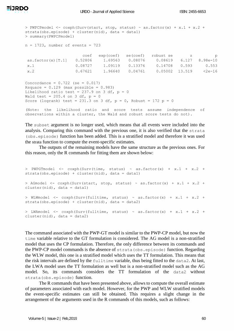
> PWPCPmodel <- coxph(Surv(start, stop, status) ~ as.factor(x) + x.1 + x.2 +

strata(obs.episode) + cluster(nid), data = data1)

> summary(PWPCPmodel)

n = 1723, number of events = 723

coef exp(coef) se(coef) robust se z p

as.factor(x)[T.1] 0.52806 1.69563 0.08076 0.08619 6.127 8.98e-10

x.1 0.08727 1.09119 0.13376 0.14708 0.593 0.553

x.2 0.67621 1.96640 0.04761 0.05002 13.519 <2e-16

Concordance = 0.722 (se = 0.017)

Rsquare = 0.129 (max possible = 0.983)

Likelihood ratio test = 237.9 on 3 df, p = 0

Wald test = 205.4 on 3 df, p = 0

Score (logrank) test = 231.3 on 3 df, p = 0, Robust = 172 p = 0

(Note: the likelihood ratio and score tests assume independence of

observations within a cluster, the Wald and robust score tests do not).

The subset argument is no longer used, which means that all events were included into the

analysis. Comparing this command with the previous one, it is also verified that the strata (obs.episode) function has been added. This is a stratified model and therefore it was used

the strata function to compute the event-specific estimates. The outputs of the remaining models have the same structure as the previous ones. For

this reason, only the R commands for fitting them are shown below:

> PWPGTmodel <- coxph(Surv(time, status) ~ as.factor(x) + x.1 + x.2 +


> AGmodel <- coxph(Surv(start, stop, status) ~ as.factor(x) + x.1 + x.2 +

cluster(nid), data = data1)

> WLWmodel <- coxph(Surv(fulltime, status) ~ as.factor(x) + x.1 + x.2 +


> LWAmodel <- coxph(Surv(fulltime, status) ~ as.factor(x) + x.1 + x.2 +

cluster(nid), data = data2)

The command associated with the PWP-GT model is similar to the PWP-CP model, but now the time variable relative to the GT formulation is considered. The AG model is a non-stratified

model that uses the CP formulation. Therefore, the only difference between its commands and

the PWP-CP model commands is the absence of strata(obs.episode) function. Regarding

the WLW model, this one is a stratified model which uses the TT formulation. This means that

the risk intervals are defined by the fulltime variable, thus being fitted to the data2. At last,

the LWA model uses the TT formulation as well but is a non-stratified model such as the AG

model. So, its commands considers the TT formulation of the data2 without strata(obs.episode) function.

The R commands that have been presented above, allows to compute the overall estimate

of parameters associated with each model. However, for the PWP and WLW stratified models

the event-specific estimates can still be obtained. This requires a slight change in the

arrangement of the arguments used in the R commands of this models, such as follows:



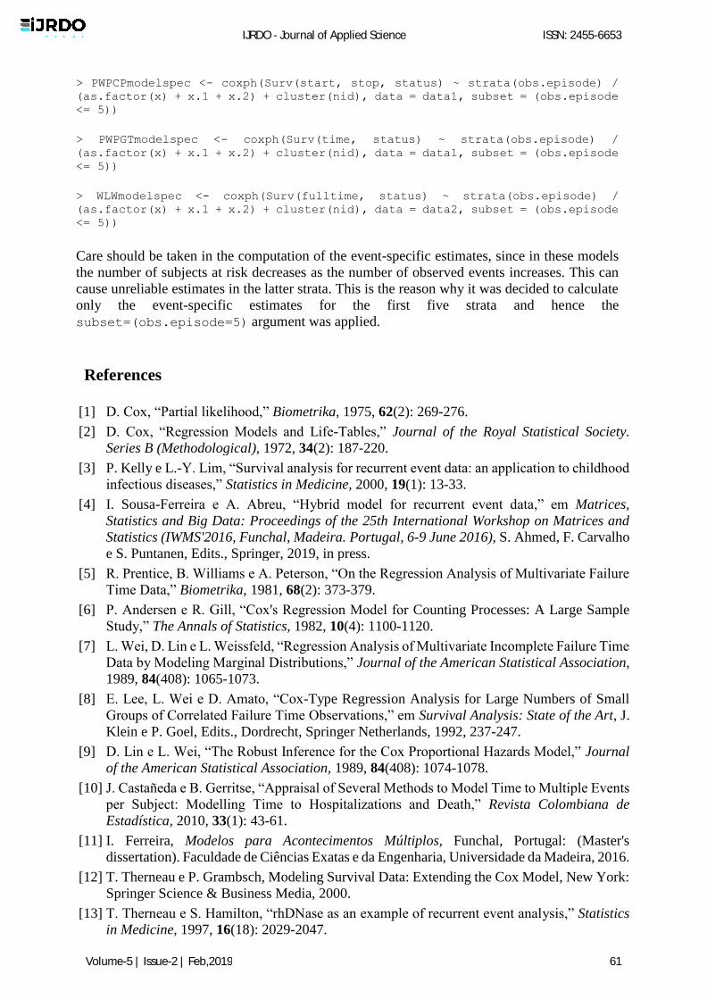
> PWPCPmodelspec <- coxph(Surv(start, stop, status) ~ strata(obs.episode) /

(as.factor(x) + x.1 + x.2) + cluster(nid), data = data1, subset = (obs.episode

<= 5))

> PWPGTmodelspec <- coxph(Surv(time, status) ~ strata(obs.episode) /


<= 5))

> WLWmodelspec <- coxph(Surv(fulltime, status) ~ strata(obs.episode) /


<= 5))

Care should be taken in the computation of the event-specific estimates, since in these models

the number of subjects at risk decreases as the number of observed events increases. This can

cause unreliable estimates in the latter strata. This is the reason why it was decided to calculate

only the event-specific estimates for the first five strata and hence the subset=(obs.episode=5) argument was applied.

References

[1] D. Cox, “Partial likelihood,” Biometrika, 1975, 62(2): 269-276.

[2] D. Cox, “Regression Models and Life-Tables,” Journal of the Royal Statistical Society.

Series B (Methodological), 1972, 34(2): 187-220.

[3] P. Kelly e L.-Y. Lim, “Survival analysis for recurrent event data: an application to childhood

infectious diseases,” Statistics in Medicine, 2000, 19(1): 13-33.

[4] I. Sousa-Ferreira e A. Abreu, “Hybrid model for recurrent event data,” em Matrices,

Statistics and Big Data: Proceedings of the 25th International Workshop on Matrices and

Statistics (IWMS'2016, Funchal, Madeira. Portugal, 6-9 June 2016), S. Ahmed, F. Carvalho

e S. Puntanen, Edits., Springer, 2019, in press.

[5] R. Prentice, B. Williams e A. Peterson, “On the Regression Analysis of Multivariate Failure

Time Data,” Biometrika, 1981, 68(2): 373-379.

[6] P. Andersen e R. Gill, “Cox's Regression Model for Counting Processes: A Large Sample

Study,” The Annals of Statistics, 1982, 10(4): 1100-1120.

[7] L. Wei, D. Lin e L. Weissfeld, “Regression Analysis of Multivariate Incomplete Failure Time

Data by Modeling Marginal Distributions,” Journal of the American Statistical Association,

1989, 84(408): 1065-1073.

[8] E. Lee, L. Wei e D. Amato, “Cox-Type Regression Analysis for Large Numbers of Small

Groups of Correlated Failure Time Observations,” em Survival Analysis: State of the Art, J.

Klein e P. Goel, Edits., Dordrecht, Springer Netherlands, 1992, 237-247.

[9] D. Lin e L. Wei, “The Robust Inference for the Cox Proportional Hazards Model,” Journal

of the American Statistical Association, 1989, 84(408): 1074-1078.

[10] J. Castañeda e B. Gerritse, “Appraisal of Several Methods to Model Time to Multiple Events

per Subject: Modelling Time to Hospitalizations and Death,” Revista Colombiana de

Estadística, 2010, 33(1): 43-61.

[11] I. Ferreira, Modelos para Acontecimentos Múltiplos, Funchal, Portugal: (Master's

dissertation). Faculdade de Ciências Exatas e da Engenharia, Universidade da Madeira, 2016.

[12] T. Therneau e P. Grambsch, Modeling Survival Data: Extending the Cox Model, New York:

Springer Science & Business Media, 2000.

[13] T. Therneau e S. Hamilton, “rhDNase as an example of recurrent event analysis,” Statistics

in Medicine, 1997, 16(18): 2029-2047.



[14] R Development Core Team, R: A Language and Environment for Statistical Computing,

Vienna, Austria: R Foundation for Statistical Computing (ISBN: 3-900051-07-0), 2018.

[15] J. Box-Steffensmeier e S. De Boef, “Repeated events survival models: the conditional frailty

model,” Statistics in Medicine, 2006, 25(20): 3518-3533.

[16] J. Cai e D. Schaubel, “Analysis of Recurrent Event Data,” em Handbook of Statistics:

Advances in Survival Analysis, vol. 23, N. Balakrishnan e C. Rao, Edits., North Holland,

Elsevier, 2003, 603-623.

[17] R. Cook e J. Lawless, “Analysis of repeated events,” Statistical Methods in Medical

Research, 2002, 11(2): 141-166.

[18] L. Wei e D. Glidden, “An overview of statistical methods for multiple failure time data in

clinical trials,” Statistics in Medicine, 1997, 16(8): 833-839.

[19] E. Kaplan e P. Meier, “Nonparametric Estimation from Incomplete Observations,” Journal

of the American Statistical Association, 1958, 53(282): 457-481.

[20] L. Amorim e J. Cai, “Modelling recurrent events: a tutorial for analysis in epidemiology,”

International Journal of Epidemiology, 2015, 44(1): 324-333.

[21] D. Moriña e A. Navarro, “The R package survsim for the simulation of simple and complex

survival data,” Journal of Statistical Software, 2014, 59(2): 1-20.

[22] D. Moriña e A. Navarro, survsim: Simulation of simple and complex survival data, (R

package version 1.1.5), 2018.

[23] T. Therneau, survival: A package for survival analysis in S, R package version 2.43-3, 2018.

[24] C. Metcalfe e S. Thompson, “Wei, Lin and Weissfeld's marginal analysis of multivariate

failure time data: should it be applied to a recurrent events outcome?,” Statistical Methods

in Medical Research, 2007, 16(2): 103-122.

[25] D. Lin, “Cox regression analysis of multivariate failure time data: The marginal approach,”

Statistics in Medicine, 1994, 13(21): 2233-2247.



Abstract Ivo Sousa -Ferreira 016 survsim survivalAna Maria ...

Documents

Transcript of Abstract Ivo Sousa -Ferreira 016 survsim survivalAna Maria ...