2000PhD dissertation Options for Co-management of an Indonesian Coastal Fishery
141
Options for co-management of an Indonesian coastal fishery
Transcript of 2000PhD dissertation Options for Co-management of an Indonesian Coastal Fishery

Options for co-management of anIndonesian coastal fishery

Promotor: Dr. E.A. HuismanHoogleraar in de Visteelt en Visserij
Co-promotor: Dr. ir. M.A.M. MachielsUniversitair docent bij de leerstoelgroep Visteelt en Visserij
Options for co-management of anIndonesian coastal fishery
C. Pet-Soede
Proefschrift
ter verkrijging van de graad van doctorop gezag van de rector magnificus
van Wageningen Universiteit,dr. C.M. Karssen,
in het openbaar te verdedigenop vrijdag 21 januari 2000
des namiddags te half twee in de Aula.
All photos made by Lida Pet-Soede except for:photo 4 and photo 13 by Tom Buijsephoto 7 by Wim van Densenphoto 8 by Rene Hagels
Printing: Ponsen & Looijen b.v., Wageningen
CIP-DATA KONINKLIJKE BIBLIOTHEEK, DEN HAAG
Pet-Soede, C.
Options for co-management of an Indonesian coastal fishery / C. Pet-Soede. – [S.1. : s.n.]. – III. ThesisWageningen Universiteit. – With ref. – With summary in Dutch.ISBN 90-5808-184-2
Abstract
Pet-Soede, C., 2000, Options for co-management of an Indonesian coastal fisheryPerceptions of fisheries authorities and fishers on the status of the fisheries and fish stocks in SpermondeArchipelago, a coastal shelf off SW Sulawesi, Indonesia, seem to concur. However, constraints imposed bythe administrative and physical environment and by the weak contrasts in fishery outcome within Spermondecause these partners cannot find realistic arguments for a causal relation between catch and effort from theirexperiences. Therefore co-management for fisheries in this area is not yet viable. More informative use offisheries data by standardising the unit of effort, accounting for the fast developments in motorization, andcombining data on fisheries and ecological grounds rather than on administrative grounds will increase themanagement value of already available official data. Exchange of experiences between local fisheriesauthorities and fishers from districts or provinces with highly contrasting levels of fishing intensity willfacilitate discussions on the need and benefits of effort regulations.
PhD Thesis, Fish Culture and Fisheries Group, Wageningen University, P.O.Box 338, 6700 AHWageningen, The Netherlands
This research was funded by WOTRO, the Netherlands Foundation for the Advancement of TropicalResearch (grant WK 79-36). The research was done in the framework of the WOTRO program “SustainableManagement of the Coastal Area of SW Sulawesi 1994-1998” as one of the topics studied by amultidisciplinary group of scientists from various institutes in Indonesia and the Netherlands.
Table of contents
Summary 1
Samenvatting 5
Chapter 1. Introduction 9
Chapter 2. Trends in an Indonesian coastal fishery based on catch and effortstatistics and implications for the perception of the state of thestocks by fisheries officials 19
Chapter 3. Can fishers allocate their fishing effort in space and time on thebasis of their catch rates? An example from SpermondeArchipelago, SW Sulawesi, Indonesia 37
Chapter 4. Cross shelf distribution of fish communities related to reefcomplexity in Spermonde Archipelago, a coastal area in SWSulawesi, Indonesia 61
Chapter 5. Impact of Indonesian coral reef fisheries on fish communitystructure and the resultant catch composition 81
Chapter 6. Limited options for co-management of reef fisheries in Spermonde,a coastal zone off SW Sulawesi, Indonesia 103
References 121
Dankwoord 131
Curriculum vitae 135

1
Summary
The objective of this study was to identify those factors that influence the perceptions of bothfisheries authorities and fishers of the status of the fisheries and the fish stocks in SpermondeArchipelago, a coastal shelf off SW Sulawesi, Indonesia. This to evaluate the capacity of theseauthorities and fishers, being potential partners in the much aspired co-management, to perceivetime trends and spatial patterns in catch rates and to relate them to differences in fishing intensity.Concurrence of perceptions of the state of the fisheries and of the stocks is a prerequisite for co-management situations to develop. First, annual statistics for the fisheries in Spermonde, on whichthe authorities rely, were evaluated for changes in catch biomass and composition and these wererelated to changes in fishing effort. Second, the fishing activities and catches of individual fisherswere monitored at sea during a full year cycle. Third, by Underwater Visual Census (UVC) fishdensity, biomass, size and species composition of reef fish communities were correlated withspatial patterns in habitat complexity and fishing effort. Fourth, catch rates and the structure of thefish community in Spermonde were compared with those in and around Komodo National Park, offWest Flores, where fishing intensity is much lower. Finally, interviews were held with authoritiesand fishers in Spermonde to inventory their perceptions more directly, and to interpret theseperceptions in relation to trends, patterns and uncertainties as estimated objectively from catchstatistics and field data.
Indonesia’s coastal fishery is of a small- to medium-scale character with little input ofcomplex technology, small capital investments, but high input of manpower. Landings in thecoastal province of South Sulawesi contributed 8.4% to the Indonesian marine landings (2.83thousand tons). Landings in Spermonde, a distinct coastal shelf administered by four of the 21districts in South Sulawesi, increased from 32,000 tons in 1977 to 53,000 tons in 1995. Total effort inSpermonde increased only slightly from 1.6 million trips to 1.9 million trips. Although trips are still usedas standard unit of effort, it is known as an unreliable indicator, due to increasing motorization of thefishing units. Motorization allows fishers to enlarge their resource space and their fishing effort viagreater mobility. Only the annual landings of two of the 45 official fish categories declined significantlyover the period 1977 – 1995, with remarkable absence of auto-correlation in the annual landings foralmost all categories. Variances around long-term averages or trends could be related to catch sizeand categories. Information relevant to the status of the fishery in Spermonde, as being an ecologicalentity, is lost at the national level where annual totals for the province of South Sulawesi are furtheraggregated in four major fish groups (demersal fish, coral reef fish, small pelagic fish, large pelagicfish) in 11 coastal regions.
Surveys at sea revealed that on average 517 fishing units operated each day in the 2800km2 of Spermonde, most of which (59%) used hook and line to catch demersal and small pelagicfish from 4 m long dugout canoes. Given the more sedentary nature of the reef fish they target for,their fishery is the first to consider for possible co-management. Due to their low average catch
rate of 2.9 kg⋅day-1 hook and line fishers contributed only 5% to the total catch from the area of 21t·day-1. Medium-scale lift net units (16% of total number of units) target for small pelagic fish from10 - 20 m long motorised boats, contributing 70% (175 kg.day-1) to the total landings. Theremaining units used gill nets, explosives, longlines, purse seines or Danish seines. The resource
Summary
2
spaces of individual fishers were constrained by the size of their boats and by weather conditions.Fishing intensity in the total resource area of Spermonde was 3 times higher in the denselypopulated south-east than in the north-west, where Catch per Unit Effort (CpUE) of hook and linefishers was 2 times as high as in the south-east. Mean size of fish in the catches was significantlylarger at reefs with low fishing intensity than at more intensively fished reefs, particularly forpiscivorous groupers and barracuda’s. Due to the small spatial scale of the individual resourcespaces of hook and line fishers, they can hardly experience and perceive such large-scaledifferences in catch rates and size of fish, let alone possible causal relationships. This wasparticularly so for lift net fishers, who in theory could cover the whole of Spermonde, but whoexperienced high variability in their catch rates (0 - 1500 kg·day-1) at all sites, due to the migratoryand schooling behaviour of their target fish.
The Underwater Visual Census (UVC) revealed that fish biomass at reefs in Spermondewas three times lower in the inner, ecological zone running parallel to the coast line than in the threeouter zones. Also fish biomass was 1.4–1.8 times lower at shallow reef locations than at deep reeflocations. Fish density, biomass, individual size and taxonomic diversity increased with reef rugosity(average 2.1) and live substrate cover (average 52%). Total fish density was ca. 2 times and fishbiomass ca. 3 times higher at reefs with excellent live substrate cover than at reefs with almost nocover. But biomass and mean length of herbivorous fish, particularly rabbitfish (Siganus spp.) andsurgeonfish (Acanthurus spp.), decreased with live substrate cover. The apparent lower fish biomassin the inner, coastal zone could only partially be explained by the on average smaller depth and lowerhabitat complexity. Fishing pressure and detrimental coastal processes must have contributed to thislower fish biomass as well.
Biomass density and individual size of reef fish as observed with UVC were not related topatterns fishing intensity as observed during surveys at sea in Spermonde. The fishing intensity inKomodo area (65 boats·km-2 reef) was 8 times lower than in Spermonde (557 boats·km-2 reef).UVC at the reefs in Komodo made clear that fish density in the two areas was similar (3 fish·m-2),but mean individual size was twice as large in Komodo (14 cm) as in Spermonde (7 cm). So meanfish biomass (382 g·m-2) was four times as high as in Spermonde (86 g·m-2), with even largerdifference (factor 17) for fish > 40 cm. The trophic composition of total fish biomass, however, didnot differ largely between the two areas. The overall CpUE in the fishery was eight times higher inKomodo (48 kg·trip-1) than in Spermonde (5.8 kg·trip-1), so with much lower fishing intensity total fishyield in Komodo (3.1 t·km-2) was nearly as high as in Spermonde (3.2 t·km-2 reef·yr-1).
In interviews the majority of both local fisheries authorities and fishers claimed a decline inquality of the fish stocks in Spermonde in the period 1987 – 1997 especially near shore, which theyattributed to increasing numbers of fishers. Official catch statistics could not have informed theauthorities on such downward trends. Fisheries officers at the district and provincial level had littlemeans to process their own statistics in a format that allowed for proper evaluation of trendsanyway. In spite of a concurrence in ultimate perceptions, the constraints to perceptions ofauthorities and fishers imposed by the administrative and physical environment and by the weakcontrasts within Spermonde, make it that authorities and fishers have difficulties to find realarguments for a causal relation between catch and effort from their experiences. So co-management for the fishery in this coastal area seems not yet viable. However, more informativeuse of fisheries data by standardising the unit of effort, accounting for the fast developments inmotorization, and combination of data on fisheries and ecological grounds rather than on

Summary
3
administrative grounds, could increase the management value of data that are already available.Exchange of experiences between local fisheries authorities from districts or provinces withcontrasting levels of fishing intensity will supply a better ground for the evaluation of developmentsin the fisheries and the state of the stocks, by providing a reference to one’s personal experience.Selection of more vulnerable key species, such as highly valued piscivores like groupers, for theevaluation of time trends and the incorporation of size measurements for these categories in theofficial catch statistics will allow the faster detection of downward trends caused by increasingfishing pressure. Increased awareness of fishers on differences in catch rates and compositionsbetween intensively fished areas and areas with restricted entry, will facilitate discussions on theneed and benefits of effort regulations.

5
Samenvatting
Het doel van deze studie was om te beoordelen of in de kustvisserij in Spermonde, ZuidwestSulawesi, Indonesië, aan een van de belangrijkste voorwaarde voor co-management van devisserij wordt voldaan, namelijk of zowel visserijautoriteiten als vissers ontwikkelingen in de visserijen de visstand kunnen waarnemen en beoordelen. De vraag daarbij is of beide partijen,beheerders én brongebruikers, trends en ruimtelijke patronen in vangstsucces niet alleen kunnenwaarnemen, maar of zij daarmee ook kunnen zien dat er mogelijk een oorzakelijk verband istussen vangstsucces en visserijdruk. Pas wanneer die perceptie en beoordeling van de visserij ende visstand onderling overeenkomt, en beiden partijen ook kunnen inzien welke de consequentieszijn van een te hoge visserijdruk, is er een basis voor het gezamenlijk beheer van de lokalevisserij. Voor het beantwoorden van die vraag is onderzoek gedaan aan de informatiewaarde enhet potentiële gebruik van de officiële visserijstatistiek, aan de ruimtelijke patronen invisserijinspanning en vangstsucces in de Spermonde Archipel en aan de omvang en samenstellingvan de visgemeenschap op de riffen in het gebied, zoals die worden bepaald doorhabitatkenmerken en door visserijdruk. Tenslotte is beoordeeld welke de beperkingen enmogelijkheden zijn voor autoriteiten én voor vissers om veranderingen in vangstsucces door de tijden om verschillen in vangstsucces tussen onderscheidenlijke gebieden in de archipel te kunnenwaarnemen en beoordelen.
De kustvisserij van Indonesië is kleinschalig met weinig gebruik van complexetechnologie, met geringe kapitaalinvesteringen, maar met een hoge inzet aan mankracht. Devisaanvoer in de kustprovincie van Zuid Sulawesi draagt 8.4% bij aan de totale aanvoer aan zeevisin Indonesië van 2.83 miljoen ton. De visaanvoer vanuit de Spermonde Archipel, onderdeel van dieprovincie, wordt geregistreerd door vier kustdistricten, die met 17 andere districten deadministratieve eenheid Zuid Sulawesi vormen. De aanvoer uit Spermonde is toegenomen van32,000 ton vis in 1977 tot 53,000 ton vis in 1995. In dezelfde periode is de totale visserijinspanningin Spermonde slechts licht toegenomen, van 1.6 miljoen vistrips tot 1.9 miljoen vistrips, maar deeenheid vistrip is een slechte maat voor de effectieve visserijinspanning. Door toenemendemotorisering zijn vissers in staat hun visgebied en hun visserijinspanning te vergroten dankzij eengrotere mobiliteit. Slechts de aanvoer van twee van de 45 officiële viscategorieën liet eensignificante afname zien over de periode 1977 – 1995. Opvallend was de afwezigheid van seriëlecorrelatie in de jaarlijkse aanlandingen van zo goed als alle categorieën. Op provinciaal niveauwordt de aanvoer uit de vier kustdistricten niet gegroepeerd voor een aparte evaluatie van devisserij in de Spermonde. Relevante informatie met betrekking tot de status van de visserij perviscategorie raakt zeker verloren in de nationale visserijstatisiek, waar de jaarlijkse totale vangstenvoor de provincies verder worden geaggregeerd in vier hoofdgroepen (demersale vis, koraalrifvis,kleine pelagische vis, grote pelagische vis) voor 11 kustregio’s.
Een jaar lang intensieve bemonstering van de visserij op zee leerde dat iedere daggemiddeld 517 viseenheden actief zijn in de 2800 km2 grote Spermonde. De meeste eenheden(59% van het aantal trips) gebruiken handlijnen om demersale en kleine pelagische vis te vangenvanuit 4 m lange houten kano’s. Middelgrote liftneteenheden (16%) richten zich op het vangen vankleine pelagische vis vanuit 10 - 20 m lange gemotoriseerde boten. De overige viseenhedengebruiken kieuwnetten, explosieven, ringzegens of Deense zegens. Vanwege hun lage
Samenvatting
6
gemiddelde vangst van 2.9 kg⋅dag-1 dragen lijnvissers slechts 5% bij aan de totale vangst van 21
t·dag-1, terwijl liftneteenheden 70% bijdragen (175 kg⋅dag-1·boot-1). De afstand waarop wordt gevistword beperkt door de grootte van de boot en door de weersomstandigheden. Bekeken op deruimtelijke schaal van de gehele Spermonde was de visserijdruk 3 maal hoger in het dichtbevolktezuidoosten dan in het noordwesten van de Spermonde. De dagelijkse vangsten waren significanthoger in de minder zwaar beviste gebieden. Maar omdat vissers vanwege de grote variatie indagelijkse vangsten al amper onderscheid kunnen maken in vangstsucces op de kleinereruimtelijke schaal van hun eigen gebruiksruimte, kunnen zij zelf zulke grootschalige patronen nietwaarnemen. Dit geldt met name voor liftnetvissers, die mobieler zijn en elke locatie binnenSpermonde kunnen bevissen, maar die te maken hebben met zeer variabele vangsten (0 - 1500kg·day-1) vanwege het migrerende en scholende gedrag van de soorten waarop zij vissen.
Met een onderwatersurvey langs 47 riftransecten van ieder 100 m werd aangetoond datde visbiomassa in de binnenste van de vier ecologische zones, die parallel aan de kust lopen, 3maal lager was dan in de andere zones. Verder was de visbiomassa op ondiepe riflocaties 1.4 –1.8 maal lager dan op diepe riflocaties. Na correctie voor deze ruimtelijke effecten, bleek devisdichtheid, vislengte, visbiomassa en de soortdiversiteit van de vis toe te nemen met derifcomplexiteit. Die rifcomplexiteit werd geïndexeerd met de ruigheid van het rif en met hetpercentage van het rifoppervlak dat bedekt is met levend substraat. Bij een studie naar degeïsoleerde effecten van de visserij op de rifgemeenschap in Spermonde moet men dus rekeninghouden met de invloed van deze habitatkenmerken. De ruigheid van het rif (omtrekdwarsdoorsnede / projectie op grondvlak) op de transecten was gemiddeld 2.1 en het percentagerifoppervlak bedekt met levend substraat 52%. De gemiddelde waardes voor dezehabitatparameters waren het laagst in de binnenste kustzone. De totale visdichtheid was ongeveer2 maal en de visbiomassa ongeveer 3 maal zo hoog op riffen met een hoog percentage levendsubstraat dan op riffen met nauwelijks of geen levend substraat. Voor herbivore vis was het effecttegengesteld. De biomassa en de gemiddelde lengte van herbivore vissoorten als rabbitfish(Siganus spp.) en surgeonfish (Acanthurus spp.) nam af met het percentage levend substraat.Uiteindelijk kon de lagere visbiomassa in de binnenste kustzone slechts gedeeltelijk wordenverklaard door een gemiddeld lagere habitatcomplexiteit in deze zone. Visserijdruk en mogelijk ookandere activiteiten in het kustgebied, die zorgen voor achteruitgang van het mariene milieu,moeten eveneens hebben bijgedragen aan de lagere visbiomassa in de binnenste zone.
De verschillen in biomassa en lengte van de rifvis, zoals waargenomen tijdens deonderwatersurvey in Spermonde, hadden geen eenduidig verband met de ruimtelijke patronen invisserijdruk zoals waargenomen tijdens de bemonstering van de visserij op zee. Toch was degemiddelde lengte van de vis in de vangsten van de rifvissers in gebieden met lagere visserijdruksignificant groter dan in gebieden met hoge visserijdruk. Dit gold met name voor de visetendegroupers en barracudas. Voor een beter inzicht in het effecten van de visserijdruk op devisgemeenschap werd een vergelijking gemaakt tussen Spermonde en het Komodo National Park,ten westen van Flores. De visserijdruk in Komodo (65 boten·km-2 rif) is 8 maal lager dan inSpermonde (557 boten·km-2 rif). Bij dit sterkere contrast in visserijdruk, was de hoeveelheid vis diewerd waargenomen tijdens vergelijkbare onderwatersurveys gelijk: 2.5 fish·m-2 in Komodo en 2.8fish·m-2 in Spermonde. De gemiddelde vislengte was echter 2 maal zo groot in Komodo (14 cm) alsin Spermonde (7 cm) en de visbiomassa (382 g·m-2) 4 maal zo hoog als in Spermonde (86 g·m-2),met een nog groter verschil (factor 17) voor vis groter dan 40 cm. Commercieel belangrijke soorten
Samenvatting
7
als haaien, groupers, en Napoleon wrasses kwamen in Komodo in hogere dichtheden voor dan inSpermonde. Het vangstsucces van de beroepsvissers per eenheid visserijinspanning was inKomodo (48 kg·trip-1) 8 maal hoger dan in Spermonde (5.8 kg·trip-1). Dus met een veel lagerevisserijdruk was de totale visoogst in Komodo (3.1 t·km-2 rif·jaar-1) net zo hoog als in Spermonde(3.2 t·km-2 rif·jaar-1).
Tijdens interviews met lokale visserijautoriteiten en vissers werd gevraagd naar eenoordeel over de visstand in de Spermonde en naar oorzaken voor een eventueel gepercipieerdeteruggang daarin. Het merendeel van hen verklaarde dat de visbestanden, vooral die dichtbij dekust, in de periode 1987-1997 waren teruggelopen vanwege een toename in het aantal vissers. Devisserijautoriteiten op het niveau van district en provincie hadden weinig technische enorganisatorische mogelijkheden om hun gegevens zodanig te bewerken dat zij hun individueleideeën over trends in de aanvoer uit Spermonde ook statistisch konden onderbouwen, laat staandat zij ruimtelijke patronen binnen Spermonde konden evalueren. Vanwege deze beperkingen envanwege de vage ruimtelijke contrasten in visserijdruk en vangstsucces die door de vissersworden ervaren, hebben beide partijen moeite met het zien van een direct oorzakelijk verbandtussen vangst en visserijdruk. Dit alles betekent dat een basis voor gezamenlijk beheer in de vormvan co-management, namelijk een gelijkluidend oordeel over de visstand en een overeenkomstigidee over de effecten van de visserij, in dit gebied nog onvoldoende aanwezig is. Een oplossingaan de kant van de visserijautoriteiten is een meer informatief gebruik van de beschikbarevisserijstatistieken, met een betere standaard voor de eenheid voor visserijinspanning, waarbijrekening wordt gehouden met de snelle ontwikkelingen in motorisatie. De visserijgegevens zoudenruimtelijk meer moet worden gecombineerd op visserijkundige en ecologische gronden in plaatsvan alleen maar op administratieve gronden (district, provincie). Dit zal de informatiewaarde van devisserijstatistiek voor het visserijbeheer sterk vergroten. Uitwisseling van ervaringen tussenvisserijautoriteiten uit districten of provincies met sterk contrasterende niveaus in visserijdruk zalde individuele vaardigheid om visserijgegevens uit het eigen gebied te evalueren helpenversterken. Verder zou gebruik gemaakt kunnen worden van voor visserijdruk gevoeligeindicatoren in de aanvoer, zoals de gemiddelde lengte van hoog gewaardeerde visetende soortenals groupers, die het mogelijk maken om een neergaande trend in de visstand sneller en beterwaar te nemen. Verdere ontwikkeling van het begrip bij vissers met betrekking tot het oorzakelijkverband tussen vangst en visserijinspanning zal moeilijk blijven. Maar de informatieve waarde vanhet zichtbare effect van de instelling van gesloten gebieden op ontwikkelingen in de visstand zoudit begrip kunnen versterken.
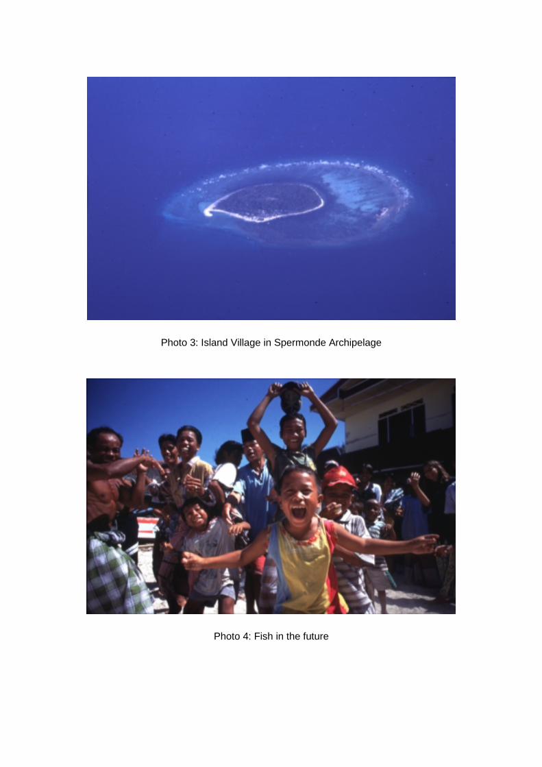
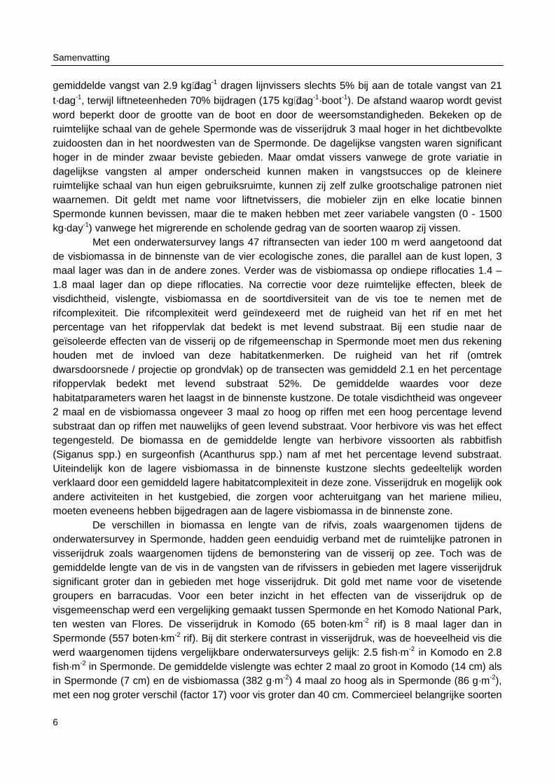
Photo 3: Island Village in Spermonde Archipelage
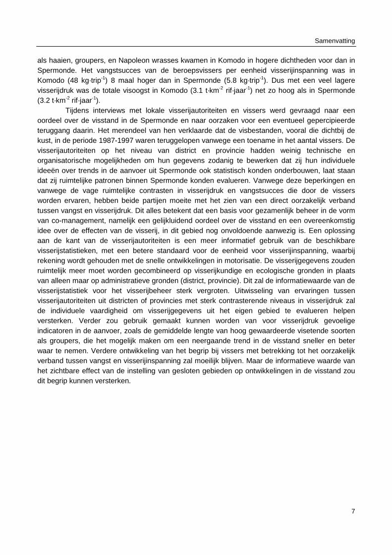
Photo 4: Fish in the future
9
Chapter 1
Introduction
Management problems of Indonesian coastal fisheries
Indonesian coastal fisheries
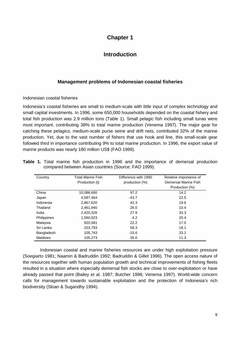
Indonesia’s coastal fisheries are small to medium-scale with little input of complex technology andsmall capital investments. In 1996, some 650,000 households depended on the coastal fishery andtotal fish production was 2.9 million tons (Table 1). Small pelagic fish including small tunas weremost important, contributing 38% to total marine production (Venema 1997). The major gear forcatching these pelagics, medium-scale purse seine and drift nets, contributed 32% of the marineproduction. Yet, due to the vast number of fishers that use hook and line, this small-scale gearfollowed third in importance contributing 9% to total marine production. In 1996, the export value ofmarine products was nearly 180 million US$ (FAO 1999).
Table 1. Total marine fish production in 1996 and the importance of demersal productioncompared between Asian countries (Source: FAO 1999).
Country Total Marine FishProduction (t)
Difference with 1990production (%)
Relative importance ofDemersal Marine Fish
Production (%)
China 10,086,660 97.2 14.2Japan 4,587,464 -43.7 22.5Indonesia 2,867,620 42.3 19.6Thailand 2,461,940 26.0 10.4India 2,420,326 27.9 33.3Philippines 1,560,923 4.2 20.4Malaysia 920,581 22.2 17.0Sri Lanka 203,793 58.3 18.1Bangladesh 105,743 -15.6 33.1Maldives 105,273 35.0 11.3
Indonesian coastal and marine fisheries resources are under high exploitation pressure(Soegiarto 1981; Naamin & Badruddin 1992; Badruddin & Gillet 1996). The open access nature ofthe resources together with human population growth and technical improvements of fishing fleetsresulted in a situation where especially demersal fish stocks are close to over-exploitation or havealready passed that point (Bailey et al. 1987; Butcher 1996; Venema 1997). World-wide concerncalls for management towards sustainable exploitation and the protection of Indonesia’s richbiodiversity (Sloan & Sugandhy 1994).
Chapter 1
10
Difficulties in managing coastal fishery resources
Sharing the concern for deteriorating fishery resources, the Indonesian government has enlargedits role in fisheries management (Ruddle 1993; Meereboer 1995). The role of traditionalcommunities has correspondingly diminished (Darmoredjo 1983; Bailey & Zerner 1992). Thisgeneral trend was caused by under-valuation of the capacity of local management systems thatindeed proved ineffective in maintaining the fish resources at a sustainable level. Stateintervention, however, seldom proved to be more successful in this respect (Mermet 1990; Oakley1990; Christy 1992a; Johannes et al. 1992; Johannes 1994; King & Faasili 1999). The use of largeand medium-sized trawl nets was successfully banned from Indonesian waters since 1981(Martosubroto 1987; McElroy 1991). Yet, the ongoing destructive practice of blast fishing on thecoral reefs is a clear example of the failure of national enforcement programs for small-scalefisheries. Patrol and control of Indonesia’s extended coastal waters with its thousands of islandsand approximately 81,000 km of coastline needs large inputs of budget and manpower andenforcement in especially distant provinces is virtually non-existing. Decentralised managementand shared responsibility seem to be the answers to logistical problems. Furthermore, increasedinvolvement of stakeholders in the management of their resources creates a feeling of ownershipthat possibly confronts corruption also.
The current believe is that co-management, defined by Pomeroy (1994) as: “Adecentralised management system incorporating resource-user participation and holisticdevelopment approaches in the implementation of management efforts”, is the only effectiveapproach (Naamin & Badruddin 1992; Christy 1992b; Dorsey 1992; Johannes et al. 1992; Medleyet al. 1993; Dahuri 1994; Pomeroy & Carlos 1997). Implementation of co-management principlesremains complex and difficult. Especially the tropical multi-species and multi-gear fisheries includesocial-economic and social-cultural processes at the local level and complex legal and regulatoryprocesses at the national and provincial level, that make involving and satisfying all stakeholders inthe management process difficult (Munro & Williams 1985; McCay & Acheson 1987; Christy1992a; Medley et al. 1993). Studies focused on possibilities to use existing traditional managementsystems that include exclusive property rights to solve present day problems. Yet, one importantmisinterpretation is that these traditional systems have a conservation intent whereas they aremore often the outcome of conflicts over scarce resources (McCay & Acheson 1987).
When a number of studies focused on socio-economic and cultural factors of coastal andmarine fisheries, more information became available that could be used in facilitating the co-management process. Dorsey (1992) proposed to use credit systems to allow for fishers to makethe switch to new technologies and to lessen the power of moneylenders and middlemen. Castilloand Rivera (1991) described how involvement of fishers in the research process built self-confidence, which made that fishers felt they were respected discussion partners. Pomeroy andCarlos (1997) explained how prospects of benefits from management regulations influenced thewill to participate. Nielsen et al. (1996) categorised factors that influence the success of co-management as biological, physical, technical and socio-economic or -cultural. Zerner (1993),Bailey and Zerner (1993), Kendrick (1993) and Ruddle (1993) all focused on historicaldevelopments that led to the erosion of traditional management systems in different parts ofIndonesia. Jentoft and McCay (1995) compared institutional set-ups of co-management systems indifferent countries. Experiences in the Asia-Pacific region in particular showed that fisherscooperate in implementing Marine Protected Areas (MPAs) as fisheries management tool if they
Introduction
11
have reason to believe that these provide benefits in some form (Munro & Williams 1985; Oakley1990; Medley et al. 1993; Pomeroy & Carlos 1997).
The value of these studies for increasing the awareness on options and constraints to co-management of fisheries resources is obvious, yet, an important issue is missing. To allow forsuccessful co-management, partners need to agree on the state of the stocks, identify a decline inthe stocks as a problem, and agree on the relation between fishing effort and the developments inthe fish stocks. This point is easily illustrated. If fisheries authorities, mainly using statisticalinformation, perceive a decline in the catch per fisher or a change in catch composition and identifythis as a problem, they can start their lobby for restrictive management. If fisheries planners ormanagers subscribe the same problem and if they have a clear perception of the rate of changeand of the location of the stocks that are most seriously affected, they can allocate their time andbudget to address the problems most efficiently. Further, if fishers acknowledge a link between forexample changes in fish density and their fishing activities, they are more likely to accept effortrestrictions that affect their day-to-day activities or they may even take personal responsibility formanaging the local resources (Pomeroy et al. 1996). Concurrence in perceptions on the status ofthe fish stocks is essential for a balanced discussion on management needs and options and forevaluation of the effects of any management regulation.
Fisheries authorities and fishers can only form a perception on the state of fish stocks andchanges in their status, if fish stocks produce unambiguous signals (Johannes 1994). Without theindication that the quality of the fish stocks is changing, there is no obvious reason to worry, letalone to discuss or adjust management regulations. The chance that such signals are perceivedand a fisheries problem identified depends on the strength of the signal and on the spatial andtemporal boundaries to one’s experience. The strength of the signal depends partly on the natureand behaviour of fish stocks and partly on logistic and methodological features that limit thecapabilities of authorities and fishers to perceive trends or other signals from the environment.Differences between these partners in co-management in the dimensions of their experiences maycause some to regard a particular event as a signal of change, whereas others may regard thesame event as a regular occurring state of nature or even as noise (Hilborn 1987). Differences inperceptions often result in disregard of fisher knowledge due to differences in the public status ofthe partners (Johannes 1994).
Objectives and approach
The aim of this study is to assess factors that influence perceptions of fishers and authorities atdifferent administrative levels on the status of the fish stocks in a coastal shelf area, to assesswhether one of the major conditions for co-managing fisheries in such an area is met. The studywas made in Spermonde Archipelago, a 40 km wide shelf area off SW Sulawesi in which most ofthe reef fisheries were concentrated. Answers are pursued for two questions:
• Did the status of the fishery and of the fish community in Spermonde change due to increasedfishing effort?
• Who can perceive and evaluate such changes?
Chapter 1
12
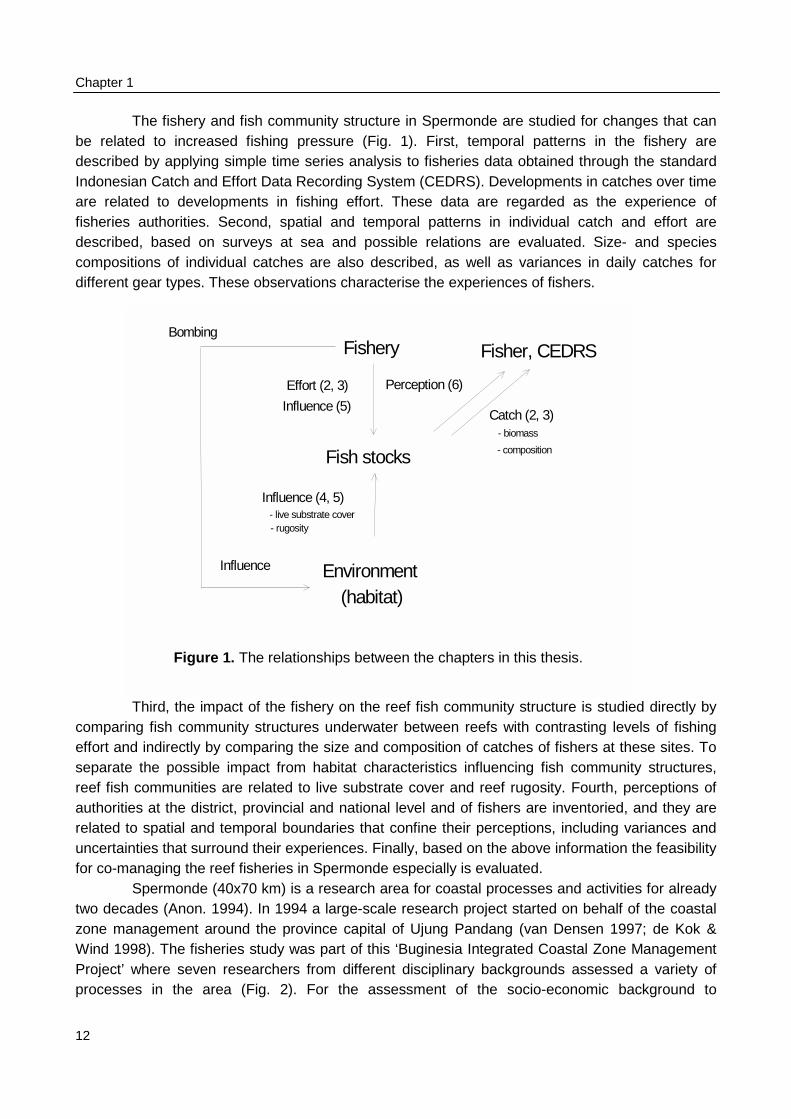
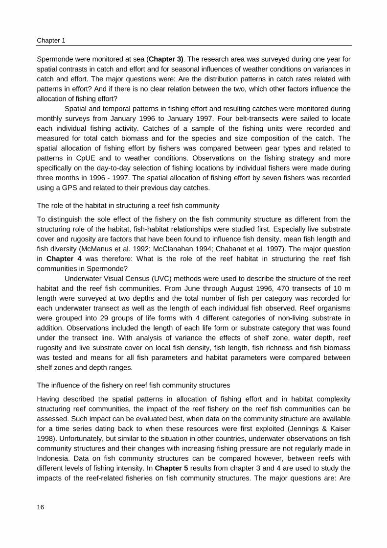
The fishery and fish community structure in Spermonde are studied for changes that canbe related to increased fishing pressure (Fig. 1). First, temporal patterns in the fishery aredescribed by applying simple time series analysis to fisheries data obtained through the standardIndonesian Catch and Effort Data Recording System (CEDRS). Developments in catches over timeare related to developments in fishing effort. These data are regarded as the experience offisheries authorities. Second, spatial and temporal patterns in individual catch and effort aredescribed, based on surveys at sea and possible relations are evaluated. Size- and speciescompositions of individual catches are also described, as well as variances in daily catches fordifferent gear types. These observations characterise the experiences of fishers.
comparieffort anseparatereef fishauthoritirelated uncertaifor co-m
two deczone mWind 19Project’ process
S
Fish stocks
Environment(habitat)
Fishery Fisher, CEDR
Effort (2, 3)
Influence (5)
Influence (4, 5)
Bombing
Influence
Catch (2, 3)
Perception (6)
- biomass
- composition
- live substrate cover- rugosity
Figure 1. The relationships between the chapters in this thesis.
Third, the impact of the fishery on the reef fish community structure is studied directly byng fish community structures underwater between reefs with contrasting levels of fishingd indirectly by comparing the size and composition of catches of fishers at these sites. To the possible impact from habitat characteristics influencing fish community structures, communities are related to live substrate cover and reef rugosity. Fourth, perceptions ofes at the district, provincial and national level and of fishers are inventoried, and they areto spatial and temporal boundaries that confine their perceptions, including variances andnties that surround their experiences. Finally, based on the above information the feasibilityanaging the reef fisheries in Spermonde especially is evaluated.Spermonde (40x70 km) is a research area for coastal processes and activities for already
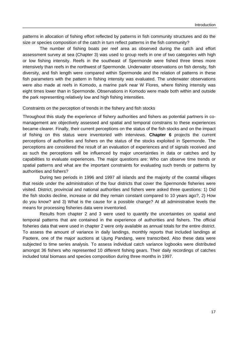
ades (Anon. 1994). In 1994 a large-scale research project started on behalf of the coastalanagement around the province capital of Ujung Pandang (van Densen 1997; de Kok &98). The fisheries study was part of this ‘Buginesia Integrated Coastal Zone Managementwhere seven researchers from different disciplinary backgrounds assessed a variety of
es in the area (Fig. 2). For the assessment of the socio-economic background to
Introduction
13
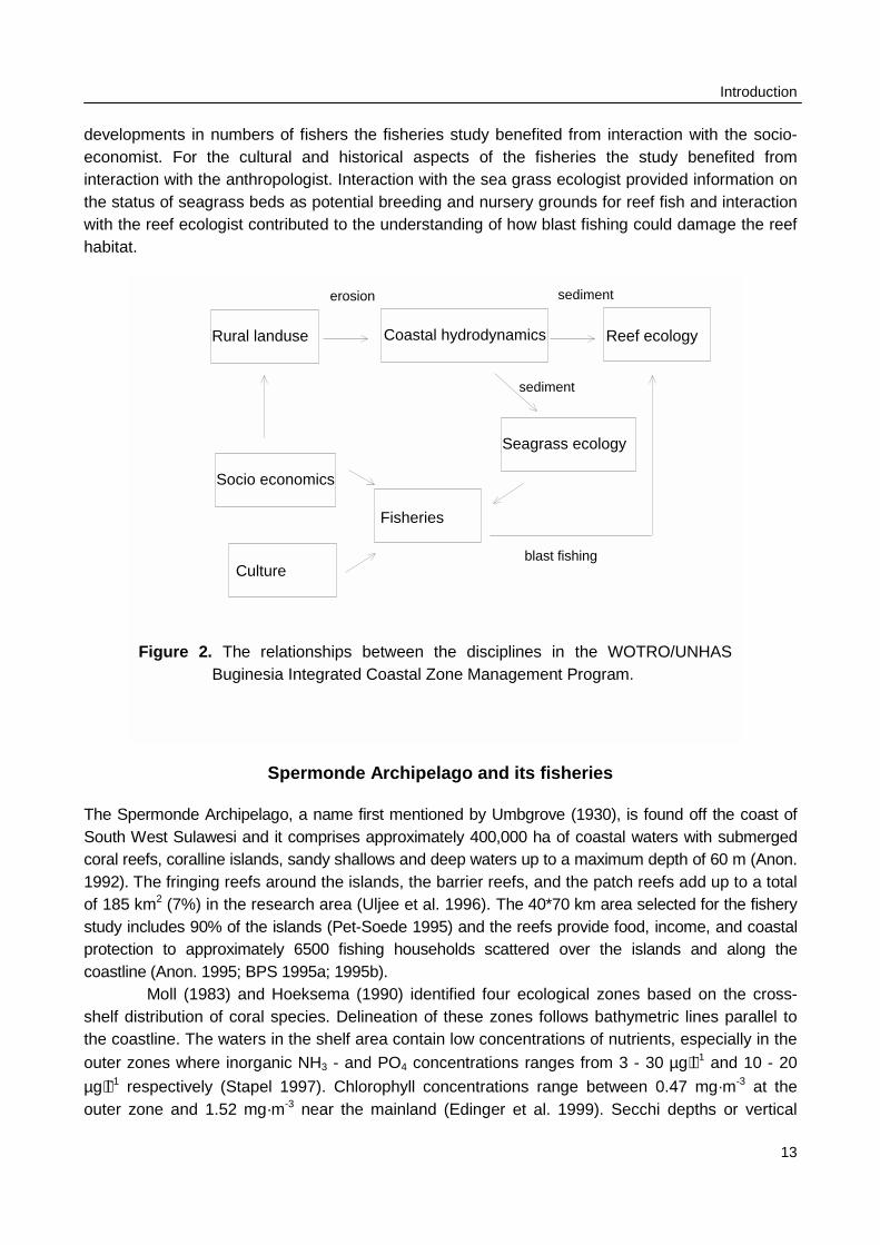
developments in numbers of fishers the fisheries study benefited from interaction with the socio-economist. For the cultural and historical aspects of the fisheries the study benefited frominteraction with the anthropologist. Interaction with the sea grass ecologist provided information onthe status of seagrass beds as potential breeding and nursery grounds for reef fish and interactionwith the reef ecologist contributed to the understanding of how blast fishing could damage the reefhabitat.
Spermonde Archipelago and its fisheries
The Spermonde Archipelago, a name first mentioned by Umbgrove (1930), is found off the coast ofSouth West Sulawesi and it comprises approximately 400,000 ha of coastal waters with submergedcoral reefs, coralline islands, sandy shallows and deep waters up to a maximum depth of 60 m (Anon.1992). The fringing reefs around the islands, the barrier reefs, and the patch reefs add up to a totalof 185 km2 (7%) in the research area (Uljee et al. 1996). The 40*70 km area selected for the fisherystudy includes 90% of the islands (Pet-Soede 1995) and the reefs provide food, income, and coastalprotection to approximately 6500 fishing households scattered over the islands and along thecoastline (Anon. 1995; BPS 1995a; 1995b).
Moll (1983) and Hoeksema (1990) identified four ecological zones based on the cross-shelf distribution of coral species. Delineation of these zones follows bathymetric lines parallel tothe coastline. The waters in the shelf area contain low concentrations of nutrients, especially in the
outer zones where inorganic NH3 - and PO4 concentrations ranges from 3 - 30 µg⋅l-1 and 10 - 20
µg⋅l-1 respectively (Stapel 1997). Chlorophyll concentrations range between 0.47 mg·m-3 at theouter zone and 1.52 mg·m-3 near the mainland (Edinger et al. 1999). Secchi depths or vertical
Rural landuse Coastal hydrodynamics Reef ecology
Seagrass ecology
Fisheries
Socio economics
Cultureblast fishing
erosion sediment
sediment
Figure 2. The relationships between the disciplines in the WOTRO/UNHASBuginesia Integrated Coastal Zone Management Program.
Chapter 1
14
water transparency vary between 15 - 27 m in the outer zones and 2 - 13 m near the mainland.There are two monsoon periods with heaviest rainfall and strongest wind speeds during the NWmonsoon, from December through April, when average rainfall can be as high as 500 mm per day.Southward currents occur year round with speeds between 12 - 38 cm·s-1 (Storm 1989).Predominant waves are to the southeast or east during the rainy season and to the north or north-east during the dry season (Storm 1989).
The fishery in Spermonde operates a large variety of gears from small- to medium-scaleboats. Official fisheries statistics reveal a total fish yield from the area in 1995 of 52,500 tons or130 kg·km-2 with a total value of US$ 18 million and an overall Catch-per-Unit-Effort (CpUE) of 40kg·trip-1 (Anon. 1995a). A 75% majority of the boats are non-powered canoes, 20% use outboardengines and only 5% use inboard engines. These data originate from the standard Catch andEffort Data Recording System (CEDRS) for each of the four districts Pangkep, Maros, UjungPandang, and Takalar under which administration the islands and coastal villages in Spermondereside (Anon. 1995a). Landings are officially monitored once every three months and the type ofboats and fishing gears and the number of units per gear are counted once every 2 - 5 yearsduring a socio-demographic census (Pers. comm. Head Provincial Fisheries Department).According to these statistics demersal fish species contribute less than 20% to total landings andthe small pelagic fringescale sardine (Sardinella fimbriata) is the most important fish category.
An average day at sea learns that shrimp gillnets are indeed operated in shallow watersnear the South Sulawesi mainland, yet as catches of large shrimp are prohibited the nets arecurrently deployed to catch crabs (Pers. comm. Head District Fisheries Department Pangkep). Thelarge quantities of Peneus monodon or tiger prawn are cultured in mostly intensive tambaks orshrimp ponds along the coast of Maros and Pangkep and these are the area’s second mostimportant export commodity after cacao beans (Anon. 1991). At sea most fishers operate a varietyof hook and line gear during the day. A single baited hook is hand-held to catch emperors(Lethrinus spp.), snappers (Lutjanus spp.), threadfishbream (Nemipiterus spp.), and jacks(Carangidae). A single line with multiple hooks is hand-held to catch Indian mackerel (Rastrelligerspp.) and scads (Selaroides spp.). Thicker lines with artificial or dead fish bait are trolled near thereefs for Spanish mackerel (Scomberomorus commerson) and groupers (Serranidae). Drift longlines are set for sharks and rays. During the night the major fishing activity is with lift nets operatedfrom boat platforms. Bag-like nets are dropped in the water and electric or kerosene lamps are lit toattract anchovy (Engraulidae), herrings (Clupeidae) and mackerels (Auxis spp). The samecategories are targeted by purse seiners that use lamps in a similar fashion, yet they close a netaround a school and pull it rather than have the net in the water before the lamps are lit.
Lift netters and purse seiners mostly transport their catches to the fish auctions butcatches of other gears are collected at sea or the islands and transported to the mainland marketsby fish buyers or middlemen. Two major auctions, Rajawali and Paotere, cater for the increasingdemand for fish by the more than one million Ujung Pandang citizens (Titus 1998). Fish prices varydaily between US$ 0.20 - 2.00 per kg and are mostly determined by the market demand. Rabbitfish(Siganus spp.) and rock cods (Plectropomus spp.) are most expensive and wrasses (Labridae) arethe cheapest fish category (Anon. 1994b). There are hardly any facilities to freeze or otherwisepreserve fresh fish, so if prices are low due to a large supply, fishers can only salt and dry their fishto preserve it for times when landings are low (Anon. 1993).
Introduction
15
Costs of operation are lowest for hook and line fishers and include 1-2 l kerosene and apack of cigarettes per day. Costs for depreciation and maintenance of small boats and small-scalegear range between US$ 50 - 100 per year (Pet-Soede et al. 1999a). Operation costs for medium-scale lift net and purse seine operations include larger amounts of diesel and kerosene and dailyfood for 6 - 10 crew. Costs for depreciation and maintenance for these medium-scale boats andgear range between US$ 400 - 1000 per year. Profits are divided following a system where crewand boat owner take different shares (Meereboer 1998). Profits are low and this is one of thefactors that have created strong patron-client relations between fishers and their bosses(Meereboer 1998). The low profits in the traditional fishery are also thought to be the incentive forthe increasing use of bombs and cyanide in the more recent illegal fishery (Pet-Soede et al.1999a). The increasing demand for fish and the deteriorating quality of the resource base to thefishery have put sustained exploitation of fish resources in Spermonde at risk.
Introduction to chapters
Trends in official catch and effort statistics
The quality of Indonesian official fisheries data is often criticised (Dudley & Harris 1987; Venema1997). The data are used by the National Fisheries Department to assess the status of Indonesianfish stocks and to decide on the number of fishing licenses. The official fisheries data can beregarded as the experience of fisheries authorities. In Chapter 2 of this thesis, time series ofofficial annual catch and effort data for the research area Spermonde Archipelago are studied fortrends, to evaluate how the information that is enclosed in these time series could be put tomaximal and management relevant use. The major question is: Do the official fisheries data forSpermonde indicate changes in the fishery and if so, for what segments (fish category, gearcategory, boat category) of the fishery are these trends most obvious?
Annual catch and effort were transcribed from South Sulawesi Province fisheries booksthat were available from the years 1977 - 1995. In these yearbooks catches for 45 fish categories,effort in trips for 27 gear categories, and number of units for 13 boat categories are reported foreach of the 18 districts in South Sulawesi. Data of four districts were combined to represent catchand effort for Spermonde and data of all districts were combined to represent catch and effort forthe entire province. Simple regression and auto-correlation techniques were applied to these timeseries of catch and effort data to search for linear trends and to distinguish between more or lessvariable segments of the fishery at different levels of data aggregation (per taxonomic fish categoryand gear category, per major fish group and gear group and for the total catch and total effort).
Spatial and temporal patterns in the fishery
Spatial and temporal patterns in the allocation of fishing effort and resultant catches are of specificinterest for the assessment of the impact of a fishery on fish stocks and for the evaluation ofmanagement options and their consequences (Medley et al. 1993). These patterns can be regardedas the potential experience of fishers. Because such patterns can not be deduced from officialstatistics at greater detail than between years and for an entire district, individual fishing activities in
Chapter 1
16
Spermonde were monitored at sea (Chapter 3). The research area was surveyed during one year forspatial contrasts in catch and effort and for seasonal influences of weather conditions on variances incatch and effort. The major questions were: Are the distribution patterns in catch rates related withpatterns in effort? And if there is no clear relation between the two, which other factors influence theallocation of fishing effort?
Spatial and temporal patterns in fishing effort and resulting catches were monitored duringmonthly surveys from January 1996 to January 1997. Four belt-transects were sailed to locateeach individual fishing activity. Catches of a sample of the fishing units were recorded andmeasured for total catch biomass and for the species and size composition of the catch. Thespatial allocation of fishing effort by fishers was compared between gear types and related topatterns in CpUE and to weather conditions. Observations on the fishing strategy and morespecifically on the day-to-day selection of fishing locations by individual fishers were made duringthree months in 1996 - 1997. The spatial allocation of fishing effort by seven fishers was recordedusing a GPS and related to their previous day catches.
The role of the habitat in structuring a reef fish community
To distinguish the sole effect of the fishery on the fish community structure as different from thestructuring role of the habitat, fish-habitat relationships were studied first. Especially live substratecover and rugosity are factors that have been found to influence fish density, mean fish length andfish diversity (McManus et al. 1992; McClanahan 1994; Chabanet et al. 1997). The major questionin Chapter 4 was therefore: What is the role of the reef habitat in structuring the reef fishcommunities in Spermonde?
Underwater Visual Census (UVC) methods were used to describe the structure of the reefhabitat and the reef fish communities. From June through August 1996, 470 transects of 10 mlength were surveyed at two depths and the total number of fish per category was recorded foreach underwater transect as well as the length of each individual fish observed. Reef organismswere grouped into 29 groups of life forms with 4 different categories of non-living substrate inaddition. Observations included the length of each life form or substrate category that was foundunder the transect line. With analysis of variance the effects of shelf zone, water depth, reefrugosity and live substrate cover on local fish density, fish length, fish richness and fish biomasswas tested and means for all fish parameters and habitat parameters were compared betweenshelf zones and depth ranges.
The influence of the fishery on reef fish community structures
Having described the spatial patterns in allocation of fishing effort and in habitat complexitystructuring reef communities, the impact of the reef fishery on the reef fish communities can beassessed. Such impact can be evaluated best, when data on the community structure are availablefor a time series dating back to when these resources were first exploited (Jennings & Kaiser1998). Unfortunately, but similar to the situation in other countries, underwater observations on fishcommunity structures and their changes with increasing fishing pressure are not regularly made inIndonesia. Data on fish community structures can be compared however, between reefs withdifferent levels of fishing intensity. In Chapter 5 results from chapter 3 and 4 are used to study theimpacts of the reef-related fisheries on fish community structures. The major questions are: Are
Introduction
17
patterns in allocation of fishing effort reflected by patterns in fish community structures and do thesize or species composition of the catch in turn reflect patterns in the fish community?
The number of fishing boats per reef area as observed during the catch and effortassessment survey at sea (Chapter 3) was used to group reefs in one of two categories with highor low fishing intensity. Reefs in the southeast of Spermonde were fished three times moreintensively than reefs in the northwest of Spermonde. Underwater observations on fish density, fishdiversity, and fish length were compared within Spermonde and the relation of patterns in thesefish parameters with the pattern in fishing intensity was evaluated. The underwater observationswere also made at reefs in Komodo, a marine park near W Flores, where fishing intensity waseight times lower than in Spermonde. Observations in Komodo were made both within and outsidethe park representing relatively low and high fishing intensities.
Constraints on the perception of trends in the fishery and fish stocks
Throughout this study the experience of fishery authorities and fishers as potential partners in co-management are objectively assessed and spatial and temporal constrains to these experiencesbecame clearer. Finally, their current perceptions on the status of the fish stocks and on the impactof fishing on this status were inventoried with interviews. Chapter 6 projects the currentperceptions of authorities and fishers on the status of the stocks exploited in Spermonde. Theperceptions are considered the result of an evaluation of experiences and of signals received andas such the perceptions will be influenced by major uncertainties in data or catches and bycapabilities to evaluate experiences. The major questions are: Who can observe time trends orspatial patterns and what are the important constraints for evaluating such trends or patterns byauthorities and fishers?
During two periods in 1996 and 1997 all islands and the majority of the coastal villagesthat reside under the administration of the four districts that cover the Spermonde fisheries werevisited. District, provincial and national authorities and fishers were asked three questions: 1) Didthe fish stocks decline, increase or did they remain constant compared to 10 years ago?, 2) Howdo you know? and 3) What is the cause for a possible change? At all administrative levels themeans for processing fisheries data were inventoried.
Results from chapter 2 and 3 were used to quantify the uncertainties on spatial andtemporal patterns that are contained in the experience of authorities and fishers. The officialfisheries data that were used in chapter 2 were only available as annual totals for the entire district.To assess the amount of variance in daily landings, monthly reports that included landings atPaotere, one of the major auctions at Ujung Pandang, were transcribed. Also these data weresubjected to time series analysis. To assess individual catch variance logbooks were distributedamongst 36 fishers who represented 10 different fishing gears. Their daily recordings of catchesincluded total biomass and species composition during three months in 1997.
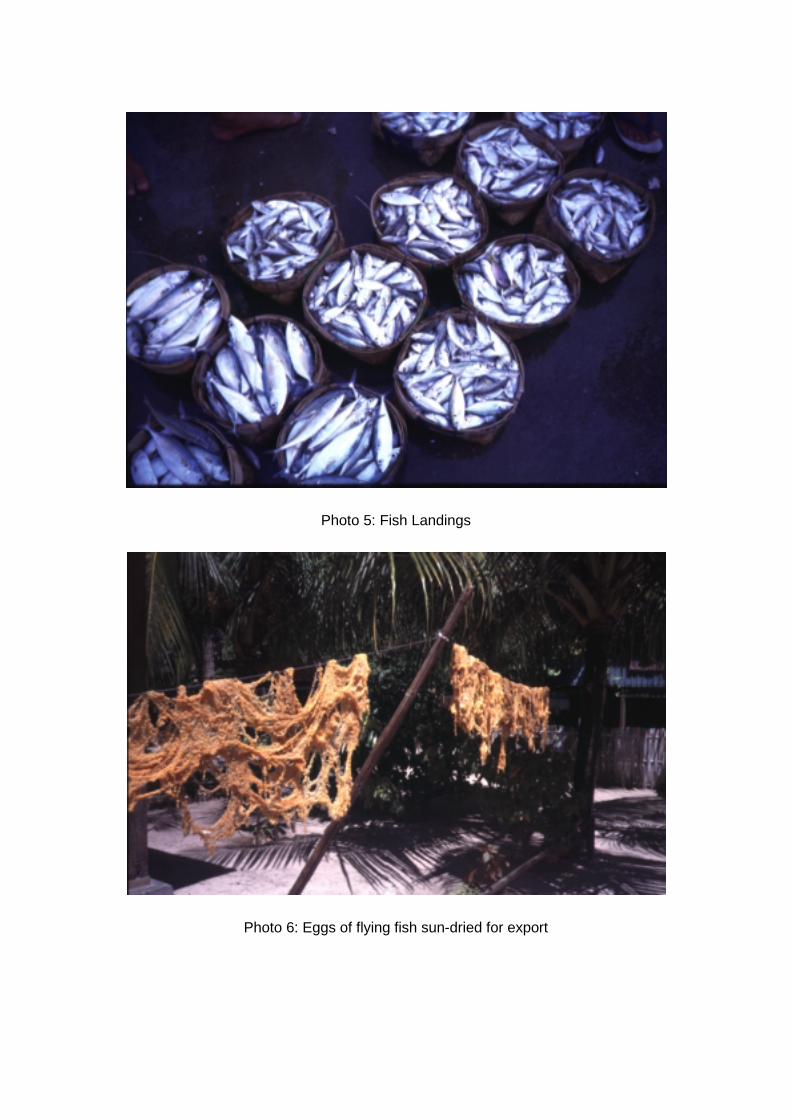
Photo 5: Fish Landings
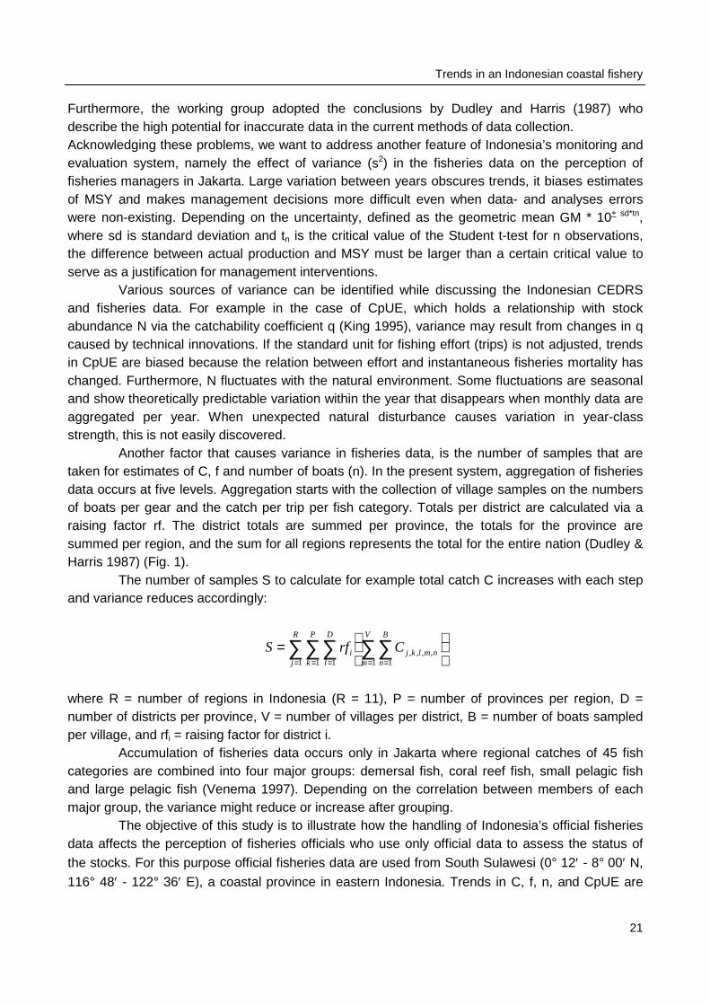
Photo 6: Eggs of flying fish sun-dried for export
19
Chapter 2
Trends in an Indonesian coastal fishery based on catch and effortstatistics and implications for the perception of the state of the stocks
by fisheries officials
C. Pet-Soede, M.A.M. Machiels, M.A. Stam and W.L.T. van Densen
Fisheries Research 42 (1999): 41 – 56
Abstract
Indonesia’s capture fisheries are monitored in each district of all 27 provinces with a comprehensive catchand effort data recording system that was installed in 1976. The annual data are sent to the IndonesianDirectorate General of Fisheries (DGF) in Jakarta, where these are aggregated for 11 coastal regions.Catches for the 45 recognised fish categories are accumulated in four major fish groups and analysed withconventional fisheries surplus models to estimate Maximum Sustainable Yields (MSYs). These estimateshave been used by DGF, to determine the number of fishing licenses for each region in the nation’sEconomic Exclusive Zone (EEZ). This paper discusses the effect of data aggregation and accumulation onthe variance around trends in fisheries data for the South Sulawesi province. Simple regression techniquesare applied to time series of catch, effort, catch-per-unit-effort, and numbers of boats. At the lowest level ofdata aggregation and accumulation we find the highest variance. Although high variance obscures theperception on the state of fish stocks at the lowest levels, perceptions at the highest levels are notnecessarily more useful for fisheries management. Bias caused by motorization of the fleet, by using CpUEas an indicator of fisheries mortality and by combining data from administrative units that have no ecologicalor biological meaning obscures the detection of trends.
Chapter 2
20
Introduction
Developments in Indonesia’s national demography and social-economy suggest that the fisheryhas changed since the first fisheries data were collected. The nation’s demersal resources werealready heavily exploited in 1978 due to the high number of fishermen in coastal areas (Bailey etal. 1987). The annual population growth of 1.7%1 puts a continuously increasing pressure on fishresources. Coastal small-scale fishery is usually a last refuge if other income generating activitiesare not available (Betke 1985). The flow of non-fishers that migrate to expanding coastalpopulation centres such as Jakarta, Medan, Ujung Pandang and Surabaya looking for industrialwork, requires a growing local supply of fish (Butcher 1996). Developing export markets directedpart of the fishing activities towards catching highly valued species (Martosubroto 1987). Newtechnologies were introduced and species composition of individual catches changed (B. Wahyudi,personal communications). Locally intensified fishing pressure affected the spatial scale at whichfishers exploit their resources (Martosubroto et al. 1991). New technologies and motorization of thefishing fleet allow fishermen to exploit previously inaccessible resources.
Hypothetically, Indonesia’s fisheries data that have been collected since 1976 with acomprehensive catch and effort data recording system (CEDRS) should confirm thesedevelopments. The capture fisheries are monitored in each of the 27 provinces (Yamamoto 1980).At the highest administration level of the Indonesian Directorate General of Fisheries (DGF),annual total catches (C) for four fish resource groups are divided by annual total effort (f) tocalculate the catch-per-unit-effort (CpUE) for each vessel that is licensed to fish that specificresource. CpUEs for the years 1975 through 1979 are used to calculate the Maximum SustainableYield (MSY) for each group with Schaefer’s surplus production model (1954). Based on acomparison of the actual catch in each new year with this MSY, conclusions are drawn on the levelof exploitation (Bailey et al. 1987). So far, differences between actual production and MSY havebeen considered as caused by under-exploitation and after division by average CpUE, the numberof boats that is needed to catch the remaining potential in each region is obtained (Venema 1997).The number of licenses is adjusted accordingly. The 27 Provincial Fisheries Offices are toadminister these specifications and the Navy is responsible for surveillance and control of thelicenses at sea (Badruddin & Gillet 1996).
Estimates for MSY were updated in 1991 and 1994 and although this is an improvementbecause more data points (years) have been included in the Schaefer model, the FAO workinggroup that reviewed the methods of stock assessment has concluded that two major errors havebeen made:1. The assumption that CpUE remains constant is not valid because in a situation of over
exploitation, each added component to the fishery leads to a decrease in the CpUE of allvessels in the fleet.
2. The difference between MSY and actual production can be caused by either under exploitationor over exploitation. In the latter case, a sustainable higher production can be obtained only byfishing less rather than by adding more vessels (Venema 1997).
1 (1997: www.usembassy.jakarta.org/econ/country.html)
Trends in an Indonesian coastal fishery
21
Furthermore, the working group adopted the conclusions by Dudley and Harris (1987) whodescribe the high potential for inaccurate data in the current methods of data collection.Acknowledging these problems, we want to address another feature of Indonesia’s monitoring andevaluation system, namely the effect of variance (s2) in the fisheries data on the perception offisheries managers in Jakarta. Large variation between years obscures trends, it biases estimatesof MSY and makes management decisions more difficult even when data- and analyses errorswere non-existing. Depending on the uncertainty, defined as the geometric mean GM * 10+ sd*tn,where sd is standard deviation and tn is the critical value of the Student t-test for n observations,the difference between actual production and MSY must be larger than a certain critical value toserve as a justification for management interventions.
Various sources of variance can be identified while discussing the Indonesian CEDRSand fisheries data. For example in the case of CpUE, which holds a relationship with stockabundance N via the catchability coefficient q (King 1995), variance may result from changes in qcaused by technical innovations. If the standard unit for fishing effort (trips) is not adjusted, trendsin CpUE are biased because the relation between effort and instantaneous fisheries mortality haschanged. Furthermore, N fluctuates with the natural environment. Some fluctuations are seasonaland show theoretically predictable variation within the year that disappears when monthly data areaggregated per year. When unexpected natural disturbance causes variation in year-classstrength, this is not easily discovered.
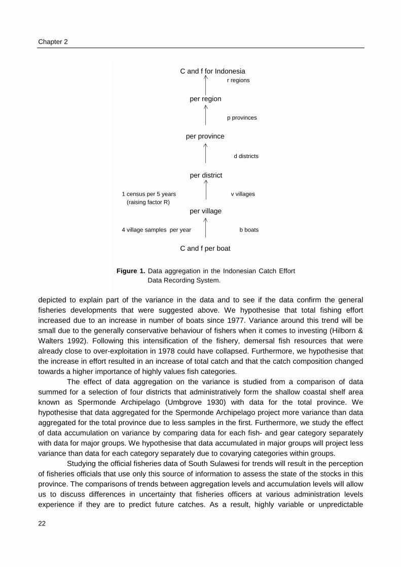
Another factor that causes variance in fisheries data, is the number of samples that aretaken for estimates of C, f and number of boats (n). In the present system, aggregation of fisheriesdata occurs at five levels. Aggregation starts with the collection of village samples on the numbersof boats per gear and the catch per trip per fish category. Totals per district are calculated via araising factor rf. The district totals are summed per province, the totals for the province aresummed per region, and the sum for all regions represents the total for the entire nation (Dudley &Harris 1987) (Fig. 1).
The number of samples S to calculate for example total catch C increases with each stepand variance reduces accordingly:
∑∑∑ ∑∑= = = = =
=
R
j
P
k
D
l
V
m
B
nnmlkji CrfS
1 1 1 1 1,,,,
where R = number of regions in Indonesia (R = 11), P = number of provinces per region, D =number of districts per province, V = number of villages per district, B = number of boats sampledper village, and rfi = raising factor for district i.
Accumulation of fisheries data occurs only in Jakarta where regional catches of 45 fishcategories are combined into four major groups: demersal fish, coral reef fish, small pelagic fishand large pelagic fish (Venema 1997). Depending on the correlation between members of eachmajor group, the variance might reduce or increase after grouping.
The objective of this study is to illustrate how the handling of Indonesia’s official fisheriesdata affects the perception of fisheries officials who use only official data to assess the status of
the stocks. For this purpose official fisheries data are used from South Sulawesi (0° 12′ - 8° 00′ N,
116° 48′ - 122° 36′ E), a coastal province in eastern Indonesia. Trends in C, f, n, and CpUE are
Chapter 2
22
depicted to explain pafisheries developmentincreased due to an insmall due to the generWalters 1992). Followalready close to over-ethe increase in effort retowards a higher impor
The effect of summed for a selectioknown as Spermondehypothesise that data aaggregated for the totaof data accumulation owith data for major grovariance than data for
Studying the oof fisheries officials thaprovince. The comparisus to discuss differenexperience if they are
C and f for Indonesia r regions
per region
p provinces
per province
d districts
per district
1 census per 5 years v villages (raising factor R)
per village
4 village samples per year b boats
C and f per boat
Figure 1. Data aggregation in the Indonesian Catch EffortData Recording System.
rt of the variance in the data and to see if the data confirm the generals that were suggested above. We hypothesise that total fishing effortcrease in number of boats since 1977. Variance around this trend will beally conservative behaviour of fishers when it comes to investing (Hilborn &ing this intensification of the fishery, demersal fish resources that werexploitation in 1978 could have collapsed. Furthermore, we hypothesise thatsulted in an increase of total catch and that the catch composition changedtance of highly values fish categories.data aggregation on the variance is studied from a comparison of datan of four districts that administratively form the shallow coastal shelf area Archipelago (Umbgrove 1930) with data for the total province. Weggregated for the Spermonde Archipelago project more variance than datal province due to less samples in the first. Furthermore, we study the effectn variance by comparing data for each fish- and gear category separately
ups. We hypothesise that data accumulated in major groups will project lesseach category separately due to covarying categories within groups.fficial fisheries data of South Sulawesi for trends will result in the perceptiont use only this source of information to assess the state of the stocks in thisons of trends between aggregation levels and accumulation levels will allowces in uncertainty that fisheries officers at various administration levels to predict future catches. As a result, highly variable or unpredictable
Trends in an Indonesian coastal fishery
23
fisheries can be separated from the more stable or predictable ones and the overall value offisheries data that project large unexplained variance for fisheries management can be discussed.The size of the variance provides critical values at which C or CpUE provides a signal that adeviation from the trend has occurred and that management intervention is justified from the officialdata.
Materials and methods
Fishery characteristics of the study area
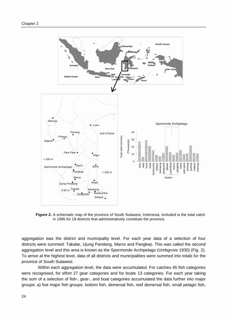
In 1993, South Sulawesi contributed most (8.4%) of all 27 Indonesian provinces to the nation’stotal marine production of 2.83 million tons (Venema 1997). The total value of the fish caught inSouth Sulawesi in 1995 was approximately 112.5 million US dollars. The largest contributors in thisprovince were the districts Bone, Luwu and Polmas (Fig. 2). The length of South Sulawesi’scoastline is 5400 km and the average density of fisher households was 5 per km which total 27,000(Venema 1997). The total number of fishing units or boats in the province was approximately29,000 and these made around 6 million trips per year (Anon. 1995a). The SpermondeArchipelago was first described by Umbgrove (1930) and comprises approximately 400,000 ha ofcoastal waters with submerged coral reefs, coralline islands, sandy shallows and deeper waters upto a maximum depth of 60 m. The four districts that administratively constitute the SpermondeArchipelago, counted around 6,500 fishing households that operated around 6,700 boats. The totaleffort in this shallow area was around 1.9 million trips, which resulted in 52,572 tons of fish with atotal value of approximately 22.5 million dollar (Anon. 1995a).
Small and large pelagic fishes contributed 73% to the total catch of 1995 in SouthSulawesi and 70% in the Spermonde Archipelago. Large pelagic fish were more important in theprovince than in Spermonde Archipelago; this major group contributed 27% to provincial catchesand only 11% to Spermonde’s catches. Small pelagic gear contributed 68% to total effort inSpermonde and only 39% to total effort in the province. In both areas 75% of the boats were non-powered canoes, 20% were motorized boats with outboard engines, and the remaining 5% weremotorized boats with inboard engines. The most important fish category in the province’s catcheswas “others” and in Spermonde Archipelago the most important category was “fringe scalesardine” or Sardinella fimbriata. Most effort in the province was with gears of the category “driftgillnet” and in Spermonde the most important gear is “shrimp gillnet”.
Data collection
Fisheries data for the province of South Sulawesi were transcribed from 19 fisheries yearbooks
(Anon. 1977 - 1995). Annual total C (tonnes⋅year-1) per fish category, f (trips⋅year-1) per gear
category and number (n⋅year-1) for 13 boat categories were available from 1977 through 1995 foreach of the 16 Kabupaten (districts) and two Kotamadya (municipalities) in the province (Fig. 2).
Data handling
The fisheries data for C, f and n varied in their level of aggregation and accumulation. Threeaggregation levels and three accumulation levels were recognised. The lowest level of data
Chapter 2
24
aggregation was the district and municipality level. For each year data of a selection of fourdistricts were summed: Takalar, Ujung Pandang, Maros and Pangkep. This was called the secondaggregation level and this area is known as the Spermonde Archipelago (Umbgrove 1930) (Fig. 2).To arrive at the highest level, data of all districts and municipalities were summed into totals for theprovince of South Sulawesi.
Within each aggregation level, the data were accumulated. For catches 45 fish categorieswere recognised, for effort 27 gear categories and for boats 13 categories. For each year takingthe sum of a selection of fish-, gear-, and boat categories accumulated the data further into majorgroups: a) five major fish groups: bottom fish, demersal fish, reef demersal fish, small pelagic fish,
��������������
����������������������������������������������������������������������������������������������������������������������������������������������������������������������������������������������������������������������������������������������������������������������������������������������������������������������������������������
����������
���������� ����
��������
������������������������������������������������������������������������������������������������������������
�������������������������������������������������������� ������������
�����������������������������������������������
�����
������������������������������������������������������������������������������������������������������������������������������������������������������������������������������������������������������������������������������������������������
������
���������������������������������������������������������������������������������������������������������������������������������������
�������������� ���������
��������������������������
��������
��������������������������
������������������
�������������������������
���������������������
������������������������������������������������������������������������������������������������������������������������������������������������������������������������������������������������������������������������������������������������������������
����������������
�������������
������������
������������������
����������
������
����
������
���������
�����
AmbonSumatra
Timor
Bali
Lombok
Irian Jaya
Komodo
Flores
Sulawesi
Kalimantan
Java
Java Sea
Pacific Ocean
Indian Ocean
Ujung Pandang
Mamuju
Majene
Polmas
Pangkep
Sinjai
Bantaeng
Jeneponto
Takalar
Pare Pare
Bulukumba
Selayar
Luwu
Wajo
BoneBarru
Pinrang
Spermonde Archipelago
> 200 m
Gulf of Bone
> 200 m
0-60 m
Maros
luw
uw
ajo
bone
sinj
aibu
luku
mba
sela
yar
bant
aeng
jene
pont
ota
kala
ru.
pand
ang
mar
ospa
ngke
pba
rru
pare
-par
epi
nran
gpo
lmas
maj
ene
mam
uju
District
0
10
20
30
40
(Tho
usan
ds)
Tot
al c
atch
(to
nnes
)
��������������������
����������
������������������������������������
������������������������
���������������������
��������
��������
���������������
������������������������
������������������
��������������
������������
������������
����������
������������������
������������������������
���������������������
������������������������
Spermonde Archipelago
Figure 2. A schematic map of the province of South Sulawesi, Indonesia. Included is the total catchin 1995 for 18 districts that administratively constitute the province.
Trends in an Indonesian coastal fishery
25
and large pelagic fish (Table 1); b) four major gear groups: demersal gear, reef gear, small pelagicgear, and large pelagic gear (Table 2); and c) three major boat groups: non-powered boats, boatswith outboard engines, and boats with inboard engines (Table 3). To arrive at the highest level,data of all categories were summed for each year.
As a result of these data treatments time series of 19 years for total C, total f, and total nand per category and per major group were now available. These time series were analysed fortwo areas: the entire province of South Sulawesi and the Spermonde Archipelago alone.
Annual totals for C at each accumulation level were divided by annual totals for f tocalculate the total CpUE (kg/trip) for the time series of 1977 - 1995. At the lowest accumulation
level this resulted in values for 1215 (45⋅27) theoretical combinations of fish category with gearcategory. The major gear type was selected for each of the 45 fish categories to calculate 45realistic CpUEs (Table 4). Due to the format of the fisheries yearbooks, calculation of CpUE wasdone only at the highest aggregation level.
Data analysis
The loose definition of Chatfield (1989) was followed that a trend is a long-term change in themean level. Means and standard deviations (sd) were calculated for 10log(C), 10log(f), 10log(n) and10log(CpUE) for the two levels of data aggregation (South Sulawesi and Spermonde) and for thethree levels of data accumulation (total, major groups, and categories) from 1977 - 1995. The datawere 10log-transformed to normalise the distribution and to get a relative measure for the totalvariance, independent of the mean, which enabled comparison of the magnitude of variancebetween and within aggregation and accumulation levels.
First and second order polynomials were fitted to the data using time (years) as theindependent or explanatory variable X (n = 19; P < 0.05) (Buijse et al. 1991). The linear regressionmodel was 10logY = aX + b + e and the polynomial model was 10logY = a1X
2 + a2X + b + e. C, f, n,or CpUE were response variable Y; b was a random variable, and e was the unexplained varianceor error. The catch data were studied for periodicity by applying auto-correlation techniques (P <0.05) to the residuals that remained after de-trending of the catch data. Auto-correlation with timesteps of one year and time-lags of one and two years was also applied to the effort data to findwhether fishing effort showed little variance from year-to-year as assumed earlier. The geometricmeans (GM) were calculated for all totals, major groups, and categories as the back transformedmean of the 10log-transformed variables (Sokal & Rohlf 1995). Only linear trends were discussed,because these should also be detected and perceived by fisheries officials at the lowestadministration levels that had only simple computation equipment available.The accumulation of categories into major groups and major groups into totals might affect thevariance due to correlation between categories or major groups. Generally, the variance of a sumof variables equals the sum of the variances plus a covariance term (Sokal & Rohlf 1995):
)()(2)()()( 21122
22
1212 ysysrysysyys ++=+
where s1 and s2 are standard deviations of variable y1 and y2 and r12 is the correlation coefficientbetween variable y1 and y2.
Chapter 2
26
If the categoriand the variance of thebetween categories orvariances and if the variance of their sum depending on means awith correlation coefficcombinations of major
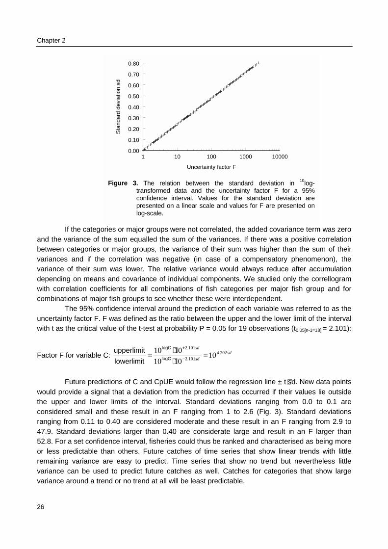
The 95% confuncertainty factor F. F with t as the critical val
Factor F for variable C
Future predictwould provide a signalthe upper and lower considered small and ranging from 0.11 to 047.9. Standard deviati52.8. For a set confideor less predictable tharemaining variance arvariance can be usedvariance around a tren
F
1 10 100 1000 10000
Uncertainty factor F
0.00
0.10
0.20
0.30
0.40
0.50
0.60
0.70
0.80
Sta
ndar
d de
viat
ion
sd
igure 3. The relation between the standard deviation in 10log-transformed data and the uncertainty factor F for a 95%confidence interval. Values for the standard deviation arepresented on a linear scale and values for F are presented onlog-scale.
es or major groups were not correlated, the added covariance term was zero sum equalled the sum of the variances. If there was a positive correlation
major groups, the variance of their sum was higher than the sum of theircorrelation was negative (in case of a compensatory phenomenon), thewas lower. The relative variance would always reduce after accumulationnd covariance of individual components. We studied only the correllogramients for all combinations of fish categories per major fish group and forfish groups to see whether these were interdependent.idence interval around the prediction of each variable was referred to as thewas defined as the ratio between the upper and the lower limit of the intervalue of the t-test at probability P = 0.05 for 19 observations (t0.05[n-1=18] = 2.101):
: sdsd
sd202.4
101.2
101.2
101010
1010 =⋅⋅= −
+
logC
logC
lowerlimit
upperlimit
ions of C and CpUE would follow the regression line ± t⋅sd. New data points that a deviation from the prediction has occurred if their values lie outsidelimits of the interval. Standard deviations ranging from 0.0 to 0.1 arethese result in an F ranging from 1 to 2.6 (Fig. 3). Standard deviations.40 are considered moderate and these result in an F ranging from 2.9 toons larger than 0.40 are considerate large and result in an F larger thannce interval, fisheries could thus be ranked and characterised as being moren others. Future catches of time series that show linear trends with littlee easy to predict. Time series that show no trend but nevertheless little to predict future catches as well. Catches for categories that show larged or no trend at all will be least predictable.
Trends in an Indonesian coastal fishery
27
Results
Developments in catch, effort and catch-per-unit-effort in South Sulawesi and the SpermondeArchipelago
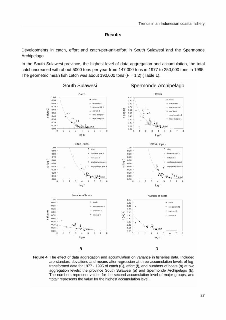
In the South Sulawesi province, the highest level of data aggregation and accumulation, the totalcatch increased with about 5000 tons per year from 147,000 tons in 1977 to 250,000 tons in 1995.The geometric mean fish catch was about 190,000 tons (F = 1.2) (Table 1).
0 1 2 3 4 5 6 7 8
log C
0.00
0.10
0.20
0.30
0.40
0.50
0.60
0.70
0.80
0.90
1.00
s (lo
g C
)
Catch
4 total523
1
totals
bottom fish 1
demersal fish 2
reef fish 3
small pelagics 4
large pelagics 5
0 1 2 3 4 5 6 7 8
log f
0.00
0.10
0.20
0.30
0.40
0.50
0.60
0.70
0.80
0.90
1.00
s (lo
g f)
Effort - trips -
totals
demersal gear 1
reef gear 2
smallpelagic gear 3
large pelagic gear 4
total1 3 42
0 1 2 3 4 5 6 7 8
log n
0.00
0.10
0.20
0.30
0.40
0.50
0.60
0.70
0.80
0.90
1.00
s (lo
g n)
Number of boats
1
totals
non-powered 1
outboard 2
inboard 3
total
23
0 1 2 3 4 5 6 7 8
log C
0.00
0.10
0.20
0.30
0.40
0.50
0.60
0.70
0.80
0.90
1.00
s (lo
g C
)
Catch
4 total5 23
1
totals
bottom fish 1
demersal fish 2
reef fish 3
small pelagics 4
large pelagics 5
0 1 2 3 4 5 6 7 8
log f
0.00
0.10
0.20
0.30
0.40
0.50
0.60
0.70
0.80
0.90
1.00
s (lo
g f)
Effort - trips -
total
2
1,43
totals
demersal gear 1
reef gear 2
smallpelagic gear 3
large pelagic gear 4
0 1 2 3 4 5 6 7 8
log n
0.00
0.10
0.20
0.30
0.40
0.50
0.60
0.70
0.80
0.90
1.00
s (lo
g n)
Number of boats
1
totals
non-powered 1
outboard 2
inboard 3
total23
South Sulawesi Spermonde Archipelago
a b
Figure 4. The effect of data aggregation and accumulation on variance in fisheries data. Includedare standard deviations and means after regression at three accumulation levels of log-transformed data for 1977 - 1995 of catch (C), effort (f), and numbers of boats (n) at twoaggregation levels: the province South Sulawesi (a) and Spermonde Archipelago (b).The numbers represent values for the second accumulation level of major groups, and“total” represents the value for the highest accumulation level.
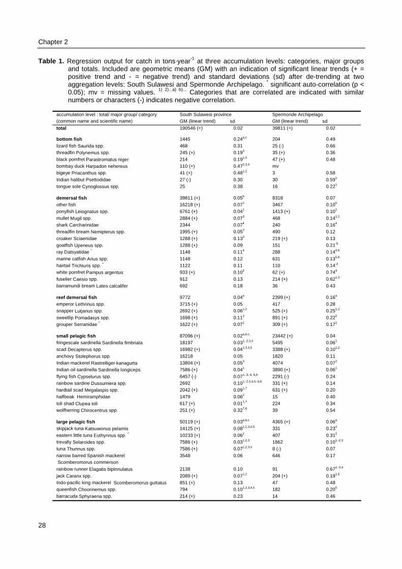
Chapter 2
28
Table 1. Regression output for catch in tons·year-1 at three accumulation levels: categories, major groupsand totals. Included are geometric means (GM) with an indication of significant linear trends (+ =positive trend and - = negative trend) and standard deviations (sd) after de-trending at twoaggregation levels: South Sulawesi and Spermonde Archipelago. * significant auto-correlation (p <0.05); mv = missing values. 1) 2)...a) b)... Categories that are correlated are indicated with similarnumbers or characters (-) indicates negative correlation.
accumulation level : total/ major group/ category(common name and scientific name)
South Sulawesi provinceGM (linear trend) sd
Spermonde ArchipelagoGM (linear trend) sd
total 190546 (+) 0.02 39811 (+) 0.02
bottom fish 1445 0.24a,c 204 0.49lizard fish Saurida spp. 468 0.31 25 (-) 0.66threadfin Polynemus spp. 245 (+) 0.193 35 (+) 0.36
black pomfret Parastromatus niger 214 0.191,4 47 (+) 0.48bombay duck Harpadon nehereus 110 (+) 0.472,3,4 mvbigeye Priacanthus spp. 41 (+) 0.481,2 3 0.58
Indian halibut Psettodidae 27 (-) 0.30 30 0.591
tongue sole Cynoglossus spp. 25 0.38 16 0.221
demersal fish 39811 (+) 0.05b 8318 0.07other fish 16218 (+) 0.071 3467 0.105
ponyfish Leiognatus spp. 6761 (+) 0.041 1413 (+) 0.101
mullet Mugil spp. 2884 (+) 0.073 468 0.141,2
shark Carcharinidae 2344 0.074 240 0.164
threadfin bream Nemipterus spp. 1995 (+) 0.052 490 0.12
croaker Sciaenidae 1288 (+) 0.133 219 (+) 0.13goatfish Upeneus spp. 1288 (+) 0.09 151 0.21-5
ray Datsyatidae * 1148 0.114 288 0.144,6
marine catfish Arius spp. 1148 0.12 631 0.135,6
hairtail Trichiuris spp. * 1122 0.11 110 0.14-2
white pomfret Pampus argentus 933 (+) 0.102 62 (+) 0.743
fuselier Caesio spp. 912 0.13 214 (+) 0.621,3
barramundi bream Lates calcalifer 692 0.18 36 0.43
reef demersal fish 9772 0.04a 2399 (+) 0.16a
emperor Lethrinus spp. 3715 (+) 0.05 417 0.28snapper Lutjanus spp. 2692 (+) 0.061,2 525 (+) 0.251,2
sweetlip Pomadasys spp. 1698 (+) 0.112 891 (+) 0.222
grouper Serranidae * 1622 (+) 0.071 309 (+) 0.171
small pelagic fish 87096 (+) 0.02a,b,c 23442 (+) 0.04fringescale sardinella Sardinella fimbriata 18197 0.031,-2,3,4 5495 0.061
scad Decapterus spp. 16982 (+) 0.041,3,4,5 3388 (+) 0.101,2
anchovy Stolephorus spp. 16218 0.05 1820 0.11Indian mackerel Rastrelliger kanagurta 13804 (+) 0.053 4074 0.072
Indian oil sardinella Sardinella longiceps 7586 (+) 0.041 3890 (+) 0.061
flying fish Cypselurus spp. 6457 (-) 0.071,-3,-4,-5,6 2291 (-) 0.24rainbow sardine Dussumiera spp. 2692 0.101,-2,3,4,5,-6,8 331 (+) 0.14hardtail scad Megalaspis spp. 2042 (+) 0.091,7 631 (+) 0.20
halfbeak Hemiramphidae 1479 0.062 15 0.40toli shad Clupea toli 617 (+) 0.011,7 224 0.34wolfherring Chirocentrus spp. 251 (+) 0.327,8 39 0.54
large pelagic fish 50119 (+) 0.03a,b,c 4365 (+) 0.06a
skipjack tuna Katsuwonus pelamis 14125 (+) 0.081,2,3,4,5 331 0.234
eastern little tuna Euthynnus spp. * 10233 (+) 0.061 407 0.312
trevally Selaroides spp. 7586 (+) 0.031,2,3 1862 0.101,-2,3
tuna Thunnus spp. 7586 (+) 0.071,2,3,4 8 (-) 0.07
narrow barred Spanish mackerel Scomberomorus commerson
3548 0.06 646 0.17
rainbow runner Elagatis bipinnulatus 2138 0.10 91 0.672,-3,4
jack Caranx spp. 2089 (+) 0.071,2 204 (+) 0.191,5
Indo-pacific king mackerel Scomberomorus guttatus 851 (+) 0.13 47 0.48queenfish Choorinemus spp. 794 0.101,2,3,4,5 182 0.205
barracuda Sphyraena spp. 214 (+) 0.23 14 0.46
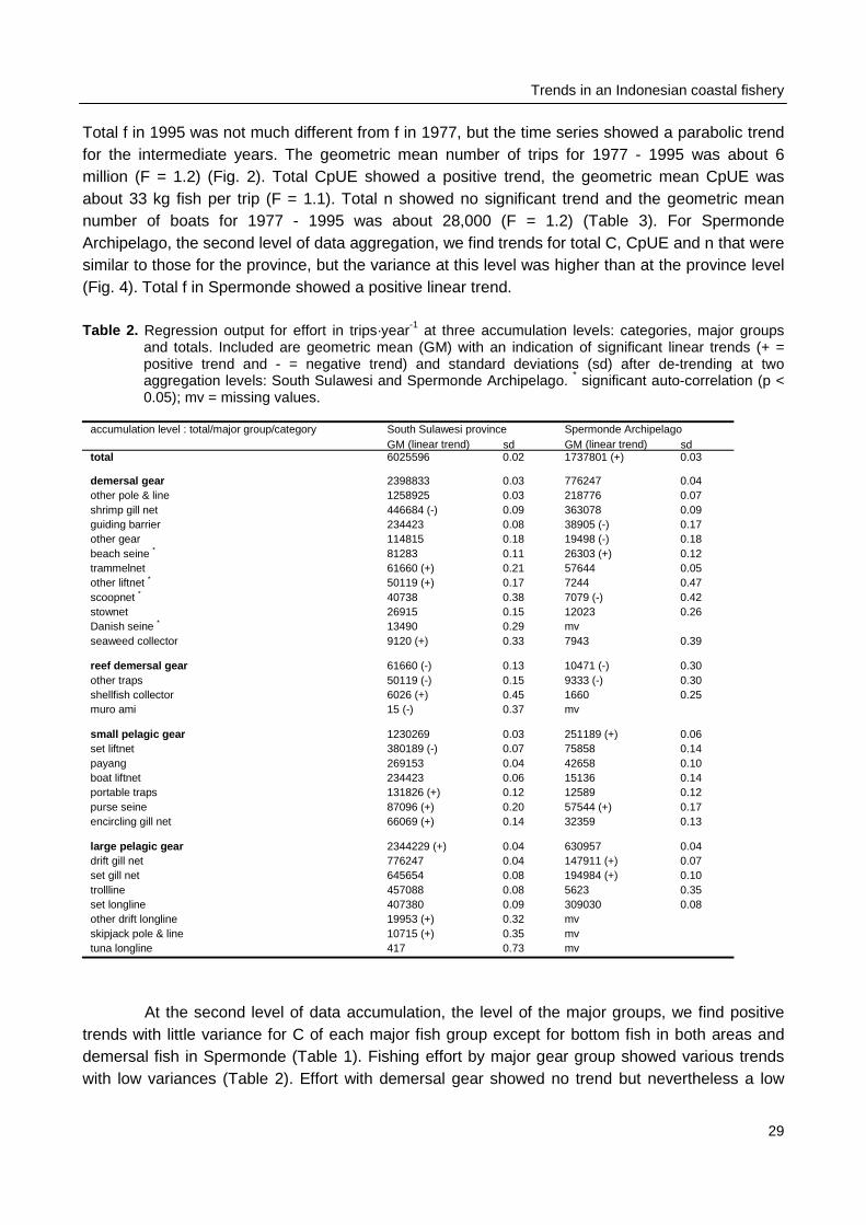
Trends in an Indonesian coastal fishery
29
Total f in 1995 was not much different from f in 1977, but the time series showed a parabolic trendfor the intermediate years. The geometric mean number of trips for 1977 - 1995 was about 6million (F = 1.2) (Fig. 2). Total CpUE showed a positive trend, the geometric mean CpUE wasabout 33 kg fish per trip (F = 1.1). Total n showed no significant trend and the geometric meannumber of boats for 1977 - 1995 was about 28,000 (F = 1.2) (Table 3). For SpermondeArchipelago, the second level of data aggregation, we find trends for total C, CpUE and n that weresimilar to those for the province, but the variance at this level was higher than at the province level(Fig. 4). Total f in Spermonde showed a positive linear trend.
Table 2. Regression output for effort in trips·year-1 at three accumulation levels: categories, major groupsand totals. Included are geometric mean (GM) with an indication of significant linear trends (+ =positive trend and - = negative trend) and standard deviations (sd) after de-trending at twoaggregation levels: South Sulawesi and Spermonde Archipelago. * significant auto-correlation (p <0.05); mv = missing values.
accumulation level : total/major group/category South Sulawesi provinceGM (linear trend) sd
Spermonde ArchipelagoGM (linear trend) sd
total 6025596 0.02 1737801 (+) 0.03
demersal gear 2398833 0.03 776247 0.04other pole & line 1258925 0.03 218776 0.07shrimp gill net 446684 (-) 0.09 363078 0.09guiding barrier 234423 0.08 38905 (-) 0.17other gear 114815 0.18 19498 (-) 0.18beach seine * 81283 0.11 26303 (+) 0.12trammelnet 61660 (+) 0.21 57644 0.05other liftnet * 50119 (+) 0.17 7244 0.47scoopnet * 40738 0.38 7079 (-) 0.42stownet 26915 0.15 12023 0.26Danish seine * 13490 0.29 mvseaweed collector 9120 (+) 0.33 7943 0.39
reef demersal gear 61660 (-) 0.13 10471 (-) 0.30other traps 50119 (-) 0.15 9333 (-) 0.30shellfish collector 6026 (+) 0.45 1660 0.25muro ami 15 (-) 0.37 mv
small pelagic gear 1230269 0.03 251189 (+) 0.06set liftnet 380189 (-) 0.07 75858 0.14payang 269153 0.04 42658 0.10boat liftnet 234423 0.06 15136 0.14portable traps 131826 (+) 0.12 12589 0.12purse seine 87096 (+) 0.20 57544 (+) 0.17encircling gill net 66069 (+) 0.14 32359 0.13
large pelagic gear 2344229 (+) 0.04 630957 0.04drift gill net 776247 0.04 147911 (+) 0.07set gill net 645654 0.08 194984 (+) 0.10trollline 457088 0.08 5623 0.35set longline 407380 0.09 309030 0.08other drift longline 19953 (+) 0.32 mvskipjack pole & line 10715 (+) 0.35 mvtuna longline 417 0.73 mv
At the second level of data accumulation, the level of the major groups, we find positivetrends with little variance for C of each major fish group except for bottom fish in both areas anddemersal fish in Spermonde (Table 1). Fishing effort by major gear group showed various trendswith low variances (Table 2). Effort with demersal gear showed no trend but nevertheless a low
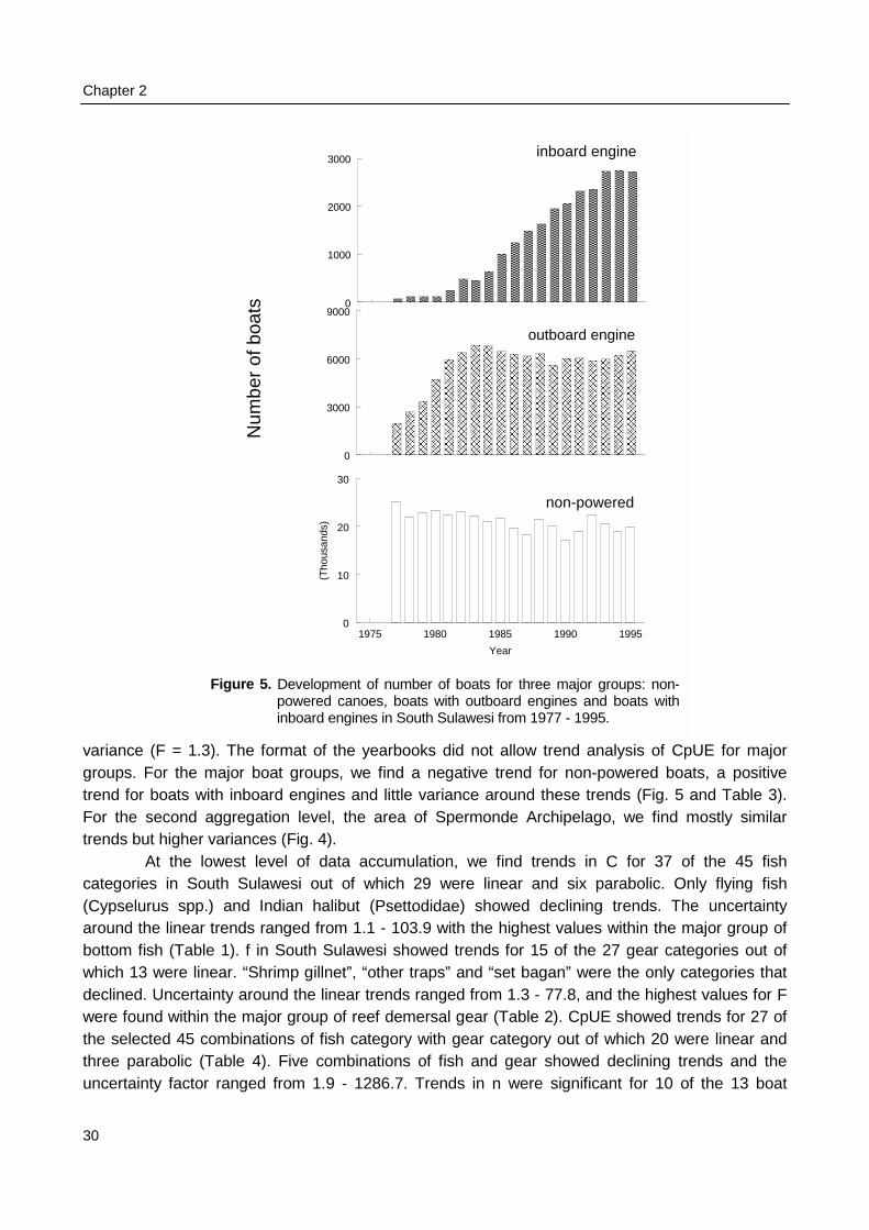
Chapter 2
30
variance (F = 1.3). The format of the yearbooks did not allow trend analysis of CpUE for majorgroups. For the major boat groups, we find a negative trend for non-powered boats, a positivetrend for boats with inboard engines and little variance around these trends (Fig. 5 and Table 3).For the second aggregation level, the area of Spermonde Archipelago, we find mostly similartrends but higher variances (Fig. 4).
At the lowest level of data accumulation, we find trends in C for 37 of the 45 fishcategories in South Sulawesi out of which 29 were linear and six parabolic. Only flying fish(Cypselurus spp.) and Indian halibut (Psettodidae) showed declining trends. The uncertaintyaround the linear trends ranged from 1.1 - 103.9 with the highest values within the major group ofbottom fish (Table 1). f in South Sulawesi showed trends for 15 of the 27 gear categories out ofwhich 13 were linear. “Shrimp gillnet”, “other traps” and “set bagan” were the only categories thatdeclined. Uncertainty around the linear trends ranged from 1.3 - 77.8, and the highest values for Fwere found within the major group of reef demersal gear (Table 2). CpUE showed trends for 27 ofthe selected 45 combinations of fish category with gear category out of which 20 were linear andthree parabolic (Table 4). Five combinations of fish and gear showed declining trends and theuncertainty factor ranged from 1.9 - 1286.7. Trends in n were significant for 10 of the 13 boat
0
1000
2000
3000
����������������������������������������
��������
��������
���������������
������������������������
������������������������������
�����������������������������������
������������������������
������������������������
�����������������������������������
������������������������������������������
������������������������������������������������
��������������������������������������������������������
����������������������������������������������������������������
0
3000
6000
9000
����������������
������������
��������������������
������������������������������
������������������������������������
�������������������������������������������������
�������������������������������������������������
����������������������������
�����������������������������������
������������������������������
������������������������������������
�������������������������������������������������
������������������������������������������
������������������������
������������������������������
������������������������������
������������������������������������
������������������������������������������
�������������������������������������������������
1975 1980 1985 1990 1995
Year
0
10
20
30
(Tho
usan
ds)
Num
ber
of b
oats
non-powered
outboard engine
inboard engine
Figure 5. Development of number of boats for three major groups: non-powered canoes, boats with outboard engines and boats withinboard engines in South Sulawesi from 1977 - 1995.
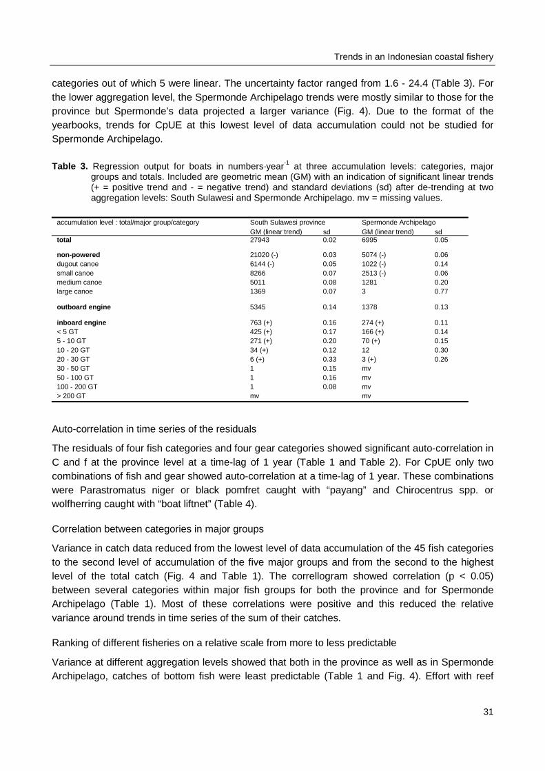
Trends in an Indonesian coastal fishery
31
categories out of which 5 were linear. The uncertainty factor ranged from 1.6 - 24.4 (Table 3). Forthe lower aggregation level, the Spermonde Archipelago trends were mostly similar to those for theprovince but Spermonde’s data projected a larger variance (Fig. 4). Due to the format of theyearbooks, trends for CpUE at this lowest level of data accumulation could not be studied forSpermonde Archipelago.
Table 3. Regression output for boats in numbers·year-1 at three accumulation levels: categories, majorgroups and totals. Included are geometric mean (GM) with an indication of significant linear trends(+ = positive trend and - = negative trend) and standard deviations (sd) after de-trending at twoaggregation levels: South Sulawesi and Spermonde Archipelago. mv = missing values.
accumulation level : total/major group/category South Sulawesi provinceGM (linear trend) sd
Spermonde ArchipelagoGM (linear trend) sd
total 27943 0.02 6995 0.05
non-powered 21020 (-) 0.03 5074 (-) 0.06dugout canoe 6144 (-) 0.05 1022 (-) 0.14small canoe 8266 0.07 2513 (-) 0.06medium canoe 5011 0.08 1281 0.20large canoe 1369 0.07 3 0.77
outboard engine 5345 0.14 1378 0.13
inboard engine 763 (+) 0.16 274 (+) 0.11< 5 GT 425 (+) 0.17 166 (+) 0.145 - 10 GT 271 (+) 0.20 70 (+) 0.1510 - 20 GT 34 (+) 0.12 12 0.3020 - 30 GT 6 (+) 0.33 3 (+) 0.2630 - 50 GT 1 0.15 mv50 - 100 GT 1 0.16 mv100 - 200 GT 1 0.08 mv> 200 GT mv mv
Auto-correlation in time series of the residuals
The residuals of four fish categories and four gear categories showed significant auto-correlation inC and f at the province level at a time-lag of 1 year (Table 1 and Table 2). For CpUE only twocombinations of fish and gear showed auto-correlation at a time-lag of 1 year. These combinationswere Parastromatus niger or black pomfret caught with “payang” and Chirocentrus spp. orwolfherring caught with “boat liftnet” (Table 4).
Correlation between categories in major groups
Variance in catch data reduced from the lowest level of data accumulation of the 45 fish categoriesto the second level of accumulation of the five major groups and from the second to the highestlevel of the total catch (Fig. 4 and Table 1). The correllogram showed correlation (p < 0.05)between several categories within major fish groups for both the province and for SpermondeArchipelago (Table 1). Most of these correlations were positive and this reduced the relativevariance around trends in time series of the sum of their catches.
Ranking of different fisheries on a relative scale from more to less predictable
Variance at different aggregation levels showed that both in the province as well as in SpermondeArchipelago, catches of bottom fish were least predictable (Table 1 and Fig. 4). Effort with reef
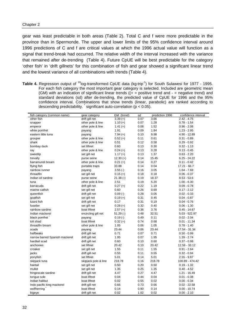
Chapter 2
32
gear was least predictable in both areas (Table 2). Total C and f were more predictable in theprovince than in Spermonde. The upper and lower limits of the 95% confidence interval around1996 predictions of C and f are critical values at which the 1996 actual value will function as asignal that trend-break had occurred. The relative width of the interval increased with the variancethat remained after de-trending (Table 4). Future CpUE will be best predictable for the category‘other fish’ in ‘drift gillnets’ for this combination of fish and gear showed a significant linear trendand the lowest variance of all combinations with trends (Table 4).
Table 4. Regression output of 10log-transformed CpUE data (kg·trip-1) for South Sulawesi for 1977 - 1995.For each fish category the most important gear category is selected. Included are geometric mean(GM) with an indication of significant linear trends ((+ = positive trend and - = negative trend) andstandard deviations (sd) after de-trending, the predicted value of CpUE for 1996 and the 95%confidence interval. Combinations that show trends (linear, parabolic) are ranked according todescending predictability. * significant auto-correlation (p < 0.05).
fish category (common name) gear category GM (trend) sd prediction 1996 confidence intervalother fish drift gill net 3.39 (+) 0.07 3.66 2.42 - 4.75snapper other pole & line 1.10 (+) 0.07 1.28 0.78 - 1.54emperor other pole & line 1.41 (+) 0.08 1.52 0.96 - 2.08white pomfret payang 1.91 0.09 1.84 1.23 - 2.95eastern little tuna payang 7.94 (+) 0.10 9.98 4.90 - 12.89grouper other pole & line 0.52 (+) 0.11 0.61 0.31 - 0.89shark other pole & line 0.51 0.12 0.58 0.29 - 0.92bombay duck set liftnet 0.60 0.13 0.30 0.32 - 1.13ray other pole & line 0.24 (+) 0.13 0.28 0.13 - 0.45sweetlip set gill net 1.17 (+) 0.13 1.37 0.63 - 2.20trevally purse seine 12.30 (+) 0.14 15.45 6.25 - 24.22barramundi bream other pole & line 0.21 (+) 0.14 0.27 0.11 - 0.42flying fish portable traps 33.88 0.14 0.04 17.21 - 66.7rainbow runner payang 3.55 (-) 0.16 3.05 1.64 - 7.69threadfin set gill net 0.15 (+) 0.18 0.18 0.06 - 0.37Indian oil sardine purse seine 21.38 (-) 0.19 18.37 8.53 - 53.6tuna other pole & line 2.51 0.19 5.20 1.00 - 6.30barracuda drift gill net 0.27 (+) 0.22 1.19 0.09 - 0.78marine catfish set gill net 0.60 0.26 0.69 0.17 - 2.12queenfish drift gill net 0.09 (-) 0.28 0.05 0.02 - 0.33goatfish set gill net 0.19 (+) 0.31 0.45 0.04 - 0.87lizard fish drift gill net 0.17 0.31 0.19 0.04 - 0.76fuselier set gill net 0.28 (+) 0.32 0.40 0.06 - 1.30rainbow sardine boat liftnet 2.57 (+) 0.36 3.76 0.45 - 14.67Indian mackerel encircling gill net 51.29 (-) 0.48 32.51 5.03 - 522.97black pomfret * payang 0.19 (-) 0.49 0.11 0.02 - 2.04toli shad boat liftnet 0.32 (+) 0.74 0.68 0.01 - 11.34threadfin bream other pole & line 1.05 0.06 1.05 0.78 - 1.40scads payang 23.44 0.06 23.44 17.54 - 31.34halfbeaks drift gill net 0.71 0.07 0.71 0.50 - 0.99narrow barred Spanish mackerel drift gill net 1.95 0.07 1.95 1.39 - 2.74hardtail scad drift gill net 0.60 0.10 0.60 0.37 - 0.98anchovies set liftnet 20.42 0.10 20.42 12.59 - 33.12croaker set gill net 1.55 0.11 1.55 0.91 - 2.64jacks drift gill net 0.55 0.11 0.55 0.32 - 0.94ponyfish set liftnet 5.01 0.14 5.01 2.55 - 9.87skipjack tuna skipjack pole & line 218.78 0.16 218.78 100.89 - 474.42hairtail set gill net 0.50 0.20 0.50 0.19 - 1.32mullet set gill net 1.35 0.25 1.35 0.40 - 4.52fringescale sardine drift gill net 4.47 0.27 4.47 1.21 - 16.49tongue sole boat liftnet 0.04 0.44 0.04 0.01 - 0.38Indian halibut boat liftnet 0.02 0.55 0.02 0.00 - 0.34Indo pacific king mackerel drift gill net 0.66 0.73 0.66 0.02 - 22.58wolfherring * boat liftnet 0.14 0.90 0.14 0.00 - 10.74bigeye drift gill net 0.02 1.02 0.02 0.00 - 2.10
Trends in an Indonesian coastal fishery
33
CpUE for ‘toli shad’ caught in ‘boat liftnet’ showed a linear trend but the largest variance ofall combinations with trends. Therefore future predictions of CpUE for this combination of fish andgear are uncertain (Table 4). CpUE of ‘threadfin bream’ caught in ‘other pole & line’ showed notrend but nevertheless little variance and future predictions of CpUE for this combination will bemore certain than for example predictions of CpUE for ‘bigeye’ caught in ‘drift gillnet’, thecombination that showed the largest variance (Table 4).
Discussion
Fishery developments
Part of the variance in the official fisheries data for the province of South Sulawesi could beexplained by linear trends. Especially at the higher aggregation levels we found trends with littlevariance and therefore we expect that fisheries officials could perceive the increase in total catchfrom the 1977-1995 data as well. Although this increase supported our initial hypothesis, this wasnot the result of the hypothesised increase in total effort. The number of trips did not increase withtime, and therefore the increase in total catch must have resulted from a change in theeffectiveness of a fishing trip rather than from increasing numbers of fishing operations. Indeed thetotal number of fishing boats did not increase with time, but the relative importance of motorizedboats changed significantly over the 19 years (Fig. 5). Due to this motorization of the fleet, onefishing trip in 1995 included more fishing time than in 1977 when relatively more time per trip wasneeded to travel to and from a fishing location. Motorization also increased the size of the resourcespace that was available to fishers so that in 1995 different fish stocks could be exploited than in1977.
The other hypothesis, that demersal fish resources would collapse with effort and thatcatch composition would change in favour of highly valued fish categories, was not supported bythe data either. Only the catch of one bottom fish category declined since 1977, the remainingdemersal categories showed increasing catches and the total catch composition did not changesignificantly. Although it is possible that the fishery in South Sulawesi is very different from what isdescribed for other provinces in Indonesia, in our view it is more likely that actual trends wereconcealed by bad data quality, the use of number of trips to describe fishing effort, and possibleunderreporting of highly valued species. Especially bottom fish showed high variance in their dataand this was often caused by outliers and zero-landings. As these fish categories are low valuedon local fish markets, they are regarded by-catch and not regularly included in the official datarecordings. For the demersal categories that showed increasing catches, the motorization of thefleet might have obscured actual declining trends. Because their motors allowed fishers to fishfurther away, the resource space in 1995 is larger than in 1977 and the CpUE in 1995 is related todifferent fish stocks than in 1977. Highly valued fish categories such as Serranidae andScombridae were mostly exported, therefore a large part of their catches were not landed at localauctions where official data were recorded, but were sold directly to exporting companies. Ifrecordings of these exports would be available within the yearbooks, we could have corrected thedata and might have found changes in catch composition.
Chapter 2
34
The effect of data handling on the perception of trends
Generally, the variance in fisheries data decreased with increasing level of aggregation andaccumulation and therefore the results were in support of our initial hypotheses. The nationalfisheries service in Jakarta analyses trends in annual data that are aggregated at an even higherlevel than used in this paper. This service combines totals for each variable per province in a totalper region. If our calculations serve as an example, we may expect that national fisheries officerswill encounter less variance at this regional level than what we found at the provincial level and sotheir perception of fisheries developments may seem “clear-cut”. Yet, we question the relevance ofit for management purposes. At such regional level of data aggregation and accumulation, total C, fand CpUE are calculated regardless of ecological or other differences that may exist betweenadministrative areas. For example, different life-history patterns between fish categories that thushold different relationships with varying environmental factors and the fishery are not accountedfor. The comparison of trends between two aggregation levels in this paper illustrated that evenwhile most trends are similar for both areas, specific differences existed. If fisheries officials wouldassess stocks of tuna (Thunnus spp.) they might overlook the importance of restrictivemanagement for this category in the Spermonde Archipelago because no alarming trend wasfound for the total province. The impacts imposed by the various types of fishing gear on separatefish stocks are not separated either, when data are accumulated for major groups and this willhamper effective management for specific fish categories.
The value of the current CEDRS for Indonesia’s fish stock assessment
The above mentioned effects are but a few of the factors that reduce the usefulness of the currentset-up of Indonesia’s fish stock assessment for management purposes. Trend analysis of fisheriesdata at lower levels of data aggregation and accumulation than the regional level may providemanagers with information that holds a closer relationship with fisheries ecology. Yet, the lowestlevel at which data are currently available still involves accumulation. In Indonesia’s CEDRS, atleast 30 of the 45 fish categories include more than one fish species. The second largest fishcategory “other”, which contributes 8.5% to the overall mean catch in the province, is a goodexample. Trends for this category will be difficult to translate into a management strategy for thiscategory because it includes a large variety of species with different life-history strategies.
Another problem arises when new data points become available: because of largerconfidence intervals around expected values for C or CpUE at lower levels of aggregation andaccumulation, justification for management intervention is weaker because the chance that thisnew datapoint serves as a signal of trend breach is lower. Gulland (1985) already mentioned thatmost fisheries administrators and industrials want to hear specific and exact terms. Depending onpolitics, this almost inevitably results in the agreement on the highest or lowest value out of theconfidence interval. Relevant information that can be obtained from studying data at a loweraggregation and accumulation level is a distinction between fisheries that show less irregularpatterns than others. This serves a purpose in discussions on expected effects of managementinterventions.
All the above results were based on the assumption that the data were accurate and valid.Yet, as already pointed out in the introduction, several authors questioned and criticised the qualityof Indonesia’s fisheries data. Therefore, we must explain part of the remaining variance as caused
Trends in an Indonesian coastal fishery
35
by data errors (Hilborn and Walters 1992). When we look again at some of the patterns in fishingeffort, we see standard deviations ranging up to 0.45 (Table 2). Because of generally acceptedassumptions that small-scale fishermen behave conservatively when it comes to investing in afishery or to disposing of fishing gear, we would expect to find small changes in effort from year toyear (Mangel & Clark 1983; Gates 1984; Sampson 1991; Medley et al. 1993). The number of tripshowever, showed no auto-correlation for all gear types. This challenged us to perform an extraexercise, in which we studied data on numbers of fishing units rather than fishing trips for auto-correlation. Only five out of 27 gear categories showed auto-correlation with a time-lag of 1 yearand this points towards bad data quality rather than towards irregular behaviour of fishermen. If theestimates of numbers of fishing units are indeed inaccurate, the multiplier effect of the appliedraising factor in the sampling strategy makes that estimates of catches are equally doubtful.
Conclusion
Aggregation and accumulation of fisheries data facilitates the perception of trends. Yet, due topossible covariance within groups and possible mixing of ecologically different fisheries, detailedinformation is lost at higher aggregation levels or observed trends are not relevant at loweraggregation levels. When fisheries management is based only on official data that are highlyaggregated, alarming trends at low aggregation levels can not be effectively addressed byassigning regulations to problem areas only and regional restrictions will affect fishers in healthyfisheries unnecessary. These features together with the low data quality and the still accepted useof number of trips as a measure for fishing effort, has consequences for the effectiveness ofIndonesia’s current CEDRS. The value of CpUE as indicator for the status of the stocks is low andtherefore there is need for a simple, cost-effective CEDRS that supplies managers at allaggregation levels with information that produces unbiased and obvious signals.
Acknowledgements
The present study was carried out within the framework of the WOTRO/UNHAS Buginesia project on CoastalZone Management, a co-operative project between the Indonesian counterpart Hassanuddin University(Sulawesi, Indonesia) and Wageningen University – Wageningen Institute of Animal Sciences, UtrechtUniversity – Faculty of Geographical Research, the University of Amsterdam – Faculty of Social Science, theUniversity of Twente – Faculty of Technology and Management, the Netherlands Institute of Ecology –Centre for Estuarine and Coastal Ecology Yerseke, and the National Museum of Natural History - Leiden.The Netherlands Foundation for the Advancement of Tropical Research (WOTRO) is thanked for financialsupport. The Department of Fisheries of the Hassanuddin University is acknowledged for their hospitality andco-operation. The Provincial Dinas Perikanan is acknowledged for their yearbooks. The authors wish tothank Dr. Alfian Noor, counterpart co-ordinator of the Buginesia Program for his efforts to assure smoothprogress in the co-operation. Feite van der Veen is thanked for his help with data-analysis. Dr. Tom Buijsecontributed valuable comments to the manuscript. We also thank Rene Hagels and Micha Oudakker for theirassistance in the field and with data entry.
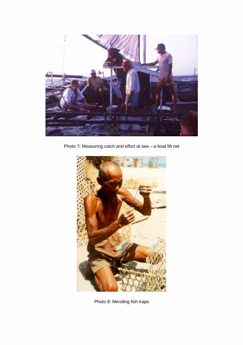
Photo 7: Measuring catch and effort at sea – a boat lift net
Photo 8: Mending fish traps
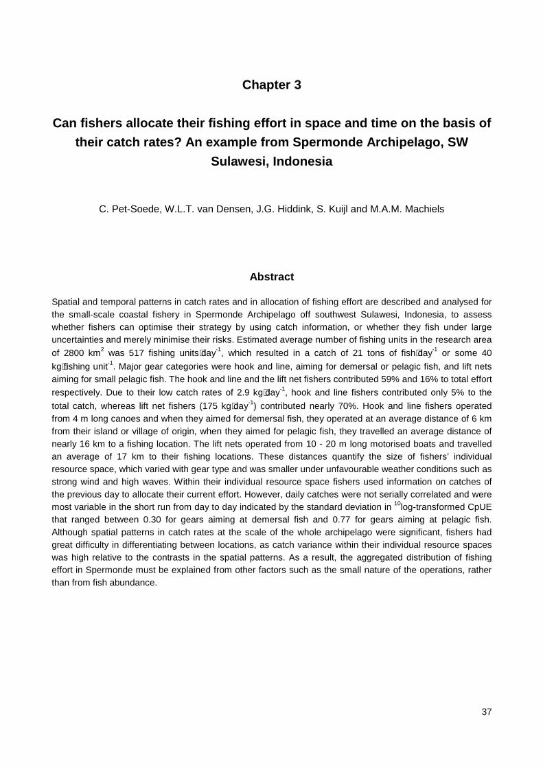
37
Chapter 3
Can fishers allocate their fishing effort in space and time on the basis oftheir catch rates? An example from Spermonde Archipelago, SW
Sulawesi, Indonesia
C. Pet-Soede, W.L.T. van Densen, J.G. Hiddink, S. Kuijl and M.A.M. Machiels
Abstract
Spatial and temporal patterns in catch rates and in allocation of fishing effort are described and analysed forthe small-scale coastal fishery in Spermonde Archipelago off southwest Sulawesi, Indonesia, to assesswhether fishers can optimise their strategy by using catch information, or whether they fish under largeuncertainties and merely minimise their risks. Estimated average number of fishing units in the research area
of 2800 km2 was 517 fishing units⋅day-1, which resulted in a catch of 21 tons of fish⋅day-1 or some 40
kg⋅fishing unit-1. Major gear categories were hook and line, aiming for demersal or pelagic fish, and lift netsaiming for small pelagic fish. The hook and line and the lift net fishers contributed 59% and 16% to total effort
respectively. Due to their low catch rates of 2.9 kg⋅day-1, hook and line fishers contributed only 5% to the
total catch, whereas lift net fishers (175 kg⋅day-1) contributed nearly 70%. Hook and line fishers operatedfrom 4 m long canoes and when they aimed for demersal fish, they operated at an average distance of 6 kmfrom their island or village of origin, when they aimed for pelagic fish, they travelled an average distance ofnearly 16 km to a fishing location. The lift nets operated from 10 - 20 m long motorised boats and travelledan average of 17 km to their fishing locations. These distances quantify the size of fishers’ individualresource space, which varied with gear type and was smaller under unfavourable weather conditions such asstrong wind and high waves. Within their individual resource space fishers used information on catches ofthe previous day to allocate their current effort. However, daily catches were not serially correlated and weremost variable in the short run from day to day indicated by the standard deviation in 10log-transformed CpUEthat ranged between 0.30 for gears aiming at demersal fish and 0.77 for gears aiming at pelagic fish.Although spatial patterns in catch rates at the scale of the whole archipelago were significant, fishers hadgreat difficulty in differentiating between locations, as catch variance within their individual resource spaceswas high relative to the contrasts in the spatial patterns. As a result, the aggregated distribution of fishingeffort in Spermonde must be explained from other factors such as the small nature of the operations, ratherthan from fish abundance.
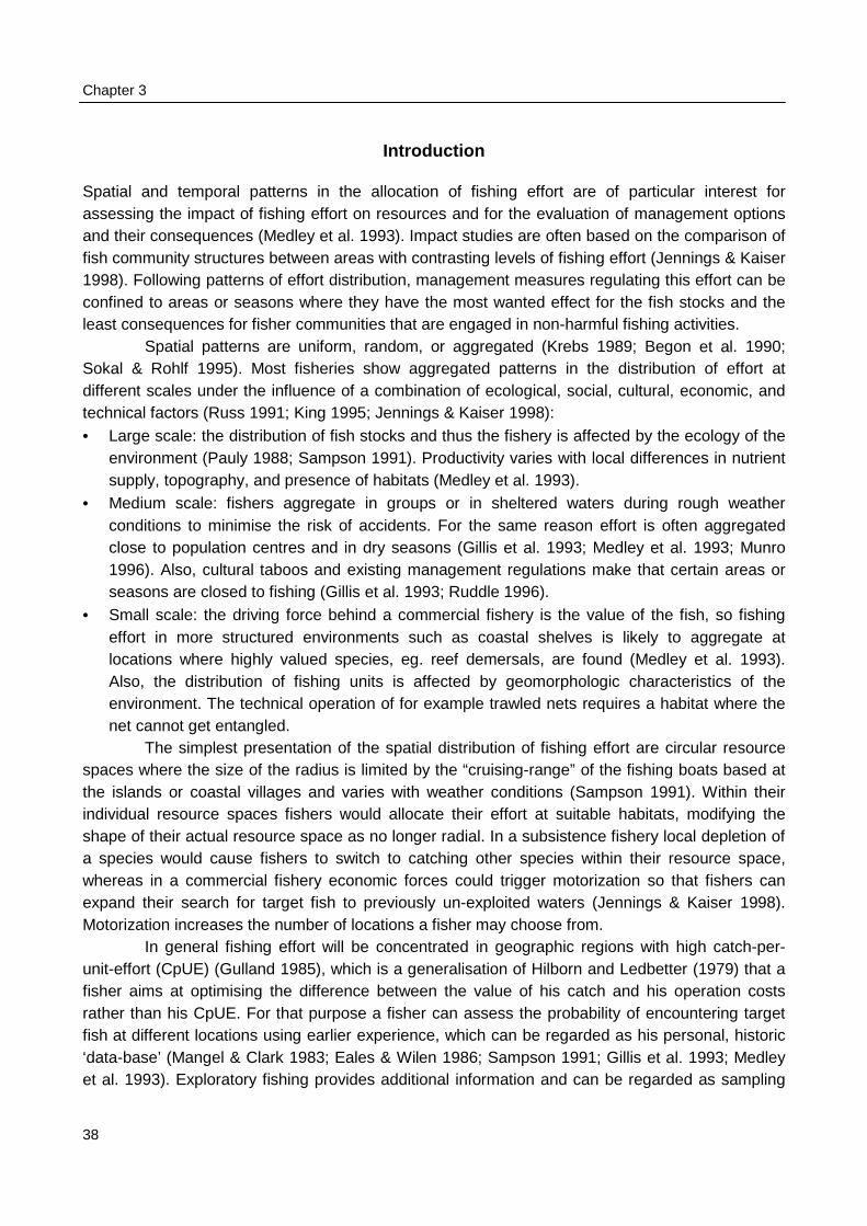
Chapter 3
38
Introduction
Spatial and temporal patterns in the allocation of fishing effort are of particular interest forassessing the impact of fishing effort on resources and for the evaluation of management optionsand their consequences (Medley et al. 1993). Impact studies are often based on the comparison offish community structures between areas with contrasting levels of fishing effort (Jennings & Kaiser1998). Following patterns of effort distribution, management measures regulating this effort can beconfined to areas or seasons where they have the most wanted effect for the fish stocks and theleast consequences for fisher communities that are engaged in non-harmful fishing activities.
Spatial patterns are uniform, random, or aggregated (Krebs 1989; Begon et al. 1990;Sokal & Rohlf 1995). Most fisheries show aggregated patterns in the distribution of effort atdifferent scales under the influence of a combination of ecological, social, cultural, economic, andtechnical factors (Russ 1991; King 1995; Jennings & Kaiser 1998):
• Large scale: the distribution of fish stocks and thus the fishery is affected by the ecology of theenvironment (Pauly 1988; Sampson 1991). Productivity varies with local differences in nutrientsupply, topography, and presence of habitats (Medley et al. 1993).
• Medium scale: fishers aggregate in groups or in sheltered waters during rough weatherconditions to minimise the risk of accidents. For the same reason effort is often aggregatedclose to population centres and in dry seasons (Gillis et al. 1993; Medley et al. 1993; Munro1996). Also, cultural taboos and existing management regulations make that certain areas orseasons are closed to fishing (Gillis et al. 1993; Ruddle 1996).
• Small scale: the driving force behind a commercial fishery is the value of the fish, so fishingeffort in more structured environments such as coastal shelves is likely to aggregate atlocations where highly valued species, eg. reef demersals, are found (Medley et al. 1993).Also, the distribution of fishing units is affected by geomorphologic characteristics of theenvironment. The technical operation of for example trawled nets requires a habitat where thenet cannot get entangled.
The simplest presentation of the spatial distribution of fishing effort are circular resourcespaces where the size of the radius is limited by the “cruising-range” of the fishing boats based atthe islands or coastal villages and varies with weather conditions (Sampson 1991). Within theirindividual resource spaces fishers would allocate their effort at suitable habitats, modifying theshape of their actual resource space as no longer radial. In a subsistence fishery local depletion ofa species would cause fishers to switch to catching other species within their resource space,whereas in a commercial fishery economic forces could trigger motorization so that fishers canexpand their search for target fish to previously un-exploited waters (Jennings & Kaiser 1998).Motorization increases the number of locations a fisher may choose from.
In general fishing effort will be concentrated in geographic regions with high catch-per-unit-effort (CpUE) (Gulland 1985), which is a generalisation of Hilborn and Ledbetter (1979) that afisher aims at optimising the difference between the value of his catch and his operation costsrather than his CpUE. For that purpose a fisher can assess the probability of encountering targetfish at different locations using earlier experience, which can be regarded as his personal, historic‘data-base’ (Mangel & Clark 1983; Eales & Wilen 1986; Sampson 1991; Gillis et al. 1993; Medleyet al. 1993). Exploratory fishing provides additional information and can be regarded as sampling
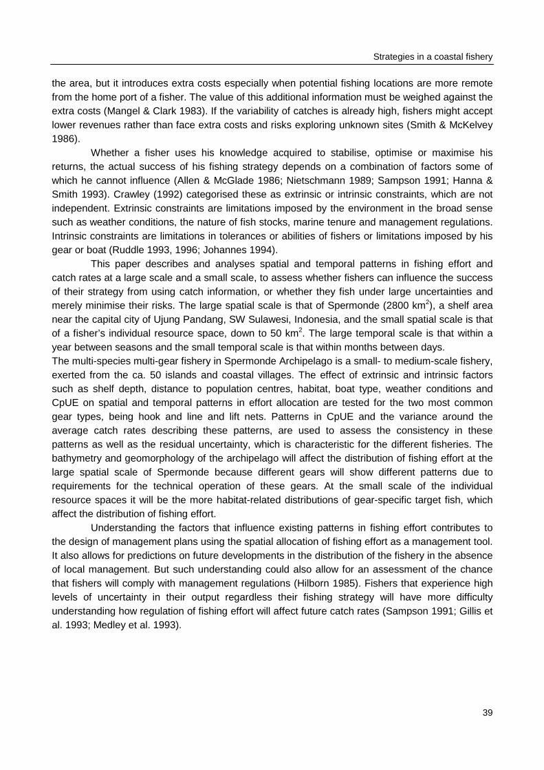
Strategies in a coastal fishery
39
the area, but it introduces extra costs especially when potential fishing locations are more remotefrom the home port of a fisher. The value of this additional information must be weighed against theextra costs (Mangel & Clark 1983). If the variability of catches is already high, fishers might acceptlower revenues rather than face extra costs and risks exploring unknown sites (Smith & McKelvey1986).
Whether a fisher uses his knowledge acquired to stabilise, optimise or maximise hisreturns, the actual success of his fishing strategy depends on a combination of factors some ofwhich he cannot influence (Allen & McGlade 1986; Nietschmann 1989; Sampson 1991; Hanna &Smith 1993). Crawley (1992) categorised these as extrinsic or intrinsic constraints, which are notindependent. Extrinsic constraints are limitations imposed by the environment in the broad sensesuch as weather conditions, the nature of fish stocks, marine tenure and management regulations.Intrinsic constraints are limitations in tolerances or abilities of fishers or limitations imposed by hisgear or boat (Ruddle 1993, 1996; Johannes 1994).
This paper describes and analyses spatial and temporal patterns in fishing effort andcatch rates at a large scale and a small scale, to assess whether fishers can influence the successof their strategy from using catch information, or whether they fish under large uncertainties andmerely minimise their risks. The large spatial scale is that of Spermonde (2800 km2), a shelf areanear the capital city of Ujung Pandang, SW Sulawesi, Indonesia, and the small spatial scale is thatof a fisher’s individual resource space, down to 50 km2. The large temporal scale is that within ayear between seasons and the small temporal scale is that within months between days.The multi-species multi-gear fishery in Spermonde Archipelago is a small- to medium-scale fishery,exerted from the ca. 50 islands and coastal villages. The effect of extrinsic and intrinsic factorssuch as shelf depth, distance to population centres, habitat, boat type, weather conditions andCpUE on spatial and temporal patterns in effort allocation are tested for the two most commongear types, being hook and line and lift nets. Patterns in CpUE and the variance around theaverage catch rates describing these patterns, are used to assess the consistency in thesepatterns as well as the residual uncertainty, which is characteristic for the different fisheries. Thebathymetry and geomorphology of the archipelago will affect the distribution of fishing effort at thelarge spatial scale of Spermonde because different gears will show different patterns due torequirements for the technical operation of these gears. At the small scale of the individualresource spaces it will be the more habitat-related distributions of gear-specific target fish, whichaffect the distribution of fishing effort.
Understanding the factors that influence existing patterns in fishing effort contributes tothe design of management plans using the spatial allocation of fishing effort as a management tool.It also allows for predictions on future developments in the distribution of the fishery in the absenceof local management. But such understanding could also allow for an assessment of the chancethat fishers will comply with management regulations (Hilborn 1985). Fishers that experience highlevels of uncertainty in their output regardless their fishing strategy will have more difficultyunderstanding how regulation of fishing effort will affect future catch rates (Sampson 1991; Gillis etal. 1993; Medley et al. 1993).
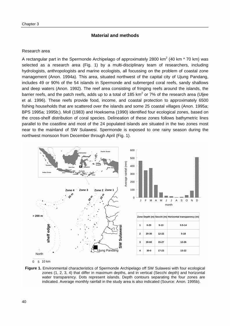
Chapter 3
4
Material and methods
Research area
A rectangular part in the Spermonde Archipelago of approximately 2800 km2 (40 km * 70 km) wasselected as a research area (Fig. 1) by a multi-disciplinary team of researchers, includinghydrologists, anthropologists and marine ecologists, all focussing on the problem of coastal zonemanagement (Anon. 1994a). This area, situated northwest of the capital city of Ujung Pandang,includes 49 or 90% of the 54 islands in Spermonde and submerged coral reefs, sandy shallowsand deep waters (Anon. 1992). The reef area consisting of fringing reefs around the islands, thebarrier reefs, and the patch reefs, adds up to a total of 185 km2 or 7% of the research area (Uljeeet al. 1996). These reefs provide food, income, and coastal protection to approximately 6500fishing households that are scattered over the islands and some 25 coastal villages (Anon. 1995a;BPS 1995a; 1995b;). Moll (1983) and Hoeksema (1990) identified four ecological zones, based onthe cross-shelf distribution of coral species. Delineation of these zones follows bathymetric linesparallel to the coastline and most of the 24 populated islands are situated in the two zones mostnear to the mainland of SW Sulawesi. Spermonde is exposed to one rainy season during thenorthwest monsoon from December through April (Fig. 1).
����������������
���������������������������������������������������������������������������������������������������������������������������������������
�������
����� ���������
��������������������������������������������
�������������������������������������������� ������������
����������������������������������������
���
������������������������������������������������������������������������������������������������
��������������������������������������������������������������������������������
��� ������
��������������������
������������
����������
������
�������������������
���������������������
����������������������������������������������������������������������������������������������������������������������
����������������������������
������������� ����������
���������
���
������������
AmbonSumatra
Timor
Bali
Lombok
Irian Jaya
Komodo
Flores
Sulawesi
Kalimantan
Java
Java Sea
Pacific Ocean
Indian Ocean
0 5 10 km
Ujung PandangNorth
SW
Su
law
esi
Zone 1Zone 2Zone 3Zone 4
shel
f ed
ge
> 200 m
30 m
30 m 20
m
Zone Depth (m) Secchi (m) Horizontal transparency (m)
1 0-20 5-13 0.5-14
2 20-30 12-22 5-18
3 30-60 15-27 12-26
4 30-0 17-23 13-22
J F M A M J J A S O N D
month
0
100
200
300
400
500
600
Ave
rage
rai
nfal
l (m
m) ��������
����������������������������������������������������������������
�������������������������������������������������
������������������������������������������������
������������������������������������
����������������
��������������
���������������������������
������������
���������������
��������������������������������������������������������������������������������
Figure 1. Environmental characteristics of Spermonde Archipelago off SW Sulawesi with four ecologicalzones (1, 2, 3, 4) that differ in maximum depths, and in vertical (Secchi depth) and horizontalwater transparency. Dots represent islands. Depth contours separating the four zones areindicated. Average monthly rainfall in the study area is also indicated (Source: Anon. 1995b).
0
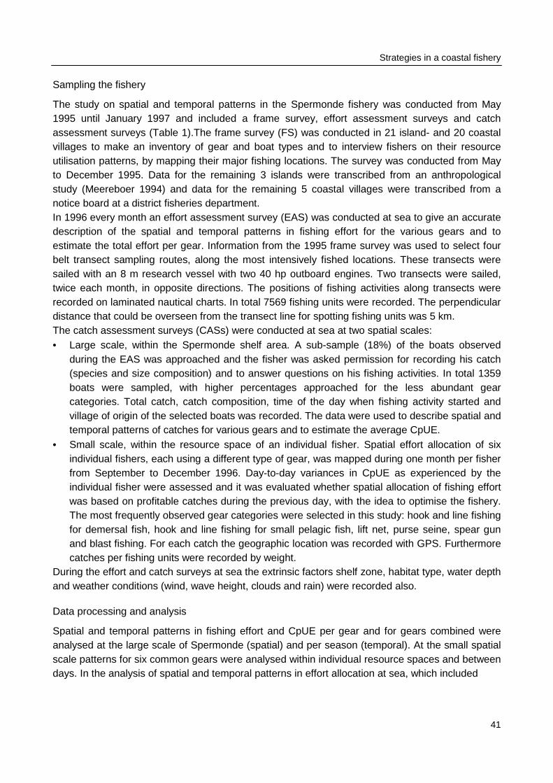
Strategies in a coastal fishery
41
Sampling the fishery
The study on spatial and temporal patterns in the Spermonde fishery was conducted from May1995 until January 1997 and included a frame survey, effort assessment surveys and catchassessment surveys (Table 1).The frame survey (FS) was conducted in 21 island- and 20 coastalvillages to make an inventory of gear and boat types and to interview fishers on their resourceutilisation patterns, by mapping their major fishing locations. The survey was conducted from Mayto December 1995. Data for the remaining 3 islands were transcribed from an anthropologicalstudy (Meereboer 1994) and data for the remaining 5 coastal villages were transcribed from anotice board at a district fisheries department.In 1996 every month an effort assessment survey (EAS) was conducted at sea to give an accuratedescription of the spatial and temporal patterns in fishing effort for the various gears and toestimate the total effort per gear. Information from the 1995 frame survey was used to select fourbelt transect sampling routes, along the most intensively fished locations. These transects weresailed with an 8 m research vessel with two 40 hp outboard engines. Two transects were sailed,twice each month, in opposite directions. The positions of fishing activities along transects wererecorded on laminated nautical charts. In total 7569 fishing units were recorded. The perpendiculardistance that could be overseen from the transect line for spotting fishing units was 5 km.The catch assessment surveys (CASs) were conducted at sea at two spatial scales:• Large scale, within the Spermonde shelf area. A sub-sample (18%) of the boats observed
during the EAS was approached and the fisher was asked permission for recording his catch(species and size composition) and to answer questions on his fishing activities. In total 1359boats were sampled, with higher percentages approached for the less abundant gearcategories. Total catch, catch composition, time of the day when fishing activity started andvillage of origin of the selected boats was recorded. The data were used to describe spatial andtemporal patterns of catches for various gears and to estimate the average CpUE.
• Small scale, within the resource space of an individual fisher. Spatial effort allocation of sixindividual fishers, each using a different type of gear, was mapped during one month per fisherfrom September to December 1996. Day-to-day variances in CpUE as experienced by theindividual fisher were assessed and it was evaluated whether spatial allocation of fishing effortwas based on profitable catches during the previous day, with the idea to optimise the fishery.The most frequently observed gear categories were selected in this study: hook and line fishingfor demersal fish, hook and line fishing for small pelagic fish, lift net, purse seine, spear gunand blast fishing. For each catch the geographic location was recorded with GPS. Furthermorecatches per fishing units were recorded by weight.
During the effort and catch surveys at sea the extrinsic factors shelf zone, habitat type, water depthand weather conditions (wind, wave height, clouds and rain) were recorded also.
Data processing and analysis
Spatial and temporal patterns in fishing effort and CpUE per gear and for gears combined wereanalysed at the large scale of Spermonde (spatial) and per season (temporal). At the small spatialscale patterns for six common gears were analysed within individual resource spaces and betweendays. In the analysis of spatial and temporal patterns in effort allocation at sea, which included
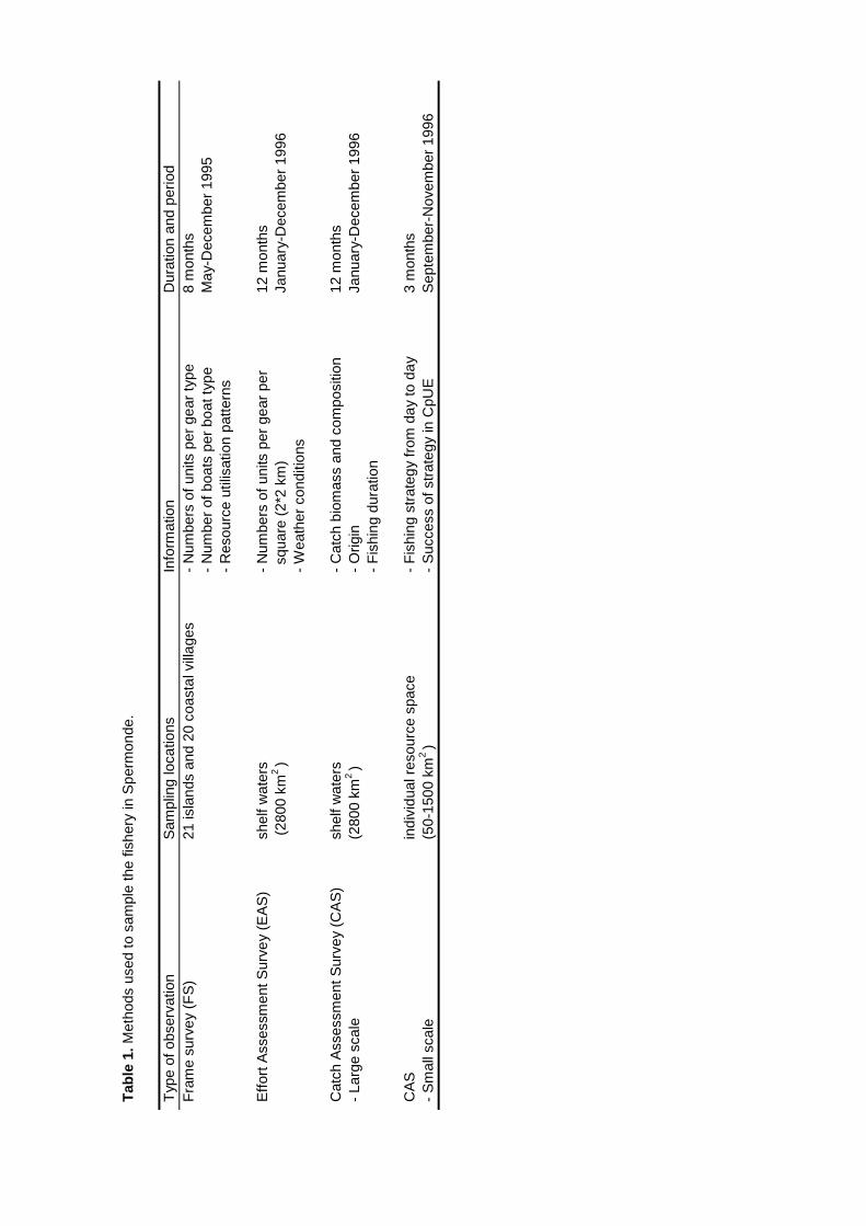
Tab
le 1
. Met
hods
use
d to
sam
ple
the
fishe
ry in
Spe
rmon
de.
Typ
e of
obs
erva
tion
Sam
plin
g lo
catio
nsIn
form
atio
nD
urat
ion
and
perio
dF
ram
e su
rvey
(F
S)
21 is
land
s an
d 20
coa
stal
vill
ages
- N
umbe
rs o
f uni
ts p
er g
ear
type
- N
umbe
r of
boa
ts p
er b
oat t
ype
- R
esou
rce
utili
satio
n pa
ttern
s
8 m
onth
sM
ay-D
ecem
ber
1995
Eff
ort A
sses
smen
t Sur
vey
(EA
S)
shel
f wat
ers
(28
00 k
m2 )
- N
umbe
rs o
f uni
ts p
er g
ear
per
squ
are
(2*2
km
)-
Wea
ther
con
ditio
ns
12 m
onth
sJa
nuar
y-D
ecem
ber
1996
Cat
ch A
sses
smen
t Sur
vey
(CA
S)
- La
rge
scal
esh
elf w
ater
s(2
800
km2 )
- C
atch
bio
mas
s an
d co
mpo
sitio
n-
Orig
in-
Fis
hing
dur
atio
n
12 m
onth
sJa
nuar
y-D
ecem
ber
1996
CA
S-
Sm
all s
cale
indi
vidu
al r
esou
rce
spac
e(5
0-15
00 k
m2 )
- F
ishi
ng s
trat
egy
from
day
to d
ay
- S
ucce
ss o
f str
ateg
y in
CpU
E3
mon
ths
Sep
tem
ber-
Nov
embe
r 19
96
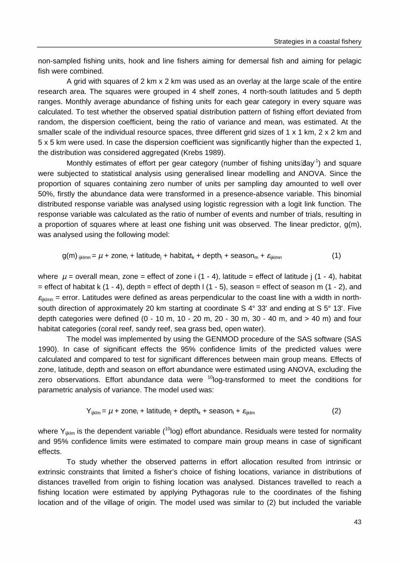
Strategies in a coastal fishery
43
non-sampled fishing units, hook and line fishers aiming for demersal fish and aiming for pelagicfish were combined.
A grid with squares of 2 km x 2 km was used as an overlay at the large scale of the entireresearch area. The squares were grouped in 4 shelf zones, 4 north-south latitudes and 5 depthranges. Monthly average abundance of fishing units for each gear category in every square wascalculated. To test whether the observed spatial distribution pattern of fishing effort deviated fromrandom, the dispersion coefficient, being the ratio of variance and mean, was estimated. At thesmaller scale of the individual resource spaces, three different grid sizes of 1 x 1 km, 2 x 2 km and5 x 5 km were used. In case the dispersion coefficient was significantly higher than the expected 1,the distribution was considered aggregated (Krebs 1989).
Monthly estimates of effort per gear category (number of fishing units⋅day-1) and squarewere subjected to statistical analysis using generalised linear modelling and ANOVA. Since theproportion of squares containing zero number of units per sampling day amounted to well over50%, firstly the abundance data were transformed in a presence-absence variable. This binomialdistributed response variable was analysed using logistic regression with a logit link function. Theresponse variable was calculated as the ratio of number of events and number of trials, resulting ina proportion of squares where at least one fishing unit was observed. The linear predictor, g(m),was analysed using the following model:
g(m) ijklmn = µ + zonei + latitudej + habitatk + depthl + seasonm + εijklmn (1)
where µ = overall mean, zone = effect of zone i (1 - 4), latitude = effect of latitude j (1 - 4), habitat= effect of habitat k (1 - 4), depth = effect of depth l (1 - 5), season = effect of season m (1 - 2), and
εijklmn = error. Latitudes were defined as areas perpendicular to the coast line with a width in north-
south direction of approximately 20 km starting at coordinate S 4° 33′ and ending at S 5° 13′. Fivedepth categories were defined (0 - 10 m, 10 - 20 m, 20 - 30 m, 30 - 40 m, and > 40 m) and fourhabitat categories (coral reef, sandy reef, sea grass bed, open water).
The model was implemented by using the GENMOD procedure of the SAS software (SAS1990). In case of significant effects the 95% confidence limits of the predicted values werecalculated and compared to test for significant differences between main group means. Effects ofzone, latitude, depth and season on effort abundance were estimated using ANOVA, excluding thezero observations. Effort abundance data were 10log-transformed to meet the conditions forparametric analysis of variance. The model used was:
Yijklm = µ + zonei + latitudej + depthk + seasonl + εijklm (2)
where Yijklm is the dependent variable (10log) effort abundance. Residuals were tested for normalityand 95% confidence limits were estimated to compare main group means in case of significanteffects.
To study whether the observed patterns in effort allocation resulted from intrinsic orextrinsic constraints that limited a fisher’s choice of fishing locations, variance in distributions ofdistances travelled from origin to fishing location was analysed. Distances travelled to reach afishing location were estimated by applying Pythagoras rule to the coordinates of the fishinglocation and of the village of origin. The model used was similar to (2) but included the variable
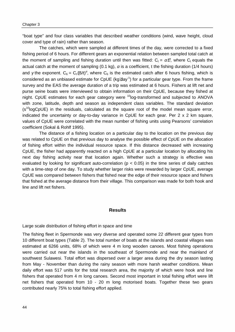
Chapter 3
44
“boat type” and four class variables that described weather conditions (wind, wave height, cloudcover and type of rain) rather than season.
The catches, which were sampled at different times of the day, were corrected to a fixedfishing period of 6 hours. For different gears an exponential relation between sampled total catch atthe moment of sampling and fishing duration until then was fitted: Ct = α⋅tγ, where Ct equals the
actual catch at the moment of sampling (0.1 kg), α is a coefficient, t the fishing duration (1/4 hours)
and γ the exponent. C6 = Ct⋅(6/t)α, where C6 is the estimated catch after 6 hours fishing, which is
considered as an unbiased estimate for CpUE (kg⋅day-1) for a particular gear type. From the framesurvey and the EAS the average duration of a trip was estimated at 6 hours. Fishers at lift net andpurse seine boats were interviewed to obtain information on their CpUE, because they fished atnight. CpUE estimates for each gear category were 10log-transformed and subjected to ANOVAwith zone, latitude, depth and season as independent class variables. The standard deviation(s10logCpUE) in the residuals, calculated as the square root of the model mean square error,indicated the uncertainty or day-to-day variance in CpUE for each gear. Per 2 x 2 km square,values of CpUE were correlated with the mean number of fishing units using Pearsons’ correlationcoefficient (Sokal & Rohlf 1995).
The distance of a fishing location on a particular day to the location on the previous daywas related to CpUE on that previous day to analyse the possible effect of CpUE on the allocationof fishing effort within the individual resource space. If this distance decreased with increasingCpUE, the fisher had apparently reacted on a high CpUE at a particular location by allocating hisnext day fishing activity near that location again. Whether such a strategy is effective wasevaluated by looking for significant auto-correlation (p < 0.05) in the time series of daily catcheswith a time-step of one day. To study whether larger risks were rewarded by larger CpUE, averageCpUE was compared between fishers that fished near the edge of their resource space and fishersthat fished at the average distance from their village. This comparison was made for both hook andline and lift net fishers.
Results
Large scale distribution of fishing effort in space and time
The fishing fleet in Spermonde was very diverse and operated some 22 different gear types from10 different boat types (Table 2). The total number of boats at the islands and coastal villages wasestimated at 6266 units, 68% of which were 4 m long wooden canoes. Most fishing operationswere carried out near the islands in the southeast of Spermonde and near the mainland ofsouthwest Sulawesi. Total effort was dispersed over a larger area during the dry season lastingfrom May - November than during the rainy season with more harsh weather conditions. Meandaily effort was 517 units for the total research area, the majority of which were hook and linefishers that operated from 4 m long canoes. Second most important in total fishing effort were liftnet fishers that operated from 10 - 20 m long motorised boats. Together these two gearscontributed nearly 75% to total fishing effort applied.
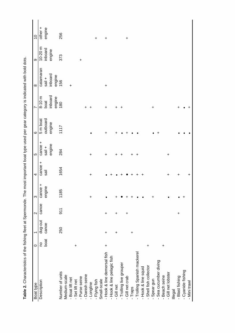
Tab
le 2
. Cha
ract
eris
tics
of th
e fis
hing
flee
t at S
perm
onde
. The
mos
t im
port
ant b
oat t
ype
used
per
gea
r ca
tego
ry is
indi
cate
d w
ith b
old
dots
.
Boa
t typ
e0
12
34
56
78
910
Des
crip
tion
no boat
dug-
out
cano
eca
noe
cano
e +
engi
neca
noe
+sa
ilca
noe
+sa
il +
engi
ne
5 m
boa
tou
tboa
rden
gine
8-10
mbo
atin
boar
den
gine
cata
mar
ansa
il +
inbo
ard
engi
ne
10-2
0 m
inbo
ard
engi
ne
othe
r +
engi
ne
Num
ber
of u
nits
250
911
1185
1654
284
1117
180
156
373
256
Med
ium
-sca
le-
Boa
t lift
net
+-
Set
lift
net
+-
Pur
se s
eine
+-
Dan
ish
sein
e+
- Lo
nglin
e+
++
• •••+
- F
lyin
g fis
h+
Sm
all-s
cale
- H
ook
& li
ne d
emer
sal f
ish
++
+• •••
• •••+
++
++
- H
ook
& li
ne p
elag
ic fi
sh+
- G
ill n
et+
++
• •••+
++
- T
rolli
ng li
ve g
roup
er●
++
• •••+
- G
ill n
et c
rab
++
●+
+-
Tra
ps+
++
+• •••
- T
rolli
ng S
pani
sh m
acke
rel
• •••+
+• •••
- H
ook
& li
ne s
quid
• •••+
- S
hell
fish
colle
ctor
+-
Spe
ar g
un+
• •••+
- S
ea c
ucum
ber
divi
ng+
- B
each
sei
ne+
- G
ill n
et lo
bste
r• •••
++
Illeg
al-
Bla
st fi
shin
g+
• •••+
• •••+
- C
yani
de fi
shin
g+
• •••• •••
- M
ini t
raw
l+
• •••+
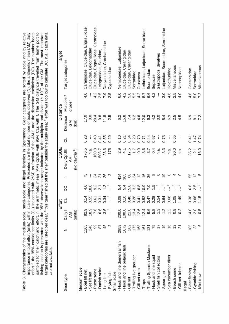
Tab
le 3
. C
hara
cter
istic
s of
the
med
ium
-sca
le,
smal
l-sca
le a
nd i
llega
l fis
herie
s in
Spe
rmon
de.
Gea
r ca
tego
ries
are
sort
ed b
y sc
ale
and
by r
elat
ive
impo
rtan
ce in
tota
l effo
rt (
units
) w
ithin
sca
le c
ateg
orie
s. P
rese
nted
are
the
tot
al n
umbe
r of
boa
ts o
bser
ved
(N),
the
arit
hmet
ic m
ean
(AM
) da
ilyef
fort
f,
the
95%
con
fiden
ce l
imits
(C
L) i
ndic
ated
with
2*S
E a
s fr
actio
n of
the
AM
f,
and
the
disp
ersi
on c
oeffi
cien
t (D
C).
The
num
ber
boat
ssa
mpl
ed f
or t
heir
catc
h an
d ef
fort
, n,
the
arit
hmet
ic m
ean
(AM
) C
pUE
with
95%
CLs
with
f.
The
GM
dis
tanc
e tr
avel
led
from
hom
e po
rt t
ofis
hing
loca
tion
is p
rese
nted
with
the
95%
obs
erva
tions
ran
ge i
ndic
ated
by
the
mul
tiplie
r an
d di
vide
r (*
: 10
2s)
of t
he G
M.
The
mos
t im
port
ant
targ
et c
ateg
orie
s ar
e lis
ted
per
gear
. a this
gea
r fis
hed
off t
he s
helf
outs
ide
the
stud
y ar
ea; b e
ffort
was
too
low
to c
alcu
late
DC
. n.a
.: ca
tch
data
are
not a
vaila
ble.
Effo
rtC
pUE
Dis
tanc
eT
arge
tG
ear
type
ND
aily
fA
M(u
nits
)
CL
DC
nD
aily
CpU
EA
M(k
g·da
ytrip
-1)
CL
Dis
tanc
eG
M(k
m)
Mul
tiplie
r/di
vide
rT
arge
t cat
egor
ies
Med
ium
sca
le-
Boa
t lift
net
1165
82.9
0.14
4.6
7517
6.5
0.28
17.0
4.0
Car
angi
dae,
Clu
peid
ae, E
ngra
ulid
ae-
Set
lift
net
246
18.9
0.55
18.8
---
n.a.
---
0.0
---
Clu
peid
ae, L
eiog
natid
ae-
Pur
se s
eine
997.
60.
619.
224
160.
80.
4820
.44.
2C
lupe
idae
, Eng
raul
idae
, Car
angi
dae
- D
anis
h se
ine
876.
60.
312.
121
503.
70.
419.
82.
5Le
iogn
atid
ae, S
aurid
ae,
- Lo
ng li
ne48
3.6
0.34
1.3
2628
.60.
5511
.87.
9D
asya
tidid
ae, C
arch
arin
idae
- F
lyin
g fis
h2
---a
--- a
--- a
217
50.
292.
52.
5C
ypse
lurid
aeS
mal
l sca
le-
Hoo
k an
d lin
e de
mer
sal f
ish
2959
200.
00.
085.
441
42.
90.
106.
26.
0N
emip
terid
ae, L
utja
nida
e-
Hoo
k an
d lin
e pe
lagi
c fis
h16
7210
0.0
0.10
5.4
365
4.1
0.21
15.8
4.2
Clu
peid
ae, C
aran
gida
e-
Gill
net
282
21.0
0.48
15.8
6817
.50.
547.
45.
8C
lupe
idae
, Car
angi
dae
- T
rolli
ng li
ve g
roup
er17
513
.40.
283.
313
41.
70.
236.
25.
5S
erra
nida
e-
Gill
net
cra
b16
812
.60.
416.
812
0.9
0.70
4.6
4.2
Cru
stac
ea-
Tra
ps16
112
.40.
5210
.916
8.6
0.71
12.0
8.7
Leth
rinid
ae, L
utja
nida
e, S
erra
nida
e-
Tro
lling
Spa
nish
Mac
kere
l13
19.
60.
477.
036
3.7
0.44
9.3
6.6
Sco
mbr
idae
- H
ook
and
line
squi
d75
5.8
0.28
1.5
80.
40.
674.
24.
2S
epiid
ae-
She
ll fis
h co
llect
ors
171.
30.
54--
- b0
n.a.
---
0.0
---
Gas
trop
ods,
Biv
alve
s-
Spe
ar g
un19
1.2
0.64
--- b
193.
30.
735.
43.
0Lu
tjani
dae,
Sco
mbr
idae
, Ser
rani
dae
- S
ea c
ucum
ber
dive
r16
1.2
0.68
--- b
0n.
a.--
-6.
94.
6H
olot
hurid
ae-
Bea
ch s
eine
120.
91.
05--
- b4
30.0
0.65
2.5
2.5
Mis
cella
neou
s-
Gill
net
lob
ster
210.
21.
49--
- b0
n.a.
---
4.5
4.0
Nep
hrop
idae
Illeg
al-
Bla
st fi
shin
g18
514
.00.
386.
655
35.2
0.41
6.9
4.6
Cae
sion
idae
- C
yani
de fi
shin
g23
2.0
0.66
2.5
122.
11.
478.
15.
0S
erra
nida
e-
Min
i tra
wl
60.
51.
15--
- b5
16.0
0.74
7.2
7.2
Mis
cella
neou
s
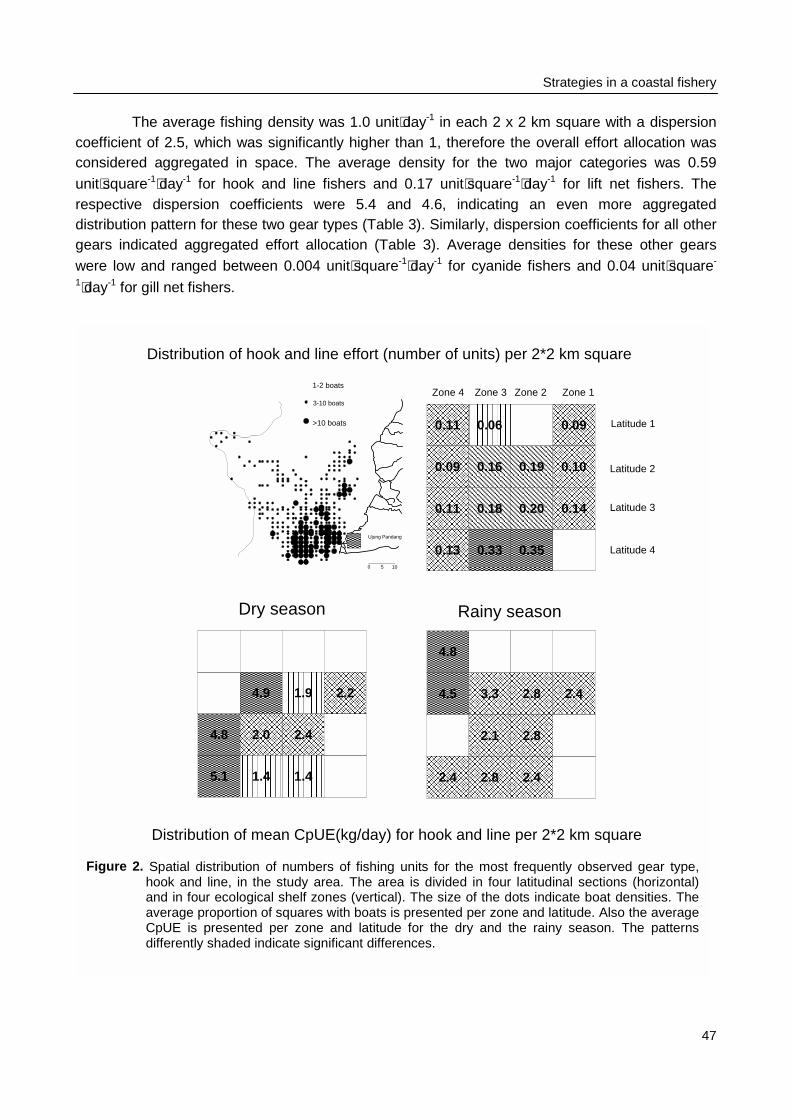
Strategies in a coastal fishery
47
The average fishing density was 1.0 unit⋅day-1 in each 2 x 2 km square with a dispersioncoefficient of 2.5, which was significantly higher than 1, therefore the overall effort allocation wasconsidered aggregated in space. The average density for the two major categories was 0.59
unit⋅square-1⋅day-1 for hook and line fishers and 0.17 unit⋅square-1⋅day-1 for lift net fishers. Therespective dispersion coefficients were 5.4 and 4.6, indicating an even more aggregateddistribution pattern for these two gear types (Table 3). Similarly, dispersion coefficients for all othergears indicated aggregated effort allocation (Table 3). Average densities for these other gearswere low and ranged between 0.004 unit⋅square-1⋅day-1 for cyanide fishers and 0.04 unit⋅square-
1⋅day-1 for gill net fishers.
0 5 10
�������������������� Ujung Pandang
1-2 boats
3-10 boats
>10 boats
Distribution of hook and line effort (number of units) per 2*2 km square
Distribution of mean CpUE(kg/day) for hook and line per 2*2 km square
Dry season Rainy season
Latitude 1
Latitude 2
Latitude 3
Latitude 4
������������������������������������������������������������ �����������������
���������������������������������������������������
������������������������������������������������������������������������
��������������������������������������������������������������������������������
�����������������������������������������������������������������������������������������������������
���������������������������������������������������
�����������������������������������������������������������������������������������������������������
���������������������������������������������������
��������������������������������������������������������������������������������
������������������������������������������������������������������������������������
4.8
2.1
4.5 3.3 2.8 2.4
2.8
2.4 2.8 2.4
������������������������������������������������������������������������
��������������������������������������������������������������������������������
�����������������������������������������������������������������������������������������������������
����������������������������������
������������������������������������������������������
������������������������������������������������������������
��������������������������������������������������������������������������������
���������������������������������������������������
������������������������������������������������������������������������
��������������������������������������������������������������������������������
�����������������������������������������������������������������������������������������������������
���������������������������������������������������
��������������������������������������������������������������������������������
������������������������������������������������������������������������������������
0.19 0.10
0.11 0.18 0.20
0.13 0.33 0.35
0.11 0.06 0.09
0.14
0.160.09
����������������������������������������������������������������������������
��������������������������������������������������������������������������������
�����������������������������������������������������������������������������������������������
���������������������������������������������������������
����������������������������������������������������������������������������
�����������������������������������������������������������������������������������������������
��������������������������������������
���������������������������������������������������������
���������������������������������������������������������
1.9 2.2
4.8 2.0 2.4
5.1 1.4 1.4
4.9
Zone 1Zone 2Zone 3Zone 4
Figure 2. Spatial distribution of numbers of fishing units for the most frequently observed gear type,hook and line, in the study area. The area is divided in four latitudinal sections (horizontal)and in four ecological shelf zones (vertical). The size of the dots indicate boat densities. Theaverage proportion of squares with boats is presented per zone and latitude. Also the averageCpUE is presented per zone and latitude for the dry and the rainy season. The patternsdifferently shaded indicate significant differences.
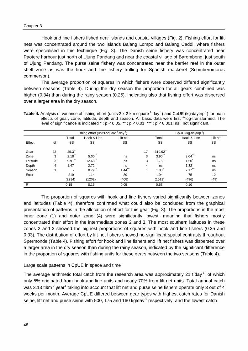
Chapter 3
48
Hook and line fishers fished near islands and coastal villages (Fig. 2). Fishing effort for liftnets was concentrated around the two islands Balang Lompo and Balang Caddi, where fisherswere specialised in this technique (Fig. 3). The Danish seine fishery was concentrated nearPaotere harbour just north of Ujung Pandang and near the coastal village of Barombong, just southof Ujung Pandang. The purse seine fishery was concentrated near the barrier reef in the outershelf zone as was the hook and line fishery trolling for Spanish mackerel (Scomberomoruscommerson).
The average proportion of squares in which fishers were observed differed significantlybetween seasons (Table 4). During the dry season the proportion for all gears combined washigher (0.34) than during the rainy season (0.25), indicating also that fishing effort was dispersedover a larger area in the dry season.
Table 4. Analysis of variance of fishing effort (units·2 x 2 km square-1·day-1) and CpUE (kg·daytrip-1) for maineffects of gear, zone, latitude, depth and season. All basic data were first 10log-transformed. Thelevel of significance is indicated * : p < 0.05, ** : p < 0.01; *** : p < 0.001; ns : not significant.
Fishing effort (units·square-1·day-1) CpUE (kg·daytrip-1)
Total Hook & Line Lift net Total Hook & Line Lift netEffect df SS SS SS SS SS SS
Gear 22 25.3*** 17 319.92***
Zone 3 2.18*** 5.00 ** ns 3 3.90*** 3.04*** nsLatitude 3 9.91*** 12.63 ** ns 3 1.75* 1.50* nsDepth 4 1.47* 2.72 ** ns 4 ns 1.82* nsSeason 1 - 0.79 ** 1.44*** 1 1.83** 2.17*** nsError 219
(2234)114
(1202)39
(408)194
(1011)75
(496)12(49)
R2 0.15 0.16 0.05 0.63 0.10
The proportion of squares with hook and line fishers varied significantly between zonesand latitudes (Table 4), therefore confirmed what could also be concluded from the graphicalpresentation of patterns in the allocation of effort for this gear (Fig. 3). The proportions in the mostinner zone (1) and outer zone (4) were significantly lowest, meaning that fishers mostlyconcentrated their effort in the intermediate zones 2 and 3. The most southern latitudes in thesezones 2 and 3 showed the highest proportions of squares with hook and line fishers (0.35 and0.33). The distribution of effort by lift net fishers showed no significant spatial contrasts throughoutSpermonde (Table 4). Fishing effort for hook and line fishers and lift net fishers was dispersed overa larger area in the dry season than during the rainy season, indicated by the significant differencein the proportion of squares with fishing units for these gears between the two seasons (Table 4).
Large scale patterns in CpUE in space and time
The average arithmetic total catch from the research area was approximately 21 t⋅day-1, of whichonly 5% originated from hook and line units and nearly 70% from lift net units. Total annual catchwas 3.13 t⋅km-2⋅year1 taking into account that lift net and purse seine fishers operate only 3 out of 4weeks per month. Average CpUE differed between gear types with highest catch rates for Danish
seine, lift net and purse seine with 500, 175 and 160 kg⋅day-1 respectively, and the lowest catch
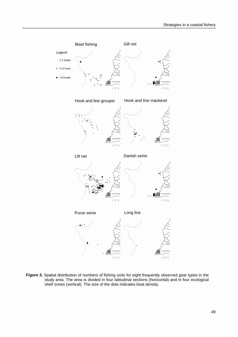
Strategies in a coastal fishery
0 5 10
���������������� Ujung Pandang
0 5 10
������������������ Ujung Pandang
0 5 10
������������������ Ujung Pandang
0 5 10
������������������ Ujung Pandang
Blast fishing Gill net
Hook and line mackerelHook and line grouper
Legend
1-2 boats
3-10 boats
>10 boats
0 5 10
���������������� Ujung Pandang
0 5 10
���������� Ujung Pandang
0 5 10
���������Ujung Pandang
0 5 10
�����Ujung Pandang
Lift net Danish seine
Long linePurse seine
Figure 3. Spatial distribution of numbers of fishing units for eight frequently observed gear types in thestudy area. The area is divided in four latitudinal sections (horizontal) and in four ecologicalshelf zones (vertical). The size of the dots indicates boat density.
49
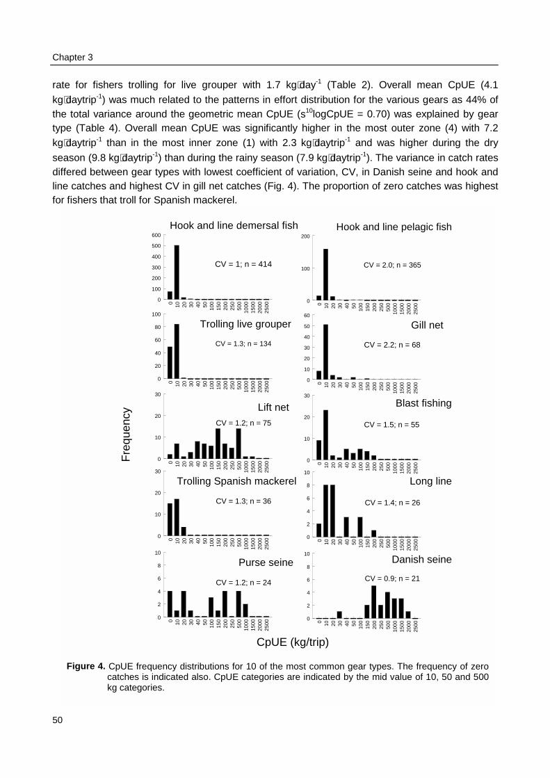
Chapter 3
50
rate for fishers trolling for live grouper with 1.7 kg⋅day-1 (Table 2). Overall mean CpUE (4.1
kg⋅daytrip-1) was much related to the patterns in effort distribution for the various gears as 44% ofthe total variance around the geometric mean CpUE (s10logCpUE = 0.70) was explained by geartype (Table 4). Overall mean CpUE was significantly higher in the most outer zone (4) with 7.2
kg⋅daytrip-1 than in the most inner zone (1) with 2.3 kg⋅daytrip-1 and was higher during the dry
season (9.8 kg⋅daytrip-1) than during the rainy season (7.9 kg⋅daytrip-1). The variance in catch ratesdiffered between gear types with lowest coefficient of variation, CV, in Danish seine and hook andline catches and highest CV in gill net catches (Fig. 4). The proportion of zero catches was highestfor fishers that troll for Spanish mackerel.
Figure
010 20 30 40 50 10
015
020
025
050
010
0015
0020
0025
00
0
100
200
300
400
500
600
CV = 1; n = 414
0 10 20 30 40 50 100
150
200
250
500
1000
1500
2000
2500
0
100
200
CV = 2.0; n = 365
0 10 20 30 40 50 100
150
200
250
500
1000
1500
2000
2500
0
20
40
60
80
100
CV = 1.3; n = 134
010 20 30 40 50 10
015
020
025
050
010
0015
0020
0025
00
0
10
20
30
40
50
60
CV = 2.2; n = 68
0 10 20 30 40 50 100
150
200
250
500
1000
1500
2000
2500
0
10
20
30
CV = 1.2; n = 75
010 20 30 40 50 10
015
020
025
050
010
0015
0020
0025
00
0
10
20
30
CV = 1.5; n = 55
0 10 20 30 40 50 100
150
200
250
500
1000
1500
2000
2500
0
10
20
30
CV = 1.3; n = 36
0 10 20 30 40 50 100
150
200
250
500
1000
1500
2000
2500
0
2
4
6
8
10
CV = 1.4; n = 26
0 10 20 30 40 50 100
150
200
250
500
1000
1500
2000
2500
0
2
4
6
8
10
CV = 1.2; n = 24
0 10 20 30 40 50 100
150
200
250
500
1000
1500
2000
2500
0
2
4
6
8
10
CV = 0.9; n = 21
Fre
quen
cy
CpUE (kg/trip)
Hook and line demersal fish Hook and line pelagic fish
Gill netTrolling live grouper
Lift net Blast fishing
Long line
Danish seinePurse seine
Trolling Spanish mackerel
4. CpUE frequency distributions for 10 of the most common gear types. The frequency of zerocatches is indicated also. CpUE categories are indicated by the mid value of 10, 50 and 500kg categories.
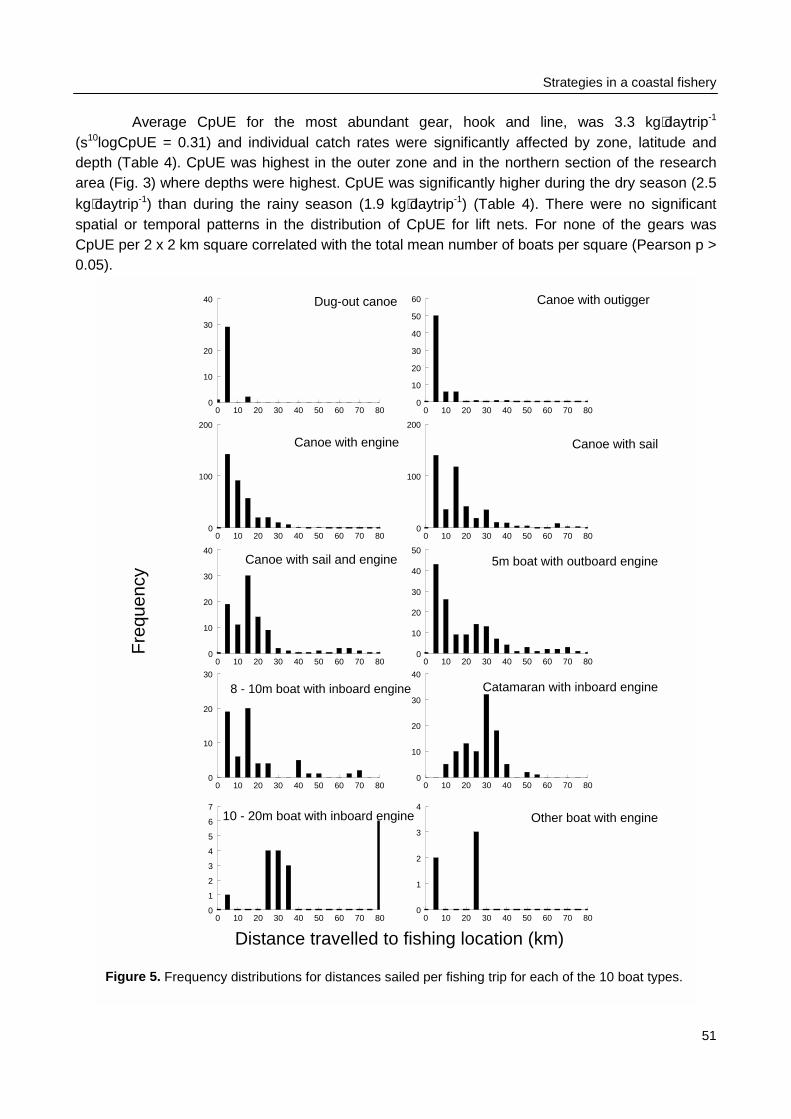
Strategies in a coastal fishery
51
Average CpUE for the most abundant gear, hook and line, was 3.3 kg⋅daytrip-1
(s10logCpUE = 0.31) and individual catch rates were significantly affected by zone, latitude anddepth (Table 4). CpUE was highest in the outer zone and in the northern section of the researcharea (Fig. 3) where depths were highest. CpUE was significantly higher during the dry season (2.5
kg⋅daytrip-1) than during the rainy season (1.9 kg⋅daytrip-1) (Table 4). There were no significantspatial or temporal patterns in the distribution of CpUE for lift nets. For none of the gears wasCpUE per 2 x 2 km square correlated with the total mean number of boats per square (Pearson p >0.05).
0 10 20 30 40 50 60 70 800
10
20
30
40
0 10 20 30 40 50 60 70 800
10
20
30
40
50
60
0 10 20 30 40 50 60 70 800
100
200
0 10 20 30 40 50 60 70 800
100
200
0 10 20 30 40 50 60 70 800
10
20
30
40
0 10 20 30 40 50 60 70 800
10
20
30
40
50
0 10 20 30 40 50 60 70 800
10
20
30
0 10 20 30 40 50 60 70 800
10
20
30
40
0 10 20 30 40 50 60 70 800
1
2
3
4
5
6
7
0 10 20 30 40 50 60 70 800
1
2
3
4
Dug-out canoe Canoe with outigger
Canoe with sailCanoe with engine
Canoe with sail and engine
8 - 10m boat with inboard engine
10 - 20m boat with inboard engine Other boat with engine
Catamaran with inboard engine
5m boat with outboard engine
Fre
quen
cy
Distance travelled to fishing location (km)
Figure 5. Frequency distributions for distances sailed per fishing trip for each of the 10 boat types.
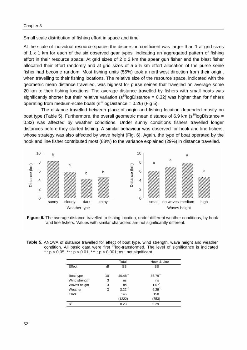
Chapter 3
5
Small scale distribution of fishing effort in space and time
At the scale of individual resource spaces the dispersion coefficient was larger than 1 at grid sizesof 1 x 1 km for each of the six observed gear types, indicating an aggregated pattern of fishingeffort in their resource space. At grid sizes of 2 x 2 km the spear gun fisher and the blast fisherallocated their effort randomly and at grid sizes of 5 x 5 km effort allocation of the purse seinefisher had become random. Most fishing units (55%) took a northwest direction from their origin,when travelling to their fishing locations. The relative size of the resource space, indicated with thegeometric mean distance travelled, was highest for purse seines that travelled on average some20 km to their fishing locations. The average distance travelled by fishers with small boats wassignificantly shorter but their relative variation (s10logDistance = 0.32) was higher than for fishersoperating from medium-scale boats (s10logDistance = 0.26) (Fig 5).
The distance travelled between place of origin and fishing location depended mostly onboat type (Table 5). Furthermore, the overall geometric mean distance of 6.9 km (s10logDistance =0.32) was affected by weather conditions. Under sunny conditions fishers travelled longerdistances before they started fishing. A similar behaviour was observed for hook and line fishers,whose strategy was also affected by wave height (Fig. 6). Again, the type of boat operated by thehook and line fisher contributed most (88%) to the variance explained (29%) in distance travelled.
sunny cloudy dark rainy
Weather type
0
2
4
6
8
10
Dis
tanc
e (k
m)
������������������������������������������������������������������������������������������������������������������������������������������������������������������
���������������������������������������������������������������������������������������������������������
��������������������������������������������������������������������������������
�������������������������������������������������������������������������������������
a
b
b b
small no waves medium high
Waves height
0
2
4
6
8
10
Dis
tanc
e (k
m)
����������������������������������������������������������������������������������������������������������������
����������������������������������������������������������������������������������������������������������������������������������������
���������������������������������������������������������������������������������������������������������������������������������������������������������������������������
������������������������������������������������������������������������������������������������
aa
a
b
Figure 6. The average distance travelled to fishing location, under different weather conditions, by hookand line fishers. Values with similar characters are not significantly different.
2
Table 5. ANOVA of distance travelled for effect of boat type, wind strength, wave height and weathercondition. All basic data were first 10log-transformed. The level of significance is indicated* : p < 0.05, ** : p < 0.01; *** : p < 0.001; ns : not significant.
Total Hook & Line
Effect df SS SS
Boat type 10 40.48*** 56.79***
Wind strength 3 ns nsWaves height 3 ns 1.67*
Weather 3 3.22*** 6.29***
Error 145(1222)
158(753)
R2 0.23 0.29
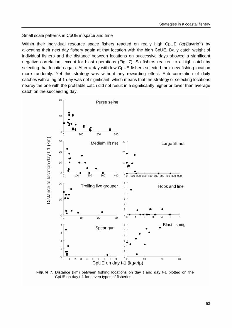
Strategies in a coastal fishery
Small scale patterns in CpUE in space and time
Within their individual resource space fishers reacted on really high CpUE (kg⋅daytrip-1) byallocating their next day fishery again at that location with the high CpUE. Daily catch weight ofindividual fishers and the distance between locations on successive days showed a significantnegative correlation, except for blast operations (Fig. 7). So fishers reacted to a high catch byselecting that location again. After a day with low CpUE fishers selected their new fishing locationmore randomly. Yet this strategy was without any rewarding effect. Auto-correlation of dailycatches with a lag of 1 day was not significant, which means that the strategy of selecting locationsnearby the one with the profitable catch did not result in a significantly higher or lower than averagecatch on the succeeding day.
Figu
0 100 200 3000
10
20Purse seine
Blast fishing
Medium lift net Large lift net
Trolling live grouper
Spear gun
Hook and line
0 10 20 300
1
2
3
4
5
6
0 100 200 300 4000
10
20
30
0 100 200 300 400 500 600 700 800 9000
10
20
30
0 1 2 3 4 5 60
1
2
3
4
5
6
0 10 20 300
10
20
0 1 2 3 4 5 6 7 8 90
1
2
3
4
Dis
tanc
e to
loca
tion
day
t-1
(km
)
CpUE on day t-1 (kg/trip)
re 7. Distance (km) between fishing locations on day t and day t-1 plotted on theCpUE on day t-1 for seven types of fisheries.
53
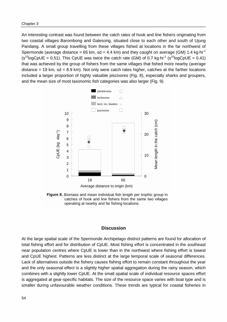
Chapter 3
54
An interesting contrast was found between the catch rates of hook and line fishers originating fromtwo coastal villages Barombong and Galesong, situated close to each other and south of UjungPandang. A small group travelling from these villages fished at locations in the far northwest ofSpermonde (average distance = 65 km, sd = 4.4 km) and they caught on average (GM) 1.4 kg·hr-1
(s10logCpUE = 0.51). This CpUE was twice the catch rate (GM) of 0.7 kg·hr-1 (s10logCpUE = 0.41)that was achieved by the group of fishers from the same villages that fished more nearby (averagedistance = 19 km, sd = 8.9 km). Not only were catch rates higher, catches at the farther locationsincluded a larger proportion of highly valuable piscivores (Fig. 8), especially sharks and groupers,and the mean size of most taxonomic fish categories was also larger (Fig. 9).
At the large sptotal fishing effnear populatioand CpUE higLack of alternaand the only secombines with is aggregated asmaller during
F
19 65
Average distance to origin (km)
0
1
2
3
4
5
6
7
8
9
10
CpU
E (
kg . d
ay-1)
���������������������������������� ���������������������������������������������������������������������������������������������������� ��������������������������������
planktivores�������������� herbivores�������
bent. inv. feeders
piscivores
0
10
20
30
Mea
n le
ngth
in th
e ca
tch
(cm
)
igure 8. Biomass and mean individual fish length per trophic group incatches of hook and line fishers from the same two villagesoperating at nearby and far fishing locations.
Discussion
atial scale of the Spermonde Archipelago distinct patterns are found for allocation ofort and for distribution of CpUE. Most fishing effort is concentrated in the southeastn centres where CpUE is lower than in the northwest where fishing effort is lowesthest. Patterns are less distinct at the large temporal scale of seasonal differences.tives outside the fishery causes fishing effort to remain constant throughout the yearasonal effect is a slightly higher spatial aggregation during the rainy season, whicha slightly lower CpUE. At the small spatial scale of individual resource spaces effortt gear-specific habitats. The size of the resource space varies with boat type and is
unfavourable weather conditions. These trends are typical for coastal fisheries in
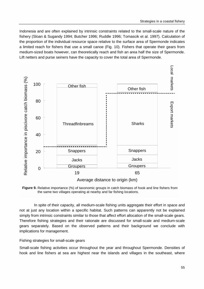
Strategies in a coastal fishery
Indonesia and are often explained by intrinsic constraints related to the small-scale nature of thefishery (Sloan & Sugandy 1994; Butcher 1996; Ruddle 1996; Tomascik et al. 1997). Calculation ofthe proportion of the individual resource space relative to the surface area of Spermonde indicatesa limited reach for fishers that use a small canoe (Fig. 10). Fishers that operate their gears frommedium-sized boats however, can theoretically reach and fish an area half the size of Spermonde.Lift netters and purse seiners have the capacity to cover the total area of Spermonde.
Innot at jussimply froThereforegears sepimplication
Fishing st
Small-scahook and
1
Rel
ativ
e im
port
ance
in p
isci
vore
cat
ch b
iom
ass
(%)
Figure 9
19 65
Average distance to origin (km)
0
20
40
60
80
00
Export m
arketsLocal m
arkets
Sharks
Snappers
Jacks
Groupers
Other fish
Threadfinbreams
Other fish
Snappers
Jacks
Groupers
. Relative importance (%) of taxonomic groups in catch biomass of hook and line fishers fromthe same two villages operating at nearby and far fishing locations.
55
spite of their capacity, all medium-scale fishing units aggregate their effort in space andt any location within a specific habitat. Such patterns can apparently not be explainedm intrinsic constraints similar to those that affect effort allocation of the small-scale gears. fishing strategies and their rationale are discussed for small-scale and medium-scalearately. Based on the observed patterns and their background we conclude withs for management.
rategies for small-scale gears
le fishing activities occur throughout the year and throughout Spermonde. Densities of line fishers at sea are highest near the islands and villages in the southeast, where
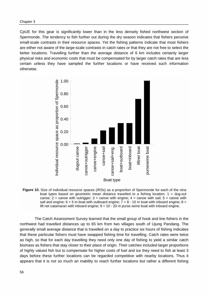
Chapter 3
56
CpUE for this gear is significantly lower than in the less densely fished northwest section ofSpermonde. The tendency to fish further out during the dry season indicates that fishers perceivesmall-scale contrasts in their resource spaces. Yet the fishing patterns indicate that most fishersare either not aware of the large-scale contrasts in catch rates or that they are not free to select thebetter locations. Travelling further than the average distance of 6 km includes certainly largerphysical risks and economic costs that must be compensated for by larger catch rates that are lesscertain unless they have sampled the further locations or have received such informationotherwise.
The Canorthwest had tgenerally small athat these particas high, so thatbiomass as fisheof highly valueddays before theappears that it i
Figure 10. Sizeboat canosail alift ne
dugo
ut c
anoe
cano
e+ou
trig
ger
cano
e+en
gine
cano
e+sa
il
cano
e+sa
il+en
g.
boat
+ou
tboa
rd
boat
+in
boar
d
liftn
et b
oat
purs
esei
ne b
oat
Boat type
0.00
0.20
0.40
0.60
0.80
1.00
Indi
vidu
al r
esou
rce
spac
e as
pro
port
ion
of S
perm
onde
of individual resource spaces (IRSs) as a proportion of Spermonde for each of the ninetypes based on geometric mean distance travelled to a fishing location. 1 = dug-oute; 2 = canoe with outrigger; 3 = canoe with engine; 4 = canoe with sail; 5 = canoe withnd engine; 6 = 5 m boat with outboard engine; 7 = 8 - 10 m boat with inboard engine; 8 =t catamaran with inboard engine; 9 = 10 - 20 m purse seine boat with inboard engine.
tch Assessment Survey learned that the small group of hook and line fishers in theravelled distances up to 65 km from two villages south of Ujung Pandang. Theverage distance that is travelled on a day to practice six hours of fishing indicates
ular fishers must have swapped fishing time for travelling. Catch rates were twice for each day travelling they need only one day of fishing to yield a similar catchrs that stay closer to their place of origin. Their catches included larger proportions
fish but to compensate for higher costs of fuel and ice they need to fish at least 3se further locations can be regarded competitive with nearby locations. Thus its not so much an inability to reach further locations but rather a different fishing
Strategies in a coastal fishery
57
strategy. The question is now: are hook and line fishers unable to perceive the apparent spatialcontrasts in CpUE and catch composition or are they reluctant to adjust their current strategy intomaking multi-day trips?
Historic developments in Spermonde fishery indicates that socio-cultural attitudes tofishing may differ between islands or villages (Meereboer 1998), yet it is more likely that theparticular knowledge on high CpUE or on the better chance to catch a high priced fish in thenorthwest section, is not wide-spread. Withholding information remains a common survival strategyin competitive fisheries even when it has been shown to cause inefficient exploitation of theresources at the level of the total system (Allen & McGlade 1986). The day-to-day experience ofhook and line fishers provides them no obvious reason to travel and explore farther locations withsuitable habitat and the constraints placed by their boats cause them to be area specialists ratherthan area movers (Hilborn 1985). At the small scale of the individual resource spaces, fishers inSpermonde reacted on an ad hoc basis on the size of their daily catch, but this was not an effectivestrategy. So their daily experience seem not to contribute to their knowledge base on possible localpatterns in the spatial distribution of the fish.
The uncertainty around their generally low CpUE makes it that small-scale fishers do noteasily escape their present situation by switching to other gear or boat types (Smith 1990). Wetend to conclude that small-scale fishers in Spermonde cannot easily observe the large scalecontrasts in CpUE and aim at minimising physical and economic risks by selecting suitable habitatsclose to their villages, rather than at maximising catch rates by switching between gears orlocations.
Fishing strategies for medium-scale gears
The large-scale patterns in effort allocation by medium-scale gears cannot simply be explained byrisk minimisation, because in theory, the boats from which these gears are operated can reach farmore locations than where they actually fish. Purse seine and lift net boats could in fact fish at anylocation with a suitable habitat within Spermonde. Yet at the large spatial scale of Spermonde,habitat characteristics do not affect the density of these medium-scale fishing units. In spite of thewide-spread distribution of suitable sandy habitats, Danish seiners aggregated at an averagedistance of less than 10 km from their villages. Purse seine units on the other hand, travelled morethan 20 km straight west to fish in the outer zone without exploiting areas more nearby theirvillages. Only lift net units appear to utilise all locations within their reach, but highest densities arestill found near their origin.
The revenues from the high daily catch of 500 kg for Danish seiners would theoreticallyallow for some exploratory fishing, yet there is hardly any reason to change their strategy. Thetechnical operation of the gear is time-consuming and because they are almost certain to catch atleast 150 kg·daytrip-1 they apparently prefer to use their time for fishing rather than for travelling.Although we cannot eliminate the possibility that they are already fishing the maximum CpUE forthis gear in the area, the relatively high variability in catch rates causes to believe that Danishseine fishers minimise economic risk instead, by spending maximum time on operating their gear.
Average catches of lift nets and purse seines are lower than for Danish seiners. Yet thevariability in catch rates is high due to the migratory and schooling behaviour of their pelagic targetspecies (Dudley & Tampubolon 1986). Because there were no significant spatial patterns in CpUEfor lift nets it is difficult to understand why a relatively large number of the lift net boats actually fish
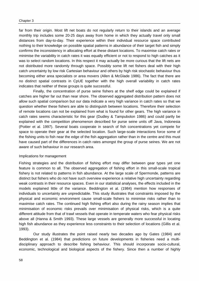
Chapter 3
58
far from their origin. Most lift net boats do not regularly return to their islands and an averagemonthly trip includes some 20-25 days away from home in which they actually travel only smalldistances from day-to-day. Their experience within their individual resource space contributednothing to their knowledge on possible spatial patterns in abundance of their target fish and simplyconfirms the inconsistency in allocating effort at these distant locations. To maximise catch rates orminimise the variability in catch rates it was equally efficient or not to respond to high catches as itwas to select random locations. In this respect it may actually be more curious that the lift nets arenot distributed more randomly through space. Possibly some lift net fishers deal with their highcatch uncertainty by low risk Cartesian behaviour and others by high risk stochastic behaviour thusbecoming either area specialists or area movers (Allen & McGlade 1986). The fact that there areno distinct spatial contrasts in CpUE together with the high overall variability in catch ratesindicates that neither of these groups is quite successful.
Finally, the concentration of purse seine fishers at the shelf edge could be explained ifcatches are higher far out than near shore. The observed aggregated distribution pattern does notallow such spatial comparison but our data indicate a very high variance in catch rates so that wequestion whether these fishers are able to distinguish between locations. Therefore their selectionof remote locations can not be explained from what is found for other gears. The high variance incatch rates seems characteristic for this gear (Dudley & Tampubolon 1986) and could partly beexplained with the competition phenomenon described for purse seine units off Java, Indonesia(Poitier et al. 1997). Several boats cooperate in search of fish concentrations yet compete forspace to operate their gear at the selected location. Such large-scale interactions force some ofthe fishing units to fish near the edge of the fish aggregation rather than in the centre and this musthave caused part of the differences in catch rates amongst the group of purse seines. We are notaware of such behaviour in our research area.
Implications for management
Fishing strategies and the distribution of fishing effort may differ between gear types yet onefeature is common to all. The observed aggregation of fishing effort in this small-scale tropicalfishery is not related to patterns in fish abundance. At the large scale of Spermonde, patterns aredistinct but fishers who do not have such overview experience a relative high uncertainty regardingweak contrasts in their resource spaces. Even in our statistical analyses, the effects included in themodels explained little of the variance. Beddington et al. (1984) mention how responses ofindividuals to uncertainty are unpredictable. This study illustrates that constraints imposed by thephysical and economic environment cause small-scale fishers to minimise risks rather than tomaximise catch rates. The continued high fishing effort also during the rainy season implies thatminimisation of economic risks prevails over minimisation of physical risks, which is a quitedifferent attitude from that of trawl vessels that operate in temperate waters who fear physical risksabove all (Hanna & Smith 1993). These large vessels are generally more successful in locatinghigh fish abundance as they experience less constraints to their selection of locations (Gillis et al.1993).
Our study illustrates the point raised nearly two decades ago by Gates (1984) andBeddington et al. (1984) that predictions on future developments in fisheries need a multi-disciplinary approach to describe fishing behaviour. This should incorporate socio-cultural,economic, technological and biological aspects of the fishery. Since then a number of highly
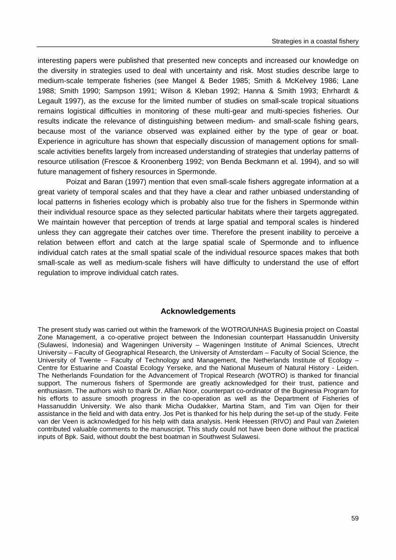
Strategies in a coastal fishery
59
interesting papers were published that presented new concepts and increased our knowledge onthe diversity in strategies used to deal with uncertainty and risk. Most studies describe large tomedium-scale temperate fisheries (see Mangel & Beder 1985; Smith & McKelvey 1986; Lane1988; Smith 1990; Sampson 1991; Wilson & Kleban 1992; Hanna & Smith 1993; Ehrhardt &Legault 1997), as the excuse for the limited number of studies on small-scale tropical situationsremains logistical difficulties in monitoring of these multi-gear and multi-species fisheries. Ourresults indicate the relevance of distinguishing between medium- and small-scale fishing gears,because most of the variance observed was explained either by the type of gear or boat.Experience in agriculture has shown that especially discussion of management options for small-scale activities benefits largely from increased understanding of strategies that underlay patterns ofresource utilisation (Frescoe & Kroonenberg 1992; von Benda Beckmann et al. 1994), and so willfuture management of fishery resources in Spermonde.
Poizat and Baran (1997) mention that even small-scale fishers aggregate information at agreat variety of temporal scales and that they have a clear and rather unbiased understanding oflocal patterns in fisheries ecology which is probably also true for the fishers in Spermonde withintheir individual resource space as they selected particular habitats where their targets aggregated.We maintain however that perception of trends at large spatial and temporal scales is hinderedunless they can aggregate their catches over time. Therefore the present inability to perceive arelation between effort and catch at the large spatial scale of Spermonde and to influenceindividual catch rates at the small spatial scale of the individual resource spaces makes that bothsmall-scale as well as medium-scale fishers will have difficulty to understand the use of effortregulation to improve individual catch rates.
Acknowledgements
The present study was carried out within the framework of the WOTRO/UNHAS Buginesia project on CoastalZone Management, a co-operative project between the Indonesian counterpart Hassanuddin University(Sulawesi, Indonesia) and Wageningen University – Wageningen Institute of Animal Sciences, UtrechtUniversity – Faculty of Geographical Research, the University of Amsterdam – Faculty of Social Science, theUniversity of Twente – Faculty of Technology and Management, the Netherlands Institute of Ecology –Centre for Estuarine and Coastal Ecology Yerseke, and the National Museum of Natural History - Leiden.The Netherlands Foundation for the Advancement of Tropical Research (WOTRO) is thanked for financialsupport. The numerous fishers of Spermonde are greatly acknowledged for their trust, patience andenthusiasm. The authors wish to thank Dr. Alfian Noor, counterpart co-ordinator of the Buginesia Program forhis efforts to assure smooth progress in the co-operation as well as the Department of Fisheries ofHassanuddin University. We also thank Micha Oudakker, Martina Stam, and Tim van Oijen for theirassistance in the field and with data entry. Jos Pet is thanked for his help during the set-up of the study. Feitevan der Veen is acknowledged for his help with data analysis. Henk Heessen (RIVO) and Paul van Zwietencontributed valuable comments to the manuscript. This study could not have been done without the practicalinputs of Bpk. Said, without doubt the best boatman in Southwest Sulawesi.
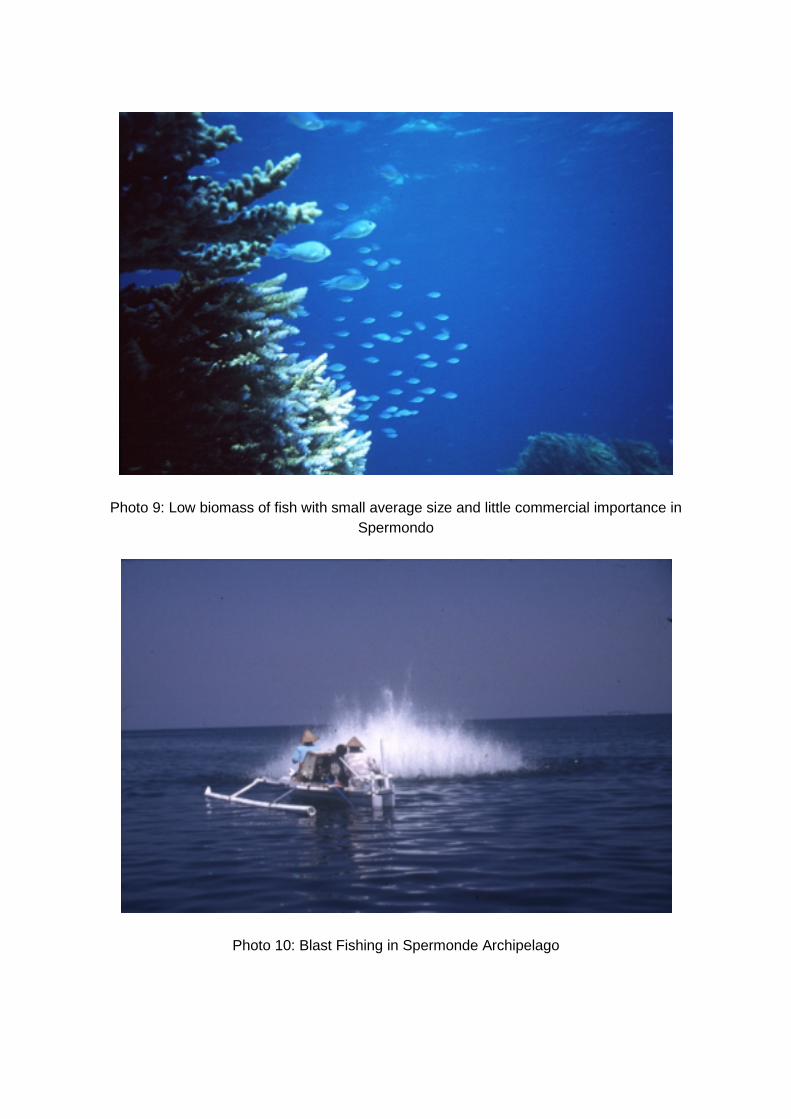
Photo 9: Low biomass of fish with small average size and little commercial importance inSpermondo
Photo 10: Blast Fishing in Spermonde Archipelago
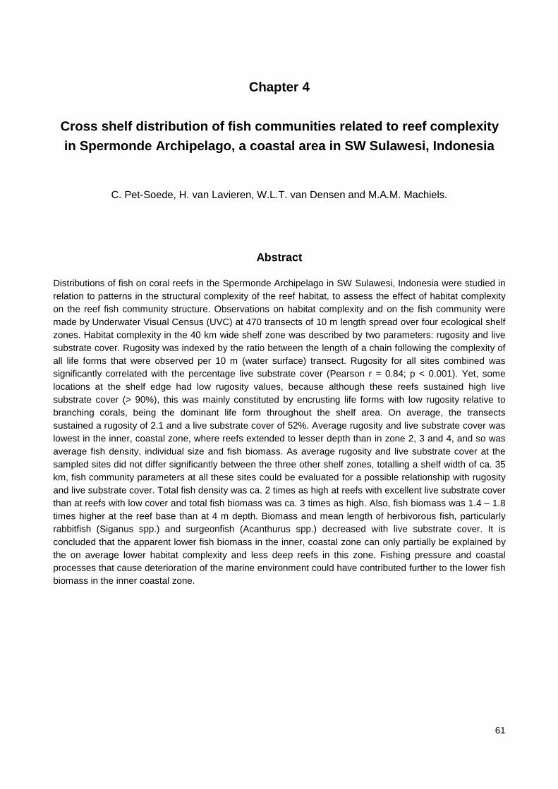
61
Chapter 4
Cross shelf distribution of fish communities related to reef complexityin Spermonde Archipelago, a coastal area in SW Sulawesi, Indonesia
C. Pet-Soede, H. van Lavieren, W.L.T. van Densen and M.A.M. Machiels.
Abstract
Distributions of fish on coral reefs in the Spermonde Archipelago in SW Sulawesi, Indonesia were studied inrelation to patterns in the structural complexity of the reef habitat, to assess the effect of habitat complexityon the reef fish community structure. Observations on habitat complexity and on the fish community weremade by Underwater Visual Census (UVC) at 470 transects of 10 m length spread over four ecological shelfzones. Habitat complexity in the 40 km wide shelf zone was described by two parameters: rugosity and livesubstrate cover. Rugosity was indexed by the ratio between the length of a chain following the complexity ofall life forms that were observed per 10 m (water surface) transect. Rugosity for all sites combined wassignificantly correlated with the percentage live substrate cover (Pearson r = 0.84; p < 0.001). Yet, somelocations at the shelf edge had low rugosity values, because although these reefs sustained high livesubstrate cover (> 90%), this was mainly constituted by encrusting life forms with low rugosity relative tobranching corals, being the dominant life form throughout the shelf area. On average, the transectssustained a rugosity of 2.1 and a live substrate cover of 52%. Average rugosity and live substrate cover waslowest in the inner, coastal zone, where reefs extended to lesser depth than in zone 2, 3 and 4, and so wasaverage fish density, individual size and fish biomass. As average rugosity and live substrate cover at thesampled sites did not differ significantly between the three other shelf zones, totalling a shelf width of ca. 35km, fish community parameters at all these sites could be evaluated for a possible relationship with rugosityand live substrate cover. Total fish density was ca. 2 times as high at reefs with excellent live substrate coverthan at reefs with low cover and total fish biomass was ca. 3 times as high. Also, fish biomass was 1.4 – 1.8times higher at the reef base than at 4 m depth. Biomass and mean length of herbivorous fish, particularlyrabbitfish (Siganus spp.) and surgeonfish (Acanthurus spp.) decreased with live substrate cover. It isconcluded that the apparent lower fish biomass in the inner, coastal zone can only partially be explained bythe on average lower habitat complexity and less deep reefs in this zone. Fishing pressure and coastalprocesses that cause deterioration of the marine environment could have contributed further to the lower fishbiomass in the inner coastal zone.
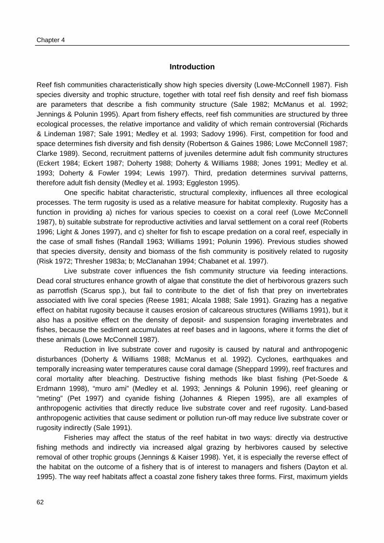
Chapter 4
62
Introduction
Reef fish communities characteristically show high species diversity (Lowe-McConnell 1987). Fishspecies diversity and trophic structure, together with total reef fish density and reef fish biomassare parameters that describe a fish community structure (Sale 1982; McManus et al. 1992;Jennings & Polunin 1995). Apart from fishery effects, reef fish communities are structured by threeecological processes, the relative importance and validity of which remain controversial (Richards& Lindeman 1987; Sale 1991; Medley et al. 1993; Sadovy 1996). First, competition for food andspace determines fish diversity and fish density (Robertson & Gaines 1986; Lowe McConnell 1987;Clarke 1989). Second, recruitment patterns of juveniles determine adult fish community structures(Eckert 1984; Eckert 1987; Doherty 1988; Doherty & Williams 1988; Jones 1991; Medley et al.1993; Doherty & Fowler 1994; Lewis 1997). Third, predation determines survival patterns,therefore adult fish density (Medley et al. 1993; Eggleston 1995).
One specific habitat characteristic, structural complexity, influences all three ecologicalprocesses. The term rugosity is used as a relative measure for habitat complexity. Rugosity has afunction in providing a) niches for various species to coexist on a coral reef (Lowe McConnell1987), b) suitable substrate for reproductive activities and larval settlement on a coral reef (Roberts1996; Light & Jones 1997), and c) shelter for fish to escape predation on a coral reef, especially inthe case of small fishes (Randall 1963; Williams 1991; Polunin 1996). Previous studies showedthat species diversity, density and biomass of the fish community is positively related to rugosity(Risk 1972; Thresher 1983a; b; McClanahan 1994; Chabanet et al. 1997).
Live substrate cover influences the fish community structure via feeding interactions.Dead coral structures enhance growth of algae that constitute the diet of herbivorous grazers suchas parrotfish (Scarus spp.), but fail to contribute to the diet of fish that prey on invertebratesassociated with live coral species (Reese 1981; Alcala 1988; Sale 1991). Grazing has a negativeeffect on habitat rugosity because it causes erosion of calcareous structures (Williams 1991), but italso has a positive effect on the density of deposit- and suspension foraging invertebrates andfishes, because the sediment accumulates at reef bases and in lagoons, where it forms the diet ofthese animals (Lowe McConnell 1987).
Reduction in live substrate cover and rugosity is caused by natural and anthropogenicdisturbances (Doherty & Williams 1988; McManus et al. 1992). Cyclones, earthquakes andtemporally increasing water temperatures cause coral damage (Sheppard 1999), reef fractures andcoral mortality after bleaching. Destructive fishing methods like blast fishing (Pet-Soede &Erdmann 1998), “muro ami” (Medley et al. 1993; Jennings & Polunin 1996), reef gleaning or“meting” (Pet 1997) and cyanide fishing (Johannes & Riepen 1995), are all examples ofanthropogenic activities that directly reduce live substrate cover and reef rugosity. Land-basedanthropogenic activities that cause sediment or pollution run-off may reduce live substrate cover orrugosity indirectly (Sale 1991).
Fisheries may affect the status of the reef habitat in two ways: directly via destructivefishing methods and indirectly via increased algal grazing by herbivores caused by selectiveremoval of other trophic groups (Jennings & Kaiser 1998). Yet, it is especially the reverse effect ofthe habitat on the outcome of a fishery that is of interest to managers and fishers (Dayton et al.1995). The way reef habitats affect a coastal zone fishery takes three forms. First, maximum yields
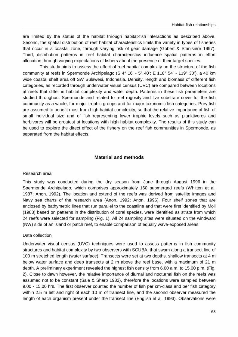
Habitat-fish relationships
63
are limited by the status of the habitat through habitat-fish interactions as described above.Second, the spatial distribution of reef habitat characteristics limits the variety in types of fisheriesthat occur in a coastal zone, through varying risk of gear damage (Gobert & Stanisière 1997).Third, distribution patterns in reef habitat characteristics influence spatial patterns in effortallocation through varying expectations of fishers about the presence of their target species.
This study aims to assess the effect of reef habitat complexity on the structure of the fishcommunity at reefs in Spermonde Archipelago (S 4° 16′ - 5° 40′; E 118° 54′ - 119° 30′), a 40 kmwide coastal shelf area off SW Sulawesi, Indonesia. Density, length and biomass of different fishcategories, as recorded through underwater visual census (UVC) are compared between locationsat reefs that differ in habitat complexity and water depth. Patterns in these fish parameters arestudied throughout Spermonde and related to reef rugosity and live substrate cover for the fishcommunity as a whole, for major trophic groups and for major taxonomic fish categories. Prey fishare assumed to benefit most from high habitat complexity, so that the relative importance of fish ofsmall individual size and of fish representing lower trophic levels such as planktivores andherbivores will be greatest at locations with high habitat complexity. The results of this study canbe used to explore the direct effect of the fishery on the reef fish communities in Spermonde, asseparated from the habitat effects.
Material and methods
Research area
This study was conducted during the dry season from June through August 1996 in theSpermonde Archipelago, which comprises approximately 160 submerged reefs (Whitten et al.1987; Anon. 1992). The location and extend of the reefs was derived from satellite images andNavy sea charts of the research area (Anon. 1992; Anon. 1996). Four shelf zones that areenclosed by bathymetric lines that run parallel to the coastline and that were first identified by Moll(1983) based on patterns in the distribution of coral species, were identified as strata from which24 reefs were selected for sampling (Fig. 1). All 24 sampling sites were situated on the windward(NW) side of an island or patch reef, to enable comparison of equally wave-exposed areas.
Data collection
Underwater visual census (UVC) techniques were used to assess patterns in fish communitystructures and habitat complexity by two observers with SCUBA, that swam along a transect line of100 m stretched length (water surface). Transects were set at two depths, shallow transects at 4 mbelow water surface and deep transects at 2 m above the reef base, with a maximum of 21 mdepth. A preliminary experiment revealed the highest fish density from 6.00 a.m. to 15.00 p.m. (Fig.2). Close to dawn however, the relative importance of diurnal and nocturnal fish on the reefs wasassumed not to be constant (Sale & Sharp 1983), therefore the locations were sampled between9.00 - 15.00 hrs. The first observer counted the number of fish per cm-class and per fish categorywithin 2.5 m left and right of each 10 m of transect line, and the second observer measured thelength of each organism present under the transect line (English et al. 1993). Observations were
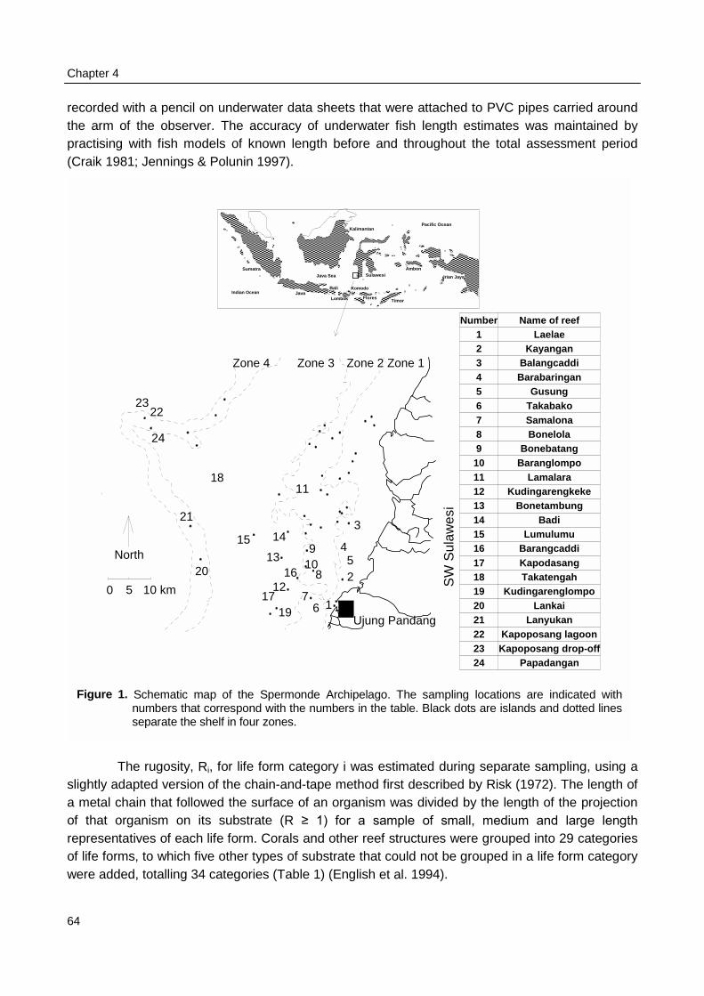
Chapter 4
64
recorded with a pencil on underwater data sheets that were attached to PVC pipes carried aroundthe arm of the observer. The accuracy of underwater fish length estimates was maintained bypractising with fish models of known length before and throughout the total assessment period(Craik 1981; Jennings & Polunin 1997).
sligha meof threprof lifwere
Fig
��������������
������������������������������������������������������������������������������������������������������������������������������������������������������������������������������
������
���� ������
�����
��������������������������������������������������
������������������������������������� �������������
������������������������������������������
�����
����������������������������������������������������������������������������������������������������������������
����������������������������������������������������������������������������������
����������� �����������������������������
������������������
���������������
�������������������������� ���������������������������
���������������������������������������������������������������������������������
������������������
��������������� ����������
��������
�����
������
�
AmbonSumatra
Timor
Bali
Lombok
Irian Jaya
Komodo
Flores
Sulawesi
Kalimantan
Java
Java Sea
Pacific Ocean
Indian Ocean
Number Name of reef1 Laelae2 Kayangan3 Balangcaddi4 Barabaringan5 Gusung6 Takabako7 Samalona8 Bonelola9 Bonebatang10 Baranglompo11 Lamalara12 Kudingarengkeke13 Bonetambung14 Badi15 Lumulumu16 Barangcaddi17 Kapodasang18 Takatengah19 Kudingarenglompo20 Lankai21 Lanyukan22 Kapoposang lagoon23 Kapoposang drop-off24 Papadangan
0 5 10 km1
2
3
45
67
8
910
11
12
13
1415
16
17
18
19
20
2322
21
24
Ujung Pandang
Zone 1Zone 2Zone 3Zone 4
North
SW
Sul
awes
i
ure 1. Schematic map of the Spermonde Archipelago. The sampling locations are indicated withnumbers that correspond with the numbers in the table. Black dots are islands and dotted linesseparate the shelf in four zones.
The rugosity, Ri, for life form category i was estimated during separate sampling, using atly adapted version of the chain-and-tape method first described by Risk (1972). The length oftal chain that followed the surface of an organism was divided by the length of the projectionat organism on its substrate (R ≥ 1) for a sample of small, medium and large length
esentatives of each life form. Corals and other reef structures were grouped into 29 categoriese forms, to which five other types of substrate that could not be grouped in a life form category added, totalling 34 categories (Table 1) (English et al. 1994).
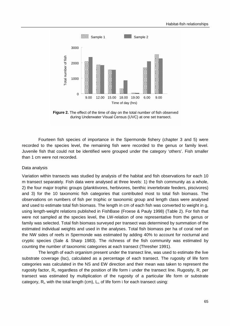
Habitat-fish relationships
Fourteenrecorded to the sJuvenile fish that than 1 cm were no
Data analysis
Variation within trm transect separa2) the four major tand 3) for the 1observations on nand used to estimusing length-weigwere not sampledfamily was selecteestimated individuthe NW sides of rcryptic species (Scounting the numb
The lengsubstrate coveragcategories was carugosity factor, Ri
transect was estcategory, Ri, with
F
9.00 12.00 15.00 18.00 19.00 6.00 9.00
Time of day (hrs)
0
1000
2000
3000
Tot
al n
umbe
r of
fish ��������
��������������������������������������������������������
�������������������������������������������������
������������������������������������������
�������������� �������
������������������������������������
������������������������������������������������������
������������������������
Sample 1
���������������������������������������������������������������������������������
���������������������������������������������������������������
������������������������������������������������
�������������������������������� ��������
����������������������������������������������������������������
��������������������������������������������������������
����������������������������
Sample 2
igure 2. The effect of the time of day on the total number of fish observedduring Underwater Visual Census (UVC) at one set transect.
65
fish species of importance in the Spermonde fishery (chapter 3 and 5) werepecies level, the remaining fish were recorded to the genus or family level.could not be identified were grouped under the category ‘others’. Fish smallert recorded.
ansects was studied by analysis of the habitat and fish observations for each 10tely. Fish data were analysed at three levels: 1) the fish community as a whole,rophic groups (planktivores, herbivores, benthic invertebrate feeders, piscivores)0 taxonomic fish categories that contributed most to total fish biomass. Theumbers of fish per trophic or taxonomic group and length class were analysedate total fish biomass. The length in cm of each fish was converted to weight in g,ht relations published in FishBase (Froese & Pauly 1998) (Table 2). For fish that at the species level, the LW-relation of one representative from the genus ord. Total fish biomass surveyed per transect was determined by summation of theal weights and used in the analyses. Total fish biomass per ha of coral reef oneefs in Spermonde was estimated by adding 40% to account for nocturnal andale & Sharp 1983). The richness of the fish community was estimated byer of taxonomic categories at each transect (Thresher 1991).
th of each organism present under the transect line, was used to estimate the livee (lsc), calculated as a percentage of each transect. The rugosity of life formlculated in the NS and EW direction and their mean was taken to represent the
, regardless of the position of life form i under the transect line. Rugosity, R, perimated by multiplication of the rugosity of a particular life form or substratethe total length (cm), Li, of life form i for each transect using:
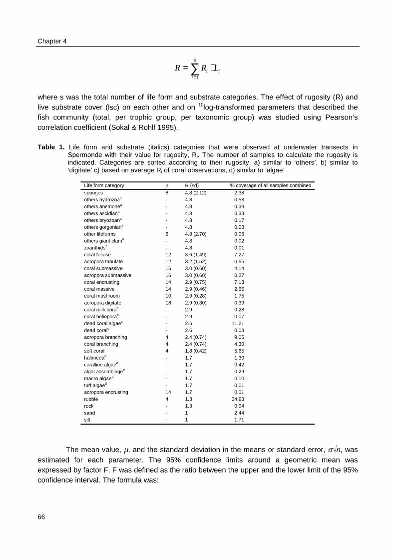
Chapter 4
66
∑=
⋅=s
iii LRR
1
where s was the total number of life form and substrate categories. The effect of rugosity (R) andlive substrate cover (lsc) on each other and on 10log-transformed parameters that described thefish community (total, per trophic group, per taxonomic group) was studied using Pearson’scorrelation coefficient (Sokal & Rohlf 1995).
Table 1. Life form and substrate (italics) categories that were observed at underwater transects inSpermonde with their value for rugosity, Ri. The number of samples to calculate the rugosity isindicated. Categories are sorted according to their rugosity. a) similar to ‘others’, b) similar to‘digitate’ c) based on average Ri of coral observations, d) similar to ‘algae’
Life form category n R (sd) % coverage of all samples combined
sponges 8 4.8 (2.12) 2.38others hydrozoaa - 4.8 0.58others anemonea - 4.8 0.38others ascidiana - 4.8 0.33others bryozoana - 4.8 0.17others gorgoniana - 4.8 0.08other lifeforms 6 4.8 (2.70) 0.06others giant clama - 4.8 0.02zoanthidsa - 4.8 0.01coral foliose 12 3.6 (1.49) 7.27acropora tabulate 12 3.2 (1.52) 0.55coral submassive 16 3.0 (0.60) 4.14acropora submassive 16 3.0 (0.60) 0.27coral encrusting 14 2.9 (0.75) 7.13coral massive 14 2.9 (0.46) 2.65coral mushroom 10 2.9 (0.28) 1.75acropora digitate 16 2.9 (0.80) 0.39coral milleporab - 2.9 0.28coral helioporab - 2.9 0.07dead coral algaec - 2.6 11.21dead coralc - 2.6 0.03acropora branching 4 2.4 (0.74) 9.05coral branching 4 2.4 (0.74) 4.30soft coral 4 1.8 (0.42) 5.65halimedad - 1.7 1.30coralline algaed - 1.7 0.42algal assemblaged - 1.7 0.29macro algaed - 1.7 0.10turf algaed - 1.7 0.01acropora encrusting 14 1.7 0.01rubble 4 1.3 34.93rock - 1.3 0.04sand - 1 2.44silt - 1 1.71
The mean value, µ, and the standard deviation in the means or standard error, σ√n, wasestimated for each parameter. The 95% confidence limits around a geometric mean wasexpressed by factor F. F was defined as the ratio between the upper and the lower limit of the 95%confidence interval. The formula was:
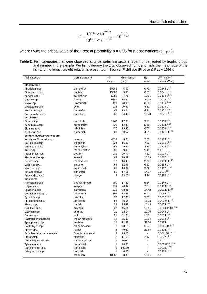
Habitat-fish relationships
67
nt
nt
nt
Fσ
σµ
σµ 2
log
log
101010
1010 =××=
−
where t was the critical value of the t-test at probability p = 0.05 for n observations (t0.05[n-1]).
Table 2. Fish categories that were observed at underwater transects in Spermonde, sorted by trophic groupand number in the sample. Per fish category the total observed number of fish, the mean size of thefish and the length-weight relation is presented. * Source: FishBase (Froese & Pauly 1998).
Fish category Common name N insample
Mean length(cm)
sd(cm)
LW relation*
L = cm; W = g
planktivoresAbudefduf spp. damselfish 50265 5.59 9.79 0.0642 L2.52
Stolephorus spp. anchovy 15300 5.63 6.05 0.0041 L3.33
Apogon spp. cardinalfish 6281 4.71 16.61 0.0124 L3.28
Caesio spp. fuselier 5181 14.84 20.28 0.0074 L3.15
Naso spp. unicornfish 429 20.98 8.36 0.0136L3.13
Decapterus spp. scad 214 20.87 4.51 0.0104 L3
Heniochus spp. bannerfish 69 13.64 4.24 0.0132L3.37
Pomacanthus spp. angelfish 66 24.49 10.48 0.0371 L2.97
herbivoresScarus spp. parrotfish 1746 17.03 9.67 0.0136 L3.11
Acanthurus spp. surgeonfish 623 14.40 5.40 0.0178L3.14
Siganus spp. rabbitfish 475 19.45 6.67 0.0254 L2.95
Kyphosus spp. rudderfish 23 20.57 4.51 0.01216 L3.08
benthic invertebrate feedersXyrichtys/ Choerodon spp. wrasse 4512 9.26 7.02 0.0238 L2.75
Ballistoides spp. triggerfish 824 16.97 7.66 0.0516 L2.88
Chaetodon spp. butterflyfish 665 9.54 3.33 0.0874 L2.18
Arius spp. marine catfish 300 9.00 5.48 n.a.Parupeneus spp. goatfish 231 20.77 7.12 0.0915 L2.42
Plectorinchus spp. sweetlip 84 26.87 10.28 0.0827 L2.72
Zanclus spp. moorish idol 77 14.43 2.39 0.01599 L3.17
Lethrinus spp. emperor 68 22.57 6.93 0.0189 L2.94
Myripristi spp. squirrelfish 61 16.02 3.02 0.0187 L3.04
Tetraodontidae pufferfish 55 17.11 14.27 0.057L2.80
Priacanthus spp. bigeye 2 24.00 4.24 0.0392 L2.78
piscivoresNemipterus spp. threadfinbream 790 17.49 5.14 0.0149 L3.14
Lutjanus spp. snapper 679 20.87 7.67 0.0153L3.09
Spyraena spp. barracuda 511 28.31 14.42 0.00986 L2.88
Cephalopholis spp. other trout 199 14.47 6.01 0.0099 L3.21
Synodus spp. lizardfish 93 12.83 5.85 0.0002 L4.08
Plectropomus spp. coral trout 58 25.05 11.03 0.00923 L3.08
Platax spp. batfish 24 25.42 10.43 0.045 L2.98
Fistularia spp. flutefish 22 45.14 15.01 0.00005228 L3.16
Dasyatis spp. stingray 21 32.14 12.70 0.0048 L2.72
Caranx spp. jack 21 31.38 15.51 0.023 L2.94
Rastrelliger kanagurta Indian mackerel 12 25.00 10.54 0.0014 L3.38
Epinephelus spp. seabass 11 31.91 33.00 0.016 L3
Rastrelliger spp. other mackerel 8 23.13 6.54 0.006138L3.22
Aprion spp. jobfish 5 49.80 21.55 0.013 L2.93
Scomberomorus commerson Spanish mackerel 4 95.00 - 0.006138 L3.22
Pterois spp. stonefish 2 11.50 2.12 0.0372 L2.89
Chromileptes altivelis barramundi cod 1 29.00 - n.a.Tylosurus spp. houndsfish 1 76.00 - 0.0005415 L3.17
Carcharhinus spp. reef shark 1 140.00 - 0.0015L3.38
Leiognathus spp. ponyfish 1 6.00 - 0.0263 L2.75
other fish 10552 3.38 13.51 n.a.
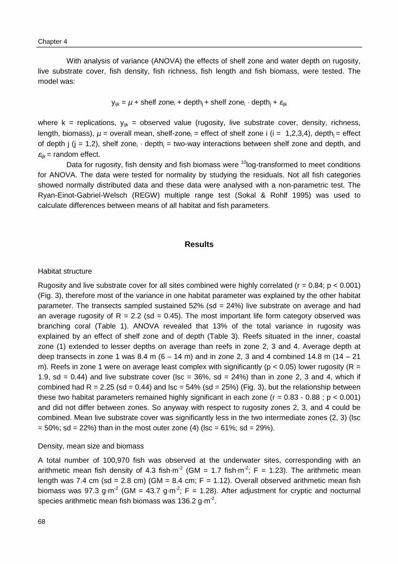
Chapter 4
68
With analysis of variance (ANOVA) the effects of shelf zone and water depth on rugosity,live substrate cover, fish density, fish richness, fish length and fish biomass, were tested. Themodel was:
yijk = µ + shelf zonei + depthj + shelf zonei · depthj + εijk
where k = replications, yijk = observed value (rugosity, live substrate cover, density, richness,
length, biomass), µ = overall mean, shelf-zonei = effect of shelf zone i (i = 1,2,3,4), depthj = effectof depth j (j = 1,2), shelf zonei · depthj = two-way interactions between shelf zone and depth, and
εijk = random effect.Data for rugosity, fish density and fish biomass were 10log-transformed to meet conditions
for ANOVA. The data were tested for normality by studying the residuals. Not all fish categoriesshowed normally distributed data and these data were analysed with a non-parametric test. TheRyan-Einot-Gabriel-Welsch (REGW) multiple range test (Sokal & Rohlf 1995) was used tocalculate differences between means of all habitat and fish parameters.
Results
Habitat structure
Rugosity and live substrate cover for all sites combined were highly correlated (r = 0.84; p < 0.001)(Fig. 3), therefore most of the variance in one habitat parameter was explained by the other habitatparameter. The transects sampled sustained 52% (sd = 24%) live substrate on average and hadan average rugosity of R = 2.2 (sd = 0.45). The most important life form category observed wasbranching coral (Table 1). ANOVA revealed that 13% of the total variance in rugosity wasexplained by an effect of shelf zone and of depth (Table 3). Reefs situated in the inner, coastalzone (1) extended to lesser depths on average than reefs in zone 2, 3 and 4. Average depth atdeep transects in zone 1 was 8.4 m (6 – 14 m) and in zone 2, 3 and 4 combined 14.8 m (14 – 21m). Reefs in zone 1 were on average least complex with significantly (p < 0.05) lower rugosity (R =1.9, sd = 0.44) and live substrate cover (lsc = 36%, sd = 24%) than in zone 2, 3 and 4, which ifcombined had R = 2.25 (sd = 0.44) and lsc = 54% (sd = 25%) (Fig. 3), but the relationship betweenthese two habitat parameters remained highly significant in each zone (r = 0.83 - 0.88 ; p < 0.001)and did not differ between zones. So anyway with respect to rugosity zones 2, 3, and 4 could becombined. Mean live substrate cover was significantly less in the two intermediate zones (2, 3) (lsc= 50%; sd = 22%) than in the most outer zone (4) (lsc = 61%; sd = 29%).
Density, mean size and biomass
A total number of 100,970 fish was observed at the underwater sites, corresponding with anarithmetic mean fish density of 4.3 fish·m-2 (GM = 1.7 fish·m-2; F = 1.23). The arithmetic meanlength was 7.4 cm (sd = 2.8 cm) (GM = 8.4 cm; F = 1.12). Overall observed arithmetic mean fishbiomass was 97.3 g·m-2 (GM = 43.7 g·m-2; F = 1.28). After adjustment for cryptic and nocturnalspecies arithmetic mean fish biomass was 136.2 g·m-2.
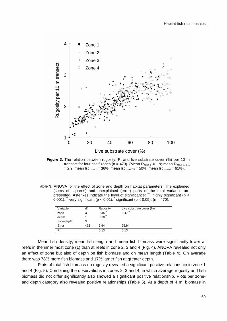
Habitat-fish relationships
69
Table 3. ANOVA for the effect of zone and depth on habitat parameters. The explained(sums of squares) and unexplained (error) parts of the total variance arepresented. Asterixes indicate the level of significance: *** highly significant (p <0.001), ** very significant (p < 0.01), * significant (p < 0.05). (n = 470).
Variable df Rugosity Live substrate cover (%)
zone 3 0.35*** 3.47***
depth 1 0.18***
zone·depth 3Error 462 3.64 26.94
R2 0.13 0.13
Mean fish density, mean fish length and mean fish biomass were significantly lower atreefs in the inner most zone (1) than at reefs in zone 2, 3 and 4 (Fig. 4). ANOVA revealed not onlyan effect of zone but also of depth on fish biomass and on mean length (Table 4). On averagethere was 78% more fish biomass and 17% larger fish at greater depth.
Plots of total fish biomass on rugosity revealed a significant positive relationship in zone 1and 4 (Fig. 5). Combining the observations in zones 2, 3 and 4, in which average rugosity and fishbiomass did not differ significantly also showed a significant positive relationship. Plots per zone-and depth category also revealed positive relationships (Table 5). At a depth of 4 m, biomass in
0 20 40 60 80 100
Live substrate cover (%)
1
2
3
4
Rug
osity
per
10
m tr
anse
ct
Zone 1
Zone 2
Zone 3
Zone 4
Figure 3. The relation between rugosity, R, and live substrate cover (%) per 10 mtransect for four shelf zones (n = 470). (Mean Rzone 1 = 1.9; mean Rzone 2, 3, 4
= 2.2; mean lsczone 1 = 36%; mean lsczone 2,3 = 50%; mean lsczone 4 = 61%).
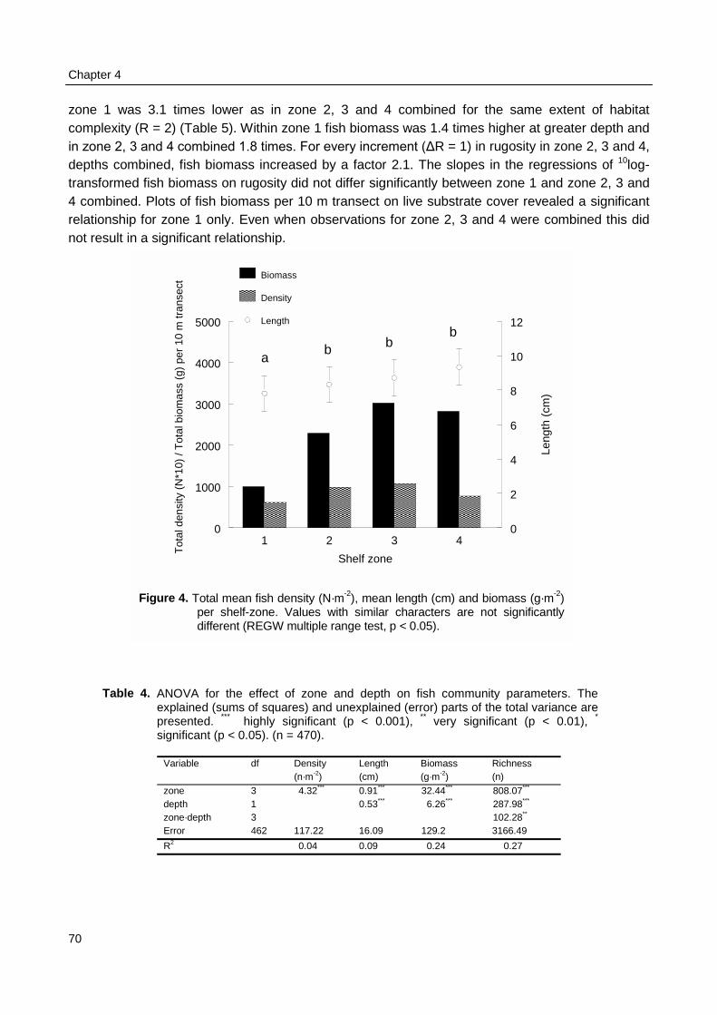
Chapter 4
70
zone 1 was 3.1 times lower as in zone 2, 3 and 4 combined for the same extent of habitatcomplexity (R = 2) (Table 5). Within zone 1 fish biomass was 1.4 times higher at greater depth andin zone 2, 3 and 4 combined 1.8 times. For every increment (ΔR = 1) in rugosity in zone 2, 3 and 4,depths combined, fish biomass increased by a factor 2.1. The slopes in the regressions of 10log-transformed fish biomass on rugosity did not differ significantly between zone 1 and zone 2, 3 and4 combined. Plots of fish biomass per 10 m transect on live substrate cover revealed a significantrelationship for zone 1 only. Even when observations for zone 2, 3 and 4 were combined this didnot result in a significant relationship.
Table
1 2 3 4
Shelf zone
0
1000
2000
3000
4000
5000
Tot
al d
ensi
ty (
N*1
0) /
Tot
al b
iom
ass
(g)
per
10 m
tran
sect
0
2
4
6
8
10
12
Leng
th (
cm)
������������������������
������������������������������������
������������������������������������������������
������������������������������������
ab b
b
Biomass����������������������
Density
Length
Figure 4. Total mean fish density (N·m-2), mean length (cm) and biomass (g·m-2)per shelf-zone. Values with similar characters are not significantlydifferent (REGW multiple range test, p < 0.05).
4. ANOVA for the effect of zone and depth on fish community parameters. Theexplained (sums of squares) and unexplained (error) parts of the total variance arepresented. *** highly significant (p < 0.001), ** very significant (p < 0.01), *
significant (p < 0.05). (n = 470).
Variable df Density(n·m-2)
Length(cm)
Biomass(g·m-2)
Richness(n)
zone 3 4.32*** 0.91*** 32.44*** 808.07***
depth 1 0.53*** 6.26*** 287.98***
zone·depth 3 102.28**
Error 462 117.22 16.09 129.2 3166.49
R2 0.04 0.09 0.24 0.27
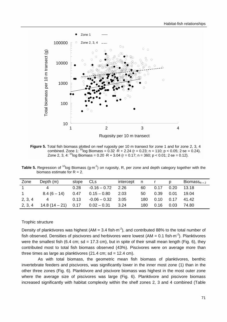
Habitat-fish relationships
71
Table 5. Regression of 10log Biomass (g·m-2) on rugosity, R, per zone and depth category together with thebiomass estimate for R = 2.
Zone Depth (m) slope CLs intercept n r p BiomassR = 2
1 4 0.28 -0.16 – 0.72 2.26 60 0.17 0.20 13.181 8.4 (6 – 14) 0.47 0.15 – 0.80 2.03 50 0.39 0.01 19.042, 3, 4 4 0.13 -0.06 – 0.32 3.05 180 0.10 0.17 41.422, 3, 4 14.8 (14 – 21) 0.17 0.02 – 0.31 3.24 180 0.16 0.03 74.80
Trophic structure
Density of planktivores was highest (AM = 3.4 fish·m-2), and contributed 88% to the total number offish observed. Densities of piscivores and herbivores were lowest (AM = 0.1 fish·m-2). Planktivoreswere the smallest fish (6.4 cm; sd = 17.3 cm), but in spite of their small mean length (Fig. 6), theycontributed most to total fish biomass observed (43%). Piscivores were on average more thanthree times as large as planktivores (21.4 cm; sd = 12.4 cm).
As with total biomass, the geometric mean fish biomass of planktivores, benthicinvertebrate feeders and piscivores, was significantly lower in the inner most zone (1) than in theother three zones (Fig. 6). Planktivore and piscivore biomass was highest in the most outer zonewhere the average size of piscivores was large (Fig. 6). Planktivore and piscivore biomassincreased significantly with habitat complexity within the shelf zones 2, 3 and 4 combined (Table
1 2 3 4
Rugosity per 10 m transect
10
100
1000
10000
100000T
otal
bio
mas
s pe
r 10
m tr
anse
ct (
g)
Zone 1
Zone 2, 3, 4
Figure 5. Total fish biomass plotted on reef rugosity per 10 m transect for zone 1 and for zone 2, 3, 4combined. Zone 1: 10log Biomass = 0.32 ·R + 2.24 (r = 0.23; n = 110; p < 0.05; 2·se = 0.24).Zone 2, 3, 4: 10log Biomass = 0.20 ·R + 3.04 (r = 0.17; n = 360; p < 0.01; 2·se = 0.12).
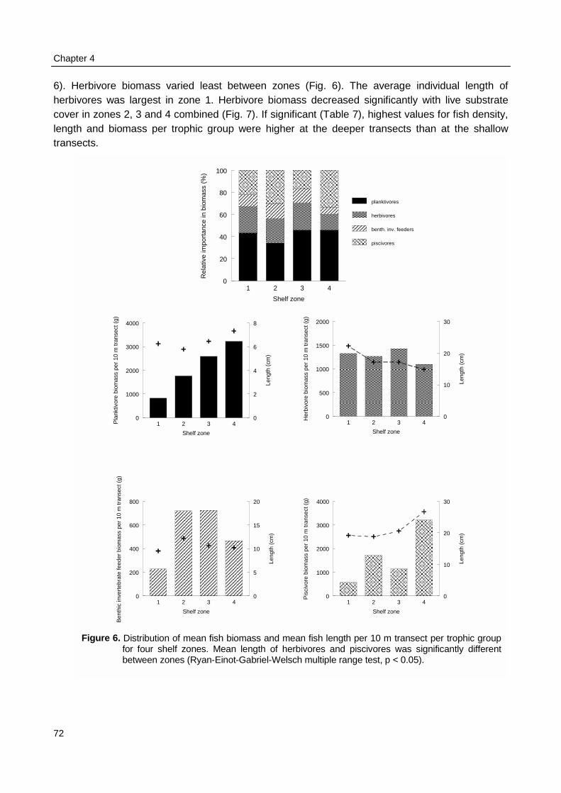
Chapter 4
72
6). Herbivore biomass varied least between zones (Fig. 6). The average individual length ofherbivores was largest in zone 1. Herbivore biomass decreased significantly with live substratecover in zones 2, 3 and 4 combined (Fig. 7). If significant (Table 7), highest values for fish density,length and biomass per trophic group were higher at the deeper transects than at the shallowtransects.
F
1 2 3 4
Shelf zone
0
20
40
60
80
100
Rel
ativ
e im
port
ance
in b
iom
ass
(%)
planktivores
��������������������������������������������������������
���������������������������������������
������������������������������������������������
���������������������������������
�����������herbivores
���������������������������� �������������
��������������������������
������������������������
��������������������������������� benth. inv. feeders
������������������������������������������
����������������������������������������������������
������������������������������������
�������������������������������������������������������
����������������������
piscivores
1 2 3 4
Shelf zone
0
1000
2000
3000
4000
Pla
nktiv
ore
biom
ass
per
10 m
tran
sect
(g)
0
2
4
6
8
Leng
th (
cm)
1 2 3 4
Shelf zone
0
500
1000
1500
2000
Her
bivo
re b
iom
ass
per
10 m
tran
sect
(g)
0
10
20
30
Leng
th (
cm)
��������������������������������������������������������������������������������������������������
�����������������������������������������������������������������������������
�������������������������������������������������������������������������������������������
������������������������������������������������������������������
1 2 3 4
Shelf zone
0
1000
2000
3000
4000
Pis
civo
re b
iom
ass
per
10 m
tran
sect
(g)
0
10
20
30
Leng
th (
cm)
����������������������������
��������������������������������������������
���������������������������������������
����������������������������������������������������������������������������������������
1 2 3 4
Shelf zone
0
200
400
600
800
Ben
thic
inve
rteb
rate
feed
er b
iom
ass
per
10 m
tran
sect
(g)
0
5
10
15
20
Leng
th (
cm)
���������������������������������������
���������������������������������������������������������������������������������������������������
������������������������������������������������������������������������������������������������������������
������������������������������������������������������������
igure 6. Distribution of mean fish biomass and mean fish length per 10 m transect per trophic groupfor four shelf zones. Mean length of herbivores and piscivores was significantly differentbetween zones (Ryan-Einot-Gabriel-Welsch multiple range test, p < 0.05).
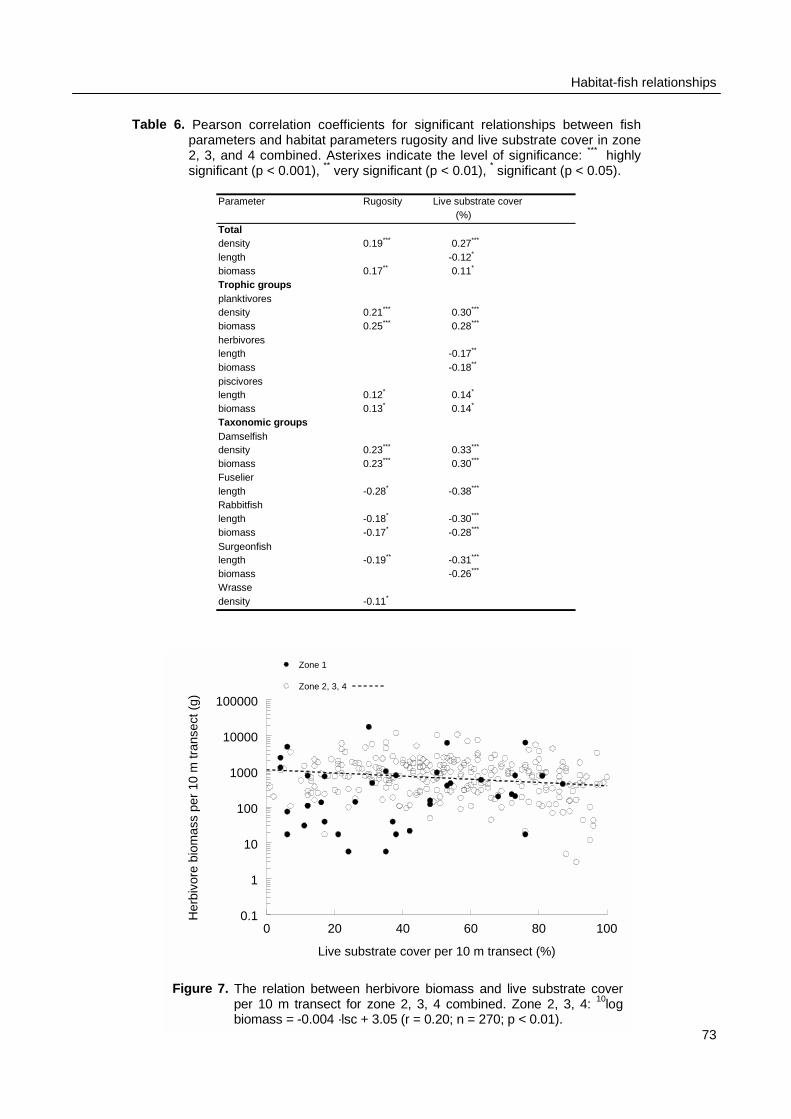
Habitat-fish relationships
Table 6. Pearson correlation coefficients for significant relationships between fishparameters and habitat parameters rugosity and live substrate cover in zone2, 3, and 4 combined. Asterixes indicate the level of significance: *** highlysignificant (p < 0.001), ** very significant (p < 0.01), * significant (p < 0.05).
Parameter Rugosity Live substrate cover(%)
Totaldensity 0.19*** 0.27***
length -0.12*
biomass 0.17** 0.11*
Trophic groupsplanktivoresdensity 0.21*** 0.30***
biomass 0.25*** 0.28***
herbivoreslength -0.17**
biomass -0.18**
piscivoreslength 0.12* 0.14*
biomass 0.13* 0.14*
Taxonomic groupsDamselfishdensity 0.23*** 0.33***
biomass 0.23*** 0.30***
Fuselierlength -0.28* -0.38***
Rabbitfishlength -0.18* -0.30***
biomass -0.17* -0.28***
Surgeonfishlength -0.19** -0.31***
biomass -0.26***
Wrassedensity -0.11*
0 20 40 60 80 100
Live substrate cover per 10 m transect (%)
0.1
1
10
100
1000
10000
100000
Her
bivo
re b
iom
ass
per
10 m
tran
sect
(g)
Zone 1
Zone 2, 3, 4
Figure 7. The relation between herbivore biomass and live substrate coverper 10 m transect for zone 2, 3, 4 combined. Zone 2, 3, 4: 10logbiomass = -0.004 ·lsc + 3.05 (r = 0.20; n = 270; p < 0.01).
73
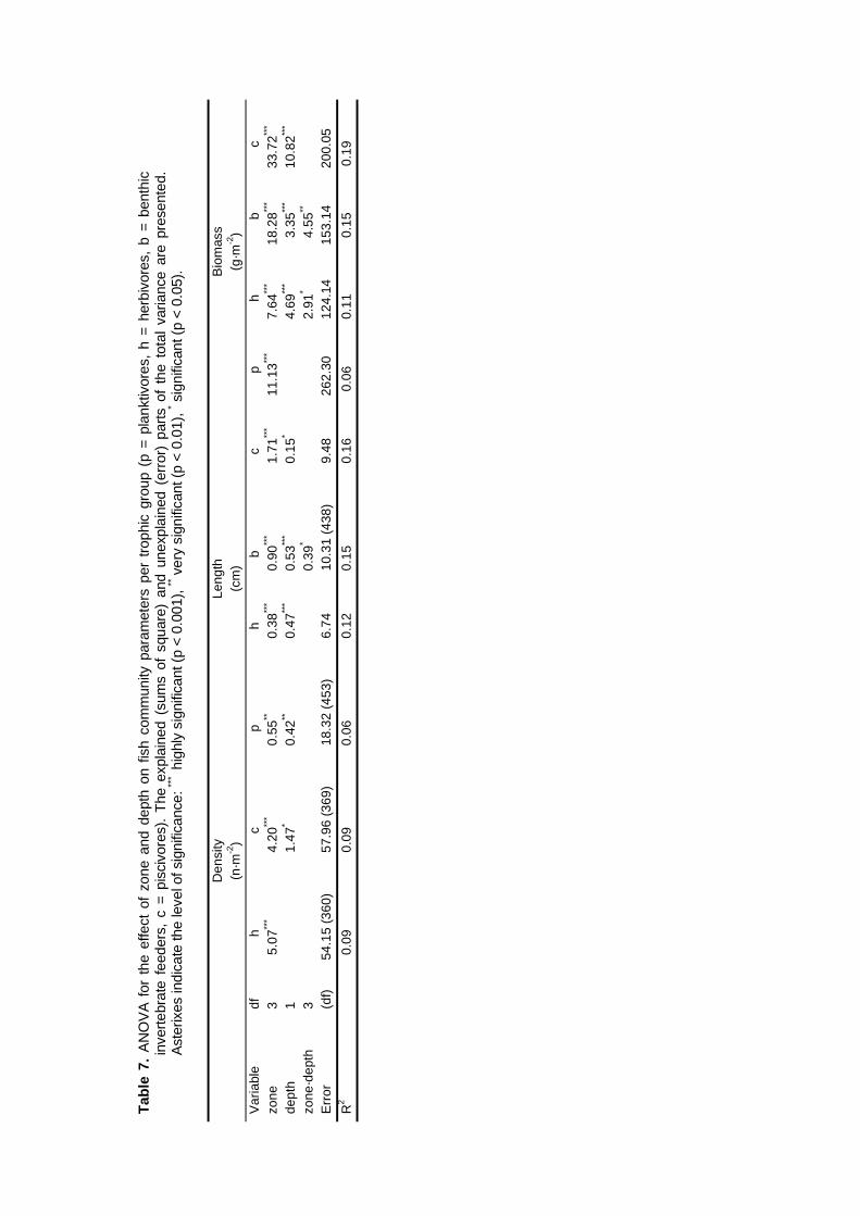
Tab
le 7
. A
NO
VA
for
the
effe
ct o
f zo
ne a
nd d
epth
on
fish
com
mun
ity p
aram
eter
s pe
r tr
ophi
c gr
oup
(p =
pla
nktiv
ores
, h
= h
erbi
vore
s, b
= b
enth
icin
vert
ebra
te f
eede
rs,
c =
pisc
ivor
es).
The
exp
lain
ed (
sum
s of
squ
are)
and
une
xpla
ined
(er
ror)
par
ts o
f th
e to
tal
varia
nce
are
pres
ente
d.A
ster
ixes
indi
cate
the
leve
l of s
igni
fican
ce: **
* h
ighl
y si
gnifi
cant
(p
< 0.
001)
, ** v
ery
sign
ifica
nt (p
< 0
.01)
, * sig
nific
ant (
p <
0.05
).
Den
sity
(n·m
-2)
Leng
th(c
m)
Bio
mas
s(g
·m-2
)
Var
iabl
edf
hc
ph
bc
ph
bc
zone
35.
07**
*4.
20**
*0.
55**
0.38
***
0.90
***
1.71
***
11.1
3***
7.64
***
18.2
8***
33.7
2***
dept
h1
1.47
*0.
42**
0.47
***
0.53
***
0.15
*4.
69**
*3.
35**
*10
.82**
*
zone
·dep
th3
0.39
*2.
91*
4.55
**
Err
or(d
f)54
.15
(360
)57
.96
(369
)18
.32
(453
)6.
7410
.31
(438
)9.
4826
2.30
124.
1415
3.14
200.
05
R2
0.09
0.09
0.06
0.12
0.15
0.16
0.06
0.11
0.15
0.19
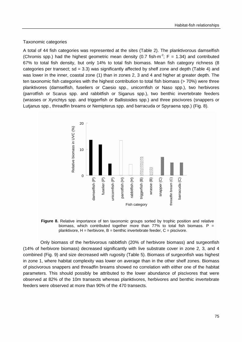
Habitat-fish relationships
Taxonomic categories
A total of 44 fish categories was represented at the sites (Table 2). The planktivorous damselfish(Chromis spp.) had the highest geometric mean density (0.7 fish·m-2; F = 1.34) and contributed67% to total fish density, but only 14% to total fish biomass. Mean fish category richness (8categories per transect; sd = 3.3) was significantly affected by shelf zone and depth (Table 4) andwas lower in the inner, coastal zone (1) than in zones 2, 3 and 4 and higher at greater depth. Theten taxonomic fish categories with the highest contribution to total fish biomass (> 70%) were threeplanktivores (damselfish, fuseliers or Caesio spp., unicornfish or Naso spp.), two herbivores(parrotfish or Scarus spp. and rabbitfish or Siganus spp.), two benthic invertebrate feeders(wrasses or Xyrichtys spp. and triggerfish or Ballistoides spp.) and three piscivores (snappers orLutjanus spp., threadfin breams or Nemipterus spp. and barracuda or Spyraena spp.) (Fig. 8).
Only biom(14% of herbivore combined (Fig. 9) ain zone 1, where hof piscivorous snapparameters. This sobserved at 82% ofeeders were obse
Figure 8. bp
dam
selfi
sh (
P)
fuse
lier
(P)
unic
ornf
ish
(P)
parr
otfis
h (H
)
rabb
itfis
h (H
)
trig
gerf
ish
(B)
wra
sse
(B)
snap
per
(C)
barr
acud
a (C
)
Fish category
0
10
20
Rel
ativ
e bi
omas
s in
UV
C (
%)
����������������������������������������
������������������������
������������������������������
����������������������������
����������������������������
thre
adfin
bre
am (
C)
Relative importance of ten taxonomic groups sorted by trophic position and relativeiomass, which contributed together more than 77% to total fish biomass. P =lanktivore, H = herbivore, B = benthic invertebrate feeder, C = piscivore.
75
ass of the herbivorous rabbitfish (20% of herbivore biomass) and surgeonfishbiomass) decreased significantly with live substrate cover in zone 2, 3, and 4nd size decreased with rugosity (Table 5). Biomass of surgeonfish was highest
abitat complexity was lower on average than in the other shelf zones. Biomasspers and threadfin breams showed no correlation with either one of the habitathould possibly be attributed to the lower abundance of piscivores that weref the 10m transects whereas planktivores, herbivores and benthic invertebrate
rved at more than 90% of the 470 transects.
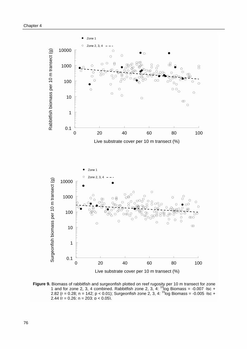
Chapter 4
76
Fig
0 20 40 60 80 100
Live substrate cover per 10 m transect (%)
0.1
1
10
100
1000
10000R
abbi
tfish
bio
mas
s pe
r 10
m tr
anse
ct (
g)
Zone 1
Zone 2, 3, 4
0 20 40 60 80 100
Live substrate cover per 10 m transect (%)
0.1
1
10
100
1000
10000
Sur
geon
fish
biom
ass
per
10 m
tran
sect
(g)
Zone 1
Zone 2, 3, 4
ure 9. Biomass of rabbitfish and surgeonfish plotted on reef rugosity per 10 m transect for zone1 and for zone 2, 3, 4 combined. Rabbitfish zone 2, 3, 4: 10log Biomass = -0.007 ·lsc +2.82 (r = 0.28; n = 142; p < 0.01); Surgeonfish zone 2, 3, 4: 10log Biomass = -0.005 ·lsc +2.44 (r = 0.26; n = 203; p < 0.05).
Habitat-fish relationships
77
Discussion
On first glance the patterns in distribution of reef fish in Spermonde appear affected by shelf zoneor the location of the reef within the shelf area. Reefs located in the outer zones of Spermondecontain more fish and include more fish categories than reefs located near the mainland of SWSulawesi and the fish are generally larger, especially at the deeper parts of these outer reefs. As aresult the standing stock biomass of fish is higher at reefs that are located furthest from themainland than at reefs in the inner coastal zone. The distributions of the two parameters describinghabitat complexity, rugosity and live substrate cover, follow the same pattern as the fishparameters, so rugosity and live substrate cover were also lower in the inner most shelf zone thanin the outer zones. The significant and consistent lower values in zone 1 indicate indeed an effectof shelf zone, which would bias conclusions on the effect of habitat complexity on the structure ofthe reef fish community when all sites are combined. Mean rugosity and live substrate cover didnot vary largely between the outer three zones however, and because the same significant positivecorrelation was found between rugosity and live substrate cover, all three zones could becombined. So it was concluded that the observed correlations between fish community parametersand habitat parameters in zone 2, 3 and 4 combined illustrate how habitat complexity affects thefish community composition and structure.
The fish community in coastal zone 1, where habitat complexity was lowest on average,was dominated by herbivores of relatively large individual size. In the fish community in the outerzone with much higher total biomass, small planktivores and relatively large piscivores dominated,so it appears that both biomass and the trophic structure of the fish community is affected byhabitat complexity. Furthermore, the positive relation between species diversity, indexed here withfish richness, and rugosity and live substrate cover suggests that competition amongst species isminimised at reefs that provide maximum amounts of shelter and food. Our study provides nounambiguous evidence that these shifts in the fish community are due to shifts in speciescomposition however. Probably the only clear change in the taxonomic composition of the reef fishcommunity is illustrated by the decrease with habitat complexity of herbivorous rabbitfish andsurgeonfish biomass, which was a factor 2 higher at the reefs with low live substrate cover than atreefs with very high substrate cover.
The decrease in mean fish size with habitat complexity supports the hypothesisedbeneficiary role of highly complex reefs for small prey fish in providing shelter, but the dominanceof herbivores at least complex reefs does not confirm a higher importance of planktivores andherbivores with increasing complexity. The generally large mean size of the herbivores however,indicates that these can not be considered prey for the majority of the piscivores in the system. Thedistribution of herbivores is therefore not so much determined by the shelter function of the habitatbut rather by the feeding function where reefs with large portions of dead coral covered with algaeappear to attract and sustain more and larger herbivores than reefs with little dead coral.
The major conclusion is that patterns in the distribution of reef fish biomass in Spermondeare indeed significantly related with patterns in habitat complexity, yet contrasts are weak. Ourresults illustrate that both habitat parameters, rugosity and live substrate cover should be includedin analysis of fish distributions, because of their different functions for fish. Also, although thesehabitat parameters were highly correlated, observations at the shelf edge showed that low rugositycould concur with high live substrate cover (> 90%) when reefs constitute large proportions of
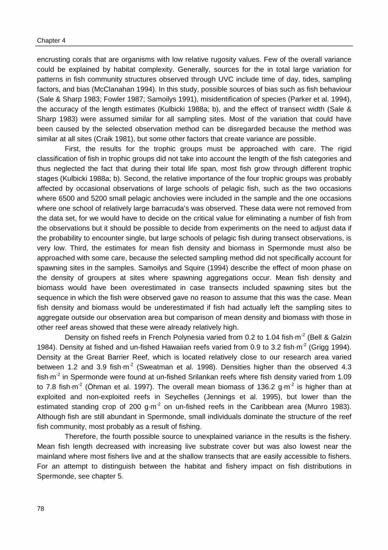
Chapter 4
78
encrusting corals that are organisms with low relative rugosity values. Few of the overall variancecould be explained by habitat complexity. Generally, sources for the in total large variation forpatterns in fish community structures observed through UVC include time of day, tides, samplingfactors, and bias (McClanahan 1994). In this study, possible sources of bias such as fish behaviour(Sale & Sharp 1983; Fowler 1987; Samoilys 1991), misidentification of species (Parker et al. 1994),the accuracy of the length estimates (Kulbicki 1988a; b), and the effect of transect width (Sale &Sharp 1983) were assumed similar for all sampling sites. Most of the variation that could havebeen caused by the selected observation method can be disregarded because the method wassimilar at all sites (Craik 1981), but some other factors that create variance are possible.
First, the results for the trophic groups must be approached with care. The rigidclassification of fish in trophic groups did not take into account the length of the fish categories andthus neglected the fact that during their total life span, most fish grow through different trophicstages (Kulbicki 1988a; b). Second, the relative importance of the four trophic groups was probablyaffected by occasional observations of large schools of pelagic fish, such as the two occasionswhere 6500 and 5200 small pelagic anchovies were included in the sample and the one occasionswhere one school of relatively large barracuda’s was observed. These data were not removed fromthe data set, for we would have to decide on the critical value for eliminating a number of fish fromthe observations but it should be possible to decide from experiments on the need to adjust data ifthe probability to encounter single, but large schools of pelagic fish during transect observations, isvery low. Third, the estimates for mean fish density and biomass in Spermonde must also beapproached with some care, because the selected sampling method did not specifically account forspawning sites in the samples. Samoilys and Squire (1994) describe the effect of moon phase onthe density of groupers at sites where spawning aggregations occur. Mean fish density andbiomass would have been overestimated in case transects included spawning sites but thesequence in which the fish were observed gave no reason to assume that this was the case. Meanfish density and biomass would be underestimated if fish had actually left the sampling sites toaggregate outside our observation area but comparison of mean density and biomass with those inother reef areas showed that these were already relatively high.
Density on fished reefs in French Polynesia varied from 0.2 to 1.04 fish·m-2 (Bell & Galzin1984). Density at fished and un-fished Hawaiian reefs varied from 0.9 to 3.2 fish·m-2 (Grigg 1994).Density at the Great Barrier Reef, which is located relatively close to our research area variedbetween 1.2 and 3.9 fish·m-2 (Sweatman et al. 1998). Densities higher than the observed 4.3fish·m-2 in Spermonde were found at un-fished Srilankan reefs where fish density varied from 1.09to 7.8 fish·m-2 (Öhman et al. 1997). The overall mean biomass of 136.2 g·m-2 is higher than atexploited and non-exploited reefs in Seychelles (Jennings et al. 1995), but lower than theestimated standing crop of 200 g·m-2 on un-fished reefs in the Caribbean area (Munro 1983).Although fish are still abundant in Spermonde, small individuals dominate the structure of the reeffish community, most probably as a result of fishing.
Therefore, the fourth possible source to unexplained variance in the results is the fishery.Mean fish length decreased with increasing live substrate cover but was also lowest near themainland where most fishers live and at the shallow transects that are easily accessible to fishers.For an attempt to distinguish between the habitat and fishery impact on fish distributions inSpermonde, see chapter 5.
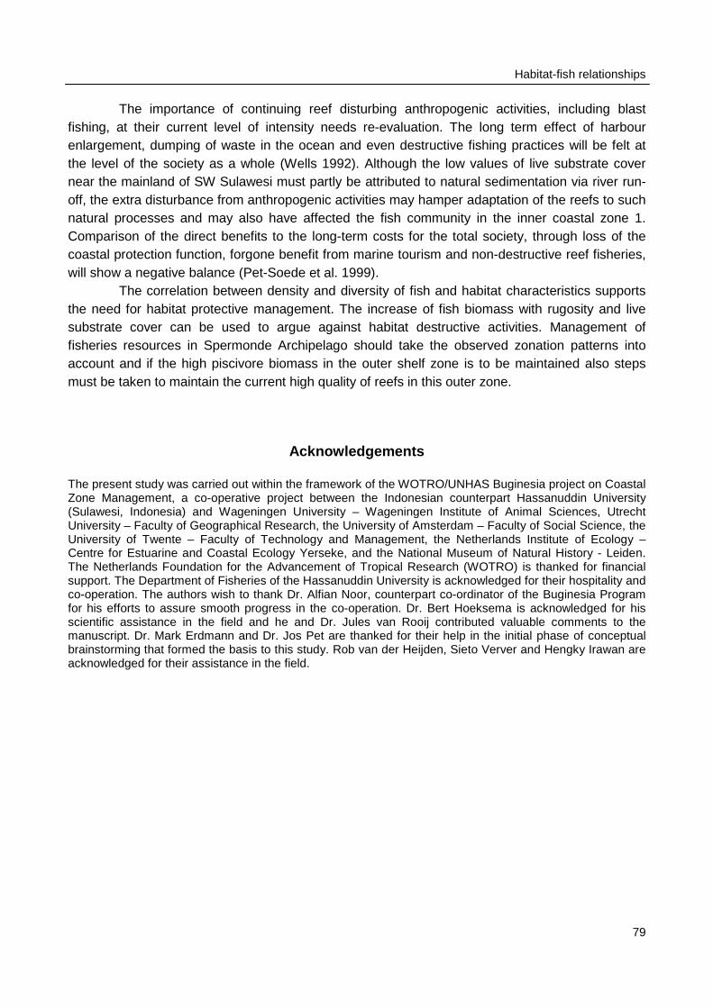
Habitat-fish relationships
79
The importance of continuing reef disturbing anthropogenic activities, including blastfishing, at their current level of intensity needs re-evaluation. The long term effect of harbourenlargement, dumping of waste in the ocean and even destructive fishing practices will be felt atthe level of the society as a whole (Wells 1992). Although the low values of live substrate covernear the mainland of SW Sulawesi must partly be attributed to natural sedimentation via river run-off, the extra disturbance from anthropogenic activities may hamper adaptation of the reefs to suchnatural processes and may also have affected the fish community in the inner coastal zone 1.Comparison of the direct benefits to the long-term costs for the total society, through loss of thecoastal protection function, forgone benefit from marine tourism and non-destructive reef fisheries,will show a negative balance (Pet-Soede et al. 1999).
The correlation between density and diversity of fish and habitat characteristics supportsthe need for habitat protective management. The increase of fish biomass with rugosity and livesubstrate cover can be used to argue against habitat destructive activities. Management offisheries resources in Spermonde Archipelago should take the observed zonation patterns intoaccount and if the high piscivore biomass in the outer shelf zone is to be maintained also stepsmust be taken to maintain the current high quality of reefs in this outer zone.
Acknowledgements
The present study was carried out within the framework of the WOTRO/UNHAS Buginesia project on CoastalZone Management, a co-operative project between the Indonesian counterpart Hassanuddin University(Sulawesi, Indonesia) and Wageningen University – Wageningen Institute of Animal Sciences, UtrechtUniversity – Faculty of Geographical Research, the University of Amsterdam – Faculty of Social Science, theUniversity of Twente – Faculty of Technology and Management, the Netherlands Institute of Ecology –Centre for Estuarine and Coastal Ecology Yerseke, and the National Museum of Natural History - Leiden.The Netherlands Foundation for the Advancement of Tropical Research (WOTRO) is thanked for financialsupport. The Department of Fisheries of the Hassanuddin University is acknowledged for their hospitality andco-operation. The authors wish to thank Dr. Alfian Noor, counterpart co-ordinator of the Buginesia Programfor his efforts to assure smooth progress in the co-operation. Dr. Bert Hoeksema is acknowledged for hisscientific assistance in the field and he and Dr. Jules van Rooij contributed valuable comments to themanuscript. Dr. Mark Erdmann and Dr. Jos Pet are thanked for their help in the initial phase of conceptualbrainstorming that formed the basis to this study. Rob van der Heijden, Sieto Verver and Hengky Irawan areacknowledged for their assistance in the field.
Photo 11: High biomass density in Komodo
Photo 12: Underwater Visual Cencus
81
Chapter 5
Impact of Indonesian coral reef fisheries on fish community structure
and the resultant catch composition
C. Pet-Soede, W.L.T. van Densen, J.S. Pet and M.A.M. Machiels
Abstract
Species and size composition of fish community structures were studied with Underwater Visual Census(UVC), on Indonesian coral reefs subjected to different levels of fishing intensity. Comparisons were madebetween reefs within Spermonde Archipelago off SW Sulawesi, between reefs inside and outside a marinepark in Komodo coastal area off West Flores, and between the reef areas of Spermonde and Komodo. InSpermonde the species and size composition of the commercial catch at sites with high and low fishingintensity was recorded to determine how these catches reflected shifts in fish community structure. Overallfishing intensity in Spermonde was 557 boatdays·km-2 reef·yr-1, eight times higher than in Komodo (65boatdays·km-2 reef·yr-1), but catch rates were eight times lower in Spermonde (5.8 kg·trip-1) than at reefs inKomodo (48 kg·trip-1). So total catch was similar (3.2 t·km-2 reef in Spermonde; 3.1 t·km-2 reef in Komodo).Within Spermonde fishing intensity was three times as high at reefs in the densely populated southeastsection than at reefs in the northwest section. The various types of reef fishery yielded predominantly reefpiscivores, so they were highly selective. Mean length of fish in the catch was significantly related to fishingintensity, where especially piscivorous groupers (Serranidae) and barracuda’s (Spyraenidae) were larger atthe least intensively fished reefs. Spatial patterns in the fish community within Spermonde as observed withUVC, were not significantly related to patterns in fishing intensity. Within Komodo, total fish biomass andbiomass of piscivores as observed with UVC were significantly higher inside than outside the park, the latterdue to larger average length of piscivores inside (35 cm) than outside (27 cm) the park. Fish communities atreefs differed largely between Spermonde and Komodo, in mean individual length (Spermonde: 7 cm andKomodo 14 cm) and in total biomass (Spermonde: 85 g·m-2 and Komodo 382 g·m-2) but numerical densitieswere almost similar (Spermonde 2.82 fish·m-2 and Komodo 2.5 fish·m-2). Biomass density of fish < 20 cm,mainly planktivores, was ca. 1.5 times higher at the intensively fished reefs in Spermonde than at reefs in themarine park in Komodo, but biomass density for fish > 40 cm was 17 times higher inside Komodo (72% oftotal fish biomass) than in Spermonde (23% of total fish biomass). Our results indicate that an effect offishing pressure on the fish community structure can only be detected by UVC when comparing sites whichlargely differ in fishing intensity (Spermonde and Komodo) or when comparing sites with low and withmedium fishing intensity (inside and outside a marine park). The species and size composition of commercialcatches still demonstrate the differential effect of fishing intensity on fish community structures and so on theresultant catches in the on average intensively fished reef area of Spermonde.
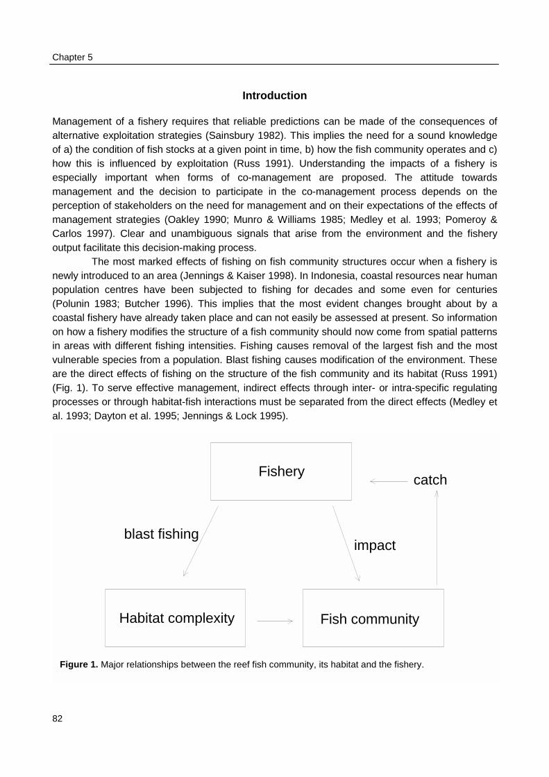
Chapter 5
8
Introduction
Management of a fishery requires that reliable predictions can be made of the consequences ofalternative exploitation strategies (Sainsbury 1982). This implies the need for a sound knowledgeof a) the condition of fish stocks at a given point in time, b) how the fish community operates and c)how this is influenced by exploitation (Russ 1991). Understanding the impacts of a fishery isespecially important when forms of co-management are proposed. The attitude towardsmanagement and the decision to participate in the co-management process depends on theperception of stakeholders on the need for management and on their expectations of the effects ofmanagement strategies (Oakley 1990; Munro & Williams 1985; Medley et al. 1993; Pomeroy &Carlos 1997). Clear and unambiguous signals that arise from the environment and the fisheryoutput facilitate this decision-making process.
The most marked effects of fishing on fish community structures occur when a fishery isnewly introduced to an area (Jennings & Kaiser 1998). In Indonesia, coastal resources near humanpopulation centres have been subjected to fishing for decades and some even for centuries(Polunin 1983; Butcher 1996). This implies that the most evident changes brought about by acoastal fishery have already taken place and can not easily be assessed at present. So informationon how a fishery modifies the structure of a fish community should now come from spatial patternsin areas with different fishing intensities. Fishing causes removal of the largest fish and the mostvulnerable species from a population. Blast fishing causes modification of the environment. Theseare the direct effects of fishing on the structure of the fish community and its habitat (Russ 1991)(Fig. 1). To serve effective management, indirect effects through inter- or intra-specific regulatingprocesses or through habitat-fish interactions must be separated from the direct effects (Medley etal. 1993; Dayton et al. 1995; Jennings & Lock 1995).
Fishery
Habitat complexity Fish community
impactblast fishing
catch
Figure 1. Major relationships between the reef fish community, its habitat and the fishery.
2
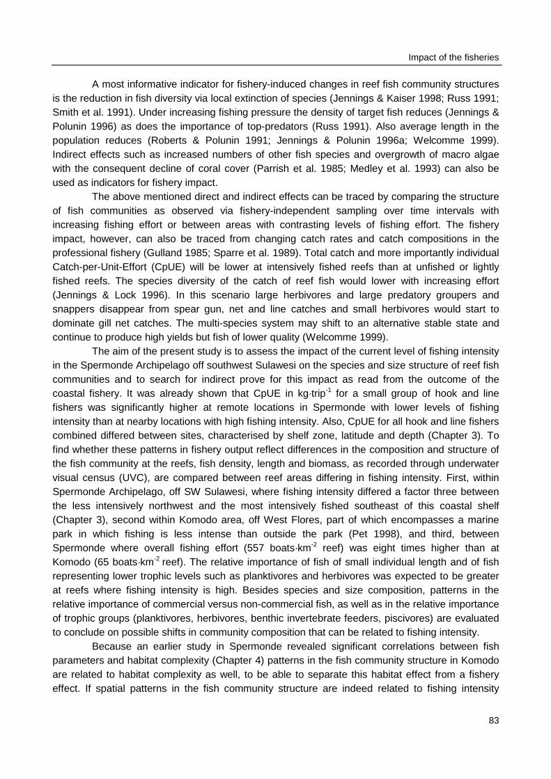
Impact of the fisheries
83
A most informative indicator for fishery-induced changes in reef fish community structuresis the reduction in fish diversity via local extinction of species (Jennings & Kaiser 1998; Russ 1991;Smith et al. 1991). Under increasing fishing pressure the density of target fish reduces (Jennings &Polunin 1996) as does the importance of top-predators (Russ 1991). Also average length in thepopulation reduces (Roberts & Polunin 1991; Jennings & Polunin 1996a; Welcomme 1999).Indirect effects such as increased numbers of other fish species and overgrowth of macro algaewith the consequent decline of coral cover (Parrish et al. 1985; Medley et al. 1993) can also beused as indicators for fishery impact.
The above mentioned direct and indirect effects can be traced by comparing the structureof fish communities as observed via fishery-independent sampling over time intervals withincreasing fishing effort or between areas with contrasting levels of fishing effort. The fisheryimpact, however, can also be traced from changing catch rates and catch compositions in theprofessional fishery (Gulland 1985; Sparre et al. 1989). Total catch and more importantly individualCatch-per-Unit-Effort (CpUE) will be lower at intensively fished reefs than at unfished or lightlyfished reefs. The species diversity of the catch of reef fish would lower with increasing effort(Jennings & Lock 1996). In this scenario large herbivores and large predatory groupers andsnappers disappear from spear gun, net and line catches and small herbivores would start todominate gill net catches. The multi-species system may shift to an alternative stable state andcontinue to produce high yields but fish of lower quality (Welcomme 1999).
The aim of the present study is to assess the impact of the current level of fishing intensityin the Spermonde Archipelago off southwest Sulawesi on the species and size structure of reef fishcommunities and to search for indirect prove for this impact as read from the outcome of thecoastal fishery. It was already shown that CpUE in kg·trip-1 for a small group of hook and linefishers was significantly higher at remote locations in Spermonde with lower levels of fishingintensity than at nearby locations with high fishing intensity. Also, CpUE for all hook and line fisherscombined differed between sites, characterised by shelf zone, latitude and depth (Chapter 3). Tofind whether these patterns in fishery output reflect differences in the composition and structure ofthe fish community at the reefs, fish density, length and biomass, as recorded through underwatervisual census (UVC), are compared between reef areas differing in fishing intensity. First, withinSpermonde Archipelago, off SW Sulawesi, where fishing intensity differed a factor three betweenthe less intensively northwest and the most intensively fished southeast of this coastal shelf(Chapter 3), second within Komodo area, off West Flores, part of which encompasses a marinepark in which fishing is less intense than outside the park (Pet 1998), and third, betweenSpermonde where overall fishing effort (557 boats·km-2 reef) was eight times higher than atKomodo (65 boats·km-2 reef). The relative importance of fish of small individual length and of fishrepresenting lower trophic levels such as planktivores and herbivores was expected to be greaterat reefs where fishing intensity is high. Besides species and size composition, patterns in therelative importance of commercial versus non-commercial fish, as well as in the relative importanceof trophic groups (planktivores, herbivores, benthic invertebrate feeders, piscivores) are evaluatedto conclude on possible shifts in community composition that can be related to fishing intensity.
Because an earlier study in Spermonde revealed significant correlations between fishparameters and habitat complexity (Chapter 4) patterns in the fish community structure in Komodoare related to habitat complexity as well, to be able to separate this habitat effect from a fisheryeffect. If spatial patterns in the fish community structure are indeed related to fishing intensity
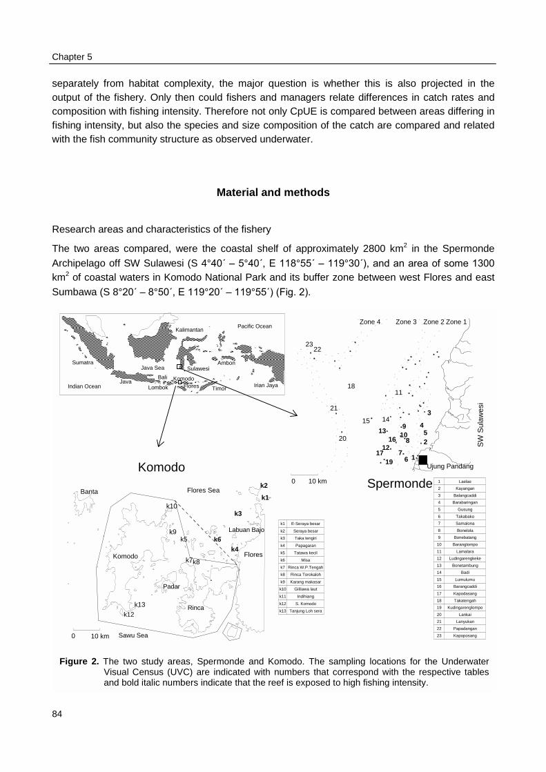
Chapter 5
8
separately from habitat complexity, the major question is whether this is also projected in theoutput of the fishery. Only then could fishers and managers relate differences in catch rates andcomposition with fishing intensity. Therefore not only CpUE is compared between areas differing infishing intensity, but also the species and size composition of the catch are compared and relatedwith the fish community structure as observed underwater.
Material and methods
Research areas and characteristics of the fishery
The two areas compared, were the coastal shelf of approximately 2800 km2 in the Spermonde
Archipelago off SW Sulawesi (S 4°40΄ – 5°40΄, E 118°55΄ – 119°30΄), and an area of some 1300km2 of coastal waters in Komodo National Park and its buffer zone between west Flores and east
Sumbawa (S 8°20΄ – 8°50΄, E 119°20΄ – 119°55΄) (Fig. 2).����������������������������������
1 Laelae
2 Kayangan
3 Balangcaddi
4 Barabaringan
5 Gusung
6 Takabako
7 Samalona
8 Bonelola
9 Bonebatang
10 Baranglompo
11 Lamalara
12 Ludingarengkeke
13 Bonetambung
14 Badi
15 Lumulumu
16 Barangcaddi
17 Kapodasang
18 Takatengah
19 Kudingarenglompo
20 Lankai
21 Lanyukan
22 Papadangan
23 Kapoposang
1
2
3
45
67
8
910
11
12
13
1415
16
17
18
19
20
2322
21
Ujung Pandang
Zone 1Zone 2Zone 3Zone 4
SW
Sul
awes
i10 km0
Rinca
Labuan Bajo
FloresKomodo
Padar
Banta Flores Sea
Sawu Sea
k9
k13
k12
k5
k3
k6
k1
k2
k4
k7k8
k10
0 10 km
k1 E-Seraya besar
k2 Seraya besar
k3 Taka tengiri
k4 Papagaran
k5 Tatawa kecil
k6 Misa
k7 Rinca W.P.Tengah
k8 Rinca Torokaloh
k9 Karang makasar
k10 Gililawa laut
k11 Indihiang
k12 S. Komodo
k13 Tanjung Loh sera
KomodoSpermonde
����� ������
��������������������������������������������������������������������������������������������������������������������������������������������������������������������������
�����������
�� �����
������������������������������������������������������������������������������������
������������
������������������
���������������������������
������������������
�������
����
�������������������������������������������������������������������������������������������������������������������������������������������������
��������������������������������������������������������������������������������������������
����������
���������� ��������
������������
���
�����������������������
�����������
����������������
��������������
������������������������������������������������������������������������������������������������������������������������������������������������������������
�����������������������
������������������ ����
�������
����
�������
��������������
AmbonSumatra
Timor
Bali
Lombok Irian JayaKomodo
Flores
Sulawesi
Kalimantan
Java
Java Sea
Pacific Ocean
Indian Ocean
��������������������
������������
Figure 2. The two study areas, Spermonde and Komodo. The sampling locations for the UnderwaterVisual Census (UVC) are indicated with numbers that correspond with the respective tablesand bold italic numbers indicate that the reef is exposed to high fishing intensity.
4
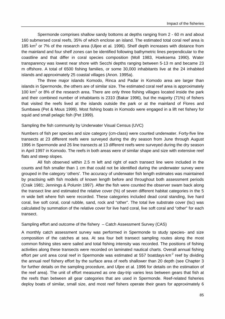
Impact of the fisheries
85
Spermonde comprises shallow sandy bottoms at depths ranging from 2 - 60 m and about160 submersed coral reefs, 35% of which enclose an island. The estimated total coral reef area is185 km2 or 7% of the research area (Uljee et al. 1996). Shelf depth increases with distance fromthe mainland and four shelf zones can be identified following bathymetric lines perpendicular to thecoastline and that differ in coral species composition (Moll 1983, Hoeksema 1990). Watertransparency was lowest near shore with Secchi depths ranging between 5-13 m and became 23m offshore. A total of 6500 fishing families, or some 30,000 inhabitants live at the 24 inhabitedislands and approximately 25 coastal villages (Anon. 1995a).
The three major islands Komodo, Rinca and Padar in Komodo area are larger thanislands in Spermonde, the others are of similar size. The estimated coral reef area is approximately100 km2 or 8% of the research area. There are only three fishing villages located inside the parkand their combined number of inhabitants is 2310 (Bakar 1996), but the majority (71%) of fishersthat visited the reefs lived at the islands outside the park or at the mainland of Flores andSumbawa (Pet & Mous 1999). Most fishing boats in Komodo were engaged in a lift net fishery forsquid and small pelagic fish (Pet 1999).
Sampling the fish community by Underwater Visual Census (UVC)
Numbers of fish per species and size category (cm-class) were counted underwater. Forty-five linetransects at 23 different reefs were surveyed during the dry season from June through August1996 in Spermonde and 26 line transects at 13 different reefs were surveyed during the dry seasonin April 1997 in Komodo. The reefs in both areas were of similar shape and size with extensive reefflats and steep slopes.
All fish observed within 2.5 m left and right of each transect line were included in thecounts and fish smaller than 1 cm that could not be identified during the underwater survey weregrouped in the category ‘others’. The accuracy of underwater fish length estimates was maintainedby practising with fish models of known length before and throughout both assessment periods(Craik 1981; Jennings & Polunin 1997). After the fish were counted the observer swam back alongthe transect line and estimated the relative cover (%) of seven different habitat categories in the 5m wide belt where fish were recorded. These categories included dead coral standing, live hardcoral, live soft coral, coral rubble, sand, rock and “other”. The total live substrate cover (lsc) wascalculated by summation of the relative cover for live hard coral, live soft coral and “other” for eachtransect.
Sampling effort and outcome of the fishery – Catch Assessment Survey (CAS)
A monthly catch assessment survey was performed in Spermonde to study species- and sizecomposition of the catches at sea. At sea four belt transect sampling routes along the mostcommon fishing sites were sailed and total fishing intensity was recorded. The positions of fishingactivities along these transects were recorded on laminated nautical charts. Overall annual fishingeffort per unit area coral reef in Spermonde was estimated at 557 boatdays·km-2 reef by dividingthe annual reef fishery effort by the surface area of reefs shallower than 20 depth (see Chapter 3for further details on the sampling procedure, and Uljee et al. 1996 for details on the estimation ofthe reef area). The unit of effort measured as one day-trip varies less between gears that fish atthe reefs than between all gear categories that are used in Spermonde. Reef-related fisheriesdeploy boats of similar, small size, and most reef fishers operate their gears for approximately 6
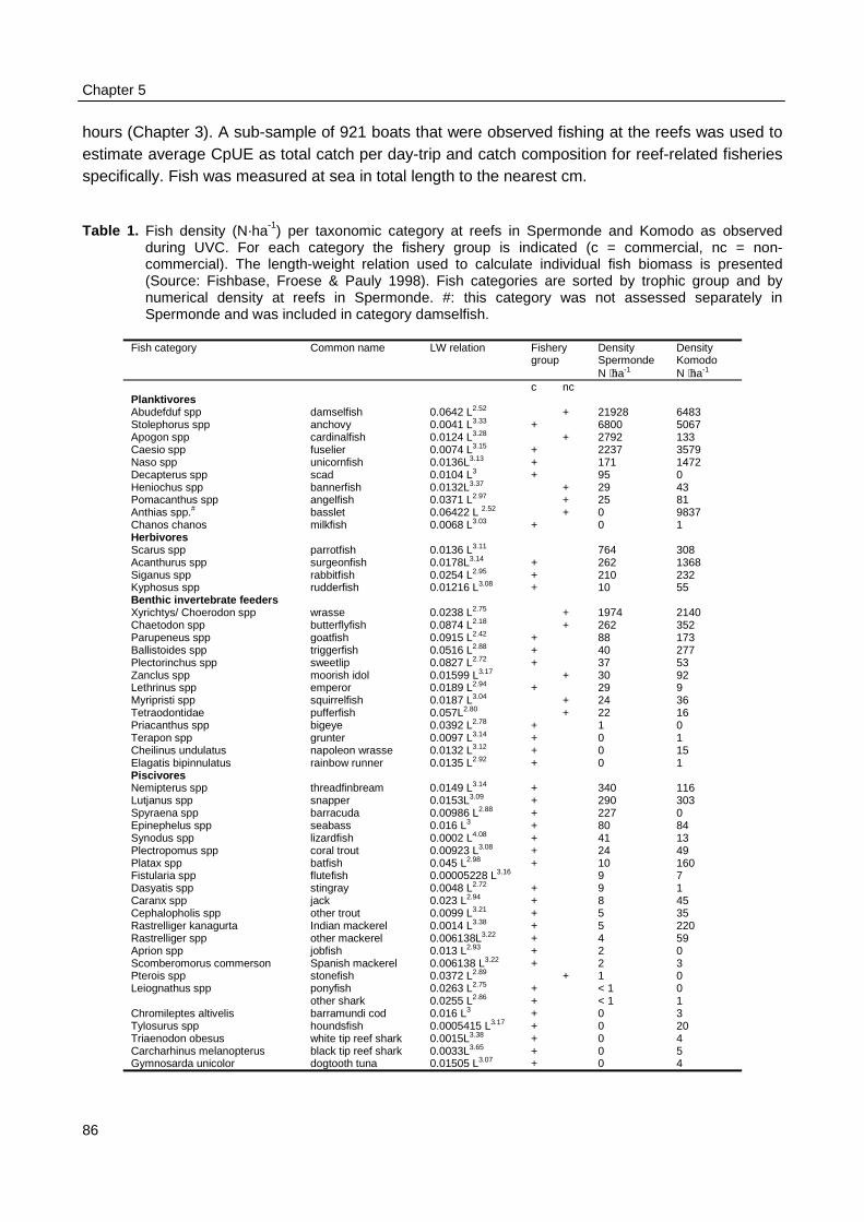
Chapter 5
86
hours (Chapter 3). A sub-sample of 921 boats that were observed fishing at the reefs was used toestimate average CpUE as total catch per day-trip and catch composition for reef-related fisheriesspecifically. Fish was measured at sea in total length to the nearest cm.
Table 1. Fish density (N·ha-1) per taxonomic category at reefs in Spermonde and Komodo as observedduring UVC. For each category the fishery group is indicated (c = commercial, nc = non-commercial). The length-weight relation used to calculate individual fish biomass is presented(Source: Fishbase, Froese & Pauly 1998). Fish categories are sorted by trophic group and bynumerical density at reefs in Spermonde. #: this category was not assessed separately inSpermonde and was included in category damselfish.
Fish category Common name LW relation Fisherygroup
DensitySpermondeN ⋅ha-1
DensityKomodoN ⋅ha-1
c ncPlanktivoresAbudefduf spp damselfish 0.0642 L2.52 + 21928 6483Stolephorus spp anchovy 0.0041 L3.33 + 6800 5067Apogon spp cardinalfish 0.0124 L3.28 + 2792 133Caesio spp fuselier 0.0074 L3.15 + 2237 3579Naso spp unicornfish 0.0136L3.13 + 171 1472Decapterus spp scad 0.0104 L3 + 95 0Heniochus spp bannerfish 0.0132L3.37 + 29 43Pomacanthus spp angelfish 0.0371 L2.97 + 25 81Anthias spp.# basslet 0.06422 L 2.52 + 0 9837Chanos chanos milkfish 0.0068 L3.03 + 0 1HerbivoresScarus spp parrotfish 0.0136 L3.11 764 308Acanthurus spp surgeonfish 0.0178L3.14 + 262 1368Siganus spp rabbitfish 0.0254 L2.95 + 210 232Kyphosus spp rudderfish 0.01216 L3.08 + 10 55Benthic invertebrate feedersXyrichtys/ Choerodon spp wrasse 0.0238 L2.75 + 1974 2140Chaetodon spp butterflyfish 0.0874 L2.18 + 262 352Parupeneus spp goatfish 0.0915 L2.42 + 88 173Ballistoides spp triggerfish 0.0516 L2.88 + 40 277Plectorinchus spp sweetlip 0.0827 L2.72 + 37 53Zanclus spp moorish idol 0.01599 L3.17 + 30 92Lethrinus spp emperor 0.0189 L2.94 + 29 9Myripristi spp squirrelfish 0.0187 L3.04 + 24 36Tetraodontidae pufferfish 0.057L2.80 + 22 16Priacanthus spp bigeye 0.0392 L2.78 + 1 0Terapon spp grunter 0.0097 L3.14 + 0 1Cheilinus undulatus napoleon wrasse 0.0132 L3.12 + 0 15Elagatis bipinnulatus rainbow runner 0.0135 L2.92 + 0 1PiscivoresNemipterus spp threadfinbream 0.0149 L3.14 + 340 116Lutjanus spp snapper 0.0153L3.09 + 290 303Spyraena spp barracuda 0.00986 L2.88 + 227 0Epinephelus spp seabass 0.016 L3 + 80 84Synodus spp lizardfish 0.0002 L4.08 + 41 13Plectropomus spp coral trout 0.00923 L3.08 + 24 49Platax spp batfish 0.045 L2.98 + 10 160Fistularia spp flutefish 0.00005228 L3.16 9 7Dasyatis spp stingray 0.0048 L2.72 + 9 1Caranx spp jack 0.023 L2.94 + 8 45Cephalopholis spp other trout 0.0099 L3.21 + 5 35Rastrelliger kanagurta Indian mackerel 0.0014 L3.38 + 5 220Rastrelliger spp other mackerel 0.006138L3.22 + 4 59Aprion spp jobfish 0.013 L2.93 + 2 0Scomberomorus commerson Spanish mackerel 0.006138 L3.22 + 2 3Pterois spp stonefish 0.0372 L2.89 + 1 0Leiognathus spp ponyfish 0.0263 L2.75 + < 1 0
other shark 0.0255 L2.86 + < 1 1Chromileptes altivelis barramundi cod 0.016 L3 + 0 3Tylosurus spp houndsfish 0.0005415 L3.17 + 0 20Triaenodon obesus white tip reef shark 0.0015L3.38 + 0 4Carcharhinus melanopterus black tip reef shark 0.0033L3.65 + 0 5Gymnosarda unicolor dogtooth tuna 0.01505 L3.07 + 0 4
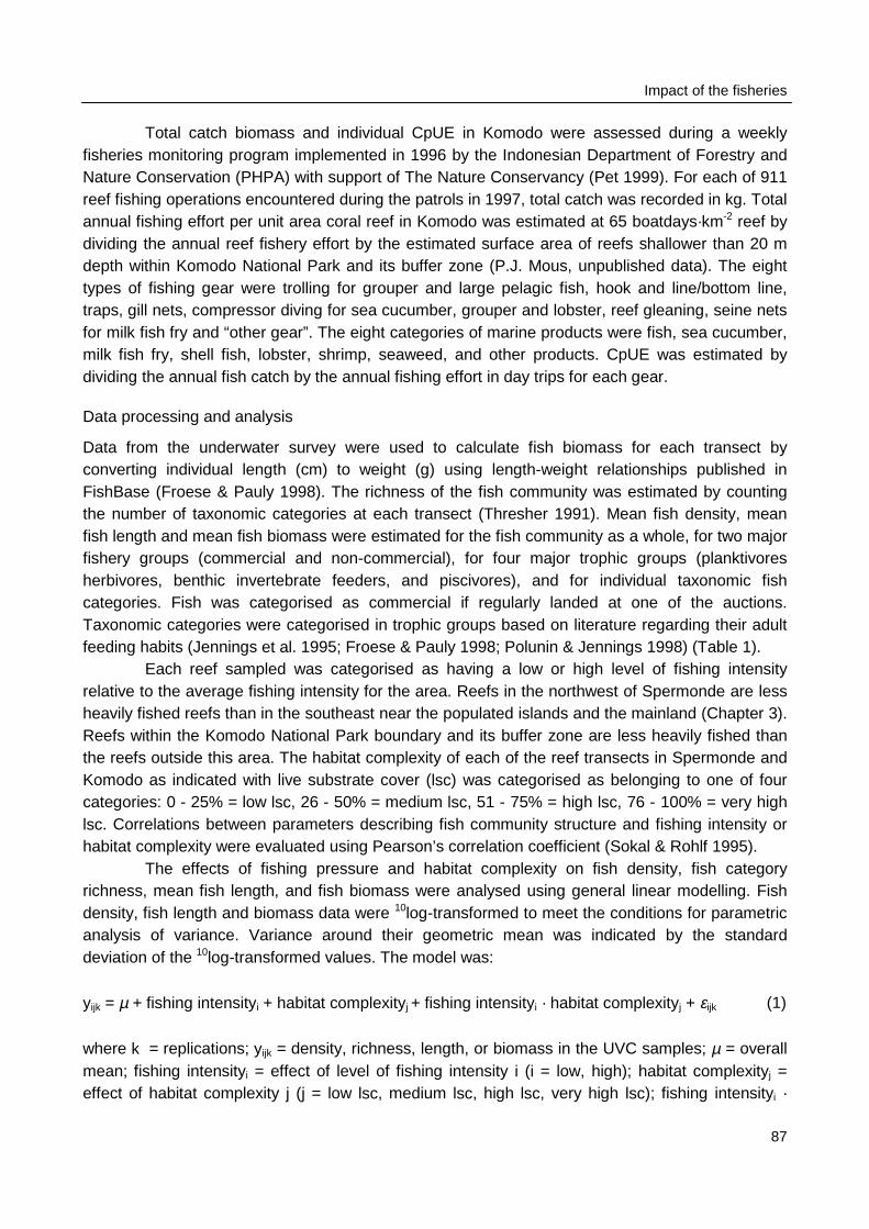
Impact of the fisheries
87
Total catch biomass and individual CpUE in Komodo were assessed during a weeklyfisheries monitoring program implemented in 1996 by the Indonesian Department of Forestry andNature Conservation (PHPA) with support of The Nature Conservancy (Pet 1999). For each of 911reef fishing operations encountered during the patrols in 1997, total catch was recorded in kg. Totalannual fishing effort per unit area coral reef in Komodo was estimated at 65 boatdays·km-2 reef bydividing the annual reef fishery effort by the estimated surface area of reefs shallower than 20 mdepth within Komodo National Park and its buffer zone (P.J. Mous, unpublished data). The eighttypes of fishing gear were trolling for grouper and large pelagic fish, hook and line/bottom line,traps, gill nets, compressor diving for sea cucumber, grouper and lobster, reef gleaning, seine netsfor milk fish fry and “other gear”. The eight categories of marine products were fish, sea cucumber,milk fish fry, shell fish, lobster, shrimp, seaweed, and other products. CpUE was estimated bydividing the annual fish catch by the annual fishing effort in day trips for each gear.
Data processing and analysis
Data from the underwater survey were used to calculate fish biomass for each transect byconverting individual length (cm) to weight (g) using length-weight relationships published inFishBase (Froese & Pauly 1998). The richness of the fish community was estimated by countingthe number of taxonomic categories at each transect (Thresher 1991). Mean fish density, meanfish length and mean fish biomass were estimated for the fish community as a whole, for two majorfishery groups (commercial and non-commercial), for four major trophic groups (planktivoresherbivores, benthic invertebrate feeders, and piscivores), and for individual taxonomic fishcategories. Fish was categorised as commercial if regularly landed at one of the auctions.Taxonomic categories were categorised in trophic groups based on literature regarding their adultfeeding habits (Jennings et al. 1995; Froese & Pauly 1998; Polunin & Jennings 1998) (Table 1).
Each reef sampled was categorised as having a low or high level of fishing intensityrelative to the average fishing intensity for the area. Reefs in the northwest of Spermonde are lessheavily fished reefs than in the southeast near the populated islands and the mainland (Chapter 3).Reefs within the Komodo National Park boundary and its buffer zone are less heavily fished thanthe reefs outside this area. The habitat complexity of each of the reef transects in Spermonde andKomodo as indicated with live substrate cover (lsc) was categorised as belonging to one of fourcategories: 0 - 25% = low lsc, 26 - 50% = medium lsc, 51 - 75% = high lsc, 76 - 100% = very highlsc. Correlations between parameters describing fish community structure and fishing intensity orhabitat complexity were evaluated using Pearson’s correlation coefficient (Sokal & Rohlf 1995).
The effects of fishing pressure and habitat complexity on fish density, fish categoryrichness, mean fish length, and fish biomass were analysed using general linear modelling. Fishdensity, fish length and biomass data were 10log-transformed to meet the conditions for parametricanalysis of variance. Variance around their geometric mean was indicated by the standarddeviation of the 10log-transformed values. The model was:
yijk = µ + fishing intensityi + habitat complexityj + fishing intensityi · habitat complexityj + εijk (1)
where k = replications; yijk = density, richness, length, or biomass in the UVC samples; µ = overallmean; fishing intensityi = effect of level of fishing intensity i (i = low, high); habitat complexityj =effect of habitat complexity j (j = low lsc, medium lsc, high lsc, very high lsc); fishing intensityi ·
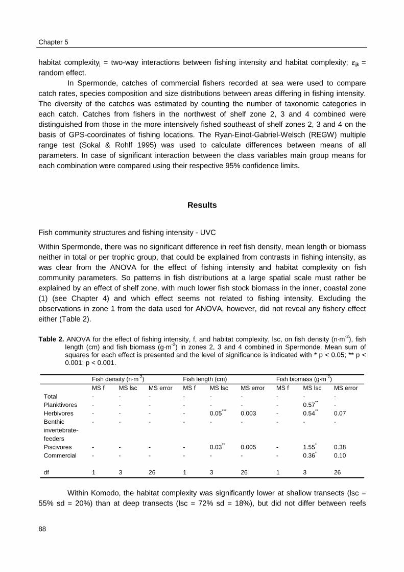
Chapter 5
88
habitat complexityj = two-way interactions between fishing intensity and habitat complexity; εijk =random effect.
In Spermonde, catches of commercial fishers recorded at sea were used to comparecatch rates, species composition and size distributions between areas differing in fishing intensity.The diversity of the catches was estimated by counting the number of taxonomic categories ineach catch. Catches from fishers in the northwest of shelf zone 2, 3 and 4 combined weredistinguished from those in the more intensively fished southeast of shelf zones 2, 3 and 4 on thebasis of GPS-coordinates of fishing locations. The Ryan-Einot-Gabriel-Welsch (REGW) multiplerange test (Sokal & Rohlf 1995) was used to calculate differences between means of allparameters. In case of significant interaction between the class variables main group means foreach combination were compared using their respective 95% confidence limits.
Results
Fish community structures and fishing intensity - UVC
Within Spermonde, there was no significant difference in reef fish density, mean length or biomassneither in total or per trophic group, that could be explained from contrasts in fishing intensity, aswas clear from the ANOVA for the effect of fishing intensity and habitat complexity on fishcommunity parameters. So patterns in fish distributions at a large spatial scale must rather beexplained by an effect of shelf zone, with much lower fish stock biomass in the inner, coastal zone(1) (see Chapter 4) and which effect seems not related to fishing intensity. Excluding theobservations in zone 1 from the data used for ANOVA, however, did not reveal any fishery effecteither (Table 2).
Table 2. ANOVA for the effect of fishing intensity, f, and habitat complexity, lsc, on fish density (n·m-2), fishlength (cm) and fish biomass (g·m-2) in zones 2, 3 and 4 combined in Spermonde. Mean sum ofsquares for each effect is presented and the level of significance is indicated with * p < 0.05; ** p <0.001; p < 0.001.
Fish density (n·m-2) Fish length (cm) Fish biomass (g·m-2)MS f MS lsc MS error MS f MS lsc MS error MS f MS lsc MS error
Total - - - - - - - - -Planktivores - - - - - - - 0.57** -Herbivores - - - - 0.05*** 0.003 - 0.54** 0.07Benthicinvertebrate-feeders
- - - - - - - - -
Piscivores - - - - 0.03** 0.005 - 1.55* 0.38Commercial - - - - - - - 0.36* 0.10
df 1 3 26 1 3 26 1 3 26
Within Komodo, the habitat complexity was significantly lower at shallow transects (lsc =55% sd = 20%) than at deep transects (lsc = 72% sd = 18%), but did not differ between reefs
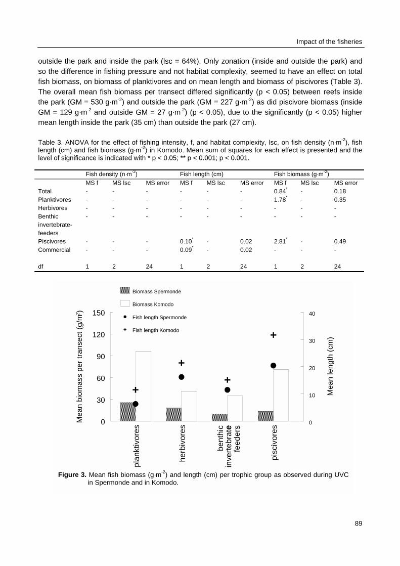
Impact of the fisheries
outside the park and inside the park (lsc = 64%). Only zonation (inside and outside the park) andso the difference in fishing pressure and not habitat complexity, seemed to have an effect on totalfish biomass, on biomass of planktivores and on mean length and biomass of piscivores (Table 3).The overall mean fish biomass per transect differed significantly (p < 0.05) between reefs insidethe park (GM = 530 g·m-2) and outside the park (GM = 227 g·m-2) as did piscivore biomass (insideGM = 129 g·m-2 and outside GM = 27 g·m-2) (p < 0.05), due to the significantly (p < 0.05) highermean length inside the park (35 cm) than outside the park (27 cm).
Table 3. ANOVA for the effect of fishing intensity, f, and habitat complexity, lsc, on fish density (n·m-2), fishlength (cm) and fish biomass (g·m-2) in Komodo. Mean sum of squares for each effect is presented and thelevel of significance is indicated with * p < 0.05; ** p < 0.001; p < 0.001.
Fish density (n·m-2) Fish length (cm) Fish biomass (g·m-2)MS f MS lsc MS error MS f MS lsc MS error MS f MS lsc MS error
Total - - - - - - 0.84* - 0.18Planktivores - - - - - - 1.78* - 0.35Herbivores - - - - - - - - -Benthicinvertebrate-feeders
- - - - - - - - -
Piscivores - - - 0.10* - 0.02 2.81* - 0.49Commercial - - - 0.09* - 0.02 - - -
df 1 2 24 1 2 24 1 2 24
Fig
plan
ktiv
ores
herb
ivor
es e
pisc
ivor
es
0
30
60
90
120
150
Mea
n bi
omas
s pe
r tr
anse
ct (
g/m
2)
0
10
20
30
40
Mea
n le
ngth
(cm
)
����������������������������������������������������
���������������������������������������
��������������������������
��������������������������������
���������Biomass Spermonde
Biomass Komodo
Fish length Spermonde
Fish length Komodo
feed
ers
bent
hic
inve
rteb
rate
ure 3. Mean fish biomass (g·m-2) and length (cm) per trophic group as observed during UVCin Spermonde and in Komodo.
89
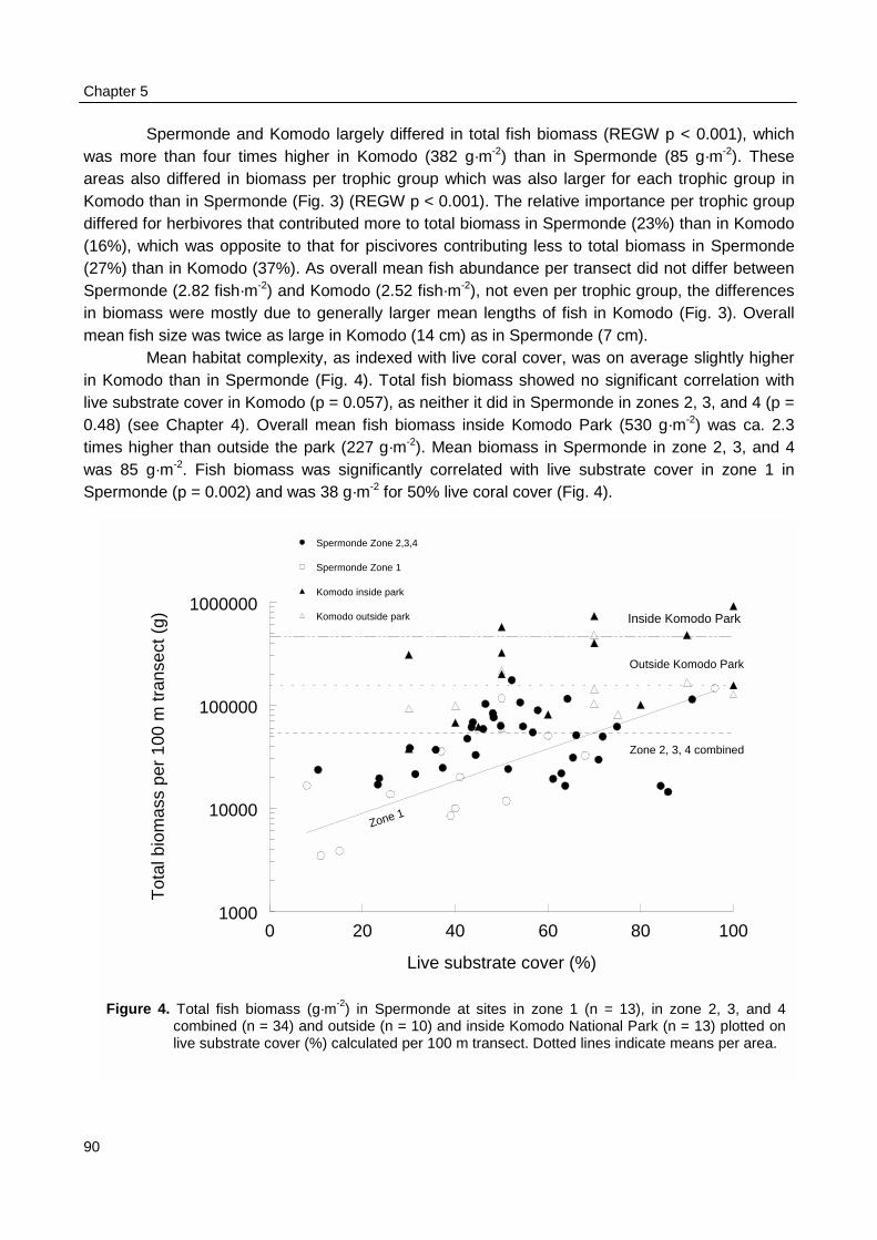
Chapter 5
90
Spermonde and Komodo largely differed in total fish biomass (REGW p < 0.001), whichwas more than four times higher in Komodo (382 g·m-2) than in Spermonde (85 g·m-2). Theseareas also differed in biomass per trophic group which was also larger for each trophic group inKomodo than in Spermonde (Fig. 3) (REGW p < 0.001). The relative importance per trophic groupdiffered for herbivores that contributed more to total biomass in Spermonde (23%) than in Komodo(16%), which was opposite to that for piscivores contributing less to total biomass in Spermonde(27%) than in Komodo (37%). As overall mean fish abundance per transect did not differ betweenSpermonde (2.82 fish·m-2) and Komodo (2.52 fish·m-2), not even per trophic group, the differencesin biomass were mostly due to generally larger mean lengths of fish in Komodo (Fig. 3). Overallmean fish size was twice as large in Komodo (14 cm) as in Spermonde (7 cm).
Mean habitat complexity, as indexed with live coral cover, was on average slightly higherin Komodo than in Spermonde (Fig. 4). Total fish biomass showed no significant correlation withlive substrate cover in Komodo (p = 0.057), as neither it did in Spermonde in zones 2, 3, and 4 (p =0.48) (see Chapter 4). Overall mean fish biomass inside Komodo Park (530 g·m-2) was ca. 2.3times higher than outside the park (227 g·m-2). Mean biomass in Spermonde in zone 2, 3, and 4was 85 g·m-2. Fish biomass was significantly correlated with live substrate cover in zone 1 inSpermonde (p = 0.002) and was 38 g·m-2 for 50% live coral cover (Fig. 4).
0 20 40 60 80 100
Live substrate cover (%)
1000
10000
100000
1000000
Tot
al b
iom
ass
per
100
m tr
anse
ct (
g)
Spermonde Zone 2,3,4
Spermonde Zone 1
Komodo inside park
Komodo outside park Inside Komodo Park
Outside Komodo Park
Zone 2, 3, 4 combined
Zone 1
Figure 4. Total fish biomass (g·m-2) in Spermonde at sites in zone 1 (n = 13), in zone 2, 3, and 4combined (n = 34) and outside (n = 10) and inside Komodo National Park (n = 13) plotted onlive substrate cover (%) calculated per 100 m transect. Dotted lines indicate means per area.
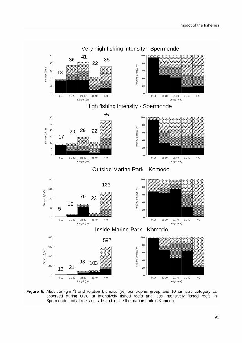
Impact of the fisheries
0-10 11-20 21-30 31-40 >40
Length (cm)
0
10
20
30
40
50
Bio
mas
s (g
/m2)
������������������
��������������������������������
������������������������������������������������������
����������������������������������
������������������������������
������������������������������������
����������������������������������������������������
����������������������������������
���������������������������������������������
������������������
������������������������������������������������
������������������������������������
����������������������������������
������������������������������
0-10 11-20 21-30 31-40 >40
Length (cm)
0
20
40
60
80
100
Rel
ativ
e bi
omas
s (%
)
����������������
������������������������������������
������������������������������������������������������������������
������������������������������
������������������������������������������������������
��������������������������������
������������������������������������
�������������������������������������������������
������������������������������
������������������������������������������������������������������������
����������������������������������������������������������������������
���������������������������������������������������
������������������������������������������������������������
������������������������������������������������������
0-10 11-20 21-30 31-40 >40
Length (cm)
0
10
20
30
40
50
60
Bio
mas
s (g
/m2)
��������������������������������������������������
������������������������������������
����������������������������������
���������������������������������������������
��������������������������������������������������
�����������������������������������������������������
������������������������������
���������������������������������������������������������������������������������������
�����������������
������������������������������������������������������������
0-10 11-20 21-30 31-40 >40
Length (cm)
0
20
40
60
80
100
Rel
ativ
e bi
omas
s (%
)
����������������
������������������������������������������������������������������������
���������������������������������������������������
������������������������������������������������������������
������������������������������������������������������
��������������������������������
������������������������������������
����������������������������������
������������������������������������������������
������������������
����������������������������������������������������������������������
�������������������������������������������������������������������������������������
������������������������������������������������������������
������������������������������������������������������������������������������������������
0-10 11-20 21-30 31-40 >40
Length (cm)
0
50
100
150
200
Bio
mas
s (g
/m2)
����������������������������������
������������������������������������
��������������������������������������������������������������������������������
����������������
������������������
�����������������
������������������������������
����������������������������������
������������������
�����������������
������������������������������������������������������������
0-10 11-20 21-30 31-40 >40
Length (cm)
0
20
40
60
80
100
Rel
ativ
e bi
omas
s (%
) ����������������������������������������������������������������������
����������������������������������
���������������������������������������������������������������
������������������������������������
������������������������������������������������
������������������������������������
����������������������������������
������������������������������
������������������������������������
������������������������������������������������������������������������������������������������
������������������������������������������������������������������������������������������
0-10 11-20 21-30 31-40 >40
Length (cm)
0
200
400
600
800
Bio
mas
s (g
/m2)
����������������������������������������������������������������������
�����������������������������������������������
���������������������������������������������������������������������
���������������������������������������������
���������������������������������������������������������������������
���������������������������������������������
0-10 11-20 21-30 31-40 >40
Length (cm)
0
20
40
60
80
100
Rel
ativ
e bi
omas
s (%
)
����������������
������������������������������������
��������������������������������������������������������������������
���������������������������������������������
������������������
����������������������������������������������������������������������
��������������������������������
������������������������������������������������������������������������
��������������������������������������������������������������������
������������������������������
������������������������������������������������������������������������
Very high fishing intensity - Spermonde
High fishing intensity - Spermonde
Outside Marine Park - Komodo
Inside Marine Park - Komodo
18
3641
2235
55
22292017
519
70 23
133
597
103932113
Figure 5. Absolute (g·m-2) and relative biomass (%) per trophic group and 10 cm size category asobserved during UVC at intensively fished reefs and less intensively fished reefs inSpermonde and at reefs outside and inside the marine park in Komodo.
91
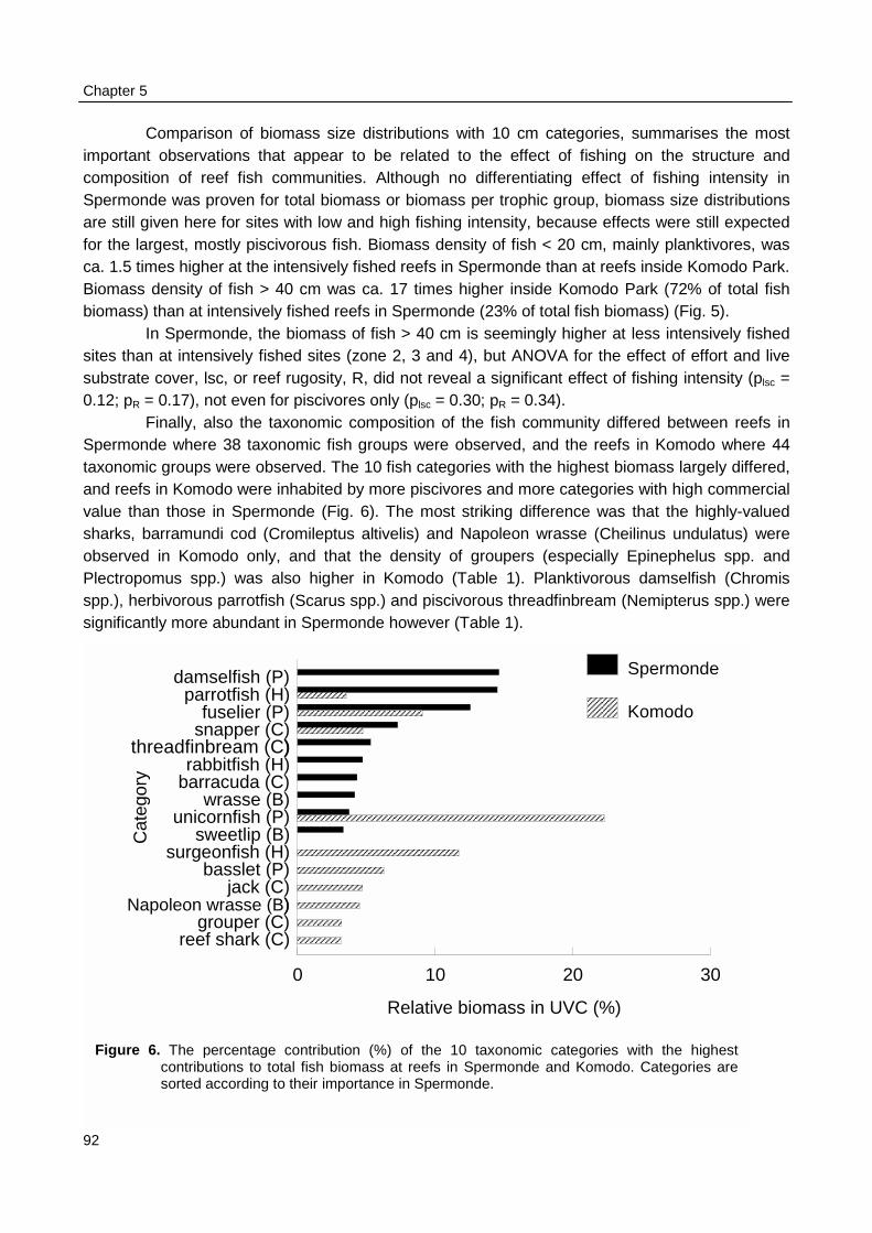
Chapter 5
92
Comparison of biomass size distributions with 10 cm categories, summarises the mostimportant observations that appear to be related to the effect of fishing on the structure andcomposition of reef fish communities. Although no differentiating effect of fishing intensity inSpermonde was proven for total biomass or biomass per trophic group, biomass size distributionsare still given here for sites with low and high fishing intensity, because effects were still expectedfor the largest, mostly piscivorous fish. Biomass density of fish < 20 cm, mainly planktivores, wasca. 1.5 times higher at the intensively fished reefs in Spermonde than at reefs inside Komodo Park.Biomass density of fish > 40 cm was ca. 17 times higher inside Komodo Park (72% of total fishbiomass) than at intensively fished reefs in Spermonde (23% of total fish biomass) (Fig. 5).
In Spermonde, the biomass of fish > 40 cm is seemingly higher at less intensively fishedsites than at intensively fished sites (zone 2, 3 and 4), but ANOVA for the effect of effort and livesubstrate cover, lsc, or reef rugosity, R, did not reveal a significant effect of fishing intensity (plsc =0.12; pR = 0.17), not even for piscivores only (plsc = 0.30; pR = 0.34).
Finally, also the taxonomic composition of the fish community differed between reefs inSpermonde where 38 taxonomic fish groups were observed, and the reefs in Komodo where 44taxonomic groups were observed. The 10 fish categories with the highest biomass largely differed,and reefs in Komodo were inhabited by more piscivores and more categories with high commercialvalue than those in Spermonde (Fig. 6). The most striking difference was that the highly-valuedsharks, barramundi cod (Cromileptus altivelis) and Napoleon wrasse (Cheilinus undulatus) wereobserved in Komodo only, and that the density of groupers (especially Epinephelus spp. andPlectropomus spp.) was also higher in Komodo (Table 1). Planktivorous damselfish (Chromisspp.), herbivorous parrotfish (Scarus spp.) and piscivorous threadfinbream (Nemipterus spp.) weresignificantly more abundant in Spermonde however (Table 1).
damselfish (P)parrotfish (H)
fuselier (P)snapper (C)
)rabbitfish (H)
barracuda (C)wrasse (B)
unicornfish (P)sweetlip (B)
surgeonfish (H)basslet (P)
jack (C))
grouper (C)reef shark (C)
Cat
egor
y
0 10 20 30
Relative biomass in UVC (%)
�����������������������������������������������������������������������������������������������������������������
���������������������������������������������������������������������������������������������������������������
����������������������������������������������������������������������������������������������������������������������������������������������������������������������������������
Spermonde������������������������ Komodo
threadfinbream (C)
Napoleon wrasse (B)
Figure 6. The percentage contribution (%) of the 10 taxonomic categories with the highestcontributions to total fish biomass at reefs in Spermonde and Komodo. Categories aresorted according to their importance in Spermonde.
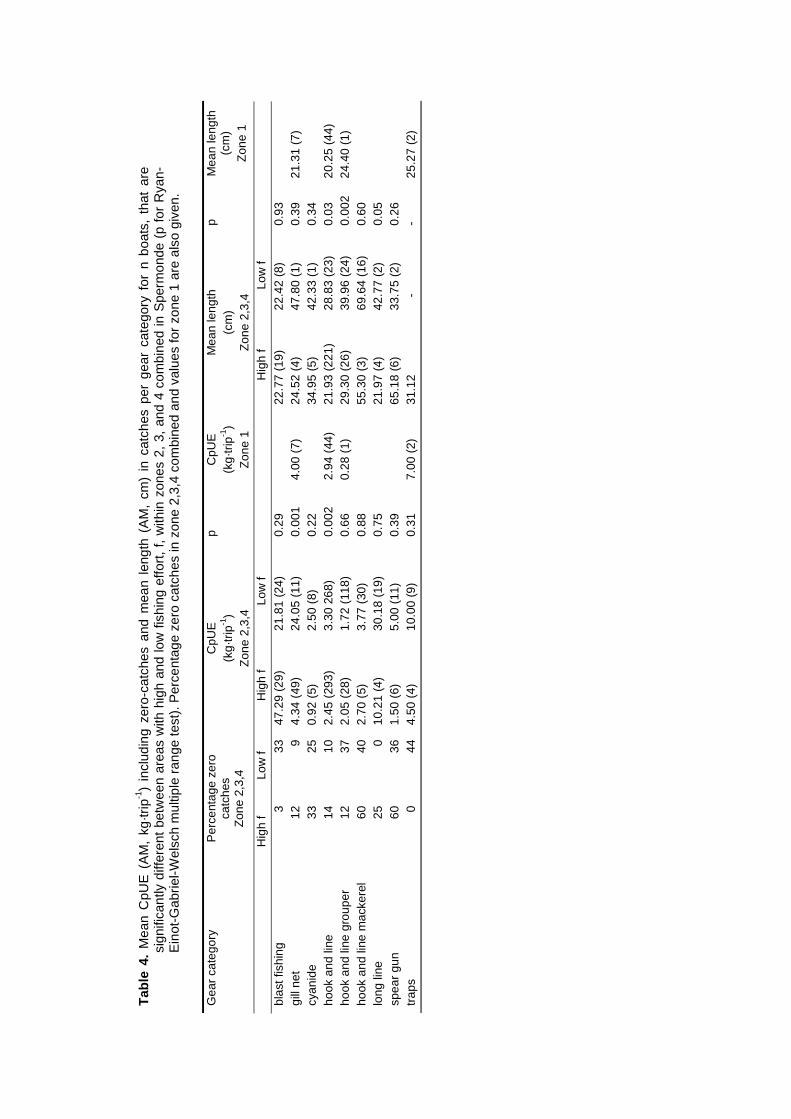
Tab
le 4
. M
ean
CpU
E (
AM
, kg
·trip
-1)
incl
udin
g ze
ro-c
atch
es a
nd m
ean
leng
th (
AM
, cm
) in
cat
ches
per
gea
r ca
tego
ry f
or n
boa
ts,
that
are
sign
ifica
ntly
diff
eren
t be
twee
n ar
eas
with
hig
h an
d lo
w f
ishi
ng e
ffort
, f,
with
in z
ones
2,
3, a
nd 4
com
bine
d in
Spe
rmon
de (
p fo
r R
yan-
Ein
ot-G
abrie
l-Wel
sch
mul
tiple
ran
ge te
st).
Per
cent
age
zero
cat
ches
in z
one
2,3,
4 co
mbi
ned
and
valu
es fo
r zo
ne 1
are
als
o gi
ven.
Gea
r ca
tego
ryP
erce
ntag
e ze
roca
tche
sZ
one
2,3,
4
CpU
E(k
g·tr
ip-1
)Z
one
2,3,
4
pC
pUE
(kg·
trip
-1)
Zon
e 1
Mea
n le
ngth
(cm
)Z
one
2,3,
4
pM
ean
leng
th(c
m)
Zon
e 1
Hig
h f
Low
fH
igh
fLo
w f
Hig
h f
Low
f
blas
t fis
hing
333
47.2
9 (2
9)21
.81
(24)
0.29
22.7
7 (1
9)22
.42
(8)
0.93
gill
net
129
4.34
(49
)24
.05
(11)
0.00
14.
00 (
7)24
.52
(4)
47.8
0 (1
)0.
3921
.31
(7)
cyan
ide
3325
0.92
(5)
2.50
(8)
0.22
34.9
5 (5
)42
.33
(1)
0.34
hook
and
line
1410
2.45
(29
3)3.
30 2
68)
0.00
22.
94 (
44)
21.9
3 (2
21)
28.8
3 (2
3)0.
0320
.25
(44)
hook
and
line
gro
uper
1237
2.05
(28
)1.
72 (
118)
0.66
0.28
(1)
29.3
0 (2
6)39
.96
(24)
0.00
224
.40
(1)
hook
and
line
mac
kere
l60
402.
70 (
5)3.
77 (
30)
0.88
55.3
0 (3
)69
.64
(16)
0.60
long
line
250
10.2
1 (4
)30
.18
(19)
0.75
21.9
7 (4
)42
.77
(2)
0.05
spea
r gu
n60
361.
50 (
6)5.
00 (
11)
0.39
65.1
8 (6
)33
.75
(2)
0.26
trap
s0
444.
50 (
4)10
.00
(9)
0.31
7.00
(2)
31.1
2-
-25
.27
(2)
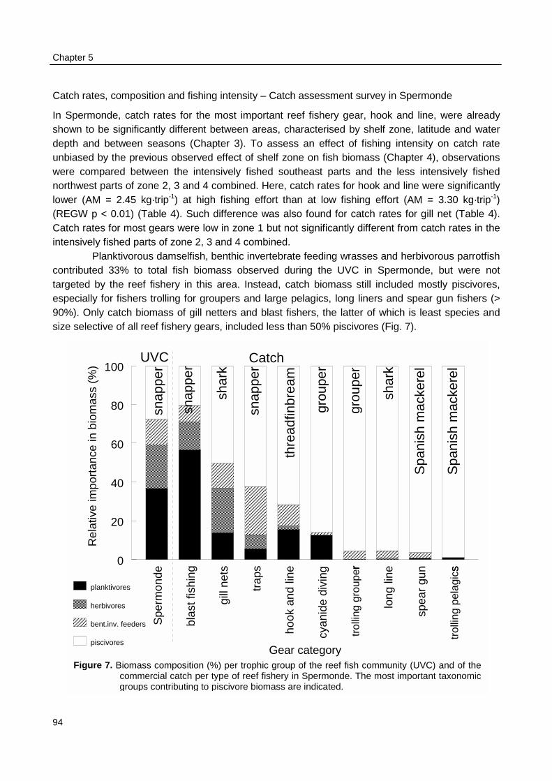
Chapter 5
94
Catch rates, composition and fishing intensity – Catch assessment survey in Spermonde
In Spermonde, catch rates for the most important reef fishery gear, hook and line, were alreadyshown to be significantly different between areas, characterised by shelf zone, latitude and waterdepth and between seasons (Chapter 3). To assess an effect of fishing intensity on catch rateunbiased by the previous observed effect of shelf zone on fish biomass (Chapter 4), observationswere compared between the intensively fished southeast parts and the less intensively fishednorthwest parts of zone 2, 3 and 4 combined. Here, catch rates for hook and line were significantlylower (AM = 2.45 kg·trip-1) at high fishing effort than at low fishing effort (AM = 3.30 kg·trip-1)(REGW p < 0.01) (Table 4). Such difference was also found for catch rates for gill net (Table 4).Catch rates for most gears were low in zone 1 but not significantly different from catch rates in theintensively fished parts of zone 2, 3 and 4 combined.
Planktivorous damselfish, benthic invertebrate feeding wrasses and herbivorous parrotfishcontributed 33% to total fish biomass observed during the UVC in Spermonde, but were nottargeted by the reef fishery in this area. Instead, catch biomass still included mostly piscivores,especially for fishers trolling for groupers and large pelagics, long liners and spear gun fishers (>90%). Only catch biomass of gill netters and blast fishers, the latter of which is least species andsize selective of all reef fishery gears, included less than 50% piscivores (Fig. 7).
Spe
rmon
de
blas
t fis
hing
gill
nets
trap
s
hook
and
line
cyan
ide
divi
ng
r
long
line
spea
r gu
n s
Gear category
0
20
40
60
80
100
Rel
ativ
e im
port
ance
in b
iom
ass
(%)
���������������������������������������������������������������������������
����������������������������������������������������
�������������������������������������������������������������������������������� ��������������
����������������������������
�����������������
�������������� ���������������� �������������
���������������������������������������������
���������������������������������������
������������������������������������������������ ��������������
��������������������������������������������������������
��������������������������������������������������� ���������������
����������������������������
��������������������������������
������������������������������
planktivores���������
herbivores������������������
bent.inv. feeders
piscivores
CatchUVC
Spa
nish
mac
kere
l
Spa
nish
mac
kere
l
shar
k
grou
per
grou
per
thre
adfin
brea
m
snap
per
shar
k
snap
per
snap
per
trol
ling
grou
per
trol
ling
pela
gics
Figure 7. Biomass composition (%) per trophic group of the reef fish community (UVC) and of thecommercial catch per type of reef fishery in Spermonde. The most important taxonomicgroups contributing to piscivore biomass are indicated.
Impact of the fisheries
95
Overall mean length of fish in the catch was 24.5 cm. Mean length of fish was significantlyhigher in catches at sites with low fishing intensity for hook and line fishers, fishers trolling forgrouper, and long liners aiming at sharks (Table 4). The geometric mean length of groupers thathave high export value was significantly larger at sites with low fishing intensity and so was themean length of barracuda’s that are important for the local markets (Table 5). Mean length forthese categories was always smaller in catches in zone 1.
Table 5. Mean size (AM, cm) in the catch for n boats, that are significantly different between areas with highand low fishing effort, f, within zones 2, 3, and 4 combined in Spermonde (p for Ryan-Einot-Gabriel-Welsch multiple range test). Values for Zone 1 are also given.
Fish category Mean length(cm)
p Mean length(cm)
High f Low f Zone 1Epinephelus spp. 24.5 (46) 30.3 (20) 0.026 19.4 (16)Plectropomus spp. 30.7 (24) 38.8 (23) 0.001 25.1 (5)Spyraena spp. 35.4 (21) 77.0 (6) 0.0001 26.0 (5)
There were on average 2.6 taxonomic categories in the individual catch per boat. Catchesin the intensively fished southeast of zone 2, 3, and 4 in Spermonde included more categories thanin the lightly fished northwest (REGW p < 0.05), due to a larger importance of hook and line fishersin the southeast, who’s combined catch was most diverse, with in total 51 different taxonomiccategories (Table 6). Their catches were dominated by threadfin bream (Nemipterus spp).
Table 6. Catch rates (CpUE, kg·daytrip-1) as observed at sea (see also Chapter 3) for Spermonde and forKomodo and the number of taxonomic categories in the catch in Spermonde. 1: only grouper withcyanide; 2: lobster and seacucumber.
Gear category CpUE(kg·daytrip-1)
Number of taxonomic categoriesSpermonde
Spermonde Komodo Individual catch All catchescombined
spear gun 24.8 - 1.2 4diving 16.21 192 1.9 5blast fishing 15.7 - 4.2 35traps 8.5 205 3.1 18gill net 7.5 23 3.6 30hook and line/ bottom line 4.9 79 2.9 51trolling large pelagic fish 3.7 72 1.7 8trolling live grouper 1.7 - 1.4 14
Catch rates from Spermonde and Komodo compared
The annual catch of the reef fishery was estimated 3.2 t km-2 reef in Spermonde and almost similarcatch was obtained from the reefs in Komodo (3.1 t km-2 reef). The mean CpUE for all reeffisheries combined was 5.8 kg·trip-1 in Spermonde, eight times lower than the overall mean CpUEin Komodo (48 kg·trip-1) (Table 6). Also per gear type, catch rates were much lower in Spermondethan in Komodo (Table 6).
Chapter 5
96
Discussion
Comparison of catch rates and catch compositions within Spermonde indicates that fishers catchmore fish at less intensively fished areas and that the mean length at capture of especiallypiscivorous fish decreases with fishing intensity, but such direct relation between fishing intensity,fish biomass and fish length is not supported by patterns as observed underwater in Spermonde.Only when fish community structures are compared between areas with large contrasts in meanfishing intensity such as Spermonde and Komodo do trends appear to be directly related withfishing intensity. Fish are significantly larger and fish biomass is significantly higher at reefs inKomodo that are fished 8 times less intense than reefs in Spermonde. This trend persiststhroughout all levels of data aggregation, for the entire fish community, for different trophic andfishery groups, and even for many individual taxonomic fish categories. Mean fish density does notindicate a fishery influence at the level of the entire fish community or the major groups within it butat the level of individual taxonomic categories, numerical densities of especially commerciallyimportant fish, were larger inside Komodo National Park than in Spermonde.
The overall high taxonomic diversity of catches per gear type illustrates the multi-speciescharacter of the fisheries in Spermonde. Therefore, even when significant, the few contrasts inmean length of fish throughout Spermonde that indicated a fishery impact may be hard to perceiveby the majority of the fishers. Specialists that target groupers may be able to observe a differencein mean length of these fish, but only if they were to frequent locations with high fishing intensity aswell as locations with low fishing intensity. A previous study on strategies applied by fishers inSpermonde indicated however, that most, really small-scale reef fishers are forced to select fishinglocations near their village due to the small nature of their operations, which constrains theirindividual resource space (Chapter 3). Whereas the authors could oversee the entire Spermondearea with higher biomass of fish > 40 cm in areas with low fishing effort, although at a 90%confidence interval, it was nevertheless concluded that such contrasts in Spermonde were weakwhen compared with another reef area, Komodo, with fishing intensity being almost an order ofsize lower.
Most of the patterns observed through comparison of fish communities betweenSpermonde and Komodo confirm the effects of fishing discussed in other studies (McManus 1992;McClanahan 1994; Sluka et al. 1996; Öhman et al. 1997; Rooker et al. 1997), yet as in many ofthese other studies, they can be criticised by reef ecologists who question the level of similaritybetween sites compared (Roberts & Polunin 1991; Polunin et al. 1996). In general it holds, that inabsence of time series of observations on fish community structures at permanent locations, manyscientists face major challenges when they aim at describing a fishery impact through spatialcomparison (Jennings & Kaiser 1998). In our case, one could argue that the comparison of fishcommunity structures between reefs in Spermonde and Komodo is not permitted, due todifferences in oceanographic and geographic features. Up-welling currents in Komodo cause alower water temperature than in Spermonde (pers. obs.), which could affect the growth of fish(Medley et al. 1993; McGhee 1994). Colder water is associated with lower natural mortality ratesand hence larger mean lengths than in warmer water (Pauly 1980).
In Spermonde most reefs have similar shapes and lengths and are surrounded byrelatively shallow waters, whereas in Komodo many reefs adjoin deep-water straits or even havethe shape of a pinnacle surrounded by deep-water. Polunin (1996) mentions how the shape and
Impact of the fisheries
97
size of reefs may determine net primary productivity and therefore fish productivity. Reef marginsare productive so smaller reefs have relatively higher fish productivity than large reefs because ofthe greater contribution of reef margins per unit reef area. Also, corrugated reef margins willproduce more fish than smoother margins (Roberts & Polunin 1992). The relative small distancebetween the reefs sampled within Spermonde and within Komodo facilitates exchange of fish. Thesimilar shape and size of the reefs and of the position of the transects compensate for effects ofspecies and size specific behaviour in selection of reef habitat. The distribution of the samplingsites throughout both areas is supposed to give a good representation of variance within eacharea. The most important conclusion then was that patterns in the fish community withinSpermonde were related to patterns in habitat complexity and within Komodo to patterns in fishingintensity.
The descriptions of fish communities in each area indicate quite some similarity betweenthe two areas and the fishery involves the same type of gears. Of the numerically most abundanttaxonomic fish categories in the reef community, eight are the same. Fish were not recorded at thespecies level. Yet, as Spermonde and Komodo are not located far apart, species diversity wasassumed similar and characteristic to the Indo-Pacific region. Reefs in both areas arecharacterised by a high numerical density of planktivores typical for Indo-Pacific reefs with highprimary productivity (Russ 1989), and the reefs in Spermonde and Komodo support a largepiscivorous biomass. All transects were positioned in the same manner at similar depths on reefsthat had extensive areas of reef flat and reef slopes (Sale & Sharp 1983). On average, the reefhabitat as described at the smallest spatial scale was more complex in Komodo, but the habitatcomplexity at reefs in Spermonde ranged also into the highest category of 75 - 100% live substratecover, with corresponding high rugosity (Chapter 4). The higher relative importance of herbivoresin total fish biomass in Spermonde must be explained from a proportion of reefs with the lowestcategory of 0 - 25% live substrate cover with larger proportions of dead coral covered with algae onwhich many herbivores (Sale 1991; Williams 1991).
The relation between fish parameters and habitat complexity appears weak in Komodo,but biomass nevertheless followed a similar increase with habitat complexity (p = 0.06 for livesubstrate cover). At similar habitat complexity, biomass was much higher inside Komodo Park thanin Spermonde. Now knowing how habitat complexity affects fish biomass densities in both areas,and knowing the basic taxonomic correspondence it is reasonable to assume that when fishingintensity is decreased, the fish community structure and composition in Spermonde will resemblemore the one in Komodo.
This brings us to the question whether or not the reef fish resources in Spermonde areover-fished. Annual yield in Spermonde is not particularly high when compared with literature databut neither is annual yield for Komodo. Following the relation proposed by Arias-Gonzales et al.(1994) between the size of the resource base and yield in tropical reef fisheries, Spermonde wouldyield 4.9 t·km-2 reef rather than the current 3.2 t·km-2 reef. Yield in Spermonde is also lower thanthe 10 t km-2 yr-1 proposed by Munro and Williams (1985) as the maximum yield sustained by coralreefs, but higher however than the 1.1 t km-2 yr-1 estimated by Munro (1977) as the potentialharvest from coralline shelves in the tropical Atlantic under moderate exploitation. Only too oftenare annual yields presented to characterise a coral reef area as over-fished without mentioning thelevel of fishing intensity or the CpUE. Yield in Spermonde with its daily fishing intensity of 1.6fishers·km-2 or annual fishing duration of some 3350 hr·km-2 reef is lower than in Fiji (8.2 t·km-2)
Chapter 5
98
where fishing intensity was similar at 3580 hr·km-2·yr-1 (Polunin & Jennings 1998). Yield inSpermonde was also lower than the 8 t·km-2 reef in Kenya where daily fishing intensity was higherwith 10 fishers·km-2 reef (McClanahan & Kaunda-Arara 1996). So, are fish stocks in Spermondeunder- or over-exploited, or are differences related to use of other gears or to differences inspecies diversity or for example in primary production that is regarded an important factor forpotential catches (Christensen 1996)?
McManus (1997) distinguished between growth over-fishing, recruitment over-fishing,biological over-fishing, ecosystem over-fishing, economic over-fishing and Malthusian over-fishing.Growth over-fishing is characterised by a situation where length at capture is smaller than length atthe optimum production level of the system and where overall fish productivity may continue to behigh because of a higher growth rate and higher food-chain efficiency of smaller fish (Polunin 1996;Welcomme 1999). The small length in the catch suggests growth over-fishing in Spermonde. Thissmall length of fish indicates a lower egg and larval output per unit area than in Komodo throughthe relation between length and fecundity (Polunin & Roberts 1996; Welcomme 1999). Thereforeone may argue that the fish resources are subjected to recruitment over-fishing, where the numberof recruits decreases with increasing fishing effort. Then, the CpUE is almost an order of size lowerin Spermonde than in Komodo and nearest to the lowest levels in the range published by Dalzell(1996) so that there could be a situation of economic over-fishing, where fishing continues beyondthe economic optimum return level. Finally, blast fishing is a common practice in Spermonde (Pet-Soede & Erdmann 1998), which could indicate Malthusian over-fishing where as a result of humanpopulation growth, recruitment and ecosystem over-fishing occur and destructive fishing practicesare applied with increasing frequency.
Our results do not allow for clear-cut conclusions on particular forms of over-fishing. Firstof all, simple comparison of fishery yields carries little value because of underlying differences inapproaches and fishing intensities. The same counts for comparison of the relative importance ofcertain fish categories, which is easily illustrated by the wide ranges published by Polunin (1996)for the relative importance of planktivores (8 - 70%) and piscivores (2 - 54%) and the very smallrange for herbivores (16 – 24%) to total reef fish biomass. Quantitative information on the fisheryinput and output is particularly important when such features as trophic composition and total yieldare used to discuss a fishery impact. In other studies that indicate a contrast in fishery output orfish community structures in relation to contrasts in fishing intensities, the range of fishingintensities is usually wide and includes mostly very low values (e.g. marine parks) as well as highvalues for fishing intensity. Jennings and Lock (1996: Fig. 8.2) could conclude on a decrease inCpUE measured in kg·hr-1 of a factor 3.5 approximately for the full range of observations at sixFijian reefs with annual fishing intensities between 72 – 4300 (factor 60) person hrs·km-2 reef (seealso Jennings & Polunin 1995 and Polunin & Jennings 1998) because the largest decrease alreadyoccurred at the lowest levels of fishing intensity. Within Spermonde, annual fishing effort mightdiffer a factor 3 on average and even a factor 10 at maximum between the less intensivelynorthwest and the intensively fished southeast, really low levels of fishing intensity are not existingso it will be difficult to perceive contrasts in CpUE within Spermonde. Similarly, trophic compositiondid not differ noticeably between reefs within Spermonde.
Secondly, fish density was similar between Spermonde and Komodo, which gives amplereason to assume that recruitment over-fishing is not so much a factor that structures fishcommunities but rather that settlement of fish in Spermonde is at its optimum and is merely limited
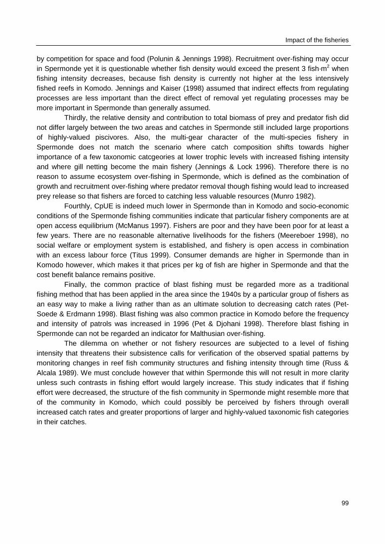
Impact of the fisheries
99
by competition for space and food (Polunin & Jennings 1998). Recruitment over-fishing may occurin Spermonde yet it is questionable whether fish density would exceed the present 3 fish·m2 whenfishing intensity decreases, because fish density is currently not higher at the less intensivelyfished reefs in Komodo. Jennings and Kaiser (1998) assumed that indirect effects from regulatingprocesses are less important than the direct effect of removal yet regulating processes may bemore important in Spermonde than generally assumed.
Thirdly, the relative density and contribution to total biomass of prey and predator fish didnot differ largely between the two areas and catches in Spermonde still included large proportionsof highly-valued piscivores. Also, the multi-gear character of the multi-species fishery inSpermonde does not match the scenario where catch composition shifts towards higherimportance of a few taxonomic catcgeories at lower trophic levels with increased fishing intensityand where gill netting become the main fishery (Jennings & Lock 1996). Therefore there is noreason to assume ecosystem over-fishing in Spermonde, which is defined as the combination ofgrowth and recruitment over-fishing where predator removal though fishing would lead to increasedprey release so that fishers are forced to catching less valuable resources (Munro 1982).
Fourthly, CpUE is indeed much lower in Spermonde than in Komodo and socio-economicconditions of the Spermonde fishing communities indicate that particular fishery components are atopen access equilibrium (McManus 1997). Fishers are poor and they have been poor for at least afew years. There are no reasonable alternative livelihoods for the fishers (Meereboer 1998), nosocial welfare or employment system is established, and fishery is open access in combinationwith an excess labour force (Titus 1999). Consumer demands are higher in Spermonde than inKomodo however, which makes it that prices per kg of fish are higher in Spermonde and that thecost benefit balance remains positive.
Finally, the common practice of blast fishing must be regarded more as a traditionalfishing method that has been applied in the area since the 1940s by a particular group of fishers asan easy way to make a living rather than as an ultimate solution to decreasing catch rates (Pet-Soede & Erdmann 1998). Blast fishing was also common practice in Komodo before the frequencyand intensity of patrols was increased in 1996 (Pet & Djohani 1998). Therefore blast fishing inSpermonde can not be regarded an indicator for Malthusian over-fishing.
The dilemma on whether or not fishery resources are subjected to a level of fishingintensity that threatens their subsistence calls for verification of the observed spatial patterns bymonitoring changes in reef fish community structures and fishing intensity through time (Russ &Alcala 1989). We must conclude however that within Spermonde this will not result in more clarityunless such contrasts in fishing effort would largely increase. This study indicates that if fishingeffort were decreased, the structure of the fish community in Spermonde might resemble more thatof the community in Komodo, which could possibly be perceived by fishers through overallincreased catch rates and greater proportions of larger and highly-valued taxonomic fish categoriesin their catches.
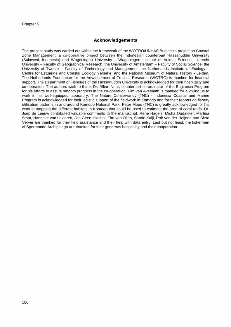
Chapter 5
100
Acknowledgements
The present study was carried out within the framework of the WOTRO/UNHAS Buginesia project on CoastalZone Management, a co-operative project between the Indonesian counterpart Hassanuddin University(Sulawesi, Indonesia) and Wageningen University – Wageningen Institute of Animal Sciences, UtrechtUniversity – Faculty of Geographical Research, the University of Amsterdam – Faculty of Social Science, theUniversity of Twente – Faculty of Technology and Management, the Netherlands Institute of Ecology –Centre for Estuarine and Coastal Ecology Yerseke, and the National Museum of Natural History - Leiden.The Netherlands Foundation for the Advancement of Tropical Research (WOTRO) is thanked for financialsupport. The Department of Fisheries of the Hassanuddin University is acknowledged for their hospitality andco-operation. The authors wish to thank Dr. Alfian Noor, counterpart co-ordinator of the Buginesia Programfor his efforts to assure smooth progress in the co-operation. Pim van Avesaath is thanked for allowing us towork in his well-equipped laboratory. The Nature Conservancy (TNC) - Indonesia Coastal and MarineProgram is acknowledged for their logistic support of the fieldwork in Komodo and for their reports on fisheryutilisation patterns in and around Komodo National Park. Peter Mous (TNC) is greatly acknowledged for hiswork in mapping the different habitats in Komodo that could be used to estimate the area of coral reefs. Dr.Joep de Leeuw contributed valuable comments to the manuscript. Rene Hagels, Micha Oudakker, MartinaStam, Hanneke van Lavieren, Jan Geert Hiddink, Tim van Oijen, Sande Kuijl, Rob van der Heijden and SietoVerver are thanked for their field assistance and their help with data entry. Last but not least, the fishermenof Spermonde Archipelago are thanked for their generous hospitality and their cooperation.

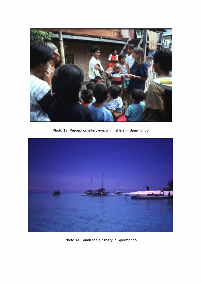
Photo 13: Perception interviews with fishers in Spermondo
Photo 14: Small scale fishery in Spermondo
103
Chapter 6
Limited options for co-management of reef fisheries in Spermonde,a coastal zone off SW Sulawesi, Indonesia
C. Pet-Soede, W.L.T. van Densen, T. van Oijen and M.A.M. Machiels
Abstract
Deteriorating quality of Indonesia’s coastal fishery resources and their resourse base calls for restrictivemanagement. Logistic constraints related to the vast area of national waters force Indonesian authorities toconsider a decentralised co-management approach where authorities and fishers are partners in thedecision-making process. Disagreement between these partners on the need for management will obstructimplementation of measures in such a co-management system. Perceptions of authorities and fishers on thestate of the fisheries and the fish stocks will be mostly based on personal experiences and on experiences ofothers if these are shared in some form. The experiences of fisheries authorities and fishers in the intensivelyfished Spermonde Archipelago, a coastal shelf off SW Sulawesi, Indonesia, are objectively assessed fromofficial fisheries data, logbooks, from observation at sea on individual catch and effort and from inventories ofperceptions of authorities and fishers using interviews. Local authorities and fishers claim a decline in qualityof the fish stocks over the period 1987-1997 and both groups point to the increased number of fishers as amajor cause. Biological, physical, technical and administrative attributes, however, are shown to setboundaries to the experience and so the perception of both partners, which must create rather largeuncertainties regarding the status of the stocks and the impact of the fishery at various spatial scales inSpermonde. Fisheries authorities have great difficulty in translating landing statistics into patterns in catchand effort at a spatial scale that is thought relevant in co-management of reef fisheries especially. Fisherscannot oversee a larger area than their individual resource space at which spatial scale significantrelationships between catch and effort hardly exist. More informative use of fisheries data by standardisingthe unit of effort, accounting for the fast developments in motorization, and combination of data on fisheriesand ecological grounds rather than on administrative grounds, will increase the management value of datathat are already available. Exchange of experiences between local fisheries authorities from districts orprovinces with highly contrasting levels of fishing intensity will provide a better ground for the evaluation ofdevelopments in the fisheries and the state of the stocks, by providing a reference to one’s personalexperience. Incorporation of size measurements for highly valued piscivorous indicator species, such asgroupers, will allow a faster detection of downward trends that are related to increasing fishing pressure.Increased awareness of fishers on differences in catch rates and compositions between intensively fishedareas and areas with restricted entry, will facilitate discussions on the need and benefits of effort regulations.
Chapter 6
104
Introduction
The coastal fishery resources in Indonesia are under high exploitation pressure (Naamin &Badruddin 1992; Badruddin & Gillet 1996). Habitat destructive fishing practices, land-basedactivities, and mechanical damage from ship grounding and anchoring threaten the quality of thefisheries’ resource base further (Soegiarto & Polunin 1982; Pet-Soede & Erdmann 1997; 1998;Edinger et al. 1999). Processes and factors that induced this situation are similar to what isdescribed in other tropical coastal areas and include the open access nature of the resources(Berkes 1994) and a strong human population growth (Darmoredjo 1983; Bailey & Zerner 1992).The management of the Indonesian fishery resources is the responsibility of the centralgovernment in Jakarta, assisted by the Directorate General of Fisheries (DGF) at which office thetotal allowable number of fishing licenses is determined from estimates of maximum sustainableyields (MSYs) for a combination of fish categories (Ruddle 1993; Venema 1997). By law (No. 91985: Fisheries Law) this licensing system applies to medium- to large-scale operations only,subsistence and small-scale fishers are exempted (Badruddin & Gillet 1996). Use of destructivefishing techniques is prohibited throughout all Indonesian waters by the same law and officiallyallowed gears are long line, pole & line, purse seine, fish net (except in the Malaka Strait ExclusiveEconomic Zone), gill nets no longer than 2.5 km and various sorts of line fishing (Minister ofAgriculture Decree No. 816: 1990). Budgetary and logistical constraints to the monitoring andcontrolling ability at the national level, together with a growing awareness of the importance ofregion specific problems, initiated a de-centralisation process for resource management.Indonesia’s national government now strives to share its management responsibility and authoritywith the provincial governments. One step further is that local authorities share managementresponsibility with the fishers, being the local resource users, in what is called co-management(Christy 1992a; Dorsey 1992; Johannes et al. 1992; Naamin & Badrudin 1992; Dahuri 1994;Pomeroy 1994; Pomeroy & Carlos 1997; Soepanto & Nikijuluw 1999).
In the Spermonde Archipelago, a coastal shelf off SW Sulawesi, Indonesia, where overallfishing intensity was high (517 boats·km-2), catch rates (CpUE) in the reef fishery were low andranged from 2.9 kg·trip-1 for hook and line to 35.2 kg·trip-1 for blast fishing (Chapter 3). A day trip isstill the unit of effort, which applies to all types of fisheries operating at various technical scales.Total reef catches included large proportions of low-valued threadfin bream (Nemipteridae). Thelength and species compositions of catches in the less intensively fished areas included slightlymore high-valued grouper (Serranidae), and other fish of larger mean length (Chapter 5). Thesecatch features indicate a high pressure on stocks of reef fish. Patterns in fish distributions asobserved with Underwater Visual Census (UVC) in Spermonde, do not support such fishing effect(Chapter 5), but when fish community structures and catch rates were compared betweenSpermonde and Komodo National Park, a large difference in total fish biomass especially for fish >40 cm (factor 17) and for catch rates (factor 3 - 8) was observed (Chapter 5).
Implementation of co-management principles remains complex (Munro & Williams 1985;McCay & Acheson 1987; Christy 1992b; Medley et al. 1993; Brown 1997). Many studies providedpractical approaches to on the ground management but in our view, a major problem lies at thebasis of the co-management principle itself. As it holds for all forms of fisheries management (vanDensen 1990), co-management is a continuous decision-making process with problem
Constraints to perceptions
105
identification, setting objectives, taking measures and evaluating information on the outcome of thefishery. Disagreement on the state of the stocks and on the causal relation between developmentsin fish stocks and the level of fishing effort or the type of exploitation obstructs this process fromthe earliest stage of problem identification onwards. It might even not be agreed upon thatreduction of fishing effort in whatever form will pay. In this respect we argue that perceptions thatdo not concur constrain the co-management process and anyway the successful implementation ofpossible fishery regulations. Perception is defined here as the evaluation of one’s personalexperience through space and time and of information derived through other peoples’ experiences.
Often, an apparent lack of concern for the deteriorating quality of fishery resources iscaused by an inability to observe downward trends. Once fisheries officers perceive negativedevelopments in fish stock sizes or compositions, they have a reason to start their lobby forrestrictive management. If managers have a clear perception of downward trends, because theyare monotonous with little variance around them, or of contrasty spatial patterns in the outcome ofthe fishery, they can allocate their time and budget to address the problems most efficiently. Iffishers acknowledge a link between for example changes in fish abundance or stock biomass andtheir fishing activities, they are more likely to accept restrictions that affect their day-to-dayactivities and may as a fisher community take responsibility for managing the resources (Pomeroyet al. 1996). Fisheries authorities and fishers can only form a perception on the state of fish stocksand changes in this status, if fish stocks produce unambiguous signals (Johannes 1994). In thisstudy, the experiences and perceptions are inventoried for those fisheries authorities and fishersthat are to be partners if co-management would be installed for the reef fishery resources inSpermonde. Particular attention is given to biological, physical, technical and administrative factorsthat govern perceptions on the status of the fish stocks and that will constrain future co-management incentives in Spermonde area (Nielsen et al. 1996). It will be clear that whether or notperceptions of authorities and fishers are conform scientific biological conclusions, insight in thefactors that affect these perceptions is important to determine whether authorities and fisher couldtruly act as partners in co-management.
Fisheries statistics, individual catches and interviews
The Spermonde coastal shelf area of 400,000 ha forms a distinct ecological entity (Umbgrove1930) as it encompasses all reef areas off SW Sulawesi. The fishery for this area is administeredaccording to national standards by four fisheries offices one in each of the coastal districts Takalar,Ujung Pandang, Maros and Pangkep in the South Sulawesi province. This province encompasses21 districts in total. Our focus in this study is on perceptions of authorities and fishers ondevelopments in reef fish catches, as related to developments and patterns in fishing intensity,because previous studies provided ample proof for fishery-related differences in distributions ofreef fish, piscivores in particular (Chapters 3 and 5). Also, their sedentary nature provides the bestchance for effective localised management and allows evaluation of the effect of co-managementonce implemented (Oakerson 1992). The experience of fisheries authorities with the performanceof the fishery refers mostly to records written on a data-form by fisheries officers or as available ina computer data-base, which are structured and processed in an administrative environment
Chapter 6
106
(Chapter 2). These more remote experiences with the Spermonde fisheries differ from theexperiences of individual fishers that are gained in the more proxy physical environment of thecoastal sea, and which might be replenished with signals from the ecosystem other than their dailycatches (Chapter 3).
The experiences of fisheries authorities at three different administrative levels (district,province and nation) who are responsible for monitoring of the fishery resources in Spermonde arediscussed using the official fisheries statistics for Spermonde (Chapter 2). It was assessed howmany and which elements (fish catch categories, gear categories) that are identified in the Catchand Effort Data Recording System (CEDRS) indicate a significant linear trend and with how large arate of change. Per administrative level, perceptions are inventoried by interviewing responsibleadministrators and from the fisheries reports for which the means of data processing are alsostudied. The fisheries authorities interviewed were selected by their function.
The experiences of fishers, who are the resource users in Spermonde, were assessedfrom catch and effort data collected during surveys at sea throughout Spermonde (Chapters 3 and5). It was studied at which spatial and temporal scale patterns in Catch-per-Unit-Effort (CpUE) aresignificant and for which elements (fish catch category, gear category) these patterns are mostclear. Perceptions of fishers, approached randomly, were inventoried with the same type ofinterviews as used with the fisheries authorities.
The first question in the interview was of a multiple-choice character with only four possibleanswers. The two other questions were open questions. By asking the same questions to allrespondents in the same manner, we did not eliminate the problem of misinterpretation, yet the littletime needed to complete the interview allowed for large sample size. Respondents were asked:
1. How much fish is there in Spermonde Archipelago now, compared to 10 years ago(Options: more, less, the same, don’t know)
2. How do you know?3. What is the cause for the current situation?
This approach starting from the experience of the potential partners in co-management,allows for a discussion of factors that could have influenced their perceptions, such as the natureof the fish stocks and the fishery, the “sampling/fishing strategy” that continues to add to one’sexperience, and the means and methods used to convert experiences into information. Do thesefactors create uncertainty in an assessment of the status of certain fish stocks or in the judgementof the fishery impact of certain fishing gears? Is the administrative standard for collectingprocessing, aggregating and evaluating information on the fish stocks suitable to detect changes intheir status or patterns in their spatial distribution? Is the “sample size in the experience” ofauthorities and fishers large enough (space, time) to detect trends and patterns?
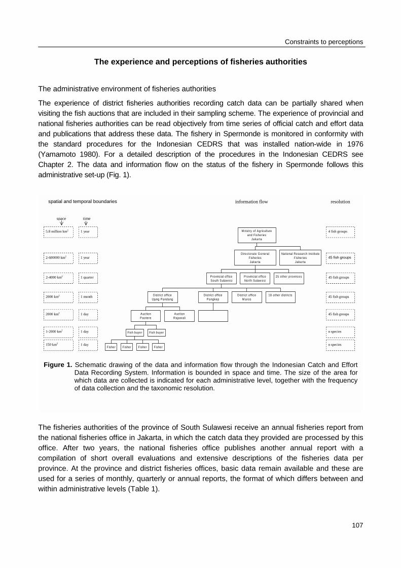
Constraints to perceptions
107
The experience and perceptions of fisheries authorities
The administrative environment of fisheries authorities
The experience of district fisheries authorities recording catch data can be partially shared whenvisiting the fish auctions that are included in their sampling scheme. The experience of provincial andnational fisheries authorities can be read objectively from time series of official catch and effort dataand publications that address these data. The fishery in Spermonde is monitored in conformity withthe standard procedures for the Indonesian CEDRS that was installed nation-wide in 1976(Yamamoto 1980). For a detailed description of the procedures in the Indonesian CEDRS seeChapter 2. The data and information flow on the status of the fishery in Spermonde follows thisadministrative set-up (Fig. 1).
The fisheries authorities of the province of South Sulawesi receive an annual fisheries report fromthe national fisheries office in Jakarta, in which the catch data they provided are processed by thisoffice. After two years, the national fisheries office publishes another annual report with acompilation of short overall evaluations and extensive descriptions of the fisheries data perprovince. At the province and district fisheries offices, basic data remain available and these areused for a series of monthly, quarterly or annual reports, the format of which differs between andwithin administrative levels (Table 1).
Fisher Fisher Fisher Fisher
Fish buyer Fish buyer
AuctionPaotere
Auct ionRajaw ali
District officeUjung Pandang
Dis trict officePangkep
D istric t officeM aros
18 o ther d istric ts
Provinc ial off iceSouth Sulaw esi
Provincial o fficeNorth Sulaw esi
25 o ther provinces
Directora te G eneralFisheriesJakarta
National Research Ins tituteFisheriesJakarta
M nistry of Agricultureand Fisheries
Jakarta
45 fish groups
n species
45 fish groups
n species
45 fish groups
45 fish groups
4 fish groups
2-4000 km2
150 km2
2000 km2
1-2000 km2
2000 km2
2-600000 km2
5.8 million km2
space
1 quarter
1 day
1 month
1 day
1 day
1 year
1 year
time
spatial and temporal boundaries information flow resolution
Figure 1. Schematic drawing of the data and information flow through the Indonesian Catch and EffortData Recording System. Information is bounded in space and time. The size of the area forwhich data are collected is indicated for each administrative level, together with the frequencyof data collection and the taxonomic resolution.
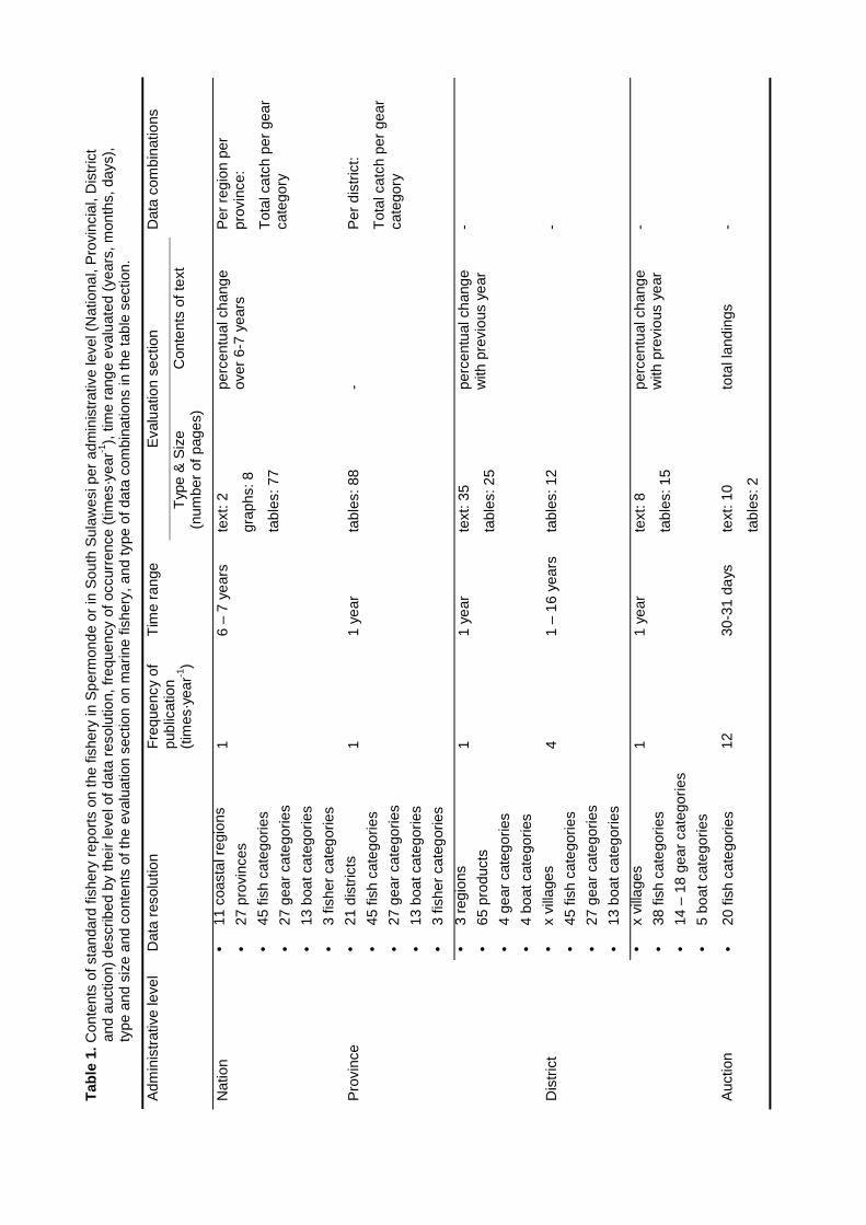
Tab
le 1
. Con
tent
s of
sta
ndar
d fis
hery
rep
orts
on
the
fishe
ry in
Spe
rmon
de o
r in
Sou
th S
ulaw
esi p
er a
dmin
istr
ativ
e le
vel (
Nat
iona
l, P
rovi
ncia
l, D
istr
ict
and
auct
ion)
des
crib
ed b
y th
eir
leve
l of d
ata
reso
lutio
n, fr
eque
ncy
of o
ccur
renc
e (t
imes
·yea
r-1),
tim
e ra
nge
eval
uate
d (y
ears
, mon
ths,
day
s),
type
and
siz
e an
d co
nten
ts o
f the
eva
luat
ion
sect
ion
on m
arin
e fis
hery
, and
type
of d
ata
com
bina
tions
in th
e ta
ble
sect
ion.
Eva
luat
ion
sect
ion
Adm
inis
trat
ive
leve
lD
ata
reso
lutio
nF
requ
ency
of
publ
icat
ion
(tim
es·y
ear-1
)
Tim
e ra
nge
Typ
e &
Siz
e(n
umbe
r of
pag
es)
Con
tent
s of
text
Dat
a co
mbi
natio
ns
Nat
ion
• 11
coa
stal
reg
ions
• 27
pro
vinc
es
• 45
fish
cat
egor
ies
• 27
gea
r ca
tego
ries
• 13
boa
t cat
egor
ies
• 3
fishe
r ca
tego
ries
16
– 7
year
ste
xt: 2
grap
hs: 8
tabl
es: 7
7
perc
entu
al c
hang
eov
er 6
-7 y
ears
Per
reg
ion
per
prov
ince
:
Tot
al c
atch
per
gea
rca
tego
ry
Pro
vinc
e•
21 d
istr
icts
• 45
fish
cat
egor
ies
• 27
gea
r ca
tego
ries
• 13
boa
t cat
egor
ies
• 3
fishe
r ca
tego
ries
11
year
tabl
es: 8
8-
Per
dis
tric
t:
Tot
al c
atch
per
gea
rca
tego
ry
• 3
regi
ons
• 65
pro
duct
s
• 4
gear
cat
egor
ies
• 4
boat
cat
egor
ies
11
year
text
: 35
tabl
es: 2
5
perc
entu
al c
hang
ew
ith p
revi
ous
year
-
Dis
tric
t•
x vi
llage
s
• 45
fish
cat
egor
ies
• 27
gea
r ca
tego
ries
• 13
boa
t cat
egor
ies
41
– 16
yea
rsta
bles
: 12
-
• x
villa
ges
• 38
fish
cat
egor
ies
• 14
– 1
8 ge
ar c
ateg
orie
s
• 5
boat
cat
egor
ies
11
year
text
: 8
tabl
es: 1
5
perc
entu
al c
hang
ew
ith p
revi
ous
year
-
Auc
tion
• 20
fish
cat
egor
ies
1230
-31
days
text
: 10
tabl
es: 2
tota
l lan
ding
s-
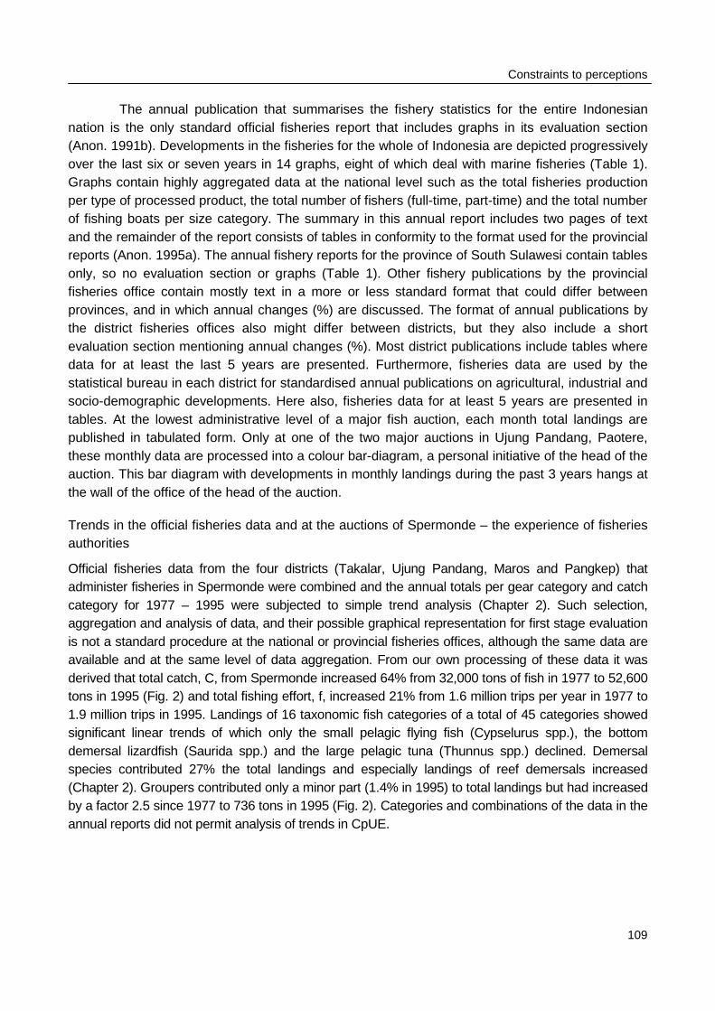
Constraints to perceptions
109
The annual publication that summarises the fishery statistics for the entire Indonesiannation is the only standard official fisheries report that includes graphs in its evaluation section(Anon. 1991b). Developments in the fisheries for the whole of Indonesia are depicted progressivelyover the last six or seven years in 14 graphs, eight of which deal with marine fisheries (Table 1).Graphs contain highly aggregated data at the national level such as the total fisheries productionper type of processed product, the total number of fishers (full-time, part-time) and the total numberof fishing boats per size category. The summary in this annual report includes two pages of textand the remainder of the report consists of tables in conformity to the format used for the provincialreports (Anon. 1995a). The annual fishery reports for the province of South Sulawesi contain tablesonly, so no evaluation section or graphs (Table 1). Other fishery publications by the provincialfisheries office contain mostly text in a more or less standard format that could differ betweenprovinces, and in which annual changes (%) are discussed. The format of annual publications bythe district fisheries offices also might differ between districts, but they also include a shortevaluation section mentioning annual changes (%). Most district publications include tables wheredata for at least the last 5 years are presented. Furthermore, fisheries data are used by thestatistical bureau in each district for standardised annual publications on agricultural, industrial andsocio-demographic developments. Here also, fisheries data for at least 5 years are presented intables. At the lowest administrative level of a major fish auction, each month total landings arepublished in tabulated form. Only at one of the two major auctions in Ujung Pandang, Paotere,these monthly data are processed into a colour bar-diagram, a personal initiative of the head of theauction. This bar diagram with developments in monthly landings during the past 3 years hangs atthe wall of the office of the head of the auction.
Trends in the official fisheries data and at the auctions of Spermonde – the experience of fisheriesauthorities
Official fisheries data from the four districts (Takalar, Ujung Pandang, Maros and Pangkep) thatadminister fisheries in Spermonde were combined and the annual totals per gear category and catchcategory for 1977 – 1995 were subjected to simple trend analysis (Chapter 2). Such selection,aggregation and analysis of data, and their possible graphical representation for first stage evaluationis not a standard procedure at the national or provincial fisheries offices, although the same data areavailable and at the same level of data aggregation. From our own processing of these data it wasderived that total catch, C, from Spermonde increased 64% from 32,000 tons of fish in 1977 to 52,600tons in 1995 (Fig. 2) and total fishing effort, f, increased 21% from 1.6 million trips per year in 1977 to1.9 million trips in 1995. Landings of 16 taxonomic fish categories of a total of 45 categories showedsignificant linear trends of which only the small pelagic flying fish (Cypselurus spp.), the bottomdemersal lizardfish (Saurida spp.) and the large pelagic tuna (Thunnus spp.) declined. Demersalspecies contributed 27% the total landings and especially landings of reef demersals increased(Chapter 2). Groupers contributed only a minor part (1.4% in 1995) to total landings but had increasedby a factor 2.5 since 1977 to 736 tons in 1995 (Fig. 2). Categories and combinations of the data in theannual reports did not permit analysis of trends in CpUE.
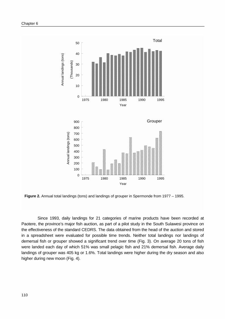
Chapter 6
110
Since 1993, daily landings for 21 categories of marine products have been recorded atPaotere, the province’s major fish auction, as part of a pilot study in the South Sulawesi province onthe effectiveness of the standard CEDRS. The data obtained from the head of the auction and storedin a spreadsheet were evaluated for possible time trends. Neither total landings nor landings ofdemersal fish or grouper showed a significant trend over time (Fig. 3). On average 20 tons of fishwere landed each day of which 51% was small pelagic fish and 21% demersal fish. Average dailylandings of grouper was 405 kg or 1.6%. Total landings were higher during the dry season and alsohigher during new moon (Fig. 4).
1975 1980 1985 1990 1995
Year
0
10
20
30
40
50
(Tho
usan
ds)
Ann
ual l
andi
ngs
(ton
s)������������������������������������������������
��������������������������������������������������������
���������������������������������������������
������������������������������������������������
����������������������������������������������������������������������
����������������������������������������
��������������������������������������������������
������������������������������������������������������������
��������������������������������������������������������������������������������
�������������������������������������������������������
������������������������������������������������������������������
�����������������������������������������������������������������������������
��������������������������������������������
������������������������������������������������������������������������
�����������������������������������������������������������������������������
����������������������������������������������������������������������������������������
�������������������������������������������������������
������������������������������������������������������������������
�����������������������������������������������������������������������������
1975 1980 1985 1990 1995
Year
0
100
200
300
400
500
600
700
800
900
Ann
ual l
andi
ngs
(ton
s)
������������������������
���������������������
���������������
������������������������������������������
���������������������
����������������
�������������������������
������������������������
��������������������������������������������������������
������������������������������
������������������������������������������������������������
�������������������������������������������������
����������������������������
������������������������������������������
��������������������������������������������������������
����������������������������������������������������������������
����������������������������������������
������������������������������������������������������������
�����������������������������������������������������������������������������
Total
Grouper
Figure 2. Annual total landings (tons) and landings of grouper in Spermonde from 1977 – 1995.
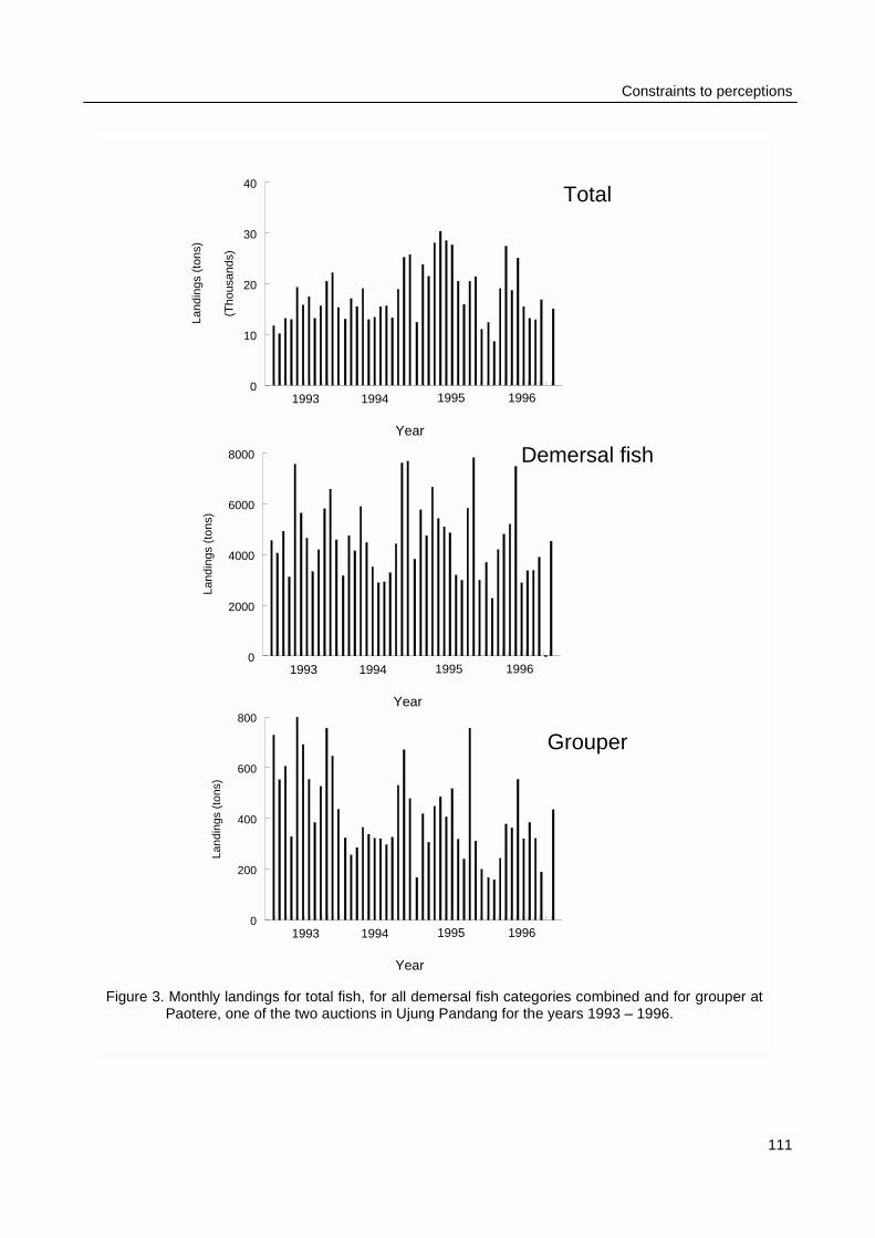
Constraints to perceptions
111
0
10
20
30
40
(Tho
usan
ds)
Land
ings
(to
ns)
1993 1994 1995 1996
Year
0
2000
4000
6000
8000
Land
ings
(to
ns)
1993 1994 1995 1996
Year
0
200
400
600
800
Land
ings
(to
ns)
1993 1994 1995 1996
Year
Total
Demersal fish
Grouper
Figure 3. Monthly landings for total fish, for all demersal fish categories combined and for grouper atPaotere, one of the two auctions in Ujung Pandang for the years 1993 – 1996.
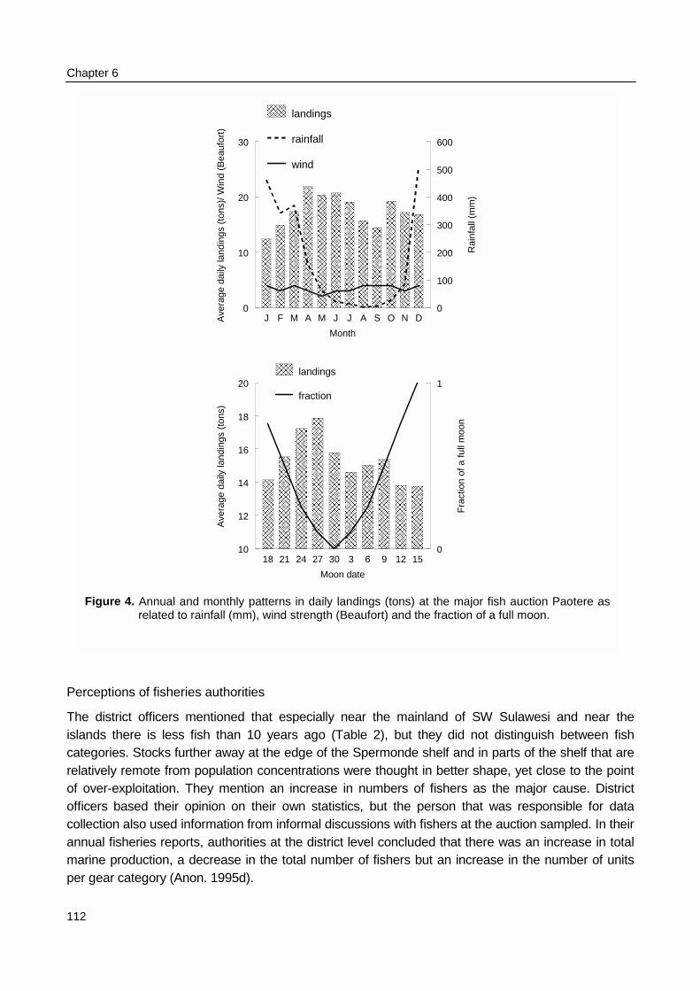
Chapter 6
112
Perceptions of fisheries authorities
The district officers mentioned that especially near the mainland of SW Sulawesi and near theislands there is less fish than 10 years ago (Table 2), but they did not distinguish between fishcategories. Stocks further away at the edge of the Spermonde shelf and in parts of the shelf that arerelatively remote from population concentrations were thought in better shape, yet close to the pointof over-exploitation. They mention an increase in numbers of fishers as the major cause. Districtofficers based their opinion on their own statistics, but the person that was responsible for datacollection also used information from informal discussions with fishers at the auction sampled. In theirannual fisheries reports, authorities at the district level concluded that there was an increase in totalmarine production, a decrease in the total number of fishers but an increase in the number of unitsper gear category (Anon. 1995d).
J F M A M J J A S O N D
Month
0
10
20
30
Ave
rage
dai
ly la
ndin
gs (
tons
)/ W
ind
(Bea
ufor
t)
0
100
200
300
400
500
600
Rai
nfal
l (m
m)
������������������������������������������������
�������������������������������������������������
����������������������������������������
����������������������������������������������������������������������
���������������������������������������������
���������������������������������������������������������������
���������������������������������������������
�������������������������������������������������
�����������������������������������
������������������������������������������������������������������������
������������������������������������������������
����������������������������������������������������������������
����������������������
landings
rainfall
wind
18 21 24 27 30 3 6 9 12 15
Moon date
10
12
14
16
18
20
Ave
rage
dai
ly la
ndin
gs (
tons
)
0
1
Fra
ctio
n of
a fu
ll m
oon
������������������������������������
������������������������������������������������������������������������
��������������������������������������������������������������������������������
����������������������������������������������������������������������������������������
��������������������������������������������������������
������������������������������������������
������������������������������������������
������������������������������������������������������������������������
������������������������������������������������
������������������������������������������������
��������������������
landings
fraction
Figure 4. Annual and monthly patterns in daily landings (tons) at the major fish auction Paotere asrelated to rainfall (mm), wind strength (Beaufort) and the fraction of a full moon.
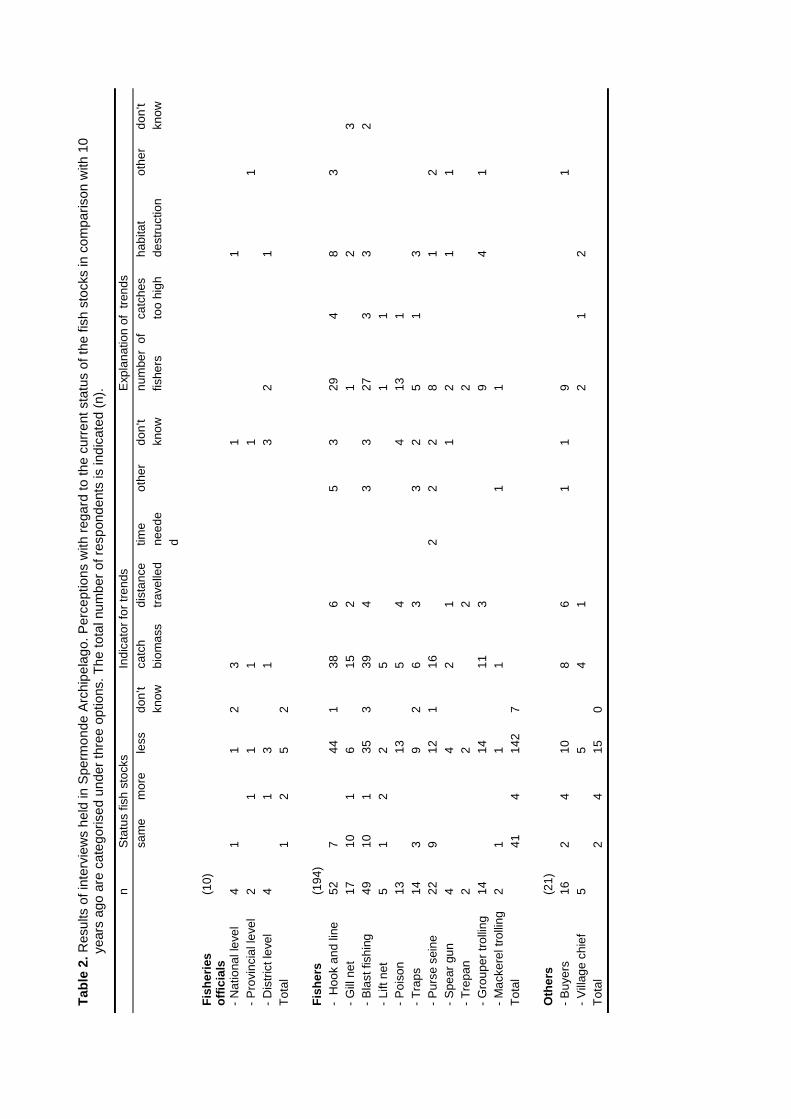
Tab
le 2
. Res
ults
of i
nter
view
s he
ld in
Spe
rmon
de A
rchi
pela
go. P
erce
ptio
ns w
ith r
egar
d to
the
curr
ent s
tatu
s of
the
fish
stoc
ks in
com
paris
on w
ith 1
0ye
ars
ago
are
cate
goris
ed u
nder
thre
e op
tions
. The
tota
l num
ber
of r
espo
nden
ts is
indi
cate
d (n
).
nS
tatu
s fis
h st
ocks
Indi
cato
r fo
r tr
ends
Exp
lana
tion
of t
rend
s
sam
em
ore
less
don’
tkn
owca
tch
biom
ass
dist
ance
trav
elle
dtim
ene
ede
d
othe
rdo
n’t
know
num
ber
offis
hers
catc
hes
too
high
habi
tat
dest
ruct
ion
othe
rdo
n’t
know
Fis
her
ies
off
icia
ls(1
0)
- N
atio
nal l
evel
- P
rovi
ncia
l lev
el-
Dis
tric
t lev
el
4 2 4
11 1
1 1 3
23 1 1
1 1 32
1 11
Tot
al1
25
2
Fis
her
s(1
94)
- H
ook
and
line
- G
ill n
et-
Bla
st fi
shin
g-
Lift
net
- P
oiso
n-
Tra
ps-
Pur
se s
eine
- S
pear
gun
- T
repa
n-
Gro
uper
trol
ling
- M
acke
rel t
rolli
ng
52 17 49 5 13 14 22 4 2 14 2
7 10 10 1 3 9 1
1 1 2
44 6 35 2 13 9 12 4 2 14 1
1 3 2 1
38 15 39 5 5 6 16 2 11 1
6 2 4 4 3 1 2 3
2
5 3 3 2 1
3 3 4 2 2 1
29 1 27 1 13 5 8 2 2 9 1
4 3 1 1 1
8 2 3 3 1 1 4
3 2 1 1
3 2
Tot
al41
414
27
Oth
ers
(21)
- B
uyer
s-
Vill
age
chie
f16 5
24
10 58 4
6 11
19 2
12
1
Tot
al2
415
0
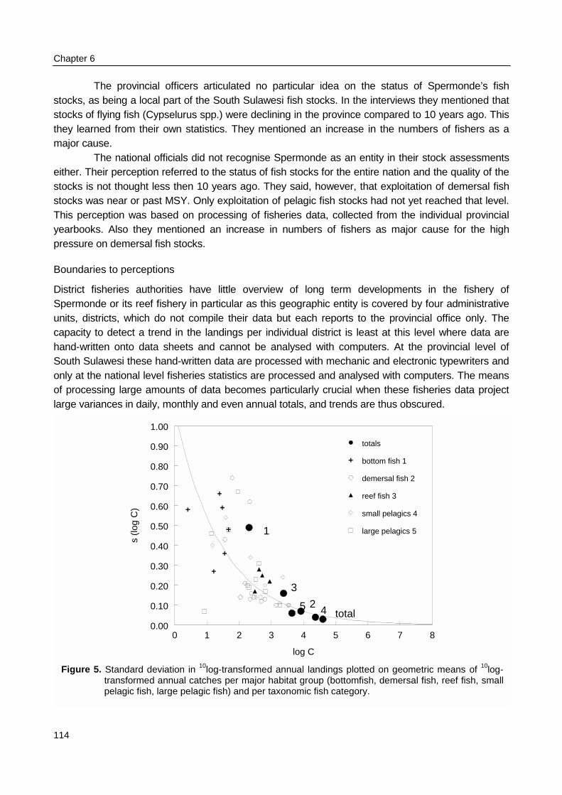
Chapter 6
114
The provincial officers articulated no particular idea on the status of Spermonde’s fishstocks, as being a local part of the South Sulawesi fish stocks. In the interviews they mentioned thatstocks of flying fish (Cypselurus spp.) were declining in the province compared to 10 years ago. Thisthey learned from their own statistics. They mentioned an increase in the numbers of fishers as amajor cause.
The national officials did not recognise Spermonde as an entity in their stock assessmentseither. Their perception referred to the status of fish stocks for the entire nation and the quality of thestocks is not thought less then 10 years ago. They said, however, that exploitation of demersal fishstocks was near or past MSY. Only exploitation of pelagic fish stocks had not yet reached that level.This perception was based on processing of fisheries data, collected from the individual provincialyearbooks. Also they mentioned an increase in numbers of fishers as major cause for the highpressure on demersal fish stocks.
Boundaries to perceptions
District fisheries authorities have little overview of long term developments in the fishery ofSpermonde or its reef fishery in particular as this geographic entity is covered by four administrativeunits, districts, which do not compile their data but each reports to the provincial office only. Thecapacity to detect a trend in the landings per individual district is least at this level where data arehand-written onto data sheets and cannot be analysed with computers. At the provincial level ofSouth Sulawesi these hand-written data are processed with mechanic and electronic typewriters andonly at the national level fisheries statistics are processed and analysed with computers. The meansof processing large amounts of data becomes particularly crucial when these fisheries data projectlarge variances in daily, monthly and even annual totals, and trends are thus obscured.
Figure 5. Sttrape
0 1 2 3 4 5 6 7 8
log C
0.00
0.10
0.20
0.30
0.40
0.50
0.60
0.70
0.80
0.90
1.00
s (lo
g C
)
4 total5 2
3
1
totals
bottom fish 1
demersal fish 2
reef fish 3
small pelagics 4
large pelagics 5
andard deviation in 10log-transformed annual landings plotted on geometric means of 10log-nsformed annual catches per major habitat group (bottomfish, demersal fish, reef fish, smalllagic fish, large pelagic fish) and per taxonomic fish category.
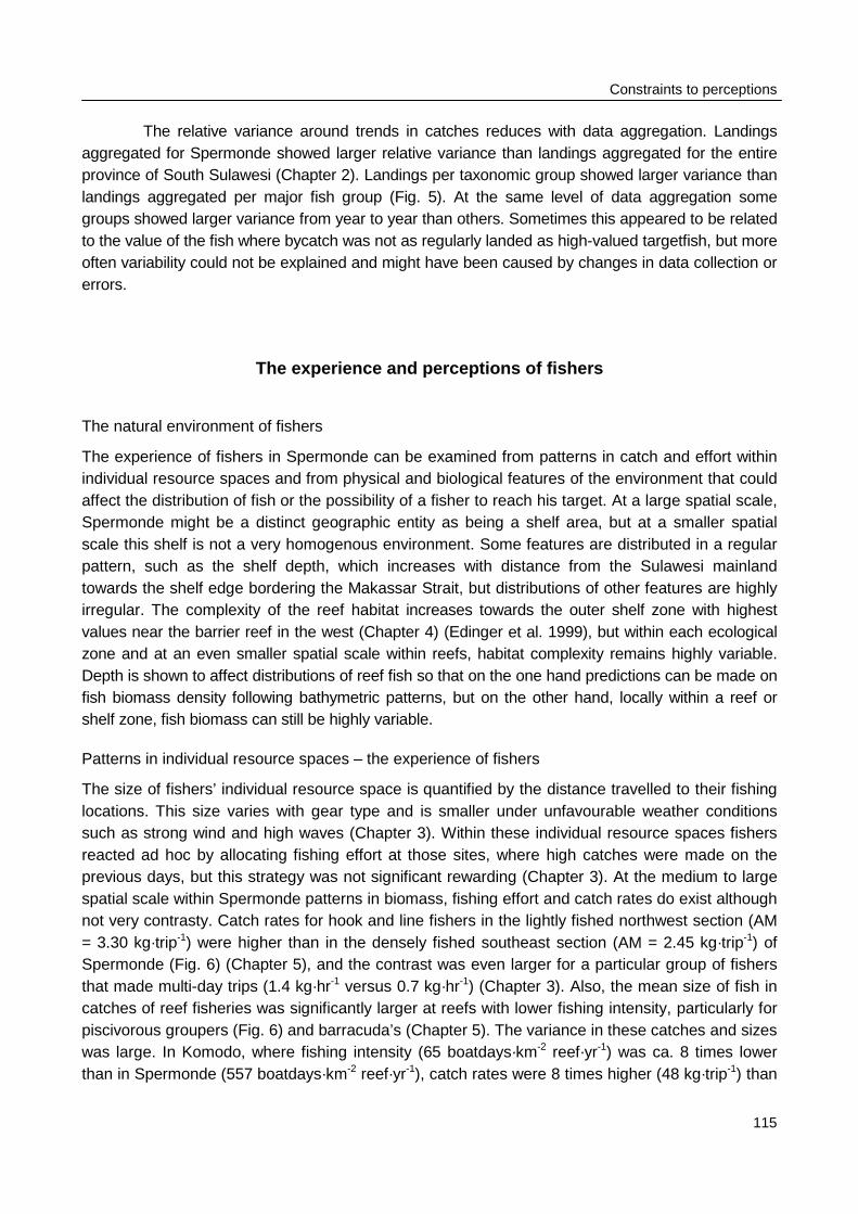
Constraints to perceptions
115
The relative variance around trends in catches reduces with data aggregation. Landingsaggregated for Spermonde showed larger relative variance than landings aggregated for the entireprovince of South Sulawesi (Chapter 2). Landings per taxonomic group showed larger variance thanlandings aggregated per major fish group (Fig. 5). At the same level of data aggregation somegroups showed larger variance from year to year than others. Sometimes this appeared to be relatedto the value of the fish where bycatch was not as regularly landed as high-valued targetfish, but moreoften variability could not be explained and might have been caused by changes in data collection orerrors.
The experience and perceptions of fishers
The natural environment of fishers
The experience of fishers in Spermonde can be examined from patterns in catch and effort withinindividual resource spaces and from physical and biological features of the environment that couldaffect the distribution of fish or the possibility of a fisher to reach his target. At a large spatial scale,Spermonde might be a distinct geographic entity as being a shelf area, but at a smaller spatialscale this shelf is not a very homogenous environment. Some features are distributed in a regularpattern, such as the shelf depth, which increases with distance from the Sulawesi mainlandtowards the shelf edge bordering the Makassar Strait, but distributions of other features are highlyirregular. The complexity of the reef habitat increases towards the outer shelf zone with highestvalues near the barrier reef in the west (Chapter 4) (Edinger et al. 1999), but within each ecologicalzone and at an even smaller spatial scale within reefs, habitat complexity remains highly variable.Depth is shown to affect distributions of reef fish so that on the one hand predictions can be made onfish biomass density following bathymetric patterns, but on the other hand, locally within a reef orshelf zone, fish biomass can still be highly variable.
Patterns in individual resource spaces – the experience of fishers
The size of fishers’ individual resource space is quantified by the distance travelled to their fishinglocations. This size varies with gear type and is smaller under unfavourable weather conditionssuch as strong wind and high waves (Chapter 3). Within these individual resource spaces fishersreacted ad hoc by allocating fishing effort at those sites, where high catches were made on theprevious days, but this strategy was not significant rewarding (Chapter 3). At the medium to largespatial scale within Spermonde patterns in biomass, fishing effort and catch rates do exist althoughnot very contrasty. Catch rates for hook and line fishers in the lightly fished northwest section (AM= 3.30 kg·trip-1) were higher than in the densely fished southeast section (AM = 2.45 kg·trip-1) ofSpermonde (Fig. 6) (Chapter 5), and the contrast was even larger for a particular group of fishersthat made multi-day trips (1.4 kg·hr-1 versus 0.7 kg·hr-1) (Chapter 3). Also, the mean size of fish incatches of reef fisheries was significantly larger at reefs with lower fishing intensity, particularly forpiscivorous groupers (Fig. 6) and barracuda’s (Chapter 5). The variance in these catches and sizeswas large. In Komodo, where fishing intensity (65 boatdays·km-2 reef·yr-1) was ca. 8 times lowerthan in Spermonde (557 boatdays·km-2 reef·yr-1), catch rates were 8 times higher (48 kg·trip-1) than
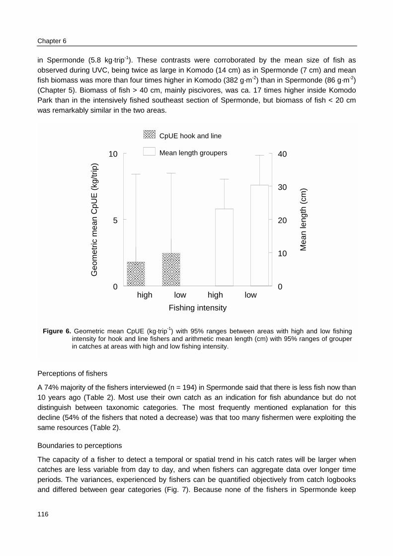
Chapter 6
116
in Spermonde (5.8 kg·trip-1). These contrasts were corroborated by the mean size of fish asobserved during UVC, being twice as large in Komodo (14 cm) as in Spermonde (7 cm) and meanfish biomass was more than four times higher in Komodo (382 g·m-2) than in Spermonde (86 g·m-2)(Chapter 5). Biomass of fish > 40 cm, mainly piscivores, was ca. 17 times higher inside KomodoPark than in the intensively fished southeast section of Spermonde, but biomass of fish < 20 cmwas remarkably similar in the two areas.
Perceptions o
A 74% majori10 years agodistinguish bedecline (54% same resourc
Boundaries to
The capacity catches are lperiods. The and differed
Figure 6. Geintein c
high low high low
Fishing intensity
0
5
10
Geo
met
ric m
ean
CpU
E (
kg/tr
ip)
0
10
20
30
40
Mea
n le
ngth
(cm
)
������������������������������������������������������������
������������������������������������������������������������������������������������������
���������������������� CpUE hook and line
Mean length groupers
ometric mean CpUE (kg·trip-1) with 95% ranges between areas with high and low fishingnsity for hook and line fishers and arithmetic mean length (cm) with 95% ranges of grouperatches at areas with high and low fishing intensity.
f fishers
ty of the fishers interviewed (n = 194) in Spermonde said that there is less fish now than (Table 2). Most use their own catch as an indication for fish abundance but do nottween taxonomic categories. The most frequently mentioned explanation for thisof the fishers that noted a decrease) was that too many fishermen were exploiting thees (Table 2).
perceptions
of a fisher to detect a temporal or spatial trend in his catch rates will be larger wheness variable from day to day, and when fishers can aggregate data over longer timevariances, experienced by fishers can be quantified objectively from catch logbooksbetween gear categories (Fig. 7). Because none of the fishers in Spermonde keep
Constraints to perceptions
117
written records of their catches, it will be hard for them to observe trends over time even for fishersthat experience limited variance. Hook and line fishers that target sedentary reef speciesexperience relatively little variability in catch rates (s10logCpUE ranged between 0.15 – 0.34) (Fig.7). Highest catch variance was observed for lift net and purse seine operations, who target smallpelagic fish species with migratory and schooling behaviour, which behaviour causes largevariance in their local abundance and catchability. Most migratory species show seasonalmigration following climate-related spatial distribution patterns in temperature and primaryproduction. Experienced fishers can anticipate the seasonal arrival of their target fish butuncertainty about the distribution of the fish within their resource space remains.
Not only catch rates but also compositions of catches differed between and within fishinggears. Catches of hook and line fishers were most diverse with 51 different fish categories in theircatches combined, yet an individual blast fisher sees more categories in one day (AM = 4.2) than theaverage hook and line fisher (AM = 2.9). Thus the experience of blast fishers includes information onthe broadest range of fish categories, due to its much less selective fishing behaviour and largercatch rates.
0.1 1 10 100 1000
GM catch (kg)
0.00
0.20
0.40
0.60
0.80
1.00
s lo
g(C
atch
)
lift net (3%)
purse seine (7%)
grouper trolling (50%)
pelagic trolling (25%)
hook & line (0%)
grouper traps (0%)
blast fishing (3%)
Danish seine (0%)
Figure 7. Standard deviation in 10log-transformed daily catches plotted on geometric means of 10log-transformed daily catches, excluding zero catches, for 8 different gear categories.
Chapter 6
118
Conclusions
Spatial and temporal boundaries to experiences are important factors that constrain perception oflarge-scale pattern and trends in a fishery and of the status of its resources. This is particularly validfor fishers who are physically confined to a limited resource space and who do not easily aggregateinformation over larger time intervals with the concomitant reduction in uncertainty around trends.Fisheries authorities do have data available that could be used to evaluate trends for a variety ofspatial and temporal scales, yet at present these are not fully utilised. But even when aggregated inspatial entities, such aggregations will probably not reveal the contrasts we observed during ourcatch assessment surveys at sea, because of the weakness of the contrasts and because ofdifficulties in relating auction data to fishing grounds. Theoretically, authorities could also comparetheir fisheries data with those from a reference area, like Komodo, with contrasting levels of fishingintensity, but fishers have no opportunity to experience these differences unless they can frequentsuch more contrasting areas.
At present local authorities and fishers seem to agree that the condition of the fish stocks inSpermonde is less than 10 years ago. Yet, we must conclude that provincial authorities will not easilyfind arguments for effort restrictions in their official data statistics, so that national support forrestrictive management will be limited. Moreover, the current tendency of Indonesia’s government toupgrade the fishery will make it more difficult for officers to convince managers of the need forrestrictions of fishing effort (Anon. 1995c). Still, the tendency of fishers to frequent remote grounds,partly as a consequence of falling catch rates, is already captured in the standard CEDRS by thetrends in the number of motorised boats. If these data could be used to rework the presently usednumber of fishing trips into a better measure for fishing effort, catch statistics will hold a closerrelation to the actual developments in the fishery. The possibilities to evaluate data for ecological orphysical entities rather than for administrative entities should be elaborated as their potential alreadyexist. Data should be combined for districts such as the four that encompass Spermonde to allow forlocal management.
To summarise, national, provincial and district fisheries authorities could make better use oftheir data by:
• Making more use of graphs for first stage evaluation of fisheries data at lower levels of dataaggregation;
• Including more years, all that are available, in their evaluation/analysis;
• Performing simple trend analysis of their time series of catch and effort data, which requireslimited computerisation and capacity for statistical data analysis;
• Analysing their data at species level and looking for species and size shifts in fisheries landings,for large piscivores especially;
• Incorporating developments of motorage in their analysis;
• Making assessments for areas that are ecologically or physically distinct;
• Comparing data with those of other districts or provinces where fishing effort largely differs.
Constraints to perceptions
119
Acknowledgements
The present study was carried out within the framework of the WOTRO/UNHAS Buginesia project on CoastalZone Management, a co-operative project between the Indonesian counterpart Hassanuddin University(Sulawesi, Indonesia) and Wageningen University – Wageningen Institute of Animal Sciences, Utrecht University– Faculty of Geographical Research, the University of Amsterdam – Faculty of Social Science, the University ofTwente – Faculty of Technology and Management, the Netherlands Institute of Ecology – Centre for Estuarineand Coastal Ecology Yerseke, and the National Museum of Natural History - Leiden. The NetherlandsFoundation for the Advancement of Tropical Research (WOTRO) is thanked for financial support. Dr. H.S. Dillonis greatly acknowledged for his help in setting up meetings with high fisheries officials in Jakarta. The fisheriesauthorities at the districts of Pangkep, Maros, Ujung Pandang and Takalar and of the province of South Sulawesiare greatly acknowledged for their help with the frame survey and for their cooperation during the interviews andfor their fisheries reports. The heads of the two major auctions in Ujung Pandang and their technical officers aregreatly acknowledged for their data and support during the fieldwork during which their auctions were visitedmonthly. The fisheries officers at the National Fisheries Department are thanked for their cooperation withinterviews and for their reports. The Department of Fisheries of the Hassanuddin University is acknowledged fortheir hospitality and co-operation. The authors wish to thank Dr. Alfian Noor, counterpart co-ordinator of theBuginesia Program for his efforts to assure smooth progress in the co-operation. Rene Hagels, Micha Oudakker,Martina Stam, Hanneke van Lavieren, Jan Geert Hiddink, Sande Kuijl, Rob van der Heijden and Sieto Verver arethanked for their field assistance. Last but not least, the fishermen of Spermonde Archipelago are thanked fortheir generous hospitality and their cooperation.

121
References
Alcala, A.C. (1988) Effects of marine reserves on coral fish abundances and yields of Philippine coral reefs.Ambio 17(3): 194-9.
Allen, P.M. & McGlade, J.M. (1986) Dynamics of discovery and exploitation: the case of the Scotian shelfgroundfish fisheries. Canadian Journal of Fisheries and Aquatic Science 43: 1187-1200.
Anonymous (1991a) Sulawesi Selatan dalam angka statistik tahunan. South Sulawesi in figures. UjungPandang: Kantor Statistik Propinsi Sulawesi Selatan dan Bappeda Dati I Sulawesi Selatan.
Anonymous (1991b) Statistik Perikanan Indonesia – Fisheries Statistics of Indonesia 1989. DirectorateJenderal Perikanan, Department Pertanian, Jakarta 110 pp.
Anonymous (1992) Indonesia, Makassar Strait, Sulawesi - West Coast, approaches to Ujung Pandang. Mapno. 139 from the joint surveys of Indonesia and USA to 1983 with additions from Patukangansurvey 1992.
Anonymous (1993) Laporan Tahunan Perikanan Sulawesi Selatan. Annual Fisheries Report SulawesiSelatan. 133 pp.
Anonymous (1994a) Sustainable management of the coastal area of SW Sulawesi. A proposal for amultidisciplinary research project within the WOTRO Programme "sustainable management of thecoastal zone in tropical areas" Appendix A: Scientific Publications of the Buginesia Programme.
Anonymous (1994b) List of fish prices. Department of Fisheries, University Hassanuddin, Ujung PandangSouth Sulawesi, Indonesia. 2 pp.
Anonymous (1995a) Laporan statistik perikanan Sulawesi Selatan 1995. (Fisheries Statistics South SulawesiProvince 1995). 158 pp.
Anonymous (1995b) Meterological data weather station Ujung Pandang South Sulawesi.Anonymous (1995c) Rencana Pembangunan Lima Tahun Keenam 1994/1995 – 1998/1999. Buku II & III.
Propinsi Daerah Tingkat I Sulawesi Selatan. (Five year development plan No. 6. ProvincialGovernment South Sulawesi).
Anonymous (1996) South Sulawesi Thematic Map. Marine Resource Evaluation & Planning Project - Part A.Directorate General of Regional Development, Ministry of Home Affairs & BCEOM, Jakarta (6SPOT-XS satellite image sheets, scale 1:50.000).
Arias-Gonzales, J.E., Galzin, R., Nielson, J., Mahon, R. & Aitken, K. (1994) Reference area as a factor affectingpotential yield estimates of coral reef fishes. NAGA - The ICLARM Quarterly 17(4): 37-40. Manila,International Centre for Living Aquatic Resources Management
Badruddin, M. & Gillet, R. (1996) Translations of Indonesia fisheries law relevant to fisheries management inthe extended economic zone. Strengthening marine fisheries development in Indonesia, Technicalpaper 9, TCP/INS/4553. Rome: Food and Agricultural Organisation of the United Nations.
Bailey C. & Zerner C. (1993) Community-based management institutions in Indonesia. MAST 5(1): 1-17.Bailey, C., Dwiponggo, A. & Marahudin, F. (1987) Indonesian marine capture fisheries. ICLARM Studies and
Reviews 10, 196 pp. Manila: International Centre for Living Aquatic Resources ManagementBakar, A. (1996) Resource utilization in and around Komodo National Park. The Nature Conservancy Indonesia
Program, Jakarta.25 pp.Beddington, J.R., Arntz, W.E., Bailey, R.S., Brewer, G.D., Glantz, M.H., Laurec, A.J.Y., May, R.M., Nellen,
W.P., Smetacek, V.S., Thurow, F.R.M., Troadec, J.P. & Walters, C.J. (1984) Management underuncertainty – Group report. In: Exploitation of Marine Communities, ed. R.M. May, pp. 227-44.Dahlem Konferenzen. Berlin Springer Verlag.
Begon, M., Harper, J.L. & Townsend, C.R. (1990) Ecology: individuals, populations, and communities.Oxford: Blackwell Scientific Publications. 945 pp.
Bell, J.D. & Galzin, R. (1984) Influence of live coral cover on coral-reef fish communities. Marine EcologyProgress Series 15: 265-74.
Benda-Beckmann von, F., Benda-Beckmann von, K. & Marks, H. (1994) Coping with insecurity. An “underall”perspective on social security in the Third World. Focaal 22/23: 7-31.
Berkes, F. (1994) Co-management: bridging the two solitudes. Northern Perspective 22(2-3).Betke, F. (1985) Die "Blaue Revolution" - eine erneute Entwicklungstragodie? Indonesiens Seefischerei
heute. Indonesian seafishery today - the blue revolution, a new development tragedy. InternationalAsian forum 16(3/4): 303-22.
References
122
BPS (1992) Sensus Penduduk 1980-1990 Sulawesi Selatan. (Population Statistics South SulawesiProvince), Bureau Pusat Statistik.
BPS (1995a) Takalar dalam angka 1994. (Statistics 1994 – district Takalar), Bureau Pusat Statistik.BPS (1995b) Kotamadya Ujung Pandang dalam angka 1994. (Statistics 1994 – municipality Ujung
Pandang), Bureau Pusat Statistik.Brown, B.E, (1997) Integrated coastal management: South Asia. Department of Marine Sciences and
Coastal Management, University of Newcastle, Newcastle upon Tyne, United Kingdom.Buijse, A.D., Densen, W.L.T. van & Machiels, M.A.M. (1991) Characteristics in the inter-annual variation of
yield from the professional fisheries in freshwater bodies of the temperate and the tropical zones.In: Catch effort sampling strategies, ed. I.G. Cowx, pp. 305-22. Fishing News Books, Oxford.
Butcher, J. (1996) The marine fisheries of the western archipelago towards an economic history, 1850 to the1960s. In: The fish resources of Western Indonesia, eds D. Pauly & P. Martosubroto, pp. 24-39.ICLARM Studies and Reviews 23, 312 pp. Manila: International Centre for Living AquaticResources Management.
Campos, W.L., DelNorte-Campos, A.G.C., & McManus, J.W. (1994) Yield estimates, catch, effort and fisherypotential of the reef flat in Cape Bolinao, Philippines. Journal of Applied Ichthyology 10: 82-95.
Castillo, G.A. & Rivera, R.A. (1991) Municipal fishermen as research partners. In: Towards an integratedmanagement of tropical coastal resources, eds Chou Loke Ming, Chua Thia-Eng, Khoo Hong Woo,Lim Poh Eng, Paw, J.N. Silvestre, G.T., Valencia, M.J., White, A.T. & Wong Poh Kam. pp. 233-5Proceedings of the ASEAN/US Technical Workshop on integrated tropical coastal zonemanagement. ICLARM Conference Proceedings 22. Manila: and International Centre for LivingAquatic Resources Management.
Chabanet, P., Ralambondrainy, H., Amanieu, M., Faure, G. & Galzin, R. (1997) Relationships between coralreef substrata and fish. Coral Reefs 16: 93-102.
Chatfield, C. (1989) The analysis of time series: an introduction. London: Chapman and Hall: 241 pp.Christensen, V. (1996) Managing fisheries involving predator and prey species. Reviews in Fish Biology and
Fisheries 6: 417-42.Christy, F.T. Jr. (1992a) Enhancement, efficiency and equity TURFs: experiences in management. FAO
Fisheries Report No. 474. Suppl., 1: 143-56. Rome: Food and Agricultural Organisation of theUnited Nations.
Christy, F.T. Jr. (1992b) Territorial use rights in fisheries: suggestions for governmental measures. FAOFisheries Report No. 474. Suppl., 2: 378-85. Rome: Food and Agricultural Organisation of theUnited Nations.
Clarke, R.D. (1989) Population fluctuation, competition and microhabitat distribution of two species of tubeblennies, Acanthemblemaria (Teleostei: Chaenopsidae). Bulletin of Marine Science 44: 1174-85.
Craik, G.J.S. (1981) Underwater survey of coral trout Plectropomus leopardus (Serranidae) populations inthe Capricornia section of the Great Barrier Reef Marine Park. Proceedings of the 4th InternationalCoral Reef Symposium, Manila, Philippines 1: 53-8.
Crawley, M.J. (1992) Foraging theory. In: Natural enemies: the population biology of predators, parasites anddiseases, ed. M.J. Crawley, pp. 90-114. Blackwell Scientific Publications, Oxford.
Dahuri, R. (1994) The challenge of sustainable coastal development in East Kalimantan, Indonesia. Coastalmanagement in Tropical Asia March: 12-5.
Dalzell, P. (1996) Catch rates, selectivity and yields of reef fishing. In: Reef Fisheries, eds N.V.C. Polunin &C.M. Roberts, pp. 161-92. Chapman & Hall, London.
Darmoredjo, S. (1983) Fisheries development in Indonesia - case study. In: FAO Fisheries Report 295.Proceedings of the Expert consultation on strategies for fisheries development. Case studies andworking papers. Rome 10-14 May 1983. pp 596-608. Rome: Food and Agricultural Organisation ofthe United Nations.
Dayton, P.K., Thrush, S.F., Tundi Agardy, M. & Hofman, R.J. (1995) Viewpoint. Environmental effects ofmarine fishing. Aquatic Conservation: Freshwater and Marine Ecosystems 5: 205-32.
Densen, W.L.T. van, (1990) Structure for the decision-making process in inland fisheries management. In:Management of freshwater fisheries, eds W.L.T. van Densen, B. Steinmetz & R.H. Hughes, pp.301-12. Pudoc Wageningen The Netherlands.
Densen, W.L.T. van, (1997) Sustainable development of the coastal zone. WOTRO Integrated Programme1993-1998. WOTRO Report for the year 1996. WOTRO, ‘s Gravenhage. pp. 15-8.
Department of Fisheries (1977-1995) Laporan Statistik Perikanan Sulawesi Selatan. Dinas PerikananPropinsi. (Fisheries statistics South Sulawesi Province).
References
123
DJP (1980) Collection, processing and presentation of fisheries statistical data. Books I-IV. (DirektoratJenderal Perikanan. Kententuan kerja pengumpulan, pengolahan, dan penyagian data statistikperikanan. Buku I-IV.) Jakarta. Indonesia.
Doherty, P.J. (1988) Large-scale variability in the recruitment of a coral reef fish. Proceedings of the 6th
International Coral Reef Symposium, Townsville, Australia 2: 667-72.Doherty, P.J. & Williams, D.McB. (1988) The replenishment of coral reef fish populations. Oceanography
Biology Annual Reviews 26: 487-551.Doherty, P. & Fowler, T. (1994) An empirical test of recruitment limitation in a coral reef fish. Science 263:
935-9.Dorsey, J.F. (1992) Credit as a tool for community-based fisheries management with particular reference to
South East Asia. FAO Fisheries Report No. 474 Suppl. 1: 386-92. Rome: Food and AgriculturalOrganisation of the United Nations.
Dudley, R.G. & Tampubolon, G. (1986) The artisanal seine- and lift-net fisheries of the north coast of Java.Aquaculture and Fisheries management 17, 167-84.
Dudley, R.G. & Harris, K.C. (1987) The fisheries statistics system of Java, Indonesia: operational realities ina developing country. Aquaculture and Fisheries Management 18: 365-74.
Eales, J. & Wilen, J.E. (1986) An examination of fishing location choice in the pink shrimp fishery. MarineResource Economics 2(4): 332-51.
Eckert, G.J. (1984) Annual and spatial variation in recruitment of labroid fishes among seven reefs in theCapricorn/Bunker Group, Great Barrier Reef. Marine Biology 78: 123-7.
Eckert, G.J. (1987) Estimates of adult and juvenile mortality for labrid fishes at One Tree Reef, Great BarrierReef. Marine Biology 95: 167-71.
Edinger, E.N., Jompa, J., Limmon, G.V. & Widjatmoko, W. (1999) Reef degradation, coral biodiversity andreef management in Indonesia. Indonesian Journal of Coastal and Marine Resources 2(2): 1-16.
Eggleston, D.B. (1995) Recruitment in Nassau grouper Epinephelus striatus: post-settlement abundance,microhabitat features, and ontogenetic habitat shifts. Marine Ecology Progress Series 124: 9-22.
Ehrhardt, N.M. & Legault, C.M. (1997) The role of uncertainty in fish stock assessment and management: acase study of the Spanish mackerel, Scomberomorus maculatus, in the US Gulf of Mexico.Fisheries Research 29, 145-58.
English, C., Wilkinson, C. & Baker, V. (1994) Survey manual for tropical marine resources. AIDAB. Cairns:Australian Institute for Marine Science. pp. 34-49.
FAO (1998) Food balance sheet Indonesia 1996. Http://apps.fao.org/lim500/nhp-wrap.pl?FoodBalanceSheet&Domain=FoodBalanceSheet.
FAO (1999) Fisheries statistics – primary product 1998. Http://apps.fao.org/lim500/nhp-wrap.pl?Fishery.Primary&Domain=SUA.
Froese, R., & Pauly, D. (1998) FishBase 98. Concepts, design and data sources. 293 pp. Manila:International Centre for Living Aquatic Resources Management.
Fowler, A.J. (1987) The development of sampling strategies for popultion studies of coral reef fishes. A casestudy. Coral Reefs 6: 49-58.
Fresco, L.O. & Kroonenberg, S.B. (1992) Time and spatial scales in ecological sustainability. Land UsePolicy July, 155-68.
Gates, J.M. (1984) Principal types of uncertainty in fishing operations. Marine Resource Economics 1(1): 31-49.
Gillis, D.M., Peterman, R.M. & Tyler, A.V. (1993) Movement dynamics in a fishery: application of the idealfree distribution to spatial allocation of effort. Canadian Journal of Fisheries and Aquatic Science50: 323-33.
Gobert, B. & Stanisière, J.Y. (1997) Répartion spatiale de l’effort de pêche aux nasses en Martinique(Antilles). Aquatic Living Resources 10: 93-100.
Grigg, R.W. (1994) Effects of sewage discharge, fishing pressure and habitat complexity on coral ecosystemsand reef fishes in Hawaii. Marine Ecology Progress Series 103: 25-34.
Gulland, J.A. (1985) Fish stock assessment. A manual of basic methods. FAO series on Food andAgriculture, New York: Wiley & Sons, 223 pp.
Hanna, S.S. & Smith, C.L. (1993) Attitudes of trawl vessel captains about work, resource use, and fisherymanagement. North American Journal of Fisheries Management 13: 367-75.
Hilborn, R. (1985) Fleet dynamics and individual variation: why some people catch more fish than others.Canadian Journal of Fisheries and Aquatic Science 42: 2-13.
Hilborn, R. (1987) Living with uncertainty in resource management. North American Journal of FisheriesManagement 7(1): 1-5.
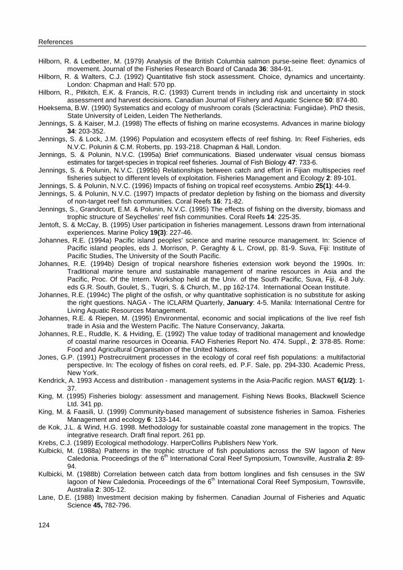
References
124
Hilborn, R. & Ledbetter, M. (1979) Analysis of the British Columbia salmon purse-seine fleet: dynamics ofmovement. Journal of the Fisheries Research Board of Canada 36: 384-91.
Hilborn, R. & Walters, C.J. (1992) Quantitative fish stock assessment. Choice, dynamics and uncertainty.London: Chapman and Hall: 570 pp.
Hilborn, R., Pitkitch, E.K. & Francis, R.C. (1993) Current trends in including risk and uncertainty in stockassessment and harvest decisions. Canadian Journal of Fishery and Aquatic Science 50: 874-80.
Hoeksema, B.W. (1990) Systematics and ecology of mushroom corals (Scleractinia: Fungiidae). PhD thesis,State University of Leiden, Leiden The Netherlands.
Jennings, S. & Kaiser, M.J. (1998) The effects of fishing on marine ecosystems. Advances in marine biology34: 203-352.
Jennings, S. & Lock, J.M. (1996) Population and ecosystem effects of reef fishing. In: Reef Fisheries, edsN.V.C. Polunin & C.M. Roberts, pp. 193-218. Chapman & Hall, London.
Jennings, S. & Polunin, N.V.C. (1995a) Brief communications. Biased underwater visual census biomassestimates for target-species in tropical reef fisheries. Journal of Fish Biology 47: 733-6.
Jennings, S. & Polunin, N.V.C. (1995b) Relationships between catch and effort in Fijian multispecies reeffisheries subject to different levels of exploitation. Fisheries Management and Ecology 2: 89-101.
Jennings, S. & Polunin, N.V.C. (1996) Impacts of fishing on tropical reef ecosystems. Ambio 25(1): 44-9.Jennings, S. & Polunin, N.V.C. (1997) Impacts of predator depletion by fishing on the biomass and diversity
of non-target reef fish communities. Coral Reefs 16: 71-82.Jennings, S., Grandcourt, E.M. & Polunin, N.V.C. (1995) The effects of fishing on the diversity, biomass and
trophic structure of Seychelles’ reef fish communities. Coral Reefs 14: 225-35.Jentoft, S. & McCay, B. (1995) User participation in fisheries management. Lessons drawn from international
experiences. Marine Policy 19(3): 227-46.Johannes, R.E. (1994a) Pacific island peoples' science and marine resource management. In: Science of
Pacific island peoples, eds J. Morrison, P. Geraghty & L. Crowl, pp. 81-9. Suva, Fiji: Institute ofPacific Studies, The University of the South Pacific.
Johannes, R.E. (1994b) Design of tropical nearshore fisheries extension work beyond the 1990s. In:Traditional marine tenure and sustainable management of marine resources in Asia and thePacific, Proc. Of the Intern. Workshop held at the Univ. of the South Pacific, Suva, Fiji, 4-8 July.eds G.R. South, Goulet, S., Tuqiri, S. & Church, M., pp 162-174. International Ocean Institute.
Johannes, R.E. (1994c) The plight of the osfish, or why quantitative sophistication is no substitute for askingthe right questions. NAGA - The ICLARM Quarterly, January: 4-5. Manila: International Centre forLiving Aquatic Resources Management.
Johannes, R.E. & Riepen, M. (1995) Environmental, economic and social implications of the live reef fishtrade in Asia and the Western Pacific. The Nature Conservancy, Jakarta.
Johannes, R.E., Ruddle, K. & Hviding, E. (1992) The value today of traditional management and knowledgeof coastal marine resources in Oceania. FAO Fisheries Report No. 474. Suppl., 2: 378-85. Rome:Food and Agricultural Organisation of the United Nations.
Jones, G.P. (1991) Postrecruitment processes in the ecology of coral reef fish populations: a multifactorialperspective. In: The ecology of fishes on coral reefs, ed. P.F. Sale, pp. 294-330. Academic Press,New York.
Kendrick, A. 1993 Access and distribution - management systems in the Asia-Pacific region. MAST 6(1/2): 1-37.
King, M. (1995) Fisheries biology: assessment and management. Fishing News Books, Blackwell ScienceLtd. 341 pp.
King, M. & Faasili, U. (1999) Community-based management of subsistence fisheries in Samoa. FisheriesManagement and ecology 6: 133-144.
de Kok, J.L. & Wind, H.G. 1998. Methodology for sustainable coastal zone management in the tropics. Theintegrative research. Draft final report. 261 pp.
Krebs, C.J. (1989) Ecological methodology. HarperCollins Publishers New York.Kulbicki, M. (1988a) Patterns in the trophic structure of fish populations across the SW lagoon of New
Caledonia. Proceedings of the 6th International Coral Reef Symposium, Townsville, Australia 2: 89-94.
Kulbicki, M. (1988b) Correlation between catch data from bottom longlines and fish censuses in the SWlagoon of New Caledonia. Proceedings of the 6th International Coral Reef Symposium, Townsville,Australia 2: 305-12.
Lane, D.E. (1988) Investment decision making by fishermen. Canadian Journal of Fisheries and AquaticScience 45, 782-796.
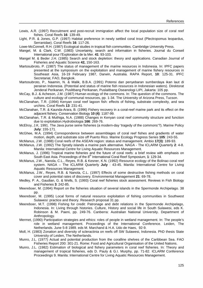
References
125
Lewis, A.R. (1997) Recruitment and post-recruit immigration affect the local population size of coral reeffishes. Coral Reefs 16: 139-49.
Light, P.R. & Jones, G.P. (1997) Habitat preference in newly settled coral trout (Plectropomus leopardus,Serranidae). Coral Reefs 16: 117-26.
Lowe-McConnell, R.H. (1987) Ecological studies in tropical fish communities. Cambridge University Press.Mangel, M. & Clark, C.W. (1983) Uncertainty, search and information in fisheries. Journal du Conseil
International pour l’Exploration de la Mer. 41: 93-103.Mangel M. & Beder J.H. (1985) Search and stock depletion: theory and applications. Canadian Journal of
Fisheries and Aquatic Science 42, 150-163.Martosubroto, P. (1987) The status of management of the marine resources in Indonesia. In: IPFC papers
presented at the symposium on the exploitation and management of marine fishery resources inSoutheast Asia, 16-19 February 1987, Darwin, Australia. RAPA Report, 10: 125-31. IPFCSecretariat, FAO, Bangkok.
Martosubroto, P., Naamin, N. & Malik, B.B.A. (1991) Potensi dan penyebaran sumberdaya ikan laut diperairan Indonesia. (Potential and status of marine fish resources in Indonesian waters). DirektoratJenderal Perikanan, Puslitbang Perikanan, Puslaitbang Oseanologi LIPI, Jakarta: 105 pp.
McCay, B.J. & Acheson, J.M. (1987) Human ecology of the commons. In: The question of the commons. Theculture and ecology of communal resources, pp. 1-34. The University of Arizona Press, Tucson.
McClanahan, T.R. (1994) Kenyan coral reef lagoon fish: effects of fishing, substrate complexity, and seaurchins. Coral Reefs 13: 231-41.
McClanahan, T.R. & Kaunda-Arara, B. (1996) Fishery recovery in a coral-reef marine park and its effect on theadjacent fishery. Conservation Biology 10 (4): 1187-99.
McClanahan, T.R. & Muthiga, N.A. (1988) Changes in Kenyan coral reef community structure and functiondue to exploitation.Hydrobiologia 166: 269-76.
McElroy, J.K. 1991. The Java purse seine fisheries (a modern-day ‘tragedy of the commons’?). Marine PolicyJuly: 155-171.
McGhee, M.A. (1994) Correspondence between assemblages of coral reef fishes and gradients of watermotion, depth, and substrate size off Puerto Rico. Marine Ecology Progress Series 105: 243-55.
McManus, J.W. (1988) Coral reefs of the ASEAN region: status and management. Ambio 17(3): 189-93.McManus, J.W. (1992) The Spratly islands a marine park alternative. NAGA - The ICLARM Quarterly 2: 4-8.
Manila: International Centre for Living Aquatic Resources Management.McManus, J. (1996) Tropical marine fisheries and the future of coral reefs: a brief review with emphasis on
South East Asia. Proceedings of the 8th International Coral Reef Symposium, 1: 129-34.McManus, J.W., Nanola, C.L., Reyes, R.B. & Kesner, K.N. (1992) Resource ecology of the Bolinao coral reef
system. NAGA – The ICLARM Quarterly July : 43-45. Manila: International Centre for LivingAquatic Resources Management.
McManus, J.W., Reyes, R.B. & Nanola, C.L. (1997) Effects of some destructive fishing methods on coralcover and potential rates of discovery. Environmental Management 21: 69-78.
Medley, P. A., Gaudian, G. & Wells, S. (1993) Coral reef fisheries stock assessment. Reviews in Fish Biologyand Fisheries 3: 242-85.
Meereboer, M. (1994) Report on the fisheries situation of several islands in the Spermonde Archipelago. 38pp.
Meereboer, M. (1995) Local forms of natural resource exploitation of fishing communities in SouthwestSulawesi: practice and theory. Research proposal 31 pp.
Meereboer, M.T. (1998) Fishing for credit: Patronage and debt relations in the Spermonde Archipelago,Indonesia. In: Living through histories. Culture, History and social life in South Sulawesi, eds K.Robinson & M. Paeni, pp. 249-76. Canberra: Australian National University. Department ofAnthropology.
Mermet, (1990) Participation strategies and ethics: roles of people in wetland management. In: The people’srole in wetland management. Proceedings of the International Conference. Leiden, TheNetherlands. June 5-8 1989. eds M. Marchand & H.A. Udo de Haes, 92-9.
Moll, H. (1983) Zonation and diversity of scleractinia on reefs off SW Sulawesi, Indonesia. PhD thesis StateUniversity of Leiden, The Netherlands.
Munro, J.L. (1977) Actual and potential production from the coralline shelves of the Caribbean Sea. FAOFisheries Report 200: 301-21. Rome: Food and Agricultural Organisation of the United Nations.
Munro, J.L. (1982) Estimation of biological and fishery parameters in coral reef fisheries. In: Theory andmanagement of tropical fisheries, eds D. Pauly & G.I. Murphy, pp. 71-82. ICLARM ConferenceProceedings 9. Manila: International Centre for Living Aquatic Resources Management.
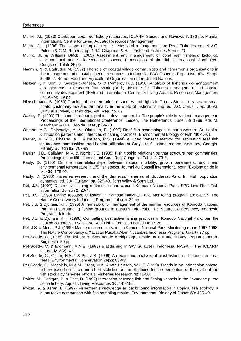
References
126
Munro, J.L. (1983) Caribbean coral reef fishery resources. ICLARM Studies and Reviews 7, 132 pp. Manila:International Centre for Living Aquatic Resources Management.
Munro, J.L. (1996) The scope of tropical reef fisheries and management. In: Reef Fisheries eds N.V.C.Polunin & C.M. Roberts, pp. 1-14. Chapman & Hall, Fish and Fisheries Series 20.
Munro, JL & Williams DMcb. (1985) Assessment and management of coral reef fisheries: biologicalenvironmental and socio-economic aspects. Proceedings of the fifth International Coral ReefCongress, Tahiti, 35 pp.
Naamin, N. & Badrudin, M. (1992) The role of coastal village communities and fishermen’s organisations inthe management of coastal fisheries resources in Indonesia. FAO Fisheries Report No. 474. Suppl.2: 490-7. Rome: Food and Agricultural Organisation of the United Nations.
Nielsen, J.P. Sen, S. Sverdrup-Jensen, S. & Pomeroy R.S. (1996) Analysis of fisheries co-managementarrangements: a research framework (Draft). Institute for Fisheries management and coastalcommunity development (IFM) and International Centre for Living Aquatic Resources Management(ICLARM). 19 pp.
Nietschmann, B. (1989) Traditional sea territories, resources and rights in Torres Strait. In: A sea of smallboats: customary law and territoriality in the world of inshore fishing, ed. J.C. Cordell , pp. 60-93.Cultural survival, Cambridge, MA, Rep. no. 62.
Oakley, P. (1990) The concept of participation in development. In: The people’s role in wetland management.Proceedings of the International Conference. Leiden, The Netherlands. June 5-8 1989. eds M.Marchand & H.A. Udo de Haes, p 66-73.
Öhman, M.C., Rajasuriya, A. & Ólafsson, E. (1997) Reef fish assemblages in north-western Sri Lanka:distribution patterns and infuences of fishing practices. Environmental Biology of Fish 49: 45-61.
Parker, Jr. R.O., Chester, A.J. & Nelson, R.S. (1994) A video transect method for estimating reef fishabundance, composition, and habitat utilization at Gray’s reef national marine sanctuary, Georgia.Fishery Bulletin 92: 787-99.
Parrish, J.D., Callahan, M.V. & Norris, J.E. (1985) Fish trophic relationships that structure reef communities.Proceedings of the fifth International Coral Reef Congress, Tahiti, 4: 73-8.
Pauly, D. (1980) On the inter-relationships between natural mortality, growth parameters, and meanenvironmental temperature in 175 fish stocks. Journal du Conseil International pour l”Exploration de laMer 39: 175-92.
Pauly, D. (1988) Fisheries research and the demersal fisheries of Southeast Asia. In: Fish populationdynamics, ed. J.A. Gulland, pp. 329-48. John Wiley & Sons Ltd.
Pet, J.S. (1997) Destructive fishing methods in and around Komodo National Park. SPC Live Reef FishInformation Bulletin 2: 20-4.
Pet, J.S. (1998) Marine resource utilization in Komodo National Park. Monitoring program 1996-1997. TheNature Conservancy Indonesia Program, Jakarta. 32 pp.
Pet, J.S. & Djohani, R.H. (1996) A framework for management of the marine resources of Komodo NationalPark and surrounding fishing grounds in Eastern Indonesia. The Nature Conservancy, IndonesiaProgram, Jakarta.
Pet, J.S. & Djohani. R.H. (1998) Combatting destructive fishing practices in Komodo National Park: ban thehookah compressor! SPC Live Reef Fish Information Bulletin 4: 17-28.
Pet, J.S. & Mous, P.J. (1999) Marine resource utilization in Komodo National Park. Monitoring report 1997-1998.The Nature Conservancy & Yayasan Pusaka Alam Nusantara Indonesia Program, Jakarta 37 pp.
Pet-Soede, C. (1995) The fishery of Spermonde Archipelago, results of a frame survey. Report programBuginesia. 59 pp.
Pet-Soede, C. & Erdmann, M.V.E. (1998) Blastfishing in SW Sulawesi, Indonesia. NAGA – The ICLARMQuarterly 2(2): 4-9.
Pet-Soede, C., Cesar, H.S.J. & Pet, J.S. (1999) An economic analysis of blast fishing on Indonesian coralreefs. Environmental Conservation 26(2): 83-93.
Pet-Soede, C., Machiels, M.A.M., Stam, M.A. & van Densen, W.L.T. (1999) Trends in an Indonesian coastalfishery based on catch and effort statistics and implications for the perception of the state of thefish stocks by fisheries officials. Fisheries Research 42:41-56.
Poitier, M., Petitgas, P. & Petit, D. (1997) Interaction between fish and fishing vessels in the Javanese purseseine fishery. Aquatic Living Resources 10, 149-156.
Poizat, G. & Baran, E. (1997) Fishermen's knowledge as background information in tropical fish ecology: aquantitative comparison with fish sampling results. Environmental Biology of Fishes 50: 435-49.
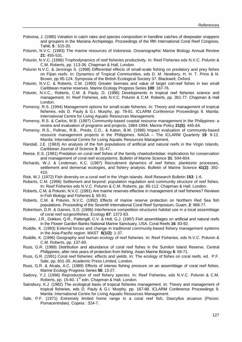
References
127
Polovina, J. (1985) Variation in catch rates and species composition in handline catches of deepwater snappersand groupers in the Mariana Archipelago. Proceedings of the fifth International Coral Reef Congress,Tahiti, 5 : 515-20.
Polunin, N.V.C. (1983) The marine resources of Indonesia. Oceanographic Marine Biology Annual Review21: 455-531.
Polunin, N.V.C. (1996) Trophodynamics of reef fisheries productivity. In: Reef Fisheries eds N.V.C. Polunin &C.M. Roberts, pp. 113-36. Chapman & Hall, London.
Polunin N.V.C. & Jennings S. (1998) Differential effects of small-scale fishing on predatory and prey fisheson Fijian reefs. In: Dynamics of Tropical Communities, eds D. M. Newbery, H. H. T. Prins & N.Brown, pp 95-124. Symposia of the British Ecological Society 37. Blackwell, Oxford.
Polunin, N.V.C. & Roberts, C.M. (1993) Greater biomass and value of target corl-reef fishes in two smallCaribbean marine reserves. Marine Ecology Progress Series 100: 167-76.
Polunin, N.V.C., Roberts, C.M. & Pauly, D. (1996) Developments in tropical reef fisheries science andmanagement. In: Reef Fisheries, eds N.V.C. Polunin & C.M. Roberts, pp. 361-77. Chapman & HallLondon.
Pomeroy, R.S. (1994) Management options for small-scale fisheries. In: Theory and management of tropicalfisheries, eds D. Pauly & G.I. Murphy, pp. 78-81. ICLARM Conference Proceedings 9. Manila:International Centre for Living Aquatic Resources Management.
Pomeroy, R.S. & Carlos, M.B. (1997) Community-based coastal resource management in the Philippines: areview and evaluation of programs and projects, 1984-1994. Marine Policy 21(5): 445-64.
Pomeroy, R.S., Pollnac, R.B., Predo, C.D., & Katon, B.M. (1996) Impact evaluation of community-basedresource management projects in the Philippines. NAGA – The ICLARM Quarterly 19: 9-12.Manila: International Centre for Living Aquatic Resources Management.
Randall, J.E. (1963) An analysis of the fish populations of artificial and natural reefs in the Virgin Islands.Caribbean Journal of Science 3: 31-47.
Reese, E.S. (1981) Predation on coral reef fishes of the family chaetodontidae: implications for conservationand management of coral reef ecosystems. Bulletin of Marine Science 31: 594-604.
Richards, W.J. & Lindeman, K.C. (1987) Recruitment dynamics of reef fishes: planktonic processes,settlement and demersal ecologies, and fishery analysis. Bulletin of Marine Science 41(2): 392-410.
Risk, M.J. (1972) Fish diversity on a coral reef in the Virgin islands. Atoll Research Bulletin 153: 1-6.Roberts, C.M. (1996) Settlement and beyond: population regulation and community structure of reef fishes.
In: Reef Fisheries eds N.V.C. Polunin & C.M. Roberts, pp. 85-112. Chapman & Hall. London.Roberts, C.M. & Polunin, N.V.C. (1991) Are marine reserves effective in management of reef fisheries? Reviews
in Fish Biology and Fisheries 1: 65-91.Roberts, C.M. & Polunin, N.V.C. (1992) Effects of marine reserve protection on Northern Red Sea fish
populations. Proceeding of the Seventh International Coral Reef Symposium, Guam, 2: 969-77.Robertson, D.R. & Gaines, S.D. (1986) Interference competition structures habitat use in a local assemblage
of coral reef surgeonfishes. Ecology 67: 1372-83.Rooker, J.R., Dokken, Q.R., Pattengill, C.V. & Holt, G.J. (1997) Fish assemblages on artificial and natural reefs
in the Flower Garden Banks National Marine Sanctuary, USA. Coral Reefs 16: 83-92.Ruddle, K. (1993) External forces and change in traditional community-based fishery management systems
in the Asia-Pacific region. MAST 6(1/2): 1-37.Ruddle, K. (1996) Geography and human ecology of reef fisheries. In: Reef Fisheries, eds N.V.C. Polunin &
C.M. Roberts, pp. 137-60.Russ, G.R. (1989) Distribution and abundance of coral reef fishes in the Sumilon Island Reserve. Central
Philippines, after nine years of protection from fishing. Asian Marine Biology 6: 59-71.Russ, G.R. (1991) Coral reef fisheries: effects and yields. In: The ecology of fishes on coral reefs. ed. P.F.
Sale, pp. 601-35. Academic Press Limited, London.Russ, G.R. & Alcala, A.C. (1989) Effects of intense fishing pressure on an assemblage of coral reef fishes.
Marine Ecology Progress Series 56: 13-27.Sadovy, Y.J. (1996) Reproduction of reef fishery species. In: Reef Fisheries, eds N.V.C. Polunin & C.M.
Roberts, pp. 15-60. 1st edn. Chapman & Hall. London.Sainsbury, K.J. (1982) The ecological basis of tropical fisheries management. In: Theory and management of
tropical fisheries, eds D. Pauly & G.I. Murphy, pp. 167-88. ICLARM Conference Proceedings 9.Manila: International Centre for Living Aquatic Resources Management.
Sale, P.F. (1971) Extremely limited home range in a coral reef fish, Dascyllus aruanus (Pisces:Pomacentridae). Copeia : 324-7.
References
128
Sale, P.F. (1982) The structure and dynamics of coral reef fish communities. In: Theory and management oftropical fisheries, eds D. Pauly & G.I. Murphy, pp. 241-53.
Sale, P.F. (1991) The ecology of fishes on coral reefs. 1st edn. Academic Press, California.Sale, P.F. & Sharp, B.J. (1983) Correction for bias in visual transect censuses of coral reef fishes. Coral
Reefs 2: 37-42.Samoilys, M.A. (1991) Review of the underwater visual census method developed by DPI/ACIAR project:
visual assessment of reef fish stocks. Conference and Workshop Series QC92006. Discussion groupworkshop proceedings Townsville. 55 pp.
Samoilys, M.A. (1997) Movement is a large predatory fish: coral trout Plectropomus leopardus (Pisces:Serranidae) on Heron Reef, Australia. Coral Reefs 16: 151-8
Samoilys, M.A. & Squire, L.C. (1994) Preliminary observations on the spawning behaviour of coral troutPlectropomus leopardus (Pisces: Serranidae), on the Great Barrier Reef. Bulletin of MarineScience 54: 332-42.
Sampson, D.B. (1991) Fishing tactics and fish abundance, and their influence on catch rates. ICES Journal ofMarine Science 48: 291-301.
SAS Institute Inc. (1990) SAS Technical report P243, SAS/STAT Software: The GENMOD procedure,release 6.09, Cary, NC, SAS Institute Inc. 88 pp.
Schaefer, M. (1954) Some aspects of the dynamics of populations important to the management of thecommercial marine fisheries. Bull.I-ATTC/Bol.CIAT 1: 27-56.
Sheppard, C.R.C. (1999) Coral decline and weather patterns over 20 years in the Chagos Archipelago,Central Indian Ocean. Ambio 28: 472-7.
Sloan, N.A. & Sugandhy, A. (1994) An overview of Indonesian coastal environmental management. CoastalManagement 22: 215-33.
Sluka, R.D., Chiappone, M. & Sullivan, K.M. (1996) Habitat preference of groupers in the exuma cays.Bahamas Journal of Science 4(1): 8-14.
Smith, C.L. (1990) Resource scarcity and inequality in the distribution of catch. North American Journal ofFisheries Management 10: 269-78.
Smith, C.L. & McKelvey, R. (1986) Specialist and generalist: roles for coping with variability. North AmericanJournal of Fisheries Management 6: 88-99.
Smith, P.J., Francis, R.I.C.C. & McVeagh, M. (1991) Loss of genetic diversity due to fishing pressure. FisheriesResearch 10: 309-16.
Soegiarto, A. (1981) The development of a marine park system in Indonesia. Proceedings of the FourthInternational Coral Reef Symposium, Manila, 1: 287-91.
Soegiarto, A., & Polunin, N.V.C. (1982) The marine environment of Indonesia. Report for the Government ofIndonesia under sponsorship of IUCN and WWF. 257 pp.
Soepanto & Nikijuluw, V.P.H. (1999) Resource based collaborative commercial fisheries management inIndonesia. Indonesian Journal of Coastal and Marine Resources 2(2): 17-28.
Sokal, R.R. & Rohlf, F.J. (1995) Biometry: the principles and practice of statistics in biological research. 3rd
edn. WH Freeman and Company, New York, 887 pp..Sparre, P., Ursin, E. & Venema, S.C. (1989) Introductions to tropical fish stock assessment. FAO Fisheries
Technical Paper No. 306 (1&2). Rome: Food and Agricultural Organisation of the United Nations.Stapel, J. (1997) Nutrient dynamics in Indonesian seagrass beds: factors determining conservation and loss
of nitrogen and phosphorus. PhD thesis State University of Nijmegen, The Netherlands.Storm, C. (1989) Influence of river systems and coastal hydrodynamics on the water quality during one
monsoonal period. A hydro geographical survey of a tropical coastal area in the SpermondeArchipelago, Southwest Sulawesi, Indonesia. Geopro report 04. Geografic Institute VakgroepFysische Geografie, State University of Utrecht, The Netherlands.
Sweatman, H., Bass, D., Cheal, A., Coleman, G., Miller, I., Ninio, R., Osborne, K., Oxley, W., Ryan, D.,Thompson, A. & Tomkins, P. (1998) Long-term monitoring of the Great Barrier Reef. Status ReportNo. 3 1998. AIMS Townsville, Australia.
Thresher, R.E. (1983a) Environmental correlates of the distribution of planktivores fishes in the One TreeLagoon. Marine Ecology Progress Series 10: 137-45.
Thresher, R.E. (1983b) Habitat effects on reproductive success in the coral reef fish, Acanthochromispolyacanthus (Pomacentridae). Ecology 64: 1184-99.
Thresher, R.E. (1991) Geographic variability in the ecology of coral reef fishes: evidence, evolution, andpossible implications. In: The ecology of fishes on coral reefs, ed. P.F. Sale, pp. 401-36. 1st edn.Academic Press, California.
References
129
Titus, M.J. (1999) Determinants and trends of urban development in Ujung Pandang, Indonesia. Paperpresented at Buginesia Workshop on Intergrated Coastal Zone Management, Leiden, TheNetherlands. 23 pp.
Tomascik, T., Mah, A.J., Nontji, A. & Moosa, M.K. (1997) The ecology of the Indonesian seas Part I. Peripluseditions ltd. Hongkong. 642 pp.
Uljee, I., Engelen, G. & White, R. (1996) RamCo Demo Guide, Workdocument CZM-C 96.08, Coastal ZoneManagement Centre, National Institute for Coastal and Marine Management, P.O. Box 20907,2500 EX The Hague, the Netherlands.
Umbgrove, J.H.F. (1930) De koraalriffen van den Spermonde Archipel (S. Celebes). Summary in English.Leidsche Geologische Mededeelingen 3: 228-47.
Venema, S.C. (1997) Report on the Indonesia/FAO/DANIDA workshop on the assessment of the potential ofthe marine fishery resources of Indonesia. Jakarta 13-24 March 1995. FI:GCP/INT/575/DEN.Report on Activity No. 15. Rome: Food and Agricultural Organisation of the United Nations.
Welcomme, R.L. (1999) A review of a model for qualitative evauation of exploitation levels in multi-speciesfisheries. Fisheries Management and Ecology 6:1-19.
Wells, S.M. (1992) “Successful” coral reef management programmes. Intercoast Network 17: 1-3. CoastalResources Center, University of Rhode Island, Narragansett, RI.
Whitten, A.J., Mustafa, M. & Henderson, G.S. (1987) The ecology of Sulawesi. 1st edn Gadjah MadaUniversity Press Jakarta.
Williams, D. McB. (1991) Patterns and processes in the distribution of coral reef fishes. In: The ecology offishes on coral reefs, ed. P.F. Sale, pp. 437-74. 1st edn. Academic Press, California.
Wilson, J.A. & Kleban, P. (1992) Practical implications of chaos in fisheries. MAST 5(1): 67-75.Yamamoto,T. (1980) A standard statistical system for current fishery statistics in Indonesia. A report
prepared for the fisheries development and management project, Indonesia. FI:DP/INS/72/064.Field Document No. 7. Rome: Food and Agricultural Organisation of the United Nations.
Zeller, D.C. (1997) Home range and activity patterns of the coral trout Plectropomus leopardus (Serranidae).Marine Ecology Progress Series 154: 65-77.
Zerner, C. (1993) Community management of marine resources in the Maluku islands. FAO Fisheries ReportNo. 474 Suppl. 1: 127-42. Rome: Food and Agricultural Organisation of the United Nations.

131
Dankwoord
Dit proefschrift is het product van een goede en stimulerende samenwerking met veel capabele enenthousiaste mensen en van een warme ondersteuning door familie en vrienden. Daarom wil ik hierdeze mensen bedanken.
Bedankt
Terima kasihThanks
Wim van Densen voor zijn motivatie en inspiratie. Hij heeft het project bedacht, het voorstelgeschreven, gedurende de afgelopen 5 jaar het onderzoek begeleid en gedragen en dit proefschrift dehuidige structuur gegeven.Marcel Machiels voor zijn pragmatisme en zijn statistische kennis. Hij heeft vooral gedurende demoeilijke laatste 1.5 jaar een belangrijke en duidelijke hand gehad in de uitvoering van de analyses enhet structureren van de teksten.Feite van der Veen voor zijn hulp bij data analyse en zijn fantastische inzet voor het fysiek tot standkomen van dit boek. Hij heeft de volledige lay-out van het proefschrift voor zijn rekening genomen.Bram Huisman als mijn promotor. Hij heeft gedurende het gehele project veel interesse getoond enbruikbare suggesties gegeven.
Maya Borel-Best, Piet Nienhuis, en Franz von Benda-Beckmann als leden van debegeleidingscommissie. Zij hebben bruikbaar commentaar gegevens tijdens de jaarlijksebijeenkomsten.De stichting WOTRO voor de financiële ondersteuning van dit onderzoek.Pieter Augustinus, Milan Titus, Leontine Visser, Hans Riezebos, Herman Wind, Martin Hemminga,Maya Borel-Best, Nico Schulte Nordholt, en Gerard van der Velde als leden van het Buginesia team inNederland voor hun interesse. De bijeenkomsten waren enerverend en leerzaam.Pim van Avesaath, Bert Hoeksema, Marie Trees Meereboer, Jean Luc de Kok, Alette van derWouden, Astrid Kievid en Philip Visman als leden van het Buginesia team in Indonesie voor degedeelde ervaringen en humor.Rene Hagels, Micha Oudakker, Martina Stam, Hanneke van Lavieren, Tim van Oijen, Jan GeertHiddink, Sande Kuijl, Amiruddin, Rob van der Heijden en Sieto Verwer voor al het werk dat ze verzethebben tijdens hun stages en veldonderzoeken in Indonesië en voor de gezellige BBQ’s.
LIPI Jakarta for acting as the sponsor of the work in Sulawesi and for providing the necessarypaperwork for visas.Professor Natsir Nessa for acting as my supervisor in Indonesia and for his interest.
132
Dr. Alfian Noor as the Indonesian project co-ordinator for his help with all kinds of little problems andfor his interest.Ir. Sudirman as my counterpart for his knowledge on the fish and fishery in Spermonde.All fisheries officials at the auctions Paotere and Rajawali, at the district offices of Takalar, UjungPandang, Maros, Pangkep and Barru, at the province office for South Sulawesi and at the nationaloffice in Jakarta for allowing me to visit the fish markets, accompanying me on many visits and forhelping me with all sorts of information.All fishers in Spermonde Archipelago for trusting me and providing me with all the information Ineeded and with the best fresh cooked fish during fieldtrips.Pak M. Said for his understanding of the waters and the weather, which, together with his technicalabilities and his eagerness to catch fish, saved me from dangerous situations and rice-only mealswhile at sea.Buang and Ibrahim for taking over Said’s difficult job as boatman.Rusli for his save driving.Ibu Tuminah and Azis and Muliati for taking excellent care of my family and friends.
Tom Buijse, Henk Heessen, Bert Hoeksema, Joep de Leeuw, Jules van Rooij en Paul van Zwietenvoor hun commentaar op manuscripten van verschillende hoofdstukken.Gerrie van Eck voor haar belangrijke ondersteuning van allerlei administratieve zaken.De collega’s van de visteelt en visserij groep voor de gezellige koffiepauzes en interesse.Peter Mous, Feite van der Veen, Joep de Leeuw, Rob Grift, Paul van Zwieten, Hans vanOostenbrugge, Erwin Winter en Leo Nagelkerken als directe collega’s voor hun goede inhoudelijke,praktische maar ook levensbeschouwende discussies over visserij, natuurbeheer, het leven in hetalgemeen, duiken met PADI of IOB in of buiten de tropen, trouwen, kinderen, solliciteren en voor deillusie dat een vrouwelijke input wel nuttig is in dit soort discussies.Herman Cesar voor zijn positieve werkbenadering en interesse in mijn werk.Rili Djohani voor haar interesse en het delen van ervaring betreffende bescherming van Indonesischeriffen.
Arnaz Mehta and Mark Erdmann for their friendship and sharing of good times. They showed me whatisland and slimy invertebrate life was all about. We shared the first ripping-current dives at Komodo,the worst nights amongst rats, dragons and cockroaches at Loh Liang and the best BalineseMargaritha’s.Helen Fox for her positive attitude, humour and the best non-Japanese Sushi-rolls.Feisol and Jeannine Hashim for their warm welcome to their houses in Bali and Bajo.
Joost Backx en Vera Minten voor hun onvoorwaardelijke vriendschap en opvang.Tom Buijse voor gesprekken, tapas avonden en goede zorgen tijdens de laatste fase.Peter Mous voor het delen van de stress uren, pizza’s en automaat koffie gedurende de laatste fasevan het schrijven.Annemiek Verhallen voor haar interesse en de belangrijke lunchgesprekken.

133
Grietje de Groot voor het delen van emotionele dikke buiken tijden.Judith, Winne, Emmy, Hester, Grietje, Valerie, Bea, Ellen, Catherine, Mirjam, Nathalie, Danielle,Margot als Vierus voor het feit dat zij zorgden dat ik tijdens de periodes in Nederland zo weer in hetvertrouwde jaarclubnest kon duiken.Rotary Club Woerden voor hun warmte.Shaema en Rodolf Hoeffelman voor de goede tijd in Ujung Pandang en Jakarta.
Mijn ouders voor hun liefde, vertrouwen in mijn kunnen, warme ondersteuning en hun opvang van onsgezinnetje in Nederland.Mijn schoonouders voor het bieden van een rustpunt in een hectisch leven.Jan en Christel, Heleen en Marcel en Mariette voor hun telefoontjes op de juiste momenten.Jos als degene die me er in moeilijke momenten doorheen heeft getrokken. Zijn drang tot eerlijkheiden perfectie blijft een voorbeeld.Eva voor haar armpjes om mijn nek na een lange werkdag.

135
Curriculum Vitae
Cornelia (Lida) Soede werd op 28 oktober 1967 in Woerden geboren. In 1986 behaalde zij het VWOdiploma aan het Dr. F.H. de Bruyne Lyceum in Utrecht. In 1993 studeerde zij af aan de LandbouwUniversiteit Wageningen als ingenieur in de Landbouwwetenschappen met de hoofdvakkenVisserijkunde, Visteelt en Agrarische sociologie van niet-westerse landen, en een stage voorVisserijkunde. In 1994 werd zij in dienst gesteld bij NWO als onderzoeker in opleiding engestationeerd in Ujung Pandang, Indonesië bij het door WOTRO gefinancierde Buginesiaonderzoeksproject voor geïntegreerd kustzone beheer. Gedurende 4 jaar werd dit project uitgevoerdin samenwerking met de Universiteit Hasanuddin te Ujung Pandang, en de Faculteit RuimtelijkeWetenschappen van de Universiteit van Utrecht, de Faculteit Technische Bedrijfskunde van deUniversiteit Twente, de Faculteit Sociale Wetenschappen van de Universiteit van Amsterdam, hetNatuurhistorisch Museum Leiden, en het Centrum voor Estuarine en Marine Kust onderzoek van hetNederlands Instituut voor Ecologisch Onderzoek Yerseke. Tijdens dit project werd het visserijonderzoek dat in dit proefschrift beschreven is opgestart en uitgevoerd. Lida Soede is getrouwd metJos Pet en samen hebben zij een dochter Eva.