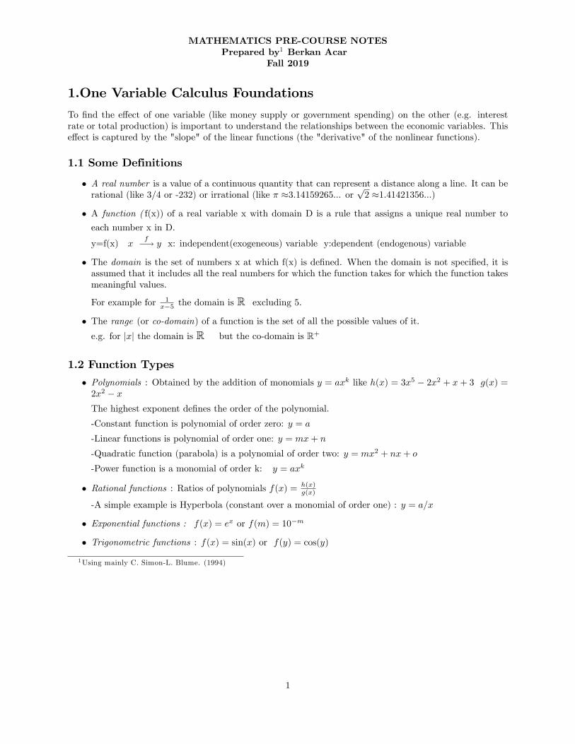
MATHEMATICS PRE-COURSE NOTESPrepared by1 Berkan Acar

Fall 2019

1.One Variable Calculus Foundations

To �nd the e¤ect of one variable (like money supply or government spending) on the other (e.g. interestrate or total production) is important to understand the relationships between the economic variables. Thise¤ect is captured by the "slope" of the linear functions (the "derivative" of the nonlinear functions).

1.1 Some Definitions

� A real number is a value of a continuous quantity that can represent a distance along a line. It can berational (like 3/4 or -232) or irrational (like � �3.14159265... or

p2 �1.41421356...)

� A function ( f(x)) of a real variable x with domain D is a rule that assigns a unique real number to

each number x in D.

y=f(x) xf�! y x: independent(exogeneous) variable y:dependent (endogenous) variable

� The domain is the set of numbers x at which f(x) is de�ned. When the domain is not speci�ed, it isassumed that it includes all the real numbers for which the function takes for which the function takesmeaningful values.

For example for 1x�5 the domain is R excluding 5.

� The range (or co-domain) of a function is the set of all the possible values of it.e.g. for jxj the domain is R but the co-domain is R+

1.2 Function Types

� Polynomials : Obtained by the addition of monomials y = axk like h(x) = 3x5 � 2x2 + x+ 3 g(x) =2x2 � xThe highest exponent de�nes the order of the polynomial.

-Constant function is polynomial of order zero: y = a

-Linear functions is polynomial of order one: y = mx+ n

-Quadratic function (parabola) is a polynomial of order two: y = mx2 + nx+ o

-Power function is a monomial of order k: y = axk

� Rational functions : Ratios of polynomials f(x) = h(x)g(x)

-A simple example is Hyperbola (constant over a monomial of order one) : y = a=x

� Exponential functions : f(x) = ex or f(m) = 10�m

� Trigonometric functions : f(x) = sin(x) or f(y) = cos(y)

1Using mainly C. Simon-L. Blume. (1994)

1

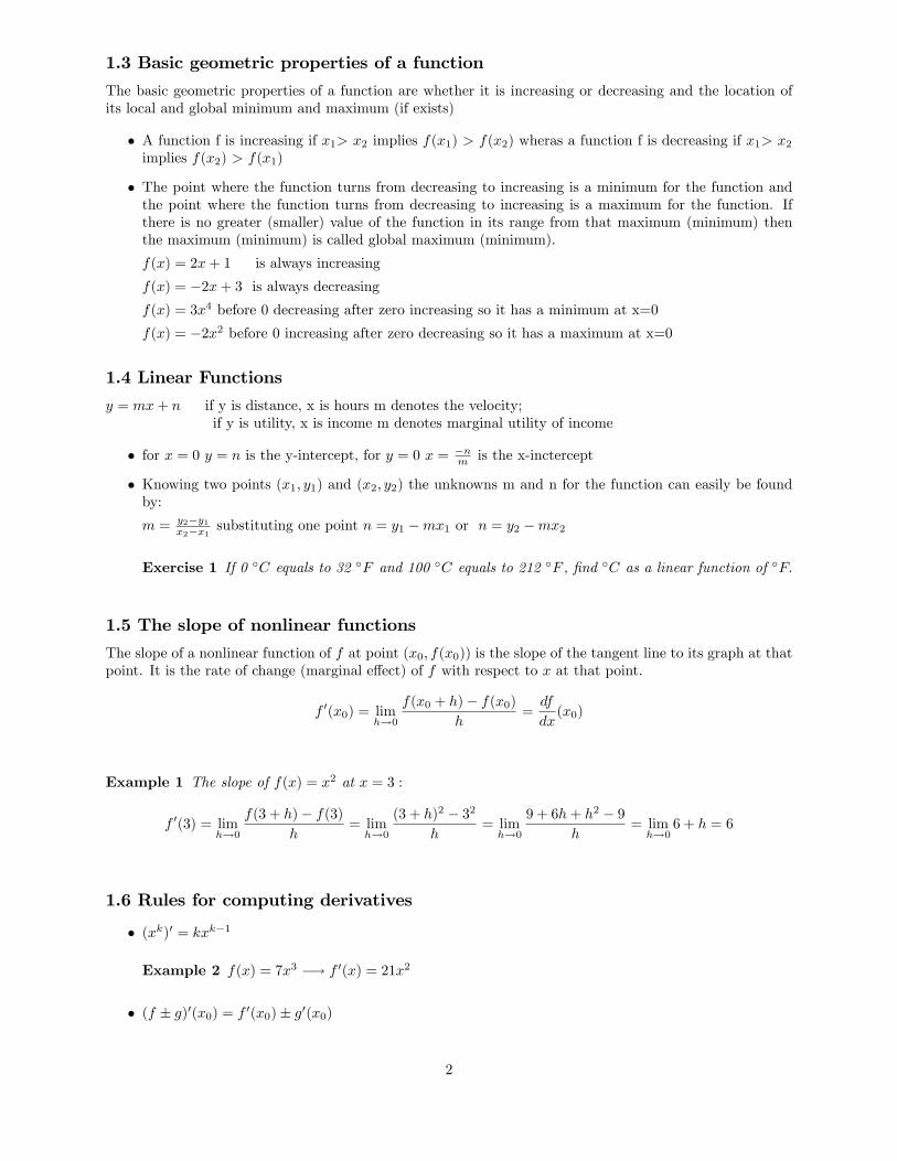
1.3 Basic geometric properties of a function

The basic geometric properties of a function are whether it is increasing or decreasing and the location ofits local and global minimum and maximum (if exists)

� A function f is increasing if x1> x2 implies f(x1) > f(x2) wheras a function f is decreasing if x1> x2implies f(x2) > f(x1)

� The point where the function turns from decreasing to increasing is a minimum for the function andthe point where the function turns from decreasing to increasing is a maximum for the function. Ifthere is no greater (smaller) value of the function in its range from that maximum (minimum) thenthe maximum (minimum) is called global maximum (minimum).

f(x) = 2x+ 1 is always increasing

f(x) = �2x+ 3 is always decreasing

f(x) = 3x4 before 0 decreasing after zero increasing so it has a minimum at x=0

f(x) = �2x2 before 0 increasing after zero decreasing so it has a maximum at x=0

1.4 Linear Functions

y = mx+ n if y is distance, x is hours m denotes the velocity;if y is utility, x is income m denotes marginal utility of income

� for x = 0 y = n is the y-intercept, for y = 0 x = �nm is the x-inctercept

� Knowing two points (x1; y1) and (x2; y2) the unknowns m and n for the function can easily be foundby:

m = y2�y1x2�x1 substituting one point n = y1 �mx1 or n = y2 �mx2

Exercise 1 If 0 �C equals to 32 �F and 100 �C equals to 212 �F , �nd �C as a linear function of �F:

1.5 The slope of nonlinear functions

The slope of a nonlinear function of f at point (x0; f(x0)) is the slope of the tangent line to its graph at thatpoint. It is the rate of change (marginal e¤ect) of f with respect to x at that point.

f 0(x0) = limh!0

f(x0 + h)� f(x0)h

=df

dx(x0)

Example 1 The slope of f(x) = x2 at x = 3 :

f 0(3) = limh!0

f(3 + h)� f(3)h

= limh!0

(3 + h)2 � 32h

= limh!0

9 + 6h+ h2 � 9h

= limh!0

6 + h = 6

1.6 Rules for computing derivatives

� (xk)0 = kxk�1

Example 2 f(x) = 7x3 �! f 0(x) = 21x2

� (f � g)0(x0) = f 0(x0)� g0(x0)

2

Example 3 f(x) = 2x7 g(x) = 4x12

(f � g)(x) = 2x7 � 4x 12 �! (f � g)0(x) = f 0(x)� g0(x) = 14x6 � 2x� 1

2

� (kf)0(x0) = kf 0(x0)

� (f:g)0(x0) = f 0(x0)g(x0) + f(x0)g0(x0) �Product rule: (f:g)0 = f 0g + fg0

Example 4 f(x) = x� 1 g(x) = x2 + x+ 1(x3 � 1)0 = (f:g)0(x) = 1:(x2 + x+ 1) + (x� 1):(2x+ 1) = 3x2

� ( fg )0(x0) =

f 0(x0)g(x0)�f(x0)g0(x0)g(x0)2

�Quotient rule: ( fg )0 = f 0g�fg0

g2

Example 5 f(x) = x� 1 g(x) = x+ 1�x�1x+1

�0= x+1�(x�1)

(x+1)2= 2

(x+1)2

� ([f(x)]n)0 = n [f(x)]n�1 f 0(x) �From Chain rule: ddx [f(g(x))] = f0(g(x))g0(x)

1.7 Di¤erentiability

� If f(x) has a tangent line at point x0 or limh!0f(x0+h)�f(x0)

h exists then f(x) is di¤entiable at pointx0.

� If a function is di¤erentiable at every point in its domain we say that it is a di¤erentiable (smooth)function.

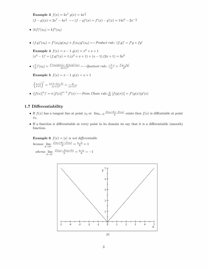
Example 6 f(x) = jxj is not di¤erentiablebecause lim

h!0+

f(x0+h)�f(x0)h = h�0

h = 1

wheras limh!0�

f(x0)�f(x0+h)h = 0�h

h = �1

3

1.8 Continuity

� A function is continuous if its graph has no breaks (no jumps for the same point) in its domain.

� For a function to be di¤erentiable, it must be continuous but not vice versa. For instance f(x) = jxjis not di¤erentiable but it is continous.

For continuity, for every points in the domain (let x0) the equality limx!x0

f(x) = f(x0) must hold.

� A continuously di¤erentiable function is a function whose derivative is continuous (C1): Every poly-nomial is C1:

Example 7

f(x) =

�x2; x � 0�x2; x < 0

�is continuous �! f 0(x) =

�2x; x � 0�2x; x < 0

�is continuous so f(x) is C1

Example 8 f(x) = x23 i s continous but not di¤erentiable

f 0(x) = limh!0

f(0 + h)� f(0)h

= limh!0

h23

h= h�

13 do not exists

�!1 if h > 0! �1 if h < 0

�so f(x) is not C1

1.9 Higher order derivatives

� If f(x) is C1 then we can ask whether f 0(f 0(x)) exists that is f 00(x) = ddx (

dfdx )

� Polynomials are C1

Example 9

f(x) = 3x7 + 2x3 �! f 0(x) = 21x6 + 6x2 �! f 00(x) = 126x5 + 12x

Example 10

f(x) =

�x2; x � 0�x2; x < 0

�is continuous and C1 but �! f 00(x) =

�2; x � 0�2; x < 0

�does not exist

� If f 00 is continuous then f is C2 (twice continously di¤erentiable)

� If f (n) is continuous then f is Cn: All polynomials are C1

Example 11 f(x) = 3x�32 is continuous in its domain R+

f 0(x) =�92x�52 �! f 00(x) =

45

4x�72 are also continuous in R+

4

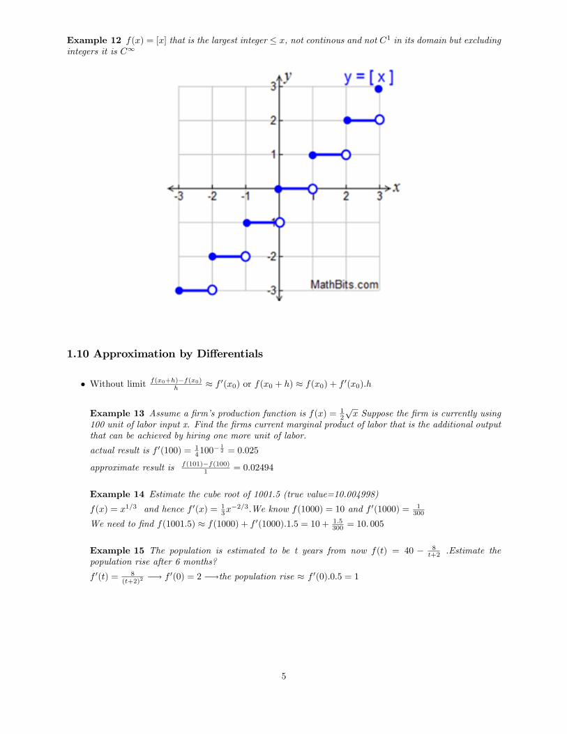
Example 12 f(x) = [x] that is the largest integer � x, not continous and not C1 in its domain but excludingintegers it is C1

1.10 Approximation by Di¤erentials

� Without limit f(x0+h)�f(x0)h � f 0(x0) or f(x0 + h) � f(x0) + f 0(x0):h

Example 13 Assume a �rm�s production function is f(x) = 12

px Suppose the �rm is currently using

100 unit of labor input x. Find the �rms current marginal product of labor that is the additional outputthat can be achieved by hiring one more unit of labor.

actual result is f 0(100) = 14100

� 12 = 0:025

approximate result is f(101)�f(100)1 = 0:02494

Example 14 Estimate the cube root of 1001.5 (true value=10.004998)

f(x) = x1=3 and hence f 0(x) = 13x

�2=3.We know f(1000) = 10 and f 0(1000) = 1300

We need to �nd f(1001:5) � f(1000) + f 0(1000):1:5 = 10 + 1:5300 = 10: 005

Example 15 The population is estimated to be t years from now f(t) = 40 � 8t+2 .Estimate the

population rise after 6 months?

f 0(t) = 8(t+2)2

�! f 0(0) = 2 �!the population rise � f 0(0):0:5 = 1

5

2.One Variable Calculus: Applications

2.1 Using �rst and second derivatives to sketch graphs

1. Find the critical (stationary) points at which f 0(x) = 0 or f 0(x) is not de�ned, order those pointsshowing on the x axis as (�1; x1), (x1; x2)...(xk;1)

2. Find the sign of the f 0(x) as x goes to 1 for (xk;1) and �1. Alternate the sign for the subsequentinterval if the critical point is not even times repeated (double, quadruple etc.). Otherwise do notchange the sign.

3. The function f(x) is increasing in the intervals with positive sign whereas it is decreasing in theintervals with the negative sign. If f 0(x) is positive (negative) always then f(x) is always increasing(or decreasing).

4. Do the �rst two steps for f 00(x) instead of f 0(x).

5. The function f(x) is convex (upward curved, the slope of f 0(x) is increasing) in the intervals withpositive sign, whereas it is concave (downward curved,the slope of f 0(x) is decreasing) in the intervalswith the negative sign. If f 00(x) is positive (negative) always then f(x) is always convex (or concave).

� De�nition 1 f is convex in the interval [a; b] i¤ f((1� t)a+ tb) � (1� t)f(a) + tf(b) with 0 � t � 1(the secant line joining two points on the funtion is above the graph of the function)

De�nition 2 f is concave in the interval [a; b] i¤ f((1� t)a+ tb) � (1� t)f(a) + tf(b) with 0 � t � 1(the secant line joining two points on the funtion is below the graph of the f function)

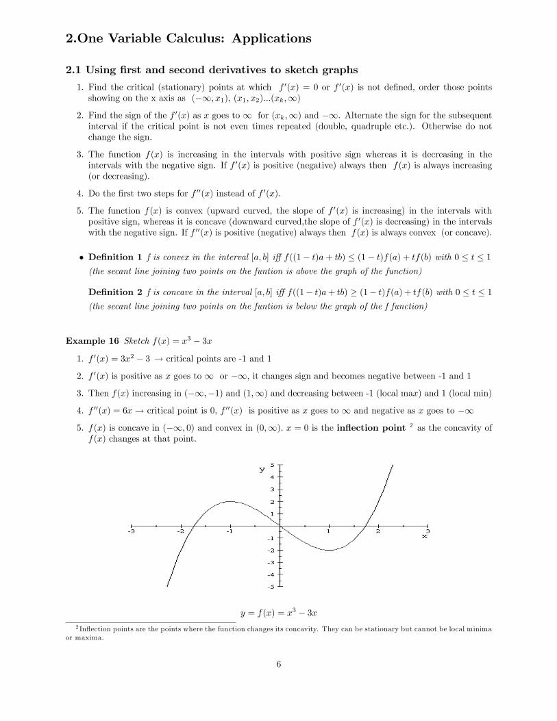
Example 16 Sketch f(x) = x3 � 3x

1. f 0(x) = 3x2 � 3 ! critical points are -1 and 1

2. f 0(x) is positive as x goes to 1 or �1, it changes sign and becomes negative between -1 and 1

3. Then f(x) increasing in (�1;�1) and (1;1) and decreasing between -1 (local max) and 1 (local min)

4. f 00(x) = 6x! critical point is 0, f 00(x) is positive as x goes to 1 and negative as x goes to �1

5. f(x) is concave in (�1; 0) and convex in (0;1): x = 0 is the in�ection point 2 as the concavity off(x) changes at that point.

y = f(x) = x3 � 3x2 In�ection points are the points where the function changes its concavity. They can be stationary but cannot be local minima

or maxima.

6

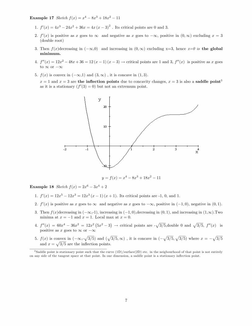
Example 17 Sketch f(x) = x4 � 8x3 + 18x2 � 11

1. f 0(x) = 4x3 � 24x2 + 36x = 4x (x� 3)2 . Its critical points are 0 and 3.

2. f 0(x) is positive as x goes to 1 and negative as x goes to �1; positive in (0;1) excluding x = 3(double root)

3. Then f(x)decreasing in (�1;0) and increasing in (0;1) excluding x=3, hence x=0 is the globalminimum.

4. f 00(x) = 12x2� 48x+36 = 12 (x� 1) (x� 3)! critical points are 1 and 3, f 00(x) is positive as x goesto 1 or �1

5. f(x) is convex in (�1;1) and (3;1) , it is concave in (1; 3):x = 1 and x = 3 are the in�ection points due to concavity changes, x = 3 is also a saddle point3

as it is a stationary (f 0(3) = 0) but not an extremum point.

y = f(x) = x4 � 8x3 + 18x2 � 11

Example 18 Sketch f(x) = 2x6 � 3x4 + 2

1. f 0(x) = 12x5 � 12x3 = 12x3 (x� 1) (x+ 1). Its critical points are -1, 0, and 1.

2. f 0(x) is positive as x goes to 1 and negative as x goes to �1; positive in (�1; 0), negative in (0; 1):

3. Then f(x)decreasing in (�1;-1), increasing in (�1; 0);decreasing in (0; 1); and increasing in (1,1):Twominima at x = �1 and x = 1. Local max at x = 0.

4. f 00(x) = 60x4 � 36x2 = 12x2�5x2 � 3

�! critical points are -

p3=5;double 0 and

p3=5, f 00(x) is

positive as x goes to 1 or �1

5. f(x) is convex in (�1;-p3=5) and (

p3=5;1) , it is concave in (�

p3=5;

p3=5) where x = �

p3=5

and x =p3=5 are the in�ection points.

3Saddle point is stationary point such that the curve (1D)/surface(2D) etc. in the neigbourhood of that point is not entirelyon any side of the tangent space at that point. In one dimension, a saddle point is a stationary in�ection point.

7

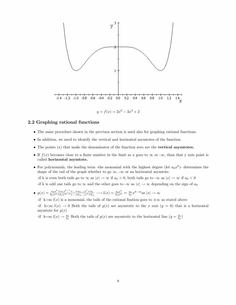
y = f(x) = 2x6 � 3x4 + 2

2.2 Graphing rational functions

� The same procedure shown in the previuos section is used also for graphing rational functions.

� In addition, we need to identify the vertical and horizontal asymtotes of the function.

� The points (x) that make the denominator of the function zero are the vertical asymtotes.

� If f(x) becomes close to a �nite number in the limit as x goes to 1 or -1; than that y axis point iscalled horizontal asymtote.

� For polynomials, the leading term -the monomial with the highest degree (let a0xk)- determines theshape of the tail of the graph whether to go 1, -1 or an horizontal asymtote.

-if k is even both tails go to 1 as jxj ! 1 if a0 > 0, both tails go to -1 as jxj ! 1 if a0 < 0

-if k is odd one tails go to 1 and the other goes to -1 as jxj ! 1 depending on the sign of a0

� g(x) = a0xk+a1x

k�1+:::+ak�1x1+ak

b0xm+b1xm�1+:::+bm�1x1+bm�! l(x) = a0x

k

b0xm= a0

b0xk�mas jxj ! 1

-if k>m l(x) is a monomial, the tails of the rational funtion goes to �1 as stated above

-if k<m l(x) ! 0 Both the tails of g(x) are asymtotic to the x axis (y = 0) that is a horizontalasymtote for g(x)

-if k=m l(x)! a0b0Both the tails of g(x) are asymtotic to the horizontal line (y = a0

b0)

8

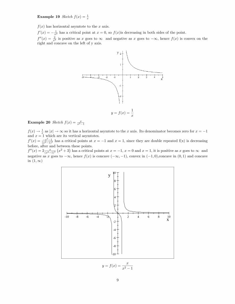
Example 19 Sketch f(x) = 1x

f(x) has horizontal asymtote to the x axis.

f 0(x) = � 1x2 has a critical point at x = 0; so f(x)is decreasing in both sides of the point.

f 00(x) = 2x3 is positive as x goes to 1 and negative as x goes to �1; hence f(x) is convex on the

right and concave on the left of y axis.

y = f(x) =1

x

Example 20 Sketch f(x) = xx2�1

f(x)! 1x as jxj ! 1 so it has a horizontal asymtote to the x axis. Its denominator becomes zero for x = �1

and x = 1 which are its vertical asymtotes.f 0(x) = �x2�1

(x2�1)2 has a critical points at x = �1 and x = 1; since they are double repeated f(x) is decreasingbefore, after and between these points.f 00(x) = 2 x

(x2�1)3�x2 + 3

�has a critical points at x = �1, x = 0 and x = 1; it is positive as x goes to1 and

negative as x goes to �1; hence f(x) is concave (�1;�1); convex in (�1; 0);concave in (0; 1) and concavein (1;1)

­10 ­8 ­6 ­4 ­2 2 4 6 8 10

­10

­8

­6

­4

­2

2

4

6

8

10

x

y

y = f(x) =x

x2 � 1

9

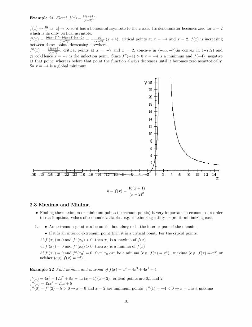
Example 21 Sketch f(x) = 16(x+1)

(x�2)2

f(x)! 16x as jxj ! 1 so it has a horizontal asymtote to the x axis. Its denominator becomes zero for x = 2

which is its only vertical asymtote.f 0(x) = 16(x�2)2�16(x+1)2(x�2)

(x�2)4 = � 16(x�2)3 (x+ 4) ; critical points at x = �4 and x = 2; f(x) is increasing

between these points decreasing elsewhere.f 00(x) = 32(x+7)

(x�2)4 , critical points at x = �7 and x = 2; concave in (�1;�7);in convex in (�7; 2) and(2;1):Hence x = �7 is the in�ection point. Since f 00(�4) > 0 x = �4 is a minimum and f(�4) negativeat that point, whereas before that point the function always decreases until it becomes zero asmytotically.So x = �4 is a global minimum.

y = f(x) =16(x+ 1)

(x� 2)2

2.3 Maxima and Minima

� Finding the maximum or minimum points (extremum points) is very important in economics in orderto reach optimal values of economic variables. e.g. maximizing utility or pro�t, minimizing cost.

1. � An extremum point can be on the boundary or in the interior part of the domain.

� If it is an interior extremum point then it is a critical point. For the crtical points:

-if f 0(x0) = 0 and f 00(x0) < 0; then x0 is a maxima of f(x)

-if f 0(x0) = 0 and f 00(x0) > 0; then x0 is a minima of f(x)

-if f 0(x0) = 0 and f 00(x0) = 0; then x0 can be a minima (e.g. f(x) = x4) , maxima (e.g. f(x) =-x4) orneither (e.g. f(x) = x3) .

Example 22 Find minima and maxima of f(x) = x4 � 4x3 + 4x2 + 4

f 0(x) = 4x3 � 12x2 + 8x = 4x (x� 1) (x� 2) ; critical points are 0,1 and 2f 00(x) = 12x2 � 24x+ 8f 00(0) = f 00(2) = 8 > 0! x = 0 and x = 2 are minimum points f 00(1) = �4 < 0! x = 1 is a maxima

10

Global Maxima and MinimaIn three cases global maximum or minumum points are found easily:

1. When the domain of f(x) is an interval in R 1 and it has only one critical point that is a local max(min) then that point is global max (min)

The proof comes from the idea that if the point were not a global max (min) then there should beanother critical point between two max (min).

2. If f is a C2 function whose domain is an interval and f 00 is never zero, then f has at most one criticalpoint that is a global min f 00(x) > 0 and a global max f 00(x) < 0

The proof: If f 00 > 0 always then f 0 is an increasing function such that it can have a value "0" onlyone time and from the previous theorem it is global min.

3. A continuous functions whose domain is a closed and bounded interval [a,b] must have a global maxand a global min (Weierstrass theorem).

In this case, we �nd critical points and evaluate the function at these points and the boundary points.The point with largest value of f is the global maximum and the point with the smallest vlue of is theglobal minimum.

Example 23 A �rm produces every book with a cost of $5. Every book is sold for $10 and each day 10 booksare sold currently. The �rm expects to sell one additional book for each dollar decrease in price. What arethe demand and pro�t functions and the price P that maximizes the pro�t?

X = mP + n , m = �1; current (X;P ) = (10; 10); substituting them in the demand equation we �ndX = 20� P then the pro�t becomes: � = (P � 5)(20� P ) = �P 2 + 25P � 100�0 = �2P + 25 ! P = 12:5 is the only critical point, �00 = �2 < 0 then P = 12:5 is the global maximumpoint that maximes the pro�t of the �rm.

2.4 APPLICATIONS TO ECONOMICS

In this section we brie�y analyse the properties of some general types of functions which are used in economicapplications and studies.

2.4.1 Production Function

� It relates the amount of output (x) to the amount of input (q) : x = f(q)

� Continuous or maybe C2

� Increasing

� There is a level of input until which the function is convex and then it is concave

2.4.2 Cost Function

� A cost funtion assigns a cost to the level of output: C(x)

� MC(x) = C 0(x) is the marginal cost that measures the additional cost incurred from the productionof one unit more when the current output is x.

� The average cost is the cost per unit produced: AC(x) = C(x)=x

� The essential properties of cost funtion:C(x) is a naturally increasing function. Moreover, Let C(x) is C1 then

-if MC>AC, AC is increasing (Doing better than average rises average)

-if MC<AC, AC is decreasing (Doing worse than average decreases average)

-at an interior minimum of AC, MC=AC

The proof comes from: AC0(x) = ddx (

C(x)x ) = C0(x)x�C(x)

x2 = C0(x)�C(x)=xx = MC�AC

x

11

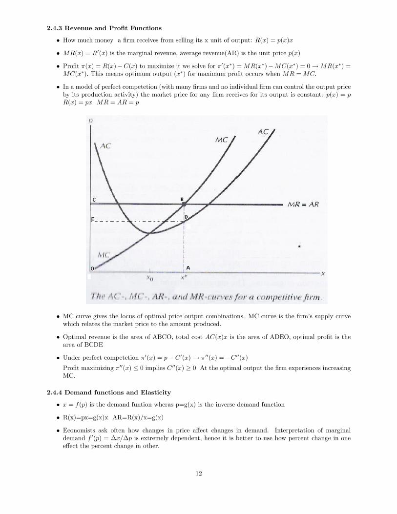
2.4.3 Revenue and Pro�t Functions

� How much money a �rm receives from selling its x unit of output: R(x) = p(x)x

� MR(x) = R0(x) is the marginal revenue, average revenue(AR) is the unit price p(x)

� Pro�t �(x) = R(x)�C(x) to maximize it we solve for �0(x�) =MR(x�)�MC(x�) = 0!MR(x�) =MC(x�): This means optimum output (x�) for maximum pro�t occurs when MR =MC:

� In a model of perfect competetion (with many �rms and no individual �rm can control the output priceby its production activity) the market price for any �rm receives for its output is constant: p(x) = pR(x) = px MR = AR = p

� MC curve gives the locus of optimal price output combinations. MC curve is the �rm�s supply curvewhich relates the market price to the amount produced.

� Optimal revenue is the area of ABCO, total cost AC(x)x is the area of ADEO, optimal pro�t is thearea of BCDE

� Under perfect competetion �0(x) = p� C 0(x) ! �00(x) = �C 00(x)Pro�t maximizing �00(x) � 0 implies C 00(x) � 0 At the optimal output the �rm experiences increasingMC.

2.4.4 Demand functions and Elasticity

� x = f(p) is the demand funtion wheras p=g(x) is the inverse demand function

� R(x)=px=g(x)x AR=R(x)/x=g(x)

� Economists ask often how changes in price a¤ect changes in demand. Interpretation of marginaldemand f 0(p) = �x=�p is extremely dependent, hence it is better to use how percent change in onee¤ect the percent change in other.

12

� Price elasticity of demand:

" =�xx�pp

=

�x�pxp

= f 0(p)p

x=f 0(p)

f(p)p

� In general as �pp "

�xx # so " is negative

� if �pp "�xx ! 0 then the good is inelastic (fuel, medical care goods)

-A good whose " 2 (�1; 0] is inelastic-A good whose " 2 (�1;�1) is elastic (luxury goods, goods with many close substitutes)-A good whose " = �1 is unit elastic

� If price of a good rises total expenditure (E(x)) of consumers4 rises if the good is inelastic and itdecreases if the good is elastic.

Proof comes from E(x) = px = pf(p)! E0(x) = pf 0(p) + 1f(p)! E0(x)f(p) =

pf 0(p)f(p) + 1 = "+ 1

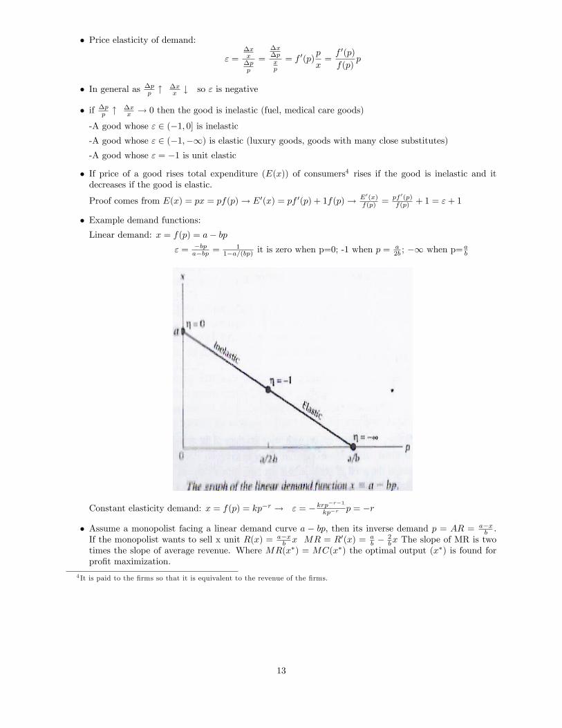
� Example demand functions:Linear demand: x = f(p) = a� bp

" = �bpa�bp =

11�a=(bp) it is zero when p=0; -1 when p =

a2b ; �1 when p=a

b

Constant elasticity demand: x = f(p) = kp�r ! " = �krp�r�1

kp�r p = �r

� Assume a monopolist facing a linear demand curve a � bp; then its inverse demand p = AR = a�xb :

If the monopolist wants to sell x unit R(x) = a�xb x MR = R0(x) = a

b �2bx The slope of MR is two

times the slope of average revenue. Where MR(x�) = MC(x�) the optimal output (x�) is found forpro�t maximization.

4 It is paid to the �rms so that it is equivalent to the revenue of the �rms.

13

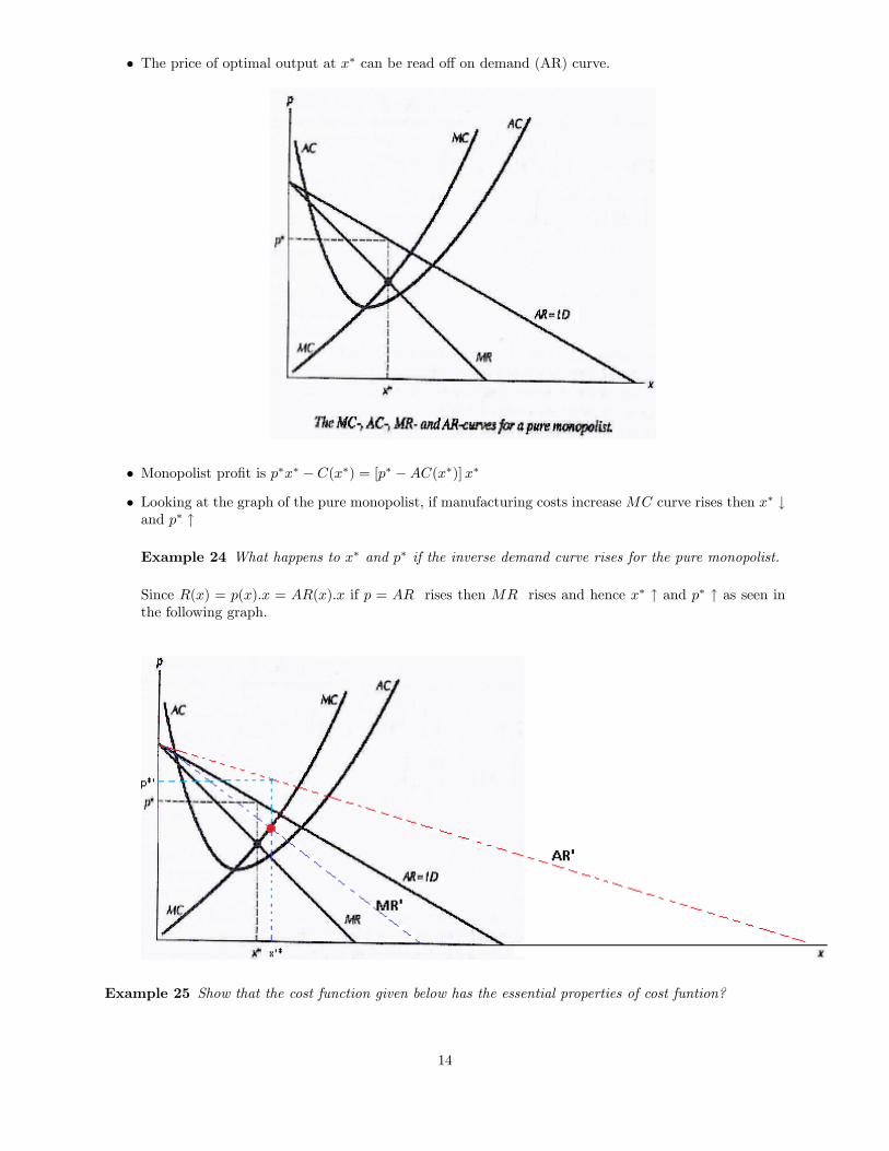
� The price of optimal output at x� can be read o¤ on demand (AR) curve.

� Monopolist pro�t is p�x� � C(x�) = [p� �AC(x�)]x�

� Looking at the graph of the pure monopolist, if manufacturing costs increaseMC curve rises then x� #and p� "

Example 24 What happens to x� and p� if the inverse demand curve rises for the pure monopolist.

Since R(x) = p(x):x = AR(x):x if p = AR rises then MR rises and hence x� " and p� " as seen inthe following graph.

Example 25 Show that the cost function given below has the essential properties of cost funtion?

14

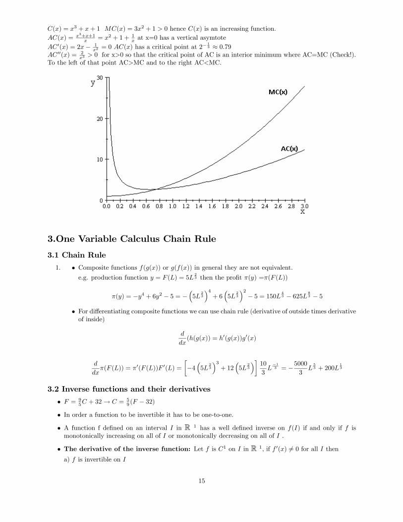
C(x) = x3 + x+ 1 MC(x) = 3x2 + 1 > 0 hence C(x) is an increasing function.AC(x) = x3+x+1

x = x2 + 1 + 1x at x=0 has a vertical asymtote

AC 0(x) = 2x� 1x2 = 0 AC(x) has a critical point at 2

� 13 � 0:79

AC 00(x) = 2x3 > 0 for x>0 so that the critical point of AC is an interior minimum where AC=MC (Check!).

To the left of that point AC>MC and to the right AC<MC.

3.One Variable Calculus Chain Rule

3.1 Chain Rule

1. � Composite functions f(g(x)) or g(f(x)) in general they are not equivalent.e.g. production function y = F (L) = 5L

23 then the pro�t �(y) =�(F (L))

�(y) = �y4 + 6y2 � 5 = ��5L

23

�4+ 6

�5L

23

�2� 5 = 150L 4

3 � 625L 83 � 5

� For di¤erentiating composite functions we can use chain rule (derivative of outside times derivativeof inside)

d

dx(h(g(x)) = h0(g(x))g0(x)

d

dx�(F (L)) = �0(F (L))F 0(L) =

��4�5L

23

�3+ 12

�5L

23

�� 103L

�13 = �5000

3L

53 + 200L

13

3.2 Inverse functions and their derivatives

� F = 95C + 32! C = 5

9 (F � 32)

� In order a function to be invertible it has to be one-to-one.

� A function f de�ned on an interval I in R 1 has a well de�ned inverse on f(I) if and only if f ismonotonically increasing on all of I or monotonically decreasing on all of I .

� The derivative of the inverse function: Let f is C1 on I in R 1, if f 0(x) 6= 0 for all I thena) f is invertible on I

15

b) its inverse g is a is C1 on f(I)

c) for all z in the domain of inverse function g (f(x) = z then g(z) = x)

g0(z) =1

f 0(g(z))

Example 26 f(x) = x�1x+1 �nd derivative of inverse at x=2

f(2) = 13 f

0(x) = 2(x+1)2

then g0(z) = 1f 0(g(z)) ! g0( 13 ) =

1f 0(2) =

92

Or directly its inverse g(y) = 1+y1�y g0(y) = 2

(1�y)2 ! g0( 13 ) =92

Example 27 f(x) = x2 + x+ 2 �nd the derivative of inverse of f(x) at f(1)

f(1) = 4 f 0(x) = 2x+ 1 f 0(1) = 3 g0(f(1)) = 1f 0(1) =

13

�Note: g(y) =

�1�p1�4(2�y)2 = �1�

p4y�72

�

4 Exponential and Logarithmic Functions

� f(t) = at where a > 0 is called an exponential function.

if t is a positive integer then t means �multiply a by itself t times�

if t=0 f(t) = 1 by de�nition

if t=1/n f(t) = npa nth root of a

if t=m/n f(t) = npam mth power of the nth root of a

if t<0 f(t) = at = 1ajtj

that is the reciprocal of ajtj

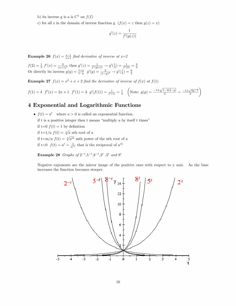
Example 28 Graphs of 2�t,5�t,8�t,2t ,5t and 8t

Negative exponents are the mirror image of the pozitive ones with respect to y axis. As the baseincreases the function becomes steeper.

16

� The number e = limn!1

�1 + 1

n

�n � 2:7If one deposits A Euro in an account which pays an annual interest rate r compounded continously,then after t years the account will grow to Aert

limn!1

�1 +

r

n

�n= lim

n!1

�1 +

1nr

�nlet

n

r= m! lim

n!1

�1 +

1

m

�rm= er

� Logarithm is the inverse of exponent. If ay = z then the power to which one must raise a toyield z is y = loga z aloga z = z loga a

z = z

� Base 10 logarithm=Log y = Logx! 10y = x Log1000 = Log103 = 3

� Base e logarithm=ln lnx = y ! ey = x

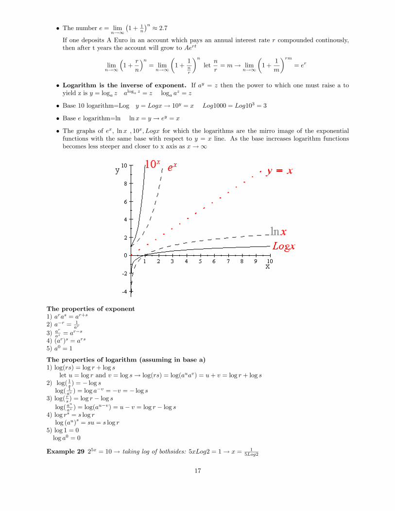
� The graphs of ex, lnx ; 10x; Logx for which the logarithms are the mirro image of the exponentialfunctions with the same base with respect to y = x line. As the base increases logarithm functionsbecomes less steeper and closer to x axis as x!1

The properties of exponent1) aras = ar+s

2) a�r = 1ar

3) ar

as = ar�s

4) (ar)s = ars

5) a0 = 1

The properties of logarithm (assuming in base a)1) log(rs) = log r + log s

let u = log r and v = log s! log(rs) = log(auav) = u+ v = log r + log s2) log(1s ) = � log slog( 1av ) = log a

�v = �v = � log s3) log( rs ) = log r � log slog(a

u

av ) = log(au�v) = u� v = log r � log s

4) log rs = s log rlog (au)

s= su = s log r

5) log 1 = 0log a0 = 0

Example 29 25x = 10! taking log of bothsides: 5xLog2 = 1! x = 15Log2

17

Example 30 How long A Euros deposited in saving account to double when annual interest rate r is com-pounded continuously?

2A = Aert ! ln 2 = rt! t = ln 2r if r is 10% knowing ln 2 � 0:69! t = 0:69

0:10 = 6:9 years

� Taking ln of nonlinear equations may induce them into linear equations (linearization)

e.g. constant electicity demand function q = kp" ! ln q = ln k + " ln p

In logarithmic coordoìinates demand is now a linear function whose slope is the elasticity "

4.1 Derivatives of exponential and logarithm:

� a) (ex)0 = ex

ddx ( limn!1

�1 + r

n

�n) = lim

n!1n�1 + r

n

�n�1 1n = lim

n!1

�1 + r

n

�n�1= lim

n!1

�1 + r

n

�nas n!1

b)(lnx)0 = 1x

(lnx)0 = limh!0

ln(x+h)�ln(x)h = lim

h!0

1h ln(

x+hx ) = lim

h!0ln(1 + h

x )1h = lim

h!0ln(1 + 1=x

1=h )1h = ln e1=x = 1=x

c) (eu(x))0 = eu(x):u0(x) obtained by chain rule

d) (ln(u(x))0 = u0(x)u(x) if u(x) > 0 obtained by chain rule

e) (bx)0 = bx: ln b

(bx)0 = (ex ln b)0 using c) (bx)0 = ex ln b: ln b = bx: ln b

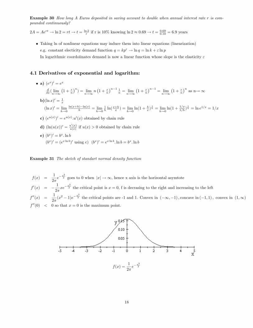
Example 31 The sketch of standart normal density function

f(x) =1

2�e�

x2

2 goes to 0 when jxj ! 1, hence x axis is the horizontal asymtote

f 0(x) = � 1

2�xe�

x2

2 the critical point is x = 0, f is decrasing to the right and increasing to the left

f 00(x) =1

2�(x2 � 1)e� x2

2 the critical points are -1 and 1. Convex in (�1;�1) ; concave in (�1; 1) ; convex in (1;1)

f 00(0) < 0 so that x = 0 is the maximum point.

f(x) =1

2�e�

x2

2

18

Example 32 The sketch of xe�x

f(x) = xe�x goes to 0 when x!1, hence + x axis is the horizontal asymtotef 0(x) = (1� x)e�x the critical point is x = 1, f is decrasing to the right and increasing to the leftf 00(x) = (x� 2)e�x the critical point is x = 2. Convex in (�1; 2) and concave in (2;1)f 00(1) < 0 so that x = 1 is the maximum point.

f(x) = xe�x

4.2 Applications

4.2.1 Present Value

If we put B Euros into a saving account with annual interest rate r which is compounded continuously, thenafter t years it becomes A = Bert:Conversely in order to generate A Euros t years from now in an accountcompunded interest rate r continuously, we would have to invest B = Ae�rt Euros that is the present value(PV) of B Euros t years from now.Annuity is a sequence of payments at regular intervals over a speci�ed period. The present value of anannuity that pays A Euros at the end of the next N years with an interest rate r of continous compounding.PV = Ae�r +Ae�2r + :::+Ae�nr = A(e�r + e�2r + :::+ e�nr) Using the property of geometric series5 :

= Ae�r(1�e�rn)

1�e�r =A(1�e�rn)

er�1

Example 33 Assuming 10% interest rate compunded continuously, what is the present value of an annuitythay pays 500 Euros a year?

a)for the next 5 years:500(1�e�0:5)

e0:1�1 = 1870: 6

b)forever: 500e0:1�1 = 4754: 2

5

X = a+ a1 + :::+ an =a(1�an)1�a (Found by subtracting X=a from X)

19

� It is sometimes covenient to compute PV of an annuity using annual compounding

PV =A

1 + r+

A

(1 + r)2 + :::+

A

(1 + r)n using again geometric series expansion

= A

11+r (1�

�11+r

�n)

1� 11+r

=A

r

�1�

�1

1 + r

�n�=

A

ras n!1

In order to generate A Euros per year from an account paying annual interest with rate r one mustdeposit inti the account Ar initially.

Example 34 Redo the previous example with annual compunding?

a)for the next 5 years: 5000:1

�1�

�11:1

�5�= 1895: 4

b)forever: 5000:1 = 5000

4.2.2 Optimal Holding Time

Suppose the market value of your real estate will be V (t) Euros t years from now. If the interest rateremains constant (r) and continuously compunded during this period then the present value of the realestate is V (t)e�rt:Maximizing the present value gives the optimal time to sell it.

�V (t)e�rt

�0= V 0(t)e�rt � rV (t)e�rt = 0

V 0(t)

V (t)= r at the optimal selling time

percent growth rate of the value of the real estate =percent rate of change of money in the bank

Logarithmic Derivative: Since the logarithm turns exponentiation to into multiplication and multiplica-tion into addition and division onto substraction, it can often simplify the computation of the derivative ofa complex function.

(ln(u(x))0=u0(x)

u(x)! u0(x) = u(x) (ln(u(x))

0

Example 35 Use logarithmic derivative to compute the derivative of

y =4px2 � 1x2 + 1

ln y =1

4ln�x2 � 1

�� ln

�x2 + 1

�y0 = y(ln y)0 =

4px2 � 1x2 + 1

:

�1

4

2x

x2 � 1 �2x

x2 + 1

�=

4px2 � 1x2 + 1

��3x3 + 5x

2(x2 � 1) (x2 + 1)

�=

�3x3 + 5x2(x2 � 1) 34 (x2 + 1)2

Example 36 Derivative of xx?

(xx)0= xx(x lnx)0 = xx(lnx+ 1)

Example 37 The value of a land is increasing according to the formula V = 2000et14 :If the interest rate is

10%, how long it should be held to max its present value?

lnV = ln 2000 + t14 ! (lnV )

0= V 0(t)

V (t) = r =14 t� 34 ! r = 0:1 then t = 3:39

20

5 Linear Algebra

In general, an equation is linear if it has the form

a1x1 + a2x2 + :::+ anxn = b

where the letters a1; a2; ::; an; b are the �xed numbers and therefore the are called parameters wherasx1; x2; :::; xn stand for the variables.As a key feature of linear equations, each term contains at most one variable and that variable can have onlythe �rst power. Linear equations are easy to handle (they build on the techniques learned in high school,such as the solution of two linear equations in two unknowns such as substitution or elimination of variablesand they build on simple geometry of the plane and the cube which are easy to visualize). These equationscan often have exact solutions unlike nonlinear systems. With suitable assumptions or linearizations theycan be good approximations of the nonlinear systems. Moreover, some of the most frequently studied modelsare linear.

5.1 Example of linear economic models

5.1.1 Tax bene�ts of charitable contributions

A �rm earns before-tax pro�ts of $100,000. It has agreed to donate 10% percent of its after-tax pro�ts toa charity fund. It must pay a state tax of 5 percent of its pro�ts (after the donation) and a federal tax of40 percent of its pro�ts (after the donation and state taxes are paid). How much does the company pay instate taxes, federal taxes, and charitable donation?

� Let S, F and C are state taxes, federal taxes, and charitable donation. After tax pro�ts are 100,000-(S+F); so C becomes C = 0:1(100; 000� (S + F ))! C + 0:1S + 0:1F = 10; 000

� S is 5% of pro�ts net of the donation then S = 0:05(100:000� C)! 0:05C + S = 5; 000

� Federal taxes are 40% the pro�t after deducting C and S! F = 0:4(100:000�C�S)! 0:4C+0:4S+F = 40; 000

In summary we get three linear equations, subsituting the second equation to the others we get two equationswith two unknowns:

C + 0:1(5000� 0:05C) + 0:1F = 10; 000

0:4C + 0:4(5000� 0:05C) + F = 40; 000

Then the solution becomse C=5956 S=4702 F=35737 and after tax&contribution pro�t is $53605

Without donation the after tax pro�ts become $57000 meaning that $5956 donation costs $3395 to the �rm.

5.1.2 Linear Model of Production

As a simpli�cation constant return to scale production is assumed that is the amount of output linearlyproportional to the amount of input. e.g. 50 cars need 50 times the input of one car.

� In an open Leontief system of economy, the production of a good i (there are n+1 goods in the economy)can be described by a set of input output coe¢ cients where aij denotes the input of good i neededto produce one unit of good j. The output of good i must be allocated between production activitiesand consumption. Good 0 is labor that is supplied by consumers so the consumption (demand) foreach good i is given exogenously (this is why it is called open system) that is not solved for in themodel. Each good i is used for producing other goods and consumption (ci). Good "0" is labor thatis supplied by consumers so its consumption c0 is negative.

xi = ai1x1 + ai2x2 + :::+ ainxn + ci

21

� Explicitly (gross output=used as input+consumption):(1� a11)x1 �a12x2 � ::::::::� a1nxn = c1�a21x1 + (1� a22)x2 � ::::::::� a2nxn = c2.................................................

�an1x1 �an2x2 � :::+ (1� ann)xn = cn�a01x1 �a02x2 � :::::::::� a0nxn = c0

5.1.3 Markov Models of Employment

� Using transition probabilities from unemployment to employment or from employment to uneployment,these models are commonly used to understand the log run employment behaviour.

� Let xt and yt are the number of employed and unemployed, q and p are the probability of employmentfor them respectively. Assuming �nding job or leaving job are independent of number of weeks worked.Then the number of employed and unemployed in the next period (say week) is given as:

xt+1 = qxt + pyt

yt+1 = (1� q)xt + (1� p)yt

� Normalizing the total number of employed and unemployed to 1, in the steady state:

x = qx+ py

y = (1� q)x+ (1� p)yx+ y = 1

� The �rst two equations are the same equations with minus sign so in fact we have two equations

(q � 1)x+ py = 0

x+ y = 1

� Then x = p1+p�q and y =

1�q1+p�q

� Using q = 0:998 and p = 0:136 (Hall,1966) for US white males in 1966x = 0:136

1+0:136�0:998 = 0:986 y = 1� x = 1:4% of white males were unemployed on average in 1966.

5.1.4 IS-LM Analysis

IS (Investments, Savings) and LM(Liquidity, Money) analysis is a linear model of a closed economy withtotal national income (Y) total national spending (Consumption, Investment and Government expenditures)

Y = C + I +G

� For IS analysis, on the consumer side spending is proportional to total income C = bY (0 < b < 1)where b is called marginal propensity to consume, while s=1-b is the marginal propensity to save.

� On the �rms side, either they invest to keep their money in the bank with an interest rate (r) soinvestment is a decreasing function of r.

I = I0 � ar

� Putting these together gives the IS schedule:

Y = bY + I0 � ar +G

22

� Or we write it assY + ar = I0 +G

� IS equation describes the real side of the economy by summarizing consumption, investment and savingdecisions.

On the other hand, the LM equation is determined by the money market equilibrium condition that moneysupply (Ms) equals money demand (Md). Md has two components: the transactions or precautionarydemand (Mdt) and the speculative demand (Mds).The transactions demand derives from the fact that mosttransactions are denominated in money. Thus, as national income rises, so does the demand for funds. Sothat Mdt = mYThe speculative demand comes from the portfolio management problem faced by an investor in the economy.The investor must decide whether to hold bonds or money. Money is more liquid but returns no interest,while bonds pay at rate r. It is usually argued that the speculative demand for money varies inversely withthe interest rate (directly with the price of bonds). The simplest such relationship is the linear one:

Mds =M0 � hr

Equating the supply to the demand:Ms = mY +M

0 � hr

Hence we can write IS-LM system of equations as:

sY + ar = I0 +G

mY � hr = Ms �M0

where the solution (Y; r) depend upon the policy parameters Ms, and G and on the behavioral parametersa; h; I0;m;M0 and s:

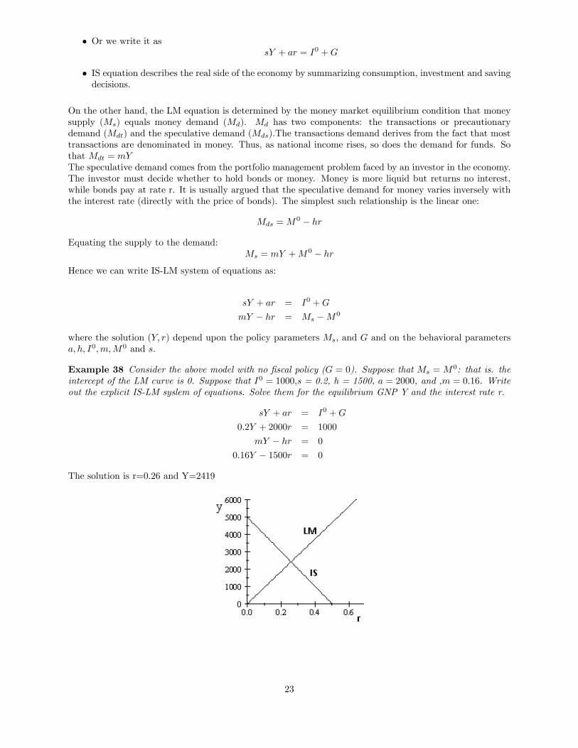
Example 38 Consider the above model with no �scal policy (G = 0). Suppose that Ms = M0: that is. the

intercept of the LM curve is 0. Suppose that I0 = 1000;s = 0.2, h = 1500, a = 2000, and ,m = 0:16. Writeout the explicit IS-LM syslem of equations. Solve them for the equilibrium GNP Y and the interest rate r.

sY + ar = I0 +G

0:2Y + 2000r = 1000

mY � hr = 0

0:16Y � 1500r = 0

The solution is r=0.26 and Y=2419

23

5.1.5 Investment and Arbitrage

For the investment decisions there will be di¤erent possible states of nature and for each of them the theportfolios give di¤ferent returns.

� If a portfolio provides same return in every state of nature it is called riskless. For A assets and Sstates this equalities of riskless (or risk-free) asset can be shown as:

AXi=1

R1ixi =AXi=1

R2ixi = ::: =AXi=1

Rsixi

where xi is the portfolio weight for asset i, Rsi is the return (future value/ current value).

� A nonzero A-tuple(x1; :::; xA) is called an arbitrage portfolio if x1 + ::: + xA = 0 instead of 1. Insuch a portfolio, the money received from the short sales is used in purchase of the long positions, sothat the portfolio costs nothing.

� A portfolio is called dupplicable if there is a di¤erent portfolio with exactly the same return in everystate.

AXi=1

Rsixi =AXi=1

Rsiwi for each s=1,...S

� A state s* is called insurable if there is a portfolio (x1;x2;:::xA) which has a positive return if states* occurs and zero return if any other state occurs:

AXi=1

Rs�ixi > 0

AXi=1

Rsixi = 0 for all s 6= s�

� It is sometimes convenient to assign a price to each of the s states of nature, then the state returnrelations can be written as:

p1R11 + p2R21 + ::::+ psRs1 = 1

p1R12 + p2R22 + ::::+ psRs2 = 1

:

:

:

p1R1A + p2R2A + ::::+ psRsA = 1

Example 39

Suppose that there are two assets and three possible states. If state 1 occurs, asset 1 returns R11 = 1and asset 2 returns R12 = 3. If state 2 occurs, R21 = 2 and R22 = 2. If state 3 occurs, R31 = 3 andR32 = 1. If both assets have the same current value and if the investor buys n1 = 3 shares of asset 1and n2 = 1 share of asset 2, the corresponding portfolio is ( 34 ;

14 ) and the returns are:

R113

4+R12

1

4=

3

2in state 1

R213

4+R22

1

4= 2 in state 2

R313

4+R32

1

4=

5

2in state 3

Note that portfolio ( 12 ;12 ) yields a return of 2 in all three states, hence it is a risk-free portfolio.

24

5.2 Systems of Linear Equations

There are essentially three ways of solving systems of linear equations: substitution,elimination of variables,andmatrix methods.

5.2.1 Substitution and elimination of variables methods

� Substitution is simply made by writing one variable in terms of other(s) using an equation andsubstituting this relation into the other equation(s).

Example 40 An example for linear production model (look section 5.1.2 for detail) of 3 goods (x1; x2; x3)given their production input-output proportions and exogenous consumption amounts (130,74,95) canbe written as:

x1 = 0x1 + 0:4x2 + 0:3x3 + 130! x1 � 0:4x2 � 0:3x3 = 130x2 = 0:2x1 + 0:12x2 + 0:14x3 + 74! �0:2x1 + 0:88x2 � 0:14x3 = 74x3 = 0:5x1 + 0:2x2 + 0:05x3 + 95! �0:5x1 � 0:2x2 + 0:95x3 = 95

substituting x1 = 0:4x2 + 0:3x3 + 130 into the other equations :

�0:2 (0:4x2 + 0:3x3 + 130) + 0:88x2 � 0:14x3 = 74

�0:5 (0:4x2 + 0:3x3 + 130)� 0:2x2 + 0:95x3 = 95

Simplifying them we get:

0:8x2 � 0:2x3 = 100

�0:4x2 + 0:8x3 = 160

substituting x2 = 100+0:2x30:8 = 125 + 0:25x3 into the other equation :

�0:4 (125 + 0:25x3) + 0:8x3 = 160

x3 = 300

x2 =100 + 0:2x3

0:8= 200

x1 = 0:4x2 + 0:3x3 + 130 = 300

� Elimination of variables is generally more conducive to the theoretical analysis. It is done bymultiplying equations and adding them up such that eliminating unknown(s) to solve the equationwith less unknowns. This is called Gauss elimination.

Example 41 We do the previous example with elimination of variables. Multiplying the �rst one by 0.2 andadding it to second to eliminate x1 ; multiplying the �rst one by 0.5 and adding it to the third to eliminatex1:

0:2(x1 � 0:4x2 � 0:3x3) = 0:2 � 130+ �0:2x1 + 0:88x2 � 0:14x3 = 74

0:8x2 � 0:2x3 = 100

0:5 (x1 � 0:4x2 � 0:3x3) = 0:5 � 130+ �0:5x1 � 0:2x2 + 0:95x3 = 95

�0:4x2 + 0:8x3 = 160 Then multiplying the above found by 0.5 and adding it to the this:

25

0.5(0:8x2 � 0:2x3) = 0:5 � 100+ �0:4x2 + 0:8x3 = 160

0:7x3 = 210means our system transforms into

x1 � 0:4x2 � 0:3x3 = 130

0:8x2 � 0:2x3 = 100

0:7x3 = 210

x3 = 300 by back subtitution into the others we �nd x2 = 200 and x1 = 300

As variant of Gauss elimination, the �rst nonzero coe¢ cient is transformed to 1 instead of back subtitution6

x1 � 0:4x2 � 0:3x3 = 130

x2 � 0:25x3 = 125

x3 = 300

Then adding to the second equation 0.25 times the third we �nd x2 = 200; then adding 0.3 times the thirdand 0.4 times the second to the �rst equation we �nd x1 = 300:

6. Matrix Algebra

� We can write a linear system of equations in matrix form.266664a11 : : : a1n: :: aij :: :ak1 : : : akn

377775.266664x1:::xn

377775 =266664b1:::bk

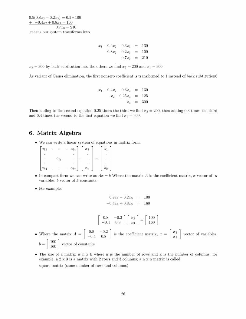
377775� In compact form we can write as Ax = b Where the matrix A is the coe¢ cient matrix, x vector of nvariables, b vector of k constants.

� For example:

0:8x2 � 0:2x3 = 100

�0:4x2 + 0:8x3 = 160

�0:8 �0:2�0:4 0:8

� �x2x3

�=

�100160

�

� Where the matrix A =

�0:8 �0:2�0:4 0:8

�is the coe¢ cient matrix, x =

�x2x3

�vector of variables,

b =

�100160

�vector of constants

� The size of a matrix is n x k where n is the number of rows and k is the number of columns; forexample, a 2 x 3 is a matrix with 2 rows and 3 columns; a n x n matrix is called

square matrix (same number of rows and columns)

26

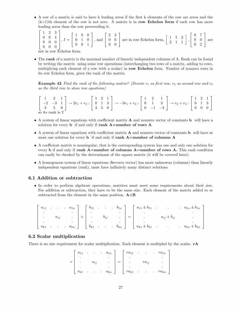
� A row of a matrix is said to have k leading zeros if the �rst k elements of the row are zeros and the(k+1)th element of the row is not zero. A matrix is in row Echelon form if each row has moreleading zeros than the row preceeeding it.26641 2 30 0 40 0 00 0 0

3775, I =24 1 0 00 1 00 0 1

35 ; and24 2 30 60 0

35 are in row Echelon form, � 1 5 22 1 1

�,

24 0 79 00 2

35 arenot in row Echelon form.

� The rank of a matrix is the maximal number of linearly independent columns of A. Rank can be foundby writing the matrix using some row operations (interchanging two rows of a matrix, adding to rows,multiplying each element of a row with a scalar) in row Echelon form. Number of nonzero rows inits row Echelon form, gives the rank of the matrix.

Example 42 Find the rank of the following matrix? (Denote r1 as �rst row, r2 as second row and r3as the third row to show row opeations)24 1 2 1�2 �3 13 5 0

35! 2r1 + r2 :

24 1 2 10 1 33 5 0

35! �3r1 + r3 :24 1 2 10 1 30 �1 �3

35! r2 + r3 :

24 1 2 10 1 30 0 0

35so its rank is 2

� A system of linear equations with coe¢ cient matrix A and nonzero vector of constants b will have asolution for every b if and only if rank A=number of rows A

� A system of linear equations with coe¢ cient matrix A and nonzero vector of constants b will have atmost one solution for every b if and only if rank A=number of columns A

� A coe¢ cient matrix is nonsingular, that is the corresponding system has one and only one solution forevery b if and only if rank A=number of columns A=number of rows A. This rank conditioncan easily be checked by the determinant of the square matrix (it will be covered later).

� A homogenous system of linear equations (b=zero vector) has more unknowns (columns) than linearlyindependent equations (rank), must have ini�nitely many distinct solutions.

6.1 Addition or subtraction

� In order to perform algebraic operations, matrices must meet some requirements about their size.For addition or subtraction, they have to be the same size. Each element of the matrix added to orsubtracted from the element in the same position. A�B

266664a11 : : : a1n: :: aij :: :ak1 : : : akn

377775�266664b11 : : : b1n: :: bij :: :bk1 : : : bkn

377775 =266664a11 � b11 : : : a1n � b1n

: :: aij � bij :: :

ak1 � bk1 : : : akn � bkn

3777756.2 Scalar multiplication

There is no size requirement for scalar multiplication. Each element is multipled by the scalar. rA

r

266664a11 : : : a1n: :: aij :: :ak1 : : : akn

377775 =266664ra11 : : : ra1n: :: raij :: :

rak1 : : : rakn

377775

27

6.3 Matrix multiplication

� We can de�ne the matrix product AB if and only if

number of columns of A=number of rows of B

� If A is k x m matrix and B is m x n matrix AB becomes k x n :

(kxm) (mxn) = (kxn)

� IA = A where I = (kxk) Identity matrix (with all ones on the diagonal and other terms 0)

� To obtain the (i,j)th entry of AB, multiply the ith row of A and the jth column of B as the following:

�ai1 ai2 : : : aim

�26666664b1jb2j

bmj

37777775 = ai1b1j + ai2b2j + :::+ aimbmj

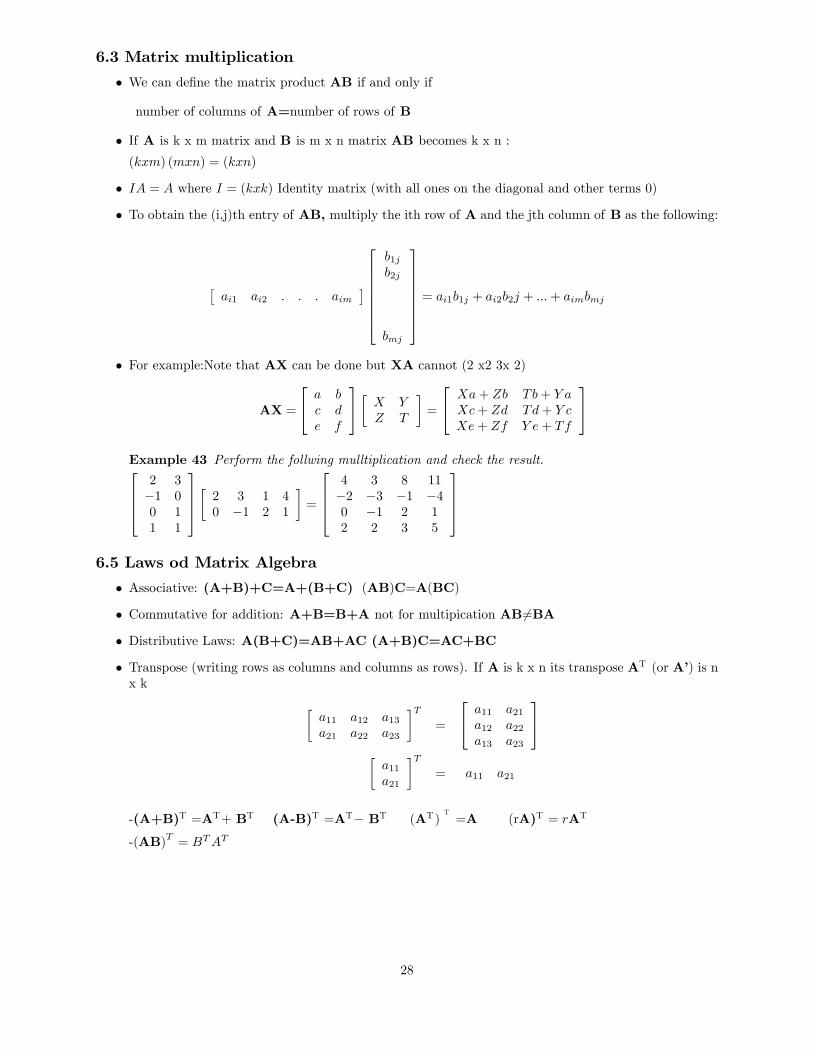
� For example:Note that AX can be done but XA cannot (2 x2 3x 2)

AX =

24 a bc de f

35� X YZ T

�=

24 Xa+ Zb Tb+ Y aXc+ Zd Td+ Y cXe+ Zf Y e+ Tf

35Example 43 Perform the follwing mulltiplication and check the result.2664

2 3�1 00 11 1

3775� 2 3 1 40 �1 2 1

�=

26644 3 8 11�2 �3 �1 �40 �1 2 12 2 3 5

37756.5 Laws od Matrix Algebra

� Associative: (A+B)+C=A+(B+C) (AB)C=A(BC)

� Commutative for addition: A+B=B+A not for multipication AB 6=BA

� Distributive Laws: A(B+C)=AB+AC (A+B)C=AC+BC

� Transpose (writing rows as columns and columns as rows). If A is k x n its transpose AT (or A�) is nx k �

a11 a12 a13a21 a22 a23

�T=

24 a11 a21a12 a22a13 a23

35�a11a21

�T= a11 a21

-(A+B)T =AT+ BT (A-B)T =AT� BT (AT)T=A (rA)T = rAT

-(AB)T = BTAT

28

6.6 Special Kinds of Matrices

A k x n matrix is a

� Square matrix if k=n that is equal number of rows and columns

� Column matrix if n=1

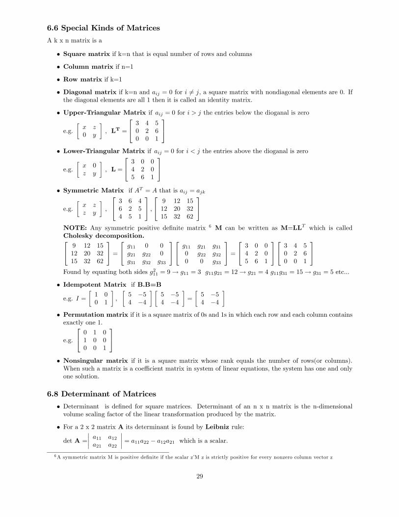
� Row matrix if k=1

� Diagonal matrix if k=n and aij = 0 for i 6= j, a square matrix with nondiagonal elements are 0. Ifthe diagonal elements are all 1 then it is called an identity matrix.

� Upper-Triangular Matrix if aij = 0 for i > j the entries below the dioganal is zero

e.g.�x z0 y

�, LT =

24 3 4 50 2 60 0 1

35� Lower-Triangular Matrix if aij = 0 for i < j the entries above the dioganal is zero

e.g.�x 0z y

�, L =

24 3 0 04 2 05 6 1

35� Symmetric Matrix if AT = A that is aij = ajk

e.g.�x zz y

�,

24 3 6 46 2 54 5 1

35 ;24 9 12 1512 20 3215 32 62

35NOTE: Any symmetric positive de�nite matrix 6 M can be written as M=LLT which is calledCholesky decomposition.24 9 12 1512 20 3215 32 62

35 =24 g11 0 0g21 g22 0g31 g32 g33

3524 g11 g21 g310 g22 g320 0 g33

35 =24 3 0 04 2 05 6 1

3524 3 4 50 2 60 0 1

35Found by equating both sides g211 = 9! g11 = 3 g11g21 = 12! g21 = 4 g11g31 = 15! g31 = 5 etc...

� Idempotent Matrix if B.B=B

e.g. I =�1 00 1

�;

�5 �54 �4

� �5 �54 �4

�=

�5 �54 �4

�� Permutation matrix if it is a square matrix of 0s and 1s in which each row and each column containsexactly one 1.

e.g.

24 0 1 01 0 00 0 1

35� Nonsingular matrix if it is a square matrix whose rank equals the number of rows(or columns).When such a matrix is a coe¢ cient matrix in system of linear equations, the system has one and onlyone solution.

6.8 Determinant of Matrices

� Determinant is de�ned for square matrices. Determinant of an n x n matrix is the n-dimensionalvolume scaling factor of the linear transformation produced by the matrix.

� For a 2 x 2 matrix A its determinant is found by Leibniz rule:

det A =

���� a11 a12a21 a22

���� = a11a22 � a12a21 which is a scalar.

6A symmetric matrix M is positive de�nite if the scalar z�M z is strictly positive for every nonzero column vector z

29

� For the determinant of 3 x 3, 4x 4 or higher size matrix, again Leibniz rule is used (multiplying theelements of a selected row or column aij with (�1)i+j times the ijth cofactor Cij (determinant of thesubmatrix obtained by deleting row i and column j from A) and adding them up).��������

a11 a12 a13 a14a21 a22 a23 a24a31 a32 a33 a34a41 a42 a43 a44

�������� = a11������a22 a23 a24a32 a33 a34a42 a43 a44

�������a12������a21 a23 a24a31 a33 a34a41 a43 a44

������+a13������a21 a22 a24a31 a32 a34a41 a42 a44

�������a14������a21 a22 a23a31 a32 a33a41 a42 a43

������Note: signs come from the (�1)i+j where ij is the position of the �rst multiplicative terms (11; 12; 13; 14)for the above������a22 a23 a24a32 a33 a34a42 a43 a44

������ = a22(�1)1+1���� a33 a34a43 a44

����+ a23(�1)1+2 ���� a32 a34a42 a44

����+ a24(�1)1+3 ���� a32 a33a42 a43

����= a22a33a44 � a22a34a43 � a23a32a44 + a23a42a34 + a32a24a43 � a24a33a42

Doing for all 3 x 3 matrices and substituting the results the 4 x 4 expansion we �nd the determinant.

Example 44 Find the the following determinant of matrix using di¤ferent row or columns for the �rstmultiplicative terms?������6 �2 2�2 5 02 0 7

������ = 6���� 5 00 7

����+ 2 ���� �2 02 7

����+ 2 ���� �2 52 0

���� = 6 � 35� 2 � 14� 2 � 10 = 162or������6 �2 2�2 5 02 0 7

������ = 2���� �2 25 0

����+ 7 ���� 6 �2�2 5

���� = �2 � 10 + 7 � 26 = 162or������6 �2 2�2 5 02 0 7

������ = 2���� �2 52 0

����+7 ���� 6 �2�2 5

���� = �2 � 10 + 7 � 26 = 162� det(AT )=detA , det(AB)=(detA)(detB) but det(A+B)6=(detA)+(detB) in general

� A square matrix is nonsingular if and only if its determinant is nonzero.

6.7 Inverse of Matrices

� For a linear system of equations Ax = b we want to �nd the vector of unknown variables as x = A�1b,hence we need to �nd the inverse of the coee¢ ent matrix (A�1) to solve the linear system easily withmatrix method.

� The inverse of a matrix, A�1 exists only if the matrix is a square matrix. Not every square matrix hasan inverse. If it has an inverse the matrix is called nonsingular, otherwise it is called singular.

� For a nonsingular matrix nxn matrix A, AA�1 = I identity matrix

� For any nxn matrix A, let Cij denote the ijth cofactor of A,that is, (�1)i+j times the determinant ofthe submatrix obtained by deleting row i and column j from A. The transpose of the cofactor matrixis called the adjoint of A. Then the inverse is found as:

A�1 =1

detAadjA

30

Example 45 Find the inverse of the following matrix A.

A =

24 1 �1 12 �1 21 2 3

35! C11 =

���� �1 22 3

���� = �7 C12 = ����� 2 21 3

���� = �4 C13 =

���� 2 �11 2

���� = 5detA = �7 � 1� 4 � �1 + 5 � 1 = 2

C21 = ����� �1 12 3

���� = 5 C22 = +

���� 1 11 3

���� = 2 C23 = ����� 1 �11 2

���� = �3C31 =

���� �1 1�1 2

���� = �1 C32 = ����� 1 12 2

���� = 0 C33 =

���� 1 �12 �1

���� = 1

ThenC =

24 �7 �4 55 2 �3�1 0 1

35! adjA = CT =

24 �7 5 �1�4 2 05 �3 1

35! A�1 = 1detAadjA =

12

24 �7 5 �1�4 2 05 �3 1

35� 2x2 case is the most known case which is also derived from the Leibniz rule

A =

�a bc d

�! C =

�d �c�b a

�! A�1 =

1

detAadjA =

1

ad� bc

�d �b�c a

�

6.8 Eigen Values and Eigen Vectors of a Matrix

An eigenvector or characteristic vector of a linear transformation is a non-zero vector that changes by onlya scalar factor when that linear transformation is applied to it.Eigen values and vectors are very useful inmany applications such as solving di¤erence equations and studying stationary points higher dimensionalfunctions.� is an eigen value for an nxn matrix A if and only if there is a vector v 6= 0 and

Av = �v

Then the vector v is called the eigen vector of the matrix A.

Eigen values of a matrix is found by Av � �v = (A��I) v = 0 where I is the identity matrix.So we want want for v 6= 0 (A��I) v = 0 that means also jA��Ij = 0; from this determinant we �nd thecharacteristic polynomial of the matrix P (�) whose roots gives the eigen values of the matrix. Substitutingeach eigen value to Av = �v we �nd the eigen vectors of the matrix for each eigen value.

Example 46 Find the eigen values and the eigen vectors of the following matrix A.

A =

24 3 2 0�1 0 00 0 1

35

jA��Ij =

������3� � 2 0�1 0� � 00 0 1� �

������ = (1� �) (�1)3+3���� 3� � 2�1 0� �

���� = 0= (1� �) (�� (3� �) + 2) = (1� �)

��2 � 3�+ 2

�= (1� �)2 (2� �) = 0

Hence the eigen values are �1= 1 and �2= 2: Lets use as a general corresponding eigen vector

24 xyz

35

31

for �1 = 1!

24 3 2 0�1 0 00 0 1

3524 xyz

35 = 1 �24 xyz

353x+ 2y = x! y = �x�x = y

z = z24 xyz

35 =

24 �yyz

35 = y24 �11

0

35+ z24 001

35if y = 0 z = 1 v1 =

24 001

35 ; if y = 1 z = 0 v2 =24 �11

0

35

for �1 = 2!

24 3 2 0�1 0 00 0 1

3524 xyz

35 = 2 �24 xyz

353x+ 2y = 2x! x = �2y�x = 2y

z = 2z ! z = 024 xyz

35 =

24 �2yy0

35 = y24 �21

0

35if y = 1 v3 =

24 �210

357 Functions of Several Variables

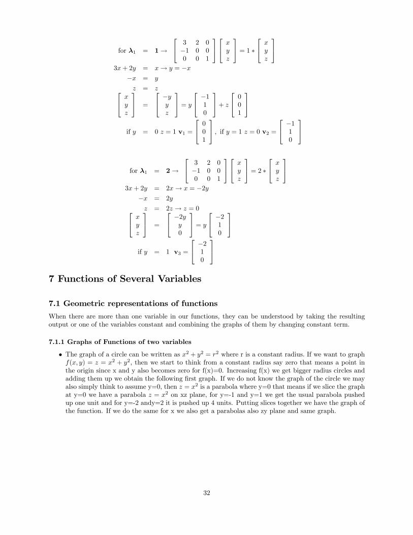
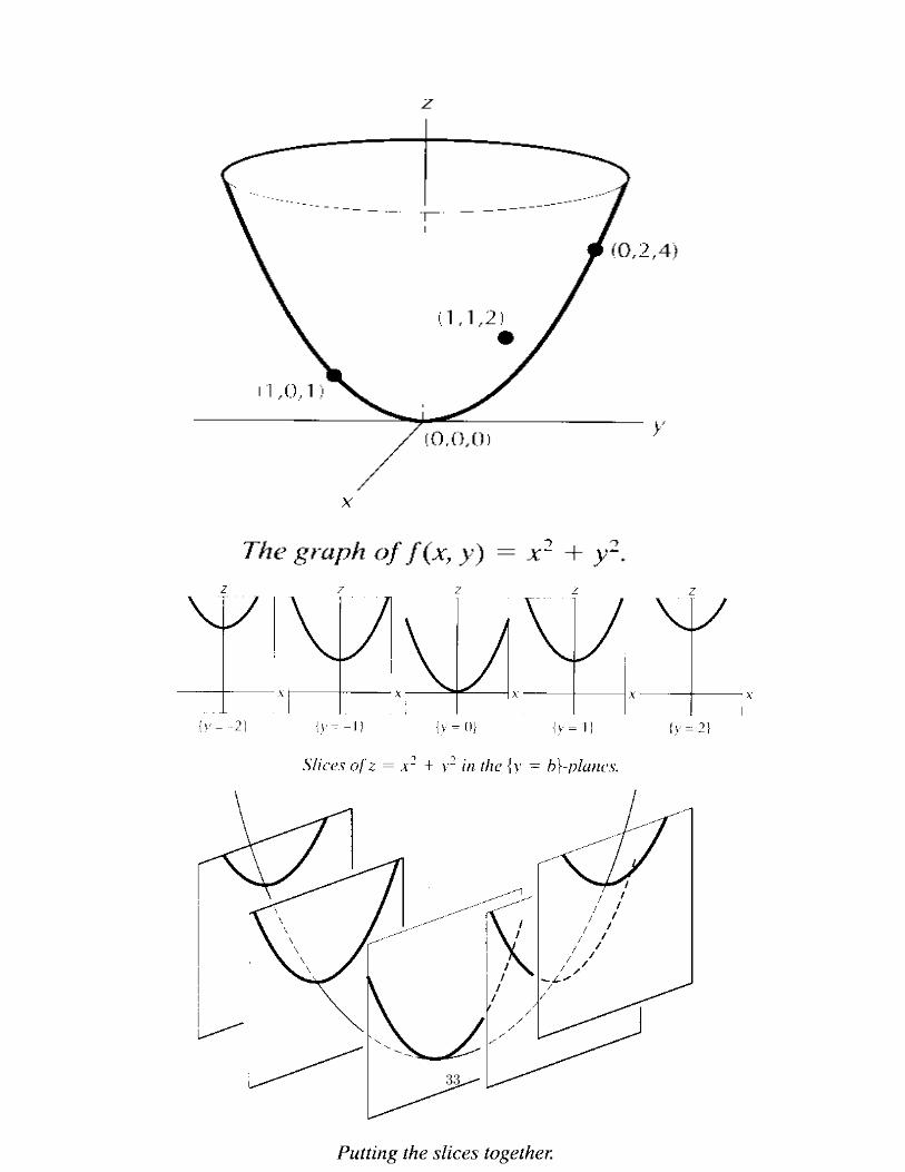
7.1 Geometric representations of functions

When there are more than one variable in our functions, they can be understood by taking the resultingoutput or one of the variables constant and combining the graphs of them by changing constant term.

7.1.1 Graphs of Functions of two variables

� The graph of a circle can be written as x2 + y2 = r2 where r is a constant radius: If we want to graphf(x; y) = z = x2 + y2; then we start to think from a constant radius say zero that means a point inthe origin since x and y also becomes zero for f(x)=0. Increasing f(x) we get bigger radius circles andadding them up we obtain the following �rst graph. If we do not know the graph of the circle we mayalso simply think to assume y=0, then z = x2 is a parabola where y=0 that means if we slice the graphat y=0 we have a parabola z = x2 on xz plane, for y=-1 and y=1 we get the usual parabola pushedup one unit and for y=-2 andy=2 it is pushed up 4 units. Putting slices together we have the graph ofthe function. If we do the same for x we also get a parabolas also zy plane and same graph.

32

33

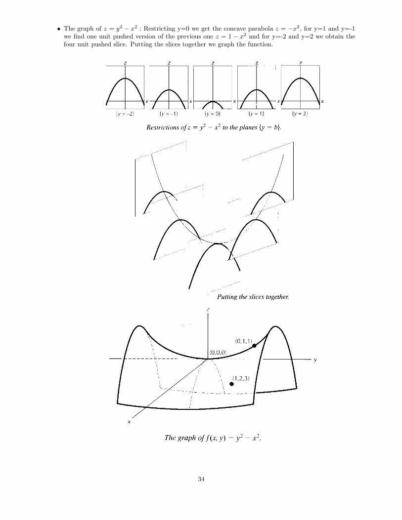
� The graph of z = y2 � x2 : Restricting y=0 we get the concave parabola z = �x2; for y=1 and y=-1we �nd one unit pushed version of the previous one z = 1 � x2 and for y=-2 and y=2 we obtain thefour unit pushed slice. Putting the slices together we graph the function.

34

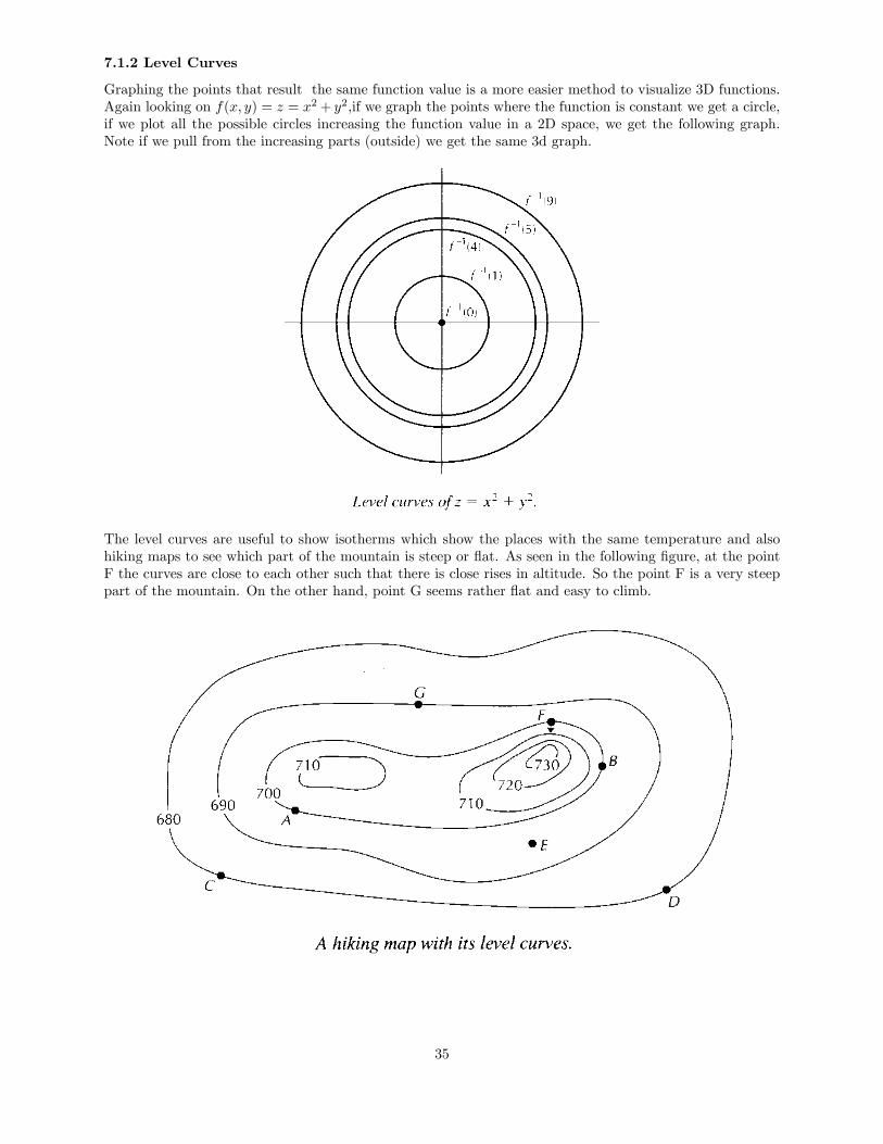
7.1.2 Level Curves

Graphing the points that result the same function value is a more easier method to visualize 3D functions.Again looking on f(x; y) = z = x2+ y2;if we graph the points where the function is constant we get a circle,if we plot all the possible circles increasing the function value in a 2D space, we get the following graph.Note if we pull from the increasing parts (outside) we get the same 3d graph.

The level curves are useful to show isotherms which show the places with the same temperature and alsohiking maps to see which part of the mountain is steep or �at. As seen in the following �gure, at the pointF the curves are close to each other such that there is close rises in altitude. So the point F is a very steeppart of the mountain. On the other hand, point G seems rather �at and easy to climb.

35

7.1.3 Planar level sets in Economics

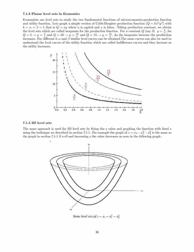
Economists use level sets to study the two fundemental functions of microeconomics-production functionand utility function. Lets graph a simple version of Cobb-Dougless production function (Q = kx�y�) withk = � = � = 1 that is Q = xy where x is capital and y is labor. Taking production constant, we obtainthe level sets which are called isoquants for the production function. For a constant Q (say 3) y = 3

x ; forQ = 5 ! y = 5

x and Q = 10 ! y = 10x and Q = 15 ! y = 15

x : As the isoquants increase the productionincreases. For di¤erent k; � and � similar level curves can be obtained.The same curves can also be used tounderstand the level curves of the utility function which are called indi¤erence curves and they increase asthe utility increases.

7.1.4 3D level sets

The same approach is used for 3D level sets by �xing the z value and graphing the function with �xed zusing the technique we described in section 7.1.1. For example the graph of z = x3 � x21 � x22 is the same asthe graph in section 7.1.1 if z=0 and increasing z the value decreases as seen in the following graph.

36

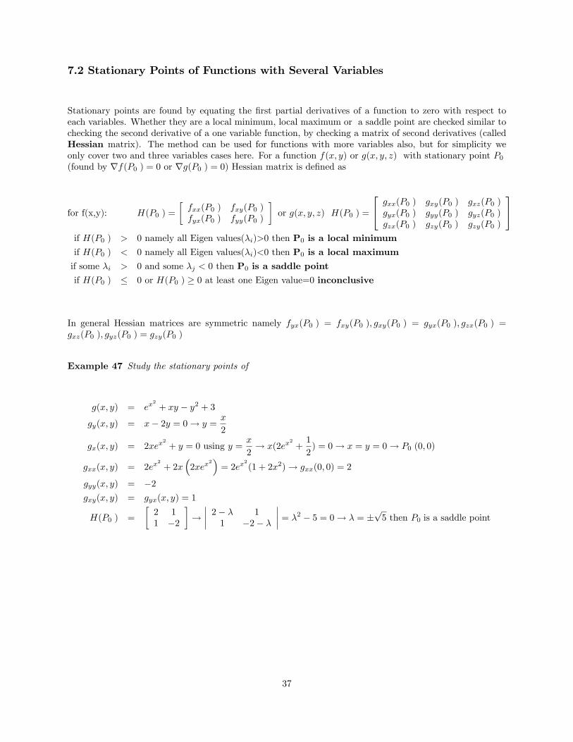
7.2 Stationary Points of Functions with Several Variables

Stationary points are found by equating the �rst partial derivatives of a function to zero with respect toeach variables. Whether they are a local minimum, local maximum or a saddle point are checked similar tochecking the second derivative of a one variable function, by checking a matrix of second derivatives (calledHessian matrix). The method can be used for functions with more variables also, but for simplicity weonly cover two and three variables cases here. For a function f(x; y) or g(x; y; z) with stationary point P0(found by rf(P0 ) = 0 or rg(P0 ) = 0) Hessian matrix is de�ned as

for f(x,y): H(P0 ) =

�fxx(P0 ) fxy(P0 )fyx(P0 ) fyy(P0 )

�or g(x; y; z) H(P0 ) =

24 gxx(P0 ) gxy(P0 ) gxz(P0 )gyx(P0 ) gyy(P0 ) gyz(P0 )gzx(P0 ) gzy(P0 ) gzy(P0 )

35if H(P0 ) > 0 namely all Eigen values(�i)>0 then P0 is a local minimumif H(P0 ) < 0 namely all Eigen values(�i)<0 then P0 is a local maximumif some �i > 0 and some �j < 0 then P0 is a saddle pointif H(P0 ) � 0 or H(P0 ) � 0 at least one Eigen value=0 inconclusive

In general Hessian matrices are symmetric namely fyx(P0 ) = fxy(P0 ); gxy(P0 ) = gyx(P0 ); gzx(P0 ) =gxz(P0 ); gyz(P0 ) = gzy(P0 )

Example 47 Study the stationary points of

g(x; y) = ex2

+ xy � y2 + 3gy(x; y) = x� 2y = 0! y =

x

2

gx(x; y) = 2xex2

+ y = 0 using y =x

2! x(2ex

2

+1

2) = 0! x = y = 0! P0 (0; 0)

gxx(x; y) = 2ex2

+ 2x�2xex

2�= 2ex

2

(1 + 2x2)! gxx(0; 0) = 2

gyy(x; y) = �2gxy(x; y) = gyx(x; y) = 1

H(P0 ) =

�2 11 �2

�!���� 2� � 1

1 �2� �

���� = �2 � 5 = 0! � = �p5 then P0 is a saddle point

37

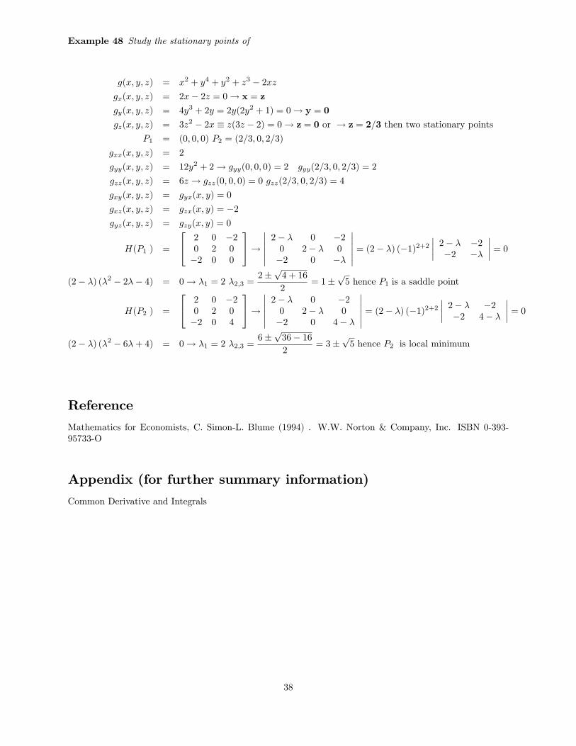
Example 48 Study the stationary points of

g(x; y; z) = x2 + y4 + y2 + z3 � 2xzgx(x; y; z) = 2x� 2z = 0! x = z

gy(x; y; z) = 4y3 + 2y = 2y(2y2 + 1) = 0! y = 0

gz(x; y; z) = 3z2 � 2x � z(3z � 2) = 0! z = 0 or ! z = 2=3 then two stationary points

P1 = (0; 0; 0) P2 = (2=3; 0; 2=3)

gxx(x; y; z) = 2

gyy(x; y; z) = 12y2 + 2! gyy(0; 0; 0) = 2 gyy(2=3; 0; 2=3) = 2

gzz(x; y; z) = 6z ! gzz(0; 0; 0) = 0 gzz(2=3; 0; 2=3) = 4

gxy(x; y; z) = gyx(x; y) = 0

gxz(x; y; z) = gzx(x; y) = �2gyz(x; y; z) = gzy(x; y) = 0

H(P1 ) =

24 2 0 �20 2 0�2 0 0

35!������2� � 0 �20 2� � 0�2 0 ��

������ = (2� �) (�1)2+2���� 2� � �2�2 ��

���� = 0(2� �) (�2 � 2�� 4) = 0! �1 = 2 �2;3 =

2�p4 + 16

2= 1�

p5 hence P1 is a saddle point

H(P2 ) =

24 2 0 �20 2 0�2 0 4

35!������2� � 0 �20 2� � 0�2 0 4� �

������ = (2� �) (�1)2+2���� 2� � �2�2 4� �

���� = 0(2� �) (�2 � 6�+ 4) = 0! �1 = 2 �2;3 =

6�p36� 162

= 3�p5 hence P2 is local minimum

Reference

Mathematics for Economists, C. Simon-L. Blume (1994) . W.W. Norton & Company, Inc. ISBN 0-393-95733-O

Appendix (for further summary information)

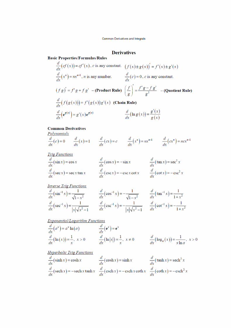
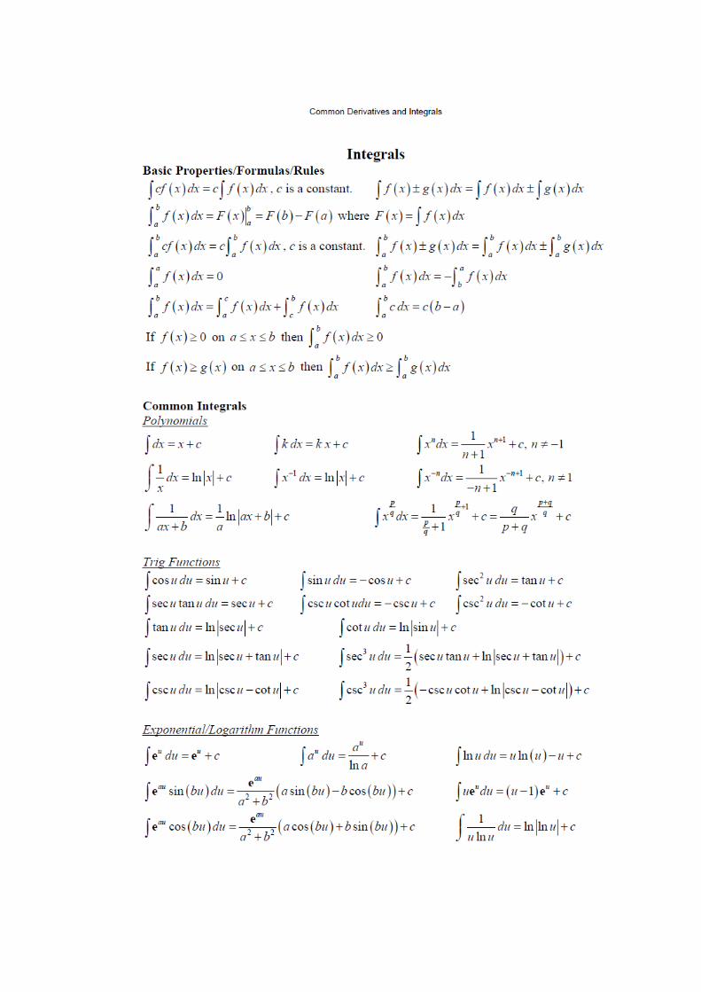
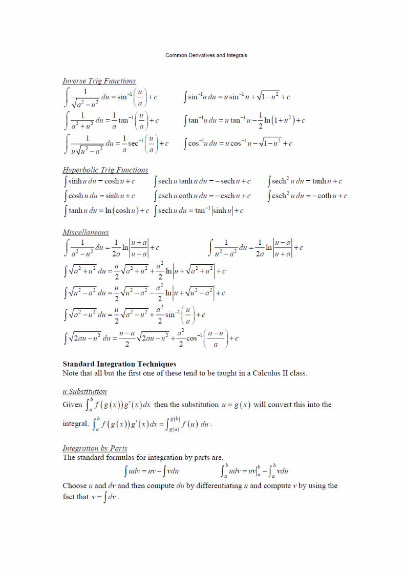
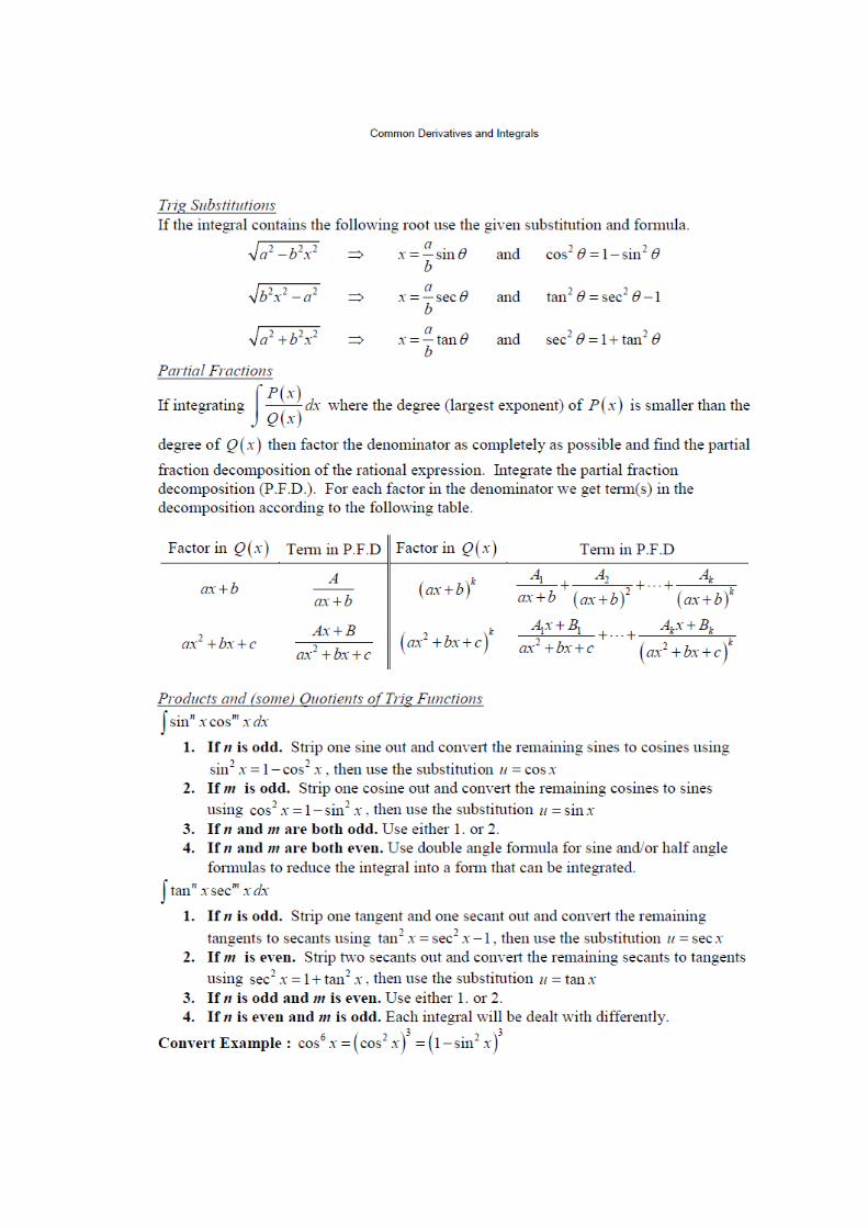
Common Derivative and Integrals

38