10a. Markov Chain Monte Carlo · Prof. Daniel Cremers 10a. Markov Chain Monte Carlo. Dr. Rudolph...
44
Computer Vision Group Prof. Daniel Cremers 10a. Markov Chain Monte Carlo
Transcript of 10a. Markov Chain Monte Carlo · Prof. Daniel Cremers 10a. Markov Chain Monte Carlo. Dr. Rudolph...

Computer Vision Group Prof. Daniel Cremers
10a. Markov Chain Monte Carlo
Dr. Rudolph TriebelComputer Vision Group
Machine Learning for Computer Vision
Markov Chain Monte Carlo
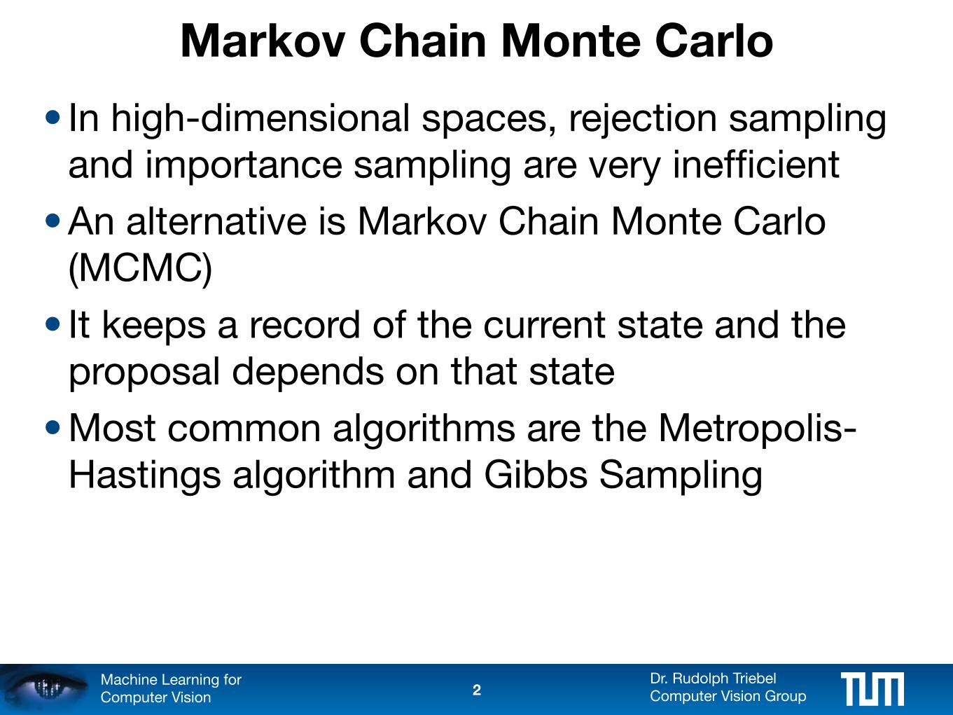
• In high-dimensional spaces, rejection sampling and importance sampling are very inefficient
• An alternative is Markov Chain Monte Carlo (MCMC)
• It keeps a record of the current state and the proposal depends on that state
• Most common algorithms are the Metropolis-Hastings algorithm and Gibbs Sampling
2
Dr. Rudolph TriebelComputer Vision Group
Machine Learning for Computer Vision
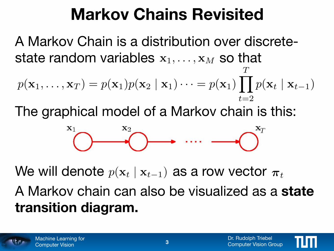
Markov Chains Revisited
A Markov Chain is a distribution over discrete-state random variables so that
The graphical model of a Markov chain is this:
We will denote as a row vector
A Markov chain can also be visualized as a state transition diagram.
3
x1, . . . ,xM
p(x1, . . . ,xT ) = p(x1)p(x2 | x1) · · · = p(x1)TY
t=2
p(xt | xt�1)
p(xt | xt�1) ⇡t
T
Dr. Rudolph TriebelComputer Vision Group
Machine Learning for Computer Vision
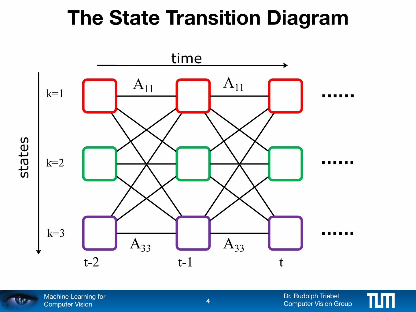
The State Transition Diagram
A33 A33
A11 A11k=1
k=2
k=3
time
t-2 t-1 t
4
states
Dr. Rudolph TriebelComputer Vision Group
Machine Learning for Computer Vision
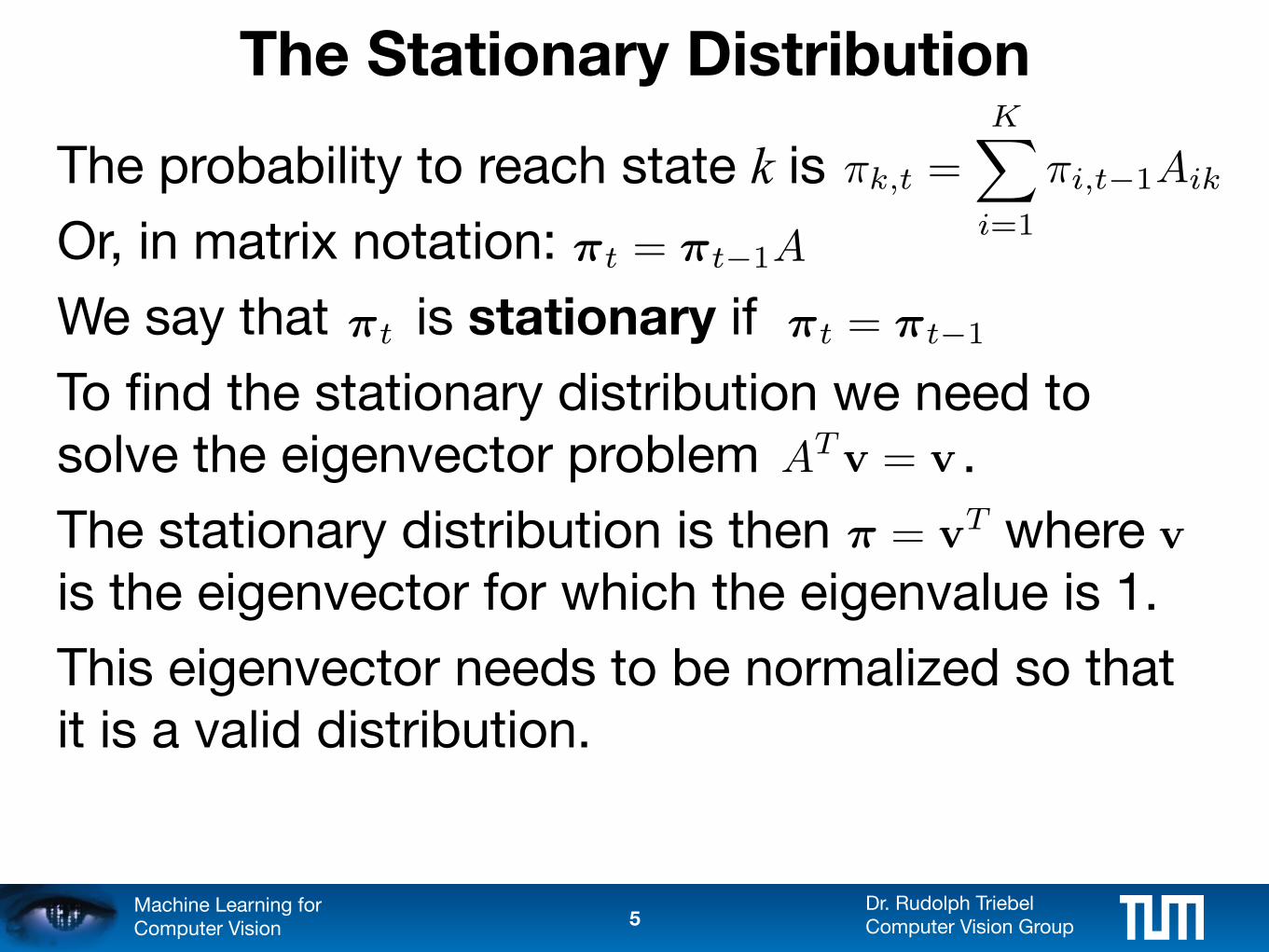
The Stationary Distribution
The probability to reach state k isOr, in matrix notation:
We say that is stationary if
To find the stationary distribution we need to solve the eigenvector problem .
The stationary distribution is then where is the eigenvector for which the eigenvalue is 1.
This eigenvector needs to be normalized so that it is a valid distribution.
5
⇡t = ⇡t�1A
⇡k,t =KX
i=1
⇡i,t�1Aik
⇡t = ⇡t�1⇡t
ATv = v
⇡ = vT v
Dr. Rudolph TriebelComputer Vision Group
Machine Learning for Computer Vision
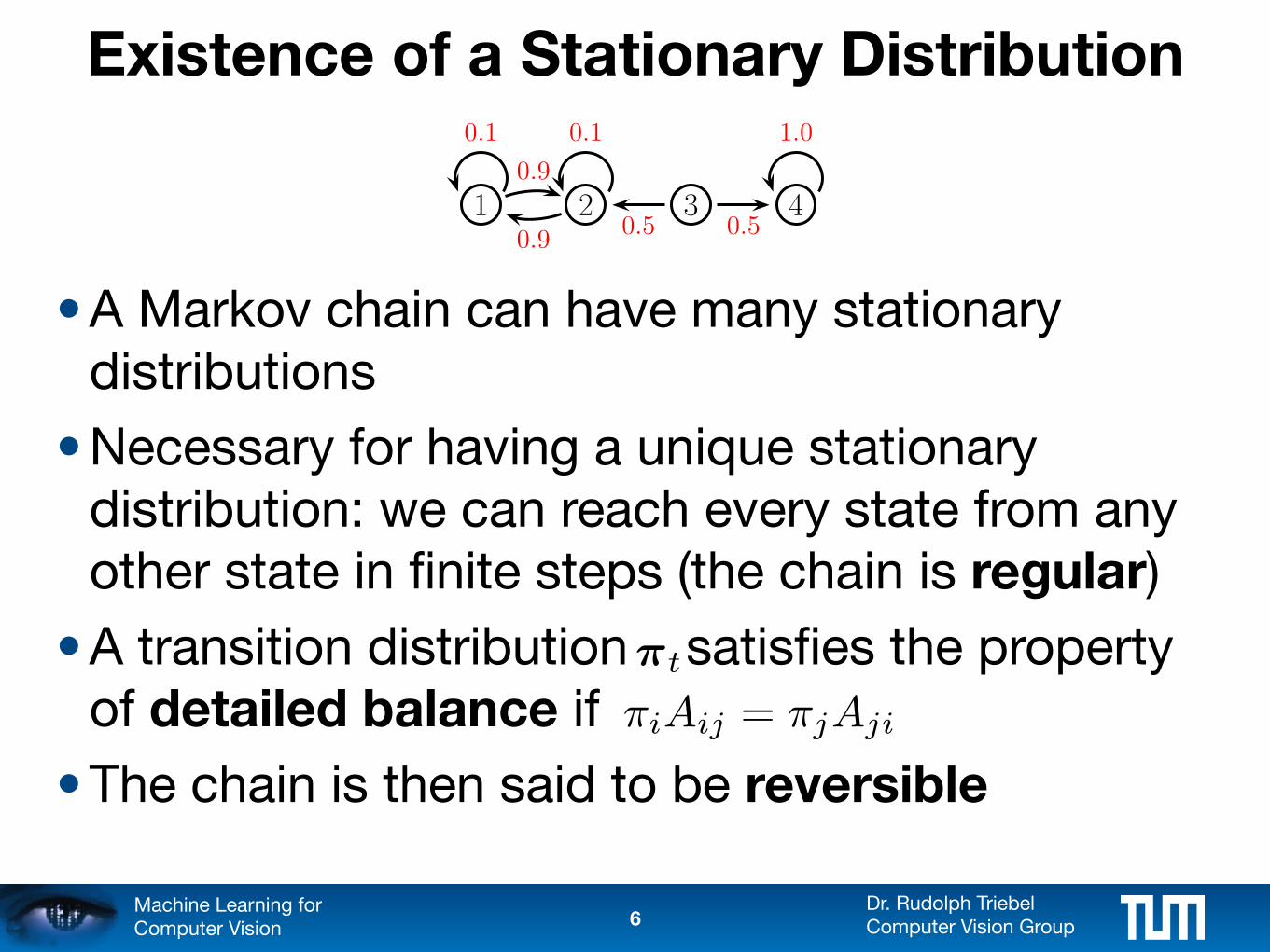
Existence of a Stationary Distribution
• A Markov chain can have many stationary distributions
• Necessary for having a unique stationary distribution: we can reach every state from any other state in finite steps (the chain is regular)
• A transition distribution satisfies the property of detailed balance if
• The chain is then said to be reversible
6
1 2 3 4
0.9
0.90.5 0.5
1.00.10.1
⇡t
⇡iAij = ⇡jAji
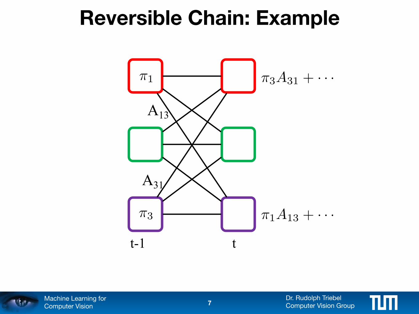
⇡1
⇡3 ⇡1A13 + · · ·
⇡3A31 + · · ·
Dr. Rudolph TriebelComputer Vision Group
Machine Learning for Computer Vision
Reversible Chain: Example
A31
t-1 t
7
A13
Dr. Rudolph TriebelComputer Vision Group
Machine Learning for Computer Vision
Existence of a Stationary Distribution
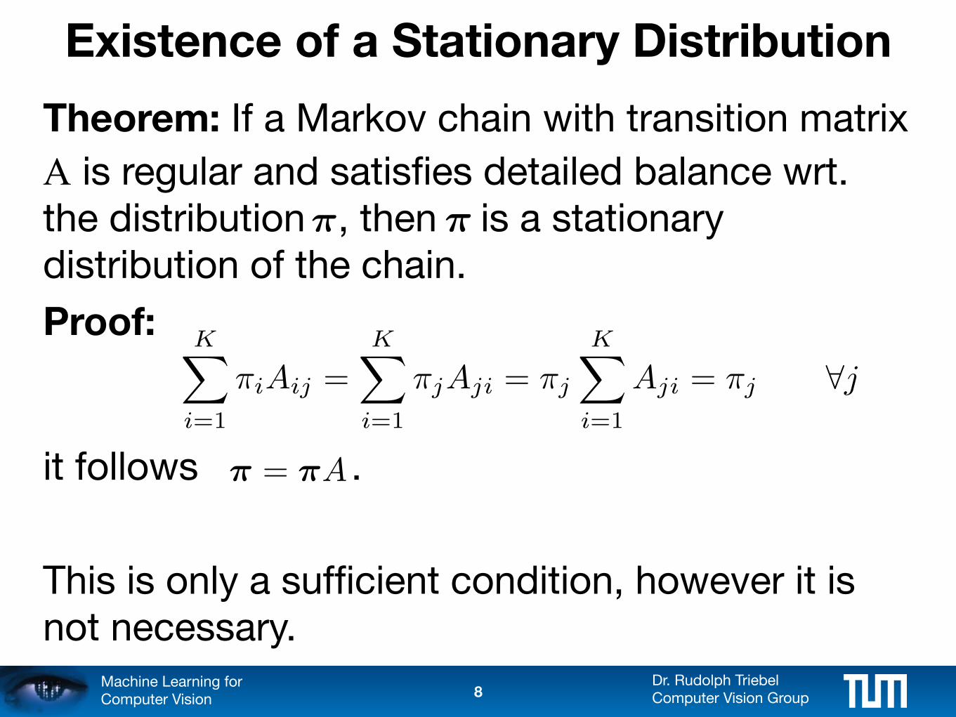
Theorem: If a Markov chain with transition matrix
A is regular and satisfies detailed balance wrt. the distribution , then is a stationary distribution of the chain.
Proof:
it follows .
This is only a sufficient condition, however it is not necessary.
8
⇡ ⇡
KX
i=1
⇡iAij =KX
i=1
⇡jAji = ⇡j
KX
i=1
Aji = ⇡j 8j
⇡ = ⇡A
Dr. Rudolph TriebelComputer Vision Group
Machine Learning for Computer Vision
Sampling with a Markov Chain
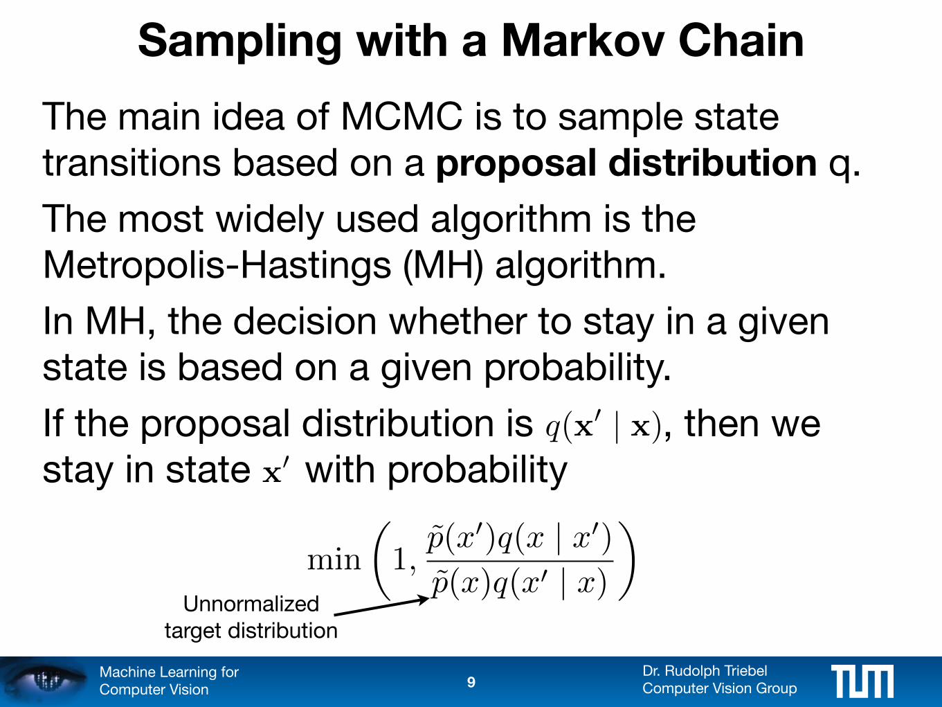
The main idea of MCMC is to sample state transitions based on a proposal distribution q.
The most widely used algorithm is the Metropolis-Hastings (MH) algorithm.
In MH, the decision whether to stay in a given state is based on a given probability.
If the proposal distribution is , then we stay in state with probability
9
q(x0 | x)x
0
min
✓1,
p̃(x0)q(x | x0)
p̃(x)q(x0 | x)
◆
Unnormalized target distribution
Dr. Rudolph TriebelComputer Vision Group
Machine Learning for Computer Vision
The Metropolis-Hastings Algorithm
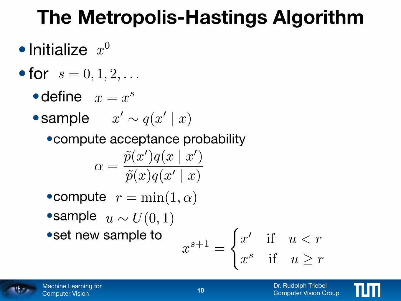
• Initialize
• for
•define
•sample
•compute acceptance probability
•compute
•sample
•set new sample to
10
x
0
s = 0, 1, 2, . . .
x = x
s
x
0 ⇠ q(x0 | x)
↵ =p̃(x0)q(x | x0)
p̃(x)q(x0 | x)r = min(1,↵)
u ⇠ U(0, 1)
x
s+1 =
(x
0 if u < r
x
s if u � r
Dr. Rudolph TriebelComputer Vision Group
Machine Learning for Computer Vision
Why Does This Work?
We have to prove that the transition probability of the MH algorithm satisfies detailed balance wrt the target distribution.
Theorem: If is the transition probability of the MH algorithm, then
Proof:
11
pMH(x0 | x)
p(x)pMH(x0 | x) = p(x0)pMH(x | x0)
Dr. Rudolph TriebelComputer Vision Group
Machine Learning for Computer Vision
Why Does This Work?
We have to prove that the transition probability of the MH algorithm satisfies detailed balance wrt the target distribution.
Theorem: If is the transition probability of the MH algorithm, then
Note: All formulations are valid for discrete and for continuous variables!
12
pMH(x0 | x)
p(x)pMH(x0 | x) = p(x0)pMH(x | x0)
Dr. Rudolph TriebelComputer Vision Group
Machine Learning for Computer Vision
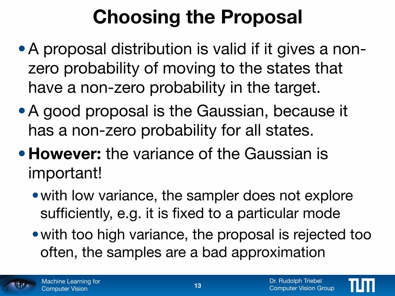
Choosing the Proposal
• A proposal distribution is valid if it gives a non-zero probability of moving to the states that have a non-zero probability in the target.
• A good proposal is the Gaussian, because it has a non-zero probability for all states.
• However: the variance of the Gaussian is important!
•with low variance, the sampler does not explore sufficiently, e.g. it is fixed to a particular mode
•with too high variance, the proposal is rejected too often, the samples are a bad approximation
13
Dr. Rudolph TriebelComputer Vision Group
Machine Learning for Computer Vision
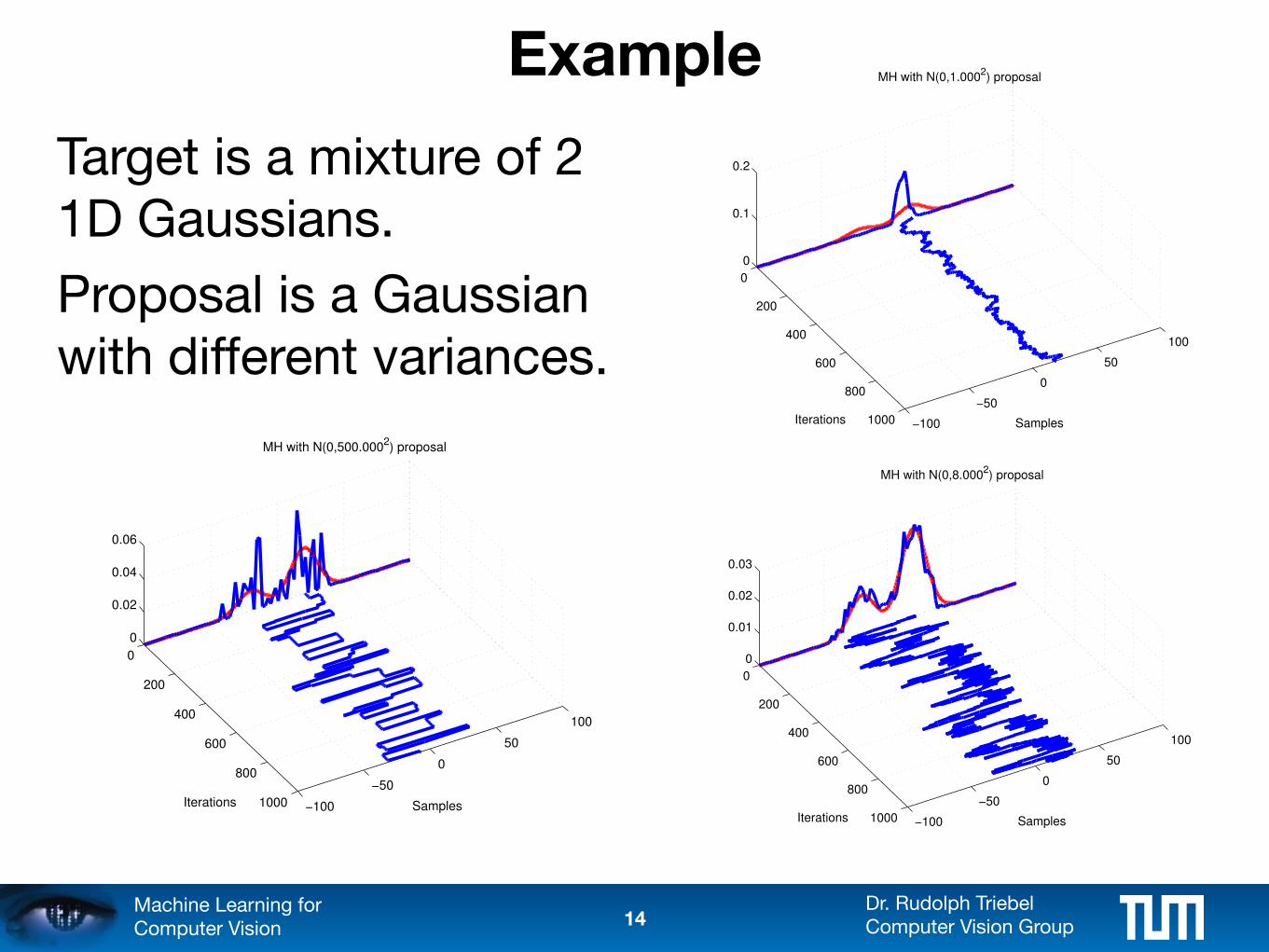
Example
Target is a mixture of 2 1D Gaussians.
Proposal is a Gaussian with different variances.
14
0
200
400
600
800
1000 !100
!50
0
50
100
0
0.1
0.2
Samples
MH with N(0,1.0002) proposal
Iterations
0
200
400
600
800
1000 !100
!50
0
50
100
0
0.01
0.02
0.03
Samples
MH with N(0,8.0002) proposal
Iterations
0
200
400
600
800
1000 !100
!50
0
50
100
0
0.02
0.04
0.06
Samples
MH with N(0,500.0002) proposal
Iterations
Dr. Rudolph TriebelComputer Vision Group
Machine Learning for Computer Vision
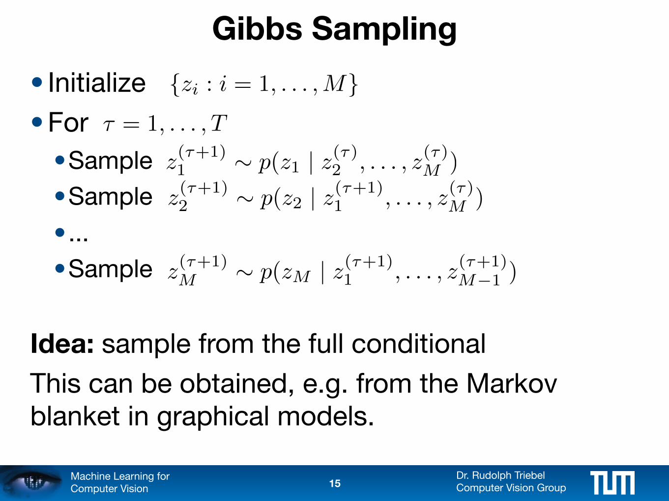
Gibbs Sampling
• Initialize
• For
•Sample
•Sample
•...
•Sample
Idea: sample from the full conditional
This can be obtained, e.g. from the Markov blanket in graphical models.
15
{zi : i = 1, . . . ,M}⌧ = 1, . . . , T
z(⌧+1)1 ⇠ p(z1 | z(⌧)2 , . . . , z(⌧)M )
z(⌧+1)2 ⇠ p(z2 | z(⌧+1)
1 , . . . , z(⌧)M )
z(⌧+1)M ⇠ p(zM | z(⌧+1)
1 , . . . , z(⌧+1)M�1 )
Dr. Rudolph TriebelComputer Vision Group
Machine Learning for Computer Vision
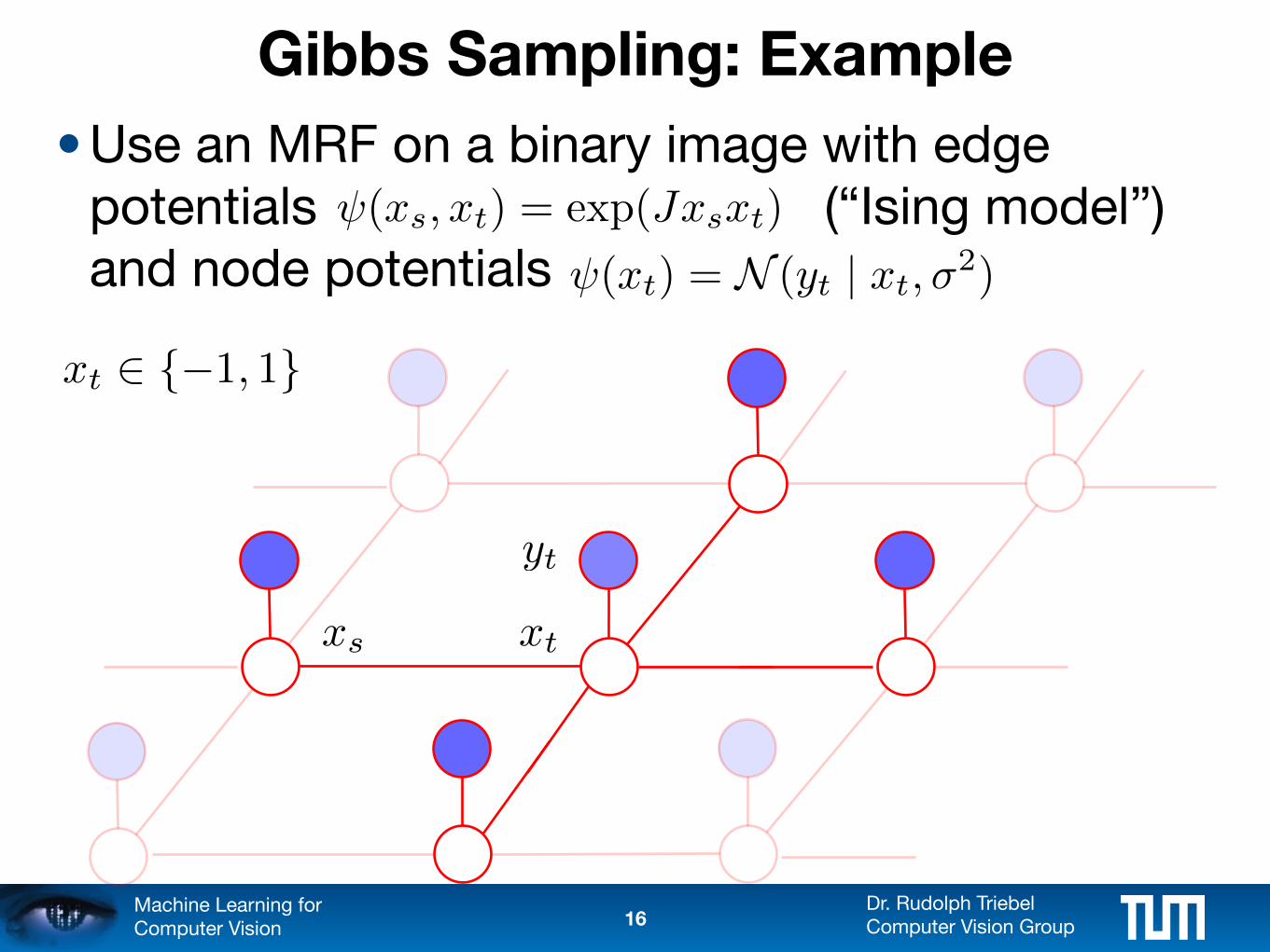
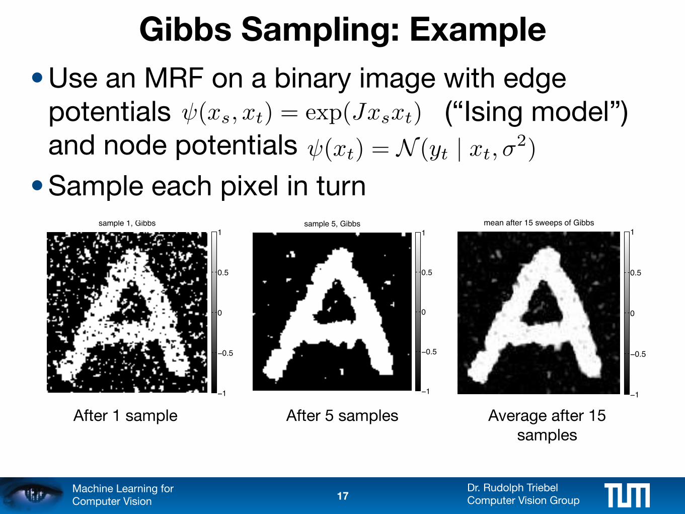
Gibbs Sampling: Example
• Use an MRF on a binary image with edge potentials (“Ising model”) and node potentials
16
(xt) = N (yt | xt,�2)
(xs, xt) = exp(Jxsxt)
xt
yt
xs
xt 2 {�1, 1}
Dr. Rudolph TriebelComputer Vision Group
Machine Learning for Computer Vision
Gibbs Sampling: Example
• Use an MRF on a binary image with edge potentials (“Ising model”) and node potentials
• Sample each pixel in turn
17
(xt) = N (yt | xt,�2)
sample 1, Gibbs
−1
−0.5
0
0.5
1sample 5, Gibbs
−1
−0.5
0
0.5
1mean after 15 sweeps of Gibbs
−1
−0.5
0
0.5
1
(xs, xt) = exp(Jxsxt)
After 1 sample After 5 samples Average after 15 samples
Dr. Rudolph TriebelComputer Vision Group
Machine Learning for Computer Vision
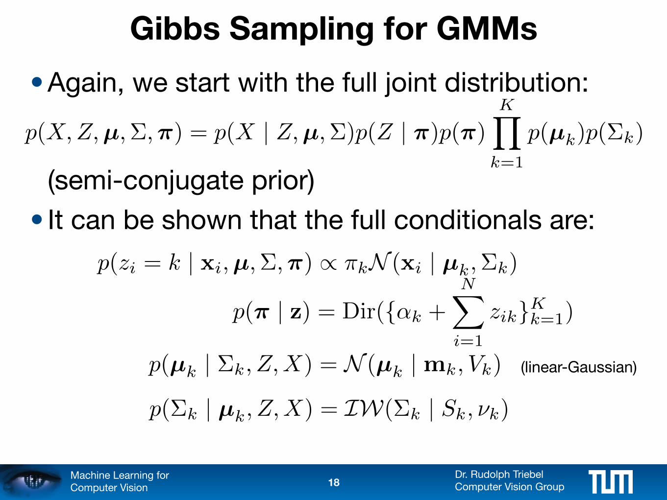
Gibbs Sampling for GMMs
• Again, we start with the full joint distribution:
(semi-conjugate prior)
• It can be shown that the full conditionals are:
18
p(X,Z,µ,⌃,⇡) = p(X | Z,µ,⌃)p(Z | ⇡)p(⇡)KY
k=1
p(µk)p(⌃k)
p(zi = k | xi,µ,⌃,⇡) / ⇡kN (xi | µk,⌃k)
p(⇡ | z) = Dir({↵k +NX
i=1
zik}Kk=1)
p(µk | ⌃k, Z,X) = N (µk | mk, Vk) (linear-Gaussian)
p(⌃k | µk, Z,X) = IW(⌃k | Sk, ⌫k)
Dr. Rudolph TriebelComputer Vision Group
Machine Learning for Computer Vision
Gibbs Sampling for GMMs
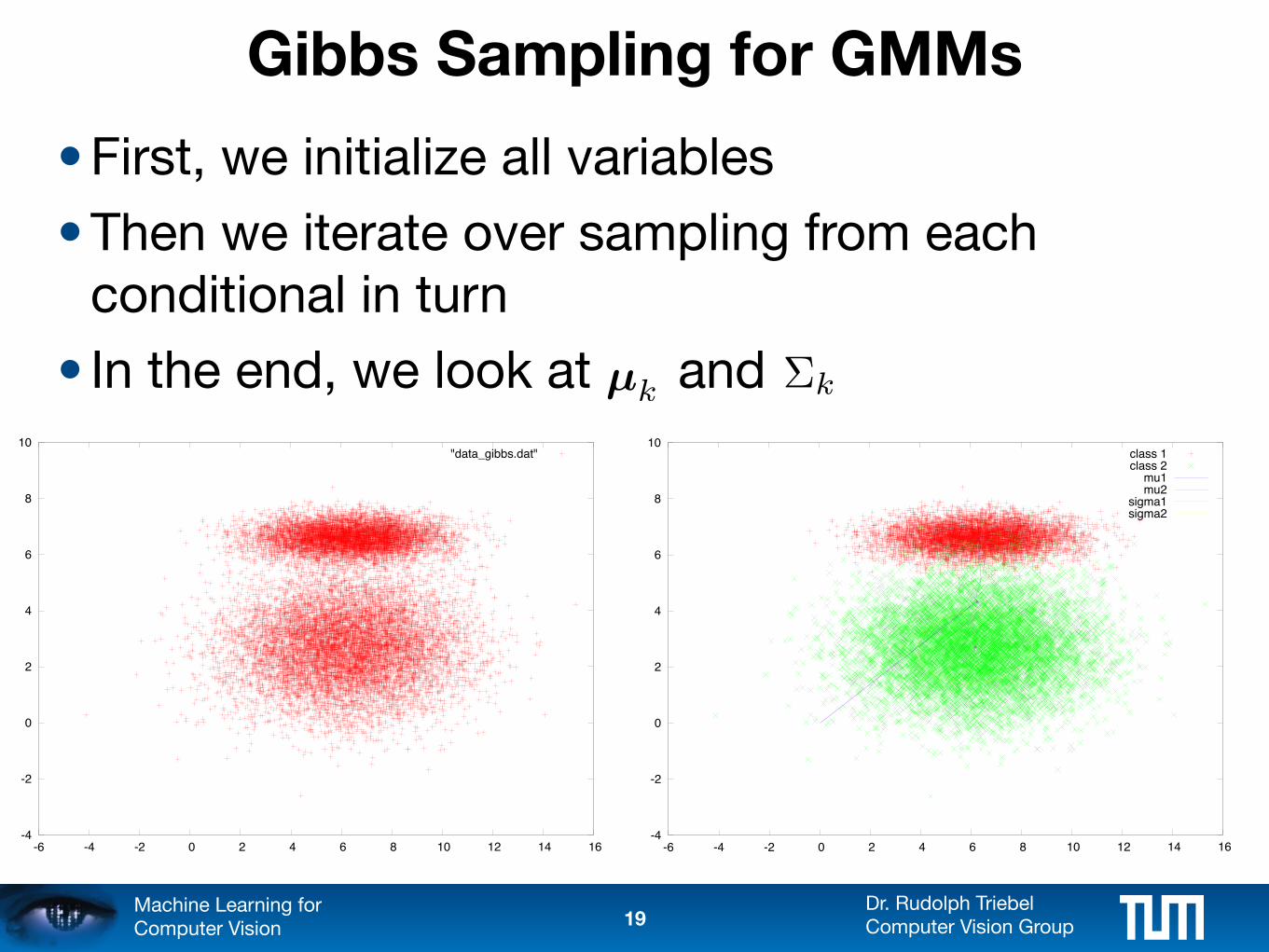
• First, we initialize all variables
• Then we iterate over sampling from each conditional in turn
• In the end, we look at and
19
µk ⌃k
-4
-2
0
2
4
6
8
10
-6 -4 -2 0 2 4 6 8 10 12 14 16
"data_gibbs.dat"
-4
-2
0
2
4
6
8
10
-6 -4 -2 0 2 4 6 8 10 12 14 16
class 1class 2
mu1mu2
sigma1sigma2
Dr. Rudolph TriebelComputer Vision Group
Machine Learning for Computer Vision
How Often Do We Have To Sample?
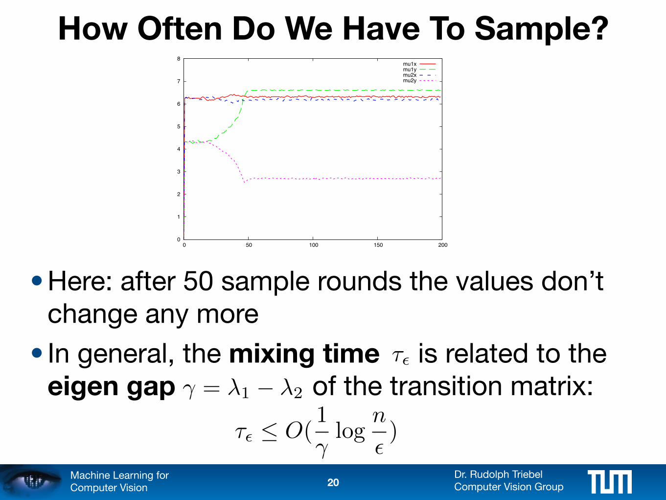
• Here: after 50 sample rounds the values don’t change any more
• In general, the mixing time is related to the eigen gap of the transition matrix:
20
0
1
2
3
4
5
6
7
8
0 50 100 150 200
mu1xmu1ymu2xmu2y
� = �1 � �2
⌧✏
⌧✏ O(
1
�log
n
✏)
Dr. Rudolph TriebelComputer Vision Group
Machine Learning for Computer Vision
Gibbs Sampling is a Special Case of MH
• The proposal distribution in Gibbs sampling is
• This leads to an acceptance rate of:
• Although the acceptance is 100%, Gibbs sampling does not converge faster, as it only updates one variable at a time.
21
q(x0 | x) = p(x0i | x�i)I(x0
�i = x�i)
↵ =p(x0)q(x | x0)
p(x)q(x0 | x) =p(x0
i | x0�i)p(x
0�i)p(xi | x0
�i)
p(xi | x�i)p(x�i)p(x0i | x�i)
= 1
Dr. Rudolph TriebelComputer Vision Group
Machine Learning for Computer Vision
Summary
• Markov Chain Monte Carlo is a family of sampling algorithms that can sample from arbitrary distributions by moving in state space
• Most used methods are the Metropolis-Hastings (MH) and the Gibbs sampling method
• MH uses a proposal distribution and accepts a proposed state randomly
• Gibbs sampling does not use a proposal distribution, but samples from the full conditionals
22

Computer Vision Group Prof. Daniel Cremers
11. Evaluation and Model Selection
Dr. Rudolph TriebelComputer Vision Group
Machine Learning for Computer Vision
Evaluation of Learning Methods
Very often, machine learning tries to find parameters of a model for a given data set.
But: Which parameters give a good model?
Intuitively, a good model behaves well on new, unseen data. This motivates the distinction of
Training data: used to generate different models
Validation data: used to adjust the model parameters so that their performance is optimal
Test data: used to evaluate the models with the optimized parameters
24
Dr. Rudolph TriebelComputer Vision Group
Machine Learning for Computer Vision
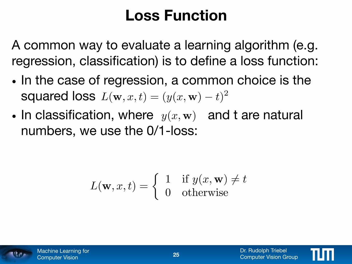
Loss Function
A common way to evaluate a learning algorithm (e.g. regression, classification) is to define a loss function:
• In the case of regression, a common choice is the squared loss
• In classification, where and t are natural numbers, we use the 0/1-loss:
25
L(y, a) = |y � a|q
Dr. Rudolph TriebelComputer Vision Group
Machine Learning for Computer Vision
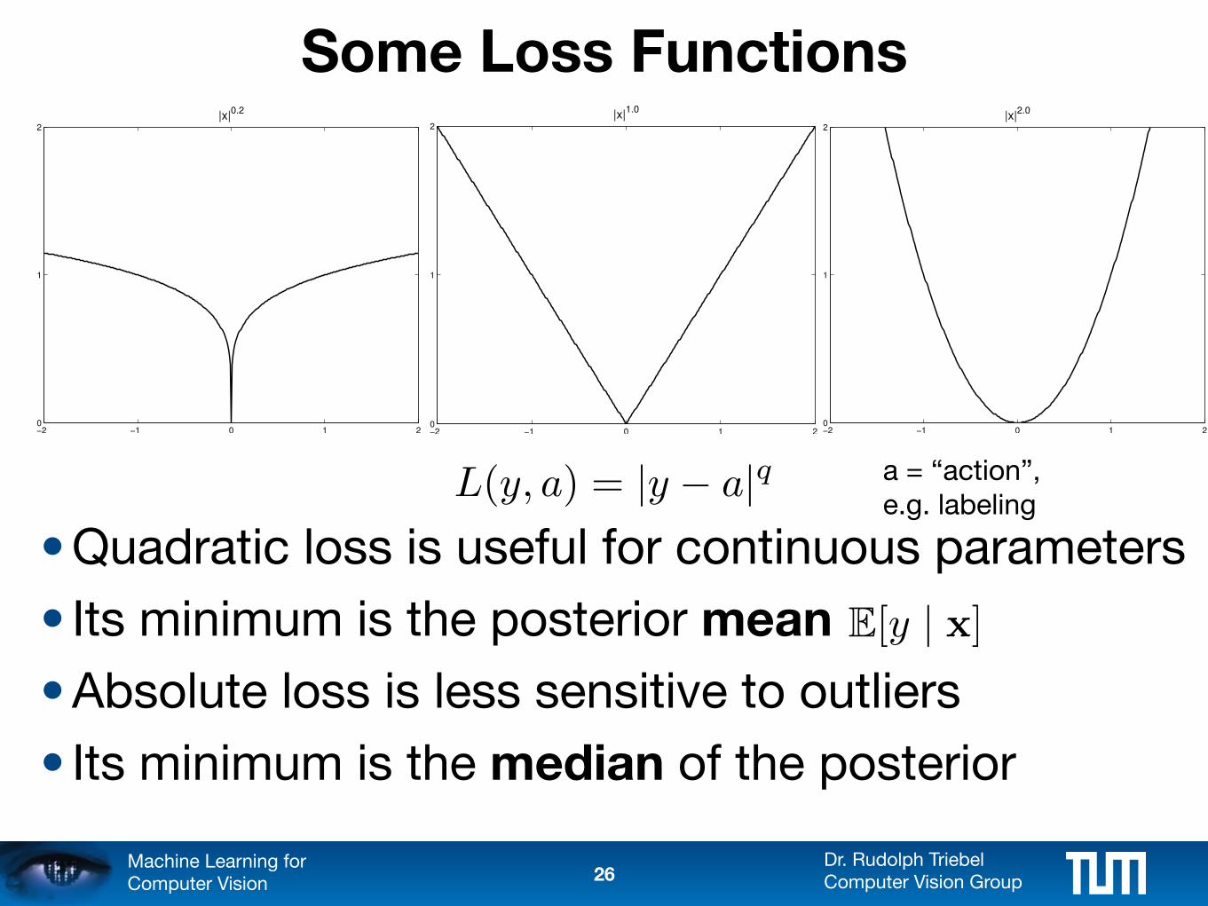
Some Loss Functions
• Quadratic loss is useful for continuous parameters
• Its minimum is the posterior mean
• Absolute loss is less sensitive to outliers
• Its minimum is the median of the posterior
26
!2 !1 0 1 20
1
2|x|0.2
!2 !1 0 1 20
1
2|x|1.0
!2 !1 0 1 20
1
2|x|2.0
a = “action”, e.g. labeling
E[y | x]
Dr. Rudolph TriebelComputer Vision Group
Machine Learning for Computer Vision
Model Selection
Model selection is used to find model parameters to optimize the classification result.
Possible methods:
• Minimizing the training error
• Hold-out testing
• Cross-validation
• Leave-one-out rule
Evaluation is done using an appropriate loss function.
27
Dr. Rudolph TriebelComputer Vision Group
Machine Learning for Computer Vision
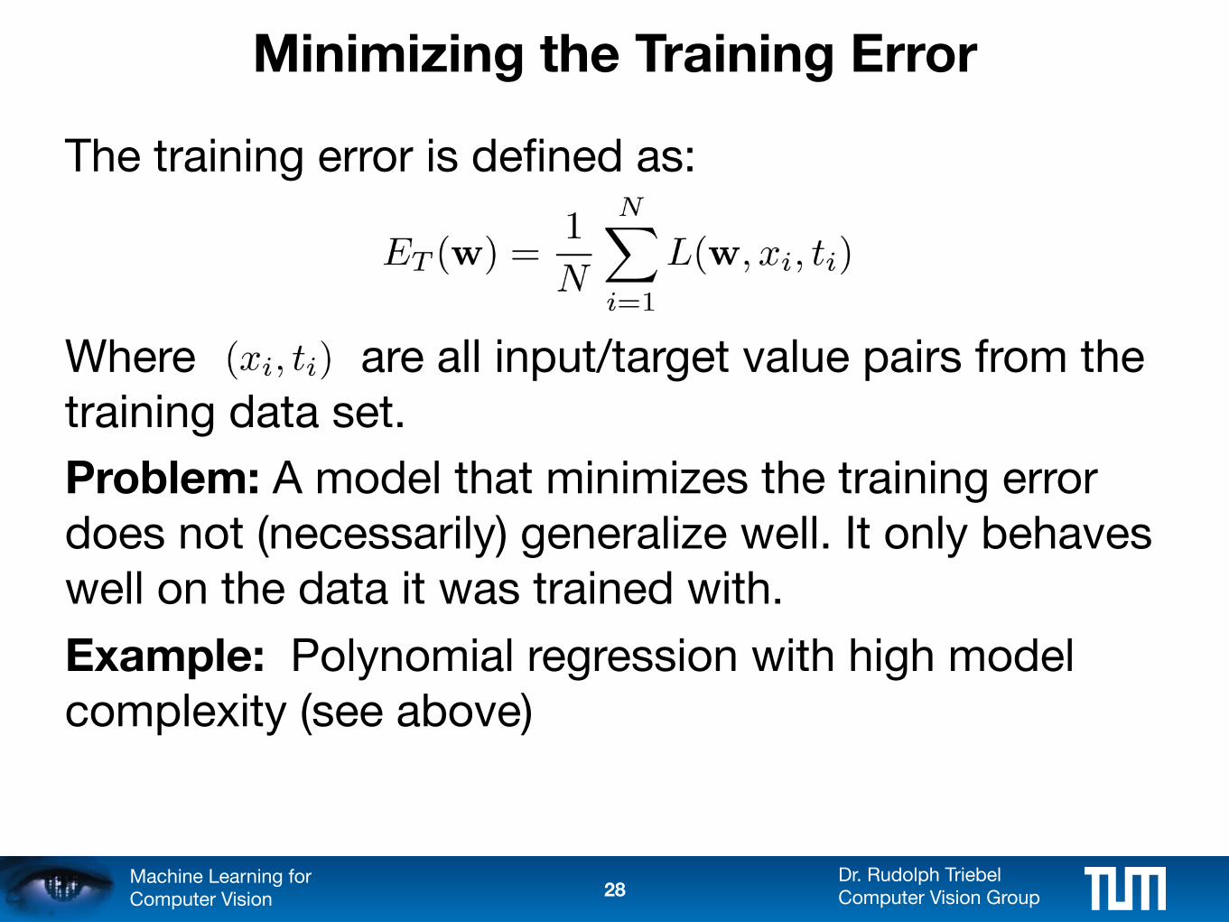
Minimizing the Training Error
The training error is defined as:
Where are all input/target value pairs from the training data set.
Problem: A model that minimizes the training error does not (necessarily) generalize well. It only behaves well on the data it was trained with.
Example: Polynomial regression with high model complexity (see above)
28
Dr. Rudolph TriebelComputer Vision Group
Machine Learning for Computer Vision
Hold-out Testing
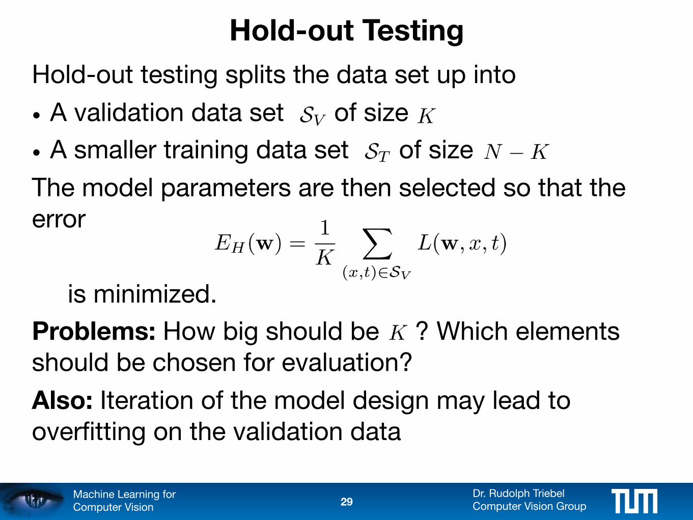
Hold-out testing splits the data set up into
• A validation data set of size
• A smaller training data set of size
The model parameters are then selected so that the error
is minimized.
Problems: How big should be ? Which elements should be chosen for evaluation?
Also: Iteration of the model design may lead to overfitting on the validation data
29
Dr. Rudolph TriebelComputer Vision Group
Machine Learning for Computer Vision
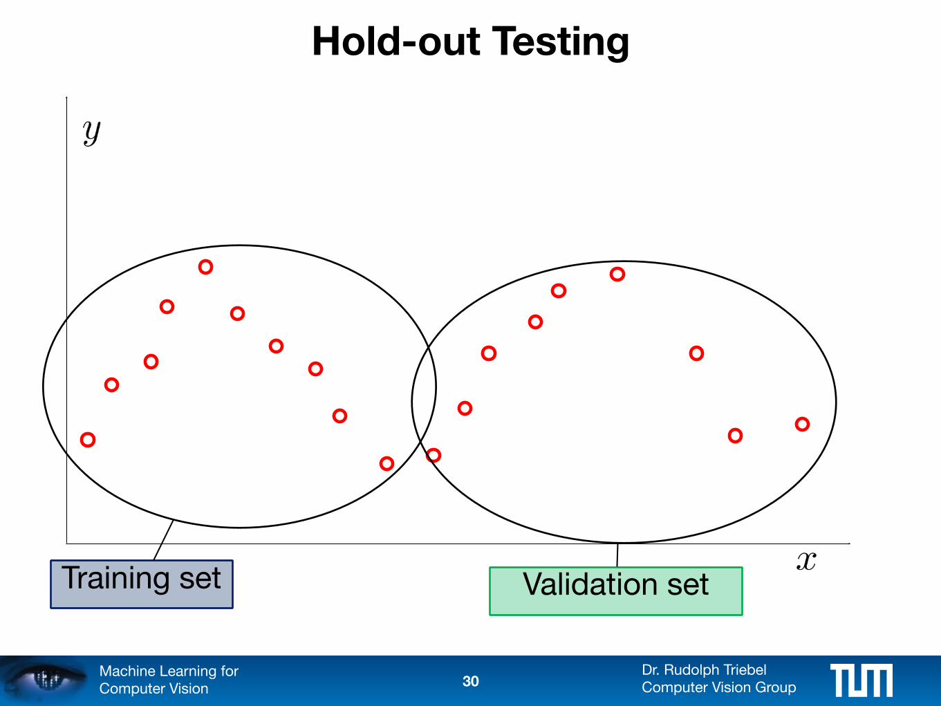
Hold-out Testing
Training set Validation set
30
Dr. Rudolph TriebelComputer Vision Group
Machine Learning for Computer Vision
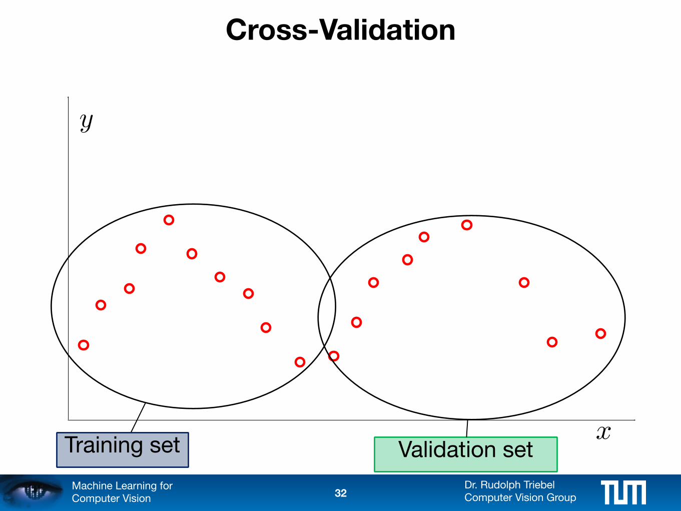
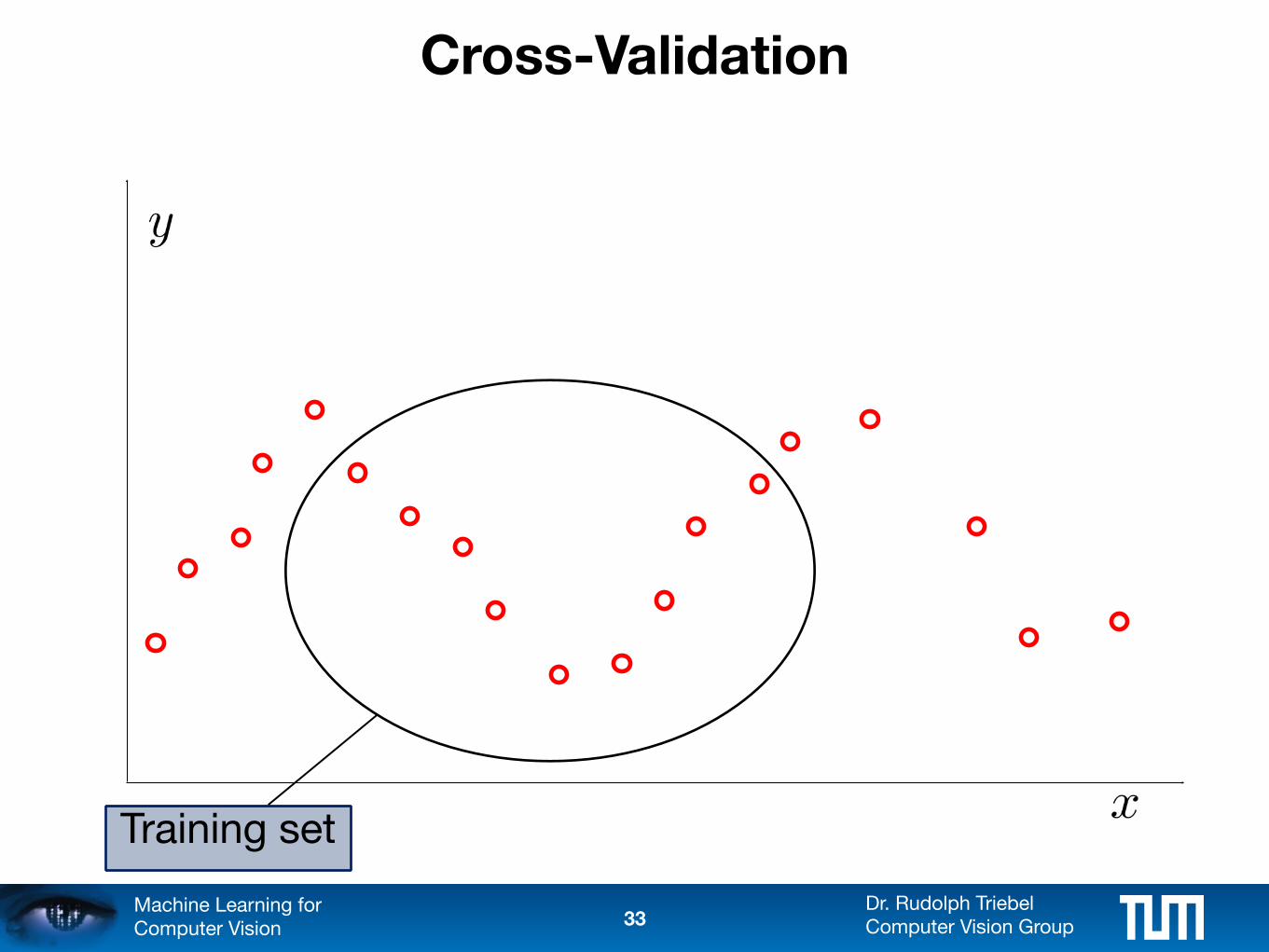
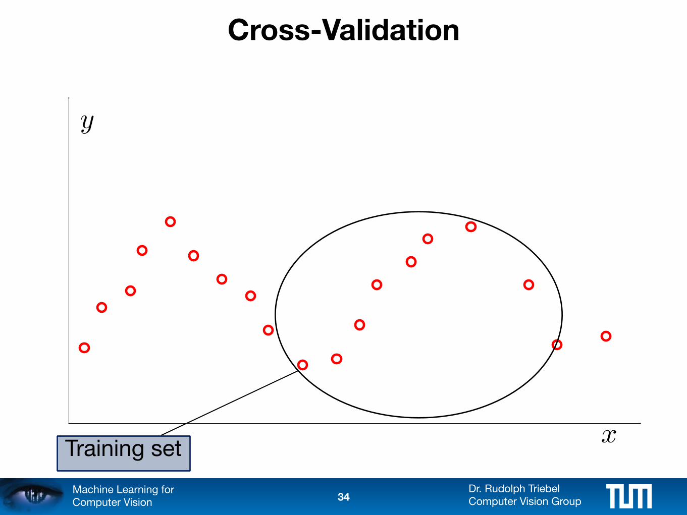
Cross Validation
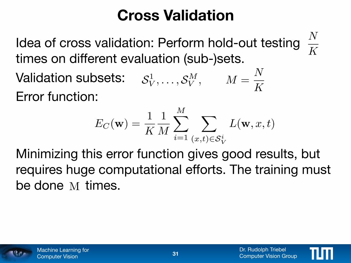
Idea of cross validation: Perform hold-out testing times on different evaluation (sub-)sets.
Validation subsets:
Error function:
Minimizing this error function gives good results, but requires huge computational efforts. The training must be done times.
31
Dr. Rudolph TriebelComputer Vision Group
Machine Learning for Computer Vision
Cross-Validation
Training set Validation set
32
Dr. Rudolph TriebelComputer Vision Group
Machine Learning for Computer Vision
Cross-Validation
Training set
33
Dr. Rudolph TriebelComputer Vision Group
Machine Learning for Computer Vision
Cross-Validation
Training set
34
Dr. Rudolph TriebelComputer Vision Group
Machine Learning for Computer Vision
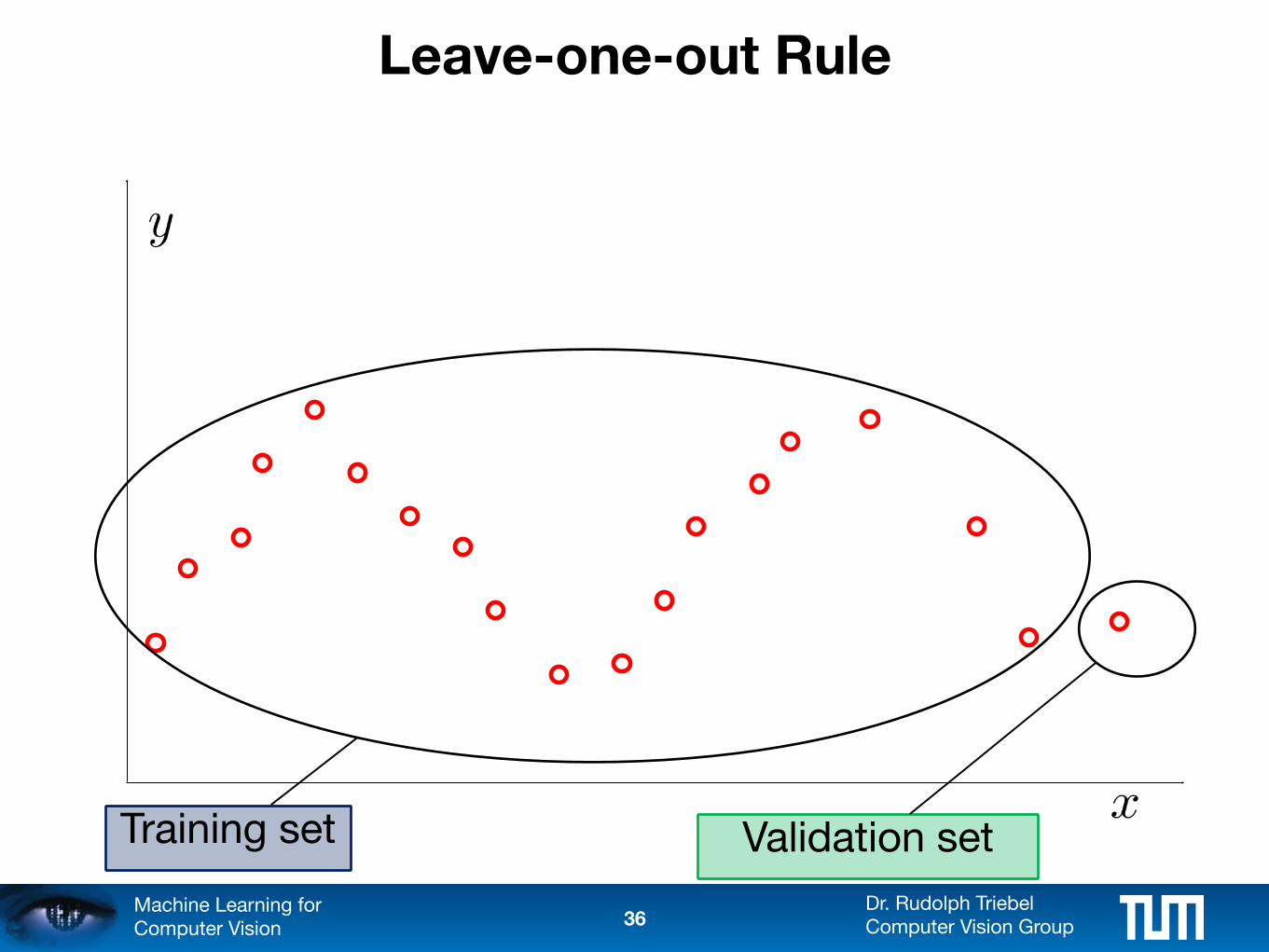
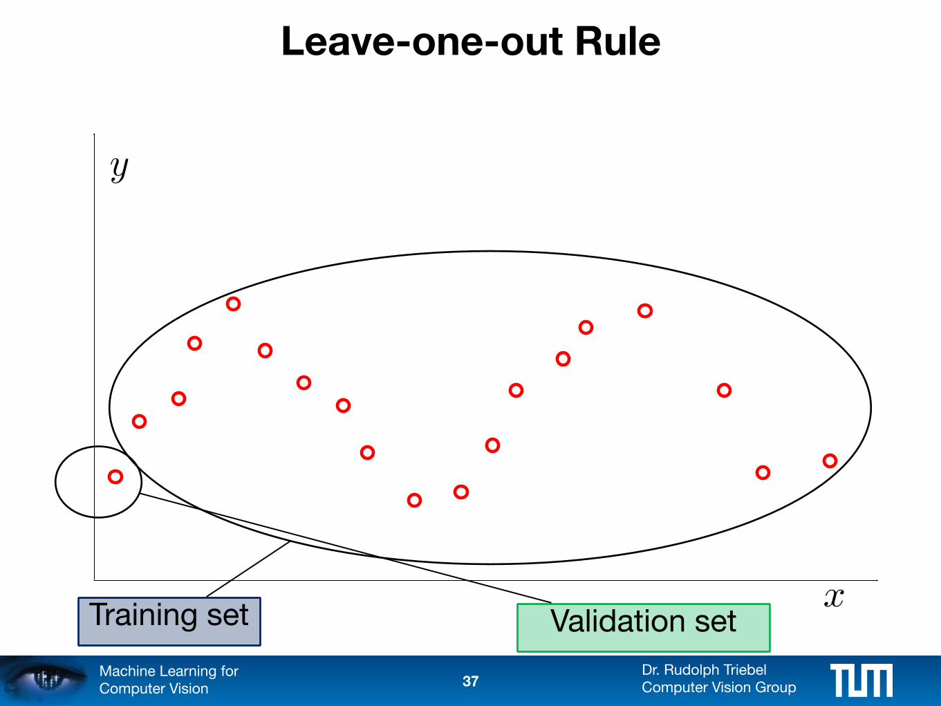
Leave-one-out Rule
Idea: do cross-validation with
• Yields similarly good results compared to cross-validation
• Still requires to do the training times
• Useful if the data set is particularly scarce
35
Dr. Rudolph TriebelComputer Vision Group
Machine Learning for Computer Vision
Leave-one-out Rule
Training set Validation set
36
Dr. Rudolph TriebelComputer Vision Group
Machine Learning for Computer Vision
Leave-one-out Rule
Training set Validation set
37
Dr. Rudolph TriebelComputer Vision Group
Machine Learning for Computer Vision
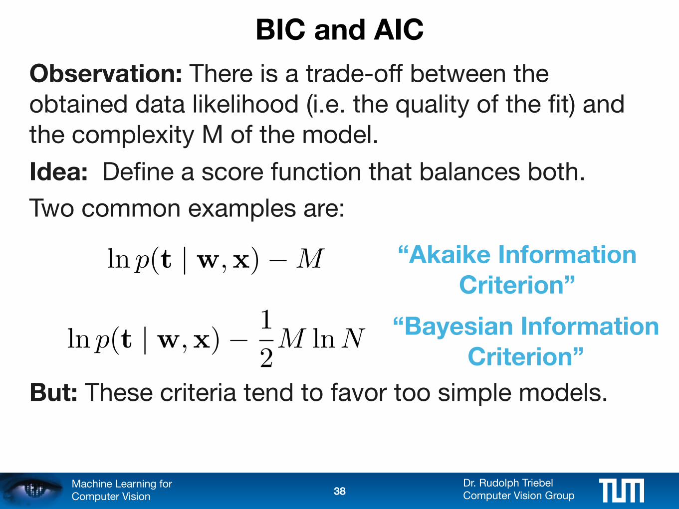
BIC and AIC
Observation: There is a trade-off between the obtained data likelihood (i.e. the quality of the fit) and the complexity M of the model.
Idea: Define a score function that balances both.
Two common examples are:
But: These criteria tend to favor too simple models.
“Akaike Information Criterion”
“Bayesian Information Criterion”
38
Dr. Rudolph TriebelComputer Vision Group
Machine Learning for Computer Vision
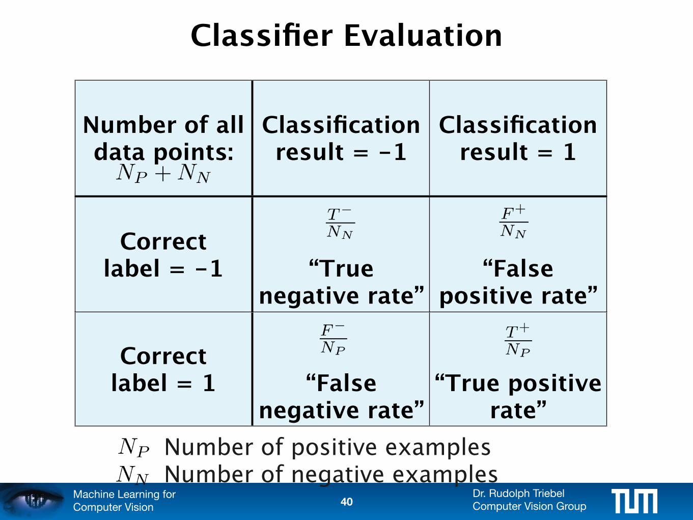
Classifier Evaluation
Different methods to evaluate a classifier
• True-positive / false-positive rates
• Precision-recall diagram
• Receiving operator characteristics (ROC curves)
• Loss function
The evaluation of a classifier is needed to find the best classification parameters
(e.g. for the kernel function)
39
Dr. Rudolph TriebelComputer Vision Group
Machine Learning for Computer Vision
Classifier Evaluation
Number of positive examples
Number of all data points:
Classification result = -1
Classification result = 1
Correct label = -1 “True
negative rate”“False
positive rate”
Correct label = 1 “False
negative rate”“True positive
rate”
Number of negative examples40
Dr. Rudolph TriebelComputer Vision Group
Machine Learning for Computer Vision
Classifier Evaluation
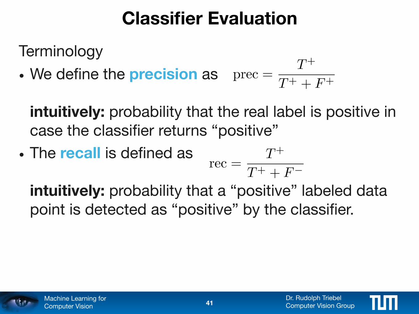
Terminology
• We define the precision as
intuitively: probability that the real label is positive in case the classifier returns “positive”
• The recall is defined as
intuitively: probability that a “positive” labeled data point is detected as “positive” by the classifier.
41
Dr. Rudolph TriebelComputer Vision Group
Machine Learning for Computer Vision
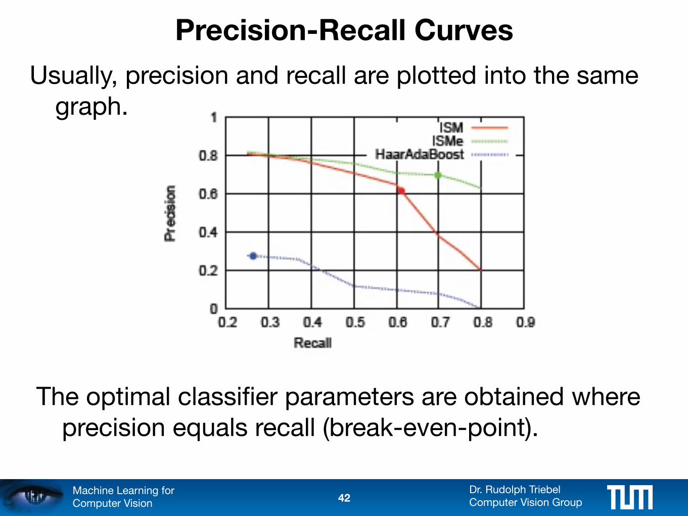
Precision-Recall Curves
Usually, precision and recall are plotted into the same graph.
The optimal classifier parameters are obtained where precision equals recall (break-even-point).
42
Dr. Rudolph TriebelComputer Vision Group
Machine Learning for Computer Vision
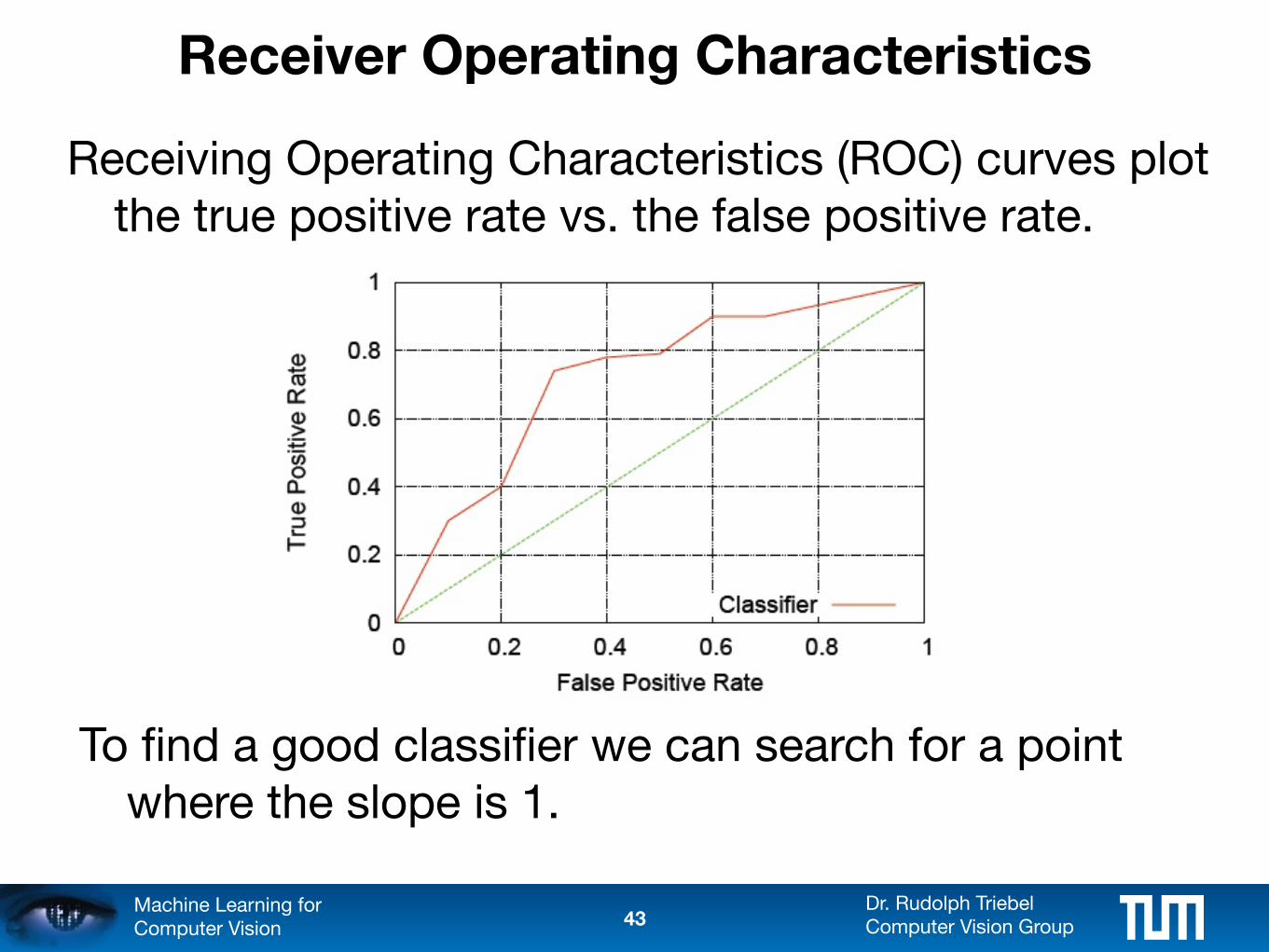
Receiver Operating Characteristics
Receiving Operating Characteristics (ROC) curves plot the true positive rate vs. the false positive rate.
To find a good classifier we can search for a point where the slope is 1.
43
Dr. Rudolph TriebelComputer Vision Group
Machine Learning for Computer Vision
Loss Function
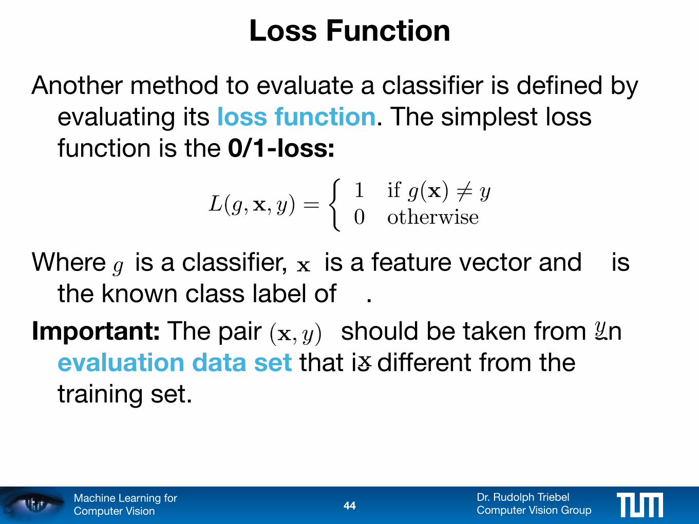
Another method to evaluate a classifier is defined by evaluating its loss function. The simplest loss function is the 0/1-loss:
Where is a classifier, is a feature vector and is the known class label of .
Important: The pair should be taken from an evaluation data set that is different from the training set.
44